Limits of Floating Exchange Rates: the Role of Foreign Currency Debt and Import

Structure

Pascal Towbin and Sebastian Weber

WP/11/42

© 2011 International Monetary Fund WP/11/42

IMF Working Paper

European Department

Limits of Floating Exchange Rates: the Role of Foreign Currency Debt and Import Structure

Prepared by Pascal Towbin and Sebastian Weber†

Authorized for distribution by Ashoka Mody

February 2011

This Working Paper should not be reported as representing the views of the IMF. The views expressed in this Working Paper are those of the author(s) and do not necessarily represent those of the IMF or IMF policy. Working Papers describe research in progress by the author(s) and are published to elicit comments and to further debate.

Abstract

A traditional argument in favor of flexible exchange rates is that they insulate output better from real shocks, because the exchange rate can adjust and stabilize demand for domestic goods through expenditure switching. This argument is weakened in models with high foreign currency debt and low exchange rate pass-through to import prices. The present study evaluates the empirical relevance of these two factors. We analyze the transmission of real external shocks to the domestic economy under fixed and flexible exchange rate regimes for a broad sample of countries in a Panel VAR and let the responses vary with foreign currency indebtedness and import structure. We find that flexible exchange rates do not insulate output better from external shocks if the country imports mainly low pass-through goods and can even amplify the output response if foreign indebtedness is high.

JEL Classification Numbers: E30, F33, F34, F41

Keywords: Exchange rate regime, balance sheet effect, pass-through, interacted panel VAR, external shock

Author’s E-Mail Address: pascal.towbin@banque-france.fr; sweber@imf.org

† This paper has benefited from suggestions by Marcel Fratzscher, Domenico Giannone, Stefan Gerlach, Cedric Tille, Charles Wyplosz, and participants at SSES Congress 2009, RES 2010, CEPII-Brugel Workshop 2010, Banque de France, and Bank of Canada. We also like to thank Harald Anderson, Ken Chikada, Irineu de Carvalho Filho, Atish Ghosh, David Gregorian, Albert Jäger, Mustafa Saiyid, and Jerome Vandenbussche for helpful comments. Part of this research was conducted while both authors were at the Graduate Institute Geneva and funding from the Swiss National Science Foundation is gratefully acknowledged. The views expressed are those of the authors and do not necessarily reflect the views of the institutions they are associated with.

2

Contents Page

I. Introduction . . . . . . . . . . . . . . . . . . . . . . . . . . . . . . . . . . . . . . 4

II. Theory . . . . . . . . . . . . . . . . . . . . . . . . . . . . . . . . . . . . . . . . . 7A. IS-LM-BP with Foreign Debt and Incomplete Pass-through . . . . . . . . . . . 9B. Adjustment to an External Demand Shock . . . . . . . . . . . . . . . . . . . . 10

1. The Peg . . . . . . . . . . . . . . . . . . . . . . . . . . . . . . . . . . . 112. The Float . . . . . . . . . . . . . . . . . . . . . . . . . . . . . . . . . . . 113. Simulation of Responses under Peg and Float . . . . . . . . . . . . . . . 13

III. Data . . . . . . . . . . . . . . . . . . . . . . . . . . . . . . . . . . . . . . . . . . 13

IV. Model and Estimation . . . . . . . . . . . . . . . . . . . . . . . . . . . . . . . . . 17A. Empirical Model and Identification . . . . . . . . . . . . . . . . . . . . . . . . 17B. Interaction Terms . . . . . . . . . . . . . . . . . . . . . . . . . . . . . . . . . 18C. Estimation and Inference . . . . . . . . . . . . . . . . . . . . . . . . . . . . . 20

V. Results . . . . . . . . . . . . . . . . . . . . . . . . . . . . . . . . . . . . . . . . . 21A. Floats versus Pegs . . . . . . . . . . . . . . . . . . . . . . . . . . . . . . . . 21B. The Role of Foreign Currency Debt . . . . . . . . . . . . . . . . . . . . . . . 22C. The Role of Import Structure . . . . . . . . . . . . . . . . . . . . . . . . . . . 27D. The Joint Role of Foreign Currency Debt and Import Structure . . . . . . . . . 29

VI. Conclusion . . . . . . . . . . . . . . . . . . . . . . . . . . . . . . . . . . . . . . . 30

References . . . . . . . . . . . . . . . . . . . . . . . . . . . . . . . . . . . . . . . . . . 32

Appendices

A. Model . . . . . . . . . . . . . . . . . . . . . . . . . . . . . . . . . . . . . . . . . 36A.1. Workers . . . . . . . . . . . . . . . . . . . . . . . . . . . . . . . . . . . . . . 36A.2. Production and Price Setting . . . . . . . . . . . . . . . . . . . . . . . . . . . 37A.3. Entrepreneurs . . . . . . . . . . . . . . . . . . . . . . . . . . . . . . . . . . . 38A.4. Monetary Policy . . . . . . . . . . . . . . . . . . . . . . . . . . . . . . . . . 39A.5. Market Clearing . . . . . . . . . . . . . . . . . . . . . . . . . . . . . . . . . 39

B. Derivation of the IS-LM-BP Equations . . . . . . . . . . . . . . . . . . . . . . . . 40B.1. IS Curve . . . . . . . . . . . . . . . . . . . . . . . . . . . . . . . . . . . . . . 40B.2. LM: Money Demand . . . . . . . . . . . . . . . . . . . . . . . . . . . . . . . 41B.3. BP: Entrepreneurs . . . . . . . . . . . . . . . . . . . . . . . . . . . . . . . . 42

C. Solving the system . . . . . . . . . . . . . . . . . . . . . . . . . . . . . . . . . . . 43C.1. The Peg . . . . . . . . . . . . . . . . . . . . . . . . . . . . . . . . . . . . . . 44C.2. The Float . . . . . . . . . . . . . . . . . . . . . . . . . . . . . . . . . . . . . 45C.3. The Pure Float . . . . . . . . . . . . . . . . . . . . . . . . . . . . . . . . . . 47C.4. Evaluating the response of ∂ 2y/∂x∂ω . . . . . . . . . . . . . . . . . . . . . . 47

3

D. Data Sources . . . . . . . . . . . . . . . . . . . . . . . . . . . . . . . . . . . . . . 48

Tables

1. Summary of Theoretical Predictions . . . . . . . . . . . . . . . . . . . . . . . . . . 122. Output and Investment Response to External Shock, Conditional on the Exchange

Rate Regime . . . . . . . . . . . . . . . . . . . . . . . . . . . . . . . . . . . . . . 233. Output and Investment Response to External Shock, Conditional on Short Term

External Debt and Exchange Rate Regime . . . . . . . . . . . . . . . . . . . . . . 264. Output and Investment Response to External Shock, Conditional on Import Struc-

ture and Exchange Rate Regime . . . . . . . . . . . . . . . . . . . . . . . . . . . . 295. Country sample . . . . . . . . . . . . . . . . . . . . . . . . . . . . . . . . . . . . 50

Figures

1. Output response to a negative external demand shock: Difference between floatand peg. . . . . . . . . . . . . . . . . . . . . . . . . . . . . . . . . . . . . . . . . 14

2. Kernel density of import structure and debt under float and peg . . . . . . . . . . . 193. Impulse Responses for an initial 10% Terms of Trade Shock under LYS classification 224. Impulse Responses for a negative 10% Terms of Trade Shock under LYS classifi-

cation . . . . . . . . . . . . . . . . . . . . . . . . . . . . . . . . . . . . . . . . . . 245. Cumulative Response of Output and Investment to a 10% ToT Shock in the second

year as a function of foreign currency debt . . . . . . . . . . . . . . . . . . . . . . 256. Impulse Responses for a Negative 10% Terms of Trade Shock under LYS classifi-

cation . . . . . . . . . . . . . . . . . . . . . . . . . . . . . . . . . . . . . . . . . . 277. Cumulative Response of Output and Investment to a 10% ToT Shock in the second

year as a function of raw material share in total imports . . . . . . . . . . . . . . . 288. Output response to a negative 10 % terms of trade shock in the second year: Dif-

ference between float and peg. . . . . . . . . . . . . . . . . . . . . . . . . . . . . . 30

4

I. INTRODUCTION

Traditional arguments for flexible exchange rate regimes, as advanced by Friedman (1953)or Mundell (1961) and Fleming (1962), emphasize the expenditure switching effect. When acountry faces an adverse real shock, a nominal depreciation can stabilize output by boostingnet exports. Since then the theoretical literature has cast doubt on the effectiveness of flex-ible exchange rates to stabilize output when there is high foreign currency debt or limitedexchange rate pass-through.

If a firm borrows in foreign currency, a depreciation increases its foreign currency debt reducesits profits and its net present value. A lower firm value makes banks more reluctant to lendand the tighter credit conditions lead to a drop in investment and output. The theoretical lit-erature has not reached a clear verdict on whether the destabilizing effects of exchange ratefluctuations through balance sheets are strong enough to make output more responsive toexternal shocks under a float than under a peg. Céspedes, Chang, and Vélasco (2004), Dev-ereux, Lane, and Xu (2006), and Gertler, Gilchrist, and Natalucci (2007) find that even withsizable foreign currency debt depreciations remain expansionary. Cook (2004) argues thatthe results depend on the source of stickiness. If, as in Céspedes, Chang, and Vélasco (2004),wages are sticky but prices are not, a depreciation is still expansionary because it lowers realwages and increases revenues. If prices are sticky and wages are not, we have the oppositecase and a fixed exchange rate is preferable. Choi and Cook (2004) introduce a banking sec-tor with domestic currency assets and foreign currency liabilities and find that fixed exchangerates perform better irrespective of the source of nominal rigidity. A related issue has arisen inthe recent financial crisis as several countries’ access to external finance sharply deterioratedand external demand fell. There is now an active debate whether a country with high foreigncurrency debt can shield its economy from such a negative external shock better under a float-ing or a fixed exchange rate. While an exchange rate depreciation may induce balance sheeteffects, a constant exchange rate implies that a real depreciation must be achieved throughwage or price disinflation, which may also be very costly. 1

Expenditure switching effects are absent if there is no exchange rate pass-through. If there ispricing-to-market (Krugman, 1986) and imported goods are priced in domestic currency, anexchange rate depreciation cannot affect the price of imported goods and the relative price ofdomestic and imported goods remains unaltered. Despite the flexible exchange rate regime

1In a recent study, Tsangarides (2010) finds that the output response to the shock during the financial crises2008/09 of countries with a peg was comparable to countries that maintained floating exchange rate regimes.

5

there is no expenditure switching effect, and monetary policy is less effective in stabilizingoutput (Devereux and Engel, 2003).

While the theoretical implications of limited exchange rate pass-through are less controversialthan those of foreign currency debt, we are not aware of any empirical analysis linking pass-through to the buffer properties of different exchange rate regimes. The literature has focusedprimarily on the extent and determinants of exchange rate pass-through. Pricing-to-marketrequires some monopoly power. Homogeneous, simple, goods markets are more competitive.Since pricing-to-market is less prevalent in homogeneous good markets, pass-through shouldbe higher. Campa and Goldberg (2005) show that for OECD countries pass-through in theraw material and energy sector is higher than in other sectors.2 They find that a large fractionof the observed decline in pass-through can be explained with a change in the import struc-ture away from primary commodities. For a given demand elasticity, exchange rate move-ments should therefore have a larger effect on import demand in countries with a high shareof homogeneous goods imports. Kohlscheen (2010) provides similar evidence for a sample ofemerging countries. Our empirical analysis uses this result to investigate how import structureaffects the insulation properties of floating exchange rates.3

The main contribution of this study is to addresses the controversy around the relevance ofbalance sheet effects empirically and to provide evidence on the role of import structure forthe insulation properties of exchange rate regimes. We introduce an Interacted Panel Vec-tor Autoregression (IPVAR) as a framework to test how country characteristics affect theresponse of the economy to shocks. Using a sample of 101 countries we estimate a PanelVAR and augment it with interaction terms that allow the VAR coefficients to vary with for-eign currency debt and import structure. With this technique we can directly analyze how theresponses of output and investment to external shocks vary with external debt, import struc-ture and exchange rate regime. While researchers routinely use interaction terms in singleequation empirics, studies that employ interaction terms in VARs are few. The use of interac-tion terms in Panel VARs is a simple way to allow for deterministically varying coefficientsacross time and countries. The framework thereby provides an alternative to the stochasticallytime-varying coefficient frameworks often employed in single country VARs.4

2Consistent with these findings, Engel (1993) finds empirically that the law of one price holds better forhomogeneous goods.

3Another strand of the literature considers the extent of pass-through to be endogenous to monetary policyand therefore to the exchange rate regime (Taylor, 2000). Under this theory, firms adjust their optimal pricingstrategy to the monetary policy regimes in place and more stable inflation increases the incentive to prices indomestic currency. Our analysis focuses on the effect of import structure and we detail this choice in Section III.

4Loayza and Raddatz (2007) are closest to our empirical approach, but only let the coefficients on exoge-nous variables vary and impose homogeneity on the dynamics of endogenous variables.

6

Our results indicate that the insulating properties of flexible exchange rate regimes are strongin economies where the import share of high pass-through goods is large and foreign currencydebt is low. With a small share of homogeneous imports and a high degree of foreign cur-rency debt fixed exchange rates display better stabilization properties, as limited pass-throughhinders the adjustment of relative prices under a float and contractionary balance sheet effectsdominate.

The results stand in contrast to early empirical studies that found no effects of the exchangerate regime on output dynamics. For instance, Baxter and Stockman (1989) and Flood andRose (1995) compared the unconditional volatility of macroeconomic variables under theBretton Woods system of fixed exchange rates and under the post Bretton Woods systemof floating exchange rates. They found little differences across the two periods, except forthe well known fact that the real exchange rate is substantially more volatile under floatingexchange rate regimes (Mussa, 1986). According to a study by Ghosh and others (1997) out-put volatility is lower under flexible regimes, whereas inflation volatility is higher. Thesestudies, however, do not discriminate between real and nominal shocks, whereas Mundell-Fleming logic suggests that fixed exchange rates are preferable if nominal disturbances domi-nate and flexible exchange rates are preferable if real disturbances dominate.

To identify real shocks, a series of studies take advantage of the fact that the rest of the worldis virtually not affected by domestic conditions in small countries. For small economies anumber of variables can therefore be treated as exogenous. Several authors compare the responseof GDP to an exogenous variable under different exchange rate regimes in a single equationframework and generally find the exchange rate regime to matter. They find that under a flex-ible exchange rate regime the output growth rate is less sensitive to variations in the terms oftrade (Edwards and Levy Yeyati, 2005), world interest rates (di Giovanni and Shambaugh,2008), and natural disasters (Ramcharan, 2007).

A drawback of the single equation approach is that it does not look at the response to a true,unexpected, shock and its transmission, but at the sensitivity of output to contemporaneousvalues of a specific exogenous variable. Broda (2004) and Broda and Tille (2003) tackle thisissue with a Panel VAR approach and treat the terms of trade as a block exogenous variable.They look at the response of real GDP to a terms of trade shock in a sample of developingcountries and find that output responds stronger under a peg. Also within a Panel VAR frame-work, Hoffmann (2007) finds that flexible exchange rates insulate better from shocks to worldoutput and world real interest rates. Miniane and Rogers (2007) provide evidence that thenominal interest rate in countries with fixed exchange rates responds more to U.S money

7

shocks. None of the studies accounts for country characteristics apart from the monetary pol-icy regime such as import structure and foreign currency debt.

To our knowledge there is no empirical study which analyzes the buffer properties of dif-ferent exchange rate regimes to external shocks for varying levels of foreign currency debt.However, there is a literature that investigates the link between the effects of exchange ratedepreciations and the level of foreign currency debt.5 Most of these studies find that depreci-ations tend to be contractionary when foreign currency debt is high (Bebczuk, Panizza, andGalindo, 2006; Cavallo and others, 2005; Galindo, Panizza, and Schiantarelli, 2003). Thesestudies use exchange rate fluctuations as an explanatory variable, whereas we look at out-put responses conditional on an exogenous shock under different exchange rate regimes. Weare not aware of any study that investigates the role of import structure for the adjustment toexternal shocks.

In the remainder Section II synthesizes the theoretical literature on the effects of foreign cur-rency debt and import structure in a stylized microfounded three equation IS-LM-BP model,based on previous work by Céspedes, Chang, and Velasco (2003). Section III and IV explainthe data and the estimation technique. Section V discusses the main results. Section VI con-cludes.

II. THEORY

To illustrate the effects of foreign currency debt and import structure, the microfounded IS-LM-BP framework by Céspedes, Chang, and Velasco (2003) with sticky prices, wages, anda financial accelerator mechanism as in Bernanke, Gertler, and Gilchrist (1998), is extendedalong two dimensions. We introduce limited exchange rate pass-through by distinguishingbetween homogeneous import goods with prices set on the world market and heterogeneousimport goods that are priced to the domestic market. Furthermore, to have a meaningful expen-diture switching effect, we abandon the assumption of a unit elasticity of substitution betweendomestic and foreign goods. The model consists of a small open economy model with twoperiods (1 and 2), and two types of agents: workers and entrepreneurs. Goods prices andwages are set one period in advance. The model exhibits with limited exchange rate pass-through and the presence of foreign currency debt two key dimensions. The two key parame-

5Hausmann, Panizza, and Stein (2001) find that "fear of floating" occurs more often in countries with highforeign currency debt. Authorities limit exchange fluctuations, although they declare themselves officially asfloaters. This can be interpreted as indirect evidence of the favorability of fixed exchange rate regimes undersuch circumstances.

8

ters are given by the share of homogeneous goods in total imports ω, and the share of foreigncurrency debt ξ .

Entrepreneurs finance the capital Q1K1 out of their net worth P1N1 and with debt. As in Bernanke,Gertler, and Gilchrist (1998) they pay a risk premium η1 that increases with the share of debt.

1+η1 =(

Q1K1

P1N1

)µ

,

where µ capture the degree of financial imperfections. The entrepreneurs’ nominal net worthP1N1 is nominal revenue P1Y1 net of wage payments (W1L1) and debt repayment (DT

1 ).

P1N1 = P1Y1−W1L1−S1ξ DT1 − (1−ξ )DT

1

The larger the share of foreign currency debt, the larger is will be the effect of fluctuations inthe exchange rate S1 on net worth. The combination of a financial accelerator and foreign cur-rency debt leads to balance sheet effects which make depreciations potentially contractionary.

Consumers consume home and foreign goods which are substitutable with elasticity φ andweights γ and 1−γ. Foreign goods in turn are a Cobb-Douglas bundle of homogeneous goodswith share ω and heterogeneous goods with share 1−ω.

The expenditure minimizing price index of the consumption bundle is

Qt =[

γP1−φ

H,t +(1− γ){(

PHOMF,t

)ω (PHET

Ft)1−ω

}1−φ] 1

1−φ

Homogeneous goods are priced on the world market in foreign currency, whereas domesticgoods are priced to market in domestic currency. A higher the share of differentiated importgoods implies more incomplete exchange rate pass-through, which in turn lowers the benefi-tial effect of depreciations on net exports due to limited expenditure switching.

The model can be reduced to a system of three (log linear) equations that correspond to thefamiliar IS-LM-BP model. The detailed derivations of the model are provided in the appendix.We use the log linear model to illustrate the response of output and investment to an adverseexternal demand shock under different exchange rate regimes.

9

A. IS-LM-BP with Foreign Debt and Incomplete Pass-through

The IS equation which pins down the response of output ( y1) is a function of investment (i1),foreign demand ( x1), and the exchange rate (s1) change in period one and is given by:

Ay1 = λ i1 +(1−λ )x1 +[(1−λ )+ω ·λg(φ)]s1, (1)

where A is a positive constant. λ < 1 is the steady state share of investment demand in domes-tic output net of consumption and, correspondingly, (1−λ ) is the share of exports. g(φ) isincreasing in the substitution elasticity (φ ) between domestic and foreign goods. A deprecia-tion (an increase of s) affects domestic output through two channels. The first term in brackets(1− λ ) stands for the export revenue effect. A depreciation increases the amount of domes-tic currency output necessary to satisfy a given demand in foreign currency. The second term(ω ·λg(φ)) captures the expenditure switching effect. The strength of the expenditure switch-ing effect increases with the share of homogeneous goods ω and therefore the exchange ratepass-through. If the country imports only differentiated goods ω = 0, the expenditure switch-ing channel is lost, since a depreciation cannot affect relative prices.

The BP curve pins down the demand for investment and is a function of the foreign interestrate (ρ), output (y1) and the exchange rate (s1). It is given by:

Γi1 =−ρ + µ (1+ψ)δyy1−µ[(

1− γ′1)

ω +ψξ]

s1 +[1−(1− γ

′1)

ω]

s1 (2)

where the coefficients Γ,δy an γ ′1are positive. The investment demand is a function of the bor-rowing cost from abroad and depends on the risk premium, the risk free rate, and the priceof investment. A higher world interest rate ρ depresses investment. The effect of output oninvestment demand depends on the degree of financial imperfection µ and the ratio of totaldebt over net worth ψ . Higher output increases net worth, lowers the risk premium and raisesinvestment. Higher leverage ψ thus amplifies the effects of output on investment demand.Whether an exchange rate depreciation increases or decreases investment depends on theextent of financial imperfections and leverage. Without imperfections (µ = 0) a deprecia-tion always increases investment since it decreases the domestic real risk free rate throughan increase in anticipated inflation (real risk free rate effect). The expansionary effects thatderive from the lower real risk free rate ([1− (1− γ ′1)ω]) can be overturned by contractionarybalance sheet effects (−µ [(1− γ ′1)ω +ψξ ]). A depreciation can be contractionary because itincreases the ratio of nominal investment to net worth. First, a depreciation increases the priceof investment, which increases the numerator of the ratio (investment cost effect). Second, it

10

increases the domestic currency value of foreign currency debt which decreases the denomi-nator (debt effect). The strength of the effect on net worth depends on firms’ leverage ψ andthe share of foreign currency debt ξ . The contractionary effects that derive from financialimperfections dominate if financial frictions µ , leverage ψ and the share of foreign currencydebt ξ are high.6

Finally, we need to specify a monetary policy rule to close the model. We consider two regimes:a peg and a float. The peg is given by a no change policy for the exchange rate, i.e.:

s1 = 0 (3)

While there is a unique way to model a peg, there is an infinite number of monetary policyregimes that can be considered as floats. We model the float as an exchange rate rule that letsthe exchange rate appreciate if the economy contracts.

s1 =−κy1 (4)

The specification is not necessarily to be understood as some form of "‘dirty float"’, but ratheras a reduced form specification for a broad class monetary policies that let the exchange ratedepreciate in response to adverse shocks (for example, by lowering the interest rate). 7

B. Adjustment to an External Demand Shock

We use the described three equation framework to illustrate the theoretical adjustment to anexternal demand shock (x1). Results for a world interest rate shock (ρ) are similar and notdiscussed for brevity. The proofs to all the results are provided in the appendix.

6While limited pass through diminishes expenditure switching in the IS curve, it also makes the effect of adepreciation on investment in the BP curve more positive, because it limits the increase in prices. The limitedincrease in prices reduces the contractionary investment cost effect and increases the expansionary real risk freerate effect. If foreign currency debt is large, the effect of limited pass-through on the price of investment in theBP curve is less important and the effect of diminished expenditure switching in the IS curve dominates.

7In the appendix we consider an alternative specification that aims for a stable money supply in the short runand a stable price level in the medium run and show that this policy can be replicated by the exchange rate rulewith an appropriately chosen κ = κ(ξ ,ω).

11

1. The Peg

Under a peg the impact of an external demand shock on output and investment is determinedby combining (1), (2) and (3), and taking the derivative of output with respect to externaldemand.

Result 1: The response of output and investment to an external demand shock is independentof the import share of differentiated goods and the level of foreign currency debt, sincethe exchange rate does not move under a peg.

The strength of the response of output increases with leverage ψ , as it amplifies the balancesheet effect related to a fall in output.

Result 2: The investment response is a multiple of the the output response and increases withleverage and the level of financial imperfection.

With no imperfection investment does not respond, since financing costs do not move.

2. The Float

To derive the impact on output under a float, we combine the IS and BP equation (1), (2)with the rule under the float (4). The effect of the external shock on output can be split in fivecomponents. The first effect is identical to the peg. The second effect reflects the expenditureswitching effect and is expansionary. It is increasing in the elasticity of substitution. The thirdeffect reflects the export value effect which is increasing in the export share. Finally, thereare two opposing effects on the cost of financing investments. On the one hand, a deprecia-tion causes the real risk free rate to fall, making investment less costly. However, on the otherhand in the presence of financial imperfections, a depreciation can cause a contraction. Adeprecation increases the ratio of investment over net worth by increasing the price of invest-ment and reducing net worth due to an increased debt burden. This effect is the balance sheeteffect which is related to the share of foreign debt.

Result 3: The ability of a float to stabilize output diminishes as the share of homogeneousimport goods declines and the level of foreign currency debt increases.

12

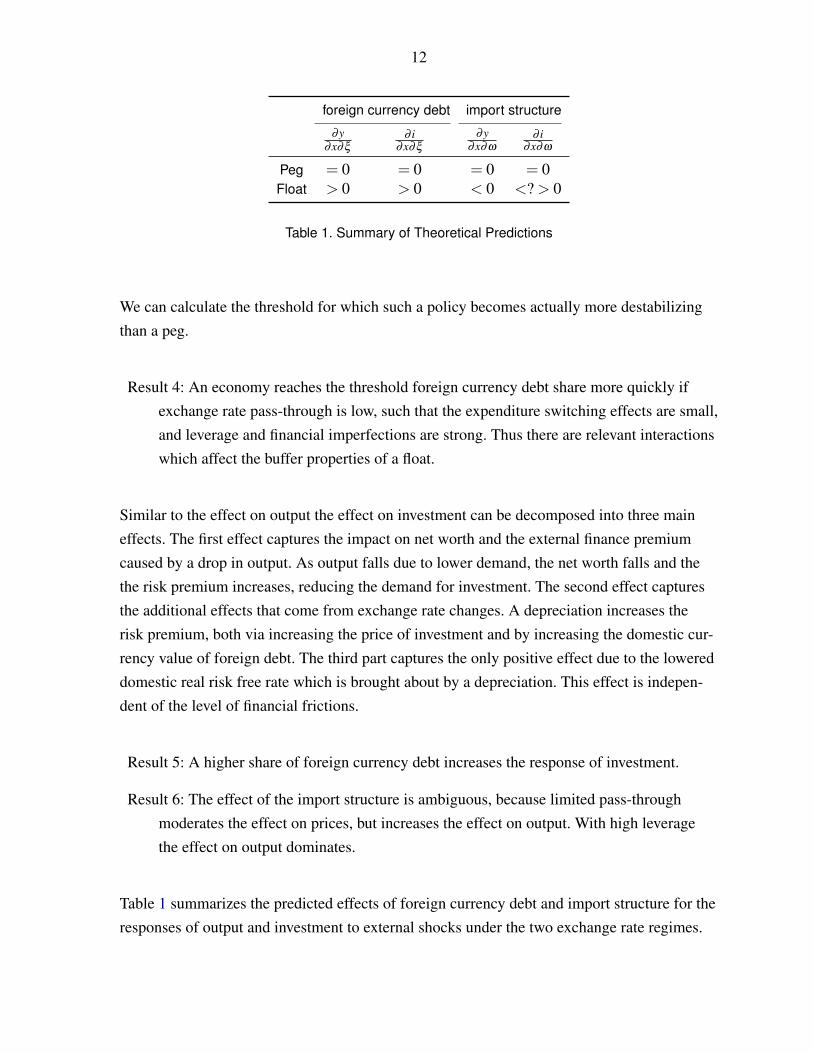
foreign currency debt import structure

∂y∂x∂ξ

∂ i∂x∂ξ

∂y∂x∂ω

∂ i∂x∂ω

Peg = 0 = 0 = 0 = 0Float > 0 > 0 < 0 <? > 0

Table 1. Summary of Theoretical Predictions

We can calculate the threshold for which such a policy becomes actually more destabilizingthan a peg.

Result 4: An economy reaches the threshold foreign currency debt share more quickly ifexchange rate pass-through is low, such that the expenditure switching effects are small,and leverage and financial imperfections are strong. Thus there are relevant interactionswhich affect the buffer properties of a float.

Similar to the effect on output the effect on investment can be decomposed into three maineffects. The first effect captures the impact on net worth and the external finance premiumcaused by a drop in output. As output falls due to lower demand, the net worth falls and thethe risk premium increases, reducing the demand for investment. The second effect capturesthe additional effects that come from exchange rate changes. A depreciation increases therisk premium, both via increasing the price of investment and by increasing the domestic cur-rency value of foreign debt. The third part captures the only positive effect due to the lowereddomestic real risk free rate which is brought about by a depreciation. This effect is indepen-dent of the level of financial frictions.

Result 5: A higher share of foreign currency debt increases the response of investment.

Result 6: The effect of the import structure is ambiguous, because limited pass-throughmoderates the effect on prices, but increases the effect on output. With high leveragethe effect on output dominates.

Table 1 summarizes the predicted effects of foreign currency debt and import structure for theresponses of output and investment to external shocks under the two exchange rate regimes.

13

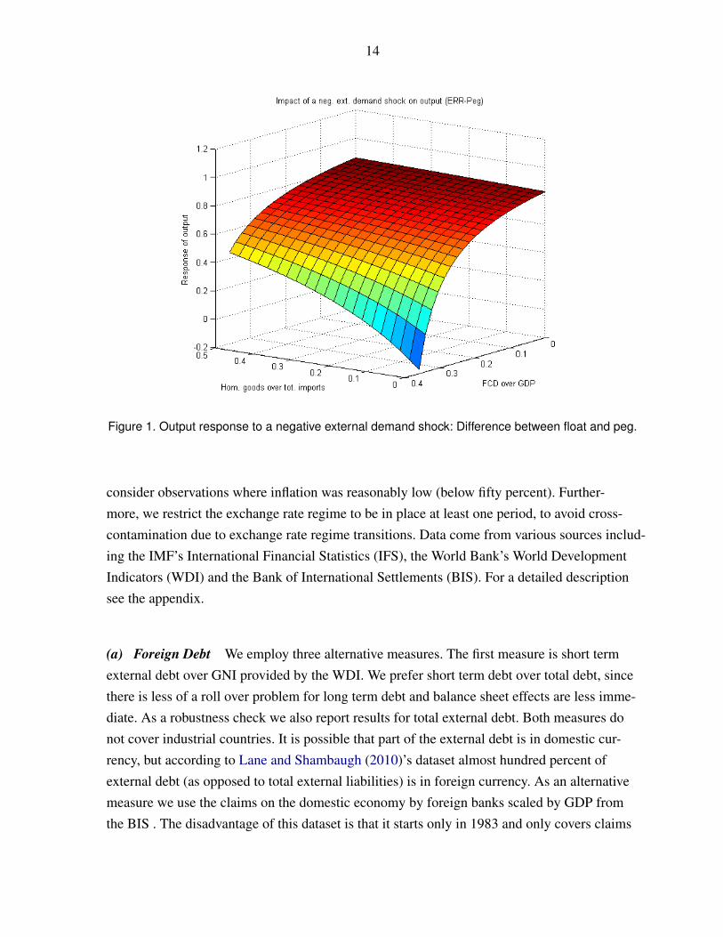
3. Simulation of Responses under Peg and Float

To illustrate graphically how the response of investment and output change with the ratioof foreign currency debt and the share of homogeneous goods in total imports, we let theparameters ξ and ω vary for given values of the other parameters. We assume values whichare standard in the literature. In particular, the share of home goods in total consumption isassumed to be γ = 0.6, the mark-up for differentiated products 10% (θ = 11) and, the elastic-ity of substitution between foreign and home consumption goods is assumed to equal φ = 2.The capital market imperfection is set to µ = 0.2 as in Céspedes, Chang, and Velasco (2003).We set κ = 2 and β = 0.96.8 K1, X1, X2 are such that output growth Y2

Y1and the real exchange

rate in both periods S1P1

and S2P2

are one. We choose ψ = 10.6 such that ratio of external debt toGDP equals 36 %. The value corresponds to the midpoint between the average short termexternal debt and the total external debt in our sample of countries.9 Using these parame-ter values we allow the share of homogeneous good imports to vary from close to zero to50% and the foreign currency debt to GDP ratio from zero to 36%, holding the overall debtlevel constant.10 Figure 1 depicts the joint role of foreign currency debt and import structure.It shows the difference in the fall of output to a negative external demand shock between acountry with a float and a country with a peg (∂y

∂x |FL− ∂y

∂x |PEG). The response under a peg is

smaller if foreign currency debt is high and the share of homogeneous goods is low.

III. DATA

We analyze the role of foreign currency debt and the import structure using a sample whichcovers yearly data for 101 countries from 1974-2007. We impose the following restrictionson the data: the sample does not include G7 countries, as the identifying assumption on theexogeneity of external shocks may not hold for large countries. Because of data quality con-cerns the study uses only countries for which we have more than five data points and discardvery poor countries with a PPP adjusted GDP per capita of less than 1000 dollars in 2007.We drop small countries with a population of less than 1 million and observations where theannual change in real GDP exceeds twenty percent. In line with previous studies we only

8Increasing κ lets the shape of the exchange rate response become increasingly concave.9In the empirical part we will be using these measures alternatively.

10There is a direct link in the model between the share of foreign debt to GDP and the parameter ξ which isderived in the appendix.

14

Figure 1. Output response to a negative external demand shock: Difference between float and peg.

consider observations where inflation was reasonably low (below fifty percent). Further-more, we restrict the exchange rate regime to be in place at least one period, to avoid cross-contamination due to exchange rate regime transitions. Data come from various sources includ-ing the IMF’s International Financial Statistics (IFS), the World Bank’s World DevelopmentIndicators (WDI) and the Bank of International Settlements (BIS). For a detailed descriptionsee the appendix.

(a) Foreign Debt We employ three alternative measures. The first measure is short termexternal debt over GNI provided by the WDI. We prefer short term debt over total debt, sincethere is less of a roll over problem for long term debt and balance sheet effects are less imme-diate. As a robustness check we also report results for total external debt. Both measures donot cover industrial countries. It is possible that part of the external debt is in domestic cur-rency, but according to Lane and Shambaugh (2010)’s dataset almost hundred percent ofexternal debt (as opposed to total external liabilities) is in foreign currency. As an alternativemeasure we use the claims on the domestic economy by foreign banks scaled by GDP fromthe BIS . The disadvantage of this dataset is that it starts only in 1983 and only covers claims

15

of banks from reporting countries. To reduce sensitivity to outliers we use log(1 + debt),where debt is the corresponding debt measure expressed in percentage points.11

(b) Import Structure In line with findings by Campa and Goldberg (2005) we use theshare of primary commodities in a country’s total imports of goods and services to measurethe extent to which a country imports high pass-through goods. The share of primary com-modities in total imports is proxied by the sum of agricultural goods, fuels, ores and metalsover total imports as provided by the WDI. Again we use log(1 + imp), where imp is theimport share of raw material in percentage points.12 The raw material share is an indirectmeasure for import price pass-through. We see several advantages over the use of a directmeasure. First, there are, to our knowledge, no direct import pass-through measures avail-able for our broad sample of countries. Estimating them would be a task of its own and wouldalso ask for a high degree of data quality and availability. Second, the literature has identifiedtwo factors that affect import price pass-through: the sectoral structure and monetary policy.Monetary policy is at least partially accounted for by our exchange rate regime variable andfrom a policy perspective it makes sense to evaluate the effects of the parts of exchange ratepass-through that are orthogonal to monetary policy separately. A further argument in favorof our measure is that pass-through varies not only over countries, but also over time. Coun-try by country pass-through estimates would be constant. In fact, the cross sectional meanof our measure varies between 23% in 1981 and 11% in 1999. Apart from the advantagesdiscussed above, a potential disadvantage of using the raw material share as a pass-throughmeasure is that a high raw material share might also have other effets than higher import pricepass-through. As detailed below, our empirical application will allow to separate the effecta higher raw material has independent from the exchange rate regime from the effect that isconditional on the exchange rate regime.

(c) Exchange Rate Regime The literature divides between de jure classification and defacto classification. According to Ghosh, Gulde, and Wolf (2002) the de jure classificationmay be understood as the intention of the authority, while the de facto classifications attemptsto capture the actual behavior of the respective authority. Since we are interested in the actual

11We do not distinguish public and private debt. While accurate data of comparable coverage is not easilyavailable, using overall debt as opposed to private debt, is likely to work against finding balance sheet effects.

12In our analysis we focus on import prices because exchange policy can affect exports both if export pricesare set in domestic or in foreign currency. If they are set in domestic currency a nominal depreciation makesthem cheaper in foreign currency. The depreciation then leads to an increase in export demand and a rise inexport volume. If prices are set in foreign currency a depreciation leads to an increase in the domestic currencyvalue of exports, while the export volume is constant.

16

conduct of exchange rate policy, our preferred exchange range classification is Levy-Yeyatiand Sturzenegger (2005)’s de facto classification (LYS) which covers the period from 1974 to2004. The authors use cluster analysis on exchange rate data and official reserves to infer theactual exchange rate policy. The classification has the advantage that it does not rely on themovements of the exchange rate alone. A country may be pursuing inflation targeting undera freely floating exchange rate, but the observed path of the exchange rate may be quite sta-ble because of the stability of underlying fundamentals. A classification which uniquely relieson the movement of the exchange rate would incorrectly label this country as maintaining a(soft) peg. To remain consistent and comparable with most of the literature (see, for exam-ple, Broda, 2004; di Giovanni and Shambaugh, 2008), we use an exchange rate dummy thattakes the value one for a peg and zero for non peg. This approach is also in line with the the-oretical framework, where we distinguish between a monetary policy that keeps the nominalexchange rate constant and a policy that lets the exchange rate vary to some degree. We willcompare our results with estimates using the IMF’s de jure classification (1974-2007).

(d) Terms of Trade We derive our terms of trade measure from various sources. The choiceof the source is guided by the length of the provided series. For most developed countries weuse the IFS terms of trade, since it is available for a long enough period. For other nations weuse UNCTAD’s terms of trade measure. If also the latter was not available for a long enoughperiod, we made use of the constant and current export and import values available from theWDI to construct the implied terms of trade.13 For a detailed description and the respectivemeasures employed see the appendix.

(e) Foreign Interest Rate To measure the real foreign interest rate we use the short termreal interest rate of the reference country of relevance. The reference country is defined asin di Giovanni and Shambaugh (2008), essentially being the country by which a home coun-try’s monetary policy is influenced.14 Depending on availability, the nominal short term rateis given by the money market or treasury bill rate and the real rate is obtained by subtractingCPI inflation from the nominal rate in the reference country.

(f) National Accounts Real GDP and investment in local currency are taken from theWDI.

13Apart from few exceptions, if various measures exist, they tend to be identical or highly correlated.14The original dataset is somewhat shorter than our sample. For missing countries we used the updated infor-

mation provided by Reinhart and Rogoff (2004) on the partner country

17

IV. MODEL AND ESTIMATION

A. Empirical Model and Identification

In order to examine the conditional response to external shocks we estimate a recursive Inter-acted Panel VAR of the form: 1 0 0

α210,it 1 0

α310,it α32

0,it 1

∆EXVit

∆INVit

∆GDPit

= µ i+L

∑l=1

α11l 0 0

α21l,it α22

l,it α23l,it

α31l,it α32

l,it α33l,it

∆EXVi,t−l

∆INVi,t−l

∆GDPi,t−l

+U it (5)

where EXVi,t is an external variable, either the log terms of trade or the foreign real interestrate, GDPi,t is log real GDP, and INVi,t is log real investment for country i in period t. Ui,t isa vector of uncorrelated iid shocks, µi is a vector of country specific intercepts and L is thenumber of lags. α

jkl,it are deterministically varying coefficients.

We identify external shocks with a small open economy assumption. Small economies’ actionshave a negligible impact on goods’ world prices and the foreign interest rate. The assump-tion implies that our two external variables do not depend on domestic conditions and impliestherefore strict exogeneity, which amounts to α12

l,it = α13l,it = 0 for all l. Various other authors

found that the exogeneity assumption for terms of trade generally holds for developing coun-tries (Broda, 2004; Loayza and Raddatz, 2007; Raddatz, 2007). Since we are only interestedin the identification of the shock to the external variable, the described partial identificationscheme is sufficient and the ordering of GDP and investment does not matter.15

Our analysis focuses on the response of output and investment to real external shocks, butdoes not attempt to identify domestic real shocks. There are several reasons for this choice.First, external shocks can be an important source of fluctuation in many developing econ-omies (Mendoza, 1995; Raddatz, 2007). Second, it improves comparability with the otherstudies that have also focused on real external shocks. Third, identification of external shocksis relatively simple for small open economies. Identification relies on the exogeneity of exter-nal variables, which has been shown to hold in various analyses of a similar type. It also doesnot impose high demands on detailed domestic data, which allows to assemble a relativelylarge data set across countries and time. While we focus on real external shocks, the dis-cussed theory would suggest that our result should also hold for other real shocks for whichidentification is more involved.

15Under the strict exogeneity assumption the model can equivalently be written in VARX form Yt =∑

Ll=1 ClYt−l + ∑

Ll=0 Dl∆EXVt−1 + Et and ∆EXVt = ∑

Ll=1 Fl∆EXVt−l +Vt , where Yt = (INVi,t ,GDPi,t)′ and Vt ,Et

are error terms.

18

B. Interaction Terms

In order to analyze how responses vary with country characteristics, we allow for interactionterms, such that the coefficients in (5) are given by:

αjk

l,it = βjk

l,1 +βjk

l,2 ·PEGit +βjk

l,3 ·FCDit +βjk

l,4 ·RAWit

+βjk

l,5 ·FCDit ·PEGit +βjk

l,6 ·RAWit ·PEGit (6)

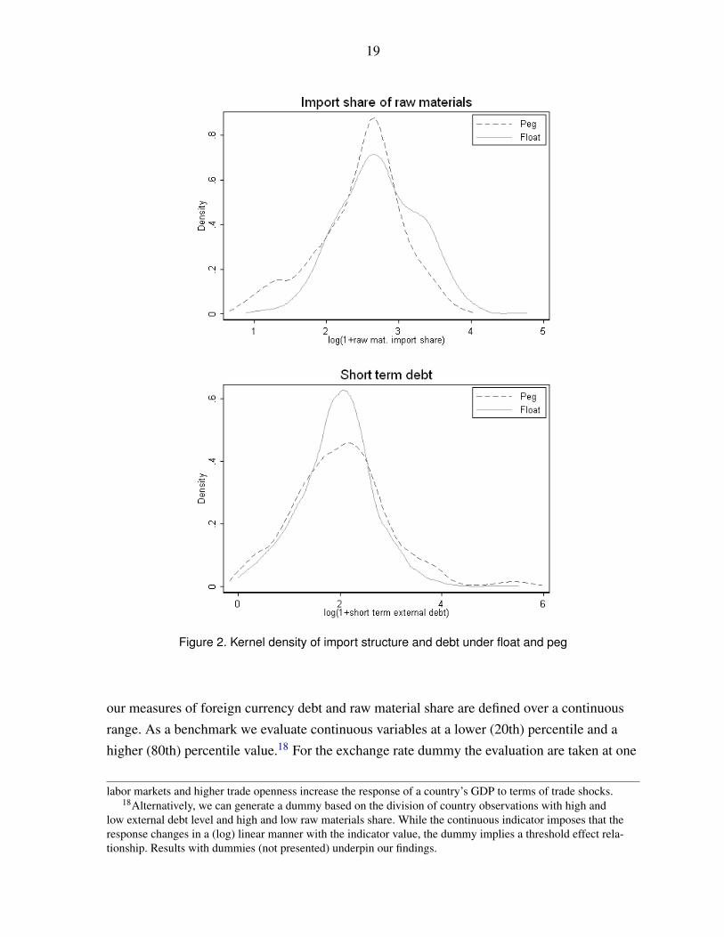
where PEGit is the exchange rate regime dummy, FCDit is the foreign currency debt mea-sure and RAWit is the share of raw materials. Several authors (Rogoff and others (2004) andSchneider and Tornell (2004)) have argued that there is a link between the exchange rateregime and the extent of foreign currency debt.16 Similarly, it is possible that there is linkbetween the import structure and the exchange rate regime. Since the the interactions of exchangerate regime, import structure, and foreign currency debt all enter separately as explanatoryvariables, a correlation of these variables does not pose a problem to the approach. In addi-tion, by also allowing explicitly for interactions between the exchange rate regime and theother two country characteristics, we can disentangle the individual effect of the respectivevariable and avoid capturing potential correlations. Empirically, however, we find no evi-dence for a link between the exchange rate regime and the level of debt or the import struc-ture. Figure 2 compares the distribution of foreign currency debt and import structure acrossexchange rate regime using kernel density estimators. The distributions appear roughly com-parable.

Previous studies that investigate stabilization properties of exchange rate regimes have setβ

jkl,3 = β

jkl,4 = β

jkl,5 = β

jkl,6 = 0. We start with the results for this specification for comparison

purposes. We then look at the effects of import structure and foreign currency debt separatelyby either setting β

jkl,3 = β

jkl,5 = 0 or β

jkl,4 = β

jkl,6 = 0. Finally, we look at the most general case

in which all coefficients are unrestricted. While we allow the coefficients to vary with countrycharacteristics for output and investment, we restrict the external dynamics to be independentof country characteristics, i.e. α11

l = β 11l,1 for all l. A Wald test does not reject the null hypoth-

esis and confirms the appropriateness of the assumption. As in every VAR single coefficientsα

jkl,it cannot be interpreted. We can, however, evaluate the coefficients at specific values and

then compute impulse responses.17 While the exchange rate regime is a dummy variable,

16However, Arteta (2005) finds an opposite pattern.17Loayza and Raddatz (2007) apply a similar technique, but let only the coefficients on the external variable

coefficients vary with country characteristics. The procedures leaves more degrees of freedom, but assumes thatthere is only heterogeneity in the initial response, but not in the transmission. The authors find that less flexible

19

Figure 2. Kernel density of import structure and debt under float and peg

our measures of foreign currency debt and raw material share are defined over a continuousrange. As a benchmark we evaluate continuous variables at a lower (20th) percentile and ahigher (80th) percentile value.18 For the exchange rate dummy the evaluation are taken at one

labor markets and higher trade openness increase the response of a country’s GDP to terms of trade shocks.18Alternatively, we can generate a dummy based on the division of country observations with high and

low external debt level and high and low raw materials share. While the continuous indicator imposes that theresponse changes in a (log) linear manner with the indicator value, the dummy implies a threshold effect rela-tionship. Results with dummies (not presented) underpin our findings.

20

(peg) and zero (float).

C. Estimation and Inference

We estimate the Panel VAR using OLS and allow for country fixed effects Since the errorterms are uncorrelated across equations by construction, we can estimate (5) equation byequation without loss in efficiency. We choose two lags following the Schwartz Criterion.19

Pesaran and Smith (1995) have shown that if there is heterogeneity in the slope coefficientsacross countries, estimates that impose a common slope are biased. The authors propose amean group estimator. However, using Monte Carlo simulations, Rebucci (2003) shows thatin typical macro panels fixed effects panel VAR estimators outperform mean group estimatorsunless slope heterogeneity is considerable. The reason is that the small sample bias may bemore detrimental to the mean group estimator than the slope heterogeneity bias to the fixedeffects estimator. Additionally, we are allowing slope coefficients to differ with country char-acteristics through the interaction terms. The use of interaction terms should therefore allevi-ate the bias from slope heterogeneity.

Since the impulse responses are a non linear function of the OLS estimates, analytical stan-dard errors that rely on first order asymptotics may be inaccurate. To address this issue we usebootstrapped standard errors as proposed by Runkle (1987) adjusted for the fact that we aredealing with a Panel and make use of interaction terms.20 The procedure may be describedin the following way. 1) Estimate (5) by OLS 2) Draw errors εi,t from a normal distributionN(0, Σ) where Σ is the estimated covariance matrix 3) use εi,t and the initial observations ofthe sample and the estimates of α

jkl,it to simulate recursively Yi,1.21 4) After the first period is

simulated for all variables in the system interact the variables with the interaction terms andnow repeat 2 and 3 as many times as there are errors.22 5) The artificial sample, together withthe interaction variables, is then used to re-estimate the coefficients of (5) and (cumulative)

19In the presence of fixed effects and lagged dependent variables, IV (or GMM) estimators are preferablefrom an asymptotic point of view if N is large and T is small. Fixed estimates are consistent for a large T.

20The programs to perform the estimation method as well as the programs to generate impulse responses andbootstrapped confidence intervals are available from the authors upon request.

21Different to the original procedure which was not described for the Panel VAR context, we draw initialobservations panel specific and perform the simulation for each country.

22We simulated the response for each country over the entire sample length and eliminated at the end of thesimulation those observations that where missing in the original sample to maintain the same weight for eachcountry as in the initial data. Since the procedure requires the multiplication of the newly generated data withthe interaction terms in the respective period, missing observations need to be filled by interpolation. Theseobservations will however not be part of the newly generated data as explained above.

21

IRFs are computed. 6) The procedure (step 2 to 5) is repeated 500 times. The 90 % confi-dence interval is drawn from the simulated estimates.

We test in two ways whether interactions with exchange rate regime, foreign currency debt,or raw material share have a statistically significant effect on the dynamics of the variables.The first way, as for example done by Broda (2004), is to check with a Wald test whether theinteraction terms in the recursive VAR model are jointly significant. We test separately for thejoint significance of all interaction terms, the significance of all interaction terms involvingFCD or RAW and the significance of all interactions between PEG and FCD or RAW . Sucha procedure tests whether the interaction terms can explain a statistically significant frac-tion of the overall variation in the dependent variables. The test allows no direct inference onwhether there are significant differences in the response to a specific shock, at a specific timehorizon. To address this question we look directly at the empirical distribution of impulseresponse differences and evaluate which fraction lies above zero. The bootstrap procedureautomatically accounts for cross correlation between the impulse responses. We report thedifference between pegs and floats, conditional on the level of foreign currency debt or importstructure. We also bootstrap the difference in the peg-float difference between high and lowforeign currency debt or high and low raw material share. We thereby account for the effectthat import structure and foreign currency debt have irrespective of the exchange rate regime.

V. RESULTS

A. Floats versus Pegs

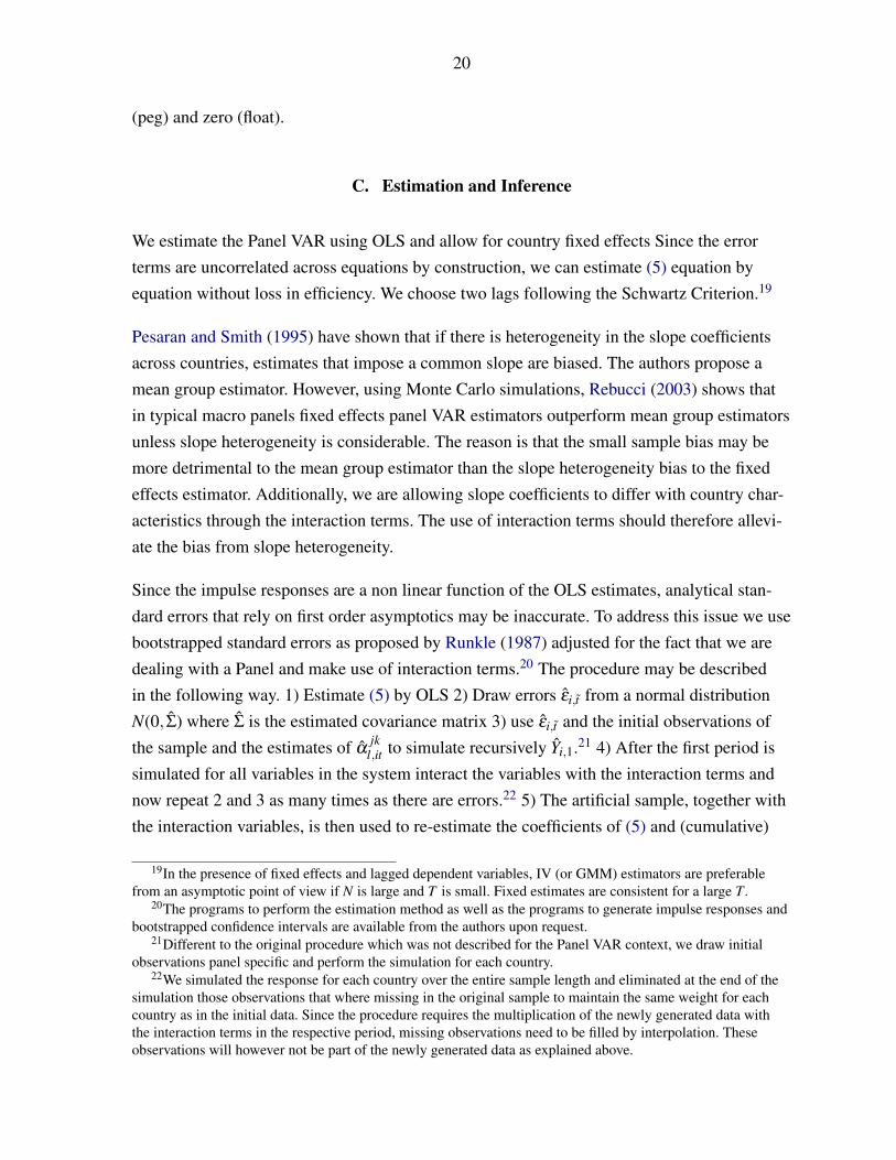
As a first step we contrast the response of output and investment under different exchangerate regimes, irrespective of the degree of foreign currency debt and of the import structure.Figure 3 shows the cumulative response of output and investment to a negative 10% termsof trade shock using the LYS exchange rate classification. With a peg output falls by about0.9 % after two years, whereas under a float output falls by about 0.5 %. The result is there-fore in line with the classic argument that flexible exchange rates are better suited to absorbreal shocks and confirms previous empirical studies by Edwards and Levy Yeyati (2005) andBroda (2004). As shown in Table 2 the interaction terms are jointly significant according to aWald test.The difference between the two output responses is marginally statistically signifi-cant. The responses of investment are similar and not statistically significantly different.

22

Figure 3. Impulse Responses for an initial 10% Terms of Trade Shock under LYS classification

Table 2 presents the results for alternative specifications. With the IMF’s de jure exchangerate regime classification, we again find evidence that the output response under a float issmaller. The results for a shock to the foreign interest rate are similar to those for the termsof trade shock. After a 100 bps shock output falls by about 0.2 % under a peg after two years,whereas output under a float remains virtually unchanged.

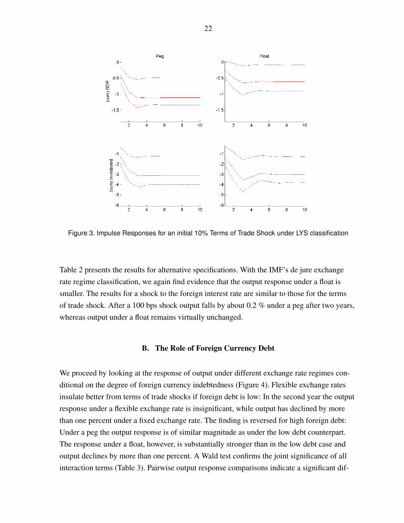
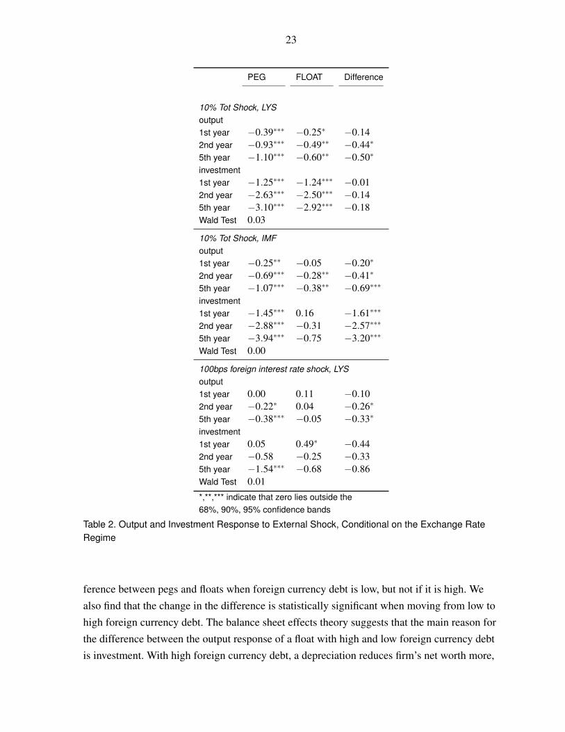
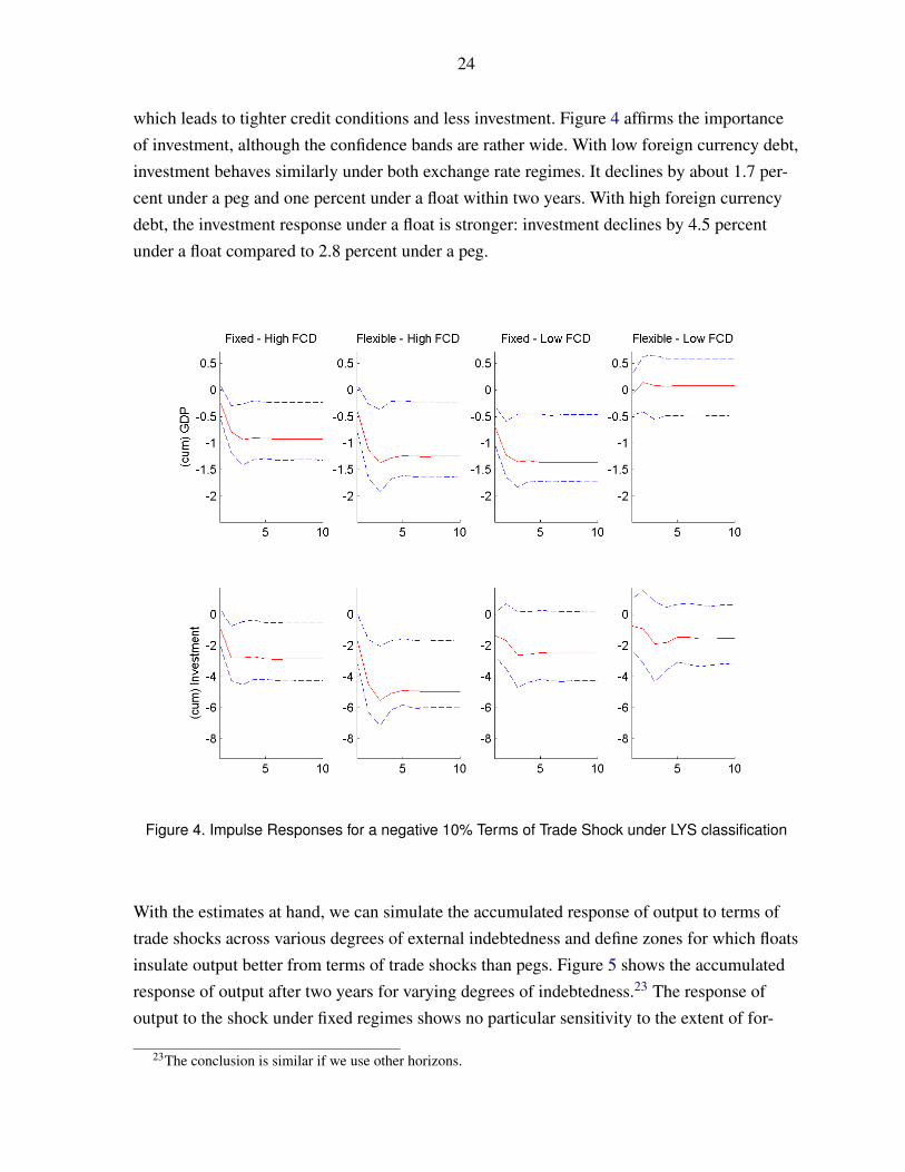
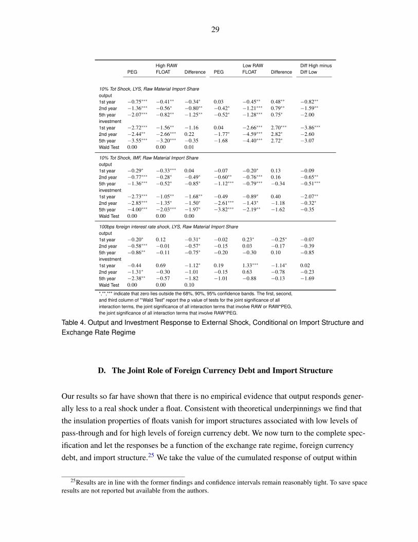
B. The Role of Foreign Currency Debt

We proceed by looking at the response of output under different exchange rate regimes con-ditional on the degree of foreign currency indebtedness (Figure 4). Flexible exchange ratesinsulate better from terms of trade shocks if foreign debt is low: In the second year the outputresponse under a flexible exchange rate is insignificant, while output has declined by morethan one percent under a fixed exchange rate. The finding is reversed for high foreign debt:Under a peg the output response is of similar magnitude as under the low debt counterpart.The response under a float, however, is substantially stronger than in the low debt case andoutput declines by more than one percent. A Wald test confirms the joint significance of allinteraction terms (Table 3). Pairwise output response comparisons indicate a significant dif-

23

PEG FLOAT Difference

10% Tot Shock, LYSoutput1st year −0.39∗∗∗ −0.25∗ −0.142nd year −0.93∗∗∗ −0.49∗∗ −0.44∗

5th year −1.10∗∗∗ −0.60∗∗ −0.50∗

investment1st year −1.25∗∗∗ −1.24∗∗∗ −0.012nd year −2.63∗∗∗ −2.50∗∗∗ −0.145th year −3.10∗∗∗ −2.92∗∗∗ −0.18Wald Test 0.03

10% Tot Shock, IMFoutput1st year −0.25∗∗ −0.05 −0.20∗

2nd year −0.69∗∗∗ −0.28∗∗ −0.41∗

5th year −1.07∗∗∗ −0.38∗∗ −0.69∗∗∗

investment1st year −1.45∗∗∗ 0.16 −1.61∗∗∗

2nd year −2.88∗∗∗ −0.31 −2.57∗∗∗

5th year −3.94∗∗∗ −0.75 −3.20∗∗∗

Wald Test 0.00

100bps foreign interest rate shock, LYSoutput1st year 0.00 0.11 −0.102nd year −0.22∗ 0.04 −0.26∗

5th year −0.38∗∗∗ −0.05 −0.33∗

investment1st year 0.05 0.49∗ −0.442nd year −0.58 −0.25 −0.335th year −1.54∗∗∗ −0.68 −0.86Wald Test 0.01

*,**,*** indicate that zero lies outside the68%, 90%, 95% confidence bands

Table 2. Output and Investment Response to External Shock, Conditional on the Exchange RateRegime

ference between pegs and floats when foreign currency debt is low, but not if it is high. Wealso find that the change in the difference is statistically significant when moving from low tohigh foreign currency debt. The balance sheet effects theory suggests that the main reason forthe difference between the output response of a float with high and low foreign currency debtis investment. With high foreign currency debt, a depreciation reduces firm’s net worth more,

24

which leads to tighter credit conditions and less investment. Figure 4 affirms the importanceof investment, although the confidence bands are rather wide. With low foreign currency debt,investment behaves similarly under both exchange rate regimes. It declines by about 1.7 per-cent under a peg and one percent under a float within two years. With high foreign currencydebt, the investment response under a float is stronger: investment declines by 4.5 percentunder a float compared to 2.8 percent under a peg.

Figure 4. Impulse Responses for a negative 10% Terms of Trade Shock under LYS classification

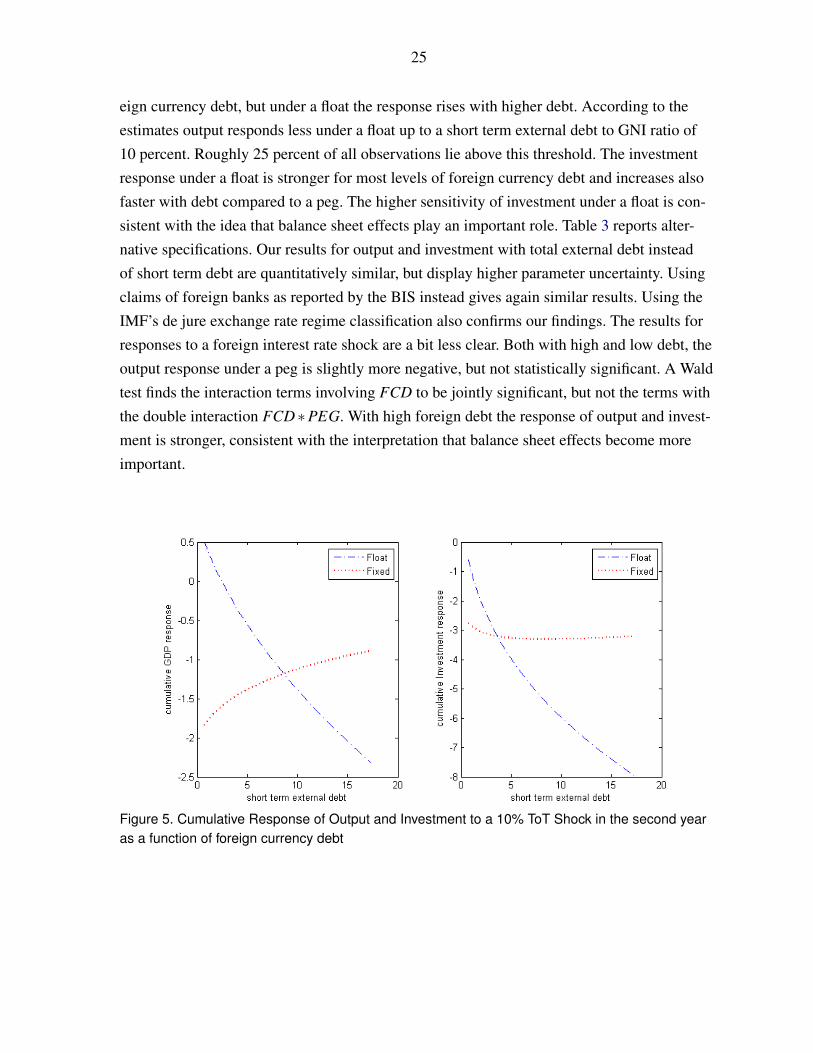
With the estimates at hand, we can simulate the accumulated response of output to terms oftrade shocks across various degrees of external indebtedness and define zones for which floatsinsulate output better from terms of trade shocks than pegs. Figure 5 shows the accumulatedresponse of output after two years for varying degrees of indebtedness.23 The response ofoutput to the shock under fixed regimes shows no particular sensitivity to the extent of for-

23The conclusion is similar if we use other horizons.

25

eign currency debt, but under a float the response rises with higher debt. According to theestimates output responds less under a float up to a short term external debt to GNI ratio of10 percent. Roughly 25 percent of all observations lie above this threshold. The investmentresponse under a float is stronger for most levels of foreign currency debt and increases alsofaster with debt compared to a peg. The higher sensitivity of investment under a float is con-sistent with the idea that balance sheet effects play an important role. Table 3 reports alter-native specifications. Our results for output and investment with total external debt insteadof short term debt are quantitatively similar, but display higher parameter uncertainty. Usingclaims of foreign banks as reported by the BIS instead gives again similar results. Using theIMF’s de jure exchange rate regime classification also confirms our findings. The results forresponses to a foreign interest rate shock are a bit less clear. Both with high and low debt, theoutput response under a peg is slightly more negative, but not statistically significant. A Waldtest finds the interaction terms involving FCD to be jointly significant, but not the terms withthe double interaction FCD ∗PEG. With high foreign debt the response of output and invest-ment is stronger, consistent with the interpretation that balance sheet effects become moreimportant.

Figure 5. Cumulative Response of Output and Investment to a 10% ToT Shock in the second yearas a function of foreign currency debt

26

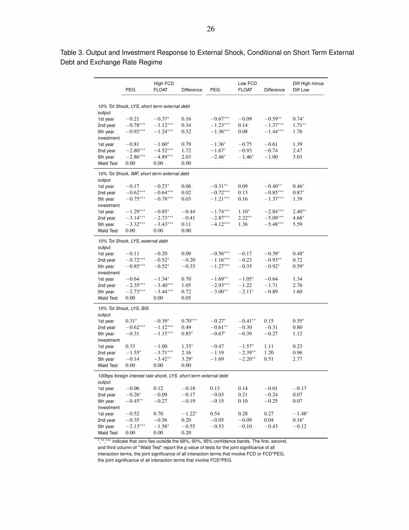
Table 3. Output and Investment Response to External Shock, Conditional on Short Term ExternalDebt and Exchange Rate Regime

High FCD Low FCD Diff High minusPEG FLOAT Difference PEG FLOAT Difference Diff Low

10% Tot Shock, LYS, short term external debtoutput1st year −0.21 −0.37∗ 0.16 −0.67∗∗∗ −0.09 −0.59∗∗ 0.74∗

2nd year −0.78∗∗∗ −1.12∗∗∗ 0.34 −1.23∗∗∗ 0.14 −1.37∗∗∗ 1.71∗∗

5th year −0.92∗∗∗ −1.24∗∗∗ 0.32 −1.36∗∗∗ 0.08 −1.44∗∗∗ 1.76investment1st year −0.81 −1.60∗ 0.79 −1.36∗ −0.75 −0.61 1.392nd year −2.80∗∗∗ −4.52∗∗∗ 1.72 −1.67∗ −0.93 −0.74 2.475th year −2.86∗∗∗ −4.89∗∗∗ 2.03 −2.46∗ −1.46∗ −1.00 3.03Wald Test 0.00 0.00 0.00

10% Tot Shock, IMF, short term external debtoutput1st year −0.17 −0.23∗ 0.06 −0.31∗∗ 0.09 −0.40∗∗ 0.46∗

2nd year −0.62∗∗∗ −0.64∗∗∗ 0.02 −0.72∗∗∗ 0.13 −0.85∗∗∗ 0.87∗

5th year −0.75∗∗∗ −0.78∗∗∗ 0.03 −1.21∗∗∗ 0.16 −1.37∗∗∗ 1.39investment1st year −1.29∗∗∗ −0.85∗ −0.44 −1.74∗∗∗ 1.10∗ −2.84∗∗∗ 2.40∗∗

2nd year −3.14∗∗∗ −2.73∗∗∗ −0.41 −2.87∗∗∗ 2.22∗∗ −5.09∗∗∗ 4.68∗

5th year −3.32∗∗∗ −3.43∗∗∗ 0.11 −4.12∗∗∗ 1.36 −5.48∗∗∗ 5.59Wald Test 0.00 0.00 0.00

10% Tot Shock, LYS, external debtoutput1st year −0.11 −0.20 0.09 −0.56∗∗∗ −0.17 −0.39∗ 0.48∗

2nd year −0.72∗∗∗ −0.52∗ −0.20 −1.16∗∗∗ −0.23 −0.93∗∗ 0.725th year −0.85∗∗∗ −0.52∗ −0.33 −1.27∗∗∗ −0.35 −0.92∗ 0.59∗

investment1st year −0.64 −1.34∗ 0.70 −1.69∗∗ −1.05∗ −0.64 1.342nd year −2.35∗∗∗ −3.40∗∗∗ 1.05 −2.93∗∗∗ −1.22 −1.71 2.765th year −2.73∗∗∗ −3.44∗∗∗ 0.72 −3.00∗∗ −2.11∗ −0.89 1.60Wald Test 0.00 0.00 0.05

10% Tot Shock, LYS, BISoutput1st year 0.31∗ −0.39∗ 0.70∗∗∗ −0.27∗ −0.41∗∗ 0.15 0.55∗

2nd year −0.62∗∗∗ −1.12∗∗∗ 0.49 −0.61∗∗ −0.30 −0.31 0.805th year −0.31 −1.15∗∗∗ 0.85∗ −0.67∗ −0.39 −0.27 1.12investment1st year 0.33 −1.00 1.33∗ −0.47 −1.57∗ 1.11 0.232nd year −1.55∗ −3.71∗∗∗ 2.16 −1.19 −2.39∗∗ 1.20 0.965th year −0.14 −3.42∗∗ 3.29∗ −1.69 −2.20∗∗ 0.51 2.77Wald Test 0.00 0.00 0.00

100bps foreign interest rate shock, LYS, short term external debtoutput1st year −0.06 0.12 −0.18 0.13 0.14 −0.01 −0.172nd year −0.26∗ −0.09 −0.17 −0.03 0.21 −0.24 0.075th year −0.45∗∗ −0.27 −0.19 −0.15 0.10 −0.25 0.07investment1st year −0.52 0.70 −1.22∗ 0.54 0.28 0.27 −1.48∗

2nd year −0.35 −0.56 0.20 −0.05 −0.09 0.04 0.16∗

5th year −2.13∗∗∗ −1.58∗ −0.55 −0.53 −0.10 −0.43 −0.12Wald Test 0.00 0.00 0.20

*,**,*** indicate that zero lies outside the 68%, 90%, 95% confidence bands. The first, second,and third column of "‘Wald Test" report the p value of tests for the joint significance of allinteraction terms, the joint significance of all interaction terms that involve FCD or FCD*PEG,the joint significance of all interaction terms that involve FCD*PEG.

27

Figure 6. Impulse Responses for a Negative 10% Terms of Trade Shock under LYS classification

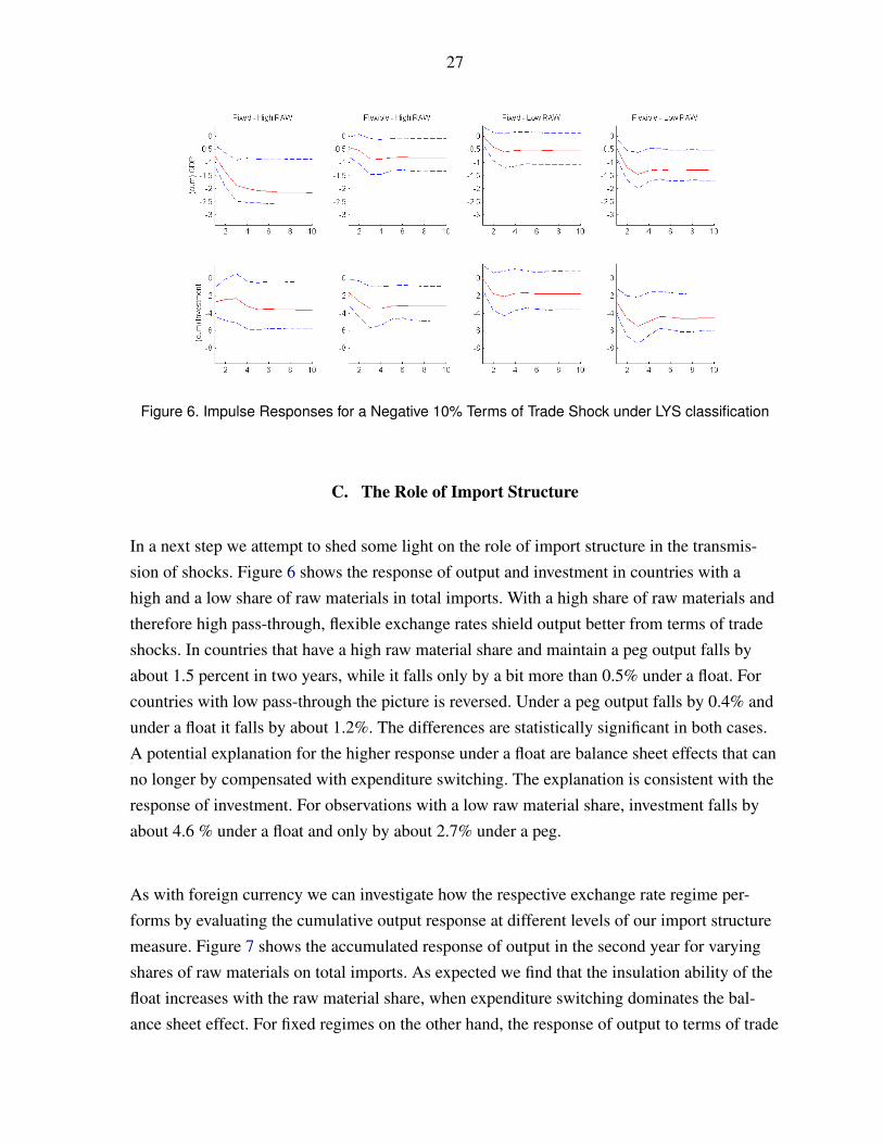
C. The Role of Import Structure

In a next step we attempt to shed some light on the role of import structure in the transmis-sion of shocks. Figure 6 shows the response of output and investment in countries with ahigh and a low share of raw materials in total imports. With a high share of raw materials andtherefore high pass-through, flexible exchange rates shield output better from terms of tradeshocks. In countries that have a high raw material share and maintain a peg output falls byabout 1.5 percent in two years, while it falls only by a bit more than 0.5% under a float. Forcountries with low pass-through the picture is reversed. Under a peg output falls by 0.4% andunder a float it falls by about 1.2%. The differences are statistically significant in both cases.A potential explanation for the higher response under a float are balance sheet effects that canno longer by compensated with expenditure switching. The explanation is consistent with theresponse of investment. For observations with a low raw material share, investment falls byabout 4.6 % under a float and only by about 2.7% under a peg.

As with foreign currency we can investigate how the respective exchange rate regime per-forms by evaluating the cumulative output response at different levels of our import structuremeasure. Figure 7 shows the accumulated response of output in the second year for varyingshares of raw materials on total imports. As expected we find that the insulation ability of thefloat increases with the raw material share, when expenditure switching dominates the bal-ance sheet effect. For fixed regimes on the other hand, the response of output to terms of trade

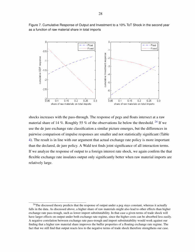
28

Figure 7. Cumulative Response of Output and Investment to a 10% ToT Shock in the second yearas a function of raw material share in total imports

shocks increases with the pass-through. The response of pegs and floats intersect at a rawmaterial share of 14 %. Roughly 55 % of the observations lie below the threshold. 24 If weuse the de jure exchange rate classification a similar picture emerges, but the differences inpairwise comparison of impulse responses are smaller and not statistically significant (Table4). The result is in line with our argument that actual exchange rate policy is more importantthan the declared, de jure policy. A Wald test finds joint significance of all interaction terms.If we analyze the response of output to a foreign interest rate shock, we again confirm the thatflexible exchange rate insulates output only significantly better when raw material imports arerelatively large.

24The discussed theory predicts that the response of output under a peg stays constant, whereas it actuallyfalls in the data. As discussed above, a higher share of raw materials might also lead to other effects than higherexchange rate pass-trough, such as lower import substitutability. In that case a given terms of trade shock willhave larger effects on output under both exchange rate regime, since the higher costs can be absorbed less easily.A negative correlation between exchange rate pass-trough and import substitutability would work against ourfinding that a higher raw material share improves the buffer properties of a floating exchange rate regime. Thefact that we still find that output reacts less to the negative terms of trade shock therefore strengthens our case.

29

High RAW Low RAW Diff High minusPEG FLOAT Difference PEG FLOAT Difference Diff Low

10% Tot Shock, LYS, Raw Material Import Shareoutput1st year −0.75∗∗∗ −0.41∗∗ −0.34∗ 0.03 −0.45∗∗ 0.48∗∗ −0.82∗∗

2nd year −1.36∗∗∗ −0.56∗ −0.80∗∗ −0.42∗ −1.21∗∗∗ 0.79∗∗ −1.59∗∗

5th year −2.07∗∗∗ −0.82∗∗ −1.25∗∗ −0.52∗ −1.28∗∗∗ 0.75∗ −2.00investment1st year −2.72∗∗∗ −1.56∗∗ −1.16 0.04 −2.66∗∗∗ 2.70∗∗∗ −3.86∗∗∗

2nd year −2.44∗∗ −2.66∗∗∗ 0.22 −1.77∗ −4.59∗∗∗ 2.82∗ −2.605th year −3.55∗∗∗ −3.20∗∗∗ −0.35 −1.68 −4.40∗∗∗ 2.72∗ −3.07Wald Test 0.00 0.00 0.01

10% Tot Shock, IMF, Raw Material Import Shareoutput1st year −0.29∗ −0.33∗∗∗ 0.04 −0.07 −0.20∗ 0.13 −0.092nd year −0.77∗∗∗ −0.28∗ −0.49∗ −0.60∗∗ −0.76∗∗∗ 0.16 −0.65∗∗

5th year −1.36∗∗∗ −0.52∗ −0.85∗ −1.12∗∗∗ −0.79∗∗∗ −0.34 −0.51∗∗∗

investment1st year −2.73∗∗∗ −1.05∗∗ −1.68∗∗ −0.49 −0.89∗ 0.40 −2.07∗∗

2nd year −2.85∗∗∗ −1.35∗ −1.50∗ −2.61∗∗∗ −1.43∗ −1.18 −0.32∗

5th year −4.00∗∗∗ −2.03∗∗∗ −1.97∗ −3.82∗∗∗ −2.19∗∗ −1.62 −0.35Wald Test 0.00 0.00 0.00

100bps foreign interest rate shock, LYS, Raw Material Import Shareoutput1st year −0.20∗ 0.12 −0.31∗ −0.02 0.23∗ −0.25∗ −0.072nd year −0.58∗∗∗ −0.01 −0.57∗ −0.15 0.03 −0.17 −0.395th year −0.86∗∗ −0.11 −0.75∗ −0.20 −0.30 0.10 −0.85investment1st year −0.44 0.69 −1.12∗ 0.19 1.33∗∗∗ −1.14∗ 0.022nd year −1.31∗ −0.30 −1.01 −0.15 0.63 −0.78 −0.235th year −2.38∗∗ −0.57 −1.82 −1.01 −0.88 −0.13 −1.69Wald Test 0.00 0.00 0.10

*,**,*** indicate that zero lies outside the 68%, 90%, 95% confidence bands. The first, second,and third column of "‘Wald Test" report the p value of tests for the joint significance of allinteraction terms, the joint significance of all interaction terms that involve RAW or RAW*PEG,the joint significance of all interaction terms that involve RAW*PEG.

Table 4. Output and Investment Response to External Shock, Conditional on Import Structure andExchange Rate Regime

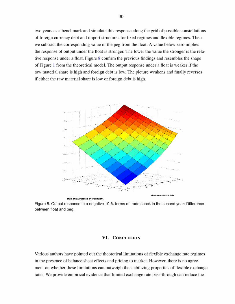
D. The Joint Role of Foreign Currency Debt and Import Structure

Our results so far have shown that there is no empirical evidence that output responds gener-ally less to a real shock under a float. Consistent with theoretical underpinnings we find thatthe insulation properties of floats vanish for import structures associated with low levels ofpass-through and for high levels of foreign currency debt. We now turn to the complete spec-ification and let the responses be a function of the exchange rate regime, foreign currencydebt, and import structure.25 We take the value of the cumulated response of output within

25Results are in line with the former findings and confidence intervals remain reasonably tight. To save spaceresults are not reported but available from the authors.

30

two years as a benchmark and simulate this response along the grid of possible constellationsof foreign currency debt and import structures for fixed regimes and flexible regimes. Thenwe subtract the corresponding value of the peg from the float. A value below zero impliesthe response of output under the float is stronger. The lower the value the stronger is the rela-tive response under a float. Figure 8 confirm the previous findings and resembles the shapeof Figure 1 from the theoretical model. The output response under a float is weaker if theraw material share is high and foreign debt is low. The picture weakens and finally reversesif either the raw material share is low or foreign debt is high.

Figure 8. Output response to a negative 10 % terms of trade shock in the second year: Differencebetween float and peg.

VI. CONCLUSION

Various authors have pointed out the theoretical limitations of flexible exchange rate regimesin the presence of balance sheet effects and pricing to market. However, there is no agree-ment on whether these limitations can outweigh the stabilizing properties of flexible exchangerates. We provide empirical evidence that limited exchange rate pass-through can reduce the

31

capacity of floating exchange rate regimes to buffer against external shocks and the presenceof high foreign currency debt can even cause the flexible exchange rate regime to be moredestabilizing than a peg. Previous studies on the role of exchange rate regimes have either notdistinguished between the various shocks that hit the economy or not accounted for differ-ences in the frictions or the economic structure that affect the response to shocks. Using anInteracted Panel VAR for a large sample of countries, we assess the role of foreign currencydebt and limited pass-through, by allowing the response of output and investment to an exter-nal shock to vary with the exchange rate regime, the foreign currency debt and the importstructure. We show that our findings are consistent with a stylized three equation IS-LM-BPmodel with foreign currency debt in the spirit of Céspedes, Chang, and Velasco (2003) whichwe extended to allow for limited pass-through. In this framework, a flexible exchange ratedoes not necessarily shield output better from real external shocks than pegs when foreigncurrency debt is high and pass-through low since contractionary balance sheet effects domi-nate the expansionary expenditure switching effects. While our results indicate that under afloat output only tends to fall by less in response to an external shock if foreign debt is lowand the import share of raw materials is high policy makers will also care about other aspectswhen choosing an exchange rate regime, such as its effects on inflation, trade volumes, longterm growth or on the likelihood of financial crises. Our framework is silent on these dimen-sions, but our results suggest that ceteris paribus the case for a float weakens if a country hashigh foreign currency debt and imports mainly low pass-through goods due to the increasedvolatility.

32

REFERENCES

Arteta, Carlos O., 2005, “Exchange Rate Regimes and Financial Dollarization: Does Flexibil-ity Reduce Currency Mismatches in Bank Intermediation?” The B.E. Journal of Macroecon-omics, Vol. 0, No. 1.

Baxter, Marianne, and Alan C. Stockman, 1989, “Business cycles and the exchange-rateregime : Some international evidence,” Journal of Monetary Economics, Vol. 23, No. 3, pp.377–400.

Bebczuk, Ricardo N., Ugo Panizza, and Arturo Galindo, 2006, “An Evaluation of the Con-tractionary Devaluation Hypothesis,” RES Working Papers 4486, Inter-American Develop-ment Bank, Research Department.

Bernanke, Ben, Mark Gertler, and Simon Gilchrist, 1998, “The Financial Accelerator in aQuantitative Business Cycle Framework,” NBER Working Papers 6455, National Bureau ofEconomic Research, Inc.

Broda, Christian, 2004, “Terms of trade and exchange rate regimes in developing countries,”Journal of International Economics, Vol. 63, No. 1, pp. 31–58.

Broda, Christian, and Cedric Tille, 2003, “Coping with terms-of-trade shocks in developingcountries,” Current Issues in Economics and Finance.

Campa, José Manuel, and Linda S. Goldberg, 2005, “Exchange Rate Pass-Through intoImport Prices,” The Review of Economics and Statistics, Vol. 87, No. 4, pp. 679–690.

Cavallo, Michele, Kate Kisselev, Fabrizio Perri, and Nouriel Roubini, 2005, “Exchange rateovershooting and the costs of floating,” Working Paper Series 2005-07, Federal Reserve Bankof San Francisco.

Céspedes, Luis Felipe, Roberto Chang, and Andres Vélasco, 2004, “Balance Sheets andExchange Rate Policy,” American Economic Review, Vol. 94, No. 4, pp. 1183–1193.

Céspedes, Luis Felipe, Roberto Chang, and Andrés Velasco, 2003, “Must Original Sin CauseMacroeconomic Damnation?” Working Papers Central Bank of Chile 234, Central Bank ofChile.

Choi, Woon Gyu, and David Cook, 2004, “Liability dollarization and the bank balance sheetchannel,” Journal of International Economics, Vol. 64, No. 2, pp. 247–275.

Cook, David, 2004, “Monetary policy in emerging markets: Can liability dollarization explaincontractionary devaluations?” Journal of Monetary Economics, Vol. 51, No. 6, pp. 1155–1181.

Devereux, Michael B., and Charles Engel, 2003, “Monetary Policy in the Open EconomyRevisited: Price Setting and Exchange-Rate Flexibility,” Review of Economic Studies, Vol. 70,No. 4, pp. 765–783.

33

Devereux, Michael B., Philip R. Lane, and Juanyi Xu, 2006, “Exchange Rates and MonetaryPolicy in Emerging Market Economies,” Economic Journal, Vol. 116, No. 511, pp. 478–506.

di Giovanni, Julian, and Jay C. Shambaugh, 2008, “The impact of foreign interest rates onthe economy: The role of the exchange rate regime,” Journal of International Economics,Vol. 74, No. 2, pp. 341–361.

Edwards, Sebastian, and Eduardo Levy Yeyati, 2005, “Flexible exchange rates as shockabsorbers,” European Economic Review, Vol. 49, No. 8, pp. 2079–2105.

Engel, Charles, 1993, “Real exchange rates and relative prices : An empirical investigation,”Journal of Monetary Economics, Vol. 32, No. 1, pp. 35–50.

Fleming, John M., 1962, “Domestic Financial Policies under Fixed and under. FloatingExchange Rates,” IMF StaffPapers 9, IMF StaffPapers.

Flood, Robert P., and Andrew K. Rose, 1995, “Fixing exchange rates A virtual quest for fun-damentals,” Journal of Monetary Economics, Vol. 36, No. 1, pp. 3–37.

Friedman, Milton, 1953, “The Case for Flexible Exchange Ratess,” Essays in Positive Econ-omics.

Galindo, Arturo, Ugo Panizza, and Fabio Schiantarelli, 2003, “Debt composition and balancesheet effects of currency depreciation: a summary of the micro evidence,” Emerging MarketsReview, Vol. 4, No. 4, pp. 330–339.

Gertler, Mark, Simon Gilchrist, and Fabio M. Natalucci, 2007, “External Constraints on Mon-etary Policy and the Financial Accelerator,” Journal of Money, Credit and Banking, Vol. 39,No. 2-3, pp. 295–330.

Ghosh, A.R., A.M. Gulde, and H.C. Wolf, 2002, Exchange Rate Regimes: Choices and Con-sequences (MIT Press).

Ghosh, Atish R., Anne-Marie Gulde, Jonathan D. Ostry, and Holger C. Wolf, 1997, “Does theNominal Exchange Rate Regime Matter?” NBER Working Papers 5874, National Bureau ofEconomic Research, Inc.

Hausmann, Ricardo, Ugo Panizza, and Ernesto Stein, 2001, “Why do countries float the waythey float?” Journal of Development Economics, Vol. 66, No. 2, pp. 387–414.

Hoffmann, Mathias, 2007, “Fixed versus Flexible Exchange Rates: Evidence from Develop-ing Countries,” Economica, Vol. 74, No. 295, pp. 425–449.

Kehoe, Timothy J., and Kim J. Ruhl, 2008, “Are Shocks to the Terms of Trade Shocks to Pro-ductivity?” Review of Economic Dynamics, Vol. 11, No. 4, pp. 804–819.

Kohlscheen, Emanuel, 2010, “Emerging floaters: Pass-throughs and (some) new commoditycurrencies,” Journal of International Money and Finance, Vol. 29, No. 8, pp. 1580 – 1595.

34

Krugman, Paul, 1986, “Pricing to Market when the Exchange Rate Changes,” NBER Work-ing Papers 1926, National Bureau of Economic Research, Inc.

Lane, Philip R., and Jay C. Shambaugh, 2010, “Financial Exchange Rates and InternationalCurrency Exposures,” American Economic Review, Vol. 100, No. 1, pp. 518–40.

Levy-Yeyati, Eduardo, and Federico Sturzenegger, 2005, “Classifying exchange rate regimes:Deeds vs. words,” European Economic Review, Vol. 49, No. 6, pp. 1603–1635.

Loayza, Norman, and Claudio E. Raddatz, 2007, “The Structural Determinants of ExternalVulnerability,” The World Bank Economic Review, Vol. 21, No. 3, pp. 359–387.

Mendoza, Enrique G, 1995, “The Terms of Trade, the Real Exchange Rate, and EconomicFluctuations,” International Economic Review, Vol. 36, No. 1, pp. 101–37.

Miniane, Jacques, and John H. Rogers, 2007, “Capital Controls and the International Trans-mission of U.S. Money Shocks,” Journal of Money, Credit and Banking, Vol. 39, No. 5, pp.1003–1035.

Mundell, Robert A., 1961, “A Theory of Optimum Currency Areas,” American EconomicReview, , No. 51, pp. 657–665.

Mussa, Michael, 1986, “Nominal exchange rate regimes and the behavior of real exchangerates: Evidence and implications,” Carnegie-Rochester Conference Series on Public Policy,Vol. 25, No. 1, pp. 117–214.

Pesaran, M. Hashem, and Ron Smith, 1995, “Estimating long-run relationships from dynamicheterogeneous panels,” Journal of Econometrics, Vol. 68, No. 1, pp. 79–113.

Raddatz, Claudio, 2007, “Are external shocks responsible for the instability of output in low-income countries?” Journal of Development Economics, Vol. 84, No. 1, pp. 155–187.

Ramcharan, Rodney, 2007, “Does the exchange rate regime matter for real shocks? Evidencefrom windstorms and earthquakes,” Journal of International Economics, Vol. 73, No. 1, pp.31–47.

Rebucci, Alessandro, 2003, “On the Heterogeneity Bias of Pooled Estimators in StationaryVAR Specifications,” IMF Working Papers 03/73, International Monetary Fund.

Reinhart, Carmen M., and Kenneth S. Rogoff, 2004, “The Modern History of Exchange RateArrangements: A Reinterpretation,” The Quarterly Journal of Economics, Vol. 119, No. 1, pp.1–48.

Rogoff, Kenneth, Ashoka Mody, Nienke Oomes, Robin Brooks, and Aasim M. Husain, 2004,“Evolution and Performance of Exchange Rate Regimes,” IMF Occasional Papers 229, Inter-national Monetary Fund.

Runkle, David E., 1987, “Vector autoregressions and reality,” Staff Report 107, FederalReserve Bank of Minneapolis.

35

Schneider, Martin, and Aaron Tornell, 2004, “Balance Sheet Effects, Bailout Guarantees andFinancial Crises,” Review of Economic Studies, Vol. 71, pp. 883–913.

Taylor, John B., 2000, “Low inflation, pass-through, and the pricing power of firms,” Euro-pean Economic Review, Vol. 44, No. 7, pp. 1389–1408.

Tsangarides, Charalambos G., 2010, “Crisis and Recovery: Role of the Exchange RateRegime in Emerging Market Countries,” IMF Working Papers 10/242, International Mone-tary Fund.

36

APPENDIX A. MODEL

The model follows Céspedes, Chang, and Velasco (2003) microfounded IS-LM-BP modelwith sticky prices, wages, and a financial accelerator mechanism as in Bernanke, Gertler,and Gilchrist (1998) and extends it by investigating the consequences of limited exchangerate pass-through. Furthermore, to have a meaningful expenditure switching effect, we aban-don the assumption of a unit elasticity of substitution between domestic and foreign goods.The model consists of a small open economy with two periods, 1 and 2. There are two typesof agents: workers and entrepreneurs. We analyze the consequences of an adverse externaldemand shock in the initial period under different exchange regimes. In the second period nofurther shocks occur.

A.1. Workers

A worker’s utility depends on consumption (Ct), labor (Lt) and real money holdings (Mt/Qt)in periods 1 and 2

U =2

∑t=1

βt[

logCt−σ −1

σ

1υ

Lυt + log

(Mt

Qt

)].

Workers choose consumption and money holdings. They supply labor in a monopolisticallycompetitive market. They set their wage one period in advance and then supply the amount oflabor demanded by firms at the wage set. Log utility in consumption implies that expectedlabor supply will always be one Et−1Lt = 1. Consumption is an aggregate over domestic(CH,t) and foreign goods (CF,t)

Ct = υ

[γC1−φ

H,t +(1− γ)C1−φ

F,t

] 11−φ

,

where φ is the elasticity of substitution, γ is a preference parameter related to the expendi-ture share of domestic goods and υ = γ−γ (1− γ)−(1−γ) is a constant. Foreign goods are aCobb-Douglas composite of homogeneous goods (CHOM

F,t ) with expenditure share ω and dif-ferentiated products (CHET

F,t ) with share 1−ω .26

CF,t =(

CHOMF,t

)ω (CHET

F,t)1−ω

,

26Both CH,t =[∫ 1

0 Cθ−1

θ

H, jt d j] θ

θ−1and CHET

F,t =[∫ 1

0

(CHET

F, jt

) θ−1θ d j

] θ

θ−1

are CES aggregates over varieties with

elasticity of substitution θ .

37

The only asset workers can hold is money and the worker’s budget constraint is

QtCt = WtLt +Mt−1−Mt +Tt (7)

Seignorage is rebated via lump sum transfers Tt such that workers spend all income on con-sumption in equilibrium. The expenditure minimizing price index of the consumption bundleis

Qt =[

γP1−φ

H,t +(1− γ){(

PHOMF,t

)ω (PHET

Ft)1−ω

}1−φ] 1

1−φ

where PH,t and PHETF,t are the expenditure minimizing price indices for home and foreign dif-

ferentiated goods.

A.2. Production and Price Setting

Domestic varieties are produced by a continuum of firms j with production function

Yjt = AKαjt L

1−α

jt ,

where K jt is the firms’s capital and composite labor is

L jt =[∫ 1

0L

σ−1σ

i jt di] σ

σ−1

.

Firm j maximizes profits Π jt = PjtYjt −∫ 1

0 WitLi jtdi−RtK jt and sets prices in advance. Profitmaximization implies a constant markup over expected marginal costs MCH,t .

PH,t =θ

θ −1Et−1MCH,t

The market for foreign homogeneous goods is perfectly competitive. We normalize the for-eign currency price of foreign homogeneous goods to one. The price in domestic currency istherefore the nominal exchange rate

PHOMF,t = St .

38

Foreign firms producing differentiated goods set their price in domestic currency one periodin advance at a mark-up over their expected marginal costs resulting in the price index27

PHETF,t =

θ

θ −1Et−1StMCF,t .

If a shock occurs, the exchange rate reacts, but because differentiated goods are priced indomestic currency, exchange rate pass-through to import prices will be limited.

A.3. Entrepreneurs

Entrepreneurs own domestic firms and provide capital. They start with a given amount of cap-ital K1 and a given external debt. The external debt can be denominated in foreign currency(D∗1) or domestic currency (D1). The investment good has the same composition as the con-sumption bundle and firms buy it at price Q1. Capital depreciates completely after one period,so that investment is the capital stock in the next period. In the first period entrepreneurs buycapital. In the second period they use their profits to buy foreign goods. Entrepreneurs financeinvestment through their net worth and external debt.

P1N1 +S1D∗2 +D2 = Q1I1

Entrepreneur’s net worth is the return on capital plus profits minus debt repayment

P1N1 = R1K1 +Π1−S1D∗1−D1 = P1Y1−W1L1−S1D∗1−D1

Because of capital market imperfections entrepreneurs pay a premium (η1) that increaseswith the ratio of investment over net worth. µ is a measure for the strength of imperfections.28

1+η1 =(

Q1I1

P1N1

)µ

Assuming entrepreneurs to be risk neutral, no arbitrage implies that the expected yield oncapital equals the cost of foreign borrowing

R2

Q1= (1+ρ)(1+η1)

S2

S1

27For simplicity we assume that their marginal costs in foreign currency MCFt are constant at θ−1

θ, which

implies that, if no shocks occur, all foreign goods will be supplied at the same price St .28Céspedes, Chang, and Vélasco (2004) provide a microfounded motivation for µ .

39

where ρ is the foreign interest rate.

A.4. Monetary Policy

We consider two alternative monetary policies: an exchange rate peg, and a floating exchangerate. Small letters denote log deviations from the no shock equilibrium. Under a peg the exchangerate is constant

st = 0. (8)

Under the float, the monetary authority keeps the money supply constant in the period wherethe shock occurs and lets the exchange rate adjust endogenously. Over the long term the author-ity cares about price stability and adjusts the money supply such that the price level in thesecond period stays constant.

m1 = 0, p2 = 0. (9)

We will show that this policy has a reduced form representation, which can be described by arule under which the monetary authority lets it the exchange rate depreciate when an adverseshock occurs, given by:

st =−κyt . (10)

A.5. Market Clearing

In the initial period the demand for domestic goods comes from domestic consumption, domes-tic investment, and exports. Foreigners demand an exogenous amount of domestic goodsdenoted in foreign currency X .

Y1 = γ

(P1

Q1

)−θ

(I1 +C1)+S1

P1X1 (11)

In the second period, there is no further investment and, given that entrepreneurs consumeonly imports, the market clearing condition is

40

Y2 = γ

(P2

Q2

)−θ

C2 +S2

P2X2. (12)

APPENDIX B. DERIVATION OF THE IS-LM-BP EQUATIONS

The steps follow closely Céspedes, Chang, and Velasco (2003) and are therefore brief.

B.1. IS Curve

Using the pricing rule and the fact that workers consume all income, the log linear version ofthe market clearing condition in period 2 (12) is

y2 = κ [(φ −1)(q2− p2)+ y2]+ (1−κ)(s2− p2) (13)

where κ = γ (1−α)(1−θ−1)( P2

Q2

)1−φ

.

The log linearized version of the price index in period 2 is

q2 =(1− γ

′2)

s2 + γ′2 p2, (14)

where γ ′2 = 1− (1− γ)(

S2Q2

)(1−φ).29 Using equations (13) and (14) gives output as a function

of the real exchange rate

y2 = Ξ(s2− p2) , (15)

where Ξ = [1+(φ −1)(1− γ ′2)κ/(1−κ)]≥ 1.

Using (15) in the log linear version of (7) the consumption level in period 2 is given by

c2 = y2− (q2− p2) (16)

29The share of differentiated goods plays no role, because no shocks occur in the second period and foreignproducers of differentiated goods take shocks in the initial period into account.

41

Since no shock occurs in the second period l = 0, output deviations in the second period aredriven by investment.

y2 = αi1 (17)

The linearized version of the market clearing condition in the first period (11) is

τy1 +(1− τ) [c1 +φq1] = λ [i1 +φq1]+ (1−λ )(s1 + x1) (18)

where τ = 1

1−γ

(P1Q1

)−φ

(1−α)(1−θ−1)> 1 and λ =

γ

(P1Q1

)−φ

I1

γ

(PQ

)−φ

I1+S1P1

X1

< 1.

Since capital is predetermined and wages are preset we have from the workers budget con-straint (7).

q1 + c1 =y1

1−α(19)

The price index in period 1 is

q1 =(1− γ

′1)

ωs1 (20)

where γ ′1 = 1− (1− γ)(

S1Q1

)(1−φ). Combining (18), (19) and (20) gives the IS curve

Ay1 = λ i1 +(1−λ )x1 +[(1−λ )+λωg(φ)]s1

where A is given by(1−τα

1−α

). τ > 1 is the ratio of output to output net of consumption and α is

the capital share in production and g(φ) = (1− γ ′1) [φ +(φ −1)(τ−1)/λ ].

B.2. LM: Money Demand

From the consumer maximization problem we have that the log linear version of money demandin period one and two is respectively

ζ (m1−q1)+(1−ζ )(c2 +q2−q1) = c1 (21)

ζ (m2−q2) = c2 (22)

42

where ζ = 1−β Q1C1/Q2C2 , which is assumed to be positive. Combining the above equationwith (16), (17), (19), and (20) gives

m1 =1ζ

y1

1−α− (1−ζ )

ζαi1−

(1−ζ )ζ

p2 (23)

The LM schedule which describes the demand for money (m1) under the float is thus givenby:30

m1 = By1−Ci1 (24)

where B = 1ζ (1−α) and C = (1−ζ )α

ζare positive constants. Money demand increases with out-

put and decreases with investment, since for a given output more investment means less con-sumption, which depresses money demand. Under the peg the money supply adjusts.

B.3. BP: Entrepreneurs

The return on investment must satisfy the arbitrage condition with foreign returns adjusted bya risk premium

r2−q1− p2 = ρ +η1 +(s2− p2)− s1 (25)

The marginal product of capital is given by r2− p2 = −i1 (1−α). Using this result, (20) and(15) gives:

i1Φ−1 =−(ρ +η1)+ [1− (1− γ)ω]s1 (26)

where Φ = Ξ

Ξ(1−α)+α≥ 1.

The log linear version of the risk premium is

η1 = µ [q1 + i1−n1] (27)

The log linear version of net worth equation

n1 = (1+ψ)δyy1−ψξ s1 (28)

where δy = θ−1 [1− (1−α)(1−θ−1)]−1 and ψ = (S1D∗1 +D1)/P1N1 is the debt to net

worth ratio.

30The LM curve is independent of the exchange rate due to the log in real money holdings. Allowing a moregeneral framework does not affect the results.

43

Using (28) in (27) gives:

η = µ{

i− (1+ψ)δyy+[(1− γ)ω +ψξ ]s}

which can be used in (26) to derive the BP schedule:31

Γi1 =−ρ + µ (1+ψ)δyy1−µ [(1− γ)ω +ψξ ]s1 +[1− (1− γ)ω]s1

Note also that there is a direct link between ψ and the share of debt to GDP. To see this notethat

P1N1

P1Y1=

R1K1 + Π1

P1Y1−

S1D∗1P1Y1

− D1

P1Y1

=P1Y1−W1L1

P1Y1−

S1D∗1P1Y1

− D1

P1Y1

Using the standard pricing rule W1LP1Y1

= (1−α) θ−1θ

this implies

P1N1

P1Y1= 1− (1−α)

(1−θ

−1)− S1D∗1 + D1

P1Y1

Varying the share of foreign currency debt to GDP ratio(S1D∗1/P1Y1

)gives the implied (P1N1/P1Y1)

ratio (for a given level of domestic debt D1/P1Y1), which in turn allows to determine the totaldebt to net worth ratio ψ = (S1D∗1 +D1)/P1N1 and the implied foreign currency share intotal debt ratio ξ = S1D∗1/

(S1D∗1 + D1

). Consider the standard parametrization θ = 11 and

α = 1/3 then we have for a domestic debt to GDP ratio of 12% and a foreign debt to GDPratio of 24% that P1N1/P1Y1 = 0.04 and ψ = 9 and ξ = 2/3.

APPENDIX C. SOLVING THE SYSTEM

In the following we use equations (1), (2) and (24) and combine them with the monetarypolicy to determine the respective implied response of output and investment to an externaldemand shock.

31Where Γ =(Φ−1 + µ

),

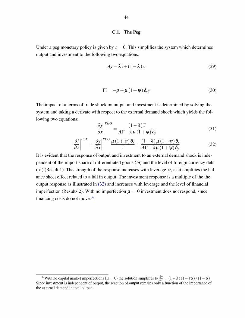
44

C.1. The Peg

Under a peg monetary policy is given by s = 0. This simplifies the system which determinesoutput and investment to the following two equations:

Ay = λ i+(1−λ )x (29)

Γi =−ρ + µ (1+ψ)δyy (30)

The impact of a terms of trade shock on output and investment is determined by solving thesystem and taking a derivate with respect to the external demand shock which yields the fol-lowing two equations:

∂y∂x

∣∣∣∣PEG

=(1−λ )Γ

AΓ−λ µ (1+ψ)δy(31)

∂ i∂x

∣∣∣∣PEG

=∂y∂x

∣∣∣∣PEGµ (1+ψ)δy

Γ=

(1−λ )µ (1+ψ)δy

AΓ−λ µ (1+ψ)δy(32)

It is evident that the response of output and investment to an external demand shock is inde-pendent of the import share of differentiated goods (ω) and the level of foreign currency debt( ξ ) (Result 1). The strength of the response increases with leverage ψ , as it amplifies the bal-ance sheet effect related to a fall in output. The investment response is a multiple of the theoutput response as illustrated in (32) and increases with leverage and the level of financialimperfection (Results 2). With no imperfection µ = 0 investment does not respond, sincefinancing costs do not move.32

32With no capital market imperfections (µ = 0) the solution simplifies to ∂y∂x = (1−λ )(1− τα)/(1−α) .

Since investment is independent of output, the reaction of output remains only a function of the importance ofthe external demand in total output.

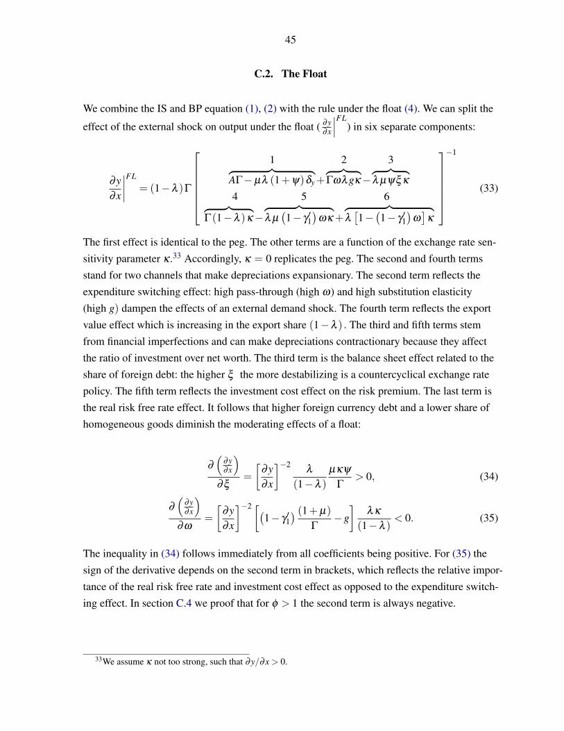
45

C.2. The Float

We combine the IS and BP equation (1), (2) with the rule under the float (4). We can split the

effect of the external shock on output under the float ( ∂y∂x

∣∣∣FL) in six separate components:

∂y∂x

∣∣∣∣FL

= (1−λ )Γ

1 2 3︷ ︸︸ ︷

AΓ−µλ (1+ψ)δy +︷ ︸︸ ︷Γωλgκ−

︷ ︸︸ ︷λ µψξ κ

4 5 6︷ ︸︸ ︷Γ(1−λ )κ−

︷ ︸︸ ︷λ µ(1− γ

′1)

ωκ +︷ ︸︸ ︷λ[1−(1− γ

′1)

ω]

κ

−1

(33)

The first effect is identical to the peg. The other terms are a function of the exchange rate sen-sitivity parameter κ .33 Accordingly, κ = 0 replicates the peg. The second and fourth termsstand for two channels that make depreciations expansionary. The second term reflects theexpenditure switching effect: high pass-through (high ω) and high substitution elasticity(high g) dampen the effects of an external demand shock. The fourth term reflects the exportvalue effect which is increasing in the export share (1−λ ) . The third and fifth terms stemfrom financial imperfections and can make depreciations contractionary because they affectthe ratio of investment over net worth. The third term is the balance sheet effect related to theshare of foreign debt: the higher ξ the more destabilizing is a countercyclical exchange ratepolicy. The fifth term reflects the investment cost effect on the risk premium. The last term isthe real risk free rate effect. It follows that higher foreign currency debt and a lower share ofhomogeneous goods diminish the moderating effects of a float:

∂

(∂y∂x

)∂ξ

=[

∂y∂x

]−2λ

(1−λ )µκψ

Γ> 0, (34)

∂

(∂y∂x

)∂ω

=[

∂y∂x

]−2[(1− γ

′1) (1+ µ)

Γ−g]

λκ

(1−λ )< 0. (35)

The inequality in (34) follows immediately from all coefficients being positive. For (35) thesign of the derivative depends on the second term in brackets, which reflects the relative impor-tance of the real risk free rate and investment cost effect as opposed to the expenditure switch-ing effect. In section C.4 we proof that for φ > 1 the second term is always negative.

33We assume κ not too strong, such that ∂y/∂x > 0.

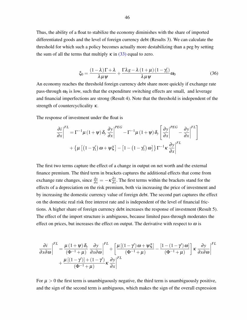
46

Thus, the ability of a float to stabilize the economy diminishes with the share of importeddifferentiated goods and the level of foreign currency debt (Results 3). We can calculate thethreshold for which such a policy becomes actually more destabilizing than a peg by settingthe sum of all the terms that multiply κ in (33) equal to zero.

ξ0 =(1−λ )Γ+λ

λ µψ+

Γλg−λ (1+ µ)(1− γ ′1)λ µψ

ω0 (36)

An economy reaches the threshold foreign currency debt share more quickly if exchange ratepass-through ω0 is low, such that the expenditure switching effects are small, and leverageand financial imperfections are strong (Result 4). Note that the threshold is independent of thestrength of countercyclicality κ .

The response of investment under the float is

∂ i∂x

∣∣∣∣FL

= Γ−1

µ (1+ψ)δy∂y∂x

∣∣∣∣PEG

−Γ−1

µ (1+ψ)δy

[∂y∂x

∣∣∣∣PEG

− ∂y∂x

∣∣∣∣FL]

+{

µ[(

1− γ′1)

ω +ψξ]−[1−(1− γ

′1)

ω]}

Γ−1

κ∂y∂x

∣∣∣∣FL

The first two terms capture the effect of a change in output on net worth and the externalfinance premium. The third term in brackets captures the additional effects that come fromexchange rate changes, since ∂ s

∂x = −κ∂y∂x . The first terms within the brackets stand for the

effects of a depreciation on the risk premium, both via increasing the price of investment andby increasing the domestic currency value of foreign debt. The second part captures the effecton the domestic real risk free interest rate and is independent of the level of financial fric-tions. A higher share of foreign currency debt increases the response of investment (Result 5).The effect of the import structure is ambiguous, because limited pass-through moderates theeffect on prices, but increases the effect on output. The derivative with respect to ω is

∂ i∂x∂ω

∣∣∣∣FL

=µ (1+ψ)δy

(Φ−1 + µ)∂y

∂x∂ω

∣∣∣∣FL

+[

µ [(1− γ ′)ω +ψξ ](Φ−1 + µ)

− [1− (1− γ ′)ω](Φ−1 + µ)

]κ

∂y∂x∂ω

∣∣∣∣FL

+µ [(1− γ ′)]+(1− γ ′)

(Φ−1 + µ)κ

∂y∂x

∣∣∣∣FL

For µ > 0 the first term is unambiguously negative, the third term is unambiguously positive,and the sign of the second term is ambiguous, which makes the sign of the overall expression

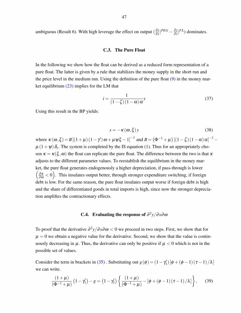
47

ambiguous (Result 6). With high leverage the effect on output (∂y∂x |

PEG− ∂y∂x |

FL) dominates.

C.3. The Pure Float

In the following we show how the float can be derived as a reduced form representation of apure float. The latter is given by a rule that stabilizes the money supply in the short run andthe price level in the medium run. Using the definition of the pure float (9) in the money mar-ket equilibrium (23) implies for the LM that

i =1

(1−ζ )(1−α)αy (37)

Using this result in the BP yields:

s =−κ (ω,ξ )y (38)

where κ (ω,ξ )= B [(1+ µ)(1− γ ′)ω + µψξ −1]−1 and B =(Φ−1 + µ

)[(1−ζ )(1−α)α]−1−

µ (1+ψ)δy. The system is completed by the IS equation (1). Thus for an appropriately cho-sen κ = κ(ξ ,ω) the float can replicate the pure float. The difference between the two is that κ

adjusts to the different parameter values. To reestablish the equilibrium in the money mar-ket, the pure float generates endogenously a higher depreciation, if pass-through is lower(

∂κ

∂ω< 0)

. This insulates output better, through stronger expenditure switching, if foreigndebt is low. For the same reason, the pure float insulates output worse if foreign debt is highand the share of differentiated goods in total imports is high, since now the stronger deprecia-tion amplifies the contractionary effects.

C.4. Evaluating the response of ∂ 2y/∂x∂ω

To proof that the derivative ∂ 2y/∂x∂ω < 0 we proceed in two steps. First, we show that forµ = 0 we obtain a negative value for the derivative. Second, we show that the value is contin-uously decreasing in µ . Thus, the derivative can only be positive if µ < 0 which is not in thepossible set of values.

Consider the term in brackets in (35) . Substituting out g(φ)= (1− γ ′1) [φ +(φ −1)(τ−1)/λ ]we can write.

(1+ µ)(Φ−1 + µ)

(1− γ

′1)−g =

(1− γ

′1){ (1+ µ)

(Φ−1 + µ)− [φ +(φ −1)(τ−1)/λ ]

}, (39)

48

since (1− γ ′1) > 0, it is sufficient to determine the sign of the term in curly brackets.

Now consider µ = 0. Since Φ = Ξ

Ξ(1−α)+α> 1, multiplying all terms with Φ−1 will not

change the sign of term in curly brackets and we have:

1−α

[φ +(φ −1) τ−1

λ

]Ξ

− (1−α)[

φ +(φ −1)τ−1

λ

]≤ 0

The inequality follows form the fact that for φ = 1 , we have Ξ = 1 and thus the entire term

is zero. For any value of φ > 1 the term is negative since [φ+(φ−1) τ−1λ

]Ξ

and[φ +(φ −1) τ−1

λ

]are increasing in φ . The last step is to show that (39) is decreasing in µ . This is the case since

g and γ ′1 are independent of µ and∂ [(1+µ)/(Φ−1+µ)]

∂ µ< 0 since Φ−1 < 1 for φ > 1.

APPENDIX D. DATA SOURCES

In the following we describe the indices and transformations which we applied to the data:

Exchange Rate Regimes: The de jure classification needed to be unified since it is based onthe changing IMF Annual Report on Exchange Arrangements and Exchange Restric-tions (AREAER). The classification went through four distinct phases of change. It ispossible to group the countries consistently into 3 broad categories, floating, interme-diate and fixed regimes. The original IMF classification is coded in four taxonomies:Taxonomy 1 from 1975 to 1976 includes: "Pegged to a single currency" (1), "Pegged toa composite (including the SDR)" (2), "Floating - adjusted according to a set of indica-tors" (3), "Floating - common margins" (4) and "Floating - independently" (5). Taxon-omy 2 from 1977 to 1981 distinguishes: "Pegged to a single currency" (1), "Pegged toa composite (including the SDR)" (2), "Adjusted according to a set of indicators" (3),"Cooperative exchange arrangements" (4), "Other" (5). Taxonomy 3 ranges from 1982to 1998 with: "Pegged to a single currency" (1), "Pegged to a composite (including theSDR)" (2), "Flexibility limited vis-à-vis a single currency" (3), "Flexibility limited vis-à-vis a cooperative arrangement" (4), "Adjusted according to a set of indicators" (5),"Other managed floating" (6) and "Independently floating" (7). Taxonomy 4 from 1998to today: "Exchange arrangement with no separate legal tender" (1), "Currency boardarrangement" (2), "Conventional pegged arrangement" (3), "Conventional peg to a bas-ket" (3,5), "Pegged exchange rate within horizontal bands" (4), "Crawling peg" (5),"Crawling band" (5), "Managed floating (7) and "Independently floating" (8). The "har-monized" IMF de jure classification is then based on the following mapping:

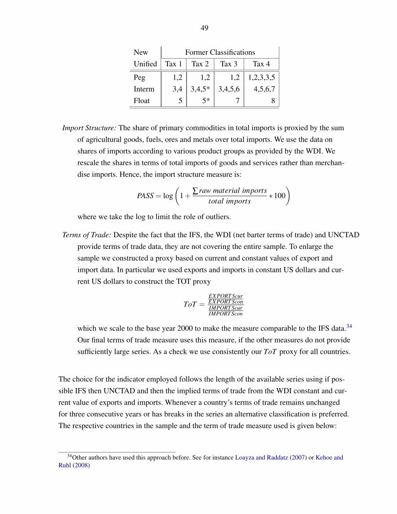
49

New Former ClassificationsUnified Tax 1 Tax 2 Tax 3 Tax 4

Peg 1,2 1,2 1,2 1,2,3,3,5Interm 3,4 3,4,5* 3,4,5,6 4,5,6,7Float 5 5* 7 8

Import Structure: The share of primary commodities in total imports is proxied by the sumof agricultural goods, fuels, ores and metals over total imports. We use the data onshares of imports according to various product groups as provided by the WDI. Werescale the shares in terms of total imports of goods and services rather than merchan-dise imports. Hence, the import structure measure is:

PASS = log(

1+ ∑raw material importstotal imports

∗100)

where we take the log to limit the role of outliers.

Terms of Trade: Despite the fact that the IFS, the WDI (net barter terms of trade) and UNCTADprovide terms of trade data, they are not covering the entire sample. To enlarge thesample we constructed a proxy based on current and constant values of export andimport data. In particular we used exports and imports in constant US dollars and cur-rent US dollars to construct the TOT proxy

ToT =EXPORT ScurEXPORT SconIMPORT ScurIMPORT Scon

which we scale to the base year 2000 to make the measure comparable to the IFS data.34

Our final terms of trade measure uses this measure, if the other measures do not providesufficiently large series. As a check we use consistently our ToT proxy for all countries.

The choice for the indicator employed follows the length of the available series using if pos-sible IFS then UNCTAD and then the implied terms of trade from the WDI constant and cur-rent value of exports and imports. Whenever a country’s terms of trade remains unchangedfor three consecutive years or has breaks in the series an alternative classification is preferred.The respective countries in the sample and the term of trade measure used is given below:

34Other authors have used this approach before. See for instance Loayza and Raddatz (2007) or Kehoe andRuhl (2008)

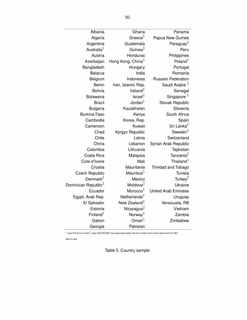
50

Albania Ghana PanamaAlgeria Greece1 Papua New Guinea

Argentina Guatemala Paraguay2

Australia1 Guinea2 PeruAustria Honduras Philippines

Azerbaijan Hong Kong, China1 Poland1

Bangladesh Hungary PortugalBelarus India RomaniaBelgium Indonesia Russian Federation

Benin Iran, Islamic Rep. Saudi Arabia 2

Bolivia Ireland1 SenegalBotswana Israel1 Singapore 1

Brazil Jordan1 Slovak RepublicBulgaria Kazakhstan Slovenia

Burkina Faso Kenya South AfricaCambodia Korea, Rep. SpainCameroon Kuwait Sri Lanka1

Chad Kyrgyz Republic Sweden1

Chile Latvia SwitzerlandChina Lebanon Syrian Arab Republic

Colombia Lithuania TajikistanCosta Rica Malaysia Tanzania2

Cote d’Ivoire Mali Thailand1

Croatia Mauritania Trinidad and TobagoCzech Republic Mauritius1 Tunisia

Denmark1 Mexico Turkey2

Dominican Republic2 Moldova2 UkraineEcuador Morocco1 United Arab Emirates

Egypt, Arab Rep. Netherlands1 UruguayEl Salvador New Zealand1 Venezuela, RB

Estonia Nicaragua2 VietnamFinland1 Norway1 Zambia

Gabon Oman1 ZimbabweGeorgia Pakistan

1 Uses IFS terms of trade 2 Uses UNCTAD/WDI. No superscript implies that the constant and current values from the WDI

data is used.

Table 5. Country sample

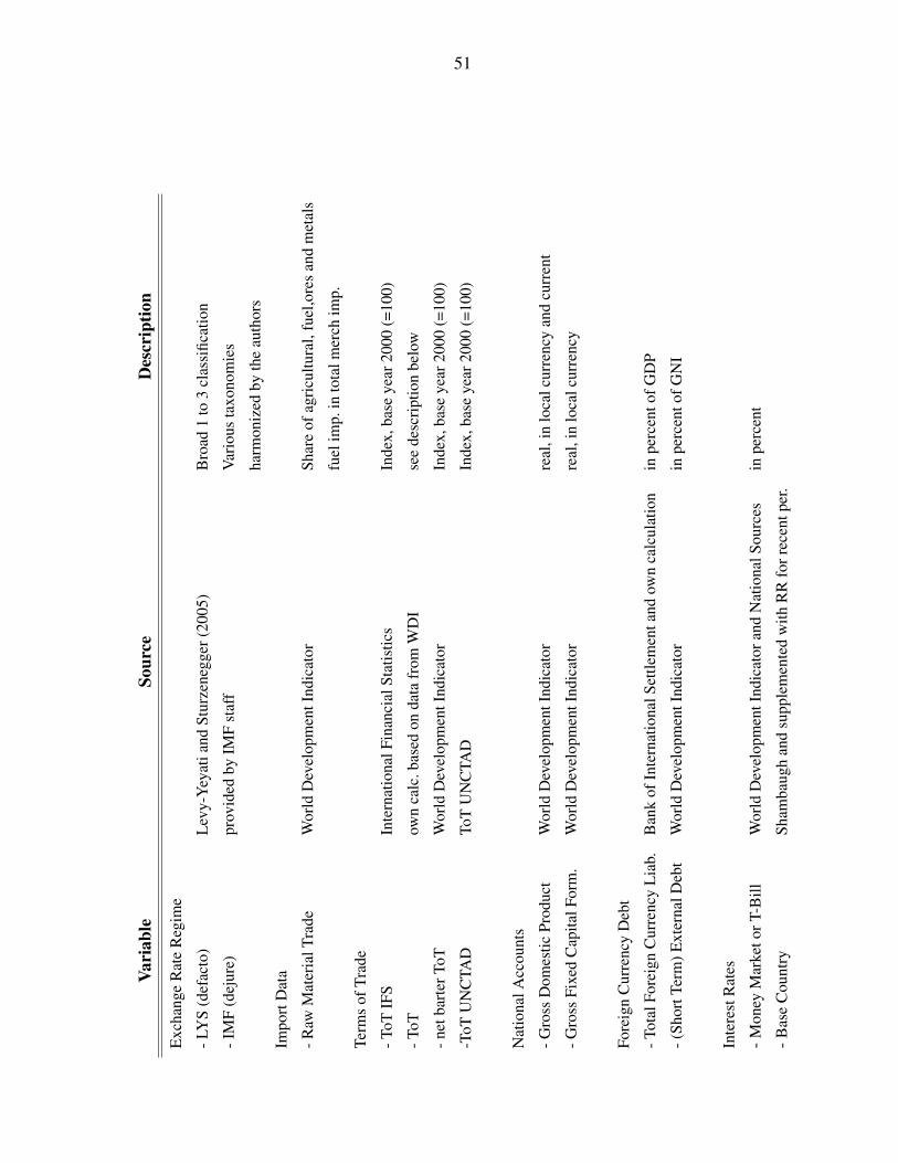
51

V ari

able

Sour

ceD

escr

iptio

n

Exc

hang

eR

ate

Reg

ime

-LY

S(d

efac

to)

Lev

y-Y

eyat

iand

Stur

zene

gger

(200

5)B

road

1to

3cl

assi

ficat

ion

-IM

F(d

ejur

e)pr

ovid

edby

IMF

staf

fV

ario

usta

xono

mie

s

harm

oniz

edby

the

auth

ors

Impo

rtD

ata

-Raw

Mat

eria

lTra

deW

orld

Dev

elop

men

tInd

icat

orSh

are

ofag

ricu

ltura

l,fu

el,o

res

and

met

als

fuel

imp.

into

talm

erch

imp.

Term

sof

Trad

e

-ToT

IFS

Inte

rnat

iona

lFin

anci

alSt

atis

tics

Inde

x,ba

seye

ar20

00(=

100)

-ToT

own

calc

.bas

edon

data

from

WD

Ise

ede

scri

ptio

nbe

low

-net

bart

erTo

TW

orld

Dev

elop

men

tInd

icat

orIn

dex,

base

year

2000

(=10

0)

-ToT

UN

CTA

DTo

TU

NC

TAD

Inde

x,ba

seye

ar20

00(=

100)

Nat

iona

lAcc

ount

s

-Gro

ssD

omes

ticPr

oduc

tW

orld

Dev

elop

men

tInd

icat

orre

al,i

nlo

calc

urre

ncy

and

curr

ent

-Gro

ssFi

xed

Cap

italF

orm

.W

orld

Dev

elop

men

tInd

icat

orre

al,i

nlo

calc

urre

ncy

Fore

ign

Cur

renc

yD

ebt

-Tot

alFo

reig

nC

urre

ncy

Lia

b.B

ank

ofIn

tern

atio

nalS

ettle

men

tand

own

calc

ulat

ion

inpe

rcen

tofG

DP

-(Sh

ortT

erm

)Ext

erna

lDeb

tW

orld

Dev

elop

men

tInd

icat

orin

perc

ento

fGN

I

Inte

rest

Rat

es

-Mon

eyM

arke

torT

-Bill

Wor

ldD

evel

opm

entI

ndic

ator

and

Nat

iona

lSou

rces

inpe

rcen

t

-Bas

eC

ount

rySh

amba

ugh

and

supp

lem

ente

dw

ithR

Rfo

rrec

entp

er.