Embed Size (px)
Citation preview
Limits of stress-test based bank regulation: Cues fromthe Covid-19 crisis∗
Isha Agarwal† and Tirupam Goel‡
October 15, 2020
Abstract
Stress-tests can enhance welfare by providing complementary information aboutbanks’ risk exposures to regulators, which allows them to use capital surcharges tobetter align baseline regulation to individual banks. This paper provides sugges-tive evidence of inaccuracies in stress-testing using the Covid-19 crisis, and developsa model to study the attendant welfare consequences. We show that inaccuraciesreduce welfare by causing excessive (insufficient) regulation of a less (more) riskybank, and by hampering banks’ ex-ante incentives. Accuracy and the optimal sur-charge have a non-linear relationship, and exhibit a phase shift – for accuracy belowa threshold, the optimal surcharge is zero.
JEL Codes: G21, G28, C61
Keywords: Bank Capital Requirements; Stress-tests; Information Asymmetry; Ad-verse Incentives; Covid-19.
∗The authors thank Elena Carletti, Jean-Edouard Colliard, Ingo Fender, Neil Esho, Eswar S. Prasad,Nikola Tarashev, Alberto Teguia, Egon Zakrajsek, two anonymous referees, and seminar participants atCornell for useful comments. Matlab programs to reproduce the results in this paper are available athttps://sites.google.com/site/tirupam/. The views expressed in this paper are those of the authors andnot necessarily of the Bank for International Settlements.†Sauder School of Business, University of British Columbia. Email: [email protected].‡Bank for International Settlements. Email: [email protected] (corresponding author).
1

1 Introduction
Stress-tests have become an important policy tool for regulators globally after the Great
Financial Crisis (GFC) [Baudino et al., 2018]. They complement financial reporting and
disclosures in revealing private information about banks’ risk exposures to regulators [Mor-
gan et al., 2014].1 This enables regulators to better align baseline capital requirements to
individual banks’ risk profiles. In both the U.S. and the Euro Area, for instance, stress-
test results are used to determine bank-specific quantitative and/or qualitative regulatory
requirements.2
There are, however, limits to the accuracy of stress-tests, which means that regulation
based on test results can be misdirected. For one, models used in the stress-test may not
fully capture banks’ risk exposures or their response to the crisis, and may lead to assess-
ments that turn out to be inaccurate ex-post [Acharya et al., 2014; Philippon et al., 2017].
Relatedly, reliance on historical data to define stress scenarios may miss unprecedented
events [Breuer et al., 2018]. In addition, bank-level inputs to stress-test models may be
noisy or not comparable across banks [Ong et al., 2010]. Moreover, technical and compu-
tational glitches can lead to faulty results.3 As such, stress-tests may exhibit Type-I and
Type-II errors, as a result of which a less (more) risky bank may fail (pass) the test and
face excessive (insufficient) regulation.
In this paper, we use the Covid-19 crisis to provide suggestive evidence of potential
inaccuracies in stress-tests, and develop and estimate a model to study the attendant
welfare and policy implications. To the best of our knowledge, this is the first paper on1Indeed, the GFC underscored that banks, especially the large and more complex ones, can be very
opaque [Gorton, 2008], and that this can give rise to information asymmetries viz-a-viz the regulators.2In the U.S., capital surcharges (among other requirements) are determined on the basis of stress-test
results. See https://www.govinfo.gov/content/pkg/FR-2020-03-18/pdf/2020-04838.pdf for more details.In the Euro Area, stress-tests conducted by the European Banking Authority (EBA) are a crucial inputinto the Supervisory Review and Evaluation Process (SREP) which entails capital planning, reporting,and governance requirements tailored to individual banks. See https://eba.europa.eu/eba-launches-2020-eu-wide-stress-test-exercise for more details.
3For example, in September 2020, the U.S. Federal Reserve Bank published corrections to its previouslyissued stress-test results [Fed, 2020b].
2

both fronts.
Several factors make the Covid-19 crisis a useful natural experiment to obtain cues
about the accuracy of the 2020 US stress-test. For one, the Covid-19 crisis was unexpected,
like stress-test scenarios also are. Second, the crisis featured an economic scenario that, in
many ways, is similar to the ones that stress-tests typically feature. Third, the 2020 US
stress test happened just before the crisis, which means that banks did not have time to
adjust to the test results before the crisis hit. As such, a comparison of banks’ performances
– in terms of the decline in capital ratios – in the test viz-a-viz the crisis can provide cues
about potential inaccuracies in stress-testing. Granted that stress-tests may not strive to
forecast stressed capital ratios. Yet, broad concordance in the performance of banks in
the test and in an economic crisis is to be expected because test results underpin bank
regulation and thus have a material impact on the financial system.
We find that banks have fared very differently in both relative and absolute terms
during the crisis as compared to the stress-test. Many banks that saw a decline in their
CET1 ratios in the test were able to increase their ratios in Q2 2020. Noted that the
full effect of the crisis on CET1 ratios may only be felt over a longer horizon (say once
non-performing assets are recognised). Yet, that loan-loss provisions are forward looking
and already rose substantially for most banks in Q2 in anticipation of future losses, the Q2
CET1 ratios ideally already reflects banks’ overall performance in the Covid-19 crisis. As
such, the discordance between test and actual performance points to potential Type-I/II
errors. It further implies that the 2020 U.S. stress-test may have led to inefficiently harsh
or liberal regulation for some banks.4
To assess the welfare and policy implications of potential inaccuracies in stress-testing,
we build a tractable three-period model of stress-test based bank capital regulation under
information asymmetry. The bank is a financial intermediary that takes deposits from the4This is via the imposition of Stressed Capital Buffers (SCBs) that depend on how poorly a bank did
in the test. See [Fed, 2020a] for details.
3

household and invests in a risky project. The return on the project can be high or low,
depending on the bank’s type, which in turn depends on the effort it exerts ex-ante. On
the back of a mis-priced deposit insurance, the bank over-borrows relative to the social
optimal.5 Over-borrowing increases the probability of failure (which can be costly) and
poses an externality. A minimum capital-ratio requirement can mitigate this externality.6
However, the regulator cannot observe the bank’s type, which means it cannot impose
the correspondingly optimal requirement, and must adopt a baseline requirement that is
independent of banks’ types.
We introduce stress-tests in the model as a regulatory (supervisory) tool that provides a
potentially inaccurate signal about the bank’s type, based on which the regulator imposes
a capital surcharge on top of the baseline requirement. However, the regulator faces a
trade-off. Stress-tests help overcome (some) information frictions and align regulation
to individual banks’ risk profiles. This improves welfare. Yet, inaccuracies can lead to
inefficiently low or high requirements for some banks. Inaccuracies also hamper banks’
ex-ante incentives to improve their risk profile.7 This lowers welfare. We use the model to
assess this trade-off formally and characterise the optimal surcharge.
Our main contribution is to analytically derive the relationship between optimal sur-
charge and stress-test accuracy, as jointly measured by the Type-I and Type-II error rates.
We show that this relationship is non-linear, and that it exhibits a phase-shift. When
test accuracy is below a threshold, we prove that the optimal surcharge is zero. This is
because lower accuracy implies that a high-type bank can fail the test more often and face
an inefficiently high requirement. This not only reduces welfare ceteris paribus because the5Typical reasons for a mis-priced deposit insurance include the inability of the insurer to observe banks’
risk profiles or impose risk-sensitive premium payments. See Flannery et al. [2017] for elaboration.6A large literature provides several rationales for capital-ratio requirements, such as fire-sale externali-
ties [Kara and Ozsoy, 2016], moral hazard issues [Christiano and Ikeda, 2016], implicit guarantees [Nguyen,2015], and household preference for safe and liquid assets [Begenau, 2019]. The approach in this paper isrelated to that of Kareken and Wallace [1978], Santos [2001], and Van den Heuvel [2008] who show thatover-borrowing, led by mis-priced deposit insurance or otherwise, justifies capital regulation.
7In a similar vein, Prescott [2004] shows that poorly executed supervisory audits can create adverseincentives ex-ante.
4

opportunity cost of a tighter constraint is greater for a high-type bank, it also diminishes
the ex-ante incentives of the bank to exert effort towards becoming a high-type. For in-
termediate levels of accuracy, we show that the optimal surcharge increases with accuracy,
but is still smaller than what the full information benchmark would imply. In case of a
perfectly accurate stress-test, any surcharge has a strong disciplining effect in terms of
eliciting greater ex-ante effort from banks, and accordingly the optimal surcharge is the
highest.8
When bank failure is costly, the regulator faces a more complex trade-off. We show
that in this case, not only is the optimal baseline capital requirement stricter, the optimal
surcharge for a given level of accuracy is also higher.
To illustrate our qualitative findings, and to draw quantitative implications, we calibrate
the model to U.S. data. We find that the optimal baseline capital requirement lies in the
range of 11% to 12%, and is higher for a low-type bank or when failure cost is large. The
optimal capital surcharge varies between 0 - 0.6% depending on the exogenously given
level of accuracy. In an extension of the model, we endogenise the accuracy to study the
following trade-off: while a more accurate stress-test can identify banks more precisely,
implementing such a test can be prohibitively costly for regulators and banks. We show
that as the unit cost of accuracy decreases, the regulator optimally increases both the
accuracy of the test as well as the surcharge for banks that fail the test.
Our paper belongs to a growing literature on bank stress-tests in the post-GFC period.
Most studies in this literature have focused on the trade-offs associated with transparency
and disclosure policy in stress-testing. For instance, greater disclosure can help enhance
market discipline but also hamper ex-ante risk-sharing [Goldstein and Sapra, 2013; Gold-
stein and Leitner, 2018]. Relatedly, secrecy of stress-test models can prevent gaming but8Our paper formalises the intuition James Bullard (President of the Federal Reserve Bank of St. Louis)
had in the context of quantitative easing: while state-contingent policies are generally desirable, they workwell when the states on which the policy is contingent are known. See this article for a coverage of hisremark. Relatedly, our paper supports the remarks made by Mark Zelmer (Deputy Superintendent, OSFICanada) in 2013 in the context of risk-sensitivity of capital requirements.
5

may discourage productive investment[Leitner and Williams, 2020].9 These studies typi-
cally assume that stress-tests reveal the true risk profiles of banks.
A smaller strand of the stress-testing literature provides evidence of potential errors in
stress-testing. Acharya et al. [2014] find that the stress-test based assessments of banks’
capital adequacy are not in line either with market-data based assessments, nor with banks’
actual performance during the European Sovereign Debt crisis in 2011. For the 2014 stress-
test conducted by the European Banking Authority, Philippon et al. [2017] find that while
model-based losses are good predictors of realized losses around announcements of macroe-
conomic news, banks headquartered in countries with weak banking system have higher
realized losses compared with their losses predicted by the 2014 stress test. Frame et al.
[2015] show that stress-tests conducted by the U.S. Office of Federal Housing Enterprise
Oversight in the pre-GFC period failed to detect risks on the balance sheets of Fannie
Mae and Freddie Mac. Covas et al. [2014] show that stress-test assessments can be more
informative and less prone to gaming if they are based on density (instead of linear-model
based point) forecasts.
Despite evidence on potential limitations of stress-tests, the literature has not formally
assessed the attendant welfare and policy implications. Our paper fills this gap, and devel-
ops a parsimonious framework to study stress-test based bank regulation in the presence
of information frictions.10 We derive analytical characterisations of the optimal capital
surcharge when stress-tests are inaccurate, and calibrate the model to provide quantita-
tive illustrations. In addition, our paper provides complementary suggestive evidence on
potential inaccuracies in stress-tests based on the Covid-19 crisis.9Other studies in this literature include Corona et al. [2017] who assess how bailout regime and disclosure
policy interact, Orlov et al. [2018] who characterise the optimal disclosure policy for high- and low-riskbanks, and Bouvard et al. [2015] who show that the optimal disclosure policy must vary along the businesscycle.
10Parlatore and Philippon [2018] also model stress-tests, but focus on the optimal design of stressscenarios that enable efficient information acquisition by the regulator. More generally, Morrison andWhite [2005] study the the effectiveness of capital regulation in avoiding crisis as public confidence in theregulator’s ability to screen banks varies. Our paper, in contrast, focuses on how capital regulation mustbe optimally adjusted as stress-test accuracy changes.
6

More broadly, our paper contributes to the literature on bank-specific regulation. For
instance, Marshall and Prescott [2001] show that state-contingent fines on banks can in-
crease welfare, but assume that the states are observable. Lohmann [1992] shows that
when future states are not fully known, it is sub-optimal to commit to a state-contingent
policy. In contrast, we model stress-tests as a tool to learn about future states (banks’
types). More recently, Ahnert et al. [2020] show that sensitivity of regulation to banks’
types must depend on the precision of the attendant signal, like in our paper. Yet, while
they show that starting from high precision, lower precision implies greater sensitivity of
regulation to risk, we show that such a strategy can decrease welfare by creating adverse
incentives ex-ante. This difference stems from the fact that we allow banks to affect the
probability that they face a capital surcharge, due to which regulation can affect ex-ante
incentives.
2 The Covid-19 crisis: A test of stress-tests
In this section, we review supervisory stress-tests in the U.S., and use the Covid-19 crisis
to shed light on potential inaccuracies in stress-test assessments.
2.1 Institutional Background
The Dodd-Frank Wall Street Reform and Consumer Protection Act (Dodd-Frank Act)
was enacted in response to the Great Financial Crisis (GFC). It requires the U.S. Federal
Reserve Bank (Fed) to conduct an annual stress-test – known as the Dodd Frank Act
Stress Test (DFAST) – of large bank holding companies (BHCs).11 The goal is to evaluate
whether the tested entities have sufficient capital to absorb losses resulting from adverse
economic conditions. The first DFAST was conducted in 2013, and has evolved quite a bit11Non-bank financial companies designated by the Financial Stability Oversight Council (FSOC) for Fed
supervision are also included in the exercise.
7
since. We focus on the 2020 DFAST in our analysis [DFAST, 2020].
The DFAST considers a hypothetical severely adverse scenario – one in which the U.S.
economy experiences a significant recession and financial market stress while other major
economies also experience contraction in economic activity – and projects the revenues, ex-
penses, losses, and, crucially, the capital ratios of the participating banks. The projections
are generated using inputs provided by the tested banks and forecasting models developed
or selected by the Fed. The projections use a standard set of capital action assumptions
that entail zero common stock dividend distribution, and no issuance or repurchase of
common or preferred stock.12
The Federal Reserve imposes a capital surcharge on banks based on their performance
in the test, as measured by the projected decline in their Common Equity Tier 1 (CET1)
capital ratios in the severely adverse scenario.13 Banks that perform poorly face a higher
Stressed Capital Buffer (SCB) – a surcharge on top of the baseline capital requirements
and any other surcharges (such as the G-SIB surcharge) – among other qualitative and
quantitative requirements.
2.2 The 2020 Stress-Test
The severely adverse scenario in the 2020 DFAST comprised of a peak unemployment rate
of 10 percent, a decline in real GDP of 8.5 percent, and a drop in equity prices of 50
percent through the end of 2020, among other macroeconomic developments.14 Thirty-
three entities participated in the test and the results were published in June 2020, which
included projections for the decline in the CET1 ratio relative to the end-2019 value (see12Scheduled dividend, interest, or principal payments that qualify as additional tier 1 capital or tier 2
capital are assumed to be paid, but repurchases of these instruments is assumed to be zero.13The results also contain other capital ratios, namely the tier 1 and total capital ratios, and the tier 1
and supplementary leverage ratios. We focus our attention on the CET1 ratio since it is a core measureof capital adequacy, and also because capital surcharge is expressed in these terms.
14The severely adverse scenario was designed in late 2019 and was published in February 2020. Whilethe 2020 DFAST did not adapt the severely stress scenario to incorporate the Covid-19 crisis, it disclosedadditional information about predicted aggregate losses in the banking sector based on a sensitivity analysisviz-a-viz the Covid-19 crisis. Bank-level results from this exercise were not disclosed.
8

0 2 4 6 8
Decline in CET1 ratio in the stress−test
Northern TrustAmerican Express
TD Group USBank of New York Mellon
U.S. BancorpPNC Financial Services
State StreetM&T Bank
Huntington BancsharesSantander USA
KeyCorpCitigroup
Bank of AmericaFifth Third Bancorp
Wells FargoTruist Financial
Regions FinancialJPMorgan Chase
Barclays USCitizens Financial Group
DiscoverAlly Financial
RBC USUBS Americas
MUFG AmericasBNP ParibasCredit Suisse
Morgan StanleyCapital One
HSBC North AmericaBMO Financial
Goldman SachsDB USA
Figure 1: Decline in the CET1 ratio in the 2020 DFAST. Unit of the x-axis is percentagepoints.
Figure 1). The average decline was 2.7 percentage points, with Deutsche Bank USA and
the Goldman Sachs Group being the worst performers, and Northern Trust and American
Express being the best performers.
Performance in the stress-test and the attendant capital surcharge have a strong and
positive relationship.15 Beyond the minimum SCB of 2.5%, the two go hand-in-hand to a
large extent (see Figure 2). In fact, for some banks (eg DB USA, MUFG, HSBC, RBC)
the SCB is equal to decline in CET1 ratio in the stress-test. This observation confirms
that a bank’s performance – especially poor performance – in the test is tightly linked to
the capital requirement it faces.15This is despite other considerations that go into calibrating the SCB.
9

ALLYAMEX
BOA
BNY
BARC
BMOBNP
CAP
CITI
CFG
CS
DB
DIS
FTB
GS
HSBC
HB
JPM
KEY
M&T
MS
MUFG
NT PNC
RBC
RFC
SAN
SSTD TFC
UBS
USB WF
−1
01
23
45
67
89
Str
essed C
apital B
uffer
−1 0 1 2 3 4 5 6 7 8 9
Decline in CET1 ratio in the stress−test
45 degree line
Minimum SCB
Figure 2: A comparison of the decline in CET1 ratio in the 2020 DFAST and the StressedCapital Buffer (SCB) imposed on banks. Unit of both axes is percentage points.
2.3 Bank performance during the Covid-19 crisis
Several factors make the Covid-19 crisis a useful natural experiment to appraise the 2020
US stress-test. For one, the Covid-19 pandemic has led to an extremely severe shock to
economic activity. At least qualitatively, this is what a typical stress-test scenario emulates.
And even though the observed decline in macroeconomic indicators (such as GDP growth
rate and employment) is not necessarily equal to the one in the 2020 DFAST scenario,
they are broadly consistent.16 In addition, the Covid-19 shock was completely unexpected,
like in the case of stress-tests where the hypothetical scenarios are not known to banks in
advance. Moreover, the timing of the 2020 DFAST is also ideal for our analysis. The test
results were announced on 25th June, which means that it is unlikely that banks were able
to anticipate the attendant capital surcharges (i.e. the SCBs) and adjust/raise capital in16The U.S. economy contracted by close to 30% (YoY) in Q2 2020; the peak unemployment rate was
15%; and the Dow Jones Index plunged by close to 30% in March 2020.
10

time for their second-quarter (i.e., end-June) earnings reports. These factors imply that
endogeneity issues associated with the Q2 2020 CET1 ratios can be ruled out.17
ALLY
AMEX
BOABNY
BARCBMO
BNP
CAP
CITI CFG
CS
DB
DIS
FTBGS
HSBCHB
JPM
KEYM&T MS
MUFGNT
PNC
RBCRFC
SAN
SSTD TFC
UBS
USB WF
−6
−4
−2
02
4
Declin
e in C
ET
1 r
atio d
uring H
1:2
020
−2 0 2 4 6 8
Decline in CET1 ratio in the stress−test
Least−square fit
Figure 3: A comparison of the decline in CET1 ratio in the stress-test and the actualdecline observed between Q4:2019 and Q2:2020. Unit of both axes is percentage points.
A comparison of the decline in CET1 ratios of banks in the test with the decline observed
during the first half of 2020 reveals that the actual and projected declines in CET1 ratios
do not line-up (see Figure 3).18 In fact, while the ratios declined for almost all banks in
the test, it rose for many in reality. In the case of Deutsche Bank USA, for instance, the
CET1 ratio declined by 8 percentage points (pp) in the test, while during H1 2020, the
same ratio rose by 5 pp. A similar although less stark narrative applies to most other
banks, and points to potentials Type-I/II errors in stress-test based assessments.19
Even in terms of relative (cross-sectional) performance of banks in the test as compared17Potential endogeneity issues also suggest that the 2019 DFAST or the 2018 European Banking Au-
thority (EBA) stress-tests cannot be appraised against banks’ actual performances in the Covid-19 crisisas banks are likely to act on the test results and evolve materially in the meantime. Note that the 2020EBA stress-test was postponed to give banks operational relief.
18Bank data for end-2019 and Q1 2020 are sourced from Fitch, while Q2 2020 data are sourced from
11
ALLY
AMEX
BOA
BNY
BARCBMO
BNP
CAP
CITI
CFG
CS
DB
DIS
FTB
GS
HSBC
HB
JPM
KEY
M&T
MS
MUFG
NT
PNC
RBC
RFC
SAN
SS
TD
TFC
UBS
USB
WF
010
20
30
40
Rank b
ased o
n d
eclin
e in C
ET
1 r
atio in H
1:2
020
0 10 20 30 40
Rank based on decline in CET1 ratio in stress−test
45 degree line
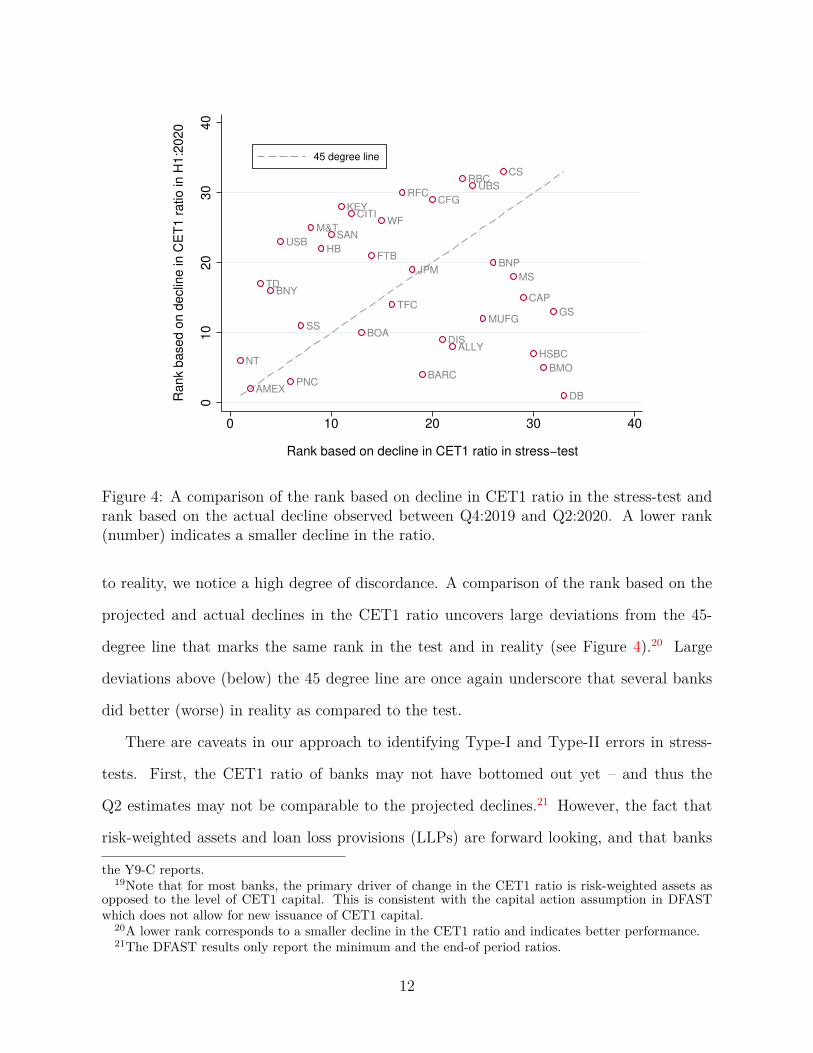
Figure 4: A comparison of the rank based on decline in CET1 ratio in the stress-test andrank based on the actual decline observed between Q4:2019 and Q2:2020. A lower rank(number) indicates a smaller decline in the ratio.
to reality, we notice a high degree of discordance. A comparison of the rank based on the
projected and actual declines in the CET1 ratio uncovers large deviations from the 45-
degree line that marks the same rank in the test and in reality (see Figure 4).20 Large
deviations above (below) the 45 degree line are once again underscore that several banks
did better (worse) in reality as compared to the test.
There are caveats in our approach to identifying Type-I and Type-II errors in stress-
tests. First, the CET1 ratio of banks may not have bottomed out yet – and thus the
Q2 estimates may not be comparable to the projected declines.21 However, the fact that
risk-weighted assets and loan loss provisions (LLPs) are forward looking, and that banks
the Y9-C reports.19Note that for most banks, the primary driver of change in the CET1 ratio is risk-weighted assets as
opposed to the level of CET1 capital. This is consistent with the capital action assumption in DFASTwhich does not allow for new issuance of CET1 capital.
20A lower rank corresponds to a smaller decline in the CET1 ratio and indicates better performance.21The DFAST results only report the minimum and the end-of period ratios.
12

front-loaded by increasing LLPs substantially in Q2, means that the Q2 capital ratios
ideally reflect banks’ overall performance in the crisis. Second, differences in some aspects
of the severely adverse scenario and the Covid-19 crisis (eg decline in house price index)
may render a comparison of the decline in capital ratios in the two cases less meaningful.
Relatedly, some banks may be less/more well-positioned to handle specific aspects of the
Covid-19 shock, so that actual and test performances may not be at par. More generally,
stress-tests may not be designed to predict future crises or bank’s capital ratios therein.
Nonetheless, broad concordance in banks’ performances in the test and in a crisis, at least
in a relative sense, is desirable, not least because stress-test results inform bank regulation
and have a material impact on the financial system. More importantly, as we show below,
such discordance can create adverse ex-ante incentives and diminish the welfare gains from
regulation.
3 Model
Our goal is to analyse the welfare and policy implications of stress-test based capital
requirements when stress-tests are potentially inaccurate. To this end, we develop a model
with the following main elements. First is a general equilibrium setup that enables us to
capture the welfare effect of regulation on the (representative) household’s utility. Second
is a dynamic setup that allows us to assess the effect of future stress-test and regulation
on banks’ ex-ante behavior. Third is a rationale for capital-regulation – specifically, an
externality that warrants regulatory intervention. Fourth is information frictions – i.e.,
the unobservability of a bank’s type by the regulator – that justify the use of stress-tests.
Accordingly, we consider an economy that lasts three periods (0, 1 and 2), and consists of
a representative household, a bank that poses an externality and whose type is stochastic,
a regulator that cannot (fully) observe the bank’s type, and the government.
13

Household The household is representative, and receives an unconditional income en-
dowment Y on dates 1 and 2. On date-1, it decides how much to consume, c1, and how
much to deposit, d, in the bank.22 Deposits are risk-free, and pay a gross return of R on
date-2. The household is also the owner of the bank and receives dividends n on date-2.
It pays a lump-sum tax T .
Bank The bank has a capital endowment of k on date-1, and issues deposits d to raise
additional funding. It invests k + d in a risky project that pays ψg(k + d) on date-2,
where g(.) is a decreasing returns to scale (DRS) return function. ψ is an investment shock
whose density fs depends on the bank’s type s on date-1, which can be high (H) or low (L).
Specifically, we assume that while both types face the same standard deviation of ψ, namely
σ, the high-type bank has a higher expected return, µH > µL, or equivalently, higher risk-
adjusted return.23 The probability p with which the bank is of high-type depends on the
effort e it exerts on date-0. The cost of exerting effort is ζ(e).
The bank’s deposit liabilities on date-2 equal Rd, and thus the net cash flow equals
ψg(k + d) − Rd. When ψ is sufficiently high and the bank is solvent, it transfers the
entire cash-flow as dividends n to the household. However, when ψ is low enough so that
the cash-flow is negative, the bank fails and shareholders receive null. We assume that
shareholders have limited liability, so that they cannot be asked for additional capital to
rescue a failing bank. Instead, the government takes the bank into receivership.
Government The government runs the deposit insurance scheme and ensures that de-
positors are fully protected against bank failure. When a bank fails, the government takes
its assets into custody, liquidates the same, and covers any shortfall in the failed bank’s22A time subscript is used only for those quantities that are relevant on multiple dates. For instance,
since d is only chosen once, on date-1, a time subscript is omitted.23The exact connotation of high and low types is not critical as long as the high-type bank is better
from a social welfare point of view. For instance, equivalent connotations of being a high-type bank maystem from having the same mean but lower standard deviation of ψ, or a lower cost of funding.
14

liabilities via a tax T on the bank’s owner, i.e. the household.24 We assume that the tax
is lump-sum. This assumption entails that the insurance scheme is mis-priced, and, as we
prove later, leads to an externality.25 The government runs a balanced budget.
Regulator The regulator is benevolent, i.e. it strives to maximise the welfare of the
household. On date-0, it announces the minimum capital-ratio requirement χ that the
bank must satisfy on date-1. However, we assume that the regulator cannot observe bank’s
type on date-1. In the baseline economy, as such, it must announce a requirement that
does not depend on banks’ types, i.e. applies universally to both types of banks on date-1.
In the economy with stress-tests, the regulator is able to obtain a noisy signal about the
bank, and classify it as a high- or low-type depending on whether it passes or fails the test.
The regulator then announces a surcharge x for failing the stress-test, effectively imposing
a bank-type specific requirement χs, s ∈ {H,L}.
Recursive formulation We now formally setup the problem statements of the agents
in the economy. The household chooses d on date-1 to maximize its expected utility over
dates 1 and 2:
U = maxd
c1 + βEc2 s.t. c1 = Y − d and c2 = Y +Rd+ n− T. (1)
The bank chooses e on date-0 which determines the probability of being an H-type on
date-1:
[Date− 0] : maxe
−ζ(e) + β(p(e)VH(χH) + (1− p(e))VL(χL)
). (2)
24Alternatively, and equivalently, we can treat T as a deposit-insurance premium imposed on the bank.25The reason for introducing an externality in our model is to rationalise capital requirements. A mis-
priced deposit insurance is not the only way to do so, but it is a relatively simple method that helps keepour model tractable. Another paper to have taken this route is Van den Heuvel [2008]. A moral hazardbetween banks and its creditors [Gertler and Kiyotaki, 2010], or implicit government guarantees [Nguyen,2015] are among the several other ways in which capital requirements can be justified.
15

where Vs(χs) is defined in Equation (3). Subsequently, the bank of type s ∈ {H,L} chooses
d on date-1 to maximize the expected dividend it pays on date-2:
[Date− 1] : Vs(χs) = maxd
β∫ ∞
Rdg(k+d)
(ψg(k + d)−Rd︸ ︷︷ ︸
n
)fs(ψ)dψ s.t.
kχs
≥ d. (3)
The lower limit on the integral is the ψ cut-off – call it ψc – below which the bank fails
(and dividends n equal zero). χs are the bank-type specific minimum capital-ratio require-
ments (although the requirements will be the same in the absence of stress tests). The
government’s budget constraint is as follows:
T =
Rd− ψg(k + d) If the bank fails i.e. ψ ≤ Rd
g(k+d)
0 Otherwise(4)
4 Qualitative Analysis
We begin by assessing the equilibrium conditions in the baseline economy. We then char-
acterise – as a benchmark – the optimal regulation in the absence of stress tests. Finally,
we analyse the optimal capital surcharge based on stress-test results, including when bank
failure is socially costly.
4.1 The competitive equilibrium
The first-order condition (FOC) of the bank’s problem on date-0 shows that the effort the
bank exerts depends on the wedge, say ω, between the value of being a high- as opposed
to low-type on date-1:
− ζ ′(e) + βp′(e)(VH(χH)− VL(χL)
)︸ ︷︷ ︸
ω
= 0 (5)
16

To see how the effort changes as the wedge increases, we take the total derivative of the
Equation 5 with respect to ω, from where it is straightforward to note Lemma 1:
− ζ ′′(e) dedω
+ βp′′(e)ω dedω
+ βp′(e) = 0 (6)
Lemma 1. If ζ(.) is increasing and convex, and p(.) is increasing and concave, then the
bank exerts more effort when the difference in the value of being a high type compared to a
low type increases, i.e. de/dω > 0.
The pre-conditions for Lemma 1 to hold are sufficient but not necessary. For instance,
the result still holds if ζ(.) is increasing and linear. Nonetheless, that becoming a high-type
bank is increasingly difficult is a realistic assumption to have.
Lemma 1 underscores an important insight. The minimum requirements (χH , χL) an-
nounced on date-0 affect the wedge ω by impacting the value of the bank on date-1. As
such, the minimum requirements are a key factor in bank’s effort choice on date-0.26
As regards the date-1 FOCs, we have the following:
Bank: β∫ ∞
Rdg(k+d)
(ψg′(k + d)−R
)fs(ψ)dψ − Λs = 0 (7)
Household: R = 1/β (8)
Note in the bank’s FOC that Λs is the Lagrange multiplier on the regulatory constraint,
and that two of the three terms which arise from a routine application of the Leibniz rule
are equal to zero. The system of FOCs (5), (7), (8) and the government’s budget constraint
(4) together characterise the competitive equilibrium of the model economy for a given set
of minimum capital-ratio requirements (χH , χL).26Lemma 1 is related to a similar result proven in Christiano and Ikeda [2016], except for the channel
through which regulation has an impact on the bank’s effort.
17
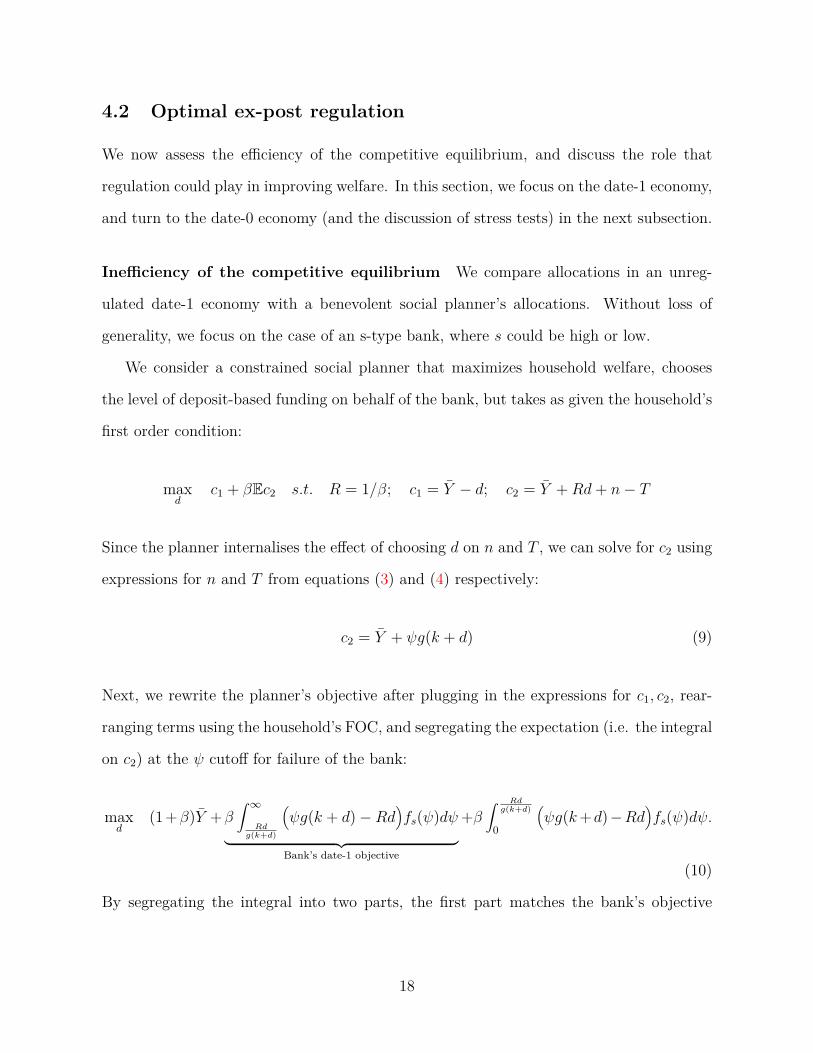
4.2 Optimal ex-post regulation
We now assess the efficiency of the competitive equilibrium, and discuss the role that
regulation could play in improving welfare. In this section, we focus on the date-1 economy,
and turn to the date-0 economy (and the discussion of stress tests) in the next subsection.
Inefficiency of the competitive equilibrium We compare allocations in an unreg-
ulated date-1 economy with a benevolent social planner’s allocations. Without loss of
generality, we focus on the case of an s-type bank, where s could be high or low.
We consider a constrained social planner that maximizes household welfare, chooses
the level of deposit-based funding on behalf of the bank, but takes as given the household’s
first order condition:
maxd
c1 + βEc2 s.t. R = 1/β; c1 = Y − d; c2 = Y +Rd+ n− T
Since the planner internalises the effect of choosing d on n and T , we can solve for c2 using
expressions for n and T from equations (3) and (4) respectively:
c2 = Y + ψg(k + d) (9)
Next, we rewrite the planner’s objective after plugging in the expressions for c1, c2, rear-
ranging terms using the household’s FOC, and segregating the expectation (i.e. the integral
on c2) at the ψ cutoff for failure of the bank:
maxd
(1 +β)Y +β∫ ∞
Rdg(k+d)
(ψg(k + d)−Rd
)fs(ψ)dψ︸ ︷︷ ︸
Bank’s date-1 objective
+β∫ Rd
g(k+d)
0
(ψg(k+d)−Rd
)fs(ψ)dψ.
(10)
By segregating the integral into two parts, the first part matches the bank’s objective
18

function, and thus facilitates a comparison of bank’s and planner’s FOCs, as shown below:
β∫ ∞
Rdg(k+d)
(ψg′(k + d)−R
)fs(ψ)dψ + β
∫ Rdg(k+d)
0
(ψg′(k + d)−R
)fs(ψ)dψ︸ ︷︷ ︸
Bank-failure externality
= 0. (11)
Equation (11) uncovers a wedge between the planner’s FOC and the bank’s FOC in the
unregulated economy (i.e. equation (7) with Λs = 0). This wedge stems from limited
liability and a mis-priced deposit insurance. Basically the bank does not internalise the
left tail of the distribution of ψ – the part that corresponds to bank failure. The planner,
on the contrary, chooses the level of deposits taking into account the entire distribution
of ψ. We refer to this wedge as the bank-failure externality, which the following lemma
characterises.27
Lemma 2. The bank’s capital ratio, defined as k/d, is smaller in the competitive equilib-
rium as compared to that in the constrained planner’s problem, i.e. second best.
Proof. Assume that the externality term is positive. Then, β∫∞
Rdg(k+d)
(ψg′(k+d)−R
)fs(ψ)dψ
must also be positive. But this is a contradiction since the overall expression for the
planner’s FOC must equal zero. As such, the externality term must be negative. In turn,
this implies that β∫∞
Rdg(k+d)
(ψg′(k + d) − R
)fs(ψ)dψ > 0. We know that dCE (the level of
deposits in the competitive equilibrium) satisfies β∫∞
Rdg(k+d)
(ψg′(k+d)−R
)fs(ψ)dψ = 0. But
since g(.) is concave, it must be that dCE > d∗ where d∗ solves the constrained planner’s
problem. �
Implementability of the constrained efficient allocation That the competitive
equilibrium exhibits an externality implies that WCE ≤ W ∗ where WCE is the welfare
in the competitive equilibrium and W ∗ is the second-best welfare. The question that27The finding that the bank takes more leverage than what is socially optimal is not unique to this paper,
nor is it our main contribution. Several other studies have related findings, such as Van den Heuvel [2008]and Christiano and Ikeda [2016], for instance. Our approach is to develop a relatively parsimonious modelthat has the mechanisms needed to study the welfare effects of stress-test based capital requirements.
19

follows is whether a regulatory intervention can help implement or approach the second
best.
To this end, we consider a benevolent regulator that sets a minimum capital-ratio
requirement k/d ≥ χs on the bank in order to maximize welfare. In choosing χ
s, the
regulator faces the following trade-off. A higher χs forces the bank to reduce deposit-based
funding and accordingly its failure probability, which has a welfare improving effect due to
a smaller bank-failure externality. Yet, a higher χs depresses expected output, which has
a welfare reducing effect.
In effect, the regulator’s decision problem is very similar to that of a constrained plan-
ner. This is because choosing deposits on behalf of the bank to maximise welfare is equiva-
lent to imposing a minimum capital-ratio requirement with the same objective when capital
is fixed and the requirement is binding. This is formally seen by comparing equations (7)
and (11). Indeed, the first terms are identical. And to the extent the Lagrange multiplier
Λs on (i.e. the shadow cost of) the regulatory constraint in (7) is equal to the absolute
value of the bank-failure externality term in (11), the solution to the two equations must
be identical. We note this result in the lemma below, and denote the optimal regulation
for an s-type bank by χos.
Lemma 3. The solution to the constrained planner’s problem can be implemented via a
minimum capital-ratio requirement.28
Before turning to the date-0 problem, we document a result that will be useful later.
It compares the optimal date-1 regulation for high- and low-type banks.
Lemma 4. The regulator optimally sets stricter ex-post regulation on the low-type bank as
compared to a high-type bank, i.e. χoL > χoH .
28A capital-ratio requirement is not the only regulatory tool that can implement the second best. A tax(or a deposit insurance premium) that is a function of the balance sheet choice of the bank can achievethe same outcome.
20
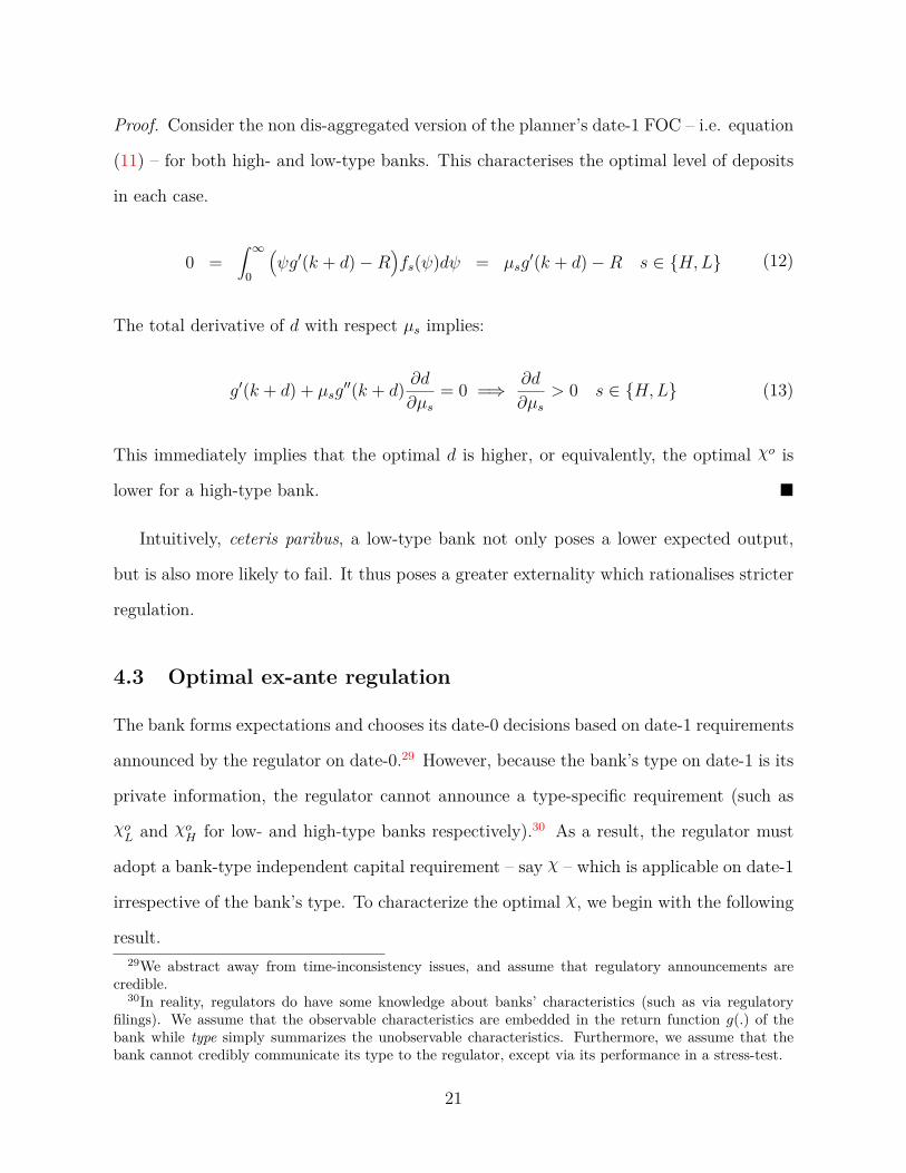
Proof. Consider the non dis-aggregated version of the planner’s date-1 FOC – i.e. equation
(11) – for both high- and low-type banks. This characterises the optimal level of deposits
in each case.
0 =∫ ∞
0
(ψg′(k + d)−R
)fs(ψ)dψ = µsg
′(k + d)−R s ∈ {H,L} (12)
The total derivative of d with respect µs implies:
g′(k + d) + µsg′′(k + d) ∂d
∂µs= 0 =⇒ ∂d
∂µs> 0 s ∈ {H,L} (13)
This immediately implies that the optimal d is higher, or equivalently, the optimal χo is
lower for a high-type bank. �
Intuitively, ceteris paribus, a low-type bank not only poses a lower expected output,
but is also more likely to fail. It thus poses a greater externality which rationalises stricter
regulation.
4.3 Optimal ex-ante regulation
The bank forms expectations and chooses its date-0 decisions based on date-1 requirements
announced by the regulator on date-0.29 However, because the bank’s type on date-1 is its
private information, the regulator cannot announce a type-specific requirement (such as
χoL and χo
H for low- and high-type banks respectively).30 As a result, the regulator must
adopt a bank-type independent capital requirement – say χ – which is applicable on date-1
irrespective of the bank’s type. To characterize the optimal χ, we begin with the following
result.29We abstract away from time-inconsistency issues, and assume that regulatory announcements are
credible.30In reality, regulators do have some knowledge about banks’ characteristics (such as via regulatory
filings). We assume that the observable characteristics are embedded in the return function g(.) of thebank while type simply summarizes the unobservable characteristics. Furthermore, we assume that thebank cannot credibly communicate its type to the regulator, except via its performance in a stress-test.
21

Lemma 5. Assume that regulation χ binds for both bank types on date-1. Then the effort
the bank exerts on date-0 decreases as χ rises.
Proof. As shown in Lemma 1, the bank’s date-0 effort e depends on ω = VH(χ) − VL(χ),
i.e. the wedge between the value of being a high- versus low-type on date-1. The key then
to proving this lemma is to characterise how regulation impacts ω.
ω = β∫ ∞
Rdg(k+d)
(ψg(k + d)−Rd
)fH(ψ)dψ − β
∫ ∞Rd
g(k+d)
(ψg(k + d)−Rd
)fL(ψ)dψ
where d = k/χ. The derivative of ω with respect to χ gives:
∂ω
∂χ= −kβχ2
∫ ∞
Rdg(k+d)
(ψg′(k + d)−R
)fH(ψ)dψ︸ ︷︷ ︸
ΛH
−∫ ∞
Rdg(k+d)
(ψg′(k + d)−R
)fL(ψ)dψ︸ ︷︷ ︸
ΛL
(14)
where Λs is the Lagrange multiplier on the regulatory constraint in the bank’s problem.
To sign this expression, we proceed as follows. First note that since the regulatory
requirement is the same for both types of banks, their deposit choices and thus the failure
cutoffs ψc are also the same. Then let FH and FL be the distribution functions of ψ for
high- and low-type banks, truncated below at ψc. Since µH > µL, FH FOSD FL, that
is FH(ψ) ≤ FL(ψ) ∀ ψ. Finally, since (ψg′(k + d) − R) is an increasing function of ψ, it
follows that:
∫ (ψg′(k + d)−R
)dFH(ψ)−
∫ (ψg′(k + d)−R
)dFL(ψ) = ΛH − ΛL > 0.31
31To prove this formally, consider continuous distribution functions G and H such that ∀x,H(x) ≤G(x), and define y(x) = H−1(G(x)). Then for any increasing function w(x),
∫w(y(x))dH(y(x)) =∫
w(y(x))dG(x). Next, note that y(x) = H−1(G(x)) =⇒ y(x) ≥ x since ∀x,H(x) ≤ G(x). In turn,since w(.) is an increasing function, w(y(x)) ≥ w(x). Thus,
∫w(y(x))dG(x) ≥
∫w(x)dG(x). Indeed,
intuitively, the shadow cost of the minimum capital-ratio constraint should be greater for a bank whoseassets are ceteris paribus more profitable.
22

In turn, this implies that ∂ω∂χ
< 0. Then from Lemma 1 we know that ∂e∂ω
> 0, which
completes the proof since:∂e
∂χ= ∂e
∂ω
∂ω
∂χ< 0.
�
Lemma 5 points to an important trade-off the regulator faces while setting χ. Compared
to no regulation (χ = 0), a higher χ can improve welfare ex-post by mitigating some of
the externality the bank poses, especially in case of a low-type bank. Yet, a higher χ
can reduce welfare due to its adverse impact on effort exerted ex-ante. Moreover, as the
following proposition shows, a high χ can be inefficient ex-post, especially in case of a
high-type bank.
Proposition 1. The optimal ex-ante requirement χo in the case where the regulator cannot
observe the bank’s type, is saddled by the optimal ex-post requirement for low- and high-type
banks, ie χoL > χo > χoH .
Proof. The optimal ex-ante requirement, χo, solves the following problem:
maxχ
βp(e)UH(χ) + β(1− p(e))UL(χ).
Here Us is the household’s expected lifetime utility over dates 1 and 2 when the bank turns
out to be of type s. Also, both e and Us depend on χ. The planner’s problem can be
re-written equivalently as follows.
≡ p(e)(Y (1 + β)− d+ βµHg(k + d)
)+ (1− p(e))
(Y (1 + β)− d+ βµLg(k + d)
)
≡ Y (1 + β)− d+ βg(k + d)(p(e)(µH − µL) + µL
)︸ ︷︷ ︸
µavg
Here µavg is the expected efficiency of the bank, which has the following properties: (i)
23
µex = µH when p(e) ≡ 1; (ii) µex = µL when p(e) ≡ 0; (iii) µL ≤ µex ≤ µH . We know from
the proof of Lemma 4 that as µ increases, the regulator chooses a smaller χ (ie loosens the
requirement). This immediately leads to the current proposition. �
Intuitively, this proposition shows that when there is information asymmetry, the reg-
ulator chooses a middle-ground relative to ex-post optimal levels of bank-type specific
requirements.
4.4 Mitigating information frictions via stress-tests
Stress test allows the regulator to gather information about banks’ types. It thus helps
mitigate some information frictions and allows capital requirements to be better aligned
to the banks’ types. This is desirable as it can improve welfare.
In this subsection, we incorporate stress tests in our model. We assume that the test
delivers a noisy signal η to the regulator about the bank’s type. The signal distribution
QH of high-type banks dominates (in the first order stochastic (FOSD) sense) the signal
distribution QL of low-type banks. Depending on it’s preferences for true- and false-
positive and negative rates, the supervisor uses a signal cutoff ηc above (below) which
the bank is considered pass (fail) and is deemed to be of the high- (low-) type. Thus the
probability that a high-type bank passes the test is given as qH = 1−QH(ηc), and the same
for an L type bank is given as qL = 1−QL(ηc). Moreover, QH <FOSD QL =⇒ qH > qL.32
The accuracy of the stress-test is fully captured by the tuple (qH , qL). Any test can
thus be represented by a point in the set [0, 1]× [0, 1], as shown in Figure 6. In this format,
(1 − qH) denotes the ’false positive’ or Type-I error rate (high-type bank fails the test),
while qL is the ’false negative’ or Type-II error rate (low-type bank passes the test). A
convenient benchmark, which is equivalent to the full-information case, is when qH = 1 and
qL = 0, i.e. a perfect stress-test that exactly identifies the type of the bank. In all other32For sake of brevity, we do not model the signal distributions or the regulator’s preferences that underpin
the signal cutoff ηc. Instead, we directly work with pass probabilities.
24

Date-0 Date-1
pass =⇒ χo
fail =⇒ χo + x
Date-2ψ ∼ N(µH , σ2)
ψ ∼ N(µL, σ2)
H
L
pass
fail
pass
fail
qH
1− qH
qL
1− qL
p(e)
1− p(e)
Exert effort eIncur cost ζ(e)
Figure 5: The timeline of events when there is information asymmetry about the bank’stype, and stress tests serves as a tool to (partially) mitigate information frictions.
cases, we refer to the test as imperfect because an H type bank can fail the test (qH < 1)
or an L type bank can pass the test (qL > 0).
The regulator uses the outcome of the stress-test to adjust the baseline capital require-
ment χo. We assume that a bank that passes the stress test is deemed high-type and is
allowed to operate at χo. A failed bank is deemed to be of the low-type, and is penalized
and its capital-ratio requirement in increased by a surcharge x ≥ 0 (see Figure 5 for the
timeline).33
The core question of interest then is as follows: what is the welfare maximising level
of surcharge x that the regulator must announce on date-0. The choice of x is non-trivial,
and must balance a three-way trade-off.
1. In case of the low-type bank, the surcharge (upon failing the test) increases welfare
ceteris paribus as long as x < χoL − χo. This is because the surcharge brings the
ex-ante requirement (χo + x) closer to the ex-post optimal (χoL).
2. In case of the high-type bank, the surcharge (upon failing the test) decreases welfare33This is not the only way in which capital requirements may be imposed following the result of a
stress-test. For instance, a regulator may choose to relax the requirement for a bank that passes the test.However, in practice, this is not typical. In the US, for instance, banks that do well in the test also haveto satisfy a minimum stress-capital buffer of 2.5%, while those that do poorly face additional requirements(recall Figure 2). Our specification follows this spirit.
25

ceteris paribus. This is because χo +x > χo > χoH , as a result of which the surcharge
takes the ex-ante requirement away from the ex-post optimal.
3. The surcharge affects the wedge between the expected value of being high- versus
low-type on date-1, and thus impacts the bank’s behaviour on date-0. Depending on
the accuracy of the stress test, this can lead to an increase or decrease in the bank’s
effort. We prove this result in Lemma 6 below. Accordingly, ceteris paribus, a higher
surcharge can increase or decrease in welfare through its effect on effort.
Lemma 6. The bank’s effort may increase or decrease with a surcharge, depending on the
accuracy of the stress test.
Proof. The date-0 problem of the bank is:
maxe
− ζ(e) + βp(e) (qHVH(χo) + (1− qH)VH(χo + x))︸ ︷︷ ︸EVH
+
β(1− p(e)) (qLV (χo) + (1− qL)VL(χo + x))︸ ︷︷ ︸EVL
(15)
We begin by noting that similar to the case without stress testing, the effort the bank exerts
increases with the expected value function wedge ω = EVH − EVL. Taking the derivative
of ω with respect to x at x = 0 gives:
∂ω
∂x
∣∣∣∣∣x=0
= (1− qH)V ′H(χo)− (1− qL)V ′L(χo)
where V ′ indicates the derivative of the value function. To determine the sign of this
expression, divide everything by V ′L(χo):
sgn
(∂ω
∂x
∣∣∣∣∣x=0
)= sgn
(1− qL)− (1− qH) V′H(χo)V ′L(χo)︸ ︷︷ ︸
ν
26

qL
qHsurcharge > 0
Perfect stress-test
qH =(1− 1
ν
)+ qL
ν; ν > 1
surcharge ↑=⇒ effort ↑
surcharge ↑=⇒ effort ↓
surcharge = 01
1
qH = τ0 − τ1qL; τ1 < 0
Figure 6: Stress-test accuracy, effect on ex-ante effort, and optimal penalties
Next, recall from the proof of Lemma (5) that V ′H(χo) − V ′L(χo) < 0, which implies that
ν > 1. Thus, the effect of surcharge on the bank’s effort choice depends on the accuracy
of the test as follows:
(1− qL)− (1− qH)ν
> 0 =⇒ efforts increases with surcharge
= 0 =⇒ efforts does not change with surcharge
< 0 =⇒ effort decreases with surcharge
�
Intuitively, ν captures the relative shadow cost of tightening regulation for the high-
and low-type banks. Ceteris paribus, a higher ν makes imposing a surcharge less desirable
by making it more likely that the bank reduces effort. Relatedly, it is clear from Lemma 6
that with a perfect stress test, i.e. when (qH = 1, qL = 0), effort increases with surcharge.
And that with an imperfect stress test, such as when qH = qL = 0.5, effort decreases with
surcharge. We indicate these insights qualitatively (i.e., not to scale) in Figure 6.
Next we assess the relationship between accuracy of the stress-test and the optimal
27

surcharge.
Proposition 2. No surcharge must be imposed if the accuracy of stress testing as measured
by a (well-defined) linear combination of the Type-1 and Type-II error rates is higher than
a cutoff.
Proof. Welfare as a function of the surcharge x can be written based on the planner’s
problem as follows (note that e also depends on x in this expression):
maxx
W (x) = βp(e)(qHUH(χo) + (1− qH)UH(χo + x)
)+
β(1− p(e))(qLUL(χo) + (1− qL)UL(χo + x)
)
Our goal is to identify ‘a’ non-trivial set of (qH , qL) where W (0) > W (x) ∀ x > 0, i.e. a zero
surcharge is optimal.34 A sufficient condition for this to be the case is W ′(x) < 0 ∀ x > 0.
To this end, we consider the first-order condition of the planner’s problem:
dW
dx= p′(e)e′(x)
(qHUH(χo) + (1− qH)UH(χo + x)
)+ p(e)(1− qH)U ′H(χo + x)−
p′(e)e′(x)(qLUL(χo) + (1− qL)UL(χo + x)
)+ (1− p(e))(1− qL)U ′L(χo + x)
To characterise the sign of this expression, we make a few assumptions, again with the goal
to find sufficient conditions under which the optimal surcharge is zero.
– First we assume that x ∈ [0, χoL − χo]. The upper bound corresponds to a surcharge
amount that results in a requirement for the low-type banks that is equal to the ex-
post optimal requirement χoL. In principle the optimal surcharge could be higher (due
to its effect on improving ex-ante effort), but that would entail a welfare decreasing
effect in case of both high- and low-type banks.34Our goal is to not fully characterise the set of (qH , qL) for which the optimal surcharge is zero. We
only wish to show that with low-enough accuracy, imposing a surcharge is sub-optimal.
28

– Second, we assume that (qH , qL) are such that the effort exerted by the bank decreases
as surcharge increases (as per Lemma 6).
Next, since Us(χo + x), s ∈ {L,H} is a concave function of x, χoL > χo > χoH implies the
following: (i) UH(χo) > UH(χo + x); (ii) U ′H(χo + x) < 0; (iii) UL(χo) < UL(χo + x); and
(iv) U ′L(χo + x) > 0; ∀ x ∈ [0, χoL − χo]. It then follows that:
dW
dx< p′(e)e′(x)UH(χo)+p(e)(1−qH)U ′H(χo)−p′(e)e′(x)UL(χo)+(1−p(e))(1−qL)U ′L(χo)
Finally, we re-arrange and set the right-hand-side expression to zero:
p(e)U ′H(χo) + (1− p(e))U ′L(χo)− p(e)qHU ′H(χo)− (1− p(e))qLU ′L(χo)+
p′(e)e′(x)(UH(χo)− UL(χo)
)︸ ︷︷ ︸
A<0
= 0
=⇒ A
p(e)U ′H(χo) + 1 + (1− p(e))U ′L(χo)p(e)U ′H(χo)︸ ︷︷ ︸
τ0<>0
−qL(1− p(e))U ′L(χo)p(e)U ′H(χo)︸ ︷︷ ︸
τ1<0
= qH
=⇒ qH = τ0 − τ1qL (16)
In equation (16), while the slope is positive, the intercept can be positive or negative,
depending on the underlying parameters. Also, when qL = 1, qH < 1. The equation
implies that when qH < τ0− τ1qL the surcharge should be zero, as also indicated in Figure
6. �
Intuitively, the proposition shows that when qH is low and/or qL is high – both of
which reflect a relatively less accurate stress-test – the surcharge must be zero. The next
proposition identifies the conditions under which the optimal surcharge is strictly positive.
Proposition 3. If the stress-test is accurate in identifying high-type banks qH = 1, but is
possibly inaccurate in identifying low-type banks 1 > qL ≥ 0, then a surcharge can improve
29
welfare.
Proof. First note that a higher x does not affect EVH , but decreases EVL (recall equation
(15)). As a result, the bank increases effort as surcharge increases. Second, consider the
planner’s problem:
maxx
βp(e)UH(χo) + β(1− p(e))(qLUL(χo) + (1− qL)UL(χo + x)
)
Note that since the high-type bank never fails, it is never penalised. A low-type bank
can be penalised upon failure, and this increases welfare as long as x ≤ χoL − χo. Beyond
this threshold, the effective regulation on the low-type bank is higher than χoL, which is
sub-optimal (recall Proposition 4).
Combining the effect of a surcharge on effort e and UL(χo + x), both of which increase
as x increases, and given that UH(χo) > UL(χo), it is clear that welfare must increase as x
rises above zero. �
Together, Propositions 2 and 3 capture the key result of this paper, which is that there
is a phase shift in the relation between optimal surcharge and stress-test accuracy, with
the optimal surcharge being zero (positive) if the level of accuracy of the stress tests is
sufficiently low (high). While we do not analytically map the optimal surcharge for every
level of accuracy (qH , qL), in part because that is unlikely to yield additional insights, we
compute the full mapping in the qualitative analysis section (see Figure 10).
4.5 Failure costs
Failure of a bank can impose a social cost. This cost can stem from, for instance, forced
sale of a failed bank’s assets, as well as due to resolution related expenses. It can be a major
cost in the case of large banks (due to contagion/knock-on effects), when the resolution
framework is not well functioning, or during a crisis when many banks are in insolvency at
30

the same time.
Failure costs pose an additional trade-off for regulators. A higher surcharge (compared
to the case without failure costs) may be justified on the grounds that it lowers the expected
failure rate and attendant social costs. Yet, to the extent the stress test is not sufficiently
accurate, a higher surcharge would not only lower welfare in the case of a high type bank,
but also would lower the ex-ante effort exerted by the bank. As such, it is not obvious as
to whether the surcharge must be adjusted upwards or downwards as failure costs increase.
To formally assess the effect of failure cost on optimal regulation, we adapt the model
as follows. We assume that once a bank fails, the recovery value of its assets is less that a
hundred percent. This cost – denoted ∆ – is borne by the deposit insurance and is funded
via taxes:
T (ψ) =
Rd− ψg(k + d)(1−∆) If the bank fails i.e. ψ ≤ Rd
g(k+d)
0 Otherwise
In what follows, we prove that the failure cost exacerbates the externality banks pose,
and rationalises a higher ex-post requirement χo and also a higher ex-ante surcharge x
associated with failing the stress test.
We begin by assessing the ex-post requirement, while abstracting away from bank-type
as before. Household consumption on date-2 in this case is given as:
c2 = Y + ψg(k + d)−∆ψg(k + d)1(ψ ≤ Rd
g(k + d)
).
Accordingly, the planner’s problem is:
maxd
(1+β)Y+β∫ ∞
Rdg(k+d)
(ψg(k+d)−Rd
)df(ψ) +β
∫ Rdg(k+d)
0
(ψg(k+d)−Rd−∆ψg(k+d)
)df(ψ),
31

while the attendant first-order-condition is:
0 = β∫ ∞
Rdg(k+d)
(ψg′(k + d)−R
)f(ψ)dψ +
β∫ Rd
g(k+d)
0
(ψg′(k + d)(1−∆)−R
)f(ψ)dψ − β∆ψg(k + d)
∂ Rdg(k+d)
∂df
(Rd
g(k + d)
)︸ ︷︷ ︸
Bank-failure externality
(17)
We know from the discussion of equation (11) that the externality term in that equation,
namely β∫ Rd
g(k+d)0
(ψg′(k+d)−R
)f(ψ)dψ, is negative. This means that the left term in the
second row of equation (17) is also negative, and even lower in value. At the same time,
since g(.) is concave:
∂ Rdg(k+d)
∂d=R(g(k + d)− dg′(k + d)
)g(k + d)2 > 0.
As such, the externality term in equation (17) is negative and larger in magnitude relative
to the externality term in equation (11). Thus failure cost amplifies the bank-failure exter-
nality. In turn, as shown in Lemma 3, greater externality rationalises a higher minimum
capital-ratio requirement. We note this result in Lemma 7.
Lemma 7. The regulator must optimally impose a higher ex-post minimum capital-ratio
requirement on a bank that, all else equal, exhibits a higher failure cost.
Next we examine how the optimal surcharge must change as failure cost increases.
Unfortunately, it is not possible to characterise the change generally. However, it is possible
to make progress if we assume that the probability of being a high-type (or equivalently
low-type) bank is given and that there is no effort choice involved. The planner’s problem
in that case is given as follows:
maxx
W (x) = βp(qHUH(χo,∆) + (1− qH)UH(χo + x,∆)
)+
32

β(1− p)(qLUL(χo,∆) + (1− qL)UL(χo + x,∆)
)+
Here ∆ in the utility function formally expresses the dependence of welfare on failure
costs. The attendant first-order condition is as follows, where the Di operator indicates
the derivative with respect to the ith argument of U :
p(1− qH)D1UH(χo + x,∆) + (1− p)(1− qL)D1UL(χo + x,∆) = 0
Next, we take the total derivative of this expression with respect to ∆:
p(1− qH)(D11UH(χo + x,∆) dx
d∆ +D12UH(χo + x,∆))
+
(1− p)(1− qL)(D11UL(χo + x,∆) dx
d∆ +D12UL(χo + x,∆))
= 0
=⇒ −(p(1− qH)D11UH(χo + x,∆) + (1− p)(1− qL)D11UL(χo + x,∆)
)︸ ︷︷ ︸
A
dx
d∆ =
p(1− qH)D12UH(χo + x,∆) + (1− p)(1− qL)D12UL(χo + x,∆)
Since both UH and UL are concave functions of x, A < 0. To sign the RHS, consider
Us, s = {H,L}:
Us(χo + x,∆) = Y − d+ βg(k + d)(µs −∆∫ Rd
g(k+d)
0ψfs(ψ)dψ) where d = k
χo + x
=⇒ D2Us(χo + x,∆) = −βg(k + d)∫ Rd
g(k+d)
0ψfs(ψ)dψ)
=⇒ D21Us(χo + x,∆) = −βg′(k + d)dd
dx
∫ Rdg(k+d)
0ψfs(ψ)dψ+
g(k + d) ddd
[Rd
g(k + d)
]Rd
g(k + d)fs(
Rd
g(k + d)
)dd
dx
As x increases, d decreases i.e. dd
dx< 0. Also, as d increases, the upper limit on the
33

integral is increases (recall g(.) is concave), which means that by application of Leibniz
rule, D21Us(χo + x,∆) > 0. Since U is a continuous function in both its arguments,
D21Us(χo + x,∆) = D12Us(χo + x,∆) > 0 for both s = H,L. This immediately leads to
the following Proposition.
Proposition 4. Assuming p(e) ≡ p, the optimal surcharge must increase as ∆ increases.
Relaxing the assumption that p(e) = p does not lead to a general result, that is, dxd∆
cannot be signed unless the specific values of the parameters of the model are known. As
such, we pursue this more general case in the quantitative analysis. Nonetheless, the above
proposition suggests that if the stress test is sufficiently accurate so that effort e and thus
the probability of being a high-type bank increase as the surcharge increases, then it is
likely that the surcharge must be optimally adjusted upwards as the failure cost increases.
5 Quantitative analysis
To illustrate the empirical relevance of our findings, we calibrate the model using data
on large US banks that typically participate in the Comprehensive Capital Analysis and
Review (CCAR) exercise. For the calibration, we focus on the post-GFC to pre-Covid
period – i.e. 2010-2019 – to abstract away from any crisis led large movements in the
data. We estimate the model parameters jointly using method of moments i.e. we set
the parameters such that model generated moments are equal to the corresponding data
moments (see Table 1).
We consider the following moments as targets. First is the pooled mean of return
on risk-weighted assets, while taking into account interest as well as non-interest income.
Dividing by risk-weighted assets (instead of just assets) helps align the moment condition
with the interpretation of high- and low-type bank in our model (recall that high- and
low-type banks have the same standard deviation of return on assets, and vary only in
terms of the mean return on assets). Second is the pooled mean of equity capital to assets
34

Parameter Description Value Target moments Valueα Payoff exponent: (k+d)α 0.914 Gross Return on risk-adjusted assets 10.19%µ Mean of ψ 1.336 Equity capital to assets ratio 10.38%σ Standard-deviation of ψ 0.102 Value-at-risk threshold 1%Y Household income 117.8 Household savings rate 7.32%β Discount factor 0.99 Deposit interest-rate 1%∆ Failure cost 0.22 US bank failure losses 22%
Table 1: Parameter values and target moments. Bank micro-data are sourced from Fitch,US household savings rate from FRED, and bank failure losses from FDIC. Note that thelast two parameters and target moments have a one-to-one mapping (i.e. they need not beestimated jointly), and that without loss of generality k is normalised to unity. The valueof the moments in data are exactly match with those implied by the mode.
ratio. Third is a typical regulatory or bank-management imposed value-at-risk threshold of
1%. Fourth is the household savings rate, defined as the average savings of US households
out of their personal disposable income during 2010-2019. Next, we set the interest rate to
1% – a standard value in the literature. Finally, ∆ is set in line with the losses associated
with bank failures in the US during 2010-2019. According to the Federal Deposit Insurance
Commission (FDIC), there have been 367 bank failures during this period, and the median
estimated loss is about 21% of the failed bank’s assets, while the attendant inter-quartile
range is 13% to 30%. Our target moment is the mean, which is 22%.
As regards the functional forms, we assume the cost of exerting effort by the bank on
date-0 as ζ(e) = e2/2, and the attendant probability of the bank becoming a high-type
on date-1 as p(e) = 1 − 1/(1 + e). The exact functional form does not matter for our
qualitative results as long as ζ(.) is (weakly) convex and p(.) is concave. As regards µH
and µL, we assume a symmetric perturbation of 50 basis points around µ. Finally, we treat
qH and qL as free parameters that we conduct comparative statics with respect to.
Optimal ex-post regulation We begin by analyzing the impact of a minimum capital-
ratio requirement on the bank’s behavior and overall welfare on date-1. Without loss of
generality, we consider a high-type bank. Starting from the unregulated economy, a higher
minimum capital-ratio requirement forces the bank to deleverage (first panel in Figure 7).
35

10% 11% 12% 13% 14%6
7
8
9Deposits
10% 11% 12% 13% 14%0%
0.2%
0.4%
0.6%
0.8%
1%Failure Probability
10% 11% 12% 13% 14%8
9
10
11Expected Output
10% 11% 12% 13% 14%
236.41
236.42
236.43Welfare
Figure 7: The effect of minimum capital-ratio requirement (x-axis) on the high-type bankand on overall welfare.
This reduces the failure probability (second panel), but also lowers expected output (third
panel). The overall effect – one that weighs welfare gains from lower bank failure against
the welfare loss from lower expected output – is an inverted U-shaped welfare profile as a
function of χ. This finding is consistent with Lemmas 2 and 3 where we showed that the
unregulated equilibrium is sub-optimal and that a minimum capital-ratio requirement can
improve welfare, and also with the broader literature (eg Begenau [2019], Christiano and
Ikeda [2016]).
Relatedly, as bank failure costs increases, not only is the optimal requirement higher
(as proven in Lemma 7), the welfare gain from regulation is also higher (see left-hand panel
in Figure 8).
Finally, we compare the optimal ex-post requirement for low- and high-type banks.
Consistent with Lemma 4, we find that the requirement is higher for the low-type bank
(see right-hand panel of Figure 8, dotted lines).
36

10% 11% 12% 13% 14%
Minimum capital-ratio requirement
236.41
236.42
236.43Welfare
= 10%
= 20%
= 30%
9% 10% 11% 12% 13% 14%
Minimum capital-ratio requirement
236.36
236.4
236.44
236.48Welfare
Ex-post (H-type)
Ex-post (L-type)
Ex-ante
Figure 8: Left-hand panel: The welfare maximizing regulation for varying levels of bankfailure costs. Right-hand panel: Optimal ex-post requirement depending on bank type, andthe optimal ex-ante requirement in the absence of stress tests.
Optimal ex-ante regulation When the regulator cannot observe banks’ types ex-post,
the optimal ex-ante requirement announced on date-0 cannot be bank-type specific. Con-
sistent with Proposition 1, we find that it is saddled by the ex-post optimal requirements
(see solid line in the right-hand panel of Figure 8).
Next we assess how a stress-test led surcharge affects bank’s behavior. A higher sur-
charge decreases the value of both high- and low-type banks (left-hand panel of Figure 9).
This means that as long as the stress test is not perfect, both EVH and EVL decrease as
x increases. The decrease, however, is starker for a high-type bank – indeed the oppor-
tunity cost of not being able to use its balance sheet capacity is higher for a bank whose
assets have a higher return. This regularity has important implications for how a surcharge
should be imposed.
37

0% 0.2% 0.4% 0.6% 0.8% 1%
Surcharge: x
1.8
1.85
1.9
1.95Value of the bank: V
H, Pass
H, Fail
L, Pass
L, Fail
0% 0.2% 0.4% 0.6% 0.8% 1%
Surcharge: x
0.09
0.092
0.094
0.096
0.098
0.1
= EVH
- EVL
Perfect: 1 0
Imperfect: 0.8 0.2
Poor: 0.5 0.5
Accuracy qH
qL
0% 0.2% 0.4% 0.6% 0.8% 1%
Surcharge: x
236.421
236.422
236.423
236.424
236.425Welfare
Figure 9: Left-hand panel: The value V of the bank in various cases as a function of thesurcharge. Centre panel: The expected value wedge changes in response to the surchargefor different levels of accuracy of the stress test. Right-hand panel: Optimal surcharge.
Relatedly, as we showed in Lemma 6, the difference between EVH and EVL – namely ω
– can increase or decrease depending on the accuracy of the test (see centre panel of Figure
9). This immediately means that the effort banks exert can also increase or decrease as
the surcharge is raised (recall that e depends on ω; see the proof of Lemma 5). This is
a key insight of the paper – a higher surcharge may not necessarily act as a disciplining
device if the basis on which the surcharge is imposed is uncertain.
Overall, the optimal surcharge depends on the following trade-off. Penalizing banks
that fail the stress tests can improve welfare to the extent a low-type bank is penalised.
As such, a sufficiently inaccurate test may not increase expected welfare. Moreover, in
this case, banks may reduce the effort they exert. We confirm this insight quantitatively.
For very low level of accuracy, consistent with proposition 2, the optimal surcharge is zero
(right-hand panel of Figure 9). For higher levels of accuracy, including the case of a perfect
stress test, the optimal surcharge is higher (recall Proposition 3).
We illustrate the optimal surcharge for each accuracy level of the stress-test in the
left-hand panel of Figure 10, thus confirming the broad indications sketched in Figure 6.
Indeed, a phase shift is evident: for sufficiently low levels of accuracy, the optimal surcharge
is zero. Moving closer to a perfect stress test (qH = 1, qL = 0) increases the size of the
38

0% 0.2% 0.4% 0.6% 0.8% 1%
Surcharge: x
236.422
236.4225
236.423
236.4235
236.424
236.4245
We
lfa
re
Optimal surcharge (qH
= 0.8, qL = 0.2)
= 20%
= 22%
= 24%
Figure 10: Left-hand panel: Optimal surcharge as a function of the accuracy of the stress-test. Right-hand panel: Change in optimal surcharge as the cost of failure increases.
optimal surcharge.
Finally, we elaborate upon the result proven in Proposition 4, and show that as the
failure cost increases, the optimal surcharge also increases (see the right-hand panel of
Figure 10).
Endogenous accuracy Thus far, we consider the accuracy of the stress test – as sum-
marised by (qH , qL) – to be given exogenously. In reality, regulators may be able to choose
this accuracy, and may prefer to set it at a high level given the welfare gains it entails.
Yet, there may be constraints in choosing a high level of accuracy.
For one, by subjecting banks to a much harder test – one that entails a more severe
crisis scenario – the regulator may be able to lower the false negative rate, and yet, the
false positive rate may surge. Then, in order to reduce the false positive rate, the test
may have to become more comprehensive and intrusive, which is likely to be very costly
not just for the regulator, but also for the banks. Indeed, a more extensive asset quality
review would not only require additional supervisory force, but also more bank employees
dedicated to satisfying regulation and attending to supervision. Moreover, there may be
fundamental constraints to designing a more accurate stress-test – each crisis or stress
scenario is different, and designing one scenario that is all en-compassing may not be
possible.
39
0 1 2 3 4 5
Accuracy: y
0
0.2
0.4
0.6
0.8
1Pass probability
qH
(y)
qL(y)
Welfare (contours)
0 1 2 3 4 5
Accuracy: y
0%
0.2%
0.4%
0.6%
0.8%
1%
Surc
harg
e: x
Low
Medium
High
Cost of accuracy: c
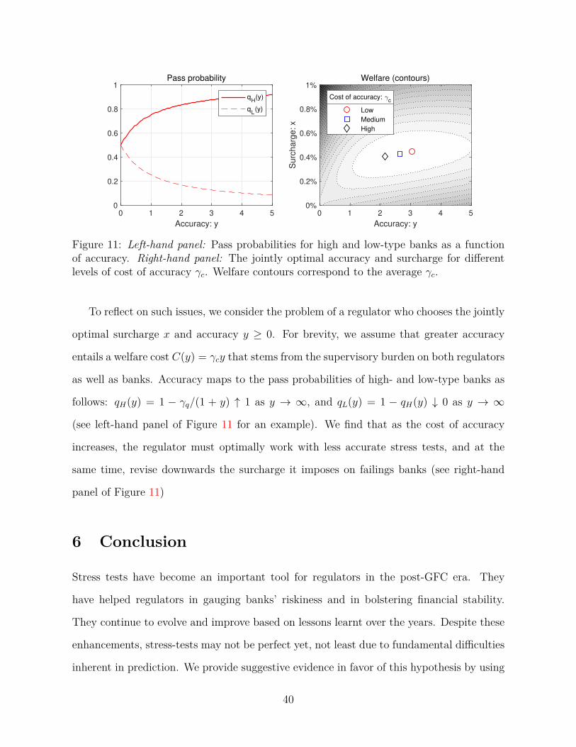
Figure 11: Left-hand panel: Pass probabilities for high and low-type banks as a functionof accuracy. Right-hand panel: The jointly optimal accuracy and surcharge for differentlevels of cost of accuracy γc. Welfare contours correspond to the average γc.
To reflect on such issues, we consider the problem of a regulator who chooses the jointly
optimal surcharge x and accuracy y ≥ 0. For brevity, we assume that greater accuracy
entails a welfare cost C(y) = γcy that stems from the supervisory burden on both regulators
as well as banks. Accuracy maps to the pass probabilities of high- and low-type banks as
follows: qH(y) = 1 − γq/(1 + y) ↑ 1 as y → ∞, and qL(y) = 1 − qH(y) ↓ 0 as y → ∞
(see left-hand panel of Figure 11 for an example). We find that as the cost of accuracy
increases, the regulator must optimally work with less accurate stress tests, and at the
same time, revise downwards the surcharge it imposes on failings banks (see right-hand
panel of Figure 11)
6 Conclusion
Stress tests have become an important tool for regulators in the post-GFC era. They
have helped regulators in gauging banks’ riskiness and in bolstering financial stability.
They continue to evolve and improve based on lessons learnt over the years. Despite these
enhancements, stress-tests may not be perfect yet, not least due to fundamental difficulties
inherent in prediction. We provide suggestive evidence in favor of this hypothesis by using
40

the Covid-19 crisis as a natural experiment to assess stress-testing. We show that banks’
performances in the 2020 U.S. stress-test and during the crisis are highly discordant, both
in absolute and relative (cross-sectional) terms. In particular, some of the worst performers
in the test actually raised their CET1 ratios during the crisis.
Given that stress-test results underpin banks’ capital requirements, inaccurate results
can have a large impact on banks’ capital costs, on their operations, and on overall economic
welfare. A healthy and less-risky bank may unfairly fail the test and face inefficiently strict
regulation (and vice-versa). To assess the implications, we build a model of stress-testing,
and show that inaccuracies not only reduce welfare directly, but also by creating adverse ex-
ante incentives. As such, stress-test based regulatory actions must be less strenuous when
accuracy is lower, or when increasing accuracy is fundamentally challenging or prohibitively
costly. We illustrate the quantitative implications of our theoretical findings based on U.S.
data.
Our model is parsimonious and tractable, and is amenable to extensions that al-
low studying related questions of interest. For instance, some regulators have discussed
maintaining a surprise element in stress-tests on the grounds that it can help avoid pre-
positioning or complacency by banks.35 The welfare effects of surprise or extraneous noise
in stress tests is not obvious because while it can limit the scope for gaming by banks,
higher regulatory uncertainty can weaken the link between the effort banks exert and their
performance in the stress-test. This can make banks exert less effort towards improv-
ing their risk-return profile. Our model can be used to study this trade-off by making
regulation a discretionary function of the signal received from the test.35See, for instance, the remarks by Mr Jerome H Powell, Chair of US Federal Reserve System, at
the research conference titled ”Stress Testing: A Discussion and Review” on 9 July 2019. In fact, thecontinuous evolution of the stress-test regime may be motivated by this pursuit.
41

References
Acharya, V., R. Engle, and D. Pierret (2014). Testing macroprudential stress tests: The
risk of regulatory risk weights. Journal of Monetary Economics 65, 36–53.
Ahnert, T., J. Chapman, and C. Wilkins (2020). Should bank capital regulation be risk
sensitive? Journal of Financial Intermediation, 100870.
Baudino, P., R. Goetschmann, J. Henry, K. Taniguchi, and W. Zhu (2018). Stress-testing
banks: A comparative analysis. FSI Insights on policy implementation (12).
Begenau, J. (2019). Capital requirements, risk choice, and liquidity provision in a business-
cycle model. Journal of Financial Economics.
Bouvard, M., P. Chaigneau, and A. D. Motta (2015). Transparency in the financial system:
Rollover risk and crises. The Journal of Finance 70 (4), 1805–1837.
Breuer, T., M. Jandacka, K. Rheinberger, and M. Summer (2018). How to find plausible,
severe, and useful stress scenarios. Eighteenth issue (September 2009) of the International
Journal of Central Banking.
Christiano, L. and D. Ikeda (2016). Bank leverage and social welfare. American Economic
Review 106 (5), 560–64.
Corona, C., L. Nan, and G. Zhang (2017). The coordination role of stress test disclosure
in bank risk taking. Technical report, Working paper.
Covas, F. B., B. Rump, and E. Zakrajsek (2014). Stress-testing us bank holding compa-
nies: A dynamic panel quantile regression approach. International Journal of Forecast-
ing 30 (3), 691–713.
DFAST (2020). Dodd-frank act stress test 2020: Supervisory stress-test methodology and
results. Federal Reserve Bank.
42

Fed (2020a). Press release: Federal reserve board approves rule to simplify its capital rules
for large banks, preserving the strong capital requirements already in place (march).
Fed (2020b). Press release: Federal reserve board releases corrected stress test results
stemming from an error in projected trading losses and as a result, revised the capital
requirements for two banks (september).
Flannery, M., B. Hirtle, and A. Kovner (2017). Evaluating the information in the federal
reserve stress tests. Journal of Financial Intermediation 29, 1–18.
Frame, W. S., K. Gerardi, and P. Willen (2015). The failure of supervisory stress testing:
Fannie mae, freddie mac, and the of federal housing enterprise oversight.
Gertler, M. and N. Kiyotaki (2010). Financial intermediation and credit policy in business
cycle analysis. Handbook of Monetary Economics 3, 547.
Goldstein, I. and Y. Leitner (2018). Stress tests and information disclosure. Journal of
Economic Theory 177, 34–69.
Goldstein, I. and H. Sapra (2013). Should banks’ stress test results be disclosed? an
analysis of the costs and benefits. Foundations and Trends in Finance, forthcoming.
Gorton, G. B. (2008). The panic of 2007. Technical report, National Bureau of Economic
Research.
Kara, G. and S. M. Ozsoy (2016). Bank regulation under fire sale externalities.
Kareken, J. H. and N. Wallace (1978). Deposit insurance and bank regulation: A partial-
equilibrium exposition. Journal of business, 413–438.
Leitner, Y. and B. Williams (2020). Model secrecy and stress tests. Available at SSRN
3606654 .
43

Lohmann, S. (1992). Optimal commitment in monetary policy: credibility versus flexibility.
The American Economic Review 82 (1), 273–286.
Marshall, D. A. and E. S. Prescott (2001). Bank capital regulation with and without
state-contingent penalties. In Carnegie-Rochester Conference Series on Public Policy,
Volume 54, pp. 139–184. Elsevier.
Morgan, D. P., S. Peristiani, and V. Savino (2014). The information value of the stress
test. Journal of Money, Credit and Banking 46 (7), 1479–1500.
Morrison, A. D. and L. White (2005). Crises and capital requirements in banking. American
Economic Review 95 (5), 1548–1572.
Nguyen, T. T. (2015). Bank capital requirements: A quantitative analysis. Charles A.
Dice Center Working Paper (2015-14).
Ong, M. L. L., M. R. Maino, and N. Duma (2010). Into the great unknown: Stress testing
with weak data. Number 10-282. International Monetary Fund.
Orlov, D., P. Zryumov, and A. Skrzypacz (2018). Design of macro-prudential stress tests.
Parlatore, C. and T. Philippon (2018). Designing stress scenarios. In 2018 Meeting Papers,
Number 1090. Society for Economic Dynamics.
Philippon, T., P. Pessarossi, and B. Camara (2017). Backtesting european stress tests.
Technical report, National Bureau of Economic Research.
Prescott, E. S. (2004). Auditing and bank capital regulation. FRB Richmond Economic
Quarterly 90 (4), 47–63.
Santos, J. A. (2001). Bank capital regulation in contemporary banking theory: A review
of the literature. Financial Markets, Institutions & Instruments 10 (2), 41–84.
44

Van den Heuvel, S. J. (2008). The welfare cost of bank capital requirements. Journal of
Monetary Economics 55 (2), 298–320.
45