Embed Size (px)
Citation preview
LINEAR ALGEBRA ANDMATRICES
Shmuel Friedland, Mohsen Aliabadi
University of Illinois at Chicago, USA

The first named author dedicates this book to his wife Margaret
The second named author dedicates this book to the memory of his parents
Contents
Preface . . . . . . . . . . . . . . . . . . . . . . . . . . . . . . . . . . . . . . . . . 7
1 Preliminaries 81.1 Basic facts in abstract algebra . . . . . . . . . . . . . . . . . . . . . . . . 8
1.1.1 Groups . . . . . . . . . . . . . . . . . . . . . . . . . . . . . . . . . 81.1.2 Rings . . . . . . . . . . . . . . . . . . . . . . . . . . . . . . . . . . 91.1.3 Fields and division rings . . . . . . . . . . . . . . . . . . . . . . . 101.1.4 Vector spaces, modules and algebras . . . . . . . . . . . . . . . 111.1.5 More about groups . . . . . . . . . . . . . . . . . . . . . . . . . . 121.1.6 The group of bijections on a set X . . . . . . . . . . . . . . . . . 141.1.7 More about rings . . . . . . . . . . . . . . . . . . . . . . . . . . . 141.1.8 More about fields . . . . . . . . . . . . . . . . . . . . . . . . . . . 151.1.9 The characteristic of a ring . . . . . . . . . . . . . . . . . . . . . 15
1.2 Basic facts in set theory . . . . . . . . . . . . . . . . . . . . . . . . . . . . 161.3 Basic facts in analysis . . . . . . . . . . . . . . . . . . . . . . . . . . . . . 161.4 Basic facts in topology . . . . . . . . . . . . . . . . . . . . . . . . . . . . 181.5 Basic facts in graph theory . . . . . . . . . . . . . . . . . . . . . . . . . . 18
1.5.1 Worked-out Problems . . . . . . . . . . . . . . . . . . . . . . . . . 201.5.2 Problems . . . . . . . . . . . . . . . . . . . . . . . . . . . . . . . . 22
1.6 Dimension and basis . . . . . . . . . . . . . . . . . . . . . . . . . . . . . 221.6.1 More details on vector space . . . . . . . . . . . . . . . . . . . . 221.6.2 Dimension . . . . . . . . . . . . . . . . . . . . . . . . . . . . . . . 241.6.3 Worked-out Problems . . . . . . . . . . . . . . . . . . . . . . . . . 251.6.4 Problems . . . . . . . . . . . . . . . . . . . . . . . . . . . . . . . . 26
1.7 Matrices . . . . . . . . . . . . . . . . . . . . . . . . . . . . . . . . . . . . . 281.7.1 Basic properties of matrices . . . . . . . . . . . . . . . . . . . . . 281.7.2 Elementary row operation . . . . . . . . . . . . . . . . . . . . . . 291.7.3 Gaussian Elimination . . . . . . . . . . . . . . . . . . . . . . . . . 291.7.4 Solution of linear systems . . . . . . . . . . . . . . . . . . . . . . 311.7.5 Invertible matrices . . . . . . . . . . . . . . . . . . . . . . . . . . 341.7.6 Row and column spaces of A . . . . . . . . . . . . . . . . . . . . 361.7.7 Special types of matrices . . . . . . . . . . . . . . . . . . . . . . . 38
1.8 Sum of subspaces . . . . . . . . . . . . . . . . . . . . . . . . . . . . . . . . 391.8.1 Sum of two subspaces . . . . . . . . . . . . . . . . . . . . . . . . . 391.8.2 Sums of many subspaces . . . . . . . . . . . . . . . . . . . . . . . 401.8.3 Dual spaces and annihilators . . . . . . . . . . . . . . . . . . . . 411.8.4 Worked-out Problems . . . . . . . . . . . . . . . . . . . . . . . . . 421.8.5 Problems . . . . . . . . . . . . . . . . . . . . . . . . . . . . . . . . 43
2
1.9 Permutations . . . . . . . . . . . . . . . . . . . . . . . . . . . . . . . . . . 441.9.1 The permutation group . . . . . . . . . . . . . . . . . . . . . . . . 441.9.2 Worked-out Problems . . . . . . . . . . . . . . . . . . . . . . . . . 461.9.3 Problems . . . . . . . . . . . . . . . . . . . . . . . . . . . . . . . . 47
1.10 Linear, multilinear maps and functions . . . . . . . . . . . . . . . . . . . 471.10.1 Worked-out Problems . . . . . . . . . . . . . . . . . . . . . . . . . 501.10.2 Problems . . . . . . . . . . . . . . . . . . . . . . . . . . . . . . . . 51
1.11 Definition and properties of the determinant . . . . . . . . . . . . . . . 511.11.1 Geometric interpretation of determinant (First encounter) . . . 511.11.2 Explicit formula of the determinant and its properties . . . . . 521.11.3 Matrix inverse . . . . . . . . . . . . . . . . . . . . . . . . . . . . . 561.11.4 Worked-out Problems . . . . . . . . . . . . . . . . . . . . . . . . . 581.11.5 Problems . . . . . . . . . . . . . . . . . . . . . . . . . . . . . . . . 60
1.12 Permanents . . . . . . . . . . . . . . . . . . . . . . . . . . . . . . . . . . . 611.12.1 A combinatorial approach of Philip Hall Theorem . . . . . . . . 611.12.2 Permanents . . . . . . . . . . . . . . . . . . . . . . . . . . . . . . . 611.12.3 Worked-out Problems . . . . . . . . . . . . . . . . . . . . . . . . . 631.12.4 Problems . . . . . . . . . . . . . . . . . . . . . . . . . . . . . . . . 64
1.13 An application of Philip Hall Theorem . . . . . . . . . . . . . . . . . . . 641.13.1 Worked-out Problems . . . . . . . . . . . . . . . . . . . . . . . . . 671.13.2 Problems . . . . . . . . . . . . . . . . . . . . . . . . . . . . . . . . 67
1.14 Polynomial rings . . . . . . . . . . . . . . . . . . . . . . . . . . . . . . . . 671.14.1 Polynomials . . . . . . . . . . . . . . . . . . . . . . . . . . . . . . 671.14.2 Finite fields and finite extension of fields . . . . . . . . . . . . . 691.14.3 Worked-out Problems . . . . . . . . . . . . . . . . . . . . . . . . . 701.14.4 Problems . . . . . . . . . . . . . . . . . . . . . . . . . . . . . . . . 71
1.15 The general linear group . . . . . . . . . . . . . . . . . . . . . . . . . . . 721.15.1 Matrix Groups . . . . . . . . . . . . . . . . . . . . . . . . . . . . . 731.15.2 Worked-out Problems . . . . . . . . . . . . . . . . . . . . . . . . . 741.15.3 Problems . . . . . . . . . . . . . . . . . . . . . . . . . . . . . . . . 74
1.16 Complex numbers . . . . . . . . . . . . . . . . . . . . . . . . . . . . . . . 741.16.1 Worked-out Problems . . . . . . . . . . . . . . . . . . . . . . . . . 751.16.2 Problems . . . . . . . . . . . . . . . . . . . . . . . . . . . . . . . . 75
1.17 Linear operators (Second encounter) . . . . . . . . . . . . . . . . . . . . 761.17.1 Worked-out Problems . . . . . . . . . . . . . . . . . . . . . . . . . 771.17.2 Problems . . . . . . . . . . . . . . . . . . . . . . . . . . . . . . . . 771.17.3 Trace . . . . . . . . . . . . . . . . . . . . . . . . . . . . . . . . . . 781.17.4 Worked-out Problems . . . . . . . . . . . . . . . . . . . . . . . . . 791.17.5 Problems . . . . . . . . . . . . . . . . . . . . . . . . . . . . . . . . 79
2 Tensor products 802.1 Universal property of tensor products . . . . . . . . . . . . . . . . . . . 802.2 Matrices and tensors . . . . . . . . . . . . . . . . . . . . . . . . . . . . . . 812.3 Tensor product of linear operators and Kronecker product . . . . . . . 82
2.3.1 Worked-out Problems . . . . . . . . . . . . . . . . . . . . . . . . . 842.3.2 Problems . . . . . . . . . . . . . . . . . . . . . . . . . . . . . . . . 84
3
3 Canonical forms 853.1 Jordan canonical forms . . . . . . . . . . . . . . . . . . . . . . . . . . . . 853.2 An application of diagonalizable matrices . . . . . . . . . . . . . . . . . 92
3.2.1 Worked-out Problems . . . . . . . . . . . . . . . . . . . . . . . . . 933.2.2 Problems . . . . . . . . . . . . . . . . . . . . . . . . . . . . . . . . 94
3.3 Matrix polynomials . . . . . . . . . . . . . . . . . . . . . . . . . . . . . . 963.4 Minimal polynomial and decomposition to invariant subspaces . . . . 99
3.4.1 Worked-out Problems . . . . . . . . . . . . . . . . . . . . . . . . . 1023.4.2 Problems . . . . . . . . . . . . . . . . . . . . . . . . . . . . . . . . 104
3.5 Quotient of vector spaces and induced linear operators . . . . . . . . . 1063.6 Isomorphism theorems for vector spaces . . . . . . . . . . . . . . . . . . 1073.7 Existence and uniqueness of the Jordan canonical form . . . . . . . . . 108
3.7.1 Worked-out Problems . . . . . . . . . . . . . . . . . . . . . . . . . 1133.7.2 Problems . . . . . . . . . . . . . . . . . . . . . . . . . . . . . . . . 113
3.8 Cyclic subspaces and rational canonical forms . . . . . . . . . . . . . . 1143.8.1 Worked-out Problems . . . . . . . . . . . . . . . . . . . . . . . . . 1193.8.2 Problems . . . . . . . . . . . . . . . . . . . . . . . . . . . . . . . . 120
4 Applications of Jordan canonical form 1214.1 Functions of Matrices . . . . . . . . . . . . . . . . . . . . . . . . . . . . . 121
4.1.1 Linear recurrence equation . . . . . . . . . . . . . . . . . . . . . . 1264.1.2 Worked-out Problems . . . . . . . . . . . . . . . . . . . . . . . . . 1264.1.3 Problems . . . . . . . . . . . . . . . . . . . . . . . . . . . . . . . . 127
4.2 Power stability, convergence and boundedness of matrices . . . . . . . 1274.3 eAt and stability of certain systems of ODE . . . . . . . . . . . . . . . . 130
4.3.1 Worked-out Problems . . . . . . . . . . . . . . . . . . . . . . . . . 1324.3.2 Problems . . . . . . . . . . . . . . . . . . . . . . . . . . . . . . . . 133
5 Inner product spaces 1345.1 Inner product . . . . . . . . . . . . . . . . . . . . . . . . . . . . . . . . . . 1345.2 Explanation of G-S process in standard Euclidean space . . . . . . . . 1385.3 An example of G-S process . . . . . . . . . . . . . . . . . . . . . . . . . . 1395.4 QR Factorization . . . . . . . . . . . . . . . . . . . . . . . . . . . . . . . . 1395.5 An example of QR algorithm . . . . . . . . . . . . . . . . . . . . . . . . . 1405.6 The best fit line . . . . . . . . . . . . . . . . . . . . . . . . . . . . . . . . 1425.7 Geometric interpretation of the determinant (Second encounter) . . . 143
5.7.1 Worked-out Problems . . . . . . . . . . . . . . . . . . . . . . . . . 1455.7.2 Problems . . . . . . . . . . . . . . . . . . . . . . . . . . . . . . . . 145
5.8 Special transformations in IPS . . . . . . . . . . . . . . . . . . . . . . . . 1485.9 Symmetric bilinear and hermitian forms . . . . . . . . . . . . . . . . . . 1535.10 Max-min characterizations of eigenvalues . . . . . . . . . . . . . . . . . 154
5.10.1 Worked-out Problems . . . . . . . . . . . . . . . . . . . . . . . . . 1585.10.2 Problems . . . . . . . . . . . . . . . . . . . . . . . . . . . . . . . . 160
5.11 Positive definite operators and matrices . . . . . . . . . . . . . . . . . . 1635.12 Inequalities for traces . . . . . . . . . . . . . . . . . . . . . . . . . . . . . 167
5.12.1 Worked-out Problems . . . . . . . . . . . . . . . . . . . . . . . . . 1695.12.2 Problems . . . . . . . . . . . . . . . . . . . . . . . . . . . . . . . . 169
5.13 Schur’s Unitary Triangularization . . . . . . . . . . . . . . . . . . . . . . 170
4
5.14 Singular Value Decomposition . . . . . . . . . . . . . . . . . . . . . . . . 1715.15 Characterizations of singular values . . . . . . . . . . . . . . . . . . . . . 176
5.15.1 Worked-out Problems . . . . . . . . . . . . . . . . . . . . . . . . . 1805.15.2 Problems . . . . . . . . . . . . . . . . . . . . . . . . . . . . . . . . 182
5.16 Moore-Penrose generalized inverse . . . . . . . . . . . . . . . . . . . . . 1845.16.1 Worked-out Problems . . . . . . . . . . . . . . . . . . . . . . . . . 1855.16.2 Problems . . . . . . . . . . . . . . . . . . . . . . . . . . . . . . . . 186
6 Perron-Frobenius theorem 1876.1 Perron-Frobenius theorem . . . . . . . . . . . . . . . . . . . . . . . . . . 1876.2 Irreducible matrices . . . . . . . . . . . . . . . . . . . . . . . . . . . . . . 1956.3 Recurrence equation with non-negative coefficients . . . . . . . . . . . . 197
6.3.1 Worked-out Problems . . . . . . . . . . . . . . . . . . . . . . . . . 1986.3.2 Problems . . . . . . . . . . . . . . . . . . . . . . . . . . . . . . . . 198
References . . . . . . . . . . . . . . . . . . . . . . . . . . . . . . . . . . . . . . . 199Index . . . . . . . . . . . . . . . . . . . . . . . . . . . . . . . . . . . . . . . . . . 200
5
Preface
Linear algebra and matrix theory, abbreviated here as LAMT, is a foundation formany advanced topics in mathematics, and an essential tool for computer sciences,physics, engineering, bioinformatics, economics, and social sciences. A first coursein linear algebra for engineers is like a cook book, where various results are givenwith very little rigorous justifications. For mathematics students, on the other hand,linear algebra comes at a time when they are being introduced to abstract conceptsand formal proofs as the foundations of mathematics. In this case, very little offundamental concepts of LAMT are covered. For a second course in LAMT thereare a number of options. One option is to study the numerical aspects of LAMT, asfor example in the book [8]. A totally different option, as in the popular book [11],which views LAMT as a part of a basic abstract course in algebra.
This book is aimed to be an introductory course in LAMT for beginning gradu-ate students and an advanced (second) course in LAMT for undergraduate students.Reconciling such a dichotomy was made possible thanks to more than a decade ofteaching the subject by the first author, in the Department of Mathematics, Statis-tics and Computer Science, the University of Illinois at Chicago, to both graduatestudents, and to advanced undergraduate students.
In this book, we used the abstract notions and arguments to give the com-plete proof of the Jordan canonical form, and more generally, the rational canonicalforms of square matrices over fields. Also, we provide the notion of tensor prod-ucts of vector spaces and linear transformations. Matrices are treated in depth:stability of matrix iterations, the eigenvalue properties of linear transformations ininner product space, singular value decomposition, and mini-max characterizationsof Hermitian matrices and non-negative irreducible matrices.
We now briefly outline out the contents of this book. There are six chapters.The first chapter is a survey of basic notions. Some sections in this chapter are fromother areas of mathematics, as elementary set theory, analysis, topology, and com-binatorics. These sections can be assigned to students for self-study. Other sectionsdeal with basic facts in LAMT, which may be skipped if the students are alreadyfamiliar with them. The second chapter is a brief introduction to tensor productsof finite dimensional vector spaces, tensor products of linear transformations, andtheir representations as Kronecker product. This chapter can either be skipped orcan be taught later in the course The third chapter is a rigorous exposition of theJordan canonical form over an algebraically closed field (which is usually the com-plex numbers in the engineering world), and a rational canonical form for linearoperators and matrices. Again, the section dealing with cyclic subspaces and ratio-nal canonical forms can be skipped without losing consistency. Chapter 4 deals withapplications of the Jordan canonical form of matrices with real and complex entries.First, we discuss the precise expression of f(A), where A is a square matrix and fis a polynomial, in terms of the components of A. We then discuss the extension ofthis formula to functions f which are analytic at a neighborhood of the spectrum ofA. The instructor may choose one particular application to teach from this chapter.Fifth chapter, the longest one, is devoted to properties of inner product spaces, andspecial linear operators such as normal, Hermitian and unitary. We bring the min-max and max-min characterizations of the eigenvalues of Hermitian matrices, thesingular value decomposition and its minimal low rank approximation properties.
6

The last chapter deals with basic aspects of the Perron-Frobenius theory, which arenot usually found in a typical linear algebra book.
One of the main objectives of this book is to show the variety of topics and toolsthat modern linear algebra and matrix theory encompass. To facilitate the readingof this book we have a good number of worked-out problems, helping the reader,especially those preparing for an exam such as a graduate preliminary exam, tobetter-understand the notions and results discussed in each section. We also providea number of problems for instructors to assign, as well, to complement the material.
Perhaps, it will be hard to cover all these topics in a one-semester graduatecourse. However, as many sections of these book are independent, the instructormay choose appropriate sections as needed.
August 2016 Shmuel Friedland
Mohsen Aliabadi
7
Chapter 1
Preliminaries
1.1 Basic facts in abstract algebra
1.1.1 Groups
A binary operation on a set A is a map which sends elements of the Cartesian productA ×A to A. A group denoted by G, is a set of elements with a binary operation ⊕,i.e. a⊕ b ∈ G, for each a, b ∈ G. This operation is
(i) associative: (a⊕ b)⊕ c = a⊕ (b⊕ c);
(ii) there exists a neutral element such that a⊕ = a, for each a ∈ G;
(iii) for each a ∈ G, there exists a unique ⊖a such that a⊕(⊖a) =.
The group G is called abelian (commutative) if a⊕ b = b⊕ a, for each a, b ∈ G. Oth-erwise, it is called nonabelian (noncommutative).
Examples of abelian groups
1. The following subsets of complex numbers where ⊕ is the standard addition+, ⊖ is the standard subtraction − and the neutral element is 0.
(a) The set of integers Z.
(b) The set of rational numbers Q.
(c) The set of real numbers R.
(d) The set of complex numbers C
2. The following subsets of C∗ ∶= C/0, i.e. all non-zero complex numbers, wherethe operation ⊕ is the standard product, the neutral element is 1, and ⊖a isa−1.
(a) Q∗ ∶= Q/0.
(b) R∗ ∶= R/0.
(c) C∗ ∶= C/0.
8
An example of nonabelian groupThe quaternion group is a group with eight elements, which is denoted as (Q8,⊕)and defined as follows:Q8 = 1,−1, i,−i, j,−j, k,−k, 1 is the identity element and(−1)⊕ (−1) = 1(−1)⊕ i = −i(−1)⊕ j = −j(−1)⊕ k = −ki⊕ j = kj ⊕ i = −kj ⊕ k = ik ⊕ j = −ik ⊕ i = ji⊕ k = −j,and the remaining relations can be deduced from these. Clearly, Q8 is not abelianas for instance i⊕ j ≠ j ⊕ i.
1.1.2 Rings
From now on, we will denote the operation ⊕ by +. An abelian group R is calleda ring , if there exists a second operation, called product, denoted by ab , for anya, b ∈ R, which satisfies:
(i) associativity: (ab)c = a(bc);
(ii) distributivity: a(b + c) = ab + ac, (b + c)a = ba + ca, (a, b, c ∈ R);
(iii) existence of identity 1 ∈ R: 1a = a1 = a, for all a ∈ R.
Also, R is called a commutative ring if ab = ba, for all a, b ∈ R. Otherwise, R iscalled a noncommutative ring.
Examples of rings
1. For a positive integer n > 1, the set of n×n complex valued matrices, denotedby Cn×n, with the addition A +B, product AB, and with the identity In, then × n identity matrix . (We will introduce the concept of a matrix in section1.5.) Furthermore, the following subsets of Cn×n:
(a) Zn×n, the ring of n × n matrices with integer entries. (Noncommutativering).
(b) Qn×n, the ring of n×n matrices with rational entries. (Noncommutativering).
(c) Rn×n, the ring of n×n matrices with real entries. (Noncommutative ring).
(d) Cn×n. (Noncommutative ring).
(e) D(n,S), the set of n×n diagonal matrices with entries in S = Z,Q,R,C.(Commutative ring).
(Diagonal matrices are square matrices in which their entries outside the maindiagonal are zero.)
9
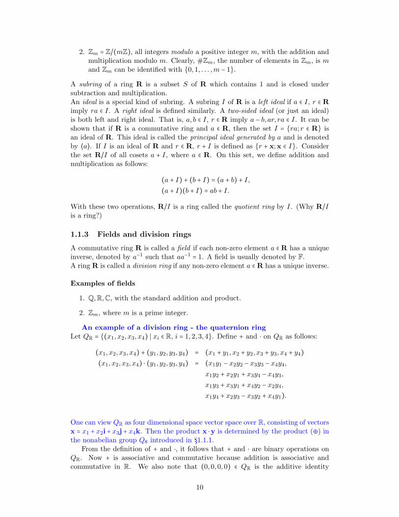
2. Zm = Z/(mZ), all integers modulo a positive integer m, with the addition andmultiplication modulo m. Clearly, #Zm, the number of elements in Zm, is mand Zm can be identified with 0,1, . . . ,m − 1.
A subring of a ring R is a subset S of R which contains 1 and is closed undersubtraction and multiplication.An ideal is a special kind of subring. A subring I of R is a left ideal if a ∈ I, r ∈ Rimply ra ∈ I. A right ideal is defined similarly. A two-sided ideal (or just an ideal)is both left and right ideal. That is, a, b ∈ I, r ∈ R imply a − b, ar, ra ∈ I. It can beshown that if R is a commutative ring and a ∈ R, then the set I = ra; r ∈ R isan ideal of R. This ideal is called the principal ideal generated by a and is denotedby ⟨a⟩. If I is an ideal of R and r ∈ R, r + I is defined as r + x;x ∈ I. Considerthe set R/I of all cosets a + I, where a ∈ R. On this set, we define addition andmultiplication as follows:
(a + I) + (b + I) = (a + b) + I,(a + I)(b + I) = ab + I.
With these two operations, R/I is a ring called the quotient ring by I. (Why R/Iis a ring?)
1.1.3 Fields and division rings
A commutative ring R is called a field if each non-zero element a ∈ R has a uniqueinverse, denoted by a−1 such that aa−1 = 1. A field is usually denoted by F.A ring R is called a division ring if any non-zero element a ∈ R has a unique inverse.
Examples of fields
1. Q,R,C, with the standard addition and product.
2. Zm, where m is a prime integer.
An example of a division ring - the quaternion ringLet QR = (x1, x2, x3, x4) ∣ xi ∈ R, i = 1,2,3,4. Define + and ⋅ on QR as follows:
(x1, x2, x3, x4) + (y1, y2, y3, y4) = (x1 + y1, x2 + y2, x3 + y3, x4 + y4)(x1, x2, x3, x4) ⋅ (y1, y2, y3, y4) = (x1y1 − x2y2 − x3y3 − x4y4,
x1y2 + x2y1 + x3y4 − x4y3,
x1y3 + x3y1 + x4y2 − x2y4,
x1y4 + x2y3 − x3y2 + x4y1).
One can view QR as four dimensional space vector space over R, consisting of vectorsx = x1 + x2i+ x3j+ x4k. Then the product x ⋅y is determined by the product (⊕) inthe nonabelian group Q8 introduced in §1.1.1.
From the definition of + and ⋅, it follows that + and ⋅ are binary operations onQR. Now + is associative and commutative because addition is associative andcommutative in R. We also note that (0,0,0,0) ∈ QR is the additive identity
10
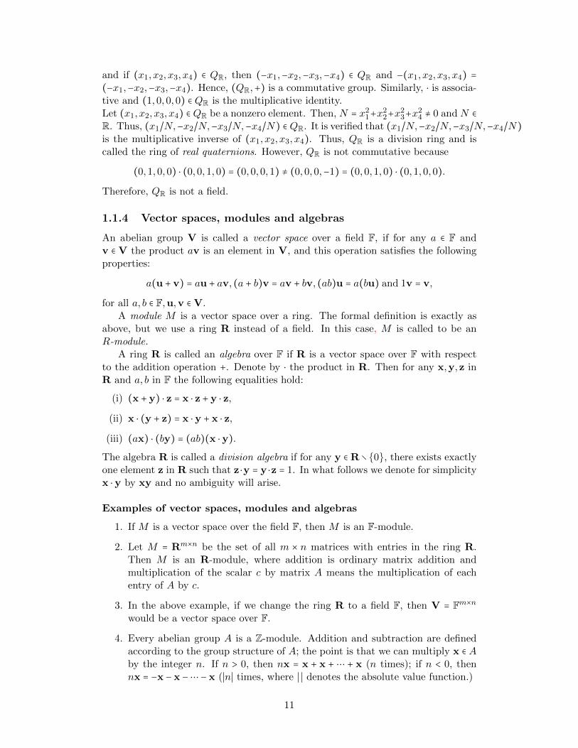
and if (x1, x2, x3, x4) ∈ QR, then (−x1,−x2,−x3,−x4) ∈ QR and −(x1, x2, x3, x4) =(−x1,−x2,−x3,−x4). Hence, (QR,+) is a commutative group. Similarly, ⋅ is associa-tive and (1,0,0,0) ∈ QR is the multiplicative identity.Let (x1, x2, x3, x4) ∈ QR be a nonzero element. Then, N = x2
1+x22+x2
3+x24 ≠ 0 and N ∈
R. Thus, (x1/N,−x2/N,−x3/N,−x4/N) ∈ QR. It is verified that (x1/N,−x2/N,−x3/N,−x4/N)is the multiplicative inverse of (x1, x2, x3, x4). Thus, QR is a division ring and iscalled the ring of real quaternions. However, QR is not commutative because
(0,1,0,0) ⋅ (0,0,1,0) = (0,0,0,1) ≠ (0,0,0,−1) = (0,0,1,0) ⋅ (0,1,0,0).
Therefore, QR is not a field.
1.1.4 Vector spaces, modules and algebras
An abelian group V is called a vector space over a field F, if for any a ∈ F andv ∈ V the product av is an element in V, and this operation satisfies the followingproperties:
a(u + v) = au + av, (a + b)v = av + bv, (ab)u = a(bu) and 1v = v,
for all a, b ∈ F,u,v ∈ V.A module M is a vector space over a ring. The formal definition is exactly as
above, but we use a ring R instead of a field. In this case, M is called to be anR-module.
A ring R is called an algebra over F if R is a vector space over F with respectto the addition operation +. Denote by ⋅ the product in R. Then for any x,y,z inR and a, b in F the following equalities hold:
(i) (x + y) ⋅ z = x ⋅ z + y ⋅ z,
(ii) x ⋅ (y + z) = x ⋅ y + x ⋅ z,
(iii) (ax) ⋅ (by) = (ab)(x ⋅ y).The algebra R is called a division algebra if for any y ∈ R∖0, there exists exactlyone element z in R such that z ⋅y = y ⋅z = 1. In what follows we denote for simplicityx ⋅ y by xy and no ambiguity will arise.
Examples of vector spaces, modules and algebras
1. If M is a vector space over the field F, then M is an F-module.
2. Let M = Rm×n be the set of all m × n matrices with entries in the ring R.Then M is an R-module, where addition is ordinary matrix addition andmultiplication of the scalar c by matrix A means the multiplication of eachentry of A by c.
3. In the above example, if we change the ring R to a field F, then V = Fm×nwould be a vector space over F.
4. Every abelian group A is a Z-module. Addition and subtraction are definedaccording to the group structure of A; the point is that we can multiply x ∈ Aby the integer n. If n > 0, then nx = x + x + ⋯ + x (n times); if n < 0, thennx = −x − x −⋯ − x (∣n∣ times, where ∣ ∣ denotes the absolute value function.)
11
5. Every commutative ring R is an algebra over itself.
6. An arbitrary ring R is always a Z-algebra.
7. If R is a commutative ring, then Rn×n, the set of all n×n matrices with entriesin R is an R-algebra.
1.1.5 More about groups
A setG is called to be a semigroup if it has a binary operation satisfying the condition(ab)c = a(bc), for any a, b, c ∈ G. (Here, the product operation is replaced by ⊕.)
A subset H of G is called a subgroup of G if H also forms a group under theoperation of G. The set of the integers Z is a subgroup of the group of rationalnumbers Q under ordinary addition.
A subgroup N of a group G is called a normal subgroup if for each element n inN and each g in G, the element gng−1 is still in N . We use the notation N ⊲ Gto denote that N is a normal subgroup of G. For example, all subgroups N of anabelian group G are normal (why?).
The center of a group G, denoted by Z(G), is the set of elements that commutewith every element of G, i.e.
Z(G) = z ∈ G; zg = gz, ∀g ∈ G.
Clearly, Z(G) ⊲ G.
For a subgroup H of a group G and an element x of G, define xH to be the setxh;h ∈ H. A subset of G of the form xH is said to be a left coset of H (a rightcoset of H is defined similarly.) For a normal subgroup N of the group G, thequotient group of N in G, written G/N and read “G modulo N”, is the set of cosetsof N in G. It is easy to see that G/N is a group with the following operation:
(Na)(Nb) = Nab, for all a, b ∈ G.
A group G is called finitely generated if there exist x1, . . . ,xn in G such that everyx in G can be written in the form x = x±1
i1⋯x±1
im, where i1, . . . , im ∈ 1, . . . , n and m
ranges over all positive integers. In this case, we say that the set x1, . . . ,xn is agenerating set of G.A cyclic group is a finitely generated group, which is generated by a single element.A group homomorphism is a map ϕ ∶ G1 → G2 between two groups G1 and G2
such that the group operation is preserved, i.e. ϕ(xy) = ϕ(x)ϕ(y), for any x,y ∈G1. A group homomorphism is called an isomorphism if it is bijective. If ϕ is anisomorphism, we say that G1 is isomorphic to G2 and we use the notation G1 ≅ G2.It is easy to show that the isomorphisms of groups form an equivalence relation onthe class of all groups. (See Section 1.2 about equivalence relation.)The kernel of a group homomorphism ϕ ∶ G1 → G2 is denoted by kerϕ and it isthe set of all elements of G1 which are mapped to the identity element of G2. The
12
kernel is a normal subgroup of G1. Also, the image of ϕ is denoted by Imϕ and isdefined as follows:
Imϕ = y ∈ G2;∃x ∈ G1 such that ϕ(x) = y.
Clearly, Imϕ is a subgroup of G2. (and even its normal subgroup). Also, the cokernelof ϕ is denoted by cokerϕ and defined as cokerϕ = G2/Imϕ.
Now, we are ready to give the three isomorphism theorems in the context of groups.The interested reader is referred to [11] to see the proofs and more details aboutthese theorems.
First isomorphism theorem
Let G1 and G2 be two groups and ϕ ∶ G1 → G2 be a group homomorphism. Then,G1/kerϕ ≅ Imϕ. In particular, if ϕ is surjective, then G1/kerϕ is isomorphic to G2.
Second isomorphism theorem
Let G a group and S be a subgroup of G and N be a normal subgroup of G. Then
1. The product SN = sn; s ∈ S and n ∈ N is a subgroup of G.
2. S ∩N ⊲ S.
3. SN/N ≃ S/S ∩N .
Third isomorphism theorem
1. If N ⊲ G and K is a subgroup of G such that N ⊆ K ⊆ G, then K/N is asubgroup of G/N .
2. Every subgroup of G/N is of the form K/N , for some subgroup K of G suchthat N ⊆K ⊆ G.
3. If K is a normal subgroup of G such that N ⊆ K ⊆ G, then K/N is a normalsubgroup of G/N .
4. Every normal subgroup of G/N is of the form K/N , for some normal subgroupK of G such that N ⊆K ⊆ G.
5. If K is a normal subgroup of G such that N ⊆K ⊆ G, then the quotient group
(G/N)/ (K/N) is isomorphic to G/K.
Assume that G is a finite group and H its subgroup. Then G is a disjoint unionof cosets of H. Hence the order of H, (#H), divides the order of G - Lagrange’stheorem. Note that this is the case for vector spaces, i.e. if V is a finite vectorspace (this should not be assumed as a finite dimensional vector space.), and W isits subspace, then #W divides #V . We will define the concept of “dimension” forvector spaces in subsection 1.6.2.
13

1.1.6 The group of bijections on a set X
Let X ,Y be two sets. Then, φ ∶ X → Y is called a mapping , i.e. for each x ∈ X ,φ(x) is an element in Y. Moreover, φ ∶ X → X is called the identity map if φ(x) = x,for each x ∈ X . The identity map is denoted as id or idX . Let ψ ∶ Y → Z. Then, onedefines the composition map ψ φ ∶ X → Z as follows (ψ φ)(x) = ψ(φ(x)). A mapφ ∶ X → Y is called bijection if there exists ψ ∶ Y → X such that ψφ = idX , φψ = idYand ψ is denoted as φ−1. Denote by S(X ) the set of all bijections of X onto itself. Itis easy to show that S(X ) forms a group under the composition, with the identityelement idX . Assume that X is a finite set. Then, any bijection ψ ∈ S(X ) is calleda permutation and S(X ) is called a permutation group.
Let X be a finite set. Then S(X ) has n! elements if n is the number of elementsin X . Assume that X = x1, . . . , xn. We can construct a bijection φ on X as follows:
(1) Assign one of the n elements of X to φ(x1). (There are n possibilities forφ(x1) in X .)
(2) Assign one of the n − 1 elements of X − φ(x1) to φ(x2). (There are n − 1possibilities for φ(x2) in X − φ(x1).)
⋮
(n) Assign the one remaining element to φ(xn). (There is only one possibility forφ(xn).)
This method can generate n(n − 1)⋯1 = n! different bijections of X .
1.1.7 More about rings
If R and S are two rings, then a ring homomorphism from R to S is a functionϕ ∶ R→ S such that
(i) ϕ(a + b) = ϕ(a) + ϕ(b),
(ii) ϕ(ab) = ϕ(a)ϕ(b),
for each a, b ∈ R.A ring homomorphism is called an isomorphism if it is bijective.Note that we have three isomorphism theorems for rings which are similar to iso-morphism theorems in groups. See [11] for more details.
Remark 1.1.1 If ϕ ∶ (R,+, ⋅) → (S,+, ⋅) is a ring homomorphism, then ϕ ∶(R,+)→ (S,+) is a group homomorphism.
Remark 1.1.2 If R is a ring and S ⊂ R is a subring, then the inclusion i ∶ SR is a ring homomorphism. (Why?)
14
1.1.8 More about fields
Let F be a field. Then by F[x] we denote the set of all polynomials p(x) = anxn +⋯ + a0, where x0 ≡ 1. p is called monic if an = 1. The degree of p, denoted as deg p,is n if an ≠ 0. F[x] is a commutative ring under the standard addition and productof polynomials. F[x] is called the polynomial ring in x over F. Here 0 and 1 arethe constant polynomials having value 0 and 1, respectively. Moreover F[x] doesnot have zero divisors, i.e. if p(x)g(x) = 0, then either p or q is zero polynomial. Apolynomial p(x) ∈ F[x] is called irreducible (primitive) if the decomposition p(x) =q(x)r(x) in F[x] implies that either q(x) or r(x) is a constant polynomial.
A subfield F of a ring R is a subring of R that is a field. For example, Q is asubfield of R under the usual addition. Note that Z2 is not a subfield of Q, eventhough Z2 = 0,1 can be viewed as a subset of Q and both are fields. (Why is Z2
not a subfield of Q?) If F is a subfield of a field E, one also says that E is a fieldextension of F, and one writes E/F is a field extension. Also, if C is a subset of E,we define F(C) to be the intersection of all subfields of E which contains F ∪C. Itis verified that F(C) is a field and F(C) is called the subfield of E generated by Cover F. In the case C = a, we simply use the notation F(a) for F(C).If E/F is a field extension and α ∈ E, then α is called to be algebraic over F, ifα is a root of some polynomial with coefficients in F; otherwise α is called to betranscendental over F. If m(x) is a monic irreducible polynomial with coefficientsin F and m(x) = 0, then m(x) is called a minimal polynomial of α over F.
Theorem 1.1.3 If E/F is a field extension and α ∈ E is algebraic over F, then
1. The element α has a minimal polynomial over F.
2. Its minimal polynomial is determined uniquely.
3. If f(α) = 0, for some non-zero f(x) ∈ F[x], then m(x) divides f(x).
The interested reader is referred to [11] to see the proof of Theorem 1.1.3.
1.1.9 The characteristic of a ring
Give a ring R and a positive integer n. For any x ∈ R, by n ⋅ x, we mean
n ⋅ x = x +⋯ + x´¹¹¹¹¹¹¹¹¹¹¹¹¹¹¹¹¸¹¹¹¹¹¹¹¹¹¹¹¹¹¹¹¹¶n terms
.
It may happen that for a positive integer c we have
c ⋅ 1 = 1 +⋯ + 1´¹¹¹¹¹¹¹¹¹¹¹¹¹¹¹¸¹¹¹¹¹¹¹¹¹¹¹¹¹¹¹¶c terms
= 0.
For example in Zm = Z/(mZ), we have m ⋅1 =m = 0. On the other hand in Z, c ⋅1 = 0implies c = 0, and then no such positive integer exists.The smallest positive integer c for which c ⋅ 1 = 0 is called the characteristic of R. Ifno such number c exists, we say that R has characteristic zero. The characteristicof R is denoted by charR. It can be shown that any finite ring is of non-zerocharacteristic. Also, it is proven that the characteristic of a field is either zero or
15
prime. (See Worked-out Problem 1.5.1-2.) Notice that in a field F with charF = 2,we have 2x = 0, for any x ∈ F. This property makes fields of characteristic 2exceptional. For instance, see Theorem 1.11.3 or Worked-out Problem 1.11.4-3.
1.2 Basic facts in set theory
A relation from a set A to a set B is a subset of A ×B where
A ×B = (a, b); a ∈ A and b ∈ B.
A relation on a set A is a relation from A to A, i.e. a subset of A × A. Given arelation R on A, i.e. R ⊆ A ×A, we write x ∼ y if (x, y) ∈ R.An equivalence relation on a set A is a relation on A that satisfies the followingproperties:
(i) Reflexivity: For all x ∈ A, x ∼ x,
(ii) Symmetricity: For all x, y ∈ A, x ∼ y implies y ∼ x,
(iii) Transitivity: For all x, y, z ∈ A, x ∼ y and y ∼ z imply x ∼ z.
If ∼ is an equivalence relation on A and x ∈ A, the set Ex = y ∈ A; x ∼ y is calledthe equivalence class of x. Another notation for the equivalence class Ex of x is [x].A collection of non-empty subsets A1,A2, . . . of A is called a partition of A if it hasthe following properties:
(i) Ai ∩Aj = ∅ if i ≠ j,
(ii) ∪iAi = A.
The following fundamental results are about the connection between equivalencerelation and a partition of a set. See [19] for their proofs and more details.
Theorem 1.2.1 Given an equivalence relation on a set A. The set of distinctequivalence classes forms a partition of A.
Theorem 1.2.2 Given a partition of A into sets A1, . . . ,An. The relation de-fined by “x ∼ y if and only if x and y belong to the same set Ai from the partition”is an equivalence relation on A.
1.3 Basic facts in analysis
A metric space is an ordered pair (X,d), where X is a set and d is a metric on X,i.e. a function d ∶X ×X → R, such that for any x, y, z ∈X, the following conditionshold:
(i) non-negativityd(x, y) ≥ 0,
(ii) identity of indiscerniblesd(x, y) = 0 if and only if x = y,
16
(iii) symmetryd(x, y) = d(y, x),
(iv) triangle inequalityd(x, z) ≤ d(x, y) + d(y, z).
For any point x in X, we define the open ball of radius r > 0 (where r is a realnumber.) about x as the set B(x, r) = y ∈X ∶ d(x, y) < r.A subset U of X is called open if for every x in U , there exists an r > 0 such thatB(x, r) is contained in U . The complement of an open set is called closed.A metric space X is called bounded if there exists some real number r, such thatd(x, y) ≤ r, for all x, y in X.
Example 1.3.1 (Rn, d) is a metric space for d(x, y) =√∑ni=1(xi − yi)2, where
x = (x1, . . . , xn) and y = (y1, . . . , yn). This metric space is well-known as Euclideanmetric space. The Euclidean metric on Cn is the Euclidean metric on R2n, whereCn viewed as R2n ≡ Rn ×Rn.
If sn ⊆ X is a sequence and s ∈ X, it is called sn converges to s if the followingcondition holds:“for any positive real ε, there exists N such that d(sn, s) < ε, for any n > N”. Thisis denoted by sn → s or limn→∞ sn = s.For X = R the limit inferior of sn is denoted by lim infn→∞ sn and is defined bylim infn→∞ sn ∶= limn→∞ (infm≥n sm). Similarly, the limit superior of sn is denotedby lim supn→∞ sn and defined by lim supn→∞ sn ∶= limn→∞ (supm≥n sm). Note thatlim infn→∞ sn and lim supn→∞ sn can take the values ±∞.The subset Y of X is called compact if every sequence in Y has a subsequence thatconverges to a point in Y .It can be shown that if F ⊆ Rn (or F ⊆ Cn), the following statements are equivalent:
(i) F is compact.
(ii) F is closed and bounded.
The interested reader is referred [18] to see the proof of the above theorem.
The sequence sn ⊆X is called Cauchy if the following condition holds:“For any positive real number ε, there is a positive integer N such that for all naturalnumbers m,n > N , d(xn, xm) < ε”.It can be shown that every convergent sequence is a Cauchy sequence. But theconverse is not true necessarily. For example if X = (0,∞) with d(x, y) = ∣x − y∣,then sn = 1
n is a Cauchy sequence in X but not convergent. (As sn converges to 0and 0 /∈X.)A metric space X in which every Cauchy sequence converges in X is called complete.For example, the set of real numbers is complete under the metric induced by theusual absolute value but the set of rational numbers is not. (Why?)We end up this section with Big O notation.In mathematics, it is important to get a handle on the approximation error. For
example it is written ex = 1 + x + x2
2+O(x3), to express the fact that the error is
smaller in an absolute value than some constant times x3 if x is close enough to
17
0. For formal definition, suppose f(x) and g(x) are two functions defined on somesubsets of real numbers. We write
f(x) = O(g(x)) , x→ 0
if and only if there exist positive constants ε and C such that
∣f(x)∣ < C ∣g(x)∣ , for all ∣x∣ < ε.
1.4 Basic facts in topology
A topological space is a set X together with a collection of its subsets T , whoseelements are called open sets, satisfy
(i) ∅ ∈ T ,
(ii) X ∈ T ,
(iii) The intersection of a finite number of sets in T is also in T ,
(iv) The union of an arbitrary number of sets in T is also in T .
(Here, P (X) denotes the power set of X and T ⊂ P (X).)Note that a closed set is a set whose complement is an open set. Let (X,T ) and(Y,T ′) be two topological spaces. A map f ∶ X → Y is said to be continuous ifU ∈ T ′ implies f−1(U) ∈ T , for any U ∈ T ′.The interested reader is encouraged to investigate the relation between continuitybetween metric spaces and topological spaces. In particular, the above definitioninspires to check whether the inverse image of an open set under a continuousfunction is open or not, in metric space sense? We finish this section by definingpath connectedness for topological spaces. A topological space X is said to be pathconnected if for any two points x1 and x2 ∈ X, there exists a continuous functionf ∶ [0,1]→X such that f(0) = x1 and f(1) = x2.The reader is referred to [13] for more results on topological spaces.
1.5 Basic facts in graph theory
A graph G consists of a set V (or V (G)) of vertices, a set E (or E(G)) of edges,and a mapping associating to each edge e ∈ E(G) an unordered pair x, y of verticescalled the ends of e. The cardinality of V(G) is called the order of G. Also, thecardinality of E(G) is called the degree of G. We say an edge is incident with itsends, and that is joints its ends. Two vertices are adjacent if they are jointed by agraph edge. The adjacency matrix , sometimes also called the connection matrix ofa graph is a matrix with rows and columns labeled by graph vertices, with a 1 or 0in position (vi, vj) according to whether vi and vj are adjacent or not. (Here vi andvj are two vertices of the graph.)
18
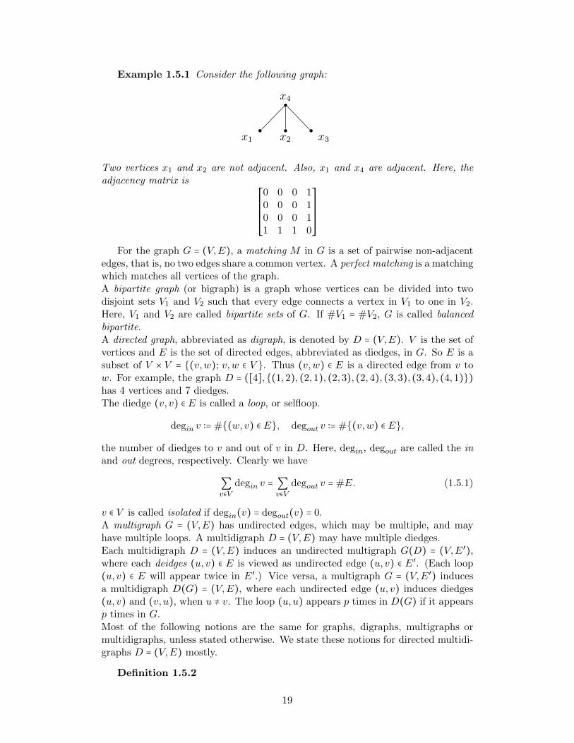
Example 1.5.1 Consider the following graph:
......
x1
.
x3
.
x4
.
x2
1
Two vertices x1 and x2 are not adjacent. Also, x1 and x4 are adjacent. Here, theadjacency matrix is
⎡⎢⎢⎢⎢⎢⎢⎢⎣
0 0 0 10 0 0 10 0 0 11 1 1 0
⎤⎥⎥⎥⎥⎥⎥⎥⎦For the graph G = (V,E), a matching M in G is a set of pairwise non-adjacent
edges, that is, no two edges share a common vertex. A perfect matching is a matchingwhich matches all vertices of the graph.A bipartite graph (or bigraph) is a graph whose vertices can be divided into twodisjoint sets V1 and V2 such that every edge connects a vertex in V1 to one in V2.Here, V1 and V2 are called bipartite sets of G. If #V1 = #V2, G is called balancedbipartite.A directed graph, abbreviated as digraph, is denoted by D = (V,E). V is the set ofvertices and E is the set of directed edges, abbreviated as diedges, in G. So E is asubset of V × V = (v,w); v,w ∈ V . Thus (v,w) ∈ E is a directed edge from v tow. For example, the graph D = ([4],(1,2), (2,1), (2,3), (2,4), (3,3), (3,4), (4,1))has 4 vertices and 7 diedges.The diedge (v, v) ∈ E is called a loop, or selfloop.
degin v ∶= #(w, v) ∈ E, degout v ∶= #(v,w) ∈ E,
the number of diedges to v and out of v in D. Here, degin, degout are called the inand out degrees, respectively. Clearly we have
∑v∈V
degin v = ∑v∈V
degout v = #E. (1.5.1)
v ∈ V is called isolated if degin(v) = degout(v) = 0.A multigraph G = (V,E) has undirected edges, which may be multiple, and mayhave multiple loops. A multidigraph D = (V,E) may have multiple diedges.Each multidigraph D = (V,E) induces an undirected multigraph G(D) = (V,E′),where each deidges (u, v) ∈ E is viewed as undirected edge (u, v) ∈ E′. (Each loop(u, v) ∈ E will appear twice in E′.) Vice versa, a multigraph G = (V,E′) inducesa multidigraph D(G) = (V,E), where each undirected edge (u, v) induces diedges(u, v) and (v, u), when u ≠ v. The loop (u,u) appears p times in D(G) if it appearsp times in G.Most of the following notions are the same for graphs, digraphs, multigraphs ormultidigraphs, unless stated otherwise. We state these notions for directed multidi-graphs D = (V,E) mostly.
Definition 1.5.2
19
1. A walk in D = (V,E) given by v0v1⋯vp, where (vi−1, vi) ∈ E for i = 1, . . . , p.One views it as a walk that starts at v0 and ends at vp. The length of the walkp, is the number of edges in the walk.
2. A path is a walk where vi ≠ vj for i ≠ j.
3. A closed walk is walk where vp = v0.
4. A cycle is a closed walk where vi ≠ vj, for 0 ≤ i < j < p. A loop (v, v) ∈ E isconsidered a cycle of length 1. Note that a closed walk vwv, where v ≠ w, isconsidered as a cycle of length 2 in a digraph, but not a cycle in undirectedmultigraph!
5. A Hamiltonian cycle is a cycle through the graph that visits each node exactlyonce.
6. Two vertices v,w ∈ V , v ≠ w are called strongly connected if there exist twowalks in D, the first starts at v and ends in w, and the second starts in w andends in v. For multigraphs G = (V,E) the corresponding notion is u, v areconnected.
7. A multidigraph D = ([n],E) is called strongly connected if either n = 1 and(1,1) ∈ E, or n > 1 and any two vertices in D are strongly connected.
8. A multidiraph g = (V,E) is called connected if either n = 1, or n > 1 andany two vertices in G are connected. (Note that a simple graph on one vertexG = ([1],∅) is considered connected directed graph D(G) = G is not stronglyconnected.)
9. Two multidigraphs D1 = (V1,E1), D2 = (V2,E2) are called isomorphic if thereexists a bijection φ ∶ V1 → V2 which induces a bijection φ ∶ E1 → E2. That is if(u1, v1) ∈ E1 is a diedge of multiplicity k in E1, then (φ(u1), φ(v1)) ∈ E2 is adiedge of multiplicity k and vice versa.
The interested reader is referred to [3] to see more details about the aboveconcepts.
1.5.1 Worked-out Problems
1. Show that the number e (the base of the natural logarithm) is transcendentalover Q.Solution:Assume that I(t) = ∫ t0 et−uf(u)du, where t is a complex number and f(x) is apolynomial with complex coefficients to be specified later. If f(x) = ∑nj=0 ajx
j ,
we set f(x) = ∑nj=0 ∣aj ∣xj , where ∣ ∣ denotes the norm of complex numbers.Integration by parts gives
I(t) = et∞∑j=0
f (j)(0) −∞∑j=0
f (j)(t) = etn
∑j=0
f (j)(0) −n
∑j=0
f (j)(t), (1.5.2)
where n is the degree of f(x).Assume that e is a root of g(x) = ∑ri=0 bix
i ∈ Z[X], where b0 ≠ 0. Let p be a
20
prime greater than maxr, ∣b0∣, and define f(x) = xp−1(x−1)p(x−2)p⋯(x−r)p.Consider J = b0I(0) + b1I(1) +⋯ + brI(r).Since g(e) = 0, the contribution of the first summand on the right-hand sideof (1.5.2) to J is 0. Thus,
J = −r
∑k=0
n
∑j=0
bkf(j)(k),
where n = (r + 1)p − 1. The definition of f(x) implies that many of the termsabove are zero, and we can write
J = −n
∑j=p−1
b0f(j)(0) +
r
∑k=1
n
∑j=p
bkf(j)(k).
Each of the terms on the right is divisible by p! except for
fp−1(0) = (p − 1)!(−1)rp(r!)p,
where we have used that p > r. Thus, since p > ∣b0∣ as well, we see that J isan integer which is divisible by (p− 1)!, but not by p. That is, J is an integerwith
∣J ∣ ≥ (p − 1)!.
Since
f(k) = kp−1(k + 1)p(k + 2)p⋯(k + r)p ≤ (2r)n for 0 ≤ k ≤ r,
we deduce that
∣J ∣ ≤r
∑j=0
∣bj ∣∣I(j)∣ ≤r
∑j=0
∣bj ∣jej f(j) ≤ c ((2r)(r+1))p,
where c is a constant independent of p. This gives a contradiction.
2. Prove the following statements.
(a) Any finite ring R is of non-zero characteristic.
(b) The characteristic of a field F is either zero or prime.
Solution:
(a) Assume to the contrary charR = 0. Without loss of generality, we mayassume that 0 ≠ 1. For any m,n ∈ Z, m ⋅ 1 = n ⋅ 1 implies (m − n) ⋅ 1 = 0and since we assumed charR = 0, it follows m = n. Therefore, the setn ⋅ 1;n ∈ Z is an infinite subset of R which is a contradiction.
(b) Assume that m = charF is non-zero and m = nk; then 0 = (nk) ⋅ 1 =nk ⋅ (1 ⋅ 1) = (n ⋅ 1)(k ⋅ 1). Then, either n = 0 or k = 0 and this implieseither n =m or k =m. Hence, m is prime.
21
1.5.2 Problems
1. Let Z6 be the set of all integers modulo 6. Explain why this is not a field.
2. Assume that G and H are two groups. Let Hom(G,H) denote the set of allgroup homomorphisms from G to H. Show that
(a) Hom(G,H) is a group under the composition of functions if H is a sub-group of G.
(b) #Hom(Zm,Zn) = gcd(m,n), where m,n ∈ N, where # denotes the cardi-nality of the set.
3. Prove that ϕ ∶ Q→ Qn×n by ϕ(a) =
⎡⎢⎢⎢⎢⎢⎢⎢⎣
a 0 ⋯ 00 a ⋯ 0⋮ ⋮ ⋱ ⋮0 0 ⋯ a
⎤⎥⎥⎥⎥⎥⎥⎥⎦
is a ring homomorphism.
1.6 Dimension and basis
As most algebraic structures, vector spaces contain substructures called subspace.Let V be a vector space over a field F. (For simplicity of the exposition you mayassume that F = R or F = C.) A subset U ⊂ V is called a subspace of V, if a1u1 +a2u2 ∈ U, for each u1,u2 ∈ U and a1, a2 ∈ F. The subspace U ∶= 0 is called the zero,or the trivial subspace of V. The elements of V are called vectors. Let x1, . . . ,xn ∈ Vbe n vectors. Then, for any a1, . . . , an ∈ F, called scalars, a1x1+ . . .+anxn is called alinear combinations of x1, . . . ,xn. Moreover, 0 = ∑ni=1 0xi is the trivial combination.Also, x1, . . . ,xn are linearly independent , if the equality 0 = ∑ni=1 aixi implies thata1 = . . . = an = 0. Otherwise, x1, . . . ,xn are linearly dependent . The set of alllinear combination of x1, . . . ,xn is called the span of x1, . . . ,xn, and denoted byspanx1, . . . ,xn. In particular, we use the notation span(x) to express spanx,for any x ∈ V . Clearly, spanx1, . . . ,xn is a subspace of V. (Why?) In general, thespan of a set S ⊆ V is the set of all linear combinations of S, i.e. the set of all linearcombinations of all finite subsets of S.
1.6.1 More details on vector space
If V is a vector space, it is called finitely generated if V = spanx1, . . . ,xn, for somevectors x1, . . . ,xn, x1, . . . ,xn is a spanning set of V. (In this book we consideronly finitely generated vector spaces.) We will use the following notation for apositive integer n:
[n] ∶= 1,2, . . . , n − 1, n (1.6.1)
Observe the following ”obvious” relation for any n ∈ N. (Here, N is the set of allpositive integers 1,2, . . . ,.)
spanu1, . . . ,ui−1,ui+1, . . . ,un ⊆ spanu1, . . . ,un, for each i ∈ [n]. (1.6.2)
It is enough to consider the case i = n. (We assume here that for n = 1, the span ofempty set is the zero subspace U = 0.) Then, for n = 1, (1.6.2) holds. Supposethat n > 1. Clearly, any linear combination of u1, . . . ,un−1, which is u = ∑n−1
i=1 biuiis a linear combination of u1, . . . ,un: u = 0un +∑n−1
i=1 biui. Hence, (1.6.2) holds.
22
Theorem 1.6.1 Suppose that n > 1. Then, there exists i ∈ [n] such that
spanu1, . . . ,un = spanu1, . . . ,ui−1,ui+1, . . . ,un, (1.6.3)
if and only if u1, . . . ,un are linearly dependent vectors.
Proof. Suppose that (1.6.3) holds. Then, ui = b1u1 + ⋯ + bi−1ui−1 + bi+1ui+1 +⋯ + bnun. Hence, ∑ni=1 aiui = 0, where aj = bj , for j ≠ i and ai = −1. Then,u1, . . . ,un are linearly dependent. Assume that u1, . . . ,un are linearly dependent.Then, there exist scalars a1, . . . , an ∈ F, not all of them are equal to zero, so thata1u1 + . . . + anun = 0. Assume that ai ≠ 0. For simplicity of notation, (or byrenaming indices in [n]), we may assume that i = n. This yields un = − 1
an∑n−1i=1 aiui.
Let u ∈ spanu1, . . . ,un. Therefore,
u =n
∑i=1
biui = bnun +n−1
∑i=1
biui = −bnn−1
∑i=1
aian
ui +n−1
∑i=1
biui =n−1
∑i=1
anbi − aibnan
ui.
That is, u ∈ u1, . . . ,un−1. This proves the theorem. ◻
Corollary 1.6.2 Let u1, . . . ,un ∈ V. Assume that not all ui’s are zero vectors.Then, there exist d ≥ 1 integers 1 ≤ i1 < i2 < . . . < id ≤ n such that ui1 , . . . ,uid arelinearly independent and spanui1 , . . . ,uid = spanu1, . . . ,un.
Proof. Suppose that u1, . . . ,un are linearly independent. Then, d = n and ik = k,for k = 1, . . . , n and we are done.
Assume that u1, . . . ,un are linearly dependent. Applying Theorem 1.6.1, weconsider now n−1 vectors u1, . . . ,ui−1,ui+1, . . . ,un as given by Theorem 1.6.1. Notethat it is not possible that all vectors in u1, . . . ,ui−1,ui+1, . . . ,un are zero sincethis will imply that ui = 0. This will contradict the assumption that not all ui arezero. Apply the previous arguments to u1, . . . ,ui−1,ui+1, . . . ,un and continue in thismethod until one gets d linearly independent vectors ui1 , . . . ,uid . ◻
Corollary 1.6.3 Let V be a finitely generated nontrivial vectors space, i.e. con-tains more than one element. Then, there exist n ∈ N and n linearly independentvectors v1, . . . ,vn such that V = spanv1, . . . ,vn.
The linear equation ∑ni=1 aixi = b with unknowns x1,x2, . . . ,xn is called homo-geneous if b = 0. Otherwise, it is called non-homogeneous. In the following lemmawe use the fact that any m homogeneous linear equations with n variables have anontrivial solution if m < n. (This will be proved later using REF of matrices.)
Lemma 1.6.4 Let n >m ≥ 1 be integers. Then, any w1, . . . ,wn ∈ spanu1, . . . ,umare linearly dependent.
Proof. Observe that wj = ∑mi=1 aijuj , for some aij ∈ F, 1 ≤ j ≤ n. Then
n
∑j=1
xjwj =n
∑j=1
xjm
∑i=1
aijui =m
∑i=1
(n
∑j=1
aijxj)ui.
23
Consider the following m homogeneous equations in n unknowns: ∑nj=1 aijxj = 0,for i = 1, . . . ,m. Since n > m, we have a nontrivial solution (x1, . . . , xn). Thus,
∑nj=1 xjwj = 0. ◻
Theorem 1.6.5 Let V = spanv1, . . .vn and assume that v1, . . . ,vn are lin-early independent. Then, the following holds.
1. Any vector u can be expressed as a unique linear combination of v1, . . . ,vn.
2. For an integer N > n, any N vectors in V are linearly dependent.
3. Assume that u1, . . . ,un∈ V are linearly independent. Then, V = spanu1, . . . ,un.
Proof. Assume that ∑ni=1 xivi = ∑ni=1 yivi. Thus, ∑ni=1(xi − yi)vi = 0. Asv1, . . . ,vn are linearly independent, it follows that xi−yi = 0, for i = 1, . . . , n. Hence,1 holds.
Lemma 1.6.4 implies 2.Suppose that u1, . . . ,un are linearly independent. Let v ∈ V and consider
n + 1 vectors u1, . . . ,un,v. Next, 2 implies that u1, . . . ,un,v are linearly depen-dent. Thus, there exist n + 1 scalars a1, . . . , an+1, not all of them zero, such thatan+1v +∑ni=1 aiui = 0. Assume first that an+1 = 0. Then, ∑ni=1 aiui = 0. Since notall ai’s are zero, it follows that u1, . . . ,un are linearly dependent, which contradictsour assumption. Hence, an+1 ≠ 0 and v = ∑ni=1
−aian+1
ui. ◻
1.6.2 Dimension
A vector space V over the field F is called to be finite dimensional if there is afinite subset x1, . . . , xn of V such that V = spanx1, . . . , xn. Otherwise, V iscalled infinite dimensional. The dimension of a trivial vector space, consisting ofthe zero vector, V = 0, is zero. The dimension of a finite dimensional non-zerovector space V is the number of vectors in any spanning linearly independent set,namely if V contains an independent set of n vectors but contains no independentset of n + 1 vectors, we say that V has dimension n. Also, the dimension of aninfinite dimensional vector space is infinity. The dimension of V is denoted bydimFV or simply dimV if there is no ambiguity in the background field. In thisbook V is assumed a vector space over the field F unless stated otherwise. SeeWorked-out Problem 1.6.3-2 on the existence of basis for vector spaces. Assumethat dimV = n. Suppose that V = spanx1, . . . ,xn. Then, x1, . . . ,xn is a basisof V, i.e. each vector x can be uniquely expressed as ∑ni=1 aixi. Thus, for eachx ∈ V, one corresponds a unique column vector a = (a1, . . . , an)⊺ ∈ Fn, where Fn isthe vector space on column vectors with n coordinates in F. It will be convenientto denote x = ∑ni=1 aixi by the equality x = [x1,x2, . . . ,xn]a. (Note that we use thestandard way to multiply row by column.)
Assume now that y1, . . . ,yn are n vectors in V. Then
yi =n
∑j=1
yjixj ,
24
for some yji ∈ F, 1 ≤ i, j ≤ n.Denote by Y = [yji]ni=j=1 the n × n matrix with the element yji in j-th row and
i-th column. The above equalities are equivalent to the identity
[y1, . . . ,yn] = [x1, . . . ,xn]Y. (1.6.4)
Then, y1, . . . ,yn is a basis if and only if Y is invertible matrix. (See subsection1.7.5 for details on invertible matrices.) In this case, Y is called the matrix of thechange of basis from [y1, . . . ,yn] to [x1, . . . ,xn]. The matrix of the change of ba-sis from [x1, . . . ,xn] to [y1, . . . ,yn] is given by Y −1. (Just multiply the identity(1.6.4) by Y −1 from the right.) Suppose also that [z1, . . . ,zn] is a basis in V. Let[z1, . . . ,zn] = [y1, . . . ,yn]Z. Then, [z1, . . . ,zn] = [x1, . . . ,xn](Y Z). (Use (1.6.4)).Here, Y Z is the matrix of the change of basis, from [z1, . . . ,zn] to [x1, . . . ,xn]. Seethe next section about matrices and their properties.
We end up this section by investigating the linear analogue of a result in grouptheory. It is a well-known fact in elementary group theory that a subgroup ofa finitely generated group is not finitely generated necessarily. See [9] for moredetails. Nevertheless, it is not the case for vector spaces, i.e. any subspace of a finitedimensional vector space is finite dimensional. Now, if V is a finite dimensionalvector space over the field F with the basis x1, . . . ,xn and W is its subspace,this question can be asked that if there exists a subset J ⊆ [n] for which W =spanxi ∶ i ∈ J? It is easy to show that this is not the case. For example if V = R3
as a real vector space with the standard basis X = (1,0,0), (0,1,0), (1,1,0) andW = span(1,1,1), (1,1, 1
2), then W is spanned by none of two elements of X.(Why?)
1.6.3 Worked-out Problems
1. Let C[−1,1] be the set of all real continuous functions on the interval [−1,1]
(a) Show that C[−1,1] is a vector space over R.
(b) Let U(a, b) ⊂ C[−1,1] be all functions such that f(a) = b, for a ∈ [−1,1]and b ∈ R. For which values of b, U(a, b) is a subspace?
(c) Is C[−1,1] finite dimensional?
Solution:
(a) We use the following elementary facts:“The sum of two continuous functions is continuous” and “Multiplying acontinuous function by a real number is continuous”.If f(x) ∈ C[−1,1] and a ∈ R, (af)(x) = af(x). Obviously, af is also inC[−1,1].Furthermore, if f(x), g(x) ∈ C[−1,1], then (f+g)(x) = f(x)+g(x). Usingthe above facts, f + g is also continuous.The zero function is in C[−1,1] and works as neutral element for theoperation ”+” defined as above. Also, g(x) = 1 is in C[−1,1] and 1f = f ,for any f ∈ C[−1,1].Then, C[−1,1] satisfies all properties of a vector space.
25
(b) If U(a, b) is a subspace, it must contain 0-function. Then, 0(a) = 0, i.e.b = 0. Now, if f and g are in U(a, b) and c and d are real numbers, thencf(a) + dg(a) = (c + d)b = 0. Then, cf + dg ∈ U(a, b). Since U(a, b) isclosed under addition and product by scaler, it is a subspace.
(c) No, C[−1,1] is infinite dimensional. If n is an arbitrary positive integer,then 1, x, x2, . . . , xn are linearly independent. Indeed, if (a0, . . . , an) isnon-zero, then the assumption that p(x) = ∑ni=0 aix
i is a zero functionimplies that p(x) has infinitely many roots. This contradicts the wellknown statement that p(x) has at most n roots.
2. Let V be vector space and dimV = n. show that
(a) A set A of n vectors in V spans V if and only if A is independent.
(b) V has a basis and every basis consists of n vectors.
Solution:
(a) Assume that A = x1,⋯,xn. Since dimV = n, the set x,x1,⋯,xn isdependent, for every x ∈ V . If A is independent, then x is in the span ofA. Therefore, A spans V.Conversely, if A is dependent, one of its elements can be removed withoutchanging the span of A. Thus, A cannot span V, by Problem 1.6.4-9.
(b) Since dimV = n, V contains an independent set of n vectors, and (a)shows that every such set is a basis of V; the statement follows from thedefinition of dimension and Problem 1.6.4-9.
1.6.4 Problems
1. * A complex number ζ is called m-th root of unity if ζm = 1. ζ is called aprimitive unity root of order m > 1 if ζm = 1 and ζk ≠ 1, for k ∈ [m − 1].Let l be the number of integers in [m − 1] which are coprime with m. LetQ[ζ] ∶= a0 + a1ζ + ⋯ + al−1ζ
l−1, a0, . . . , al−1 ∈ Q. Show that Q[ζ] is a field.It is a finite extension of Q. More precisely, Q[ζ] can be viewed as a vectorspace over Q of dimension l.(Hints:
(a) Let ξ = e 2πim . Show that ζ is an m-th root of unity if and only if ζ = ξk and
k ∈ [m]. Furthermore, ζ is primitive if and only if k and m are coprime.
(b) Let ζ be an m-th primitive root of unity. Show that ζ, ζ2, . . . , ζm−1, ζm
are all m-th root of unity.
(c) Show that xm − 1 has simple roots.
(d) Let p1(x)⋯pj(x) be the decomposition of xm − 1 to irreducible factors inQ[x]. Assume that ζ, a primitive m-th root of unity, is a root of p1. Letl = deg pl. Show that Q[ζ] ∶= a0 + a1ζ +⋯ + al−1ζ
l−1, a0, . . . , al−1 ∈ Q isan extension field of Q of degree l which contains all m roots of unity.
(e) ** Show that l is the number of m-primitive roots of unity.
26
(f) ** Show that l is given by the Euler’s function φ(m). Namely, assumethat m = pd11 ⋯pdrr , where 1 < p1 < ⋯ < pr are primes and d1, . . . , dr are
positive integers. Then, φ(m) = (p1 − 1)pd1−11 ⋯(pr − 1)pdr−1
r .)
Special cases:
(a) m = 4: x4−1 = (x2+1)(x+1)(x−1). The 4-th primitive roots of unity are±i. They are roots of x2+1. Q[i] is called the Gaussian field of rationals.The set Z[i] = a + bi, a, b ∈ Z is called the Gaussian integers domain.
(b) m = 6: x6 − 1 = (x2 − x + 1)(x2 + x + 1)(x + 1)(x − 1). The primitive roots
of order 6 are 12 ±
√3
2 i, which are the two roots of x2 − x + 1.
2. Quaternions Q is a four dimensional noncommutative division algebra thatgeneralizes complex numbers. Any quaternion is written as a vector q = a0 +a1i + a2j + a3k. The product of two quaternions is determined by using thefollowing equalities.
i2 = j2 = k2 = −1, ij = −ji = k, jk = −kj = i, ki = −ik = j.
Let q = a0 − a1i − a2j − a3k. Show
(a) The map T (q) = q is an involution. (T is a bijection preserving additionand multiplication and T 2 = id.)
(b) Q is a noncommutative division algebra, i.e. if q ≠ 0, then there existsa unique r such that rq = qr = 1. (You can try to use the identityqq = qq = ∣q∣2 = ∑3
i=0 a2i ).
3. Let Pm be the subset of all polynomials of degree m at most over the field F.Show that the polynomials 1, x, . . . , xm form a basis in Pm.
4. Let fj be a non-zero polynomial in Pm of degree j, for j = 0, . . . ,m. Show thatf0, . . . , fm form a basis in Pm.
5. Find a basis in P4 such that each polynomial is of degree 4.
6. Does exist a basis in P4 such that each polynomial is of degree 3?
7. Write up the set of all vectors in R4 whose coordinates are two 0’s and two1’s. (There are six such vectors.) Show that these six vectors span R4. Findall the collections of four vectors out of these six which form a basis in R4.
8. Prove the Completion lemma: let V be a vector space of dimension m. Letv1, . . . ,vn ∈ V be n linearly independent vectors. (Here m ≥ n) Then, thereexist m − n vectors vn+1, . . . ,vm such that v1, . . . ,vm is a basis in V.
9. Assume that a vector space V is spanned by a set of n vectors, (n ∈ N). Showthat dimV ≤ n.
10. Let V be a vector space over a field F and S ⊆ V, show that
(a) span(span(S)) = span(S)(b) span(S) is the smallest subspace of V containing S.
(c) span(S) = S if and only if S is a subspace of V.
27
1.7 Matrices
1.7.1 Basic properties of matrices
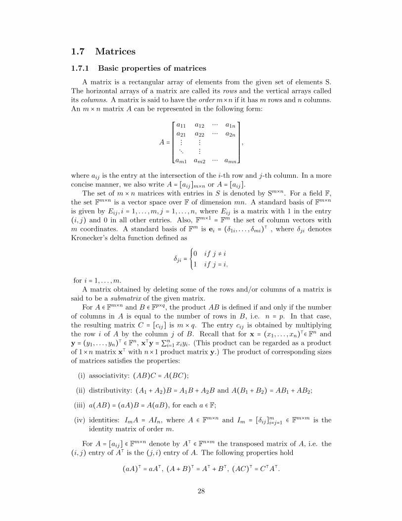
A matrix is a rectangular array of elements from the given set of elements S.The horizontal arrays of a matrix are called its rows and the vertical arrays calledits columns. A matrix is said to have the order m×n if it has m rows and n columns.An m × n matrix A can be represented in the following form:
A =
⎡⎢⎢⎢⎢⎢⎢⎢⎢⎢⎣
a11 a12 ⋯ a1n
a21 a22 ⋯ a2n
⋮ ⋮⋱ ⋮am1 am2 ⋯ amn
⎤⎥⎥⎥⎥⎥⎥⎥⎥⎥⎦
,
where aij is the entry at the intersection of the i-th row and j-th column. In a moreconcise manner, we also write A = [aij]m×n or A = [aij].
The set of m × n matrices with entries in S is denoted by Sm×n. For a field F,the set Fm×n is a vector space over F of dimension mn. A standard basis of Fm×nis given by Eij , i = 1, . . . ,m, j = 1, . . . , n, where Eij is a matrix with 1 in the entry(i, j) and 0 in all other entries. Also, Fm×1 = Fm the set of column vectors withm coordinates. A standard basis of Fm is ei = (δ1i, . . . , δmi)⊺ , where δji denotesKronecker’s delta function defined as
δji =⎧⎪⎪⎨⎪⎪⎩
0 if j ≠ i1 if j = i,
for i = 1, . . . ,m.A matrix obtained by deleting some of the rows and/or columns of a matrix is
said to be a submatrix of the given matrix.For A ∈ Fm×n and B ∈ Fp×q, the product AB is defined if and only if the number
of columns in A is equal to the number of rows in B, i.e. n = p. In that case,the resulting matrix C = [cij] is m × q. The entry cij is obtained by multiplyingthe row i of A by the column j of B. Recall that for x = (x1, . . . , xn)⊺∈ Fn andy = (y1, . . . , yn)⊺ ∈ Fn, x⊺y = ∑ni=1 xiyi. (This product can be regarded as a productof 1×n matrix x⊺ with n×1 product matrix y.) The product of corresponding sizesof matrices satisfies the properties:
(i) associativity: (AB)C = A(BC);
(ii) distributivity: (A1 +A2)B = A1B +A2B and A(B1 +B2) = AB1 +AB2;
(iii) a(AB) = (aA)B = A(aB), for each a ∈ F;
(iv) identities: ImA = AIn, where A ∈ Fm×n and Im = [δij]mi=j=1 ∈ Fm×m is theidentity matrix of order m.
For A = [aij] ∈ Fm×n denote by A⊺ ∈ Fn×m the transposed matrix of A, i.e. the(i, j) entry of A⊺ is the (j, i) entry of A. The following properties hold
(aA)⊺ = aA⊺, (A +B)⊺ = A⊺ +B⊺, (AC)⊺ = C⊺A⊺.
28
The matrix A = [aij] ∈ Fm×n is called diagonal if aij = 0, for i ≠ j. Denote byD(m,n) ⊂ Fm×n the vector subspace of diagonal matrices. A square diagonal matrixwith the diagonal entries d1, . . . , dn is denoted by diag(d1, . . . , dn) ∈ Fn×n. A matrixA is called a block matrix if A = [Aij]p,qi=j=1, where each entry Aij is an mi × mj
matrix. Then, A ∈ Fm×n where m = ∑pi=1mi and n = ∑qj=1 nj . A block matrix A iscalled block diagonal if Aij = 0mi×mj , for i ≠ j. A block diagonal matrix with p = q isdenoted by diag(A11, . . . ,App). A different notation is ⊕pl=1All ∶= diag(A11, . . . ,App),and ⊕pl=1All is called the direct sum of the square matrices A11, . . . ,App.
1.7.2 Elementary row operation
Elementary operations on the rows of A ∈ Fm×n are defined as follows:
1. Multiply row i by a non-zero a ∈ F.
2. Interchange two distinct rows i and j in A.
3. Add to row j, row i multiplied by a, where i ≠ j.
A matrix A ∈ Fn×n is said to be in a row echelon form (REF) if it satisfies thefollowing conditions:
1. All non-zero rows are above any rows of all zeros.
2. Each leading entry of a row is in a column to the right of the leading entry ofthe row above it.
3. All entries in a column below a leading entry are zeros.
Also, A can be brought to a unique canonical form, called the reduced row echelonform, abbreviated as RREF by the elementary row operation. The RREF of zeromatrix 0m×n is 0m×n. For A ≠ 0m×n, RREF of A given by B is of the following form:In addition to the conditions 1,2 and 3 above, it must satisfy the followings:
1. The leading entry in each non-zero row is 1.
2. Each leading 1 is the only non-zero entry in its column.
A pivot position in the matrix A is a location in A that corresponds to a leading 1in the RREF of A. First non-zero entry of each row of a REF of A is called a pivot,and the columns in which pivots appear are pivot columns. The process of findingpivots is called pivoting.
An elementary row-interchange matrix is an n×n matrix which can be obtainedfrom the identity matrix In by performing on In a single elementary row operation.
1.7.3 Gaussian Elimination
Gaussian elimination is a method to bring a matrix either to is REF or its RREFor similar forms. It is often used for solving matrix equations of the form
Ax = b. (1.7.1)
29
In the following, we may assume that A is full-rank, i.e. the rank of A equals thenumber of rows.
To perform Gaussian elimination starting with the system of equations
⎡⎢⎢⎢⎢⎢⎢⎢⎣
a11 a12 ⋯ a1k
a21 a22 ⋯ a2k
⋮ak1 ak2 ⋯ akk
⎤⎥⎥⎥⎥⎥⎥⎥⎦
⎡⎢⎢⎢⎢⎢⎢⎢⎣
x1
x2
⋮xk
⎤⎥⎥⎥⎥⎥⎥⎥⎦
=
⎡⎢⎢⎢⎢⎢⎢⎢⎣
b1b2⋮bk
⎤⎥⎥⎥⎥⎥⎥⎥⎦
, (1.7.2)
compose the “augmented matrix equation”
⎡⎢⎢⎢⎢⎢⎢⎢⎣
a11 a12 ⋯ a1k b1a21 a22 ⋯ a2k b2⋮ak1 ak2 ⋯ akk bk
⎤⎥⎥⎥⎥⎥⎥⎥⎦
(1.7.3)
Here, the column vector is the variable x carried along for labeling the matrix rows.Now, perform elementary row operations to put the augmented matrix into theupper triangular form
⎡⎢⎢⎢⎢⎢⎢⎢⎣
a′11 a′12 ⋯ a′1k b′10 a′22 ⋯ a′2k b′2⋮0 0 ⋯ a′kk b′k
⎤⎥⎥⎥⎥⎥⎥⎥⎦
. (1.7.4)
Solve the equation of the k-th row for xk, then substitute back into the equation ofthe (k − 1)-st row to obtain a solution for xk−1, etc. We get the formula
xi =1
a′ii
⎛⎝b′i −
k
∑j=i+1
a′ijxj⎞⎠.
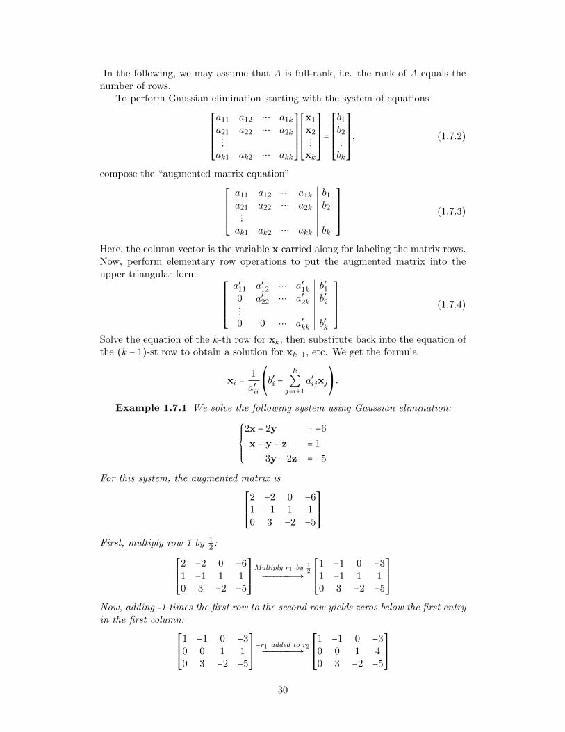
Example 1.7.1 We solve the following system using Gaussian elimination:
⎧⎪⎪⎪⎪⎨⎪⎪⎪⎪⎩
2x − 2y = −6
x − y + z = 1
3y − 2z = −5
For this system, the augmented matrix is
⎡⎢⎢⎢⎢⎢⎣
2 −2 0 −61 −1 1 10 3 −2 −5
⎤⎥⎥⎥⎥⎥⎦First, multiply row 1 by 1
2 :
⎡⎢⎢⎢⎢⎢⎣
2 −2 0 −61 −1 1 10 3 −2 −5
⎤⎥⎥⎥⎥⎥⎦
Multiply r1 by 12−−−−−−−−Ð→⎡⎢⎢⎢⎢⎢⎣
1 −1 0 −31 −1 1 10 3 −2 −5
⎤⎥⎥⎥⎥⎥⎦Now, adding -1 times the first row to the second row yields zeros below the first entryin the first column:
⎡⎢⎢⎢⎢⎢⎣
1 −1 0 −30 0 1 10 3 −2 −5
⎤⎥⎥⎥⎥⎥⎦
−r1 added to r2−−−−−−−−Ð→⎡⎢⎢⎢⎢⎢⎣
1 −1 0 −30 0 1 40 3 −2 −5
⎤⎥⎥⎥⎥⎥⎦
30
Interchanging the second and third rows then gives the desired upper-triangular co-efficient matrix:
⎡⎢⎢⎢⎢⎢⎣
1 −1 0 −30 0 1 40 3 −2 −5
⎤⎥⎥⎥⎥⎥⎦
r2↔r1−−−−Ð→⎡⎢⎢⎢⎢⎢⎣
1 −1 0 −30 3 −2 −50 0 1 4
⎤⎥⎥⎥⎥⎥⎦
The third row now says z = 4. Back-substituting this value into the second row givesy = 1, and back-substitution of both these values into the first row yields x = −2. Thesolution system is therefore (x,y,z) = (−2,1,4).
1.7.4 Solution of linear systems
Consider the following system of the linear equations:
a11x1 + a12x2 +⋯ + a1nxn = b1a21x1 + a22x2 +⋯ + a2nxn = b2⋮an1x1 + an2x2 +⋯ + annxn = bn
(1.7.5)
Assume that A = [aij]1≤i,j≤n and b =
⎡⎢⎢⎢⎢⎢⎢⎢⎣
b1b2⋮bn
⎤⎥⎥⎥⎥⎥⎥⎥⎦
.
Definition 1.7.2 Let A ∶= [A∣b] be the augmented m × (n + 1) matrix repre-senting the system (1.7.5). Suppose that C = [C ∣c] is a REF of A. Assume thatC has k-pivots in the columns 1 ≤ `1 < ⋯ < `k ≤ n. Then, the variable x`1 , . . . , x`kcorresponding to these pivots are called the lead variables. The other variables arecalled free variables.
Definition 1.7.3 A map f ∶ Rn → R is called affine if f(x) = a1x1+⋯+anxn+b.Also, f is called a linear function if b = 0.
The following theorem describes exactly the set of all solutions of (1.7.5).
Theorem 1.7.4 Let A ∶= [A∣b] be the augmented m×(n+1) matrix representingthe system (1.7.5). Suppose that C = [C ∣c] be a REF of A. Then, the system (1.7.5)is solvable if and only if C does not have a pivot in the last column n + 1.Assume that (1.7.5) is solvable. Then each lead variable is a unique affine functionin free variables. These affine functions can be determined as follows:
1. Consider the linear system corresponding to C. Move all the free variables tothe right-hand side of the system. Then, one obtains a triangular system inlead variables, where the right-had side are affine functions in free variables.
2. Solve this triangular system by back substitution.
In particular, for a solvable system, we have the following alternative.
1. The system has a unique solution if and only if there are no free variables.
31
2. The system has infinitely many solutions if and only if there is at least onefree variable.
Proof. We consider the linear system equations corresponding to C. As anERO (elementary row operation) on A corresponds to an EO (elementary operation)on the system (1.7.5), it follows that the system represented by C is equivalent to(1.7.5). Suppose first that C has a pivot in the last column. Thus, the correspondingrow of C which contains the pivot on the column n + 1 is (0,0, . . . ,0,1)⊺. Thisequation is unsolvable, hence the whole system corresponding to C is unsolvable.Therefore, the system (1.7.5) is unsolvable.Assume now that C does not have a pivot in the last column. Move all the freevariables to the right-hand side of the system given by C. It is a triangular systemin the lead variables where the right-hand side of each equation is an affine functionin the free variables. Now use back substitution to express each lead variable as anaffine function of the free variables.Each solution of the system is determined by the value of the free variables whichcan be chosen arbitrarily. Hence, the system has a unique solution if and only if ithas no free variables. The system has many solutions if and only if it has at leastone free variable. ◻
Consider the following example of C:
⎡⎢⎢⎢⎢⎢⎣
1 −2 3 −1 00 1 3 1 40 0 0 1 5
⎤⎥⎥⎥⎥⎥⎦, (1.7.6)
x1, x2, x4 are lead variables, x3 is a free variable.
x4 = 5,
x2 + 3x3 + x4 = 4⇒ x2 = −3x3 − x4 + 4⇒x2 = −3x3 − 1,
x1 − 2x2 + 3x3 − x4 = 0⇒ x1 = 2x2 − 3x3 + x4 = 2(−3x3 − 1) − 3x3 + 5⇒x1 = −9x3 + 3.
◻
Notation 1.7.5 Let S and T be two subsets of a set X. Then, the set T ∖ S isthe set of elements of T which are not in S. (T ∖ S may be empty.)
Theorem 1.7.6 Let A ∶= [A∣b] be the augmented m×(n+1) matrix representingthe system (1.7.5). Suppose that C = [C ∣c] is a RREF of A. Then, the system (1.7.5)is solvable if and only if C does not have a pivot in the last column n + 1.Assume that (1.7.5) is solvable. Then, each lead variable is a unique affine functionin free variables determined as follows. The leading variable x`i appears only in theequation i, for 1 ≤ i ≤ r = rank A. Shift all other variables in the equation, (which arefree variables), to the other side of the equation to obtain x`i as an affine functionin free variables.
32
Proof. Since RREF is a row echelon form, Theorem 1.7.4 yields that (1.7.5) issolvable if and only if C does not have a pivot in the last column n + 1. Assumethat C does not have a pivot in the last column n + 1. Then, all the pivots of Cappear in C. Hence, rank A = rank C = rank A(= r). The pivots of C = [cij] ∈ Rm×nare located at row i and the column `i, denote as (i, `i), for i = 1, . . . , r. Since C isalso in RREF, in the column `i there is only one non-zero element which is equal 1and is located in row i.Consider the system of linear equations corresponding to C, which is equivalent to(1.7.5). Hence, the lead variable `i appears only in the i-th equation. Left hand-side of this equation is of the form x`i plus a linear function in free variables whoseindices are greater than x`i . The right-hand is ci, where c = (c1, . . . , cm)⊺. Hence,by moving the free variables to the right-hand side, we obtain the exact form of x`i .
x`i = ci − ∑j∈`i,`i+1,...,n∖j`1 ,j`2 ,...,j`r
cijxj , for i = 1, . . . , r. (1.7.7)
(Therefore, `i, `i + 1, . . . , n consists of n − `i + 1 integers from j`i to n, whilej`1 , j`2 , . . . , j`r consists of the columns of the pivots in C.) ◻
Example 1.7.7 Consider
⎡⎢⎢⎢⎢⎢⎣
1 0 b 0 u0 1 d 0 v0 0 0 1 w
⎤⎥⎥⎥⎥⎥⎦,
x1, x2, x4 lead variables x3 free variable ;
x1 + bx3 = u⇒ x1 = −bx3 + u,x2 + dx3 = v⇒ x2 = −dx3 + v,x4 = w.
Definition 1.7.8 The system (1.7.5) is called homogeneous if b = 0, i.e. b1 =⋯ = bm = 0. A homogeneous system of linear equations has a solution x = 0, whichis called the trivial solution.Let A be a square n × n, then A is called nonsingular if the corresponding homoge-neous system of n equations in n unknowns has only solution x = 0. Otherwise, Ais called singular.
Theorem 1.7.9 Let A be an m × n matrix. Then, its RREF is unique.
Proof. Let U be a RREF of A. Consider the augmented matrix A ∶= [A∣0]corresponding to the homogeneous system of equations. Clearly, U = [U ∣0] is aRREF of A. Put the free variables on the other side of the homogeneous systemcorresponding to A, where each lead variable is a linear function of the free variables.Note that the exact formulas for the lead variables determine uniquely the columnof the RREF which correspond to the free variables.Assume that U1 is another RREF of A. Then, U and U1 have the same pivots.Hence, U and U1 have the same pivots. Thus, U and U1 have the same columns
33
which correspond to pivots. By considering the homogeneous system of linear equa-tions corresponding to U1 = [U1∣0], we find also the solution of the homogeneoussystem A, by writing down the lead variables as linear functions in free variables.Since U and U1 give rise to the same lead and free variables, we deduce that the eachlinear function in free variables corresponding to a lead variable x`1 correspondingto U and U1 are equal. That is, the matrices U and U1 have the same row i, fori = 1, . . . , rank A. All other rows of U and U1 are zero rows. Hence, U = U1. ◻
Corollary 1.7.10 The matrix A ∈ Rn×n is nonsingular if and only if rank A = n,i.e. the RREF of A is the identity matrix
In =
⎡⎢⎢⎢⎢⎢⎢⎢⎣
1 0 ⋯ 0 00 1 ⋯ 0 0⋮ ⋮ ⋮ ⋮0 0 ⋯ 0 1
⎤⎥⎥⎥⎥⎥⎥⎥⎦
∈ Rn×n. (1.7.8)
Proof. The matrix A is nonsingular if and only if no free variable. Thus,rank A = n and the RREF is In. ◻
1.7.5 Invertible matrices
A matrix A ∈ Fm×m is called invertible if there exists B ∈ Fm×m such that AB =BA = Im. Note that such B is unique. If AC = CA = Im, then B = BIm =B(AC) = (BA)C = ImC = C. We denote B, the inverse of A by A−1. Denote byGL(m,F) ⊂ Fm×m the set of all invertible matrices. Note that GL(m,F) is a groupunder the multiplication, with the unit In. (Observe that for A and B ∈ GL(m,F)(AB)−1 = B−1A−1.)
A matrix E ∈ Fm×m is called elementary if it is obtained from Im by applyingone elementary row operation. Note that applying an elementary row operation onA is equivalent to EA, where E is the corresponding elementary row operation. Byreversing the corresponding elementary operation we see that E is invertible, andE−1 is also an elementary matrix.
The following theorem is well-known as the fundamental theorem of invertiblematrices; in the next subsections, we will see a more detailed version of the funda-mental theorem of invertible matrices.
Theorem 1.7.11 Let A ∈ Fm×m. The following statements are equivalent.
1. A is invertible.
2. Ax = 0 has only the trivial solution.
3. The RREF of A is Im.
4. A is a product of elementary matrices.
Proof. 1⇒ 2. The equation Ax = 0 implies that x = Imx = A−1(Ax) = A−10 = 0.2⇒ 3. The system Ax = 0 does not have free variables, hence the number of pivotsis the number of rows, i.e., the RREF of A is Im.
34
3⇒ 4. There exists a sequence of elementary matrices so that EpEp−1⋯E1A = Im.Hence, A = E−1
1 E−12 ⋯E−1
p , and each E−1j is also elementary.
4⇒ 1. As each elementary matrix is invertible, so is their product, which is equalto A. ◻
Theorem 1.7.12 Let A ∈ Fn×n. Define the matrix B = [A In] ∈ Fn×(2n). LetC = [C1 C2],C1,C2 ∈ Fn×n be the RREF of B. Then, A is invertible if and only ifC1 = In. Furthermore, if C1 = In then A−1 = C2.
Proof. The fact that “A is invertible if and only if C1 = In” follows straightfor-ward from Theorem 1.7.11. Note that for any matrix F = [F1F2], F1, F2 ∈ Fn×p,G ∈Fl×m, we have GF = [(GF1)(GF2)]. Let H be a product of elementary matrices suchthat HB = [IC2]. Thus, HA = In and HIn = C1. Hence, H = A−1 and C1 = A−1. ◻
We can extract the following algorithm from Theorem 1.7.12 to calculate theinverse of a matrix if it was invertible:
Gauss-Jordan algorithm for A−1
Form the matrix B = [A∣In].
Perform the ERO to obtain RREF of B ∶ C = [D∣F ].
A is invertible ⇔D = In.
If D = In, then A−1 = F .
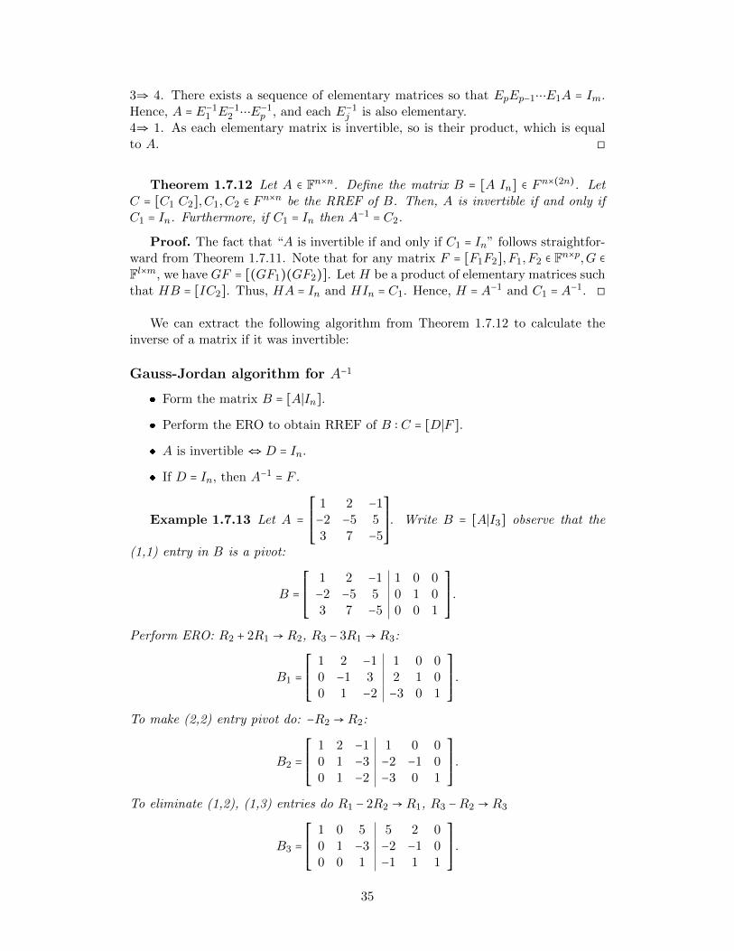
Example 1.7.13 Let A =⎡⎢⎢⎢⎢⎢⎣
1 2 −1−2 −5 53 7 −5
⎤⎥⎥⎥⎥⎥⎦. Write B = [A∣I3] observe that the
(1,1) entry in B is a pivot:
B =⎡⎢⎢⎢⎢⎢⎣
1 2 −1 1 0 0−2 −5 5 0 1 03 7 −5 0 0 1
⎤⎥⎥⎥⎥⎥⎦.
Perform ERO: R2 + 2R1 → R2, R3 − 3R1 → R3:
B1 =⎡⎢⎢⎢⎢⎢⎣
1 2 −1 1 0 00 −1 3 2 1 00 1 −2 −3 0 1
⎤⎥⎥⎥⎥⎥⎦.
To make (2,2) entry pivot do: −R2 → R2:
B2 =⎡⎢⎢⎢⎢⎢⎣
1 2 −1 1 0 00 1 −3 −2 −1 00 1 −2 −3 0 1
⎤⎥⎥⎥⎥⎥⎦.
To eliminate (1,2), (1,3) entries do R1 − 2R2 → R1, R3 −R2 → R3
B3 =⎡⎢⎢⎢⎢⎢⎣
1 0 5 5 2 00 1 −3 −2 −1 00 0 1 −1 1 1
⎤⎥⎥⎥⎥⎥⎦.
35
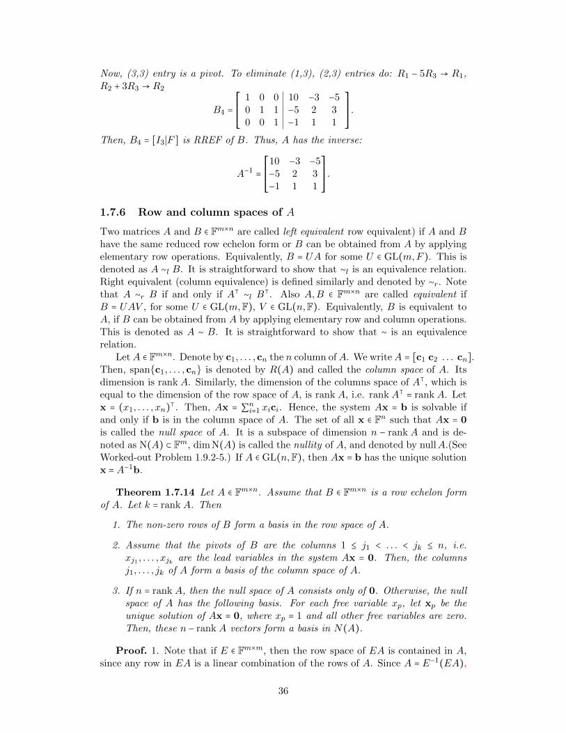
Now, (3,3) entry is a pivot. To eliminate (1,3), (2,3) entries do: R1 − 5R3 → R1,R2 + 3R3 → R2
B4 =⎡⎢⎢⎢⎢⎢⎣
1 0 0 10 −3 −50 1 1 −5 2 30 0 1 −1 1 1
⎤⎥⎥⎥⎥⎥⎦.
Then, B4 = [I3∣F ] is RREF of B. Thus, A has the inverse:
A−1 =⎡⎢⎢⎢⎢⎢⎣
10 −3 −5−5 2 3−1 1 1
⎤⎥⎥⎥⎥⎥⎦.
1.7.6 Row and column spaces of A
Two matrices A and B ∈ Fm×n are called left equivalent row equivalent) if A and Bhave the same reduced row echelon form or B can be obtained from A by applyingelementary row operations. Equivalently, B = UA for some U ∈ GL(m,F ). This isdenoted as A ∼l B. It is straightforward to show that ∼l is an equivalence relation.Right equivalent (column equivalence) is defined similarly and denoted by ∼r. Notethat A ∼r B if and only if A⊺ ∼l B⊺. Also A,B ∈ Fm×n are called equivalent ifB = UAV , for some U ∈ GL(m,F), V ∈ GL(n,F). Equivalently, B is equivalent toA, if B can be obtained from A by applying elementary row and column operations.This is denoted as A ∼ B. It is straightforward to show that ∼ is an equivalencerelation.
LetA ∈ Fm×n. Denote by c1, . . . ,cn the n column ofA. We writeA = [c1 c2 . . . cn].Then, spanc1, . . . ,cn is denoted by R(A) and called the column space of A. Itsdimension is rank A. Similarly, the dimension of the columns space of A⊺, which isequal to the dimension of the row space of A, is rank A, i.e. rank A⊺ = rank A. Letx = (x1, . . . , xn)⊺. Then, Ax = ∑ni=1 xici. Hence, the system Ax = b is solvable ifand only if b is in the column space of A. The set of all x ∈ Fn such that Ax = 0is called the null space of A. It is a subspace of dimension n − rank A and is de-noted as N(A) ⊂ Fm, dim N(A) is called the nullity of A, and denoted by nullA.(SeeWorked-out Problem 1.9.2-5.) If A ∈ GL(n,F), then Ax = b has the unique solutionx = A−1b.
Theorem 1.7.14 Let A ∈ Fm×n. Assume that B ∈ Fm×n is a row echelon formof A. Let k = rank A. Then
1. The non-zero rows of B form a basis in the row space of A.
2. Assume that the pivots of B are the columns 1 ≤ j1 < . . . < jk ≤ n, i.e.xj1 , . . . , xjk are the lead variables in the system Ax = 0. Then, the columnsj1, . . . , jk of A form a basis of the column space of A.
3. If n = rank A, then the null space of A consists only of 0. Otherwise, the nullspace of A has the following basis. For each free variable xp, let xp be theunique solution of Ax = 0, where xp = 1 and all other free variables are zero.Then, these n − rank A vectors form a basis in N(A).
Proof. 1. Note that if E ∈ Fm×m, then the row space of EA is contained in A,since any row in EA is a linear combination of the rows of A. Since A = E−1(EA),
36
it follows that the row space of A is contained in the row space of EA. Hence, therow space of A and EA are the same. Therefore, the row space of A and B are thesame. Since the last m − k rows of B are zero rows, it follows that the row spaceof B spanned by the first k rows b⊺1 , . . . ,b
⊺k. We claim that b⊺1 , . . . ,b
⊺k are linearly
independent. Indeed, consider xb⊺1 + . . . +xkbk = 0⊺. Since all the entries below thefirst pivot in B are zero, we deduce that x1 = 0. Continue in the same manner toobtain that x2 = 0, . . . , xk = 0. Then, b⊺1 , . . . ,b
⊺k form a basis in the row space of B
and A.2. We first show that cj1 , . . . ,cjk are linearly independent. Consider the equality
∑kj=1 xijcij = 0. This is equivalent to the system Ax = 0, where x = (x1, . . . , xn)⊺and xp = 0 if xp is a free variable. Since all free variables are zero, all lead variablesare zero, i.e. xji = 0, for i = 1, . . . , k. Thus, cj1 , . . . ,cjk are linearly independent.It is left to show that cp, where xp is a free variable, is a linear combination ofcj1 , . . . ,cjk . Again, consider Ax = 0, where each xp = 1 and all other free variablesare zero. We have a unique solution to Ax = 0, which states that 0 = cp+∑ki=1 xjicji ,i.e. cp = ∑ki=1 −xjicji .
3. This follows for the way we write down the general solution of the systemAx = 0 in terms of free variables. ◻
Remark 1.7.15 Let x1, . . . ,xn ∈ Fm. To find a basis in U ∶= spanx1, . . . ,xnconsisting of k vectors in x1, . . . ,xn, apply Theorem 1.7.14 to the column spaceof the matrix A = [x1 x2 . . .xn]. To find an appropriate basis in U, apply Theorem1.7.14 to the row space of A⊺.
Lemma 1.7.16 Let A ∈ Fm×n. Then, A is equivalent to a block diagonal matrixIrank A ⊕ 0.
Proof. First, bring A to REF matrix B with all pivots equal to 1. Now performthe elementary column operations corresponding to the elementary row operationson B⊺. This will give a matrix C with r pivots equal to 1 and all other elementszero. Now, interchange the corresponding columns to obtain Ir⊕0. It is left to showthat r = rank A. First, recall that if B = UA, then the row space of A and B arethe same. Then, rank A = rank B, which is the dimension of the row space. Next, ifC = BV , then C and B have the same column space. Thus, rank B = rank C, whichis the dimension of the column space. This means r = rank A. ◻
The following theorem is a more detailed case of Theorem 1.7.11. Its proof isleft as Problem 1.8.5-4.
Theorem 1.7.17 Let A ∈ Fn×n. The following statements are equivalent:
(1) A is invertible (non-singular),
(2) Ax = b has a unique solution for every b ∈ Fn,
(3) Ax = 0 has only the trivial (zero) solution,
(4) The reduced row echelon form of A is In,
37
(5) A is a product of elementary matrices,
(6) detA ≠ 0,
(7) rank A = n,
(8) N(A) = 0,
(9) nullA = 0,
(10) The column vectors of A are linearly independent,
(11) The column vectors of A span Fn,
(12) The column vectors of A a basis for Fn,
(13) The row vectors of A are linearly independent,
(14) The row vectors of A span Fn,
(15) The row vectors of A a basis for Fn.
1.7.7 Special types of matrices
The following are some special types of matrices in Fn×n.
1. A is symmetric if A⊺ = A. Denote by S(n,F) the subspace of n × n symmetricmatrices.
2. A is skew-symmetric, or anti-symmetric, if A⊺ = −A. Denote by A(n,F) thesubspace of the skew-symmetric matrices.
3. A = [aij] is called upper triangular if aij = 0, for each j < i. Denote by U(n,F)the subspace of upper triangular matrices.
4. A = [aij] is called lower triangular if aij = 0 for each j > i. Denote by L(n,F)the subspace of lower triangular matrices.
A triangular matrix is one that is either lower triangular or upper triangular.
Let α = α1 < α2 < . . . < αp ⊂ [m],β = β1 < β2 < . . . < βp ⊂ [n] Then A[α,β]is an p × q submatrix of A, which is obtained by erasing in A all rows andcolumns which are not in α and β, respectively. Assume that p < m,q < n.Denote by A(α,β) the (m − p) × (n − q) submatrix of A, which is obtainedby erasing in A all rows and columns which are in α and β, respectively. Fori ∈ [m], j ∈ [n] denote by A(i, j) ∶= A(i,j). Assume that A ∈ Fn×n. Notethat A[α,β] is called a principal if and only if α = β.
5. A = [aij] is called tridiagonal if aij = 0 for all i, j with ∣i − j∣ > 1.
6. A = [aij] is called upper Hessenberg if aij = 0 for i > j + 1.
7. A ∈ Rn×n is called orthogonal if AA⊺ = A⊺A = In.
38
1.8 Sum of subspaces
1.8.1 Sum of two subspaces
Let V be a vector space and U and W be its two subspaces. To determine thesmallest subspace of V containing U and W, we make the following definition.
Definition 1.8.1 For any two subspaces U,W ⊆ V denote, U + W ∶= v ∶=u +w,u ∈ U,w ∈ W, where we take all possible vectors u ∈ U, w ∈ W.
Theorem 1.8.2 Let V be a vector space and U,W be subspaces in V. Then
(a) U +W and U ∩W are subspaces of V.
(b) Assume that V is finite dimensional. Then
1. U,W,U∩W are finite dimensional. Let l = dimU∩W ≥ 0, p = dimU ≥1, q = dimW ≥ 1
2. There exists a basis v1, . . . ,vm in U+W such that v1, . . . ,vl is a basisin U ∩W, v1, . . . ,vp is a basis in U and v1, . . . ,vl,vp+1, . . . ,vp+q+1is a basis in W.
3. dim(U +W) = dimU + dimW − dimU ∩WIdentity #(A∪B) = #A+#B−#(A∩B) for finite sets A, B is analogousto 3.
4. U + W ⊆ span(U ∪ W), i.e. U + W is the smallest subspaces of Vcontaining U and W.
Proof.(a) 1. Let u,w ∈ U ∩ W. Since u,w ∈ U, it follows au + bw ∈ U. Similarlyau + bw ∈ W. Hence, au + bw ∈ U ∩W and U ∩W is a subspace.(a) 2. Assume that u1,u2 ∈ U, w1,w2 ∈ W. Then, a(u1 + w1) + b(u2 + w2) =(au1 + bu2) + (aw1 + bw2) ∈ U +W. Hence, U +W is a subspace.(b) 1. Any subspace of an m-dimensional space has dimension m at most.(b) 2. Let v1, . . . ,vl be a basis in U∩W. Complete this linearly independent setin U and W to a basis v1, . . . ,vp in U and a basis v1, . . . ,vl,vp+1, . . . ,vp+q−lin W. Hence, for any u ∈ U, w ∈ W, u + w ∈ span(v1, . . . ,vp+q−l). HenceU +W = spanv1, . . . ,vp+q−l.We now show that v1, . . . ,vp+q−l are linearly independent. Suppose that a1v1 +⋯ + ap+q−lvp+q−l = 0. So u ∶= a1v1 + ⋯ + apvp = −ap+1vp+1 + ⋯ − ap+q−lvp+q−l ∶= w.Note that u ∈ U, w ∈ W. So w ∈ U ∩ W. Hence, w = b1v1 + ⋯ + blvl. Sincev1, . . . ,vl,vp+1, . . . ,vp+q−l are linearly independent, then ap+1 = ⋯ = ap+q−l = b1 = ⋯ =bl = 0. So w = 0 = u. Since v1, . . . ,vp are linearly independent, then a1 = ⋯ = ap = 0.Hence, v1, . . . ,vp+q−l are linearly independent.(b) 3. Note that from (b) 2, dim(U +W) = p + q − l.Observe that U +W = W +U.(b) 4. Clearly, every element u +w of U +W is in span(U +W). Thus, U +W ⊆span(U +W). ◻
39
Definition 1.8.3 The subspace X ∶= U+W of V is called a direct sum of U andW, if any vector v ∈ U+W has a unique representation of the form v = u+w, whereu ∈ U, w ∈ W. Equivalently, if u1 +w1 = u2 +w2, where u1,u2 ∈ U, w1,w2 ∈ W,then u1 = u2, v1 = v2.A direct sum of U and W is denoted by U⊕W. Here, U is said to be a complementof W in U⊕W. Also, U (or W) is called a summand of X.
Proposition 1.8.4 For two finite dimensional vector subspaces U,W ⊆ V, thefollowing are equivalent:
(a) U +W = U⊕W
(b) U ∩W = 0
(c) dimU ∩W = 0
(d) dim(U +W) = dimU + dimW
(e) For any bases u1, . . . ,up, w1, . . . ,wq in U, W, respectively u1, . . . ,up,w1, . . . ,wqis a basis in U +W.
Proof. Straightforward. ◻
Example 1.8.5 Let A ∈ Rm×n, B ∈ Rl×n. Then, N(A)∩N(B) = N((AB)). Note
that x ∈ N(A) ∩N(B) if and only if Ax = Bx = 0.
Example 1.8.6 Let A ∈ Rm×n, B ∈ Rm×l. Then, R(A) + R(B) = R((AB)).Note that x ∈ R(A) +R(B) is the span of the columns of A and B.
1.8.2 Sums of many subspaces
Definition 1.8.7 Let U1, . . . ,Uk be k subspaces of V. Then, X ∶= U1 +⋯+Uk
is the subspace consisting all vectors of the form u1 + u2 + ⋯ + uk, where ui ∈ Ui,i = 1, . . . , k. U1 + ⋯ + Uk is called a direct sum of U1, . . . ,Uk, and denoted by⊕ki=1U1 ∶= U1 ⊕ ⋯ ⊕ Uk if any vector in X can be represented in a unique way asu1 + u2 +⋯ + uk, where ui ∈ Ui, i = 1, . . . , k.
Proposition 1.8.8 For finite dimensional vector subspaces Ui ⊆ V, i = 1, . . . , k,the following statements are equivalent:
(a) U1 +⋯ +Uk = ⊕ki=1Ui,
(b) dim(U1 +⋯ +Uk) = ∑ki=1 dimUi
(c) For any bases u1,i, . . . ,upi,i in Ui, the vectors uj,i form a basis in U1+⋯+Uk,where 1 ≤ i ≤ k and 1 ≤ j ≤ pi.
40
Proof. (a) ⇒ (c). Choose a basis u1,i, . . . ,upi,i in Ui, i = 1, . . . , k. Sine ev-ery vector in ⊕ki=1Ui has a unique representation as u1 + ⋯ + uk, where ui ∈ Ui fori = 1, . . . , k, it follows that 0 can be written in the unique form as a trivial linearcombination of all u1,i, . . . ,upi,i, for i ∈ [k]. So all these vectors are linearly inde-pendent and span ⊕ki=1Ui.Similarly, (c)⇒ (a).Clearly (c)⇒ (b).(b)⇒ (c). It is left as an exercise. ◻
Note that Proposition 1.8.8 states that the dimension of a direct sum is the sumof the dimensions of its summands.
1.8.3 Dual spaces and annihilators
Let V be a vector space over the field F. Then V′ = L(V,F), the space of the linearfunctionals on V, is called the dual space. For S ⊆ V we define the annihilator of Sas
S⊥ = f ∈ V′ ∶ f(v) = 0, for all v ∈ S.
Theorem 1.8.9 Let V be a vector space and S ⊆ V.
(i) S⊥ is a subspace of V′ (although S does not have to be subspace of V).
(ii) S⊥ = (spanS)⊥.
(iii) Assume that V is finite dimensional with a basis v1, . . . ,vn. Let i ∈ 1, . . . , nand Vi = v1, . . . ,vi−1,vi+1, . . . ,vn . Then dimV ⊥i = 1. Let fi be a basis in V ⊥i .Then f1, . . . , fn is a basis in V′. (It is called the dual basis of v1, . . . ,vn.)Furthermore, fi+1, . . . , fn is a basis of span(v1, . . . ,vi)⊥.
Proof. First we show that S⊥ is a subspace of V′. Note that the zero functionalobviously sends every vector in S to zero, so 0 ∈ S⊥. If c, d ∈ F and f1, f2 ∈ S⊥, thenfor each v ∈ S
(cf1 + df2)(v) = cf1(v) + df2(v) = 0.
Then, cf1 + df2 ∈ S⊥ and S⊥ is a subspace of V′.Next we show that S⊥ = (spanS)⊥. Take f ∈ S⊥. Then if v ∈ spanS we can write
v = c1v1 +⋯ + cmvm,
for scalars ci ∈ F and vi ∈ S. Thus
f(v) = c1f(v1) +⋯ + cmf(vm) = 0,
so f ∈ (spanS)⊥. On the other hand if f ∈ (spanS)⊥ then clearly f(v) = 0, for allv ∈ S. This completes the proof of (ii).(iii) Let fi ∈ V′ be given by the equalities fi(vj) = δij for j = 1, . . . , n. Clearly,fi ∈ V ⊥i . Assume that f ∈ V ⊥i . Let f(vi) = a. Consider g = f − afi. So g ∈ V ⊥i andg(vi) = f(vi)− afi(vi) = 0. So g ∈ v1, . . . ,vn⊥. Hence g = 0 and f = afi. Thus fiis a basis in V ⊥i . Observe next that f1, . . . , fn are linearly independent. Assume that
∑nj=1 ajfj = 0. Then 0 = (∑nj=1 ajfj)(vi) = aifi(vi) = ai for i = 1, . . . , n. We now show
41
that f1, . . . , fn is a basis in V′. Let f ∈ V′ and assume that f(vi) = ai for i = 1, . . . , n.Then g = f −∑ni=1 aifi ∈ v1, . . . ,vn⊥. Hence g = 0 and f = ∑ni=1 f(vi)fi. Assumethat f ∈ V span
i . Let f = ∑nj=1 ajfj . Assume that k ∈ 1, . . . , i. Hence 0 = f(vk) = ak.Hence f = ∑nj=i+1 ajfj . Vice versa, suppose that f = ∑nj=i+1 ajfj . Then f ∈ V span
i .Hence fi+1, . . . , fn is a basis of V ⊥i . ◻
1.8.4 Worked-out Problems
1. Consider the set of all polynomials of degree two at most with real coefficientsand denote it by P2. P2 is a real vector space with the usual addition andscalar multiplication. Show that the polynomials 1, x− 1, (x− 1)2 form a basisin this vector space.Solution:Using Taylor series at x = 1, we have p(x) = p(1)+ p′(1)(x− 1)+ p′′(1)
2! (x− 1)2,
where all other terms in Taylor series are zero, i.e. p(k)(x) = 0, for k ≥ 3.Then, 1, x − 1, (x − 1)2 spans P2. Suppose that a linear combination of1, x − 1, (x − 1)2 is identically zero; p(x) = a + b(x − 1) + c(x − 1)2 = 0. Then,0 = p(1) = a, 0 = p′(1) = b and 0 = p′′(1) = 2c. Hence, 1, x − 1 and (x − 1)2 arelinearly independent. Thus, it is a basis for P2.
2. Let V be the set of all complex numbers of the form a + ib√
5, where a, b arerational numbers and i =
√−1. It is easy to see that V is a vector space over
Q.
(a) Find the dimension of V over Q.
(b) Define a product on V such that V is a field.
Solution:
(a) Let u = 1+i0√
5 and v = 0+i√
5. Then, a+ib√
5 = au+bv and so 1, i√
5spans V. In addition, u and v are linearly independent. As u and v arenon-zero, suppose that v = tu, for some t ∈ Q. Thus, t = v
u = i√
5, whichis not a rational number. Hence, dimQV = 2.
(b) Define(a + ib
√5)(c + id
√5) = (ac − 5bd) + i(ad + bc)
√5.
If (a, b) ≠ 0, then (a + ib√
5)−1 = a−ib√
5a2+5b2
.
3. Let A ∈ Fn×n be an invertible matrix. Show that
(a) (A−1)⊺ = (A⊺)−1
(b) A is symmetric if and only if A−1 is symmetric.
Solution:
(a) (A−1)⊺A⊺ = (AA−1)⊺ = (In)⊺ = In. Then, (A−1)⊺ = (A⊺)−1.
(b) Assume that A is symmetric. Using part (a), we have (A−1)⊺ = (A⊺)−1.On the other hand A⊺ = A. Then, (A−1)⊺ = A−1. The Converse isobtained by considering (A−1)−1 = A and using the same argument.
42

4. If A ∈ Fm×n, show that the dimension of its row space equals the dimension ofits column space.Solution:Use the row operations to find an equivalent echelon form matrix C. UsingTheorem 1.7.14, we know that the dimension of the row space of A equals thenumber of non-zero rows of C. Note that each non-zero row of C has exactlyone pivot and the different rows have pivots in different columns. Therefore,the number of pivot columns equals the number of non-zero rows. But byTheorem 1.7.14, the number of pivot columns of C equals the number vectorin a basis for the column space of A. Thus, the dimension of the column spaceequals the number of non-zero rows of B. This means the dimensions of therow space and column space are the same.
5. Let A and B be n × n matrices over the field F. Prove that if I − AB isinvertible, then I −BA is in invertible and (I −BA)−1 = I +B(I −AB)−1A.Solution:
(I −BA)(I +B(I −AB)−1A) = I −BA +B(I −AB)−1A −BAB(I −AB−1)A.
After the identity matrix, we can factor B on the left and A on the right, andwe get:
(I −BA)(I +B(I −AB)−1A) = I −B[−I + (I −AB)−1 −AB(I −AB)−1]A= I −B[−I + (I −AB)(I −AB)−1]A= I + 0 = I.
1.8.5 Problems
1. Let A ∈ Fn×n be an invertible matrix. Show that
(a) A is skew-symmetric if and only if A−1 is skew-symmetric.
(b) A is lower triangular if and only if A−1 is lower triangular.
(c) A is upper triangular if and only if A−1 is upper triangular.
2. Let A = [aij] ∈ Fn×n with the following property. Its row echelon form (REF)is an upper triangular matrix U with 1’s on the main diagonals and there isno pivoting. That is, first a11 ≠ 0. Apply the Gauss elimination to obtain
a matrix A1 = [a(1)ij ], where the first column of A1 is e1 the first column of
the identity. Let B1 = [a(1)ij ]ni=j=2 be the matrix obtained by deleting the firstrow and column of A1. Then, B1 satisfies the same assumptions as A, i.e.
a(1)22 ≠ 0. Now continue as above to obtain U . Show that A = LU , where L is
a corresponding nonsingular lower triangular matrix.
3. Let A ∈ Fl×m,B ∈ Fm×n. Show rank AB ≤ minrank A, rank B. Furthermore,if A or B are invertible, then equality holds. Give an example where inequalityholds strictly.(Hint: Use the fact that each column of AB is a combination of the columnsof A and then use Worked-out Problem 1.8.4-4.)
43
4. Prove Theorem 1.7.17.
5. Let V be a finite dimensional vector space and U be a subspace of V. Provethat U has a complement in V.
6. Let V be a finite dimensional vector space and U is a subspace of V. Sup-pose W1 and W2 are complements to U in V. Prove that W1 and W2 areisomorphic.
7. Prove the following statements:
(a) Row equivalence is an equivalence relation.
(b) Row equivalent matrices have the same row space.
(c) Let F be a field. Then the set of matrices of rank r, whose rows, (viewed ascolumn vectors), span a given subspace U ⊆ Fn of dimension r, correspondexactly one row equivalence class in Fm×n .
The set of subspaces of given dimension in a fixed vector space is called Grass-mannian. In part (c) of the above problem, we have constructed a bijec-tion between the Grassmannian of r-dimensional subspaces of Fn (denoted byGr(r,Fm) and the set of reduced row echelon matrices with n columns and rnon-zero rows. We will study this notion in Section 5.10
1.9 Permutations
1.9.1 The permutation group
Denote by Sn the group of the permutations of the set [n] ∶= 1, . . . , n onto itself.Indeed Sn = S([n]). The smallest integer N > 0 such that for ω ∈ Sn, ωN = id iscalled the order of ω. If a1, . . . , ar ∈ [n] are distinct, then the symbol (a1, . . . , ar)denotes the permutation ω of [n] which sends a1 to a2, sends a2 to a3, ..., sendsar−1 to ar, sends ar to a1, and fixes all the other numbers in [n]. In other words,ω(a1) = a2, ω(a2) = a3, ..., ω(ar) = a1 and ω(i) = i, if i ∈ a1, . . . , ar. Such apermutation is called cyclic. The number r is called the length of the cycle. Forexample the permutation of S4 that sends 1 to 3, 3 to 2, 2 to 4 and 4 to 1 is cyclic,while the permutation that sends 1 to 3, 3 to 1, 2 to 4 and 4 to 2 is not.
Remark 1.9.1 The cyclic permutation ω by (a1, . . . , ar) has order r. Note thatω(a1) = a2, ω2(a1) = a3, ..., ωr−1(a1) = ar, ωr(a1) = a1, by definition of ω. Likewise,for any i = 1, . . . , r, we have ωr(ai) = ai.
Now, introduce the following polynomials
Pω(x) ∶= ∏1≤i<j≤n
(xω(i) − xω(j)),x = (x1, . . . , xn), for each ω ∈ Sn. (1.9.1)
Define
sign(ω) ∶= Pω(x)Pid(x)
. (1.9.2)
44
Theorem 1.9.2 For each ω ∈ Sn, sign(ω) ∈ 1,−1. The map sign ∶ Sn →1,−1 is a group homomorphism, i.e.
sign(ω σ) = sign(ω)sign(σ), for each ω,σ ∈ Sn. (1.9.3)
Proof. Clearly, if ω(i) < ω(j), then the factor (xω(i) −xω(j)) appears in Pid(x).If ω(i) > ω(j), then the factor −(xω(i) − xω(j)) appears in Pid(x). Hence sign(ω) ∈1,−1. Observe next that
Pωσ(x)Pid(x)
= Pωσ(x)Pσ(x)
Pσ(x)Pid(x)
= sign(ω)sign(σ).
(To show the equalityPωσ(x)Pσ(x) = sign(ω), introduce new variables yi = xσ(i), for
i ∈ [n].)◻
An element τ ∈ Sn is called a transposition if there exists a pair of integers1 ≤ i < j ≤ n such that τ(i) = j, τ(j) = i. Furthermore, τ(k) = k for k ≠ i, j.(Transposition is a cycle of length 2.) Note that τ τ =id, i.e. τ−1 = τ .
Theorem 1.9.3 For an integer n ≥ 2, each ω ∈ Sn is a product of transpositions
ω = τ1 τ2 ⋯ τm. (1.9.4)
The parity of m is unique. More precisely, sign(ω) = (−1)m.
Proof. We agree that in (1.9.4), m = 0 if and only if ω = id. (This is true forany n ∈ N.) We prove the theorem by induction on n. For n = 2, S2 consists of twoelements id and a unique permutation τ , which satisfies τ(1) = 2, τ(2) = 1.) Thus,τ τ =id. In this case, the lemma follows straightforward.
Suppose that theorem holds for n = N ≥ 2 and assume that n = N +1. Let ω ∈ Sn.Suppose first that ω(n) = n. Then, ω can be identified with the bijection ω′ ∈ Sn−1,where ω′(i) = ω(i), for i = 1, . . . , n − 1. Use the induction hypothesis to express ω′
as a product of m transposition τ ′1 τ ′2 ⋯ τ ′m in Sn−1. Clearly, each τ ′i extends toa transposition τi in Sn. Hence, (1.9.4) holds.
Suppose now that ω(n) = i < n. Let τ be the transposition that interchange iand n. Let ω′ = τ ω. Then, ω′(n) = τ(ω(n)) = n. The previous arguments showthat ω′ = τ1 . . . τl. Therefore, ω = τ ω′ = τ τ1 . . . τl.
It is left to show that the parity of m is unique. First observe that sign(τ) = −1.Using Problem 1.9.3-4 and Theorem 1.9.2, we obtain sign(ω) = (−1)m. Hence, theparity of m is fixed. ◻
Remark 1.9.4 Note that the product decomposition is not unique if n > 1. Forexample for (1,2,3,4,5) we have the following product decompositions:
(5,4)(5,6)(2,1)(2,5)(2,3)(1,3)´¹¹¹¹¹¹¹¹¹¹¹¹¹¹¹¹¹¹¹¹¹¹¹¹¹¹¹¹¹¹¹¹¹¹¹¹¹¹¹¹¹¹¹¹¹¹¹¹¹¹¹¹¹¹¹¹¹¹¹¹¹¹¹¹¹¹¹¹¹¹¹¹¹¹¹¹¹¹¹¹¹¹¹¹¹¹¹¹¹¹¹¹¹¹¹¹¹¹¹¹¹¹¹¹¹¹¸¹¹¹¹¹¹¹¹¹¹¹¹¹¹¹¹¹¹¹¹¹¹¹¹¹¹¹¹¹¹¹¹¹¹¹¹¹¹¹¹¹¹¹¹¹¹¹¹¹¹¹¹¹¹¹¹¹¹¹¹¹¹¹¹¹¹¹¹¹¹¹¹¹¹¹¹¹¹¹¹¹¹¹¹¹¹¹¹¹¹¹¹¹¹¹¹¹¹¹¹¹¹¹¹¹¹¶
6 transpositions
= (1,2)(2,3)(3,4)(4,5)´¹¹¹¹¹¹¹¹¹¹¹¹¹¹¹¹¹¹¹¹¹¹¹¹¹¹¹¹¹¹¹¹¹¹¹¹¹¹¹¹¹¹¹¹¹¹¹¹¹¹¹¹¹¹¹¹¹¹¹¹¹¹¹¹¸¹¹¹¹¹¹¹¹¹¹¹¹¹¹¹¹¹¹¹¹¹¹¹¹¹¹¹¹¹¹¹¹¹¹¹¹¹¹¹¹¹¹¹¹¹¹¹¹¹¹¹¹¹¹¹¹¹¹¹¹¹¹¹¹¶
4 transpositions
= (1,5)(1,4)(1,3)(1,2)´¹¹¹¹¹¹¹¹¹¹¹¹¹¹¹¹¹¹¹¹¹¹¹¹¹¹¹¹¹¹¹¹¹¹¹¹¹¹¹¹¹¹¹¹¹¹¹¹¹¹¹¹¹¹¹¹¹¹¹¹¹¹¹¹¸¹¹¹¹¹¹¹¹¹¹¹¹¹¹¹¹¹¹¹¹¹¹¹¹¹¹¹¹¹¹¹¹¹¹¹¹¹¹¹¹¹¹¹¹¹¹¹¹¹¹¹¹¹¹¹¹¹¹¹¹¹¹¹¹¶
4 transpositions
= ⋯
45
We finish this section with the definition of a permutation matrix.
Definition 1.9.5 A permutation matrix is a square matrix obtained from thesame size identity matrix by a permutation of rows. A permutation matrix is calledelementary if it is obtained by permutation of exactly two distinct rows.
Clearly, every permutation matrix has exactly one 1 in each row and column. It iseasy to show that every elementary permutation matrix is symmetric. Note that anelementary permutation matrix corresponds to a transposition in Sn. Theorem 1.9.3implies that every permutation matrix is a product of elementary row-interchangematrices. Note that a general permutation matrix is not symmetric.
We denote by Pn the set of all permutation matrices. It is easy to see that#Pn = n!. Indeed, there is a one-to-one correspondence between Pn and Sn, the setof all permutations of [n] and every P = [pij] ∈ Pn is associated to a permutationσ ∈ Sn for which σ(i) = j if pij = 1.In Section 1.13, we will be familiarized with a new family of matrices called doublystochastic matrices and will see their relation with permutation matrices.
1.9.2 Worked-out Problems
1. In Sn consider all elements ω such that sign(ω) = 1, denote it by An.
(a) Show that it is a subgroup of Sn.
(b) How many elements it has?
(c) Show that S3 is not a commutative group.
Solution:
(a) Since id ∈ An, then An is a non-empty subset of Sn. Now, if σ and ω aretwo elements of An, then
sign(σω−1) (1)== sign(σ)sign(ω−1) (2)== sign(σ)sign(ω) = 1.
(1): Use Theorem 1.9.3.(2): Use Problem 1.9.3-2.Then, σω−1 ∈ An and this means An is a subgroup of Sn. Note that Anis called to be the alternating group on n elements.
(b) Let σ ∈ Sn be a transposition. Then, for any ω ∈ An, sign(σω) =sign(σ)sign(ω) = (−1)(1) = −1. It follows σAn∪An = Sn. Since #σAn = #Anand An ∩ σAn = ∅, then #An = #Sn
2 = n!2 .
(c) Take σ(1) = 2, σ(2) = 3, σ(3) = 1, ω(1) = 2, ω(2) = 1 and ω(3) = 3. Wehave
(σω)(1) = σ(ω(1)) = σ(2) = 3,
(ωσ)(1) = ω(σ(1)) = ω(2) = 1.
Thus, σω ≠ ωσ and S3 is not commutative.
46
1.9.3 Problems
Assume that ω andτ ∈ Sn. Show that
1. sign(id) = 1.
2. sign(ω−1) = sign(ω).(Hint: Use the previous problem and the fact that sign(ωω−1) = sign(id).)
3. Assume that 1 ≤ i < j ≤ n. We say that ω changes the order of the pair (i, j)if ω(i) > ω(j). Let N(ω) be number of pairs (i, j) such that ω changes theirorder. Then, sign(ω) = (−1)N(ω).
4. Assume that 1 ≤ i < j ≤ n. Let τ be the transposition τ(i) = j, τ(j) = i. Then,N(τ) = 2(j − i) − 1. Hence, sign(τ) = −1 for any transposition τ .
5. Give an example of permutation matrix which is not symmetric.
6. Let X be a set. Show that S(X ) is a group.
7. Show that if X has one or two elements, then S(X ) is a commutative group.
8. Show that if X has at least three elements, then S(X ) is not a commutativegroup.
9. Show that Z(Sn) = 1, for n ≥ 3.
10. Let An = σ ∈ Sn; sign(ω) = 1. Show that
(a) An ⊲ Sn,
(b) Sn/An ≈ Z2,
(c) #An = n!2 .
Note that An is called an alternating group on [n]. See Worked-out Problem1.9.2-1.
1.10 Linear, multilinear maps and functions
Roughly speaking, a linear operator is a function from one vector space to anotherthat preserves the vector space operations. In what follows, we give its precisedefinition and related concepts.
Let U and V be two vector spaces over a field F. A map T ∶ U → V is calledlinear or a linear operator (linear transformation) if T (au + bv) = aT (u) + bT (v),for all a, b ∈ F and u,v ∈ V. The set of linear maps from U to V is denoted byL(U,V). For the case U = V, we simply use the notation L(V). A linear operatorT ∶ U→V is called linear isomorphism if T is bijective. In this case, U is called tobe isomorphic to V and it is denoted by U ≅ V. Also, the kernel and image of Tare denoted by kerT and Im T , respectively and defined as follows:
kerT = x ∈ U; T (x) = 0,Im T = T (x); x ∈ U.
47
It is easy to show that kerT and Im T are subspaces of U and V, respectively.Furthermore, the nullity and the rank of T are denoted by nullT and rank T anddefined as follows:
nullT = dim(kerT ),rank T = dim(Im T ).
Let U1, . . . ,Uk be vector spaces (k ≥ 2). Denote byk×i=1
Ui ∶= U1 × . . . ×Uk the set
of all tuples (u1, . . . ,uk), where ui ∈ Ui, for i ∈ [k]. A map T ∶ k×i=1
Ui → V is called
multilinear or a multilinear operator if it is linear with respect to each variable ui,while all other variable are fixed, i.e.
T (u1, . . . ,ui−1, avi + bwi,ui+1, . . . ,uk) =aT (u1, . . . ,ui−1,vi,ui+1, . . . ,uk) + bT (u1, . . . ,ui−1,wi,ui+1, . . . ,uk),
for all a, b ∈ F, uj ∈ Uj , j ∈ [k] ∖ i,vi,wi ∈ Ui and i ∈ [k].Note that if k = 2, then T is called bilinear.Suppose that U1 = . . . = Uk = U. Denote ×
kU ∶= U × . . . ×U
´¹¹¹¹¹¹¹¹¹¹¹¹¹¹¹¹¹¹¹¹¹¹¹¹¹¸¹¹¹¹¹¹¹¹¹¹¹¹¹¹¹¹¹¹¹¹¹¹¹¹¹¶k
. A map T ∶ ×kU→V
is called a symmetric map if
T (uσ(1), . . . ,uσ(k)) = T (u1, . . . ,uk),
for each permutation σ ∈ Sk and each u1, . . . ,uk. A map T ∶ ×kU → V is called a
skew-symmetric map if
T (uσ(1), . . . ,uσ(k)) = sign(σ)T (u1, . . . ,uk), for each permutation σ ∈ Sk.
Since each permutation is a product of transpositions, and sign(τ) = −1, for anytransposition, a map T is skew-symmetric if and only if
T (uτ(1), . . . ,uτ(k)) = −T (u1, . . . ,uk), for each transposition τ ∈ Sk. (1.10.1)
In this book most of the maps are linear or multilinear. If V = F, then the map Tis called linear, multilinear, symmetric and skew-symmetric functions, respectively.
Example 1.10.1 Consider the multilinear map T ∶ Fm × Fn → Fm×n given byT (x,y) = xy⊺. Then, T (Fm×Fn) is the set of all matrices of rank one and zero.
Example 1.10.2 Consider T and Q ∶ Fm × Fm → Fm×m given by T (x,y) =xy⊺ + yx⊺, Q(x,y) = xy⊺ − yx⊺. Then, T and Q are multilinear symmetric andskew-symmetric map, respectively. Also, T (Fm×Fm) is the set of all symmetricmatrices of rank two, one and zero.
48
Examples of linear operators
1. If A ∈ Fm×n, then the map TA ∶ Fn → Fmx ↦ Ax
is linear.
2. The derivative map D ∶ R[z] → R[z] given by D(f) = dfdz is linear (Here, R[z]
denotes all polynomials with variable z and real coefficients and f ∈ R[z].)
3. The integral map T ∶ R[z]→ R[z] given by T (f) = ∫ 10 f(z)dz is linear.
Remark 1.10.3 Consider the linear operator given in example 1. The functionTA is called the linear operator associated to the matrix A.
Notation 1.10.4 The vectors e1 = (1,0, . . . ,0)⊺, e2 = (0,1, . . . ,0)⊺, . . ., en =(0, . . . ,0,1)⊺ in Fn will be called the standard basis vectors. Generally, all the com-ponents of ei’s are zero except for the i-th component which is one. Any vectorx = (x1, . . . , xn)⊺ ∈ Fn may be written x = x1e1 + x2e2 +⋯ + xnen.
Theorem 1.10.5 Let T ∶ Fn → Fm be a linear operator. Then, T = TA for someA ∈ Fm×n. The j-th column of A equals T (ej), for j = 1, . . . , n.
Proof. For any x = (x1, . . . , xn)⊺ ∈ Fn, we have T (x) = T (∑ni=1 xiei) = ∑ni=1 xiT (ei).Consequently, T is entirely determined by its value on the standard basis vectors,which we may write
T (e1) = (a11, a21, . . . , am1)⊺, . . . , T (en) = (a1n, a2n, . . . , amn)⊺.
Combining this with the previous formula, we obtain
T (x) = x1
⎡⎢⎢⎢⎢⎢⎢⎢⎣
a11
a21
⋮am1
⎤⎥⎥⎥⎥⎥⎥⎥⎦
+⋯ + xn
⎡⎢⎢⎢⎢⎢⎢⎢⎣
a1n
a2n
⋮amn
⎤⎥⎥⎥⎥⎥⎥⎥⎦
=⎡⎢⎢⎢⎢⎢⎣
∑nj=1 aijxj⋮
∑nj=1 amjxj
⎤⎥⎥⎥⎥⎥⎦
Then, T = TA for the matrix A = [aij]m×n. ◻
Corollary 1.10.6 There is a one-to-one correspondence between linear opera-tors T ∶ Fn → Fm and m × n matrices, i.e. Fm×n.
Definition 1.10.7 An inner product space is a vector space V over the field F(F = R or F = C), together with an inner product, i.e. with a map ⟨⋅, ⋅⟩ ∶ V ×V → Fthat satisfies the following three axioms for all vectors x,y,z ∈ V and all scalarsa ∈ F:
(i) Conjugate symmetry:⟨x,y⟩ = ⟨y,x⟩
(See Section 1.9 for the above notation).
49
(ii) Linearity in the first component:
⟨ax,y⟩ = a⟨x,y⟩⟨x + y,z⟩ = ⟨x,z⟩ + ⟨y,z⟩
(iii) Positive-definiteness:
⟨x,x⟩ ≥ 0
⟨x,x⟩ = 0⇒ x = 0
We will discuss about this map with more details in chapter 5.
Definition 1.10.8 For vectors u = (u1, u2, u3)⊺ and v = (v1, v2, v3)⊺ in R3, thecross product is defined by
u × v = (u2v3 − u3v2,−u1v3 + u3v1, u1v2 − u2v1)⊺.
Example 1.10.9 Assume that U = V = R3. Let T (x,y) = x × y be the crossproduct in R3. Then, T ∶ R3 ×R3 → R3 is a bilinear skew-symmetric map.
Example 1.10.10 If a vector space V over the real numbers carries an innerproduct, then the inner product is a bilinear map V ×V → R.
Example 1.10.11 Matrix multiplication is a bilinear map, Fm×n×Fn×p → Fm×p.
Remark 1.10.12 Note that in the definition of a linear operator, the back-ground fields of the vector spaces of the domain and codomain must be the same.
For example, consider the identity linear operator id ∶ V →Vx ↦ x
. If the background
fields of the vector space V as domain and codomain are not the same, then the iden-tity function is not a linear operator necessarily. If we look at the identity functionid ∶ C → C, where C in the domain is a vector space over R and it is a vector spaceover Q for codomain. If id is a linear operator, then it is a linear isomorphism.This contradicts the case dimRC = 2 < dimQC. (See the first Worked-out Problem.)
1.10.1 Worked-out Problems
1. Let V and W be finite dimensional vector spaces over the field F. Show thatV ≅ W if and only if dimV = dimW.Solution:Assume that T ∶ V → W is a linear isomorphism and v1, . . . ,vn is a basisfor V. We claim that T (v1), . . . , T (vn) is a basis for W. First, we verifythat T (vi)’s are linearly independent. Suppose that ∑ni=1 ciT (vi) = 0, for someci ∈ F. Since T is linear, then T (∑ni=1 civi) = 0 = T (0) and as T is injective, so
∑ni=1 civi = 0. Since vi’s are linearly independent, thus ci = 0, 1 ≤ i ≤ n. Thisverifies that T (v1), . . . , T (vn) are linearly independent. Next, we show thatT (vi)’s span W. Choose y ∈ W, since T is surjective, one can find x ∈ V, forwhich T (x) = y. Now, if x = ∑ni=1 civi, for some ci ∈ F, then y = ∑ni=1 ciT (vi).Thus, dimW = n. Conversely, assume that dimV = dimW and v1, . . . ,vnand w1, . . . ,wn are bases for V and W, respectively. Then, the map vi ↦wi
is a linear isomorphism from V to W.
50
2. Prove the rank-nullity theorem:For any A ∈ Fm×n we have
rank A + nullA = n.
Solution:If rank A = 0, then by Theorem 1.7.17, the only solution to Ax = 0 is the trivialsolution x = 0. Hence, in this case, nullA = 0 and the statement holds. Nowsuppose that rank A = r < n. In this case, there are n − r > 0 free variablesin the solution to Ax = 0. Let t1, . . . , tn−r denote these free variables (chosenas those variable not attached to a leading one in any row-echelon form ofA), and let x1, . . . ,xn−r denote the solution obtained by sequentially settingeach free variable to 1 and the remaining free variables to zero. Note thatx1, . . . ,xn−1 is linearly independent. Moreover, every solution to Ax = 0is a linear combination of x1, . . . ,xn−r which shows that x1, . . . ,xn−r spansN(A). Then, x1, . . . ,xn−r is a basis for N(A) and nullA = n − r.
1.10.2 Problems
1. If U, V and W are vector spaces over the field F, show that
(a) If T1 ∈ L(U,V) and T2 ∈ L(V,W), then T2 T1 ∈ L(U,W).(b) nullT2 T1 ≤ nullT1 + nullT2.
(Hint: Use Worked-out Problem 1.10.1-2.)
2. Assume that V is a vector space over the field F. Let W be a subspace of V.Show that there exists a T1 ∈ L(V,F) such that ker(T1) = W. Show also thatthere is a T2 ∈ L(V,F) such that Im(T2) = W.
3. If U and V are vector spaces over the field F, show that L(U,V) is a vectorspace over F, too.
4. Consider the matrices A = [cos θ − sin θsin θ cos θ
] ∈ R2×2 and B = [eiθ] ∈ C1×1 = C.
Show that TA and TB both are counterclockwise rotation through angle θ.(Then, A and B represent the same motion.)
1.11 Definition and properties of the determinant
Given a square matrix A. It is important to be able to determine whether or not A isinvertible, and if it is invertible, how to compute A−1. This arises, for example, whentrying to solve the non-homogeneous equation Ax = y, or trying to find eigenvaluesby determining whether or not A − λI is invertible. (See Section 3.1 to find thedefinition and details on eigenvalues.)
1.11.1 Geometric interpretation of determinant (First encounter)
Let A be a n × n real matrix. As we mentioned already, we can view A as a lineartransformation from Rn to Rn given by x→ Ax.
51
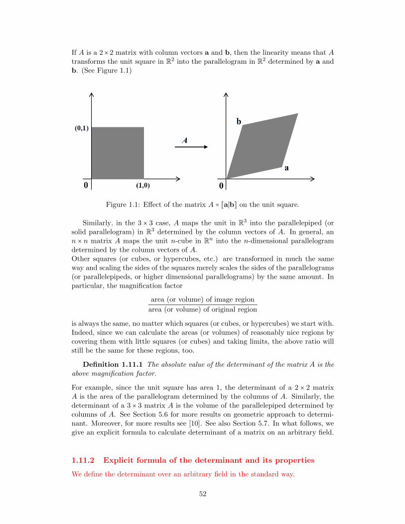
If A is a 2× 2 matrix with column vectors a and b, then the linearity means that Atransforms the unit square in R2 into the parallelogram in R2 determined by a andb. (See Figure 1.1)
Figure 1.1: Effect of the matrix A = [a∣b] on the unit square.
Similarly, in the 3 × 3 case, A maps the unit in R3 into the parallelepiped (orsolid parallelogram) in R3 determined by the column vectors of A. In general, ann × n matrix A maps the unit n-cube in Rn into the n-dimensional parallelogramdetermined by the column vectors of A.Other squares (or cubes, or hypercubes, etc.) are transformed in much the sameway and scaling the sides of the squares merely scales the sides of the parallelograms(or parallelepipeds, or higher dimensional parallelograms) by the same amount. Inparticular, the magnification factor
area (or volume) of image region
area (or volume) of original region
is always the same, no matter which squares (or cubes, or hypercubes) we start with.Indeed, since we can calculate the areas (or volumes) of reasonably nice regions bycovering them with little squares (or cubes) and taking limits, the above ratio willstill be the same for these regions, too.
Definition 1.11.1 The absolute value of the determinant of the matrix A is theabove magnification factor.
For example, since the unit square has area 1, the determinant of a 2 × 2 matrixA is the area of the parallelogram determined by the columns of A. Similarly, thedeterminant of a 3 × 3 matrix A is the volume of the parallelepiped determined bycolumns of A. See Section 5.6 for more results on geometric approach to determi-nant. Moreover, for more results see [10]. See also Section 5.7. In what follows, wegive an explicit formula to calculate determinant of a matrix on an arbitrary field.
1.11.2 Explicit formula of the determinant and its properties
We define the determinant over an arbitrary field in the standard way.
52
Definition 1.11.2 For A ∈ Fn×n, we define the determinant of A by the formula:
detA = ∑ω∈Sn
sign(ω)a1ω(1)a2ω(2) . . . anω(n), A = [aij]∈ Fn×n. (1.11.1)
In what follows, we verify that the formulas given in Definition 1.11.1 and Def-inition 1.11.2 are the same for 2 × 2 real matrices. This can be generalized for real
matrices of any size. We assume that A = [a11 a12
a21 a22]. We are going to calculate the
area of the parallelogram determined by a and b. We have
a = A(1,0)⊺ = (a11, a21)⊺
b = A(0,1)⊺ = (a12, a22)⊺
The equation of the line passing through the origin and a is f(x, y) = a21a11x−y. Next,
we have
d(b, f) =∣a21a12a11
− a22∣√
(a21a11)
2+ 1
d(a,0) =√a2
11 + a221
Here, d denotes the distance of two points or a point and a line. Then, the area ofimage region in Figure 1.1 is equal to
√a2
11 + a221 ⋅
∣a21a12a11− a22∣
√(a21a11
)2+ 1
= ∣a11a22 − a21a12∣ .
As the area of the original region (unit square) in Figure 1.1 is 1, then the magni-fication factor (∣detA∣) is ∣a11a22 − a21a21∣. Clearly, we obtain the same value for∣detA∣ by formula 1.11.1.Note that here we used the distance formula between a line L = ax + by + c and a
point p = (x0, y0) which is denoted by d(p,L) and given as d(p,L) = ∣ax0+by0+c∣√a2+b2
.
In the following theorem, we study the main properties of the determinant function.
Theorem 1.11.3 Assume that the characteristic of F is different from 2, i.e.2 ≠ 0 in F. Then, the determinant function det ∶ Fn×n → F is the unique skew-symmetric multilinear functions in the rows of A satisfying the normalization con-dition:
det In = 1.
Furthermore, it satisfies the following properties:
1. detA = detA⊺.
2. detA is a multilinear function in rows or columns of A.
3. The determinant of a lower triangular or an upper triangular matrix is aproduct of the diagonal entries of A.
53
4. Let B obtained from A by permuting two rows or columns of A. Then detB =−detA.
5. If A has two equal rows or columns, then detA = 0.
6. A is invertible if and only if detA ≠ 0.
7. Let A,B ∈ Fn×n. Then, detAB = detAdetB.
8. ( Laplace row and column expansion for determinants) For i, j ∈ [n] denote byA(i, j) ∈ F(n−1)×(n−1) the matrix obtained from A by deleting its i-th row andj-th column. Then
detA =n
∑j=1
aij(−1)i+j detA(i, j) =n
∑i=1
aji(−1)i+j detA(i, j), (1.11.2)
for i = 1, . . . , n.
(If A = [aij] ∈ Fn×n, we sometimes denote detA by
RRRRRRRRRRRRRR
a11 a12 ⋯ a1n
⋮ ⋮ ⋯ ⋮an1 an2 ⋯ ann
RRRRRRRRRRRRRR.)
Proof. First, observe that if the determinant function exists, then it must bedefined by (1.11.1). Indeed,
ri =n
∑j=1
aije⊺j , ej = (δj1, . . . , δjn)⊺.
Let T ∶⊕nFn → F be a multilinear skew-symmetric function. Use multilinearity of T
to deduceT (r1, . . . , rn) = ∑
i1,...,in∈[n]a1i1 . . . aninT (ei1 , . . . ,ein).
Since T is skew-symmetric, T (ei1 , . . . ,ein) = 0 if ip = iq, for some 1 ≤ p < q ≤ n.Indeed, if we interchange eip = eiq , then we do not change the value of the T .On the other hand, since T is skew-symmetric, then the value of T is equal to−T , when we interchange eip = eiq . As the characteristic of F is not 2, we deducethat T (ei1 , . . . ,ein) = 0, if ip = iq. Hence, in the above expansion of T (r1, . . . , rn),the only non-zero terms are where i1, . . . , in = [n]. Each such set of n indicesi1, . . . , in corresponds uniquely to a permutation ω ∈ Sn, where ω(j) = ij , forj ∈ [n]. Now e1, . . . ,en can be brought to eσ(1), . . . ,eσ(n) by using transposi-tions. The composition of this transpositions yields σ. Since T is skew-symmetric,it follows that T (eσ(1), . . . ,eσ(n)) = sign(ω)T (e1, . . . ,en). As T (In) = 1, we deducethat T (eσ(1), . . . ,eσ(n)) = sign(ω).
1. In (1.11.1) note that if j = ω(i), then i = ω−1(j). Since ω is a bijection,we deducethat when i = 1, . . . , n, then j takes each value in [n]. Since sign(ω) = sign(ω−1), weobtain
detA = ∑ω∈Sn
sign(ω)aω−1(1)1aω−1(2)2 . . . aω−1(n)n =
∑ω∈Sn
sign(ω−1)aω−1(1)1aω−1(2)2 . . . aω−1(n)n = detA⊺.
54
(Note that since Sn is a group, when ω varies over Sn, so is ω−1.)2. Fix all rows of A except the row i. From (1.11.1) it follows that detA is a linearfunction in the row i of A, i.e. detA is a multilinear function in the rows of A. Inview of the identity detA = detA⊺, we deduce that detA is a multilinear functionof the columns of A.3. Assume that A is upper triangular. Then, anω(n) = 0 if ω(n) ≠ n. Therefore, allnon-zero terms in (1.11.1) are zero unless ω(n) = n. Thus, assume that ω(n) = n.Then, a(n−1)ω(n−1) = 0 unless ω(n − 1) = n − 1. Hence, all non-zero terms in (1.11.1)must come from all ω satisfying ω(n) = n,ω(n − 1) = n − 1. Continuing in the samemanner we deduce that the only non-zero term in (1.11.1) comes from ω =id. Assign(id) = 1, it follows that detA = ∏n
i=1 aii. Since detA = detA⊺, we deduce theclaim for lower triangular matrices.4. Note that a permutation of two elements 1 ≤ i < j ≤ n in [n] is achieved by atransposition τ ∈ Sn. Therefore, B = [bpq] and bpq = aτ(p)q. As in the proof of 1 welet τ(i) = j, then j = τ−1(i) = τ(i). Hence
detB = ∑ω∈Sn
sign(ω)aτ(1)ω(1)aτ(2)ω(2) . . . aτ(n)ω(n) =
∑ω∈Sn
sign(ω)a1ω(τ(1))a2ω(τ(2)) . . . anω(τ(n)) =
∑ω∈Sn
−sign(ω τ)a1(ωτ)(1)a2(ωτ)(2) . . . an(ωτ)(n) = −detA.
5. Suppose A has two identical rows. Interchange these two rows to obtainB = A. Then, detA = detB = −detA, where the last equality is established in 4.Thus, 2 detA = 0 and this means detA = 0 as charF ≠ 2.6. Use 2, 3 and 5 to deduce that detEA = detE detA if E is an elementary matrix.(Note that detE ≠ 0.) Hence, if E1, . . . ,Ek are elementary matrices, we deducethat det(Ek . . .E1) = ∏k
i=1 detEi. Let B be the reduced row echelon form of A.Therefore, B = EkEk−1 . . .E1A. Hence, detB = (∏n
i=1 detEi)detA. If In ≠ B, thenthe last row of B is zero, so detB = 0 which implies that detA = 0. If B = In, thendetA =∏n
i=1(detEi)−1.7. Assume that either detA = 0 or detB = 0. We claim that (AB)x = 0 has anontrivial solution. Suppose detB = 0. Using 6 and Theorem 1.7.11, we concludethat the equation Bx = 0 has a nontrivial solution which satisfies ABx = 0. Supposethat B is invertible and Ay = 0, for some y ≠ 0. Then, AB(B−1y) = 0 which impliesthat detAB = 0. Hence in these cases detAB = 0 = detAdetB. Suppose that A andB are invertible. Then, each of them is a product of elementary matrices. Use thearguments in the proof of 6 to deduce that detAB = detAdetB.8. First we prove the first part of formula 1.11.2 for i = n. Clearly, (1.11.1) yieldsthe equality
detA =n
∑j=1
anj ∑ω∈Sn,ω(n)=j
sign(ω)a1ω(1) . . . a(n−1)ω(n−1). (1.11.3)
In the above sum, let j = n. Hence, ω(n) = n and then ω can be viewed asω′ ∈ Sn−1. Also sign(ω) = sign(ω′). Hence, ∑ω′∈Sn−1 sign(ω)a1ω′(1) . . . a(n−1)ω′(n−1) =detA(n,n). Note that (−1)n+n = 1. This justifies the form of the last term of ex-pansion 1.11.2 for i = n. To justify the sign of any term in 1.11.2 for i = n, we take
55
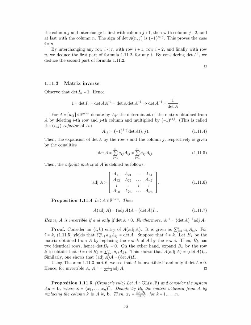
the column j and interchange it first with column j +1, then with column j +2, andat last with the column n. The sign of detA(n, j) is (−1)n+j . This proves the casei = n.
By interchanging any row i < n with row i + 1, row i + 2, and finally with rown, we deduce the first part of formula 1.11.2, for any i. By considering detA⊺, wededuce the second part of formula 1.11.2.
◻
1.11.3 Matrix inverse
Observe that det In = 1. Hence
1 = det In = detAA−1 = detAdetA−1 ⇒ detA−1 = 1
detA.
For A = [aij] ∈ Fn×n denote by Aij the determinant of the matrix obtained fromA by deleting i-th row and j-th column and multiplied by (−1)i+j . (This is calledthe (i, j) cofactor of A.)
Aij ∶= (−1)i+j detA(i, j). (1.11.4)
Then, the expansion of detA by the row i and the column j, respectively is givenby the equalities
detA =n
∑j=1
aijAij =n
∑i=1
aijAij . (1.11.5)
Then, the adjoint matrix of A is defined as follows:
adj A ∶=
⎡⎢⎢⎢⎢⎢⎢⎢⎣
A11 A21 . . . An1
A12 A22 . . . An2
⋮ ⋮ ⋮ ⋮A1n A2n . . . Ann
⎤⎥⎥⎥⎥⎥⎥⎥⎦
. (1.11.6)
Proposition 1.11.4 Let A ∈ Fn×n. Then
A(adj A) = (adj A)A = (detA)In. (1.11.7)
Hence, A is invertible if and only if detA ≠ 0. Furthermore, A−1 = (detA)−1adj A.
Proof. Consider an (i, k) entry of A(adj A). It is given as ∑nj=1 aijAkj . Fori = k, (1.11.5) yields that ∑nj=1 aijAij = detA. Suppose that i ≠ k. Let Bk be thematrix obtained from A by replacing the row k of A by the row i. Then, Bk hastwo identical rows, hence detBk = 0. On the other hand, expand Bk by the rowk to obtain that 0 = detBk = ∑nj=1 aijAkj . This shows that A(adj A) = (detA)In.Similarly, one shows that (adj A)A = (detA)In.
Using Theorem 1.11.3 part 6, we see that A is invertible if and only if detA ≠ 0.Hence, for invertible A, A−1 = 1
detAadj A. ◻
Proposition 1.11.5 (Cramer’s rule) Let A ∈ GL(n,F) and consider the systemAx = b, where x = (x1, . . . , xn)⊺. Denote by Bk the matrix obtained from A byreplacing the column k in A by b. Then, xk = detBk
detA , for k = 1, . . . , n.
56
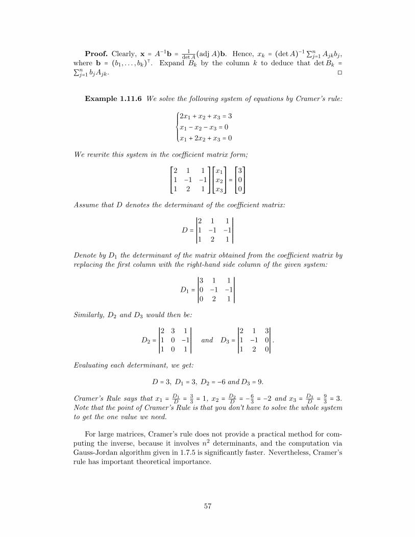
Proof. Clearly, x = A−1b = 1detA(adj A)b. Hence, xk = (detA)−1∑nj=1Ajkbj ,
where b = (b1, . . . , bk)⊺. Expand Bk by the column k to deduce that detBk =∑nj=1 bjAjk. ◻
Example 1.11.6 We solve the following system of equations by Cramer’s rule:
⎧⎪⎪⎪⎪⎨⎪⎪⎪⎪⎩
2x1 + x2 + x3 = 3
x1 − x2 − x3 = 0
x1 + 2x2 + x3 = 0
We rewrite this system in the coefficient matrix form;
⎡⎢⎢⎢⎢⎢⎣
2 1 11 −1 −11 2 1
⎤⎥⎥⎥⎥⎥⎦
⎡⎢⎢⎢⎢⎢⎣
x1
x2
x3
⎤⎥⎥⎥⎥⎥⎦=⎡⎢⎢⎢⎢⎢⎣
300
⎤⎥⎥⎥⎥⎥⎦
Assume that D denotes the determinant of the coefficient matrix:
D =RRRRRRRRRRRRRR
2 1 11 −1 −11 2 1
RRRRRRRRRRRRRRDenote by D1 the determinant of the matrix obtained from the coefficient matrix byreplacing the first column with the right-hand side column of the given system:
D1 =RRRRRRRRRRRRRR
3 1 10 −1 −10 2 1
RRRRRRRRRRRRRRSimilarly, D2 and D3 would then be:
D2 =RRRRRRRRRRRRRR
2 3 11 0 −11 0 1
RRRRRRRRRRRRRRand D3 =
RRRRRRRRRRRRRR
2 1 31 −1 01 2 0
RRRRRRRRRRRRRR.
Evaluating each determinant, we get:
D = 3, D1 = 3, D2 = −6 and D3 = 9.
Cramer’s Rule says that x1 = D1
D = 33 = 1, x2 = D2
D = −63 = −2 and x3 = D3
D = 93 = 3.
Note that the point of Cramer’s Rule is that you don’t have to solve the whole systemto get the one value we need.
For large matrices, Cramer’s rule does not provide a practical method for com-puting the inverse, because it involves n2 determinants, and the computation viaGauss-Jordan algorithm given in 1.7.5 is significantly faster. Nevertheless, Cramer’srule has important theoretical importance.
57
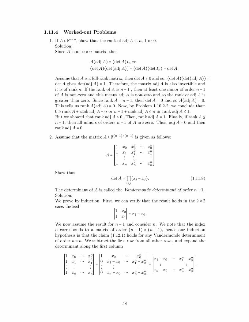
1.11.4 Worked-out Problems
1. If A ∈ Fn×n, show that the rank of adj A is n, 1 or 0.Solution:Since A is an n × n matrix, then
A(adj A) = (detA)In ⇒(detA)(det(adj A)) = (detA)(det In) = detA.
Assume thatA is a full-rank matrix, then detA ≠ 0 and so: (detA)(det(adj A)) =detA gives det(adj A) = 1. Therefore, the matrix adj A is also invertible andit is of rank n. If the rank of A is n− 1 , then at least one minor of order n− 1of A is non-zero and this means adj A is non-zero and so the rank of adj A isgreater than zero. Since rank A = n − 1, then detA = 0 and so A(adj A) = 0.This tells us rank A(adj A) = 0. Now, by Problem 1.10.2-2, we conclude that:0 ≥ rank A + rank adj A − n or n − 1 + rank adj A ≤ n or rank adj A ≤ 1.But we showed that rank adj A > 0. Then, rank adj A = 1. Finally, if rank A ≤n − 1, then all minors of orders n − 1 of A are zero. Thus, adj A = 0 and thenrank adj A = 0.
2. Assume that the matrix A ∈ F(n+1)×(n+1) is given as follows:
A =
⎡⎢⎢⎢⎢⎢⎢⎢⎣
1 x0 x20 ⋯ xn0
1 x1 x21 ⋯ xn1
⋮ ⋮ ⋮ ⋮1 xn x2
n ⋯ xnn
⎤⎥⎥⎥⎥⎥⎥⎥⎦
Show thatdetA =∏
i>j(xi − xj). (1.11.8)
The determinant of A is called the Vandermonde determinant of order n + 1.Solution:We prove by induction. First, we can verify that the result holds in the 2 × 2case. Indeed
∣1 x0
1 x1∣ = x1 − x0.
We now assume the result for n − 1 and consider n. We note that the indexn corresponds to a matrix of order (n + 1) × (n + 1), hence our inductionhypothesis is that the claim (1.12.1) holds for any Vandermonde determinantof order n × n. We subtract the first row from all other rows, and expand thedeterminant along the first column
RRRRRRRRRRRRRRRRRRR
1 x0 ⋯ xn01 x1 ⋯ xn1⋮ ⋮ ⋮1 xn ⋯ xnn
RRRRRRRRRRRRRRRRRRR
=
RRRRRRRRRRRRRRRRRRR
1 x0 ⋯ xn00 x1 − x0 ⋯ xn1 − xn0⋮ ⋮ ⋮0 xn − x0 ⋯ xnn − xn0
RRRRRRRRRRRRRRRRRRR
=RRRRRRRRRRRRRR
x1 − x0 ⋯ xn1 − xn0⋮ ⋮
xn − x0 ⋯ xnn − xn0
RRRRRRRRRRRRRR.
58
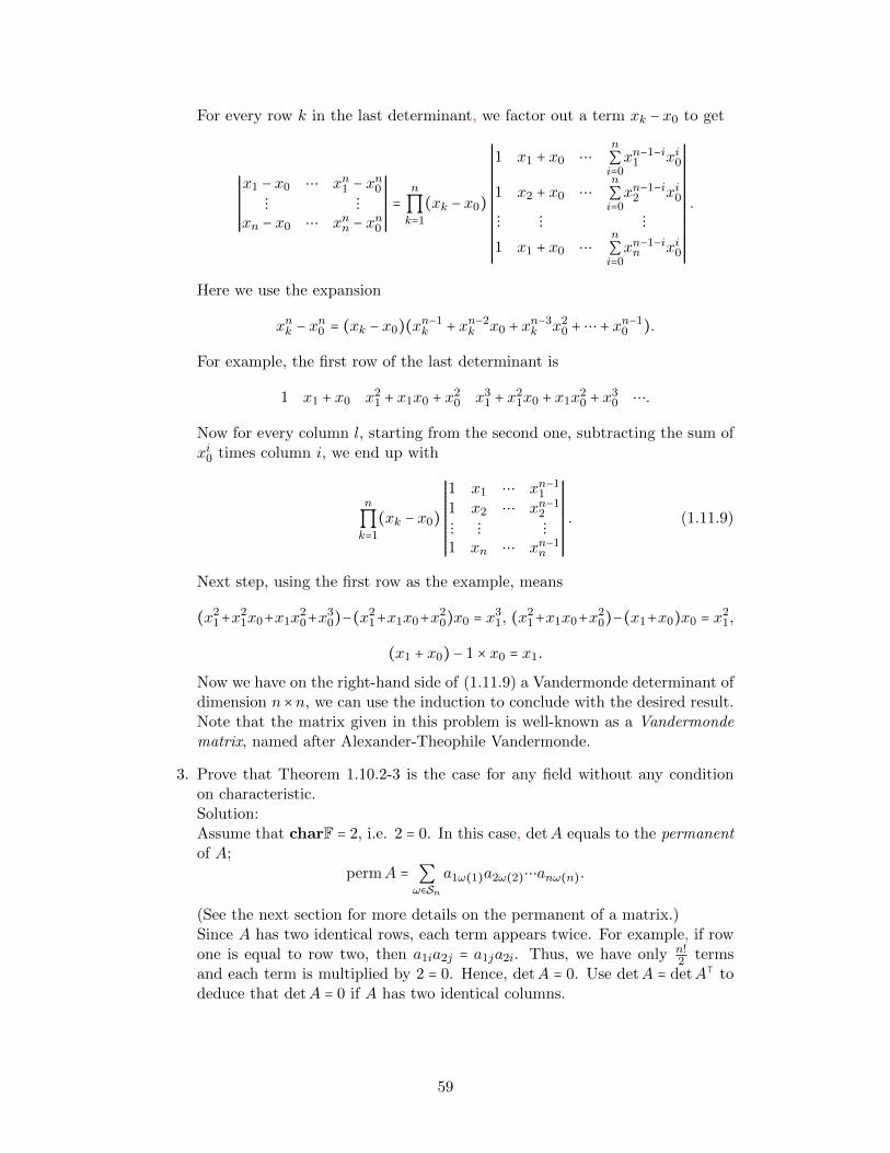
For every row k in the last determinant, we factor out a term xk − x0 to get
RRRRRRRRRRRRRR
x1 − x0 ⋯ xn1 − xn0⋮ ⋮
xn − x0 ⋯ xnn − xn0
RRRRRRRRRRRRRR=
n
∏k=1
(xk − x0)
RRRRRRRRRRRRRRRRRRRRRRRRRRRRRR
1 x1 + x0 ⋯n
∑i=0xn−1−i
1 xi0
1 x2 + x0 ⋯n
∑i=0xn−1−i
2 xi0
⋮ ⋮ ⋮1 x1 + x0 ⋯
n
∑i=0xn−1−in xi0
RRRRRRRRRRRRRRRRRRRRRRRRRRRRRR
.
Here we use the expansion
xnk − xn0 = (xk − x0)(xn−1k + xn−2
k x0 + xn−3k x2
0 +⋯ + xn−10 ).
For example, the first row of the last determinant is
1 x1 + x0 x21 + x1x0 + x2
0 x31 + x2
1x0 + x1x20 + x3
0 ⋯.
Now for every column l, starting from the second one, subtracting the sum ofxi0 times column i, we end up with
n
∏k=1
(xk − x0)
RRRRRRRRRRRRRRRRRRR
1 x1 ⋯ xn−11
1 x2 ⋯ xn−12
⋮ ⋮ ⋮1 xn ⋯ xn−1
n
RRRRRRRRRRRRRRRRRRR
. (1.11.9)
Next step, using the first row as the example, means
(x21+x2
1x0+x1x20+x3
0)−(x21+x1x0+x2
0)x0 = x31, (x2
1+x1x0+x20)−(x1+x0)x0 = x2
1,
(x1 + x0) − 1 × x0 = x1.
Now we have on the right-hand side of (1.11.9) a Vandermonde determinant ofdimension n×n, we can use the induction to conclude with the desired result.Note that the matrix given in this problem is well-known as a Vandermondematrix, named after Alexander-Theophile Vandermonde.
3. Prove that Theorem 1.10.2-3 is the case for any field without any conditionon characteristic.Solution:Assume that charF = 2, i.e. 2 = 0. In this case, detA equals to the permanentof A;
permA = ∑ω∈Sn
a1ω(1)a2ω(2)⋯anω(n).
(See the next section for more details on the permanent of a matrix.)Since A has two identical rows, each term appears twice. For example, if rowone is equal to row two, then a1ia2j = a1ja2i. Thus, we have only n!
2 termsand each term is multiplied by 2 = 0. Hence, detA = 0. Use detA = detA⊺ todeduce that detA = 0 if A has two identical columns.
59
1.11.5 Problems
1. Let A = [aij] ∈ Fn×n be a symmetric tridiagonal matrix, . If B is a matrixformed from A by deleting the first two rows and columns, show that
detA = a11 detA(1,1) − a212 detB
2. If A ∈ Fm×n and B ∈ Fn×p, show that
rank A + rank B − n ≤ rank AB (1.11.10)
(Hint: Use Problem 1.10.2-1.b and Worked-out Problem 1.10.1-2.)The combination of the inequality (1.11.10) with the inequality mentioned inProblem 1.8.5-3, is well-known as Sylvester’s Inequality.
3. Let A,B ∈ Fn×n. Prove that
rank (A +B) ≤ rank A + rank B.
4. If A,B ∈ Fn×n, prove or disprove the following statement:
”rank (A +B) ≤ minrank A, rank B.”
Compare this statement with Problem 1.8.5-3.
5. If A,B ∈ Fn×n and A −B = AB, prove that AB = BA.
6. Let A ∈ Fm×n and denote by Ak the upper left k × k submatrix of A. Assumethat detAi ≠ 0 for i = 1, . . . , k. Show that the i-th pivot of A is detAi
detAi−1for
i = 1, . . . , k. (Assume that detA0 = 1.)
7. Let A ∈ Rn×n. Prove that rank AA⊺ = rank A⊺A.
8. Let A ∈ R2×2 be an orthogonal matrix. Show the followings:
(a) if detA = 1, then A = [cos θ − sin θsin θ cos θ
], for some θ, 0 ≤ θ < 2π. That is, A
counterclockwise rotates every point in R2 by an angle θ.
(b) if detA = −1, then A = [cos θ sin θsin θ − cos θ
], for some θ, 0 ≤ θ < 2π. That
is, A reflects every point in R2 about a line passing through the origin.Determine this line. Or equivalently, there exists an invertible matrix P
such that P −1AP = [1 00 −1
].
(See problem 1.10.2-4.)
60
1.12 Permanents
1.12.1 A combinatorial approach of Philip Hall Theorem
The following theorem is well-known as Philip Hall Theorem and gives us the nec-essary and sufficient conditions to have a perfect matching in a bipartite graph. See[23] for more results on this theorem and its proof.
Theorem 1.12.1 If G = (V,E) is a bipartite graph with the bipartite sets Xand Y , then G has a perfect matching if and only if #X = #Y and for any subsetS ⊂X, #S ≤ #N(S), where N(S) denotes the neighborhood of S in Y , i.e. the setof all vertices in Y adjacent to some elements of S.
If A = Aini=1 is a family of non-empty subsets of a finite set S, a system of distinctrepresentative (SDR) of A is a tuple (a1, . . . , an) with ai ∈ Ai and ai ≠ aj , 1 ≤ i, j ≤ n,i ≠ j. This is also called a transversal of A.
Theorem 1.12.2 Let A = Aini=1 is a family of non-empty subsets of a finiteset A. Then, A has an SDR if and only if
#⋃i∈JAi≥#J,
for any J ⊆ [n].
It is easy to check that the above theorem is equivalent to Philip Hall Theorem.Indeed, construct a bipartite graph with X = a1, . . . , an and Y = A1, . . . ,An.Furthermore, there is an edge (ai,Aj) if and only if ai ∈ Aj .The interested reader can verify that the number of perfect matchings in a bipartitegraph G with bipartite sets X and Y and #X = #Y = n is equal to perm A, whereA is the adjacency matrix of G.
We end up this section with the linear version of Philip Hall Theorem.Let V be a vector space over the field F and let V = V1, . . . ,Vn be a family ofvector subspaces of V. A free transversal for V is a family of linearly independentvectors x1, . . . ,xn such that xi ∈ Vi, i = 1, . . . , n. The following result of Rado [16]gives a linear version of Philip Hall Theorem for the existence of a free transversalfor V. The interested reader is referred to [1] to see the proof and more details.
Theorem 1.12.3 Let V be a vector space over the field F and let V = V1, . . . ,Vnbe a family of vector subspaces of V. Then, V admits a free transversal if and onlyif
dim span(⋃i∈J
Vi) ≥ #J,
for all J ⊂ [n].
1.12.2 Permanents
Recall that if A ∈ Fn×n, the permanent of A = [aij] is denoted by perm A and definedas
permA = ∑w∈Sn
n
∏i=1
aiw(i).
61
From the definition of permanent, it follows that permA = permA⊺.
The matrix A ∈ Fm×n whose entries are either 1 or 0 is called a (0,1)-matrix. Aspecial class of (0,1)-matrices, namely the (0,1)-matrices in Fn×n that have exactlyk ones in each row and column. We denote this class by C(n, k). We define
S(n, k) ∶= maxpermA; A ∈ C(n, k),s(n, k) ∶= minpermA; A ∈ C(n, k).
The following result, known as Fekete’s lemma. It will be used to find an upperbound for the permanent function. See [23] for more details about Fekete’s lemma.
Lemma 1.12.4 Let f ∶ N → N be a function for which f(m + n) ≥ f(m)f(n),
for all m,n ∈ N. Then limn→∞ f(n)1n exists (possibly ∞).
It is easy to check the following inequalities:
S(n1 + n2, k) ≥ S(n1, k)S(n2, k),s(n1 + n2, k) ≤ s(n1, k)s(n2, k).
By applying these inequalities to Fekete’s lemma, we can define:
S(k) ∶= limn→∞
S(n, k)1n ,
s(k) ∶= limn→∞
s(n, k)1n .
Note that a function f ∶ Rn → R is called to be convex if f(tx + (1 − t)y) ≤ tf(x) +(1 − t)f(y), for any x, y ∈ Rn and t ∈ [0,1]. Note that it can be shown that thenecessary and sufficient condition for a continuous function f on [0,1], such that f ′
and f ′′ exist on(0,1), is that the second derivative is always non-negative. (Try tojustify!)
Lemma 1.12.5 If t1, . . . , tn are non-negative real numbers, then
(∑ni=1 tin
)∑ni=1 ti
≤n
∏i=1
ttii .
Proof. Since x lnx is a convex function, we have
∑ni=1 tin
ln(∑ni=1 tin
) ≤ ∑ni=1 ti ln tin
,
which proves the assertion. ◻
It was conjectured by H. Minc that if A ∈ Rn×n is a (0,1)-matrix with row-sumsr1, . . . , rn, then
perm A ≤n
∏j=1
(rj !)1rj .
This conjecture was proved by L.M. Bregman [4].The following short proof of this theorem was given by A. Schrijver [20].
62
Proof by induction on n: For n = 1 the statement is obvious. Suppose that it satisfiesfor (n − 1) × (n − 1) matrices. We will show that
(permA)npermA ⩽ (n
∏i=1
ri!1ri )
npermA
,
which implies the above inequality. In the following inequalities, the variables i, jand k range from 1 to n. Let S be the set of all permutations ω ∈ Sn for whichaiω(i) = 1, for i = 1, . . . , n. Clearly, #S = perm A. Using Lemma 1.12.5,
∏i
(perm A)perm A ⩽∏i
⎛⎜⎜⎝rperm Ai ∏
kaik=1
perm Aperm Aikik
⎞⎟⎟⎠,
where Aik denotes the minor obtained from A by deleting row i and column k. Now,
∏i
⎛⎜⎜⎝rpermAi ∏
kaik=1
permApermAikik
⎞⎟⎟⎠= ∏ω∈S
((∏i
ri)(∏i
permAiω(i))) ,
because the number of factors ri equals permA on both sides, while the numberof factors permAik equals the number of ω ∈ S for which ω(i) = k. Applying theinduction hypothesis to each Aiω(i), we conclude that the recent expression is lessthan or equal to
∏ω∈S
⎛⎜⎜⎜⎜⎜⎝
(∏i
ri)
⎛⎜⎜⎜⎜⎜⎝
∏i
⎛⎜⎜⎜⎜⎜⎝
∏jj≠i
aiω(i)=0
rj !1rj
⎞⎟⎟⎟⎟⎟⎠
⎛⎜⎜⎜⎜⎜⎝
∏jj≠i
aiω(i)=1
(rj − 1)!1
(rj−1)
⎞⎟⎟⎟⎟⎟⎠
⎞⎟⎟⎟⎟⎟⎠
⎞⎟⎟⎟⎟⎟⎠
. (1.12.1)
Changing the order of multiplication and considering that the number of i such thati ≠ j and ajω(j) = 0 is n − ri, whereas the number of i such that i ≠ j and ajω(i) = 1is rj − 1 we get
(1.12.1) = ∏ω∈S
⎛⎝(∏i
ri)⎛⎝∏j
rj !(n−rj)
rj (rj − 1)!(rj−1)
(rj−1)⎞⎠⎞⎠. (1.12.2)
That (1.12.2) equals ∏ω∈S
(∏iri!
nri ) = (∏
iri!
1ri )
nperm A
is trivial. Since (perm A)npermA =
∏i(permA)permA, the proof is complete.
Now, if G is a balanced bipartite graph with adjacency matrix A ∈ 0,1n×n and
row-sums r1, . . . , rn, then by Bregman ’s theorem, ∏nj=1(rj !)
1rj is an upper bound
for the number of perfect matchings in G.
1.12.3 Worked-out Problems
1. Assume that Tn ⊆ (N ∪ 0)n×n is the set of matrices with row-sums andcolumn-sums 3; tn = minperm A; A ∈ Tn. Denote by Xn the set of all
63
matrices obtained from elements of Tn by decreasing one positive entry by 1;xn = minperm A; A ∈ Xn. Show that tn ⩾ ⌈3
2xn⌉, where ⌈ ⌉ denotes theceiling function.Solution:Choose A ∈ Tn with first row y = (y1, y2, y3,0, . . . ,0), where yi ⩾ 0, for i = 1,2,3.Then
2y = y1(y1 − 1, y2, y3,0, . . . ,0) +y2(y1, y2 − 1, y3,0, . . . ,0) +y3(y1, y2, y3 − 1,0, . . . ,0).
Since S(n1 + n2, k) ≥ S(n1, k)S(n2, k), then 2tn ⩾ (y1 + y2 + y3)xn = 3xn.
1.12.4 Problems
1. Show that
(a) S(n, k) ≥ k!
(b) S(k) ≤ (k!) 1k
(c) Show by example that S(k) ≥ (k!) 1k . This shows that S(k) = (k!) 1
k .
(Hint: Use Bregman’s theorem.)
1.13 An application of Philip Hall Theorem
Recall that a permutation matrix is a square matrix that has exactly one entry of1 in each row and each column and zero elsewhere. Now, we define a more generalfamily of matrices called doubly stochastic as mentioned in Section 1.9.
Definition 1.13.1 A doubly stochastic matrix is a square matrix A = [aij] ofnon-negative real entries, each of whose rows and columns sum 1, i.e.
∑i
aij =∑j
aij = 1.
The set of all n × n doubly stochastic matrices is denoted by Ωn. If we denote alln × n permutation matrices by Pn, then clearly Pn ⊂ Ωn.
Definition 1.13.2 A subset A of a real vector space V is said to be convex ifλx + (1 − λ)y ∈ A, for all vectors x,y ∈ A and all scalars λ ∈ [0,1]. Via induction,this can be seen to be equivalent to the requirement that ∑ni=1 λixi ∈ A, for all vectorsx1, . . . ,xn ∈ A and all scalars λ1, . . . , λn ⩾ 0 with ∑ni=1 λi = 1. A point x ∈ A is calledan extreme point of A if y,z ∈ A, 0 < t < 1, and x = ty + (1 − t)z imply x = y = z.With this restrictions on λi’s, an expression of the form ∑ni=1 λixi is said to be aconvex combination of x1, . . . ,xn. The convex hull of a set B ⊂ V is defined as∑λixi ∶ xi ∈ B, λi ≥ 0 and ∑λi = 1. The convex hull of B can also be defined asthe smallest convex set containing B. (Why?)
The importance of extreme points can be seen from the following theorem whoseproof can be found in [2].
64
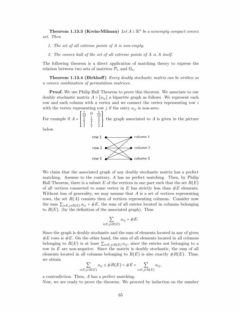
Theorem 1.13.3 (Krein-Milman) Let A ⊂ Rn be a nonempty compact convexset. Then
1. The set of all extreme points of A is non-empty.
2. The convex hull of the set of all extreme points of A is A itself.
The following theorem is a direct application of matching theory to express therelation between two sets of matrices Pn and Ωn.
Theorem 1.13.4 (Birkhoff) Every doubly stochastic matrix can be written asa convex combination of permutation matrices.
Proof. We use Philip Hall Theorem to prove this theorem. We associate to ourdoubly stochastic matrix A = [aij] a bipartite graph as follows. We represent eachrow and each column with a vertex and we connect the vertex representing row iwith the vertex representing row j if the entry aij is non-zero.
For example if A =⎡⎢⎢⎢⎢⎢⎣
712 0 5
1216
12
13
14
12
14
⎤⎥⎥⎥⎥⎥⎦, the graph associated to A is given in the picture
below.
row 1 column 1
row 2 column 2
row 3 column 3
We claim that the associated graph of any doubly stochastic matrix has a perfectmatching. Assume to the contrary, A has no perfect matching. Then, by PhilipHall Theorem, there is a subset E of the vertices in one part such that the set R(E)of all vertices connected to some vertex in E has strictly less than #E elements.Without loss of generality, we may assume that A is a set of vertices representingrows, the set R(A) consists then of vertices representing columns. Consider nowthe sum ∑i∈E,j∈R(E) aij = #E, the sum of all entries located in columns belongingto R(E). (by the definition of the associated graph). Thus
∑i∈E,j∈R(E)
aij = #E.
Since the graph is doubly stochastic and the sum of elements located in any of given#E rows is #E. On the other hand, the sum of all elements located in all columnsbelonging to R(E) is at least ∑i∈E,j∈R(E) aij , since the entries not belonging to arow in E are non-negative. Since the matrix is doubly stochastic, the sum of allelements located in all columns belonging to R(E) is also exactly #R(E). Thus,we obtain
∑i∈E,j∈R(E)
aij ≤ #R(E) < #E = ∑i∈E,j∈R(E)
aij ,
a contradiction. Then, A has a perfect matching.Now, we are ready to prove the theorem. We proceed by induction on the number
65
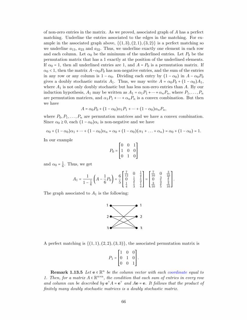
of non-zero entries in the matrix. As we proved, associated graph of A has a perfectmatching. Underline the entries associated to the edges in the matching. For ex-ample in the associated graph above, (1,3), (2,1), (3,2) is a perfect matching sowe underline a13, a23 and a32. Thus, we underline exactly one element in each rowand each column. Let α0 be the minimum of the underlined entries. Let P0 be thepermutation matrix that has a 1 exactly at the position of the underlined elements.If α0 = 1, then all underlined entries are 1, and A = P0 is a permutation matrix. Ifα0 < 1, then the matrix A−α0P0 has non-negative entries, and the sum of the entriesin any row or any column is 1 − α0. Dividing each entry by (1 − α0) in A − α0P0
gives a doubly stochastic matrix A1. Thus, we may write A = α0P0 + (1 − α0)A1,where A1 is not only doubly stochastic but has less non-zero entries than A. By ourinduction hypothesis, A1 may be written as A1 = α1P1 +⋯+αnPn, where P1, . . . , Pnare permutation matrices, and α1P1 +⋯+ αnPn is a convex combination. But thenwe have
A = α0P0 + (1 − α0)α1P1 +⋯ + (1 − α0)αnPn,where P0, P1, . . . , Pn are permutation matrices and we have a convex combination.Since α0 ≥ 0, each (1 − α0)αi is non-negative and we have
α0 + (1 − α0)α1 +⋯ + (1 − α0)αn = α0 + (1 − α0)(α1 + . . . + αn) = α0 + (1 − α0) = 1.
In our example
P0 =⎡⎢⎢⎢⎢⎢⎣
0 0 11 0 00 1 0
⎤⎥⎥⎥⎥⎥⎦and α0 = 1
6 . Thus, we get
A1 =1
1 − 16
(A − 1
6P0) =
6
5
⎡⎢⎢⎢⎢⎢⎣
712 0 1
40 1
213
14
13
14
⎤⎥⎥⎥⎥⎥⎦=⎡⎢⎢⎢⎢⎢⎣
710 0 3
100 3
525
310
25
310
⎤⎥⎥⎥⎥⎥⎦.
The graph associated to A1 is the following:
1 1
2 2
3 3
A perfect matching is (1,1), (2,2), (3,3), the associated permutation matrix is
P1 =⎡⎢⎢⎢⎢⎢⎣
1 0 00 1 00 0 1
⎤⎥⎥⎥⎥⎥⎦.
Remark 1.13.5 Let e ∈ Rn be the column vector with each coordinate equal to1. Then, for a matrix A ∈ Rn×n, the condition that each sum of entries in every rowand column can be described by e⊺A = e⊺ and Ae = e. It follows that the product offinitely many doubly stochastic matrices is a doubly stochastic matrix.
66
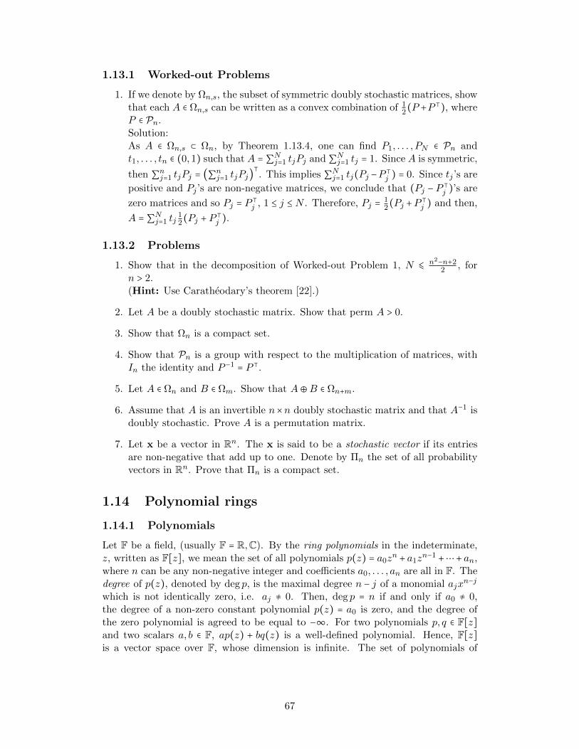
1.13.1 Worked-out Problems
1. If we denote by Ωn,s, the subset of symmetric doubly stochastic matrices, showthat each A ∈ Ωn,s can be written as a convex combination of 1
2(P +P⊺), where
P ∈ Pn.Solution:As A ∈ Ωn,s ⊂ Ωn, by Theorem 1.13.4, one can find P1, . . . , PN ∈ Pn andt1, . . . , tn ∈ (0,1) such that A = ∑Nj=1 tjPj and ∑Nj=1 tj = 1. Since A is symmetric,
then ∑nj=1 tjPj = (∑nj=1 tjPj)⊺. This implies ∑Nj=1 tj(Pj −P ⊺
j ) = 0. Since tj ’s are
positive and Pj ’s are non-negative matrices, we conclude that (Pj − P ⊺j )’s are
zero matrices and so Pj = P ⊺j , 1 ≤ j ≤ N . Therefore, Pj = 1
2(Pj +P⊺j ) and then,
A = ∑Nj=1 tj12(Pj + P
⊺j ).
1.13.2 Problems
1. Show that in the decomposition of Worked-out Problem 1, N ⩽ n2−n+22 , for
n > 2.(Hint: Use Caratheodary’s theorem [22].)
2. Let A be a doubly stochastic matrix. Show that perm A > 0.
3. Show that Ωn is a compact set.
4. Show that Pn is a group with respect to the multiplication of matrices, withIn the identity and P −1 = P ⊺.
5. Let A ∈ Ωn and B ∈ Ωm. Show that A⊕B ∈ Ωn+m.
6. Assume that A is an invertible n×n doubly stochastic matrix and that A−1 isdoubly stochastic. Prove A is a permutation matrix.
7. Let x be a vector in Rn. The x is said to be a stochastic vector if its entriesare non-negative that add up to one. Denote by Πn the set of all probabilityvectors in Rn. Prove that Πn is a compact set.
1.14 Polynomial rings
1.14.1 Polynomials
Let F be a field, (usually F = R,C). By the ring polynomials in the indeterminate,z, written as F[z], we mean the set of all polynomials p(z) = a0z
n + a1zn−1 +⋯+ an,
where n can be any non-negative integer and coefficients a0, . . . , an are all in F. Thedegree of p(z), denoted by deg p, is the maximal degree n − j of a monomial ajx
n−j
which is not identically zero, i.e. aj ≠ 0. Then, deg p = n if and only if a0 ≠ 0,the degree of a non-zero constant polynomial p(z) = a0 is zero, and the degree ofthe zero polynomial is agreed to be equal to −∞. For two polynomials p, q ∈ F[z]and two scalars a, b ∈ F, ap(z) + bq(z) is a well-defined polynomial. Hence, F[z]is a vector space over F, whose dimension is infinite. The set of polynomials of
67
degree at most n, is n + 1 dimensional subspace of F[z]. Given two polynomialsp = ∑ni=0 aiz
n−i, q = ∑mj=0 bjzm−j ∈ F[z], one can form the product
p(z)q(z) =n+m∑k=0
(k
∑i=0
aibk−i)zn+m−k, where ai = bj = 0, for i > n and j >m.
Note that pq = qp and deg pq = deg p + deg q. The addition and the product in F[z]satisfy all the nice distribution identities as the addition and multiplication in F.This implies that F[z] is a commutative ring with the addition and product definedabove. Here, the constant polynomial p ≡ 1 is the identity element, and the zeropolynomial as the zero element. (That is the reason for the name ring of polynomialsin one indeterminate (variable) over F.)
Given two polynomials p, q ∈ F[z], one can divide p by q /≡ 0 with the residuer, i.e. p = tq + r, for some unique t, r ∈ F[z], where deg r < deg q. For p, q ∈ F[z],let (p, q) denote greatest common divisor of p, q. If p and q are identically zero,then (p, q) is the zero polynomial. Otherwise, (p, q) is a polynomial s of the highestdegree that divides p and q. Note that s is determined up to a multiple of a non-zeroscalar and it can be chosen as a unique monic polynomial:
s(z) = zl + s1zl−1 + . . . + sl ∈ F[z]. (1.14.1)
For p, q /≡ 0, s can be found using the Euclid algorithm:
pi(z) = ti(z)pi+1(z) + pi+2(z), deg pi+2 < deg pi+1 i = 1, . . . (1.14.2)
Start this algorithm with p1 = p, p2 = q. Continue it until pk = 0 the first time. (Notethat k ≥ 3). Then, pk−1 = (p, q). It is easy to show, for example by induction, thateach pi is of the form uip + viq, for some polynomials ui, vi. Hence, the Euclideanalgorithm yields
(p(z), q(z)) = u(z)p(z) + v(z)q(z), for some u(z), v(z) ∈ F[z]. (1.14.3)
(This formula holds for any p, q ∈ F[z] .) Note that p, q ∈ F[z] are called coprime if(p, q)∈ F.
Note that if we divide p(z) by z − a, we get the residue p(a), i.e. p(z) = (z −a)q(z) + p(a). Hence, z − a divides p(z) if and only if p(a) = 0, i.e. a is the root ofp. A monic p(z) splits to a product of linear factors if
p(z) = (z − z1)(z − z2) . . . (z − zn) =n
∏i=1
(z − zi). (1.14.4)
Note that z1, . . . , zn are the roots of p.Let z = (z1, . . . , zn)⊺ ∈ Fn. Denote
σk(z) ∶= ∑1≤i1<i2<...<ik≤n
zi1zi2 . . . zik , k = 1, . . . , n. (1.14.5)
Then, σk(z) is called the k − th elementary symmetric polynomial in z1, . . . , zn.Observe that
σ1(z) = z1 + z2 + . . . + zn, n summands,
σ2(z) = z1z2 + . . . + z1zn + z2z3 + . . . + znzn +⋯ + zn−1zn,n(n + 1)
2summands,
σn(z) = z1z2 . . . zn, n terms in the product.
68
A straightforward calculation shows
n
∏i=1
(z − zi) = zn +n
∑i=1
(−1)iσi(z)zn−i. (1.14.6)
Remark 1.14.1 For a field F, the ring of polynomials p(z1, . . . , zn) in vari-ables z1, . . . , zn and with coefficients in F is denoted by F[z1, . . . , zn]. The fieldof fractions of the polynomial ring F[z1, . . . , zn] over F is the field of fractions
f(z1,...,zn)g(z1,...,zn) ; f, g ∈ F[z1, . . . , zn], g ≠ 0 and this is denoted by F(z1, . . . , zn).
1.14.2 Finite fields and finite extension of fields
A finite field of order q exists if and only if the order q is a prime power pk. (Why?)The field of order q is denoted by Fq. For the prime number p, Fp is isomorphic toZp, while Fpk can be viewed as a vector space of dimension k over Fp. Moreover, itcan be proved that for any prime p and positive integer n, there exists an irreduciblepolynomial π(x) ∈ Fp[x] of degree n such that Fp[x]/⟨π(x)⟩ ≅ Fpn .
Suppose that E/F is a field extension. Then, E may be considered as a vectorspace over F. The dimension of this vector space is called the degree of the fieldextension, and it is denoted by [E ∶ F]. The degree may be finite or infinite, thefield extension being called a finite extension or infinite extension accordingly. Anextension E/F is also sometimes said to be simply finite if it is a finite extension;this should not be confused with the fields themselves being finite fields (fields withfinitely many elements). For example, [C ∶ R] = 2 as dimRC = 2.
A polynomial p(z) ∈ F[z] is called irreducible, if all polynomials q that divide pare either constant non-zero polynomials or polynomials of the form ap(z), wherea ∈ F∖0. The field F is called an algebraically closed field if any monic polynomialp(z) ∈ F[z] splits to linear factors in F[z]. It is easy to see that F is algebraicallyclosed if and only if the only irreducible monic polynomials are z − a, for all a ∈ F.Then, F is not algebraically closed if and only if there exists an irreducible monicpolynomial in F[z] of degree greater than 1. For example, R is not algebraicallyclosed as x2 + 1 ∈ R[x] is irreducible over R.If f(z) = a0 + a1z + ⋯ + anzn ∈ F[z], an extension field E of F is called a splittingfield for f(z) over F if there exist elements c1, . . . , cn ∈ E such that
(i) f(z) = an(z − c1)⋯(z − cn),
(ii) E = F(c1, . . . , cn).
For example Q(√
2) is a splitting field of x2 − 2 ∈ Q[x] over Q.
Theorem 1.14.2 Let F be a field. Assume that p(z) = zd + ∑di=1 aizd−i be an
irreducible polynomial, where d > 1. Denote by F[z]/⟨p(z)⟩ the set of all polynomialsmodulo p(z). That is, for f(z), g(z) ∈ F[z], f(z) ≡ g(z) if the polynomial f(z)−g(z)is divided by p(z). Then, this set is a field, denoted by Fp(z), under the addition andproduct modulo p(z). Moreover, Fp(z) is a vector space over F of dimension d. Theset of all constant polynomials in Fp(z) is isomorphic to F. (Fp(z) is called a finiteextension of F, and more precisely an extension of degree d).
69
1.14.3 Worked-out Problems
1. An element λ ∈ F is called an eigenvalue of A ∈ Fn×n if there exists 0 ≠ x ∈ Fnsuch that Ax = λx. This x ≠ 0 is called an eigenvector of A corresponding toλ. It can be shown that λ is an eigenvalue of A if and only if it is a root of thepolynomial det(zIn −A). (See Problem 1.14.4-5.) Also, det(zIn −A) is calledthe characteristic polynomial of A and it is denoted by PA(z) or simply P (z).
(a) Give an example of A ∈ F2×23 that does not have an eigenvalue in F3.
(b) Does this matrix have a multiple eigenvalue in some field extension of F3,where the characteristic polynomial of A splits?
Solution:
(a) Consider A = [0 21 0
] ∈ F2×23 . If A has an eigenvalue in F3, then by Problem
1.14.4-5, det(zI −A) = 0 has solution in F3. Then, z2 − 2 = 0 has root inF3. But 02 = 0, 12 = 1 and 22 = 1 in F3. Thus, A has no eigenvalue in F3.
(b) Assume that λ is a multiple eigenvalue of A, then z2 − 2 = (z − a)2 =z2 − 2az + a2. This means 2a = 0 and since charF3) ≠ 2, then a = 0, whichis impossible. Therefore, A does not have any multiple eigenvalue in anyextension of F3.
2. Let A ∈ Rn×n be a skew-symmetric matrix. Show that if n is odd, then A issingular.Solution:We know that detA = detA⊺. On the other hand, −A = A⊺ as A is skew-symmetric. This means detA = detA⊺ = det(−A) = (−1)n detA. Since n isodd, then (−1)n = −1. Thus, detA = −detA and so detA = 0. Therefore, A issingular.
3. If A is an invertible matrix and B is a matrix such that AB exists, prove thatrank AB = rank B.Solution:Assume that C = AB. Since A is invertible, then B = A−1C. Using Problem1.8.5-3, we have
rank C ≤ rank B,
andrank B = rank (A−1C) ≤ rank C.
Then, rank B = rank C = rank AB.
4. If A ∈ Fn×n satisfies A2 = A, show that rank A + rank (In −A) = n.Solution:Since A−A2 = 0, then A(In −A) = 0. As the sum of the matrices A and In −Ais the matrix In, using Sylvester Inequality we have:
n = rank (A + In −A) ≤ rank A + rank (In −A). (1.14.7)
70
Again since 0 = rank (A − A2) = rank (A(In − A)), by Sylvester Inequality0 ≥ rank A + rank (In −A) − n, i.e.
n ≥ rank A + rank (In −A). (1.14.8)
Hence from (1.14.7) and (1.14.8), we get rank A + rank (In −A) = n.
5. Show that a finite dimensional vector space over an infinite field cannot bewritten as a finite union of its proper subspaces.Solution:Assume that V is a vector space over the infinite field F. Assume to the
contrary, V =n
⋃i=1
Vi, where Vi’s are proper subspaces of V. Pick a non-zero
vector x ∈ V1. Choose y ∈ V∖V1, and note that there are infinitely manyvectors of the form x+cy, with c ∈ F∗. Now, x+cy in never in V1 and so thereis Vj , j ≠ 1, with infinitely many of these vectors, so it contains y, and thus
contains x. Since x was arbitrary, we see V1 is contained inn
⋃i=2
Vi; clearly this
process can be repeated to find a contradiction.
6. Show that a finite dimensional vector space over an arbitrary filed (not an infi-nite field necessarily) cannot be written as the union of two proper subspaces.First Solution:Bearing in mind the previous problem, the statement is clear for vector spacesover infinite fields. Assume that the background field F is finite and V =V1 ∪V2, where V1 and V2 are proper subspaces. Using Problem 1.14.4-3, itfollows #F = q, where q is a prime power. Assume that dimFV = n. Thus,#V = qn. Clearly, the cardinality of Vi’s can be at most qn−1 (because ofLagrange’s theorem). Since Vi’s have at least the zero element in common,#V1 ∪V2 ⩽ 2qn−1 − 1 which is strictly less than qn as q≥2. This shows thatthe statement is valid for vector spaces over finite fields as well.Second Solution:Assume to the contrary, there exist two proper subspaces V1 and V2 of V forwhich V = V1 ∪V2. Choose the elements x and y of V1 ∖V2 and V2 ∖V1,respectively. Then, x + y ∈ V1 ∪V2 since V = V1 ∪V2. This contradicts thecases x /∈ V2 and y /∈ V1.
1.14.4 Problems
1. Prove Theorem 1.14.2.
2. Show that there is only one monic irreducible polynomial of degree two overF2. Describe the extension of F2 of degree 2.
3. Show that every finite field is of order pm, for some prime p and positive integerm.(Hint: Use Lagrange’s theorem for groups to show that there is no prime otherthan p which divides #F, where F is considered as a finite field.)
4. Show that any finite extension of Fp, where p ≥ 2 is prime, has pd elements.
5. The characteristic polynomial of A ∈ Fn×n is defined as det(zIn −A).
71
(a) Show that the characteristic polynomial is a monic polynomial of degreen.
(b) Prove that the coefficient of zn−k of the characteristic polynomial of A isthe sum of all minors detA[α,α], where α runs over all subsets of [n] ofcardinality k.
(c) Show that λ is an eigenvalue of A if and only if λ is a zero of the charac-teristic polynomial of A.
6. Find an A ∈ F2×22 , which does not have eigenvalues in Z2.
7. Show that C is a 2-extension of R, i.e. the degree of C over R as a fieldextension is 2. What is the corresponding irreducible polynomial in R[z]?
8. Let p ≥ 3 be a prime and consider the polynomial fp = ∑p−1i=0 z
i ∈ Q[z]. Showthat this polynomial is irreducible over Q[z].
9. If F is a finite field, show that F∗ = F∖0 is a cyclic group under multiplication.
10. Show that any finite field has prime characteristic.(Hint: Use Worked-out Problem 1.5.1-2)
11. Find a non-zero symmetric matrix A ∈ Fn×np (p a prime) such that A2 = 0.
12. Find a non-zero matrix A ∈ C2×2 such that AA⊺ = 0.
13. Prove that if the union of two subspaces is a subspace, then one of the twosubspaces contains the other.
1.15 The general linear group
If F is a field, then GL(n,F), the subset of n × n invertible matrices of Fn×n, is agroup under matrix multiplication. (Here, n is a positive integer.) This group iscalled the general linear group of degree n.It is not immediately clear whether GL(n,F) is an infinite group when F is. However,such is the case. If a ∈ F is non-zero, then aIn is an invertible n × n matrix withinverse a−1In. Indeed, the set of all such matrices forms a subgroup of GL(n,F)that is isomorphic to F∗ = F ∖ 0.Obviously, if F is a finite field, GL(n,F) is. An interesting question: how manyelements this group has. Before answering this question completely, let’s look atparticular case n = 1; clearly GL(1,Fq) ≅ F∗q , which has q−1 elements (note thathere q is a prime power and Fq denotes a field with q elements.)
Theorem 1.15.1 The number of elements of GL(n,Fq) isn−1
∏k=0
(qn − qk).
Proof. We will count the n × n matrices whose rows are linearly independent.The first row can be anything other than the zero row, so there are qn − 1 possibil-ities. The second row must be linearly independent from the first, which is to saythat it must not be a multiple of the first. Since there are q multiples of the first
72
row, there are qn − q possibilities for the second row. In general, the ith row mustbe linearly independent from the first i − 1 rows, which means that it cannot be alinear combination of the first i − 1 rows. There are qi−1 linear combinations of thefirst i − 1 rows, so there are qn − qi−1 possibilities for the ith row. Once we buildthe entire matrix this way, we know that the rows are all linearly independent bychoice. Also, we can build any n × n matrix whose rows are linearly independent
in this fashion. Thus, there are (qn − 1)(qn − q)⋯(qn − qn−1) =n−1
∏k=0
(qn − qk) such
matrices. ◻
Now, we consider an interesting subgroup of GL(n,F). The determinant function,det ∶ GL(n,F)→ F∗ is a group homomorphism; it maps the identity matrix to 1, andit is multiplicative, as desired. We define the special linear group SL(n,F), to be thekernel of this homomorphism. Put another way, SL(n,F) = M ∈ GL(n,F); detM =1.
1.15.1 Matrix Groups
This subsection is devoted to subgroups of general linear groups. We will show thatany subgroup of GL(n,C) is isomorphic to a subgroup of GL(m,R), for some m.
Definition 1.15.2 A subgroup G of GL(n,F) with the operation of matrix mul-tiplication is called a matrix group over F.
Example 1.15.3 SL(n,F) is a matrix group over F.
Definition 1.15.4 A subgroup H of a matrix group G is called a matrix sub-group of G.
Example 1.15.5 We can consider GL(n,F) as a subgroup of GL(n + 1,F) byidentifying the matrix A = [aij] with
[A 00 1
] =
⎡⎢⎢⎢⎢⎢⎢⎢⎣
a11 . . . a1n 0⋮ ⋱ ⋮ ⋮an1 . . . ann 00 . . . 0 1
⎤⎥⎥⎥⎥⎥⎥⎥⎦
.
Hence, GL(n,F) is a matrix subgroup of GL(n + 1,F). Similarly, it is verified thatSL(n,F) is a matrix subgroup of SL(n + 1,F).
Example 1.15.6 Consider the upper triangular matrix A = [aij] ∈ Fn×n withaii = 1, 1 ≤ i ≤ n. Then, A is called unipotent. The upper trinangular subgroup ofGL(n,F) is UT (n,F) = A ∈ GL(n,F); A is upper trinangular, while the unipotentsubgroup of GL(n,F) is
SUT (n,F) = A ∈ GL(n,F); A is unipotent.
Note that SUT (n,F) is a matrix subgroup of UT (n,F).
For the case SUT (2,F) = [1 c0 1
] ∈ GL(2,F); c ∈ F, the function σ ∶ F→ SUT (2,F)
73
defined as σ(c) = [1 c0 1
], is a group isomorphism. Then, we can view F as a matrix
group.Note that the complex numbers can be viewed as a 2-dimensional real vector space.Similarly, every A ∈ Cn×n can be viewed as a 2n × 2n real matrix as follows:
Consider the function f ∶ C→ R2×2 defined as x+yi↦ [x −yy x
]. It is easily verified
that f is an injective ring homomorphism. Thus, we can view C as a subring ofR2×2. Note that f(z) = f(z)⊺. (See Section 1.15 for the conjugate of a complexnumber.)Given A = [aij] ∈ Cn×n with ars = xrs + yrsi, we write A = [xij] + i[yij], where thematrices X = [xij] and Y = [yij] are real symmetric. Define a function fn ∶ Cn×n →
R2n×2n by A↦ [X −YY X
], which is an injective ring homomorphism.
Let J2n = [On −InIn On
] ∈ R2n×2n. Then J22n = −I2n and J⊺2n = −J2n. We have
fn(A) = [ X OnOn X
] + [ Y OnOn Y
]J2n;
fn(A) = fn(A)⊺.
Note that fn(GL(n,C)) is a subgroup of GL(2n,R), so any subgroup G of GL(n,C)can be viewed as a matrix subgroup of GL(2n,R) by identifying it with fn(G). (Here,we use the fact that fn is continuous.)
1.15.2 Worked-out Problems
1. Determine the number of elements of SL(n,Fq).Solution:Consider the group homomorphism det ∶ GL(n,Fq)→ F∗q . This map is surjec-tive and sine SL(n,Fq) is the kernel of the homomorphism, it follows from theFirst Isomorphism Theorem that GL(n,Fq)/SL(n,Fq) ≅ F∗q . Therefore,
# SL(n,Fq) =# GL(n,Fq)
#F∗q= ∏
n−1k=0(qn − qk)q − 1
.
Note that since ker(det) = SL(n,Fq), then SL(n,Fq) ⊲ GL(n,Fq). Also, thisis the case for infinite fields.
1.15.3 Problems
1. Prove that Z(GL(n,F)) = a ⋅ In; a ∈ F∗.
2. Prove that Z(SL(n,F)) = a ⋅ In; a ∈ F∗ and an = 1.
1.16 Complex numbers
Denote by C, the field of complex numbers. A complex number z can be writtenin the form z = x + iy, where x, y ∈ R. Here, i2 = −1. Sometimes in this book we
74
denote i by√−1. Then, C can be viewed as R2, where the vector (x, y)⊺ represents
z. Note that x = Rz, the real part of z, and y = Iz, the imaginary part of z. Inaddition, z = x − iy is the conjugate of z. Note that ∣z∣ =
√x2 + y2 is the absolute
value of z or the modulus of z. For z ≠ 0, the argument of z is defined as arctan yx .
The polar representation of z is z = reiθ = r(cos θ + i sin θ). Here, r and θ are themodulus and the argument of z(≠ 0), respectively. Let w = u+ iv = R(cosψ+ i sinψ),where u, v ∈ R. Then
z +w = (x + u) + i(y + v), zw = (xu − yv) + i(xv + yu) = rRei(θ+ψ),w
z= 1
zzwz = R
rei(ψ−θ) if z ≠ 0.
For a complex number w = Reiψ and a positive integer n ≥ 2, the equation zn−w = 0
has n-complex distinct roots for w ≠ 0, which are R1n ei
ψ+2kπn for k = 0,1, . . . , n − 1.
The fundamental theorem of algebra states that any monic polynomial p(z) ∈C[z] of degree n ≥ 2 splits to linear factors, i.e. p(z) =∏n
i=1(z − zi). See [6] for moredetails about fundamental theorem of algebra. The interested reader is referred to[21] to see an improvement of the fundamental theorem of algebra.
1.16.1 Worked-out Problems
1. Find the real part of (cos 0.7 + i sin 0.7)53.Solution:This is the same as (e0.7i)53 = e37.1i = cos(37.1) + i sin(37.1).Then, the real part is simply cos(37.1).
2. Write (1 − i)100 as a + ib, where a and b are real.Solution:The complex number 1 − i has modulus
√2 and argument −π4 . That is
1 − i =√
2(cos(−π4) + i sin(−π
4))⇒
(1 − i)100 = (√
2)100 (cos(−100π
4) + i sin(−100π
4))
= 250 (cos (−25π) + i sin (−25π))= 250 (−1 + 0i) = −250.
1.16.2 Problems
1. Show that p(z) = z2 + bz + c ∈ R[z] is irreducible over R if and only if b2 < 4c.
2. Show that any monic polynomial p(z) ∈ R[z] of degree at least 2 splits to aproduct of irreducible linear and quadratic monic polynomials over R[z].
3. Deduce from the previous problem that any p(z) ∈ R[z] of odd degree musthave a real root.
4. Show that for θ ∈ R and n ∈ N, (cos θ + i sin θ)n = cosnθ + i sinnθ.
75
1.17 Linear operators (Second encounter)
Let V and U be two finite dimensional subspaces over F, where dimV = n,dimU =m. Recall that a map T ∶ V → U is called a linear transformation (or linearoperator) if T (au + bv) = aT (u) + bT (v), for all a, b ∈ F and u,v ∈ V. Assume thatα =v1, . . . ,vn and β =u1, . . . ,um are two bases in V and U, respectively. Then,T is completely determined by T (vj) = ∑mi=1 aijui, j = 1, . . . , n. Let A = [aij]m,nj=i=1 ∈Fm×n. Then, the above equality is equivalent to
T [v1,v2, . . . ,vn] = [T (v1), T (v2), . . . , T (vn)] = [u1,u2, . . . ,um]A. (1.17.1)
The matrix A is called the representation matrix of T in the ordered bases α andβ; we write [T ]βα. Note that if V = U and α = β, we write [T ]β instead of [T ]ββ.Assume that
[y1, . . . ,yn] = [v1,v2, . . . ,vn]Y, [x1, . . . ,xm] = [u1,u2, . . . ,um]X, (1.17.2)
where Y ∈ GL(n,F) and X ∈ GL(m,F) are other bases in V and U, respectively.Then
T [y1,y2, . . . ,yn] = [x1,x2, . . . ,xm]X−1AY. (1.17.3)
Denote by V′ ∶= L(V,F), the set of all linear functions on V. Then, V′ is calledthe dual space of V. If v,w ∈ U′, then av + bw is the linear transformation, (alsocalled linear functional), defined as follows: (av + bw)(u) = av(u) + bw(u). It isstraightforward to show that U′ is a vector space over the background field of V asa vector space.
Proposition 1.17.1 Let U be a finite dimensional vector space. Then, U′ isisomorphic to U.
Proof. Choose a basis u1, . . . ,un for U. Let vi ∈ U′ be the following lineartransformation vi(uj) = δij , for i, j ∈ [n]. (This basis is called a dual basis in U.) Itis straightforward to show that v1, . . . ,vn is a basis in U′. ◻
If U is finite dimensional, then all three spaces U,U′,U′′ ∶= (U′)′ are isomorphic.
There is a natural isomorphism φ ∶ U→U′′. Namely
φ(u)(v) ∶= v(u), u ∈ U, v ∈ U′.
Let T ∈ L(V,U). Then, there exists a unique T ′ ∈ L(U′,V′) defined as follows.
(T ′w)(v) = w(Tv), w ∈ U′. (1.17.4)
Assume that U and V are finite dimensional. Choose the bases u1, . . . ,umand v1, . . . ,vn in U and V, respectively. Assume that T is represented in thesebases by A ∈ Fm×n. Choose dual bases in U′ and V′, respectively. Then, T ′ isrepresented in these dual bases by A⊺.
Denote by L(V) ∶= L(V,V). Any T ∈ L(V) is represented by a matrix A ∈ Fn×nin a basis [v1, . . . ,vn] of V as follows:
T [v1, . . . ,vn] = [v1, . . . ,vn], i.e. T (vj) =n
∑i=1
aijvi, for j ∈ [n]. (1.17.5)
76
1.17.1 Worked-out Problems
1. If A and B ∈ Fn×n, then A is called to be similar to B if there exists aninvertible matrix P such that B = P −1AP . It is straightforward to show thatthe relation “A similar to B” is an equivalence relation in Fn×n. Equivalently,we say that A and B are similar.If A and B ∈ Fn×n are similar, show that A and B have the same characteristicpolynomials. Give an example where the opposite claim does not hold.Solution:Since A and B are similar, then B = PAP−1, for some P ∈ GL(n,F). Thus , thecharacteristic polynomial of B = det(zI −B) = det(zI −PAP−1) = det(P (zI −A)P −1) = detP.det(zI−A).(detP )−1 = det(zI−A) = characteristic polynomialof A.
For the second part, consider the matrices A = [0 00 0
] and B = [0 10 0
] in R2×2.
Then, det(zI−A) = det(zI−B) = z2. If A and B are similar, then XAX−1 = 0,for any X ∈ GL(2,R). But B ≠ 0 and then B is not similar to A.
2. Assume that V is a finite dimensional vector space. Let T ∶ V →V be a lineartransformation. Show that the following statements are equivalent:
(a) T is not one-to-one.
(b) T is not onto.
(c) detT = 0.
(d) T has 0 as an eigenvalue.
Solution:Assume that T is represented by A ∈ Fn×n, where n = dimV. Put r = rank Aand m = nullA.(a) ⇒ (b) Since m > 0, then r < n. Then, r = dim(Rang(T )) < n and so T isnot onto.(b) ⇒ (c) Since r < n, then detA = 0 and so detT = 0.(c) ⇒ (d) Since detT = 0, then detA = 0 and so det(0I − A) = 0. Thereforeλ = 0 is an eigenvalue of T .(d) ⇒ (a) Since T has 0 as an eigenvalue, then Ax = 0x = 0, for some non-zerox. Thus, nullA > 0 and so T is not one-to-one.
1.17.2 Problems
1. Show that any n-dimensional vector space V over the field F is isomorphic toFn.
2. Show that any finite dimensional vector space V over F is isomorphic to (V′)′.Define an explicit isomorphism from V to (V′)′.
3. Show that any T ∈ L(V,U) is an isomorphism if and only if T is representedby an invertible matrix in some bases of V and U.
4. Recall that the matrices A and B ∈ Fn×n are called similar if B = P −1AP , forsome P ∈ GL(n,F). Show that similarity is an equivalence relation on Fn×n.
77
5. Show that the matrices A and B ∈ Fn×n are similar if and only if they representthe same linear transformation T ∈ L(V) in different bases, for a given n-dimensional vector space V over F.
6. Suppose that A and B ∈ Fn have the same characteristic polynomial, whichhas n distinct roots in F. Show that A and B are similar.
7. Show that every square matrix is similar (over the splitting field of its charac-teristic polynomial) to an upper triangular matrix.
8. Show that the eigenvalues of a triangular matrix are the entries on its maindiagonal.
9. Assume that A ∈ Rn×n and λ ∈ C is an eigenvalue of A. Show that λ is also aneigenvalue of A.
10. Let V and W two vector spaces over a field F and T ∈ L(V,W). Show that
(a) If dimV > dimW, then T is not one-to-one.
(b) If dimV = dimW, then T is one-to-one if and only if T is onto.
11. Let A,B ∈ Fn×n are similar. Prove that detA = detB.
1.17.3 Trace
As we saw before, the determinant is a function that assigns a scalar value to everysquare matrix. Another important scalar-valued function is the trace.
The trace of A = [aij] ∈ Fn×n is denoted as trA and defined to be the sum of theelements on the main diagonal of A, i.e.
trA =n
∑i=0
aii
Clearly, det(zI −A) = zn − trAzn−1 +⋯. Assume that A is similar to B ∈ Fn×n. AsA and B have the same characteristic polynomial, it follows that trA = trB. Let Vbe an n-dimensional vector space over F. Assume that T ∈ L(V) is represented byA and B, respectively, in two different bases in V. Therefore A and B are similar.Hence trA = trB. Then, the trace of T is denoted by trT and defined to be trA.
Note that the trace is only defined for a square matrix. The following propertiesare obvious about the trace:If A,B ∈ Fn×n and c ∈ F, then
1. trA +B = trA + trB
2. tr cA = c trA
3. trA = trA⊺
4. trAB = trBA
Furthermore, if A ∈ Fm×n and B ∈ Fn×m, then trAB = trBA. Also, the trace isinvariant under cyclic permutations, i.e.
trABCD = trBCDA = trCDAB = trDABC,
where A,B,C,D ∈ Fn×n. This is known as the cyclic property. Note that arbitrarypermutations are not allowed; in general trABC ≠ trACB.
78
1.17.4 Worked-out Problems
1. If A,B ∈ Fn×n, char F ≠ 2, and A is symmetric and B is skew-symmetric, provethat trAB = 0.Solution:
trAB(3)= tr(AB)⊺ = trB⊺A⊺ = tr−BA (2)= − trBA = − trAB.
Then, trAB = 0.(Here, (2) and (3) mean the second and third properties mentioned for trace.)
1.17.5 Problems
1. Deduce the cyclic property by proving trABC = trBCA = trCAB, whereA,B,C ∈ Fn×n.
2. Let A,B ∈ Fn. Prove or disprove the following statements:
(a) trAB = trA trB,
(b) tr(A−1) = 1trA , if A is invertible,
(c) det(xI −A) = x2 − trA + detA, if A ∈ F2×2.
3. Determine if the map ϕ ∶ Fn×n → F by ϕ(A) = trA is a ring homomorphism.
79
Chapter 2
Tensor products
2.1 Universal property of tensor products
Let U1, . . . ,Ud and V be given finite dimensional subspaces over F, where d > 1 is aninteger. Denote by U1 ×⋯Ud the product set, all d-tuples of the form (u1, . . . ,ud).Let L ∶ U1 × ⋯×Ud → V be a multilinear map. That is, for any fixed i ∈ [d] andvectors uj ∈ Uj , for j ∈ [d]∖i, the restriction of L to (u1, . . . ,ui−1,Ui,ui+1, . . . ,ud)is linear in u ∈ Ui. Note that for any 1 ≤ p < q ≤ d, we have equality
L(u1, . . . ,up−1, aup,up+1, . . . ,ud) = aL(u1, . . . ,up−1,up,up+1, . . . ,ud)= L(u1, . . . ,uq−1, auq,uq+1, . . . ,ud).(2.1.1)
Theorem 2.1.1 Let U1, . . . ,Ud be given finite dimensional subspaces over F(d > 1). Then, there exists a unique vector space U over F, up to an isomorphism,of dimension ∏i∈[d] dimUi with the following properties.
1. There exists a multilinear map ι ∶ U1×⋯×Ud →U with the following properties.
(a) ι((u1, . . . ,ud)) = 0 if and only if ui = 0, for some i ∈ [d].(b) Assume that ui,vi ≠ 0, for i ∈ [d]. Then, ι((u1, . . . ,ud)) = ι((v1, . . . ,vd))
if and only if there exist scalars ti ∈ F, i ∈ [d] satisfying ∏i∈[d] ti = 1 suchthat vi = tiui, for i ∈ [d].
2. Let V be a finite dimensional vector space over F. Assume that L ∶ U1 ×⋯ × Ud → V is a multilinear map. Then, there exists a unique linear mapL ∶ U→V such that L = L ι.
Usually one denotes:
U1 ⊗⋯⊗Ud = ⊗i∈[d]Ui ∶= U, u1 ⊗⋯⊗ ud = ⊗i∈[d]ui ∶= ι((u1, . . . ,ud)). (2.1.2)
Property 2 is called the lifting property. It is usually started in terms of a commu-tative diagram.
U1 ×⋯ ×Ud U1 ⊗⋯⊗Ud
V
L L
ι
80
Proof.
1. Assume that e1,i, . . . ,emi,i is a basis in Ui, for i ∈ [d]. Let U be a finitevector space of dimension m ∶= m1⋯md. Choose a basis of cardinality m anddenote the elements of this basis by ej1,1⊗⋯⊗ejd,d, where ji ∈ [mi] for i ∈ [d].Assume that
ui = ∑ji∈[mi]
uji,ieji,i, i ∈ [mi]. (2.1.3)
Define ι by the formula
ι((u1, . . . ,ud)) ∶= ∑j1∈[m1],...,jd∈[md]
uj1,1⋯ujd,dej1,1 ⊗⋯⊗ ejd,d. (2.1.4)
It is straightforward to see that ι is multilinear. Suppose that some ui = 0.Clearly, ι((u1, . . . ,ud)) = 0. Assume that each ui ≠ 0. Then, uji,i ≠ 0, for someji ∈ [mi] for each i ∈ [d]. Thus, the coefficient uj1,1⋯ujd,d of the basis elementej1,1⊗⋯⊗ejd,d is non-zero, hence ι((u1, . . . ,ud)) ≠ 0. To show part 1b, considerfirst the case d = 2. Let u1 = x = (x1, . . . , xp)⊺, u2 = y = (y1, . . . , yq)⊺, wherep =m1, q =m2. The coefficients of e1,ie2,j correspond to the rank one matrixxy⊺. Similarly, let v1 = z, v2 = w. Then, the equality ι((u1,u2)) = ι((v1,v2))is equivalent to xy⊺ = zw⊺. Hence, z = t1x, w = t2y and t1t2 = 1. The cased ≥ 3 follows by induction, where we use the obvious identity:
U1 ⊗⋯⊗Ud = U1 ⊗ (U2 ⊗⋯⊗Ud). (2.1.5)
2. Let L be define by L(ej1,1 ⊗⋯⊗ ejd,d) ∶= L((ej1,1, . . . ,ejd,d), for ji ∈ [mi] and
i ∈ [d]. Then, L extends uniquely to a linear map from U to V. It is straight-forward to show that L = L ι.The isomorphism to two representation of a tensor product follows from 2. ◻
In quantum mechanics the tensor product U = U1 ⊗ ⋯ ⊗ Ud over C is associatedwith the d-partite system. That is, a vector in Ui of length one represents the stateof the particle i, while a tensor in U of length one represents the d-partite system,which is usually quantum entanglement, [14] .
2.2 Matrices and tensors
We start with the case d = 2. Assume that U1 = E and U2 = F are two vectorspaces, and assume that dimE =m and dimF = n. Let e1, . . . ,em and f1, . . . , fnbe bases in E and F, respectively. Then, it follows from 2.1.1 that E⊗F has a basisei⊗ fj , i ∈ [m], j ∈ [n]. Thus, any vector in E⊗F is of the from ∑m,ni=j=1 aijei⊗ fj . Let
A = [aij]m,ni=j=1 ∈ Fm×n. Hence, Fm ⊗ Fn is isomorphic to the space of m × n matricesover the field F, denoted as Fm×n. In particular
e⊗ f ↔ ef⊺, e ∈ Fm, f ∈ Fn. (2.2.1)
Hence, all tensors of the form e⊗ f are called rank one tensors.A more functorial isomorphism is the following. Let F′ denote the dual space to F,
81
i.e. all linear transformations from F to F, denoted as L(F,F). Denote G ∶= F′.Then, g ∶ F → F is a linear functional. Recall next that G′ is isomorphic to F,where we define f(g) ∶= g(f). Then, e⊗ f can be viewed as an element of the spaceof linear transformations L(F′,E), namely
(e⊗ f)(g) = f(g)e = g(f)e.
Hence, E⊗F is isomorphic to L(F′,E).Let 3 ≤ d ∈ N and m1, . . . ,md ∈ N. Denote by Fm1×⋯×md the linear space of alld-mode tensors A ∶= [aj1⋯jd], where ji ∈ [mi] for i ∈ [d]. Let Ui = Fmi , for i ∈ [d].By assuming that e1,i, . . . ,emi,i is a standard basis in Fmi , for i ∈ [d], the proofof Theorem 2.1.1 yields that ⊗i∈[d]Fmi is isomorphic to Fm1×⋯×md .Note that u ∈ ⊗i∈[d]Ui is called a rank one tensor, or decomposable, if u = ⊗i∈[d]ui,where each ui is a non-zero vector. (If ui is allowed to be zero, then u is at mostrank one matrix.) Zero vector has rank zero. Each 0 ≠ u ∈ ⊗i∈[d]Ui is a sum of rankone tensors. Moreover, rank u = k if u is a sum of rank one tensors, and if u is asum of k′ rank one tensors than k′ ≥ k.
2.3 Tensor product of linear operators and Kroneckerproduct
Let Ti ∈ L(Ui,Vi) be linear operators for i ∈ [d]. Then, ⊗i∈[d]Ti acts on the rankone tensors in ⊗i∈[d]Ui as follows:
(⊗i∈[d]Ti)(⊗i∈[d]ui) ∶= ⊗i∈[d]Ti(ui). (2.3.1)
It is straightforward to check that that the above action of ⊗i∈[d]Ti on rank onetensors extends to a linear operator in L(⊗i∈[d]Ui,⊗i∈[d]Vi), denoted as ⊗i∈[d]Ti.Assume that Qi ∈ L(Vi,Wi), for i ∈ [d]. Then
(⊗i∈[d]Qi)((⊗i∈[d]Ti)(⊗i∈[d]ui)) = (⊗i∈[d]Qi)(⊗i∈[d]Ti(ui)) = ⊗i∈[d](QiTi)(ui).
Hence(⊗i∈[d]Qi)(⊗i∈[d]Ti) = ⊗i∈[d]QiTi. (2.3.2)
In particular, if Ui = Vi and Ti is invertible for i ∈ [d], then
(⊗i∈[d]Ti)−1 = ⊗i∈[d]T−1i .
We now discuss a particular case of the tensor product T1 ⊗ T2. Assume that
U1 = Fn, V1 = Fm, U2 = Fq, V2 = Fp.
By choosing the standard bases in all the above four vector spaces, we have that T1,T2 are represented by the matrices A = [aij] ∈ Fm×n, B = [bkl] ∈ Fp×q, respectively.Thus, the action of T1 and T2 can be described respectively as
x↦ Ax, x = (x1, . . . , xn)⊺, y ↦ By, y = (y1, . . . , yq)⊺.
Recall that in 2.2 we associated with u1 ⊗ u2 the matrix xy⊺. Hence, in view of(2.3.1) the action of T1 ⊗ T2 on u1 ⊗u2 is given by xy⊺ ↦ (Ax)(By)⊺ = A(xy⊺)B⊺.
82
Thus, if we identify Fn ⊗ Fq with Fn×q, the space of n × q matrices, then the actionof T1 ⊗ T2 is equivalent to
X ↦ AXB⊺, X ∈ Fn×q. (2.3.3)
In order to represent T1 ⊗T2 as a matrix, we need to convert the matrix X = [xjl] ∈Fn×q to a column vector Fnq. This task is achieved by arranging the pairs (i, j),j ∈ [n], l ∈ [q] in the lexicographical order:
(1,1), . . . , (1, q), (2,1), . . . , (2, q), . . . , (n,1), . . . , (n, q).
Letc(X) ∶= (x11, . . . , x1q, x21, . . . , x2q, . . . , xn1, . . . , xnq)⊺. (2.3.4)
Note that
c(xy⊺) =
⎡⎢⎢⎢⎢⎢⎢⎢⎣
x1yx2y⋮
xny
⎤⎥⎥⎥⎥⎥⎥⎥⎦
. (2.3.5)
As the transformation (2.3.3) is a linear transformation from Fn×q to Fm×p, it followsthat we must have an equality of the form c(AXB⊺) = Cc(X), for some matrixC ∈ F(mp)×(nq). Use the choice X = xy⊺ and (2.3.5) to deduce that C has thefollowing block matrix from:
⎡⎢⎢⎢⎢⎢⎢⎢⎣
a11B a12B ⋯ a1nBa21B a22B ⋯ a2nB⋮ ⋮ ⋮ ⋮
am1B am2B ⋯ amnB
⎤⎥⎥⎥⎥⎥⎥⎥⎦
. (2.3.6)
The above matrix is called the Kronecker (tensor) product of A and B and denotedby A⊗B. In most references, A⊗B is just identified with A ⊗ B. Observe thatc(xy⊺) = x⊗y. Similarly, we can define the Kronecker tensor product of more thantwo matrices by the formula:
⊗i∈[d]Ai = (⊗i∈[d−1]Ai)⊗Ad.
Equivalently, we can define ⊗i∈[d]Ai as follows; assume that Ai = [ajiki,i] ∈ Fmi×ni ,for i ∈ [d]. Let
A = [a(j1,j2,...,dd)(k1,k2,...,kd)] ∈ R(m1m2⋯md)×(n1n2⋯nd), (2.3.7)
a(j1,j2,...,dd)(k1,k2,...,kd) = aj1k1,1aj2k2,2,⋯ajdkd,d.Here, we arrange the indices (j1, j2, . . . , jd) and (k1, k2, . . . , kd) in the lexicographicalorder.Another possibility is to view each Ai as a linear operator in L(Fni ,Fmi). Then,⊗i∈[d]Ai is viewed as a tensor product of operators.Let Ai ∈ Fmi×ni , Bi ∈ Fni×pi for i ∈ [d]. Then, we have identity
(⊗i∈[d]Ai)(⊗i∈[d]Bi) = ⊗i∈[d]AiBi. (2.3.8)
This identity holds if the above product are Kronecker products.
83
2.3.1 Worked-out Problems
1. A square matrix A is called diagonalizable if it is similar to a diagonal matrix,i.e. if there exists an invertible matrix P such that P −1AP is a diagonalmatrix. Otherwise, A is called nondiagonalizable.Let A ∈ Fm×m and B ∈ Fn×n. Assume that the characteristic polynomials of Aand B split in F:
det(λIm −A) = ∏i∈[m]
(λ − αi), det(λIn −B) = ∏j∈[n]
(λ − βj).
Show thatdet(λImn −A⊗B) = ∏
i∈[m],j∈[n](λ − αiβj). (2.3.9)
Furthermore, if A and B are diagonalizable, prove that A⊗B is diagonalizable.Solution:Since the characteristic polynomials of A and B split, it is well-known thatA and B are similar to upper triangular matrices: A = UA1U
−1, B = V B1V1
(Problem 1.17.2-7). As the characteristic polynomials of A1, B1 are equalto A, B, respectively, it follows that the diagonal entries of A1 and B1 areα1, . . . , αm and β1, . . . , βn, respectively. Observe that
A⊗B = (U ⊗ V )(A1 ⊗A2)(U−1 ⊗ V −1) = (U ⊗ V )(A1 ⊗A2)(U ⊗ V )−1.
Thus, the characteristic polynomials of A⊗B and A1⊗B1 are equal. Observethat A1⊗B1 is also upper triangular with the diagonal entries
α1β1, . . . , α1βn, α2β1, . . . , α2βn, . . . , αmβ1, . . . , αmβn.
Hence, the characteristic polynomial of A1 ⊗B1 is ∏i∈[m],j∈[n](λ−αiβj). Thisestablishes (2.3.9).Assume that A and B are diagonalizable, i.e. one can assume that A1 and A2
are diagonal matrices. Clearly, A1⊗B1 is a diagonal matrix. Hence, A⊗B isa diagonal matrix.
Note that diagonalization is the process of finding a corresponding diagonalmatrix for a diagonalizable matrix or linear transformation.
2.3.2 Problems
1. Let A ∈ Fm×m and B ∈ Fn×n. Assume that x1, . . . ,xk and y1, . . . ,yl are lin-early independent eigenvectors of A and B with the corresponding eigenvaluesα1, . . . , αk and β1, . . . , βl, respectively. Show that x1⊗y1, . . . ,x1⊗yl, . . . ,xk ⊗y1, . . . ,xk ⊗ yl are kl linearly independent vectors of A ⊗ B with the corre-sponding α1β1, α1βl, . . . , αkβl, respectively.
2. Let Ai ∈ Fmi×mi for i ∈ [d], where d ∈ N. Assume that the characteristic poly-nomial of Ai splits in F: det(λImi −Ai) =∏ji∈[mi](λ−αji,i), for i ∈ [d]. Provethat det(λIm1⋯md − ⊗i∈[d]Ai) = ∏ji∈[mi],i∈[d](λ − αj1,1⋯αjd,d). Furthermore,show that if each Ai is diagonalizable, then ⊗i∈[d]Ai is diagonalizable. (Thisstatement can be viewed as a generalization of Worked-out Problem 2.3.1-1)
84
Chapter 3
Canonical forms
In this chapter, we will discuss two different canonical forms for similarity; theJordan canonical form, which applies only when the base field is algebraically closedand the rational canonical form, which applies in all cases.
3.1 Jordan canonical forms
For a matrix A ∈ Fn×n , the polynomial p(z) ∶= det(zIn−A) is called the characteristicpolynomial of A. An element λ ∈ F is called an eigenvalue of A if there exists0 ≠ x ∈ Fn such that Ax = λx. This x ≠ 0 is called an eigenvector of A correspondingto λ. Note that for an eigenvalue λ of, since Ax = λx, (for some x ≠ 0), then xis in the kernel of λIn − A. Using Theorem 1.7.17, λIn − A is not invertible anddet(λIn −A) = 0. On the other hand, if λ ∈ F is a root of p(z), then λIn −A is notinvertible and reusing Theorem 1.7.17 yields ker(λIn−A) ≠ 0. If 0 ≠ x ∈ ker(λIn−A),then Ax = λx and then λ is an eigenvalue of A. Therefore, if we call the set ofeigenvalues of A as spectrum of A and denote it by spec A, then we have
spec A = λ ∈ F; p(λ) = 0.
Geometrically, an eigenvector corresponding to a real, nonzero eigenvalue points ina direction that is stretched, and the eigenvalue is the factor by which it is stretched.If the eigenvalue is negative, the direction is reversed. In particular, the eigenvectordoes not change its direction under TA ∈ L(V), where V is a vector space.
Note that for an algebraically closed field F, every matrix has at least one eigen-value. However, the definition of eigenvalue does not show how to compute themin practice. To do this, we need to use the fact that eigenvalues are the roots ofdet(zIn − A). If λ is an eigenvalue of A, then eigenvectors for λ are elements ofthe null space of A − λIn, which can be found via row reduction. Then, the prob-lem of finding λ is solved by investigating the case A − λIn is singular. Thus, wehave reduced the problem of determining eigenvalues to the problem of determininginvertibility of a matrix. This can be considered as a motivation to define determi-nant.
Lemma 3.1.1 Let A ∈ Fn×n. Then, det(zIn−A) = zn+∑ni=1 aizn−i and (−1)iai is
the sum of all i× i principal minors of A. Assume that det(zIn−A) = (z−z1) . . . (z−zn), and denote z ∶= (z1, . . . , zn)⊺ ∈ Fn. Then, (−1)iai = σi(z), for i = 1, . . . , n.
85
Proof. Consider det(zI −A). To obtain the coefficient of zn−i, we need to takethe product of some n−i diagonal elements of zIn−A: (z−aj1j1) . . . (z−ajn−ijn−i). Wetake zn−i in this product. Then, this product is multiplied by the det(−A[α,α]),where α is the complement of j1, . . . , jn−i in the set [n]. This shows that (−1)iaiis the sum of all principal minors of A of order i.
Suppose that det(zIn −A) splits to linear factors in F[z]. Then, (1.14.6) impliesthat (−1)iai = σi(z). ◻
Corollary 3.1.2 Let A ∈ Fn×n and assume that det(zIn − A) = ∏ni=1(z − zi).
Then
trA ∶=n
∑i=1
aii =n
∑i=1
zi, detA =n
∏i=1
zi.
Definition 3.1.3 Let GL(n,F) ⊂ Fn×n denote the set (group) of all n×n invert-ible matrices with entries in a given field F. Two matrices A,B ∈ Fn×n are calledsimilar, and this is denoted by A ∼ B, if B = PAP−1, for some P ∈ GL(n,F). The setof all B ∈ Fn×n similar to a fixed A ∈ Fn×n is called the similarity class correspondingto A, or simply a similarity class.
The following proposition is straightforward:
Proposition 3.1.4 Let F be a field. Then, the similarity relation on Fn×n is anequivalence relation. Furthermore, if B = UAU−1 then
1. For any integer m ≥ 2, Bm = UAmU−1.
2. If A is invertible, then B is invertible and B−1 = UA−1U−1.
Corollary 3.1.5 Let V be an n-dimensional vector space over F. Assume thatT ∶ V → V is a linear transformation. Then, the set of all representation matricesof T in different bases is a similarity class. (Use (1.17.2) and (1.17.3), wherem = n, xi = yi, i = 1, . . . , n,X = Y .) Hence, the characteristic polynomial of T isdefined as det(zIn −A) = zn +∑n−1
i=0 aizi, where A is the representation matrix of T
in any basis [u1, . . . ,un], and this definition is independent of the choice of a basis.In particular, detT ∶= detA, and trTm = trAm, for any non-negative integer. (T 0
is the identity operator, i.e. T 0(v) = v, for all v ∈ V, and A0 = I.)
An element v ∈ V is called an eigenvector of T corresponding to the eigenvalueλ ∈ F, if v ≠ 0 and T (v) = λv. This is equivalent to the existence 0 ≠ x ∈ Fn suchthat Ax = λx. Hence, (λI −A)x = 0 which implies that det(λI −A) = 0. Thus, λ isthe zero of the characteristic polynomial of A and T . The assumption λ is a zeroof the characteristic polynomial yields that the system (λI − A)x has a nontrivialsolution x ≠ 0.
Corollary 3.1.6 Let A ∈ Fn×n. Then, λ is an eigenvalue of A if and only if λ isa zero of the characteristic polynomial of A det(zI −A). Let V be an n-dimensionalvector space over F. Assume that T ∶ V →V is a linear transformation. Then, λ isan eigenvalue of T if and only if λ is a zero of the characteristic polynomial of T .
86
Example 3.1.7 Here, we first show that 5 is an eigenvalue of A = [1 24 3
] ∈ R2×2.
We must show that there is a non-zero vector x ∈ R2 such that Ax = 5x. Clearly,this is equivalent to the equation (A − 5I)x = 0. Then, we need to compute the null
space of the matrix A − 5I = [−4 24 −2
].
Since the rows (or columns) of A − 5I are clearly linearly dependent, using the fun-damental theorem of invertible matrices, N(A) > 0. Thus, Ax = 5x has a nontrivialsolution and this tells us 5 is an eigenvalue of A. Next, we find its eigenvectors bycomputing the null space.
[ A − 5I 0 ] = [ −4 2 04 −2 0
]→ [ 1 −12 0
0 0 0] .
Therefore, if x = [x1
x2] is an eigenvector corresponding to 5, then x1 − 1
2x2 = 0, or
x1 = 12x2. Thus, the eigenvectors are of the form x = [
12x2
x2], equivalently the non-
zero multiples of [121].
Note that the set of all eigenvectors corresponding to an eigenvalue λ of an n × nmatrix A is the set of non-zero vectors in the null space of A−λI. This means thatthe set of eigenvectors of A together with the zero vector in Fn is the null space ofA − λI.
Definition 3.1.8 Assume that A is an n×n matrix and λ is an eigenvalue of A.The collection of all eigenvectors corresponding to λ, together with the zero vector,is called the eigenspace of λ and in denoted by Eλ. Then, in the above example,
E5 = t [12] ; t ∈ R.
Moreover, for any m ∈ N and λ ∈ F, we define Emλ as follows:
Emλ = x ∈ F; (A − λI)mx = 0.
It can be shown that Emλ ≠ 0 for some m if and only if λ is an eigenvalue of A, andEmλ ∩Emµ ≠ 0, for some m,n > 0 yields λ = µ. Furthermore, if p(x) = ∏
λ(x − λ)nλ
is the characteristic polynomial of A, then Emλ ⊆ Enλλ for all m, dimEnλλ = nλ andFn = ⊕
λEnλλ .
The proof is left as an exercise.
Definition 3.1.9 A linear operator T ∶ V →V is said diagonalizable if it admitsa diagonal matrix representation with respect to some basis of V, i.e. there is a basisβ of V such that the matrix [T ]β is diagonal.
Note that a basis of Fn consisting of eigenvectors of A is called an eigenbasis for A.Diagonal matrices are possess a very simple structure and they allow for a very
fast computation of determinants and inverses, for instance. Here, we will have acloser look at how to transform matrices into diagonal form. More specifically, wewill look at T ∈ L(V) of finite-dimensional vector spaces, which are similar to adiagonal matrix.
87
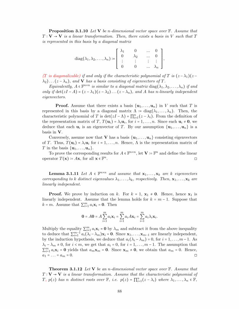
Proposition 3.1.10 Let V be n-dimensional vector space over F. Assume thatT ∶ V → V is a linear transformation. Then, there exists a basis in V such that Tis represented in this basis by a diagonal matrix
diag(λ1, λ2, . . . , λn) ∶=
⎡⎢⎢⎢⎢⎢⎢⎢⎣
λ1 0 ... 00 λ2 ... 0⋮ ⋮ ⋮ ⋮0 0 ... λn
⎤⎥⎥⎥⎥⎥⎥⎥⎦
,
(T is diagonalizable) if and only if the characteristic polynomial of T is (z −λ1)(z −λ2) . . . (z − λn), and V has a basis consisting of eigenvectors of T .
Equivalently, A ∈ Fn×n is similar to a diagonal matrix diag(λ1, λ2, . . . , λn) if andonly if det(zI −A) = (z − λ1)(z − λ2) . . . (z − λn), and A has n-linearly independenteigenvectors.
Proof. Assume that there exists a basis u1, . . . ,un in V such that T isrepresented in this basis by a diagonal matrix Λ ∶= diag(λ1, . . . , λn). Then, thecharacteristic polynomial of T is det(zI −Λ) =∏n
i=1(z − λi). From the definition ofthe representation matrix of T , T (ui) = λiui, for i = 1, . . . , n. Since each ui ≠ 0, wededuce that each ui is an eigenvector of T . By our assumption u1, . . . ,un is abasis in V.
Conversely, assume now that V has a basis u1, . . . ,un consisting eigenvectorsof T . Thus, T (ui) = λiui for i = 1, . . . , n. Hence, Λ is the representation matrix ofT in the basis u1, . . . ,un.
To prove the corresponding results for A ∈ Fn×n, let V ∶= Fn and define the linearoperator T (x) ∶= Ax, for all x ∈ Fn. ◻
Lemma 3.1.11 Let A ∈ Fn×n and assume that x1, . . . ,xk are k eigenvectorscorresponding to k distinct eigenvalues λ1, . . . , λk, respectively. Then, x1, . . . ,xk arelinearly independent.
Proof. We prove by induction on k. For k = 1, x1 ≠ 0. Hence, hence x1 islinearly independent. Assume that the lemma holds for k = m − 1. Suppose thatk =m. Assume that ∑mi=1 aixi = 0. Then
0 = A0 = Am
∑i=1
aixi =m
∑i=1
aiAxi =m
∑i=1
aiλixi.
Multiply the equality ∑mi=1 aixi = 0 by λm and subtract it from the above inequalityto deduce that ∑m−1
i=1 ai(λi −λm)xi = 0. Since x1, . . . ,xm−1 are linearly independent,by the induction hypothesis, we deduce that ai(λi −λm) = 0, for i = 1, . . . ,m− 1. Asλi − λm ≠ 0, for i < m, we get that ai = 0, for i = 1, . . . ,m − 1. The assumption that
∑mi=1 aixi = 0 yields that amxm = 0. Since xm ≠ 0, we obtain that am = 0. Hence,a1 = . . . = am = 0. ◻
Theorem 3.1.12 Let V be an n-dimensional vector space over F. Assume thatT ∶ V →V is a linear transformation. Assume that the characteristic polynomial ofT , p(z) has n distinct roots over F, i.e. p(z) = ∏n
i=1(z − λi) where λ1, . . . , λn ∈ F,
88
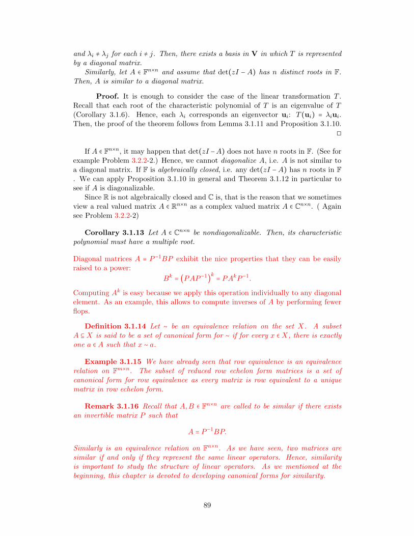
and λi ≠ λj for each i ≠ j. Then, there exists a basis in V in which T is representedby a diagonal matrix.
Similarly, let A ∈ Fn×n and assume that det(zI − A) has n distinct roots in F.Then, A is similar to a diagonal matrix.
Proof. It is enough to consider the case of the linear transformation T .Recall that each root of the characteristic polynomial of T is an eigenvalue of T(Corollary 3.1.6). Hence, each λi corresponds an eigenvector ui: T (ui) = λiui.Then, the proof of the theorem follows from Lemma 3.1.11 and Proposition 3.1.10.
◻
If A ∈ Fn×n, it may happen that det(zI −A) does not have n roots in F. (See forexample Problem 3.2.2-2.) Hence, we cannot diagonalize A, i.e. A is not similar toa diagonal matrix. If F is algebraically closed, i.e. any det(zI −A) has n roots in F. We can apply Proposition 3.1.10 in general and Theorem 3.1.12 in particular tosee if A is diagonalizable.
Since R is not algebraically closed and C is, that is the reason that we sometimesview a real valued matrix A ∈ Rn×n as a complex valued matrix A ∈ Cn×n. ( Againsee Problem 3.2.2-2)
Corollary 3.1.13 Let A ∈ Cn×n be nondiagonalizable. Then, its characteristicpolynomial must have a multiple root.
Diagonal matrices A = P −1BP exhibit the nice properties that they can be easilyraised to a power:
Bk = (PAP−1)k = PAkP −1.
Computing Ak is easy because we apply this operation individually to any diagonalelement. As an example, this allows to compute inverses of A by performing fewerflops.
Definition 3.1.14 Let ∼ be an equivalence relation on the set X. A subsetA ⊆X is said to be a set of canonical form for ∼ if for every x ∈X, there is exactlyone a ∈ A such that x ∼ a.
Example 3.1.15 We have already seen that row equivalence is an equivalencerelation on Fm×n. The subset of reduced row echelon form matrices is a set ofcanonical form for row equivalence as every matrix is row equivalent to a uniquematrix in row echelon form.
Remark 3.1.16 Recall that A,B ∈ Fn×n are called to be similar if there existsan invertible matrix P such that
A = P −1BP.
Similarly is an equivalence relation on Fn×n. As we have seen, two matrices aresimilar if and only if they represent the same linear operators. Hence, similarityis important to study the structure of linear operators. As we mentioned at thebeginning, this chapter is devoted to developing canonical forms for similarity.
89
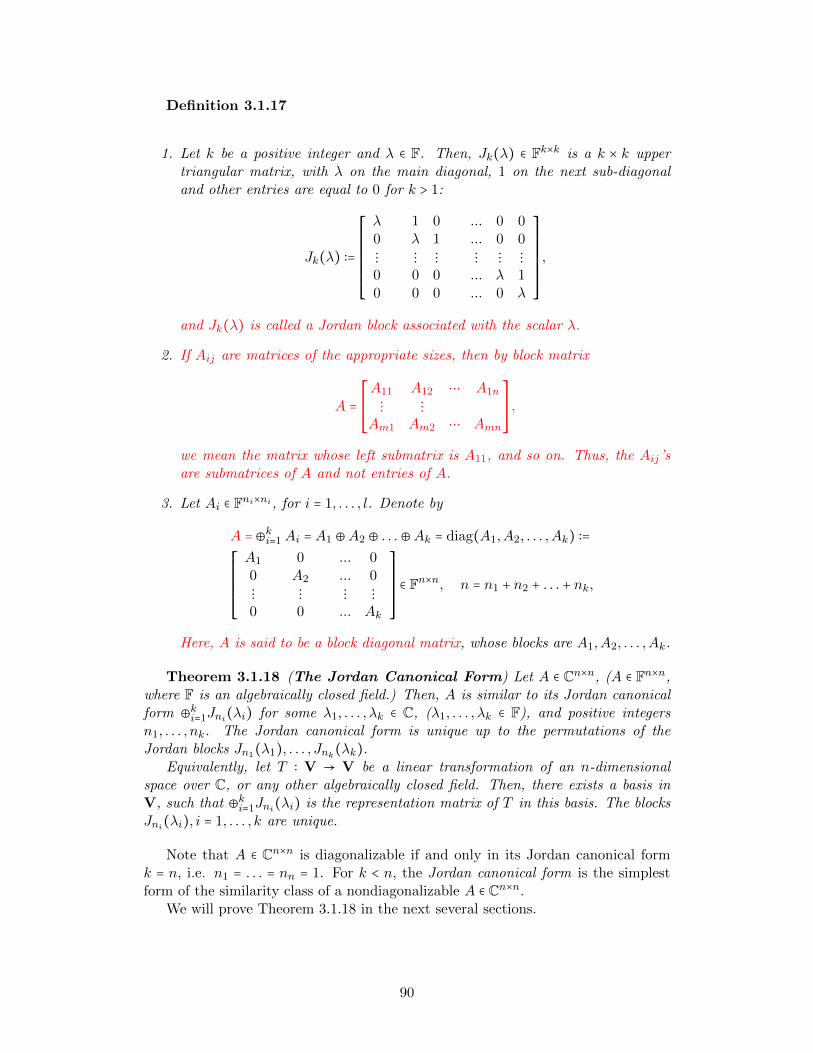
Definition 3.1.17
1. Let k be a positive integer and λ ∈ F. Then, Jk(λ) ∈ Fk×k is a k × k uppertriangular matrix, with λ on the main diagonal, 1 on the next sub-diagonaland other entries are equal to 0 for k > 1:
Jk(λ) ∶=
⎡⎢⎢⎢⎢⎢⎢⎢⎢⎢⎣
λ 1 0 ... 0 00 λ 1 ... 0 0⋮ ⋮ ⋮ ⋮ ⋮ ⋮0 0 0 ... λ 10 0 0 ... 0 λ
⎤⎥⎥⎥⎥⎥⎥⎥⎥⎥⎦
,
and Jk(λ) is called a Jordan block associated with the scalar λ.
2. If Aij are matrices of the appropriate sizes, then by block matrix
A =⎡⎢⎢⎢⎢⎢⎣
A11 A12 ⋯ A1n
⋮ ⋮Am1 Am2 ⋯ Amn
⎤⎥⎥⎥⎥⎥⎦,
we mean the matrix whose left submatrix is A11, and so on. Thus, the Aij’sare submatrices of A and not entries of A.
3. Let Ai ∈ Fni×ni, for i = 1, . . . , l. Denote by
A =⊕ki=1 Ai = A1 ⊕A2 ⊕ . . .⊕Ak = diag(A1,A2, . . . ,Ak) ∶=⎡⎢⎢⎢⎢⎢⎢⎢⎣
A1 0 ... 00 A2 ... 0⋮ ⋮ ⋮ ⋮0 0 ... Ak
⎤⎥⎥⎥⎥⎥⎥⎥⎦
∈ Fn×n, n = n1 + n2 + . . . + nk,
Here, A is said to be a block diagonal matrix, whose blocks are A1,A2, . . . ,Ak.
Theorem 3.1.18 (The Jordan Canonical Form) Let A ∈ Cn×n, (A ∈ Fn×n,where F is an algebraically closed field.) Then, A is similar to its Jordan canonicalform ⊕ki=1Jni(λi) for some λ1, . . . , λk ∈ C, (λ1, . . . , λk ∈ F), and positive integersn1, . . . , nk. The Jordan canonical form is unique up to the permutations of theJordan blocks Jn1(λ1), . . . , Jnk(λk).
Equivalently, let T ∶ V → V be a linear transformation of an n-dimensionalspace over C, or any other algebraically closed field. Then, there exists a basis inV, such that ⊕ki=1Jni(λi) is the representation matrix of T in this basis. The blocksJni(λi), i = 1, . . . , k are unique.
Note that A ∈ Cn×n is diagonalizable if and only in its Jordan canonical formk = n, i.e. n1 = . . . = nn = 1. For k < n, the Jordan canonical form is the simplestform of the similarity class of a nondiagonalizable A ∈ Cn×n.
We will prove Theorem 3.1.18 in the next several sections.
90
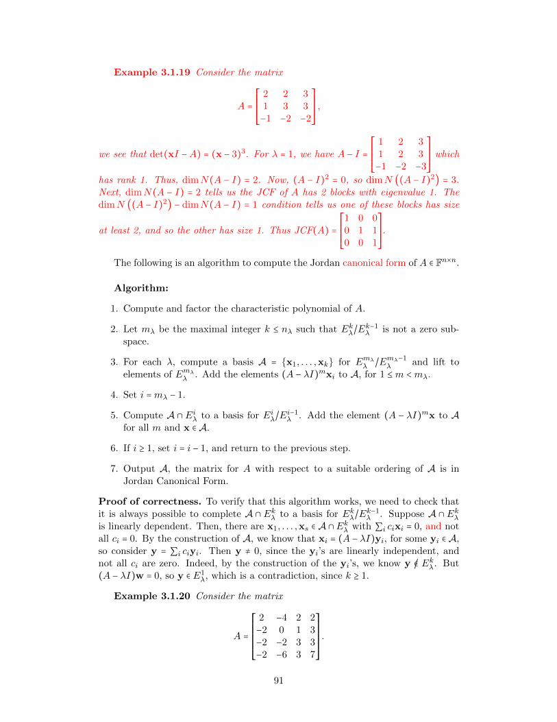
Example 3.1.19 Consider the matrix
A =⎡⎢⎢⎢⎢⎢⎣
2 2 31 3 3−1 −2 −2
⎤⎥⎥⎥⎥⎥⎦,
we see that det(xI −A) = (x − 3)3. For λ = 1, we have A − I =⎡⎢⎢⎢⎢⎢⎣
1 2 31 2 3−1 −2 −3
⎤⎥⎥⎥⎥⎥⎦which
has rank 1. Thus, dimN(A − I) = 2. Now, (A − I)2 = 0, so dimN ((A − I)2) = 3.Next, dimN(A − I) = 2 tells us the JCF of A has 2 blocks with eigenvalue 1. ThedimN ((A − I)2) − dimN(A − I) = 1 condition tells us one of these blocks has size
at least 2, and so the other has size 1. Thus JCF(A) =⎡⎢⎢⎢⎢⎢⎣
1 0 00 1 10 0 1
⎤⎥⎥⎥⎥⎥⎦.
The following is an algorithm to compute the Jordan canonical form of A ∈ Fn×n.
Algorithm:
1. Compute and factor the characteristic polynomial of A.
2. Let mλ be the maximal integer k ≤ nλ such that Ekλ/Ek−1λ is not a zero sub-
space.
3. For each λ, compute a basis A = x1, . . . ,xk for Emλλ /Emλ−1λ and lift to
elements of Emλλ . Add the elements (A − λI)mxi to A, for 1 ≤m <mλ.
4. Set i =mλ − 1.
5. Compute A ∩ Eiλ to a basis for Eiλ/Ei−1λ . Add the element (A − λI)mx to A
for all m and x ∈ A.
6. If i ≥ 1, set i = i − 1, and return to the previous step.
7. Output A, the matrix for A with respect to a suitable ordering of A is inJordan Canonical Form.
Proof of correctness. To verify that this algorithm works, we need to check thatit is always possible to complete A ∩ Ekλ to a basis for Ekλ/Ek−1
λ . Suppose A ∩ Ekλis linearly dependent. Then, there are x1, . . . ,xs ∈ A ∩Ekλ with ∑i cixi = 0, and notall ci = 0. By the construction of A, we know that xi = (A − λI)yi, for some yi ∈ A,so consider y = ∑i ciyi. Then y ≠ 0, since the yi’s are linearly independent, andnot all ci are zero. Indeed, by the construction of the yi’s, we know y /∈ Ekλ. But(A − λI)w = 0, so y ∈ E1
λ, which is a contradiction, since k ≥ 1.
Example 3.1.20 Consider the matrix
A =
⎡⎢⎢⎢⎢⎢⎢⎢⎣
2 −4 2 2−2 0 1 3−2 −2 3 3−2 −6 3 7
⎤⎥⎥⎥⎥⎥⎥⎥⎦
.
91
Then, the characteristic polynomial of A is (x − 2)2(x − 4)2. A basis for E12 is
(2,1,0,2)⊺, (0,1,2,0)⊺, so since there is a two-dimensional 2 blocks, each of sizeone. To confirm this, check that Em2 = E1
2 for all m > 1. A basis for E14 is
(0,1,1,1)⊺, while a basis for E24 is (0,1,1,1)⊺, (1,0,0,1)⊺, so we can take
(1,0,0,1)⊺ as a basis for E24/E1
4 . Then (A − 4I)(1,0,0,1)⊺ = (0,1,1,1)⊺, soour basis is then (2,1,0,2)⊺, (0,1,2,0)⊺, (0,1,1,1)⊺, (1,0,01)⊺. The matrix of thetransformation with respect to this basis is:
⎡⎢⎢⎢⎢⎢⎢⎢⎣
2 0 0 00 2 0 00 0 4 10 0 0 4
⎤⎥⎥⎥⎥⎥⎥⎥⎦
.
3.2 An application of diagonalizable matrices
The sequence of Fibonacci numbers Fn
0,1,1,2,3,5,8,13,21,34, . . .
is defined recursively as follows:One begins with F0 = 0 and F1 = 1. After that every number is defined to be sumof its two predecessors:
Fn = Fn−1 + Fn−2, for n > 1.
Johannes Kepler (1571-1630) observed that the ratio of consecutive Fibonacci num-bers converges to the golden ratio.
Theorem 3.2.1 (Kepler) lim Fn+1Fn
= 1+√
52 .
The purpose of this section is using of linear algebra tools to prove Kepler’s theorem.In order to this, we will need to find an explicit formula for Fibonacci numbers.Particularly, we need the following lemma. See also subsection 4.1.1.
Lemma 3.2.2 For n > 1, Fn = (1+√
5)n−(1−√
5)n2n
√5
.
Proof. Let T be the linear operator on R2 represented by the matrix
A = [1 11 0
]
with respect to the standard basis of R2. Then, for the vector vk whose coordinates
are two consecutive Fibonacci numbers (Fk, Fk−1)⊺, we have that T (vk) = A [ FkFk−1
] =
[1 11 0
] [ FkFk−1
] = [Fk + Fk−1
Fk] = [Fk+1
Fk] = vk+1. Therefore, [Fn+1
Fn] = An [1
0] and this
equation helps us to calculate the powers An of A by using the diagonalization. Westart with finding the eigenvalues of A which are
λ1 =1 +
√5
2and λ2 =
1 −√
5
2,
92
and we conclude that A is diagonalizable as its eigenvalues are real and distinct.Next, we find the eigenvectors corresponding to λ1 and λ2. We solve the equations
A [x1
y1] = λ1 [
x1
y1], A [x2
y2] = λ2 [
x2
y2] and it is obtained that [x1
y1] = [λ1
1] and [x2
y2] =
[λ2
1]. Therefore, the matrix of change of basis between standard basis and the
basis of eigenvectors is p = [λ1 λ2
1 1] and so p−1Ap = [λ1 0
0 λ2]. This means An =
p [λn1 0
0 λn2]p−1. Totally, we have
[Fn+1
Fn] = An [1
0] = p [λ
n1 0
0 λn2]p−1 [1
0]
= 1
λ1 − λ2[λ1 λ2
1 1] [λ
n1 0
0 λn2] [ 1 −λ2
−1 λ1] [1
0]
= 1
λ1 − λ2[λ
n+11 − λn+1
2
λn1 − λn2] .
Equating the entries of the vectors in the last formula we obtain
Fn =λn1 − λn2λ1 − λ2
= (1 +√
5)n − (1 −√
5)n
2n√
5,
as claimed. ◻
We now are ready to prove Kepler’s theorem by using the above lemma.
limn→∞
Fn+1
Fn= lim
n→∞(1 +
√5)n+1 − (1 −
√5)n+1
2n+1√
5
2n√
5
(1 +√
5)n − (1 −√
5)n
= 1
2limn→∞
(1 +√
5)n+1 − (1 −√
5)n+1
(1 +√
5)n − (1 −√
5)n
= 1
2limn→∞
(1 +√
5) − (1−√
51+
√5)n(1 −
√5)
1 − (1−√
51+
√5)n = 1 +
√5
2.
Note that
limn→∞
(1 −√
5
1 +√
5)n
= 0
because
∣1 −√
5
1 +√
5∣ < 1.
3.2.1 Worked-out Problems
1. Show that the Jordan block Jk(λ) ∈ Fn×n is similar to Jk(λ)⊺.Solution:
93
Consider the k × k permutation matrix P =
⎡⎢⎢⎢⎢⎢⎢⎢⎣
0 ⋯ 10 1 0
⋱ ⋮1 ⋯ 0
⎤⎥⎥⎥⎥⎥⎥⎥⎦
.
Then, P −1Jk(λ)P = Jk(λ)⊺ and so Jk(λ) ∼ Jk(λ)⊺.
2. Assume that the characteristic polynomial of A splits in F. Show that A issimilar to A⊺.Solution:Denote by JCF (A), a Jordan canonical form of A. Using Theorem 3.1.18, A issimilar to JCF (A) = ⊕
iJki(λi). Clearly, A⊺ ∼ ⊕
iJki(λi)⊺. Using the previous
problem, we conclude that ⊕iJki(λi) ∼⊕
iJki(λi)⊺ and this yields A ∼ A⊺.
3.2.2 Problems
1. Let V be a vector space over F. (You may assume that F = C). Let T ∶ V →Vbe a linear transformation. Suppose that ui is an eigenvector of T with thecorresponding eigenvalue λi, for i = 1, . . . ,m. Show by induction on m that ifλ1, . . . , λm are m distinct scalars, then u1, . . . ,um are linearly independent.
2. Let A = [ 0 1−1 0
] ∈ R2×2.
(a) Show that A is not diagonalizable over the real numbers R.
(b) Show that A is diagonalizable over the complex numbers C.
(c) Find U ∈ C2×2 and a diagonal Λ ∈ C2×2 such that A = UΛU−1.
3. Let A = ⊕ki=1Jni(λi). Show that det(zI −A) = ∏ki=1(z − λi)ni . (You may use
the fact that the determinant of an upper triangular matrix is the product ofits diagonal entries.)
4. Let A = ⊕ki=1Ai, where Ai ∈ Cni×ni , i = 1, . . . , k. Show that det(zIn − A) =∏ki=1 det(zIni −Ai).
(Hint: First show the identity for k = 2 using the determinant expansion byrows. Then use induction for k > 2.)
5. (a) Show that any eigenvector of Jn(λ) ∈ Cn×n is in the subspace spanned bye1. Conclude that Jn(λ) is not diagonalizable unless n = 1.
(b) What is the rank of zIn − Jn(λ) for a fixed λ ∈ C and for each z ∈ C?
(c) What is the rank of zI −⊕ki=1Jni(λi) for fixed λ1, . . . , λk ∈ C and for eachz ∈ C?
6. Let A ∈ Cn×n and assume that det(zIn − A) = zn + a1zn−1 + . . . + an−1z + an
has n distinct complex roots. Show that An + a1An−1 + . . . an−1A + anIn = 0,
where 0 ∈ Cn×n denotes the zero matrix, i.e. the matrix whose all entries are0. (This is a special case of the Cayley-Hamilton theorem, which states thatthe above identity holds for any A ∈ Cn×n.)(Hint: Use the fact that A is diagonalizable.)
94
7. If A,B ∈ Fn×n, show that AB and BA have the same characteristic polynomial.
8. Let 1 ≤ m ≤ n ∈ N and suppose that A ∈ Cm×n and B ∈ Cn×m. Prove thatdet(zI −BA) = zn−m det(zI −AB).(In particular, if m = n, then the characteristic polynomials of AB and BAare the same, see the previous problem.)
9. If A ∈ Rn×n is a symmetric matrix, show that all of its eigenvalues are real.
10. If A ∈ Fn×n is an invertible matrix and PA(z) and PA−1(z) denote the character-istic polynomial of A and A−1, respectively, show that PA−1(z) = zn
PA(0)PA(1z ).
11. If A ∈ Rn×n with n distinct eigenvalues λ1, . . . , λn, show that Rn =n⊕i=1Eλi .
12. If A ∈ Fn×n is a diagonalizable matrix with the characteristic polynomial
pA(z) =k
∏i=1
(z − λi)di and V = B ∈ Fn×n; AB = BA, prove that dimV =
∑ki=1 d2i .
13. Prove that a matrix is invertible if and only if it does not have a zero eigenvalue.(See Theorem 1.9.2.)
14. Let A be a square matrix with the block form A = [X Y0 Z
], where X and Z
are square matrices. Show that detA = detX detZ.
15. Let A ∈ Fm×n.
(a) Prove that A in its reduced row echelon form must have the block form
Ji = [Ii 00 0
] .
(b) Show that A is equivalent to exactly one matrix of the form Ji.
(c) Conclude that the set of these matrices is a set of canonical form forequivalence, (See Lemma 1.7.16.)
16. Assume that A is a doubly stochastic matrix. Show that for each eigenvalueλ of A, λ ≤ 1.
17. Show that the matrix A = [cos θ − sin θsin θ cos θ
] ∈ R2×2 has complex eigenvalues if
θ is not a multiple of π. Give the geometric interpretation of it. (See alsoProblem 1.10.2-4.)
18. Let A ∈ Fn×n. Prove that
(a) if λ is an eigenvalue of A, then λk is an eigenvalue of Ak, for any k ∈ N.
(b) if λ is an eigenvalue of A and A is invertible, then λ−1 is an eigenvalue ofA−1.
95
3.3 Matrix polynomials
Let P (z) = [pij(z)]m,ni=j=1 be an m × n matrix whose entries are polynomials in F[z].The set of all such m × n matrices is denoted by F[z]m×n. Clearly, F[z]m×n is avector space over F, of infinite dimension. Given p(z) ∈ F[z] and P (z) ∈ F[z]m×n,one can define p(z)P (z) ∶= [p(z)pij(z)] ∈ F[z]m×n. Again, this product satisfies nicedistribution properties. Thus, F[z]m×n is a module over the ring F[z]. (Note F[z]is not a field!)
Let P (z) = [pij(z)] ∈ F[z]m×n. Then, degP (z) ∶= maxi,j deg pij(z) = l. Write
pij(z) =l
∑k=0
pij,kzl−k, Pk ∶= [pij,k]m,ni=j=1 ∈ F
m×n for k = 0, . . . , l.
ThenP (z) = P0z
l + P1zl−1 + . . . + Pl, Pi ∈ Fm×n, i = 0, . . . , l, (3.3.1)
is a matrix polynomial with coefficients in Fm×n.Assume that P (z),Q(z) ∈ F[z]n×n. Then, we can define P (z)Q(z) ∈ F[z]. Note
that in general P (z)Q(z) ≠ Q(z)P (z). Hence, F[z]n×n is a noncommutative ring.For P (z) ∈ Fn×n of the form (3.3.1) and any A ∈ Fn×n, we define
P (A) =l
∑i=0
PiAl−i = P0A
l + P1Al−1 + . . . + Pl, where A0 = In.
Given two polynomials p, q ∈ F[z], one can divide p by q /≡ 0 with the residuer, i.e. p = tq + r, for some unique t, r ∈ F[z], where deg r < deg q. One can triviallygeneralize that to polynomial matrices:
Proposition 3.3.1 Let p(z), q(z) ∈ F[z] and assume that q(z) /≡ 0. Let p(z) =t(z)q(z) + r(z), where t(z), r(z) ∈ F[z] are unique polynomials with deg r(z) <deg q(z). Let n > 1 be an integer, and define the following scalar polynomials:P (z) ∶= p(z)In,Q(z) ∶= q(z)In, T (z) ∶= t(z)In,R(z) ∶= r(z)In ∈ F[z]n×n. Then,P (A) = T (A)Q(A) +R(A), for any A ∈ Fn×n.
Proof. Since AiAj = Ai+j , for any non-negative integer, with A0 = In, the equal-ity P (A) = T (A)Q(A) +R(A) follows trivially from the equality p(z) = t(z)q(z) +r(z). ◻
Recall that p is divisible by q, denoted as q∣p, if p = tq, i.e. r is the zeropolynomial. Note that if q(z) = (z − a), then p(z) = t(z)(z − a) + p(a). Thus,(z −a)∣p if and only if p(a) = 0. Similar results hold for square polynomial matrices,which are not scalar.
Lemma 3.3.2 Let P (z) ∈ F[z]n×n,A ∈ Fn×n. Then, there exists a uniqueTleft(z), of degree degP − 1 if degP > 0 or degree −∞ if degP ≤ 0, such that
P (z) = Tleft(z)(zI −A) + P (A). (3.3.2)
In particular, P (z) is divisible from the right by zI −A if and only if P (A) = 0.
96
Proof. We prove the lemma by induction on degP . If degP ≤ 0, i.e. P (z) =P0 ∈ Fn×n, then Tleft = 0, P (A) = P0 and the lemma trivially holds. Suppose thatthe lemma holds for all P with degP ≤ l − 1, where l ≥ 1. Let P (z) be of degreel ≥ 1 of the form (3.3.1). Then P (z) = P0z
l + P (z), where P (z) = ∑li=1 Pizl−1. By
the induction assumption P (z) = Tleft(z)(zIn−A)+ P (A), where Tleft(z) is unique.A straightforward calculation shows that
P0zl = Tleft(z)(zIn −A) + P0A
l, where Tleft(z) =l−1
∑i=0
P0Aizl−i−1,
and Tleft is unique. Hence, Tleft(z) = Tleft(z)+ Tleft is unique, P (A) = P0Al + P (A)
and (3.3.2) follows.Suppose that P (A) = 0. Then P (z) = Tleft(z)(zI −A), i.e. P (z) is divisible by
zIn −A from the right. Assume that P (z) is divisible by (zIn −A) from the right,i.e. there exists T (z) ∈ F[z]n×n such that P (z) = T (z)(zIn − A). Subtract (3.3.2)from P (z) = T (z)(zIn −A) to deduce that 0 = (T (z) − Tleft(z))(zIn −A) − P (A).Hence, T (z) = Tleft(z) and P (A) = 0. ◻
The above lemma can be generalized to any Q(z) = Q0zl+Q1z
l−1+. . .+Ql ∈ F[z],where Q0 ∈ GL(n,F); there exists unique Tleft(z),Rleft(z) ∈ F[z] such that
P (z) = Tleft(z)Q(z) +Rleft(z), degRleft < degQ, Q(z) =l
∑i=0
Qizl−i, Q0 ∈ GL(n,F).
(3.3.3)Here we agree that (Azi)(Bzj) = (AB)zi+j , for any A,B ∈ Fn×n and non-negativeintegers i, j.
Theorem 3.3.3 (Cayley-Hamilton theorem) Let A ∈ Fn×n and p(z) = det(zIn−A) be the characteristic polynomial of A. Let P (z) = p(z)In ∈ F[z]n×n. Then,P (A) = 0.
Proof. Let A(z) = zIn − A. Fix z ∈ F and let B(z) = [bij(z)] be the adjointmatrix of A(z), whose entries are the cofactors of A(z). That is bij(z) is (−1)i+jtimes the determinant of the matrix obtained from A(z) by deleting row j andcolumn i. If one views z as indeterminate, then B(z) ∈ F[z]n×n. Consider theidentity
A(z)B(z) = B(z)A(z) = detA(z)In = p(z)In = P (z).Hence, (zIn −A) divides P (z) from the right. Lemma 3.3.2 yields that P (A) = 0.
◻
Note that the Cayley-Hamilton theorem holds even if F is not algebraically closedby doing a field extension.
For p, q ∈ F[z], let (p, q) denote the greatest common divisor of p, q. If p and q areidentically zero, then (p, q) is the zero polynomial. Otherwise (p, q) is a polynomials of the highest degree that divides p and q. Also s is determined up to a multipleof a non-zero scalar and it can be chosen as a unique monic polynomial:
s(z) = zl + s1zl−1 + . . . + sl ∈ F[z]. (3.3.4)
Equality (1.14.3) yields.
97
Corollary 3.3.4 Let p, q ∈ F[z] be coprime. Then, there exist u, v ∈ F[z] suchthat 1 = up + vq. Let n > 1 be an integer and define P (z) ∶= p(z)In,Q(z) ∶=q(z)In, U(z) ∶= u(z)In, V (z) ∶= u(z)In ∈ F[z]n×n. Then, for any A ∈ Fn×n, wehave the identity In = U(A)P (A)+V (A)Q(A), where U(A)P (A) = P (A)U(A) andV (A)Q(A) = Q(A)V (A).
Let us consider that case where p and q ∈ F[z] are both non-zero polynomialsthat split (to linear factors) over F. Thus
p(z) = p0(z − α1) . . . (z − αi), p0 ≠ 0, q(z) = q0(z − β1) . . . (z − βj), q0 ≠ 0.
In that case (p, q) = 1, if p and q do not have a common root. If p and q have acommon zero, then (p, q) is a non-zero polynomial that has the maximal number ofcommon roots of p and q counting with multiplicities.
From now on, for any p ∈ F[z] and A ∈ Fn×n we identify p(A) with P (A), whereP (z) = p(z)In.
Definition 3.3.5 For an eigenvalue λ, its algebraic multiplicity is the multiplic-ity of λ as a root of the characteristic polynomial and it is denoted by ma(λ). Thegeometric multiplicity of λ is the maximal number of linearly independent eigenvec-tors corresponding to it and it is denoted by mg(λ). Also λ is called an algebraicallysimple eigenvalue if its algebraic multiplicity is one.
Example 3.3.6 Consider the matrix A = [1 10 1
]. Let us find its eigenvalues
and eigenvectors. Characteristic polynomial is (1 − x)2. So λ = 1 is a double root.Eigenvectors corresponding to this eigenvalue:
[1 − λ 10 1 − λ] [
x1
x2] = [0
0]⇒ [0 1
0 0] [x1
x2] = [0
0] .
So x2 = 0, and x1 can be anything. There is only one linearly independent vector:
[01]
Consider another example: the identity matrix,
A = [1 00 1
] .
Then, by the same way, λ = 1 is a double root of the characteristic polynomial andthe only eigenvalue. But any non-zero vector can serve as its eigenvector, becausefor any x ∈ R2 we have: Ax = x = 1⋅x. So, it has two linearly independent eigenvector
[10] and [0
1].
Here, for both matrices λ = 1 is the only eigenvalue with algebraic multiplicity two.
But its geometric multiplicity is one for [1 10 1
] and two for [1 00 1
].
Theorem 3.3.7 Let A ∈ Fn×n and λ is an eigenvalue of A. Then mg(λ) ≤ma(λ).
98
Proof. Set m = mg(λ) and let x1, . . . ,xm be a basis for Eλ. Extend it to abasis x1, . . . ,xn for Fn. Let P ∈ Fn×n be the invertible matrix with column vectorsx1, . . . ,xn and B = P −1AP . Then, for each 1 ≤ j ≤m, we have
Bej = P −1APej = P −1Avj = P −1λvj = λ(P −1vj) = λej ,
and so B has the block form
B = [λIm X0 Y
]
Using Problem 3.2.2-13 and the fact that similar matrices have the same character-istic polynomials, we have
PA(t) = PB(t) = det [(t − λ)Im −X0 tIn−m − Y ] = det((t − λ)Im)det(tIn−m − Y )
= (t − λ)mPY (t).
This shows that λ appears at least m times as a root of PA(t), and then ma(t) ≥m.
3.4 Minimal polynomial and decomposition to invariantsubspaces
Recall that Fn×n is a vector space over F of dimension n2. Let A ∈ Fn×n and considerthe powers A0 = In,A,A2, . . . ,Am. Let m be the smallest positive integer such thatthese m + 1 matrices are linearly dependent as vectors in Fn×n. (Note that A0 ≠ 0.)Thus, there exists (b0, . . . , bm)⊺ ∈ Fn for which (b0, . . . , bm)⊺ ≠ 0 and ∑mi=0 biA
m−i = 0.If b0 = 0, then A0, . . . ,Am−1 are linearly dependent, which contradicts the definitionof m. Hence, b0 ≠ 0. Divide the linear dependence by b0 to obtain ∑mi=0 aiA
m−i = 0,where ai = bi
b0, 0 ≤ i ≤m.
Define ψ(z) = zm +∑mi=0 aizm−i ∈ F[z]. Then, ψ(A) = 0. Here, ψ is called the
minimal polynomial of A. In principle m ≤ n2, but in fact m ≤ n.
Theorem 3.4.1 Let A ∈ Fn×n and ψ(z) be its minimal polynomial. Assume thatp(z) ∈ F[z] is an annihilating polynomial of A, i.e. p(A) = 0n×n. Then, ψ divides p.In particular, the characteristic polynomial p(z) = det(zIn −A) is divisible by ψ(z).Hence, degψ ≤ deg p = n.
Proof. Divide the annihilating polynomial p by ψ to obtain p(z) = t(z)ψ(z) +r(z), where deg r < degψ =m. Proposition 3.3.1 yields that p(A) = t(A)ψ(A)+r(A),which implies that r(A) = 0. Assume that l = deg r(z) ≥ 0, i.e. r is not identicallythe zero polynomial. Therefore, A0, . . . ,Al are linearly dependent, which contradictsthe definition of m. Hence r(z) ≡ 0.
The Cayley-Hamilton theorem yields that the characteristic polynomial p(z) ofA annihilates A. Hence, ψ∣p and degψ ≤ deg p = n. ◻
Comparing the minimal polynomial of an algebraic element in a field extensionwith the minimal polynomial of a matrix, we can see their common features. Forexample, if E/F is a field extension and we denote the minimal polynomial of analgebraic element α ∈ E by p(z) and if we denote the minimal polynomial of A ∈ Fn×n
99
by ψ(z), then both p(z) and ψ(z) are annihilator for α and A, respectively and bothare non-zero polynomials of minimum degree with this character. According to thedefinition, p(z) is irreducible over F. Now, this question can be asked that if ψ(z)is necessarily irreducible over F, too? We will answer to this question in the lastWorked-out Problem!
Theorem 3.4.2 Let A ∈ Fn×n. Denote by q(z) the g.c.d (monic polynomial),of all the entries of adj (zIn −A) ∈ F[z]n×n, which is the g.c.d of all (n − 1) × (n −1) minors of (zIn − A). Then, q(z) divides the characteristic polynomial p(z) =det(zIn −A) of A. Furthermore, the minimal polynomial of A is equal to
p(z)q(z) .
Proof. Expand det(zIn −A) by the first column. Since q(z) divides each (n −1)× (n− 1) minor of zIn −A, we deduce that q(z) divides p(z). Let φ(z) = p(z)
q(z) . As
q(z) divides each entry of adj (zIn −A), we deduce that adj (zIn −A) = q(z)C(z),for some C(z) ∈ F[z]n×n. Divide the equality p(z)In = adj (zIn − A)(zIn − A) byq(z) to deduce that φ(z)In = C(z)(zIn −A). Lemma 3.3.2 yields that φ(A) = 0.
Let ψ(z) be the minimal polynomial of A. Theorem 3.4.1 yields that ψ di-vides φ. We now show that φ divides ψ. Theorem 3.4.1 implies that p(z) =s(z)ψ(z), for some monic polynomial s(z). Since ψ(A) = 0, Lemma 3.3.2 yieldsthat ψ(z)In =D(z)(zIn−A), for some D(z) ∈ Fn×n[z]. Thus, p(z)In = s(z)ψ(z)In =s(z)D(z)(zIn−A). Since p(z)In = adj (zIn−A)(zIn−A), we conclude that s(z)D(z) =adj (zIn−A). As all the entries of D(z) are polynomials, it follows that s(z) dividesall the entries of adj (zIn −A). Since q(z) is the g.c.d of all entries of adj (zIn −A),we deduce that s(z) divides q(z). Consider the equality p(z) = s(z)ψ(z) = q(z)φ(z).Thus, ψ(z) = q(z)
s(z)φ(z). Hence, φ(z) divides ψ(z). As ψ(z) and φ(z) are monic, we
deduce that ψ(z) = φ(z). ◻
Proposition 3.4.3 Let A ∈ Fn×n and assume that λ ∈ F is an eigenvalue ofA with the corresponding eigenvector x ∈ Fn. Then, for any h(z) ∈ F[z], h(A)x =h(λ)x. In particular, λ is a root of the minimal polynomial ψ(z) of A, i.e. ψ(λ) = 0.
Proof. Clearly, Amx = λmx. Hence, h(A)x = h(λ)x. Assume that h(A) = 0. Asx ≠ 0, we deduce that h(λ) = 0. Then, ψ(λ) = 0. ◻
Combining Theorem 3.4.1 and Proposition 3.4.3, we conclude that the mini-mal polynomial and the characteristic polynomial of a matrix have the same roots.(probably with the different multiplicities).
Definition 3.4.4 A matrix A ∈ Fn×n is called nonderogatory if the minimalpolynomial of A is equal to its characteristic polynomial.
Definition 3.4.5 Let V be a finite dimensional vector space over F, and assumethat V1, . . . ,Vi are non-zero subspaces of V. Then, V is a direct sum of V1, . . . ,Vi,denoted as V = ⊕ij=1Vj if any vector v ∈ V has a unique representation as v =v1+ . . .+vi, where vj ∈ Vj, for j = 1, . . . , i. Equivalently, let [vj1, . . . ,vjlj ] be a basis
of Vj, for j = 1, . . . , i. Then, dimV = ∑ij=1 dimVj = ∑ij=1 lj and the dimV vectorsv11, . . . ,v1l1 , . . . ,vi1, . . . ,vili are linearly independent.
100
Let T ∶ V →V be a linear operator. A subspace U of V is called a T -invariantsubspace, or simply an invariant subspace when there is no ambiguity about T , ifT (u) ∈ U, for each u ∈ U. We denote this fact by TU ⊆ U. Denote by T ∣U therestriction of T to the invariant subspace of T . Clearly, T ∣U is a linear operator onU.
Note that V and the zero subspace 0 are invariant subspaces. Those are calledtrivial invariant subspaces. The subspace U is called a nontrivial invariant subspaceif it is an invariant subspace such that 0 < dimU < dimV.
Since the representation matrices of T in different bases form a similarity class,we can define the minimal polynomial ψ(z) ∈ F[z] of T , as the minimal polynomialof any representation matrix of T. Equivalently, ψ(z) is the monic polynomial ofthe minimal degree which annihilates T ; ψ(T ) = 0.
Theorem 3.4.6 (Primary decomposition Theorem) Let T ∶ V → V be alinear operator on a finite non-zero dimensional vector space V. Let ψ(z) be theminimal polynomial of T . Assume that ψ(z) decomposes to ψ(z) = ψ1(z) . . . ψk(z),where each ψi(z) is a monic polynomial of degree at least 1. Suppose furthermorethat for each pair i ≠ j, ψi(z) and ψj(z) are coprime. Then, V is a direct sum ofV1, . . . ,Vk, where each Vi is a nontrivial invariant subspace of T . Furthermore,the minimal polynomial of T ∣Vi is equal to ψi(z), for i = 1, . . . , k. Moreover, eachVi is uniquely determined by ψi(z) for i = 1, . . . , k.
Proof. We prove the theorem by induction on k ≥ 2. Let k = 2. Then,ψ(z) = ψ1(z)ψ2(z). Let V1 ∶= ψ2(T )V and V2 = ψ1(T )V be the images of theoperators ψ2(T ), ψ1(T ), respectively. Observe that
TV1 = T (ψ2(T )V) = (Tψ2(T ))V = (ψ2(T )T )V = ψ2(T )(TV) ⊆ ψ2(T )V = V1.
Thus, V1 is a T-invariant subspace. Assume that V1 = 0. This is equivalentto ψ2(T ) = 0. By Theorem 3.4.1, ψ divides ψ2 which is impossible since degψ =degψ1 + degψ2 > degψ1. Thus, dimV1 > 0. Similarly, V2 is a non-zero T -invariantsubspace. Let Ti = T ∣Vi , for i = 1,2. Clearly
ψ1(T1)V1 = ψ1(T )V1 = ψ1(T )(ψ2(T )V) = (ψ1(T )ψ2(T ))V = 0,
since ψ is the minimal polynomial of T . Hence, ψ1(T1) = 0, i.e. ψ1 is an annihilatingpolynomial of T1. Similarly, ψ2(T2) = 0.
Let U = V1∩V2. Then, U is an invariant subspace of T . We claim that U = 0,i.e. dimU = 0. Assume to the contrary that dimU ≥ 1. Let Q ∶= T ∣U and denote byφ ∈ F[z] the minimal polynomial of Q. Clearly, degφ ≥ 1. Since U ⊆ Vi, it followsthat ψi is an annihilating polynomial of Q for i = 1,2. Hence, φ∣ψ1 and φ∣ψ2, i.e. φis a nontrivial factor of ψ1 and ψ2. This contradicts the assumption that ψ1 and ψ2
are coprime. Hence, V1 ∩V2 = 0.Since (ψ1, ψ2) = 1, there exist polynomials f, g ∈ F[z] such that ψ1f + ψ2g = 1.
Hence, I = ψ1(T )f(T ) + ψ2(T )g(T ), where I is the identity operator Iv = v onV. In particular, for any v ∈ V we have v = v2 + v1, where v1 = ψ2(T )(g(T )v) ∈V1,v2 = ψ1(T )(f(T )v) ∈ V2. Since V1 ∩ V2 = 0, it follows that V = V1 ⊕ V2.Let ψi be the minimal polynomial of Ti. Then, ψi∣ψi for i = 1,2. Hence, ψ1ψ2∣ψ1ψ2.Let v ∈ V. Therefore, v = v1 + v2, where vi ∈ Vi, i = 1,2. Using the facts that
101
ψ1(T )ψ2(T ) = ψ2(T )ψ1(T ), ψi is the minimal polynomial of Ti, and the definitionof Ti, we deduce
ψ1(T )ψ2(T )v = ψ2(T )ψ1(T )v1 + ψ1(T )ψ2(T )v2 = 0.
Hence, the monic polynomial θ(z) ∶= ψ1(z)ψ2(z) is an annihilating polynomial ofT . Thus, ψ(z)∣θ(z) which implies that ψ(z) = θ(z), hence ψi = ψ for i = 1,2.
It is left to show that V1 and V2 are unique. Let Vi ∶= v ∈ V ∶ ψi(T )v = 0,for i = 1,2. Therefore, Vi is a subspace that contains Vi, for i = 1,2. If ψi(T )v = 0,then
ψi(T )(T (v)) = (ψi(T )T )v = (Tψi(T )v) = T (ψi(T )v) = T0 = 0.
Hence Vi is T -invariant subspace. We claim that Vi = Vi. Suppose to the contrarythat dim Vi > dimVi, for some i ∈ 1,2. Let j ∈ 1,2 and j ≠ i. Then, dim(Vi ∩Vj) ≥ 0. As before we conclude that U ∶= Vi∩Vj is T -invariant subspace. As above,the minimal polynomial of T ∣U must divide ψ1(z) and ψ2(z), which contradicts theassumption that (ψ1, ψ2) = 1. This concludes the proof of the theorem for k = 2.
Assume that k ≥ 3. Let ψ2 ∶= ψ2 . . . ψk. Then, (ψ1, ψ2) = 1 and ψ = ψ1ψ2. ThenV = V1 ⊕ V2, where T ∶ V1 →V1 has the minimal polynomial ψ1, and T ∶ V2 → V2
has the minimal polynomial ψ2. Note that V1 and V2 are unique. Apply the in-duction hypothesis for T ∣V2 to deduce the theorem. ◻
3.4.1 Worked-out Problems
1. Let A ∈ Fn×n. Show that A and A⊺ have the same minimal polynomial.Solution:If ψ(z) denotes the minimal polynomial of A, since ψ(A⊺) = ψ(A)⊺, then ψ(z)is the minimal polynomial of A⊺ as well.
2. Let A ∈ Cn×n and A2 = −A.
(a) List all possible eigenvalues of A.
(b) Show that A is diagonalizable.
(c) Assume that B2 = −A. Is B diagonalizable?
Solution:
(a) If λ is an eigenvalue of A, then Au = λu, for some non-zero u ∈ Cn. Then,A2u = λ2u = −Au = −λu and so (λ2 + λ)u = 0. This means λ(λ + 1) = 0and then λ1 = 0 and λ2 = −1 are possible eigenvalues.
(b) Clearly, p(z) = z2 + z is an annihilating polynomial of A. Using Theorem3.3.3, its minimal polynomial is either z2 + z or z or z + 1. Each ofthem has simple roots. Hence, by the next Worked-out Problem, A isdiagonalizable.
(c) No. Obviously A = [0 00 0
] satisfies A2 = −A = 0 and B2 = −A = 0,
where B = [0 10 0
]. But since PB(z) = det(zI −B) = z2 and ψB(z)∣PB(z),
then ψB(z) is either z or z2 and clearly ψB(B) = 0 if ψB(z) = z. Then,ψB(z) = z2 and by the next worked-out problem B is not diagonalizable.
102
3. If A ∈ Fn×n, show that A is diagonalizable over F if and only if det(zI − A)splits to linear factors over F and its minimal polynomial has simple roots.Solution:First, assume that ψA(z) = (z − λ1)⋯(z − λm) is the minimal polynomial ofA. Then, λi’s are the eigenvalues of A which are distinct. For any eigenvalueλi, let Eλi = v ∈ Fn; Av = λiv be the corresponding eigenspaces. We
will show that Fn =m
⊕i=1
Eλi . According to Worked-out Problem 3.4.1-5, the
eigenvectors with different eigenvalues are linearly independent, so it suffices
to show Fn =m⊕i=1
Eλi , as the sum will then be direct by linear independence.
Now, we want to find polynomials h1(z), . . . , hm(z) in F[z] such that
1 =m
∑i=1
hi(z), hi(z) ≡ 0 ( modψAz − λi
). (3.4.1)
The congruence condition implies the polynomial (z − λi)hi(z) is divisible byψA(z). If we substitute the matrix A for z in (3.4.1) and apply both sides toany vector v ∈ Fn, we get v = ∑mi=1 hi(A)(v),
(A − λiI)hi(A)(v) = 0. (3.4.2)
The second equation says that hi(A)(v) lies in Eλi and the first equation saysv is a sum of such eigenvectors, so Fn = ⊕m
i=1 Eλi . Then, using bases fromeach Eλi provides an eigenbasis for A. Now we find hi(z)’s fitting (3.4.2).For 1 < i < m, let fi(z) = ψA(z)/(z − λi) = ∏
j≠i(z − λi). Since λi’s are distinct,
the polynomials f1(z), . . . , fm(z) are relatively prime as an m-tuple, so someF[z]-linear combination of them equals 3.4.1:
1 =m
∑i=1
gi(z)fi(z), (3.4.3)
where gi(z) ∈ F[z]. Let hi(z) = gi(z)fi(z). By now, we have proved Fn =m
⊕i=1
Eλi . Thus, Fn has a basis of eigenvectors for A and by Proposition 3.1.10,
A is diagonalizable.Now, assume that A is diagonalizable, so all eigenvalues of A are in F andFn is the direct sum of the eigenvectors for A. We want to show the minimalpolynomial of A in F[z] splits and has distinct roots. Let λ1, . . . , λm be the
different eigenvalues of A, so V =m
⊕i=1
Eλi . We will show that f(z) =m
∏i=1
(z−λi) ∈F[z] is the minimal polynomial of A in F [z]. By hypothesis, the eigenvectorsof A span Fn. Let v be an eigenvector, say Av = λv. Then, A−λ annihilates v.The matrices (A−λiI)’s commute with each other and one of them annihilatesv, so their product f(A) annihilates v. Thus, f(A) annihilates the span of theeigenvectors, which is Fn, so f(A) = 0. The minimal polynomial is therefore afactor f(z). At the same time, each root of f(z) is an eigenvalue of A and sois a root of the minimal polynomial of A. Since the roots of f(z) each occuronce, f(z) must be the minimal polynomial of A.
103
4. Let A ∈ Cn×n be of finite order, i.e. Am = In, for some positive integer m.Then, A is diagonalizable.Solution:Since Am = In, A is annihilated by zm − 1. Then, the minimal polynomial ofA is a factor of zm − 1. The polynomial zm − 1 has distinct root in C. Theprevious problem completes the proof.
5. Show that eigenvectors for distinct eigenvalues are linearly independent.Solution:Assume that A ∈ Fn×n and v1, . . . ,vm are eigenvectors of A with distincteigenvalues λ1, . . . , λm, we show that vi’s are linearly independent by inductionon m. The case m = 1 is obvious. If m > 1, suppose ∑mi=1 civi = 0, for someci ∈ F. Since Av1 = λivi and A∑mi=1 civi = 0, then
m
∑i=1
ciλivi = 0. (3.4.4)
Multiplying by linear relation ∑mi=1 civi = 0 by λm, we get
m
∑i=1
ciλmvi = 0. (3.4.5)
Subtracting (3.4.5) from (3.4.4), we get ∑m−1i=1 ci(λi − λm)vi = 0. By induction
hypothesis, ci(λi − λm) = 0, for i = 1, . . . ,m − 1. Since λ1, . . . , λm−1, λm aredistinct, λi−λm ≠ 0, for i = 1, . . . ,m−1. Then, ci = 0, for i = 1, . . . ,m−1. Thusthe linear relation ∑mi=1 civi = 0 becomes cmvm = 0. The vector vm is non-zero,then cm = 0.
6. Show that the minimal polynomial of a matrix A ∈ Fn×n is not necessarilyirreducible over F.Solution:
If A = [0 10 0
] ∈ R2×2, then ψA(z) = z2 which is reducible over R.
3.4.2 Problems
1. Let A,B ∈ Fn×n and p(z) ∈ F[z]. Show the following statements:
(a) If B = UAU−1, for some U ∈ GL(n,F), then p(B) = Up(A)U−1.
(b) If A ∼ B, then A and B have the same minimal polynomial.
(c) Let Ax = λx. Then, p(A)x = p(λ)x. Deduce that each eigenvalue of A isa root of the minimal polynomial of A.
(d) Assume that A has n distinct eigenvalues. Then, A is nonderogatory.
2. (a) Show that the Jordan block Jk(λ) ∈ Fk×k is nonderogatory.
(b) Let λ1, . . . , λk ∈ F be k distinct elements. Let
A = ⊕k,lii=j=1Jmij(λi), where mi =mi1 ≥ . . . ≥mili ≥ 1, for i = 1, . . . , k.(3.4.6)
Here mij and li are positive integers be integers. Find the minimal poly-nomial of A. When A is nonderogatory?
104
3. Find the characteristic and the minimal polynomials of
C ∶=
⎡⎢⎢⎢⎢⎢⎢⎢⎣
2 2 −2 4−4 −3 4 −6
1 1 −1 22 2 −2 4
⎤⎥⎥⎥⎥⎥⎥⎥⎦
4. Let A ∶= [ x yu v
]. Then, A is a point in four dimensional space R4.
(a) What is the condition that A has a multiple eigenvalue (det(zI2 −A) =(z − λ)2) ? Conclude that the set (variety) all 2 × 2 matrices with amultiple eigenvalue is a quadratic hypersurface in R4, i.e. it satisfies apolynomial equation in (x, y, u, v) of degree 2. Hence its dimension is 3.
(b) What is the condition that A has a multiple eigenvalue and it is a diag-onalizable matrix, i.e. similar to a diagonal matrix? Show that this is aline in R4. Hence its dimension is 1.
(c) Conclude that the set (variety) of 2 × 2 matrices which have multipleeigenvalues and diagonalizable is “much smaller” than the set of 2 × 2matrix with multiple eigenvalue.
This fact holds for any n × n matrices in Rn×n or Cn×n.
5. Show that A ∈ Fn×n is diagonalizable if and only if mg(λ) = ma(λ), for anyeigenvalue λ of A.
6. Let A ∈ Fn×n and λ is an eigenvalue of it. Show that the multiplicity of λ isat least the dimension of the eigenspace Eλ.
7. Programming ProblemSpectrum and pseudo spectrum: Let A = [aij]ni,j=1 ∈ Cn×n. Then, det(zIn−A) =(z −λ1)⋯(z −λn) and the spectrum of A is given as spec A ∶= λ1, . . . , λn. Incomputations, the entries of A are known or given up to a certain precision.Say, in regular precision each aij is known with precision to eight digits: a1 ⋅a2⋯a8×10m for some integer, e.g. 1.2345678×10⁻¹², in floating point notation.Thus, with a given matrix A, we associate a whole class of matrices C(A) ⊂Cn×n of matrices B ∈ Cn×n that are represented by A. For each B ∈ C(A),we have the spectrum spec B. Then, the pseudo spectrum of A is the unionof all the spectra of B ∈ C(A): pspec A ∶= ∪B∈C(A)spec B. Note that spec Aand pspec A are subsets of the complex plane C and can be easily plotted bycomputer. The shape of pspec A gives an idea of our real knowledge of thespectrum of A, and to changes of the spectrum of A under perturbations.The purpose of this programming problems to give the reader a taste of thissubject.In all the computations use double precision.
(a) Choose at random A = [aij] ∈ R5×5 as follows, each entry aij is chosen atrandom from the interval [−1,1], using uniform distribution. Find thespectrum of A and plot the eigenvalues of A on the X−Y axis as complexnumbers, marked say as +, where the center of + is at each eigenvalue.
105
i. For each ε = 0.1,0.01,0.0001,0.000001 do the following:For i = 1, . . . ,100, choose Bi ∈ R5×5 at random as A in the item (a)and find the spectrum of A+εBi. Plot these spectra, each eigenvalueof A+ εBi plotted as on the X −Y axis, together with the plot of thespectrum of A. (Altogether you will have 4 graphs.)
(b) Let A ∶= diag[0.1C, [−0.5]], i.e. A ∈ R5×5 be a block diagonal matrixwhere the first 4×4 block is 0.1C, where the matrix C is given in Problempart (i) of part (a) above with this specific A. (Again you will have 4graphs.)
(c) Repeat (a) by choosing at random a symmetric matrix A = [aij] ∈ R5×5.That is choose at random aij for 1 ≤ i ≤ j, and let aji = aij for i < j.
i. Repeat the part (i) of (a). (Bj are not symmetric!) You will have 4graphs.
ii. Repeat part (i) of (a), with the restriction that each Bj is a randomsymmetric matrix, as explained in (c). You will have 4 graphs.
(d) Can you draw some conclusions about these numerical experiments?
8. Assume that A,B ∈ Fn×n are similar and A = PBP −1. Let Eλ(A) be theλ-eigenspace for A and Eλ(B) be the λ-eigenspace for B. Prove that Eλ(B) =P −1Eλ(A), i.e.
Eλ(B) = P −1x; x ∈ Eλ(A).
Note that although similar matrices have the same eigenvalues (Worked-out Problem1.17.1), they do not usually have the same eigenvectors or eigenspaces. The aboveproblem states that there is a precise relation between the eigenspaces of similarmatrices.
3.5 Quotient of vector spaces and induced linear oper-ators
We have already defined the concepts of kernel, image, and cokernel of a grouphomomorphism. We have the similar definitions for a linear transformation. If Vand W are two vector spaces over the field F and T ∈ L(V,W), then we have:kerT = x ∈ V ∶ T (x) = 0, Im T = T (x) ∶ x ∈ V and cokerT = W/Im T .
Let V be a finite dimensional vector space over F. Assume that U is a subspace ofV. Then by V/U we denote the set of cosets x+U ∶= y ∈ V, y = x+u for all u ∈ U.An element in V ∶= V/U is denoted by x ∶= x +U.
Note that codimension of U is denoted by codim U and defined as codim U =dimV − dimU. One of the results in the following lemma is that codim U =dimV/U.
Lemma 3.5.1 Let V be a finite dimensional vector space over F. Assume thatU is a subspace of V. Then, V/U is a finite dimensional vectors space over F,where (x + U) + (y + U) ∶= (x + y + U) and a(x + U) ∶= ax + U. Specifically, theneutral element is identified with the coset 0 + U = U. In particular, dimV/U =
106
dimV − dimU. More precisely, if U has a basis u1, . . . ,um and V has a basisu1, . . . ,um,um+1, . . . ,um+l, then V has a basis um+1, . . . , um+l. (Note that ifU = 0, then V = V and if U = V, then V is the trivial subspace consisting of thezero element.)
The proof is straightforward and is left as an exercise.
Lemma 3.5.2 Assume that the assumptions of Lemma 3.5.1 hold. Let T ∈L(V) ∶= L(V,V). Assume furthermore that U is an invariant subspace of T . Then,T induces a linear operator T ∶ V → V by the equality: T (x +U) ∶= T (x) +U, i.e.T (x) = T (x).
Proof. We first need to show that T (x) is independent of the coset represen-tative. Namely T (x + u) + U = T (x) + (T (u) + U) = T (x) + U, for each u ∈ U.Since T (u) ∈ U, we deduce that T (u) +U = U. The linearity of T follows from thelinearity of T . ◻
3.6 Isomorphism theorems for vector spaces
The notion of isomorphism gives a sense in which several examples of vector spacesthat we have seen so far are the same. For example, assume that V is the vectorspace of row vectors with two real components and W is the vector space of columnvectors with two real components. Clearly, V and W are the same in some senseand we can associate to each row vector (a b) the corresponding column vector (a
b).
We see that T (x y) = (xy) is linear and R(T ) = W and N(T ) = 0. So T is an
isomorphism. The importance of this concept is that any property of V as a vectorspace can be translated into an equivalent property of W. For instance, if we havea set of row vectors and want to know if they are linearly independent, it wouldsuffice to answer the same question for the corresponding row vectors.
We already studied the isomorphism theorems for groups in Section 1.1. Here,we investigate the similar theorems for vector spaces.
Theorem 3.6.1 Let V and W be vector spaces over the field F and T ∈ L(V,W).If V′ and W′ are subspaces of V and W, respectively, and T (V′) ⊆ W′, then T in-duces a linear transformation T ∶ V/V′ →W/W′ defined by T (v+V′) = T (v)+W′.
Proof. First, we show that T is well-defined. If x +V′ = y +V′, for x,y ∈ V,then x − y ∈ V′ and so T (x) − T (y) ∈ T (V′) ⊆ W′. Then, T (x) +W′ = T (y) +W′,and T (x +W) = T (y +W). By linearity of T it follows that T is also linear. ◻
The first isomorphism theorem. If T ∶ V →W is a linear operator, then
V/ker(T ) = Im(T ).
Proof. Let V′ = ker(T ) and W′ = 0. Then, T induces a linear transformationT ∶ V/kerT → Im(T ) defined by T (v + ker(T )) = T (v). If y ∈ Im(T ), there existsx ∈ V such that T (x) = y, and so T (x + ker(T )) = y. Therefore, T is surjective.Now, we check that T is injective, for x ∈ V, x+kerT ∈ ker T if and only if T (x) = 0,that is, x ∈ kerT . Thus, T is injective. Using the previous theorem, we conclude
107
that T is linear. We are done! ◻
The first isomorphism theorem implies that up to isomorphism, images of linearoperators on V are the same as quotient space of V. The second and third isomor-phism theorems are consequences of the first isomorphism theorem.The second isomorphism theorem. Let V be a vector space and let V1 and V2
be subspaces of V. ThenV1 +V2
V2≅ V1
V1 ∩V2
Proof. Let T ∶ V1 +V2 → V1
V1∩V2be defined by T (v1 + v2) = v1 + (V1 ∩V2). It
is easy to show that T is a well-defined surjective linear operator with kernel V2.An application of the first isomorphism theorem then completes the proof. ◻
The third isomorphism theorem. Let V be a vector space, and suppose thatV1 ⊂ V2 ⊂ V are subspaces of V. Then
V/V1
V2/V1≅ V
V2.
Proof. Let T ∶ V/V1 → V/V2 be defined by T (v + V1) = v + V2. It is easyto show that T is a well-defined surjective linear transformation whose kernel isV2/V1. The rest follows from the first isomorphism theorem. ◻
Figure 3.1: Kernel and Image of a linear mapping T ∶ V →W.
3.7 Existence and uniqueness of the Jordan canonicalform
Definition 3.7.1 A matrix A ∈ Fn×n or a linear transformation T ∶ V → V iscalled nilpotent if Am = 0 or Tm = 0 , respectively. The minimal m ≥ 1 for whichAm = 0 or Tm = 0 is called the index of nilpotency of A and T , respectively anddenoted by index A or index T , respectively.
Examples
1. The matrix A = [0 10 0
] is nilpotent, since A2 = 0.
2. Any triangular matrix with zero along the main diagonal is nilpotent. For
example, the matrix A =
⎡⎢⎢⎢⎢⎢⎢⎢⎣
0 2 1 60 0 1 20 0 0 30 0 0 0
⎤⎥⎥⎥⎥⎥⎥⎥⎦
is nilpotent and its index of nilpotency
108
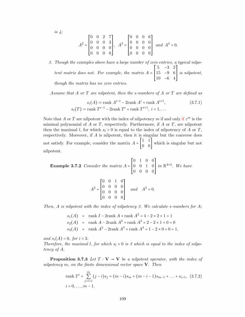
is 4;
A2 =
⎡⎢⎢⎢⎢⎢⎢⎢⎣
0 0 2 70 0 0 30 0 0 00 0 0 0
⎤⎥⎥⎥⎥⎥⎥⎥⎦
, A3 =
⎡⎢⎢⎢⎢⎢⎢⎢⎣
0 0 0 60 0 0 00 0 0 00 0 0 0
⎤⎥⎥⎥⎥⎥⎥⎥⎦
and A4 = 0.
3. Though the examples above have a large number of zero entries, a typical nilpo-
tent matrix does not. For example, the matrix A =⎡⎢⎢⎢⎢⎢⎣
5 −3 215 −9 610 −6 4
⎤⎥⎥⎥⎥⎥⎦is nilpotent,
though the matrix has no zero entries.
Assume that A or T are nilpotent, then the s-numbers of A or T are defined as
si(A) ∶= rank Ai−1 − 2rank Ai + rank Ai+1, (3.7.1)
si(T ) ∶= rank T i−1 − 2rank T i + rank T i+1, i = 1, . . .
Note that A or T are nilpotent with the index of nilpotency m if and only if zm is theminimal polynomial of A or T , respectively. Furthermore, if A or T , are nilpotentthen the maximal l, for which sl > 0 is equal to the index of nilpotency of A or T ,respectively. Moreover, if A is nilpotent, then it is singular but the converse does
not satisfy. For example, consider the matrix A = [1 10 0
] which is singular but not
nilpotent.
Example 3.7.2 Consider the matrix A =⎡⎢⎢⎢⎢⎢⎣
0 1 0 00 0 1 00 0 0 0
⎤⎥⎥⎥⎥⎥⎦in R4×4. We have
A2 =
⎡⎢⎢⎢⎢⎢⎢⎢⎣
0 0 1 00 0 0 00 0 0 00 0 0 0
⎤⎥⎥⎥⎥⎥⎥⎥⎦
and A3 = 0.
Then, A is nilpotent with the index of nilpotency 3. We calculate s-numbers for A;
s1(A) = rank I − 2rank A + rank A2 = 4 − 2 × 2 + 1 = 1
s2(A) = rank A − 2rank A2 + rank A3 = 2 − 2 × 1 + 0 = 0
s3(A) = rank A2 − 2rank A3 + rank A4 = 1 − 2 × 0 + 0 = 1,
and si(A) = 0, for i > 3.Therefore, the maximal l, for which sl > 0 is 3 which is equal to the index of nilpo-tency of A.
Proposition 3.7.3 Let T ∶ V → V be a nilpotent operator, with the index ofnilpotency m, on the finite dimensional vector space V. Then
rank T i =m
∑j=i+1
(j − i)sj = (m − i)sm + (m − i − 1)sm−1 + . . . + si+1, (3.7.2)
i = 0, . . . ,m − 1.
109
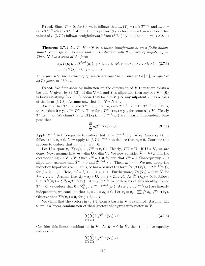
Proof. Since T l = 0, for l ≥ m, it follows that sm(T ) = rank Tm−1 and sm−1 =rank Tm−2 − 2rank Tm−1 if m > 1. This proves (3.7.2) for i =m − 1,m − 2. For othervalues of i, (3.7.2) follows straightforward from (3.7.1) by induction on m− i ≥ 2. ◻
Theorem 3.7.4 Let T ∶ V → V be a linear transformation on a finite dimen-sional vector space. Assume that T is nilpotent with the index of nilpotency m.Then, V has a basis of the form
xj , T (xj), . . . T lj−1(xj), j = 1, . . . , i, where m = l1 ≥ . . . ≥ li ≥ 1 (3.7.3)
and T lj(xj) = 0, j = 1, . . . , i.
More precisely, the number of lj, which are equal to an integer l ∈ [m], is equal tosl(T ) given in (3.7.1).
Proof. We first show by induction on the dimension of V that there exists abasis in V given by (3.7.3). If dimV = 1 and T is nilpotent, then any x ∈ V ∖ 0is basis satisfying (3.7.3). Suppose that for dimV ≤ N any nilpotent T has a basisof the form (3.7.3). Assume now that dimV = N + 1.
Assume that Tm = 0 and Tm−1 ≠ 0. Hence, rank Tm−1 = dim Im Tm−1 > 0. Thus,there exists 0 ≠ y1 ∈ Im Tm−1. Therefore, Tm−1(x1) = y1, for some x1 ∈ V. ClearlyTm(x1) = 0. We claim that x1, T (x1), . . . , Tm−1(x1) are linearly independent. Sup-pose that
m
∑i=1
aiTi−1(xi) = 0. (3.7.4)
Apply Tm−1 to this equality to deduce that 0 = a1Tm−1(x1) = a1y1. Since y1 ≠ 0, it
follows that a1 = 0. Now apply to (3.7.4) Tm−2 to deduce that a2 = 0. Continue thisprocess to deduce that a1 = . . . = am = 0.
Let U = spanx1, T (x1), . . . , Tm−1(x1). Clearly, TU ⊂ U. If U = V, we aredone. Now, assume that m = dimU < dimV. We now consider V ∶= V/U and thecorresponding T ∶ V → V. Since Tm = 0, it follows that Tm = 0. Consequently, T isnilpotent. Assume that Tm
′ = 0 and Tm′−1 ≠ 0. Then, m ≥ m′. We now apply the
induction hypothesis to T . Thus, V has a basis of the form xj , T (xj), . . . T lj−1(xj),
for j = 2, . . . , i. Here, m′ = l2 ≥ . . . ≥ li ≥ 1. Furthermore, T lj(xj) = 0 in V forj = 2, . . . , i. Assume that xj = zj + U, for j = 2, . . . , i. As T lj(xj) = 0, it followsthat T lj(zj) = ∑mi=1 aiT
i−1(x1). Apply Tm−lj to both sides of this identity. Since
Tm = 0, we deduce that 0 = ∑lji=1 aiTm−lj−1+i−1(x1). As x1, . . . , T
m−1(x1) are linearly
independent, we conclude that a1 = . . . = alj = 0. Let xj ∶= zj −∑m−lji=1 alj+iTi−1(x1).
Observe that T lj(xj) = 0, for j = 2, . . . , i.We claim that the vectors in (3.7.3) form a basis in V, as claimed. Assume that
there is a linear combination of these vectors that gives zero vector in V:
i
∑j=1
lj
∑k=1
bjkTk−1(xj) = 0. (3.7.5)
Consider this linear combination in V. As x1 = 0 in V, then the above equalityreduces to:
i
∑j=2
lj
∑k=1
bjkTk−1(xj) = 0.
110
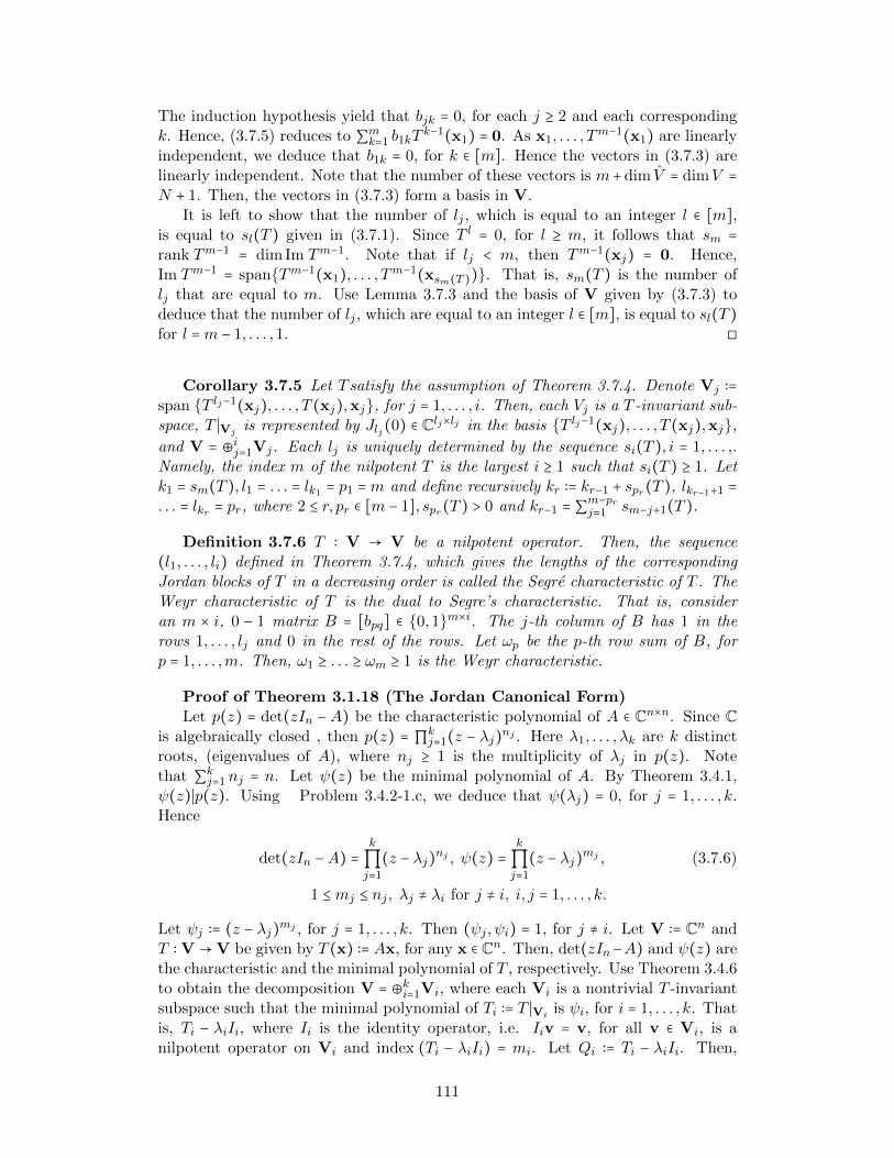
The induction hypothesis yield that bjk = 0, for each j ≥ 2 and each correspondingk. Hence, (3.7.5) reduces to ∑mk=1 b1kT
k−1(x1) = 0. As x1, . . . , Tm−1(x1) are linearly
independent, we deduce that b1k = 0, for k ∈ [m]. Hence the vectors in (3.7.3) arelinearly independent. Note that the number of these vectors is m+dim V = dimV =N + 1. Then, the vectors in (3.7.3) form a basis in V.
It is left to show that the number of lj , which is equal to an integer l ∈ [m],is equal to sl(T ) given in (3.7.1). Since T l = 0, for l ≥ m, it follows that sm =rank Tm−1 = dim Im Tm−1. Note that if lj < m, then Tm−1(xj) = 0. Hence,Im Tm−1 = spanTm−1(x1), . . . , Tm−1(xsm(T )). That is, sm(T ) is the number oflj that are equal to m. Use Lemma 3.7.3 and the basis of V given by (3.7.3) todeduce that the number of lj , which are equal to an integer l ∈ [m], is equal to sl(T )for l =m − 1, . . . ,1. ◻
Corollary 3.7.5 Let T satisfy the assumption of Theorem 3.7.4. Denote Vj ∶=span T lj−1(xj), . . . , T (xj),xj, for j = 1, . . . , i. Then, each Vj is a T -invariant sub-space, T ∣Vj is represented by Jlj(0) ∈ Clj×lj in the basis T lj−1(xj), . . . , T (xj),xj,
and V = ⊕ij=1Vj. Each lj is uniquely determined by the sequence si(T ), i = 1, . . . ,.Namely, the index m of the nilpotent T is the largest i ≥ 1 such that si(T ) ≥ 1. Letk1 = sm(T ), l1 = . . . = lk1 = p1 =m and define recursively kr ∶= kr−1 + spr(T ), lkr−1+1 =. . . = lkr = pr, where 2 ≤ r, pr ∈ [m − 1], spr(T ) > 0 and kr−1 = ∑m−prj=1 sm−j+1(T ).
Definition 3.7.6 T ∶ V → V be a nilpotent operator. Then, the sequence(l1, . . . , li) defined in Theorem 3.7.4, which gives the lengths of the correspondingJordan blocks of T in a decreasing order is called the Segre characteristic of T . TheWeyr characteristic of T is the dual to Segre’s characteristic. That is, consideran m × i, 0 − 1 matrix B = [bpq] ∈ 0,1m×i. The j-th column of B has 1 in therows 1, . . . , lj and 0 in the rest of the rows. Let ωp be the p-th row sum of B, forp = 1, . . . ,m. Then, ω1 ≥ . . . ≥ ωm ≥ 1 is the Weyr characteristic.
Proof of Theorem 3.1.18 (The Jordan Canonical Form)Let p(z) = det(zIn −A) be the characteristic polynomial of A ∈ Cn×n. Since C
is algebraically closed , then p(z) = ∏kj=1(z − λj)nj . Here λ1, . . . , λk are k distinct
roots, (eigenvalues of A), where nj ≥ 1 is the multiplicity of λj in p(z). Notethat ∑kj=1 nj = n. Let ψ(z) be the minimal polynomial of A. By Theorem 3.4.1,ψ(z)∣p(z). Using Problem 3.4.2-1.c, we deduce that ψ(λj) = 0, for j = 1, . . . , k.Hence
det(zIn −A) =k
∏j=1
(z − λj)nj , ψ(z) =k
∏j=1
(z − λj)mj , (3.7.6)
1 ≤mj ≤ nj , λj ≠ λi for j ≠ i, i, j = 1, . . . , k.
Let ψj ∶= (z − λj)mj , for j = 1, . . . , k. Then (ψj , ψi) = 1, for j ≠ i. Let V ∶= Cn andT ∶ V →V be given by T (x) ∶= Ax, for any x ∈ Cn. Then, det(zIn−A) and ψ(z) arethe characteristic and the minimal polynomial of T , respectively. Use Theorem 3.4.6to obtain the decomposition V = ⊕ki=1Vi, where each Vi is a nontrivial T -invariantsubspace such that the minimal polynomial of Ti ∶= T ∣Vi is ψi, for i = 1, . . . , k. Thatis, Ti − λiIi, where Ii is the identity operator, i.e. Iiv = v, for all v ∈ Vi, is anilpotent operator on Vi and index (Ti − λiIi) = mi. Let Qi ∶= Ti − λiIi. Then,
111
Qi is nilpotent and index Qi = mi. Apply Theorem 3.7.4 and Corollary 3.7.5 todeduce that Vi = ⊕qjj=1Vi,j , where each Vi,j is Qi-invariant subspace, and each Vi,jhas a basis in which Qi is represented by a Jordan block Jmij(0), for j = 1, . . . , qj .According to Corollary 3.7.5
mi =mi1 ≥ . . .miqi ≥ 1, i = 1, . . . , k. (3.7.7)
Furthermore, the above sequence is completely determined by rank Qji , j = 0,1, . . .for i = 1, . . . , k. Noting that Ti = Qi + λiIi, it easily follows that each Vi,j is a Ti-invariant subspace, hence T -invariant subspace. Moreover, in the same basis of Vi,j
that Qi represented by Jmij(0), Ti is represented by Jmij(λi), for j = 1, . . . , qi andi = 1, . . . , k. This shows the existence of the Jordan canonical form.
We now show that the Jordan canonical form is unique, up to a permutationof factors. Note that the minimal polynomial of A is completely determined by itsJordan canonical form. Namely, ψ(z) = ∏k
i=1(z − zi)mi1 , where mi1 is the biggestJordan block with the eigenvalues λi. (See Problem 3.4.2-2.) Thus, mi1 = mi, fori = 1, . . . , k. Now, Theorem 3.4.6 yields that the subspaces V1, . . . ,Vk are uniquelydetermined by ψ. Thus, each Ti and Qi = T − λiIi are uniquely determined. UsingTheorem 3.7.4, we get that rank Qji , j = 0,1, . . . determines the sizes of the Jordanblocks of Qi. Hence, all the Jordan blocks corresponding to λi are uniquely deter-mined for each i ∈ [k]. ◻
Corollary 3.7.7 Let A ∈ Fn×n and assume that the characteristic polynomial ofp(z) = det(zIn −A) splits to linear factors, i.e. (3.7.6) holds. Let B be the Jordancanonical form of A. Then
1. The multiplicity of the eigenvalue λi in the minimal polynomial ψ(z) of A isthe size of the biggest Jordan block corresponding to λi in B.
2. The number of Jordan blocks in B corresponding to λi is the nullity of A−λiIn,i.e. the number of Jordan block in B corresponding to A − λiIn is the numberof linearly independent eigenvectors of A corresponding to the eigenvalue λi.
3. Let λi be an eigenvalue of A. Then, the number of the Jordan blocks of orderi corresponding to λi in B is given in (3.7.9).
Proof.1. Since Jn(0)n = 0 and Jn(0)n−1 ≠ 0, it follows that the minimal polynomial ofJn(λ) is (z−λn)n = det(zIn−Jn(λ)). Use Problem 3.7.2-3.a to deduce the first partof the corollary.2. Since Jn(0) has one independent eigenvector, use Problem 3.7.2-3.b to deducethe second part of the corollary.3. Use Problem 3.7.2-2.a to establish the last part of the corollary. ◻
112
3.7.1 Worked-out Problems
1. Show that the only nilpotent diagonalizable matrix is the zero matrix.Solution:Assume that A ∈ Fn×n is a diagonalizable and nilpotent matrix with the indexof nilpotency m. Since A is diagonalizable, then A = C−1DC, for a diagonalmatrix D and C ∈ GL(n,F). Thus, Dm = (CAC−1)m = CAMC−1 = 0. How-ever, if the diagonal entries of D are d1, . . . , dn, then the diagonal entries ofDm are just dm1 , . . . , d
mn . Since Dm = 0, then dmi = 0, for all i and hence di = 0,
for all i. This means D = 0 and it follows that A = 0.
2. Show that the index of nilpotency of the nilpotent matrix A ∈ Fn×n is less thanor equal to n.Solution:We already discussed that the minimal polynomial of a nilpotent matrix is zm,for some positive integer m. Since the minimal polynomial and the character-istic polynomial of a matrix have the same roots (probably with the differentmultiplicities), then the characteristic polynomial of A is zn and based on thedefinition of minimal polynomial, m ≤ n. Now, the statement follows from thefact that the index of nilpotency and the degree of the minimal polynomial ofA are the same.
3. The matrix A ∈ Fn×n is called idempotent if A2 = A. Show that if A is idem-potent, then detA is equal 0 or 1.Solution:Since A2 = A, taking determinant of both sides of this equation, we find
detA = det(A2). (3.7.8)
Then, det(A2) = (detA)2 = detA. Hence, detA(detA−1) = 0 and so detA = 0or 1.
3.7.2 Problems
1. Let T ∶ V → V be nilpotent with m = index T . Let (ω1, . . . , ωm) be the Weyrcharacteristic. Show that rank T j = ∑mp=j+1 ωp, for j = 1, . . . ,m−1.
2. Let A ∈ Cn×n and assume that det(zIn −A) =∏ki=1(z − λi)ni , where λ1, . . . , λk
are k distinct eigenvalues of A. Let
si(A,λj) ∶= rank (A − λjIn)i−1 − 2rank (A − λjIn)i + rank (A − λjIn)i+1,(3.7.9)
i = 1, . . . , nj , j = 1, . . . , k.
(a) Show that si(A,λj) is the number of Jordan blocks of order i correspond-ing to λj for i = 1, . . . , nj .
(b) Show that in order to find all Jordan blocks of A corresponding to λjone can stop computing si(A,λj) at the smallest i ∈ [nj] such that1s1(A,λj) + 2s2(A,λj) . . . + isi(A,λj) = nj .
3. Let C = F ⊕G = diag(F,G), F ∈ Fl×l,G ∈ Fm×m.
113
(a) Assume that ψF , ψG are the minimal polynomials of F and G, respec-tively. Show that ψC , the minimal polynomial of C, is equal to ψFψG
(ψF ,ψG) .
(b) Show that nullC = nullF + nullG. In particular, if G is invertible, i.e. 0is not eigenvalue of G, then nullC = nullF .
3.8 Cyclic subspaces and rational canonical forms
In this section, we study the structure of a linear operator on a finite dimensionalvector space, using the primary decomposition theorem of section 3.4. Let T ∶ V →Vbe a linear operator and assume that V is finite dimensional over the field F. Let0 ≠ u ∈ V. Consider the sequence of vectors u = T 0(u), T (u), T 2(u), . . .. SincedimV < ∞, there exists a positive integer l ≥ 1 such that u, T (u), . . . , T l−1(u) arelinearly independent, and u, T (v), . . . , T l(u) are linearly dependent. Hence, l is thesmallest integer such that
T l(u) = −l
∑i=1
aiTl−i(u), (3.8.1)
for some scalars ai ∈ F, 1 ≤ i ≤ l.Clearly, l ≤ dimV. The polynomial ψu(z) ∶= zl+∑li=1 aiz
l−i is called the minimalpolynomial of u, with respect to T . It is a monic polynomial and has the minimumdegree among annihilating polynomials of u. Its property is similar to the propertyof the minimal polynomial of T . Namely, if a polynomial φ ∈ F[z] annihilates u, i.e.,φ(T )(u) = 0, then ψu∣φ. In particular, the minimal polynomial ψ(z) of T is divisibleby ψu, since ψ(T )(u) = 0(u) = 0. Assume that U = spanT i(u); i = 0,1, . . ..Clearly, every vector w ∈ U can be uniquely represented as φ(T )(u), where φ ∈ F[z]and degφ ≤ l − 1. Hence, U is a T -invariant subspace. The subspace U is called thecyclic subspace, generated by u. Note that in the basis u1 = u,u2 = T (u), . . . ,ul =T l−1(u), the linear transformation T ∣U is given by the matrix
⎡⎢⎢⎢⎢⎢⎢⎢⎢⎢⎣
0 0 0 . . . 0 −al1 0 0 . . . 0 −al−1
0 1 0 . . . 0 −al−2
⋮ ⋮ ⋮ . . . ⋮ ⋮0 0 0 . . . 1 −a1
⎤⎥⎥⎥⎥⎥⎥⎥⎥⎥⎦
∈ Fl×l. (3.8.2)
The above matrix is called the companion matrix , corresponding to the polynomialψu(z). (Sometimes, the transpose of the above matrix is called the companionmatrix.)
Lemma 3.8.1 Let V be a finite dimensional vector space and T ∈ L(V). Sup-pose u and w are two non-zero elements of V and ψu and ψw are the minimalpolynomials of u and w with respect to T , respectively and (ψu, ψw) = 1.Then,ψu+w = ψu ⋅ ψw.
Proof. Let U and W be the cyclic invariant subspaces generated by u and w,respectively. We claim that the T -invariant subspace X ∶= U ∩ W is the trivialsubspace 0. Assume to the contrary, there exists 0 ≠ x ∈ X. Let X1 ⊂ X bea nontrivial cyclic subspace generated by x and ψx be the minimal polynomial
114
corresponding to x. Since X1 ⊂ U, it follows that x = φ(T )(u), for some φ(z) ∈F[z]. Hence, ψu(T )(x) = 0. Thus ψx∣ψu. Similarly ψx∣ψw. This contradicts theassumption that (ψu, ψw) = 1. Hence, U ∩W = 0. Let φ = ψuψw. Clearly
φ(T )(u +w) = ψw(T )(ψu(T )(u)) + ψu(T )(ψw(T )(w) = 0 + 0 = 0.
Thus, φ is an annihilating polynomial of u+w. Let θ(z) be an annihilating polyno-mial of u +w. Then, 0 = θ(T )(u) + θ(T )(w). Since U and V are T -invariant sub-spaces and U∩W = 0, it follows that 0 = θ(T )(u) = θ(T )(w). Hence, ψu∣θ,ψw∣θ.As (ψu, ψw) = 1, it follows that φ∣θ. Hence, ψu+w = φ. ◻
Theorem 3.8.2 Let T ∶ V → V be a linear operator and 1 ≤ dimV < ∞. Letψ(z) be the minimal polynomial of T . Then, there exists 0 ≠ u ∈ V such that ψu = ψ.
Proof. Assume first that ψ(z) = (φ(z))l, where φ(z) is irreducible in F[z], i.e.φ(z) is not divisible by any polynomial θ such 1 ≤ deg θ < degφ, and l is a positiveinteger. Let 0 ≠ w ∈ V. Recall that ψw∣ψ. Hence, ψw = (φ)l(w), where l(w) ∈ [l] isa positive integer. Assume to the contrary that 1 ≤ l(w) ≤ l − 1, for each 0 ≠ w ∈ V.Then, (φ(T ))l−1(w) = 0. As (φ(T ))l−1(0) = 0, we deduce that (φ(z))l−1 is anannihilating polynomial of T . Therefore, ψ∣φl−1 which is impossible. Hence thereexists u ≠ 0 such that l(u) = l, i.e. ψu = ψ.
Consider now the general case
ψ(z) =k
∏i=1
(φi(z))li , li ∈ N, φi irreducible , (φi, φj) = 1, for i ≠ j, (3.8.3)
where k > 1. Theorem 3.4.6 implies that V = ⊕ki=1Vi, where Vi = kerφlii (T ) and φliiis the minimal polynomial of T ∣Vi. The first case of the proof yields the existenceof 0 ≠ ui ∈ Vi such that ψui = φlii for i = 1, . . . , k. Let wj = u1 + . . .+uj . Use Lemma
3.8.1 to deduce that ψwj =∏ji=1 φ
lii . Hence, ψu = ψ for u ∶= wk. ◻
Theorem 3.8.3 (The cyclic decomposition theorem for V) Let T ∶ V →V be a linear operator and 0 < dimV <∞. Then, there exists a decomposition of Vto a direct sum of r T -cyclic subspaces V = ⊕ri=1Ui with the following properties. As-sume that ψi is the minimal polynomial of T ∣Ui, then ψ1 is the minimal polynomialof T . Furthermore, ψi+1∣ψi, for i = 1, . . . , r − 1.
Proof. We prove the theorem by induction on dimV. For dimV = 1, any 0 ≠ uis an eigenvector of T : T (u) = λu, so V is cyclic, and ψ(z) = ψ1(z) = z −λ. Assumenow that the theorem holds of all non-zero vector spaces of dimension less than n+1.Suppose that dimV = n + 1. Let ψ(z) be the minimal polynomial of T , m = degψand T is nonderogatory, i.e., m = n + 1, which is the degree of the characteristicpolynomial of T . Theorem 3.8.2 implies that V is a cyclic subspace.This yieldsr = 1, and the theorem holds in this case.
Assume now that T is derogatory. Then, m < n + 1. Theorem 3.8.2 implies theexistence of 0 ≠ u1 such that ψu1 = ψ. Let U1 be the cyclic subspace generated byu1. Let V ∶= V/U1. Thus, 1 ≤ dim V = dimV −m ≤ n. We now apply the induction
115
hypothesis to T ∶ V → V. Therefore, V = ⊕ri=2Ui, where Ui is a cyclic subspacegenerated by ui, i = 2, . . . , r. The minimal polynomial of ui is ψi, i = 2, . . . , r andψ2 is the minimal polynomial of T , and ψi+1∣ψi, for i = 2, . . . , r − 1. Observe firstthat for any polynomial φ(z), we have the identity φ(T )([x]) = [φ(T )(x)]. Sinceψ(T )(x) = 0, it follows that ψ1 ∶= ψ(z) is an annihilating polynomial of T . Hence,ψ2∣ψ1.
Observe next that since ψi+1∣ψi, for i = 1, . . . , r − 1, it follows that ψi∣ψ1 = ψ.Consequently, ψ = θiψi, where θi is a monic polynomial and i = 2, . . ., r. Since[0] = ψi(T )([ui]) = [ψi(T )(ui)], it follows that ψi(T )(ui) ∈ U1. Hence, ψi(T )(ui) =ωi(T )(u1), for some ω(z) ∈ F[z]. Hence, 0 = ψ(T )(ui) = θi(T )(ψi(T )(ui)) =θi(T )(ωi(T )(u1)). Therefore, ψu1 = ψ divides θiωi. Then, ψi∣ωi and so ωi = ψiαi.Define ui = ui −αi(T )(u1), for i = 2, . . . , r. The rest of the proof of theorem followsfrom Problem 3.8.2-5. ◻
The cyclic decomposition theorem can be used to determine a set of canonicalforms for similarity as follows.
Theorem 3.8.4 (Rational canonical form) Let A ∈ Fn×n. Then, there existr monic polynomials ψ1, . . . , ψr, of degree one at least, satisfying the following con-ditions: First ψi+1∣ψi, for i = 1, . . . , r. Second, ψ1 = ψ is the minimal polynomial ofA. Then, A is similar to ⊕ri=1C(ψi), where C(ψi) is the companion matrix of theform (3.8.2) corresponding to the polynomial ψi.
Decompose each ψi = ψi,1 . . . ψi,ti to the product of its irreducible components, asin the decomposition of ψ = ψ1 given in (3.8.3). Then, A is similar to ⊕r,tii=l=1C(ψi,l).
Suppose finally that ψ(z) = ∏kj=1(z − λj)mj , where λ1, . . . , λk are the k distinct
eigenvalues of A. Then, A is similar to the Jordan canonical form given in Theorem3.1.18.
Proof. Identify A with T ∶ Fn → Fn, where T (x) = Ax. Use Theorem 3.8.3to decompose Fn = ⊕ri=1Ui, where each Ui is a cyclic invariant subspace such thatT ∣Ui has the minimal polynomial ψi. Since Ui is cyclic, then T ∣Ui is representedby C(ψi) in the appropriate basis of Ui as shown in the beginning of this section.Hence, A is similar to ⊕ri=1C(ψi).
Consider next Ti ∶= T ∣Ui. Use Theorem 3.4.6 to deduce that Ui decomposes toa direct sum of Ti invariant subspaces ⊕til=1Ui,l, where the minimal polynomial ofTi,l ∶= Ti∣Ui,l is ψi,l. Since Ui was cyclic, i.e., Ti was nonderogatory, it follows thateach Ti,l must be nonderogatory, i.e. Ui,l cyclic. (See Problem 3.8.2-3.) Recall thateach Ti,l is represented in a corresponding basis by C(ψi,l). Hence, A is similar to⊕r,tii=l=1C(ψi,l).
Suppose finally that ψ(z) splits to linear factors. Hence, ψi,l = (z − λl)mi,l andTi,l − λlI is nilpotent of index mi,l. Thus, there exists a basis in Ui,l such that Ti,lis represented by the Jordan block Jmi,l(λl). Therefore, A is similar to a sum ofcorresponding Jordan blocks. ◻
The polynomials ψ1, . . . , ψk appearing in Theorem 3.8.3 are called invariant polyno-mials of T or its representation matrixA, in any basis. The polynomials ψi,1, . . . , ψi,ti , i =1, . . . , k appearing in Theorem 3.8.4 are called the elementary divisors of A, or thecorresponding linear transformation T represented by A. We now show that thesepolynomials are uniquely defined.
116
Lemma 3.8.5 (Cauchy-Binet formula) For two positive integers 1 ≤ p ≤m, de-note by Qp,m the set of all subsets α of 1, . . . ,m of cardinality p. Let A ∈ Fm×n,B ∈Fn×l and denote C = AB ∈ Fm×l. Then, for any integer p ∈ [min(m,n, l)],α ∈Qp,m,β ∈ Qp,l the following identity holds.
detC[α,β] = ∑γ∈Qp,n
detA[α,γ]detB[γ,β]. (3.8.4)
Proof. It is enough to check the case where α = β = 1, . . . , p. This is equivalentto the assumption that p = m = l ≤ n. For p = m = n = l, the Cauchy-Binetformula reduces to detAB = (detA)(detB). Thus, it is sufficient to consider thecase p =m = l < n. Let C = [cij]pi=j=1. Then, cij = ∑ntj=1 aitjbtjj for i, j = 1, . . . , p. Usemultilinearity of the determinant to deduce
detC = det[n
∑tj=1
aitjbtjj]ni=j=1 =n
∑t1,...,tp=1
det[aitjbtjj]ni=j=1 =
n
∑t1,...,tp=1
detA[1, . . . , p,t1, . . . , tp]bt11bt22 . . . btpp.
Observe next that detA[1, . . . , p,t1, . . . , tp] = 0 if ti = tj , for some 1 ≤ i < j ≤ p,since the columns ti and tj in A[1, . . . , p,t1, . . . , tp] are equal. Consider the sum
∑t1,t2,...,tp=γ∈Qp,n
A[1, . . . , p,t1, . . . , tp]bt11bt22 . . . btpp.
The above arguments yield that this sum is
det(A[⟨p⟩,γ]C[γ, ⟨p⟩]) = (detA[⟨p⟩,γ])(detC[γ, ⟨p⟩]).
This establishes (3.8.4). ◻
Proposition 3.8.6 Let A(z) ∈ Fm×n[z]. Denote by r = rank A(z) the size ofthe biggest minor of A(z) which is not a zero polynomial. For an integer k ∈ [r], letδk(z) be the greatest common divisor of all k × k minors of A(z), which is assumedto be a monic polynomial. Assume that δ0 = 1. Then, δi∣δi+1, for i = 0, . . . , r − 1.
Proof. Expand a non-zero (k + 1) × (k + 1) minor of A(z) to deduce thatδk(z)∣δk+1(z). In particular, δi∣δj , for 1 ≤ i < j ≤ r. ◻
Proposition 3.8.7 Let A(z) ∈ F[z]m×n. Assume that P ∈ GL(m,F) and Q ∈GL(n,F). Let B(z) = PA(z)Q. Then
1. rank A(z) = rank B(z) = r.
2. δk(A(z)) = δk(B(z)), for k = 0, . . . , r.
Proof. Use Cauchy-Binet to deduce that rank B(z) ≤ rank A(z). Since A(z) =P −1B(z)Q−1, it follows that rank A(z) ≤ rank B(z). Hence, rank A(z) = rank B(z) =r. Use the Cauchy-Binet to deduce that δk(A(z))∣δk(B(z)). AsA(z) = P −1B(z)Q−1,we deduce also that δk(B(z))∣δk(A(z)). ◻
117
Definition 3.8.8 Let A ∈ Fn×n and define A(z) ∶= zIn−A. Then, the polynomi-als of degree 1 at least in the sequence φi = δn−i+1
δn−i(z) , i = 1, . . . , n are called the invariantpolynomials of A.
Note that the product of all invariant polynomials is det(zIn−A). In view of Propo-sition 3.8.7, we obtain that similar matrices have the same invariant polynomials.Hence, for linear transformation T ∶ V →V, we can define its invariant polynomialsof T by any representation matrix of T in a basis of V.
Theorem 3.8.9 Let T ∶ V →V be a linear operator. Then, the invariant poly-nomials of T are the polynomials ψ1, . . . , ψr appearing in Theorem 3.8.3.
To prove this theorem we need the following lemma:
Lemma 3.8.10 Let A = diag(B,C)(= B ⊕ C) ∈ Fn×n, where B ∈ Fl×l,C ∈Fm×m,m = n− l. Let p ∈ [n− 1] and assume that α = α1, . . . , αp,β = β1, . . . , βp ∈Qp,n:
1 ≤ α1 < . . . < αp ≤ n, 1 ≤ β1 < . . . < βp ≤ n.
If #α ∩ [l] ≠ #β ∩ [l], then detA[α,β] = 0.
Proof. Let k ∶= #α ∩ [l], i.e. αk ≤ l, αk+1 > l. Consider a term in detA[α,β].Up to a sign it is ∏p
j=1 aαjβσ(j) , for some bijection σ ∶ [p] → [p]. Then, this productis zero unless σ([k]) = [k] and βk ≤ l, βk+1 > l. ◻
Proof of Theorem 3.8.9. From the proof of Theorem 3.8.3, it follows thatV has a basis in which T is represented by C ∶= ⊕ri=1C(ψi). Assume that C(ψi) ∈Fli×li , i ∈ [r], where n = ∑ri=1 li.
Let θ ∶= zl+a1zm−1+. . .+al. Then, the companion matrix C(θ) is given by (3.8.2).
Consider the submatrix of B(z) of zIl −C(θ) obtained by deleting the first row anthe last column. It is an upper triangular matrix with −1 on the diagonal. Hence,detB(z) = (−1)l−1. Therefore, δl−1(zIm −C(θ)) = 1. Thus, δl−j(zIl −C(θ)) = 1, forj ≥ 1.
We claim that δn−j(zIn − C) = ∏ri=j+1ψj , for j ∈ [r]. Consider a minor of or-
der n − j of the block diagonal matrix zIn − C of the form (zIn − C)[α,β], whereα,β ∈ Qn−j,n. Lemma 3.8.10 claims that det(zIn − C)[α,β] = 0, unless we chooseour minor such that in each submatrix (zIli − C(ψi)), we delete the same numberof rows and columns. Deleting the first row and last column in (zIli − C(ψi)), weget a minor with value (−1)li−1. Recall also that δli−k(zIli − C(ψi)) = 1, for k ≥ 1.Since ψi+1∣ψi, it follows that δn−j(zIn −C) is obtained by deleting the first row andthe last column in (zIli −C(ψi)), for i = 1, . . . , j and j = 1, . . . , r. (ψr+1 ∶= 1.) Thus,
δn−j(zIn −C) =∏ri=j+1ψj , for j ∈ [r]. Hence, ψi = δn−i+1(zIn−C)
δn−i(zIn−C) . ◻
Note that the above theorem implies that the invariant polynomials of A satisfyφi+1∣φi, for i = 1, . . . , r − 1.
The irreducible factors φi,1, . . . , φi,ti of ψi given in Theorem 3.8.4, for i = 1, . . . , r
are called the elementary divisors of A. The matrices ⊕ki=1C(ψi) and ⊕k,tii=l=1C(ψi,l)are called the rational canonical forms of A. Those are the canonical forms in thecase that the characteristic polynomial of A does not split to linear factors over F.Note that the diagonal elements of the Jordan canonical form of a matrix A are
118
the eigenvalues of A, each appearing the number of times equal to its algebraicmultiplicity. However, the rational canonical form does not expose the eigenvaluesof the matrix, even when these eigenvalues lie in the base field.
Example 3.8.11 Let T ∈ L(R7) with the minimal polynomial ψ(z) = (z−1)(z2+1)2. Since its elementary divisors are z−1 and (z2+1)2, then we have the followingpossibilities for the list of elementary divisors:
1. z − 1, z − 1, z − 1, (z2 + 1)2
2. z − 1, (z2 + 1)2, z2 + 1
These correspond to the following rational canonical forms:
1.
⎡⎢⎢⎢⎢⎢⎢⎢⎢⎢⎢⎢⎢⎢⎢⎣
−1 0 0 0 0 0 00 −1 0 0 0 0 00 0 −1 0 0 0 00 0 0 0 0 0 −10 0 0 1 0 0 00 0 0 0 1 0 −20 0 0 0 0 1 0
⎤⎥⎥⎥⎥⎥⎥⎥⎥⎥⎥⎥⎥⎥⎥⎦
2.
⎡⎢⎢⎢⎢⎢⎢⎢⎢⎢⎢⎢⎢⎢⎢⎣
−1 0 0 0 0 0 00 0 0 0 −1 0 00 1 0 0 0 0 00 0 1 0 −2 0 00 0 0 1 0 0 00 0 0 0 0 0 −10 0 0 0 0 1 0
⎤⎥⎥⎥⎥⎥⎥⎥⎥⎥⎥⎥⎥⎥⎥⎦
3.8.1 Worked-out Problems
1. Consider the following matrix:
C =
⎡⎢⎢⎢⎢⎢⎢⎢⎣
2 2 −2 4−4 −3 4 −61 1 −1 22 2 −2 4
⎤⎥⎥⎥⎥⎥⎥⎥⎦
.
Assume that the minimal polynomial of C is ψC(z) = z(z − 1)2. Find therational canonical form of C.Solution:Since
pC(z)ψ1(z) = z, then ψ2(z) = z. According to the definition of the companion
matrix,
C(ψ1) =⎡⎢⎢⎢⎢⎢⎣
0 0 01 0 −10 1 2
⎤⎥⎥⎥⎥⎥⎦,
119
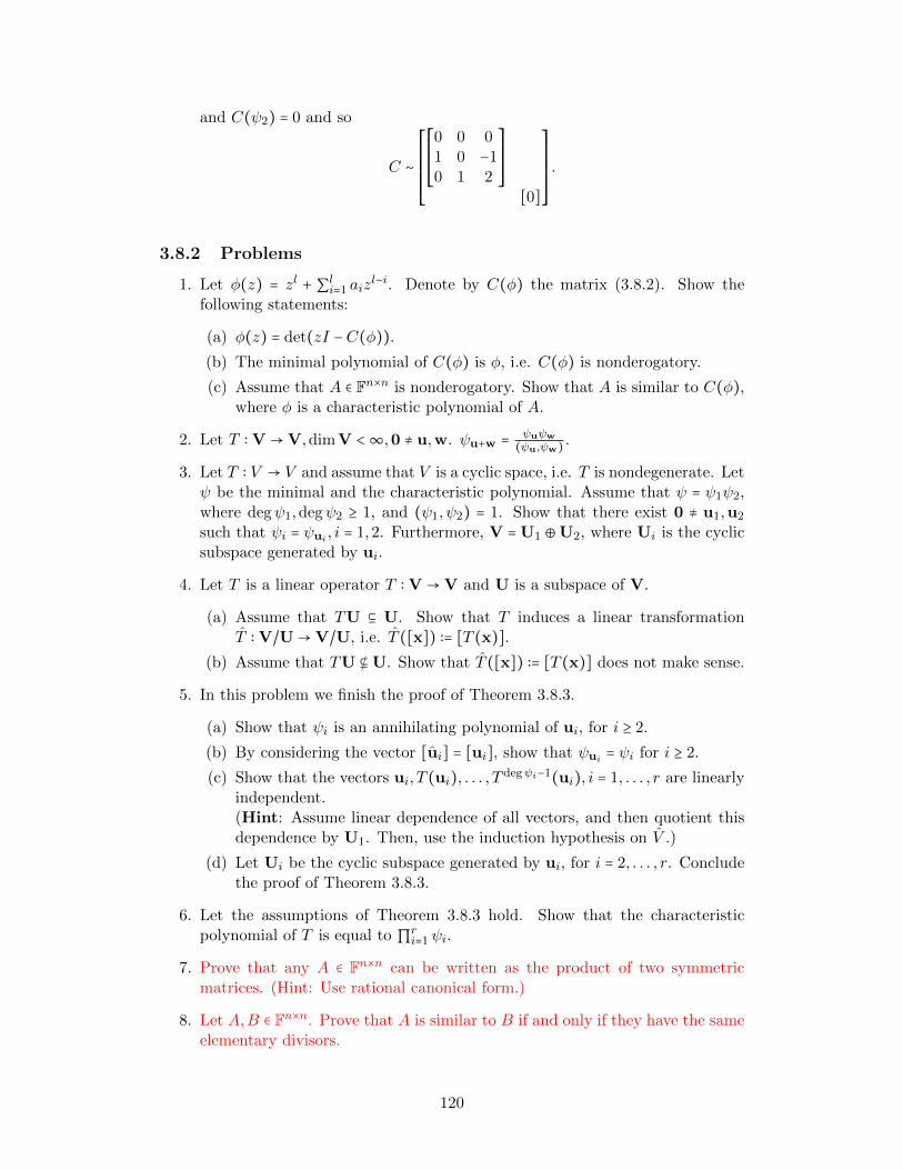
and C(ψ2) = 0 and so
C ∼
⎡⎢⎢⎢⎢⎢⎢⎢⎣
⎡⎢⎢⎢⎢⎢⎣
0 0 01 0 −10 1 2
⎤⎥⎥⎥⎥⎥⎦[0]
⎤⎥⎥⎥⎥⎥⎥⎥⎦
.
3.8.2 Problems
1. Let φ(z) = zl + ∑li=1 aizl−i. Denote by C(φ) the matrix (3.8.2). Show the
following statements:
(a) φ(z) = det(zI −C(φ)).(b) The minimal polynomial of C(φ) is φ, i.e. C(φ) is nonderogatory.
(c) Assume that A ∈ Fn×n is nonderogatory. Show that A is similar to C(φ),where φ is a characteristic polynomial of A.
2. Let T ∶ V →V,dimV <∞,0 ≠ u,w. ψu+w = ψuψw
(ψu,ψw) .
3. Let T ∶ V → V and assume that V is a cyclic space, i.e. T is nondegenerate. Letψ be the minimal and the characteristic polynomial. Assume that ψ = ψ1ψ2,where degψ1,degψ2 ≥ 1, and (ψ1, ψ2) = 1. Show that there exist 0 ≠ u1,u2
such that ψi = ψui , i = 1,2. Furthermore, V = U1 ⊕U2, where Ui is the cyclicsubspace generated by ui.
4. Let T is a linear operator T ∶ V →V and U is a subspace of V.
(a) Assume that TU ⊆ U. Show that T induces a linear transformationT ∶ V/U→V/U, i.e. T ([x]) ∶= [T (x)].
(b) Assume that TU ⊈ U. Show that T ([x]) ∶= [T (x)] does not make sense.
5. In this problem we finish the proof of Theorem 3.8.3.
(a) Show that ψi is an annihilating polynomial of ui, for i ≥ 2.
(b) By considering the vector [ui] = [ui], show that ψui = ψi for i ≥ 2.
(c) Show that the vectors ui, T (ui), . . . , T degψi−1(ui), i = 1, . . . , r are linearlyindependent.(Hint: Assume linear dependence of all vectors, and then quotient thisdependence by U1. Then, use the induction hypothesis on V .)
(d) Let Ui be the cyclic subspace generated by ui, for i = 2, . . . , r. Concludethe proof of Theorem 3.8.3.
6. Let the assumptions of Theorem 3.8.3 hold. Show that the characteristicpolynomial of T is equal to ∏r
i=1ψi.
7. Prove that any A ∈ Fn×n can be written as the product of two symmetricmatrices. (Hint: Use rational canonical form.)
8. Let A,B ∈ Fn×n. Prove that A is similar to B if and only if they have the sameelementary divisors.
120
Chapter 4
Applications of Jordancanonical form
4.1 Functions of Matrices
Let A ∈ Cn×n. Consider the iterations
xl = Axl−1, xl−1 ∈ Cn, l = 1, . . . (4.1.1)
Clearly, xl = Alx0. To compute xl from xl−1, one need to perform n(2n − 1) flops,(operations: n2 multiplications and n(n − 1) additions). If we want to computex108 , we need 108n(2n − 1) operations, if we simply program the iterations (4.1.1).If n = 10, it will take us some time to do these iterations, and we will probably runto the roundoff error, which will render our computations meaningless. Is there anybetter way to find x108? The answer is yes, and this is the purpose of this section.
For a scalar function f and a matrix A ∈ Cn×n we denote by f(A) to be a matrixof the same dimension as A. This provides a generalization of a scalar variablematrix f(z), z ∈ C. If f(x) is a polynomial or rational function, it is natural todefine f(A) by substituting A for x, replacing division by matrix inversion and
replacing 1 by the identity matrix. For example if f(x) = 1+x31−x then
f(A) = (I −A)−1(I +A3),
if 1 is not an eigenvalue of A. As rational functions of a matrix commute, so it doesnot matter if we write (I −A)−1(I +A3) or (I +A3)(I −A)−1. In what follows, weare going to provide the formal definition of a matrix function. Let A ∈ Cn×n. UsingTheorem 3.1.18 (The Jordan canonical form) we have
P −1AP =k⊕i=1Jni(λi),
for some P ∈ GL(n,C), and λi’s are the eigenvalues of A each of order ni. Thefunction f is said to be defined on the spectrum of A if the values
f (j)(λi), j = 0,1, . . . , ni − 1 i ∈ [k]
exist. These are called the values of the function f on the spectrum of A.
121
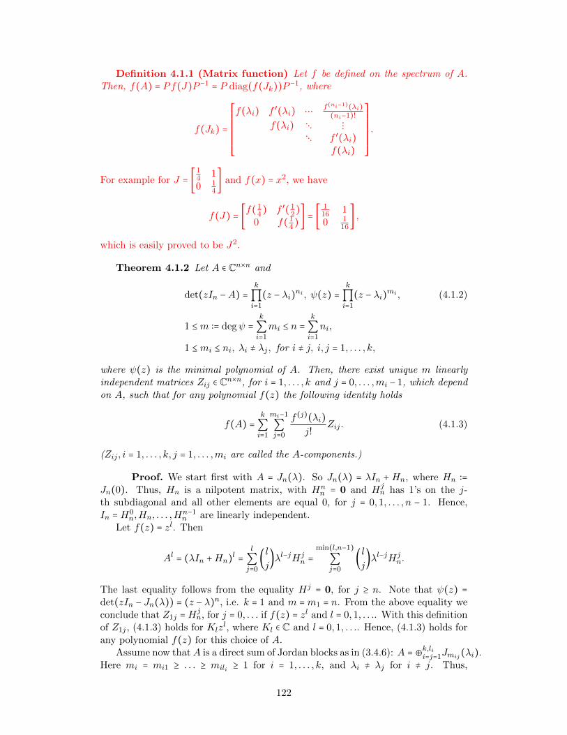
Definition 4.1.1 (Matrix function) Let f be defined on the spectrum of A.Then, f(A) = Pf(J)P −1 = P diag(f(Jk))P −1, where
f(Jk) =
⎡⎢⎢⎢⎢⎢⎢⎢⎢⎣
f(λi) f ′(λi) ⋯ f(ni−1)(λi)(ni−1)!
f(λi) ⋱ ⋮⋱ f ′(λi)
f(λi)
⎤⎥⎥⎥⎥⎥⎥⎥⎥⎦
.
For example for J = [14 1
0 14
] and f(x) = x2, we have
f(J) = [f(14) f ′(1
2)0 f(1
4)] = [
116 1
0 116
] ,
which is easily proved to be J2.
Theorem 4.1.2 Let A ∈ Cn×n and
det(zIn −A) =k
∏i=1
(z − λi)ni , ψ(z) =k
∏i=1
(z − λi)mi , (4.1.2)
1 ≤m ∶= degψ =k
∑i=1
mi ≤ n =k
∑i=1
ni,
1 ≤mi ≤ ni, λi ≠ λj , for i ≠ j, i, j = 1, . . . , k,
where ψ(z) is the minimal polynomial of A. Then, there exist unique m linearlyindependent matrices Zij ∈ Cn×n, for i = 1, . . . , k and j = 0, . . . ,mi − 1, which dependon A, such that for any polynomial f(z) the following identity holds
f(A) =k
∑i=1
mi−1
∑j=0
f (j)(λi)j!
Zij . (4.1.3)
(Zij , i = 1, . . . , k, j = 1, . . . ,mi are called the A-components.)
Proof. We start first with A = Jn(λ). So Jn(λ) = λIn +Hn, where Hn ∶=Jn(0). Thus, Hn is a nilpotent matrix, with Hn
n = 0 and Hjn has 1’s on the j-
th subdiagonal and all other elements are equal 0, for j = 0,1, . . . , n − 1. Hence,In =H0
n,Hn, . . . ,Hn−1n are linearly independent.
Let f(z) = zl. Then
Al = (λIn +Hn)l =l
∑j=0
(lj)λl−jHj
n =min(l,n−1)∑j=0
(lj)λl−jHj
n.
The last equality follows from the equality Hj = 0, for j ≥ n. Note that ψ(z) =det(zIn − Jn(λ)) = (z − λ)n, i.e. k = 1 and m =m1 = n. From the above equality weconclude that Z1j =Hj
n, for j = 0, . . . if f(z) = zl and l = 0,1, . . .. With this definitionof Z1j , (4.1.3) holds for Klz
l, where Kl ∈ C and l = 0,1, . . .. Hence, (4.1.3) holds forany polynomial f(z) for this choice of A.
Assume now thatA is a direct sum of Jordan blocks as in (3.4.6): A = ⊕k,lii=j=1Jmij(λi).Here mi = mi1 ≥ . . . ≥ mili ≥ 1 for i = 1, . . . , k, and λi ≠ λj for i ≠ j. Thus,
122
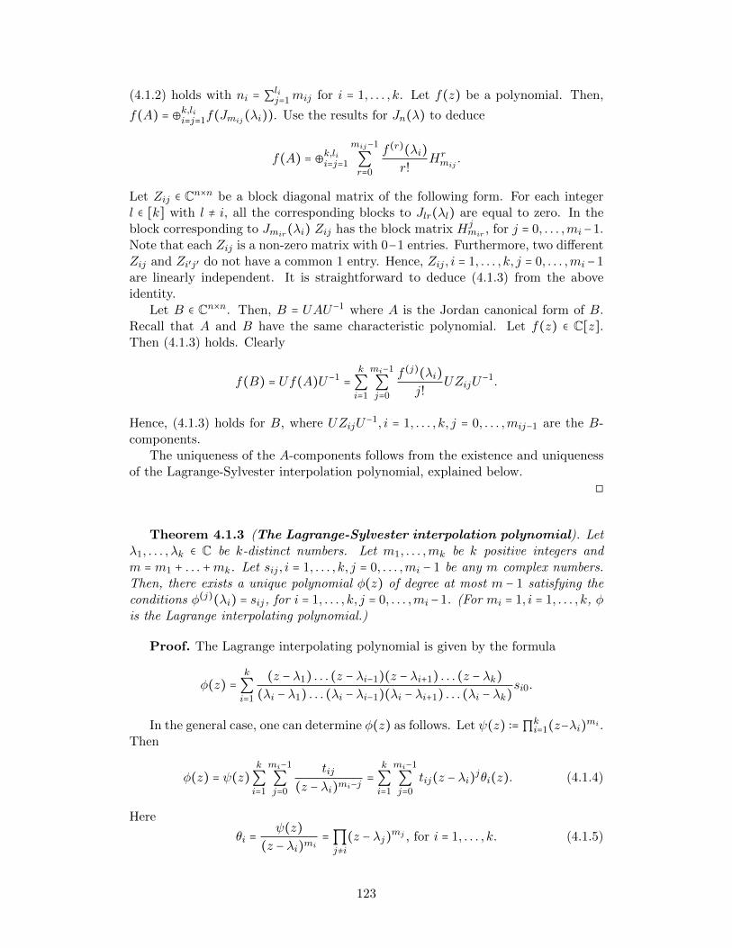
(4.1.2) holds with ni = ∑lij=1mij for i = 1, . . . , k. Let f(z) be a polynomial. Then,
f(A) = ⊕k,lii=j=1f(Jmij(λi)). Use the results for Jn(λ) to deduce
f(A) = ⊕k,lii=j=1
mij−1
∑r=0
f (r)(λi)r!
Hrmij .
Let Zij ∈ Cn×n be a block diagonal matrix of the following form. For each integerl ∈ [k] with l ≠ i, all the corresponding blocks to Jlr(λl) are equal to zero. In theblock corresponding to Jmir(λi) Zij has the block matrix Hj
mir , for j = 0, . . . ,mi−1.Note that each Zij is a non-zero matrix with 0−1 entries. Furthermore, two differentZij and Zi′j′ do not have a common 1 entry. Hence, Zij , i = 1, . . . , k, j = 0, . . . ,mi −1are linearly independent. It is straightforward to deduce (4.1.3) from the aboveidentity.
Let B ∈ Cn×n. Then, B = UAU−1 where A is the Jordan canonical form of B.Recall that A and B have the same characteristic polynomial. Let f(z) ∈ C[z].Then (4.1.3) holds. Clearly
f(B) = Uf(A)U−1 =k
∑i=1
mi−1
∑j=0
f (j)(λi)j!
UZijU−1.
Hence, (4.1.3) holds for B, where UZijU−1, i = 1, . . . , k, j = 0, . . . ,mij−1 are the B-
components.The uniqueness of the A-components follows from the existence and uniqueness
of the Lagrange-Sylvester interpolation polynomial, explained below.◻
Theorem 4.1.3 (The Lagrange-Sylvester interpolation polynomial). Letλ1, . . . , λk ∈ C be k-distinct numbers. Let m1, . . . ,mk be k positive integers andm = m1 + . . . +mk. Let sij , i = 1, . . . , k, j = 0, . . . ,mi − 1 be any m complex numbers.Then, there exists a unique polynomial φ(z) of degree at most m − 1 satisfying theconditions φ(j)(λi) = sij, for i = 1, . . . , k, j = 0, . . . ,mi − 1. (For mi = 1, i = 1, . . . , k, φis the Lagrange interpolating polynomial.)
Proof. The Lagrange interpolating polynomial is given by the formula
φ(z) =k
∑i=1
(z − λ1) . . . (z − λi−1)(z − λi+1) . . . (z − λk)(λi − λ1) . . . (λi − λi−1)(λi − λi+1) . . . (λi − λk)
si0.
In the general case, one can determine φ(z) as follows. Let ψ(z) ∶=∏ki=1(z−λi)mi .
Then
φ(z) = ψ(z)k
∑i=1
mi−1
∑j=0
tij
(z − λi)mi−j=
k
∑i=1
mi−1
∑j=0
tij(z − λi)jθi(z). (4.1.4)
Here
θi =ψ(z)
(z − λi)mi=∏j≠i
(z − λj)mj , for i = 1, . . . , k. (4.1.5)
123
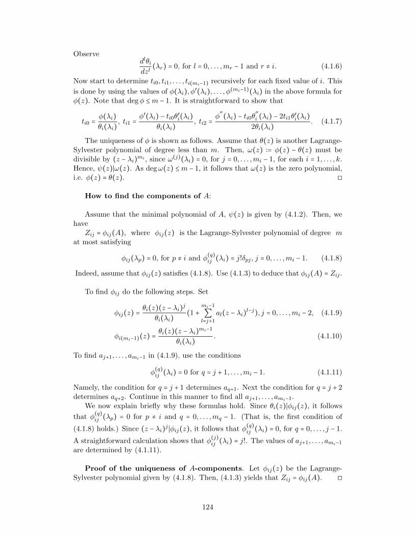
Observedlθidzl
(λr) = 0, for l = 0, . . . ,mr − 1 and r ≠ i. (4.1.6)
Now start to determine ti0, ti1, . . . , ti(mi−1) recursively for each fixed value of i. This
is done by using the values of φ(λi), φ′(λi), . . . , φ(mi−1)(λi) in the above formula forφ(z). Note that degφ ≤m − 1. It is straightforward to show that
ti0 =φ(λi)θi(λi)
, ti1 =φ′(λi) − ti0θ′i(λi)
θi(λi), ti2 =
φ′′(λi) − ti0θ
′′
i (λi) − 2ti1θ′i(λi)
2θi(λi). (4.1.7)
The uniqueness of φ is shown as follows. Assume that θ(z) is another Lagrange-Sylvester polynomial of degree less than m. Then, ω(z) ∶= φ(z) − θ(z) must bedivisible by (z − λi)mi , since ω(j)(λi) = 0, for j = 0, . . . ,mi − 1, for each i = 1, . . . , k.Hence, ψ(z)∣ω(z). As degω(z) ≤m − 1, it follows that ω(z) is the zero polynomial,i.e. φ(z) = θ(z). ◻
How to find the components of A:
Assume that the minimal polynomial of A, ψ(z) is given by (4.1.2). Then, wehave
Zij = φij(A), where φij(z) is the Lagrange-Sylvester polynomial of degree mat most satisfying
φij(λp) = 0, for p ≠ i and φ(q)ij (λi) = j!δpj , j = 0, . . . ,mi − 1. (4.1.8)
Indeed, assume that φij(z) satisfies (4.1.8). Use (4.1.3) to deduce that φij(A) = Zij .
To find φij do the following steps. Set
φij(z) =θi(z)(z − λi)j
θi(λi)(1 +
mi−1
∑l=j+1
al(z − λi)l−j), j = 0, . . . ,mi − 2, (4.1.9)
φi(mi−1)(z) =θi(z)(z − λi)mi−1
θi(λi). (4.1.10)
To find aj+1, . . . , ami−1 in (4.1.9), use the conditions
φ(q)ij (λi) = 0 for q = j + 1, . . . ,mi − 1. (4.1.11)
Namely, the condition for q = j + 1 determines aq+1. Next the condition for q = j + 2determines aq+2. Continue in this manner to find all aj+1, . . . , ami−1.
We now explain briefly why these formulas hold. Since θi(z)∣φij(z), it follows
that φ(q)ij (λp) = 0 for p ≠ i and q = 0, . . . ,mq − 1. (That is, the first condition of
(4.1.8) holds.) Since (z − λi)j ∣φij(z), it follows that φ(q)ij (λi) = 0, for q = 0, . . . , j − 1.
A straightforward calculation shows that φ(j)ij (λi) = j!. The values of aj+1, . . . , ami−1
are determined by (4.1.11).
Proof of the uniqueness of A-components. Let φij(z) be the Lagrange-Sylvester polynomial given by (4.1.8). Then, (4.1.3) yields that Zij = φij(A). ◻
124
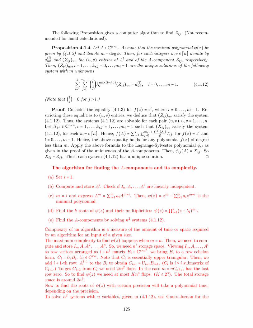
The following Proposition gives a computer algorithm to find Zij . (Not recom-mended for hand calculations!).
Proposition 4.1.4 Let A ∈ Cn×n. Assume that the minimal polynomial ψ(z) begiven by (4.1.2) and denote m = degψ. Then, for each integers u, v ∈ [n] denote by
a(l)uv and (Zij)uv the (u, v) entries of Al and of the A-component Zij, respectively.
Then, (Zij)uv, i = 1, . . . , k, j = 0, . . . ,mi − 1 are the unique solutions of the followingsystem with m unknowns
k
∑i=1
mi−1
∑j=0
(lj)λmax(l−j,0)
i (Zij)uv = a(l)uv , l = 0, . . . ,m − 1. (4.1.12)
(Note that (lj) = 0 for j > l.)
Proof. Consider the equality (4.1.3) for f(z) = zl, where l = 0, . . . ,m − 1. Re-stricting these equalities to (u, v) entries, we deduce that (Zij)uv satisfy the system(4.1.12). Thus, the systems (4.1.12) are solvable for each pair (u, v), u, v = 1, . . . , n.Let Xij ∈ Cn×n, i = 1, . . . , k, j = 1, . . . ,mi − 1 such that (Xij)uv satisfy the system
(4.1.12), for each u, v ∈ [n]. Hence, f(A) = ∑ki=1∑mi−1j=0
f(j)(λi)j! Tij , for f(z) = zl and
l = 0, . . . ,m − 1. Hence, the above equality holds for any polynomial f(z) of degreeless than m. Apply the above formula to the Lagrange-Sylvester polynomial φij asgiven in the proof of the uniqueness of the A-components. Then, φij(A) = Xij . SoXij = Zij . Thus, each system (4.1.12) has a unique solution. ◻
The algorithm for finding the A-components and its complexity.
(a) Set i = 1.
(b) Compute and store Ai. Check if In,A, . . . ,Ai are linearly independent.
(c) m = i and express Am = ∑mi=1 aiAm−i. Then, ψ(z) = zm − ∑mi=1 aiz
m−i is theminimal polynomial.
(d) Find the k roots of ψ(z) and their multiplicities: ψ(z) =∏ki=1(z − λi)mi .
(e) Find the A-components by solving n2 systems (4.1.12).
Complexity of an algorithm is a measure of the amount of time or space requiredby an algorithm for an input of a given size.The maximum complexity to find ψ(z) happens when m = n. Then, we need to com-pute and store In,A,A
2, . . . ,An. So, we need n3 storage space. Viewing In,A, . . . ,Ai
as row vectors arranged as i × n2 matrix Bi ∈ Ci×n2, we bring Bi to a row echelon
form: Ci = UiBi, Ui ∈ Ci×i. Note that Ci is essentially upper triangular. Then, weadd i + 1-th row: Ai+1 to the Bi to obtain Ci+1 = Ui+1Bi+1. (Ci is i × i submatrix ofCi+1.) To get Ci+1 from Ci we need 2in2 flops. In the case m = nCn2+1 has the lastrow zero. So to find ψ(z) we need at most Kn4 flops. (K ≤ 2?). The total storagespace is around 2n3.Now to find the roots of ψ(z) with certain precision will take a polynomial time,depending on the precision.To solve n2 systems with n variables, given in (4.1.12), use Gauss-Jordan for the
125
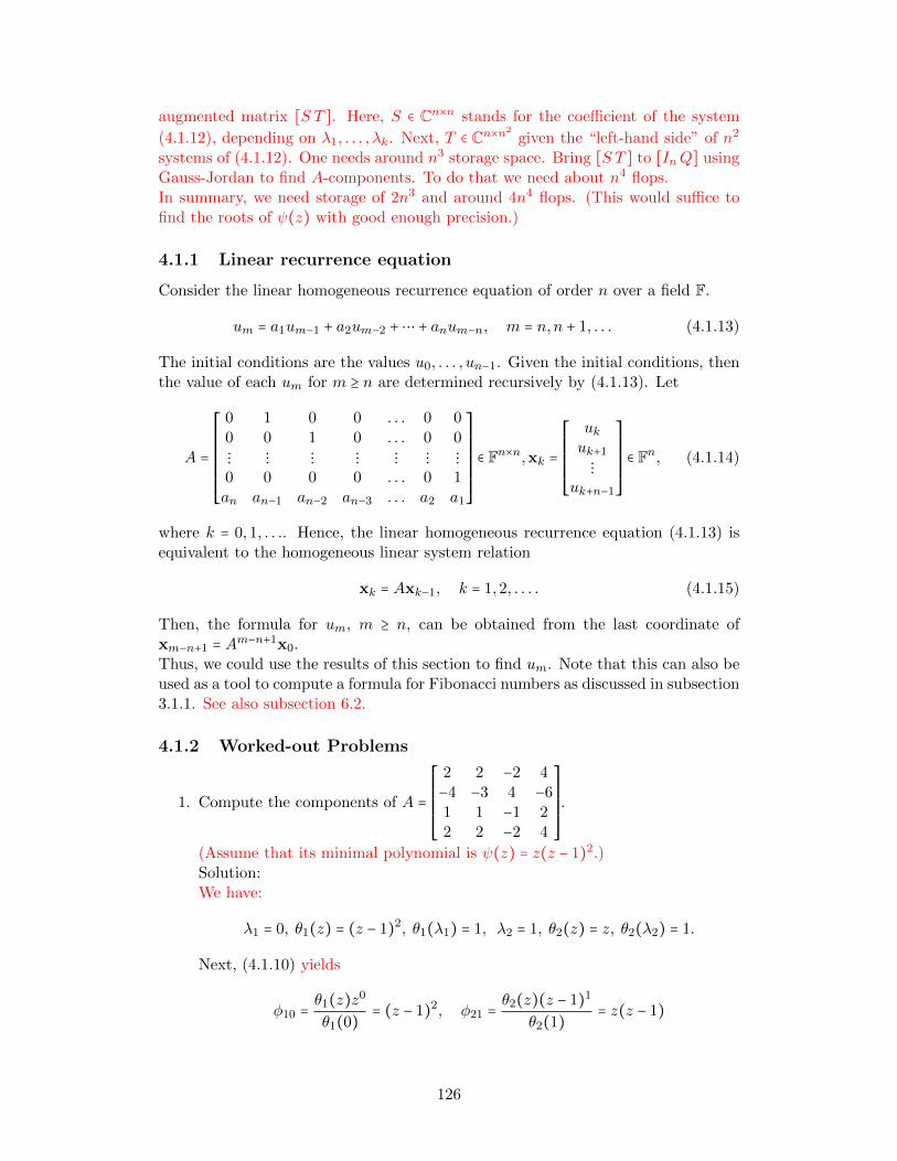
augmented matrix [S T ]. Here, S ∈ Cn×n stands for the coefficient of the system
(4.1.12), depending on λ1, . . . , λk. Next, T ∈ Cn×n2given the “left-hand side” of n2
systems of (4.1.12). One needs around n3 storage space. Bring [S T ] to [InQ] usingGauss-Jordan to find A-components. To do that we need about n4 flops.In summary, we need storage of 2n3 and around 4n4 flops. (This would suffice tofind the roots of ψ(z) with good enough precision.)
4.1.1 Linear recurrence equation
Consider the linear homogeneous recurrence equation of order n over a field F.
um = a1um−1 + a2um−2 +⋯ + anum−n, m = n,n + 1, . . . (4.1.13)
The initial conditions are the values u0, . . . , un−1. Given the initial conditions, thenthe value of each um for m ≥ n are determined recursively by (4.1.13). Let
A =
⎡⎢⎢⎢⎢⎢⎢⎢⎢⎢⎣
0 1 0 0 . . . 0 00 0 1 0 . . . 0 0⋮ ⋮ ⋮ ⋮ ⋮ ⋮ ⋮0 0 0 0 . . . 0 1an an−1 an−2 an−3 . . . a2 a1
⎤⎥⎥⎥⎥⎥⎥⎥⎥⎥⎦
∈ Fn×n,xk =
⎡⎢⎢⎢⎢⎢⎢⎢⎣
ukuk+1
⋮uk+n−1
⎤⎥⎥⎥⎥⎥⎥⎥⎦
∈ Fn, (4.1.14)
where k = 0,1, . . .. Hence, the linear homogeneous recurrence equation (4.1.13) isequivalent to the homogeneous linear system relation
xk = Axk−1, k = 1,2, . . . . (4.1.15)
Then, the formula for um, m ≥ n, can be obtained from the last coordinate ofxm−n+1 = Am−n+1x0.Thus, we could use the results of this section to find um. Note that this can also beused as a tool to compute a formula for Fibonacci numbers as discussed in subsection3.1.1. See also subsection 6.2.
4.1.2 Worked-out Problems
1. Compute the components of A =
⎡⎢⎢⎢⎢⎢⎢⎢⎣
2 2 −2 4−4 −3 4 −61 1 −1 22 2 −2 4
⎤⎥⎥⎥⎥⎥⎥⎥⎦
.
(Assume that its minimal polynomial is ψ(z) = z(z − 1)2.)Solution:We have:
λ1 = 0, θ1(z) = (z − 1)2, θ1(λ1) = 1, λ2 = 1, θ2(z) = z, θ2(λ2) = 1.
Next, (4.1.10) yields
φ10 =θ1(z)z0
θ1(0)= (z − 1)2, φ21 =
θ2(z)(z − 1)1
θ2(1)= z(z − 1)
126
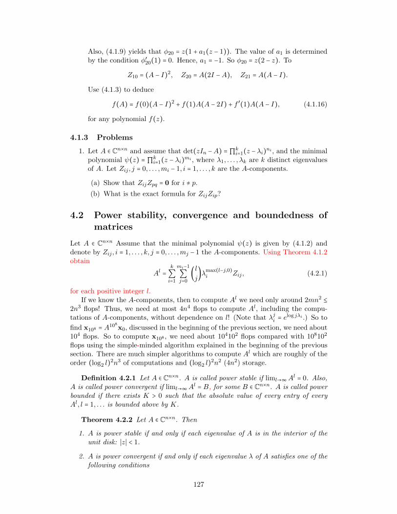
Also, (4.1.9) yields that φ20 = z(1 + a1(z − 1)). The value of a1 is determinedby the condition φ′20(1) = 0. Hence, a1 = −1. So φ20 = z(2 − z). To
Z10 = (A − I)2, Z20 = A(2I −A), Z21 = A(A − I).
Use (4.1.3) to deduce
f(A) = f(0)(A − I)2 + f(1)A(A − 2I) + f ′(1)A(A − I), (4.1.16)
for any polynomial f(z).
4.1.3 Problems
1. Let A ∈ Cn×n and assume that det(zIn −A) =∏ki=1(z −λi)ni , and the minimal
polynomial ψ(z) = ∏ki=1(z − λi)mi , where λ1, . . . , λk are k distinct eigenvalues
of A. Let Zij , j = 0, . . . ,mi − 1, i = 1, . . . , k are the A-components.
(a) Show that ZijZpq = 0 for i ≠ p.(b) What is the exact formula for ZijZip?
4.2 Power stability, convergence and boundedness ofmatrices
Let A ∈ Cn×n Assume that the minimal polynomial ψ(z) is given by (4.1.2) anddenote by Zij , i = 1, . . . , k, j = 0, . . . ,mj − 1 the A-components. Using Theorem 4.1.2obtain
Al =k
∑i=1
mi−1
∑j=0
(lj)λmax(l−j,0)
i Zij , (4.2.1)
for each positive integer l.If we know the A-components, then to compute Al we need only around 2mn2 ≤
2n3 flops! Thus, we need at most 4n4 flops to compute Al, including the compu-tations of A-components, without dependence on l! (Note that λji = elog jλi .) So to
find x108 = A108x0, discussed in the beginning of the previous section, we need about104 flops. So to compute x108 , we need about 104102 flops compared with 108102
flops using the simple-minded algorithm explained in the beginning of the previoussection. There are much simpler algorithms to compute Al which are roughly of theorder (log2 l)2n3 of computations and (log2 l)2n2 (4n2) storage.
Definition 4.2.1 Let A ∈ Cn×n. A is called power stable if liml→∞Al = 0. Also,
A is called power convergent if liml→∞Al = B, for some B ∈ Cn×n. A is called power
bounded if there exists K > 0 such that the absolute value of every entry of everyAl, l = 1, . . . is bounded above by K.
Theorem 4.2.2 Let A ∈ Cn×n. Then
1. A is power stable if and only if each eigenvalue of A is in the interior of theunit disk: ∣z∣ < 1.
2. A is power convergent if and only if each eigenvalue λ of A satisfies one of thefollowing conditions
127
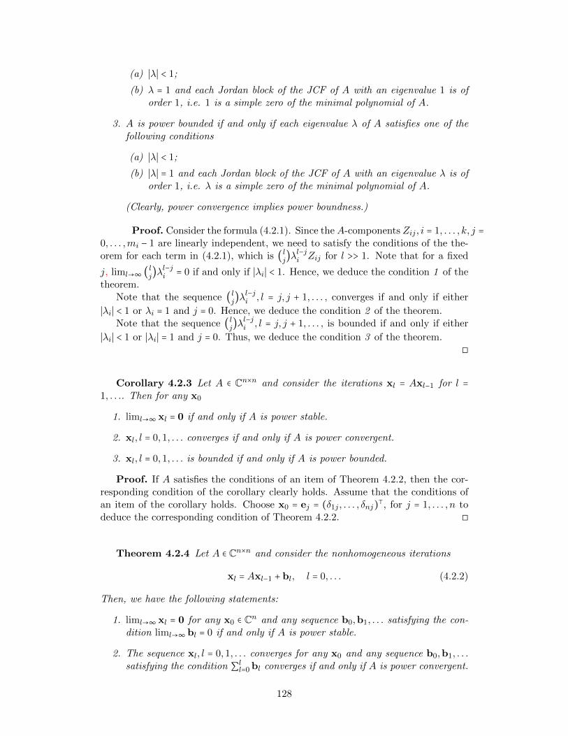
(a) ∣λ∣ < 1;
(b) λ = 1 and each Jordan block of the JCF of A with an eigenvalue 1 is oforder 1, i.e. 1 is a simple zero of the minimal polynomial of A.
3. A is power bounded if and only if each eigenvalue λ of A satisfies one of thefollowing conditions
(a) ∣λ∣ < 1;
(b) ∣λ∣ = 1 and each Jordan block of the JCF of A with an eigenvalue λ is oforder 1, i.e. λ is a simple zero of the minimal polynomial of A.
(Clearly, power convergence implies power boundness.)
Proof. Consider the formula (4.2.1). Since theA-components Zij , i = 1, . . . , k, j =0, . . . ,mi − 1 are linearly independent, we need to satisfy the conditions of the the-orem for each term in (4.2.1), which is (l
j)λl−ji Zij for l >> 1. Note that for a fixed
j, liml→∞ (lj)λl−ji = 0 if and only if ∣λi∣ < 1. Hence, we deduce the condition 1 of the
theorem.Note that the sequence (l
j)λl−ji , l = j, j + 1, . . . , converges if and only if either
∣λi∣ < 1 or λi = 1 and j = 0. Hence, we deduce the condition 2 of the theorem.Note that the sequence (l
j)λl−ji , l = j, j + 1, . . . , is bounded if and only if either
∣λi∣ < 1 or ∣λi∣ = 1 and j = 0. Thus, we deduce the condition 3 of the theorem.◻
Corollary 4.2.3 Let A ∈ Cn×n and consider the iterations xl = Axl−1 for l =1, . . .. Then for any x0
1. liml→∞ xl = 0 if and only if A is power stable.
2. xl, l = 0,1, . . . converges if and only if A is power convergent.
3. xl, l = 0,1, . . . is bounded if and only if A is power bounded.
Proof. If A satisfies the conditions of an item of Theorem 4.2.2, then the cor-responding condition of the corollary clearly holds. Assume that the conditions ofan item of the corollary holds. Choose x0 = ej = (δ1j , . . . , δnj)⊺, for j = 1, . . . , n todeduce the corresponding condition of Theorem 4.2.2. ◻
Theorem 4.2.4 Let A ∈ Cn×n and consider the nonhomogeneous iterations
xl = Axl−1 + bl, l = 0, . . . (4.2.2)
Then, we have the following statements:
1. liml→∞ xl = 0 for any x0 ∈ Cn and any sequence b0,b1, . . . satisfying the con-dition liml→∞ bl = 0 if and only if A is power stable.
2. The sequence xl, l = 0,1, . . . converges for any x0 and any sequence b0,b1, . . .satisfying the condition ∑ll=0 bl converges if and only if A is power convergent.
128
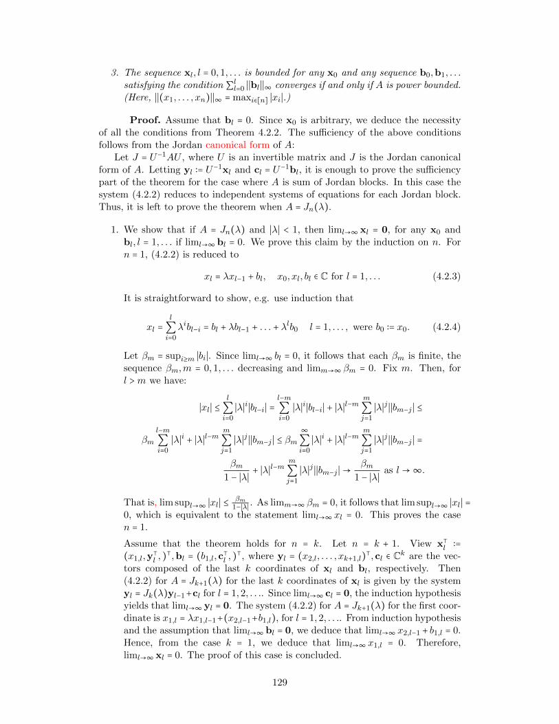
3. The sequence xl, l = 0,1, . . . is bounded for any x0 and any sequence b0,b1, . . .satisfying the condition ∑ll=0 ∣∣bl∣∣∞ converges if and only if A is power bounded.(Here, ∣∣(x1, . . . , xn)∣∣∞ = maxi∈[n] ∣xi∣.)
Proof. Assume that bl = 0. Since x0 is arbitrary, we deduce the necessityof all the conditions from Theorem 4.2.2. The sufficiency of the above conditionsfollows from the Jordan canonical form of A:
Let J = U−1AU , where U is an invertible matrix and J is the Jordan canonicalform of A. Letting yl ∶= U−1xl and cl = U−1bl, it is enough to prove the sufficiencypart of the theorem for the case where A is sum of Jordan blocks. In this case thesystem (4.2.2) reduces to independent systems of equations for each Jordan block.Thus, it is left to prove the theorem when A = Jn(λ).
1. We show that if A = Jn(λ) and ∣λ∣ < 1, then liml→∞ xl = 0, for any x0 andbl, l = 1, . . . if liml→∞ bl = 0. We prove this claim by the induction on n. Forn = 1, (4.2.2) is reduced to
xl = λxl−1 + bl, x0, xl, bl ∈ C for l = 1, . . . (4.2.3)
It is straightforward to show, e.g. use induction that
xl =l
∑i=0
λibl−i = bl + λbl−1 + . . . + λlb0 l = 1, . . . , were b0 ∶= x0. (4.2.4)
Let βm = supi≥m ∣bi∣. Since liml→∞ bl = 0, it follows that each βm is finite, thesequence βm,m = 0,1, . . . decreasing and limm→∞ βm = 0. Fix m. Then, forl >m we have:
∣xl∣ ≤l
∑i=0
∣λ∣i∣bl−i∣ =l−m∑i=0
∣λ∣i∣bl−i∣ + ∣λ∣l−mm
∑j=1
∣λ∣j ∣∣bm−j ∣ ≤
βml−m∑i=0
∣λ∣i + ∣λ∣l−mm
∑j=1
∣λ∣j ∣∣bm−j ∣ ≤ βm∞∑i=0
∣λ∣i + ∣λ∣l−mm
∑j=1
∣λ∣j ∣∣bm−j ∣ =
βm1 − ∣λ∣ + ∣λ∣l−m
m
∑j=1
∣λ∣j ∣∣bm−j ∣→βm
1 − ∣λ∣ as l →∞.
That is, lim supl→∞ ∣xl∣ ≤ βm1−∣λ∣ . As limm→∞ βm = 0, it follows that lim supl→∞ ∣xl∣ =
0, which is equivalent to the statement liml→∞ xl = 0. This proves the casen = 1.
Assume that the theorem holds for n = k. Let n = k + 1. View x⊺l ∶=(x1,l,y
⊺l , )
⊺,bl = (b1,l,c⊺l , )⊺, where yl = (x2,l, . . . , xk+1,l)⊺,cl ∈ Ck are the vec-
tors composed of the last k coordinates of xl and bl, respectively. Then(4.2.2) for A = Jk+1(λ) for the last k coordinates of xl is given by the systemyl = Jk(λ)yl−1+cl for l = 1,2, . . .. Since liml→∞ cl = 0, the induction hypothesisyields that liml→∞ yl = 0. The system (4.2.2) for A = Jk+1(λ) for the first coor-dinate is x1,l = λx1,l−1+(x2,l−1+b1,l), for l = 1,2, . . .. From induction hypothesisand the assumption that liml→∞ bl = 0, we deduce that liml→∞ x2,l−1 + b1,l = 0.Hence, from the case k = 1, we deduce that liml→∞ x1,l = 0. Therefore,liml→∞ xl = 0. The proof of this case is concluded.
129
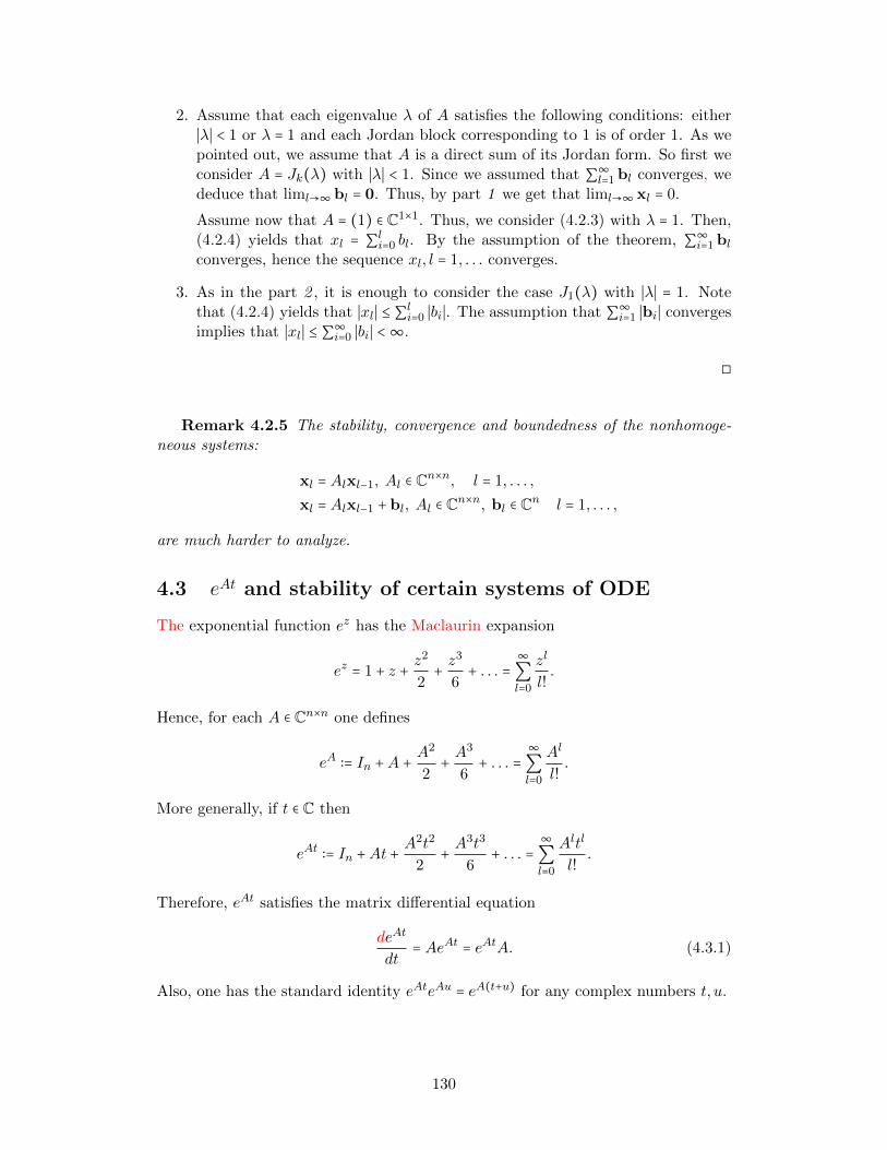
2. Assume that each eigenvalue λ of A satisfies the following conditions: either∣λ∣ < 1 or λ = 1 and each Jordan block corresponding to 1 is of order 1. As wepointed out, we assume that A is a direct sum of its Jordan form. So first weconsider A = Jk(λ) with ∣λ∣ < 1. Since we assumed that ∑∞
l=1 bl converges, wededuce that liml→∞ bl = 0. Thus, by part 1 we get that liml→∞ xl = 0.
Assume now that A = (1) ∈ C1×1. Thus, we consider (4.2.3) with λ = 1. Then,(4.2.4) yields that xl = ∑li=0 bl. By the assumption of the theorem, ∑∞
i=1 blconverges, hence the sequence xl, l = 1, . . . converges.
3. As in the part 2 , it is enough to consider the case J1(λ) with ∣λ∣ = 1. Notethat (4.2.4) yields that ∣xl∣ ≤ ∑li=0 ∣bi∣. The assumption that ∑∞
i=1 ∣bi∣ convergesimplies that ∣xl∣ ≤ ∑∞
i=0 ∣bi∣ <∞.
◻
Remark 4.2.5 The stability, convergence and boundedness of the nonhomoge-neous systems:
xl = Alxl−1, Al ∈ Cn×n, l = 1, . . . ,
xl = Alxl−1 + bl, Al ∈ Cn×n, bl ∈ Cn l = 1, . . . ,
are much harder to analyze.
4.3 eAt and stability of certain systems of ODE
The exponential function ez has the Maclaurin expansion
ez = 1 + z + z2
2+ z
3
6+ . . . =
∞∑l=0
zl
l!.
Hence, for each A ∈ Cn×n one defines
eA ∶= In +A + A2
2+ A
3
6+ . . . =
∞∑l=0
Al
l!.
More generally, if t ∈ C then
eAt ∶= In +At +A2t2
2+ A
3t3
6+ . . . =
∞∑l=0
Altl
l!.
Therefore, eAt satisfies the matrix differential equation
deAt
dt= AeAt = eAtA. (4.3.1)
Also, one has the standard identity eAteAu = eA(t+u) for any complex numbers t, u.
130
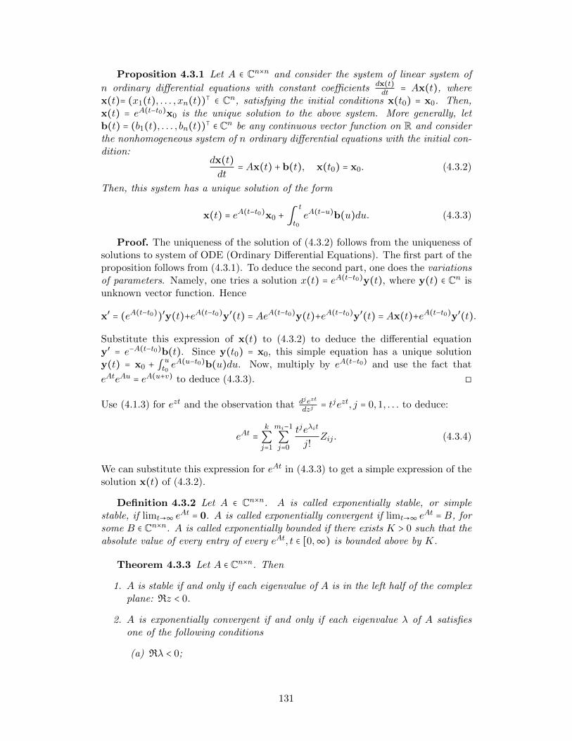
Proposition 4.3.1 Let A ∈ Cn×n and consider the system of linear system of
n ordinary differential equations with constant coefficientsdx(t)dt = Ax(t), where
x(t)= (x1(t), . . . , xn(t))⊺ ∈ Cn, satisfying the initial conditions x(t0) = x0. Then,x(t) = eA(t−t0)x0 is the unique solution to the above system. More generally, letb(t) = (b1(t), . . . , bn(t))⊺ ∈ Cn be any continuous vector function on R and considerthe nonhomogeneous system of n ordinary differential equations with the initial con-dition:
dx(t)dt
= Ax(t) + b(t), x(t0) = x0. (4.3.2)
Then, this system has a unique solution of the form
x(t) = eA(t−t0)x0 + ∫t
t0eA(t−u)b(u)du. (4.3.3)
Proof. The uniqueness of the solution of (4.3.2) follows from the uniqueness ofsolutions to system of ODE (Ordinary Differential Equations). The first part of theproposition follows from (4.3.1). To deduce the second part, one does the variationsof parameters. Namely, one tries a solution x(t) = eA(t−t0)y(t), where y(t) ∈ Cn isunknown vector function. Hence
x′ = (eA(t−t0))′y(t)+eA(t−t0)y′(t) = AeA(t−t0)y(t)+eA(t−t0)y′(t) = Ax(t)+eA(t−t0)y′(t).
Substitute this expression of x(t) to (4.3.2) to deduce the differential equationy′ = e−A(t−t0)b(t). Since y(t0) = x0, this simple equation has a unique solutiony(t) = x0 + ∫ ut0 e
A(u−t0)b(u)du. Now, multiply by eA(t−t0) and use the fact that
eAteAu = eA(u+v) to deduce (4.3.3). ◻
Use (4.1.3) for ezt and the observation that djezt
dzj= tjezt, j = 0,1, . . . to deduce:
eAt =k
∑j=1
mi−1
∑j=0
tjeλit
j!Zij . (4.3.4)
We can substitute this expression for eAt in (4.3.3) to get a simple expression of thesolution x(t) of (4.3.2).
Definition 4.3.2 Let A ∈ Cn×n. A is called exponentially stable, or simplestable, if limt→∞ eAt = 0. A is called exponentially convergent if limt→∞ eAt = B, forsome B ∈ Cn×n. A is called exponentially bounded if there exists K > 0 such that theabsolute value of every entry of every eAt, t ∈ [0,∞) is bounded above by K.
Theorem 4.3.3 Let A ∈ Cn×n. Then
1. A is stable if and only if each eigenvalue of A is in the left half of the complexplane: Rz < 0.
2. A is exponentially convergent if and only if each eigenvalue λ of A satisfiesone of the following conditions
(a) Rλ < 0;
131
(b) λ = 2πli, for some integer l, and each Jordan block of the JCF of A withan eigenvalue λ is of order 1, i.e. λ is a simple zero of the minimalpolynomial of A.
3. A is exponentially bounded if and only if each eigenvalue λ of A satisfies oneof the following conditions
(a) Rλ < 0;
(b) Rλ = 0 and each Jordan block of the JCF of A with an eigenvalue λ is oforder 1, i.e. λ is a simple zero of the minimal polynomial of A.
Proof. Consider the formula (4.3.4). Since theA-components Zij , i = 1, . . . , k, j =0, . . . ,mi−1 are linearly independent, we need to satisfy the conditions of the theoremfor each term in (4.3.4), which is tj
j! eλitZij . Note that for a fixed j, limt→∞
tj
j! eλit = 0
if and only if Rλi < 0. Hence, we deduce the condition 1 of the theorem.Note that the function tj
j! eλit converges as t → ∞ if and only if either Rλi < 0 or
eλi = 1 and j = 0. Hence, we deduce the condition 2 of the theorem.Note that the function tj
j! eλit is bounded for t ≥ 0 if and only if either Rλi < 0 or
∣eλi ∣ = 1 and j = 0. Hence, we deduce the condition 3 of the theorem. ◻
Corollary 4.3.4 Let A ∈ Cn×n and consider the system of differential equationsdx(t)dt = Ax(t),x(t0) = x0. Then, for any x0
1. limt→∞ x(t) = 0 if and only if A is stable.
2. x(t) converges as t→∞ if and only if A is exponentially convergent.
3. x(t), t ∈ [0,∞) is bounded if and only if A is exponentially bounded.
Theorem 4.3.5 Let A ∈ Cn×n and consider the system of differential equations(4.3.2). Then, for any x0 ∈ Cn, we have the following statements:
1. limt→∞ x(t) = 0, for any continuous function b(t), such that limt→∞ b(t) = 0,if and only if A is stable.
2. x(t) converges as t→∞, for any continuous function b(t), such that ∫ ∞t0 b(u)duconverges, if and only if A is exponentially convergent.
3. x(t), t ∈ [0,∞) is bounded for any continuous function b(t), such that ∫ ∞t0 ∣b(u)∣duconverges if and only if A is exponentially bounded.
Proof. It is left as Problem 4.3.2-2.
4.3.1 Worked-out Problems
1. Let B = [bij]ni,j=1 ∈ Rn×n and assume that each entry of B in non-negative.Assume that there exists a vector u = (u1, . . . , un)⊺ with positive coordinatessuch that Bu = u.
(a) Show that Bk = [b(k)ij ]ni,j=1 has non-negative entries for each k ∈ N.
132
(b) Show that b(k)ij ≤ ui
uj, for i, j = 1, . . . , n and k ∈ N.
(c) Show that each eigenvalue of B satisfies ∣λ∣ ≤ 1.
(d) Suppose that λ is an eigenvalue of B and ∣λ∣ = 1. What is the multiplicityof λ in the minimal polynomial of B?
Solution:
(a) It is immediate as It is clear since B is a non-negative matrix.
(b) Since Bu = u, by induction on k, we can show that Bku = u, for any
k ∈ N. Now, we have ui = ∑np=1 b(k)ip up ≥ b
(k)ij uj , for all 1 ≤ i, j ≤ n. Then
bij ≤ uiuj
.
(c) According to part (b), B is power bounded. The statement is immediatefrom the third part of Theorem 4.2.2.
(d) According to the third part of Theorem 4.2.2, λ would be a simple zeroof the minimal polynomial of B.
4.3.2 Problems
1. Consider the nonhomogeneous system xl = Alxl−1, Al ∈ Cn×n, l = 1, . . ..Assume that the sequence Al, l = 1, . . . , is periodic, i.e. Al+p = Al for alll = 1, . . . , and a fixed positive integer p.
(a) Show that for each x0 ∈ Cn liml→∞ xl = 0 if and only if B ∶= ApAp−1 . . .A1
is power stable.
(b) Show that for each x0 ∈ Cn the sequence xl, l = 1, . . . , converges if andonly if the following conditions satisfy. First, B is power convergent, i.e.liml→∞B
l = C. Second, AiC = C, for i = 1, . . . , p.
(c) Find a necessary and sufficient conditions such that for each x0 ∈ Cn thesequence xl, l = 1, . . . ,, is bounded.
2. Prove Theorem 4.3.5.
3. For any A ∈ Fn×n, prove that det eA = etrA.
4. Let A ∈ Rn×n and P ∈ GL(n,R). Prove that eP−1AP = P −1eAP .
133
Chapter 5
Inner product spaces
Through this chapter, we assume that F is either the real field or complex field andV is a vector space over F. (Unless stated otherwise.) Assume that T ∈ L(U,V).We abbreviate T (x) to Tx and no ambiguity will arise.
5.1 Inner product
In this section, we shall study a certain type of scalar-valued function on pairs ofvectors, known as an inner product. The first example of an inner product is thedot product in R3. The dot product of x = (x1, x2, x3) and y = (y1, y2, y3) in R3
is the scalar ∑3i=1 xiyi. Geometrically, this scalar is the product of the length of x,
the length of y and the cosine of the angle between x and y. Then, we can definelength and angle in R3 algebraically. An inner product on a vector space is thegeneralization of the dot product. This section deals with inner product and itsproperties. Then, we may turn to discuss length and angle (orthogonality).
Definition 5.1.1 The function ⟨⋅, ⋅⟩ ∶ V × V → F is called an inner product ifthe following conditions hold for any x,y,z ∈ V and a ∈ F:
(i) Conjugate symmetry:⟨x,y⟩ = ⟨y,x⟩,
(ii) Linearity in the first argument:⟨ax + y,z⟩ = a⟨x,z⟩ + ⟨y,z⟩,
(iii) Positive-definiteness:⟨x,x⟩ ⩾ 0⟨x,x⟩ = 0 if and only if x = 0.
If the second condition in positive-definiteness is dropped, the resulting structureis called a semi-inner product. Other standard properties of inner products arementioned in Problems 5.7.2-1 and 5.7.2-2.The vector space V endowed with the inner product ⟨⋅, ⋅⟩ is called the inner productspace. We will use the abbreviation IPS for inner product space.
Example 5.1.2 On Rn we have the standard inner product (the dot product)defined by ⟨x,y⟩ = ∑ni=1 xi,yi, where x = (x1, . . . , xn) ∈ Rn and y = (y1, . . . , yn) ∈ Rn.
134
Note that inner product generalizes the notion of the dot product of vectors in Rn.
Example 5.1.3 On Cn we have the standard inner product defined by ⟨x,y⟩ =∑ni=1 xi,yi, where x = (x1, . . . , xn) ∈ Cn and y = (y1, . . . , yn) ∈ Cn.
Example 5.1.4 Let V = Fn×n. For A = [aij] and B = [bij] ∈ V, define innerproduct
⟨A,B⟩ =∑i,j
aijbij .
Define conjugate transpose B∗ = (B)⊺. Then
⟨A,B⟩ = trB∗A.
Example 5.1.5 (Integration) Let V be the vector space of all F-value contin-uous functions on [0,1]. For f, g ∈ V, define
⟨f, g⟩ = ∫1
0fgdt.
This is an inner product on V. In some context, this is called L2 inner productspace. This can be done in any ”space” where you have an idea of integration andit comes under Measure Theory.
Matrix of Inner Product. Let e1, . . . , en be a basis of V. Let pij = ⟨ei, ej⟩ andP = [pij] ∈ Fn×n. Then, for v = x1e1 + . . . + xnen ∈ V and w = y1e1 +⋯ + ynen ∈ V wehave
⟨v,w⟩ =∑xiyjpij = (x1, . . . , xn)P⎛⎜⎜⎜⎝
y1
y2
⋮yn
⎞⎟⎟⎟⎠.
This matrix P is called the matrix of the inner product with respect to the basise1, . . . , en .
Definition 5.1.6 A function ∥ ∥ ∶ V → F is called a norm on V if it has thefollowing properties for all x,y ∈ V and a ∈ F:
(i) Positive definiteness:∥x∥ ⩾ 0∥x∥ = 0 if and only if x = 0,
(ii) Homogeneity:∥ax∥ = ∣a∣∥x∥,
(iii) Triangle inequality:∥x + y∥ ⩽ ∥x∥ + ∥y∥.
The vector space V endowed with the norm ∥ ∥ is called the normed linear space.
Note that the notion of norm generalizes the notion of length of a vector in Rn.
Example 5.1.7 On Rn we have the following norms for x = (x1, . . . ,xn) ∈ Rn:
135
(1) ∥x∥∞ = max∣x1∣, . . . , ∣xn∣,
(2) ∥x∥1 = ∣x1∣ + ∣x2∣ +⋯ + ∣xn∣,
(3) ∥x∥p = (∣x1∣p + ∣x2∣p +⋯ + ∣xn∣p)1p , (p is a real number, p ≥ 1).
The interested reader is encouraged to verify the above properties to see that (1), (2)and (3) define norms.
Note that ∥ ∥p is called the `p norm. The `2 norm is called the Euclidean norm. TheEuclidean norm on the matrix space Fm×n is called the Frobenius norm:
∥A∥F =⎛⎝∑i,j
∣aij ∣2⎞⎠
12
, A = [aij] ∈ Fm×n.
Let ∥ ∥t be a norm on Fn and A ∈ Fn. Define ∥A∥ = max∥Ax∥t; ∥x∥t = 1, x ∈ Fn.Then ∥ ∥ is a norm called operator norm induced by ∥ ∥t.The operator norm on Fm×n induced by Euclidean norm is called the spectral norm,denoted ∥ ∥∞:
∥A∥∞ = max∥Ax∥2; ∥x∥2 = 1, x ∈ Fn .
Remark 5.1.8 If ⟨ , ⟩ is an inner product, the function ∥ ∥ ∶ V → F defined as
∥x∥ = (⟨x,x⟩)12 is a norm (Why? Use Theorem 5.1.9 to justify it.). This norm is
called the induced norm by the inner product ⟨ , ⟩. Also, ∥x∥ is called the length ofx.
Also, if ∥ ∥ ∶ V → R is a norm, the metric space (V, d) defined as d(x, y) = ∥x−y∥is called the induced metric by the norm ∥ ∥.
Theorem 5.1.9 (The Cauchy-Schwarz inequality) Let V be an IPS andx,y ∈ V. Then we have
∣⟨x,y⟩∣ ≤ ∥x∥∥y∥,
with equality holds if and only if x and y are linearly dependent. Here ∥ ∥ is theinduced norm by inner product.
Proof. If either x or y is zero, the result follows. Assume that x,y ≠ 0. Then,for any real number r ∈ R,
0 ≤ ∥x + ry∥2 = ⟨x + ry,x + ry⟩= ⟨x,x⟩ + r⟨x,y⟩ + r⟨y,x⟩ + r2⟨y,y⟩= ⟨x,x⟩ + r⟨y,x⟩ + r⟨x,y⟩ + r2⟨y,y⟩≤ ⟨x,x⟩ + 2r∣⟨y,x⟩∣ + r2⟨y,y⟩ = f(r).
This implies that the quadratic polynmial f(r) must have non-positive discriminant,that is,
4∣⟨y,x⟩∣2 − 4⟨y,y⟩⟨x,x⟩ ≤ 0,
136
from which the Cauchy-Schwarz inequality follows. Moreover, if equality holds, thenthere exists an r ∈ F such that f(r) = 0, that is, 0 = ∥x + ry∥2, and so x + ry = 0,which implies that x is a scalar multiple of y. ◻
Proposition 5.1.10 Let V be a real vector space. Identify Vc with the set ofpairs (x,y), x,y ∈ V. Then, Vc is a vector space over C with
(a + ib)(x,y) ∶= a(x,y) + b(−y,x), for all a, b ∈ R, x,y ∈ V.
If V has a basis e1, ...,en over F, then (e1,0), ..., (en,0) is a basis of Vc overC. Any inner product ⟨⋅, ⋅⟩ on V over R induces the following inner product on Vc:
⟨(x,y), (u,v)⟩ = ⟨x,u⟩ + ⟨y,v⟩ + i(⟨y,u⟩ − ⟨x,v⟩), for x,y,u,v ∈ V.
We leave the proof of this proposition to the reader as Problem 5.7.2-3.
Definition 5.1.11 (Angle) Let x,y ∈ Rn be non-zero and ⟨⋅, ⋅⟩ denote the stan-dard inner product. Since ∣⟨x,y⟩∣ ≤ ∥x∥∥y∥, we can define the angle between x, y asfollows:
∠(x,y) = arccos⟨x,y⟩∥x∥∥y∥ .
In particular, vectors x and y are orthogonal (denoted by x ⊥ y) if ⟨x,y⟩ = 0. Wecan define this notion in any inner product space as follows:
Definition 5.1.12 Let V be an IPS. Then(i) x,y ∈ V are called orthogonal if ⟨x,y⟩ = 0.(ii) S,T ⊂ V are called orthogonal if ⟨x,y⟩ = 0, for any x ∈ S, y ∈ T .(iii) For any S ⊂ V, S⊥ ⊂ V denotes the maximal orthogonal set to S, i.e. S⊥ = v ∈V; ⟨v,w⟩ = 0, for all w ∈ S.(iv) x1, ...,xm⊂ V is called an orthonormal set if
⟨xi,xj⟩ = δij , (i, j = 1, ...,m),
where δij denotes the Kronecker delta.(v) x1, ...,xn⊂ V is called an orthonormal basis if it is an orthonormal set whichis a basis in V.
Note that S⊥ is always a subspace of V (even if A was not). Furthermore,
(i) 0⊥ = V,
(ii) V⊥ = 0,
(iii) S⊥ = (spanS)⊥.
137
Gram-Schmidt algorithm. Let V be an IPS and S = x1, ...,xm ⊂ V a finite(possibly empty) set. Then, S = e1, ...,ep is the orthonormal set (p ≥ 1) or theempty set (p = 0) obtained from S using the following recursive steps:(a) If x1 = 0, remove it from S. Otherwise, replace x1 by ∣∣x1∣∣−1x1.(b) Assume that x1, ...,xk is an orthonormal set and 1 ≤ k < m. Let yk+1 =xk+1 −∑ki=1⟨xk+1,xi⟩xi. If yk+1 = 0, remove xk+1 from S. Otherwise, replace xk+1
by ∣∣yk+1∣∣−1yk+1.Indeed, the Gram-Schmidt process is a method for orthonormalization of a set
of vectors in an inner product space.
Corollary 5.1.13 Let V be an IPS and S = x1, ...,xn ⊂ V be n linearly inde-pendent vectors. Then, the Gram-Schmidt algorithm on S is given as follows:
y1 ∶= x1, r11 ∶= ∣∣y1∣∣, e1 ∶=y1
r11,
rji ∶= ⟨xi,ej⟩, j = 1, ..., i − 1, (5.1.1)
pi−1 ∶=i−1
∑j=1
rjiej , yi ∶= xi − pi−1,
rii ∶= ∣∣yi∣∣, ei ∶=yirii, i = 2, ..., n.
In particular, ei ∈ Si and ∣∣yi∣∣ = dist(xi, Si−1), where Si = spanx1, ...,xi, fori = 1, ..., n and S0 = 0. (See Problem 5.7.2-4 for the definition of dist(xi, Si−1).)
Corollary 5.1.14 Any (ordered) basis in a finite dimensional IPS, V inducesan orthonormal basis by the Gram-Schmidt algorithm.
See Problem 5.7.2-4 for some known properties related to the above notions.
5.2 Explanation of G-S process in standard Euclideanspace
First observe that ri(k+1) ∶= ⟨xk+1,ei⟩ is the scalar projection of xk+1 on ei. Nextobserve that pk is the projection of xk+1 on e1, . . . ,ek = spanx1, . . . ,xk. Hence,yk+1 = xk+1 − pk ⊥ spane1, . . . ,ek. Thus, r(k+1)(k+1) = ∣∣xk+1 − pk∣∣ is the distanceof xk+1 to spane1, . . . ,ek = spanx1, . . . ,xk. The assumption that x1, . . . ,xn arelinearly independent yields that r(k+1)(k+1) > 0. Hence, ek+1 = r−1
(k+1)(k+1)(xk+1 −pk)is a vector of unit length orthogonal to e1, . . . ,ek.
138
5.3 An example of G-S process
Let x1 = (1,1,1,1)⊺,x2 = (−1,4,4,−1)⊺, x3 = (4,−2,2,0)⊺. Then
r11 = ∣∣x1∣∣ = 2,e1 =1
r11x1 = (1
2,1
2,1
2,1
2)⊺,
r12 = e⊺1x2 = 3,p1 = r12e1 = 3e1 = (3
2,3
2,3
2,3
2)⊺,
y2 = x2 − p1 = (−5
2,5
2,5
2,−5
2)⊺, r22 = ∣∣y2∣∣ = 5,
e2 =1
r22(y2) = (−1
2,1
2,1
2,−1
2)⊺,
r13 = e⊺1x3 = 2, r23 = e⊺2x3 = −2,
p2 = r13e1 + r23e2 = (2,0,0,2)⊺,y3 = x3 − p2 = (2,−2,2,−2)⊺, r33 = ∣∣y3∣∣ = 4,
e3 =1
r33(x3 − p2) = (1
2,−1
2,1
2,−1
2)⊺.
5.4 QR Factorization
A QR Factorization of a real matrix A is its decomposition into a product A =QRof unitary matrix Q and an upper triangular matrix R. QR factorization is oftenused to solve the least square problem. (Theorem 5.5.7)
Let A = [a1 a2 . . .an] ∈ Rm×n and assume that rank A = n, i.e. the columns of Aare linearly independent. Perform G-S process with the book keeping as above:
r11 ∶= ∣∣a1∣∣, e1 ∶= 1r11
a1.
Assume that e1, . . . ,ek−1 were computed. Then, rik ∶= e⊺i ak for i = 1, . . . , k − 1,pk−1 ∶= r1ke1+r2ke2+. . . r(k−1)kek−1 and rkk ∶= ∣∣ak−pk−1∣∣, ek ∶= 1
rkk(ak−pk−1),
for k = 2, ..., n.
Let Q = [e1 e2 . . .en] ∈ Rm×n and R =
⎡⎢⎢⎢⎢⎢⎢⎢⎢⎢⎣
r11 r12 r13 . . . r1n
0 r22 r23 . . . r2n
0 0 r33 . . . r3n
⋮ ⋮ ⋮ ⋮ ⋮0 0 0 . . . rnn
⎤⎥⎥⎥⎥⎥⎥⎥⎥⎥⎦Then, A = QR, Q⊺Q = In and A⊺A = R⊺R. The LSS (Least Squares Solution) of
Ax = b is given by the upper triangular system Rx = Q⊺b which can be solved byback substitution. Formally, x = R−1Q⊺b. (See Theorem 5.5.7.)
Proof. A⊺Ax = R⊺Q⊺QRx = R⊺Rx = A⊺b = R⊺Q⊺b. Multiply from left by(R⊺)−1 to get Rx = Q⊺b
Note that QQ⊺b is the projection of b on the columns space of A. The ma-trix P ∶= QQ⊺ is called an orthogonal projection. It is symmetric and P 2 = P , as(QQ⊺)(QQ⊺) = Q(Q⊺Q)Q⊺ = Q(I)Q⊺ = QQ⊺. Note that QQ⊺ ∶ Rm → Rm is theorthogonal projection.
The assumption that rank A = n is equivalent to the assumption that A⊺A isinvertible. So, the LSS A⊺Ax = A⊺b has unique solution x = (A⊺A)−1b. Hence, theprojection of b on the column space of A is Pb = Ax = A(A⊺A)−1A⊺b. Therefore,P = A(A⊺A)−1A⊺.
139
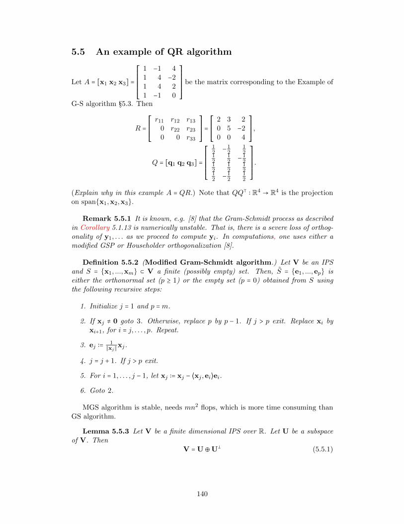
5.5 An example of QR algorithm
Let A = [x1 x2 x3] =
⎡⎢⎢⎢⎢⎢⎢⎢⎣
1 −1 41 4 −21 4 21 −1 0
⎤⎥⎥⎥⎥⎥⎥⎥⎦
be the matrix corresponding to the Example of
G-S algorithm §5.3. Then
R =⎡⎢⎢⎢⎢⎢⎣
r11 r12 r13
0 r22 r23
0 0 r33
⎤⎥⎥⎥⎥⎥⎦=⎡⎢⎢⎢⎢⎢⎣
2 3 20 5 −20 0 4
⎤⎥⎥⎥⎥⎥⎦,
Q = [q1 q2 q3] =
⎡⎢⎢⎢⎢⎢⎢⎢⎣
12 −1
212
12
12 −1
212
12
12
12 −1
212
⎤⎥⎥⎥⎥⎥⎥⎥⎦
.
(Explain why in this example A = QR.) Note that QQ⊺ ∶ R4 → R4 is the projectionon spanx1,x2,x3.
Remark 5.5.1 It is known, e.g. [8] that the Gram-Schmidt process as describedin Corollary 5.1.13 is numerically unstable. That is, there is a severe loss of orthog-onality of y1, . . . as we proceed to compute yi. In computations, one uses either amodified GSP or Householder orthogonalization [8].
Definition 5.5.2 (Modified Gram-Schmidt algorithm.) Let V be an IPSand S = x1, ...,xm ⊂ V a finite (possibly empty) set. Then, S = e1, ...,ep iseither the orthonormal set (p ≥ 1) or the empty set (p = 0) obtained from S usingthe following recursive steps:
1. Initialize j = 1 and p =m.
2. If xj ≠ 0 goto 3. Otherwise, replace p by p − 1. If j > p exit. Replace xi byxi+1, for i = j, . . . , p. Repeat.
3. ej ∶= 1∥xj∥xj.
4. j = j + 1. If j > p exit.
5. For i = 1, . . . , j − 1, let xj ∶= xj − ⟨xj ,ei⟩ei.
6. Goto 2.
MGS algorithm is stable, needs mn2 flops, which is more time consuming thanGS algorithm.
Lemma 5.5.3 Let V be a finite dimensional IPS over R. Let U be a subspaceof V. Then
V = U⊕U⊥ (5.5.1)
140
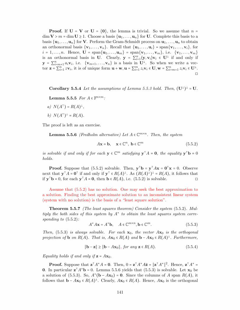
Proof. If U = V or U = 0, the lemma is trivial. So we assume that n =dimV >m = dimU ≥ 1. Choose a basis u1, . . . ,un for U. Complete this basis to abasis u1, . . . ,un for V. Perform the Gram-Schmidt process on u1, . . . ,un to obtainan orthonormal basis v1, . . . ,vn. Recall that u1, . . . ,ui = spanv1, . . . ,vi, fori = 1, . . . , n. Hence, U = spanu1, . . . ,um = spanv1, . . . ,vm, i.e. v1, . . . ,vmis an orthonormal basis in U. Clearly, y = ∑ni=1⟨y,vi⟩vi ∈ U⊥ if and only ify = ∑ni=m+1 aivi, i.e. vm+1, . . . ,vn is a basis in U⊥. So when we write a vec-tor z = ∑ni=1 zvi, it is of unique form u +w,u = ∑mi=1 zivi ∈ U,w = ∑ni=m+1 zivi ∈ U⊥.
◻
Corollary 5.5.4 Let the assumptions of Lemma 5.5.3 hold. Then, (U⊥)⊥ = U.
Lemma 5.5.5 For A ∈ Fn×m:
a) N(A⊺) = R(A)⊥,
b) N(A⊺)⊥ = R(A).
The proof is left as an exercise.
Lemma 5.5.6 (Fredholm alternative) Let A ∈ Cm×n. Then, the system
Ax = b, x ∈ Cn, b ∈ Cm (5.5.2)
is solvable if and only if for each y ∈ Cm satisfying y⊺A = 0, the equality y⊺b = 0holds.
Proof. Suppose that (5.5.2) solvable. Then, y⊺b = y⊺Ax = 0⊺x = 0. Observenext that y⊺A = 0⊺ if and only if y⊺ ∈ R(A)⊥. As (R(A)⊥)⊥ = R(A), it follows thatif y⊺b = 0, for each y⊺A = 0, then b ∈ R(A), i.e. (5.5.2) is solvable. ◻
Assume that (5.5.2) has no solution. One may seek the best approximation toa solution. Finding the best approximate solution to an inconsistent linear system(system with no solution) is the basis of a “least square solution”.
Theorem 5.5.7 (The least squares theorem) Consider the system (5.5.2). Mul-tiply the both sides of this system by A∗ to obtain the least squares system corre-sponding to (5.5.2):
A∗Ax = A∗b, A ∈ Cm×n,b ∈ Cm. (5.5.3)
Then, (5.5.3) is always solvable. For each x0, the vector Ax0 is the orthogonalprojection of b on R(A). That is, Ax0 ∈ R(A) and b −Ax0 ∈ R(A)⊥. Furthermore,
∥b − z∥ ≥ ∥b −Ax0∥, for any z ∈ R(A). (5.5.4)
Equality holds if and only if z = Ax0.
Proof. Suppose that z⊺A∗A = 0. Then, 0 = z⊺A∗Az = ∥z⊺A∗∥2. Hence, z⊺A∗ =0. In particular z⊺A∗b = 0. Lemma 5.5.6 yields that (5.5.3) is solvable. Let x0 bea solution of (5.5.3). So, A∗(b −Ax0) = 0. Since the columns of A span R(A), itfollows that b −Ax0 ∈ R(A)⊥. Clearly, Ax0 ∈ R(A). Hence, Ax0 is the orthogonal
141
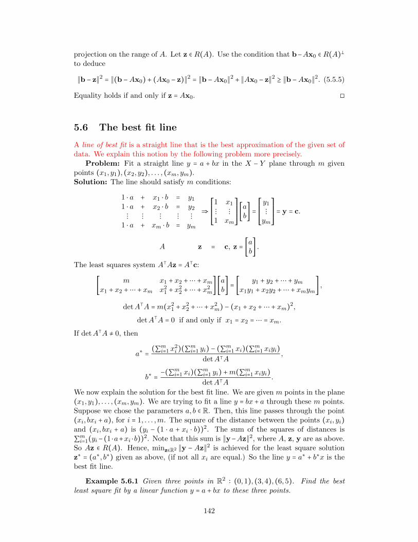
projection on the range of A. Let z ∈ R(A). Use the condition that b−Ax0 ∈ R(A)⊥to deduce
∥b − z∥2 = ∥(b −Ax0) + (Ax0 − z)∥2 = ∥b −Ax0∥2 + ∥Ax0 − z∥2 ≥ ∥b −Ax0∥2. (5.5.5)
Equality holds if and only if z = Ax0. ◻
5.6 The best fit line
A line of best fit is a straight line that is the best approximation of the given set ofdata. We explain this notion by the following problem more precisely.
Problem: Fit a straight line y = a + bx in the X − Y plane through m givenpoints (x1, y1), (x2, y2), . . . , (xm, ym).Solution: The line should satisfy m conditions:
1 ⋅ a + x1 ⋅ b = y1
1 ⋅ a + x2 ⋅ b = y2
⋮ ⋮ ⋮ ⋮ ⋮1 ⋅ a + xm ⋅ b = ym
⇒⎡⎢⎢⎢⎢⎢⎣
1 x1
⋮ ⋮1 xm
⎤⎥⎥⎥⎥⎥⎦[ab] =
⎡⎢⎢⎢⎢⎢⎣
y1
⋮ym
⎤⎥⎥⎥⎥⎥⎦= y = c.
A z = c, z = [ab] .
The least squares system A⊺Az = A⊺c:
[ m x1 + x2 +⋯ + xmx1 + x2 +⋯ + xm x2
1 + x22 +⋯ + x2
m] [ab] = [ y1 + y2 +⋯ + ym
x1y1 + x2y2 +⋯ + xmym] ,
detA⊺A =m(x21 + x2
2 +⋯ + x2m) − (x1 + x2 +⋯ + xm)2,
detA⊺A = 0 if and only if x1 = x2 = ⋯ = xm.If detA⊺A ≠ 0, then
a∗ = (∑mi=1 x2i )(∑mi=1 yi) − (∑mi=1 xi)(∑mi=1 xiyi)
detA⊺A,
b∗ = −(∑mi=1 xi)(∑mi=1 yi) +m(∑mi=1 xiyi)detA⊺A
.
We now explain the solution for the best fit line. We are given m points in the plane(x1, y1), . . . , (xm, ym). We are trying to fit a line y = bx+ a through these m points.Suppose we chose the parameters a, b ∈ R. Then, this line passes through the point(xi, bxi + a), for i = 1, . . . ,m. The square of the distance between the points (xi, yi)and (xi, bxi + a) is (yi − (1 ⋅ a + xi ⋅ b))2. The sum of the squares of distances is
∑mi=1(yi−(1 ⋅a+xi ⋅b))2. Note that this sum is ∥y−Az∥2, where A, z, y are as above.So Az ∈ R(A). Hence, minz∈R2 ∥y − Az∥2 is achieved for the least square solutionz∗ = (a∗, b∗) given as above, (if not all xi are equal.) So the line y = a∗ + b∗x is thebest fit line.
Example 5.6.1 Given three points in R2 ∶ (0,1), (3,4), (6,5). Find the bestleast square fit by a linear function y = a + bx to these three points.
142
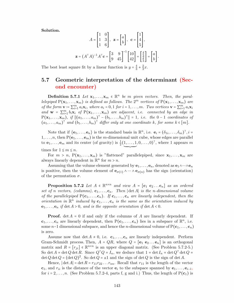
Solution.
A =⎡⎢⎢⎢⎢⎢⎣
1 01 31 6
⎤⎥⎥⎥⎥⎥⎦, z = [a
b] , c =
⎡⎢⎢⎢⎢⎢⎣
145
⎤⎥⎥⎥⎥⎥⎦,
z = (A⊺A)−1A⊺c = [3 99 45
]−1
[1042
] = [4323
] = [ab] .
The best least square fit by a linear function is y = 43 +
23x.
5.7 Geometric interpretation of the determinant (Sec-ond encounter)
Definition 5.7.1 Let x1, . . . ,xm ∈ Rn be m given vectors. Then, the paral-lelepiped P(x1, . . . ,xm) is defined as follows. The 2m vertices of P(x1, . . . ,xm) areof the form v ∶= ∑mi=1 aixi, where ai = 0,1 for i = 1, . . . ,m. Two vertices v = ∑mi=1 aixiand w = ∑mi=1 bixi of P(x1, . . . ,xm) are adjacent, i.e. connected by an edge inP(x1, . . . ,xm), if ∣∣(a1, . . . , am)⊺ − (b1, . . . , bm)⊺∣∣ = 1, i.e. the 0 − 1 coordinates of(a1, . . . , am)⊺ and (b1, . . . , bm)⊺ differ only at one coordinate k, for some k ∈ [m].
Note that if e1, . . . ,en is the standard basis in Rn, i.e. ei = (δ1i, . . . , δni)⊺, i =1, . . . , n, then P(e1, . . . ,em) is the m-dimensional unit cube, whose edges are parallelto e1, . . . ,em and its center (of gravity) is 1
2(1, . . . ,1´¹¹¹¹¹¹¹¹¹¸¹¹¹¹¹¹¹¹¹¶,0, . . . ,0)⊺, where 1 appears m
times for 1 ≤m ≤ n.For m > n, P(x1, . . . ,xm) is ”flattened” parallelepiped, since x1, . . . ,xm are
always linearly dependent in Rn for m > n.Assuming that the volume element generated by e1, . . . ,en, denoted as e1∧⋯∧en
is positive, then the volume element of eσ(1) ∧ ⋯ ∧ eσ(n) has the sign (orientation)of the permutation σ.
Proposition 5.7.2 Let A ∈ Rn×n and view A = [c1 c2 . . .cn] as an orderedset of n vectors, (columns), c1, . . . ,cn. Then ∣detA∣ is the n-dimensional volumeof the parallelepiped P(c1, . . . ,cn). If c1, . . . ,cn are linearly independent, then theorientation in Rn induced by c1, . . . ,cn is the same as the orientation induced bye1, . . . ,en if detA > 0, and is the opposite orientation if detA < 0.
Proof. detA = 0 if and only if the columns of A are linearly dependent. Ifc1, . . . ,cn are linearly dependent, then P(c1, . . . ,cn) lies in a subspace of Rn, i.e.some n−1 dimensional subspace, and hence the n-dimensional volume of P(c1, . . . ,cn)is zero.
Assume now that detA ≠ 0, i.e. c1, . . . ,cn are linearly independent. PerformGram-Schmidt process. Then, A = QR, where Q = [e1 e2 . . .en] is an orthogonalmatrix and R = [rji] ∈ Rn×n is an upper diagonal matrix. (See Problem 5.7.2-5.)So detA = detQdetR. Since Q⊺Q = In, we deduce that 1 = det In = detQ⊺ detQ =detQdetQ = (detQ)2. So detQ = ±1 and the sign of detQ is the sign of detA.
Hence, ∣detA∣ = detR = r11r22 . . . rnn. Recall that r11 is the length of the vectorc1, and rii is the distance of the vector ei to the subspace spanned by e1, . . . ,ei−1,for i = 2, . . . , n. (See Problem 5.7.2-4, parts f, g and i.) Thus, the length of P(c1) is
143
r11. The distance of c2 to P(c1) is r22. Thus, the area, i.e. 2-dimensional volume ofP(c1,c2) is r11r22. Continuing in this manner we deduce that the i − 1 dimensionalvolume of P(c1, . . . ,ci−1) is r11 . . . r(i−1)(i−1). As the distance of ci to P(c1, . . . ,ci−1)is rii, it follows that the i-dimensional volume of P(c1, . . . ,ci) is r11 . . . rii. Fori = n, we get that ∣detA∣ = r11 . . . rnn, which is equal to the n-dimensional volumeof P(c1, . . . , cn).
As we already pointed out, the sign of detA is equal to the sign of detQ = ±1. IfdetQ = 1, it is possible to ”rotate” the standard basis in Rn to the basis given by thecolumns of an orthogonal matrix Q with detQ = 1. If detQ = −1, we need one reflec-tion, i.e. replace the standard basis e1, . . . ,en by the new basis e2,e1,e3, . . . ,enand rotate the new basis e2,e1,e3, . . . ,en to the basis consisting of the columnsof an orthogonal matrix Q′, where detQ′ = 1. ◻
Theorem 5.7.3 (The Hadamard determinant inequality) Let A = [c1, . . . ,cn] ∈Cn×n. Then, ∣detA∣ ≤ ∣∣c1∣∣ ∣∣c2∣∣ . . . ∣∣cn∣∣. Equality holds if and only if either ci = 0,for some i or ⟨ci,cj⟩ = 0, for all i ≠ j, i.e. c1, . . . ,cn is an orthogonal system.
Proof. Assume first that detA = 0. Clearly, the Hadamard inequality holds.Equality in Hadamard inequality holds if and only if ci = 0, for some i.
Assume now that detA ≠ 0 and perform the Gram-Schmidt process. From(5.1.1), it follows that A = QR, where Q is a unitary matrix, i.e. Q∗Q = In andR = [rji] ∈ Cn×n is upper triangular with rii real and positive numbers. So detA =detQdetR. Thus
1 = det In = detQ∗Q = detQ∗ detQ = detQdetQ = ∣detQ∣2 ⇒ ∣detQ∣ = 1.
Hence, ∣detA∣ = detR = r11r22 . . . rnn. According to Problem 5.7.2-4 and the proofof Proposition 5.7.2, we know that ∣∣ci∣∣ ≥ dist(ci, spanc1, . . . ,ci−1) = rii, for i =2, . . . , n. Hence, ∣detA∣ = detR ≤ ∣∣c1∣∣ ∣∣c2∣∣ . . . ∣∣cn∣∣. Equality holds if∣∣ci∣∣ = dist(ci, spanc1, . . . ,ci−1), for i = 2, . . . , n. Use Problem 5.7.2-4 to deducethat ∣∣ci∣∣ = dist(ci, spanc1, . . . ,ci−1) if an only if ⟨ci,cj⟩ = 0, for j = 1, . . . , i − 1.Use these conditions for i = 2, . . . to deduce that equality in Hadamard inequalityholds if and only if c1, . . . ,cn is an orthogonal system. ◻
An application of Fredholm alternative
Let A = [aij] ∈ Zn×n2 be a symmetric matrix. It has been proven in [5] that diagA ∈Im A. Here, we give Noga Alon’s short proof for this statement:
x⊺Ax =n
∑i,j=1
aijxixj = 2 ∑1≤i<j≤n
aijxixj + x⊺ diagA = x⊺ diagA.
Then, if x⊺A = 0, so x⊺ diagA = 0. The Fredholm alternative implies that diagA inthe range of A.
144
5.7.1 Worked-out Problems
1. Let A = [aij]ni,j=1 ∈ Cn×n such that ∣aij ∣ ≤ 1, for i, j = 1, . . . , n. Show that
∣detA∣ = nn2 if and only if A∗A = AA∗ = nIn.Solution:
Assume first that ∣detA∣ = nn2 and set cj =
⎡⎢⎢⎢⎢⎢⎢⎢⎣
a1j
a2j
⋮anj
⎤⎥⎥⎥⎥⎥⎥⎥⎦
. Then, Theorem 5.7.3 and
the assumption ∣aij ∣ ≤ 1 yield ∥ci∥ = √n, for any 1 ≤ i ≤ n. Reusing the
assumption ∣aij ∣ ≤ 1 follows ∣aij ∣ = 1, for i, j = 1, . . . , n. Finally, as c1, . . . ,cnis an orthogonal system, then A∗A = AA∗ = nIn.Conversely, assume that A∗A = AA∗ = nIn. We have ∣detA∣2 = detAdetA∗ =detAA∗ = detnIn = nn. Then ∣detA∣ = nn2 .
2. Let u =
⎡⎢⎢⎢⎢⎢⎢⎢⎣
1−11−1
⎤⎥⎥⎥⎥⎥⎥⎥⎦
, v =
⎡⎢⎢⎢⎢⎢⎢⎢⎣
20−21
⎤⎥⎥⎥⎥⎥⎥⎥⎦
and U = spanu,v. Find an orthogonal projection of
the matrix
⎡⎢⎢⎢⎢⎢⎢⎢⎣
1100
⎤⎥⎥⎥⎥⎥⎥⎥⎦
on U using least squares with a corresponding matrix.
Solution:
Define A =
⎡⎢⎢⎢⎢⎢⎢⎢⎣
1 2−1 01 −2−1 1
⎤⎥⎥⎥⎥⎥⎥⎥⎦
and b =
⎡⎢⎢⎢⎢⎢⎢⎢⎣
1100
⎤⎥⎥⎥⎥⎥⎥⎥⎦
. The least squares theorem implies that
the system A∗Ax = A∗b is solvable, x0 = 135 [8
2] and Ax0 ∈ R(A), i.e. Ax0 =
135
⎡⎢⎢⎢⎢⎢⎢⎢⎣
18−2−14−6
⎤⎥⎥⎥⎥⎥⎥⎥⎦
is an orthogonal projection of b.
3. Find A = [aij] ∈ C3×3 satisfying ∣aij ∣ ≤ 1 and ∣detA∣2 = 27.Solution:
Define A =⎡⎢⎢⎢⎢⎢⎣
1 1 11 ξ1 ξ2
1 ξ21 ξ2
2
⎤⎥⎥⎥⎥⎥⎦, where ξk = e
2kπ3i = cos 2kπ
3 + i sin 2kπ3 , k = 1,2. Clearly,
∣aij ∣ ≤ 1 and AA∗ = A∗A = 3In. Using Worked-out Problem 5.7.1-1, we obtain
∣detA∣ = 332 =
√27.
5.7.2 Problems
1. Let V be an IPS over F. Show that
145
(a) ⟨0,x⟩ = ⟨x,0⟩ = 0,
(b) for F = R, ⟨z, ax + by⟩ = a⟨z,x⟩ + b⟨z,y⟩, for all a, b ∈ R, x,y,z ∈ V,
(c) for F = C, ⟨z, ax + by⟩ = a⟨z,x⟩ + b⟨z,y⟩, for all a, b ∈ C, x,y,z ∈ V.
2. Let V be an IPS. Show that
(a) ∣∣ax∣∣ = ∣a∣ ∣∣x∣∣, for a ∈ F and x ∈ V.
(b) The triangle inequality
∣∣x + y∣∣ ≤ ∣∣x∣∣ + ∣∣y∣∣,
and equality holds if either x = 0 or y = ax, for some non-negative a ∈ R.(Hint: Use the Cauchy-Schwarz inequality.)(c) Pythagorean law; if x ⊥ y, then
∥x + y∥2 = ∥x∥2 + ∥y∥2.
(d) Parallelogram identity;
∥x + y∥2 + ∥x − y∥2 = 2∥x∥2 + 2∥y∥2.
3. Prove Proposition 5.1.10.
4. Let V be a finite dimensional IPS of dimension n. Assume that S ⊂ V.
(a) Show that if x1, ...,xm is an orthonormal set, then x1, ...,xm are linearlyindependent.
(b) Assume that e1, ...,en is an orthonormal basis in V. Show that for anyx ∈ V, the orthonormal expansion holds
x =n
∑i=1
⟨x,ei⟩ei. (5.7.1)
Furthermore, for any x,y ∈ V
⟨x,y⟩ =n
∑i=1
⟨x,ei⟩⟨y,ei⟩. (5.7.2)
(c) Assume that S is a finite set. Let S be the set obtained by the Gram-Schmidt process. Show that S = ∅ if and only if spanS = 0. Moreover,prove that if S ≠ ∅, then e1, ...,ep is an orthonormal basis in span S.
(d) Show that there exists an orthonormal basis e1, ...,en in V and 0 ≤m ≤ nsuch that
e1, ...,em ∈ S, span S = spane1, ...,em,S⊥ = spanem+1, ...,en,(S⊥)⊥ = spanS.
146
(e) Assume from here to the end of the problem that S is a subspace of V.Show V = S ⊕ S⊥.(f) Let x ∈ V and let x = u + v, for unique u ∈ S, v ∈ S⊥. Let P (x) ∶= u bethe projection of x on S. Show that P ∶ V → V is a linear transformationsatisfying
P 2 = P, Range P = S, Ker P = S⊥.
(g) Show that
dist(x, S) ∶= ∣∣x − Px∣∣ ≤ ∣∣x −w∣∣ for any w ∈ S,and equality holds if and only if w = Px. (5.7.3)
(h) Show in part (g) that equality holds if and only if w = Px.
(i) Show that dist(x, S) = ∣∣x − w∣∣, for some w ∈ S if and only if x − w isorthogonal to S.
(j) Let e1, . . . ,em be an orthonormal basis of S. Show that for each x ∈ V,Px = ∑pi=1⟨y,ei⟩ei.(Note that Px is called the least square approximation to x in the subspaceS.)
5. Let X ∈ Cm×n and assume that m ≥ n and rank X = n. Let x1, ...,xn ∈ Cm bethe columns of X, i.e. X = [x1, ...,xn]. Assume that Cm is an IPS with thestandard inner product < x,y >= y∗x. Perform the Gram-Schmidt algorithm(1.1) to obtain the matrix Q = [e1, ...,en] ∈ Cm×n. Let R = [rji]n1 ∈ Cn×n be theupper triangular matrix with rji, j ≤ i given by (5.1.1). Show that QTQ = Inand X = QR. (This is the QR algorithm.) Show that if in addition X ∈ Rm×n,then Q and R are real valued matrices.
6. Let C ∈ Cn×n and assume that λ1, ..., λn are n eigenvalues of C counted withtheir multiplicities. View C as an operator C ∶ Cn → Cn. View Cn as 2n-dimensional vector space over R. Let C = A +
√−1B, A,B ∈ Rn×n.
a. Then, C ∶= [ A −BB A
] ∈ R2n×2n represents the operator C ∶ Cn → Cn as an
operator over R in suitably chosen basis.
b. Show that λ1, λ1, ..., λn, λn are the 2n eigenvalues of C counting with mul-tiplicities.
c. Show that the Jordan canonical form of C is obtained by replacing eachJordan block λI +H in C by two Jordan blocks λI +H and λI +H.
7. Let A = [aij]i,j ∈ Cn×n. Assume that ∣aij ∣ ≤K, for all i, j = 1, . . . , n. Show that
∣detA∣ ≤Knnn2 .
8. Show that for each n, there exists a matrix A = [aij]ni,j=1 ∈ Cn×n such that
∣aij ∣ = 1, for i, j = 1, . . . , n and ∣detA∣ = nn2 .
9. Let A = [aij] ∈ Rn×n and assume that aij = ±1, i, j = 1, . . . , n. Show that ifn > 2, then the assumption that ∣detA∣ = nn2 yields that n is divisible by 4.
147
10. Show that for any n = 2m, m = 0,1, . . . there exists A = [aij] ∈ Rn×n such thataij = ±1, i, j = 1, . . . , n and ∣detA∣ = nn2 . (Hint : Try to prove by induction on m
that A ∈ R2m×2m can be chosen symmetric, and then construct B ∈ R2m+1×2m+1
using A.)
Note: A matrix H = [aij]i,j ∈ Rn×n such that aij = ±1, for i, j = 1, . . . , n and∣detH ∣ = nn2 is called a Hadamard matrix. Hadamard matrices admit severalother characterizations; an equivalent definition states that a Hadamard ma-trix H is an n×n matrix satisfying the identity HH⊺ = nIn. (See Worked-outProblem 5.7.1-1.) Also, another equivalent definition for a Hadamard matrixH is an n × n matrix with entries in −1,1 such that two distinct rows orcolumns have inner product zero. It is conjectured that for each n divisibleby 4, there exists a Hadamard matrix. It is known that a necessary conditionfor the existence of an n × n Hadamard matrix is that n = 1,2,4k, for somek, i.e. there exists no n × n Hadamard matrices for n /∈ 1,2,4k, k ∈ N. Thatthis condition is also sufficient is known as the Hadamard conjecture, and hasbeen the subject of a vast amount of literature in recent decades.
11. Let V be an IPS and T ∈ L(V). Assume that v,w ∈ V are two eigenvectorsof T with distinct eigenvalues. Prove that ⟨v,w⟩ = 0.
12. Consider rotation matrices A = [cos θ − sin θsin θ cos θ
] ∈ R2×2, θ ∈ [0,2π). Assume
that T ∈ L(V) is orthogonal, where V is a finite dimensional real vectorspace. Show that there exists a basis β of V such that [T ]β is block diagonal,and the blocks are either 2×2 rotation matrices or 1×1 matrices consisting of1 or -1.(See Problem 1.10.2-4 and Problem 3.2.2-17).
5.8 Special transformations in IPS
Proposition 5.8.1 Let V be an IPS and T ∶ V → V a linear transformation.Then, there exists a unique linear transformation T ∗ ∶ V → V such that ⟨Tx,y⟩ =⟨x, T ∗y⟩, for all x,y ∈ V.
We leave its proof as Problems 5.10.2-1 and 5.10.2-2.
Definition 5.8.2 Let V be an IPS and T ∶ V → V be a linear transformation.Then(a) T is called self-adjoint if T ∗ = T ;(b) T is called anti self-adjoint if T ∗ = −T ;(c) T is called unitary if T ∗T = TT ∗ = I;(d) T is called normal if T ∗T = TT ∗.
Note that a self-adjoint transformation (matrix) is also called Hermitian.Denote by S(V), AS(V), U(V) and N(V) the sets of self-adjoint, anti self-
adjoint, unitary and normal operators on V, respectively.
148
Proposition 5.8.3 Let V be an IPS over F with an orthonormal basis E =e1, ...,en. Let T ∶ V → V be a linear transformation and A = [aij] ∈ Fn×n be therepresentation matrix of T in the basis E:
aij = ⟨Tej ,ei⟩, i, j = 1, ..., n. (5.8.1)
Then, for F = R:
(a) T ∗ is represented by A⊺,
(b) T is self−adjoint if and only if A = A⊺,
(c) T is anti self−adjoint if and only if A = −A⊺,
(d) T is unitary if and only if A is orthogonal , i.e. AA⊺ = A⊺A = I,(e) T is normal if and only if A is normal , i.e. AA⊺ = A⊺A,
and for F = C:
(a) T ∗ is represented by A∗ (∶= A⊺),(b) T is self−adjoint if and only if A = A∗,
(c) T is anti self−adjoint if and only if A is anti hermitian , i.e. A = −A∗,
(d) T is unitary if and only if A is unitary , i.e. AA∗ = A∗A = I,(e) T is normal if and only if A is normal , i.e. AA∗ = A∗A.
We leave the proof as Problem 5.10.2-3.Let V be a real vector space. The complexification of V is defined by taking thetensor product of V with the complex field and it is denoted by Vc.
Proposition 5.8.4 Let V be an IPS over R and T ∈ L(V). Let Vc be thecomplexification of V. Then, that there exists a unique Tc ∈ L(Vc) such that Tc∣V =T . Furthermore, T is self-adjoint, unitary or normal if and only if Tc is self-adjoint,unitary or normal, respectively.
We leave the proof as Problem 5.10.2-4.
Definition 5.8.5 For a field F, let
S(n,F) ∶= A ∈ Fn×n ∶ A = A⊺,AS(n,F) ∶= A ∈ Fn×n ∶ A = −A⊺,O(n,F) ∶= A ∈ Fn×n ∶ AA⊺ = A⊺A = I,SO(n,F) ∶= A ∈ O(n,F) ∶ detA = 1,DO(n,F) ∶= D(n,F) ∩O(n,F),N(n,R) ∶= A ∈ Rn×n ∶ AA⊺ = A⊺A,N(n,C) ∶= A ∈ Cn×n ∶ AA∗ = A∗A,Hn ∶= A ∈ Cn×n ∶ A = A∗,AHn ∶= A ∈ Cn×n ∶ A = −A∗,Un ∶= A ∈ Cn×n ∶ AA∗ = A∗A = I,SUn ∶= A ∈ Un ∶ detA = 1,DUn ∶= D(n,C) ∩Un.
149
See Problem 5.10.2-5 for relations between these classes.
Theorem 5.8.6 Let V be an IPS over C of dimension n. Then, a linear trans-formation T ∶ V →V is normal if and only if V has an orthonormal basis consistingof eigenvectors of T .
Proof. Suppose first that V has an orthonormal basis e1, ...,en such thatTei = λiei, i = 1, ..., n. From the definition of T ∗, it follows that T ∗ei = λiei, i =1, ..., n. Hence, TT ∗ = T ∗T .
Assume now T is normal. Since C is algebraically closed, T has an eigenvalueλ1. Let V1 be the subspace of V spanned by all eigenvectors of T corresponding tothe eigenvalue λ1. Clearly, TV1 ⊂ V1. Let x ∈ V1. Then, Tx = λ1x. Thus
TT ∗x = (TT ∗)x = (T ∗T )x = T ∗Tx = λ1T∗x⇒ T ∗V1 ⊂ V1.
Hence, TV⊥1 , T∗V⊥1 ⊂ V⊥1 . Since V = V1 ⊕V⊥1 , it is enough to prove the theorem for
T ∣V1 and T ∣V⊥1 .As T ∣V1 = λ1IV1 , it is straightforward to show T ∗∣V1 = λ1IV1 (see Problem
5.10.2-2). Hence, for T ∣V1 the theorem trivially holds. For T ∣V⊥1 the theorem fol-lows by induction. ◻
Theorem 5.8.7 is an important result of linear algebra, called spectral theoremfor normal matrices which states that normal matrices are diagonal with respect toan orthonormal basis. See [17] for its proof and more details.
Theorem 5.8.7 Assume that A ∈ Cn×n is a normal matrix. Then, A is unitarilysimilar to a diagonal matrix. That is, there exists a unitary matrix U ∈ Cn×n and adiagonal matrix Λ ∈ Cn×n such that A = UΛU∗ = UΛU−1. This is called the spectraldecomposition of A. (The columns of U is an orthonormal basis of Cn consisting ofeigenvectors of A, and the diagonal entries of Λ are the corresponding eigenvaluesof A.)
The proof of Theorem 5.8.6 yields the following corollary.
Corollary 5.8.8 Let V be an IPS over R of dimension n. Then, the lineartransformation T ∶ V → V with a real spectrum is normal if and only if V has anorthonormal basis consisting of eigenvectors of T .
Definition 5.8.9 If T is a linear transformation, the set of all distinct eigen-values of T is called the spectrum of T and it is denoted by spec T .
Proposition 5.8.10 Let V be an IPS over C and T ∈ N(V). Then
(a) T is self − adjoint if and only if spec T ⊂ R,(b) T is unitary if and only if spec T ⊂ S1 = z ∈ C ∶ ∣z∣ = 1.
150
Proof. Since T is normal, there exists an orthonormal basis e1, ...,en suchthat Tei = λiei, i = 1, ..., n. Hence, T ∗ei = λiei. Then
T = T ∗ if and only if λi = λi, i = 1, ..., n,
TT ∗ = T ∗T = I if and only if ∣λi∣ = 1, i = 1, ..., n.
◻
Combine Proposition 5.8.4 and Corollary 5.8.8 with the above proposition todeduce the following corollary:
Corollary 5.8.11 Let V be an IPS over R and T ∈ S(V). Then, spec T ⊂ Rand V has an orthonormal basis consisting of the eigenvectors of T .
Corollary 5.8.11 gives another key factor about hermitian matrices and states thatall eigenvalues of a hermitian matrix must be real. Note that a matrix A ∈ Rn×n with
all real eigenvalues need not be hermitian. For instance, A = [1 20 2
] has eigenvalues
1 and 2 but A ≠ A∗.
Proposition 5.8.12 Let V be an IPS over R and let T ∈ U(V). Then, V =⊕i∈−1,1,2,...,kVi, where k ≥ 1, Vi and Vj are orthogonal for i ≠ j, such that(a) T ∣V−1 = −IV−1 dimV−1 ≥ 0,(b) T ∣V1 = IV1 , dimV1 ≥ 0,(c) TVi = Vi, dimVi = 2, spec (T ∣Vi) ⊂ S1/−1,1, for i = 2, ..., k.
We leave the proof as Problem 5.10.2-7.
Proposition 5.8.13 Let V be an IPS over R and T ∈ AS(V). Then, V =⊕i∈1,2,...,kVi, where k ≥ 1, Vi and Vj are orthogonal, for i ≠ j, such that(a) T ∣V1 = 0V1 dimV0 ≥ 0,(b) TVi = Vi, dimVi = 2, spec (T ∣Vi) ⊂
√−1R/0, for i = 2, ..., k.
We leave the proof as Problem 5.10.2-8.
Theorem 5.8.14 Let V be an IPS over C of dimension n and T ∈ L(V). Letλ1, ..., λn ∈ C be n eigenvalues of T counted with their multiplicities. Then, thereexists an orthonormal basis g1, ...,gn of V with the following properties:
T spang1, ...,gi ⊂ spang1, ...,gi, ⟨Tgi,gi⟩ = λi, i = 1, ..., n. (5.8.2)
Let V be an IPS over R of dimension n and T ∈ L(V) and assume that spec T ⊂ R.Let λ1, ..., λn ∈ R be n eigenvalues of T counted with their multiplicities. Then, thereexists an orthonormal basis g1, ...,gn of V such that (5.8.2) holds.
Proof. Assume first that V is IPS over C of dimension n. The proof is byinduction on n. For n = 1, the theorem is trivial. Assume that n > 1. Sinceλ1 ∈ spec T , it follows that there exists g1 ∈ V, ⟨g1,g1⟩ = 1, such that Tg1 = λ1g1.Let U ∶= span(g1)⊥. Let P be the orthogonal projection on U. Observe thatPv = v − ⟨v,g1⟩g1, for any vector v ∈ V. Let T1 ∶= PT ∣U. Clearly, T1 ∈ L(V). Let
151
λ2, ..., λn be the eigenvalues of T1 counted with their multiplicities. The inductionhypothesis yields the existence of an orthonormal basis g2, ...,gn of U such that
T1spang2, ...,gi ⊂ spang2, ...,gi, ⟨T1gi,gi⟩ = λi, i = 1, ..., n.
As T1u = Tu − ⟨Tu,g1⟩g1, it follows that T spang1, ...,gi ⊂ spang1, ...,gi,for i = 1, ..., n. Hence, in the orthonormal basis g1, ...,gn, T is presented by anupper diagonal matrix B = [bij]n1 , with b11 = λ1 and bii = λi, i = 2, ..., n. Therefore,λ1, λ2, ..., λn are the eigenvalues of T counted with their multiplicities. This estab-lishes the theorem in this case. The real case is treated similarly. ◻
Combine the above results with Problems 5.10.2-6 and 5.10.2-12 to deduce thefollowing corollary:
Corollary 5.8.15 Let A ∈ Cn×n and λ1, ..., λn ∈ C be n eigenvalues of A countedwith their multiplicities. Then, there exists an upper triangular matrix B = [bij]n1 ∈Cn×n, such that bii = λi, i = 1, ..., n, and a unitary matrix U ∈ Un such that A =UBU−1. If A ∈ N(n,C), then B is a diagonal matrix.
Let A ∈ Rn×n and assume that spec T ⊂ R. Then, A = UBU−1, where U can bechosen a real orthogonal matrix and B a real upper triangular matrix. If A ∈ N(n,R)and spec A ⊂ R, then B is a diagonal matrix.
It is easy to show that U in the above corollary can be chosen in SUn or SO(n,R),respectively (Problem 5.10.2-11).
Definition 5.8.16 Let V be a vector space and assume that T ∶ V → V is alinear operator. Let 0 ≠ v ∈ V. Then, W = spanv, Tv, T 2v, . . . is called a cyclicinvariant subspace of T generated by v. (It is also referred as a Krylov subspaceof T generated by v.) Sometimes, we will call W just a cyclic subspace, or Krylovsubspace.
Theorem 5.8.17 Let V be a finite dimensional IPS and T ∶ V →V be a linearoperator. For 0 ≠ v ∈ V, let W = spanv, Tv, ..., T r−1v be a cyclic T -invariantsubspace of dimension r generated by v. Let u1, ...,ur be an orthonormal basis ofW obtained by the Gram-Schmidt process from the basis v, Tv, . . . , T r−1v of W.Then, ⟨Tui,uj⟩ = 0, for 1 ≤ i ≤ j − 2, i.e. the representation matrix of T ∣W in thebasis u1, . . . ,u is upper Hessenberg. If T is self-adjoint, then the representationmatrix of T ∣W in the basis u1, . . . ,ur is a tridiagonal hermitian matrix.
Proof. Let Wj = spanv, . . . , T j−1v, for j = 1, ..., r + 1. Clearly, TWj ⊂Wj+1, for j = 1, ..., r. The assumption that W is T -invariant subspace yieldsW = Wr = Wr+1. Since dimW = r, it follows that v, ..., T r−1v are linearly indepen-dent. Hence, v, . . . , T r−1v is a basis for W. Recall that spanu1, ...,uj = Wj , forj = 1, . . . , r. Let r ≥ j ≥ i+2. Then, Tui ∈ TWi ⊂ Wi+1. As uj ⊥Wi+1, it follows that⟨Tui,uj⟩ = 0. Assume that T ∗ = T . Let r ≥ i ≥ j+2. Then, ⟨Tui,uj⟩ = ⟨ui, Tuj⟩ = 0.Hence, the representation matrix of T ∣W in the basis u1, . . . ,ur is a tridiagonalhermitian matrix. ◻
152
5.9 Symmetric bilinear and hermitian forms
Definition 5.9.1 Let V be a vector space over F and Q ∶ V×V → F. Q is calleda symmetric bilinear form (on V) if the following conditions are satisfied:(i) Q(x,y) = Q(y,x), for all x,y ∈ V (symmetricity);(ii) Q(ax + bz, y) = aQ(x,y) + bQ(z,y), for all a, b ∈ F and x,y,z ∈ V (bilinearity).
For F = C, Q it is called hermitian form or sesquilinear (on V) if Q satisfies theconditions (iii) and (ii) where(iii) Q(x,y) = Q(y,x), for all x,y ∈ V (barsymmetricity).
Something to notice about the definition of a bilinear form is the similarity ithas to an inner product. In essence, a bilinear form is a generalization of an innerproduct.
Example 5.9.2 The dot product on Rn is a symmetric bilinear form.
Example 5.9.3 On Cn, let Q((x1, . . . , xn), (y1, . . . , yn)) = ∑ni=1 xiyi. RegardingCn as a real vector space, Q is bilinear. But veiwing Cn as a complex vector space,Q is not bilinear (it is not linear in its second component). Moreover, Q(x,y) =Q(y,x). Then Q is a hermitian form.
The following results are elementary, we leave their proofs as Problems 5.10.2-14and 5.10.2-15.
Proposition 5.9.4 Let V be a vector space over F with a basis E = e1, ...,en.Then, there is a 1 − 1 correspondence between a symmetric bilinear form Q on Vand A ∈ S(n,F):
Q(x,y) = η⊺Aξ,
x =n
∑i=1
ξiei, y =n
∑i=1
ηiei, ξ = (ξ1, ..., ξn)⊺, η = (η1, ..., ηn)⊺ ∈ Fn.
Let V be a vector space over C with a basis E = e1, ...,en. Then, there is 1 − 1correspondence between a hermitian form Q on V and A ∈ Hn:
Q(x,y) = η∗Aξ,
x =n
∑i=1
ξiei, y =n
∑i=1
ηiei, ξ = (ξ1, ..., ξn)⊺, η = (η1, ..., ηn)⊺ ∈ Cn.
Definition 5.9.5 Let the assumptions of Proposition 5.9.4 hold. Then, A iscalled the representation matrix of Q in the basis E.
Proposition 5.9.6 Let the assumptions of Proposition 5.9.4 hold and assumethat F = f1, ..., fn is another basis of V. Then, the symmetric bilinear form Q isrepresented by B ∈ S(n,F) in the basis F , where B is congruent to A:
B = U⊺AU, U ∈ GL(n,F),and U is the matrix corresponding to the basis change from F to E. For F = C thehermitian form Q is presented by B ∈ Hn in the basis F , where B hermite congruentto A:
B = U∗AU, U ∈ GL(n,C),and U is the matrix corresponding to the basis change from F to E.
153
Proposition 5.9.7 Let V be an n-dimensional vector space over R. Let Q ∶V ×V → R be a symmetric bilinear form and A ∈ S(n,R) the representation matrixof Q with respect to a basis E in V and Vc be the extension of V over C. Then,there exists a unique hermitian form Qc ∶ Vc ×Vc → C such that Qc∣V×V = Q andQc is presented by A with respect to the basis E in Vc.
We leave its proof as Problem 5.10.2-16.
Convention 5.9.8 Let V be a finite dimensional IPS over F. Let Q ∶ V×V → Fbe either a symmetric bilinear form for F = R or a hermitian form for F = C. Then,a representation matrix A of Q is chosen with respect to an orthonormal basis E.
The following proposition is straightforward.
Proposition 5.9.9 Let V is an n-dimensional IPS over F and Q ∶ V ×V → Fbe either a symmetric bilinear form for F = R or a hermitian form for F = C. Then,there exists a unique T ∈ S(V) such that Q(x,y) = ⟨Tx,y⟩, for any x,y ∈ V. In anyorthonormal basis of V, Q and T represented by the same matrix A. In particular,the characteristic polynomial p(λ) of T is called the characteristic polynomial of Q.Here, Q has only real roots:
λ1(Q) ≥ ... ≥ λn(Q),
which are called the eigenvalues of Q. Furthermore, there exists an orthonormalbasis F = f1, ..., fn in V such that D = diag(λ1(Q), ..., λn(Q)) is the representationmatrix of Q in F .
Vice versa, for any T ∈ S(V) and any subspace U ⊂ V, the form Q(T,U) definedby
Q(T,U)(x,y) ∶= ⟨Tx,y⟩, for x,y ∈ U
is either a symmetric bilinear form for F = R or a hermitian form for F = C.
In the rest of the book, we use the following normalization unless stated other-wise.
Normalization 5.9.10 Let V is an n-dimensional IPS over F. Assume thatT ∈ S(V). Then, arrange the eigenvalues of T counted with their multiplicities inthe decreasing order
λ1(T ) ≥ ... ≥ λn(T ).
The same normalization applies to real symmetric matrices and complex hermitianmatrices.
5.10 Max-min characterizations of eigenvalues
Given a hermitian matrix (linear transformation), we can obtain its largest (resp.smallest) eigenvalue by maximizing (resp. minimizing) the corresponding quadraticform over all the unit vectors. This section is devoted to the max-min characteriza-tion of eigenvalues of hermitian matrices.First, we recall the Grassmannian of given dimensional in a fixed vector space.
154
Definition 5.10.1 Let V be a finite dimensional space over the field F. Denoteby Gr(m,V) the set of all m-dimensional subspaces in V of dimension m ∈ [n]∪0.
Theorem 5.10.2 (The convoy principle ) Let V be an n-dimensional IPS andT ∈ S(V). Then
λk(T ) = maxU∈Gr(k,V)
min0≠x∈U
⟨Tx,x⟩⟨x,x⟩ = max
U∈Gr(k,V)λk(Q(T,U)), k = 1, ..., n,(5.10.1)
where the form Q(T,U) is defined in Proposition 5.9.9. For k ∈ [n], let U bean invariant subspace of T spanned by eigenvectors e1, ...,ek corresponding to theeigenvalues λ1(T ), ..., λk(T ). Then, λk(T ) = λk(Q(T,U)). Let U ∈ Gr(k,V) andassume that λk(T ) = λk(Q(T,U)). Then, the subspace U contains an eigenvectorof T corresponding to λk(T ).
In particular
λ1(T ) = max0≠x∈V
⟨Tx,x⟩⟨x,x⟩ , λn(T ) = min
0≠x∈V
⟨Tx,x⟩⟨x,x⟩ (5.10.2)
Moreover for any x ≠ 0:
λ1(T ) = ⟨Tx,x⟩⟨x,x⟩ if and only if Tx = λ1(T )x,
λn(T ) = ⟨Tx,x⟩⟨x,x⟩ if and only if Tx = λn(T )x,
The quotient⟨Tx,x⟩⟨x,x⟩ , 0 ≠ x ∈ V is called Rayleigh quotient. The characterization
(5.10.2) is called convoy principle.Proof. Choose an orthonormal basis E = e1, ...,en such that
Tei = λi(T )ei, < ei,ej >= δij i, j = 1, ..., n. (5.10.3)
Then⟨Tx,x⟩⟨x,x⟩ = ∑
ni=1 λi(T )∣xi∣2
∑ni=1 ∣xi∣2, x =
n
∑i=1
xiei ≠ 0. (5.10.4)
The above equality yields straightforward (5.10.2) and the equality cases in thesecharacterizations. Let U ∈ Gr(k,V). Then, the minimal characterization of λk(Q(T,U))yields the equality
λk(Q(T,U)) = min0≠x∈U
⟨Tx,x⟩⟨x,x⟩ , for any U ∈ Gr(k,U). (5.10.5)
Next, there exists 0 ≠ x ∈ U such that ⟨x,ei⟩ = 0, for i = 1, ..., k − 1. (For k = 1 thiscondition is void.) Hence
⟨Tx,x⟩⟨x,x⟩ = ∑
ni=k λi(T )∣xi∣2
∑ni=k ∣xi∣2≤ λk(T )⇒ λk(T ) ≥ λk(Q(T,U)).
155
Let
λ1(T ) = ... = λn1(T ) > λ(T )n1+1(T ) = ... = λn2(T ) > ... >λnr−1+1(T ) = ... = λnr(T ) = λn(T ), n0 = 0 < n1 < ... < nr = n. (5.10.6)
Assume that nj−1 < k ≤ nj and λk(Q(T,U)) = λk(T ). Then, for x ∈ U with⟨x,ei⟩ = 0, we have equality λk(Q(T,U)) = λk(T ) if and only if x = ∑nji=k xiei. Thus,Tx = λk(T )x.
Let Uk = spane1, ...,ek and 0 ≠ x = ∑ki=1 xiei ∈ Uk. Then
⟨Tx,x⟩⟨x,x⟩ = ∑
ki=1 λi(T )∣xi∣2
∑ki=1 ∣xi∣2≥ λk(T )⇒ λk(Q(T,Uk)) ≥ λk(T ).
Hence, λk(Q(T,Uk)) = λk(T ). ◻
Note that (5.10.1) can be stated as
maxmin⟨Tx,x⟩,x ∈ U, ∥x∥ = 1 and U ∈ Gr(k,V).
It can be shown that for k > 1 and λ1(T ) > λk(T ), there exists U ∈ Gr(k,V) suchthat λk(T ) = λk(T,U) and U is not an invariant subspace of T , in particular Udoes not contain all e1, ...,ek satisfying (5.10.3). (See Problem 5.10.2-18.)
Corollary 5.10.3 Let the assumptions of Theorem 5.10.2 hold. Let 1 ≤ ` ≤ n.Then
λk(T ) = maxW∈Gr(`,V)
λk(Q(T,W)), k = 1, ..., `. (5.10.7)
Proof. For k ≤ `, apply Theorem 5.10.2 to λk(Q(T,W)) to deduce that λk(Q(T,W)) ≤λk(T ). Let U` = spane1, ...,e`. Then
λk(Q(T,U`)) = λk(T ), k = 1, ..., `.
◻
Theorem 5.10.4 (Courant-Fischer principle) Let V be an n-dimensional IPSand T ∈ S(V). Then
λk(T ) = minW∈Gr(k−1,V)
max0≠x∈W⊥
⟨Tx,x⟩⟨x,x⟩ , k = 1, ..., n.
See Problem 5.10.2-19 for the proof of the theorem and the following corollary.
Corollary 5.10.5 Let V be an n-dimensional IPS and T ∈ S(V). Let k, ` ∈ [n]be integers satisfying k ≤ `. Then
λn−`+k(T ) ≤ λk(Q(T,W)) ≤ λk(T ), for any W ∈ Gr(`,V).
The following theorem, by Weyl, allows us to obtain an upper bound for thek-th eigenvalue of S + T .
156
Theorem 5.10.6 Let V be an n-dimensional IPS and S,T ∈ S(V). Then, forany i, j ∈ N, i + j − 1 ≤ n the inequality λi+j−1(S + T ) ≤ λi(S) + λj(T ) holds.(Thisinequality is well-known as Weyl inequality.)
Proof. Let Ui−1,Vj−1 ⊂ V be eigenspaces of S and T spanned by the firsti − 1, j − 1 eigenvectors of S and T , respectively. So
⟨Sx,x⟩ ≤ λi(S)⟨x,x⟩, ⟨Ty,y⟩ ≤ λj(T )⟨y,y⟩, for all x ∈ U⊥i−1,y ∈ V⊥j−1.
Note that dimUi−1 = i − 1,dimVj−1 = j − 1.. Let W = Ui−1 + Vj−1. Then,dimW = l−1 ≤ i+j−2. Assume that z ∈ W⊥. Then, ⟨(S+T )z,z⟩ = ⟨Sz,z⟩+⟨Tz,z⟩ ≤(λi(S) + λj(T ))⟨z,z⟩. Hence, max0≠z∈W⊥
⟨(S+T )z,z⟩⟨z,z⟩ ≤ λi(S) + λj(T ). Use Theorem
5.10.4 to deduce that λi+j−1(S + T ) ≤ λl(S + T ) ≤ λi(S) + λj(T ). ◻
Definition 5.10.7 Let V be an n-dimensional IPS. Fix an integer k ∈ [n].Then, Fk = f1, ..., fk is called an orthonormal k-frame if < fi, fj >= δij, for i, j =1, ..., k. Denote by Fr(k,V) the set of all orthonormal k-frames in V.
Note that each Fk ∈ Fr(k,V) induces U = spanFk ∈ Gr(k,V). Vice versa, anyU ∈ Gr(k,V) induces the set Fr(k,U) of all orthonormal k-frames which span U.
Theorem 5.10.8 Let V be an n-dimensional IPS and T ∈ S(V). Then, for anyinteger k ∈ [n]
k
∑i=1
λi(T ) = maxf1,...,fk∈Fr(k,V)
k
∑i=1
⟨T fi, fi⟩.
Furthermorek
∑i=1
λi(T ) =k
∑i=1
⟨T fi, fi⟩,
for some k-orthonormal frame Fk = f1, ..., fk if and only if spanFk is spanned bye1, ...,ek satisfying (5.10.3).
Proof. Define
trQ(T,U) ∶=k
∑i=1
λi(Q(T,U)), for U ∈ Gr(k,V),
(5.10.8)
trk T ∶=k
∑i=1
λi(T ).
Let Fk = f1, ..., fk ∈ Fr(k,V). Set U = spanFk. Then, in view of Corollary 5.10.3
k
∑i=1
⟨T fi, fi⟩ = trQ(T,U) ≤k
∑i=1
λi(T ).
Let Ek ∶= e1, ...,ek, where e1, ...,en are given by (5.10.3). Clearly, trk T = trQ(T, spanEk).This shows the maximal characterization of trk T .
157
Let U ∈ Gr(k,V) and assume that trk T = trQ(T,U). Hence, λi(T ) = λi(Q(T,U)),for i = 1, ..., k. Then, there exists Gk = g1, ...,gk ∈ Fr(k,U)) such that
min0≠x∈spang1,...,gi
⟨Tx,x⟩⟨x,x⟩ = λi(Q(T,U)) = λi(T ), i = 1, ..., k.
Use Theorem 5.10.2 to deduce that Tgi = λi(T )gi, for i = 1, ..., k. ◻
Theorem 5.10.9 Let V be an n-dimensional IPS and T ∈ S(V). Then, for anyinteger k, l ∈ [n], such that k + l ≤ n
l+k∑i=l+1
λi(T ) = minW∈Gr(l,V)
maxf1,...,fk∈Fr(k,V∩W⊥)
k
∑i=1
⟨T fi, fi⟩.
Proof. Let Wj ∶= spane1, ...,ej, j = 1, . . . , n, where e1, ...,en are given by(5.10.3). Then, V1 ∶= V ∩Wl is an invariant subspace of T . Let T1 ∶= T ∣V1. Then,λi(T1) = λl+i(T ), for i = 1, . . . , n − l. Theorem 5.10.8 for T1 yields
maxf1,...,fk∈Fr(k,V∩W⊥
l)
k
∑i=1
⟨T fi, fi⟩ =l+k∑i=l+1
λi(T ).
Let T2 ∶= T ∣Wl+k and W ∈ Gr(l,V). Set U ∶= Wl+k ∩W⊥. Then, dimU ≥ k. ApplyTheorem 5.10.8 to −T2 to deduce
k
∑i=1
λi(−T2) ≥k
∑i=1
⟨−T fi, fi⟩, for f1, ..., fk ∈ Fr(k,U).
The above inequality is equivalent to the inequality
l+k∑i=l+1
λi(T ) ≤k
∑i=1
⟨T fi, fi⟩, for f1, ..., fk ∈ Fr(k,U) ≤
maxf1,...,fk∈Fr(k,V∩W⊥)
k
∑i=1
⟨T fi, fi⟩.
The above inequalities yield the theorem. ◻
5.10.1 Worked-out Problems
1. Let A,B ∈Hn.
(a) Show that λi(A +B) ≤ λi(A) + λi(B), for any i ∈ [n].(b) Show that λi(A) + λn(B) ≤ λi(A +B).(c) Give the necessary and sufficient condition to have the equality λ1(A +
B) = λ1(A) + λ1(B).
Solution:
(a) Apply the Weyl inequality for j = 1.
158
(b) Replace A and B by −A and −B and i by j in the previous part:
λj(−A −B) ≤ λj(−A) + λj(−B).
We have λj(−A−B) = −λn−j+1(A+B), λj(−A) = −λn−j+1(A) and λ1(−B) =−λn(B).Then, λn−j+1(A+B) ≥ λn−j+1(A)+λn(B). Setting i = n− j +1, we obtainthe desired inequality.
(c) Assume that λ1(A +B)x = (A +B)x, where ∥x∥ = 1. Then, λ1(A +B) =x∗(A +B)x = x∗Ax + x∗Bx ≤ λ1(A) + λ1(B). Equality holds if and onlyif x is an eigenvector of A and B corresponding to λ1(A) and λ1(B),i.e. equality holds if and only if A and B have a common eigenvector xcorresponding to λ1(A) and λ1(B).
2. Let S,T ∈ S(V). We say T≻S if ⟨Tx,x⟩ > ⟨Sx,x⟩, for all 0 ≠ x ∈ V. T is calledpositive definite if T≻0 , where 0 is the zero operator in L(V).Assume that K ∈ S(n,R) is a positive definite matrix. Define in Rn an innerproduct ⟨x,y⟩ ∶= y⊺Kx. Let A ∈ Rn×n and view AK as a linear transformationfrom Rn to Rn by x ↦ (AK)x. Show that AK is self-adjoint with respect tothe above inner product if and only if A ∈ S(n,R).Solution:Assume first that AK is self-adjoint, then we have:
⟨AKx,y⟩ = y⊺KAKx = y⊺K⊺A⊺Kx = y⊺(AK)⊺K = ⟨x,AKy⟩.
On the other hand, since KA is self-adjoint (as AK is), then we have:
y⊺KAKx = y⊺K⊺A⊺Kx.
Since this is true for all x and y, then KAK = KA⊺K and as K is positivedefinite, then A ∈ S(n,R).Conversely, assume that A ∈ S(n,R). Then
⟨x,Ay⟩ = ⟨Ax,y⟩⇒AyKx = yKAx⇒yAKx = yKAx. (5.10.9)
As K ∈ S(n,R), then (5.10.9) yields yAKx = yKAx. Since this is true for allx and y, then KA =KA = (KA)⊺. This implies that AK is self-adjoint.
3. Prove that every real square matrix is the sum of a symmetric matrix and askew-symmetric matrix.Solution:For any matrix A = [aij], consider the symmetric matrix B = [bij] and skew-symmetric matrix C = [cij] with bij = aij+aji
2 and cij = aij−aji2 , for i ≤ j. Then,
note that for i ≤ j, we have bij + cij = aij and bji + cji = bij − cij = aji, soA = B +C as desired.
4. Let ⟨, ⟩ be a bilinear form on a real vector space V. Show that there is asymmetric form (, ) and a skew-symmetric form [, ] so that ⟨, ⟩ = (, ) + [, ].
159
Solution:Note that a bilinear form is symmetric or skew-symmetric if and only if itscorresponding matrix is symmetric or skew-symmetric. Then, let A be thematrix for ⟨, ⟩; by the previous problem, we can find B symmetric and C skew-symmetric such that A = B +C. Then, take (u, v) = u⊺Bv and [u, v] = u⊺Cv.Note that ⟨u, v⟩ = (u, v) + [u, v] and (, ) and [, ] are symmetric and skew-symmetric, as desired.
5.10.2 Problems
1. Prove Proposition 5.8.1.
2. Let P,Q ∈ L(V), a, b ∈ F. Show that (aP + bQ)∗ = aP ∗ + bQ∗.
3. Prove Proposition 5.8.3.
4. Prove Proposition 5.8.4 for finite dimensional V. (Hint: Choose an orthonor-mal basis in V.)
5. Show the following statements:
SO(n,F) ⊂ O(n,F) ⊂ GL(n,F),S(n,R) ⊂ Hn ⊂ N(n,C),AS(n,R) ⊂ AHn ⊂ N(n,C),S(n,R),AS(n,R) ⊂ N(n,R) ⊂ N(n,C),O(n,R) ⊂ Un ⊂ N(n,C),SO(n,F), O(n,F), SUn, Un are groups
S(n,F) is an F−vector space of dimension (n + 1
2),
AS(n,F) is an F−vector space of dimension (n2),
Hn is an R−vector space of dimension n2,
AHn = iHn,
6. Let E = e1, ...,en be an orthonormal basis in IPS V over F. Let G =g1, ...,gn be another basis in V. Show that F is an orthonormal basis if andonly if the the matrix of change of bases either from E to G or from G to Eis a unitary matrix.
7. Prove Proposition 5.8.12
8. Prove Proposition 5.8.13
9. a. Show that A ∈ SO(2,R) is of the form A = [cos θ − sin θsin θ cos θ
] , θ ∈ R.
b. Show that SO(2,R) = eAS(2,R). That is, for any B ∈ AS(2,R), eB ∈SO(2,R) , and for any A ∈ SO(n,R) one can find B ∈ AS(2,R) such that
A = eB. (Hint : Consider the power series for eB, B = [0 −θθ 0
].)
160
c. Show that SO(n,R) = eAS(n,R). (Hint : Use Propositions 5.8.12 and 5.8.13and part b.)
d. Show that SO(n,R) is a path connected space. (See part e.)
e. Let V be an n-dimensional IPS over F = R with n > 1. Let p ∈ [n − 1].Assume that x1, ...,xp and y1, ...,yp are two orthonormal systems in V.Show that these two orthonormal systems are path connected. That is, thereare p continuous mappings zi(t) ∶ [0,1] → V, i = 1, ..., p, such that for eacht ∈ [0,1], z1(t), ...,zp(t) is an orthonormal system and zi(0) = xi,zi(1) =yi, i = 1, ..., p.(See also Problem 1.10.2-4.)
10. a. Show that Un = eAHn . (Hint : Use Proposition 5.8.10 and its proof.)
b. Show that Un is path connected.
c. Prove Problem 9e for F = C.
11. Show that
(a) D1DD∗1 =D, for any D ∈ D(n,C), D1 ∈ DUn.
(b) A ∈ N(n,C) if and only if A = UDU∗, U ∈ SUn, D ∈ D(n,C).(c) A ∈ N(n,R), σ(A) ⊂ R if and only if A = UDU⊺, U ∈ SOn, D ∈ D(n,R).
12. Show that an upper triangular or a lower triangular matrix B ∈ Cn×n is normalif and only if B is diagonal. (Hint: consider the equality (BB∗)11 = (B∗B)11.)
13. Let the assumptions of Theorem 5.8.17 hold. Show that instead of performingthe Gram-Schmidt process on v, Tv, ..., T r−1v, one can perform the followingprocess. Let w1 ∶= 1
∥v∥v. Assume that one already obtained i orthonormal
vectors w1, ...,wi. Let wi+1 ∶= Twi − ∑ij=1⟨Twi,wj⟩wj . If wi+1 = 0, thenstop the process, i.e. one is left with i orthonormal vectors. If wi+1 ≠ 0 thenwi+1 ∶= 1
∥wi+1∥wi+1 and continue the process. Show that the process ends after
obtaining r orthonormal vectors w1, . . . ,wr and ui = wi, for i = 1, ..., r. (Thisis a version of Lanczos tridiagonalization process.)
14. Prove Proposition 5.9.4.
15. Prove Proposition 5.9.6.
16. Prove Proposition 5.9.7.
17. Prove Proposition 5.9.9.
18. Let V be a 3-dimensional IPS and T ∈ L(V) be self-adjoint. Assume that
λ1(T ) > λ2(T ) > λ3(T ), Tei = λi(T )ei, i = 1,2,3.
Let W = spane1,e3.
(a) Show that for each t ∈ (λ3(T ), λ1(T )), there exists W(t) ∈ Gr(1,W) suchthat λ1(Q(T,W(t))) = t.(b) Let t ∈ [λ2(T ), λ1(T )] and set U(t) = spanW(t),e2 ∈ Gr(2,V). Showthat λ2(T ) = λ2(Q(T,U(t)).
161
19. (a) Let the assumptions of Theorem 5.10.4 hold and W ∈ Gr(k − 1,V). Showthat there exists 0 ≠ x ∈ W⊥ such that ⟨x,ei⟩ = 0, for k+1, ..., n, where e1, ...,ensatisfy (5.10.3). Conclude that λ1(Q(T,W⊥)) ≥ ⟨Tx,x⟩
⟨x,x⟩ ≥ λk(T ).(b) Let U` = spane1, ...,e`. Show that λ1(Q(T,U⊥` )) = λ`+1(T ), for ` =1, ..., n − 1.
(c) Prove Theorem 5.10.4.
(d) Prove Corollary 5.10.5. (Hint: Choose U ∈ Gr(k,W) such that U ⊂W∩spanen−`+k+1, ...,en⊥. Then, λn−`+k(T ) ≤ λk(Q(T,U)) ≤ λk(Q(T,W)).)
20. Let B = [bij]ni,j=1 ∈ Hn and denote by A ∈ Hn−1 the matrix obtained from Bby deleting the j − th row and column.
(a) Show the Cauchy interlacing inequalities
λi(B) ≥ λi(A) ≥ λi+1(B), for i = 1, ..., n − 1.
(b) Prove the inequality λ1(B) + λn(B) ≤ λ1(A) + bii.(Hint. Express the traces of B and A respectively in terms of eigenvaluesto obtain
λ1(B) + λn(B) = bii + λ1(A) +n−1
∑i=2
(λi(A) − λi(B)).
Then use the Cauchy interlacing inequalities.)
21. Let B ∈ Hn be the following 2 × 2 block matrix B = [ B11 B12
B∗12 B22
]. Show that
λ1(B) + λn(B) ≤ λ1(B11) + λ1(B22).
(Hint. Assume that Bx = λ1(B)x,x⊺ = x⊺1 ,x⊺2, partitioned as B. ConsiderU = span(x⊺1 ,0)⊺, (0,x⊺2)⊺. Analyze λ1(Q(T,U)) + λ2(Q(T,U)).)
22. Let T ∈ S(V). Denote by ι+(T ), ι0(T ), ι−(T ) the number of positive, zeroand negative eigenvalues among λ1(T ) ≥ ... ≥ λn(T ). The triple ι(T ) ∶=(ι+(T ), ι0(T ), ι−(T )) is called the inertia of T . For B ∈ Hn, let ι(B) ∶=(ι+(B), ι0(B), ι−(B)) be the inertia of B, where ι+(B), ι0(B), ι−(B) is thenumber of positive, zero and negative eigenvalues of B, respectively. LetU ∈ Gr(k,V). Prove the statements (a), (b), (c) and (d).
(a) Assume that λk(Q(T,U)) > 0, i.e. Q(T,U) > 0. Then, k ≤ ι+(T ). Ifk = ι+(T ), then one can choose U to be an invariant subspace of V spannedby the eigenvectors of T corresponding to positive eigenvalues of T . (Usuallysuch a subspace is not unique.)
(b) Assume that λk(Q(T,U)) ≥ 0, i.e. Q(T,U) ≥ 0. Then, k ≤ ι+(T ) + ι0(T ).If k = ι+(T )+ ι0(T ), then U is the unique invariant subspace of V spanned bythe eigenvectors of T corresponding to non-negative eigenvalues of T .
(c) Assume that λ1(Q(T,U)) < 0, i.e. Q(T,U) < 0. Then, k ≤ ι−(T ). Ifk = ι−(T ), then U can be chosen to be an invariant subspace of V spanned
162
by the eigenvectors of T , corresponding to negative eigenvalues of T . (Usuallysuch a subspace may not be unique.)
(d) Assume that λ1(Q(T,U)) ≤ 0, i.e. Q(T,U) ≤ 0. Then, k ≤ ι−(T ) + ι0(T ).If k = ι−(T ) + ι0(T ), then U is a unique invariant subspace of V spanned bythe eigenvectors of T corresponding to non-positive eigenvalues of T .
23. Let B ∈ Hn and assume that A = PBP ∗, for some P ∈ GL(n,C). Show thatι(A) = ι(B).
24. Prove that for symmetric real matrices the signs of pivots are the signs ofeigenvalues.
25. Show the following statements:
(a) The set of hermitian matrices is not a subspace of Cn×n over C, (with theusual addition and scalar multiplication)
(b) The set of hermitian matrices is subspace of Cn×n over R, (with the usualaddition and scalar multiplication.)
26. Let V be a complex vector space, T ∈ N(V) and f ∈ C[z]. Show the followingstatements:
(a) f(T ) ∈ N(V),(b) The minimal polynomial of T has distinct roots.
27. Let A ∈ Cn×n be a hermitian matrix. Prove that rank A equals the number ofnon-zero eigenvalues of A.
5.11 Positive definite operators and matrices
To find the matrix analogues of positive (non-negative) real numbers, we introducepositive (non-negative) definite matrices.
Definition 5.11.1 Let V be a finite dimensional IPS over F. Let S and T ∈S(V). Then, T≻S, (T⪰S) if ⟨Tx,x⟩ > ⟨Sx,x⟩, (⟨Tx,x⟩ ≥ ⟨Sx,x⟩), for all 0 ≠ x ∈V. Also, T is called positive (non-negative) definite if T≻0 (T⪰0), where 0 is thezero operator in L(V).
Denote by S+(V)o and S+(V) the open set of positive definite self-adjoint operatorsand the closed set of non-negative self-adjoint operators, respectively.(S+(V)o⊂S+(V)⊂ S(V)).
Definition 5.11.2 Let P and Q be either symmetric bilinear forms or hermitianforms. Then, Q≻P, (Q⪰P ) if Q(x,x) > P (x,x), (Q(x,x) ≥ P (x,x)), for all 0 ≠x ∈ V. Also, Q is called positive (non-negative) definite if Q≻0 (Q⪰0), where 0 isthe zero operator in L(V).
Note that for A ∈ Cn×n, A is hermitian if and only if x∗Ax is real for all x ∈ Cn. Thissuggests the following definition of positive (non-negative) definiteness for A ∈ Hn.
163
Definition 5.11.3 For A and B ∈ Hn, B≻A (B⪰A) if x∗Bx > x∗Ax (x∗Bx ≥x∗Ax), for all 0 ≠ x ∈ Cn. Moreover, B∈ Hn is called positive (non-negative) definiteif B≻0 (B⪰0). Denote by Ho
n,+ ⊂ Hn,+ ⊂ Hn the open set of positive definite n × nhermitian matrices and the closed set of n × n non-negative hermitian matrices,respectively. Let S+(n,R) ∶= S(n,R) ∩Hn,+, S+(n,R)o ∶= S(n,R) ∩Ho
n,+.
Use Theorem 5.10.2 to deduce the following corollary which states that alleignevalues of a positive definite matrix (or linear operator) are strictly positivereal numbers.
Corollary 5.11.4 Let V be n-dimensional IPS and T ∈ S(V). Then, T≻0 (T⪰0)if and only if λn(T ) > 0 (λn(T ) ≥ 0). Let S ∈ S(V) and assume that T≻S (T⪰S).Then, λi(T ) > λi(S) (λi(T ) ≥ λi(S)), for i = 1, ..., n.
We can apply Corollary 5.11.4 to derive an equivalent definition for positive (non-negative) definite operators as follows.An operator is positive (non-negative) definite if it is symmetric and all its eigenval-ues are positive (non-negative). Moreover, since the trace of a matrix is the sum ofits eigenvalues then the trace of a positive definite matrix is a positive real number.Also, since the determinant of a matrix is the product of its eigenvalues, then thedeterminant of a positive definite matrix is a positive real number. In particular,positive definite matrices are always invertible.
Proposition 5.11.5 Let V be a finite dimensional IPS. Assume that T ∈ S(V).Then, T⪰0 if and only if there exists S ∈ S(V) such that T = S2. Furthermore, T≻0if and only if S is invertible. For T ∈ S(V) with T⪰0, there exists a unique S⪰0 in
S(V) such that T = S2. This S is called the square root of T and is denoted by T12 .
Proof. Assume first that T⪰0. Let e1, ...,en be an orthonormal basis consist-ing of eigenvectors of T as in (5.10.3). Since λi(T ) ≥ 0, i = 1, ..., n, we can defineP ∈ L(V) as follows
Pei =√λi(T )ei, i = 1, ..., n.
Clearly, P is self-adjoint non-negative and T = P 2.Suppose now that T = S2, for some S ∈ S(V). Then, T ∈ S(V) and ⟨Tx,x⟩ =
⟨Sx, Sx⟩ ≥ 0. Hence, T⪰0. Clearly, ⟨Tx,x⟩ = 0 if and only if Sx = 0. Hence, T≻0if and only if S ∈ GL(V). Suppose that S⪰0. Then, λi(S) =
√λi(T ), i = 1, ..., n.
Furthermore, each eigenvector of S is an eigenvector of T . It is straightforward toshow that S = P , where P is defined above. Clearly, T≻0 if and only if
√λn(T ) > 0,
i.e. if and only if S is invertible. ◻
Corollary 5.11.6 Let B ∈ Hn (or S(n,R)). Then, B⪰0 if and only there existsA ∈ Hn (or S(n,R)) such that B = A2. Furthermore, B≻0 if and only if A isinvertible. For B⪰0, there exists a unique A⪰0 such that B = A2. This A is denoted
by B12 .
164
Definition 5.11.7 Let V be an IPS. Given a list of vectors x1, . . . ,xn ∈ V, thematrix ⎡⎢⎢⎢⎢⎢⎣
⟨x1,x1⟩ ⋯ ⟨x1,xn⟩⋮ ⋯ ⋮
⟨xn,x1⟩ ⋯ ⟨xn,xn⟩
⎤⎥⎥⎥⎥⎥⎦is denoted by G(x1, . . . ,xn) and is called the Gramian matrix.
Theorem 5.11.8 Let V be an IPS over F. Let x1, ...,xn ∈ V. Then, theGramian matrix G(x1, ...,xn) ∶= (⟨xi,xj⟩)n1 is a hermitian non-negative definite ma-trix. (If F = R, then G(x1, ...,xn) is real symmetric non-negative definite.) Also,G(x1, ...,xn) > 0 if and only x1, ...,xn are linearly independent. Furthermore, forany integer k ∈ [n − 1],
detG(x1, ...,xn) ≤ detG(x1, ...,xk) detG(xk+1, ...,xn). (5.11.1)
Equality holds if and only if either detG(x1, ...,xk) detG(xk+1, ...,xn) = 0 or ⟨xi,xj⟩ =0, for i = 1, ..., k and j = k + 1, ..., n.
Proof. Clearly, G(x1, ...,xn) ∈ Hn. If V is an IPS over R then G(x1, ...,xn) ∈S(n,R). Let a = (a1, ..., an)⊺ ∈ Fn. Then
a∗G(x1, ...,xn)a = ⟨n
∑i=1
aixi,n
∑j=1
ajxj⟩ ≥ 0.
Equality holds if and only if∑ni=1 aixi = 0. Hence, G(x1, ...,xn) ≥ 0 andG(x1, ...,xn) >0 if and only if x1, ...,xn are linearly independent. In particular, detG(x1, ...,xn) ≥ 0and detG(x1, ...,xn) > 0 if and only if x1, ...,xn are linearly independent.
We now prove the inequality (5.11.1). Assume first that the right-hand side of(5.11.1) is zero. Then, either x1, ...,xk or xk+1, ...,xn are linearly dependent. Hence,x1, ...,xn are linearly dependent and detG = 0.
Assume now that the right-hand side of (5.11.1) is positive. Hence, x1, ...,xkand xk+1, ...,xn are linearly independent. If x1, ...,xn are linearly dependent, thendetG = 0 and strict inequality holds in (5.11.1). It is left to show the inequality(5.11.1) and the equality case when x1, ...,xn are linearly independent. Perform theGram-Schmidt algorithm on x1, ...,xn as given in (5.1.1). Let Sj = spanx1, ...,xj,for j = 1, ..., n. Corollary 5.1.1 yields that spane1, ...,en−1 = Sn−1. Hence, yn = xn−∑n−1j=1 bjxj , for some b1, ..., bn−1 ∈ F. Let G′ be the matrix obtained from G(x1, ...,xn)
by subtracting from the n-th row bj times j-th row. Thus, the last row of G′ is(⟨yn,x1⟩, ..., ⟨yn,xn⟩) = (0, ...,0, ∥yn∥2). Clearly, detG(x1, ...,xn) = detG′. ExpanddetG′ by the last row to deduce
detG(x1, ...,xn) = detG(xi, ...,xn−1) ∥yn∥2 = ... =
detG(x1, ...,xk)n
∏i=k+1
∥yi∥2 = (5.11.2)
detG(x1, ...,xk)n
∏i=k+1
dist(xi, Si−1)2, k = n − 1, ...,1.
165
Perform the Gram-Schmidt process on xk+1, ...,xn to obtain the orthogonal set ofvectors yk+1, ..., yn such that
Sj ∶= spanxk+1, ...,xj = spanyk+1, ..., yj, dist(xj , Sj−1) = ∥yj∥,
for j = k + 1, ..., n, where Sk = 0. Use (5.11.2) to deduce that detG(xk+1, ...,xn) =∏nj=k+1 ∥yj∥2. As Sj−1 ⊂ Sj−1, for j > k, it follows that
∥yj∥ = dist(xj , Sj−1) ≤ dist(xj , Sj−1) = ∥yj∥, j = k + 1, ..., n.
This shows (5.11.1). Assume now equality holds in (5.11.1). Then, ∥yj∥ = ∥yj∥,for j = k + 1, ..., n. Since Sj−1 ⊂ Sj−1 and yj − xj ∈ Sj−1 ⊂ Sj−1, it follows thatdist(xj , Sj−1) = dist(yj , Sj−1) = ∥yj∥. Hence, ∥yj∥ = dist(yj , Sj−1). Part (h) ofProblem 5.1.4 yields that yj is orthogonal on Sj−1. In particular each yj is orthog-onal to Sk, for j = k + 1, ..., n. Hence, xj ⊥ Sk, for j = k + 1, ..., n, i.e. ⟨xj ,xi⟩ = 0,for j > k and i ≤ k. Clearly, if the last condition holds, then detG(x1, ...,xn) =detG(x1, ...,xk) detG(xk+1, ...,xn). ◻
Note that detG(x1, ...,xn) has the following geometric meaning. Consider aparallelepiped Π in V spanned by x1, ...,xn starting from the origin 0. That is,Π is a convex hull spanned by the vectors 0 and ∑i∈S xi for all nonempty subsetsS ⊂ 1, ..., n. Then,
√detG(x1, ...,xn) is the n-volume of Π. The inequality (5.11.1)
and equalities (5.11.2) are ”obvious” from this geometrical point of view.
Corollary 5.11.9 Let 0 ≤ B = [bij]n1 ∈ Hn,+. Then
detB ≤ det [bij]k1 det [bij]nk+1, for k = 1, ..., n − 1.
For a fixed k, equality holds if and only if either the right-hand side of the aboveinequality is zero or bij = 0, for i = 1, ..., k and j = k + 1, ..., n.
Proof. From Corollary 5.11.6, it follows that B = X2, for some X ∈ Hn. Letx1, ...,xn ∈ Cn be the n-columns of XT = (x1, ...,xn). Let ⟨x,y⟩ = y∗x. SinceX ∈ Hn, we deduce that B = G(x1, ...,xn). ◻
Theorem 5.11.10 Let V be an n-dimensional IPS and T ∈ S(V), then thefollowing statements are equivalent(a) T≻0.(b) Let g1, ...,gn be a basis of V. Then, det(⟨Tgi,gj⟩)ki,j=1 > 0, k = 1, ..., n.
Proof. (a) ⇒ (b). According to Proposition 5.11.5, T = S2, for some S ∈ S(V)∩GL(V). Then, ⟨Tgi,gj⟩ = ⟨Sgi, Sgj⟩. Hence, det(⟨Tgi,gj⟩)ki,j=1 = detG(Sg1, ..., Sgk).Since, S is invertible and g1, ...,gk linearly independent, it follows that Sg1, ..., Sgkare linearly independent. Theorem 5.11.1 implies that detG(Sg1, ..., Sgk) > 0, fork = 1, ..., n.(b) ⇒ (a). The proof is by induction on n. For n = 1, (a) is obvious. Assumethat (a) holds for n = m − 1. Let U ∶= spang1, ...,gn−1 and Q ∶= Q(T,U). Then,there exists P ∈ S(U) such that < Px,y >= Q(x,y) =< Tx,y >, for any x,y ∈ U.By induction P≻0. Corollary 5.10.3 yields that λn−1(T ) ≥ λn−1(P ) > 0. Hence,
166
T has at least n − 1 positive eigenvalues. Let e1, ...,en be given by (5.10.3). Then,det(⟨Tei,ej⟩)ni,j=1 =∏n
i=1 λi(T ) > 0. Let A = [apq]n1 ∈ GL(n,C) be the transformationmatrix from the basis g1, ...,gn to e1, ...,en, i.e.
gi =n
∑p=1
apiep, i = 1, ..., n.
It is straightforward to show that
(⟨Tgi,gj⟩)n1 = AT (⟨Tep,eq⟩)A⇒(5.11.3)
det(⟨Tgi,gj⟩)n1 = det(⟨Tei,ej⟩)n1 ∣detA∣2 = ∣detA∣2n
∏i=1
λi(T ).
Since, det(⟨Tgi,gj⟩)n1 > 0 and λ1(T ) ≥ ... ≥ λn−1(T ) > 0, it follows that λn(T ) > 0. ◻
The following result is straightforward, its proof is left as Problem 5.12.2-1.
Proposition 5.11.11 Let V be a finite dimensional IPS over F with the innerproduct ⟨⋅, ⋅⟩. Assume that T ∈ S(V). Then, T≻0 if and only if (x,y) ∶= ⟨Tx,y⟩ isan inner product on V. Vice versa any inner product (⋅, ⋅) ∶ V × V → R is of theform (x,y) =< Tx,y > for a unique self-adjoint positive definite operator T ∈ L(V).
Example 5.11.12 Each B ∈ Hn with B≻0 induces an inner product on Cn:⟨x,y⟩ = y∗Bx. Each B ∈ S(n,R) with B≻0 induces an inner product on Rn: ⟨x,y⟩ =yTBx. Furthermore, any inner product on Cn or Rn is of the above form. Inparticular, the standard inner products on Cn and Rn are induced by the identitymatrix I.
5.12 Inequalities for traces
Let V be a finite dimensional IPS over F. Let T ∶ V →V be a linear operator. Then,trT is the trace of the representation matrix A of with respect to any orthonormalbasis of V. See Problem 5.12.2-3.
Theorem 5.12.1 Let V be an n-dimensional IPS over F. Assume that S,T ∈S(V). Then, trST is bounded from below and above by ∑ni=1 λi(S)λn−i+1(T ) and
∑ni=1 λi(S)λi(T ), respectively. Namely, we have:
n
∑i=1
λi(S)λn−i+1(T ) ≤ trST ≤n
∑i=1
λi(S)λi(T ). (5.12.1)
Equality for the upper bound holds if and only if ST = TS and there exists anorthonormal basis x1, ...,xn in V such that
Sxi = λi(S)xi, Txi = λi(T )xi, i = 1, ..., n. (5.12.2)
Equality for the lower bound holds if and only if ST = TS and there exists anorthonormal basis x1, ...,xn of V such that
Sxi = λi(S)xi, Txi = λn−i+1(T )xi, i = 1, ..., n. (5.12.3)
167
Proof. Let y1, ...,yn be an orthonormal basis of V such that
Tyi = λi(T )yi, i = 1, ..., n,
λ1(T ) = ... = λi1(T ) > λi1+1(T ) = ... = λi2(T ) > ... >λik−1+1(T ) = ... = λik(T ) = λn(T ), 1 ≤ i1 < ... < ik = n.
If k = 1, then i1 = n and it follows that T = λ1I. Then, the theorem is trivial in thiscase. Assume that k > 1. Then
trST =n
∑i=1
λi(T )⟨Syi,yi⟩ =
n−1
∑i=1
(λi(T ) − λi+1(T ))(i
∑l=1
⟨Syl,yl⟩) + λn(T )(n
∑l=1
⟨Syl,yl⟩) =
k−1
∑j=1
(λij(T ) − λij+1(T ))ij
∑l=1
⟨Syl,yl⟩ + λn(T ) trS.
Theorem 5.10.8 yields that ∑ijl=1⟨Syl,yl⟩ ≤ ∑ijl=1 λl(S). Substitute these inequalities
for j = 1, ..., k−1 in the above identity to deduce the upper bound in (5.12.1). Clearlythe condition (5.12.2) implies that trST is equal to the upper bound in (5.12.1). As-
sume now that trST is equal to the upper bound in (5.12.1). Then, ∑ijl=1⟨Syl,yl⟩ =∑ijl=1 λl(S) for j = 1, ..., k−1. Theorem 5.10.8 yields that spany1, ...,yij is spannedby some ij eigenvectors of S corresponding to the first ij eigenvalues of S, forj = 1, ..., k − 1. Let x1, ...,xi1 be an orthonormal basis of spany1, ...,yi1 consist-ing of the eigenvectors of S corresponding to the eigenvalues of λ1(S), ..., λi1(S).Since any 0 ≠ x ∈ spany1, ...,yi1 is an eigenvector of T corresponding to the eigen-value λi1(T ), it follows that (5.12.2) holds, for i = 1, ..., i1. Consider spany1, ...,yi2.The above arguments imply that this subspace contains i2 eigenvectors of S and Tcorresponding to the first i2 eigenvalues of S and T . Hence, U2 is the orthogo-nal complement of spanx1, ...,xi1 in spany1, ...,yi2, spanned by xi1+1, ...,xi2 ,which are i2 − i1 orthonormal eigenvectors of S corresponding to the eigenvaluesλi1+(S), ..., λi2(S). Since any non-zero vector in U2 is an eigenvector of T corre-sponding to the eigenvalue λi2(T ), we deduce that (5.12.2) holds for i = 1, ..., i2.Continuing in the same manner we obtain (5.12.2).
To prove the equality case in the lower bound, consider the equality in the upperbound for trS(−T ). ◻
Corollary 5.12.2 Let V be an n-dimensional IPS over F. Assume that S andT ∈ S(V). Then
n
∑i=1
(λi(S) − λi(T ))2 ≤ tr(S − T )2. (5.12.4)
Equality holds if and only if ST = TS and V has an orthonormal basis x1, ...,xnsatisfying (5.12.2).
Proof. Note that
n
∑i=1
(λi(S) − λi(T ))2 = trS2 + trT 2 − 2n
∑i=1
λi(S)λi(T ).
168
◻
Corollary 5.12.3 Let S,T ∈ Hn. Then, the inequalities (5.12.1) and (5.12.4)hold. Equality in the upper bounds holds if and only if there exists U ∈ Un such thatS = U diagλ(S)U∗, T = U diagλ(T )U∗. Equality in the lower bound of (5.12.1) holdsif and only if there exists V ∈ Un such that S = V diagλ(S)V ∗,−T = V diagλ(−T )V ∗.
5.12.1 Worked-out Problems
1. Let V denote the vector space of real n×nmatrices. Prove that ⟨A,B⟩ = trA⊺Bis a positive definite bilinear form on V. Find an orthonormal basis for thisform.Solution:First note that ⟨A1 + A2,B⟩ = tr((A1 + A2)⊺B) = tr(A⊺
1B + A⊺2B) = trA⊺
1B +trA⊺
2B = ⟨A1,B⟩ + ⟨A2,B⟩ and ⟨cA,B⟩ = tr cA⊺B = c trA⊺B = c⟨A,B⟩, so theform is bilinear in A. The exact same proof establishes bilinearity in B. Now,note that ⟨0,0⟩ = 0, and
⟨A,A⟩ = trA⊺A =n
∑i=1
(A⊺A)ii =n
∑i=1
n
∑j=1
(A⊺)ijAji =n
∑i=1
n
∑j=1
A2ij > 0,
for A ≠ 0, so the form is positive definite and bilinear.For the next part, let Mij be the matrix with a 1 in the (i, j) entry and 0’selsewhere. We claim that Mij for 1 ≤ i, j ≤ n forms the desired orthonormalbasis; it is clear that these matrices form a basis for V. Then, note that for(a, b) ≠ (x, y) we have
⟨Mab,Mxy⟩ = tr(M⊺abMxy) =
n
∑i=1
(M⊺abMxy)ii =
n
∑i=1
n
∑j=1
(M⊺ab)ij(Mxy)ji =
n
∑i=1
n
∑j=1
δajδbiδxjδyi = 0,
where δ is the Kronecker delta function and where we’ve used the fact that aterm in the sum is non-zero only when a = x = j and b = y = i, which neveroccurs. Thus, this basis is orthogonal. Furthermore, we find
⟨Mab,Mab⟩ = tr(M⊺abMab) = trMbb = 1,
since M⊺abMab =Mbb. Therefore, Mij ’s form the desired orthonormal basis.
5.12.2 Problems
1. Show Proposition 5.11.11.
2. Consider the Holder inequality
n
∑l=1
xlylal ≤ (n
∑l=1
xpl al)1p (
n
∑l=1
yql al)1q , (5.12.5)
for any x = (x1, . . . , xn)⊺,y = (y1, . . . , yn)⊺,a = (a1, . . . , an) ∈ Rn+ and p, q ∈(1,∞) such that 1
p +1q = 1.
169
(a) Let A ∈ Hn,+,x ∈ Cn and 0 ≤ i < j < k be three integers. Show that
x∗Ajx ≤ (x∗Aix)k−jk−i (x∗Akx)
j−ik−i . (5.12.6)
(Hint: Diagonalize A.)
(b) Assume that A = eB, for some B ∈ Hn. Show that (5.12.6) holds for anythree real numbers i < j < k.
3. Let V be an n-dimensional IPS over F.
(a) Assume that T ∶ V → V is a linear transformation. Show that for anyorthonormal basis x1, ...,xn,
trT =n
∑i=1
⟨Txi,xi⟩.
Furthermore, if F = C, then trT is the sum of the n eigenvalues of T .
(b) Let S,T ∈ S(V). Show that trST = trTS ∈ R.
4. Let A ∈ Rm×n and rank A = n. Show that A⊺A is positive definite.
5. Let A ∈ Rn×n be symmetric. Show that eA is symmetric and positive definite.
6. Show that a matrix A ∈ Fm×n is positive definite if it is symmetric and all itspivots are positive.(Hint: Use Problem 5.10.2-24.)
7. Determine whether the following matrices are positive definite.
(a) A =⎡⎢⎢⎢⎢⎢⎣
−2 1 0−1 2 −10 1 2
⎤⎥⎥⎥⎥⎥⎦
(b) B =⎡⎢⎢⎢⎢⎢⎣
2 −1 0−1 2 10 1 2
⎤⎥⎥⎥⎥⎥⎦(Hint: Use Problem 5.10.2-24 and Problem 5.12.2-4.)
5.13 Schur’s Unitary Triangularization
Schur’s unitary triangularization theorem says that every matrix is unitarily equiv-alent to a triangular matrix. Precisely, it reals as follows. (See Theorem 5.8.7)
Theorem 5.13.1 Let A ∈ Fn×n. Then, there exists a unitary U ∈ Fn×n and anupper triangular Λ ∈ Fn×n such that A = UΛU∗. The diagonal entries of Λ are theeigenvalues of A. (Here F = C.)
170
Proof. by induction on n: The results holds for n = 1. Assume that n > 1 andthe statement holds for matrices of order n−1. Let A ∈ Fn×n and λ be an eigenvalueof it, and x1 ∈ Fn be a corresponding eigenvector with ∥x1∥2 = 1. Extend x1 to anorthonormal basis x1, . . . ,xn of Fn. Set U1 = [x1, . . . ,xn]. Then U1 is unitary and
U∗1AU1 = [λ y⊺
0 A1] ,
where A1 ∈ F(n−1)×(n−1). By induction hypothesis, there exists a unitary U2 ∈F(n−1)×(n−1) such that U∗
2A1U2 is upper triangular. Set U = U1 diag(1, U2) ∈ Fn×n.Then, U is unitary and
U∗AU = [λ y⊺U2
0 U∗2A1U2
] = Λ,
is upper triangular. The diagonal entries of the upper triangular matrix Λ are theeigenvalues of A. ◻
5.14 Singular Value Decomposition
Singular value decomposition is based on a theorem which says that a rectangularmatrix A can be broken down into the product of three matrices; a unitary matrixU , a diagonal matrix Σ, and the transpose of a unitary matrix V.
Let U and V be two finite dimensional IPS over F, with the inner products⟨⋅, ⋅⟩U and ⟨⋅, ⋅⟩V, respectively. Let u1, ...,um and v1, ...,vn be bases in U andV, respectively. Let T ∶ V →U be a linear operator. In these bases, T is representedby a matrix A = [aij] ∈ Fm×n as given by
Tvj =m
∑i=1
aijui, j = 1, . . . , n.
Let T ∗ ∶ U∗ = U → V∗ = V. Then, T ∗T ∶ V → V and TT ∗ ∶ U → U are self-adjointoperators. As
⟨T ∗Tv,v⟩V = ⟨Tv, Tv⟩V ≥ 0, ⟨TT ∗u,u⟩U = ⟨T ∗u, T ∗u⟩U ≥ 0,
it follows that T ∗T⪰0, TT ∗⪰0. Assume that:
T ∗Tci = λi(T ∗T )ci, ⟨ci,ck⟩V = δik, i, k = 1, ..., n, (5.14.1)
λ1(T ∗T ) ≥ ... ≥ λn(T ∗T ) ≥ 0,
TT ∗dj = λj(TT ∗)dj , ⟨dj ,dl⟩U = δjl, j, l = 1, ...,m, (5.14.2)
λ1(TT ∗) ≥ ... ≥ λm(TT ∗) ≥ 0,
Proposition 5.14.1 Let U and V be two finite dimensional IPS over F andT ∶ V → U be a linear transformation. Then, rank T = rank T ∗ = rank T ∗T =rank TT ∗ = r. Furthermore, the self-adjoint non-negative definite operators T ∗Tand TT ∗ have exactly r positive eigenvalues, and
λi(T ∗T ) = λi(TT ∗) > 0, i = 1, ..., rank T. (5.14.3)
171
Moreover, for i ∈ [r], Tci and T ∗di are eigenvectors of TT ∗ and T ∗T correspondingto the eigenvalue λi(TT ∗) = λi(T ∗T ), respectively. Furthermore, if c1, ...,cr satisfy(5.14.1), then di ∶= Tci
∣∣Tci∣∣ , i = 1, ..., r satisfies (5.14.2), for i = 1, ..., r. Similar resultholds for d1, ...,dr.
Proof. Clearly, Tx = 0 if and only if ⟨Tx, Tx⟩ = 0 if and only if T ∗Tx = 0.Hence
rank T ∗T = rank T = rank T ∗ = rank TT ∗ = r.Thus, T ∗T and TT ∗ have exactly r positive eigenvalues. Let i ∈ [r]. Then, T ∗Tci ≠0. Hence, Tci ≠ 0. (5.14.1) yields that TT ∗(Tci) = λi(T ∗T )(Tci). Similarly,T ∗T (T ∗di) = λi(TT ∗)(T ∗di) ≠ 0. Hence, (5.14.3) holds. Assume that c1, ...,crsatisfy (5.14.1). Let d1, ..., dr be defined as above. By the definition, ∣∣di∣∣ = 1, i =1, ..., r. Assume that 1 ≤ i < j ≤ r. Then
0 = ⟨ci,cj⟩ = λi(T ∗T )⟨ci,cj⟩ = ⟨T ∗Tci,cj⟩ = ⟨Tci, Tcj⟩⇒ ⟨di, dj⟩ = 0.
Hence, d1, ..., dr is an orthonormal system. ◻
Definition 5.14.2 Let
Rn ∶= x = (x1, . . . , xn)⊺ ∈ Rn;x1 ≥ x2 ≥ ⋯ ≥ xn.
For x = (x1, . . . , xn)⊺ ∈ Rn, let x = (x1, . . . , xn)⊺ ∈ Rn be the unique rearrangementof the coordinates of x in a decreasing order. That is, there exists a permutation πin [n] such that xi = xπ(i), i = 1, . . . , n.Let x = (x1, . . . , xn)⊺, y = (y1, . . . , yn)⊺ ∈ Rn. Then x is weakly majorized by y (ory weakly majorizes x), denoted by x ⪯, if
k
∑i=1
xi ≤k
∑i=1
yi, k = 1, . . . , n.
Also, x is majorized by y, denoted by x ≺ y, x ⪯ y and ∑ni=1 xi = ∑ni=1 yi.
Theorem 5.14.3 (Hardy-Littlewood-Polya) Let x,y ∈ Rn. Then x ≺ y ifand only if there exists A ∈ Ωn such that x = Ay, [7].
Let
σi(T ) =√λi(T ∗T ), for i = 1, ...r, σi(T ) = 0 for i > r,
(5.14.4)
σ(p)(T ) ∶= (σ1(T ), ..., σp(T ))⊺ ∈ Rp, p ∈ N.
Then, σi(T ) = σi(T ∗), i = 1, ...,min(m,n) are called the singular values of Tand T ∗, respectively. Note that the singular values are arranged in a decreasingorder. The positive singular values are called principal singular values of T and T ∗,respectively. Note that
∣∣Tci∣∣2 = ⟨Tci, Tci⟩ = ⟨T ∗Tci,ci⟩ = λi(T ∗T ) = σ2i ⇒
∣∣Tci∣∣ = σi, i = 1, ..., n,
∣∣T ∗dj ∣∣2 = ⟨T ∗dj , T ∗dj⟩ = ⟨TT ∗dj ,di⟩ = λi(TT ∗) = σ2j ⇒
∣∣Tdj ∣∣ = σj , j = 1, ...,m.
172
Let c1, ...cn be an orthonormal basis of V satisfying (5.14.1). Choose an orthonor-mal basis d1, ...,dm as follows:Set di ∶= Tci
σi, i = 1, ..., r. Then, complete the orthonormal set d1, ...,dr to an or-
thonormal basis of U. Since spand1, ...,dr is spanned by all eigenvectors of TT ∗
corresponding to non-zero eigenvalues of TT ∗, it follows that kerT ∗ = spandr+1, ...,dm.Hence, (5.14.2) holds. In these orthonormal bases of U and V, the operators T andT ∗ are represented quite simply:
Tci = σi(T )di, i = 1, ..., n, where di = 0, for i >m,(5.14.5)
T ∗dj = σj(T )cj , j = 1, ...,m, where cj = 0, for j > n.
Let
Σ = [sij]m,ni,j=1, sij = 0, for i ≠ j, sii = σi, for i = 1, ...,min(m.n). (5.14.6)
In the case m ≠ n, we call Σ a diagonal matrix with the diagonal σ1, ..., σmin(m,n).Then, in the bases [d1, ...,dm] and [c1, ...,cn], T and T ∗ are represented by thematrices Σ and Σ⊺, respectively.
Lemma 5.14.4 Let U, V, T , Σ, [c1, ...,cn] and [d1, ...,dm] be as above. As-sume that
(i) T is presented by the matrix A ∈ Fm×n (then T ∗ is presented by A∗.)
(ii) U ∈ U(m) is the unitary matrix representing the change of basis [d1, ...,dm]to [c1, ...,cn].
(iii) V ∈ U(n) is the unitary matrix representing the change of basis [u1, ...,um] to[v1, ...,vn].
(iv) u1, . . . ,um is an orthonormal set.
(v) v1, . . . ,vn is an orthonormal set.
ThenA = UΣV ∗ ∈ Fm×n. (5.14.7)
Proof. By the definition, Tvj = ∑mi=1 aijui. Let U = [uip]mi,p=1, V = [vjq]nj,q=1.Then
Tcq =n
∑j=1
vjqTvj =n
∑j=1
vjqm
∑i=1
aijui =n
∑j=1
vjqm
∑i=1
aijm
∑p=1
uipdp.
Use the first equality of (5.14.5) to deduce that U∗AV = Σ. ◻
Definition 5.14.5 (5.14.7) is called the singular value decomposition (SVD) ofA.
173
Theorem 5.14.6 (Singular value decomposition) Let A ∈ Fm×n where F =R or C. Then there exists a factorization, called singular value decomposition of Aof the form
A = UΣV ∗,
where U ∈ U(m), V ∈ U(n) and Σ ∈ Fm×n is a matrix with non-negative real entriesin its diagonal.
Proof. It is immediate from Lemma 5.14.4. ◻
Proposition 5.14.7 For the field F, denote by Rm,n,k(F) ⊂ Fm×n the set of allmatrices of rank k ∈ [min(m,n)] at most. Then, A ∈Rm,n,k(F) if and only if A canbe expressed as a sum of at most k matrices of rank 1. Furthermore, Rm,n,k(F) isa variety in Fm×n given by the polynomial conditions: Each (k + 1) × (k + 1) minorof A is equal to zero. (By variety one means a set of points in Fn satisfying a finitenumber of polynomial equation.)
For the proof see Problem 5.14.2-2.
Definition 5.14.8 Let A ∈ Cm×n and assume that A has the SVD given by(5.14.7), where U = [u1, . . . ,um] and V = [v1, . . . ,vn]. Denote by Ak ∶= ∑ki=1 σiuiv
∗i ∈
Cm×n, for k = 1, . . . , rank A. For k > rank A, we define Ak ∶= A (= Arank A).
Note that for 1 ≤ k < rank A, the matrix Ak is uniquely defined if and only ifσk > σk+1. (See Problem 5.14.2-1.)
An m ×m matrix B is called an m ×m principal submatrix of an n × n matrixA, if B is obtained from A by removing n −m rows and the same n −m columns.Let B be a square submatrix of A. Then, detB is called a minor of A. Moreover,detB is called a principal minor of order m if B is an m×m principal submatrix ofA.
Theorem 5.14.9 For the field F and A = [aij] ∈ Fm×n, the following conditionshold:
∣∣A∣∣F ∶=√
trA∗A =√
trAA∗ =
¿ÁÁÀrank A
∑i=1
σi(A)2. (5.14.8)
∣∣A∣∣2 ∶= maxx∈Fn,∣∣x∣∣2=1
∣∣Ax∣∣2 = σ1(A). (5.14.9)
minB∈Rm,n,k(F)
∣∣A −B∣∣2 = ∣∣A −Ak∣∣ = σk+1(A), k = 1, ..., rank A − 1. (5.14.10)
σi(A) ≥ σi((aipjq)m′,n′
p=1,q=1) ≥ σi+(m−m′)+(n−n′)(A),(5.14.11)
m′ ∈ [m], n′ ∈ [n], 1 ≤ i1 < ... < im′ ≤m, 1 ≤ j1 < ... < jn′ ≤ n.
Proof. The proof of (5.14.8) is left as Problem 5.14.2-7. We now show theequality in (5.14.9). View A as an operator A ∶ Cn → Cm. From the definition of∣∣A∣∣2, it follows
∣∣A∣∣22 = max0≠x∈Rn
x∗A∗Ax
x∗x= λ1(A∗A) = σ1(A)2,
174
which proves (5.14.9).We now prove (5.14.10). In the SVD of A, assume that U = u1, ...,um and
V = v1, ...,vn. Then, (5.14.7) is equivalent to the following representation of A:
A =r
∑i=1
σiuiv∗i , u1, ...,ur ∈ Rm, v1, ...,vr ∈ Rn, u∗i uj = v∗i vj = δij , i, j = 1, ..., r,
(5.14.12)where r = rank A. Let B = ∑ki=1 σiuiv
∗i ∈Rm,n,k. Then, in view of (5.14.9)
∣∣A −B∣∣2 = ∣∣r
∑k+1
σiuiv∗i ∣∣2 = σk+1.
Let B ∈Rm,n,k. To show (5.14.10), it is enough to show that ∣∣A −B∣∣2 ≥ σk+1. Let
W ∶= x ∈ Rn ∶ Bx = 0.
Then codim W ≥ k. Furthermore
∣∣A −B∣∣22 ≥ max∣∣x∣∣2=1,x∈W
∣∣(A −B)x∣∣2 = max∣∣x∣∣2=1,x∈W
x∗A∗Ax ≥ λk+1(A∗A) = σ2k+1,
where the last inequality follows from the min-max characterization of λk+1(A∗A).Let C = [aijq]m,n
′
i,q=1. Then, C∗C is a principal submatrix of A∗A of dimension n′.The interlacing inequalities between the eigenvalues of A∗A and C∗C yield (5.14.11),
for m′ =m. Let D = (aipjq)m′,n′
p,q=1 . Then, DD∗ is a principle submatrix of CC∗. Usethe interlacing properties of the eigenvalues of CC∗ and DD∗ to deduce (5.14.11). ◻
We now restate the above materials for linear operators.
Definition 5.14.10 Let U and V be finite dimensional vector spaces over F.For k ∈ Z+, denote Lk(V,U) ∶= T ∈ L(V,U) ∶ rank T ≤ k. Assume furthermorethat U and V are IPS. Let T ∈ L(V,U) and assume that the orthonormal basesof [d1, . . . ,dm] and [c1, . . . ,cn] of U and V, respectively satisfy (5.14.5). DefineT0 ∶= 0 and Tk ∶= T , for an integer k ≥ rank T . Let k ∈ [rank T − 1]. DefineTk ∈ L(V,U) by the equality Tk(v) = ∑ki=1 σi(T )⟨v,ci⟩di, for any v ∈ V.
It is straightforward to show that Tk ∈ Lk(V,U) and Tk is unique if and onlyif σk(T ) > σk+1(T ). See Problem 5.14.2-8. Theorem 5.14.9 yields the followingcorollary:
Corollary 5.14.11 Let U and V be finite dimensional IPS over F and T ∶ V →U be a linear operator. Then
∣∣T ∣∣F ∶=√
trT ∗T =√
trTT ∗ =
¿ÁÁÀrank T
∑i=1
σi(T )2. (5.14.13)
∣∣T ∣∣2 ∶= maxx∈V,∣∣x∣∣2=1
∣∣Tx∣∣2 = σ1(T ). (5.14.14)
minQ∈Lk(V,U)
∣∣T −Q∣∣2 = σk+1(T ), k = 1, ..., rank T − 1. (5.14.15)
175
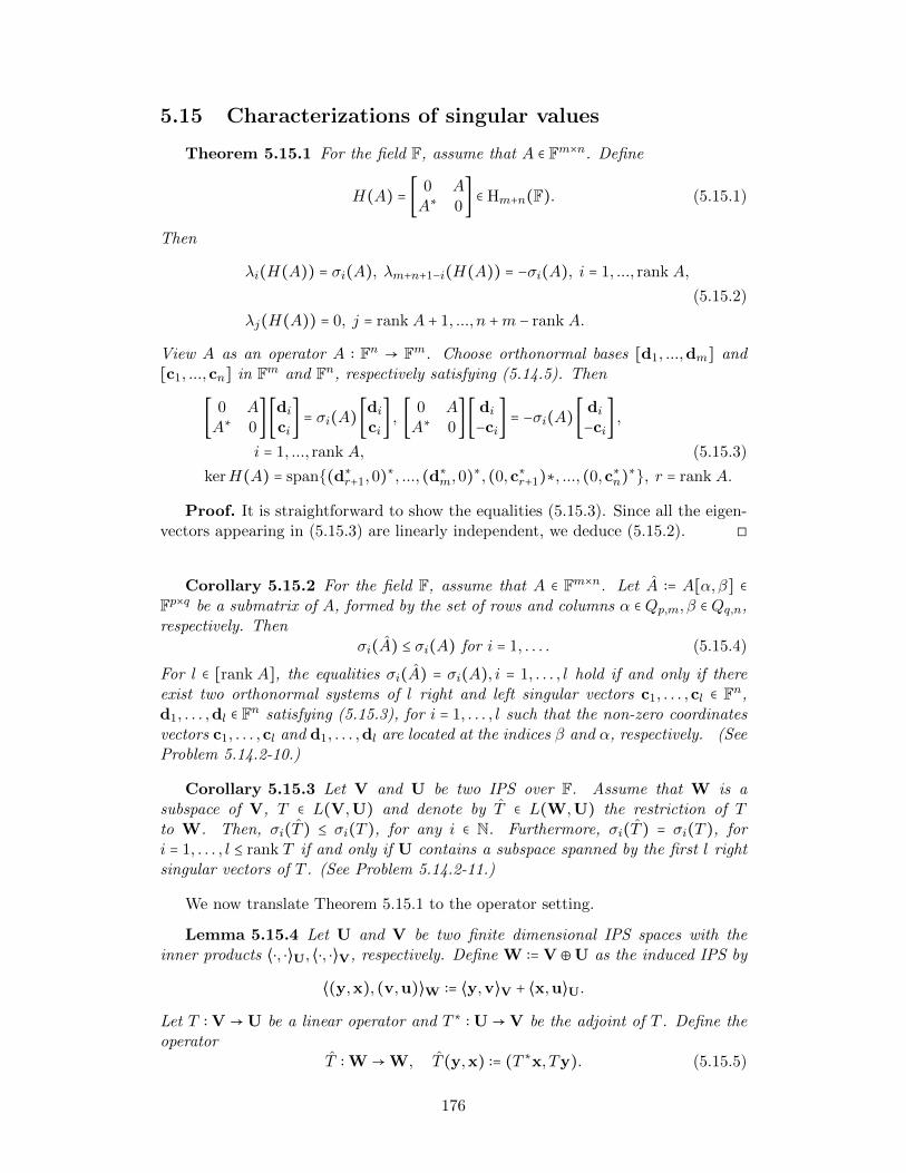
5.15 Characterizations of singular values
Theorem 5.15.1 For the field F, assume that A ∈ Fm×n. Define
H(A) = [ 0 AA∗ 0
] ∈ Hm+n(F). (5.15.1)
Then
λi(H(A)) = σi(A), λm+n+1−i(H(A)) = −σi(A), i = 1, ..., rank A,
(5.15.2)
λj(H(A)) = 0, j = rank A + 1, ..., n +m − rank A.
View A as an operator A ∶ Fn → Fm. Choose orthonormal bases [d1, ...,dm] and[c1, ...,cn] in Fm and Fn, respectively satisfying (5.14.5). Then
[ 0 AA∗ 0
] [dici
] = σi(A) [dici
] , [ 0 AA∗ 0
] [ di−ci
] = −σi(A) [ di−ci
] ,
i = 1, ..., rank A, (5.15.3)
kerH(A) = span(d∗r+1,0)∗, ..., (d∗m,0)∗, (0,c∗r+1)∗, ..., (0,c∗n)∗, r = rank A.
Proof. It is straightforward to show the equalities (5.15.3). Since all the eigen-vectors appearing in (5.15.3) are linearly independent, we deduce (5.15.2). ◻
Corollary 5.15.2 For the field F, assume that A ∈ Fm×n. Let A ∶= A[α,β] ∈Fp×q be a submatrix of A, formed by the set of rows and columns α ∈ Qp,m, β ∈ Qq,n,respectively. Then
σi(A) ≤ σi(A) for i = 1, . . . . (5.15.4)
For l ∈ [rank A], the equalities σi(A) = σi(A), i = 1, . . . , l hold if and only if thereexist two orthonormal systems of l right and left singular vectors c1, . . . ,cl ∈ Fn,d1, . . . ,dl ∈ Fn satisfying (5.15.3), for i = 1, . . . , l such that the non-zero coordinatesvectors c1, . . . ,cl and d1, . . . ,dl are located at the indices β and α, respectively. (SeeProblem 5.14.2-10.)
Corollary 5.15.3 Let V and U be two IPS over F. Assume that W is asubspace of V, T ∈ L(V,U) and denote by T ∈ L(W,U) the restriction of Tto W. Then, σi(T ) ≤ σi(T ), for any i ∈ N. Furthermore, σi(T ) = σi(T ), fori = 1, . . . , l ≤ rank T if and only if U contains a subspace spanned by the first l rightsingular vectors of T . (See Problem 5.14.2-11.)
We now translate Theorem 5.15.1 to the operator setting.
Lemma 5.15.4 Let U and V be two finite dimensional IPS spaces with theinner products ⟨⋅, ⋅⟩U, ⟨⋅, ⋅⟩V, respectively. Define W ∶= V⊕U as the induced IPS by
⟨(y,x), (v,u)⟩W ∶= ⟨y,v⟩V + ⟨x,u⟩U.
Let T ∶ V →U be a linear operator and T ∗ ∶ U →V be the adjoint of T . Define theoperator
T ∶ W →W, T (y,x) ∶= (T ∗x, Ty). (5.15.5)
176
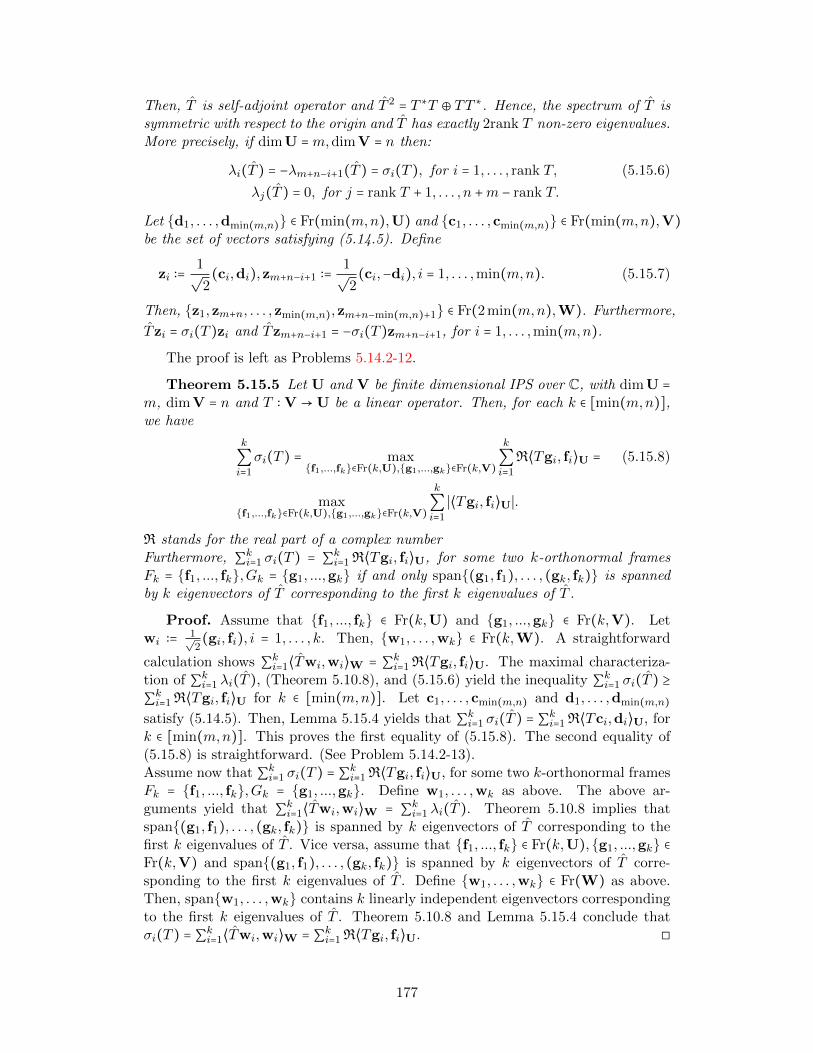
Then, T is self-adjoint operator and T 2 = T ∗T ⊕ TT ∗. Hence, the spectrum of T issymmetric with respect to the origin and T has exactly 2rank T non-zero eigenvalues.More precisely, if dimU =m,dimV = n then:
λi(T ) = −λm+n−i+1(T ) = σi(T ), for i = 1, . . . , rank T, (5.15.6)
λj(T ) = 0, for j = rank T + 1, . . . , n +m − rank T.
Let d1, . . . ,dmin(m,n) ∈ Fr(min(m,n),U) and c1, . . . ,cmin(m,n) ∈ Fr(min(m,n),V)be the set of vectors satisfying (5.14.5). Define
zi ∶=1√2(ci,di),zm+n−i+1 ∶=
1√2(ci,−di), i = 1, . . . ,min(m,n). (5.15.7)
Then, z1,zm+n, . . . ,zmin(m,n),zm+n−min(m,n)+1 ∈ Fr(2 min(m,n),W). Furthermore,
Tzi = σi(T )zi and Tzm+n−i+1 = −σi(T )zm+n−i+1, for i = 1, . . . ,min(m,n).
The proof is left as Problems 5.14.2-12.
Theorem 5.15.5 Let U and V be finite dimensional IPS over C, with dimU =m, dimV = n and T ∶ V →U be a linear operator. Then, for each k ∈ [min(m,n)],we have
k
∑i=1
σi(T ) = maxf1,...,fk∈Fr(k,U),g1,...,gk∈Fr(k,V)
k
∑i=1
R⟨Tgi, fi⟩U = (5.15.8)
maxf1,...,fk∈Fr(k,U),g1,...,gk∈Fr(k,V)
k
∑i=1
∣⟨Tgi, fi⟩U∣.
R stands for the real part of a complex numberFurthermore, ∑ki=1 σi(T ) = ∑ki=1 R⟨Tgi, fi⟩U, for some two k-orthonormal framesFk = f1, ..., fk,Gk = g1, ...,gk if and only span(g1, f1), . . . , (gk, fk) is spannedby k eigenvectors of T corresponding to the first k eigenvalues of T .
Proof. Assume that f1, ..., fk ∈ Fr(k,U) and g1, ...,gk ∈ Fr(k,V). Letwi ∶= 1√
2(gi, fi), i = 1, . . . , k. Then, w1, . . . ,wk ∈ Fr(k,W). A straightforward
calculation shows ∑ki=1⟨Twi,wi⟩W = ∑ki=1 R⟨Tgi, fi⟩U. The maximal characteriza-tion of ∑ki=1 λi(T ), (Theorem 5.10.8), and (5.15.6) yield the inequality ∑ki=1 σi(T ) ≥∑ki=1 R⟨Tgi, fi⟩U for k ∈ [min(m,n)]. Let c1, . . . ,cmin(m,n) and d1, . . . ,dmin(m,n)satisfy (5.14.5). Then, Lemma 5.15.4 yields that ∑ki=1 σi(T ) = ∑ki=1 R⟨Tci,di⟩U, fork ∈ [min(m,n)]. This proves the first equality of (5.15.8). The second equality of(5.15.8) is straightforward. (See Problem 5.14.2-13).Assume now that ∑ki=1 σi(T ) = ∑ki=1 R⟨Tgi, fi⟩U, for some two k-orthonormal framesFk = f1, ..., fk,Gk = g1, ...,gk. Define w1, . . . ,wk as above. The above ar-guments yield that ∑ki=1⟨Twi,wi⟩W = ∑ki=1 λi(T ). Theorem 5.10.8 implies thatspan(g1, f1), . . . , (gk, fk) is spanned by k eigenvectors of T corresponding to thefirst k eigenvalues of T . Vice versa, assume that f1, ..., fk ∈ Fr(k,U),g1, ...,gk ∈Fr(k,V) and span(g1, f1), . . . , (gk, fk) is spanned by k eigenvectors of T corre-sponding to the first k eigenvalues of T . Define w1, . . . ,wk ∈ Fr(W) as above.Then, spanw1, . . . ,wk contains k linearly independent eigenvectors correspondingto the first k eigenvalues of T . Theorem 5.10.8 and Lemma 5.15.4 conclude thatσi(T ) = ∑ki=1⟨Twi,wi⟩W = ∑ki=1 R⟨Tgi, fi⟩U. ◻
177
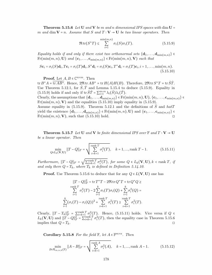
Theorem 5.15.6 Let U and V be m and n dimensional IPS spaces with dimU =m and dimV = n. Assume that S and T ∶ V →U be two linear operators. Then
R tr(S∗T ) ≤min(m,n)∑i=1
σi(S)σi(T ). (5.15.9)
Equality holds if and only if there exist two orthonormal sets d1, . . . ,dmin(m,n) ∈Fr(min(m,n),U) and c1, . . . ,cmin(m,n) ∈ Fr(min(m,n),V) such that
Sci = σi(S)di, Tci = σi(T )di, S∗di = σi(S)ci, T ∗di = σi(T )ci, i = 1, . . . ,min(m,n).(5.15.10)
Proof. Let A,B ∈ Cn×m. ThentrB∗A = trAB∗. Hence, 2R trAB∗ = trH(A)H(B). Therefore, 2R trS∗T = tr ST .Use Theorem 5.12.1, for S, T and Lemma 5.15.4 to deduce (5.15.9). Equality in(5.15.9) holds if and only if tr ST = ∑m+ni=1 λi(S)λi(T ).Clearly, the assumptions that d1, . . . ,dmin(m,n) ∈ Fr(min(m,n),U), c1, . . . ,cmin(m,n) ∈Fr(min(m,n),V) and the equalities (5.15.10) imply equality in (5.15.9).Assume equality in (5.15.9). Theorem 5.12.1 and the definitions of S and hatTyield the existence d1, . . . ,dmin(m,n) ∈ Fr(min(m,n),U) and c1, . . . ,cmin(m,n) ∈Fr(min(m,n),V), such that (5.15.10) hold. ◻
Theorem 5.15.7 Let U and V be finite dimensional IPS over F and T ∶ V →Ube a linear operator. Then
minQ∈Lk(V,U)
∣∣T −Q∣∣F =
¿ÁÁÀrank T
∑i=k+1
σ2i (T ), k = 1, ..., rank T − 1. (5.15.11)
Furthermore, ∣∣T − Q∣∣F =√∑rank Ti=k+1 σ2
i (T ), for some Q ∈ Lk(V,U), k < rank T , ifand only there Q = Tk, where Tk is defined in Definition 5.14.10.
Proof. Use Theorem 5.15.6 to deduce that for any Q ∈ L(V,U) one has
∣∣T −Q∣∣2F = trT ∗T − 2R trQ∗T + trQ∗Q ≥rank T
∑i=1
σ2i (T ) − 2
k
∑i=1
σi(T )σi(Q) +k
∑i=1
σ2i (Q) =
k
∑i=1
(σi(T ) − σi(Q))2 +rank T
∑i=k+1
σ2i (T ) ≥
rank T
∑i=k+1
σ2i (T ).
Clearly, ∣∣T − Tk∣∣2F = ∑rank Ti=k+1 σ2
i (T ). Hence, (5.15.11) holds. Vice versa if Q ∈Lk(V,U) and ∣∣T −Q∣∣2F = ∑rank T
i=k+1 σ2i (T ), then the equality case in Theorem 5.15.6
implies that Q = Tk. ◻
Corollary 5.15.8 For the field F, let A ∈ Fm×n. Then
minB∈Rm,n,k(F)
∣∣A −B∣∣F =
¿ÁÁÀrank A
∑i=k+1
σ2i (A), k = 1, ..., rank A − 1. (5.15.12)
178
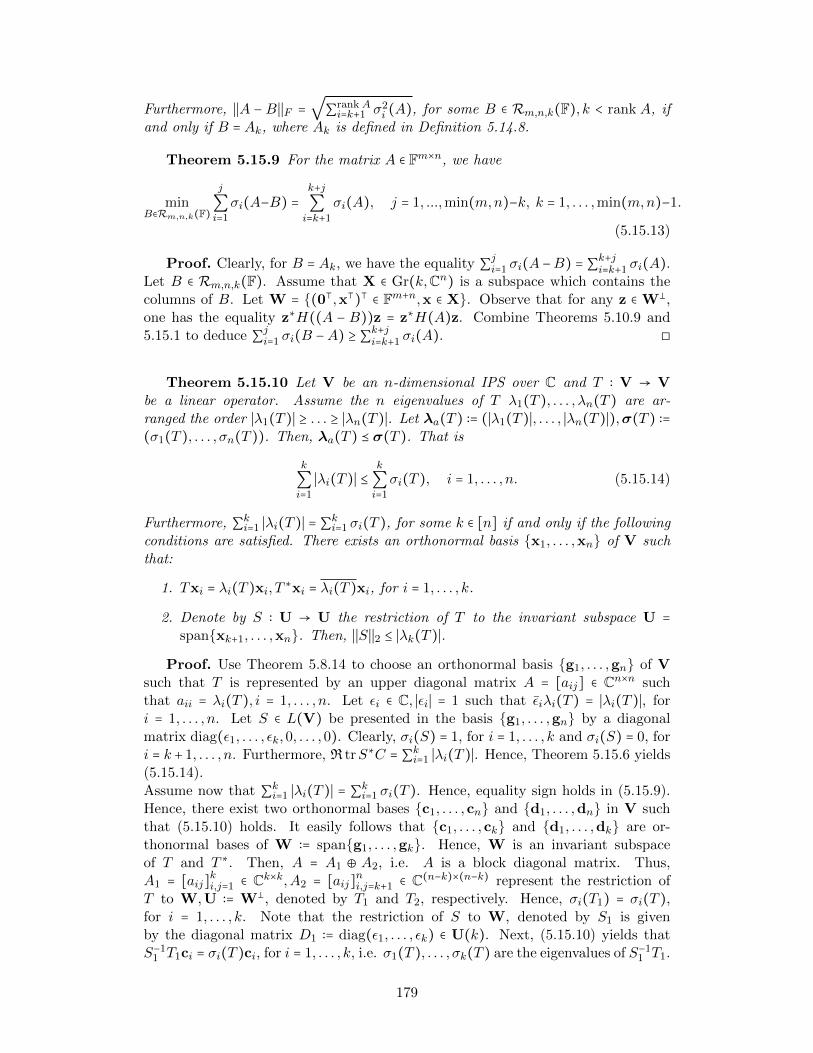
Furthermore, ∣∣A − B∣∣F =√∑rank Ai=k+1 σ2
i (A), for some B ∈ Rm,n,k(F), k < rank A, ifand only if B = Ak, where Ak is defined in Definition 5.14.8.
Theorem 5.15.9 For the matrix A ∈ Fm×n, we have
minB∈Rm,n,k(F)
j
∑i=1
σi(A−B) =k+j∑i=k+1
σi(A), j = 1, ...,min(m,n)−k, k = 1, . . . ,min(m,n)−1.
(5.15.13)
Proof. Clearly, for B = Ak, we have the equality ∑ji=1 σi(A−B) = ∑k+ji=k+1 σi(A).Let B ∈ Rm,n,k(F). Assume that X ∈ Gr(k,Cn) is a subspace which contains thecolumns of B. Let W = (0⊺,x⊺)⊺ ∈ Fm+n,x ∈ X. Observe that for any z ∈ W⊥,one has the equality z∗H((A − B))z = z∗H(A)z. Combine Theorems 5.10.9 and5.15.1 to deduce ∑ji=1 σi(B −A) ≥ ∑k+ji=k+1 σi(A). ◻
Theorem 5.15.10 Let V be an n-dimensional IPS over C and T ∶ V → Vbe a linear operator. Assume the n eigenvalues of T λ1(T ), . . . , λn(T ) are ar-ranged the order ∣λ1(T )∣ ≥ . . . ≥ ∣λn(T )∣. Let λa(T ) ∶= (∣λ1(T )∣, . . . , ∣λn(T )∣),σ(T ) ∶=(σ1(T ), . . . , σn(T )). Then, λa(T ) ⪯ σ(T ). That is
k
∑i=1
∣λi(T )∣ ≤k
∑i=1
σi(T ), i = 1, . . . , n. (5.15.14)
Furthermore, ∑ki=1 ∣λi(T )∣ = ∑ki=1 σi(T ), for some k ∈ [n] if and only if the followingconditions are satisfied. There exists an orthonormal basis x1, . . . ,xn of V suchthat:
1. Txi = λi(T )xi, T ∗xi = λi(T )xi, for i = 1, . . . , k.
2. Denote by S ∶ U → U the restriction of T to the invariant subspace U =spanxk+1, . . . ,xn. Then, ∣∣S∣∣2 ≤ ∣λk(T )∣.
Proof. Use Theorem 5.8.14 to choose an orthonormal basis g1, . . . ,gn of Vsuch that T is represented by an upper diagonal matrix A = [aij] ∈ Cn×n suchthat aii = λi(T ), i = 1, . . . , n. Let εi ∈ C, ∣εi∣ = 1 such that εiλi(T ) = ∣λi(T )∣, fori = 1, . . . , n. Let S ∈ L(V) be presented in the basis g1, . . . ,gn by a diagonalmatrix diag(ε1, . . . , εk,0, . . . ,0). Clearly, σi(S) = 1, for i = 1, . . . , k and σi(S) = 0, fori = k + 1, . . . , n. Furthermore, R trS∗C = ∑ki=1 ∣λi(T )∣. Hence, Theorem 5.15.6 yields(5.15.14).Assume now that ∑ki=1 ∣λi(T )∣ = ∑ki=1 σi(T ). Hence, equality sign holds in (5.15.9).Hence, there exist two orthonormal bases c1, . . . ,cn and d1, . . . ,dn in V suchthat (5.15.10) holds. It easily follows that c1, . . . ,ck and d1, . . . ,dk are or-thonormal bases of W ∶= spang1, . . . ,gk. Hence, W is an invariant subspaceof T and T ∗. Then, A = A1 ⊕ A2, i.e. A is a block diagonal matrix. Thus,A1 = [aij]ki,j=1 ∈ Ck×k,A2 = [aij]ni,j=k+1 ∈ C(n−k)×(n−k) represent the restriction ofT to W,U ∶= W⊥, denoted by T1 and T2, respectively. Hence, σi(T1) = σi(T ),for i = 1, . . . , k. Note that the restriction of S to W, denoted by S1 is givenby the diagonal matrix D1 ∶= diag(ε1, . . . , εk) ∈ U(k). Next, (5.15.10) yields thatS−1
1 T1ci = σi(T )ci, for i = 1, . . . , k, i.e. σ1(T ), . . . , σk(T ) are the eigenvalues of S−11 T1.
179
Clearly, S−11 T1 is presented in the basis [g1, . . . ,gk] by the matrix D−1
1 A1, which isa diagonal matrix with ∣λ1(T )∣, . . . , ∣λk(T )∣ on the main diagonal. That is, S−1
1 T1
has eigenvalues ∣λ1(T )∣, . . . , ∣λk(T )∣. Therefore, σi(T ) = ∣λi(T )∣, for i = 1, . . . , k.Theorem 5.14.9 yields that
trA∗1A1 =
k
∑i,j=1
∣aij ∣2 =k
∑i=1
σ2i (A1) =
k
∑i=1
σ2i (T1) =
k
∑i=1
∣λi(T )∣2.
As λ1(T ), . . . , λk(T ) are the diagonal elements of A1, it follows from the aboveequality that A1, is a diagonal matrix. Hence, we can choose xi = gi, for i = 1, . . . , nto obtain the part 1 of the equality case.Let Tx = λx, where ∣∣x∣∣ = 1 and ρ(T ) = ∣λ∣. Recall that ∣∣T ∣∣2 = σ1(T ), whereσ1(T )2 = λ1(T ∗T ) is the maximal eigenvalue of the self-adjoint operator T ∗T . Themaximum characterization of λ1(T ∗T ) yields that ∣λ∣2 = ⟨Tx, Tx⟩ = ⟨T ∗Tx,x⟩ ≤λ1(T ∗T ) = ∣∣T ∣∣22. Hence, ρ(T ) ≤ ∣∣T ∣∣2.Assume now that ρ(T ) = ∣∣T ∣∣2. If ρ(T ) = 0, then ∣∣T ∣∣2 = 0. This means T = 0and theorem holds trivially in this case. Assume that ρ(T ) > 0. Hence, the eigen-vector x1 ∶= x is also the eigenvector of T ∗T corresponding to λ1(T ∗T ) = ∣λ∣2.Hence, ∣λ∣2x = T ∗Tx = T ∗(λx), which implies that T ∗x = λx. Let U = span(x)⊥be the orthogonal complement of span(x). Since T span(x) = span(x), it followsthat T ∗U ⊆ U. Similarly, since T ∗span(x) = span(x), then TU ⊆ U. Thus,V = span(x)⊕U and span(x) and U are invariant subspaces of T and T ∗. Hence,span(x) and U are invariant subspaces of T ∗T and TT ∗. Let T1 be the restriction ofT to U. Then, T ∗1 T1 is the restriction of T ∗T . Therefore, ∣∣T1∣∣22 ≥ λ1(T ∗T ) = ∣∣T ∣∣22.The above result implies the equality ρ(T ) = ∣∣T ∣∣2. ◻
Corollary 5.15.11 Let U be an n-dimensional IPS over C and T ∶ U→U be alinear operator. Denote by ∣λ(T )∣ = (∣λ1(T )∣, ..., ∣λn(T )∣)T the absolute eigenvaluesof T , (counting with their multiplicities), arranged in a decreasing order. Then,∣λ(T )∣ = (σ1(T ), ..., σn(T ))⊺ if and only if T is a normal operator.
5.15.1 Worked-out Problems
1. Let A ∈ Cn×n and σ1(A) ≥ ⋯ ≥ σn(A) ≥ 0 be the singular values of A. Letλ1(A), . . . , λn(A) be the eigenvalues of A listed with their multiplicities and∣λ1(A)∣ ≥ ⋯ ≥ ∣λn(A)∣.
(a) Show that ∣λ1(A)∣ ≤ σ1(A).(b) What is a necessary and sufficient condition for the equality ∣λ1(A)∣ =
σ1(A)?(c) Is it true that σn(A) ≤ ∣λn(A)∣?(d) Show that ∑ni=1 σi(A)2 ≥ ∑ni=1 ∣λi(A)∣2.
Solution:
(a) Let Ax = λ1(A)x, for ∥x∥ = 1. Then, ∥Ax∥ = ∣λ1(A)∣∥x∥ = ∣λ1(A)∣ ≤max∥y∥=1(∥Ay∥) = σ1(A).
180
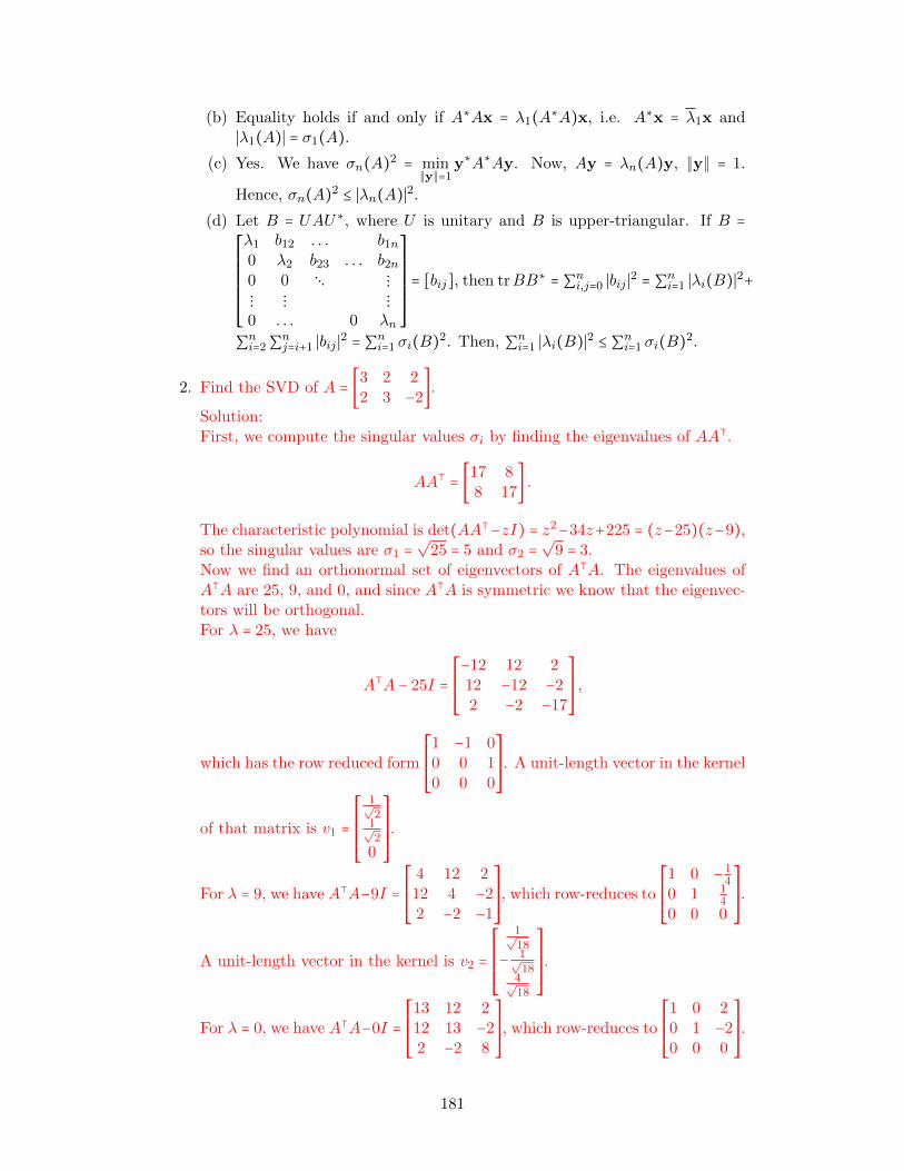
(b) Equality holds if and only if A∗Ax = λ1(A∗A)x, i.e. A∗x = λ1x and∣λ1(A)∣ = σ1(A).
(c) Yes. We have σn(A)2 = min∥y∥=1
y∗A∗Ay. Now, Ay = λn(A)y, ∥y∥ = 1.
Hence, σn(A)2 ≤ ∣λn(A)∣2.
(d) Let B = UAU∗, where U is unitary and B is upper-triangular. If B =⎡⎢⎢⎢⎢⎢⎢⎢⎢⎢⎣
λ1 b12 . . . b1n0 λ2 b23 . . . b2n0 0 ⋱ ⋮⋮ ⋮ ⋮0 . . . 0 λn
⎤⎥⎥⎥⎥⎥⎥⎥⎥⎥⎦
= [bij], then trBB∗ = ∑ni,j=0 ∣bij ∣2 = ∑ni=1 ∣λi(B)∣2+
∑ni=2∑nj=i+1 ∣bij ∣2 = ∑ni=1 σi(B)2. Then, ∑ni=1 ∣λi(B)∣2 ≤ ∑ni=1 σi(B)2.
2. Find the SVD of A = [3 2 22 3 −2
].
Solution:First, we compute the singular values σi by finding the eigenvalues of AA⊺.
AA⊺ = [17 88 17
] .
The characteristic polynomial is det(AA⊺−zI) = z2−34z+225 = (z−25)(z−9),so the singular values are σ1 =
√25 = 5 and σ2 =
√9 = 3.
Now we find an orthonormal set of eigenvectors of A⊺A. The eigenvalues ofA⊺A are 25, 9, and 0, and since A⊺A is symmetric we know that the eigenvec-tors will be orthogonal.For λ = 25, we have
A⊺A − 25I =⎡⎢⎢⎢⎢⎢⎣
−12 12 212 −12 −22 −2 −17
⎤⎥⎥⎥⎥⎥⎦,
which has the row reduced form
⎡⎢⎢⎢⎢⎢⎣
1 −1 00 0 10 0 0
⎤⎥⎥⎥⎥⎥⎦. A unit-length vector in the kernel
of that matrix is v1 =
⎡⎢⎢⎢⎢⎢⎢⎣
1√2
1√2
0
⎤⎥⎥⎥⎥⎥⎥⎦
.
For λ = 9, we have A⊺A−9I =⎡⎢⎢⎢⎢⎢⎣
4 12 212 4 −22 −2 −1
⎤⎥⎥⎥⎥⎥⎦, which row-reduces to
⎡⎢⎢⎢⎢⎢⎣
1 0 −14
0 1 14
0 0 0
⎤⎥⎥⎥⎥⎥⎦.
A unit-length vector in the kernel is v2 =
⎡⎢⎢⎢⎢⎢⎢⎣
1√18
− 1√18
4√18
⎤⎥⎥⎥⎥⎥⎥⎦
.
For λ = 0, we have A⊺A−0I =⎡⎢⎢⎢⎢⎢⎣
13 12 212 13 −22 −2 8
⎤⎥⎥⎥⎥⎥⎦, which row-reduces to
⎡⎢⎢⎢⎢⎢⎣
1 0 20 1 −20 0 0
⎤⎥⎥⎥⎥⎥⎦.
181
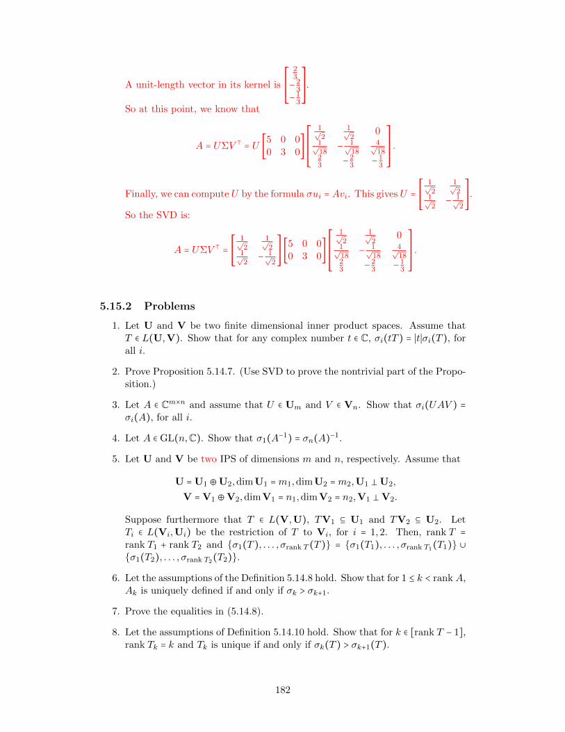
A unit-length vector in its kernel is
⎡⎢⎢⎢⎢⎢⎣
23−2
3−1
3
⎤⎥⎥⎥⎥⎥⎦.
So at this point, we know that
A = UΣV ⊺ = U [5 0 00 3 0
]
⎡⎢⎢⎢⎢⎢⎢⎣
1√2
1√2
01√18
− 1√18
4√18
23 −2
3 −13
⎤⎥⎥⎥⎥⎥⎥⎦
.
Finally, we can compute U by the formula σui = Avi. This gives U =⎡⎢⎢⎢⎢⎣
1√2
1√2
1√2
− 1√2
⎤⎥⎥⎥⎥⎦.
So the SVD is:
A = UΣV ⊺ =⎡⎢⎢⎢⎢⎣
1√2
1√2
1√2
− 1√2
⎤⎥⎥⎥⎥⎦[5 0 00 3 0
]
⎡⎢⎢⎢⎢⎢⎢⎣
1√2
1√2
01√18
− 1√18
4√18
23 −2
3 −13
⎤⎥⎥⎥⎥⎥⎥⎦
.
5.15.2 Problems
1. Let U and V be two finite dimensional inner product spaces. Assume thatT ∈ L(U,V). Show that for any complex number t ∈ C, σi(tT ) = ∣t∣σi(T ), forall i.
2. Prove Proposition 5.14.7. (Use SVD to prove the nontrivial part of the Propo-sition.)
3. Let A ∈ Cm×n and assume that U ∈ Um and V ∈ Vn. Show that σi(UAV ) =σi(A), for all i.
4. Let A ∈ GL(n,C). Show that σ1(A−1) = σn(A)−1.
5. Let U and V be two IPS of dimensions m and n, respectively. Assume that
U = U1 ⊕U2,dimU1 =m1,dimU2 =m2,U1 ⊥U2,
V = V1 ⊕V2,dimV1 = n1,dimV2 = n2,V1 ⊥V2.
Suppose furthermore that T ∈ L(V,U), TV1 ⊆ U1 and TV2 ⊆ U2. LetTi ∈ L(Vi,Ui) be the restriction of T to Vi, for i = 1,2. Then, rank T =rank T1 + rank T2 and σ1(T ), . . . , σrank T (T ) = σ1(T1), . . . , σrank T1(T1) ∪σ1(T2), . . . , σrank T2(T2).
6. Let the assumptions of the Definition 5.14.8 hold. Show that for 1 ≤ k < rank A,Ak is uniquely defined if and only if σk > σk+1.
7. Prove the equalities in (5.14.8).
8. Let the assumptions of Definition 5.14.10 hold. Show that for k ∈ [rank T − 1],rank Tk = k and Tk is unique if and only if σk(T ) > σk+1(T ).
182
9. Let V be an n-dimensional IPS. Assume that T ∈ L(V) is a normal operator.Let λ1(T ), . . . , λn(T ) be the eigenvalues of T arranged in the order ∣λ1(T )∣ ≥. . . ≥ ∣λn(T )∣. Show that σi(T ) = ∣λi(T )∣, for i = 1, . . . , n.
10. Let the assumptions of Corollary 5.15.2 hold.
(a) Since rank A ≤ rank A, show that the inequalities (5.15.4) reduce toσi(A) = σi(A) = 0 for i > rank A.
(b) Since H(A) is a submatrix of H(A), use the Cauchy interlacing principleto deduce the inequalities (5.15.4) for i = 1, . . . , rank A. Furthermore, ifp′ ∶=m−#α, q′ = n−#β, then the Cauchy interlacing principle gives thecomplementary inequalities σi(A) ≥ σi+p′+q′(A) for any i ∈ N.
(c) Assume that σi(A) = σi(A), for i = 1, . . . , l ≤ rank A. Compare themaximal characterization of the sum of the first k eigenvalues of H(A)and H(A) given by Theorem 5.10.8, for k = 1, . . . , l to deduce the lastpart of Corollary (5.15.2).
11. Prove Corollary 5.15.3 by choosing any orthonormal basis in U, an orthonor-mal basis in V whose first dimW elements span W, and using Problem 10.
12. Prove Lemma 5.15.4.
13. Under the assumptions of Theorem 5.15.5, show the equalities.
maxf1,...,fk∈Fr(k,U),g1,...,gk∈Fr(k,V)
k
∑i=1
R⟨Tgi, fi⟩U =
maxf1,...,fk∈Fr(k,U),g1,...,gk∈Fr(k,V)
k
∑i=1
∣⟨Tgi, fi⟩U∣.
14. Let U and V be and finite dimensional IPS. Assume that P and T ∈ L(U,V).Show that R tr(P ∗T ) ≥ −∑min(m,n)
i=1 σi(S)σi(T ). Equality holds if and only ifS = −P and T satisfies the conditions of Theorem 5.15.6.
15. Show that if A,B ∈ Fm×n and B is a submatrix of A, then ∥B∥∞ ≤ ∥A∥∞.
16. Let A ∈ Fm×n be with singular value decomposition UΣV ∗.
(a) Show that ∥A∥2 = σ1 (the largest singular value).
(b) If A is invertible, show that
∥A−1∥2 =1
σn.
17. Show that the singular values of a positive definite hermitian matrix are thesame as its eigenvalues.
183
5.16 Moore-Penrose generalized inverse
The purpose of constructing a generalized inverse is to obtain a matrix that canserve as the inverse in some sense for a wider class of matrices than invertible ones.A generalized inverse exists for an arbitrary matrix A ∈ Cm×n.Let A ∈ Cm×n. Then, (5.14.12) is called the reduced SVD of A. It can be written as
A = UrΣrV∗r , r = rank A, Σr ∶= diag(σ1(A), . . . , σr(A)) ∈ Sr(R),
(5.16.1)
Ur = [u1, . . . ,ur] ∈ Cm×r, Vr = [v1, . . . ,vr] ∈ Cn×r, U∗r Ur = V ∗
r Vr = Ir, .
Note that
AA∗ui = σi(A)2ui,A∗Avi = σi(A)2vi,
vi =1
σi(A)A∗ui,ui =
1
σi(A)Avi, i = 1, . . . , r.
ThenA ∶= VrΣ−1
r U∗r ∈ Cn×m, (5.16.2)
is the Moore-Penrose generalized inverse of A. If A ∈ Rm×n, then we assume thatU ∈ Rm×r and V ∈ Rn×r, i.e. U and V are real values matrices over the real numbersR.
Theorem 5.16.1 Let A ∈ Cm×n. Then, the Moore-Penrose generalized inverseA ∈ Cn×m satisfies the following properties.
1. rank A = rank A.
2. AAA = A, AAA = A, A∗AA = AAA∗ = A∗.
3. AA and AA are Hermitian non-negative definite idempotent matrices, i.e.(AA)2 = AA and (AA)2 = AA, having the same rank as A.
4. The least square solution of Ax = b, i.e. the solution of the system A∗Ax =A∗b, has a solution y = Ab. This solution has the minimal norm ∣∣y∣∣, for allpossible solutions of A∗Ax = A∗b.
5. If rank A = n, then A = (A∗A)−1A∗. In particular, if A ∈ Cn×n is invertiblethen A = A−1.
To prove the above theorem we need the following proposition.
Proposition 5.16.2 Let E ∈ Cl×m and G ∈ Cm×n. Thenrank EG ≤ min(rank E, rank G). If l = m and E is invertible, then rank EG =rank G. If m = n and G is invertible, then rank EG = rank E.
Proof. Let e1, . . . ,em ∈ Cl,g1, . . . ,gn ∈ Cm be the columns of E and G, respec-tively. Then, rank E = dim spane1, . . . ,el. Observe that EG = [Eg1, . . . ,Egn] ∈Cl×n. Clearly Egi is a linear combination of the columns of E. Hence, Egi ∈spane1, . . . ,el. Therefore, spanEg1, . . . ,Egn ⊆ spane1, . . . ,el, which impliesthat rank EG ≤ rank E. Note that (EG)T = GTET . Hence
184
rank EG = rank (EG)T ≤ rank GT = rank G. Thusrank EG ≤ min(rank E, rank G). Suppose E is invertible. Then, rank EG ≤ rank G =rank E−1(EG) ≤ rank EG. It follows rank EG = rank G. Similarly, rank EG =rank E if G is invertible. ◻
Proof of Theorem 5.16.1.
1. Proposition 5.16.2 yields that rank A = rank VrΣ−1r U
∗r ≤ rank Σ−1
r U∗r ≤ rank Σ−1
r =r = rank A. Since Σr = V ∗
r AUr, Proposition 5.16.2 implies that rank A ≥
rank Σ−1r = r. Hence, rank A = rank A.
2. AA = (UrΣrV∗r )(VrΣ−1
r U∗r ) = UrΣrΣ
−1r U
∗r = UrU∗
r . Hence
AAA = (UrU∗r )(UrΣrV
∗r ) = UrΣV ∗
r = A.
Hence A∗AA = (VrΣrU∗r )(UrU∗
r ) = A∗. Similarly AA = VrV ∗r and AAA =
A,AAA∗ = A∗.
3. Since AA = UrU∗r , we deduce that (AA)∗ = (UrU∗
r )∗ = (U∗r )∗U∗
r = AA, i.e.AA is Hermitian. Next, (AA)2 = (UrU∗
r )2 = (UrU∗r )(UrU∗
r ) = (UrU∗r ) = AA,
i.e. AA is idempotent. Thus, AA is non-negative definite. As AA = UrIrU∗r ,
the arguments of part 1 yield that rank AA = r. Similar arguments apply toAA = VrV ∗
r .
4. Since A∗AA = A∗, it follows that A∗A(Ab) = A∗b, i.e. y = Ab is a leastsquare solution. It is left to show that if A∗Ax = A∗b, then ∣∣x∣∣ ≥ ∣∣Ab∣∣ andequality holds if and only if x = Ab.We now consider the system A∗Ax = A∗b. To analyze this system, we use thefull form of SVD given in (5.14.7). It is equivalent to
(V ΣTU∗)(UΣV ∗)x = V ΣTU∗b. Multiplying by V ∗, we obtain the systemΣTΣ(V ∗x) = ΣT (U∗b). Let z = (z1, . . . , zn)T ∶= V ∗x,
c = (c1, . . . , cm)T ∶= U∗b. Note that z∗z = x∗V V x = x∗x, i.e. ∣∣z∣∣ = ∣∣x∣∣. Afterthese substitutions, the least square system in z1, . . . , zn variables is given inthe form σi(A)2zi = σi(A)ci, for i = 1, . . . , n. Since σi(A) = 0, for i > r, weobtain that zi = 1
σi(A)ci, for i = 1, . . . , r while zr+1, . . . , zn are free variables.
Thus, ∣∣z∣∣2 = ∑ri=11
σi(A)2 +∑ni=r+1 ∣zi∣2. Hence, the least square solution with
the minimal length ∣∣z∣∣ is the solution with zi = 0, for i = r + 1, . . . , n. Thissolution corresponds to the x = Ab.
5. Since rank A∗A = rank A = n, it follows that A∗A is an invertible matrix.Hence, the least square solution is unique and is given by x = (A∗A)−1A∗b.Thus, for each b one has (A∗A)−1A∗b = Ab, hence A = (A∗A)−1A∗.If A is an n×n invertible matrix, it follows that (A∗A)−1A∗ = A−1(A∗)−1A∗ =A−1. ◻
5.16.1 Worked-out Problems
1. A linear transformation T on a vector space V is called a projection if T 2 = T .
185
(a) Show that if T is a projection on V, then so is I − T , where I is theidentity operator on V.
(b) Show that if T is a projection on V, then V = kerT ⊕ ImT .
(c) Show that if T is a projection on T , its only possible eigenvalues are 0and 1.
(d) Show that if T is a projection on V and V is finite-dimensional, then Tis diagonalizable.
Solution:
(a) For any v ∈ V, (I−T )2v = (I−T )(I−T )v = (I−T )(v−Tv) = v−Tv−T (v−Tv) = v −Tv −Tv +T 2v. Using T 2 = T , this reduces to v −Tv = (I −T )v.So, (I − T )2 = I − T and I − T is a projection, too.
(b) For any v ∈ V, of course Tv ∈ Im(T ). Now, T (v − Tv) = Tv − T 2v = 0, sov −Tv ∈ ker(T ). As v = (v −Tv)+Tv, we have v ∈ ker(T )+ Im(T ) and soV = ker(T ) + Im(T ).To show the sum is direct, suppose that v ∈ ker(T )∩Im(T ). Then, Tv = 0and also v = Tw, for some w ∈ V. Then, 0 = Tv = T (Tw) = T 2w = Tw = v.So ker(T ) ∩ Im(T ) = 0, and thus V = ker(T )⊕ Im(T ).
(c) One can do this directly, using the definition of eigenvalues. Supposingthat λ is an eigenvalue of the projection T , we have Tv = λv, for somenon-zero vector v. Then, T 2v = T (Tv) = T (λv) = λTv = λ2v. But asT 2 = T , this is also Tv = λv; since v ≠ 0, λ2 = λ and so λ is either 0 or 1.
(d) Since V = ker(T )⊕ Im(T ), if we choose a basis for ker(T ) and a basis forIm(T ), together they form a basis for V. Clearly, each element of thebasis for ker(T ) is an eigenvector corresponding to 0. Also, any vectorin the basis for Im(T ) is v = Tw, for some w ∈ V; as such Tv = T 2w =Tw = 1v and so an eigenvector corresponding to 1. We have a basis of Vconsisting of eigenvectors, so T is diagonalizable.
5.16.2 Problems
1. A matrix P ∈ Rn×n is called an orthogonal projection if P is a projection anda symmetric matrix. Let V ⊆ Rn be the subspace spanned by the columnsof P . Show that for any a ∈ Rn and b ∈ PV the following inequality holds:∣∣a − b∣∣ ≥ ∣∣a − Pa∣∣. Furthermore, equality holds if and only if b = Pa. Thatis, Pa is the orthogonal projection of a on the column space of P .
2. Let A ∈ Rm×n and assume that the SVD of A is given by (5.14.7), whereU ∈ O(m,R), V ∈ O(n,R).
(a) What is the SVD of AT ?
(b) Show that (AT ) = (A)T .
(c) Suppose that B ∈ Rl×m. Is it true that (BA) = AB? Justify!
3. Let A ∈ Cm×n. Show that
(a) N(A∗) = N(A).(b) R(A∗) = R(A).
186
Chapter 6
Perron-Frobenius theorem
The Perron-Frobenius theorem provides a simple characterization of the eigenvec-tors and eigenvalues of certain types of matrices called non-negative matrices inparticular irreducible and primitive matrices. The importance of this theorem liesin the fact the eigenvalue problems on these types of matrices aries in many differentfields of mathematics. As an example of applications of Perron-Frobenius theorem,at the end of this chapter, we will show that it can be used as a tool to give ageneralization of Kepler’s Theorem.
6.1 Perron-Frobenius theorem
Denote by Rm×n+ , the set of matrices A = [aij]m,ni,j=1, where each entry aij ∈ R, aij ≥ 0.We denote a non-negative matrix by A ≥ 0. We say that A is a non-zero non-negativeif A ≥ 0 and A ≠ 0. This is denoted by A ≩ 0. We say that A is a positive matrixif all the entries of A are positive, i.e. aij > 0, for all i, j. We denote that by A > 0.Similar notation is for vectors, i.e. n = 1. From now on, we assume that all matricesare square matrices unless stated otherwise. A non-negative square matrix A ∈ Rn×n+is called irreducible, if (I +A)n−1 > 0. A non-negative matrix is called primitive ifAp > 0, for some positive integer p.
Theorem 6.1.1 (Perron-Frobenius) Let A ∈ Rn×n+ . Denote by ρ(A), thespectral radius of A, i.e. the maximum of the absolute values of the eigenvaluesof A. Then, the following conditions hold.
1. ρ(A) is an eigenvalue of A.
2. There exists x ≩ 0 such that Ax = ρ(A)x.
3. Assume that λ is an eigenvalue of A, λ ≠ ρ(A) and ∣λ∣ = ρ(A). Then,index (λ) ≤ index (ρ(A)). Furthermore, ζ = λ
ρ(A) is a root of unity of order nat most, i.e. ζm = 1, for some m with m ≤ n.
4. Suppose that A is primitive. Then, ρ(A) > 0 and ρ(A) is a simple root ofthe characteristic polynomial, and there exists x > 0 such that Ax = ρ(A)x.Furthermore, if λ is an eigenvalue of A different from ρ(A), then ∣λ∣ < ρ(A).
5. Suppose that A is irreducible. Then, ρ(A) > 0 and ρ(A) is a simple root ofthe characteristic polynomial and there exists x > 0 such that Ax = ρ(A)x. Let
187
λ0 ∶= ρ(A), λ1, . . . , λm−1 be all distinct eigenvalues of A satisfying ∣λ∣ = ρ(A).Then, all these eigenvalues are simple roots of the characteristic polynomial of
A. Furthermore, λj = ρ(A)ζj, for j = 0, . . . ,m−1, where ζ = e 2πim is a primitive
m−th root of 1. Finally, the characteristic polynomials of ζA and A are equal.
We first prove this result for symmetric non-negative matrices.
Proposition 6.1.2 Let A = A⊺ ≥ 0 be a symmetric matrix with non-negativeentries. Then, the conditions of Theorem 6.1.1 hold.
Proof. Recall that A is diagonalizable by an orthogonal matrix. Hence, theindex of each eigenvalue of A is 1. Next, recall that each eigenvalue is given by theRayleigh quotient x⊺Ax
x⊺x . For x = (x1, . . . , xn)⊺, let ∣x∣ ∶= (∣x1∣, . . . , ∣xn∣)⊺. Note that
x⊺x = ∣x∣⊺∣x∣. Also ∣x⊺Ax∣ ≤ ∣x∣⊺A∣x∣. Hence, ∣x⊺Axx⊺x ∣ ≤ ∣x∣⊺A∣x∣∣x∣⊺∣x∣ . Thus, the maximum
of the Rayleigh quotient is achieved for some x ≩ 0. This shows that ρ(A) is aneigenvalue of A, and there exists an eigenvector x ≩ 0 corresponding to A.
Suppose that A > 0. Then, Ax = ρ(A)x,x ≩ 0. So, Ax > 0. Hence, ρ(A) > 0and x > 0. Assume that there exists another eigenvector y, which is not collinearwith x, corresponding to ρ(A). Then, y can be chosen to be orthogonal to thepositive eigenvector x corresponding to ρ(A), i.e. x⊺y = 0. Hence, y has positiveand negative coordinates. Therefore
∣y⊺Ay
y⊺y∣ < ∣y∣⊺A∣y∣
∣y∣⊺∣y∣ ≤ ρ(A).
This gives the contradiction ρ(A) < ρ(A). Therefore, ρ(A) is a simple root of thecharacteristic polynomial of A. In a similar way, we deduce that each eigenvalue λof A, different from ρ(A), satisfies ∣λ∣ < ρ(A).
Since the eigenvectors of Ap are the same as A, we deduce the same results if A isa non-negative symmetric matrix which is primitive. Suppose that A is irreducible.Then, (tI+A)n−1 > 0, for any t > 0. Clearly, ρ(tI+A) = ρ(A)+t. Hence, the eigenvec-tor corresponding to ρ(A) is positive. Therefore, ρ(A) > 0. Each eigenvalue of tI+Ais of the form λ + t, for some eigenvalue λ of A. Since (tI +A) is primitive for anyt > 0, it follows that ∣λ+ t∣ < ρ(A)+ t. Let t→ 0+ to deduce that ∣λ∣ ≤ ρ(A). Since allthe eigenvalues of A are real, we can have an equality for some eigenvalue λ ≠ ρ(A)
if and only if λ = −ρ(A). This will be the case if A has the form C = [ 0 BB⊺ 0
], for
some B ∈ Rm×l+ . It can be shown that if A is a symmetric irreducible matrix suchthat −ρ(A) is an eigenvalue of A, then A = PCP ⊺, for some permutation matrix P .We already showed that C and −C have the same eigenvalues, counted with theirmultiplicities. Hence, −A and A have the same characteristic polynomial. ◻
Recall the `∞ norm on Cn and the corresponding operator norm on Cn×n:
∥(x1, . . . , xn)⊺∥∞ ∶= maxi∈[n]
∣xi∣, ∥A∥∞ ∶= max∥x∥∞≤1
∥Ax∥∞, A ∈ Cn×n. (6.1.1)
Lemma 6.1.3 Let A = [aij]i,j∈[n] ∈ Cn×n. Then
∥A∥∞ = maxi∈[n]
∑j∈[n]
∣aij ∣. (6.1.2)
188
Proof. Let a ∶= maxi∈[n]∑j∈[n] ∣aij ∣. Assume that ∥(x1, . . . , xn)⊺∥ ≤ 1. Then
∣(Ax)i∣ = ∣ ∑j∈[n]
aijxj ∣ ≤ ∑j∈[n]
∣aij ∣ ∣xj ∣ ≤ ∑j∈[n]
∣aij ∣ ≤ a,
for each i ∈ [n]. Hence, ∥A∥∞ ≤ a.From the definition of a, it follows that a = ∑j∈[n] ∣akj ∣, for some k ∈ [n]. Let
xj be a complex number of modulus 1, i.e. xj = 1, such that ∣akj ∣ = akjxj , for eachj ∈ [n]. Let x = (x1, . . . , xn)⊺. Clearly ∥x∥∞ = 1. Furthermore, a = ∑j∈[n] akjxj .Hence, maxi∈[n] ∥Ax∥∞ ≥ a. Therefore a = ∥A∥∞. ◻
Definition 6.1.4 Let A = [aij] ∈ Cn×n. Denote ∣A∣ ∶= [∣aij ∣] ∈ Rn×n+ . For x =(x1, . . . , xn)⊺ ≥ 0, define r(A,x) ∶= mint ≥ 0, ∣A∣x ≤ tx.
(Note that r(A,x) may take a value ∞.) It is straightforward to show that
r(A,x) ∶= maxi∈[n]
∑j∈[n] ∣aij ∣xjxi
, for x > 0. (6.1.3)
Lemma 6.1.5 Let A = [aij] ∈ Cn×n and 1 ∶= (1, . . . ,1)⊺ ∈ Cn. Then
1. ∥A∥∞ = r(A,1).
2. Assume that x = (x1, . . . , xn)⊺ > 0. Then, each eigenvalue λ of A satisfies∣λ∣ ≤ r(A,x). That is, ρ(A) ≤ r(A,x). In particular
ρ(A) ≤ ∥A∥∞. (6.1.4)
Proof. The statement ∥A∥∞ = r(A,1) follows straightforward from the definitionof ∥A∥∞ and r(A,1).
We now show (6.1.4). Assume that Az = λz, where z = (z1, . . . , zn)⊺ ∈ Cn ∖ 0.Without loss of generality, we may assume that ∣zk∣ = ∥z∥∞ = 1, for some k ∈ [n].Then
∣λ∣ = ∣λzk∣ = ∣(Az)k∣ ≤n
∑j=1
∣akj ∣ ∣zj ∣ ≤n
∑j=1
∣akj ∣ ≤ ∥A∥∞.
Assume that x = (x1, . . . , xn)⊺ > 0. Let D = diag(x1, . . . , xn). Define A1 ∶= D−1AD.A straightforward calculation shows that r(A,x) = r(A1,1) = ∥A1∥∞. Clearly, Aand A1 are similar. Use (6.1.4) for A1 to deduce that ∣λ∣ ≤ r(A,x). ◻
Lemma 6.1.6 Let A ∈ Rn×n+ . Then, r(A,x) ≥ r(A, (I +A)x).
Proof. As Ax ≤ r(A,x)x, we deduce
A((I +A)x) = (I +A)(Ax) ≤ (I +A)(r(A,x)x) = r(A,x)A((I +A)x)).
The definition of r(A, (I +A)x) yields the lemma. ◻
The next result is a basic step in the proof of Theorem 6.1.1 and is due toWielandt, e.g., [7].
189
Theorem 6.1.7 Let A ∈ Rn×n+ be an irreducible matrix. Then
ρ(A) = minx>0
r(A,x) > 0. (6.1.5)
Equality holds if and only if Ax = ρ(A)x. There is a unique positive eigenvectorx > 0 corresponding to ρ(A), up to a multiple by a constant. (This eigenvector iscalled Perron-Frobenius eigenvector) That is, rank (ρ(A)I −A) = n − 1. Any otherreal eigenvector of A corresponding to λ ≠ ρ(A) has two coordinates with oppositesigns.
Proof. Since for any a > 0 and x > 0, we have that r(A,ax) = r(A,x), it isenough to assume that x is a probability vector, i.e. ∥x∥1 = ∑ni=1 xi = 1. Clearly, Πn,the set of all probability vectors in Rn, is a compact set. (Problem 1.13.2-7) Wenow consider the extremal problem
r(A) ∶= infx∈Πn
r(A,x). (6.1.6)
We claim that this infimum is achieved for some y ∈ Πn. As r(A,x) ≥ 0, for x ≥ 0, itfollows that there exists a sequence xm ∈ Πn such limm→∞ r(A,xm) = r(A). Clearly,r(A,xm) ≥ r(A). Hence, by considering a subsequence if necessary, we can assumethat r(A,xm) is a nonincreasing sequence, i.e., r(A,xl) ≥ r(A,xm), for m > l. Thus,r(A,xl)xm ≥ r(A,xm)xm ≥ Axm. As limm→∞ xm = y, it follows that r(A,xl)y ≥ Ay.Hence, r(A,xl) ≥ r(A,y)⇒ r(A) ≥ r(A,y). From the definition of r(A), we deducethat r(A) ≤ r(A,y). Hence, r(A) = r(A,y).
Assume first that y is not an eigenvector of A. Let z ∶= r(A)y −Ay. So z ≥ 0and z ≠ 0. Since A is irreducible, then (I +A)n−1 > 0. Hence, (I +A)n−1z > 0. Thisis equivalent to
r(A)((I +A)n−1y) > (I +A)n−1(Ay) = A((I +A)n−1y).
Let u ∶= (I + A)n−1y. Then, the above inequality yields that r(A,u) < r(A). Letv = bu ∈ Πn, for a corresponding b > 0. So r(A,v) = r(A,u) < r(A). This contradictsthe definition of r(A). Hence, Ay = r(A)y. Clearly, (I +A)n−1y = (1 + r(A))n−1y.As y ∈ Πn and (I +A)n−1 > 0, it follows that (I +A)n−1y > 0. Hence, y > 0. Part 2of Lemma 6.1.5 yields that ρ(A) ≤ r(A,y) = r(A). As r(A) is an eigenvalue of A, itfollows that r(A) = ρ(A). Since A is irreducible, A ≠ 0. Hence r(A) = r(A,y) > 0.Combine the definition of r(A) with the fact that Ay = r(A)y to deduce (6.1.5).
We next claim that rank (ρ(A)I−A) = n−1, i.e. the dimension of the eigenspaceof A corresponding to A is one. Assume to the contrary that w ∈ Rn is an eigenvectorof A corresponding to ρ(A) which is not collinear with y, i.e. w ≠ ty, for any t ∈ R.Consider w + ty. Since y > 0 for t ≫ 0 and −t ≫ 0, we have that w + ty > 0 andw + ty < 0, respectively. Hence, there exists t0 ∈ R such that u ∶= w + t0y ≥ 0 and atleast one of the coordinates of u equals zero. As w and y are linearly independent,it follows that u ≠ 0. Also, Au = ρ(A)u. Since A is irreducible, we obtain that(1 + ρ(A))n−1u = (I + A)n−1u > 0. This contradicts the assumption that u has atleast one zero coordinates.
Suppose finally that Av = λv, for some λ ≠ ρ(A) and v ≠ 0. Observe thatA⊺ ≥ 0 and (I +A⊺)n−1 = ((I +A)n−1)⊺ > 0. That is, A⊺ is irreducible. Hence, thereexists u > 0 such that A⊺u = ρ(A⊺)u. Recall that ρ(A⊺) = ρ(A). Consider now
190
u⊺Av = λu⊺v = ρ(A)u⊺v. As ρ(A) ≠ λ, we deduce that u⊺v = 0. As u > 0, it followsthat v has two coordinates with opposite signs. ◻
We now give the full proof of Theorem 6.1.1. We use the following well-knownresult for the roots of monic polynomials of complex variables [15].
Lemma 6.1.8 (Continuity of the roots of a polynomial) Let p(z) = zn +a1z
n−1+. . .+an be a monic polynomial of degree n with complex coefficients. Assumethat p(z) =∏n
j=1(z−zj(p)). Given ε > 0, then there exists δ(ε) > 0 such that for each
coefficient vector b = (b1, . . . , bn) satisfying ∑nj=1 ∣bj − aj ∣2 < δ(ε)2 one can rearrange
the roots of q(z) = zn+ b1zn−1+ . . .+ bn =∏nj=1(z−zj(q)) such that ∣zj(q)−zj(p)∣ < ε,
for each j ∈ [n].
Corollary 6.1.9 Assume that Am ∈ Cn×n converges to A ∈ Cn×n, m ∈ N. Then,limm→∞ ρ(Am) = ρ(A). That is, the function ρ(⋅) ∶ Cn×n → [0,∞), that assigns toeach A its spectral radius, is a continuous function.
Proof of 1. and 2. of Theorem 6.1.1. Assume that A ∈ Rn×n+ , i.e. Ahas non-negative entries. Let Jn ∈ Rn×n+ be a matrix whose all entries are 1. LetAm = A+ 1
mJn, for m ∈ N. Then, each Am is a positive matrix and limm→∞Am = A.Corollary 6.1.9 yields that limm→∞ ρ(Am) = ρ(A). Clearly, each Am is irreducible.Hence, by Theorem 6.1.7, there exists a probability vector xm ∈ Πn such thatAmxm = ρ(Am)xm. As Πn is compact, there exists a subsequence mk, k ∈ N suchthat limk→∞ xmk = x ∈ Πn. Consider the equalities Amkxmk = ρ(Amk)xmk . Letk → ∞ to deduce that Ax = ρ(A)x. So ρ(A) is an eigenvector of A with a corre-sponding probability vector x. ◻In what follows, we need the following lemma:
Lemma 6.1.10 Let B ∈ Cn×n and assume that rank B = n − 1. Then, adj B =uv⊺ ≠ 0, where Bu = B⊺v = 0. Suppose furthermore that A ∈ Rn×n+ and ρ(A) is ageometrically simple eigenvalue, i.e. rank B = n − 1, where B = ρ(A)In −A. Then,adj B = uv⊺ and u,v ≩ 0 are the eigenvectors of A and A⊺ corresponding to theeigenvalue ρ(A).
Proof. Recall that the entries of adj B are all n−1 minors of B. Since rank B =n−1, we deduce that adj B ≠ 0. Recall next thatB(adj B) = (adj B)B = detB In = 0,as rank B = n − 1. Let adj B = [u1 u2 . . .un]. As B(adj B) = 0, we deduce thatBui = 0, for i ∈ [n]. Since rank B = n − 1, the dimension of the null space is one.So the null space of B is spanned by u ≠ 0. Hence, ui = viu, for some vi, i ∈ [n].Let v = (v1, . . . , vn)⊺. Then, adj B = uv⊺. Since adj B ≠ 0, it follows that v ≠ 0. As0 = (adj B)B = uv⊺B = u(B⊺v) and u ≠ 0, it follows that B⊺v = 0.
Assume now that A ∈ Rn×n+ . Then, part 1 of Theorem 6.1.1 yields that ρ(A)is an eigenvalue of A. Hence, B = ρ(A)In − A is singular. Suppose that rank B =n − 1. We claim that adj B ≥ 0. We first observe that for t > ρ(A), we havedet(tIn −A) = ∏n
j=1(t − λj(A)) > 0. Indeed, if λj(A) is real, then t − λj(A) > 0. Ifλj(A) is not real, i.e. a complex number, then λj(A) is also an eigenvalue of A.Recall that t > ρ(A) ≥ ∣λj(A)∣. Hence, (t − λj(A))(t − λj(A)) = ∣t − λj(A)∣2 > 0. So
191
det(tIn −A) > 0. Furthermore,
adj (tIn −A) = det(tIn −A)(tIn −A)−1 =
det(tIn −A)t−1(In − t−1A)−1 = det(tIn −A)t−1∞∑j=0
(t−1A)j .
As Aj ≥ 0, for each non-negative integer j, it follows that adj (tIn − A) ≥ 0, fort > ρ(A). Let t ρ(A), (t converges to ρ(A) from above), to deduce that adj B ≩ 0.As B = uv⊺, we can assume that u,v ≩ 0. ◻
Lemma 6.1.11 Let A ∈ Rn×n+ be an irreducible matrix. Then, ρ(A) is an alge-braically simple eigenvalue.
Proof. We may assume that n > 1. Theorem 6.1.7 implies that ρ(A) is geomet-rically simple, i.e. null(ρ(A)I − A) = 1. Hence, rank (ρ(A)I − A) = n−1. Lemma6.1.10 yields that adj (ρ(A)I −A) = uv⊺, where Au = ρ(A)u,A⊺v = ρ(A)v,u,v 0.Theorem 6.1.7 implies that u,v > 0. Hence, uv⊺ is a positive matrix. In particular,truv⊺ = v⊺u > 0. Since
(det(λI −A))′(λ = ρ(A)) = tr adj (ρ(A)I −A) = v⊺u > 0,
we deduce that ρ(A) is a simple root of the characteristic polynomial of A. ◻For A ∈ Rn×n+ and x 0 denote s(A,x) = maxt ≥ 0,Ax ≥ tx. From the defini-tion of r(A,x), we immediately conclude that r(A,x) ≥ s(A,x). We now give acomplementary part of Theorem 6.1.7.
Lemma 6.1.12 Let A ∈ Rn×n+ be an irreducible matrix. Then
ρ(A) = maxx>0
s(A,x) > 0. (6.1.7)
Equality holds if and only if Ax = ρ(A)x.
The proof of this lemma is similar to the proof of Theorem 6.1.7, and we skip it.
As usual, denote by S1 ∶= z ∈ C, ∣z∣ = 1 the unit circle in the complex plane.
Lemma 6.1.13 Let A ∈ Rn×n+ be irreducible, C ∈ Cn×n. Assume that ∣C ∣ ≤ A.Then, ρ(C) ≤ ρ(A). Equality holds, i.e. there exists λ ∈ spec C, such that λ = ζρ(A),for some ζ ∈ S1, if and only if there exists a complex diagonal matrix D ∈ Cn×n, whosediagonal entries are equal to 1, such that C = ζDAD−1. The matrix D is unique upto a multiplication by t ∈ S1.
Proof. We can assume that n > 1. Suppose that A = [aij],C = [cij]. Theorem6.1.7 yields that there exists u > 0 such that Au = ρ(A)u. Hence, r(A,u) = ρ(A).Since ∣C ∣ ≤ A, it follows that r(C,u) ≤ r(A,u) = ρ(A). Lemma 6.1.5 yields thatρ(C) ≤ r(C,u). Hence, ρ(C) ≤ ρ(A).
Suppose that ρ(C) = ρ(A). Hence, we have equalities ρ(C) = r(C,u) = ρ(A) =r(A,u). So, λ = ζρ(A) is an eigenvalue of C, for some ζ ∈ S1. Furthermore, for thecorresponding eigenvector z of C we have
∣λ∣ ∣z∣ = ∣Cz∣ ≤ ∣C ∣ ∣z∣ ≤ A∣z∣.
192
Hence, ρ(A)∣z∣ ≤ A∣z∣. Therefore s(A, ∣z∣) ≥ ρ(A). Lemma 6.1.12 yields thats(A, ∣z∣) = ρ(A) and ∣z∣ is the corresponding non-negative eigenvector. Therefore,∣Cz∣ = ∣C ∣∣z∣ = A∣z∣. Theorem 6.1.7 yields that ∣z∣ = u.
Let zi = diui, ∣di∣ = 1, for i = 1, . . . , n. The equality ∣Cz∣ = ∣C ∣ ∣z∣ = A∣z∣ combinedwith the triangle inequality and ∣C ∣ ≤ A, yields first that ∣C ∣ = A. Furthermore, foreach fixed i, the non-zero complex numbers ci1z1, . . . , cinzn have the same argument,i.e. cij = ζiaij dj , for j = 1, . . . , n and some complex number ζj , where ∣ζi∣ = 1.Recall that λzi = (Cz)i. Hence, ζi = ζdi, for i = 1, . . . , n. Thus, C = ζDAD−1,where D = diag(d1, . . . , dn). It is straightforward to see that D is unique up to amultiplication by t, for any t ∈ S1.
Suppose now that for D = diag(d1, . . . , dn), where ∣d1∣ = . . . = ∣dn∣ = 1 and ∣ζ ∣ = 1,we have that C = ζDAD−1. Then, λi(C) = ζλi(A), for i = 1, . . . , n. So ρ(C) = ρ(A).Furthermore, cij = ζdicij dj , i, j = 1, . . . , n. Then, ∣C ∣ = A. ◻
Lemma 6.1.14 Let ζ1, . . . , ζh ∈ S1 be h distinct complex numbers which form amultiplicative semi-group, i.e. for any integers i, j ∈ [h], ζiζj ∈ ζ1, . . . , ζh. Then,
the set ζ1, . . . , ζh is the set, (the group), of all h roots of 1: e2πi√−1
h , i = 1, . . . , h.
(Here, we denote the complex number i by√−1 to simplify notations.)
Proof. Let ζ ∈ T ∶= ζ1, . . . ζh. Consider the sequence ζi, i = 1, . . .. Sinceζi+1 = ζζi, for i = 1, . . . , and T is a semigroup, it follows that each ζi is in T . As T isa finite set, we must have two positive integers such that ζk = ζ l, for k < l. Assumethat k and l are the smallest possible positive integers. So ζp = 1, where p = l−k ≥ 1,and Tp ∶= ζ, ζ2, . . . , ζp−1, ζp = 1 are all p roots of 1. Here, ζ is called a p-primitive
root of 1, i.e. ζ = e2πp1
√−1
p , where p1 is an positive integer less than p. Furthermore,p1 and p are coprime, which is denoted by (p1, p) = 1. Note that ζi ∈ T , for anyinteger i.
Next, we choose ζ ∈ T , such that ζ is a primitive p-root of 1 of the maximalpossible order. We claim that p = h, which is equivalent to the equality T = Tp.Assume to the contrary that Tp ⊊ T . Let η ∈ T /Tp. The previous arguments showthat η is a q-primitive root of 1. Therefore, Tq ⊂ T , and Tq ⊊ Tp. Thus, q cannotdivide p. Also, the maximality of p yields that q ≤ p. Let (p, q) = r be the g.c.d., thegreatest common divisor of p and q. So 1 ≤ r < q. Recall that Euclid’s algorithm,which is applied to the division of p by q with a residue, yields that there exist twointegers i, j such that ip + jq = r. Let l ∶= pq
r > p be the least common multiplier of
p and q. Observe that ζ ′ = e2π√−1
p ∈ Tp, η′ = e2π√−1
q ∈ Tq. So
ξ ∶= (η′)i(ζ ′)j = e2π(ip+jq)
√−1
pq = e2π√−1l ∈ T .
As ξ is an l-primitive root of 1, we obtain a contradiction to the maximality of p.So p = h and T is the set of all h-roots of unity. ◻
Theorem 6.1.15 Let A ∈ Rn×n+ be irreducible and assume that for a positiveinteger h ≥ 2, A has h − 1 distinct eigenvalues λ1, . . . , λh−1, which are distinct fromρ(A), such that ∣λ1∣ = . . . = ∣λh−1∣ = ρ(A). Then, the following conditions hold
193
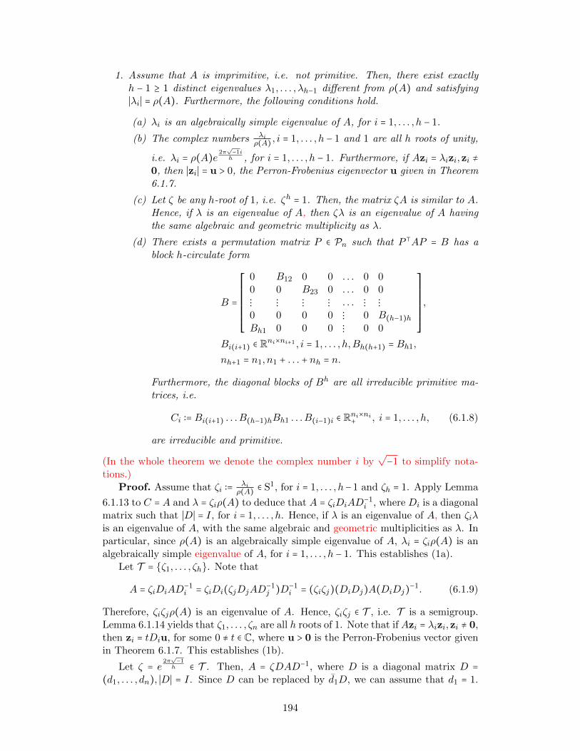
1. Assume that A is imprimitive, i.e. not primitive. Then, there exist exactlyh − 1 ≥ 1 distinct eigenvalues λ1, . . . , λh−1 different from ρ(A) and satisfying∣λi∣ = ρ(A). Furthermore, the following conditions hold.
(a) λi is an algebraically simple eigenvalue of A, for i = 1, . . . , h − 1.
(b) The complex numbers λiρ(A) , i = 1, . . . , h − 1 and 1 are all h roots of unity,
i.e. λi = ρ(A)e 2π√−1ih , for i = 1, . . . , h − 1. Furthermore, if Azi = λizi,zi ≠
0, then ∣zi∣ = u > 0, the Perron-Frobenius eigenvector u given in Theorem6.1.7.
(c) Let ζ be any h-root of 1, i.e. ζh = 1. Then, the matrix ζA is similar to A.Hence, if λ is an eigenvalue of A, then ζλ is an eigenvalue of A havingthe same algebraic and geometric multiplicity as λ.
(d) There exists a permutation matrix P ∈ Pn such that P ⊺AP = B has ablock h-circulate form
B =
⎡⎢⎢⎢⎢⎢⎢⎢⎢⎢⎣
0 B12 0 0 . . . 0 00 0 B23 0 . . . 0 0⋮ ⋮ ⋮ ⋮ . . . ⋮ ⋮0 0 0 0 ⋮ 0 B(h−1)hBh1 0 0 0 ⋮ 0 0
⎤⎥⎥⎥⎥⎥⎥⎥⎥⎥⎦
,
Bi(i+1) ∈ Rni×ni+1 , i = 1, . . . , h,Bh(h+1) = Bh1,
nh+1 = n1, n1 + . . . + nh = n.
Furthermore, the diagonal blocks of Bh are all irreducible primitive ma-trices, i.e.
Ci ∶= Bi(i+1) . . .B(h−1)hBh1 . . .B(i−1)i ∈ Rni×ni+ , i = 1, . . . , h, (6.1.8)
are irreducible and primitive.
(In the whole theorem we denote the complex number i by√−1 to simplify nota-
tions.)Proof. Assume that ζi ∶= λi
ρ(A) ∈ S1, for i = 1, . . . , h−1 and ζh = 1. Apply Lemma
6.1.13 to C = A and λ = ζiρ(A) to deduce that A = ζiDiAD−1i , where Di is a diagonal
matrix such that ∣D∣ = I, for i = 1, . . . , h. Hence, if λ is an eigenvalue of A, then ζiλis an eigenvalue of A, with the same algebraic and geometric multiplicities as λ. Inparticular, since ρ(A) is an algebraically simple eigenvalue of A, λi = ζiρ(A) is analgebraically simple eigenvalue of A, for i = 1, . . . , h − 1. This establishes (1a).
Let T = ζ1, . . . , ζh. Note that
A = ζiDiAD−1i = ζiDi(ζjDjAD
−1j )D−1
i = (ζiζj)(DiDj)A(DiDj)−1. (6.1.9)
Therefore, ζiζjρ(A) is an eigenvalue of A. Hence, ζiζj ∈ T , i.e. T is a semigroup.Lemma 6.1.14 yields that ζ1, . . . , ζn are all h roots of 1. Note that if Azi = λizi,zi ≠ 0,then zi = tDiu, for some 0 ≠ t ∈ C, where u > 0 is the Perron-Frobenius vector givenin Theorem 6.1.7. This establishes (1b).
Let ζ = e 2π√−1
h ∈ T . Then, A = ζDAD−1, where D is a diagonal matrix D =(d1, . . . , dn), ∣D∣ = I. Since D can be replaced by d1D, we can assume that d1 = 1.
194
(6.1.9) yields that A = ζhDhAD−h = IAI−1. Lemma 6.1.13 implies that Dh =diag(dh1 , . . . , dhn) = tI. Since d1 = 1, it follows that Dh = I. So all the diagonalentries of D are h-roots of unity. Let P ∈ Pn be a permutation matrix such that thediagonal matrix E = P ⊺DP is of the following block diagonal form
E = In1 ⊕ µ1In2 ⊕ . . .⊕ µl−1Inl , µi = e2πki
√−1
h ,
i = 1, . . . , l − 1, 1 ≤ k1 < k2 < . . . < kl−1 ≤ h − 1.
Note that l ≤ h and equality holds if and only if ki = i. Let µ0 = 1.Let B = P ⊺AP . Partition B to a block matrix [Bij]li=j=1, where Bij ∈ Rni×nj+ , for
i, j = 1, . . . , l. Then, the equality A = ζDAD−1 yields B = ζEBE−1. The structureof B and E implies the equalities
Bij = ζµi−1
µj−1Bij , i, j = 1, . . . , l.
Since all the entries of Bij are non-negative, we obtain that Bij = 0 if ζ µi−1µj−1≠
1. Hence, Bii = 0, for i = 1, . . . , l. Since B is irreducible, it follows that not allBi1, . . . ,Bil are zero matrices for each i = 1, . . . , l. First, start with i = 1. Sinceµ0 = 1 and j1 ≥ 1, it follows that µj ≠ ζ, for j > 1. Then, B1j = 0 for j = 3, . . . , l.Hence, B12 ≠ 0, which implies that µ1 = ζ, i.e. k1 = 1. Now, let i = 2 and considerj = 1, . . . , l. As ki ∈ k1 + 1, k1 + 2, . . . , h − 1, for i > 1, it follows that B2j = 0, forj ≠ 3. Hence, B23 ≠ 0 which yields that k2 = 2. Applying these arguments fori = 3, . . . , l−1, we deduce that Bij = 0 for j ≠ i+1, Bi(i+1) ≠ 0, ki = i for i = 1, . . . , l−1.It is left to consider i = l. Note that
ζµl−1
µj−1= ζ l
ζj−1= ζ l−(j−1), which is different from 1, for j ∈ [`] ∖ 1.
Hence, Blj = 0 for j > 1. Since B is irreducible, B11 ≠ 0. So ζ l = 1. As l ≤ h wededuce that l = h. Hence, B has the block form given in (1d). ◻
6.2 Irreducible matrices
Denote by R+ ⊃ Z+ the set of non-negative real numbers and non-negative integers,respectively. Let S ⊂ C. By Sn(S) ⊂ Sn×n denote the set of all symmetric matricesA = [aij] with entries in S. Assume that 0 ∈ S. Then, by Sn,0(S) ⊂ Sn(S) thesubset of all symmetric matrices with entries in S and zero diagonal. Denote by1 = (1, . . . ,1)⊺ ∈ Rn the vector of length n whose all coordinates are 1. For any t ∈ R,we let signt = 0 if t = 0 and signt = t
∣t∣ if t ≠ 0.
Let D = (V,E) be a multidigraph. Assume that #V = n and label the vertices of Vas 1, . . . , n. We have a bijection φ1 ∶ V → [n]. This bijection induces an isomorphicgraph D1 = ([n],E1). With D1 we associate the following matrix A(D1) = [aij]ni,j=1 ∈Zn×n+ . Then, aij is the number of directed edges from the vertex i to the vertex j.(If aij = 0 then there no diedges from i to j.) When no confusion arises, we letA(D) ∶= A(D1), and we call A(D) the adjacency matrix of D. Note that a differentbijection φ2 ∶ V → [n] gives rise to a different A(D2), where A(D2) = P ⊺A(D1)P ,
195
for some permutation matrix P ∈ Pn.If D is a simple digraph then A(D) ∈ 0,1n×n. If D is a multidigraph, then aij ∈ Z+is the number of diedges from i to j. Hence A(G) ∈ Zn×n+ . If G is a multigraph, thenA(G) = A(D(G)) ∈ Sn(Z+). If G is a simple graph, then A(G) ∈ Sn,0(0,1).
Proposition 6.2.1 Let D = (V,E) be a multidigraph on n vertices. Let A(D)be a representation matrix of D. For an integer k ≥ 1 let A(D)k = [a(k)ij ] ∈ Zn×n+ .
Then, a(k)ij is the number of walks of length k from the vertex i to the vertex j. In
particular, 1⊺A1 and trA are the total number of walks and the toral number ofclosed walks of length k in D.
Proof. For k = 1 the proposition is obvious. Assume that k > 1. Recall that
a(k)ij = ∑
i1,...,ik−1∈[n]aii1ai1i2⋯aik−1j . (6.2.1)
The summand aii1ai1i2⋯aik−1j gives the number of walks of the form i0i1i2⋯ik−1ik,where i0 = i, ik = j. Indeed, if one of the terms in this product is zero, i.e. thereis no diedge (ip, ip+1), then the product is zero. Otherwise each positive integeraipip+1 counts the number of diedges (ip, ip+1). Hence, aii1ai1i2⋯aik−1j is the numberof walks of the form i0i1i2⋯ik−1ik. The total number of walks from i = i0 to j = ikof length k is the sum given by (6.2.1). To find out the total number of walks in D
of length k is ∑ni=j=1 a(k)ij = 1⊺A1. The total number of closed walks in D of length
k is ∑ki=1 a(k)ii = trA(D)k. ◻
With a multipartite graph G = (V1∪V2,E), where #V1 =m, #V2 = n, we associate arepresentation matrix B(G) = [bij]m,ni=j=1 as follows. Let ψ1 ∶ V1 → [m], φ1 ∶ V2 → [m]be bijections. This bijection induces an isomorphic graph D1 = ([m] ∪ [n],E1).Then, bij is the number of edges connecting i ∈ [m] to j ∈ [n] in D1.A non-negative matrix A = [aij]ni=j=1 ∈ Rn×n+ induces the following digraph D(A) =([n],E). The diedge (i, j) is in E if and only if aij > 0. Note that of A(D(A)) =[signaij] ∈ 0,1n×n.
Theorem 6.2.2 Let D = ([n],E) be a multidigraph. Then, D is strongly con-nected if and only if (I+A(D))n−1 > 0, in particular, a non-negative matrix A ∈ Rn×n+is irreducible if and only if (I +A)n−1 > 0.
Proof. Apply the Newton binomial theorem for (1 + t)n−1 to the matrix (I +A(D))n−1
(I +A(D))n−1 =n−1
∑p=0
(n − 1
p)A(D)p.
Recall that all the binomial coefficients (n−1p
) are positive for p = 0, . . . , n−1. Assume
first that (I +A(D))n−1 is positive. Hence the (i, j) entry of A(D)p is positive forsome p = p(i, j). Let i ≠ j. Since A(D)0 = I, we deduce that p(i, j) > 0. UseProposition 6.2.1 to deduce that there is a walk of length p from the vertex i to thevertex j.Suppose that D is strongly connected. Then, for each i ≠ j we must have a pathpf length p ∈ [1, n − 1] which connects i and j. Hence, all off-diagonal entries of
196
(I +A(D))n−1 are positive. Clearly, (I +A(D))n−1 ≥ I. Hence, (I +A(D))n−1 > 0.Let A ∈ Rn×n+ . Then, the (i, j) entry of (I + A)n−1 is positive if and only if the(i, j) entry of (I + A(D(A)))n−1 is positive. Hence, A is irreducible if and only if(I +A)n−1 > 0. ◻
6.3 Recurrence equation with non-negative coefficients
Recall that the matrix A = [aij] ∈ Rn×n+ is called irreducible if (I + A)n−1 > 0. Wenow correspond a digraph D = D(A) of order n to A as follows. The vertex set isV = a1, . . . , an. There is an arcα = (ai, aj) from ai to aj if and only if aij > 0,(i, j ∈ [n]). It is shown that A is irreducible if and only if D is strongly connected.(Theorem 6.2.2.)We have already seen that A ∈ Rn×n+ is called primitive if Ap > 0, for some positiveinteger p. It is proved that if A is an irreducible matrix such that the g.c.d. of thelengths of all cycles in D(A) is 1, then A is primitive. See [7] for more details onprimitive matrices.Consider the following homogeneous recurrence equation:
xk = Axk−1, k = 1,2, . . . (6.3.1)
A =
⎡⎢⎢⎢⎢⎢⎢⎢⎢⎢⎣
0 1 0 . . . 0 00 0 1 . . . 0 0⋮ ⋮ ⋮ ⋮ ⋮ ⋮0 0 0 . . . 0 1an an−1 an−2 . . . a2 a1
⎤⎥⎥⎥⎥⎥⎥⎥⎥⎥⎦
∈ Rn×n, xk =
⎡⎢⎢⎢⎢⎢⎢⎢⎣
ukuk+1
⋮uk+n−1
⎤⎥⎥⎥⎥⎥⎥⎥⎦
∈ Rn
(See subsection 4.1.1.)Assume that a1, . . . , an ≥ 0. Note that from the form of A, we have 1→ 2→ 3→ ⋯→n. Thus, the condition for A to be irreducible is that a1 > 0, i.e. n→ 1. Note that thecondition a1 > 0 implies that D(A) has a Hamiltonian cycle. For example, if a2 > 0(in addition to a1 > 0), then D(A) has a cycle of length n − 1 ∶ 2 → 3 → ⋯ → n → 2.Since A is assumed to be irreducible (a1 > 0) and the g.c.d. of the cycles in DA is 1(as the g.c.d. of n and n − 1 is 1), then A is primitive.Now, we are ready to give a generalization of Kepler’s Theorem for Fibonacci num-bers which can be considered as an application of Perron-Frobenius theorem.
Theorem 6.3.1 Consider the homogeneous recurrence equation (6.3.1). As-sume that a1 > 0 and a2, . . . , an ≥ 0. Suppose furthermore that an1 , . . . , ani > 0 where1 < n1 < ⋯ < ni ≤ n. Assume that the g.c.d. of n,n − ni + 1 is 1. Suppose that(u0, . . . , un−1)⊺ ≩ 0. Then
limm→∞
um+1
um= ρ(A). (6.3.2)
More precisely:
limk→∞
1
ρ(A)kxk = (v⊺x0)u, (6.3.3)
where u, v are defined below.
197
Proof. The assumptions of the theorem yield that A is primitive. Then, Perron-Frobenius theorem yields that ρ(A) > 0, is a simple eigenvalue of A, and all othereigenvalues of A satisfy ∣λ∣ < ρ(A). The component of A corresponding to ρ(A) isof the form uv⊺, where u,v > 0 are the right and the left eigenvector of A satisfying
Au = ρ(A)u, A⊺v = ρ(A)v, v⊺u = 1.
Hence, writing down Am in terms of its components and taking Amx0, we see thatthe leading term is
xk = ρ(A)kuv⊺x0 +O(tk), t = max∣λj(A)∣, ∣λj(A)∣ < ρ(A).
As v⊺x0 > 0, we deduce the theorem. ◻
6.3.1 Worked-out Problems
1. Let A ∈ Rn×n+ be irreducible. Show that A is primitive if and only if one of thefollowing conditions hold:
(a) n = 1 and A > 0.
(b) n > 1 and each eigenvalue λ of A different from ρ(A) satisfies the inequal-ity ∣λ∣ < ρ(A).
Solution:If n = 1, then A is primitive if and only if A > 0. Assume now that n > 1. Soρ(A) > 0. Considering B = 1
ρ(A)A, it is enough to consider the case ρ(A) = 1.
Assume first that if λ ≠ 1 is an eigenvalue of A, then ∣λ∣ < 1. Theorem 6.1.7implies Au = u,A⊺w = w for some u,w > 0. So w⊺u > 0. Let v ∶= (w⊺u)−1w.Then, A⊺v = v and v⊺u = 1. Part 2. of Theorem 4.6 yields limk→∞A
k = Z10 ≥0, where Z10 is the component of A corresponding to an algebraically simpleeigenvalue 1 = ρ(A). Problem 4.1.3-1.a yields that Z10 = uv⊺ > 0. So thereexists an integer k0 ≥ 1, such that Ak > 0, for k ≥ k0, i.e. A is primitive.Assume now A has exactly h > 1 distinct eigenvalues λ satisfying ∣λ∣ = 1.Lemma 6.1.15 implies that there exists a permutation matrix P such that B =P ⊺AP is of the form (1d) of Theorem 6.1.15 . Note that Bh is a block diagonalmatrix. Hence, Bhj = (Bh)j is a block diagonal matrix for j = 1, . . . , .... Hence,Bhj is never a positive matrix, so Ahj is never a positive matrix. Hence A isnot primitive.
6.3.2 Problems
1. Let B ∈ Rn×n+ be an irreducible, imprimitive matrix, having h > 1 distincteigenvalues λ satisfying ∣λ∣ = ρ(B). Suppose furthermore that B has the form(1d) of Theorem 6.1.15 . Show that Bh is a block diagonal matrix, whereeach diagonal block is an irreducible primitive matrix whose spectral radiusis ρ(B)h. In particular, show that the last claim of (1d) of Theorem 6.1.15holds.
198
Bibliography
[1] J.L. Arocha, B.L. Iano, M. Takane. The Theorem of Philip Hall for VectorSpaces, An. Inst. Mat. Univ. Nac. Autonoma Mexico 32 (1992), 1-8 (1993).
[2] A. Barvinok, A course in convexity, GSM 54, Amer. Math. Soc., Providence,RI, 2002.
[3] J.A. Bondy, U.S.R. Murty, Graph Theory, Graduate Texts in Mathematics,Springer, 2008.
[4] L.M. Bregman. Some Properties of Nonnegative Matrices and Their Per-manents. Soviet Math. Dokl. 14 (1973), 945-949 [Dokl. Akad. Nauk SSSR211 (1973), 27-30.
[5] Y. Filmus. Range of Symmetric Matrices over GF(2). Unpublished note,University of Toronto, 2010.
[6] B. Fine, G. Rosenberger. The Fundamental Theorem of Algebra. Under-graduate Texts n Mathematics, Springer-Verlag, New York, 1997.
[7] S. Friedland, Matrices: Algebra, Analysis and Applications, World Scien-tific, Singapore, 2016.
[8] G.H. Golub and C.F. Van Loan. Matrix Computation, John Hopkins Univ.Press, 4th Ed., Baltimore, 2013.
[9] R. J. Gregorac, A Note on Finitely Generated Groups. Proc. Amer. Math.Soc. 18. 1967, pp. 756-758.
[10] J. Hannah. A Geometric Approach to Determinant. The American Math-ematical Monthly. Vol. 103, No. 5 (May, 1996), pp. 401-409.
[11] I.N. Herstein. Abstract Algebra. 3rd Ed. Wiley, New York, 1996.
[12] R.A. Horn and C.R. Johnson, Matrix Analysis, Cambridge University Press,2013.
[13] B. Mendelson. Introduction to Topology, 3rd Ed. Dover Publications, Inc,New York, 1990.
[14] M.A. Nielsen and I.L. Chuang, Quantum Computation and Quantum In-formation, Cambridge University Press, 2010.
199
[15] A. Ostrowski, Solution of Equations in Euclidean and Banach Spaces, Aca-demic Press, 1973.
[16] R. Rado. A Theorem on Independence Relations, Quart. J. Math, OxfordSer. 13 (1942), 83-89.
[17] S. Roman, Advanced Linear Algebra, Springer-Verlag, Graduate Texts inMathematics Vol. 135, 1992.
[18] W. Rudin. Principles of Mathematical Analysis, 3rd Ed. International Se-ries in Pure and Applied Mathematics. New York, 1974.
[19] R. Schindler. Set Theory: Exploring Independence and Truth. Universitext.Springer, Cham (2014).
[20] A. Schrijver. A Short Proof of Minc’s Conjecture. Journal of CombinationalTheory, Series A 25, 80-83 (1978).
[21] J. Shipman. Improving of Fundamental Theorem of Algebra. Math. Interl-ligencer 29 (2009), no. 4, 9-14. 00-01 (12D05).
[22] G. Toth. Measures of Symmetry for Convex Sets and Stability. Universitext.Springer, Cham (2015).
[23] J.H. Van Lint, R.M. Wilson, A Course in Combinatorics, Cambridge Uni-versity Press, Cambridge, 1992.
200
Index
Adjacency matrix, 18Adjoint matrix, 97Affine function, 31Algebra, 11Algebraic element, 99Algebraic multiplicity, 98Algebraically closed field, 69Algebraically simple eigenvalue, 98Anti self-adjoint, 148Augmented matrix, 30
Balanced bipartite graph, 63Basis, 22Bijection, 27Binary operation, 8Bipartite graph, 19Block diagonal matrix, 37Block matrix, 29
Canonical Form, 85Caratheodary’s theorem, 67Cauchy-Binet formula, 117Cayley-Hamilton theorem, 94Center of a group, 12Closed set, 163Codimension, 106Cokernel , 13Cokernel of group homomorphism, 106Column spaces, 36Columns of a matrix, 28Commutative group, 8Commutative ring, 9Compact set, 67Companion matrix, 114Complex number, 8Convergent sequence, 17Convex combination, 64Convex function, 62Convex hull, 64Convex set, 64
Convoy principle, 155Coset, 12Courant-Fischer principle, 156Cramer’s rule, 56Cross product, 50Cyclic group, 12Cyclic invariant subspace, 114Cyclic property, 78Cyclic subspace, 114
Degree of field extension, 69Determinant of matrix, 52Diagonal matrices, 84Diagonalizable matrix, 84Division algebra, 11Division ring, 10Doubly stochastic matrices, 46Dual space, 76
Edge, 18Eigenspace, 87Eigenvector , 70Elementary matrix, 34Elementary row operation, 29Equivalence relation, 12Euclidean metric space, 17
Fekete’s lemma, 62Field, 67Field extension, 15Finite dimensional vector space, 25Finite field extension, 69Finitely generated group, 25Finitely generated vector space, 22First isomorphism theorem, 13Fredholm alternative, 141Free transversal, 61Free variable, 31Fundamental theorem of algebra, 75Fundamental theorem of invertible ma-
trices, 34
201
Gauss-Jordan algorithm, 35Gaussian elimination, 29General linear group, 72Geometric multiplicity, 98Gram-Schmidt algorithm, 147Graph, 18Group, 8
Holder inequality, 169Hadamard conjecture, 148Hadamard determinant inequality, 144Hadamard matrix, 148Homogeneous system, 33Homomorphism, 12
Idempotent matrix, 184Index of nilpotency, 108Induced norm by inner product, 136Inner product, 49Inner product space, 49Invariant polynomials, 116Invariant subspace, 99Involution, 27Irreducible matrix, 188Irreducible polynomial, 69Isomorphism, 12Isomorphism theorems for groups , 13
Kronecker’s delta function, 28Krylov subspace, 152
Lagrange-Sylvester interpolation polyno-mial, 123
Lead variable, 31Least squares system, 141Least squares theorem, 145Left coset, 12Lifting property, 80Linear combination, 22Linear isomorphism, 47Linear operator, 47Linearly dependent, 22Linearly independent, 22Lower triangular matrix, 43
Maclaurin expansion, 130Mapping, 18Matching, 19Matrix, 9
Matrix of inner product, 135Matrix of the change of basis, 25Matrix polynomial, 96Max-min characterizations of eigenvalues,
154Maximal orthogonal set , 137Metric, 16Metric space, 16Minimal polynomial, 15Modified Gram-Schmidt algorithm, 140Module, 11Moore-Penrose generalized inverse, 184Multilinear operator, 48
Neutral element, 8Nilpotent matrix, 109Noncommutative division algebra, 27Noncommutative ring, 9Nontrivial invariant subspace, 101Norm, 20Normal subgroup, 12Normalization condition, 53Normed linear space, 135Numerically unstable, 140
ODE, 130Open ball, 17Orthogonal matrix, 143Orthogonal projection, 139Orthonormal k-frame, 157Orthonormal basis, 137Orthonormal sets, 137
Path, 18Perfect matching, 19Permutation, 14Permutation group, 14Permutation matrix, 46Perron-Frobenius eigenvector, 194Perron-Frobenius theorem, 187Pivot, 29Positive definite operators , 163Primitive matrix, 194Primitive unity root , 26Principal minor, 174
QR Factorization, 139Quaternions, 27
202
Rank, 30Rank one tensor, 81Rational canonical form, 118Rayleigh quotient, 155Reduced row echelon form, 29Reduced SVD of, 184Representation matrix, 76Ring, 9
S-numbers, 109Scalar, 11Second isomorphism theorem, 13Segre’s characteristic, 111Self-adjoint linear transformation, 148Sequence, 17Similar matrices, 118Similarity class, 86Singular value, 171Singular value decomposition, 171Skew-symmetric matrix, 38, 159Span, 42Spanning set, 22Special linear group, 73Spectral radius , 187Spectral theorem, 150Subgroup, 12Submatrix, 28Subring, 15Subspace, 61Sylvester’s Inequality, 60Symmetric bilinear form, 153Symmetric function, 48Symmetric matrix, 70Symmetric tridiagonal matrix, 60System of distinct representative, 61
Tensor product of linear operators, 82Third isomorphism theorem, 13Transposition, 45Triangular matrix, 38Trivial combination , 22Trivial subspace, 22
Upper diagonal matrix, 179Upper triangular matrix, 43
Vandermonde determinant, 58Vandermonde matrix, 59Vandermonde, Alexander-Theophile, 59
Vector, 11Vector space, 11Vertex , 19
Weyl inequality, 157Weyr characteristic, 111
203