Embed Size (px)
Citation preview
LINEAR ALGEBRA
GABRIEL NAGY
Mathematics Department,Michigan State University,East Lansing, MI, 48824.
JULY 15, 2012
Abstract. These are the lecture notes for the course MTH 415, Applied Linear Algebra,a one semester class taught in 2009-2012. These notes present a basic introduction tolinear algebra with emphasis on few applications. Chapter 1 introduces systems of linearequations, the Gauss-Jordan method to find solutions of these systems which transformsthe augmented matrix associated with a linear system into reduced echelon form, wherethe solutions of the linear system are simple to obtain. We end the Chapter with two ap-plications of linear systems: First, to find approximate solutions to differential equationsusing the method of finite differences; second, to solve linear systems using floating-pointnumbers, as happens in a computer. Chapter 2 reviews matrix algebra, that is, we in-troduce the linear combination of matrices, the multiplication of appropriate matrices,and the inverse of a square matrix. We end the Chapter with the LU-factorization of amatrix. Chapter 3 reviews the determinant of a square matrix, the relation between anon-zero determinant and the existence of the inverse matrix, a formula for the inversematrix using the matrix of cofactors, and the Cramer rule for the formula of the solu-tion of a linear system with an invertible matrix of coefficients. The advanced part ofthe course really starts in Chapter 4 with the definition of vector spaces, subspaces, thelinear dependence or independence of a set of vectors, bases and dimensions of vectorspaces. Both finite and infinite dimensional vector spaces are presented, however finitedimensional vector spaces are the main interest in this notes. Chapter 5 presents lineartransformations between vector spaces, the components of a linear transformation in abasis, and the formulas for the change of basis for both vector components and transfor-mation components. Chapter 6 introduces a new structure on a vector space, called aninner product. The definition of an inner product is based on the properties of the dotproduct in Rn. We study the notion of orthogonal vectors, orthogonal projections, bestapproximations of a vector on a subspace, and the Gram-Schmidt orthonormalizationprocedure. The central application of these ideas is the method of least-squares to findapproximate solutions to inconsistent linear systems. One application is to find the bestpolynomial fit to a curve on a plane. Chapter 8 introduces the notion of a normed space,which is a vector space with a norm function which does not necessarily comes from aninner product. We study the main properties of the p-norms on Rn or Cn, which areuseful norms in functional analysis. We briefly discuss induced operator norms. The lastSection is an application of matrix norms. It discusses the condition number of a matrixand how to use this information to determine ill-conditioned linear systems. Finally,Chapter 9 introduces the notion of eigenvalue and eigenvector of a linear operator. Westudy diagonalizable operators, which are operators with diagonal matrix componentsin a basis of its eigenvectors. We also study functions of diagonalizable operators, withthe exponential function as a main example. We also discuss how to apply these ideasto find solution of linear systems of ordinary differential equations.
Date: July 15, 2012, [email protected].
G. NAGY – LINEAR ALGEBRA July 15, 2012 I
Table of Contents
Overview 1Notation and conventions 1Acknowledgments 2
Chapter 1. Linear systems 31.1. Row and column pictures 31.1.1. Row picture 31.1.2. Column picture 61.1.3. Exercises 101.2. Gauss-Jordan method 111.2.1. The augmented matrix 111.2.2. Gauss elimination operations 121.2.3. Square systems 131.2.4. Exercises 151.3. Echelon forms 161.3.1. Echelon and reduced echelon forms 161.3.2. The rank of a matrix 191.3.3. Inconsistent linear systems 211.3.4. Exercises 241.4. Non-homogeneous equations 251.4.1. Matrix-vector product 251.4.2. Linearity of matrix-vector product 271.4.3. Homogeneous linear systems 281.4.4. The span of vector sets 301.4.5. Non-homogeneous linear systems 311.4.6. Exercises 341.5. Floating-point numbers 351.5.1. Main definitions 351.5.2. The rounding function 371.5.3. Solving linear systems 381.5.4. Reducing rounding errors 401.5.5. Exercises 42
Chapter 2. Matrix algebra 432.1. Linear transformations 432.1.1. A matrix is a function 432.1.2. A matrix is a linear function 472.1.3. Exercises 502.2. Linear combinations 512.2.1. Linear combination of matrices 512.2.2. The transpose, adjoint, and trace of a matrix 522.2.3. Linear transformations on matrices 552.2.4. Exercises 562.3. Matrix multiplication 572.3.1. Algebraic definition 572.3.2. Matrix composition 592.3.3. Main properties 612.3.4. Block multiplication 62
II G. NAGY – LINEAR ALGEBRA july 15, 2012
2.3.5. Matrix commutators 652.3.6. Exercises 672.4. Inverse matrix 682.4.1. Main definition 682.4.2. Properties of invertible matrices 712.4.3. Computing the inverse matrix 722.4.4. Exercises 742.5. Null and range spaces 752.5.1. Definition of the spaces 752.5.2. Main properties 782.5.3. Gauss operations 792.5.4. Exercises 832.6. LU-factorization 842.6.1. Main definitions 842.6.2. A sufficient condition 852.6.3. Solving linear systems 892.6.4. Exercises 90
Chapter 3. Determinants 913.1. Definitions and properties 913.1.1. Determinant of 2× 2 matrices 913.1.2. Determinant of 3× 3 matrices 953.1.3. Determinant of n× n matrices 983.1.4. Exercises 1013.2. Applications 1023.2.1. Inverse matrix formula 1023.2.2. Cramer’s rule 1043.2.3. Determinants and Gauss operations 1053.2.4. Exercises 107
Chapter 4. Vector spaces 1084.1. Spaces and subspaces 1084.1.1. Subspaces 1104.1.2. The span of finite sets 1124.1.3. Algebra of subspaces 1134.1.4. Internal direct sums 1154.1.5. Exercises 1174.2. Linear dependence 1184.2.1. Linearly dependent sets 1184.2.2. Main properties 1194.2.3. Exercises 1214.3. Bases and dimension 1224.3.1. Basis of a vector space 1224.3.2. Dimension of a vector space 1254.3.3. Extension of a set to a basis 1274.3.4. The dimension of subspace addition 1284.3.5. Exercises 1304.4. Vector components 1314.4.1. Ordered bases 131
G. NAGY – LINEAR ALGEBRA July 15, 2012 III
4.4.2. Vector components in a basis 1314.4.3. Exercises 136
Chapter 5. Linear transformations 1375.1. Linear transformations 1375.1.1. The null and range spaces 1385.1.2. Injections, surjections and bijections 1395.1.3. Nullity-Rank Theorem 1415.1.4. Exercises 1435.2. Properties of linear transformations 1445.2.1. The inverse transformation 1445.2.2. The vector space of linear transformations 1475.2.3. Linear functionals and the dual space 1495.2.4. Exercises 1535.3. The algebra of linear operators 1545.3.1. Polynomial functions of linear operators 1565.3.2. Functions of linear operators 1575.3.3. The commutator of linear operators 1585.3.4. Exercises 1595.4. Transformation components 1605.4.1. The matrix of a linear transformation 1605.4.2. Action as matrix-vector product 1625.4.3. Composition and matrix product 1655.4.4. Exercises 1675.5. Change of basis 1685.5.1. Vector components 1685.5.2. Transformation components 1705.5.3. Determinant and trace of linear operators 1735.5.4. Exercises 175
Chapter 6. Inner product spaces 1766.1. Dot product 1766.1.1. Dot product in R2 1766.1.2. Dot product in Fn 1796.1.3. Exercises 1846.2. Inner product 1856.2.1. Inner product 1856.2.2. Inner product norm 1886.2.3. Norm distance 1906.2.4. Exercises 1916.3. Orthogonal vectors 1926.3.1. Definition and examples 1926.3.2. Orthonormal basis 1946.3.3. Vector components 1966.3.4. Exercises 1986.4. Orthogonal projections 1996.4.1. Orthogonal projection onto subspaces 1996.4.2. Orthogonal complement 2026.4.3. Exercises 205
IV G. NAGY – LINEAR ALGEBRA july 15, 2012
6.5. Gram-Schmidt method 2066.5.1. Exercises 2106.6. The adjoint operator 2116.6.1. The Riesz Representation Theorem 2116.6.2. The adjoint operator 2126.6.3. Normal operators 2136.6.4. Bilinear forms 2146.6.5. Exercises 216
Chapter 7. Approximation methods 2177.1. Best approximation 2177.1.1. Fourier expansions 2177.1.2. Null and range spaces of a matrix 2197.1.3. Exercises 2227.2. Least squares 2237.2.1. The normal equation 2237.2.2. Least squares fit 2267.2.3. Linear correlation 2297.2.4. QR-factorization 2307.2.5. Exercises 2327.3. Finite difference method 2337.3.1. Differential equations 2337.3.2. Difference quotients 2347.3.3. Method of finite differences 2367.3.4. Exercises 2417.4. Finite element method 2427.4.1. Differential equations 2427.4.2. The Galerkin method 2437.4.3. Finite element method 2437.4.4. Exercises 244
Chapter 8. Normed spaces 2458.1. The p-norm 2458.1.1. Not every norm is an inner product norm 2498.1.2. Equivalent norms 2528.1.3. Exercises 2558.2. Operator norms 2568.2.1. Exercises 2628.3. Condition numbers 2638.3.1. Exercises 265
Chapter 9. Spectral decomposition 2669.1. Eigenvalues and eigenvectors 2669.1.1. Main definitions 2669.1.2. Characteristic polynomial 2699.1.3. Eigenvalue multiplicities 2709.1.4. Operators with distinct eigenvalues 2729.1.5. Exercises 2749.2. Diagonalizable operators 275
G. NAGY – LINEAR ALGEBRA July 15, 2012 V
9.2.1. Eigenvectors and diagonalization 2759.2.2. Functions of diagonalizable operators 2779.2.3. The exponential of diagonalizable operators 2799.2.4. Exercises 2829.3. Differential equations 2839.3.1. Non-repeated real eigenvalues 2869.3.2. Non-repeated complex eigenvalues 2909.3.3. Exercises 2949.4. Normal operators 2959.4.1. Exercises 300
Chapter 10. Appendix 30110.1. Review exercises 30110.2. Practice Exams 31010.3. Answers to exercises 31710.4. Solutions to Practice Exams 336References 356
G. NAGY – LINEAR ALGEBRA July 15, 2012 1
Overview
Linear algebra is a collection of ideas involving algebraic systems of linear equations,vectors and vector spaces, and linear transformations between vector spaces.
Algebraic equations are called a system when there is more than one equation, and theyare called linear when the unknown appears as a multiplicative factor with power zero or one.An example of a linear system of two equations in two unknowns is given in Eqs. (1.3)-(1.4)below. Systems of linear equations are the main subject of Chapter 1.
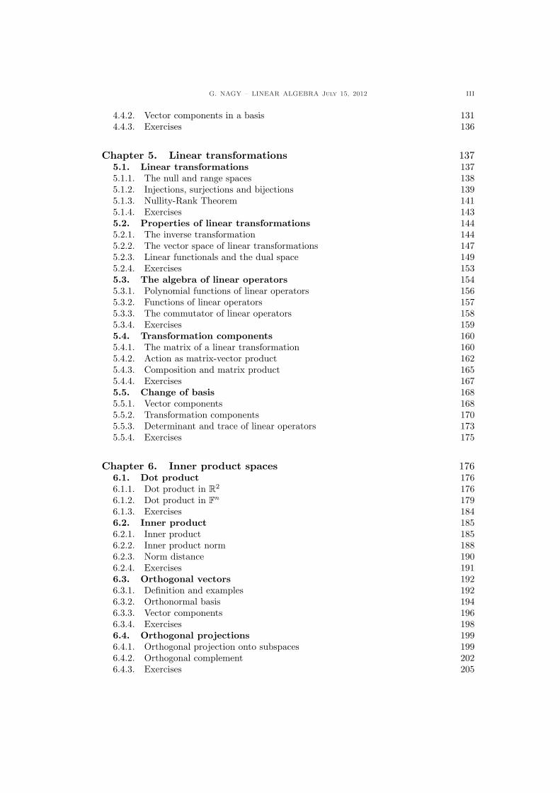
Examples of vectors are oriented segments on a line, plane, or space. An oriented segmentis an ordered pair of points in these sets. Such ordered pair can be drawn as an arrow thatstarts on the first point and ends on the second point. Fix a preferred point in the line, planeor space, called the origin point, and then there exists a one-to-one correspondence betweenpoints in these sets and arrows that start at the origin point. The set of oriented segmentswith common origin in a line, plane, and space are called R, R2 and R3, respectively.A sketch of vectors in these sets can be seen in Fig. 1. Two operations are defined onoriented segments with common origin point: An oriented segment can be stretched orcompressed; and two oriented segments with the same origin point can be added using theparallelogram law. An addition of several stretched or compressed vectors is called a linearcombination. The set of all oriented segments with common origin point together with thisoperation of linear combination is the essential structure called vector space. The origin ofthe word “space” in the term “vector space” originates precisely in these examples, whichwere associated with the physical space.
0 0 0
Figure 1. Example of vectors in the line, plane, and space, respectively.
Linear transformations are a particular type of functions between vector spaces thatpreserve the operation of linear combination. An example of a linear transformation is a2×2 matrix A =
[1 23 4
]together with a matrix-vector product that specifies how this matrix
transforms a vector on the plane into another vector on the plane. The result is thus afunction A : R2 → R2.
These notes try to be an elementary introduction to linear algebra with few applications.
Notation and conventions. We use the notation F ∈ {R,C} to mean that F = R orF = C. Vectors will be denoted by boldface letters, like u and v. The exception are acolumn vectors in Fn which are denoted in sanserif, like u and v. This notation permitsto differentiate between a vector and its components on a basis. In a similar way, lineartransformations between vector spaces are denoted by boldface capital letters, like T andS. The exception are matrices in Fm,n which are denoted by capital sanserif letters like Aand B. Again, this notation is useful to differentiate between a linear transformation and its

2 G. NAGY – LINEAR ALGEBRA july 15, 2012
components on two bases. Below is a list of few mathematical symbols used in these notes:
R Set of real numbers, Q Set of rational numbers,Z Set of integer numbers, N Set of positive integers,
{0} Zero set, ∅ Empty set,∪ Union of sets, ∩ Intersection of sets,
:= Definition, ⇒ Implies,∀ For all, ∃ There exists,
Proof Beginning of a proof, ¤ End of a proof,Example Beginning of an example, C End of an example.
Acknowledgments. I thanks all my students for pointing out several misprints and forhelping make these notes more readable. I am specially grateful to Zhuo Wang and WenningFeng.
G. NAGY – LINEAR ALGEBRA July 15, 2012 3
Chapter 1. Linear systems
1.1. Row and column pictures
1.1.1. Row picture. A central problem in linear algebra is to find solutions of a system oflinear equations. A 2 × 2 linear system consists of two linear equations in two unknowns.More precisely, given the real numbers A11, A12, A21, A22, b1, and b2, find all numbers xand y solutions of both equations
A11x + A12y = b1, (1.1)
A21x + A22y = b2. (1.2)
These equations are called a system because there is more than one equation, and they arecalled linear because the unknowns, x and y, appear as multiplicative factors with powerzero or one (for example, there is no term proportional to x2 or to y3). The row picture ofa linear system is the method of finding solutions to this system as the intersection of allsolutions to every single equation in the system. The individual equations are called rowequations, or simply rows of the system.
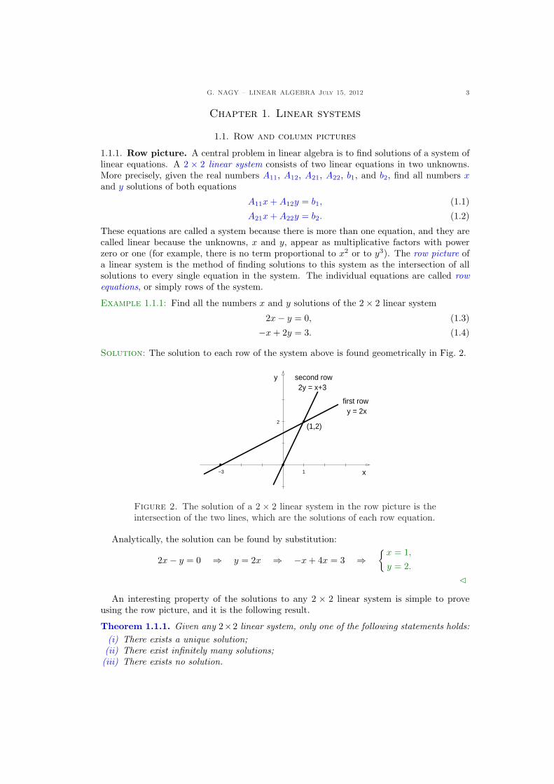
Example 1.1.1: Find all the numbers x and y solutions of the 2× 2 linear system
2x− y = 0, (1.3)
−x + 2y = 3. (1.4)
Solution: The solution to each row of the system above is found geometrically in Fig. 2.
2y = x+3
−3
(1,2)
y = 2x2
1 x
first row
y second row
Figure 2. The solution of a 2 × 2 linear system in the row picture is theintersection of the two lines, which are the solutions of each row equation.
Analytically, the solution can be found by substitution:
2x− y = 0 ⇒ y = 2x ⇒ −x + 4x = 3 ⇒{
x = 1,
y = 2.
C
An interesting property of the solutions to any 2 × 2 linear system is simple to proveusing the row picture, and it is the following result.
Theorem 1.1.1. Given any 2×2 linear system, only one of the following statements holds:(i) There exists a unique solution;(ii) There exist infinitely many solutions;(iii) There exists no solution.
4 G. NAGY – LINEAR ALGEBRA july 15, 2012
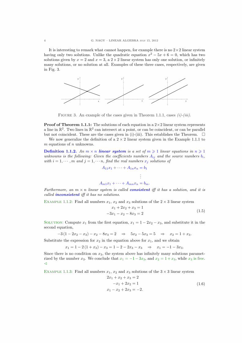
It is interesting to remark what cannot happen, for example there is no 2×2 linear systemhaving only two solutions. Unlike the quadratic equation x2 − 5x + 6 = 0, which has twosolutions given by x = 2 and x = 3, a 2× 2 linear system has only one solution, or infinitelymany solutions, or no solution at all. Examples of these three cases, respectively, are givenin Fig. 3.
x
y
x
y
x
y
Figure 3. An example of the cases given in Theorem 1.1.1, cases (i)-(iii).
Proof of Theorem 1.1.1: The solutions of each equation in a 2×2 linear system representsa line in R2. Two lines in R2 can intersect at a point, or can be coincident, or can be parallelbut not coincident. These are the cases given in (i)-(iii). This establishes the Theorem. ¤
We now generalize the definition of a 2 × 2 linear system given in the Example 1.1.1 tom equations of n unknowns.
Definition 1.1.2. An m × n linear system is a set of m > 1 linear equations in n > 1unknowns is the following: Given the coefficients numbers Aij and the source numbers bi,with i = 1, · · · ,m and j = 1, · · ·n, find the real numbers xj solutions of
A11x1 + · · ·+ A1nxn = b1
...Am1x1 + · · ·+ Amnxn = bm.
Furthermore, an m × n linear system is called consistent iff it has a solution, and it iscalled inconsistent iff it has no solutions.
Example 1.1.2: Find all numbers x1, x2 and x3 solutions of the 2× 3 linear systemx1 + 2x2 + x3 = 1
−3x1 − x2 − 8x3 = 2(1.5)
Solution: Compute x1 from the first equation, x1 = 1− 2x2 − x3, and substitute it in thesecond equation,
−3 (1− 2x2 − x3)− x2 − 8x3 = 2 ⇒ 5x2 − 5x3 = 5 ⇒ x2 = 1 + x3.
Substitute the expression for x2 in the equation above for x1, and we obtain
x1 = 1− 2 (1 + x3)− x3 = 1− 2− 2x3 − x3 ⇒ x1 = −1− 3x3.
Since there is no condition on x3, the system above has infinitely many solutions paramet-rized by the number x3. We conclude that x1 = −1− 3x3, and x2 = 1+x3, while x3 is free.C
Example 1.1.3: Find all numbers x1, x2 and x3 solutions of the 3× 3 linear system2x1 + x2 + x3 = 2−x1 + 2x2 = 1
x1 − x2 + 2x3 = −2.
(1.6)
G. NAGY – LINEAR ALGEBRA July 15, 2012 5
Solution: While the row picture is appropriate to solve small systems of linear equations,it becomes difficult to carry out on 3× 3 and bigger linear systems. The solution x1, x2, x3
of the system above can be found as follows: Substitute the second equation into the first,
x1 = −1 + 2x2 ⇒ x3 = 2− 2x1 − x2 = 2 + 2− 4x2 − x2 ⇒ x3 = 4− 5x2;
then, substitute the second equation and x3 = 4− 5x2 into the third equation,
(−1 + 2x2)− x2 + 2(4− 5x2) = −2 ⇒ x2 = 1,
and then, substituting backwards, x1 = 1 and x3 = −1. We conclude that the solution is asingle point in space given by (1, 1,−1). C
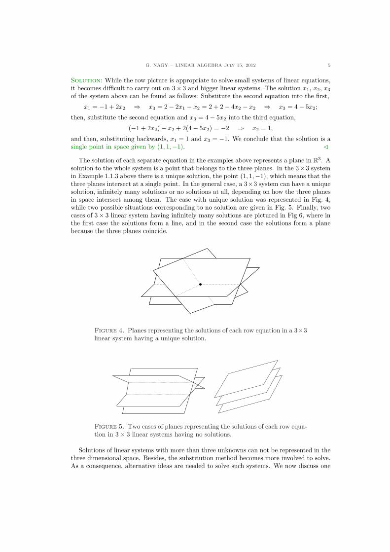
The solution of each separate equation in the examples above represents a plane in R3. Asolution to the whole system is a point that belongs to the three planes. In the 3×3 systemin Example 1.1.3 above there is a unique solution, the point (1, 1,−1), which means that thethree planes intersect at a single point. In the general case, a 3×3 system can have a uniquesolution, infinitely many solutions or no solutions at all, depending on how the three planesin space intersect among them. The case with unique solution was represented in Fig. 4,while two possible situations corresponding to no solution are given in Fig. 5. Finally, twocases of 3× 3 linear system having infinitely many solutions are pictured in Fig 6, where inthe first case the solutions form a line, and in the second case the solutions form a planebecause the three planes coincide.
Figure 4. Planes representing the solutions of each row equation in a 3×3linear system having a unique solution.
Figure 5. Two cases of planes representing the solutions of each row equa-tion in 3× 3 linear systems having no solutions.
Solutions of linear systems with more than three unknowns can not be represented in thethree dimensional space. Besides, the substitution method becomes more involved to solve.As a consequence, alternative ideas are needed to solve such systems. We now discuss one
6 G. NAGY – LINEAR ALGEBRA july 15, 2012
Figure 6. Two cases of planes representing the solutions of each row equa-tion in 3× 3 linear systems having infinitely many solutions.
of such ideas, the use of vectors to interpret and find solutions of linear systems. In the nextSection we introduce another idea, the use of matrices and vectors to solve linear systemsfollowing the Gauss-Jordan method. This latter procedure is suitable to solve large systemsof linear equations in an efficient way.
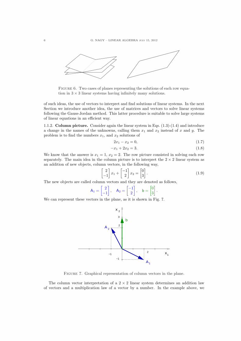
1.1.2. Column picture. Consider again the linear system in Eqs. (1.3)-(1.4) and introducea change in the names of the unknowns, calling them x1 and x2 instead of x and y. Theproblem is to find the numbers x1, and x2 solutions of
2x1 − x2 = 0, (1.7)
−x1 + 2x2 = 3. (1.8)
We know that the answer is x1 = 1, x2 = 2. The row picture consisted in solving each rowseparately. The main idea in the column picture is to interpret the 2 × 2 linear system asan addition of new objects, column vectors, in the following way,[
2−1
]x1 +
[−12
]x2 =
[03
]. (1.9)
The new objects are called column vectors and they are denoted as follows,
A1 =[
2−1
], A2 =
[−12
], b =
[03
].
We can represent these vectors in the plane, as it is shown in Fig. 7.
x
−1
−1
b
2A
A1
x12
2
3
2
Figure 7. Graphical representation of column vectors in the plane.
The column vector interpretation of a 2 × 2 linear system determines an addition lawof vectors and a multiplication law of a vector by a number. In the example above, we
G. NAGY – LINEAR ALGEBRA July 15, 2012 7
know that the solution is given by x1 = 1 and x2 = 2, therefore in the column pictureinterpretation the following equation must hold[
2−1
]+
[−12
]2 =
[03
].
The study of this example suggests that the multiplication law of a vector by numbers andthe addition law of two vectors can be defined by the following equations, respectively,[−1
2
]2 =
[(−1)2(2)2
],
[2−1
]+
[−24
]=
[2− 2−1 + 4
].
The study of several examples of 2× 2 linear systems in the column picture determines thefollowing definition.
Definition 1.1.3. The linear combination of the 2-vectors u =[u1
u2
]and v =
[v1
v2
], with
the real numbers a and b, is defined as follows,
a
[u1
u2
]+ b
[v1
v2
]=
[au1 + bv1
au2 + bv2
].
A linear combination includes the particular cases of addition (a = b = 1), and multipli-cation of a vector by a number (b = 0), respectively given by,[
u1
u2
]+
[v1
v2
]=
[u1 + v1
u2 + v2
], a
[u1
u2
]=
[au1
au2
].
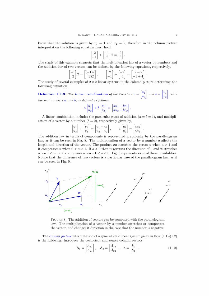
The addition law in terms of components is represented graphically by the parallelogramlaw, as it can be seen in Fig. 8. The multiplication of a vector by a number a affects thelength and direction of the vector. The product au stretches the vector u when a > 1 andit compresses u when 0 < a < 1. If a < 0 then it reverses the direction of u and it stretcheswhen a < −1 and compresses when −1 < a < 0. Fig. 8 represents some of these possibilities.Notice that the difference of two vectors is a particular case of the parallelogram law, as itcan be seen in Fig. 9.
Vv
wv
w
2
2
1 1
1
2x
(v+w)
x 1
(v+w)2
V+W
W
a > 1
V
− V
a = −1
0 < a < 1
Va
Va
Figure 8. The addition of vectors can be computed with the parallelogramlaw. The multiplication of a vector by a number stretches or compressesthe vector, and changes it direction in the case that the number is negative.
The column picture interpretation of a general 2×2 linear system given in Eqs. (1.1)-(1.2)is the following: Introduce the coefficient and source column vectors
A1 =[A11
A21
], A2 =
[A12
A22
], b =
[b1
b2
], (1.10)
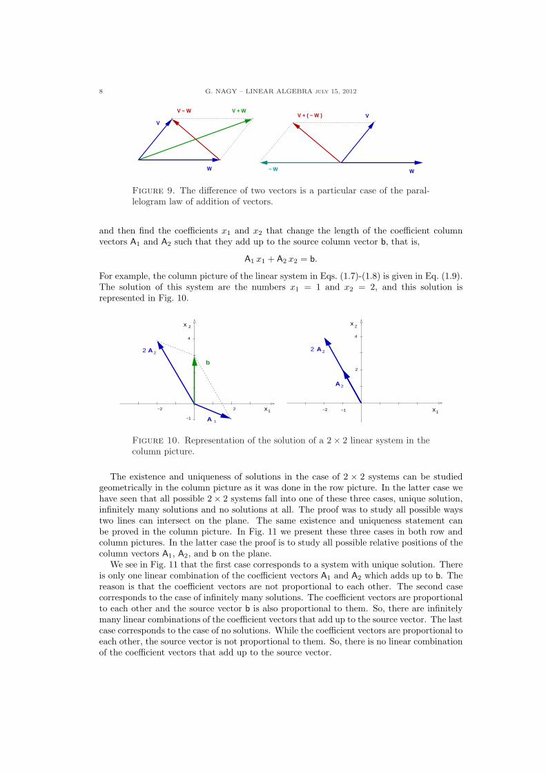
8 G. NAGY – LINEAR ALGEBRA july 15, 2012
− WW
V
V − W V + WV
W
V + ( − W )
Figure 9. The difference of two vectors is a particular case of the paral-lelogram law of addition of vectors.
and then find the coefficients x1 and x2 that change the length of the coefficient columnvectors A1 and A2 such that they add up to the source column vector b, that is,
A1 x1 + A2 x2 = b.
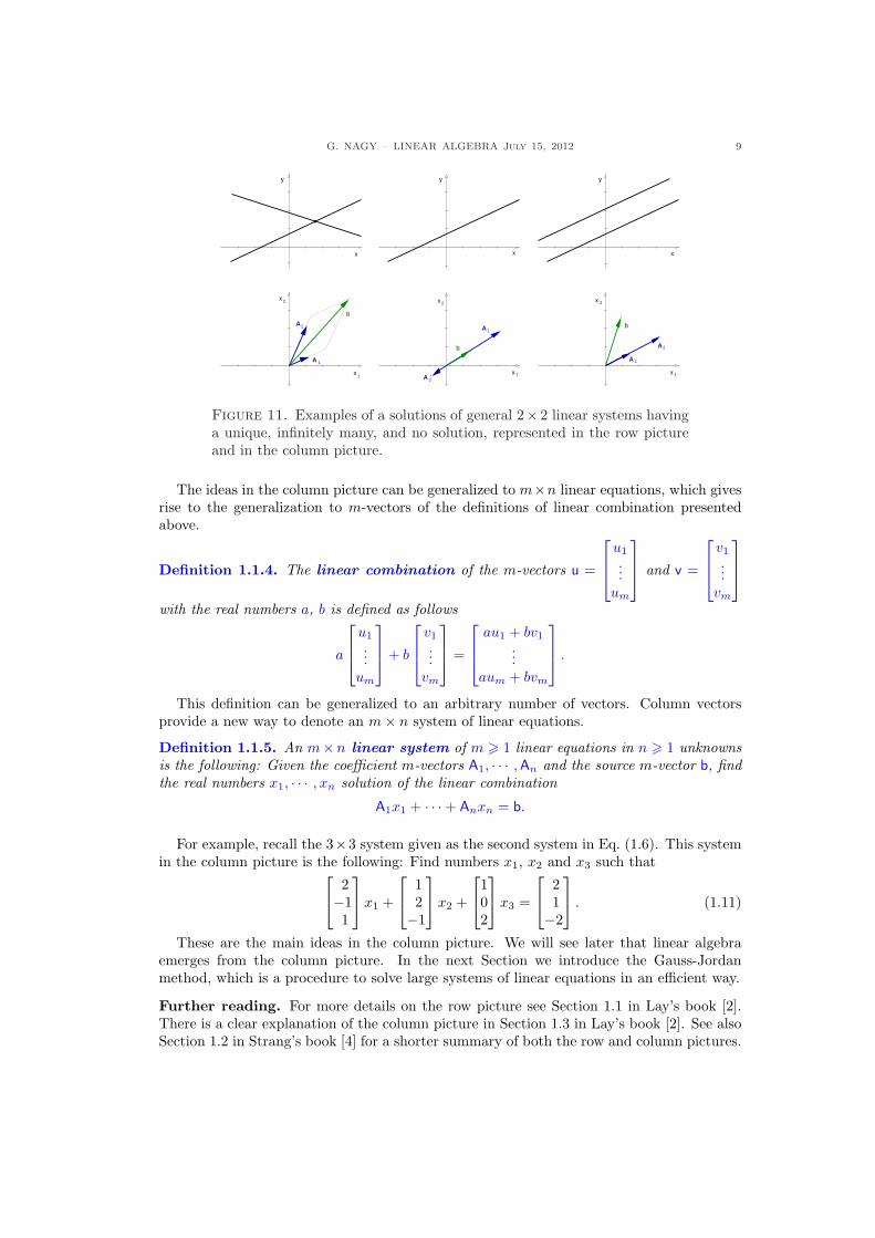
For example, the column picture of the linear system in Eqs. (1.7)-(1.8) is given in Eq. (1.9).The solution of this system are the numbers x1 = 1 and x2 = 2, and this solution isrepresented in Fig. 10.
x
b
2A2
A 1
x1
4
2−2
−1
2 2
2A
2A2
4
2
−1−2 x1
x
Figure 10. Representation of the solution of a 2× 2 linear system in thecolumn picture.
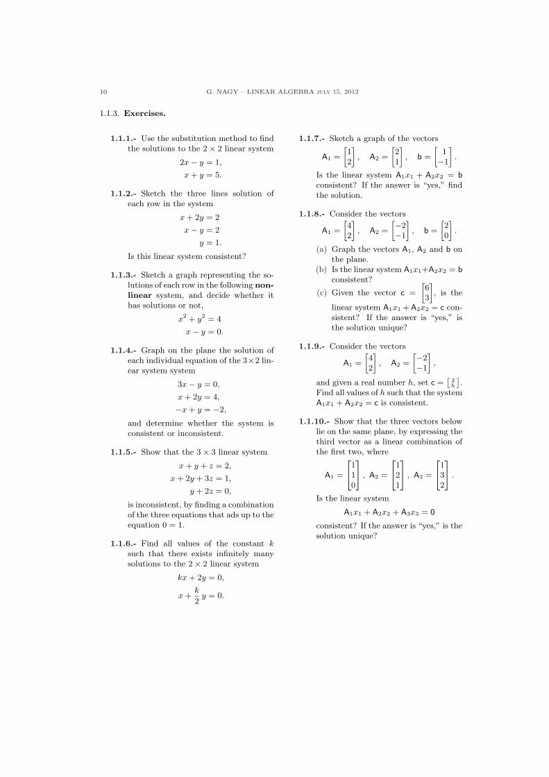
The existence and uniqueness of solutions in the case of 2 × 2 systems can be studiedgeometrically in the column picture as it was done in the row picture. In the latter case wehave seen that all possible 2× 2 systems fall into one of these three cases, unique solution,infinitely many solutions and no solutions at all. The proof was to study all possible waystwo lines can intersect on the plane. The same existence and uniqueness statement canbe proved in the column picture. In Fig. 11 we present these three cases in both row andcolumn pictures. In the latter case the proof is to study all possible relative positions of thecolumn vectors A1, A2, and b on the plane.
We see in Fig. 11 that the first case corresponds to a system with unique solution. Thereis only one linear combination of the coefficient vectors A1 and A2 which adds up to b. Thereason is that the coefficient vectors are not proportional to each other. The second casecorresponds to the case of infinitely many solutions. The coefficient vectors are proportionalto each other and the source vector b is also proportional to them. So, there are infinitelymany linear combinations of the coefficient vectors that add up to the source vector. The lastcase corresponds to the case of no solutions. While the coefficient vectors are proportional toeach other, the source vector is not proportional to them. So, there is no linear combinationof the coefficient vectors that add up to the source vector.
G. NAGY – LINEAR ALGEBRA July 15, 2012 9
x
y
x
y
x
y
b2
A
2x
A
1
x 1
b
2x
A 1
x 1
b
2A
2x
x 1
A 1
A 2
Figure 11. Examples of a solutions of general 2× 2 linear systems havinga unique, infinitely many, and no solution, represented in the row pictureand in the column picture.
The ideas in the column picture can be generalized to m×n linear equations, which givesrise to the generalization to m-vectors of the definitions of linear combination presentedabove.
Definition 1.1.4. The linear combination of the m-vectors u =
u1
...um
and v =
v1
...vm
with the real numbers a, b is defined as follows
a
u1
...um
+ b
v1
...vm
=
au1 + bv1
...aum + bvm
.
This definition can be generalized to an arbitrary number of vectors. Column vectorsprovide a new way to denote an m× n system of linear equations.
Definition 1.1.5. An m×n linear system of m > 1 linear equations in n > 1 unknownsis the following: Given the coefficient m-vectors A1, · · · , An and the source m-vector b, findthe real numbers x1, · · · , xn solution of the linear combination
A1x1 + · · ·+ Anxn = b.
For example, recall the 3×3 system given as the second system in Eq. (1.6). This systemin the column picture is the following: Find numbers x1, x2 and x3 such that
2−11
x1 +
12−1
x2 +
102
x3 =
21−2
. (1.11)
These are the main ideas in the column picture. We will see later that linear algebraemerges from the column picture. In the next Section we introduce the Gauss-Jordanmethod, which is a procedure to solve large systems of linear equations in an efficient way.
Further reading. For more details on the row picture see Section 1.1 in Lay’s book [2].There is a clear explanation of the column picture in Section 1.3 in Lay’s book [2]. See alsoSection 1.2 in Strang’s book [4] for a shorter summary of both the row and column pictures.
10 G. NAGY – LINEAR ALGEBRA july 15, 2012
1.1.3. Exercises.
1.1.1.- Use the substitution method to findthe solutions to the 2× 2 linear system
2x− y = 1,
x + y = 5.
1.1.2.- Sketch the three lines solution ofeach row in the system
x + 2y = 2
x− y = 2
y = 1.
Is this linear system consistent?
1.1.3.- Sketch a graph representing the so-lutions of each row in the following non-linear system, and decide whether ithas solutions or not,
x2 + y2 = 4
x− y = 0.
1.1.4.- Graph on the plane the solution ofeach individual equation of the 3×2 lin-ear system system
3x− y = 0,
x + 2y = 4,
−x + y = −2,
and determine whether the system isconsistent or inconsistent.
1.1.5.- Show that the 3× 3 linear system
x + y + z = 2,
x + 2y + 3z = 1,
y + 2z = 0,
is inconsistent, by finding a combinationof the three equations that ads up to theequation 0 = 1.
1.1.6.- Find all values of the constant ksuch that there exists infinitely manysolutions to the 2× 2 linear system
kx + 2y = 0,
x +k
2y = 0.
1.1.7.- Sketch a graph of the vectors
A1 =
»12
–, A2 =
»21
–, b =
»1−1
–.
Is the linear system A1x1 + A2x2 = bconsistent? If the answer is “yes,” findthe solution.
1.1.8.- Consider the vectors
A1 =
»42
–, A2 =
»−2−1
–, b =
»20
–.
(a) Graph the vectors A1, A2 and b onthe plane.
(b) Is the linear system A1x1+A2x2 = bconsistent?
(c) Given the vector c =
»63
–, is the
linear system A1x1 + A2x2 = c con-sistent? If the answer is “yes,” isthe solution unique?
1.1.9.- Consider the vectors
A1 =
»42
–, A2 =
»−2−1
–,
and given a real number h, set c =ˆ
2h
˜.
Find all values of h such that the systemA1x1 + A2x2 = c is consistent.
1.1.10.- Show that the three vectors belowlie on the same plane, by expressing thethird vector as a linear combination ofthe first two, where
A1 =
24
110
35 , A2 =
24
121
35 , A3 =
24
132
35 .
Is the linear system
A1x1 + A2x2 + A3x3 = 0
consistent? If the answer is “yes,” is thesolution unique?
G. NAGY – LINEAR ALGEBRA July 15, 2012 11
1.2. Gauss-Jordan method
1.2.1. The augmented matrix. Solutions to m × n linear systems can be obtained inan efficient way using the Gauss-Jordan method. Efficient here means to perform as fewalgebraic operations as possible either to find the solution or to show that the solution doesnot exist. Before introducing this method, we need several definitions.
Definition 1.2.1. The coefficients matrix, the source vector, and the augmentedmatrix of the m× n linear system
A11x1 + · · ·+ A1nxn = b1
...Am1x1 + · · ·+ Amnxn = bm,
are given by, respectively,
A =
A11 · · · A1n
......
Am1 · · · Amn
, b =
b1
...bm
,
[A|b]
=
A11 · · · A1n
∣∣∣∣ b1
......
∣∣∣∣...
Am1 · · · Amn
∣∣∣ bm
.
We call A an m × n matrix, with m the number of rows and n the number of columns.The source vector b is a particular case of an m × 1 matrix. The augmented matrix of anm×n linear system is given by the coefficient matrix and the source vector together, henceit is an m× (n + 1) matrix.
Example 1.2.1: Find the coefficient matrix, the source vector and the augmented matrixof the 2× 2 linear system
2x1 − x2 = 0, (1.12)
−x1 + 2x2 = 3. (1.13)
Solution: The coefficient matrix is 2 × 2, the source vector is 2 × 1, and the augmentedmatrix is 2× 3, given respectively by
A =[
2 −1−1 2
], b =
[03
], [A|b] =
[2 −1
∣∣ 0−1 2
∣∣ 3
]. (1.14)
C
Example 1.2.2: Find the coefficient matrix, the source vector and the augmented matrixof the 2× 3 linear system
2x1 − x2 = 0,
−x1 + 2x2 + 3x3 = 0.
Solution: The coefficient matrix is 2 × 3, the source vector is 2 × 1, and the augmentedmatrix is 2× 4, given respectively by
A =[
2 −1 0−1 2 3
], b =
[00
], [A|b] =
[2 −1 0
∣∣ 0−1 2 3
∣∣ 0
].
Notice that the coefficent matrix in this example is equal to the augmented matrix in theprevious Example. This means that the vertical separator in the definition of the augmented
12 G. NAGY – LINEAR ALGEBRA july 15, 2012
matrix is important. If one does not write down the vertical separator in Example 1.2.1,then one is actually working on the system in Example 1.2.2. C
We also use the alternative notation A = [Aij ] to denote a matrix with components Aij ,and b = [bi] to denote a vector with components bi, where i = 1, · · · ,m and j = 1, · · · , n.
Definition 1.2.2. The diagonal of an m× n matrix A = [Aij ] is the set of all coefficientsAii for i = 1, · · · ,m. A matrix is upper triangular iff every coefficient below the diagonalvanishes, and lower triangular iff every coefficient above the diagonal vanishes.
Example 1.2.3: Highlight the diagonal coefficients in 3× 3, 2× 3 and 3× 2 matrices.
Solution: The diagonal coefficients in the 3 × 3, 2 × 3 and 3 × 2 matrices below arehighlighted in green, where the coefficients with ∗ denote non-diagonal coefficients:
A11 ∗ ∗∗ A22 ∗∗ ∗ A33
,
[A11 ∗ ∗∗ A22 ∗
],
A11 ∗∗ A22
∗ ∗
.
C
Example 1.2.4: Write down the most general 3 × 3, 2 × 3 and 3 × 2 upper triangularmatrices, highlighting the diagonal elements.
Solution: The following matrices are upper triangular:
A11 ∗ ∗0 A22 ∗0 0 A33
,
[A11 ∗ ∗0 A22 ∗
],
A11 ∗0 A22
0 0
.
C
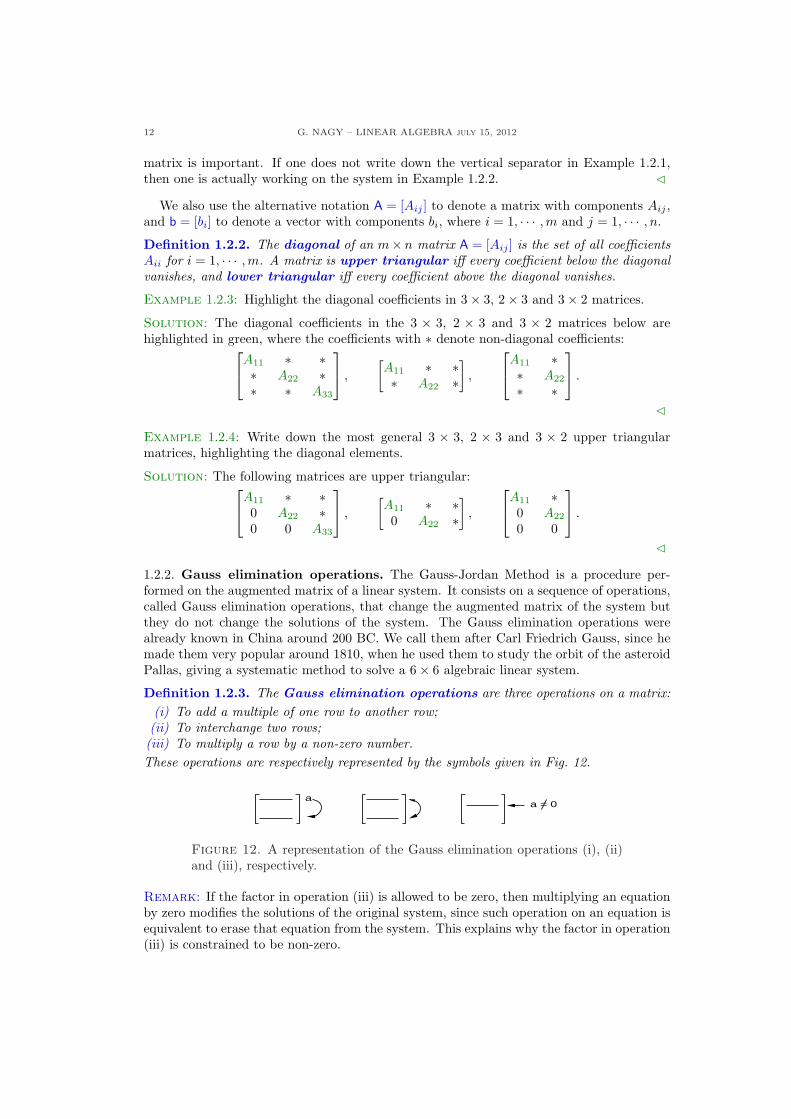
1.2.2. Gauss elimination operations. The Gauss-Jordan Method is a procedure per-formed on the augmented matrix of a linear system. It consists on a sequence of operations,called Gauss elimination operations, that change the augmented matrix of the system butthey do not change the solutions of the system. The Gauss elimination operations werealready known in China around 200 BC. We call them after Carl Friedrich Gauss, since hemade them very popular around 1810, when he used them to study the orbit of the asteroidPallas, giving a systematic method to solve a 6× 6 algebraic linear system.
Definition 1.2.3. The Gauss elimination operations are three operations on a matrix:(i) To add a multiple of one row to another row;(ii) To interchange two rows;(iii) To multiply a row by a non-zero number.These operations are respectively represented by the symbols given in Fig. 12.
aa = 0
Figure 12. A representation of the Gauss elimination operations (i), (ii)and (iii), respectively.
Remark: If the factor in operation (iii) is allowed to be zero, then multiplying an equationby zero modifies the solutions of the original system, since such operation on an equation isequivalent to erase that equation from the system. This explains why the factor in operation(iii) is constrained to be non-zero.
G. NAGY – LINEAR ALGEBRA July 15, 2012 13
The Gauss elimination operations change the coefficients of the augmented matrix of asystem but do not change its solution. Two systems of linear equations having the samesolutions are called equivalent. The Gauss-Jordan Method is an algorithm using theseoperations that transforms any linear system into an equivalent system where the solutionsare given explicitly. We describe the Gauss-Jordan Method only through examples.
Example 1.2.5: Find the solution of the 2× 2 linear system with augmented matrix givenin Eq. (1.14) using Gauss operations.
Solution: [2 −1
∣∣ 0−1 2
∣∣ 3
]→
[2 −1
∣∣ 0−2 4
∣∣ 6
]→
[2 −1
∣∣ 00 3
∣∣ 6
]→
[2 −1
∣∣ 00 1
∣∣ 2
]→
[2 0
∣∣ 20 1
∣∣ 2
]→
[1 0
∣∣ 10 1
∣∣ 2
].
The Gauss operations have changed the augmented matrix of the original system as follows:[2 −1
∣∣ 0−1 2
∣∣ 3
]→
[1 0
∣∣ 10 1
∣∣ 2
].
Since the Gauss operations do not change the solution of the associated linear systems,the augmented matrices above imply that the following two linear systems have the samesolutions,
2x1 − x2 = 0,
−x1 + 2x2 = 3.
}⇔
{x1 = 1,
x2 = 2.
On the last system the solution is given explicitly, x1 = 1, x2 = 2, since no additionalalgebraic operations are needed to find the solution. C
A precise way to define the notion of an augmented matrix corresponding to a linearsystem with solutions “easy to read” is captured in the notions of echelon form of a matrix,and reduced echelon form of a matrix. Next Section is dedicated to present these notionsin some detail.
1.2.3. Square systems. In the rest of this Section we study a particular type of linearsystems having the same number of equations and unknowns.
Definition 1.2.4. An m×n linear system is called a square system iff holds that m = n.
An example of a square system is the 2 × 2 linear system in Eqs. (1.12)-(1.13). In therest of this Section we introduce the Gauss operations and back substitution method to findsolutions to square linear systems. We later on compare this method with the Gauss-JordanMethod restricted to square linear systems.
We start using Gauss operations and back substitution to find solutions to square n × nlinear systems. This method has two main parts: First, use Gauss operations to transformthe augmented matrix of the system into an upper triangular form. Second, use backsubstitution to compute the solution to the system.
Example 1.2.6: Use the Gauss operations and back substitution to solve the 3× 3 system
2x1 + x2 + x3 = 2−x1 + 2x2 = 1
x1 − x2 + 2x3 = −2.
Solution: We have already seen in Example 1.1.3 that the solution of this system is givenby x1 = x2 = 1, x3 = −1. Let us find that solution using Gauss operations with back
14 G. NAGY – LINEAR ALGEBRA july 15, 2012
substitution. First transform the augmented matrix of the system into upper triangularform:
2 1 1
∣∣ 2−1 2 0
∣∣ 11 −1 2
∣∣ −2
→
1 −1 2∣∣ −2
−1 2 0∣∣ 1
2 1 1∣∣ 2
→
1 −1 2∣∣ −2
0 1 2∣∣ −1
0 3 −3∣∣ 6
1 −1 2∣∣ −2
0 1 2∣∣ −1
0 0 −9∣∣ 9
→
1 −1 2∣∣ −2
0 1 2∣∣ −1
0 0 1∣∣ −1
.
We now write the linear system corresponding to the last augmented matrix,
2x1 − x2 + 2x3 = −2x2 + 2x3 = −1
x3 = −1.
We now use the back substitution to obtain the solution, that is, introduce x3 = −1 intothe second equation, which gives us x2 = 1. Then, substitute x3 = −1 and x2 = 1 into thefirst equation, which gives us x1 = 1. C
We now use the Gauss-Jordan Method to find solutions to square n × n linear systems.This is a minor modification of the Gauss operations and back substitution method. Thedifference is that now we do not stop doing Gauss operations when the augmented matrixbecomes upper triangular. We keep doing Gauss operations in order to make zeros abovethe diagonal. Then, back substitution will no be needed to find the solution of the linearsystem. The solution will be given explicitly at the end of the procedure.
Example 1.2.7: Use the Gauss-Jordan method to solve the same 3× 3 linear system as inExample 1.2.6, that is,
2x1 + x2 + x3 = 2−x1 + 2x2 = 1
x1 − x2 + 2x3 = −2.
Solution: In Example 1.2.6 we performed Gauss operations on the augmented matrix ofthe system above until we obtained an upper triangular matrix, that is,
2 1 1
∣∣ 2−1 2 0
∣∣ 11 −1 2
∣∣ −2
→
1 −1 2∣∣ −2
0 1 2∣∣ −1
0 0 1∣∣ −1
.
The idea now is to continue with Gauss operations, as follows:
1 −1 2∣∣ −2
0 1 2∣∣ −1
0 0 1∣∣ −1
→
1 0 4∣∣ −3
0 1 2∣∣ −1
0 0 1∣∣ −1
→
1 0 0∣∣ 1
0 1 0∣∣ 1
0 0 1∣∣ −1
⇒
x1 = 1,
x2 = 1,
x3 = −1.
In the last step we do not need to do back substitution to compute the solution. It isobtained without doing any further algebraic operation. C
Further reading. Almost every linear algebra book describes the Gauss-Jordan method.See Section 1.2 in Lay’s book [2] for a summary of echelon forms and the Gauss-Jordanmethod. See Sections 1.2 and 1.3 in Meyer’s book [3] for more details on Gauss eliminationoperations and back substitution. Also see Section 1.3 in Strang’s book [4].
G. NAGY – LINEAR ALGEBRA July 15, 2012 15
1.2.4. Exercises.
1.2.1.- Use Gauss operations andback substitution to find thesolution of the 3×3 linear sys-tem
x1 + x2 + x3 = 1,
x1 + 2x2 + 2x3 = 1,
x1 + 2x2 + 3x3 = 1.
1.2.2.- Use Gauss operations andback substitution to find thesolution of the 3×3 linear sys-tem
2x1 − 3x2 = 3,
4x1 − 5x2 + x3 = 7,
2x1 − x2 − 3x3 = 5.
1.2.3.- Find the solution of thefollowing linear system withGauss-Jordan’s method,
4x2 − 3x3 = 3,
−x1 + 7x2 − 5x3 = 4,
−x1 + 8x2 − 6x3 = 5.
1.2.4.- Find the solutions to the following two linearsystems, which have the same matrix of coefficientA but different source vectors b1 and b2, givenrespectively by,
4x1 − 8x2 + 5x3 = 1,
4x1 − 7x2 + 4x3 = 0,
3x1 − 4x2 + 2x3 = 0,
4x1 − 8x2 + 5x3 = 0,
4x1 − 7x2 + 4x3 = 1,
3x1 − 4x2 + 2x3 = 0.
Solve these two systems at one time using theGauss-Jordan method on an augmented matrixof the form [A|b1|b2].
1.2.5.- Use the Gauss-Jordan method to solve the fol-lowing three linear systems at the same time,
2x1 − x2 = 1, = 0, = 0,
−x1 + 2x2 − x3 = 0, = 1, = 0,
−x2 + x3 = 0, = 0, = 1.
16 G. NAGY – LINEAR ALGEBRA july 15, 2012
1.3. Echelon forms
1.3.1. Echelon and reduced echelon forms. The Gauss-Jordan method is a procedurethat uses Gauss operations to transform the augmented matrix of an m × n linear systeminto the augmented matrix of an equivalent system whose solutions can be found withoutperforming further algebraic operations. A precise way to define the notion of a linear systemwith solutions that can be found without doing further algebraic operations is captured inthe notions of echelon form and reduced echelon form of its augmented matrix.
Definition 1.3.1. An m× n matrix is in echelon form iff the following conditions hold:
(i) The zero rows are located at the bottom rows of the matrix;(ii) The first non-zero coefficient on a row is always to the right of the first non-zero
coefficient of the row above it.
The pivot coefficient is the first non-zero coefficient on every non-zero row in a matrix inechelon form.
Example 1.3.1: The 6× 8, 3× 5 and 3× 3 matrices given below are in echelon form, wherepivots are highlighted and the ∗ means any non-zero number.
∗ ∗ ∗ ∗ ∗ ∗ ∗ ∗0 0 ∗ ∗ ∗ ∗ ∗ ∗0 0 0 ∗ ∗ ∗ ∗ ∗0 0 0 0 0 0 ∗ ∗0 0 0 0 0 0 0 00 0 0 0 0 0 0 0
,
∗ ∗ ∗ ∗ ∗0 0 ∗ ∗ ∗0 0 0 0 0
,
∗ ∗ ∗0 ∗ ∗0 0 ∗
.
C
Example 1.3.2: The following matrices are in echelon form, with pivots highlighted:
[1 30 1
],
[2 3 20 4 −2
],
2 1 10 3 40 0 0
.
C
Definition 1.3.2. An m×n matrix is in reduced echelon form iff the matrix is in echelonform and the following two conditions hold:
(i) The pivot coefficient is equal to 1;(ii) The pivot coefficient is the only non-zero coefficient in that column.
We denote by EA a reduced echelon form of a matrix A.
Example 1.3.3: The 6× 8, 3× 5 and 3× 3 matrices given below are in echelon form, wherepivots are highlighted and the ∗ means any non-zero number.
1 ∗ 0 0 ∗ ∗ 0 ∗0 0 1 0 ∗ ∗ 0 ∗0 0 0 1 ∗ ∗ 0 ∗0 0 0 0 0 0 1 ∗0 0 0 0 0 0 0 00 0 0 0 0 0 0 0
,
1 ∗ 0 ∗ ∗0 0 1 ∗ ∗0 0 0 0 0
,
1 0 00 1 00 0 1
.
C
G. NAGY – LINEAR ALGEBRA July 15, 2012 17
Example 1.3.4: And the following matrices are not only in echelon form but also in reducedechelon form; again, pivot coefficients are highlighted:
[1 00 1
],
[1 0 40 1 5
],
1 0 00 1 00 0 0
.
C
Summarizing, the Gauss-Jordan method uses Gauss operations to transform the aug-mented matrix of a linear system into reduced echelon form. Then, the solutions of thelinear system can be obtained without doing further algebraic operations.
Example 1.3.5: Consider a 3 × 3 linear system with augmented matrix having a reducedechelon form given below. Then, the solution of this linear system is simple to obtain:
1 0 0∣∣ −1
0 1 0∣∣ 3
0 0 1∣∣ 2
⇒
x1 = −1x2 = 3x3 = 2.
C
We use the notation EA for a reduced echelon form of an m×n matrix A, since a reducedechelon form of a matrix has an important property: It is unique. We state this propertyin Proposition 1.3.3 below. Since the proof is somehow involved, after the proof we show adifferent proof for the particular case of 2× 2 matrices.
Proposition 1.3.3. The reduced echelon EA form of an m× n matrix A is unique.
Proof of Proposition 1.3.3: We assume that there exists an m× n matrix A having tworeduced echelon forms EA and EA, and we will show that EA = EA. Introduce the columnvector notation for matrices (see Sect. 1.4) and for vectors (see Sect. 1.4), respectively,
A =[A1, · · · , An
], EA =
[E1, · · · , En
], EA =
[E1, · · · , En
], x =
x1
...xn
.
If the reduced echelon forms EA and EA were different, then they should start differing at aparticular column, say column i, with 1 6 i 6 n. That is, there would be vectors Ei and Ei
satisfying Ei 6= Ei and Ej = Ej for j = 1, · · · , (i− 1). The proof of Proposition 1.3.3 reducesto show that this is not the case, by studying the following two cases:(a) The vector of one of the reduced echelon form matrices, say the column vector Ei of EA,
does not contain a pivot coefficient.(b) Both vectors Ei and Ei do contain a pivot coefficient.
Consider the case in (a). The definition of reduced echelon form implies that the vectorEi = [ej ] has non-zero components among the first k components, with 0 6 k < i, hence,ej = 0 for j = (k + 1), · · · , n. Furthermore, the definition of reduced echelon form alsoimplies that there are k columns to the left of vector Ei with pivot coefficients. Let usdenote these columns by Epj , for j = 1, · · · , k. We use a new subindex pj , since the kcolumns need not be the first k columns. This information about the reduced echelon formmatrix EA can be translated into a vector x solution of the linear system with augmentedmatrix
[EA
∣∣0]. This solution is the vector x = [xj ] with non-zero components xpj = ej for
j = 1, · · · , k, and xi = −1, while the rest of the components vanish, since the followingequations hold,
e1Ep1 + · · ·+ ekEpk+ (−1)Ei = 0 ⇔ xp1Ep1 + · · ·+ xpk
Epk+ xiEi = 0.
18 G. NAGY – LINEAR ALGEBRA july 15, 2012
Recall now that the solution of a linear system is not changed when Gauss operations areperformed on the coefficient matrix. Since Gauss operations change EA → A → EA, thesame vector x above is solution of the linear system with augmented matrix
[EA
∣∣0], that is,
xp1 Ep1 + · · ·+ xpkEpk
+ xiEi = 0 ⇔ e1Ep1 + · · ·+ ekEpk+ (−1)Ei = 0.
Since Ej = Ej for j = 1, · · · , k, the second equation above implies that Ei = Ei also holds.We conclude that the first vector in EA that differs from a vector in EA cannot be a vectorwithout pivot coefficients.
Consider the case in (b), that is, if Ei and Ei are the first vectors from EA and EA,respectively, which are different, then both vectors have pivot coefficients. (If only one ofthese vectors had a pivot coefficient, then the argument in case (a) on the vector withoutpivot coefficient would imply that the first vector could not have a pivot coefficient.) Supposethat the vector Ei = [ej ] has the pivot coefficient at the position k0, that is, ej = 0 for j 6= k)
and ek0 = 1. Similarly, suppose that the vector Ei = [ej ] has the pivot coefficient at theposition k1, that is, ej = 0 for j 6= k) and ek1 = 1. By definition of reduced echelon formall rows in EA above the k0 row have pivots columns to the left of Ei. This statement alsoapplies to matrix EA, since Ei is the first column that differs from EA. Therefore k0 6 k1.The exactly same argument also applies to matrix EA concluding that k1 6 k0. Therefore,k0 = k1, and so, Ei = Ei. We conclude that the first vector in EA that differs from a vectorin EA cannot be a vector with pivot a coefficient. Therefore, parts (a) and (b) establish theProposition. ¤
The proof above is not straightforward to understand, so it might be a good idea topresent a simpler proof for the particular case of 2× 2 matrices.Alternative proof of Proposition 1.3.3 in the case of 2 × 2 matrices: We startrecalling once again the following observation that holds for any m × n matrix A: SinceGauss operations do not change the solutions of the homogeneous system [A|0], if a matrixA has two different reduced echelon forms, EA and EA, then the set of solutions of the systems[EA|0] and [EA|0] must coincide with the solutions of the system [A|0]. What we are going toshow now is the following: All possible 2× 2 reduced echelon form matrices E have differentsolutions to the homogeneous equation [E|0]. This property then establishes that every 2×2matrix A has a unique reduced echelon form.
Given any 2× 2 matrix A, all possible reduced echelon forms are the following:
EA =[1 c0 0
], c ∈ R, EA =
[0 10 0
], EA =
[1 00 1
].
We claim that all these matrices determine different sets of solutions to the equation [EA|0].In the first case, the set of solutions are lines given by
x1 = −c x2, c ∈ R. (1.15)
In the second case, the set of solutions is a single line given by
x2 = 0, x1 ∈ R.
Notice that this line does not belong to the set given in Eq. (1.15). In the third case, thesolution is a single point
x1 = 0, x2 = 0.
Since all these sets of solutions are different, and only one corresponds to the equation[A|0], then there is only one reduced echelon form EA for matrix A. This establishes theProposition for 2× 2 matrices. ¤
G. NAGY – LINEAR ALGEBRA July 15, 2012 19
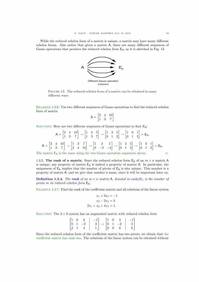
While the reduced echelon form of a matrix is unique, a matrix may have many differentechelon forms. Also notice that given a matrix A, there are many different sequences ofGauss operations that produce the reduced echelon form EA, as it is sketched in Fig. 13.
A EA
Different Gauss operation
schemes
Figure 13. The reduced echelon form of a matrix can be obtained in manydifferent ways.
Example 1.3.6: Use two different sequences of Gauss operations to find the reduced echelonform of matrix
A =[2 4 101 3 7
]
Solution: Here are two different sequences of Gauss operations to find EA:
A =[2 4 101 3 7
]→
[1 2 51 3 7
]→
[1 2 50 1 2
]→
[1 0 10 1 2
]= EA,
A =[2 4 101 3 7
]→
[1 3 72 4 10
]→
[1 2 50 −2 −4
]→
[1 2 50 1 2
]→
[1 0 10 1 2
]= EA.
The matrix EA is the same using the two Gauss operation sequences above. C
1.3.2. The rank of a matrix. Since the reduced echelon form EA of an m × n matrix Ais unique, any property of matrix EA is indeed a property of matrix A. In particular, theuniqueness of EA implies that the number of pivots of EA is also unique. This number is aproperty of matrix A, and we give that number a name, since it will be important later on.
Definition 1.3.4. The rank of an m× n matrix A, denoted as rank(A), is the number ofpivots in its reduced echelon form EA.
Example 1.3.7: Find the rank of the coefficient matrix and all solutions of the linear system
x1 + 3x3 = −1x2 − 2x3 = 3
2x1 + x2 + 4x3 = 1.
Solution: The 3× 3 system has an augmented matrix with reduced echelon form
1 0 3∣∣ −1
0 1 −2∣∣ 3
2 1 4∣∣ 1
→
1 0 3∣∣ −1
0 1 −2∣∣ 3
0 0 0∣∣ 0
Since the reduced echelon form of the coefficient matrix has two pivots, we obtain that thecoefficient matrix has rank two. The solutions of the linear system can be obtained without
20 G. NAGY – LINEAR ALGEBRA july 15, 2012
any further calculations, since the coefficient matrix is already in reduced echelon form.These solutions are the following,
1 0 3∣∣ −1
0 1 −2∣∣ 3
0 0 0∣∣ 0
⇒
x1 = −1− 3x3,
x2 = 3 + 2x3,
x3 : free variable.
We call x3 a free variable, since there is a solution for every value of this variable. C
Definition 1.3.5. A variable in a linear system is called a free variable iff there is asolution of the linear system for every value of that variable.
In Example 1.3.7 the free variable is x3, since for every value of x3 the other two variablesx1 and x2 are fixed by the system. Notice that only the number of free variables is relevant,but not which particular variable is the free one. In the following example we express thesolutions in Example 1.3.7 in terms of x1 as a free variable.
Example 1.3.8: Express the solutions in Example 1.3.7 in terms of x1 as a free variable.
Solution: The solutions given in Example 1.3.7 can also be expressed as
x1 : free variable,
x2 = 3 +23
(−1− x1),
x3 =13
(−1− x1).
C
As the reader may have noticed there is a relation between the rank of the coefficientmatrix and the number of free variables in the solution of the linear system.
Theorem 1.3.6. The number of free variables in the solutions of an m×n consistent linearsystem with augmented matrix [A|b] is given by
(n− rank(A)
).
Proof of Theorem 1.3.6: The number of non-pivots columns in EA is actually the numberof variables not fixed by the linear system with augmented matrix [A|b]. The number of non-pivot columns is the total number of columns minus the pivot columns, that is,
(n−rank(A)
).
This establishes the Theorem. ¤We saw in Example 1.3.7 that the 3 × 3 coefficient matrix has rank(A) = 2. Since the
system has n = 3 variables, we conclude, without actually computing the solution, that thesolution has n− rank(A) = 3 = 2 = 1 free variable. The free variable can be any variable inthe system. The relevant information is that there is one free variable.
Example 1.3.9: We now present three examples of consistent linear systems.(i) Show that the 2 × 2 linear system below is consistent with coefficient matrix having
rank one and solutions having one free variable,
2x1 − x2 = 1
−12
x1 +14
x1 = −14.
Solution: Gauss operations transform the augmented matrix of the system as follows,[2 −1
∣∣ 1−1/2 1/4
∣∣ −1/4
]→
[2 −1
∣∣ 10 0
∣∣ 0
].
The system is consistent, has rank one, and has a free variable, hence the system hasinfinitely many solutions.
G. NAGY – LINEAR ALGEBRA July 15, 2012 21
(ii) Show that the 2 × 3 linear system below is consistent with coefficient matrix havingrank two and solution having one free variable,
x1 + 2x2 + 3x3 = 1,
3x1 + 5x2 + 2x3 = 2.
Solution: Perform the following Gauss operations on the augmented matrix,[1 2 3
∣∣ 13 5 2
∣∣ 2
]→
[1 2 3
∣∣ 10 −1 −7
∣∣ −1
]→
[1 0 −11
∣∣ −10 1 7
∣∣ 1
].
We see that the 2× 3 system has rank two, hence one free variable.(iii) Show that the 3 × 2 linear system below is consistent with coefficient matrix having
rank two and solution having no free variables,
x1 + 3x2 = 2,
2x1 + 2x2 = 0,
3x1 + x2 = −2.
Solution: Perform the following Gauss operations on the augmented matrix,
1 3∣∣ 2
2 2∣∣ 0
3 1∣∣ −2
→
1 3∣∣ 2
0 −4∣∣ −4
0 −8∣∣ −8
→
1 0∣∣ −1
0 1∣∣ 1
0 0∣∣ 0
.
We see that the 3× 2 system has rank two, hence no free variables. C
1.3.3. Inconsistent linear systems. Not every linear system has solutions. We now useboth the reduced echelon form of the coefficent matrix and of the augmented matrix tocharacterize inconsistent linear systems. We start with an example.
Example 1.3.10: Show that the following 2× 2 linear system has no solutions,
2x1 − x2 = 0 (1.16)
−12
x1 +14
x1 = −14. (1.17)
Solution: One way to see that there is no solution is the following: Multiplying the secondequation by −4 one obtains the equation
2x1 − x2 = 1,
whose solutions form a parallel line to the line given in Eq. (1.16). Therefore, the systemin Eqs. (1.16)-(1.17) has no solution. A second way to see that the system above has nosolution is using Gauss operations. The system above has augmented matrix
[2 −1
∣∣ 0− 1
214
∣∣ − 14
]→
[2 −1
∣∣ 00 0
∣∣ 1
].
The echelon form above corresponds to the linear system
2x1 − x2 = 00 = 1.
The solutions of this second system coincide with the solutions of Eqs. (1.16)-(1.17). Sincethe second system has no solution, the system in Eqs. (1.16)-(1.17) has no solution. C
This example is a particular cases of the following result.
22 G. NAGY – LINEAR ALGEBRA july 15, 2012
Theorem 1.3.7. An m × n linear system with augmented matrix [A|b] is inconsistent iffthe reduced echelon form of its augmented matrix contains a row of the form [0, · · · , 0 | 1];equivalently rank(A) < rank(A|b). Furthermore, a consistent system contains:
(i) A unique solution iff it has no free variables; equivalently rank(A) = n.(ii) Infinitely many solutions iff it has at least one free variable; equivalently rank(A) < n.
This Theorem says that a system is inconsistent iff its augmented matrix has a pivot in thesource vector column, which is the last column in an augmented matrix. In that case thesystem includes an equation of the form 0 = 1, which has no solution.
The idea of the proof if this Theorem is to study all possible reduced echelon forms EA ofan arbitrary matrix A, and then to study all possible augmented matrices [EA|c]. One thenconcludes that there are three main cases, no solutions, unique solutions, or infinitely manysolutions.Proof of Theorem 1.3.7: We only give the proof in the case of 3× 3 linear systems. Thereduced echelon form EA of a 3 × 3 matrix A determines a 3 × 4 augmented matrix [EA|c].There are 14 possible forms for this matrix. We start with the case of three pivots:
1 0 0∣∣ ∗
0 1 0∣∣ ∗
0 0 1∣∣ ∗
,
1 0 ∗ ∣∣ ∗0 1 ∗ ∣∣ ∗0 0 0
∣∣ 1
,
1 ∗ 0
∣∣ ∗0 0 1
∣∣ ∗0 0 0
∣∣ 1
,
0 1 0∣∣ ∗
0 0 1∣∣ ∗
0 0 0∣∣ 1
.
In the first case we have a unique solution, and rank(A) = 3. The other three cases cor-respond to no solutions. We now continue with the case of two pivots, which contains sixpossibilities, with the first three given by
1 0 ∗∣∣ ∗
0 1 ∗∣∣ ∗
0 0 0∣∣ 0
,
1 ∗ 0∣∣ ∗
0 0 1∣∣ ∗
0 0 0∣∣ 0
,
0 1 0∣∣ ∗
0 0 1∣∣ ∗
0 0 0∣∣ 0
,
which correspond to infinitely many solutions, with one free variable, rank(A) = 2. Theother three possibilities are given by
1 ∗ ∗ ∣∣ ∗0 0 0
∣∣ 10 0 0
∣∣ 0
,
0 1 ∗ ∣∣ ∗0 0 0
∣∣ 10 0 0
∣∣ 0
,
0 0 1∣∣ ∗
0 0 0∣∣ 1
0 0 0∣∣ 0
;
which correspond to no solution. Finally, we have the case of one pivot. It contains fourpossibilities, the first three of them are given by
1 ∗ ∗ ∣∣ ∗0 0 0
∣∣ 00 0 0
∣∣ 0
,
0 1 ∗ ∣∣ ∗0 0 0
∣∣ 00 0 0
∣∣ 0
,
0 0 1∣∣ ∗
0 0 0∣∣ 0
0 0 0∣∣ 0
;
which correspond to infinitely many solutions, with two free variables and rank(A) = 1. Thelast possibility is the trivial case
0 0 0∣∣ 1
0 0 0∣∣ 0
0 0 0∣∣ 0
,
which has no solutions. This establishes the Theorem for 3× 3 linear systems. ¤
Example 1.3.11: Sow that the 2× 2 linear system below is inconsistent:
2x1 − x2 = 1
−12
x1 +14
x1 = −14.
G. NAGY – LINEAR ALGEBRA July 15, 2012 23
Solution: The proof of the statement above is the following: Gauss-Jordan operationstransform the augmented matrix of the system as follows,[
2 −1∣∣ 0
− 12
14
∣∣ − 14
]→
[2 −1
∣∣ 00 0
∣∣ − 14
]→
[2 −1
∣∣ 00 0
∣∣ 1
].
Since there is a line of the form [0, 0|1], the system is inconsistent. We can also say that thecoefficient matrix has rank one, but the definition of free variables does not apply, since thesystem is inconsistent. C
Example 1.3.12: Find all numbers h and k such that the system below has only one, many,or no solutions,
x1 + hx2 = 1x1 + 2x2 = k.
Solution: Start finding the associated augmented matrix and reducing it into echelon form,[1 h
∣∣ 11 2
∣∣ k
]→
[1 h
∣∣ 10 2− h
∣∣ k − 1
].
Suppose h 6= 2, for example set h = 1, then[1 1
∣∣ 10 1
∣∣ k − 1
]→
[1 0
∣∣ 2− k0 1
∣∣ k − 1
],
so the system has a unique solution for all values of k. (The same conclusion holds if onesets h to any number different of 2.) Suppose now that h = 2, then,[
1 2∣∣ 1
0 0∣∣ k − 1
].
If k = 1 then [1 2
∣∣ 10 0
∣∣ 0
]⇒
{x1 = 1− 2x2,
x2 : free variable.so there are infinitely many solutions. If k 6= 1, the system is inconsistent, since[
1 2∣∣ 1,
0 0∣∣ k − 1 6= 0.
]
Summarizing, for h 6= 2 the system has a unique solution for every k. If h = 2 and k = 1the system has infinitely many solutions, if h = 2 and k 6= 1 the system has no solution. C
Further reading. See Sections 2.1, 2.2 and 2.3 in Meyer’s book [3] for a detailed discussionon echelon forms and rank, reduced echelon forms and inconsistent systems, respectively.Again, see Section 1.2 in Lay’s book [2] for a summary of echelon forms and the Gauss-Jordan method. Section 1.3 in Strang’s book [4] also helps.
24 G. NAGY – LINEAR ALGEBRA july 15, 2012
1.3.4. Exercises.
1.3.1.- Find the rank and the pivot columnsof the matrix
A =
24
1 2 1 12 4 2 23 6 3 4
35 .
1.3.2.- Find all the solutions x of the linearsystem Ax = 0, where the matrix A isgiven by
A =
24
1 2 1 32 1 −1 01 0 0 1
35
1.3.3.- Find all the solutions x of the linearsystem Ax = b, where the matrix A andthe vector b are given by
A =
24
1 2 42 −1 −73 2 0
35 , b =
24
3−41
35 .
1.3.4.- Construct a 3 × 4 matrix A and 3-vectors b, c, such that [A|b] is the aug-mented matrix of a consistent systemand [A|c] is the augmented matrix of aninconsistent system.
1.3.5.- Let A be an m × n matrix havingrank(A) = m. Explain why the systemwith augmented matrix [A|b] is consis-tent for every m-vector b.
1.3.6.- Consider the following system of lin-ear equations, where k represents anyreal number,
2x1 + kx2 = 1,
−4x1 + 2x2 = 4.
(a) Find all possible values of the num-ber k such that the system above isinconsistent.
(b) Set k = 2. In this case, find the
solution x =
»x1
x2
–.
G. NAGY – LINEAR ALGEBRA July 15, 2012 25
1.4. Non-homogeneous equations
In this Section we introduce the definitions of homogeneous and non-homogeneous linearsystems and discuss few relations between their solutions. We start, however, introducingnew notation. We first define a vector form for the solution of a linear system and we thenintroduce a matrix-vector product in order to express a linear system in a compact way. Oneadvantage of this notation appears in this Section: It is simple to realize that solutions of anon-homogeneous linear system are translations of solutions of the associated homogeneoussystem. A somehow deeper insight on the relation between matrices and vectors can beobtained from the matrix-vector product, which will be discussed in the next Chapter. Herewe can summarize this insight as follows: A matrix can be thought as a function acting onthe space of vectors.
1.4.1. Matrix-vector product. We start generalizing the vector notation to include theunknowns of a linear system. First, recall that given an m× n linear system
A11x1 + · · ·+ A1nxn = b1, (1.18)...
Am1x1 + · · ·+ Amnxn = bm, (1.19)
we have introduced the m×n coefficients matrix A = [Aij ] and the source m-vector b = [bi],where i = 1, · · · ,m and j = 1, · · · , n. Now, introduce the unknown n-vector x = [xj ]. Thematrix A and the vectors b, x can be used to express a linear system if we introduce anoperation between a matrix and a vector. The result of this operation must be the left-handside in Eqs. (1.18)-(1.19).
Definition 1.4.1. The matrix-vector product of an m × n matrix A = [Aij ] and ann-vector x = [xj ], where i = 1, · · · , m an j = 1, · · · , n, is the m-vector
Ax =
A11 · · · A1n
......
An1 · · · Ann
x1
...xn
=
A11x1 + · · ·+ A1nxn
...Am1x1 + · · ·+ Amnxn
.
We now use the matrix, vectors above together with the matrix-vector product to expressa linear system in a compact notation.
Theorem 1.4.2. Given the algebraic linear system in Eqs. (1.18)-(1.19), introduce thecoefficient matrix A, the unknown vector x, and the source vector b, as follows,
A =
A11 · · · A1n
......
An1 · · · Ann
, x =
x1
...xn
, b =
b1
...bn
.
Then, the algebraic linear system can be written as
Ax = b.
Proof of Theorem 1.4.2: From the definition of the matrix-vector product we have that
Ax =
A11 · · · A1n
......
An1 · · · Ann
x1
...xn
=
A11x1 + · · ·+ A1nxn
...An1x1 + · · ·+ A1nxn
.
26 G. NAGY – LINEAR ALGEBRA july 15, 2012
Then, we conclude thatA11x1 + · · ·+ A1nxn = b1,
...An1x1 + · · ·+ Annxn = bn,
⇔
A11x1 + · · ·+ a1nxn
...An1x1 + · · ·+ A1nxn
=
b1
...bn
⇔ Ax = b.
¤Therefore, an m × n linear system with augmented matrix [A|b] can now be expressed
as using the matrix-vector product as Ax = b, where x is the variable n-vector and b is theusual source m-vector.
Example 1.4.1: Use the matrix-vector product to express the linear system
2x1 − x2 = 3,
−x1 + 2x2 = 0.
Solution: The matrix of coefficient A, the variable vector x and the source vector b arerespectively given by
A =[
2 −1−1 2
], x =
[x1
x2
], b =
[30
].
The coefficient matrix can be written as
A =[
2 −1−1 2
]=
[A:1, A:2
], A:1 =
[2−1
], A:2 =
[−12
].
The linear system above can be written in the compact way Ax = b, that is,[2 −1−1 2
] [x1
x2
]=
[30
].
We now verify that the notation above actually represents the original linear system:[30
]=
[2 −1−1 2
] [x1
x2
]=
[2−1
]x1 +
[−12
]x2 =
[2x1
−x1
]+
[−x2
2x2
]=
[2x1 − x2
−x1 + 2x2
],
which indeed is the original linear system. C
Example 1.4.2: Use the matrix-vector product to express the 2× 3 linear system
2x1 − 2x2 + 4x3 = 6,
x1 + 3x2 + 2x3 = 10.
Solution: The matrix of coefficients A, variable vector x and source vector b are given by
A =[2 −2 41 3 2
], x =
x1
x2
x3
, b =
[610
].
Therefore, the linear system above can be written as Ax = b, that is,[2 −2 41 3 2
]
x1
x2
x3
=
[610
].
We now verify that this notation reproduces the linear system above:[
610
]=
[2 −2 41 3 2
]
x1
x2
x3
=
[21
]x1 +
[−23
]x2 +
[42
]x3 =
[2x1 − 2x2 + 4x3
x1 + 3x2 + 2x3
],
G. NAGY – LINEAR ALGEBRA July 15, 2012 27
which indeed is the linear system above. C
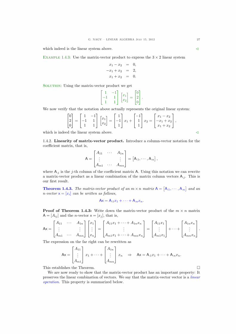
Example 1.4.3: Use the matrix-vector product to express the 3× 2 linear system
x1 − x2 = 0,
−x1 + x2 = 2,
x1 + x2 = 0.
Solution: Using the matrix-vector product we get
1 −1−1 11 1
[x1
x2
]=
020
.
We now verify that the notation above actually represents the original linear system:
020
=
1 −1−1 11 1
[x1
x2
]=
1−11
x1 +
−111
x2 =
x1 − x2
−x1 + x2
x1 + x2
,
which is indeed the linear system above. C
1.4.2. Linearity of matrix-vector product. Introduce a column-vector notation for thecoefficient matrix, that is,
A =
A11 · · · A1n
......
Am1 · · · Amn
=
[A:1, · · · ,A:n
],
where A:j is the j-th column of the coefficient matrix A. Using this notation we can rewritea matrix-vector product as a linear combination of the matrix column vectors A:j . This isour first result.
Theorem 1.4.3. The matrix-vector product of an m×n matrix A =[A:1, · · · , A:n
]and an
n-vector x = [xi] can be written as follows,
Ax = A:1x1 + · · ·+ A:nxn.
Proof of Theorem 1.4.3: Write down the matrix-vector product of the m × n matrixA = [Aij ] and the n-vector x = [xj ], that is,
Ax =
A11 · · · A1n
......
Am1 · · · Amn
x1
...xn
=
A11x1 + · · ·+ A1nxn
...Am1x1 + · · ·+ Amnxn
=
A11x1
...Am1x1
+ · · ·+
A1nxn
...Amnxn
.
The expression on the far right can be rewritten as
Ax =
A11
...Am1
x1 + · · ·+
A1n
...Amn
xn ⇒ Ax = A:1x1 + · · ·+ A:nxn.
This establishes the Theorem. ¤We are now ready to show that the matrix-vector product has an important property: It
preserves the linear combination of vectors. We say that the matrix-vector vector is a linearoperation. This property is summarized below.
28 G. NAGY – LINEAR ALGEBRA july 15, 2012
Theorem 1.4.4. For every m× n matrix A, every n-vectors x, y and for every numbers a,b, the matrix-vector product satisfies that
A(ax + by) = aAx + bAy.
In words, the Theorem says that the matrix-vector product of a linear combination of vectorsis the linear combination of the matrix-vector products. The expression above contains theparticular cases a = b = 1 and b = 0, which are respectively given by
A(x + y) = Ax + Ay, A(ax) = aAx.
Proof of Theorem 1.4.4: From the definition of the matrix-vector product we see that:
A(ax + by) = [A:1, · · · , A:n]
ax1 + by1
...axn + byn
= A:1(ax1 + by1) + · · ·+ A:n(axn + byn).
Reorder terms in the expression above to get,
A(ax + by) = a(A:1x1 + · · ·+ A:nxn
)+ b
(A:1y1 + · · ·+ A:nyn
)= a Ax + b Ay.
This establishes the Theorem. ¤
1.4.3. Homogeneous linear systems. All possible linear systems can be classified intotwo main classes, homogeneous and non-homogeneous, depending whether the source vectorvanishes or not. This classification will be useful to express solutions of non-homogeneoussystems in terms of solutions of the associated homogeneous system.
Definition 1.4.5. The m×n linear system Ax = b is called homogeneous iff it holds thatb = 0; and is called non-homogeneous iff it holds that b 6= 0.
Every m × n homogeneous linear system has at least one solution, given by x = 0,called the trivial solution of the homogeneous system. The following example shows thathomogeneous linear systems can also have non-trivial solutions.
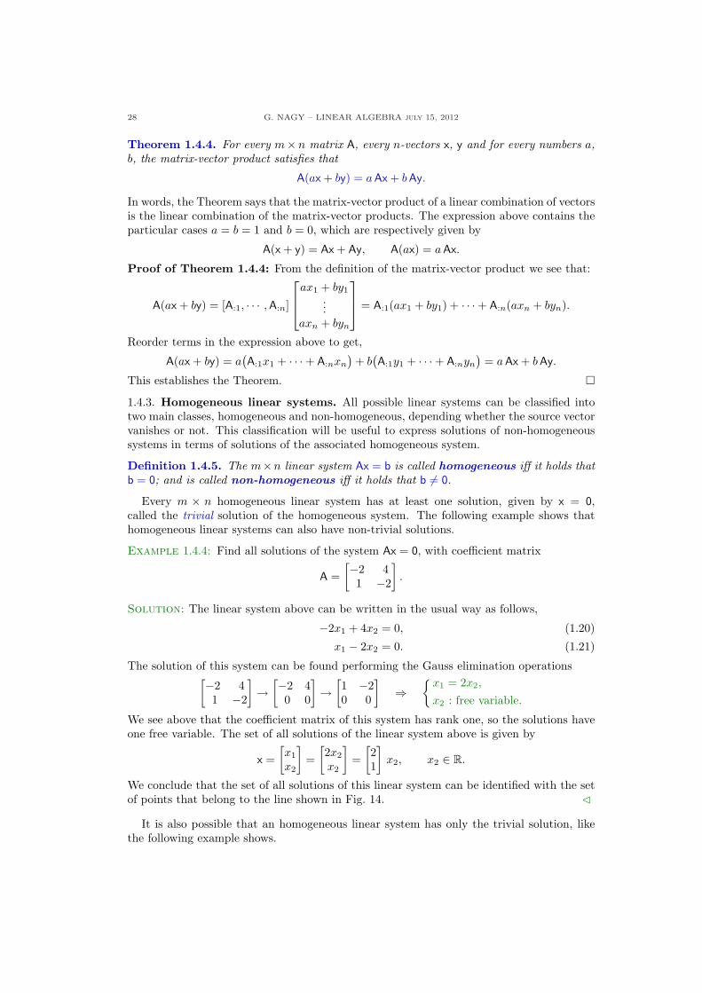
Example 1.4.4: Find all solutions of the system Ax = 0, with coefficient matrix
A =[−2 4
1 −2
].
Solution: The linear system above can be written in the usual way as follows,
−2x1 + 4x2 = 0, (1.20)
x1 − 2x2 = 0. (1.21)
The solution of this system can be found performing the Gauss elimination operations[−2 4
1 −2
]→
[−2 40 0
]→
[1 −20 0
]⇒
{x1 = 2x2,
x2 : free variable.
We see above that the coefficient matrix of this system has rank one, so the solutions haveone free variable. The set of all solutions of the linear system above is given by
x =[x1
x2
]=
[2x2
x2
]=
[21
]x2, x2 ∈ R.
We conclude that the set of all solutions of this linear system can be identified with the setof points that belong to the line shown in Fig. 14. C
It is also possible that an homogeneous linear system has only the trivial solution, likethe following example shows.
G. NAGY – LINEAR ALGEBRA July 15, 2012 29
12
1
21
2x
x
Figure 14. We plot the solutions of the homogeneous linear system givenin Eqs. (1.20)-(1.21).
Example 1.4.5: Find all solutions of the system Ax = 0 with coefficient matrix
A =[
2 −1−1 2
].
Solution: The linear system above can be written in the usual way as follows,
2x1 − x2 = 0,
−x1 + 2x2 = 0.
The solutions of this system can be found performing the Gauss elimination operations[
2 −1−1 2
]→
[1 −22 −1
]→
[1 −20 3
]→
[1 00 1
]⇒
{x1 = 0,
x2 = 0.
We see that the coefficient matrix of this system has rank two, so the solutions have no freevariable. The solution is unique and is the trivial solution x = 0. C
Examples 1.4.4 and 1.4.5 are particular cases of the following statement: An m × nhomogeneous linear system has non-trivial solutions iff the system has at least one freevariable. We show more examples of this statement.
Example 1.4.6: Find all solutions of the 2 × 3 homogeneous linear system Ax = 0 withcoefficient matrix
A =[2 −2 41 3 2
].
Solution: The linear system above can be written in the usual way as follows,
2x1 − 2x2 + 4x3 = 0, (1.22)
x1 + 3x2 + 2x3 = 0. (1.23)
The solutions of system above can be obtained through the Gauss elimination operations
[1 3 22 −2 4
]→
[1 3 20 −8 0
]→
[1 0 20 1 0
]⇒
x1 = −2x3,
x2 = 0,
x3 : free variable.
The set of all solutions of the linear system above can be written in vector notation,
x =
x1
x2
x3
=
−2x3
0x3
=
−201
x3, x3 ∈ R.
30 G. NAGY – LINEAR ALGEBRA july 15, 2012
In Fig. 15 we emphasize that the solution vector x belongs to the space R3, while the columnvectors of the coefficient matrix of this same system belong to the space R2. C
−2
x
x
3x
2
1
x1
221
A1
3
1
2
3
1 2 3 4 1
A
−2 −1 y
2y
2A
Figure 15. The picture on the left represents the solutions of the ho-mogeneous linear system given in Eq. (1.22)-(1.23), which are 3-vectors,elements in R3. The picture on the right represents the column vectors ofthe coefficient matrix in this system which are 2-vectors, elements in R2.
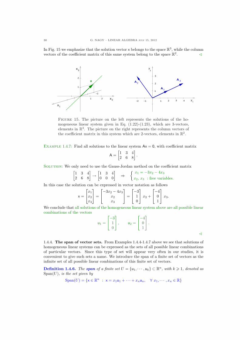
Example 1.4.7: Find all solutions to the linear system Ax = 0, with coefficient matrix
A =[1 3 42 6 8
].
Solution: We only need to use the Gauss-Jordan method on the coefficient matrix[1 3 42 6 8
]→
[1 3 40 0 0
]⇒
{x1 = −3x2 − 4x3
x2, x3 : free variables.
In this case the solution can be expressed in vector notation as follows
x =
x1
x2
x3
=
−3x2 − 4x3
x2
x3
=
−310
x2 +
−401
x3.
We conclude that all solutions of the homogeneous linear system above are all possible linearcombinations of the vectors
u1 =
−310
, u2 =
−401
.
C
1.4.4. The span of vector sets. From Examples 1.4.4-1.4.7 above we see that solutions ofhomogeneous linear systems can be expressed as the sets of all possible linear combinationsof particular vectors. Since this type of set will appear very often in our studies, it isconvenient to give such sets a name. We introduce the span of a finite set of vectors as theinfinite set of all possible linear combinations of this finite set of vectors.
Definition 1.4.6. The span of a finite set U = {u1, · · · , uk} ⊂ Rn, with k > 1, denoted asSpan(U), is the set given by
Span(U) = {x ∈ Rn : x = x1u1 + · · ·+ xnun, ∀ x1, · · · , xn ∈ R}
G. NAGY – LINEAR ALGEBRA July 15, 2012 31
Recall that the symbol “ ∀ ” means “for all”. Using this definition we express the solutionsof Ax = 0 in Example 1.4.7 as
x ∈ Span({
u1 =
−310
, u2 =
−401
}).
In this case, the set of all solutions forms a plane in R3, which contains the vectors u1 andu2. In the case of Example 1.4.4 the solutions x belong to a line in R2 given by
x ∈ Span({[
21
]}).
Example 1.4.8: Find the set S = Span({[
12
],
[14
]})⊂ R2.
Solution: Since the vectors are not proportional to each other, the set of all linear combi-nations of these vectors is the whole plane. We conclude that S = R2. C
Example 1.4.9: Find the set S = Span({[
12
],
[−1−2
]})⊂ R2.
Solution: Since the vectors lay on a line, the set of all linear combinations of these vectors
also belongs to the same line. We conclude that S ={
a
[12
], a ∈ R
}. C
1.4.5. Non-homogeneous linear systems. Spans of vector sets are not only useful toexpress solution sets to homogeneous equations, they are also useful to characterize when anon-homogeneous linear system is consistent.
Theorem 1.4.7. An m×n linear system Ax = b, with coefficient matrix A =[A:1, · · · , A:n
],
is consistent iff b ∈ Span({
A:1, · · · , A:n
}).
In words, a non-homogeneous linear system is consisten iff the source vector belongs to theSpan of the coefficient matrix column vectors.Proof of Theorem 1.4.7:
(⇒) Suppose that x = [xi] is any solution of the linear system Ax = b. Using the columnvector notation for matrix A we get that
b = Ax = A:1x1 + · · ·+ A:nxn.
This last expression says that b ∈ Span({
A:1, · · · , A:n
}).
(⇐) If b ∈ Span({
A:1, · · · , A:n
}), then there exists constants c1, · · · , cn such that
b = A:1c1 + · · ·+ A:ncn = Ac, c = [ci].
This last equation says that the vector x = c is a solution of the linear system Ax = b, sothe system is consistent. This establishes the Theorem. ¤
Knowing the solutions of an homogeneous linear system provides important informationabout the solutions of an inhomogeneous linear system with the same coefficient matrix.The next result establishes this relation in a precise way.
Theorem 1.4.8. If the m × n linear system Ax = b is consistent and the vector xp is oneparticular solution of this linear system, then any solution x to this system can be decomposedas x = xp + xh, where the vector xh is a solution of the homogeneous linear system Axh = 0.
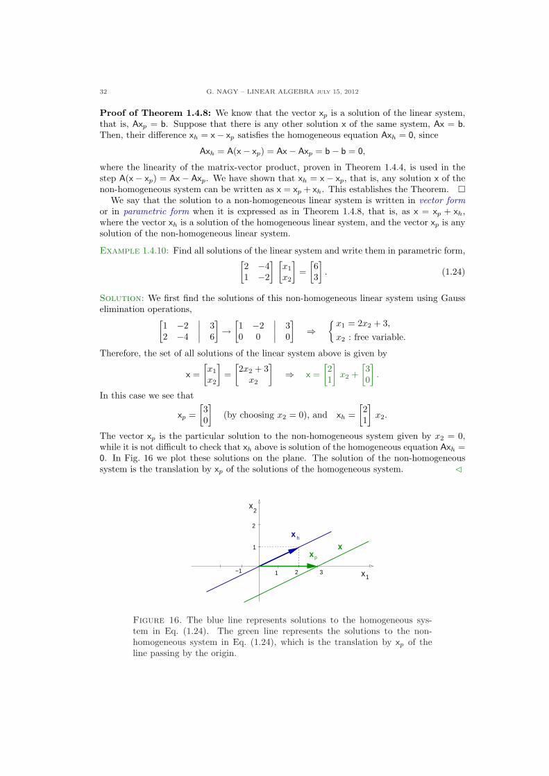
32 G. NAGY – LINEAR ALGEBRA july 15, 2012
Proof of Theorem 1.4.8: We know that the vector xp is a solution of the linear system,that is, Axp = b. Suppose that there is any other solution x of the same system, Ax = b.Then, their difference xh = x− xp satisfies the homogeneous equation Axh = 0, since
Axh = A(x− xp) = Ax− Axp = b− b = 0,
where the linearity of the matrix-vector product, proven in Theorem 1.4.4, is used in thestep A(x− xp) = Ax− Axp. We have shown that xh = x− xp, that is, any solution x of thenon-homogeneous system can be written as x = xp + xh. This establishes the Theorem. ¤
We say that the solution to a non-homogeneous linear system is written in vector formor in parametric form when it is expressed as in Theorem 1.4.8, that is, as x = xp + xh,where the vector xh is a solution of the homogeneous linear system, and the vector xp is anysolution of the non-homogeneous linear system.
Example 1.4.10: Find all solutions of the linear system and write them in parametric form,[2 −41 −2
] [x1
x2
]=
[63
]. (1.24)
Solution: We first find the solutions of this non-homogeneous linear system using Gausselimination operations,
[1 −2
∣∣ 32 −4
∣∣ 6
]→
[1 −2
∣∣ 30 0
∣∣ 0
]⇒
{x1 = 2x2 + 3,
x2 : free variable.
Therefore, the set of all solutions of the linear system above is given by
x =[x1
x2
]=
[2x2 + 3
x2
]⇒ x =
[21
]x2 +
[30
].
In this case we see that
xp =[30
](by choosing x2 = 0), and xh =
[21
]x2.
The vector xp is the particular solution to the non-homogeneous system given by x2 = 0,while it is not difficult to check that xh above is solution of the homogeneous equation Axh =0. In Fig. 16 we plot these solutions on the plane. The solution of the non-homogeneoussystem is the translation by xp of the solutions of the homogeneous system. C
p
−1
1
2
x
x
2
121 3
xx
x h
Figure 16. The blue line represents solutions to the homogeneous sys-tem in Eq. (1.24). The green line represents the solutions to the non-homogeneous system in Eq. (1.24), which is the translation by xp of theline passing by the origin.

G. NAGY – LINEAR ALGEBRA July 15, 2012 33
Further reading. See Sections 2.4 and 2.5 in Meyer’s book [3] for a detailed discussion onhomogeneous and non-homogeneous linear systems, respectively. See Section 1.4 in Lay’sbook [2] for a detailed discussion of the matrix-vector product, and Section 1.5 for detaileddiscussions on homogeneous and non-homogeneous linear systems.
34 G. NAGY – LINEAR ALGEBRA july 15, 2012
1.4.6. Exercises.
1.4.1.- Find the general solution of the ho-mogeneous linear system
x1 + 2x2 + x3 + 2x4 = 0
2x1 + 4x2 + x3 + 3x4 = 0
3x1 + 6x2 + x3 + 4x4 = 0.
1.4.2.- Find all the solutions x of the linearsystem Ax = b, where A and b are givenby
A =
24
1 −2 −12 1 81 −1 1
35 , b =
24
121
35 ,
and write these solutions in parametricform, that is, in terms of column vec-tors.
1.4.3.- Prove the following statement: Ifthe vectors c and d are solutions ofthe homogeneous linear system Ax = 0,then c + d is also a solution.
1.4.4.- Find the general solution of the non-homogeneous linear system
x1 + 2x2 + x3 + 2x4 = 3
2x1 + 4x2 + x3 + 3x4 = 4
3x1 + 6x2 + x3 + 4x4 = 5.
1.4.5.- Suppose that the solution to a sys-tem of linear equation is given by
x1 = 5 + 4x3
x2 = −2− 7x3
x3 free.
Use column vectors to describe this setas a line in R3.
1.4.6.- Suppose that the solution to a sys-tem of linear equation is given by
x1 = 3x4
x2 = 8 + 4x4
x3 = 2− 5x4
x4 free.
Use column vectors to describe this setas a line in R4.
1.4.7.- Consider the following system of lin-ear equations, where k represents anyreal number,2
42 2 34 8 126 2 k
3524
x1
x2
x3
35 =
24
0−44
35 .
(a) Find all possible values of the num-ber k such that the system abovehas a unique solution.
(b) Find all possible values of the num-ber k such that the system abovehas infinitely many solutions, andexpress those solutions in paramet-ric form.
G. NAGY – LINEAR ALGEBRA July 15, 2012 35
1.5. Floating-point numbers
1.5.1. Main definitions. Floating-point numbers are a finite subset of the rational num-bers. Many different types of floating-point numbers exist, all of them are characterized byhaving a finite number of digits when written in a particular base. Digital computers usefloating-point numbers to carry out almost every arithmetic operation. When an m × nalgebraic linear system is solved using a computer, every Gauss operations is performed ina particular set of floating-point numbers. In this Section we study what type of approxi-mations occur in this process.
Definition 1.5.1. A non-zero rational number x is a floating-point number in baseb ∈ N, of precision p ∈ N, with exponent n ∈ Z in the range −N 6 n 6 N ∈ N, iff thereexist integers di, for i = 1, · · · , p, satisfying 0 6 di 6 b−1 and d1 6= 0, such that the numberx has the form
x = ±0.d1 · · · dp × bn. (1.25)
We call p the precision, b the base and N the exponent range of the floating point numberx. We denote by Fp,b,N the set of all floating-point numbers of fixed precision p, base b andexponent range N .
In this notes we always work in base b = 10. Computers usually work with base b = 2,but also with base b = 16, and they present their results with base b = 10.
Example 1.5.1: The following numbers belong to the set F3,10,3,
210 = 0.210× 10³, 1 = 0.100× 10, −0.02 = −0.200× 10−1,215106
= 0.215× 10⁻³.
The set F3,10,3 is a finite subset of the rational numbers. The biggest number and thesmallest number in absolute value are the following, respectively,
0.999× 103 = 999 0.100× 10−3 = 0.0001.
Any number bigger 999 or closer to 0 than 0.0001 does not belong to F3,10,3. Here are otherexamples of numbers that do not belong to F3,10,3,
1000 = 0.100×10⁴ 210.3 = 0.2103×10³, 1.001 = 0.1001×10, 0.000027 = 0.270×10⁻⁴.
In the first case the number is too big, we need an exponent n = 4 to specify it. In thesecond and third cases we need a precision p = 4 to specify those numbers. In the last casethe number is too close to zero, we need an exponent n = −4 to specify it. C
Example 1.5.2: The set of floating-point numbers F1,10,1 is small enough to picture it onthe real line. The set of all positive elements in F1,10,1 is shown on Fig. 17, and this is theunion of the following three sets,
{0.01, 0.02, 0.03, 0.04, 0.05, 0.06, 0.07, 0.08, 0.09} = {0.i× 10−1}9i=1;
{0.1, 0.2, 0.3, 0.4, 0.5, 0.6, 0.7, 0.8, 0.9} = {0.i× 100}9i=1;
{1, 2, 3, 4, 5, 6, 7, 8, 9} = {0.i× 101}9i=1.
One can see in this example that the elements on F1,10,1 are not homogeneously distributedon the interval [0, 10]. The irregular distribution of the floating-point numbers plays animportant role when one computes the addition of a small number to a big number. C
Example 1.5.3: In Table 1 we show the main set of floating-point numbers used nowadaysin computers. For example, the format called Binary64 represents all floating-point numbers
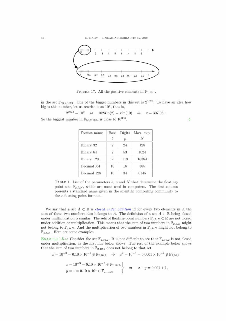
36 G. NAGY – LINEAR ALGEBRA july 15, 2012
0 2 3 4 5 6 7 8 9
0.90.80.70.60.50.40.30.20.1
1
10
Figure 17. All the positive elements in F1,10,1.
in the set F53,2,1024. One of the bigger numbers in this set is 21023. To have an idea howbig is this number, let us rewrite it as 10x, that is,
21023 = 10x ⇔ 1023 ln(2) = x ln(10) ⇔ x = 307.95...
So the biggest number in F53,2,1024 is close to 10308. C
Format name Base Digits Max. exp.b p N
Binary 32 2 24 128
Binary 64 2 53 1024
Binary 128 2 113 16384
Decimal l64 10 16 385
Decimal 128 10 34 6145
Table 1. List of the parameters b, p and N that determine the floating-point sets Fp,b,N , which are most used in computers. The first columnpresents a standard name given in the scientific computing community tothese floating-point formats.
We say that a set A ⊂ R is closed under addition iff for every two elements in A thesum of these two numbers also belongs to A. The definition of a set A ⊂ R being closedunder multiplication is similar. The sets of floating-point numbers Fp,b,N ⊂ R are not closedunder addition or multiplication. This means that the sum of two numbers in Fp,b,N mightnot belong to Fp,b,N . And the multiplication of two numbers in Fp,b,N might not belong toFp,b,N . Here are some examples.
Example 1.5.4: Consider the set F2,10,2. It is not difficult to see that F2,10,2 is not closedunder multiplication, as the first line below shows. The rest of the example below showsthat the sum of two numbers in F2,10,2 does not belong to that set.
x = 10−3 = 0.10× 10⁻² ∈ F2,10,2 ⇒ x2 = 10−6 = 0.0001× 10⁻² /∈ F2,10,2,
x = 10−3 = 0.10× 10⁻² ∈ F2,10,2,
y = 1 = 0.10× 101 ∈ F2,10,2,
}⇒ x + y = 0.001 + 1,
G. NAGY – LINEAR ALGEBRA July 15, 2012 37
x + y = 1.001 ⇒ x + y = 0.1001× 10 /∈ F2,10,2.
C
1.5.2. The rounding function. Since the set Fp,b,N is not closed under addition or mul-tiplication, not every arithmetic calculation involving real numbers can be performed inFp.,b,N . A way to perform a sequence of arithmetic operations in Fp,b,N is first, to projectthe real numbers into the floating-point numbers, and then to perform the calculation. Sincethe result might not be in the set Fp,b,N , one must project again the result onto Fp,b,N . Theaction to project a real number into the floating-point set is called to round-off the realnumber. There are many different ways to do this. We now present a common round-offfunction.
Definition 1.5.2. Given the floating-point number set Fp,b,N , let xN = 0.9 · · · 9× bN be thebiggest number in Fp,b,N . The rounding function f` : R ∩ [−xN , xN ] → Fp,b,N is definedas follow: Given x ∈ R ∩ [−xN , xN ], with x = ±0.d1 · · · dpdp+1 · · · × bn and −N 6 n 6 N ,holds
f`(x) =
{ ± 0.d1 · · · dp × bn if dp+1 < 5,
± (0.d1 · · · dp + b−p)× bn if dp+1 > 5.
Example 1.5.5: We now present few numbers not in F3,10,3 and their respective round-offs
x = 0.2103× 10³, f`(x) = 0.210× 10³,
x = 0.21037× 10³, f`(x) = 0.210× 10³,
x = 0.2105× 10³, f`(x) = 0.211× 10³,
x = 0.21051× 10³, f`(x) = 0.211× 10³.
C
The rounding function has the following properties:
Proposition 1.5.3. Given Fp,b,N there always exist x, y ∈ R such that
f`
[f`(x) + f`(y)
] 6= f`(x + y), f`
[f`(x)f`(y)
] 6= f`(xy).
We do not prove this Proposition, we only provide a particular example, in the case thatthe floating-point number is F2,10,2.
Example 1.5.6: The real numbers x = 21/2 and y = 11/2 add up to x + y = 16. Only oneof them belongs to F2,10,2, since
x = 0.105× 10² /∈ F2,10,2 ⇒ f`(x) = 0.11× 10²,
y = 0.55× 10 ∈ F2,10,2 ⇒ f`(y) = 0.55× 10 = y.
We now verify that for these numbers holds that f`
[f`(x) + f`(y)
] 6= f`(x + y), since
x + y = 0.16× 10² ∈ F2,10,2 ⇒ f`(x + y) = 0.16× 102 = x + y,
f`
[f`(x) + f`(y)
]= f`(0.11× 10² + 0.55× 10) = f`(0.165× 10²) = 0.17× 10².
Therefore, we conclude that
17 = f`
[f`(x) + f`(y)
] 6= f`(x + y) = 16.
C
38 G. NAGY – LINEAR ALGEBRA july 15, 2012
1.5.3. Solving linear systems. Arithmetic operations are, in general, not possible inFp.b.N , since this set is not closed under these operations. Rounding after each arithmeticoperation is a procedure that determines numbers in Fp,b,N which are close to the resultof the arithmetic operations. The difference between these two numbers is the error of theprocedure, is the error of making calculations in a finite set of numbers. One could thinkthat the Gauss-Jordan method could be carried out in the set Fp,b,N , if one round-off eachintermediate calculation. This Subsection presents an example that this is not the case.The Gauss-Jordan method is, in general, not possible in any set Fp,b,N using rounding aftereach arithmetic operation.
Example 1.5.7: Use the floating-point set F3,10,3 and Gauss operations to find the solutionof the 2× 2 linear system
5 x1 + x2 = 6,
9.43x1 + 1.57 x2 = 11.
Solution: Note that the solution is x1 = 1, x2 = 1. The calculation we do now showsthat the Gauss-Jordan method is not possible in the set F3,10,3 using round-off functions;the Gauss-Jordan method does not work in this example. The fist step in the Gauss-Jordanmethod is to compute the augmented matrix of the system and perform a Gauss operationto make the coefficient in the position of a21 vanish, that is,
[5 1
∣∣ 69.43 1.57
∣∣ 11
]→
[5 1
∣∣ 60 −0.316
∣∣ −0.316
].
This operation cannot be performed in the set F3,10,3 using rounding. In order to understandthis, let us review what we did in the calculation above. We multiplied the first row by−9.43/5 and add that result to the second row. The result using real numbers is that thenew coefficient obtained after this calculation is a21 = 0. If we do this calculation in the setF3,10,3 using rounding, we have to do the following calculation:
a21 = f`
(9.43− f`
[f`(5) f`
(9.435
)]),
that is, we round the quotient −9.43/5, then we multiply by 5, we round again, then wesubtract that from 9.43, and we finally round the result:
a21 = f`
(9.43− f`
[5 f`(1.886)
])
= f`
(9.43− f`
[5 (1.89)
])
= f`
[9.43− f`(9.45)
]
= f`
[9.43− 9.45
]
= f`(−0.02)= −0.02.
Therefore, with this Gauss operation on F3,10,3 using rounding one obtains a21 = −0.02 6= 0.The same type of calculation on the other coefficients a22, b2, produces the following newaugmented matrix
[5 1
∣∣ 69.43 1.57
∣∣ 11
]→
[5 1
∣∣ 6−0.02 −0.32
∣∣ −0.3
].
The Gauss-Jordan method cannot follow unless the coefficient a21 = 0. But this is notpossible in our example. A usual procedure used in scientific computation is to modifythe Gauss-Jordan method. The modification introduces further approximation errors in
G. NAGY – LINEAR ALGEBRA July 15, 2012 39
the calculation. The modification in our example is the following: Replace the coefficienta21 = −0.02 by a21 = 0. The modified Gauss-Jordan method in our example is given by
[5 1
∣∣ 69.43 1.57
∣∣ 11
]→
[5 1
∣∣ 60 −0.32
∣∣ −0.3
]. (1.26)
What we have done here is not a rounding error. It is a modification of the Gauss-Jordanmethod to find an approximate solution of the linear system in the set F3,10,3. The rest ofthe calculation to find the solution of the linear system is the following:
[5 1
∣∣ 60 −0.32
∣∣ −0.3
]→
[5 1
∣∣ 60 1
∣∣∣ f`
(0.30.32
)]
;
since
f`
( 0.30.32
)= f`(0.9375) = 0.938,
we have that[5 1
∣∣ 60 1
∣∣∣ f`
(0.30.32
)]→
[5 1
∣∣ 60 1
∣∣ 0.938
]→
[5 0
∣∣ f`(6− 0.938)0 1
∣∣ 0.938
];
since
f)`(6− 0.938) = f`(5.062) = 5.06,
we also have that[5 0
∣∣ 5.060 1
∣∣ 0.938
]→
[1 0
∣∣∣ f`
(5.065
)
0 1∣∣ 0.938
];
since
f`
(5.065
)= f`(1.012) = 1.01,
we conclude that [1 0
∣∣ 1.010 1
∣∣ 0.938
]⇒
x1 = 0.101× 10,
x2 = 0.938..
We conclude that the solution in the set F3,10,3 differs from the exact solution x1 = 1,x2 = 1. The errors in the result are produced by rounding errors and by the modificationof the Gauss-Jordan method discussed in Eq. (1.26). C
We finally comment that the round-off error becomes important when adding a smallnumber to a big number, or when dividing by a small number. Here is an example of theformer case.
Example 1.5.8: Add together the numbers x = 103 and y = 4 in the set F3,10,4.
Solution: Since x = 0.100× 10⁴ and y = 0.400× 10, both numbers belong to F3,10,4 andso f`(x) = x, f`(y) = y. Therefore, their addition is the following,
f`(x + y) = f`(1000 + 4) = f`(0.1004× 10³) = 1× 103 = x.
That is, f(x + y) = x, and the information of y is completely lost. C
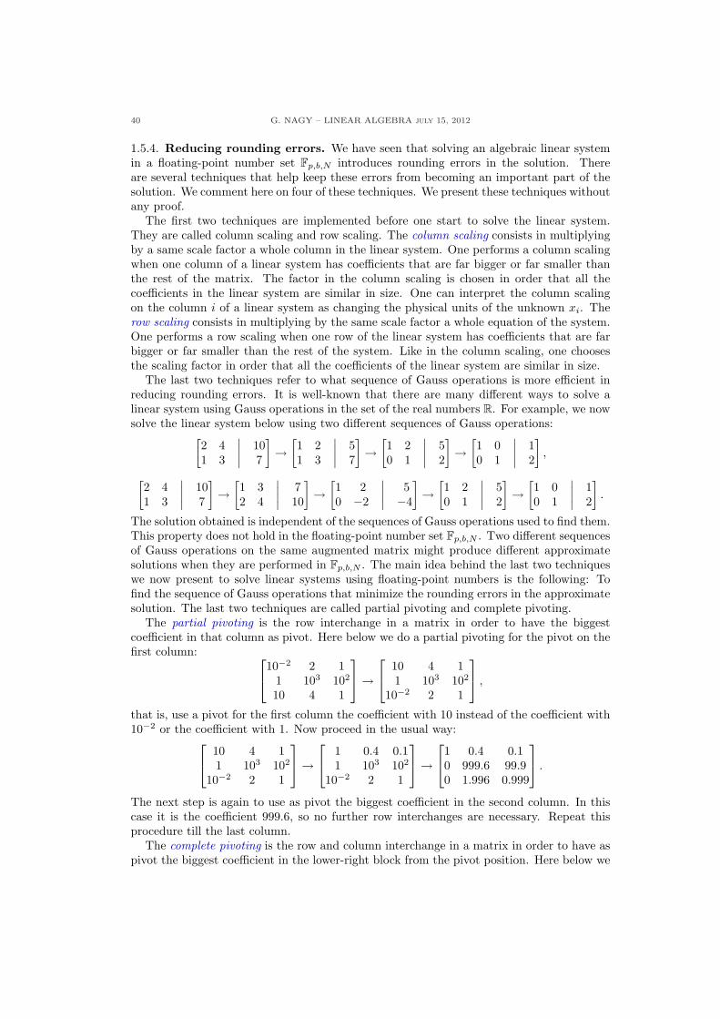
40 G. NAGY – LINEAR ALGEBRA july 15, 2012
1.5.4. Reducing rounding errors. We have seen that solving an algebraic linear systemin a floating-point number set Fp,b,N introduces rounding errors in the solution. Thereare several techniques that help keep these errors from becoming an important part of thesolution. We comment here on four of these techniques. We present these techniques withoutany proof.
The first two techniques are implemented before one start to solve the linear system.They are called column scaling and row scaling. The column scaling consists in multiplyingby a same scale factor a whole column in the linear system. One performs a column scalingwhen one column of a linear system has coefficients that are far bigger or far smaller thanthe rest of the matrix. The factor in the column scaling is chosen in order that all thecoefficients in the linear system are similar in size. One can interpret the column scalingon the column i of a linear system as changing the physical units of the unknown xi. Therow scaling consists in multiplying by the same scale factor a whole equation of the system.One performs a row scaling when one row of the linear system has coefficients that are farbigger or far smaller than the rest of the system. Like in the column scaling, one choosesthe scaling factor in order that all the coefficients of the linear system are similar in size.
The last two techniques refer to what sequence of Gauss operations is more efficient inreducing rounding errors. It is well-known that there are many different ways to solve alinear system using Gauss operations in the set of the real numbers R. For example, we nowsolve the linear system below using two different sequences of Gauss operations:
[2 4
∣∣ 101 3
∣∣ 7
]→
[1 2
∣∣ 51 3
∣∣ 7
]→
[1 2
∣∣ 50 1
∣∣ 2
]→
[1 0
∣∣ 10 1
∣∣ 2
],
[2 4
∣∣ 101 3
∣∣ 7
]→
[1 3
∣∣ 72 4
∣∣ 10
]→
[1 2
∣∣ 50 −2
∣∣ −4
]→
[1 2
∣∣ 50 1
∣∣ 2
]→
[1 0
∣∣ 10 1
∣∣ 2
].
The solution obtained is independent of the sequences of Gauss operations used to find them.This property does not hold in the floating-point number set Fp,b,N . Two different sequencesof Gauss operations on the same augmented matrix might produce different approximatesolutions when they are performed in Fp,b,N . The main idea behind the last two techniqueswe now present to solve linear systems using floating-point numbers is the following: Tofind the sequence of Gauss operations that minimize the rounding errors in the approximatesolution. The last two techniques are called partial pivoting and complete pivoting.
The partial pivoting is the row interchange in a matrix in order to have the biggestcoefficient in that column as pivot. Here below we do a partial pivoting for the pivot on thefirst column:
10−2 2 1
1 103 102
10 4 1
→
10 4 11 103 102
10−2 2 1
,
that is, use a pivot for the first column the coefficient with 10 instead of the coefficient with10−2 or the coefficient with 1. Now proceed in the usual way:
10 4 11 103 102
10−2 2 1
→
1 0.4 0.11 103 102
10−2 2 1
→
1 0.4 0.10 999.6 99.90 1.996 0.999
.
The next step is again to use as pivot the biggest coefficient in the second column. In thiscase it is the coefficient 999.6, so no further row interchanges are necessary. Repeat thisprocedure till the last column.
The complete pivoting is the row and column interchange in a matrix in order to have aspivot the biggest coefficient in the lower-right block from the pivot position. Here below we
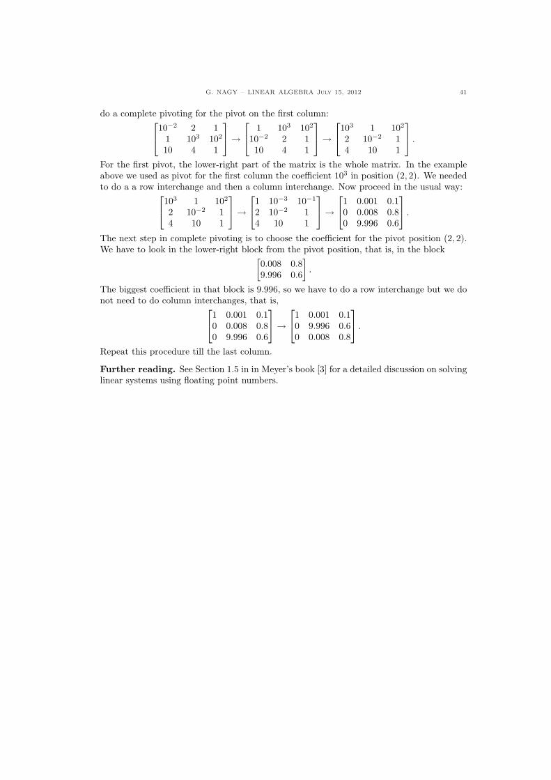
G. NAGY – LINEAR ALGEBRA July 15, 2012 41
do a complete pivoting for the pivot on the first column:
10−2 2 11 103 102
10 4 1
→
1 103 102
10−2 2 110 4 1
→
103 1 102
2 10−2 14 10 1
.
For the first pivot, the lower-right part of the matrix is the whole matrix. In the exampleabove we used as pivot for the first column the coefficient 103 in position (2, 2). We neededto do a a row interchange and then a column interchange. Now proceed in the usual way:
103 1 102
2 10−2 14 10 1
→
1 10−3 10−1
2 10−2 14 10 1
→
1 0.001 0.10 0.008 0.80 9.996 0.6
.
The next step in complete pivoting is to choose the coefficient for the pivot position (2, 2).We have to look in the lower-right block from the pivot position, that is, in the block[
0.008 0.89.996 0.6
].
The biggest coefficient in that block is 9.996, so we have to do a row interchange but we donot need to do column interchanges, that is,
1 0.001 0.10 0.008 0.80 9.996 0.6
→
1 0.001 0.10 9.996 0.60 0.008 0.8
.
Repeat this procedure till the last column.
Further reading. See Section 1.5 in in Meyer’s book [3] for a detailed discussion on solvinglinear systems using floating point numbers.
42 G. NAGY – LINEAR ALGEBRA july 15, 2012
1.5.5. Exercises.
1.5.1.- Consider the following system:
10−3 x1 − x2 = 1,
x1 + x2 = 0.
(a) Solve this system in F3,10,6 withrounding, but without partial orcomplete pivoting.
(b) Find the system that is exactly sat-isfied by your solution in (a), andnote how close is this system to theoriginal system.
(c) Use partial pivoting to solve thissystem in F3,10,5 with rounding.
(d) Find the system that is exactly sat-isfied by your solution in (c), andnote how close is this system to theoriginal system.
(e) Solve this system in R without par-tial or complete pivoting, and com-pare this exact solution with the so-lutions in (a) and (c).
(f) Round the exact solution up tothree digits, an compare it with theresults from (a) and (c).
1.5.2.- Consider the following system:
x1 + x2 = 3,
−10 x1 + 105 x2 = 105.
(a) Solve this system in F4,10,6 withpartial pivoting but no scaling.
(b) Solve this system in F4,10,6 withcomplete pivoting but no scaling.
(c) Use partial pivoting to solve thissystem in F3,10,5 with rounding.
(d) This time row scale the original sys-tem, and then solve it in F4,10,6 withpartial pivoting.
(e) Solve this system in R and comparethis exact solution with the solu-tions in (a)-(d).
1.5.3.- Consider the linear system
−3 x1 + x2 = −2,
10 x1 − 3 x2 = 7.
Solve this system in F3,10,6 without par-tial pivoting, and then solve it againwith partial pivoting. Compare your re-sults with the exact solution.
G. NAGY – LINEAR ALGEBRA July 15, 2012 43
Chapter 2. Matrix algebra
2.1. Linear transformations
In Sect. 1.4 we introduced the matrix-vector product because it provided a convenientnotation to express a system of linear equations in a compact way. Here we study a deepermeaning of the matrix-vector product. It is the key to interpret a matrix as a function actingon vectors. We will see that a matrix is a particular type of function, called linear functionor linear transformation. We also show examples of functions determined by matrices.
From now on we consider both real-valued and complex-valued matrices and vectors. Weuse the notation F ∈ {R,C} to mean that F can be either F = R or F = C. Elements in Fare called scalars. So a scalar is a real number or a complex number. We denote by Fn theset of all n-vectors x = [xi] with components xi ∈ F, where i = 1, · · · , n. Finally we denoteby Fm,n the set of all m×n matrices A = [Aij ] with components Aij ∈ F, where i = 1 · · ·mand j = 1, · · · , n.
2.1.1. A matrix is a function. The matrix-vector product provides a new interpretationfor a matrix. A matrix is not only an artifact for a compact notation, it defines a functionon the set of vectors. Here is a precise definition.
Definition 2.1.1. Every m× n matrix A ∈ Fm,n defines the function A : Fn → Fm, wherethe image of an n-vector x is the m-vector y = Ax, the matrix-vector product of A and x.
Example 2.1.1: Compute the function defined by the 2× 3 matrix A =[2 −2 41 3 2
].
Solution: The matrix A defines a function A : R3 → R2, since for every x ∈ R3 holds,
x =
x1
x2
x3
, Ax =
[2 −2 41 3 2
]
x1
x2
x3
⇒ y = Ax =
[2x1 − 2x2 + 4x3
x1 + 3x2 + 2x3
]∈ R2.
For example, given x =
111
∈ R3, then y = Ax =
[2 −2 41 3 2
]
111
=
[46
]∈ R2. C
Example 2.1.2: Describe the function defined by the 2× 2 matrix A =[1 00 −1
].
Solution: The matrix A defines a function A : R2 → R2, which can be interpreted asa reflection along the horizontal line. Indeed, the action of the matrix A on an arbitraryelement in x ∈ R2 is the following,
Ax =[1 00 −1
] [x1
x2
]=
[x1
−x2
].
Here are particular cases, represented in Fig. 18,
A
[21
]=
[2−1
], A
[−1−3
]=
[−13
], A
[10
]=
[10
]. (2.1)
C
Example 2.1.3: Describe the function defined by the 2× 2 matrix A =[0 11 0
].
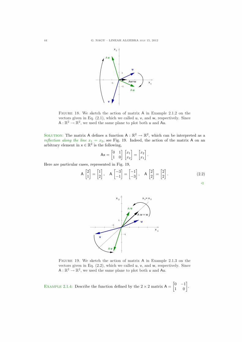
44 G. NAGY – LINEAR ALGEBRA july 15, 2012
x
v
2
1
−1
−1
A v
u
A u
1Aw=w
x
Figure 18. We sketch the action of matrix A in Example 2.1.2 on thevectors given in Eq. (2.1), which we called u, v, and w, respectively. SinceA : R2 → R2, we used the same plane to plot both u and Au.
Solution: The matrix A defines a function A : R2 → R2, which can be interpreted as areflection along the line x1 = x2, see Fig. 19. Indeed, the action of the matrix A on anarbitrary element in x ∈ R2 is the following,
Ax =[0 11 0
] [x1
x2
]=
[x2
x1
].
Here are particular cases, represented in Fig. 19,
A
[21
]=
[12
], A
[−3−1
]=
[−1−3
], A
[22
]=
[22
]. (2.2)
C
u
1
x = x
v
21
1
−1
−1
x
2x
A
A w = w
v
A u
Figure 19. We sketch the action of matrix A in Example 2.1.3 on thevectors given in Eq. (2.2), which we called u, v, and w, respectively. SinceA : R2 → R2, we used the same plane to plot both u and Au.
Example 2.1.4: Describe the function defined by the 2× 2 matrix A =[0 −11 0
].
G. NAGY – LINEAR ALGEBRA July 15, 2012 45
Solution: The matrix A defines a function A : R2 → R2, that can be interpreted as arotation by an angle π/2 counterclockwise, see Fig. 20. Indeed, the action of the matrix Aon an arbitrary element in x ∈ R2 is the following,
Ax =[0 −11 0
] [x1
x2
]=
[−x2
x1
].
Here are particular cases, represented in Fig. 20,
A
[21
]=
[−12
], A
[−31
]=
[−1−3
], A
[22
]=
[−22
]. (2.3)
C
1
1
−1
−1
x 2
A
v u
uAw
wA
v
x
Figure 20. We sketch the action of matrix A in Example 2.1.3 on thevectors given in Eq. (2.2), which we called u, v, and w, respectively. SinceA : R2 → R2, we used the same plane to plot both u and Au.
Example 2.1.5: Describe the function defined by the 2× 2 matrix A =[cos(θ) − sin(θ)sin(θ) cos(θ)
],
where θ is a fixed real number.
Solution: The matrix A defines a function A : R2 → R2, that can be interpreted asa rotation by an angle θ counterclockwise. To verify this, first compute y = Ax for anarbitrary vector x, and then check that vector y is the counterclockwise rotation by θ ofvector x.[y1
y2
]=
[cos(θ) − sin(θ)sin(θ) cos(θ)
] [x1
x2
]=
[x1 cos(θ)− x2 sin(θ)x1 sin(θ) + x2 cos(θ)
]⇒
{y1 = x1 cos(θ)− x2 sin(θ),
y2 = x1 sin(θ) + x2 cos(θ).
We now show that the components y1 and y2 above are precisely the counterclockwiserotation by θ of the vector x. From Fig. 21 we see that the following relation holds:
y1 = cos(θ + φ) ‖y‖, y2 = sin(θ + φ) ‖y‖,where ‖y‖ is the magnitude of the vector y. Since a rotation does not change the magnitudeof the vector, then ‖y‖ = ‖x‖ and so,
y1 = cos(θ + φ) ‖x‖, y2 = sin(θ + φ) ‖x‖.Recalling now the formulas for the cosine and the sine of a sum of two angles,
cos(θ + φ) = cos(θ) cos(φ)− sin(θ) sin(φ),
sin(θ + φ) = sin(θ) cos(φ) + cos(θ) sin(φ),
46 G. NAGY – LINEAR ALGEBRA july 15, 2012
we obtain that
y1 = cos(θ) cos(φ) ‖x‖ − sin(θ) sin(φ) ‖x‖,y2 = sin(θ) cos(φ) ‖x‖+ cos(θ) sin(φ) ‖x‖.
Recalling that
x1 = cos(φ) ‖x‖, x2 = sin(φ) ‖x‖,we obtain the formula
y1 = cos(θ)x1 − sin(θ)x2,
y2 = sin(θ) x1 + sin(θ) x2.
This is precisely the expression that defines matrix A. Therefore, the action of the matrixA above is a rotation by θ counterclockwise. C
x
0
0
2x
x 1
y = xA
Figure 21. The vector y is the rotation by an angle θ counterclockwise ofthe vector x.
Example 2.1.6: Describe the function defined by the 2× 2 matrix A =[2 00 2
].
Solution: The matrix A defines a function A : R2 → R2, which can be interpreted as adilation, see Fig. 22. Indeed, the action of the matrix A on an arbitrary element in x ∈ R2
is the following, Ax = 2x. C
Example 2.1.7: Describe the function defined by the 2× 2 matrix A =[2 00 1
].
Solution: The matrix A defines a function A : R2 → R2, which can be interpreted as ashear, see Fig. 23. Indeed, the action of the matrix A on an arbitrary element in x ∈ R2 isthe following,
Ax =[2 00 1
] [x1
x2
]=
[2x1
x2
].
C

G. NAGY – LINEAR ALGEBRA July 15, 2012 47
21
2x
x 1
Figure 22. We sketch the action of matrix A in Example 2.1.6. Given anyvector x with end point on the circle of radius one, the vector Ax = 2x is avector parallel to x and with end point on the dashed circle of radius two.
x
1 2 x 1
2
Figure 23. We sketch the action of matrix A in Example 2.1.7. Given anyvector x with end point on the circle of radius one, the vector Ax = 2x is avector parallel to x and with end point on the dashed curve.
2.1.2. A matrix is a linear function. We have seen several examples of functions givenby matrices. All these functions are defined using the matrix-vector product. We have seenin Theorem 1.4.4 that the matrix-vector product is a linear operation. That is, given anym× n matrix A, for all vectors x, y ∈ Fn and all scalars a, b ∈ F holds that
A(ax + by) = a Ax + b Ay
This property of the function defined by a matrix will be important later on, so any functionwith this property will be given a particular name.
Definition 2.1.2. A function T : Fn → Fm is called a linear transformation iff for allvectors x, y ∈ Fn and for all scalars a, b ∈ F holds
T (ax + by) = aT (x) + b T (y).
The expression above contains the particular cases a = b = 1 and b = 0, which are respec-tively given by
T (x + y) = T (x) + T (y), T (ax) = aT (x).We will also use the name linear function for a linear transformation. At the end of Sec-tion 2.2 we generalize the definition of a linear transformation to include functions on the
48 G. NAGY – LINEAR ALGEBRA july 15, 2012
space of matrices. We will present two examples of linear functions on the space of matrices,the transpose and the trace functions. In this Section we present simpler examples of linearfunctions.
Example 2.1.8: Show that the only linear transformations T : R → R are straight linesthrough the origin.
Solution: Since y = T (x) is linear and x ∈ R, we have that
y = T (x) = T (x× 1) = xT (1).
If we denote T (1) = m, we then conclude that a linear transformation T : R→ R must be
y = mx,
which is a straight line through the origin with slope m. C
Example 2.1.9: Any m× n matrix A ∈ Fm,n defines a linear transformation T : Fn → Fm
by the equation T (x) = Ax. In particular, all the functions defined in Examples 2.1.1-2.1.7are linear transformations. Consider the most general 2× 2 matrix,
A =[A11 A12
A21 A22
]∈ F2,2
and explicitly show that the function T (x) = Ax is a linear transformation.
Solution: The explicit form of the function T : F2 → F2 given by T (x) = Ax is
T([
x1
x2
])=
[A11 A12
A21 A22
] [x1
x2
]⇒ T
([x1
x2
])=
[A11x1 + A12x2
A21x1 + A22x2
].
This function is linear, as it can be seen from the following explicit computation,
T (cx + dy) = T(c
[x1
x2
]+ d
[y1
y2
])
= T([
cx1 + dy1
cx2 + dy2
])
=[A11(cx1 + dy1) + A12(cx2 + dy2)A21(cx1 + dy1) + A22(cx2 + dy2)
]
=[A11cx1 + A12cx2
A21cx1 + A22cx2
]+
[A11dy1 + A12dy2
A21dy1 + A22dy2
]
= c
[A11x1 + A12x2
A21x1 + A22x2
]+ d
[A11y1 + A12y2
A21y1 + A22y2
]
= c T (x) + d T (y).
This establishes that T is a linear transformation. Notice that this proof is just a repetitionof the Theorem 1.4.4 proof in the case of 2× 2 matrices. C
Example 2.1.10: Find a function T : R2 → R2 that projects a vector onto the line x1 = x2,see Fig. 24. Show that this function is linear. Finally, find a matrix A such that T (x) = Ax.
Solution: From Fig. 24 one can see that a possible way to compute the projection of avector x onto the line x1 = x2 is the following: Add to the vector x its reflection along theline x1 = x2, and divide the result by two, that is,
T([
x1
x2
])=
12
([x1
x2
]+
[x2
x1
])⇒ T
([x1
x2
])=
(x1 + x2)2
[11
].
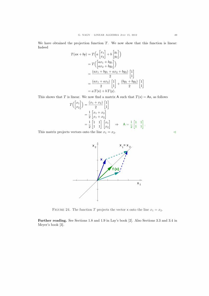
G. NAGY – LINEAR ALGEBRA July 15, 2012 49
We have obtained the projection function T . We now show that this function is linear:Indeed
T (ax + by) = T(a
[x1
x2
]+ b
[y1
y2
])
= T([
ax1 + by1
ax2 + by2
])
=(ax1 + by1 + ax2 + by2)
2
[11
]
=(ax1 + ax2)
2
[11
]+
(by1 + by2)2
[11
]
= aT (x) + b T (y).
This shows that T is linear. We now find a matrix A such that T (x) = Ax, as follows
T([
x1
x2
])=
(x1 + x2)2
[11
]
=12
[x1 + x2
x1 + x2
]
=12
[1 11 1
] [x1
x2
]⇒ A =
12
[1 11 1
].
This matrix projects vectors onto the line x1 = x2. C
f (x)
2x
x 1
x = x 21
x
Figure 24. The function T projects the vector x onto the line x1 = x2.
Further reading. See Sections 1.8 and 1.9 in Lay’s book [2]. Also Sections 3.3 and 3.4 inMeyer’s book [3].
50 G. NAGY – LINEAR ALGEBRA july 15, 2012
2.1.3. Exercises.
2.1.1.- Determine which of the followingfunctions T : R2 → R2 is linear:
(a)
T“»x1
x2
–”=
»3x2
2 + x1
–.
(b)
T“»x1
x2
–”=
»x1 + x2
x1 − x2
–.
(c)
T“»x1
x2
–”=
»x1x2
0
–.
2.1.2.- Let T : R2 → R2 be the linear trans-formation given by T (x) = Ax, where
A =
»1 22 3
–.
Find x ∈ R2 such that T (x) =
»57
–.
2.1.3.- Given the matrix and vector
A =
»1 −5 −7−3 7 5
–, b =
»−2−2
–,
define the function T : R3 → R2 asT (x) = Ax, and then find all vectors xsuch that T (x) = b.
2.1.4.- Let T : R2 → R2 be a linear trans-formation such that
T“»1
0
–”=
»31
–, T
“»01
–”=
»13
–.
Find the values of T“»x1
x2
–”for any vec-
tor
»x1
x2
–= x1
»10
–+ x2
»01
–∈ R2.
2.1.5.- Describe geometrically what is theaction of T over a vector x ∈ R2, where
(a) T (x) =
»−1 00 −1
– »x1
x2
–;
(b) T (x) =
»2 00 2
– »x1
x2
–;
(c) T (x) =
»0 00 1
– »x1
x2
–;
(d) T (x) =
»0 11 0
– »x1
x2
–.
2.1.6.- Let x =
»x1
x2
–, v =
»−25
–, u =
»7−3
–,
and let T : R2 → R2 be the linear trans-formation T (x) = x1v + x2u. Find amatrix A such that T (x) = Ax for allx ∈ R2.
G. NAGY – LINEAR ALGEBRA July 15, 2012 51
2.2. Linear combinations
One could say that the idea to introduce matrix operations originates from the interpre-tation of a matrix as a function. A matrix A ∈ Fm,n determines a function A : Fn → Fm.Such functions are generalizations of scalar valued functions of a single variable, f : R→ R.It is well-known how to compute the linear combination of two functions f , g : R→ R and,when possible, how to compute their composition and their inverses. Matrices determinea particular generalizations of scalar functions where the operations mentioned above onscalar functions can be defined on matrices. The result is called the linear combination ofmatrices, and when possible, the product of matrices and the inverse of a matrix. Sincematrices are generalizations of scalar valued functions, there are few operations on matri-ces that reduce to the identity operation in the the case of scalar functions. Among suchoperations belong the transpose of a matrix and the trace of a matrix.
2.2.1. Linear combination of matrices. The addition of two matrices and the multipli-cation of a matrix by scalar are defined component by component.
Definition 2.2.1. Let A = [Aij ] and B = [Bij ] be m × n matrices in Fm,n and a, b ∈ Fbe any scalars. The linear combination of A and B is also and m × n matrix in Fm,n,denoted as a A + b B, and given by
aA + b B = [a Aij + bBij ].
Recall that the notation aA + bB = [(aA + bB)ij ] means that the numbers (aA + bB)ij
are the components of the matrix aA + bB. Using this notation the definition above can beexpressed in terms of matrix components as follows
(aA + bB)ij = aAij + bBij .
This definition contains the particular cases a = b = 1 and b = 0, given by, respectively,
(A + B)ij = Aij + Bij , (aA)ij = aAij .
Example 2.2.1: Consider the matrices
A =[
2 −1−1 2
]B =
[3 02 −1
].
(a) Find the matrix A + B and 3A.(b) Find a matrix C such that 2C + 6A = 4B.
Solution:Part (a): The definition above gives,
A + B =[
2 −1−1 2
]+
[3 02 −1
]⇒ A + B =
[5 −11 1
], 3A =
[6 −3−3 6
].
Part (b): Matrix C is given by
C =12(4B− 6A
)
The definition above implies that
C = 2B− 3A = 2[3 02 −1
]− 3
[2 −1−1 2
]=
[6 04 −2
]− 3
[6 −3−3 6
],
therefore, we conclude that
C =[0 37 −8
].
C
52 G. NAGY – LINEAR ALGEBRA july 15, 2012
We now summarize the main properties of the matrix linear combination.
Theorem 2.2.2. For all matrices A, B ∈ Fm,n and all scalars a, b ∈ F, hold:(a) (ab)A = a(bA), (associativity);(b) a(A + B) = aA + aB, (distributivity);(c) (a + b)A = aA + bA, (distributivity);(d) 1 A = A, (1 ∈ R is the identity).
The definition of linear combination of matrices is defined as the linear combination of theircomponents, which are real of complex numbers. Therefore, all properties in Theorem 2.2.2on linear combinations of matrices are obtained from the analogous properties on the linearcombination of real or complex numbers.Proof of Theorem 2.2.2: We use components notation.
(a): [(ab)A
]ij
= (ab)Aij = a(bAij) = a(bA)ij =[a(bA)
]ij
.
(b):[a(A + B)
]ij
= a(A + B)ij = a(Aij + Bij) = aAij + aBij = (aA)ij + (aB)ij =[aA + aB
]ij
.
(c): [(a + b)A
]ij
= (a + b)Aij = aAij + bAij = (aA)ij + (bA)ij =[aA + bA
]ij
.
(d):(1A)ij = 1 Aij = Aij .
¤2.2.2. The transpose, adjoint, and trace of a matrix. Since matrices are generaliza-tions of scalar-valued functions, one can define operations on matrices that, unlike linearcombinations, have no analogue on scalar-valued functions. One of such operations is thetranspose of a matrix, which is a new matrix with the rows and columns interchanged.
Definition 2.2.3. The transpose of a matrix A = [Aij ] ∈ Fm,n is the matrix denoted asAT =
[(AT )kl
] ∈ Fn,m, with its components given by(AT
)kl
= Alk.
Example 2.2.2: Find the transpose of the 2× 3 matrix A =[1 3 52 4 6
].
Solution: Matrix A has components Aij with i = 1, 2 and j = 1, 2, 3. Therefore, itstranspose has components (AT )ji = Aij , that is, AT has three rows and two columns,
AT =
1 23 45 6
.
C
Example 2.2.3: Show that the transpose operation satisfies (AT )T = A.
Solution: The proof is: [(AT )T
]ij
= (AT )ji = Aij .
An example of this property is the following: In Example 2.2.2 we showed that[1 3 52 4 6
]T
=
1 23 45 6
.
G. NAGY – LINEAR ALGEBRA July 15, 2012 53
Therefore,([
1 3 52 4 6
]T)T
=
1 23 45 6
T
=[1 3 52 4 6
].
C
If a matrix has complex-valued coefficients, then the complex conjugate of a matrix, alsocalled the conjugate, is defined as the conjugate of each component.
Definition 2.2.4. The complex conjugate of a matrix A = [Aij ] ∈ Fm,n is the matrix
A =[Aij
] ∈ Fm,n.
Example 2.2.4: Find the conjugate if matrix A =[
1 2 + i−i 3− 4i
].
Solution: We have to conjugate each component of matrix A, that is,
A =[1 2− ii 3 + 4i
].
C
Example 2.2.5: Show that a matrix A has real coefficients iff A = A; and a matrix haspurely imaginary coefficients iff A = −A. Show one example of each case.
Solution: The first condition is A = A, that is, Aij = Aij holds for every matrix component,which implies 2i Im(Aij) = Aij − Aij = 0. Therefore, every matrix component Aij is real.The second condition is A = −A, that is, Aij = −Aij holds for every matrix component,which implies 2Re(Aij) = Aij + Aij = 0. Therefore, every matrix component Aij is purelyimaginary. Here are examples of these two situations:
A =[1 23 4
]⇒ A =
[1 23 4
]= A;
A =[
i 2i3i 4i
]⇒ A =
[ −i −2i−3i −4i
]= −A.
C
Definition 2.2.5. The adjoint of a matrix A ∈ Fm,n is the matrix A∗ = AT ∈ Fn,m.
It is not difficult to show, using components, that(A
)T = (AT ), that is, the order of thetranspose an conjugate operation does not change the resulting matrix. This property isthe reason why there is no parenthesis in the definition of A∗.
Example 2.2.6: Find the adjoint of matrix A =[
1 2 + i−i 3− 4i
].
Solution: We need to switch rows with columns and complex conjugate the result, that is,
A∗ =[
1 i2− i 3 + 4i
].
C
The transpose, conjugate and adjoint operations are useful to specify different matrix classeshaving particular symmetries. These matrix classes are the symmetric, the skew-symmetric,the Hermitian, and the skew-Hermitian matrices. Here is a precise definition.
54 G. NAGY – LINEAR ALGEBRA july 15, 2012
Definition 2.2.6. An n× n matrix A is called:(a) symmetric iff holds A = AT ;(b) skew-symmetric iff holds A = −AT ;(c) Hermitian iff holds A = A∗;(d) skew-Hermitian iff holds A = −A∗.
Example 2.2.7: We present examples of each of the classes introduced in Def. 2.2.6.Part (a): Matrices A and B are symmetric. Notice that A is also Hermitian, while B is
not Hermitian,
A =
1 2 32 7 43 4 8
= AT , B =
1 2 + 3i 32 + 3i 7 4i
3 4i 8
= BT .
Part (b): Matrix C is skew-symmetric,
C =
0 −2 32 0 −4−3 4 0
⇒ CT =
0 2 −3−2 0 43 −4 0
= −C.
Notice that the diagonal elements in a skew-symmetric matrix must vanish, since Cij = −Cji
in the case i = j means Cii = −Cii, that is, Cii = 0.Part (c): Matrix D is Hermitian but is not symmetric:
D =
1 2 + i 32− i 7 4 + i
3 4− i 8
⇒ DT =
1 2− i 32 + i 7 4− i
3 4 + i 8
6= D,
however,
D∗ = DT
=
1 2 + i 32− i 7 4 + i
3 4− i 8
= D.
Notice that the diagonal elements in a Hermitian matrix must be real numbers, since thecondition Aij = Aji in the case i = j implies Aii = Aii, that is, 2iIm(Aii) = Aii − Aii = 0.We can also verify what we said in part (a), matrix A is Hermitian since A∗ = A
T= AT = A.
Part (d): The following matrix E is skew-Hermitian:
E =
i 2 + i −3−2 + i 7i 4 + i
3 −4 + i 8i
⇒ ET =
i −2 + i 32 + i 7i −4 + i−3 4 + i 8i
therefore,
E∗ = ET
−i −2− i 3
2− i −7i −4− i−3 4− i −8i
= −E.
A skew-Hermitian matrix has purely imaginary elements in its diagonal, and the off diagonalelements have skew-symmetric real parts with symmetric imaginary parts. C
The trace of a square matrix is a number, the sum of all the diagonal matrix coefficients.
Definition 2.2.7. The trace of a square matrix A =[Aij
] ∈ Fn,n, denoted as tr (A) ∈ F,is the scalar given by
tr (A) = A11 + · · ·+ Ann.
G. NAGY – LINEAR ALGEBRA July 15, 2012 55
Example 2.2.8: Find the trace of the matrix A =
1 2 34 5 67 8 9
.
Solution: We add up the diagonal elements: tr (A) = 1 + 5 + 9, that is, tr (A) = 15. C
2.2.3. Linear transformations on matrices. The operation of computing the transposematrix can be thought as function on the set of all m×n matrices. The transpose operationis in fact a function T : Fm,n → Fn,m given by T (A) = AT . In a similar way, the operationof computing the trace of a square matrix can be thought as a function on the set of allsquare matrices. The trace is a function tr : Fn,n → F, where tr (A) = A11 + · · ·+Ann. Onecan verify that transpose function T and the trace function tr are indeed linear functions.
Theorem 2.2.8. Both the transpose function T : Fm,n → Fn,m, given by T(A) = AT , andthe trace function tr : Fn,n → F, given by tr (A) = A11 + · · ·+ Ann, are linear functions.
Proof of Theorem 2.2.8: We start with the transpose function T (A) = AT , which inmatrix components has the form
(T (A)
)ij
= Aji. Therefore, given two matrices A, B ∈ Fm,n
and arbitrary scalars a, b ∈ F, holds.(T (aA + bB)
)ij
=(aA + bB
)ji
= a Aji + bBji
= a(T (A)
)ij
+ b(T (B)
)ij
,
so we conclude thatT (aA + bB) = aT (A) + b T (B),
showing that the transpose operation is a linear function. We now consider the trace func-tion. Given any two matrices all A, B ∈ Fn,n and arbitrary scalars a, b ∈ F, holds,
tr (aA + bB) =n∑
i=1
(aA + bB
)ii
=n∑
i=1
(aAii + bBii
)
= a
n∑
i=1
Aii + b
n∑
i=1
Bii
= a tr (A) + b tr (B).
This shows that the trace is a linear function. This establishes the Theorem. ¤
56 G. NAGY – LINEAR ALGEBRA july 15, 2012
2.2.4. Exercises.
2.2.1.- Construct an example of a 3×3 ma-trix satisfying:
(a) Is symmetric and skew-symmetric.(b) Is Hermitian and symmetric.(c) Is Hermitian but not symmetric.
2.2.2.- Find the numbers x, y, z solution ofthe equation
2
»x + 2 y + 3
3 0
–=
»3 6y z
–T
2.2.3.- Given any square matrix A showthat A+AT is a symmetric matrix, whileA− AT is a skew-symmetric matrix.
2.2.4.- Prove that there is only one wayto express a matrix A ∈ Fn,n as asum of a symmetric matrix and a skew-symmetric matrix.
2.2.5.- Prove the following statements:
(a) If A = [Aij ] is a skew-symmetricmatrix, then holds Aii = 0.
(b) If A = [Aij ] is a skew-Hermitianmatrix, then the non-zero coeffi-cients Aii are purely imaginary.
(c) If A is a real and symmetric matrix,then B = iA is skew-Hermitian.
2.2.6.- Prove that for all A, B ∈ Fm,n andall a, b ∈ F holds
(aA + bB)∗ = a A∗ + b B∗.
2.2.7.- Prove that the transpose functionT : Fm,n → Fn,m and trace functiontr : Fn,n → F are linear functions.
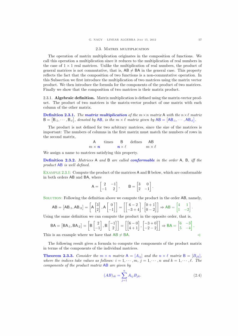
G. NAGY – LINEAR ALGEBRA July 15, 2012 57
2.3. Matrix multiplication
The operation of matrix multiplication originates in the composition of functions. Wecall this operation a multiplication since it reduces to the multiplication of real numbers inthe case of 1 × 1 real matrices. Unlike the multiplication of real numbers, the product ofgeneral matrices is not commutative, that is, AB 6= BA in the general case. This propertyreflects the fact that the composition of two functions is a non-commutative operation. Inthis Subsection we first introduce the multiplication of two matrices using the matrix vectorproduct. We then introduce the formula for the components of the product of two matrices.Finally we show that the composition of two matrices is their matrix product.
2.3.1. Algebraic definition. Matrix multiplication is defined using the matrix-vector prod-uct. The product of two matrices is the matrix-vector product of one matrix with eachcolumn of the other matrix.
Definition 2.3.1. The matrix multiplication of the m×n matrix A with the n×` matrixB =
[B:1, · · · , B:`
], denoted by AB, is the m× ` matrix given by AB =
[AB:1, · · · ,AB:`
].
The product is not defined for two arbitrary matrices, since the size of the matrices isimportant: The numbers of columns in the first matrix must match the numbers of rows inthe second matrix,
Am× n
times Bn× `
defines ABm× `
We assign a name to matrices satisfying this property.
Definition 2.3.2. Matrices A and B are called conformable in the order A, B, iff theproduct AB is well defined.
Example 2.3.1: Compute the product of the matrices A and B below, which are conformablein both orders AB and BA, where
A =[
2 −1−1 2
], B =
[3 02 −1
].
Solution: Following the definition above we compute the product in the order AB, namely,
AB =[AB:1,AB:2
]=
[A
[32
],A
[0−1
]]=
[[6− 2−3 + 4
],
[0 + 10− 2
]]⇒ AB =
[4 11 −2
].
Using the same definition we can compute the product in the opposite order, that is,
BA =[BA:1, BA:2
]=
[B
[2−1
], B
[−12
]]=
[[6− 04 + 1
],
[−3 + 0−2− 2
]]⇒ BA =
[6 −35 −4
].
This is an example where we have that AB 6= BA. C
The following result gives a formula to compute the components of the product matrixin terms of the components of the individual matrices.
Theorem 2.3.3. Consider the m × n matrix A = [Aij ] and the n × ` matrix B = [Bjk],where the indices take values as follows: i = 1, · · · ,m, j = 1, · · · , n and k = 1, · · · , `. Thecomponents of the product matrix AB are given by
(AB)ik =n∑
j=1
AijBjk. (2.4)
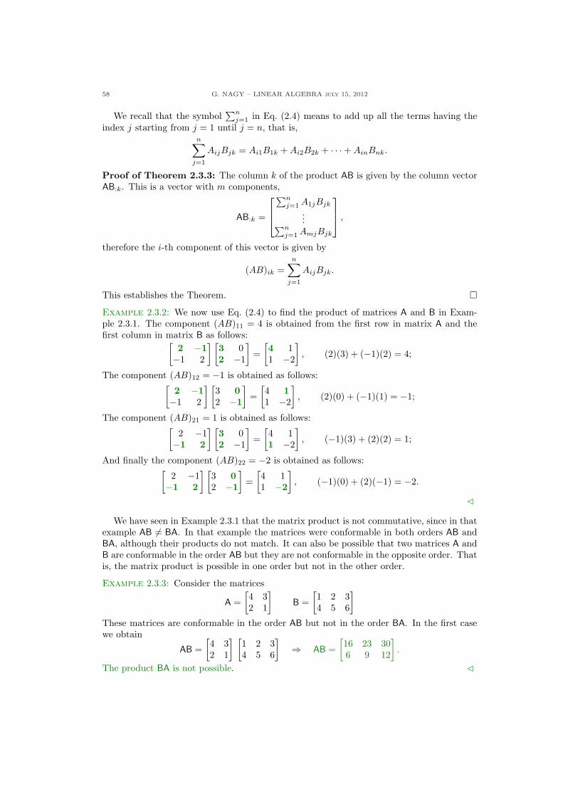
58 G. NAGY – LINEAR ALGEBRA july 15, 2012
We recall that the symbol∑n
j=1 in Eq. (2.4) means to add up all the terms having theindex j starting from j = 1 until j = n, that is,
n∑
j=1
AijBjk = Ai1B1k + Ai2B2k + · · ·+ AinBnk.
Proof of Theorem 2.3.3: The column k of the product AB is given by the column vectorAB:k. This is a vector with m components,
AB:k =
∑nj=1 A1jBjk
...∑nj=1 AmjBjk
,
therefore the i-th component of this vector is given by
(AB)ik =n∑
j=1
AijBjk.
This establishes the Theorem. ¤Example 2.3.2: We now use Eq. (2.4) to find the product of matrices A and B in Exam-ple 2.3.1. The component (AB)11 = 4 is obtained from the first row in matrix A and thefirst column in matrix B as follows:[
2 −1−1 2
] [3 02 −1
]=
[4 11 −2
], (2)(3) + (−1)(2) = 4;
The component (AB)12 = −1 is obtained as follows:[2 −1−1 2
] [3 02 −1
]=
[4 11 −2
], (2)(0) + (−1)(1) = −1;
The component (AB)21 = 1 is obtained as follows:[2 −1−1 2
] [3 02 −1
]=
[4 11 −2
], (−1)(3) + (2)(2) = 1;
And finally the component (AB)22 = −2 is obtained as follows:[2 −1−1 2
] [3 02 −1
]=
[4 11 −2
], (−1)(0) + (2)(−1) = −2.
C
We have seen in Example 2.3.1 that the matrix product is not commutative, since in thatexample AB 6= BA. In that example the matrices were conformable in both orders AB andBA, although their products do not match. It can also be possible that two matrices A andB are conformable in the order AB but they are not conformable in the opposite order. Thatis, the matrix product is possible in one order but not in the other order.
Example 2.3.3: Consider the matrices
A =[4 32 1
]B =
[1 2 34 5 6
]
These matrices are conformable in the order AB but not in the order BA. In the first casewe obtain
AB =[4 32 1
] [1 2 34 5 6
]⇒ AB =
[16 23 306 9 12
].
The product BA is not possible. C
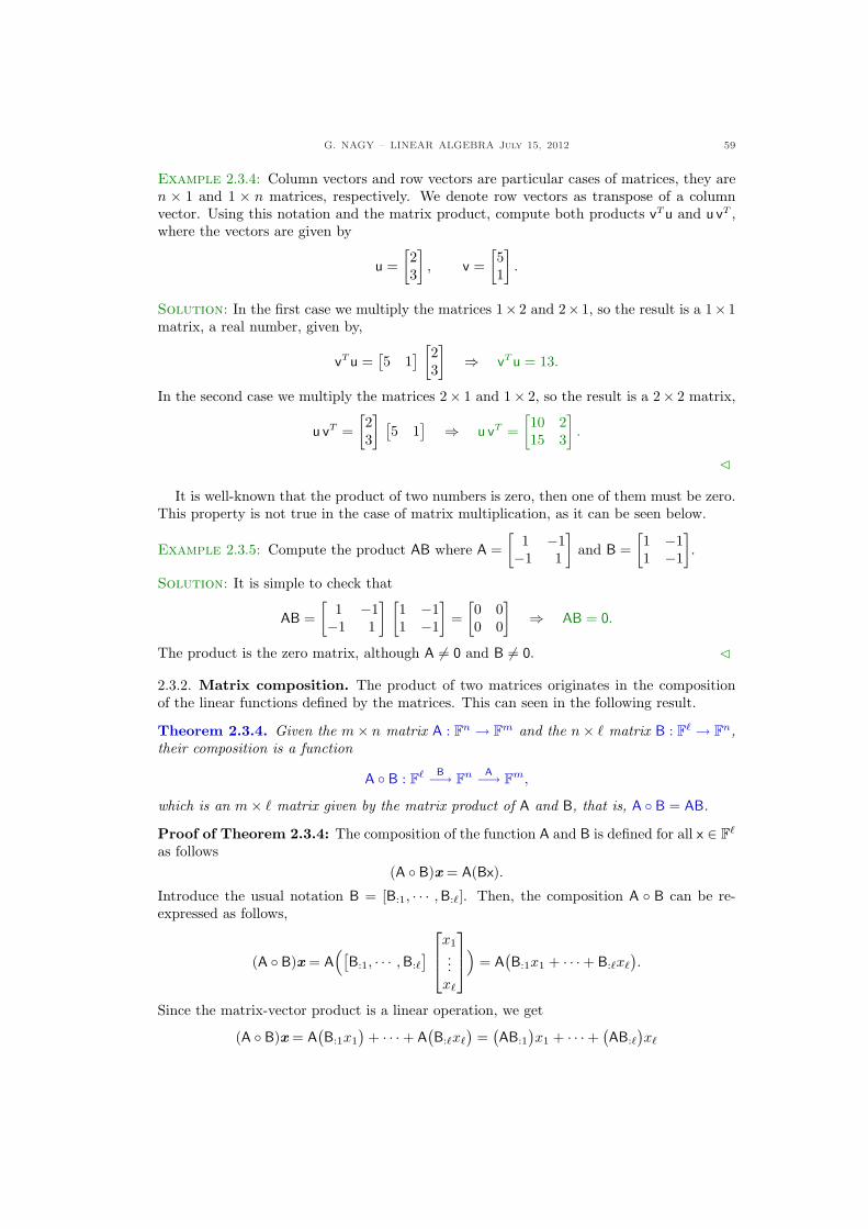
G. NAGY – LINEAR ALGEBRA July 15, 2012 59
Example 2.3.4: Column vectors and row vectors are particular cases of matrices, they aren × 1 and 1 × n matrices, respectively. We denote row vectors as transpose of a columnvector. Using this notation and the matrix product, compute both products vT u and u vT ,where the vectors are given by
u =[23
], v =
[51
].
Solution: In the first case we multiply the matrices 1× 2 and 2× 1, so the result is a 1× 1matrix, a real number, given by,
vT u =[5 1
] [23
]⇒ vT u = 13.
In the second case we multiply the matrices 2× 1 and 1× 2, so the result is a 2× 2 matrix,
u vT =[23
] [5 1
] ⇒ u vT =[10 215 3
].
C
It is well-known that the product of two numbers is zero, then one of them must be zero.This property is not true in the case of matrix multiplication, as it can be seen below.
Example 2.3.5: Compute the product AB where A =[
1 −1−1 1
]and B =
[1 −11 −1
].
Solution: It is simple to check that
AB =[
1 −1−1 1
] [1 −11 −1
]=
[0 00 0
]⇒ AB = 0.
The product is the zero matrix, although A 6= 0 and B 6= 0. C
2.3.2. Matrix composition. The product of two matrices originates in the compositionof the linear functions defined by the matrices. This can seen in the following result.
Theorem 2.3.4. Given the m× n matrix A : Fn → Fm and the n× ` matrix B : F` → Fn,their composition is a function
A ◦ B : F` B−→ Fn A−→ Fm,
which is an m× ` matrix given by the matrix product of A and B, that is, A ◦ B = AB.
Proof of Theorem 2.3.4: The composition of the function A and B is defined for all x ∈ F`
as follows(A ◦ B)x = A(Bx).
Introduce the usual notation B = [B:1, · · · , B:`]. Then, the composition A ◦ B can be re-expressed as follows,
(A ◦ B)x = A([
B:1, · · · , B:`
]
x1
...x`
)= A
(B:1x1 + · · ·+ B:`x`
).
Since the matrix-vector product is a linear operation, we get
(A ◦ B)x = A(B:1x1
)+ · · ·+ A
(B:`x`
)=
(AB:1
)x1 + · · ·+ (
AB:`
)x`
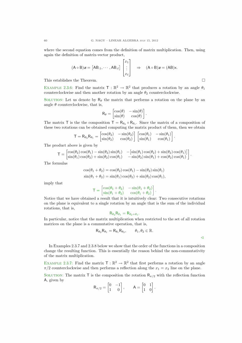
60 G. NAGY – LINEAR ALGEBRA july 15, 2012
where the second equation comes from the definition of matrix multiplication. Then, usingagain the definition of matrix-vector product,
(A ◦ B)x =[AB:1, · · · , AB:`
]
x1
...x`
⇒ (A ◦ B)x = (AB)x.
This establishes the Theorem. ¤Example 2.3.6: Find the matrix T : R2 → R2 that produces a rotation by an angle θ1
counterclockwise and then another rotation by an angle θ2 counterclockwise.
Solution: Let us denote by Rθ the matrix that performs a rotation on the plane by anangle θ counterclockwise, that is,
Rθ =[cos(θ) − sin(θ)sin(θ) cos(θ)
].
The matrix T is the the composition T = Rθ2 ◦ Rθ1 . Since the matrix of a composition ofthese two rotations can be obtained computing the matrix product of them, then we obtain
T = Rθ2Rθ1 =[cos(θ2) − sin(θ2)sin(θ2) cos(θ2)
] [cos(θ1) − sin(θ1)sin(θ1) cos(θ1)
].
The product above is given by
T =[cos(θ2) cos(θ1)− sin(θ2) sin(θ1) −[
sin(θ1) cos(θ2) + sin(θ2) cos(θ1)]
sin(θ1) cos(θ2) + sin(θ2) cos(θ1) − sin(θ2) sin(θ1) + cos(θ2) cos(θ1)
].
The formulas
cos(θ1 + θ2) = cos(θ2) cos(θ1)− sin(θ2) sin(θ1)
sin(θ1 + θ2) = sin(θ1) cos(θ2) + sin(θ2) cos(θ1),
imply that
T =[cos(θ1 + θ2) − sin(θ1 + θ2)sin(θ1 + θ2) cos(θ1 + θ2)
].
Notice that we have obtained a result that it is intuitively clear: Two consecutive rotationson the plane is equivalent to a single rotation by an angle that is the sum of the individualrotations, that is,
Rθ2Rθ1 = Rθ2+θ1 .
In particular, notice that the matrix multiplication when restricted to the set of all rotationmatrices on the plane is a commutative operation, that is,
Rθ2Rθ1 = Rθ1Rθ2 , θ1, θ2 ∈ R.
C
In Examples 2.3.7 and 2.3.8 below we show that the order of the functions in a compositionchange the resulting function. This is essentially the reason behind the non-commutativityof the matrix multiplication.
Example 2.3.7: Find the matrix T : R2 → R2 that first performs a rotation by an angleπ/2 counterclockwise and then performs a reflection along the x1 = x2 line on the plane.
Solution: The matrix T is the composition the rotation Rπ/2 with the reflection functionA, given by
Rπ/2 =[0 −11 0
], A =
[0 11 0
].
G. NAGY – LINEAR ALGEBRA July 15, 2012 61
The matrix T is given by
T = ARπ/2 =[0 11 0
] [0 −11 0
]⇒ T =
[1 00 −1
].
Therefore, the function T is a reflection along the horizontal line x2 = 0. C
Example 2.3.8: Find the matrix S : R2 → R2 that first performs a reflection along thex1 = x2 line on the plane an then performs a rotation by an angle π/2 counterclockwise.
Solution: The matrix S is the composition the reflection function A and then the rotationRπ/2, given in the previous Example 2.3.7. The matrix S is the given by
S = Rπ/2A =[0 −11 0
] [0 11 0
]⇒ S =
[−1 00 1
].
Therefore, the function S is a reflection along the vertical line x1 = 0. C
2.3.3. Main properties. We summarize the main properties of the matrix multiplication.
Theorem 2.3.5. The following properties hold for all m × n matrix A, n ×m matrix B,n× ` matrices C, D, and `× k matrix E:
(a) AB 6= BA in the general case, so the product is non-commutative;(b) A(C + D) = AC + AD, and (C + D)E = CE + DE;(c) A(CE) = (AC)E, associativity;(d) ImA = AIn = A;(e) (AC)T = CT AT , and (AC)∗ = C∗A∗.(f) tr (AB) = tr (BA).
Proof of Theorem 2.3.5:Part (a): When m 6= n the matrix AB is m ×m while BA is n × n, so they cannot be
equal. When m = n, the matrices in Example 2.3.4 and 2.3.5 show that this product is notcommutative.
Part (b): This property can be shown as follows:
A(C + D) = A([
C:1, · · · , C:`
]+
[D:1, · · · , D:`
])
= A[(C:1 + D:1), · · · , (C:` + D:`)
]
=[A(C:1 + D:1), · · · , A(C:` + D:`)
]
=[(AC:1 + AD:1), · · · , (AC:` + AD:`)
]
=[AC:1, · · · , AC:`
]+
[AD:1, · · · ,AD:`
]
= AC + AD.
The other equation is proven in a similar way.Part (c): This property is proven using the component expression for the matrix product:
[A(CE)
]ij
=n∑
k=1
Aik(CE)kj =n∑
k=1
Aik
(∑
l=1
CklElj
);
however, the order of the sums can be interchanged,
n∑
k=1
Aik
(∑
l=1
CklElj
)=
∑
l=1
( n∑
k=1
AikCkl
)Elj ;
62 G. NAGY – LINEAR ALGEBRA july 15, 2012
So, from this last expression is not difficult to show that:
∑
l=1
( n∑
k=1
AikCkl
)Elj =
∑
l=1
(AC)ilElj =[(AC)E
]ij
;
We have just proved that [A(CE)
]ij
=[(AC)E
]ij
.
Part (d): We can use components again, recalling that the components of Im are givenby (Im)ij = 0 if i 6= j and is (Im)ii = 1. Therefore,
(ImA)ij =m∑
k=1
(Im)ikAkj = (Im)iiAij = Aij .
Analogously,
(AIn)ij =n∑
k=1
Aik(In)kj = Aij(In)jj = Aij .
Part (e): Use components once more:
[(AC)T
]ij
= (AC)ji =n∑
k=1
AjkCki =n∑
k=1
(AT )kj(CT )ik =n∑
k=1
(CT )ik(AT )kj =[CT AT
]ij
.
The second equation follows from the proof above and the property of the complex conjugate:
(AC) = A C.
Indeed
(AC)∗ = (AC)T = CT AT = CT AT = C∗A∗.
Part (f): Recall that the trace of a matrix A is given by
tr (A) = A11 + · · ·+ Ann =n∑
i=1
Aii.
Then it is simple to see that
tr (AB) =m∑
i=1
( n∑
j=1
AijBji
)=
m∑
i=1
( n∑
j=1
BjiAij
)=
n∑
j=1
( m∑
i=1
BjiAij
)= tr (BA).
This establishes the Theorem. ¤We use the notation A2 = AA, A3 = A2A, and An = An−1A. Notice that the matrix
product is not commutative, so the formula (a + b)2 = a2 + 2ab + b2 does not hold formatrices. Instead we have:
(A + B)2 = (A + B)(A + B) = A2 + AB + BA + B2.
2.3.4. Block multiplication. The multiplication of two large matrices can be simplifiedin the case that each matrix can be subdivided in appropriate blocks. If these matrix blocksare conformable the multiplication of the original matrices reduces to the multiplication ofthe smaller matrix blocks. The next result is presents a simple case.
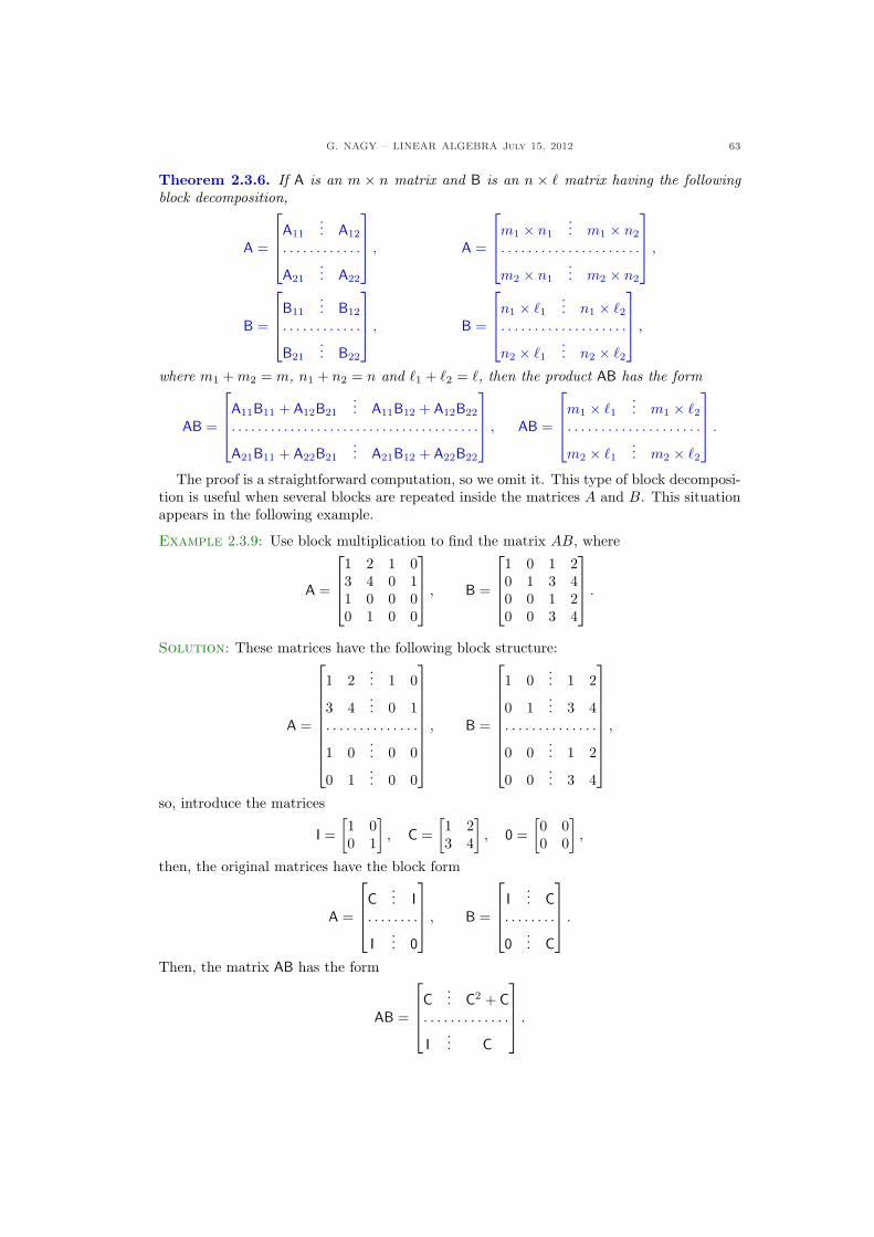
G. NAGY – LINEAR ALGEBRA July 15, 2012 63
Theorem 2.3.6. If A is an m × n matrix and B is an n × ` matrix having the followingblock decomposition,
A =
A11
... A12
. . . . . . . . . . . .
A21
... A22
, A =
m1 × n1
... m1 × n2
. . . . . . . . . . . . . . . . . . . . .
m2 × n1
... m2 × n2
,
B =
B11
... B12
. . . . . . . . . . . .
B21
... B22
, B =
n1 × `1... n1 × `2
. . . . . . . . . . . . . . . . . . .
n2 × `1... n2 × `2
,
where m1 + m2 = m, n1 + n2 = n and `1 + `2 = `, then the product AB has the form
AB =
A11B11 + A12B21
... A11B12 + A12B22
. . . . . . . . . . . . . . . . . . . . . . . . . . . . . . . . . . . . . .
A21B11 + A22B21
... A21B12 + A22B22
, AB =
m1 × `1... m1 × `2
. . . . . . . . . . . . . . . . . . . .
m2 × `1... m2 × `2
.
The proof is a straightforward computation, so we omit it. This type of block decomposi-tion is useful when several blocks are repeated inside the matrices A and B. This situationappears in the following example.
Example 2.3.9: Use block multiplication to find the matrix AB, where
A =
1 2 1 03 4 0 11 0 0 00 1 0 0
, B =
1 0 1 20 1 3 40 0 1 20 0 3 4
.
Solution: These matrices have the following block structure:
A =
1 2... 1 0
3 4... 0 1
. . . . . . . . . . . . . .
1 0... 0 0
0 1... 0 0
, B =
1 0... 1 2
0 1... 3 4
. . . . . . . . . . . . . .
0 0... 1 2
0 0... 3 4
,
so, introduce the matrices
I =[1 00 1
], C =
[1 23 4
], 0 =
[0 00 0
],
then, the original matrices have the block form
A =
C... I
. . . . . . . .
I... 0
, B =
I... C
. . . . . . . .
0... C
.
Then, the matrix AB has the form
AB =
C... C2 + C
. . . . . . . . . . . . .
I... C
.
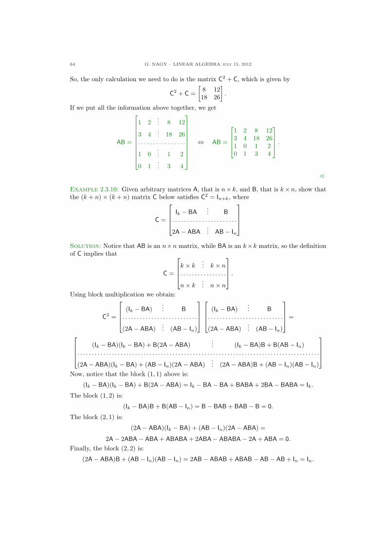
64 G. NAGY – LINEAR ALGEBRA july 15, 2012
So, the only calculation we need to do is the matrix C2 + C, which is given by
C2 + C =[
8 1218 26
].
If we put all the information above together, we get
AB =
1 2... 8 12
3 4... 18 26
. . . . . . . . . . . . . . . .
1 0... 1 2
0 1... 3 4
⇔ AB =
1 2 8 123 4 18 261 0 1 20 1 3 4
.
C
Example 2.3.10: Given arbitrary matrices A, that is n× k, and B, that is k×n, show thatthe (k + n)× (k + n) matrix C below satisfies C2 = In+k, where
C =
Ik − BA... B
. . . . . . . . . . . . . . . . . . . . . .
2A− ABA... AB− In
Solution: Notice that AB is an n×n matrix, while BA is an k×k matrix, so the definitionof C implies that
C =
k × k... k × n
. . . . . . . . . . . . . . . .
n× k... n× n
.
Using block multiplication we obtain:
C2 =
(Ik − BA)... B
. . . . . . . . . . . . . . . . . . . . . . . . . .
(2A− ABA)... (AB− In)
(Ik − BA)... B
. . . . . . . . . . . . . . . . . . . . . . . . . .
(2A− ABA)... (AB− In)
=
(Ik − BA)(Ik − BA) + B(2A− ABA)... (Ik − BA)B + B(AB− In)
. . . . . . . . . . . . . . . . . . . . . . . . . . . . . . . . . . . . . . . . . . . . . . . . . . . . . . . . . . . . . . . . . . . . . . . . . . . . . . . . . . . .
(2A− ABA)(Ik − BA) + (AB− In)(2A− ABA)... (2A− ABA)B + (AB− In)(AB− In)
Now, notice that the block (1, 1) above is:
(Ik − BA)(Ik − BA) + B(2A− ABA) = Ik − BA− BA + BABA + 2BA− BABA = Ik.
The block (1, 2) is:
(Ik − BA)B + B(AB− In) = B− BAB + BAB− B = 0.
The block (2, 1) is:
(2A− ABA)(Ik − BA) + (AB− In)(2A− ABA) =
2A− 2ABA− ABA + ABABA + 2ABA− ABABA− 2A + ABA = 0.
Finally, the block (2, 2) is:
(2A− ABA)B + (AB− In)(AB− In) = 2AB− ABAB + ABAB− AB− AB + In = In.
G. NAGY – LINEAR ALGEBRA July 15, 2012 65
Therefore, we have shown that: C2 =
Ik... 0
. . . . . . . . .
0... In
= Ik+n. C
2.3.5. Matrix commutators. Matrix multiplication is in general not commutative. Giventwo n× n matrices A and B, their product AB is in general different from BA. We call thedifference between these two matrices the commutator of A and B.
Definition 2.3.7. The commutator of two n× n matrices A and B, is the matrix
[A, B] = AB− BA.
Furthermore, we say that the square matrices A, B commute iff holds [A,B] = 0.
Therefore, the symbol [A, B] denotes an n × n matrix, the commutator of A and B. Thecommutator of two operators defined on an inner product space is an important conceptin quantum mechanics. When we say an operator, we should think in something like amatrix, and when we say an inner product space, we should think in something like Fn. Anobservation of a physical property, like position or momentum, of a quantum mechanicalsystem, like an electron, is described by an operator acting on a vector, the latter describingthe state of the quantum mechanical system. By observing nature, one discovers that twoproperties can be simultaneously measured without limit in the measurement precision iffthe associated operators commute. If the operators do not commute, then their commutatordetermines the maximum precision of their simultaneous observation. This is the physicalcontent of the Heisenberg uncertainty principle.
Example 2.3.11: We have seen in Example 2.3.6 that two rotation matrices R(θ1) and R(θ2)commute for all θ1, θ2 ∈ R, that is,
[R(θ1),R(θ2)] = R(θ1)R(θ2)− R(θ2)R(θ1) ⇒ [R(θ1), R(θ2)] = 0. C
Theorem 2.3.8. For all matrices A, B, C ∈ Fn,n and scalars a, b, c ∈ F holds:(a) [A, B] = −[B, A], (antisymmetry);(b) [aA, bB] = ab [A, B], (linearity);(c) [A, B + C] = [A, B] + [A, C], (linearity on the right entry);(d) [A + B,C] = [A, C] + [B,C], (linearity on the left entry);(e) [A, BC] = [A,B]C + B[A, C], (right derivation property);(f) [AB, C] = [A,C]B + A[B, C], (left derivation property);(g)
[[A, B],C
]+
[[C, A], B
]+
[[B,C], A
]= 0, (Jacobi property).
Proof of Theorem 2.3.8: All properties are simple to show.Part (a):
[A, B] = AB− BA = −(BA− AB
)= −[B, A].
Part (b):[aA, bB] = aAbB− bBaA = ab
(AB− BA
)= ab [A, B].
Part (c):
[A, B + C] = A(B + C)− (B + C)A = AB + AC− BA− CA = [A, B] + [A,C].
Part (d): The proof is similar to the previous calculation.Part (e):
[A, BC] = A(BC)− (BC)A = ABC + (BAC− BAC)− BCA = [A, B]C + B[A,C].
Part (f): The proof is similar to the previous calculation.

66 G. NAGY – LINEAR ALGEBRA july 15, 2012
Part (g): We write down each term and we verify that they all add up to zero:[[A, B],C
]= (AB− BA)C− C(AB− BA);
[[C,A], B
]= (CA− AC)B− B(CA− AC);[
[B, C], A]
= (BC− CB)A− A(BC− CB).
These three equations add up to the zero matrix. This establishes the Theorem. ¤We finally highlight that these properties implies that [A,Am] = 0 holds for all m ∈ N.
Further reading. Almost every book in linear algebra explains matrix multiplication. SeeSection 3.5 in Meyer’s book [3], and Section 3.6 for block multiplication. Also Strang’sbook [4]. The definition of commutators can be found in Section 2.3.1 in Hassani’s book [1].Commutators play an important role in the Spectral Theorem, which we study in Chapter 9.
G. NAGY – LINEAR ALGEBRA July 15, 2012 67
2.3.6. Exercises.
2.3.1.- Given the matrices
A =
24
1 −2 30 −5 44 −3 8
35 , B =
24
1 20 43 7
35 ,
and the vector C =
24
123
35, compute the
following products, if possible:
(a) AB, BA, CB and CT B.(b) A2, B2, CT C and CCT .
2.3.2.- Consider the matrices
A =
»2 13 1
–, B =
»1 13 0
–, C =
»1 42 3
–.
(a) Compute [A, B].(b) Find the product ABC.
2.3.3.- Find A2 and A3 for the matrix
A =
24
0 1 10 0 10 0 0
35 .
2.3.4.- Given a real number a find the ma-trix An, where n is any positive integerand
A =
»1 a0 1
–.
2.3.5.- Given any square matrices A, B,prove that
(A+B)2 = A2+2AB+B2 ⇔ [A, B] = 0.
2.3.6.- Given a = 1/3, divide the matrix
A =
26666664
1 0 0 a a a0 1 0 a a a0 0 1 a a a0 0 0 a a a0 0 0 a a a0 0 0 a a a
37777775
into appropriate blocks, and using blockmultiplication find the matrix A300.
2.3.7.- Prove that for all matrices A ∈ Fn,m
and B ∈ Fm,n holds
tr (AB) = tr (BA).
2.3.8.- Let A be an m × n matrix. Showthat tr
`AT A
´= 0 iff A = 0.
2.3.9.- Prove that: If A, B ∈ Fn,n aresymmetric matrices and commute, thentheir product AB is also a symmetricmatrix.
2.3.10.- Let A be an arbitrary n × n ma-trix. Use the trace function to showthat there exists no n× n matrix X so-lution of the matrix equation
[A, X] = In.
68 G. NAGY – LINEAR ALGEBRA july 15, 2012
2.4. Inverse matrix
In this Section we introduce the concept of the inverse of a square matrix. Not everysquare matrix is invertible. In the case of 2 × 2 matrices we present a condition on thematrix coefficients that is equivalent to the invertibility of the matrix, and we also presenta formula for the inverse matrix. Later on in Section 3.2 we generalize this formula forn× n matrices. The inverse of a matrix is useful to compute solutions to systems of linearequations.
2.4.1. Main definition. We start recalling that the matrix In ∈ Fn,n is called the identitymatrix iff holds that Inx = x for all x ∈ Fn. Choosing the vector x = ei, consisting of a 1 inthe row i and zero every where else, it is simple to see that the components of the identitymatrix are given by
In = [Iij ] with{
Iii = 1,
Iij = 0, i 6= j.
The cases n = 2 and n = 3 are shown below,
I2 =[1 00 1
], I3 =
1 0 00 1 00 0 1
.
We also use the column vector notation for the identity matrix,
In = [e1, · · · , en],
that is, we denote the identity column vectors I:i = ei for i = 1, · · · , n. For example, in thecase of I3 we have that
I3 = [e1, e2, e3] =
1 0 00 1 00 0 1
⇒ e1 =
100
, e2 =
010
, e3 =
001
.
We are now ready to introduce the notion of the inverse matrix.
Definition 2.4.1. A matrix A ∈ Fn,n is called invertible iff there exists a matrix, denotedas A−1, such that
(A−1
)A = In and A
(A−1
)= In.
Since the matrix product is non-commutative, the products A(A−1
)= In and
(A−1
)A =
In must be specified in the definition above. Notice that we do not need to assume that theinverse matrix belongs to Fn,n, since both products A
(A−1
)and
(A−1
)A are well-defined,
we conclude that the inverse matrix must be n× n.
Example 2.4.1: Verify that the matrix and its inverse are given by
A =[2 21 3
], A−1 =
14
[3 −2−1 2
].
Solution: We have to compute the products,
A(A−1
)=
[2 21 3
]14
[3 −2−1 2
]=
14
[4 00 4
]⇒ A
(A−1
)= I2.
It is simple to check that the equation(A−1
)A = I2 also holds. C
Example 2.4.2: The only real numbers that are equal to is own inverses are a = 1 anda = −1. This is not true in the case of matrices. Verify that the matrix A below is its owninverse, that is,
A =[1 10 −1
]= A−1.
G. NAGY – LINEAR ALGEBRA July 15, 2012 69
Solution: We have to compute the products,
A(A−1
)=
[1 10 −1
] [1 10 −1
]=
[1 00 1
]⇒ A
(A−1
)= I2.
It is simple to check that the equation(A−1
)A = I2 also holds. C
Not every square matrix is invertible. The following Example show a 2× 2 matrix with noinverse.
Example 2.4.3: Show that matrix A =[1 23 6
]has no inverse.
Solution: Suppose there exists the inverse matrix
A−1 =[a bc d
]
Then, the following equation holds,
A(A−1
)= I2 ⇔
[1 23 6
] [a bc d
]=
[1 00 1
].
The last equation impliesa + 2c = 1,
3(a + 2c) = 0,
b + 2d = 0,
3(b + 2d) = 1.
However, both systems are inconsistent, so the inverse matrix A−1 does not exist. C
In the case of 2 × 2 matrices there is a simple way to find out whether a matrix hasinverse or not. If the 2×2 matrix is invertible, then there is a simple formula for the inversematrix. This is summarized in the following result.
Theorem 2.4.2. Given a 2 × 2 matrix A =[a bc d
], introduce the number ∆ = ad − bc.
The matrix A is invertible iff ∆ 6= 0. Furthermore, if A is invertible, its inverse is given by
A−1 =1∆
[d −b−c a
]. (2.5)
The number ∆ is called the determinant of A, since it is the number that determines whetherA is invertible or not, and soon we will see that it is the number that determines whethera system of linear equations has a unique solution or not. Also later on we will studygeneralizations to n× n matrices of the Theorem above. That will require a generalizationto n× n matrices of the determinant ∆ of a matrix.
Example 2.4.4: Compute the inverse of matrix A =[2 21 3
], given in Example 2.4.1.
Solution: Following Theorem 2.4.2 we first compute ∆ = 6 − 4 = 4. Since ∆ 6= 0, thenA−1 exists and it is given by
A−1 =14
[3 −2−1 2
].
C
Example 2.4.5: Theorem 2.4.2 says that the matrix in Example 2.4.3 is not invertible, since
A =[1 23 6
]⇒ ∆ = 6− (3)(2) ⇒ ∆ = 0.
C
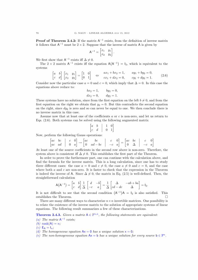
70 G. NAGY – LINEAR ALGEBRA july 15, 2012
Proof of Theorem 2.4.2: If the matrix A−1 exists, from the definition of inverse matrixit follows that A−1 must be 2× 2. Suppose that the inverse of matrix A is given by
A−1 =[x1 y1
x2 y2
].
We first show that A−1 exists iff ∆ 6= 0.The 2 × 2 matrix A−1 exists iff the equation A
(A−1
)= I2, which is equivalent to the
systems[a bc d
] [x1 y1
x2 y2
]=
[1 00 1
]⇔
ax1 + bx2 = 1,
cx1 + dx2 = 0,
ay1 + by2 = 0,
cy1 + dy2 = 1.(2.6)
Consider now the particular case a = 0 and c = 0, which imply that ∆ = 0. In this case theequations above reduce to:
bx2 = 1,
dx2 = 0,
by2 = 0,
dy2 = 1.
These systems have no solution, since from the first equation on the left b 6= 0, and from thefirst equation on the right we obtain that y2 = 0. But this contradicts the second equationon the right, since dy2 is zero and so can never be equal to one. We then conclude there isno inverse matrix in this case.
Assume now that at least one of the coefficients a or c is non-zero, and let us return toEqs. (2.6). Both systems can be solved using the following augmented matrix
[a b
∣∣ 1 0c d
∣∣ 0 1
]
Now, perform the following Gauss operations:[ac bc
∣∣ c 0ac ad
∣∣ 0 a
]→
[ac bc
∣∣ c 00 ad− bc
∣∣ −c a
]=
[ac bc
∣∣ c 00 ∆
∣∣ −c a
]
At least one of the source coefficients in the second row above is non-zero. Therefore, thesystem above is consistent iff ∆ 6= 0. This establishes the first part of the Theorem.
In order to prove the furthermore part, one can continue with the calculation above, andfind the formula for the inverse matrix. This is a long calculation, since one has to studythree different cases: the case a = 0 and c 6= 0, the case a 6= 0 and c = 0, and the casewhere both a and c are non-zero. It is faster to check that the expression in the Theoremis indeed the inverse of A. Since ∆ 6= 0, the matrix in Eq. (2.5) is well-defined. Then, thestraightforward calculation
A(A−1
)=
[a bc d
]1∆
[d −b−c a
]=
1∆
[∆ −ab + ba
cd− dc ∆
]= I2.
It is not difficult to see that the second condition(A−1
)A = I2 is also satisfied. This
establishes the Theorem. ¤There are many different ways to characterize n×n invertible matrices. One possibility is
to relate the existence of the inverse matrix to the solution of appropriate systems of linearequations. The following result summarizes a few of these characterizations.
Theorem 2.4.3. Given a matrix A ∈ Fn,n, the following statements are equivalent:(a) The matrix A−1 exists;(b) rank(A) = n;(c) EA = In;(d) The homogeneous equation Ax = 0 has a unique solution x = 0;(e) The non-homogeneous equation Ax = b has a unique solution for every source b ∈ Fn.
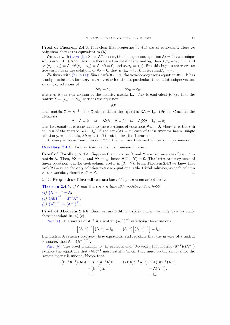
G. NAGY – LINEAR ALGEBRA July 15, 2012 71
Proof of Theorem 2.4.3: It is clear that properties (b)-(d) are all equivalent. Here weonly show that (a) is equivalent to (b).
We start with (a)⇒ (b): Since A−1 exists, the homogeneous equation Ax = 0 has a uniquesolution x = 0. (Proof: Assume there are two solutions x1 and x2, then A(x2 − x1) = 0, andso (x2 − x1) = A−1A(x2 − x1) = A−10 = 0, and so x2 = x1.) But this implies there are nofree variables in the solutions of Ax = 0, that is, EA = In, that is, rank(A) = n.
We finish with (b) ⇒ (a): Since rank(A) = n, the non-homogeneous equation Ax = b hasa unique solution x for every source vector b ∈ Rn. In particular, there exist unique vectorsx1, · · · , xn solutions of
Ax1 = e1, · · · Axn = en.
where ei is the i-th column of the identity matrix In. This is equivalent to say that thematrix X =
[x1, · · · , xn
]satisfies the equation
AX = In.
This matrix X = A−1 since X also satisfies the equation XA = In. (Proof: Consider theidentities
A− A = 0 ⇔ AXA− A = 0 ⇔ A(XA− In) = 0;The last equation is equivalent to the n systems of equations Ayi = 0, where yi is the i-thcolumn of the matrix (XA − In); Since rank(A) = n, each of these systems has a uniquesolution yi = 0, that is, XA = In.) This establishes the Theorem. ¤
It is simple to see from Theorem 2.4.3 that an invertible matrix has a unique inverse.
Corollary 2.4.4. An invertible matrix has a unique inverse.
Proof of Corollary 2.4.4: Suppose that matrices X and Y are two inverses of an n × nmatrix A. Then, AX = In and AY = In, hence A(X − Y) = 0. The latter are n systems oflinear equations, one for each column vector in (X−Y). From Theorem 2.4.3 we know thatrank(A) = n, so the only solution to these equations is the trivial solution, so each columnvector vanishes, therefore X = Y. ¤2.4.2. Properties of invertible matrices. They are summarized below.
Theorem 2.4.5. If A and B are n× n invertible matrices, then holds:
(a)(A−1
)−1 = A;(b)
(AB
)−1 = B−1A−1;(c)
(AT
)−1 =(A−1
)T .
Proof of Theorem 2.4.5: Since an invertible matrix is unique, we only have to verifythese equations in (a)-(c).
Part (a): The inverse of A−1 is a matrix(A−1
)−1 satisfying the equations[(
A−1)−1
](A−1
)= In,
(A−1
)[(A−1
)−1]
= In.
But matrix A satisfies precisely these equations, and recalling that the inverse of a matrixis unique, then A =
(A−1
)−1.Part (b): The proof is similar to the previous one. We verify that matrix
(B−1
)((A−1
)satisfies the equations that (AB)−1 must satisfy. Then, they must be the same, since theinverse matrix is unique. Notice that,(
B−1A−1)(AB) = B−1
(A−1A
)B,
=(B−1
)B,
= In;
(AB)(B−1A−1
)= A
(BB−1
)A−1,
= A(A−1
),
= In.
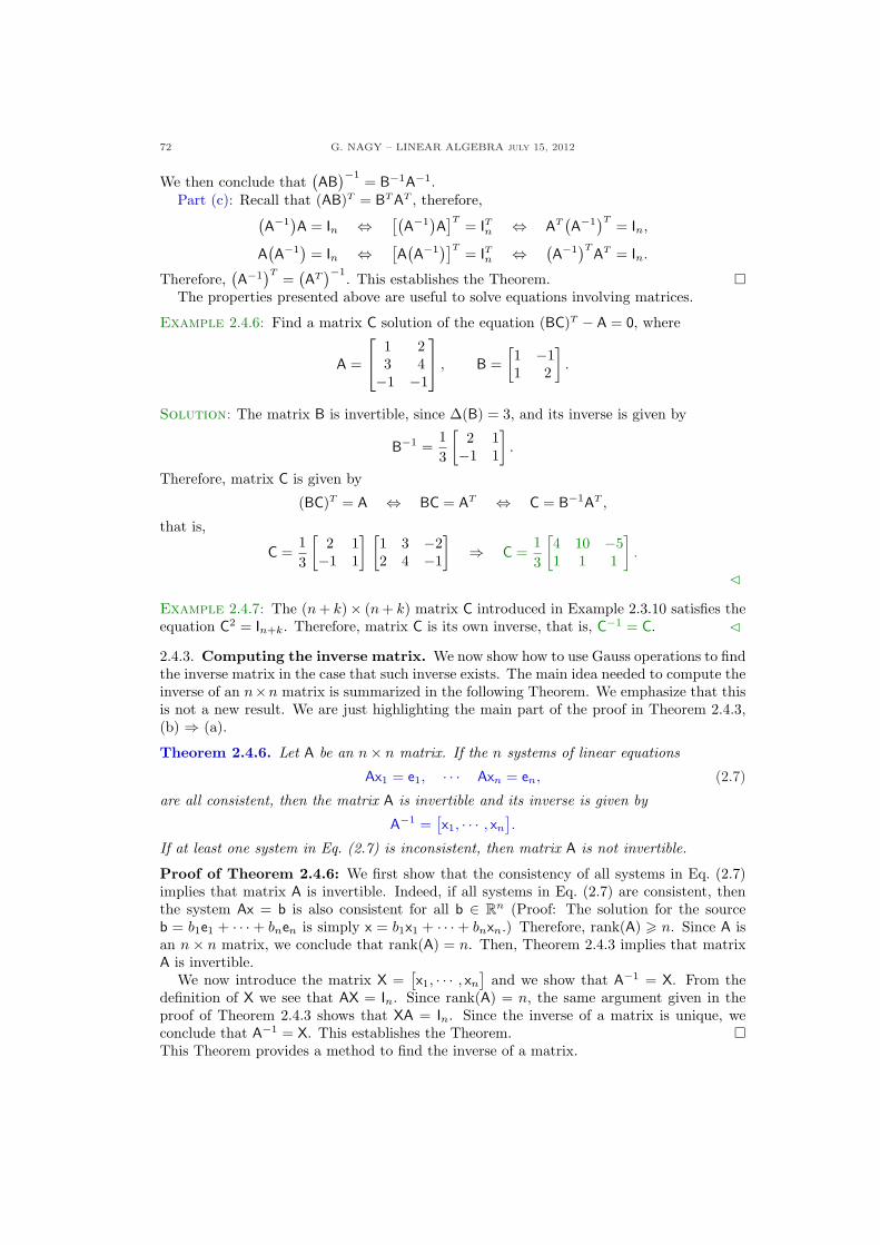
72 G. NAGY – LINEAR ALGEBRA july 15, 2012
We then conclude that(AB
)−1 = B−1A−1.Part (c): Recall that (AB)T = BT AT , therefore,
(A−1
)A = In ⇔ [(
A−1)A
]T = ITn ⇔ AT(A−1
)T = In,
A(A−1
)= In ⇔ [
A(A−1
)]T = ITn ⇔ (A−1
)TAT = In.
Therefore,(A−1
)T =(AT
)−1. This establishes the Theorem. ¤The properties presented above are useful to solve equations involving matrices.
Example 2.4.6: Find a matrix C solution of the equation (BC)T − A = 0, where
A =
1 23 4−1 −1
, B =
[1 −11 2
].
Solution: The matrix B is invertible, since ∆(B) = 3, and its inverse is given by
B−1 =13
[2 1−1 1
].
Therefore, matrix C is given by
(BC)T = A ⇔ BC = AT ⇔ C = B−1AT ,
that is,
C =13
[2 1−1 1
] [1 3 −22 4 −1
]⇒ C =
13
[4 10 −51 1 1
].
C
Example 2.4.7: The (n + k)× (n + k) matrix C introduced in Example 2.3.10 satisfies theequation C2 = In+k. Therefore, matrix C is its own inverse, that is, C−1 = C. C
2.4.3. Computing the inverse matrix. We now show how to use Gauss operations to findthe inverse matrix in the case that such inverse exists. The main idea needed to compute theinverse of an n×n matrix is summarized in the following Theorem. We emphasize that thisis not a new result. We are just highlighting the main part of the proof in Theorem 2.4.3,(b) ⇒ (a).
Theorem 2.4.6. Let A be an n× n matrix. If the n systems of linear equations
Ax1 = e1, · · · Axn = en, (2.7)
are all consistent, then the matrix A is invertible and its inverse is given by
A−1 =[x1, · · · , xn
].
If at least one system in Eq. (2.7) is inconsistent, then matrix A is not invertible.
Proof of Theorem 2.4.6: We first show that the consistency of all systems in Eq. (2.7)implies that matrix A is invertible. Indeed, if all systems in Eq. (2.7) are consistent, thenthe system Ax = b is also consistent for all b ∈ Rn (Proof: The solution for the sourceb = b1e1 + · · · + bnen is simply x = b1x1 + · · · + bnxn.) Therefore, rank(A) > n. Since A isan n× n matrix, we conclude that rank(A) = n. Then, Theorem 2.4.3 implies that matrixA is invertible.
We now introduce the matrix X =[x1, · · · , xn
]and we show that A−1 = X. From the
definition of X we see that AX = In. Since rank(A) = n, the same argument given in theproof of Theorem 2.4.3 shows that XA = In. Since the inverse of a matrix is unique, weconclude that A−1 = X. This establishes the Theorem. ¤This Theorem provides a method to find the inverse of a matrix.
G. NAGY – LINEAR ALGEBRA July 15, 2012 73
Corollary 2.4.7. The inverse of an invertible n× n matrix A is computed with the Gaussoperations such that
[A
∣∣In] −→ [
In∣∣A−1
].
Proof of Corollary 2.4.7: One solves the n linear systems in Eq. (2.7). Since all thesesystems share the same coefficient matrix, matrix A, one can solve them all at the sametime, introducing the augmented matrix[
A∣∣e1, · · · , en
]=
[A
∣∣In].
In the proof of Theorem 2.4.6 we show that rank(A) = n. Therefore, its reduced echelonform is EA = In, so the Gauss method implies that[
A∣∣In
]=
[A
∣∣e1, · · · , en
]→ [EA
∣∣x1, · · · , xn
]=
[In
∣∣A−1] ⇔ [
A∣∣In
] −→ [In
∣∣A−1].
This establishes the Corollary. ¤
Example 2.4.8: Find the inverse of the matrix A =[2 41 3
].
Solution: We have to solve the two systems of equations Ax1 = e1 and Ax2 = e2, that is,[2 41 3
] [x1
x2
]=
[10
] [2 41 3
] [y1
y2
]=
[01
].
We solve both systems at the same time using the Gauss method on the augmented matrix[2 4
∣∣ 1 01 3
∣∣ 0 1
]→
[1 2
∣∣ 1/2 01 3
∣∣ 0 1
]→
[1 2
∣∣ 1/2 00 1
∣∣ −1/2 1
]→
[1 0
∣∣ 3/2 −20 1
∣∣ −1/2 1
]
therefore, A−1 = 12
[3 −4−1 2
]. C
Example 2.4.9: Find the inverse of the matrix A =
1 2 32 5 73 7 9
.
Solution: We compute the inverse matrix as follows:
1 2 3∣∣ 1 0 0
2 5 7∣∣ 0 1 0
3 7 9∣∣ 0 0 1
→
1 2 3∣∣ 1 0 0
0 1 1∣∣ −2 1 0
0 1 0∣∣ −3 0 1
→
1 0 1∣∣ 5 −2 0
0 1 1∣∣ −2 1 0
0 0 −1∣∣ −1 −1 1
→
1 0 0∣∣ 4 −3 1
0 1 0∣∣ −3 0 1
0 0 1∣∣ 1 1 −1
⇒ A−1 =
4 −3 1−3 0 11 1 −1
.
C
Example 2.4.10: Is matrix A =[1 22 4
]invertible?
Solution: No, since[1 2
∣∣ 1 02 4
∣∣ 0 1
]→
[1 2
∣∣ 1 00 0
∣∣ −2 1
], are inconsistent. C
Further reading. Almost any book in linear algebra introduces the inverse matrix. SeeSections 3.7 and 3.9 in Meyer’s book [3].
74 G. NAGY – LINEAR ALGEBRA july 15, 2012
2.4.4. Exercises.
2.4.1.- When possible, find the inverse ofthe following matrices. (Check your an-swers using matrix multiplication.)
(a)
A =
»1 21 3
–;
(b)
A =
24−1 −2 13 2 −61 1 −2
35 ;
(c)
A =
24
1 2 34 5 67 8 9
35 .
2.4.2.- Find the values of the constant ksuch that the matrix A below is not in-vertible,
A =
24
1 1 −12 3 k1 k 3
35 .
2.4.3.- Consider the matrix
A =
24
0 −1 02 0 10 1 −1
35 ,
(a) Find the inverse of matrix A.(b) Use the previous part to find a so-
lution to the linear system
Ax = b, b =
24
1−13
35 .
2.4.4.- Show that for every invertible ma-trix A holds that [A, A−1] = 0.
2.4.5.- Find a matrix X such that the equa-tion X = AX + B holds for
A =
24
0 −1 00 0 −10 0 0
35 , B =
24
1 22 13 3
35 .
2.4.6.- If A is invertible and symmetric,then show that A−1 is also symmetric.
2.4.7.- Prove that: If the square matrix Asatisfies A2 = 0, then the matrix (I−A)is invertible.
2.4.8.- Prove that: If the square matrix Asatisfies A3 = 0, then the matrix (I−A)is invertible.
2.4.9.- Let A be a square matrix. Prove thefollowing statements:
(a) If A contains a zero column then Ais not invertible;
(b) If one column is multiple of anothercolumn in A, then matrix A is notinvertible.
(c) Use the trace function to prove thefollowing statement: If A is an m×nmatrix and B is an n × m matrixsuch that AB = Im and BA = In,then m = n.
2.4.10.- Consider the invertible matricesA ∈ Fr,r, B ∈ Fs,s and the matrixC ∈ Fr,s. Prove that the inverse of
2664
A... C
. . . . . . . . .
0... B
3775
is given by2664
A−1... −A−1CB−1
. . . . . . . . . . . . . . . . . . . . .
0... B−1
3775 .
G. NAGY – LINEAR ALGEBRA July 15, 2012 75
2.5. Null and range spaces
2.5.1. Definition of the spaces. A matrix A ∈ Fm,n defines two functions, A : Fn → Fm
and AT : Fm → Fn, which in turn, determine two sets in Fn and two sets in Fm. In thisSection we define these sets, we call them null and range spaces, and study the main relationsamong them. We start introducing the two spaces associated with the function A.
Definition 2.5.1. Consider the matrix A ∈ Fm,n defining the linear function A : Fn → Fm.The null space of the function A is the set N(A) ⊂ Fn given by
N(A) ={x ∈ Fn : Ax = 0
}.
The range space of the function A is set R(A) ⊂ Fm given by
R(A) ={y ∈ Fm : y = Ax, for all x ∈ Fn
}.
In Fig. 25 we show a picture, usual in set theory, sketching the null and range spacesassociated with a matrix A. One can see in these pictures that for a function A : Fn → Fm,the null space is a subset in Fn, while the range space is a subset in Fm. Recall that thehomogeneous equation Ax = 0 always has the trivial solution x = 0. This property impliesboth that 0 ∈ Fn also belongs to N(A) and that 0 ∈ Fm also belongs to R(A).
00
n
m
N ( A )
A
F
F
0
A
0
n
m
R ( A )
F
F
Figure 25. Sketch of the null space, N(A), and the range space, R(A), ofa linear function determined by the m× n matrix A.
The four spaces associated with a matrix A are N(A) and R(A) together with N(AT )and R(AT ). Notice that these null and range spaces are subsets of different spaces. Moreprecisely, a matrix A ∈ Fm.n defines the functions and subsets,
A : Fn → Fm and AT : Fm → Fn,
N(A), R(AT ) ⊂ Fn, while R(A), N(AT ) ⊂ Fm.
Example 2.5.1: Find the N(A) and R(A) for the function A : R3 → R2 given by
A =[1 2 32 4 1
].
Solution: We first find N(A), the null space of A. This is the set of elements x ∈ R3 thatare solutions of the equation Ax = 0. We use the Gauss method to find all such solutions,
[1 2 32 4 1
]→
[1 2 30 0 −5
]→
[1 2 00 0 1
]⇒
x1 = −2x2
x3 = 0,
x2 : free variable.
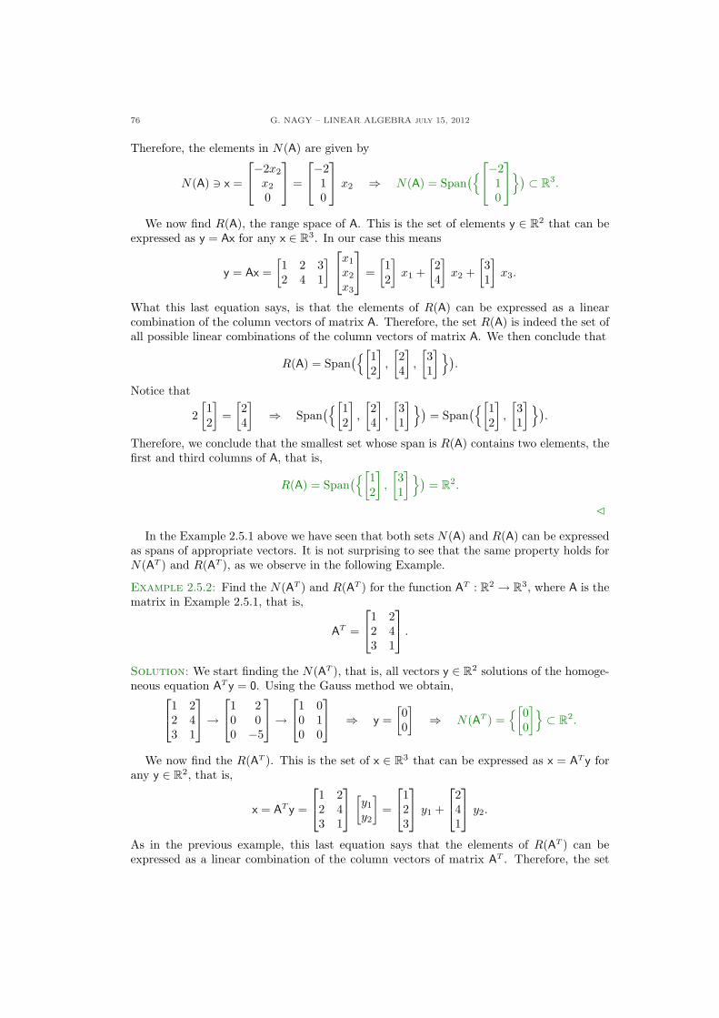
76 G. NAGY – LINEAR ALGEBRA july 15, 2012
Therefore, the elements in N(A) are given by
N(A) 3 x =
−2x2
x2
0
=
−210
x2 ⇒ N(A) = Span
({−210
}) ⊂ R3.
We now find R(A), the range space of A. This is the set of elements y ∈ R2 that can beexpressed as y = Ax for any x ∈ R3. In our case this means
y = Ax =[1 2 32 4 1
]
x1
x2
x3
=
[12
]x1 +
[24
]x2 +
[31
]x3.
What this last equation says, is that the elements of R(A) can be expressed as a linearcombination of the column vectors of matrix A. Therefore, the set R(A) is indeed the set ofall possible linear combinations of the column vectors of matrix A. We then conclude that
R(A) = Span({[
12
],
[24
],
[31
] }).
Notice that
2[12
]=
[24
]⇒ Span
({[12
],
[24
],
[31
] })= Span
({[12
],
[31
] }).
Therefore, we conclude that the smallest set whose span is R(A) contains two elements, thefirst and third columns of A, that is,
R(A) = Span({[
12
],
[31
] })= R2.
C
In the Example 2.5.1 above we have seen that both sets N(A) and R(A) can be expressedas spans of appropriate vectors. It is not surprising to see that the same property holds forN(AT ) and R(AT ), as we observe in the following Example.
Example 2.5.2: Find the N(AT ) and R(AT ) for the function AT : R2 → R3, where A is thematrix in Example 2.5.1, that is,
AT =
1 22 43 1
.
Solution: We start finding the N(AT ), that is, all vectors y ∈ R2 solutions of the homoge-neous equation AT y = 0. Using the Gauss method we obtain,
1 22 43 1
→
1 20 00 −5
→
1 00 10 0
⇒ y =
[00
]⇒ N(AT ) =
{[00
]}⊂ R2.
We now find the R(AT ). This is the set of x ∈ R3 that can be expressed as x = AT y forany y ∈ R2, that is,
x = AT y =
1 22 43 1
[y1
y2
]=
123
y1 +
241
y2.
As in the previous example, this last equation says that the elements of R(AT ) can beexpressed as a linear combination of the column vectors of matrix AT . Therefore, the set
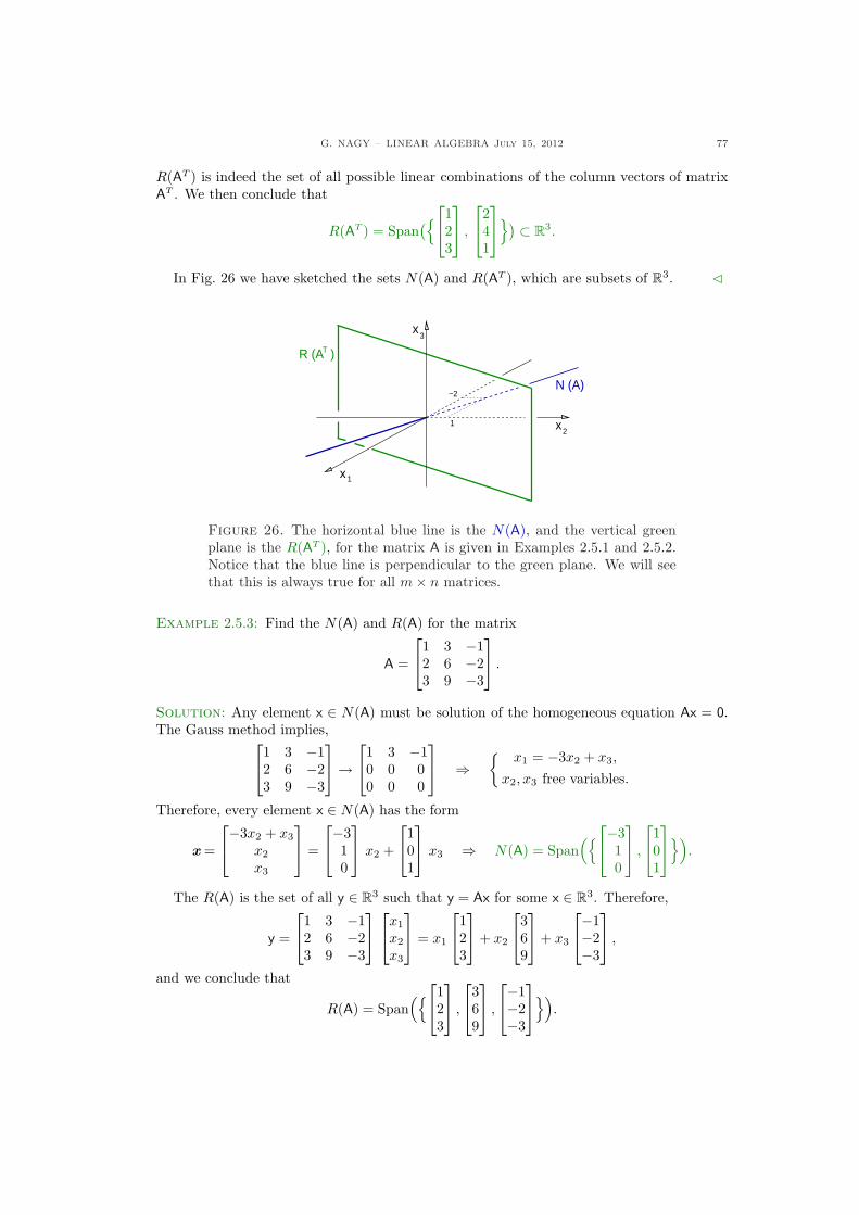
G. NAGY – LINEAR ALGEBRA July 15, 2012 77
R(AT ) is indeed the set of all possible linear combinations of the column vectors of matrixAT . We then conclude that
R(AT ) = Span({
123
,
241
}) ⊂ R3.
In Fig. 26 we have sketched the sets N(A) and R(AT ), which are subsets of R3. C
3
N (A)−2
R (A )T
1
x 1
x2
x
Figure 26. The horizontal blue line is the N(A), and the vertical greenplane is the R(AT ), for the matrix A is given in Examples 2.5.1 and 2.5.2.Notice that the blue line is perpendicular to the green plane. We will seethat this is always true for all m× n matrices.
Example 2.5.3: Find the N(A) and R(A) for the matrix
A =
1 3 −12 6 −23 9 −3
.
Solution: Any element x ∈ N(A) must be solution of the homogeneous equation Ax = 0.The Gauss method implies,
1 3 −12 6 −23 9 −3
→
1 3 −10 0 00 0 0
⇒
{x1 = −3x2 + x3,
x2, x3 free variables.
Therefore, every element x ∈ N(A) has the form
x =
−3x2 + x3
x2
x3
=
−310
x2 +
101
x3 ⇒ N(A) = Span
({−310
,
101
}).
The R(A) is the set of all y ∈ R3 such that y = Ax for some x ∈ R3. Therefore,
y =
1 3 −12 6 −23 9 −3
x1
x2
x3
= x1
123
+ x2
369
+ x3
−1−2−3
,
and we conclude that
R(A) = Span({
123
,
369
,
−1−2−3
}).
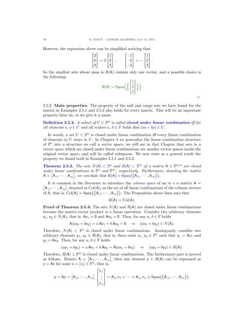
78 G. NAGY – LINEAR ALGEBRA july 15, 2012
However, the expression above can be simplified noticing that
369
= 3
123
,
−1−2−3
= −
123
.
So the smallest sets whose span is R(A) contain only one vector, and a possible choice isthe following:
R(A) = Span({
123
}).
C
2.5.2. Main properties. The property of the null and range sets we have found for thematrix in Examples 2.5.1 and 2.5.2 also holds for every matrix. This will be an importantproperty later on, so we give it a name.
Definition 2.5.2. A subset of U ⊂ Fn is called closed under linear combination iff forall elements x, y ∈ U and all scalars a, b ∈ F holds that (ax + by) ∈ U .
In words, a set U ⊂ Fn is closed under linear combination iff every linear combinationof elements in U stays in U . In Chapter 4 we generalize the linear combination structureof Fn into a structure we call a vector space; we will see in that Chapter that sets in avector space which are closed under linear combinations are smaller vector spaces inside theoriginal vector space, and will be called subspaces. We now state as a general result theproperty we found both in Examples 2.5.1 and 2.5.2.
Theorem 2.5.3. The sets N(A) ⊂ Fn and R(A) ⊂ Fm of a matrix A ∈ Fm,n are closedunder linear combinations in Fn and Fm, respectively. Furthermore, denoting the matrixA =
[A:1, · · · , A:n
], we conclude that R(A) = Span
({A:1, · · · , A:n
}).
It is common in the literature to introduce the column space of an m × n matrix A =[A:1, · · · , A:n
], denoted as Col(A), as the set of all linear combinations of the column vectors
of A, that is, Col(A) = Span({
A:1, · · · , A:n
}). The Proposition above then says that
R(A) = Col(A).
Proof of Theorem 2.5.3: The sets N(A) and R(A) are closed under linear combinationsbecause the matrix-vector product is a linear operation. Consider two arbitrary elementsx1, x2 ∈ N(A), that is, Ax1 = 0 and Ax2 = 0. Then, for any a, b ∈ F holds
A(ax1 + bx2) = a Ax1 + b Ax2 = 0 ⇒ (ax1 + bx2) ∈ N(A).
Therefore, N(A) ⊂ Fn is closed under linear combinations. Analogously, consider twoarbitrary elements y1, y2 ∈ R(A), that is, there exist x1, x2 ∈ Fn such that y1 = Ax1 andy2 = Ax2. Then, for any a, b ∈ F holds
(ay1 + by2) = aAx1 + bAx2 = A(ax1 + bx2) ⇒ (ay2 + by2) ∈ R(A).
Therefore, R(A) ⊂ Fm is closed under linear combinations. The furthermore part is provedas follows. Denote A =
[A:1, · · · ,A:n
], then any element y ∈ R(A) can be expressed as
y = Ax for some x = [xi] ∈ Fn, that is,
y = Ax =[A:1, · · · , A:n
]
x1
...xn
= A:1 x1 + · · ·+ A:n xn ∈ Span
({A:1, · · · ,A:n
}).
G. NAGY – LINEAR ALGEBRA July 15, 2012 79
This implies that R(A) ⊂ Col(A). The opposite inclusion, Col(A) ⊂ R(A) is trivial, sinceany element of the form y = A:1 x1 + · · · + A:n xn ∈ Col(A) also belongs to R(A), sincey = Ax, where x = [xi]. This establishes the Theorem. ¤
The null and range spaces of a square matrix characterize whether the matrix is invertibleor not. The following result is a simple rewriting of Theorem 2.4.3.
Theorem 2.5.4. Given a matrix A ∈ Fn,n, the following statements are equivalent:(a) The matrix A−1 exists;(b) N(A) = {0};(c) R(A) = Fn.
Proof of Theorem 2.5.4: This result follows from Theorem 2.4.3. More precisely, part (b)follows from Theorem 2.4.3 part (c). While part (c) follows from Theorem 2.4.3 part (e). ¤2.5.3. Gauss operations. In this section we study the relations between the four spacesassociated with the matrices A and B in the case that matrix B can be obtained from matrixA by performing Gauss operations. We use the following notation: A
row←→ B to indicate thatA can be transformed into matrix B by performing Gauss operations on the rows of A.
Theorem 2.5.5. If matrices A, B ∈ Fm,n, then(a) A
row←→ B ⇔ N(A) = N(B);(b) A
row←→ B ⇔ R(AT ) = R(BT ).
It is simple to see that this result is true. Gauss operations do not change the solutions oflinear systems, so the linear system Ax = 0 has exactly the same solutions x as the linearsystem Bx = 0, that is, N(A) = N(B). The second property must be also true, since Gaussoperations on the rows of A are equivalent to Gauss operations on the columns of AT . Now,it is simple to see that each of the Gauss operations on the columns of AT do not changethe Col(AT ), hence R(AT ) = R(BT ).
One could say that the paragraph above is enough for a proof of the Theorem. However,we would like to have a more detailed presentation of the ideas above. One way is to usematrix multiplication to express the Gauss operation property that they do not change thesolutions to linear systems. One can prove the following: If the m × n matrices A and Bare related by Gauss operations on their rows, then there exists an m×m invertible matrixG such that GA = B. The proof of this property is simple. Each one of the Gauss opera-tions is associated with an invertible matrix, E, called an elementary Gauss matrix. Everyelementary Gauss matrix is invertible, since every Gauss operation can always be reversed.The result of several Gauss operations on a matrix A is the product of the appropriateelementary Gauss matrices in the same order as the Gauss operations are performed. If thematrix B is obtained from matrix A by doing Gauss operations given by matrices Ei, fori = 1, · · · , k, in that order, we can express the result of the Gauss method as follows:
Ek · · ·E1A = B, G = Ek · · ·E1 ⇒ GA = B.
Since each elementary Gauss matrix is invertible, then the matrix G is also invertible. Thefollowing example shows all 3× 3 elementary Gauss matrices.
Example 2.5.4: Find all the elementary Gauss matrices which operate on 3× n matrices.
Solution: In the case of 3 × n matrices, the elementary Gauss matrices are 3 × 3. Wepresent these matrices for each one of the three main types of Gauss operations. Considerthe matrices Ei for i = 1, 2, 3 are given by
E1 =
k 0 00 1 00 0 1
, E2 =
1 0 00 k 00 0 1
, E3 =
1 0 00 1 00 0 k
;
80 G. NAGY – LINEAR ALGEBRA july 15, 2012
then, the product EiA represents the Gauss operation of multiplying by k the first, secondand third row of A, respectively. Consider the matrices Ei for i = 4, 5, 6 given by
E4 =
0 1 01 0 00 0 1
, E5 =
0 0 10 1 01 0 0
, E6 =
1 0 00 0 10 1 0
;
then, the product EiA for i = 4, 5, 6 represents the Gauss operation of interchanging the firstand second, the first and third, and the second and third rows of A, respectively. Finally,consider the matrices Ei for j = 7, · · · , 12 given by
E7 =
1 0 0k 1 00 0 1
, E8 =
1 0 00 1 0k 0 1
, E9 =
1 0 00 1 00 k 1
,
E10 =
1 k 00 1 00 0 1
, E11 =
1 0 k0 1 00 0 1
, E12 =
1 0 00 1 k0 0 1
;
then, the product EiA for i = 7, · · · , 12 represents the Gauss operation of multiplying by kone row of A and add the result to another row of A. C
Proof of Theorem 2.5.5: Recall the comment below Theorem 2.5.5: If the m×n matricesA and B are related by Gauss operations on their rows, then there exits an m×m invertiblematrix G such that GA = B. This observation is the key to show that N(A) = N(B), sincegiven any element x ∈ N(A)
Ax = 0 ⇔ GAx = 0,
where the equivalence follows from G being invertible. Then it is simple to see that
0 = GAx = Bx ⇔ x ∈ N(B).
Therefore, we have shown that N(A) = N(B).We now show the converse statement. If N(A) = N(B) this means that their reduced
echelon forms are the same, that is, EA = EB. This means that there exist Gauss operationson the rows of A that transform it into matrix B.
We now show that R(AT ) = R(BT ). Given any element x ∈ R(AT ) we know that thereexists an element y ∈ Fm such that
x = AT y = AT GT(GT
)−1y = (GA)T y = BT y, y =
(GT
)−1y.
We have shown that given any x ∈ R(AT ), then x ∈ R(BT ), that is, R(AT ) ⊂ R(BT ). Theopposite implication is proven in the same way: Given any x ∈ R(BT ) there exists y ∈ Fm
such thatx = BT y = BT
(GT
)−1GT y =
(G−1B
)Ty = AT y, y = GT y.
We have shown that given any x ∈ R(BT ), then x ∈ R(AT ), that is, R(BT ) ⊂ R(AT ).Therefore, R(AT ) = R(BT ).
We now show that the converse statement. Assume that R(AT ) = R(BT ). This meansthat every row in matrix A is a linear combination of the rows in matrix B. This also meansthat there exists Gauss operations on the rows of A such that transform A into B. Thisestablishes the Theorem. ¤
Example 2.5.5: Verify Theorem 2.5.5 for matrix A =[1 2 32 4 1
]and EA =
[1 2 00 0 1
].
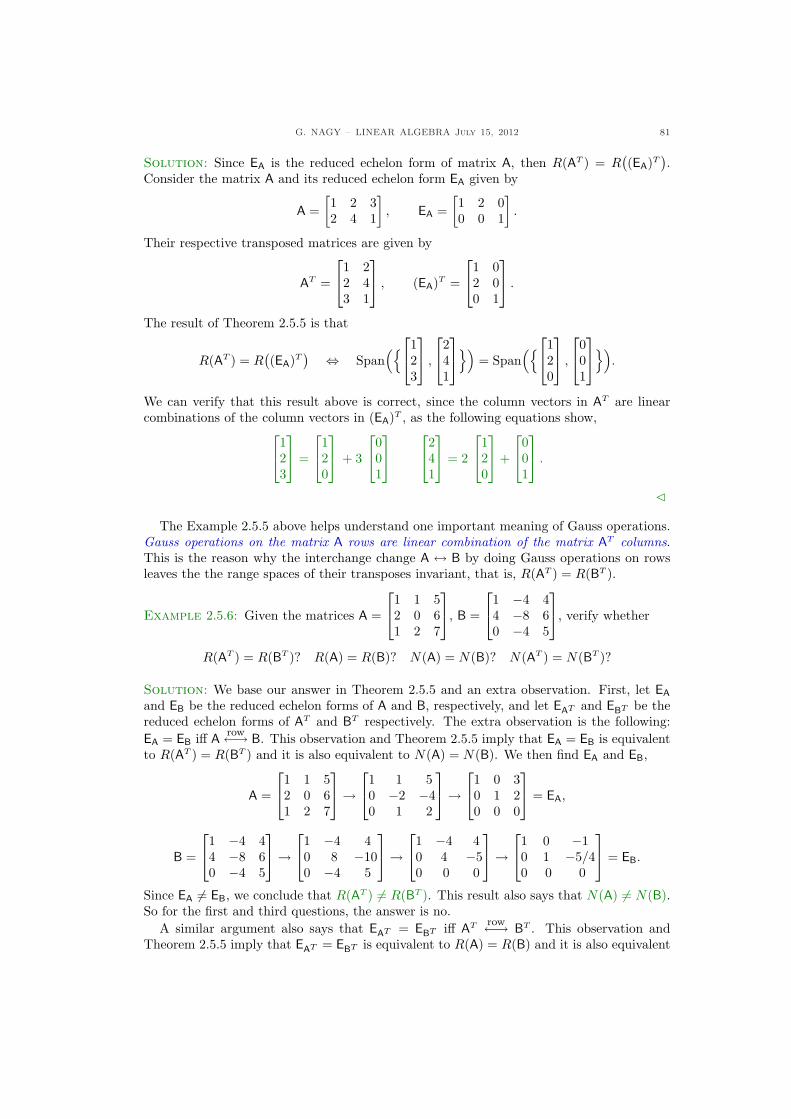
G. NAGY – LINEAR ALGEBRA July 15, 2012 81
Solution: Since EA is the reduced echelon form of matrix A, then R(AT ) = R((EA)T
).
Consider the matrix A and its reduced echelon form EA given by
A =[1 2 32 4 1
], EA =
[1 2 00 0 1
].
Their respective transposed matrices are given by
AT =
1 22 43 1
, (EA)T =
1 02 00 1
.
The result of Theorem 2.5.5 is that
R(AT ) = R((EA)T
) ⇔ Span({
123
,
241
})= Span
({
120
,
001
}).
We can verify that this result above is correct, since the column vectors in AT are linearcombinations of the column vectors in (EA)T , as the following equations show,
123
=
120
+ 3
001
241
= 2
120
+
001
.
C
The Example 2.5.5 above helps understand one important meaning of Gauss operations.Gauss operations on the matrix A rows are linear combination of the matrix AT columns.This is the reason why the interchange change A ↔ B by doing Gauss operations on rowsleaves the the range spaces of their transposes invariant, that is, R(AT ) = R(BT ).
Example 2.5.6: Given the matrices A =
1 1 52 0 61 2 7
, B =
1 −4 44 −8 60 −4 5
, verify whether
R(AT ) = R(BT )? R(A) = R(B)? N(A) = N(B)? N(AT ) = N(BT )?
Solution: We base our answer in Theorem 2.5.5 and an extra observation. First, let EA
and EB be the reduced echelon forms of A and B, respectively, and let EAT and EBT be thereduced echelon forms of AT and BT respectively. The extra observation is the following:EA = EB iff A
row←→ B. This observation and Theorem 2.5.5 imply that EA = EB is equivalentto R(AT ) = R(BT ) and it is also equivalent to N(A) = N(B). We then find EA and EB,
A =
1 1 52 0 61 2 7
→
1 1 50 −2 −40 1 2
→
1 0 30 1 20 0 0
= EA,
B =
1 −4 44 −8 60 −4 5
→
1 −4 40 8 −100 −4 5
→
1 −4 40 4 −50 0 0
→
1 0 −10 1 −5/40 0 0
= EB.
Since EA 6= EB, we conclude that R(AT ) 6= R(BT ). This result also says that N(A) 6= N(B).So for the first and third questions, the answer is no.
A similar argument also says that EAT = EBT iff AT row←→ BT . This observation andTheorem 2.5.5 imply that EAT = EBT is equivalent to R(A) = R(B) and it is also equivalent
82 G. NAGY – LINEAR ALGEBRA july 15, 2012
to N(AT ) = N(BT ). We then find EAT and EBT ,
AT =
1 2 11 0 25 6 7
→
1 2 10 −2 10 −4 2
→
1 0 20 1 −1/20 0 0
= EAT ,
BT =
1 4 0−4 −8 −44 6 5
→
1 4 00 8 −40 −10 5
→
1 4 00 2 −10 0 0
→
1 0 20 1 −1/20 0 0
= EBT .
Since EAT = EBT , we conclude that R(A) = R(B). This result on the reduced echelon formsalso says that N(AT ) = N(BT ). So for the second and four questions, the answer is yes. C
We finish this Section with two results concerning the ranks of a matrix and its transpose.The first result says that transposition operation on a matrix does not change its rank.
Theorem 2.5.6. Every matrix A ∈ Fm,n satisfies that rank(A) = rank(AT ).
We delay the proof of the first result to Chapter 6, where we introduce the notion of innerproduct in a vector space. Using an inner product in Fn, the proof of Theorem 2.5.6 belowis simple. We now introduce a particular name for those matrices having the maximumpossible rank.
Definition 2.5.7. An m× n matrix A has full rank iff rank(A) = min(m,n).
Our last result of this Section concerns full rank matrices and relates the rank of a matrixA to the size of both N(A) and N(AT ).
Theorem 2.5.8. If matrix A ∈ Fm,n has full rank, then hold:(a) If m = n, then rank(A) = rank(AT ) = n = m ⇔ {0} = N(A) = N(AT ) ⊂ Fn;
(b) If m < n, then rank(A) = rank(AT ) = m < n ⇔{ {0} & N(A) ⊂ Fn,
{0} = N(AT ) ⊂ Fm;
(c) If m > n, then rank(A) = rank(AT ) = n < m ⇔{ {0} = N(A) ⊂ Fn,
{0} & N(AT ) ⊂ Fm.
Proof of Theorem 2.5.8: We start recaling that the rank of a matrix A is the number ofpivot columns in its reduced echelon form EA.
If an m × n matrix A has rank(A) = n, this means two things: First, n 6 m; andsecond, that every column in EA has a pivot. The latter property implies that there is nofree variables in the solution of the equation Ax = 0, and so x = 0 is the unique solution.We conclude that N(A) = {0}. In order to study N(AT ) we need to consider the twopossible cases n = m or n < m. If n = m, then the matrices A and AT are square, and thesame argument about free variables applies to solutions of AT y = 0, so we conclude thatN(AT ) = {0}. This proves (a). In the case that n < m, then there are free variables in thesolution of the equation AT y = 0, therefore {0} & N(AT ). This proves (c).
If an m × n matrix A has rank(A) = m, recalling that rank(A) = rank(AT ), this meanstwo things: First, m 6 n; and second, that every column in EAT has a pivot. The latterproperty shows that AT is full rank, so the argument above shows that N(AT ) = {0}. Sincethe case n = m has already been studied, so we only need to consider the case m < n. In thiscase there are free variables in the solution to the equation Ax = 0, therefore {0} & N(A).This proves (b), and we have established the Theorem. ¤
Further reading. Section 4.2 in Meyer’s book [3] follows closely the descriptions of thefour spaces given here, although in more depth.
G. NAGY – LINEAR ALGEBRA July 15, 2012 83
2.5.4. Exercises.
2.5.1.- Find R(A) and R(AT ) for the matrixA below and express them as the spanof the smallest possible set of vectors,where
A =
24
1 2 2 32 4 1 33 6 1 4
35 .
2.5.2.- Find the N(A), R(A), N(AT ) andR(AT ) for the matrix A below and ex-press them as the span of the smallestpossible set of vectors, where
A =
24
1 2 1 1 5−2 −4 0 4 −21 2 2 4 9
35 .
2.5.3.- Let A be a 3× 3 matrix such that
R(A) = Span“n24
123
35 ,
24
1−12
35o”
,
N(A) = Span“n24−210
35o”
.
(a) Show that the linear system Ax = bis consistent for
b =
24
185
35 .
(b) Show that the system Ax = b abovehas infinitely many solutions.
2.5.4.- Prove:
(a) Ax = b is consistent iff b ∈ R(A).(b) The consistent system Ax = b has a
unique solution iff N(A) = {0}.
2.5.5.- Prove: A matrix A ∈ Fn,n is invert-ible iff R(A) = Fn.
2.5.6.- Let A ∈ Fn,n be an invertible ma-trix. Find the spaces N(A), R(A),N(AT ), and R(AT ).
2.5.7.- Consider the matrices
A =
24
1 5 32 1 −31 3 1
35 , B =
24
1 0 −20 1 10 0 0
35 .
Answer the questions below. If the an-swer is yes, give a proof; if the answeris no, give a counter-example.
(a) Is R(A) = R(B)?(b) Is R(AT ) = R(BT )?(c) Is N(A) = N(B)?(d) Is N(AT ) = N(BT )?
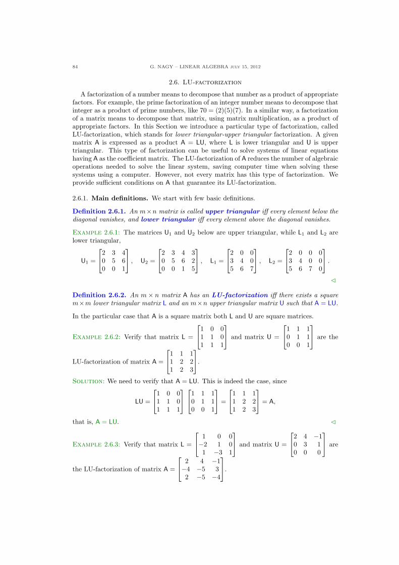
84 G. NAGY – LINEAR ALGEBRA july 15, 2012
2.6. LU-factorization
A factorization of a number means to decompose that number as a product of appropriatefactors. For example, the prime factorization of an integer number means to decompose thatinteger as a product of prime numbers, like 70 = (2)(5)(7). In a similar way, a factorizationof a matrix means to decompose that matrix, using matrix multiplication, as a product ofappropriate factors. In this Section we introduce a particular type of factorization, calledLU-factorization, which stands for lower triangular-upper triangular factorization. A givenmatrix A is expressed as a product A = LU, where L is lower triangular and U is uppertriangular. This type of factorization can be useful to solve systems of linear equationshaving A as the coefficient matrix. The LU-factorization of A reduces the number of algebraicoperations needed to solve the linear system, saving computer time when solving thesesystems using a computer. However, not every matrix has this type of factorization. Weprovide sufficient conditions on A that guarantee its LU-factorization.
2.6.1. Main definitions. We start with few basic definitions.
Definition 2.6.1. An m×n matrix is called upper triangular iff every element below thediagonal vanishes, and lower triangular iff every element above the diagonal vanishes.
Example 2.6.1: The matrices U1 and U2 below are upper triangular, while L1 and L2 arelower triangular,
U1 =
2 3 40 5 60 0 1
, U2 =
2 3 4 30 5 6 20 0 1 5
, L1 =
2 0 03 4 05 6 7
, L2 =
2 0 0 03 4 0 05 6 7 0
.
C
Definition 2.6.2. An m× n matrix A has an LU-factorization iff there exists a squarem×m lower triangular matrix L and an m×n upper triangular matrix U such that A = LU.
In the particular case that A is a square matrix both L and U are square matrices.
Example 2.6.2: Verify that matrix L =
1 0 01 1 01 1 1
and matrix U =
1 1 10 1 10 0 1
are the
LU-factorization of matrix A =
1 1 11 2 21 2 3
.
Solution: We need to verify that A = LU. This is indeed the case, since
LU =
1 0 01 1 01 1 1
1 1 10 1 10 0 1
=
1 1 11 2 21 2 3
= A,
that is, A = LU. C
Example 2.6.3: Verify that matrix L =
1 0 0−2 1 01 −3 1
and matrix U =
2 4 −10 3 10 0 0
are
the LU-factorization of matrix A =
2 4 −1−4 −5 32 −5 −4
.
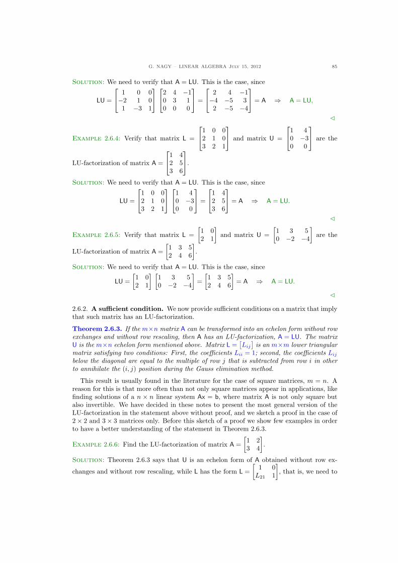
G. NAGY – LINEAR ALGEBRA July 15, 2012 85
Solution: We need to verify that A = LU. This is the case, since
LU =
1 0 0−2 1 01 −3 1
2 4 −10 3 10 0 0
=
2 4 −1−4 −5 32 −5 −4
= A ⇒ A = LU,
C
Example 2.6.4: Verify that matrix L =
1 0 02 1 03 2 1
and matrix U =
1 40 −30 0
are the
LU-factorization of matrix A =
1 42 53 6
.
Solution: We need to verify that A = LU. This is the case, since
LU =
1 0 02 1 03 2 1
1 40 −30 0
=
1 42 53 6
= A ⇒ A = LU.
C
Example 2.6.5: Verify that matrix L =[1 02 1
]and matrix U =
[1 3 50 −2 −4
]are the
LU-factorization of matrix A =[1 3 52 4 6
].
Solution: We need to verify that A = LU. This is the case, since
LU =[1 02 1
] [1 3 50 −2 −4
]=
[1 3 52 4 6
]= A ⇒ A = LU.
C
2.6.2. A sufficient condition. We now provide sufficient conditions on a matrix that implythat such matrix has an LU-factorization.
Theorem 2.6.3. If the m×n matrix A can be transformed into an echelon form without rowexchanges and without row rescaling, then A has an LU-factorization, A = LU. The matrixU is the m×n echelon form mentioned above. Matrix L =
[Lij
]is an m×m lower triangular
matrix satisfying two conditions: First, the coefficients Lii = 1; second, the coefficients Lij
below the diagonal are equal to the multiple of row j that is subtracted from row i in otherto annihilate the (i, j) position during the Gauss elimination method.
This result is usually found in the literature for the case of square matrices, m = n. Areason for this is that more often than not only square matrices appear in applications, likefinding solutions of a n × n linear system Ax = b, where matrix A is not only square butalso invertible. We have decided in these notes to present the most general version of theLU-factorization in the statement above without proof, and we sketch a proof in the case of2× 2 and 3× 3 matrices only. Before this sketch of a proof we show few examples in orderto have a better understanding of the statement in Theorem 2.6.3.
Example 2.6.6: Find the LU-factorization of matrix A =[1 23 4
].
Solution: Theorem 2.6.3 says that U is an echelon form of A obtained without row ex-
changes and without row rescaling, while L has the form L =[
1 0L21 1
], that is, we need to
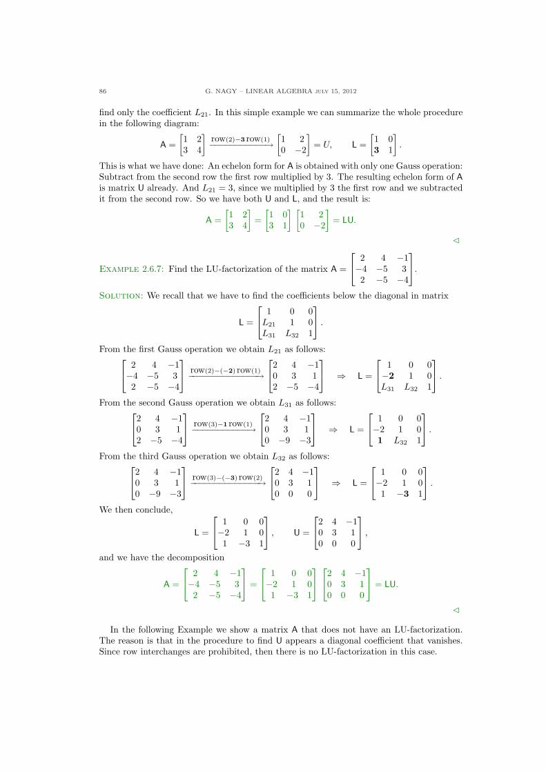
86 G. NAGY – LINEAR ALGEBRA july 15, 2012
find only the coefficient L21. In this simple example we can summarize the whole procedurein the following diagram:
A =[1 23 4
]row(2)−3 row(1)−−−−−−−−−−−→
[1 20 −2
]= U, L =
[1 03 1
].
This is what we have done: An echelon form for A is obtained with only one Gauss operation:Subtract from the second row the first row multiplied by 3. The resulting echelon form of Ais matrix U already. And L21 = 3, since we multiplied by 3 the first row and we subtractedit from the second row. So we have both U and L, and the result is:
A =[1 23 4
]=
[1 03 1
] [1 20 −2
]= LU.
C
Example 2.6.7: Find the LU-factorization of the matrix A =
2 4 −1−4 −5 32 −5 −4
.
Solution: We recall that we have to find the coefficients below the diagonal in matrix
L =
1 0 0L21 1 0L31 L32 1
.
From the first Gauss operation we obtain L21 as follows:
2 4 −1−4 −5 32 −5 −4
row(2)−(−2) row(1)−−−−−−−−−−−−−−→
2 4 −10 3 12 −5 −4
⇒ L =
1 0 0−2 1 0L31 L32 1
.
From the second Gauss operation we obtain L31 as follows:
2 4 −10 3 12 −5 −4
row(3)−1 row(1)−−−−−−−−−−−→
2 4 −10 3 10 −9 −3
⇒ L =
1 0 0−2 1 01 L32 1
.
From the third Gauss operation we obtain L32 as follows:
2 4 −10 3 10 −9 −3
row(3)−(−3) row(2)−−−−−−−−−−−−−−→
2 4 −10 3 10 0 0
⇒ L =
1 0 0−2 1 01 −3 1
.
We then conclude,
L =
1 0 0−2 1 01 −3 1
, U =
2 4 −10 3 10 0 0
,
and we have the decomposition
A =
2 4 −1−4 −5 32 −5 −4
=
1 0 0−2 1 01 −3 1
2 4 −10 3 10 0 0
= LU.
C
In the following Example we show a matrix A that does not have an LU-factorization.The reason is that in the procedure to find U appears a diagonal coefficient that vanishes.Since row interchanges are prohibited, then there is no LU-factorization in this case.
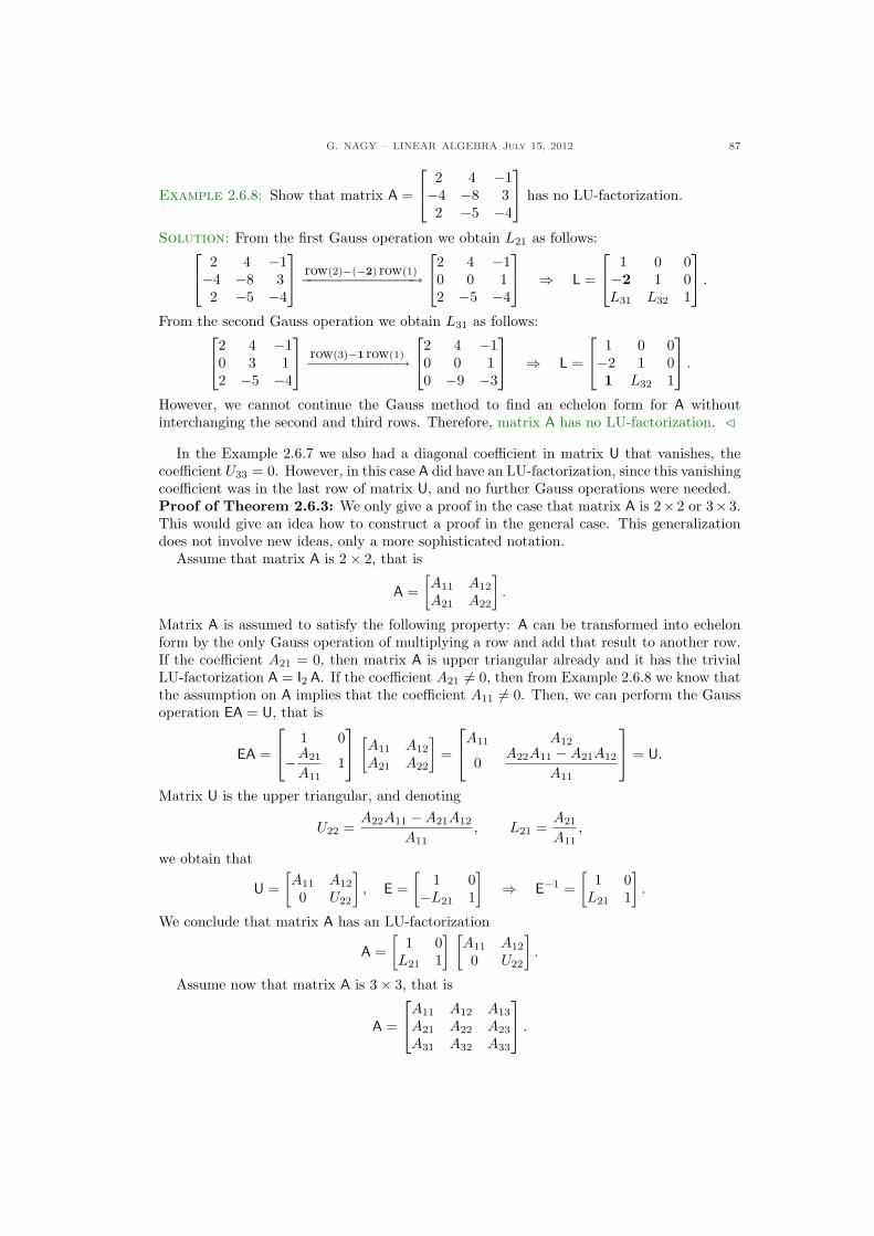
G. NAGY – LINEAR ALGEBRA July 15, 2012 87
Example 2.6.8: Show that matrix A =
2 4 −1−4 −8 32 −5 −4
has no LU-factorization.
Solution: From the first Gauss operation we obtain L21 as follows:
2 4 −1−4 −8 32 −5 −4
row(2)−(−2) row(1)−−−−−−−−−−−−−−→
2 4 −10 0 12 −5 −4
⇒ L =
1 0 0−2 1 0L31 L32 1
.
From the second Gauss operation we obtain L31 as follows:
2 4 −10 3 12 −5 −4
row(3)−1 row(1)−−−−−−−−−−−→
2 4 −10 0 10 −9 −3
⇒ L =
1 0 0−2 1 01 L32 1
.
However, we cannot continue the Gauss method to find an echelon form for A withoutinterchanging the second and third rows. Therefore, matrix A has no LU-factorization. C
In the Example 2.6.7 we also had a diagonal coefficient in matrix U that vanishes, thecoefficient U33 = 0. However, in this case A did have an LU-factorization, since this vanishingcoefficient was in the last row of matrix U, and no further Gauss operations were needed.Proof of Theorem 2.6.3: We only give a proof in the case that matrix A is 2× 2 or 3× 3.This would give an idea how to construct a proof in the general case. This generalizationdoes not involve new ideas, only a more sophisticated notation.
Assume that matrix A is 2× 2, that is
A =[A11 A12
A21 A22
].
Matrix A is assumed to satisfy the following property: A can be transformed into echelonform by the only Gauss operation of multiplying a row and add that result to another row.If the coefficient A21 = 0, then matrix A is upper triangular already and it has the trivialLU-factorization A = I2 A. If the coefficient A21 6= 0, then from Example 2.6.8 we know thatthe assumption on A implies that the coefficient A11 6= 0. Then, we can perform the Gaussoperation EA = U, that is
EA =
1 0
−A21
A111
[A11 A12
A21 A22
]=
A11 A12
0A22A11 −A21A12
A11
= U.
Matrix U is the upper triangular, and denoting
U22 =A22A11 −A21A12
A11, L21 =
A21
A11,
we obtain that
U =[A11 A12
0 U22
], E =
[1 0−L21 1
]⇒ E−1 =
[1 0
L21 1
].
We conclude that matrix A has an LU-factorization
A =[
1 0L21 1
] [A11 A12
0 U22
].
Assume now that matrix A is 3× 3, that is
A =
A11 A12 A13
A21 A22 A23
A31 A32 A33
.
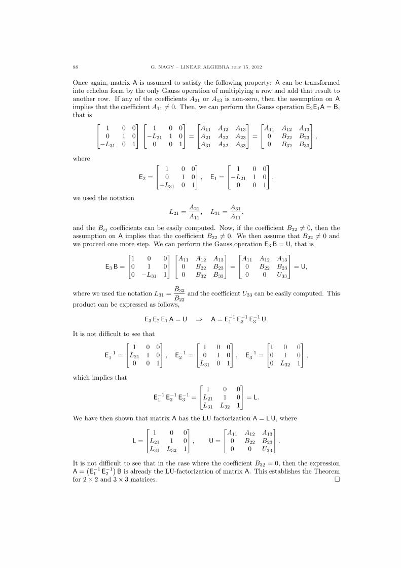
88 G. NAGY – LINEAR ALGEBRA july 15, 2012
Once again, matrix A is assumed to satisfy the following property: A can be transformedinto echelon form by the only Gauss operation of multiplying a row and add that result toanother row. If any of the coefficients A21 or A13 is non-zero, then the assumption on Aimplies that the coefficient A11 6= 0. Then, we can perform the Gauss operation E2E1A = B,that is
1 0 00 1 0−L31 0 1
1 0 0−L21 1 0
0 0 1
=
A11 A12 A13
A21 A22 A23
A31 A32 A33
=
A11 A12 A13
0 B22 B23
0 B32 B33
,
where
E2 =
1 0 00 1 0−L31 0 1
, E1 =
1 0 0−L21 1 0
0 0 1
,
we used the notation
L21 =A21
A11, L31 =
A31
A11,
and the Bij coefficients can be easily computed. Now, if the coefficient B32 6= 0, then theassumption on A implies that the coefficient B22 6= 0. We then assume that B22 6= 0 andwe proceed one more step. We can perform the Gauss operation E3 B = U, that is
E3 B =
1 0 00 1 00 −L31 1
A11 A12 A13
0 B22 B23
0 B32 B33
=
A11 A12 A13
0 B22 B23
0 0 U33
= U,
where we used the notation L31 =B32
B22and the coefficient U33 can be easily computed. This
product can be expressed as follows,
E3 E2 E1 A = U ⇒ A = E−11 E−1
2 E−13 U.
It is not difficult to see that
E−11 =
1 0 0L21 1 00 0 1
, E−1
2 =
1 0 00 1 0
L31 0 1
, E−1
3 =
1 0 00 1 00 L32 1
,
which implies that
E−11 E−1
2 E−13 =
1 0 0L21 1 0L31 L32 1
= L.
We have then shown that matrix A has the LU-factorization A = LU, where
L =
1 0 0L21 1 0L31 L32 1
, U =
A11 A12 A13
0 B22 B23
0 0 U33
.
It is not difficult to see that in the case where the coefficient B32 = 0, then the expressionA =
(E−1
1 E−12
)B is already the LU-factorization of matrix A. This establishes the Theorem
for 2× 2 and 3× 3 matrices. ¤
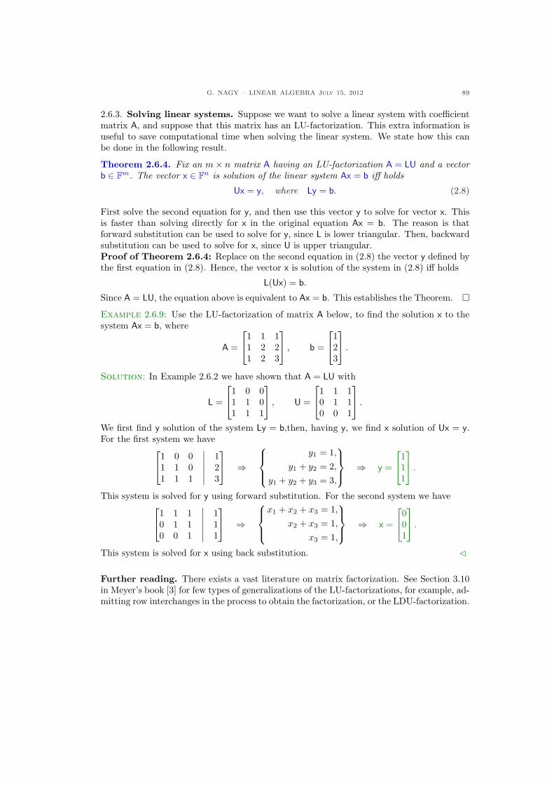
G. NAGY – LINEAR ALGEBRA July 15, 2012 89
2.6.3. Solving linear systems. Suppose we want to solve a linear system with coefficientmatrix A, and suppose that this matrix has an LU-factorization. This extra information isuseful to save computational time when solving the linear system. We state how this canbe done in the following result.
Theorem 2.6.4. Fix an m× n matrix A having an LU-factorization A = LU and a vectorb ∈ Fm. The vector x ∈ Fn is solution of the linear system Ax = b iff holds
Ux = y, where Ly = b. (2.8)
First solve the second equation for y, and then use this vector y to solve for vector x. Thisis faster than solving directly for x in the original equation Ax = b. The reason is thatforward substitution can be used to solve for y, since L is lower triangular. Then, backwardsubstitution can be used to solve for x, since U is upper triangular.Proof of Theorem 2.6.4: Replace on the second equation in (2.8) the vector y defined bythe first equation in (2.8). Hence, the vector x is solution of the system in (2.8) iff holds
L(Ux) = b.
Since A = LU, the equation above is equivalent to Ax = b. This establishes the Theorem. ¤Example 2.6.9: Use the LU-factorization of matrix A below, to find the solution x to thesystem Ax = b, where
A =
1 1 11 2 21 2 3
, b =
123
.
Solution: In Example 2.6.2 we have shown that A = LU with
L =
1 0 01 1 01 1 1
, U =
1 1 10 1 10 0 1
.
We first find y solution of the system Ly = b,then, having y, we find x solution of Ux = y.For the first system we have
1 0 0∣∣ 1
1 1 0∣∣ 2
1 1 1∣∣ 3
⇒
y1 = 1,
y1 + y2 = 2,
y1 + y2 + y3 = 3,
⇒ y =
111
.
This system is solved for y using forward substitution. For the second system we have
1 1 1∣∣ 1
0 1 1∣∣ 1
0 0 1∣∣ 1
⇒
x1 + x2 + x3 = 1,
x2 + x3 = 1,
x3 = 1,
⇒ x =
001
.
This system is solved for x using back substitution. C
Further reading. There exists a vast literature on matrix factorization. See Section 3.10in Meyer’s book [3] for few types of generalizations of the LU-factorizations, for example, ad-mitting row interchanges in the process to obtain the factorization, or the LDU-factorization.
90 G. NAGY – LINEAR ALGEBRA july 15, 2012
2.6.4. Exercises.
2.6.1.- Find the LU-factorization of matrix
A =
»5 2
−15 −3
–.
2.6.2.- Find the LU-factorization of matrix
A =
»2 1 34 6 7
–.
2.6.3.- Find the LU-factorization of matrix
A =
24
2 1 24 5 56 −3 5
35 .
2.6.4.- Determine if the matrix below hasan LU-factorization,
A =
2664
1 2 4 173 6 −12 32 3 −3 20 2 −2 6
3775 .
2.6.5.- Find the LU-factorization of a tridi-agonal matrix
T =
2664
2 −1 0 0−1 2 −1 00 −1 2 −10 0 −1 1
3775 .
2.6.6.- Use the LU-factorization to find thesolutions to the system Ax = b, where
A =
24
2 2 24 7 76 18 22
35 , b =
24
122412
35 .
2.6.7.- Find the values of the number csuch that matrix A below has no LU-factorization,
A =
24
c 2 01 c 10 1 c
35 .
G. NAGY – LINEAR ALGEBRA July 15, 2012 91
Chapter 3. Determinants
3.1. Definitions and properties
A determinant is a scalar associated to a square matrix which can be used to determinewhether the matrix is invertible or not, and this property is the origin of its name. Thedeterminant has a clear geometrical meaning in the case of 2× 2 and 3× 3 matrices. In theformer case the absolute value of the determinant is the area of a parallelogram formed withthe matrix column vectors; in the latter case the absolute value of the determinant is thevolume of the parallelepiped formed with the matrix column vectors. The determinant forn×n matrices is introduced as a suitable generalization of these properties. In this Sectionwe present the determinant for 2×2 and 3×3 matrices and we study their main properties.We then present the definition of determinant for n × n matrices and we mention withoutproof its main properties.
3.1.1. Determinant of 2×2 matrices. We start introducing the determinant as a scalar-valued function on 2× 2 matrices.
Definition 3.1.1. The determinant of a 2× 2 matrix A =[A11 A12
A21 A22
]is the value of the
function det : F2,2 → F given by det(A) = A11A22 −A12A21.
Depending on the context we will use for the determinant any of the following notations,
det(A) = |A| = ∆ =∣∣∣∣A11 A12
A21 A22
∣∣∣∣ .
For example,∣∣∣∣A11 A12
A21 A22
∣∣∣∣ = A11A22 −A12A21.
Example 3.1.1: The value of the determinant can be any real number, as the followingthree cases show:∣∣∣∣
1 23 4
∣∣∣∣ = 4− 6 = −2,
∣∣∣∣2 13 4
∣∣∣∣ = 8− 3 = 5,
∣∣∣∣1 22 4
∣∣∣∣ = 4− 4 = 0.
C
We have seen in Theorem 2.4.2 in Section 2.4 that a 2 × 2 matrix is invertible iff itsdeterminant is non-zero. We now see that there is an interesting geometrical interpretationof this property.
Theorem 3.1.2. Given a matrix A = [A1,A2] ∈ R2,2, the absolute value of its determinant,| det(A)|, is the area of the parallelogram formed by the vectors A1, A2.
Proof of Theorem 3.1.2: Denote the matrix A as follows
A =[a bc d
]⇒ A1 =
[ac
], A2 =
[bd
].
The case where all the coefficients in matrix A are positive is shown in Fig. 27. We can seein this Figure that the area of the parallelogram formed by the vectors A1 and A2 is relatedto the area of the rectangle with sides b and c. More precisely, the area of the parallelogramis equal to the area of the rectangle minus the area of the two triangles marked with a “−”sign in Fig. 27 plus the area of the triangle marked with “+” sign. Denoting the area of theparallelogram by Ap, we obtain the following equation,
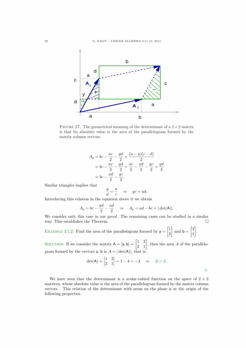
92 G. NAGY – LINEAR ALGEBRA july 15, 2012
A
−
−
+
a
c
y
2
d
b
1A
a
a b
d
c
Figure 27. The geometrical meaning of the determinant of a 2×2 matrixis that its absolute value is the area of the parallelogram formed by thematrix column vectors.
Ap = bc− ac
2− yd
2+
(a− y)(c− d)2
= bc− ac
2− yd
2+
ac
2− ad
2− yc
2+
yd
2
= bc− ad
2− yc
2.
Similar triangles implies thaty
d=
a
c⇒ yc = ad.
Introducing this relation in the equation above it we obtain
Ap = bc− ad
2− ad
2⇒ Ap = ad− bc = | det(A)|.
We consider only this case in our proof. The remaining cases can be studied in a similarway. This establishes the Theorem. ¤
Example 3.1.2: Find the area of the parallelogram formed by a =[12
]and b =
[21
].
Solution: If we consider the matrix A = [a, b] =[1 22 1
], then the area A of the parallelo-
gram formed by the vectors a, b is A = | det(A)|, that is,
det(A) =∣∣∣∣1 22 1
∣∣∣∣ = 1− 4 = −3 ⇒ A = 3.
C
We have seen that the determinant is a scalar-valued function on the space of 2 × 2matrices, whose absolute value is the area of the parallelogram formed by the matrix columnvectors . This relation of the determinant with areas on the plane is at the origin of thefollowing properties.
G. NAGY – LINEAR ALGEBRA July 15, 2012 93
Theorem 3.1.3. For every vectors a1, a2, b ∈ F2 and scalar k ∈ F, the determinantfunction det : F2,2 → F satisfies:
(a) det([a1, a2]
)= −det
([a2, a1]
);
(b) det([k a1, a2]
)= det
([a1, k a2]
)= k det
([a1, a2]
);
(c) det([a1, k a1]
)= 0;
(d) det([(a1 + b), a2]
)= det
([a1, a2]
)+ det
([b, a2]
).
Proof of Theorem 3.1.3: Introduce the notation
a1 =[ac
], a2 =
[bd
], ⇒ [
a1, a2
]=
[a bc d
].
Part (a):
det([a1, a2]
)=
∣∣∣∣a bc d
∣∣∣∣ = ad− bc
det([a2, a1]
)=
∣∣∣∣b ad c
∣∣∣∣ = bc− ad,
⇒ det([a1, a2]
)= −det
([a2, a1]
).
Part (b):
det([k a1, a2]
)=
∣∣∣∣ka bkc d
∣∣∣∣ = k(ad− bc) = k
∣∣∣∣a bc d
∣∣∣∣ = k det([a1, a2]
),
det([a1, k a2]
)=
∣∣∣∣a kbc kd
∣∣∣∣ = k(ad− bc) = k
∣∣∣∣a bc d
∣∣∣∣ = k det([a1, a2]
).
Part (c):
det([a1, k a1]
)= det
([k a1, a1]
)= − det
([a1, k a1]
) ⇒ det([a1, k a1]
)= 0.
Part (d): Introduce the notation b =[b1
b2
]. Then,
det([(a1 + b), a2]
)=
∣∣∣∣(a + b1) b(c + b2) d
∣∣∣∣= (a + b1)d− (c + b2)b
= (ad− cb) + (b1d− b2b)
=∣∣∣∣a bc d
∣∣∣∣ +∣∣∣∣b1 bb2 d
∣∣∣∣= det
([a1, a2]
)+ det
([b, a2]
).
This establishes the Theorem. ¤Moreover, the determinant function also satisfies the following further properties.
Theorem 3.1.4. Let A, B ∈ F2,2. Then it holds:
(a) Matrix A is invertible iff det(A) 6= 0;(b) det(A) = det(AT );(c) det(AB) = det(A) det(B).
(d) If matrix A is invertible, then det(A−1) =1
det(A).
Proof of Theorem 3.1.4:Part (a): It has been proven in Theorem 2.4.2.
94 G. NAGY – LINEAR ALGEBRA july 15, 2012
Part (b): Denote A =[a bc d
]. Then holds
det(A) =∣∣∣∣a bc d
∣∣∣∣ = ad− bc =∣∣∣∣a cb d
∣∣∣∣ = det(AT
).
Part (c): Denoting A =[A11 A12
A21 A22
]and B =
[B11 B12
B21 B22
]we obtain,
AB =[(A11B11 + A12B21) (A11B12 + A12B22)(A21B11 + A22B21) (A21B12 + A22B22)
].
Therefore,
det(AB) = (A11B11 + A12B21)(A21B12 + A22B22)− (A11B12 + A12B22)(A21B11 + A22B21)= A11B11A21B12 + A11B11A22B22 + A12B21A21B12 + A12B21A22B22
−A21B11A11B12 −A21B11A12B22 −A22B21A11B12 −A22B21A12B22
= A11B11A22B22 + A12B21A21B12 −A21B11A12B22 −A22B21A11B12
= (A11A22 −A21A12)B11B22 − (A11A22 −A12A21)B12B21
= (A11A22 −A21A12) (B11B22 −B12B21)
= det(A) det(B).
Part (d): Since A(A−1) = I2, we obtain
1 = det(I2) = det(A(A−1)
)= det(A) det
(A−1
) ⇒ det(A−1
)=
1det(A)
.
This establishes the Theorem. ¤We finally mention that det(A) = det(AT ) implies that Theorem 3.1.3 can be generalized
from properties involving columns of the matrix into properties involving rows of the matrix.Introduce the following notation that generalizes column vectors to include row vectors:
A =[A11 A12
A21 A22
]=
[a:1, a:2
]=
[a1:
a2:
],
where
a:1 =[A11
A21
], a:2 =
[A12
A22
], a1: =
[A11 A12
], a2: =
[A21 A22
].
The first two vectors above are the usual column vectors of matrix A, and the last two are itsrow vectors. When working with both, column vectors and row vectors, we use the notationabove; when working only with column vectors, we drop the colon and we denote them, forexample, as A:1 = A1. Using this notation, it is simple to verify the following result.
Theorem 3.1.5. For all column vectors aT1:, aT
2:, bT1: ∈ F2 and scalars k ∈ F, the determinant
function det : F2,2 → F satisfies:
(a) det([
a1:
a2:
])= −det
([a2:
a1:
]);
(b) det([
k a1:
a2:
])= det
([a1:
k a2:
])= k det
([a1:
a2:
]);
(c) det([
a1:
k a1:
])= 0;
(d) det([
(a1: + b1:)a2:
])= det
([a1:
a2:
])+ det
([b1:
a2:
]).
The proof is left as an exercise.
G. NAGY – LINEAR ALGEBRA July 15, 2012 95
3.1.2. Determinant of 3 × 3 matrices. The determinant for 3 × 3 matrices is definedrecursively in terms of 2× 2 determinants.
Definition 3.1.6. The determinant on 3× 3 matrices is the function det : F3,3 → F,
det(A) =
∣∣∣∣∣∣
A11 A12 A13
A21 A22 A23
A31 A32 A33
∣∣∣∣∣∣= A11
∣∣∣∣A22 A23
A32 A33
∣∣∣∣−A12
∣∣∣∣A21 A23
A31 A33
∣∣∣∣ + A13
∣∣∣∣A21 A22
A31 A32
∣∣∣∣ .
We see that the determinant of a 3 × 3 matrix is computed as a linear combination of thedeterminants of 2× 2 matrices,
det(A) = A11 det(A11
)−A12 det(A12
)+ A13 det
(A13
),
where we introduced the 2× 2 matrices
A11 =[A22 A23
A32 A33
], A12 =
[A21 A23
A31 A33
], A13 =
[A21 A21
A31 A31
];
These matrices are three of the nine matrices called the minors of matrix A.
Definition 3.1.7. The 2×2 matrix Aij is called the (i, j)-minor of a 3×3 matrix A iff Aij
is obtained from A by removing the row i and the column j. The (i, j)-cofactor of matrixA is the number Cij = (−1)(i+j) det
(Aij
).
These definitions are common in the literature, and they allow to write down a compactexpression for the determinant of a 3× 3 matrix. Indeed, the expression in Definition 3.1.6now has the form
det(A) = A11C11 + A12C12 + A13C13.
Of course, all the complexity in the definition of determinant is now hidden in the definitionof the cofactors. The latter expression is not simpler than the one in Definition 3.1.6, itonly looks simpler.
Example 3.1.3: Find the determinant of the matrix A =
1 3 −12 1 13 2 1
.
Solution: We use the definition above, that is,∣∣∣∣∣∣
1 3 −12 1 13 2 1
∣∣∣∣∣∣= 1
∣∣∣∣1 12 1
∣∣∣∣− 3∣∣∣∣2 13 1
∣∣∣∣ + (−1)∣∣∣∣2 13 2
∣∣∣∣
= (1− 2)− 3(2− 3)− (4− 3)= 1 + 3− 1= 1.
We conclude that det(A) = 1. C
As in the 2× 2 case, the determinant of a real-valued 3× 3 matrix can be any real num-ber, positive, negative of zero. The absolute value of the determinant has the geometricalmeaning, see Fig. 28.
Theorem 3.1.8. The number | det(A)|, the absolute value of the determinant of matrixA = [A:1, A:2, A:3], is the volume of the parallelepiped formed by the vectors A:1, A:2, A:3.
We do not give a prove of this statement. See the references at the end of the Section.
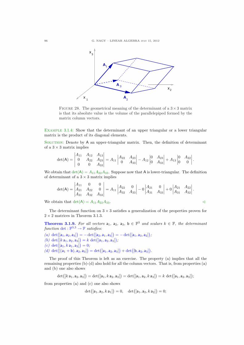
96 G. NAGY – LINEAR ALGEBRA july 15, 2012
2
A
2
1
1
x
3x
x
3
A
A
Figure 28. The geometrical meaning of the determinant of a 3×3 matrixis that its absolute value is the volume of the parallelepiped formed by thematrix column vectors.
Example 3.1.4: Show that the determinant of an upper triangular or a lower triangularmatrix is the product of its diagonal elements.
Solution: Denote by A an upper-triangular matrix. Then, the definition of determinantof a 3× 3 matrix implies
det(A) =
∣∣∣∣∣∣
A11 A12 A13
0 A22 A23
0 0 A33
∣∣∣∣∣∣= A11
∣∣∣∣A22 A23
0 A33
∣∣∣∣−A12
∣∣∣∣0 A23
0 A33
∣∣∣∣ + A13
∣∣∣∣0 A22
0 0
∣∣∣∣ .
We obtain that det(A) = A11A22A33. Suppose now that A is lower-triangular. The definitionof determinant of a 3× 3 matrix implies
det(A) =
∣∣∣∣∣∣
A11 0 0A21 A22 0A31 A32 A33
∣∣∣∣∣∣= A11
∣∣∣∣A22 0A32 A33
∣∣∣∣− 0∣∣∣∣A21 0A31 A33
∣∣∣∣ + 0∣∣∣∣A21 A22
A31 A32
∣∣∣∣ .
We obtain that det(A) = A11A22A33. C
The determinant function on 3× 3 satisfies a generalization of the properties proven for2× 2 matrices in Theorem 3.1.3.
Theorem 3.1.9. For all vectors a1, a2, a3, b ∈ F3 and scalars k ∈ F, the determinantfunction det : F3,3 → F satisfies:
(a) det([a1, a2, a3]
)= − det
([a2, a1, a3]
)= −det
([a1, a3, a2]
);
(b) det([k a1, a2, a3]
)= k det
([a1, a2, a3]
);
(c) det([a1, k a1, a3]
)= 0;
(d) det([(a1 + b), a2, a3]
)= det
([a1, a2, a3]
)+ det
([b, a2, a3]
).
The proof of this Theorem is left as an exercise. The property (a) implies that all theremaining properties (b)-(d) also hold for all the column vectors. That is, from properties (a)and (b) one also shows
det([k a1, a2, a3]
)= det
([a1, k a2, a3]
)= det
([a1, a2, k a3]
)= k det
([a1, a2, a3]
);
from properties (a) and (c) one also shows
det([a1, a2, k a1]
)= 0, det
([a1, a2, k a2]
)= 0;
G. NAGY – LINEAR ALGEBRA July 15, 2012 97
and from properties (a) and (d) one also shows
det([a1, (a2 + b), a3]
)= det
([a1, a2, a3]
)+ det
([a1, b, a3]
),
det([a1, a2, (a3 + b)]
)= det
([a1, a2, a3]
)+ det
([a1, a2, b]
).
The following result is a generalization of Theorem 3.1.4.
Theorem 3.1.10. Let A, B ∈ F3,3. Then it holds:(a) Matrix A is invertible iff det(A) 6= 0;(b) det(A) = det(AT );(c) det(AB) = det(A) det(B).
(d) If matrix A is invertible, then det(A−1) =1
det(A).
The proof of this Theorem is left as an exercise. Like in the case of matrices 2 × 2,Theorem 3.1.9 can be generalized from properties involving column vector to propertiesinvolving row vectors.
Theorem 3.1.11. For all vectors aT1:, aT
2:, aT3:, bT
1: ∈ F3 and scalars k ∈ F, the determinantfunction det : F3,3 → F satisfies:
(a) det(
a1:
a2:
a3:
)= − det
(
a2:
a1:
a3:
); = − det
(
a3:
a2:
a1:
); = −det
(
a1:
a3:
a2:
);
(b) det(
k a1:
a2:
a3:
)= k det
(
a1:
a2:
a3:
);
(c) det(
a1:
k a1:
a3:
)= 0;
(d) det(
(a1: + b1:)a2:
a3:
)= det
(
a1:
a2:
a3:
)+ det
(
b1:
a2:
a3:
).
The proof is left as an exercise. The property (a) implies that all the remaining properties(b)-(d) also hold for all the row vectors. That is, from properties (a) and (b) one also shows
det(
k a1:
a2:
a3:
)= det
(
a1:
k a2:
a3:
)= det
(
a1:
a2:
k a3:
)= k det
(
a1:
a2:
a3:
);
from properties (a) and (c) one also shows
det(
a1:
a2:
k a1:
)= 0; det
(
a1:
k a2:
a2:
)= 0;
from properties (a) and (d) one also shows
det(
a1:
(a2: + b2:)a3:
)= det
(
a1:
a2:
a3:
)+ det
(
a1:
b2:
a3:
),
det(
a1:
a2:
(a3: + b3:)
)= det
(
a1:
a2:
a3:
)+ det
(
a1:
a2:
b3:
).
98 G. NAGY – LINEAR ALGEBRA july 15, 2012
3.1.3. Determinant of n × n matrices. The notion of determinant can be generalizedto n × n matrices with n > 1. One way to find an appropriate generalization is to realizethat the determinant of 2 × 2 and 3 × 3 matrices are related to the notion of areas andvolumes, respectively. One then studies the properties of areas an volumes, like the onesgiven in Theorem 3.1.3 and 3.1.9. It can be shown that generalizations of these propertiesdetermine a unique function det : Fn,n → F. In this notes we only present the final result,the definition of determinant for n× n matrices. The reader is referred to the literature fora constructive proof of the function determinant.
Definition 3.1.12. The determinant of a matrix A = [Aij ] ∈ Fn,n, with n > 1 andi, j = 1, · · · , n, is the value of the function det : Fn,n → F is given by
det(A) = A11 C11 + · · ·+ A1n C1n, (3.1)
where the number Cij, called (i, j)-cofactor of matrix A, is the scalar given by
Cij = (−1)(i+j) det(Aij
),
and where the matrices Aij ∈ F(n−1),(n−1), called the (i, j)-minors of A, are obtained frommatrix A by eliminating the row i and the column j, which are highlighted below
Aij =
A11 · · · A1j · · · A1n
......
...Ai1 · · · Aij · · · Ain
......
...An1 · · · Anj · · · Ann
.
Example 3.1.5: Use Eq. (3.1) to compute the determinant of a 2× 2 matrix.
Solution: Consider the matrix A =[A11 A12
A21 A22
]. The four minor matrices are given by
A11 = A22, A12 = A21, A21 = A12, A22 = A11.
This means, generalizing the notion of determinant to numbers by det(a) = a, that thecofactors are
C11 = A22, C12 = −A21, C21 = −A12, C22 = A11.
So, we obtain that
det(A) = A11C11 + A12C12 ⇔ det(A) = A11A22 −A12A21.
Notice that we do not need to compute all four cofactors to compute the determinant of thematrix; just two of them are enough. C
Example 3.1.6: Use Eq. (3.1) to compute the determinant of a 3× 3 matrix.
Solution: Consider the matrix
A =
A11 A12 A13
A21 A22 A23
A31 A32 A33
.
G. NAGY – LINEAR ALGEBRA July 15, 2012 99
The nine minor matrices are given by
A11 =[A22 A23
A32 A33
]A12 =
[A21 A23
A31 A33
]A13 =
[A21 A22
A31 A32
]
A21 =[A12 A13
A32 A33
]A22 =
[A11 A13
A31 A33
]A23 =
[A11 A12
A31 A32
]
A31 =[A12 A13
A22 A23
]A32 =
[A11 A13
A21 A23
]A23 =
[A11 A12
A21 A22
].
Then, Def. 3.1.12 agrees with Def. 3.1.6, since
det(A) = A11C11 + A12C12 + A13C13
is equivalent to
det(A) = A11
∣∣∣∣A22 A23
A32 A33
∣∣∣∣−A12
∣∣∣∣A21 A23
A31 A33
∣∣∣∣ + A13
∣∣∣∣A21 A22
A31 A32
∣∣∣∣ .
C
We now state several results that summarize the main properties of the determinant ofn×n matrices. We state the results without proof. The frost result says that the determinantof a matrix can be computed using expansions along any row or any column in the matrix.
Theorem 3.1.13. The determinant of an n×n matrix A = [Aij ] can be computed expandingalong any row or any column of matrix A, that is,
det(A) = Ai1Ci1 + · · ·+ AinCin, i = 1, · · · , n,
= A1jC1j + · · ·+ AnjCnj , j = 1, · · · , n.
Example 3.1.7: Show all possible expansions of the determinant of a 3×3 matrix A = [Aij ].
Solution: The expansions along each of the three rows are the following:
det(A) = A11C11 + A12C12 + A13C13
= A21C21 + A22C22 + A23C23
= A31C31 + A32C32 + A33C33;
The expansions along each of the three columns are the following:
det(A) = A11C11 + A21C21 + A31C31
= A12C12 + A22C22 + A32C32
= A13C13 + A23C23 + A33C33.
C
Example 3.1.8: Compute the determinant of A =
1 3 −12 1 13 2 1
with an expansion by the
third column.
100 G. NAGY – LINEAR ALGEBRA july 15, 2012
Solution: The expansion by the third column is the following,∣∣∣∣∣∣
1 3 −12 1 13 2 1
∣∣∣∣∣∣= (−1)
∣∣∣∣2 13 2
∣∣∣∣− (1)∣∣∣∣1 33 2
∣∣∣∣ + (1)∣∣∣∣1 32 1
∣∣∣∣
= −(4− 3)− (2− 9) + (1− 6)= −1 + 7− 5= 1,
That is, det(A) = 1. This result agrees with Example 3.1.3. C
The generalization of Theorem 3.1.9 to n× n matrices is the following.
Theorem 3.1.14. For all vectors ai, aj,b ∈ Fn, with i, j = 1, · · · , n, and for all scalarsk ∈ F, the determinant function det : Fn,n → F satisfies:(a) det
([a1, · · · , ai, · · · , aj , · · · , an]
)= −det
([a1, · · · , aj , · · · , ai, · · · , an]
);
(b) det([a1, · · · , k ai, · · · , an]
)= k det
([a1, · · · , ai, · · · , an]
);
(c) det([a1, · · · , k ai, · · · , ai, · · · , an]
)= 0;
(d) det([a1, · · · , (ai + b), · · · , an]
)= det
([a1, · · · , ai, · · · , an]
)+ det
([b, · · · , b, · · · , an]
).
The generalization of Theorem 3.1.10 to n× n matrices is the following.
Theorem 3.1.15. Let A, B ∈ Fn,n. Then it holds:(a) Matrix A is invertible iff det(A) 6= 0;(b) det(A) = det(AT );(c) det
(A
)= det(A);
(d) det(AB) = det(A) det(B).
(e) If matrix A is invertible, then det(A−1) =1
det(A).
The proof of this Proposition is left as an exercise. Like in the case of matrices 2 × 2,Theorem 3.1.9 can be generalized from properties involving column vector to propertiesinvolving row vectors.
Theorem 3.1.16. For all vectors aTi:, aT
j:, bTi: ∈ Fn and scalars k ∈ F, the determinant
function det : Fn,n → F satisfies:∣∣∣∣∣∣∣∣∣∣∣∣∣∣∣∣∣
a1:
...ai:
...aj:
...an:
∣∣∣∣∣∣∣∣∣∣∣∣∣∣∣∣∣
= −
∣∣∣∣∣∣∣∣∣∣∣∣∣∣∣∣∣
a1:
...aj:
...ai:
...an:
∣∣∣∣∣∣∣∣∣∣∣∣∣∣∣∣∣
;
∣∣∣∣∣∣∣∣∣∣∣∣
a1:
...k ai:
...an:
∣∣∣∣∣∣∣∣∣∣∣∣
= k
∣∣∣∣∣∣∣∣∣∣∣∣
a1:
...ai:
...an:
∣∣∣∣∣∣∣∣∣∣∣∣
;
∣∣∣∣∣∣∣∣∣∣∣∣∣∣∣∣∣
a1:
...k ai:
...ai:
...an:
∣∣∣∣∣∣∣∣∣∣∣∣∣∣∣∣∣
= 0;
∣∣∣∣∣∣∣∣∣∣∣∣
a1:
...(ai: + bi:)
...an:
∣∣∣∣∣∣∣∣∣∣∣∣
=
∣∣∣∣∣∣∣∣∣∣∣∣
a1:
...ai:
...an:
∣∣∣∣∣∣∣∣∣∣∣∣
+
∣∣∣∣∣∣∣∣∣∣∣∣
a1:
...bi:
...an:
∣∣∣∣∣∣∣∣∣∣∣∣
.
G. NAGY – LINEAR ALGEBRA July 15, 2012 101
3.1.4. Exercises.
3.1.1.- Find the determinant of matrices
A =
24
2 1 16 2 1−2 2 1
35 , B =
24
2 1 16 0 1−2 0 1
35 .
3.1.2.- Find the volume of the parallelepi-ped formed by the vectors
x1 =
24
30−4
35 , x2 =
24
020
35 , x3 =
24
101
35 .
3.1.3.- Find the determinants of the upperand lower triangular matrices
U =
24
1 2 30 4 50 0 6
35 , L =
24
1 0 02 3 04 5 6
35 .
3.1.4.- Find the determinant of the matrix
A =
24
0 0 10 2 34 5 6
35 .
3.1.5.- Give an example to show that ingeneral
det(A + B) 6= det(A) + det(B).
3.1.6.- If A ∈ Fn,n express
det(2A), det(−A), det(A2)
in terms of det(A) and n.
3.1.7.- Given matrices A, P ∈ Fn,n, with Pinvertible, let B = P−1AP. Prove thatdet(B) = det(A).
3.1.8.- Prove that for all matrix A ∈ Fn,n
holds that det(A∗) = det(A).
3.1.9.- Prove that for all A ∈ Fn,n holdsthat det(A∗A) > 0.
3.1.10.- Prove that for all A ∈ Fn,n and allk ∈ F holds that det(k A) = kn det(A).
3.1.11.- Prove that a skew-symmetric ma-trix A ∈ Fn,n, with n odd, must satisfythat det(A) = 0.
3.1.12.- Let A ∈ Fn,n be a matrix satisfyingthat AT A = In. Prove that
det(A) = ±1.
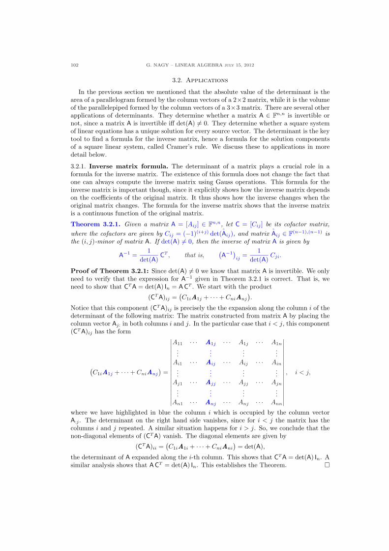
102 G. NAGY – LINEAR ALGEBRA july 15, 2012
3.2. Applications
In the previous section we mentioned that the absolute value of the determinant is thearea of a parallelogram formed by the column vectors of a 2×2 matrix, while it is the volumeof the parallelepiped formed by the column vectors of a 3×3 matrix. There are several otherapplications of determinants. They determine whether a matrix A ∈ Fn,n is invertible ornot, since a matrix A is invertible iff det(A) 6= 0. They determine whether a square systemof linear equations has a unique solution for every source vector. The determinant is the keytool to find a formula for the inverse matrix, hence a formula for the solution componentsof a square linear system, called Cramer’s rule. We discuss these to applications in moredetail below.
3.2.1. Inverse matrix formula. The determinant of a matrix plays a crucial role in aformula for the inverse matrix. The existence of this formula does not change the fact thatone can always compute the inverse matrix using Gauss operations. This formula for theinverse matrix is important though, since it explicitly shows how the inverse matrix dependson the coefficients of the original matrix. It thus shows how the inverse changes when theoriginal matrix changes. The formula for the inverse matrix shows that the inverse matrixis a continuous function of the original matrix.
Theorem 3.2.1. Given a matrix A = [Aij ] ∈ Fn,n, let C = [Cij ] be its cofactor matrix,where the cofactors are given by Cij = (−1)(i+j) det(Aij), and matrix Aij ∈ F(n−1),(n−1) isthe (i, j)-minor of matrix A. If det(A) 6= 0, then the inverse of matrix A is given by
A−1 =1
det(A)CT , that is,
(A−1
)ij
=1
det(A)Cji.
Proof of Theorem 3.2.1: Since det(A) 6= 0 we know that matrix A is invertible. We onlyneed to verify that the expression for A−1 given in Theorem 3.2.1 is correct. That is, weneed to show that CT A = det(A) In = ACT . We start with the product
(CT A)ij =(C1iA1j + · · ·+ CniAnj
).
Notice that this component (CT A)ij is precisely the the expansion along the column i of thedeterminant of the following matrix: The matrix constructed from matrix A by placing thecolumn vector Aj: in both columns i and j. In the particular case that i < j, this component(CT A)ij has the form
(C1iA1j + · · ·+ CniAnj
)=
∣∣∣∣∣∣∣∣∣∣∣∣∣∣∣∣∣
A11 · · · A1j · · · A1j · · · A1n
......
......
Ai1 · · · Aij · · · Aij · · · Ain
......
......
Aj1 · · · Ajj · · · Ajj · · · Ajn
......
......
An1 · · · Anj · · · Anj · · · Ann
∣∣∣∣∣∣∣∣∣∣∣∣∣∣∣∣∣
, i < j,
where we have highlighted in blue the column i which is occupied by the column vectorA:j . The determinant on the right hand side vanishes, since for i < j the matrix has thecolumns i and j repeated. A similar situation happens for i > j. So, we conclude that thenon-diagonal elements of (CT A) vanish. The diagonal elements are given by
(CT A)ii =(C1iA1i + · · ·+ CniAni
)= det(A),
the determinant of A expanded along the i-th column. This shows that CT A = det(A) In. Asimilar analysis shows that ACT = det(A) In. This establishes the Theorem. ¤
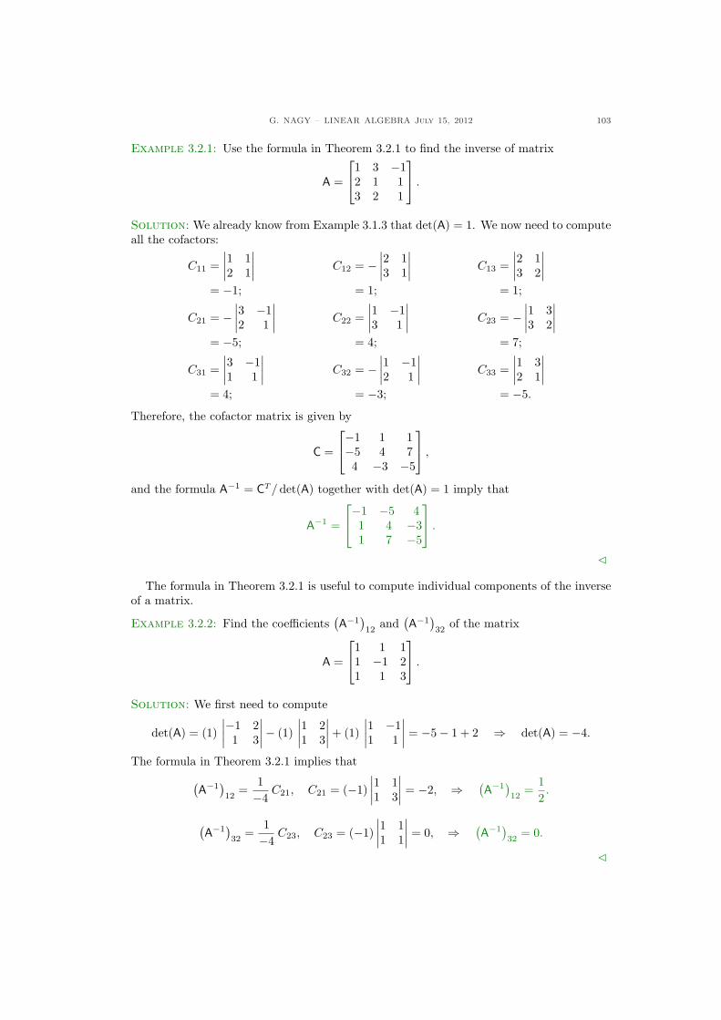
G. NAGY – LINEAR ALGEBRA July 15, 2012 103
Example 3.2.1: Use the formula in Theorem 3.2.1 to find the inverse of matrix
A =
1 3 −12 1 13 2 1
.
Solution: We already know from Example 3.1.3 that det(A) = 1. We now need to computeall the cofactors:
C11 =∣∣∣∣1 12 1
∣∣∣∣= −1;
C12 = −∣∣∣∣2 13 1
∣∣∣∣= 1;
C13 =∣∣∣∣2 13 2
∣∣∣∣= 1;
C21 = −∣∣∣∣3 −12 1
∣∣∣∣= −5;
C22 =∣∣∣∣1 −13 1
∣∣∣∣= 4;
C23 = −∣∣∣∣1 33 2
∣∣∣∣= 7;
C31 =∣∣∣∣3 −11 1
∣∣∣∣= 4;
C32 = −∣∣∣∣1 −12 1
∣∣∣∣= −3;
C33 =∣∣∣∣1 32 1
∣∣∣∣= −5.
Therefore, the cofactor matrix is given by
C =
−1 1 1−5 4 74 −3 −5
,
and the formula A−1 = CT / det(A) together with det(A) = 1 imply that
A−1 =
−1 −5 41 4 −31 7 −5
.
C
The formula in Theorem 3.2.1 is useful to compute individual components of the inverseof a matrix.
Example 3.2.2: Find the coefficients(A−1
)12
and(A−1
)32
of the matrix
A =
1 1 11 −1 21 1 3
.
Solution: We first need to compute
det(A) = (1)∣∣∣∣−1 21 3
∣∣∣∣− (1)∣∣∣∣1 21 3
∣∣∣∣ + (1)∣∣∣∣1 −11 1
∣∣∣∣ = −5− 1 + 2 ⇒ det(A) = −4.
The formula in Theorem 3.2.1 implies that
(A−1
)12
=1−4
C21, C21 = (−1)∣∣∣∣1 11 3
∣∣∣∣ = −2, ⇒ (A−1
)12
=12.
(A−1
)32
=1−4
C23, C23 = (−1)∣∣∣∣1 11 1
∣∣∣∣ = 0, ⇒ (A−1
)32
= 0.
C
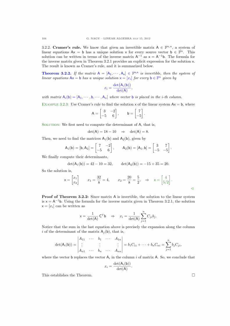
104 G. NAGY – LINEAR ALGEBRA july 15, 2012
3.2.2. Cramer’s rule. We know that given an invertible matrix A ∈ Fn,n, a system oflinear equations Ax = b has a unique solution x for every source vector b ∈ Fn. Thissolution can be written in terms of the inverse matrix A−1 as x = A−1b. The formula forthe inverse matrix given in Theorem 3.2.1 provides an explicit expression for the solution x.The result is known as Cramer’s rule, and it is summarized below.
Theorem 3.2.2. If the matrix A = [A1, · · · ,An] ∈ Fn,n is invertible, then the system oflinear equations Ax = b has a unique solution x = [xi] for every b ∈ Fn given by
xi =det
(Ai(b)
)
det(A),
with matrix Ai(b) = [A1, · · · , b, · · · ,An] where vector b is placed in the i-th column.
Example 3.2.3: Use Cramer’s rule to find the solution x of the linear system Ax = b, where
A =[
3 −2−5 6
], b =
[7−5
].
Solution: We first need to compute the determinant of A, that is,
det(A) = 18− 10 ⇒ det(A) = 8.
Then, we need to find the matrices A1(b) and A2(b), given by
A1(b) = [b, A2] =[
7 −2−5 6
], A2(b) = [A1, b] =
[3 7−5 −5
].
We finally compute their determinants,
det(A1(b)) = 42− 10 = 32, det(A2(b)) = −15 + 35 = 20.
So the solution is,
x =[x1
x2
]x1 =
328
= 4, x2 =208
=52, ⇒ x =
[4
5/2
].
C
Proof of Theorem 3.2.2: Since matrix A is invertible, the solution to the linear systemis x = A−1b. Using the formula for the inverse matrix given in Theorem 3.2.1, the solutionx = [xi] can be written as
x =1
det(A)CT b ⇒ xi =
1det(A)
n∑
j=1
Cjibj .
Notice that the sum in the last equation above is precisely the expansion along the columni of the determinant of the matrix Aj(b), that is,
det(Ai(b)) =
∣∣∣∣∣∣∣
A11 · · · b1 · · · A1n
......
...An1 · · · bn · · · Ann
∣∣∣∣∣∣∣= b1C1i + · · ·+ bnCni =
n∑
j=1
bjCji,
where the vector b replaces the vector Ai in the column i of matrix A. So, we conclude that
xi =det(Ai(b))
det(A).
This establishes the Theorem. ¤
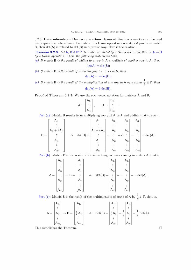
G. NAGY – LINEAR ALGEBRA July 15, 2012 105
3.2.3. Determinants and Gauss operations. Gauss elimination operations can be usedto compute the determinant of a matrix. If a Gauss operation on matrix A produces matrixB, then det(A) is related to det(B) in a precise way. Here is the relation.
Theorem 3.2.3. Let A, B ∈ Fm,n be matrices related by a Gauss operation, that is, A→ Bby a Gauss operation. Then, the following statements hold:(a) If matrix B is the result of adding to a row in A a multiple of another row in A, then
det(A) = det(B);
(b) If matrix B is the result of interchanging two rows in A, then
det(A) = −det(B);
(c) If matrix B is the result of the multiplication of one row in A by a scalar1k∈ F, then
det(A) = k det(B).
Proof of Theorem 3.2.3: We use the row vector notation for matrices A and B,
A =
A1:
...An:
, B =
B1:
...Bn:
.
Part (a): Matrix B results from multiplying row j of A by k and adding that to row i,
B =
A1:
...Ai: + kAj:
...Aj:
...An:
⇒ det(B) =
∣∣∣∣∣∣∣∣∣∣∣∣∣∣∣∣∣
A1:
...Ai: + kAj:
...Aj:
...An:
∣∣∣∣∣∣∣∣∣∣∣∣∣∣∣∣∣
=
∣∣∣∣∣∣∣∣∣∣∣∣∣∣∣∣∣
A1:
...Ai:
...Aj:
...An:
∣∣∣∣∣∣∣∣∣∣∣∣∣∣∣∣∣
+ k
∣∣∣∣∣∣∣∣∣∣∣∣∣∣∣∣∣
A1:
...Aj:
...Aj:
...An:
∣∣∣∣∣∣∣∣∣∣∣∣∣∣∣∣∣
=
∣∣∣∣∣∣∣∣∣∣∣∣∣∣∣∣∣
A1:
...Ai:
...Aj:
...An:
∣∣∣∣∣∣∣∣∣∣∣∣∣∣∣∣∣
= det(A).
Part (b): Matrix B is the result of the interchange of rows i and j in matrix A, that is,
A =
A1:
...Ai:
...Aj:
...An:
→ B =
A1:
...Aj:
...Ai:
...An:
⇒ det(B) =
∣∣∣∣∣∣∣∣∣∣∣∣∣∣∣∣∣
A1:
...Aj:
...Ai:
...An:
∣∣∣∣∣∣∣∣∣∣∣∣∣∣∣∣∣
= −
∣∣∣∣∣∣∣∣∣∣∣∣∣∣∣∣∣
A1:
...Ai:
...Aj:
...An:
∣∣∣∣∣∣∣∣∣∣∣∣∣∣∣∣∣
= −det(A).
Part (c): Matrix B is the result of the multiplication of row i of A by1k∈ F, that is,
A =
A1:
...Ai:
...An:
→ B =
A1:
...1k Ai:
...An:
⇒ det(B) =
∣∣∣∣∣∣∣∣∣∣∣∣
A1:
...1k Ai:
...An:
∣∣∣∣∣∣∣∣∣∣∣∣
=1k
∣∣∣∣∣∣∣∣∣∣∣∣
A1:
...Ai:
...An:
∣∣∣∣∣∣∣∣∣∣∣∣
=1k
det(A).
This establishes the Theorem. ¤
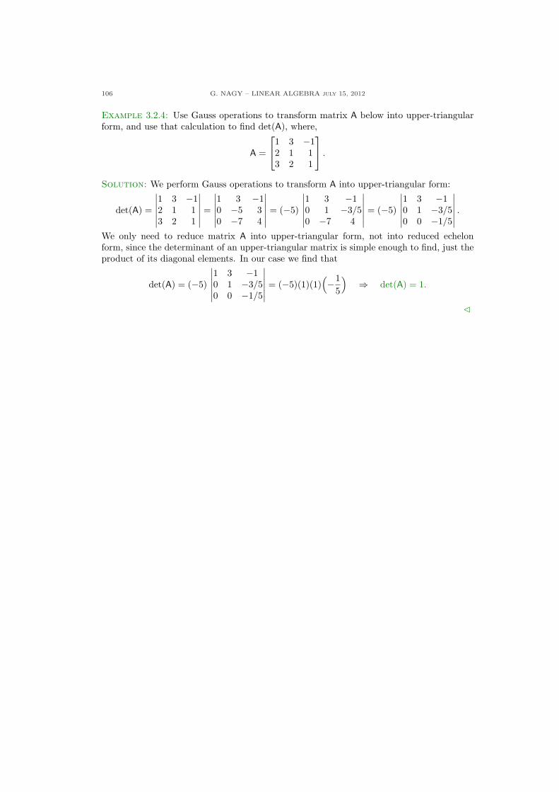
106 G. NAGY – LINEAR ALGEBRA july 15, 2012
Example 3.2.4: Use Gauss operations to transform matrix A below into upper-triangularform, and use that calculation to find det(A), where,
A =
1 3 −12 1 13 2 1
.
Solution: We perform Gauss operations to transform A into upper-triangular form:
det(A) =
∣∣∣∣∣∣
1 3 −12 1 13 2 1
∣∣∣∣∣∣=
∣∣∣∣∣∣
1 3 −10 −5 30 −7 4
∣∣∣∣∣∣= (−5)
∣∣∣∣∣∣
1 3 −10 1 −3/50 −7 4
∣∣∣∣∣∣= (−5)
∣∣∣∣∣∣
1 3 −10 1 −3/50 0 −1/5
∣∣∣∣∣∣.
We only need to reduce matrix A into upper-triangular form, not into reduced echelonform, since the determinant of an upper-triangular matrix is simple enough to find, just theproduct of its diagonal elements. In our case we find that
det(A) = (−5)
∣∣∣∣∣∣
1 3 −10 1 −3/50 0 −1/5
∣∣∣∣∣∣= (−5)(1)(1)
(−1
5
)⇒ det(A) = 1.
C
G. NAGY – LINEAR ALGEBRA July 15, 2012 107
3.2.4. Exercises.
3.2.1.- Use determinants to compute A−1,where
A =
24
2 1 16 2 1−2 2 1
35 .
3.2.2.- Find the coefficients (A−1)12 and(A−1)32, where
A =
24
1 5 72 1 04 1 3
35 .
3.2.3.- Use Gauss operations to reduce ma-trices A and B below to upper triangu-lar form and evaluate their determinant,where
A =
24
1 2 32 4 11 4 4
35 , B =
24
1 3 5−1 4 23 −2 4
35 .
3.2.4.- Use Gauss operations to prove theformula˛˛˛1 a a2
1 b b2
1 c c2
˛˛˛ = (b− a)(c− a)(c− b).
3.2.5.- Use the det(A) to find the valuesof the constant k such that the systemAx = b has a unique solution for everysource vector b, where
A =
24
1 k 00 1 −1k 0 1
35 .
3.2.6.- Use Cramer’s rule to find the solu-tion to the linear system
a x1 + b x2 = 1
c x1 + d x2 = 0.
where a, b, c, d ∈ R.
3.2.7.- Use Cramer’s rule to find the solu-tion to the linear system2
41 1 11 1 00 1 1
3524
x1
x2
x3
35 =
24
123
35 .
108 G. NAGY – LINEAR ALGEBRA july 15, 2012
Chapter 4. Vector spaces
4.1. Spaces and subspaces
A vector space is any set where the linear combination operation is defined on its elements.In a vector space, also called a linear space, the elements are not important. The actualelements that constitute the vector space are left unspecified, only the relation among themis determined. An example of a vector space is the set Fn of n-vectors with the operationof linear combination studied in Chapter 1. Another example is the set Fm,n of all m × nmatrices with the operation of linear combination studied in Chapter 2. We now definea vector space and comment its main properties. A subspace is introduced later on as asmaller vector space inside the original one. We end this Section with the concept of spanof a set of vectors, which is a way to construct a subspace from any subset in a vector space.
Definition 4.1.1. A set V is a vector space over the scalar field F ∈ {R,C} iff thereare two operations defined on V , called vector addition and scalar multiplication with thefollowing properties: For all u, v, w ∈ V the vector addition satisfies
(A1) u + v ∈ V , (closure of V );(A2) u + v = v + u, (commutativity);(A3) (u + v) + w = u + (v + w), (associativity);(A4) ∃ 0 ∈ V : 0 + u = u ∀ u ∈ V , (existence of a neutral element);(A5) ∀ u ∈ V ∃ (−u) ∈ V : u + (−u) = 0, (existence of an opposite element);
furthermore, for all a, b ∈ F the scalar multiplication satisfies
(M1) au ∈ V , (closure of V );(M2) 1u = u, (neutral element);(M3) a(bu) = (ab)u, (associativity);(M4) a(u + v) = au + av, (distributivity);(M5) (a + b)u = au + bu, (distributivity).
The definition of a vector space does not specify the elements of the set V , it onlydetermines the properties of the vector addition and scalar multiplication operations. Weuse the convention that elements in a vector space, called vectors, are represented in boldface.Nevertheless, we allow several exceptions, the first two of them are given in Examples 4.1.1and 4.1.2. We now present several examples of vector spaces.
Example 4.1.1: A vector space is the set Fn of n-vectors u = [ui] with components ui ∈ Fand the operations of column vector addition and scalar multiplication given by
[ui] + [vi] = [ui + vi], a[ui] = [aui].
This space of column vectors was introduced in Chapter 1. Elements in these vector spacesare not represented in boldface, instead we keep the previous sanserif font, u ∈ Fn. Thereason for this notation will be clear in Sect. 4.4. C
Example 4.1.2: A vector space is the set Fm,n of m × n matrices A = [Aij ] with matrixcoefficients Aij ∈ F and the operations of addition and scalar multiplication given by
[Aij
]+
[Bij
]=
[Aij + Bij
], a
[Aij
]=
[aAij
],
These operations were introduced in Chapter 2. As in the previous example, elements inthese vector spaces are not represented in boldface, instead we keep the previous capitalsanserif font, A ∈ Fm,n. The reason for this notation will be clear in Sect. 4.4. C
G. NAGY – LINEAR ALGEBRA July 15, 2012 109
Example 4.1.3: Let Pn(U) be the set of all polynomials having degree n > 0 and domainU ⊂ F, that is,
Pn(U) ={p(x) = a0 + a1x + · · ·+ anxn, with a0, · · · , an ∈ F and x ∈ U ⊂ F}
.
The set Pn(U) together with the addition of polynomials (p + q)(x) = p(x) + q(x) and thescalar multiplication (ap)(x) = ap(x) is a vector space. In the case U = R we use thenotation Pn = Pn(R). C
Example 4.1.4: Let Ck([a, b],F
)be the set of scalar valued functions with domain [a, b] ⊂ R
with the k-th derivative being a continuous function, that is,
Ck([a, b],F
)=
{f : [a, b]→ F such that f (k) is continuous
}.
The set Ck([a, b],F
)together with the addition of functions (f + g)(x) = f (x) + g(x) and
the scalar multiplication (af )(x) = a f (x) is a vector space. The particular case Ck(R,R)is denoted simply as Ck. The set of real valued continuous function is then C0. C
Example 4.1.5: Let ` be the set of absolute convergent series, that is,
` ={a =
∑an : an ∈ F and
∞∑n=0
|an| exists}
.
The set ` with the addition of series a + b =∑
(an + bn) and the scalar multiplicationca =
∑c an is a vector space. C
The properties (A1)-(M5) given in the definition of vector space are not redundant. Asan example, these properties do not include the condition that the neutral element 0 isunique, since it follows from the definition.
Theorem 4.1.2. The element 0 in a vector space is unique.
Proof Theorem 4.1.2: Suppose that there exist two neutral elements 01 and 02 in thevector space V , that is,
01 + u = u and 02 + u = u for all u ∈ V
Taking u = 02 in the first equation above, and u = 01 in the second equation above weobtain that
01 + 02 = 02, 02 + 01 = 01.
These equations above simply that the two neutral elements must be the same, since
02 = 01 + 02 = 02 + 01 = 01;
where in the second equation we used that the addition operation is commutative. Thisestablishes the Theorem. ¤Theorem 4.1.3. It holds that 0u = 0 for all element u in a vector space V .
Proof Theorem 4.1.3: For every u ∈ V holds
u = 1u = (1 + 0)u = 1u + 0u = u + 0u = 0u + u ⇒ u = 0u + u.
This last equation says that 0u is a neutral element, 0. Theorem 4.1.2 says that the neutralelement is unique, so we conclude that, for all u ∈ V holds that
0u = 0.
This establishes the Theorem. ¤Also notice that the property (A5) in the definition of vector space says that the opposite
element exists, but it does not say whether it is unique. The opposite element is actuallyunique.
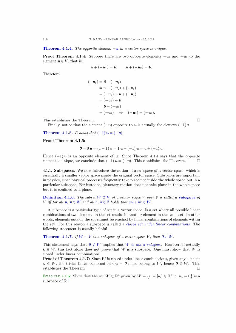
110 G. NAGY – LINEAR ALGEBRA july 15, 2012
Theorem 4.1.4. The opposite element −u in a vector space is unique.
Proof Theorem 4.1.4: Suppose there are two opposite elements −u1 and −u2 to theelement u ∈ V , that is,
u + (−u1) = 0, u + (−u2) = 0.
Therefore,
(−u1) = 0 + (−u1)
= u + (−u2) + (−u1)
= (−u2) + u + (−u1)
= (−u2) + 0
= 0 + (−u2)
= (−u2) ⇒ (−u1) = (−u2).
This establishes the Theorem. ¤Finally, notice that the element (−u) opposite to u is actually the element (−1)u.
Theorem 4.1.5. It holds that (−1)u = (−u).
Proof Theorem 4.1.5:
0 = 0u = (1− 1)u = 1u + (−1)u = u + (−1)u.
Hence (−1)u is an opposite element of u. Since Theorem 4.1.4 says that the oppositeelement is unique, we conclude that (−1)u = (−u). This establishes the Theorem. ¤
4.1.1. Subspaces. We now introduce the notion of a subspace of a vector space, which isessentially a smaller vector space inside the original vector space. Subspaces are importantin physics, since physical processes frequently take place not inside the whole space but in aparticular subspace. For instance, planetary motion does not take plane in the whole spacebut it is confined to a plane.
Definition 4.1.6. The subset W ⊂ V of a vector space V over F is called a subspace ofV iff for all u, v ∈W and all a, b ∈ F holds that au + bv ∈W .
A subspace is a particular type of set in a vector space. Is a set where all possible linearcombinations of two elements in the set results in another element in the same set. In otherwords, elements outside the set cannot be reached by linear combinations of elements withinthe set. For this reason a subspace is called a closed set under linear combinations. Thefollowing statement is usually helpful
Theorem 4.1.7. If W ⊂ V is a subspace of a vector space V , then 0 ∈W .
This statement says that 0 /∈ W implies that W is not a subspace. However, if actually0 ∈ W , this fact alone does not prove that W is a subspace. One must show that W isclosed under linear combinations.Proof of Theorem 4.1.7: Since W is closed under linear combinations, given any elementu ∈ W , the trivial linear combination 0u = 0 must belong to W , hence 0 ∈ W . Thisestablishes the Theorem. ¤
Example 4.1.6: Show that the set W ⊂ R3 given by W ={u = [ui] ∈ R3 : u3 = 0
}is a
subspace of R3:
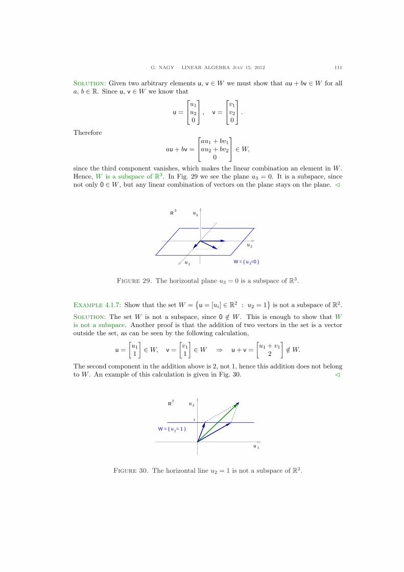
G. NAGY – LINEAR ALGEBRA July 15, 2012 111
Solution: Given two arbitrary elements u, v ∈ W we must show that au + bv ∈ W for alla, b ∈ R. Since u, v ∈W we know that
u =
u1
u2
0
, v =
v1
v2
0
.
Therefore
au + bv =
au1 + bv1
au2 + bv2
0
∈W,
since the third component vanishes, which makes the linear combination an element in W .Hence, W is a subspace of R3. In Fig. 29 we see the plane u3 = 0. It is a subspace, sincenot only 0 ∈W , but any linear combination of vectors on the plane stays on the plane. C
3W = { u =0 }
3uR3
1u
u 2
Figure 29. The horizontal plane u3 = 0 is a subspace of R3.
Example 4.1.7: Show that the set W ={u = [ui] ∈ R2 : u2 = 1
}is not a subspace of R2.
Solution: The set W is not a subspace, since 0 /∈ W . This is enough to show that Wis not a subspace. Another proof is that the addition of two vectors in the set is a vectoroutside the set, as can be seen by the following calculation,
u =[u1
1
]∈W, v =
[v1
1
]∈W ⇒ u + v =
[u1 + v1
2
]/∈W.
The second component in the addition above is 2, not 1, hence this addition does not belongto W . An example of this calculation is given in Fig. 30. C
1
2W = { u = 1 }
1
2uR2
u
Figure 30. The horizontal line u2 = 1 is not a subspace of R2.
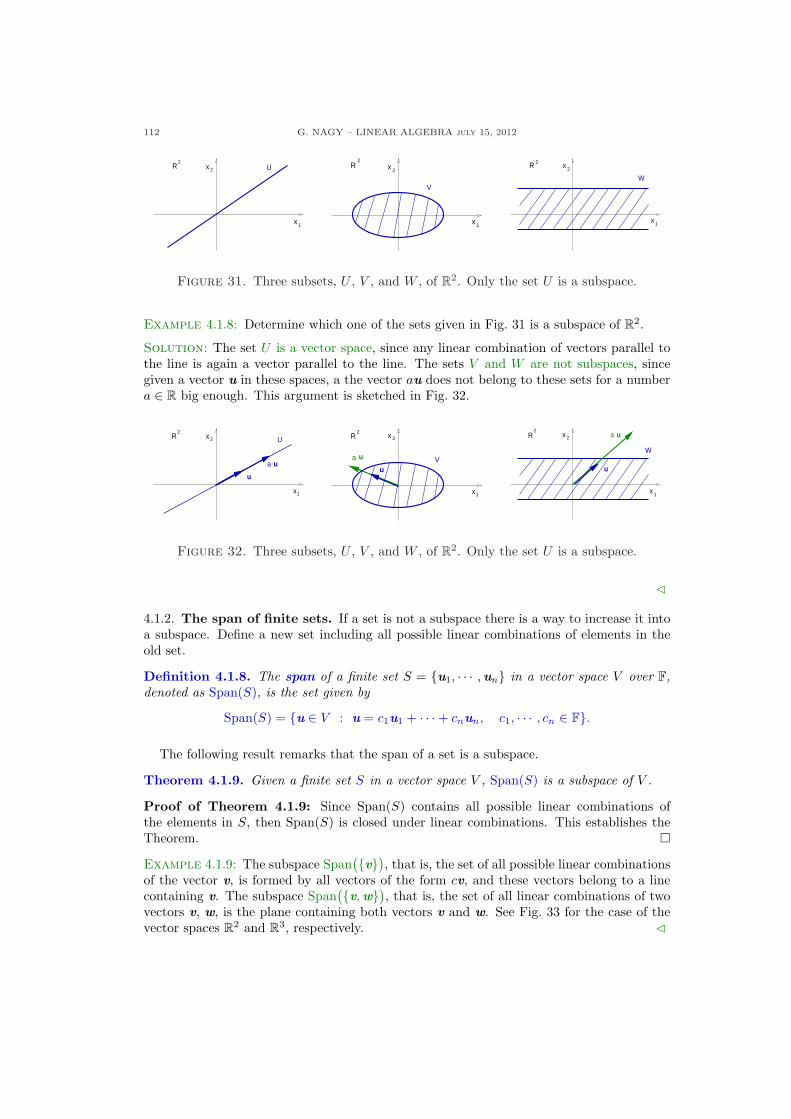
112 G. NAGY – LINEAR ALGEBRA july 15, 2012
1
2xR2
U
x
V
R2
x 2
x 1 1
2xR 2
W
x
Figure 31. Three subsets, U , V , and W , of R2. Only the set U is a subspace.
Example 4.1.8: Determine which one of the sets given in Fig. 31 is a subspace of R2.
Solution: The set U is a vector space, since any linear combination of vectors parallel tothe line is again a vector parallel to the line. The sets V and W are not subspaces, sincegiven a vector u in these spaces, a the vector au does not belong to these sets for a numbera ∈ R big enough. This argument is sketched in Fig. 32.
1
u
a u
U2xR2
x 1
Vu
ua
x 2R2
x
W
2xR2
ua
u
x 1
Figure 32. Three subsets, U , V , and W , of R2. Only the set U is a subspace.
C
4.1.2. The span of finite sets. If a set is not a subspace there is a way to increase it intoa subspace. Define a new set including all possible linear combinations of elements in theold set.
Definition 4.1.8. The span of a finite set S = {u1, · · · ,un} in a vector space V over F,denoted as Span(S), is the set given by
Span(S) = {u ∈ V : u = c1u1 + · · ·+ cnun, c1, · · · , cn ∈ F}.
The following result remarks that the span of a set is a subspace.
Theorem 4.1.9. Given a finite set S in a vector space V , Span(S) is a subspace of V .
Proof of Theorem 4.1.9: Since Span(S) contains all possible linear combinations ofthe elements in S, then Span(S) is closed under linear combinations. This establishes theTheorem. ¤
Example 4.1.9: The subspace Span({v}), that is, the set of all possible linear combinations
of the vector v, is formed by all vectors of the form cv, and these vectors belong to a linecontaining v. The subspace Span
({v,w}), that is, the set of all linear combinations of twovectors v, w, is the plane containing both vectors v and w. See Fig. 33 for the case of thevector spaces R2 and R3, respectively. C
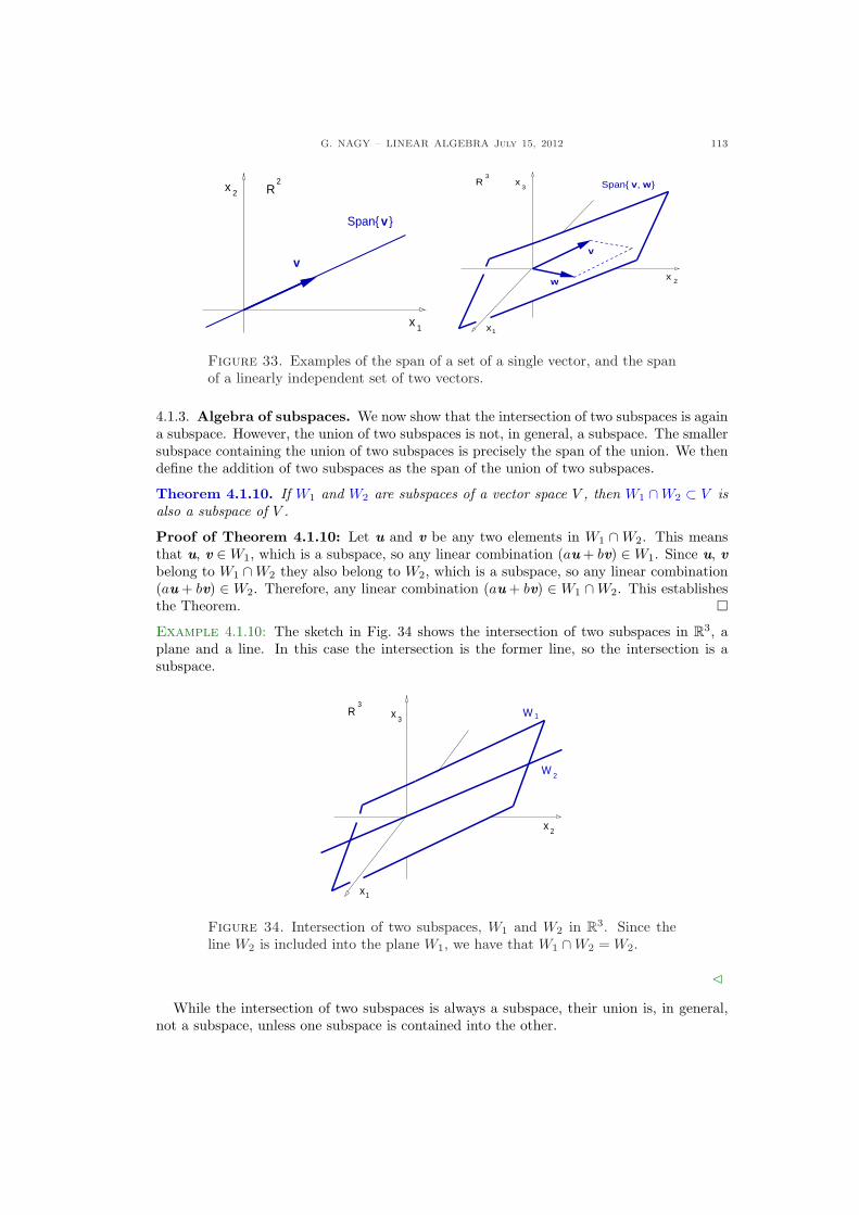
G. NAGY – LINEAR ALGEBRA July 15, 2012 113
1
v
2x R2
Span{ }v
x
Span{ , }
w
v
3xR
3
2x
x1
v w
Figure 33. Examples of the span of a set of a single vector, and the spanof a linearly independent set of two vectors.
4.1.3. Algebra of subspaces. We now show that the intersection of two subspaces is againa subspace. However, the union of two subspaces is not, in general, a subspace. The smallersubspace containing the union of two subspaces is precisely the span of the union. We thendefine the addition of two subspaces as the span of the union of two subspaces.
Theorem 4.1.10. If W1 and W2 are subspaces of a vector space V , then W1 ∩W2 ⊂ V isalso a subspace of V .
Proof of Theorem 4.1.10: Let u and v be any two elements in W1 ∩W2. This meansthat u, v ∈W1, which is a subspace, so any linear combination (au + bv) ∈W1. Since u, vbelong to W1 ∩W2 they also belong to W2, which is a subspace, so any linear combination(au + bv) ∈ W2. Therefore, any linear combination (au + bv) ∈ W1 ∩W2. This establishesthe Theorem. ¤Example 4.1.10: The sketch in Fig. 34 shows the intersection of two subspaces in R3, aplane and a line. In this case the intersection is the former line, so the intersection is asubspace.
x
x1
W3xR
3
1
W 2
2
Figure 34. Intersection of two subspaces, W1 and W2 in R3. Since theline W2 is included into the plane W1, we have that W1 ∩W2 = W2.
C
While the intersection of two subspaces is always a subspace, their union is, in general,not a subspace, unless one subspace is contained into the other.
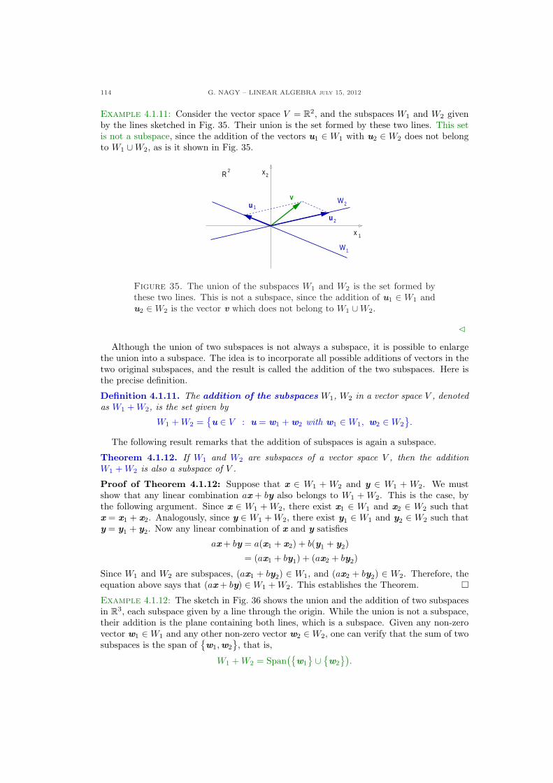
114 G. NAGY – LINEAR ALGEBRA july 15, 2012
Example 4.1.11: Consider the vector space V = R2, and the subspaces W1 and W2 givenby the lines sketched in Fig. 35. Their union is the set formed by these two lines. This setis not a subspace, since the addition of the vectors u1 ∈ W1 with u2 ∈ W2 does not belongto W1 ∪W2, as is it shown in Fig. 35.
W
R 2x2
1u
u 2
v
W1
x 1
2
Figure 35. The union of the subspaces W1 and W2 is the set formed bythese two lines. This is not a subspace, since the addition of u1 ∈ W1 andu2 ∈W2 is the vector v which does not belong to W1 ∪W2.
C
Although the union of two subspaces is not always a subspace, it is possible to enlargethe union into a subspace. The idea is to incorporate all possible additions of vectors in thetwo original subspaces, and the result is called the addition of the two subspaces. Here isthe precise definition.
Definition 4.1.11. The addition of the subspaces W1, W2 in a vector space V , denotedas W1 + W2, is the set given by
W1 + W2 ={u ∈ V : u = w1 + w2 with w1 ∈W1, w2 ∈W2
}.
The following result remarks that the addition of subspaces is again a subspace.
Theorem 4.1.12. If W1 and W2 are subspaces of a vector space V , then the additionW1 + W2 is also a subspace of V .
Proof of Theorem 4.1.12: Suppose that x ∈ W1 + W2 and y ∈ W1 + W2. We mustshow that any linear combination ax + by also belongs to W1 + W2. This is the case, bythe following argument. Since x ∈ W1 + W2, there exist x1 ∈ W1 and x2 ∈ W2 such thatx = x1 + x2. Analogously, since y ∈ W1 + W2, there exist y1 ∈ W1 and y2 ∈ W2 such thaty = y1 + y2. Now any linear combination of x and y satisfies
ax + by = a(x1 + x2) + b(y1 + y2)
= (ax1 + by1) + (ax2 + by2)
Since W1 and W2 are subspaces, (ax1 + by2) ∈ W1, and (ax2 + by2) ∈ W2. Therefore, theequation above says that (ax + by) ∈W1 + W2. This establishes the Theorem. ¤Example 4.1.12: The sketch in Fig. 36 shows the union and the addition of two subspacesin R3, each subspace given by a line through the origin. While the union is not a subspace,their addition is the plane containing both lines, which is a subspace. Given any non-zerovector w1 ∈W1 and any other non-zero vector w2 ∈W2, one can verify that the sum of twosubspaces is the span of
{w1,w2
}, that is,
W1 + W2 = Span({
w1
} ∪ {w2
}).
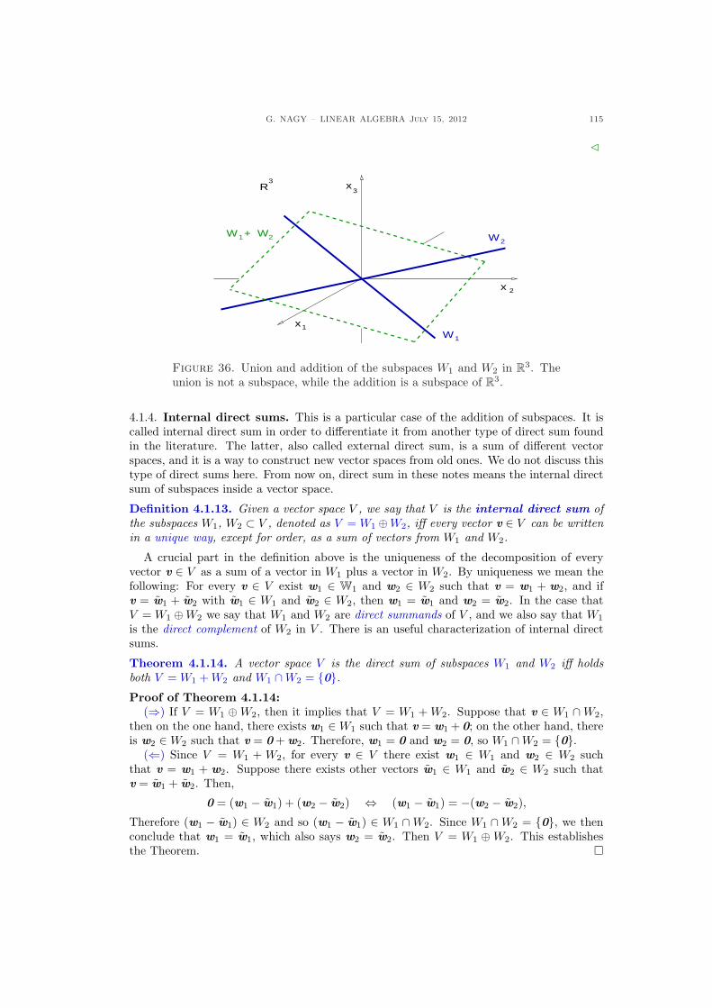
G. NAGY – LINEAR ALGEBRA July 15, 2012 115
C
3
x
W + W1 2
x3
x1
2
2W
W1
R
Figure 36. Union and addition of the subspaces W1 and W2 in R3. Theunion is not a subspace, while the addition is a subspace of R3.
4.1.4. Internal direct sums. This is a particular case of the addition of subspaces. It iscalled internal direct sum in order to differentiate it from another type of direct sum foundin the literature. The latter, also called external direct sum, is a sum of different vectorspaces, and it is a way to construct new vector spaces from old ones. We do not discuss thistype of direct sums here. From now on, direct sum in these notes means the internal directsum of subspaces inside a vector space.
Definition 4.1.13. Given a vector space V , we say that V is the internal direct sum ofthe subspaces W1, W2 ⊂ V , denoted as V = W1 ⊕W2, iff every vector v ∈ V can be writtenin a unique way, except for order, as a sum of vectors from W1 and W2.
A crucial part in the definition above is the uniqueness of the decomposition of everyvector v ∈ V as a sum of a vector in W1 plus a vector in W2. By uniqueness we mean thefollowing: For every v ∈ V exist w1 ∈ W1 and w2 ∈ W2 such that v = w1 + w2, and ifv = w1 + w2 with w1 ∈ W1 and w2 ∈ W2, then w1 = w1 and w2 = w2. In the case thatV = W1 ⊕W2 we say that W1 and W2 are direct summands of V , and we also say that W1
is the direct complement of W2 in V . There is an useful characterization of internal directsums.
Theorem 4.1.14. A vector space V is the direct sum of subspaces W1 and W2 iff holdsboth V = W1 + W2 and W1 ∩W2 = {0}.Proof of Theorem 4.1.14:
(⇒) If V = W1 ⊕W2, then it implies that V = W1 + W2. Suppose that v ∈ W1 ∩W2,then on the one hand, there exists w1 ∈W1 such that v = w1 + 0; on the other hand, thereis w2 ∈W2 such that v = 0 + w2. Therefore, w1 = 0 and w2 = 0, so W1 ∩W2 = {0}.
(⇐) Since V = W1 + W2, for every v ∈ V there exist w1 ∈ W1 and w2 ∈ W2 suchthat v = w1 + w2. Suppose there exists other vectors w1 ∈ W1 and w2 ∈ W2 such thatv = w1 + w2. Then,
0 = (w1 − w1) + (w2 − w2) ⇔ (w1 − w1) = −(w2 − w2),
Therefore (w1 − w1) ∈ W2 and so (w1 − w1) ∈ W1 ∩W2. Since W1 ∩W2 = {0}, we thenconclude that w1 = w1, which also says w2 = w2. Then V = W1 ⊕W2. This establishesthe Theorem. ¤
116 G. NAGY – LINEAR ALGEBRA july 15, 2012
Example 4.1.13: Denote by Sym and SkewSym the sets of all symmetric and all skew-symmetric n× n matrices. Show that Fn,n = Sym⊕ SkewSym.
Solution: Given any matrix A ∈ Fn,n, holds
A = A +12(AT − AT
)=
12(A + AT
)+
12(A− AT
).
We then can decompose matrix as A = B + C, where matrix B =(A + AT
)/2 ∈ Sym while
matrix C =(A−AT
)/2 ∈ SkewSym. That is, we can write any square matrix as a symmetric
matrix plus a skew-symmetric matrix, hence Fn,n ⊂ Sym + SkewSym. The other inclusionis obvious, that is, Sym + SkewSym ⊂ Fn,n, because each term in the sum is a subset ofFn,n. So, we conclude that
Fn,n = Sym + SkewSym.
Now we must show that Sym∩SkewSym = {0}. This is the case, as the following argumentshows. If matrix D ∈ Sym ∩ SkewSym, then matrix D is symmetric, D = DT , but matrix Dis also skew-symmetric, D = −DT . This implies that D = −D, that is, D = 0, proving ourassertion that Sym ∩ SkewSym = {0}. We then conclude that
Fn,n = Sym⊕ SkewSym.
C
G. NAGY – LINEAR ALGEBRA July 15, 2012 117
4.1.5. Exercises.
4.1.1.- Determine which of the followingsubsets of Rn, with n > 1, are in factsubspaces. Justify your answers.
(a) {x ∈ Rn : xi > 0 i = 1, · · · , n};(b) {x ∈ Rn : x1 = 0};(c) {x ∈ Rn : x1x2 = 0 n > 2};(d) {x ∈ Rn : x1 + · · ·+ xn = 0};(e) {x ∈ Rn : x1 + · · ·+ xn = 1};(f) {x ∈ Rn : Ax = b, A 6= 0, b 6= 0}.
4.1.2.- Determine which of the followingsubsets of Fn,n, with n > 1, are in factsubspaces. Justify your answers.
(a) {A ∈ Fn,n : A = AT };(b) {A ∈ Fn,n : A invertible};(c) {A ∈ Fn,n : A not invertible};(d) {A ∈ Fn,n : A upper-triangular};(e) {A ∈ Fn,n : A2 = A};(f) {A ∈ Fn,n : tr (A) = 0}.(g) Given a matrix X ∈ Fn,n, define
{A ∈ Fn,n : [A, X] = 0}.
4.1.3.- Find W1 + W2 ⊂ R3, where W1 is aplane passing through the origin in R3
and W2 is a line passing through theorigin in R3 not contained in W1.
4.1.4.- Sketch a picture of the subspacesspanned by the following vectors:
(a)n24
123
35 ,
24
369
35 ,
24−2−4−6
35o
;
(b)n24
020
35 ,
24
110
35 ,
24
230
35o
;
(c)n24
100
35 ,
24
110
35 ,
24
111
35o
.
4.1.5.- Given two finite subsets S1, S2 in avector space V , show that
Span(S1 ∪ S2) =
Span(S1) + Span(S2).
4.1.6.- Let W1 ⊂ R3 be the subspace
W1 = Span“n24
123
35 ,
24
101
35o”
.
Find a subspace W2 ⊂ R3 such thatR3 = W1 ⊕W2.
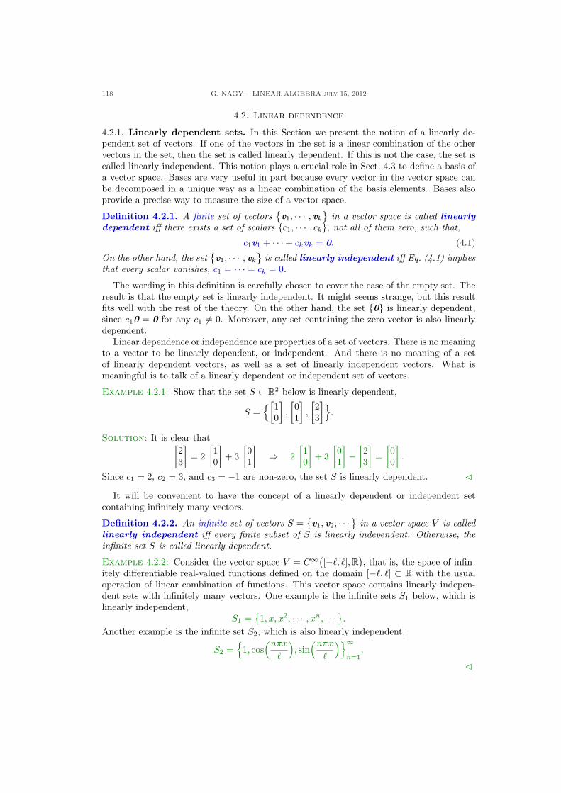
118 G. NAGY – LINEAR ALGEBRA july 15, 2012
4.2. Linear dependence
4.2.1. Linearly dependent sets. In this Section we present the notion of a linearly de-pendent set of vectors. If one of the vectors in the set is a linear combination of the othervectors in the set, then the set is called linearly dependent. If this is not the case, the set iscalled linearly independent. This notion plays a crucial role in Sect. 4.3 to define a basis ofa vector space. Bases are very useful in part because every vector in the vector space canbe decomposed in a unique way as a linear combination of the basis elements. Bases alsoprovide a precise way to measure the size of a vector space.
Definition 4.2.1. A finite set of vectors{v1, · · · , vk
}in a vector space is called linearly
dependent iff there exists a set of scalars {c1, · · · , ck}, not all of them zero, such that,
c1v1 + · · ·+ ckvk = 0. (4.1)
On the other hand, the set{v1, · · · , vk
}is called linearly independent iff Eq. (4.1) implies
that every scalar vanishes, c1 = · · · = ck = 0.
The wording in this definition is carefully chosen to cover the case of the empty set. Theresult is that the empty set is linearly independent. It might seems strange, but this resultfits well with the rest of the theory. On the other hand, the set {0} is linearly dependent,since c10 = 0 for any c1 6= 0. Moreover, any set containing the zero vector is also linearlydependent.
Linear dependence or independence are properties of a set of vectors. There is no meaningto a vector to be linearly dependent, or independent. And there is no meaning of a setof linearly dependent vectors, as well as a set of linearly independent vectors. What ismeaningful is to talk of a linearly dependent or independent set of vectors.
Example 4.2.1: Show that the set S ⊂ R2 below is linearly dependent,
S ={[
10
],
[01
],
[23
]}.
Solution: It is clear that[23
]= 2
[10
]+ 3
[01
]⇒ 2
[10
]+ 3
[01
]−
[23
]=
[00
].
Since c1 = 2, c2 = 3, and c3 = −1 are non-zero, the set S is linearly dependent. C
It will be convenient to have the concept of a linearly dependent or independent setcontaining infinitely many vectors.
Definition 4.2.2. An infinite set of vectors S ={v1, v2, · · ·
}in a vector space V is called
linearly independent iff every finite subset of S is linearly independent. Otherwise, theinfinite set S is called linearly dependent.
Example 4.2.2: Consider the vector space V = C∞([−`, `],R
), that is, the space of infin-
itely differentiable real-valued functions defined on the domain [−`, `] ⊂ R with the usualoperation of linear combination of functions. This vector space contains linearly indepen-dent sets with infinitely many vectors. One example is the infinite sets S1 below, which islinearly independent,
S1 ={1, x, x2, · · · , xn, · · ·}.
Another example is the infinite set S2, which is also linearly independent,
S2 ={
1, cos(nπx
`
), sin
(nπx
`
)}∞n=1
.
C
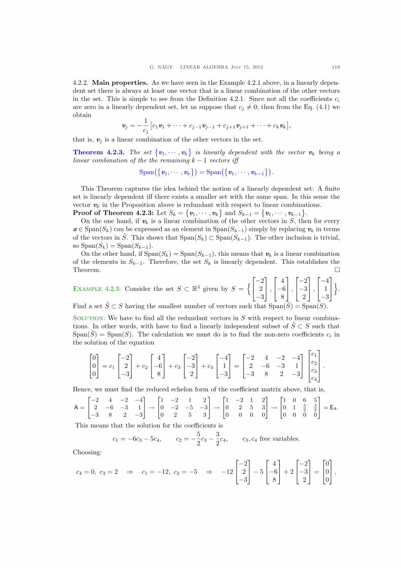
G. NAGY – LINEAR ALGEBRA July 15, 2012 119
4.2.2. Main properties. As we have seen in the Example 4.2.1 above, in a linearly depen-dent set there is always at least one vector that is a linear combination of the other vectorsin the set. This is simple to see from the Definition 4.2.1. Since not all the coefficients ci
are zero in a linearly dependent set, let us suppose that cj 6= 0; then from the Eq. (4.1) weobtain
vj = − 1cj
[c1v1 + · · ·+ cj−1vj−1 + cj+1vj+1 + · · ·+ ckvk
],
that is, vj is a linear combination of the other vectors in the set.
Theorem 4.2.3. The set{v1, · · · , vk
}is linearly dependent with the vector vk being a
linear combination of the the remaining k − 1 vectors iff
Span({
v1, · · · , vk
})= Span
({v1, · · · , vk−1
}).
This Theorem captures the idea behind the notion of a linearly dependent set: A finiteset is linearly dependent iff there exists a smaller set with the same span. In this sense thevector vk in the Proposition above is redundant with respect to linear combinations.Proof of Theorem 4.2.3: Let Sk =
{v1, · · · , vk
}and Sk−1 =
{v1, · · · , vk−1
}.
On the one hand, if vk is a linear combination of the other vectors in S, then for everyx ∈ Span(Sk) can be expressed as an element in Span(Sk−1) simply by replacing vk in termsof the vectors in S. This shows that Span(Sk) ⊂ Span(Sk−1). The other inclusion is trivial,so Span(Sk) = Span(Sk−1).
On the other hand, if Span(Sk) = Span(Sk−1), this means that vk is a linear combinationof the elements in Sk−1. Therefore, the set Sk is linearly dependent. This establishes theTheorem. ¤
Example 4.2.3: Consider the set S ⊂ R3 given by S ={
−22−3
,
4−68
,
−2−32
,
−41−3
}.
Find a set S ⊂ S having the smallest number of vectors such that Span(S) = Span(S).
Solution: We have to find all the redundant vectors in S with respect to linear combina-tions. In other words, with have to find a linearly independent subset of S ⊂ S such thatSpan(S) = Span(S). The calculation we must do is to find the non-zero coefficients ci inthe solution of the equation
000
= c1
−22−3
+ c2
4−68
+ c3
−2−32
+ c4
−41−3
=
−2 4 −2 −42 −6 −3 1−3 8 2 −3
c1
c2
c3
c4
.
Hence, we must find the reduced echelon form of the coefficient matrix above, that is,
A =
24−2 4 −2 −42 −6 −3 1−3 8 2 −3
35→
24
1 −2 1 20 −2 −5 −30 2 5 3
35→
24
1 −2 1 20 2 5 30 0 0 0
35→
24
1 0 6 50 1 5
232
0 0 0 0
35 = EA.
This means that the solution for the coefficients is
c1 = −6c3 − 5c4, c2 = −52c3 − 3
2c4, c3, c4 free variables.
Choosing:
c4 = 0, c3 = 2 ⇒ c1 = −12, c2 = −5 ⇒ −12
−22−3
− 5
4−68
+ 2
−2−32
=
000
,
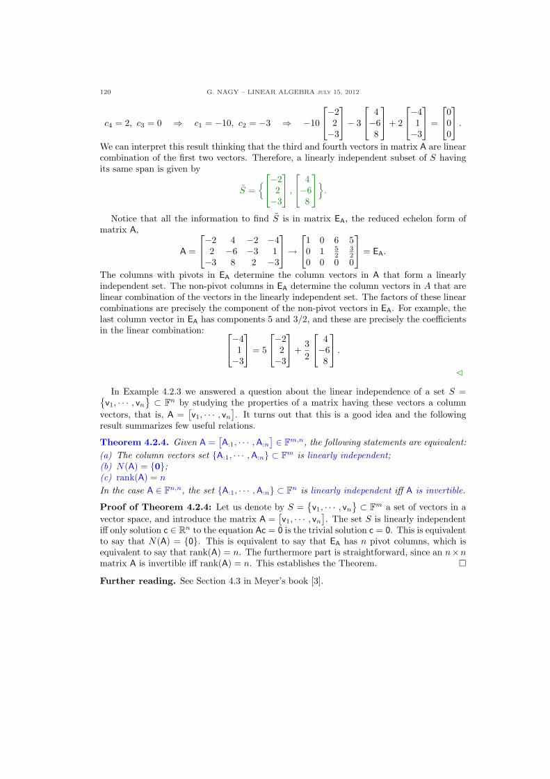
120 G. NAGY – LINEAR ALGEBRA july 15, 2012
c4 = 2, c3 = 0 ⇒ c1 = −10, c2 = −3 ⇒ −10
−22−3
− 3
4−68
+ 2
−41−3
=
000
.
We can interpret this result thinking that the third and fourth vectors in matrix A are linearcombination of the first two vectors. Therefore, a linearly independent subset of S havingits same span is given by
S ={
−22−3
,
4−68
}.
Notice that all the information to find S is in matrix EA, the reduced echelon form ofmatrix A,
A =
−2 4 −2 −42 −6 −3 1−3 8 2 −3
→
1 0 6 50 1 5
232
0 0 0 0
= EA.
The columns with pivots in EA determine the column vectors in A that form a linearlyindependent set. The non-pivot columns in EA determine the column vectors in A that arelinear combination of the vectors in the linearly independent set. The factors of these linearcombinations are precisely the component of the non-pivot vectors in EA. For example, thelast column vector in EA has components 5 and 3/2, and these are precisely the coefficientsin the linear combination:
−41−3
= 5
−22−3
+
32
4−68
.
C
In Example 4.2.3 we answered a question about the linear independence of a set S ={v1, · · · , vn
} ⊂ Fn by studying the properties of a matrix having these vectors a columnvectors, that is, A =
[v1, · · · , vn
]. It turns out that this is a good idea and the following
result summarizes few useful relations.
Theorem 4.2.4. Given A =[A:1, · · · ,A:n
] ∈ Fm,n, the following statements are equivalent:(a) The column vectors set {A:1, · · · ,A:n} ⊂ Fm is linearly independent;(b) N(A) = {0};(c) rank(A) = n
In the case A ∈ Fn,n, the set {A:1, · · · ,A:n} ⊂ Fn is linearly independent iff A is invertible.
Proof of Theorem 4.2.4: Let us denote by S ={v1, · · · , vn
} ⊂ Fm a set of vectors in avector space, and introduce the matrix A =
[v1, · · · , vn
]. The set S is linearly independent
iff only solution c ∈ Rn to the equation Ac = 0 is the trivial solution c = 0. This is equivalentto say that N(A) = {0}. This is equivalent to say that EA has n pivot columns, which isequivalent to say that rank(A) = n. The furthermore part is straightforward, since an n×nmatrix A is invertible iff rank(A) = n. This establishes the Theorem. ¤
Further reading. See Section 4.3 in Meyer’s book [3].
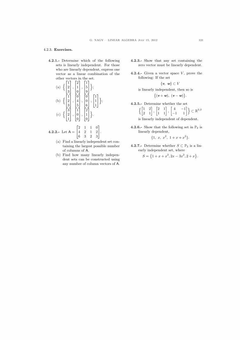
G. NAGY – LINEAR ALGEBRA July 15, 2012 121
4.2.3. Exercises.
4.2.1.- Determine which of the followingsets is linearly independent. For thosewho are linearly dependent, express onevector as a linear combination of theother vectors in the set.
(a)n24
123
35 ,
24
210
35 ,
24
159
35o
;
(b)n24
123
35 ,
24
045
35 ,
24
006
35 ,
24
111
35o
;
(c)n24
321
35 ,
24
100
35 ,
24
210
35o
.
4.2.2.- Let A =
24
2 1 1 04 2 1 26 3 2 3
35.
(a) Find a linearly independent set con-taining the largest possible numberof columns of A.
(b) Find how many linearly indepen-dent sets can be constructed usingany number of column vectors of A.
4.2.3.- Show that any set containing thezero vector must be linearly dependent.
4.2.4.- Given a vector space V , prove thefollowing: If the set
{v, w} ⊂ V
is linearly independent, then so is˘(v + w), (v−w)
¯.
4.2.5.- Determine whether the setn»1 2
2 1
–,
»2 11 1
–,
»4 −1−1 1
–o⊂ R2,2
is linearly independent of dependent.
4.2.6.- Show that the following set in P2 islinearly dependent,
{1, x, x2, 1 + x + x2}.
4.2.7.- Determine whether S ⊂ P2 is a lin-early independent set, where
S =˘1 + x + x2, 2x− 3x2, 2 + x
¯.
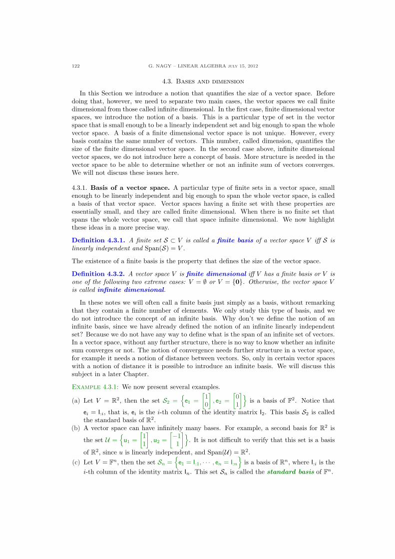
122 G. NAGY – LINEAR ALGEBRA july 15, 2012
4.3. Bases and dimension
In this Section we introduce a notion that quantifies the size of a vector space. Beforedoing that, however, we need to separate two main cases, the vector spaces we call finitedimensional from those called infinite dimensional. In the first case, finite dimensional vectorspaces, we introduce the notion of a basis. This is a particular type of set in the vectorspace that is small enough to be a linearly independent set and big enough to span the wholevector space. A basis of a finite dimensional vector space is not unique. However, everybasis contains the same number of vectors. This number, called dimension, quantifies thesize of the finite dimensional vector space. In the second case above, infinite dimensionalvector spaces, we do not introduce here a concept of basis. More structure is needed in thevector space to be able to determine whether or not an infinite sum of vectors converges.We will not discuss these issues here.
4.3.1. Basis of a vector space. A particular type of finite sets in a vector space, smallenough to be linearly independent and big enough to span the whole vector space, is calleda basis of that vector space. Vector spaces having a finite set with these properties areessentially small, and they are called finite dimensional. When there is no finite set thatspans the whole vector space, we call that space infinite dimensional. We now highlightthese ideas in a more precise way.
Definition 4.3.1. A finite set S ⊂ V is called a finite basis of a vector space V iff S islinearly independent and Span(S) = V .
The existence of a finite basis is the property that defines the size of the vector space.
Definition 4.3.2. A vector space V is finite dimensional iff V has a finite basis or V isone of the following two extreme cases: V = ∅ or V = {0}. Otherwise, the vector space Vis called infinite dimensional.
In these notes we will often call a finite basis just simply as a basis, without remarkingthat they contain a finite number of elements. We only study this type of basis, and wedo not introduce the concept of an infinite basis. Why don’t we define the notion of aninfinite basis, since we have already defined the notion of an infinite linearly independentset? Because we do not have any way to define what is the span of an infinite set of vectors.In a vector space, without any further structure, there is no way to know whether an infinitesum converges or not. The notion of convergence needs further structure in a vector space,for example it needs a notion of distance between vectors. So, only in certain vector spaceswith a notion of distance it is possible to introduce an infinite basis. We will discuss thissubject in a later Chapter.
Example 4.3.1: We now present several examples.
(a) Let V = R2, then the set S2 ={
e1 =[10
], e2 =
[01
]}is a basis of F2. Notice that
ei = I:i, that is, ei is the i-th column of the identity matrix I2. This basis S2 is calledthe standard basis of R2.
(b) A vector space can have infinitely many bases. For example, a second basis for R2 is
the set U ={
u1 =[11
], u2 =
[−11
]}. It is not difficult to verify that this set is a basis
of R2, since u is linearly independent, and Span(U) = R2.(c) Let V = Fn, then the set Sn =
{e1 = I:1, · · · , en = I:n
}is a basis of Rn, where I:i is the
i-th column of the identity matrix In. This set Sn is called the standard basis of Fn.
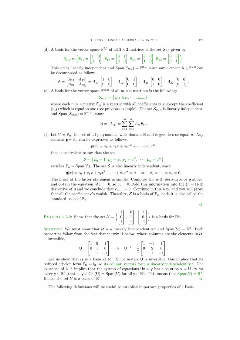
G. NAGY – LINEAR ALGEBRA July 15, 2012 123
(d) A basis for the vector space F2,2 of all 2× 2 matrices is the set S2,2 given by
S2,2 ={
E11 =[1 00 0
], E12 =
[0 10 0
],E21 =
[0 01 0
], E22 =
[0 00 1
]};
This set is linearly independent and Span(S2,2) = F2,2, since any element A ∈ F2,2 canbe decomposed as follows,
A =[A11 A12
A21 A22
]= A11
[1 00 0
]+ A12
[0 10 0
]+ A21
[0 01 0
]+ A22
[0 00 1
].
(e) A basis for the vector space Fm,n of all m× n matrices is the following:
Sm,n ={E11,E12, · · · ,Emn
},
where each m× n matrix Eij is a matrix with all coefficients zero except the coefficient(i, j) which is equal to one (see previous example). The set Sm,n is linearly independent,and Span(Sm,n) = Fm,n, since
A = [Aij ] =m∑
i=1
n∑
j=1
AijEij .
(f) Let V = Pn, the set of all polynomials with domain R and degree less or equal n. Anyelement p ∈ Pn can be expressed as follows,
p(x) = a0 + a1x + a2x2 + · · ·+ anxn,
that is equivalent to say that the set
S ={p0 = 1, p1 = x, p2 = x2, · · · , pn = xn
}
satisfies Pn = Span(S). The set S is also linearly independent, since
q(x) = c0 + c1x + c2x2 + · · ·+ cnxn = 0 ⇒ c0 = · · · = cn = 0.
The proof of the latter statement is simple: Compute the n-th derivative of q above,and obtain the equation n! cn = 0, so cn = 0. Add this information into the (n− 1)-thderivative of q and we conclude that cn−1 = 0. Continue in this way, and you will provethat all the coefficient c’s vanish. Therefore, S is a basis of Pn, ands it is also called thestandard basis of Pn.
C
Example 4.3.2: Show that the set U ={
101
,
011
,
10−1
}is a basis for R3.
Solution: We must show that U is a linearly independent set and Span(U) = R3. Bothproperties follow from the fact that matrix U below, whose columns are the elements in U ,is invertible,
U =
1 0 10 1 01 1 −1
⇒ U−1 =
12
1 −1 10 2 01 1 −1
.
Let us show that U is a basis of R3: Since matrix U is invertible, this implies that itsreduced echelon form EU = I3, so its column vectors form a linearly independent set. Theexistence of U−1 implies that the system of equations Ux = y has a solution x = U−1y forevery y ∈ R3, that is, y ∈ Col(U) = Span(U) for all y ∈ R3. This means that Span(U) = R3.Hence, the set U is a basis of R3. C
The following definitions will be useful to establish important properties of a basis.
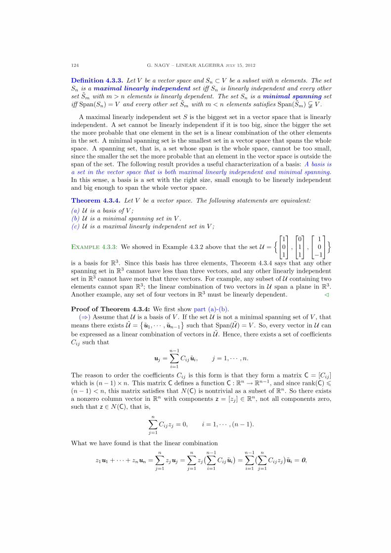
124 G. NAGY – LINEAR ALGEBRA july 15, 2012
Definition 4.3.3. Let V be a vector space and Sn ⊂ V be a subset with n elements. The setSn is a maximal linearly independent set iff Sn is linearly independent and every otherset Sm with m > n elements is linearly dependent. The set Sn is a minimal spanning setiff Span(Sn) = V and every other set Sm with m < n elements satisfies Span(Sm) & V .
A maximal linearly independent set S is the biggest set in a vector space that is linearlyindependent. A set cannot be linearly independent if it is too big, since the bigger the setthe more probable that one element in the set is a linear combination of the other elementsin the set. A minimal spanning set is the smallest set in a vector space that spans the wholespace. A spanning set, that is, a set whose span is the whole space, cannot be too small,since the smaller the set the more probable that an element in the vector space is outside thespan of the set. The following result provides a useful characterization of a basis: A basis isa set in the vector space that is both maximal linearly independent and minimal spanning.In this sense, a basis is a set with the right size, small enough to be linearly independentand big enough to span the whole vector space.
Theorem 4.3.4. Let V be a vector space. The following statements are equivalent:
(a) U is a basis of V ;(b) U is a minimal spanning set in V .(c) U is a maximal linearly independent set in V ;
Example 4.3.3: We showed in Example 4.3.2 above that the set U ={
101
,
011
,
10−1
}
is a basis for R3. Since this basis has three elements, Theorem 4.3.4 says that any otherspanning set in R3 cannot have less than three vectors, and any other linearly independentset in R3 cannot have more that three vectors. For example, any subset of U containing twoelements cannot span R3; the linear combination of two vectors in U span a plane in R3.Another example, any set of four vectors in R3 must be linearly dependent. C
Proof of Theorem 4.3.4: We first show part (a)-(b).(⇒) Assume that U is a basis of V . If the set U is not a minimal spanning set of V , that
means there exists U ={u1, · · · , un−1
}such that Span(U) = V . So, every vector in U can
be expressed as a linear combination of vectors in U . Hence, there exists a set of coefficientsCij such that
uj =n−1∑
i=1
Cijui, j = 1, · · · , n.
The reason to order the coefficients Cij is this form is that they form a matrix C = [Cij ]which is (n− 1)× n. This matrix C defines a function C : Rn → Rn−1, and since rank(C) 6(n− 1) < n, this matrix satisfies that N(C) is nontrivial as a subset of Rn. So there existsa nonzero column vector in Rn with components z = [zj ] ∈ Rn, not all components zero,such that z ∈ N(C), that is,
n∑
j=1
Cijzj = 0, i = 1, · · · , (n− 1).
What we have found is that the linear combination
z1u1 + · · ·+ znun =n∑
j=1
zjuj =n∑
j=1
zj
(n−1∑
i=1
Cijui
)=
n−1∑
i=1
( n∑
j=1
Cijzj
)ui = 0,
G. NAGY – LINEAR ALGEBRA July 15, 2012 125
with at least one of the coefficients zj non-zero. This means that the set U is not linearlyindependent. But this contradicts that U is a basis. Therefore, the set U is a minimalspanning set of V .
(⇐) Assume that U is a minimal spanning set of V . If U is not a basis, that means U isnot a linearly independent set. At least one element in U must be a linear combination ofthe others. Let us arrange the order of the basis vectors such that the vector un is a linearcombination of the other vectors in U . Then, the set U =
{u, · · · ,un−1
}must still span V ,
that is Span(U) = V . But this contradicts the assumption that U is a minimal spanning setof V .
We now show part (a)-(c).(⇐) Assume that U is a maximal linearly independent set in V . If U is not a basis, that
means Span(U) $ V , so there exists un+1 ∈ V such that un+1 /∈ Span(U). Hence, the setU =
{u, · · · ,un+1
}is a linearly independent set. However, this contradicts the assumption
that U is a maximal linearly independent set. We conclude that U is a basis of V .(⇒) Assume that U is a basis of V . If the set U is not a maximal linearly independent
set in V , then there exists a maximal linearly independent set U ={u1, · · · , uk
}, with
k > n. By the argument given just above, U is a basis of V . By part (b) the set U mustbe a minimal spanning set of V . However, this is not true, since U is smaller and spans V .Therefore, U must be a maximal linearly independent set in V .
This establishes the Theorem. ¤
4.3.2. Dimension of a vector space. The characterization of a basis given in Theo-rem 4.3.4 above implies that the number of elements in a basis is always the same as in anyother basis.
Theorem 4.3.5. The number of elements in any basis of a finite dimensional vector spaceis the same as in any other basis.
Proof of Theorem (4.3.5: Let Vn and Vm be two bases of a vector space V with nand m elements, respectively. If m > n, the property that Vm is a minimal spanning setimplies that Span(Vn) & Span(Vm) = V . The former inclusion contradicts that Vn is abasis. Therefore, n = m. (A similar proof can be constructed with the maximal linearlyindependence property of a basis.) This establishes the Theorem. ¤
The number of elements in a basis of a finite dimensional vector space is a characteristicof the vector space, so we give that characteristic a name.
Definition 4.3.6. The dimension of a finite dimensional vector space V with a finitebasis, denoted as dim V , is the number of elements in any basis of V . The extreme cases ofV = ∅ and V = {0} are defined as zero dimensional.
From the definition above we see that dim{0} = 0 and dim ∅ = 0.
Example 4.3.4: We now present several examples.(a) The set Sn =
{e1 = I:1, · · · , en = I:n
}is a basis for Fn, so dimFn = n.
(b) A basis for the vector space F2,2 of all 2× 2 matrices is the set S2,2 is given by
S2,2 ={
E11 =[1 00 0
], E12 =
[0 10 0
],E21 =
[0 01 0
], E22 =
[0 00 1
]},
so we conclude that dimF2,2 = 4.(c) A basis for the vector space Fm,n of all m× n matrices is the following:
Sm,n ={E11,E12, · · · ,Emn
},
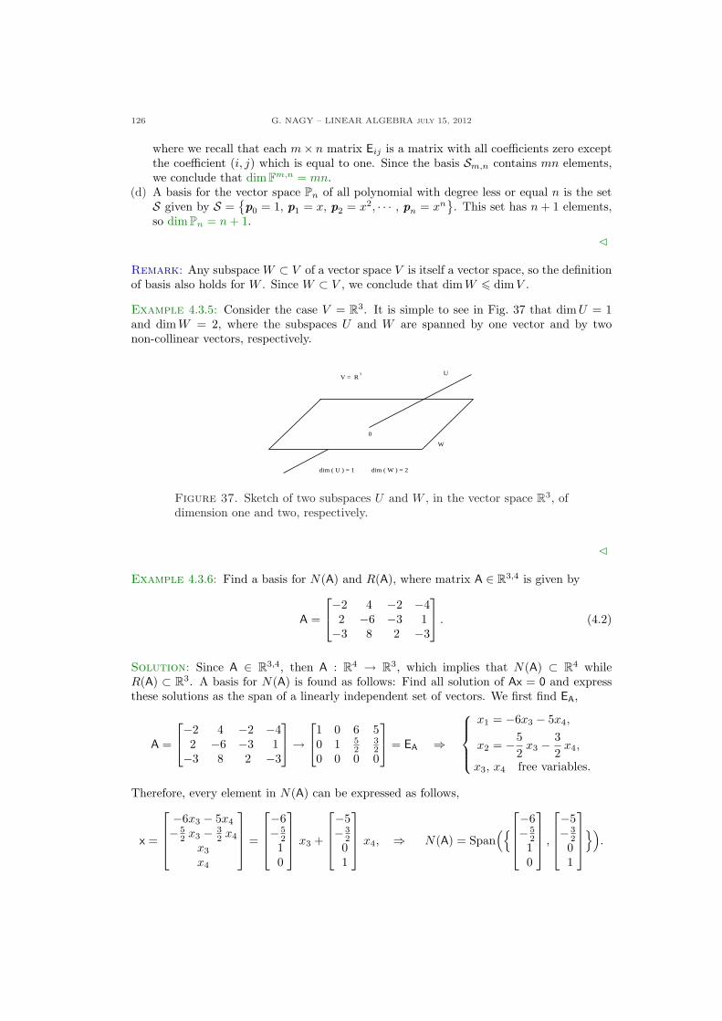
126 G. NAGY – LINEAR ALGEBRA july 15, 2012
where we recall that each m× n matrix Eij is a matrix with all coefficients zero exceptthe coefficient (i, j) which is equal to one. Since the basis Sm,n contains mn elements,we conclude that dimFm,n = mn.
(d) A basis for the vector space Pn of all polynomial with degree less or equal n is the setS given by S =
{p0 = 1, p1 = x, p2 = x2, · · · , pn = xn
}. This set has n + 1 elements,
so dimPn = n + 1.
C
Remark: Any subspace W ⊂ V of a vector space V is itself a vector space, so the definitionof basis also holds for W . Since W ⊂ V , we conclude that dim W 6 dim V .
Example 4.3.5: Consider the case V = R3. It is simple to see in Fig. 37 that dim U = 1and dim W = 2, where the subspaces U and W are spanned by one vector and by twonon-collinear vectors, respectively.
dim ( U ) = 1 dim ( W ) = 2
V = RU3
0
W
Figure 37. Sketch of two subspaces U and W , in the vector space R3, ofdimension one and two, respectively.
C
Example 4.3.6: Find a basis for N(A) and R(A), where matrix A ∈ R3,4 is given by
A =
−2 4 −2 −42 −6 −3 1−3 8 2 −3
. (4.2)
Solution: Since A ∈ R3,4, then A : R4 → R3, which implies that N(A) ⊂ R4 whileR(A) ⊂ R3. A basis for N(A) is found as follows: Find all solution of Ax = 0 and expressthese solutions as the span of a linearly independent set of vectors. We first find EA,
A =
−2 4 −2 −42 −6 −3 1−3 8 2 −3
→
1 0 6 50 1 5
232
0 0 0 0
= EA ⇒
x1 = −6x3 − 5x4,
x2 = −52
x3 − 32
x4,
x3, x4 free variables.
Therefore, every element in N(A) can be expressed as follows,
x =
−6x3 − 5x4
− 52 x3 − 3
2 x4
x3
x4
=
−6− 5
210
x3 +
−5− 3
201
x4, ⇒ N(A) = Span
({
−6− 5
210
,
−5− 3
201
}).
G. NAGY – LINEAR ALGEBRA July 15, 2012 127
Since the vectors in the span above form a linearly independent set, we conclude that abasis for N(A) is the set N given by
N ={
−6− 5
210
,
−5− 3
201
}.
We now find a basis for R(A). We know that R(A) = Col(A), that is, the span of the columnvectors of matrix A. We only need to find a linearly independent subset of column vectorsof A. This information is given in EA, since the pivot columns in EA indicate the columns inA which form a linearly independent set. In our case, the pivot columns in EA are the firstand second columns, so we conclude that a basis for R(A) is the set R given by
R ={
−22−3
,
4−68
}.
C
4.3.3. Extension of a set to a basis. We know that a basis of a vector space is not unique,and the following result says that actually any linearly independent set can be extended intoa basis of a vector space.
Theorem 4.3.7. If Sk ={u1, · · · ,uk
}is a linearly independent set in a vector spave V
with basis V ={v1, · · · , vn
}, where k < n, then, there always exists a basis of V given by
an extension of the set Sk of the form S ={u1, · · · ,uk, vi1 , · · · , vin−k
}.
The statement above says that a linearly independent set Sk can be extended into a basisS of a a vector space V simply incorporating appropriate vectors from any basis of V . If abasis V of V has n vectors, and the set Sk has k < n vectors, then one can always selectn− k vectors from the basis V to enlarge the set Sk into a basis of V .Proof of Theorem 4.3.7: Introduce the set Sk+n
sk+n ={u1, · · · ,uk, v1, · · · , vn
}.
We know that Span(Sk+n) = V since V ⊂ Sk+n. We also know that Sk+n is linearly de-pendent, since the maximal linearly independent set contains n elements and Sk+n containsn + k > n elements. The idea is to eliminate the vi such that Sk ∪ {vi} is linearly depen-dent. Since the maximal linearly independent set contains n elements and the Sk is linearlyindependent, there are k elements in V that will be eliminated. The resulting set is S, whichis a basis of V containing Sk. This establishes the Theorem. ¤
Example 4.3.7: Given the 3 × 4 matrix A defined in Eq. (4.2) in Example 4.3.6 above,extend the basis of N(A) ⊂ R4 into a basis of R4.
Solution: We know from Example 4.3.6 that a basis for the N(A) is the set N given by
N ={
−6− 5
210
,
−5− 3
201
}.
128 G. NAGY – LINEAR ALGEBRA july 15, 2012
Following the idea in the proof of Theorem 4.3.7, we look for a linear independent set ofvectors among the columns of the matrix
M =
−6 −5 1 0 0 0− 5
2 − 32 0 1 0 0
1 0 0 0 1 00 1 0 0 0 1
.
That is, matrix M include the basis vectors of N(A) and the four vectors ei of the standardbasis of R4. It is important to place the basis vectors of N(A) in the first columns of M. Inthis way, the Gauss method will select these first vectors as part of the linearly independentset of vectors. Find now the reduced echelon form matrix EM,
EM =
1 0 0 0 1 00 1 0 0 0 10 0 1 0 6 50 0 0 1 5 3
.
Therefore, the first four vectors in M are form a linearly independent set, so a basis of R4
that includes N is given by
V ={
−6− 5
210
,
−5− 3
201
,
1000
,
0100
}.
C
4.3.4. The dimension of subspace addition. Recall that the sum and the intersectionof two subspaces is again a subspace in a given vector space. The following result relatesthe dimension of a sum of subspaces with the dimension of the individual subspaces and thedimension of their intersection.
Theorem 4.3.8. If W1, W2 ⊂ V are subspaces of a vector space V , then holds
dim(W1 + W2) = dim W1 + dim W2 − dim(W1 ∩W2).
Proof of Theorem 4.3.8: We find the dimension of W1 + W2 finding a basis of this sum.The key idea is to start with a basis of W1 ∩ W2. Let B0 =
{z1, · · · , zl
}be a basis for
W1 ∩W2. Enlarge that basis into basis B1 for W1 and B2 for W2 as follows,
B1 ={z1, · · · , zl,x1, · · · ,xn
}, B2 =
{z1, · · · , zl,y1, · · · ,ym
}.
We use the notation l = dim(W1 ∩W2), l + n = dim W1 and l + m = dim W2. We nowpropose as basis for W1 + W2 the set
B ={z1, · · · , zl,x1, · · · ,xn,y1, · · · ,ym
}.
By construction this set satisfies that Span(B) = W1 + W2. We only need to show that B islinearly independent. Assume that the set B is linearly dependent. This means that thereis non-zero constants ai, bj and ck solutions of the equation
n∑
i=1
aixi +m∑
j=1
bjyj +l∑
k=1
ckzk = 0. (4.3)
G. NAGY – LINEAR ALGEBRA July 15, 2012 129
This implies that the vector∑n
i=1 aixi, which by definition belongs to W1, also belongs toW2, since
n∑
i=1
aixi = −( m∑
j=1
bjyj +l∑
k=1
ckzk
)∈W2.
Therefore,∑n
i=1 aixi belongs to W1 ∩W2, and so is a linear combination of the elements ofB0, that is, there exists scalars dk such that
n∑
i=1
aixi =l∑
i=1
dkzk.
Since B1 is a basis of W1, this implies that all the coefficients ai and dk vanish. Introducethis information into Eq. (4.3) and we conclude that
m∑
j=1
bjyj +l∑
k=1
ckzk = 0.
Analogously, the set B2 is a basis, so all the coefficients bj and ck must vanish. This impliesthat the set B is linearly independent, hence a basis of W1 + W2. Therefore, the dimensionof the sum is given by
dim(W1 + W2) = n + m + k = (n + k) + (m + k)− k = dim W1 + dim W2 − dim(W1 ∩W2).
This establishes the Theorem. ¤The following corollary is immediate.
Corollary 4.3.9. If a vector space can be decomposed as V = W1 ⊕W2, then
dim(W1 ⊕W2) = dim W1 + dim W2.
The proof is straightforward from Theorem 4.3.8, since the condition of subspaces directsum, W1 ∩W2 = {0}, says that dim
(W1 ∩W2) = 0.
130 G. NAGY – LINEAR ALGEBRA july 15, 2012
4.3.5. Exercises.
4.3.1.- Find a basis for each of the spacesN(A), R(A), N(AT ), R(AT ), where
A =
24
1 2 2 32 4 1 33 6 1 4
35 .
4.3.2.- Find the dimension of the spacespanned by
n2664
12−13
3775 ,
2664
1002
3775 ,
2664
28−48
3775 ,
2664
1111
3775 ,
2664
3306
3775o
.
4.3.3.- Find the dimension of the followingspaces:
(a) The space Pn of polynomials of de-gree less or equal n.
(b) The space Fm,n of m× n matrices.(c) The space of real symmetric n × n
matrices.(d) The space of real skew-symmetric
n× n matrices.
4.3.4.- Find an example to show that thefollowing statement is false: Given a ba-sis {v1, v2} of R2, then every subspaceW ⊂ R2 has a basis containing at leastone of the basis vectors v1, v2.
4.3.5.- Given the matrix A and vector v,
A =
24
1 2 2 0 52 4 3 1 83 6 1 5 5
35 , v =
266664
−81330
377775
,
verify that v ∈ N(A), and then find abasis of N(A) containing v.
4.3.6.- Determine whether or not the set
B =n24
232
35 ,
24
11−1
35o
is a basis for the subspace
Span“n24
123
35 ,
24
587
35 ,
24
341
35o”
⊂ R3.
G. NAGY – LINEAR ALGEBRA July 15, 2012 131
4.4. Vector components
4.4.1. Ordered bases. In the previous Section we introduced a finite basis in a vectorspace. Although a vector space can have different bases, every basis has the same numberof elements, which provides a measure of the vector space size, called the dimension of thevector space. In this Section we study another property of a basis. Every vector in a finitedimensional vector space can be expressed in a unique way as a linear combination of thebasis vectors. This property can be clearly stated in an ordered basis, which is a basis withthe basis vectors given in a specific order.
Definition 4.4.1. An ordered basis of an n-dimensional vector space V is a sequence(v1, · · · , vn) of vectors such that the set {v1, · · · , vn} is a basis of V .
Recall that a sequence is an ordered set, that is, a set with elements given in a particularorder.
Example 4.4.1: The following four ordered basis of R3 are all different,
(
100
,
010
,
001
),
(
010
,
100
,
001
),
(
010
,
001
,
100
),
(
001
,
010
,
100
),
however, they determine the same basis S3 ={
100
,
010
,
001
}. C
4.4.2. Vector components in a basis. The following result states that given a vectorspace with an ordered basis, there exists a correspondence between vectors and certainsequences of scalars.
Theorem 4.4.2. Let V be an n-dimensional vector space over the scalar field F with anordered basis
(u1, · · · ,un
). Then, every vector v ∈ V determines a unique scalars’ sequence(
v1, · · · , vn
) ⊂ F such thatv = v1u1 + · · ·+ vnun. (4.4)
And every scalars’ sequence (v1, · · · , vn) ⊂ F determines a unique vector v ∈ V by Eq. (4.4).
Proof of Theorem 4.4.2: Denote by U =(u1, · · · ,un
)the ordered basis of V . Since U
is a basis, Span(U) = V and U is linearly independent. The first property implies that forevery v ∈ V there exist scalars v1, · · · , vn such that v is a linear combination of the basisvectors, that is,
v = v1u1 + · · ·+ vnun.
The second property of a basis implies that the linear combination above is unique. Indeed,if there exists another linear combination
v = ν1u1 + · · ·+ νnun,
then 0 = v − v = (v1 − ν1)u1 + · · · + (vn − νn)un. Since U is linearly independent, thisimplies that each coefficient above vanishes, so v1 = ν1, · · · , vn = νn.
The converse statement is simple to show, since the scalars are given in a specific order.Every scalars’ sequence (v1, · · · , vn) determines a unique linear combination with an orderedbasis
(u1, · · · ,un
)given by v1u1 + · · ·+ vnun. This unique linear combination determines
a unique vector in the vector space. This establishes the Theorem. ¤Theorem 4.4.2 says that there exists a correspondence between vectors in a vector space
with an ordered basis and scalars’ sequences. This correspondence is called a coordinatemap and the scalars are called vector components in the basis. Here is a precise definition.
132 G. NAGY – LINEAR ALGEBRA july 15, 2012
Definition 4.4.3. Let V be an n-dimensional vector space over F with an ordered basisU = (u1, · · · ,un). The coordinate map is the function [ ]u : V → Fn, with [v ]u = vu, and
vu =
v1
...vn
⇔ v = v1u1 + · · ·+ vnun.
The scalars v1, · · · , vn are called the vector components of v in the ordered basis U .
Therefore, we use the notation [v ]u = vu ∈ Fn for the components of a vector v ∈ V in anordered basis U . We remark that the coordinate map is defined only after an ordered basisis fixed in V . Different ordered bases on V determine different coordinate maps betweenV and Fn. When the situation under study involves only one ordered basis, we suppressthe basis subindex. The coordinate map will be denoted by [ ] : V → Fn and the vectorcomponents by v = [v]. In the particular case that V = Fn and the basis is the standardbasis Sn, then the coordinate map [ ]s is the identity map, so v = [v]s = v. In this case wefollow the convention established in the first Chapters, that is, we denote vectors in Fn byv instead of v. When the situation under study involves more than one ordered basis wekeep the sub-indices in the coordinate map, like [ ]u, and in the vector components, like vu,to keep track of the basis attached to these expressions.
Example 4.4.2: Let V be the set of points on the plane with a preferred origin. LetS =
(e1, e2
)be an ordered basis, pictured in Fig. 38.
(a) Find the components vs = [v]s ∈ R2 of the vector v = e1 + 3e2 in the ordered basis S.(b) Find the components vu = [v]u ∈ R2 of the same vector v given in part (a) but now in
the ordered basis U =(u1 = e1 + e2, u2 = −e1 + e2
).
Solution: Part (a) is straightforward to compute, since the definition of component of avector says that the numbers multiplying the basis vectors in the equation v = e1 + 3e2 arethe components of the vector, that is,
v = e1 + 3e2 ⇔ vs =[13
].
Part (b) is more involved. We are looking for numbers v1 and v2 such that
v = v1u1 + v2u2 ⇔ vu =[v1
v2
]. (4.5)
From the definition of the basis U we know the components of the basis vectors in U interms of the standard basis, that is,
u1 = e1 + e2 ⇔ u1s =[11
],
u2 = −e1 + e2 ⇔ u2s =[−1
1
].
In other words, we can write the ordered basis U as the column vectors of the matrixUs =
[U]s
=[[u1]s, [u2]s
]given by
Us =[u1s, u2s
]=
[1 −11 1
].
Expressing Eq. (4.5) in the standard basis means
e1 + 3e2 = v = v1(e1 + e2) + v2(−e1 + e2) ⇔[13
]= v1
[11
]+ v2
[−11
].
G. NAGY – LINEAR ALGEBRA July 15, 2012 133
The last equation on the right is a matrix equation for the unknowns vu =[v1
v2
],
[1 −11 1
] [v1
v2
]=
[13
]⇔ Usvu = vs.
We find the solution using the Gauss method,[1 −1
∣∣ 11 1
∣∣ 3
]→
[1 0
∣∣ 20 1
∣∣ 1
]⇒ vu =
[21
]⇔ v = 2u1 + u2.
A sketch of what has been computed is in Fig. 38. In this Figure is clear that the vectorv is fixed, and we have only expressed this fixed vector in as a linear combination of twodifferent bases. It is clear in this Fig. 38 that one has to stretch the vector u1 by two andadd the result to the vector u2 to obtain v. C
v
e
2
e 2u2
x
x 1
u
1
1
Figure 38. The vector v = e1 + 3e2 expressed in terms of the basis U ={u1 = e1 + e2,u2 = −e1 + e2
}is given by v = 2u1 + u2.
Example 4.4.3: Consider the vector space P2 of all polynomials of degree less or equal two,and let us consider the case of F = R. An ordered basis is S =
(p0 = 1, p1 = x, p2 = x2
).
The coordinate map is [ ]s : P2 → R3 defined as follows, [p]s = ps, where
ps =
abc
⇔ p(x) = a + bx + cx2.
The column vector ps represents the components of the vector p in the ordered basis S. Theequation above defines a correspondence between every element in P2 and every element inR3. The coordinate map depend on the choice of the ordered basis. For example, choosingthe ordered basis S =
(p0 = x2, p1 = x, p2 = 1
), the corresponding coordinate map is
[ ]s : P2 → R3 defined by [p]s = ps, where
ps =
cba
⇔ p(x) = a + bx + cx2.
134 G. NAGY – LINEAR ALGEBRA july 15, 2012
The coordinate maps above generalize to the spaces Pn and Rn+1 for all n ∈ N. Giventhe ordered basis S =
(p0 = 1,p1 = x, · · · ,pn = xn
), the corresponding coordinate map
[ ]s : Pn → Rn+1 defined by [p]s = ps, where
ps =
a0
...an
⇔ p(x) = a0 + · · ·+ anxn.
C
Example 4.4.4: Consider V = P2 with ordered basis S =(p0 = 1, p1 = x, p2 = x2
).
(a) Find rs = [r]s, the components of r(x) = 3 + 2x + 4x2 in the ordered basis S.(b) Find rq = [r]q, the components of the same polynomial r given in part (a) but now in
the ordered basis Q =(q0 = 1, q1 = 1 + x, q2 = 1 + x + x2,
).
Solution:Part (a):This is straightforward to compute, since r(x) = 3 + 2x + 4x2 implies that
r(x) = 3p0(x) + 2p1(x) + 4p2(x) ⇔ rs =
324
.
Part (b): This is more involved, as in Example 4.4.2. We look for numbers r1, r2, r3 suchthat
r(x) = r0 q0(x) + r1 q1(x) + r2 q2(x) ⇔ rq =
r0
r1
r2
. (4.6)
From the definition of the basis Q we know the components of the basis vectors in Q interms of the S basis, that is,
q0(x) = p0(x) ⇔ q0s =
100
,
q1(x) = p0(x) + p1(x) ⇔ q1s =
110
q2(x) = p0(x) + p1(x) + p2(x) ⇔ q2s =
111
.
Now we can write the ordered basis Q in terms of the column vectors of the matrix Qs =[Q]s
=[q0s, q1s, q2s
], as follows,
Qs =
1 1 10 1 10 0 1
.
Expressing Eq. (4.6) in the standard basis means
324
= r0
100
+ r1
110
+ r2
111
.
G. NAGY – LINEAR ALGEBRA July 15, 2012 135
The last equation on the right is a matrix equation for the unknowns r0, r1, and r2
1 1 10 1 10 0 1
r0
r1
r2
=
324
⇔ Qsrq = rs.
We find the solution using the Gauss method,
1 1 1∣∣ 3
0 1 1∣∣ 2
0 0 1∣∣ 4
→
1 0 0∣∣ 1
0 1 0∣∣ −2
0 0 1∣∣ 4
,
hence the solution is
rq =
1−24
⇔ r(x) = q0(x)− 2 q1(x) + 4 q2(x).
We can verify that this is the solution, since
r(x) = q0(x)− 2 q1(x) + 4 q2(x)
= 1− 2 (1 + x) + 4 (1 + x + x2)
= (1− 2 + 4) + (−2 + 4)x + 4x2
= 3 + 2x + 4x2
= 3p0(x) + 2p1(x) + 4p2(x).
C
Example 4.4.5: Given any ordered basis U =(u1,u2,u3
)of a 3-dimensional vector space
V , find Uu =[U]
u⊂ F3,3, that is, find ui = [ui]u for i = 1, 2, 3, the components of the basis
vectors ui in its own basis U .
Solution: The answer is simple: The definition of vector components in a basis says that
u1 = u1 + 0u2 + 0u3 ⇔ u1u =
100
= e1,
u2 = 0u1 + u2 + 0u3 ⇔ u2u =
010
= e2,
u3 = 0u1 + 0u2 + u3 ⇔ u3u =
001
= e3.
In other words, using the coordinate map φu : V → F3, we can always write any basis Uas components in its own basis as follows, Uu =
[e1, e2, e3
]= I3. This example says that
there is nothing special about the standard basis S = {e1, · · · , en} of Fn, where ei = I:i isthe i-th column of the identity matrix In. Given any n-dimensional vector space V over Fwith any ordered basis V, the components of the basis vectors expressed on its own basis isalways the standard basis of Fn, that is, the result is always
[V]v
= In. C
136 G. NAGY – LINEAR ALGEBRA july 15, 2012
4.4.3. Exercises.
4.4.1.- Let S =`e1, e2, e3
´be the standard
basis of R3. Find the components of thevector v = e1 + e2 + 2e3 in the orderedbasis U“u1s =
24
101
35 , u2s =
24
011
35 , u3s =
24
110
35”.
4.4.2.- Let S =`e1, e2, e3
´be the standard
basis of R3. Find the components of thevector
vs =
24
874
35
in the ordered basis U given by
“u1s =
24
111
35 , u2s =
24
122
35 , u3s =
24
123
35”.
4.4.3.- Consider the vector space V = P2
with the ordered basis S given by
S =`p0 = 1, p1 = x, p2 = x2´.
(a) Find the components of the poly-nomial r(x) = 2 + 3x − x2 in theordered basis S.
(b) Find the components of the samepolynomial r given in part (a) butnow in the ordered basis Q given by`
q0 = 1, q1 = 1− x, q2 = x + x2,´.
4.4.4.- Let S be the standard ordered basisof R2,2, that is,
S = (E11, E12, E21, E22) ⊂ R2,2,
with
E11 =
»1 00 0
–, E12 =
»0 10 0
–,
E21 =
»0 01 0
–, E22 =
»0 00 1
–.
(a) Show that the ordered set M belowis a basis of R2,2, where
M = (M1, M2, M3, M4) ⊂ R2,2,
with
M1 =
»0 11 0
–, M2 =
»0 −11 0
–,
M3 =
»1 00 1
–, M4 =
»1 00 −1
–,
where the matrices above are writ-ten in the standard basis.
(b) Consider the matrix A written inthe standard basis S,
A =
»1 23 4
–.
Find the components of the matrixA in the ordered basis M.
G. NAGY – LINEAR ALGEBRA July 15, 2012 137
Chapter 5. Linear transformations
5.1. Linear transformations
We now introduce the notion of a linear transformation between vector spaces. Vectorspaces are defined not by the elements they are made of but by the relation among theseelements. They are defined by the properties of the operation we called linear combinationsof the vector space elements. Linear transformations are a very special type of functionsthat preserve the linear combinations on both vector spaces where they are defined. Lineartransformations generalize the definition of a linear function introduced in Sect. 2.1 betweenthe spaces Fn and Fm to any two vector spaces. Linear transformations are also called inthe literature as linear maps or linear mappings.
Definition 5.1.1. Given the vector spaces V and W over F, the function T : V → W iscalled a linear transformation iff for all u, v ∈ V and all scalars a, b ∈ F holds
T(au + bv) = aT(u) + bT(v).
In the case that V = W a linear transformation T : V → V is called a linear operator.
Taking a = b = 0 in the definition above we see that every linear transformation satisfiesthat T(0) = 0. As we said in Sect. 2.1, if a function does not satisfy this condition,then it cannot be a linear transformation. We now consider several examples of lineartransformations. We do not prove that these examples are indeed linear transformations;the proofs are left to the reader.
Example 5.1.1: We give several examples of linear transformations.(a) The transformation IV : V → V defined by IV (v) = v for all v ∈ V is called the identity
transformation. The transformation 0 : V → W defined by 0(v) = 0 for all v ∈ V iscalled the zero transformation.
(b) Every example of a matrix as a linear function given in Sect. 2.1 is a linear transfor-mation. More precisely, if V = Fn and W = Fm, then any m × n matrix A defines alinear transformation A : Fn → Fm by A(x) = Ax. Therefore, rotations, reflections,projections, dilations are linear transformations in the sense given in Def. 5.1.1 above.In particular, square matrices are now called linear operators.
(c) The vector spaces V and W are part of the definition of the linear transformation. Forexample, a matrix A alone does not determine a linear transformation, since the vectorspaces must also be specified. For example, and m × n matrix A defines two differentlinear transformations, the first one A : Rn → Rm, and the second one A : Cn → Cm.Although the action of these transformations is the same, the matrix-vector productA(x) = Ax, the linear transformations are different. We will see in Chapter 9 that inthe case m = n these transformations may have different eigenvalues and eigenvectors.
(d) Let V = P3, W = P2 and let D : P3 → P2 be the differentiation transformation
D(p) =dp
dx.
That is, given a polynomial p ∈ P3, the transformation D acting on p is a polynomialone degree less than p given by the derivative of p. For example,
p(x) = 2 + 3x + x2 − x3 ∈ P3 ⇒ D(p)(x) = 3 + 2x− 3x2 ∈ P2.
The transformation D is linear, since for all polynomials p, q ∈ P3 and scalars a, b ∈ Fholds
D(ap + bq)(x) =d
dx
[ap(x) + b q(x)
]= a
dp(x)dx
+ bdq(x)dx
= aD(p)(x) + bD(q)(x).
138 G. NAGY – LINEAR ALGEBRA july 15, 2012
(e) Notice that the differentiation transformation introduced above can also be defined asa linear operator: Let V = W = P3, and introduce D : P3 → P3 with the same action
as above, that is, D(p) =dp
dx. The vector spaces used to define the transformation are
important. The transformation defined in this example D : P3 → P3 is different for theone defined above D : P3 → P2. Although the action is the same, since the action ofboth transformations is to take the derivative of their arguments, the transformationsare different. We comment on these issues later on.
(f) Let V = P2, W = P3 and let S : P2 → P3 be the integral transformation
S(p)(x) =∫ x
0
p(t) dt.
For example,
p(x) = 2 + 3x + x2 ∈ P2 ⇒ S(p)(x) = 2x +32
x2 +13
x3 ∈ P3.
The transformation S is linear, since for all polynomials p, q ∈ P2 and scalars a, b ∈ Fholds
S(ap+ bq)(x) =∫ x
0
[ap(t)+ b q(t)
]dt = a
∫ x
0
p(t) dt + b
∫ x
0
q(t) dt = aS(p)(x)+ bS(q)(x).
(g) Let V = C1(R,R
), the space of all functions f : R → R having one continuous deriva-
tive,that is f ′ is continuous. Let W = C0(R,R
), the space of all continuous functions
f : R → R. Notice that V & W , since f (x) = |x|, the absolute value function, belongsto W but it does not belong to V . The differentiation transformation D : V →W ,
D(f )(x) =df
dx(x),
is a linear transformation. The integral transformation S : W → V ,
S(f )(x) =∫ x
0
f (t) dt,
is also a linear transformation.C
5.1.1. The null and range spaces. The range and null spaces of an m× n matrix intro-duced in Sect. 2.5 can be also be defined for linear transformations between arbitrary vectorspaces.
Definition 5.1.2. Let V , W be vector spaces and T : V → W be a linear transformation.The null space of the transformation T is the set N(T) ⊂ V given by
N(T) ={x ∈ V : T(x) = 0
}
The range space of the transformation T is the set R(T) ⊂W given by
R(T) ={y ∈W : y = T(x) for all x ∈ V
}.
The null space of a linear transformation is also called the kernel of the transformationand denoted as ker(T). The range space of a linear transformation is also called the imageof the transformation.
Example 5.1.2: In the case of V = Rn, W = Rm and A = A an m × n matrix, we haveseen many examples of the sets N(A) and R(A) in Sect. 2.5. Additional examples in thecase of more general linear transformations are the following:
G. NAGY – LINEAR ALGEBRA July 15, 2012 139
(a) Let V = P3, W = P2, and let D : P3 → P2 be the differentiation transformation
D(p) =dp
dx.
Recalling that D(p) = 0 iff p(x) = c, with c constant, we conclude that N(D) is the setof constant polynomials, that is
N(D) = Span({p0 = 1}) ⊂ P3.
Let us now find the set R(D). Notice that the derivative of a degree three polynomialis a degree two polynomial, never a degree three. We conclude that R(D) = P2.
(b) Let V = P2, W = P3, and let S : P2 → P3 be the integration transformation
S(p)(x) =∫ x
0
p(t) dt.
Recalling that S(p) = 0 iff p(x) = 0, we conclude that
N(S) ={p(x) = 0
} ⊂ P2.
Let us now find the set R(S). Notice that the integral of a nonzero constant polynomialis a polynomial of degree one. We conclude that
R(S) ={p(x) ∈ P3 : p(x) = a1x + a2x
2 + a3x3}.
Therefore, non-zero constant polynomials do not belong to R(S), so R(S) & P3.C
Given a linear transformation T : V → W between vector spaces V and W , it is notdifficult to show that the sets N(T) ⊂ V and R(T) ⊂ W are also subspaces of theirrespective vector spaces.
Theorem 5.1.3. Let V and W be vector spaces and T : V →W be a linear transformation.Then, the sets N(T ) ⊂ V and R(T ) ⊂W are subspaces of V and W , respectively.
The proof is formally the same as the proof of Theorem 2.5.3 in Sect. 2.5.Proof of Theorem 5.1.3: The sets N(T ) and R(T ) are subspaces because the transfor-mation T is linear. Consider two arbitrary elements x1, x2 ∈ N(T ), that is, T(x1) = 0 andT(x2) = 0. Then, for any a, b ∈ F holds
T(ax1 + bx2) = aT(x1) + bT(x2) = 0 ⇒ (ax1 + bx2) ∈ N(T).
Therefore, N(T ) ⊂ V is a subspace. Analogously, consider two arbitrary elements y1,y2 ∈ R(T ), that is, there exist x1, x2 ∈ V such that y1 = T(x1) and y2 = T(x2). Then, forany a, b ∈ F holds
(ay1 + by2) = aT(x1) + bT(x2) = T(ax1 + bx2) ⇒ (ay2 + by2) ∈ R(T ).
Therefore, R(T ) ⊂W is a subspace. This establishes the Theorem. ¤
5.1.2. Injections, surjections and bijections. We now specify useful properties a lineartransformation might have.
Definition 5.1.4. Let V and W be vector spaces and T : V →W be a linear transformation.(a) T is injective (or one-to-one) iff for all vectors v1, v2 ∈ V holds
v1 6= v2 ⇒ T(v1) 6= T(v2).
(b) T is surjective (or onto) iff R(T ) = W .(c) T is bijective (or an isomorphism) iff T is both injective and surjective.
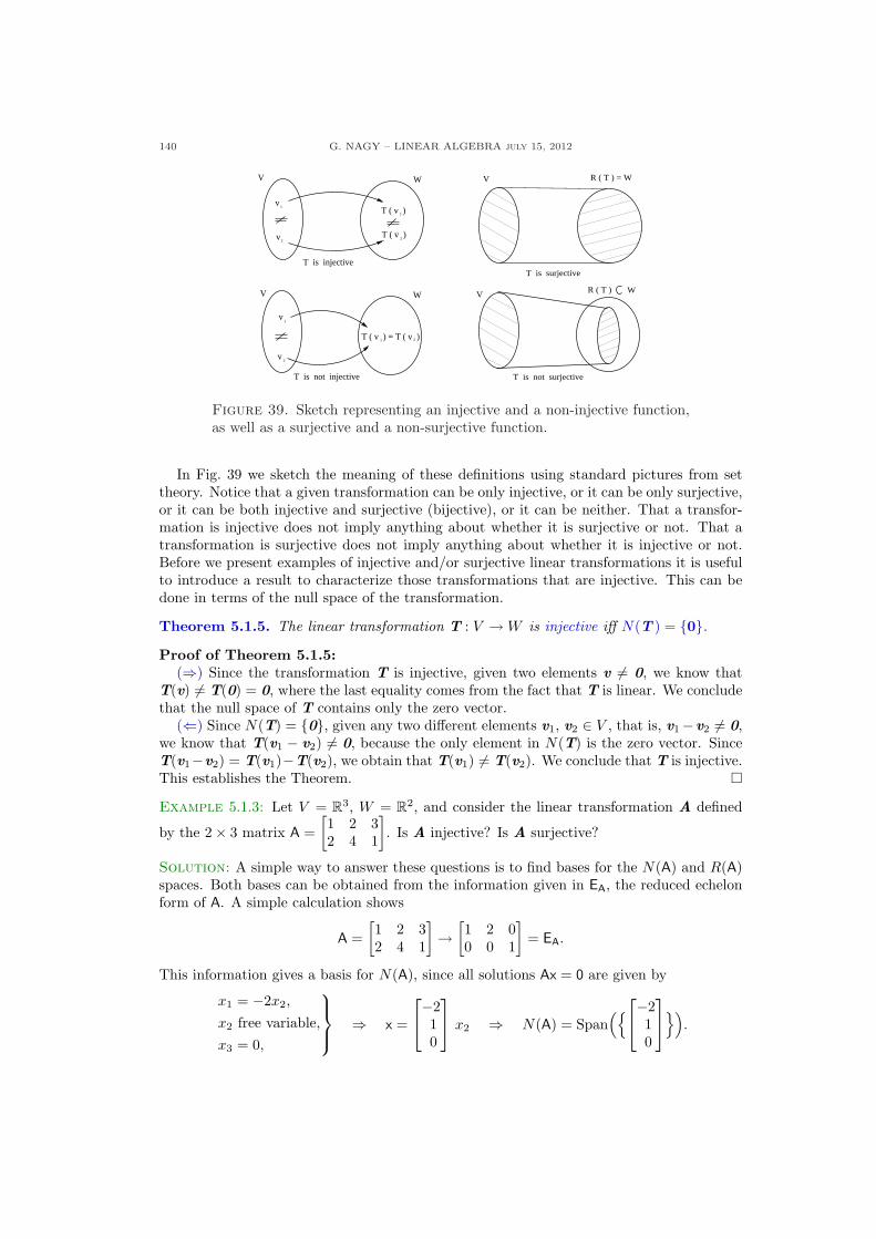
140 G. NAGY – LINEAR ALGEBRA july 15, 2012
W
1
2
2
1
v
v
T ( v ) = T ( v )1 2
V W
T is not injective
T is injective
T ( v )v
vT ( v )1
2
V
WV
T is surjective
T is not surjective
R ( T ) = WV
R ( T )
Figure 39. Sketch representing an injective and a non-injective function,as well as a surjective and a non-surjective function.
In Fig. 39 we sketch the meaning of these definitions using standard pictures from settheory. Notice that a given transformation can be only injective, or it can be only surjective,or it can be both injective and surjective (bijective), or it can be neither. That a transfor-mation is injective does not imply anything about whether it is surjective or not. That atransformation is surjective does not imply anything about whether it is injective or not.Before we present examples of injective and/or surjective linear transformations it is usefulto introduce a result to characterize those transformations that are injective. This can bedone in terms of the null space of the transformation.
Theorem 5.1.5. The linear transformation T : V →W is injective iff N(T ) = {0}.Proof of Theorem 5.1.5:
(⇒) Since the transformation T is injective, given two elements v 6= 0, we know thatT(v) 6= T(0) = 0, where the last equality comes from the fact that T is linear. We concludethat the null space of T contains only the zero vector.
(⇐) Since N(T) = {0}, given any two different elements v1, v2 ∈ V , that is, v1−v2 6= 0,we know that T(v1 − v2) 6= 0, because the only element in N(T) is the zero vector. SinceT(v1−v2) = T(v1)−T(v2), we obtain that T(v1) 6= T(v2). We conclude that T is injective.This establishes the Theorem. ¤
Example 5.1.3: Let V = R3, W = R2, and consider the linear transformation A defined
by the 2× 3 matrix A =[1 2 32 4 1
]. Is A injective? Is A surjective?
Solution: A simple way to answer these questions is to find bases for the N(A) and R(A)spaces. Both bases can be obtained from the information given in EA, the reduced echelonform of A. A simple calculation shows
A =[1 2 32 4 1
]→
[1 2 00 0 1
]= EA.
This information gives a basis for N(A), since all solutions Ax = 0 are given by
x1 = −2x2,
x2 free variable,x3 = 0,
⇒ x =
−210
x2 ⇒ N(A) = Span
({−210
}).
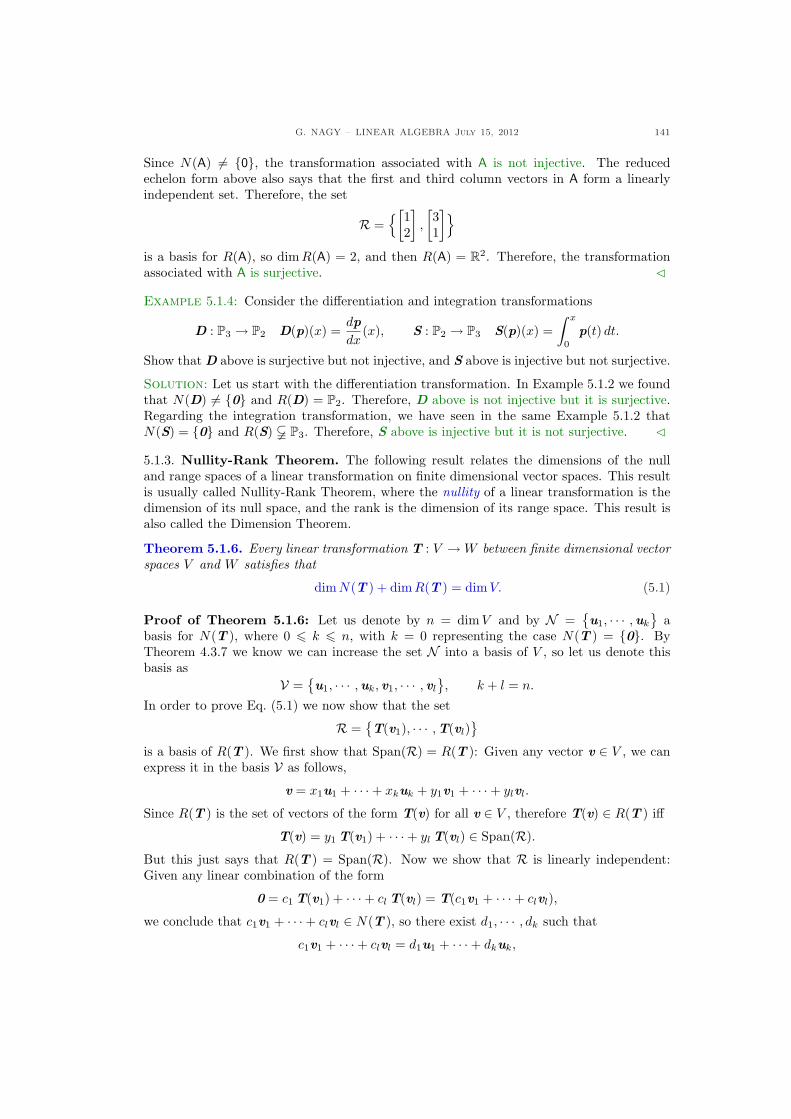
G. NAGY – LINEAR ALGEBRA July 15, 2012 141
Since N(A) 6= {0}, the transformation associated with A is not injective. The reducedechelon form above also says that the first and third column vectors in A form a linearlyindependent set. Therefore, the set
R ={[
12
],
[31
]}
is a basis for R(A), so dim R(A) = 2, and then R(A) = R2. Therefore, the transformationassociated with A is surjective. C
Example 5.1.4: Consider the differentiation and integration transformations
D : P3 → P2 D(p)(x) =dp
dx(x), S : P2 → P3 S(p)(x) =
∫ x
0
p(t) dt.
Show that D above is surjective but not injective, and S above is injective but not surjective.
Solution: Let us start with the differentiation transformation. In Example 5.1.2 we foundthat N(D) 6= {0} and R(D) = P2. Therefore, D above is not injective but it is surjective.Regarding the integration transformation, we have seen in the same Example 5.1.2 thatN(S) = {0} and R(S) & P3. Therefore, S above is injective but it is not surjective. C
5.1.3. Nullity-Rank Theorem. The following result relates the dimensions of the nulland range spaces of a linear transformation on finite dimensional vector spaces. This resultis usually called Nullity-Rank Theorem, where the nullity of a linear transformation is thedimension of its null space, and the rank is the dimension of its range space. This result isalso called the Dimension Theorem.
Theorem 5.1.6. Every linear transformation T : V →W between finite dimensional vectorspaces V and W satisfies that
dim N(T ) + dim R(T ) = dim V. (5.1)
Proof of Theorem 5.1.6: Let us denote by n = dim V and by N ={u1, · · · ,uk
}a
basis for N(T ), where 0 6 k 6 n, with k = 0 representing the case N(T ) = {0}. ByTheorem 4.3.7 we know we can increase the set N into a basis of V , so let us denote thisbasis as
V ={u1, · · · ,uk, v1, · · · , vl
}, k + l = n.
In order to prove Eq. (5.1) we now show that the set
R ={T(v1), · · · ,T(vl)
}
is a basis of R(T ). We first show that Span(R) = R(T ): Given any vector v ∈ V , we canexpress it in the basis V as follows,
v = x1u1 + · · ·+ xkuk + y1v1 + · · ·+ ylvl.
Since R(T ) is the set of vectors of the form T(v) for all v ∈ V , therefore T(v) ∈ R(T ) iff
T(v) = y1 T(v1) + · · ·+ yl T(vl) ∈ Span(R).
But this just says that R(T ) = Span(R). Now we show that R is linearly independent:Given any linear combination of the form
0 = c1 T(v1) + · · ·+ cl T(vl) = T(c1v1 + · · ·+ clvl),
we conclude that c1v1 + · · ·+ clvl ∈ N(T ), so there exist d1, · · · , dk such that
c1v1 + · · ·+ clvl = d1u1 + · · ·+ dkuk,

142 G. NAGY – LINEAR ALGEBRA july 15, 2012
which is equivalent to
d1u1 + · · ·+ dkuk − c1v1 − · · · − clvl = 0.
Since V is a basis we conclude that all coefficients ci and dj must vanish, for i = 1, · · · , land j1, · · · , k. This shows that R is a linearly independent set. Then R is a basis of R(T )and so,
dim N(T ) = k, dim R(T ) = l = n− k.
This establishes the Theorem. ¤One simple consequence of the Dimension Theorem is that an injective linear operator is
also surjective, and vice versa.
Corollary 5.1.7. A linear operator on a finite dimensional vector space is injective iff itis surjective.
The proof is left as an exercise, Exercise 5.1.7. In the case that the linear transformationis given by an m × n matrix, Theorem 5.1.6 establishes a relation between the the nullityand the rank of the matrix.
Corollary 5.1.8. Every m× n matrix A satisfies that dim N(A) + rank(A) = n.
Proof of Corollary 5.1.8: This Corollary is just a particular case of Theorem 5.1.6.Indeed, an m × n matrix A defines a linear transformation given by A : Fn → Fm byA(x) = Ax. Since rank(A) = dim R(A) and dimFn = n, Eq. (5.1) implies that dimN(A) +rank(A) = n. This establishes the Corollary.
An alternative wording of this result uses EA, the reduced echelon form of A. SinceN(A) = N(EA), the dim N(A) is the number of non-pivot columns in EA. We also knowthat rank(A) is the number of pivot columns in EA. Therefore dim N(A) + rank(A) is thetotal number of columns in A, which is n. ¤
G. NAGY – LINEAR ALGEBRA July 15, 2012 143
5.1.4. Exercises.
5.1.1.- Consider the operator A : R2 → R2
given by the matrix A =1
2
»1 11 1
–,
which projects a vector
»x1
x2
–onto the
line x1 = x2 on R2. Is A injective? IsA surjective?
5.1.2.- Fix any real number θ ∈ [0, 2π), anddefine the operator R(θ) : R2 → R2 by
the matrix R(θ) =
»cos(θ) − sin(θ)sin(θ) cos(θ)
–,
which is a rotation by an angle θ coun-terclockwise. Is R(θ) injective? Is R(θ)surjective?
5.1.3.- Let Fn,n be the vector space of alln × n matrices, and fix A ∈ Fn,n. De-termine which of the following transfor-mations T : Fn,n → Fn,n is linear.
(a) T(X) = AX− XA;(b) T(X) = XT ;(c) T(X) = XT + A;(d) T(X) = A tr (X).(e) T(X) = X + XT .
5.1.4.- Fix a vector v ∈ Fn and then definethe function T : Fn → F by T(x) = vT x.Show that T is a linear transformation.Is T a linear operator? Is T a linearfunctional?
5.1.5.- Show that the mapping ∆ : P3 → P1
is a linear transformation, where
∆(p)(x) =d2p
dx2(x)
Is ∆ injective? Is ∆ surjective?
5.1.6.- If the following statement is true,give a proof; if it is false, show it with anexample. If a linear transformation onvector spaces T : V → W is injective,then the image of a linearly independentset in V is a linearly independent set inW .
5.1.7.- Prove the following statement: Alinear operator T : V → V on a finitedimensional vector space V is injectiveiff T is surjective.
5.1.8.- Prove the following statement: IfV and W are finite dimensional vectorspaces with dim V > dim W , then everylinear transformation T : V → W is notinjective.
144 G. NAGY – LINEAR ALGEBRA july 15, 2012
5.2. Properties of linear transformations
5.2.1. The inverse transformation. Bijective transformations are invertible. We nowintroduce the inverse of a bijective transformation and we then show that if the invertibletransformation is linear, then the inverse is again a linear transformation.
Definition 5.2.1. The inverse of a bijective transformation T : V → W is the transfor-mation T−1 : W → V defined for all w ∈W and v ∈ V as follows,
T−1(w) = v ⇔ T(v) = w. (5.2)
The inverse transformation defined above makes sense only in the case that the originaltransformation is bijective, hence bijective transformations are called invertible.
Example 5.2.1: Given a real number θ ∈ (0, π), define the transformation T : R2 → R2
T(x) = Rθ x, Rθ =[cos(θ) − sin(θ)sin(θ) cos(θ)
].
Find the inverse transformation.
Solution: Since the transformation above is a rotation counterclockwise by an angle θ,the inverse transformation is a rotation clockwise by the same angle θ. In other words,(Rθ)−1 = R−θ. Therefore, we conclude that,
T−1 = (Rθ)−1 = R−θ ⇒ (Rθ)−1 =[
cos(θ) sin(θ)− sin(θ) cos(θ)
],
where we have used the relations cos(−θ) = cos(θ) and sin(−θ) = − sin(θ). C
It is common in the literature to define the inverse matrix in an equivalent way, whichwe state here as a Theorem.
Theorem 5.2.2. The transformation T−1 : W → V is the inverse of a bijective transfor-mation T ∈ L(V ) iff holds
T−1 ◦T = IV , T ◦T−1 = IW .
Proof of Theorem 5.2.2:(⇒) Replace w = T(v) into the expression of T−1, that is, T−1(T(v)) = v, for all v ∈ V .
This says that T−1 ◦T is the identity operator in V . In a similar way, replace v = T−1(w)into the expression of T, that is, T(T−1(w)) = w, for all w ∈ W . This says that T−1 ◦Tis the identity in W .
(⇐) If w = T(v), then T−1(w) = T−1(T(v)) = v. Conversely, if v = T−1(w), thenT(v) = T(T−1(w)) = w. We conclude that
T−1(w) = v ⇔ T(v) = w.
This establishes the Theorem. ¤Using this theorem is simple to prove that the result in the previous example can be
generalized to any linear transformation defined by an invertible matrix.
Example 5.2.2: Prove the following statement: If T : Fn → Fn is given by T(x) = Ax withA invertible, then T is invertible and T−1(y) = A−1y.
Solution: Denote S(y) = A−1y. Then S(T(x)) = A−1Ax = x for all x ∈ Fn. This showsthat S ◦T = In. The transformation S also satisfies T(S(y)) = AA−1y = y for all y ∈ Fn.This shows that T ◦ S = In. Therefore, T−1 = S, that is, T−1(y) = A−1y. C
G. NAGY – LINEAR ALGEBRA July 15, 2012 145
Example 5.2.3: Let V = P3, W = P2 and let D : V → W be the differentiation transfor-mation
D(p) =dp
dx.
Is this transformation invertible?
Solution: For every constant polynomial p(x) = c ∈ P3, with c ∈ F, holds D(c) = 0. Sothe null space of the differentiation transformation is non-trivial, that is, N(D) 6= {0}. Sincethe transformation is not injective, it is not bijective. We conclude that the differentiationtransformation above is not invertible. C
Example 5.2.4: Let V = {p ∈ P3 : p(0) = 0}, W = P2 and let D : V → W be thedifferentiation transformation
D(p) =dp
dx.
Is this transformation invertible?
Solution: First, notice that V is a vector space, since given any two elements p, q ∈ V , thelinear combination satisfies (ap+bq)(0) = ap(0)+bq(0) = 0 for all a, b ∈ F, so (ap+bq) ∈ V .Also notice that the only constant polynomial p(x) = c belonging to V is the trivial onec = 0. So, the N(D) = {0} and the differentiation operator is injective. It is simple to seethat this operator is also surjective, since every element in W also belongs to R(D). Indeed,for every constants a2, a1, a0 ∈ F the arbitrary polynomial r(x) = a2x
2+a1x+a0 ∈W is theimage under D of the polynomial p(x) = a2x
3/3+a1x2/2+a0x ∈ V , that is, D(p) = r. So,
W = R(D), the differentiation transformation is surjective, so it is bijective. We concludethat D : V →W is invertible. C
We now show a couple of properties of the inverse transformation. We start showing thatthe inverse of a bijective linear transformation is also linear.
Theorem 5.2.3. If the bijective transformation T : V → W is linear, then the inversetransformation T−1 : W → V is also a linear transformation.
Proof of Theorem 5.2.3: Since the linear transformation T is bijective, hence invertible,we now that for every pair of vectors v1, v2 ∈ V there exist vectors w1, w2 ∈W such that
T(v1) = w1 ⇔ T−1(w1) = v1,
T(v2) = w2 ⇔ T−1(w2) = v2.
Since T : V →W is linear, for all a1, a2 ∈ F holds
T(a1v1 + a2v2) = a1T(v1) + a2T(v2),= a1w1 + a2w2.
By definition of the inverse transformation, the last equation above is equivalent to
T−1(a1w1 + a2w2) = a1v1 + a2v2,
= a1T−1(w1) + a2T
−1(w2).
The last equation above says that T−1 : W → V is a linear transformation. This establishesthe Theorem. ¤
We now show that the inverse of a linear transformation is not only a linear transformationbut it is also a bijection.
Theorem 5.2.4. If the linear transformation T : V → W is a bijection, then the inverselinear transformation T−1 : W → V also is a bijection.
146 G. NAGY – LINEAR ALGEBRA july 15, 2012
Proof of Theorem 5.2.4: Since T is a bijection, it is invertible so, for every w1, w2 ∈Wthere exist v1, v2 ∈ V such that
T−1(w1) = v1 ⇔ T(v1) = w1,
T−1(w2) = v2 ⇔ T(v2) = w2.
In order to show that T−1 is injective pick up w1 and w2 with w1 6= w2 and show that thisimplies v1 6= v2. This is indeed the case, since subtracting the first line from the secondline above we get 0 6= w2 − w1 = T(v2 − v1). Since T is injective, its null space is trivial,so v2 − v1 6= 0. We then conclude that T−1 is injective. This inverse transformation isalso surjective, which is simple to see from the definition of inverse transformation: For allv ∈ V there exists w ∈W such that
T(v) = w ⇔ T−1(w) = v.
We conclude that R(T−1) = V , so T−1 is surjective. This establishes the Theorem. ¤A simple corollary of Theorem 5.2.4 is that T−1 is invertible. It is not difficult to show
that(T−1
)−1 = T. We have mentioned in Sect. 5.1 that a bijective linear transformationis also called and isomorphism. This is the reason for the following definition.
Definition 5.2.5. The vector spaces V and W are called isomorphic iff there exist anisomorphism T : V →W .
Different vector spaces which are isomorphic are the same space from the point of viewof linear algebra. This means that any linear combination performed in one of the spacescan be translated to the other space through the isomorphism, and any linear operatordefined on one of these vector spaces can be translated into a unique linear operator on theother space. This translation is not unique, since there exist infinitely many isomorphismsbetween isomorphic vector spaces.
Example 5.2.5: Show that the vector space V = {p ∈ P3 : p(0) = 0} is isomorphic to P2.
Solution: We have seen in Example 5.2.4 that the differentiation D : V → P2 is a bijection,that is, an isomorphism. Therefore, the spaces V and P2 are isomorphic. We mention thatthis isomorphism relates the polynomials in V and P2 as follows
V 3 p(x) = a3x3 + a2x
2 + a1x 7→ dp
dx= 3a3x
2 + 2a2x + a1 ∈ P2.
C
Example 5.2.6: Show whether the vector spaces F2,2 and F4 are isomorphic or not.
Solution: In order to see if these vector spaces are isomorphic, we need to find a bijectivetransformation between the spaces. We propose the following transformation: T : F2,2 → F4
given by
T([
x11 x12
x21 x22
])=
x11
x12
x21
x22
.
It is simple to see that T is a bijection, so we conclude that F2,2 is isomorphic to F4.We mention that this is not the only isomorphism between these vector spaces. Another
G. NAGY – LINEAR ALGEBRA July 15, 2012 147
isomorphism is the following:
S([
x11 x12
x21 x22
])=
x22
x21
x12
x11
.
C
Example 5.2.7: Show whether the vector spaces P2(F,F) and F3 are isomorphic or not.
Solution: In order to see if these vector spaces are isomorphic, we need to find a bijectivetransformation between the spaces. We propose the following transformation: T : P2 → F3
given by
T(a2x
2 + a1x + a0
)=
a2
a1
a0
.
It is simple to see that T is a bijection, so we conclude that P2 is isomorphic to F3. Wemention that this is not the only isomorphism between these vector spaces. Another iso-morphism is the following:
S(a2x
2 + a1x + a0
)=
a0
a2
a1
.
C
Theorem 5.2.6. Every n-dimensional vector space over the field F is isomorphic to Fn.
The proof is left as Exercise 5.2.5. This result says that nothing essentially differentfrom Fn should be expected from any finite dimensional vector space. On the other hand,infinite dimensional vector spaces are essentially different from Fn. Several results that holdfor finite dimensional vector spaces do not hold for infinite dimensional ones. An exampleis the Nullity-Rank Theorem stated in Section 5.1. One could say that finite dimensionalvector spaces are all alike; every infinite dimensional vector space is special in its own way.
5.2.2. The vector space of linear transformations. Linear transformations from V toW can be combined in different ways to obtain new linear transformations. Two lineartransformations can be added together and a linear transformation can be multiplied by ascalar. The space of all linear transformations with these operations is a vector space. Thisis why a linear transformation can be seen either as a function between vector spaces or asa vector in the space of all linear transformations. As an example of these ideas recall theset of all m × n matrices, denoted as Fm,n. This set is a vector space, since two matricescan be added together and a matrix can be multiplied by a scalar. Since any element in thisset, an m × n matrix A, is also a linear transformation A : Fn → Fm, the set of all lineartransformations from Fn to Fm is a vector space. This is why an m × n matrix A can beinterpreted either as a linear transformation between vector spaces A : Fn → Fm or as avector in the space of matrices, A ∈ Fm,n.
Definition 5.2.7. Given the vector spaces V and W over F, we denote by L(V,W ) theset of all linear transformations from V to W . The set L(V, V ) containing all linearoperators from V to V is denoted as L(V ). Furthermore, given T, S ∈ L(V, W ) and scalarsa, b ∈ F, introduce the linear combination of linear transformations as follows
(aT + bS)(v) = aT(v) + bS(v) for all v ∈ V.
148 G. NAGY – LINEAR ALGEBRA july 15, 2012
Notice that the zero transformation 0 : V → W , given by 0(v) = 0 for all v ∈ V , be-longs to L(V,W ). Moreover, the space L(V, W ) with the addition and scalar multiplicationoperations above is indeed a vector space.
Theorem 5.2.8. The set L(V, W ) of linear transformations from V to W together with theaddition and scalar multiplication operations in Definition 5.2.7 is a vector space.
The proof is to verify all properties in the Definition 4.1.1, and we left it to the reader.We conclude that a linear transformations can be interpreted either as linear maps betweenvector spaces or as vectors in the space L(V, W ). Furthermore, for finite dimensional vectorspaces we have the following result.
Theorem 5.2.9. If V and W are finite dimensional vector spaces, then L(V,W ) is alsofinite dimensional and dim L(V, W ) = (dim V )(dim W ).
Proof of Theorem 5.2.9: We introduce a set of linear transformations and we show thatthis set is indeed a basis for L(V,W ). Before that let us denote n = dim V , m = dimW ,and let us introduce both a basis V = {vi} of V and a basis W = {wj} of W , where theindices take values i = 1, · · · , n and j = 1, · · · , m. The proposal for a basis of L(V,W ) isthe set S = {Sij}, with elements defined as follows,
Sij(vk) ={
wj for i = k,
0 for i 6= k,where i = 1, · · · , n and j = 1, · · · ,m.
So, the map Sij transforms the basis vector vi into the basis vector wj and the rest of thebasis vectors in V into the zero vector in W . We now show that S is a basis for L(V, W ). Letus first prove that S spans L(V, W ). Indeed, for every linear transformation T ∈ L(V,W )and every vector v ∈ V holds,
T(v) =n∑
i=1
viT(vi),
where we used the decomposition v =∑n
i=1 vivi of vector v in the basis V. Since T(vi) ∈W ,it can be decomposed in the W basis as follows,
T(vi) =m∑
j=1
Tij wj .
Replacing the last equation on the previous one we get,
T(v) =n∑
i=1
( m∑
j=1
viTij wj
),
The basis vector wj can be written in terms of the maps Sij as wj = Skj(vk). Choosingindex k to be the value of index i in the sums above we get,
T(v) =n∑
i=1
( m∑
j=1
viTij Sij(vi))
=n∑
i=1
( m∑
j=1
Tij Sij(vivi)).
Here is the critical step: Since Sij(vk) = 0 for k 6= i, the following equation holds,Sij(vivi) = Sij(v). Introducing this property in the equation above we get
T(v) =n∑
i=1
( m∑
j=1
Tij Sij(v))
for all v ∈ V,
G. NAGY – LINEAR ALGEBRA July 15, 2012 149
that is,
T =n∑
i=1
m∑
j=1
Tij Sij ⇒ T ∈ Span(S) ⊂ L(V,W ).
Since the map T is an arbitrary element in L(V, W ), we conclude that L(V, W ) ⊂ Span(S)
,hence Span
(S)= L(V, W ). We now show that S is a linearly independent set. Indeed,
suppose there exist scalars cij satisfying
n∑
i=1
m∑
j=1
cij Sij = 0.
Interchange the sums and evaluate this expression at the basis vector vk, we obtain,
0 =m∑
j=1
( n∑
i=1
cij Sij(vk))
=m∑
j=1
ckj wj .
Since the set W is a basis of W , this implies that the coefficients ckj = 0 for j = 1, · · · ,m.The same argument holds for every k = 1, · · · , n, so we conclude that every coefficient cij
vanishes. The set S is linearly independent, and so, it is a basis for L(V,W ). Since the setcontains nm elements, we conclude that dimL(V,W ) =
(dim V
)(dim W
). This establishes
the Theorem. ¤
5.2.3. Linear functionals and the dual space. An important example of linear trans-formations is the case where the target vector space W is the set of scalars F, the latter,let us recall, is always a vector space. We often use boldface Greek letters to denote linearfunctionals.
Definition 5.2.10. Given the vector space V over F, the linear transformation φ : V → Fis called a linear functional. The vector space of linear functionals L(V,F) is denoted asV ∗ and called the dual space of V .
Example 5.2.8: Show that the projection onto the first component π1 : F3 → F is a linearfunctional, where
π1
(
x1
x2
x3
)= x1.
Solution: We only need to show that π1 is a linear transformation. This is indeed thecase, since for all x, y ∈ F3 and all a, b ∈ F holds
π1(ax + by) = ax1 + by1 = a π1(x) + b π1(y).
Since the map is defined from F3 into F, we conclude that π1 is a linear functional. C
Example 5.2.9: Consider the vector space V = C([a, b],R
)of continuous real-valued func-
tions with domain in the interval [a, b] ⊂ R. Show that the function φ : V → R given belowis a linear functional, where
φ(f ) =∫ b
a
f (x) dx.
150 G. NAGY – LINEAR ALGEBRA july 15, 2012
Solution: We only need to show that the function φ : V → R is a linear transformations.This is the case, since for all f , g ∈ V and all scalars c, d ∈ R holds,
φ(cf + dg) =∫ b
a
(c f (x) + d g(x)
)dx
= c
∫ b
a
f (x) dx + d
∫ b
a
g(x) dx
= c φ(f ) + d φ(g).
We conclude that φ ∈ V ∗. C
Example 5.2.10: Show that the trace map tr : Fn,n → F is a linear functional.
Solution: We have already seen that the trace map is a linear map. Since the trace of amatrix is a scalar, we conclude that the trace map is a linear functional, so tr ∈ (
Fn,n)∗. C
The following result says that the dual space of a finite dimensional vector space isisomorphic to the original vector space. This means that the vector space and its dual are thesame from the point of view of linear algebra. This result is not true for infinite dimensionalvector spaces. This is one reason why infinite dimensional vector spaces, like functionspaces, have more structure and are more complicated to study than finite dimensionalvector spaces.
Theorem 5.2.11. Every finite dimensional vector space is isomorphic to its dual space.
We give two proofs of the same result. In the first proof, we show that an n-dimensionalvector space V is isomorphic to Fn, and that V ∗ is isomorphic to Fn. We conclude that Vis isomorphic to V ∗. The second proof is more abstract, and makes use of what is called adual basis of V ∗.Proof of Theorem 5.2.11: (First proof.) We already know that the ordered basis V =(v1, · · · , vn) of an n-dimensional vector space V determines the isomorphism [ ]v : V → Fn,called the coordinate map, as follows
[x]v = xv =
x1
...xn
v
⇔ x = x1v1 + · · ·+ xnvn.
So, any vector x ∈ V can be associated with a column vector xv ∈ Fn. We now show thatthe dual space V ∗ is also isomorphic to the vector space Fn. Once this is shown we canconclude that V is isomorphic to V ∗. An arbitrary linear functional φ ∈ V ∗ satisfies that
φ(x) = φ(x1v1 + · · ·+ xnvn)
= x1 φ(v1) + · · ·+ xn φ(vn)
=[φ(v1), · · · , φ(vn)
]v
x1
...xn
v
∈ F
for all x ∈ V . Denoting the scalars φi = φ(vi), for i = 1, · · · , n, we introduce the coordinatemap [ ]v : V ∗ → Fn as follows
[φ]v =[φ1, · · · , φn
]v⇔ φ(x) =
[φ1, · · · , φn
]v
x1
...xn
v
.
G. NAGY – LINEAR ALGEBRA July 15, 2012 151
The coordinate map defined on the space V ∗ of linear functionals associates a linear func-tional with a row vector. We have chosen a row vector instead of a column vector so wecan use the matrix-vector product to express the action of φ on a vector x. We concludethat, once a basis is fixed in a finite dimensional vector space, vectors can be associated withcolumn vectors, while linear functionals can be associated with row vectors. This establishesthe Theorem. ¤Proof of Theorem 5.2.11: (Second proof.) Since V ∗ = L(V,F), by Theorem 5.2.9 weknow that dim V ∗ = dim V , where we used the fact the space of scalars, F, is itself a vectorspace and dimF = 1. From the proof of Theorem 5.2.9 we know that a basis of V ∗ is givenby the set of linear functionals Φ = {φi} defined as follows: Given a basis V = {vi} of V ,for i = 1 · · · , n = dim V , the linear functionals φi satisfy
φi : V → F, φi(vk) ={ 1 for i = k,
0 for i 6= k,i, k = 1, · · · , n.
Such a basis Φ is called the dual basis of V. Now that we have a basis in V and a basis in V ∗
it is simple to find an isomorphism between these spaces. We propose the map R : V → V ∗
that changes one basis into the other,
R(vi) = φi.
We now show that this linear transformation R is an isomorphism. It is injective becauseof the following argument. Consider an arbitrary element v ∈ N(R), that is,
R(v) = 0,
where 0 : V → F is the zero map. Introducing the basis decomposition v =∑n
i=1 vi vi inthe expression above we get
0 =n∑
i=1
vi R(vi) =n∑
i=1
vi φi.
Since the set Φ is a basis of V ∗, then Φ is linearly independent, which implies that allcoefficients vi above vanish. We conclude that the vector v =
∑ni=1 vi vi = 0, that is, the
null space of R is trivial. Hence R is injective. This property together with the Nullity-RankTheorem and the fact that dim V ∗ = dim V imply that R is also surjective. We concludethat V is isomorphic to V ∗. This establishes the Theorem. ¤
In the second proof above we introduced a particular basis of the dual space, called thedual basis.
Definition 5.2.12. Given an n-dimensional vector space V with a basis V = {v1, · · · , vn},the dual basis of V is a particular basis Φ = {φ1, · · · , φn} of the dual space V ∗ that fori, j = 1, · · · , n the basis linear functionals φi satisfy
φi(vj) ={ 1 for i = j,
0 for i 6= j.
Example 5.2.11: Find the dual basis of the basis U ⊂ R2, where
U ={
u1 =[11
], u2 =
[−11
]}.
Solution: We need to find a set Φ = {φ1, φ2} of linear functionals satisfying the equations
φ1(u1) = 1, φ2(u1) = 0,
φ1(u2) = 0, φ2(u2) = 1.
152 G. NAGY – LINEAR ALGEBRA july 15, 2012
The two equation on the left can be solved independently of the two equations on theright. Recall that the most general expression for the linear functionals φ1 : R2 → R andφ2 : R2 → R is given by
φ1
([x1
x2
])= a1x1 + a2x2. φ2
([x1
x2
])= b1x1 + b2x2.
We only need to find the components a1, a2 and b1, b2. The a’s can be obtained from thetwo equations on the left above, that is,
φ1(u1) = 1 ⇒ φ1
([11
])= a1 + a2 = 1
φ1(u2) = 0 ⇒ φ1
([−11
])= −a1 + a2 = 0.
⇒a1 = 1/2,
a2 = 1/2.
A similar calculation for φ2 implies,
φ2(u1) = 0 ⇒ φ2
([11
])= b1 + b2 = 0
φ2(u2) = 1 ⇒ φ1
([−11
])= −b1 + b2 = 1.
⇒b1 = −1/2,
b2 = 1/2.
So we conclude that the dual basis of U is the basis Φ = {φ1, φ2} defined as follows
φ1
([x1
x2
])=
12
(x1 + x2), φ1
([x1
x2
])=
12
(−x1 + x2).
If we associate the linear functionals above with row vectors in R2 with the isomorphism
[φ ] =[a1, a2
] ⇔ φ([
x1
x2
])= a1x1 + a2x2,
then, the answer of the Example is given by the row vectors
[φ1] =12
[1, 1
], [φ2] =
12
[−1, 1].
Associating linear functionals components with row vector is useful, because the matrix-vector product can be used to represent the action of a functional onto a vector. Thescalar obtained by the action of a linear functional onto a vector is the scalar given by thematrix-vector product of a row vector times a column vector. For example,
φ1(u1) =12
[1, 1
] [11
]= 1, φ1(u2) =
12
[1, 1
] [−11
]= 0,
φ2(u1) =12
[−1, 1] [
11
]= 0, φ2(u2) =
12
[−1, 1] [−1
1
]= 1.
C
G. NAGY – LINEAR ALGEBRA July 15, 2012 153
5.2.4. Exercises.
5.2.1.- Show that the linear transformationT : F2 → F2 given below is invert-ible and find the inverse transformation,where
T“»x1
x2
–”=
»x1 + x2
3x1 − 2x2
–.
5.2.2.- Consider the vector space
V = {p ∈ P4 : p(0) = 0,dp
δx(0) = 0}.
Then show that the linear transforma-tion ∆ : V → P2 given below is invert-ible and find the inverse transformation,where
∆(p) =d2p
dx2.
5.2.3.- Use the Nullity-Rank Theorem 5.1.6to show that if the finite dimensionalvector spaces V and W are isomorphic,then they have the same dimension.
5.2.4.- Show that the spaces Pn and Fn+1
are isomorphic.
5.2.5.- Use the coordinate map to proveTheorem 5.2.6: Every n-dimensionalvector space over the field F is isomor-phic to Fn.
5.2.6.- Show that the projection onto thei-component πI : Fn → F is a linearfunctional, where
πi
“264
x1
...xn
375”
= xi.
5.2.7.- Let V = P2([0, 1]) be the vectorspace of polynomials up to degree twoon the domain [0, 1] ⊂ R. Show thatthe function φ : V → R given below isa linear functional, where
φ(p) =
Z 1
0
p(x) dx.
5.2.8.- Given the basis U ⊂ R2 below, findits dual basis, where
U =n
u1 =
»21
–, u2 =
»31
–o.
154 G. NAGY – LINEAR ALGEBRA july 15, 2012
5.3. The algebra of linear operators
A vector space where one can multiply two vectors to obtain a third vector is called analgebra. We have seen that the set L(V, W ) is a vector space. A multiplication can bedefined between linear transformations in many different ways, but the most interesting onefrom the physical point of view is the composition of linear transformations. If T : U → Vand S : V →W are linear transformations, then S ◦T : U →W defined as
(S ◦T )(u) = S(T(u)
)for all u ∈ U,
is also a linear transformation. This operation is not defined on a single vector space, but onthree different spaces, namely, L(U, V ), L(V,W ) and L(U,W ). However, in the particularcase that U = V = W the composition of linear operators is defined on a single vector spaceL(V, V ), denoted simply as L(V ). The vector space L(V ) is an algebra of linear operators.We start introducing the definition of an algebra over a field.
Definition 5.3.1. An algebra V over the field F is a vector space V over the field Fequipped with an operation V × V → V called multiplication, satisfying,
u(av + bw) = auv + buw for all u, v,w ∈ V and a, b ∈ F.The algebra is called associative iff the product satisfies
u(vw) = (uv)w for all u, v,w ∈ V.
The algebra is called commutative iff the product satisfies
uv = vu for all u, v ∈ V.
An algebra is called with identity iff there is an element i ∈ V satisfying
iu = ui = u for all u ∈ V.
Maybe the best known example of an algebra is the vector space R3 equipped withthe cross product, also called vector product. This is a non-associative, non-commutativealgebra.
Example 5.3.1: Let S = (e1, e2, e3) be the standard ordered basis of R3 and introduce thecross product of vectors u, v ∈ R3 as follows
u× v = (u2v3 − u3v2) e1 − (u1v3 − u3v1) e2 + (u1v2 − u2v1) e3,
where u = u1 e1 + u2 e2 + u3 e3 and v = v1 e1 + v2 e2 + v3 e3. Show that R3 equipped withthe cross product is a non-associative, non-commutative algebra.
Solution: It is convenient to express the cross product of two vectors using the determinantnotation. Indeed, the cross product above is equal to the following expression
u× v =
∣∣∣∣∣∣
e1 e2 e3
u1 u2 u3
v1 v2 v3
∣∣∣∣∣∣,
where in the first row of the array above contains the basis vectors and the other tworows contain vector components. So, the array above is not a matrix, but the definitionof determinant of a matrix when used on this array produces the cross product of twovectors. This notation is convenient since the cross product shares all the properties thatthe determinant has. For example, the cross product satisfies the following two properties:
u× (av) =
∣∣∣∣∣∣
e1 e2 e3
u1 u2 u3
av1 av2 av3
∣∣∣∣∣∣= a
∣∣∣∣∣∣
e1 e2 e3
u1 u2 u3
v1 v2 v3
∣∣∣∣∣∣= a (u× v);
G. NAGY – LINEAR ALGEBRA July 15, 2012 155
u× (v + w) =
∣∣∣∣∣∣
e1 e2 e3
u1 u2 u3
(v1 + w1) (v2 + w2) (v3 + w3)
∣∣∣∣∣∣
=
∣∣∣∣∣∣
e1 e2 e3
u1 u2 u3
v1 v2 v3
∣∣∣∣∣∣+
∣∣∣∣∣∣
e1 e2 e3
u1 u2 u3
w1 w2 v3
∣∣∣∣∣∣= u× v + u× w.
These two properties show that R3 with the cross product form an algebra. This algebra isnot commutative, since
u× v =
∣∣∣∣∣∣
e1 e2 e3
u1 u2 u3
v1 v2 v3
∣∣∣∣∣∣= −
∣∣∣∣∣∣
e1 e2 e3
v1 v2 v3
u1 u2 u3
∣∣∣∣∣∣= −(v × u).
In particular, notice that the equation above implies that u× u = 0. Finally, this algebra isnot associative as the following argument shows. First, from the definition of cross productit is simple to see that
e1 × e2 = e3, e3 × e1 = e2, e2 × e3 = e1.
Using the first two equations we obtain the following relations,
e1 × (e1 × e2) = e1 × e3 = −e2,
(e1 × e1)× e2 = 0× e2 = 0,
showing that the algebra is not associative. C
In these notes we concentrate on only one example, the algebra of linear operators on avector space, which we now describe in the following result.
Theorem 5.3.2. The vector space L(V ) of linear operators on a vector space V over thefield F equipped with the composition operation is an associative algebra with identity. Thisalgebra is not commutative. Furthermore, dim L(V ) = (dim V )2.
Proof of Theorem 5.3.2: The vector space L(V ) equipped with the composition operationis an algebra. Indeed, given arbitrary linear operators R, S, T ∈ L(V ), the followingequations holds for all v ∈ V , and all scalars all a, b ∈ F,
(T ◦ (aS + bR )
)(v) = T
(aS(v) + bR(v)
)
= aT(S(v)
)+ bT
(R(v)
)
= aT ◦ S(v) + bT ◦R(v).
Therefore, we established that the composition operation satisfies
T ◦ (aS + bR ) = aT ◦ S + bT ◦R,
proving that the vector space L(V ) equipped with the composition operation is and algebra.This algebra is associative, since for all linear operators R, S, T ∈ L(V ), the followingequations holds for all v ∈ V ,
(T ◦ (S ◦R )
)(v) = T
(S ◦R )(v)
)
= T(S(R(v)
))
=(T ◦ S )(
R(v))
=((
T ◦ S ) ◦R )(v),
156 G. NAGY – LINEAR ALGEBRA july 15, 2012
so we conclude thatT ◦ (S ◦R ) =
(T ◦ S ) ◦R.
This algebra has identity, since the identity transformation IV ∈ L(V ) satisfies the equationIV ◦ T = T = T ◦ IV for all T ∈ L(V ). Finally, this algebra is not commutative. We justneed to show one example with this property. We choose V = R2 and the transformationsgiven by matrices
A =[0 11 0
], B =
[0 −11 0
].
We have seen in Example 2.1.3 and 2.1.4 that A is a reflection along the axis x1 = x2 whileB is a rotation by π/2 counterclockwise. It is simple to see that
A ◦ B =[0 11 0
] [0 −11 0
]=
[1 00 −1
]
B ◦ A =[0 −11 0
] [0 11 0
]=
[−1 00 1
].
Therefore, the algebra is not commutative. Finally, the result that dimL(V ) = n2 followsfrom Theorem 5.2.9. This establishes the Theorem. ¤Example 5.3.2: Show that the vector space Fn,n equipped with the matrix multiplicationoperation is an associative algebra with identity.
Solution: We know that Fn,n = L(Fn), and we also know that matrix multiplication isequal to matrix composition, that is, for all A, B ∈ Fn,n and all x ∈ Fn holds
(AB)x = A(Bx) = (A ◦ B)(x) ⇒ AB = A ◦ B.
Therefore, Theorem 5.3.2 implies that Fn,n equipped with the matrix multiplication opera-tion is an associative algebra with identity. C
5.3.1. Polynomial functions of linear operators. Polynomial functions of vectors inan algebra can be defined using linear combinations and multiplications of vectors. In theparticular case of the algebra of linear operators, we use the notation T ◦ S = TS for thecomposition of linear operators in L(V ), and also Tn = TTn−1 for the n-th power of theoperator T, which is defined for all positive integers n > 1. The consistency of this equationfor n = 1 demands the definition T 0 = IV . It follows that functions like the operator-valuedpolynomial below can be defined.
Definition 5.3.3. An operator-valued polynomial of degree n defined by the scalarsa0, · · · , an ∈ F is the function p : L(V )→ L(V ) given by
p(T ) = a0IV + a1T + a2T2 + · · ·+ anT
n.
Example 5.3.3: Consider the vector space V = R2 and given any real number θ introducethe linear operator
Rθ =[cos(θ) − sin(θ)sin(θ) cos(θ)
].
Find the explicit expression of the operator (Rθ)n for any positive integer n.
Solution: We have seen in Example 2.1.5 that the operator Rθ is a rotation by an angleθ counterclockwise. We have also seen in Example 2.3.6 that given two operators Rθ1 andRθ2 , the following formula holds,
Rθ1Rθ2 = Rθ1+θ2 .
G. NAGY – LINEAR ALGEBRA July 15, 2012 157
In the particular case of θ1 = θ2 we obtain(Rθ
)2 = R2θ. Analogously,(Rθ
)3 = Rθ
(Rθ
)2 = RθR2θ = R3θ.
This calculation suggests the formula(Rθ
)n = Rnθ for all positive integer n. We now provethis formula using induction in n. Assume that the formula holds for an arbitrary value ofn and then prove that the formula also holds for (n + 1). Indeed,
(Rθ
)(n+1) = Rθ
(Rθ
)n = RθRnθ = R(n+1)θ.
We then conclude that(Rθ
)n = Rnθ holds for every positive integer n. C
5.3.2. Functions of linear operators. Negative powers of an operator can be defined inthe case that the operator is invertible. In that case, if one defines T−n =
(T−1
)n for anypositive integer n, then the exponents satisfy the usual well known rules that hold when thebase is a real number. That is, for an invertible operator T holds that TmTn = T (m+n)
and(Tm
)n = Tmn, for all integers m, n.It is much more complicated to define further generalizations of these operator-valued
power functions to include fractional exponents and real number exponents. The general ideabehind such generalizations is the same used to define an infinitely differentiable functionof an operator. Such functions are defined using Taylor expansions similar to those usedon real-valued functions. Let us recall that the Taylor expansion centered at x0 ∈ R of aninfinitely differentiable real-valued function is given by
f(x) =∞∑
n=0
f (n)(x0)n!
(x− x0)n = f(x0) + f ′(x0) (x− x0) + f ′′(x0) (x− x0)2 + · · · .
Example 5.3.4: Find the Taylor series expansion of the real valued exponential functionf(x) = ex centered x0 = 0.
Solution: Since x0 = 0, the Taylor expansion formula above has the form
f(x) =∞∑
n=0
f (n)(0)n!
xn = f(0) + f ′(0) x + f ′′(0) x2 + · · · .
Since the exponential function f(x) = ex satisfies that f (n)(x) = f(x) for all positive integern, and f(0) = e0 = 1, we obtain the formula
ex =∞∑
n=0
xn
n!= 1 + x +
x2
2!+
x3
3!+ · · · .
C
Coming back to linear operators on a vector space, one can use the right hand side ofthe Taylor expansion formulas to define a function of a linear operator. However, such ideacannot be applied to linear operators until one understands the meaning of an infinite sumof linear operators. We discuss these ideas in Chapter 9. What we can do right now isto truncate the Taylor series and define a particular type of polynomial functions of linearoperators as follows. Given the real-valued function f : R → R, a vector space V , and alinear operator T ∈ L(V ), introduce the Taylor polynomial fN(T ) for any positive integerN as follows
fN(T ) =N∑
n=0
f (n)(x0)n!
(T− x0 IV
)n,
that is,
fN(T ) = f(x0)IV + f′(x0)
(T− x0 IV
)+ · · ·+ f (N)(x0)
N !(T− x0 IV
)N.
158 G. NAGY – LINEAR ALGEBRA july 15, 2012
The Taylor polynomial of degree N simplify in the case that x0 = 0, that is
fN(T ) =N∑
n=0
f (n)(0)n!
T n = f(0)IV + f′(0)T + · · ·+ f (N)(0)
N !T N .
In order to define the limit of fN(T ) as N → ∞ it is needed a notion of distance betweenlinear operators. We come back to this point in Chapter 9.
5.3.3. The commutator of linear operators. We know that the composition of linearmaps depends on the order the operators appear. We say that function composition is notcommutative. The commutator of two linear operators measures the lack of commutativityof these two operators.
Definition 5.3.4. The commutator, [T,S ], of the operators T, S ∈ L(V ) is given by,
[T,S ] = TS− ST.
In the case where L(V ) = Fn,n the commutator of linear operators defined above agreeswith the definition of matrix commutators introduced at the end of Section 2.3. An imme-diate consequence of the definition above are the following properties.
Theorem 5.3.5. For S, T, U ∈ L(V ) and a, b ∈ F, we have:(a) [T,S ] = −[S,T ], antisymmetry;(b) [aT, bS ] = ab [T,S ], linearity;(c) [U, (T + S)] = [U,T ] + [U,S ], linearity in the right entry;(d) [(U + T),S ] = [U,S ] + [T,S ], linearity in the left entry;(e) [UT,S ] = U [T,S ] + [U,S ]T, left derivation property;(f) [U,TS ] = T [U,S ] + [U,T ]S, right derivation property;(g)
[[S,T ],U
]+
[[U,S ],T
]+
[[T,U ],S
]= 0, Jacobi identity.
Proof of Theorem 5.3.5: Properties (a)-(d) and (g) follow from the definition of commu-tator in a straightforward way. We just show here the left derivation property:
[UT,S ] = UTS− SUT
= UTS− SUT + UST−UST
= (UTS−UST) + (UST− SUT)
= U[T,S ] + [U,S ]T.
The proof of the right derivation property is similar. This establishes the Theorem. ¤The commutator of two linear operators in a vector space is an important concept in
quantum mechanics, since it indicates how well two properties of the physical system de-scribed by these operators can be measured simultaneously. The Heisenberg uncertaintyrelations are statements about the commutators of linear operators.
G. NAGY – LINEAR ALGEBRA July 15, 2012 159
5.3.4. Exercises.
5.3.1.- Let T, S ∈ L(F2) be the linear op-erators given by
T“»x1
x2
–”=
»x2
x1
–, S“»x1
x2
–”=
»0x1
–.
Compute explicitly the operators
(a) 3T− 2S;(b) T ◦ S and S ◦T;(c) T 2 and S 2.
5.3.2.- Find the dimension of the vectorspaces L(F4), L(P2) and L(F3,2).
5.3.3.- Let T : R2 → R2 be the linear oper-ator
T“»x1
x2
–”=
»2x1
4x1 − x2
–.
Find the operator T−2.
5.3.4.- Let T : R2 → R2 be the linear oper-ator
T“»x1
x2
–”=
»x1 + 2x2
3x1 + 4x2
–.
Find the operator
p(T ) = T 2 − 2T− 3 I2.
5.3.5.- Use the definition of the rotationmatrix Rθ given in Example 5.3.2 andthe formula
`Rθ
´n= Rnθ to explicitly
verify that`Rθ
´n`Rθ
´−n= I2.
5.3.6.- Prove the properties (a), (b) and (c)in Theorem 5.3.5.
160 G. NAGY – LINEAR ALGEBRA july 15, 2012
5.4. Transformation components
5.4.1. The matrix of a linear transformation. We have seen in Sections 2.1 and 5.1that every m× n matrix defines a linear transformation between the vector spaces Fn andFm equiped with standard bases. We now show that every linear transformation T : V →Wbetween finite dimensional vector spaces V and W has associated a matrix T. The matrixassociated with such linear transformation is not unique. In order to compute the matrix ofa linear transformation a basis must be chosen both in V and in W . The matrix associatedwith a linear transformation depends on the choice of bases done in V and W . We can saythat the matrix T of a linear transformation T : V → W are the components of T in thegiven bases for V and W , analogously to the components v of a vector v ∈ V in a basis forV studied in Section 4.4.
Definition 5.4.1. Let both V and W be finite dimensional vector spaces over the field Fwith respective ordered bases V =
(v1, · · · , vn
)and W =
(w1, · · · ,wm
), and let the map
[ ]w : W → Fm be the coordinate map on W . The matrix of the linear transformationT : V →W in the ordered bases V and W is the m× n matrix
Tvw =[[T(v1)]w, · · · , [T(vn)]w
]. (5.3)
Let us explain the notation in Eq. (5.3). Given any basis vector vi ∈ V ⊂ V , wherei = 1, · · · , n, we know that T(vi) is a vector in W . Like any vector in a vector space,T(vi) can be decomposed in a unique way in terms of the basis vectors in W, and followingSect. 4.4 we denote them as [T(vi)]w. When there is no possibility of confusion, we denoteTvw simply as T.
Example 5.4.1: Consider the vector spaces V = W = R2, both with the standard basis,
that is, S =(e1 =
[10
], e2 =
[01
]). Let the linear operator T : R2 → R2 be given by
[T
([x1
x2
]
s
)]s
=[3x1 + 2x2
4x1 − x2
]
s
. (5.4)
(a) Find the matrix Tss associated with the linear operator above.
(b) Consider the ordered basis U for R2 given by U =(u1s =
[11
], u2s =
[−11
]). Find the
matrix Tuu associated with the linear operator above.
Solution:Part (a): The definition of Tss implies Tss =
[[T(e1)]s, [T(e2)]s
]. From Eq. (5.4) we
know that [T
([10
]
s
)]s
=[34
]
s
,[T
([01
]
s
)]s
=[
2−1
]
s
.
Therefore,
Tss =[3 24 −1
].
Part (b): By definition Tuu =[ [
T(u1)]u,[T(u2)
]u
]. Notice that from the definition
of basis U we have uis = [ui]s, the column vector form with the components of the basisvectors ui in the standard basis S. So, we can use the definition of T in Eq. (5.4), that is,
[T(u1)]s =[T
([11
]
s
)]s
=[53
]
s
, [T(u2)]s =[T
([−11
]
s
)]s
=[−1−5
]
s
.
G. NAGY – LINEAR ALGEBRA July 15, 2012 161
The results above are vector components in the standard basis S, so we need to translatethese results into components on the U basis. We translate them in the usual way, solvinga linear system for each of these two vectors:
[53
]
s
= y1
[11
]
s
+ y2
[−11
]
s
,
[−1−5
]
s
= z1
[11
]
s
+ z2
[−11
]
s
.
The solutions are the components we are looking for, since
[T(u1)]u =[y1
y2
]
u
, [T(u2)]u =[z1
z2
]
u
.
We can solve both systems above at the same time using the augmented matrix[1 −1
∣∣ 5 −11 1
∣∣ 3 −5
]→
[1 0
∣∣ 4 −30 1
∣∣ −1 −2
].
We have obtained that
[T(u1)]u =[
4−1
]
u
, [T(u2)]u =[−3−2
]
u
.
So we conclude that
Tuu =[
4 −3−1 −2
].
C
From the Definition 5.4.1 it is clear that the matrix associated with a linear transformationT : V →W depends on the choice of bases V and W for the spaces V and W , respectively.In the case that V = W the matrix of the linear operator T : V → V usually means Tvv,that is, to choose the same basis V for the domain space V and the range space V . But thisis not the only choice. One can choose different bases V and V for the domain and rangespaces, respectively. In this case, the matrix associated with the linear operator T is Tvv,that is,
Tvv =[[T(v1)]v, · · · , [T(vn)]v
].
Example 5.4.2: Consider the linear operator defined in Eq. (5.4) in Example 5.4.1. Find theassociated matrices Tus and Tsu, where S and U are the bases defined in that Example 5.4.1.
Solution: The first matrix is simple to obtain, since
Tus =[[T(u1)]s, [T(u2)]s
]
and it is straightforward to compute[T
([11
]
s
)]s
=[53
]
s
,[T
([−11
]
s
)]s
=[−1−5
]
s
,
so, we then conclude that
Tus =[5 −13 −5
]
us
.
We now computeTsu =
[[T(e1)]u, [T(e2)]u
].
From the definition of T we know that[T
([10
]
s
)]s
=[34
]
s
,[T
([01
]
s
)]s
=[
2−1
]
s
.
162 G. NAGY – LINEAR ALGEBRA july 15, 2012
The results are expressed in the standard basis S, so we need to translate them into the Ubasis, as follows[
34
]
s
= y1
[11
]
s
+ y2
[−11
]
s
,
[2−1
]
s
= z1
[11
]
s
+ z2
[−11
]
s
.
The solutions are the components we are looking for, since
[T(e1)]u =[y1
y2
]
u
, [T(e2)]u =[z1
z2
]
u
.
We can solve both systems above at the same time using the augmented matrix[1 −1
∣∣ 3 21 1
∣∣ 4 −1
]→
[2 0
∣∣ 7 10 2
∣∣ 1 −3
].
We have obtained that
[T(e1)]u =12
[71
]
u
, [T(e2)]u =12
[1−3
]
u
.
So we conclude that
Tsu =12
[7 11 −3
]
su
.
C
5.4.2. Action as matrix-vector product. An important property of the matrix associ-ated with a linear transformation T is that the action of the transformation onto a vectorcan be represented as the matrix-vector product between the transformation matrix T thevector components in the appropriate bases.
Theorem 5.4.2. Let V and W be finite dimensional vector spaces with ordered bases Vand W, respectively. Let T : V → W be a linear transformation with associated matrixTvw. Then, the components of the vector T(x) ∈W in the basis W can be expressed as thematrix-vector product
[T(x)]w = Tvw xv,
where xv = [x]v are the components of the vector x ∈ V in the basis V.Proof of Theorem 5.4.2: Given any vector x ∈ V , the definition of its vector componentsin the basis V =
{v1, · · · , vn
}implies that
xv =
x1
...xn
V
⇔ x = x1v1 + · · ·+ xnvn.
Since T is a linear transformation we know that
T(x) = x1 T(v1) + · · ·+ xn T(vn).
The equation above holds in any basis of W , in particular in W, that is,
[T(x)]w = x1 [T(v1)]w + · · ·+ xn [T(vn)]w
=[[T(v1)]w, · · · [T(vn)]w
]
x1
...xn
v
= Tvw xv.
This establishes the Theorem. ¤
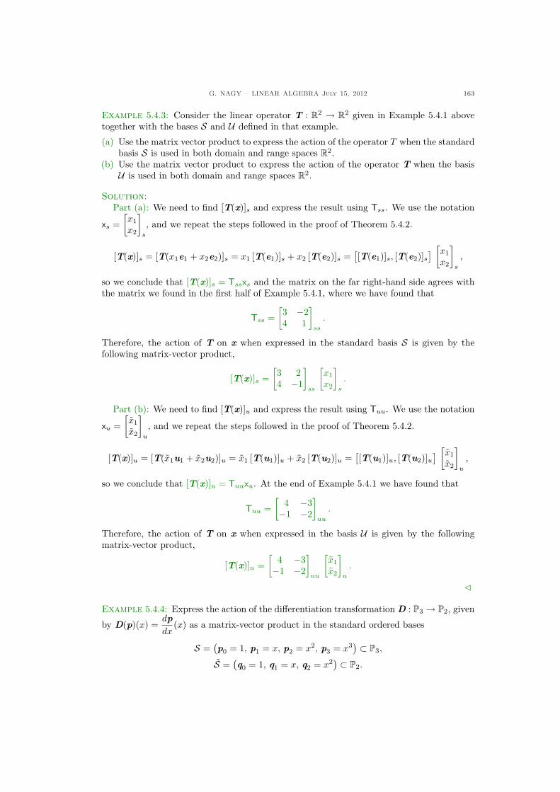
G. NAGY – LINEAR ALGEBRA July 15, 2012 163
Example 5.4.3: Consider the linear operator T : R2 → R2 given in Example 5.4.1 abovetogether with the bases S and U defined in that example.
(a) Use the matrix vector product to express the action of the operator T when the standardbasis S is used in both domain and range spaces R2.
(b) Use the matrix vector product to express the action of the operator T when the basisU is used in both domain and range spaces R2.
Solution:Part (a): We need to find [T(x)]s and express the result using Tss. We use the notation
xs =[x1
x2
]
s
, and we repeat the steps followed in the proof of Theorem 5.4.2.
[T(x)]s = [T(x1e1 + x2e2)]s = x1 [T(e1)]s + x2 [T(e2)]s =[[T(e1)]s, [T(e2)]s
] [x1
x2
]
s
,
so we conclude that [T(x)]s = Tssxs and the matrix on the far right-hand side agrees withthe matrix we found in the first half of Example 5.4.1, where we have found that
Tss =[3 −24 1
]
ss
.
Therefore, the action of T on x when expressed in the standard basis S is given by thefollowing matrix-vector product,
[T(x)]s =[3 24 −1
]
ss
[x1
x2
]
s
.
Part (b): We need to find [T(x)]u and express the result using Tuu. We use the notation
xu =[x1
x2
]
u
, and we repeat the steps followed in the proof of Theorem 5.4.2.
[T(x)]u = [T(x1u1 + x2u2)]u = x1 [T(u1)]u + x2 [T(u2)]u =[[T(u1)]u, [T(u2)]u
] [x1
x2
]
u
,
so we conclude that [T(x)]u = Tuuxu. At the end of Example 5.4.1 we have found that
Tuu =[
4 −3−1 −2
]
uu
.
Therefore, the action of T on x when expressed in the basis U is given by the followingmatrix-vector product,
[T(x)]u =[
4 −3−1 −2
]
uu
[x1
x2
]
u
.
C
Example 5.4.4: Express the action of the differentiation transformation D : P3 → P2, given
by D(p)(x) =dp
dx(x) as a matrix-vector product in the standard ordered bases
S =(p0 = 1, p1 = x, p2 = x2, p3 = x3
) ⊂ P3,
S =(q0 = 1, q1 = x, q2 = x2
) ⊂ P2.
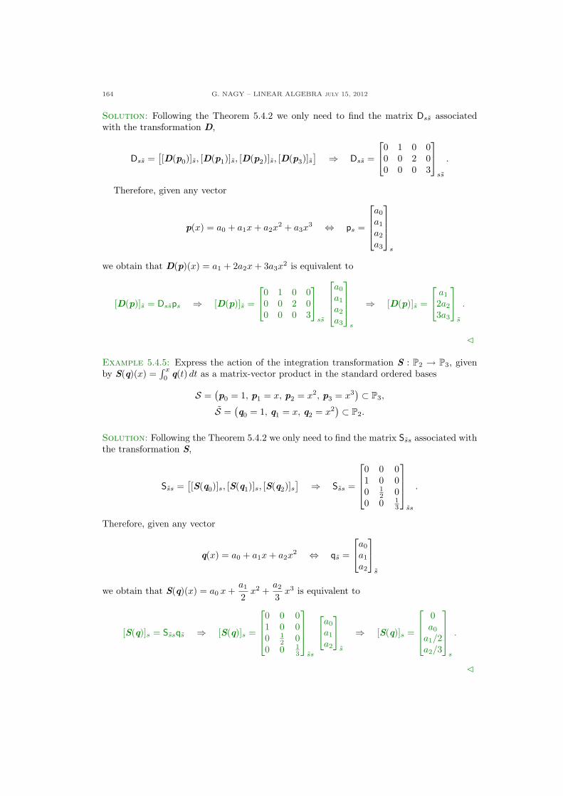
164 G. NAGY – LINEAR ALGEBRA july 15, 2012
Solution: Following the Theorem 5.4.2 we only need to find the matrix Dss associatedwith the transformation D,
Dss =[[D(p0)]s, [D(p1)]s, [D(p2)]s, [D(p3)]s
] ⇒ Dss =
0 1 0 00 0 2 00 0 0 3
ss
.
Therefore, given any vector
p(x) = a0 + a1x + a2x2 + a3x
3 ⇔ ps =
a0
a1
a2
a3
s
we obtain that D(p)(x) = a1 + 2a2x + 3a3x2 is equivalent to
[D(p)]s = Dssps ⇒ [D(p)]s =
0 1 0 00 0 2 00 0 0 3
ss
a0
a1
a2
a3
s
⇒ [D(p)]s =
a1
2a2
3a3
s
.
C
Example 5.4.5: Express the action of the integration transformation S : P2 → P3, givenby S(q)(x) =
∫ x
0q(t) dt as a matrix-vector product in the standard ordered bases
S =(p0 = 1, p1 = x, p2 = x2, p3 = x3
) ⊂ P3,
S =(q0 = 1, q1 = x, q2 = x2
) ⊂ P2.
Solution: Following the Theorem 5.4.2 we only need to find the matrix Sss associated withthe transformation S,
Sss =[[S(q0)]s, [S(q1)]s, [S(q2)]s
] ⇒ Sss =
0 0 01 0 00 1
2 00 0 1
3
ss
.
Therefore, given any vector
q(x) = a0 + a1x + a2x2 ⇔ qs =
a0
a1
a2
s
we obtain that S(q)(x) = a0 x +a1
2x2 +
a2
3x3 is equivalent to
[S(q)]s = Sssqs ⇒ [S(q)]s =
0 0 01 0 00 1
2 00 0 1
3
ss
a0
a1
a2
s
⇒ [S(q)]s =
0a0
a1/2a2/3
s
.
C
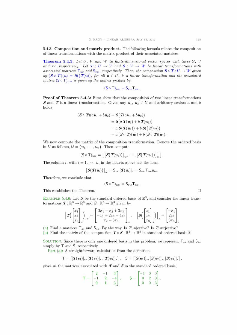
G. NAGY – LINEAR ALGEBRA July 15, 2012 165
5.4.3. Composition and matrix product. The following formula relates the compositionof linear transformations with the matrix product of their associated matrices.
Theorem 5.4.3. Let U , V and W be finite-dimensional vector spaces with bases U , Vand W, respectively. Let T : U → V and S : V → W be linear transformations withassociated matrices Tuv and Svw, respectively. Then, the composition S ◦T : U →W givenby (S ◦ T )(u) = S(
(T(u)
), for all u ∈ U , is a linear transformation and the associated
matrix (S ◦ T)uw is given by the matrix product by
(S ◦ T)uw = SvwTuv.
Proof of Theorem 5.4.3: First show that the composition of two linear transformationsS and T is a linear transformation. Given any u1, u2 ∈ U and arbitrary scalars a and bholds
(S ◦T)(au1 + bu2) = S(T(au1 + bu2)
)
= S(aT(u1) + bT(u2)
)
= aS(T(u1)
)+ bS(
(T(u2)
)
= a (S ◦T)(u1) + b (S ◦T)(u2).
We now compute the matrix of the composition transformation. Denote the ordered basisin U as follows, U =
(u1, · · · ,un
). Then compute
(S ◦ T)uw =[ [
S(T(u1)
)]w, · · · , [S(
T(un))]
w
].
The column i, with i = 1, · · · , n, in the matrix above has the form[S(T(ui)
)]w
= Svw[T(ui)]v = SvwTuvuiu.
Therefore, we conclude that(S ◦ T)uw = SvwTuv.
This establishes the Theorem. ¤
Example 5.4.6: Let S be the standard ordered basis of R3, and consider the linear trans-formations T : R3 → R3 and S : R3 → R3 given by
[T
(
x1
x2
x3
s
)]s
=
2x1 − x2 + 3x3
−x1 + 2x2 − 4x3
x2 + 3x3
s
,[S(
x1
x2
x3
s
)]s
=
−x1
2x2
3x3
s
(a) Find a matrices Tss and Sss. By the way, Is T injective? Is T surjective?(b) Find the matrix of the composition T ◦ S : R3 → R3 in standard ordered basis S.
Solution: Since there is only one ordered basis in this problem, we represent Tss and Sss
simply by T and S, respectively.Part (a): A straightforward calculation from the definitions
T =[[T(e1)]s, [T(e2)]s, [T(e3)]s
], S =
[[S(e1)]s, [S(e2)]s, [S(e3)]s
],
gives us the matrices associated with T and S in the standard ordered basis,
T =
2 −1 3−1 2 −40 1 3
, S =
−1 0 00 2 00 0 3
.
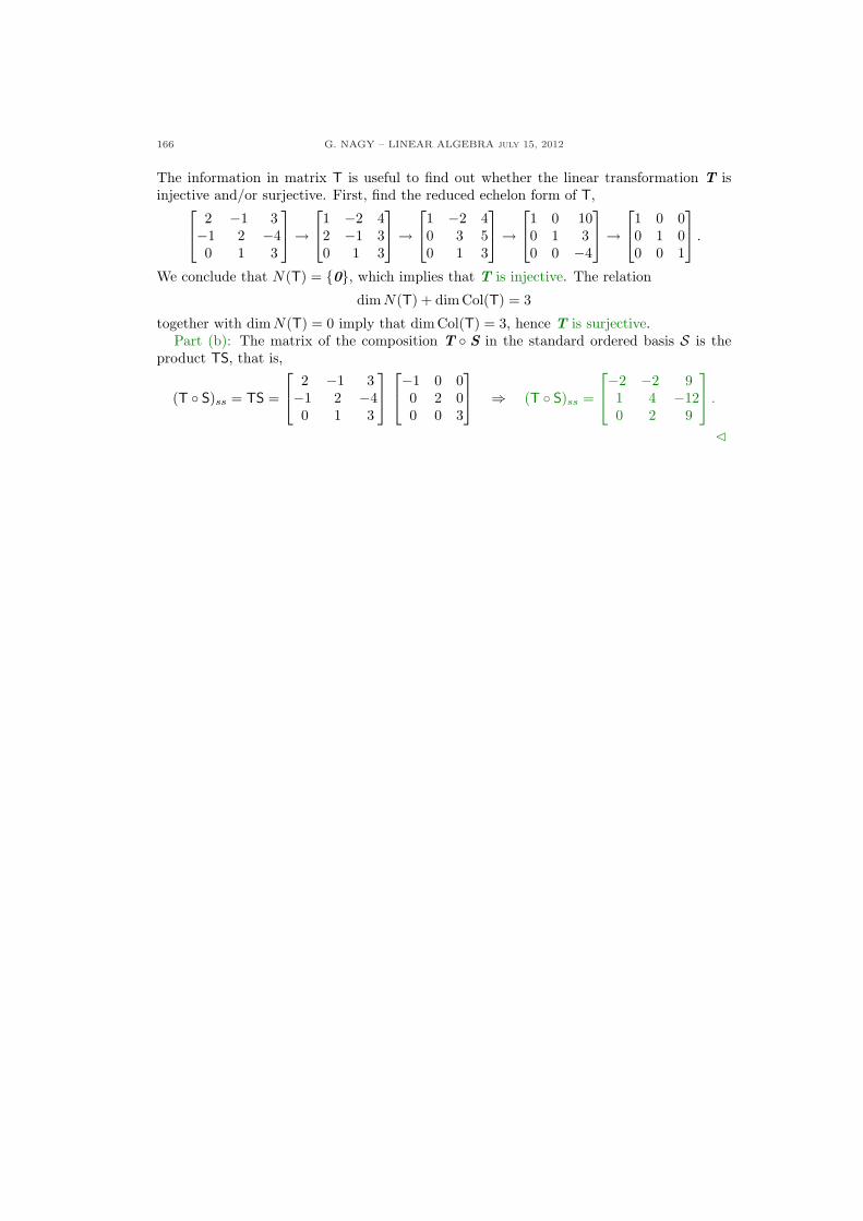
166 G. NAGY – LINEAR ALGEBRA july 15, 2012
The information in matrix T is useful to find out whether the linear transformation T isinjective and/or surjective. First, find the reduced echelon form of T,
2 −1 3−1 2 −40 1 3
→
1 −2 42 −1 30 1 3
→
1 −2 40 3 50 1 3
→
1 0 100 1 30 0 −4
→
1 0 00 1 00 0 1
.
We conclude that N(T) = {0}, which implies that T is injective. The relation
dim N(T) + dim Col(T) = 3
together with dim N(T) = 0 imply that dim Col(T) = 3, hence T is surjective.Part (b): The matrix of the composition T ◦ S in the standard ordered basis S is the
product TS, that is,
(T ◦ S)ss = TS =
2 −1 3−1 2 −40 1 3
−1 0 00 2 00 0 3
⇒ (T ◦ S)ss =
−2 −2 91 4 −120 2 9
.
C
G. NAGY – LINEAR ALGEBRA July 15, 2012 167
5.4.4. Exercises.
5.4.1.- Consider T : R2 → R2 the linearoperator given byhT“»x1
x2
–
s
”is
=
»x1 + x2
−2x1 + 4x2
–
s
,
where S denote the standard orderedbasis of R2. Find the matrix Tuu as-sociated with the linear operator T inand the ordered basis U of R2 given by
“[u1]s =
»11
–
s
, [u2]s =
»12
–
s
”.
5.4.2.- Let T : R3 → R3 be given by
hT“24
x1
x2
x3
35
s
”is
=
24
x1 − x2
−x1 + x2
x1 − x3
35
s
,
S is the standard ordered basis of R3.
(a) Find the matrix Tuu of the linearoperator T in the ordered basis
U =“24
101
35
s
,
24
011
35
s
,
24
110
35
s
”.
(b) Verify that [T(v)]u = Tuuvu, where
vs =
24
112
35
s
.
5.4.3.- Fix an m × n matrix A and definethe linear transformation T : Rn → Rm
as follows: [T(x)]s = Axs, where S ⊂Rn and S ⊂ Rm are standard orderedbases. Show that Tss = A.
5.4.4.- Find the matrix associated with thelinear transformation T : P3 → P2,
T(p)(x) =d2p
dx2(x)− dp
dx(x),
in the standard ordered bases of P3, P2.
5.4.5.- Find the matrices in the standardbases of P3 and P2 of the transforma-tions
S ◦D : P3 → P3, D ◦ S : P2 → P2,
that is, the composition of the differen-tiation and integration transformations,as defined in Sect. 5.1.
168 G. NAGY – LINEAR ALGEBRA july 15, 2012
5.5. Change of basis
In this Section we summarize the main calculations needed to find the change of vectorand linear transformation components under a change of basis. We provide simple formulasto compute this change efficiently.
5.5.1. Vector components. We have seen in Sect. 4.4 that every vector v in a finitedimensional vector space V with an ordered basis V, can be expressed in a unique way asa linear combination of the basis elements, with vv = [v ]v denoting the coefficients in thatlinear combination. These components depend on the basis chosen in V . Given two differentordered bases V, V ⊂ V , the components vv and vv associated with a vector v ∈ V are ingeneral different. We now use the matrix-vector product to find a simple formula relatingvv to vv.
Let us recall the following notation. Given an n-dimensional vector space V , let V andV be two ordered bases of V given by
V =(v1, · · · , vn
)and V =
(v1, · · · , vn
).
Let I : V → V be the identity transformation, that is, I(v) = v for all v ∈ V , and introducethe change of basis matrices
Ivv =[v1v, · · · , vnv
]and Ivv =
[v1v, · · · , vnv
],
where we denoted, as usual, viv = [vi]v and viv = [vi]v, for i = 1, · · · , n. Since the setsV and V are bases of V , the matrices Ivv and Ivv are invertible, and it is not difficult toshow that (Ivv)−1 = Ivv. Finally, introduce the following notation for the change of basismatrices,
P = Ivv and P−1 = Ivv.
Theorem 5.5.1. Let V be a finite dimensional vector space, let V and V be two orderedbases of V , and let P = Ivv be the change of basis matrix. Then, the components xv andxv of any vector x ∈ V in the ordered bases V and V, respectively, are related by the linearequation
xv = P−1xv. (5.5)
Remark: Eq. (5.5) is equivalent to the inverse equation xv = P xv.Proof of Theorem 5.5.1: Let V be an n-dimensional vector space with two ordered basesV =
(v1, · · · , vn
)and V =
(v1, · · · , vn
). Given any vector x ∈ V , then the definition of
vector components xv = [x]v in the basis V implies
xv =
x1
...xn
v
⇔ x = x1v1 + · · ·+ xnvn.
Express the second equation above in terms of components in the ordered basis V,
xv = x1 v1v + · · ·+ xn vnv =[v1v, · · · , vnv
]
x1
...xn
v
⇒ xv = Ivv xv.
We conclude that xv = P−1xv. This establishes the Theorem. ¤
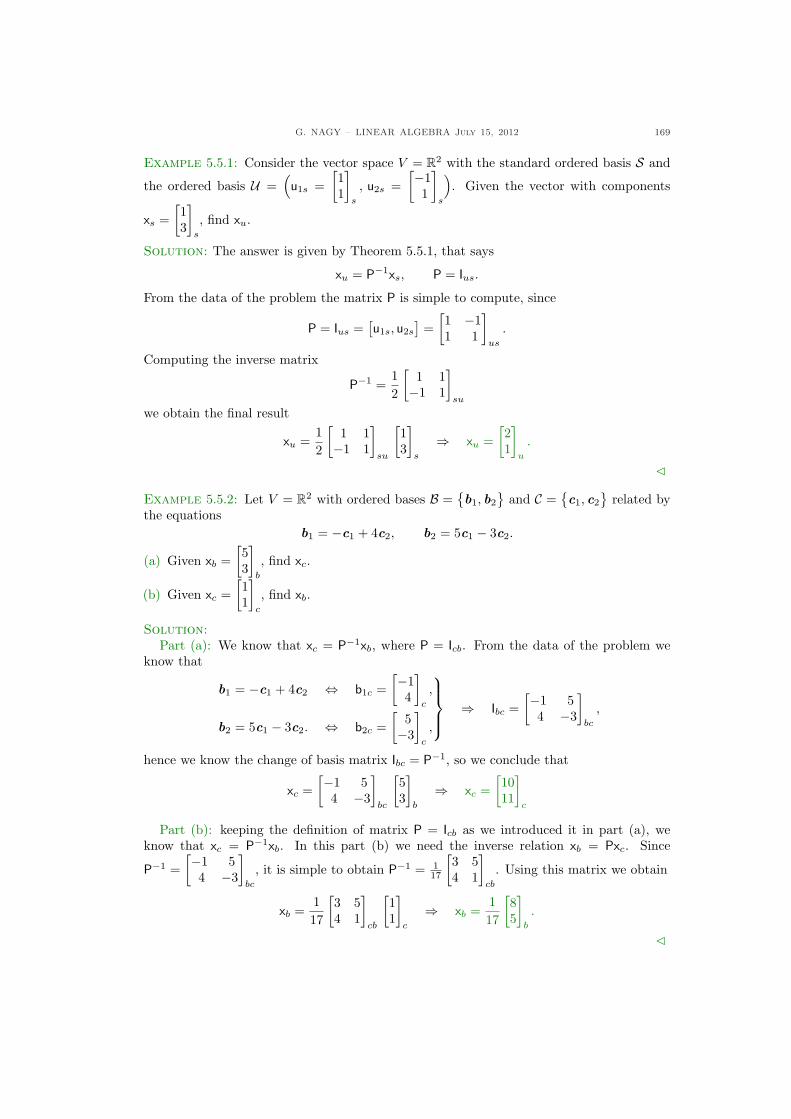
G. NAGY – LINEAR ALGEBRA July 15, 2012 169
Example 5.5.1: Consider the vector space V = R2 with the standard ordered basis S and
the ordered basis U =(u1s =
[11
]
s
, u2s =[−1
1
]
s
). Given the vector with components
xs =[13
]
s
, find xu.
Solution: The answer is given by Theorem 5.5.1, that says
xu = P−1xs, P = Ius.
From the data of the problem the matrix P is simple to compute, since
P = Ius =[u1s, u2s
]=
[1 −11 1
]
us
.
Computing the inverse matrix
P−1 =12
[1 1−1 1
]
su
we obtain the final result
xu =12
[1 1−1 1
]
su
[13
]
s
⇒ xu =[21
]
u
.
C
Example 5.5.2: Let V = R2 with ordered bases B ={b1, b2
}and C =
{c1, c2
}related by
the equationsb1 = −c1 + 4c2, b2 = 5c1 − 3c2.
(a) Given xb =[53
]
b
, find xc.
(b) Given xc =[11
]
c
, find xb.
Solution:Part (a): We know that xc = P−1xb, where P = Icb. From the data of the problem we
know that
b1 = −c1 + 4c2 ⇔ b1c =[−1
4
]
c
,
b2 = 5c1 − 3c2. ⇔ b2c =[
5−3
]
c
,
⇒ Ibc =[−1 5
4 −3
]
bc
,
hence we know the change of basis matrix Ibc = P−1, so we conclude that
xc =[−1 5
4 −3
]
bc
[53
]
b
⇒ xc =[1011
]
c
Part (b): keeping the definition of matrix P = Icb as we introduced it in part (a), weknow that xc = P−1xb. In this part (b) we need the inverse relation xb = Pxc. Since
P−1 =[−1 5
4 −3
]
bc
, it is simple to obtain P−1 = 117
[3 54 1
]
cb
. Using this matrix we obtain
xb =117
[3 54 1
]
cb
[11
]
c
⇒ xb =117
[85
]
b
.
C
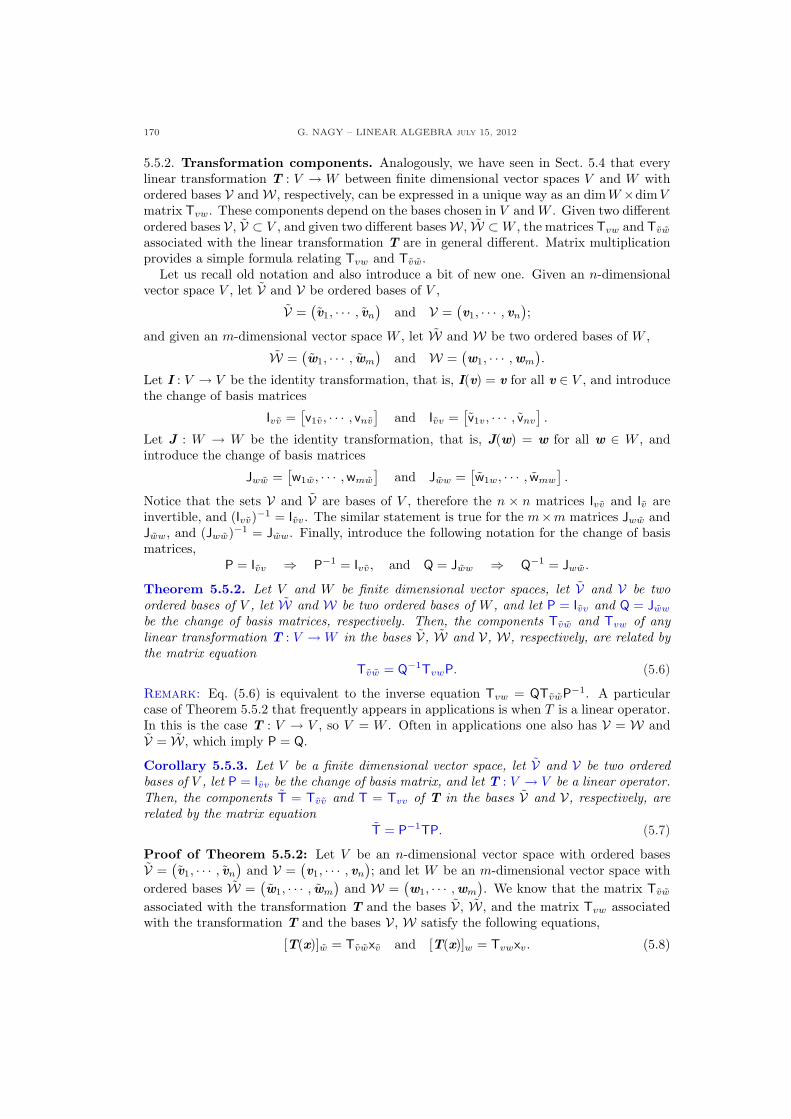
170 G. NAGY – LINEAR ALGEBRA july 15, 2012
5.5.2. Transformation components. Analogously, we have seen in Sect. 5.4 that everylinear transformation T : V → W between finite dimensional vector spaces V and W withordered bases V andW, respectively, can be expressed in a unique way as an dim W ×dim Vmatrix Tvw. These components depend on the bases chosen in V and W . Given two differentordered bases V, V ⊂ V , and given two different basesW, W ⊂W , the matrices Tvw and Tvw
associated with the linear transformation T are in general different. Matrix multiplicationprovides a simple formula relating Tvw and Tvw.
Let us recall old notation and also introduce a bit of new one. Given an n-dimensionalvector space V , let V and V be ordered bases of V ,
V =(v1, · · · , vn
)and V =
(v1, · · · , vn
);
and given an m-dimensional vector space W , let W and W be two ordered bases of W ,
W =(w1, · · · , wm
)and W =
(w1, · · · ,wm
).
Let I : V → V be the identity transformation, that is, I(v) = v for all v ∈ V , and introducethe change of basis matrices
Ivv =[v1v, · · · , vnv
]and Ivv =
[v1v, · · · , vnv
].
Let J : W → W be the identity transformation, that is, J(w) = w for all w ∈ W , andintroduce the change of basis matrices
Jww =[w1w, · · · , wmw
]and Jww =
[w1w, · · · , wmw
].
Notice that the sets V and V are bases of V , therefore the n × n matrices Ivv and Iv areinvertible, and (Ivv)−1 = Ivv. The similar statement is true for the m×m matrices Jww andJww, and (Jww)−1 = Jww. Finally, introduce the following notation for the change of basismatrices,
P = Ivv ⇒ P−1 = Ivv, and Q = Jww ⇒ Q−1 = Jww.
Theorem 5.5.2. Let V and W be finite dimensional vector spaces, let V and V be twoordered bases of V , let W and W be two ordered bases of W , and let P = Ivv and Q = Jww
be the change of basis matrices, respectively. Then, the components Tvw and Tvw of anylinear transformation T : V →W in the bases V, W and V, W, respectively, are related bythe matrix equation
Tvw = Q−1TvwP. (5.6)
Remark: Eq. (5.6) is equivalent to the inverse equation Tvw = QTvwP−1. A particularcase of Theorem 5.5.2 that frequently appears in applications is when T is a linear operator.In this is the case T : V → V , so V = W . Often in applications one also has V = W andV = W, which imply P = Q.
Corollary 5.5.3. Let V be a finite dimensional vector space, let V and V be two orderedbases of V , let P = Ivv be the change of basis matrix, and let T : V → V be a linear operator.Then, the components T = Tvv and T = Tvv of T in the bases V and V, respectively, arerelated by the matrix equation
T = P−1TP. (5.7)
Proof of Theorem 5.5.2: Let V be an n-dimensional vector space with ordered basesV =
(v1, · · · , vn
)and V =
(v1, · · · , vn
); and let W be an m-dimensional vector space with
ordered bases W =(w1, · · · , wm
)and W =
(w1, · · · ,wm
). We know that the matrix Tvw
associated with the transformation T and the bases V, W, and the matrix Tvw associatedwith the transformation T and the bases V, W satisfy the following equations,
[T(x)]w = Tvwxv and [T(x)]w = Tvwxv. (5.8)
G. NAGY – LINEAR ALGEBRA July 15, 2012 171
Since T(x) ∈W , Theorem 5.5.1 says that its components in the bases W andW are relatedby the equation
[T(x)]w = Q−1 [T(x)]w, with Q = Jww.
Therefore, the first equation in (5.8) implies that
Tvwxv = Q−1[T(x)]w
= Q−1Tvwxv
= Q−1TvwP xv, with P = Ivv,
where in the second line above we used the second equation in (5.8), and in the third lineabove we used the inverse form of Theorem 5.5.1. Since the equation above holds for allx ∈ V we conclude that
Tvw = Q−1TvwP.
This establishes the Theorem. ¤
Example 5.5.3: Let S be the standard ordered basis of R2, and let T : R2 → R2 be thelinear operator given by [
T([
x1
x2
]
s
)]s
=[x2
x1
]
s
,
that is, a reflection along the line x2 = x1. Find the matrix Tuu, where the ordered basis Uis given by U =
(u1s =
[11
]
s
, u2s =[−1
1
]
s
).
Solution: From the definition of T is straightforward to obtain Tss, as follows,
Tss =[ [
T([
10
]
s
)]s,[T
([01
]
s
)]s
]⇒ Tss =
[0 11 0
]
ss
.
Since T is a linear operator and we want to compute the matrix Tuu from matrix Tss,we can use Corollary 5.5.3, which says that these matrices are related by the similaritytransformation
Tuu = P−1TssP, where P = Ius.
From the data of the problem we know that
Ius =[u1s, u2s
]us =
[1 −11 1
]
us
,
therefore,
P =[1 −11 1
]
us
, P−1 =12
[1 1−1 1
]
su
.
We then conclude that
Tuu =12
[1 1−1 1
]
su
[0 11 0
]
ss
[1 −11 1
]
us
⇒ Tuu =[1 00 −1
]
uu
.
Remark: We can see in this Example that the matrix associated with the reflection trans-formation T is diagonal in the basis U . For this particular transformation we have that
T(u1) = u1, T(u2) = −u2.
Non-zero vectors v with this property, that T(v) = λv, are called eigenvectors of the operatorT and the scalar λ is called eigenvalue of T. In this example the elements in the basis U areeigenvectors of the reflection operator, and the matrix of T in this special basis is diagonal.Basis formed with eigenvectors of a given linear operator will be studied in a later on. C
172 G. NAGY – LINEAR ALGEBRA july 15, 2012
Example 5.5.4: Let S be the standard ordered basis of R2, and let T : R2 → R2 be thelinear operator given by
[T
([x1
x2
]
s
)]s
=(x1 + x2)
2
[11
]
s
,
that is, a projection along the line x2 = x1. Find the matrix Tuu, where the ordered basis
U =(u1s =
[11
]
s
, u2s =[−1
1
]
s
).
Solution: From the definition of T is straightforward to obtain Tss, as follows,
Tss =[[
T([
10
]
s
)]s,[T
([01
]
s
)]s
]⇒ Tss =
12
[1 11 1
]
ss
.
Since T is a linear operator and we want to compute the matrix Tuu from matrix Tss,we again use Corollary 5.5.3, which says that these matrices are related by the similaritytransformation
Tuu = P−1TssP, where P = Ius.
In Example 5.5.3 we have already computed
P =[1 −11 1
]
us
, P−1 =12
[1 1−1 1
]
su
.
We then conclude that
Tuu =12
[1 1−1 1
]
su
12
[1 11 1
]
ss
[1 −11 1
]
us
⇒ Tuu =[1 00 0
]
uu
.
Remark: Again in this Example we can see that the matrix associated with the reflectiontransformation T is diagonal in the basis U , with diagonal elements equal to one and zero.For this particular transformation we have that the basis vectors in U are eigenvectors of Twith eigenvalues 1 and 0, that is, T(u1) = u1 and T(u2) = 0. C
Example 5.5.5: Let U and V be standard ordered bases of R3 and R2, respectively, letT : R3 → R2 be the linear transformation
[T
(
x1
x2
x3
u
)]v
=[x1 − x2 + x3
x2 − x3
]
v
,
and introduce the ordered bases
U =(u1u =
110
u
, u2u =
011
u
, u3u =
101
u
)⊂ R3,
V =(v1v =
[12
]
v
, v2v =[21
]
v
)⊂ R2.
Find the matrices Tuv and Tuv.
Solution: We start finding the matrix Tuv, which by definition is given by
Tuv =
[T
(
100
u
)]v,[T
(
010
u
)]v,[T
(
001
u
)]v
G. NAGY – LINEAR ALGEBRA July 15, 2012 173
hence we obtain Tuv =[1 −1 10 1 −1
]
uv
. Theorem 5.5.2 says that the matrices Tuv and Tuv
are related by the equation
Tuv = Q−1TuvP, where Q = Jvv and P = Iuu.
From the data of the problem we know that
Iuu =[u1u, u2u, u3u
]uu
=
1 0 11 1 00 1 1
uu
⇒ P =
1 0 11 1 00 1 1
uu
,
Jvv =[v1v, v2v
]vv
=[1 22 1
]
vv
⇒ Q =[1 22 1
]
vv
, Q−1 =13
[−1 22 −1
]
vv
.
Therefore, we need to compute the matrix product
Tuv =13
[−1 22 −1
]
vv
[1 −1 10 1 −1
]
uv
1 0 11 1 00 1 1
uu
and the result is Tuv = 13
[2 0 −4−1 0 5
]
uv
. C
5.5.3. Determinant and trace of linear operators. The type of matrix transformationgiven by Eq. (5.7) will be important later on, so we give such transformations a name.
Definition 5.5.4. The n×n matrices A and B are related by a similarity transformationiff there exists and invertible n× n matrix P such that
B = P−1AP.
Therefore, similarity transformations are transformations among matrices. They appearin two different contexts. The first, or active context, is when matrix A and matrix B aboveare written in the same basis. In this case a similarity transformation changes matrix A intomatrix B. The second, or passive context, is when matrix A and matrix B are two matricescorresponding to the same linear transformation. In this case matrices A and B are writtenin different basis, and the similarity transformation is the change of basis equation for thelinear transformation matrices.
The following results says that, no matter in which contex one uses a similarity transfor-mation, the determinant and trace of a matrix are invariant under similarity transformations.
Theorem 5.5.5. If the square matrices A, B are related by the similarity transformationB = P−1AP, then holds
det(B) = det(A), tr (B) = tr (A).
Proof of Theorem: 5.5.5: The determinant is invariant under similarity transformations,since
det(B) = det(P−1AP) = det(P−1) det(A) det(P) = det(A).The trace is also invariant under similarity transformations, since
tr (B) = tr (P−1AP) = tr (PP−1A) = tr (A).
This establishes the Theorem. ¤We now use this result in the passive context for similarity transformations. This means
that the determinant and trace are independent of the vector basis one uses to write down thematrix. Therefore, a determinant or a trace is an operation on a linear transformation, noton a particular matrix representation of a linear transformation. This observation suggeststhe following definition.
174 G. NAGY – LINEAR ALGEBRA july 15, 2012
Definition 5.5.6. Let V be a finite dimensional vector space, let T ∈ L(V ) be a linearoperator, and let Tvv be the matrix of the linear operator in an arbitrary ordered basis V ofV . The determinant and trace of a linear operator T ∈ L(V ) are respectively given by,
det(T) = det(Tvv), tr (T) = tr (Tvv).
We repeat that the determinant and trace of a linear operator are well-defined, since givenany other ordered basis V of V , we know that the matrices Tvv and Tvv are related by asimilarity transformation. However, the determinant and trace are invariant under similatirytransformations. So no matter what vector basis we use to compute determinant and traceof a linear operator, we always get the same result.
G. NAGY – LINEAR ALGEBRA July 15, 2012 175
5.5.4. Exercises.
5.5.1.- Let U = (u1,u2) be an ordered basisof R2 given by
u1 = 2e1 − 9e2, u2 = e1 + 8e2,
where S = (e1, e2) is the standard or-dered basis of R2.
(a) Find both change of basis matricesIus and Isu.
(b) Given the vector x = 2u1 +u2, findboth xs and xu.
5.5.2.- Consider the ordered bases of R3,B = (b1, b2, b3) and C = (c1, c2, c3),where
c1 = b1 − 2b2 + b3,
c2 = −b2 + 3b3,
c3 = −2b1 + b3.
(a) Find both the change of basis ma-trices Ibc and Icb.
(b) Let x = c1 − 2c2 + 2c3. Find bothxb and xc.
5.5.3.- Consider the ordered bases U and Sof R2 given by
U =“u1s =
»12
–
s
, u2s =
»21
–
s
”,
S =“e1s =
»10
–
s
, e2s =
»01
–
s
o.
(a) Given xu =
»32
–
u
find xs.
(b) Find e1u and e2u.
5.5.4.- Consider the ordered bases of R2
B =“b1s =
»12
–
s
, b2s =
»1−2
–
s
”
C =“c1s =
»11
–
s
, c2s =
»−11
–
s
”,
where S is the standard ordered basis.
(a) Given xc =
»23
–
c
, find xs.
(b) For the same x above, find xb.
5.5.5.- Let S = (e1, e2) be the standard or-dered basis of R2 and B = (b1, b2) be
another ordered basis. Let A =
»1 22 3
–
be the matrix that transforms the com-ponents of a vector x ∈ R2 from the ba-sis S into the basis B, that is, xb = Axs.Find the components of the basis vec-tors b1, b2 in the standard basis, thatis, find b1s and b2s.
5.5.6.- Show that similarity is a transitiveproperty, that is, if matrix A is similarto matrix B, and B is similar to matrixC, then A is similar to C.
5.5.7.- Consider R3 with the standard or-dered basis S and the ordered basis
U =“24
100
35
s
,
24
110
35
s
,
24
111
35
s
”.
Let T : R3 → R3 be the linear operator
hT“24
x1
x2
x3
35
s
”is
=
24
x1 + 2x2 − x3
−x2
x1 + 7x3
35
s
.
Find both matrices Tss and Tuu.
5.5.8.- Consider R2 with ordered bases
S =“e1s =
»10
–
s
, e2s =
»01
–
s
”,
U =“u1s =
»11
–
s
, u2s =
»1−1
–
s
”.
Let T : R2 → R2 be a linear transfor-mation given by
[T(u1)]s =
»13
–
s
, [T(u2)]s =
»31
–
s
.
Find the matrix Tus, then the matricesTss, Tuu, and finally Tsu.
176 G. NAGY – LINEAR ALGEBRA july 15, 2012
Chapter 6. Inner product spaces
An inner product space is a vector space with an additional structure called inner product.This additional structure is an operation that associates each pair of vectors in the vectorspace with a scalar. An inner product extends to any vector space the main conceptsincluded in the dot product, which is defined on Rn. These main concepts include the lengthof a vector, the notioin of perpendicular vectors, and distance between vectors. When theseideas are introduced in function vector spaces, they allow to define the notion of convergenceof an infinite sum of vectors. This, in turns, provides a way to evaluate the accuracy ofapproximate solutions to differential equations.
6.1. Dot product
6.1.1. Dot product in R2. We review the definition of the dot product between vectorsin R2, and we describe its main properties, including the Cauchy-Schwarz inequality. Wethen use the dot product to introduce the notion of length of a vector, distance and anglebetween vectors, including the special case of perpendicular vectors. We then review thatall these notions can be generalized in a straightforward way from R2 to Fn, n > 1.
Definition 6.1.1. Given any vectors x, y ∈ R2 with components x =[x1
x2
], y =
[y1
y2
]in the
standard ordered basis S. The dot product on R2 with is the function · : R2 × R2 → R,
x · y = x1y1 + x2y2.
The dot product norm of a vector x ∈ R2 is the value of the function ‖ ‖ : R2 → R,
‖x‖ =√
x · x.The norm distance between x, y ∈ R2 is the value of the function d : R2 × R2 → R,
d(x, y) = ‖x− y‖.The dot product can be expressed using the transpose of a vector components in the
standard basis, as follows,
xT y = [x1, x2][y1
y2
]= x1y1 + x2y2 = x · y.
The dot product norm and the norm distance can be expressed in term of vector componentsin the standard ordered basis S as follows,
‖x‖ =√
(x1)2 + (x2)2, d(x, y) =√
(x1 − y1)2 + (x2 − y2)2.
The geometrical meaning of the norm and distance is clear form this expression in com-ponents, as is shown in Fig. 40. The norm of a vector is the Euclidean length from theorigin point to the head point of the vector, while the distance between two vectors in theEuclidean distance between the head points of the two vectors.
It is important that we summarize the main properties of the dot product in R2, sincethey are the main guide to construct the generalizations of the dot product to other vectorspaces.
Theorem 6.1.2. The dot product on R2 satisfies, for every vector x, y, z ∈ R2 and everyscalar a, b ∈ R, the following properties:(a) x · y = y · x, (Symmetry);(b) x · (ay + bz) = a (x · y) + b (x · z), (Linearity on the second argument);(c) x · x > 0, and x · x = 0 iff x = 0, (Positive definiteness).
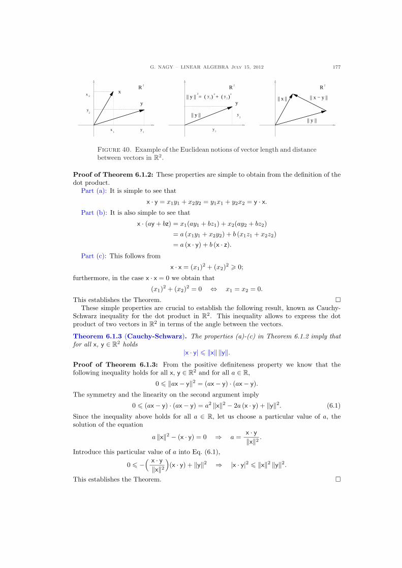
G. NAGY – LINEAR ALGEBRA July 15, 2012 177
y
y
x
1
2
R2
x1
y2
x
y
2y
1
2y
2|| y || = ( ) + ( )
R2
|| y ||
y1
y2
2
|| y ||
R2
|| x || || x − y ||
Figure 40. Example of the Euclidean notions of vector length and distancebetween vectors in R2.
Proof of Theorem 6.1.2: These properties are simple to obtain from the definition of thedot product.
Part (a): It is simple to see that
x · y = x1y1 + x2y2 = y1x1 + y2x2 = y · x.Part (b): It is also simple to see that
x · (ay + bz) = x1(ay1 + bz1) + x2(ay2 + bz2)
= a (x1y1 + x2y2) + b (x1z1 + x2z2)
= a (x · y) + b (x · z).Part (c): This follows from
x · x = (x1)2 + (x2)2 > 0;
furthermore, in the case x · x = 0 we obtain that
(x1)2 + (x2)2 = 0 ⇔ x1 = x2 = 0.
This establishes the Theorem. ¤These simple properties are crucial to establish the following result, known as Cauchy-
Schwarz inequality for the dot product in R2. This inequality allows to express the dotproduct of two vectors in R2 in terms of the angle between the vectors.
Theorem 6.1.3 (Cauchy-Schwarz). The properties (a)-(c) in Theorem 6.1.2 imply thatfor all x, y ∈ R2 holds
|x · y| 6 ‖x‖ ‖y‖.Proof of Theorem 6.1.3: From the positive definiteness property we know that thefollowing inequality holds for all x, y ∈ R2 and for all a ∈ R,
0 6 ‖ax− y‖2 = (ax− y) · (ax− y).
The symmetry and the linearity on the second argument imply
0 6 (ax− y) · (ax− y) = a2 ‖x‖2 − 2a (x · y) + ‖y‖2. (6.1)
Since the inequality above holds for all a ∈ R, let us choose a particular value of a, thesolution of the equation
a ‖x‖2 − (x · y) = 0 ⇒ a =x · y‖x‖2 .
Introduce this particular value of a into Eq. (6.1),
0 6 −( x · y‖x‖2
)(x · y) + ‖y‖2 ⇒ |x · y|2 6 ‖x‖2 ‖y‖2.
This establishes the Theorem. ¤
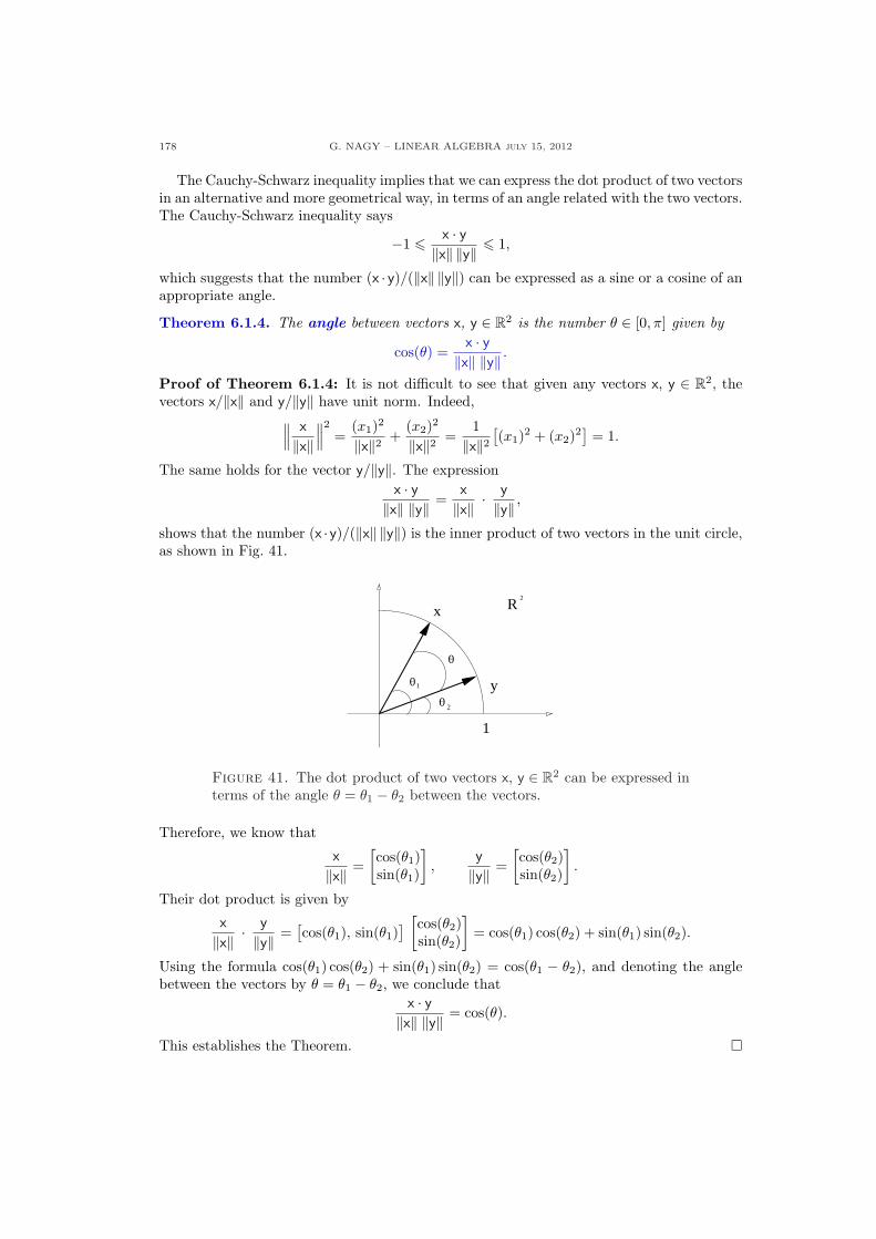
178 G. NAGY – LINEAR ALGEBRA july 15, 2012
The Cauchy-Schwarz inequality implies that we can express the dot product of two vectorsin an alternative and more geometrical way, in terms of an angle related with the two vectors.The Cauchy-Schwarz inequality says
−1 6 x · y‖x‖ ‖y‖ 6 1,
which suggests that the number (x · y)/(‖x‖ ‖y‖) can be expressed as a sine or a cosine of anappropriate angle.
Theorem 6.1.4. The angle between vectors x, y ∈ R2 is the number θ ∈ [0, π] given by
cos(θ) =x · y‖x‖ ‖y‖ .
Proof of Theorem 6.1.4: It is not difficult to see that given any vectors x, y ∈ R2, thevectors x/‖x‖ and y/‖y‖ have unit norm. Indeed,
∥∥∥ x
‖x‖∥∥∥
2
=(x1)2
‖x‖2 +(x2)2
‖x‖2 =1‖x‖2
[(x1)2 + (x2)2
]= 1.
The same holds for the vector y/‖y‖. The expressionx · y‖x‖ ‖y‖ =
x
‖x‖ ·y
‖y‖ ,
shows that the number (x ·y)/(‖x‖ ‖y‖) is the inner product of two vectors in the unit circle,as shown in Fig. 41.
1
R2
0
0
0
1
2
y
x
Figure 41. The dot product of two vectors x, y ∈ R2 can be expressed interms of the angle θ = θ1 − θ2 between the vectors.
Therefore, we know that
x
‖x‖ =[cos(θ1)sin(θ1)
],
y
‖y‖ =[cos(θ2)sin(θ2)
].
Their dot product is given by
x
‖x‖ ·y
‖y‖ =[cos(θ1), sin(θ1)
] [cos(θ2)sin(θ2)
]= cos(θ1) cos(θ2) + sin(θ1) sin(θ2).
Using the formula cos(θ1) cos(θ2) + sin(θ1) sin(θ2) = cos(θ1 − θ2), and denoting the anglebetween the vectors by θ = θ1 − θ2, we conclude that
x · y‖x‖ ‖y‖ = cos(θ).
This establishes the Theorem. ¤
G. NAGY – LINEAR ALGEBRA July 15, 2012 179
Recall the notion of perpendicular vectors.
Definition 6.1.5. The vectors x, y ∈ R2 are orthogonal, denoted as x ⊥ y, iff the angleθ ∈ [0, π] between the vectors is θ = π/2.
The notion of orthogonal vectors in Def. 6.1.5 can be expressed in terms of the dotproduct, and it is equivalent to Pythagoras Theorem on right triangles.
Theorem 6.1.6. Let x, y ∈ R2 be non-zero vectors, then the following statement holds,
x ⊥ y ⇔ x · y = 0 ⇔ ‖x− y‖2 = ‖x‖2 + ‖y‖2.Proof of Theorem 6.1.6: The non-zero vectors x and y ∈ R2 are orthogonal iff θ = π/2,which is equivalent to
x · y‖x‖ ‖y‖ = 0 ⇔ x · y = 0.
The last part of the Proposition comes from the following calculation,
‖x− y‖2 = (x1 − y1)2 + (x2 − y2)2
= (x1)2 + (x2)2 + (y1)2 + (y2)2 − 2(x1y1 + x2y2)
= ‖x‖2 + ‖y‖2 − 2 x · y.Hence, x ⊥ y iff x · y = 0 iff Pythagoras Theorem holds for the triangle with sides given byx, y and hypotenuse x− y. This establishes the Theorem. ¤
Example 6.1.1: Find the length of the vectors x =[12
]and y =
[31
], the angle between
them, and then find a non-zero vector z orthogonal to x.
Solution: We first find the length, that is, the norms of x and y,
‖x‖2 = x · x = xT x =[1 2
],
[12
]= 1 + 4 ⇒ ‖x‖ =
√5,
‖y‖2 = y · y = yT y =[3 1
] [31
]= 9 + 1 ⇒ ‖y‖ =
√10.
We now find the angle between x and y,
cos(θ) =x · y‖x‖ ‖y‖ =
[1 2
] [31
]
√5√
10=
55√
2=
1√2⇒ θ =
π
4.
We now find z such that z ⊥ x, that is,
0 =[z1 z2
] [12
]= z1 + 2z2 ⇒
{z1 = −2z2
z2 free variable
}⇒ z =
[−21
]z2.
C
6.1.2. Dot product in Fn. The notion of dot product reviewed above can be generalizedin a straightforward way from R2 to Fn, n > 1, where F ∈ {R,C}.Definition 6.1.7. The dot product on the vector space Fn, with n > 1, is the function· : Fn × Fn → F given by
x · y = x∗ y,
where x, y denote components in the standard basis of Fn. The dot product norm of avector x ∈ Fn is the value of the function ‖ ‖ : Fn → R,
‖x‖ =√
x · x.
180 G. NAGY – LINEAR ALGEBRA july 15, 2012
The norm distance between x, y ∈ Fn is the value of the function d : Fn × Fn → R,
d(x, y) = ‖x− y‖.The vectors x, y ∈ Fn are orthogonal, denoted as x ⊥ y, iff holds x · y = 0.
Notice that we defined two vectors to be orthogonal by the condition that their dotproduct vanishes. This is the appropriate generalization to Fn of the ideas we saw in R2.The concept of angle is more difficult to study. In the case that F = C is not clear what theangle between vectors mean. In the case F = R and n > 3 we have to define angle by thenumber (x · y)/(‖x‖ ‖y‖). This will be done after we prove the Cauchy-Schwarz inequality,which then is used to show that the number (x · y)/(‖x‖ ‖y‖) ∈ [−1, 1]. The formulas abovefor the dot product, norm and distance can be expressed in terms of the vector componentsin the standard basis as follows,
x · y = x1y1 + · · ·+ xnyn,
‖x‖ =√|x1|2 + · · ·+ |xn|2,
d(x, y) =√|x1 − y1|2 + · · ·+ |xn − yn|2,
where we used the standard notation x =
x1
...xn
, y =
y1
...yn
, and |xi|2 = xixi, for i = 1, · · ·n.
In the particular case that F = R all the vector components are real numbers, so xi = xi.
Example 6.1.2: Find whether x is orthogonal to y and/or z, where
x =
1234
, y =
−54−32
, z =
−4−321
.
Solution: We need to compute the dot products x · y and x · z. We obtain
xT y =[1 2 3 4
]
−54−32
= −5 + 8− 9 + 8 ⇒ x · y = 2 ⇒ x 6⊥ y,
xT z =[1 2 3 4
]
−4−321
= −4− 6 + 6 + 4 ⇒ x · z = 0 ⇒ x ⊥ z.
C
Example 6.1.3: Find x · y, where x =
2 + 3ii
1− i
and y =
2i1
1 + 3i
.
Solution: The first product x · y is given by
x∗ y =[2− 3i −i 1 + i
]
2i1
1 + 3i
= (2− 3i)(2i)− i + (1 + i)(1 + 3i),
so x · y = 4i + 6− i + 1− 3 + i + 3i, that is, x · y = 4 + 7i. C
The dot product satisfies the following properties.
G. NAGY – LINEAR ALGEBRA July 15, 2012 181
Theorem 6.1.8. The dot product on Fn, with n > 1, satisfies for every vector x, y, z ∈ Fn
and every scalar a, b ∈ F, the following properties:(a1) x · y = y · x, (Symmetry F = R);(a2) x · y = y · x, (Conjugate symmetry, for F = C);(b) x · (ay + bz) = a (x · y) + b (x · z), (Linearity on the second argument);(c) x · x > 0, and x · x = 0 iff x = 0, (Positive definiteness).
Proof of Theorem 6.1.8: Use the expression of the dot product in terms of the vectorcomponents. The property in (a1) can be established as follows,
x · y = x1y1 + · · ·+ xnyn = y1x1 + · · ·+ ynxn = y · x.The property in (a2) can be established as follows,
x · y = x1y1 + · · ·+ xnyn = (y1x1 + · · ·+ ynxn) = y · x.The property in (b) is shown in a similar way,
x · (ay + bz) = x∗(a y + b z) = a x∗ y + b x∗ z = a (x · y) + b (x · z).The property in (c) follows from
x · x = x∗ x = |x1|2 + · · ·+ |xn|2 > 0;
furthermore, in the case that x · x = 0 we obtain that
|x1|2 + · · ·+ |xn|2 = 0 ⇔ x1 = · · · = xn = 0 ⇔ x = 0.
This establishes the Theorem. ¤The positive definiteness property (c) above shows that the dot product norm is indeed a
real-valued and not a complex-valued function, since x · x > 0 implies that ‖x‖ =√
x · x ∈ R.In the case of F = R, the symmetry property and the linearity in the second argumentproperty imply that the dot product on Rn is also linear in the first argument. This is areason to call the dot product on Rn a bilinear form. Finally, notice that in the case F = C,the conjugate symmetry property and the linearity in the second argument imply that thedot product on Cn is conjugate linear on the first argument. The proof is the following:
(ay + bz) · x = x · (ay + bz) = a (x · y) + b (x · z) = a (x · y) + b (x · z),that is, for all x, y, z ∈ Cn and all a, b ∈ C holds
(ay + bz) · x = a (y · x) + b (z · x).Hence we say that the dot product on Cn is conjugate linear in the first argument.
Example 6.1.4: Compute the dot product of x =[2 + 3i6i− 9
]with y =
[3i2
].
Solution: This is a straightforward computation
x · y = x∗y =[2− 3i −6i− 9
] [3i2
]= 6i + 9− 12i− 18 ⇒ x · y = −9− 6i.
Notice that x = (2 + 3i)x, with x =[
13i
], so we could use the conjugate linearity in the first
argument to compute
x · y =((2 + 3i)x
) · y = (2− 3i) (x · y) = (2− 3i)[1 −3i
] [3i2
]= (2− 3i)(3i− 6i),
and we obtain the same result, x · y = −9− 6i. Finally, notice that y · x = −9 + 6i. C
An important result is that the dot product in Fn satisfies the Cauchy-Schwarz inequality.
182 G. NAGY – LINEAR ALGEBRA july 15, 2012
Theorem 6.1.9 (Cauchy-Schwarz). The properties (a1)-(c) in Theorem 6.1.8 imply thatfor all x, y ∈ Fn holds
|x · y| 6 ‖x‖ ‖y‖.Remark: The proof of the Cauchy-Schwarz inequality only uses the three properties of thedot product presented in Theorem 6.1.8. Any other function f : Fn × Fn → F having thesethree properties also satisfies the Cauchy-Schwarz inequality.Proof of Theorem 6.1.9: From the positive definiteness property we know that thefollowing inequality holds for all x, y ∈ Fn and for all a ∈ F,
0 6 ‖ax− y‖2 = (ax− y) · (ax− y).
The symmetry and the linearity on the second argument imply
0 6 (ax− y) · (ax− y) = a a ‖x‖2 − a (x · y)− a (y · x) + ‖y‖2. (6.2)
Since the inequality above holds for all a ∈ F, let us choose a particular value of a, thesolution of the equation
a a ‖x‖2 − a (x · y) = 0 ⇒ a =x · y‖x‖2 .
Introduce this particular value of a into Eq. (6.2),
0 6 −( x · y‖x‖2
)(x · y) + ‖y‖2 ⇒ |x · y|2 6 ‖x‖2 ‖y‖2.
This establishes the Theorem. ¤In the case F = R, the Cauchy-Schwarz inequality in Rn implies that the number
(x · y)/(‖x‖ ‖y‖) ∈ [−1, 1], which is a necessary and sufficient condition for the followingdefinition of angle between two vectors in Rn.
Definition 6.1.10. The angle between vectors x, y ∈ Rn is the number θ ∈ [0, π] given by
cos(θ) =x · y‖x‖ ‖y‖ .
The dot product norm function in Definition 6.1.7 satisfies the following properties.
Theorem 6.1.11. The dot product norm function on Fn, with n > 1, satisfies for everyvector x, y ∈ Fn and every scalar a ∈ F the following properties:(a) ‖x‖ > 0, and ‖x‖ = 0 iff x = 0, (Positive definiteness);(b) ‖ax‖ = |a| ‖x‖, (Scaling);(c) ‖x + y‖ 6 ‖x‖+ ‖y‖, (Triangle inequality).
Proof of Theorem 6.1.11: Properties (a) and (b) are straightforward to show from thedefinition of dot product, and their proof is left as an exercise. We show here how toobtain the triangle inequality, property (c). The proof uses the Cauchy-Schwarz inequalitypresented in Theorem 6.1.9. Given any vectors x, y ∈ Fn holds
‖x + y‖2 = (x + y) · (x + y)
= ‖x‖2 + (x · y) + (y · x) + ‖y‖26 ‖x‖2 + 2 |x · y|+ ‖y‖2
6 ‖x‖2 + 2 ‖x‖ ‖y‖+ ‖y‖2 =(‖x‖+ ‖y‖)2
,
We conclude that ‖x + y‖2 6(‖x‖+ ‖y‖)2. This establishes the Theorem. ¤
A vector v ∈ Fn is called normal or unit vector iff ‖v‖ = 1. Examples of unit vectors arethe standard basis vectors. Unit vectors parallel to a given vector are simple to find.
G. NAGY – LINEAR ALGEBRA July 15, 2012 183
Theorem 6.1.12. If v ∈ Fn is non-zero, thenv
‖v‖ is a unit vector parallel to v.
Proof of Theorem 6.1.12: Notice that u =v
‖v‖ is parallel to v, and it is straightforward
to check that u is a unit vector, since
‖u‖ =∥∥∥ v
‖v‖∥∥∥ =
1‖v‖ ‖v‖ = 1.
This establishes the Theorem. ¤
Example 6.1.5: Find a unit vector parallel to x =
123
.
Solution: First compute the norm of x,
‖x‖ =√
1 + 4 + 9 =√
14,
therefore u =1√14
123
is a unit vector parallel to v. C
184 G. NAGY – LINEAR ALGEBRA july 15, 2012
6.1.3. Exercises.
6.1.1.- Consider the vector space R4 withstandard basis S and dot product. Findthe norm of u and v, their distance andthe angle between them, where
u =
2664
21−4−2
3775 , v =
2664
1−11−1
3775 .
6.1.2.- Use the dot product on R2 to findtwo unit vectors orthogonal to
x =
»32
–.
6.1.3.- Use the dot product on C2 to find aunit vector parallel to
x =
»1 + 2i2− i
–.
6.1.4.- Consider the vector space R2 withthe dot product.
(a) Give an example of a linearly inde-pendent set {x, y} with x 6⊥ y.
(b) Give an example of a linearly de-pendent set {x, y} with x ⊥ y.
6.1.5.- Consider the vector space Fn withthe dot product, and let Re denote thereal part of a complex number. Showthat for all x, y ∈ Fn holds
‖x− y‖2 = ‖x‖2 + ‖y‖2 − 2Re(x · y).
6.1.6.- Use the result in Exercise 6.1.5above to prove the following generaliza-tions of the Pythagoras Theorem to Fn
with the dot product.
(a) For x, y ∈ Rn holds
x ⊥ y ⇔ ‖x + y‖2 = ‖x‖2 + ‖y‖2.(b) For x, y ∈ Cn holds
x ⊥ y ⇒ ‖x + y‖2 = ‖x‖2 + ‖y‖2.
6.1.7.- Prove that the parallelogram lawholds for the dot product norm in Fn,that is, show that for all x, y ∈ Fn holds
‖x + y‖2 + ‖x− y‖2 = 2‖x‖2 + 2‖y‖2.This law states that the sum of thesquares of the lengths of the four sidesof a parallelogram formed by x and yequals the sum of the square of thelengths of the two diagonals.
G. NAGY – LINEAR ALGEBRA July 15, 2012 185
6.2. Inner product
6.2.1. Inner product. An inner product on a vector space is a generalization of the dotproduct on Rn or Cn introduced in Sect. 6.1. The inner product is not defined with aparticular formula, or requiring a particular basis in the vector space. Instead, the innerproduct is defined by a list of properties that must satisfy. We did something similar whenwe introduced the concept of a vector space. In that case we defined a vector space as a setof any kind of elements where linear combinations are possible, instead of defining the setby explicitly giving its elements.
Definition 6.2.1. Let V be a vector space over the scalar field F ∈ {R,C}. A function〈 , 〉 : V × V → F is called an inner product iff for every x, y, z ∈ V and every a, b ∈ Fthe function 〈 , 〉 satisfies:
(a1) 〈x,y〉 = 〈y,x〉, (Symmetry, for F = R);(a2) 〈x,y〉 = 〈y,x〉, (Conjugate symmetry, for F = C);(b) 〈x, (ay + bz)〉 = a〈x,y〉+ b〈x, z〉, (Linearity on the second argument);(c) 〈x,x〉 > 0, and 〈x,x〉 = 0 iff x = 0, (Positive definiteness).An inner product space is a pair
(V, 〈 , 〉) of a vector space with an inner product.
Different inner products can be defined on a given vector space. The dot product is aninner product in Fn. A different inner product can be defined in Fn, as can be seen in thefollowing example.
Example 6.2.1: We show that Rn can have different inner products.(a) The dot product on Rn is an inner product, since the expression
〈x, y〉 = xTs ys =
[x1 · · · xn
]s
y1
...yn
s
= x1y1 + · · ·+ xnyn, (6.3)
satisfies all the properties in Definition 6.2.1, with S the standard ordered basis in Rn.(b) A different inner product in Rn can be introduced by a formula similar to the one in
Eq. (6.3) by choosing a different ordered basis. If U is any ordered basis of Rn, then
〈x, y〉 = xTuyu.
defines an inner product on Rn. The inner product defined using the basis U is not equalto the inner product defined using the standard basis S. Let P = Ius be the change ofbasis matrix, then we know that xu = P−1xs. The inner product above can be expressedin terms of the S basis as follows,
〈x, y〉 = xTs Mys, M =
(P−1
)T (P−1
),
and in general, M 6= In. Therefore, the inner product above is not equal to the dotproduct. Also, see Example 6.2.2.
C
Example 6.2.2: Let S be the standard ordered basis in R2, and introduce the ordered basisU as the following rescaling of S,
U =(u1 =
12e1,u2 =
13e2
).
Express the inner product 〈x, y〉 = xTuyu in terms of xs and ys. Is this inner product the
same as the dot product?
186 G. NAGY – LINEAR ALGEBRA july 15, 2012
Solution: The definition of the inner product says that 〈x, y〉 = xTuyu. Introducing the
notation xu =[x1
x2
]
u
and yu =[y1
y2
]
u
, we obtain the usual expression 〈x, y〉 = x1y1 + x2y2.
The components xu and xs are related by the change of basis formula
xu = P−1xs, P = Ius =[1/2 00 1/3
]
us
⇒ P−1 =[2 00 3
]
su
=(P−1
)T.
Therefore,
〈x, y〉 = xTuyu = xT
s
(P−1
)TP−1ys =
[x1, x2
]s
[4 00 9
]
su
[y1
y2
]
s
where we used the standard notation xs =[x1
x2
]
s
and ys =[y1
y2
]
s
. We conclude that
〈x, y〉 = xTs
(P−1
)2ys ⇔ 〈x, y〉 = 4x1y1 + 9x2y2.
The inner product 〈x, y〉 = xTuyu is different from the dot product x · y = xT
s ys. C
Example 6.2.3: Determine whether the function 〈 , 〉 : R3 × R3 → R below is an innerproduct in R3, where
〈x, y〉 = x1y1 + x2y2 + x3y3 + 3x1y2 + 3x2y1.
Solution: The function 〈 , 〉 seems to be symmetric and linear. It is not so clear whetherthis function is positive, because of the presence of crossed terms. So, before spending timeto prove the symmetry and linearity properties, we first concentrate on the property thatmight fail, positivity. If positivity fails, we don’t need to prove the remaining properties.The crossed terms 3(x1y2 + x2y1) in the definition of the inner product suggest that theproduct is not positive, since the factor 3 makes them too important compared with theother terms. Let us try to find an example, that is a vector x 6= 0 such that 〈x, x〉 6 0. Letus try with
x =
1−10
⇒ 〈x, x〉 = 12 + (−1)2 + 02 + 3[(1)(−1) + (−1)(1)] = 2− 6 = −4.
Since 〈x, x〉 = −4, the function 〈 , 〉 is not positive, hence it is not an inner product. C
Example 6.2.4: Consider the vector space Fm,n of all m× n matrices. Show that an innerproduct on that space is the function 〈 , 〉F : Fm,n × Fm,n → F
〈A, B〉F = tr (A∗B).
The inner product is called Frobenius inner product.
Solution: We show that the Frobenius function 〈 , 〉F above satisfies the three propertiesin Def. 6.2.1. We use the component notation A = [Aij ], B = [Bkl], with i, k = 1, · · · ,mand j, l = 1, · · · , n, so
(A∗B)jl =m∑
i=1
(A
T )ji
Bil =m∑
i=1
AijBil ⇒ 〈A,B〉F =n∑
j=1
n∑
i=1
AijBij .
The first property is satisfied, since
〈A,A〉F = tr (A∗A) =n∑
j=1
m∑
i=1
∣∣Aij
∣∣2 > 0,
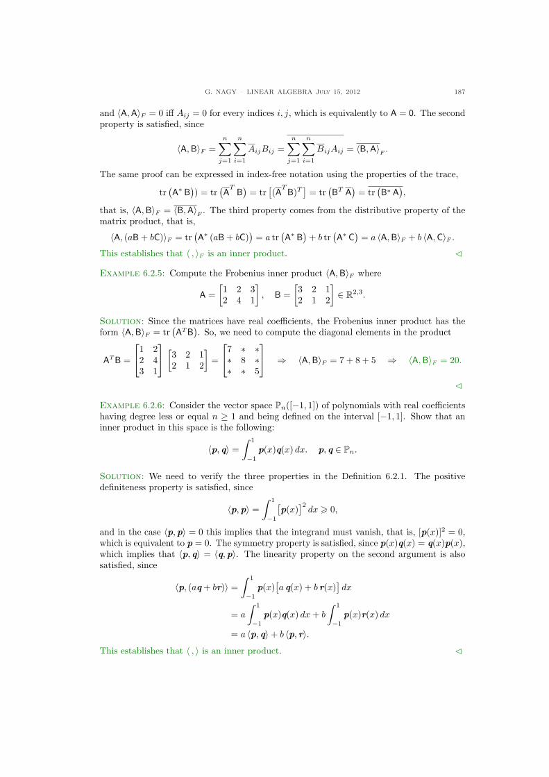
G. NAGY – LINEAR ALGEBRA July 15, 2012 187
and 〈A, A〉F = 0 iff Aij = 0 for every indices i, j, which is equivalently to A = 0. The secondproperty is satisfied, since
〈A,B〉F =n∑
j=1
n∑
i=1
AijBij =n∑
j=1
n∑
i=1
BijAij = 〈B, A〉F .
The same proof can be expressed in index-free notation using the properties of the trace,
tr(A∗ B
)) = tr
(A
TB
)= tr
[(A
TB)T
]= tr
(BT A
)= tr
(B∗ A
),
that is, 〈A, B〉F = 〈B,A〉F . The third property comes from the distributive property of thematrix product, that is,
〈A, (aB + bC)〉F = tr(A∗ (aB + bC)
)= a tr
(A∗ B
)+ b tr
(A∗ C
)= a 〈A, B〉F + b 〈A, C〉F .
This establishes that 〈 , 〉F is an inner product. C
Example 6.2.5: Compute the Frobenius inner product 〈A,B〉F where
A =[1 2 32 4 1
], B =
[3 2 12 1 2
]∈ R2,3.
Solution: Since the matrices have real coefficients, the Frobenius inner product has theform 〈A,B〉F = tr
(AT B
). So, we need to compute the diagonal elements in the product
AT B =
1 22 43 1
[3 2 12 1 2
]=
7 ∗ ∗∗ 8 ∗∗ ∗ 5
⇒ 〈A,B〉F = 7 + 8 + 5 ⇒ 〈A, B〉F = 20.
C
Example 6.2.6: Consider the vector space Pn([−1, 1]) of polynomials with real coefficientshaving degree less or equal n ≥ 1 and being defined on the interval [−1, 1]. Show that aninner product in this space is the following:
〈p, q〉 =∫ 1
−1
p(x)q(x) dx. p, q ∈ Pn.
Solution: We need to verify the three properties in the Definition 6.2.1. The positivedefiniteness property is satisfied, since
〈p,p〉 =∫ 1
−1
[p(x)
]2dx > 0,
and in the case 〈p,p〉 = 0 this implies that the integrand must vanish, that is, [p(x)]2 = 0,which is equivalent to p = 0. The symmetry property is satisfied, since p(x)q(x) = q(x)p(x),which implies that 〈p, q〉 = 〈q,p〉. The linearity property on the second argument is alsosatisfied, since
〈p, (aq + br)〉 =∫ 1
−1
p(x)[a q(x) + b r(x)
]dx
= a
∫ 1
−1
p(x)q(x) dx + b
∫ 1
−1
p(x)r(x) dx
= a 〈p, q〉+ b 〈p, r〉.This establishes that 〈 , 〉 is an inner product. C
188 G. NAGY – LINEAR ALGEBRA july 15, 2012
Example 6.2.7: Consider the vector space Ck([a, b],R), with k > 0 and a < b, of k-timescontinuously differentiable real-valued functions f : [a, b] → R. An inner product in thisvector space is given by
〈f , g〉 =∫ b
a
f (x)g(x) dx.
Any positive function µ ∈ C0([a, b],R) determines an inner product in Ck([a, b],R) as follows
〈f , g〉µ =∫ b
a
µ(x) f (x)g(x) dx.
The function µ is called a weigh function. An inner product in the vector space Ck([a, b],C)of k-times continuously differentiable complex-valued functions f : [a, b] ⊂ R → C is thefollowing,
〈f , g〉 =∫ b
a
f (x)g(x) dx.
C
An inner product satisfies the following inequality.
Theorem 6.2.2 (Cauchy-Schwarz). If(V, 〈 , 〉) is an inner product space over F, then
for every x, y ∈ V holds|〈x,y〉|2 6 〈x,x〉 〈y,y〉.
Furthermore, equality holds iff y = ax, with a = 〈x,y〉/〈x,x〉.Proof of Theorem 6.2.2: From the positive definiteness property we know that for everyx, y ∈ V and every scalar a ∈ F holds 0 6 〈(ax − y), (ax − y)〉. The symmetry and thelinearity on the second argument imply
0 6 〈(ax− y), (ax− y)〉 = a a 〈x,x〉 − a 〈x,y〉 − a 〈y,x〉+ 〈y,y〉. (6.4)
Since the inequality above holds for all a ∈ F, let us choose a particular value of a, thesolution of the equation
a a 〈x,x〉 − a 〈x,y〉 = 0 ⇒ a =〈x,y〉〈x,x〉 .
Introduce this particular value of a into Eq. (6.4),
0 6 −( 〈x,y〉〈x,x〉
)〈x,y〉+ 〈y,y〉 ⇒ |〈x,y〉|2 6 〈x,x〉 〈y,y〉.
Finally, notice that equality holds iff ax = y, and in this case, computing the inner productwith x we obtain a〈x,x〉 = 〈x,y〉. This establishes the Theorem. ¤
6.2.2. Inner product norm. The inner product on a vector space determines a particularnotion of length, or norm, of a vector, and we call it the inner product norm. After weintroduce this norm we show its main properties. In Chapter 8 later on we use theseproperties to define a more general notion of norm as any function on the vector spacesatisfying these properties. The inner product norm is just a particular case of this broadernotion of length. A normed space is a vector space with any norm.
Definition 6.2.3. The inner product norm determined in an inner product space(V, 〈 , 〉)
is the function ‖ ‖ : V → R given by
‖x‖ =√〈x,x〉.
G. NAGY – LINEAR ALGEBRA July 15, 2012 189
The Cauchy-Schwarz inequality is often expressed using the inner product norm as follows:For every x, y ∈ V holds
|〈x,y〉| 6 ‖x‖ ‖y‖.A vector x ∈ V is a normal or unit vector iff ‖x‖ = 1.
Theorem 6.2.4. If v 6= 0 belongs to(V, 〈 , 〉), then
v
‖v‖ is a unit vector parallel to v.
The proof is the same of Theorem 6.1.12.
Example 6.2.8: Consider the inner product space(Fm,n, 〈 , 〉F
), where Fm,n is the vector
space of all m×n matrices and 〈 , 〉F is the Frobenius inner product defined in Example 6.2.4.The associated inner product norm is called the Frobenius norm and is given by
‖A‖F =√〈A,A〉F =
√tr
(A∗A
).
If A = [Aij ], with i = 1, · · · ,m and j = 1, · · · , n, then
‖A‖F =( m∑
i=1
n∑
j=1
|Aij |2)1/2
.
C
Example 6.2.9: Find an explicit expression for the Frobenius norm of any element A ∈ F2,2.
Solution: The Frobenius norm of an arbitrary matrix A =[A11 A12
A21 A22
]∈ F2,2 is given by
‖A‖2F = tr([
A11 A21
A12 A22
] [A11 A12
A21 A22
] ).
Since we are only interested in the diagonal elements of the matrix product in the equationabove, we obtain
‖A‖2F = tr[|A11|2 + |A21|2 ∗
∗ |A12|2 + |A22|2]
which gives the formula
‖A‖2F = |A11|2 + |A12|2 + |A21|2 + |A22|2.
This is the explicit expression of the sum ‖A‖F =( 2∑
i=1
2∑
j=1
|Aij |2)1/2
. C
The inner product norm function has the following properties.
Theorem 6.2.5. The inner product norm introduced in Definition 6.2.3 satisfies that forevery x, y ∈ V and every a ∈ F holds,
(a) ‖x‖ > 0, and ‖x‖ = 0 iff x = 0, (Positive definiteness);(b) ‖ax‖ = |a| ‖x‖, (Scaling);(c) ‖x + y‖ 6 ‖x‖+ ‖y‖, (Triangle inequality).
Proof of Theorem 6.2.5: Properties (a) and (b) are straightforward to show from thedefinition of inner product, and their proof is left as an exercise. We show here how to
190 G. NAGY – LINEAR ALGEBRA july 15, 2012
obtain the triangle inequality, property (c). Given any vectors x, y ∈ V holds
‖x + y‖2 = 〈(x + y), (x + y)〉= ‖x‖2 + 〈x,y〉+ 〈y,x〉+ ‖y‖26 ‖x‖2 + 2 |〈x,y〉|+ ‖y‖2
6 ‖x‖2 + 2 ‖x‖ ‖y‖+ ‖y‖2 =(‖x‖+ ‖y‖)2
,
where the last inequality comes from the Cauchy-Schwarz inequality. We then conclude that‖x + y‖2 6
(‖x‖+ ‖y‖)2. This establishes the Theorem. ¤6.2.3. Norm distance. The norm on an inner product space determines a particular notionof distance between vectors. After we introduce this norm we show its main properties.
Definition 6.2.6. The norm distance between two vectors in a vector space V with anorm function ‖ ‖ : V → R is the value of the function d : V × V → R given by
d(x,y) = ‖x− y‖.
Theorem 6.2.7. The norm distance in Definition 6.2.6 satisfies for every x, y, z ∈ V that(a) d(x,y) > 0, and d(x,y) = 0 iff x = y, (Positive definiteness);(b) d(x,y) = d(y,x), (Symmetry);(c) d(x,y) 6 d(x, z) + d(z,y), (Triangle inequality).
Proof of Theorem 6.2.7: Properties (a) and (b) are straightforward from properties (a)and (b), and their proof are left as an exercise. We show how the triangle inequality for thedistance comes from the triangle inequality for the norm. Indeed
d(x,y) = ‖x− y‖ = ‖(x− z)− (y− z)‖ 6 ‖x− z‖+ ‖y− z‖ = d(x, z) + d(z,y),
where we used the symmetry of the distance function on the last term above. This establishesthe Theorem. ¤
The presence of an inner product, and hence a norm and a distance, on a vector spacepermits to introduce the notion of convergence of an infinite sequence of vectors. We saythat the sequence {xn}∞n=0 ⊂ V converges to x ∈ V iff
limn→∞
d(xn,x) = 0.
Some of the most important concepts related to convergence are closeness of a subspace,completeness of the vector space, and the continuity of linear operators and linear trans-formations. In the case of finite dimensional vector spaces the situation is straightforward.All subspaces are closed, all inner product spaces are complete and all linear operators andlinear transformations are continuous. However, in the case of infinite dimensional vectorspaces, things are not so simple.
G. NAGY – LINEAR ALGEBRA July 15, 2012 191
6.2.4. Exercises.
6.2.1.- Determine which of the followingfunctions 〈 , 〉 : R3 × R3 → R definesan inner product on R3. Justify youranswers.
(a) 〈x, y〉 = x1y1 + x3y3;(b) 〈x, y〉 = x1y1 − x2y2 + x3y3;(c) 〈x, y〉 = 2x1y1 + x2y2 + 4x3y3;(d) 〈x, y〉 = x2
1 y21 + x2
2 y22 + x2
3 y23 .
We used the standard notation
x =
24
x1
x2
x3
35 , y =
24
y1
y2
y3
35 .
6.2.2.- Prove that an inner product func-tion 〈 , 〉 : V × V → F satisfies the fol-lowing properties:
(a) 〈x, y 〉 = 0 for all x ∈ V , then y = 0.(b) 〈ax, y 〉 = a 〈x, y 〉 for all x, y ∈ V .
6.2.3.- Given a matrix M ∈ R2,2 introducethe function 〈 , 〉M : R2 × R2 → R,
〈y, x〉M = yT Mx.
For each of the matrices M below de-termine whether 〈 , 〉M defines an innerproduct or not. Justify your answers.
(a) M =
»4 11 9
–;
(b) M =
»4 −33 9
–;
(c) M =
»4 10 9
–.
6.2.4.- Fix any A ∈ Rn,n with N(A) = {0}and introduce M = AT A. Prove that〈 , 〉M : Rn × Rn → R, given by
〈y, x〉 = yT Mx.
is an inner product in Rn.
6.2.5.- Find k ∈ R such that the matricesA, B ∈ R2,2 are perpendicular in theFrobenius inner product,
A =
»1 23 4
–, B =
»1 2k 1
–.
6.2.6.- Evaluate the Frobenius norm for thematrices
A =
»1 −2−1 2
–, B =
24
0 1 00 0 11 0 0
35 .
6.2.7.- Prove that ‖A‖F = ‖A∗‖F for allA ∈ Fm,n.
6.2.8.- Consider the vector space P2([0, 1])with inner product
〈p, q 〉 =
Z 1
0
p(x)q(x) dx.
Find a unit vector parallel to
p(x) = 3− 5x2.
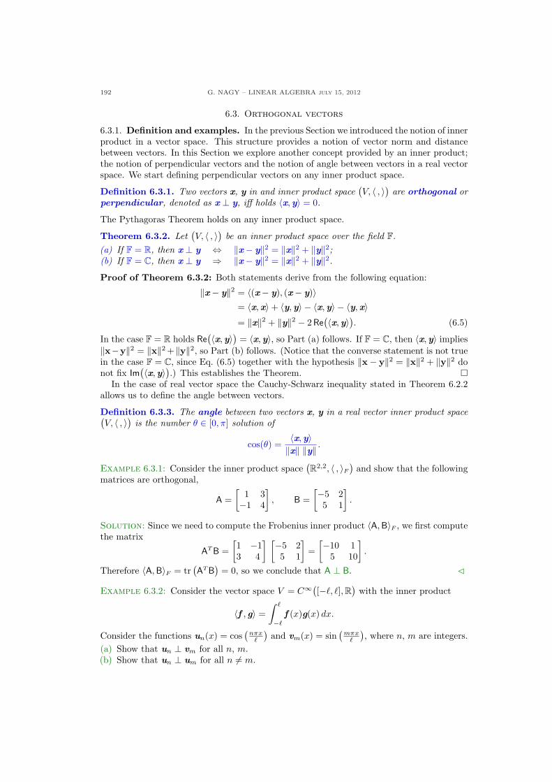
192 G. NAGY – LINEAR ALGEBRA july 15, 2012
6.3. Orthogonal vectors
6.3.1. Definition and examples. In the previous Section we introduced the notion of innerproduct in a vector space. This structure provides a notion of vector norm and distancebetween vectors. In this Section we explore another concept provided by an inner product;the notion of perpendicular vectors and the notion of angle between vectors in a real vectorspace. We start defining perpendicular vectors on any inner product space.
Definition 6.3.1. Two vectors x, y in and inner product space(V, 〈 , 〉) are orthogonal or
perpendicular, denoted as x ⊥ y, iff holds 〈x,y〉 = 0.
The Pythagoras Theorem holds on any inner product space.
Theorem 6.3.2. Let(V, 〈 , 〉) be an inner product space over the field F.
(a) If F = R, then x ⊥ y ⇔ ‖x− y‖2 = ‖x‖2 + ‖y‖2;(b) If F = C, then x ⊥ y ⇒ ‖x− y‖2 = ‖x‖2 + ‖y‖2.Proof of Theorem 6.3.2: Both statements derive from the following equation:
‖x− y‖2 = 〈(x− y), (x− y)〉= 〈x,x〉+ 〈y,y〉 − 〈x,y〉 − 〈y,x〉= ‖x‖2 + ‖y‖2 − 2 Re
(〈x,y〉). (6.5)
In the case F = R holds Re(〈x,y〉) = 〈x,y〉, so Part (a) follows. If F = C, then 〈x,y〉 implies
‖x−y‖2 = ‖x‖2 +‖y‖2, so Part (b) follows. (Notice that the converse statement is not truein the case F = C, since Eq. (6.5) together with the hypothesis ‖x− y‖2 = ‖x‖2 + ‖y‖2 donot fix Im
(〈x,y〉).) This establishes the Theorem. ¤In the case of real vector space the Cauchy-Schwarz inequality stated in Theorem 6.2.2
allows us to define the angle between vectors.
Definition 6.3.3. The angle between two vectors x, y in a real vector inner product space(V, 〈 , 〉) is the number θ ∈ [0, π] solution of
cos(θ) =〈x,y〉‖x‖ ‖y‖ .
Example 6.3.1: Consider the inner product space(R2,2, 〈 , 〉F
)and show that the following
matrices are orthogonal,
A =[
1 3−1 4
], B =
[−5 25 1
].
Solution: Since we need to compute the Frobenius inner product 〈A,B〉F , we first computethe matrix
AT B =[1 −13 4
] [−5 25 1
]=
[−10 15 10
].
Therefore 〈A, B〉F = tr(AT B
)= 0, so we conclude that A ⊥ B. C
Example 6.3.2: Consider the vector space V = C∞([−`, `],R
)with the inner product
〈f , g〉 =∫ `
−`
f (x)g(x) dx.
Consider the functions un(x) = cos(
nπx`
)and vm(x) = sin
(mπx
`
), where n, m are integers.
(a) Show that un ⊥ vm for all n, m.(b) Show that un ⊥ um for all n 6= m.
G. NAGY – LINEAR ALGEBRA July 15, 2012 193
(c) Show that vn ⊥ vm for all n 6= m.
Solution: Recall the identities
sin(θ) cos(φ) =12[sin(θ − φ) + sin(θ + φ)
], (6.6)
cos(θ) cos(φ) =12[cos(θ − φ) + cos(θ + φ)
], (6.7)
sin(θ) sin(φ) =12[cos(θ − φ)− cos(θ + φ)
]. (6.8)
Part (a): Using identity in Eq. (6.6) is simple to show that
〈un, vm〉 =∫ `
−`
cos(nπx
`
)sin
(mπx
`
)dx
=12
∫ `
−`
[sin
( (n−m)πx
`
)+ sin
( (n + m)πx
`
)]. (6.9)
First, assume that both n−m and n + m are non-zero,
〈un, vm〉 = −12
[ `
(n−m)πcos
( (n−m)πx
`
)∣∣∣`
−`+
`
(n + m)πcos
( (n + m)πx
`
)∣∣∣`
−`
]. (6.10)
Since cos((n±m)π) = cos(−(n±m)π), we conclude that both terms above vanish.Second, in the case that n −m = 0 the first term in Eq. (6.9) vanishes identically and
we need to compute the term with (n + m), which also vanishes by the second term inEq. (6.10). Analogously, in the case of (n + m) = 0 the second term in Eq. (6.9) vanishesidentically and we need to compute the term with (n−m) which also vanishes by the firstterm in Eq. (6.10). Therefore, 〈un, vm〉 = 0 for all n, m integers, and so un ⊥ vm in thiscase.
Part (b): Using identity in Eq. (6.7) is simple to show that
〈un,um〉 =∫ `
−`
cos(nπx
`
)cos
(mπx
`
)dx
=12
∫ `
−`
[cos
( (n−m)πx
`
)+ cos
( (n + m)πx
`
)]. (6.11)
We know that n−m is non-zero. Now, assume that n + m is non-zero, then
〈un,um〉 =12
[ `
(n−m)πsin
( (n−m)πx
`
)∣∣∣`
−`+
`
(n + m)πsin
( (n + m)πx
`
)∣∣∣`
−`
]
=`
(n−m)πsin((n−m)π) +
`
(n + m)πsin((n + m)π). (6.12)
Since sin((n±m)π) = 0 for (n±m) integer, we conclude that both terms above vanish.In the case of (n + m) = 0 the second term in Eq. (6.11) vanishes identically and we
need to compute the term with (n−m) which also vanishes by the first term in Eq. (6.12).Therefore, 〈un,um〉 = 0 for all n 6= m integers, and so un ⊥ um in this case.
Part (c): Using identity in Eq. (6.8) is simple to show that
〈vn, vm〉 =∫ `
−`
sin(nπx
`
)sin
(mπx
`
)dx
=12
∫ `
−`
[cos
( (n−m)πx
`
)− cos
( (n + m)πx
`
)]. (6.13)
194 G. NAGY – LINEAR ALGEBRA july 15, 2012
Since the only difference between Eq. (6.13) and (6.11) is the sign of the second term,repeating the argument done in case (b) we conclude that 〈vn, vm〉 = 0 for all n 6= mintegers, and so vn ⊥ vm in this case. C
6.3.2. Orthonormal basis. We saw that an important property of a basis is that everyvector in a vector space can be decomposed in a unique way in terms of the basis vectors.This decomposition is particularly simple to find in an inner product space when the basisis an orthonormal basis. Before we introduce such basis we define an orthonormal set.
Definition 6.3.4. The set U = {u1, · · · ,up}, p > 1, in an inner product space(V, 〈 , 〉) is
called an orthonormal set iff for all i, j = 1, · · · , p holds
〈ui,uj〉 ={ 0 if i 6= j,
1 if i = j.
The set U is called an orthogonal set iff holds that 〈ui,uj〉 = 0 if i 6= j and 〈ui,ui〉 6= 0.
Example 6.3.3: Consider the vector space V = C∞([−`, `],R
)with the inner product
〈f , g〉 =∫ `
−`
f (x)g(x) dx.
Show that the set
U ={u0 =
1√2`
, un(x) =1√`
cos(nπx
`
), vm(x) =
1√`
sin(mπx
`
)}∞n=1
is an orthonormal set.
Solution: We have shown in Example 6.3.2 that U is an orthogonal set. We only needto compute the norm of the vectors u0, un and vn, for n = 1, 2, · · · . The norm of the firstvector is simple to compute,
〈u0,u0〉 =∫ `
−`
12`
dx = 1.
The norm of the cosine functions is computed as follows,
〈un,un〉 =1`
∫ `
−`
cos2(nπx
`
)dx
=12`
∫ `
−`
[1 + cos
(2nπx
`
)]dx
= 1 +`
2nπ
[sin
(2nπx
`
)∣∣∣`
−`
]⇒ 〈un,un〉 = 1.
A similar calculation for the sine functions gives the result
〈vn, vn〉 =1`
∫ `
−`
sin2(nπx
`
)dx
=12`
∫ `
−`
[1− cos
(2nπx
`
)]dx
= 1− `
2nπ
[sin
(2nπx
`
)∣∣∣`
−`
]⇒ 〈vn, vn〉 = 1.
Therefore, U is an orthonormal set. C
A straightforward result is the following:
Theorem 6.3.5. An orthogonal set in an inner product space is linearly independent.
G. NAGY – LINEAR ALGEBRA July 15, 2012 195
Proof of Theorem 6.3.5: Let U = {u1, · · · ,up}, p > 1, be an orthogonal set. The zerovector is not included since 〈ui,ui〉 6= 0 for all i = 1, · · · , p. Let c1, · · · , cp ∈ F be scalarssuch that
c1u1 + · · ·+ cpup = 0.
Then, for any ui ∈ U holds
0 = 〈ui, (c1u1 + · · ·+ cpup〉 = c1〈ui,u1〉+ · · ·+ cp〈ui,up〉.Since the set U is orthogonal, 〈ui,uj〉 = 0 for i 6= j and 〈ui,ui〉 6= 0, so we conclude that
ci〈ui,ui〉 = 0 ⇒ ci = 0, i = 1, · · · , p.
Therefore, U is a linearly independent set. This establishes the Thorem. ¤Definition 6.3.6. A basis U of an inner product space is called an orthonormal basis(orthogonal basis) iff the basis U is an orthonormal (orthogonal) set.
Example 6.3.4: Consider the inner product space(R2, ·). Determine whether the following
bases are orthonormal, orthogonal or neither:
S ={
e1 =[10
], e2 =
[01
]}, U =
{u1 =
[11
], u2 =
[−11
]}, V =
{v1 =
[13
], v2 =
[31
]}.
Solution: The basis S is orthonormal, since e1 · e2 = 0 and e1 · e1 = e2 · e2 = 1. The basisU is orthogonal since u1 · u2 = 0, but it is not orthonormal. Finally, the basis V is neitherorthonormal nor orthogonal. C
Theorem 6.3.7. Given the set U = {u1, · · · , up}, p > 1, in the inner product space(Fn, ·),
introduce the matrix U = [u1, · · · , up]. Then the following statements hold:(a) U is an orthonormal set iff matrix U satisfies U∗U = Ip.(b) U is an orthonormal basis of Fn iff matrix U satisfies U−1 = U∗.
Matrices satisfying the property mentioned in part (b) of Theorem 6.3.7 appear frequentlyin Quantum Mechanics, so they are given a name.
Definition 6.3.8. A matrix U ∈ Fn,n is called unitary iff holds U−1 = U∗.
These matrices are called unitary because they do not change the norm of vectors in Fn
equipped with the dot product. Indeed, given any x ∈ Fn with norm ‖x‖, the vector Ux ∈ Fn
has the same norm, since
‖Ux‖2 =(Ux
)∗(Ux
)= x∗U∗Ux = x∗U−1Ux = x∗x = ‖x‖2.
Proof of Theorem 6.3.7:Part (a): This is proved by a straightforward computation,
U∗U =
u∗1...
u∗p
[u1, · · · , up
]=
u∗1u1 · · · u∗1up
......
u∗pu1 · · · u∗pup
=
u1 · u1 · · · u1 · up
......
up · u1 · · · up · up
= Ip.
Part (b): It follows from part (a): If U is a basis of Fn, then p = n; since U is anorthonormal set, part (a) implies U∗U = In. Since U is an n × n matrix, it follows thatU∗ = U−1. This establishes the Theorem. ¤
Example 6.3.5: Consider v1 =
112
, v2 =
20−1
, in the inner product space
(R3, ·).
(a) Show that v1 ⊥ v2;
196 G. NAGY – LINEAR ALGEBRA july 15, 2012
(b) Find x ∈ R3 such that x ⊥ v1 and x ⊥ v2.(c) Rescale the elements of {v1, v2, x} so that the new set is an orthonormal set.
Solution:Part (a):
[1 1 2
]
20−1
= 2 + 0− 2 = 0 ⇒ v1 ⊥ v2.
Part (b): We need to find x =
x1
x2
x3
such that
v1 · x =[1 1 2
]
x1
x2
x3
= 0, v2 · x =
[2 0 −1
]
x1
x2
x3
= 0,
The equations above can be written in matrix notation as
AT x = 0, where A =[v1, v2
]=
1 21 02 −1
.
Gauss elimination operation on AT imply
[1 1 22 0 −1
]→
[1 0 −1/20 1 5/2
]⇒
x1 =12
x3,
x2 = −52
x3,
x3 free.
There is a solution for any choice of x3 6= 0, so we choose x3 = 2, that is, x =
1−52
.
Part (c): The vectors v1, v2 and x are mutually orthogonal. Their norms are:
‖v1‖ =√
6, ‖v2‖ =√
5, ‖x‖ =√
30.
Therefore, the orthonormal set is
{u1 =
1√6
112
, u2 =
1√5
20−1
, u3 =
1√30
1−52
}.
Finally, notice that the inverse of the matrix
U =
1√6
2√5
1√30
1√6
0 − 5√30
2√6− 1√
52√30
is U−1 =
1√6
1√6
2√6
2√5
0 − 1√5
1√30− 5√
302√30
= UT .
C
6.3.3. Vector components. Given a basis in a finite dimensional vector space, we knowthat every vector in the vector space can be decomposed in a unique way as a linear com-bination of the basis vectors. What we do not know is a general formula to compute thevector components in such a basis. However, in the particular case that the vector spaceadmits an inner product and the basis is an orthonormal basis, we have such formula forthe vector components. The formula is very simple and is the main result in the followingstatement.
G. NAGY – LINEAR ALGEBRA July 15, 2012 197
Theorem 6.3.9. If(V, 〈 , 〉) is an n-dimensional inner product space with an orthonormal
basis U = {u1, · · · ,un}, then every vector x ∈ V can be decomposed as
x = 〈u1,x〉u1 + · · ·+ 〈un,x〉un. (6.14)
Proof of Theorem 6.3.9: Since U is a basis, we know that for all x ∈ V there exist scalarsc1, · · · , cn such that
x = c1u1 + · · ·+ cnun.
Therefore, the inner product 〈ui,x〉 for any i = 1, · · · , n is given by
〈ui,x〉 = c1 〈ui,u1〉+ · · ·+ cn 〈ui,un〉.Since U is an orthonormal set, 〈ui,x〉 = ci. This establishes the Theorem. ¤
The result in Theorem 6.3.9 provides a remarkable simple formula for vector componentsin an orthonormal basis. We will get back to this subject in some depth in Section 7.1.In that Section we will name the coefficients 〈ui,x〉 in Eq. (6.14) as Fourier coefficients ofthe vector x in the orthonormal set U = {u1, · · · ,un}. When the set U is an orthonormalordered basis of a vector space V , the coordinate map [ ]u : V → Fn is expressed in termsof the Fourier coefficients as follows,
[x ]u =
〈u1,x〉
...〈un,x〉
.
So, the coordinate map has a simple expression when it is defined by an orthonormal basis.
Example 6.3.6: Consider the inner product space(R3, ·) with the standard ordered basis
S, and find the vector components of x =
123
in the orthonormal ordered basis
U =(u1 =
1√6
112
, u2 =
1√5
20−1
, u3 =
1√30
1−52
).
Solution: The vector components of x in the orthonormal basis U are given by
xu =
〈u1, x〉〈u2, x〉〈u3, x〉
⇒ u =
9√6
− 1√5
− 3√30
.
Remark: We have done a change of basis, from the standard basis S to the U basis. Infact, we can express the calculation above as follows
xu = P−1xs, where P = Ius =
1√6
2√5
1√30
1√6
0 − 5√30
2√6− 1√
52√30
= U.
Since U is an orthonormal basis, U−1 = UT , so we conclude that
xu = UT xs =
1√6
1√6
2√6
2√5
0 − 1√5
1√30− 5√
302√30
123
=
9√6
− 1√5
− 3√30
.
C
198 G. NAGY – LINEAR ALGEBRA july 15, 2012
6.3.4. Exercises.
6.3.1.- Prove that the following form of thePythagoras Theorem holds on complexvector spaces: Two vectors x, y in aninner product space
`V, 〈 , 〉´ over C are
orthogonal iff for all a, b ∈ C holds
‖ax + by‖2 = ‖ax‖2 + ‖by‖2.
6.3.2.- Consider the vector space R3 withthe dot product. Find all vectors x ∈ R3
which are orthogonal to the vector
v =
24
123
35 .
6.3.3.- Consider the vector space R3 withthe dot product. Find all vectors x ∈ R3
which are orthogonal to the vectors
v1 =
24
123
35 , v2 =
24
101
35 .
6.3.4.- Let P3([−1, 1]) be the space of poly-nomials up to degree three defined onthe interval [−1, 1] ⊂ R with the innerproduct
〈p, q 〉 =
Z 1
−1
p(x)q(x) dx.
Show that the set (p0,p1,p2,p3) is anorthogonal basis of P3, where
p0(x) = 1,
p1(x) = x,
p2(x) =1
2(3x2 − 1),
p3(x) =1
2(5x3 − 3x).
(These polynomials are the first four ofthe Legendre polynomials.)
6.3.5.- Consider the vector space R3 withthe dot product.
(a) Show that the following ordered ba-sis U is orthonormal,
“ 1√2
24
1−10
35 ,
1√3
24
111
35 ,
1√6
24−1−12
35”.
(b) Use part (a) to find the componentsin the ordered basis U of the vector
x =
24
10−2
35 .
6.3.6.- Consider the vector space R2,2 withthe Frobenius inner product.
(a) Show that the ordered basis givenby U = (E1, E2, E3, E4) is orthonor-mal, where
E1 =1√2
»0 11 0
–E2 =
1√2
»1 00 −1
–
E3 =1
2
»1 −11 1
–E4 =
1
2
»1 1−1 1
–.
(b) Use part (a) to find the componentsin the ordered basis U of the matrix
A =
»1 11 1
–.
6.3.7.- Consider the inner product space`R2,2, 〈 , 〉F
´, and find the cosine of the
angle between the matrices
A =
»1 32 4
–, B =
»2 −22 0
–.
6.3.8.- Find the third column in matrix Ubelow such that UT = U−1, where
U =
24
1/√
3 1/√
14 U13
1/√
3 2/√
14 U23
1/√
3 −3/√
14 U33
35 .
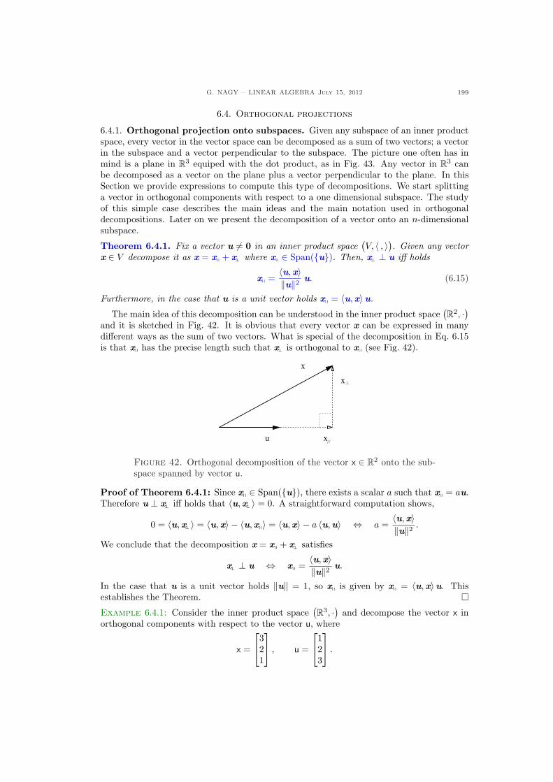
G. NAGY – LINEAR ALGEBRA July 15, 2012 199
6.4. Orthogonal projections
6.4.1. Orthogonal projection onto subspaces. Given any subspace of an inner productspace, every vector in the vector space can be decomposed as a sum of two vectors; a vectorin the subspace and a vector perpendicular to the subspace. The picture one often has inmind is a plane in R3 equiped with the dot product, as in Fig. 43. Any vector in R3 canbe decomposed as a vector on the plane plus a vector perpendicular to the plane. In thisSection we provide expressions to compute this type of decompositions. We start splittinga vector in orthogonal components with respect to a one dimensional subspace. The studyof this simple case describes the main ideas and the main notation used in orthogonaldecompositions. Later on we present the decomposition of a vector onto an n-dimensionalsubspace.
Theorem 6.4.1. Fix a vector u 6= 0 in an inner product space(V, 〈 , 〉). Given any vector
x ∈ V decompose it as x = xq + xp− where xq ∈ Span({u}). Then, xp− ⊥ u iff holds
xq =〈u,x〉‖u‖2 u. (6.15)
Furthermore, in the case that u is a unit vector holds xq = 〈u,x〉u.
The main idea of this decomposition can be understood in the inner product space(R2, ·)
and it is sketched in Fig. 42. It is obvious that every vector x can be expressed in manydifferent ways as the sum of two vectors. What is special of the decomposition in Eq. 6.15is that xq has the precise length such that xp− is orthogonal to xq (see Fig. 42).
x
u x
x
Figure 42. Orthogonal decomposition of the vector x ∈ R2 onto the sub-space spanned by vector u.
Proof of Theorem 6.4.1: Since xq ∈ Span({u}), there exists a scalar a such that xq = au.Therefore u ⊥ xp− iff holds that 〈u,xp−〉 = 0. A straightforward computation shows,
0 = 〈u,xp−〉 = 〈u,x〉 − 〈u,xq〉 = 〈u,x〉 − a 〈u,u〉 ⇔ a =〈u,x〉‖u‖2 .
We conclude that the decomposition x = xq + xp− satisfies
xp− ⊥ u ⇔ xq =〈u,x〉‖u‖2 u.
In the case that u is a unit vector holds ‖u‖ = 1, so xq is given by xq = 〈u,x〉u. Thisestablishes the Theorem. ¤Example 6.4.1: Consider the inner product space
(R3, ·) and decompose the vector x in
orthogonal components with respect to the vector u, where
x =
321
, u =
123
.
200 G. NAGY – LINEAR ALGEBRA july 15, 2012
Solution: We first compute xq =u · x‖u‖2 u. Since
u · x =[1 2 3
]
321
= 3 + 4 + 3 = 10, ‖u‖2 =
[1 2 3
]
123
= 1 + 4 + 9 = 14,
we obtain xq =57
123
. We now compute x p− as follows,
x p− = x− xq =
321
− 5
7
123
=
17
21147
− 1
7
51015
=
17
164−8
⇒ x p− =
47
41−2
.
Therefore, x can be decomposed as
x =57
123
+
47
41−2
.
Remark: We can verify that this decomposition is orthogonal with respect to u, since
u · x p− =47
[1 2 3
]
41−2
=
47
(4 + 2− 6) = 0.
C
We now decompose a vector into orthogonal components with respect to a p-dimensionalsubspace with p > 1.
Theorem 6.4.2. Fix an orthogonal set U = {u1, · · · ,up}, with p > 1, in an inner productspace
(V, 〈 , 〉). Given any vector x ∈ V , decompose it as x = xq + xp− , where xq ∈ Span(U).
Then, xp− ⊥ ui, for i = 1, · · · , p iff holds
xq =〈u1,x〉‖u1‖2 u1 + · · ·+ 〈up,x〉
‖up‖2 up. (6.16)
Furthermore, in the case that U is an orthonormal basis holds
xq = 〈u1,x〉u1 + · · ·+ 〈up,x〉up. (6.17)
Remark: The set U in Theorem 6.4.2 must be an orthogonal set. If the vectors u1, · · · ,up
are not mutually orthogonal, then the vector xq computed in Eq. (6.17) is not the orthogonalprojection of vector x, that is, (x − xq) 6⊥ ui for i = 1, · · · , p. Therefore, before usingEq. (6.17) in a particular application one should verify that the set U one is working with isin fact an orthogonal set. A particular case of the orthogonal projection of a vector in theinner product space
(R3, ·) onto a plane is sketched in Fig. 43.
Proof of Theorem 6.4.2: Since xq ∈ Span(U), there exist scalars ai, for i = 1, · · · , p suchthat xq = a1u1+· · ·+apup. The vector xp− ⊥ ui iff holds that 〈ui,xp−〉 = 0. A straightforwardcomputation shows that, for i = 1, · · · , p holds
0 = 〈ui,xp−〉 = 〈ui,x〉 − 〈ui,xq〉= 〈ui,x〉 − a1 〈ui,u1〉 − · · · − ap 〈ui,up〉
= 〈ui,x〉 − ai〈ui,ui〉 ⇔ ai =〈ui,x〉‖ui‖2 .
G. NAGY – LINEAR ALGEBRA July 15, 2012 201
x
u1
u 2R
3
x
U
x
Figure 43. Orthogonal decomposition of the vector x ∈ R3 onto the sub-space U spanned by the vectors u1 and u2.
We conclude that the decomposition x = xq + xp− satisfies xp− ⊥ ui for i = 1, · · · , p iff holds
xq =〈u1,x〉‖u1‖2 u1 + · · ·+ 〈up,x〉
‖up‖2 up.
In the case that U is an orthonormal set holds ‖ui‖ = 1 for i = 1, · · · , p, so xq is given byEq. (6.17). This establishes the Theorem. ¤
Example 6.4.2: Consider the inner product space(R3, ·) and decompose the vector x in
orthogonal components with respect to the subspace U , where
x =
123
, U = Span
({u1 =
25−1
, u2 =
−211
}).
Solution: In order to use Eq. (6.16) we need an orthogonal basis of U . So, need need toverify whether u1 is orthogonal to u2. This is indeed the case, since
u1 · u2 =[2 5 −1
]−211
= −4 + 5− 1 = 0.
So now we use u1 and u2 to compute xq using Eq. (6.17). We need the quantities
u1 · x =[2 5 −1
]
123
= 9, u1 · u1 =
[2 5 −1
]
25−1
= 30,
u2 · x =[−2 1 1
]
123
= 3, u2 · u2 =
[−2 1 1]
−211
= 6.
Now is simple to compute xq, since
xq =930
25−1
+
36
−211
=
310
25−1
+
12
−211
=
110
615−3
+
110
−10
55
,
therefore,
xq =110
−4202
⇒ xq =
15
−2101
.
202 G. NAGY – LINEAR ALGEBRA july 15, 2012
The vector x p− is obtained as follows,
x p− = x− xq =
123
− 1
5
−2101
=
15
51015
− 1
5
−2101
=
15
7014
⇒ x p− =
75
102
.
We conclude that
x =15
−2101
+
75
102
.
Remark: We can verify that x p− ⊥ U , since
u1 · x p− =75
[2 5 −1
]
102
=
75
(2 + 0− 2) = 0,
u2 · x p− =75
[−2 1 1]
102
=
75
(2 + 0− 2) = 0.
C
6.4.2. Orthogonal complement. We have seen that any vector in an inner product spacecan be decomposed as a sum of orthogonal vectors, that is, x = xq + xp− with 〈xq,xp−〉 = 0.Inner product spaces can be decomposed in a somehow analogous way as a direct sum oftwo mutually orthogonal subspaces. In order to understand such decomposition, we need tointroduce the notion of the orthogonal complement of a subspace. Then we will show thata finite dimensional inner product space is the direct sum of a subspace and it orthogonalcomplement. It is precisely this result that motivates the word “complement” in the nameorthogonal complement of a subspace.
Definition 6.4.3. The orthogonal complement of a subspace W in an inner productspace
(V, 〈 , 〉), denoted as W⊥, is the set W⊥ = {u ∈ V : 〈u,w〉 = 0 ∀ w ∈W}.
Example 6.4.3: In the inner product space(R3, ·), the orthogonal complement to a line is
a plane, and the orthogonal complement to a plane is a line, as it is shown in Fig. 44. C
0
RU
U
3
V
R3
0
V
Figure 44. The orthogonal complement to the plane U is the line U⊥,and the orthogonal complement to the line V is the plane V ⊥.
As the sketch in Fig. 44 suggests, the orthogonal complement of a subspace is a subspace.
Theorem 6.4.4. The orthogonal complement W⊥ of a subspace W in an inner productspace is also a subspace.
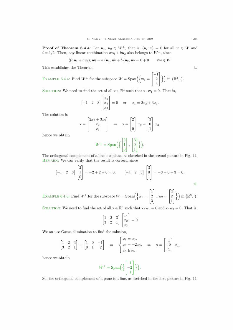
G. NAGY – LINEAR ALGEBRA July 15, 2012 203
Proof of Theorem 6.4.4: Let u1, u2 ∈ W⊥, that is, 〈ui,w〉 = 0 for all w ∈ W andi = 1, 2. Then, any linear combination au1 + bu2 also belongs to W⊥, since
〈(au1 + bu2),w〉 = a 〈u1,w〉+ b 〈u2,w〉 = 0 + 0 ∀w ∈W.
This establishes the Theorem. ¤
Example 6.4.4: Find W⊥ for the subspace W = Span({
w1 =
−123
})in
(R3, ·).
Solution: We need to find the set of all x ∈ R3 such that x · w1 = 0. That is,
[−1 2 3]
x1
x2
x3
= 0 ⇒ x1 = 2x2 + 3x3.
The solution is
x =
2x2 + 3x3
x2
x3
⇒ x =
210
x2 +
301
x3,
hence we obtain
W⊥ = Span({
210
,
301
}).
The orthogonal complement of a line is a plane, as sketched in the second picture in Fig. 44.Remark: We can verify that the result is correct, since
[−1 2 3]
210
= −2 + 2 + 0 = 0,
[−1 2 3]
301
= −3 + 0 + 3 = 0.
C
Example 6.4.5: Find W⊥ for the subspace W = Span({
w1 =
123
, w2 =
321
})in
(R3, ·).
Solution: We need to find the set of all x ∈ R3 such that x ·w1 = 0 and x ·w2 = 0. That is,
[1 2 33 2 1
]
x1
x2
x3
= 0
We an use Gauss elimination to find the solution,
[1 2 33 2 1
]→
[1 0 −10 1 2
]⇒
x1 = x3,
x2 = −2x3,
x3 free.⇒ x =
1−21
x3,
hence we obtain
W⊥ = Span({
1−21
}).
So, the orthogonal complement of a pane is a line, as sketched in the first picture in Fig. 44.
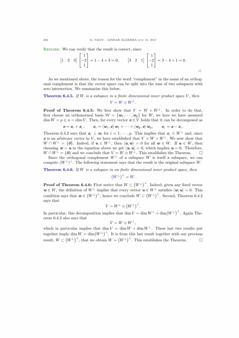
204 G. NAGY – LINEAR ALGEBRA july 15, 2012
Remark: We can verify that the result is correct, since
[1 2 3
]
1−21
= 1− 4 + 3 = 0,
[3 2 1
]
1−21
= 3− 4 + 1 = 0.
C
As we mentioned above, the reason for the word “complement” in the name of an orthog-onal complement is that the vector space can be split into the sum of two subspaces withzero intersection. We summarize this below.
Theorem 6.4.5. If W is a subspace in a finite dimensional inner product space V , then
V = W ⊕W⊥.
Proof of Theorem 6.4.5: We first show that V = W + W⊥. In order to do that,first choose an orthonormal basis W = {w1, · · · ,wp} for W , we here we have assumeddim W = p 6 n = dim V . Then, for every vector x ∈ V holds that it can be decomposed as
x = xq + xp− , xq = 〈w1,x〉w1 + · · ·+ 〈wp,x〉wp, xp− = x− xq.
Theorem 6.4.2 says that xp− ⊥ wi for i = 1, · · · , p. This implies that xp− ∈ W⊥ and, sincex is an arbitrary vector in V , we have established that V = W + W⊥. We now show thatW ∩ W⊥ = {0}. Indeed, if u ∈ W⊥, then 〈u,w〉 = 0 for all w ∈ W . If u ∈ W , thenchoosing w = u in the equation above we get 〈u,u〉 = 0, which implies u = 0. Therefore,W ∩W⊥ = {0} and we conclude that V = W ⊕W⊥. This establishes the Theorem. ¤
Since the orthogonal complement W⊥ of a subspace W is itself a subspace, we cancompute (W⊥)⊥. The following statement says that the result is the original subspace W .
Theorem 6.4.6. If W is a subspace in an finite dimensional inner product space, then(W⊥)⊥ = W.
Proof of Theorem 6.4.6: First notice that W ⊂ (W⊥)⊥. Indeed, given any fixed vector
w ∈ W , the definition of W⊥ implies that every vector u ∈ W⊥ satisfies 〈w,u〉 = 0. Thiscondition says that w ∈ (
W⊥)⊥, hence we conclude W ⊂ (W⊥)⊥. Second, Theorem 6.4.2
says thatV = W⊥ ⊕ (
W⊥)⊥.
In particular, this decomposition implies that dim V = dim W⊥ + dim(W⊥)⊥. Again The-
orem 6.4.2 also says thatV = W ⊕W⊥,
which in particular implies that dim V = dim W + dim W⊥. These last two results puttogether imply dim W = dim
(W⊥)⊥. It is from this last result together with our previous
result, W ⊂ (W⊥)⊥, that we obtain W =
(W⊥)⊥. This establishes the Theorem. ¤
G. NAGY – LINEAR ALGEBRA July 15, 2012 205
6.4.3. Exercises.
6.4.1.- Consider the inner product space`R3, · ´ and use Theorem 6.4.1 to find
the orthogonal decomposition of vectorx along vector u, where
x =
24
123
35 , u =
24
111
35 .
6.4.2.- Consider the subspace W given by
Span“n
w1 =
24
121
35 , w2 =
24
2−13
35o”
in the inner product space`R3, · ´.
(a) Find an orthogonal decompositionof the vector w2 with respect to thevector w1. Using this decomposi-tion, find an orthogonal basis forthe space W .
(b) Find the decomposition of the vec-tor x below in orthogonal compo-nents with respect to the subspaceW , where
x =
24
430
35 .
6.4.3.- Consider the subspace W given by
Span“n
w1 =
24
20−2
35 , w2 =
24
2−10
35 ,o”
in the inner product space`R3, · ´. De-
compose the vector x below into orthog-onal components with respect to W ,where
x =
24
11−1
35 .
(Notice that w1 6⊥ w2.)
6.4.4.- Given the matrix A below, find a ba-sis for the space R(A)⊥, where
A =
24
1 21 12 0
35 .
6.4.5.- Consider the subspace
W = Spann24
1−12
35o
in the inner product space`R3, · ´.
(a) Find a basis for the space W⊥, thatis, find a basis for the orthogonalcomplement of the space W .
(b) Use Theorem 6.4.1 to transform thebasis of W⊥ found in part (a) intoan orthogonal basis.
6.4.6.- Consider the inner product space`R4, · ´, and find a basis for the orthog-
onal complement of the subspace Wgiven by
W = Span“n2664
1203
3775 ,
2664
2416
3775o”
.
6.4.7.- Let X and Y be subspaces of a fi-nite dimensional inner product space`V, 〈 , 〉´. Prove the following:
(a) X ⊂ Y ⇒ Y ⊥ ⊂ X⊥;
(b) (X + Y )⊥ = X⊥ ∩ Y ⊥;(c) Use part (b) to show that
(X ∩ Y )⊥ = X⊥ + Y ⊥.
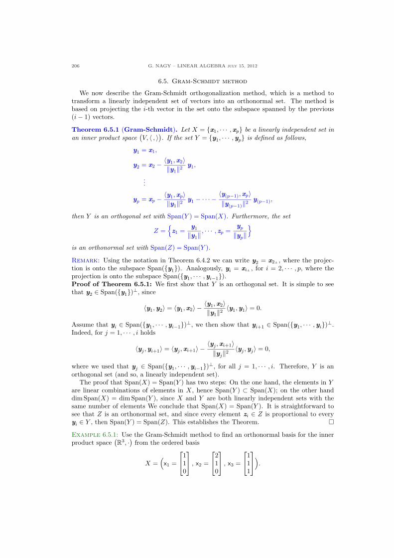
206 G. NAGY – LINEAR ALGEBRA july 15, 2012
6.5. Gram-Schmidt method
We now describe the Gram-Schmidt orthogonalization method, which is a method totransform a linearly independent set of vectors into an orthonormal set. The method isbased on projecting the i-th vector in the set onto the subspace spanned by the previous(i− 1) vectors.
Theorem 6.5.1 (Gram-Schmidt). Let X = {x1, · · · ,xp} be a linearly independent set inan inner product space
(V, 〈 , 〉). If the set Y = {y1, · · · ,yp} is defined as follows,
y1 = x1,
y2 = x2 − 〈y1,x2〉‖y1‖2
y1,
...
yp = xp − 〈y1,xp〉‖y1‖2
y1 − · · · −〈y(p−1),xp〉‖y(p−1)‖2
y(p−1),
then Y is an orthogonal set with Span(Y ) = Span(X). Furthermore, the set
Z ={z1 =
y1
‖y1‖, · · · , zp =
yp
‖yp‖}
is an orthonormal set with Span(Z) = Span(Y ).
Remark: Using the notation in Theorem 6.4.2 we can write y2 = x2 p− , where the projec-tion is onto the subspace Span({y1}). Analogously, yi = xi p− , for i = 2, · · · , p, where theprojection is onto the subspace Span({y1, · · · ,yi−1}).Proof of Theorem 6.5.1: We first show that Y is an orthogonal set. It is simple to seethat y2 ∈ Span({y1})⊥, since
〈y1,y2〉 = 〈y1,x2〉 − 〈y1,x2〉‖y1‖2
〈y1,y1〉 = 0.
Assume that yi ∈ Span({y1, · · · ,yi−1})⊥, we then show that yi+1 ∈ Span({y1, · · · ,yi})⊥.Indeed, for j = 1, · · · , i holds
〈yj ,yi+1〉 = 〈yj ,xi+1〉 −〈yj ,xi+1〉‖yj‖2
〈yj ,yj〉 = 0,
where we used that yj ∈ Span({y1, · · · ,yi−1})⊥, for all j = 1, · · · , i. Therefore, Y is anorthogonal set (and so, a linearly independent set).
The proof that Span(X) = Span(Y ) has two steps: On the one hand, the elements in Yare linear combinations of elements in X, hence Span(Y ) ⊂ Span(X); on the other handdimSpan(X) = dimSpan(Y ), since X and Y are both linearly independent sets with thesame number of elements We conclude that Span(X) = Span(Y ). It is straightforward tosee that Z is an orthonormal set, and since every element zi ∈ Z is proportional to everyyi ∈ Y , then Span(Y ) = Span(Z). This establishes the Theorem. ¤
Example 6.5.1: Use the Gram-Schmidt method to find an orthonormal basis for the innerproduct space
(R3, ·) from the ordered basis
X =(x1 =
110
, x2 =
210
, x3 =
111
).
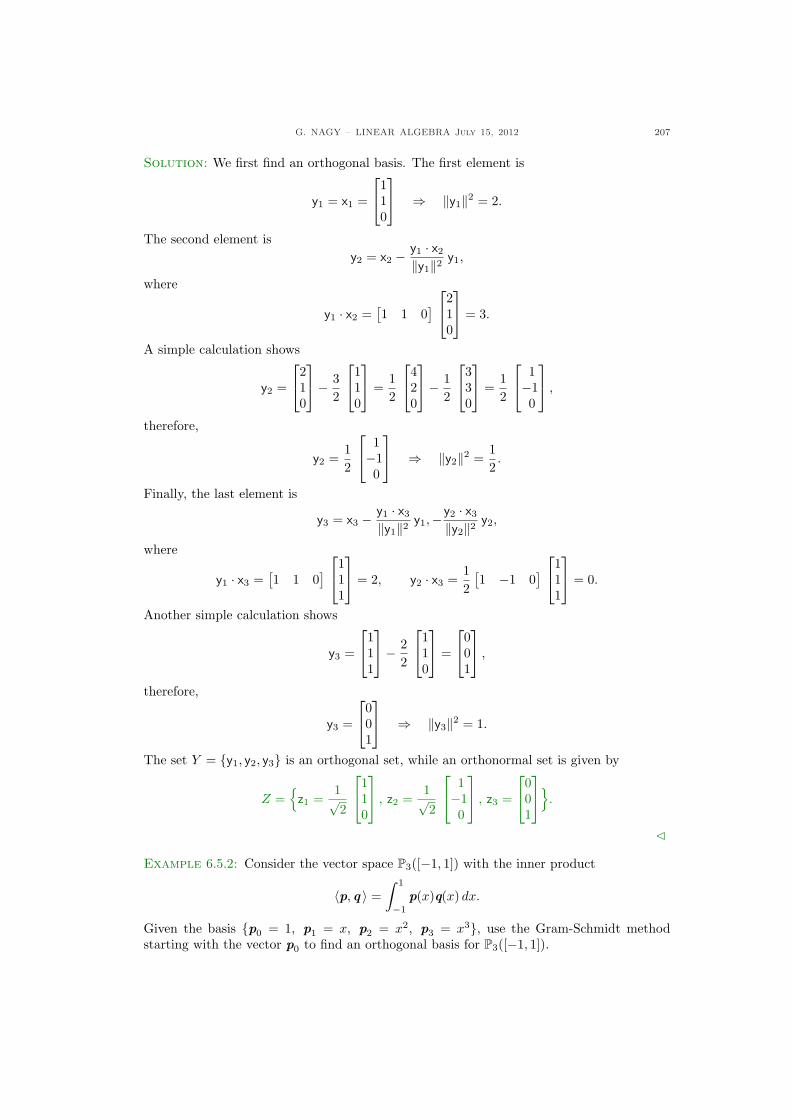
G. NAGY – LINEAR ALGEBRA July 15, 2012 207
Solution: We first find an orthogonal basis. The first element is
y1 = x1 =
110
⇒ ‖y1‖2 = 2.
The second element isy2 = x2 − y1 · x2
‖y1‖2 y1,
where
y1 · x2 =[1 1 0
]
210
= 3.
A simple calculation shows
y2 =
210
− 3
2
110
=
12
420
− 1
2
330
=
12
1−10
,
therefore,
y2 =12
1−10
⇒ ‖y2‖2 =
12.
Finally, the last element is
y3 = x3 − y1 · x3
‖y1‖2 y1,−y2 · x3
‖y2‖2 y2,
where
y1 · x3 =[1 1 0
]
111
= 2, y2 · x3 =
12
[1 −1 0
]
111
= 0.
Another simple calculation shows
y3 =
111
− 2
2
110
=
001
,
therefore,
y3 =
001
⇒ ‖y3‖2 = 1.
The set Y = {y1, y2, y3} is an orthogonal set, while an orthonormal set is given by
Z ={
z1 =1√2
110
, z2 =
1√2
1−10
, z3 =
001
}.
C
Example 6.5.2: Consider the vector space P3([−1, 1]) with the inner product
〈p, q 〉 =∫ 1
−1
p(x)q(x) dx.
Given the basis {p0 = 1, p1 = x, p2 = x2, p3 = x3}, use the Gram-Schmidt methodstarting with the vector p0 to find an orthogonal basis for P3([−1, 1]).
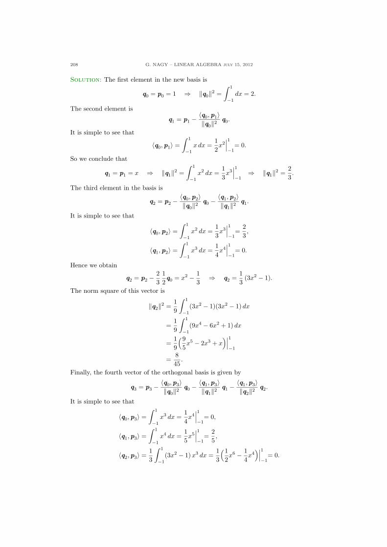
208 G. NAGY – LINEAR ALGEBRA july 15, 2012
Solution: The first element in the new basis is
q0 = p0 = 1 ⇒ ‖q0‖2 =∫ 1
−1
dx = 2.
The second element is
q1 = p1 −〈q0,p1〉‖q0‖2
q0.
It is simple to see that
〈q0,p1〉 =∫ 1
−1
x dx =12x2
∣∣∣1
−1= 0.
So we conclude that
q1 = p1 = x ⇒ ‖q1‖2 =∫ 1
−1
x2 dx =13x3
∣∣∣1
−1⇒ ‖q1‖2 =
23.
The third element in the basis is
q2 = p2 −〈q0,p2〉‖q0‖2
q0 −〈q1,p2〉‖q1‖2
q1.
It is simple to see that
〈q0,p2〉 =∫ 1
−1
x2 dx =13x3
∣∣∣1
−1=
23,
〈q1,p2〉 =∫ 1
−1
x3 dx =14x4
∣∣∣1
−1= 0.
Hence we obtain
q2 = p2 −23
12q0 = x2 − 1
3⇒ q2 =
13
(3x2 − 1).
The norm square of this vector is
‖q2‖2 =19
∫ 1
−1
(3x2 − 1)(3x2 − 1) dx
=19
∫ 1
−1
(9x4 − 6x2 + 1) dx
=19
(95x5 − 2x3 + x
)∣∣∣1
−1
=845
.
Finally, the fourth vector of the orthogonal basis is given by
q3 = p3 −〈q0,p3〉‖q0‖2
q0 −〈q1,p3〉‖q1‖2
q1 −〈q1,p3〉‖q2‖2
q2.
It is simple to see that
〈q0,p3〉 =∫ 1
−1
x3 dx =14x4
∣∣∣1
−1= 0,
〈q1,p3〉 =∫ 1
−1
x4 dx =15x5
∣∣∣1
−1=
25,
〈q2,p3〉 =13
∫ 1
−1
(3x2 − 1) x3 dx =13
(12x6 − 1
4x4
)∣∣∣1
−1= 0.
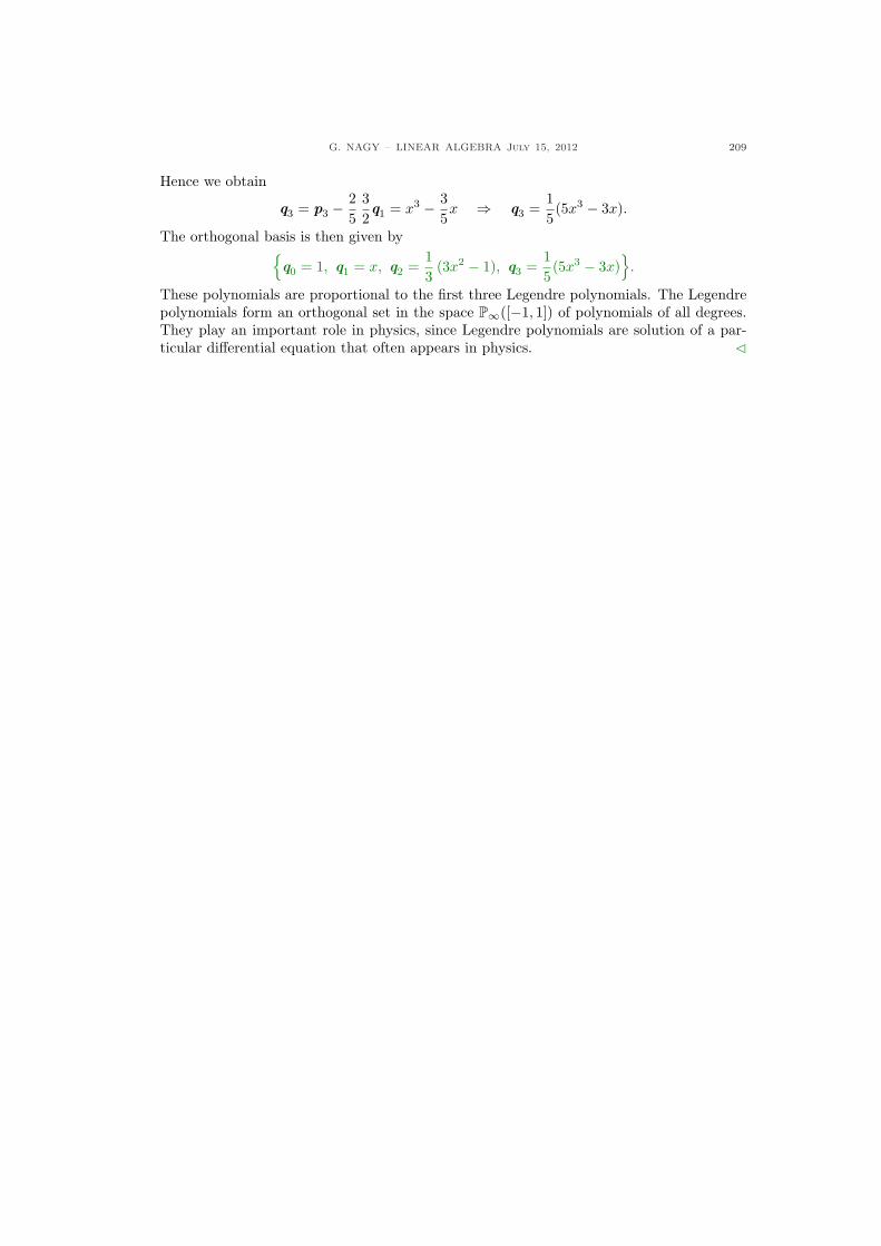
G. NAGY – LINEAR ALGEBRA July 15, 2012 209
Hence we obtain
q3 = p3 −25
32q1 = x3 − 3
5x ⇒ q3 =
15(5x3 − 3x).
The orthogonal basis is then given by{q0 = 1, q1 = x, q2 =
13
(3x2 − 1), q3 =15(5x3 − 3x)
}.
These polynomials are proportional to the first three Legendre polynomials. The Legendrepolynomials form an orthogonal set in the space P∞([−1, 1]) of polynomials of all degrees.They play an important role in physics, since Legendre polynomials are solution of a par-ticular differential equation that often appears in physics. C
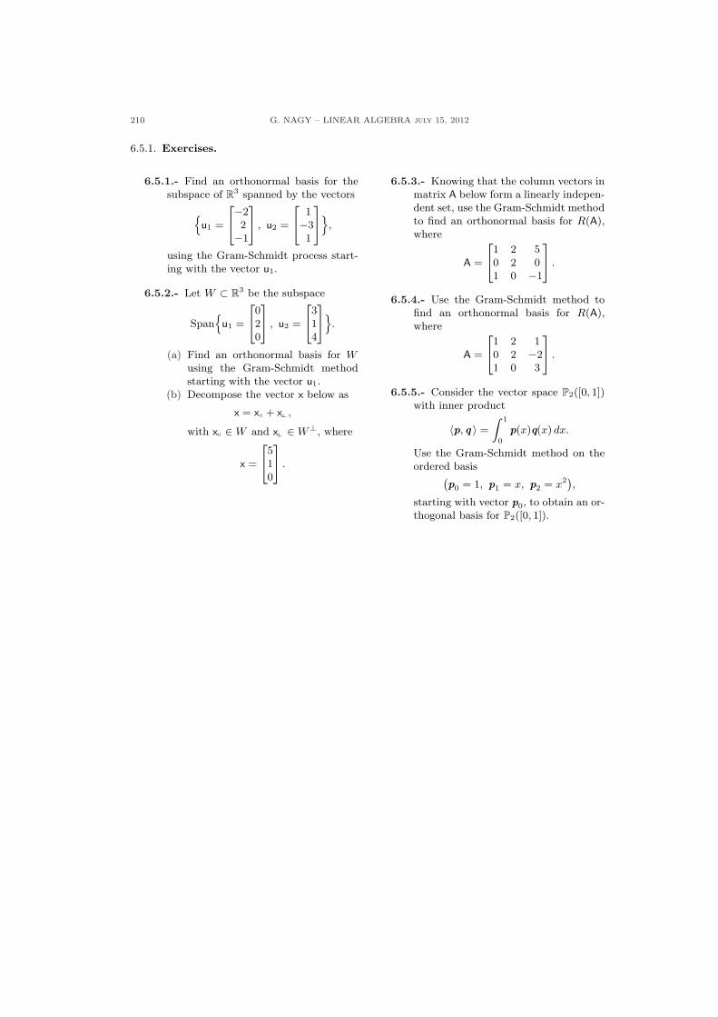
210 G. NAGY – LINEAR ALGEBRA july 15, 2012
6.5.1. Exercises.
6.5.1.- Find an orthonormal basis for thesubspace of R3 spanned by the vectors
nu1 =
24−22−1
35 , u2 =
24
1−31
35o
,
using the Gram-Schmidt process start-ing with the vector u1.
6.5.2.- Let W ⊂ R3 be the subspace
Spann
u1 =
24
020
35 , u2 =
24
314
35o
.
(a) Find an orthonormal basis for Wusing the Gram-Schmidt methodstarting with the vector u1.
(b) Decompose the vector x below as
x = xq + xp− ,
with xq ∈ W and xp− ∈ W⊥, where
x =
24
510
35 .
6.5.3.- Knowing that the column vectors inmatrix A below form a linearly indepen-dent set, use the Gram-Schmidt methodto find an orthonormal basis for R(A),where
A =
24
1 2 50 2 01 0 −1
35 .
6.5.4.- Use the Gram-Schmidt method tofind an orthonormal basis for R(A),where
A =
24
1 2 10 2 −21 0 3
35 .
6.5.5.- Consider the vector space P2([0, 1])with inner product
〈p, q 〉 =
Z 1
0
p(x)q(x) dx.
Use the Gram-Schmidt method on theordered basis`
p0 = 1, p1 = x, p2 = x2´,starting with vector p0, to obtain an or-thogonal basis for P2([0, 1]).
G. NAGY – LINEAR ALGEBRA July 15, 2012 211
6.6. The adjoint operator
6.6.1. The Riesz Representation Theorem. The Riesz Representation Theorem is astatement concerning linear functionals on an inner product space. Recall that a linearfunctional on a vector space V over a scalar field F is a linear function f : V → F, that is,for all x, y ∈ V and all a, b ∈ F holds f(ax + by) = a f(x) + b f(y) ∈ F. An example of alinear functional on R3 is the function
R3 3 x =
x1
x2
x3
7→ f(x) = 3x1 + 2x2 + x3 ∈ R.
This function can be expressed in terms of the dot product in R3 as follows
f(x) = u · x, u =
321
.
The Riesz Representation Theorem says that what we did in this example can be done in thegeneral case. In an inner product space
(V, 〈 , 〉) every linear functional f can be expressed
in terms of the inner product.
Theorem 6.6.1. Consider a finite dimensional inner product space(V, 〈 , 〉) over the scalar
field F. For every linear functional f : V → F there exists a unique vector uf ∈ V such thatholds
f(v) = 〈uf , v〉 ∀v ∈ V.
Proof of Theorem 9.4.1: Introduce the set
N = {v ∈ V : f(v) = 0 } ⊂ V.
This set is the analogous to linear functionals of the null space of linear operators. Since f isa linear function the set N is a subspace of V . (Proof: Given two elements v1, v2 ∈ N andtwo scalars a, b ∈ F, holds that f(av1 +bv2) = a f(v1)+b f(v2) = 0+0, so (av1 +bv2) ∈ N .)Introduce the orthogonal complement of N , that is,
N⊥ = {w ∈ V : 〈w, v〉 = 0 ∀v ∈ V },which is also a subspace of V . If N⊥ = {0}, then N =
(N⊥)⊥ =
({0})⊥ = V . Since thenull space of f is the whole vector space, the functional f is identically zero, so only for thechoice uf = 0 holds f(v) = 〈0, v〉 for all v ∈ V .
In the case that N⊥ 6= {0} we now show that this space cannot be very big, in fact ithas dimension one, as the following argument shows. Choose u ∈ N⊥ such that f(u) = 1.Then notice that for every w ∈ N⊥ the vector w− f(w)u is trivially in N⊥ but it is also inN , since
f(w− f(w) u
)= f(w)− f(w) f(u) = f(w)− f(w) = 0.
A vector both in N and N⊥ must vanish, so w = f(w) u. Then every vector in N⊥ isproportional to u, so dim N⊥ = 1. This information is used to split any vector v ∈ V asfollows v = a u + x where x ∈ V and a ∈ F. It is clear that
f(v) = f(a u + x) = a f(u) + f(x) = a f(u) = a.
However, the function with values g(v) =⟨ u
‖u‖2 , v⟩
has precisely the same values as f ,
since for all v ∈ V holds
g(v) =⟨ u
‖u‖2 , v⟩
=⟨ u
‖u‖2 , (a u + x)⟩
=a
‖u‖2 〈u, u〉+ 1‖u‖2 〈u,x〉 = a.
212 G. NAGY – LINEAR ALGEBRA july 15, 2012
Therefore, choosing uf = u/‖u‖2, holds that
f(v) = 〈uf , v〉 ∀v ∈ V.
Since dim N⊥ = 1, the choice of uf is unique. This establishes the Theorem. ¤
6.6.2. The adjoint operator. Given a linear operator defined on an inner product space,a new linear operator can be defined through an equation involving the inner product.
Proposition 6.6.2. If T ∈ L(V ) is a linear operator on a finite-dimensional inner productspace
(V, 〈 , 〉), then there exists a unique linear operator T ∗ ∈ L(V ), called the adjoint of
T, such that for all vectors u, v ∈ V holds
〈v,T ∗(u)〉 = 〈T(v),u〉.Proof of Proposition 9.4.2: We first establish the following statement: For every vectoru ∈ V there exists a unique vector w ∈ V such that
〈T(v),u〉 = 〈v,w〉 ∀v ∈ V. (6.18)
The proof starts noticing that for a fixed u ∈ V the scalar-valued function fu : V → Fgiven by fu(v) = 〈u,T(v)〉 is a linear functional. Therefore, the Riesz RepresentationTheorem 6.6.1 implies that there exists a unique vector w ∈ V such that fu(v) = 〈w, v〉.This establishes that for every vector u ∈ V there exists a unique vector w ∈ V such thatEq. (6.18) holds. Now that this statement is proven we can define a map, that we chooseto denote as T ∗ : V → V , given by u 7→ T ∗(u) = w. We now show that this map T ∗ islinear. Indeed, for all u1, u2 ∈ V and all a, b ∈ F holds
〈v,T ∗(au1 + bu2)〉 = 〈T(v), (au1 + bu2)〉 ∀v ∈ V,
= a 〈T(v),u1〉+ b 〈T(v),u2)〉= a〈v,T ∗(u1)〉+ b〈v,T ∗(u2)〉=
⟨v,
[aT ∗(u1) + bT ∗(u2)
]⟩ ∀v ∈ V,
hence T ∗(au1 + bu2) = aT ∗(u1) + bT ∗(u2). This establishes the Proposition. ¤The next result relates the adjoint of a linear operator with the concept of the adjoint
of a square matrix introduced in Sect. 2.2. Recall that given a basis in the vector space,every linear operator has associated a unique square matrix. Let us use the notation [T ]and [T ∗] for the matrices on a given basis of the operators T and T ∗, respectively.
Proposition 6.6.3. Let(V, 〈 , 〉) be a finite-dimensional vector space, let V be an orthonor-
mal basis of V , and let [T ] be the matrix of the linear operator T ∈ L(V ) in the basis V.Then, the matrix of the adjoint operator T ∗ in the basis V is given by [T ∗] = [T ]∗.
Proposition 6.6.3 says that the matrix of the adjoint operator is the adjoint of the matrixof the operator, however this is true only in the case that the basis used to compute therespective matrices is orthonormal. If the basis is not orthonormal, the relation betweenthe matrices [T ] and [T ∗] is more involved.Proof of Proposition 6.6.3: Let V = {e1, · · · , en} be an orthonormal basis of V , that is,
〈ei, ej〉 ={ 0 if i 6= j,
1 if i = j.
The components of two arbitrary vectors u, v ∈ V in the basis V is denoted as follows
u =∑
i
uiei, v =∑
i
viei.
G. NAGY – LINEAR ALGEBRA July 15, 2012 213
The action of the operator T can also be decomposed in the basis V as follows
T(ej) =∑
i
[T ]ijei, [T ]ij = [T(ej)]i.
We use the same notation for the adjoint operator, that is,
T ∗(ej) =∑
i
[T ∗]ijei, [T ∗]ij = [T ∗(ej)]i.
The adjoint operator is defined such that the equation 〈v,T ∗(u)〉 = 〈T(v),u〉 holds for allu, v ∈ V . This equation can be expressed in terms of components in the basis V as follows
∑
ijk
⟨viei, uj [T ∗(ej)]kek
⟩=
∑
ijk
⟨vi[T(ei)]kek, ujej
⟩,
that is, ∑
ijk
viuj [T ∗]kj〈ei, ek〉 =∑
ijk
vi[T ]kiuj〈ek, ej〉.
Since the basis V is orthonormal we obtain the equation∑
ij
viuj [T ∗]ij =∑
ijk
vi[T ]jiuj ,
which holds for all vectors u, v ∈ V , so we conclude
[T ∗]ij = [T ]ji ⇔ [T ∗] = [T ]T ⇔ [T ∗] = [T ]∗.
This establishes the Proposition. ¤
Example 6.6.1: Consider the inner product space(C3, ·). Find the adjoint of the linear
operator T with matrix in the standard basis of C3 given by
[T(x)] =
x1 + 2ix2 + ix3
ix1 − x3
x1 − x2 + ix3
, [x] =
x1
x2
x3
.
Solution: The matrix of this operator in the standard basis of C3 is given by
[T ] =
1 2i ii 0 −11 −1 i
.
Since the standard basis is an orthonormal basis with respect to the dot product, Proposi-tion 6.6.3 implies that
[T ∗] = [T ]∗ =
1 2i ii 0 −11 −1 i
∗
=
1 −i 1−2i 0 −1−i −1 −i
⇒ [T ∗(x)] =
x1 − ix2 + x3
−2ix1 − x3
−ix1 − x2 − ix3
.
C
6.6.3. Normal operators. Recall now that the commutator of two linear operators T,S ∈ L(V ) is the linear operator [T,S] ∈ L(V ) given by
[T,S](u) = T(S(u))− S(T(u)) ∀u ∈ V.
Two operators T, S ∈ L(V ) are said to commute iff their commutator vanishes, that is,[T,S] = 0. Examples of operators that commute are two rotations on the plane. Examplesof operators that do not commute are two arbitrary rotations in space.
214 G. NAGY – LINEAR ALGEBRA july 15, 2012
Definition 6.6.4. A linear operator T defined on a finite-dimensional inner product space(V, 〈 , 〉) is called a normal operator iff holds [T,T ∗] = 0, that is, the operator commutes
with its adjoint.
An interesting characterization of normal operators is the following: A linear operatorT on an inner product space is normal iff ‖T(u)‖ = ‖T ∗(u)‖ holds for all u ∈ V . Normaloperators are particularly important because for these operators hold the Spectral Theorem,which we study in Chapter 9.
Two particular cases of normal operators are often used in physics. A linear operator Ton an inner product space is called a unitary operator iff T ∗ = T−1, that is, the adjointis the inverse operator. Unitary operators are normal operators, since
T ∗ = T−1 ⇒{
TT ∗ = I,
T ∗T = I,⇒ [T,T ∗] = 0.
Unitary operators preserve the length of a vector, since
‖v‖2 = 〈v, v〉 = 〈v,T−1(T(v))〉 = 〈v,T ∗(T(v))〉 = 〈T(v),T(v)〉 = ‖T(v)‖2.Unitary operators defined on a complex inner product space are particularly important inquantum mechanics. The particular case of unitary operators on a real inner product spaceare called orthogonal operators. So, orthogonal operators do not change the length of avector. Examples of orthogonal operators are rotations in R3.
A linear operator T on an inner product space is called an Hermitian operator iffT ∗ = T, that is, the adjoint is the original operator. This definition agrees with thedefinition of Hermitian matrices given in Chapter 2.
Example 6.6.2: Consider the inner product space(C3, ·) and the linear operator T with
matrix in the standard basis of C3 given by
[T(x)] =
x1 − ix2 + x3
ix1 − x3
x1 − x2 + x3
, [x] =
x1
x2
x3
.
Show that T is Hermitian.
Solution: We need to compute the adjoint of T. The matrix of this operator in thestandard basis of C3 is given by
[T ] =
1 −i 1i 0 −11 −1 1
.
Since the standard basis is an orthonormal basis with respect to the dot product, Proposi-tion 6.6.3 implies that
[T ∗] = [T ]∗ =
1 −i 1i 0 −11 −1 1
∗
=
1 −i 1i 0 −11 −1 1
= [T ].
Therefore, T ∗ = T. C
6.6.4. Bilinear forms.
Definition 6.6.5. A bilinear form on a vector space V over F is a function a : V ×V → Flinear on both arguments, that is, for all u, v1, v2 ∈ V and all b1, b2 ∈ F holds
a(u, (b1v1 + b2v2)
)= b1a(u, v1) + b2a(u, v2),
a((b1v1 + b2v2),u
)= b1a(v1,u) + b2a(v2,u).
G. NAGY – LINEAR ALGEBRA July 15, 2012 215
The bilinear form a : V × V → F is called symmetric iff for all u, v ∈ V holds
a(u, v) = a(v,u).
An example of a symmetric bilinear form is any the inner product on a real vector space.Indeed, given a real inner product space
(V, 〈 , 〉), the function 〈 , 〉 : V × V → R is a
symmetric bilinear form, since it is symmetric and
〈u, (b1v1 + b2v2)〉 = b1〈u, v1〉+ b2〈u, v2〉.We will shortly see that another example of a bilinear form appears on the weak formulationof the boundary value problem in Eq. (7.30).
On the other hand, an inner product on a complex vector space is not a bilinear form,since it is conjugate linear on the first argument instead of linear. Such functions are calledsesquilinear forms. That is, a sesquilinear form on a complex vector space V is a functiona : V × V → C that is conjugate linear on the first argument and linear on the secondargument. Sesquilinear forms are important in the case of studying differential equationsinvolving complex functions.
Definition 6.6.6. Consider a bilinear form a : V × V → F on an inner product space(V, 〈 , 〉) over F. The bilinear form a is called positive iff there exists a real number k > 0
such that for all u ∈ V holdsa(u,u) > k ‖u‖2.
The bilinear form a is called bounded iff there exists a real number K > 0 such that forall u, v ∈ V holds
a(u, v) 6 K ‖u‖ ‖v‖.An example of a positive bilinear form is any inner product on a real vector space. The
Schwarz inequality implies that such inner product is also a bounded bilinear form. In fact,an inner product on a real vector space is a symmetric, positive, bounded bilinear form. Wewill shortly see that the bilinear form that appears on a weak formulation of the boundaryvalue problem in Eq. (7.30) is symmetric, positive and bounded. We will see that theseproperties imply the existence and uniqueness of solutions to the weak formulation of theboundary value problem.

216 G. NAGY – LINEAR ALGEBRA july 15, 2012
6.6.5. Exercises.
6.6.1.- . 6.6.2.- .
G. NAGY – LINEAR ALGEBRA July 15, 2012 217
Chapter 7. Approximation methods
7.1. Best approximation
The first half of this Section is dedicated to show that the Fourier series approximation ofa function is a particular case of the orthogonal decomposition of a vector onto a subspacein an inner product space, studied in Section 6.4. Once we realize that it is not difficult tosee why such Fourier approximations are useful. We show that the orthogonal projectionxq of a vector x onto a subspace U is the vector in the subspace U closest to x. This isthe origin of the name “best approximation” for xq. What is intuitively clear in
(R3, ·) is
true in every inner product space, hence it is true for the Fourier series approximation ofa function. In the second half of this Section we show a deep relation between the Nullspace of a matrix and the Range space of the adjoint matrix. The former is the orthogonalcomplement of the latter. A consequence of this relation is a simple proof to the propertythat a matrix and its adjoint matrix have the same rank. Another consequence is given inthe next Section, where we obtain a simple equation, called the normal equation, to find aleast squares solution of an inconsistent linear system.
7.1.1. Fourier expansions. We have seen that orthonormal bases have a practical ad-vantage over arbitrary basis. The components [x ]u of a vector x in an orthonormal basisUn = {u1, · · · ,un} of the inner product space
(V, 〈 , 〉) are given by the simple expression
[x ]u =
〈u1,x〉
...〈un,x〉
⇔ x = 〈u1,x〉u1 + · · ·+ 〈un,x〉un.
In the case that an orthonormal set Up is not a basis of V , that is, p < dim V , one can alwaysintroduce the orthogonal projection of a vector x ∈ V onto the subspace Up = Span(Up),
xq = 〈u1,x〉u1 + · · ·+ 〈up,x〉up.
We have seen that in this case, xq 6= x. In fact we called the difference vector xp− = x− xq,since this vector satisfies that xp− ⊥ xq. We now give the projection vector xq a new name.
Definition 7.1.1. The Fourier expansion of a vector x ∈ V with respect to an orthonor-mal set Up = {u1, · · · ,up} ⊂
(V, 〈 , 〉) is the unique vector xq ∈ Span(Up) given by
xq = 〈u1,x〉u1 + · · ·+ 〈up,x〉up. (7.1)
The scalars 〈ui,x〉 are the Fourier coefficient of the vector x with respect to the set Up.
A reason to the name “Fourier expansion” to the orthogonal projection of a vector ontoa subspace is given in the following example.
Example 7.1.1: Given the vector space of continuous functions V = C([−`, `],R
)with
inner product given by 〈f , g〉 =∫ `
−`
f (x)g(x) dx, find the Fourier expansion of an arbitrary
function f ∈ V with respect to the orthonormal set
UN ={u0 =
1√2`
, un =1√`
cos(nπx
`
), vn =
1√`
sin(nπx
`
)}N
n=1.
Solution: Using Eq. (7.1) on a function f ∈ V we get
f q = 〈u0, f 〉u0 +N∑
n=1
[〈un, f 〉un + 〈vn, f 〉 vn
].
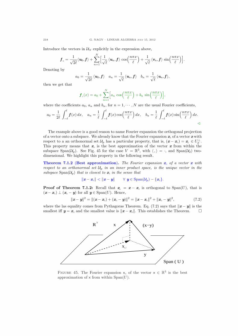
218 G. NAGY – LINEAR ALGEBRA july 15, 2012
Introduce the vectors in UN explicitly in the expression above,
f q =1√2`〈u0, f 〉+
N∑n=1
[ 1√`〈un, f 〉 cos
(nπx
`
)+
1√`〈vn, f 〉 sin
(nπx
`
)].
Denoting by
a0 =1√2`〈u0, f 〉 an =
1√`〈un, f 〉 bn =
1√`〈un, f 〉,
then we get that
f q(x) = a0 +N∑
n=1
[an cos
(nπx
`
)+ bn sin
(nπx
`
)],
where the coefficients a0, an and bn, for n = 1, · · · , N are the usual Fourier coefficients,
a0 =12`
∫ `
−`
f (x) dx, an =1`
∫ `
−`
f (x) cos(nπx
`
)dx, bn =
1`
∫ `
−`
f (x) sin(nπx
`
)dx.
C
The example above is a good reason to name Fourier expansion the orthogonal projectionof a vector onto a subspace. We already know that the Fourier expansion xq of a vector x withrespect to a an orthonormal set Up has a particular property, that is, (x − xq) = xp− ∈ U⊥
p .This property means that xq is the best approximation of the vector x from within thesubspace Span(Up). See Fig. 45 for the case V = R3, with 〈 , 〉 = ·, and Span(U2) two-dimensional. We highlight this property in the following result.
Theorem 7.1.2 (Best approximation). The Fourier expansion xq of a vector x withrespect to an orthonormal set Up in an inner product space, is the unique vector in thesubspace Span(Up) that is closest to x, in the sense that
‖x− xq‖ < ‖x− y‖ ∀ y ∈ Span(Up)− {xq}.
Proof of Theorem 7.1.2: Recall that xp− = x − xq is orthogonal to Span(U), that is(x− xq) ⊥ (xq − y) for all y ∈ Span(U). Hence,
‖x− y‖2 = ‖(x− xq) + (xq − y)‖2 = ‖x− xq‖2 + ‖xq − y‖2, (7.2)
where the las equality comes from Pythagoras Theorem. Eq. (7.2) says that ‖x− y‖ is thesmallest iff y = xq and the smallest value is ‖x− xq‖. This establishes the Theorem. ¤
Span ( U )
x
y
(x−y)xR3
Figure 45. The Fourier expansion xq of the vector x ∈ R3 is the bestapproximation of x from within Span(U).
G. NAGY – LINEAR ALGEBRA July 15, 2012 219
Example 7.1.2: Given the vector space of continuous functions V = C([−1, 1],R
)with the
inner product given by 〈f , g〉 =∫ 1
−1
f (x)g(x) dx, find the Fourier expansion of the function
f (x) = x with respect to the orthonormal set
UN ={u0 =
1√2`
, un =1√`
cos(nπx
`
), vn =
1√`
sin(nπx
`
)}N
n=1.
Solution: We use the formulas in Example 7.1.1 above to the function f (x) = x on theinterval [−1, 1], since ` = 1. The coefficient a0 above is given by
a0 =12
∫ 1
−1
x dx =14(x2
∣∣1−1
) ⇒ a0 = 0.
The coefficients an, bn, for n = 1, · · · , N computed with one integration by parts,∫
x cos(nπx) dx =x
nπsin(nπx) +
1n2π2
cos(nπx),∫
x sin(nπx) dx = − x
nπcos(nπx) +
1n2π2
sin(nπx).
The coefficients an vanish, since
an =∫ 1
−1
x cos(nπx) dx =[ x
nπsin(nπx)
]∣∣∣1
−1+
1n2π2
cos(nπx)∣∣∣1
−1⇒ an = 0.
The coefficients bn are given by
bn =∫ 1
−1
x sin(nπx) dx = −[ x
nπcos(nπx)
]∣∣∣1
−1+
1n2π2
sin(nπx)∣∣∣1
−1⇒ bn =
2(−1)(n+1)
nπ.
Therefore, the Fourier expansion of f (x) = x with respect to UN is given by
f q(x) =2π
N∑n=1
(−1)(n+1)
nsin(nπx).
Remark: First, a simpler proof that the coefficients a0 and an vanish is to realized that weare integrating an odd function on the interval [−1, 1]. The odd function is the product ofan odd function times an even function. Second, Theorem 7.1.2 tells us that the functionf q above is only combination of the sine and cosine functions in UN that approximates bestthe function f (x) = x on the interval [−1, 1]. C
7.1.2. Null and range spaces of a matrix. The null and range spaces associated with amatrix A ∈ Fm,n and its adjoint matrix A∗ are deeply related.
Theorem 7.1.3. For every matrix A ∈ Fm,n holds N(A) = R(A∗)⊥ and N(A∗) = R(A)⊥.
Since for every subspace W on a finite dimensional inner product space holds (W⊥)⊥ = W ,we also have the relations
N(A)⊥ = R(A∗), N(A∗)⊥ = R(A).
In the case of real-valued matrices, the Theorem above says that
N(A) = R(AT )⊥ and N(AT ) = R(A)⊥.
220 G. NAGY – LINEAR ALGEBRA july 15, 2012
Before we state the proof of this Theorem let us review the following notation: Givenan m × n matrix A ∈ Fm,n, we write it either in terms of column vectors A:j ∈ Fm forj = 1, · · · , n, or in terms of row vectors Ai: ∈ Fn for i = 1, · · · ,m, as follows,
A =[A:1 · · · A:n
], A =
A1:
...Am:
.
Since the same type of definition holds for the n×m matrix A∗, that is,
A∗ =[(A∗):1 · · · (A∗):m
], A∗ =
(A∗)1:...
(A∗)n:
,
then we have the relations
(A:j)∗ = (A∗)j:, (Ai:)∗ = (A∗):i.
For example, consider the 2× 3 matrix
A =[1 2 34 5 6
]⇒ A:1 =
[14
], A:2 =
[25
], A:3 =
[36
],
A1: =[1 2 3
],
A2: =[4 5 6
]..
The transpose is a 3× 2 matrix that can be written as follows
AT =
1 42 53 6
⇒ (AT ):1 =
123
, (AT ):2 =
456
,
(AT )1: =[1 4
],
(AT )2: =[2 5
],
(AT )3: =[3 6
].
.
So, for example we have the relation
(A:3)T =[3 6
]= (AT )3:, (A2:)T =
456
= (AT ):2.
Proof of Theorem 7.1.3: We first show that the N(A) = R(A∗)⊥. A vector x ∈ Fn
belongs to N(A) iff holds
Ax = 0 ⇔
A1:
...Am:
x = 0 ⇔
[(A∗):1
]∗...[
(A∗):m]∗
x = 0 ⇔
(A∗):1 · x = 0,
...
(A∗):m · x = 0.
So, x ∈ N(A) iff x is orthogonal to every column vector in A∗, that is, x ∈ R(A∗)⊥.The equation N(A∗) = R(A)⊥ comes from N(B) = R(B∗)⊥ taking B = A∗. Nevertheless,
we repeat the proof above, just to understand the previous argument. A vector y ∈ Fm
belongs to N(A∗) iff
A∗y = 0 ⇔
(A∗)1:...
(A∗)n:
y = 0 ⇔
(A:1)∗...
(A:n)∗
y = 0 ⇔
A:1 · y = 0,
...A:n · y = 0.
So, y ∈ N(A∗) iff y is orthogonal to every column vector in A, that is, y ∈ R(A)⊥. Thisestablishes the Theorem. ¤
G. NAGY – LINEAR ALGEBRA July 15, 2012 221
Example 7.1.3: Verify Theorem 7.1.3 for the matrix A =[1 2 33 2 1
].
Solution: We first find the N(A), that is, all x ∈ R3 solutions of Ay = 0. Gauss operationson matrix A imply
[1 2 33 2 1
]→
[1 0 −10 1 2
]⇒
x1 = x3,
x2 = −2x3,
x3 free,⇒ N(A) = Span
({
1−21
}).
It is simple to find R(AT ), since
R(AT ) = Span({
123
,
321
}).
Theorem 7.1.3 is verified, since
[1 2 3
]
1−21
= 1−4+3 = 0,
[3 2 1
]
1−21
= 3−4+1 = 0 ⇒ N(A) = R(AT )⊥.
Let us verify the same Theorem for AT . We first find N(AT ), that is, all y ∈ R2 solutions ofAT y = 0. Gauss operations on matrix AT imply
1 32 23 1
→
1 00 10 0
⇒ y =
[00
]⇒ N(AT ) = {0}.
The space R(A) is given by
R(A) = Span({[
13
],
[22
],
[31
]})= Span
({ [13
],
[22
]})= R2.
Since (R2)⊥ = {0}, Theorem 7.1.3 is verified. C
Theorem 7.1.3 provides a simple proof for a result we used in Chapter 2.
Theorem 7.1.4. For every matrix A ∈ Fm,n holds that rank(A) = rank(A∗).
Proof of Theorem 7.1.4: Recall the Nullity-Rank result in Corollary 5.1.8, which saysthat for all matrix A ∈ Fm,n holds dim N(A) + dim R(A) = n. Equivalently,
dim R(A) = n− dim N(A) = n− dim R(A∗)⊥,
since N(A) = R(A∗)⊥. From the orthogonal decomposition Fn = R(A∗)⊕R(A∗)⊥ we knowthat dim R(A∗) = n− dim R(A∗)⊥. We then conclude that
dim R(A) = dim R(A∗).
This establishes the Theorem. ¤
222 G. NAGY – LINEAR ALGEBRA july 15, 2012
7.1.3. Exercises.
7.1.1.- Consider the inner product space`R3, · ´ and the orthonormal set U ,
nu1 =
1√2
24
1−10
35 , u2 =
1√3
24
111
35o
.
Find the best approximation of x belowin the subspace Span(U), where
x =
24
10−2
35 .
7.1.2.- Consider the inner product space`R2,2, 〈 , 〉F
´and the orthonormal set
U = {E1, E2}, where
E1 =1√2
»0 11 0
–, E2 =
1√2
»1 00 −1
–.
Find the best approximation of matrixA below in the subspace Span(U), where
A =
»1 11 1
–.
7.1.3.- Consider the inner product space
P2([0, 1]), with 〈p, q 〉 =R 1
0p(x)q(x) dx,
and the subspace U = Span(U), whereU = {q0 = 1, q1 = (x− 1
2)}.
(a) Show that U is an orthogonal set.(b) Find rq, the best approximation
with respect to U of the polynomialr(x) = 2x + 3x2.
(c) Verify whether (r−rq) ∈ U⊥ or not.
7.1.4.- Consider the space C∞([−`, `],R)with inner product
〈f , g〉 =
Z `
−`
f (x)g(x) dx,
and the orthonormal set U given by
u0 =1√2`
u1 =1√`
cos“πx
`
”
v1 =1√`
sin“πx
`
”.
Find the best approximation of
f (x) =
x 0 6x 6 `,
−x −` 6x < 0.
in the space Span(U)
7.1.5.- For the matrix A ∈ R3,3 below,verify that N(A) = R(AT )⊥ and that
N(AT ) = R(A)⊥, where
A =
24
2 1 1−1 −1 0−2 −1 −1
35 .
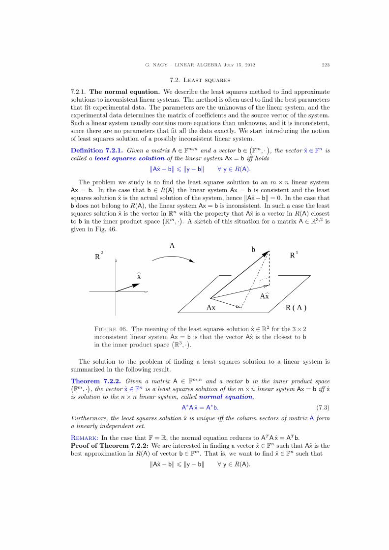
G. NAGY – LINEAR ALGEBRA July 15, 2012 223
7.2. Least squares
7.2.1. The normal equation. We describe the least squares method to find approximatesolutions to inconsistent linear systems. The method is often used to find the best parametersthat fit experimental data. The parameters are the unknowns of the linear system, and theexperimental data determines the matrix of coefficients and the source vector of the system.Such a linear system usually contains more equations than unknowns, and it is inconsistent,since there are no parameters that fit all the data exactly. We start introducing the notionof least squares solution of a possibly inconsistent linear system.
Definition 7.2.1. Given a matrix A ∈ Fm,n and a vector b ∈ (Fm, · ), the vector x ∈ Fn is
called a least squares solution of the linear system Ax = b iff holds
‖Ax− b‖ 6 ‖y − b‖ ∀ y ∈ R(A).
The problem we study is to find the least squares solution to an m × n linear systemAx = b. In the case that b ∈ R(A) the linear system Ax = b is consistent and the leastsquares solution x is the actual solution of the system, hence ‖Ax− b‖ = 0. In the case thatb does not belong to R(A), the linear system Ax = b is inconsistent. In such a case the leastsquares solution x is the vector in Rn with the property that Ax is a vector in R(A) closestto b in the inner product space
(Rm, ·). A sketch of this situation for a matrix A ∈ R3,2 is
given in Fig. 46.
3
x
b
Ax
Ax
A
R R
R ( A )
2
Figure 46. The meaning of the least squares solution x ∈ R2 for the 3× 2inconsistent linear system Ax = b is that the vector Ax is the closest to bin the inner product space
(R3, ·).
The solution to the problem of finding a least squares solution to a linear system issummarized in the following result.
Theorem 7.2.2. Given a matrix A ∈ Fm,n and a vector b in the inner product space(Fm, ·), the vector x ∈ Fn is a least squares solution of the m× n linear system Ax = b iff x
is solution to the n× n linear system, called normal equation,
A∗A x = A∗b. (7.3)
Furthermore, the least squares solution x is unique iff the column vectors of matrix A forma linearly independent set.
Remark: In the case that F = R, the normal equation reduces to AT A x = AT b.Proof of Theorem 7.2.2: We are interested in finding a vector x ∈ Fn such that Ax is thebest approximation in R(A) of vector b ∈ Fm. That is, we want to find x ∈ Fn such that
‖Ax− b‖ 6 ‖y − b‖ ∀ y ∈ R(A).
224 G. NAGY – LINEAR ALGEBRA july 15, 2012
Theorem 7.1.2 says that the best approximation of b is when Ax = bq, where bq is theorthogonal projection of b onto the subspace R(A). This means that
(Ax− b) ∈ R(A)⊥ = N(A∗) ⇔ A∗(Ax− b) = 0.
We then conclude that x must be solution of the normal equation
A∗Ax = A∗b.
The furthermore can be shown as follows. The column vectors of matrix A form a linearlyindependent set iff N(A) = {0}. Lemma 7.2.3 stated below establishes that, for all matrixA holds that N(A) = N(A∗A). This result in our case implies that N(A∗A) = {0}. Sincematrix A∗A is a square, n× n, matrix, we conclude that it is invertible. This is equivalentto say that the solution x to the normal equation is unique; moreover, it is given by x =(A∗A)−1A∗b. This establishes the Theorem. ¤
In the proof of Theorem 7.2.2 above we used the following result:
Lemma 7.2.3. If A ∈ Fm,n, then N(A) = N(A∗A).
Proof of Lemma 7.2.3: We first show that N(A) ⊂ N(A∗A). Indeed,
x ∈ N(A) ⇒ Ax = 0 ⇒ A∗Ax = 0 ⇒ x ∈ N(A∗A).
Now, suppose that there exists x ∈ N(A∗A) such that x /∈ N(A). Therefore, x 6= 0 andAx 6= 0, which imply that
0 6= ‖Ax‖2 = x∗A∗Ax ⇒ A∗Ax 6= 0.
However, this last equation contradicts the assumption that x ∈ N(A∗A). Therefore, weconclude that N(A) = N(A∗A). This establishes the Lemma. ¤Example 7.2.1: Show that the 3× 2 linear system Ax = b is inconsistent; then find a least
squares solutions x =[x1
x2
]to that system, where
A =
1 32 23 1
, b =
−11−1
.
Solution: We first show that the linear system above is inconsistent, since Gauss operationon the augmented matrix [A|b] imply
1 3∣∣ −1
2 2∣∣ 1
3 1∣∣ −1
→
1 3∣∣ −1
0 −4∣∣ 3
0 −8∣∣ 2
→
1 3∣∣ −1
0 −4∣∣ 3
0 0∣∣ 1
.
In order to find the least squares solution to the system above we first construct the normalequation. We need to compute
AT A =[1 2 33 2 1
]
1 32 23 1
=
[14 1010 14
], AT b =
[1 2 33 2 1
] −11−1
=
[−2−2
].
Therefore, the normal equation is given by[14 1010 14
] [x1
x2
]=
[−2−2
].
Since the column vectors of A form a linearly independent set, matrix AT A is invertible,(AT A
)−1 =196
[14 −10−10 14
]=
148
[7 −5−5 7
].
G. NAGY – LINEAR ALGEBRA July 15, 2012 225
The least squares solution is unique and given by
x =124
[7 −5−5 7
] [−1−1
]⇒ x =
112
[−1−1
].
Remark: We now verify that (Ax− b) ∈ R(A)⊥. Indeed,
Ax− b =
1 32 23 1
1
12
[−1−1
]−
−11−1
= −1
3
111
−
−11−1
⇒ Ax− b =
23
1−21
.
Since
[1 −2 1
]
123
= 1− 4 + 3 = 0,
[1 −2 1
]
321
= 3− 4 + 1 = 0,
we have verified that (Ax− b) ∈ R(A)⊥. C
We finish this Subsection with an alternative proof of Theorem 7.2.2 in the particularcase that involves real-valued matrices, that is, F = R. The proof is interesting in its own,since it is based in solving a constrained minimization problem.Alternative proof of Theorem 7.2.2 for F = R: The vector x ∈ Rn is a least squaressolution of the system Ax = b iff the function f : Rn → R given by f(x) = ‖Ax− b‖2 has aminimum at x = x. We then find all minima of function f . We first express f as follows,
f(x) = (Ax− b) · (Ax− b)= (Ax) · (Ax)− 2b · (Ax) + b · b= xT AT Ax− 2bT Ax + bT b.
We now need to find all solutions to the equation ∇xf(x) = 0. Recalling the definition of agradient vector
∇xf =
∂f
∂x1...
∂f
∂xn
,
it is simple to see that, for any vector a ∈ Rn, holds,
∇x(aT x) = a, ∇x(xT a) = a.
Therefore, the gradient of f is given by
∇xf = 2AT Ax− 2AT b.
We are interested in the stationary points, the x solutions of
∇xf(x) = 0 ⇔ AT A x = AT b.
We conclude that all stationary points x are solutions of the normal equation, Eq. (7.3).These stationary points must be a minimum of f , since f is quadratic on the vector compo-nents xi having the degree two terms all positive coefficients. This establishes the first partof Theorem 7.2.2 in the case that F = R. ¤
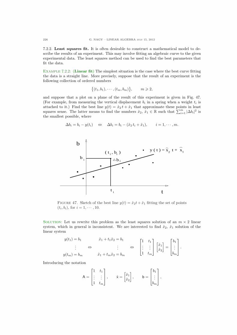
226 G. NAGY – LINEAR ALGEBRA july 15, 2012
7.2.2. Least squares fit. It is often desirable to construct a mathematical model to de-scribe the results of an experiment. This may involve fitting an algebraic curve to the givenexperimental data. The least squares method can be used to find the best parameters thatfit the data.
Example 7.2.2: (Linear fit) The simplest situation is the case where the best curve fittingthe data is a straight line. More precisely, suppose that the result of an experiment is thefollowing collection of ordered numbers
{(t1, b1), · · · , (tm, bm)
}, m > 2,
and suppose that a plot on a plane of the result of this experiment is given in Fig. 47.(For example, from measuring the vertical displacement bi in a spring when a weight ti isattached to it.) Find the best line y(t) = x2 t + x1 that approximate these points in leastsquares sense. The latter means to find the numbers x2, x1 ∈ R such that
∑mi=1 |∆bi|2 is
the smallest possible, where
∆bi = bi − y(ti) ⇔ ∆bi = bi − (x2 ti + x1), i = 1, · · · , m.
i t
b
b i
i i( t , b ) 2y ( t ) = x t + x1
bi
t
Figure 47. Sketch of the best line y(t) = x2t + x1 fitting the set of points(ti, bi), for i = 1, · · · , 10.
Solution: Let us rewrite this problem as the least squares solution of an m × 2 linearsystem, which in general is inconsistent. We are interested to find x2, x1 solution of thelinear system
y(t1) = b1
...
y(tm) = bm
⇔x1 + t1x2 = b1
...x1 + tmx2 = bm
⇔
1 t1...
...1 tm
[x1
x2
]=
b1
...bm
.
Introducing the notation
A =
1 t1...
...1 tm
, x =
[x1
x2
], b =
b1
...bm
,
G. NAGY – LINEAR ALGEBRA July 15, 2012 227
we are then interested in finding the solution x of the m×2 linear system Ax = b. Introducingalso the vector
∆b =
∆b1
...∆bm
,
it is clear that Ax− b = ∆b, and so we obtain the important relation
‖Ax− b‖2 = ‖∆b‖2 =m∑
i=1
(∆bi
)2.
Therefore, the vector x that minimizes the square of the deviation from the line,∑m
i=1(∆bi)2,is precisely the same vector x ∈ R2 that minimizes the number ‖Ax − b‖2. We studied thelatter problem at the begining of this Section. We called it a least squares problem, and thesolution x is the solution of the normal equation
AT A x = AT b.
It is simple to see that
AT A =[
1 · · · 1t1 · · · tm
]
1 t1...
...1 tm
=
[m
∑ti∑
ti∑
t2i
],
AT b =[
1 · · · 1t1 · · · tm
]
b1
...bm
=
[ ∑bi∑
tibi
].
Therefore, we are interested in finding the solution to the 2× 2 linear system[m
∑ti∑
ti∑
t2i
] [x1
x2
]=
[ ∑bi∑
tibi
].
Suppose that at least one of the ti is different from 1, then matrix AT A is invertible and theinverse is (
AT A)−1 =
1
m∑
t2i −(∑
ti)2
[ ∑t2i −∑
ti−∑
ti m
].
We conclude that the solution to the normal equation is[x1
x2
]=
1
m∑
t2i −(∑
ti)2
[ ∑t2i −∑
ti−∑
ti m
] [ ∑bi∑
tibi
].
So, the slope x2 and vertical intercept x1 of the best fitting line are given by
x2 =m
∑tibi − (
∑ti)(
∑bi)
m∑
t2i −(∑
ti)2 , x1 =
(∑
t2i )(∑
bi)− (∑
ti)(∑
tibi)
m∑
t2i −(∑
ti)2 .
C
Example 7.2.3: (Polynomial fit) Find the best polynomial of degree (n − 1) > 0, sayp(t) = xn t(n−1) + · · ·+ x1, that approximates in least squares sense the set of points{
(t1, b1), · · · , (tm, bm)}, m > n.
(See Fig. 48 for an example in the case that the fitting curve is a parabola, n = 3.) FollowingExample 7.2.2, the least squares approximation means to find the numbers xn, · · · , x1 ∈ Rsuch that
∑mi=1 |∆bi|2 is the smallest possible, where
∆bi = bi − p(ti) ⇔ ∆bi = bi − (xn t(n−1)i + · · ·+ x1), i = 1, · · · ,m.
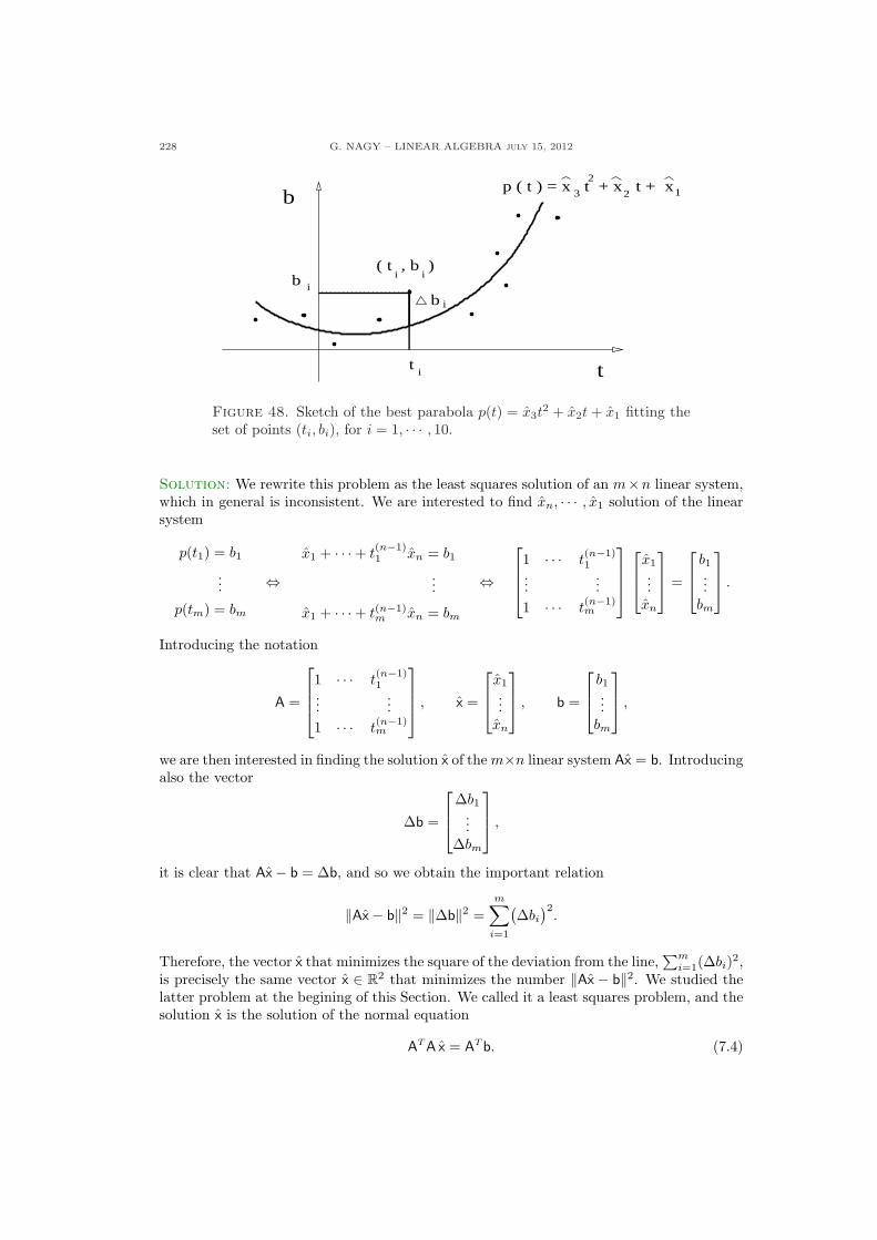
228 G. NAGY – LINEAR ALGEBRA july 15, 2012
2
t
b
ti
b i
( t , b )i ib i
p ( t ) = x t + x t + x3 2 1
Figure 48. Sketch of the best parabola p(t) = x3t2 + x2t + x1 fitting the
set of points (ti, bi), for i = 1, · · · , 10.
Solution: We rewrite this problem as the least squares solution of an m×n linear system,which in general is inconsistent. We are interested to find xn, · · · , x1 solution of the linearsystem
p(t1) = b1
...
p(tm) = bm
⇔x1 + · · ·+ t
(n−1)1 xn = b1
...
x1 + · · ·+ t(n−1)m xn = bm
⇔
1 · · · t(n−1)1
......
1 · · · t(n−1)m
x1
...xn
=
b1
...bm
.
Introducing the notation
A =
1 · · · t(n−1)1
......
1 · · · t(n−1)m
, x =
x1
...xn
, b =
b1
...bm
,
we are then interested in finding the solution x of the m×n linear system Ax = b. Introducingalso the vector
∆b =
∆b1
...∆bm
,
it is clear that Ax− b = ∆b, and so we obtain the important relation
‖Ax− b‖2 = ‖∆b‖2 =m∑
i=1
(∆bi
)2.
Therefore, the vector x that minimizes the square of the deviation from the line,∑m
i=1(∆bi)2,is precisely the same vector x ∈ R2 that minimizes the number ‖Ax − b‖2. We studied thelatter problem at the begining of this Section. We called it a least squares problem, and thesolution x is the solution of the normal equation
AT A x = AT b. (7.4)
G. NAGY – LINEAR ALGEBRA July 15, 2012 229
It is simple to see that Eq. (7.4) is an n× n linear system, since
AT A =
1 · · · 1...
...t(n−1)1 · · · t
(n−1)m
1 · · · t(n−1)1
......
1 · · · t(n−1)m
,
AT b =
1 · · · 1...
...t(n−1)1 · · · t
(n−1)m
b1
...bm
.
We do not compute these expressions explicitly here. In the case that the columns of Aform a linearly independent set, the solution x to the normal equation is
x =(AT A
)−1AT b.
The components of x provide the parameters for the best polynomial fitting the data in leastsquares sense. C
7.2.3. Linear correlation. In statistics a correlation coefficient measures the departure oftwo random variables from independence. For centered data, that is, for data with zeroaverage, the correlation coefficient can be viewed as the cosine of the angle in an abstractRn space between two vectors constructed with the random variables data. We now defineand find the correlation coefficient for two variables as given in Example 7.2.2.
Once again, suppose that the result of an experiment is the following collection of orderednumbers {
(t1, b1), · · · , (tm, bm)}, m > 2. (7.5)
Introduce the vectors e, t, b ∈ Rm as follows,
e =
1...1
, t =
t1...
tm
, b =
b1
...bm
.
Before introducing the correlation coefficient, let us use these vectors above to write downthe least squares coefficients x found in Example 7.2.2. The matrix of coefficients can bewritten as A = [e, t], therefore,
AT A =[eT
tT
] [e, t
]=
[e · e t · ee · t t · t
], AT b =
[eT
tT
]b =
[e · bt · b
].
The least squares solution can be written as follows,[x1
x2
]=
1(e · e)(t · t)− (t · e)2
[t · t −e · t−e · t e · e
] [e · bt · b
],
that is,
x2 =(e · e)(t · b)− (e · t)(e · b)
(e · e)(t · t)− (t · e)2 , x1 =(e · b)(t · t)− (e · t)(t · b)
(e · e)(t · t)− (t · e)2 .
Introduce the average values
t =e · te · e , b =
e · be · e .
These are indeed the average values of ti and bi, since
e · e = m, e · t =m∑
i=1
ti, e · b =m∑
i=1
bi.
230 G. NAGY – LINEAR ALGEBRA july 15, 2012
Introduce the zero-average vectors t = (t− t e) and b = (b− b e). The correlation coefficientof the data given in (7.5) is given by
cor(t, b) =t · b‖t‖ ‖b‖ .
Therefore, the correlation coefficient between the data vectors t and b is the angle betweenthe zero-average vectors t and b in Rm.
In order to understand what measures this angle, let us consider the case where all theordered pairs in (7.5) lies on a line, that is, there exists a solution x of the linear systemAx = b (a solution, not only a least squares solution). In that case we have
x1e + x2t = b ⇒ x1 + x2t = b,
and this implies that
x2 (t− t e) = (b− b e) ⇔ x2 t = b ⇔ cor(t, b) = 1.
That is, in the case that t is linearly related to b we obtain that the zero-average vectors tand b are parallel, so the correlation coefficient is equal one.
7.2.4. QR-factorization. The Gram-Schmidt method can be used to factor any m × nmatrix A into a product of an m × n matrix Q with orthonormal column vectors and anupper triangular n × n matrix R. We will see that the QR-factorization is useful to solvethe normal equation associated to a least squares problem.
Theorem 7.2.4. If the column vectors of matrix A ∈ Fm,n form a linearly independent set,then there exist matrices Q ∈ Fm,n and R ∈ Fn,n satisfying that Q∗Q = In, matrix R is uppertriangular with positive diagonal elements, and the following equation holds
A = QR.
Proof of Theorem 7.2.4: Use the Gram-Schmidt method to obtain an orthonormal set{q1, · · · , qn} from the column vectors of the m× n matrix A = [A:1, · · · , A:n], that is,
p1 = A:1 q1 =p1
‖p1‖ ,
p2 = A:2 −(A:2 · q1
)q1 q2 =
p2
‖p2‖ ,...
...
pn = A:n −(A:n · q1
)q1 − · · · −
(A:n · qn−1
)qn−1 qn =
pn
‖pn‖ .
Define matrix Q = [q1, · · · , qn], which then satisfies the equation Q∗Q = In. Notice that theequations above can be expressed as follows,
A:1 = ‖p1‖ q1,
A:2 = ‖p2‖ q2 +(q1 · A:2
)q1
...
A:n = ‖pn‖ qn +(q1 · A:n
)q1 +
(q2 · A:n
)q2 + · · ·+ (
qn−1 · A:n
)qn−1.
G. NAGY – LINEAR ALGEBRA July 15, 2012 231
After some time staring at the equations above, one can rewrite it as a matrix product
[A:1, · · · ,A:n
]=
[q1, · · · , qn
]
‖p1‖ (q1 · A:2) · · · (q1 · A:n)0 ‖p2‖ · · · (q2 · A:n)...
......
0 0 · · · (qn−1 · A:n)0 0 · · · ‖pn‖
(7.6)
Define matrix R by equation above as the matrix satisfying A = QR. Then, Eq. (7.6) saysthat matrix R is n× n, upper triangular, with positive diagonal elements. This establishesthe Theorem. ¤
Example 7.2.4: Find the QR-factorization of matrix A =
1 2 11 1 10 0 1
.
Solution: First use the Gram-Schmidt method to transform the column vectors of matrixA into an orthonormal set. This was done in Example 6.5.1. The result defines the matrixQ as follows
Q =
1√2
1√2
01√2− 1√
20
0 0 1
.
Having matrix A and Q, and knowing that Theorem 7.2.4 is true, then we can computematrix R by the equation R = QT A. Since the column vectors of Q form an orthonormalset, we have that QT = Q−1, and in this particular case Q−1 = Q, so matrix R is given by
R = QA =
1√2
1√2
01√2− 1√
20
0 0 1
1 2 11 1 10 0 1
⇒ R =
√2 3√
2
√2
0 1√2
00 0 1
.
The QR-factorization of matrix A is then given by
A =
1√2
1√2
01√2− 1√
20
0 0 1
√2 3√
2
√2
0 1√2
00 0 1
.
C
The QR-factorization is useful to solve the normal equation in a least squares problem.
Theorem 7.2.5. Assume that the matrix A ∈ Fm,n admits the QR-factorization A = QR.The vector x ∈ Fn is solution of the normal equation A∗A x = A∗b iff it is solution of
Rx = Q∗b.
Proof of Theorem 7.2.5: Just introduce the QR-factorization into the normal equationA∗A x = A∗b as follows,(
R∗Q∗)(
QR)x = R∗Q∗b ⇔ R∗R x = R∗Q∗b ⇔ R∗
(R x− Q∗b
)= 0.
Since R is a square, upper triangular matrix with non-zero coefficients, we conclude that Ris invertible. Therefore, from the last equation above we conclude that x is solution of thenormal equation iff holds
Rx = Q∗b.
This establishes the Theorem. ¤
232 G. NAGY – LINEAR ALGEBRA july 15, 2012
7.2.5. Exercises.
7.2.1.- Consider the matrix A and the vec-tor b given by
A =
24
1 00 11 1
35 , b =
24
110
35 .
(a) Find the least-squares solution x tothe linear system Ax = b.
(b) Verify that the solution x satisfies
(Ax− b) ∈ R(A)⊥.
7.2.2.- Consider the matrix A and the vec-tor b given by
A =
24
2 20 −1−2 0
35 , b =
24
11−1
35 .
(a) Find the least-squares solution x tothe linear system Ax = b.
(b) Find the orthogonal projection ofthe source vector b onto the sub-space R(A).
7.2.3.- Find all the least-squares solutionsx to the linear system Ax = b, where
A =
24
1 22 43 6
35 , b =
24
111
35 .
7.2.4.- Find the best line in least-squaressense that fits the measurements, wheret1 is the independent variable and bi isthe dependent variable,
t1 = −2, b1 = 4,
t2 = −1, b2 = 3,
t3 = 0, b3 = 1,
t4 = 2, b4 = 0.
7.2.5.- Find the correlation coefficient cor-responding to the measurements givenin Exercise 7.2.4 above.
7.2.6.- Use Gram-Schmidt method on thecolumns of matrix A below to find itsQR factorization, where
A =
24
1 12 32 1
35 .
7.2.7.- Find the QR factorization of matrix
A =
24
1 1 01 0 10 1 1
35 .
G. NAGY – LINEAR ALGEBRA July 15, 2012 233
7.3. Finite difference method
A differential equation is an equation where the unknown is a function and both thefunction itself and its derivatives appear in the equation. The differential equation is calledlinear iff the unknown function and its derivatives appear linearly in the equation. Solutionsof linear differential equations can be approximated by solutions of appropriate n× n alge-braic linear systems in the limit that n approaches infinity. The finite difference method isa way to obtain an n× n linear system from the original differential equation. Derivativesare approximated by difference quotients, thus reducing a differential equation to an alge-braic linear system. Since a derivative can be approximated by infinitely many differencequotients, there are infinitely many n × n linear systems that approximate a differentialequation. One tries to choose the linear system whose solution is the best approximation ofthe solution of the original differential equation. Computers are used to find the vector in Rn
solution of the n× n linear system. Many approximations of the solution to the differentialequation are obtained from this array of n numbers. One way to obtain a function from avector in Rn is to find a degree n polynomial that contains all these n points. This is calleda polynomial interpolation of the algebraic solution. In this Section we only show how toobtain n× n algebraic linear systems that approximate a simple differential equation.
7.3.1. Differential equations. A differential equation is an equation where the unknownis a function and both the function and its derivatives appear in the equation. A simpleexample is the following: Given a continuously differentiable function f : [0, 1]→ R, find afunction u : [0, 1]→ R solution of the differential equation
du
dx(x) = f(x),
To find a solution to a differential equation requires to perform appropriate integrations,thus integration constants are introduced in the solution. This suggests that the solution ofa differential equation is not unique, and extra conditions must be added to the problem toselect only one solution. In the differential equation above the solutions u are given by
u(x) =∫ x
0
f(t) dt + c,
with c ∈ R. An extra condition is needed to obtain a unique solution, for example thecondition u(0) = 1. Then, the unique solution u is computed as follows
1 = u(0) =∫ 0
0
f(t) dt + c ⇒ c = 1 ⇒ u(x) =∫ x
0
f(t) dt + 1.
The example above is simple enough that no approximation is needed to obtain the solution.An ordinary differential equation is a differential equation where the unknown function
u depends on one variable, as in the example above. A partial differential equation is adifferential equation where the unknown function depends on more than one variable andthe equation contains derivatives of more than one variable. In this Section we use the finitedifference method to find a solution to two different problems. The first one involves anordinary differential equation while the second one involves a partial differential equation,called the heat equation.
The first problem is to find an approximate solution to a boundary value problem for anordinary differential equation: Given a continuously differentiable function f : [0, 1] → R,
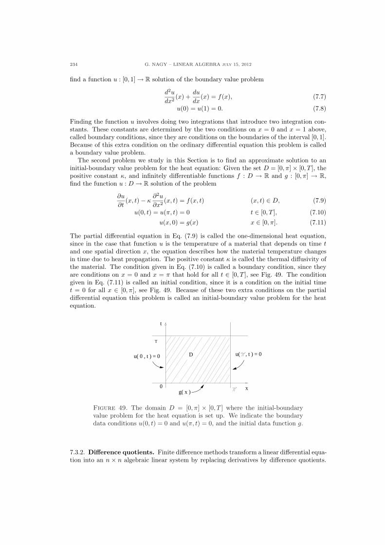
234 G. NAGY – LINEAR ALGEBRA july 15, 2012
find a function u : [0, 1]→ R solution of the boundary value problem
d2u
dx2(x) +
du
dx(x) = f(x), (7.7)
u(0) = u(1) = 0. (7.8)
Finding the function u involves doing two integrations that introduce two integration con-stants. These constants are determined by the two conditions on x = 0 and x = 1 above,called boundary conditions, since they are conditions on the boundaries of the interval [0, 1].Because of this extra condition on the ordinary differential equation this problem is calleda boundary value problem.
The second problem we study in this Section is to find an approximate solution to aninitial-boundary value problem for the heat equation: Given the set D = [0, π]× [0, T ], thepositive constant κ, and infinitely differentiable functions f : D → R and g : [0, π] → R,find the function u : D → R solution of the problem
∂u
∂t(x, t)− κ
∂2u
∂x2(x, t) = f(x, t) (x, t) ∈ D, (7.9)
u(0, t) = u(π, t) = 0 t ∈ [0, T ], (7.10)
u(x, 0) = g(x) x ∈ [0, π]. (7.11)
The partial differential equation in Eq. (7.9) is called the one-dimensional heat equation,since in the case that function u is the temperature of a material that depends on time tand one spatial direction x, the equation describes how the material temperature changesin time due to heat propagation. The positive constant κ is called the thermal diffusivity ofthe material. The condition given in Eq. (7.10) is called a boundary condition, since theyare conditions on x = 0 and x = π that hold for all t ∈ [0, T ], see Fig. 49. The conditiongiven in Eq. (7.11) is called an initial condition, since it is a condition on the initial timet = 0 for all x ∈ [0, π], see Fig. 49. Because of these two extra conditions on the partialdifferential equation this problem is called an initial-boundary value problem for the heatequation.
u( 0 , t ) = 0
T
D
g( x )
t
0 x
u( , t ) = 0
Figure 49. The domain D = [0, π] × [0, T ] where the initial-boundaryvalue problem for the heat equation is set up. We indicate the boundarydata conditions u(0, t) = 0 and u(π, t) = 0, and the initial data function g.
7.3.2. Difference quotients. Finite difference methods transform a linear differential equa-tion into an n × n algebraic linear system by replacing derivatives by difference quotients.
G. NAGY – LINEAR ALGEBRA July 15, 2012 235
Derivatives can be approximated by difference quotients in many different ways. For exam-ple, a derivative of a function u can be expressed in the following equivalent ways,
du
dx(x) = lim
∆x→0
u(x + ∆x)− u(x)∆x
,
= lim∆x→0
u(x)− u(x−∆x)∆x
,
= lim∆x→0
u(x + ∆x)− u(x−∆x)2∆x
.
However, for a fixed nonzero value of ∆x, the expressions below are, in general, different.
Definition 7.3.1. The forward difference quotient d+ and the backward differencequotient d- of a continuous function u : R→ R at x ∈ R are given by
d+u(x) =u(x + ∆x)− u(x)
∆x, d-u(x) =
u(x)− u(x−∆x)∆x
.
The centered difference quotient dc of a continuous function u at x ∈ R is given by
dcu(x) =u(x + ∆x)− u(x−∆x)
2∆x. (7.12)
In the case that the function u has second continuous derivative, the Taylor ExpansionTheorem implies that the forward and backward differences differ from the actual derivativeby terms order ∆x. The proof is not difficult, since
u(x + ∆x) = u(x) +du
dx(x)∆x + O
((∆x)2
) ⇒ d+u(x) =du
dx(x) + O
(∆x
),
u(x−∆x) = u(x)− du
dx(x)∆x + O
((∆x)2
) ⇒ d-u(x) =du
dx(x) + O
(∆x
),
where O((∆x)n
)denotes a function satisfying
[O
((∆x)n
)]/(∆x)n approaches a constant
as ∆x → 0. In the case that the function u has third continuous derivative, the TaylorExpansion Theorem implies that the centered difference quotient differs from the actualderivative by terms of order (∆x)2. Again, the proof is not difficult, and it is based on theTaylor expansion of the function u. Compute this expansion in two different ways,
u(x + ∆x) = u(x) +du
dx(x)∆x +
12
d2u
dx2(x) (∆x)2 + O
((∆x)3
), (7.13)
u(x−∆x) = u(x)− du
dx(x)∆x +
12
d2u
dx2(x) (∆x)2 + O
((∆x)3
), (7.14)
Subtracting the two expressions above we obtain that
u(x + ∆x)− u(x−∆x) = 2du
dx(x)∆x + O
((∆x)3
) ⇒ dcu(x) =du
dx(x) + O
((∆x)2
),
which establishes that centered difference quotients differ from the derivative by order (∆x)2.If a function is infinitely continuously differentiable, centered difference quotients are moreaccurate than forward or backward differences.
Second and higher derivatives of a function can also be approximated by difference quo-tients. Again, there are infinitely many ways to approximate second derivatives by differencequotients. The freedom to choose difference quotients is higher for second derivatives thanfor first derivatives. We now present two difference quotients to give an idea of this freedom.On the one hand, one possible approximation is to use the centered difference quotient twice,since a second derivative is the derivative of the derivative function. Using the more precisenotation
dc∆xu(x) =u(x + ∆x)− u(x−∆x)
2∆x,
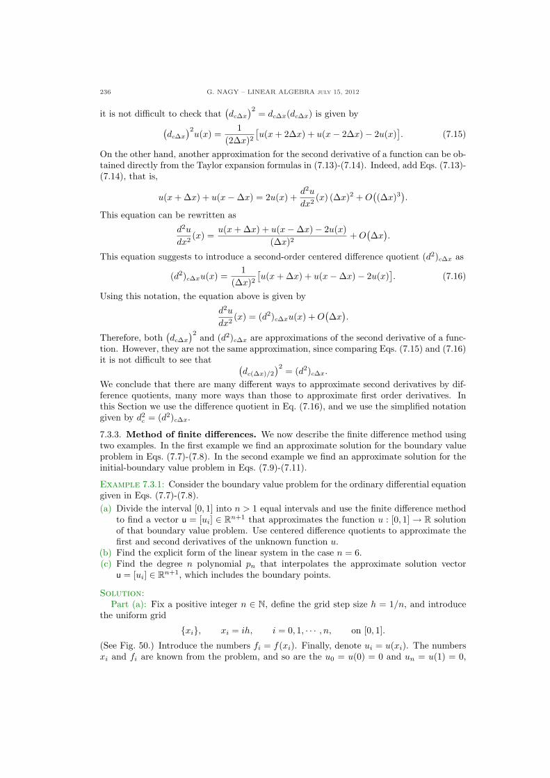
236 G. NAGY – LINEAR ALGEBRA july 15, 2012
it is not difficult to check that(dc∆x
)2 = dc∆x(dc∆x) is given by(dc∆x
)2u(x) =
1(2∆x)2
[u(x + 2∆x) + u(x− 2∆x)− 2u(x)
]. (7.15)
On the other hand, another approximation for the second derivative of a function can be ob-tained directly from the Taylor expansion formulas in (7.13)-(7.14). Indeed, add Eqs. (7.13)-(7.14), that is,
u(x + ∆x) + u(x−∆x) = 2u(x) +d2u
dx2(x) (∆x)2 + O
((∆x)3
).
This equation can be rewritten as
d2u
dx2(x) =
u(x + ∆x) + u(x−∆x)− 2u(x)(∆x)2
+ O(∆x
).
This equation suggests to introduce a second-order centered difference quotient (d2)c∆x as
(d2)c∆xu(x) =1
(∆x)2[u(x + ∆x) + u(x−∆x)− 2u(x)
]. (7.16)
Using this notation, the equation above is given by
d2u
dx2(x) = (d2)c∆xu(x) + O
(∆x
).
Therefore, both(dc∆x
)2 and (d2)c∆x are approximations of the second derivative of a func-tion. However, they are not the same approximation, since comparing Eqs. (7.15) and (7.16)it is not difficult to see that (
dc(∆x)/2
)2 = (d2)c∆x.
We conclude that there are many different ways to approximate second derivatives by dif-ference quotients, many more ways than those to approximate first order derivatives. Inthis Section we use the difference quotient in Eq. (7.16), and we use the simplified notationgiven by d2
c = (d2)c∆x.
7.3.3. Method of finite differences. We now describe the finite difference method usingtwo examples. In the first example we find an approximate solution for the boundary valueproblem in Eqs. (7.7)-(7.8). In the second example we find an approximate solution for theinitial-boundary value problem in Eqs. (7.9)-(7.11).
Example 7.3.1: Consider the boundary value problem for the ordinary differential equationgiven in Eqs. (7.7)-(7.8).(a) Divide the interval [0, 1] into n > 1 equal intervals and use the finite difference method
to find a vector u = [ui] ∈ Rn+1 that approximates the function u : [0, 1] → R solutionof that boundary value problem. Use centered difference quotients to approximate thefirst and second derivatives of the unknown function u.
(b) Find the explicit form of the linear system in the case n = 6.(c) Find the degree n polynomial pn that interpolates the approximate solution vector
u = [ui] ∈ Rn+1, which includes the boundary points.
Solution:Part (a): Fix a positive integer n ∈ N, define the grid step size h = 1/n, and introduce
the uniform grid
{xi}, xi = ih, i = 0, 1, · · · , n, on [0, 1].
(See Fig. 50.) Introduce the numbers fi = f(xi). Finally, denote ui = u(xi). The numbersxi and fi are known from the problem, and so are the u0 = u(0) = 0 and un = u(1) = 0,
G. NAGY – LINEAR ALGEBRA July 15, 2012 237
while the ui for i = 1, · · · , n − 1 are the unknowns. We now use the original differentialequation to construct an (n− 1)× (n− 1) linear system for these unknowns ui.
]0 = 0 / 6 1 / 6 2 / 6 3 / 6 4 / 6 5 / 6 6 / 6 = 1
n = 6 x = 1 / 6 h = 1 / 6 = x
[
Figure 50. A uniform grid for n = 6 on the domain [0, 1].
We use centered difference quotient given in Eqs. (7.12) and (7.16) to approximate the firstand second derivatives of the function u, respectively. We choose ∆x = h, and we denotethe difference quotients evaluated at grid points xi as follows,
dcu(xi) = dcui, d2cu(xi) = d2
cui.
Therefore, we obtain the following formulas for the difference quotients,
dcui =ui+1 − ui−1
2h, d2
cui =ui+1 + ui−1 − 2ui
h2. (7.17)
Now we state the approximate problem we will solve: Given the constants {fi}n−1i=1 , find
the vector u = [ui] ∈ Rn+1 solution of the (n − 1) × (n − 1) linear system and boundaryconditions, respectively,
d2cui + dcui = fi, i = 1, · · · , n− 1, (7.18)
u0 = un = 0. (7.19)
Eq. (7.18) is indeed a linear system for u = [ui], since it is equivalent to the system
(2 + h)ui+1 − 4ui + (2− h)ui−1 = 2h2fi, i = 1, · · · , n− 1.
When the boundary conditions in Eq. (7.19) are introduced in the equation above, we obtainan (n− 1)× (n− 1) linear system for the unknowns ui, where i = 1, · · · , (n− 1).
Part (b): In the case n = 6, we have h = 1/6, so we denote a = 2− 1/6, b = 2 + 1/6 andc = 2/36. Also recall the boundary conditions u0 = u6 = 0. Then, the system above andits augmented matrix are given by, respectively,
−4u1 + bu2 = c f1,
au1 − 4u2 + bu3 = c f2,
au2 − 4u3 + bu4 = c f3,
au3 − 4u4 + bu5 = c f4,
au4 − 4u5 = c f5,
⇔
−4 b 0 0 0∣∣ c f1
a −4 b 0 0∣∣ c f2
0 a −4 b 0∣∣ c f3
0 0 a −4 b∣∣ c f4
0 0 0 a −4∣∣ c f5
.
We then conclude that the solution u of the boundary value problem in Eq. (7.7) can beapproximated by the solution u = [ui] ∈ R7 of the 5 × 5 linear system above plus the twoboundary conditions. The same type of approximate solution can be found for all n ∈ N.
Part (c): The output of the finite difference method is a vector u = [ui] ∈ R(n+1). Anapproximate solution to the ordinary differential equation in Eqs. (7.7) can be constructedfrom the vector u in many different ways. One way is polynomial interpolation, that is,
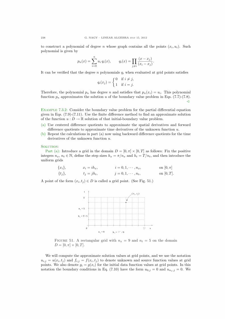
238 G. NAGY – LINEAR ALGEBRA july 15, 2012
to construct a polynomial of degree n whose graph contains all the points (xi, ui). Suchpolynomial is given by
pn(x) =n∑
i=0
ui qi(x), qi(x) =∏
j 6=i
(x− xj)(xi − xj)
.
It can be verified that the degree n polynomials qi when evaluated at grid points satisfies
qi(xj) ={ 0 if i 6= j,
1 if i = j.
Therefore, the polynomial pn has degree n and satisfies that pn(xi) = ui. This polynomialfunction pn approximates the solution u of the boundary value problem in Eqs. (7.7)-(7.8).
C
Example 7.3.2: Consider the boundary value problem for the partial differential equationgiven in Eqs. (7.9)-(7.11). Use the finite difference method to find an approximate solutionof the function u : D → R solution of that initial-boundary value problem.
(a) Use centered difference quotients to approximate the spatial derivatives and forwarddifference quotients to approximate time derivatives of the unknown function u.
(b) Repeat the calculations in part (a) now using backward difference quotients for the timederivatives of the unknown function u.
Solution:Part (a): Introduce a grid in the domain D = [0, π] × [0, T ] as follows: Fix the positive
integers nx, nt ∈ N, define the step sizes hx = π/nx and ht = T/nt, and then introduce theuniform grids
{xi}, xi = ihx, i = 0, 1, · · · , nx, on [0, π]
{tj}, tj = jht, j = 0, 1, · · · , nt, on [0, T ].
A point of the form (xi, tj) ∈ D is called a grid point. (See Fig. 51.)
j
����
t
x0
T
n = 9
tn = 5
h = T / 5t
h = / 9xx
( x , t )i
Figure 51. A rectangular grid with nx = 9 and nt = 5 on the domainD = [0, π]× [0, T ].
We will compute the approximate solution values at grid points, and we use the notationui,j = u(xi, tj) and fi,j = f(xi, tj) to denote unknown and source function values at gridpoints. We also denote gi = g(xi) for the initial data function values at grid points. In thisnotation the boundary conditions in Eq. (7.10) have the form u0,j = 0 and unx,j = 0. We
G. NAGY – LINEAR ALGEBRA July 15, 2012 239
finally introduce the forward difference quotient in time d+t and the second order centereddifference quotient in space d2
cx as follows,
d+tui,j =ui,(j+1) − ui,j
ht, d2
cxui,j =u(i+1),j + u(i−1),j − 2ui,j
h2x
.
Now we state the approximate problem we will solve: Given the constants fi,j and gi, fori = 0, 1, · · · , nx and j = 0, 1, · · · , ny, find the constants ui,j solution of the linear equationsand boundary conditions, respectively,
d+tui,j − κd2cxui,j = fi,j , (7.20)
u0,j = unx,j = 0, (7.21)ui,0 = gi. (7.22)
This system is simpler to solve than it looks at first sight. Let us rewrite it in as follows,1ht
(ui,(j+1) − ui,j
)− κ
h2x
(u(i+1),j + u(i−1),j − 2ui,j
)= fij ,
which is equivalent to the equation
ui,(j+1) = r(u(i+1),j + u(i−1),j
)+ (1− 2r)ui,j + htfi,j , (7.23)
where r = κht/h2cx. This last equation says that the solution at the time tj+1 can be
computed if the solution at the previous time tj is known. Since the solution at the initialtime t0 = 0 is known an equal to gi, and since solution at the boundary of the domain u0,j
and unx,j is known from the boundary conditions, then the solution ui,j can be computedfrom Eq. (7.23) time step after time step. For this reason the linear system in Eqs. (7.20)-(7.22) above is an example of an explicit method.
Part (b): We now repeat the calculations in part (a) using a backward difference quotientin time. We introduce the notation d-t for the backward difference quotient in time, and wekeep the notation d2
cx for the second order centered difference quotient in space,
d-tui,j =ui,j − ui,(j−1)
ht, d2
cxui,j =u(i+1),j + u(i−1),j − 2ui,j
h2x
.
Now we state the approximate problem we will solve: Given the constants fi,j and gi, fori = 0, 1, · · · , nx and j = 0, 1, · · · , ny, find the constants ui,j solution of the linear equationsand boundary conditions, respectively,
d-tui,j − κd2cxui,j = fi,j , (7.24)
u0,j = unx,j = 0, (7.25)ui,0 = gi. (7.26)
This system is simpler to solve than it looks at first sight. Let us rewrite it in as follows,1ht
(ui,j − ui,(j−1)
)− κ
h2x
(u(i+1),j + u(i−1),j − 2ui,j
)= fij ,
which is equivalent to the equation
(+2r)ui,j − r(u(i+1),j + u(i−1),j
)= ui,(j−1) + htfi,j , (7.27)
where r = κht/h2cx, as above. This last equation says that the solution at the time tj+1 can
be computed if the solution at the previous time tj is known. However, in this case we needto solve an (nx−1)× (nx−1) linear system at each time step. Such system is similar to theone that appeared in Example 7.3.1. Since the solution at the initial time t0 = 0 is known anequal to gi, and since solution at the boundary of the domain u0,j and unx,j is known fromthe boundary conditions, then the solution ui,j can be computed from Eq. (7.27) time step
240 G. NAGY – LINEAR ALGEBRA july 15, 2012
after time step. We emphasize that the solution is computed by solving an (nx−1)×(nx−1)system at every time step. For this reason the linear system in Eqs. (7.24)-(7.26) above isan example of an implicit method. C
What we have seen in this Section is just the first part of the story. We have seenhow we can use linear algebra to obtain approximate solutions of few problems involvingdifferential equations. The second part is to study how the solutions of the approximateproblems approaches the solution of the original problem as the grid step size approacheszero. Consider the approximate solution u ∈ Rn+1 found in Example 7.3.1. Does theinterpolation polynomial pn constructed with the components of u approximate the functionu : [0, 1] → R solution to the boundary value problem in Eq. (7.7) in the limit n → ∞?A similar question can be asked for the solutions {ui,j} obtained in parts (b) and (c) inExample 7.3.2. We will study the answers to these questions in the following Chapters.
One last remark is the following. Comparing parts (a) and (b) in Example 7.3.2 we seethat explicit methods are simpler to solve than implicit methods. A matrix must be invertedto solve an implicit method, while this is not needed to solve an explicit method. So, whyare implicit methods studied at all? The reason is that in the limit n→∞ the approximatesolutions of explicit methods do not approximate the solution of the original differentialequation as good as a solution of an implicit method. Moreover, the solution of an explicitmethod may not converge at all, while the solutions of implicit methods always converges.
Further reading. See Section 1.4 in Meyer’s book [3] for a detailed discussion on dis-cretizations of two-point boundary values problems.
G. NAGY – LINEAR ALGEBRA July 15, 2012 241
7.3.4. Exercises.
7.3.1.- Consider the boundary value prob-lem for the function u given by
d2u
dx2(x) = 25 x,
u(0) = 0, u(1) = 0,
x ∈ [0, 1].
Divide the interval [0, 1] into five equalsubintervals and use the finite differencemethod to find an approximate solutionvector u = [ui] to the boundary valueproblem above, where i = 0, · · · , 5. Usecentered difference quotients given inEq. (7.17) to approximate the deriva-tives of function u.
7.3.2.- Given an infinite differentiable func-tion u : R→ R. apply twice the forwarddifference quotient d+ to show that thesecond order forward difference quotienthas the form
d2+u(x) =
u(x + 2∆x)− 2u(x + ∆x) + u(x)
(∆x)2.
7.3.3.- Given an infinite differentiable func-tion u : R → R. apply twice the back-ward difference quotient d+ to show thatthe second order backward differencequotient has the form
d2-u(x) =
u(x)− 2u(x−∆x) + u(x− 2∆x)
(∆x)2.
7.3.4.- Consider the boundary value prob-lem given in the Exercise 7.3.1. Di-vide again the interval [0, 1] into fiveequal subintervals and find the 4×4 lin-ear system that approximates the orig-inal problem using forward differencequotients to approximate derivatives offunction u. You do not need to solvethe linear system.
7.3.5.- Consider the boundary value prob-lem given Problem 7.3.1. Divide againthe interval [0, 1] into five equal subin-tervals and find the 4× 4 linear systemthat approximates the original problemusing backward difference quotients toapproximate derivatives of function u.You do not need to solve the linear sys-tem.
7.3.6.- Consider the boundary value prob-lem for the function u given by
d2u
dx2(x) + 2
du
dx(x) = 25 x,
u(0) = 0, u(1) = 0,
x ∈ [0, 1].
Divide the interval [0, 1] into five equalsubintervals and use the finite differ-ence method to find an algebraic lin-ear system that approximates the origi-nal boundary value problem above. Usecentered difference quotients given inEq. (7.17) to approximate derivatives offunction u. You do not need to solve thelinear system.
242 G. NAGY – LINEAR ALGEBRA july 15, 2012
7.4. Finite element method
The finite element method permits the computation of approximate solutions to dif-ferential equations. Boundary value problems involving a differential equations are firsttransformed into integral equations. The boundary conditions are included into the inte-gral equation by performing integration by parts. The original problem is transformed intoinverting a bilinear form on a vector space. The approximate problem is obtained whenthe integral equation is solved not on the whole vector space but on a finite dimensionalsubspace. By a careful choice of the subspace, the calculations needed to obtain the approx-imate solution can be simplified. In this Section we study the same differential equationswe have seen in Sect. 7.3 when we described the finite difference methods. Finite differ-ence methods are different form finite element methods. The former method approximatesderivatives by difference quotients in order to obtain the approximate problem involving analgebraic linear system. The latter method produces an algebraic linear system by restrict-ing an integral version of the original differential equation onto a finite dimensional subspaceof the original vector space where the integral equation is defined.
7.4.1. Differential equations. We now recall the boundary value problem we are inter-ested to study. This is the first problem we studied in Sect. 7.3, that is, to find an approxi-mate solution to a boundary value problem for an ordinary differential equation: Given aninfinitely differentiable function f : [0, 1]→ R, find a function u : [0, 1]→ R solution of theboundary value problem
d2u
dx2(x) +
du
dx(x) = f(x), (7.28)
u(0) = u(1) = 0. (7.29)
Recall that finding the function u involves doing two integrations that introduce two in-tegration constants. These constants are determined by the two conditions on x = 0 andx = 1 above, called boundary conditions, since they are conditions on the boundaries ofthe interval [0, 1]. Because of this extra condition on the ordinary differential equation thisproblem is called a boundary value problem.
This problem can be expressed using linear transformations on vector spaces. Considerthe inner product spaces
(V, 〈 , 〉) and
(W, 〈 , 〉), where V = C∞0 ([0, 1],R) is the space of
infinitely many differentiable functions that vanish at x = 0 and x = 1, W = C∞([0, 1],R)is the space of infinitely many differentiable functions, while the inner product is defined as
〈f , g〉 =∫ 1
0
f (x)g(x) dx.
Introduce the linear transformation L : V →W defined by
L(v) =d2v
dx2+
dv
dx
Then, the boundary value problem in Eqs. (7.28)-(7.29) can be expressed in the followingway: Given a vector f ∈W , find a vector u ∈ V solution of the equation
L(u) = f . (7.30)
Notice that the boundary conditions in Eq. (7.29) have been included into the definition ofthe vector space V . The problem defined by Eqs. (7.28)-(7.29), which is equivalently definedby Eq. (7.30), is called the strong formulation of the problem.
So, we have expressed a boundary value problem for a differential equation in terms oflinear transformations between appropriate infinite dimensional vector spaces. The nextstep is to use the inner product defined on V and W to transform the differential equation
G. NAGY – LINEAR ALGEBRA July 15, 2012 243
in (7.30) into an integro-differential equation, which will be called the weak formulation ofthe problem. This idea is summarized below.
7.4.2. The Galerkin method. The Galerkin method refers to a collection of ideas totransform a problem involving a linear transformation between infinite dimensional innerproduct spaces into a problem involving a matrix as a function between finite dimensionalsubspaces. We describe in this Section the original idea, introduced by Boris Galerkinaround 1915. Galerkin worked only with partial differential equations, but we now knowthat his idea works in the more general context of a linear transformation between infinitedimensional inner product spaces. For this reason we describe Galerkin’s idea in this moregeneral context. The Galerkin method is to transform the strong formulation of the problemin (7.30) into what is called the weak formulation of the problem. This transformation isdone using the inner product defined on the infinite dimensional vector spaces. Before wedescribe this transformation we need few definitions.
7.4.3. Finite element method.

244 G. NAGY – LINEAR ALGEBRA july 15, 2012
7.4.4. Exercises.
7.4.1.- . 7.4.2.- .
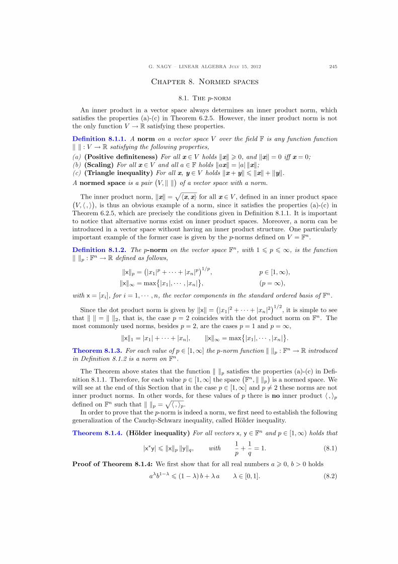
G. NAGY – LINEAR ALGEBRA July 15, 2012 245
Chapter 8. Normed spaces
8.1. The p-norm
An inner product in a vector space always determines an inner product norm, whichsatisfies the properties (a)-(c) in Theorem 6.2.5. However, the inner product norm is notthe only function V → R satisfying these properties.
Definition 8.1.1. A norm on a vector space V over the field F is any function function‖ ‖ : V → R satisfying the following properties,(a) (Positive definiteness) For all x ∈ V holds ‖x‖ > 0, and ‖x‖ = 0 iff x = 0;(b) (Scaling) For all x ∈ V and all a ∈ F holds ‖ax‖ = |a| ‖x‖;(c) (Triangle inequality) For all x, y ∈ V holds ‖x + y‖ 6 ‖x‖+ ‖y‖.A normed space is a pair
(V, ‖ ‖) of a vector space with a norm.
The inner product norm, ‖x‖ =√〈x,x〉 for all x ∈ V , defined in an inner product space(
V, 〈 , 〉), is thus an obvious example of a norm, since it satisfies the properties (a)-(c) inTheorem 6.2.5, which are precisely the conditions given in Definition 8.1.1. It is importantto notice that alternative norms exist on inner product spaces. Moreover, a norm can beintroduced in a vector space without having an inner product structure. One particularlyimportant example of the former case is given by the p-norms defined on V = Fn.
Definition 8.1.2. The p-norm on the vector space Fn, with 1 6 p 6 ∞, is the function‖ ‖p : Fn → R defined as follows,
‖x‖p =(|x1|p + · · ·+ |xn|p
)1/p, p ∈ [1,∞),
‖x‖∞ = max{|x1|, · · · , |xn|
}, (p =∞),
with x = [xi], for i = 1, · · · , n, the vector components in the standard ordered basis of Fn.
Since the dot product norm is given by ‖x‖ =(|x1|2 + · · ·+ |xn|2
)1/2, it is simple to seethat ‖ ‖ = ‖ ‖2, that is, the case p = 2 coincides with the dot product norm on Fn. Themost commonly used norms, besides p = 2, are the cases p = 1 and p =∞,
‖x‖1 = |x1|+ · · ·+ |xn|, ‖x‖∞ = max{|x1|, · · · , |xn|
}.
Theorem 8.1.3. For each value of p ∈ [1,∞] the p-norm function ‖ ‖p : Fn → R introducedin Definition 8.1.2 is a norm on Fn.
The Theorem above states that the function ‖ ‖p satisfies the properties (a)-(c) in Defi-nition 8.1.1. Therefore, for each value p ∈ [1,∞] the space
(Fn, ‖ ‖p
)is a normed space. We
will see at the end of this Section that in the case p ∈ [1,∞] and p 6= 2 these norms are notinner product norms. In other words, for these values of p there is no inner product 〈 , 〉pdefined on Fn such that ‖ ‖p =
√〈 , 〉p.In order to prove that the p-norm is indeed a norm, we first need to establish the following
generalization of the Cauchy-Schwarz inequality, called Holder inequality.
Theorem 8.1.4. (Holder inequality) For all vectors x, y ∈ Fn and p ∈ [1,∞) holds that
|x∗y| 6 ‖x‖p ‖y‖q, with1p
+1q
= 1. (8.1)
Proof of Theorem 8.1.4: We first show that for all real numbers a > 0, b > 0 holds
aλb1−λ 6 (1− λ) b + λa λ ∈ [0, 1]. (8.2)
246 G. NAGY – LINEAR ALGEBRA july 15, 2012
This inequality can be shown using the auxiliary function
f(t) = (1− λ) + λ t− tλ.
Its derivative is f ′(t) = λ[1− t(λ−1)], so the function f satisfies
f(1) = 0, f ′(t) > 0 for t > 1, f ′(t) < 0 for 0 6 t < 1.
We conclude that f(t) > 0 for t ∈ [0,∞). Given two real numbers a > 0, b > 0, we haveproven that f(a/b) > 0, that is,
aλ
bλ6 (1− λ) + λ
a
b⇔ aλb1−λ 6 (1− λ) b + λa.
Having established Eq. (8.2), we use it to prove Holder inequality. Let x = [xi], y = [yj ] ∈ Fn
be arbitrary vectors, where i, j = 1, · · · , n, and introduce the rescaled vectors
x =x
‖x‖p , y =y
‖y‖q ,1p
+1q
= 1.
These rescaled vectors satisfy that ‖x‖p = 1 and ‖y‖q = 1. Denoting x = [xi] and y = [yi],use the inequality in Eq. (8.2) in the case that a = xi, b = yi and λ = 1/p, as follows,
|xiyi| =( |xi|p∑n
j=1 |xj |p) 1
p( |yi|q∑n
j=1 |yj |q)1− 1
p
6(1− 1
p
)( |yi|q∑nj=1 |yj |q
)+
1p
( |xi|p∑nj=1 |xj |p
)
6 1q|yi|q +
1p|xi|p.
Adding up over all components,
|x∗y| 6n∑
i=1
|xiyi| 6 1q|yi|q +
1p|xi|p =
1q‖y‖qq +
1p‖x‖pp =
1q
+1p
= 1.
Therefore, |x∗y| 6 1, which is equivalent to∣∣∣ x∗
‖x‖py
‖y‖q∣∣∣ 6 1 ⇔ |x∗y| 6 ‖x‖p ‖y‖q.
This establishes the Theorem. ¤The Holder inequality plays an important role to show that the p-norms satisfy the
triangle inequality. We saw the same situation when the Cauchy-Schwarz inequality playeda crucial role to prove that the inner product norm satisfied the triangle inequality.Proof of Theorem 8.1.3: We show the proof for p ∈ [1,∞). The case p = ∞ is left asan exercise. So, we assume that p ∈ [1,∞), we introduce q by the equation 1
p + 1q = 1.
In order to show that the p-norm is a norm we need to show that the p-norm satisfies theproperties (a)-(c) in Definition 8.1.1. The first two properties a simple to prove. The p-normis positive, since for all x ∈ Fn holds
‖x‖p =( n∑
i=1
|xi|p) 1
p > 0, and( n∑
i=1
|xi|p) 1
p
= 0 ⇔ |xi| = 0 ⇔ x = 0.
The p-norm satisfies the scaling property, since for all x ∈ Fn and all a ∈ F holds
‖ax‖p =( n∑
i=1
|axi|p) 1
p
=( n∑
i=1
|a|p |xi|p) 1
p
=(|a|p
n∑
i=1
|xi|p) 1
p
= |a| ‖x‖p.
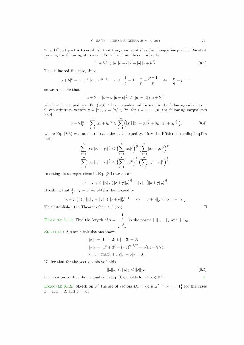
G. NAGY – LINEAR ALGEBRA July 15, 2012 247
The difficult part is to establish that the p-norm satisfies the triangle inequality. We startproving the following statement: For all real numbers a, b holds
|a + b|p 6 |a| |a + b| pq + |b| |a + b| pq . (8.3)
This is indeed the case, since
|a + b|p = |a + b| |a + b|p−1, and1q
= 1− 1p
=p− 1
p⇔ p
q= p− 1,
so we conclude that
|a + b| = |a + b| |a + b| pq 6 (|a|+ |b|) |a + b| pq ,
which is the inequality in Eq. (8.3). This inequality will be used in the following calculation.Given arbitrary vectors x = [xi], y = [yi] ∈ Fn, for i = 1, · · · , n, the following inequalitieshold
‖x + y‖pp =n∑
i=1
|xi + yi|p 6n∑
i=1
(|xi| |xi + yi|
pq + |yi| |xi + yi|
pq
), (8.4)
where Eq. (8.3) was used to obtain the last inequality. Now the Holder inequality impliesboth
n∑
i=1
|xi| |xi + yi|pq 6
( n∑
i=1
|xi|p) 1
p( n∑
i=1
|xi + yi|p) 1
q
,
n∑
i=1
|yi| |xi + yi|pq 6
( n∑
i=1
|yi|p) 1
p( n∑
i=1
|xi + yi|p) 1
q
.
Inserting these expressions in Eq. (8.4) we obtain
‖x + y‖pp 6 ‖x‖p(‖x + y‖p
) pq + ‖y‖p
(‖x + y‖p) p
q .
Recalling that pq = p− 1, we obtain the inequality
‖x + y‖pp 6(‖x‖p + ‖y‖p
) ‖x + y‖(p−1)p ⇔ ‖x + y‖p 6 ‖x‖p + ‖y‖p.
This establishes the Theorem for p ∈ [1,∞). ¤
Example 8.1.1: Find the length of x =
12−3
in the norms ‖ ‖1, ‖ ‖2 and ‖ ‖∞.
Solution: A simple calculations shows,
‖x‖1 = |1|+ |2|+ | − 3| = 6,
‖x‖2 =[12 + 22 + (−3)2
]1/2 =√
14 = 3.74,
‖x‖∞ = max{|1|, |2|, | − 3|} = 3.
Notice that for the vector x above holds
‖x‖∞ 6 ‖x‖2 6 ‖x‖1. (8.5)
One can prove that the inequality in Eq. (8.5) holds for all x ∈ Fn. C
Example 8.1.2: Sketch on R2 the set of vectors Bp ={x ∈ R2 : ‖x‖p = 1
}for the cases
p = 1, p = 2, and p =∞.
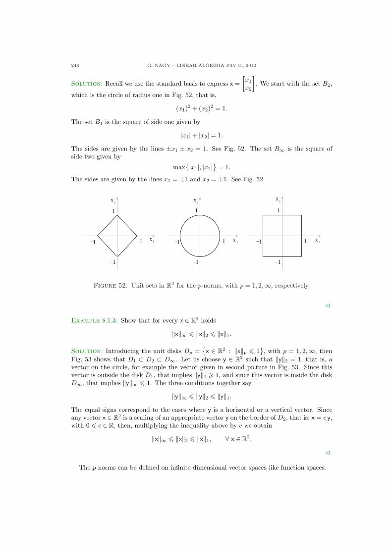
248 G. NAGY – LINEAR ALGEBRA july 15, 2012
Solution: Recall we use the standard basis to express x =[x1
x2
]. We start with the set B2,
which is the circle of radius one in Fig. 52, that is,
(x1)2 + (x2)2 = 1.
The set B1 is the square of side one given by
|x1|+ |x2| = 1.
The sides are given by the lines ±x1 ± x2 = 1. See Fig. 52. The set B∞ is the square ofside two given by
max{|x1|, |x2|
}= 1.
The sides are given by the lines x1 = ±1 and x2 = ±1. See Fig. 52.
1
1
−1
2x
x 1−1
1
1
−1
2x
x 1−1
1
1
−1
x 1
2x
−1
Figure 52. Unit sets in R2 for the p-norms, with p = 1, 2,∞, respectively.
C
Example 8.1.3: Show that for every x ∈ R2 holds
‖x‖∞ 6 ‖x‖2 6 ‖x‖1.
Solution: Introducing the unit disks Dp ={x ∈ R2 : ‖x‖p 6 1
}, with p = 1, 2,∞, then
Fig. 53 shows that D1 ⊂ D2 ⊂ D∞. Let us choose y ∈ R2 such that ‖y‖2 = 1, that is, avector on the circle, for example the vector given in second picture in Fig. 53. Since thisvector is outside the disk D1, that implies ‖y‖1 > 1, and since this vector is inside the diskD∞, that implies ‖y‖∞ 6 1. The three conditions together say
‖y‖∞ 6 ‖y‖2 6 ‖y‖1.The equal signs correspond to the cases where y is a horizontal or a vertical vector. Sinceany vector x ∈ R2 is a scaling of an appropriate vector y on the border of D2, that is, x = c y,with 0 6 c ∈ R, then, multiplying the inequality above by c we obtain
‖x‖∞ 6 ‖x‖2 6 ‖x‖1, ∀ x ∈ R2.
C
The p-norms can be defined on infinite dimensional vector spaces like function spaces.
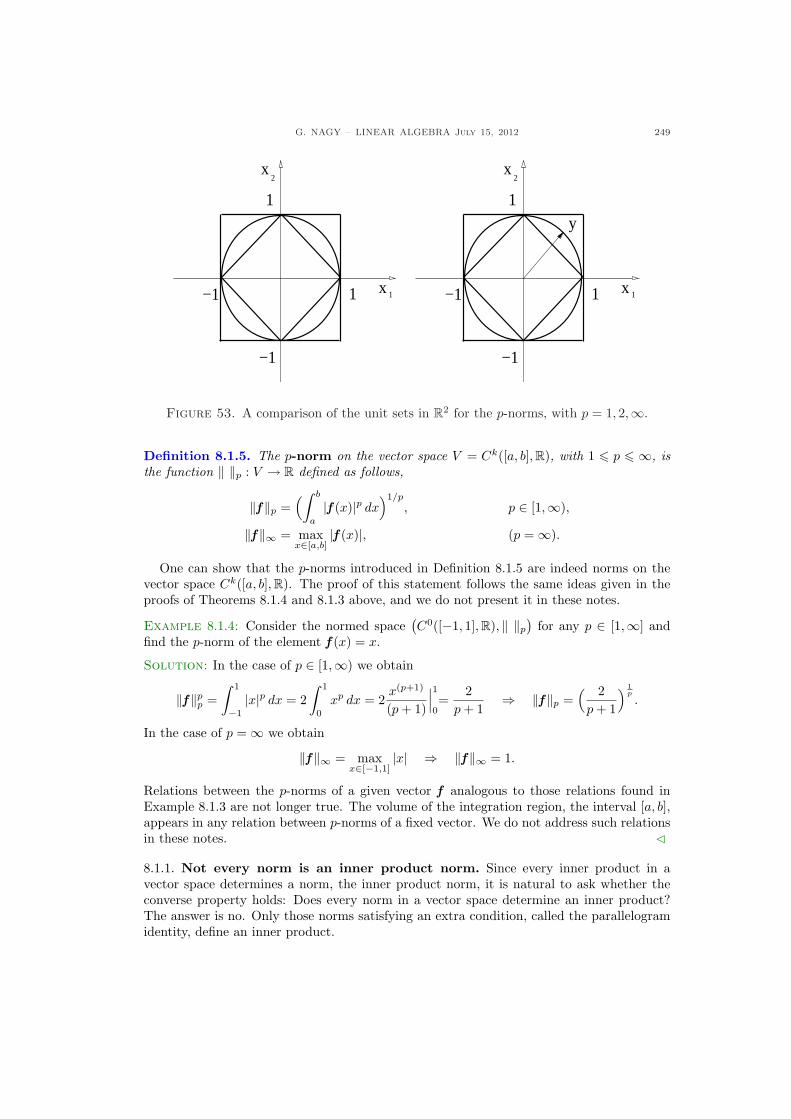
G. NAGY – LINEAR ALGEBRA July 15, 2012 249
1
1
−1
2x
x 1−1
y
1
−1
2x
x 1−1
1
Figure 53. A comparison of the unit sets in R2 for the p-norms, with p = 1, 2,∞.
Definition 8.1.5. The p-norm on the vector space V = Ck([a, b],R), with 1 6 p 6 ∞, isthe function ‖ ‖p : V → R defined as follows,
‖f ‖p =(∫ b
a
|f (x)|p dx)1/p
, p ∈ [1,∞),
‖f ‖∞ = maxx∈[a,b]
|f (x)|, (p =∞).
One can show that the p-norms introduced in Definition 8.1.5 are indeed norms on thevector space Ck([a, b],R). The proof of this statement follows the same ideas given in theproofs of Theorems 8.1.4 and 8.1.3 above, and we do not present it in these notes.
Example 8.1.4: Consider the normed space(C0([−1, 1],R), ‖ ‖p
)for any p ∈ [1,∞] and
find the p-norm of the element f (x) = x.
Solution: In the case of p ∈ [1,∞) we obtain
‖f ‖pp =∫ 1
−1
|x|p dx = 2∫ 1
0
xp dx = 2x(p+1)
(p + 1)
∣∣∣1
0=
2p + 1
⇒ ‖f ‖p =( 2
p + 1
) 1p
.
In the case of p =∞ we obtain
‖f ‖∞ = maxx∈[−1,1]
|x| ⇒ ‖f ‖∞ = 1.
Relations between the p-norms of a given vector f analogous to those relations found inExample 8.1.3 are not longer true. The volume of the integration region, the interval [a, b],appears in any relation between p-norms of a fixed vector. We do not address such relationsin these notes. C
8.1.1. Not every norm is an inner product norm. Since every inner product in avector space determines a norm, the inner product norm, it is natural to ask whether theconverse property holds: Does every norm in a vector space determine an inner product?The answer is no. Only those norms satisfying an extra condition, called the parallelogramidentity, define an inner product.
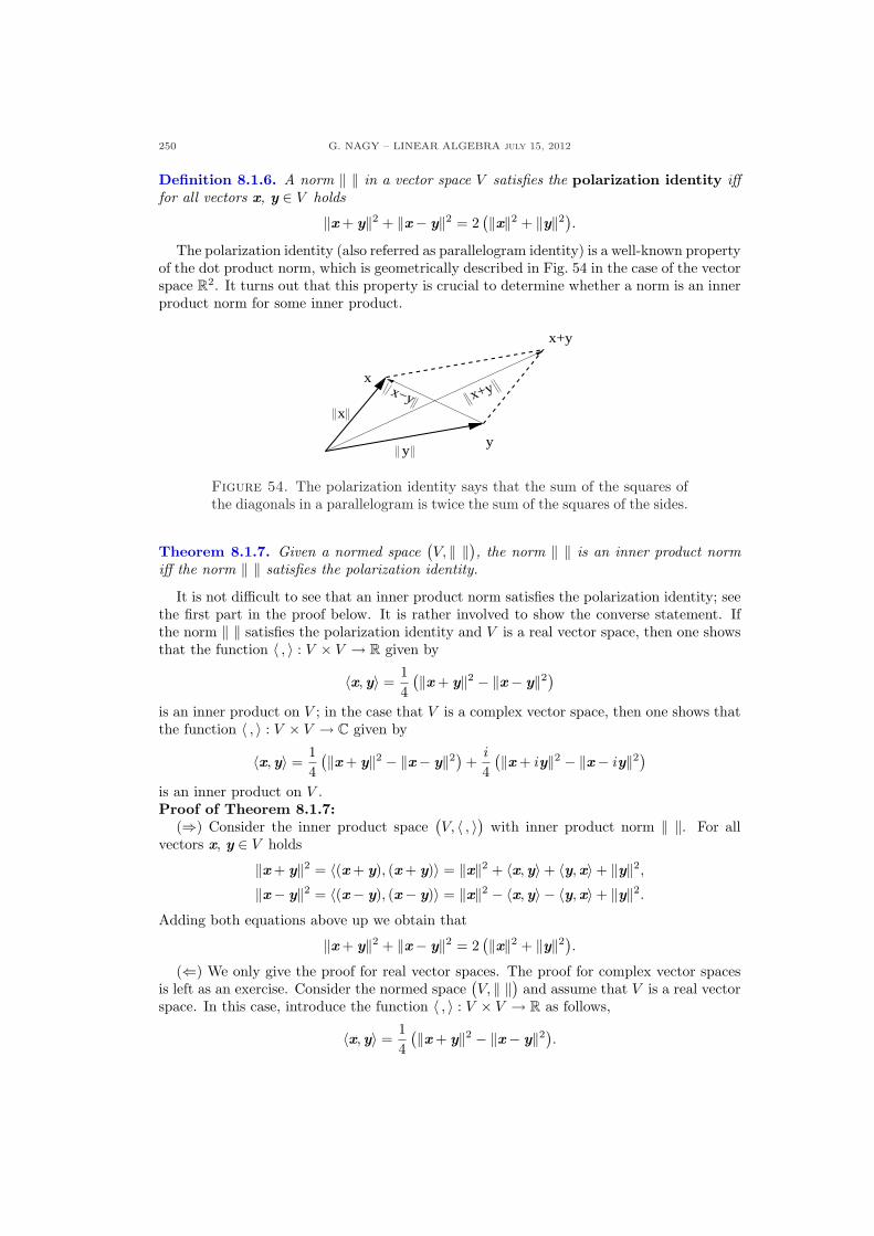
250 G. NAGY – LINEAR ALGEBRA july 15, 2012
Definition 8.1.6. A norm ‖ ‖ in a vector space V satisfies the polarization identity ifffor all vectors x, y ∈ V holds
‖x + y‖2 + ‖x− y‖2 = 2(‖x‖2 + ‖y‖2).
The polarization identity (also referred as parallelogram identity) is a well-known propertyof the dot product norm, which is geometrically described in Fig. 54 in the case of the vectorspace R2. It turns out that this property is crucial to determine whether a norm is an innerproduct norm for some inner product.
x
x
y
x+y
y
x+yx−y
Figure 54. The polarization identity says that the sum of the squares ofthe diagonals in a parallelogram is twice the sum of the squares of the sides.
Theorem 8.1.7. Given a normed space(V, ‖ ‖), the norm ‖ ‖ is an inner product norm
iff the norm ‖ ‖ satisfies the polarization identity.
It is not difficult to see that an inner product norm satisfies the polarization identity; seethe first part in the proof below. It is rather involved to show the converse statement. Ifthe norm ‖ ‖ satisfies the polarization identity and V is a real vector space, then one showsthat the function 〈 , 〉 : V × V → R given by
〈x,y〉 =14
(‖x + y‖2 − ‖x− y‖2)
is an inner product on V ; in the case that V is a complex vector space, then one shows thatthe function 〈 , 〉 : V × V → C given by
〈x,y〉 =14
(‖x + y‖2 − ‖x− y‖2) +i
4(‖x + iy‖2 − ‖x− iy‖2)
is an inner product on V .Proof of Theorem 8.1.7:
(⇒) Consider the inner product space(V, 〈 , 〉) with inner product norm ‖ ‖. For all
vectors x, y ∈ V holds
‖x + y‖2 = 〈(x + y), (x + y)〉 = ‖x‖2 + 〈x,y〉+ 〈y,x〉+ ‖y‖2,‖x− y‖2 = 〈(x− y), (x− y)〉 = ‖x‖2 − 〈x,y〉 − 〈y,x〉+ ‖y‖2.
Adding both equations above up we obtain that
‖x + y‖2 + ‖x− y‖2 = 2(‖x‖2 + ‖y‖2).
(⇐) We only give the proof for real vector spaces. The proof for complex vector spacesis left as an exercise. Consider the normed space
(V, ‖ ‖) and assume that V is a real vector
space. In this case, introduce the function 〈 , 〉 : V × V → R as follows,
〈x,y〉 =14
(‖x + y‖2 − ‖x− y‖2).
G. NAGY – LINEAR ALGEBRA July 15, 2012 251
Notice that this function satisfies 〈x,0〉 = 14
(‖x‖2 − ‖x‖2) = 0 for all x ∈ V . We now showthat this function 〈 , 〉 is an inner product on V . It is positive definite, since
〈x,x〉 =14‖2x‖2 = ‖x‖2
and the norm is positive definite, so we obtain that
〈x,x〉 > 0, and 〈x,x〉 = 0 ⇔ x = 0.
The function 〈 , 〉 is symmetric, since
〈x,y〉 =14
(‖x + y‖2 − ‖x− y‖2) =14
(‖y + x‖2 − ‖y− x‖2) = 〈y,x〉.The difficult part is to show that the function 〈 , 〉 is linear in the second argument. Here iswhere we need the polarization identity. We start with the following expressions, which areobtained from the polarization identity,
‖x + y + z‖2 + ‖x + y− z‖2 = 2 ‖x + y‖2 + 2 ‖z‖2,‖x− y + z‖2 + ‖x− y− z‖2 = 2 ‖x− y‖2 + 2 ‖z‖2.
If we subtract the second equation from the first one, and ordering the terms conveniently,we obtain,[‖x+(y+z)‖2−‖x− (y+z)‖2
]+
[‖x+(y−z)‖2−‖x− (y−z)‖2
]= 2
[‖x+y‖2−‖x−y‖2
]
which can be written in terms of the function 〈 , 〉 as follows,
〈x, (y + z)〉+ 〈x, (y− z)〉 = 2〈x,y〉. (8.6)
Several relations come from this equation. For the first relation, take y = z, and recall that〈x,0〉 = 0, then we obtain
〈x, 2y〉 = 2 〈x,y〉. (8.7)
The second relation derived from Eq. (8.6) is obtained renaming the vectors y + z = u andy− z = v, that is,
〈x,u〉+ 〈x, v〉 = 2⟨x,
(u + v)2
⟩= 〈x, (u + v)〉,
where the equation on the far right comes from Eq. (8.7). We have shown that for all x, u,v ∈ V holds
〈x, (u + v)〉 = 〈x,u〉+ 〈x, v〉which is a particular case of the linearity in the second argument property of an innerproduct. We only need to show that for all x, y ∈ V and all a ∈ R holds
〈x, ay〉 = a 〈x,y〉.We have proven the case a = 2 in Eq. (8.7). The case a = n ∈ N is proven by induction: If〈x, ny〉 = n 〈x,y〉, then the same relation holds for (n + 1), since
〈x, (n + 1)y〉 = 〈x, (ny + y)〉= 〈x, ny〉+ 〈x,y〉= n 〈x,y〉+ 〈x,y〉= (n + 1) 〈x,y〉.
The case a = 1/n with n ∈ N comes from the relation
〈x,y〉 =⟨x,
n
ny⟩
= n⟨x,
1ny⟩⇒
⟨x,
1ny⟩
=1n〈x,y〉.
252 G. NAGY – LINEAR ALGEBRA july 15, 2012
These two cases show that for any rational number a = p/q ∈ Q holds⟨x,
p
qy⟩
= p⟨x,
1qy⟩
=p
q〈x,y〉. (8.8)
Finally, the same property holds for all a ∈ R by the following continuity argument. Fixarbitrary vectors x, y ∈ V and define the function f : R→ R by
a 7→ f(a) = 〈x, ay〉.We left as an exercise to show that f is a continuous function. Now, using Eq. (8.8) weknow that this function satisfies
f(a) = a f(1) ∀ a ∈ Q.
Let {ak}∞k=1 ⊂ Q be a sequence of rational numbers that converges to a ∈ R. Since f is acontinuous function we know that limk→∞ f(ak) = f(a). Since the sequence is constructedwith rational numbers, for every element in this sequence holds
f(ak) = ak f(1)
which implies thatlim
k→∞f(ak) =
(lim
k→∞ak
)f(1) = a f(1).
So we have shown that for all a ∈ R holds f(a) = a f(1), that is,
〈x, ay〉 = a 〈x,y〉.Since x, y ∈ V are fixed but arbitrary, we have shown that the function 〈 , 〉 in linear in thesecond argument. We conclude that this function is an inner product on V . This establishesthe Theorem in the case that V is a real vector space. ¤
Example 8.1.5: Show that for p 6= 2 the p-norm on the vector space Fn introduced inDefinition 8.1.2 does not satisfy the polarization identity.
Solution: Consider the vectors e1 and e2, the first two columns of the identity matrix In.It is simple to compute,
‖e1 + e2‖2p = 22/p, ‖e1 − e2‖2p = 22/p, ‖e1‖2p = ‖e2‖2p = 1
therefore,‖e1 + e2‖2p + ‖e1 − e2‖2p = 2
p+2p and 2
(‖e1‖2p + ‖e2‖2p)
= 4.
We conclude that the p-norm satisfies the polarization identity only in the case p = 2. C
8.1.2. Equivalent norms. We have seen that a norm in a vector space determines a notionof distance between vectors given by the norm distance introduced in Definition 6.2.6. Thenotion of distance is the structure needed to define the convergence of an infinite sequenceof vectors. A sequence of vectors {xi}∞i=1 in a normed space
(V, ‖ ‖) converges to a vector
x ∈ V ifflim
k→∞‖x− xk‖ = 0,
that is, for every ε > 0 there exists n ∈ N such that for all k > n holds that ‖x − xk‖ < ε.With the notion of convergence of a sequence it is possible to introduce concepts like thecontinuous and differentiable functions defined on the vector space. Therefore, the calculuscan be extended from Rn to any normed vector space.
We have also seen that there is no unique norm in a vector space. This implies that thereis no unique notion of norm distance. It is important to know whether two different normsprovide the same notion of convergence of a sequence. By this we mean that every sequencethat converges (diverges) with respect to one norm distance also converges (diverges) with
G. NAGY – LINEAR ALGEBRA July 15, 2012 253
respect to the other norm distance. In order to answer this question it is useful the followingnotion.
Definition 8.1.8. The norms ‖ ‖a and ‖ ‖b defined on a vector space V are called to beequivalent iff there exist real constants K > k > 0 such that for all x ∈ V holds
k ‖x‖b 6 ‖x‖a 6 K ‖x‖b.It is simple to see that if two norms defined on a vector space are equivalent, then they
have the same notion of convergence. What it is non-trivial to prove is that the conversealso holds. Since two norms have the same notion of convergence iff they are equivalent, itis important to know whether a vector space can have non-equivalent norms. The followingresult addresses the case of finite dimensional vector spaces.
Theorem 8.1.9. If V is a finite dimensional, then all norms defined on V are equivalent.
This result says that there is a unique notion of convergence in any finite dimensionalvector space. So, functions that are continuous or differentiable with respect to one normare also continuous or differentiable with respect to any other norm. This is not the caseof infinite dimensional vector spaces. It is possible to find non-equivalent norms on infinitedimensional vector spaces. Therefore, functions defined on such a vector space can becontinuous with respect to one norm and discontinuous with respect to the other norm.Proof of Theorem 8.1.9: Let ‖ ‖a and ‖ ‖b be two norms defined on a finite dimensionalvector space V . Let dimV = n, and fix a basis V = {v1, · · · , vn} of V . Then, any vectorx ∈ V can be decomposed in terms of the basis vectors as
x = x1v1 + · · ·+ xnvn.
Since ‖ ‖a is a norm, we can obtain the following bound on ‖x‖a for every x ∈ V in termsof (
∑ni=1 |xi|) as follows.
‖x‖a = ‖x1v1 + · · ·+ xnvn‖a6 |x1| ‖v1‖a + · · ·+ |xn| ‖vn‖a
6(|x1|+ · · ·+ |xn|
)amax ⇒ ‖x‖a 6
( n∑
i=1
|xi|)
amax.
where amax = max{‖v1‖a, · · · , ‖vn‖a}. A lower bound can also be found as follows. Intro-duce the set
S ={
[xi] ∈ Fn :n∑
i=1
|xi| = 1}⊂ Fn,
and then introduce the function fa : S → R as follows
fa([xi]) =∥∥∥
n∑
i=1
xivi
∥∥∥a.
Since function fa is a continuous and defined on a closed and bounded set of Fn, then fa
has attains a maximum and a minimum values on S. We are here interested only in theminimum value. If [yi] ∈ S is a point where fa takes its minimum value, let let us denote
fa([yi]) = amin.
254 G. NAGY – LINEAR ALGEBRA july 15, 2012
Since the norm ‖ ‖a is positive, we know that amin > 0. The existence of this minimumvalue of fa implies the following bound on ‖x‖a for all x ∈ V , namely,
‖x‖a =∥∥∥
n∑
i=1
xivi
∥∥∥a
=
(∑nj=1 |xj |
)(∑n
j=1 |xj |)
∥∥∥n∑
i=1
xivi
∥∥∥a
=( n∑
j=1
|xj |)∥∥∥
n∑
i=1
[ xi(∑nj=1 |xj |
)]vi
∥∥∥a
=( n∑
j=1
|xj |)∥∥∥
n∑
i=1
xi vi
∥∥∥a
=( n∑
j=1
|xj |)
fa([xi]) ⇒ ‖x‖a >( n∑
j=1
|xj |)
amin.
Summarizing, we have found real numbers amax > amin > 0 such that the following inequal-ity holds for all x ∈ V ,
amin
( n∑
j=1
|xj |)
6 ‖x‖a 6( n∑
j=1
|xj |)
amax.
Since no special property of norm ‖ ‖a has been used, the same type of inequality holdsfor norm ‖ ‖b, that is, there exist real numbers bmax > bmin > 0 such that the followinginequality holds for all x ∈ B,
bmin
( n∑
j=1
|xj |)
6 ‖x‖b 6( n∑
j=1
|xj |)
bmax.
These inequalities imply that norms ‖ ‖a and ‖ ‖b are equivalent, since
‖x‖b amin
bmax6 bmax
bmaxamin
( n∑
j=1
|xj |)
6 ‖x‖a 6( n∑
j=1
|xj |)
amaxbmin
bmin6 amax
bmin‖x‖b.
(Start reading the inequality form the center, at ‖x‖a, and first see the inequalities tothe right; then go to the center again and read the inequalities to the left.) Denotingk = amin/bmax and K = amax/bmin, we have obtained that
k ‖x‖b 6 ‖x‖a 6 K ‖x‖b ∀ x ∈ V.
This establishes the Theorem. ¤
G. NAGY – LINEAR ALGEBRA July 15, 2012 255
8.1.3. Exercises.
8.1.1.- Consider the vector space C4 and forp = 1, 2,∞ find the p-norms of the vec-tors
x =
2664
21−4−2
3775 , y =
2664
1 + i1− i
14i
3775 .
8.1.2.- Determine which of the followingfunctions ‖ ‖ : R2 → R defines a normon R2. We denote x = [xi] the com-ponents of x in a standard basis of R2.Justify your answers.
(a) ‖x‖ = |x1|;(b) ‖x‖ = |x1 + x2|;(c) ‖x‖ = |x1|2 + |x2|2;(d) ‖x‖ = 2|x1|+ 3|x2|.
8.1.3.- True or false? Justify your answer:If ‖ ‖a and ‖ ‖b are two norms on avector space V , then ‖ ‖ defined as
‖x‖ = ‖x‖a + ‖x‖b ∀ x ∈ V
is also a norm on V .
8.1.4.- Consider the space P2([0, 1]) withthe p-norm
‖q‖p =“Z 1
0
|q(x)|p dx” 1
p,
for p ∈ [1,∞). Find the p-norm ofthe vector q(x) = −3x2. Also find thesupremum norm of q, defined as
‖q‖∞ = maxx∈[0,1]
|q(x)|.
256 G. NAGY – LINEAR ALGEBRA july 15, 2012
8.2. Operator norms
We have seen that the space of all linear transformations L(V, W ) between the vectorspaces V and W is itself a vector space. As in any vector space, it is possible to definenorm functions ‖ ‖ : L(V,W ) → R on the vector space L(V,W ). For example, We will seethat in the case where V = Fn and W = Fm, one of such norms is the Frobenius norm,which is the inner product norm corresponding to the Frobenius inner product introducedin Section 6.2. More precisely, the Frobenius norm is given by
‖A‖F =√〈A, A〉F ∀ A ∈ Fm,n.
It is simple to see that
‖A‖F =√
tr(A∗A
)=
( m∑
i=1
n∑
j=1
|Aij |2) 1
2.
However, in the case where V and W are normed spaces with norms ‖ ‖v and ‖ ‖w, thereexists a particular norm on L(V, W ) which is induced from the norms on V and W . Thisinduced norm can be defined on elements L(V, W ) by recalling that the element T ∈ L(V,W )as a function T : V →W .
Definition 8.2.1. Let(V, ‖ ‖v
)and
(W, ‖ ‖w
)be finite dimensional normed spaces. The
induced norm on the space L(V,W ) of all linear transformations T : V →W is a function‖ ‖ : L(V,W )→ R given by
‖T ‖ = max‖x‖v=1
‖T(x)‖w.
In the particular case that V = W and ‖ ‖v = ‖ ‖w = ‖ ‖, the induced norm on L(V ) iscalled the operator norm, and is given by
‖T ‖ = max‖x‖=1
‖T(x)‖.
The definition above says that given arbitrary norms on the vector spaces V and W ,they induce a norm on the vector space L(V, W ) of linear transformations T : V → W . Aparticular case of this definition is when V = Fn and W = Fm, we fix standard bases on Vand W , and we introduce p-norms on these spaces. So, the normed spaces
(Fn, ‖ ‖p
)and(
Fm, ‖ ‖q)
induce a norm on the vector space Fm,n as follows.
Definition 8.2.2. Consider the normed spaces(Fn, ‖ ‖p
)and
(Fm, ‖ ‖q
), with p, q ∈ [1,∞].
The induced (p, q)-norm on the space L(Fn,Fm) is the function ‖ ‖p,q : L(Fn,Fm) → Rgiven by
‖T ‖p,q = max‖x‖p=1
‖T(x)‖q ∀T ∈ L(Fn,Fm).
In the particular case of p = q we denote ‖ ‖p,p = ‖ ‖p. In the case p = q and n = m theinduced norm on L(Fn) is called the p-operator norm and is given by
‖T ‖p = max‖x‖p=1
‖T(x)‖p ∀T ∈ L(Fn).
In the case p = q above we use the same notation ‖ ‖p for the p-norm on Fn, the (p, p)-norm on L(Fn,Fm) and the p-operator nor in L(Fn). The context should help to decidewhich norm we use on every particular situation.
Example 8.2.1: Consider the particular case V = W = R2 with standard ordered basesand the p = 2 norms in both, V and W . In this case, the space L(R2) can be identified with
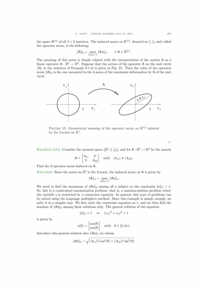
G. NAGY – LINEAR ALGEBRA July 15, 2012 257
the space R2,2 of all 2× 2 matrices. The induced norm on R2,2, denoted as ‖ ||2 and calledthe operator norm, is the following:
‖A‖2 = max‖x‖2=1
‖Ax‖2, ∀ A ∈ R2,2.
The meaning of this norm is deeply related with the interpretation of the matrix A as alinear operator A : R2 → R2. Suppose that the action of the operator A on the unit circle(B2 in the notation of Example 8.1.2) is given in Fig. 55. Then the value of the operatornorm ‖A‖2 is the size measured in the 2-norm of the maximum deformation by A of the unitcircle.
2
1 x 1 x 11
2x 2
A x
|| A ||
Figure 55. Geometrical meaning of the operator norm on R2,2 inducedby the 2-norm on R2.
C
Example 8.2.2: Consider the normed space(R2, ‖ ‖2
), and let A : R2 → R2 be the matrix
A =[A11 00 A22
]with |A11| 6= |A22|.
Find the 2-operator norm induced on A.
Solution: Since the norm on R2 is the 2-norm, the induced norm on A is given by
‖A‖2 = max‖x‖2=1
‖Ax‖2.
We need to find the maximum of ‖Ax‖2 among all x subject to the constraint ‖x‖2 = 1.So, this is a constrained maximization problem, that is, a maxima-minima problem wherethe variable x is restricted by a constraint equation. In general, this type of problems canbe solved using the Lagrange multipliers method. Since this example is simple enough, wesolve it in a simpler way. We first solve the constraint equation on x, and we then find themaxima of ‖Ax‖2 among these solutions only. The general solution of the equation
‖x‖2 = 1 ⇔ (x1)2 + x2)2 = 1
is given by
x(θ) =[cos(θ)sin(θ)
]with θ ∈ [0, 2π).
Introduce this general solution into ‖Ax‖2 we obtain
‖Ax‖2 =√
(A11)2 cos2(θ) + (A22)2 sin2(θ).
258 G. NAGY – LINEAR ALGEBRA july 15, 2012
Since the maximum in θ of the function ‖Ax‖2 is the same as the maximum of ‖Ax‖22, weneed to find the maximum on θ of the function f(θ) = ‖Ax(θ)‖22, that is,
f(θ) = (A11)2 cos2(θ) + (A22)2 sin2(θ).
The solution is simple, find θ solutions of
f ′(θ) =df
dθ(θ) = 0 ⇒ 2
[−(A11)2 + (A22)2]sin(θ) cos(θ) = 0.
Since we assumed that |A11| 6= |A22|, then
sin(θ) = 0 ⇒ θ1 = 0, θ2 = π,
cos(θ) = 0 ⇒ θ3 =π
2, θ4 =
3π
2.
We obtained four solutions for θ. We evaluate f at these solutions,
f(0) = f(π) = (A11)2, f(π
2)
= f(3π
2)
= (A22)2.
Recalling that ‖Ax(θ)‖2 =√
f(θ), we obtain
‖A‖2 = max{|A11|, |A22|
}.
C
It was mentioned in Example 8.2.2 above that finding the operator norm requires solvinga constrained maximization problem. In the case that the operator norm is induced from adot product norm, the constrained maximization problem can be solved in an explicit form.
Proposition 8.2.3. Consider the vector spaces Rn and Rm with inner product given by thedot products, inner product norms ‖ ‖2, and the vector space L(Rn,Rm) with the induced2-norm.
‖A‖2 = max‖x‖2=1
‖Ax‖2 ∀ A ∈ L(Rn,Rm).
Introduce the scalars λi ∈ R, with i = 1, · · · , k 6 n, as all the roots of the polynomial
p(λ) = det(AT A− λ In
).
Then, all scalars λi are non-negative real numbers and the induced 2-norm of the transfor-mation A is given by
‖A‖2 = max{λ1, · · · , λk
}.
Proof of Proposition 8.2.3: Introduce the functions f : Rm → R and g : Rn → R asfollows,
f(x) = ‖Ax‖22 =(Ax
) · (Ax)
= xT AT Ax, g(x) = ‖x‖22 = x · x = xT x.
To find the induced norm of T is then equivalent to solve the constrained maximizationproblem: Find the maximum of f(x) for x ∈ Rn subject to the constraint g(x) = 1. Thevectors x that provide solutions to the constrained maximization problem must we solutionsof the Euler-Lagrange equations
∇f = λ∇g (8.9)where λ ∈ R, and we introduced the gradient row vectors
∇f =[
∂f
∂x1· · · ∂f
∂xn
], ∇f =
[∂g
∂x1· · · ∂g
∂xn
].
In order to understand why the solution x must satisfy the Euler-Lagrange equations abovewe need to recall two properties of the gradient vector. First, the gradient of a functionf : Rn → R is a vector that determines the direction on Rn where f has the maximumincrease. Second, which is deeply related to the first property, the gradient vector of a
G. NAGY – LINEAR ALGEBRA July 15, 2012 259
function is perpendicular to the surfaces where the function has a constant value. Thesurfaces of constant value of a function are called level surfaces of the function. Therefore,the function f has a maximum or minimum value at x on the constraint level surface g = 1if ∇f is perpendicular to the level surface g = 1 at that x. (Proof: Suppose that at aparticular x on the constraint surface g = 1 the projection of ∇f onto the constraint surfaceis nonzero; then the values of f increase along that direction on the constraint surface; thismeans that f does not attain a maximum value at that x on g = 1.) We conclude that bothgradients ∇f and ∇g are parallel, which is precisely what Eq. (8.9) says. In our particularproblem we obtain for f and g the following:
f(x) = xT AT Ax ⇒ ∇f(x) = 2xT AT A,
g(x) = xT x ⇒ ∇g(x) = 2xT .
We must look for x 6= 0 solution of the equation
xT AT A = λ xT ⇔ AT Ax = λ x,
where the condition x 6= 0 comes from ‖x‖2 = 1. Therefore, λ must not be any scalar but theprecise scalar or scalars such that the matrix (AT A − λ In) is not invertible. An equivalentcondition is that
p(λ) = det(AT A− λ In
)= 0.
The function p is a polynomial of degree n in λ so it has at most n real roots. Let us denotethese roots by λ1, · · · , λk, with 1 6 k 6 n. For each of these values λi the matrix AT A−λi Inis not invertible, so N(AT A− λi In) is non-trivial. Let xi be any element in N(AT A− λi In),that is,
AT Axi = λi xi, i = 1, · · · , k.
At this point it is not difficult to see that λi > 0 for i = 0, · · · , k. Indeed, multiply theequation above by xT
i , that is,xTi AT Axi = λi xT
i xi.
Since both xTi AT Axi and xT
i xi are non-negative numbers, so is λi. Returning to xi, onlythese vectors are the candidates to find a solution to our maximization problem, and f hasthe values
f(xi) = xTi AT Axi = λi xT
i xi = λi ⇒ f(xi) = λi, i = 1, · · · , k.
The induced 2-norm of A is the maximum of these scalar λi. This establishes the Proposition.¤
Example 8.2.3: Consider the vector spaces R3 and R2 with the dot product. Find theinduced 2-norm of the 2× 3 matrix
A =[1 0 10 1 −1
].
Solution: Following the Proposition 8.2.3 the value of the induced norm ‖A‖2 is themaximum of the λi roots of the polynomial
p(λ) = det(AT A− λ I3
)= 0.
We start computing
AT A =
1 00 11 −1
[1 0 10 1 −1
]=
1 0 10 1 −11 −1 2
.
260 G. NAGY – LINEAR ALGEBRA july 15, 2012
The next step is to find the polynomial
p(λ) =
∣∣∣∣∣∣
(1− λ) 0 10 (1− λ) −11 −1 (2− λ)
∣∣∣∣∣∣= (1− λ)
[(1− λ)(2− λ)− 1
]+ (1− λ),
therefore, we obtain p(λ) = −λ(λ− 1)(λ− 3). We have three roots
λ1 = 0, λ2 = 1, λ3 = 3.
We then conclude that the induced norm of A is given by
‖A‖2 = 3.
C
In the case that the norm in a normed space is not an inner product norm the inducednorm on linear operators is not simple to evaluate. The constrained maximization problemis in general complicated to solve. Two particular cases can be solved explicitly though,when the operator norm is induced from the p-norms with p = 1 and p =∞.
Proposition 8.2.4. Consider the normed spaces(Rn, ‖ ‖p
)and
(Rm, ‖ ‖p
)and the vector
space L(Rn,Rm) with the induced p-norm.
‖A‖p = max‖x‖p=1
‖A(x)‖p ∀ A ∈ L(Rn,Rm).
If p = 1 or p =∞, then the following formulas hold, respectively,
‖A‖1 = maxj∈{1,··· ,n}
m∑
i=1
|Aij |, ‖A‖∞ = maxi∈{1,··· ,m}
n∑
j=1
|Aij |.
Proof of proposition 8.2.4: From the definition of the induced p-norm for p = 1,
‖A‖1 = max‖x‖1=1
‖Ax‖1.
From the p-norm on Rm we know that ‖Ax‖1 =m∑
i=1
∣∣∣n∑
j=1
Aijxj
∣∣∣, therefore,
‖Ax‖1 6m∑
i=1
n∑
j=1
|Aij | |xj | =n∑
j=1
|xj |m∑
i=1
|Aij | 6( n∑
j=1
|xj |)
maxj∈{1,··· ,n}
( m∑
i=1
|Aij |);
and introducing the condition ‖x‖1 = 1 we obtain the inequality
‖Ax‖1 6 maxj∈{1,··· ,n}
m∑
i=1
|Aij |.
Recalling the column vector notation A =[A:1, · · · , A:n
], we notice that ‖A:j‖1 =
∑mi=1 |Aij |,
so the inequality above can be expressed as
‖Ax‖1 6 maxj∈{1,··· ,n}
‖A:j‖1.
Since the left hand side is independent of x, the inequality also holds for the maximum in‖x‖1 = 1, that is,
‖A‖1 6 maxj∈{1,··· ,n}
‖A:j‖1.It is now clear that the equality has to be achieved, since the ‖Ax‖1 in the case x = ej , withej a standard basis vector, takes the value ‖Aej‖1 = ‖A:j‖1. Therefore,
‖A‖1 = maxj∈{1,··· ,n}
‖A:j‖1.
G. NAGY – LINEAR ALGEBRA July 15, 2012 261
The second part of Proposition 8.2.4 can be proven as follows. From the definition of theinduced p-norm for p =∞ we know that
‖A‖∞ = max‖x‖∞=1
‖Ax‖∞.
From the p-norm on Rm we see
‖Ax‖∞ = maxi∈{1,··· ,m}
∣∣∣n∑
j=1
Aijxj
∣∣∣ 6 maxi∈{1,··· ,m}
n∑
j=1
|Aij | |xj | 6 maxi∈{1,··· ,m}
n∑
j=1
|Aij |.
Since the far right hand side does not depend on x, the inequality must hold for the maximumin x with ‖x‖∞ = 1, so we conclude that
‖A‖∞ 6 maxi∈{1,··· ,m}
n∑
j=1
|Aij |.
As in the previous p = 1 case, the value on the right hand side above is achieved for ‖Ax‖∞in the case of x with components ±1 depending on the sign of Aij . More precisely, choosex as follows,
xj ={ 1 if Aij > 0,
−1 if Aij < 0,⇒
n∑
j=1
Aijxj =n∑
j=1
|Aij |, i = 1, · · · ,m.
Therefore, for that x we have ‖x‖∞ = 1 and ‖Ax‖∞ = maxi∈{1,··· ,m}
n∑
j=1
|Aij |. So, we conclude
‖A‖∞ = maxi∈{1,··· ,m}
n∑
j=1
|Aij |.
This establishes the Proposition ¤Example 8.2.4: Find the induced p-norm, where p = 1,∞, for the 2× 3 matrix
A =[1 4 12 1 −1
].
Solution: Proposition 8.2.4 says that ‖A‖1 is the largest absolute value sum of componentsamong columns of A, while ‖A‖∞ is the largest absolute value sum among rows of A. In thefirst case we have:
‖A‖1 = maxj=1,2,3
2∑
i=1
|Aij |;
since2∑
i=1
|Ai1| = 3,
2∑
i=1
|Ai2| = 5,
2∑
i=1
|Ai3| = 2,
therefore, ‖A‖1 = 5. In the second case e have:
‖A‖∞ = maxi=1,2
2∑
j=1
|Aij |;
since3∑
j=1
|A1j | = 6,
3∑
j=1
|A2j | = 4,
therefore, ‖A‖∞ = 6. C
262 G. NAGY – LINEAR ALGEBRA july 15, 2012
8.2.1. Exercises.
8.2.1.- Evaluate the induced p-norm, wherep = 1, 2,∞, for the matrices
A =
»1 −2−1 2
–, B =
24
0 1 00 0 11 0 0
35 .
8.2.2.- In the normed space`R2, ‖ ‖2
´, find
the induced norm of A : R2 → R2
A =1√3
»3 −1
0√
8
–.
8.2.3.- Consider the space`Fn, ‖ ‖p
´and
the space Fn,n with the induced norm‖ ‖p. Prove that for all A, B ∈ Fn,n andall x ∈ Fn holds
(a) ‖Ax‖p 6 ‖A‖p ‖x‖p;(b) ‖AB‖p 6 ‖A‖p ‖B‖p.
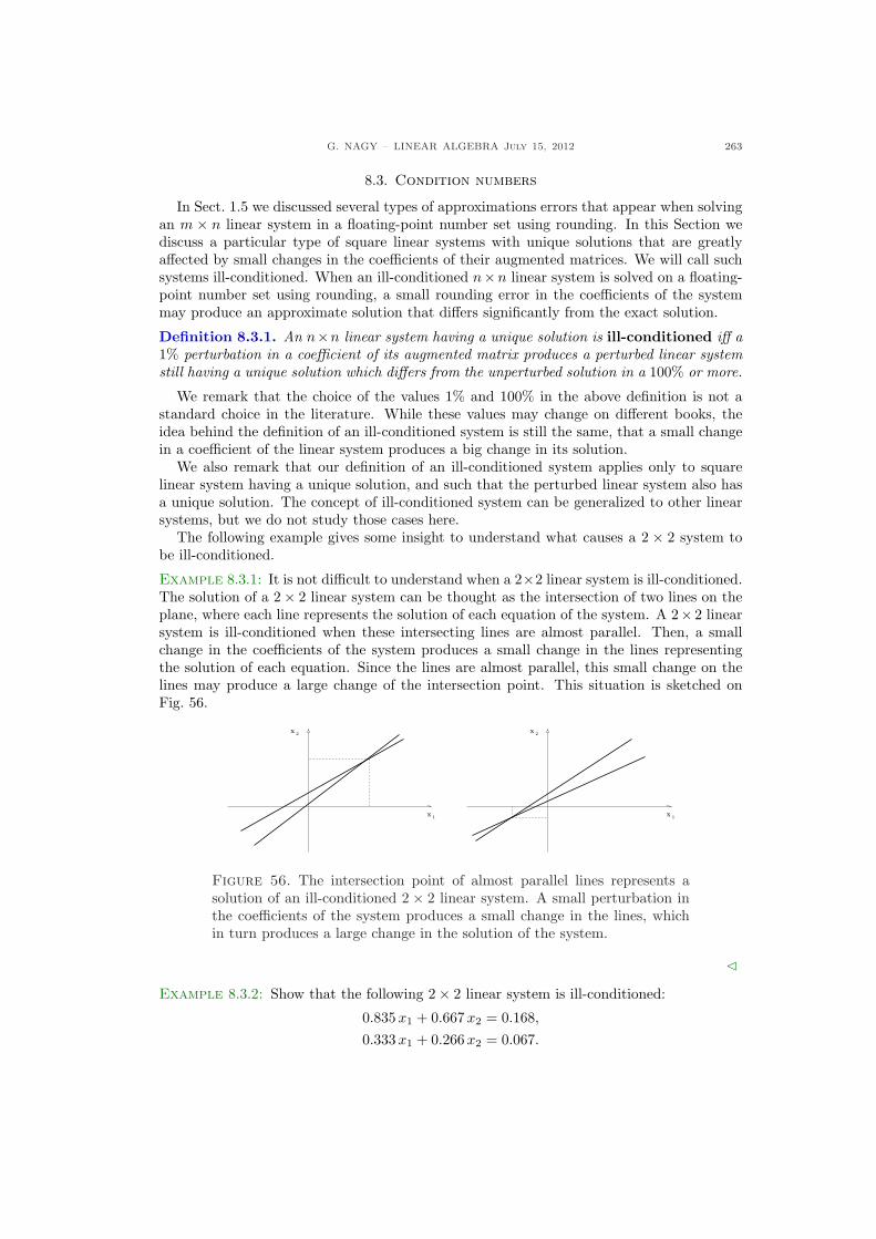
G. NAGY – LINEAR ALGEBRA July 15, 2012 263
8.3. Condition numbers
In Sect. 1.5 we discussed several types of approximations errors that appear when solvingan m × n linear system in a floating-point number set using rounding. In this Section wediscuss a particular type of square linear systems with unique solutions that are greatlyaffected by small changes in the coefficients of their augmented matrices. We will call suchsystems ill-conditioned. When an ill-conditioned n×n linear system is solved on a floating-point number set using rounding, a small rounding error in the coefficients of the systemmay produce an approximate solution that differs significantly from the exact solution.
Definition 8.3.1. An n×n linear system having a unique solution is ill-conditioned iff a1% perturbation in a coefficient of its augmented matrix produces a perturbed linear systemstill having a unique solution which differs from the unperturbed solution in a 100% or more.
We remark that the choice of the values 1% and 100% in the above definition is not astandard choice in the literature. While these values may change on different books, theidea behind the definition of an ill-conditioned system is still the same, that a small changein a coefficient of the linear system produces a big change in its solution.
We also remark that our definition of an ill-conditioned system applies only to squarelinear system having a unique solution, and such that the perturbed linear system also hasa unique solution. The concept of ill-conditioned system can be generalized to other linearsystems, but we do not study those cases here.
The following example gives some insight to understand what causes a 2 × 2 system tobe ill-conditioned.
Example 8.3.1: It is not difficult to understand when a 2×2 linear system is ill-conditioned.The solution of a 2× 2 linear system can be thought as the intersection of two lines on theplane, where each line represents the solution of each equation of the system. A 2× 2 linearsystem is ill-conditioned when these intersecting lines are almost parallel. Then, a smallchange in the coefficients of the system produces a small change in the lines representingthe solution of each equation. Since the lines are almost parallel, this small change on thelines may produce a large change of the intersection point. This situation is sketched onFig. 56.
x 1
2x
x 1
2x
Figure 56. The intersection point of almost parallel lines represents asolution of an ill-conditioned 2 × 2 linear system. A small perturbation inthe coefficients of the system produces a small change in the lines, whichin turn produces a large change in the solution of the system.
C
Example 8.3.2: Show that the following 2× 2 linear system is ill-conditioned:
0.835 x1 + 0.667 x2 = 0.168,
0.333 x1 + 0.266 x2 = 0.067.
264 G. NAGY – LINEAR ALGEBRA july 15, 2012
Solution: We first note that the solution to the linear system above is given by
x1 = 1, x2 = −1.
In order to show that the system above is ill-conditioned we only need to find a coefficientin the system such that a small change in that coefficient produces a large change in thesolution. Consider the following change on the second source coefficient:
0.067→ 0.066.
One can check that the solution to the new system
0.835 x1 + 0.667 x2 = 0.168,
0.333 x1 + 0.266 x2 = 0.066,
is given byx1 = −666, x2 = 834.
We then conclude that the system is ill-conditioned. C
Summarizing, solving a linear system in a floating-point number set using rounding in-troduces approximation errors in the coefficients of the system. The modified Gauss-Jordanmethod on the floating point number set also introduces approximation errors in the solutionof the system. Both type of approximation errors can be controlled, that is, be kept small,choosing a particular scheme of Gauss operations; for example partial pivoting and completepivoting. However, if the original linear system we solve is ill-conditioned, then even verysmall approximation errors in the system coefficients and in the Gauss operations may resultin a huge error in the solutions. Therefore, it is important to prevent solving ill-conditionedsystems when approximation errors are unavoidable. How handle such situations is oneimportant research area in numerical analysis.
G. NAGY – LINEAR ALGEBRA July 15, 2012 265
8.3.1. Exercises.
8.3.1.- Consider the ill-conditioned systemfrom Example 8.3.2,
0.835 x1 + 0.667 x2 = 0.168,
0.333 x1 + 0.266 x2 = 0.067.
(a) Solve this system in F5,10,6 withoutscaling, partial or complete pivot-ing.
(b) Solve this system in F6,10,6 withoutscaling, partial or complete pivot-ing.
(c) Compare the results found in parts(a) and (b) with the result in R.
8.3.2.- Perturb the ill-conditioned systemgiven in Exercise 8.3.1 as follows,
0.835 x1 + 0.667 x2 = 0.1669995,
0.333 x1 + 0.266 x2 = 0.066601.
Find the solution of this system in Rand compare it with the solution in Ex-ercise 8.3.1.
8.3.3.- Find the solution in R of the follow-ing system
8 x1 + 5 x2 + 2 x3 = 15,
21 x1 + 19 x2 + 16 x3 = 56,
39 x1 + 48 x2 + 53 x3 = 140.
Then, change 15 to 14 in the first equa-tion and solve it again in R. Is this sys-tem ill-conditioned?
266 G. NAGY – LINEAR ALGEBRA july 15, 2012
Chapter 9. Spectral decomposition
In Sect.5.4 we discussed the matrix representation of linear transformations defined onfinite dimensional vector spaces. We saw that this representation is basis-dependent. Thematrix of a linear transformation can be complicated in one basis and simple in anotherbasis. In the case of linear operators sometimes there exists a special basis where theoperator matrix is the simplest possible: A diagonal matrix. In this Chapter we study thoselinear operators on finite dimensional vector spaces having a diagonal matrix representation,called normal operators. We start introducing the eigenvalues and eigenvectors of a linearoperator. Later on we present the main result, the Spectral Theorem for normal operators.We use this result to define functions of operators. We finally mention how to apply theseideas to find solutions to a linear system of ordinary differential equations.
9.1. Eigenvalues and eigenvectors
9.1.1. Main definitions. Sometimes a linear operator has the following property: Theimage under the operator of a particular line in the vector space is again the same line. Inthat case we call the line special, eigen in German. Any non-zero vector in that line is alsospecial and is called an eigenvector.
Definition 9.1.1. Let V be a finite dimensional vector space over the field F. The scalarλ ∈ F and the non-zero vector x ∈ V are called eigenvalue and eigenvector of the linearoperator T ∈ L(V ) iff holds
T(x) = λx. (9.1)
The set σT ⊂ F of all eigenvalues of the operator T is called the spectrum of T. Thesubspace Eλ = N(T − λ I) ⊂ V , the null space of the operator (T − λ I), is called theeigenspace of T corresponding to λ.
An eigenvector of a linear operator T : V → V is a vector that remain invariant except byscaling under the action of T. The change in scaling of the eigenvector x under T determinesthe eigenvalue λ. Since the operator T is linear, given an eigenvector x and any non-zeroscalar a ∈ F, the vector ax is also an eigenvector. (Proof: T(ax) = aT(x) = λ(ax).) Theelements of the eigenspace Eλ are all eigenvectors with eigenvalue λ and the zero vector.Indeed, a vector x ∈ Eλ iff holds (T− λ I)(x) = 0, where I ∈ L(V ) is the identity operator,and this equation implies that x = 0 or T(x) = λx.
Eigenvalues and eigenvectors are notions defined on an operator, independently of anybasis on the vector space. However, given a basis in a vector space, the eigenvalue-eigenvectorequation can be expressed in terms of a matrix-vector product. This is summarized in thefollowing result.
Theorem 9.1.2. If Tvv ∈ Fn,n is the matrix of a linear operator T ∈ L(V ) in any orderedbasis V ⊂ V , then the eigenvalue λ ∈ F and eigenvector components xv ∈ Fn of the operatorT satisfy the eigenvalue-eigenvector equation
Tvvxv = λ xv. (9.2)
The eigenvalues and eigenvectors of a linear operator are the eigenvalues and eigenvectorsof any matrix representation of the operator on any ordered basis of the vector space.Proof of Theorem 9.1.2: The eigenvalue-eigenvector equation in (9.1) written in anordered basis V ⊂ V is given by
[T(x1v1 + · · ·+ xnvn)
]v
= λ[x]v ⇔ [[T(v1)]v, · · · , [T(vn)]v
][x]v = λ[x]v,
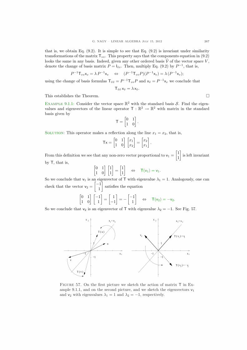
G. NAGY – LINEAR ALGEBRA July 15, 2012 267
that is, we obtain Eq. (9.2). It is simple to see that Eq. (9.2) is invariant under similaritytransformations of the matrix Tvv. This property says that the components equation in (9.2)looks the same in any basis. Indeed, given any other ordered basis V of the vector space V ,denote the change of basis matrix P = Ivv. Then, multiply Eq. (9.2) by P−1, that is,
P−1Tvvxv = λP−1xv ⇔ (P−1TvvP )(P−1xv) = λ (P−1xv);
using the change of basis formulas Tvv = P−1TvvP and xv = P−1xv we conclude that
Tvv xv = λ xv.
This establishes the Theorem. ¤
Example 9.1.1: Consider the vector space R2 with the standard basis S. Find the eigen-values and eigenvectors of the linear operator T : R2 → R2 with matrix in the standardbasis given by
T =[0 11 0
].
Solution: This operator makes a reflection along the line x1 = x2, that is,
Tx =[0 11 0
] [x1
x2
]=
[x2
x1
].
From this definition we see that any non-zero vector proportional to v1 =[11
]is left invariant
by T, that is, [0 11 0
] [11
]=
[11
]⇔ T(v1) = v1.
So we conclude that v1 is an eigenvector of T with eigenvalue λ1 = 1. Analogously, one can
check that the vector v2 =[−1
1
]satisfies the equation
[0 11 0
] [−11
]=
[1−1
]= −
[−11
]⇔ T(v2) = −v2.
So we conclude that v2 is an eigenvector of T with eigenvalue λ2 = −1. See Fig. 57.
x = x
x
2x
1
1
−1−1
u
v
1 2
T ( v )
T ( u )
2
x
2x
1
1
−1−1
x = x1 2
T ( v ) = v
T ( v ) = − v
v1 1
2
2
Figure 57. On the first picture we sketch the action of matrix T in Ex-ample 9.1.1, and on the second picture, and we sketch the eigenvectors v1
and v2 with eigenvalues λ1 = 1 and λ2 = −1, respectively.
268 G. NAGY – LINEAR ALGEBRA july 15, 2012
In this example the spectrum is σT = {1,−1} and the respective eigenspaces are
E1 = Span({[
11
]}), E−1 = Span
({[−11
]}).
C
Example 9.1.2: Not every linear operator has eigenvalues and eigenvectors. Consider thevector space R2 with standard basis and fix θ ∈ (0, π). The linear operator T : R2 → R2
with matrix
T =[cos(θ) − sin(θ)sin(θ) cos(θ)
]
acts on the plane rotating every vector by an angle θ counterclockwise. Since θ ∈ (0, π),there is no line on the plane left invariant by the rotation. Therefore, this operator has noeigenvalues and eigenvectors. C
Example 9.1.3: Consider the vector space R2 with standard basis. Show that the linear
operator T : R2 → R2 with matrix T =[1 33 1
]has the eigenvalues and eigenvectors
v1 =[11
], λ1 = 4, and v2 =
[1−1
], λ2 = −2.
Solution: We only verify that Eq. (9.1) holds for the vectors and scalars above, since
Tv1 =[1 33 1
] [11
]=
[44
]= 4
[11
]= λ1v1 ⇒ Tv1 = λ1v1
Tv2 =[1 33 1
] [1−1
]=
[−22
]= −2
[1−1
]= λ2v2 ⇒ Tv2 = λ2v2.
In this example the spectrum is σT = {4,−2} and the respective eigenspaces are
E4 = Span({[
11
]}), E−2 = Span
({[1−1
]}).
C
Example 9.1.4: Consider the vector space V = C∞(R,R). Show that the vector f (x) = eax,with a 6= 0, is an eigenvector with eigenvalue a of the linear operator D : V → V , given by
D(f )(x) =df
dx(x).
Solution: The proof is straightforward, since
D(f )(x) =df
dx(x) = aeax = a f (x) ⇒ D(f )(x) = a f (x).
C
Example 9.1.5: Consider again the vector space V = C∞(R,R) and show that the vectorf (x) = cos(ax), with a 6= 0, is an eigenvector with eigenvalue −a2 of the linear operator
T : V → V , given by T(f )(x) =d2f
dx2(x).
Solution: Again, the proof is straightforward, since
T(f )(x) =d2f
dx2(x) = −a2 cos(ax) = −a2 f (x) ⇒ T(f )(x) = −a2 f (x).
C
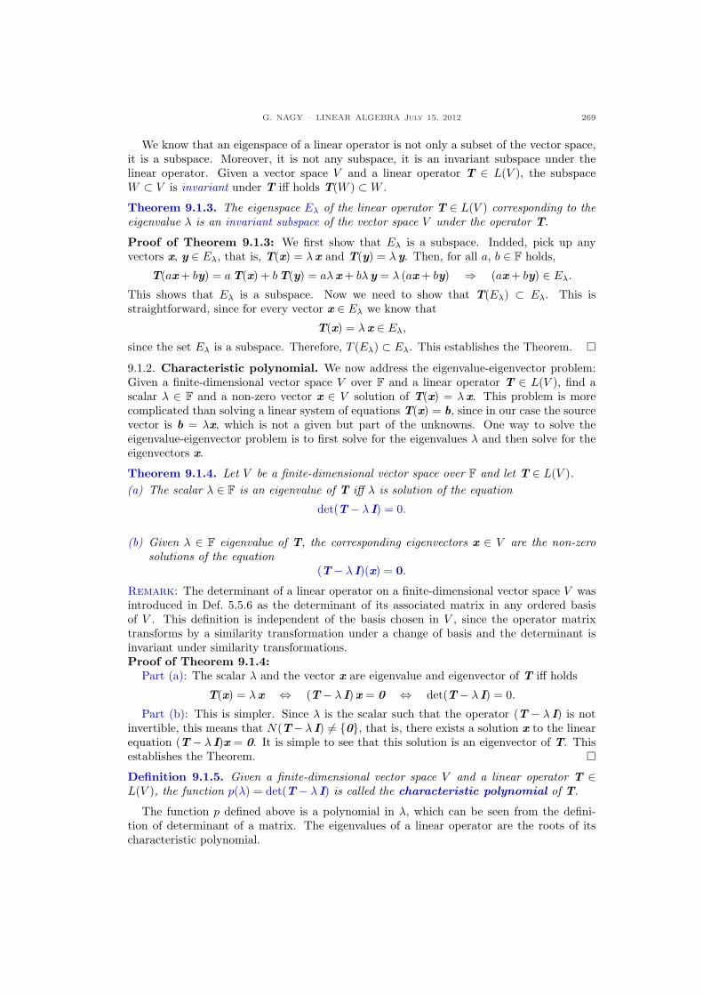
G. NAGY – LINEAR ALGEBRA July 15, 2012 269
We know that an eigenspace of a linear operator is not only a subset of the vector space,it is a subspace. Moreover, it is not any subspace, it is an invariant subspace under thelinear operator. Given a vector space V and a linear operator T ∈ L(V ), the subspaceW ⊂ V is invariant under T iff holds T(W ) ⊂W .
Theorem 9.1.3. The eigenspace Eλ of the linear operator T ∈ L(V ) corresponding to theeigenvalue λ is an invariant subspace of the vector space V under the operator T.
Proof of Theorem 9.1.3: We first show that Eλ is a subspace. Indded, pick up anyvectors x, y ∈ Eλ, that is, T(x) = λx and T(y) = λy. Then, for all a, b ∈ F holds,
T(ax + by) = aT(x) + bT(y) = aλx + bλy = λ (ax + by) ⇒ (ax + by) ∈ Eλ.
This shows that Eλ is a subspace. Now we need to show that T(Eλ) ⊂ Eλ. This isstraightforward, since for every vector x ∈ Eλ we know that
T(x) = λx ∈ Eλ,
since the set Eλ is a subspace. Therefore, T (Eλ) ⊂ Eλ. This establishes the Theorem. ¤9.1.2. Characteristic polynomial. We now address the eigenvalue-eigenvector problem:Given a finite-dimensional vector space V over F and a linear operator T ∈ L(V ), find ascalar λ ∈ F and a non-zero vector x ∈ V solution of T(x) = λx. This problem is morecomplicated than solving a linear system of equations T(x) = b, since in our case the sourcevector is b = λx, which is not a given but part of the unknowns. One way to solve theeigenvalue-eigenvector problem is to first solve for the eigenvalues λ and then solve for theeigenvectors x.
Theorem 9.1.4. Let V be a finite-dimensional vector space over F and let T ∈ L(V ).(a) The scalar λ ∈ F is an eigenvalue of T iff λ is solution of the equation
det(T− λ I) = 0.
(b) Given λ ∈ F eigenvalue of T, the corresponding eigenvectors x ∈ V are the non-zerosolutions of the equation
(T− λ I)(x) = 0.
Remark: The determinant of a linear operator on a finite-dimensional vector space V wasintroduced in Def. 5.5.6 as the determinant of its associated matrix in any ordered basisof V . This definition is independent of the basis chosen in V , since the operator matrixtransforms by a similarity transformation under a change of basis and the determinant isinvariant under similarity transformations.Proof of Theorem 9.1.4:
Part (a): The scalar λ and the vector x are eigenvalue and eigenvector of T iff holds
T(x) = λx ⇔ (T− λ I)x = 0 ⇔ det(T− λ I) = 0.
Part (b): This is simpler. Since λ is the scalar such that the operator (T − λ I) is notinvertible, this means that N(T− λ I) 6= {0}, that is, there exists a solution x to the linearequation (T− λ I)x = 0. It is simple to see that this solution is an eigenvector of T. Thisestablishes the Theorem. ¤Definition 9.1.5. Given a finite-dimensional vector space V and a linear operator T ∈L(V ), the function p(λ) = det(T− λ I) is called the characteristic polynomial of T.
The function p defined above is a polynomial in λ, which can be seen from the defini-tion of determinant of a matrix. The eigenvalues of a linear operator are the roots of itscharacteristic polynomial.
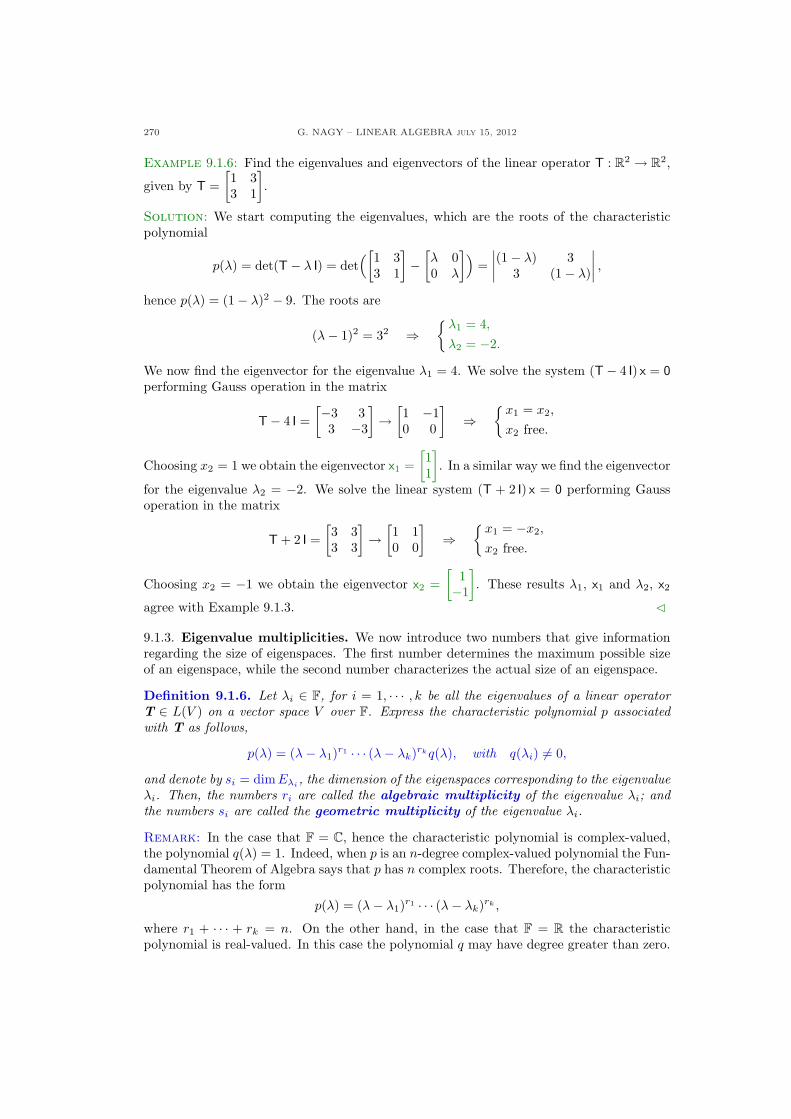
270 G. NAGY – LINEAR ALGEBRA july 15, 2012
Example 9.1.6: Find the eigenvalues and eigenvectors of the linear operator T : R2 → R2,
given by T =[1 33 1
].
Solution: We start computing the eigenvalues, which are the roots of the characteristicpolynomial
p(λ) = det(T− λ I) = det([
1 33 1
]−
[λ 00 λ
])=
∣∣∣∣(1− λ) 3
3 (1− λ)
∣∣∣∣ ,
hence p(λ) = (1− λ)2 − 9. The roots are
(λ− 1)2 = 32 ⇒{
λ1 = 4,
λ2 = −2.
We now find the eigenvector for the eigenvalue λ1 = 4. We solve the system (T− 4 I) x = 0performing Gauss operation in the matrix
T− 4 I =[−3 3
3 −3
]→
[1 −10 0
]⇒
{x1 = x2,
x2 free.
Choosing x2 = 1 we obtain the eigenvector x1 =[11
]. In a similar way we find the eigenvector
for the eigenvalue λ2 = −2. We solve the linear system (T + 2 I) x = 0 performing Gaussoperation in the matrix
T + 2 I =[3 33 3
]→
[1 10 0
]⇒
{x1 = −x2,
x2 free.
Choosing x2 = −1 we obtain the eigenvector x2 =[
1−1
]. These results λ1, x1 and λ2, x2
agree with Example 9.1.3. C
9.1.3. Eigenvalue multiplicities. We now introduce two numbers that give informationregarding the size of eigenspaces. The first number determines the maximum possible sizeof an eigenspace, while the second number characterizes the actual size of an eigenspace.
Definition 9.1.6. Let λi ∈ F, for i = 1, · · · , k be all the eigenvalues of a linear operatorT ∈ L(V ) on a vector space V over F. Express the characteristic polynomial p associatedwith T as follows,
p(λ) = (λ− λ1)r1 · · · (λ− λk)rkq(λ), with q(λi) 6= 0,
and denote by si = dim Eλi , the dimension of the eigenspaces corresponding to the eigenvalueλi. Then, the numbers ri are called the algebraic multiplicity of the eigenvalue λi; andthe numbers si are called the geometric multiplicity of the eigenvalue λi.
Remark: In the case that F = C, hence the characteristic polynomial is complex-valued,the polynomial q(λ) = 1. Indeed, when p is an n-degree complex-valued polynomial the Fun-damental Theorem of Algebra says that p has n complex roots. Therefore, the characteristicpolynomial has the form
p(λ) = (λ− λ1)r1 · · · (λ− λk)rk ,
where r1 + · · · + rk = n. On the other hand, in the case that F = R the characteristicpolynomial is real-valued. In this case the polynomial q may have degree greater than zero.
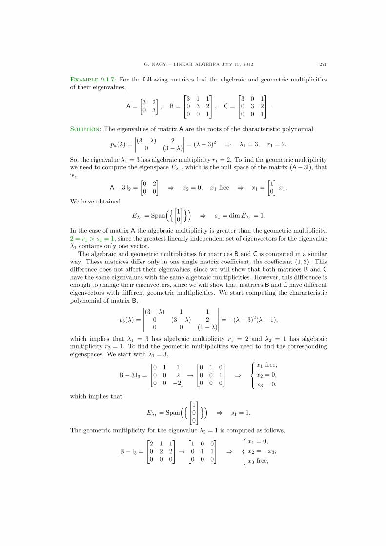
G. NAGY – LINEAR ALGEBRA July 15, 2012 271
Example 9.1.7: For the following matrices find the algebraic and geometric multiplicitiesof their eigenvalues,
A =[3 20 3
], B =
3 1 10 3 20 0 1
, C =
3 0 10 3 20 0 1
.
Solution: The eigenvalues of matrix A are the roots of the characteristic polynomial
pa(λ) =∣∣∣∣(3− λ) 2
0 (3− λ)
∣∣∣∣ = (λ− 3)2 ⇒ λ1 = 3, r1 = 2.
So, the eigenvalue λ1 = 3 has algebraic multiplicity r1 = 2. To find the geometric multiplicitywe need to compute the eigenspace Eλ1 , which is the null space of the matrix (A− 3I), thatis,
A− 3 I2 =[0 20 0
]⇒ x2 = 0, x1 free ⇒ x1 =
[10
]x1.
We have obtained
Eλ1 = Span({[
10
]})⇒ s1 = dim Eλ1 = 1.
In the case of matrix A the algebraic multiplicity is greater than the geometric multiplicity,2 = r1 > s1 = 1, since the greatest linearly independent set of eigenvectors for the eigenvalueλ1 contains only one vector.
The algebraic and geometric multiplicities for matrices B and C is computed in a similarway. These matrices differ only in one single matrix coefficient, the coefficient (1, 2). Thisdifference does not affect their eigenvalues, since we will show that both matrices B and Chave the same eigenvalues with the same algebraic multiplicities. However, this difference isenough to change their eigenvectors, since we will show that matrices B and C have differenteigenvectors with different geometric multiplicities. We start computing the characteristicpolynomial of matrix B,
pb(λ) =
∣∣∣∣∣∣
(3− λ) 1 10 (3− λ) 20 0 (1− λ)
∣∣∣∣∣∣= −(λ− 3)2(λ− 1),
which implies that λ1 = 3 has algebraic multiplicity r1 = 2 and λ2 = 1 has algebraicmultiplicity r2 = 1. To find the geometric multiplicities we need to find the correspondingeigenspaces. We start with λ1 = 3,
B− 3 I3 =
0 1 10 0 20 0 −2
→
0 1 00 0 10 0 0
⇒
x1 free,x2 = 0,
x3 = 0,
which implies that
Eλ1 = Span({
100
})⇒ s1 = 1.
The geometric multiplicity for the eigenvalue λ2 = 1 is computed as follows,
B− I3 =
2 1 10 2 20 0 0
→
1 0 00 1 10 0 0
⇒
x1 = 0,
x2 = −x3,
x3 free,
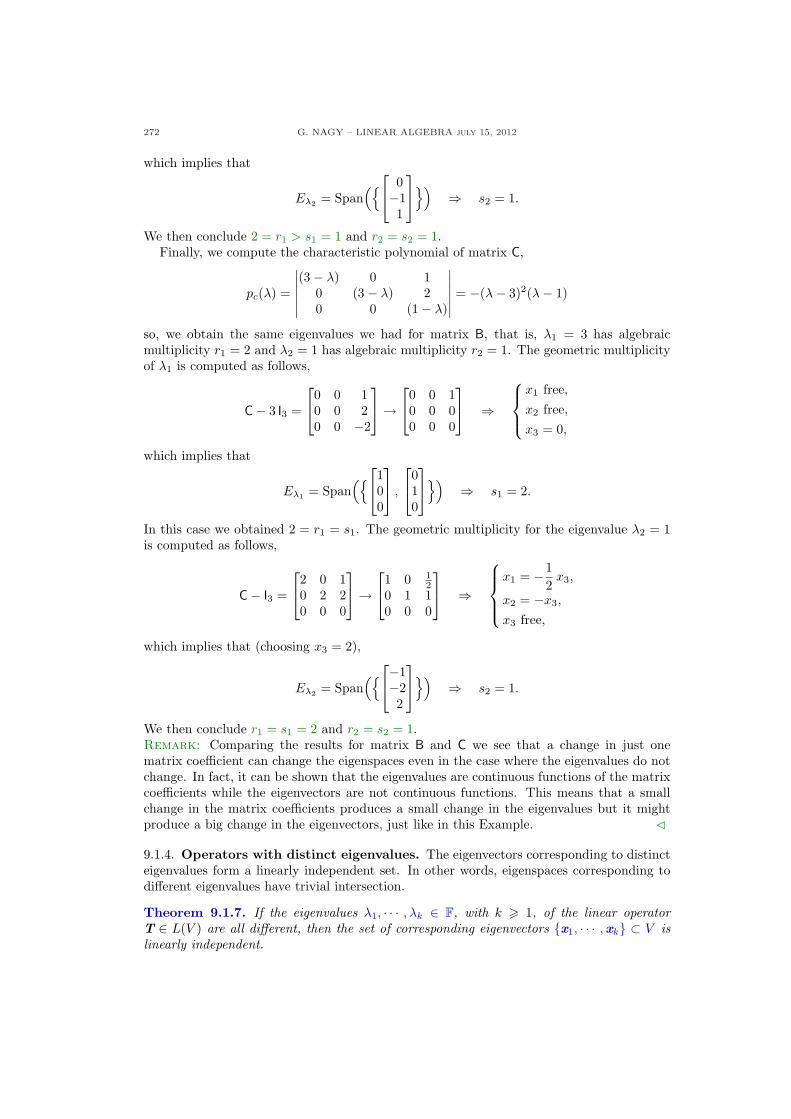
272 G. NAGY – LINEAR ALGEBRA july 15, 2012
which implies that
Eλ2 = Span({
0−11
})⇒ s2 = 1.
We then conclude 2 = r1 > s1 = 1 and r2 = s2 = 1.Finally, we compute the characteristic polynomial of matrix C,
pc(λ) =
∣∣∣∣∣∣
(3− λ) 0 10 (3− λ) 20 0 (1− λ)
∣∣∣∣∣∣= −(λ− 3)2(λ− 1)
so, we obtain the same eigenvalues we had for matrix B, that is, λ1 = 3 has algebraicmultiplicity r1 = 2 and λ2 = 1 has algebraic multiplicity r2 = 1. The geometric multiplicityof λ1 is computed as follows,
C− 3 I3 =
0 0 10 0 20 0 −2
→
0 0 10 0 00 0 0
⇒
x1 free,x2 free,x3 = 0,
which implies that
Eλ1 = Span({
100
,
010
})⇒ s1 = 2.
In this case we obtained 2 = r1 = s1. The geometric multiplicity for the eigenvalue λ2 = 1is computed as follows,
C− I3 =
2 0 10 2 20 0 0
→
1 0 12
0 1 10 0 0
⇒
x1 = −12
x3,
x2 = −x3,
x3 free,
which implies that (choosing x3 = 2),
Eλ2 = Span({
−1−22
})⇒ s2 = 1.
We then conclude r1 = s1 = 2 and r2 = s2 = 1.Remark: Comparing the results for matrix B and C we see that a change in just onematrix coefficient can change the eigenspaces even in the case where the eigenvalues do notchange. In fact, it can be shown that the eigenvalues are continuous functions of the matrixcoefficients while the eigenvectors are not continuous functions. This means that a smallchange in the matrix coefficients produces a small change in the eigenvalues but it mightproduce a big change in the eigenvectors, just like in this Example. C
9.1.4. Operators with distinct eigenvalues. The eigenvectors corresponding to distincteigenvalues form a linearly independent set. In other words, eigenspaces corresponding todifferent eigenvalues have trivial intersection.
Theorem 9.1.7. If the eigenvalues λ1, · · · , λk ∈ F, with k > 1, of the linear operatorT ∈ L(V ) are all different, then the set of corresponding eigenvectors {x1, · · · ,xk} ⊂ V islinearly independent.
G. NAGY – LINEAR ALGEBRA July 15, 2012 273
Proof of Theorem 9.1.7: If k = 1, the Theorem is trivially true, so assume k > 2. Letc1, · · · , ck ∈ F be scalars such that
c1x1 + · · ·+ ckxk = 0. (9.3)
Now perform the following two steps: First, apply the operator T to both sides of theequation above. Since T(xi) = λixi, we obtain,
c1λ1 x1 + · · ·+ ckλk xk = 0. (9.4)
Second, multiply Eq. (9.3) by λ1 and subtract it from Eq.(9.4). The result is
c2(λ2 − λ1)x2 + · · ·+ ck(λk − λ1)xk = 0. (9.5)
Notice that all factors λi−λ1 6= 0 for i = 2, · · · , k. Repeat these two steps: First, apply theoperator T on both sides of Eq. (9.5), that is,
c2(λ2 − λ1)λ2 x2 + · · ·+ ck(λk − λ1) λk xk = 0; (9.6)
second, multiply Eq. (9.5) by λ2 and subtract it from Eq. (9.6), that is,
c2(λ2 − λ1) (λ3 − λ2)x3 + · · ·+ ck(λk − λ1) (λk − λ2)xk = 0. (9.7)
Repeat the idea in these two steps until one reaches the equation
ck(λk − λ1) · · · (λk − λk−1)xk = 0.
Since the eigenvalues λi are all different, we conclude that ck = 0. Introducing this infor-mation at the very begining we get that
c1x1 + · · ·+ ck−1xk−1 = 0.
Repeating the whole procedure we conclude that ck−1 = 0. In this way one shows that allcoefficient c1 = · · · = ck = 0. Therefore, the set {x1, · · · ,xk} is linearly independent. Thisestablishes the Theorem. ¤
Further reading. A detailed presentation of eigenvalues and eigenvectors of a matrix canbe found in Sections 5.1 and 5.2 in Lay’s book [2], while a shorter and deeper summary canbe found in Section 7.1 in Meyer’s book [3]. Also see Chapter 4 in Hassani’s book [1].
274 G. NAGY – LINEAR ALGEBRA july 15, 2012
9.1.5. Exercises.
9.1.1.- Find the spectrum and all eigen-spaces of the operators A : R2 → R2
and B : R3 → R3,
A =
»−10 −714 11
–,
B =
24
1 1 00 3 11 −1 2
35 .
9.1.2.- Show that for θ ∈ (0, π) the rota-tion operator R(θ) : R2 → R2 has noeigenvalues, where
R(θ) =
»cos(θ) − sin(θ)sin(θ) cos(θ)
–.
Consider now matrix above as a linearoperator R(θ) : C2 → C2. Show thatthis linear operator has eigenvalues, andfind them.
9.1.3.- Let A : R3 → R3 be the linear oper-ator given by
A =
24
2 −1 30 1 h0 0 2
35 .
(a) Find all the eigenvalues and theircorresponding algebraic multiplici-ties of the matrix A.
(b) Find the value(s) of h ∈ R suchthat the matrix A above has a two-dimensional eigenspace, and find abasis for this eigenspace.
(c) Set h = 1, and find a basis for allthe eigenspaces of matrix A above.
9.1.4.- Find all the eigenvalues with theircorresponding algebraic multiplicities,and find all the associated eigenspacesof the matrix A ∈ R3,3 given by
A =
24
2 1 10 2 30 0 1
35 .
9.1.5.- Let k ∈ R and consider the matrixA ∈ R4,4 given by
A =
2664
2 −2 4 −10 3 k 00 0 2 40 0 0 1
3775 .
(a) Find the eigenvalues of A and theiralgebraic multiplicity.
(b) Find the number k such that ma-trix A has an eigenspace Eλ that istwo dimensional, and find a basisfor this Eλ.
9.1.6.- Comparing the characteristic poly-nomials for A ∈ Fn,n and AT , show thatthese two matrices have the same eigen-values.
9.1.7.- Let A ∈ R3,3 be an invertible matrixwith eigenvalues 2, −1 and 3. Find theeigenvalues of:
(a) A−1.
(b) Ak, for any k ∈ N.(c) A2 − A.
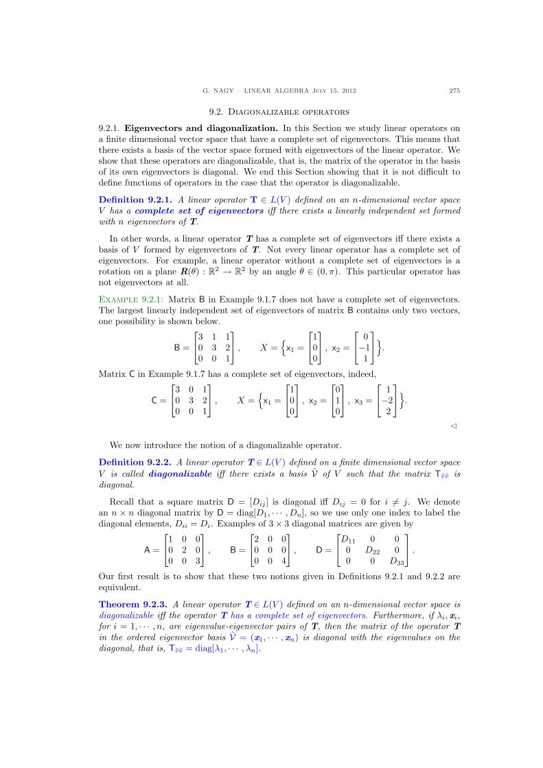
G. NAGY – LINEAR ALGEBRA July 15, 2012 275
9.2. Diagonalizable operators
9.2.1. Eigenvectors and diagonalization. In this Section we study linear operators ona finite dimensional vector space that have a complete set of eigenvectors. This means thatthere exists a basis of the vector space formed with eigenvectors of the linear operator. Weshow that these operators are diagonalizable, that is, the matrix of the operator in the basisof its own eigenvectors is diagonal. We end this Section showing that it is not difficult todefine functions of operators in the case that the operator is diagonalizable.
Definition 9.2.1. A linear operator T ∈ L(V ) defined on an n-dimensional vector spaceV has a complete set of eigenvectors iff there exists a linearly independent set formedwith n eigenvectors of T.
In other words, a linear operator T has a complete set of eigenvectors iff there exists abasis of V formed by eigenvectors of T. Not every linear operator has a complete set ofeigenvectors. For example, a linear operator without a complete set of eigenvectors is arotation on a plane R(θ) : R2 → R2 by an angle θ ∈ (0, π). This particular operator hasnot eigenvectors at all.
Example 9.2.1: Matrix B in Example 9.1.7 does not have a complete set of eigenvectors.The largest linearly independent set of eigenvectors of matrix B contains only two vectors,one possibility is shown below.
B =
3 1 10 3 20 0 1
, X =
{x1 =
100
, x2 =
0−11
}.
Matrix C in Example 9.1.7 has a complete set of eigenvectors, indeed,
C =
3 0 10 3 20 0 1
, X =
{x1 =
100
, x2 =
010
, x3 =
1−22
}.
C
We now introduce the notion of a diagonalizable operator.
Definition 9.2.2. A linear operator T ∈ L(V ) defined on a finite dimensional vector spaceV is called diagonalizable iff there exists a basis V of V such that the matrix Tvv isdiagonal.
Recall that a square matrix D = [Dij ] is diagonal iff Dij = 0 for i 6= j. We denotean n × n diagonal matrix by D = diag[D1, · · · , Dn], so we use only one index to label thediagonal elements, Dii = Di. Examples of 3× 3 diagonal matrices are given by
A =
1 0 00 2 00 0 3
, B =
2 0 00 0 00 0 4
, D =
D11 0 00 D22 00 0 D33
.
Our first result is to show that these two notions given in Definitions 9.2.1 and 9.2.2 areequivalent.
Theorem 9.2.3. A linear operator T ∈ L(V ) defined on an n-dimensional vector space isdiagonalizable iff the operator T has a complete set of eigenvectors. Furthermore, if λi,xi,for i = 1, · · · , n, are eigenvalue-eigenvector pairs of T, then the matrix of the operator Tin the ordered eigenvector basis V = (x1, · · · ,xn) is diagonal with the eigenvalues on thediagonal, that is, Tvv = diag[λ1, · · · , λn].
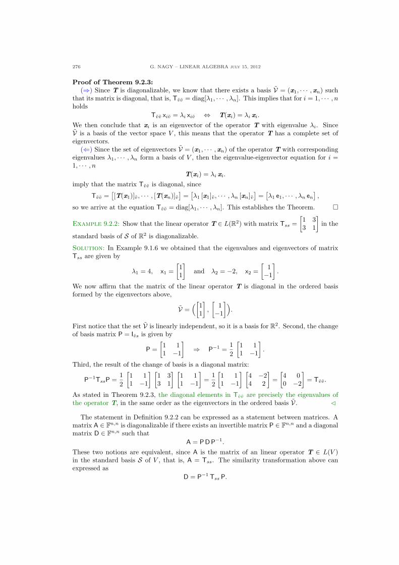
276 G. NAGY – LINEAR ALGEBRA july 15, 2012
Proof of Theorem 9.2.3:(⇒) Since T is diagonalizable, we know that there exists a basis V = (x1, · · · ,xn) such
that its matrix is diagonal, that is, Tvv = diag[λ1, · · · , λn]. This implies that for i = 1, · · · , nholds
Tvv xiv = λi xiv ⇔ T(xi) = λi xi.
We then conclude that xi is an eigenvector of the operator T with eigenvalue λi. SinceV is a basis of the vector space V , this means that the operator T has a complete set ofeigenvectors.
(⇐) Since the set of eigenvectors V = (x1, · · · ,xn) of the operator T with correspondingeigenvalues λ1, · · · , λn form a basis of V , then the eigenvalue-eigenvector equation for i =1, · · · , n
T(xi) = λi xi.
imply that the matrix Tvv is diagonal, since
Tvv =[[T(x1)]v, · · · , [T(xn)]v
]=
[λ1 [x1]v, · · · , λn [xn]v
]=
[λ1 e1, · · · , λn en
],
so we arrive at the equation Tvv = diag[λ1, · · · , λn]. This establishes the Theorem. ¤
Example 9.2.2: Show that the linear operator T ∈ L(R2) with matrix Tss =[1 33 1
]in the
standard basis of S of R2 is diagonalizable.
Solution: In Example 9.1.6 we obtained that the eigenvalues and eigenvectors of matrixTss are given by
λ1 = 4, x1 =[11
]and λ2 = −2, x2 =
[1−1
].
We now affirm that the matrix of the linear operator T is diagonal in the ordered basisformed by the eigenvectors above,
V =([
11
],
[1−1
]).
First notice that the set V is linearly independent, so it is a basis for R2. Second, the changeof basis matrix P = Ivs is given by
P =[1 11 −1
]⇒ P−1 =
12
[1 11 −1
].
Third, the result of the change of basis is a diagonal matrix:
P−1TssP =12
[1 11 −1
] [1 33 1
] [1 11 −1
]=
12
[1 11 −1
] [4 −24 2
]=
[4 00 −2
]= Tvv.
As stated in Theorem 9.2.3, the diagonal elements in Tvv are precisely the eigenvalues ofthe operator T, in the same order as the eigenvectors in the ordered basis V. C
The statement in Definition 9.2.2 can be expressed as a statement between matrices. Amatrix A ∈ Fn,n is diagonalizable if there exists an invertible matrix P ∈ Fn,n and a diagonalmatrix D ∈ Fn,n such that
A = PDP−1.
These two notions are equivalent, since A is the matrix of an linear operator T ∈ L(V )in the standard basis S of V , that is, A = Tss. The similarity transformation above canexpressed as
D = P−1 Tss P.
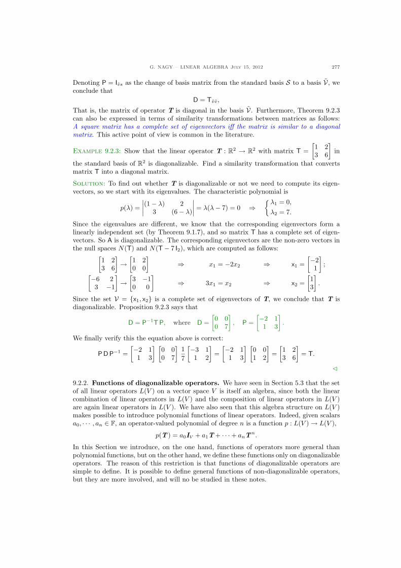
G. NAGY – LINEAR ALGEBRA July 15, 2012 277
Denoting P = Ivs as the change of basis matrix from the standard basis S to a basis V, weconclude that
D = Tvv,
That is, the matrix of operator T is diagonal in the basis V. Furthermore, Theorem 9.2.3can also be expressed in terms of similarity transformations between matrices as follows:A square matrix has a complete set of eigenvectors iff the matrix is similar to a diagonalmatrix. This active point of view is common in the literature.
Example 9.2.3: Show that the linear operator T : R2 → R2 with matrix T =[1 23 6
]in
the standard basis of R2 is diagonalizable. Find a similarity transformation that convertsmatrix T into a diagonal matrix.
Solution: To find out whether T is diagonalizable or not we need to compute its eigen-vectors, so we start with its eigenvalues. The characteristic polynomial is
p(λ) =∣∣∣∣(1− λ) 2
3 (6− λ)
∣∣∣∣ = λ(λ− 7) = 0 ⇒{
λ1 = 0,
λ2 = 7.
Since the eigenvalues are different, we know that the corresponding eigenvectors form alinearly independent set (by Theorem 9.1.7), and so matrix T has a complete set of eigen-vectors. So A is diagonalizable. The corresponding eigenvectors are the non-zero vectors inthe null spaces N(T) and N(T− 7 I2), which are computed as follows:
[1 23 6
]→
[1 20 0
]⇒ x1 = −2x2 ⇒ x1 =
[−21
];
[−6 23 −1
]→
[3 −10 0
]⇒ 3x1 = x2 ⇒ x2 =
[13
].
Since the set V = {x1, x2} is a complete set of eigenvectors of T, we conclude that T isdiagonalizable. Proposition 9.2.3 says that
D = P−1T P, where D =[0 00 7
], P =
[−2 11 3
].
We finally verify this the equation above is correct:
PD P−1 =[−2 1
1 3
] [0 00 7
]17
[−3 11 2
]=
[−2 11 3
] [0 01 2
]=
[1 23 6
]= T.
C
9.2.2. Functions of diagonalizable operators. We have seen in Section 5.3 that the setof all linear operators L(V ) on a vector space V is itself an algebra, since both the linearcombination of linear operators in L(V ) and the composition of linear operators in L(V )are again linear operators in L(V ). We have also seen that this algebra structure on L(V )makes possible to introduce polynomial functions of linear operators. Indeed, given scalarsa0, · · · , an ∈ F, an operator-valued polynomial of degree n is a function p : L(V )→ L(V ),
p(T ) = a0IV + a1T + · · ·+ anTn.
In this Section we introduce, on the one hand, functions of operators more general thanpolynomial functions, but on the other hand, we define these functions only on diagonalizableoperators. The reason of this restriction is that functions of diagonalizable operators aresimple to define. It is possible to define general functions of non-diagonalizable operators,but they are more involved, and will no be studied in these notes.
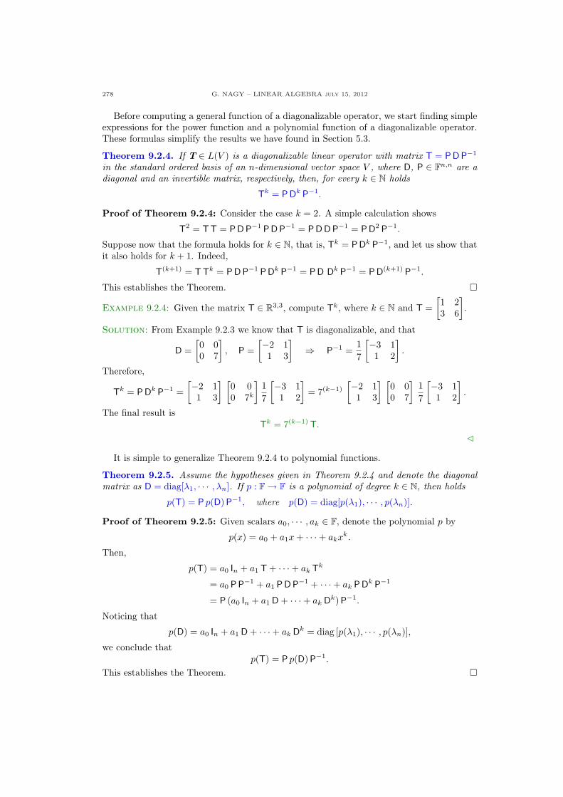
278 G. NAGY – LINEAR ALGEBRA july 15, 2012
Before computing a general function of a diagonalizable operator, we start finding simpleexpressions for the power function and a polynomial function of a diagonalizable operator.These formulas simplify the results we have found in Section 5.3.
Theorem 9.2.4. If T ∈ L(V ) is a diagonalizable linear operator with matrix T = PD P−1
in the standard ordered basis of an n-dimensional vector space V , where D, P ∈ Fn,n are adiagonal and an invertible matrix, respectively, then, for every k ∈ N holds
Tk = P Dk P−1.
Proof of Theorem 9.2.4: Consider the case k = 2. A simple calculation shows
T2 = TT = PD P−1 PD P−1 = PD D P−1 = PD2 P−1.
Suppose now that the formula holds for k ∈ N, that is, Tk = PDk P−1, and let us show thatit also holds for k + 1. Indeed,
T(k+1) = TTk = PD P−1 PDk P−1 = PD Dk P−1 = PD(k+1) P−1.
This establishes the Theorem. ¤
Example 9.2.4: Given the matrix T ∈ R3,3, compute Tk, where k ∈ N and T =[1 23 6
].
Solution: From Example 9.2.3 we know that T is diagonalizable, and that
D =[0 00 7
], P =
[−2 11 3
]⇒ P−1 =
17
[−3 11 2
].
Therefore,
Tk = PDk P−1 =[−2 1
1 3
] [0 00 7k
]17
[−3 11 2
]= 7(k−1)
[−2 11 3
] [0 00 7
]17
[−3 11 2
].
The final result isTk = 7(k−1) T.
C
It is simple to generalize Theorem 9.2.4 to polynomial functions.
Theorem 9.2.5. Assume the hypotheses given in Theorem 9.2.4 and denote the diagonalmatrix as D = diag[λ1, · · · , λn]. If p : F→ F is a polynomial of degree k ∈ N, then holds
p(T) = P p(D)P−1, where p(D) = diag[p(λ1), · · · , p(λn)].
Proof of Theorem 9.2.5: Given scalars a0, · · · , ak ∈ F, denote the polynomial p by
p(x) = a0 + a1x + · · ·+ akxk.
Then,
p(T) = a0 In + a1 T + · · ·+ ak Tk
= a0 PP−1 + a1 P DP−1 + · · ·+ ak PDk P−1
= P (a0 In + a1 D + · · ·+ ak Dk)P−1.
Noticing that
p(D) = a0 In + a1 D + · · ·+ ak Dk = diag [p(λ1), · · · , p(λn)],
we conclude thatp(T) = P p(D)P−1.
This establishes the Theorem. ¤
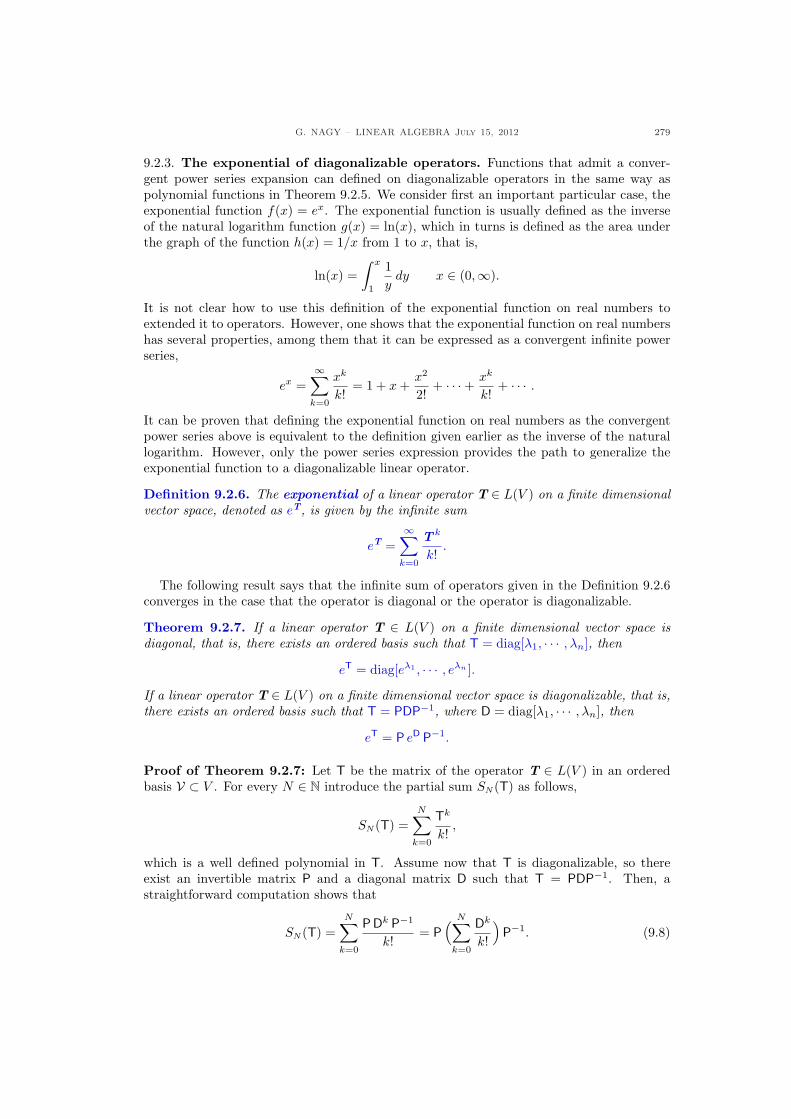
G. NAGY – LINEAR ALGEBRA July 15, 2012 279
9.2.3. The exponential of diagonalizable operators. Functions that admit a conver-gent power series expansion can defined on diagonalizable operators in the same way aspolynomial functions in Theorem 9.2.5. We consider first an important particular case, theexponential function f(x) = ex. The exponential function is usually defined as the inverseof the natural logarithm function g(x) = ln(x), which in turns is defined as the area underthe graph of the function h(x) = 1/x from 1 to x, that is,
ln(x) =∫ x
1
1y
dy x ∈ (0,∞).
It is not clear how to use this definition of the exponential function on real numbers toextended it to operators. However, one shows that the exponential function on real numbershas several properties, among them that it can be expressed as a convergent infinite powerseries,
ex =∞∑
k=0
xk
k!= 1 + x +
x2
2!+ · · ·+ xk
k!+ · · · .
It can be proven that defining the exponential function on real numbers as the convergentpower series above is equivalent to the definition given earlier as the inverse of the naturallogarithm. However, only the power series expression provides the path to generalize theexponential function to a diagonalizable linear operator.
Definition 9.2.6. The exponential of a linear operator T ∈ L(V ) on a finite dimensionalvector space, denoted as eT, is given by the infinite sum
eT =∞∑
k=0
T k
k!.
The following result says that the infinite sum of operators given in the Definition 9.2.6converges in the case that the operator is diagonal or the operator is diagonalizable.
Theorem 9.2.7. If a linear operator T ∈ L(V ) on a finite dimensional vector space isdiagonal, that is, there exists an ordered basis such that T = diag[λ1, · · · , λn], then
eT = diag[eλ1 , · · · , eλn ].
If a linear operator T ∈ L(V ) on a finite dimensional vector space is diagonalizable, that is,there exists an ordered basis such that T = PDP−1, where D = diag[λ1, · · · , λn], then
eT = P eD P−1.
Proof of Theorem 9.2.7: Let T be the matrix of the operator T ∈ L(V ) in an orderedbasis V ⊂ V . For every N ∈ N introduce the partial sum SN(T) as follows,
SN(T) =N∑
k=0
Tk
k!,
which is a well defined polynomial in T. Assume now that T is diagonalizable, so thereexist an invertible matrix P and a diagonal matrix D such that T = PDP−1. Then, astraightforward computation shows that
SN(T) =N∑
k=0
PDk P−1
k!= P
( N∑
k=0
Dk
k!
)P−1. (9.8)
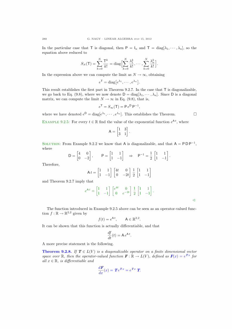
280 G. NAGY – LINEAR ALGEBRA july 15, 2012
In the particular case that T is diagonal, then P = In and T = diag[λ1, · · · , λn], so theequation above reduced to
SN(T) =N∑
k=0
Tk
k!= diag
[ N∑
k=0
λk1
k!, · · · ,
N∑
k=0
λkn
k!
].
In the expression above we can compute the limit as N →∞, obtaining
eT = diag[eλ1 , · · · , eλn
].
This result establishes the first part in Theorem 9.2.7. In the case that T is diagonalizable,we go back to Eq. (9.8), where we now denote D = diag[λ1, · · · , λn]. Since D is a diagonalmatrix, we can compute the limit N →∞ in Eq. (9.8), that is,
eT = S∞(T) = P eD P−1,
where we have denoted eD = diag[eλ1 , · · · , eλn ]. This establishes the Theorem. ¤
Example 9.2.5: For every t ∈ R find the value of the exponential function eA t, where
A =[1 33 1
].
Solution: From Example 9.2.2 we know that A is diagonalizable, and that A = PD P−1,where
D =[4 00 −2
], P =
[1 11 −1
]⇒ P−1 =
12
[1 11 −1
].
Therefore,
A t =[1 11 −1
] [4t 00 −2t
]12
[1 11 −1
]
and Theorem 9.2.7 imply that
eA t =[1 11 −1
] [e4t 00 e−2t
]12
[1 11 −1
].
C
The function introduced in Example 9.2.5 above can be seen as an operator-valued func-tion f : R→ R2,2 given by
f(t) = eA t, A ∈ R2,2.
It can be shown that this function is actually differentiable, and that
df
dt(t) = A eA t.
A more precise statement is the following.
Theorem 9.2.8. If T ∈ L(V ) is a diagonalizable operator on a finite dimensional vectorspace over R, then the operator-valued function F : R → L(V ), defined as F(x) = eT x forall x ∈ R, is differentiable and
dF
dx(x) = T eT x = eT x T.
G. NAGY – LINEAR ALGEBRA July 15, 2012 281
Proof of Theorem 9.2.8: Fix an ordered basis V ⊂ V and denote by T the matrix ofT in that basis. Since T is diagonalizable, then T = PDP−1, with D = diag[λ1, · · · , λn].Denoting by F the matrix of F in the basis V, it is simple to see that
dF
dx(x) =
d
dx
(P eD x P−1
)= P
( d
dxeD x
)P−1.
It is not difficult to see that the expression of the far right in equation above is given byd
dxeD x = diag
[ d
dx
(eλ1x
), · · · , d
dx
(eλnx
)]= diag [λ1e
λ1x, · · · , λneλnx] = D eD x = eD x D,
where we used the expression D = diag[λ1, · · · , λn]. Recalling that
PD eD x P−1 = PD P−1 P eD x P−1 = T eT x,
we conclude thatd
dxeT x = T eT x = eT x T.
This establishes the Theorem. ¤
Example 9.2.6: Find the derivative of f(t) = eA t, where A =[1 33 1
].
Solution: From Example 9.2.5 we know that
eA t =[1 11 −1
] [e4t 00 e−2t
]12
[1 11 −1
].
Then, Theorem 9.2.8 implies thatd
dteA t =
[1 11 −1
] [4e4t 00 −2e−2t
]12
[1 11 −1
].
C
We end this Section presenting a result without proof, that says that given any scalar-valued function with a convergent power series, that function can be extended into anoperator-valued function in the case that the operator is diagonalizable.
Theorem 9.2.9. Let f : F→ F be a function given by a power series
f(z) =∞∑
k=0
ck(z − z0)k,
which converges for |z−z0| < r, for some positive real number r. If LD(V ) is the subspace ofdiagonalizable operators on the finite dimensional vector space V , then the operator-valuedfunction F : LD(V )→ LD(V ) given by
F(T ) =∞∑
k=0
ck(T− z0 IV )k
converges iff every eigenvalue λi of T satisfies that |λi − z0| < r for all i = 1, · · · , n.
282 G. NAGY – LINEAR ALGEBRA july 15, 2012
9.2.4. Exercises.
9.2.1.- Which of the following matrices can-not be diagonalized?
A =
»2 −22 −2
–,
B =
»2 02 −2
–,
C =
»2 02 2
–.
9.2.2.- Verify that the matrix
A =
»7/5 1/5−1 1/2
–
has eigenvalues λ1 = 1 and λ2 = 9/10and associated eigenvectors
x1 =
»−12
–, x2 =
»−25
–.
Use this information to compute
limk→∞
Ak.
9.2.3.- Given the matrix and vector ,
A =
»1 33 1
–, x0 =
»21
–
compute the function x : R→ R2
x(t) = eA tx0.
Verify that this function is solution ofthe differential equation
d
dtx(t) = Ax(t)
and satisfies that x(t = 0) = x0.
9.2.4.- Let A ∈ R3,3 be a matrix with eigen-values 2, −1 and 3. Find the determi-nant of A.
9.2.5.- Let A ∈ R4,4 be a matrix that canbe decomposed as A = PDP−1, withmatrix P an invertible matrix and thematrix
D = diag(2,1
4, 2, 3).
Knowing only this information aboutthe matrix A, is it possible to computethe det(A)? If your answer is no, ex-plain why not; if your answer is yes,compute det(A) and show your work.
9.2.6.- Let A ∈ R4,4 be a matrix that canbe decomposed as A = PDP−1, withmatrix P an invertible matrix and thematrix
D = diag(2, 0, 2, 5).
Knowing only this information aboutthe matrix A, is it possible to whether Ainvertible? Is it possible to know tr (A)?If your answer is no, explain why not; ifyour answer is yes, compute tr (A) andshow your work.
G. NAGY – LINEAR ALGEBRA July 15, 2012 283
9.3. Differential equations
Eigenvalues and eigenvectors of a matrix are useful to find solutions to systems of dif-ferential equations. In this Section we first recall what is a system of first order, linear,homogeneous, differential equations with constant coefficients. Then we use the eigenvaluesand eigenvectors of the coefficient matrix to obtain solutions to such differential equations.
In order to introduce a linear, first order system of differential equations we need somenotation. Let A : R → Rn,n be a real matrix-valued function, x, b : R → Rn be realvector-valued functions, with values A(t), x(t), and b(t) given by
A(t) =
A11(t) · · · A1n(t)...
...An1(t) · · · Ann(t)
, x(t) =
x1(t)...
xn(t)
, b(t) =
b1(t)...
bn(t)
.
So, A(t) is an n × n matrix for each value of t ∈ R. An example in the case n = 2 is thematrix-valued function
A(t) =[cos(2πt) − sin(2πt)sin(2πt) cos(2πt)
].
The values of this function are rotation matrices on R2, counterclockwise by an angle 2πt.So the bigger the parameter t the bigger the is rotation. Derivatives of matrix- and vector-valued functions are computed component-wise, and we use the notation ˙ = d
dt ; for example
dx
dt(t) =
dx1
dt(t)
...dxn
dt(t)
is denoted as x(t) =
x1(t)...
xn(t)
.
We are now ready to introduce the main definitions.
Definition 9.3.1. A system of first order linear differential equations on n un-knowns, with n > 1, is the following: Given a real matrix-valued function A : R → Rn,n,and a real vector-valued function b : R → Rn, find a vector-valued function x : R → Rn
solution ofx(t) = A(t) x(t) + b(t). (9.9)
The system in (9.9) is called homogeneous iff b(t) = 0 for all t ∈ R. The system in (9.9)is called of constant coefficients iff the matrix- and vector-valued functions are constant,that is, A(t) = A0 and b(t) = b0 for all t ∈ R.
The differential equation in (9.9) is called first order because it contains only first deriva-tives of the the unknown vector-valued function x; it is called linear because the unknownx appears linearly in the equation. In this Section we are interested in finding solutions toan initial value problem involving a constant coefficient, homogeneous differential system.
Definition 9.3.2. An initial value problem (IVP) for an homogeneous constant coeffi-cients linear differential equation is the following: Given a matrix A ∈ Rn,n and a vectorx0 ∈ Rn, find a vector-valued function x : R → Rn solution of the differential equation andinitial condition
x(t) = Ax(t), x(0) = x0.
In this Section we only consider the case where the coefficient matrix A ∈ Rn,n has acomplete set of eigenvectors, that is, matrix A is diagonalizable. In this case it is possible tofind all solutions of the initial value problem for an homogeneous and constant coefficientdifferential equation. These solutions are linear combination of vectors proportional to the
284 G. NAGY – LINEAR ALGEBRA july 15, 2012
eigenvectors of matrix A, where the scalars involved in the linear combination depend onthe eigenvalues of matrix A. The explicit form of the solution depends on these eigenvaluesand can be classified in three groups: Non-repeated real eigenvalues, non-repeated complexeigenvalues, and repeated eigenvalues. We consider in these notes only the first two casesof non-repeated eigenvalues. In this case, the main result is the following.
Theorem 9.3.3. Assume that matrix A ∈ Rn,n has a complete set of eigenvectors denoted asV = {v1, · · · , vn} with corresponding eigenvalues {λ1, · · · , λn}, all different, and fix x0 ∈ Rn.Then the initial value problem
x(t) = Ax(t), x(0) = x0, (9.10)
has a unique solution given byx(t) = eAt x0, (9.11)
whereeAt = P eDt P−1, P =
[v1, · · · , vn
], eDt = diag
[eλ1t, · · · , eλnt
].
The solution given in Eq. (9.11) is often written in an equivalent way, as follows:
x(t) = P eDt P−1 x0 =(P eDt
) (P−1 x0
),
then, introducing the notation
P eDt =[v1 eλ1t, · · · , vn eλnt
], c = P−1 x0, c =
c1
...cn
,
we write the solution x(t) in the form
x(t) = c1 v1 eλ1t + · · ·+ cn vn eλnt, P c = x0.
This latter notation is common in the literature on ordinary differential equations. Thesolution x(t) is expressed as a linear combination of the eigenvectors vi of the coefficientmatrix A, where the components are functions of the variable t given by cie
λit, for i =1, · · · , n. So the eigenvalues and eigenvectors of matrix A are the crucial information to findthe solution x(t) of the initial value problem in Eq. (9.3.2), as can be seen from the followingcalculation: Consider the function
yi(t) = eλitvi, i = 1, · · · , n.
This function is solution of the differential equation above, since
yi(t) =d
dt
(eλit
)vi = λie
λit vi = eλit (λivi) = eλitAvi = A (eλitvi) = A yi(t),
hence, yi(t) = A yi(t). This calculation is the essential part in the proof of Theorem 9.3.3.Proof of Theorem 9.3.3: Since matrix A has a complete set of eigenvectors V, then forevery value of t ∈ R there exist t dependent scalars c1(t), · · · , cn(t) such that
x(t) = c1(t) v1 + · · ·+ cn(t) vn. (9.12)
The t-derivative of the expression above is
x(t) = c1(t) v1 + · · ·+ cn(t) vn.
Recalling that Avi = λi vi, the action of matrix A in Eq. (9.12) is
Ax(t) = c1(t) λ1 v1 + · · ·+ cn(t) λn vn.
The vector x(t) is solution of the differential equation in (9.3.2) iff x(t) = Ax(t), that is,
c1(t) v1 + · · ·+ cn(t) vn. = c1(t)λ1 v1 + · · ·+ cn(t)λn vn,
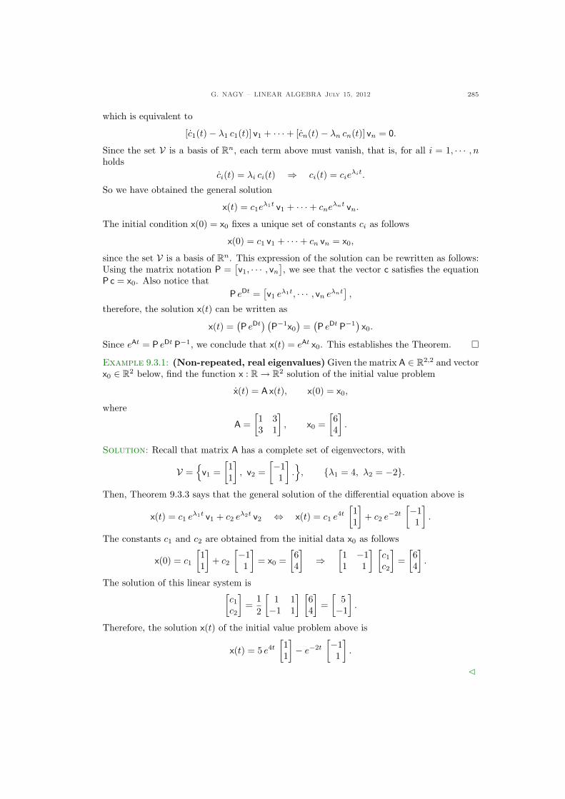
G. NAGY – LINEAR ALGEBRA July 15, 2012 285
which is equivalent to
[c1(t)− λ1 c1(t)] v1 + · · ·+ [cn(t)− λn cn(t)] vn = 0.
Since the set V is a basis of Rn, each term above must vanish, that is, for all i = 1, · · · , nholds
ci(t) = λi ci(t) ⇒ ci(t) = cieλit.
So we have obtained the general solution
x(t) = c1eλ1t v1 + · · ·+ cneλnt vn.
The initial condition x(0) = x0 fixes a unique set of constants ci as follows
x(0) = c1 v1 + · · ·+ cn vn = x0,
since the set V is a basis of Rn. This expression of the solution can be rewritten as follows:Using the matrix notation P =
[v1, · · · , vn
], we see that the vector c satisfies the equation
P c = x0. Also notice thatP eDt =
[v1 eλ1t, · · · , vn eλnt
],
therefore, the solution x(t) can be written as
x(t) =(P eDt
) (P−1x0
)=
(P eDt P−1
)x0.
Since eAt = P eDt P−1, we conclude that x(t) = eAt x0. This establishes the Theorem. ¤
Example 9.3.1: (Non-repeated, real eigenvalues) Given the matrix A ∈ R2,2 and vectorx0 ∈ R2 below, find the function x : R→ R2 solution of the initial value problem
x(t) = Ax(t), x(0) = x0,
where
A =[1 33 1
], x0 =
[64
].
Solution: Recall that matrix A has a complete set of eigenvectors, with
V ={
v1 =[11
], v2 =
[−11
].}
, {λ1 = 4, λ2 = −2}.
Then, Theorem 9.3.3 says that the general solution of the differential equation above is
x(t) = c1 eλ1t v1 + c2 eλ2t v2 ⇔ x(t) = c1 e4t
[11
]+ c2 e−2t
[−11
].
The constants c1 and c2 are obtained from the initial data x0 as follows
x(0) = c1
[11
]+ c2
[−11
]= x0 =
[64
]⇒
[1 −11 1
] [c1
c2
]=
[64
].
The solution of this linear system is[c1
c2
]=
12
[1 1−1 1
] [64
]=
[5−1
].
Therefore, the solution x(t) of the initial value problem above is
x(t) = 5 e4t
[11
]− e−2t
[−11
].
C
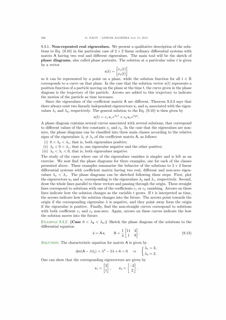
286 G. NAGY – LINEAR ALGEBRA july 15, 2012
9.3.1. Non-repeated real eigenvalues. We present a qualitative description of the solu-tions to Eq. (9.10) in the particular case of 2 × 2 linear ordinary differential systems withmatrix A having two real and different eigenvalues. The main tool will be the sketch ofphase diagrams, also called phase portraits. The solution at a particular value t is givenby a vector
x(t) =[x1(t)x2(t)
]
so it can be represented by a point on a plane, while the solution function for all t ∈ Rcorresponds to a curve on that plane. In the case that the solution vector x(t) represents aposition function of a particle moving on the plane at the time t, the curve given in the phasediagram is the trajectory of the particle. Arrows are added to this trajectory to indicatethe motion of the particle as time increases.
Since the eigenvalues of the coefficient matrix A are different, Theorem 9.3.3 says thatthere always exist two linearly independent eigenvectors v1 and v2 associated with the eigen-values λ1 and λ2, respectively. The general solution to the Eq. (9.10) is then given by
x(t) = c1 v1 eλ1t + c2 v2 eλ2t.
A phase diagram contains several curves associated with several solutions, that correspondto different values of the free constants c1 and c2. In the case that the eigenvalues are non-zero, the phase diagrams can be classified into three main classes according to the relativesigns of the eigenvalues λ1 6= λ2 of the coefficient matrix A, as follows:
(i) 0 < λ2 < λ1, that is, both eigenvalues positive;(ii) λ2 < 0 < λ1, that is, one eigenvalue negative and the other positive;(iii) λ2 < λ1 < 0, that is, both eigenvalues negative.The study of the cases where one of the eigenvalues vanishes is simpler and is left as anexercise. We now find the phase diagrams for three examples, one for each of the classespresented above. These examples summarize the behavior of the solutions to 2 × 2 lineardifferential systems with coefficient matrix having two real, different and non-zero eigen-values λ2 < λ1. The phase diagrams can be sketched following these steps: First, plotthe eigenvectors v2 and v1 corresponding to the eigenvalues λ2 and λ1, respectively. Second,draw the whole lines parallel to these vectors and passing through the origin. These straightlines correspond to solutions with one of the coefficients c1 or c2 vanishing. Arrows on theselines indicate how the solution changes as the variable t grows. If t is interpreted as time,the arrows indicate how the solution changes into the future. The arrows point towards theorigin if the corresponding eigenvalue λ is negative, and they point away form the originif the eigenvalue is positive. Finally, find the non-straight curves correspond to solutionswith both coefficient c1 and c2 non-zero. Again, arrows on these curves indicate the howthe solution moves into the future.
Example 9.3.2: (Case 0 < λ2 < λ1.) Sketch the phase diagram of the solutions to thedifferential equation
x = Ax, A =14
[11 31 9
]. (9.13)
Solution: The characteristic equation for matrix A is given by
det(A− λ I2) = λ2 − 5λ + 6 = 0 ⇒{
λ1 = 3,
λ2 = 2.
One can show that the corresponding eigenvectors are given by
v1 =[31
], v2 =
[−22
].
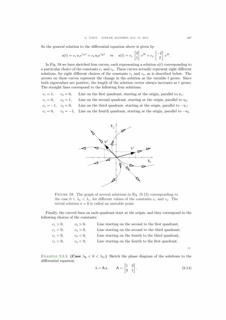
G. NAGY – LINEAR ALGEBRA July 15, 2012 287
So the general solution to the differential equation above is given by
x(t) = c1 v1eλ1t + c2 v2e
λ2t ⇔ x(t) = c1
[31
]e3t + c2
[−22
]e2t.
In Fig. 58 we have sketched four curves, each representing a solution x(t) corresponding toa particular choice of the constants c1 and c2. These curves actually represent eight differentsolutions, for eight different choices of the constants c1 and c2, as is described below. Thearrows on these curves represent the change in the solution as the variable t grows. Sinceboth eigenvalues are positive, the length of the solution vector always increases as t grows.The straight lines correspond to the following four solutions:
c1 = 1, c2 = 0, Line on the first quadrant, starting at the origin, parallel to v1;c1 = 0, c2 = 1, Line on the second quadrant, starting at the origin, parallel to v2;c1 = −1, c2 = 0, Line on the third quadrant, starting at the origin, parallel to −v1;c1 = 0, c2 = −1, Line on the fourth quadrant, starting at the origin, parallel to −v2.
1
x2
x1
v2
v
Figure 58. The graph of several solutions to Eq. (9.13) corresponding tothe case 0 < λ2 < λ1, for different values of the constants c1 and c2. Thetrivial solution x = 0 is called an unstable point.
Finally, the curved lines on each quadrant start at the origin, and they correspond to thefollowing choices of the constants:
c1 > 0, c2 > 0, Line starting on the second to the first quadrant;c1 < 0, c2 > 0, Line starting on the second to the third quadrant;c1 < 0, c2 < 0, Line starting on the fourth to the third quadrant,c1 > 0, c2 < 0, Line starting on the fourth to the first quadrant.
C
Example 9.3.3: (Case λ2 < 0 < λ1.) Sketch the phase diagram of the solutions to thedifferential equation
x = Ax, A =[1 33 1
]. (9.14)
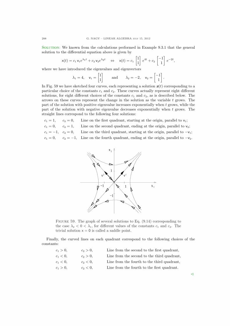
288 G. NAGY – LINEAR ALGEBRA july 15, 2012
Solution: We known from the calculations performed in Example 9.3.1 that the generalsolution to the differential equation above is given by
x(t) = c1 v1eλ1t + c2 v2e
λ2t ⇔ x(t) = c1
[11
]e4t + c2
[−11
]e−2t,
where we have introduced the eigenvalues and eigenvectors
λ1 = 4, v1 =[11
]and λ2 = −2, v2 =
[−11
].
In Fig. 59 we have sketched four curves, each representing a solution x(t) corresponding to aparticular choice of the constants c1 and c2. These curves actually represent eight differentsolutions, for eight different choices of the constants c1 and c2, as is described below. Thearrows on these curves represent the change in the solution as the variable t grows. Thepart of the solution with positive eigenvalue increases exponentially when t grows, while thepart of the solution with negative eigenvalue decreases exponentially when t grows. Thestraight lines correspond to the following four solutions:
c1 = 1, c2 = 0, Line on the first quadrant, starting at the origin, parallel to v1;c1 = 0, c2 = 1, Line on the second quadrant, ending at the origin, parallel to v2;c1 = −1, c2 = 0, Line on the third quadrant, starting at the origin, parallel to −v1;c1 = 0, c2 = −1, Line on the fourth quadrant, ending at the origin, parallel to −v2.
1
x
x 1
2
v2 v1
1−1
−1
Figure 59. The graph of several solutions to Eq. (9.14) corresponding tothe case λ2 < 0 < λ1, for different values of the constants c1 and c2. Thetrivial solution x = 0 is called a saddle point.
Finally, the curved lines on each quadrant correspond to the following choices of theconstants:
c1 > 0, c2 > 0, Line from the second to the first quadrant,c1 < 0, c2 > 0, Line from the second to the third quadrant,c1 < 0, c2 < 0, Line from the fourth to the third quadrant,c1 > 0, c2 < 0, Line from the fourth to the first quadrant.
C
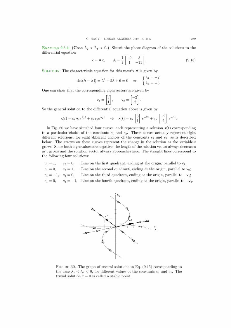
G. NAGY – LINEAR ALGEBRA July 15, 2012 289
Example 9.3.4: (Case λ2 < λ1 < 0.) Sketch the phase diagram of the solutions to thedifferential equation
x = Ax, A =14
[−9 31 −11
]. (9.15)
Solution: The characteristic equation for this matrix A is given by
det(A− λ I) = λ2 + 5λ + 6 = 0 ⇒{
λ1 = −2,
λ2 = −3.
One can show that the corresponding eigenvectors are given by
v1 =[31
], v2 =
[−22
].
So the general solution to the differential equation above is given by
x(t) = c1 v1eλ1t + c2 v2e
λ2t ⇔ x(t) = c1
[31
]e−2t + c2
[−22
]e−3t.
In Fig. 60 we have sketched four curves, each representing a solution x(t) correspondingto a particular choice of the constants c1 and c2. These curves actually represent eightdifferent solutions, for eight different choices of the constants c1 and c2, as is describedbelow. The arrows on these curves represent the change in the solution as the variable tgrows. Since both eigenvalues are negative, the length of the solution vector always decreasesas t grows and the solution vector always approaches zero. The straight lines correspond tothe following four solutions:
c1 = 1, c2 = 0, Line on the first quadrant, ending at the origin, parallel to v1;c1 = 0, c2 = 1, Line on the second quadrant, ending at the origin, parallel to v2;c1 = −1, c2 = 0, Line on the third quadrant, ending at the origin, parallel to −v1;c1 = 0, c2 = −1, Line on the fourth quadrant, ending at the origin, parallel to −v2.
2
v2
v 1
x1
x
Figure 60. The graph of several solutions to Eq. (9.15) corresponding tothe case λ2 < λ1 < 0, for different values of the constants c1 and c2. Thetrivial solution x = 0 is called a stable point.
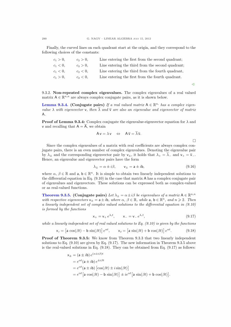
290 G. NAGY – LINEAR ALGEBRA july 15, 2012
Finally, the curved lines on each quadrant start at the origin, and they correspond to thefollowing choices of the constants:
c1 > 0, c2 > 0, Line entering the first from the second quadrant;c1 < 0, c2 > 0, Line entering the third from the second quadrant;c1 < 0, c2 < 0, Line entering the third from the fourth quadrant,c1 > 0, c2 < 0, Line entering the first from the fourth quadrant.
C
9.3.2. Non-repeated complex eigenvalues. The complex eigenvalues of a real valuedmatrix A ∈ Rn,n are always complex conjugate pairs, as it is shown below.
Lemma 9.3.4. (Conjugate pairs) If a real valued matrix A ∈ Rn, has a complex eigen-value λ with eigenvector v, then λ and v are also an eigenvalue and eigenvector of matrixA.
Proof of Lemma 9.3.4: Complex conjugate the eigenvalue-eigenvector equation for λ andv and recalling that A = A, we obtain
A v = λ v ⇔ A v = λ v.
¤Since the complex eigenvalues of a matrix with real coefficients are always complex con-
jugate pairs, there is an even number of complex eigenvalues. Denoting the eigenvalue pairby λ± and the corresponding eigenvector pair by v±, it holds that λ+ = λ− and v+ = v−.Hence, an eigenvalue and eigenvector pairs have the form
λ± = α± iβ, v± = a± ib, (9.16)
where α, β ∈ R and a, b ∈ Rn. It is simple to obtain two linearly independent solutions tothe differential equation in Eq. (9.10) in the case that matrix A has a complex conjugate pairof eigenvalues and eigenvectors. These solutions can be expressed both as complex-valuedor as real-valued functions.
Theorem 9.3.5. (Conjugate pairs) Let λ± = α± iβ be eigenvalues of a matrix A ∈ Rn,n
with respective eigenvectors v± = a± ib, where α, β ∈ R, while a, b ∈ Rn, and n > 2. Thena linearly independent set of complex valued solutions to the differential equation in (9.10)is formed by the functions
x+ = v+ eλp-t, x− = v− eλ-t, (9.17)
while a linearly independent set of real valued solutions to Eq. (9.10) is given by the functions
x1 =[a cos(βt)− b sin(βt)
]eαt, x2 =
[a sin(βt) + b cos(βt)
]eαt. (9.18)
Proof of Theorem 9.3.5: We know from Theorem 9.3.3 that two linearly independentsolutions to Eq. (9.10) are given by Eq. (9.17). The new information in Theorem 9.3.5 aboveis the real-valued solutions in Eq. (9.18). They can be obtained from Eq. (9.17) as follows:
x± = (a± ib) e(α±iβ)t
= eαt(a± ib) e±iβt
= eαt(a± ib)[cos(βt)± i sin(βt)
]
= eαt[a cos(βt)− b sin(βt)
]± ieαt[a sin(βt) + b cos(βt)
].
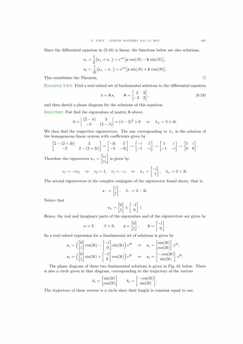
G. NAGY – LINEAR ALGEBRA July 15, 2012 291
Since the differential equation in (9.10) is linear, the functions below are also solutions,
x1 =12(x+ + x−
)= eαt
[a cos(βt)− b sin(βt)
],
x2 =12i
(x+ − x−
)= eαt
[a sin(βt) + b cos(βt)
].
This establishes the Theorem. ¤
Example 9.3.5: Find a real-valued set of fundamental solutions to the differential equation
x = Ax, A =[
2 3−3 2
], (9.19)
and then sketch a phase diagram for the solutions of this equation.
Solution: Fist find the eigenvalues of matrix A above,
0 =∣∣∣∣
(2− λ) 3−3 (2− λ)
∣∣∣∣ = (λ− 2)2 + 9 ⇒ λ± = 2± 3i.
We then find the respective eigenvectors. The one corresponding to λ+ is the solution ofthe homogeneous linear system with coefficients given by
[2− (2 + 3i) 3−3 2− (2 + 3i)
]=
[−3i 3−3 −3i
]→
[−i 1−1 −i
]→
[1 i−1 −i
]→
[1 i0 0
].
Therefore the eigenvector v+ =[v1
v2
]is given by
v1 = −iv2 ⇒ v2 = 1, v1 = −i, ⇒ v+ =[−i
1
], λ+ = 2 + 3i.
The second eigenvectors is the complex conjugate of the eigenvector found above, that is,
v− =[i1
], λ− = 2− 3i.
Notice that
v± =[01
]±
[−10
]i.
Hence, the real and imaginary parts of the eigenvalues and of the eigenvectors are given by
α = 2, β = 3, a =[01
], b =
[−10
].
So a real-valued expression for a fundamental set of solutions is given by
x1 =([
01
]cos(3t)−
[−10
]sin(3t)
)e2t ⇒ x1 =
[sin(3t)cos(3t)
]e2t,
x2 =([
01
]sin(3t) +
[−10
]cos(3t)
)e2t ⇒ x2 =
[− cos(3t)sin(3t)
]e2t.
The phase diagram of these two fundamental solutions is given in Fig. 61 below. Thereis also a circle given in that diagram, corresponding to the trajectory of the vectors
x1 =[sin(3t)cos(3t)
]x2 =
[− cos(3t)sin(3t)
].
The trajectory of these vectors is a circle since their length is constant equal to one.
292 G. NAGY – LINEAR ALGEBRA july 15, 2012
(2)
b
a
x2
1x
x (1)
x
Figure 61. The graph of the fundamental solutions x1 and x2 of the Eq. (9.19).
In the particular case that the matrix A in Eq. (9.10) is 2 × 2, then any solutions is alinear combination of the solutions given in Eq. (9.18). That is, the general solution of givenby
x(t) = c1 x1(t) + c2 x2(t),where
x1 =[a cos(βt)− b sin(βt)
]eαt, x2 =
[a sin(βt) + b cos(βt)
]eαt.
We now do a qualitative study of the phase diagrams of the solutions for this case. We firstfix the vectors a and b, and the plot phase diagrams for solutions having α > 0, α = 0,and α < 0. These diagrams are given in Fig. 62. One can see that for α > 0 the solutionsspiral outward as t increases, and for α < 0 the solutions spiral inwards to the origin as tincreases..
(2)x2
x1
ab
x (1)
x
x
x2
x1
ab
(2)
(1)x(1)
x2
x1
ab
x
x
(2)
Figure 62. The graph of the fundamental solutions x1 and x2 (dashed line)of the Eq. (9.18) in the case of α > 0, α = 0, and α < 0, respectively.
Finally, let us study the following cases: We fix α > 0 and the vector a, and we plotthe phase diagrams for solutions with two choices of the vector b, as shown in Fig. 63. Itcan then bee seen that the relative directions of the vectors a and b determines the rotationdirection of the solutions as t increases.
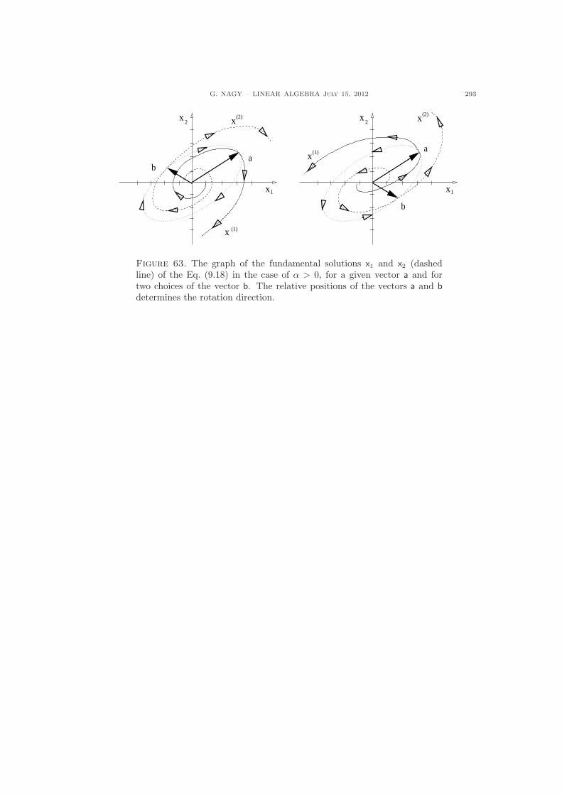
G. NAGY – LINEAR ALGEBRA July 15, 2012 293
(2)x2
x1
ab
x (1)
x(2)x
2
x1
a
b
x
x(1)
Figure 63. The graph of the fundamental solutions x1 and x2 (dashedline) of the Eq. (9.18) in the case of α > 0, for a given vector a and fortwo choices of the vector b. The relative positions of the vectors a and bdetermines the rotation direction.
294 G. NAGY – LINEAR ALGEBRA july 15, 2012
9.3.3. Exercises.
9.3.1.- Given the matrix A ∈ R2,2 and vec-tor x0 ∈ R2 below, find the functionx : R → R2 solution of the initial valueproblem
x(t) = Ax(t), x(0) = x0,
where
A =
»1 33 1
–, x0 =
»34
–.
9.3.2.- Given the matrix A and the vectorx0 in Exercise 9.3.1 above, compute theoperator valued function eA t and verifythat the solution x of the initial valueproblem given in Exercise 9.3.1 can bewritten as
x(t) = eA t x0.
9.3.3.- Given the matrix A ∈ R2,2 below,find all functions x : R → R2 solutionsof the differential equation
x(t) = Ax(t),
where
A =
»1 −15 −3
–.
Since this matrix has complex eigenval-ues, express the solutions as linear com-bination of real vector valued functions.
9.3.4.- Given the matrix A ∈ R3,3 and vec-tor x0 ∈ R3 below, find the functionx : R → R3 solution of the initial valueproblem
x(t) = Ax(t), x(0) = x0,
where
A =
24
3 0 10 2 20 0 1
35 , x0 =
24
123
35 .
G. NAGY – LINEAR ALGEBRA July 15, 2012 295
9.4. Normal operators
In this Section we introduce a particular type of linear operators called normal operators,which are defined on vector spaces having an inner product. Particular cases are Hermitianoperators and unitary operators, which are widely used in physics. Rotations in space areexamples of unitary operators on real vector spaces, while physical observables in quantummechanics are examples of Hermitian operators. In this Section we restrict our descriptionto finite dimensional inner product spaces. These definitions generalize the notions of uni-tary and Hermitian matrices already introduced in Chapter 2. We first describe the RieszRepresentation Theorem, needed to verify that the notion of adjoint of a linear operator iswell-defined. After reviewing the commutator of two operators we then introduce normaloperators and discuss the particular cases of unitary and Hermitian operators. Finally wecomment on the relations between these notions and the unitary and Hermitian matricesalready introduced in Chapter 2.
The Riesz Representation Theorem is a statement concerning linear functionals on aninner product space. Given a vector space V over the scalar field F, a linear functionalis a scalar-valued linear function f : V → F, that is, for all x, y ∈ V and all a, b ∈ F holdsf(ax + by) = a f(x) + b f(y) ∈ F. An example of a linear functional on R3 is the function
R3 3 x =
x1
x2
x3
7→ f(x) = 3x1 + 2x2 + x3 ∈ R.
This function can be expressed in terms of the dot product in R3 as follows
f(x) = u · x, u =
321
.
The Riesz Representation Theorem says that what we did in this example can be done in thegeneral case. In an inner product space
(V, 〈 , 〉) every linear functional f can be expressed
in terms of the inner product.
Theorem 9.4.1. Consider a finite dimensional inner product space(V, 〈 , 〉) over the scalar
field F. For every linear functional f : V → F there exists a unique vector uf ∈ V such thatholds
f(v) = 〈uf , v〉 ∀v ∈ V.
Proof of Theorem 9.4.1: Introduce the set
N = {v ∈ V : f(v) = 0 } ⊂ V.
This set is the analogous to linear functionals of the null space of linear operators. Since f isa linear function the set N is a subspace of V . (Proof: Given two elements v1, v2 ∈ N andtwo scalars a, b ∈ F, holds that f(av1 +bv2) = a f(v1)+b f(v2) = 0+0, so (av1 +bv2) ∈ N .)Introduce the orthogonal complement of N , that is,
N⊥ = {w ∈ V : 〈w, v〉 = 0 ∀v ∈ V },
which is also a subspace of V . If N⊥ = {0}, then N =(N⊥)⊥ =
({0})⊥ = V . Since thenull space of f is the whole vector space, the functional f is identically zero, so only for thechoice uf = 0 holds f(v) = 〈0, v〉 for all v ∈ V .
In the case that N⊥ 6= {0} we now show that this space cannot be very big, in fact ithas dimension one, as the following argument shows. Choose u ∈ N⊥ such that f(u) = 1.
296 G. NAGY – LINEAR ALGEBRA july 15, 2012
Then notice that for every w ∈ N⊥ the vector w− f(w)u is trivially in N⊥ but it is also inN , since
f(w− f(w) u
)= f(w)− f(w) f(u) = f(w)− f(w) = 0.
A vector both in N and N⊥ must vanish, so w = f(w) u. Then every vector in N⊥ isproportional to u, so dim N⊥ = 1. This information is used to split any vector v ∈ V asfollows v = a u + x where x ∈ V and a ∈ F. It is clear that
f(v) = f(a u + x) = a f(u) + f(x) = a f(u) = a.
However, the function with values g(v) =⟨ u
‖u‖2 , v⟩
has precisely the same values as f ,
since for all v ∈ V holds
g(v) =⟨ u
‖u‖2 , v⟩
=⟨ u
‖u‖2 , (a u + x)⟩
=a
‖u‖2 〈u, u〉+ 1‖u‖2 〈u,x〉 = a.
Therefore, choosing uf = u/‖u‖2, holds that
f(v) = 〈uf , v〉 ∀v ∈ V.
Since dim N⊥ = 1, the choice of uf is unique. This establishes the Theorem. ¤Given a linear operator defined on an inner product space, a new linear operator can be
defined through an equation involving the inner product.
Proposition 9.4.2. Let T ∈ L(V ) be a linear operator on a finite-dimensional inner productspace
(V, 〈 , 〉). There exists one and only one linear operator T ∗ ∈ L(V ) such that
〈v,T ∗(u)〉 = 〈T(v),u〉holds for all vectors u, v ∈ V .
Given any linear operator T on a finite-dimensional inner product space, the operatorT ∗ whose existence is guaranteed in Proposition 9.4.2 is called the adjoint of T.Proof of Proposition 9.4.2: We first establish the following statement: For every vectoru ∈ V there exists a unique vector w ∈ V such that
〈T(v),u〉 = 〈v,w〉 ∀v ∈ V. (9.20)
The proof starts noticing that for a fixed u ∈ V the scalar-valued function fu : V → Fgiven by fu(v) = 〈u,T(v)〉 is a linear functional. Therefore, the Riesz RepresentationTheorem 9.4.1 implies that there exists a unique vector w ∈ V such that fu(v) = 〈w, v〉.This establishes that for every vector u ∈ V there exists a unique vector w ∈ V such thatEq. (9.20) holds. Now that this statement is proven we can define a map, that we chooseto denote as T ∗ : V → V , given by u 7→ T ∗(u) = w. We now show that this map T ∗ islinear. Indeed, for all u1, u2 ∈ V and all a, b ∈ F holds
〈v,T ∗(au1 + bu2)〉 = 〈T(v), (au1 + bu2)〉 ∀v ∈ V,
= a 〈T(v),u1〉+ b 〈T(v),u2)〉= a〈v,T ∗(u1)〉+ b〈v,T ∗(u2)〉=
⟨v,
[aT ∗(u1) + bT ∗(u2)
]⟩ ∀v ∈ V,
hence T ∗(au1 + bu2) = aT ∗(u1) + bT ∗(u2). This establishes the Proposition. ¤The next result relates the adjoint of a linear operator with the concept of the adjoint
of a square matrix introduced in Sect. 2.2. Recall that given a basis in the vector space,every linear operator has associated a unique square matrix. Let us use the notation [T ]and [T ∗] for the matrices on a given basis of the operators T and T ∗, respectively.
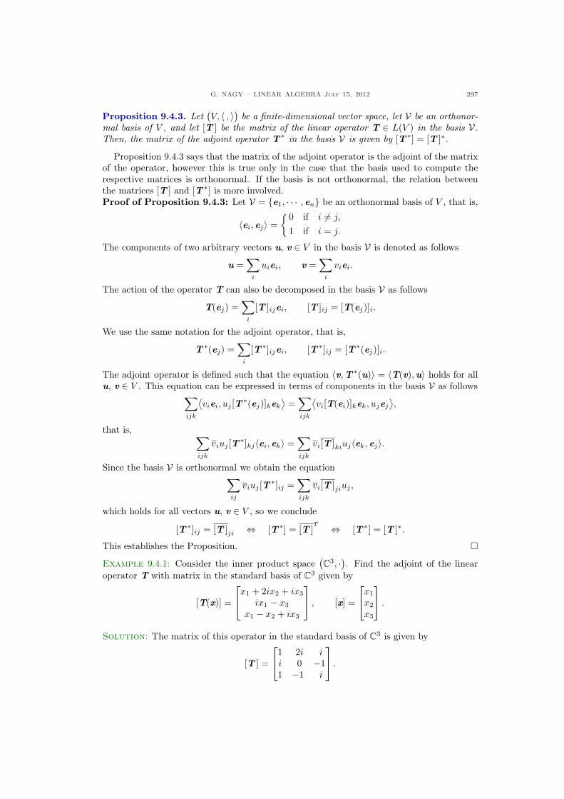
G. NAGY – LINEAR ALGEBRA July 15, 2012 297
Proposition 9.4.3. Let(V, 〈 , 〉) be a finite-dimensional vector space, let V be an orthonor-
mal basis of V , and let [T ] be the matrix of the linear operator T ∈ L(V ) in the basis V.Then, the matrix of the adjoint operator T ∗ in the basis V is given by [T ∗] = [T ]∗.
Proposition 9.4.3 says that the matrix of the adjoint operator is the adjoint of the matrixof the operator, however this is true only in the case that the basis used to compute therespective matrices is orthonormal. If the basis is not orthonormal, the relation betweenthe matrices [T ] and [T ∗] is more involved.Proof of Proposition 9.4.3: Let V = {e1, · · · , en} be an orthonormal basis of V , that is,
〈ei, ej〉 ={ 0 if i 6= j,
1 if i = j.
The components of two arbitrary vectors u, v ∈ V in the basis V is denoted as follows
u =∑
i
uiei, v =∑
i
viei.
The action of the operator T can also be decomposed in the basis V as follows
T(ej) =∑
i
[T ]ijei, [T ]ij = [T(ej)]i.
We use the same notation for the adjoint operator, that is,
T ∗(ej) =∑
i
[T ∗]ijei, [T ∗]ij = [T ∗(ej)]i.
The adjoint operator is defined such that the equation 〈v,T ∗(u)〉 = 〈T(v),u〉 holds for allu, v ∈ V . This equation can be expressed in terms of components in the basis V as follows
∑
ijk
⟨viei, uj [T ∗(ej)]kek
⟩=
∑
ijk
⟨vi[T(ei)]kek, ujej
⟩,
that is, ∑
ijk
viuj [T ∗]kj〈ei, ek〉 =∑
ijk
vi[T ]kiuj〈ek, ej〉.
Since the basis V is orthonormal we obtain the equation∑
ij
viuj [T ∗]ij =∑
ijk
vi[T ]jiuj ,
which holds for all vectors u, v ∈ V , so we conclude
[T ∗]ij = [T ]ji ⇔ [T ∗] = [T ]T ⇔ [T ∗] = [T ]∗.
This establishes the Proposition. ¤
Example 9.4.1: Consider the inner product space(C3, ·). Find the adjoint of the linear
operator T with matrix in the standard basis of C3 given by
[T(x)] =
x1 + 2ix2 + ix3
ix1 − x3
x1 − x2 + ix3
, [x] =
x1
x2
x3
.
Solution: The matrix of this operator in the standard basis of C3 is given by
[T ] =
1 2i ii 0 −11 −1 i
.
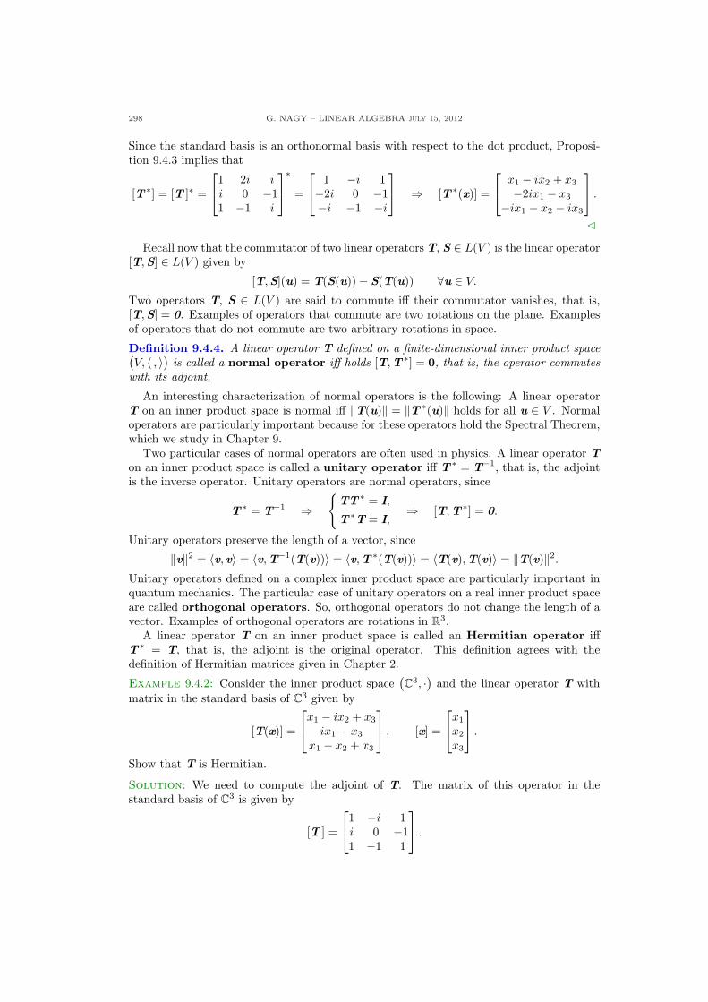
298 G. NAGY – LINEAR ALGEBRA july 15, 2012
Since the standard basis is an orthonormal basis with respect to the dot product, Proposi-tion 9.4.3 implies that
[T ∗] = [T ]∗ =
1 2i ii 0 −11 −1 i
∗
=
1 −i 1−2i 0 −1−i −1 −i
⇒ [T ∗(x)] =
x1 − ix2 + x3
−2ix1 − x3
−ix1 − x2 − ix3
.
C
Recall now that the commutator of two linear operators T, S ∈ L(V ) is the linear operator[T,S] ∈ L(V ) given by
[T,S](u) = T(S(u))− S(T(u)) ∀u ∈ V.
Two operators T, S ∈ L(V ) are said to commute iff their commutator vanishes, that is,[T,S] = 0. Examples of operators that commute are two rotations on the plane. Examplesof operators that do not commute are two arbitrary rotations in space.
Definition 9.4.4. A linear operator T defined on a finite-dimensional inner product space(V, 〈 , 〉) is called a normal operator iff holds [T,T ∗] = 0, that is, the operator commutes
with its adjoint.
An interesting characterization of normal operators is the following: A linear operatorT on an inner product space is normal iff ‖T(u)‖ = ‖T ∗(u)‖ holds for all u ∈ V . Normaloperators are particularly important because for these operators hold the Spectral Theorem,which we study in Chapter 9.
Two particular cases of normal operators are often used in physics. A linear operator Ton an inner product space is called a unitary operator iff T ∗ = T−1, that is, the adjointis the inverse operator. Unitary operators are normal operators, since
T ∗ = T−1 ⇒{
TT ∗ = I,
T ∗T = I,⇒ [T,T ∗] = 0.
Unitary operators preserve the length of a vector, since
‖v‖2 = 〈v, v〉 = 〈v,T−1(T(v))〉 = 〈v,T ∗(T(v))〉 = 〈T(v),T(v)〉 = ‖T(v)‖2.Unitary operators defined on a complex inner product space are particularly important inquantum mechanics. The particular case of unitary operators on a real inner product spaceare called orthogonal operators. So, orthogonal operators do not change the length of avector. Examples of orthogonal operators are rotations in R3.
A linear operator T on an inner product space is called an Hermitian operator iffT ∗ = T, that is, the adjoint is the original operator. This definition agrees with thedefinition of Hermitian matrices given in Chapter 2.
Example 9.4.2: Consider the inner product space(C3, ·) and the linear operator T with
matrix in the standard basis of C3 given by
[T(x)] =
x1 − ix2 + x3
ix1 − x3
x1 − x2 + x3
, [x] =
x1
x2
x3
.
Show that T is Hermitian.
Solution: We need to compute the adjoint of T. The matrix of this operator in thestandard basis of C3 is given by
[T ] =
1 −i 1i 0 −11 −1 1
.
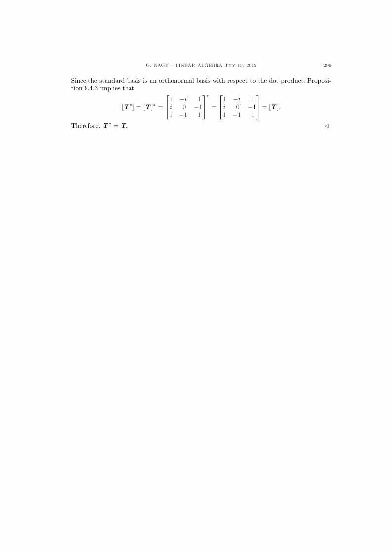
G. NAGY – LINEAR ALGEBRA July 15, 2012 299
Since the standard basis is an orthonormal basis with respect to the dot product, Proposi-tion 9.4.3 implies that
[T ∗] = [T ]∗ =
1 −i 1i 0 −11 −1 1
∗
=
1 −i 1i 0 −11 −1 1
= [T ].
Therefore, T ∗ = T. C

300 G. NAGY – LINEAR ALGEBRA july 15, 2012
9.4.1. Exercises.
9.4.1.- . 9.4.2.- .
G. NAGY – LINEAR ALGEBRA July 15, 2012 301
Chapter 10. Appendix
10.1. Review exercises
Chapter 1: Linear systems
1.- Consider the linear system
2x1 + 3x2 − x3 = 6
−x1 − x2 + 2x3 = −2
x1 + 2x3 = 2
(a) Use Gauss operations to find thereduced echelon form of the aug-mented matrix for this system.
(b) Is this system consistent? If “yes,”find all the solutions.
2.- Find all the solutions x to the linear sys-tem Ax = b and express them in vectorform, where
A =
24
1 −2 −12 1 81 −1 1
35 , b =
24
121
35 .
3.- Consider the matrix and the vector
A =
24
1 −2 71 1 12 2 2
35 , b =
24
013
35 .
Is the vector b a linear combination ofthe column vectors of A?
4.- Let s be a real number, and consider thesystem
sx1 − 2sx2 = −1,
3x1 + 6sx2 = 3.
(a) Determine the values of the param-eter s for which the system abovehas a unique solution.
(b) For all the values of s such that thesystem above has a unique solution,find that solution.
5.- Find the values of k such that the sys-tem below has no solution; has one so-lution; has infinitely many solutions;
kx1 + x2 = 1
x1 + kx2 = 1.
6.- Find a condition on the components ofvector b such that the system Ax = b isconsistent, where
A =
24
1 1 −12 0 −63 1 −7
35 , b =
24
b1
b2
b3
35 .
7.- Find the general solution to the homo-geneous linear system with coefficientmatrix
A =
24
1 3 −1 52 1 3 03 2 4 1
35 ,
and write this general solution in vectorform.
8.- (a) Find a value of the constants h andk such that the non-homogeneouslinear system below is consistentand has one free variable.
x1 + h x2 + 5x3 = 1,
x2 − 2x3 = k,
x1 + 3x2 − 3x3 = 5.
(b) Using the value of the constants hand k found in part (a), find thegeneral solution to the system givenin part (a).
9.- (a) Find the general solution to the sys-tem below and write it in vectorform,
x1 + 2x2 − x3 = 2,
3x1 + 7x2 − 3x3 = 7,
x1 + 4x2 − x3 = 4.
(b) Sketch a graph on R3 of the generalsolution found in part (a).
302 G. NAGY – LINEAR ALGEBRA july 15, 2012
Chapter 2: Matrix algebra
1.- Consider the vectors
u =
»11
–, v =
»1−1
–,
and the linear function T : R2 → R2
such that
T (u) =
»13
–, T (v) =
»31
–.
Find the matrix A = [T (e1), T (e2)] ofthe linear transformation, where
e1 =1
2(u + v), e2 =
1
2(u− v).
Show your work.
2.- Find the matrix for the linear transfor-mation T : R2 → R2 representing a re-flection on the plane along the verticalaxis followed by a rotation by θ = π/3counterclockwise.
3.- Which of the following matrices belowis equal to (A + B)2 for every squarematrices A and B?
(B + A)2,
A2 + 2AB + B2,
(A + B)(B + A),
A2 + AB + BA + B2,
A(A + B) + (A + B)B.
4.- Find a matrix A solution of the matrixequation
AB + 2 I2 =
»5 4−2 3
–,
where
B =
»7 32 1
–.
5.- Consider the matrix
A =
24
5 3 s1 2 −12 1 1
35 .
Find the value(s) of the constant s suchthat the matrix A is invertible.
6.- Let A be an n × n matrix, D be andm×m matrix, and C be and m×n ma-trix. Assume that both A and D areinvertible matrices and denote by A−1,D−1 their respective inverse matrices.Let M be the (n + m) × (n + m) ma-trix
M =
»A 0C D
–.
Find an m×n matrix X (in terms of anyof the matrices A, D, A−1, D−1, and C)such that M is invertible and the inverseis given by
M−1 =
»A−1 0X D−1
–.
7.- Consider the matrix and the vector
A =
24
1 −2 71 1 12 2 2
35 , b =
24
013
35 .
(a) Does vector b belong to the R(A)?(b) Does vector b belong to the N(A)?
8.- Consider the matrix
A =
24
1 2 6 −7−2 3 2 00 −1 −2 2
35 .
Find N(A) and the R(AT ).
9.- Consider the matrix
A =
24
2 1 34 5 76 9 12
35 .
(a) Find the LU-factorization of A.(b) Use the LU-factorization above to
find the solutions x1 and x2 of thesystems Ax = e1 and Ax2 = e2,where
e1 =
24
100
35 , e2 =
24
010
35 .
(c) Use the LU-factorization above tofind A−1.
G. NAGY – LINEAR ALGEBRA July 15, 2012 303
Chapter 3: Determinants
1.- Find the determinant of the matrices
A =
»1 + i −3i−4i 1− 2i
–,
B =
2664
0 −1 0 00 −2 3 −20 0 −1 −3−2 0 0 1
3775 ,
C =
»cos(θ) − sin(θ)sin(θ) cos(θ)
–.
2.- Given matrix A below, find the cofac-tors matrix C, and explicitly show thatACT = det(A) I3, where
A =
24
1 3 −14 0 12 1 3
35 .
3.- Given matrix A below, find the coeffi-cients (A−1)13 and (A−1)23 of the in-verse matrix A−1, where
A =
24
5 3 11 2 −12 1 1
35 .
4.- Find the change in the area of the par-allelogram formed by the vectors
u =
»12
–, v =
»21
–,
when this parallelogram is transformedunder the following linear transforma-tion, A : R2 → R2,
A =
»2 11 2
–.
5.- Find the volume of the parallelepipedformed by the vectors
v1 =
24
123
35 , v2 =
24
321
35 , v3 =
24
11−1
35 .
6.- Consider the matrix
A =
»4 21 3
–.
Find the values of the scalar λ such thatthe matrix (A− λ I2) is not invertible.
7.- Prove the following: If there exists aninteger k > 1 such that A ∈ Fn,n satis-fies Ak = 0, then det(A) = 0.
8.- Assume that matrix A ∈ Fn,n satisfiesthe equation A2 = In. Find all possiblevalues of det(A).
9.- Use Cramer’s rule to find the solutionof the linear system Ax = b, where
A =
24
1 4 −11 1 12 0 3
35 , b =
24
100
35 .
304 G. NAGY – LINEAR ALGEBRA july 15, 2012
Chapter 4: Vector spaces
1.- Determine which of the following sub-sets of R3,3 are subspaces:
(a) The symmetric matrices.(b) The skew-symmetric matrices.(c) The matrices A with A2 = A.(d) The matrices A with tr (A) = 0.(e) The matrices A with det(A) = 0.
In the case that the set is a subspace,find a basis of this subspace.
2.- Find the dimension and give a basis ofthe subspace W ⊂ R3 given by
n24−a + b + c− 3d
b + 3c− da + 2b + 8c
35with a, b, c, d ∈ R
o.
3.- Find the dimension of both the nullspace and the range space of the matrix
A =
24
1 1 1 5 22 1 4 7 30 −1 2 −3 −1
35 .
4.- Consider the matrix
A =
24
1 −1 50 1 −21 3 −3
35 .
(a) Find a basis for the null space of A.(b) Find a basis for the subspace in R3
consisting of all vectors b ∈ R3 suchthat the linear system Ax = b isconsistent.
5.- Show whether the following statementis true or false: Given a vector space V ,if the set
{v1, v2, v3} ⊂ V
is linearly independent, then so is theset
{w1, w2, w3},where
w1 = (v1 + v2),
w2 = (v1 + v3),
w3 = (v2 + v3).
6.- Show that the set U ⊂ P3 given by allpolynomials satisfying the condition
Z 1
0
p(x) dx = 0
is a subspace of P3. Find a basis for U .
7.- Determine whether the set U ⊂ P2 ofall polynomials of the form
p(x) = a + ax + ax2
with a ∈ F, is a subspace of P2.
G. NAGY – LINEAR ALGEBRA July 15, 2012 305
Chapter 5: Linear transformations
1.- Consider the matrix
A =
24
1 2 6 −7−2 3 2 00 −1 −2 2
35 .
(1) Find a basis for R(A).(2) Find a basis for N(A).(3) Consider the linear transfor-
mation A : R4 → R3 deter-mined by A. Is it injective? Isit surjective? Justify your an-swers.
2.- Let T : R3 → R2 be the linear transfor-mation given by
[T (xs)]s =
»2x1 + 6x2 − 2x3
3x1 + 8x2 + 2x3
–
s
,
[x]s =
24
x1
x2
x3
35 ,
where S and S are the standard basesin R3 and R2, respectively.
(a) Is T injective? Is T surjective?(b) Find all solutions of the linear sys-
tem T (xs) = bs, where
bs =
»2−1
–.
(c) Is the set of all solutions found inpart (b) a subspace of R3?
3.- Let A : C3 → C4 be the linear transfor-mation
A =
2664
1 0 i0 i 1
1− i 0 1 + ii 1 0
3775 .
Find a basis for N(A) and R(A).
4.- Let D : P3 → P3 be the differentiationoperator,
D(p)(x) =dp
dx(x),
and I : P3 → P3 the identity operator.Let S = (1, x, x2, x3) be the standardordered basis of P3. Show that the ma-trix of the operator
(I−D2) : P3 → P3
in the basis S is invertible.
306 G. NAGY – LINEAR ALGEBRA july 15, 2012
Chapter 6: Inner product spaces
1.- Let`V, 〈 , 〉´ be a real inner product
space. Show that (x − y) ⊥ (x + y) iff‖x‖ = ‖y‖.
2.- Consider the inner product space givenby`Fn, · ´. Prove that for every matrix
A ∈ Fn,n holds
x · (Ay) = (A∗x) · y.
3.- A matrix A ∈ Fn,n is called unitary iff
AA∗ = A∗A = In.
Show that a unitary matrix does notchange the norm of a vector in the in-ner product space
`Fn, · ´, that is, for all
x ∈ Fn and all unitary matrix A ∈ Fn,n
holds‖Ax‖ = ‖x‖.
4.- Find all vectors in the inner productspace
`R4, · ´ perpendicular to both
v =
2664
1441
3775 and u =
2664
2982
3775 .
5.- Consider the inner product space givenby`C3, · ´ and the subspace W ⊂ C3
spanned by the vectors
u =
24
1 + i1i
35 , v =
24−10
2− i
35 .
(a) Use the Gram-Schmidt method tofind an orthonormal basis for W .
(b) Extend the orthonormal basis of Winto an orthonormal basis for C3.

G. NAGY – LINEAR ALGEBRA July 15, 2012 307
Chapter 7: Approximation methods
1.- . 2.- .

308 G. NAGY – LINEAR ALGEBRA july 15, 2012
Chapter 8: Normed spaces
1.- . 2.- .

G. NAGY – LINEAR ALGEBRA July 15, 2012 309
Chapter 9: Spectral decomposition
1.- . 2.- .
310 G. NAGY – LINEAR ALGEBRA july 15, 2012
10.2. Practice Exams
Instructions to use the Practice Exams. The idea of these lecture notes is to help anyoneinterested in learning linear algebra. More often than not such person is a college student.An unfortunate aspect of our education system is that students must pass an exam to provethey understood the ideas of a given subject. To prepare the student for such exam is thepurpose of the practice exams in this Section.
These practice exams once were actual exams taken by student in previous courses. Theseexams can be useful to other students if they are used properly; one way is the following:Study the course material first, do all the exercises at the end of every Section; do the reviewproblems in Section 10.1; then and only then take the first practice exam and do it. Thinkof it as an actual exam. Do not look at the notes or any other literature. Do the wholeexam. Watch your time. You have only two hours to do it. After you finish, you can gradeyourself. You have the solutions to the exam at the end of the Chapter. Never, ever look atthe solutions before you finish the exam. If you do it, the practice exam is worthless. Really,worthless; you will not have the solutions when you do the actual exam. The story does notfinish here. Pay close attention at the exercises you did wrong, if any. Go back to the classmaterial and do extra problems on those subjects. Review all subjects you think you arenot well prepared. Then take the second practice exam. Follow a similar procedure. Reviewthe subject related to the practice exam exercises you had difficulties to solve. Then, do thenext practice exam. You have three of them. After doing the last one, you should have agood idea of what your actual grade in the class should be.
G. NAGY – LINEAR ALGEBRA July 15, 2012 311
Practice Exam 1. (Two hours.)
1. Consider the matrix A =
5 3 11 2 −12 1 1
. Find the coefficients (A−1)21 and (A−1)32 of the
matrix A−1, that is, of the inverse matrix of A. Show your work.
2. (a) Find k ∈ R such that the volume of the parallelepiped formed by the vectors belowis equal to 4, where
v1 =
123
, v2 =
321
, v3 =
k11
(b) Set k = 1 and define the matrix A = [v1, v2, v3]. Matrix A determines the lineartransformation A : R3 → R3. Is this linear transformation injective (one-to-one)? Isit surjective (onto)?
3. Determine whether the subset V ⊂ R3 is a subspace, where
V ={
−a + ba− 2ba− 7b
with a, b ∈ R
}.
If the set is a subspace, find an orthogonal basis in the inner product space(R3, · ).
4. True or False: (Justify your answers.)(a) If the set of columns of A ∈ Fm,n is a linearly independent set, then Ax = b has
exactly one solution for every b ∈ Fm.(b) The set of column vectors of an 5× 7 is never linearly independent.
5. Consider the vector space R2 with the standard basis S and let T : R2 → R2 be thelinear transformation
[T ]ss =[1 22 3
]
ss
.
Find [T ]bb, the matrix of T in the basis B, where B ={
[b1]s =[12
]
s
, [b2]s =[
1−2
]
s
}.
6. Consider the linear transformations T : R3 → R2 and S : R3 → R3 given by
[T
(
x1
x2
x3
s3
)]s2
=[
x1 − x2 + x3
−x1 + 2x2 + x3
]
s2
,[S(
x1
x2
x3
s3
)]s3
=
3x3
2x2
x1
s3
,
where S3 and S2 are the standard basis of R3 and R2, respectively.(a) Find a matrix [T ]s3s2 and the matrix [S ]s3s3 . Show your work.(b) Find the matrix of the composition T ◦ S : R3 → R2 in the standard basis, that is,
find [T ◦ S ]s3s2 .(c) Is T ◦ S injective (one-to-one)? Is T ◦ S surjective (onto)? Justify your answer.
7. Consider the matrix A =
1 11 22 1
and the vector b =
211
.
312 G. NAGY – LINEAR ALGEBRA july 15, 2012
(a) Find the least-squares solution x to the matrix equation Ax = b.(b) Verify whether the vector A x−b belong to the space R(A)⊥? Justify your answers.
8. Consider the matrix A =[−1/2 −3
1/2 2
].
(a) Show that matrix A is diagonalizable.(b) Using that A is diagonalizable, find the lim
k→∞Ak.
9. Let(V, 〈 , 〉) be an inner product space with inner product norm ‖ ‖. Let T : V → V be
a linear transformation and x, y ∈ V be vectors satisfying the following conditions:
T(x) = 2x, T(y) = −3y, ‖x ‖ = 1/3, ‖y ‖ = 1, x ⊥ y.
(a) Compute ‖v ‖ for the vector v = 3x− y.(b) Compute ‖T(v)‖ for the vector v given above.
10. Consider the matrix A =
2 −1 20 1 h0 0 2
.
(a) Find all eigenvalues of matrix A and their corresponding algebraic multiplicities.(b) Find the value(s) of the real number h such that the matrix A above has a two-
dimensional eigenspace, and find a basis for this eigenspace.
G. NAGY – LINEAR ALGEBRA July 15, 2012 313
Practice Exam 2. (Two hours.)
1. Consider the matrix A =
−2 3 −11 2 −1−2 −1 1
. Find the coefficients (A−1)13 and (A−1)21 of
the inverse matrix of A. Show your work.
2. Consider the vector space P3([0, 1]) with the inner product
〈p, q 〉 =∫ 1
0
p(x)q(x) dx.
Given the set U = {p1 = x2, p2 = x3}, find an orthogonal basis for the subspaceU = Span
(U)using the Gram-Schmidt method on the set U starting with the vector p1.
3. Consider the matrix A =
1 3 1 12 6 3 03 9 5 −1
.
(a) Verify that the vector v =
31−4−2
belongs to the null space of A.
(b) Extend the set {v} into a basis of the null space of A.
4. Use Cramer’s rule to find the solution to the linear system
2x1 + x2 − x3 = 0x1 + x3 = 1
x1 + 2x2 + 3x3 = 0.
5. Let S3 and S2 be standard bases of R3 and R2, respectively, and consider the lineartransformation T : R3 → R2 given by
[T
(
x1
x2
x3
s3
)]s2
=[−x1 + 2x2 − x3
x1 + x3
]
s2
,
and introduce the bases U ⊂ R3 and V ⊂ R2 given by
U ={
[u1]s3 =
110
s3
, [u2]s3 =
101
s3
, [u3]s3 =
011
s3
},
V ={
[v1]s2 =[12
]
s2
, [v2]s2 =[−3
2
]
s2
}.
Find the matrices [T ]s3s2 and [T ]uv. Show your work.
6. Consider the inner product space(R2,2, 〈 , 〉F
)and the subspace
W = Span{
E1 =[0 11 0
], E2 =
[1 00 −1
]}⊂ R2,2.
Find a basis for W⊥, the orthogonal complement of W .
314 G. NAGY – LINEAR ALGEBRA july 15, 2012
7. Consider the matrix A =
1 21 −1−2 1
and the vector b =
010
.
(a) Find the least-squares solution x to the matrix equation Ax = b.(b) Verify that the vector A x−b, where x is the least-squares solution found in part (7a),
belongs to the space R(A)⊥, the orthogonal complement of R(A).
8. Suppose that a matrix A ∈ R3,3 has eigenvalues λ1 = 1, λ2 = 2, and λ3 = 4.(a) Find the trace of A, find the trace of A2, and find the determinant of A.(b) Is matrix A invertible? If your answer is “yes”, then prove it and find det(A−1); if
your answer is “no”, then prove it.
9. Consider the matrix A =[7 53 −7
].
(a) Find the eigenvalues and eigenvectors of A.(b) Compute the matrix eA.
10. Find the function x : R→ R2 solution of the initial value problemd
dtx(t) = A x(t), x(0) = x0,
where the matrix A =[ −5 2−12 5
]and the vector x0 =
[11
].
G. NAGY – LINEAR ALGEBRA July 15, 2012 315
Practice Exam 3. (Two hours.)
1. (a) Find the LU-factorization of the matrix A =
1 2 3−1 2 22 −8 −3
.
(b) Use the LU-factorization above to find the solution of the linear system Ax = b,
where b =
1−2−1
.
2. Determine whether the following sets W1 and W2 are subspaces of the vector spaceP2
([0, 1]
). If your answer is “yes,” find a basis of the subspace.
(a) W1 = {p ∈ P2
([0, 1]
):
∫ 1
0
p(x) dx 6 1 };
(b) W2 = {p ∈ P2
([0, 1]
):
∫ 1
0
xp(x) dx = 0 }.3. Find a basis of R4 containing a basis of the null space of matrix
A =
1 2 −4 32 1 1 31 1 −1 23 2 0 5
.
4. Given a matrix A ∈ Fn,n, introduce its characteristic polynomial pA(λ) = det(A− λ In).This polynomial has the form pA(λ) = a0 + a1λ + · · · + anλn for appropriate scalarsa0, · · · , an. Now introduce a matrix-valued function PA : Fn,n → Fn,n as follows
PA(X) = a0 In + a1X + · · ·+ anXn.
Determine whether the following statement is true or false and justify your answer: Ifmatrix A ∈ Fn,n is diagonalizable, then PA(A) = 0. (That is, PA(A) is the zero matrix.)
5. Consider the vector space R2 with ordered bases
S =(e1s =
[10
]
s
, e2s =[01
]
s
), U =
(u1s =
[21
]
s
, u2s =[12
]
s
).
Let T : R2 → R2 be a linear transformation given by
[T (u1)]s =[−3
1
]
s
, [T (u2)]s =[13
]
s
.
(a) Find the matrix Tss.(b) Find the matrix Tuu.
6. Consider the matrix A =
1 22 −11 1
and the vector b =
111
.
(a) Find the least-squares solution x to the matrix equation Ax = b.(b) Find the vector on R(A) that is the closest to the vector b in R3.
7. Consider the inner product space(C3, ·) and the subspace W ⊂ C3 given by
W = Span({
i1i
}).
(a) Find a basis for W⊥, the orthogonal complement of W .(b) Find an orthonormal basis for W⊥.
316 G. NAGY – LINEAR ALGEBRA july 15, 2012
8. (a) Find the eigenvalues and eigenvectors of matrix A =[5 44 5
], and show that A is
diagonalizable.(b) Knowing that matrix A above is diagonalizable, explicitly find a square root of
matrix A, that is, find a matrix X such that X2 = A. How many square roots doesmatrix A have?
9. Consider the matrix A =[8 −183 −7
].
(a) Find the eigenvalues and eigenvectors of A.(b) Compute explicitly the matrix-valued function eA t for t ∈ R.
10. Find the function x : R→ R2 solution of the initial value problemd
dtx(t) = A x(t), x(0) = x0,
where the matrix A =[−7 12−4 7
]and the vector x0 =
[11
].
G. NAGY – LINEAR ALGEBRA July 15, 2012 317
10.3. Answers to exercises
Chapter 1: Linear systems
Section 1.1: Row and Column Pictures
1.1.1.- x = 2, y = 3.
1.1.2.- The system is not consistent.
1.1.3.- The nonlinear system has twosolutions,
`x =
√2, y =
√2´,
`x = −
√2, y = −
√2´.
1.1.4.- The system is inconsistent.
1.1.5.- Subtract the first equation fromthe second. To the resulting equationsubtract the third equation. One gets0 = 1. The system is inconsistent.
1.1.6.- k = ±2.
1.1.7.- The system is consistent. Thesolution is
x1 = −1, x2 = 1.
1.1.8.-
(a) The vectors A1 and A2 are collinear,while vector b is not parallel to A1
and A2.(b) The system is not consistent.(c) The system is consistent and the so-
lution is not unique. The solutionsare x1 = 3 + x2/2 and x2 arbitrary.
1.1.9.- h = 1.
1.1.10.- A3 = −A1 + 2A2. The system
A1x1 + A2x2 + A3x3 = 0
is consistent with infinitely many solu-tions given by
x1 = x3, x2 = −2x3,
and x3 arbitrary.
Section 1.2: Gauss-Jordan method
1.2.1.- x1 = 1, x2 = 0, x3 = 0.
1.2.2.- x1 = 3, x2 = 1, x3 = 0.
1.2.3.- x1 = 1, x2 = 0, x3 = −1.
1.2.4.- x1 = 2, x2 = 4, x3 = 5.x1 = −4, x2 = −7, x3 = −8.
1.2.5.- x1 = 1, x2 = 1, x3 = 1.x1 = 1, x2 = 2, x3 = 2.x1 = 1, x2 = 2, x3 = 3.
Section 1.3: Echelon forms
1.3.1.- rank(A) = 2, pivot columns arethe first and fourth.
1.3.2.- x1 = −x4, x2 = 0, x3 = −2x4
and x4 is a free variable.
1.3.3.- x1 = −1 + 2x3, x2 = 2 − 3x3
and x3 is a free variable.
1.3.4.- For example:
A =
24
1 0 1 10 1 1 10 0 0 0
35 b =
24
110
35 c =
24
001
35 .
1.3.5.- Matrix A has a reduced echelonform EA with a pivot on every column,therefore EA has no row with all coef-ficients zero. Hence, any system withsuch coefficient matrix A is always con-sistent.
1.3.6.-
(a) k = −1.
(b) x =
»−1/21
–.
318 G. NAGY – LINEAR ALGEBRA july 15, 2012
Section 1.4: Non-homogeneous equations
1.4.1.- x =
2664
−2100
3775x2 +
2664
−10−11
3775x4.
1.4.2.- x =
24
100
35+
24−3−21
35x3.
1.4.3.- Hint: Recall that the matrix-vector product is a linear operation.
1.4.4.- x =
2664
−2100
3775x2+
2664
−10−11
3775x4.+
2664
1020
3775.
1.4.5.- x =
24
5−20
35+
24
4−71
35x3. Writing
the solution as x = y + zx3, the solutionvectors have end points on line passingthrough the end point of y and the lineis tangent to the line parallel to z.
1.4.6.- x =
2664
0820
3775 +
2664
34−51
3775x4. Writing
the solution as x = y + zx4, the solutionvectors have end points on line passingthrough the end point of y and the lineis tangent to the line parallel to z.
1.4.7.-
(a) For k 6= 3 there exists a unique so-lution.
(b) If k = 3 the solutions are
x =
24
1−10
35+
24
0−3/2
1
35x3.
Section 1.5: Floating-point numbers
1.5.1.-
(a) x1 = 0, x2 = −1.(b) Hint: Modify the coefficients of the
original system so that the approx-imate solution is an exact solutionof the modified system.One answer is: We keep the firstequation coefficients and we modifythe sources:
10−3x1 − x2 = 1
x1 + x2 = −1.
(c) x1 = 1, x2 = −1.(d) One answer is: We keep the first
equation coefficients and we modifythe sources:
10−3x1 − x2 = 1 + 10−3
x1 + x2 = 0.
(e) x1 =1
1 + 10−3, x2 =
−1
1 + 10−3.
(f) x1 = 0.999, x2 = −0.999.
1.5.2.-
(a) x1 = 0, x2 = 1.(b) x1 = 2, x2 = 1.(c) x1 = 2, x2 = 1.(d) x1 = 2, x2 = 1.
(e) x1 =2
1 + 10−3,
x2 =1 + 3× 10⁻³
1 + 10−3.
1.5.3.- Without partial pivoting:
x1 = 1.01, x2 = 1.03.
With partial pivoting:
x1 = 1, x2 = 1.
Solution in R:
x1 = 1, x2 = 1.
G. NAGY – LINEAR ALGEBRA July 15, 2012 319
Chapter 2: Matrix algebra
Section 2.1: Linear transformations
2.1.1.-
(a) T is not linear.(b) T is linear.(c) T is not linear.
2.1.2.- x =
»−13
–.
2.1.3.- x =
24
310
35+
24−3−21
35x3.
2.1.4.- T“»x1
x2
–”=
»3x1 + x2
x1 + 3x2
–.
2.1.5.-
(a) Rotation by an angle π.(b) Expansion by 2.(c) Projection onto x2 axis.(d) Reflection along the line x1 = x2.
2.1.6.- A =
»−2 75 −3
–.
Section 2.2: Linear combinations
2.2.1.-
(a) A =
24
0 0 00 0 00 0 0
35.
(b) A =
24
1 2 32 5 43 4 6
35.
(c) A =
24
1 2 + i 32− i 5 4− i
3 4 + i 6
35.
2.2.2.- x = −1/2, y = −6, z = 0.
2.2.3.- Hint: Compute the transposeof A + AT . Do the same with A− AT .
2.2.4.- Hint: Express A = C + D, withC symmetric and D skew-symmetric.Find the expressions of matrices C andD in terms of matrix A.
2.2.5.-
(a) Hint: Introduce i = j in the skew-symmetric matrix component con-dition.
(b) Hint: Introduce i = j in the skew-Hermitian matrix component con-dition.
(c) Hint: Compute BT .
2.2.6.- Hint: Use the properties of theadjoint (complex conjugate and trans-pose) operation.
2.2.7.- Hint: See the proof of Theo-rem 2.2.8.
320 G. NAGY – LINEAR ALGEBRA july 15, 2012
Section 2.3: Matrix multiplication
2.3.1.-
(a) BA, CB not possible,
AB =
24
10 1512 828 52
35 , CT B =
ˆ10 31
˜.
(b) B2 is not possible, and
A2 =
24
13 −1 1916 13 1236 −17 64
35 ,
CT C =ˆ14˜, CCT =
24
1 2 32 4 63 6 9
35 .
2.3.2.-
(a) [A, B] =
»0 00 0
–.
(b) ABC =
»9 2612 33
–.
2.3.3.-
A2 =
24
0 0 10 0 00 0 0
35 , A3 =
24
0 0 00 0 00 0 0
35 .
2.3.4.- An =
»1 na0 1
–.
2.3.5.- Hint: Expand (A + B)2 and re-call that AB = BA iff [A, B] = 0.
2.3.6.- If B = a
24
1 1 11 1 11 1 1
35, then
A =
2664
I3... B
. . . . . . . . .
0... B
3775 .
Recalling that a = 1/3, we obtain,
An =
2664
I3... 2(n−1)B
. . . . . . . . . . . . . . .
0... B
3775 .
2.3.7.- Hint: Write down in compo-nents each side of the equation.
2.3.8.- Hint: Express tr (AT A) in com-ponents, and show that it is the sum ofsquares of every component of matrixA.
2.3.9.- Hint: Recall that AB is sym-metric iff (AB)T = AB.
2.3.10.- Hint: Take the trace on eachside of [A, X] = I and use the propertiesof the trace to get a contradiction.
G. NAGY – LINEAR ALGEBRA July 15, 2012 321
Section 2.4: Inverse matrix
2.4.1.-
(a) A−1 =
»3 −2−1 1
–.
(b) A−1 =
24−2 3 −100 −1 3−1 1 −4
35.
(c) A is not invertible.
2.4.2.- k = 2 or k = −3.
2.4.3.-
(a) A−1 =
24
1/2 1/2 1/2−1 0 0−1 0 −1
35.
(b) x =
24
3/2−1−4
35.
2.4.4.- Hint: Just write down the com-mutator of two matrices:
[A, B] = AB− BA,
with B = A−1.
2.4.5.- X =
24
2 4−1 −23 3
35.
2.4.6.- Hint: Use that`A−1´T =
`AT ´−1
.
2.4.7.- Hint: Generalize for matricesthe identity for real numbers,
(1− a)(1 + a) = 1− a2.
2.4.8.- Hint: Generalize for matricesthe identity for real numbers,
(1− a)(1 + a + a2) = 1− a3.
2.4.9.-
(a) Hint: Use Theorem 2.4.3.(b) Hint: Use Theorem 2.4.3.(c) Hint: tr (AB) = tr (BA).
2.4.10.- Hint: Multiply the matricesusing block multiplication.
322 G. NAGY – LINEAR ALGEBRA july 15, 2012
Section 2.5: Null and Range spaces
2.5.1.-
R(A) = Span“n24
123
35 ,
24
211
35o”
,
R(AT ) = Span“n2664
1223
3775 ,
2664
2413
3775o”
.
2.5.2.-N(A) =
Span“n266664
−21000
377775
,
266664
20−310
377775
,
266664
−10−401
377775o”
,
R(A) = Span“n24
1−21
35 ,
24
102
35o”
,
N(AT ) = Span“n24−2−1/2
1
35o”
,
R(AT ) = Span“n266664
12115
377775
,
266664
−2−404−2
377775o”
.
2.5.3.-
(a) The system Ax = b is consistentsince b ∈ R(A), because of
b =
24
185
35 = 3
24
123
35− 2
24
1−12
35 ∈ R(A).
(b) Since N(A) 6= {0}, given any solu-tion x of the system Ax = b, thenanother solution is
x = x + c
24−210
35 ,
for any c ∈ R.
2.5.4.-
(a) A linear system Ax = b is consistentiff b is a linear combination of thecolumns of A iff b ∈ R(A).
(b) Hint: A(x+ x) = Ax for every vectorx ∈ N(A).
2.5.5.- Theorem 2.4.3 part (c) saysthat A is invertible iff EA = I, whichis equivalent to say that R(A) = Fn.
2.5.6.-
N(A) = N(AT ) = {0},R(A) = R(AT ) = Fn.
2.5.7.-
(a) No, since EAT 6= EBT .(b) Yes, since EA = EB.(c) Yes, since EA = EB.(d) No, since EAT 6= EBT .
G. NAGY – LINEAR ALGEBRA July 15, 2012 323
Section 2.6: LU-factorization
2.6.1.- A = LU where
L =
»1 0−3 1
–, U =
»5 20 3
–.
2.6.2.- A = LU where
L =
»1 02 1
–, U =
»2 1 30 4 1
–.
2.6.3.- A = LU where
L =
24
1 0 02 1 03 −2 1
35 , U =
24
2 1 20 3 10 0 1
35 .
2.6.4.- Matrix A does not hav an LU-factorization.
2.6.5.- T = LU where
L =
2664
1 0 0 0−1/2 1 0 0
0 −2/3 1 00 0 −3/4 1
3775 ,
U =
2664
2 −1 0 00 3/2 −1 00 0 4/3 −10 0 0 1/4
3775 .
2.6.6.- A = LU where
L =
24
1 0 02 1 03 4 1
35 , U =
24
2 2 20 3 30 0 4
35 .
Then,
y =
24
120
−24
35 , x =
24
66−6
35 .
2.6.7.- c = 0 or c = ±√2.
324 G. NAGY – LINEAR ALGEBRA july 15, 2012
Chapter 3: Determinants
Section 3.1: Definitions and properties
3.1.1.- det(A) = 8 and det(B) = −8.
3.1.2.- V = 14.
3.1.3.-
det(U) = (1)(4)(6) = 24,
det(L) = (1)(3)(6) = 18.
3.1.4.- det(A) = −8.
3.1.5.- For example:
A =
»1 00 0
–, B =
»0 00 1
–.
On the one hand det(A + B) = 1, whileon the other hand det(A) = det(B) = 0.
3.1.6.-
det(2A) = 2n det(A)
det(−A) = (−1)n det(A)
det(A2) =ˆdet(A)
˜2.
3.1.7.-
det(B) = det(P−1AP)
= det(P−1) det(A) det(P)
=1
det(P)det(A) det(P)
= det(A).
3.1.8.-
det(A∗) = det`A
T ´
= det`A´
= det(A).
3.1.9.-
det`A∗A
´= det
`A∗´
det(A)
= det(A) det(A)
=˛det(A)
˛2 > 0.
3.1.10.-
det(kA) =˛kA1, · · · , kAn
˛
= kn˛A1, · · · , An
˛
= kn det(A).
3.1.11.-
det(A) = det`AT ´
= det(−A)
= (−1)n det(A)
= − det(A) ⇒ 2 det(A) = 0.
Therefore, det(A) = 0.
3.1.12.-
1 = det(In)
= det`AT A
´
= det`AT ´ det(A)
=ˆdet(A)
˜2 ⇒ det(A) = ±1.
Section 3.2: Applications
3.2.1.- A−1 =1
8
24
0 1 −1−8 4 416 −6 −2
35.
3.2.2.-`A−1´
12=
8
41,`A−1´
32= −19
41.
3.2.3.- det(A) = 10 and det(B) = 0.
3.2.4.- Hint:˛˛˛1 a a2
1 b b2
1 c c2
˛˛˛ =
˛˛˛1 a a2
0 (b− a) (b2 − a2)0 0 (c− a)(c− b)
˛˛˛ .
3.2.5.- k 6= ±1.
3.2.6.- x =1
(ad− bc)
»d−c
–.
3.2.7.- x =
24−24−1
35.
G. NAGY – LINEAR ALGEBRA July 15, 2012 325
Chapter 4: Vector Spaces
Section 4.1: Spaces and subspaces
4.1.1.-
(a) No.(b) Yes.(c) No.(d) Yes.(e) No.(f) No.
4.1.2.-
(a) Yes.(b) No.(c) No.(d) Yes.(e) No.(f) Yes.(g) Yes.
4.1.3.- The result is W1+W2 = R3. Anexample is W1 = Span
`{e1, e2}´, and
W2 = Span`{e3}
´. Then,
W1 + W2 = Span`{e1, e2, e3}
´= R3.
4.1.4.-
(a) The line Span“n24
123
35o”
.
(b) The plane Span“n24
100
35 ,
24
010
35o”
.
(c) The space R3.
4.1.5.- If S1 = {u1, · · · ,uk} and S2 ={v1, · · · , vl}, then
Span(S1 ∪ S2) =
{(a1u1+· · ·+akuk)+(b1v1+· · ·+blvl)}for every set of scalars a1, · · · , ak ∈ F,b1 · · · , bl ∈ F. From the definition ofsum of subspaces we see that this lastsubspace can be rewritten as
Span(S1 ∪ S2) =
{a1u1 + · · ·+akuk}+{b1v1 + · · ·+ blvl}= Span(S1) + Span(S2).
4.1.6.- Find a vector not in Span(W1).
Denoting u =
24
u1
u2
u3
35, we compute
24
1 1 u1
2 0 u2
3 1 u3
35→
→24
1 1 u1
0 −2 u2 − 2u1
0 0 u3 − u1 − u2
35 .
Choose any solution of u3−u1−u2 6= 0.
For example, u =
24
100
35, and
W2 = Span({u}).
Section 4.2: Linear dependence
326 G. NAGY – LINEAR ALGEBRA july 15, 2012
4.2.1.-
(a) Linearly dependent.(b) Linearly dependent. (A four vector
set in R3 is always linearly depen-dent.)
(c) Linearly independent.
4.2.2.-
(a) One possible solution is:
n24
123
35 ,
24
112
35 ,
24
023
35o
.
(b) 11 sets.
4.2.3.- If S = {0, v1, · · · , vk}, then
10 + 0v1 + · · ·+ 0vk = 0.
4.2.4.- Hint: Show that the constantsc1, c2 sastisfying
c1(v + w) + c2(v−w) = 0
are both zero iff the constants c1, c2 sat-isfying
c1v + c2w = 0
are both zero. Once that is proven, andsince the latter statement is true, so isthe former.
4.2.5.- Linearly dependent.
4.2.6.- Hint: Use the definition. Provethat there are non-zero constants c1, c2,c3, c4 solutions of
c1 + c2c + c3x2 + c4(1 + x + x2) = 0.
4.2.7.- Linearly independent.
G. NAGY – LINEAR ALGEBRA July 15, 2012 327
Section 4.3: Bases and dimension
4.3.1.- Bases are not unique. Here arepossible choices:
NA =n2664
−2100
3775 ,
2664
−10−11
3775o
,
RA =n24
123
35 ,
24
211
35o
,
NAT =n24
1/3−5/3
1
35o
,
RAT =n2664
1223
3775 ,
2664
2413
3775o
.
4.3.2.- The dimension is 3.
4.3.3.-
(a) dimPn = n + 1.(b) dimFm,n = mn.(c) dim(Symn) = n(n + 1)/2.(d) dim(SkewSymn) = n(n− 1)/2.
4.3.4.- One example is the following:v1 = e1, v2 = e2, and
W = Span“n»1
1
–o”.
4.3.5.- To verify that v ∈ N(A) com-pute Av and check that the result is 0.A basis for N(A) containing v is
N =n266664
−81330
377775
,
266664
−21000
377775
,
266664
−10−201
377775o
.
4.3.6.- The set B is a basis of thatsubspace.
328 G. NAGY – LINEAR ALGEBRA july 15, 2012
Section 4.4: Vector components
4.4.1.-
vu =
24
110
35 .
4.4.2.-
vu =
24
92−3
35 .
4.4.3.-
(a) rs =
24
23−1
35.
(b) rq =
24
6−4−1
35.
4.4.4.-
(a) Hint: Prove that Span(M) = R2,2,and thatM is linearly independent.For the first part, show that for ev-ery matrix
B =
»B11 B12
B21 B22
–
there exist constants c1, c2, c3, c4
solution of
c1M1 + c2M2 + c3M3 + c4M4 = B.
For the second part, choose B = 0and show that the only constantsc1, c2, c3, c4 solution of
c1M1 + c2M2 + c3M3 + c4M4 = 0
are c1 = c2 = c3 = c4 = 0.(b)
A =5
2M1 +
1
2M2 +
5
2M3 − 3
2M4.
Using the notation
DM =
»d1 d2
d3 d4
–⇔
D = d1M1 + d2M2 + d3M3 + d4M4
then we get
AM =1
2
»5 15 −3
–.
G. NAGY – LINEAR ALGEBRA July 15, 2012 329
Chapter 5: Linear transformations
Section 5.1: Linear transformations
5.1.1.- The projection A neither injec-tive nor surjective.
5.1.2.- The rotation R(θ) is both injec-tive and surjective for θ ∈ [0, 2π).
5.1.3.-
(a) Linear.(b) Linear.(c) Non-linear.(d) Linear.(e) Linear.
5.1.4.- Hint: Show that
T(ax + by) = aT(x) + bT(y)
for all x, y ∈ Fn and all a, b ∈ F.T is not a linear operator, it is a linearfunctional.
5.1.5.- Hint: Show that
∆(ap + bq) = a∆(p) + b∆(q)
for all p,p ∈ P3 and all a, b ∈ F.∆ is not injective, but it is surjective.
5.1.6.- Hint: Recall the definition of alinearly independent set.
5.1.7.- Hint: Recall the Nullity-RankTheorem 5.1.6.
5.1.8.- Hint: Recall the Nullity-RankTheorem 5.1.6.
Section 5.2: The inverse transformations
5.2.1.- Hint: Show that T is bijective.The inverse transformation is
T−1“»y1
y2
–”=
1
5
»2y1 + y2
3y1 − y2
–.
5.2.2.- Hint: Show that ∆ is bijective.The inverse transformation is
∆−1(b0 + b1x + b2x2) =
b0
2x2 +
b1
6x3 +
b2
12x4.
5.2.3.- Hint: Choose any isomorphismT : V → W and use the Nullity-RankTheorem.
5.2.4.- Hint: Use the coordinate mapto find an isomorphism between thesespaces.
5.2.5.- Hint: Generalize the proof inExercise 5.2.4.
5.2.6.- Hint: Generalize the proof inExample 5.2.8.
5.2.7.- Hint: Use the ideas given inExample 5.2.9.
5.2.8.- The basis {φ1, φ2} is given by
φ1
“»x1
x2
–”= −x1 + 3x2,
φ2
“»x1
x2
–”= x1 − 2x2.
Using row vector notation,
[φ1] =ˆ−1, 3
˜,
[φ2] =ˆ1,−2
˜.
330 G. NAGY – LINEAR ALGEBRA july 15, 2012
Section 5.3: The algebra of linear operators
5.3.1.-
(a) (3T− 2S)“»x1
x2
–”=
»3x2
x1
–.
(b) (T ◦ S )“»x1
x2
–”=
»x1
0
–.
(S ◦T )“»x1
x2
–”=
»0x2
–.
(c) T 2“»x1
x2
–”=
»x1
x2
–.
S 2“»x1
x2
–”=
»00
–.
5.3.2.- dim L(F4) = 16, dim L(P2) = 9,dim L(F3,2) = 36.
5.3.3.-
T−2“»x1
x2
–”=
»x1/4
−x1 + x2
–.
5.3.4.-
p(T )“»x1
x2
–”=
»2x1 + 6x2
9x1 + 11x2
–.
5.3.5.- Hint: Use that cos2(α) +sin2(α) = 1.
5.3.6.- Hint: Use the definition of thecommutator.
Section 5.4: Transformation components
5.4.1.- Tuu =
»2 00 3
–.
5.4.2.-
(a) Tuu =1
2
24
2 −3 1−2 1 10 1 −1
35.
(b) To verify [T(v)]u = Tuuvu one mustcompute the left-hand side and theright-hand side, and check one ob-tains the same result. For the left-hand side:
[T(vs)]s =
24
00−1
35
s
and 24
00−1
35
s
=1
2
24−1−11
35
u
.
For the right-hand side:
vu =
24
110
35
u
,
and Tuuvu is given by
1
2
24
2 −3 1−2 1 10 1 −1
3524
110
35
u
=1
2
24−1−11
35
u
.
5.4.3.- Hint: Recall the definition
Tss =ˆ[T(e1)]s, · · · [T(en)]s
˜.
If A = [A1, · · · , An], then for i = 1, · · ·nholds [T(ei)]s = Aei = Ai. Therefore,
Tss = A.
5.4.4.- Tss =
24
0 −1 2 00 0 −2 60 0 0 −3
35.
5.4.5.-
(D ◦ S)ss =
24
1 0 00 1 00 0 1
35 .
(S ◦ D)ss =
2664
0 0 0 00 1 0 00 0 1 00 0 0 1
3775 .
G. NAGY – LINEAR ALGEBRA July 15, 2012 331
Section 5.5: Change of basis
5.5.1.-
(a) Ius =
»2 1−9 8
–,
Isu =1
25
»8 −19 2
–.
(b) xs =
»5
−10
–, xu =
»21
–.
5.5.2.-
(a) Ibc =1
9
24−1 −6 −22 3 4−5 −3 −1
35,
Icb =
24
1 0 −2−2 −1 01 3 1
35.
(b) xb =
24−30−3
35, xc =
24
1−22
35.
5.5.3.-
(a) xs =
»78
–.
(b) e1u =1
3
»−12
–, e2u =
1
3
»2−1
–.
5.5.4.-
(a) xs =
»−15
–.
(b) xb =1
4
»3−7
–.
5.5.5.- b1s =
»−32
–, b2s =
»2−1
–.
5.5.6.- Hint: Find an invertible matrixP such that C = P−1AP.
5.5.7.-
Tss =
24
1 2 −10 −1 01 0 7
35 ,
Tuu =
24
1 4 3−1 −2 −91 1 8
35 .
5.5.8.-
Tus =
»1 33 1
–, Tss =
»2 −12 1
–,
Tuu =
»2 2−1 1
–, Tsu =
»2 00 −1
–.
332 G. NAGY – LINEAR ALGEBRA july 15, 2012
Chapter 6: Inner product spaces
Section 6.1: The dot product
6.1.1.- ‖u‖ = 5, ‖v‖ = 2,
d(u, v) =√
31, θ = arccos(−1/10).
6.1.2.-
u =1√13
»−23
–, v =
1√13
»2−3
–.
6.1.3.- u =1√10
»1 + 2i2− i
–.
6.1.4.-
(a)n»1
0
–,
»11
–o.
(b)n»0
0
–,
»11
–o.
6.1.5.- Hint: Expand the expression
‖x− y‖2 = (x− x) · (x− y).
6.1.6.-
(a) Hint: For every x, y ∈ Rn holds
Re(x · y) = 0 ⇔ x · y = 0.
(b) Hint: For x, y ∈ Cn satisfying Im(x ·y) 6= 0 holds
Re(x · y) = 0 6⇒ x · y = 0.
6.1.7.- Hint: Use Problem 6.1.5.
Section 6.2: Inner product
6.2.1.-
(a) No.(b) No.(c) Yes.(d) No.
6.2.2.-
(a) Hint: Choose a particular x.(b) Hint: Use the properties of the in-
ner product.
6.2.3.-
(a) Yes.(b) No.(c) No.
6.2.4.- Hint: N(A) = {0} is neededto show the positivity property of theinner product.
6.2.5.- k = −3.
6.2.6.- ‖A‖F =√
10, ‖B‖F =√
3.
6.2.7.- Hint: Use properties of thetrace operation.
6.2.8.- q = ±1
2(3− 5x2).
G. NAGY – LINEAR ALGEBRA July 15, 2012 333
Section 6.3: Orthogonal vectors
6.3.1.- Hint: (⇐): choose particularvalues for a, b. Choose b = 1, a = 〈x, y〉.
6.3.2.- x ∈ Span“n24−210
35 ,
24−301
35o”
.
6.3.3.- x ∈ Span“n24−1−11
35o”
.
6.3.4.- Hint: Compute all inner prod-ucts 〈pi,pj〉 for i, j = 0, 1, 2, 3.
6.3.5.-
(a) Show that UT U = I3, where thecolumns in U are the basis vectorsin U .
(b) [x]u = Ux =1√6
24√
3
−√2−5
35.
6.3.6.-
(a) Hint: Compute all inner products〈Ei, Ej〉 for i, j = 1, 2, 3, 4.
(b) Hint: Use the definition,[A]i = 〈Mi, A〉F .
6.3.7.- θ = π/2.
6.3.8.- U:3 =1√42
24−541
35.
Section 6.4: Orthogonal projections
6.4.1.- x =
24
222
35+
24−101
35.
6.4.2.-
(a) w2 =
24
1/21
1/2
35+
24
3/2−25/2
35.
(b) x =5
3
24
121
35+
1
3
24
7−1−5
35.
6.4.3.- x =1
3
24
21−4
35+
1
3
24
121
35.
6.4.4.- R⊥ =n24
2−41
35o
.
6.4.5.-
(a) W⊥ =n24
110
35 ,
24−201
35o
.
(b) W⊥ =n24
110
35 ,
24−111
35o
.
6.4.6.- W⊥ =n2664
−2100
3775 ,
2664
−3001
3775o
.
6.4.7.-
(a) Hint: Use the definition of the or-thogonal complement of a subspace.
(b) Hint: Show (X + Y )⊥ ⊂ X⊥ ∩ Y ⊥
using (a). Show the other inclusion,
X⊥∩Y ⊥ ⊂ (X+Y )⊥ using the def-inition of orhtogonal complement ofa subspace.
(c) Hint: Use part (b), that is,
(X + Y )⊥ = X⊥∩ Y ⊥, for X = X⊥
and Y = Y ⊥.
334 G. NAGY – LINEAR ALGEBRA july 15, 2012
Section 6.5: Gram-Schmidt method
6.5.1.-n1
3
24−22−1
35 ,
1√2
24−1−10
35o
.
6.5.2.-
(a)n24
010
35 ,
1
5
24
304
35o
.
(b) x =1
5
24
9512
35+
4
5
24
40−3
35.
6.5.3.-
n 1√2
24
101
35 ,
1√6
24
12−1
35 ,
1√3
24
1−1−1
35o
.
6.5.4.-n 1√
2
24
101
35 ,
1√6
24
12−1
35o
.
6.5.5.-nq0 = 1, q1 = −1
2+ x,
q2 =1
6− x + x2
o.
Section 6.6: The adjoint operator
6.6.1.- 6.6.2.-

G. NAGY – LINEAR ALGEBRA July 15, 2012 335
Chapter 7: Approximation methods
Section 7.1: Best approximation
7.1.1.- 7.1.2.-
Section 7.2: Least squares
7.2.1.- 7.2.2.-
Section 7.3: Finite difference method
7.3.1.- 7.3.2.-
Section 7.4: Finite element method
7.4.1.- 7.4.2.-
336 G. NAGY – LINEAR ALGEBRA july 15, 2012
10.4. Solutions to Practice Exams
Solutions to Practice Exam 1.
1. Consider the matrix A =
24
5 3 11 2 −12 1 1
35. Find the coefficients (A−1)21 and (A−1)32 of the matrix
A−1, that is, of the inverse matrix of A. Show your work.
Solution: The formula for the inverse matrix A−1 = CT / det(A) implies that
`A−1´
21=
C12
det(A)
`A−1´
32=
C23
det(A).
We start computing the det(A), that is,˛˛˛5 3 11 2 −12 1 1
˛˛˛ = 5
˛˛2 −11 1
˛˛− 3
˛˛1 −12 1
˛˛+˛˛1 22 1
˛˛ = 15− 9− 3 ⇒ det(A) = 3.
Now the cofactors,
C12 = (−1)(1+2)
˛˛1 −12 1
˛˛ = −3, C23 = (−1)(2+3)
˛˛5 32 1
˛˛ = 1.
Therefore, we conclude that
`A−1´
21= −1 ,
`A−1´
32=
1
3.
C
2. (a) Find k ∈ R such that the volume of the parallelepiped formed by the vectors below is equalto 4, where
v1 =
24
123
35 , v2 =
24
321
35 , v3 =
24
k11
35
(b) Set k = 1 and define the matrix A = [v1, v2, v3]. Matrix A determines the linear transfor-mation A : R3 → R3. Is this linear transformation injective (one-to-one)? Is it surjective(onto)?
Solution:(a) The volume of a parallelepiped formed with vectors v1, v2, and v3 is the absolute value of
the determinant of a matrix with these vectors as column vectors. In this case that determinantis given by ˛
˛˛1 3 k2 2 13 1 1
˛˛˛ =
˛˛2 11 1
˛˛− 3
˛˛2 13 1
˛˛+ k
˛˛2 23 1
˛˛ = 4− 4k.
The volume of the parallelepiped is V = 4 iff holds
4 = |4− 4k| ⇒8<:
4 = 4− 4k ⇒ k = 0 ,
4 = −4 + 4k ⇒ k = 2 .
(b) If k = 1, then det(A) = 0. This implies that the set {v1, v2v3} is linearly dependent, soN(A) 6= {0}, which implies that A is not injective. This matrix is also not surjective, sincethe Nullity-Rank Theorem implies
3 = dim N(A) + dim R(A) > 1 + dim R(A) ⇒ dim R(A) 6 2.
This establishes that R(A) 6= R3. C
G. NAGY – LINEAR ALGEBRA July 15, 2012 337
3. Determine whether the subset V ⊂ R3 is a subspace, where
V =n24−a + ba− 2ba− 7b
35 with a, b ∈ R
o.
If the set is a subspace, find an orthogonal basis in the inner product space`R3, · ´.
Solution: Vectors in V can be written as follows,24−a + ba− 2ba− 7b
35 =
24−111
35 a +
24
1−2−7
35 b
which implies that
V = Span“n
v1 =
24−111
35 , v2 =
24
1−2−7
35o”
⇒ V is a subspace.
A basis for this subspace V is the set {v1, v2} since these vectors are not collinear. This basisis not orthogonal though, because
v1 · v2 = −10 6= 0.
We construct and orthogonal basis for V by projecting v2 onto v1. That is, let us find the vector
v2 p− = v2 − v1 · v2
‖v1‖2 v2 −24
1−2−7
35− (−10)
3
24−111
35 =
1
3
“24
3−6−21
35+
24−101010
35”
⇒ v2 p− =1
3
24−74
−11
35 .
Since any non-zero vector proportional v2 p− is orthogonal to v1, an orthogonal basis for thesubspace V is
n24−111
35 ,
24−74
−11
35o
.
C
4. True or False: (Justify your answers.)(a) If the set of columns of A ∈ Fm,n is a linearly independent set, then Ax = b has exactly one
solution for every b ∈ Fm.(b) The set of column vectors of an 5× 7 is never linearly independent.
Solution:(a) False. The reason why this statement is false lies in the part of the sentence “for every
b ∈ Fm”. Do not get confused by the “exactly one solution” part. We now give an example ofa system where the set of coefficient column vectors is linearly independent but the system hasno solution. Take A ∈ R3,2 and b ∈ R3 given by,
A =
24
1 00 10 0
35 , b =
24
001
35 .
In this case Ax = b has no solution.(b) True. The biggest linearly independent set in R5 contains five vectors, so any set
containing seven vectors is linearly dependent. C
5. Consider the vector space R2 with the standard basis S and let T : R2 → R2 be the lineartransformation
[T ]ss =
»1 22 3
–
ss
.
338 G. NAGY – LINEAR ALGEBRA july 15, 2012
Find [T ]bb, the matrix of T in the basis B, where B =n
[b1]s =
»12
–
s
, [b2]s =
»1−2
–
s
o.
Solution: From the change of basis formulas we know that
[T ]bb = P−1[T ]ssP, P = Ibs =
»1 12 −2
–, P−1 =
1
4
»2 12 −1
–.
Therefore, we obtain
[T ]bb =1
4
»2 12 −1
– »1 22 3
–
ss
»1 12 −2
–⇒ [T ]bb =
1
2
»9 −51 −1
–.
C
6. Consider the linear transformations T : R3 → R2 and S : R3 → R3 given by
hT“24
x1
x2
x3
35
s3
”is2
=
»x1 − x2 + x3
−x1 + 2x2 + x3
–
s2
,hS“24
x1
x2
x3
35
s3
”is3
=
24
3x3
2x2
x1
35
s3
,
where S3 and S2 are the standard basis of R3 and R2, respectively.(a) Find a matrix [T ]s3s2 and the matrix [S ]s3s3 . Show your work.(b) Find the matrix of the composition T ◦ S : R3 → R2 in the standard basis, that is, find
[T ◦ S ]s3s2 .(c) Is T ◦ S injective (one-to-one)? Is T ◦ S surjective (onto)? Justify your answer.
Solution:(a) From the definition of the matrix of a linear transformation we get,
[T ]s3s2 =
»1 −1 1−1 2 1
–, [S ]s3s3 =
24
0 0 30 2 01 0 0
35 .
(b) Recalling the formula [T ◦ S ]s3s2 = [T ]s3s2 [S ]s3s3 , we obtain
[T ◦ S ]s3s2 =
»1 −1 1−1 2 1
– 24
0 0 30 2 01 0 0
35 ⇒ [T ◦ S ]s3s2 =
»1 −2 31 4 −3
–.
(c) We now obtain the reduced echelon form of matrix [T ◦ S ]s3s2 to find out whether thiscomposition is injective or surjective.
[T ◦ S ]s3s2 =
»1 −2 31 4 −3
–→»1 −2 30 6 −6
–→»1 0 10 1 −1
–.
Since dim N(T ◦ S) = 3 − rank(T ◦ S) = 1, we conclude that T ◦ S is not injective. Sincedim R(T ◦ S) = 2 = dimR2 and R(T ◦ S) ⊂ R2, we conclude that R(T ◦ S) = R2, which showsthat T ◦ S is surjective.. C
7. Consider the matrix A =
24
1 11 22 1
35 and the vector b =
24
211
35.
(a) Find the least-squares solution x to the matrix equation Ax = b.
(b) Verify whether the vector A x− b belong to the space R(A)⊥? Justify your answers.
Solution:
G. NAGY – LINEAR ALGEBRA July 15, 2012 339
(a) We find the normal equation AT Ax = AT b for x and we solve it as follows.
AT A =
»1 1 21 2 1
– 24
1 11 22 1
35 ⇒ AT A =
»6 55 6
–.
AT b =
»1 1 21 2 1
– 24
211
35 ⇒ AT b = 5
»11
–.
The normal equation is
»6 55 6
–x = 5
»11
–⇒ x =
1
(36− 25)
»6 −5−5 6
–5
»11
–⇒ x =
5
11
»11
–.
(b) We first compute the vector
(A x− b) =
24
1 11 22 1
35 5
11
»11
–−24
211
35 =
5
11
24
233
35− 11
11
24
211
35 =
1
11
24−12
44
35 .
We conclude that
(A x− b) =4
11
24−311
35 .
Now it is simple to verify that (A x− b) ∈ R(A)⊥, since24−311
35 ·24
112
35 = 0,
24−311
35 ·24
121
35 = 0 ⇒ (A x− b) ∈ R(A)⊥ .
C
8. Consider the matrix A =
»−1/2 −31/2 2
–.
(a) Show that matrix A is diagonalizable.
(b) Using that A is diagonalizable, find the limk→∞
Ak.
Solution:(a) We need to compute the eigenvalues and eigenvectors of matrix A. The eigenvalues are
the solutions of the characteristic equation
p(λ) =
˛˛˛
“− 1
2− λ
”−3
12
(2− λ)
˛˛˛ = (λ− 2)
“λ +
1
2
”+
3
2= λ2 − 3
2λ +
1
2= 0.
We then obtain,
λ+ = 1 , λ− =1
2.
The eigenvector corresponding to λ+ = 1 is a non-zero solution of A − I2)v+ = 0. The Gauss
method implies,
»− 32
−312
1
–→»1 20 0
–⇒ v+
1 = −2v+2 ⇒ v+ =
»−21
–.
The eigenvector corresponding to λ− = 1/2 is a non-zero solution of A − I2)v+ = 0 and it is
computed as follows,
»−1 −312
32
–→»1 30 0
–⇒ v−1 = −3v−2 ⇒ v− =
»−31
–.
340 G. NAGY – LINEAR ALGEBRA july 15, 2012
WE now know that matrix A is diagonalizable since {v+, v−} is linearly independent. Introduc-ing matrices P and D as follows,
P =
»−2 −31 1
–, D =
»1 00 1
2
–,
we conclude that A = PDP−1, that is,
A =
»−2 −31 1
– »1 00 1
2
– »1 3−1 −2
–.
(b) Knowing that A is diagonalizable it is simple to compute limk→∞ Ak. The calculation is
limk→∞
Ak = limk→∞
»−2 −31 1
– "1 0
0“
12
”k
# »1 3−1 −2
–
=
»−2 −31 1
– »1 00 0
–
=
»−2 01 0
– »1 3−1 −2
–⇒ lim
k→∞Ak =
»−2 −61 3
–.
C
9. Let`V, 〈 , 〉´ be an inner product space with inner product norm ‖ ‖. Let T : V → V be a linear
transformation and x, y ∈ V be vectors satisfying the following conditions:
T(x) = 2 x, T(y) = −3 y, ‖x ‖ = 1/3, ‖y ‖ = 1, x ⊥ y.
(a) Compute ‖v ‖ for the vector v = 3x− y.(b) Compute ‖T(v)‖ for the vector v given above.
Solution:(a)
‖v‖2 = ‖3x− y‖2= 〈(3x− y), (3x− y)〉= 9‖x‖2 + ‖y‖2 − 3〈x, y〉 − 3〈y, x〉= 9‖x‖2 + ‖y‖2
= 9“1
3
”2
+ 1 ⇒ ‖v‖ =√
2 .
(b) We first compute T(v) = T(3x−y) = 3T(x)−T(y). Recall that T(x) = 2x, T(y) = −3y,we conclude that T(v) == 6x− 3y. Then, it is simple to see that
‖T(v)‖2 = ‖6x− 3y‖2= 〈(6x− 3y), (6x− 3y)〉= 36‖x‖2 + 9‖y‖2
= 36“1
3
”2
+ 9
= 4 + 9 ⇒ ‖T(v)‖ =√
13 .
C
10. Consider the matrix A =
24
2 −1 20 1 h0 0 2
35.
(a) Find all eigenvalues of matrix A and their corresponding algebraic multiplicities.
G. NAGY – LINEAR ALGEBRA July 15, 2012 341
(b) Find the value(s) of the real number h such that the matrix A above has a two-dimensionaleigenspace, and find a basis for this eigenspace.
Solution:(a) Since matrix A is upper triangular, its eigenvalues are the diagonal elements. Denoting
by λ the eigenvalues and r their corresponding algebraic multiplicities we obtain,
λ1 = 2, r1 = 2 , and λ2 = 1, r2 = 1 .
(b) Since the eigenvalue λ2 = 1 has algebraic multiplicity r2 = 1, this eigenvalue cannot havea two-dimensional eigenspace, since dimFλ2 6 r2 = 1. The only candidate is the eigenspaceEλ1 . Let us compute the non-zero elements in this eigenspace,
A− 2I3 =
24
0 −1 20 −1 h0 0 0
35→
24
0 1 −20 0 h− 20 0 0
35 .
We look for the value of h such that the eigenspace Eλ1 is two-dimensional, which means thatthe reduced echelon form associated with the matrix above has rank equal to one. This meansthat this matrix has only one pivot, which in turns is a condition on h. The condition is
h = 2 .
In this case, the eigenspace is given by the solutions of the homogeneous linear system with thecoefficient matrix2
40 1 −20 0 00 0 0
35 ⇒
x2 = −2x3
x1, x3 free.⇒ x =
24
100
35 x2 +
24
0−21
35 x3.
Therefore, a basis for Eλ1 is given by
n24
100
35 ,
24
0−21
35o
.
C
342 G. NAGY – LINEAR ALGEBRA july 15, 2012
Solutions to Practice Exam 2.
1. Consider the matrix A =
24−2 3 −11 2 −1−2 −1 1
35. Find the coefficients (A−1)13 and (A−1)21 of the
inverse matrix of A. Show your work.
Solution: The formula for the inverse matrix A−1 = CT / det(A) implies that
`A−1´
13=
C31
det(A)
`A−1´
21=
C12
det(A).
We start computing the det(A), that is,˛˛˛−2 3 −11 2 −1−2 −1 1
˛˛˛ = −2
˛˛ 2 −1−1 1
˛˛− 3
˛˛ 1 −1−2 1
˛˛−˛˛ 1 2−2 −1
˛˛ = −2 + 3− 3,
which gives us the result det(A) = −2. Now the cofactors,
C31 = (−1)(3+1)
˛˛3 −12 −1
˛˛ = −1, C12 = (−1)(1+2)
˛˛ 1 −1−2 1
˛˛ = 1.
Therefore, we conclude that
`A−1´
13=
1
2,
`A−1´
12= −1
2.
C
2. Consider the vector space P3([0, 1]) with the inner product
〈p, q 〉 =
Z 1
0
p(x)q(x) dx.
Given the set U = {p1 = x2, p2 = x3}, find an orthogonal basis for the subspace U = Span`U´
using the Gram-Schmidt method on the set U starting with the vector p1.
Solution: We call the orthogonal basis {q1, q2}. Stating with vector p1 means q1 = p1, hence
q1(x) = x2 .
The vector q2 is found with the formula
q2 = p2 −〈q1,p2〉‖q1‖2
q1.
We need to compute the scalars
‖q1‖2 =
Z 1
0
x4 dx =x5
5
˛˛1
0⇒ ‖q1‖2 =
1
5.
〈q1,p2〉 =
Z 1
0
x5 dx =x6
6
˛˛1
0⇒ 〈q1,p2〉 =
1
6.
Therefore, we conclude that
q2 = x3 − 5
6x2 .
C
3. Consider the matrix A =
24
1 3 1 12 6 3 03 9 5 −1
35.
G. NAGY – LINEAR ALGEBRA July 15, 2012 343
(a) Verify that the vector v =
2664
31−4−2
3775 belongs to the null space of A.
(b) Extend the set {v} into a basis of the null space of A.
Solution:(a) The vector v belongs to N(A), since
Av =
24
1 3 1 12 6 3 03 9 5 −1
35
2664
31−4−2
3775 =
24
3 + 3− 4− 26 + 6− 12 + 09 + 9− 20 + 2
35 =
24
000
35 ⇒ Av = 0 .
(b) We first need to find a basis for the N(A). So we find all solutions to the homogeneousequation Ax = 0. We perform Gauss operations on matrix A;
A →24
1 3 1 10 0 1 −20 0 2 −4
35→
24
1 3 0 30 0 1 −20 0 0 0
35 3R
x1 = −3x2 − 3x4,
x3 = 2x4.
Therefore, the solution x has the form
x =
2664
−3100
3775x2 +
2664
−3021
3775x4 ⇒ U =
n2664
−3100
3775 ,
2664
−3021
3775o
is a basis of N(A).
The following calculations is useful to find a basis of N(A) containing v:
2664
3 −3 −31 1 0−4 0 22 0 1
3775→
2664
1 −1 −11 1 0−4 0 22 0 1
3775→
2664
1 −1 −10 2 10 −4 20 −2 3
3775 .
From the last matrix we know that the pivot columns are the first and second columns. Thatsays that the set N below form a basis to the N(A), where
N =n2664
31−42
3775 ,
2664
−3100
3775o
.
This set includes vector v. C
4. Use Cramer’s rule to find the solution to the linear system
2x1 + x2 − x3 = 0
x1 + x3 = 1
x1 + 2x2 + 3x3 = 0.
Solution: If we write this system in the form Ax = b, then
A =
24
2 1 −11 0 11 2 3
35 , b =
24
010
35 .
344 G. NAGY – LINEAR ALGEBRA july 15, 2012
Following Cramer’s rule, the components of the solution vector x = [xi], for i = 1, 2, 3, are givenby xi = det(Ai)/ det(A). Since
det(A) =
˛˛˛2 1 −11 0 11 2 3
˛˛˛ = −(3− 1)− 2(2 + 1) ⇒ det(A) = −8,
we obtain,
x1 =1
(−8)
˛˛˛2 1 −11 0 11 2 3
˛˛˛ =
−(3 + 2)
(−8)⇒ x1 =
5
8;
x2 =1
(−8)
˛˛˛2 1 −11 0 11 2 3
˛˛˛ =
(6 + 1)
(−8)⇒ x2 = −7
8;
x3 =1
(−8)
˛˛˛2 1 −11 0 11 2 3
˛˛˛ =
−(4− 1)
(−8)⇒ x3 =
3
8.
We conclude that
v =1
8
24
5−73
35 .
C
5. Let S3 and S2 be standard bases of R3 and R2, respectively, and consider the linear transfor-mation T : R3 → R2 given by
hT“24
x1
x2
x3
35
s3
”is2
=
»−x1 + 2x2 − x3
x1 + x3
–
s2
,
and introduce the bases U ⊂ R3 and V ⊂ R2 given by
U =n
[u1]s3 =
24
110
35
s3
, [u2]s3 =
24
101
35
s3
, [u3]s3 =
24
011
35
s3
o,
V =n
[v1]s2 =
»12
–
s2
, [v2]s2 =
»−32
–
s2
o.
Find the matrices [T ]s3s2 and [T ]uv. Show your work.
Solution: Matrix [T ]s3s2 =ˆT(e1)]s2 , T(e2)]s2 , T(e3)]s2
˜, that is,
[T ]s3s2 =
»−1 2 −11 0 1
–.
The matrix [T ]uv can be computed with the change of basis formula
[T ]uv = Q−1[T ]s3s2P
where the change of basis matrices Q and P are given by
Q = Ivs2 =
»1 −32 2
–⇒ Q−1 = Is2v =
1
8
»2 −23 1
–, P = Ius3 =
24
1 1 01 0 10 1 1
35 .
G. NAGY – LINEAR ALGEBRA July 15, 2012 345
Therefore, the matrix [T ]uv is given by
[T ]uv =1
8
»2 −23 1
– »−1 2 −11 0 1
– 24
1 1 01 0 10 1 1
35
=1
8
»2 −23 1
– »1 −2 11 2 1
–⇒ [T ]uv =
1
8
»5 2 5−1 6 −1
–.
C
6. Consider the inner product space`R2,2, 〈 , 〉F
´and the subspace
W = Spann
E1 =
»0 11 0
–, E2 =
»1 00 −1
–o⊂ R2,2.
Find a basis for W⊥, the orthogonal complement of W .
Solution: We first find the whole subspace W⊥ and afterwards we find a basis. The matrixX ∈ W |⊥ iff 〈E1, X〉F = 0 and 〈E2, X〉F = 0. If we denote
X =
»x11 x12
x21 x22
–,
then the equations above have the form
0 = 〈E1, X〉F
= tr“»0 1
1 0
– »x11 x12
x21 x22
–”
= x21 + x12;
0 = 〈E2, X〉F
= tr“»1 0
0 −1
– »x11 x12
x21 x22
–”
= x11 − x22.
We can express the solutions in the following way,
x11 = x22, x21 = −x12.
Then, a general element X ∈ W⊥ has the form
X =
»x22 x12
−x12 x22
–=
»1 00 1
–x22
»0 1−1 0
–x12
for arbitrary scalars x22, x12. So a basis of W⊥ is given by
n»1 00 1
–,
»0 1−1 0
–o.
C
7. Consider the matrix A =
24
1 21 −1−2 1
35 and the vector b =
24
010
35.
(a) Find the least-squares solution x to the matrix equation Ax = b.(b) Verify that the vector A x − b, where x is the least-squares solution found in part (7a),
belongs to the space R(A)⊥, the orthogonal complement of R(A).
Solution:(a) We first compute the normal equation AT Ax = AT b. The coefficient matrix is
AT A =
»1 1 −22 −1 1
– 24
1 21 −1−2 1
35 =
»6 −1−1 6
–;
346 G. NAGY – LINEAR ALGEBRA july 15, 2012
while the source vector is
AT b =
»1 1 −22 −1 1
– 24
010
35 =
»1−1
–.
Therefore, the least-squares solution x is obtained as follows,»
6 −1−1 6
– »x1
x2
–=
»1−1
–⇒
»x1
x2
–=
1
35
»6 11 6
– »1−1
–⇒ x =
1
7
»1−1
–.
(b) We first compute the vector (Ax− b), which is given by
(Ax− b) =
24
1 21 −1−2 1
35 =
1
7
»1−1
–−24
010
35 =
1
7
24−12−3
35−
24
010
35 ⇒ (Ax− b) =
1
7
24−1−5−3
35 .
It is simple to see that24
11−2
35 ·24−1−5−3
35 = −1− 5 + 6 = 0 ,
24
2−11
35 ·24−1−5−3
35 = −2 + 5− 3 = 0 .
C
8. Suppose that a matrix A ∈ R3,3 has eigenvalues λ1 = 1, λ2 = 2, and λ3 = 4.(a) Find the trace of A, find the trace of A2, and find the determinant of A.(b) Is matrix A invertible? If your answer is “yes”, then prove it and find det(A−1); if your
answer is “no”, then prove it.
Solution: Since Matrix A is 3× 3 and has three different eigenvalues, then A is diagonalizable.Therefore, there exists an invertible matrix P such that A = PDp−1, where D = diag[1, 2, 4].
(a)
tr (A) = tr`PD P−1´ = tr
`P−1PD
´= tr
`D´
= 1 + 2 + 4 ⇒ tr (A) = 7 .
tr (A2) = tr`PD2 P−1´ = tr
`P−1PD2´ = tr
`D2´ = 1 + 4 + 16 ⇒ tr (A2) = 21 .
det(A) = det`PD P−1´ = det(P−1) det(D) det(P) =
1
det(P)det(D) det(P) = det(D).
Since det(D) = (1)(2)(4), we conclude that
det(A) = 8 .
(b) Since matrix A has non-zero determinant, then it is invertible. We also know thatdet`A−1
´= 1/ det(A), therefore
det`A−1´ =
1
8.
C
9. Consider the matrix A =
»7 53 −7
–.
(a) Find the eigenvalues and eigenvectors of A.(b) Compute the matrix eA.
Solution:(a) The eigenvalues are the roots of the characteristic polynomial,
p(λ) =
˛˛(7− λ) 5
3 (−7− λ)
˛˛ = (λ− 7)(λ + 7)− 15 = λ2 − 64.
G. NAGY – LINEAR ALGEBRA July 15, 2012 347
Therefore, the eigenvalues are
λ+ = 8 , λ− = −8 .
The corresponding eigenvectors are the following: For λ+ = 8 we obtain,
A− 8 I2 =
»−1 53 −15
–→»1 −50 0
–⇒ v+
1 = 5v+2 ⇒ v+ =
»51
–.
For λ− = −8 we obtain
A + 8 I2 =
»15 53 1
–→»3 10 0
–⇒ 3v−1 = −v−2 ⇒ v− =
»1−3
–.
(b) Since A = PDP−1, then eA = PeAP−1, where
P =
»5 11 −3
–⇒ P−1 =
1
16
»3 11 −5
–.
Therefore, it is simple to compute
eA =
»5 11 −3
– »8 00 −8
–1
16
»3 11 −5
–,
=1
2
»5 −11 3
– »3 11 −5
–,
=1
2
»14 106 −14
–⇒ eA =
»7 53 −7
–.
C
10. Find the function x : R→ R2 solution of the initial value problem
d
dtx(t) = Ax(t), x(0) = x0,
where the matrix A =
» −5 2−12 5
–and the vector x0 =
»11
–.
Solution: We first need to compute the eigenvalues and eigenvectors of matrix A. The eigen-values are the roots of the characteristic polynomial,
p(λ) =
˛˛(−5− λ) 2−12 (5− λ)
˛˛ = (λ + 5)(λ− 5) + 24 = λ2 − 1.
Therefore, the eigenvalues are
λ+ = 1 , λ− = −1 .
The corresponding eigenvectors are the following: For λ+ = 1 we obtain,
A− I2 =
» −6 2−12 4
–→»−3 1
0 0
–⇒ 3v+
1 = v+2 ⇒ v+ =
»13
–.
For λ− = −1 we obtain
A + I2 =
»−4 212 6
–→»−2 1
0 0
–⇒ 2v−1 = v−2 ⇒ v− =
»12
–.
Since the general solution to the differential equation above is
x(t) = c+v+eλ+t + c−v−eλ−t,
we conclude that
x(t) = c+
»13
–et + c−
»12
–e−t.
348 G. NAGY – LINEAR ALGEBRA july 15, 2012
The initial condition implies that»11
–= x0 = x(0) = c+
»13
–+ c−
»12
–.
We need to solve the linear system»1 13 2
– »c+
c−
–=
»11
–⇒
»c+
c−
–=
1
(−1)
»2 −1−3 1
– »11
–⇒
»c+
c−
–=
»−12
–.
So the solution to the initial value problem above is
x(t) = −»13
–et + 2
»12
–e−t .
C
G. NAGY – LINEAR ALGEBRA July 15, 2012 349
Solutions to Practice Exam 3.
1. (a) Find the LU-factorization of the matrix A =
24
1 2 3−1 2 22 −8 −3
35.
(b) Use the LU-factorization above to find the solution of the linear system Ax = b, where
b =
24
1−2−1
35.
Solution:(a) We use Gauss operations to transform matrix A into upper triangular, as follows,
A =
24
1 2 3−1 2 22 −8 −3
35→
24
1 2 30 4 50 −12 −9
35→
24
1 2 30 4 20 0 6
35 = U .
The factors used to construct matrix U define the lower triangular matrix L as follows,
L =
24
1 0 0−1 1 02 −3 1
35 .
(b) We find the solution x of Ax = b using the LU-factorization A = LU as follows:
LU x = b ⇔
L y = b,
U x = y.
We first find vector y using forward substitution,24
1 0 0−1 1 02 −3 1
3524
y1
y2
y3
35 =
24
1−2−1
35 ⇒ y =
24
1−1−6
35 .
We now solve for vector x using back substitution,
24
1 2 30 4 50 0 6
3524
x1
x2
x3
35 =
24
1−1−6
35 ⇒ x =
24
21−1
35 .
C
2. Determine whether the following sets W1 and W2 are subspaces of the vector space P2
`[0, 1]
´.
If your answer is “yes,” find a basis of the subspace.
(a) W1 = {p ∈ P2
`[0, 1]
´:
Z 1
0
p(x) dx 6 1 };
(b) W2 = {p ∈ P2
`[0, 1]
´:
Z 1
0
xp(x) dx = 0 }.
Solution:
(a) W1 is not a subspace. Take any element p ∈ W1 satisfying
Z 1
0
p(x) dx < −1. Multiply
that element by (−1). The result is not in W1, since
Z 1
0
−p(x) dx > 1.
(b) W2 is a subspace. Proof: given two elements p ∈ W2, q ∈ W2, that is,
Z 1
0
xp(x) dx = 0,
Z 1
0
x q(x) dx = 0,
350 G. NAGY – LINEAR ALGEBRA july 15, 2012
then an arbitrary linear combination (ap + bq) also belongs to W2, sinceZ 1
0
x`ap(x) + bq(x)
´dx = a
Z 1
0
xp(x) dx + b
Z 1
0
x q(x) dx = 0.
C
3. Find a basis of R4 containing a basis of the null space of matrix
A =
2664
1 2 −4 32 1 1 31 1 −1 23 2 0 5
3775 .
Solution: We first find a basis of N(A) using the Gauss method,2664
1 2 −4 32 1 1 31 1 −1 23 2 0 5
3775→
2664
1 2 −4 30 −3 9 −30 −1 3 −10 −4 12 −4
3775→
2664
1 2 −4 30 1 −3 10 0 0 00 0 0 0
3775→
2664
1 0 2 10 1 −3 10 0 0 00 0 0 0
3775
Therefore, a vector x = [xi] ∈ R4 belongs to N(A) iff
x1 = −2x3 − x4,
x2 = 3x3 − x4,
ff⇒ x =
2664
−2310
3775 x3 +
2664
−1−101
3775 x4,
so a basis for N(A) is the set
N =n2664
−2310
3775 ,
2664
−1−101
3775o
.
Now we can find a basis of R4 containing N as follows. We start with any basis of R4, say thestandard basis, and we construct a matrix, B as follows:
B =
2664
−2 −1 1 0 0 03 −1 0 1 0 01 0 0 0 1 00 1 0 0 0 1
3775 .
We then transform B into reduced echelon form using Gauss operations. The pivot positionsindicate the vectors forming a linearly independent set:2664
−2 −1 1 0 0 03 −1 0 1 0 01 0 0 0 1 00 1 0 0 0 1
3775→
2664
1 0 0 0 1 00 1 0 0 0 1−2 −1 1 0 0 03 −1 0 1 0 0
3775→
2664
1 0 0 0 1 00 1 0 0 0 10 0 1 0 2 10 0 0 1 −3 1
3775 .
Therefore, a basis of R4 containing N is the following,
n2664
−2310
3775 ,
2664
−1−101
3775 ,
2664
1000
3775 ,
2664
0100
3775o
.
C
G. NAGY – LINEAR ALGEBRA July 15, 2012 351
4. Given a matrix A ∈ Fn,n, introduce its characteristic polynomial pA(λ) = det(A − λ In). Thispolynomial has the form pA(λ) = a0 +a1λ+ · · ·+anλn for appropriate scalars a0, · · · , an. Nowintroduce a matrix-valued function PA : Fn,n → Fn,n as follows
PA(X) = a0 In + a1X + · · ·+ anXn.
Determine whether the following statement is true or false and justify your answer: If matrixA ∈ Fn,n is diagonalizable, then PA(A) = 0. (That is, PA(A) is the zero matrix.)
Solution: We start with a comment: PA(X) 6= det(A−X I). Notice that the left-hand side is amatrix while the right hand side is a scalar. So an argument saying that the statement is truebecause det(A− A) = 0 is wrong. Once again, PA(A) ∈ Fn,n and det(A− A) = 0 ∈ F.
Having clarified that, let us start saying that matrix A is diagonalizable, that is, there existsan invertible matrix P and a diagonal matrix D = diag[λ1, · · · , λn] such that A = PDP−1,where λ1, · · · , λn are eigenvalues of matrix A. Therefore,
PA(A) = PA
`PDP−1´
= a0 PP−1 + a1 PD P−1 + · · ·+ an PDnP−1
= P`a0 I+a1D + · · ·+ an Dn´P−1
= PdiagˆpA(λ1), · · · , pA(λn)
˜P−1.
Since λ1, · · · , λn are eigenvalues of matrix A, we get that
pA(λ1) = 0, · · · , pA(λn) = 0.
We then conclude that PA(A) = 0. So the statement is true. C
5. Consider the vector space R2 with ordered bases
S =“e1s =
»10
–
s
, e2s =
»01
–
s
”, U =
“u1s =
»21
–
s
, u2s =
»12
–
s
”.
Let T : R2 → R2 be a linear transformation given by
[T (u1)]s =
»−31
–
s
, [T (u2)]s =
»13
–
s
.
(a) Find the matrix Tss.(b) Find the matrix Tuu.
Solution:(a) From the data of the problem we get matrix
Tus =
»−3 11 3
–.
We compute matrix Tss with the change of basis formula
Tss = Q−1TusP, P = Isu, Q = Iss.
From the data of the problem we get
Ius =
»2 11 2
–⇒ P =
1
3
»2 −1−1 2
–.
Therefore,
Tss =
»−3 11 3
–1
3
»2 −1−1 2
–⇒ Tss =
1
3
»−7 5−1 5
–.
(b) We compute matrix Tuu with the change of basis formula
Tuu = Q−1TusP, P = Iuu, Q = Ius =
»2 11 2
–.
352 G. NAGY – LINEAR ALGEBRA july 15, 2012
Therefore,
Tuu =1
3
»2 −1−1 2
– »−3 11 3
–⇒ Tuu =
1
3
»−7 −15 5
–.
C
6. Consider the matrix A =
24
1 22 −11 1
35 and the vector b =
24
111
35.
(a) Find the least-squares solution x to the matrix equation Ax = b.(b) Find the vector on R(A) that is the closest to the vector b in R3.
Solution:(a) We first compute the normal equation AT Ax = AT b. The coefficient matrix is
AT A =
»1 2 12 −1 1
– 24
1 22 −11 1
35 =
»6 11 6
–;
while the source vector is
AT b =
»1 2 12 −1 1
– 24
111
35 =
»42
–.
Therefore, the least-squares solution x is obtained as follows,
»6 11 6
– »x1
x2
–=
»42
–⇒
»x1
x2
–=
1
35
»6 −1−1 6
– »42
–⇒ x =
2
35
»114
–.
(b) The vector in R(A) that is the closest to b is the vector bq = Ax, that is,
Bq = Ax =
24
1 22 −11 1
35 =
2
35
»114
–⇒ bq =
2
35
24
191815
35 .
We now check if the above result is true. If bq is correct, then (b− bq) ∈ R(A)⊥. Let us verifythis last condition: We first compute the vector (b− bq), which is given by
(b− bq) =1
35
“24
353535
35−
24
383630
35”
⇒ (b− bq) =1
35
24−3−15
35 .
It is simple to see that24
121
35 ·24−3−15
35 = −3− 2 + 5 = 0,
24
2−11
35 ·24−3−15
35 = −6 + 1 + 5 = 0.
C
7. Consider the inner product space`C3, ·´ and the subspace W ⊂ C3 given by
W = Span“n24
i1i
35o”
.
(a) Find a basis for W⊥, the orthogonal complement of W .(b) Find an orthonormal basis for W⊥.
G. NAGY – LINEAR ALGEBRA July 15, 2012 353
Solution:(a) The vector w ∈ W⊥ iff holds
0 =
24
i1i
35 ·24
w1
w2
w3
35 =
ˆ−i 1 −i˜ ·24
w1
w2
w3
35 = −iw1 + w2 − iw3 ⇒ w1 = −iw2 − w3.
Therefore,
w =
24−i10
35w2 +
24−101
35w3.
A basis for W⊥ is the set U given by
U =n
u1 =
24−i10
35 , u2 =
24−101
35o
.
(b) The basis above is not orthonormal, since24−i10
35 ·24−101
35 =
ˆi 1 0
˜24−101
35 = −i 6= 0.
We use the Gram-Schmidt method to find an orthonormal basis,
u2p− = u2 − u1 · u2
‖u1‖2 u1.
We already computed u1 · u2 = −i, while we also need
‖u1‖2 =
24−i10
35 ·24−i10
35 =
ˆi 1 0
˜24−i10
35 = 2.
Then,
u2p− =
24−101
35− (−i)
2
24−i10
35 =
1
2
“24−202
35+
24
1i0
35”
⇒ w2p− =1
2
24−1i2
35 .
It is simple to see that an orthonormal basis of W⊥ is given by
V =n
v1 =1√2
24−i10
35 , v2 =
1√6
24−1i2
35o
.
C
8. (a) Find the eigenvalues and eigenvectors of matrix A =
»5 44 5
–, and show that A is diago-
nalizable.(b) Knowing that matrix A above is diagonalizable, explicitly find a square root of matrix A,
that is, find a matrix X such that X2 = A. How many square roots does matrix A have?
Solution:(a) The eigenvalues are the roots of the characteristic polynomial,
p(λ) =
˛˛(5− λ) 4
4 (5− λ)
˛˛ = (λ− 5)2 − 16 = λ2 − 10λ + 9.
Therefore, the eigenvalues are computed by the well-known formula
λ± =1
2
`10±√100− 36
´=
1
2
`10±
√64´
= 5± 4 ⇒λ+ = 9 ,
λ− = 1 .
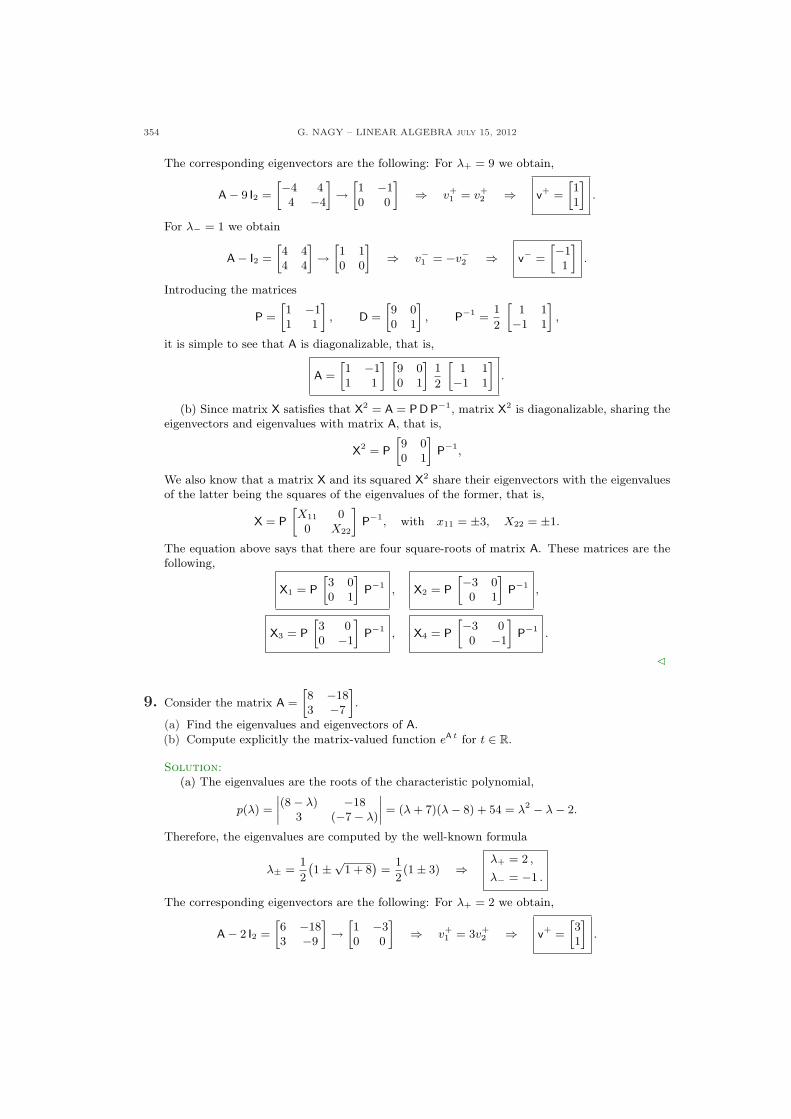
354 G. NAGY – LINEAR ALGEBRA july 15, 2012
The corresponding eigenvectors are the following: For λ+ = 9 we obtain,
A− 9 I2 =
»−4 44 −4
–→»1 −10 0
–⇒ v+
1 = v+2 ⇒ v+ =
»11
–.
For λ− = 1 we obtain
A− I2 =
»4 44 4
–→»1 10 0
–⇒ v−1 = −v−2 ⇒ v− =
»−11
–.
Introducing the matrices
P =
»1 −11 1
–, D =
»9 00 1
–, P−1 =
1
2
»1 1−1 1
–,
it is simple to see that A is diagonalizable, that is,
A =
»1 −11 1
– »9 00 1
–1
2
»1 1−1 1
–.
(b) Since matrix X satisfies that X2 = A = PDP−1, matrix X2 is diagonalizable, sharing theeigenvectors and eigenvalues with matrix A, that is,
X2 = P
»9 00 1
–P−1,
We also know that a matrix X and its squared X2 share their eigenvectors with the eigenvaluesof the latter being the squares of the eigenvalues of the former, that is,
X = P
»X11 00 X22
–P−1, with x11 = ±3, X22 = ±1.
The equation above says that there are four square-roots of matrix A. These matrices are thefollowing,
X1 = P
»3 00 1
–P−1 , X2 = P
»−3 00 1
–P−1 ,
X3 = P
»3 00 −1
–P−1 , X4 = P
»−3 00 −1
–P−1 .
C
9. Consider the matrix A =
»8 −183 −7
–.
(a) Find the eigenvalues and eigenvectors of A.
(b) Compute explicitly the matrix-valued function eA t for t ∈ R.
Solution:(a) The eigenvalues are the roots of the characteristic polynomial,
p(λ) =
˛˛(8− λ) −18
3 (−7− λ)
˛˛ = (λ + 7)(λ− 8) + 54 = λ2 − λ− 2.
Therefore, the eigenvalues are computed by the well-known formula
λ± =1
2
`1±√1 + 8
´=
1
2(1± 3) ⇒
λ+ = 2 ,
λ− = −1 .
The corresponding eigenvectors are the following: For λ+ = 2 we obtain,
A− 2 I2 =
»6 −183 −9
–→»1 −30 0
–⇒ v+
1 = 3v+2 ⇒ v+ =
»31
–.
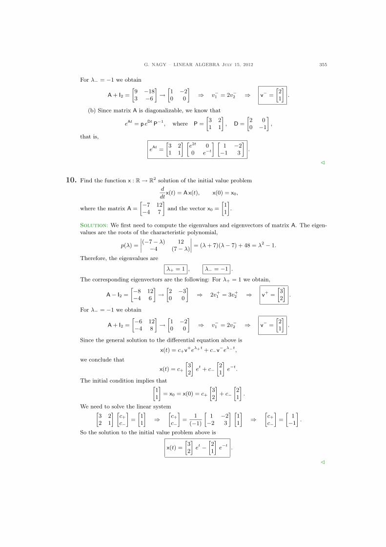
G. NAGY – LINEAR ALGEBRA July 15, 2012 355
For λ− = −1 we obtain
A + I2 =
»9 −183 −6
–→»1 −20 0
–⇒ v−1 = 2v−2 ⇒ v− =
»21
–.
(b) Since matrix A is diagonalizable, we know that
eAt = p eDt P−1, where P =
»3 21 1
–, D =
»2 00 −1
–,
that is,
eAt =
»3 21 1
– »e2t 00 e−t
– »1 −2−1 3
–.
C
10. Find the function x : R→ R2 solution of the initial value problem
d
dtx(t) = Ax(t), x(0) = x0,
where the matrix A =
»−7 12−4 7
–and the vector x0 =
»11
–.
Solution: We first need to compute the eigenvalues and eigenvectors of matrix A. The eigen-values are the roots of the characteristic polynomial,
p(λ) =
˛˛(−7− λ) 12
−4 (7− λ)
˛˛ = (λ + 7)(λ− 7) + 48 = λ2 − 1.
Therefore, the eigenvalues are
λ+ = 1 , λ− = −1 .
The corresponding eigenvectors are the following: For λ+ = 1 we obtain,
A− I2 =
»−8 12−4 6
–→»2 −30 0
–⇒ 2v+
1 = 3v+2 ⇒ v+ =
»32
–.
For λ− = −1 we obtain
A + I2 =
»−6 12−4 8
–→»1 −20 0
–⇒ v−1 = 2v−2 ⇒ v− =
»21
–.
Since the general solution to the differential equation above is
x(t) = c+v+eλ+t + c−v−eλ−t,
we conclude that
x(t) = c+
»32
–et + c−
»21
–e−t.
The initial condition implies that»11
–= x0 = x(0) = c+
»32
–+ c−
»21
–.
We need to solve the linear system»3 22 1
– »c+
c−
–=
»11
–⇒
»c+
c−
–=
1
(−1)
»1 −2−2 3
– »11
–⇒
»c+
c−
–=
»1−1
–.
So the solution to the initial value problem above is
x(t) =
»32
–et −
»21
–e−t .
C

356 G. NAGY – LINEAR ALGEBRA july 15, 2012
References
[1] S. Hassani. Mathematical physics. Springer, New York, 2000. Corrected second printing.[2] D. Lay. Linear algebra and its applications. Addison Wesley, New York, 2005. Third updated edition.[3] C. Meyer. Matrix analysis and applied linear algebra. SIAM, Philadelphia, 2000.[4] G. Strang. linear algebra and its applications. Brooks/Cole, India, 2005. Fourth edition.