Embed Size (px)
Citation preview
Linear Algebra via Exterior Products
This book is a pedagogical introduction to the
coordinate-free approach in finite-dimensional linear
algebra, at the undergraduate level. Throughout this
book, extensive use is made of the exterior (“wedge”)
product of vectors. In this approach, the book derives,
without matrix calculations, the standard properties of
determinants, the formulas of Jacobi and Liouville, the
Cayley-Hamilton theorem, properties of Pfaffians, the
Jordan canonical form, as well as some generalizations
of these results. Every concept is logically motivated
and discussed; exercises with some hints are provided.
Sergei Winitzki received a
PhD in theoretical physics
from Tufts University, USA
(1997) and has been a re-
searcher and part-time lec-
turer at universities in the
USA, UK, and Germany.
Dr. Winitzki has authored anumber of research articles and two books on his
main professional interest, theoretical physics. He is
presently employed as a senior academic fellow at the
Ludwig-Maximilians-University, Munich (Germany).
Linear Algebra via Exterior Products
Sergei Winitzki, Ph.D.
Contents
Preface iv
0 Introduction and summary 10.1 Notation . . . . . . . . . . . . . . . . . . . . . . . . . . . . . . . . . . . . . . . . . . . . . . . . . . . . . . . . . . . . . . . 10.2 Sample quiz problems . . . . . . . . . . . . . . . . . . . . . . . . . . . . . . . . . . . . . . . . . . . . . . . . . . . . . . . 10.3 A list of results . . . . . . . . . . . . . . . . . . . . . . . . . . . . . . . . . . . . . . . . . . . . . . . . . . . . . . . . . . . . 2
1 Linear algebra without coordinates 51.1 Vector spaces . . . . . . . . . . . . . . . . . . . . . . . . . . . . . . . . . . . . . . . . . . . . . . . . . . . . . . . . . . . . . 5
1.1.1 Three-dimensional Euclidean geometry . . . . . . . . . . . . . . . . . . . . . . . . . . . . . . . . . . . . . . . . . 51.1.2 From three-dimensional vectors to abstract vectors . . . . . . . . . . . . . . . . . . . . . . . . . . . . . . . . . . 51.1.3 Examples of vector spaces . . . . . . . . . . . . . . . . . . . . . . . . . . . . . . . . . . . . . . . . . . . . . . . . . 71.1.4 Dimensionality and bases . . . . . . . . . . . . . . . . . . . . . . . . . . . . . . . . . . . . . . . . . . . . . . . . . 81.1.5 All bases have equally many vectors . . . . . . . . . . . . . . . . . . . . . . . . . . . . . . . . . . . . . . . . . . . 10
1.2 Linear maps in vector spaces . . . . . . . . . . . . . . . . . . . . . . . . . . . . . . . . . . . . . . . . . . . . . . . . . . . 111.2.1 Abstract definition of linear maps . . . . . . . . . . . . . . . . . . . . . . . . . . . . . . . . . . . . . . . . . . . . 111.2.2 Examples of linear maps . . . . . . . . . . . . . . . . . . . . . . . . . . . . . . . . . . . . . . . . . . . . . . . . . . 121.2.3 Vector space of all linear maps . . . . . . . . . . . . . . . . . . . . . . . . . . . . . . . . . . . . . . . . . . . . . . 131.2.4 Eigenvectors and eigenvalues . . . . . . . . . . . . . . . . . . . . . . . . . . . . . . . . . . . . . . . . . . . . . . . 13
1.3 Subspaces . . . . . . . . . . . . . . . . . . . . . . . . . . . . . . . . . . . . . . . . . . . . . . . . . . . . . . . . . . . . . . 141.3.1 Projectors and subspaces . . . . . . . . . . . . . . . . . . . . . . . . . . . . . . . . . . . . . . . . . . . . . . . . . 141.3.2 Eigenspaces . . . . . . . . . . . . . . . . . . . . . . . . . . . . . . . . . . . . . . . . . . . . . . . . . . . . . . . . . 14
1.4 Isomorphisms of vector spaces . . . . . . . . . . . . . . . . . . . . . . . . . . . . . . . . . . . . . . . . . . . . . . . . . . 151.5 Direct sum of vector spaces . . . . . . . . . . . . . . . . . . . . . . . . . . . . . . . . . . . . . . . . . . . . . . . . . . . . 15
1.5.1 V andW as subspaces of V ⊕W ; canonical projections . . . . . . . . . . . . . . . . . . . . . . . . . . . . . . . . 151.6 Dual (conjugate) vector space . . . . . . . . . . . . . . . . . . . . . . . . . . . . . . . . . . . . . . . . . . . . . . . . . . . 16
1.6.1 Dual basis . . . . . . . . . . . . . . . . . . . . . . . . . . . . . . . . . . . . . . . . . . . . . . . . . . . . . . . . . . 161.6.2 Hyperplanes . . . . . . . . . . . . . . . . . . . . . . . . . . . . . . . . . . . . . . . . . . . . . . . . . . . . . . . . . 18
1.7 Tensor product of vector spaces . . . . . . . . . . . . . . . . . . . . . . . . . . . . . . . . . . . . . . . . . . . . . . . . . . 191.7.1 First examples . . . . . . . . . . . . . . . . . . . . . . . . . . . . . . . . . . . . . . . . . . . . . . . . . . . . . . . . 191.7.2 Example: Rm ⊗ Rn . . . . . . . . . . . . . . . . . . . . . . . . . . . . . . . . . . . . . . . . . . . . . . . . . . . . . 201.7.3 Dimension of tensor product is the product of dimensions . . . . . . . . . . . . . . . . . . . . . . . . . . . . . . 201.7.4 Higher-rank tensor products . . . . . . . . . . . . . . . . . . . . . . . . . . . . . . . . . . . . . . . . . . . . . . . 211.7.5 * Distributivity of tensor product . . . . . . . . . . . . . . . . . . . . . . . . . . . . . . . . . . . . . . . . . . . . . 22
1.8 Linear maps and tensors . . . . . . . . . . . . . . . . . . . . . . . . . . . . . . . . . . . . . . . . . . . . . . . . . . . . . . 221.8.1 Tensors as linear operators . . . . . . . . . . . . . . . . . . . . . . . . . . . . . . . . . . . . . . . . . . . . . . . . 221.8.2 Linear operators as tensors . . . . . . . . . . . . . . . . . . . . . . . . . . . . . . . . . . . . . . . . . . . . . . . . 231.8.3 Examples and exercises . . . . . . . . . . . . . . . . . . . . . . . . . . . . . . . . . . . . . . . . . . . . . . . . . . 231.8.4 Linear maps between different spaces . . . . . . . . . . . . . . . . . . . . . . . . . . . . . . . . . . . . . . . . . . . 25
1.9 Index notation for tensors . . . . . . . . . . . . . . . . . . . . . . . . . . . . . . . . . . . . . . . . . . . . . . . . . . . . . 271.9.1 Definition of index notation . . . . . . . . . . . . . . . . . . . . . . . . . . . . . . . . . . . . . . . . . . . . . . . . 271.9.2 Advantages and disadvantages of index notation . . . . . . . . . . . . . . . . . . . . . . . . . . . . . . . . . . . 28
1.10 Dirac notation for vectors and covectors . . . . . . . . . . . . . . . . . . . . . . . . . . . . . . . . . . . . . . . . . . . . . 291.10.1 Definition of Dirac notation . . . . . . . . . . . . . . . . . . . . . . . . . . . . . . . . . . . . . . . . . . . . . . . . 291.10.2 Advantages and disadvantages of Dirac notation . . . . . . . . . . . . . . . . . . . . . . . . . . . . . . . . . . . 29
2 Exterior product 302.1 Motivation . . . . . . . . . . . . . . . . . . . . . . . . . . . . . . . . . . . . . . . . . . . . . . . . . . . . . . . . . . . . . . 30
2.1.1 Two-dimensional oriented area . . . . . . . . . . . . . . . . . . . . . . . . . . . . . . . . . . . . . . . . . . . . . . 302.1.2 Parallelograms in R3 and in Rn . . . . . . . . . . . . . . . . . . . . . . . . . . . . . . . . . . . . . . . . . . . . . 31
2.2 Exterior product . . . . . . . . . . . . . . . . . . . . . . . . . . . . . . . . . . . . . . . . . . . . . . . . . . . . . . . . . . . 322.2.1 Definition of exterior product . . . . . . . . . . . . . . . . . . . . . . . . . . . . . . . . . . . . . . . . . . . . . . . 322.2.2 * Symmetric tensor product . . . . . . . . . . . . . . . . . . . . . . . . . . . . . . . . . . . . . . . . . . . . . . . . 34
i

Contents
2.3 Properties of spaces ∧kV . . . . . . . . . . . . . . . . . . . . . . . . . . . . . . . . . . . . . . . . . . . . . . . . . . . . . . 352.3.1 Linear maps between spaces ∧kV . . . . . . . . . . . . . . . . . . . . . . . . . . . . . . . . . . . . . . . . . . . . 352.3.2 Exterior product and linear dependence . . . . . . . . . . . . . . . . . . . . . . . . . . . . . . . . . . . . . . . . . 362.3.3 Computing the dual basis . . . . . . . . . . . . . . . . . . . . . . . . . . . . . . . . . . . . . . . . . . . . . . . . . 382.3.4 Gaussian elimination . . . . . . . . . . . . . . . . . . . . . . . . . . . . . . . . . . . . . . . . . . . . . . . . . . . . 392.3.5 Rank of a set of vectors . . . . . . . . . . . . . . . . . . . . . . . . . . . . . . . . . . . . . . . . . . . . . . . . . . . 402.3.6 Exterior product in index notation . . . . . . . . . . . . . . . . . . . . . . . . . . . . . . . . . . . . . . . . . . . . 412.3.7 * Exterior algebra (Grassmann algebra) . . . . . . . . . . . . . . . . . . . . . . . . . . . . . . . . . . . . . . . . . 42
3 Basic applications 443.1 Determinants through permutations: the hard way . . . . . . . . . . . . . . . . . . . . . . . . . . . . . . . . . . . . . . 443.2 The space ∧NV and oriented volume . . . . . . . . . . . . . . . . . . . . . . . . . . . . . . . . . . . . . . . . . . . . . . . 443.3 Determinants of operators . . . . . . . . . . . . . . . . . . . . . . . . . . . . . . . . . . . . . . . . . . . . . . . . . . . . . 47
3.3.1 Examples: computing determinants . . . . . . . . . . . . . . . . . . . . . . . . . . . . . . . . . . . . . . . . . . . 483.4 Determinants of square tables . . . . . . . . . . . . . . . . . . . . . . . . . . . . . . . . . . . . . . . . . . . . . . . . . . . 49
3.4.1 * Index notation for ∧NV and determinants . . . . . . . . . . . . . . . . . . . . . . . . . . . . . . . . . . . . . . . 503.5 Solving linear equations . . . . . . . . . . . . . . . . . . . . . . . . . . . . . . . . . . . . . . . . . . . . . . . . . . . . . . 51
3.5.1 Existence of solutions . . . . . . . . . . . . . . . . . . . . . . . . . . . . . . . . . . . . . . . . . . . . . . . . . . . 523.5.2 Kramer’s rule and beyond . . . . . . . . . . . . . . . . . . . . . . . . . . . . . . . . . . . . . . . . . . . . . . . . . 52
3.6 Vandermonde matrix . . . . . . . . . . . . . . . . . . . . . . . . . . . . . . . . . . . . . . . . . . . . . . . . . . . . . . . . 543.6.1 Linear independence of eigenvectors . . . . . . . . . . . . . . . . . . . . . . . . . . . . . . . . . . . . . . . . . . 553.6.2 Polynomial interpolation . . . . . . . . . . . . . . . . . . . . . . . . . . . . . . . . . . . . . . . . . . . . . . . . . 55
3.7 Multilinear actions in exterior powers . . . . . . . . . . . . . . . . . . . . . . . . . . . . . . . . . . . . . . . . . . . . . . 563.7.1 * Index notation . . . . . . . . . . . . . . . . . . . . . . . . . . . . . . . . . . . . . . . . . . . . . . . . . . . . . . . 57
3.8 Trace . . . . . . . . . . . . . . . . . . . . . . . . . . . . . . . . . . . . . . . . . . . . . . . . . . . . . . . . . . . . . . . . . 573.9 Characteristic polynomial . . . . . . . . . . . . . . . . . . . . . . . . . . . . . . . . . . . . . . . . . . . . . . . . . . . . . 59
3.9.1 Nilpotent operators . . . . . . . . . . . . . . . . . . . . . . . . . . . . . . . . . . . . . . . . . . . . . . . . . . . . . 62
4 Advanced applications 634.1 The space ∧N−1V . . . . . . . . . . . . . . . . . . . . . . . . . . . . . . . . . . . . . . . . . . . . . . . . . . . . . . . . . . 63
4.1.1 Exterior transposition of operators . . . . . . . . . . . . . . . . . . . . . . . . . . . . . . . . . . . . . . . . . . . . 634.1.2 * Index notation . . . . . . . . . . . . . . . . . . . . . . . . . . . . . . . . . . . . . . . . . . . . . . . . . . . . . . . 64
4.2 Algebraic complement (adjoint) and beyond . . . . . . . . . . . . . . . . . . . . . . . . . . . . . . . . . . . . . . . . . . 654.2.1 Definition of algebraic complement . . . . . . . . . . . . . . . . . . . . . . . . . . . . . . . . . . . . . . . . . . . 654.2.2 Algebraic complement of a matrix . . . . . . . . . . . . . . . . . . . . . . . . . . . . . . . . . . . . . . . . . . . . 674.2.3 Further properties and generalizations . . . . . . . . . . . . . . . . . . . . . . . . . . . . . . . . . . . . . . . . . 67
4.3 Cayley-Hamilton theorem and beyond . . . . . . . . . . . . . . . . . . . . . . . . . . . . . . . . . . . . . . . . . . . . . . 694.4 Functions of operators . . . . . . . . . . . . . . . . . . . . . . . . . . . . . . . . . . . . . . . . . . . . . . . . . . . . . . . 70
4.4.1 Definitions. Formal power series . . . . . . . . . . . . . . . . . . . . . . . . . . . . . . . . . . . . . . . . . . . . . 704.4.2 Computations: Sylvester’s method . . . . . . . . . . . . . . . . . . . . . . . . . . . . . . . . . . . . . . . . . . . . 724.4.3 * Square roots of operators . . . . . . . . . . . . . . . . . . . . . . . . . . . . . . . . . . . . . . . . . . . . . . . . . 74
4.5 Formulas of Jacobi and Liouville . . . . . . . . . . . . . . . . . . . . . . . . . . . . . . . . . . . . . . . . . . . . . . . . . 764.5.1 Derivative of characteristic polynomial . . . . . . . . . . . . . . . . . . . . . . . . . . . . . . . . . . . . . . . . . 774.5.2 Derivative of a simple eigenvalue . . . . . . . . . . . . . . . . . . . . . . . . . . . . . . . . . . . . . . . . . . . . 784.5.3 General trace relations . . . . . . . . . . . . . . . . . . . . . . . . . . . . . . . . . . . . . . . . . . . . . . . . . . . 78
4.6 Jordan canonical form . . . . . . . . . . . . . . . . . . . . . . . . . . . . . . . . . . . . . . . . . . . . . . . . . . . . . . . 794.6.1 Minimal polynomial . . . . . . . . . . . . . . . . . . . . . . . . . . . . . . . . . . . . . . . . . . . . . . . . . . . . 82
4.7 * Construction of projectors onto Jordan cells . . . . . . . . . . . . . . . . . . . . . . . . . . . . . . . . . . . . . . . . . . 83
5 Scalar product 875.1 Vector spaces with scalar product . . . . . . . . . . . . . . . . . . . . . . . . . . . . . . . . . . . . . . . . . . . . . . . . . 87
5.1.1 Orthonormal bases . . . . . . . . . . . . . . . . . . . . . . . . . . . . . . . . . . . . . . . . . . . . . . . . . . . . . 875.1.2 Correspondence between vectors and covectors . . . . . . . . . . . . . . . . . . . . . . . . . . . . . . . . . . . . 895.1.3 * Example: bilinear forms on V ⊕ V ∗ . . . . . . . . . . . . . . . . . . . . . . . . . . . . . . . . . . . . . . . . . . . 905.1.4 Scalar product in index notation . . . . . . . . . . . . . . . . . . . . . . . . . . . . . . . . . . . . . . . . . . . . . 90
5.2 Orthogonal subspaces . . . . . . . . . . . . . . . . . . . . . . . . . . . . . . . . . . . . . . . . . . . . . . . . . . . . . . . 915.2.1 Affine hyperplanes . . . . . . . . . . . . . . . . . . . . . . . . . . . . . . . . . . . . . . . . . . . . . . . . . . . . . 92
5.3 Orthogonal transformations . . . . . . . . . . . . . . . . . . . . . . . . . . . . . . . . . . . . . . . . . . . . . . . . . . . . 925.3.1 Examples and properties . . . . . . . . . . . . . . . . . . . . . . . . . . . . . . . . . . . . . . . . . . . . . . . . . 925.3.2 Transposition . . . . . . . . . . . . . . . . . . . . . . . . . . . . . . . . . . . . . . . . . . . . . . . . . . . . . . . . 93
5.4 Applications of exterior product . . . . . . . . . . . . . . . . . . . . . . . . . . . . . . . . . . . . . . . . . . . . . . . . . 94
ii
Contents
5.4.1 Orthonormal bases, volume, and ∧NV . . . . . . . . . . . . . . . . . . . . . . . . . . . . . . . . . . . . . . . . . 945.4.2 Vector product in R3 and Levi-Civita symbol ε . . . . . . . . . . . . . . . . . . . . . . . . . . . . . . . . . . . . . 945.4.3 Hodge star and Levi-Civita symbol in N dimensions . . . . . . . . . . . . . . . . . . . . . . . . . . . . . . . . . 955.4.4 Reciprocal basis . . . . . . . . . . . . . . . . . . . . . . . . . . . . . . . . . . . . . . . . . . . . . . . . . . . . . . . 97
5.5 Scalar product in ∧kV . . . . . . . . . . . . . . . . . . . . . . . . . . . . . . . . . . . . . . . . . . . . . . . . . . . . . . . 985.5.1 Scalar product in ∧NV . . . . . . . . . . . . . . . . . . . . . . . . . . . . . . . . . . . . . . . . . . . . . . . . . . . 985.5.2 Volumes of k-dimensional parallelepipeds . . . . . . . . . . . . . . . . . . . . . . . . . . . . . . . . . . . . . . . 98
5.6 Scalar product for complex spaces . . . . . . . . . . . . . . . . . . . . . . . . . . . . . . . . . . . . . . . . . . . . . . . . 1005.6.1 Symmetric and Hermitian operators . . . . . . . . . . . . . . . . . . . . . . . . . . . . . . . . . . . . . . . . . . . 1015.6.2 Unitary transformations . . . . . . . . . . . . . . . . . . . . . . . . . . . . . . . . . . . . . . . . . . . . . . . . . . 102
5.7 Antisymmetric operators . . . . . . . . . . . . . . . . . . . . . . . . . . . . . . . . . . . . . . . . . . . . . . . . . . . . . 1025.8 * Pfaffians . . . . . . . . . . . . . . . . . . . . . . . . . . . . . . . . . . . . . . . . . . . . . . . . . . . . . . . . . . . . . . 103
5.8.1 Determinants are Pfaffians squared . . . . . . . . . . . . . . . . . . . . . . . . . . . . . . . . . . . . . . . . . . . 1045.8.2 Further properties . . . . . . . . . . . . . . . . . . . . . . . . . . . . . . . . . . . . . . . . . . . . . . . . . . . . . 105
A Complex numbers 107A.1 Basic definitions . . . . . . . . . . . . . . . . . . . . . . . . . . . . . . . . . . . . . . . . . . . . . . . . . . . . . . . . . . . 107A.2 Geometric representation . . . . . . . . . . . . . . . . . . . . . . . . . . . . . . . . . . . . . . . . . . . . . . . . . . . . . 107A.3 Analytic functions . . . . . . . . . . . . . . . . . . . . . . . . . . . . . . . . . . . . . . . . . . . . . . . . . . . . . . . . . . 107A.4 Exponent and logarithm . . . . . . . . . . . . . . . . . . . . . . . . . . . . . . . . . . . . . . . . . . . . . . . . . . . . . . 108
B Permutations 109
C Matrices 111C.1 Definitions . . . . . . . . . . . . . . . . . . . . . . . . . . . . . . . . . . . . . . . . . . . . . . . . . . . . . . . . . . . . . . 111C.2 Matrix multiplication . . . . . . . . . . . . . . . . . . . . . . . . . . . . . . . . . . . . . . . . . . . . . . . . . . . . . . . . 111C.3 Linear equations . . . . . . . . . . . . . . . . . . . . . . . . . . . . . . . . . . . . . . . . . . . . . . . . . . . . . . . . . . 112C.4 Inverse matrix . . . . . . . . . . . . . . . . . . . . . . . . . . . . . . . . . . . . . . . . . . . . . . . . . . . . . . . . . . . . 113C.5 Determinants . . . . . . . . . . . . . . . . . . . . . . . . . . . . . . . . . . . . . . . . . . . . . . . . . . . . . . . . . . . . 113C.6 Tensor product . . . . . . . . . . . . . . . . . . . . . . . . . . . . . . . . . . . . . . . . . . . . . . . . . . . . . . . . . . . 114
D Distribution of this text 115D.1 Motivation . . . . . . . . . . . . . . . . . . . . . . . . . . . . . . . . . . . . . . . . . . . . . . . . . . . . . . . . . . . . . . 115D.2 GNU Free Documentation License . . . . . . . . . . . . . . . . . . . . . . . . . . . . . . . . . . . . . . . . . . . . . . . . 115
D.2.1 Preamble . . . . . . . . . . . . . . . . . . . . . . . . . . . . . . . . . . . . . . . . . . . . . . . . . . . . . . . . . . . 115D.2.2 Applicability and definitions . . . . . . . . . . . . . . . . . . . . . . . . . . . . . . . . . . . . . . . . . . . . . . . 115D.2.3 Verbatim copying . . . . . . . . . . . . . . . . . . . . . . . . . . . . . . . . . . . . . . . . . . . . . . . . . . . . . . 116D.2.4 Copying in quantity . . . . . . . . . . . . . . . . . . . . . . . . . . . . . . . . . . . . . . . . . . . . . . . . . . . . 116D.2.5 Modifications . . . . . . . . . . . . . . . . . . . . . . . . . . . . . . . . . . . . . . . . . . . . . . . . . . . . . . . . 116D.2.6 Combining documents . . . . . . . . . . . . . . . . . . . . . . . . . . . . . . . . . . . . . . . . . . . . . . . . . . . 117D.2.7 Collections of documents . . . . . . . . . . . . . . . . . . . . . . . . . . . . . . . . . . . . . . . . . . . . . . . . . 117D.2.8 Aggregation with independent works . . . . . . . . . . . . . . . . . . . . . . . . . . . . . . . . . . . . . . . . . . 117D.2.9 Translation . . . . . . . . . . . . . . . . . . . . . . . . . . . . . . . . . . . . . . . . . . . . . . . . . . . . . . . . . . 117D.2.10 Termination . . . . . . . . . . . . . . . . . . . . . . . . . . . . . . . . . . . . . . . . . . . . . . . . . . . . . . . . . 117D.2.11 Future revisions of this license . . . . . . . . . . . . . . . . . . . . . . . . . . . . . . . . . . . . . . . . . . . . . . 117D.2.12 Addendum: How to use this License for your documents . . . . . . . . . . . . . . . . . . . . . . . . . . . . . . 118D.2.13 Copyright . . . . . . . . . . . . . . . . . . . . . . . . . . . . . . . . . . . . . . . . . . . . . . . . . . . . . . . . . . 118
Index 119
iii
Preface
In a first course of linear algebra, one learns the various uses ofmatrices, for instance the properties of determinants, eigenvec-tors and eigenvalues, and methods for solving linear equations.The required calculations are straightforward (because, concep-tually, vectors and matrices are merely “arrays of numbers”) ifcumbersome. However, there is a more abstract and more pow-erful approach: Vectors are elements of abstract vector spaces,and matrices represent linear transformations of vectors. Thisinvariant or coordinate-free approach is important in algebraand has found many applications in science.The purpose of this book is to help the reader make a tran-
sition to the abstract coordinate-free approach, and also to givea hands-on introduction to exterior products, a powerful toolof linear algebra. I show how the coordinate-free approach to-gether with exterior products can be used to clarify the basicresults of matrix algebra, at the same time avoiding all the labo-rious matrix calculations.Here is a simple theorem that illustrates the advantages of the
exterior product approach. A triangle is oriented arbitrarily inthree-dimensional space; the three orthogonal projections of thistriangle are triangles in the three coordinate planes. Let S be thearea of the initial triangle, and let A,B,C be the areas of thethree projections. Then
S2 = A2 +B2 + C2.
If one uses bivectors to represent the oriented areas of the tri-angle and of its three projections, the statement above is equiv-alent to the Pythagoras theorem in the space of bivectors, andthe proof requires only a few straightforward definitions andchecks. A generalization of this result to volumes of k-dimen-sional bodies embedded in N -dimensional spaces is then ob-tained with no extra work. I hope that the readers will appre-ciate the beauty of an approach to linear algebra that allows usto obtain such results quickly and almost without calculations.The exterior product is widely used in connection with n-
forms, which are exterior products of covectors. In this bookI do not use n-forms — instead I use vectors, n-vectors, andtheir exterior products. This approach allows amore straightfor-ward geometric interpretation and also simplifies calculationsand proofs.To make the book logically self-contained, I present a proof
of every basic result of linear algebra. The emphasis is noton computational techniques, although the coordinate-free ap-proach doesmake many computations easier and more elegant.1
The main topics covered are tensor products; exterior prod-
ucts; coordinate-free definitions of the determinant det A, thetrace TrA, and the characteristic polynomial QA (λ); basic prop-erties of determinants; solution of linear equations, includingover-determined or under-determined systems, using Kramer’s
rule; the Liouville formula det exp A = expTrA as an iden-tity of formal series; the algebraic complement (cofactor) ma-
1Elegant means shorter and easier to remember. Usually, elegant derivationsare those in which some powerful basic idea is exploited to obtain the resultquickly.
trix; Jacobi’s formula for the variation of the determinant; vari-ation of the characteristic polynomial and of eigenvalue; theCayley-Hamilton theorem; analytic functions of operators; Jor-dan canonical form; construction of projectors onto Jordan cells;Hodge star and the computation of k-dimensional volumes
through k-vectors; definition and properties of the Pfaffian PfA
for antisymmetric operators A. All these standard results are de-rived without matrix calculations; instead, the exterior productis used as a main computational tool.This book is largely pedagogical, meaning that the results are
long known, and the emphasis is on a clear and self-contained,logically motivated presentation aimed at students. Therefore,some exercises with hints and partial solutions are included, butnot references to literature.2 I have tried to avoid being overlypedantic while keeping the exposition mathematically rigorous.Sections marked with a star ∗ are not especially difficult but
contain material that may be skipped at first reading. (Exercisesmarked with a star aremore difficult.)The first chapter is an introduction to the invariant approach
to vector spaces. I assume that readers are familiar with elemen-tary linear algebra in the language of row/column vectors andmatrices; Appendix C contains a brief overview of that mate-rial. Good introductory books (which I did not read in detail butwhich have a certain overlap with the present notes) are “Finite-dimensional Vector Spaces” by P. Halmos and “Linear Algebra”by J. Hefferon (the latter is a free book).I started thinking about the approach to linear algebra based
on exterior products while still a student. I am especially grate-ful to Sergei Arkhipov, Leonid Positsel’sky, and Arkady Vain-trob who have stimulated my interest at that time and taughtme much of what I could not otherwise learn about algebra.Thanks are also due to Prof. Howard Haber (UCSC) for con-structive feedback on an earlier version of this text.
2The approach to determinants via exterior products has been known since atleast 1880 but does not seem especially popular in textbooks, perhaps dueto the somewhat abstract nature of the tensor product. I believe that thisapproach to determinants and to other results in linear algebra deserves tobe more widely appreciated.
iv
0 Introduction and summary
All the notions mentioned in this section will be explainedbelow. If you already know the definition of tensor and exteriorproducts and are familiar with statements such as End V ∼= V ⊗V ∗, you may skip to Chapter 2.
0.1 Notation
The following conventions are used throughout this text.I use the bold emphasis to define a new word, term, or no-
tion, and the definition always appears near the boldface text(whether or not I write the word “Definition”).Ordered sets are denoted by round parentheses, e.g. (1, 2, 3).
Unordered sets are denoted using the curly parentheses,e.g. {a, b, c}.The symbol ≡means “is now being defined as” or “equals by
a previously given definition.”
The symbol!= means “as we already know, equals.”
A set consisting of all elements x satisfying some propertyP (x) is denoted by { x |P (x) is true }.A map f from a set V to W is denoted by f : V → W . An
element v ∈ V is then mapped to an element w ∈ W , which iswritten as f : v 7→ w or f(v) = w.The sets of rational numbers, real numbers, and complex
numbers are denoted respectively by Q, R, and C.Statements, Lemmas, Theorems, Examples, and Exercises are
numbered only within a single subsection, so references are al-ways to a certain statement in a certain subsection.1 A referenceto “Theorem 1.1.4”means the unnumbered theorem in Sec. 1.1.4.Proofs, solutions, examples, and exercises are separated from
the rest by the symbol �. More precisely, this symbol means “Ihave finished with this; now we look at something else.”V is a finite-dimensional vector space over a field K. Vectors
from V are denoted by boldface lowercase letters, e.g. v ∈ V .The dimension of V is N ≡ dimV .The standard N -dimensional space over real numbers (the
space consisting ofN -tuples of real numbers) is denoted by RN .The subspace spanned by a given set of vectors {v1, ...,vn} is
denoted by Span {v1, ...,vn}.The vector space dual to V is V ∗. Elements of V ∗ (covectors)
are denoted by starred letters, e.g. f∗ ∈ V ∗. A covector f∗ actson a vector v and produces a number f∗(v).The space of linear maps (homomorphisms) V → W is
Hom (V,W ). The space of linear operators (also called endo-morphisms) of a vector space V , i.e. the space of all linear mapsV → V , is End V . Operators are denoted by the circumflex ac-
cent, e.g. A. The identity operator on V is 1V ∈ End V (some-times also denoted 1 for brevity).The direct sum of spaces V and W is V ⊕ W . The tensor
product of spaces V and W is V ⊗ W . The exterior (anti-commutative) product of V and V is V ∧V . The exterior prod-uct of n copies of V is ∧nV . Canonical isomorphisms of vec-
1I was too lazy to implement a comprehensive system of numbering for allthese items.
tor spaces are denoted by the symbol ∼=; for example, End V ∼=V ⊗ V ∗.The scalar product of vectors is denoted by 〈u,v〉. The nota-
tion a × b is used only for the traditional vector product (alsocalled cross product) in 3-dimensional space. Otherwise, theproduct symbol × is used to denote the continuation a long ex-pression that is being split between lines.The exterior (wedge) product of vectors is denoted by a∧b ∈
∧2V .Any two nonzero tensors a1 ∧ ... ∧ aN and b1 ∧ ... ∧ bN in an
N -dimensional space are proportional to each other, say
a1 ∧ ... ∧ aN = λb1 ∧ ... ∧ bN .
It is then convenient to denote λ by the “tensor ratio”
λ ≡ a1 ∧ ... ∧ aN
b1 ∧ ... ∧ bN.
The number of unordered choices of k items from n is denotedby
(n
k
)
=n!
k!(n− k)!.
The k-linear action of a linear operator A in the space ∧nV is
denoted by ∧nAk. (Here 0 ≤ k ≤ n ≤ N .) For example,
(∧3A2)a ∧ b ∧ c ≡ Aa ∧ Ab ∧ c + Aa ∧ b ∧ Ac
+ a ∧ Ab ∧ Ac.
The imaginary unit (√−1) is denoted by a roman “i,” while
the base of natural logarithms is written as an italic “e.” Forexample, I would write eiπ = −1. This convention is designedto avoid conflicts with the much used index i and with labeledvectors such as ei.I write an italic d in the derivatives, such as df/dx, and in inte-
grals, such as∫f(x)dx, because in these cases the symbols dx do
not refer to a separate well-defined object “dx” but are a part ofthe traditional symbolic notation used in calculus. Differentialforms (or, for that matter, nonstandard calculus) do make “dx”into a well-defined object; in that case I write a roman “d” in“dx.” Neither calculus nor differential forms are actually used inthis book; the only exception is the occasional use of the deriva-tive d/dx applied to polynomials in x. I will not need to make adistinction between d/dx and ∂/∂x; the derivative of a functionf with respect to x is denoted by ∂xf .
0.2 Sample quiz problems
The following problems can be solved using techniques ex-plained in this book. (These problems are of varying difficulty.)In these problems V is an N -dimensional vector space (with ascalar product if indicated).Exterior multiplication: If two tensors ω1, ω2 ∈ ∧kV (with 1 ≤k ≤ N − 1) are such that ω1 ∧ v = ω2 ∧ v for all vectors v ∈ V ,show that ω1 = ω2.
1
0 Introduction and summary
Insertions: a) It is given that ψ ∈ ∧kV (with 1 ≤ k ≤ N −1) andψ ∧a = 0, where a ∈ V and a 6= 0. Further, a covector f∗ ∈ V ∗ isgiven such that f∗(a) 6= 0. Show that
ψ =1
f∗(a)a ∧ (ιf∗ψ).
b) It is given that ψ ∧ a = 0 and ψ ∧ b = 0, where ψ ∈ ∧kV(with 2 ≤ k ≤ N − 1) and a,b ∈ V such that a ∧ b 6= 0. Showthat there exists χ ∈ ∧k−2V such that ψ = a ∧ b ∧ χ.c) It is given that ψ ∧ a ∧ b = 0, where ψ ∈ ∧kV (with 2 ≤ k ≤
N − 2) and a,b ∈ V such that a ∧ b 6= 0. Is it always true thatψ = a ∧ b ∧ χ for some χ ∈ ∧k−2V ?Determinants: a) Suppose A is a linear operator defined by A =∑N
i=1 ai ⊗ b∗i , where ai ∈ V are given vectors and bi ∈ V ∗ are
given covectors; N = dim V . Show that
det A =a1 ∧ ... ∧ aN
e1 ∧ ... ∧ eN
b∗1 ∧ ... ∧ b∗
N
e∗1 ∧ ... ∧ e∗N,
where {ej} is an arbitrary basis and{e∗j}is the corresponding
dual basis. Show that the expression above is independent ofthe choice of the basis {ej}.b) Suppose that a scalar product is given in V , and an operator
A is defined by
Ax ≡N∑
i=1
ai 〈bi,x〉 .
Further, suppose that {ej} is an orthonormal basis in V . Showthat
det A =a1 ∧ ... ∧ aN
e1 ∧ ... ∧ eN
b1 ∧ ... ∧ bN
e1 ∧ ... ∧ eN,
and that this expression is independent of the choice of the or-thonormal basis {ej} and of the orientation of the basis.Hyperplanes: a) Let us suppose that the “price” of the vectorx ∈ V is given by the formula
Cost (x) ≡ C(x,x),
whereC(a,b) is a known, positive-definite bilinear form. Deter-mine the “cheapest” vector x belonging to the affine hyperplanea∗(x) = α, where a∗ ∈ V ∗ is a nonzero covector and α is a num-ber.b)We are nowworking in a vector spacewith a scalar product,
and the “price” of a vector x is 〈x,x〉. Two affine hyperplanesare given by equations 〈a,x〉 = α and 〈b,x〉 = β, where a andb are given vectors, α and β are numbers, and x ∈ V . (It isassured that a and b are nonzero and not parallel to each other.)Determine the “cheapest” vector x belonging to the intersectionof the two hyperplanes.Too few equations: A linear operator A is defined by A =∑k
i=1 ai ⊗ b∗i , where ai ∈ V are given vectors and b∗
i ∈ V ∗
are given covectors, and k < N = dimV . Show that the vector
equation Ax = c has no solutions if a1 ∧ ... ∧ ak ∧ c 6= 0. In casea1 ∧ ... ∧ ak ∧ c = 0, show that solutions x surely exist whenb∗
1 ∧ ... ∧ b∗k 6= 0 but may not exist otherwise.
Operator functions: It is known that the operator A satisfies the
operator equation A2 = −1. Simplify the operator-valued func-
tions 1+A3−A
, cos(λA), and√
A+ 2 to linear formulas involving A.
(Here λ is a number, while the numbers 1, 2, 3 stand for multi-ples of the identity operator.) Compare the results with the com-plex numbers 1+i
3−i , cos(λi),√i + 2 and generalize the conclusion
to a theorem about computing analytic functions f(A).
Inverse operator: It is known that AB = λ1V , where λ 6= 0 is
a number. Prove that also BA = λ1V . (Both A and B are linearoperators in a finite-dimensional space V .)Trace and determinant: Consider the space of polynomials inthe variables x and y, where we admit only polynomials of the
form a0 + a1x + a2y + a3xy (with aj ∈ R). An operator A isdefined by
A ≡ x∂
∂x− ∂
∂y.
Show that A is a linear operator in this space. Compute the trace
and the determinant of A. If A is invertible, compute A−1(x+y).
Cayley-Hamilton theorem: Express det A through TrA and
Tr(A2) for an arbitrary operator A in a two-dimensional space.
Algebraic complement: Let A be a linear operator and˜A its al-
gebraic complement.a) Show that
Tr˜A = ∧N AN−1.
Here∧N AN−1 is the coefficient at (−λ) in the characteristic poly-
nomial of A (that is, minus the coefficient preceding the deter-minant).b) For t-independent operators A and B, show that
∂
∂tdet(A+ tB) = Tr(
˜AB).
Liouville formula: Suppose X(t) is a defined as solution of thedifferential equation
∂tX(t) = A(t)X(t) − X(t)A(t),
where A(t) is a given operator. (Operators that are functions oft can be understood as operator-valued formal power series.)
a) Show that the determinant of X(t) is independent of t.b) Show that all the coefficients of the characteristic polyno-
mial of X(t) are independent of t.Hodge star: Suppose {v1, ...,vN} is a basis in V , not necessar-ily orthonormal, while {ej} is a positively oriented orthonormalbasis. Show that
∗(v1 ∧ ... ∧ vN ) =v1 ∧ ... ∧ vN
e1 ∧ ... ∧ eN.
Volume in space: Consider the space of polynomials of degreeat most 4 in the variable x. The scalar product of two polynomi-als p1(x) and p2(x) is defined by
〈p1, p2〉 ≡1
2
∫ 1
−1
p1(x)p2(x)dx.
Determine the three-dimensional volume of the tetrahedronwith vertices at the “points” 0, 1 + x, x2 + x3, x4 in this five-dimensional space.
0.3 A list of results
Here is a list of some results explained in this book. If you al-ready know all these results and their derivations, you may notneed to read any further.Vector spaces may be defined over an abstract number field,
without specifying the number of dimensions or a basis.
2
0 Introduction and summary
The set{a+ b
√41 | a, b ∈ Q
}is a number field.
Any vector can be represented as a linear combination of basisvectors. All bases have equally many vectors.The set of all linear maps from one vector space to another is
denoted Hom(V,W ) and is a vector space.The zero vector is not an eigenvector (by definition).An operator having in some basis the matrix representation
(0 10 0
)
cannot be diagonalized.
The dual vector space V ∗ has the same dimension as V (forfinite-dimensional spaces).Given a nonzero covector f∗ ∈ V ∗, the set of vectors v ∈ V
such that f∗(v) = 0 is a subspace of codimension 1 (a hyper-plane).The tensor product of Rm and Rn has dimensionmn.
Any linear map A : V → W can be represented by a tensor
of the form∑k
i=1 v∗i ⊗ wi ∈ V ∗ ⊗ W . The rank of A is equal
to the smallest number of simple tensor product terms v∗i ⊗ wi
required for this representation.The identity map 1V : V → V is represented as the tensor
∑Ni=1 e∗i ⊗ ei ∈ V ∗⊗V , where {ei} is any basis and {e∗i } its dual
basis. This tensor does not depend on the choice of the basis{ei}.A set of vectors {v1, ...,vk} is linearly independent if and only
if v1 ∧ ... ∧ vk 6= 0. If v1 ∧ ... ∧ vk 6= 0 but v1 ∧ ... ∧ vk ∧ x = 0then the vector x belongs to the subspace Span {v1, ...,vk}.The dimension of the space ∧kV is
(Nk
), where N ≡ dimV .
Insertion ιa∗ω of a covector a∗ ∈ V ∗ into an antisymmetrictensor ω ∈ ∧kV has the property
v ∧ (ιa∗ω) + ιa∗(v ∧ ω) = a∗(v)ω.
Given a basis {ei}, the dual basis {e∗i }may be computed as
e∗i (x) =e1 ∧ ... ∧ x ∧ ... ∧ eN
e1 ∧ ... ∧ eN,
where x replaces ei in the numerator.The subspace spanned by a set of vectors {v1, ...,vk}, not nec-
essarily linearly independent, can be characterized by a certainantisymmetric tensor ω, which is the exterior product of thelargest number of vi’s such that ω 6= 0. The tensor ω, computedin this way, is unique up to a constant factor.The n-vector (antisymmetric tensor) v1 ∧ ... ∧ vn represents
geometrically the oriented n-dimensional volume of the paral-lelepiped spanned by the vectors vi.
The determinant of a linear operator A is the coefficient thatmultiplies the oriented volume of any parallelepiped trans-
formed by A. In our notation, the operator ∧N AN acts in ∧NV
as multiplication by det A.If each of the given vectors {v1, ...,vN} is expressed through
a basis {ei} as vj =∑N
i=1 vijei, the determinant of the matrix vij
is found as
det(vij) = det(vji) =v1 ∧ ... ∧ vN
e1 ∧ ... ∧ eN.
A linear operator A : V → V and its canonically defined trans-
pose AT : V ∗ → V ∗ have the same characteristic polynomials.
If det A 6= 0 then the inverse operator A−1 exists, and a lin-
ear equation Ax = b has the unique solution x = A−1b. Oth-
erwise, solutions exist if b belongs to the image of A. Explicit
solutions may be constructed using Kramer’s rule: If a vectorb belongs to the subspace spanned by vectors {v1, ...,vn} thenb =
∑ni=1 bivi, where the coefficients bi may be found (assum-
ing v1 ∧ ... ∧ vn 6= 0) as
bi =v1 ∧ ... ∧ x ∧ ... ∧ vn
v1 ∧ ... ∧ vn
(here x replaces vi in the exterior product in the numerator).Eigenvalues of a linear operator are roots of its characteristic
polynomial. For each root λi, there exists at least one eigenvec-tor corresponding to the eigenvalue λi.If {v1, ...,vk} are eigenvectors corresponding to all different
eigenvalues λ1, ..., λk of some operator, then the set {v1, ...,vk}is linearly independent.The dimension of the eigenspace corresponding to λi is not
larger than the algebraic multiplicity of the root λi in the charac-teristic polynomial.(Below in this section we always denote by N the dimension of the
space V .)
The trace of an operator A can be expressed as ∧N A1.
We have Tr(AB) = Tr(BA). This holds even if A, B are maps
between different spaces, i.e. A : V →W and B : W → V .
If an operator A is nilpotent, its characteristic polynomial is
(−λ)N, i.e. the same as the characteristic polynomial of a zero
operator.
The j-th coefficient of the characteristic polynomial of A is
(−1)j(∧N Aj).
Each coefficient of the characteristic polynomial of A can beexpressed as a polynomial function of N traces of the form
Tr(Ak), k = 1, ..., N .The space ∧N−1V is N -dimensional like V itself, and there
is a canonical isomorphism between End(∧N−1V ) and End(V ).This isomorphism, called exterior transposition, is denoted by
(...)∧T . The exterior transpose of an operator X ∈ EndV is de-fined by
(X∧Tω) ∧ v ≡ ω ∧ Xv, ∀ω ∈ ∧N−1V, v ∈ V.
Similarly, one defines the exterior transposition map betweenEnd(∧N−kV ) and End(∧kV ) for all k = 1, ..., N .The algebraic complement operator (normally defined as a
matrix consisting of minors) is canonically defined through ex-
terior transposition as˜A ≡ (∧N−1AN−1)∧T . It can be expressed
as a polynomial in A and satisfies the identity˜AA = (det A)1V .
Also, all other operators
A(k) ≡(∧N−1AN−k
)∧T, k = 1, ..., N
can be expressed as polynomials in Awith known coefficients.
The characteristic polynomial of A gives the zero operator if
applied to the operator A (the Cayley-Hamilton theorem). A
similar theorem holds for each of the operators ∧kA1, 2 ≤ k ≤N − 1 (with different polynomials).
A formal power series f(t) can be applied to the operator tA;
the result is an operator-valued formal series f(tA) that has theusual properties, e.g.
∂tf(tA) = Af ′(tA).
3
0 Introduction and summary
If A is diagonalized with eigenvalues {λi} in the eigenbasis
{ei}, then a formal power series f(tA) is diagonalized in thesame basis with eigenvalues f(tλi).
If an operator A satisfies a polynomial equation such as
p(A) = 0, where p(x) is a known polynomial of degree k (not
necessarily, but possibly, the characteristic polynomial of A)
then any formal power series f(tA) is reduced to a polynomial
in tA of degree not larger than k − 1. This polynomial can becomputed as the interpolating polynomial for the function f(tx)at points x = xi where xi are the (all different) roots of p(x). Suit-able modifications are available when not all roots are different.So one can compute any analytic function f(A) of the operator
A as long as one knows a polynomial equation satisfied by A.
A square root of an operator A (i.e. a linear operator B such
that BB = A) is not unique and does not always exist. In twoand three dimensions, one can either obtain all square roots ex-
plicitly as polynomials in A, or determine that some square roots
are not expressible as polynomials in A or that square roots of Ado not exist at all.If an operator A depends on a parameter t, one can express the
derivative of the determinant of A through the algebraic com-
plement˜A (Jacobi’s formula),
∂t det A(t) = Tr(˜A∂tA).
Derivatives of other coefficients qk ≡ ∧N AN−k of the character-istic polynomial are given by similar formulas,
∂tqk = Tr[(∧N−1AN−k−1)∧T∂tA
].
The Liouville formula holds: det exp A = expTrA.Any operator (not necessarily diagonalizable) can be reduced
to a Jordan canonical form in a Jordan basis. The Jordan basisconsists of eigenvectors and root vectors for each eigenvalue.
Given an operator A whose characteristic polynomial isknown (hence all roots λi and their algebraic multiplicities mi
are known), one can construct explicitly a projector Pλionto a
Jordan cell for any chosen eigenvalue λi. The projector is found
as a polynomial in Awith known coefficients.(Below in this section we assume that a scalar product is fixed in V .)A nondegenerate scalar product provides a one-to-one corre-
spondence between vectors and covectors. Then the canonically
transposed operator AT : V ∗ → V ∗ can be mapped into an op-
erator in V , denoted also by AT . (This operator is representedby the transposed matrix only in an orthonormal basis.) We have
(AB)T = BT AT and det(AT ) = det A.Orthogonal transformations have determinants equal to ±1.
Mirror reflections are orthogonal transformations and have de-terminant equal to −1.Given an orthonormal basis {ei}, one can define the unit vol-
ume tensor ω = e1 ∧ ... ∧ eN . The tensor ω is then independentof the choice of {ei} up to a factor ±1 due to the orientation ofthe basis (i.e. the ordering of the vectors of the basis), as long asthe scalar product is kept fixed.Given a fixed scalar product 〈·, ·〉 and a fixed orientation of
space, the Hodge star operation is uniquely defined as a linearmap (isomorphism) ∧kV → ∧N−kV for each k = 0, ..., N . Forinstance,
∗e1 = e2 ∧ e3 ∧ ... ∧ eN ; ∗(e1 ∧ e2) = e3 ∧ ... ∧ eN ,
if {ei} is any positively oriented, orthonormal basis.The Hodge star map satisfies
〈a,b〉 = ∗(a ∧ ∗b) = ∗(b ∧ ∗a), a,b ∈ V.
In a three-dimensional space, the usual vector product andtriple product can be expressed through the Hodge star as
a × b = ∗(a ∧ b), a · (b × c) = ∗(a ∧ b ∧ c).
The volume of an N -dimensional parallelepiped spanned by{v1, ...,vN} is equal to
√
det(Gij), where Gij ≡ 〈vi,vj〉 is thematrix of the pairwise scalar products.Given a scalar product in V , a scalar product is canonically
defined also in the spaces ∧kV for all k = 2, ..., N . This scalarproduct can be defined by
〈ω1, ω2〉 = ∗(ω1 ∧ ∗ω2) = ∗(ω2 ∧ ∗ω1) = 〈ω2, ω1〉 ,
where ω1,2 ∈ ∧kV . Alternatively, this scalar product is de-fined by choosing an orthonormal basis {ej} and postulatingthat ei1 ∧ ...∧eik
is normalized and orthogonal to any other suchtensor with different indices {ij|j = 1, ..., k}. The k-dimension-al volume of a parallelepiped spanned by vectors {v1, ...,vk} is
found as√
〈ψ, ψ〉with ψ ≡ v1 ∧ ... ∧ vk ∈ ∧kV .The insertion ιvψ of a vector v into a k-vector ψ ∈ ∧kV (or the
“interior product”) can be expressed as
ιvψ = ∗(v ∧ ∗ψ).
If ω ≡ e1 ∧ ... ∧ eN is the unit volume tensor, we have ιvω = ∗v.Symmetric, antisymmetric, Hermitian, and anti-Hermitian
operators are always diagonalizable (if we allow complex eigen-values and eigenvectors). Eigenvectors of these operators can bechosen orthogonal to each other.Antisymmetric operators are representable as elements of
∧2V of the form∑n
i=1 ai∧bi, where one needs nomore thanN/2terms, and the vectors ai, bi can be chosen mutually orthogonalto each other. (For this, we do not need complex vectors.)
The Pfaffian of an antisymmetric operator A in even-dimen-
sional space is the number Pf A defined as
1
(N/2)!A ∧ ... ∧A︸ ︷︷ ︸
N/2
= (Pf A)e1 ∧ ... ∧ eN ,
where {ei} is an orthonormal basis. Some basic properties of thePfaffian are
(Pf A)2 = det A,
Pf (BABT ) = (det B)(Pf A),
where A is an antisymmetric operator (AT = −A) and B is anarbitrary operator.
4
1 Linear algebra without coordinates
1.1 Vector spaces
Abstract vector spaces are developed as a generalization of thefamiliar vectors in Euclidean space.
1.1.1 Three-dimensional Euclidean geometry
Let us begin with something you already know. Three-dimen-sional vectors are specified by triples of coordinates, r ≡(x, y, z). The operations of vector sum and vector product ofsuch vectors are defined by
(x1, y1, z1) + (x2, y2, z2) ≡ (x1 + x2, y1 + y2, z1 + z2) ; (1.1)
(x1, y1, z1) × (x2, y2, z2) ≡ (y1z2 − z1y2, z1x2 − x1z2,
x1y2 − y1x2). (1.2)
(I assume that these definitions are familiar to you.) Vectors canbe rescaled by multiplying them with real numbers,
cr = c (x, y, z) ≡ (cx, cy, cz) . (1.3)
A rescaled vector is parallel to the original vector and pointseither in the same or in the opposite direction. In addition, ascalar product of two vectors is defined,
(x1, y1, z1) · (x2, y2, z2) ≡ x1x2 + y1y2 + z1z2. (1.4)
These operations encapsulate all of Euclidean geometry in apurely algebraic language. For example, the length of a vector r
is
|r| ≡√
r · r =√
x2 + y2 + z2, (1.5)
the angle α between vectors r1 and r2 is found from the relation(the cosine theorem)
|r1| |r2| cosα = r1 · r2,
while the area of a triangle spanned by vectors r1 and r2 is
S =1
2|r1 × r2| .
Using these definitions, one can reformulate every geomet-ric statement (such as, “a triangle having two equal sides hasalso two equal angles”) in terms of relations between vectors,which are ultimately reducible to algebraic equations involvinga set of numbers. The replacement of geometric constructionsby algebraic relations is useful because it allows us to free our-selves from the confines of our three-dimensional intuition; weare then able to solve problems in higher-dimensional spaces.The price is a greater complication of the algebraic equationsand inequalities that need to be solved. To make these equa-tions more transparent and easier to handle, the theory of linearalgebra is developed. The first step is to realize what featuresof vectors are essential and what are just accidental facts of ourfamiliar three-dimensional Euclidean space.
1.1.2 From three-dimensional vectors to abstractvectors
Abstract vector spaces retain the essential properties of the fa-miliar Euclidean geometry but generalize it in two ways: First,the dimension of space is not 3 but an arbitrary integer number(or even infinity); second, the coordinates are “abstract num-bers” (see below) instead of real numbers. Let us first pass tohigher-dimensional vectors.Generalizing the notion of a three-dimensional vector to a
higher (still finite) dimension is straightforward: instead oftriples (x, y, z) one considers sets of n coordinates (x1, ..., xn).The definitions of the vector sum (1.1), scaling (1.3) and scalarproduct (1.4) are straightforwardly generalized to n-tuples of co-ordinates. In this way we can describe n-dimensional Euclideangeometry. All theorems of linear algebra are proved in the sameway regardless of the number of components in vectors, so thegeneralization to n-dimensional spaces is a natural thing to do.Question: The scalar product can be generalized to n-dimen-sional spaces,
(x1, ..., xn) · (y1, ..., yn) ≡ x1y1 + ...+ xnyn,
but what about the vector product? The formula (1.2) seems tobe complicated, and it is hard to guess what should be written,say, in four dimensions.Answer: It turns out that the vector product (1.2) cannot be
generalized to arbitrary n-dimensional spaces.1 At this pointwe will not require the vector spaces to have either a vector ora scalar product; instead we will concentrate on the basic alge-braic properties of vectors. Laterwewill see that there is an alge-braic construction (the exterior product) that replaces the vectorproduct in higher dimensions.
Abstract numbers
The motivation to replace the real coordinates x, y, z by com-plex coordinates, rational coordinates, or by some other, moreabstract numbers comes from many branches of physics andmathematics. In any case, the statements of linear algebra al-most never rely on the fact that coordinates of vectors are realnumbers. Only certain properties of real numbers are actuallyused, namely that one can add or multiply or divide numbers.So one can easily replace real numbers by complex numbers orby some other kind of numbers as long as one can add, multi-ply and divide them as usual. (The use of the square root as inEq. (1.5) can be avoided if one considers only squared lengths ofvectors.)Instead of specifying each time that one works with real num-
bers or with complex numbers, one says that one is workingwith some “abstract numbers” that have all the needed proper-ties of numbers. The required properties of such “abstract num-bers” are summarized by the axioms of a number field.
1A vector product exists only in some cases, e.g. n = 3 and n = 7. This is atheorem of higher algebra which we will not prove here.
5
1 Linear algebra without coordinates
Definition: A number field (also called simply a field) is a setK which is an abelian group with respect to addition and mul-tiplication, such that the distributive law holds. More precisely:There exist elements 0 and 1, and the operations +, −, ∗, and /are defined such that a + b = b + a, a ∗ b = b ∗ a, 0 + a = a,1 ∗ a = a, 0 ∗ a = 0, and for every a ∈ K the numbers −a and 1/a(for a 6= 0) exist such that a + (−a) = 0, a ∗ (1/a) = 1, and alsoa ∗ (b+ c) = a ∗ b+ a ∗ c. The operations − and / are defined bya− b ≡ a+ (−b) and a/b = a ∗ (1/b).In a more visual language: A field is a set of elements on
which the operations +, −, ∗, and / are defined, the elements0 and 1 exist, and the familiar arithmetic properties such asa + b = b + a, a + 0 = 0, a − a = 0, a ∗ 1 = 1, a/b ∗ b = a (forb 6= 0), etc. are satisfied. Elements of a field can be visualizedas “abstract numbers” because they can be added, subtracted,multiplied, and divided, with the usual arithmetic rules. (Forinstance, division by zero is still undefined, even with abstractnumbers!) I will call elements of a number field simply numberswhen (in my view) it does not cause confusion.
Examples of number fields
Real numbers R are a field, as are rational numbers Q and com-plex numbers C, with all arithmetic operations defined as usual.Integer numbers Z with the usual arithmetic are not a field be-cause e.g. the division of 1 by a nonzero number 2 cannot be aninteger.Another interesting example is the set of numbers of the form
a+b√
3, where a, b ∈ Q are rational numbers. It is easy to see thatsums, products, and ratios of such numbers are again numbersfrom the same set, for example
(a1 + b1√
3)(a2 + b2√
3)
= (a1a2 + 3b1b2) + (a1b2 + a2b1)√
3.
Let’s check the division property:
1
a+ b√
3=a− b
√3
a− b√
3
1
a+ b√
3=a− b
√3
a2 − 3b2.
Note that√
3 is irrational, so the denominator a2 − 3b2 is neverzero as long as a and b are rational and at least one of a, b is non-zero. Therefore, we can divide numbers of the form a + b
√3
and again get numbers of the same kind. It follows that the set{a+ b
√3 | a, b ∈ Q
}is indeed a number field. This field is usu-
ally denoted by Q[√
3] and called an extension of rational num-bers by
√3. Fields of this form are useful in algebraic number
theory.A field might even consist of a finite set of numbers (in which
case it is called a finite field). For example, the set of three num-bers {0, 1, 2} can be made a field if we define the arithmetic op-erations as
1 + 2 ≡ 0, 2 + 2 ≡ 1, 2 ∗ 2 ≡ 1, 1/2 ≡ 2,
with all other operations as in usual arithmetic. This is the fieldof integers modulo 3 and is denoted by F3. Fields of this formare useful, for instance, in cryptography.Any fieldmust contain elements that play the role of the num-
bers 0 and 1; we denote these elements simply by 0 and 1. There-fore the smallest possible field is the set {0, 1} with the usualrelations 0 + 1 = 1, 1 · 1 = 1 etc. This field is denoted by F2.
Most of the time we will not need to specify the number field;it is all right to imagine that we always use R or C as the field.(See Appendix A for a brief introduction to complex numbers.)Exercise: Which of the following sets are number fields:a){x+ iy
√2 |x, y ∈ Q
}, where i is the imaginary unit.
b){x+ y
√2 |x, y ∈ Z
}.
Abstract vector spaces
After a generalization of the three-dimensional vector geometryto n-dimensional spaces and real numbers R to abstract numberfields, we arrive at the following definition of a vector space.Definition V1: An n-dimensional vector space over a field K isthe set of all n-tuples (x1, ..., xn), where xi ∈ K; the numbers xi
are called components of the vector (in older books they werecalled coordinates). The operations of vector sum and the scal-ing of vectors by numbers are given by the formulas
(x1, ..., xn) + (y1, ..., yn) ≡ (x1 + y1, ..., xn + yn) , xi, yi ∈ K;
λ (x1, ..., xn) ≡ (λx1, ..., λxn) , λ ∈ K.
This vector space is denoted by Kn.Most problems in physics involve vector spaces over the field
of real numbers K = R or complex numbers K = C. However,most results of basic linear algebra hold for arbitrary numberfields, and for now we will consider vector spaces over an arbi-trary number field K.Definition V1 is adequate for applications involving finite-
dimensional vector spaces. However, it turns out that fur-ther abstraction is necessary when one considers infinite-dimen-sional spaces. Namely, one needs to do away with coordinatesand define the vector space by the basic requirements on thevector sum and scaling operations.We will adopt the following “coordinate-free” definition of a
vector space.Definition V2: A set V is a vector space over a number field K
if the following conditions are met:
1. V is an abelian group; the sum of two vectors is denoted bythe “+” sign, the zero element is the vector 0. So for anyu,v ∈ V the vector u + v ∈ V exists, u + v = v + u, and inparticular v + 0 = v for any v ∈ V .
2. An operation of multiplication by numbers is defined,such that for each λ ∈ K, v ∈ V the vector λv ∈ V is deter-mined.
3. The following properties hold, for all vectors u,v ∈ V andall numbers λ, µ ∈ K:
(λ+ µ)v = λv + µv, λ (v + u) = λv + λu,
1v = v, 0v = 0.
These properties guarantee that the multiplication by num-bers is compatible with the vector sum, so that usual rulesof arithmetic and algebra are applicable.
Below I will not be so pedantic as to write the boldface 0 for thezero vector 0 ∈ V ; denoting the zero vector simply by 0 nevercreates confusion in practice.Elements of a vector space are called vectors; in contrast,
numbers from the field K are called scalars. For clarity, since
6
1 Linear algebra without coordinates
this is an introductory text, I will print all vectors in boldfacefont so that v, a, x are vectors but v, a, x are scalars (i.e. num-bers). Sometimes, for additional clarity, one uses Greek let-ters such as α, λ, µ to denote scalars and Latin letters to de-note vectors. For example, one writes expressions of the formλ1v1 + λ2v2 + ... + λnvn; these are called linear combinationsof vectors v1, v2, ..., vn.The definition V2 is standard in abstract algebra. As we will
see below, the coordinate-free language is well suited to provingtheorems about general properties of vectors.
Question: I do not understand how to work with abstract vec-tors in abstract vector spaces. According to the vector space ax-ioms (definition V2), I should be able to add vectors togetherand multiply them by scalars. It is clear how to add the n-tuples(v1, ..., vn), but how can I compute anything with an abstractvector v that does not seem to have any components?Answer: Definition V2 is “abstract” in the sense that it does
not explain how to add particular kinds of vectors, instead itmerely lists the set of properties any vector space must satisfy.To define a particular vector space, we of course need to spec-ify a particular set of vectors and a rule for adding its elementsin an explicit fashion (see examples below in Sec. 1.1.3). Defini-tion V2 is used in the following way: Suppose someone claimsthat a certain setX of particular mathematical objects is a vectorspace over some number field, then we only need to check thatthe sum of vectors and the multiplication of vector by a numberare well-defined and conform to the properties listed in Defini-tion V2. If every property holds, then the setX is a vector space,and all the theorems of linear algebra will automatically hold forthe elements of the set X . Viewed from this perspective, Defini-tion V1 specifies a particular vector space—the space of rows ofnumbers (v1, ..., vn). In some cases the vector space at hand isexactly that of Definition V1, and then it is convenient to workwith components vj when performing calculations with specificvectors. However, components are not needed for proving gen-eral theorems. In this book, when I say that “a vector v ∈ V isgiven,” I imagine that enough concrete information about v willbe available when it is actually needed.
1.1.3 Examples of vector spaces
Example 0. The familiar example is the three-dimensional Eu-clidean space. This space is denoted by R3 and is the set of alltriples (x1, x2, x3), where xi are real numbers. This is a vectorspace over R.
Example 1. The set of complex numbers C is a vector space overthe field of real numbers R. Indeed, complex numbers can beadded and multiplied by real numbers.
Example 2. Consider the set of all three-dimensional vectorsv ∈ R3 which are orthogonal to a given vector a 6= 0; here weuse the standard scalar product (1.4); vectors a and b are calledorthogonal to each other if a · b = 0. This set is closed undervector sum and scalar multiplication because if u · a = 0 andv · a = 0, then for any λ ∈ R we have (u + λv) · a = 0. Thus weobtain a vector space (a certain subset of R3) which is definednot in terms of components but through geometric relations be-tween vectors of another (previously defined) space.
Example 3. Consider the set of all real-valued continuous func-tions f (x) defined for x ∈ [0, 1] and such that f (0) = 0 andf (1) = 0. This set is a vector space overR. Indeed, the definition
of a vector space is satisfied if we define the sum of two func-tions as f (x) + f (y) and the multiplication by scalars, λf (x),in the natural way. It is easy to see that the axioms of the vectorspace are satisfied: If h (x) = f (x)+λg (x), where f (x) and g (x)are vectors from this space, then the function h (x) is continuouson [0, 1] and satisfies h (0) = h (1) = 0, i.e. the function h (x) isalso an element of the same space.
Example 4. To represent the fact that there are λ1 gallons of wa-ter and λ2 gallons of oil, wemaywrite the expression λ1X+λ2Y,where X and Y are formal symbols and λ1,2 are numbers. Theset of all such expressions is a vector space. This space is calledthe space of formal linear combinations of the symbols X andY. The operations of sum and scalar multiplication are definedin the natural way, so that we can perform calculations such as
1
2(2X + 3Y) − 1
2(2X − 3Y) = 3Y.
For the purpose of manipulating such expressions, it is unim-portant that X and Y stand for water and oil. We may simplywork with formal expressions such as 2X + 3Y, where X andY and “+” are symbols that do not mean anything by them-selves except that they can appear in such linear combinationsand have familiar properties of algebraic objects (the operation“+” is commutative and associative, etc.). Such formal construc-tions are often encountered in mathematics.
Question: It seems that such “formal” constructions are absurdand/or useless. I know how to add numbers or vectors, buthow can I add X + Y if X and Y are, as you say, “meaninglesssymbols”?Answer: Usually when we write “a+ b” we imply that the op-
eration “+” is already defined, so a+b is another number if a andb are numbers. However, in the case of formal expressions de-scribed in Example 4, the “+” sign is actually going to acquire anew definition. So X+Y is not equal to a new symbol Z, insteadX+Y is just an expression that we can manipulate. Consider theanalogy with complex numbers: the number 1 + 2i is an expres-sion that we manipulate, and the imaginary unit, i, is a symbolthat is never “equal to something else.” According to its defini-tion, the expressionX+Y cannot be simplified to anything else,just like 1 + 2i cannot be simplified. The symbols X, Y, i are notmeaningless: their meaning comes from the rules of computationswith these symbols.
Maybe it helps to change notation. Let us begin by writing apair (a, b) instead of aX + bY. We can define the sum of suchpairs in the natural way, e.g.
(2, 3) + (−2, 1) = (0, 4) .
It is clear that these pairs build a vector space. Now, to remindourselves that the numbers of the pair stand for, say, quantitiesof water and oil, we write (2X, 3Y) instead of (2, 3). The sym-bols X and Y are merely part of the notation. Now it is naturalto change the notation further and to write simply 2X instead of(2X, 0Y) and aX+ bY instead of (aX, bY). It is clear that we donot introduce anything new when we write aX + bY instead of(aX, bY): We merely change the notation so that computationsappear easier. Similarly, complex numbers can be understood aspairs of real numbers, such as (3, 2), for which 3 + 2i is merely amore convenient notation that helps remember the rules of com-putation. �
7
1 Linear algebra without coordinates
Example 5. The set of all polynomials of degree at most n inthe variable xwith complex coefficients is a vector space over C.Such polynomials are expressions of the form p (x) = p0 + p1x+...+ pnx
n, where x is a formal variable (i.e. no value is assignedto x), n is an integer, and pi are complex numbers.Example 6. Consider now the set of all polynomials in the vari-ables x, y, and z, with complex coefficients, and such that thecombined degree in x, in y, and in z is at most 2. For instance,the polynomial 1 + 2ix − yz −
√3x2 is an element of that vec-
tor space (while x2y is not because its combined degree is 3). Itis clear that the degree will never increase above 2 when anytwo such polynomials are added together, so these polynomialsindeed form a vector space over the field C.Exercise. Which of the following are vector spaces over R?
1. The set of all complex numbers z whose real part is equal to0. The complex numbers are added and multiplied by realconstants as usual.
2. The set of all complex numbers z whose imaginary part isequal to 3. The complex numbers are added andmultipliedby real constants as usual.
3. The set of pairs of the form (apples, $3.1415926), where thefirst element is always the word “apples” and the second el-ement is a price in dollars (the pricemay be an arbitrary realnumber, not necessarily positive or with an integer numberof cents). Addition and multiplication by real constants isdefined as follows:
(apples, $x) + (apples, $y) ≡ (apples, $(x+ y))
λ · (apples, $x) ≡ (apples, $(λ · x))
4. The set of pairs of the form either (apples, $x) or(chocolate, $y), where x and y are real numbers. The pairsare added as follows,
(apples, $x) + (apples, $y) ≡ (apples, $(x+ y))
(chocolate, $x) + (chocolate, $y) ≡ (chocolate, $(x+ y))
(chocolate, $x) + (apples, $y) ≡ (chocolate, $(x+ y))
(that is, chocolate “takes precedence” over apples). Themultiplication by a number is defined as in the previousquestion.
5. The set of “bracketed complex numbers,” denoted [z],where z is a complex number such that |z| = 1. For ex-ample: [i],
[12 − 1
2 i√
3], [−1]. Addition and multiplication
by real constants λ are defined as follows,
[z1] + [z2] = [z1z2] , λ · [z] =[zeiλ
].
6. The set of infinite arrays (a1, a2, ...) of arbitrary real num-bers. Addition and multiplication are defined term-by-term.
7. The set of polynomials in the variable x with real coeffi-cients and of arbitrary (but finite) degree. Addition andmultiplication is defined as usual in algebra.
Question: All these abstract definitions notwithstanding,would it be all right if I always keep in the back of my mindthat a vector v is a row of components (v1, ..., vn)?
Answer: It will be perfectly all right as long as you work withfinite-dimensional vector spaces. (This intuition often fails whenworking with infinite-dimensional spaces!) Even if all we needis finite-dimensional vectors, there is another argument in fa-vor of the coordinate-free thinking. Suppose I persist in vi-sualizing vectors as rows (v1, ..., vn); let us see what happens.First, I introduce the vector notation and write u + v insteadof (u1 + v1, ..., un + vn); this is just for convenience and to savetime. Then I check the axioms of the vector space (see the defi-nition V2 above); row vectors of course obey these axioms. Sup-pose I somehow manage to produce all proofs and calculationsusing only the vector notation and the axioms of the abstractvector space, and suppose I never use the coordinates vj explic-itly, even though I keep them in the back of my mind. Then allmy results will be valid not only for collections of components(v1, ..., vn) but also for any mathematical objects that obey theaxioms of the abstract vector space. In fact I would then realizethat I have been working with abstract vectors all along whilecarrying the image of a row vector (v1, ..., vn) in the back of mymind.
1.1.4 Dimensionality and bases
Unlike the definition V1, the definition V2 does not include anyinformation about the dimensionality of the vector space. So,on the one hand, this definition treats finite- and infinite-dimen-sional spaces on the same footing; the definition V2 lets us es-tablish that a certain set is a vector space without knowing itsdimensionality in advance. On the other hand, once a particu-lar vector space is given, we may need some additional work tofigure out the number of dimensions in it. The key notion usedfor that purpose is “linear independence.”We say, for example, the vectorw ≡ 2u−3v is “linearly depen-
dent” on u and v. A vector x is linearly independent of vectorsu
and v if x cannot be expressed as a linear combination λ1u+λ2v.A set of vectors is linearly dependent if one of the vectors is
a linear combination of others. This property can be formulatedmore elegantly:Definition: The set of vectors {v1, ...,vn} is a linearly depen-dent set if there exist numbers λ1, ..., λn ∈ K, not all equal tozero, such that
λ1v1 + ...+ λnvn = 0. (1.6)
If no such numbers exist, i.e. if Eq. (1.6) holds only with all λi =0, the vectors {vi} constitute a linearly independent set.Interpretation: As a first example, consider the set {v} con-
sisting of a single nonzero vector v 6= 0. The set {v} is a linearlyindependent set because λv = 0 only if λ = 0. Now consider theset {u,v,w}, where u = 2v and w is any vector. This set is lin-early dependent because there exists a nontrivial linear combi-nation (i.e. a linear combination with some nonzero coefficients)which is equal to zero,
u − 2v = 1u + (−2)v + 0w = 0.
More generally: If a set {v1, ...,vn} is linearly dependent, thenthere exists at least one vector equal to a linear combination ofother vectors. Indeed, by definition there must be at least onenonzero number among the numbers λi involved in Eq. (1.6);suppose λ1 6= 0, then we can divide Eq. (1.6) by λ1 and expressv1 through other vectors,
v1 = − 1
λ1(λ2v2 + ...+ λnvn) .
8
1 Linear algebra without coordinates
In other words, the existence of numbers λi, not all equal to zero,is indeed the formal statement of the idea that at least some vec-tor in the set {vi} is a linear combination of other vectors. Bywriting a linear combination
∑
i λivi = 0 and by saying that“not all λi are zero” we avoid specifying which vector is equal toa linear combination of others.Remark: Often instead of saying “a linearly independent set ofvectors” one says “a set of linearly independent vectors.” Thisis intended to mean the same thing but might be confusing be-cause, taken literally, the phrase “a set of independent vectors”means a set in which each vector is “independent” by itself.Keep in mind that linear independence is a property of a set ofvectors; this property depends on the relationships between allthe vectors in the set and is not a property of each vector takenseparately. It would be more consistent to say e.g. “a set of mu-tually independent vectors.” In this text, I will pedantically stickto the phrase “linearly independent set.”Example 1: Consider the vectors a = (0, 1), b = (1, 1) in R2. Isthe set {a,b} linearly independent? Suppose there exists a linearcombination αa + βb = 0 with at least one of α, β 6= 0. Then wewould have
αa + βb = (0, α) + (β, β) = (β, α + β)!=0.
This is possible only if β = 0 and α = 0. Therefore, {a,b} islinearly independent.Exercise 1: a) A set {v1, ...,vn} is linearly independent. Provethat any subset, say {v1, ...,vk}, where k < n, is also a linearlyindependent set.b) Decidewhether the given sets {a,b} or {a,b, c} are linearly
independent sets of vectors fromR2 or other spaces as indicated.For linearly dependent sets, find a linear combination showingthis.
1. a =(2,√
2), b = ( 1√
2, 1
2 ) in R2
2. a = (−2, 3), b = (6,−9) in R2
3. a = (1 + 2i, 10, 20), b = (1 − 2i, 10, 20) in C3
4. a = (0, 10i, 20i, 30i), b = (0, 20i, 40i, 60i), c = (0, 30i, 60i, 90i)in C4
5. a = (3, 1, 2), b = (1, 0, 1), c = (0,−1, 2) in R3
The number of dimensions (or simply the dimension) of a vec-tor space is the maximum possible number of vectors in a lin-early independent set. The formal definition is the following.Definition: A vector space is n-dimensional if linearly inde-pendent sets of n vectors can be found in it, but no linearly in-dependent sets of n+1 vectors. The dimension of a vector spaceV is then denoted by dimV ≡ n. A vector space is infinite-dimensional if linearly independent sets having arbitrarily manyvectors can be found in it.By this definition, in an n-dimensional vector space there ex-
ists at least one linearly independent set of n vectors {e1, ..., en}.Linearly independent sets containing exactly n = dimV vectorshave useful properties, to which we now turn.Definition: A basis in the space V is a linearly independent setof vectors {e1, ..., en} such that for any vector v ∈ V there existnumbers vk ∈ K such that v =
∑nk=1 vkek. (In other words,
every other vector v is a linear combination of basis vectors.)The numbers vk are called the components (or coordinates) ofthe vector v with respect to the basis {ei}.
Example 2: In the three-dimensional Euclidean space R3, the setof three triples (1, 0, 0), (0, 1, 0), and (0, 0, 1) is a basis becauseevery vector x = (x, y, z) can be expressed as
x = (x, y, z) = x (1, 0, 0) + y (0, 1, 0) + z (0, 0, 1) .
This basis is called the standard basis. Analogously one definesthe standard basis in Rn. �
The following statement is standard, and I write out its fullproof here as an example of an argument based on the abstractdefinition of vectors.Theorem: (1) If a set {e1, ..., en} is linearly independent andn = dimV , then the set {e1, ..., en} is a basis in V . (2) For agiven vector v ∈ V and a given basis {e1, ..., en}, the coefficientsvk involved in the decomposition v =
∑nk=1 vkek are uniquely
determined.Proof: (1) By definition of dimension, the set {v, e1, ..., en}
must be linearly dependent. By definition of linear dependence,there exist numbers λ0, ..., λn, not all equal to zero, such that
λ0v + λ1e1 + ...+ λnen = 0. (1.7)
Now if we had λ0 = 0, it would mean that not all numbers in thesmaller set {λ1, ..., λn} are zero; however, in that case Eq. (1.7)would contradict the linear independence of the set {e1, ..., en}.Therefore λ0 6= 0 and Eq. (1.7) shows that the vector v can be ex-pressed through the basis, v =
∑nk=1 vkek with the coefficients
vk ≡ −λk/λ0.(2) To show that the set of coefficients {vk} is unique, we as-
sume that there are two such sets, {vk} and {v′k}. Then
0 = v − v =n∑
k=1
vkek −n∑
k=1
v′kek =n∑
k=1
(vk − v′k) ek.
Since the set {e1, ..., en} is linearly independent, all coefficientsin this linear combination must vanish, so vk = v′k for all k. �
If we fix a basis {ei} in a finite-dimensional vector space Vthen all vectors v ∈ V are uniquely represented by n-tuples{v1, ..., vn} of their components. Thus we recover the originalpicture of a vector space as a set of n-tuples of numbers. (Belowwe will prove that every basis in an n-dimensional space has thesame number of vectors, namely n.) Now, if we choose anotherbasis {e′i}, the same vector v will have different components v′k :
v =n∑
k=1
vkek =n∑
k=1
v′ke′k.
Remark: One sometimes reads that “the components are trans-formed” or that “vectors are sets of numbers that transform un-der a change of basis.” I do not use this language because itsuggests that the components vk, which are numbers such as13 or
√2, are somehow not simply numbers but “know how to
transform.” I prefer to say that the components vk of a vectorv in a particular basis {ek} express the relationship of v to thatbasis and are therefore functions of the vector v and of all basisvectors ej . �
For many purposes it is better to think about a vector v notas a set of its components {v1, ..., vn} in some basis, but as ageometric object; a “directed magnitude” is a useful heuristicidea. Geometric objects exist in the vector space independentlyof a choice of basis. In linear algebra, one is typically interestedin problems involving relations between vectors, for example
9
1 Linear algebra without coordinates
u = av + bw, where a, b ∈ K are numbers. No choice of basis isnecessary to describe such relations between vectors; I will callsuch relations coordinate-free or geometric. As I will demon-strate later in this text, many statements of linear algebra aremore transparent and easier to prove in the coordinate-free lan-guage. Of course, in many practical applications one absolutelyneeds to perform specific calculations with components in anappropriately chosen basis, and facility with such calculationsis important. But I find it helpful to keep a coordinate-free (ge-ometric) picture in the back of my mind even when I am doingcalculations in coordinates.
Question: I am not sure how to determine the number of di-mensions in a vector space. According to the definition, I shouldfigure out whether there exist certain linearly independent setsof vectors. But surely it is impossible to go over all sets of nvectors checking the linear independence of each set?Answer: Of course it is impossible when there are infinitely
many vectors. This is simply not the way to go. We can deter-mine the dimensionality of a given vector space by proving thatthe space has a basis consisting of a certain number of vectors. Aparticular vector space must be specified in concrete terms (seeSec. 1.1.3 for examples), and in each case we should manage tofind a general proof that covers all sets of n vectors at once.
Exercise 2: For each vector space in the examples in Sec. 1.1.3,find the dimension or show that the dimension is infinite.Solution for Example 1: The set C of complex numbers is a
two-dimensional vector space over R because every complexnumber a + ib can be represented as a linear combination oftwo basis vectors (1 and i) with real coefficients a, b. The set{1, i} is linearly independent because a+ ib = 0 only when botha = b = 0.Solution for Example 2: The space V is defined as the set of
triples (x, y, z) such that ax + by + cz = 0, where at least one ofa, b, c is nonzero. Suppose, without loss of generality, that a 6= 0;then we can express
x = − b
ay − c
az.
Now the two parameters y and z are arbitrary while x is de-termined. Hence it appears plausible that the space V is two-dimensional. Let us prove this formally. Choose as the possiblebasis vectors e1 = (− b
a , 1, 0) and e2 =(− c
a , 0, 1). These vec-
tors belong to V , and the set {e1, e2} is linearly independent(straightforward checks). It remains to show that every vec-tor x ∈ V is expressed as a linear combination of e1 and e2.Indeed, any such x must have components x, y, z that satisfyx = − b
ay − caz. Hence, x = ye1 + ze2.
Exercise 3: Describe a vector space that has dimension zero.Solution: If there are no linearly independent sets in a space
V , it means that all sets consisting of just one vector {v} arealready linearly dependent. More formally, ∀v ∈ V : ∃λ 6= 0 suchthat λv = 0. Thus v = 0, that is, all vectors v ∈ V are equal tothe zero vector. Therefore a zero-dimensional space is a spacethat consists of only one vector: the zero vector.
Exercise 4∗: Usually a vector space admits infinitely manychoices of a basis. However, above I cautiously wrote that avector space “has at least one basis.” Is there an example of avector space that has only one basis?Hints: The answer is positive. Try to build a new basis from an
existing one and see where that might fail. This has to do with
finite number fields (try F2), and the only available example israther dull.
1.1.5 All bases have equally many vectors
We have seen that any linearly independent set of n vectors in ann-dimensional space is a basis. The following statement showsthat a basis cannot have fewer than n vectors. The proof is some-what long and can be skipped unless you would like to gainmore facility with coordinate-free manipulations.Theorem: In a finite-dimensional vector space, all bases haveequally many vectors.Proof: Suppose that {e1, ..., em} and {f1, ..., fn} are two bases
in a vector space V andm 6= n. I will show that this assumptionleads to contradiction, and then it will follow that any two basesmust have equally many vectors.Assume thatm > n. The idea of the proof is to take the larger
set {e1, ..., em} and to replace one of its vectors, say es, by f1, sothat the resulting set ofm vectors
{e1, ..., es−1, f1, es+1, ..., em} (1.8)
is still linearly independent. I will prove shortly that such a re-placement is possible, assuming only that the initial set is lin-early independent. Then I will continue to replace other vectorsek by f2, f3, etc., always keeping the resulting set linearly inde-pendent. Finally, I will arrive to the linearly independent set
{f1, ..., fn, ek1
, ek2, ..., ekm−n
},
which contains all fj as well as (m− n) vectors ek1, ek2
, ..., ekm−n
left over from the original set; there must be at least one suchvector left over because (by assumption) there are more vectorsin the basis {ej} than in the basis {fj}, in other words, becausem− n ≥ 1. Since the set {fj} is a basis, the vector ek1
is a linearcombination of {f1, ..., fn}, so the set {f1, ..., fn, ek1
, ...} cannot belinearly independent. This contradiction proves the theorem.It remains to show that it is possible to find the index s such
that the set (1.8) is linearly independent. The required state-ment is the following: If {ej | 1 ≤ j ≤ m} and {fj | 1 ≤ j ≤ n} aretwo bases in the space V , and if the set S ≡ {e1, ..., ek, f1, ..., fl}(where l < n) is linearly independent then there exists an indexs such that es in S can be replaced by fl+1 and the new set
T ≡ {e1, ..., es−1, fl+1, es+1, ..., ek, f1, ..., fl} (1.9)
is still linearly independent. To find a suitable index s, we try todecompose fl+1 into a linear combination of vectors from S. Inother words, we ask whether the set
S′ ≡ S ∪ {fl+1} = {e1, ..., ek, f1, ..., fl+1}
is linearly independent. There are two possibilities: First, if S′
is linearly independent, we can remove any es, say e1, from it,and the resulting set
T = {e2, ..., ek, f1, ..., fl+1}
will be again linearly independent. This set T is obtained from Sby replacing e1 with fl+1, so now there is nothing left to prove.Now consider the second possibility: S′ is linearly dependent.In that case, fl+1 can be decomposed as
fl+1 =
k∑
j=1
λjej +
l∑
j=1
µjfj , (1.10)
10
1 Linear algebra without coordinates
where λj , µj are some constants, not all equal to zero. Supposeall λj are zero; then fl+1 would be a linear combination of otherfj ; but this cannot happen for a basis {fj}. Therefore not all λj ,1 ≤ j ≤ k are zero; for example, λs 6= 0. This gives us theindex s. Now we can replace es in the set S by fl+1; it remainsto prove that the resulting set T defined by Eq. (1.9) is linearlyindependent.This last proof is again by contradiction: if T is linearly depen-
dent, there exists a vanishing linear combination of the form
s−1∑
j=1
ρjej + σl+1fl+1 +
k∑
j=s+1
ρjej +
l∑
j=1
σjfj = 0, (1.11)
where ρj , σj are not all zero. In particular, σl+1 6= 0 becauseotherwise the initial set S would be linearly dependent,
s−1∑
j=1
ρjej +
k∑
j=s+1
ρjej +
l∑
j=1
σjfj = 0.
If we now substitute Eq. (1.10) into Eq. (1.11), we will obtain avanishing linear combination that contains only vectors from theinitial set S in which the coefficient at the vector es is σl+1λs 6= 0.This contradicts the linear independence of the set S. Thereforethe set T is linearly independent. �
Exercise 1: Completing a basis. If a set {v1, ...,vk}, vj ∈ V islinearly independent and k < n ≡ dimV , the theorem says thatthe set {vj} is not a basis in V . Prove that there exist (n− k)additional vectors vk+1, ..., vn ∈ V such that the set {v1, ...,vn}is a basis in V .Outline of proof: If {vj} is not yet a basis, it means that there
exists at least one vector v ∈ V which cannot be representedby a linear combination of {vj}. Add it to the set {vj}; provethat the resulting set is still linearly independent. Repeat thesesteps until a basis is built; by the above Theorem, the basis willcontain exactly n vectors.Exercise 2: Eliminating unnecessary vectors. Suppose that aset of vectors {e1, ..., es} spans the space V , i.e. every vectorv ∈ V can be represented by a linear combination of {vj}; andsuppose that s > n ≡ dimV . By definition of dimension, theset {ej} must be linearly dependent, so it is not a basis in V .Prove that one can remove certain vectors from this set so thatthe remaining vectors are a basis in V .Hint: The set has too many vectors. Consider a nontrivial lin-
ear combination of vectors {e1, ..., es} that is equal to zero. Showthat one can remove some vector ek from the set {e1, ..., es} suchthat the remaining set still spans V . The procedure can be re-peated until a basis in V remains.Exercise 3: Finding a basis. Consider the vector space of poly-nomials of degree at most 2 in the variable x, with real coef-ficients. Determine whether the following four sets of vectorsare linearly independent, and which of them can serve as a ba-sis in that space. The sets are {1 + x, 1 − x}; {1, 1 + x, 1 − x};{1, 1 + x− x2
};{1, 1 + x, 1 + x+ x2
}.
Exercise 4: Not a basis. Suppose that a set {v1, ...,vn} in an n-dimensional space V is not a basis; show that this set must belinearly dependent.
1.2 Linear maps in vector spaces
An important role in linear algebra is played by matrices, whichusually represent linear transformations of vectors. Namely,
with the definition V1 of vectors as n-tuples vi, one defines ma-trices as square tables of numbers,Aij , that describe transforma-tions of vectors according to the formula
ui ≡n∑
j=1
Aijvj . (1.12)
This transformation takes a vector v into a new vector u = Av
in the same vector space. For example, in two dimensions onewrites the transformation of column vectors as
[u1
u2
]
=
(A11 A12
A21 A22
)[v1v2
]
≡[A11v1 + A12v2A21v1 + A22v2
]
.
The composition of two transformations Aij and Bij is a trans-formation described by the matrix
Cij =
n∑
k=1
AikBkj . (1.13)
This is the law of matrix multiplication. (I assume that all this isfamiliar to you.)More generally, a map from an m-dimensional space V to an
n-dimensional space W is described by a rectangular m × nmatrix that transforms m-tuples into n-tuples in an analogousway. Most of the time we will be working with transformationswithin one vector space (described by square matrices).This picture of matrix transformations is straightforward but
relies on the coordinate representation of vectors and so hastwo drawbacks: (i) The calculations with matrix componentsare often unnecessarily cumbersome. (ii) Definitions and cal-culations cannot be easily generalized to infinite-dimensionalspaces. Nevertheless, many of the results have nothing to dowith components and do apply to infinite-dimensional spaces.We need a different approach to characterizing linear transfor-mations of vectors.The way out is to concentrate on the linearity of the transfor-
mations, i.e. on the properties
A (λv) = λA (v) ,
A (v1 + v2) = A (v1) + A (v2) ,
which are easy to check directly. In fact it turns out that the mul-tiplication law and the matrix representation of transformationscan be derived from the above requirements of linearity. Belowwe will see how this is done.
1.2.1 Abstract definition of linear maps
First, we define an abstract linear map as follows.
Definition: A map A : V → W between two vector spaces V ,W is linear if for any λ ∈ K and u,v ∈ V ,
A (u + λv) = Au + λAv. (1.14)
(Note, pedantically, that the “+” in the left side of Eq. (1.14) isthe vector sum in the space V , while in the right side it is thevector sum in the spaceW .)Linearmaps are also called homomorphisms of vector spaces.
Linear maps acting from a space V to the same space are calledlinear operators or endomorphisms of the space V .
11
1 Linear algebra without coordinates
At first sight it might appear that the abstract definition of alinear transformation offers much less information than the def-inition in terms of matrices. This is true: the abstract definitiondoes not specify any particular linear map, it only gives condi-tions for a map to be linear. If the vector space is finite-dimen-sional and a basis {ei} is selected then the familiar matrix pic-ture is immediately recovered from the abstract definition. Let
us first, for simplicity, consider a linear map A : V → V .
Statement 1: If A is a linear map V → V and {ej} is a basis thenthere exist numbers Ajk (j, k = 1, ..., n) such that the vector Av
has components∑
k Ajkvk if a vector v has components vk inthe basis {ej}.Proof: For any vector v we have a decomposition v =
∑nk=1 vkek with some components vk. By linearity, the result
of application of the map A to the vector v is
Av = A(
n∑
k=1
vkek
)=
n∑
k=1
vk(Aek).
Therefore, it is sufficient to know how the map A transforms the
basis vectors ek, k = 1, ..., n. Each of the vectors Aek has (in thebasis {ei}) a decomposition
Aek =
n∑
j=1
Ajkej , k = 1, ..., n,
where Ajk with 1 ≤ j, k ≤ n are some coefficients; these Ajk
are just some numbers that we can calculate for a specific givenlinear transformation and a specific basis. It is convenient toarrange these numbers into a square table (matrix) Ajk . Finally,
we compute Av as
Av =n∑
k=1
vk
n∑
j=1
Ajkej =n∑
j=1
ujej ,
where the components uj of the vector u ≡ Av are
uj ≡n∑
k=1
Ajkvk.
This is exactly the law (1.12) of multiplication of the matrix Ajk
by a column vector vk. Therefore the formula of the matrix rep-resentation (1.12) is a necessary consequence of the linearity of atransformation. �
The analogousmatrix representation holds for linear maps A :V →W between different vector spaces.
It is helpful to imagine that the linear transformation A some-how exists as a geometric object (an object that “knows howto transform vectors”), while the matrix representation Ajk ismerely a set of coefficients needed to describe that transforma-tion in a particular basis. The matrix Ajk depends on the choiceof the basis, but there any many properties of the linear transfor-
mation A that do not depend on the basis; these properties can bethought of as the “geometric” properties of the transformation.2
Below we will be concerned only with geometric properties ofobjects.
2Example: the properties A11 = 0, A11 > A12, and Aij = −2Aji are not
geometric properties of the linear transformation A because they may holdin one basis but not in another basis. However, the number
Pni=1
Aii turnsout to be geometric (independent of the basis), as we will see below.
Definition: Two linear maps A, B are equal if Av = Bv for all
v ∈ V . The composition of linear maps A, B is the map AB
which acts on vectors v as (AB)v ≡ A(Bv).Statement 2: The composition of two linear transformations isagain a linear transformation.Proof: I give two proofs to contrast the coordinate-free lan-
guage with the language of matrices, and also to show thederivation of the matrix multiplication law.(Coordinate-free proof :) We need to demonstrate the prop-
erty (1.14). If A and B are linear transformations then we have,by definition,
AB (u + λv) = A(Bu + λBv) = ABu + λABv.
Therefore the composition AB is a linear map.(Proof using matrices:) We need to show that for any vector v
with components vi and for any two transformation matricesAij and Bij , the result of first transforming with Bij and thenwithAij is equivalent to transforming v with some other matrix.We calculate the components v′i of the transformed vector,
v′i =
n∑
j=1
Aij
n∑
k=1
Bjkvk =
n∑
k=1
n∑
j=1
AijBjk
vk ≡n∑
k=1
Cikvk,
where Cik is the matrix of the new transformation. �
Note that we need to work more in the second proof be-cause matrices are defined through their components, as “tablesof numbers.” So we cannot prove linearity without also find-ing an explicit formula for the matrix product in terms of matrixcomponents. The first proof does not use such a formula.
1.2.2 Examples of linear maps
The easiest example of a linear map is the identity operator 1V .This is a map V → V defined by 1V v = v. It is clear that thismap is linear, and that its matrix elements in any basis are givenby the Kronecker delta symbol
δij ≡{
1, i = j;0, i 6= j.
We can also define a map which multiplies all vectors v ∈ Vby a fixed number λ. This is also obviously a linear map, andwedenote it by λ1V . If λ = 0, we may write 0V to denote the mapthat transforms all vectors into the zero vector.Another example of a linear transformation is the following.
Suppose that the set {e1, ..., en} is a basis in the space V ; thenany vector v ∈ V is uniquely expressed as a linear combinationv =
∑nj=1 vjej . We denote by e∗1 (v) the function that gives the
component v1 of a vector v in the basis {ej}. Then we define the
map M by the formula
Mv ≡ v1e2 = e∗1 (v) e2.
In other words, the new vector Mv is always parallel to e2 buthas the coefficient v1. It is easy to prove that this map is linear(you need to check that the first component of a sum of vectorsis equal to the sum of their first components). The matrix corre-
sponding to M in the basis {ej} is
Mij =
0 0 0 ...1 0 0 ...0 0 0 ...... ... ... ...
.
12
1 Linear algebra without coordinates
The map that shifts all vectors by a fixed vector, Sav ≡ v + a,is not linear because
Sa (u + v) = u + v + a 6= Sa (u) + Sa (v) = u + v + 2a.
Question: I understand how to work with a linear transforma-tion specified by its matrix Ajk . But how can I work with an
abstract “linear map” A if the only thing I know about A is thatit is linear? It seems that I cannot specify linear transformationsor perform calculations with them unless I use matrices.Answer: It is true that the abstract definition of a linear map
does not include a specification of a particular transformation,unlike the concrete definition in terms of a matrix. However, itdoes not mean that matrices are always needed. For a particularproblem in linear algebra, a particular transformation is alwaysspecified either as a certainmatrix in a given basis, or in a geomet-
ric, i.e. basis-free manner, e.g. “the transformation B multipliesa vector by 3/2 and then projects onto the plane orthogonal tothe fixed vector a.” In this book I concentrate on general prop-erties of linear transformations, which are best formulated andstudied in the geometric (coordinate-free) language rather thanin the matrix language. Below we will see many coordinate-freecalculations with linear maps. In Sec. 1.8 we will also see howto specify arbitrary linear transformations in a coordinate-freemanner, although it will then be quite similar to the matrix no-tation.
Exercise 1: If V is a one-dimensional vector space over a field
K, prove that any linear operator A on V must act simply as amultiplication by a number.Solution: Let e 6= 0 be a basis vector; note that any nonzero
vector e is a basis in V , and that every vector v ∈ V is propor-
tional to e. Consider the action of A on the vector e: the vectorAe must also be proportional to e, say Ae = ae where a ∈ K
is some constant. Then by linearity of A, for any vector v = ve
we get Av = Ave = ave = av, so the operator A multiplies allvectors by the same number a. �
Exercise 2: If {e1, ..., eN} is a basis in V and {v1, ...,vN} is a setof N arbitrary vectors, does there exist a linear map A such that
Aej = vj for j = 1, ..., N? If so, is this map unique?Solution: For any x ∈ V there exists a unique set of N num-
bers x1, ..., xN such that x =∑N
i=1 xiei. Since A must be lin-
ear, the action of A on x must be given by the formula Ax =∑N
i=1 xivi. This formula defines Ax for all x. Hence, the map Aexists and is unique. �
1.2.3 Vector space of all linear maps
Suppose that V and W are two vector spaces and consider all
linearmaps A : V →W . The set of all suchmaps is itself a vectorspace because we can add two linear maps and multiply linear
maps by scalars, getting again a linear map. More formally, if A
and B are linear maps from V to W and λ ∈ K is a number (a
scalar) then we define λA and A+ B in the natural way:
(λA)v ≡ λ(Av),
(A+ B)v ≡ Av + Bv, ∀v ∈ V.
In words: the map λA acts on a vector v by first acting on it
with A and then multiplying the result by the scalar λ; the map
A+ B acts on a vector v by adding the vectors Av and Bv. It is
straightforward to check that the maps λA and A+ B defined inthis way are linear maps V → W . Therefore, the set of all linearmaps V → W is a vector space. This vector space is denotedHom (V,W ), meaning the “space of homomorphisms” from VtoW .The space of linear maps from V to itself is called the space of
endomorphisms of V and is denoted EndV . Endomorphismsof V are also called linear operators in the space V . (We havebeen talking about linear operators all along, but we did not callthem endomorphisms until now.)
1.2.4 Eigenvectors and eigenvalues
Definition 1: Suppose A : V → V is a linear operator, and a
vector v 6= 0 is such that Av = λv where λ ∈ K is some number.Then v is called the eigenvector of Awith the eigenvalue λ.The geometric interpretation is that v is a special direction for
the transformation A such that A acts simply as a scaling by acertain number λ in that direction.Remark: Without the condition v 6= 0 in the definition, it wouldfollow that the zero vector is an eigenvector for any operatorwith any eigenvalue, which would not be very useful, so weexclude the trivial case v = 0.Example 1: Suppose A is the transformation that rotates vec-tors around some fixed axis by a fixed angle. Then any vectorv parallel to the axis is unchanged by the rotation, so it is an
eigenvector of Awith eigenvalue 1.Example 2: Suppose A is the operator of multiplication by a
number α, i.e. we define Ax ≡ αx for all x. Then all nonzerovectors x 6= 0 are eigenvectors of Awith eigenvalue α.Exercise 1: Suppose v is an eigenvector of Awith eigenvalue λ.Show that cv for any c ∈ K, c 6= 0, is also an eigenvector withthe same eigenvalue.
Solution: A(cv) = cAv = cλv = λ(cv).Example 3: Suppose that an operator A ∈ End V is such that ithas N = dimV eigenvectors v1, ..., vN that constitute a basis inV . Suppose that λ1, ..., λN are the corresponding eigenvalues
(not necessarily different). Then the matrix representation of Ain the basis {vj} is a diagonalmatrix
Aij = diag (λ1, ..., λN ) ≡
λ1 0 . . . 00 λ2 . . . 0...
.... . .
...0 0 . . . λN
.
Thus a basis consisting of eigenvectors (the eigenbasis), if it ex-ists, is a particularly convenient choice of basis for a given oper-ator.Remark: The task of determining the eigenbasis (also calledthe diagonalization of an operator) is a standard, well-studiedproblem for which efficient numerical methods exist. (This bookis not about these methods.) However, it is important to knowthat not all operators can be diagonalized. The simplest exampleof a non-diagonalizable operator is one with the matrix repre-
sentation
(0 10 0
)
in R2. This operator has only one eigenvec-
tor,(10
), so we have no hope of finding an eigenbasis. The the-
ory of the “Jordan canonical form” (see Sec. 4.6) explains howto choose the basis for a non-diagonalizable operator so that itsmatrix in that basis becomes as simple as possible.
13
1 Linear algebra without coordinates
Definition 2: A map A : V → W is invertible if there exists a
map A−1 : W → V such that AA−1 = 1W and A−1A = 1V . The
map A−1 is called the inverse of A.
Exercise 2: Suppose that an operator A ∈ End V has an eigen-
vector with eigenvalue 0. Show that A describes a non-invertibletransformation.Outline of the solution: Show that the inverse of a linear op-
erator (if the inverse exists) is again a linear operator. A linearoperator must transform the zero vector into the zero vector. We
have Av = 0 and yet we must have A−10 = 0 if A−1 exists. �
Exercise 3: Suppose that an operator A ∈ End V in an n-dimen-sional vector space V describes a non-invertible transformation.
Show that the operator A has at least one eigenvector v witheigenvalue 0.Outline of the solution: Let {e1, ..., en} be a basis; consider the
set of vectors {Ae1, ..., Aen} and show that it is not a basis, hencelinearly dependent (otherwise Awould be invertible). Then there
exists a linear combination∑
j cj(Aej) = 0 where not all cj arezero; v ≡
∑
j cjej is then nonzero, and is the desired eigenvec-tor. �
1.3 Subspaces
Definition: A subspace of a vector space V is a subset S ⊂ Vsuch that S is itself a vector space.A subspace is not just any subset of V . For example, if v ∈ V
is a nonzero vector then the subset S consisting of the singlevector, S = {v}, is not a subspace: for instance, v + v = 2v, but2v 6∈ S.Example 1. The set {λv | ∀λ ∈ K} is called the subspacespanned by the vector v. This set is a subspace because we canadd vectors from this set to each other and obtain again vectorsfrom the same set. More generally, if v1, ...,vn ∈ V are somevectors, we define the subspace spanned by {vj} as the set ofall linear combinations
Span {v1, ...,vn} ≡ {λ1v1 + ...+ λnvn | ∀λi ∈ K} .It is obvious that Span {v1, ...,vn} is a subspace of V .If {ej} is a basis in the space V then the subspace spanned by
the vectors {ej} is equal to V itself.Exercise 1: Show that the intersection of two subspaces is alsoa subspace.
Example 2: Kernel of an operator. Suppose A ∈ EndV is a
linear operator. The set of all vectors v such that Av = 0 is
called the kernel of the operator A and is denoted by ker A. Informal notation,
ker A ≡ {u ∈ V | Au = 0}.This set is a subspace of V because if u,v ∈ ker A then
A (u + λv) = Au + λAv = 0,
and so u + λv ∈ ker A.Example 3: Image of an operator. Suppose A : V → V is a
linear operator. The image of the operator A, denoted imA, is
by definition the set of all vectors v obtained by acting with Aon some other vectors u ∈ V . In formal notation,
im A ≡ {Au | ∀u ∈ V }.This set is also a subspace of V (prove this!).
Exercise 2: In a vector space V , let us choose a vector v 6= 0.
Consider the set S0 of all linear operators A ∈ EndV such that
Av = 0. Is S0 a subspace? Same question for the set S3 of opera-
tors A such that Av = 3v. Same question for the set S′ of all op-
erators A for which there exists some λ ∈ K such that Av = λv,where λmay be different for each A.
1.3.1 Projectors and subspaces
Definition: A linear operator P : V → V is called a projector if
P P = P .Projectors are useful for defining subspaces: The result of a
projection remains invariant under further projections, P (Pv) =
Pv, so a projector P defines a subspace im P , which consists of
all vectors invariant under P .As an example, consider the transformation of R3 given by
the matrix
P =
1 0 a0 1 b0 0 0
,
where a, b are arbitrary numbers. It is easy to check that P P = Pfor any a, b. This transformation is a projector onto the subspacespanned by the vectors (1, 0, 0) and (0, 1, 0). (Note that a and bcan be chosen at will; there are many projectors onto the samesubspace.)Statement: Eigenvalues of a projector can be only the numbers0 and 1.Proof: If v ∈ V is an eigenvector of a projector P with the
eigenvalue λ then
λv = Pv = P Pv = P λv = λ2v ⇒ λ (λ− 1)v = 0.
Since v 6= 0, we must have either λ = 0 or λ = 1. �
1.3.2 Eigenspaces
Another way to specify a subspace is through eigenvectors ofsome operator.
Exercise 1: For a linear operator A and a fixed number λ ∈ K,
the set of all vectors v ∈ V such that Av = λv is a subspace of V .
The subspace of all such vectors is called the eigenspace of Awith the eigenvalue λ. Any nonzero vector from that subspace
is an eigenvector of Awith eigenvalue λ.
Example: If P is a projector then im P is the eigenspace of Pwith eigenvalue 1.Exercise 2: Show that eigenspaces Vλ and Vµ corresponding todifferent eigenvalues, λ 6= µ, have only one common vector —the zero vector. (Vλ ∩ Vµ = {0}.)By definition, a subspace U ⊂ V is invariant under the action
of some operator A if Au ∈ U for all u ∈ U .
Exercise 3: Show that the eigenspace of A with eigenvalue λ is
invariant under A.Exercise 4: In a space of polynomials in the variable x of any (fi-nite) degree, consider the subspace U of polynomials of degree
not more than 2 and the operator A ≡ x ddx , that is,
A : p(x) 7→ xdp(x)
dx.
Show that U is invariant under A.
14
1 Linear algebra without coordinates
1.4 Isomorphisms of vector spaces
Two vector spaces are isomorphic if there exists a one-to-onelinear map between them. This linear map is called the isomor-phism.
Exercise 1: If {v1, ...,vN} is a linearly independent set of vec-
tors (vj ∈ V ) and M : V → W is an isomorphism then the set
{Mv1, ..., MvN} is also linearly independent. In particular, Mmaps a basis in V into a basis inW .
Hint: First show that Mv = 0 if and only if v = 0. Then
consider the result of M (λ1v1 + ...+ λNvN ).
Statement 1: Any vector space V of dimension n is isomorphicto the space Kn of n-tuples.Proof: To demonstrate this, it is sufficient to present some iso-
morphism. We can always choose a basis {ei} in V , so that anyvector v ∈ V is decomposed as v =
∑ni=1 λiei. Then we define
the isomorphism map M between V and the space Kn as
Mv ≡ (λ1, ..., λn) .
It is easy to see that M is linear and one-to-one. �
Vector spaces Km and Kn are isomorphic only if they haveequal dimension, m = n. The reason they are not isomorphicform 6= n is that they have different numbers of vectors in a ba-sis, while one-to-one linear maps must preserve linear indepen-dence and map a basis to a basis. (For m 6= n, there are plentyof linear maps from Km to Kn but none of them is a one-to-onemap. It also follows that a one-to-one map between Km and Kn
cannot be linear.)Note that the isomorphism M constructed in the proof of
Statement 1 will depend on the choice of the basis: a different
basis {e′i} yields a different map M ′. For this reason, the iso-
morphism M is not canonical.
Definition: A linearmap between two vector spaces V andW iscanonically defined or canonical if it is defined independentlyof a choice of bases in V and W . (We are of course allowed tochoose a basiswhile constructing a canonical map, but at the endwe need to prove that the resultingmap does not depend on thatchoice.) Vector spaces V and W are canonically isomorphic ifthere exists a canonically defined isomorphism between them; Iwrite V ∼= W in this case.
Examples of canonical isomorphisms:
1. Any vector space V is canonically isomorphic to itself, V ∼=V ; the isomorphism is the identity map v → v which isdefined regardless of any basis. (This is trivial but still, avalid example.)
2. If V is a one-dimensional vector space then EndV ∼= K. Youhave seen the map End V → K in the Exercise 1.2.2, whereyou had to show that any linear operator in V is a multi-plication by a number; this number is the element of K cor-responding to the given operator. Note that V 6∼= K unlessthere is a “preferred” vector e ∈ V , e 6= 0 which would bemapped into the number 1 ∈ K. Usually vector spaces donot have any special vectors, so there is no canonical iso-morphism. (However, EndV does have a special element— the identity 1V .)
At this point I cannot give more interesting examples of canon-ical maps, but I will show many of them later. My intuitive
picture is that canonically isomorphic spaces have a fundamen-tal structural similarity. An isomorphism that depends on thechoice of basis, as in the Statement 1 above, is unsatisfactory ifwe are interested in properties that can be formulated geometri-cally (independently of any basis).
1.5 Direct sum of vector spaces
If V andW are two given vector spaces over a field K, we definea new vector space V ⊕W as the space of pairs (v,w), wherev ∈ V and w ∈ W . The operations of vector sum and scalarmultiplication are defined in the natural way,
(v1,w1) + (v2,w2) = (v1 + v2,w1 + w2) ,
λ (v1,w1) = (λv1, λw1) .
The new vector space is called the direct sum of the spaces VandW .Statement: The dimension of the direct sum is dim (V ⊕W ) =dimV + dimW .Proof: If v1, ..., vm and w1, ..., wn are bases in V and W re-
spectively, consider the set ofm+ n vectors
(v1, 0) , ..., (vm, 0) , (0,w1) , ..., (0,wn) .
It is easy to prove that this set is linearly independent. Then it isclear that any vector (v,w) ∈ V ⊕W can be represented as a lin-ear combination of the vectors from the above set, therefore thatset is a basis and the dimension of V ⊕W ism + n. (This proofis sketchy but the material is standard and straightforward.) �
Exercise 1: Complete the proof.Hint: If (v,w) = 0 then v = 0 and w = 0 separately.
1.5.1 V and W as subspaces of V ⊕W ; canonicalprojections
If V and W are two vector spaces then the space V ⊕ W hasa certain subspace which is canonically isomorphic to V . Thissubspace is the set of all vectors from V ⊕W of the form (v, 0),where v ∈ V . It is obvious that this set forms a subspace (itis closed under linear operations) and is isomorphic to V . Todemonstrate this, we present a canonical isomorphism which
we denote PV : V ⊕W → V . The isomorphism PV is the canon-ical projection defined by
PV (v,w) ≡ v.
It is easy to check that this is a linear and one-to-one map of the
subspace {(v, 0) |v ∈ V } to V , and that P is a projector. Thisprojector is canonical because we have defined it without refer-ence to any basis. The relation is so simple that it is convenientto write v ∈ V ⊕W instead of (v, 0) ∈ V ⊕W .Similarly, we define the subspace isomorphic to W and the
corresponding canonical projection.It is usually convenient to denote vectors from V ⊕W by for-
mal linear combinations, e.g. v + w, instead of the pair notation(v,w). A pair (v, 0) is denoted simply by v ∈ V ⊕W .Exercise 1: Show that the spaceRn⊕Rm is isomorphic to Rn+m,but not canonically.Hint: The image of Rn ⊂ Rn ⊕ Rm under the isomorphism is
a subspace of Rn+m, but there are no canonically defined sub-spaces in that space.
15
1 Linear algebra without coordinates
1.6 Dual (conjugate) vector space
Given a vector space V , we define another vector space V ∗
called the dual or the conjugate to V . The elements of V ∗ arelinear functions on V , that is to say, maps f∗ : V → K havingthe property
f∗ (u + λv) = f∗ (u) + λf∗ (v) , ∀u,v ∈ V, ∀λ ∈ K.
The elements of V ∗ are called dual vectors, covectors or linearforms; I will say “covectors” to save space.Definition: A covector is a linearmap V → K. The set of all cov-ectors is the dual space to the vector space V . The zero covectoris the linear function that maps all vectors into zero. Covectorsf∗ and g∗ are equal if
f∗ (v) = g∗ (v) , ∀v ∈ V.
It is clear that the set of all linear functions is a vector spacebecause e.g. the sum of linear functions is again a linear function.This “space of all linear functions” is the space we denote by V ∗.In our earlier notation, this space is the same as Hom(V,K).Example 1: For the space R2 with vectors v ≡ (x, y), we maydefine the functions f∗ (v) ≡ 2x, g∗ (v) ≡ y − x. It is straightfor-ward to check that these functions are linear.Example 2: Let V be the space of polynomials of degree notmore than 2 in the variable xwith real coefficients. This space Vis three-dimensional and contains elements such as p ≡ p(x) =a+ bx+ cx2. A linear function f∗ on V could be defined in a waythat might appear nontrivial, such as
f∗(p) =
∫ ∞
0
e−xp(x)dx.
Nevertheless, it is clear that this is a linear function mapping Vinto R. Similarly,
g∗(p) =d
dx
∣∣∣∣x=1
p(x)
is a linear function. Hence, f∗ and g∗ belong to V ∗.Remark: One says that a covector f∗ is applied to a vector v
and yields a number f∗(v), or alternatively that a covector actson a vector. This is similar to writing cos(0) = 1 and saying thatthe cosine function is applied to the number 0, or “acts on thenumber 0,” and then yields the number 1. Other notations for acovector acting on a vector are 〈f∗,v〉 and f∗ · v, and also ιvf
∗
or ιf∗v (here the symbol ι stands for “insert”). However, in thistext I will always use the notation f∗(v) for clarity. The notation〈x,y〉 will be used for scalar products.Question: It is unclear how to visualize the dual space when itis defined in such abstract terms, as the set of all functions hav-ing some property. How do I know which functions are there,and how can I describe this space in more concrete terms?Answer: Indeed, we need some work to characterize V ∗ more
explicitly. We will do this in the next subsection by constructinga basis in V ∗.
1.6.1 Dual basis
Suppose {e1, ..., en} is a basis in V ; then any vector v ∈ V isuniquely expressed as a linear combination
v =
n∑
j=1
vjej .
The coefficient v1, understood as a function of the vector v, is alinear function of v because
u + λv =
n∑
j=1
ujej + λ
n∑
j=1
vjej =
n∑
j=1
(ui + λvj) ej,
therefore the first coefficient of the vector u + λv is u1 + λv1.So the coefficients vk, 1 ≤ k ≤ n, are linear functions of thevector v; therefore they are covectors, i.e. elements of V ∗. Let usdenote these covectors by e∗1, ..., e
∗n. Please note that e
∗1 depends
on the entire basis {ej} and not only on e1, as it might appearfrom the notation e∗1. In other words, e∗1 is not a result of some“star” operation applied only to e1. The covector e∗1 will changeif we change e2 or any other basis vector. This is so because thecomponent v1 of a fixed vector v depends not only on e1 but alsoon every other basis vector ej .Theorem: The set of n covectors e∗1, ..., e
∗n is a basis in V ∗. Thus,
the dimension of the dual space V ∗ is equal to that of V .Proof: First, we show by an explicit calculation that any cov-
ector f∗ is a linear combination of{e∗j}. Namely, for any f∗ ∈ V ∗
and v ∈ V we have
f∗ (v) = f∗(
n∑
j=1
vjej
)=
n∑
j=1
vjf∗ (ej) =
n∑
j=1
e∗j (v) f∗ (ej) .
Note that in the last line the quantities f∗ (ej) are some numbersthat do not depend on v. Let us denote φj ≡ f∗ (ej) for brevity;then we obtain the following linear decomposition of f∗ throughthe covectors
{e∗j},
f∗ (v) =
n∑
j=1
φje∗j (v) ⇒ f∗ =
n∑
j=1
φje∗j .
So indeed all covectors f∗ are linear combinations of e∗j .
It remains to prove that the set{e∗j}is linearly independent.
If this were not so, we would have∑
i λie∗i = 0 where not all
λi are zero. Act on a vector ek (k = 1, ..., n) with this linearcombination and get
0!=(
n∑
i=1
λie∗i )(ek) = λk, k = 1, ..., n.
Hence all λk are zero. �
Remark: The theorem holds only for finite-dimensional spaces!For infinite-dimensional spaces V , the dual space V ∗ may be“larger” or “smaller” than V . Infinite-dimensional spaces aresubtle, and one should not think that they are simply “spaceswith infinitely many basis vectors.” More detail (muchmore de-tail!) can be found in standard textbooks on functional analysis.�
The set of covectors{e∗j}is called the dual basis to the basis
{ej}. The covectors e∗j of the dual basis have the useful property
e∗i (ej) = δij
(please check this!). Here δij is the Kronecker symbol: δij = 0 ifi 6= j and δii = 1. For instance, e∗1 (e1) = 1 and e∗1 (ek) = 0 fork ≥ 2.Question: I would like to see a concrete calculation. How doI compute f∗ (v) if a vector v ∈ V and a covector f∗ ∈ V ∗ are“given”?
16
1 Linear algebra without coordinates
Answer: Vectors are usually “given” by listing their compo-nents in some basis. Suppose {e1, ..., eN} is a basis in V and{e∗1, ..., e∗N} is its dual basis. If the vector v has components vk
in a basis {ek} and the covector f∗ ∈ V ∗ has components f∗k in
the dual basis {e∗k}, then
f∗ (v) =N∑
k=1
f∗ke∗k
(N∑
l=1
vlel
)=
N∑
k=1
f∗kvk. (1.15)
Question: The formula (1.15) looks like the scalar product (1.4).How come?Answer: Yes, it does look like that, but Eq. (1.15) does not de-
scribe a scalar product because for one thing, f∗ and v are fromdifferent vector spaces. I would rather say that the scalar productresembles Eq. (1.15), and this happens only for a special choiceof basis (an orthonormal basis) in V . This will be explained inmore detail in Sec. 5.1.
Question: The dual basis still seems too abstract to me. Sup-pose V is the three-dimensional space of polynomials in thevariable xwith real coefficients and degree no more than 2. Thethree polynomials
{1, x, x2
}are a basis in V . How can I compute
explicitly the dual basis to this basis?Answer: An arbitrary vector from this space is a polynomial
a + bx + cx2. The basis dual to{1, x, x2
}consists of three cov-
ectors. Let us denote the set of these covectors by {e∗1, e∗2, e∗3}.These covectors are linear functions defined like this:
e∗1(a+ bx+ cx2
)= a,
e∗2(a+ bx+ cx2
)= b,
e∗3(a+ bx+ cx2
)= c.
If you like, you can visualize them as differential operators act-ing on the polynomials p(x) like this:
e∗1(p) = p(x)|x=0 ; e∗2(p) =dp
dx
∣∣∣∣x=0
; e∗3(p) =1
2
d2p
dx2
∣∣∣∣x=0
.
However, this is a bit too complicated; the covector e∗3 just ex-tracts the coefficient of the polynomial p(x) at x2. To make itclear that, say, e∗2 and e∗3 can be evaluatedwithout taking deriva-tives or limits, we may write the formulas for e∗j (p) in anotherequivalent way, e.g.
e∗2(p) =p(1) − p(−1)
2, e∗3(p) =
p(1) − 2p(0) + p(−1)
2.
It is straightforward to check that these formulas are indeedequivalent by substituting p(x) = a+ bx+ cx2.
Exercise 1: Compute f∗ and g∗ from Example 2 in terms of thebasis {e∗i } defined above.
Question: I’m still not sure what to do in the general case. Forexample, the set
{1, 1 + x, 1 + x+ 1
2x2}
is also a basis in thespace V of quadratic polynomials. How do I explicitly computethe dual basis now? The previous trick with derivatives doesnot work.Answer: Let’s denote this basis by {f1, f2, f3}; we are looking
for the dual basis {f∗1 , f∗2 , f∗3 }. It will certainly be sufficiently ex-plicit if we manage to express the covectors f∗j through the cov-ectors {e∗1, e∗2, e∗3} that we just found previously. Since the set ofcovectors {e∗1, e∗2, e∗3} is a basis in V ∗, we expect that f∗1 is a linear
combination of {e∗1, e∗2, e∗3} with some constant coefficients, andsimilarly f∗2 and f∗3 . Let us, for instance, determine f∗1 . We write
f∗1 = Ae∗1 +Be∗2 + Ce∗3
with unknown coefficients A,B,C. By definition, f∗1 acting onan arbitrary vector v = c1f1 + c2f2 + c3f3 must yield c1. Recallthat e∗i , i = 1, 2, 3 yield the coefficients of the polynomial at 1, x,and x2. Therefore
c1!= f∗1 (v) = f∗1 (c1f1 + c2f2 + c3f3)
= (Ae∗1 +Be∗2 + Ce∗3) (c1f1 + c2f2 + c3f3)
= (Ae∗1 +Be∗2 + Ce∗3)(c1 + c2 (1 + x) + c3
(1 + x+ 1
2x2))
= Ac1 +Ac2 +Ac3 +Bc2 +Bc3 + 12Cc3.
Since this must hold for every c1, c2, c3, we obtain a system ofequations for the unknown constants A,B,C:
A = 1;
A+B = 0;
A+B + 12C = 0.
The solution is A = 1, B = −1, C = 0. Therefore f∗1 = e∗1 − e∗2.In the same way we can determine f∗2 and f∗3 . �
Here are some useful properties of covectors.Statement: (1) If f∗ 6= 0 is a given covector, there exists a basis{v1, ...,vN} of V such that f∗ (v1) = 1 while f∗ (vi) = 0 for 2 ≤i ≤ N .(2) Once such a basis is found, the set {a,v2, ...,vN} will still
be a basis in V for any vector a such that f∗ (a) 6= 0.Proof: (1) By definition, the property f∗ 6= 0 means that there
exists at least one vector u ∈ V such that f∗(u) 6= 0. Given thevector u, we define the vector v1 by
v1 ≡ 1
f∗ (u)u.
It follows (using the linearity of f∗) that f∗(v1) = 1. Then byExercise 1 in Sec. 1.1.5 the vector v1 can be completed to somebasis {v1,w2, ...,wN}. Thereafter we define the vectors v2, ...,vN by the formula
vi ≡ wi − f∗ (wi)v1, 2 ≤ i ≤ N,
and obtain a set of vectors {v1, ...,vN} such that f∗(v1) = 1 andf∗(vi) = 0 for 2 ≤ i ≤ N . This set is linearly independentbecause a linear dependence among {vj},
0 =N∑
i=1
λivi =(λ1 −
N∑
i=2
λif∗(wi)
)v1 +
N∑
i=2
λiwi,
together with the linear independence of the basis{v1,w2, ...,wN}, forces λi = 0 for all i ≥ 2 and hence alsoλ1 = 0. Therefore, the set {v1, ...,vN} is the required basis.(2) If the set {a,v2, ...,vN} were linearly dependent,
λa +N∑
j=2
λjvj = 0,
with λj , λ not all zero, then we would have
f∗(λa +
N∑
j=2
λjvj
)= λf∗ (a) = 0,
17
1 Linear algebra without coordinates
which forces λ = 0 since by assumption f∗(a) 6= 0. However,λ = 0 entails
N∑
j=2
λjvj = 0,
with λj not all zero, which contradicts the linear independenceof the set {v2, ...,vN}. �
Exercise 2: Suppose that {v1, ...,vk}, vj ∈ V is a linearly inde-pendent set (not necessarily a basis). Prove that there exists atleast one covector f∗ ∈ V ∗ such that
f∗(v1) = 1, while f∗(v2) = ... = f∗(vk) = 0.
Outline of proof: The set {v1, ...,vk} can be completed to a basisin V , see Exercise 1 in Sec. 1.1.5. Then f∗ is the covector dual tov1 in that basis.
Exercise 3: Prove that the space dual to V ∗ is canonically iso-morphic to V , i.e. V ∗∗ ∼= V (for finite-dimensional V ).Hint: Vectors v ∈ V can be thought of as linear functions on
V ∗, defined by v(f∗) ≡ f∗(v). This provides a map V → V ∗∗, sothe space V is a subspace of V ∗∗. Show that this map is injective.The dimensions of the spaces V , V ∗, and V ∗∗ are the same; de-duce that V as a subspace of V ∗∗ coincides with the whole spaceV ∗∗.
1.6.2 Hyperplanes
Covectors are convenient for characterizing hyperplanes.Let us begin with a familiar example: In three dimensions, the
set of points with coordinate x = 0 is a plane. The set of pointswhose coordinates satisfy the linear equation x + 2y − z = 0 isanother plane.Instead of writing a linear equation with coordinates, one can
write a covector applied to the vector of coordinates. For exam-ple, the equation x + 2y − z = 0 can be rewritten as f∗(x) = 0,
where x ≡ {x, y, z} ∈ R3, while the covector f∗ ∈(R3)∗
is ex-
pressed through the dual basis{e∗j}as
f∗ ≡ e∗1 + 2e∗2 − e∗3.
The generalization of this to N dimensions is as follows.
Definition 1: The hyperplane (i.e. subspace of codimension 1)annihilated by a covector f∗ ∈ V ∗ is the set of all vectors x ∈ Vsuch that f∗(x) = 0. (Note that the zero vector, x = 0, belongs tothe hyperplane.)
Statement: The hyperplane annihilated by a nonzero covectorf∗ is a subspace of V of dimension N − 1 (whereN ≡ dimV ).Proof: It is clear that the hyperplane is a subspace of V be-
cause for any x1 and x2 in the hyperplane we have
f∗(x1 + λx2) = f∗(x1) + λf∗(x2) = 0.
Hence any linear combination of x1 and x2 also belongs to thehyperplane, so the hyperplane is a subspace.To determine the dimension of this subspace, wewould like to
construct a basis for the hyperplane. Since f∗ ∈ V ∗ is a nonzerocovector, there exists some vector u ∈ V such that f∗ (u) 6= 0.(This vector does not belong to the hyperplane.) The idea is tocomplete u to a basis {u,v1, ...,vN−1} in V , such that f∗(u) 6= 0but f∗(vi) = 0; then {v1, ...,vN−1} will be a basis in the hyper-plane. To find such a basis {u,v1, ...,vN−1}, let us first complete
u to some basis {u,u1, ...,uN−1}. Then we define vi = ui − ciuwith appropriately chosen ci. To achieve f∗(vi) = 0, we set
ci =f∗(ui)
f∗(u).
It remains to prove that {u,v1, ...,vN−1} is again a basis. Apply-ing f∗ to a supposedly existing vanishing linear combination,
λu +
N−1∑
i=1
λivi = 0,
we obtain λ = 0. Expressing vi through u and ui, we ob-tain a vanishing linear combination of vectors {u,u1, ...,uN−1}with coefficients λi at ui. Hence, all λi are zero, and so the set{u,v1, ...,vN−1} is linearly independent and thus a basis in V .Finally, we show that {v1, ...,vN−1} is a basis in the hyper-
plane. By construction, every vi belongs to the hyperplane, andso does every linear combination of the vi’s. It remains to showthat every x such that f∗(x) = 0 can be expressed as a linearcombination of the {vj}. For any such x we have the decompo-sition in the basis{u,v1, ...,vN−1},
x = λu +
N−1∑
i=1
λivi.
Applying f∗ to this, we find λ = 0. Hence, x is a linear com-bination only of the {vj}. This shows that the set {vj} spansthe hyperplane. The set {vj} is linearly independent since it is asubset of a basis in V . Hence, {vj} is a basis in the hyperplane.Therefore, the hyperplane has dimension N − 1. �
Hyperplanes considered so far always contain the zero vector.Another useful construction is that of an affine hyperplane: Ge-ometrically speaking, this is a hyperplane that has been shiftedaway from the origin.
Definition 2: An affine hyperplane is the set of all vectors x ∈V such that f∗(x) = α, where f∗ ∈ V ∗ is nonzero, and α is anumber.
Remark: An affine hyperplane with α 6= 0 is not a subspaceof V and may be described more constructively as follows. Wefirst obtain a basis {v1, ...,vN−1} of the hyperplane f∗(x) = 0,as described above. We then choose some vector u such thatf∗(u) 6= 0; such a vector exists since f∗ 6= 0. We can then mul-tiply u by a constant λ such that f∗(λu) = α, that is, the vectorλu belongs to the affine hyperplane. Now, every vector x of theform
x = λu +
N−1∑
i=1
λivi,
with arbitrary λi, belongs to the hyperplane since f∗(x) = αby construction. Thus, the set {x | f∗(x) = α} is a hyperplanedrawn through λu parallel to the vectors {vi}. Affine hyper-planes described by the same covector f∗ but with different val-ues of α will differ only in the choice of the initial vector λu andthus are parallel to each other, in the geometric sense.
Exercise: Intersection of many hyperplanes. a) Supposef∗1 , ..., f
∗k ∈ V . Show that the set of all vectors x ∈ V such that
f∗i (x) = 0 (i = 1, ...k) is a subspace of V .b)* Show that the dimension of that subspace is equal toN−k
(where N ≡ dimV ) if the set {f∗1 , ..., f∗k} is linearly independent.
18
1 Linear algebra without coordinates
1.7 Tensor product of vector spaces
The tensor product is an abstract construction which is impor-tant in many applications. The motivation is that we would liketo define a product of vectors, u⊗v, which behaves as we expecta product to behave, e.g.
(a + λb) ⊗ c = a⊗ c + λb ⊗ c, ∀λ ∈ K, ∀a,b, c ∈ V,
and the same with respect to the second vector. This propertyis called bilinearity. A “trivial” product would be a ⊗ b = 0for all a,b; of course, this product has the bilinearity propertybut is useless. It turns out to be impossible to define a nontrivialproduct of vectors in a general vector space, such that the resultis again a vector in the same space.3 The solution is to define aproduct of vectors so that the resulting object u⊗v is not a vectorfrom V but an element of another space. This space is constructedin the following definition.Definition: Suppose V andW are two vector spaces over a fieldK; then one defines a new vector space, which is called the ten-sor product of V andW and denoted by V ⊗W . This is the spaceof expressions of the form
v1 ⊗ w1 + ...+ vn ⊗ wn, (1.16)
where vi ∈ V , wi ∈ W . The plus sign behaves as usual (com-mutative and associative). The symbol ⊗ is a special separatorsymbol. Further, we postulate that the following combinationsare equal,
λ (v ⊗ w) = (λv) ⊗ w = v ⊗ (λw) , (1.17)
(v1 + v2) ⊗ w = v1 ⊗ w + v2 ⊗ w, (1.18)
v ⊗ (w1 + w2) = v ⊗ w1 + v ⊗ w2, (1.19)
for any vectors v,w,v1,2,w1,2 and for any constant λ. (Onecould say that the symbol ⊗ “behaves as a noncommutativeproduct sign”.) The expression v ⊗ w, which is by definitionan element of V ⊗W , is called the tensor product of vectors v
and w. In the space V ⊗W , the operations of addition and mul-tiplication by scalars are defined in the natural way. Elements ofthe tensor product space are called tensors.Question: The set V ⊗W is a vector space. What is the zerovector in that space?Answer: Since V ⊗W is a vector space, the zero element 0 ∈
V ⊗ W can be obtained by multiplying any other element ofV ⊗ W by the number 0. So, according to Eq. (1.17), we have0 = 0 (v ⊗ w) = (0v) ⊗ w = 0 ⊗ w = 0 ⊗ (0w) = 0 ⊗ 0. In otherwords, the zero element is represented by the tensor 0⊗0. It willnot cause confusion if we simply write 0 for this zero tensor. �
Generally, one calls something a tensor if it belongs to a spacethat was previously defined as a tensor product of some othervector spaces.According to the above definition, we may perform calcula-
tions with the tensor product expressions by expanding brack-ets or moving scalar factors, as if ⊗ is a kind of multiplication.For example, if vi ∈ V and wi ∈W then
1
3(v1 − v2) ⊗ (w1 − 2w2) =
1
3v1 ⊗ w1 −
1
3v2 ⊗ w1
− 2
3v1 ⊗ w2 +
2
3v2 ⊗ w2.
3The impossibility of this is proved in abstract algebra but I do not know theproof.
Note that we cannot simplify this expression any further, be-cause by definition no other combinations of tensor products areequal except those specified in Eqs. (1.17)–(1.19). This calculationillustrates that⊗ is a formal symbol, so in particular v⊗w is nota new vector from V or fromW but is a new entity, an elementof a new vector space that we just defined.Question: The logic behind the operation ⊗ is still unclear.How could we write the properties (1.17)–(1.19) if the operation⊗was not yet defined?Answer: We actually define the operation ⊗ through these
properties. In other words, the object a ⊗ b is defined as anexpression with which one may perform certain manipulations.Here is a more formal definition of the tensor product space. Wefirst consider the space of all formal linear combinations
λ1v1 ⊗ w1 + ...+ λnvn ⊗ wn,
which is a very large vector space. Then we introduce equiva-lence relations expressed by Eqs. (1.17)–(1.19). The space V ⊗Wis, by definition, the set of equivalence classes of linear combi-nations with respect to these relations. Representatives of theseequivalence classes may be written in the form (1.16) and cal-culations can be performed using only the axioms (1.17)–(1.19).�
Note that v ⊗w is generally different from w ⊗ v because thevectors v and w can belong to different vector spaces. Pedanti-cally, one can also define the tensor product space W ⊗ V andthen demonstrate a canonical isomorphism V ⊗W ∼= W ⊗ V .Exercise: Prove that the spaces V ⊗W andW⊗V are canonicallyisomorphic.Answer: A canonical isomorphism will map the expression
v ⊗ w ∈ V ⊗W into w ⊗ v ∈W ⊗ V . �
The representation of a tensor A ∈ V ⊗W in the form (1.16) isnot unique, i.e. there may be many possible choices of the vectorsvj and wj that give the same tensor A. For example,
A ≡ v1 ⊗ w1 + v2 ⊗ w2 = (v1 − v2) ⊗ w1 + v2 ⊗ (w1 + w2) .
This is quite similar to the identity 2 + 3 = (2 − 1) + (3 + 1),except that in this case we can simplify 2 + 3 = 5 while in thetensor product space no such simplification is possible. I stressthat two tensor expressions
∑
k vk ⊗ wk and∑
k v′k ⊗ w′
k areequal only if they can be related by a chain of identities of theform (1.17)–(1.19); such are the axioms of the tensor product.
1.7.1 First examples
Example 1: polynomials. Let V be the space of polynomialshaving a degree ≤ 2 in the variable x, and let W be the spaceof polynomials of degree ≤ 2 in the variable y. We consider thetensor product of the elements p(x) = 1 + x and q(y) = y2 − 2y.Expanding the tensor product according to the axioms, we find
(1 + x) ⊗(y2 − 2y
)= 1 ⊗ y2 − 1 ⊗ 2y + x⊗ y2 − x⊗ 2y.
Let us compare this with the formula we would obtain by mul-tiplying the polynomials in the conventional way,
(1 + x)(y2 − 2y
)= y2 − 2y + xy2 − 2xy.
Note that 1 ⊗ 2y = 2 ⊗ y and x ⊗ 2y = 2x ⊗ y according tothe axioms of the tensor product. So we can see that the tensorproduct space V ⊗W has a natural interpretation through the
19
1 Linear algebra without coordinates
algebra of polynomials. The space V ⊗W can be visualized asthe space of polynomials in both x and y of degree at most 2in each variable. To make this interpretation precise, we canconstruct a canonical isomorphism between the space V ⊗ Wand the space of polynomials in x and y of degree at most 2 ineach variable. The isomorphism maps the tensor p(x) ⊗ q(y) tothe polynomial p(x)q(y).
Example 2: R3 ⊗ C. Let V be the three-dimensional space R3,and let W be the set of all complex numbers C considered as avector space over R. Then the tensor product of V andW is, bydefinition, the space of combinations of the form
(x1, y1, z1) ⊗ (a1 + b1i) + (x2, y2, z2) ⊗ (a2 + b2i) + ...
Here “i” can be treated as a formal symbol; of course we knowthat i2 = −1, but our vector spaces are over R and so we willnot need to multiply complex numbers when we perform calcu-lations in these spaces. Since
(x, y, z) ⊗ (a+ bi) = (ax, ay, az) ⊗ 1 + (bx, by, bz)⊗ i,
any element of R3 ⊗ C can be represented by the expression v1⊗1 + v2 ⊗ i, where v1,2 ∈ R3. For brevity one can write suchexpressions as v1 + v2i. One also writes R3 ⊗R C to emphasizethe fact that it is a space over R. In other words, R3 ⊗R C is thespace of three-dimensional vectors “with complex coefficients.”This space is six-dimensional.
Exercise: We can consider R3 ⊗R C as a vector space over C ifwe define the multiplication by a complex number λ by λ(v ⊗z) ≡ v ⊗ (λz) for v ∈ V and λ, z ∈ C. Compute explicitly
λ (v1 ⊗ 1 + v2 ⊗ i) =?
Determine the dimension of the space R3 ⊗R C when viewed asa vector space over C in this way.
Example 3: V ⊗ K is isomorphic to V . Since K is a vectorspace over itself, we can consider the tensor product of V andK. However, nothing is gained: the space V ⊗ K is canoni-cally isomorphic to V . This can be easily verified: an elementx of V ⊗ K is by definition an expression of the form x =v1 ⊗λ1 + ...+vn ⊗λn, however, it follows from the axiom (1.17)that v1 ⊗ λ1 = (λ1v1)⊗ 1, therefore x = (λ1v1 + ...+ λnvn)⊗ 1.Thus for any x ∈ V ⊗ K there exists a unique v ∈ V such thatx = v ⊗ 1. In other words, there is a canonical isomorphismV → V ⊗ K which maps v into v ⊗ 1.
1.7.2 Example: Rm ⊗ Rn
Let {e1, ..., em} and {f1, ..., fn} be the standard bases in Rm andRn respectively. The vector space Rm ⊗ Rn consists, by defini-tion, of expressions of the form
v1 ⊗ w1 + ...+ vk ⊗ wk =
k∑
i=1
vi ⊗ wi, vi ∈ Rm, wi ∈ Rn.
The vectors vi,wi can be decomposed as follows,
vi =
m∑
j=1
λijej , wi =
n∑
l=1
µilfl, (1.20)
where λij and µij are some coefficients. Then
k∑
i=1
vi ⊗ wi =k∑
i=1
m∑
j=1
λijej
⊗(
n∑
l=1
µilfl
)
=
m∑
j=1
n∑
l=1
(k∑
i=1
λijµil
)
(ej ⊗ fl)
=m∑
j=1
n∑
l=1
Cjlej ⊗ fl,
where Cjl ≡ ∑ki=1 λijµil is a certain set of numbers. In other
words, an arbitrary element of Rm ⊗ Rn can be expressed as alinear combination of ej⊗fl. In Sec. 1.7.3 (after some preparatorywork) we will prove that the the set of tensors
{ej ⊗ fl | 1 ≤ j ≤ m, 1 ≤ l ≤ n}
is linearly independent and therefore is a basis in the spaceRm ⊗ Rn. It follows that the space Rm ⊗ Rn has dimension mnand that elements of Rm ⊗ Rn can be represented by rectangulartables of components Cjl, where 1 ≤ j ≤ m, 1 ≤ l ≤ n. In otherwords, the space Rm ⊗ Rn is isomorphic to the linear space ofrectangular m × n matrices with coefficients from K. This iso-morphism is not canonical because the components Cjl dependon the choice of the bases {ej} and {fj}.
1.7.3 Dimension of tensor product is the productof dimensions
We have seen above that the dimension of a direct sum V ⊕Wis the sum of dimensions of V and of W . Now the analogousstatement: The dimension of a tensor product space V ⊗ W isequal to dimV · dimW .To prove this statement, we will explicitly construct a basis in
V ⊗W out of two given bases in V and inW . Throughout thissection, we consider finite-dimensional vector spaces V and Wand vectors vj ∈ V , wj ∈W .Lemma 1: a) If {v1, ...,vm} and {w1, ...,wn} are two bases intheir respective spaces then any element A ∈ V ⊗ W can beexpressed as a linear combination of the form
A =
m∑
j=1
n∑
k=1
λjkvj ⊗ wk
with some coefficients λjk .b) Any tensor A ∈ V ⊗W can be written as a linear combina-
tion A =∑
k ak ⊗ bk, where ak ∈ V and bk ∈ W , with at mostmin (m,n) terms in the sum.Proof: a) The required decomposition was given in Exam-
ple 1.7.2.b) We can group the n terms λjkwk into new vectors bj and
obtain the required formula withm terms:
A =
m∑
j=1
n∑
k=1
λjkvj ⊗ wk =
m∑
j=1
vj ⊗ bj , bj ≡n∑
k=1
λjkwk.
I will call this formula the decomposition of the tensor A in thebasis {vj}. Since a similar decomposition with n terms existsfor the basis {wk}, it follows that A has a decomposition with at
20
1 Linear algebra without coordinates
most min (m,n) terms (not all terms in the decomposition needto be nonzero). �
We have proved that the set {vj ⊗ wk} allows us to expressany tensor A as a linear combination; in other words, the set
{vj ⊗ wk | 1 ≤ j ≤ m, 1 ≤ k ≤ n}
spans the space V ⊗W . This set will be a basis in V ⊗W if itis linearly independent, which we have not yet proved. This isa somewhat subtle point; indeed, how do we show that thereexists no linear dependence, say, of the form
λ1v1 ⊗ w1 + λ2v2 ⊗ w2 = 0
with some nonzero coefficients λi? Is it perhaps possible to jug-gle tensor products to obtain such a relation? The answer isnegative, but the proof is a bit circumspect. We will use covec-tors from V ∗ in a nontraditional way, namely not as linear mapsV → K but as maps V ⊗W →W .Lemma 2: If f∗ ∈ V ∗ is any covector, we define the map f∗ :V ⊗W →W (tensors into vectors) by the formula
f∗(∑
k
vk ⊗ wk
)≡∑
k
f∗ (vk)wk. (1.21)
Then this map is a linear map V ⊗W →W .Proof: The formula (1.21) defines the map explicitly (and
canonically!). It is easy to see that any linear combinations oftensors are mapped into the corresponding linear combinationsof vectors,
f∗ (vk ⊗ wk + λv′k ⊗ w′
k) = f∗ (vk)wk + λf∗ (v′k)w′
k.
This follows from the definition (1.21) and the linearity of themap f∗. However, there is one potential problem: there existmany representations of an element A ∈ V ⊗W as an expressionof the form
∑
k vk ⊗ wk with different choices of vk,wk. Thuswe need to show that the map f∗ is well-defined by Eq. (1.21),i.e. that f∗(A) is always the same vector regardless of the choiceof the vectors vk andwk used to representA asA =
∑
k vk⊗wk.Recall that different expressions of the form
∑
k vk ⊗ wk can beequal as a consequence of the axioms (1.17)–(1.19).In other words, we need to prove that a tensor equality
∑
k
vk ⊗ wk =∑
k
v′k ⊗ w′
k (1.22)
entailsf∗(∑
k
vk ⊗ wk
)= f∗
(∑
k
v′k ⊗ w′
k
).
To prove this, we need to use the definition of the tensor prod-uct. Two expressions in Eq. (1.22) can be equal only if they arerelated by a chain of identities of the form (1.17)–(1.19), thereforeit is sufficient to prove that the map f∗ transforms both sides ofeach of those identities into the same vector. This is verified byexplicit calculations, for example we need to check that
f∗ (λv ⊗ w) = λf∗ (v ⊗ w) ,
f∗ [(v1 + v2) ⊗ w] = f∗ (v1 ⊗ w) + f∗ (v2 ⊗ w) ,
f∗ [v ⊗ (w1 + w2)] = f∗ (v ⊗ w1) + f∗ (v ⊗ w2) .
These simple calculations look tautological, so please check thatyou can do them and explain why they are necessary for thisproof. �
Lemma 3: If {v1, ...,vm} and {u1, ...,un} are two linearly inde-pendent sets in their respective spaces then the set
{vj ⊗ wk} ≡ {v1 ⊗ w1,v1 ⊗ w2, ...,vm ⊗ wn−1,vm ⊗ wn}
is linearly independent in the space V ⊗W .Proof: We need to prove that a vanishing linear combination
m∑
j=1
n∑
k=1
λjkvj ⊗ wk = 0 (1.23)
is possible only if all λjk = 0. Let us choose some fixed valuej1; we will now prove that λj1k = 0 for all k. By the result ofExercise 1 in Sec. 1.6 there exists a covector f∗ ∈ V ∗ such thatf∗ (vj) = δj1j for j = 1, ..., n. Then we apply the map f∗ : V ⊗W → W defined in Lemma 1 to Eq. (1.23). On the one hand, itfollows from Eq. (1.23) that
f∗[
m∑
j=1
n∑
k=1
λjkvj ⊗ wk
]= f∗ (0) = 0.
On the other hand, by definition of the map f∗ we have
f∗[
m∑
j=1
n∑
k=1
λjkvj ⊗ wk
]=
m∑
j=1
n∑
k=1
λjkf∗ (vj)wk
=
m∑
j=1
n∑
k=1
λjkδj1jwk =
n∑
k=1
λj1kwk.
Therefore∑
k λj1kwk = 0. Since the set {wk} is linearly inde-pendent, we must have λj1k = 0 for all k = 1, ..., n. �
Nowwe are ready to prove the main statement of this section.
Theorem: If V andW are finite-dimensional vector spaces then
dim (V ⊗W ) = dimV · dimW.
Proof: By definition of dimension, there exist linearly inde-pendent sets of m ≡ dim V vectors in V and of n ≡ dimWvectors in W , and by the basis theorem these sets are bases inV and W respectively. By Lemma 1 the set of mn elements{vj ⊗ wk} spans the space V ⊗W , and by Lemma 3 this set islinearly independent. Therefore this set is a basis. Hence, thereare no linearly independent sets of mn + 1 elements in V ⊗W ,so dim (V ⊗W ) = mn. �
1.7.4 Higher-rank tensor products
The tensor product of several spaces is defined similarly, e.g.U⊗V ⊗W is the space of expressions of the form
u1 ⊗ v1 ⊗ w1 + ...+ un ⊗ vn ⊗ wn, ui,vi,wi ∈ V.
Alternatively (and equivalently) one can define the space U ⊗V ⊗W as the tensor product of the spaces U ⊗ V andW .
Exercise∗: Prove that (U ⊗ V ) ⊗W ∼= U ⊗ (V ⊗W ).
Definition: If we only work with one space V and if all otherspaces are constructed out of V and V ∗ using the tensor product,then we only need spaces of the form
V ⊗ ...⊗ V︸ ︷︷ ︸
m
⊗V ∗ ⊗ ...⊗ V ∗︸ ︷︷ ︸
n
.
21
1 Linear algebra without coordinates
Elements of such spaces are called tensors of rank (m,n). Forexample, vectors v ∈ V have rank (1, 0), covectors f∗ ∈ V ∗ haverank (0, 1), tensors from V ⊗ V ∗ have rank (1, 1), tensors fromV ⊗ V have rank (2, 0), and so on. Scalars from K have rank(0, 0).In many applications, the spaces V and V ∗ are identified
(e.g. using a scalar product; see below). In that case, the rankis reduced to a single number — the sum of m and n. Thus, inthis simplified counting, tensors from V ⊗ V ∗ as well as tensorsfrom V ⊗ V have rank 2.
1.7.5 * Distributivity of tensor product
We have two operations that build new vector spaces out of oldones: the direct sum V ⊕W and the tensor product V ⊗W . Isthere something like the formula (U ⊕ V ) ⊗ W ∼= (U ⊗W ) ⊕(V ⊗W )? The answer is positive. I will not need this construc-tion below; this is just another example of how different spacesare related by a canonical isomorphism.Statement: The spaces (U ⊕ V ) ⊗ W and (U ⊗W ) ⊕ (V ⊗W )are canonically isomorphic.Proof: An element (u,v) ⊗ w ∈ (U ⊕ V ) ⊗W is mapped into
the pair (u⊗ w,v ⊗ w) ∈ (U ⊗W ) ⊕ (V ⊗W ). It is easy to seethat this map is a canonical isomorphism. I leave the details toyou. �
Exercise: Let U , V , andW be some vector spaces. Demonstratethe following canonical isomorphisms:
(U ⊕ V )∗ ∼= U∗ ⊕ V ∗,
(U ⊗ V )∗ ∼= U∗ ⊗ V ∗.
1.8 Linear maps and tensors
The tensor product construction may appear an abstract play-thing at this point, but in fact it is a universal tool to describelinear maps.
We have seen that the set of all linear operators A : V → Vis a vector space because one can naturally define the sum oftwo operators and the product of a number and an operator.This vector space is called the space of endomorphisms of Vand denoted by End V .In this section I will show that linear operators can be thought
of as elements of the space V ⊗V ∗. This gives a convenient wayto represent a linear operator by a coordinate-free formula. Laterwe will see that the space Hom (V,W ) of linear maps V → W iscanonically isomorphic toW ⊗ V ∗.
1.8.1 Tensors as linear operators
First, we will show that any tensor from the space V ⊗ V ∗ actsas a linear map V → V .Lemma: A tensor A ∈ V ⊗ V ∗ expressed as
A ≡k∑
j=1
vj ⊗ f∗j
defines a linear operator A : V → V according to the formula
Ax ≡k∑
j=1
f∗j (x)vj . (1.24)
Proof: Compare this linear map with the linear map definedin Eq. (1.21), Lemma 2 of Sec. 1.7.3. We need to prove two state-ments:
(1) The transformation is linear, A(x + λy) = Ax + λAy.
(2) The operator A does not depend on the decomposition ofthe tensor A using particular vectors vj and covectors f∗j : twodecompositions of the tensor A,
A =
k∑
j=1
vj ⊗ f∗j =
l∑
j=1
wj ⊗ g∗j ,
yield the same operator,
Ax =
k∑
j=1
f∗j (x)vj =
l∑
j=1
g∗j (x)wj , ∀x.
The first statement, A (x + λy) = Ax + λAy, follows from thelinearity of f∗j as a map V → K and is easy to verify by explicitcalculation:
A(x + λy) =k∑
j=1
f∗j (x + λy)vj
=
k∑
j=1
f∗j (x)vj + λ
k∑
j=1
f∗j (y)vj
= Ax + λAy.
The second statement is proved using the axioms (1.17)–(1.19)of the tensor product. Two different expressions for the ten-sor A can be equal only if they are related through the ax-
ioms (1.17)–(1.19). So it suffices to check that the operator Aremains unchanged when we use each of the three axioms to
replace∑k
j=1 vj ⊗ f∗j by an equivalent tensor expression. Letus check the first axiom: We need to compare the action of∑
j (uj + vj)⊗ f∗j on a vector x ∈ V and the action of the sum of∑
j uj ⊗ f∗j and∑
j vj ⊗ f∗j on the same vector:
Ax =
[∑
j
(uj + vj) ⊗ f∗j
]
x
=∑
j
f∗j (x) (uj + vj)
=
[∑
j
uj ⊗ f∗j
]
x +
[∑
j
vj ⊗ f∗j
]
x.
The action of A on x remains unchanged for every x, which
means that the operator A itself is unchanged. Similarly, we(more precisely, you) can check directly that the other two ax-
ioms also leave A unchanged. It follows that the action of A on avector x, as defined by Eq. (1.24), is independent of the choice ofrepresentation of the tensor A through vectors vj and covectorsf∗j . �
Question: I am wondering what kind of operators correspondto tensor expressions. For example, take the single-term tensorA = v ⊗ w∗. What is the geometric meaning of the correspond-
ing operator A?
22
1 Linear algebra without coordinates
Answer: Let us calculate: Ax = w∗ (x)v, i.e. the operator Aacts on any vector x ∈ V and produces a vector that is alwaysproportional to the fixed vector v. Hence, the image of the oper-
ator A is the one-dimensional subspace spanned by v. However,
A is not necessarily a projector because in general AA 6= A:
A(Ax) = w∗ (v)w∗ (x)v 6= w∗ (x)v, unless w∗ (v) = 1.
Exercise 1: An operator A is given by the formula
A = 1V + λv ⊗ w∗,
where λ ∈ K, v ∈ V , w∗ ∈ V ∗. Compute Ax for any x ∈ V .
Answer: Ax = x + λw∗ (x)v.Exercise 2: Let n ∈ V and f∗ ∈ V ∗ such that f∗(n) = 1. Showthat the operator P ≡ 1V −n⊗f∗ is a projector onto the subspaceannihilated by f∗.
Hint: You need to show that P P = P ; that any vector x anni-
hilated by f∗ is invariant under P (i.e. if f∗(x) = 0 then Px = x);
and that for any vector x, f∗(Px) = 0.
1.8.2 Linear operators as tensors
We have seen that any tensor A ∈ V ⊗ V ∗ has a corresponding
linear map in End V . Now conversely, let A ∈ End V be a linearoperator and let {v1, ...,vn} be a basis in V . We will now findsuch covectors f∗k ∈ V ∗ that the tensor
∑
k vk⊗f∗k corresponds to
A. The required covectors f∗k ∈ V ∗ can be defined by the formula
f∗k (x) ≡ v∗k(Ax), ∀x ∈ V,
where {v∗k} is the dual basis. With this definition, we have
[ n∑
k=1
vk ⊗ f∗k
]
x =
n∑
k=1
f∗k (x)vk =
n∑
k=1
v∗k(Ax)vk = Ax.
The last equality is based on the formula
n∑
k=1
v∗k (y)vk = y,
which holds because the components of a vector y in the basis{vk} are v∗
k (y). Then it follows from the definition (1.24) that[∑
k vk ⊗ f∗k]x = Ax.
Let us look at this construction in another way: we have de-fined amap ˆ : V ⊗V ∗ → End V whereby any tensorA ∈ V ⊗V ∗
is transformed into a linear operator A ∈ End V .
Theorem: (1) There is a canonical isomorphism A→ A betweenthe spaces V ⊗ V ∗ and End V . In other words, linear operatorsare canonically (without choosing a basis) and uniquelymappedinto tensors of the form
v1 ⊗ f∗1 + ...+ vn ⊗ f∗n .
Conversely, a tensor∑n
k=1 vk ⊗ f∗k is mapped into the operator
A defined by Eq. (1.24).(2) It is possible to write a tensor A as a sum of not more than
N ≡ dimV terms,
A =
n∑
k=1
vk ⊗ f∗k , n ≤ N.
Proof: (1) To prove that a map is an isomorphism of vectorspaces, we need to show that this map is linear and bijective(one-to-one). Linearity easily follows from the definition of themap ˆ: if A,B ∈ V ⊗ V ∗ are two tensors then A+ λB ∈ V ⊗ V ∗
is mapped into A + λB. To prove the bijectivity, we need to
show that for any operator A there exists a corresponding tensorA =
∑
k vk ⊗ f∗k (this we have already shown above), and thattwo different tensors A 6= B cannot be mapped into the same
operator A = B. If two different tensors A 6= B were mapped
into the same operator A = B, it would follow from the linearity
of ˆ that A−B = A − B = 0, in other words, that a nonzerotensor C ≡ A − B 6= 0 is mapped into the zero operator, C =0. We will now arrive to a contradiction. The tensor C has adecomposition C =
∑
k vk ⊗ c∗k in the basis {vk}. Since C 6=0, it follows that at least one covector c∗k is nonzero. Supposec∗1 6= 0; then there exists at least one vector x ∈ V such thatc∗1 (x) 6= 0. We now act on xwith the operator C : by assumption,
C = A− B = 0, but at the same time
0 = Cx ≡∑
k
vkc∗k (x) = v1c1 (x) + ...
This is a contradiction because a linear combination of vectorsvk with at least one nonzero coefficient cannot vanish (the vec-tors {vk} are a basis).Note that we did use a basis {vk} in the construction of the
map End V → V ⊗V ∗, when we defined the covectors f∗k . How-ever, this map is canonical because it is the same map for allchoices of the basis. Indeed, if we choose another basis {v′
k}then of course the covectors f ′∗k will be different from f∗k , but thetensor Awill remain the same,
A =
n∑
k=1
vk ⊗ f∗k = A′ =
n∑
k=1
v′k ⊗ f ′∗k ∈ V ⊗ V ∗,
because (aswe just proved) different tensors are alwaysmappedinto different operators.(2) This follows from Lemma 1 of Sec. 1.7.3. �
From now on, I will not use the mapˆexplicitly. Rather, I willsimply not distinguish between the spaces End V and V ⊗ V ∗. I
will write things like v ⊗ w∗ ∈ End V or A = x ⊗ y∗. The spaceimplied in each case will be clear from the context.
1.8.3 Examples and exercises
Example 1: The identity operator. How to represent the iden-tity operator 1V by a tensor A ∈ V ⊗ V ∗?Choose a basis {vk} in V ; this choice defines the dual basis
{v∗k} in V ∗ (see Sec. 1.6) such that v∗
j (vk) = δjk. Now apply theconstruction of Sec. 1.8.2 to find
A =
n∑
k=1
vk ⊗ f∗k , f∗k (x) = v∗k
(1V x
)= v∗
k (x) ⇒ f∗k = v∗k.
Therefore
1V =
n∑
k=1
vk ⊗ v∗k. (1.25)
Question: The identity operator 1V is defined canonically,i.e. independently of a basis in V ; it is simply the transformationthat does not change any vectors. However, the tensor repre-sentation (1.25) seems to depend on the choice of a basis {vk}.What is going on? Is the tensor 1 ∈ V ⊗V ∗ defined canonically?
23
1 Linear algebra without coordinates
Answer: Yes. The tensor∑
k vk ⊗ v∗k is the same tensor regard-
less of which basis {vk} we choose; of course the correct dualbasis {v∗
k}must be used. In other words, for any two bases {vk}and {vk}, and with {v∗
k} and {v∗k} being the corresponding dual
bases, we have the tensor equality
∑
k
vk ⊗ v∗k =
∑
k
vk ⊗ v∗k.
We have proved this in Theorem 1.8.2 when we established thattwo different tensors are alwaysmapped into different operatorsby the map ˆ. One can say that
∑
k vk ⊗v∗k is a canonically defined
tensor in V ⊗ V ∗ since it is the unique tensor corresponding tothe canonically defined identity operator 1V . Recall that a giventensor can be written as a linear combination of tensor productsin many different ways! Here is a worked-out example:Let {v1,v2} be a basis in a two-dimensional space; let {v∗
1 ,v∗2}
be the corresponding dual basis. We can choose another basis,e.g.
{w1,w2} ≡ {v1 + v2,v1 − v2} .Its dual basis is (verify this!)
w∗1 =
1
2(v∗
1 + v∗2) , w∗
2 =1
2(v∗
1 − v∗2) .
Then we compute the identity tensor:
1 = w1 ⊗ w∗1 + w2 ⊗ w∗
2 = (v1 + v2) ⊗1
2(v∗
1 + v∗2)
+ (v1 − v2) ⊗1
2(v∗
1 − v∗2)
= v1 ⊗ v∗1 + v2 ⊗ v∗
2 .
The tensor expressionsw1⊗w∗1+w2⊗w∗
2 and v1⊗v∗1+v2⊗v∗
2 areequal because of distributivity and linearity of tensor product,i.e. due to the axioms of the tensor product.Exercise 1: Matrices as tensors. Now suppose we have a matrix
Ajk that specifies the linear operator A in a basis {ek}. Whichtensor A ∈ V ⊗ V ∗ corresponds to this operator?Answer: A =
∑nj,k=1Ajkej ⊗ e∗k.
Exercise 2: Product of linear operators. Suppose A =∑n
k=1 vk ⊗ f∗k and B =∑n
l=1 wl ⊗ g∗l are two operators. Ob-
tain the tensor representation of the product AB.
Answer: AB =∑n
k=1
∑nl=1 f∗k (wl)vk ⊗ g∗
l .
Exercise 3: Verify that 1V 1V = 1V by explicit computation us-ing the tensor representation (1.25).Hint: Use the formula v∗
j (vk) = δjk .
Exercise 4: Eigenvalues. Suppose A = α1V + u ⊗ f∗ and B =u ⊗ f∗ + v ⊗ g∗, where u,v ∈ V are a linearly independent set,α ∈ K, and f∗,g∗ ∈ V ∗ are nonzero but such that f∗(v) = 0and g∗(u) = 0 while f∗(u) 6= 0 and g∗(v) 6= 0. Determine theeigenvalues and eigenvectors of the operators A and B.Solution: (I give a solution because it is an instructive calcula-
tion showing how to handle tensors in the index-free approach.Note that the vectors u,v and the covectors f∗,g∗ are “given,”which means that numbers such as f∗(u) are known constants.)For the operator A, the eigenvalue equation Ax = λx yields
αx + uf∗(x) = λx.
Either λ = α and then f∗ (x) = 0, or λ 6= α and then x is propor-tional to u; substituting x = u into the above equation, we find
λ = α + f∗ (u). Therefore the operator A has two eigenvalues,λ = α and λ = α + f∗ (u). The eigenspace with the eigenvalueλ = α is the set of all x ∈ V such that f∗ (x) = 0. The eigenspacewith the eigenvalue λ = α + f∗ (u) is the set of vectors propor-tional to u. (It might happen that f∗ (u) = 0; then there is onlyone eigenvalue, λ = α, and no second eigenspace.)
For the operator B, the calculations are longer. Since {u,v} isa linearly independent set, we may add some vectors ek to thatset in order to complete it to a basis {u,v, e3, ..., eN}. It is conve-nient to adapt this basis to the given covectors f∗ and g∗; namely,it is possible to choose this basis such that f∗(ek) = 0 andg∗(ek) = 0 for k = 3, ..., N . (Wemay replace ek 7→ ek−aku−bkvwith some suitable constants ak, bk to achieve this, using thegiven properties f∗(v) = 0, g∗(u) = 0, f∗(u) 6= 0, and g∗(v) 6=0.) Suppose x is an unknown eigenvector with the eigenvalue λ;
then x can be expressed as x = αu+βv+∑N
k=3 ykek in this basis,where α, β, and yk are unknown constants. Our goal is there-
fore to determine α, β, yk, and λ. Denote y ≡ ∑Nk=3 ykek and
transform the eigenvalue equation using the given conditionsf∗(v) = g∗(u) = 0 as well as the properties f∗(y) = g∗(y) = 0,
Bx − λx =u (αf∗ (u) + βf∗ (v) + f∗ (y) − αλ)
+ v (αg∗ (u) + βg∗ (v) + g∗ (y) − βλ) − λy
=u (αf∗ (u) − αλ) + v (βg∗ (v) − βλ) − λy = 0.
The above equation says that a certain linear combination of thevectors u, v, and y is zero. If y 6= 0, the set {u,v,y} is linearlyindependent since {u,v, e3, ..., eN} is a basis (see Exercise 1 inSec. 1.1.4). Then the linear combination of the three vectors u,v, and y can be zero only if all three coefficients are zero. Onthe other hand, if y = 0 then we are left only with two coeffi-cients that must vanish. Thus, we can proceed by consideringseparately the two possible cases, y 6= 0 and y = 0.
We begin with the case y = 0. In this case, Bx − λx = 0 isequivalent to the vanishing of the linear combination
u (αf∗(u) − αλ) + v (βg∗(v) − βλ) = 0.
Since {u,v} is linearly independent, this linear combination canvanish only when both coefficients vanish:
α (f∗ (u) − λ) = 0,
β (g∗ (v) − λ) = 0.
This is a system of two linear equations for the two unknowns αand β; when we solve it, we will determine the possible eigen-vectors x = αu+βv and the corresponding eigenvalues λ. Notethat we are looking for nonzero solutions, so α and β cannot beboth zero. If α 6= 0, we must have λ = f∗(u). If f∗(u) 6= g∗(v),the second equation forces β = 0. Otherwise, any β is a solution.Likewise, if β 6= 0 then we must have λ = g∗(v). Therefore weobtain the following possibilities:a) f∗(u) 6= g∗(v), two nonzero eigenvalues λ1 = f∗(u) with
eigenvector x1 = αu (with any α 6= 0) and λ2 = g∗(v) witheigenvector x2 = βv (with any β 6= 0).b) f∗(u) = g∗(v), one nonzero eigenvalue λ = f∗(u) = g∗(v),
two-dimensional eigenspace with eigenvectors x = αu + βvwhere at least one of α, β is nonzero.Now we consider the case y 6= 0 (recall that y is an un-
known vector from the subspace Span {e3, ..., eN}). In this case,
24
1 Linear algebra without coordinates
we obtain a system of linear equations for the set of unknowns(α, β, λ,y):
αf∗ (u) − αλ = 0,
βg∗ (v) − βλ = 0,
−λ = 0.
This system is simplified, using λ = 0, to
αf∗ (u) = 0,
βg∗ (v) = 0.
Since f∗(u) 6= 0 and g∗(v) 6= 0, the only solution is α =β = 0. Hence, the eigenvector is x = y for any nonzeroy ∈ Span {e3, ..., eN}. In other words, there is an (N − 2)-dimensional eigenspace corresponding to the eigenvalue λ = 0.�
Remark: The preceding exercise serves to show that calcula-tions in the coordinate-free approach are not always short! (Ieven specified some additional constraints on u,v, f∗,g∗ in or-der to make the solution shorter. Without these constraints,there are many more cases to be considered.) The coordinate-free approach does not necessarily provide a shorter way tofind eigenvalues of matrices than the usual methods based onthe evaluation of determinants. However, the coordinate-freemethod is efficient for the operator A. The end result is that weare able to determine eigenvalues and eigenspaces of operators
such as A and B, regardless of the number of dimensions in thespace, by using the special structure of these operators, which isspecified in a purely geometric way.
Exercise 5: Find the inverse operator to A = 1V +u⊗ f∗, where
u ∈ V , f∗ ∈ V ∗. Determine when A−1 exists.Answer: The inverse operator exists only if f∗(u) 6= −1: then
A−1 = 1V − 1
1 + f∗(u)u ⊗ f∗.
When f∗(u) = −1, the operator A has an eigenvector u with
eigenvalue 0, so A−1 cannot exist.
1.8.4 Linear maps between different spaces
So far we have been dealing with linear operators that map aspace V into itself; what about linear maps V → W betweendifferent spaces? If we replace V ∗ by W ∗ in many of our defini-tions and proofs, we will obtain a parallel set of results for linearmaps V →W .
Theorem 1: Any tensor A ≡ ∑kj=1 wj ⊗ f∗j ∈ W ⊗ V ∗ acts as a
linear map V →W according to the formula
Ax ≡k∑
j=1
f∗j (x)wj .
The space Hom (V,W ) of all linear operators V → W is canoni-cally isomorphic to the spaceW ⊗ V ∗.Proof: Left as an exercise since it is fully analogous to previous
proofs.Example 1: Covectors as tensors. We know that the numberfield K is a vector space over itself and V ∼= V ⊗ K. Thereforelinear maps V → K are tensors from V ∗⊗K ∼= V ∗, i.e. covectors,in agreement with the definition of V ∗.
Example 2: If V andW are vector spaces, what are tensors fromV ∗ ⊗W ∗?They can be viewed as (1) linear maps from V into W ∗, (2)
linear maps fromW into V ∗, (3) linear maps from V ⊗W into K.These possibilities can be written as canonical isomorphisms:
V ∗ ⊗W ∗ ∼= Hom (V,W ∗) ∼= Hom (W,V ∗) ∼= Hom (V ⊗W,K) .
Exercise 1: How can we interpret the space V ⊗ V ⊗ V ∗? Samequestion for the space V ∗ ⊗ V ∗ ⊗ V ⊗ V .
Answer: In many different ways:
V ⊗ V ⊗ V ∗ ∼= Hom (V, V ⊗ V )∼= Hom (End V, V ) ∼= Hom (V ∗,End V ) ∼= ... and
V ∗ ⊗ V ∗ ⊗ V ⊗ V ∼= Hom (V, V ∗ ⊗ V ⊗ V )∼= Hom (V ⊗ V, V ⊗ V ) ∼= Hom (End V,End V ) ∼= ...
For example, V ⊗V ⊗V ∗ can be visualized as the space of linearmaps from V ∗ to linear operators in V . The action of a tensoru⊗ v⊗w∗ ∈ V ⊗ V ⊗ V ∗ on a covector f∗ ∈ V ∗ may be definedeither as f∗ (u)v⊗w∗ ∈ V ⊗V ∗ or alternatively as f∗ (v)u⊗w∗ ∈V ⊗V ∗. Note that these two definitions are not equivalent, i.e. thesame tensors are mapped to different operators. In each case, oneof the copies of V (from V ⊗ V ⊗ V ∗) is “paired up” with V ∗.
Question: We have seen in the proof of Lemma 1 in Sec. 1.7.3that covectors f∗ ∈ V ∗ act as linear maps V ⊗W →W . However,I am now sufficiently illuminated to know that linear maps V ⊗W →W are elements of the spaceW⊗W ∗⊗V ∗ and not elementsof V ∗. How can this be reconciled?
Answer: There is an injection map V ∗ → W ⊗W ∗ ⊗ V ∗ de-fined by the formula f∗ → 1W ⊗ f∗, where 1W ∈ W ⊗ W ∗ isthe identity operator. Since 1W is a canonically defined elementofW ⊗W ∗, the map is canonical (defined without choice of ba-sis, i.e. geometrically). Thus covectors f∗ ∈ V ∗ can be naturallyconsidered as elements of the space Hom (V ⊗W,W ).
Question: The space V ⊗ V ∗ can be interpreted as End V , asEnd V ∗, or as Hom (V ⊗ V ∗,K). This means that one tensorA ∈ V ⊗ V ∗ represents an operator in V , an operator in V ∗, or amap from operators into numbers. What is the relation betweenall these different interpretations of the tensor A? For example,what is the interpretation of the identity operator 1V ∈ V ⊗ V ∗
as an element of Hom (V ⊗ V ∗,K)?
Answer: The identity tensor 1V represents the identity op-erator in V and in V ∗. It also represents the following mapV ⊗ V ∗ → K,
1V : v ⊗ f∗ 7→ f∗ (v) .
This map applied to an operator A ∈ V ⊗ V ∗ yields the trace ofthat operator (see Sec. 3.8).
The definition below explains the relation between operatorsin V and operators in V ∗ represented by the same tensor.
Definition: If A : V → W is a linear map then the transposed
operator AT : W ∗ → V ∗ is the map defined by
(AT f∗) (v) ≡ f∗(Av), ∀v ∈ V, ∀f∗ ∈ W ∗. (1.26)
In particular, this defines the transposed operator AT : V ∗ → V ∗
given an operator A : V → V .
25
1 Linear algebra without coordinates
Remark: The above definition is an example of “mathematicalstyle”: I just wrote formula (1.26) and left it for you to digest. Incase you have trouble with this formula, let me translate: The
operator AT is by definition such that it will transform an arbi-
trary covector f∗ ∈ W ∗ into a new covector (AT f∗) ∈ V ∗, whichis a linear function defined by its action on vectors v ∈ V . Theformula says that the value of that linear function applied to an
arbitrary vector v should be equal to the number f∗(Av); thus
we defined the action of the covector AT f∗ on any vector v. Note
how in the formula (AT f∗) (v) the parentheses are used to showthat the first object is acting on the second.
Since we have defined the covector AT f∗ for any f∗ ∈ W ∗,
it follows that we have thereby defined the operator AT actingin the space W ∗ and yielding a covector from V ∗. Please readthe formula again and check that you can understand it. Thedifficulty of understanding equations such as Eq. (1.26) is thatone needs to keep in mind all the mathematical notations intro-duced previously and used here, and one also needs to guessthe argument implied by the formula. In this case, the implied
argument is that we will define a new operator AT if we show, for
any f∗ ∈ W ∗, how the new covector (AT f∗) ∈ V ∗ works on anyvector v ∈ V . Only after some practice with such argumentswill it become easier to read mathematical definitions. �
Note that the transpose map AT is defined canonically
(i.e. without choosing a basis) through the original map A.
Question: How to use this definition when the operator A is
given? Eq. (1.26) is not a formula that gives AT f∗ directly; rather,it is an identity connecting some values for arbitrary v and f∗.
Answer: In order to use this definition, we need to apply AT f∗
to an arbitrary vector v and transform the resulting expression.
We could also compute the coefficients of the operator AT insome basis.
Exercise 2: IfA =∑
k wk⊗f∗k ∈W⊗V ∗ is a linear map V →W ,what is the tensor representation of its transposeAT ? What is itsmatrix representation in a suitable basis?
Answer: The transpose operator AT maps W ∗ → V ∗, so thecorresponding tensor is AT =
∑
k f∗k ⊗ wk ∈ V ∗ ⊗W . Its tensorrepresentation consists of the same vectors wk ∈ W and cov-ectors f∗k ∈ V ∗ as the tensor representation of A. The matrixrepresentation of AT is the transposed matrix of A if we use thesame basis {ej} and its dual basis
{e∗j}. �
An important characteristic of linear operators is the rank.(Note that we have already used the word “rank” to denote thedegree of a tensor product; the following definition presents adifferent meaning of the word “rank.”)
Definition: The rank of a linear map A : V → W is the dimen-
sion of the image subspace im A ⊂ W . (Recall that im A is alinear subspace ofW that contains all vectors w ∈ W expressed
as w = Av with some v ∈ V .) The rank may be denoted by
rank A ≡ dim(im A).
Theorem 2: The rank of A is the smallest number of terms nec-essary to write an operator A : V → W as a sum of single-
term tensor products. In other words, the operator A can beexpressed as
A =
rank A∑
k=1
wk ⊗ f∗k ∈W ⊗ V ∗,
with suitably chosen wk ∈ W and f∗k ∈ V ∗, but not as a sum offewer terms.Proof: We know that A can bewritten as a sum of tensor prod-
uct terms,
A =
n∑
k=1
wk ⊗ f∗k , (1.27)
where wk ∈ W , f∗k ∈ V ∗ are some vectors and covectors, and nis some integer. There are many possible choices of these vectorsand the covectors. Let us suppose that Eq. (1.27) represents achoice such that n is the smallest possible number of terms. We
will first show that n is not smaller than the rank of A; then wewill show that n is not larger than the rank of A.If n is the smallest number of terms, the set {w1, ...,wn} must
be linearly independent, or else we can reduce the number ofterms in the sum (1.27). To show this, suppose that w1 is equalto a linear combination of other wk,
w1 =
n∑
k=2
λkwk,
then we can rewrite A as
A = w1 ⊗ f∗1 +
n∑
k=2
wk ⊗ f∗k =
n∑
k=2
wk ⊗ (f∗k + λkf∗1 ) ,
reducing the number of terms from n to n− 1. Since by assump-tion the number of terms cannot be made less than n, the set{wk} must be linearly independent. In particular, the subspacespanned by {wk} is n-dimensional. (The same reasoning showsthat the set {f∗k} must be also linearly independent, but we willnot need to use this.)The rank of A is the dimension of the image of A; let us denote
m ≡ rank A. It follows from the definition of the map A that for
any v ∈ V , the image Av is a linear combination of the vectorswk,
Av =
n∑
k=1
f∗k (v)wk.
Therefore, them-dimensional subspace imA is contained withinthe n-dimensional subspace Span {w1, ...,wn}, som ≤ n.
Now, we may choose a basis {b1, ...,bm} in the subspace imA;then for every v ∈ V we have
Av =
m∑
i=1
βibi
with some coefficients βi that are uniquely determined for eachvector v; in other words, βi are functions of v. It is easy to seethat the coefficients βi are linear functions of the vector v since
A(v + λu) =m∑
i=1
(βi + λαi)bi
if Au =∑m
i=1 αibi. Hence there exist some covectors g∗i such
that βi = g∗i (v). It follows that we are able to express A as the
tensor∑m
i=1 bi ⊗ g∗i using m terms. Since the smallest possible
number of terms is n, we must havem ≥ n.We have shown that m ≤ n and m ≥ n, therefore n = m =
rank A. �
26
1 Linear algebra without coordinates
Corollary: The rank of a map A : V →W is equal to the rank of
its transpose AT : W ∗ → V ∗.
Proof: Themaps A and AT are represented by the same tensorfrom the spaceW ⊗ V ∗. Since the rank is equal to the minimum
number of terms necessary to express that tensor, the ranks of A
and AT always coincide. �
We conclude that tensor product is a general construction thatrepresents the space of linear maps between various previouslydefined spaces. For example, matrices are representations of lin-ear maps from vectors to vectors; tensors from V ∗ ⊗ V ⊗ V canbe viewed as linear maps from matrices to vectors, etc.Exercise 3: Prove that the tensor equality a⊗ a+b⊗b = v⊗w
where a 6= 0 and b 6= 0 can hold only when a = λb for somescalar λ.Hint: If a 6= λb then there exists a covector f∗ such that
f∗(a) = 1 and f∗(b) = 0. Define the map f∗ : V ⊗ V→ V asf∗(x ⊗ y) = f∗(x)y. Compute
f∗(a ⊗ a + b⊗ b) = a = f∗(v)w,
hence w is proportional to a. Similarly you can show that w isproportional to b.
1.9 Index notation for tensors
So far we have used a purely coordinate-free formalism to de-fine and describe tensors from spaces such as V ⊗ V ∗. How-ever, in many calculations a basis in V is fixed, and one needsto compute the components of tensors in that basis. Also,the coordinate-free notation becomes cumbersome for compu-tations in higher-rank tensor spaces such as V ⊗V ⊗V ∗ becausethere is no direct means of referring to an individual componentin the tensor product. The index notation makes such calcula-tions easier.Suppose a basis {e1, ..., eN} in V is fixed; then the dual basis
{e∗k} is also fixed. Any vector v ∈ V is decomposed as v =∑
k vkek and any covector as f∗ =∑
k fke∗k. Any tensor from
V ⊗ V is decomposed as
A =∑
j,k
Ajkej ⊗ ek ∈ V ⊗ V
and so on. The action of a covector on a vector is f∗ (v) =∑
k fkvk, and the action of an operator on a vector is∑
j,k Ajkvkek. However, it is cumbersome to keep writing thesesums. In the index notation, one writes only the components vk
or Ajk of vectors and tensors.
1.9.1 Definition of index notation
The rules are as follows:
• Basis vectors ek and basis tensors ek ⊗ e∗l are never writtenexplicitly. (It is assumed that the basis is fixed and known.)
• Instead of a vector v ∈ V , one writes its array of compo-nents vk with the superscript index. Covectors f∗ ∈ V ∗ arewritten fk with the subscript index. The index k runs overintegers from 1 to N . Components of vectors and tensorsmay be thought of as numbers (e.g. elements of the numberfield K).
• Tensors are written as multidimensional arrays of compo-nents with superscript or subscript indices as necessary, forexampleAjk ∈ V ∗⊗V ∗ or Blm
k ∈ V ⊗V ⊗V ∗. Thus e.g. the
Kronecker delta symbol is written as δjk when it represents
the identity operator 1V .
• The choice of indices must be consistent; each index corre-sponds to a particular copy of V or V ∗. Thus it is wrongto write vj = uk or vi + ui = 0. Correct equations arevj = uj and v
i +ui = 0. This disallows meaningless expres-sions such as v∗ + u (one cannot add vectors from differentspaces).
• Sums over indices such as∑N
k=1 akbk are not written explic-itly, the
∑symbol is omitted, and the Einstein summation
convention is used instead: Summation over all values ofan index is always implied when that index letter appearsonce as a subscript and once as a superscript. In this case theletter is called a dummy (or mute) index. Thus one writesfkv
k instead of∑
k fkvk and Ajkv
k instead of∑
k Ajkvk.
• Summation is allowed only over one subscript and one su-perscript but never over two subscripts or two superscriptsand never over three or more coincident indices. This cor-responds to requiring that we are only allowed to computethe canonical pairing of V and V ∗ [see Eq. (1.15)] but noother pairing. The expression vkvk is not allowed becausethere is no canonical pairing of V and V , so, for instance, the
sum∑N
k=1 vkvk depends on the choice of the basis. For the
same reason (dependence on the basis), expressions such asuiviwi or AiiB
ii are not allowed. Correct expressions areuiv
iwk and AikBik.
• One needs to pay close attention to the choice and the po-sition of the letters such as j, k, l,... used as indices. Indicesthat are not repeated are free indices. The rank of a tensorexpression is equal to the number of free subscript and su-
perscript indices. Thus Ajkv
k is a rank 1 tensor (i.e. a vector)
because the expression Ajkv
k has a single free index, j, anda summation over k is implied.
• The tensor product symbol⊗ is never written. For example,if v ⊗ f∗ =
∑
jk vjf∗kej ⊗ e∗k, one writes vkfj to represent
the tensor v ⊗ f∗. The index letters in the expression vkfj
are intentionally chosen to be different (in this case, k and j)so that no summation would be implied. In other words,a tensor product is written simply as a product of compo-nents, and the index letters are chosen appropriately. Thenone can interpret vkfj as simply the product of numbers. Inparticular, it makes no difference whether one writes fjv
k
or vkfj . The position of the indices (rather than the orderingof vectors) shows in every case how the tensor product isformed. Note that it is not possible to distinguish V ⊗ V ∗
from V ∗ ⊗ V in the index notation.
Example 1: It follows from the definition of δij that δi
jvj = vi.
This is the index representation of 1v = v.Example 2: Suppose w, x, y, and z are vectors from V whosecomponents are wi, xi, yi, zi. What are the components of thetensor w ⊗ x + 2y ⊗ z ∈ V ⊗ V ?Answer: wixk + 2yizk. (We need to choose another letter for
the second free index, k, which corresponds to the second copyof V in V ⊗ V .)
27
1 Linear algebra without coordinates
Example 3: The operator A ≡ 1V + λv ⊗ u∗ ∈ V ⊗ V ∗ acts on a
vector x ∈ V . Calculate the resulting vector y ≡ Ax.In the index-free notation, the calculation is
y = Ax =(1V + λv ⊗ u∗)x = x + λu∗ (x)v.
In the index notation, the calculation looks like this:
yk =(δkj + λvkuj
)xj = xk + λvkujx
j .
In this formula, j is a dummy index and k is a free index. Wecould have also written λxjvkuj instead of λvkujx
j since the or-dering of components makes no difference in the index notation.Exercise: In a physics book you find the following formula,
Hαµν =
1
2(hβµν + hβνµ − hµνβ) gαβ .
To what spaces do the tensors H , g, h belong (assuming thesequantities represent tensors)? Rewrite this formula in thecoordinate-free notation.Answer: H ∈ V ⊗ V ∗ ⊗ V ∗, h ∈ V ∗ ⊗ V ∗ ⊗ V ∗, g ∈ V ⊗ V .
Assuming the simplest case,
h = h∗1 ⊗ h∗
2 ⊗ h∗3, g = g1 ⊗ g2,
the coordinate-free formula is
H =1
2g1⊗(h∗
1 (g2)h∗2 ⊗ h∗
3 + h∗1 (g2)h
∗3 ⊗ h∗
2 − h∗3 (g2)h
∗1 ⊗ h∗
2) .
Question: I would like to decompose a vector v in the basis {ej}using the index notation, v = vjej . Is it okay to write the lowerindex j on the basis vectors ej? I also want to write vj = e∗j (v)
using the dual basis{e∗j}, but then the index j is not correctly
matched at both sides.Answer: The index notation is designed so that you never use
the basis vectors ej or e∗j — you only use components such as
vj or fj . The only way to keep the upper and the lower indicesconsistent (i.e. having the summation always over one upperand one lower index) when you want to use both the compo-nents vj and the basis vectors ej is to use upper indices on thedual basis, i.e. writing
{e∗j}. Then a covector will have com-
ponents with lower indices, f∗ = fje∗j , and the index notation
remains consistent. A further problem occurs when you have ascalar product and you would like to express the component vj
as vj = 〈v, ej〉. In this case, the only way to keep the notationconsistent is to use explicitly a suitable matrix, say gij , in orderto represent the scalar product. Then one would be able to writevj = gjk 〈v, ek〉 and keep the index notation consistent.
1.9.2 Advantages and disadvantages of indexnotation
Index notation is conceptually easier than the index-free nota-tion because one can imagine manipulating “merely” some ta-bles of numbers, rather than “abstract vectors.” In other words,we are working with less abstract objects. The price is that weobscure the geometric interpretation of what we are doing, andproofs of general theorems becomemore difficult to understand.The main advantage of the index notation is that it makes
computations with complicated tensors quicker. Consider, forexample, the space V ⊗ V ⊗ V ∗ ⊗ V ∗ whose elements can be
interpreted as operators from Hom (V ⊗ V, V ⊗ V ). The actionof such an operator on a tensor ajk ∈ V ⊗ V is expressed in theindex notation as
blm = Almjk a
jk,
where alm and blm represent tensors from V ⊗ V and Almjk is a
tensor from V ⊗ V ⊗ V ∗ ⊗V ∗, while the summation over the in-dices j and k is implied. Each index letter refers unambiguouslyto one tensor product factor. Note that the formula
blm = Almkj a
jk
describes another (inequivalent) way to define the isomorphismbetween the spaces V ⊗ V ⊗ V ∗ ⊗ V ∗ and Hom (V ⊗ V, V ⊗ V ).The index notation expresses this difference in a concise way; ofcourse, one needs to pay close attention to the position and theorder of indices.Note that in the coordinate-free notation it is muchmore cum-
bersome to describe and manipulate such tensors. Without theindex notation, it is cumbersome to perform calculations with atensor such as
Bikjl ≡ δi
jδkl − δk
j δil ∈ V ⊗ V ⊗ V ∗ ⊗ V ∗
which acts as an operator in V ⊗ V , exchanging the two vectorfactors:
(δijδ
kl − δk
j δil
)ajl = aik − aki.
The index-free definition of this operator is simple with single-term tensor products,
B (u⊗ v) ≡ u⊗ v − v ⊗ u.
Having defined B on single-term tensor products, we require
linearity and so define the operator B on the entire space V ⊗V .However, practical calculations are cumbersome if we are apply-
ing B to a complicated tensorX ∈ V ⊗V rather than to a single-term product u⊗ v, because, in particular, we are obliged to de-composeX into single-term tensor products in order to performsuch a calculation.Some disadvantages of the index notation are as follows: (1) If
the basis is changed, all components need to be recomputed. Intextbooks that use the index notation, quite some time is spentstudying the transformation laws of tensor components undera change of basis. If different bases are used simultaneously,confusion may result as to which basis is implied in a particularformula. (2) If we are using unrelated vector spaces V and W ,we need to choose a basis in each of them and always rememberwhich index belongs to which space. The index notation doesnot show this explicitly. To alleviate this problem, one may usee.g. Greek and Latin indices to distinguish different spaces, butthis is not always convenient or sufficient. (3) The geometricalmeaning of many calculations appears hidden behind a mass ofindices. It is sometimes unclear whether a long expression withindices can be simplified and how to proceed with calculations.(Do we need to try all possible relabellings of indices and seewhat happens?)Despite these disadvantages, the index notation enables one
to perform practical calculations with high-rank tensor spaces,such as those required in field theory and in general relativity.For this reason, and also for historical reasons (Einstein used theindex notation when developing the theory of relativity), most
28
1 Linear algebra without coordinates
physics textbooks use the index notation. In some cases, calcula-tions can be performed equally quickly using index and index-free notations. In other cases, especially when deriving generalproperties of tensors, the index-free notation is superior.4 I usethe index-free notation in this book because calculations in coor-dinates are not essential for this book’s central topics. However,I will occasionally show how to do some calculations also in theindex notation.
1.10 Dirac notation for vectors andcovectors
The Dirac notation was developed for quantum mechanicswhere one needs to perform many computations with opera-tors, vectors and covectors (but not with higher-rank tensors!).The Dirac notation is index-free.
1.10.1 Definition of Dirac notation
The rules are as follows:
• One writes the symbol |v〉 for a vector v ∈ V and 〈f | fora covector f∗ ∈ V ∗. The labels inside the special brack-ets | 〉 and 〈 | are chosen according to the problem at hand,e.g. one can denote specific vectors by |0〉, |1〉, |x〉, |v1〉, oreven
⟨(0)aij ; l,m
∣∣ if that helps. (Note that |0〉 is normally not
the zero vector; the latter is denoted simply by 0, as usual.)
• Linear combinations of vectors are written like this: 2 |v〉 −3 |u〉 instead of 2v − 3u.
• The action of a covector on a vector is written as 〈f |v〉; theresult is a number. The mnemonic for this is “bra-ket”, so〈f | is a “bra vector” and |v〉 is a “ket vector.” The action ofan operator A on a vector |v〉 is written A |v〉.
• The action of the transposed operator AT on a covector 〈f |is written 〈f | A. Note that the transposition label (T ) is notused. This is consistent within the Dirac notation: The cov-ector 〈f | A acts on a vector |v〉 as 〈f | A |v〉, which is the same(by definition of AT ) as the covector 〈f | acting on A |v〉.
• The tensor product symbol ⊗ is omitted. Instead of v⊗ f∗ ∈V ⊗ V ∗ or a ⊗ b ∈ V ⊗ V , one writes |v〉 〈f | and |a〉 |b〉 re-spectively. The tensor space to which a tensor belongs willbe clear from the notation or from explanations in the text.Note that one cannot write f∗ ⊗ v as 〈f | |v〉 since 〈f | |v〉 al-ready means f∗(v) in the Dirac notation. Instead, one al-ways writes |v〉 〈f | and does not distinguish between f∗⊗v
and v ⊗ f∗.
Example 1: The action of an operator a ⊗ b∗ ∈ V ⊗ V ∗ on avector v ∈ V has been defined by (a ⊗ b∗)v = b∗(v)a. In theDirac notation, this is very easy to express: one acts with |a〉 〈b|on a vector |v〉 by writing
(|a〉 〈b|) |v〉 = |a〉 〈b| |v〉 = |a〉 〈b|v〉 .In other words, we mentally remove one vertical line and getthe vector |a〉 times the number 〈b|v〉. This is entirely consistentwith the definition of the operator a ⊗ b∗ ∈ EndV .
4I have developed an advanced textbook on general relativity entirely in theindex-free notation and displayed the infrequent cases where the index no-tation is easier to use.
Example 2: The action of A ≡ 1V + 12v⊗u∗ ∈ V ⊗V ∗ on a vector
x ∈ V is written as follows:
|y〉 = A |x〉 =(1 + 1
2 |v〉 〈u|)|x〉 = |x〉 + 1
2 |v〉 〈u| |x〉
= |x〉 +〈u|x〉
2|v〉 .
Note that we have again “simplified” 〈u| |x〉 to 〈u|x〉, and the re-sult is correct. Compare this notation with the same calculationwritten in the index-free notation:
y = Ax =(1 + 1
2v ⊗ u∗)x = x +u∗(x)
2v.
Example 3: If |e1〉, ..., |eN〉 is a basis, we denote by 〈ek| the cov-ectors from the dual basis, so that 〈ej |ek〉 = δjk . A vector |v〉 isexpressed through the basis vectors as
|v〉 =∑
k
vk |ek〉 ,
where the coefficients vk can be computed as vk = 〈ek|v〉. An
arbitrary operator A is decomposed as
A =∑
j,k
Ajk |ej〉 〈ek| .
The matrix elements Ajk of the operator A in this basis arefound as
Ajk = 〈ej | A |ek〉 .The identity operator is decomposed as follows,
1 =∑
k
|ek〉 〈ek| .
Expressions of this sort abound in quantum mechanics text-books.
1.10.2 Advantages and disadvantages of Diracnotation
The Dirac notation is convenient when many calculations withvectors and covectors are required. But calculations becomecumbersome if we needmany tensor powers. For example, sup-pose we would like to apply a covector 〈f | to the second vectorin the tensor product |a〉 |b〉 |c〉, so that the answer is |a〉 〈f |b〉 |c〉.Now one cannot simply write 〈f |X with X = |a〉 |b〉 |c〉 because〈f |X is ambiguous in this case. The desired kind of action ofcovectors on tensors is difficult to express using the Dirac nota-tion. Only the index notation allows one to write and to carryout arbitrary operations with this kind of tensor product. In theexample just mentioned, one writes fja
ibjck to indicate that thecovector fj acts on the vector bj but not on the other vectors. Ofcourse, the resulting expression is harder to read because oneneeds to pay close attention to every index.
29
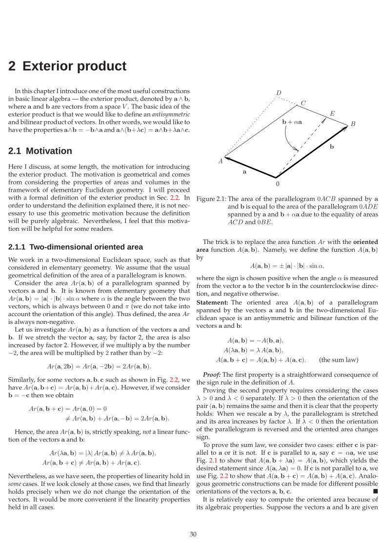
2 Exterior product
In this chapter I introduce one of themost useful constructionsin basic linear algebra — the exterior product, denoted by a∧b,where a and b are vectors from a space V . The basic idea of theexterior product is that we would like to define an antisymmetricand bilinear product of vectors. In other words, wewould like tohave the properties a∧b = −b∧a and a∧(b+λc) = a∧b+λa∧c.
2.1 Motivation
Here I discuss, at some length, the motivation for introducingthe exterior product. The motivation is geometrical and comesfrom considering the properties of areas and volumes in theframework of elementary Euclidean geometry. I will proceedwith a formal definition of the exterior product in Sec. 2.2. Inorder to understand the definition explained there, it is not nec-essary to use this geometric motivation because the definitionwill be purely algebraic. Nevertheless, I feel that this motiva-tion will be helpful for some readers.
2.1.1 Two-dimensional oriented area
We work in a two-dimensional Euclidean space, such as thatconsidered in elementary geometry. We assume that the usualgeometrical definition of the area of a parallelogram is known.Consider the area Ar(a,b) of a parallelogram spanned by
vectors a and b. It is known from elementary geometry thatAr(a,b) = |a| · |b| · sinα where α is the angle between the twovectors, which is always between 0 and π (we do not take intoaccount the orientation of this angle). Thus defined, the area Aris always non-negative.Let us investigate Ar(a,b) as a function of the vectors a and
b. If we stretch the vector a, say, by factor 2, the area is alsoincreased by factor 2. However, if we multiply a by the number−2, the area will be multiplied by 2 rather than by −2:
Ar(a, 2b) = Ar(a,−2b) = 2Ar(a,b).
Similarly, for some vectors a,b, c such as shown in Fig. 2.2, wehaveAr(a,b+c) = Ar(a,b)+Ar(a, c). However, if we considerb = −c then we obtain
Ar(a,b + c) = Ar(a, 0) = 0
6= Ar(a,b) +Ar(a,−b) = 2Ar(a,b).
Hence, the areaAr(a,b) is, strictly speaking, not a linear func-tion of the vectors a and b:
Ar(λa,b) = |λ|Ar(a,b) 6= λAr(a,b),
Ar(a,b + c) 6= Ar(a,b) +Ar(a, c).
Nevertheless, as we have seen, the properties of linearity hold insome cases. If we look closely at those cases, we find that linearlyholds precisely when we do not change the orientation of thevectors. It would be more convenient if the linearity propertiesheld in all cases.
0
A
B
D
C
E
b
a
b + αa
Figure 2.1: The area of the parallelogram 0ACB spanned by a
and b is equal to the area of the parallelogram 0ADEspanned by a and b +αa due to the equality of areasACD and 0BE.
The trick is to replace the area function Ar with the orientedarea function A(a,b). Namely, we define the function A(a,b)by
A(a,b) = ± |a| · |b| · sinα,
where the sign is chosen positive when the angle α is measuredfrom the vector a to the vector b in the counterclockwise direc-tion, and negative otherwise.
Statement: The oriented area A(a,b) of a parallelogramspanned by the vectors a and b in the two-dimensional Eu-clidean space is an antisymmetric and bilinear function of thevectors a and b:
A(a,b) = −A(b,a),
A(λa,b) = λA(a,b),
A(a,b + c) = A(a,b) +A(a, c). (the sum law)
Proof: The first property is a straightforward consequence ofthe sign rule in the definition of A.Proving the second property requires considering the cases
λ > 0 and λ < 0 separately. If λ > 0 then the orientation of thepair (a,b) remains the same and then it is clear that the propertyholds: When we rescale a by λ, the parallelogram is stretchedand its area increases by factor λ. If λ < 0 then the orientationof the parallelogram is reversed and the oriented area changessign.To prove the sum law, we consider two cases: either c is par-
allel to a or it is not. If c is parallel to a, say c = αa, we useFig. 2.1 to show that A(a,b + λa) = A(a,b), which yields thedesired statement since A(a, λa) = 0. If c is not parallel to a, weuse Fig. 2.2 to show that A(a,b + c) = A(a,b) +A(a, c). Analo-gous geometric constructions can be made for different possibleorientations of the vectors a, b, c. �
It is relatively easy to compute the oriented area because ofits algebraic properties. Suppose the vectors a and b are given
30
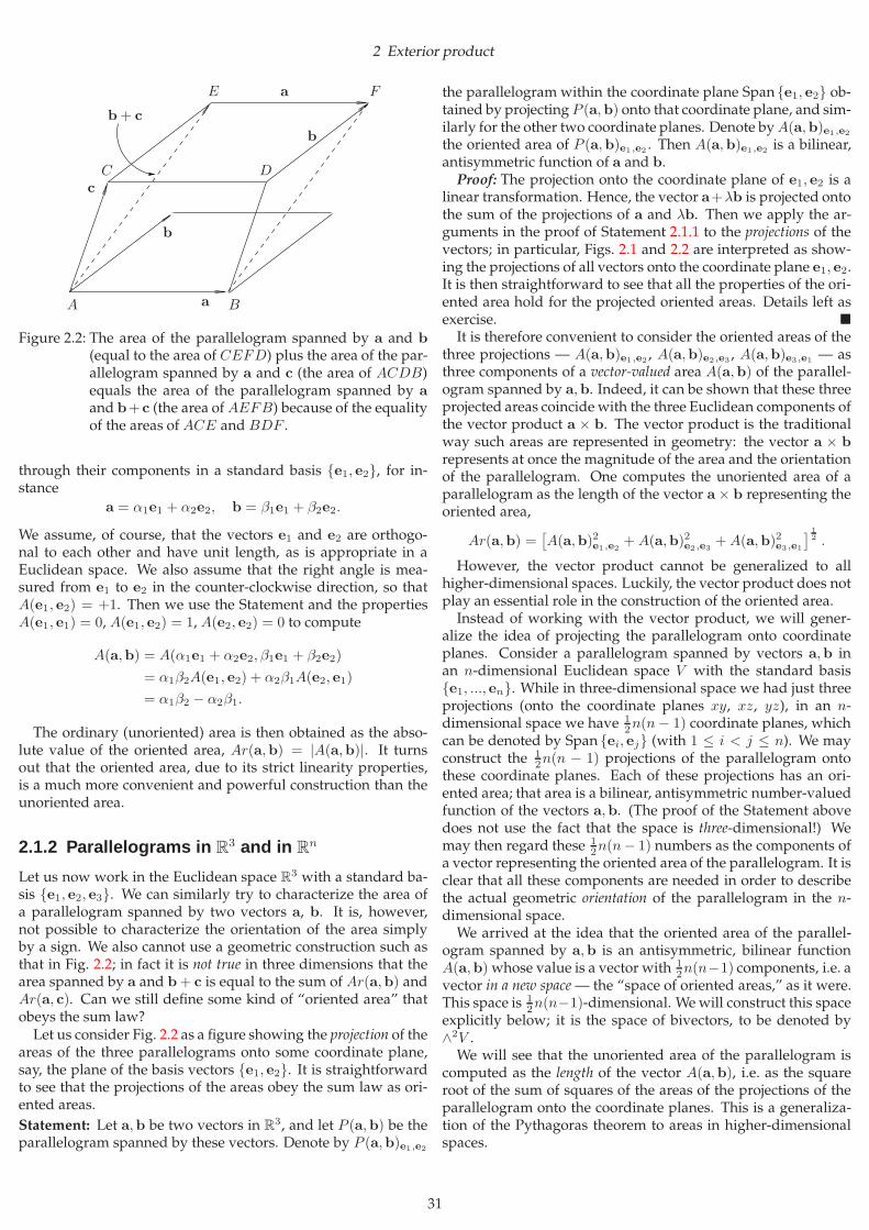
2 Exterior product
A B
DC
FE
a
a
b
b
c
b + c
Figure 2.2: The area of the parallelogram spanned by a and b
(equal to the area of CEFD) plus the area of the par-allelogram spanned by a and c (the area of ACDB)equals the area of the parallelogram spanned by a
and b+c (the area ofAEFB) because of the equalityof the areas of ACE and BDF .
through their components in a standard basis {e1, e2}, for in-stance
a = α1e1 + α2e2, b = β1e1 + β2e2.
We assume, of course, that the vectors e1 and e2 are orthogo-nal to each other and have unit length, as is appropriate in aEuclidean space. We also assume that the right angle is mea-sured from e1 to e2 in the counter-clockwise direction, so thatA(e1, e2) = +1. Then we use the Statement and the propertiesA(e1, e1) = 0, A(e1, e2) = 1, A(e2, e2) = 0 to compute
A(a,b) = A(α1e1 + α2e2, β1e1 + β2e2)
= α1β2A(e1, e2) + α2β1A(e2, e1)
= α1β2 − α2β1.
The ordinary (unoriented) area is then obtained as the abso-lute value of the oriented area, Ar(a,b) = |A(a,b)|. It turnsout that the oriented area, due to its strict linearity properties,is a much more convenient and powerful construction than theunoriented area.
2.1.2 Parallelograms in R3 and in Rn
Let us now work in the Euclidean space R3 with a standard ba-sis {e1, e2, e3}. We can similarly try to characterize the area ofa parallelogram spanned by two vectors a, b. It is, however,not possible to characterize the orientation of the area simplyby a sign. We also cannot use a geometric construction such asthat in Fig. 2.2; in fact it is not true in three dimensions that thearea spanned by a and b + c is equal to the sum of Ar(a,b) andAr(a, c). Can we still define some kind of “oriented area” thatobeys the sum law?Let us consider Fig. 2.2 as a figure showing the projection of the
areas of the three parallelograms onto some coordinate plane,say, the plane of the basis vectors {e1, e2}. It is straightforwardto see that the projections of the areas obey the sum law as ori-ented areas.
Statement: Let a,b be two vectors in R3, and let P (a,b) be theparallelogram spanned by these vectors. Denote by P (a,b)e1,e2
the parallelogram within the coordinate plane Span {e1, e2} ob-tained by projecting P (a,b) onto that coordinate plane, and sim-ilarly for the other two coordinate planes. Denote byA(a,b)e1,e2
the oriented area of P (a,b)e1,e2. Then A(a,b)e1,e2
is a bilinear,antisymmetric function of a and b.Proof: The projection onto the coordinate plane of e1, e2 is a
linear transformation. Hence, the vector a+λb is projected ontothe sum of the projections of a and λb. Then we apply the ar-guments in the proof of Statement 2.1.1 to the projections of thevectors; in particular, Figs. 2.1 and 2.2 are interpreted as show-ing the projections of all vectors onto the coordinate plane e1, e2.It is then straightforward to see that all the properties of the ori-ented area hold for the projected oriented areas. Details left asexercise. �
It is therefore convenient to consider the oriented areas of thethree projections — A(a,b)e1,e2
, A(a,b)e2,e3, A(a,b)e3,e1
— asthree components of a vector-valued area A(a,b) of the parallel-ogram spanned by a,b. Indeed, it can be shown that these threeprojected areas coincide with the three Euclidean components ofthe vector product a × b. The vector product is the traditionalway such areas are represented in geometry: the vector a × b
represents at once the magnitude of the area and the orientationof the parallelogram. One computes the unoriented area of aparallelogram as the length of the vector a × b representing theoriented area,
Ar(a,b) =[A(a,b)2
e1,e2+A(a,b)2
e2,e3+A(a,b)2
e3,e1
] 12 .
However, the vector product cannot be generalized to allhigher-dimensional spaces. Luckily, the vector product does notplay an essential role in the construction of the oriented area.Instead of working with the vector product, we will gener-
alize the idea of projecting the parallelogram onto coordinateplanes. Consider a parallelogram spanned by vectors a,b inan n-dimensional Euclidean space V with the standard basis{e1, ..., en}. While in three-dimensional space we had just threeprojections (onto the coordinate planes xy, xz, yz), in an n-dimensional space we have 1
2n(n− 1) coordinate planes, whichcan be denoted by Span {ei, ej} (with 1 ≤ i < j ≤ n). We mayconstruct the 1
2n(n − 1) projections of the parallelogram ontothese coordinate planes. Each of these projections has an ori-ented area; that area is a bilinear, antisymmetric number-valuedfunction of the vectors a,b. (The proof of the Statement abovedoes not use the fact that the space is three-dimensional!) Wemay then regard these 1
2n(n− 1) numbers as the components ofa vector representing the oriented area of the parallelogram. It isclear that all these components are needed in order to describethe actual geometric orientation of the parallelogram in the n-dimensional space.We arrived at the idea that the oriented area of the parallel-
ogram spanned by a,b is an antisymmetric, bilinear functionA(a,b) whose value is a vector with 1
2n(n−1) components, i.e. avector in a new space— the “space of oriented areas,” as it were.This space is 1
2n(n−1)-dimensional. Wewill construct this spaceexplicitly below; it is the space of bivectors, to be denoted by∧2V .We will see that the unoriented area of the parallelogram is
computed as the length of the vector A(a,b), i.e. as the squareroot of the sum of squares of the areas of the projections of theparallelogram onto the coordinate planes. This is a generaliza-tion of the Pythagoras theorem to areas in higher-dimensionalspaces.
31
2 Exterior product
The analogy between ordinary vectors and vector-valued ar-eas can be understood visually as follows. A straight linesegment in an n-dimensional space is represented by a vectorwhose n components (in an orthonormal basis) are the signedlengths of the n projections of the line segment onto the coor-dinate axes. (The components are signed, or oriented, i.e. takenwith a negative sign if the orientation of the vector is oppositeto the orientation of the axis.) The length of a straight line seg-
ment, i.e. the length of the vector v, is then computed as√
〈v,v〉.The scalar product 〈v,v〉 is equal to the sum of squared lengthsof the projections because we are using an orthonormal basis.A parallelogram in space is represented by a vector ψ whose(n2
)components are the oriented areas of the
(n2
)projections of
the parallelogram onto the coordinate planes. (The vector ψ be-longs to the space of oriented areas, not to the original n-dimen-sional space.) The numerical value of the area of the parallelo-
gram is then computed as√
〈ψ, ψ〉. The scalar product 〈ψ, ψ〉 inthe space of oriented areas is equal to the sum of squared areasof the projections because the
(n2
)unit areas in the coordinate
planes are an orthonormal basis (according to the definition ofthe scalar product in the space of oriented areas).The generalization of the Pythagoras theorem holds not only
for areas but also for higher-dimensional volumes. A generalproof of this theorem will be given in Sec. 5.5.2, using the ex-terior product and several other constructions to be developedbelow.
2.2 Exterior product
In the previous section I motivated the introduction of the anti-symmetric product by showing its connection to areas and vol-umes. In this section I will give the definition and work outthe properties of the exterior product in a purely algebraic man-ner, without using any geometric intuition. This will enable usto work with vectors in arbitrary dimensions, to obtain manyuseful results, and eventually also to appreciate more fully thegeometric significance of the exterior product.As explained in Sec. 2.1.2, it is possible to represent the ori-
ented area of a parallelogram by a vector in some auxiliaryspace. The oriented area is much more convenient to work withbecause it is a bilinear function of the vectors a and b (this isexplained in detail in Sec. 2.1). “Product” is another word for“bilinear function.” We have also seen that the oriented area isan antisymmetric function of the vectors a and b.In three dimensions, an oriented area is represented by the
cross product a × b, which is indeed an antisymmetric and bi-linear product. So we expect that the oriented area in higher di-mensions can be represented by some kind of new antisymmet-ric product of a and b; let us denote this product (to be definedbelow) by a ∧ b, pronounced “a wedge b.” The value of a ∧ b
will be a vector in a new vector space. We will also construct thisnew space explicitly.
2.2.1 Definition of exterior product
Like the tensor product space, the space of exterior products canbe defined solely by its algebraic properties. We can considerthe space of formal expressions like a ∧ b, 3a ∧ b + 2c ∧ d, etc.,and require the properties of an antisymmetric, bilinear productto hold.
Here is a more formal definition of the exterior product space:We will construct an antisymmetric product “by hand,” usingthe tensor product space.Definition 1: Given a vector space V , we define a new vectorspace V ∧ V called the exterior product (or antisymmetric ten-sor product, or alternating product, or wedge product) of twocopies of V . The space V ∧V is the subspace in V ⊗V consistingof all antisymmetric tensors, i.e. tensors of the form
v1 ⊗ v2 − v2 ⊗ v1, v1,2 ∈ V,
and all linear combinations of such tensors. The exterior productof two vectors v1 and v2 is the expression shown above; it isobviously an antisymmetric and bilinear function of v1 and v2.For example, here is one particular element from V ∧V , which
we write in two different ways using the axioms of the tensorproduct:
(u + v) ⊗ (v + w) − (v + w) ⊗ (u + v) = u⊗ v − v ⊗ u
+u⊗ w − w ⊗ u + v ⊗ w − w ⊗ v ∈ V ∧ V. (2.1)
Remark: A tensor v1 ⊗ v2 ∈ V ⊗ V is not equal to the ten-sor v2 ⊗ v1 if v1 6= v2. This is so because there is no identityamong the axioms of the tensor product that would allow us toexchange the factors v1 and v2 in the expression v1 ⊗ v2.
Exercise 1: Prove that the “exchange map” T (v1 ⊗ v2) ≡ v2 ⊗v1 is a canonically defined, linear map of V ⊗V into itself. Show
that T has only two eigenvalues which are ±1. Give examplesof eigenvectors with eigenvalues +1 and−1. Show that the sub-space V ∧V ⊂ V ⊗V is the eigenspace of the exchange operator
T with eigenvalue −1
Hint: T T = 1V ⊗V . Consider tensors of the form u⊗ v±v⊗u
as candidate eigenvectors of T . �
It is quite cumbersome to perform calculations in the tensorproduct notation as we did in Eq. (2.1). So let us write the exte-rior product as u∧v instead of u⊗v−v⊗u. It is then straight-forward to see that the “wedge” symbol ∧ indeed works like ananti-commutative multiplication, as we intended. The rules ofcomputation are summarized in the following statement.Statement 1: One may save time and write u ⊗ v − v ⊗ u ≡u ∧ v ∈ V ∧ V , and the result of any calculation will be correct,as long as one follows the rules:
u ∧ v = −v ∧ u, (2.2)
(λu) ∧ v = λ (u ∧ v) , (2.3)
(u + v) ∧ x = u ∧ x + v ∧ x. (2.4)
It follows also that u ∧ (λv) = λ (u ∧ v) and that v ∧ v = 0.(These identities hold for any vectors u,v ∈ V and any scalarsλ ∈ K.)Proof: These properties are direct consequences of the axioms
of the tensor product when applied to antisymmetric tensors.For example, the calculation (2.1) now requires a simple expan-sion of brackets,
(u + v) ∧ (v + w) = u ∧ v + u ∧w + v ∧ w.
Here we removed the term v ∧ v which vanishes due to the an-tisymmetry of ∧. Details left as exercise. �
Elements of the space V ∧ V , such as a ∧ b + c ∧ d, are some-times called bivectors.1 We will also want to define the exterior1It is important to note that a bivector is not necessarily expressible as a single-term product of two vectors; see the Exercise at the end of Sec. 2.3.2.
32
2 Exterior product
product of more than two vectors. To define the exterior prod-uct of three vectors, we consider the subspace of V ⊗ V ⊗ V thatconsists of antisymmetric tensors of the form
a ⊗ b⊗ c − b⊗ a⊗ c + c ⊗ a ⊗ b − c⊗ b ⊗ a
+b⊗ c ⊗ a − a⊗ c ⊗ b (2.5)
and linear combinations of such tensors. These tensors are calledtotally antisymmetric because they can be viewed as (tensor-valued) functions of the vectors a,b, c that change sign underexchange of any two vectors. The expression in Eq. (2.5) will bedenoted for brevity by a∧b∧c, similarly to the exterior productof two vectors, a ⊗ b − b ⊗ a, which is denoted for brevity bya ∧ b. Here is a general definition.
Definition 2: The exterior product of k copies of V (also calledthe k-th exterior power of V ) is denoted by ∧kV and is de-fined as the subspace of totally antisymmetric tensors withinV ⊗ ... ⊗ V . In the concise notation, this is the space spannedby expressions of the form
v1 ∧ v2 ∧ ... ∧ vk, vj ∈ V,
assuming that the properties of thewedge product (linearity andantisymmetry) hold as given by Statement 1. For instance,
u ∧ v1 ∧ ... ∧ vk = (−1)kv1 ∧ ... ∧ vk ∧ u (2.6)
(“pulling a vector through k other vectors changes sign ktimes”). �
The previously defined space of bivectors is in this notationV ∧ V ≡ ∧2V . A natural extension of this notation is ∧0V = Kand ∧1V = V . I will also use the following “wedge product”notation,
n∧
k=1
vk ≡ v1 ∧ v2 ∧ ... ∧ vn.
Tensors from the space ∧nV are also called n-vectors or anti-symmetric tensors of rank n.
Question: How to compute expressions containing multipleproducts such as a ∧ b ∧ c?
Answer: Apply the rules shown in Statement 1. For example,one can permute adjacent vectors and change sign,
a ∧ b ∧ c = −b ∧ a ∧ c = b ∧ c ∧ a,
one can expand brackets,
a ∧ (x + 4y) ∧ b = a ∧ x ∧ b + 4a ∧ y ∧ b,
and so on. If the vectors a,b, c are given as linear combinationsof some basis vectors {ej}, we can thus reduce a ∧ b ∧ c to alinear combination of exterior products of basis vectors, such ase1 ∧ e2 ∧ e3, e1 ∧ e2 ∧ e4, etc.
Question: The notation a∧b∧c suggests that the exterior prod-uct is associative,
a ∧ b ∧ c = (a ∧ b) ∧ c = a ∧ (b ∧ c).
How can we make sense of this?
Answer: If we want to be pedantic, we need to define the ex-terior product operation ∧ between a single-term bivector a ∧ b
and a vector c, such that the result is by definition the 3-vectora∧b∧ c. We then define the same operation on linear combina-tions of single-term bivectors,
(a ∧ b + x ∧ y) ∧ c ≡ a ∧ b ∧ c + x ∧ y ∧ c.
Thus we have defined the exterior product between ∧2V and V ,the result being a 3-vector from ∧3V . We then need to verifythat the results do not depend on the choice of the vectors suchas a,b,x,y in the representation of a bivector: A different rep-resentation can be achieved only by using the properties of theexterior product (i.e. the axioms of the tensor product), e.g. wemay replace a ∧ b by −b ∧ (a + λb). It is easy to verify that anysuch replacements will not modify the resulting 3-vector, e.g.
a ∧ b ∧ c = −b ∧ (a + λb) ∧ c,
again due to the properties of the exterior product. This consid-eration shows that calculations with exterior products are con-sistent with our algebraic intuition. We may indeed computea ∧ b ∧ c as (a ∧ b) ∧ c or as a ∧ (b ∧ c).Example 1: Suppose we work in R3 and have vectors a =(0, 1
2 ,− 12
), b = (2,−2, 0), c = (−2, 5,−3). Let us compute var-
ious exterior products. Calculations are easier if we introducethe basis {e1, e2, e3} explicitly:
a =1
2(e2 − e3) , b = 2(e1 − e2), c = −2e1 + 5e2 − 3e3.
We compute the 2-vector a ∧ b by using the properties of theexterior product, such as x ∧ x = 0 and x ∧ y = −y ∧ x, andsimply expanding the brackets as usual in algebra:
a ∧ b =1
2(e2 − e3) ∧ 2 (e1 − e2)
= (e2 − e3) ∧ (e1 − e2)
= e2 ∧ e1 − e3 ∧ e1 − e2 ∧ e2 + e3 ∧ e2
= −e1 ∧ e2 + e1 ∧ e3 − e2 ∧ e3.
The last expression is the result; note that now there is nothingmore to compute or to simplify. The expressions such as e1 ∧ e2
are the basic expressions out of which the space R3 ∧ R3 is built.Below (Sec. 2.3.2) we will show formally that the set of theseexpressions is a basis in the space R3 ∧ R3.Let us also compute the 3-vector a ∧ b ∧ c,
a ∧ b ∧ c = (a ∧ b) ∧ c
= (−e1 ∧ e2 + e1 ∧ e3 − e2 ∧ e3) ∧ (−2e1 + 5e2 − 3e3).
When we expand the brackets here, terms such as e1 ∧ e2 ∧ e1
will vanish because
e1 ∧ e2 ∧ e1 = −e2 ∧ e1 ∧ e1 = 0,
so only terms containing all different vectors need to be kept,and we find
a ∧ b ∧ c = 3e1 ∧ e2 ∧ e3 + 5e1 ∧ e3 ∧ e2 + 2e2 ∧ e3 ∧ e1
= (3 − 5 + 2) e1 ∧ e2 ∧ e3 = 0.
We note that all the terms are proportional to the 3-vector e1 ∧e2∧e3, so only the coefficient in front of e1∧e2∧e3 was needed;then, by coincidence, that coefficient turned out to be zero. Sothe result is the zero 3-vector. �
33
2 Exterior product
Question: Our original goal was to introduce a bilinear, anti-symmetric product of vectors in order to obtain a geometric rep-resentation of oriented areas. Instead, a ∧ b was defined alge-braically, through tensor products. It is clear that a ∧ b is anti-symmetric and bilinear, but why does it represent an orientedarea?Answer: Indeed, it may not be immediately clear why ori-
ented areas should be elements of V ∧ V . We have seen thatthe oriented area A(x,y) is an antisymmetric and bilinear func-tion of the two vectors x and y. Right now we have constructedthe space V ∧ V simply as the space of antisymmetric products.By constructing that space merely out of the axioms of the an-tisymmetric product, we already covered every possible bilinearantisymmetric product. This means that any antisymmetric andbilinear function of the two vectors x and y is proportional tox ∧ y or, more generally, is a linear function of x ∧ y (perhapswith values in a different space). Therefore, the space of orientedareas (that is, the space of linear combinations ofA(x,y) for var-ious x and y) is in any case mapped to a subspace of V ∧ V .We have also seen that oriented areas in N dimensions can berepresented through
(N2
)projections, which indicates that they
are vectors in some(N2
)-dimensional space. We will see below
that the space V ∧ V has exactly this dimension (Theorem 2 inSec. 2.3.2). Therefore, we can expect that the space of orientedareas coincides with V ∧V . Below we will be working in a spaceV with a scalar product, where the notions of area and volumeare well defined. Then we will see (Sec. 5.5.2) that tensors fromV ∧ V and the higher exterior powers of V indeed correspondin a natural way to oriented areas, or more generally to orientedvolumes of a certain dimension.Remark: Origin of the name “exterior.” The construction ofthe exterior product is a modern formulation of the ideas dat-ing back to H. Grassmann (1844). A 2-vector a ∧ b is inter-preted geometrically as the oriented area of the parallelogramspanned by the vectors a and b. Similarly, a 3-vector a ∧ b ∧ c
represents the oriented 3-volume of a parallelepiped spannedby {a,b, c}. Due to the antisymmetry of the exterior product,we have (a∧b)∧(a∧c) = 0, (a∧b∧c)∧(b∧d) = 0, etc. We caninterpret this geometrically by saying that the “product” of twovolumes is zero if these volumes have a vector in common. Thismotivated Grassmann to call his antisymmetric product “exte-rior.” In his reasoning, the product of two “extensive quantities”(such as lines, areas, or volumes) is nonzero only when each ofthe two quantities is geometrically “to the exterior” (outside) ofthe other.Exercise 2: Show that in a two-dimensional space V , any 3-vector such as a ∧ b ∧ c can be simplified to the zero 3-vector.Prove the same for n-vectors in N -dimensional spaces whenn > N . �
One can also consider the exterior powers of the dual spaceV ∗. Tensors from ∧nV ∗ are usually (for historical reasons) calledn-forms (rather than “n-covectors”).Question: Where is the star here, really? Is the space ∧n (V ∗)different from (∧nV )
∗?
Answer: Good that you asked. These spaces are canonicallyisomorphic, but there is a subtle technical issue worth mention-ing. Consider an example: a∗ ∧ b∗ ∈ ∧2(V ∗) can act uponu∧v ∈ ∧2V by the standard tensor product rule, namely a∗⊗b∗
acts on u ⊗ v as
(a∗ ⊗ b∗) (u⊗ v) = a∗(u)b∗(v),
so by using the definition of a∗∧b∗ and u∧v through the tensorproduct, we find
(a∗ ∧ b∗) (u ∧ v) = (a∗ ⊗ b∗ − b∗ ⊗ a∗) (u⊗ v − v ⊗ u)
= 2a∗(u)b∗(v) − 2b∗(u)a∗(v).
We got a combinatorial factor 2, that is, a factor that arises be-cause we have two permutations of the set (a,b). With ∧n (V ∗)and (∧nV )∗ we get a factor n!. It is not always convenient tohave this combinatorial factor. For example, in a finite numberfield the number n! might be equal to zero for large enough n. Inthese cases we could redefine the action of a∗ ∧ b∗ on u ∧ v as
(a∗ ∧ b∗) (u ∧ v) ≡ a∗(u)b∗(v) − b∗(u)a∗(v).
If we are not working in a finite number field, we are able todivide by any integer, so we may keep combinatorial factors inthe denominators of expressions where such factors appear. Forexample, if {ej} is a basis in V and ω = e1 ∧ ... ∧ eN is thecorresponding basis tensor in the one-dimensional space ∧NV ,
the dual basis tensor in(∧NV
)∗could be defined by
ω∗ =1
N !e∗1 ∧ ... ∧ e∗N , so that ω∗(ω) = 1.
The need for such combinatorial factors is a minor technical in-convenience that does not arise too often. We may give the fol-lowing definition that avoids dividing by combinatorial factors(but now we use permutations; see Appendix B).Definition 3: The action of a k-form f∗1 ∧ ... ∧ f∗k on a k-vectorv1 ∧ ... ∧ vk is defined by
∑
σ
(−1)|σ|f∗1 (vσ(1))...f∗k (vσ(k)),
where the summation is performed over all permutations σ ofthe ordered set (1, ..., k).Example 2: With k = 3 we have
(p∗ ∧ q∗ ∧ r∗)(a ∧ b ∧ c)
= p∗(a)q∗(b)r∗(c) − p∗(b)q∗(a)r∗(c)
+ p∗(b)q∗(c)r∗(a) − p∗(c)q∗(b)r∗(a)
+ p∗(c)q∗(a)r∗(b) − p∗(c)q∗(b)r∗(a).
Exercise 3: a) Show that a ∧ b ∧ ω = ω ∧ a ∧ b where ω is anyantisymmetric tensor (e.g. ω = x ∧ y ∧ z).b) Show that
ω1 ∧ a ∧ ω2 ∧ b ∧ ω3 = −ω1 ∧ b ∧ ω2 ∧ a ∧ ω3,
where ω1, ω2, ω3 are arbitrary antisymmetric tensors and a,b arevectors.c) Due to antisymmetry, a ∧ a = 0 for any vector a ∈ V . Is it
also true that ω ∧ ω = 0 for any bivector ω ∈ ∧2V ?
2.2.2 * Symmetric tensor product
Question: At this point it is still unclear why the antisymmetricdefinition is at all useful. Perhaps we could define somethingelse, say the symmetric product, instead of the exterior product?We could try to define a product, say a ⊙ b, with some otherproperty, such as
a⊙ b = 2b⊙ a.
34
2 Exterior product
Answer: This does not work because, for example, we wouldhave
b ⊙ a = 2a⊙ b = 4b⊙ a,
so all the “⊙” products would have to vanish.
We can define the symmetric tensor product, ⊗S , with theproperty
a ⊗S b = b ⊗S a,
but it is impossible to define anything else in a similar fashion.2
The antisymmetric tensor product is the eigenspace (within
V ⊗ V ) of the exchange operator T with eigenvalue −1. Thatoperator has only eigenvectors with eigenvalues ±1, so the onlyother possibility is to consider the eigenspace with eigenvalue+1. This eigenspace is spanned by symmetric tensors of theform u⊗ v + v ⊗ u, and can be considered as the space of sym-metric tensor products. We could write
a ⊗S b ≡ a ⊗ b + b ⊗ a
and develop the properties of this product. However, it turnsout that the symmetric tensor product is much less useful forthe purposes of linear algebra than the antisymmetric subspace.This book derives most of the results of linear algebra using theantisymmetric product as the main tool!
2.3 Properties of spaces ∧kVAswe have seen, tensors from the space V ⊗V are representableby linear combinations of the form a ⊗ b + c ⊗ d + ..., but notuniquely representable because one can transform one such lin-ear combination into another by using the axioms of the tensorproduct. Similarly, n-vectors are not uniquely representable bylinear combinations of exterior products. For example,
a ∧ b + a ∧ c + b ∧ c = (a + b) ∧ (b + c)
since b∧b = 0. In other words, the 2-vectorω ≡ a∧b+a∧c+b∧c
has an alternative representation containing only a single-termexterior product, ω = r ∧ s where r = a + b and s = b + c.
Exercise: Show that any 2-vector in a three-dimensional space isrepresentable by a single-term exterior product, i.e. to a 2-vectorof the form a ∧ b.Hint: Choose a basis {e1, e2, e3} and show that αe1∧e2+βe1∧
e3 + γe2 ∧ e3 is equal to a single-term product. �
What about higher-dimensional spaces? We will show (seethe Exercise at the end of Sec. 2.3.2) that n-vectors cannot be ingeneral reduced to a single-term product. This is, however, al-ways possible for (N − 1)-vectors in an N -dimensional space.(You showed this for N = 3 in the exercise above.)
Statement: Any (N − 1)-vector in an N -dimensional space canbe written as a single-term exterior product of the form a1 ∧ ...∧aN−1.Proof: We prove this by using induction inN . The basis of in-
duction isN = 2, where there is nothing to prove. The inductionstep: Suppose that the statement is proved for (N − 1)-vectorsin N -dimensional spaces, we need to prove it for N -vectors in(N +1)-dimensional spaces. Choose a basis {e1, ..., eN+1} in the
2This is a theorem due to Grassmann (1862).
space. AnyN -vector ω can be written as a linear combination ofexterior product terms,
ω = α1e2 ∧ ... ∧ eN+1 + α2e1 ∧ e3 ∧ ... ∧ eN+1 + ...
+ αNe1 ∧ ... ∧ eN−1 ∧ eN+1 + αN+1e1 ∧ ... ∧ eN ,
where {αi} are some constants.Note that any tensor ω ∈ ∧N−1V can be written in this way
simply by expressing every vector through the basis and by ex-panding the exterior products. The result will be a linear combi-nation of the form shown above, containing at mostN+1 single-term exterior products of the form e1 ∧ ... ∧ eN , e2 ∧ ... ∧ eN+1,and so on. We do not yet know whether these single-term exte-rior products constitute a linearly independent set; this will beestablished in Sec. 2.3.2. Presently, we will not need this prop-erty.Now we would like to transform the expression above to a
single term. Wemove eN+1 outside brackets in the firstN terms:
ω =(α1e2 ∧ ... ∧ eN + ...+ αNe1 ∧ ... ∧ eN−1
)∧ eN+1
+ αN+1e1 ∧ ... ∧ eN
≡ ψ ∧ eN+1 + αN+1e1 ∧ ... ∧ eN ,
where in the last line we have introduced an auxiliary (N − 1)-vector ψ. If it happens that ψ = 0, there is nothing left to prove.Otherwise, at least one of the αi must be nonzero; without lossof generality, suppose that αN 6= 0 and rewrite ω as
ω = ψ ∧ eN+1 + αN+1e1 ∧ ... ∧ eN = ψ ∧(eN+1 +
αN+1
αNeN
).
Nowwe note that ψ belongs to the space of (N − 1)-vectors overthe N -dimensional subspace spanned by {e1, ..., eN}. By the in-ductive assumption, ψ can be written as a single-term exteriorproduct, ψ = a1 ∧ ... ∧ aN−1, of some vectors {ai}. Denoting
aN ≡ eN+1 +αN+1
αNeN ,
we obtainω = a1 ∧ ... ∧ aN−1 ∧ aN ,
i.e. ω can be represented as a single-term exterior product. �
2.3.1 Linear maps between spaces ∧kV
Since the spaces ∧kV are vector spaces, we may consider linearmaps between them.A simplest example is a map
La : ω 7→ a ∧ ω,
mapping ∧kV → ∧k+1V ; here the vector a is fixed. It is impor-tant to check that La is a linear map between these spaces. Howdo we check this? We need to check that La maps a linear com-bination of tensors into linear combinations; this is easy to see,
La(ω + λω′) = a ∧ (ω + λω′)
= a ∧ ω + λa ∧ ω′ = Laω + λLaω′.
Let us now fix a covector a∗. A covector is a map V → K. InLemma 2 of Sec. 1.7.3 we have used covectors to define linearmaps a∗ : V ⊗W → W according to Eq. (1.21), mapping v ⊗w 7→ a∗ (v)w. Now we will apply the analogous construction
35
2 Exterior product
to exterior powers and construct a map V ∧ V → V . Let usdenote this map by ιa∗ .It would be incorrect to define the map ιa∗ by the formula
ιa∗(v∧w) = a∗ (v)w because such a definition does not respectthe antisymmetry of the wedge product and thus violates thelinearity condition,
ιa∗ (w ∧ v)!= ιa∗ ((−1)v ∧ w) = −ιa∗ (v ∧ w) 6= a∗(v)w.
So we need to act with a∗ on each of the vectors in a wedge prod-uct and make sure that the correct minus sign comes out. Anacceptable formula for the map ιa∗ : ∧2V → V is
ιa∗ (v ∧ w) ≡ a∗ (v)w − a∗ (w)v.
(Please check that the linearity condition now holds!) This ishow we will define the map ιa∗ on ∧2V .Let us now extend ιa∗ : ∧2V → V to a map
ιa∗ : ∧kV → ∧k−1V,
defined as follows:
ιa∗v ≡ a∗(v),
ιa∗(v ∧ ω) ≡ a∗(v)ω − v ∧ (ιa∗ω). (2.7)
This definition is inductive, i.e. it shows how to define ιa∗ on ∧kVif we know how to define it on ∧k−1V . The action of ιa∗ on a sumof terms is defined by requiring linearity,
ιa∗ (A+ λB) ≡ ιa∗ (A) + λιa∗ (B) , A,B ∈ ∧kV.
We can convert this inductive definition into a more explicitformula: if ω = v1 ∧ ... ∧ vk ∈ ∧kV then
ιa∗(v1 ∧ ... ∧ vk) ≡ a∗(v1)v2 ∧ ... ∧ vk − a∗(v2)v1 ∧ v3 ∧ ... ∧ vk
+ ...+ (−1)k−1
a∗(vk)v1 ∧ ... ∧ vk−1.
This map is called the interior product or the insertion map.This is a useful operation in linear algebra. The insertion mapιa∗ψ “inserts” the covector a∗ into the tensor ψ ∈ ∧kV by actingwith a∗ on each of the vectors in the exterior product that makesup ψ.Let us check formally that the insertion map is linear.
Statement: The map ιa∗ : ∧kV → ∧k−1V for 1 ≤ k ≤ N is awell-defined linear map, according to the inductive definition.Proof: First, we need to check that it maps linear combinations
into linear combinations; this is quite easy to see by induction,using the fact that a∗ : V → K is linear. However, this type oflinearity is not sufficient; we also need to check that the resultof the map, i.e. the tensor ιa∗(ω), is defined independently of therepresentation of ω through vectors such as vi. The problem is,there are many such representations, for example some tensorω ∈ ∧3V might be written using different vectors as
ω = v1 ∧ v2 ∧ v3 = v2 ∧ (v3 − v1) ∧ (v3 + v2) ≡ v1 ∧ v2 ∧ v3.
We need to verify that any such equivalent representation yieldsthe same resulting tensor ιa∗(ω), despite the fact that the defini-tion of ιa∗ appears to depend on the choice of the vectors vi. Onlythen will it be proved that ιa∗ is a linear map ∧kV → ∧k−1V .An equivalent representation of a tensor ω can be obtained
only by using the properties of the exterior product, namely
linearity and antisymmetry. Therefore, we need to verify thatιa∗(ω) does not change when we change the representation of ωin these two ways: 1) expanding a linear combination,
(x + λy) ∧ ... 7→ x ∧ ...+ λy ∧ ...; (2.8)
2) interchanging the order of two vectors in the exterior productand change the sign,
x ∧ y ∧ ... 7→ −y ∧ x ∧ ... (2.9)
It is clear that a∗(x + λy) = a∗(x) + λa∗(y); it follows by induc-tion that ιa∗ω does not change under a change of representationof the type (2.8). Now we consider the change of representationof the type (2.9). We have, by definition of ιa∗ ,
ιa∗(v1 ∧v2∧χ) = a∗(v1)v2 ∧χ−a∗(v2)v1 ∧χ+v1 ∧v2 ∧ ιa∗(χ),
where we have denoted by χ the rest of the exterior product. Itis clear from the above expression that
ιa∗(v1 ∧ v2 ∧ χ) = −ιa∗(v2 ∧ v1 ∧ χ) = ιa∗(−v2 ∧ v1 ∧ χ).
This proves that ιa∗(ω) does not change under a change of rep-resentation of ω of the type (2.9). This concludes the proof. �
Remark: It is apparent from the proof that the minus sign in theinductive definition (2.7) is crucial for the linearity of the mapιa∗ . Indeed, if we attempt to define a map by a formula such as
v1 ∧ v2 7→ a∗(v1)v2 + a∗(v2)v1,
the result will not be a linear map ∧2V → V despite the appear-ance of linearity. The correct formula must take into account thefact that v1 ∧ v2 = −v2 ∧ v1.Exercise: Show by induction in k that
Lxιa∗ω + ιa∗Lxω = a∗(x)ω, ∀ω ∈ ∧kV.
In other words, the linear operator Lxιa∗ + ιa∗Lx : ∧kV → ∧kVis simply the multiplication by the number a∗(x).
2.3.2 Exterior product and linear dependence
The exterior product is useful in many ways. One powerfulproperty of the exterior product is its close relation to linearindependence of sets of vectors. For example, if u = λv thenu ∧ v = 0. More generally:Theorem 1: A set {v1, ...,vk} of vectors from V is linearly inde-pendent if and only if (v1 ∧ v2 ∧ ... ∧ vk) 6= 0, i.e. it is a nonzerotensor from ∧kV .Proof: If {vj} is linearly dependent then without loss of gen-
erality we may assume that v1 is a linear combination of other
vectors, v1 =∑k
j=2 λjvj . Then
v1 ∧ v2 ∧ ... ∧ vk =
k∑
j=2
λjvj ∧ v2 ∧ ... ∧ vj ∧ ... ∧ vk
=
k∑
j=2
(−1)j−1
v2 ∧ ...vj ∧ vj ∧ ... ∧ vk = 0.
Conversely, we need to prove that the tensor v1 ∧ ... ∧ vk 6= 0 if{vj} is linearly independent. The proof is by induction in k. The
36
2 Exterior product
basis of induction is k = 1: if {v1} is linearly independent thenclearly v1 6= 0. The induction step: Assume that the statement isproved for k − 1 and that {v1, ...,vk} is a linearly independentset. By Exercise 1 in Sec. 1.6 there exists a covector f∗ ∈ V ∗ suchthat f∗ (v1) = 1 and f∗ (vi) = 0 for 2 ≤ i ≤ k. Now we applythe interior product map ιf∗ : ∧kV → ∧k−1V constructed inSec. 2.3.1 to the tensor v1 ∧ ... ∧ vk and find
ιf∗ (v1 ∧ ... ∧ vk) = v2 ∧ ... ∧ vk.
By the induction step, the linear independence of k − 1 vectors{v2, ...,vk} entails v2 ∧ ... ∧ vk 6= 0. The map ιf∗ is linear andcannot map a zero tensor into a nonzero tensor, therefore v1 ∧... ∧ vk 6= 0. �
It is also important to know that any tensor from the highestexterior power ∧NV can be represented as just a single-term ex-terior product of N vectors. (Note that the same property for∧N−1V was already established in Sec. 2.3.)Lemma 1: For any tensor ω ∈ ∧NV there exist vectors{v1, ...,vN} such that ω = v1 ∧ ... ∧ vN .Proof: If ω = 0 then there is nothing to prove, so we assume
ω 6= 0. By definition, the tensor ω has a representation as a sumof several exterior products, say
ω = v1 ∧ ... ∧ vN + v′1 ∧ ... ∧ v′
N + ...
Let us simplify this expression to just one exterior product. First,let us omit any zero terms in this expression (for instance, a∧a∧b ∧ ... = 0). Then by Theorem 1 the set {v1, ...,vN} is linearlyindependent (or else the term v1∧...∧vN would be zero). Hence,{v1, ...,vN} is a basis in V . All other vectors such as v′
i can bedecomposed as linear combinations of vectors in that basis. Letus denote ψ ≡ v1∧...∧vN . By expanding the brackets in exteriorproducts such as v′
1 ∧ ... ∧ v′N , we will obtain every time the
tensor ψ with different coefficients. Therefore, the final resultof simplification will be that ω equals ψ multiplied with somecoefficient. This is sufficient to prove Lemma 1. �
Now we would like to build a basis in the space ∧mV . Forthis we need to determine which sets of tensors from ∧mV arelinearly independent within that space.Lemma 2: If {e1, ..., eN} is a basis in V then any tensor A ∈∧mV can be decomposed as a linear combination of the tensorsek1
∧ ek2∧ ... ∧ ekm
with some indices kj , 1 ≤ j ≤ m.Proof: The tensor A is a linear combination of expressions of
the form v1∧...∧vm, and each vector vi ∈ V can be decomposedin the basis {ej}. Expanding the brackets around the wedgesusing the rules (2.2)–(2.4), we obtain a decomposition of an arbi-trary tensor through the basis tensors. For example,
(e1 + 2e2) ∧ (e1 − e2 + e3) − 2 (e2 − e3) ∧ (e1 − e3)
= −e1 ∧ e2 − e1 ∧ e3 + 4e2 ∧ e3
(please verify this yourself!). �
By Theorem 1, all tensors ek1∧ ek2
∧ ... ∧ ekmconstructed out
of subsets of vectors from the basis {e1, ..., ek} are nonzero, andby Lemma 2 any tensor can be decomposed into a linear combi-nation of these tensors. But are these tensors a basis in the space∧mV ? Yes:Lemma 3: If {v1, ...,vn} is a linearly independent set of vectors(not necessarily a basis in V since n ≤ N ), then:(1) The set of
(n2
)tensors
{vj ∧ vk, 1 ≤ j < k ≤ n} ≡ {v1 ∧ v2,v1 ∧ v3, ...,vn−1 ∧ vn}
is linearly independent in the space ∧2V .(2) The set of
(nm
)tensors
{vk1∧ vk2
∧ ... ∧ vkm, 1 ≤ k1 < k2 < ... < km ≤ n}
is linearly independent in the space ∧mV for 2 ≤ m ≤ n.Proof: (1) The proof is similar to that of Lemma 3 in Sec. 1.7.3.
Suppose the set {vj} is linearly independent but the set{vj ∧ vk} is linearly dependent, so that there exists a linear com-bination ∑
1≤j<k≤n
λjkvj ∧ vk = 0
with at least some λjk 6= 0. Without loss of generality, λ12 6= 0(or else we can renumber the vectors vj). There exists a covectorf∗ ∈ V ∗ such that f∗ (v1) = 1 and f∗ (vi) = 0 for 2 ≤ i ≤n. Apply the interior product with this covector to the abovetensor,
0 = ιf∗
∑
1≤j<k≤n
λjkvj ∧ vk
=n∑
k=2
λ1kvk,
therefore by linear independence of {vk} all λ1k = 0, contradict-ing the assumption λ12 6= 0.(2) The proof of part (1) is straightforwardly generalized to the
space ∧mV , using induction inm. We have just proved the basisof induction, m = 2. Now the induction step: assume that thestatement is proved form−1 and consider a set {vk1
∧ ... ∧ vkm},
of tensors of rankm, where {vj} is a basis. Suppose that this setis linearly dependent; then there is a linear combination
ω ≡∑
k1,...,km
λk1...kmvk1
∧ ... ∧ vkm= 0
with some nonzero coefficients, e.g. λ12...m 6= 0. There exists acovector f∗ such that f∗ (v1) = 1 and f∗ (vi) = 0 for 2 ≤ i ≤ n.Apply this covector to the tensor ω and obtain ιf∗ω = 0, whichyields a vanishing linear combination of tensors vk1
∧ ...∧vkm−1
of rank m − 1 with some nonzero coefficients. But this contra-dicts the induction assumption, which says that any set of ten-sors vk1
∧ ... ∧ vkm−1of rankm− 1 is linearly independent. �
Now we are ready to compute the dimension of ∧mV .Theorem 2: The dimension of the space ∧mV is
dim∧mV =
(N
m
)
=N !
m! (N −m)!,
where N ≡ dimV . For m > N we have dim∧mV = 0, i.e. thespaces ∧mV form > N consist solely of the zero tensor.Proof: We will explicitly construct a basis in the space ∧mV .
First choose a basis {e1, ..., eN} in V . By Lemma 3, the set of(Nm
)
tensors
{ek1∧ ek2
∧ ... ∧ ekm, 1 ≤ k1 < k2 < ... < km ≤ N}
is linearly independent, and by Lemma 2 any tensor A ∈ ∧mVis a linear combination of these tensors. Therefore the set{ek1
∧ ek2∧ ... ∧ ekm
} is a basis in ∧mV . By Theorem 1.1.5, thedimension of space is equal to the number of vectors in any ba-
sis, therefore dim∧mN =(Nm
).
For m > N , the existence of a nonzero tensor v1 ∧ ... ∧ vm
contradicts Theorem 1: The set {v1, ...,vm} cannot be linearlyindependent since it has more vectors than the dimension of thespace. Therefore all such tensors are equal to zero (more pedan-tically, to the zero tensor), which is thus the only element of ∧mVfor everym > N . �
37
2 Exterior product
Exercise 1: It is given that the set of four vectors {a,b, c,d} islinearly independent. Show that the tensor ω ≡ a ∧ b + c ∧ d ∈∧2V cannot be equal to a single-term exterior product of the formx ∧ y.Outline of solution:1. Constructive solution. There exists f∗ ∈ V ∗ such that
f∗(a) = 1 and f∗(b) = 0, f∗(c) = 0, f∗(d) = 0. Computeιf∗ω = b. If ω = x ∧ y, it will follow that a linear combinationof x and y is equal to b, i.e. b belongs to the two-dimensionalspace Span {x,y}. Repeat this argument for the remaining threevectors (a, c, d) and obtain a contradiction.2. Non-constructive solution. Compute ω ∧ ω = 2a ∧ b ∧ c ∧
d 6= 0 by linear independence of {a,b, c,d}. If we could expressω = x ∧ y then we would have ω ∧ ω = 0. �
Remark: While a∧b is interpreted geometrically as the orientedarea of a parallelogram spanned by a and b, a general linearcombination such as a ∧ b + c ∧ d + e ∧ f does not have thisinterpretation (unless it can be reduced to a single-term productx∧y). If not reducible to a single-term product, a∧b+c∧d canbe interpreted only as a formal linear combination of two areas.Exercise 2: Suppose that ψ ∈ ∧kV and x ∈ V are such thatx ∧ ψ = 0 while x 6= 0. Show that there exists χ ∈ ∧k−1Vsuch that ψ = x ∧ χ. Give an example where ψ and χ are notrepresentable as a single-term exterior product.Outline of solution: There exists f∗ ∈ V ∗ such that f∗(x) = 1.
Apply ιf∗ to the given equality x ∧ ψ = 0:
0!= ιf∗(x ∧ ψ) = ψ − x ∧ ιf∗ψ,
which means that ψ = x ∧ χ with χ ≡ ιf∗ψ. An example can befound with χ = a ∧ b + c ∧ d as in Exercise 1, and x such thatthe set {a,b, c,d,x} is linearly independent; then ψ ≡ x ∧ ψ isalso not reducible to a single-term product.
2.3.3 Computing the dual basis
The exterior product allows us to compute explicitly the dualbasis for a given basis.We begin with some motivation. Suppose {v1, ...,vN} is a
given basis; we would like to compute its dual basis. For in-stance, the covector v∗
1 of the dual basis is the linear functionsuch that v∗
1(x) is equal to the coefficient at v1 in the decompo-sition of x in the basis {vj},
x =N∑
i=1
xivi; v∗1(x) = x1.
We start from the observation that the tensor ω ≡ v1 ∧ ...∧vN isnonzero since {vj} is a basis. The exterior product x∧v2∧...∧vN
is equal to zero if x is a linear combination only of v2, ..., vN ,with a zero coefficient x1. This suggests that the exterior productof x with the (N − 1)-vector v2 ∧ ... ∧ vN is quite similar to thecovector v∗
1 we are looking for. Indeed, let us compute
x ∧ v2 ∧ ... ∧ vN = x1v1 ∧ v2 ∧ ... ∧ vN = x1ω.
Therefore, exterior multiplication with v2 ∧ ... ∧ vN acts quitesimilarly to v∗
1 . To make the notation more concise, let us intro-duce a special complement operation3 denoted by a star:
∗ (v1) ≡ v2 ∧ ... ∧ vN .
3The complement operation was introduced by H. Grassmann (1844).
Thenwe canwrite v∗1(x)ω = x∧∗(v1). This equation can be used
for computing v∗1 : namely, for any x ∈ V the number v∗
1(x) isequal to the constant λ in the equation x ∧ ∗(v1) = λω. To makethis kind of equation more convenient, let us write
λ ≡ v∗1(x) =
x ∧ v2 ∧ ... ∧ vN
v1 ∧ v2 ∧ ... ∧ vN=
x ∧ ∗(v1)
ω,
where the “division” of one tensor by another is to be under-stood as follows: We first compute the tensor x ∧ ∗(v1); thistensor is proportional to the tensor ω since both belong to theone-dimensional space ∧NV , so we can determine the numberλ such that x ∧ ∗(v1) = λω; the proportionality coefficient λ isthen the result of the division of x ∧ ∗(v1) by ω.For v2 we have
v1 ∧ x ∧ v3 ∧ ... ∧ vN = x2ω = v∗2(x)ω.
If we would like to have x2ω = x ∧ ∗(v2), we need to add anextra minus sign and define
∗ (v2) ≡ −v1 ∧ v3 ∧ ... ∧ vN .
Then we indeed obtain v∗2(x)ω = x ∧ ∗(v2).
It is then clear that we can define the tensors ∗(vi) for i =1, ..., N in this way. The tensor ∗(vi) is obtained from ω by re-moving the vector vi and by adding a sign that corresponds toshifting the vector vi to the left position in the exterior product.The “complement”map, ∗ : V → ∧N−1V , satisfies vj∧∗(vj) = ωfor each basis vector vj . (Once defined on the basis vectors, thecomplement map can be then extended to all vectors from V byrequiring linearity. However, we will apply the complement op-eration only to basis vectors right now.)With these definitions, we may express the dual basis as
v∗i (x)ω = x ∧ ∗(vi), x ∈ V, i = 1, ..., N.
Remark: The notation ∗(vi) suggests that e.g. ∗(v1) is some op-eration applied to v1 and is a function only of the vector v1, butthis is not so: The “complement” of a vector depends on theentire basis and not merely on the single vector! Also, the prop-erty v1 ∧ ∗(v1) = ω is not sufficient to define the tensor ∗v1.The proper definition of ∗(vi) is the tensor obtained from ω byremoving vi as just explained.Example: In the space R2, let us compute the dual basis to thebasis {v1,v2} where v1 =
(21
)and v2 =
(−11
).
Denote by e1 and e2 the standard basis vectors(10
)and
(01
).
We first compute the 2-vector
ω = v1 ∧ v2 = (2e1 + e2) ∧ (−e1 + e2) = 3e1 ∧ e2.
The “complement” operation for the basis {v1,v2} gives ∗(v1) =v2 and ∗(v2) = −v1. We now define the covectors v∗
1,2 by theiraction on arbitrary vector x ≡ x1e1 + x2e2,
v∗1(x)ω = x ∧ v2 = (x1e1 + x2e2) ∧ (−e1 + e2)
= (x1 + x2) e1 ∧ e2 =x1 + x2
3ω,
v∗2(x)ω = −x ∧ v1 = − (x1e1 + x2e2) ∧ (2e1 + e2)
= (−x1 + 2x2) e1 ∧ e2 =−x1 + 2x2
3ω.
Therefore, v∗1 = 1
3e∗1 + 1
3e∗2 and v∗
2 = − 13e
∗1 + 2
3e∗2.
38
2 Exterior product
Question: Can we define the complement operation for all x ∈V by the equation x ∧ ∗(x) = ω where ω ∈ ∧NV is a fixed ten-sor? Does the complement really depend on the entire basis? Orperhaps a choice of ω is sufficient?
Answer: No, yes, no. Firstly, ∗(x) is not uniquely specified bythat equation alone, since x∧A = ω definesA only up to tensorsof the form x ∧ ...; secondly, the equation x ∧ ∗(x) = ω indicatesthat ∗(λx) = 1
λ ∗(x), so the complement map would not be lin-ear if defined like that. It is important to keep in mind that thecomplement map requires an entire basis for its definition anddepends not only on the choice of a tensor ω, but also on thechoice of all the basis vectors. For example, in two dimensionswe have ∗(e1) = e2; it is clear that ∗(e1) depends on the choiceof e2!
Remark: The situation is different when the vector space isequipped with a scalar product (see Sec. 5.4.2 below). In thatcase, one usually chooses an orthonormal basis to define the com-plement map; then the complement map is called the Hodgestar. It turns out that the Hodge star is independent of the choiceof the basis as long as the basis is orthonormal with respect to thegiven scalar product, and as long as the orientation of the basisis unchanged (i.e. as long as the tensor ω does not change sign).In other words, the Hodge star operation is invariant under or-thogonal and orientation-preserving transformations of the ba-sis; these transformations preserve the tensor ω. So the Hodgestar operation depends not quite on the detailed choice of thebasis, but rather on the choice of the scalar product and on theorientation of the basis (the sign of ω). However, right now weare working with a general space without a scalar product. Inthis case, the complement map depends on the entire basis.
2.3.4 Gaussian elimination
Question: How much computational effort is actually neededto compute the exterior product of n vectors? It looks easy intwo or three dimensions, but in N dimensions the product of nvectors {x1, ...,xn} gives expressions such as
n∧
i=1
xn = (x11e1 + ...+ x1NeN ) ∧ ... ∧ (xn1e1 + ...+ xnNeN ) ,
which will be reduced to an exponentially large number (oforder Nn) of elementary tensor products when we expand allbrackets.
Answer: Of course, expanding all brackets is not the best wayto compute long exterior products. We can instead use a pro-cedure similar to the Gaussian elimination for computing deter-minants. The key observation is that
x1 ∧ x2 ∧ ... = x1 ∧ (x2 − λx1) ∧ ...
for any number λ, and that it is easy to compute an exteriorproduct of the form
(α1e1 + α2e2 + α3e3) ∧ (β2e2 + β3e3) ∧ e3 = α1β2e1 ∧ e2 ∧ e3.
It is easy to compute this exterior product because the secondvector (β2e2 + β3e3) does not contain the basis vector e1 and thethird vector does not contain e1 or e2. So we can simplify the
computation of a long exterior product if we rewrite
n∧
i=1
xn = x1 ∧ x2 ∧ ... ∧ xn
≡ x1 ∧ (x2 − λ11x1) ∧ ... ∧ (xn − λn1x1 − ...− λn−1,n−1xn−1) ,
where the coefficients {λij | 1 ≤ i ≤ n− 1, 1 ≤ j ≤ i} are chosenappropriately such that the vector x2 ≡ x2 − λ11x1 does notcontain the basis vector e1, and generally the vector
xk ≡ xk − λk1x1 − ...− λk−1,k−1xk−1
does not contain the basis vectors e1,..., ek−1. (That is, these ba-sis vectors have been “eliminated” from the vector xk, hence thename of the method.) Eliminating e1 from x2 can be done withλ11 = x21
x11, which is possible provided that x11 6= 0; if x11 = 0,
we need to renumber the vectors {xj}. If none of them con-tains e1, we skip e1 and proceed with e2 instead. Eliminationof other basis vectors proceeds similarly. After performing thisalgorithm, we will either find that some vector xk is itself zero,which means that the entire exterior product vanishes, or wewill find the product of vectors of the form
x1 ∧ ... ∧ xn,
where the vectors xi are linear combinations of ei, ..., eN (notcontaining e1, ..., ei).
If n = N , the product can be evaluated immediately since thelast vector, xN , is proportional to eN , so
x1 ∧ ... ∧ xn = (c11e1 + ...) ∧ ... ∧ (cnneN)
= c11c22...cnne1 ∧ ... ∧ eN .
The computation is somewhat longer if n < N , so that
xn = cnnen + ...+ cnNeN .
In that case, we may eliminate, say, en from x1, ..., xn−1 bysubtracting a multiple of xn from them, but we cannot simplifythe product any more; at that point we need to expand the lastbracket (containing xn) and write out the terms.
Example 1: We will calculate the exterior product
a ∧ b ∧ c
≡ (7e1 − 8e2 + e3) ∧ (e1 − 2e2 − 15e3) ∧ (2e1 − 5e2 − e3).
We will eliminate e1 from a and c (just to keep the coefficientssimpler):
a ∧ b ∧ c = (a − 7b) ∧ b ∧ (c − 2b)
= (6e2 + 106e3) ∧ b ∧ (−e2 + 9e3)
≡ a1 ∧ b ∧ c1.
Nowwe eliminate e2 from a1, and then the product can be eval-uated quickly:
a ∧ b ∧ c = a1 ∧ b ∧ c1 = (a1 + 6c1) ∧ b ∧ c1
= (160e3) ∧ (e1 − 2e2 − 5e3) ∧ (−e2 + 9e3)
= 160e3 ∧ e1 ∧ (−e2) = −160e1 ∧ e2 ∧ e3.
39
2 Exterior product
Example 2: Consider
a ∧ b ∧ c ≡ (e1 + 2e2 − e3 + e4)
∧ (2e1 + e2 − e3 + 3e4) ∧ (−e1 − e2 + e4).
We eliminate e1 and e2:
a ∧ b ∧ c = a ∧ (b − 2a) ∧ (c + a)
= a ∧ (−3e2 + e3 + e4) ∧ (e2 − e3 + 2e4)
≡ a ∧ b1 ∧ c1 = a ∧ b1 ∧ (c1 + 3b1)
= a ∧ b1 ∧ (2e3 + 5e4) ≡ a ∧ b1 ∧ c2.
We can now eliminate e3 from a and b1:
a ∧ b1 ∧ c2 = (a +1
2c2) ∧ (b1 −
1
2c2) ∧ c2 ≡ a2 ∧ b2 ∧ c2
= (e1 + 2e2 +7
2e4) ∧ (−3e2 −
3
2e4) ∧ (2e3 + 5e4).
Now we cannot eliminate any more vectors, so we expand thelast bracket and simplify the result by omitting the products ofequal vectors:
a2 ∧ b2 ∧ c2 = a2 ∧ b2 ∧ 2e3 + a2 ∧ b2 ∧ 5e4
= (e1 + 2e2) ∧ (−3
2e4) ∧ 2e3 + e1 ∧ (−3e2) ∧ 2e3
+ e1 ∧ (−3e2) ∧ 5e4
= 3e1 ∧ e3 ∧ e4 + 6e2 ∧ e3 ∧ e4 − 6e1 ∧ e2 ∧ e3 − 15e1 ∧ e2 ∧ e4.
2.3.5 Rank of a set of vectors
We have defined the rank of a map (Sec. 1.8.4) as the dimen-sion of the image of the map, and we have seen that the rank isequal to the minimum number of tensor product terms neededto represent the map as a tensor. An analogous concept can beintroduced for sets of vectors.Definition: If S = {v1, ...,vn} is a set of vectors (where n is notnecessarily smaller than the dimension N of space), the rankof the set S is the dimension of the subspace spanned by thevectors {v1, ...,vn}. Written as a formula,
rank (S) = dim SpanS.
The rank of a set S is equal to the maximum number of vectorsin any linearly independent subset of S. For example, considerthe set {0,v, 2v, 3v} where v 6= 0. The rank of this set is 1 sincethese four vectors span a one-dimensional subspace,
Span {0,v, 2v, 3v} = Span {v} .
Any subset of S having two or more vectors is linearly depen-dent.We will now show how to use the exterior product for com-
puting the rank of a given (finite) set S = {v1, ...,vn}.According to Theorem 1 in Sec. 2.3.2, the set S is linearly in-
dependent if and only if v1 ∧ ... ∧ vn 6= 0. So we first computethe tensor v1 ∧ ... ∧ vn. If this tensor is nonzero then the set Sis linearly independent, and the rank of S is equal to n. If, onthe other hand, v1 ∧ ... ∧ vn = 0, the rank is less than n. We candetermine the rank of S by the following procedure. First, weassume that all vj 6= 0 (any zero vectors can be omitted withoutchanging the rank of S). Then we compute v1 ∧ v2; if the result
is zero, we may omit v2 since v2 is proportional to v1 and tryv1 ∧ v3. If v1 ∧ v2 6= 0, we try v1 ∧ v2 ∧ v3, and so on. The pro-cedure can be formulated using induction in the obvious way.Eventually we will arrive at a subset {vi1 , ...,vik
} ⊂ S such thatvi1 ∧ ... ∧ ...vik
6= 0 but vi1 ∧ ... ∧ ...vik∧ vj = 0 for any other
vj . Thus, there are no linearly independent subsets of S havingk + 1 or more vectors. Then the rank of S is equal to k.The subset {vi1 , ...,vik
} is built by a procedure that dependson the order in which the vectors vj are selected. However,the next statement says that the resulting subspace spanned by{vi1 , ...,vik
} is the same regardless of the order of vectors vj .Hence, the subset {vi1 , ...,vik
} yields a basis in SpanS.Statement: Suppose a set S of vectors has rank k and containstwo different linearly independent subsets, say S1 = {v1, ...,vk}and S2 = {u1, ...,uk}, both having k vectors (but no linearlyindependent subsets having k + 1 or more vectors). Then thetensors v1 ∧ ... ∧ vk and u1 ∧ ... ∧ uk are proportional to eachother (as tensors from ∧kV ).Proof: The tensors v1∧...∧vk and u1∧...∧uk are both nonzero
by Theorem 1 in Sec. 2.3.2. We will now show that it is possibleto replace v1 by one of the vectors from the set S2, say ul, suchthat the new tensor ul∧v2∧...∧vk is nonzero and proportional tothe original tensor v1 ∧ ...∧vk. It will follow that this procedurecan be repeated for every other vector vi, until we replace allvi’s by some ui’s and thus prove that the tensors v1 ∧ ... ∧ vk
and u1 ∧ ... ∧ uk are proportional to each other.It remains to prove that the vector v1 can be replaced. We
need to find a suitable vector ul. Let ul be one of the vectorsfrom S2, and let us check whether v1 could be replaced by ul.We first note that v1 ∧ ... ∧ vk ∧ ul = 0 since there are no lin-early independent subsets of S having k + 1 vectors. Hence theset {v1, ...,vk,ul} is linearly dependent. It follows (since the set{vi | i = 1, ..., k} was linearly independent before we added ul
to it) that ul can be expressed as a linear combination of the vi’swith some coefficients αi:
ul = α1v1 + ...+ αkvk.
If α1 6= 0 then we will have
ul ∧ v2 ∧ ... ∧ vk = α1v1 ∧ v2 ∧ ... ∧ vk.
The new tensor is nonzero and proportional to the old tensor, sowe can replace v1 by ul.However, it could also happen that α1 = 0. In that case we
need to choose a different vector ul′ ∈ S2 such that the corre-sponding coefficient α1 is nonzero. It remains to prove that sucha choice is possible. If this were impossible then all ui’s wouldhave been expressible as linear combinations of vi’s with zerocoefficients at the vector v1. In that case, the exterior productu1 ∧ ... ∧ uk would be equal to a linear combination of exteriorproducts of vectors vi with i = 2, ..., k. These exterior productscontain k vectors among which only (k − 1) vectors are differ-ent. Such exterior products are all equal to zero. However, thiscontradicts the assumption u1 ∧ ... ∧ uk 6= 0. Therefore, at leastone vector ul exists such that α1 6= 0, and the required replace-ment is always possible. �
Remark: It follows from the above Statement that the subspacespanned by S can be uniquely characterized by a nonzero ten-sor such as v1 ∧ ... ∧ vk in which the constituents — the vectorsv1,..., vk — form a basis in the subspace SpanS. It does not mat-ter which linearly independent subset we choose for this pur-pose. We also have a computational procedure for determining
40
2 Exterior product
the subspace SpanS together with its dimension. Thus, we findthat a k-dimensional subspace is adequately specified by select-ing a nonzero tensor ω ∈ ∧kV of the form ω = v1 ∧ ... ∧ vk. Fora given subspace, this tensor ω is unique up to a nonzero con-stant factor. Of course, the decomposition of ω into an exteriorproduct of vectors {vi | i = 1, ..., k} is not unique, but any suchdecomposition yields a set {vi | i = 1, ..., k} spanning the samesubspace.Exercise 1: Let {v1, ...,vn} be a linearly independent set of vec-tors, ω ≡ v1 ∧ ... ∧ vn 6= 0, and x be a given vector such thatω∧x = 0. Show that x belongs to the subspace Span {v1, ...,vn}.Exercise 2: Given a nonzero covector f∗ and a vector n such thatf∗(n) 6= 0, show that the operator P defined by
Px = x − nf∗(x)
f∗(n)
is a projector onto the subspace f∗⊥, i.e. that f∗(Px) = 0 for allx ∈ V . Show that
(Px) ∧ n = x ∧ n, ∀x ∈ V.
2.3.6 Exterior product in index notation
Here I show how to perform calculations with the exterior prod-uct using the index notation (see Sec. 1.9), although I will not usethis later because the index-free notation is more suitable for thepurposes of this book.Let us choose a basis {ej} in V ; then the dual basis
{e∗j}in V
and the basis {ek1∧ ... ∧ ekm
} in ∧mV are fixed. By definition,the exterior product of two vectors u and v is
A ≡ u ∧ v = u ⊗ v − v ⊗ u,
therefore it is written in the index notation as Aij = uivj − ujvi.Note that the matrix Aij is antisymmetric: Aij = −Aji.Another example: The 3-vector u ∧ v ∧w can be expanded in
the basis as
u ∧ v ∧ w =
N∑
i,j,k=1
Bijkei ∧ ej ∧ ek.
What is the relation between the components ui, vi, wi of thevectors and the components Bijk? A direct calculation yields
Bijk = uivjwk − uivkwj + ukviwj − ukwjvi + ujwkvi − ujwiwk.(2.10)
In other words, every permutation of the set (i, j, k) of indicesenters with the sign corresponding to the parity of that permu-tation.Remark: Readers familiar with the standard definition of thematrix determinant will recognize a formula quite similar to thedeterminant of a 3× 3 matrix. The connection between determi-nants and exterior products will be fully elucidated in Chapter 3.Remark: The “three-dimensional array” Bijk is antisymmetricwith respect to any pair of indices:
Bijk = −Bjik = −Bikj = ...
Such arrays are called totally antisymmetric. �
The formula (2.10) for the components Bijk of u∧v∧w is notparticularly convenient and cannot be easily generalized. We
will now rewrite Eq. (2.10) in a different form that will be moresuitable for expressing exterior products of arbitrary tensors.Let us first consider the exterior product of three vectors as
a map E : V ⊗ V ⊗ V → ∧3V . This map is linear and can berepresented, in the index notation, in the following way:
uivjwk 7→ (u ∧ v ∧ w)ijk
=∑
l,m,n
Eijklmnu
lvmwn,
where the array Eijklmn is the component representation of the
map E. Comparing with the formula (2.10), we find that Eijklmn
can be expressed through the Kronecker δ-symbol as
Eijklmn = δi
lδjmδ
kn − δi
lδkmδ
jn + δk
l δimδ
jn − δk
l δjmδ
in + δj
l δkmδ
in − δj
l δimδ
kn.
It is now clear that the exterior product of two vectors can bealso written as
(u ∧ v)ij =∑
l,m
Eijlmu
lvm,
whereEij
lm = δilδ
jm − δj
l δim.
By analogy, the map E : V ⊗ ...⊗ V → ∧nV (for 2 ≤ n ≤ N ) canbe represented in the index notation by the array of componentsEi1...in
j1...jn. This array is totally antisymmetric with respect to all the
indices {is} and separately with respect to all {js}. Using thisarray, the exterior product of two general antisymmetric tensors,say φ ∈ ∧mV and ψ ∈ ∧nV , such that m + n ≤ N , can berepresented in the index notation by
(φ ∧ ψ)i1...im+n =1
m!n!
∑
(js,ks)
Ei1...im+n
j1...jmk1...knφj1...jmψk1...kn .
The combinatorial factor m!n! is needed to compensate for them! equal terms arising from the summation over (j1, ..., jm) dueto the fact that φj1...jm is totally antisymmetric, and similarly forthe n! equal terms arising from the summation over (k1, ..., km).It is useful to have a general formula for the arrayEi1...in
j1...jn. One
way to define it is
Ei1...in
j1...jn=
{
(−1)|σ| if (i1, ..., in) is a permutation σ of (j1, ..., jn) ;
0 otherwise.
We will now show how one can express Ei1...in
j1...jnthrough the
Levi-Civita symbol ε.The Levi-Civita symbol is defined as a totally antisymmetric
array with N indices, whose values are 0 or ±1 according to theformula
εi1...iN =
{
(−1)|σ|
if (i1, ..., iN ) is a permutation σ of (1, ..., N) ;
0 otherwise.
Comparing this with the definition of Ei1...in
j1...jn, we notice that
εi1...iN = Ei1...iN
1...N .
Depending on convenience, wemaywrite εwith upper or lowerindices since ε is just an array of numbers in this calculation.In order to expressEi1...in
j1...jnthrough εi1...iN , we obviously need
to use at least two copies of ε — one with upper and one withlower indices. Let us therefore consider the expression
Ei1...in
j1...jn≡
∑
k1,...,kN−n
εi1...ink1...kN−nεj1...jnk1...kN−n, (2.11)
41
2 Exterior product
where the summation is performed only over the N − n indices{ks}. This expression has 2n free indices i1, ..., in and j1, ...,jn, and is totally antisymmetric in these free indices (since ε istotally antisymmetric in all indices).Statement: The exterior product operator Ei1...in
j1...jnis expressed
through the Levi-Civita symbol as
Ei1...in
j1...jn=
1
(N − n)!Ei1...in
j1...jn, (2.12)
where E is defined by Eq. (2.11).
Proof: Let us compare the values ofEi1...in
j1...jnand Ei1...in
j1...jn, where
the indices {is} and {js} have some fixed values. There aretwo cases: either the set (i1, ..., in) is a permutation of the set(j1, ..., jn); in that case we may denote this permutation by σ; or(i1, ..., in) is not a permutation of (j1, ..., jn).Considering the case when a permutation σ brings (j1, ..., jn)
into (i1, ..., in), we find that the symbols ε in Eq. (2.11) will benonzero only if the indices (k1, ..., kN−n) are a permutation ofthe complement of the set (i1, ..., in). There are (N − n)! suchpermutations, each contributing the same value to the sum inEq. (2.11). Hence, we may write4 the sum as
Ei1...in
j1...jn= (N − n)! εi1...ink1...kN−nεj1...jnk1...kN−n
(no sums!),
where the indices {ks} are chosen such that the values of ε arenonzero. Since
σ (j1, ..., jn) = (i1, ..., in) ,
we may permute the first n indices in εj1...jnk1...kN−n
Ei1...in
j1...jn= (N − n)!(−1)|σ|εi1...ink1...kN−nεi1...ink1...kN−n
(no sums!)
= (N − n)!(−1)|σ|.
(In the last line, we replaced the squared ε by 1.) Thus, the re-
quired formula for E is valid in the first case.In the case when σ does not exist, we note that
Ei1...in
j1...jn= 0,
because in that case one of the ε’s in Eq. (2.11) will have at least
some indices equal and thus will be zero. Therefore E andE areequal to zero for the same sets of indices. �
Note that the formula for the top exterior power (n = N ) issimple and involves no summations and no combinatorial fac-tors:
Ei1...iN
j1...jN= εi1...iN εj1...jN
.
Exercise: The operator E : V ⊗V ⊗V → ∧3V can be consideredwithin the subspace ∧3V ⊂ V ⊗V ⊗V , which yields an operator
E : ∧3V → ∧3V . Show that in this subspace,
E = 3! 1∧3V .
Generalize to ∧nV in the natural way.
Hint: Act with E on a ∧ b ∧ c.Remark: As a rule, a summation of the Levi-Civita symbol εwith any antisymmetric tensor (e.g. another ε) gives rise to acombinatorial factor n! when the summation goes over n in-dices.
4In the equation below, I have put the warning “no sums” for clarity: A sum-mation over all repeated indices is often implicitly assumed in the index no-tation.
2.3.7 * Exterior algebra (Grassmann algebra)
The formalism of exterior algebra is used e.g. in physical theo-ries of quantum fermionic fields and supersymmetry.
Definition: An algebra is a vector space with a distributivemultiplication. In other words, A is an algebra if it is a vectorspace over a field K and if for any a, b ∈ A their product ab ∈ Ais defined, such that a (b+ c) = ab + ac and (a+ b) c = ac + bcand λ (ab) = (λa) b = a (λb) for λ ∈ K. An algebra is calledcommutative if ab = ba for all a, b.
The properties of the multiplication in an algebra can be sum-marized by saying that for any fixed element a ∈ A, the trans-formations x 7→ ax and x 7→ xa are linear maps of the algebrainto itself.
Examples of algebras:
1. AllN×N matriceswith coefficients fromK are aN2-dimen-sional algebra. The multiplication is defined by the usualmatrix multiplication formula. This algebra is not commu-tative because not all matrices commute.
2. The field K is a one-dimensional algebra over itself. (Not avery exciting example.) This algebra is commutative.
Statement: If ω ∈ ∧mV then we can define the map Lω : ∧kV →∧k+mV by the formula
Lω (v1 ∧ ... ∧ vk) ≡ ω ∧ v1 ∧ ... ∧ vk.
For elements of ∧0V ≡ K, we define Lλω ≡ λω and also Lωλ ≡λω for any ω ∈ ∧kV , λ ∈ K. Then the map Lω is linear for anyω ∈ ∧mV , 0 ≤ m ≤ N .
Proof: Left as exercise. �
Definition: The exterior algebra (also called the Grassmannalgebra) based on a vector space V is the space ∧V defined asthe direct sum,
∧V ≡ K ⊕ V ⊕ ∧2V ⊕ ...⊕ ∧NV,
with the multiplication defined by the map L, which is extendedto the whole of ∧V by linearity.
For example, if u,v ∈ V then 1 + u ∈ ∧V ,
A ≡ 3 − v + u− 2v ∧ u ∈ ∧V,
and
L1+uA = (1 + u) ∧ (3 − v + u − 2v ∧ u) = 3 − v + 4u− v ∧ u.
Note that we still write the symbol ∧ to denote multiplicationin ∧V although now it is not necessarily anticommutative; forinstance, 1 ∧ x = x ∧ 1 = x for any x in this algebra.
Remark: The summation in expressions such as 1 + u aboveis formal in the usual sense: 1 + u is not a new vector or a newtensor, but an element of a new space. The exterior algebra is thusthe space of formal linear combinations of numbers, vectors, 2-vectors, etc., all the way to N -vectors. �
Since ∧V is a direct sum of ∧0V , ∧1V , etc., the elements of ∧Vare sums of scalars, vectors, bivectors, etc., i.e. of objects havinga definite “grade”— scalars being “of grade” 0, vectors of grade1, and generally k-vectors being of grade k. It is easy to see
42
2 Exterior product
that k-vectors and l-vectors either commute or anticommute, forinstance
(a ∧ b) ∧ c = c ∧ (a ∧ b) ,
(a ∧ b ∧ c) ∧ 1 = 1 ∧ (a ∧ b ∧ c) ,
(a ∧ b ∧ c) ∧ d = −d ∧ (a ∧ b ∧ c) .
The general law of commutation and anticommutation can bewritten as
ωk ∧ ωl = (−1)klωl ∧ ωk,
where ωk ∈ ∧kV and ωl ∈ ∧lV . However, it is important to notethat sums of elements having different grades, such as 1 + a,are elements of ∧V that do not have a definite grade, becausethey do not belong to any single subspace ∧kV ⊂ ∧V . Elementsthat do not have a definite grade can of course still be multi-plied within ∧V , but they neither commute nor anticommute, forexample:
(1 + a) ∧ (1 + b) = 1 + a + b + a ∧ b,
(1 + b) ∧ (1 + a) = 1 + a + b − a ∧ b.
So ∧V is a noncommutative (but associative) algebra. Neverthe-less, the fact that elements of ∧V having a pure grade eithercommute or anticommute is important, so this kind of algebrais called a graded algebra.Exercise 1: Compute the dimension of the algebra ∧V as a vec-tor space, if dimV = N .
Answer: dim (∧V ) =∑N
i=0
(Ni
)= 2N .
Exercise 2: Suppose that an element x ∈ ∧V is a sum of ele-ments of pure even grade, e.g. x = 1 + a ∧ b. Show that x com-mutes with any other element of ∧V .Exercise 3: Compute exp (a) and exp (a ∧ b + c ∧ d) by writingthe Taylor series using the multiplication within the algebra ∧V .Hint: Simplify the expression exp(x) = 1 + x+ 1
2x∧ x+ ... forthe particular x as given.Answer: exp (a) = 1 + a;
exp (a ∧ b + c ∧ d) = 1 + a ∧ b + c ∧ d + a ∧ b ∧ c ∧ d.
43
3 Basic applications
In this section we will consider finite-dimensional vectorspaces V without a scalar product. We will denote by N thedimensionality of V , i.e. N = dimV .
3.1 Determinants through permutations:the hard way
In textbooks on linear algebra, the following definition is found.
Definition D0: The determinant of a square N ×N matrix Aij
is the number
det(Aij) ≡∑
σ
(−1)|σ|Aσ(1)1...Aσ(N)N , (3.1)
where the summation goes over all permutations σ :(1, ..., N) 7→ (k1, ..., kN ) of the ordered set (1, ..., N), and the par-ity function |σ| is equal to 0 if the permutation σ is even andto 1 if it is odd. (An even permutation is reducible to an evennumber of elementary exchanges of adjacent numbers; for in-stance, the permutation (1, 3, 2) is odd while (3, 1, 2) is even. SeeAppendix B if you need to refresh your knowledge of permuta-tions.)Let us illustrate Eq. (3.1) with 2 × 2 and 3 × 3 matrices. Since
there are only two permutations of the set (1, 2), namely
(1, 2) 7→ (1, 2) and (1, 2) 7→ (2, 1) ,
and six permutations of the set (1, 2, 3), namely
(1, 2, 3) , (1, 3, 2) , (2, 1, 3) , (2, 3, 1) , (3, 1, 2) , (3, 2, 1) ,
we can write explicit formulas for these determinants:
det
(a11 a12
a21 a22
)
= a11a22 − a21a12;
det
a11 a12 a13
a21 a22 a23
a31 a32 a33
= a11a22a33 − a11a32a23 − a21a12a33
+ a21a32a13 + a31a12a23 − a31a22a13.
We note that the determinant of anN×N matrix hasN ! terms inthis type of formula, because there areN ! different permutationsof the set (1, ..., N). A numerical evaluation of the determinantof a large matrix using this formula is prohibitively long.Using the definition D0 and the properties of permutations,
one can directly prove various properties of determinants, forinstance their antisymmetry with respect to exchanges of matrixrows or columns, and finally the relevance of det(Aij) to linearequations
∑
j Aijxj = ai, as well as the important property
det (AB) = (detA) (detB) .
Deriving these properties in this way will require long calcula-tions.
Question: To me, definition D0 seems unmotivated andstrange. It is not clear why this complicated combination of ma-trix elements has any useful properties at all. Even if so thenmaybe there exists another complicated combination of matrixelements that is even more useful?Answer: Yes, indeed: There exist other complicated combina-
tions that are also useful. All this is best understood if we do notbegin by studying the definition (3.1). Instead, we will proceedin a coordinate-freemanner and build upon geometric intuition.We will interpret the matrix Ajk not as a “table of numbers”
but as a coordinate representation of a linear transformation Ain some vector space V with respect to some given basis. We
will define an action of the operator A on the exterior productspace ∧NV in a certain way. That action will allow us to under-stand the properties and the uses of determinants without longcalculations.Another useful interpretation of the matrix Ajk is to regard
it as a table of components of a set of N vectors v1, ...,vN in agiven basis {ej}, that is,
vj =
N∑
k=1
Ajkek, j = 1, ..., N.
The determinant of the matrix Ajk is then naturally related tothe exterior product v1 ∧ ...∧vN . This construction is especiallyuseful for solving linear equations.These constructions and related results occupy the present
chapter. Most of the derivations are straightforward and shortbut require some facility with calculations involving the exte-rior product. I recommend that you repeat all the calculationsyourself.Exercise: If {v1, ...,vN} areN vectors and σ is a permutation ofthe ordered set (1, ..., N), show that
v1 ∧ ... ∧ vN = (−1)|σ| vσ(1) ∧ ... ∧ vσ(N).
3.2 The space ∧NV and oriented volume
Of all the exterior power spaces ∧kV (k = 1, 2, ...), the last non-trivial space is ∧NV where N ≡ dimV , for it is impossible tohave a nonzero exterior product of (N + 1) or more vectors. Inother words, the spaces ∧N+1V , ∧N+2V etc. are all zero-dimen-sional and thus do not contain any nonzero tensors.By Theorem 2 from Sec. 2.3.2, the space ∧NV is one-dimen-
sional. Therefore, all nonzero tensors from ∧NV are propor-tional to each other. Hence, any nonzero tensor ω1 ∈ ∧NV canserve as a basis tensor in ∧NV .The space ∧NV is extremely useful because it is so simple and
yet is directly related to determinants and volumes; this ideawill be developed now. We begin by considering an example.Example: In a two-dimensional space V , let us choose a basis{e1, e2} and consider two arbitrary vectors v1 and v2. Thesevectors can be decomposed in the basis as
v1 = a11e1 + a12e2, v2 = a21e1 + a22e2,
44
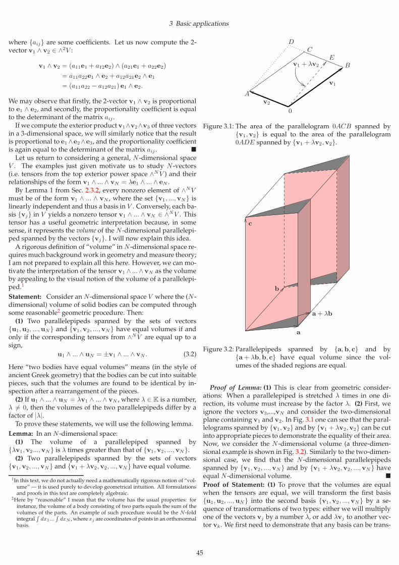
3 Basic applications
where {aij} are some coefficients. Let us now compute the 2-vector v1 ∧ v2 ∈ ∧2V :
v1 ∧ v2 = (a11e1 + a12e2) ∧ (a21e1 + a22e2)
= a11a22e1 ∧ e2 + a12a21e2 ∧ e1
= (a11a22 − a12a21) e1 ∧ e2.
We may observe that firstly, the 2-vector v1 ∧ v2 is proportionalto e1 ∧ e2, and secondly, the proportionality coefficient is equalto the determinant of the matrix aij .If we compute the exterior product v1∧v2∧v3 of three vectors
in a 3-dimensional space, we will similarly notice that the resultis proportional to e1∧e2∧e3, and the proportionality coefficientis again equal to the determinant of the matrix aij . �
Let us return to considering a general, N -dimensional spaceV . The examples just given motivate us to study N -vectors(i.e. tensors from the top exterior power space ∧NV ) and theirrelationships of the form v1 ∧ ... ∧ vN = λe1 ∧ ... ∧ eN .By Lemma 1 from Sec. 2.3.2, every nonzero element of ∧NV
must be of the form v1 ∧ ... ∧ vN , where the set {v1, ...,vN} islinearly independent and thus a basis in V . Conversely, each ba-sis {vj} in V yields a nonzero tensor v1 ∧ ... ∧ vN ∈ ∧NV . Thistensor has a useful geometric interpretation because, in somesense, it represents the volume of the N -dimensional parallelepi-ped spanned by the vectors {vj}. I will now explain this idea.A rigorous definition of “volume” inN -dimensional space re-
quiresmuch backgroundwork in geometry andmeasure theory;I am not prepared to explain all this here. However, we can mo-tivate the interpretation of the tensor v1 ∧ ...∧vN as the volumeby appealing to the visual notion of the volume of a parallelepi-ped.1
Statement: Consider anN -dimensional space V where the (N -dimensional) volume of solid bodies can be computed throughsome reasonable2 geometric procedure. Then:(1) Two parallelepipeds spanned by the sets of vectors
{u1,u2, ...,uN} and {v1,v2, ...,vN} have equal volumes if andonly if the corresponding tensors from ∧NV are equal up to asign,
u1 ∧ ... ∧ uN = ±v1 ∧ ... ∧ vN . (3.2)
Here “two bodies have equal volumes” means (in the style ofancient Greek geometry) that the bodies can be cut into suitablepieces, such that the volumes are found to be identical by in-spection after a rearrangement of the pieces.(2) If u1 ∧ ... ∧ uN = λv1 ∧ ... ∧ vN , where λ ∈ K is a number,
λ 6= 0, then the volumes of the two parallelepipeds differ by afactor of |λ|.To prove these statements, we will use the following lemma.
Lemma: In an N -dimensional space:(1) The volume of a parallelepiped spanned by
{λv1,v2...,vN} is λ times greater than that of {v1,v2, ...,vN}.(2) Two parallelepipeds spanned by the sets of vectors
{v1,v2, ...,vN} and {v1 + λv2,v2, ...,vN} have equal volume.
1In this text, we do not actually need a mathematically rigorous notion of “vol-ume” — it is used purely to develop geometrical intuition. All formulationsand proofs in this text are completely algebraic.
2Here by “reasonable” I mean that the volume has the usual properties: forinstance, the volume of a body consisting of two parts equals the sum of thevolumes of the parts. An example of such procedure would be the N -foldintegral
R
dx1...R
dxN , where xj are coordinates of points in an orthonormalbasis.
0
A
B
DC
E
v1
v2
v1 + λv2
Figure 3.1: The area of the parallelogram 0ACB spanned by{v1,v2} is equal to the area of the parallelogram0ADE spanned by {v1 + λv2,v2}.
a
b
c
a + λb
Figure 3.2: Parallelepipeds spanned by {a,b, c} and by{a + λb,b, c} have equal volume since the vol-umes of the shaded regions are equal.
Proof of Lemma: (1) This is clear from geometric consider-ations: When a parallelepiped is stretched λ times in one di-rection, its volume must increase by the factor λ. (2) First, weignore the vectors v3,...,vN and consider the two-dimensionalplane containing v1 and v2. In Fig. 3.1 one can see that the paral-lelograms spanned by {v1,v2} and by {v1 + λv2,v2} can be cutinto appropriate pieces to demonstrate the equality of their area.Now, we consider the N -dimensional volume (a three-dimen-sional example is shown in Fig. 3.2). Similarly to the two-dimen-sional case, we find that the N -dimensional parallelepipedsspanned by {v1,v2, ...,vN} and by {v1 + λv2,v2, ...,vN} haveequal N -dimensional volume. �
Proof of Statement: (1) To prove that the volumes are equalwhen the tensors are equal, we will transform the first basis{u1,u2, ...,uN} into the second basis {v1,v2, ...,vN} by a se-quence of transformations of two types: either we will multiplyone of the vectors vj by a number λ, or add λvj to another vec-tor vk. We first need to demonstrate that any basis can be trans-
45
3 Basic applications
formed into any other basis by this procedure. To demonstratethis, recall the proof of Theorem 1.1.5 in which vectors from thefirst basis were systematically replaced by vectors of the sec-ond one. Each replacement can be implemented by a certain se-quence of replacements of the kind uj → λuj or uj → uj + λui.Note that the tensor u1 ∧ ... ∧ uN changes in the same way asthe volume under these replacements: The tensor u1 ∧ ... ∧ uN
gets multiplied by λ after uj → λuj and remains unchanged af-ter uj → uj + λui. At the end of the replacement procedure,the basis {uj} becomes the basis {vj} (up to the ordering ofvectors), while the volume is multiplied by the same factor asthe tensor u1 ∧ ... ∧ uN . The ordering of the vectors in the set{vj} can be changed with possibly a sign change in the tensoru1 ∧ ... ∧ uN . Therefore the statement (3.2) is equivalent to theassumption that the volumes of {vj} and {uj} are equal. (2) Atransformation v1 → λv1 increases the volume by a factor of |λ|and makes the two tensors equal, therefore the volumes differby a factor of |λ|. �
Let us now consider the interpretation of the above Statement.Suppose we somehow know that the parallelepiped spanned bythe vectors {u1, ...,uN} has unit volume. Given this knowledge,the volume of any other parallelepiped spanned by some othervectors {v1, ...,vN} is easy to compute. Indeed, we can computethe tensors u1 ∧ ... ∧ uN and v1 ∧ ... ∧ vN . Since the space ∧NVis one-dimensional, these two tensors must be proportional toeach other. By expanding the vectors vj in the basis {uj}, it isstraightforward to compute the coefficient λ in the relationship
v1 ∧ ... ∧ vN = λu1 ∧ ... ∧ uN .
The Statement now says that the volume of a parallelepipedspanned by the vectors {v1, ...,vN} is equal to |λ|.Exercise 1: The volume of a parallelepiped spanned by vectorsa, b, c is equal to 19. Compute the volume of a parallelepipedspanned by the vectors 2a − b, c + 3a, b.Solution: Since (2a − b)∧(c + 3a)∧b = 2a∧c∧b = −2a∧b∧c,
the volume is 38 (twice 19; we ignored the minus sign since weare interested only in the absolute value of the volume). �
It is also clear that the tensor v1∧...∧vN allows us only to com-pare the volumes of two parallelepipeds; we cannot determinethe volume of one parallelepiped taken by itself. A tensor suchas v1 ∧ ... ∧ vN can be used to determine the numerical value ofthe volume only if we can compare it with another given tensor,u1 ∧ ...∧uN , which (by assumption) corresponds to a parallelepi-ped of unit volume. A choice of a “reference” tensor u1∧ ...∧uN
can be made, for instance, if we are given a basis in V ; withoutthis choice, there is no natural map from ∧NV to numbers (K).In other words, the space ∧NV is not canonically isomorphic tothe space K (even though both ∧NV and K are one-dimensionalvector spaces). Indeed, a canonical isomorphism between ∧NVand K would imply that the element 1 ∈ K has a correspondingcanonically defined tensor ω1 ∈ ∧NV . In that case there wouldbe some basis {ej} in V such that e1 ∧ ... ∧ eN = ω1, which in-dicates that the basis {ej} is in some sense “preferred” or “nat-ural.” However, there is no “natural” or “preferred” choice ofbasis in a vector space V , unless some additional structure isgiven (such as a scalar product). Hence, no canonical choice ofω1 ∈ ∧NV is possible.
Remark: When a scalar product is defined in V , there is a pre-ferred choice of basis, namely an orthonormal basis {ej} suchthat 〈ei, ej〉 = δij (see Sec. 5.1). Since the length of each of the
basis vectors is 1, and the basis vectors are orthogonal to eachother, the volume of the parallelepiped spanned by {ej} is equalto 1. (This is the usual Euclidean definition of volume.) Then thetensor ω1 ≡ ∧N
j=1 ej can be computed using this basis and usedas a unit volume tensor. We will see below (Sec. 5.5.2) that thistensor does not depend on the choice of the orthonormal basis,up to the orientation. The isomorphism between ∧NV and K isthen fixed (up to the sign), thanks to the scalar product. �
In the absence of a scalar product, one can say that the valueof the volume in an abstract vector space is not a number but atensor from the space ∧NV . It is sufficient to regard the elementv1 ∧ ... ∧ vN ∈ ∧NV as the definition of the “∧NV -valued vol-ume” of the parallelepiped spanned by {vj}. The space ∧NV isone-dimensional, so the “tensor-valued volume” has the famil-iar properties we expect (it is “almost a number”). One thing isunusual about this “volume”: It is oriented, that is, it changessign if we exchange the order of two vectors from the set {vj}.
Exercise 2: Suppose {u1, ...,uN} is a basis in V . Let x be somevector whose components in the basis {uj} are given, x =∑
j αjuj . Compute the (tensor-valued) volume of the parallel-epiped spanned by {u1 + x, ...,uN + x}.Hints: Use the linearity property, (a + x) ∧ ... = a ∧ ... + x ∧ ...,and notice the simplification
x ∧ (a + x) ∧ (b + x) ∧ ... ∧ (c + x) = x ∧ a ∧ b ∧ ... ∧ c.
Answer: The volume tensor is
(u1 + x) ∧ ... ∧ (uN + x) = (1 + α1 + ...+ αN )u1 ∧ ... ∧ uN .
Remark: tensor-valued area. The idea that the volume is “ori-ented” can be understood perhaps more intuitively by consid-ering the area of the parallelogram spanned by two vectors a, bin the familiar 3-dimensional space. It is customary to draw thevector product a× b as the representation of this area, since thelength |a × b| is equal to the area, and the direction of a × b isnormal to the area. Thus, the vector a × b can be understoodas the “oriented area” of the parallelogram. However, note thatthe direction of the vector a×b depends not only on the angularorientation of the parallelogram in space, but also on the orderof the vectors a, b. The 2-vector a ∧ b is the natural analogue ofthe vector product a × b in higher-dimensional spaces. Hence,it is algebraically natural to regard the tensor a∧b ∈ ∧2V as the“tensor-valued” representation of the area of the parallelogramspanned by {a,b}.Consider now a parallelogram spanned by a,b in a two-
dimensional plane. We can still represent the oriented area ofthis parallelogram by the vector product a× b, where we imag-ine that the plane is embedded in a three-dimensional space.The area of the parallelogram does not have a nontrivial angularorientation anymore since the vector product a×b is always or-thogonal to the plane; the only feature left from the orientationis the positive or negative sign of a × b relative to an arbitrarilychosen vector n normal to the plane. Hence, wemay say that thesign of the oriented volume of a parallelepiped is the only rem-nant of the angular orientation of the parallelepiped in spacewhen the dimension of the parallelepiped is equal to the dimen-sion of space. (See Sec. 2.1 for more explanations about the geo-metrical interpretation of volume in terms of exterior product.)�
46
3 Basic applications
3.3 Determinants of operators
Let A ∈ End V be a linear operator. Consider its action on ten-sors from the space ∧NV defined in the following way, v1 ∧ ...∧...vN 7→ Av1 ∧ ... ∧ AvN . I denote this operation by ∧N AN , so
∧N AN (v1 ∧ ... ∧ vN ) ≡ (Av1) ∧ ... ∧ (AvN ).
The notation ∧N AN underscores the fact that there areN copies
of A acting simultaneously.
We have just defined ∧N AN on single-term products v1 ∧ ...∧vN ; the action of ∧N AN on linear combinations of such productsis obtained by requiring linearity.
Let us verify that ∧N AN is a linear map; it is sufficient to checkthat it is compatible with the exterior product axioms:
A(v + λu) ∧ Av2 ∧ ... ∧ AvN = Av ∧ Av2 ∧ ... ∧ AvN
+ λAu ∧ Av2 ∧ ... ∧ AvN ;
Av1 ∧ Av2 ∧ ... ∧ AvN = −Av2 ∧ Av1 ∧ ... ∧ AvN .
Therefore, ∧N AN is now defined as a linear operator ∧NV →∧NV .By Theorem 2 in Sec. 2.3.2, the space ∧NV is one-dimensional.
So ∧N AN , being a linear operator in a one-dimensional space,must act simply as multiplication by a number. (Every linearoperator in a one-dimensional space must act as multiplicationby a number!) Thus we can write
∧N AN = α1∧N V ,
where α ∈ K is a number which is somehow associated withthe operator A. What is the significance of this number α? This
number is actually equal to the determinant of the operator A asgiven by Definition D0. But let us pretend that we do not knowanything about determinants; it is very convenient to use thisconstruction to define the determinant and to derive its proper-ties.Definition D1: The determinant det A of an operator A ∈End V is the number by which any nonzero tensor ω ∈ ∧NV
is multiplied when ∧N AN acts on it:
(∧N AN )ω = (det A)ω. (3.3)
In other words, ∧NAN = (det A)1∧N V .We can immediately put this definition to use; here are the
first results.Statement 1: The determinant of a product is the product of de-
terminants: det(AB) = (det A)(det B).Proof: Actwith ∧N AN and thenwith ∧N BN on a nonzero ten-
sor ω ∈ ∧NV . Since these operators act as multiplication by anumber, the result is the multiplication by the product of thesenumbers. We thus have
(∧N AN )(∧N BN )ω = (∧N AN )(det B)ω = (det A)(det B)ω.
On the other hand, for ω = v1 ∧ ... ∧ vN we have
(∧N AN )(∧N BN )ω = (∧N AN )Bv1 ∧ ... ∧ BvN
= ABv1 ∧ ... ∧ ABvN = ∧N (AB)Nω
= (det(AB))ω.
Therefore, det(AB) = (det A)(det B). �
Exercise 1: Prove that det(λA) = λN det A for any λ ∈ K and
A ∈ End V .Now let us clarify the relation between the determinant and
the volume. We will prove that the determinant of a transforma-
tion A is the coefficient by which the volume of parallelepipeds
will growwhenwe act with A on the vector space. After provingthis, I will derive the relation (3.1) for the determinant through
the matrix coefficients of A in some basis; it will follow that theformula (3.1) gives the same results in any basis.Statement 2: When a parallelepiped spanned by the vectors
{v1, ...,vN} is transformed by a linear operator A, so that vj 7→Avj , the volume of the parallelepiped grows by the factor
| det A |.Proof: Suppose the volume of the parallelepiped spanned by
the vectors {v1, ...,vN} is v. The transformed parallelepiped is
spanned by vectors {Av1, ..., AvN}. According to the definition
of the determinant, det A is a number such that
Av1 ∧ ... ∧ AvN = (det A)v1 ∧ ... ∧ vN .
By Statement 3.2, the volume of the transformed parallelepiped
is | det A | times the volume of the original parallelepiped. �
If we consider the oriented (i.e. tensor-valued) volume, wefind that it grows by the factor det A (without the absolutevalue). Therefore we could define the determinant also in thefollowing way:Definition D2: The determinant det A of a linear transforma-tion A is the number by which the oriented volume of any paral-lelepiped grows after the transformation. (One is then obligedto prove that this number does not depend on the choice of theinitial parallelepiped! We just proved this in Statement 1 usingan algebraic definition D1 of the determinant.)With this definition of the determinant, the property
det(AB) = (det A)(det B)
is easy to understand: The composition of the transformations
A and B multiplies the volume by the product of the individual
volume growth factors det A and det B.Finally, here is a derivation of the formula (3.1) from Defini-
tion D1.Statement 3: If {ej} is any basis in V ,
{e∗j}is the dual basis, and
a linear operator A is represented by a tensor,
A =
N∑
j,k=1
Ajkej ⊗ e∗k, (3.4)
then the determinant of A is given by the formula (3.1).
Proof: The operator A defined by Eq. (3.4) acts on the basisvectors {ej} as follows,
Aek =
N∑
j=1
Ajkej .
A straightforward calculation is all that is needed to obtain theformula for the determinant. I first consider the case N = 2 asan illustration:
∧2A2 (e1 ∧ e2) = Ae1 ∧ Ae2
= (A11e1 +A21e2) ∧ (A12e1 +A22e2)
= A11A22e1 ∧ e2 +A21A12e2 ∧ e1
= (A11A22 −A12A21) e1 ∧ e2.
47
3 Basic applications
Hence det A = A11A22 − A12A21, in agreement with the usualformula.Now I consider the general case. The action of ∧N AN on the
basis element e1 ∧ ... ∧ eN ∈ ∧NV is
∧N AN (e1 ∧ ... ∧ eN ) = Ae1 ∧ ... ∧ AeN
=
N∑
j1=1
Aj11ej1
∧ ... ∧
N∑
jN =1
AjN NejN
=N∑
j1=1
...N∑
jN=1
Aj11ej1 ∧ ... ∧AjN NejN
=
N∑
j1=1
...
N∑
jN=1
(Aj11...AjN N )ej1 ∧ ... ∧ ejN. (3.5)
In the last sum, the only nonzero terms are those in which theindices j1, ..., jN do not repeat; in other words, (j1, ..., jN ) isa permutation of the set (1, ..., N ). Let us therefore denote thispermutation by σ and write σ(1) ≡ j1, ..., σ(N) ≡ jN . Using theantisymmetry of the exterior product and the definition of theparity |σ| of the permutation σ, we can express
ej1 ∧ ... ∧ ejN= eσ(1) ∧ ... ∧ eσ(N) = (−1)
|σ|e1 ∧ ... ∧ eN .
Now we can rewrite the last line in Eq. (3.5) in terms of sumsover all permutations σ instead of sums over all {j1, ..., jN}:
∧N AN (e1 ∧ ... ∧ eN ) =∑
σ
Aσ(1)1...Aσ(N)Neσ(1) ∧ ... ∧ eσ(N)
=∑
σ
Aσ(1)1...Aσ(N)N (−1)|σ|
e1 ∧ ... ∧ eN .
Thus we have reproduced the formula (3.1). �
We have seen three equivalent definitions of the determinant,each with its own advantages: first, a direct but complicateddefinition (3.1) in terms of matrix coefficients; second, an ele-gant but abstract definition (3.3) that depends on the construc-tion of the exterior product; third, an intuitive and visual defini-tion in terms of the volume which, however, is based on the ge-ometric notion of “volume of anN -dimensional domain” ratherthan on purely algebraic constructions. All three definitions areequivalent when applied to linear operators in finite-dimension-al spaces.
3.3.1 Examples: computing determinants
Question: We have been working with operators more or lessin the same way as with matrices, like in Eq. (3.4). What is theadvantage of the coordinate-free approach if we are again com-puting with the elements of matrices?Answer: In some cases, there is no other way except to rep-
resent an operator in some basis through a matrix such as Aij .However, in many cases an interesting operator can be repre-sented geometrically, i.e. without choosing a basis. It is often use-ful to express an operator in a basis-free manner because thisyields some nontrivial information that would otherwise be ob-scured by an unnecessary (or wrong) choice of basis. It is use-ful to be able to employ both the basis-free and the component-based techniques. Here are some examples where we computedeterminants of operators defined without a basis.
Example 1: Operators of the form 1V + a ⊗ b∗ are useful ingeometry because they can represent reflections or projectionswith respect to an axis or a plane if a and b∗ are chosen appro-priately. For instance, if b∗ 6= 0, we can define a hyperplaneHb∗ ⊂ V as the subspace annihilated by the covector b∗, i.e. thesubspace consisting of vectors v ∈ V such that b∗ (v) = 0. If avector a ∈ V is such that b∗ (a) 6= 0, i.e. a 6∈ Hb∗ , then
P ≡ 1V − 1
b∗ (a)a⊗ b∗
is a projector onto Hb∗ , while the operator
R ≡ 1V − 2
b∗ (a)a ⊗ b∗
describes amirror reflectionwith respect to the hyperplaneHb∗ ,
in the sense that v + Rv ∈ Hb∗ for any v ∈ V . �
The following statement shows how to calculate determinantsof such operators. For instance, with the above definitions we
would find det P = 0 and det R = −1 by a direct application ofEq. (3.6).Statement: Let a ∈ V and b∗ ∈ V ∗. Then
det(1V + a ⊗ b∗) = 1 + b∗ (a) . (3.6)
Proof: If b∗ = 0, the formula is trivial, so we assume that b∗ 6=0. Then we need to consider two cases: b∗(a) 6= 0 or b∗(a) = 0;however, the final formula (3.6) is the same in both cases.Case 1. By Statement 1.6, if b∗ (a) 6= 0 there exists a basis
{a,v2, ...,vN} such that b∗ (vi) = 0 for 2 ≤ i ≤ N , whereN = dimV . Then we compute the determinant by applying
the operator ∧N(1V + a ⊗ b∗)N to the tensor a ∧ v2 ∧ ... ∧ vN :
since(1V + a ⊗ b∗) a = (1 + b∗ (a))a,
(1V + a⊗ b∗)vi = vi, i = 2, ..., N,
we get
∧N(1V + a ⊗ b∗)N a ∧ v2 ∧ ... ∧ vN
= (1 + b∗ (a))a ∧ v2 ∧ ... ∧ vN .
Therefore det(1V + a ⊗ b∗) = 1 + b∗ (a), as required.
Case 2. If b∗ (a) = 0, we will show that det(1V + a ⊗ b∗) = 1.
We cannot choose the basis {a,v2, ...,vN} as in case 1, so weneed to choose another basis. There exists some vector w ∈ Vsuch that b∗ (w) 6= 0 because by assumption b∗ 6= 0. It is clearthat {w,a} is a linearly independent set: otherwise we wouldhave b∗(w) = 0. Therefore, we can complete this set to a basis{w,a,v3, ...,vN}. Further, the vectors v3, ...,vN can be chosensuch that b∗ (vi) = 0 for 3 ≤ i ≤ N . Now we compute the
determinant by acting with the operator ∧N(1V + a⊗ b∗)N on
the tensor a ∧ w ∧ v3 ∧ ... ∧ vN : since(1V + a ⊗ b∗) a = a,(1V + a ⊗ b∗)w = w + b∗ (w) a,(1V + a⊗ b∗)vi = vi, i = 3, ..., N,
we get
∧N(1V + a⊗ b∗)N a ∧ w ∧ v3 ∧ ... ∧ vN
= a ∧ (w + b∗ (w) a) ∧ v3 ∧ ... ∧ vN
= a ∧ w ∧ v3 ∧ ... ∧ vN .
48
3 Basic applications
Therefore det(1V + a ⊗ b∗) = 1. �
Exercise 1: In a similar way, prove the following statement: Ifai ∈ V and b∗
i ∈ V ∗ for 1 ≤ i ≤ n < N are such that b∗i (aj) = 0
for all i > j, then
det
(
1V +
n∑
i=1
ai ⊗ b∗i
)
=
n∏
i=1
(1 + b∗i (ai)) .
Exercise 2: Consider the three-dimensional space of polynomi-als p(x) in the variable x of degree at most 2 with real coeffi-
cients. The operators A and B are defined by
(Ap)(x) ≡ p(x) + xdp(x)
dx,
(Bp)(x) ≡ x2p(1) + 2p(x).
Check that these operators are linear. Compute the determi-
nants of A and B.
Solution: The operators are linear because they are expressedas formulas containing p(x) linearly. Let us use the underbar todistinguish the polynomials 1, x from numbers such as 1. Aconvenient basis tensor of the 3rd exterior power is 1∧x∧x2, sowe perform the calculation,
(det A)(1 ∧ x ∧ x2) = (A1) ∧ (Ax) ∧ (Ax2)
= 1 ∧ (2x) ∧ (3x2) = 6(1 ∧ x ∧ x2),
and find that det A = 6. Similarly we find det B = 12. �
Exercise 3: Suppose the space V is decomposed into a direct
sum of U and W , and an operator A is such that U and W are
invariant subspaces (Ax ∈ U for all x ∈ U , and the same forW ).
Denote by AU the restriction of the operator A to the subspaceU . Show that
det A = (det AU )(det AW ).
Hint: Choose a basis in V as the union of a basis in U anda basis in W . In this basis, the operator A is represented by ablock-diagonalmatrix.
3.4 Determinants of square tables
Note that the determinant formula (3.1) applies to any squarematrix, without referring to any transformations in any vectorspaces. Sometimes it is useful to compute the determinants ofmatrices that do not represent linear transformations. Such ma-trices are really just tables of numbers. The properties of deter-minants of course remain the same whether or not the matrixrepresents a linear transformation in the context of the prob-lem we are solving. The geometric construction of the deter-minant through the space ∧NV is useful because it helps us un-derstand heuristically where the properties of the determinantcome from.
Given just a square table of numbers, it is often useful to in-troduce a linear transformation corresponding to the matrix insome (conveniently chosen) basis; this often helps solve prob-lems. An example frequently used in linear algebra is a matrixconsisting of the components of some vectors in a basis. Sup-pose {ej | j = 1, ..., N} is a basis and {vj | j = 1, ..., N} are some
vectors. Since each of the vj can be decomposed through thebasis {ej}, say
vi =
N∑
j=1
vijej , i = 1, ..., N,
wemay consider the coefficients vij as a square matrix. This ma-trix, at first glance, does not represent a linear transformation;it’s just a square-shaped table of the coefficients vij . However,
let us define a linear operator A by the condition that Aei = vi
for all i = 1, ..., N . This condition defines Ax for any vector x if
we assume the linearity of A (see Exercise 2 in Sec. 1.2.2). The
operator A has the following matrix representation with respectto the basis {ei} and the dual basis {e∗i }:
A =
N∑
i=1
vi ⊗ e∗i =
N∑
i=1
N∑
j=1
vijej ⊗ e∗i .
So the matrix vji (the transpose of vij ) is the matrix representing
the transformation A. Let us consider the determinant of thistransformation:
(det A)e1 ∧ ... ∧ eN = Ae1 ∧ ... ∧ AeN = v1 ∧ ... ∧ vN .
The determinant of the matrix vji is thus equal to the determi-
nant of the transformation A. Hence, the computation of thedeterminant of the matrix vji is equivalent to the computationof the tensor v1 ∧ ... ∧ vN ∈ ∧NV and its comparison with thebasis tensor e1 ∧ ... ∧ eN . We have thus proved the followingstatement.Statement 1: The determinant of the matrix vji made up by thecomponents of the vectors {vj} in a basis {ej} (j = 1, ..., N ) isthe number C defined as the coefficient in the tensor equality
v1 ∧ ... ∧ vN = Ce1 ∧ ... ∧ eN .
Corollary: The determinant of a matrix does not change when amultiple of one row is added to another row. The determinant islinear as a function of each row. The determinant changes signwhen two rows are exchanged.Proof: We consider the matrix vij as the table of coefficients of
vectors {vj} in a basis {ej}, as explained above. Since
(det vji)e1 ∧ ... ∧ eN = v1 ∧ ... ∧ vN ,
we need only to examine the properties of the tensor ω ≡ v1 ∧... ∧ vN under various replacements. When a multiple of row kis added to another row j, we replace vj 7→ vj + λvk for fixedj, k; then the tensor ω does not change,
v1 ∧ ... ∧ vj ∧ ... ∧ vN = v1 ∧ ... ∧ (vj + λvk) ∧ ... ∧ vN ,
hence the determinant of vij does not change. To show that thedeterminant is linear as a function of each row, we consider thereplacement vj 7→ u + λv for fixed j; the tensor ω is then equalto the sum of the tensors v1 ∧ ...∧u∧ ...∧vN and λv1 ∧ ...∧ v∧... ∧ vN . Finally, exchanging the rows k and l in the matrix vij
corresponds to exchanging the vectors vk and vl, and then thetensor ω changes sign. �
It is an important property that matrix transposition leavesthe determinant unchanged.
49
3 Basic applications
Statement 2: The determinant of the transposed operator is un-changed:
det AT = det A.
Proof: I give two proofs, one based on Definition D0 and theproperties of permutations, another entirely coordinate-free —based on Definition D1 of the determinant and definition 1.8.4of the transposed operator.First proof : According to Definition D0, the determinant of the
transposed matrix Aji is given by the formula
det(Aji) ≡∑
σ
(−1)|σ|A1,σ(1)...AN,σ(N), (3.7)
so the only difference between det(Aij) and det(Aji) is the or-der of indices in the products of matrix elements, namely Aσ(i),i
instead of Ai,σ(i). We can show that the sum in Eq. (3.7) con-sists of exactly the same terms as the sum in Eq. (3.1), only theterms occur in a different order. This is sufficient to prove thatdet(Aij) = det(Aji).The sum in Eq. (3.7) consists of terms of the form
A1,σ(1)...AN,σ(N), where σ is some permutation. Wemay reorderfactors in this term,
A1,σ(1)...AN,σ(N) = Aσ′(1),1...Aσ′(N),N ,
where σ′ is another permutation such that Ai,σ(i) = Aσ′(i),i fori = 1, ..., N . This is achieved when σ′ is the permutation inverseto σ, i.e. we need to use σ′ ≡ σ−1. Since there exists preciselyone inverse permutation σ−1 for each permutation σ, we maytransform the sum in Eq. (3.7) into a sum over all inverse per-mutations σ′; each permutation will still enter exactly once intothe new sum. Since the parity of the inverse permutation σ−1 isthe same as the parity of σ (see Statement 3 in Appendix B), the
factor (−1)|σ|
will remain unchanged. Therefore, the sum willremain the same.Second proof : The transposed operator is defined as
(AT f∗)(x) = f∗(Ax), ∀f∗ ∈ V ∗, x ∈ V.
In order to compare the determinants det A and det(AT ) accord-
ing to Definition D1, we need to compare the numbers ∧N AN
and ∧N (AT )N .Let us choose nonzero tensors ω ∈ ∧NV and ω∗ ∈ ∧NV ∗. By
Lemma 1 in Sec. 2.3.2, these tensors have representations of theform ω = v1 ∧ ... ∧ vN and ω∗ = f∗1 ∧ ... ∧ f∗N . We have
(det A)v1 ∧ ... ∧ vN = Av1 ∧ ... ∧ AvN .
Now we would like to relate this expression with the analogous
expression for AT . In order to use the definition of AT , we need
to act on the vectors Avi by the covectors f∗j . Therefore, we
act with the N -form ω∗ ∈ ∧NV ∗ ∼= (∧NV )∗ on the N -vector∧N ANω ∈ ∧NV (this canonical action was defined by Defini-tion 3 in Sec. 2.2). Since this action is linear, we find
ω∗(∧N ANω) = (det A)ω∗(ω).
(Note that ω∗(ω) 6= 0 since by assumption the tensors ω and ω∗
are nonzero.) On the other hand,
ω∗(∧N ANω)
=∑
σ
(−1)|σ|f∗1 (Avσ(1))...f∗N (Avσ(N))
=∑
σ
(−1)|σ|(AT f∗1 )(vσ(1))...(AT f∗N )(vσ(N))
=(∧N (AT )Nω∗)(ω) = (det AT )ω∗(ω).
Hence det AT = det A. �
Exercise* (Laplace expansion): As shown in the Corollaryabove, the determinant of the matrix vij is a linear function ofeach of the vectors {vi}. Consider det(vij) as a linear functionof the first vector, v1; this function is a covector that we may tem-porarily denote by f∗1 . Show that f∗1 can be represented in thedual basis
{e∗j}as
f∗1 =
N∑
i=1
(−1)i−1 B1ie∗i ,
where the coefficients B1i are minors of the matrix vij , that is,determinants of the matrix vij from which row 1 and column ihave been deleted.Solution: Consider one of the coefficients, for example B11 ≡
f∗1 (e1). This coefficient can be determined from the tensor equal-ity
e1 ∧ v2 ∧ ... ∧ vN = B11e1 ∧ ... ∧ eN . (3.8)
We could reduce B11 to a determinant of an (N − 1) × (N − 1)matrix if we could cancel e1 on both sides of Eq. (3.8). We wouldbe able to cancel e1 if we had a tensor equality of the form
e1 ∧ ψ = B11e1 ∧ e2 ∧ ... ∧ eN ,
where the (N − 1)-vector ψ were proportional to e2 ∧ ... ∧ eN .However, v2∧ ...∧vN in Eq. (3.8) is not necessarily proportionalto e2 ∧ ... ∧ eN ; so we need to transform Eq. (3.8) to a suitableform. In order to do this, we transform the vectors vi into vec-tors that belong to the subspace spanned by {e2, ..., eN}. Wesubtract from each vi (i = 2, ..., N ) a suitable multiple of e1 anddefine the vectors vi (i = 2, ..., N ) such that e∗1(vi) = 0:
vi ≡ vi − e∗1(vi)e1, i = 2, ..., N.
Then vi ∈ Span {e2, ..., eN} and also
e1 ∧ v2 ∧ ... ∧ vN = e1 ∧ v2 ∧ ... ∧ vN .
Now Eq. (3.8) is rewritten as
e1 ∧ v2 ∧ ... ∧ vN = B11e1 ∧ e2 ∧ ... ∧ eN .
Since vi ∈ Span {e2, ..., eN}, the tensors v2 ∧ ... ∧ vN and e2 ∧... ∧ eN are proportional to each other. Now we are allowed tocancel e1 and obtain
v2 ∧ ... ∧ vN = B11e2 ∧ ... ∧ eN .
Note that the vectors vi have the first components equal to zero.In other words, B11 is equal to the determinant of the matrixvij from which row 1 (i.e. the vector v1) and column 1 (thecoefficients at e1) have been deleted. The coefficients B1j forj = 2, ..., N are calculated similarly. �
3.4.1 * Index notation for ∧NV and determinants
Let us see how determinants are written in the index notation.In order to use the index notation, we need to fix a basis {ej}
and represent each vector and each tensor by their componentsin that basis. Determinants are related to the space ∧NV . Let usconsider a set of vectors {v1, ...,vN} and the tensor
ψ ≡ v1 ∧ ... ∧ vN ∈ ∧NV.
50
3 Basic applications
Since the space ∧NV is one-dimensional and its basis consistsof the single tensor e1 ∧ ... ∧ eN , the index representation of ψconsists, in principle, of the single number C in a formula suchas
ψ = Ce1 ∧ ... ∧ eN .
However, it is more convenient to use a totally antisymmetricarray of numbers having N indices, ψi1...iN , so that
ψ =1
N !
N∑
i1,...,iN=1
ψi1...iN ei1 ∧ ... ∧ eiN.
Then the coefficient C is C ≡ ψ12...N . In the formula above, thecombinatorial factor N ! compensates the fact that we are sum-ming an antisymmetric product of vectors with a totally anti-symmetric array of coefficients.To write such arrays more conveniently, one can use Levi-
Civita symbol εi1...iN (see Sec. 2.3.6). It is clear that any othertotally antisymmetric array of numbers with N indices, such asψi1...iN , is proportional to εi1...iN : For indices {i1, ..., iN} that cor-respond to a permutation σ we have
ψi1...iN = ψ12...N(−1)|σ|,
and henceψi1...iN = (ψ12...N)εi1...iN .
How to compute the index representation of ψ given the arrayvk
j of the components of the vectors {vj}? We need to representthe tensor
ψ ≡∑
σ
(−1)|σ|
vσ(1) ⊗ vσ(2) ⊗ ...⊗ vσ(N).
Hence, we can use the Levi-Civita symbol and write
ψ12...N =∑
σ
(−1)|σ|v1
σ(1) ⊗ v2σ(2) ⊗ ...⊗ vN
σ(N)
=
N∑
i1,...,iN=1
εi1...iN v1i1 ...v
NiN.
The component ψ12...N is the only number we need to representψ in the basis {ej}.The Levi-Civita symbol itself can be seen as the index repre-
sentation of the tensor
ω ≡ e1 ∧ ... ∧ eN
in the basis {ej}. (The components of ω in a different basis will,of course, differ from εi1...iN by a constant factor.)Now let us construct the index representation of the determi-
nant of an operator A. The operator is given by its matrixAij and
acts on a vector v with components vi yielding a vector u ≡ Av
with components
uk =
N∑
i=1
Aki v
i.
Hence, the operator ∧N AN acting on ψ yields an antisymmetrictensor whose component with the indices k1...kN is
[
(∧N AN )ψ]k1...kN
=[
Av1 ∧ ... ∧ AvN
]k1...kN
=∑
is,js
εi1...iNAk1
j1vj1
i1...AkN
jNvjN
iN.
Since the tensor ∧N ANψ is proportional to ψ with the coeffi-
cient det A, the same proportionality holds for the componentsof these tensors:
∑
is,js
εi1...iNAk1
j1vj1
i1...AkN
jNvjN
iN= (det A)ψk1...kN
= (det A)∑
is
εi1...iN vk1
i1...vkN
iN.
The relation above must hold for arbitrary vectors {vj}. This issufficient to derive a formula for det A. Since {vj} are arbitrary,we may select {vj} as the basis vectors {ej}, so that vk
i = δki .
Substituting this into the equation above, we find
∑
is,js
εi1...iNAk1
i1...AkN
iN= (det A)εk1...kN .
We can now solve for det A by multiplying with another Levi-Civita symbol εk1...kN
, written this time with lower indices tocomply with the summation convention, and summing over allks. By elementary combinatorics (there are N ! possibilities tochoose the indices k1, ..., kN such that they are all different), wehave ∑
k1,...,kN
εk1...kNεk1...kN = N !,
and therefore
det(A) =1
N !
∑
is,ks
εk1...kNεi1...iNAk1
i1...AkN
iN.
This formula can be seen as the index representation of
det A = ω∗(∧N ANω),
where ω∗ ∈ (∧NV )∗ is the tensor dual to ω and such thatω∗(ω) = 1. The components of ω∗ are
1
N !εk1...kN
.
We have shown how the index notation can express calcula-tions with determinants and tensors in the space ∧NV . Suchcalculations in the index notation are almost always more cum-bersome than in the index-free notation.
3.5 Solving linear equations
Determinants allow us to “determine” whether a system of lin-ear equations has solutions. I will now explain this using ex-terior products. I will also show how to use exterior productsfor actually finding the solutions of linear equations when theyexist.A system ofN linear equations forN unknowns x1, ..., xN can
be written in the matrix form,
N∑
j=1
Aijxj = bi, i = 1, ..., N. (3.9)
Here Aij is a given matrix of coefficients, and the N numbers biare also given.The first step in studying Eq. (3.9) is to interpret it in a geo-
metric way, so that Aij is not merely a “table of numbers” but a
51
3 Basic applications
geometric object. We introduce an N -dimensional vector spaceV = RN , in which a basis {ei} is fixed. There are two options(both will turn out to be useful). The first option is to interpretAij , bj , and xj as the coefficients representing some linear oper-
ator A and some vectors b,x in the basis {ej}:
A ≡N∑
i,j=1
Aijei ⊗ e∗j , b ≡N∑
j=1
bjej , x ≡N∑
j=1
xjej .
Then we reformulate Eq. (3.9) as the vector equation
Ax = b, (3.10)
from which we would like to find the unknown vector x.The second option is to interpret Aij as the components of a
set of N vectors {a1, ...,aN}with respect to the basis,
aj ≡N∑
i=1
Aijei, j = 1, ..., N,
to define b as before,
b ≡N∑
j=1
bjej,
and to rewrite Eq. (3.9) as an equation expressing b as a linearcombination of {aj}with unknown coefficients {xj},
N∑
j=1
xjaj = b. (3.11)
In this interpretation, {xj} is just a set of N unknown numbers.These numbers could be interpreted the set of components ofthe vector b in the basis {aj} if {aj}were actually a basis, whichis not necessarily the case.
3.5.1 Existence of solutions
Let us begin with the first interpretation, Eq. (3.10). When doesEq. (3.10) have solutions? The solution certainly exists when
the operator A is invertible, i.e. the inverse operator A−1 ex-
ists such that AA−1 = A−1A = 1V ; then the solution is foundas x = A−1b. The condition for the existence of A−1 is that thedeterminant of A is nonzero. When the determinant of A is zero,the solution may or may not exist, and the solution is more com-plicated. I will give a proof of these statements based on the newdefinition D1 of the determinant.Theorem 1: If det A 6= 0, the equation Ax = b has a unique
solution x for any b ∈ V . There exists a linear operator A−1
such that the solution x is expressed as x = A−1b.Proof: Suppose {ei | i = 1, ..., N} is a basis in V . It follows
from det A 6= 0 that
∧N AN (e1 ∧ ... ∧ eN) = (Ae1) ∧ ... ∧ (AeN ) 6= 0.
By Theorem 1 of Sec. 2.3.2, the set of vectors {Ae1, ..., AeN} islinearly independent and therefore is a basis in V . Thus thereexists a unique set of coefficients {ci} such that
b =
N∑
i=1
ci(Aei).
Then due to linearity of Awe have
b = AN∑
i=1
ciei;
in other words, the solution of the equation Ax = b is x ≡∑N
i=1 ciei. Since the coefficients {ci} are determined uniquely,the solution x is unique.The solution x can be expressed as a function of b as follows.
Since {Aei} is a basis, there exists the corresponding dual basis,which we may denote by
{v∗
j
}. Then the coefficients ci can be
expressed as ci = v∗i (b), and the vector x as
x =
N∑
i=1
ciei =
N∑
i=1
eiv∗i (b) =
(N∑
i=1
ei ⊗ v∗i
)b ≡ A−1b.
This shows explicitly that the operator A−1 exists and is linear.�
Corollary: If det A 6= 0, the equation Av = 0 has only the (triv-ial) solution v = 0.Proof: The zero vector v = 0 is a solution of Av = 0. By
the above theorem the solution of that equation is unique, thusthere are no other solutions. �
Theorem 2 (existence of eigenvectors): If det A = 0, there ex-ists at least one eigenvector with eigenvalue 0, that is, at least
one nonzero vector v such that Av = 0.Proof: Choose a basis {ej} and consider the set
{Ae1, ..., AeN}. This set must be linearly dependent since
Ae1 ∧ ... ∧ AeN = (det A)e1 ∧ ... ∧ eN = 0.
Hence, there must exist at least one linear combination∑N
i=1 λiAei = 0 with λi not all zero. Then the vector v ≡∑N
i=1 λiei is nonzero and satisfies Av = 0. �
Remark: If det A = 0, theremay exist more than one eigenvector
v such that Av = 0; more detailed analysis is needed to fullydetermine the eigenspace of zero eigenvalue, but we found that
at least one eigenvector v exists. If det A = 0 then the equation
Ax = b with b 6= 0 may still have solutions, although not forevery b. Moreover, when a solution x exists it will not be uniquebecause x + λv is another solution if x is one. The full analysis
of solvability of the equation Ax = b when det A = 0 is morecomplicated (see the end of Sec. 3.5.2). �
Once the inverse operator A−1 is determined, it is easy to com-
pute solutions of any number of equations Ax = b1, Ax = b2,etc., for any number of vectors b1, b2, etc. However, if we
only need to solve one such equation, Ax = b, then comput-ing the full inverse operator is too much work: We have to de-termine the entire dual basis
{v∗
j
}and construct the operator
A−1 =∑N
i=1 ei ⊗ v∗i . An easier method is then provided by
Kramer’s rule.
3.5.2 Kramer’s rule and beyond
We will now use the second interpretation, Eq. (3.11), of a linearsystem. This equation claims that b is a linear combination oftheN vectors of the set {a1, ...,aN}. Clearly, this is true for any b
if {a1, ...,aN} is a basis in V ; in that case, the solution {xj} exists
52
3 Basic applications
and is unique because the dual basis,{a∗
j
}, exists and allows us
to write the solution as
xj = a∗j (b).
On the other hand, when {a1, ...,aN} is not a basis in V it is notcertain that some given vector b is a linear combination of aj . Inthat case, the solution {xj} may or may not exist, and when itexists it will not be unique.We first consider the case where {aj} is a basis in V . In this
case, the solution {xj} exists, and we would like to determineit more explicitly. We recall that an explicit computation of thedual basis was shown in Sec. 2.3.3. Motivated by the construc-tions given in that section, we consider the tensor
ω ≡ a1 ∧ ... ∧ aN ∈ ∧NV
and additionally the N tensors {ωj | j = 1, ..., N}, defined by
ωj ≡ a1 ∧ ... ∧ aj−1 ∧ b ∧ aj+1 ∧ ... ∧ aN ∈ ∧NV. (3.12)
The tensor ωj is the exterior product of all the vectors a1 to aN
except that aj is replaced by b. Since we know that the solution
xj exists, we can substitute b =∑N
i=1 xiai into Eq. (3.12) andfind
ωj = a1 ∧ ... ∧ xjaj ∧ ... ∧ aN = xjω.
Since {aj} is a basis, the tensor ω ∈ ∧NV is nonzero (Theorem 1in Sec. 2.3.2). Hence xj (j = 1, ..., N ) can be computed as thecoefficient of proportionality between ωj and ω:
xj =ωj
ω=
a1 ∧ ... ∧ aj−1 ∧ b ∧ aj+1 ∧ ... ∧ aN
a1 ∧ ... ∧ aN.
As before, the “division” of tensors means that the nonzero ten-sor ω is to be factored out of the numerator and canceled withthe denominator, leaving a number.This formula represents Kramer’s rule, which yields explic-
itly the coefficients xj necessary to represent a vector b throughvectors {a1, ...,aN}. In its matrix formulation, Kramer’s rulesays that xj is equal to the determinant of the modified ma-trix Aij where the j-th column has been replaced by the column(b1, ..., bN ), divided by the determinant of the unmodified Aij .It remains to consider the case where {aj} is not a basis in
V . We have seen in Statement 2.3.5 that there exists a maximalnonzero exterior product of some linearly independent subset of{aj}; this subset can be found by trying various exterior prod-ucts of the aj ’s. Let us now denote by ω this maximal exteriorproduct. Without loss of generality, we may renumber the aj ’sso that ω = a1 ∧ ...∧ ar, where r is the rank of the set {aj}. If theequation
∑nj=1 xjaj = b has a solution then b is expressible as
a linear combination of the aj ’s; thus we must have ω ∧ b = 0.We can check whether ω ∧ b = 0 since we have already com-puted ω. If we find that ω ∧ b 6= 0 we know that the equation∑n
j=1 xjaj = b has no solutions.If we find that ω ∧ b = 0 then we can conclude that the vector
b belongs to the subspace Span {a1, ...,ar}, and so the equation∑n
j=1 xjaj = b has solutions, — in fact infinitely many of them.To determine all solutions, we will note that the set {a1, ...,ar}is linearly independent, so b is uniquely represented as a linearcombination of the vectors a1, ...,ar . In other words, there is aunique solution of the form
x(1)i = (x
(1)1 , ..., x(1)
r , 0, ..., 0)
that may have nonzero coefficients x(1)1 , ..., x
(1)r only up to the
component number r, after which x(1)i = 0 (r + 1 ≤ i ≤ n). To
obtain the coefficients x(1)i , we use Kramer’s rule for the sub-
space Span {a1, ...,ar}:
x(1)i =
a1 ∧ ... ∧ aj−1 ∧ b ∧ aj+1 ∧ ... ∧ ar
a1 ∧ ... ∧ ar.
We can now obtain the general solution of the equation∑n
j=1 xjaj = b by adding to the solution x(1)i an arbitrary so-
lution x(0)i of the homogeneous equation,
∑nj=1 x
(0)j aj = 0. The
solutions of the homogeneous equation build a subspace that
can be determined as an eigenspace of the operator A as con-sidered in the previous subsection. We can also determine thehomogeneous solutions using the method of this section, as fol-lows.We decompose the vectors ar+1, ...,an into linear combina-
tions of a1, ..., ar again by using Kramer’s rule:
ak =r∑
j=1
αkjaj , k = r + 1, ..., n,
αkj ≡ a1 ∧ ... ∧ aj−1 ∧ ak ∧ aj+1 ∧ ... ∧ ar
a1 ∧ ... ∧ ar.
Having computed the coefficientsαkj , we determine the (n− r)-dimensional space of homogeneous solutions. This space isspanned by the (n− r) solutions that can be chosen, for exam-ple, as follows:
x(0)(r+1)i = (α(r+1)1, ..., α(r+1)r,−1, 0, ..., 0),
x(0)(r+2)i = (α(r+2)1, ..., α(r+2)r, 0,−1, ..., 0),
...
x(0)(n)i = (αn1, ..., αnr, 0, 0, ...,−1).
Finally, the solution of the equation∑n
j=1 xjaj = b can be writ-ten as
xi = x(1)i +
n∑
k=r+1
βkx(0)(k)i , i = 1, ..., n,
where {βk | k = r + 1, ...n} are arbitrary coefficients. The for-mula above explicitly contains (n− r) arbitrary constants andis called the general solution of
∑ni=1 xiai = b. (The general
solution of something is a formula with arbitrary constants thatdescribes all solutions.)Example: Consider the linear system
2x+ y = 1
2x+ 2y + z = 4
y + z = 3
Let us apply the procedure above to this system. We interpretthis system as the vector equation xa + yb + zc = p where a =(2, 2, 0), b = (1, 2, 1), c = (0, 1, 1), and p = (1, 4, 3) are givenvectors. Introducing an explicit basis {e1, e2, e3}, we compute(using elimination)
a ∧ b = (2e1 + 2e2) ∧ (e1 + 2e2 + e3)
= 2 (e1 + e2) ∧ (e1 + 2e2 + e3)
= 2 (e1 + e2) ∧ (e2 + e3) = a ∧ c.
53
3 Basic applications
Therefore a∧b∧c = 0, and the maximal nonzero exterior prod-uct can be chosen as ω ≡ a ∧ b. Now we check whether thevector p belongs to the subspace Span {a,b}:
ω ∧ p = 2 (e1 + e2) ∧ (e2 + e3) ∧ (e1 + 4e2 + 3e3)
= 2 (e1 + e2) ∧ (e2 + e3) ∧ 3(e2 + e3) = 0.
Therefore, p can be represented as a linear combination of a andb. To determine the coefficients, we use Kramer’s rule: p =αa + βb where
α =p ∧ b
a ∧ b=
(e1 + 4e2 + 3e3) ∧ (e1 + 2e2 + e3)
2 (e1 + e2) ∧ (e2 + e3)
=−2e1 ∧ e2 − 2e1 ∧ e3 − 2e2 ∧ e3
2 (e1 ∧ e2 + e1 ∧ e3 + e2 ∧ e3)= −1;
β =a ∧ p
a ∧ b=
2 (e1 + e2) ∧ (e1 + 4e2 + 3e3)
2 (e1 + e2) ∧ (e2 + e3)
=3e1 ∧ e2 + 3e1 ∧ e3 + 3e2 ∧ e3
e1 ∧ e2 + e1 ∧ e3 + e2 ∧ e3= 3.
Therefore, p = −a + 3b; thus the inhomogeneous solution isx(1) = (−1, 3, 0).To determine the space of homogeneous solutions, we decom-
pose c into a linear combination of a and b by the same method;the result is c = − 1
2a+b. So the space of homogeneous solutionsis spanned by the single solution
x(0)(1)i =
(− 1
2 , 1,−1).
Finally, we write the general solution as
xi = x(1)i + βx
(0)(1)i =
(−1 − 1
2β, 3 + β,−β),
where β is an arbitrary constant. �
Remark: In the calculations of the coefficients according toKramer’s rule the numerators and the denominators alwayscontain the same tensor, such as e1 ∧ e2 + e1 ∧ e3 + e2 ∧ e3,multiplied by a constant factor. We have seen this in the aboveexamples. This is guaranteed to happen in every case; it is im-possible that a numerator should contain e1∧e2+e1∧e3+2e2∧e3
or some other tensor not proportional to ω. Therefore, in prac-tical calculations it is sufficient to compute just one coefficient,say at e1 ∧ e2, in both the numerator and the denominator.Exercise: Techniques based on Kramer’s rule can be appliedalso to non-square systems. Consider the system
x+ y = 1
y + z = 1
This system has infinitely many solutions. Determine the gen-eral solution.Answer: For example, the general solution can be written as
xi = (1, 0, 1) + α (1,−1, 1) ,
where α is an arbitrary number.
3.6 Vandermonde matrix
The Vandermonde matrix is defined by
Vand (x1, ..., xN ) ≡
1 1 · · · 1x1 x2 xN
x21 x2
2 x2N
......
. . .
xN−11 xN−1
2 · · · xN−1N
.
It is a curious matrix that is useful in several ways. A classicresult is an explicit formula for the determinant of this matrix.Let us first compute the determinant for a Vandermonde matrixof small size.Exercise 1: Verify that the Vandermonde determinants forN =2 and N = 3 are as follows,
∣∣∣∣
1 1x y
∣∣∣∣= y − x;
∣∣∣∣∣∣
1 1 1x y zx2 y2 z2
∣∣∣∣∣∣
= (y − x) (z − x) (z − y) .
It now appears plausible from these examples that the deter-minant that we denote by det (Vand(x1, ..., xN )) is equal to theproduct of the pairwise differences between all the xi’s.Statement 1: The determinant of the Vandermonde matrix isgiven by
det (Vand (x1, ..., xN ))
= (x2 − x1) (x3 − x1) ... (xN − xN−1)
=∏
1≤i<j≤N
(xj − xi). (3.13)
Proof: Let us represent the Vandermonde matrix as a table ofthe components of a set of N vectors {vj} with respect to somebasis {ej}. Looking at the Vandermonde matrix, we find thatthe components of the vector v1 are (1, 1, ..., 1), so
v1 = e1 + ...+ eN .
The components of the vector v2 are (x1, x2, ..., xN ); the compo-nents of the vector v3 are
(x2
1, x22, ..., x
2N
). Generally, the vector
vj (j = 1, ..., N ) has components (xj−11 , ..., xj−1
N ). It is conve-
nient to introduce a linear operator A such that Ae1 = x1e1, ...,
AeN = xNeN ; in other words, the operator A is diagonal in the
basis {ej}, and ej is an eigenvector of Awith the eigenvalue xj .
A tensor representation of A is
A =
N∑
j=1
xjej ⊗ e∗j .
Then we have a short formula for vj :
vj = Aj−1u, j = 1, ..., N ; u ≡ v1 = e1 + ...+ eN .
According to Statement 1 of Sec. 3.4, the determinant of the Van-dermonde matrix is equal to the coefficient C in the equation
v1 ∧ ... ∧ vN = Ce1 ∧ ... ∧ eN .
So our purpose now is to determine C. Let us use the formulafor vj to rewrite
v1 ∧ ... ∧ vN = u ∧ Au ∧ A2u ∧ ... ∧ AN−1u. (3.14)
Now we use the following trick: since a ∧ b = a ∧ (b + λa) forany λ, we may replace
u ∧ Au = u ∧ (Au + λu) = u ∧ (A+ λ1)u.
Similarly, we may replace the factor A2u by (A2 + λ1A + λ2)u,with arbitrary coefficients λ1 and λ2. We may pull this trick inevery factor in the tensor product (3.14) starting from the second
54
3 Basic applications
factor. In effect, we may replace Ak by an arbitrary polynomial
pk(A) of degree k as long as the coefficient at Ak remains 1. (Suchpolynomials are calledmonic polynomials.) So we obtain
u ∧ Au ∧ A2u ∧ ... ∧ AN−1u
= u ∧ p1(A)u ∧ p2(A)Au ∧ ... ∧ pN−1(A)u.
Since we may choose the monic polynomials pj(A) arbitrarily,we would like to choose them such that the formula is simplifiedas much as possible.Let us first choose the polynomial pN−1 because that polyno-
mial has the highest degree (N − 1) and so affords us the mostfreedom. Here comes another trick: If we choose
pN−1(x) ≡ (x− x1) (x− x2) ... (x− xN−1) ,
then the operator pN−1(A) will be much simplified:
pN−1(A)eN = pN−1(xN )eN ; pN−1(A)ej = 0, j = 1, ..., N − 1.
Therefore pN−1(A)u = pN−1(xN )eN . Now we repeat this trickfor the polynomial pN−2, choosing
pN−2(x) ≡ (x− x1) ... (x− xN−2)
and finding
pN−2(A)u = pN−2(xN−1)eN−1 + pN−2(xN )eN .
We need to compute the exterior product, which simplifies:
pN−2(A)u ∧ pN−1(A)u
= (pN−2(xN−1)eN−1 + pN−2(xN )eN ) ∧ pN−1(xN )eN
= pN−2(xN−1)eN−1 ∧ pN−1(xN )eN .
Proceeding inductively in this fashion, we find
u ∧ p1(A)u ∧ ... ∧ pN−1(A)u
= u ∧ p1(x2)e2 ∧ ... ∧ pN−1(xN )eN
= p1(x2)...pN−1(xN )e1 ∧ ... ∧ eN ,
where we defined each monic polynomial pj(x) as
pj(x) ≡ (x− x1)...(x− xj), j = 1, ..., N − 1.
For instance, p1(x) = x− x1. The product of the polynomials,
p1(x2)p2(x3)...pN−1(xN )
= (x2 − x1) (x3 − x1)(x3 − x2)...(xN − xN−1)
=∏
1≤i<j≤N
(xj − xi) .
yields the required formula (3.13). �
Remark: This somewhat long argument explains the procedureof subtracting various rows of the Vandermonde matrix fromeach other in order to simplify the determinant. (The calcula-tion appears long because I have motivated every step, ratherthan just go through the equations.) One can observe that thedeterminant of the Vandermonde matrix is nonzero if and onlyif all the values xj are different. This property allows one to
prove the Vandermonde formula in a much more elegant way.3
Namely, one can notice that the expression v1∧ ...∧vN is a poly-nomial in xj of degree not more than 1
2N(N − 1); that this poly-nomial is equal to zero unless every xj is different; therefore thispolynomial must be equal to Eq. (3.13) times a constant. To findthat constant, one computes explicitly the coefficient at the termx2x
23...x
N−1N , which is equal to 1, hence the constant is 1. �
In the next two subsections we will look at two interestingapplications of the Vandermonde matrix.
3.6.1 Linear independence of eigenvectors
Statement: Suppose that the vectors e1, ..., en are nonzero and
are eigenvectors of an operator A with all different eigenvaluesλ1, ..., λn. Then the set {e1, ..., en} is linearly independent. (Thenumber nmay be less than the dimension N of the vector spaceV ; the statement holds also for infinite-dimensional spaces).Proof. Let us show that the set {ej | j = 1, ..., n} is linearly
independent. By definition of linear independence, we need toshow that
∑nj=1 cjej = 0 is possible only if all the coefficients cj
are equal to zero. Let us denote u =∑n
j=1 cjej and assume that
u = 0. Consider the vectors u, Au, ..., An−1u; by assumption allthese vectors are equal to zero. The condition that these vectorsare equal to zero is a system of vector equations that looks likethis,
c1e1 + ...+ cnen = 0,
c1λ1e1 + ...+ cnλnen = 0,
...
c1λn−11 e1 + ...+ cnλ
n−1n en = 0.
This system of equations can be written in a matrix form withthe Vandermonde matrix,
1 1 · · · 1λ1 λ2 λn
......
. . .
λn−11 λn−1
2 · · · λn−1n
c1e1
c2e2
...cnen
=
00...0
.
Since the eigenvalues λj are (by assumption) all different, thedeterminant of the Vandermonde matrix is nonzero. Therefore,this system of equations has only the trivial solution, cjej = 0for all j. Since ej 6= 0, it is necessary that all cj = 0, j = 1, ...n. �
Exercise: Show that we are justified in using the matrix methodfor solving a system of equations with vector-valued unknownsciei.Hint: Act with an arbitrary covector f∗ on all the equations.
3.6.2 Polynomial interpolation
The task of polynomial interpolation consists of finding a poly-nomial that passes through specified points.
Statement: If the numbers x1, ..., xN are all different and num-bers y1, ..., yN are arbitrary then there exists a unique polynomialp(x) of degree at most N − 1 that has values yj at the points xj
(j = 1, ..., N ).
3I picked this up from a paper by C. Krattenthaler (see onlinearxiv.org/abs/math.co/9902004) where many other specialdeterminants are evaluated using similar techniques.
55
3 Basic applications
Proof. Let us try to determine the coefficients of the polyno-mial p(x). We write a polynomial with unknown coefficients,
p(x) = p0 + p1x+ ...+ pN−1xN−1,
and obtain a system of N linear equations, p(xj) = yj (j =1, ..., N ), for the N unknowns pj . The crucial observation is thatthis system of equations has the Vandermonde matrix. For ex-ample, with N = 3 we have three equations,
p(x1) = p0 + p1x1 + p2x21 = y1,
p(x2) = p0 + p1x2 + p2x22 = y2,
p(x3) = p0 + p1x3 + p2x23 = y3,
which can be rewritten in the matrix form as
1 x1 x21
1 x2 x22
1 x3 x23
p0
p1
p2
=
y1y2y3
.
Since the determinant of the Vandermonde matrix is nonzero aslong as all xj are different, these equations always have a uniquesolution {pj}. Therefore the required polynomial always existsand is unique. �
Question: The polynomial p(x) exists, but how can I write it ex-plicitly?Answer: One possibility is the Lagrange interpolating poly-
nomial; let us illustrate the idea on an example with threepoints:
p(x) = y1(x− x2) (x− x3)
(x1 − x2) (x1 − x3)+ y2
(x− x1) (x− x3)
(x2 − x1) (x2 − x3)
+ y3(x− x1) (x− x2)
(x3 − x1) (x3 − x2).
It is easy to check directly that this polynomial indeed has val-ues p(xi) = yi for i = 1, 2, 3. However, other (equivalent, butcomputationally more efficient) formulas are used in numericalcalculations.
3.7 Multilinear actions in exterior powers
As we have seen, the action of A on the exterior power ∧NV by
v1 ∧ ... ∧ vN 7→ Av1 ∧ ... ∧ AvN
has been very useful. However, this is not the only way A canact on an N -vector. Let us explore other possibilities; we willlater see that they have their uses as well.A straightforward generalization is to promote an operator
A ∈ End V to a linear operator in the space ∧kV , k < N (rather
than in the top exterior power ∧NV ). We denote this by ∧kAk:
(∧kAk)v1 ∧ ... ∧ vk = Av1 ∧ ... ∧ Avk.
This is, of course, a linear map of ∧kAk to itself (but not anymore a mere multiplication by a scalar!). For instance, in ∧2Vwe have
(∧2A2)u ∧ v = Au ∧ Av.
However, this is not the only possibility. We could, for instance,define another map of ∧2V to itself like this,
u ∧ v 7→ (Au) ∧ v + u ∧ (Av).
This map is linear in A (as well as being a linear map of ∧2V to
itself), so I denote this map by∧2A1 to emphasize that it contains
A only linearly. I call such maps extensions of A to the exteriorpower space ∧2V (this is not a standard terminology).It turns out that operators of this kind play an important role
in many results related to determinants. Let us now generalize
the examples given above. We denote by ∧mAk a linear map∧mV → ∧mV that acts on v1 ∧ ... ∧ vm by producing a sum of
terms with k copies of A in each term. For instance,
∧2A1 (a ∧ b) ≡ Aa ∧ b + a ∧ Ab;
∧3A3 (a ∧ b ∧ c) ≡ Aa ∧ Ab ∧ Ac;
∧3A2 (a ∧ b ∧ c) ≡ Aa ∧ Ab ∧ c + Aa ∧ b ∧ Ac
+ a ∧ Ab ∧ Ac.
More generally, we can write
∧kAk (v1 ∧ ... ∧ vk) = Av1 ∧ ... ∧ Avk;
∧kA1 (v1 ∧ ... ∧ vk) =
k∑
j=1
v1 ∧ ... ∧ Avj ∧ ... ∧ vk;
∧kAm (v1 ∧ ... ∧ vk) =∑
s1, ..., sk = 0, 1∑
j sj = m
As1v1 ∧ ... ∧ Askvk.
In the last line, the sum is over all integers sj , each being either
0 or 1, so that Asj is either 1 or A, and the total power of A ism.
So far we defined the action of ∧mAk only on tensors of theform v1 ∧ ... ∧ vm ∈ ∧mV . Since an arbitrary element of ∧mV isa linear combination of such “elementary” tensors, and since we
intend ∧mAk to be a linear map, we define the action of ∧mAk
on every element of ∧mV using linearity. For example,
∧2A2 (a ∧ b + c ∧ d) ≡ Aa ∧ Ab + Ac ∧ Ad.
By now it should be clear that the extension ∧mAk is indeed alinear map ∧mV → ∧mV . Here is a formal definition.
Definition: For a linear operator A in V , the k-linear extension
of A to the space ∧mV is a linear transformation ∧mV → ∧mV
denoted by ∧mAk and defined by the formula
∧m Ak(
m∧
j=1
vj
)=
∑
(s1,...,sm)
m∧
j=1
Asj vj , sj = 0 or 1,m∑
j=1
sj = k.
(3.15)In words: To describe the action of ∧mAk on a term v1∧...∧vm ∈∧mV , we sum over all possible ways to act with A on the various
vectors vj from the term v1 ∧ ... ∧ vm, where A appears exactly
k times. The action of ∧mAk on a linear combination of terms isby definition the linear combination of the actions on each term.
Also by definition we set ∧mA0 ≡ 1∧mV and ∧mAk ≡ 0∧mV fork < 0 or k > m or m > N . The meaningful values of m and k
for ∧mAk are thus 0 ≤ k ≤ m ≤ N .Example: Let the operator A and the vectors a,b, c be such that
Aa = 0, Ab = 2b, Ac = b + c. We can then apply the various
extensions of the operator A to various tensors. For instance,
∧2A1(a ∧ b) = Aa ∧ b + a ∧ Ab = 2a ∧ b,
∧2A2(a ∧ b) = Aa ∧ Ab = 0,
∧3A2(a ∧ b ∧ c) = a ∧ Ab ∧ Ac = a ∧ 2b ∧ c = 2(a ∧ b ∧ c)
56
3 Basic applications
(in the last line, we dropped terms containing Aa).
Before we move on to see why the operators ∧mAk are useful,let us obtain some basic properties of these operators.
Statement 1: The k-linear extension of A is a linear operator inthe space ∧mV .Proof: To prove the linearity of the map, we need to demon-
strate not only that ∧mAk maps linear combinations into linearcombinations (this is obvious), but also that the result of the ac-tion of ∧mAk on a tensor ω ∈ ∧mV does not depend on the par-ticular representation of ω through terms of the form v1∧...∧vm.Thus we need to check that
∧mAk (ω ∧ v1 ∧ v2 ∧ ω′) = −∧mAk (ω ∧ v2 ∧ v1 ∧ ω′) ,
where ω and ω′ are arbitrary tensors such that ω ∧v1 ∧v2 ∧ω′ ∈∧mV . But this property is a simple consequence of the definition
of ∧mAk which can be verified by explicit computation. �
Statement 2: For any two operators A, B ∈ End V , we have
∧m(AB)m
=(∧mAm
)(∧mBm
).
For example,
∧2 (AB)2(u ∧ v) = ABu ∧ ABv
= ∧2A2(Bu ∧ Bv) = ∧2A2(∧2B2
)(u ∧ v) .
Proof: This property is a direct consequence of the definition
of the operator ∧kAk:
∧kAk (v1 ∧ ... ∧ vk) = Av1 ∧ Av2 ∧ ... ∧ Avk =
k∧
j=1
Avj ,
therefore
∧m(AB)m(
k∧
j=1
vj
)=
k∧
j=1
ABvj ,
∧mAm ∧m Bm(
k∧
j=1
vj
)= ∧mAm
(k∧
j=1
Bvj
)=
k∧
j=1
ABvj .
�
Statement 3: The operator ∧mAk is k-linear in A,
∧m(λA)k = λk(∧mAk).
For this reason, ∧mAk is called a k-linear extension.Proof: This follows directly from the definition of the opera-
tor ∧mAk. �
Finally, a formula that will be useful later (you can skip to
Sec. 3.8 if you would rather see how ∧mAk is used).
Statement 4: The following identity holds for any A ∈ End Vand for any vectors {vj | 1 ≤ j ≤ m} and u,
[∧mAk (v1 ∧ ... ∧ vm)
]∧ u +
[∧mAk−1 (v1 ∧ ... ∧ vm)
]∧ (Au)
= ∧m+1Ak (v1 ∧ ... ∧ vm ∧ u) .
For example,
∧2 A2 (u ∧ v) ∧ w + ∧2A1 (u ∧ v) ∧ Aw = ∧3A2 (u ∧ v ∧ w) .(3.16)
Proof: By definition, ∧m+1Ak (v1 ∧ ... ∧ vm ∧ u) is a sum of
terms where A acts k times on the vectors vj and u. We can
gather all terms containing Au and separately all terms contain-ing u, and we will get the required expressions. Here is an ex-plicit calculation for the given example:
∧2A2 (u ∧ v) ∧ w = Au ∧ Av ∧w;
∧2A1 (u ∧ v) ∧ Aw =(Au ∧ v + u ∧ Av
)∧ Aw.
The formula (3.16) follows.It should now be clear how the proof proceeds in the general
case. A formal proof using Eq. (3.15) is as follows. ApplyingEq. (3.15), we need to sum over s1, ..., sm+1. We can considerterms where sm+1 = 0 separately from terms where sm+1 = 1:
∧m+1Ak (v1 ∧ ... ∧ vm ∧ u) =∑
(s1,...,sm);P
sj=k
(m∧
j=1
Asj vj
)∧ u
+∑
(s1,...,sm);P
sj=k−1
(m∧
j=1
Asj vj
)∧ Au
=[∧mAk (v1 ∧ ... ∧ vm)
]∧ u +
[∧mAk−1 (v1 ∧ ... ∧ vm)
]∧ Au.
�
3.7.1 * Index notation
Let us briefly note how the multilinear action such as ∧mAk canbe expressed in the index notation.
Suppose that the operator A has the index representation Aji
in a fixed basis. The operator ∧mAk acts in the space ∧mV ; ten-sors ψ in that space are represented in the index notation by to-tally antisymmetric arrays with m indices, such as ψi1...im . An
operator B ∈ End (∧mV ) must be therefore represented by an
array with 2m indices, Bj1...jm
i1...im, which is totally antisymmetric
with respect to the indices {is} and separately with respect to{js}.Let us begin with ∧mAm as the simplest case. The action of
∧mAm on ψ is written in the index notation as
[∧mAmψ]i1...im =
N∑
j1,...,jm=1
Ai1j1...Aim
jmψj1...jm .
This array is totally antisymmetric in i1, ..., im as usual.
Another example is the action of ∧mA1 on ψ:
[∧mA1ψ]i1...im =
m∑
s=1
N∑
j=1
Ais
j ψi1...is−1jis+1...im .
In other words, A acts only on the sth index of ψ, and we sumover all s.In this way, every ∧mAk can be written in the index notation,
although the expressions become cumbersome.
3.8 Trace
The trace of a squarematrixAjk is defined as the sum of its diag-onal elements, TrA ≡
∑nj=1 Ajj . This definition is quite simple
at first sight. However, if this definition is taken as fundamental
57
3 Basic applications
then one is left with many questions. Suppose Ajk is the rep-resentation of a linear transformation in a basis; is the numberTrA independent of the basis? Why is this particular combina-tion of the matrix elements useful? (Why not compute the sumof the elements of Ajk along the other diagonal of the square,∑n
j=1 A(n+1−j)j?)To clarify the significance of the trace, I will give two other
definitions of the trace: one through the canonical linear mapV ⊗ V ∗ → K, and another using the exterior powers construc-tion, quite similar to the definition of the determinant in Sec. 3.3.
Definition Tr1: The trace TrA of a tensor A ≡∑
k vk ⊗ f∗k ∈V ⊗ V ∗ is the number canonically defined by the formula
TrA =∑
k
f∗k (vk) . (3.17)
If we represent the tensor A through the basis tensors ej ⊗ e∗k,where {ej} is some basis and {e∗k} is its dual basis,
A =N∑
j=1
N∑
k=1
Ajkej ⊗ e∗k,
then e∗k(ej) = δij , and it follows that
TrA =
N∑
j,k=1
Ajke∗k(ej) =
N∑
j,k=1
Ajkδkj =
N∑
j=1
Ajj ,
in agreement with the traditional definition.
Exercise 1: Show that the trace (according to Definition Tr1)does not depend on the choice of the tensor decompositionA =
∑
k vk ⊗ f∗k . �
Here is another definition of the trace.
Definition Tr2: The trace TrA of an operator A ∈ End V is thenumber by which any nonzero tensor ω ∈ ∧NV is multiplied
when ∧N A1 acts on it:
(∧N A1)ω = (TrA)ω, ∀ω ∈ ∧NV. (3.18)
Alternatively written,
∧N A1 = (TrA)1∧N V .
First we will show that the definition Tr2 is equivalent to thetraditional definition of the trace. Recall that, according to the
definition of ∧N A1,
∧N A1 (v1 ∧ ... ∧ vN ) = Av1 ∧ v2 ∧ ... ∧ vN + ...
+ v1 ∧ ... ∧ vN−1 ∧ AvN .
Statement 1: If {ej} is any basis in V ,{e∗j}
is the dual ba-
sis, and a linear operator A is represented by a tensor A =∑N
j,k=1 Ajkej ⊗ e∗k, then the trace of A computed according to
Eq. (3.18) will agree with the formula TrA =∑N
j=1 Ajj .
Proof: The operator A acts on the basis vectors {ej} as fol-lows,
Aek =
N∑
j=1
Ajkej .
Therefore e1 ∧ ... ∧ Aej ∧ ... ∧ eN = Ajje1 ∧ ... ∧ eN , and defini-tion (3.18) gives
(TrA) e1 ∧ ... ∧ eN =
N∑
j=1
e1 ∧ ... ∧ Aej ∧ ... ∧ eN
=(
N∑
j=1
Ajj
)e1 ∧ ... ∧ eN .
Thus TrA =∑N
j=1 Ajj . �
Now we prove some standard properties of the trace.
Statement 2: For any operators A, B ∈ End V :
(1) Tr(A+ B) = TrA+ TrB.(2) Tr(AB) = Tr(BA).Proof: The formula (3.17) allows one to derive these proper-
ties more easily, but I will give proofs using the definition (3.18).(1) Since
e1 ∧ ... ∧ (A+ B)ej ∧ ... ∧ eN = e1 ∧ ... ∧ Aej ∧ ... ∧ eN
+ e1 ∧ ... ∧ Bej ∧ ... ∧ eN ,
from the definition of ∧N A1 we easily obtain ∧N (A + B)1 =
∧N A1 + ∧N B1.(2) Since ∧N A1 and ∧N B1 are operators in one-dimensional
space ∧NV , they commute, that is
(∧N A1)(∧N B1) = (∧N B1)(∧N A1) = (TrA)(TrB)1∧NV .
Now we explicitly compute the composition (∧N A1)(∧N B1)acting on e1 ∧ .... ∧ eN . First, an example with N = 2,
(∧N A1)(∧N B1) (e1 ∧ e2) = ∧N A1(Be1 ∧ e2 + e1 ∧ Be2)
= ABe1 ∧ e2 + Be1 ∧ Ae2
+ Ae1 ∧ Be2 + e1 ∧ ABe2
= ∧N (AB)1e1 ∧ e2 + Ae1 ∧ Be2 + Be1 ∧ Ae2.
Now the general calculation:
(∧N A1)(∧N B1)e1 ∧ .... ∧ eN =
N∑
j=1
e1 ∧ ... ∧ ABej ∧ ... ∧ eN
+
N∑
j=1
N∑
k = 1(k 6= j)
e1 ∧ ... ∧ Aej ∧ ... ∧ Bek ∧ ... ∧ eN .
The second sum is symmetric in A and B, therefore the identity
(∧N A1)(∧N B1)e1 ∧ .... ∧ eN = (∧N B1)(∧N A1)e1 ∧ .... ∧ eN
entails
N∑
j=1
e1 ∧ ... ∧ ABej ∧ ... ∧ eN =
N∑
j=1
e1 ∧ ... ∧ BAej ∧ ... ∧ eN ,
that is Tr(AB) = Tr(BA). �
Exercise 2: The operator Lb acts on the entire exterior algebra
∧V and is defined by Lb : ω 7→ b∧ ω, where ω ∈ ∧V and b ∈ V .Compute the trace of this operator. Hint: Use Definition Tr1 ofthe trace.
58
3 Basic applications
Answer: TrLb = 0.Exercise 3: Suppose AA = 0; show that TrA = 0 and det A = 0.
Solution: We see that det A = 0 because 0 = det(AA) =(det A)2. Now we apply the operator ∧N A1 to a nonzero ten-sor ω = v1 ∧ ... ∧ vN ∈ ∧NV twice in a row:
(∧N A1)(∧N A1)ω = (TrA)2ω
= (∧N A1)N∑
j=1
v1 ∧ ... ∧ Avj ∧ ... ∧ vN
=
N∑
i=1
N∑
j=1
v1 ∧ ... ∧ Avi ∧ ... ∧ Avj ∧ ... ∧ vN
= 2(∧N A2)ω.
(In this calculation, we omitted the terms containing AAvi since
AA = 0.) Using this trick, we can prove by induction that for1 ≤ k ≤ N
(TrA)kω = (∧N A1)kω = k!(∧N Ak)ω.
Note that ∧N AN multiplies by the determinant of A, which is
zero. Therefore (TrA)N = N !(det A) = 0 and so TrA = 0. �
3.9 Characteristic polynomial
Definition: The characteristic polynomial QA (x) of an opera-
tor A ∈ End V is defined as
QA (x) ≡ det(A− x1V
).
This is a polynomial of degreeN in the variable x.Example 1: The characteristic polynomial of the operator a1V ,where a ∈ K, is
Qa1V(x) = (a− x)N .
Setting a = 0, we find that the characteristic polynomial of the
zero operator 0V is simply (−x)N.
Example 2: Consider a diagonalizable operator A, i.e. an oper-ator having a basis {v1, ...,vN} of eigenvectors with eigenvaluesλ1, ..., λN (the eigenvalues are not necessarily all different). Thisoperator can be then written in a tensor form as
A =N∑
i=1
λivi ⊗ v∗i ,
where {v∗i } is the basis dual to {vi}. The characteristic polyno-
mial of this operator is found from
det(A− x1)v1 ∧ ... ∧ vN = (Av1 − xv1) ∧ ... ∧ (AvN − xvN )
= (λ1 − x)v1 ∧ ... ∧ (λN − x)vN .
HenceQA(x) = (λ1 − x) ... (λN − x) .
Note also that the trace of a diagonalizable operator is equal to
the sum of the eigenvalues, Tr A = λ1 + ... + λN , and the de-
terminant is equal to the product of the eigenvalues, det A =λ1λ2...λN . This can be easily verified by direct calculations in
the eigenbasis of A.
Exercise 1: If an operator A has the characteristic polynomialQA (x) then what is the characteristic polynomial of the operator
aA, where a ∈ K is a scalar?Answer:
QaA (x) = aNQA
(a−1x
).
Note that the right side of the above formula does not actuallycontain a in the denominator because of the prefactor aN . �
The principal use of the characteristic polynomial is to deter-mine the eigenvalues of linear operators. We remind the readerthat a polynomial p(x) of degreeN hasN roots if we count eachroot with its algebraic multiplicity; the number of different rootsmay be smaller than N . A root λ has algebraic multiplicity k if
p(x) contains a factor (x− λ)kbut not a factor (x− λ)
k+1. For
example, the polynomial
p(x) = (x− 3)2(x− 1) = x3 − 7x2 + 15x− 9
has two distinct roots, x = 1 and x = 3, and the root x = 3has multiplicity 2. If we count each root with its multiplicity, wewill find that the polynomial p(x) has 3 roots (“not all of themdifferent” as we would say in this case).
Theorem 1: a) The set of all the roots of the characteristic poly-nomial QA(x) is the same as the set of all the eigenvalues of the
operator A.b) The geometric multiplicity of an eigenvalue λ (i.e. the di-
mension of the space of all eigenvectors with the given eigen-value λ) is at least 1 but not larger than the algebraicmultiplicityof a root λ in the characteristic polynomial.
Proof: a) By definition, an eigenvalue of an operator A is sucha number λ ∈ K that there exists at least one vector v ∈ V , v 6= 0,such that Av = λv. This equation is equivalent to (A−λ1V )v =0. By Corollary 3.5, there would be no solutions v 6= 0 unless
det(A−λ1V ) = 0. It follows that all eigenvalues λmust be rootsof the characteristic polynomial. Conversely, if λ is a root then
det(A − λ1V ) = 0 and hence the vector equation (A − λ1V )v =0 will have at least one nonzero solution v (see Theorem 2 inSec. 3.5).b) Suppose {v1, ...,vk} is a basis in the eigenspace of eigen-
value λ0. We need to show that λ0 is a root of QA(x) withmultiplicity at least k. We may obtain a basis in the space Vas {v1, ...,vk, ek+1, ..., eN} by adding suitable new vectors {ej},j = k + 1, ..., N . Now compute the characteristic polynomial:
QA(x)(v1 ∧ ... ∧ vk ∧ ek+1 ∧ ... ∧ eN )
= (A− x1)v1 ∧ ... ∧ (A− x1)vk
∧ (A− x1)ek+1 ∧ ... ∧ (A− x1)eN
= (λ0 − x)kv1 ∧ ... ∧ vk ∧ (A− x1)ek+1 ∧ ... ∧ (A− x1)eN .
It follows thatQA(x) contains the factor (λ0 − x)k, which means
that λ0 is a root of QA(x) of multiplicity at least k. �
Remark: If an operator’s characteristic polynomial has a root λ0
of algebraic multiplicity k, it may or may not have a k-dimen-sional eigenspace for the eigenvalue λ0. We only know that λ0
is an eigenvalue, i.e. that the eigenspace is at least one-dimen-sional. �
Theorem 1 shows that all the eigenvalues λ of an operator Acan be computed as roots of the equation QA(λ) = 0, which is
called the characteristic equation for the operator A.
59
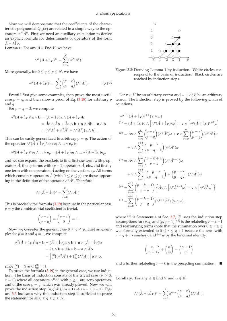
3 Basic applications
Now we will demonstrate that the coefficients of the charac-teristic polynomial QA(x) are related in a simple way to the op-
erators ∧N Ak. First we need an auxiliary calculation to derivean explicit formula for determinants of operators of the form
A− λ1V .Lemma 1: For any A ∈ End V , we have
∧N (A+ 1V )N =N∑
r=0
(∧N Ar).
More generally, for 0 ≤ q ≤ p ≤ N , we have
∧p (A+ 1V )q =
q∑
r=0
(p− r
p− q
)
(∧pAr). (3.19)
Proof: I first give some examples, then prove the most usefulcase p = q, and then show a proof of Eq. (3.19) for arbitrary pand q.For p = q = 2, we compute
∧2(A+ 1V )2a ∧ b = (A+ 1V )a ∧ (A+ 1V )b
= Aa ∧ Ab + Aa ∧ b + a ∧ Ab + a ∧ b
= [∧2A2 + ∧2A1 + ∧2A0] (a ∧ b) .
This can be easily generalized to arbitrary p = q: The action of
the operator ∧p(A+ 1V )p on e1 ∧ ... ∧ ep is
∧p(A+ 1V )pe1 ∧ ... ∧ ep = (A+ 1V )e1 ∧ ... ∧ (A+ 1V )ep,
and we can expand the brackets to find first one term with p op-
erators A, then p terms with (p− 1) operators A, etc., and finally
one term with no operators A acting on the vectors ej . All terms
which contain r operators A (with 0 ≤ r ≤ p) are those appear-
ing in the definition of the operator ∧pAr. Therefore
∧p(A+ 1V )p =
p∑
r=0
(∧pAr).
This is precisely the formula (3.19) because in the particular casep = q the combinatorial coefficient is trivial,
(p− r
p− q
)
=
(p− r
0
)
= 1.
Now we consider the general case 0 ≤ q ≤ p. First an exam-ple: for p = 2 and q = 1, we compute
∧2(A+ 1V )1a ∧ b = (A+ 1V )a ∧ b + a ∧ (A+ 1V )b
= 2a ∧ b + Aa ∧ b + a ∧ Ab
=[(
21
)(∧2A0) +
(20
)(∧2A1)
]
a ∧ b,
since(21
)= 2 and
(20
)= 1.
To prove the formula (3.19) in the general case, we use induc-tion. The basis of induction consists of the trivial case (p ≥ 0,q = 0) where all operators ∧0Ap with p ≥ 1 are zero operators,and of the case p = q, which was already proved. Now we willprove the induction step (p, q)& (p, q + 1) ⇒ (p+ 1, q + 1). Fig-ure 3.3 indicates why this induction step is sufficient to provethe statement for all 0 ≤ q ≤ p ≤ N .
0 1
1
2
2
3
3
4
4
p
q
Figure 3.3: Deriving Lemma 1 by induction. White circles cor-respond to the basis of induction. Black circles arereached by induction steps.
Let v ∈ V be an arbitrary vector and ω ∈ ∧pV be an arbitrarytensor. The induction step is proved by the following chain ofequations,
∧p+1 (A+ 1V )q+1 (v ∧ ω)
(1) = (A+ 1V )v ∧[
∧p(A+ 1V )qω]
+ v ∧[
∧p(A+ 1V )q+1ω]
(2) = Av ∧q∑
r=0
(p− r
p− q
)
(∧pAr)ω + v ∧q∑
r=0
(p− r
p− q
)
(∧pAr)ω
+ v ∧q+1∑
r=0
(p− r
p− q − 1
)
(∧pAr)ω
(3) = Av ∧q+1∑
k=1
(p− k + 1
p− q
)
(∧pAk−1)ω
+ v ∧q+1∑
r=0
[(p− r
p− q − 1
)
+
(p− r
p− q
)]
(∧pAr)ω
(4) =
q+1∑
k=0
(p− k + 1
p− q
){
Av ∧[
∧pAk−1ω]
+ v ∧[
∧pAkω]}
(1) =
q+1∑
k=0
(p− k + 1
p− q
)
(∧p+1Ak) (v ∧ ω) ,
where (1) is Statement 4 of Sec. 3.7, (2) uses the induction stepassumptions for (p, q) and (p, q + 1), (3) is the relabeling r = k−1and rearranging terms (note that the summation over 0 ≤ r ≤ qwas formally extended to 0 ≤ r ≤ q + 1 because the term withr = q + 1 vanishes), and (4) is by the binomial identity
(n
m− 1
)
+
(n
m
)
=
(n+ 1
m
)
and a further relabeling r → k in the preceding summation. �
Corollary: For any A ∈ End V and α ∈ K,
∧p(A+ α1V )q =
q∑
r=0
αq−r
(p− r
p− q
)
(∧pAr).
60
3 Basic applications
Proof: By Statement 3 of Sec. 3.7, ∧p(αA)q = αq(∧pAq). Set
A = αB, where B is an auxiliary operator, and compute
∧p(αB + α1V )q = αq ∧p (B + 1V )q = αq
q∑
r=0
(p− r
p− q
)
(∧pBr)
=
q∑
r=0
αq−r
(p− r
p− q
)
(∧p(αB)r)
=
q∑
r=0
αq−r
(p− r
p− q
)
(∧pAr).
�
Theorem 2: The coefficients qm(A), 1 ≤ m ≤ N of the charac-teristic polynomial, defined by
QA (λ) = (−λ)N +N−1∑
k=0
(−1)k qN−k(A)λk,
are the numbers corresponding to the operators ∧N Am ∈End(∧NV ):
qm(A)1∧N V = ∧N Am.
In particular, qN (A) = det A and q1(A) = TrA. More compactly,the statement can be written as
QA (λ) 1∧N V =
N∑
k=0
(−λ)N−k(∧N Ak).
Proof: This is now a consequence of Lemma 1 and its Corol-lary, where we set p = q = N and obtain
∧N (A− λ1V )N =
N∑
r=0
(−λ)N−r(∧N Ar).
�
Exercise 1: Show that the characteristic polynomial of an oper-
ator A in a three-dimensional space V can be written as
QA(λ) = det A− 12
[(TrA)2 − Tr(A2)
]λ+ (TrA)λ2 − λ3.
Solution: The first and the third coefficients of QA(λ) are, as
usual, the determinant and the trace of A. The second coefficientis equal to −∧3A2, so we need to show that
∧3A2 =1
2
[(TrA)2 − Tr(A2)
].
We apply the operator ∧3A1 twice to a tensor a ∧ b ∧ c and cal-culate:
(TrA)2a ∧ b ∧ c = (∧3A1)(∧3A1)(a ∧ b ∧ c)
= (∧3A1)(Aa ∧ b ∧ c + a ∧ Ab ∧ c + a ∧ b ∧ Ac)
= A2a ∧ b ∧ c + 2Aa ∧ Ab ∧ c + a ∧ A2b ∧ c
+ 2Aa ∧ b ∧ Ac + 2a ∧ Ab ∧ Ac + a ∧ b ∧ A2c
=[Tr(A2) + 2 ∧3 A2
]a ∧ b ∧ c.
Then the desired formula follows. �
Exercise 2 (general trace relations): Generalize the result of Ex-ercise 1 to N dimensions:a) Show that
∧N A2 = 12
[(TrA)2 − Tr(A2)
].
b)* Show that all coefficients ∧N Ak (k = 1, ..., N ) can be ex-pressed as polynomials in TrA, Tr(A2), ..., Tr(AN ).
Hint: Define a “mixed” operator ∧N (An)jAk as a sum of exte-
rior products containing j times An and k times A; for example,
[∧3(A2)1A1
]a ∧ b ∧ c ≡ A2a ∧ (Ab ∧ c + b ∧ Ac)
+ Aa ∧ (A2b ∧ c + b ∧ A2c) + a ∧ (A2b ∧ Ac + Ab ∧ A2c).
By applying several operators ∧N Ak and Tr(Ak) to an exterior
product, derive identities connecting these operators and ∧N Ak :
(∧N A1)(∧N Ak) = (k + 1) ∧N Ak+1 + ∧N (A2)1Ak−1,
Tr(Ak)Tr(A) = Tr(Ak+1) + ∧N (Ak)1A1,
for k = 2, ..., N − 1. Using these identities, show by induction
that operators of the form ∧N Ak (k = 1, ..., N ) can be all ex-
pressed through TrA, Tr(A2), ..., Tr(AN−1) as polynomials.
As an example, here is the trace relation for ∧N A3:
∧N A3 = 16 (TrA)3 − 1
2 (TrA)Tr(A2) + 13Tr(A
3).
Note that in three dimensions this formula directly yields the
determinant of A expressed through traces of powers of A. Be-low (Sec. 4.5.3) we will derive a formula for the general tracerelation. �
Since operators in ∧NV act as multiplication by a number,it is convenient to omit 1∧NV and regard expressions such as
∧N Ak as simply numbers. More formally, there is a canonicalisomorphism between End
(∧NV
)and K (even though there is
no canonical isomorphism between ∧NV and K).Exercise 3: Give an explicit formula for the canonical isomor-
phism: a) between(∧kV
)∗and ∧k(V ∗); b) between End
(∧NV
)
and K.Answer: a) A tensor f∗1 ∧ ...∧ f∗k ∈ ∧k(V ∗) acts as a linear func-
tion on a tensor v1 ∧ ... ∧ vk ∈ ∧kV by the formula
(f∗1 ∧ ... ∧ f∗k ) (v1 ∧ ... ∧ vk) ≡ det(Ajk),
where Ajk is the square matrix defined by Ajk ≡ f∗j (vk).
b) Since (∧NV )∗ is canonically isomorphic to ∧N (V ∗), an op-
erator N ∈ End(∧NV
)can be represented by a tensor
N = (v1 ∧ ... ∧ vN ) ⊗ (f∗1 ∧ ... ∧ f∗N ) ∈(∧NV
)⊗(∧NV ∗) .
The isomorphism maps N into the number det(Ajk), where Ajk
is the square matrix defined by Ajk ≡ f∗j (vk). �
Exercise 4: Show that an operator A ∈ End V and its canonical
transpose operator AT ∈ End V ∗ have the same characteristicpolynomials.
Hint: Consider the operator (A− x1V )T . �
Exercise 5: Given an operator A of rank r < N , show that
∧N Ak = 0 for k ≥ r + 1 but ∧N Ar 6= 0.Hint: If A has rank r < N then Av1 ∧ ... ∧ Avr+1 = 0 for any
set of vectors {v1, ...,vr+1}.
61
3 Basic applications
3.9.1 Nilpotent operators
There are many operators with the same characteristic polyno-mial. In particular, there are many operators which have the
simplest possible characteristic polynomial, Q0(x) = (−x)N .Note that the zero operator has this characteristic polynomial.
We will now see how to describe all such operators A that
QA(x) = (−x)N.
Definition: An operator A ∈ End V is nilpotent if there exists
an integer p ≥ 1 such that (A)p = 0, where 0 is the zero operator
and (A)p is the p-th power of the operator A.
Examples: a) The operator defined by the matrix
(0 α0 0
)
in
some basis {e1, e2} is nilpotent for any number α. This operatorcan be expressed in tensor form as αe1 ⊗ e∗2.b) In the space of polynomials of degree at most n in the vari-
able x, the linear operator ddx is nilpotent because the (n+ 1)-th
power of this operator will evaluate the (n+ 1)-th derivative,which is zero on any polynomial of degree at most n. �
Statement: If A is a nilpotent operator then QA (x) = (−x)N.
Proof: First an example: suppose that N = 2 and that A3 = 0.By Theorem 2, the coefficients of the characteristic polynomial
of the operator A correspond to the operators ∧N Ak. We needto show that all these operators are equal to zero.
Consider, for instance, ∧2A2 = q21∧2V . This operator raisedto the power 3 acts on a tensor a ∧ b ∈ ∧2V as
(∧2A2
)3a ∧ b = A3a ∧ A3b = 0
since A3 = 0. On the other hand,
(∧2A2
)3a ∧ b = (q2)
3a ∧ b.
Therefore q2 = 0. Now consider ∧2A1 to the power 3,
(∧2A1
)3a ∧ b = A2a ∧ Ab + Aa ∧ A2b
(all other terms vanish because A3 = 0). It is clear that the oper-
ator ∧2A1 to the power 6 vanishes because there will be at least
a third power of A acting on each vector. Therefore q1 = 0 aswell.Now a general argument. Let p be a positive integer such that
Ap = 0, and consider the (pN)-th power of the operator ∧N Ak
for some k ≥ 1. We will prove that (∧N Ak)pN = 0. Since ∧N Ak
is a multiplication by a number, from (∧N Ak)pN = 0 it will fol-
low that ∧N Ak is a zero operator in ∧NV for all k ≥ 1. If all thecoefficients qk of the characteristic polynomial vanish, we will
have QA (x) = (−x)N.
To prove that (∧N Ak)pN = 0, consider the action of the oper-
ator (∧N Ak)pN on a tensor e1 ∧ ... ∧ eN ∈ ∧NV . By definition of
∧N Ak, this operator is a sum of terms of the form
As1e1 ∧ ... ∧ AsN eN ,
where sj = 0 or sj = 1 are chosen such that∑N
j=1 sj = k. There-fore, the same operator raised to the power pN is expressed as
(∧N Ak)pN =∑
(s1,...,sn)
As1e1 ∧ ... ∧ AsN eN , (3.20)
where now sj are non-negative integers, 0 ≤ sj ≤ pN , such
that∑N
j=1 sj = kpN . It is impossible that all sj in Eq. (3.20) are
less than p, because then we would have∑N
j=1 sj < Np, which
would contradict the condition∑N
j=1 sj = kpN (since k ≥ 1 byconstruction). So each term of the sum in Eq. (3.20) contains at
least a p-th power of A. Since (A)p = 0, each term in the sum in
Eq. (3.20) vanishes. Hence (∧N Ak)pN = 0 as required. �
Remark: The converse statement is also true: If the character-istic polynomial of an operator A is QA(x) = (−x)N then A isnilpotent. This follows easily from the Cayley-Hamilton the-
orem (see below), which states that QA(A) = 0, so we obtain
immediately (A)N = 0, i.e. the operator A is nilpotent. We findthat one cannot distinguish a nilpotent operator from the zerooperator by looking only at the characteristic polynomial.
62
4 Advanced applications
In this chapter we work in an N -dimensional vector spaceover a number field K.
4.1 The space ∧N−1V
So far we have been using only the top exterior power, ∧NV .The next-to-top exterior power space, ∧N−1V , has the same di-mension as V and is therefore quite useful since it is a space, insome special sense, associated with V . We will now find severalimportant uses of this space.
4.1.1 Exterior transposition of operators
We have seen that a linear operator in the space ∧NV is equiv-alent to multiplication by a number. We can reformulate thisstatement by saying that the space of linear operators in ∧NV iscanonically isomorphic to K. Similarly, the space of linear oper-ators in ∧N−1V is canonically isomorphic to EndV , the space oflinear operators in V . The isomorphism map will be denoted bythe superscript ∧T . Wewill begin by defining this map explicitly.
Question: What is a nontrivial example of a linear operator in∧N−1V ?
Answer: Any operator of the form ∧N−1Ap with 1 ≤ p ≤ N−1
and A ∈ EndV . In this book, operators constructed in this waywill be the only instance of operators in ∧N−1V .
Definition: If X ∈ EndV is a given linear operator then theexterior transpose operator
X∧T ∈ End(∧N−1V
)
is canonically defined by the formula
(X∧Tω
)∧ v ≡ ω ∧ Xv,
which must hold for all ω ∈ ∧N−1V and all v ∈ V . IfY ∈ End(∧N−1V ) is a linear operator then its exterior transpose
Y ∧T ∈ EndV is defined by the formula
ω ∧(Y ∧Tv
)≡ (Y ω) ∧ v, ∀ω ∈ ∧N−1V, v ∈ V.
We need to check that the definition makes sense, i.e. that theoperators defined by these formulas exist and are uniquely de-fined.
Statement 1: The exterior transpose operators are well-defined,i.e. they exist, are unique, and are linear operators in the respec-tive spaces. The exterior transposition has the linearity property
(A+ λB)∧T = A∧T + λB∧T .
If X ∈ EndV is an exterior transpose of Y ∈ End(∧N−1V
),
i.e. X = Y ∧T , then also conversely Y = X∧T .
Proof: We need to show that the formula
(X∧Tω
)∧ v ≡ ω ∧ Xv
actually defines an operator X∧T uniquely when X ∈ EndV is a
given operator. Let us fix a tensor ω ∈ ∧N−1V ; to find X∧Tω we
need to determine a tensor ψ ∈ ∧N−1V such that ψ∧v = ω∧Xv
for all v ∈ V . When we find such a ψ, we will also show thatit is unique; then we will have shown that X∧Tω ≡ ψ is well-defined.An explicit computation of the tensor ψ can be performed in
terms of a basis {e1, ..., eN} in V . A basis in the space ∧N−1Vis formed by the set of N tensors of the form ωi ≡ e1 ∧ ... ∧ei−1 ∧ ei+1 ∧ ... ∧ eN , that is, ωi is the exterior product of thebasis vectors without the vector ei (1 ≤ i ≤ N ). In the nota-tion of Sec. 2.3.3, we have ωi = ∗(ei)(−1)i−1. It is sufficient todetermine the components of ψ in this basis,
ψ =
N∑
i=1
ciωi.
Taking the exterior product of ψ with ei, we find that only theterm with ci survives,
ψ ∧ ei = (−1)N−icie1 ∧ ... ∧ eN .
Therefore, the coefficient ci is uniquely determined from thecondition
cie1 ∧ ... ∧ eN = (−1)N−iψ ∧ ei!=(−1)N−iω ∧ Xei.
Since the operator X is given, we know all Xei and can compute
ω ∧ Xei ∈ ∧NV . So we find that every coefficient ci is uniquelydetermined.It is seen from the above formula that each coefficient ci de-
pends linearly on the operator X . Therefore the linearity prop-erty holds,
(A+ λB)∧T = A∧T + λB∧T .
The linearity of the operator X∧T follows straightforwardlyfrom the identity
(X∧T (ω + λω′)
)∧ v
!=(ω + λω′) ∧ Xv
= ω ∧ Xv + λω′ ∧ Xv
!=(X∧Tω) ∧ v + λ(X∧Tω′) ∧ v.
In the same way we prove the existence, the uniqueness, andthe linearity of the exterior transpose of an operator fromEnd(∧N−1V ). It is then clear that the transpose of the transposeis again the original operator. Details left as exercise. �
Remark: Note that the space ∧N−1V is has the same dimensionas V but is not canonically isomorphic to V . Rather, an elementψ ∈ ∧N−1V naturally acts by exterior multiplication on a vec-tor v ∈ V and yields a tensor from ∧NV , i.e. ψ is a linear map
63
4 Advanced applications
V → ∧NV , and we may express this as ∧N−1V ∼= V ∗ ⊗ ∧NV .Nevertheless, as we will now show, the exterior transpose mapallows us to establish that the space of linear operators in ∧N−1Vis canonically isomorphic to the space of linear operators in V .We will use this isomorphism extensively in the following sec-tions. A formal statement follows.Statement 2: The spaces End(∧N−1V ) and EndV are canoni-cally isomorphic.Proof: The map ∧T between these spaces is one-to-one since
no two different operators are mapped to the same operator. If
two different operators A, B had the same exterior transpose,
we would have (A− B)∧T = 0 and yet A − B 6= 0. There exists
at least one ω ∈ ∧N−1V and v ∈ V such that ω ∧ (A − B)v 6= 0,and then
0 =((A− B)∧Tω
)∧ v = ω ∧ (A− B)v 6= 0,
which is a contradiction. The map ∧T is linear (Statement 1).Therefore, it is an isomorphism between the vector spacesEnd
(∧N−1V
)and EndV . �
A generalization of Statement 1 is the following.Exercise 1: Show that the spaces End(∧kV ) and End(∧N−kV )are canonically isomorphic (1 ≤ k < N ). Specifically, if
X ∈ End(∧kV ) then the linear operator X∧T ∈ End(∧N−kV )is uniquely defined by the formula
(X∧TωN−k
)∧ ωk ≡ ωN−k ∧ Xωk,
which must hold for arbitrary tensors ωk ∈ ∧kV , ωN−k ∈∧N−kV .Remark: It follows that the exterior transpose of ∧N AN ∈End
(∧NV
)is mapped by the canonical isomorphism to an el-
ement of EndK, that is, a multiplication by a number. This isprecisely the map we have been using in the previous section todefine the determinant. In this notation, we have
det A ≡(∧N AN
)∧T.
Here we identify EndK with K.
Exercise 2: For any operators A, B ∈ End(∧kV
), show that
(AB)∧T = B∧T A∧T .
4.1.2 * Index notation
Let us see how the exterior transposition is expressed in the in-dex notation. (Below we will not use the resulting formulas.)
If an operator A ∈ EndV is given in the index notation by a
matrix Aji , the exterior transpose A∧T ∈ End
(∧N−1V
)is rep-
resented by an array Bj1...jN−1
i1...iN−1, which is totally antisymmetric
with respect to its N − 1 lower and upper indices separately.
The action of the operator B ≡ A∧T on a tensor ψ ∈ ∧N−1V iswritten in the index notation as
∑
is
Bj1...jN−1
i1...iN−1ψi1...iN−1.
(Here we did not introduce any combinatorial factors; the factor(N − 1)! will therefore appear at the end of the calculation.)By definition of the exterior transpose, for any vector v ∈ V
and for any ψ ∈ ∧N−1V we must have
(Bψ) ∧ v = ψ ∧ (Av).
Using the index representation of the exterior product through
the projection operators E (see Sec. 2.3.6),we represent the equa-tion above in the the index notation as
∑
i,is,js
Ek1...kN
j1...jN−1i(Bj1...jN−1
i1...iN−1ψi1...iN−1)vi
=∑
js,i,j
Ek1...kN
j1...jN−1jψj1...jN−1(Aj
ivi).
We may simplify this to
∑
i,is,js
εj1...jN−1i(Bj1...jN−1
i1...iN−1ψi1...iN−1)vi
=∑
is,i,j
εi1...iN−1jψi1...iN−1(Aj
i vi),
because Ek1...kN
j1...jN= εj1...jN
εk1...kN , and we may cancel the com-
mon factor εk1...kN whose indices are not being summed over.Since the equation above should hold for arbitrary ψi1...iN−1
and vi, the equation with the corresponding free indices is and ishould hold:
∑
js
εj1...jN−1iBj1...jN−1
i1...iN−1=∑
j
εi1...iN−1jAji . (4.1)
This equation can be solved for B as follows. We note that the εsymbol in the left-hand side of Eq. (4.1) has one free index, i. Letus therefore multiply with an additional ε and sum over that
index; this will yield the projection operator E (see Sec. 2.3.6).Namely, we multiply both sides of Eq. (4.1) with εk1...kN−1i andsum over i:∑
j,i
εk1...kN−1iεi1...iN−1jAji =
∑
js,i
εk1...kN−1iεj1...jN−1iBj1...jN−1
i1...iN−1
=∑
js
Ek1...kN−1
j1...jN−1B
j1...jN−1
i1...iN−1,
where in the last line we used the definition (2.11)–(2.12) of theoperator E. Now we note that the right-hand side is the index
representation of the product of the operators E and B (bothoperators act in ∧N−1V ). The left-hand side is also an operator
in ∧N−1V ; denoting this operator for brevity by X , we rewritethe equation as
EB = X ∈ End(∧N−1V
).
Using the property
E = (N − 1)!1∧N−1V
(see Exercise in Sec. 2.3.6), we may solve the equation EB = X
for B as
B =1
(N − 1)!X.
Hence, the components of B ≡ A∧T are expressed as
Bk1...kN−1
i1...iN−1=
1
(N − 1)!
∑
j,i
εk1...kN−1iεi1...iN−1jAji .
An analogous formula holds for the exterior transpose of anoperator in ∧nV , for any n = 2, ..., N . I give the formula withoutproof and illustrate it by an example.
64
4 Advanced applications
Statement: If A ∈ End (∧nV ) is given by its components Aj1...jn
i1...in
then the components of A∧T are
(A∧T
)k1...kN−n
l1...lN−n
=1
n!(N − n)!
∑
js,is
εk1...kN−ni1...inεl1...lN−nj1...jnAj1...jn
i1...in.
Example: Consider the exterior transposition A∧T of the iden-
tity operator A ≡ 1∧2V . The components of the identity operatorare given by
Aj1j2i1i2
= δj1i1δj2i2,
so the components of A∧T are
(A∧T
)k1...kN−2
l1...lN−2=
1
2!(N − 2)!
∑
js,is
εk1...kN−2i1i2εl1...lN−2j1j2Aj1j2i1i2
=1
2!(N − 2)!
∑
i1,i2
εk1...kN−2i1i2εl1...lN−2i1i2 .
Let us check that this array of components is the same as thatrepresenting the operator 1∧N−2V . We note that the expressionabove is the same as
1
(N − 2)!E
k1...kN−2
l1...lN−2,
where the numbers Ek1...kn
l1...lnare defined by Eqs. (2.11)–(2.12).
Since the operator E in ∧N−2V is equal to (N − 2)!1∧N−2V , weobtain that
A∧T = 1∧N−2V
as required.
4.2 Algebraic complement (adjoint) andbeyond
In Sec. 3.3 we defined the determinant and derived various use-ful properties by considering, essentially, the exterior transpose
of ∧N Ap with 1 ≤ p ≤ N (although we did not introducethis terminology back then). We have just seen that the exte-rior transposition can be defined more generally — as a mapfrom End(∧kV ) to End(∧N−kV ). We will see in this sectionthat the exterior transposition of the operators ∧N−1Ap with1 ≤ p ≤ N − 1 yields operators acting in V that are quite usefulas well.
4.2.1 Definition of algebraic complement
While we proved that operators like (∧N−1Ap)∧T are well-defined, we still have not obtained any explicit formulas forthese operators. We will now compute these operators explic-itly because they play an important role in the further develop-ment of the theory. It will turn out that every operator of the
form (∧N−1Ap)∧T is a polynomial in A with coefficients that are
known if we know the characteristic polynomial of A.
Example 1: Let us compute (∧N−1A1)∧T . We consider, as a firstexample, a three-dimensional (N = 3) vector space V and a
linear operator A ∈ EndV . We are interested in the operator
(∧2A1)∧T . By definition of the exterior transpose,
a ∧ b ∧ (∧2A1)∧T c =((∧2A1)(a ∧ b)
)∧ c
= Aa ∧ b ∧ c + a ∧ Ab ∧ c.
We recognize a fragment of the operator ∧3A1 and write
(∧3A1)(a ∧ b ∧ c) = Aa ∧ b ∧ c + a ∧ Ab ∧ c + a ∧ b ∧ Ac
= (Tr A)a ∧ b ∧ c,
since this operator acts as multiplication by the trace of A (Sec-tion 3.8). It follows that
a ∧ b ∧ (∧2A1)∧T c = (Tr A)a ∧ b ∧ c− a ∧ b ∧ Ac
= a ∧ b ∧((Tr A)c − Ac
).
Since this must hold for arbitrary a,b, c ∈ V , it follows that
(∧2A1)∧T = (Tr A)1V − A.
Thus we have computed the operator (∧2A1)∧T in terms of A
and the trace of A.Example 2: Let us now consider the operator (∧2A2)∧T . Wehave
a ∧ b ∧ (∧2A2)∧T c =((∧2A2)(a ∧ b)
)∧ c = Aa ∧ Ab ∧ c.
We recognize a fragment of the operator ∧3A2 and write
(∧3A2)(a ∧ b ∧ c) = Aa ∧ Ab ∧ c + a ∧ Ab ∧ Ac + Aa ∧ b ∧ Ac.
Therefore,
a ∧ b ∧ (∧2A2)∧T c = (∧3A2)(a ∧ b ∧ c)
− (a ∧ Ab + Aa ∧ b) ∧ Ac
(1) = (∧3A2)(a ∧ b ∧ c) − a ∧ b ∧ (∧2A1)∧T Ac
= a ∧ b∧(∧3A2 − (∧2A1)∧T A
)c,
where (1) used the definition of the operator (∧2A1)∧T . It fol-lows that
(∧2A2)∧T = (∧3A2)1V − (∧2A1)∧T A
= (∧3A2)1V − (Tr A)A+ AA.
Thus we have expressed the operator (∧2A2)∧T as a polynomial
in A. Note that∧3A2 is the second coefficient of the characteristicpolynomial of A.Exercise 1: Consider a three-dimensional space V , a linear op-
erator A, and show that
(∧2A2)∧T Av = (det A)v, ∀v ∈ V.
Hint: Consider a ∧ b ∧ (∧2A2)∧T Ac = Aa ∧ Ab ∧ Ac. �
These examples are straightforwardly generalized. We will
now express every operator of the form (∧N−1Ap)∧T as a poly-
nomial in A. For brevity, we introduce the notation
A(k) ≡ (∧N−1AN−k)∧T , 1 ≤ k ≤ N − 1.
65
4 Advanced applications
Lemma 1: For any operator A ∈ End V and for an integer p, 1 ≤p ≤ N , the following formula holds as an identity of operatorsin V :
(∧N−1Ap−1
)∧TA+
(∧N−1Ap
)∧T= (∧N Ap)1V .
Here, in order to provide a meaning for this formula in cases
p = 1 and p = N , we define ∧N−1AN ≡ 0 and ∧N−1A0 ≡ 1. Inthe shorter notation, this is
A(k)A+ A(k−1) = (∧N AN−k+1)1V .
Note that ∧N AN−k+1 ≡ qk−1, where qj are the coefficients of the
characteristic polynomial of A (see Sec. 3.9).Proof: We use Statement 4 in Sec. 3.7 with ω ≡ v1 ∧ ...∧vN−1,
m ≡ N − 1 and k ≡ p:
(∧N−1Apω
)∧ u +
(∧N−1Ap−1ω
)∧ (Au) = ∧N Ap (ω ∧ u) .
This holds for 1 ≤ p ≤ N − 1. Applying the definition of theexterior transpose, we find
ω ∧(∧N−1Ap
)∧Tu + ω ∧
(∧N−1Ap−1
)∧TAu = (∧N Ap)ω ∧ u.
Since this holds for all ω ∈ ∧N−1V and u ∈ V , we obtain therequired formula,
(∧N−1Ap
)∧T+ ω ∧
(∧N−1Ap−1
)∧TA = (∧N Ap)1V .
It remains to verify the case p = N . In that case we computedirectly,
(∧N−1AN−1ω
)∧ (Au) = Av1 ∧ ... ∧ AvN−1 ∧ Au
= ∧N AN (ω ∧ u) .
Hence,
(∧N−1AN−1
)∧TA = (∧N AN )1V ≡ (det A)1V .
�
Remark: In these formulas we interpret the operators ∧N Ap ∈End
(∧NV
)as simply numbers multiplying some operators.
This is justified since ∧NV is one-dimensional, and linear op-erators in it act as multiplication by numbers. In other words,we implicitly use the canonical isomorphism End
(∧NV
) ∼= K.�
Exercise 2: Use induction in p (for 1 ≤ p ≤ N − 1) and Lemma 1to express A(k) explicitly as polynomials in A:
A(N−p) ≡(∧N−1Ap
)∧T=
p∑
k=0
(−1)k(∧N Ap−k)(A)
k.
Hint: Start applying Lemma 1 with p = 1 and A(N) ≡ 1. �
Using the coefficients qk ≡ ∧N AN−k of the characteristic poly-nomial, the result of Exercise 2 can be rewritten as
(∧N−1A1
)∧T ≡ A(N−1) = qN−11V − A,(∧N−1A2
)∧T ≡ A(N−2) = qN−21V − qN−1A+ (A)2,
......,(∧N−1AN−1
)∧T ≡ A(1) = q11V + q2(−A) + ...
+ qN−1(−A)N−2 + (−A)N−1.
Note that the characteristic polynomial of A is
QA(λ) = q0 + q1(−λ) + ...+ qN−1(−λ)N−1+ (−λ)N .
Thus the operators denoted by A(k) are computed as suitable
“fragments”’ of the characteristic polynomial into which A issubstituted instead of λ.Exercise 3:* Using the definition of exterior transpose for gen-eral exterior powers (Exercise 1 in Sec. 4.1.1), show that for1 ≤ k ≤ N − 1 and 1 ≤ p ≤ k the following identity holds,
p∑
q=0
(∧N−kAp−q
)∧T(∧kAq) = (∧N Ap)1∧kV .
Deduce that the operators(∧N−kAp
)∧Tcan be expressed as
polynomials in the (mutually commuting) operators ∧kAj (1 ≤j ≤ k).Hints: Follow the proof of Statement 4 in Sec. 3.7. The idea is
to apply both sides to ωk ∧ ωN−k, where ωk ≡ v1 ∧ ... ∧ vk and
ωN−k = vN−k+1 ∧ ... ∧ vN . Since ∧N Ap acts on ωk ∧ ωN−k by
distributing p copies of A among the N vectors vj , one needs toshow that the same terms will occur when one first distributesq copies of A among the first k vectors and p − q copies of Aamong the lastN − k vectors, and then sums over all q from 0 top. Once the identity is proved, one can use induction to express
the operators(∧N−kAp
)∧T. For instance, the identity with k = 2
and p = 1 yields
(∧N−2A0
)∧T(∧2A1) +
(∧N−2A1
)∧T(∧2A0) = (∧N A1)1∧kV .
Therefore(∧N−2A1
)∧T= (TrA)1∧kV − ∧2A1.
Similarly, with k = 2 and p = 2 we find
(∧N−2A2
)∧T= (∧N A2)1∧kV −
(∧N−2A1
)∧T(∧2A1) − ∧2A2
= (∧N A2)1∧kV − (TrA)(∧2A1) + (∧2A1)2 − ∧2A2.
It follows by induction that all the operators(∧N−kAp
)∧Tare
expressed as polynomials in ∧kAj . �
At the end of the proof of Lemma 1 we have obtained a curi-ous relation,
(∧N−1AN−1
)∧TA = (det A)1V .
If det A 6= 0, we may divide by it and immediately find the fol-lowing result.
Lemma 2: If det A 6= 0, the inverse operator satisfies
A−1 =1
det A
(∧N−1AN−1
)∧T.
Thus we are able to express the inverse operator A−1 as a poly-
nomial in A. If det A = 0 then the operator A has no inverse,
but the operator(∧N−1AN−1
)∧Tis still well-defined and suffi-
ciently useful to deserve a special name.Definition: The algebraic complement (also called the adjoint)
of A is the operator
˜A ≡
(∧N−1AN−1
)∧T ∈ EndV.
66
4 Advanced applications
Exercise 4: Compute the algebraic complement of the operator
A = a⊗b∗, where a ∈ V and b ∈ V ∗, and V is anN -dimensionalspace (N ≥ 2).Answer: Zero if N ≥ 3. For N = 2 we use Example 1 to
compute
(∧1A1)∧T = (Tr A)1 − A = b∗(a)1 − a ⊗ b∗.
Exercise 5: For the operator A = a⊗b∗ inN -dimensional space,
as in Exercise 4, show that(∧N−1Ap
)∧T= 0 for p ≥ 2.
4.2.2 Algebraic complement of a matrix
The algebraic complement is usually introduced in terms of ma-trix determinants. Namely, one takes a matrix Aij and deletesthe column number k and the row number l. Then one com-putes the determinant of the resulting matrix and multiplies by(−1)k+l. The result is the element Bkl of the matrix that is the al-gebraic complement of Aij . I will now show that our definitionis equivalent to this one, if we interpret matrices as coefficientsof linear operators in a basis.
Statement: Let A ∈ EndV and let {ej} be a basis in V . Let
Aij be the matrix of the operator A in this basis. Let B =(∧N−1AN−1
)∧Tand let Bkl be the matrix of B in the same basis.
ThenBkl is equal to (−1)k+l
times the determinant of the matrixobtained fromAij by deleting the column number k and the rownumber l.Proof: Given an operator B, the matrix element Bkl in the ba-
sis {ej} can be computed as the coefficient in the following rela-tion (see Sec. 2.3.3),
Bkle1 ∧ ... ∧ eN = e1 ∧ ... ∧ ek−1 ∧ (Bel) ∧ ek+1 ∧ ... ∧ eN .
Since B =(∧N−1AN−1
)∧T, we have
Bkle1 ∧ ... ∧ eN = Ae1 ∧ ... ∧ Aek−1 ∧ el ∧ Aek+1 ∧ ... ∧ AeN .
Now the right side can be expressed as the determinant of an-
other operator, call it X ,
Bkle1 ∧ ... ∧ eN = (det X)e1 ∧ ... ∧ eN
= Xe1∧... ∧ Xek−1 ∧ Xek ∧ Xek+1 ∧ ... ∧ XeN ,
if we define X as an operator such that Xek ≡ el while on other
basis vectors Xej ≡ Aej (j 6= k). Having defined X in this way,
we have Bkl = det X .We can now determine the matrix Xij representing X in the
basis {ej}. By the definition of the matrix representation of op-erators,
Aej =
N∑
i=1
Aijei, Xej =
N∑
i=1
Xijei, 1 ≤ j ≤ N.
It follows that Xij = Aij for j 6= k while Xik = δil (1 ≤ i ≤ N ),which means that the entire k-th column in the matrix Aij hasbeen replaced by a column containing zeros except for a singlenonzero element Xlk = 1.It remains to show that the determinant of the matrix Xij is
equal to (−1)k+l
times the determinant of the matrix obtainedfrom Aij by deleting column k and row l. We may move in the
matrixXij the k-th column to the first column and the l-th row tothe first row, without changing the order of any other rows and
columns. This produces the sign factor (−1)k+l
but otherwisedoes not change the determinant. The result is
Bkl = det X = (−1)k+l det
∣∣∣∣∣∣∣∣∣
1 X12 ... X1N
0 ∗ ∗ ∗... ∗ ∗ ∗0 ∗ ∗ ∗
∣∣∣∣∣∣∣∣∣
= (−1)k+l
det
∣∣∣∣∣∣
∗ ∗ ∗∗ ∗ ∗∗ ∗ ∗
∣∣∣∣∣∣
,
where the stars represent the matrix obtained from Aij by delet-ing column k and row l, and the numbers X12, ..., X1N do notenter the determinant. This is the result we needed. �
Exercise 5:* Show that the matrix representation of the alge-braic complement can be written through the Levi-Civita sym-bol ε as
Aik =
1
(N − 1)!
∑
i2,...,iN
∑
k2,...,kN
εkk2...kNεii2...iNAk2
i2...AkN
iN.
Hint: See Sections 3.4.1 and 4.1.2.
4.2.3 Further properties and generalizations
In our approach, the algebraic complement˜A of an operator A
comes from considering the set of N − 1 operators
A(k) ≡(∧N−1AN−k
)∧T, 1 ≤ k ≤ N − 1.
(For convenience we might define A(N) ≡ 1V .)
The operators A(k) can be expressed as polynomials in Athrough the identity (Lemma 1 in Sec. 4.2.1)
A(k)A+ A(k−1) = qk−11, qj ≡ ∧N AN−j .
The numbers qj introduced here are the coefficients of the char-
acteristic polynomial of A; for instance, det A ≡ q0 and TrA ≡qN−1. It follows by induction (Exercise 2 in Sec. 4.2.1) that
A(N−k) = qN−k1 − qN−k+1A+ ...
+ qN−1(−A)k−1 + (−A)k.
The algebraic complement is˜A ≡ A1, but it appears natural to
study the properties of all the operators A(k). (The operators
A(k) do not seem to have an established name for k ≥ 2.)
Statement 1: The coefficients of the characteristic polynomial of
the algebraic complement,˜A, are
∧N ˜Ak = (det A)k−1(∧N AN−k) ≡ qk−1
0 qk.
For instance,
Tr˜A = ∧N ˜
A1 = q1 = ∧N AN−1,
det˜A = ∧N ˜
AN = qN−10 qN = (det A)N−1.
67
4 Advanced applications
Proof: Let us first assume that det A ≡ q0 6= 0. We use the
property A˜A = q01 (Lemma 2 in Sec. 4.2.1) and the multiplica-
tivity of determinants to find
det(˜A− λ1)q0 = det(q01 − λA) = (−λ)N det(A− q0
λ1)
= (−λN )QA(q0λ
),
hence the characteristic polynomial of˜A is
Q ˜A(λ) ≡ det(
˜A− λ1) =
(−λN )
q0QA(
q0λ
)
=(−λ)N
q0
[(
−q0λ
)N
+ qN−1
(
−q0λ
)N−1
+ ...+ q0
]
= (−λ)N + q1(−λ)N−1 + q2q0 (−λ)N−2+ ...+ qN−1
0 .
This agrees with the required formula.
It remains to prove the case q0 ≡ det A = 0. Although thisresult could be achieved as a limit of nonzero q0 with q0 → 0, itis instructive to see a direct proof without using the assumptionq0 6= 0 or taking limits.Consider a basis {vj} in V and the expression
(∧N ˜Ak)v1 ∧ ... ∧ vN .
This expression contains(Nk
)terms of the form
˜Av1 ∧ ... ∧ ˜
Avk ∧ vk+1 ∧ ... ∧ vN ,
where˜A is applied only to k vectors. Using the definition of
˜A,
we can rewrite such a term as follows. First, we use the defini-
tion of˜A to write
˜Av1 ∧ ψ = v1 ∧
(∧N−1AN−1
)ψ,
for any ψ ∈ ∧N−1V . In our case, we use
ψ ≡ ˜Av2 ∧ ... ∧ ˜
Avk ∧ vk+1 ∧ ... ∧ vN
and find
˜Av1 ∧ ψ = v1 ∧ A ˜
Av2 ∧ ... ∧ A ˜Avk ∧ Avk+1 ∧ ... ∧ AvN .
By assumption q0 = 0, hence A˜A = 0 =
˜AA (since
˜A, being a
polynomial in A, commutes with A) and thus
(∧N ˜Ak)v1 ∧ ... ∧ vN = 0, k ≥ 2.
For k = 1 we find
˜Av1 ∧ ψ = v1 ∧ Av2 ∧ ... ∧ AvN .
Summing N such terms, we obtain the same expression as that
in the definition of ∧N AN−1, hence
(∧N ˜A1)v1 ∧ ... ∧ vN = ∧N AN−1v1 ∧ ... ∧ vN .
This concludes the proof for the case det A = 0. �
Exercise:* Suppose that A has the simple eigenvalue λ = 0(i.e. this eigenvalue has multiplicity 1). Show that the algebraic
complement,˜A, has rank 1, and that the image of
˜A is the one-
dimensional subspace Span {v}.Hint: An operator has rank 1 if its image is one-dimensional.
The eigenvalue λ = 0 has multiplicity 1 if ∧N AN−1 6= 0. Choosea basis consisting of the eigenvector v and N − 1 other vectorsu2, ..., uN . Show that
˜Av ∧ u2 ∧ ... ∧ uN = ∧N AN−1(v ∧ u2 ∧ ... ∧ uN ) 6= 0,
while
v ∧ u2 ∧ ... ∧ ˜Auj ∧ ... ∧ uN = 0, 2 ≤ j ≤ N.
Consider other expressions, such as
˜Av ∧ v ∧ u3 ∧ ... ∧ uN or
˜Auj ∧ v ∧ u3 ∧ ... ∧ uN ,
and finally deduce that the image of˜A is precisely the one-
dimensional subspace Span {v}. �
Now we will demonstrate a useful property of the operators
A(k).
Statement 2: The trace of A(k) satisfies
TrA(k)
k= ∧N AN−k ≡ qk.
Proof: Consider the action of ∧N AN−k on a basis tensor ω ≡v1 ∧ ... ∧ vN ; the result is a sum of
(N
N−k
)terms,
∧N AN−kω = Av1 ∧ ... ∧ AvN−k ∧ vN−k+1 ∧ ... ∧ vN
+ (permutations).
Consider now the action of TrA(k) on ω,
TrA(k)ω = ∧N [A(k)]1ω
=
N∑
j=1
v1 ∧ ... ∧ A(k)vj ∧ ... ∧ vN .
Using the definition of A(k), we rewrite
v1 ∧ ... ∧ A(k)vj ∧ ... ∧ vN
= Av1 ∧ ... ∧ AvN−k ∧ vN−k+1 ∧ ... ∧ vj ∧ ... ∧ vN
+ (permutations not including Avj).
After summing over j, we will obtain all the same terms as were
present in the expression for∧N AN−kω, but each termwill occurseveral times. We can show that each term will occur exactly ktimes. For instance, the term
Av1 ∧ ... ∧ AvN−k ∧ vN−k+1 ∧ ... ∧ vj ∧ ... ∧ vN
will occur k times in the expression for TrA(k)ω because it willbe generated once by each of the terms
v1 ∧ ... ∧ A(k)vj ∧ ... ∧ vN
with N − k + 1 ≤ j ≤ N . The same argument holds for everyother term. Therefore
TrA(k)ω = k (∧N AN−k)ω = kqkω.
Since this holds for any ω ∈ ∧NV , we obtain the required state-ment. �
68
4 Advanced applications
Remark: We have thus computed the trace of every operator
A(k), as well as the characteristic polynomial of A(1) ≡ ˜A. Com-
puting the entire characteristic polynomial of each Ak is cer-tainly possible but will perhaps lead to cumbersome expres-sions. �
An interesting application of Statement 2 is the following al-gorithm for computing the characteristic polynomial of an op-erator.1 This algorithm is more economical compared with the
computation of det(A−λ1) via permutations, and requires onlyoperator (or matrix) multiplications and the computation of atrace.Statement 3: (Leverrier’s algorithm) The coefficients ∧N Ak ≡qN−k (1 ≤ k ≤ N ) of the characteristic polynomial of an operator
A can be computed together with the operators A(j) by starting
with A(N) ≡ 1V and using the descending recurrence relationfor j = N − 1, ..., 0:
qj =1
N − jTr [AA(j+1)],
A(j) = qj 1 − AA(j+1). (4.2)
At the end of the calculation, we will have
q0 = det A, A(1) =˜A, A(0) = 0.
Proof: At the beginning of the recurrence, we have
j = N − 1, qN−1 =1
N − jTr [AA(j+1)] = TrA,
which is correct. The recurrence relation (4.2) for A(j) coincideswith the result of Lemma 1 in Sec. 4.2.1 and thus yields at each
step j the correct operator A(j) — as long as qj was computedcorrectly at that step. So it remains to verify that qj is computedcorrectly. Taking the trace of Eq. (4.2) and using Tr 1 = N , weget
Tr [AA(j+1)] = Nqj − TrA(j).
We now substitute for TrA(j) the result of Statement 2 and find
Tr [AA(j+1)] = Nqj − jqj = (N − j) qj .
Thus qj is also computed correctly from the previously known
A(j+1) at each step j. �
Remark: This algorithm provides another illustration for the“trace relations” (see Exercises 1 and 2 in Sec. 3.9), i.e. for thefact that the coefficients qj of the characteristic polynomial of A
can be expressed as polynomials in the traces of A and its pow-ers. These expressions will be obtained in Sec. 4.5.3.
4.3 Cayley-Hamilton theorem andbeyond
The characteristic polynomial of an operator A has roots λ that
are eigenvalues of A. It turns out that we can substitute A as anoperator into the characteristic polynomial, and the result is the
zero operator, as if Awere one of its eigenvalues. In other words,
A satisfies (as an operator) its own characteristic equation.
1I found this algorithm in an online note by W.Kahan, “Jordan’s normal form” (downloaded fromhttp://www.cs.berkeley.edu/~wkahan/MathH110/jordan.pdfon October 6, 2009). Kahan attributes this algorithm to Leverrier, Souriau,Frame, and Faddeev.
Theorem 1 (Cayley-Hamilton): If QA (λ) ≡ det(A− λ1V ) is the
characteristic polynomial of the operator A then QA(A) = 0V .Proof: The coefficients of the characteristic polynomial are
∧N Am. When we substitute the operator A into QA(λ), we ob-tain the operator
QA(A) = (det A)1V + (∧N AN−1)(−A) + ...+ (−A)N .
We note that this expression is similar to that for the algebraic
complement of A (see Exercise 2 in Sec. 4.2.1), so
QA(A) = (det A)1V +(∧N AN−1 + ...+ (−A)N−1
)(−A)
= (det A)1V − (∧N−1AN−1)∧T A = 0V
by Lemma 1 in Sec. 4.2.1. Hence QA(A) = 0V for any operator
A. �
Remark: While it is true that the characteristic polynomial van-
ishes on A, it is not necessarily the simplest such polynomial. A
polynomial of a lower degree may vanish on A. A trivial exam-
ple of this is given by an operator A = α1, that is, the identity
operator times a constant α. The characteristic polynomial of A
is QA(λ) = (α− λ)N. In agreement with the Cayley-Hamilton
theorem, (α1 − A)N = 0. However, the simpler polynomial
p(λ) = λ − α also has the property p(A) = 0. We will lookinto this at the end of Sec. 4.6. �
We have derived the Cayley-Hamilton theorem by consider-
ing the exterior transpose of ∧N−1AN−1. A generalization is
found if we similarly use the operators of the form(∧aAb
)∧T.
Theorem 2 (Cayley-Hamilton in ∧kV ): For any operator A inV and for 1 ≤ k ≤ N , 1 ≤ p ≤ N , the following identity holds,
p∑
q=0
(∧N−kAp−q
)∧T(∧kAq) = (∧N Ap)1∧kV . (4.3)
In this identity, we set ∧kA0 ≡ 1∧kV and ∧kAr ≡ 0 for r > k. Ex-
plicit expressions can be derived for all operators(∧N−kAp
)∧T
as polynomials in the (mutually commuting) operators ∧kAj ,1 ≤ j ≤ k. (See Exercise 3 in Sec. 4.2.1.) Hence, there exist k iden-tically vanishing operator-valued polynomials involving ∧kAj .(In the ordinary Cayley-Hamilton theorem, we have k = 1 and
a single polynomial QA(A) that identically vanishes as an oper-ator in V ≡ ∧1V .) The coefficients of those polynomials will be
known functions of A. One can also obtain an identically van-
ishing polynomial in ∧kA1.Proof: Let us fix k and first write Eq. (4.3) for 1 ≤ p ≤ N − k.
These N − k equations are all of the form
(∧N−kAp
)∧T+ [...] = (∧N Ap)1∧kV , 1 ≤ p ≤ N − k.
In the p-th equation, the omitted terms in square brackets con-
tain only the operators(∧N−kAr
)∧Twith r < p and ∧kAq with
1 ≤ q ≤ k. Therefore, these equations can be used to express(∧N−kAp
)∧Tfor 1 ≤ p ≤ N − k through the operators ∧kAq
explicitly as polynomials. Substituting these expressions intoEq. (4.3), we obtain k identically vanishing polynomials in the
k operators ∧kAq (with 1 ≤ q ≤ k). These polynomials can beconsidered as a system of polynomial equations in the variables
69
4 Advanced applications
αq ≡ ∧kAq . (As an exercise, you may verify that all the op-erators αq commute.) A system of polynomial equations maybe reduced to a single polynomial equation in one of the vari-ables, say α1. (The technique for doing this in practice, calledthe “Gröbner basis,” is complicated and beyond the scope of thisbook.) �
The following two examples illustrate Theorem 2 in three andfour dimensions.Example 1: Suppose V is a three-dimensional space (N = 3)
and an operator A is given. The ordinary Cayley-Hamilton the-orem is obtained from Theorem 2 with k = 1,
q0 − q1A+ q2A2 − A3 = 0,
where qj ≡ ∧N AN−j are the coefficients of the characteristic
polynomial of A. The generalization of the Cayley-Hamiltontheorem is obtained with k = 2 (the only remaining case k = 3will not yield interesting results).We write the identity (4.3) for k = 2 and p = 1, 2, 3. Using the
properties ∧kAk+j = 0 (with j > 0) and ∧kA0 = 1, we get thefollowing three identities of operators in ∧2V :
(∧1A1
)∧T+ ∧2A1 = q21∧2V ,
(∧1A1
)∧T(∧2A1) + ∧2A2 = q11∧2V ,
(∧1A1
)∧T(∧2A2) = q01∧2V .
Let us denote for brevity α1 ≡ ∧2A1 and α2 ≡ ∧2A2. Expressing(∧1A1
)∧Tthrough α1 from the first line above and substituting
into the last two lines, we find
α2 = q11 − q2α1 + α21,
(q21 − α1)α2 = q01.
We can now express α2 through α1 and substitute into the lastequation to find
α31 − 2q2α
21 + (q1 + q22)α1 − (q1q2 − q0)1 = 0.
Thus, the generalization of the Cayley-Hamilton theorem in
∧2V yields an identically vanishing polynomial in ∧2A1 ≡ α1
with coefficients that are expressed through qj .Question: Is this the characteristic polynomial of α1?Answer: I do not know! It could be since it has the correct
degree. However, not every polynomial p(x) such that p(α) = 0for some operator α is the characteristic polynomial of α.Example 2: Let us now consider the case N = 4 and k = 2.We use Eq. (4.3) with p = 1, 2, 3, 4 and obtain the following fourequations,
(∧2A1)∧T + ∧2A1 = (∧4A1)1∧2V ,
(∧2A2)∧T + (∧2A1)∧T (∧2A1) + ∧2A2 = (∧4A2)1∧2V ,
(∧2A2)∧T (∧2A1) + (∧2A1)∧T (∧2A2) = (∧4A3)1∧2V ,
(∧2A2)∧T (∧2A2) = (∧4A4)1∧2V .
Let us denote, as before, qj = ∧4A4−j (with 0 ≤ j ≤ 3) and
αr ≡ ∧2Ar (with r = 1, 2). Using the first two equations above,
we can then express (∧2Ar)∧T through αr and substitute intothe last two equations. We obtain
(∧2A1)∧T = q31 − α1,
(∧2A2)∧T = q21 + α21 − q3α1 − α2,
and finally
(q21 + α21 − q3α1 − α2)α1 + (q31 − α1)α2 = q11,
(q21 + α21 − q3α1 − α2)α2 = q01.
One cannot express α2 directly through α1 using these last equa-tions. However, one can show (for instance, using a com-puter algebra program2) that there exists an identically vanish-ing polynomial of degree 6 in α1, namely p(α1) = 0 with
p(x) ≡ x6 − 3q3x5 +
(2q2 + 3q23
)x4 −
(4q2q3 + q33
)x3
+(q22 − 4q0 + q1q3 + 2q2q
23
)x2 −
(q1q
23 + q22q3 − 4q0q3
)x
+ q1q2q3 − q0q23 − q21 .
The coefficients of p(x) are known functions of the coefficients qjof the characteristic polynomial of A. Note that the space ∧2Vhas dimension 6 in this example; the polynomial p(x) has thesame degree.Question: In both examples we found an identically vanishing
polynomial in ∧kA1. Is there a general formula for the coeffi-cients of this polynomial?Answer: I do not know!
4.4 Functions of operators
We will now consider some calculations with operators.
Let A ∈ EndV . Since linear operators can be multiplied, it is
straightforward to evaluate AA ≡ A2 and other powers of A, as
well as arbitrary polynomials in A. For example, the operator
A can be substituted instead of x into the polynomial p(x) =
2 + 3x+ 4x2; the result is the operator 2 + 3A+ 4A2 ≡ p(A).
Exercise: For a linear operator A and an arbitrary polynomial
p(x), show that p(A) has the same eigenvectors as A (althoughperhaps with different eigenvalues). �
Another familiar function of A is the inverse operator, A−1.
Clearly, we can evaluate a polynomial in A−1 as well (if A−1
exists). It is interesting to ask whether we can evaluate an ar-
bitrary function of A; for instance, whether we can raise A to
a non-integer power, or compute exp(A), ln(A), cos(A). Gener-
ally, can we substitute A instead of x in an arbitrary function
f(x) and evaluate an operator-valued function f(A)? If so, howto do this in practice?
4.4.1 Definitions. Formal power series
The answer is that sometimes we can. There are two situationswhen f(A) makes sense, i.e. can be defined and has reasonableproperties.
The first situation is when A is diagonalizable, i.e. there exists
a basis {ei} such that every basis vector is an eigenvector of A,
Aei = λiei.
In this case, we simply define f(A) as the linear operator thatacts on the basis vectors as follows,
f(A)ei ≡ f(λi)ei.
2This can be surely done by hand, but I have not yet learned the Gröbner basistechnique necessary to do this, so I cannot show the calculation here.
70
4 Advanced applications
Definition 1: Given a function f(x) and a diagonalizable linearoperator
A =
N∑
i=1
λiei ⊗ e∗i ,
the function f(A) is the linear operator defined by
f(A) ≡N∑
i=1
f(λi) ei ⊗ e∗i ,
provided that f(x) is well-defined at the points x = λi, i =1, ..., N .This definition might appear to be “cheating” since we sim-
ply substituted the eigenvalues into f(x), rather than evaluate
the operator f(A) in some “natural” way. However, the result
is reasonable since we, in effect, define f(A) separately in each
eigenspace Span {ei} where A acts as multiplication by λi. It is
natural to define f(A) in each eigenspace as multiplication byf(λi).The second situation is when f(x) is an analytic function, that
is, a function represented by a power series
f(x) =
∞∑
n=0
cnxn,
such that the series converges to the value f(x) for some x. Fur-ther, we need this series to converge for a sufficiently wide range
of values of x such that all eigenvalues of A are within thatrange. Then one can show that the operator-valued series
f(A) =
∞∑
n=0
cn(A)n
converges. The technical details of this proof are beyond thescope of this book; one needs to define the limit of a sequence ofoperators and other notions studied in functional analysis. Hereis a simple argument that gives a condition for convergence.
Suppose that the operator A is diagonalizable and has eigenval-ues λi and the corresponding eigenvectors vi (i = 1, ..., N ) such
that {vi} is a basis and A has a tensor representation
A =
N∑
i=1
λivi ⊗ v∗i .
Note that
An =
[N∑
i=1
λivi ⊗ v∗i
]n
=
N∑
i=1
λni vi ⊗ v∗
i
due to the property of the dual basis, v∗i (vj) = δij . So if the se-
ries∑∞
n=0 cnxn converges for every eigenvalue x = λi of the op-
erator A then the tensor-valued series also converges and yieldsa new tensor
∞∑
n=0
cn(A)n =
∞∑
n=0
cn
N∑
i=1
λni vi ⊗ v∗
i
=
N∑
i=1
[ ∞∑
n=0
cnλn
]
vi ⊗ v∗i .
This argument indicates at least one case where the operator-valued power series surely converges.Instead of performing an in-depth study of operator-valued
power series, I will restrict myself to considering “formal powerseries” containing a parameter t, that is, infinite power series int considered without regard for convergence. Let us discuss thisidea in more detail.By definition, a formal power series (FPS) is an infinite se-
quence of numbers (c0, c1, c2, ...). This sequence, however, iswritten as if it were a power series in a parameter t,
c0 + c1t+ c2t2 + ... =
∞∑
n=0
cntn.
It appears that we need to calculate the sum of the above series.However, while we manipulate an FPS, we do not assign anyvalue to t and thus do not have to consider the issue of conver-gence of the resulting infinite series. Hence, we work with anFPS as with an algebraic expression containing a variable t, anexpression that we do not evaluate (although we may simplifyit). These expressions can be manipulated term by term, so that,for example, the sum and the product of two FPS are alwaysdefined; the result is another FPS. Thus, the notation for FPSshould be understood as a convenient shorthand that simplifiesworkingwith FPS, rather than an actual sum of an infinite series.At the same time, the notation for FPS makes it easy to evaluatethe actual infinite series when the need arises. Therefore, anyresults obtained using FPS will hold whenever the series con-verges.
Now I will use the formal power series to define f(tA).Definition 2: Given an analytic function f(x) shown above and
a linear operator A, the function f(tA) denotes the operator-valued formal power series
f(tA) ≡∞∑
n=0
cn(A)ntn.
(According to the definition of formal power series, the variablet is a parameter that does not have a value and serves only tolabel the terms of the series.)One can define the derivative of a formal power series, with-
out using the notion of a limit (and without discussing conver-gence).Definition 3: The derivative ∂t of a formal power series∑
k aktk is another formal power series defined by
∂t
(∞∑
k=0
aktk)≡
∞∑
k=0
(k + 1) ak+1tk.
This definition gives us the usual properties of the derivative.For instance, it is obvious that ∂t is a linear operator in the spaceof formal power series. Further, we have the important distribu-tive property:Statement 1: The Leibniz rule,
∂t [f(t)g(t)] = [∂tf(t)] g(t) + f(t) [∂tg(t)] ,
holds for formal power series.Proof: Since ∂t is a linear operation, it is sufficient to check
that the Leibniz rule holds for single terms, f(t) = ta and g(t) =tb. Details left as exercise. �
This definition of f(tA) has reasonable and expected proper-ties, such as:
71
4 Advanced applications
Exercise: For an analytic function f(x), show that
f(A)A = Af(A)
and thatd
dtf(tA) = Af ′(A)
for an analytic function f(x). Here both sides are interpreted as
formal power series. Deduce that f(A)g(A) = g(A)f(A) for anytwo analytic functions f(x) and g(x).
Hint: Linear operations with formal power series must be per-formed term by term (by definition). So it is sufficient to con-sider a single term in f(x), such as f(x) = xa. �
Now we can show that the two definitions of the operator-
valued function f(A) agree when both are applicable.
Statement 2: If f(x) is an analytic function and A is a di-agonalizable operator then the two definitions agree, i.e. for
f(x) =∑∞
n=0 cnxn and A =
∑Ni=1 λiei ⊗e∗i we have the equality
of formal power series,
∞∑
n=0
cn(tA)n =
N∑
i=1
f(tλi) ei ⊗ e∗i . (4.4)
Proof: It is sufficient to prove that the terms multiplying tn
coincide for each n. We note that the square of A is
(N∑
i=1
λiei ⊗ e∗i
)2
=
(N∑
i=1
λiei ⊗ e∗i
)
N∑
j=1
λjej ⊗ e∗j
=
N∑
i=1
λ2i ei ⊗ e∗i
because e∗i (ej) = δij . In this way we can compute any power of
A. Therefore, the term in the left side of Eq. (4.4) is
cntn(A)n = cnt
n
(N∑
i=1
λiei ⊗ e∗i
)n
= cntn
N∑
i=1
λni ei ⊗ e∗i ,
which coincides with the term at tn in the right side. �
4.4.2 Computations: Sylvester’s method
Now that we know when an operator-valued function f(A) is
defined, how can we actually compute the operator f(A)? The
first definition requires us to diagonalize A (this is already a lotof work since we need to determine every eigenvector). More-
over, Definition 1 does not apply when A is non-diagonalizable.On the other hand, Definition 2 requires us to evaluate infinitelymany terms of a power series. Is there a simpler way?
There is a situation when f(A) can be computed without sucheffort. Let us first consider a simple example where the operator
A happens to be a projector, (A)2 = A. In this case, any power of
A is again equal to A. It is then easy to compute a power series
in A:∞∑
n=0
cn(A)n = c01 +(
∞∑
n=1
cn)A.
In this way we can compute any analytic function of A (as longas the series
∑∞n=1 cn converges). For example,
cos A = 1 − 1
2!(A)2 +
1
4!(A)4 − ... = 1 − 1
2!A+
1
4!A− ...
= (1 − 1
2!+
1
4!− ...)A + 1 − A
= [(cos 1) − 1] A+ 1.
Remark: In the above computation, we obtained a formula that
expresses the end result through A. We have that formula even
though we do not know an explicit form of the operator A —
not even the dimension of the space where A acts or whether Ais diagonalizable. We do not need to know any eigenvectors of
A. We only use the given fact that A2 = A, and we are still able
to find a useful result. If such an operator A is given explicitly,we can substitute it into the formula
cos A = [(cos 1) − 1] A+ 1
to obtain an explicit expression for cos A. Note also that the re-
sult is a formula linear in A.Exercise 1: a) Given that (P )2 = P , express (λ1−P )−1 and exp P
through P . Assume that |λ| > 1 so that the Taylor series forf(x) = (λ− x)−1 converges for x = 1.
b) It is known only that (A)2 = A+ 2. Determine the possible
eigenvalues of A. Show that any analytic function of A can be
reduced to the form α1 + βA with some suitable coefficients αand β. Express (A)3, (A)4, and A−1 as linear functions of A.
Hint: Write A−1 = α1+βAwith unknown α, β. Write AA−1 =1 and simplify to determine α and β.
Exercise 2: The operator A is such that A3 + A = 0. Compute
exp(λA) as a quadratic polynomial of A (here λ is a fixed num-ber). �
Let us now consider a more general situation. Suppose we
know the characteristic polynomial QA(λ) of A. The character-istic polynomial has the form
QA(λ) = (−λ)N+
N−1∑
k=0
(−1)kqN−kλ
k,
where qi (i = 1, ..., N ) are known coefficients. The Cayley-
Hamilton theorem indicates that A satisfies the polynomialidentity,
(A)N = −N−1∑
k=0
qN−k (−1)N−k
(A)k.
It follows that any power of A larger thanN−1 can be expressed
as a linear combination of smaller powers of A. Therefore, a
power series in A can be reduced to a polynomial p(A) of de-gree not larger than N − 1. The task of computing an arbitrary
function f(A) is then reduced to the task of determining the Ncoefficients of p(x) ≡ p0 + ... + pN−1x
n−1. Once the coefficientsof that polynomial are found, the function can be evaluated as
f(A) = p(A) for any operator A that has the given characteristicpolynomial.
Determining the coefficients of the polynomial p(A) might ap-pear to be difficult because one can get rather complicated for-
mulas when one converts an arbitrary power of A to smaller
72
4 Advanced applications
powers. This work can be avoided if the eigenvalues of A areknown, by using the method of Sylvester, which I will now ex-plain.
The present task is to calculate f(A) — equivalently, the poly-
nomial p(A) — when the characteristic polynomial QA(λ) isknown. The characteristic polynomial has order N and hencehas N (complex) roots, counting each root with its multiplicity.
The eigenvalues λi of the operator A are roots of its character-istic polynomial, and there exists at least one eigenvector vi foreach λi (Theorem 1 in Sec. 3.9). Knowing the characteristic poly-nomial QA(λ), we may determine its roots λi.Let us first assume that the roots λi (i = 1, ..., N ) are all
different. Then we have N different eigenvectors vi. Theset {vi | i = 1, ..., N} is linearly independent (Statement 1 in
Sec. 3.6.1) and hence is a basis in V ; that is, A is diagonalizable.We will not actually need to determine the eigenvectors vi; itwill be sufficient that they exist. Let us now apply the function
f(A) to each of these N eigenvectors: we must have
f(A)vi = f(λi)vi.
On the other hand, we may express
f(A)vi = p(A)vi = p(λi)vi.
Since the set {vi} is linearly independent, the vanishing linearcombination
N∑
i=1
[f(λi) − p(λi)]vi = 0
must have all vanishing coefficients; hence we obtain a systemof N equations for N unknowns {p0, ..., pN−1}:
p0 + p1λi + ...+ pN−1λN−1i = f(λi), i = 1, ..., N.
Note that this system of equations has the Vandermonde ma-trix (Sec. 3.6). Since by assumption all λi’s are different, thedeterminant of this matrix is nonzero, therefore the solution{p0, ..., pN−1} exists and is unique. The polynomial p(x) is theinterpolating polynomial for f(x) at the points x = λi (i =1, ..., N ).We have proved the following theorem:
Theorem 1: If the roots {λ1, ..., λN} of the characteristic poly-
nomial of A are all different, a function of A can be computed
as f(A) = p(A), where p(x) is the interpolating polynomial forf(x) at the N points {λ1, ..., λN}.Exercise 3: It is given that the operator A has the characteristicpolynomial QA(λ) = λ2 − λ + 6. Determine the eigenvalues of
A and calculate exp(A) as a linear expression in A.
If we know that an operator A satisfies a certain operator
equation, say (A)2 − A + 6 = 0, then it is not necessary toknow the characteristic polynomial in order to compute func-
tions f(A). It can be that the characteristic polynomial has ahigh order due to many repeated eigenvalues; however, as faras analytic functions are concerned, all that matters is the possi-
bility to reduce high powers of A to low powers. This possibil-ity can be provided by a polynomial of a lower degree than thecharacteristic polynomial.
In the following theorem, we will determine f(A) knowing
only some polynomial Q(x) for which p(A) = 0.
Theorem 2: Suppose that a linear operator A and a polynomial
Q(x) are such that Q(A) = 0, and assume that the equationQ(λ) = 0 has all distinct roots λi (i = 1, ..., n), where n is notnecessarily equal to the dimension N of the vector space. Then
an analytic function f(A) can be computed as
f(A) = p(A),
where p(x) is the interpolating polynomial for the function f(x)at the points x = λi (i = 1, ..., n).Proof: The polynomial p(x) is defined uniquely by substitut-
ing xk with k ≥ n through lower powers of x in the series for
f(x), using the equation p(x) = 0. Consider the operator A1 that
acts as multiplication by λ1. This operator satisfies p(A1) = 0,
and so f(A1) is simplified to the same polynomial p(A1). Hence
we must have f(A1) = p(A1). However, f(A1) is simply the op-erator of multiplication by f(λ1). Hence, p(x) must be equalto f(x) when evaluated at x = λ1. Similarly, we find thatp(λi) = f(λi) for i = 1, ..., n. The interpolating polynomial forf(x) at the points x = λi (i = 1, ..., n) is unique and has degreen− 1. Therefore, this polynomial must be equal to p(x). �
It remains to develop a procedure for the case when not allroots λi of the polynomial Q(λ) are different. To be specific, letus assume that λ1 = λ2 and that all other eigenvalues are differ-ent. In this case we will first solve an auxiliary problem whereλ2 = λ1 + ε and then take the limit ε → 0. The equations deter-mining the coefficients of the polynomial p(x) are
p(λ1) = f(λ1), p(λ1 + ε) = f(λ1 + ε), p(λ3) = f(λ3), ...
Subtracting the first equation from the second and dividing byε, we find
p(λ1 + ε) − p(λ1)
ε=f(λ1 + ε) − f(λ1)
ε.
In the limit ε→ 0 this becomes
p′(λ1) = f ′(λ1).
Therefore, the polynomial p(x) is determined by the require-ments that
p(λ1) = f(λ1), p′(λ1) = f ′(λ1), p(λ3) = f(λ3), ...
If three roots coincide, say λ1 = λ2 = λ3, we introduce two aux-iliary parameters ε2 and ε3 and first obtain the three equations
p(λ1) = f(λ1), p(λ1 + ε2) = f(λ1 + ε2),
p(λ1 + ε2 + ε3) = f(λ1 + ε2 + ε3).
Subtracting the equations and taking the limit ε2 → 0 as before,we find
p(λ1) = f(λ1), p′(λ1) = f ′(λ1), p
′(λ1 + ε3) = f ′(λ1 + ε3).
Subtracting now the second equation from the third and takingthe limit ε3 → 0, we find p′′(λ1) = f ′′(λ1). Thus we have provedthe following.
Theorem 3: If a linear operator A satisfies a polynomial oper-
ator equation Q(A) = 0, such that the equation Q(λ) = 0 hasroots λi (i = 1, ..., n) with multiplicitiesmi,
Q(λ) = const · (λ− λ1)m1 ... (λ− λn)mn ,
73
4 Advanced applications
an analytic function f(A) can be computed as
f(A) = p(A),
where p(x) is the polynomial determined by the conditions
p(λi) = f(λi), p′(λi) = f ′(λi), ...,
dmi−1p(x)
dxmi−1
∣∣∣∣x=λi
=dmi−1f(x)
dxmi−1
∣∣∣∣x=λi
, i = 1, ..., n.
Theorems 1 to 3, which comprise Sylvester’s method, allow usto compute functions of an operator when only the eigenvaluesare known, without determining any eigenvectors and withoutassuming that the operator is diagonalizable.
4.4.3 * Square roots of operators
In the previous section we have seen that functions of operatorscan be sometimes computed explicitly. However, our methods
work either for diagonalizable operators A or for functions f(x)given by a power series that converges for every eigenvalue of
the operator A. If these conditions are not met, functions of op-erators may not exist or may not be uniquely defined. As anexample where these problems arise, we will briefly considerthe task of computing the square root of a given operator.
Given an operator Awewould like to define its square root as
an operator B such that B2 = A. For a diagonalizable operator
A =∑N
i=1 λiei ⊗ e∗i (where {ei} is an eigenbasis and {e∗i } is the
dual basis) we can easily find a suitable B by writing
B ≡N∑
i=1
√
λiei ⊗ e∗i .
Note that the numeric square root√λi has an ambiguous sign;
so with each possible choice of sign for each√λi, we obtain a
possible choice of B. (Depending on the problem at hand, theremight be a natural way of fixing the signs; for instance, if all λi
are positive then it might be useful to choose also all√λi as pos-
itive.) The ambiguity of signs is expected; what is unexpected is
that there could be many other operators B satisfying B2 = A,as the following example shows.Example 1: Let us compute the square root of the identity oper-
ator in a two-dimensional space. We look for B such that B2 = 1.
Straightforward solutions are B = ±1. However, consider thefollowing operator,
B ≡(a bc −a
)
, B2 =
(a2 + bc 0
0 a2 + bc
)
=(a2 + bc
)1.
This B satisfies B2 = 1 for any a, b, c ∈ C as long as a2 + bc = 1.The square root is quite ambiguous for the identity operator! �
We will now perform a simple analysis of square roots of op-erators in two- and three-dimensional spaces using the Cayley-Hamilton theorem.Let us assume that B2 = A, where A is a given operator, and
denote for brevity a ≡ TrA and b ≡ TrB (where a is given but
b is still unknown). In two dimensions, any operator B satisfiesthe characteristic equation
B2 − (TrB)B + (det B)1 = 0.
Taking the trace of this equation, we can express the determinantas
det B =1
2(TrB)2 − 1
2Tr(B2)
and hence
bB = A+b2 − a
21. (4.5)
This equation will yield an explicit formula for B through A ifwe only determine the value of the constant b such that b 6= 0.Squaring the above equation and taking the trace, we find
b4 − 2b2a+ c = 0, c ≡ 2Tr(A2) − a2 = a2 − 4 det A.
Hence, we obtain up to four possible solutions for b,
b = ±√
a±√
a2 − c = ±√
TrA± 2√
det A. (4.6)
Each value of b such that b 6= 0 yield possible operators Bthrough Eq. (4.5). Denoting by s1 = ±1 and s2 = ±1 the twofree choices of signs in Eq. (4.6), we may write the general solu-tion (assuming b 6= 0) as
B = s1A+ s2
√
det A1√
TrA+ 2s2√
det A
. (4.7)
It is straightforward to verify (using the Cayley-Hamilton theo-
rem for A) that every such B indeed satisfies B2 = A.
Note also that B is expressed as a linear polynomial in A.Due to the Cayley-Hamilton theorem, any analytic function of
A reduces to a linear polynomial in the two-dimensional case.Hence, we can view Eq. (4.7) as a formula yielding the analytic
solutions of the equation B2 = A.
If b = 0 is a solution of Eq. (4.6) then we must consider the
possibility that solutions B with b ≡ Tr B = 0 may exist. In
that case, Eq. (4.5) indicates that A plus a multiple of 1 must beequal to the zero operator. Note that Eq. (4.5) is a necessary con-
sequence of B2 = A, obtained only by assuming that B exists.
Hence, when A is not proportional to the identity operator, no
solutions B with Tr B = 0 can exist. On the other hand, if A isproportional to 1, solutions with Tr B = 0 exist but the presentmethod does not yield these solutions. (Note that this method
can only yield solutions B that are linear combinations of the
operator A and the identity operator!) It is easy to see that the
operators from Example 1 fall into this category, with TrB = 0.There are no other solutions except those shown in Example 1because in that example we have obtained all possible tracelesssolutions.
Another interesting example is found when A is a nilpotent(but nonzero).
Example 2: Consider a nilpotent operator A1 =
(0 10 0
)
. In
that case, both the trace and the determinant of A1 are equalto zero; it follows that b = 0 is the only solution of Eq. (4.6).
However, A1 is not proportional to the identity operator. Hence,
a square root of A1 does not exist.
74
4 Advanced applications
Remark: This problem with the nonexistence of the square rootis not the same as the nonexistence of
√−1 within real numbers;
the square root of A1 does not exist even if we allow complex
numbers! The reason is that the existence of√
A1 would be al-gebraically inconsistent (because it would contradict the Cayley-Hamilton theorem). �
Let us summarize our results so far. In two dimensions, thegeneral calculation of a square root of a given operator A pro-
ceeds as follows: If A is proportional to the identity operator,we have various solutions of the form shown in Example 1. (Notevery one of these solutions may be relevant for the problem at
hand, but they exist.) If A is not proportional to the identity op-erator, we solve Eq. (4.6) and obtain up to four possible values
of b. If the only solution is b = 0, the square root of A does not
exist. Otherwise, every nonzero value of b yields a solution Baccording to Eq. (4.5), and there are no other solutions.Example 3: We would like to determine a square root of theoperator
A =
(1 30 4
)
.
We compute det A = 4 and a = TrA = 5. Hence Eq. (4.6) givesfour nonzero values,
b = ±√
5 ± 4 = {±1,±3} .
Substituting these values of b into Eq. (4.5) and solving for B, wecompute the four possible square roots
B = ±(
1 10 2
)
, B = ±(
−1 30 2
)
.
Since b = 0 is not a solution, while A 6= λ1, there are no othersquare roots.Exercise 1: Consider a diagonalizable operator represented in acertain basis by the matrix
A =
(λ2 00 µ2
)
,
where λ and µ are any complex numbers, possibly zero, suchthat λ2 6= µ2. Use Eqs. (4.5)–(4.6) to show that the possiblesquare roots are
B =
(±λ 00 ±µ
)
.
and that there are no other square roots. �
Exercise 2: Obtain all possible square roots of the zero operatorin two dimensions. �
Let us now consider a given operator A in a three-dimensional
space and assume that there exists B such that B2 = A. We will
be looking for a formula expressing B as a polynomial in A. Aswe have seen, this will certainly not give every possible solution
B, but we do expect to get the interesting solutions that can be
expressed as analytic functions of A.
As before, we denote a ≡ TrA and b ≡ TrB. The Cayley-
Hamilton theorem for B together with Exercise 1 in Sec. 3.9(page 61) yields a simplified equation,
0 = B3 − bB2 + sB − (det B)1
= (A+ s1)B − bA− (det B)1, (4.8)
s ≡ b2 − a
2.
Note that det B = ±√
det A and hence can be consideredknown. Moving B to another side in Eq. (4.8) and squaring theresulting equation, we find
(A2 + 2sA+ s21)A = (bA+ (det B)1)2.
Expanding the brackets and using the Cayley-Hamilton theo-
rem for A in the form
A3 − aA2 + pA− (det A)1 = 0,
where the coefficient p can be expressed as
p =1
2(a2 − Tr(A2)),
we obtain after simplifications
(s2 − p− 2b det B)A = 0.
This yields a fourth-order polynomial equation for b,
(b2 − a
2
)2
− p− 2b det B = 0.
This equation can be solved, in principle. Since det B has up to
two possible values, det B = ±√
det A, we can then determineup to eight possible values of b (and the corresponding values ofs).Nowwe use a trick to express B as a function of A. We rewrite
Eq. (4.8) as
AB = −sB + bA+ (det B)1
and multiply both sides by B, substituting AB back into theequation,
A2 + sA = bAB + (det B)B
= b[−sB + bA+ (det B)1] + (det B)B.
The last line yields
B =1
(det B) − sb[A2 + (s− b2)A− b(det B)1].
This is the final result, provided that the denominator (det B −sb) does not vanish. In case this denominator vanishes, thepresent method cannot yield a formula for B in terms of A.Exercise 3:* Verify that the square root of a diagonalizable op-erator,
A =
p2 0 00 q2 00 0 r2
,
where p2, q2, r2 ∈ C are all different, can be determined usingthis approach, which yields the eight possibilities
B =
±p 0 00 ±q 00 0 ±r
.
Hint: Rather than trying to solve the fourth-order equation forb directly (a cumbersome task), one can just verify, by substitut-ing into the equation, that the eight values b = ±p± q ± r (withall the possible choices of signs) are roots of that equation.
75
4 Advanced applications
Exercise 4:*3 It is given that a three-dimensional operator A sat-isfies
Tr (A2) =1
2(Tr A)2, det A 6= 0.
Show that there exists B, unique up to a sign, such that Tr B = 0
and B2 = A.Answer:
B = ± 1√
det A
[A2 − 1
2(Tr A)A
].
4.5 Formulas of Jacobi and Liouville
Definition: The Liouville formula is the identity
det(exp A) = exp(TrA), (4.9)
where A is a linear operator and exp A is defined by the powerseries,
exp A ≡∞∑
n=0
1
n!(A)n.
Example: Consider a diagonalizable operator A (an operatorsuch that there exists an eigenbasis {ei | i = 1, ..., N}) and denote
by λi the eigenvalues, so that Aei = λiei. (The eigenvalues λi
are not necessarily all different.) Then we have (A)nei = λni ei
and therefore
(exp A)ei =
∞∑
n=0
1
n!(A)nei =
∞∑
n=0
1
n!λn
i ei = eλiei.
The trace of A is TrA =∑N
i=1 λi and the determinant is det A =∏N
i=1 λi. Hence we can easily verify the Liouville formula,
det(exp A) = eλ1 ...eλN = exp(λ1 + ...+ λn) = exp(TrA).
However, the Liouville formula is valid also for non-diagonalizable operators. �
The formula (4.9) is useful in several areas of mathematics andphysics. A proof of Eq. (4.9) for matrices can be given throughthe use of the Jordan canonical form of the matrix, which isa powerful but complicated construction that actually is notneeded to derive the Liouville formula. We will derive it us-ing operator-valued differential equations for power series. Auseful by-product is a formula for the derivative of the determi-nant.
Theorem 1 (Liouville’s formula): For an operator A in a finite-dimensional space V ,
det exp(tA) = exp(tTrA). (4.10)
Here both sides are understood as formal power series in thevariable t, e.g.
exp(tA) ≡∞∑
n=0
tn
n!(A)n,
i.e. an infinite series considered without regard for convergence(Sec. 4.4).
3This is motivated by the article by R. Capovilla, J. Dell, and T. Jacobson, Clas-sical and Quantum Gravity 8 (1991), pp. 59–73; see p. 63 in that article.
Remark: Although we establish Theorem 1 only in the sense ofequality of formal power series, the result is useful because bothsides of Eq. (4.10) will be equal whenever both series converge.Since the series for exp(x) converges for all x, one expects thatEq. (4.10) has a wide range of applicability. In particular, it holdsfor any operator in finite dimensions. �
The idea of the proof will be to represent both sides ofEq. (4.10) as power series in t satisfying some differential equa-tion. First we figure out how to solve differential equations forformal power series. Then we will guess a suitable differentialequation that will enable us to prove the theorem.
Lemma 1: The operator-valued function F (t) ≡ exp(tA) is theunique solution of the differential equation
∂tF (t) = F (t) A, F (t = 0) = 1V ,
where both sides of the equation are understood as formalpower series.Proof: The initial condition means that
F (t) = 1 + F1t+ F2t2 + ...,
where F1, F2, ..., are some operators. Then we equate termswith equal powers of t in the differential equation, which yields
Fj+1 = 1j FjA, j = 1, 2, ..., and so we obtain the desired expo-
nential series. �
Lemma 2: If φ(t) and ψ(t) are power series in twith coefficientsfrom ∧mV and ∧nV respectively, then the Leibniz rule holds,
∂t (φ ∧ ψ) = (∂tφ) ∧ ψ + φ ∧ (∂tψ) .
Proof: Since the derivative of formal power series, as definedabove, is a linear operation, it is sufficient to verify the statementin the case when φ = taω1 and ψ = tbω2. Then we find
∂t (φ ∧ ψ) = (a+ b) ta+b−1ω1 ∧ ω2,
(∂tφ) ∧ ψ + φ ∧ (∂tψ) = ata−1ω1 ∧ tbω2 + taω1 ∧ btb−1ω2.
�
Lemma 3: The inverse to a formal power series φ(t) exists (as aformal power series) if and only if φ(0) 6= 0.Proof: The condition φ(0) 6= 0 means that we can express
φ(t) = φ(0) + tψ(t) where ψ(t) is another power series. Thenwe can use the identity of formal power series,
1 = (1 + x)
[ ∞∑
n=0
(−1)nxn
]
,
to express 1/φ(t) as a formal power series,
1
φ(t)=
1
φ(0) + tψ(t)=
∞∑
n=0
(−1)n
[φ(0)]−n−1
[tψ(t)]n.
Since each term [tψ(t)]nis expanded into a series that starts with
tn, we can compute each term of 1/φ(t) by adding finitely manyother terms, i.e. the above equation does specify a well-definedformal power series. �
Corollary: If A(t) is an operator-valued formal power series, the
inverse to A(t) exists (as a formal power series) if and only if
det A(0) 6= 0.The next step towards guessing the differential equation is to
compute the derivative of a determinant.
76
4 Advanced applications
Lemma 4 (Jacobi’s formula): If A(t) is an operator-valued for-
mal power series such that the inverse A−1(t) exists, we have
∂t det A(t) = (det A)Tr [A−1∂tA] = Tr [(det A)A−1∂tA]. (4.11)
If the inverse does not exist, we need to replace det A · A−1 inEq. (4.11) by the algebraic complement,
˜A ≡
(∧N−1AN−1
)∧T
(see Sec. 4.2.1), so that we obtain the formula of Jacobi,
∂t det A = Tr [˜A∂tA].
Proof of Lemma 4: A straightforward calculation usingLemma 2 gives(∂t det A(t)
)v1 ∧ ... ∧ vN = ∂t[Av1 ∧ ... ∧ AvN ]
=
N∑
k=1
Av1 ∧ ... ∧ (∂tA)vk ∧ ... ∧ AvN .
Nowwe use the definition of the algebraic complement operatorto rewrite
Av1 ∧ ... ∧ (∂tA)vk ∧ ... ∧ AvN = v1 ∧ ... ∧ (˜A∂tAvk) ∧ ... ∧ vN .
Hence
(∂t det A)v1 ∧ ... ∧ vN =N∑
k=1
v1 ∧ ... ∧ (˜A∂tAvk) ∧ ... ∧ vN
= ∧N (˜A∂tA)1v1 ∧ ... ∧ vN
= Tr [˜A∂tA]v1 ∧ ... ∧ vN .
Therefore ∂t det A = Tr [˜A∂tA]. When A−1 exists, we may ex-
press˜A through the inverse matrix,
˜A = (det A)A−1, and obtain
Eq. (4.11).
Proof of Theorem 1: It follows from Lemma 3 that F−1(t) ex-
ists since F (0) = 1, and it follows from Lemma 4 that the oper-
ator-valued function F (t) = exp(tA) satisfies the differentialequation
∂t det F (t) = det F (t) · Tr[F−1∂tF ].
From Lemma 1, we have F−1∂tF = F−1F A = A, therefore
∂t det F (t) = det F (t) · TrA.
This is a differential equation for the number-valued formal
power series f(t) ≡ det F (t), with the initial condition f(0) = 1.The solution (which we may still regard as a formal power se-ries) is
f(t) = exp(tTrA).
Therefore
det F (t) ≡ det exp(tA) = exp(tTrA).
�
Exercise 1: (generalized Liouville’s formula) If A ∈ End V andp ≤ N ≡ dimV , show that
∧p(exp tA)p = exp(t(∧pA1)
),
where both sides are understood as formal power series of op-erators in ∧pV . (The Liouville formula is a special case withp = N .)
Exercise 2:* (Sylvester’s theorem) For any two linear maps A :
V → W and B : W → V , we have well-defined composition
maps AB ∈ EndW and BA ∈ End V . Then
det(1V + BA) = det(1W + AB).
Note that the operators at both sides act in different spaces.Hint: Introduce a real parameter t and consider the functions
f(t) ≡ det(1 + tAB), g(t) ≡ det(1 + tBA). These functions arepolynomials of finite degree in t. Consider the differential equa-tion for these functions; show that f(t) satisfies
df
dt= f(t)Tr [AB(1 + tAB)−1],
and similarly for g. Expand in series in t and use the identi-
ties Tr (AB) = Tr (BA), Tr (ABAB) = Tr (BABA), etc. Thenshow that f and g are solutions of the same differential equa-tion, with the same conditions at t = 0. Therefore, show thatthese functions are identical as formal power series. Since f andg are actually polynomials in t, they must be equal.
4.5.1 Derivative of characteristic polynomial
Jacobi’s formula expresses the derivative of the determinant,
∂t det A, in terms of the derivative ∂tA of the operator A. Thedeterminant is the last coefficient q0 of the characteristic polyno-
mial of A. It is possible to obtain similar formulas for the deriva-tives of all other coefficients of the characteristic polynomial.Statement: The derivative of the coefficient
qk ≡ ∧N AN−k
of the characteristic polynomial of A is expressed (for 0 ≤ k ≤N − 1) as
∂tqk = Tr[(∧N−1AN−k−1)∧T ∂tA
].
Note that the first operator in the brackets is the one we denoted
by A(k+1) in Sec. 4.2.3, so we can write
∂tqk = Tr [A(k+1)∂tA].
Proof: We apply the operator ∂t(∧N AN−k) to the tensor ω ≡v1 ∧ ... ∧ vN , where {vj} is a basis. We assume that the vectorsvj do not depend on t, so we can compute
[∂t(∧N AN−k)
]ω = ∂t
[∧N AN−kω
].
The result is a sum of terms such as
Av1 ∧ ... ∧ AvN−k−1 ∧ ∂tAvN−k ∧ vN−k+1 ∧ ... ∧ vN
and other terms obtained by permuting the vectors vj (withoutintroducing any minus signs!). The total number of these terms
is equal toN(
N−1N−k−1
), since we need to choose a single vector to
which ∂tA will apply, and then (N − k − 1) vectors to which Awill apply, among the (N − 1) remaining vectors. Now considerthe expression
Tr[(∧N−1AN−k−1)∧T∂tA
]ω.
This expression is the sum of terms such as
A(k+1)∂tAv1 ∧ v2 ∧ ... ∧ vN
77
4 Advanced applications
and other terms with permuted vectors vj . There will beN suchterms, since we choose one vector out ofN to apply the operator
A(k+1)∂tA. Using the definition of A(k+1), we write
A(k+1)∂tAv1 ∧ v2 ∧ ... ∧ vN
= ∂tAv1 ∧[∧N−1AN−k−1
](v2 ∧ ... ∧ vN )
= ∂tAv1 ∧ Av2 ∧ ... ∧ AvN−k ∧ vN−k+1 ∧ ... ∧ vN + ...,
where in the last line we omitted all other permutations of the
vectors. (There will be(
N−1N−k−1
)such permutations.) It follows
that the tensor expressions
∂tqkω ≡ ∂t(∧N AN−k)ω
and Tr [A(k+1)∂tA]ω consist of the same terms; thus they areequal,
∂tqkω = Tr [A(k+1)∂tA]ω.
Since this holds for any ω ∈ ∧NV , we obtain the required state-ment. �
Exercise: Assuming that A(t) is invertible, derive a formula for
the derivative of the algebraic complement, ∂t˜A.
Hint: Compute ∂t of both sides of the identity˜AA = (det A)1.
Answer:
∂t˜A =
Tr [˜A∂tA]
˜A− ˜
A(∂tA)˜A
det A.
Remark: Since˜A is a polynomial in A,
˜A = q1 − q2A+ ...+ qN−1(−A)N−2 + (−A)N−1,
all derivatives of˜Amay be expressed directly as polynomials in
A and derivatives of A, even when A is not invertible. Explicit
expressions not involving A−1 are cumbersome — for instance,
the derivative of a polynomial in Awill contain expressions like
∂t(A3) = (∂tA)A2 + A(∂tA)A+ A2∂tA.
Nevertheless, these expressions can be derived using the known
formulas for ∂tqk and A(k). �
4.5.2 Derivative of a simple eigenvalue
Suppose an operator A is a function of a parameter t; we will
consider A(t) as a formal power series (FPS). Then the eigen-
vectors and the eigenvalues of A are also functions of t. We canobtain a simple formula for the derivative of an eigenvalue λ ifit is an eigenvalue of multiplicity 1. It will be sufficient to know
the eigenvalue λ and the algebraic complement of A−λ1; we do
not need to know any eigenvectors of A explicitly, nor the othereigenvalues.
Statement: Suppose A(t) is an operator-valued formal power
series and λ(0) is a simple eigenvalue, i.e. an eigenvalue of A(0)having multiplicity 1. We also assume that there exists an FPS
λ(t) and a vector-valued FPS v(t) such that Av = λv in the senseof formal power series. Then the following identity of FPS holds,
∂tλ =Tr (
˜B∂tA)
∧N BN−1=
Tr (˜B∂tA)
Tr˜B
,
B(t) ≡ A(t) − λ(t)1V .
The number
Tr˜B(0) ≡ ∧N BN−1
∣∣∣t=0
6= 0
if and only if λ(0) is a simple eigenvalue.
Proof: We consider the derivative ∂t of the identity det B = 0:
0 = ∂t det B = Tr (˜B∂tB) = Tr [
˜B(∂tA− 1∂tλ)]
= Tr (˜B∂tA) − (Tr
˜B)∂tλ.
We have from Statement 1 in Sec. 4.2.3 the relation
Tr˜B = ∧N BN−1
for any operator B. Since (by assumption) Tr˜B(t) 6= 0 at t = 0,
we may divide by Tr˜B(t) because 1/Tr
˜B(t) is a well-defined FPS
(Lemma 3 in Sec. 4.5). Hence, we have
∂tλ =Tr (
˜B∂tA)
Tr˜B
=Tr (
˜B∂tA)
∧N BN−1.
The condition ∧N BN−1 6= 0 is equivalent to
∂
∂µQB(µ) 6= 0 atµ = 0,
which is the same as the condition that µ = 0 is a simple zero of
the characteristic polynomial of B ≡ A− λ1. �
Remark: If A(t), say, at t = 0 has an eigenvalue λ(0) of mul-tiplicity higher than 1, the formula derived in Statement 1 doesnot apply, and the analysis requires knowledge of the eigenvec-tors. For example, the eigenvalue λ(0) could have multiplic-ity 2 because there are two eigenvalues λ1(t) and λ2(t), corre-sponding to different eigenvectors, which are accidentally equalat t = 0. One cannot compute ∂tλ without specifying whichof the two eigenvalues, λ1(t) or λ2(t), needs to be considered,i.e. without specifying the corresponding eigenvectors v1(t) orv2(t). Here I do not consider these more complicated situationsbut restrict attention to the case of a simple eigenvalue.
4.5.3 General trace relations
We have seen in Sec. 3.9 (Exercises 1 and 2) that the coeffi-cients of the characteristic polynomial of an operator A can be
expressed by algebraic formulas through the N traces TrA, ...,
Tr(AN ), and we called these formulas “trace relations.” We willnow compute the coefficients in the trace relations in the generalcase.We are working with a given operator A in anN -dimensional
space.
Statement: We denote for brevity qk ≡ ∧N Ak and tk ≡ Tr(Ak),where k = 1, 2, ..., and set qk ≡ 0 for k > N . Then all qk can beexpressed as polynomials in tk, and these polynomials are equalto the coefficients at xk of the formal power series
G(x) = exp
[
t1x− t2x2
2+ ...+ (−1)
n−1tnxn
n+ ...
]
≡∞∑
k=1
xkqk
by collecting the powers of the formal variable x up to the de-sired order.
78
4 Advanced applications
Proof: Consider the expression det(1+xA) as a formal powerseries in x. By the Liouville formula, we have the followingidentity of formal power series,
ln det(1 + xA) = Tr[
ln(1 + xA)]
= Tr
[
xA− x2
2A2 + ...+ (−1)
n−1 xn
nAn + ...
]
= xt1 −x2
2t2 + ...+ (−1)
n−1tnxn
n+ ...,
where we substituted the power series for the logarithm func-
tion and used the notation tk ≡ Tr(Ak). Therefore, we have
det(1 + xA) = expG(x)
as the identity of formal power series. On the other hand,
det(1+xA) is actually a polynomial of degreeN in x, i.e. a formalpower series that has all zero coefficients from xN+1 onwards.
The coefficients of this polynomial are found by using xA in-
stead of A in Lemma 1 of Sec. 3.9:
det(1 + xA) = 1 + q1x+ ...+ qNxN .
Therefore, the coefficient at xk in the formal power seriesexpG(x) is indeed equal to qk for k = 1, ..., N . (The coefficientsat xk for k > N are all zero!) �
Example: Expanding the given series up to terms of order x4,we find after some straightforward calculations
G(x) = t1x+t21 − t2
2x2 +
[t316− t1t2
2+t33
]
x3
+
[t4124
− t21t24
+t228
+t1t33
− t44
]
x4 +O(x5).
Replacing tj with Tr(Aj) and collecting the terms at the k-thpower of x, we obtain the k-th trace relation. For example, thetrace relation for k = 4 is
∧N A4 =1
24(TrA)4 − 1
4Tr(A2)(TrA)2 +
1
8
[
Tr(A2)]2
+1
3Tr(A3)TrA− 1
4Tr(A4).
Note that this formula is valid for all N , even for N < 4; in thelatter case, ∧N A4 = 0.
4.6 Jordan canonical form
We have seen in Sec. 3.9 that the eigenvalues of a linear operatorare the roots of the characteristic polynomial, and that there ex-ists at least one eigenvector corresponding to each eigenvalue. Inthis section we will assume that the total number of roots of thecharacteristic polynomial, counting the algebraic multiplicity, isequal to N (the dimension of the space). This is the case, forinstance, when the field K is that of the complex numbers (C);otherwise not all polynomials will have roots belonging to K.The dimension of the eigenspace corresponding to an eigen-
value λ (the geometric multiplicity) is not larger than the alge-braic multiplicity of the root λ in the characteristic polynomial(Theorem 1 in Sec. 3.9). The geometric multiplicity is in any casenot less than 1 because at least one eigenvector exists (Theorem 2
in Sec. 3.5.1). However, it may happen that the algebraic multi-plicity of an eigenvalue λ is larger than 1 but the geometric mul-tiplicity is strictly smaller than the algebraic multiplicity. Forexample, an operator given in some basis by the matrix
(0 10 0
)
has only one eigenvector corresponding to the eigenvalue λ = 0of algebraic multiplicity 2. Note that this has nothing to do withmissing real roots of algebraic equations; this operator has onlyone eigenvector even if we allow complex eigenvectors. In thiscase, the operator is not diagonalizable because there are insuffi-ciently many eigenvectors to build a basis. The theory of the Jor-dan canonical form explains the structure of the operator in thiscase and finds a suitable basis that contains all the eigenvectorsand also some additional vectors (called the root vectors), suchthat the given operator has a particularly simple form when ex-pressed through that basis. This form is block-diagonal and con-sists of Jordan cells, which are square matrices such as
λ 1 00 λ 10 0 λ
,
and similarly built matrices of higher dimension.To perform the required analysis, it is convenient to consider
each eigenvalue of a given operator separately and build the re-quired basis gradually. Since the procedure is somewhat long,we will organize it by steps. The result of the procedurewill be aconstruction of a basis (the Jordan basis) in which the operator
A has the Jordan canonical form.
Step 0: Set up the initial basis. Let A ∈ EndV be a linear oper-ator having the eigenvalues λ1,...,λn, and let us consider the firsteigenvalue λ1; suppose λ1 has algebraic multiplicity m. If thegeometric multiplicity of λ1 is also equal to m, we can choosea linearly independent set of m basis eigenvectors {v1, ...,vm}and continue to work with the next eigenvalue λ2. If the geo-metric multiplicity of λ1 is less thanm, we can only choose a setof r < m basis eigenvectors {v1, ...,vr}.In either case, we have found a set of eigenvectors with
eigenvalue λ1 that spans the entire eigenspace. We can repeatStep 0 for every eigenvalue λi and obtain the spanning setsof eigenvectors. The resulting set of eigenvectors can be com-pleted to a basis in V . At the end of Step 0, we have a basis{v1, ...,vk,uk+1, ...,uN}, where the vectors vi are eigenvectors
of A and the vectors ui are chosen arbitrarily — as long as the
result is a basis in V . By construction, any eigenvector of A isa linear combination of the vi’s. If the eigenvectors vi are suffi-ciently numerous as to make a basis in V without any ui’s, the
operator A is diagonalizable and its Jordan basis is the eigenba-sis; the procedure is finished. We need to proceed with the nextsteps only in the case when the eigenvectors vi do not yet spanthe entire space V , so the Jordan basis is not yet determined.
Step 1: Determine a root vector. We will now concentrateon an eigenvalue λ1 for which the geometric multiplicity r isless than the algebraic multiplicity m. At the previous step,we have found a basis containing all the eigenvectors neededto span every eigenspace. The basis presently has the form{v1, ...,vr,ur+1, ...,uN}, where {vi | 1 ≤ i ≤ r} span the eigen-space of the eigenvalue λ1, and {ui | r + 1 ≤ i ≤ N} are either
79
4 Advanced applications
eigenvectors of A corresponding to other eigenvalues, or otherbasis vectors. Without loss of generality, we may assume thatλ1 = 0 (otherwise we need to consider temporarily the operator
A − λ11V , which has all the same eigenvectors as A). Since the
operator A has eigenvalue 0 with algebraic multiplicity m, thecharacteristic polynomial has the form QA(λ) = λmq(λ), whereq(λ) is some other polynomial. Since the coefficients of the char-
acteristic polynomial are proportional to the operators ∧N Ak for1 ≤ k ≤ N , we find that
∧N AN−m 6= 0, while ∧N AN−k = 0, 0 ≤ k < m.
In other words, we have found that several operators of the form
∧N AN−k vanish. Let us now try to obtain some informationabout the vectors ui by considering the action of these operatorson the N -vector
ω ≡ v1 ∧ ... ∧ vr ∧ ur+1 ∧ ... ∧ uN .
The result must be zero; for instance, we have
(∧N AN )ω = Av1 ∧ ... = 0
since Av1 = 0. We do not obtain any new information by con-
sidering the operator ∧N AN because the application of ∧N AN
on ω acts with A on vi, which immediately yields zero. A non-
trivial result can be obtained only if we do not act with A on anyof the r eigenvectors vi. Thus, we turn to considering the oper-
ators ∧N AN−k with k ≥ r; these operators involve sufficiently
few powers of A so that ∧N AN−kω may avoid containing any
terms Avi.The first such operator is
0!=(∧N AN−r)ω = v1 ∧ ... ∧ vr ∧ Aur+1 ∧ ... ∧ AuN .
It follows that the set {v1, ...,vr , Aur+1, ..., AuN} is linearly de-pendent, so there exists a vanishing linear combination
r∑
i=1
civi +
N∑
i=r+1
ciAui = 0 (4.12)
with at least some ci 6= 0. Let us define the vectors
v ≡r∑
i=1
civi, x ≡ −N∑
i=r+1
ciui,
so that Eq. (4.12) is rewritten as Ax = v. Note that x 6= 0, forotherwise we would have
∑ri=1 civi = 0, which contradicts the
linear independence of the set {v1, ...,vr}. Further, the vector v
cannot be equal to zero, for otherwise we would have Ax = 0,so there would exist an additional eigenvector x 6= 0 that is not alinear combination of vi, which is impossible since (by assump-tion) the set {v1, ...,vr} spans the entire subspace of all eigen-vectors with eigenvalue 0. Therefore, v 6= 0, so at least one ofthe coefficients {ci | 1 ≤ i ≤ r} is nonzero. Without loss of gener-ality, we assume that c1 6= 0. Then we can replace v1 by v in thebasis; the set {v,v2, ...,vr,ur+1, ...,uN} is still a basis because
v ∧ v2 ∧ ... ∧ vr = (c1v1 + ...) ∧ v2 ∧ ... ∧ vr
= c1v1 ∧ v2 ∧ ... ∧ vr 6= 0.
Similarly, at least one of the coefficients {ci | r + 1 ≤ i ≤ N} isnonzero. We would like to replace one of the ui’s in the basis byx; it is possible to replace ui by x as long as ci 6= 0. However,we do not wish to remove from the basis any of the eigenvectorscorresponding to other eigenvalues; so we need to choose the in-dex i such that ui is not one of the other eigenvectors and at thesame time ci 6= 0. This choice is possible; for were it impossible,the vector x were a linear combination of other eigenvectors of
A (all having nonzero eigenvalues), so Ax is again a linear com-bination of those eigenvectors, which contradicts the equations
Ax = v and Av = 0 because v is linearly independent of allother eigenvectors. Therefore, we can choose a vector ui that isnot an eigenvector and such that x can be replaced by ui. With-out loss of generality, we may assume that this vector is ur+1.The new basis, {v,v2, ...,vr,x,ur+2, ...,uN} is still linearly in-dependent because
ω ≡ v ∧ v2 ∧ ... ∧ vr ∧ x ∧ ur+2... ∧ uN 6= 0
due to cr+1 6= 0. Renaming now v → v1, x → x1, and ω → ω,we obtain a new basis {v1, ...,vr ,x1,ur+2, ...,uN} such that vi
are eigenvectors (Avi = 0) and Ax1 = v1. The vector x1 is calleda root vector of order 1 corresponding to the given eigenvalueλ1 = 0. Eventually the Jordan basis will contain all the rootvectors as well as all the eigenvectors for each eigenvalue. Soour goal is to determine all the root vectors.
Example 1: The operator A = e1 ⊗ e∗2 in a two-dimensionalspace has an eigenvector e1 with eigenvalue 0 and a root vec-
tor e2 (of order 1) so that Ae2 = e1 and Ae1 = 0. The matrixrepresentation of A in the basis {e1, e2} is
A =
(0 10 0
)
.
Step 2: Determine other root vectors. If r + 1 = m then weare finished with the eigenvalue λ1; there are no more operators
∧N AN−k that vanish, and we cannot extract any more informa-tion. Otherwise r+ 1 < m, and we will continue by considering
the operator ∧N AN−r−1, which vanishes as well:
0 = (∧N AN−r−1)ω = v1 ∧ ... ∧ vr ∧ x1 ∧ Aur+2 ∧ ... ∧ AuN .
(Note that v1 ∧ Ax1 = 0, so in writing (∧N AN−r−1)ω we omit
the terms where A acts on vi or on x1 and write only the term
where the operators A act on theN−r−1 vectors ui.) As before,it follows that there exists a vanishing linear combination
r∑
i=1
civi + cr+1x1 +
N∑
i=r+2
ciAui = 0. (4.13)
We introduce the auxiliary vectors
v ≡r∑
i=1
civi, x ≡ −N∑
i=r+2
ciui,
and rewrite Eq. (4.13) as
Ax = cr+1x1 + v. (4.14)
As before, we find that x 6= 0. There are now two possibilities:either cr+1 = 0 or cr+1 6= 0. If cr+1 = 0 then x is another root
80
4 Advanced applications
vector of order 1. As before, we show that one of the vectorsvi (but not v1) may be replaced by v, and one of the vectors ui
(but not one of the other eigenvectors or root vectors) may bereplaced by x. After renaming the vectors (v → vi and x → x2),the result is a new basis
{v1, ...,vr,x1,x2,ur+3, ...,uN} , (4.15)
such that Ax1 = v1 and Ax2 = v2. It is important to keep theinformation that x1 and x2 are root vectors of order 1.The other possibility is that cr+1 6= 0. Without loss of general-
ity, wemay assume that cr+1 = 1 (otherwise we divide Eq. (4.14)by cr+1 and redefine x and v). In this case x is a root vector of
order 2; according to Eq. (4.14), acting with A on x yields a rootvector of order 1 and a linear combination of some eigenvectors.We will modify the basis again in order to simplify the action
of A; namely, we redefine x1 ≡ x1 + v so that Ax = x1. Thenew vector x1 is still a root vector of order 1 because it satisfiesAx1 = v1, and the vector x1 in the basis may be replaced byx1. As before, one of the ui’s can be replaced by x. Renamingx1 → x1 and x → x2, we obtain the basis
{v1, ...,vr ,x1,x2,ur+3, ...,uN} ,
where now we record that x2 is a root vector of order 2.The procedure of determining the root vectors can be contin-
ued in this fashion until all the root vectors corresponding to theeigenvalue 0 are found. The end result will be a basis of the form
{v1, ...,vr,x1, ...,xm−r,um+1, ...,uN} ,
where {vi} are eigenvectors, {xi} are root vectors of various or-ders, and {ui} are the vectors that do not belong to this eigen-value.Generally, a root vector of order k for the eigenvalue λ1 = 0 is
a vector x such that (A)kx = 0. However, we have constructedthe root vectors such that they come in “chains,” for example
Ax2 = x1, Ax1 = v1, Av1 = 0. Clearly, this is the simplestpossible arrangement of basis vectors. There are atmost r chainsfor a given eigenvalue because each eigenvector vi (i = 1, ..., r)may have an associated chain of root vectors. Note that the root
chains for an eigenvalue λ 6= 0 have the form Av1 = λv1, Ax1 =
λx1 + v1, Ax2 = λx2 + x1, etc.Example 2: An operator given by the matrix
A =
20 1 00 20 10 0 20
has an eigenvector e1 with eigenvalue λ = 20 and the root
vectors e2 (of order 1) and e3 (of order 2) since Ae1 = 20e1,Ae2 = 20e2 + e1, and Ae3 = 20e3 + e2. A tensor representation
of A is
A = e1 ⊗ (20e∗1 + e∗2) + e2 ⊗ (20e∗2 + e∗3) + 20e3 ⊗ e∗3.
Step 3: Proceed to other eigenvalues. At Step 2, we determinedall the root vectors for one eigenvalue λ1. The eigenvectors andthe root vectors belonging to a given eigenvalue λ1 span a sub-space called the Jordan cell for that eigenvalue. We then repeatthe same analysis (Steps 1 and 2) for another eigenvalue anddetermine the corresponding Jordan cell. Note that it is impos-sible that a root vector for one eigenvalue is at the same time an
eigenvector or a root vector for another eigenvalue; the Jordancells have zero intersection. During the construction, we guar-antee that we are not replacing any root vectors or eigenvectorsfound for the previous eigenvalues. Therefore, the final result isa basis of the form
{v1, ...,vr,x1, ...,xN−r} , (4.16)
where {vi} are the various eigenvectors and {xi} are the corre-sponding root vectors of various orders.Definition: The Jordan basis of an operator A is a basis of theform (4.16) such that vi are eigenvectors and xi are root vectors.For each root vector x corresponding to an eigenvalue λwe have
Ax = λx + y, where y is either an eigenvector or a root vectorbelonging to the same eigenvalue.The construction in this section constitutes a proof of the fol-
lowing statement.Theorem 1: Any linear operator A in a vector space over C ad-mits a Jordan basis.Remark: The assumption that the vector space is over complexnumbersC is necessary in order to be sure that every polynomialhas as many roots (counting with the algebraic multiplicity) asits degree. If we work in a vector space over R, the constructionof the Jordan basis will be complete only for operators whosecharacteristic polynomial has only real roots. Otherwise we willbe able to construct Jordan cells only for real eigenvalues.
Example 3: An operator A defined by the matrix
A =
0 1 00 0 10 0 0
in a basis {e1, e2, e3} can be also written in the tensor notationas
A = e1 ⊗ e∗2 + e2 ⊗ e∗3.
The characteristic polynomial of A is QA(λ) = (−λ)3, so thereis only one eigenvalue, λ1 = 0. The algebraic multiplicity of λ1
is 3. However, there is only one eigenvector, namely e1. The
vectors e2 and e3 are root vectors since Ae3 = e2 and Ae2 = e1.Note also that the operator A is nilpotent, A3 = 0.
Example 4: An operator A defined by the matrix
A =
6 1 0 0 00 6 0 0 00 0 6 0 00 0 0 7 00 0 0 0 7
has the characteristic polynomial QA(λ) = (6 − λ)3(7 − λ)
2and
two eigenvalues, λ1 = 6 and λ2 = 7. The algebraic multiplic-ity of λ1 is 3. However, there are only two eigenvectors for theeigenvalue λ1, namely e1 and e3. The vector e2 is a root vectorof order 1 for the eigenvalue λ1 since
Ae2 =
6 1 0 0 00 6 0 0 00 0 6 0 00 0 0 7 00 0 0 0 7
01000
=
16000
= 6e2 + e1.
The algebraic multiplicity of λ2 is 2, and there are two eigenvec-tors for λ2, namely e4 and e5. The vectors {e1, e2, e3} span theJordan cell for the eigenvalue λ1, and the vectors {e4, e5} spanthe Jordan cell for the eigenvalue λ2.
81
4 Advanced applications
Exercise 1: Show that root vectors of order k (with k ≥ 1) be-longing to eigenvalue λ are at the same time eigenvectors of the
operator (A−λ1)k+1 with eigenvalue 0. (This gives another con-structive procedure for determining the root vectors.)
4.6.1 Minimal polynomial
Recalling the Cayley-Hamilton theorem, we note that the char-
acteristic polynomial for the operator A in Example 4 in the pre-
vious subsection vanishes on A:
(6 − A)3(7 − A)2 = 0.
However, there is a polynomial of a lower degree that also van-
ishes on A, namely p(x) = (6 − x)2(7 − x).
Let us consider the operator A in Example 3 in the previous
subsection. Its characteristic polynomial is (−λ)3, and it is clear
that (A)2 6= 0 but (A)3 = 0. Hence there is no lower-degree
polynomial p(x) that makes A vanish; the minimal polynomialis λ3.Let us also consider the operator
B =
2 0 0 0 00 2 0 0 00 0 1 0 00 0 0 1 00 0 0 0 1
.
The characteristic polynomial of this operator is
(2 − λ)2(1 − λ)
3, but it is clear that the following simpler
polynomial, p(x) = (2 − x) (1 − x), also vanishes on B. If weare interested in the lowest-degree polynomial that vanishes on
B, we do not need to keep higher powers of the factors (2 − λ)and (1 − λ) that appear in the characteristic polynomial.We may ask: what is the polynomial p(x) of a smallest degree
such that p(A) = 0? Is this polynomial unique?
Definition: The minimal polynomial for an operator A is a
monic polynomial p(x) such that p(A) = 0 and that no poly-
nomial p(x) of lower degree satisfies p(A) = 0.
Exercise 1: Suppose that the characteristic polynomial of A isgiven as
QA(λ) = (λ1 − λ)n1 (λ2 − λ)n2 ...(λs − λ)ns .
Suppose that the Jordan canonical form of A includes Jordancells for eigenvalues λ1, ..., λs such that the largest-order rootvector for λi has order ri (i = 1, ..., s). Show that the polyno-mial of degree r1 + ...+ rs defined by
p(x) ≡ (−1)r1+...+rs (λ1 − λ)r1 ... (λs − λ)
rs
is monic and satisfies p(A) = 0. If p(x) is another polynomial of
the same degree as p(x) such that p(A) = 0, show that p(x) isproportional to p(x). Show that no polynomial q(x) of lower de-
gree can satisfy q(A) = 0. Hence, p(x) is the minimal polynomial
for A.Hint: It suffices to prove these statements for a single Jordan
cell. �
We now formulate a criterion that shows whether a given op-
erator A is diagonalizable.
Definition: A polynomial p(x) of degree n is square-free if all nroots of p(x) have algebraic multiplicity 1, in other words,
p(x) = c (x− x1) ... (x− xn)
where all xi (i = 1, ..., n) are different. If a polynomial
q(x) = c (x− x1)s1 ... (x− xm)
sm
is not square-free (i.e. some si 6= 1), its square-free reduction isthe polynomial
q(x) = c (x− x1) ... (x− xm) .
Remark: In order to compute the square-free reduction of agiven polynomial q(x), one does not need to obtain the roots xi
of q(x). Instead, it suffices to consider the derivative q′(x) andto note that q′(x) and q(x) have common factors only if q(x) isnot square-free, and moreover, the common factors are exactlythe factors that we need to remove from q(x) to make it square-free. Therefore, one computes the greatest common divisor ofq(x) and q′(x) using the Euclidean algorithm and then dividesq(x) by gcd (q, q′) to obtain the square-free reduction q(x).
Theorem 2: An operator A is diagonalizable if and only if
p(A) = 0 where p(λ) is the square-free reduction of the char-acteristic polynomial QA(λ).
Proof: The Jordan canonical form of Amay contain several Jor-dan cells corresponding to different eigenvalues. Suppose that
the set of the eigenvalues of A is {λi | i = 1, ..., n}, where λi areall different and have algebraic multiplicities si; then the char-
acteristic polynomial of A is
QA(x) = (λ1 − x)s1 ... (λn − x)
sn ,
and its square-free reduction is the polynomial
p(x) = (λ1 − x) ... (λn − x) .
If the operator A is diagonalizable, its eigenvectors
{vj | j = 1, ..., N} are a basis in V . Then p(A)vj = 0 for all
j = 1, ..., N . It follows that p(A) = 0 as an operator. If the oper-
ator A is not diagonalizable, there exists at least one nontrivialJordan cell with root vectors. Without loss of generality, let usassume that this Jordan cell corresponds to λ1. Then there exists
a root vector x such that Ax = λ1x + v1 while Av1 = λ1v1.Then we can compute (λ1 − A)x = −v1 and
p(A)x = (λ1 − A)...(λn − A)x
(1)= (λn − A)...(λ2 − A)(λ1 − A)x
(2)= − (λn − λ1) ... (λ2 − λ1)v1 6= 0,
where in(1)= we used the fact that operators (λi− A) all commute
with each other, and in(2)= we used the property of an eigenvec-
tor, q(A)v1 = q(λ1)v1 for any polynomial q(x). Thus we have
shown that p(A) gives a nonzero vector on x, which means that
p(A) is a nonzero operator. �
Exercise 2: a) It is given that the characteristic polynomial of an
operator A (in a complex vector space) is λ3 + 1. Prove that the
operator A is invertible and diagonalizable.
b) It is given that the operator A satisfies the equation A3 =
A2. Is A invertible? Is A diagonalizable? (If not, give explicitcounterexamples, e.g., in a 2-dimensional space.)
82
4 Advanced applications
Exercise 3: A given operator A has a Jordan cellSpan {v1, ...,vk}with eigenvalue λ. Let
p(x) = p0 + p1x+ ...+ psxs
be an arbitrary, fixed polynomial, and consider the operator B ≡p(A). Show that Span {v1, ...,vk} is a subspace of some Jordan
cell of the operator B (although the eigenvalue of that cell may
be different). Show that the orders of the root vectors of B arenot larger than those of A.Hint: Consider for simplicity λ = 0. The vectors vj belong to
the eigenvalue p0 ≡ p(0) of the operator B. The statement that
{vj} are within a Jordan cell for B is equivalent to
v1 ∧ ... ∧ (B − p01)vi ∧ ... ∧ vk = 0 for i = 1, ..., k.
If v1 is an eigenvector of A with eigenvalue λ = 0 then it is also
an eigenvector of B with eigenvalue p0. If x is a root vector of
order 1 such that Ax = v1 then Bx = p0x + p1v, which meansthat x could be a root vector of order 1 or an eigenvector of Bdepending on whether p1 = 0. Similarly, one can show that the
root chains of B are sub-chains of the root chains A (i.e. the rootchains can only get shorter).
Example 5: A nonzero nilpotent operator A such that A1000 = 0
may have root vectors of orders up to 999. The operator B ≡A500 satisfies B2 = 0 and thus can have root vectors only up to
order 1. More precisely, the root vectors of A of orders 1 through
499 are eigenvectors of B, while root vectors of A of orders 500
through 999 are root vectors of B of order 1. However, the Jor-dan cells of these operators are the same (the entire space V is
a Jordan cell with eigenvalue 0). Also, A is not expressible as a
polynomial in B. �
Exercise 3 gives a necessary condition for being able to express
an operator B as a polynomial in A: It is necessary to deter-
mine whether the Jordan cells of A and B are “compatible” in
the sense of Exercise 3. If A’s Jordan cells cannot be embeddedas subspaces within B’s Jordan cells, or if B has a root chain that
is not a sub-chain of some root chain of A, then B cannot be apolynomial in A.Determining a sufficient condition for the existence of p(x) for
arbitrary A and B is a complicated task, and I do not consider ithere. The following exercise shows how to do this in a particu-larly simple case.
Exercise 4: Two operators A and B are diagonalizable in thesame eigenbasis {v1, ...,vN} with eigenvalues λ1, ..., λn and µ1,
..., µn that all have multiplicity 1. Show that B = p(A) for somepolynomial p(x) of degree at most N − 1.Hint: We need to map the eigenvalues {λj} into {µj}. Choose
the polynomial p(x) that maps p(λj) = µj for j = 1, ..., N . Sucha polynomial surely exists and is unique if we restrict to polyno-mials of degree not more than N − 1. �
4.7 * Construction of projectors ontoJordan cells
We now consider the problem of determining the Jordan cells.It turns out that we can write a general expression for a projec-
tor onto a single Jordan cell of an operator A. The projector is
expressed as a polynomial in A with known coefficients. (Note
that Amay or may not be diagonalizable.)
The required projector P can be viewed as an operator that
has the same Jordan cells as A but the eigenvalues are 1 for a sin-gle chosen Jordan cell and 0 for all other Jordan cells. One way
to construct the projector P is to look for a polynomial in A suchthat the eigenvalues and the Jordan cells are mapped as desired.Some examples of this were discussed at the end of the previ-ous subsection; however, the construction required a complete
knowledge of the Jordan canonical form of A with all eigenvec-tors and root vectors. We will consider a different method ofcomputing the projector P . With this method, we only need to
know the characteristic polynomial of A, a single eigenvalue,and the algebraic multiplicity of the chosen eigenvalue. We willdevelop this method beginning with the simplest case.Statement 1: If the characteristic polynomial Q (λ) of an opera-
tor A has a zero λ = λ0 of multiplicity 1, i.e. if Q(λ0) = 0 and
Q′(λ0) 6= 0, then the operator Pλ0defined by
Pλ0≡ − 1
Q′(λ0)
[∧N−1(A− λ01V )N−1
]∧T
is a projector onto the one-dimensional eigenspace of the eigen-value λ0. The prefactor can be computed also as −Q′(λ0) =
∧N (A− λ01V )N−1.Proof: We denote P ≡ Pλ0
for brevity. We will first show
that for any vector x, the vector Px is an eigenvector of A with
eigenvalue λ0, i.e. that the image of P is a subspace of the λ0-
eigenspace. Then it will be sufficient to show that Pv0 = v0 for
an eigenvector v0; it will follow that P P = P and so it will be
proved that P is a projector onto the eigenspace.Without loss of generality, we may set λ0 = 0 (or else we
consider the operator A − λ01V instead of A). Then we have
det A = 0, while the number ∧N AN−1 is equal to the last-but-one coefficient in the characteristic polynomial, which is thesame as −Q′(λ0) and is nonzero. Thus we set
P =1
∧N AN−1
(∧N−1AN−1
)∧T=
1
∧N AN−1
˜A
and note that by Lemma 1 in Sec. 4.2.1
P A =1
∧N AN−1(det A)1V = 0V .
Since P is a polynomial in A, we have P A = AP = 0. Therefore
A(Px) = 0 for all x ∈ V , so imP is indeed a subspace of theeigenspace of the eigenvalue λ0 = 0.
It remains to show that Pv0 = v0 for an eigenvector v0 such
that Av0 = 0. This is verified by a calculation: We use Lemma 1in Sec. 4.2.1, which is the identity(∧N−1AN−n
)∧TA+
(∧N−1AN−n+1
)∧T= (∧N AN−n+1)1V
valid for all n = 1, ..., N , and apply both sides to the vector v0
with n = 2:(∧N−1AN−2
)∧TAv0 +
(∧N−1AN−1
)∧Tv0 = (∧N AN−1)v0,
which yields the required formula,(∧N−1AN−1
)∧Tv0
∧N AN−1= v0,
since Av0 = 0. Therefore, Pv0 = v0 as required. �
83
4 Advanced applications
Remark: The projector Pλ0is a polynomial in A with coeffi-
cients that are known if the characteristic polynomial Q(λ) isknown. The quantity Q′(λ0) is also an algebraically constructedobject that can be calculated without taking derivatives. Moreprecisely, the following formula holds.
Exercise 1: If A is any operator in V , prove that
(−1)k ∂k
∂λkQA (λ) ≡ (−1)
k ∂k
∂λk∧N (A− λ1V )N
= k! ∧N (A− λ1V )N−k. (4.17)
Solution: An easy calculation. For example, with k = 2 andN = 2,
∂2
∂λ2∧2 (A− λ1V )2u ∧ v =
∂2
∂λ2
[
(A− λ1V )u ∧ (A− λ1V )v]
= 2u ∧ v.
The formula (4.17) shows that the derivatives of the characteris-tic polynomial are algebraically defined quantities with a poly-
nomial dependence on the operator A. �
Example 1: We illustrate this construction of the projector in atwo-dimensional space for simplicity. Let V be a space of poly-nomials in x of degree at most 1, i.e. polynomials of the form
α + βx with α, β ∈ C, and consider the linear operator A = x ddx
in this space. The basis in V is {1, x}, where we use an underbarto distinguish the polynomials 1 and x from numbers such as 1.We first determine the characteristic polynomial,
QA(λ) = det(A− λ1) =(A− λ)1 ∧ (A− λ)x
1 ∧ x= −λ(1 − λ).
Let us determine the projector onto the eigenspace of λ = 0. We
have ∧2A1 = −Q′(0) = 1 and
P0 = − 1
Q′(0)
(∧1A1
)∧T= (∧2A1)1 − A = 1 − x
d
dx.
Since P01 = 1 while P0x = 0, the image of P is the subspacespanned by 1. Hence, the eigenspace of λ = 0 is Span{1}. �
What if the eigenvalue λ0 has an algebraic multiplicity largerthan 1? Let us first consider the easier case when the geometricmultiplicity is equal to the algebraic multiplicity.
Statement 2: If λ0 is an eigenvalue of both geometric and alge-
braic multiplicity n then the operator P(n)λ0
defined by
P(n)λ0
≡[∧N AN−n
]−1[∧N−1(A− λ01V )N−n]∧T
(4.18)
is a projector onto the subspace of eigenvectors with eigenvalueλ0.Proof: As in the proof of Statement 1, we first show that the
image (im P(n)λ0
) is a subspace of the λ0-eigenspace of A, and
then show that any eigenvector v0 of A with eigenvalue λ0 sat-
isfies P(n)λ0
v0 = v0. Let us write P ≡ P(n)λ0
for brevity.
We first need to show that (A − λ01)P = 0. Since by assump-tion λ0 has algebraic multiplicity n, the characteristic polyno-mial is of the form QA(λ) = (λ0 − λ)n p(λ), where p(λ) is an-other polynomial such that p(λ0) 6= 0. Without loss of generalitywe set λ0 = 0. With λ0 = 0, the factor (−λn) in the characteristicpolynomial means that many of its coefficients qk ≡ ∧N AN−k
are equal to zero: qk = 0 for k = 0, ..., n− 1 but qn 6= 0. (Thus thedenominator in Eq. (4.18) is nonzero.)By Lemma 1 in Sec. 4.2.1, for every k = 1, ..., N we have the
identity
(∧N−1AN−k
)∧TA+
(∧N−1AN−k+1
)∧T= (∧N AN−k+1)1V .
We can rewrite this as
A(k)A+ A(k−1) = qk−11, (4.19)
where we denoted, as before,
A(k) ≡(∧N−1AN−k
)∧T.
Setting k = n, we find
A(n)A = qnP(n)A = 0.
Since qn 6= 0, we find P A = 0. Since P is a polynomial in A, it
commutes with A, so P A = AP = 0. Hence the image of P is a
subspace of the eigenspace of Awith λ0 = 0.
Now it remains to show that all vi’s are eigenvectors of P witheigenvalue 1. We set k = n+ 1 in Eq. (4.19) and obtain
A(n+1)Avi + A(n)vi = qnvi.
Since Avi = 0, it follows that A(n)vi = qnvi. Therefore Pv1 =v1. �
It remains to consider the case when the geometric multiplic-ity of λ0 is less than the algebraic multiplicity, i.e. if there existsome root vectors.Statement 3: We work with an operator A whose characteristicpolynomial is known,
QA(λ) = q0 + (−λ) q1 + ...+ (−λ)N−1 qN−1 + (−λ)N .
Without loss of generality, we assume that A has an eigenvalueλ0 = 0 of algebraic multiplicity n ≥ 1. The geometric multiplic-ity of λ0 may be less than or equal to n. (For nonzero eigenvalues
λ0, we consider the operator A− λ01 instead of A.)(1) A projector onto the Jordan cell of dimension n belonging
to eigenvalue λ0 is given by the operator
Pλ0≡
n∑
k=1
ckA(k) = 1 +
n∑
k=1
N−k∑
i=n
ckqi+k(−A)i, (4.20)
whereA(k) ≡ (∧N−1AN−k)∧T , 1 ≤ k ≤ N − 1,
and c1, ..., cn are the numbers that solve the system of equations
qn qn+1 qn+2 · · · q2n−1
0 qn qn+1 · · · q2n−2
... 0. . .
. . ....
0...
. . . qn qn+1
0 0 · · · 0 qn
c1c2...
cn−1
cn
=
00...01
.
For convenience, we have set qN ≡ 1 and qi ≡ 0 for i > N .(2) No polynomial in A can be a projector onto the subspace
of eigenvectorswithin the Jordan cell (rather than a projector ontothe entire Jordan cell) when the geometric multiplicity is strictlyless than the algebraic.
84
4 Advanced applications
Proof: (1) The Jordan cell consists of all vectors x such that
Anx = 0. We proceed as in the proof of Statement 2, startingfrom Eq. (4.19). By induction in k, starting from k = 1 untilk = n, we obtain
AA(1) = q01 = 0,
A2A(2) + AA(1) = Aq11 = 0 ⇒ A2A(2) = 0,
..., ⇒ AnA(n) = 0.
So we find AnA(k) = 0 for all k (1 ≤ k ≤ n). Since Pλ0is by
construction equal to a linear combination of these A(k), we have
AnPλ0= 0, i.e. the image of Pλ0
is contained in the Jordan cell.It remains to prove that the Jordan cell is also contained in the
image of Pλ0, that is, to show that Anx = 0 implies Pλ0
x = x.
We use the explicit formulas for A(k) that can be obtained by
induction from Eq. (4.19) starting with k = N : we have A(N) =
0, A(N−1) = qN−11 − A, and finally
A(k) = qk1−qk+1A+...+qN (−A)N−k
=
N−k∑
i=0
qk+i(−A)i, k ≥ 1.
(4.21)The operator Pλ0
is a linear combination of A(k) with 1 ≤ k ≤ n.The Jordan cell of dimension n consists of all x ∈ V such thatAnx = 0. Therefore, while computing Pλ0
x for any x such that
Anx = 0, we can restrict the summation over i to 0 ≤ i ≤ n− 1,
Pλ0x =
n∑
k=1
ck
N−k∑
i=0
qk+i(−A)ix =n∑
k=1
n−1∑
i=0
ckqk+i(−A)ix.
We would like to choose the coefficients ck such that the sumabove contains only the term (−A)0x = x with coefficient 1,
while all other powers of A will enter with zero coefficient. Inother words, we require that
n∑
k=1
n−1∑
i=0
ckqk+i(−A)i = 1 (4.22)
identically as polynomial in A. This will happen if the coeffi-cients ck satisfy
n∑
k=1
ckqk = 1,
n∑
k=1
ckqk+i = 0, i = 1, ..., n− 1.
This system of equations for the unknown coefficients ck can berewritten in matrix form as
qn qn+1 qn+2 · · · q2n−1
qn−1 qn qn+1 · · · q2n−2
... qn−1. . .
. . ....
q2...
. . . qn qn+1
q1 q2 · · · qn−1 qn
c1c2...
cn−1
cn
=
00...01
.
However, it is given that λ0 = 0 is a root of multiplicity n, there-fore q0 = ... = qn−1 = 0 while qn 6= 0. Therefore, the systemof equations has the triangular form as given in Statement 3. Its
solution is unique since qn 6= 0. Thus, we are able to choose cksuch that Pλ0
x = x for any x within the Jordan cell.
The formula for Pλ0can be simplified by writing
Pλ0=
n∑
k=1
[n−1∑
i=0
ckqk+i(−A)i +
N−k∑
i=n
ckqk+i(−A)i
]
.
The first sum yields 1 by Eq. (4.22), and so we obtain Eq. (4.20).(2) A simple counterexample is the (non-diagonalizable) op-
erator
A =
(0 10 0
)
= e1 ⊗ e∗2.
This operator has a Jordan cell with eigenvalue 0 spanned by thebasis vectors e1 and e2. The eigenvector with eigenvalue 0 is e1,
and a possible projector onto this eigenvector is P = e1 ⊗ e∗1.
However, no polynomial in A can yield P or any other projector
only onto e1. This can be seen as follows. We note that AA = 0,
and thus any polynomial in A can be rewritten as a01V + a1A.
However, if an operator of the form a01V + a1A is a projector,
and AA = 0, then we can derive that a20 = a0 and a1 = 2a0a1,
which forces a0 = 1 and a1 = 0. Therefore the only result of apolynomial formula can be the projector e1 ⊗ e∗1 + e2 ⊗ e∗2 ontothe entire Jordan cell. �
Example 2: Consider the space of polynomials in x and y of de-gree at most 1, i.e. the space spanned by {1, x, y}, and the oper-ator
A = x∂
∂x+
∂
∂y.
The characteristic polynomial of A is found as
QA(λ) =(A− λ)1 ∧ (A− λ)x ∧ (A− λ)y
1 ∧ x ∧ y
= λ2 − λ3 ≡ q0 − q1λ+ q2λ2 − q3λ
3.
Hence λ = 0 is an eigenvalue of algebraic multiplicity 2. It iseasy to guess the eigenvectors, v1 = 1 (λ = 0) and v2 = x(λ = 1), as well as the root vector v3 = y (λ = 0). However,let us pretend that we do not know the Jordan basis, and instead
determine the projector P0 onto the Jordan cell belonging to theeigenvalue λ0 = 0 using Statement 3 with n = 2 and N = 3.We have q0 = q1 = 0, q2 = q3 = 1. The system of equations for
the coefficients ck is
q2c1 + q3c2 = 0,
q2c2 = 1,
and the solution is c1 = −1 and c2 = 1. We note that in ourexample,
A2 = x∂
∂x.
So we can compute the projector P0 by using Eq. (4.20):
P0 = 1 +
2∑
k=1
3−k∑
i=2
ckqi+k(−A)i
= 1 + c1q3A2 = 1 − x
∂
∂x.
(The summation over k and i collapses to a single term k = 1,
i = 2.) The image of P0 is Span {1, y}, and we have P0P0 = P0.
Hence P0 is indeed a projector onto the Jordan cell Span {1, y}that belongs to the eigenvalue λ = 0.
85
4 Advanced applications
Exercise 2: Suppose the operator A has eigenvalue λ0 withalgebraic multiplicity n. Show that one can choose a basis{v1, ...,vn, en+1, ..., eN} such that vi are eigenvalues or rootvectors belonging to the eigenvalue λ0, and ej are such that
the vectors (A − λ01)ej (with j = n + 1,...,N ) belong tothe subspace Span {en+1, ..., eN}. Deduce that the subspaceSpan {en+1, ..., eN} is mapped one-to-one onto itself by the op-
erator A− λ01.Hint: Assume that the Jordan canonical form of A is known.
Show that
∧N−n(A− λ01)N−n(en+1 ∧ ... ∧ eN ) 6= 0.
(Otherwise, a linear combination of ej is an eigenvector witheigenvalue λ0.)Remark: Operators of the form
Rk ≡[∧N−1(A− λ01V )N−k
]∧T(4.23)
with k ≤ n are used in the construction of projectors onto theJordan cell. What if we use Eq. (4.23) with other values of k?It turns out that the resulting operators are not projectors. If
k ≥ n, the operator Rk does not map into the Jordan cell. If
k < n, the operator Rk does not map onto the entire Jordan cell
but rather onto a subspace of the Jordan cell; the image of Rk
contains eigenvectors or root vectors of a certain order. An ex-ample of this property will be shown in Exercise 3.
Exercise 3: Suppose an operator A has an eigenvalue λ0 withalgebraic multiplicity n and geometric multiplicity n − 1. Thismeans (according to the theory of the Jordan canonical form)that there exist n − 1 eigenvectors and one root vector of order1. Let us denote that root vector by x1 and let v2, ...,vn be the(n− 1) eigenvectorswith eigenvalue λ0. Moreover, let us choose
v2 such that Av1 = λ0x1 + v2 (i.e. the vectors x1,v2 are a rootchain). Show that the operator Rk given by the formula (4.23),with k = n− 1, satisfies
Rn−1x1 = const · v2; Rn−1vj = 0, j = 2, ..., n;
Rn−1ej = 0, j = n+ 1, ..., N.
In other words, the image of the operator Rn−1 contains onlythe eigenvector v2; that is, the image contains the eigenvectorrelated to a root vector of order 1.Hint: Use a basis of the form {x1,v2, ...,vn, en+1, ..., eN} as in
Exercise 2.
86
5 Scalar product
Until now we did not use any scalar product in our vectorspaces. In this chapter we explore the properties of spaces witha scalar product. The exterior product techniques are especiallypowerful when used together with a scalar product.
5.1 Vector spaces with scalar product
As you already know, the scalar product of vectors is related tothe geometric notions of angle and length. These notions aremost useful in vector spaces over real numbers, so in most ofthis chapter I will assume that K is a field where it makes senseto compare numbers (i.e. the comparison x > y is defined andhas the usual properties) and where statements such as λ2 ≥ 0(∀λ ∈ K) hold. (Scalar products in complex spaces are definedin a different way and will be considered in Sec. 5.6.)In order to understand the properties of spaces with a scalar
product, it is helpful to define the scalar product in a purely alge-braic way, without any geometric constructions. The geometricinterpretation will be developed subsequently.The scalar product of two vectors is a number, i.e. the scalar
product maps a pair of vectors into a number. We will denotethe scalar product by 〈u,v〉, or sometimes bywriting it in a func-tional form, S (u,v).A scalar product must be compatible with the linear structure
of the vector space, so it cannot be an arbitrary map. The precisedefinition is the following.Definition: Amap B : V ×V → K is a bilinear form in a vectorspace V if for any vectors u,v,w ∈ V and for any λ ∈ K,
B (u,v + λw) = B (u,v) + λB (u,w) ,
B (v + λw,u) = B (v,u) + λB (w,u) .
A bilinear form B is symmetric if B (v,w) = B (w,v) for any v,w. A bilinear form is nondegenerate if for any nonzero vectorv 6= 0 there exists another vector w such that B (v,w) 6= 0. Abilinear form is positive-definite if B (v,v) > 0 for all nonzerovectors v 6= 0.A scalar product in V is a nondegenerate, positive-definite,
symmetric bilinear form S : V ×V → K. The action of the scalarproduct on pairs of vectors is also denoted by 〈v,w〉 ≡ S (v,w).A finite-dimensional vector space over R with a scalar productis called a Euclidean space. The length of a vector v is the non-negative number
√
〈v,v〉. (This number is also called the normof v.) �
Verifying that a map S : V × V → K is a scalar product in Vrequires proving that S is a bilinear form satisfying certain prop-erties. For instance, the zero function B (v,w) = 0 is symmetricbut is not a scalar product because it is degenerate.Remark: The above definition of the scalar product is an “ab-stract definition” because it does not specify any particularscalar product in a given vector space. To specify a scalar prod-uct, one usually gives an explicit formula for computing 〈a,b〉.In the same space V , one could consider different scalar prod-ucts.
Example 1: In the space Rn, the standard scalar product is
〈(x1, ..., xN ) , (y1, ..., yN)〉 ≡N∑
j=1
xjyj. (5.1)
Let us verify that this defines a symmetric, nondegenerate, andpositive-definite bilinear form. This is a bilinear form because itdepends linearly on each xj and on each yj . This form is sym-metric because it is invariant under the interchange of xj withyj . This form is nondegenerate because for any x 6= 0 at leastone of xj , say x1, is nonzero; then the scalar product of x withthe vector w ≡ (1, 0, 0, ..., 0) is nonzero. So for any x 6= 0 thereexists w such that 〈x,w〉 6= 0, which is the nondegeneracy prop-erty. Finally, the scalar product is positive-definite because forany nonzero x there is at least one nonzero xj and thus
〈x,x〉 = 〈(x1, ..., xN ) , (x1, ..., xN )〉 ≡N∑
j=1
x2j > 0.
Remark: The fact that a bilinear form is nondegenerate does notmean that it must always be nonzero on any two vectors. It isperfectly possible that 〈a,b〉 = 0 while a 6= 0 and b 6= 0. In theusual Euclidean space, this would mean that a and b are orthog-onal to each other. Nondegeneracy means that no vector is or-thogonal to every other vector. It is also impossible that 〈a,a〉 = 0while a 6= 0 (this contradicts the positive-definiteness).Example 2: Consider the space EndV of linear operators in V .We can define a bilinear form in the space EndV as follows: For
any two operators A, B ∈ EndV we set 〈A, B〉 ≡ Tr(AB). Thisbilinear form is not positive-definite. For example, if there is an
operator J such that J2 = −1V then Tr(J J) = −N < 0 while
Tr(11) = N > 0, so neither Tr(AB) nor −Tr(AB) can be posit-ive-definite. (See Exercise 4 in Sec. 5.1.2 below for more infor-mation.)Remark: Bilinear forms that are not positive-definite (or evendegenerate) are sometimes useful as “pseudo-scalar products.”We will not discuss these cases here.Exercise 1: Prove that two vectors are equal, u = v, if and onlyif 〈u,x〉 = 〈v,x〉 for all vectors x ∈ V .Hint: Consider the vector u − v and the definition of nonde-
generacy of the scalar product.Solution: If u − v = 0 then by the linearity of the scalar prod-
uct 〈u− v,x〉 = 0 = 〈u,x〉 − 〈v,x〉. Conversely, suppose thatu 6= v; thenu−v 6= 0, and (by definition of nondegeneracy of thescalar product) there exists a vector x such that 〈u− v,x〉 6= 0.�
Exercise 2: Prove that two linear operators A and B are equal as
operators, A = B, if and only if 〈Ax,y〉 = 〈Bx,y〉 for all vectorsx,y ∈ V .Hint: Consider the vector Ax − Bx. �
5.1.1 Orthonormal bases
A scalar product defines an important property of a basis in V .
87
5 Scalar product
Definition: A set of vectors {e1, ..., ek} in a space V is orthonor-malwith respect to the scalar product if
〈ei, ej〉 = δij , 1 ≤ i, j ≤ k.
If an orthonormal set {ej} is a basis in V , it is called an orthonor-mal basis.Example 2: In the space RN of N -tuples of real numbers(x1, ..., xN ), the natural scalar product is defined by the for-mula (5.1). Then the standard basis in RN , i.e. the basis con-sisting of vectors (1, 0, ..., 0), (0, 1, 0, ..., 0), ..., (0, ..., 0, 1), is or-thonormal with respect to this scalar product. �
The standard properties of orthonormal bases are summa-rized in the following theorems.Statement: Any orthonormal set of vectors is linearly indepen-dent.Proof: If an orthonormal set {e1, ..., ek} is linearly dependent,
there exist numbers λj , not all equal to zero, such that
k∑
j=1
λjej = 0.
By assumption, there exists an index s such that λs 6= 0; then thescalar product of the above sum with es yields a contradiction,
0 = 〈0, es〉 =
⟨k∑
j=1
λjej , es
⟩
=
k∑
j=1
δjsλj = λs 6= 0.
Hence, any orthonormal set is linearly independent (although itis not necessarily a basis). �
Theorem 1: Assume that V is a finite-dimensional vector spacewith a scalar product and K is a field where one can computesquare roots (i.e. for any λ ∈ K, λ > 0 there exists another num-
ber µ ≡√λ ∈ K such that λ = µ2). Then there exists an or-
thonormal basis in V .Proof: We can build a basis by the standard orthogonaliza-
tion procedure (the Gram-Schmidt procedure). This procedureuses induction to determine a sequence of orthonormal sets{e1, ..., ek} for k = 1, ..., N .Basis of induction: Choose any nonzero vector v ∈ V and
compute 〈v,v〉; since v 6= 0, we have 〈v,v〉 > 0, so√
〈v,v〉exists, and we can define e1 by
e1 ≡ v√
〈v,v〉.
It follows that 〈e1, e1〉 = 1.Induction step: If {e1, ..., ek} is an orthonormal set, we need
to find a vector ek+1 such that {e1, ..., ek, ek+1} is again an or-thonormal set. To find a suitable vector ek+1, we first take anyvector v such that the set {e1, ..., ek,v} is linearly independent;such v exists if k < N , while for k = N there is nothing left toprove. Then we define a new vector
w ≡ v −k∑
j=1
〈ej ,v〉 ej .
This vector has the property 〈ej ,w〉 = 0 for 1 ≤ j ≤ k. We havew 6= 0 because (by construction) v is not a linear combination ofe1, ..., ek; therefore 〈w,w〉 > 0. Finally, we define
ek+1 ≡ w√
〈w,w〉,
so that 〈ek+1, ek+1〉 = 1; then the set {e1, ..., ek, ek+1} is or-thonormal. So the required set {e1, ..., ek+1} is now constructed.�
Question: What about number fields K where the square rootdoes not exist, for example the field of rational numbers Q?Answer: In that case, an orthonormal basis may or may not
exist. For example, suppose that we consider vectors in Q2 andthe scalar product
〈(x1, x2), (y1, y2)〉 = x1y1 + 5x2y2.
Then we cannot normalize the vectors: there exists no vectorx ≡ (x1, x2) ∈ Q2 such that 〈x,x〉 = x2
1 + 5x22 = 1. The proof
of this is similar to the ancient proof of the irrationality of√
2.Thus, there exists no orthonormal basis in this space with thisscalar product.Theorem 2: If {ej} is an orthonormal basis then any vector v ∈V is expanded according to the formula
v =N∑
j=1
vjej , vj ≡ 〈ej ,v〉 .
In other words, the j-th component of the vector v in the basis{e1, ..., eN} is equal to the scalar product 〈ej ,v〉.Proof: Compute the scalar product 〈ej ,v〉 and obtain vj ≡
〈ej ,v〉. �
Remark: Theorem 2 shows that the components of a vector inan orthonormal basis can be computed quickly. As we have seenbefore, the component vj of a vector v in the basis {ej} is givenby the covector e∗j from the dual basis, vj = e∗j (v). Hence, the
dual basis{e∗j}consists of linear functions
e∗j : x 7→ 〈ej ,x〉 . (5.2)
In contrast, determining the dual basis for a general (non-orthonormal) basis requires a complicated construction, such asthat given in Sec. 2.3.3.Corollary: If {e1, ..., eN} is an arbitrary basis in V , there existsa scalar product with respect to which {ej} is an orthonormalbasis.Proof: Let {e∗1, ..., e∗N} be the dual basis in V ∗. The required
scalar product is defined by the bilinear form
S (u,v) =
N∑
j=1
e∗j (u) e∗j (v) .
It is easy to show that the basis {ej} is orthonormal with respectto the bilinear form S, namely S(ei, ej) = δij (where δij is theKronecker symbol). It remains to prove that S is nondegener-ate and positive-definite. To prove the nondegeneracy: Supposethat u 6= 0; then we can decompose u in the basis {ej},
u =
N∑
j=1
ujej .
There will be at least one nonzero coefficient us, thus S (es,u) =us 6= 0. To prove that S is positive-definite, compute
S (u,u) =
N∑
j=1
u2j > 0
as long as at least one coefficient uj is nonzero. �
88
5 Scalar product
Exercise 1: Let {v1, ...,vN} be a basis in V , and let {e1, ..., eN}be an orthonormal basis. Show that the linear operator
Ax ≡N∑
i=1
〈ei,x〉vi
maps the basis {ei} into the basis {vi}.Exercise 2: Let {v1, ...,vn} with n < N be a linearly indepen-dent set (not necessarily orthonormal). Show that this set canbe completed to a basis {v1, ...,vn, en+1, ..., eN} in V , such thatevery vector ej (j = n+1, ..., N ) is orthogonal to every vector vi
(i = 1, ..., n).Hint: Follow the proof of Theorem 1 but begin the Gram-
Schmidt procedure at step n, without orthogonalizing the vec-tors vi.Exercise 3: Let {e1, ..., eN} be an orthonormal basis, and let vi ≡〈v, ei〉. Show that
〈v,v〉 =
N∑
i=1
|vi|2 .
Exercise 4: Consider the space of polynomials of degree at most2 in the variable x. Let us define the scalar product of two poly-nomials p1(x) and p2(x) by the formula
〈p1, p2〉 =1
2
∫ 1
−1
p1(x)p2(x)dx.
Find a linear polynomial q1(x) and a quadratic polynomial q2(x)such that {1, q1, q2} is an orthonormal basis in this space.Remark: Some of the properties of the scalar product are relatedin an essential way to the assumption that we are working withreal numbers. As an example of what could go wrong if wenaively extended the same results to complex vector spaces, letus consider a vector x = (1, i) ∈ C2 and compute its scalar prod-uct with itself by the formula
〈x,x〉 = x21 + x2
2 = 12 + i2 = 0.
Hence we have a nonzero vector whose “length” is zero. Tocorrect this problem when working with complex numbers, oneusually considers a different kind of scalar product designed forcomplex vector spaces. For instance, the scalar product in Cn isdefined by the formula
〈(x1, ..., xn), (y1, ..., yn)〉 =n∑
j=1
x∗jyj ,
where x∗j is the complex conjugate of the component xj . Thisscalar product is calledHermitian and has the property
〈x,y〉 = 〈y,x〉∗ ,
that is, it is not symmetric but becomes complex-conjugatedwhen the order of vectors is interchanged. According to thisscalar product, we have for the vector x = (1, i) ∈ C2 a sensibleresult,
〈x,x〉 = x∗1x1 + x∗2x2 = |1|2 + |i|2 = 2.
More generally, for x 6= 0
〈x,x〉 =
N∑
i=1
|xi|2 > 0.
In this text, I will use this kind of scalar product only once(Sec. 5.6).
5.1.2 Correspondence between vectors andcovectors
Let us temporarily consider the scalar product 〈v,x〉 as a func-tion of x for a fixed v. We may denote this function by f∗. Sof∗ : x 7→ 〈v,x〉 is a linear map V → K, i.e. (by definition) anelement of V ∗. Thus, a covector f∗ ∈ V ∗ is determined for everyv. Therefore we have defined a map V → V ∗ whereby a vectorv is mapped to the covector f∗, which is defined by its action onvectors x as follows,
v 7→ f∗; f∗ (x) ≡ 〈v,x〉 , ∀x ∈ V. (5.3)
This map is an isomorphism between V and V ∗ (not a canonicalone, since it depends on the choice of the scalar product), as thefollowing statement shows.
Statement 1: A nondegenerate bilinear form B : V ⊗ V → Kdefines an isomorphism V → V ∗ by the formula v 7→ f∗, f∗(x) ≡B(v,x).Proof: We need to show that the map B : V → V ∗ is a lin-
ear one-to-one (bijective) map. Linearity easily follows from thebilinearity of B. Bijectivity requires that no two different vec-tors are mapped into one and the same covector, and that anycovector is an image of some vector. If two vectors u 6= v are
mapped into one covector f∗ then B (u− v) = f∗− f∗ = 0 ∈ V ∗,in other words, B (u − v,x) = 0 for all x. However, from thenondegeneracy of B it follows that there exists x ∈ V such thatB (u − v,x) 6= 0, which gives a contradiction. Finally, consider
a basis {vj} in V . Its image {Bv1, ..., BvN} must be a linearlyindependent set in V ∗ because a vanishing linear combination
∑
k
λkBvk = 0 = B(∑
k
λkvk
)
entails∑
k λkvk = 0 (we just proved that a nonzero vec-tor cannot be mapped into the zero covector). Therefore
{Bv1, ..., BvN} is a basis in V ∗, and any covector f∗ is a linearcombination
f∗ =∑
k
f∗k Bvk = B
(∑
k
f∗kvk
).
It follows that any vector f∗ is an image of some vector from V .
Thus B is a one-to-one map. �
Let us show explicitly how to use the scalar product in orderto map vectors to covectors and vice versa.
Example: We use the scalar product as the bilinear form B, soB(x,y) ≡ 〈x,y〉. Suppose {ej} is an orthonormal basis. What is
the covector Be1? By Eq. (5.3), this covector acts on an arbitraryvector x as
Be1(x) = 〈e1,x〉 ≡ x1,
where x1 is the first component of the vector x in the basis {ej},i.e. x =
∑Ni=1 xiei. We find that Be1 is the same as the covector
e∗1 from the basis{e∗j}dual to {ej}.
Suppose f∗ ∈ V ∗ is a given covector. What is its pre-image
B−1f∗ ∈ V ? It is a vector v such that f∗(x) = 〈v,x〉 for anyx ∈ V . In order to determine v, let us substitute the basis vectorsej instead of x; we then obtain
f∗(ej) = 〈v, ej〉 .
89
5 Scalar product
Since the covector f∗ is given, the numbers f∗(ej) are known,and hence
v =
n∑
i=1
ej 〈v, ej〉 =
N∑
i=1
ej f∗(ej).
�
Bilinear forms can be viewed as elements of the space V ∗⊗V ∗.Statement 2: All bilinear forms in V constitute a vector spacecanonically isomorphic to V ∗ ⊗ V ∗. A basis {ej} is orthonormalwith respect to the bilinear form
B ≡N∑
j=1
e∗j ⊗ e∗j .
Proof: Left as exercise. �
Exercise 1: Let {v1, ...,vN} be a basis in V (not necessarily or-thonormal), and denote by {v∗
i } the dual basis to {vi}. Thedual basis is a basis in V ∗. Now, we can map {v∗
i } into a ba-sis {ui} in V using the covector-vector correspondence. Showthat 〈vi,uj〉 = δij . Use this formula to show that this construc-tion, applied to an orthonormal basis {ei}, yields again the samebasis {ei}.Hint: If vectors x and y have the same scalar products
〈vi,x〉 = 〈vi,y〉 (for i = 1, ..., N ) then x = y.Exercise 2: Let {v1, ...,vN} be a given (not necessarily orthonor-mal) basis in V , and denote by {v∗
i } the dual basis to {vi}. Dueto the vector-covector correspondence, {v∗
i } is mapped into abasis {uj} in V , so the tensor
1V ≡N∑
i=1
vi ⊗ v∗i
is mapped into a bilinear form B acting as
B(x,y) =
N∑
i=1
〈vi,x〉 〈ui,y〉 .
Show that this bilinear form coincides with the scalar product,i.e.
B(x,y) = 〈x,y〉 , ∀x,y ∈ V.
Hint: Since∑N
i=1 vi ⊗ v∗i = 1V , we have
∑Ni=1 vi 〈ui,y〉 = y.
Exercise 3: If a scalar product 〈·, ·〉 is given in V , a scalar product〈·, ·〉∗ can be constructed also in V ∗ as follows: Given any twocovectors f∗,g∗ ∈ V ∗, we map them into vectors u,v ∈ V andthen define
〈f∗,g∗〉∗ ≡ 〈u,v〉 .Show that this scalar product is bilinear and positive-definiteif 〈·, ·〉 is. For an orthonormal basis {ej}, show that the dualbasis
{e∗j}in V ∗ is also orthonormal with respect to this scalar
product.Exercise 4:* Consider the space EndV of linear operators in avector space V with dimV ≥ 2. A bilinear form in the space
EndV is defined as follows: for any two operators A, B ∈ EndV
we set 〈A, B〉 ≡ Tr(AB). Show that 〈A, B〉 is bilinear, symmetric,and nondegenerate, but not positive-definite.
Hint: To show nondegeneracy, consider a nonzero operator A;
there exists v ∈ V such that Av 6= 0, and then one can choosef∗ ∈ V ∗ such that f∗(Av) 6= 0; then define B ≡ v⊗ f∗ and verify
that 〈A, B〉 is nonzero. To show that the scalar product is not
positive-definite, consider C = v ⊗ f∗ + w ⊗ g∗ and choose the
vectors and the covectors appropriately so that Tr(C2) < 0.
5.1.3 * Example: bilinear forms on V ⊕ V∗
If V is a vector space then the space V ⊕ V ∗ has two canoni-cally defined bilinear forms that could be useful under certaincircumstances (when positive-definiteness is not required). Thisconstruction is used in abstract algebra, and I mention it here asan example of a purely algebraic and basis-free definition of abilinear form.
If (u, f∗) and (v,g∗) are two elements of V ⊕ V ∗, a canonicalbilinear form is defined by the formula
〈(u, f∗) , (v,g∗)〉 = f∗ (v) + g∗ (u) . (5.4)
This formula does not define a positive-definite bilinear formbecause
〈(u, f∗) , (u, f∗)〉 = 2f∗ (u) ,
which can be positive, negative, or zero for some (u, f∗) ∈ V ⊕V ∗.
Statement: The bilinear form defined by Eq. (5.4) is symmetricand nondegenerate.
Proof: The symmetry is obvious from Eq. (5.4). Then for anynonzero vector (u, f∗) we need to find a vector (v,g∗) such that〈(u, f∗) , (v,g∗)〉 6= 0. By assumption, either u 6= 0 or f∗ 6= 0 orboth. If u 6= 0, there exists a covector g∗ such that g∗ (u) 6= 0;then we choose v = 0. If f∗ 6= 0, there exists a vector v such thatf∗ (v) 6= 0, and then we choose g∗ = 0. Thus the nondegeneracyis proved. �
Alternatively, there is a canonically defined antisymmetric bi-linear form (or 2-form),
〈(u, f∗) , (v,g∗)〉 = f∗ (v) − g∗ (u) .
This bilinear form is also nondegenerate (the same proof goesthrough as for the symmetric bilinear form above). Neverthe-less, none of the two bilinear forms can serve as a scalar product:the former lacks positive-definiteness, the latter is antisymmet-ric rather than symmetric.
5.1.4 Scalar product in index notation
In the index notation, the scalar product tensor S ∈ V ∗ ⊗ V ∗
is represented by a matrix Sij (with lower indices), and so thescalar product of two vectors is written as
〈u,v〉 = uivjSij .
Alternatively, one uses the vector-to-covector map S : V → V ∗
and writes
〈u,v〉 = u∗ (v) = uivi,
where the covector u∗ is defined by
u∗ ≡ Su ⇒ ui ≡ Sijuj .
Typically, in the index notation one uses the same symbol to de-note a vector, ui, and the corresponding covector, ui. This isunambiguous as long as the scalar product is fixed.
90
5 Scalar product
5.2 Orthogonal subspaces
From now on, we work in a real,N -dimensional vector space Vequipped with a scalar product.We call two subspaces V1 ⊂ V and V2 ⊂ V orthogonal if ev-
ery vector from V1 is orthogonal to every vector from V2. Animportant example of orthogonal subspaces is given by the con-struction of the orthogonal complement.Definition: The set of vectors orthogonal to a given vector v isdenoted by v⊥ and is called the orthogonal complement of thevector v. Written as a formula:
v⊥ = {x |x ∈ V, 〈x,v〉 = 0} .
Similarly, the set of vectors orthogonal to each of the vectors
{v1, ...,vn} is denoted by {v1, ...,vn}⊥.Examples: If {e1, e2, e3, e4} is an orthonormal basis in Vthen the subspace Span {e1, e3} is orthogonal to the subspaceSpan {e2, e4} because any linear combination of e1 and e3 is or-thogonal to any linear combination of e2 and e4. The orthogonalcomplement of e1 is
e⊥1 = Span {e2, e3, e4} .
Statement 1: (1) The orthogonal complement {v1, ...,vn}⊥ is asubspace of V .(2) Every vector from the subspace Span {v1, ...,vn} is orthog-
onal to every vector from {v1, ...,vn}⊥.Proof: (1) If two vectors x,y belong to {v1, ...,vn}⊥, it means
that 〈vi,x〉 = 0 and 〈vi,y〉 = 0 for i = 1, ..., n. Since the scalarproduct is linear, it follows that
〈vi, x + λy〉 = 0, i = 1, ..., n.
Therefore, any linear combination of x and y also belongs to
{v1, ...,vn}⊥. This is the same as to say that {v1, ...,vn}⊥ is asubspace of V .
(2) Suppose x ∈ Span {v1, ...,vn} and y ∈ {v1, ...,vn}⊥; thenwe may express x =
∑ni=1 λivi with some coefficients λi, while
〈vi,y〉 = 0 for i = 1, ..., n. It follows from the linearity of thescalar product that
〈x,y〉 =n∑
i=1
〈λivi,y〉 = 0.
Hence, every such x is orthogonal to every such y. �
Definition: If U ⊂ V is a given subspace, the orthogonal com-plement U⊥ is defined as the subspace of vectors that are or-thogonal to every vector from U . (It is easy to see that all thesevectors form a subspace.)Exercise 1: Given a subspace U ⊂ V , we may choose a ba-sis {u1, ...,un} in U and then construct the orthogonal comple-
ment {u1, ...,un}⊥ as defined above. Show that the subspace
{u1, ...,un}⊥ is the same as U⊥ independently of the choice ofthe basis {uj} in U . �
The space V can be decomposed into a direct sum of orthogo-nal subspaces.Statement 2: Given a subspace U ⊂ V , we can construct its or-thogonal complement U⊥ ⊂ V . Then V = U ⊕ U⊥; in otherwords, every vector x ∈ V can be uniquely decomposed asx = u + w where u ∈ U and w ∈ U⊥.
Proof: Choose a basis {u1, ...,un} of U . If n = N , the or-thogonal complement U⊥ is the zero-dimensional subspace,so there is nothing left to prove. If n < N , we maychoose some additional vectors en+1, ..., eN such that the set{u1, ...,un, en+1, ..., eN} is a basis in V and every vector ej is or-thogonal to every vector ui. Such a basis exists (see Exercise 2 inSec. 5.1.1). Then every vector x ∈ V can be decomposed as
x =
n∑
i=1
λiui +
N∑
i=n+1
µiei ≡ u + w.
This decomposition provides the required decomposition of x
into two vectors.It remains to show that this decomposition is unique (in par-
ticular, independent of the choice of bases). If there were twodifferent such decompositions, say x = u + w = u′ + w′, wewould have
0!= 〈u − u′ + w − w′,y〉 , ∀y ∈ V.
Let us now show that u = u′ and w = w′: Taking an arbitraryy ∈ U , we have 〈w − w′,y = 0〉 and hence find that u − u′ isorthogonal to y. It means that the vector u−u′ ∈ U is orthogonalto every vector y ∈ U , e.g. to y ≡ u−u′; since the scalar productof a nonzero vector with itself cannot be equal to zero, we musthave u−u′ = 0. Similarly, by taking an arbitrary z ∈ U⊥, we findthat w −w′ is orthogonal to z, hence we must have w −w′ = 0.�
An important operation is the orthogonal projection onto asubspace.
Statement 3: There are many projectors onto a given subspace
U ⊂ V , but only one projector PU that preserves the scalar prod-uct with vectors from U . Namely, there exists a unique linear
operator PU , called the orthogonal projector onto the subspaceU , such that
PU PU = PU ; (PUx) ∈ U for ∀x ∈ V — projection property;
〈PUx,a〉 = 〈x,a〉 , ∀x ∈ V, a ∈ U — preserves 〈·, ·〉 .
Remark: The name “orthogonal projections” (this is quite dif-ferent from “orthogonal transformations” defined in the nextsection!) comes from a geometric analogy: Projecting a three-dimensional vector orthogonally onto a plane means that theprojection does not add to the vector any components parallelto the plane. The vector is “cast down” in the direction normalto the plane. The projection modifies a vector x by adding to itsome vector orthogonal to the plane; this modification preservesthe scalar products of x with vectors in the plane. Perhaps a bet-ter word would be “normal projection.”
Proof: Suppose {u1, ...,un} is a basis in the subspace U ,and assume that n < N (or else U = V and there ex-ists only one projector onto U , namely the identity opera-tor, which preserves the scalar product, so there is nothingleft to prove). We may complete the basis {u1, ...,un} of Uto a basis {u1, ...,un, en+1, ..., eN} in the entire space V . Let{u∗
1, ...,u∗n, e
∗n+1, ..., e
∗N
}be the corresponding dual basis. Then
a projector onto U can be defined by
P =
n∑
i=1
ui ⊗ u∗i ,
91
5 Scalar product
that is, Px simply omits the components of the vector x paral-
lel to any ej (j = n + 1, ..., N ). For example, the operator Pmaps the linear combination λu1 + µen+1 to λu1, omitting thecomponent parallel to en+1. There are infinitely many ways ofchoosing {ej | j = n+ 1, ..., N}; for instance, one can add to en+1
an arbitrary linear combination of {uj} and obtain another pos-sible choice of en+1. Hence there are infinitely many possibleprojectors onto U .While all these projectors satisfy the projection property, not
all of them preserve the scalar product. The orthogonal projectoris the one obtained from a particular completion of the basis,namely such that every vector ej is orthogonal to every vectorui. Such a basis exists (see Exercise 2 in Sec. 5.1.1). Using theconstruction shown above, we obtain a projector that we will
denote PU . We will now show that this projector is unique andsatisfies the scalar product preservation property.The scalar product is preserved for the following reason. For
any x ∈ V , we have a unique decomposition x = u + w, where
u ∈ U and w ∈ U⊥. The definition of PU guarantees that PUx =u. Hence
〈x,a〉 = 〈u + w,a〉 = 〈u,a〉 = 〈PUx,a〉, ∀x ∈ V, a ∈ U.
Now the uniqueness: If there were two projectors PU and P ′U ,
both satisfying the scalar product preservation property, then
〈(PU − P ′U )x,u〉 = 0 ∀x ∈ V, u ∈ U.
For a given x ∈ V , the vector y ≡ (PU − P ′U )x belongs to U and
is orthogonal to every vector in U . Therefore y = 0. It follows
that (PU − P ′U )x = 0 for any x ∈ V , i.e. the operator (PU − P ′
U )is equal to zero. �
Example: Given a nonzero vector v ∈ V , let us construct theorthogonal projector onto the subspace v⊥. It seems (judgingfrom the proof of Statement 3) that we need to chose a basis inv⊥. However, the projector (as we know) is in fact independentof the choice of the basis and can be constructed as follows:
Pv⊥x ≡ x − v〈v,x〉〈v,v〉 .
It is easy to check that this is indeed a projector onto v⊥, namely
we can check that 〈Pv⊥x,v〉 = 0 for all x ∈ V , and that v⊥ is aninvariant subspace under Pv⊥ .
Exercise 2: Construct an orthogonal projector Pv onto the spacespanned by the vector v.
Answer: Pvx = v〈v,x〉〈v,v〉 .
5.2.1 Affine hyperplanes
Suppose n ∈ V is a given vector and α a given number. The setof vectors x satisfying the equation
〈n,x〉 = α
is called an affine hyperplane. Note that an affine hyperplane isnot necessarily a subspace of V because x = 0 does not belongto the hyperplane when α 6= 0.The geometric interpretation of a hyperplane follows from the
fact that the difference of any two vectors x1 and x2, both be-longing to the hyperplane, satisfies
〈n,x1 − x2〉 = 0.
Hence, all vectors in the hyperplane can be represented as a sumof one such vector, say x0, and an arbitrary vector orthogonal ton. Geometrically, this means that the hyperplane is orthogonalto the vector n and may be shifted from the origin.Example: Let us consider an affine hyperplane given by theequation 〈n,x〉 = 1, and let us compute the shortest vector be-longing to the hyperplane. Any vector x ∈ V can be writtenas
x = λn + b,
where b is some vector such that 〈n,b〉 = 0. If x belongs to thehyperplane, we have
1 = 〈n,x〉 = 〈n, λn + b〉 = λ 〈n,n〉 .
Hence, we must have
λ =1
〈n,n〉 .
The squared length of x is then computed as
〈x,x〉 = λ2 〈n,n〉 + 〈b,b〉
=1
〈n,n〉 + 〈b,b〉 ≥ 1
〈n,n〉 .
The inequality becomes an equality when b = 0, i.e. when x =
λn. Therefore, the smallest possible length of x is equal to√λ,
which is equal to the inverse length of n.Exercise: Compute the shortest distance between two parallelhyperplanes defined by equations 〈n,x〉 = α and 〈n,x〉 = β.Answer:
|α− β|√
〈n,n〉.
5.3 Orthogonal transformations
Definition: An operator A is called an orthogonal transforma-tionwith respect to the scalar product 〈, 〉 if
〈Av, Aw〉 = 〈v,w〉 , ∀v,w ∈ V.
(We use the words “transformation” and “operator” inter-changeably since we are always working within the same vectorspace V .)
5.3.1 Examples and properties
Example 1: Rotation by a fixed angle is an orthogonal transfor-mation in a Euclidean plane. It is easy to see that such a rota-tion preserves scalar products (angles and lengths are preservedby a rotation). Let us define this transformation by a formula.If {e1, e2} is a positively oriented orthonormal basis in the Eu-
clidean plane, then we define the rotation Rα of the plane byangle α in the counter-clockwise direction by
Rαe1 ≡ e1 cosα− e2 sinα,
Rαe2 ≡ e1 sinα+ e2 cosα.
One can quickly verify that the transformed basis {Rαe1, Rαe2}is also an orthonormal basis; for example,
〈Rαe1, Rαe1〉 = 〈e1, e1〉 cos2 α+ 〈e2, e2〉 sin2 α = 1.
92
5 Scalar product
Example 2: Mirror reflections are also orthogonal transforma-tions. A mirror reflection with respect to the basis vector e1
maps a vector x = λ1e1 + λ2e2 + ... + λNeN into Me1x =
−λ1e1 + λ2e2 + ...+ λNeN , i.e. only the first coefficient changessign. A mirror reflection with respect to an arbitrary axis n
(where n is a unit vector, i.e. 〈n,n〉 = 1) can be defined as thetransformation
Mnx ≡ x − 2 〈n,x〉n.This transformation is interpreted geometrically as mirror re-flection with respect to the hyperplane n⊥. �
An interesting fact is that orthogonality entails linearity.
Statement 1: If a map A : V → V is orthogonal then it is a linear
map, A (u + λv) = Au + λAv.Proof: Consider an orthonormal basis {e1, ..., eN}. The set
{Ae1, ..., AeN} is orthonormal because
〈Aei, Aej〉 = 〈ei, ej〉 = δij .
By Theorem 1 of Sec. 5.1 the set {Ae1, ..., AeN} is linearly inde-pendent and is therefore an orthonormal basis in V . Consider an
arbitrary vector v ∈ V and its image Av after the transformation
A. By Theorem 2 of Sec. 5.1.1, we can decompose v in the basis
{ej} and Av in the basis {Aej} as follows,
v =
N∑
j=1
〈ej ,v〉 ej,
Av =N∑
j=1
〈Aej, Av〉 Aej =N∑
j=1
〈ej ,v〉 Aej .
Any other vector u ∈ V can be similarly decomposed, and sowe obtain
A (u + λv) =
N∑
j=1
〈ej,u + λv〉 Aej
=
N∑
j=1
〈ej,u〉 Aej + λ
N∑
j=1
〈ej ,v〉 Aej
= Au + λAv, ∀u,v ∈ V, λ ∈ K,
showing that the map A is linear. �
An orthogonal operator always maps an orthonormal basisinto another orthonormal basis (this was shown in the proof ofStatement 1). The following exercise shows that the converse isalso true.Exercise 1: Prove that a transformation is orthogonal if and onlyif it maps some orthonormal basis into another orthonormal ba-sis. Deduce that any orthogonal transformation is invertible.
Exercise 2: If a linear transformation A satisfies 〈Ax, Ax〉 =〈x,x〉 for all x ∈ V , show that A is an orthogonal transforma-tion. (This shows how to check more easily whether a givenlinear transformation is orthogonal.)Hint: Substitute x = y + z.
Exercise 3: Show that for any two orthonormal bases{ej | j = 1, ..., N} and {fj | j = 1, ..., N}, there exists an orthog-
onal operator R that maps the basis {ej} into the basis {fj},i.e. Rej = fj for j = 1, ..., N .Hint: A linear operator mapping {ej} into {fj} exists; show
that this operator is orthogonal.
Exercise 4: Prove that Mn (as defined in Example 2) is an or-
thogonal transformation by showing that 〈Mnx, Mnx〉 = 〈x,x〉for any x.
Exercise 5: Consider the orthogonal transformations Rα and
Mn and an orthonormal basis {e1, e2} as defined in Examples 1and 2. Show by a direct calculation that
(Rαe1) ∧ (Rαe2) = e1 ∧ e2
and that(Mne1) ∧ (Mne2) = −e1 ∧ e2.
This is the same as to say that det Rα = 1 and det Mn = −1.This indicates that rotations preserve orientation while mirrorreflections reverse orientation. �
5.3.2 Transposition
Another way to characterize orthogonal transformations is byusing transposed operators. Recall that the canonically defined
transpose to A is AT : V ∗ → V ∗ (see Sec. 1.8.4, p. 25 for a defini-tion). In a (finite-dimensional) space with a scalar product, the
one-to-one correspondence between V and V ∗ means that AT
can be identified with some operator acting in V (rather than in
V ∗). Let us also denote that operator by AT and call it the trans-
posed to A. (This transposition is not canonical but depends on
the scalar product.) We can formulate the definition of AT asfollows.Definition 1: In a finite-dimensional space with a scalar prod-
uct, the transposed operator AT : V → V is defined by
〈AT x,y〉 ≡ 〈x, Ay〉, ∀x,y ∈ V.
Exercise 1: Show that (AB)T = BT AT .Statement 1: If A is orthogonal then AT A = 1V .
Proof: By definition of orthogonal transformation, 〈Ax, Ay〉 =
〈x,y〉 for all x,y ∈ V . Then we use the definition of AT andobtain
〈x,y〉 = 〈Ax, Ay〉 = 〈AT Ax,y〉.Since this holds for all x,y ∈ V , we conclude that AT A = 1V
(see Exercise 2 in Sec. 5.1). �
Let us now see how transposed operators appear in matrixform. Suppose {ej} is an orthonormal basis in V ; then the oper-
ator A can be represented by some matrix Aij in this basis. Then
the operator AT is represented by the matrix Aji in the samebasis (i.e. by the matrix transpose of Aij), as shown in the fol-
lowing exercise. (Note that the operator AT is not representedby the transposed matrix when the basis is not orthonormal.)
Exercise 2: Show that the operator AT is represented by thetransposed matrix Aji in the same (orthonormal) basis in which
the operator A has the matrixAij . Deduce that det A = det (AT ).Solution: The matrix element Aij with respect to an orthonor-
mal basis {ej} is the coefficient in the tensor decomposition
A =∑N
i,j=1 Aijei ⊗ e∗j and can be computed using the scalarproduct as
Aij = 〈ei, Aej〉.The transposed operator satisfies
〈ei, AT ej〉 = 〈Aei, ej〉 = Aji.
93
5 Scalar product
Hence, the matrix elements of AT are Aji, i.e. the matrix el-ements of the transposed matrix. We know that det(Aji) =det(Aij). If the basis {ej} is not orthonormal, the property
Aij = 〈ei, Aej〉 does not hold and the argument fails. �
We have seen in Exercise 5 (Sec. 5.3.1) that the determinants ofsome orthogonal transformations were equal to +1 or −1. Thisis, in fact, a general property.
Statement 2: The determinant of an orthogonal transformationis equal to 1 or to −1.
Proof: An orthogonal transformation A satisfies AT A = 1V .Compute the determinant of both sides; since the determinant ofthe transposed operator is equal to that of the original operator,
we have (det A)2 = 1. �
5.4 Applications of exterior product
We will now apply the exterior product techniques to spaceswith a scalar product and obtain several important results.
5.4.1 Orthonormal bases, volume, and ∧NV
If an orthonormal basis {ej} is chosen, we can consider a specialtensor in ∧NV , namely
ω ≡ e1 ∧ ... ∧ eN .
Since ω 6= 0, the tensor ω can be considered a basis tensor in theone-dimensional space ∧NV . This choice allows one to identifythe space ∧NV with scalars (the one-dimensional space of num-bers, K). Namely, any tensor τ ∈ ∧NV must be proportional to ω(since ∧NV is one-dimensional), so τ = tω where t ∈ K is somenumber. The number t corresponds uniquely to each τ ∈ ∧NV .As we have seen before, tensors from ∧NV have the interpre-
tation of oriented volumes. In this interpretation, ω representsthe volume of a parallelepiped spanned by the unit basis vec-tors {ej}. Since the vectors {ej} are orthonormal and have unitlength, it is reasonable to assume that they span a unit volume.Hence, the oriented volume represented by ω is equal to ±1 de-pending on the orientation of the basis {ej}. The tensor ω iscalled the unit volume tensor.Once ω is fixed, the (oriented) volume of a parallelepiped
spanned by arbitrary vectors {v1, ...,vN} is equal to the constantC in the equality
v1 ∧ ... ∧ vN = Cω. (5.5)
In our notation of “tensor division,” we can also write
Vol {v1, ...,vN} ≡ C =v1 ∧ ... ∧ vN
ω.
It might appear that ω is arbitrarily chosen and will changewhen we select another orthonormal basis. However, it turnsout that the basis tensor ω does not actually depend on thechoice of the orthonormal basis, up to a sign. (The sign of ω isnecessarily ambiguous because one can always interchange, say,e1 and e2 in the orthonormal basis, and then the sign of ωwill beflipped.) We will now prove that a different orthonormal basisyields again either ω or −ω, depending on the order of vectors.In other words, ω depends on the choice of the scalar productbut not on the choice of an orthonormal basis, up to a sign.
Statement: Given two orthonormal bases {ej} and {fj}, let usdefine two tensors ω ≡ e1 ∧ ... ∧ eN and ω′ ≡ f1 ∧ ... ∧ fN . Thenω′ = ±ω.Proof: There exists an orthogonal transformation R that maps
the basis {ej} into the basis {fj}, i.e. Rej = fj for j = 1, ..., N .
Then det R = ±1 and thus
ω′ = Re1 ∧ ... ∧ ReN = (det R)ω = ±ω.
�
The sign factor ±1 in the definition of the unit-volume tensorω is an essential ambiguity that cannot be avoided; instead, onesimply chooses some orthonormal basis {ej}, computes ω ≡ e1∧... ∧ eN , and declares this ω to be “positively oriented.” Anyother nonzero N -vector ψ ∈ ∧NV can then be compared withω as ψ = Cω, yielding a constant C 6= 0. If C > 0 then ψ isalso “positively oriented,” otherwise ψ is “negatively oriented.”Similarly, any given basis {vj} is then deemed to be “positivelyoriented” if Eq. (5.5) holds with C > 0. Choosing ω is thereforecalled “fixing the orientation of space.”
Remark: right-hand rule. To fix the orientation of the basisin the 3-dimensional space, frequently the “right-hand rule” isused: The thumb, the index finger, and the middle finger of arelaxed right hand are considered the “positively oriented” ba-sis vectors {e1, e2, e3}. However, this is not really a definition inthe mathematical sense because the concept of “fingers of a righthand” is undefined and actually cannot be defined in geometricterms. In other words, it is impossible to give a purely algebraicor geometric definition of a “positively oriented” basis in termsof any properties of the vectors {ej} alone! (Not to mention thatthere is no human hand in N dimensions.) However, once anarbitrary basis {ej} is selected and declared to be “positively ori-ented,” we may look at any other basis {vj}, compute
C ≡ v1 ∧ ... ∧ vN
e1 ∧ ... ∧ eN=
v1 ∧ ... ∧ vN
ω,
and examine the sign of C. We will have C 6= 0 since {vj} is abasis. If C > 0, the basis {vj} is positively oriented. If C < 0, weneed to change the ordering of vectors in {vj}; for instance, wemay swap the first two vectors and use {v2,v1,v3, ...,vN} as thepositively oriented basis. In other words, “a positive orientationof space” simply means choosing a certain ordering of vectors ineach basis. Aswe have seen, it suffices to choose the unit volumetensor ω (rather than a basis) to fix the orientation of space. Thechoice of sign of ω is quite arbitrary and does not influence theresults of any calculations because the tensor ω always appearson both sides of equations or in a quadratic combination. �
5.4.2 Vector product in R3 and Levi-Civitasymbol ε
In the familiar three-dimensional Euclidean space, V = R3,there is a vector product a×b and a scalar product a ·b. We willnow show how the vector product can be expressed through theexterior product.
A positively oriented orthonormal basis {e1, e2, e3} definesthe unit volume tensor ω ≡ e1 ∧ e2 ∧ e3 in ∧3V . Due to thepresence of the scalar product, V can be identified with V ∗, aswe have seen.
94
5 Scalar product
Further, the space ∧2V can be identified with V by the follow-ing construction. A 2-vectorA ∈ ∧2V generates a covector f∗ bythe formula
f∗(x) ≡ x ∧Aω
, ∀x ∈ V.
Now the identification of vectors and covectors shows that f∗
corresponds to a certain vector c. Thus, a 2-vector A ∈ ∧2V ismapped to a vector c ∈ V . Let us denote this map by the “star”symbol and write c = ∗A. This map is called the Hodge star; itis a linear map ∧2V → V .Example 1: Let us compute ∗(e2 ∧ e3). The 2-vector e2 ∧ e3 ismapped to the covector f∗ defined by
f∗(x)e1 ∧ e2 ∧ e3 ≡ x ∧ e2 ∧ e3 = x1e1 ∧ e2 ∧ e3,
where x is an arbitrary vector and x1 ≡ e∗1(x) is the first compo-nent of x in the basis. Therefore f∗ = e∗1. By the vector-covectorcorrespondence, f∗ is mapped to the vector e1 since
x1 = e∗1(x) = 〈e1,x〉 .
Therefore ∗(e2 ∧ e3) = e1.Similarly we compute ∗(e1 ∧ e3) = −e2 and ∗(e1 ∧ e2) = e3.�Generalizing Example 1 to a single-term product a∧b, where
a and b are vectors from V , we find that the vector c = ∗(a ∧ b)is equal to the usually defined vector product or “cross product”c = a×b. We note that the vector product depends on the choiceof the orientation of the basis; exchanging the order of any twobasis vectors will change the sign of the tensor ω and hence willchange the sign of the vector product.Exercise 1: The vector product in R3 is usually defined throughthe components of vectors in an orthogonal basis, as in Eq. (1.2).Show that the definition
a × b ≡ ∗(a ∧ b)
is equivalent to that.Hint: Since the vector product is bilinear, it is sufficient to
show that ∗(a ∧ b) is linear in both a and b, and then to con-sider the pairwise vector products e1×e2, e2×e3, e3×e1 for anorthonormal basis {e1, e2, e3}. Some of these calculations wereperformed in Example 1. �
The Hodge star is a one-to-one map because ∗(a ∧ b) = 0 ifand only if a∧b = 0. Hence, the inverse map V → ∧2V exists. Itis convenient to denote the inverse map also by the same “star”symbol, so that we have the map ∗ : V → ∧2V . For example,
∗(e1) = e2 ∧ e3, ∗(e2) = −e1 ∧ e3,
∗ ∗ (e1) = ∗(e2 ∧ e3) = e1.
We may then write symbolically ∗∗ = 1; here one of the starsstands for the map V → ∧2V , and the other star is the map∧2V → V .The triple product is defined by the formula
(a,b, c) ≡ 〈a,b × c〉 .
The triple product is fully antisymmetric,
(a,b, c) = − (b,a, c) = − (a, c,b) = + (c,a,b) = ...
The geometric interpretation of the triple product is that of theoriented volume of the parallelepiped spanned by the vectors a,b, c. This suggests a connection with the exterior power ∧3(R3).
Indeed, the triple product can be expressed through the exte-rior product. We again use the tensor ω = e1 ∧ e2 ∧ e3. Since{ej} is an orthonormal basis, the volume of the parallelepipedspanned by e1, e2, e3 is equal to 1. Then we can express a∧b∧c
as
a ∧ b ∧ c = 〈a, ∗(b ∧ c)〉ω = 〈a,b × c〉ω = (a,b, c)ω.
Therefore we may write
(a,b,c) =a ∧ b ∧ c
ω.
In the index notation, the triple product is written as
(a,b, c) ≡ εjklajbkcl.
Here the symbol εjkl (the Levi-Civita symbol) is by definitionε123 = 1 and εijk = −εjik = −εikj . This antisymmetric array ofnumbers, εijk, can be also thought of as the index representationof the unit volume tensor ω = e1 ∧ e2 ∧ e3 because
ω = e1 ∧ e2 ∧ e3 =1
3!
3∑
i,j,k=1
εijkei ∧ ej ∧ ek.
Remark: Geometric interpretation. The Hodge star is usefulin conjunction with the interpretation of bivectors as orientedareas. If a bivector a ∧ b represents the oriented area of a par-allelogram spanned by the vectors a and b, then ∗(a ∧ b) is thevector a × b, i.e. the vector orthogonal to the plane of the par-allelogram whose length is numerically equal to the area of theparallelogram. Conversely, if n is a vector then ∗(n) is a bivectorthat may represent some parallelogram orthogonal to nwith theappropriate area.Another geometric example is the computation of the inter-
section of two planes: If a ∧ b and c ∧ d represent two parallel-ograms in space then
∗([∗(a ∧ b)] ∧ [∗(c ∧ d)]
)= (a × b) × (c × d)
is a vector parallel to the line of intersection of the two planescontaining the two parallelograms. While in three dimensionsthe Hodge star yields the same results as the cross product, theadvantage of the Hodge star is that it is defined in any dimen-sions, as the next section shows. �
5.4.3 Hodge star and Levi-Civita symbol in N
dimensions
We would like to generalize our results to an N -dimension-al space. We begin by defining the unit volume tensor ω =e1∧ ...∧eN , where {ej} is a positively oriented orthonormal ba-sis. As we have seen, the tensor ω is independent of the choiceof the orthonormal basis {ej} and depends only on the scalarproduct and on the choice of the orientation of space. (Alterna-tively, the choice of ω rather than −ω as the unit volume tensordefines the fact that the basis {ej} is positively oriented.) Belowwewill always assume that the orthonormal basis {ej} is chosento be positively oriented.The Hodge star is now defined as a linear map V → ∧N−1V
through its action on the basis vectors,
∗(ej) ≡ (−1)j−1e1 ∧ ... ∧ ej−1 ∧ ej+1 ∧ ... ∧ eN ,
where we write the exterior product of all the basis vectors ex-cept ej . To check the sign, we note the identity
ej ∧ ∗(ej) = ω, 1 ≤ j ≤ N.
95
5 Scalar product
Remark: The Hodge star map depends on the scalar productand on the choice of the orientation of the space V , i.e. on thechoice of the sign in the basis tensor ω ≡ e1 ∧ ...∧ eN , but not onthe choice of the vectors {ej} in a positively oriented orthonor-mal basis. This is in contrast with the “complement” operationdefined in Sec. 2.3.3, where the scalar product was not available:the “complement” operation depends on the choice of every vec-tor in the basis. The “complement” operation is equivalent to theHodge star only if we use an orthonormal basis.Alternatively, given some basis {vj}, we may temporarily in-
troduce a new scalar product such that {vj} is orthonormal. The“complement” operation is then the same as the Hodge star de-fined with respect to the new scalar product. The “complement”operation was introduced by H. Grassmann (1844) long beforethe now standard definitions of vector space and scalar productwere developed. �
The Hodge star can be also defined more generally as a mapof ∧kV to ∧N−kV . The construction of the Hodge star map is asfollows. We require that it be a linear map. So it suffices to definethe Hodge star on single-term products of the form a1 ∧ ... ∧ak . The vectors {ai | i = 1, ..., k} define a subspace of V , whichwe temporarily denote by U ≡ Span {ai}. Through the scalarproduct, we can construct the orthogonal complement subspaceU⊥; this subspace consists of all vectors that are orthogonal toevery ai. Thus, U is an (N − k)-dimensional subspace of V . Wecan find a basis {bi | i = k + 1, ..., N} in U⊥ such that
a1 ∧ ... ∧ ak ∧ bk+1 ∧ ... ∧ bN = ω. (5.6)
Then we define
∗(a1 ∧ ... ∧ ak) ≡ bk+1 ∧ ... ∧ bN ∈ ∧N−kV.
Examples:
∗(e1 ∧ e3) = −e2 ∧ e4 ∧ ... ∧ eN ;
∗(1) = e1 ∧ ... ∧ eN ; ∗(e1 ∧ ... ∧ eN ) = 1.
The fact that we denote different maps by the same star symbolwill not cause confusion because in each case we will write thetensor to which the Hodge star is applied. �
Even though (by definition) ej∧∗(ej) = ω for the basis vectorsej , it is not true that x ∧ ∗(x) = ω for any x ∈ V .Exercise 1: Show that x ∧ (∗x) = 〈x,x〉ω for any x ∈ V . Thenset x = a + b and show (using ∗ω = 1) that
〈a,b〉 = ∗(a ∧ ∗b) = ∗(b ∧ ∗a), ∀a,b ∈ V.
Statement: The Hodge star map ∗ : ∧kV → ∧N−kV , as definedabove, is independent of the choice of the basis in U⊥.Proof: A different choice of basis in U⊥, say {b′
i} instead of{bi}, will yield a tensor b′
k+1 ∧ ... ∧ b′N that is proportional to
bk+1 ∧ ... ∧ bN . The coefficient of proportionality is fixed byEq. (5.6). Therefore, no ambiguity remains. �
The insertion map ιa∗ was defined in Sec. 2.3.1 for covectorsa∗. Due to the correspondence between vectors and covectors,we may now use the insertion map with vectors. Namely, wedefine
ιxψ ≡ ιx∗ψ,
where the covector x∗ is defined by
x∗(v) ≡ 〈x,v〉 , ∀v ∈ V.
For example, we then have
ιx(a ∧ b) = 〈x,a〉b − 〈x,b〉 a.
Exercise 2: Show that ∗(ei) = ιeiω for basis vectors ei. Deduce
that ∗x = ιxω for any x ∈ V .
Exercise 3: Show that
∗x =N∑
i=1
〈x, ei〉 ιeiω =
N∑
i=1
(ιeix)(ιei
ω).
Here ιab ≡ 〈a,b〉. �
In the previous section, we saw that ∗ ∗ e1 = e1 (in three di-mensions). The following exercise shows what happens in Ndimensions: we may get a minus sign.
Exercise 4: a) Given a vector x ∈ V , define ψ ∈ ∧N−1V as ψ ≡∗x. Then show that
∗ψ ≡ ∗(∗x) = (−1)N−1x.
b) Show that ∗∗ = (−1)k(N−k)1 when applied to the space∧kV or ∧N−kV .Hint: Since ∗ is a linear map, it is sufficient to consider its
action on a basis vector, say e1, or a basis tensor e1 ∧ ... ∧ ek ∈∧kV , where {ej} is an orthonormal basis.
Exercise 5: Suppose that a1, ..., ak , x ∈ V are such that 〈x,ai〉 =0 for all i = 1, ..., k while 〈x,x〉 = 1. The k-vector ψ ∈ ∧kV isthen defined as a function of t by
ψ(t) ≡ (a1 + tx) ∧ ... ∧ (ak + tx) .
Show that t∂tψ = x ∧ ιxψ.Exercise 6: For x ∈ V and ψ ∈ ∧kV (1 ≤ k ≤ N ), the tensorιxψ ∈ ∧k−1V is called the interior product of x and ψ. Showthat
ιxψ = ∗(x ∧ ∗ψ).
(Note however that ψ ∧ ∗x = 0 for k ≥ 2.)
Exercise 7: a) Suppose x ∈ V and ψ ∈ ∧kV are such that x∧ψ =0 while 〈x,x〉 = 1. Show that
ψ = x ∧ ιxψ.
Hint: Use Exercise 2 in Sec. 2.3.2 with a suitable f∗.b) For any ψ ∈ ∧kV , show that
ψ =1
k
N∑
j=1
ej ∧ ιejψ,
where {ej} is an orthonormal basis.Hint: It suffices to consider ψ = ei1 ∧ ... ∧ eik
. �
The Levi-Civita symbol εi1...iNis defined in anN -dimensional
space as the coordinate representation of the unit volume tensorω ≡ e1∧ ...∧eN ∈ ∧NV (see also Sections 2.3.6 and 3.4.1). Whena scalar product is fixed, the tensor ω is unique up to a sign; ifwe assume that ω corresponds to a positively oriented basis, theLevi-Civita symbol is the index representation of ω in any pos-itively oriented orthonormal basis. It is instructive to see howone writes the Hodge star in the index notation using the Levi-Civita symbol. (I will write the summations explicitly here, butkeep in mind that in the physics literature the summations areimplicit.)Given an orthonormal basis {ej}, the natural basis in ∧kV is
the set of tensors {ei1 ∧ ... ∧ eik} where all indices i1, ..., ik are
96
5 Scalar product
different (or else the exterior product vanishes). Therefore, anarbitrary tensor ψ ∈ ∧kV can be expanded in this basis as
ψ =1
k!
N∑
i1,...,ik=1
Ai1...ikei1 ∧ ... ∧ eik,
where Ai1...ik are some scalar coefficients. I have included theprefactor 1/k! in order to cancel the combinatorial factor k! thatappears due to the summation over all the indices i1, ..., ik.Let us write the tensor ψ ≡ ∗(e1) in this way. The corre-
sponding coefficients Ai1...iN−1 are zero unless the set of indices(i1, ..., iN−1) is a permutation of the set (2, 3, ..., N). This state-ment can be written more concisely as
(∗e1)i1...iN−1 ≡ Ai1...iN−1 = ε1i1...iN−1.
Generalizing to an arbitrary vector x =∑N
j=1 xjej , we find
(∗x)i1...iN−1 ≡N∑
j=1
xj(∗ej)i1...iN−1 =
N∑
i,j=1
xjδjiεii1...iN−1.
Remark: The extra Kronecker symbol above is introduced forconsistency of the notation (summing only over a pair of op-posite indices). However, this Kronecker symbol can be inter-preted as the coordinate representation of the scalar product inthe orthonormal basis. This formula then shows how to writethe Hodge star in another basis: replace δji with the matrix rep-resentation of the scalar product. �
Similarly, we can write the Hodge star of an arbitrary k-vectorin the index notation through the ε symbol. For example, in afour-dimensional space one maps a 2-vector
∑
i,j Aijei ∧ ej into
∗(∑
i,j
Aijei ∧ ej
)=∑
k,l
Bklek ∧ el,
where
Bkl ≡ 1
2!
∑
i,j,m,n
δkmδlnεijmnAij .
A vector v =∑
i viei is mapped into
∗(v) = ∗(∑
i
viei
)=
1
3!
∑
i,j,k,l
εijklviej ∧ ek ∧ el.
Note the combinatorial factors 2! and 3! appearing in these for-mulas, according to the number of indices in ε that are beingsummed over.
5.4.4 Reciprocal basis
Suppose {v1, ...,vN} is a basis in V , not necessarily orthonor-mal. For any x ∈ V , we can compute the components of x
in the basis {vj} by first computing the dual basis,{v∗
j
}, as in
Sec. 2.3.3, and then writing
x =
N∑
i=1
xivi, xi ≡ v∗i (x).
The scalar product in V provides a vector-covector correspon-dence. Hence, each v∗
i has a corresponding vector; let us de-note that vector temporarily by ui. We then obtain a set of N
vectors, {u1, ...,uN}. By definition of the vector-covector corre-spondence, the vector ui is such that
〈ui,x〉 = v∗i (x) ≡ xi, ∀x ∈ V.
We will now show that the set {u1, ...,uN} is a basis in V . Itis called the reciprocal basis for the basis {vj}. The reciprocalbasis is useful, in particular, because the components of a vectorx in the basis {vj} are computed conveniently through scalarproducts with the vectors {uj}, as shown by the formula above.Statement 1: The set {u1, ...,uN} is a basis in V .Proof: We first note that
〈ui,vj〉 ≡ v∗i (vj) = δij .
We need to show that the set {u1, ...,uN} is linearly indepen-dent. Suppose a vanishing linear combination exists,
N∑
i=1
λiui = 0,
and take its scalar product with the vector v1,
0 =⟨v1,
N∑
i=1
λiui
⟩=
N∑
i=1
λiδ1i = λ1.
In the same way we show that all λi are zero. A linearly inde-pendent set of N vectors in an N -dimensional space is always abasis, hence {uj} is a basis. �
Exercise 1: Show that computing the reciprocal basis to an or-thonormal basis {ej} gives again the same basis {ej}. �
The following statement shows that, in some sense, the recip-rocal basis is the “inverse” of the basis {vj}.Statement 2: The oriented volume of the parallelepipedspanned by {uj} is the inverse of that spanned by {vj}.Proof: The volume of the parallelepiped spanned by {uj} is
found as
Vol {uj} =u1 ∧ ... ∧ uN
e1 ∧ ... ∧ eN,
where {ej} is a positively oriented orthonormal basis. Let us
introduce an auxiliary transformation M that maps {ej} into{vj}; such a transformation surely exists and is invertible. Since
Mej = vj (j = 1, ..., N ), we have
det M =Me1 ∧ ... ∧ MeN
e1 ∧ ... ∧ eN=
v1 ∧ ... ∧ vN
e1 ∧ ... ∧ eN= Vol {vj} .
Consider the transposed operator MT (the transposition is per-formed using the scalar product, see Definition 1 in Sec. 5.3.1).
We can now show that MT maps the dual basis {uj} into {ej}.To show this, we consider the scalar products
〈ei, MTuj〉 = 〈Mei,uj〉 = 〈vi,uj〉 = δij .
Since the above is true for any i, j = 1, ..., N , it follows that
MTuj = ej as desired.
Since det MT = det M , we have
e1 ∧ ... ∧ eN = MTu1 ∧ ... ∧ MTuN = (det M)u1 ∧ ... ∧ uN .
It follows that
Vol {uj} =u1 ∧ ... ∧ uN
e1 ∧ ... ∧ eN=
1
det M=
1
Vol {vj}.
�
The vectors of the reciprocal basis can be also computed usingthe Hodge star, as follows.
97
5 Scalar product
Exercise 2: Suppose that {vj} is a basis (not necessarily or-thonormal) and {uj} is its reciprocal basis. Show that
u1 = ∗(v2 ∧ ... ∧ vN )ω
v1 ∧ ... ∧ vN,
where ω ≡ e1∧...∧eN , {ej} is a positively oriented orthonormalbasis, and we use the Hodge star as a map from ∧N−1V to V .Hint: Use the formula for the dual basis (Sec. 2.3.3),
v∗1(x) =
x ∧ v2 ∧ ... ∧ vN
v1 ∧ v2 ∧ ... ∧ vN,
and the property〈x,u〉ω = x ∧ ∗u.
5.5 Scalar product in ∧kVIn this sectionwewill apply the techniques developed until nowto the problem of computing k-dimensional volumes.If a scalar product is given in V , one can naturally define a
scalar product also in each of the spaces ∧kV (k = 2, ..., N ). Wewill show that this scalar product allows one to compute theordinary (number-valued) volumes represented by tensors from∧kV . This is fully analogous to computing the lengths of vectorsthrough the scalar product in V . A vector v in a Euclidean spacerepresents at once the orientation and the length of a straight
line segment between two points; the length is found as√
〈v,v〉using the scalar product in V . Similarly, a tensor ψ = v1 ∧ ... ∧vk ∈ ∧kV represents at once the orientation and the volume ofa parallelepiped spanned by the vectors {vj}; the unoriented
volume of the parallelepiped will be found as√
〈ψ, ψ〉 using thescalar product in ∧kV .We begin by considering the space ∧NV .
5.5.1 Scalar product in ∧NV
Suppose {uj} and {vj} are two bases in V , not necessarily or-thonormal, and consider the pairwise scalar products
Gjk ≡ 〈uj ,vk〉 , j, k = 1, ..., N.
The coefficients Gjk can be arranged into a square-shaped table,i.e. into a matrix. The determinant of this matrix, det(Gjk), canbe computed using Eq. (3.1). Now consider two tensors ω1, ω2 ∈∧NV defined as
ω1 ≡ u1 ∧ ... ∧ uN , ω2 ≡ v1 ∧ ... ∧ vN .
Then det(Gjk), understood as a function of the tensors ω1 andω2, is bilinear and symmetric, and thus can be interpreted as thescalar product of ω1 and ω2. After some work proving the nec-essary properties, we obtain a scalar product in the space ∧NV ,given a scalar product in V .Exercise 1: We try to define the scalar product in the space ∧NVas follows: Given a scalar product 〈·, ·〉 in V and given two ten-sors ω1, ω2 ∈ ∧NV , we first represent these tensors in some wayas products
ω1 ≡ u1 ∧ ... ∧ uN , ω2 ≡ v1 ∧ ... ∧ vN ,
where {ui} and {vi} are some suitable sets of vectors, then con-sider the matrix of pairwise scalar products 〈ui,vj〉, and finally
define the scalar product 〈ω1, ω2〉 as the determinant of that ma-trix:
〈ω1, ω2〉 ≡ det 〈ui,vj〉 .
Prove that this definition really yields a symmetric bilinear formin ∧NV , independently of the particular representation of ω1, ω2
through vectors.Hint: The known properties of the determinant show that
〈ω1, ω2〉 is an antisymmetric andmultilinear function of every ui
and vj . A linear transformation of the vectors {ui} that leavesω1 constant will also leave 〈ω1, ω2〉 constant. Therefore, it can beconsidered as a linear function of the tensors ω1 and ω2. Sym-metry follows from det(Gij) = det(Gji).
Exercise 2: Given an orthonormal basis {ej | j = 1, ..., N}, let usconsider the unit volume tensor ω ≡ e1 ∧ ... ∧ eN ∈ ∧NV .a) Show that 〈ω, ω〉 = 1, where the scalar product in ∧NV is
chosen according to the definition in Exercise 1.
b) Given a linear operator A, show that det A = 〈ω,∧N ANω〉.Exercise 3: For any φ, ψ ∈ ∧NV , show that
〈φ, ψ〉 =φ
ω
ψ
ω,
where ω is the unit volume tensor. Deduce that 〈φ, ψ〉 is apositive-definite bilinear form.
Statement: The volume of a parallelepiped spanned by vectorsv1, ..., vN is equal to
√det(Gij), where Gij ≡ 〈vi,vj〉 is the
matrix of the pairwise scalar products.Proof: If v1 ∧ ... ∧ vN 6= 0, the set of vectors {vj | j = 1, ..., N}
is a basis in V . Let us also choose some orthonormal basis{ej | j = 1, ..., N}. There exists a linear transformation A that
maps the basis {ej} into the basis {vj}. Then we have Aej = vj
and hence
Gij = 〈vi,vj〉 = 〈Aei, Aej〉 = 〈AT Aei, ej〉.
It follows that the matrix Gij is equal to the matrix representa-
tion of the operator AT A in the basis {ej}. Therefore,
det(Gij) = det(AT A) = (det A)2.
Finally, we note that the volume v of the parallelepiped spannedby {vj} is the coefficient in the tensor equality
ve1 ∧ ... ∧ eN = v1 ∧ ... ∧ vN = (det A)e1 ∧ ... ∧ eN .
Hence v2 = (det A)2 = det(Gij). �
We have found that the (unoriented, i.e. number-valued) N -dimensional volume of a parallelepiped spanned by a set of N
vectors {vj} is expressed as v =√
〈ψ, ψ〉, where ψ ≡ v1∧...∧vN
is the tensor representing the oriented volume of the parallelepi-ped, and 〈ψ, ψ〉 is the scalar product in the space ∧NV . The ex-
pression |ψ| ≡√
〈ψ, ψ〉 is naturally interpreted as the “length”of the tensor ψ. In this way, we obtain a geometric interpretationof tensors ψ ∈ ∧NV as oriented volumes of parallelepipeds: Thetensor ψ represents at once the orientation of the parallelepipedand the magnitude of the volume.
5.5.2 Volumes of k-dimensional parallelepipeds
In a similar way we treat k-dimensional volumes.
98
5 Scalar product
We begin by defining a scalar product in the spaces ∧kV for2 ≤ k ≤ N . Let us choose an orthonormal basis {ej} in V and
consider the set of(Nk
)tensors
ωi1...ik≡ ei1 ∧ ... ∧ eik
∈ ∧kV.
Since the set of these tensors (for all admissible sets of indices)is a basis in ∧kV , it is sufficient to define the scalar product ofany two tensors ωi1...ik
. It is natural to define the scalar productsuch that ωi1...ik
are orthonormal:
〈ωi1...ik, ωi1...ik
〉 = 1,
〈ωi1...ik, ωj1...jk
〉 = 0 if ωi1...ik6= ±ωj1...jk
.
For any two tensors ψ1, ψ2 ∈ ∧kV , we then define 〈ψ1, ψ2〉 byexpressing ψ1, ψ2 through the basis tensors ωi1...ik
and requiringthe bilinearity of the scalar product.In the following exercise, we derive an explicit formula for
the scalar product 〈ψ1, ψ2〉 through scalar products of the con-stituent vectors.Exercise 1: Use the definition above to prove that
〈u1 ∧ ... ∧ uk,v1 ∧ ... ∧ vk〉 = det 〈ui,vj〉 . (5.7)
Hints: The right side of Eq. (5.7) is a totally antisymmetric, linearfunction of every ui due to the known properties of the determi-nant. Also, the function is invariant under the interchange of uj
with vj . The left side of Eq. (5.7) has the same symmetry andlinearity properties. Therefore, it is sufficient to verify Eq. (5.7)when vectors ui and vj are chosen from the set of orthonormalbasis vectors {ej}. Then u1 ∧ ...∧uk and v1 ∧ ...∧ vk are amongthe basis tensors ωi1...ik
. Show that the matrix 〈ui,vj〉 has atleast one row or one column of zeros unless the sets {ui} and{vj} coincide as unordered sets of vectors, i.e. unless
u1 ∧ ... ∧ uk = ±v1 ∧ ... ∧ vk.
If the above does not hold, both sides of Eq. (5.7) are zero. Itremains to verify that both sides of Eq. (5.7) are equal to 1 whenwe choose identical vectors ui = vi from the orthonormal basis,for instance if uj = vj = ej for j = 1, ..., k. �
We now come back to the problem of computing the vol-ume of a k-dimensional parallelepiped spanned by vectors{v1, ...,vk} in an n-dimensional Euclidean spaceRn. In Sec. 2.1.2we considered a parallelogram (i.e. we had k = 2), and we
projected the parallelogram onto the(N2
)coordinate planes to
define a “vector-valued” area. We now generalize that con-struction to k-dimensional parallelepipeds. We project the givenparallelepiped onto each of the k-dimensional coordinate hyper-planes in the space, which are the subspaces Span {ei1 , ..., eik
}(with 1 ≤ i1 < ... < ik ≤ n). There will be
(Nk
)such co-
ordinate hyperplanes and, accordingly, we may determine the(Nk
)oriented k-dimensional volumes of these projections. It is
natural to view these numbers as the components of the ori-ented volume of the k-dimensional parallelepiped in some ba-
sis in the(Nk
)-dimensional “space of oriented volumes.” As we
have shown before, oriented volumes are antisymmetric in thevectors vj . The space of all antisymmetric combinations of kvectors is, in our present notation, ∧kV . Thus the oriented vol-ume of the k-dimensional parallelepiped is represented by thetensor v1 ∧ ... ∧ vk ∈ ∧kV . The unoriented volume is computedas the “length” of the oriented volume, defined via the scalarproduct in ∧kV .
Statement: The unoriented k-dimensional volume v of a paral-
lelepiped spanned by k vectors {v1, ...,vk} is equal to√
〈ψ, ψ〉,where ψ ≡ v1 ∧ ... ∧ vk and 〈ψ, ψ〉 is the scalar product definedabove.Proof: Consider the orthogonal projection of the given k-
dimensional parallelepiped onto some k-dimensional coordi-nate hyperplane, e.g. onto the hyperplane Span {e1, ..., ek}.Each vector vi is projected orthogonally, i.e. by omitting thecomponents of vi at ek+1, ..., eN . Let us denote the projectedvectors by vi (i = 1, ..., k). The projection is a k-dimensionalparallelepiped spanned by {vi} in the coordinate hyperplane.Let us now restrict attention to the subspace Span {e1, ..., ek}.In this subspace, the oriented k-dimensional volume of the pro-
jected parallelepiped is represented by the tensor ψ ≡ v1∧...∧vk .
By construction, ψ is proportional to the unit volume tensor in
the subspace, ψ = λe1 ∧ ... ∧ ek for some λ. Therefore, the ori-ented k-dimensional volume of the projected parallelepiped isequal to λ.Let us now decompose the tensor ψ into the basis tensors in
∧kV ,
ψ =∑
1≤i1<...<ik≤N
ci1...ikωi1...ik
= c1...ke1 ∧ ... ∧ ek + c13...(k+1)e1 ∧ e3 ∧ ... ∧ ek+1 + ...,
where we have only written down the first two of the(Nk
)
possible terms of the expansion. The projection of {vi} ontothe hyperplane Span {e1, ..., ek} removes the components pro-
portional to ek+1, ..., eN , hence ψ is equal to the first termc1...ke1∧ ...∧ek. Therefore, the oriented volume of the projectiononto the hyperplane Span {e1, ..., ek} is equal to c1...k.By definition of the scalar product in ∧kV , all the basis tensors
ωi1...ikare orthonormal. Hence, the coefficients ci1...ik
can becomputed as
ci1...ik= 〈ψ, ei1 ∧ ... ∧ eik
〉 ≡ 〈ψ, ωi1...ik〉 .
For brevity, we may introduce the multi-index I ≡ {i1, ..., ik}and rewrite the above as
cI = 〈ψ, ωI〉 .
Then the value 〈ψ, ψ〉 can be computed as
〈ψ, ψ〉 =⟨∑
I
cIωI ,∑
J
cJωJ
⟩=∑
I,J
cIcJ 〈ωI , ωJ〉
=∑
I,J
cIcJδIJ =∑
I
|cI |2 .
In other words, we have shown that 〈ψ, ψ〉 is equal to the sum
of all(Nk
)squared projected volumes,
〈ψ, ψ〉 =∑
1≤i1<...<ik≤N
|ci1...ik|2 .
It remains to show that√
〈ψ, ψ〉 is actually equal to the unori-ented volume v of the parallelepiped. To this end, let us choose anew orthonormal basis {ej} (j = 1, ..., N ) such that every vectorvi (i = 1, ..., k) lies entirely within the hyperplane spanned bythe first k basis vectors. (This choice of basis is certainly possible,for instance, by choosing an orthonormal basis in Span {vi} and
99
5 Scalar product
then completing it to an orthonormal basis in V .) Then we will
have ψ = λe1∧...∧ek, i.e. with zero coefficients for all other basistensors. Restricting attention to the subspace Span {e1, ..., ek},we can use the results of Sec. 5.5.1 to find that the volume v isequal to |λ|. It remains to show that
√
〈ψ, ψ〉 = |λ|.The transformation from the old basis {ej} to {ej} can be per-
formed using a certain orthogonal transformation R such that
Rej = ej (j = 1, ..., N). Since the scalar product in ∧kV isdefined directly through scalar products of vectors in V (Exer-
cise 1) and since R is orthogonal, we have for any {ai} and {bi}that
〈Ra1 ∧ ... ∧ Rak, Rb1 ∧ ... ∧ Rbk〉 = det〈Rai, Rbj〉= det 〈ai,bj〉 = 〈a1 ∧ ... ∧ ak,b1 ∧ ... ∧ bk〉 .
In other words, the operator ∧kRk is an orthogonal transformationin ∧kV . Therefore,
ψ = λe1 ∧ ... ∧ ek = λRe1 ∧ ... ∧ Rek = λ(∧kRkω1...k
);
〈ψ, ψ〉 = λ2〈∧kRkω1...k,∧kRkω1...k〉 = λ2 〈ω1...k, ω1...k〉 = λ2.
Therefore,√
〈ψ, ψ〉 = |λ| = v as required. �
Remark: The scalar product in the space ∧kV is related the k-dimensional volume of a body embedded in the space V , in thesame way as the scalar product in V is related to the length of astraight line segment embedded in V . The tensor ψ = v1∧...∧vk
fully represents the orientation of the k-dimensional parallel-epiped spanned by the vectors {v1, ...,vk}, while the “length”√
〈ψ, ψ〉 of this tensor gives the numerical value of the volumeof the parallelepiped. This is a multidimensional generalizationof the Pythagoras theorem that is not easy to visualize! The tech-niques of exterior algebra enables us to calculate these quantitieswithout visualizing them.Example 1: In a Euclidean space R4 with a standard orthonor-mal basis {ej}, a three-dimensional parallelepiped is spannedby the given vectors
a = e1 + 2e2, b = e3 − e1, c = e2 + e3 + e4.
We would like to determine the volume of the parallelepiped.We compute the wedge product ψ ≡ a ∧ b ∧ c using Gaussianelimination,
ψ = (e1 + 2e2) ∧ (e3 − e1) ∧ (e2 + e3 + e4)
= (e1 + 2e2) ∧ (e3 + 2e2) ∧ (e2 + e3 + e4)
= [(e1 + 2e2) ∧ e3 + 2e1 ∧ e2] ∧(
12e3 + e4
)
= e1 ∧ e2 ∧ e3 + e1 ∧ e3 ∧ e4
+ 2e2 ∧ e3 ∧ e4 + 2e1 ∧ e2 ∧ e4.
We see that the volumes of the projections onto the four coordi-nate hyperplanes are 1, 1, 2, 2. Therefore the numerical value ofthe volume is
v =√
〈ψ, ψ〉 =√
1 + 1 + 4 + 4 =√
10.
Exercise 2: Show that the scalar product of two tensors ψ1, ψ2 ∈∧kV can be expressed through the Hodge star as
〈ψ1, ψ2〉 = ∗(ψ1 ∧ ∗ψ2
)or as 〈ψ1, ψ2〉 = ∗
(ψ2 ∧ ∗ψ1
),
depending on whether 2k ≤ N or 2k ≥ N .Hint: Since both sides are linear in ψ1 and ψ2, it is sufficient
to show that the relationship holds for basis tensors ωi1...ik≡
ei1 ∧ ... ∧ eik.
Exercise 3: Intersection of hyperplanes. Suppose U1, ...,UN−1 ⊂ V are some (N − 1)-dimensional subspaces (hyper-planes) in V . Each Ui can be represented by a tensor ψi ∈∧N−1V , e.g. by choosing ψi as the exterior product of all vec-tors in a basis in U . Define the vector
v ≡ ∗[(∗ψ1) ∧ ... ∧ (∗ψN−1)
].
If v 6= 0, show that v belongs to the intersection of all the (N−1)-dimensional hyperplanes.Hint: Show that v ∧ ψi = 0 for each i = 1, ..., N − 1. Use
Exercise 2.Exercise 4: Show that 〈v,v〉 = 〈∗v, ∗v〉 for v ∈ V (noting that∗v ∈ ∧N−1V and using the scalar product in that space). Showmore generally that
〈ψ1, ψ2〉 = 〈∗ψ1, ∗ψ2〉 ,
where ψ1, ψ2 ∈ ∧kV and thus ∗ψ1 and ∗ψ2 belong to ∧N−kV .Deduce that the Hodge star is an orthogonal transformation in∧N/2V (if N is even).Hint: Use Exercise 2.
5.6 Scalar product for complex spaces
In complex spaces, one can get useful results if one defines thescalar product in a different way. In this section we work in acomplex vector space V .AHermitian scalar product is a complex function of two vec-
tors a,b ∈ V with the properties
〈a, λb〉 = λ 〈a,b〉 , 〈λa,b〉 = λ∗ 〈a,b〉 ,〈a + b, c〉 = 〈a, c〉 + 〈b, c〉 , 〈b,a〉 = 〈a,b〉∗ ,
and nondegeneracy (∀a ∈ V , ∃b ∈ V such that 〈a,b 6= 0〉). (Notethat λ∗ in the formula above means the complex conjugate to λ.)It follows that 〈x,x〉 is real-valued. One usually also imposesthe property 〈x,x〉 > 0 for x 6= 0, which is positive-definiteness.Remark: Note that the scalar product is not linear in the first ar-gument because we have the factor λ∗ instead of λ; one says thatit is antilinear. One can also define a Hermitian scalar productthat is linear in the first argument but antilinear in the secondargument, i.e. 〈a, λb〉 = λ∗ 〈a,b〉 and 〈λa,b〉 = λ 〈a,b〉. Herewe follow the definition used in the physics literature. This def-inition is designed to be compatible with the Dirac notation forcomplex spaces (see Example 3 below).Example 1: In the vector space Cn, vectors are n-tuples of com-plex numbers, x = (x1, ..., xn). A Hermitian scalar product isdefined by the formula
〈x,y〉 =
n∑
i=1
x∗i yi.
This scalar product is nondegenerate and positive-definite.Example 2: Suppose we have a real, N -dimensional vectorspace V with an ordinary (real) scalar product 〈·, ·〉. We can con-struct a complex vector space out of V by the following construc-tion (called the complexification of V ). First we consider thespace C as a real, two-dimensional vector space over R. Thenwe consider the tensor product V ⊗ C, still a vector space overR. Elements of V ⊗ C are linear combinations of terms of the
100
5 Scalar product
form v ⊗ λ, where v ∈ V and λ ∈ C. However, the (2N -dimen-sional, real) vector space V ⊗ C can be also viewed as a vectorspace over C: the multiplication of v⊗λ by a complex number zyields v⊗ (λz). Then V ⊗C is interpreted as anN -dimensional,complex vector space. A Hermitian scalar product in this spaceis defined by
〈a ⊗ λ,b ⊗ µ〉 ≡ 〈a,b〉 λ∗µ.
Here 〈a,b〉 is the ordinary (real) scalar product in V . It is easyto verify that the properties of a Hermitian scalar product aresatisfied by the above definition. �
Using the Hermitian scalar product, one defines an orthonor-mal basis and other constructions analogous to those definedusing the ordinary (real) scalar product. For instance, the Her-mitian scalar product allows one to identify vectors and covec-tors.
Example 3: The vector-covector correspondence in complexspaces is slightly different from that in real spaces. Considera vector v ∈ V ; the corresponding covector f∗ : V → C may bedefined as
f∗(x) ≡ 〈v,x〉 ∈ C.
We denote the map v 7→ f∗ by a dagger symbol, called Hermi-
tian conjugation, so that (v)† = f∗. Due to the antilinearity ofthe scalar product, we have the property
(λv)†
= λ∗ (v)†.
In the Dirac notation, one denotes covectors by the “bra” sym-bols such as 〈v|. One then may write
(|v〉)† = 〈v| ,
i.e. one uses the same label “v” inside the special brackets. Wethen have
(λ |v〉)† = λ∗ 〈v| .
The Hermitian scalar product of vectors |a〉 and |b〉 is equal to
the action of (|a〉)† on |b〉 and denoted 〈a|b〉. Thus, the scalarproduct of |a〉 and λ |b〉 is equal to 〈a|λ |b〉 = λ 〈a|b〉, while thescalar product of λ |a〉 and |b〉 is equal to λ∗ 〈a|b〉. �
Similarly to the transposed operator AT , the Hermitian con-
jugate operator A† is defined by
〈A†x,y〉 ≡ 〈x, Ay〉, ∀x,y ∈ V.
In an orthonormal basis, the matrix describing the Hermitian
conjugate operator A† is obtained from the matrix of A by trans-posing and complex conjugating each matrix element.
Example 4: In the space of linear operators EndV , a bilinearform can be defined by
〈A, B〉 ≡ Tr (A†B).
As we will see in the next section (Exercise 2), this bilinear formis a positive-definite scalar product in the space EndV . �
In the following sections, we consider some applications ofthe Hermitian scalar product.
5.6.1 Symmetric and Hermitian operators
An operator A is symmetricwith respect to the scalar product if
〈u, Av〉 = 〈Au,v〉, ∀u,v ∈ V.
According to the definition of the transposed operator, the above
property is the same as AT = A.
The notion of a symmetric operator is suitable for a real vectorspace. In a complex vector space, one uses Hermitian conjuga-
tion instead of transposition: An operator A is calledHermitian
if A† = A.
Symmetric as well as Hermitian operators often occur in ap-plications and have useful properties.
Statement 1: a)All eigenvalues of a Hermitian operator are real(have zero imaginary part).
b) If A is a symmetric or Hermitian operator and v1, v2 are
eigenvectors of A corresponding to different eigenvalues λ1 6=λ2, then v1 and v2 are orthogonal to each other: 〈v1,v2〉 = 0.
Proof: a) If v is an eigenvector of a Hermitian operator Awitheigenvalue λ, we have
〈v, Av〉 = 〈v, λv〉 = λ 〈v,v〉= 〈Av,v〉 = 〈λv,v〉 = λ∗ 〈v,v〉 .
Since 〈v,v〉 6= 0, we have λ = λ∗, i.e. λ is purely real.
b)We compute
〈v1, Av2〉 = λ2 〈v1,v2〉!= 〈Av1,v2〉 = λ1 〈v1,v2〉 .
(In the case of Hermitian operators, we have used the fact thatλ1 is real.) Hence, either λ1 = λ2 or 〈v1,v2〉 = 0. �
Statement 2: If A is either symmetric or Hermitian and has aneigenvector v, the subspace orthogonal to v is invariant under
A.
Proof: We need to show that 〈x,v〉 = 0 entails 〈Ax,v〉 = 0.We compute
〈Ax,v〉 = 〈x, Av〉 = λ 〈x,v〉 = 0.
Hence, Ax also belongs to the subspace orthogonal to v. �
Statement 3: A Hermitian operator is diagonalizable.
Proof: We work in an N -dimensional space V . The charac-
teristic polynomial of an operator A has at least one (perhaps
complex-valued) root λ, which is an eigenvalue of A, and thusthere exists at least one eigenvector v corresponding to λ. ByStatement 2, the subspace v⊥ (the orthogonal complement of v)
is invariant under A. The space V splits into a direct sum ofSpan {v} and the subspace v⊥. We may consider the operator
A in that subspace; again we find that there exists at least oneeigenvector in v⊥. Continuing this argument, we split the entirespace into a direct sum of N orthogonal eigenspaces. Hence,
there exist N eigenvectors of A. �
Statement 4: A symmetric operator in a real N -dimensionalvector space is diagonalizable, i.e. it has N real eigenvectorswith real eigenvalues.
101
5 Scalar product
Proof: We cannot repeat the proof of Statement 3 literally,since we do not know a priori that the characteristic polynomialof a symmetric operator has all real roots; this is something weneed to prove. Thereforewe complexify the space V , i.e. we con-sider the space V ⊗C as a vector space over C. In this space, weintroduce a Hermitian scalar product as in Example 2 in Sec. 5.6.In the space V ⊗ C there is a special notion of “real” vectors;these are vectors of the form v ⊗ c with real c.The operator A is extended to the space V ⊗ C by
A(v ⊗ c) ≡ (Av) ⊗ c.
It is important to observe that the operator A transforms real
vectors into real vectors, and moreover that A is Hermitian inV ⊗ C if A is symmetric in V . Therefore, A is diagonalizable inV ⊗ C with real eigenvalues.
It remains to show that all the eigenvectors of A can be chosen
real; this will prove that A is also diagonalizable in the original
space V . So farwe only know that A hasN eigenvectors in V⊗C.Any vector from V ⊗ C can be transformed into the expressionu ⊗ 1 + v ⊗ i with u,v ∈ V . Let us assume that u ⊗ 1 + v ⊗ i isan eigenvector of Awith eigenvalue λ. If v = 0, the eigenvectoris real, and there is nothing left to prove; so we assume v 6= 0.Since λ is real, we have
A(u ⊗ 1 + v ⊗ i) = (Au) ⊗ 1 + (Av) ⊗ i
!=λu ⊗ 1 + λv ⊗ i.
If both u 6= 0 and v 6= 0, it follows that u and v are both eigen-
vectors of A with eigenvalue λ. Hence, the operator A in V ⊗ C
can be diagonalized by choosing the real eigenvectors as u ⊗ 1and v ⊗ 1 instead of the complex eigenvector u ⊗ 1 + v ⊗ i. Ifu = 0, we only need to replace the complex eigenvector v⊗ i bythe equivalent real eigenvector v ⊗ 1. We have thus shown that
the eigenvectors of A in V ⊗ C can be chosen real. �
Exercise 1: If an operator A satisfies A† = −A, it is called anti-
Hermitian. Show that all eigenvalues of A are pure imaginary
or zero, that eigenvectors of A are orthogonal to each other, and
that A is diagonalizable.
Hint: The operator B ≡ iA is Hermitian; use the properties ofHermitian operators (Statements 1,2,3).
Exercise 2: Show that Tr(AT A) > 0 for operators in a real space
with a scalar product, and Tr(A†A) > 0 for operators in acomplex space with a Hermitian scalar product. Deduce that
〈A, B〉 ≡ Tr (AT B) and 〈A, B〉 ≡ Tr (A†B) are positive-definitescalar products in the spaces of operators (assuming real or, re-spectively, complex space V with a scalar product).
Hint: Compute Tr(AT A) or Tr(A†A) directly through compo-
nents of A in an orthonormal basis.Exercise 3: Show that the set of all Hermitian operators is asubspace of EndV , and the same for anti-Hermitian operators.Then show that these two subspaces are orthogonal to eachother with respect to the scalar product of Exercise 2.Exercise 4: Consider the space EndV of linear operators andtwo of its subspaces: the subspace of traceless operators (i.e. op-
erators A with TrA = 0) and the subspace of operators propor-tional to the identity (i.e. operators λ1V for λ ∈ R). Show thatthese two subspaces are orthogonal with respect to the scalar
products 〈A, B〉 ≡ Tr(AT B) or 〈A, B〉 ≡ Tr (A†B).
5.6.2 Unitary transformations
In complex spaces, the notion analogous to orthogonal transfor-mations is unitary transformations.Definition: An operator is called unitary if it preserves the Her-mitian scalar product:
〈Ax, Ay〉 = 〈x,y〉 , ∀x,y ∈ V.
It follows that a unitary operator A satisfies A†A = 1.
Exercise 2: If A is Hermitian, show that the operators (1 +
iA)−1(1 − iA) and exp (iA) are unitary.
Hint: The Hermitian conjugate of f(iA) is f(−iA†) if f(z) is ananalytic function. This can be shown by considering each termin the power series for f(z).Exercise 3: Show that the determinant of a unitary operator is acomplex number c such that |c| = 1.
Hint: First show that det(A†) is the complex conjugate of
det A.
5.7 Antisymmetric operators
In this and the following sections we work in a real vector spaceV in which a scalar product 〈·, ·〉 is defined. The dimension of Vis N ≡ dim V .An operator A is antisymmetric with respect to the scalar
product if
〈u, Av〉 + 〈Au,v〉 = 0, ∀u,v ∈ V.
Exercise 1: Show that the set of all antisymmetric operators is asubspace of V ⊗ V ∗.
Exercise 2: Show that AT + A = 0 if and only if the operator Ais antisymmetric.Remark: Exercise 2 shows that antisymmetric operators are rep-resented by antisymmetric matrices — in an orthonormal basis.However, the matrix of an operator in some other basis does nothave to be antisymmetric. An operator can be antisymmetricwith respect to one scalar product and not antisymmetric withrespect to another.Question: Surely an antisymmetric matrix has rather specialproperties. Why is it that the corresponding operator is onlyantisymmetric with respect to some scalar product? Is it not truethat the corresponding operator has by itself special properties,regardless of any scalar product?Answer: Yes, it is true. It is a special property of an operator
that there exists a scalar productwith respect to which the operatoris antisymmetric. If we know that this is true, we can derivesome useful properties of the given operator by using that scalarproduct. �
Statement 1: A 2-vector a ∧ b ∈ ∧2V can be mapped to an op-erator in V by
a ∧ b 7→ A; Ax ≡ a 〈b,x〉 − b 〈a,x〉 , ∀x ∈ V.
This formula defines a canonical isomorphism between thespace of antisymmetric operators (with respect to the givenscalar product) and ∧2V . In other words, any antisymmetric
operator A can be represented by a 2-vector A ∈ ∧2V and viceversa.Proof: Left as exercise.
102
5 Scalar product
Statement 2: Any 2-vector A ∈ ∧2V can be written as a sum∑n
j=1 ak ∧ bk using n terms, where n is some number such
that n ≤ 12N (here N ≡ dimV ), and the set of vectors
{a1,b1, ...,an,bn} is linearly independent.Proof: By definition, a 2-vector A is representable as a linear
combination of the form
A =n∑
j=1
aj ∧ bj ,
with some vectors aj ,bj ∈ V and some value of n. We will beginwith this representation and transform it in order to minimizethe number of terms.The idea is to make sure that the set of vectors
{a1,b1, ...,an,bn} is linearly independent. If this is not so,there exists a linear relation, say
a1 = β1b1 +
n∑
j=2
(αjaj + βjbj) ,
with some coefficients αj and βj . Using this relation, the terma1 ∧ b1 can be rewritten as
a1 ∧ b1 =
n∑
j=2
(αjaj + βjbj) ∧ b1.
These terms can be absorbed by other terms aj∧bj (j = 2, ..., N ).For example, by rewriting
a2 ∧ b2 + α2a2 ∧ b1 + β2b2 ∧ b1
= (a2 − β2b1) ∧ (b2 + α2b1)
≡ a2 ∧ b2
we can absorb the term (αjaj + βjbj)∧b1 with j = 2 into a2∧b2,
replacing the vectors a2 and b2 by new vectors a2 and b2. In thisway, we can redefine the vectors aj ,bj (j = 2, ..., N ) so that theterm a1 ∧ b1 is eliminated from the expression for A. We con-tinue this procedure until the set of all the vectors aj ,bj is lin-early independent. We now denote again by {a1,b1, ...,an,bn}the resulting linearly independent set of vectors such that therepresentation A =
∑nj=1 aj ∧ bj still holds. Note that the fi-
nal number n may be smaller than the initial number. Sincethe number of vectors (2n) in the final, linearly independent set{a1,b1, ...,an,bn} cannot be greater than N , the dimension ofthe space V , we have 2n ≤ N and so n ≤ 1
2N . �
Exercise 3: A 2-vector A ∈ ∧2V satisfies A ∧ A = 0. Show thatA can be expressed as a single-term exterior product, A = a∧b.Hint: Express A as a sum of smallest number of single-term
products, A =∑n
j=1 ak ∧ bk, and show that A ∧ A = 0 impliesn = 1: By Statement 2, the set {ai,bi} is linearly independent.If n > 1, the expression A ∧ A will contain terms such as a1 ∧b1 ∧ a2 ∧ b2; a linear combination of these terms cannot vanish,since they are all linearly independent of each other. To showthat rigorously, apply suitably chosen covectors a∗
i and b∗i . �
Antisymmetric operators have the following properties.Exercise 4: Show that the trace of an antisymmetric operator isequal to zero.
Hint: Use the property Tr(AT ) = Tr(A).Exercise 5: Show that the determinant of the antisymmetric op-erator is equal to zero in an odd-dimensional space.
Remark: Note that the property of being antisymmetric is de-fined only with respect to a chosen scalar product. (An oper-ator may be represented by an antisymmetric matrix in somebasis, but not in another basis. An antisymmetric operator isrepresented by an antisymmetric matrix only in an orthonormalbasis.) The properties shown in Exercises 3 and 4 will hold for
any operator A such that some scalar product existswith respect to
which A is antisymmetric. If A is represented by an antisymmet-ric matrix in a given basis {ej}, we may define the scalar product
by requiring that {ej} be an orthonormal basis; then A will beantisymmetric with respect to that scalar product.
Exercise 6: Show that the canonical scalar product 〈A,B〉 inthe space ∧2V (see Sec. 5.5.2) coincides with the scalar product
〈A, B〉 ≡ Tr(AT B) when the 2-vectors A and B are mapped into
antisymmetric operators A and B.
Hint: It is sufficient to consider the basis tensors ei ∧ ej as
operators A and B.
Exercise 7:* Show that any 2-vector A can be written as A =∑n
i=1 λiai ∧ bi, where the set {a1,b1, ...,an,bn} is orthonormal.
Outline of solution: Consider the complexified vector spaceV ⊗ C in which a Hermitian scalar product is defined; extend
A into that space, and show that A is anti-Hermitian. Then Ais diagonalizable and has all imaginary eigenvalues. However,
the operator A is real; therefore, its eigenvalues come in pairs ofcomplex conjugate imaginary values {iλ1,−iλ1, ..., iλn,−iλn}.The corresponding eigenvectors {v1, v1, ...,vn, vn} are orthog-onal and can be rescaled so that they are orthonormal. Further,we may choose these vectors such that vi is the vector complex
conjugate to vi. The tensor representation of A is
A =
n∑
i=1
iλi (vi ⊗ v∗i − vi ⊗ v∗
i ) ,
where {v∗i , v
∗i } is the basis dual to {vi, vi}. We now define the
vectors
ai ≡vi + vi√
2, bi ≡
vi − vi
i√
2,
and verify that
Aai = −λibi, Abi = λiai (i = 1, ..., n).
Furthermore, the set of vectors {a1,b1, ...,an,bn} is orthonor-mal, and all the vectors ai, bi are real. Therefore, we can repre-
sent A in the original space V by the 2-vector
A ≡n∑
i=1
λi (ai ∧ bi) .
The set {a1,b1, ...,an,bn} yields the solution to the problem.
5.8 * Pfaffians
The Pfaffian is a construction analogous to the determinant, ex-cept that it applies only to antisymmetric operators in even-dimensional spaces with a scalar product.
103
5 Scalar product
Definition: If A is an antisymmetric operator in V and N ≡dim V is even, the Pfaffian of A is the number Pf A defined (upto a sign) as the constant factor in the tensor equality
(Pf A)e1 ∧ ... ∧ eN =1
(N/2)!A ∧ ... ∧A︸ ︷︷ ︸
N/2
=1
(N/2)!
N/2∧
k=1
A,
where {e1, ..., eN} is an orthonormal basis in V and A ∈ ∧2Vis the tensor corresponding to the operator A. (Note that bothsides in the equation above are tensors from ∧NV .)
Remark: The sign of the Pfaffian depends on the orientation ofthe orthonormal basis. Other than that, the Pfaffian does not de-pend on the choice of the orthonormal basis {ej}. If this ambi-guity is not desired, one could consider a tensor-valued Pfaffian,A ∧ ... ∧ A ∈ ∧NV ; this tensor does not depend on the choiceof the orientation of the orthonormal basis. This is quite similarto the ambiguity of the definition of volume and to the possi-bility of defining an unambiguous but tensor-valued “orientedvolume.” However, it is important to note that {ej} must bea positively oriented orthonormal basis; if we change to an arbi-trary basis, the tensor e1 ∧ ... ∧ eN will be multiplied by some
number not equal to ±1, which will make the definition of Pf Aimpossible.
Question: Can we define the Pfaffian of an operator if we donot have a scalar product in V ? Can we define the Pfaffian of anantisymmetric matrix?Answer: We need a scalar product in order tomap an operator
A ∈ EndV to a bivector A ∈ ∧2V ; this is central in the construc-tion of the Pfaffian. If we know that an operator A is antisym-metric with respect to some scalar product (i.e. if we know thatsuch a scalar product exists) then we can use that scalar product
in order to define the Pfaffian of A. In the language of matrices:If an antisymmetric matrix is given, we can postulate that thismatrix represents an operator in some basis; then we can intro-duce a scalar product such that this basis is orthonormal, so thatthis operator is an antisymmetric operator with respect to thisscalar product; and then the Pfaffian can be defined. �
To make the correspondence between operators and bivectorsmore visual, let us represent operators by their matrices in an or-thonormal basis. Antisymmetric operators are then representedby antisymmetric matrices.
Examples: First we consider a two-dimensional space V . Any
2 × 2 antisymmetric matrix A is necessarily of the form A =(
0 a−a 0
)
, where a is some number; the determinant of A is
then a2. Let us compute the Pfaffian of A. We find the represen-
tation of A as an element of ∧2V as follows, A = ae1 ∧ e2, andhence Pf A = a. We note that the determinant is equal to thesquare of the Pfaffian.Let us now consider a four-dimensional space V and a 4 × 4
antisymmetric matrix; such a matrix must be of the form
B =
0 a b c−a 0 x y−b −x 0 z−c −y −z 0
,
where the numbers a, b, c, x, y, z are arbitrary. Let us computethe Pfaffian and the determinant of the operator represented by
this matrix. We find the representation of B as an element of∧2V as follows,
B = ae1 ∧ e2 + be1 ∧ e3 + ce1 ∧ e4
+ xe2 ∧ e3 + ye2 ∧ e4 + ze3 ∧ e4.
Therefore,
1
2!B ∧ B = (az − by + cx) e1 ∧ e2 ∧ e3 ∧ e4.
(Note that the factor 12! cancels the combinatorial factor 2 re-
sulting from the antisymmetry of the exterior product.) Hence,
Pf B = az − by + cx.
Exercise: Compute the determinant of B in the example above;show that
det B = a2z2 − 2abyz + b2y2 − 2bcxy + c2x2 + 2acxz.
We see that, again, the determinant is equal to the square of thePfaffian (which is easier to compute).
Remark: The factor 1/(N/2)! used in the definition of the Pfaf-fian is a combinatorial factor. This factor could be inconvenientif we were calculating in a finite number field where one cannotdivide by (N/2)!. This inconvenience can be avoided if we de-fine the Pfaffian of a tensor A = v1 ∧ v2 + ...+ vn−1 ∧vn as zeroif n < N and as the coefficient in the tensor equality
v1 ∧ ... ∧ vN!=(Pf A)e1 ∧ ... ∧ eN
if n = N . For example, consider the tensor
A = a ∧ b + c ∧ d
in a four-dimensional space (N = 4). We compute
A ∧A = (a ∧ b + c ∧ d) ∧ (a ∧ b + c ∧ d)
= 0 + a ∧ b ∧ c ∧ d + c ∧ d ∧ a ∧ b + 0
= 2a ∧ b ∧ c ∧ d.
It is clear that the factor 2 = (N/2)! arises due to the presence of2 possible permutations of the two tensors a∧b and c∧d and istherefore a combinatorial factor. We can avoid the division by 2 inthe definition of the Pfaffian if we consider the tensor a∧b∧c∧d
right away, instead of dividing A ∧A by 2. �
5.8.1 Determinants are Pfaffians squared
In the examples in the previous section, we have seen that thedeterminant turned out to be equal to the square of the Pfaffianof the same operator. We will now prove this correspondence inthe general case.
Theorem: Given a linear operator A in an even-dimensionalspace V where a scalar product is defined, and given that the
operator A is antisymmetric with respect to that scalar product,we have
(Pf A)2 = det A.
104
5 Scalar product
Proof: We know that the tensor A ∈ ∧2V corresponding to the
operator A can be written in the form
A = v1 ∧ v2 + ...+ vn−1 ∧ vk,
where the set of vectors {v1, ...,vk} is linearly independent(Statement 2 in Sec. 5.7) and k ≤ N is an even number.We begin by considering the case k < N . In this case the
exterior product A ∧ ...∧A (where A is takenN/2 times) will beequal to zero because there are only k different vectors in thatexterior product, while the total number of vectors is N , so at
least two vectors vi must be repeated. Also det A = 0 in thiscase; this can be shown explicitly by completing {v1, ...,vk} toa basis {v1, ...,vk, ek+1, ..., eN} such that all ej are orthogonalto all vi. (This can be done by first completing {v1, ...,vk} toa basis and then applying the Gram-Schmidt orthogonalizationprocedure to the vectors ej , j = k + 1, ..., N .) Then we will have
Aej = 0 (j = k + 1, ..., N ). Acting with ∧N AN on the tensorv1 ∧ ... ∧ vk ∧ ek+1 ∧ ... ∧ eN , we find
(∧N AN )(v1 ∧ ... ∧ vk ∧ ek+1 ∧ ... ∧ eN ) = ... ∧ AeN = 0
and hence det A = 0. Thus (Pf A)2 = 0 = det A, and there isnothing left to prove in case k < N .It remains to consider the interesting case k = N . In this case,
the set {v1, ...,vN} is a basis in V . The Pfaffian Pf A is the coeffi-cient in the tensor equality
1
(N/2)!
N/2∧
k=1
A = v1 ∧ ... ∧ vN!=(Pf A)e1 ∧ ... ∧ eN ,
where {ej} is an orthonormal basis. In other words, Pf A is the(oriented) volume of the parallelepiped spanned by the vectors{vj | j = 1, ..., N}, if we assume that the vectors {ej} span a unit
volume. Now it is clear that Pf A 6= 0.Let us denote by
{v∗
j
}the dual basis to {vj}. Due to the one-
to-one correspondence between vectors and covectors, we map{v∗
j
}into the reciprocal basis {uj}. We now apply the operator
A to the reciprocal basis {uj} and find by a direct calculation
(using the property 〈vi,uj〉 = δij) that Au1 = −v2, Au2 = v1,and so on. Hence
Au1 ∧ ... ∧ AuN = (−v2) ∧ v1 ∧ ... ∧ (−vN ) ∧ vN−1
= v1 ∧ v2 ∧ ... ∧ vN .
It follows that det A is the coefficient in the tensor equality
Au1 ∧ ... ∧ AuN = v1 ∧ ... ∧ vN!=(det A)u1 ∧ ... ∧ uN . (5.8)
In particular, det A 6= 0.In order to prove the desired relationship between the de-
terminant and the Pfaffian, it remains to compute the volumespanned by the dual basis {uj}, so that the tensor u1 ∧ ... ∧ uN
can be related to e1∧...∧eN . By Statement 2 in Sec. 5.4.4, the vol-ume spanned by {uj} is the inverse of the volume spanned by
{vj}. Therefore the volume spanned by {uj} is equal to 1/Pf A.
Now we can compute the Pfaffian of A using
u1 ∧ ... ∧ uN = (Pf A)−1e1 ∧ ... ∧ eN
together with Eq. (5.8):
Pf A =v1 ∧ ... ∧ vN
e1 ∧ ... ∧ eN=
(det A)(Pf A)−1e1 ∧ ... ∧ eN
e1 ∧ ... ∧ eN
= (det A)(Pf A)−1.
Hence det A = (Pf A)2. �
5.8.2 Further properties
Having demonstrated the techniques of working with antisym-metric operators and Pfaffians, I propose to you the followingexercises that demonstrate some other properties of Pfaffians.These exercises conclude this book.Exercise 1: Let A be an antisymmetric operator; let B be an ar-
bitrary operator. Prove that Pf (BABT ) = det(B)Pf A.
Hint: If A corresponds to the bivectorA = v1∧v2+ ...+vk−1∧vk, show that BABT corresponds to the bivector Bv1 ∧ Bv2 +
...+ Bvk−1 ∧ Bvk.Exercise 2: Let A be an antisymmetric operator such that
det A 6= 0; let {ei | i = 1, ..., 2n} be a given orthonormal basis.
Prove that there exists an operator B such that the operator
BABT is represented by the bivector e1 ∧ e2 + ...+ e2n−1 ∧ e2n.
Deduce that det A = (Pf A)2.Hint: This is a paraphrase of the proof of Theorem 5.8.1. Use
the previous exercise and represent A by the bivector v1 ∧ v2 +
... + v2n−1 ∧ v2n, where the set {vi} is a basis. Define B as amap ei 7→ vi; then B−1 exists and maps vi 7→ ei. Show that
Pf A = 1/(det B).Exercise 3: Use the result of Exercise 5 in Sec. 5.7 to prove that
det A = (Pf A)2.Hint: For an operator A =
∑ni=1 λiai ∧ bi, where
{a1,b1, ...,an,bn} is a positively oriented orthonormal basis and
2n ≡ N , show that Pf A = λ1...λn and det A = λ21...λ
2n.
Exercise 4:* An operator A is antisymmetric and is representedin some orthonormal basis by a block matrix of the form
A =
(0 M
−MT 0
)
,
where M is an arbitrary n-dimensional matrix. Show that
Pf A = (−1)12n(n−1) det M.
Solution: We need to represent A by a bivector from ∧2V . The
given form of the matrix A suggests that we consider the split-ting of the space V into a direct sum of two orthogonal n-dimen-sional subspaces, V = U1 ⊕ U2, where U1 and U2 are two copiesof the same n-dimensional space U . A scalar product in U isdefined naturally (by restriction), given the scalar product in V .We will denote by 〈·, ·〉 the scalar product in U . The given matrix
form of Ameans that we have a given operator M ∈ EndU such
that A acts on vectors from V as
A (v1 ⊕ v2) = (Mv2) ⊕ (−MTv1), v1,v2 ∈ U. (5.9)
We can choose an orthonormal basis {ci | i = 1, ..., n} in Uand represent the operator M through some suitable vectors{mi| i = 1, ..., n} (not necessarily orthogonal) such that
Mu =
n∑
i=1
mi 〈ci,u〉 , u ∈ U.
105
5 Scalar product
Note that the vectors mi are found from Mci = mi. It followsthat MTu =
∑ni=1 ci 〈mi,u〉. Using Eq. (5.9), we can then write
the tensor representation of A as
A =
n∑
i=1
[(mi ⊕ 0) ⊗ (0 ⊕ ci)∗ − (0 ⊕ ci) ⊗ (mi ⊕ 0)∗] .
Hence, A can be represented by the 2-vector
A =
n∑
i=1
(mi ⊕ 0) ∧ (0 ⊕ ci) ∈ ∧2V.
The Pfaffian of A is then found from
Pf A =(m1 ⊕ 0) ∧ (0 ⊕ c1) ∧ ... ∧ (mn ⊕ 0) ∧ (0 ⊕ cn)
e1 ∧ ... ∧ e2n,
where {ei | i = 1, ..., 2n} is an orthonormal basis in V . We canchoose this basis as ei = ci ⊕0, en+i = 0⊕ci (for i = 1, ..., n). By
introducing the sign factor (−1)12n(n−1), we may rearrange the
exterior products so that all mi are together. Hence
Pf A = (−1)12n(n−1)
× (m1 ⊕ 0) ∧ ... ∧ (mn ⊕ 0) ∧ (0 ⊕ c1) ∧ ... ∧ (0 ⊕ cn)
(c1 ⊕ 0) ∧ ... ∧ (cn ⊕ 0) ∧ (0 ⊕ c1) ∧ ... ∧ (0 ⊕ cn).
Vectors corresponding to different subspaces can be factorized,and then the factors containing 0 ⊕ ci can be canceled:
Pf A = (−1)12n(n−1) m1 ∧ ... ∧ mn
c1 ∧ ... ∧ cn
c1 ∧ ... ∧ cn
c1 ∧ ... ∧ cn
= (−1)12n(n−1) m1 ∧ ... ∧ mn
c1 ∧ ... ∧ cn.
Finally, we have
m1 ∧ ... ∧ mn
c1 ∧ ... ∧ cn=Mc1 ∧ ... ∧ Mcn
c1 ∧ ... ∧ cn= det M.
This concludes the calculation. �
106
A Complex numbers
This appendix is a crash course on complex numbers.
A.1 Basic definitions
A complex number is a formal expression a+ ib, where a, b arereal numbers. In other words, a complex number is simply apair (a, b) of real numbers, written in amore convenient notationas a+ib. One writes, for example, 2+i3 or 2+3i or 3+i or−5i−8,etc. The imaginary unit, denoted “i”, is not a real number; it isa symbol which has the property i2 = −1. Using this property,we can apply the usual algebraic rules to complex numbers; thisis emphasized by the algebraic notation a+ ib. For instance, wecan add and multiply complex numbers,
(1 + i) + 5i = 1 + 6i;
(1 − i) (2 + i) = 2 − 2i + i− i2
= 3 − i;
i3 = ii2 = −i.
It is straightforward to see that the result of any arithmetic op-eration on complex numbers turns out to be again a complexnumber. In other words, one can multiply, divide, add, subtractcomplex numbers just as directly as real numbers.The set of all complex numbers is denoted by C. The set of all
real numbers is R.
Exercise: Using directly the definition of the imaginary unit,compute the following complex numbers.
1
i=? i4 =? i5 =?
(
1
2+
i√
3
2
)3
=?
The complex number a − ib is called complex conjugate toa + ib. Conjugation is denoted either with an overbar or with astar superscript,
z = a+ ib, z = z∗ = a− ib,
according to convenience. Note that
zz∗ = (a+ ib) (a− ib) = a2 + b2 ∈ R.
In order to divide by a complex number more easily, one mul-tiplies the numerator and the denominator by the complex con-jugate number, e.g.
1
3 + i=? =
1
3 + i· 3 − i
3 − i=
3 − i
9 − i2=
3 − i
10=
3
10− 1
10i.
Exercise: Compute the following complex numbers,
1 − i
1 + i=?
1 − i
4 + i− 1 + i
4 − i=?
1
a+ ib=?
where a, b ∈ R. �
Another view of complex numbers is that they are linear poly-nomials in the formal variable “i.” Since we may replace i2 by−1 and i−1 by−i wherever any power of “i” appears, we can re-duce any power series in i and/or in i−1 to a linear combinationof 1 and i.If z = a+ ib where a, b ∈ R then a is called the real part, Re z,
and b is the imaginary part, Im z. In other words,
Re (a+ ib) = a, Im (a+ ib) = b.
The absolute value or modulus of z = a+ ib is the real number|z| ≡
√a2 + b2.
Exercise: Compute
Re[
(2 + i)2]
=? |3 + 4i| =?
Prove that
Re z =z + z
2; Im z =
z − z
2i; |z|2 = zz;
|z| = |z| ; |z1z2| = |z1| |z2| ; (z1z2)∗
= z∗1z∗2
for any complex numbers z, z1, z2 ∈ C.
A.2 Geometric representation
Let us draw a complex number z = x+ iy as a point with coordi-nates (x, y) in the Euclidean plane, or a vector with real compo-nents (x, y). You can check that the sum z1 + z2 and the productof z with a real number λ, that is z 7→ zλ, correspond to the fa-miliar operations of adding two vectors and multiplying a vec-tor by a scalar. Also, the absolute value |z| is equal to the lengthof the two-dimensional vector (x, y) as computed in the usualEuclidean space.Exercise: Show that the multiplication of z = x + iy by a com-plex number r ≡ cosφ + i sinφ corresponds to rotating the vec-tor (x, y) by angle φ counterclockwise (assuming that the x axisis horizontal and points to the right, and the y axis points verti-cally upwards). Show that |rz| = |z|, which corresponds to thefact that the length of a vector does not change after a rotation.
A.3 Analytic functions
Analytic functions are such functions f(x) that can be repre-sented by a power series f(x) =
∑∞n=0 cnx
n with some coeffi-cients cn such that the series converges at least for some real x.In that case, the series will converge also for some complex x.In this sense, analytic functions are naturally extended from realto complex numbers. For example, f(x) = x2 + 1 is an analyticfunction; it can be computed just as well for any complex x asfor real x.An example of a non-analytic function is the Heaviside step
function
θ(x) =
{
0, x < 0;
1, x ≥ 0.
107
A Complex numbers
This function cannot be represented by a power series and thuscannot be naturally extended to complex numbers. In otherwords, there is no useful way to define the value of, say, θ(2i).
On the other hand, functions such as cosx,√x, x/ lnx,
∫ x
0e−t2dt,
and so on, are analytic and can be evaluated for complex x.Exercise: Compute (1 + 2i) (1 + 3i) and (1 − 2i) (1 − 3i). Whatdid you notice? Prove that f(z∗) = [f(z)]
∗for any analytic func-
tion f(z).Remark: Although
√x has no power series expansion at x = 0,
it has a Taylor expansion at x = 1, which is sufficient for analyt-icity; one can also define
√z for complex z through the property
(√z)
2= z.
Exercise: Derive an explicit formula for the square root of acomplex number,
√a+ ib, where a, b ∈ R.
Hint: Write√a+ ib = x + iy, square both sides, and solve for
x and y.Answer:
√a+ ib = ±
√√a2 + b2 + a
2+ i sign(b)
√√a2 + b2 − a
2
,
where sign(b) = 1, 0,−1 when b is positive, zero, or negative.Note that this formula may be rewritten for quicker calculationas
√a+ ib = ±
(
r + ib
2r
)
, r ≡
√√a2 + b2 + a
2.
(In this formula, the square roots in the definition of r are purelyreal and positive.)
A.4 Exponent and logarithm
The exponential function and the logarithmic function are ana-lytic functions.The exponential function is defined through the power series
ez ≡ exp z ≡ 1 +1
1!z +
1
2!z2 + ... =
∞∑
n=0
zn
n!.
This series converges for all complex z.Exercise: Verify the Euler formula,
eiφ = cosφ+ i sinφ, φ ∈ R,
by using the known Taylor series for sinx and cosx. Calculate:
e2i =? eπi =? e12πi =? e2πi =?
Exercise: Use the identity ea+b = eaeb, which holds also forcomplex numbers a, b, to show that
ea+ib = ea (cos b+ i sin b) , a, b ∈ R.
Calculate:
exp[
ln 2 +π
2i]
=? exp [1 + πi] =? cos
(1
2πi
)
=?
The logarithm of a complex number z is a complex numberdenoted ln z such that eln z = z. It is easy to see that
exp [z + 2πi] = exp z, z ∈ C,
in other words, the logarithm is defined only up to adding 2πi.So the logarithm (at least in our simple-minded approach here)is not a single-valued function. For example, we have ln (−1) =πi or 3πi or −πi, so one can write
ln (−1) = {πi + 2πni |n ∈ Z} .
Exercise: a) Calculate:
ln i =? ln (−8i) =?
b) Show that the geometric or polar representation of a com-plex number z = x+ iy = ρeiφ can be computed using the loga-rithm:
ρ = exp (Re ln z) = |z| , φ = Im ln z = arctany
x.
Determine the polar representation of the following complexnumbers: z1 = 2 + 2i, z2 =
√3 + i. Calculate also ln z1 and
ln z2.c) Powers of a complex number can be defined by zx ≡
exp [x ln z]. Here x can be also a complex number! As a rule,zx is not uniquely defined (unless x is a real integer). Calculate:
√i =?
√√√√
(
1
2+
√3
2i
)
=? 6√−1 =? ii =? 32πi =?
108
B Permutations
In this appendix I briefly review some basic properties of per-mutations.We consider the ordered set (1, ..., N) of integers. A permu-
tation of the set (1, ..., N) is a map σ : (1, ..., N) 7→ (k1, ..., kN )where the kj are all different and again range from 1 to N . Inother words, a permutation σ is a one-to-one map of the set(1, ..., N) to itself. For example,
σ : (1, 2, 3, 4, 5) 7→ (4, 1, 5, 3, 2)
is a permutation of the set of five elements.We call a permutation elementary if it exchanges only two
adjacent numbers, for example (1, 2, 3, 4) 7→ (1, 3, 2, 4). Theidentity permutation, denoted by id, does not permute any-thing. Two permutations σ1 and σ2 can be executed one af-ter another; the result is also a permutation called the product(composition) of the elementary permutations σ1 and σ2 and de-noted σ2σ1 (where σ1 is executed first, and then σ2). For exam-ple, the product of (1, 2, 3) 7→ (1, 3, 2) and (1, 2, 3) 7→ (2, 1, 3) is(1, 2, 3) 7→ (3, 1, 2). The effect of this (non-elementary) permuta-tion is to move 3 through 1 and 2 into the first place. Note thatin this way we can move any number into any other place; forthat, we need to use as many elementary permutations as placeswe are passing through.The set of all permutations of N elements is a group with re-
spect to the product of permutations. This group is not commu-tative.For brevity, let us write EP for “elementary permutation.”
Note that σσ = id when σ is an EP. Now we will prove thatthe permutation group is generated by EPs.Statement 1: Any permutation can be represented as a productof some finite number of EPs.Proof: Suppose σ : (1, ..., N) 7→ (k1, ..., kN ) is a given permu-
tation. Let us try to reduce it to EPs. If k1 6= 1 then 1 is some-where among the ki, say at the place i1. We can move 1 fromthe i1-th place to the first place by executing a product of i1 − 1EPs (since we pass through i1 − 1 places). Then we repeat thesame operation with 2, moving it to the second place, and so on.The result will be that we obtain some (perhaps a large numberof) EPs σ1, ..., σn, such that σ1...σnσ = id. Using the propertyσ2
i = id, we move σi’s to the right and obtain σ = σn...σ1. �
Any given permutation σ is thus equal to a product of EPs σ1
to σn, but this representation is in any case not unique because,say, we may insert σ1σ1 = id in any place of the product σn...σ1
without changing the result. So the number of required EPs canbe changed. However, it is very important (and we will provethis now) that the number of required EPs can only be changedby 2, never by 1.In other words, we are going to prove the following statement:
When a given permutation σ is represented as a product of EPs,σ = σn...σ1, the number n of these EPs is always either evenor odd, depending on σ but independent of the choice of therepresentation σn...σ1. Since the parity of n (parity is whethern is even or odd) is a property of the permutation σ rather thanof the representation of σ through EPs, it will make sense to saythat the permutation σ is itself even or odd.
Statement 2: If σ is represented as a product of EPs in two dif-ferent ways, namely by a product of n1 EPs and also by a prod-uct of n2 EPs, then the integers n1 and n2 are both even or bothodd.Proof: Let us denote by |σ| the smallest number of EPs re-
quired to represent a given permutation σ.1 We will now showthat |σ| is equal to the number of order violations in σ, i.e. thenumber of instances when some larger number is situated to theleft of some smaller number. For example, in the permutation(1, 2, 3, 4) 7→ (4, 1, 3, 2) there are four order violations: the pairs(4, 1), (4, 3), (4, 2), and (3, 2). It is clear that the correct order canbe restored only when each order violation is resolved, whichrequires one EP for each order violation.The construction in the proof of Statement 1 shows that there
exists a choice of exactly |σ| EPs whose product equals σ. There-fore, |σ| (the smallest number of EPs required to represent σ) isindeed equal to the number of order violations in σ.Now consider multiplying σ by some EP σ0; it is clear that the
number of order violations changes by 1, that is, |σ0σ| = |σ| ± 1,depending on whether σ0 violates the order existing in σ at thetwo adjacent places affected by σ0. For example, the permu-tation σ = (4, 1, 3, 2) has four order violations, |σ| = 4; whenwe multiply σ by σ0 = (1, 3, 2, 4), which is an EP exchanging2 and 3, we remove the order violation in σ in the pair (1, 3)since σ0σ = (4, 3, 1, 2); hence |σ0σ| = 3. Since |σ| is changed by
±1, we have (−1)|σ0σ| = − (−1)|σ| in any case. Now we con-sider two representations of σ through n1 and through n2 EPs.If σ = σn1
...σ1, where σj are EPs, we find by induction
(−1)|σ|
= (−1)|σn1...σ1| = (−1)
n1 .
Similarly for the second representation. So it follows that
(−1)|σ| = (−1)n1 = (−1)n2 .
Hence, the numbers n1 and n2 are either both even or both odd.�
It follows from the proof of Statement 2 that the number
(−1)|σ| is independent of the representation of σ through EPs.This number is called the parity of a permutation σ. For exam-ple, the permutation
σ : (1, 2, 3, 4) 7→ (1, 4, 3, 2)
has four order violations, |σ| = 4, and is therefore an even per-mutation with parity +1.
Definition: For a permutation σ, the inverse permutation σ−1
is defined by σ−1σ = σσ−1 = id.
Statement 3: The inverse permutation σ−1 exists for every per-mutation σ, is unique, and the parity of σ−1 is the same as theparity of σ.
1In Definition D0 we used the notation |σ| to mean 0 or 1 for even or odd per-
mutations. However, the formula uses only (−1)|σ|, so the present definitionof |σ| is still consistent with Definition D0.
109
B Permutations
Proof: By Statement 1, we have σ = σ1...σn where σi are EPs.Since σiσi = id, we can define explicitly the inverse permutationas
σ−1 ≡ σnσn−1...σ1.
It is obvious that σσ−1 = σ−1σ = 1, and so σ−1 exists. If therewere two different inverse permutations, say σ−1 and σ′, wewould have
σ−1 = σ−1σσ′ = σ′.
Therefore, the inverse is unique. Finally, by Statement 2, the par-ity of σ−1 is equal to the parity of the number n, and thus equalto the parity of σ. (Alternatively, we may show that |σ−1| = |σ|.)�
110
C Matrices
This appendix is a crash course on vector and matrix algebra.
C.1 Definitions
Matrices are rectangular tables of numbers; here is an exampleof a 4 × 4 matrix:
1 0 0 −√
22 1 0 03 2 1 04 3 2 1
.
Matrices are used whenever it is convenient to arrange somenumbers in a rectangular table.To write matrices symbolically, one uses two indices, for ex-
ample Aij is the matrix element in the i-th row and the j-th column. In this convention, the indices are integers rang-ing from 1 to each dimension of the matrix. For example, a3 × 2 rectangular matrix can be written as a set of coefficients{Bij | 1 ≤ i ≤ 3, 1 ≤ j ≤ 2} and is displayed as
B11 B12
B21 B22
B31 B32
.
A matrix with dimensions n × 1 is called a column since it hasthe shape
A11
...An1
.
A matrix with dimensions 1 × n is called a row since it has theshape
[A11 . . . A1n
].
Rows and columns are sometimes distinguished from other ma-trices by using square brackets.
C.2 Matrix multiplication
Matrices can be multiplied by a number just like vectors: eachmatrix element is multiplied by the number. For example,
2
u vw xy z
=
2u 2v2w 2x2y 2z
.
Now we will see how to multiply a matrix with another matrix.The easiest is to define the multiplication of a row with a col-
umn:
[a1 a2 a3
]
x1
x2
x3
= a1x1 + a2x2 + a3x3.
So the result of a multiplication of a 1 × n matrix with an n × 1matrix is simply a number. The general definition is
[a1 . . . an
]
x1
...xn
=
n∑
i=1
aixi.
Let us try to guess how to define the multiplication of a col-umn with a matrix consisting of several rows. Start with just tworows:
(a1 a2 a3
b1 b2 b3
)
x1
x2
x3
=?
We can multiply each of the two rows with the column [xi] asbefore. Then we obtain two numbers, and it is natural to putthem into a column:
(a1 a2 a3
b1 b2 b3
)
x1
x2
x3
=
[a1x1 + a2x2 + a3x3
b1x1 + b2x2 + b3x3
]
.
In general, we define the product of an m × n matrix with ann × 1 matrix (a column); the result is an m × 1 matrix (again acolumn):
a11 ... a1n
......
...am1 . . . amn
x1
...xn
=
∑ni=1 a1ixi
...∑n
i=1 amixi
.
Exercise: Calculate the following products of matrices andcolumns:
(−1 34 1
)[−2−1
]
=?
( √5 − 1 2
2√
5 + 1
)[ √5 + 1√5 − 1
]
=?
1 9 −23 0 3−6 4 3
−204
=?
1 0 0 02 1 0 00 2 1 00 0 2 1
abcd
=?
2 1 0 0 · · · 01 2 1 0 · · · 0
0 1 2 1...
0 0 1 2 0...
.... . . 1
0 0 · · · 1 2
1−11...
−11
=?
Finally, we can extend this definition to products of two ma-trices of sizes m × n and n × p. We first multiply the m × nmatrix by each of the n× 1 columns in the n× pmatrix, yielding
111
C Matrices
p columns of size m × 1, and then arrange these p columns intoanm× pmatrix. The resulting general definition can be writtenas a formula for matrix multiplication: if A is an m × n matrixand B is an n×pmatrix then the product of A and B is anm×pmatrix C whose coefficients are given by
Cik =
n∑
j=1
AijBjk, 1 ≤ i ≤ m, 1 ≤ k ≤ p.
Exercise: Calculate the following matrix products:
[2 3
](
−3 92 −6
)
=?
(−5 6−6 5
)(−5 5−6 6
)
=?
( √1+
√2√
30
0√
1−√
2√3
)( √1−
√2√
30
0√
1+√
2√3
)
=?
[0 1 2
]
3 2 12 1 01 0 0
−200
=?
[w x y z
]
2 0 0 00 2 0 00 0 2 00 0 0 2
3 0 0 00 3 0 00 0 3 00 0 0 3
abcd
=?
Matrices of size n× n are called squarematrices. They can bemultiplied with each other and, according to the rules of matrixmultiplication, again give square matrices of the same size.
Exercise 1: If A and B are two square matrices such that AB =BA then one says that the matricesA andB commutewith eachother. Determine whether the following pairs of matrices com-mute:
a) A =
(1 10 2
)
and B =
(3 01 −2
)
.
b) A =
2 0 00 2 00 0 2
and B =
3 1 −10 −1 22 8 −7
.
c) A =
√3 0 0
0√
3 0
0 0√
3
and B =
97 12 −55−8 54 2631 53 −78
.
What have you noticed?
d) Determine all possible matrices B =
(w xy z
)
that com-
mute with the given matrix A =
(1 10 2
)
. �
Note that a square matrix having the elements 1 at the diago-nal and zeros elsewhere, for example
1 0 00 1 00 0 1
,
has the property that it does not modify anything it multiplies.Therefore such matrices are called the identity matrices and de-noted by 1. One has 1A = A and A1 = A for any matrix A (forwhich the product is defined).
Exercise 2: We consider real-valued 2 × 2 matrices.a) The matrix-valued function A(φ) is defined by
A(φ) =
(cosφ − sinφsinφ cosφ
)
.
Show that A(φ1)A(φ2) = A(φ1 + φ2). Deduce that A(φ1) com-mutes with A(φ2) for arbitrary φ1, φ2.b) For every complex number z = x + iy = reiφ, let us now
define a matrix
C(z) =
(r cosφ −r sinφr sinφ r cosφ
)
=
(x −yy x
)
.
Show that C(z1) commutes with C(z2) for arbitrary complexz1, z2, and that C(z1) + C(z2) = C(z1 + z2) and C(z1)C(z2) =C(z1z2). In this way, complex numbers could be replaced bymatrices of the form C(z). The addition and the multiplicationof matrices of this form corresponds exactly to the addition andthe multiplication of complex numbers.Exercise 3: The Pauli matrices σ1, σ2, σ3 are defined as follows,
σ1 =
(0 11 0
)
, σ2 =
(0 −ii 0
)
, σ3 =
(1 00 −1
)
.
Verify that σ21 = 1 (the 2× 2 identity matrix), σ1σ2 = iσ3, σ2σ3 =
iσ1, and in general
σaσb = δab1 + i∑
c
εabcσc.
b) The expression AB − BA where A,B are two matrices iscalled the commutator of A and B and is denoted by
[A,B] = AB −BA.
Using the result of part a), compute [σa, σb].
C.3 Linear equations
A system of linear algebraic equations, for example,
2x+ y = −11
3x− y = 6
can be formulated in the matrix language as follows. One intro-duces the column vectors x ≡
(xy
)and b ≡
(−116
)and the matrix
A ≡(
2 13 −1
)
.
Then the above system of equations is equivalent to the singlematrix equation,
Ax = b,
where x is understood as the unknown vector.Exercise: Rewrite the following system of equations in matrixform:
x+ y − z = 0
y − x+ 2z = 0
3y = 2
112
C Matrices
Remark: In a system of equations, the number of unknownsmay differ from the number of equations. In that case we needto use a rectangular (non-square) matrix to rewrite the system ina matrix form.
C.4 Inverse matrix
We consider square matrices A and B. If AB = 1 and BA = 1then B is called the inverse matrix to A (and vice versa). Theinverse matrix to A is denoted by A−1, so that one has AA−1 =A−1A = 1.
Remark: The inverse matrix does not always exist; for instance,the matrix
(1 12 2
)
does not have an inverse. For finite-dimensional square matricesA and B, one can derive from AB = 1 that also BA = 1. �
The inverse matrix is useful for solving linear equations. Forinstance, if a matrix A has an inverse, A−1, then any equationAx = b can be solved immediately as x = A−1b.
Exercise 1: a) Show that the inverse to a 2 × 2 matrix A =(w xy z
)
exists when wz − xy 6= 0 and is given explicitly by
the formula
A−1 =1
wz − xy
(z −x−y w
)
.
b) Compute the inverse matrices A−1 and B−1 for A =(
1 10 2
)
and B =
(3 01 −2
)
. Then compute the solutions
of the linear systems
(1 10 2
)[xy
]
=
[−35
]
;
(3 01 −2
)[xy
]
=
[−60
]
.
Exercise 2: Show that (AB)−1 = B−1A−1, assuming that theinverse matrices to A and B exist.
Hint: Simplify the expression (AB)(B−1A−1).
Exercise 3: Show that
(1 +BA)−1 = A−1(1 +AB)−1A,
assuming that all the needed inverse matrices exist.
Hint: Use the property A(1 +BA) = A+ ABA = (1 +AB)A.�
The inverse matrix to a given n×nmatrix A can be computedby solving n systems of equations,
Ax1 = e1, ..., Axn = en,
where the vectors ei are the standard basis vectors,
e1 = (1, 0, ..., 0) , e2 = (0, 1, 0, ..., 0) ,
..., en = (0, ..., 0, 1) ,
while the vectors x1, ...,xn are unknown. When {xi} are deter-mined, their components xij form the inverse matrix.
C.5 Determinants
In the construction of the inverse matrix for a given matrix Aij ,one finds a formula of a peculiar type: Each element of the in-verse matrix A−1 is equal to some polynomial in Aij , dividedby a certain function of Aij . For example, Exercise 1a in Sec. C.4gives such a formula for 2 × 2 matrices; that formula containsthe expression wz − xy in every denominator.The expression in the denominator is the same for every ele-
ment of A−1. This expression needs to be nonzero in that for-mula, or else we cannot divide by it (and then the inverse ma-trix does not exist). In other words, this expression (which isa function of the matrix Aij ) “determines” whether the inversematrix exists. Essentially, this function (after fixing a numericalprefactor) is called the determinant of the matrix Aij .The determinant for a 2 × 2 or 3 × 3 matrix is given1 by the
formulas
det
(a bx y
)
= ay − bx,
det
a b cp q rx y z
= aqz + brx+ cpy − bpz − cqx− ary.
Determinants are also sometimes written as matrices withstraight vertical lines at both sides, e.g.
det
(1 20 3
)
≡∣∣∣∣
1 20 3
∣∣∣∣= 3.
In this notation, a determinant resembles a matrix, so it requiresthat we clearly distinguish between a matrix (a table of num-bers) and a determinant (which is a single number computedfrom a matrix).To compute the determinant of an arbitrary n × n matrix A,
one can use the procedure called the Laplace expansion.2 Firstone defines the notion of a minor Mij corresponding to someelement Aij : By definition, Mij is the determinant of a matrixobtained from A by deleting row i and column j. For example,the minor corresponding to the element b of the matrix
A =
a b cp q rx y z
is the minor corresponding to A12, hence we delete row 1 andcolumn 2 from A and obtain
M12 =
∣∣∣∣
p rx z
∣∣∣∣= pz − rx.
Then, one sums over all the elements A1i (i = 1, ..., n) in thefirst row of A, multiplied by the corresponding minors and the
sign factor (−1)i−1
. In other words, the Laplace expansion is theformula
det(A) =
n∑
i=1
(−1)i−1
A1iM1i.
A similar formula holds for any other row j instead of the first
row; one needs an additional sign factor (−1)j−1 in that case.
1I do not derive this result here; a derivation is given in the main text.2Here I will only present the Laplace expansion as a computational procedurewithout derivation. A derivation is given as an exercise in Sec. 3.4.
113
C Matrices
Example: We compute the determinant of the matrix
A =
a b cp q rx y z
using the Laplace expansion in the first row. The minors are
M11 =
∣∣∣∣
q ry z
∣∣∣∣= qz − ry,
M12 =
∣∣∣∣
p rx z
∣∣∣∣= pz − rx,
M13 =
∣∣∣∣
p qx y
∣∣∣∣= py − qx.
Hence
detA = aM11 − bM12 + bM13
= a(qx− ry) − b(pz − rx) + c(py − qx).
This agrees with the formula given previously.Exercise: Compute the following determinants.a)
∣∣∣∣
15 −12− 1
225
∣∣∣∣=?
∣∣∣∣
1 + x2 1 + x2
1 + x2 1 + x4
∣∣∣∣=?
∣∣∣∣∣∣∣∣
1 −99 −99 −990 2 −99 −990 0 3 −990 0 0 4
∣∣∣∣∣∣∣∣
=?
∣∣∣∣∣∣
1 2 34 5 67 8 9
∣∣∣∣∣∣
=?
b)
A2 =
∣∣∣∣
2 −1−1 2
∣∣∣∣=? A3 =
∣∣∣∣∣∣
2 −1 0−1 2 −10 −1 2
∣∣∣∣∣∣
=?
A4 =
∣∣∣∣∣∣∣∣
2 −1 0 0−1 2 −1 00 −1 2 −10 0 −1 2
∣∣∣∣∣∣∣∣
=?
Guess and then prove (using the Laplace expansion) the generalformula for determinants An of this form for arbitrary n,
An =
∣∣∣∣∣∣∣∣∣∣∣∣
2 −1 0 · · · 0
−1 2 −1 · · ·...
0 −1 2 · · · 0...
......
. . . −10 · · · 0 −1 2
∣∣∣∣∣∣∣∣∣∣∣∣
=?
Hint: Use the Laplace expansion to prove the recurrence relationAn+1 = 2An −An−1.
C.6 Tensor product
A matrix with rows and columns reversed is called the trans-posedmatrix. For example, if
A =
(a b cx y z
)
is a given 2 × 3 matrix then the transposed matrix, denoted byAT , is the following 3 × 2 matrix:
AT =
a xb yc z
.
Note that a row vector becomes a column vector when trans-posed, and vice versa. In general, an m × n matrix becomes ann×mmatrix when transposed.The scalar product of vectors, q · r, can be represented as a
matrix product qT r. For example, if q = (a, b, c) and r = (x, y, z)then
q · r = ax+ by + cz =[x y z
]
abc
= qT r = rT q.
Amatrix product taken in the opposite order (i.e. a column vec-tor times a row vector) gives a matrix as a result,
qrT =
abc
[x y z
]=
ax ay azbx by bzcx cy cz
.
This is known as the tensor product of two vectors. An alterna-tive notation is q⊗ rT . Note that the result of the tensor productis not a vector but a matrix, i.e. an object of a different kind. (Thespace of n× nmatrices is also denoted by Rn ⊗ Rn.)Exercise: Does the tensor product commute? In a three-dimen-sional space, compute the matrix q⊗ rT − r⊗qT . Compare thatmatrix with the vector product q × r.
114
D Distribution of this text
D.1 Motivation
A scientist receives financial support from the society and thefreedom to do research in any field. I believe it is a duty of sci-entists to make the results of their science freely available to theinterested public in the form of understandable, clearly writtentextbooks. This task has been significantly alleviated by moderntechnology. Especially in theoretical sciences where no experi-mentally obtained photographs or other such significant third-party material need to be displayed, authors are able (if not al-ways willing) to prepare the entire book on a personal computer,typing the text and drawing the diagrams using freely availablesoftware. Ubiquitous access to the Internet makes it possible tocreate texts of high typographic quality in ready-to-print form,such as a PDF file, and to distribute these texts essentially at nocost.
The distribution of texts in today’s society is inextricably con-nected with the problem of intellectual property. One could sim-ply upload PDF files to aWeb site and declare these texts to be inpublic domain, so that everyone would be entitled to downloadthem for free, print them, or distribute further. However, ma-licious persons might then prepare a slightly modified versionand inhibit further distribution of the text by imposing a non-free license on the modified version and by threatening to sueanyone who wants to distribute any version of the text, includ-ing the old public-domain version. Merely a threat of a law-suit suffices for an Internet service provider to take down anyweb page allegedly violating copyright, even if the actual law-suit may be unsuccessful.
To protect the freedom of the readers, one thus needs to re-lease the text under a copyright rather than into public domain,and at the same time one needs to make sure that the text, aswell as any future revisions thereof, remains freely distributable.I believe that a free license, such as GNU FDL (see the next sub-section), is an appropriate way of copyrighting a science text-book.
The present book is released under GNU FDL. According tothe license, everyone is allowed to print this book or distribute itin any other way. In particular, any commercial publisher mayoffer professionally printed and bound copies of the book forsale; the permission to do so is already granted. Since the FDLdisallows granting exclusive distribution rights, I (or anybodyelse) will not be able to sign a standard exclusive-rights contractwith a publisher for printing this book (or any further revisionof this book). I am happy that lulu.com offers commercial print-ing of the book at low cost and at the same time adheres to theconditions of a free license (the GNU FDL). The full text of thelicense follows.
D.2 GNU Free Documentation License
Version 1.2, November 2002
Copyright (c) 2000,2001,2002 Free Software Foundation, Inc.
59 Temple Place, Suite 330, Boston, MA 02111-1307, USA
Everyone is permitted to copy and distribute verbatim copies of thislicense document, but changing it is not allowed.
D.2.1 Preamble
The purpose of this License is to make a manual, textbook, or otherfunctional and useful document free in the sense of freedom: to as-sure everyone the effective freedom to copy and redistribute it, with orwithout modifying it, either commercially or noncommercially. Secon-darily, this License preserves for the author and publisher a way to getcredit for their work, while not being considered responsible for modi-fications made by others.
This License is a kind of “copyleft”, which means that derivativeworks of the document must themselves be free in the same sense. Itcomplements the GNU General Public License, which is a copyleft li-cense designed for free software.
We have designed this License in order to use it for manuals for freesoftware, because free software needs free documentation: a free pro-gram should come with manuals providing the same freedoms that thesoftware does. But this License is not limited to softwaremanuals; it canbe used for any textual work, regardless of subject matter or whether itis published as a printed book. We recommend this License principallyfor works whose purpose is instruction or reference.
D.2.2 Applicability and definitions
This License applies to any manual or other work, in any medium, thatcontains a notice placed by the copyright holder saying it can be dis-tributed under the terms of this License. Such a notice grants a world-wide, royalty-free license, unlimited in duration, to use that work un-der the conditions stated herein. The “Document”, below, refers to anysuch manual or work. Any member of the public is a licensee, and isaddressed as “you”. You accept the license if you copy, modify or dis-tribute the work in a way requiring permission under copyright law.
A “Modified Version” of the Document means any work containingthe Document or a portion of it, either copied verbatim, or with modi-fications and/or translated into another language.
A “Secondary Section” is a named appendix or a front-matter sec-tion of the Document that deals exclusively with the relationship of thepublishers or authors of the Document to the Document’s overall sub-ject (or to related matters) and contains nothing that could fall directlywithin that overall subject. (Thus, if the Document is in part a textbookof mathematics, a Secondary Section may not explain any mathemat-ics.) The relationship could be a matter of historical connection withthe subject or with related matters, or of legal, commercial, philosophi-cal, ethical or political position regarding them.
The “Invariant Sections” are certain Secondary Sections whose titlesare designated, as being those of Invariant Sections, in the notice thatsays that the Document is released under this License. If a section doesnot fit the above definition of Secondary then it is not allowed to bedesignated as Invariant. The Document may contain zero InvariantSections. If the Document does not identify any Invariant Sections thenthere are none.
The “Cover Texts” are certain short passages of text that are listed, asFront-Cover Texts or Back-Cover Texts, in the notice that says that theDocument is released under this License. A Front-Cover Text may be atmost 5 words, and a Back-Cover Text may be at most 25 words.
A “Transparent” copy of the Document means a machine-readablecopy, represented in a format whose specification is available to the
115
D Distribution of this text
general public, that is suitable for revising the document straightfor-wardly with generic text editors or (for images composed of pixels)generic paint programs or (for drawings) some widely available draw-ing editor, and that is suitable for input to text formatters or for auto-matic translation to a variety of formats suitable for input to text for-matters. A copy made in an otherwise Transparent file format whosemarkup, or absence of markup, has been arranged to thwart or discour-age subsequent modification by readers is not Transparent. An imageformat is not Transparent if used for any substantial amount of text. Acopy that is not “Transparent” is called “Opaque”.
Examples of suitable formats for Transparent copies include plainASCII without markup, Texinfo input format, LATEX input format,SGML or XML using a publicly available DTD, and standard-conforming simple HTML, PostScript or PDF designed for humanmodification. Examples of transparent image formats include PNG,XCF and JPG. Opaque formats include proprietary formats that can beread and edited only by proprietary word processors, SGML or XMLfor which the DTD and/or processing tools are not generally avail-able, and the machine-generated HTML, PostScript or PDF producedby some word processors for output purposes only.
The “Title Page” means, for a printed book, the title page itself, plussuch following pages as are needed to hold, legibly, the material thisLicense requires to appear in the title page. For works in formats whichdo not have any title page as such, “Title Page” means the text near themost prominent appearance of the work’s title, preceding the beginningof the body of the text.
A section “Entitled XYZ” means a named subunit of the Documentwhose title either is precisely XYZ or contains XYZ in parentheses fol-lowing text that translates XYZ in another language. (Here XYZ standsfor a specific section name mentioned below, such as “Acknowledge-ments”, “Dedications”, “Endorsements”, or “History”.) To “Preservethe Title” of such a section when you modify the Document means thatit remains a section “Entitled XYZ” according to this definition.
The Document may include Warranty Disclaimers next to the noticewhich states that this License applies to the Document. TheseWarrantyDisclaimers are considered to be included by reference in this License,but only as regards disclaiming warranties: any other implication thatthese Warranty Disclaimers may have is void and has no effect on themeaning of this License.
D.2.3 Verbatim copyingYoumay copy and distribute the Document in anymedium, either com-mercially or noncommercially, provided that this License, the copyrightnotices, and the license notice saying this License applies to the Docu-ment are reproduced in all copies, and that you add no other conditionswhatsoever to those of this License. You may not use technical mea-sures to obstruct or control the reading or further copying of the copiesyou make or distribute. However, you may accept compensation in ex-change for copies. If you distribute a large enough number of copiesyou must also follow the conditions in section D.2.4.
You may also lend copies, under the same conditions stated above,and you may publicly display copies.
D.2.4 Copying in quantityIf you publish printed copies (or copies in media that commonly haveprinted covers) of the Document, numbering more than 100, and theDocument’s license notice requires Cover Texts, you must enclose thecopies in covers that carry, clearly and legibly, all these Cover Texts:Front-Cover Texts on the front cover, and Back-Cover Texts on the backcover. Both covers must also clearly and legibly identify you as thepublisher of these copies. The front cover must present the full titlewith all words of the title equally prominent and visible. You may addother material on the covers in addition. Copying with changes limitedto the covers, as long as they preserve the title of the Document and
satisfy these conditions, can be treated as verbatim copying in otherrespects.
If the required texts for either cover are too voluminous to fit legibly,you should put the first ones listed (as many as fit reasonably) on theactual cover, and continue the rest onto adjacent pages.
If you publish or distribute Opaque copies of the Document number-ing more than 100, you must either include a machine-readable Trans-parent copy along with each Opaque copy, or state in or with eachOpaque copy a computer-network location fromwhich the general net-work-using public has access to download using public-standard net-work protocols a complete Transparent copy of the Document, free ofadded material. If you use the latter option, you must take reasonablyprudent steps, when you begin distribution of Opaque copies in quan-tity, to ensure that this Transparent copy will remain thus accessible atthe stated location until at least one year after the last time you dis-tribute an Opaque copy (directly or through your agents or retailers) ofthat edition to the public.
It is requested, but not required, that you contact the authors of theDocument well before redistributing any large number of copies, togive them a chance to provide you with an updated version of the Doc-ument.
D.2.5 ModificationsYou may copy and distribute a Modified Version of the Document un-der the conditions of sections D.2.3 and D.2.4 above, provided thatyou release the Modified Version under precisely this License, with theModified Version filling the role of the Document, thus licensing distri-bution and modification of the Modified Version to whoever possessesa copy of it. In addition, you must do these things in the ModifiedVersion:
A. Use in the Title Page (and on the covers, if any) a title distinctfrom that of the Document, and from those of previous versions (whichshould, if there were any, be listed in the History section of the Docu-ment). You may use the same title as a previous version if the originalpublisher of that version gives permission.
B. List on the Title Page, as authors, one or more persons or entitiesresponsible for authorship of the modifications in theModified Version,together with at least five of the principal authors of the Document (allof its principal authors, if it has fewer than five), unless they release youfrom this requirement.
C. State on the Title page the name of the publisher of the ModifiedVersion, as the publisher.
D. Preserve all the copyright notices of the Document.E. Add an appropriate copyright notice for your modifications adja-
cent to the other copyright notices.F. Include, immediately after the copyright notices, a license notice
giving the public permission to use the Modified Version under theterms of this License, in the form shown in the Addendum below.
G. Preserve in that license notice the full lists of Invariant Sectionsand required Cover Texts given in the Document’s license notice.
H. Include an unaltered copy of this License.I. Preserve the section Entitled “History”, Preserve its Title, and add
to it an item stating at least the title, year, new authors, and publisherof the Modified Version as given on the Title Page. If there is no sectionEntitled “History” in the Document, create one stating the title, year,authors, and publisher of the Document as given on its Title Page, thenadd an item describing the Modified Version as stated in the previoussentence.
J. Preserve the network location, if any, given in the Document forpublic access to a Transparent copy of the Document, and likewise thenetwork locations given in the Document for previous versions it wasbased on. These may be placed in the “History” section. You may omita network location for a work that was published at least four yearsbefore the Document itself, or if the original publisher of the version itrefers to gives permission.
116
D Distribution of this text
K. For any section Entitled “Acknowledgements” or “Dedications”,Preserve the Title of the section, and preserve in the section all the sub-stance and tone of each of the contributor acknowledgements and/ordedications given therein.
L. Preserve all the Invariant Sections of the Document, unaltered intheir text and in their titles. Section numbers or the equivalent are notconsidered part of the section titles.
M. Delete any section Entitled “Endorsements”. Such a section maynot be included in the Modified Version.
N. Do not retitle any existing section to be Entitled “Endorsements”or to conflict in title with any Invariant Section.
O. Preserve any Warranty Disclaimers.If the Modified Version includes new front-matter sections or appen-
dices that qualify as Secondary Sections and contain no material copiedfrom the Document, you may at your option designate some or all ofthese sections as invariant. To do this, add their titles to the list of In-variant Sections in the Modified Version’s license notice. These titlesmust be distinct from any other section titles.
You may add a section Entitled “Endorsements”, provided it con-tains nothing but endorsements of your Modified Version by variousparties—for example, statements of peer review or that the text hasbeen approved by an organization as the authoritative definition of astandard.
You may add a passage of up to five words as a Front-Cover Text,and a passage of up to 25 words as a Back-Cover Text, to the end of thelist of Cover Texts in the Modified Version. Only one passage of Front-Cover Text and one of Back-Cover Text may be added by (or througharrangements made by) any one entity. If the Document already in-cludes a cover text for the same cover, previously added by you or byarrangement made by the same entity you are acting on behalf of, youmay not add another; but you may replace the old one, on explicit per-mission from the previous publisher that added the old one.
The author(s) and publisher(s) of the Document do not by this Li-cense give permission to use their names for publicity for or to assertor imply endorsement of any Modified Version.
D.2.6 Combining documentsYou may combine the Document with other documents released underthis License, under the terms defined in section 4 above for modifiedversions, provided that you include in the combination all of the In-variant Sections of all of the original documents, unmodified, and listthem all as Invariant Sections of your combined work in its license no-tice, and that you preserve all their Warranty Disclaimers.
The combined work need only contain one copy of this License,and multiple identical Invariant Sections may be replaced with a sin-gle copy. If there are multiple Invariant Sections with the same namebut different contents, make the title of each such section unique byadding at the end of it, in parentheses, the name of the original authoror publisher of that section if known, or else a unique number. Makethe same adjustment to the section titles in the list of Invariant Sectionsin the license notice of the combined work.
In the combination, you must combine any sections Entitled “His-tory” in the various original documents, forming one section Enti-tled “History”; likewise combine any sections Entitled “Acknowledge-ments”, and any sections Entitled “Dedications”. You must delete allsections Entitled “Endorsements.”
D.2.7 Collections of documentsYou may make a collection consisting of the Document and other doc-uments released under this License, and replace the individual copiesof this License in the various documents with a single copy that is in-cluded in the collection, provided that you follow the rules of this Li-cense for verbatim copying of each of the documents in all other re-spects.
You may extract a single document from such a collection, and dis-tribute it individually under this License, provided you insert a copy ofthis License into the extracted document, and follow this License in allother respects regarding verbatim copying of that document.
D.2.8 Aggregation with independent works
A compilation of the Document or its derivatives with other separateand independent documents or works, in or on a volume of a storageor distribution medium, is called an “aggregate” if the copyright re-sulting from the compilation is not used to limit the legal rights of thecompilation’s users beyond what the individual works permit. Whenthe Document is included an aggregate, this License does not apply tothe other works in the aggregate which are not themselves derivativeworks of the Document.
If the Cover Text requirement of section D.2.4 is applicable to thesecopies of the Document, then if the Document is less than one half of theentire aggregate, the Document’s Cover Texts may be placed on cov-ers that bracket the Document within the aggregate, or the electronicequivalent of covers if the Document is in electronic form. Otherwisethey must appear on printed covers that bracket the whole aggregate.
D.2.9 Translation
Translation is considered a kind of modification, so you may distributetranslations of the Document under the terms of section D.2.5. Re-placing Invariant Sections with translations requires special permissionfrom their copyright holders, but you may include translations of someor all Invariant Sections in addition to the original versions of these In-variant Sections. You may include a translation of this License, and allthe license notices in the Document, and anyWarrany Disclaimers, pro-vided that you also include the original English version of this Licenseand the original versions of those notices and disclaimers. In case of adisagreement between the translation and the original version of thisLicense or a notice or disclaimer, the original version will prevail.
If a section in the Document is Entitled “Acknowledgements”, “Ded-ications”, or “History”, the requirement (section D.2.5) to Preserve itsTitle (section D.2.2) will typically require changing the actual title.
D.2.10 Termination
You may not copy, modify, sublicense, or distribute the Document ex-cept as expressly provided for under this License. Any other attemptto copy, modify, sublicense or distribute the Document is void, and willautomatically terminate your rights under this License. However, par-ties who have received copies, or rights, from you under this Licensewill not have their licenses terminated so long as such parties remainin full compliance.
D.2.11 Future revisions of this license
The Free Software Foundation may publish new, revised versionsof the GNU Free Documentation License from time to time. Suchnew versions will be similar in spirit to the present version, butmay differ in detail to address new problems or concerns. Seehttp://www.gnu.org/copyleft/.
Each version of the License is given a distinguishing version num-ber. If the Document specifies that a particular numbered version ofthis License “or any later version” applies to it, you have the option offollowing the terms and conditions either of that specified version orof any later version that has been published (not as a draft) by the FreeSoftware Foundation. If the Document does not specify a version num-ber of this License, you may choose any version ever published (not asa draft) by the Free Software Foundation.
117
D Distribution of this text
D.2.12 Addendum: How to use this License foryour documents
To use this License in a document you have written, include a copyof the License in the document and put the following copyright andlicense notices just after the title page:
Copyright (c) <year> <your name>. Permission is granted to copy,distribute and/or modify this document under the terms of the GNUFree Documentation License, Version 1.2 or any later version publishedby the Free Software Foundation; with no Invariant Sections, no Front-Cover Texts, and no Back-Cover Texts. A copy of the license is includedin the section entitled “GNU Free Documentation License”.
If you have Invariant Sections, Front-Cover Texts and Back-CoverTexts, replace the “with...Texts.” line with this:
with the Invariant Sections being <list their titles>, with the Front-Cover Texts being <list>, and with the Back-Cover Texts being <list>.
If you have Invariant Sections without Cover Texts, or some othercombination of the three, merge those two alternatives to suit the situ-ation.
If your document contains nontrivial examples of program code, werecommend releasing these examples in parallel under your choice offree software license, such as the GNU General Public License, to per-mit their use in free software.
D.2.13 CopyrightCopyright (c) 2000, 2001, 2002 Free Software Foundation, Inc. 59 Tem-ple Place, Suite 330, Boston, MA 02111-1307, USA
Everyone is permitted to copy and distribute verbatim copies of thislicense document, but changing it is not allowed.
118
Index
n-forms, 34n-vectors, 33
adjoint, 66affine hyperplane, 18, 92algebra, 42algebraic complement, 66algebraic multiplicity, 59analytic function, 71anti-Hermitian operator, 102antisymmetric operator, 102antisymmetric tensor, 33
bivector, 32block-diagonal matrix, 49
canonical isomorphism, 15canonical projection, 15Cayley-Hamilton theorem, 69
generalization, 69characteristic equation, 59combinatorial factor, 34, 104commutator, 112complexification, 100components of a vector, 6, 9coordinate-free approach, iv, 10covector, 16
decomposition of identity, 23determinant, 44, 47, 49, 113diagonalizable operator, 59, 70, 76, 82dividing by tensor, 38, 53dual basis, 16, 38dual space, 16dummy index, 27
eigenbasis, 13eigenspace, 14eigenvector, 13elegance, ivelementary permutation, 109endomorphism, 11, 13Euclidean space, 87Euler formula, 108extensions of operators to ∧kV , 56exterior algebra, 42exterior product, 32, 33
in index notation, 41origin of the name, 34
exterior transposition, 3, 63in index notation, 64
formal linear combination, 7
formal power series, 71, 76free index, 27
Gaussian elimination, 39general solution, 53geometric multiplicity, 59, 79geometric relation, 10Gröbner basis, 70graded algebra, 43Gram-Schmidt procedure, 88Grassmann algebra, 42Grassmann’s complement, 38, 96
Heaviside step function, 107Hermitian conjugate, 101Hermitian operator, 101Hermitian scalar product, 89, 100Hodge star, 39, 95, 100
general definition, 96homomorphism, 11, 13hyperplane, 2, 18, 48, 100
identity matrix, 112insertion map, 36, 96interior product, 36, 96invariant subspace, 14inverse matrix, 113inverse operator, 52inverse permutation, 109invertible operator, 14
Jacobi formula, 77Jordan basis, 79–81Jordan canonical form, 13, 76Jordan cell, 79, 81
Kramer’s rule, 53Kronecker symbol, 12, 16, 88
Lagrange polynomial, 56Laplace expansion, 50, 113length of a vector, 87Leverrier’s algorithm, 69Levi-Civita symbol, 41, 51, 67, 95, 96linear combination, 7linear operator, 11linearity, 11linearly (in)dependent set, 8Liouville formula, 76
minimal polynomial, 82minor, 50, 113mirror reflection, 48
119
Index
monic polynomial, 55multi-index, 99
nilpotent, 62normal projection, 91number field, 6
orientation of space, 94oriented area, 30orthogonal complement, 91orthogonal projection, 91orthonormal basis, 88
parity, 109Pauli matrices, 112permutation, 109
order violations, 109parity of, 109
Pfaffian, 4, 104polynomial interpolation, 55positively orientated basis, 94projector, 14, 23, 41, 48, 72, 83
rank of an operator, 26reciprocal basis, 97right-hand rule, 94root vector, 80rotation, 92
scalar product in ∧kV , 99scalar product in ∧NV , 98single-term exterior products, 32, 35, 37, 38square-free polynomial, 82standard basis, 9Sylvester’s method, 73, 74symmetric operator, 101
tensor, 19tensor product, 19, 114tensor-valued area, 46totally antisymmetric, 33, 41trace, 25, 57trace relations, 61, 69, 78traceless operator, 102transposed matrix, 114transposed operator, 25, 93triple product, 95
unit volume tensor, 4, 94, 95unitary operator, 102
Vandermonde matrix, 54vector product, 95
wedge product, 32
120

Index
Notes
121