Embed Size (px)
Citation preview

CHAPTER
SIX FIRST-ORDER CIRCUITS
Chapters 2 to 5 have been devoted exclusively to circuits made of resistors and independent sources. The resistors may contain two or more terminals and may be linear or nonlinear, time-varying o r time-invariant. We have shown that these resistive circuits are always governed by algebraic equations.
In this chapter, we introduce two new circuit elements, namely, two- terminal capacitors and inductors. We will see that these elements differ from resistors in a fundamental way: They are lossless, and therefore energy is not dissipated but merely stored in these elements.
A circuit is said to be dynamic if it includes some capacitor(s) or some inductor(s) or both. In general, dynamic circuits are governed by differential equations. In this initial chapter on dynamic circuits, we consider the simplest subclass described by only one first-order differential equation-hence the name first-order circuits. They include all circuits containing one 2-terminal capacitor (or inductor), plus resistors and independent sources.
The important concepts of initial state, equilibrium state, and time constant allow us to find the solution of any first-order linear time-invariant circuit driven by dc sources by inspection (Sec. 3.1). Students should master this material before plunging into the following sections where the inspection method is extended to include linear switching circuits in Sec. 4 and piecewise- linear circuits in Sec. 5. Here,-the important concept of a dynamic route plays a crucial role in the analysis of piecewise-linear circuits by inspection.
l TWO-TERMINAL CAPACITORS AND INDUCTORS
Many devices cannot be modeled accurately using only resistors. In this section, we introduce capacitors and inductors, which, together with resistors,

FIRST-ORDER CIRCUlTS 297
Let N be a two-terminal element driven by a voltage source v ( t ) [respec- tively, current source i(t)J and let i(r) [respectively, v(t)j denote the correspond- ing current (respectively, voltage) response. If we plot the locus =!?(v, L) of ( v ( ( ) , i ( t ) ) in the v-i plane and obtain afixed curve independent o f the excitation waveforms, then N can be modeled as a two-terminal resistor. If 2 ( u , i) changes with the excitation waveform, then N does not behave jike a resistor and a different model must be chosen. In this case, we can calculate the associated charge waveform q(t) using Eq. (1.2a), or the flux waveform $ ( t ) using Eq. ( f . 2 b ) , and see whether the corresponding locus 2 ( q , v) of (q ( t ) , ~ ( t ) ) in the q-v plane, or Y(4, i ) of (4(r), in the #-i plane, is a fixed curve independent of the excitation waveforms.
Exercises 1. Apply at t = 0 a voltage source v ( t ) = A sin w t (in volts) across a l-F capacitor. (a) Calculate the associated current i ( t ) , flux @(r), and charge q ( t ) for t 2 0, using Eqs. ( 1 . 2 ~ ) and (1.2b). Assume # ( O ) = - 1 Wb and q(0) =OC. (b) Sketch the loci 2 ( v , i), 2(#, i ) , and T ( q , v ) in the v-i plane, 6 - i plane, and q-U plane, respectively, for the following parameters ( A is in volts, o is in radians per second):
( c ) Does it make sense to describe this element by a v-i characteristic? cb-i characteristic? g-U characteristic? Explain. 2. Apply at t = 0 a current source i(t) = A sin wt (in amperes) across a l-H inductor. (a ) Calculate the associated voitage v ( t ) , charge q ( t ) , and flux +(t) for t > O , using Eqs. (1.2a) and (1.2b). Assume q(0 ) = -1 C and +(O) = 0 W. ( b ) Sketch the loci 2 ( v , i ) , Y ( q , v ) , and Y ( 4 , i ) in the v-i plane, q-u plane, and 6-i plane, respectively, for the following parameters ( A is in amperes, w is in radians per second):
( c ) Does it make sense to describe this element by a U-i characteristic? q-U characteristic? 4-1 characteristic? Explain.
1.1 q-v and 4-i characteristics
A two-terminal element whose A two-terminal element whose charge q ( t ) and voltage u( t ) fall on flux +(t) and current i ( t ) fall on some fixed curve in the q-v plane at some fixed curve in the 4 - i plane at any time t is called a time-invariant any time t is called a time-invariant capacitor.3 This curve is called the inductor.' This curve is called the
' This definition is generalized to that of This definition is generalized to that of a time-varying capacitor in Sec. 1.2. a time-varying inductor in Sec. 1.2.

g-v characterlsfic of the capacitor. It may be represented by the equation5
fcC% v) = 0 ( 1 . 3 ~ )
If Eq. (1-3a) can be solved for v as a single-valued function of q, namely,
the capacitor is said to be charge- controlled.
If Eq. ( 1 . 3 ~ ) can be solved for q as a single-valued function of v, namely,
the capacitor is said to be voltage- controlled.
If the function Ij(v) is differen- tiable, we can apply the chain rule to express the current entering a time-invariant voitage-controlled capacitor in a form similar to Eq. ( 1 . 1 ~ ) : ~
where
is called the small-signal capaci- tance at the operating point v.
Example la (Linear time- invariant parallel-plate capa- citor) Figure l . l a shows a familiar device made of two flat parallel metal plates sepa-
This equation is also called the con- stitutive relation of the capacitor.
6 We will henceforth use the notation 5 A dv( t ) ldt.
4 -i characterktic of the inductor. It may be represenited by the equation7
fJA i) X 0 (1 .36)
If Eq. ( E .3b) can be solved for i as a single-valued function of #, namely,
the inductor is said to be flux- controlled.
I f Eq . (1.36) can be solved for 4 as a single-valued function of i, namely,
the inductor is said to be currenl- controlled.
If the function $ ( i ) is differen- tiable, we can apply the chain rule to express the voltage across a tim-invariant current-controlled inductor in a form similar to Eq. (1.1 b y
where
is called the small-signal inductance at the operating point i .
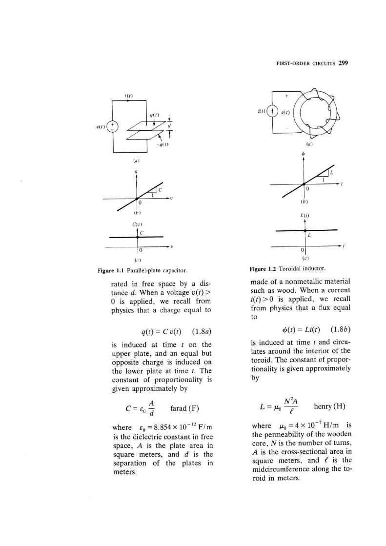
Example l b (Linear time- invariant toroidal inductor) Figure 1 . 2 ~ shows a familiar device made of a conducting wire wound around a toroid
This equation is also called the con- stitutive relation of the inductor.
S We will henceforth use the notation di(t) ldt.
FIRST-ORDER CIRCUITS 299
( c )
Figure 1.1 Parallel-plate capacitor.
rated in free space by a dis- tance d. When a voltage u( t ) > 0 is applied, we recali from physics that a charge equa1 to
is induced at time t on the upper plate, and an equal but opposite charge is induced on the lower plate at time t. The constant of proportionality is given approximately by
A d
farad (F)
where = 8.854 X 10-'' F /m is the dielectric constant in free space, A is the plate area in square meters, and d is the separation of the plates in meters.
(C)
Figure 1.2 Toroidal inductor.
made of a nonmetallic material such as wood. When a current i ( t ) > O is applied, we recall from physics that a flux equal to
is induced at time t and circu- lates around the interior of the toroid. The constant of propor- tionality is given approximately by
N% L=Po--~;- henry (H)
where p. = 4 X 10-' H/m is the permeability of the wooden core, N is the number of turns, A is the cross-sectional area in square meters, and t is the midcircumference along the to- roid in meters.

300 LINEAR AND NONLINEAR CPRCUITS
Equation ( 1.8a) defines the q-v characteristic of a linear time-in va riaptt capacitor, name- ly, a straight line through the origin with slope equal to C, as shown in Fig. 1. l b. Its small- signal capacitance C(v) = C is a constant function (Fig. l. l c ) . Consequently, Eq. ( l .6a) re- duces to Eq. (1 - la ) .
Example 2a (Nonlineas time- invariant parallel-plate capa- citor) If we fill the space be- tween the two plates in Fig. 1.la with a nonlinear ferroelec- tric material (such as barium titanate), the measured q-v characteristic in Fig. 1.3a is no longer a straight line. This non- linear behavior is due to the fact that :he dielectric constant of ferroelectric materials is not a constant-it changes with the applied electric field intensity.
Likewise, the small-signal capacitance shown in Fig. 1.3 b is a nonlinear function of v.
Figure 1.3 Nonlinear q-u characteristic.
Equation (1 .S b) defines the #-i characteristic of a linear time-invariant hdactor, name- ly, a straight line through the origin with slope equal to L, as shown in Fig. 1.2b. Its small- signal inductance L(i) = L is a constant function (Fig. 1 .2~) . Consequently, Eq. (1.6b) re- duces to Eq. (l. l b).
Example 2b (Nonlinear time- invariant toroidal inductor) If we repiace the wooden core in Fig. 1.20 with a nonlineas fer- romagnetic material (such as superperma3loy) the measured 4-i characteristic in Fig. 1.4a is no longer a straight line. This nonlinear behavior is due to the fact that the permeability of ferrornagnetic materials is not a constant-it changes with the applied magnetic field in- tensity.
Likewise, the small-signal inductance shown in Fig. 1.4b is a nonlinear function of i.
Figure 1.4 Nonlinear 4-i characteristic.

FIRST-ORDER ClRCUIE 301
Superconductor
Oxide barrier
Figure 1.5 q-v characteristic of a varactor Figure 1.6 4-i characteristic of a Josephson diode. junction.
Example 3a (Varactor diode) The varactor diode9 shown in Fig. 1 . 5 ~ is a pn-junction diode designed specially to take ad- vantage of the depletion layer when operating in reverse bias, i.e., when v < V, (typically, 0.2V < V, < 0.9V). Semicon- ductor physics proves that the charge q accumulated on the top layer is equal to
Varactor diodes are widely used in many communication circuits. For example, modem radio and TV sets are automatically tuned by applying a suitable dc bias voltage across such a diode.
Example 3b (Josephson junc- tion) The Josephson junction1° shown in Fig. l .6a consists of two superconductors separated by an insulating layer (such as oxide). Superconductor physics proves that the current i varies sinusoidally with 4, namely,
10 Josephson proposed this exotic device
in 1961 and was awarded the Nobel prize in physics in 1969 for this discovery. The Josephson junction has been used in numer- ous applications.

302 LfNEAR AND NONLINEAR CIRCUITS
provided V < y,. Here, V,, is the contact potential and
where E = permittivity of the material, Nu = number of ac- ceptor atoms per cubic cen- timeter, N,, = number of donor atoms per cubic centimeter, and A = cross-sectional area in square centimeters.
Its small-signal capacitance (Fig. 1 . 5 ~ ) is obtained by dif- ferentiating Eq. (1.9a):
i = l. sin k+ f l(&) j1.9b)
where lf, is a device parameter and
where e = electron charge and h = Planck's constant.
Note that unlike the previ- ous example, the 4-i charac- teristic in Fig. 1.6b is not cur- rent-controlled. Consequently, its small-signal inductance L(i) \ dt$(i)idi is not uniquely defined.
However, the Josephson junction is flux-controlled and has a well-defined slope (Fig. 1 . 6 ~ )
Note that unlike the previ- We call r($) the reciprocal ous examples, the q-v charac- small-signal inductance since it teristic in Fig. 1.5b is not de- has the unit of H-'. fined for v > V'. Hence, this capacitor is not voltage- controlled for all values of v > V,, . (For v > V,, the diode be- comes forward biased and be- haves like a nonlinear resistor.)
REMARK Note that Eqs. (1.9a) and (1.96), as well as Eqs. ( 1 . 1 0 ~ ) and (1.10 b), are not strictly dual equations because the corresponding variables are not duals of each other. However, if we solved for v in terms of q in Eq. (1.9a), we would obtain a dual function v = v^(q). In this case, the derivative
is called the reciprocal small-signal capacitance.

FIRST-ORDER CIRCUITS 383
Exercise (a) Show that a one- port obtained by connecting port 2 of a gyrator (assume unity coefficient) across a k-M linear inductor is equivalent to that of a k-F linear capacitor in the sense that they have identi- cal q-u characteristics. (b) Is it possible to give a simple physi- cal interpretation of the charge associated with this element? (c) Generalize the property in (a) to the case where the in- ductor is nonlinear: 4 = $(Q.
Exercise (a) Show that a one- port obtained by connecting port 2 of a gyrator (assume unity coefficient) across a k-F linear capacitor is equivalent to that of a k-H linear inductor in the sense that they have identi- cal 4-i characteristics. (b) Is It possible to give a simple physi- cal interpretation of the ~~ associated with this element? (c) Generalize the property in (a) to the case where the ca- pacitor is nonlinear: q = G(u).
1.2 Time-Varying Capacitors and Inductors
The examples presented so far are time-invariant in the sense that the q-v and 4- i characteristics do not change with time.
If the g-v characteristic changes with time, the capacitor is said to be time-varying.
For example, suppose we vary the spacing between the parallel- plate capacitor in Fig. l . l a , say by using a motor-driven cam mechan- ism, so that the capacitance C be- comes some prescribed function of time C(t). Then Eq. (1.8a) be- comes
q(t) = C(t)v(t) (1.1 la )
It folIows from Eq. (1.2a) that
Note that the current in a time- varying linear capacitor differs from Eq. (1.la) not only in the replacement of C by C(t), but also in the presence of an extra term.
If the - characteristic changes with time, the inductor is said to be rime-varying.
For example, suppose we vary the number of turns of the winding in Fig. 1.2a, say by using a motor-driven sliding contact, so that the inductance L becomes some prescribed function of time L(t). Then Eq. (1.8b) becomes
4(t) = L(t)i(t) (l. l l b)
It follows from Eq. (1.26) that
Note that the voltage in a time- varying linear inductor differs from Eq. (1.1 b) not only in the replace- ment of L by L(t), but also in the presence of an extra term.

m LINEAR A N 3 NONI.lNEAR CIRCUITS
To be specific, assume
C(t) = 2 + sin f (1.113~)
then
q( t ) = (2 + sin t)v(t) (1.140)
and
i(t) = ( 2 + sin t) du(f) + (COS f)u(t) dt
(1.15a)
The q-v characteristic of a time-varying linear capacitor con- sists of a family of straight fines, each line valid for a given instant of time. For example, the q-u characteristic of the above time- varying linear capacitor is shown in Fig. 1.7a. Its associated smalI-sig- nal capacitance consists of a family of horizontal lines (Fig. 1.7b).
(a!
To be specific, assume
L( t ) = 2 + sin t (1.13b)
then
+(t) = (2 + sin t)i(i) (1.14b)
and
di(t) v ( t ) = (2 + sin t ) -
dt + (cos t>i(t)
(1.15b)
The 4-i characteristic of a time-varying linear inductor con- sists of a family of straight lines, each line valid for a given instant of time. For example, the h-i characteristic of the above time- varying linear inductor is shown in Fig. 1.8b. Its associated small-sig- nal inductance consists of a family of horizontal lines (Fig. 1.86).
I (b! (b
Figure 1.7 Time-varying g-v characteristic of Figure 1.8 Time-varying 4-i characterisic of Eq. (1.14~). Eq. (1.146).
1

FIRST-ORDER CIRCUITS 305
Time-varying linear capacitors and inductors are useful in the modeling, analysis, and design of many communication circuits (e.g., modulators, de- modulators, parametric amplifiers).
In the most general case, a In the most general case, a time-varying nonlinear capacitor is time-varying nonlinear inductor is defined by a family of time-depen- defined by a family of tirne-depen- dent and nonlinear q-v characteris- dent and nonlinear 4-i characteris- tics, namely, tics, namely,
The two circuit variables used in defining a two-terminal resistor, inductor, or capacitor can be easily remembered with the help of the mnemonic diagram shown in Fig. 1.9. Note that out of the six exhaustive pairings of the four has$ variables v, i , g, and 4, two are related by definitions, namely, i = a and v = 4. The remaining pairs are constrained by the constitutive relation of a two- terminal element, three of which give us the resistor, inductor, and capacitor."
We will use the symbols shown in Fig. 1.9 to denote a nonlinear two- terminal resistor, inductor, or capacitor, respectively. Note that a dark band is included in each symbol in order to distinguish the two terminals. Just as in the case of a nonbilateral two-terminal resistor, such distinction is necessary if the q-v or #-i characteristic is not odd symmetric. In the special case where the element is linear, the v-i, $ 4 , and q-v characteristics are odd symmetric
Figure 1.9 Basic circuit element diagram.
f R ( v , i , f ) = O
Resistor
11 A fourth nonlinear two-terminal element called the memristor is defined by the remaining relationship between q and b. This circuit element is described in L. 0. Chua, "Memristor-The Missing Circuit Element," IEEE Trans. on Circuit Theory, vol. 18, pp. 507-519, September 1971.
0
- G V *
\ # \ / \ # . 4 &/ ' / i; h
G : .= '\/ S 1
g 0 .' /' \ \ -2
/ \ - /
/ \
0 II
0 . c "
S .='
/'

and hence remain unchanged after the two terminals are interchanged. In this case, we simply delete drawing the enclosing rectangle and revert to the standard symbol for a linear resistor, inductor, and capacitor.
2 BASIC PROPERTIES EXHIBITED BY TIME-INVARIANT CAPACITORS AND INDUCTQRS
Capacitors and inductors behave differently from resistors in many ways. The following typical properties illustrate some fundamental differences."
2.1 Memory Property
Suppose we drive the linear capacitor in Fig. l.la by a current source i(t). The corresponding voltage at any time t is obtained by integrating both sides of Eq. (1L.la) from T = - X to T = t. Assuming U(-=) = 0 (i.e., the capacitor has no initial charge when manufactured), we obtain
Note that unlike the resistor voltage which depends on the resistor current only at one instant of time t , the above capacitor voltage depends on the entire past hbtory (i.e., -a < T < t ) of i(7). Hence, capacitor has memory.
Now suppose the voltage v(t ,) at some time t,, < t is given, then Eq. (l . la) integrated from t = -2 to t becomes
In other words, instead of specifying the entire past history, we need only specify v( t ) at some conveniently chosen initial time l,,. In effect, the initial condition u(t,) summarizes the effect of i(7) from T = -X to T = to on the present value of v(t).
By duality, it follows that inductor has memory and that the inductor current is given by
The "memory" in a capacitor o r inductor is best manifested by the "dual" equivalent circuits shown in Fig. 2 . la and b which asserts the following:
I ? Unless otherwise specified, all capacitors and inductors are assumed to be time-in1 ~ r i a n t in this book.
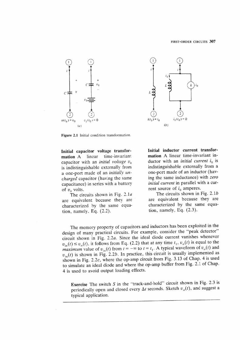
Figure 2.1 lnitiai condition transfi>rrnation.
Initial capacitor voltage transfor- mation A linear time-invariant capacitor with an initial voltage v,, is indistinguishable externally from a one-port made of an initially ltn-
charged capacitor (having the same capacitance) in series with a battery of v,, volts.
The circuits shown in Fig. 2.1~7 are equivalent because the); are characterized by the same equa- tion, nameIy. Eq. (2.2).
Initial inductor current transfor- mation A linear time-invariant in- ductor with an initial current i, is indistinguishable externally from a one-port made of an inductor (hav- ing the same inductance) with zero initial current in parallel with a cur- rent source of i, amperes.
The circuits shown in Fig. 2. l b are equivalent because they are characterized by the same equa- tion, namely, Eq. (2.3).
The memory property of capacitors and inductors has been exploited in the design of many practical circuits. For example, consider the "peak detector" circuit shown in Fig. 2.2a. Since the ideal diode current vanishes whenever vi,(t) 5 v,(?). it follows from Eq. (2.2) that at any time t , , v,(t) is equal to the maximum value of vi,(t) from t = -m to t = t , . A typical waveform of v,(t) and vi,(t) is shown in Fig. 2.2b. In practice, this circuit is usually implemented as shown in Fig. 2 . 2 ~ ~ where the op-amp circuit from Fig. 3.13 of Chap. 4 is used to simulate an ideal diode and where the op-amp buffer from Fig. 2.1 of Chap. 4 is used to avoid output loading effects.
Exercise The switch S in the "track-and-hold" circuit shown in Fig. 2.3 is periodically open and closed every At seconds. Sketch v , ( t ) , and suggest a typical application.

308 LINEAR AND NONLPMEAR CIRCUITS
Figure 2.2 A peak detector circuit.
Figure 2.3 A track-and-hold circuit.
Equation (2.2) and Fig. 2 . l a are valid only when the capacitor is linear. To show that nonlinear capacitors also exhibit memory, note that its voltage v( t ) depends on the charge and by Eq. (1,2a),
I 0" ,Off ,h, Off, on ,Off, o n , b f f , on, 0 1 ' " " ' " ' 2AT 4AT 6AT 8AT
Equation (2 .3) and Fig. 2. l b are valid only when the inductor is linear. To show that nonlinear inductors also exhibit memory, note that its current i ( t ) depends on the flux and by Eq. (1.2b),

FIRST-ORDER CIRCUITS 309
which in turn depends on the past which in turn depends on the past history of i ( ~ ) for - X < T < t,, . history of U ( T ) for -m < I < t,.
2.2 Continuity Property
Consider the circuit shown in Fig. 2.4a7 where the current source is described by the "discontinuous" square wave shown in Fig. 2.4b. Assuming that v,(O) = 0 and applying Eq. (2.2). we obtain the "continuous" capacitor voltage waveform shown in Fig. 2 . 4 ~ . This "smoothing" phenomenon turns out to be a general property shared by both capacitor voltages and inductor currents. More precisely, we can state this important property as follows:
Figure 2.4 The discontinuous capacitor current waveform in ( 6 ) is smoothed out by the capacitor to produce the continuous voltage waveform in (c).
Capacitor voltage-inductor current continuity property
(a) If the current waveform i,(t) in a linear time-invariant capacitor remains bounded in a closed interval [t,, t , ] , then the voltage waveform vc(t) across the capacitor is a continu- ous function in the open interval (t,, t,). In particular,'3 for any time T satisfying t, < T < t,, t',(T-) = v , ( T + ) .
(6) If the voltage waveform vL(t) in a linear time-invariant inductor remains bounded in a closed interval [t,, t,], then the current waveform i,(t) through the inductor is a continu- ous function in the open interval (t,, t,). In particular, for any time T satisfying t, < T < t,, i,(T-) = iL(T+).
13 We denote the left-hand limit and right-hand limit of a function f(t) at r = T by f(T-) and f ( T + ) , respectively.

310 LINEAR AND NONLINEAR CIRCUmS
PROOF We will prove only (a) since ( b ) follows by duality. Substituting t = T and t = T + dt into Eq. (2.21, where fa < T < r, and t , T+ -( t , , and subtracting, we get
Since i,(r) is bounded in [t,, t,], there is a finite constant M such that li,(t)l< M for all t in [ t , , t,]. It follows that the area under the curve i , ( r ) from T to T + dt is at most M dt (in absolute value), which tends to zero as dt-Q. Hence Eq. (2.5) implies u,(T+ dt)+ v , (T) as dt-, 0. This means that the waveform v,( S ) is continuous at r = T. m
REMARK The above continuity property does not hold if the capacitor current (respectiveky . inductor voltage) is unbounded. Before we illustrate this remark, let us first give an example showing how a capacitor current can become unbounded-at least in theory.
Suppose we apply a voltage source across a l-F linear capacitor having the waveform shown in Fig. 2.5b. It follows from Eq. (1.la) that the capacitor current waveform i ,( t) is a rectangular pulse with height equal to 1/A and width equal to A, as shown in Fig. 2 . 5 ~ . Note that the pulse height increases as A decreases. It is important to note that the area of this pulse is equai to 1, independent of A, Now in the limit where A-0, v,(t) tends to the discontinuous "'unit step" function [henceforth denoted by l ( t ) ] shown in Fig. 2.5d, i.e., 14
Figure 2.5 Circuit for generating a unit current impulse.
14 The value of the unit step function l(t) at t = 0 does not matter from the ,physical point of view. However, sometimes it is convenient to define it to be equal to j in circuit theory.
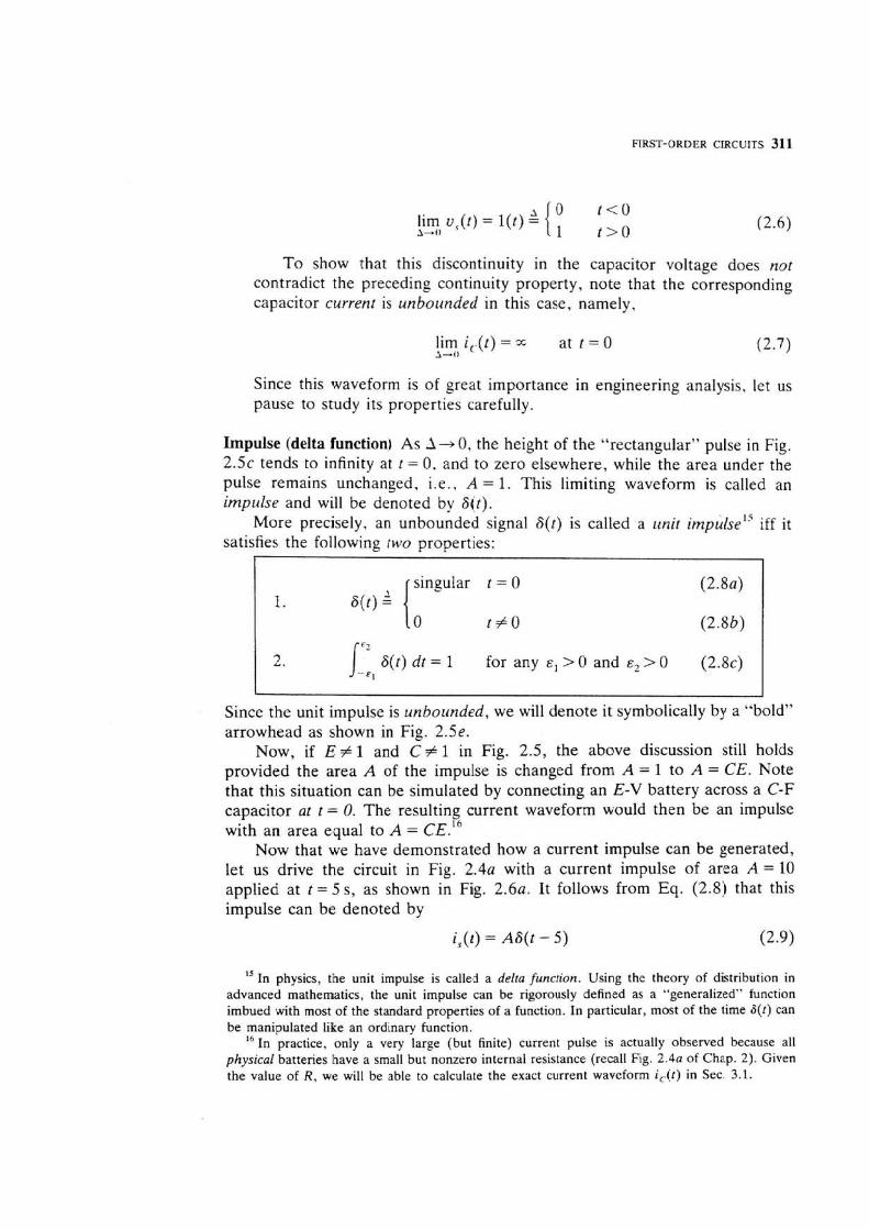
0 t<O Ifm v,(t) = l ( t> = S-0 1 t>O
T o show that this discontinuity in the capacitor voltage does not contradict the preceding continuity property, note that the corresponding capacitor current is unbounded in this case, namely,
lim i,.(t) = X at t = 0 l-4I 12.7)
Since this waveform is of great importance in engineering analysis, let us pause to study its properties carefully.
Impulse (delta function) As 3- 0, the height of the "rectangular" pulse in Fig. 2 . 5 ~ tends to infinity at t = 0, and to zero elsewhere, while the area under the pulse remains unchanged, i.e., A = l. This limiting waveform is called an impulse and will be denoted by 6jr).
More precisely, an unbounded signal S ( t ) is called a unit impulse'\ff it satisfies the following rwo properties:
singular t = 0 ( 2 . 8 ~ ) 1. 6 ( t ) A
{O t#O (2.8b)
2 . /If, 6 ( t ) dt = l for any E ] 2 0 and E , > 0 (2 .8~)
Since the unit impulse is unbounded, we will denote it symbolically by a "bold" arrowhead as shown in Fig. 2.5e.
Now, if E # l and C # l in Fig. 2.5, the above discussion still holds provided the area A of the impulse is changed from A = 1 to A = CE. Note that this situation can be simulated by connecting an E-V battery across a C-F capacitor at t = 0. The resulting current waveform would then be an impulse with an area equal to A = CE. '~
Now that we have demonstrated how a current impulse can be generated, let us drive the circuit in Fig. 2 . 4 ~ with a current impulse of area A = 10 applied at t = 5 S, as shown in Fig. 2 . 6 ~ . It follows from Eq. (2.8) that this impulse can be denoted by
15 In physics, the unit impulse is called a delta function. Using the theory of distribution in advanced mathematics, the unit impulse can be rigorously defined as a "generalized" function imbued with most of the standard properties of a function. In particular, most of the time S(t) can be manipulated like an ordinary function.
16 In practice, only a very large (but finite) current pulse is actually observed because all physical batteries have a small but nonzero internal resistance (recall Fig. 2.4a of Chap. 2). Given the value of R , we will be able to calculate the exact current waveform i,(t) in Sec. 3.1.

312 LINEAR AND NONLINEAR CIRCUITS
Substituting is([) into Eq. (2.2) with v(Q) = 0 we obtain
A Defining a new drammy variable x = T - 5 and using Eq. (2.83, we obtain
0 6 < 5 [in view of Eq. (2.8b)j 2 t > 5 [in view of Eq. (2.8c)J
(2.11)
The resulting capacitor voltage waveform is shown in Fig. 2.6b . Note that it is discontinuous at t = 5 S.
Exercise Prove that whenever the current waveform i , ( t ) en- tering a C-F linear time- invariant capacitor contains an impulse of area A at t = to , the associated capacitor voltage waveform u,(t) will change ab- ruptly at to by an amount equal to AIC.
Exercise Prove that whenever the voltage waveform v,(t) a- cross an - linear time- invariant inductor contains an impulse of area A at t = to, the associated inductor current waveform i , ( t ) will change ab- ruptly at t , by an amount equal to AIL.
2.3 Lossless Property
Since p( t ) = ~ ( t ) i(t) is the instantaneous power in watts entering a two-terminal element at any time t, the total energy w( t , , t , ) in joules entering the element during any time interval Et,, t,] is given by
Area A = 10
/ . "S Figure 2.6 The voltage waveform u,(t) IS discon- I tinuous at t = 5 S.
FIRST-ORDER CIRCUITS 313
w( f , , f 2 ) = 1; ~ ( f ) i ( f ) di joules (2.12)
For example, the total energy w,(t,, t,) entering a linear resistor with resis- tance R > 0 is given by
This energy is dissipated in the form of heat and is lost as far as the circuit is concerned. Such an element is therefore said to be lossy.
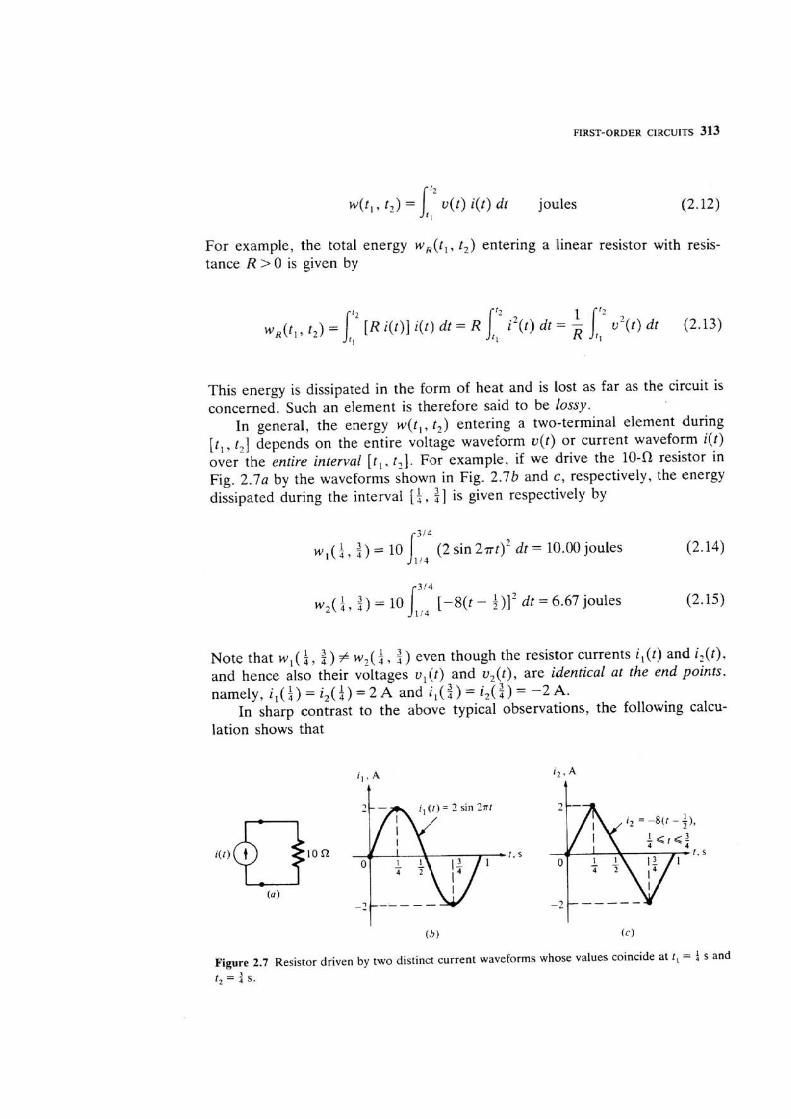
In general, the energy wft,, t , ) entering a two-terminal element during Etl, t2] depends on the entire voltage waveform v( t ) or current waveform i(r) over the entire interval [ t , , t,]. For example, if we drive the 10-fl resistor in Fig. 2.7a by the waveforms shown in Fig. 2.7b and c, respectively, the energy dissipated during the interval [ S , $1 is given respectively by
314
W , ( L , , z , ) = 10 L14 (2 sin 27rt)' dt = 10.00 joules (2.14)
Note that W , ( $ , i) # W,( $ , ) even though the resistor currents i , ( t ] and i z ( t ) . and hence also their voltages v,(t) and v,( t ) , are identical at the end points. namely, i,($) = i,($) = 2~ and i,(i) = i , ( i ) = -2 A.
In sharp contrast to the above typical observations, the following calcu- lation shows that
Figure 2.7 Resistor driven by two distinct current waveforms whose values coincide at t , = ! s and I , = t S.
314 LENEAR AND NONLINEAR CIRCUITS
The energy w,( t , , t,) entering a charge-controlled capacitor dur- ing any time intervaI It,, E,] is inde- pendent of the capacitor vslsage or charge waveforms: It is uniquely determined by the capacitor charge at the end points, namely by qQt,) and q( t2 ) . Indeed,
The energy w,(s , , C,) entering a flux-contraPled inductor during any time interval [ f , , E,] is iindepen- dent of the inductor current or flux waveforms: It is uniquely deter- mined by the inductor flux at the end points, namely, by + ( l , ) and 4(t, 1. Indeed,
It foliows from Eq. (2.26a) that It folPows from Eq. (2.16b) that
where we switched from t to q as ii
where we switched from r tf 4 as the dummy variable, and q, = q ( t l ) the dummy varaible, and 4, = 4(r,)
A and q2 = q( t z ) . and #, #( t2) .
Example For a C-F linear Example For an L-H linear in- capacitor, we have C(q) = qiC ductor, we have 44) = $ t L and hence Eq. (2.17a) reduces and hence Eq. (2.17b) reduces to to:
(2.18a) (2.18 b ) where where
A A A V, = v ( t , ) and V, = v( t , ) . I i t and I, = i(t ,) .
Exercises 1. Derive Eq. ( 2 . 1 8 ~ ) directly by substituting Eq. ( 1 . 1 ~ ) into E q . (2 .12) . 2. Derive Eq. (2.18b) directly by substituting Eq. (1.1 b ) into Eq. (2.12). 3. Give an example showing that Eq. (2.17a) does not hold if the capacitor is time-varying . 4. Give an exampIe showing that Eq. (2.17b) does not hold if the inductor is time-varying. 1

FIRST-ORDER CIRCUITS 315
Equation (2.17a) shows that the energy w,(t,, t,) entering a charge-controlled capacitor is equal to the shaded area shown in Fig. 2.8a. Any waveform pair [U( - ), q( - )] taking the values [ ~ ( t l ) , q(t,) j at f , and [v(t , ) - 9(t,)l at t, will give the same w,(t,, t?).
Now suppose v(t) and q(t) are periodic with period T = t z - f , .
Then q(t,) = q( t , + T ) = q( t , ) . and hence wc(t,, t,) = 0. Kn this case, P, and P, in Fig. 2.8a coincide, thereby resulting in a zero area.
This observation can be surn- marized as follows: Urzder periodic excitation, the total energy entering a charge-conrrolled capacitor is zero over any period.
Equation (2.17b) shows that the energy W , ( ! , , t,) entering a flux-controlled inductor is equal to the shaded area shown in Fig. 2.8b. Any waveform pair f i ( . ) , #( )] taking the values [ i(t l) , +(t,>l at l , and [i(t,), 4(t,!l at t, will give the same w,ft,, t,).
Now suppose i(t) and 4(t) are periodic with period T = t, - t , . Then 4(t,) = +(t, + T) = +(t,), and hence W,(?, , f,) = 0. In this case, P, and P, in Fig. 2.8b coincide, thereby resulting in a zero area.
This observation can be sum- marized as follows: Under periodic excitation, the total energy entering a flux-controlled inductor is zero over any period.
It follows from the above observation that the instantaneous power entering any charge-controlled capacitor or flux-controlled inductor is positive only during parts of each cycle, and must necessarily become negative elsewhere in order for the net area over each cycle to cancel out. Hence, unlike resistors, the power entering the capacitor or inductor is not dissipated. Rather, energy is stored during parts of each cycle and is "spit" out during the remaining part of the cycle. Such elements are therefore said to be lossless.
One immediate consequence of this iossless property is that in a periodic regime where u(t) = v(t + T) and i(t) = i(t + T ) for all t, the voltage waveform V([) and current waveform i(r) associated with any capacitor or inductor must necessarily cross the time axis at different instants of time. Otherwise, the integrand in Eq. (2.12) would always be positive, or negative, for all t , thereby implying w(t,, t , ) # 0.
U i
Capacitor lnductor characteristic characteristic
4
(a ) (b )
Figure 2.8 Geometric interpretation of w, ( t , , t,) and w, ( t , , t , ) .
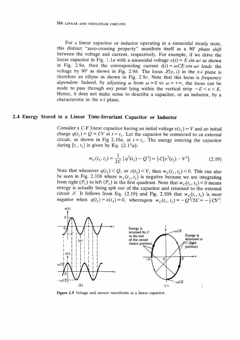
For a linear capacitor or inductor operating in a sinusoidat steady state, this distinct '"zero-crossing property" manifests itself as a 90" phase shqt between the voltage and current, respectively. For example, if we drive the linear capacitor in Fig. I . l a with a sinusoidal voatage vQt) = E sin of as shown in Fig. 2.9a, then the corresponding current it[) = wCEcos o t leads the voltage by 90" as shown in Fig. 2.96. The locus 2 ( u , i) in the v-i plane is therefore an eElipse as shown in Fig. 2 . 9 ~ . Note that this Iocus is frequency dependent. Indeed, by adjusting w from w = Q to w = +X, the locus can be made to pass through any point lying within the vertical strip -E < v < E. Hence, it does not make sense to describe a capacitor, or an inductor, by a characteristic in the v-i plane.
2.4 Energy Stored in a Linear Time-Invariant Capacitor or lnductor
Consider a C-F linear capacitor having an initial voltage u ( t , ) = V and an initial charge q ( t , ) = Q = CV at t = t , . Let the capacitor be connected to an external circuit, as shown in Fig 2.10a, at t = t , . The energy entering the capacitor during [ t , , t,] is given by Eq. (2.17a):
1 wc( t l . t,) = - [q2( t2) - = 1 c [ v Z ( t 2 ) - v2]
2C (2.19)
Note that whenever q(t ,) < Q, or v(t,) < V, then w,(t,, t,) < 0. This can also be seen in Fig. 2.10b where wc( t , , t,) is negative because we are integrating from right (P,) to left (P,) in the first quadrant. Note that w,(t,, t,) < 0 means energy is actually being spit out of the capacitor and returned to the external circuit N. It follows from Eq. (2.19) and Fig. 2.10b that w,( t , , t,) is most negative when q(t,) = u(t,) = 0, whereupon wc(t , , t,) = - ~ ' 1 2 ~ = - CV'.
delivered to
( b ) ( c )
Figure 2.9 Voltage and current waveforms in a linear capacitor.
FIRST-ORDER CIRCUITS 317
External 4
to1 (b i
Since this represents the maximum amount of energy that could be extracted from the capacitor, it is natural to say that an energy equal to
is stored in a linear capacitor C having an initial voltage v( t , ) = V or initial charge q ( t , ) = Q = 0'.
By duality, an energy equal to
is stored in a linear inductor L having an initial current i(t,) = I or initial flux 4 ( t , ) = c$ = LI.
2.5 Energy Stored in a Nonlinear Time-Invariant Capacitor or ~nductor l'
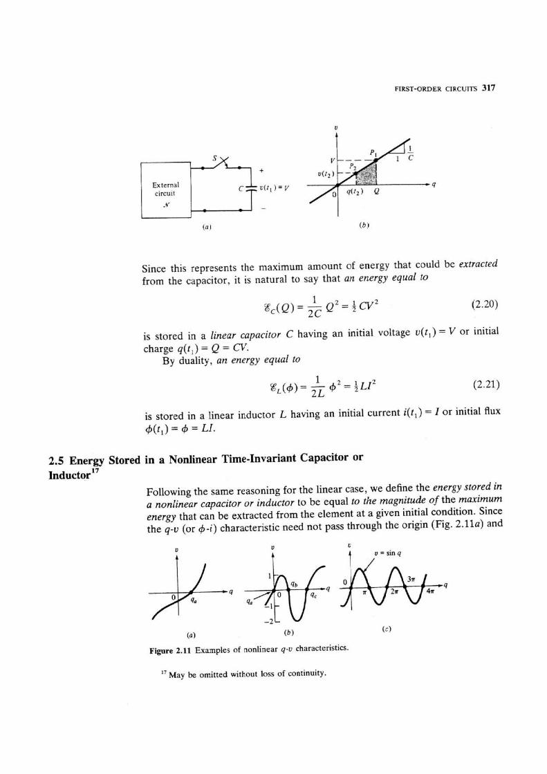
Following the same reasoning for the linear case, we define the energy stored in a nonlinear capacitor or inductor to be equal to the magnitude of the maximum energy that can be extracted from the element at a given initial condition. Since the g-v (or 4 - i ) characteristic need not pass through the origin (Fig. 2 . 1 1 ~ ) and
U
$ v = sin q
(0 1 ( b )
Figure 2.11 Examples of nonlinear q-U characteristics.
17 May be omitted without loss of continuity.
318 LINEAR AND NQNLFNEAR ClRCUilTS
can have several zero crossings (Fig. 2.11b) or infinitely many zero crossings (Fig. 2. I lc), special care is needed to derive a formula for stored energy in the nonlinear case.
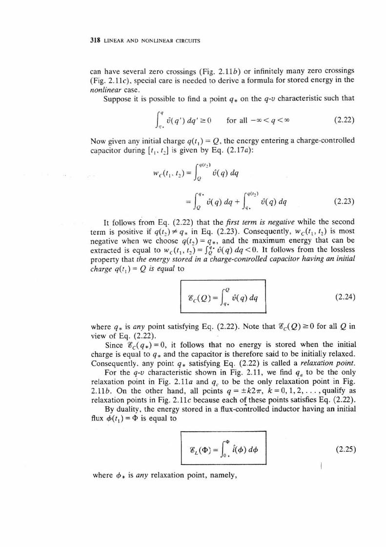
Suppose it is possible to find a point q, on the g-v characteristic such that
Now given any initial charge q(r , ) = Q , the energy entering a charge-controlled capacitor during [t,, t ,] is given by Eq. ( 2 . 1 7 ~ ) :
It folIows from Eq. (2.22) that the first term is negative whiIe the second term is positive if q(t,) # q* in Eq. (2 .23) . Consequently, w,(t,, t,) is most negative when we choose q(t,) = q,, and the maximum energy that can be extracted is equal to w,(t,, tL j = Jz* C ( q ) dq < 0. It follows from the lossless property that the energy stored in a charge-controlled capacitor having an initial charge q ( t , ) = Q is equal to
where q* is any point satisfying Eq. (2.22) . Note that %,(Q) r 0 for all Q in view of Eq. (2 .22) .
Since 8,(q,) = 0 , it follows that no energy is stored when the initial charge is equal to g, and the capacitor is therefore said to be initially relaxed. Consequently, any point q , satisfying Eq. (2.22) is called a relaxation point.
For the q-v characteristic shown in Fig. 2.11, we find q, to be the only relaxation point in Fig. 2.11a and q, to be the only relaxation point in Fig. 2.11 b. On the other hand, all points q = -C k 2 ~ , k = 0, 1 , 2 , . . . , qualify as relaxation points in Fig. 2 . 1 1 ~ because each of these points satisfies Eq. (2.22).
By duality, the energy stored in a flux-coGtrolled inductor having an initial flux 4 ( t , ) = @ is equal to
where 4+ is any relaxation point, namely,
FIRST-ORDER CIRCUITS 319
! i ( # ) d 8 ? 0 for all - m < * < m a.
Special case In the special case where the
g-U characteristic passes through 4-i characteristic passes through the origin and satisfies the origin and satisfies
the origin is a relaxation point and the origin is a relaxation point and the stored energy is simpty given the stored energy is simply given
by by
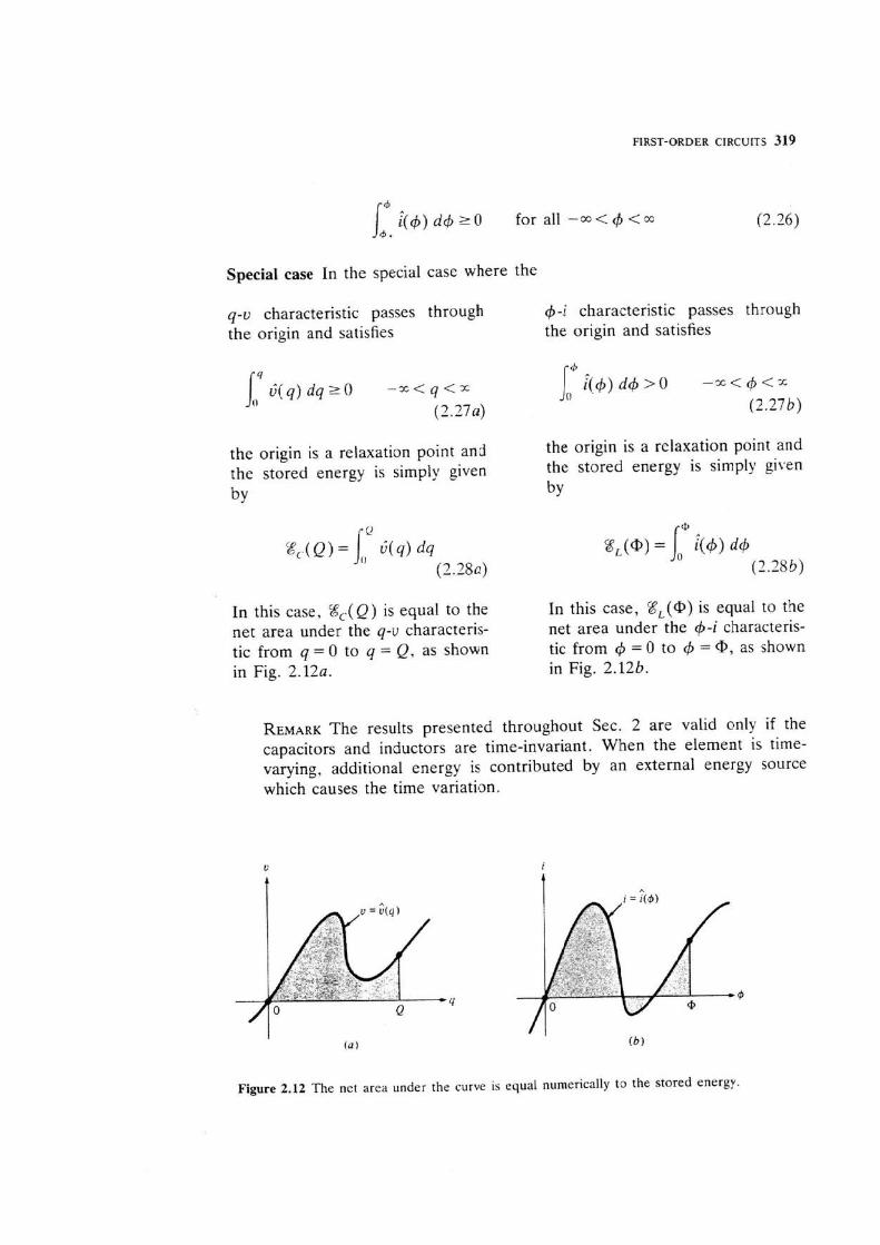
In this case, gC(Q) is equal to the In this case, g,(@) is equal to the net area under the q-v characteris- net area under the 4-i characteris- tic from q = 0 to q = Q, as shown tic from 4 = 0 to 4 = a, as shown in Fig. 2 . 1 2 ~ . in Fig. 2.12b.
REMARK The results presented throughout Sec. 2 are valid only if the capacitors and inductors are time-invariant. When the element is time- varying, additional energy is contributed by an external energy source which causes the time variation.
Figure 2.12 The net area under the curve is equal numerically to the stored energy.

320 LlNEAR AND NONLINEAR CIRCUITS
Exercises 1. Verify that out of the three zero crossings in Fig. 2.11 b, only q, qualifies as a relaxation point. 2. Find all relaxation paints associated with the Josephson junction defined earlier by Eq. (1.9b). 3. Prove that if a nonlinear capacitor or inductor has more than one relaxation point, then each point will give the same stored energy %?,(Q) or
3 FIRST-ORDER LINEAR CIRCUITS
Circuits made of one capacitor (or one inductor), resistors, and independent sources are called first-order circuirs. Note that "resistor" is understood in the broad sense: It includes controlled sources, gyrators, ideal transformers, etc.
In this section, we study first-order circuits made of linear time-invariant elements and independent sources. Any such circuit can be redrawn as shown in either Fig. 3. l a or b. where the one-port N is assumed to include all other elements (e.g., independent sources, resistors, controlled sources, gyrators, ideal transformers, etc.)."
Applying the ThPvenin-Norton equivalent one-port theorem from Chap. 5 , we can, in most instances, replace N by the equivalent circuit shown in Fig. 3.2a and b, respectively.
(Q (b )
Figure 3.1 (a) First-order RC circuit. (b) First-order RL circuit.
( 0 ) (6
Figure 3.2 Equivalent first-order circuits.
I8 Without loss of generality, we draw v, and i, as shown in Fig. 3 . lb so that i, = i (the dual of v,. = v in Fig. 3 . 1 ~ ) . This will guarantee the state equation (3.2b) will come out to be the dual of Eq. (3.2a). I

FIRST-ORDER CIRCUITS 221
Applying KVL we obtain Applying KCL we obtain
R,,i,- + v , = v,,(r) (3 . l a ) CeqvL + iL = iSC (f) (3. l b)
Substituting i, = Cc, and solving .
Sub:tituting v, = Li, and solving for G,, we obtain for i,, we obtain
When written in the above staodard form, this first-order linear differential equation is called a state eqrlntion and the variable v , (respectively, i,) is called a state variable.
Given any iniiial condition v,(t,,) at any initial time t , , our objective is to find the solution u,(t) for all t z to. We will show that v,(t) depends only on the ini- tial condition vc(to) and the waveform v,,(. ) over [ t o , t ] .
Once the solution v,(.) is found, we can apply the substi- tution theorem from Chap. 5 and replace the capacitor in Fig. 3 . l a by a voltage source v,(t).
Given any initial condition i,(t,,) at any initiat time r,,. our objective is to find the solution i, ( t ) for all t r to. We will show that i,(t) depends only on the ini- tial condition ( and the waveform is,(. ) over [to, t ] .
Once the solution l , ( . ) is found, we can apply the substi- tution theorem from Chap. 5 and replace the inductor in Fig. 3.1 b by a current source i,(t).
The resulting equivalent circuit, being resistive, can then be solved using techniques developed in the preceding chapters.
In Sec. 3.1 we show that the solution of any first-order linear circuit can be found by inspection, provided N contains only dc sources. By repeated application of this "inspection method," Sec. 3.2 shows how the solution can be easily found if N contains only piecewise-constant sources. This method is then applied in Sec. 3.3 for finding the solution--called the impulse response- when the circuit is driven by an impulse 6 ( t ) . Finally, Sec. 3.4 gives an explicit integration formuia for finding solutions under arbitrary excitations.
3.1 Circuits Driven by DC Sources
When N contains only dc sources, v,,(t) = v,, and i,,(t) = is , are con- stants in Fig. 3.2 and in Eq. (3.2). Let us rewrite Eqs. (3.2a) and (3 .2b ) as follows:

State equation
where where .l A
X = .U(. X = il.
1 ( 3 . 4a ) .l x ( t J = v,,(- X ( [ , ) = is,. ( 3 . 4 b )
.l T = R,,,C A
T = GCq L
for the RC circuit. for the RL circuit.
Given any initial condition X = x( t , , ) at t = t,,, Eq. ( 3 . 3 ) has a unique solution l y
which holds for all times t, i.e., - X < t < =. To verify that this is indeed the solution, simply substitute Eq. ( 3 . 5 ) into Eq. ( 3 . 3 ) and show that both sides are identical. Observe that at t = t,, both sides of Eq. ( 3 . 5 ) reduce to X([,) - x( t , ) . Note also that the solution given by Eq. (3 .5 ) is valid whether T is positive or negative.
The solution ( 3 . 5 ) is determined by only three parameters: x(t , , ) , x ( t , ) , and 7. We cail them initial state, equilibrium state, and time constant, respective- l y . To see why X ( [ , ) is called the equifibrium state, note that if x(t , ,) = X ( ? , ) ,
then Eq. ( 3 . 3 ) gives .?(to) = 0 and thus x ( t ) = x(t , ) for all t . Hence the circuit remains "motioniess," or in equilibrium.
Since the "inspection method" to be developed in this section depends crucially on the ability to sketch the exponential waveform quickly, the following properties are extremely useful.
A. Properties of exponential waveforms Depending on whether T is positive or negative, the exponential waveform in Eq. ( 3 . 5 ) tends either to a constant or to infinity, as the time 1 tends to infinity. Hence, it is convenient to consider these two cases separately.
r > 0 (Stable case) When r > 0, Eq. (3.5) shows that x( t ) - x(t,), i.e., the distance between the present state and the equilibrium state x( t , ) , decreases exponentially: For all initial states, the solution x ( t ) is sucked into the equilibrium and Ix(t) - .r(t,)l decreases exponentially with a time constant T.
14 We write x[ t , ) on the left side to make it easier to remember this important formula.

The solution (3.5) for T > 0 is sketched in Fig. 3.3 for two different initial states , f(t , ,) and X ( ( , , ) for t r,,. Observe that because the time constant r is positive ,
Thus, when T > O , we say the equilibrium state xft,) is stable because any initial deviation x(t,,) - x ( t , ) decays exponentially and x(t) --, x(t,) as t X.
The exponential waveforms in Fig. 3.3 can be accurately sketched using the following observations:
1. The tangent at t = t,, passes through the point it,,, x(t, ,)] and the point If,, + 7 7 x(f,)l.
2. After one time constant T, the distance between x(t) and x(t,) decreases approximately by 63 percent of the initial distance Ix(t,,) - x(t,)l.
3. After five time constants, x(t) practically attains the steady-state value x(r , ) . (Indeed, e-5 = 0.007.)
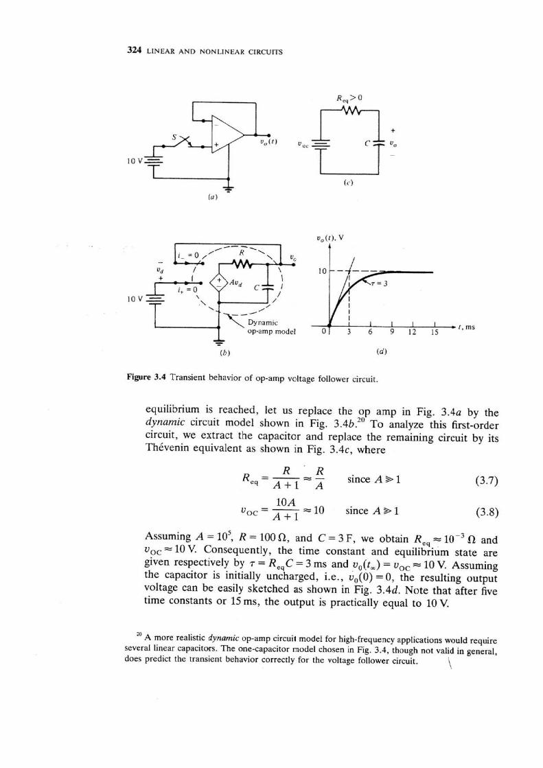
Example l (Op-amp voltage follower: Stable configuration) Consider the op-amp circuit shown in Fig. 3.4a. Using the ideal op-amp model, this circuit was analyzed earlier in Sec. 2.2 (Fig. 2.1) of Chap. 4. Assuming the switch is closed at t = 0, we found u,(t) = v,,(t) = 10 V for t r 0.
In practice, the output is observed to reach the 10-V solution after a small but finite time. In order to predict the transient behavior before the
Figure 3.3 The solution tends to the equilibrium state x(t,) as t + m when the time constant r is positive.
324 LINEAR AND NONLINEAR CIRCUITS
Figure 3.4 Transient behavior of op-amp voltage follower circuit.
equilibrium is reached, let us replace the op amp in Fig. 3.4a by the dynamic circuit model shown in Fig. 3.4b.20 Ta analyze this first-order circuit, we extract the capacitor and replace the remaining circuit by its ThCvenin equivalent as shown in Fig. 3.4c, where
R R Re' = A+l ;i since A S= 1
- l OA UOC - m = 10 since A B 1 (3.8)
Assuming A = 10: R = 100 a, and C = 3 F, we obtain R,, = I o - ~ fl and v,, = 10 V. Consequently, the time constant and equilibrium state are given respectively by T = R,,C = 3 ms and v,(t,) = v,, = 10 V. Assuming the capacitor is initially uncharged, i.e., v,(O) = 0, the resulting output voltage can be easily sketched as shown in Fig. 3.4d. Note that after five time constants or 15 ms, the output is practically equal to 10 V.
20 A more realistic dynamic op-amp circuit model for high-frequency applications would require several linear capacitors. The one-capacitor model chosen in Fig. 3.4, though not valid in general, does predict the transient behavior correctly for the voltage follower circuit. \,
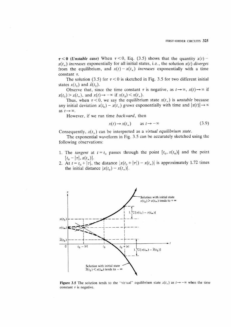
T < 0 (Unstable ease) When T < 0, Eq. (3.5) shows that the quantity x ( t ) - x(t , ) increases exponentially for all initial states, i.e., the solution x ( t ) diverges from the equilibrium, and x ( t ) - x ( t , ) increases exponentially with a time constant T.
The solution (3.5) for T < 0 is sketched in Fig, 3.5 for two different initial states x(t , , ) and i ( t , , ) .
Observe that, since the time constant T is negative, as t - m , x(t)--tr if X($, > > x( t , ) , and ~ ( t ) + - X if x(t, ,) < x( t , ) .
Thus, when 7 < 0. we say the equilibrium state X(!,) is unstable because any initial deviation x( t , , ) - x(t,) grows exponentially with time and I x ( t ) + z as t + x .
However, if we run time backward, then
Consequently, x( t , ) can be interpreted as a virtual equilibrium state. The exponential waveform in Fig. 3.5 can be accurately sketched using the
following observations:
1. The tangent at t = to passes through the point [ t , , , x ( t , , ) ] and the point [to - 171. x( t=) l -
2. At t = to + 171, the distance Ix(t, + (71) - x(t,)I is approximately 1.72 times the initial distance lx(t,,) - x(t ,) l .
Solution with initial state X([,) > x(t , ) tends to +
Solution with initial state .r(fo) <x(t , ) tends to - m I -
Figure 3.5 The solution tends to the "virtual" equilibrium state x ( r , ) as t - t -m when the time constant T is negative.

Example 2 (Op-amp voltage follower: Unstable ctprtfiguratiion) The op-amp circuit in Fig. 3.6a is identical to that of Fig. 3.4a except for an interchange between the inverting C- 31 and the noninverting (+) terminals. Using the ideal op-amp model in the linear region, we would obtain exactly the same answer as before, namely, v,, = 10 V for t 2 8, provided E,,, > 10 Let us see what happens if the op amp is replaced by the dynamic model adopted earIier in Fig. 3.43. The resulting circuit shown in Fig. 3.6b resembles that of Fig. 3.4b except for an important difference: The polarity of v, is now reversed. The parameters in the Thkvenin equivalent circuit now become
R R J i e q = - - = - - A
since A S= l A - l
10A --- ' ~ c - A - 1 - 10 since A S 1
Assuming the same parameter vafues as in Example 1, we obtain R = :'" -IQ-' and v,, = 10 V. Consequently, the time constant and equilibr~um
state are given respectively by T ---- -3ms and v,,(t,)= 10 V. Assuming v,(O) = U as in Example 1, the resulting output voltage can be easily sketched as shown in Fig. 3.6d.
Figure 3.6 Unstable transient behavior of op-amp voltage follower circuit. \

FIRST-ORDER CIRCUITS 327
Note that the solution differs drastically from that of Fig. 3.4d: It tends to -X! Of course, in practice, when v,(t) decreases to -E, , , , the op-am:, negative saturation voltage, the solution would remain constant at -E,,,. Clearly, this circuit would not function as a voltage follower in practice.
B. Efapsed time formula We will often need to calculate the time interval between two prescribed points on an exponential waveform. For example. to obtain the actual solution waveform for the circuit in Fig. 3.6, we need to calculate the time that elapsed when v,, decreases from v,, = O to U , = -15 V (assuming E,d, = 15 V) in Fig. 3-66.
Given any two points [ft,, x(t,)) and (t,, x(t,))j on an exponential wave- form (see, e.g., Figs. 3.3 and 3.5). the time it takes to go from X([,) to x(t,) is given by
Efapsed time formula
To derive Eq. (3.13). let t = ti and t = t, in Eq. ( 3 . 9 , respectively:
Dividing Eq. (3.13) by Eq. (3.14) and taking the logarithm on both sides. we obtain Eq. (3.12).
REMARK The above derivation does not depend on whether T is positive or negative.
C. Inspection method (First-order linear time-invariant circuits driven by dc sources) Consider first the first-order RC circuit in Fig. 3. la where all indepen- dent sources inside N are dc sources. Equation (3.5) gives us the voltage waveform across the capacitor, namely,
Suppose we replace the capacitor by a voltage source defined by Eq. (3.15). Assuming the resulting resistive circuit is uniquely solvable, we can apply the substitution theorem to conclude that the solution inside N of the resistive circuit is identical to that of the first-order RC circuit.
Let vj, denote the voltage across any pair of nodes, say Q and @ and assume that N contains cu independent dc voltage sources V,,, I/,,, . . . , Vsa and

p independent dc current sources I,, , fs,, . . . , I sp . Applying the superposition theorem from Chap. 5 , we know the solution vjk(t) is given by an expression of the form
where &, Hi, and K, are constatants (which depend on ekment values and circuit configuration). Substituting Eq. (3.15) for v,($) in Eq. (3.16) and rearranging terms, we obtain
where
and
Since Eq. (3.17) has exactly the same form as Eq. (3.51, and since nodes @ and @ are arbitrary, we conclude that:
The voltage ujk(t) across any pair of nodes in a first-order RC circuit driven by dc sources is an exponential waveform having the same time constant r as that of vc( t ) .
By the same reasoning, we conclude that: The current i j ( t ) in any branch j of a first-order RC circuit driven by dc
sources is an exponential waveform having the same time constant T as that of vc(t) .
It follows from duality that the voltage u,,(t) across any pair of nodes, or the current i j( t) in any branch j of a first-order RL circuit driven by dc sources is an exponential waveform having the same time constant T as that of i,(t).
The above "exponential solution waveform" property, of course, assumes that the first-order circuit is not degenerate, i.e., that it is uniquely solvable and that 0 < 171 < 03.
It is important to remember that all voltage and current waveforms in a given first-order circuit have the same time constant T as defined in Eq. (3.4).
Moreover, as we approach the equilibrium, i.e., when t-+ +a ( i f T > 0 ) or t+ -m (if T < O ) , the capacitor current and the inductor voltage.both tend to zero. This follows from Figs. 3.3 and 3.5, i, = Cc,, and v, = Li,.
Since an exponential waveform is uniquely determined by only three parameters [initial state x(t,), equilibrium state x(t,), and time con$tant T], the following "inspection method" can be used to find the voltage solution vjk( t )

across any pair of nodes Q and @ or the current solution i,(t) in any branch j. in any uniquely solvable linear first-order circuit driven by dc sources:
RC circuit: given v,(t,). RL circuit: given i,(t,,).
1. Replace the capacitor by a 1. Replace the inductor by a dc voltage source with a dc current source with a terminal voltage equal to terminal current equal to v,(r,). Label the voltage i , (l,,). Label the voltage across node-pair 0, @ as across node-pair 0. @ as vik(to) and the current i, as u,,(f,,) and the current i, as i ( t ). Solve the resulting i , ( t ,) . Solve the resulting 0 resistive circuit for v,,(t,,) resistive circuit for v,,(r,,) or i,ft,). Or i , ( t ~ ) .
2. Replace the capacitor by 2. Replace the inductor by a any open circuit. Label the short circuit. Label the vol- voltage across node-pair tage across node-pair 0, 0, @ as u,,(t,) and the @ as u,,(t,) and the cur- current i, as i,(t,). Solve rent i, as i , ( t , ) . Solve for for v j k ( t x ) or i , ( t x ) . V,&) Or q t , ) .
3. Find the Thivenin equiva- 3. Find the Norton equiva- lent circuit of N. Calculate lent circuit of N. Calculate the time constant T = the time constant T =
ReqC. GeqL. 4. If O < I T ] < X , use the 4. If O < ( T I < X , use the
above three parameters to above three parameters to sketch the exponential so- sketch the exponential so- lution waveform. lution waveform.
REMARKS 1. The above inspection method eliminates the usual step of writing the differential equation: It reduces each step to resistive circuit calculations. 2. The above method is valid only if the circuit is uniquely solvable. For example, if the one-port N in Fig. 3.1 does not have a Thivenin and Norton equivalent circuit, it is not uniquely solvable. 3. The above method assumes the circuit is not degenerate in the sense that 0 < IT^ <m. This means that Re, f 0 and is finite in Fig. 3.2a, and that G,, # O and is finite in Fig. 3.2b.
Circuits Driven by Piecewise-Constant Signals
Consider next the case where the independent sources in N of Fig. 3.1 are piecewise-constant for t > to. This means that the semi-infinite time interval to 5 t < can be partitioned into subintervals [ t j , t j+ , ) , j = 1 ,2 , . . . , such that

33a) LINEAR AND NONLINEAR CFRCUITS
all sources assume a constant value during each subinterval. Hence, we can analyze the circuit as a sequence of first-order circuits driven by dc sources, each one analyzed separately by the inspection method. Since the circuit remains unchanged except for the sources, the time constant T remains un- changed throughout the analysis.
The initial state xl(t,,) and equilibrium state x(t,) will of course vary from one subinterval to another. Although the same procedure holds in the deter- mination of x( f , ) , one must be careful in calculating the initial value at the beginning of each subinterval t j because at least one source changes its value discontinslous!y at each boundary time tj between two consecutive subintervals. In general, X(?,-) # X([ ,+ ) , where the - and + denote the limit of x(t ) as t+ t, from the left aad from the right, respectively. The initial value to be used in the calculation during the subinterval [$, tj+ ,) is X($+).
Although in general both vi,(t) and i j ( t ) can jump, the "continuity property" in Sec. 2.2 guarantees that in the usual case where the capacitor current (respectively, inductor voltage) waveform is bounded, the capacitor voltage (respectively, inductor current) waveform is a continuous function of time and therefore cannot jump. This property is the key to finding the solution by inspection, as illustrated in the following examples.
Example 1 Consider the R C circuit shown in Fig. 3 . 7 ~ : v , ( . ) is given by Fig. 3 . 7 ~ and u,(O) = 0. Our objective is to find i,(t), v , ( t ) , and v,(t) for
( d )
Figure 3.7 Solution waveforms for RC circuit. Here, T denotes the time comran?of the expo- nential.

FIRST-ORDER CIRCUITS 331
t 1 0 by inspection. Since v,(O) = 0 and v,(t) = 0 for t r 0, it follows that ic(t> = vc(t) = VR(tj = 0 for t S 0.
The solution waveforms for t > 0 consists of exponentials with a time constant 7 = RC. At t = 0+, using the continuity property, we have vc(O-t-) = vc(O-) = 0. Therefore, v,(O+) = v,(O+) - vc(O+) = E and ic(O*) = v,(O+)IR = EIR. To find the equilibrium state, we open the capacitor and find t,(t,) = 0, vc(t,) = E, and v,(t,) = 0.
These three pieces of information allow us to sketch i,(t), v,(t), and v,( t ) for t 2 0 as shown in Fig. 3.7b, c, and d, respectively. Note that i,(t) = C dvc(t) ldt and v,(t) + v,(t) = E for E 2 0, as they should. Observe also that whereas v,([) is discontinuous at t = 0, v,(t) is continuous for all t , as expected.
REMARKS 1. The circuit in Fig. 3.7 is often used to model the situation where a dc voltage source is suddenly connected across a resistive circuit which normally draws a zero-input current. The linear capacitor in this case is used to model the small parasitic capacitance between the connecting wires. Without this capacitor, the input voltage would be identical to v,(t). However, in practice, a "transient" is always observed and the circuit in Fig. 3.7a represents a more realistic situation. In this case, the time constant T gives a measure of how "fast" the circuit can respond to a step input. Such a measure is of crucial importance in the design of high-speed circuits, say in computers, measuring equipment, etc. 2. Since the term time constant is meaningful only for first-order circuits, a more general measure of "response speed" called the rise time is used in specifying practical equipments.
The rise time t , is defined as the time it takes the output waveform to rise from 10 percent to 90 percent of the steady-state value after application of a step input.
For first-order circuits, the following simple relationship between t , and T follows directly from Eq. (3.12):
Rise time
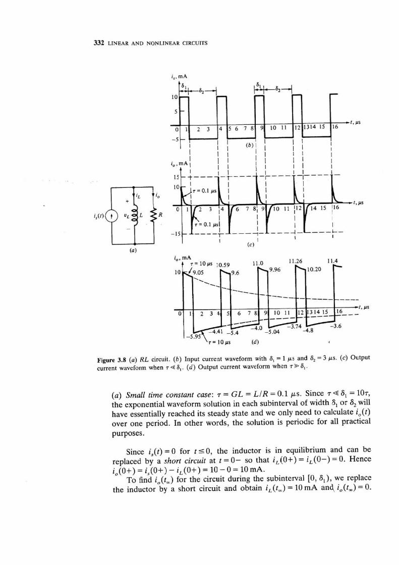
Example 2 Consider the RL circuit shown in Fig. 3.8a, driven by a periodic square-wave current source in Fig. 3.8b. Our objective is to find i,(t) through the resistor when (a) R = 10 k a , L = 1 m H and (b) R = 1 kR, L = 10mH.
332 LINEAR AND NONLINEAR CIRCUITS
i,, mA
Figure 3.8 (a ) RL circuit. (6 ) Input current waveform with 6, = l @S and 6, = 3 f i s . (c) Output current waveform when 7.&8,. ( d ) Output current waveform when 7 9 6,.
( a ) Small time constant case: 7 = GL = LIR = 0.1 PS. Since T 4 6, = 107, the exponential waveform solution in each subinterval of width S , or 6, will have essentially reached its steady state and we only need to calculate i ,(t) over one period. In other words, the solution is periodic for all practical purposes.
Since i , ( t ) = O for t SO, the inductor is in equilibrium and can be replaced by a short circuit at t = 0- so that i,(O+) = i , ( O - ) = 0. Hence i ,(O+) = i,(O+) - i , ( O + ) = 10 - 0 = 10 mA.
To find io(t,) for the circuit during the subinterval [0, ar), we replace the inductor by a short circuit and obtain i,(t,) = 10 mA and, io(t , ) = 0.
FIRST-ORDER CIRCUITS 333
At t = 6, = 1 PS, iL(S1+) = iL(8,-) = 10 mA. Hence i,(S, +) = i,(6,+) - iL(6,+) = -5 - 10 = -15 mA. Hence i, jumps at t = 6, from 0 to - 15 mA.
To find i,(t,) for the circuit during the subinterval [S,, S , + S,), we replace the inductor by a short circuit again and obtain io(t,) = 0.
At t = 6, + 6, = 4 ps , i,(t) jumps again from 0 to 15mA, and the solution repeats itself thereafter, as shown in Fig. 3 . 8 ~ .
( b ) Large time constant case: T = 10 P S . Since T S 6, = 0.17, the exponen- tial waveform does not have enough time to reach a steady state during each subinterval. Consequently, the solution io(t) is not periodic and we will have to partition 0 r t < c 0 into infinitely many subintervals [O, S,), [a,, 6, + S,), [a, -t 6,, 28, + S,), . . . We will see, however, that io(t) will tend to a periodic waveform after a few periods.
Starting at t = 0 as in (a), we find i,(O+) = 10 mA and io(t,) = 0. The exponential solution is drawn in a solid line during 0 S t < 6, and in a dotted line thereafter in Fig. 3.8d to emphasize the relative magnitudes of T and 8,.
To determine i0(6, +) = i ,(l+), it is necessary to write the solution i,(t) = 10 exp(- t / 10) in order to calculate i,(l-) = 9.05 mA. This gives us i,(l-) = i,(l-) - i,(l-) = 10- 9.05 = 0.95 mA. Since i,(l+) = i,(l-) = 0.95 mA, i,(l+) = i ,(l+) - iL( l+) = -5 - 0.95 = -5.95 mA. Hence i,(t) jumps from 9.05 to -5.95 mA at t = 1 PS, as shown in Fig. 3.8d.
Again, the exponential solution during [ l , 4) has not reached steady state when i,(t) changes from -5 to 10 mA at t = 4 ps. To calculate i,(t) at t = 4+, it is necessary to write the solution i,(t) = -5.95 exp{- [(t - 1) /10]) and obtain io(4-) = -4.41 mA. This gives i,(4+) = iL(4-) = i,(4-) - i,(4-) = -5 - (-4.41) = -0.59 mA and i0(4+) = i,(4+) - i,(4+) = 10 - (-0.59) = 10.59 mA. Hence i,(t) jumps from -4.41 to 10.59 mA at t = 4 ,as, as shown in Fig. 3.8d.
Repeating the above procedure, we find i,(t) jumps from 9.6 to -5.4mA at t = 5 ps, from -4.0 to 11.0 mA at t = 8 PS, from 9.96 to -5.04 mA at t = 9 ps, from -3.74 to 11.26 mA at t = 12 PS, from 10.20 to -4.8 mA at t = 13 ps, and from -3.6 to 11.4 mA at t = 16 ,us, etc., as shown in Fig. 3.8d.
It is clear from Fig. 3.8d that i,(t) is tending toward a periodic waveform. To determine this periodic waveform, note that if we let I, denote the "peak" value of each "falling" exponential segment in Fig. 3.8d (e.g., I , = 10, 10.59, 11, 11.26, and 11.4mA at t = 0 , 4, 8, 12, 16 ,us, etc.) then this periodic waveform must satisfy the following periodicity con- dition :
-6, I, exp - - -62 15exp- + 15 = I, 7 7
334 LINEAR AND NONLENEAR CIRCUITS
where S, = 1 PS, a2 = 3 PS, and T = 10 PS. The solution of this equation gives one point on the periodic solut.ion, namely, the peck value.
Exercise (a) Calmlate the peak value 1, from the periodicity condition. (b ) Specify the initial inductor current i ,(0) in Fig. 3.80 so that the solution, i ,(t) is periodic for t s: 0. ( c ) Sketch this periodic solution.
3.3 Linear Time-Invariant Circuits Driven by an IrnpuEse
Consider the RC circuit shown in Fig. 3.40 and the RL circuit shown in Fig. 3.9b. Let the input voltage source v,(!) and input current source i,(t) be a square pulse p A ( t ) of width A and height l l A , as shown in Fig. 3 . 9 ~ . Assuming zero initial state [i.e., u, (O-) = 0, i , ( O - ) = 01, the response voltage v , ( t ) and current i,(t) are given by the same waveform shown in Fig. 3.9d, where 7 = RC for the RC circuit and T = GL for the RL circuit. and
The input and response corresponding to h = l , ; , and f s are shown in Fig. 3.9e and f, respectively. Kote that as A-0, pA(t ) tends to the unit impulse shown in Fig. 3.9g [recall Eq. (2.8)], namely,
lim pA(t ) = 6( t ) A 4 0
(3.22)
Note also that the "peak" value h,(A) of the response waveform in Fig. 3.9d increases as A decreases. To obtain the limiting value of hA(A) as A+ 0 , we apply L7Hospital's rule:
f '(A) ( 1 / ~ ) exp(-A/T) 1 lim h,(A) = Iim - - - lim - - A 4 0 A-0 &(A) A-0 1 7
(3.23)
Hence, the response waveform in Fig. 3.9f tends to the exponential waveform
shown in Fig. 3.9h. Using the unit step function l ( t ) defined earlier in Eq. (2 .6) , we can rewrite Eq. (3.24) as follows:
1 h( t ) = - 7 exp (G) ~ ( t )

FIRST-ORDER CIRCUlTS 335
Figure 3.9 As A+O, the square pulse in (c) tends to the unit impulse 6 ( . ) in (g). The corresponding response tends to the impulse response h(t) in (h) .
Because h(t) is the response of the circuit when driven by a unit impulse under zero initial condition, it is called an impulse response. Note that h(t) = 0 for t < 0.
In Chap. 10, we will show that given the impulse response of any linear time-invariant circuit, we can use it to calculate the response when the circuit is driven by any other input waveform.

3% LINEAR A N D NONLINEAR CIRCUITS
3.4 Circuits Driven by Arbitrary Signals
Let us consider now the general case where the one-post N in Fig. 3.1 contains arbitrary independent sources. This means that the ThCvenin equivalent volt- age source a,,(t), or the Norton equivalent current source i,,(t), in Fig. 3.2 can be any function of time, say, in practice, a piecewise-continuous function of time: square wave, triangular wave, synchronization signal of a TV set, etc. Our objective is to derive an explicit solution and draw the consequences.
Consider first the RC circuit in Fig. 3 . 2 ~ whose state equation is
A where 7 = ReqC.
Explicit solution for first-order linear time-invariant RC circuits Given any prescribed waveform v,,(t), the solution of Eq. (3.25) corresponding to any initial state v,(t,) at t = to is given by
-0 - to) -(t - t ' ) = vc(to) exP uoc(tf )dt f
7 7 L
zero-input response zero-state response
for all t 2 to. Here, T = ReqC.
PROOF (a) At t = to, Eq. (3.26) reduces to
vc(t)lt=t,, = uc(to) (3.27) Hence Eq. (3.26) has the correct initial condition. (b) To prove that Eq. (3.26) is a solution of Eq. (3.25), let us differentiate both sides of Eq. (3.26) with respect to t: First we rewrite Eq. (3.26) as
vc( t ) = vC(t0) exp -" 7 - + ( f exp +) 1: exP f vOc(tr) (3.28)
Then upon differentiating we obtain for t > 0,
1 cc(?) = - - 7 vc(to) exp -(t - + (- 5 exp 2) 7 7
t' X io exp - T v0,(tt) dt' + (l T exp2)[exp 5 voc(r)], (3.29)
7

FtRST-ORDER CIRCUITS 337
where we used the fundamental theorem of calculus:
If It f(tr) dtf = f( t ) if f( - ) is continuous at time I dt o
Simplifying Eq. (3.29), we obtain
1 ;,(t) = - - vc(to) exp - ( t - 1 , )
7 7
- ' [l' ' exp - ( t - t ')
7 '0 7 7
Hence Eq. (3.26) is a solution of Eq. (3.25). ( c ) From mathematics we learned that the differential equation (3.25) has a unique solution. Hence Eq. (3.26) is indeed the solution.
Zero-input response and zero-state response The solution (3.26) consists of two terms. The first term is called the zero-input response because when all independent sources in N are set to zero, we have vo,(t) = 0 for all times, and v,( t ) reduces to the first term only. The second term is caIfed the zero-state response because when the initial state v,(t,) = 0, v,( t ) reduces to the second term only.
Example Let us find the solution v,(t) of Fig. 3 . 7 ~ using the above general formula. In this case, we have
vc(to) = 0 to = 0 and vo,(t) = E t 2 0
Substituting these parameters into Eq. (3.26), we obtain
( t - 0 ) ( t - 1') v , ( t ) = O X exp [ - - ] + J o t ' , e x p [ - 7 ] . E d t '
which coincides with that shown in Fig. 3.7c, as it should.
By duality, we have the following:

Explicit solution for first-order linear time-invariant RL circuit Given any prescribed waveform i,,(t), the solution of Eq. (3.26) corresponding to any initial state i,(t,,) at t = t,, is given by
-0 - 4,) + j-' 1 exp -(t - 5') iL(f) = iLffO) ~ X P is,(tf) dt'
7 41 7 7 , ,
zero-input response zero-state response i
for all t 2 r,,. Here, r = G,, L,
REMARKS 1. In both Eqs. (3.26) and (3.32), the zero-input response does not depend on the inputs and the zero-state response does not depend on the initial condition. In both cases, the total response can be interpreted as the superposition of two terms, one due to the initial condition acting alone (with all independent sources set to zero) and the other due to the input acting alone (with the initial condition set to zero). 2. Formulas (3.26) and (3.32) are valid for both T > 0 and r 0. Consider the stable case 7 > 0. For values of t' such that t - t' %- r , the factor exp[-(t - t') l r ] is very small: consequently the values of u,,(t) [respec- tively, i,,(t)] for such times contribute almost nothing to the integral in Eq. (3.26) [respectively, Eq. (3.32)). In other words, the stable RC circuit (respectively, the stable RL circuit) has a fading memory: Inputs that have occurred many time constants ago have practically no effect at the present time.
Thus we may say that the time constant T is a measure of the memory time of the circuit. 3. Using the impulse response h(t) for the RC circuit derived earlier in Eq. (3.24), we can rewrite the zero-state response in Eq. (3.26) as follows:
h(t - t') vOc(tr) dtr I0
Equation (3.33) is an example of a convolution integral to be deveioped in Chap. 10. 4. Once v,(t) is found using Eq. (3.26), we can replace the capacitor in Fig. 3.2a by an independent voltage source described by v,(t). We can then apply tne substitution theorem to find the corresponding solution inside N by solving the resulting linear resistive circuit using the methods from the preceding chapters. 5 . The zero-state response due to a unit step input l(t) is called the step response, and will be denoted in this book by s(t). The step response for a first-order RC (respectively. RL) circuit can be found by thb inspection method in Sec. 3.1C, upon choosing v,(O) = 0 (respectively, i,(O) = 0).

FIRST-ORDER CIRCUITS 339
The significance of the step response is that for any linear time- invariant circuit, the impulse response h ( t ) needed in the convoiutjon integral (6.5) of Chap. 10 can be derived from $ ( E ) (which is usually much easier to derive) via the formula
This important relationship is the subject of Exercise I in Chap. 10, page 615 [Eq. (4.64)].
The dual remark of course applies to the RL circuit in Fig. 3.2b.
4 FIRST-ORDER LINEAR SWITCHING CIRCUITS
Suppose now that the one-port N in Fig. 3.1 contains one or more switches, where the state (open or closed) of each switch is specified for all t 2 to. Typically, a switch may be open over several disjoint time intervals, and closed during the remaining times. Although a switch is a time-varying linear resistor, such a linear switching circuit may be analyzed as a sequence of first-order linear time-invariant circuits, each one valid over a time interval where all switches remain in a given state. This class of circuits can therefore be analyzed by the same procedure used in the preceding section. The only difference here is that unlike Sec. 3, the time constant T will generally vary whenever a switch changes state, as demonstrated in the following example.
Example Consider the RC circuit shown in Fig. 4.la, where the switch S is assumed to have been open for a long time prior to t = 0.
Given that the switch is closed at t = l S and then reopened at t = 2 S, our objective is to find vc( t ) and vo(t) for all t r 0.
Since we are only interested in vc(t) and vo( t ) , let us replace the remaining part of the circuit by its Thkvenin equivalent circuit. The result is shown in Fig. 4.1 b and c corresponding to the case where S is "open" or "closed," respectively. The corresponding time constant is T, = l s and T* = 0.9 S , respectively.
Since the switch is initially open and the capacitor is initially in equilibrium, it follows from Fig. 4.lb that vc( t ) = 6 V and v,(t) = 0 for t 5 l S. At t = 1 + we change to the equivalent circuit in Fig. 4. l c . Since, by continuity, v,(l+) = v,(l-) = 6 V, we have i,(l+) = (10 - 6)V/(2 + 1.6) k f l = 1.11 mA and hence v o ( l + ) = (1.6 kfl)(1.11 mA) == 1.78 V.
To determine vc(t,) and vo(t,) for the equivalent circuit in Fig. 4.lc, we open the capacitor and obtain v,(t,) = 0. The waveforms of vc(t) and v,(t) during [l, 2) are drawn as solid lines in Figs. 4.1 d and e , respectively. The dotted portion shows the respective waveform if S had been left closed for all t r l S.
Since S is closed at t = 2 S, we must write the equation of these two waveforms to calculate vc(2 -) = 8.68 V and v,(2-) = 0.59 V.

3 0 LINEAR AND NONLINEAR CIRCUITS
Figure 4.1 An RC switching circuit and the solution waveforms corresponding to the case where S is open during r < I s and t 2 2 S, and closed during 1 r t < 2.
At t = 2+, we return to the equivalent circuit in Fig. 4 . l b . Since v,(&+) = vc(2-) = 8.68 V, we have i,(2+) = (6 - 8.68)V/(2.4 -+ 1.6) k i l = -0.67 mA and v0(2+) = (1.6 kS1)(-0.67 mA) .= -1.07 V.
To determine v,(t,) and v,(t,) for the circuit in Fig. 4.lb, we open the capacitor and obtain v,(t,) = 6 V and vo(t,) = 0. The remaining solut- ion waveforms are therefore as shown in Figs. 4.ld and e, respectively.
5 FIRST-ORDER PIECEWISE-LINEAR CIRCUITS
Consider the first-order circuit shown in Fig. 5.1 where the resistive one-port N may now contain nonlinear resistors in addition to linear resistors and dc sources. As before, all resistors and the capacitor are time-invariant. This class of circuits includes many important nonlinear electronic circuits such as multivibrators, relaxation oscillators, time-base generators, etc. In this section, we assume that all nonlinear elements inside N are piecewise-linear so that the one-port N is described by a piecewise-linear driving-point characteqstic.
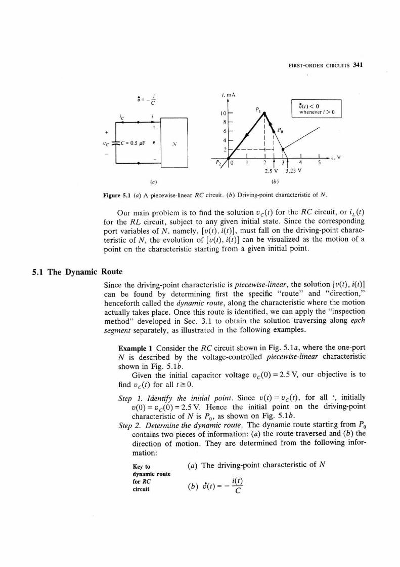
Figure 5.1 (a) A piecewise-linear RC circuit. (b) Driving-point characteristic of N.
Our main problem is to find the solution v,(t) for the RC circuit, or i,(t) for the RL circuit, subject to any given initial state. Since the corresponding port variables of N, namely, [v(t), i(t)], must fall on the driving-point charac- teristic of N , the evolution of [v([), i(t)j can be visualized as the motion of a point on the characteristic starting from a given initial point.
5.1 The Dynamic Route
Since the driving-point characteristic is piecewise-linear, the solution [v(t), i(t)] can be found by determining first the specific "route" and "direction," henceforth called the dynamic route, along the characteristic where the motion actually takes place. Once this route is identified, we can apply the "inspection method" developed in Sec. 3.1 to obtain the solution traversing along e,ach segment separately, as illustrated in the following examples.
Exampie 1 Consider the RC circuit shown in Fig. 5.la, where the one-port N is described by the voltage-controlled piecewise-linear characteristic shown in Fig. 5.1 b.
Given the initial capacitor voltage v,(O) = 2.5 V, our objective is to find v,(t) for all t r 0.
Step 1. Identify the initial point. Since v(t) = v,(t), for all t , initially v(0) = v,(0) = 2.5 V. Hence the initial point on the driving-point characteristic of N is P,, as shown on Fig. 5. lb .
Step 2. Determine the dynamic route. The dynamic route starting from P,, contains two pieces of information: (a) the route traversed and ( b ) the direction of motion. They are determined from the following infor- mation:
Key to (a) The driving-point characteristic of N dynamic route for RC i(t> circuit (b) v'(t) = - - C

342 LINEAR AND NONLINEAR CIRCUIFS
since v'(t) = - i ( t ) / C < U whenever i ( t ) > 0, the voltage v(t) decreases so long as the associated current i ( t ) is positive. Hence, for i ( t ) > 0, the dynamic route starting at P, must always move along the v-i curve toward the left, as indicated by the bold directed line segments P,+ P, and P, + P, in Fig. 5. lb. The dynamic route for this circuit ends at P, because at P,, i = Q , so v' = 0. Hence the capacitor is in equilibrium.
Step 3. U btain the solution for each straight line segment. Replace N by a sequence of Thivenin equivalent circuia corresponding to each line segment in the dynamic route. Using the method from Sec. 3.1, find a sequence of solutions w,( t ) . For this example, the dynamic route P,+ P, 4 P2 consists of only two segments. The corresponding equiv- alent circuits are shown in Fig. 5 . 2 ~ and b, respectively.
To obtain u,(t) for segment P,-, P,, we calculate 7 = -62.5 PS,
v,(O) = 2.5 V, and v,(t,) = 3.25 V. Since the time constant in this case is negative, v,(t) consists of an "unstable" exponential passing through v,(O) = 2.5 V and tending asyrngtotical~y to the "unstable" equilibrium value v,(t,) =3.25 V as t+ -m. This solution is shown in Fig. 5 . 2 ~ from P, to P,. To calculate the time t, when v,(t) = 2 V, we apply Eq. (3.12) and obtain
Applying Eq. (3.5), we can write the solution from P, to P, analytical- ly as follows (all voltages are in volts):
Figure 5.2 (a) Equivalent circuit corresponding to P,,+ P,. ( b ) Equivalent circuit corresponding to P,- P?. (c) Solution v,( t) .
1

FIRST-ORDER CIRCUITS 3-43
- t v,(t) = 3.25 + [2.5 - 3.251 exp -
62.5
= 3.25 - 0.75 exp 62.5
p s 05i131.9ps (5 -2)
To obtain u,(t) for segment P,-, P,, we calculate r2 = 100 PS, u,(t,) = 2 V, to = 31.9 ps, and v,(t,) = 0 V. The resulting exponential solution is shown in Fig. 5 . 2 ~ . Applying Eq. (3.5), we can write the solution from P, to P, analytically as foHows:
v,(t) = 2 exp -r-31.9 ps ta31 .9 ps 100 P S
Example 2 Consider the RL circuit shown in Fig. 5.3a, where N is described by the piecewise-linear characteristic shown in Fig. 5.3b.
Given the initial inductor current i,(t,) = - I , , our objective is to find i,(t) for all t L to. (Note I , is the initial current into the one-port).
Step 1. Identify initial point. Since i(t,) = I,, we identify the initial point at P, on Fig. 5.3b.
Step 2. Determine the dynamic route. The dynamic route starting from P,, is determined from the folfowing information:
whenever v > 0 , E r l
I
( b )
Figure 5.3 A piecewise-linear RL circuit.

344 LINEAR AND NONLINEAR CIRCUlTS
Key am (a) The driving-point characteristic of N dynamic route Tor RL circuit
v ( t ) ( b ) :(l) = - - L
Since 4 t ) = - v ( t ) / L 0 whenever v(t) > 0, it follows that the current solution i( t) must decrease so long as the associated u( t ) is positive.21 Hence the dynamic route from P, must always move downward and consists of three segments P, + P,, P, -+ P,, and P, + P, as shown in Fig. 5.36. The dynamic route ends at P, because at P,, u = 0 so I= 0. Hence the inductos is in equilibrium.
Step 3. Replacing N by a sequence of Norton equivalent circuits corres- ponding to each line segment in the dynamic route, we obtain the solution in Fig. 5 . 3 ~ by inspection.
REMARKS 1. After some practice, one can obtain the solution in Figs. 5 . 2 ~ and 5 . 3 ~ directly from the dynamic route, i.e., without drawing the Thtvenin or Norton equivalent circuits. 2. In the RC case, since ;(t) = - i ( t ) lC, when T > 0, the dynamic route always terminates upon intersecting the v axis (i = 0). 3. In the RL case, since i'(t) = -u( t ) / L , when r > 0, the dynamic route always terminates upon intersecting the i axis (v = 0).
Exercise (a) Calculate the time constants T,, r,, and T, in Fig. 5.3~. ( b ) Calculate t, and t,. (c) Write the solution i,(t) analytically for t r to. ( d ) Write the solution v,(t) analytically for t r C,.
5.2 Jump Phenomenon and Relaxation Oscillation
Consider the RC op-amp circuit shown in Fig. 5.4a. The driving-point charac- teristic of the resistive one-port N was derived earlier in Fig. 3.8b of Chap. 4 and is reproduced in Fig. 5.4b for convenience.*' Consider the four different initial points Q,, Q,, Q,, and Q, (corresponding to four different initial capacitor voltages at t = 0) on this characteristic. Since 3(t) = ;,(t) = -i( t) lC and C > 0, we have
v'(t) > 0 for all t such that i( t) < 0 ( 5 . 4 ~ )
21 In order to use the v-i curve directly, we will find i(t) first. The desired solution is then simply iL(t) = -i(t).
22 Note that we have relabeled the two resistors R, and R, in Fig. 3.8b of Chap. 4 as R, and R,, respectively, in Fig. 5 . 4 ~ . The symbols R,, R,, and R, in Fig. 5.4 denote the reciprocal slope of segments 1, 2, and 3, respectively, in Fig. 5.46. !

FIRST-ORDER CIRCUITS 345
71 l I ) < 0 whenever i ( t ) > 0
Figure 5.4 ( Q ) RC op-amp circuit. (b) Driving-point characteristic of N. (c) Solution locus of (v(t), i(t)) for the remodeled circuit. (d) Dynamic route for the limiting case. ( e ) Voltage waveform ~ ( t ) . ( f ) Current waveform i(t).
and v'(t) < 0 for all t such that i ( t ) > 0 (5.4b)
Hence the dynamic route from any initial point must move toward the left in the upper half plane, and toward the right in the lower half plane, as indicated by the arrow heads in Fig. 5.4b.

Since i # Q at the two breakpoints Q, and Q,, they are not equilibrium points of the circuit. It follows from Eq. (3.12) that the amount of time T it takes to go from any initial point to Q, or Q, is finite [because X ( [ , ) # x(t , )] .
Since the arrowheads from Q , and Q, (or from Q, and Q,) are oppositely directed, it is impossible to continue drawing the dynamic route (from any initial point P,) beyond Q, or Q,. In other words, an impasse is reached whenever the solution reaches Q , or Q,,
Any circuit which exhibits an impasse is the result of poor modeling. For the circuit of Fig. 5.4a, the impasse can be resolved by inserting a small linear inductor in series with the capacitor; this inductor models the inductance L of the connecting wires.
As will be shown in Chap. 7, the remodeled circuit has a well-defined solution for all t 2: 0 SO Iong as L > Q . A typical solution locus of ( v ( t ) , i ( t ) ) corresponding to the initial condition at P, is shown in Fig. 5 . 4 ~ . Our analysis in Chap. 7 will show that the transition time from P, to P,, or from P, to P,, decreases with L. In the limit L+O, the solution locus tends to the limiting case shown in Fig. 5,4d with a zero transition time. In other words in the limit where L decreases to zero, the solution jumps from the impasse point P, to P,, and from the impasse point P, to P,. We use dotted arrows to emphasize the instantaneous transition.
Both analytical and experimental studies support the existence of a jump phenomenon, such as the one depicted in Fig. 5.4d, whenever a solution reaches an impasse point such as P, or P,. This observation allows us to state the following rule which greatly simplifies the solution procedure.
Jump rule Let Q be an impasse point of any first-order RC circuit
(respectively, RL circuit). Upon reaching Q at t = T, the dynamic route can be continued by jumping (instantaneously) to another point Q' on the driving-point characteristic of N such that vc(T+) = vC(T-) [respectively, i , (T t) = i,(T-)l provided Q' is the only point having this property.
Note that the jump rule is also consistent with the continuity property of v,, or i , .
OBSERVATIONS l. The concepts of an impasse point and the jump rule are applicable regardless of whether the driving-point characteristic of N is piecewise- linear or not. 2. A first-order RC circuit has at least one impasse point if N is described by a continuous nonmonotonic current-controlled driving-point characteris- tic. The instantaneous transition in this case consists of a vertical jump in the v-i plane, assuming i is the vertical axis. i
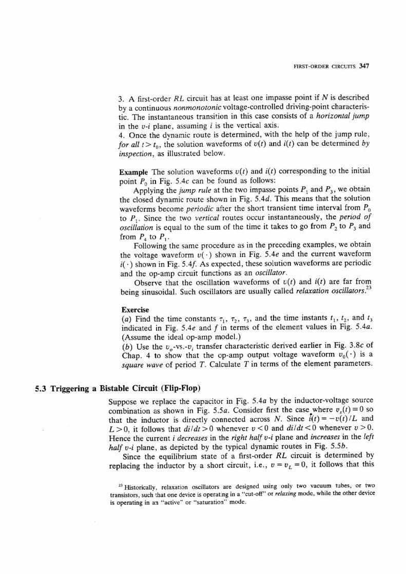
FIRST-ORDER CIRCUm 347
3. A first-order RL circuit has at least one impasse point if N is described by a continuous nonrnonotonic voltage-controlled driving-point characteris- tic. The instantaneous transition in this case consists of a horizontal jump in the v-i plane, assuming i is the vertical axis. 4. Once the dynamic route is determined, with the help of the jump rule, for all t > t,, the solution waveforms of v ( t ) and i ( t ) can be determined by inspection, as illustrated below.
Example The solution waveforms v ( t ) and i ( t ) corresponding to the initial point P, in Fig. 5 . 4 ~ can be found as follows:
Applying the jump rule at the two impasse points P, and P,, we obtain the closed dynamic route shown in Fig. 5 .4d . This means that the solution waveforms become periodic after the short transient time interval from P, to P,. Since the rwo vertical routes occur instantaneously, the period of oscillation is equaf to the sum of the time it takes to go from P, to P, and from P, to P,.
Following the same procedure as in the preceding examples, we obtain the voltage waveform v(.) shown in Fig. 5.4e and the current waveform i( - ) shown in Fig. 5.4f. As expected, these solution waveforms are periodic and the op-amp circuit functions as an oscillator.
Observe that the oscillation waveforms of v ( € ) and i ( t ) are far from being sinusoidal. Such oscillators are usually called reluxution oscil l~ton.'~
Exercise (Q) Find the time constants r,, T,, T,, and the time instants t,, ti, and t, indicated in Fig. 5.4e and f i n terms of the element values in Frg. 5 . 4 ~ . (Assume the ideal op-amp model.) (b) Use the v,-vs.+, transfer characteristic derived earlier in Fig. 3 . 8 ~ of Chap. 4 to show that the op-amp output voltage waveform v,(.) is a square wave of period T. Calculate T in terms of the element parameters.
5.3 Triggering a Bistable Circuit (Flip-Flop)
Suppose we replace the capacitor in Fig. 5 . 4 ~ by the inductor-voltage source combination as shown in Fig. 5 . 5 ~ . Consider first the case where v,(t) = 0 so that the inductor is directly connected across N. Since t t ) = -u ( t ) lL and L > 0, it follows that dildt > 0 whenever v < 0 and dildt < 0 whenever v > 0. Hence the current i decreases in the right half v-i plane and increases in the left half v-i plane, as depicted by the typical dynamic routes in Fig. 5.5b.
Since the equilibrium state of a first-order R L circuit is determined by replacing the inductor by a short circuit, i.e., v = v , = 0, it follows that this
23 Historically, relaxation oscillators are designed using only two vacuum tubes, or two transistors, such that one device is operating in a "cut-off'' or relaxing mode, while the other device is operating in an "active" or "saturation" mode.
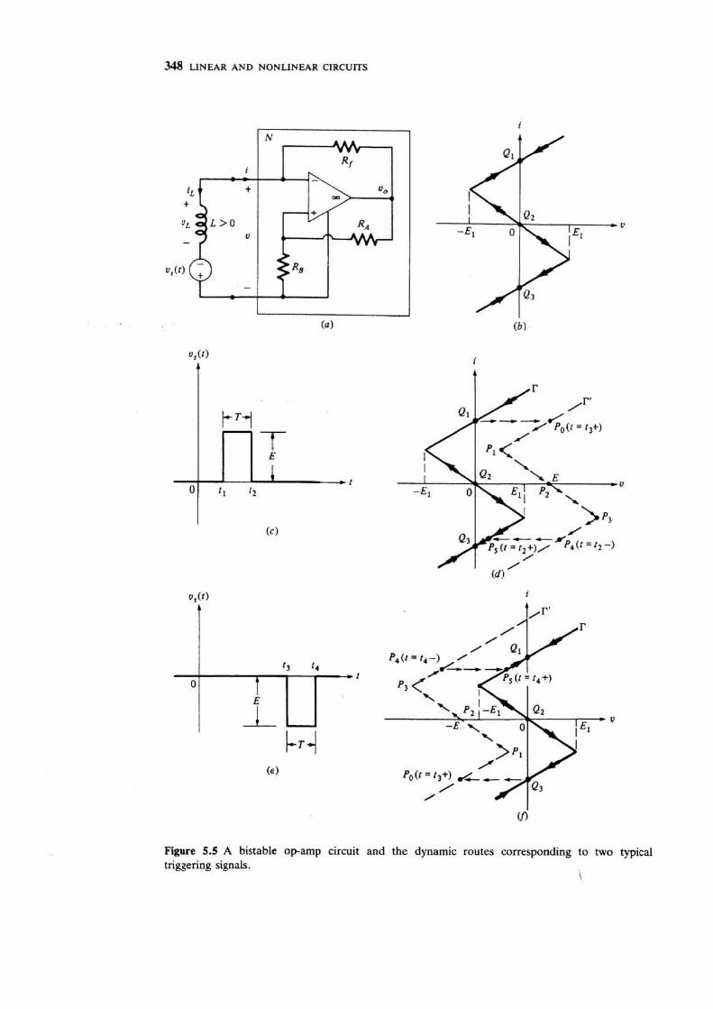
Figure 5.5 A bistable op-amp circuit and the dynamic routes corresponding to two typical triggering signals.
i

FIRST-ORDER CIRCUITS 349
circuit has three equilibrium points; namely, Q,, Q,, and Q,. These equilib- rium points are the operating points of the associated resistive circuit obtained by short-circuiting the inductor L.
Since the dynamic route in Fig. 5.5b either tends to Q , or Q,, but always diverges from Q,. we say that the equilibrium point Q, .. is unstable. Hence even though the associated resistive circuit has three operating points, Q, can never be observed in practice-the slightest noise voltage will cause the dynamic route to diverge from Q2, even if the circuit is operating initially at Q,.
Whether Q, or Q, is actually observed depends on the initial condition. Such a circuit is said to be bistable.
Bistable circuits (flip-flops) are used extensively in digital computers, where the two stable equilibrium points correspond to the two binary states; say Q, denotes "l" and Q, denotes "0." In order to perform logic operations, it is essential to switch from Q, to Q,, and vice versa. This is done by using a small triggering signal. We will now show how the voltage source in Fig. 5.5a can serve as a triggering signal.
Suppose initially the circuit is operating at Q , . Let us at t = t , apply a square pulse of width T = r, - t , as shown in Fig. 5 . 5 ~ . During the time interval t, < t < t,, u,(t) can be replaced by an E-V battery, so that the inductor sees a translated driving-point characteristic as shown in Fig. 5.5d in broken line segments. Let us denote the original and the translated piecewise-linear driving-point characteristics by I' and T' respectively. Then r holds over the time intervals t < t , and t > t2 , whereas r' holds over the time interval t , <t<C2.
Since the inductor current cannot change instantaneously [i ,( t ,-)= i,(t,+)], the dynamic route must jump horizontally from Q, to P, at time t = t , . From P,, the current i must subsequently decrease so long as o > O . Hence, the dynamic route will be as indicated ( Q , -* P, - P, -+ P, --t P:+ P,) in Fig. 5.5d. Here, we assume that at time t = t,- , the dynamic route arrives at some point P, in the lower half plane. At time t = t,+, T' switches back to T, and the dynamic route must jump horizontally from P, to P, at t = t2+. After approximately five time constants, the dynamic route has essentially reached Q,, and we have succeeded in triggering the circuit from equilibrium point Q, to equilibrium point Q2.
To trigger from Q, back to Q,, simply apply a similar triggering pulse of opposite polarity, as shown in Fig. 5.5e. The resulting dynamic route is shown in Fig. 5.5f.
Triggering criteria The following two conditions must be satisfied by the triggering signal in order to trigger from Q, to Q,, or vice versa.
Minimum pulse width condition If t, occurs before the dynamic route in Fig. 5.5d (respectively, f ) crosses the v axis at P,, the route will jump (horizontally) to a point on r in the upper left half plane (respectively, lower right half plane) and return to Q, (respectively, Q,). Hence, for successful triggering, we must

350 LINEAR AND NONLINEAR CIRCUITS
require T > T,,,, where T,,, is the time it takes to go from P, to P, in Fig. 5.5d or f.
Minimum pube height conditian If E is too smalli such that the breakpoint P, on r-s located in the left half plgne, (respectively, the right half plane), then the dynamic route will also return to Q , (respectively, Q,). Hence, for successful triggering, we must require E Emin, where Emin = E l .
Exercise fa) Express T,,, and Emi, in terms of the circuit parameters. ( b ) Sketch the solution waveforms of i(l) and v,(t) for the case when T = 1.5Tm,, and E = 1.5Emin. ( c ) Repeat ( b ) for the case where T = 0.5Tm,, and E = 0.5 Emin.
SUMMARY
A two-terminal element de- scribed by a q-v characteristic f,(q, v) = 0 is called a time- invariant capacitor. In the special case where q = CV, where C is a constant called the capacitance, the capacitor is linear and time-invariant. In this case, it can be described by
m A linear time-varying capacitor is described by
q = C(t)v
This implies that
requires an additional term com- pared to the time-invariant case.
m A two-terminal element de- scribed by a $-i characteristic f,(#~, i ) = O is called a time- invariant inductor.
m In the special case where 4 = Li, where L is a constant called the inductance, the inductor is linear and time-invariant. In this case, it can be described by
m A linear time-varying inductor is described by
4 = L(t)i
This implies that
requires an additional term com- pared to the time-invariant case.
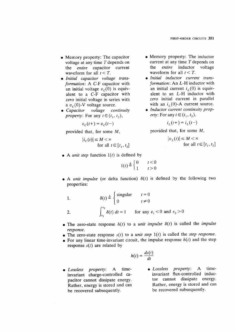
FIRST-ORDER CIRCUITS 351
e Memory property: The capacitor voltage at any time T depends on the entire capacitor current waveform for all t < T. Initial capacitor voltage trans- formation: A C-F capacitor with an initial voltage v,(O) is equiv- alent to a C-F capacitor with zero initial voltage in series with a vc(0)-V voltage source. Capacitor voltage continuity property: For any t E ( t , , t ,) ,
provided that, for some M,
ji,(t)l I M < X
for alI t E [ t , , t,]
e Memory property: The inductor current at any time T depends on the entire inductor voltage waveform for all t < T, Initial inductor current trans- formation: An L-H inductor with an initial current i , (O) is equiv- alent to an L-M inductor with zero initial current in parallel with an i,(O)-A current sourcl.
e Inductor current continuity prop- erty: For any t E (t,, t,),
provided that, for some M,
/ v , ( t ) l s M < X
for all t E [ t , , t , l
A unit step function l ( t ) is defined by
A unit impulse (or delta function) S(t) is defined by the following two properties:
singular t = 0 S( t ) ' l O t f O
1; ~ ( t ) dt = l for any E~ < 0 and > 0
The zero-state response h( t ) to a unit impulse S ( t ) is called the impulse response. The zero-state response s(t) to a unit step l(t) is called the step response. For any linear time-invariant circuit, the impulse response h(t) and the step response s( t ) are related by
Lossless property: A time- Lossless property: A time- invariant charge-controlled ca- invariant flux-controlled induc- pacitor cannot dissipate energy. tor cannot dissipate energy. Rather, energy is stored and can Rather, energy is stored and can be recovered subsequently. be recovered subsequently.

e The energy W,. entering a time- invariant charge-controlled ca- pacitor during [ t , , t,] depends on the charge at the end points, namely, q , ( s , ) and q,.(t,). In particular,
where A 41 P qc(4 1 and
q 2 = qCCt?-) ' e The energy E, stored in a C-F
capacitor with initial voltage v,(O) = V is equal to
g, is called a relaxation point for a time-invariant charge-con- trolled capacitor iff
for ail -m< q < m
The energy Ec stored in a time- invariant charge-controiled capac- itor with initial charge q ( 0 ) = Q is equal to
where q , is any relaxation point of the capacitor. A first-order linear parallel RC circuit is described by a state equation
where R,, is the Thkveliin equi- valent resistance and v,,(t) is the open-circuit voltage of the resistive one-port seen by the capacitor.
0 The energy W , entering a time- invariant flux-controlled inductor during [ t l , t2] depends aniy on the flux at the end points, name- ly, +,([,) and 4,(t,). In par- ticular,
where 4 P # ~ ( f ~ ) and 42 A 4 . @ 2 ) .
9 The energy 8, stored in an L-H inductor with initial current i , ( O ) = I is equal to
4, is called a relaxation point for a time-invariant flux-controlled inductor iff
for all - m < C$ <m
The energy stored in a time- invariant flux-controlled induc- tor with initial flux #(0) = 4, is equal to
where 4, is any relaxation point of the inductor. A first-order linear series RL circuit is described by a state equation
where G,, is the Norton equival- ent conductance and is,(t) is the short-circuit current of the resis- tive one-port seen by the in- ductor. \ \.

FIRST-ORDER CIRCUITS 353
Any first-order linear time-invariant circuit driven by dc sources is describ- ed by a state equation of the form
where T is called the time constant, and x(t,) is called the equilibrium state.
e T = R,, C for an R C circuit T = G,,L for an RL circuit
e The solution of the above state equation is always given explicitly by an exponential waveform:
for all time t. This solution is uniquely specified by three pieces of information: the
initial stare x(t,), the equilibrium state x(t,), and the time constant T. m Let x(t,) and x(t,) denote any two points on the above exponential
waveform. The elapsed time between tj and t, can be calculated explicitly as follows:
m The solution of any first-order linear time-invariant circuit driven by dc sources. or by piecewise-constant signals, or circuits containing switches can be obtained by inspection (i.e., without writing the state equation): Simply determine the three relevant pieces of information over appropriate time intervals. The solution of any first-order piecewise-linear circuit can be determined by inspection by drawing the associated dynamic route. When the dynamic route contains impasse points, the capacitor voltage waveform and the inductor current waveform must exhibit one or more instantaneous jumps.
PROBLEMS Nonlinear capacitors and inductors
1 A varactor diode behaves like a capacitor when v V, (V, =0.5V in this case). Its q-v characteristic is given by
(a) Calculate its small-signal capacitance C(v) for v < 0.5 V. ( 6 ) A voltage v( t ) = - 1 + 0.3 cos (2x1O8t) is applied. Obtain an explicit expression for the
current through the capacitor.
2 A time-invariant nonlinear inductor has the characteristic shown in Fig. P6.2. (a) Using the graph, estimate the small-signal inductance L(i) when i = 3 mA. (b) Repeat (a) for i = 2 mA.