Linear approach of the levelset function in XFEM · Linear approach of the levelset function in XFEM written by: M.A.C. Thurlings Final Bachelor Project 2 Foreword This report is

Linear approach of the levelset function in XFEM

Linear approach of the levelset function in

XFEM

M.A.C. Thurlings MT 09.41

Linear approach of the levelset function in XFEM written by: M.A.C. Thurlings

Final Bachelor Project 2

Foreword

This report is the result of the final bachelor project ‘BEP’ of M.A.C. Thurlings. The

project started on the September 31st, 2009 and ended on November 6

th, 2009. With

this report the author wants to show he is capable to do research and solve an

academic problem and thereby able to finish the bachelor at the technical university of

Eindhoven. The project was very well coached by dr. ir. P.D. Anderson and dr. ir.

M.A. Hulsen.

In the past weeks the student learned about Fortran and TFEM (Toolkit for Finite

Element Method) and some recent developments in XFEM (eXtended Finite element

method). In the process of creating the algorithm he improved his programming skills

and knowledge about finite element methods. The results are very acceptable to

continue the research on this subject.



Summary

The Finite Element Method (FEM) programs are relative new programs to solve both

simple and complex problems. New techniques are still developed to improve the

programs. A Toolkit for FEM (TFEM) is developed at the TU/e to test new

techniques.

Tests are done in TFEM to check what 2D element is best used for linear problems. It

appeared to be the quad-9 element. This element preformed best in a minimal error

and short CPU-time. With complex geometry triangle-6 elements might have

advantage.

The main goal of the research is to create a new algorithm that determines the levelset

function in an xfem program, a component of TFEM. Originally this is done with

exact formulas and solid objects. When complex shapes or time depended shapes are

used, there are no exact formulas available. A direct approach to the levelset function

is developed to cope with this problem.

The signed distance function determines the shortest distance from a given point

(usually a node in a mesh) to an object. Not only does it provide the distance but also

if this point is inside or outside the object. This is done by a sign. When the point is

inside the object the distance gets a negative sign. When it is outside it stays positive.

The signed distance function is a levelset function.

An algorithm is developed in Matlab to determine the levelset function using a linear

approach of. It uses a set of coordinates on the interface of the object to determine the

distance and sign. The levelset function is determined with distances and vectors

between known coordinates. The coordinates have to be arranged counterclockwise as

usual in fem programming.

The algorithm is tested in Matlab. The sign is determined correctly with distances as

close as the machε number to the object. An expected error in the distance exists,

because of the linear approach of the object. This error decreases as expected with the

second order for a nonlinear object with an increasing number of object coordinates.

The algorithm is implemented in the original xfem2 program from TFEM and tested.

The accuracy of the program depends on the number of object coordinates indicated

with k. They can be increased. The result of the original program is not constant for

different values of k. This is a result of an error in dividing the elements.

When the number of object coordinates is larger than 640, the program showed almost

identical results as the original program. The CPU-time for building the mesh

increased with about 6%. When other shapes are introduced the program is capable to

deal with this geometry and produce accurate results.

When a ‘nodelem’ is generated beside the ‘topology’ they can be used in calculating

the levelset function. It is not implemented in the algorithm. This is useful when the

object coordinates change in time and are no longer arranged counterclockwise.



Table of content

Linear approach of the levelset function in XFEM ............................................................ 1

Foreword ............................................................................................................................. 2

Summary ............................................................................................................................. 3

Table of content .................................................................................................................. 4

Introduction......................................................................................................................... 5

1. Learning TFEM .......................................................................................................... 6

Number of elements ........................................................................................................ 6

Changing the geometry ................................................................................................... 8

Changing the equation .................................................................................................... 9

2. First version of the linear approach in 2D ................................................................ 10

The sign......................................................................................................................... 10

The distance .................................................................................................................. 12

Tests .............................................................................................................................. 14

3. Improved linear approach in 2D ............................................................................... 16

Redeveloping distance .................................................................................................. 16

Sign for point to object coordinate................................................................................ 16

Tests .............................................................................................................................. 18

4. XFEM ....................................................................................................................... 19

Increasing object coordinates........................................................................................ 19

CPU-time ...................................................................................................................... 20

Other shapes.................................................................................................................. 21

5. Conclusion and recommendation.............................................................................. 22

6. Literature................................................................................................................... 23

7. Appendix................................................................................................................... 24

A Adjustments in the program for the Poisson equation. ......................................... 24

B Result for changing geometry and equation ......................................................... 25

C Program test 1 ....................................................................................................... 28

D Program test 2 ....................................................................................................... 30

E Program test 3 ....................................................................................................... 31

F Improved program ................................................................................................ 33

G Testresult improved program................................................................................ 35

H Program in XFEM................................................................................................. 37



Introduction

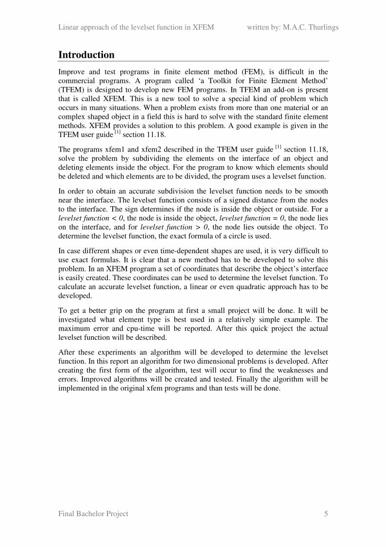
Improve and test programs in finite element method (FEM), is difficult in the

commercial programs. A program called ‘a Toolkit for Finite Element Method’

(TFEM) is designed to develop new FEM programs. In TFEM an add-on is present

that is called XFEM. This is a new tool to solve a special kind of problem which

occurs in many situations. When a problem exists from more than one material or an

complex shaped object in a field this is hard to solve with the standard finite element

methods. XFEM provides a solution to this problem. A good example is given in the

TFEM user guide [1]

section 11.18.

The programs xfem1 and xfem2 described in the TFEM user guide [1]

section 11.18,

solve the problem by subdividing the elements on the interface of an object and

deleting elements inside the object. For the program to know which elements should

be deleted and which elements are to be divided, the program uses a levelset function.

In order to obtain an accurate subdivision the levelset function needs to be smooth

near the interface. The levelset function consists of a signed distance from the nodes

to the interface. The sign determines if the node is inside the object or outside. For a

levelset function < 0, the node is inside the object, levelset function = 0, the node lies

on the interface, and for levelset function > 0, the node lies outside the object. To

determine the levelset function, the exact formula of a circle is used.

In case different shapes or even time-dependent shapes are used, it is very difficult to

use exact formulas. It is clear that a new method has to be developed to solve this

problem. In an XFEM program a set of coordinates that describe the object’s interface

is easily created. These coordinates can be used to determine the levelset function. To

calculate an accurate levelset function, a linear or even quadratic approach has to be

developed.

To get a better grip on the program at first a small project will be done. It will be

investigated what element type is best used in a relatively simple example. The

maximum error and cpu-time will be reported. After this quick project the actual

levelset function will be described.

After these experiments an algorithm will be developed to determine the levelset

function. In this report an algorithm for two dimensional problems is developed. After

creating the first form of the algorithm, test will occur to find the weaknesses and

errors. Improved algorithms will be created and tested. Finally the algorithm will be

implemented in the original xfem programs and than tests will be done.



1. Learning TFEM

The first part of the project is assigned to understand more about TFEM. This

program gives the opportunity to experiment with new developed methods in finite

element methods. The program is written in the computer language FORTRAN 95.

The Poisson equation can be approached by the program written in Paragraph 2.1.2 in

the TFEM user guide [1]

. This program gives the biggest absolute difference between

the real and the approximated solution. In this program, a number of elements are

defined. In case this number is adjusted the maximum error will change. This error

can be written as a function of the number of nodes with the unknown u.

In TFEM different element types can be used, even different kinds in one program.

This program uses the standard QUAD-9. These are square elements with 9 nodes.

Other two dimensional element types are QUAD-4, TRIANGLE-3 and TRIANGLE-

6.

Number of elements

In this first assignment the Poisson equation on a unit square with Dirichlet

boundary’s is determined. The equation [1-1] is used. fu =∇2 is addressed on the

boundary’s.

( ) ( )ππ ∗∗∗+= yxu coscos1 [1-1]

An increasing number of unknown degrees of freedom will be introduced and

checked what consequences this has for the maximum error for these 4 different

elements. It is also interesting to check the CPU-time. In case of very large programs

with large amounts of unknown degrees of freedom and complex geometry it could

take days to run a program. It is important to get the most accurate possible answer

with the smallest CPU-time. All element types will be tested on these requirements

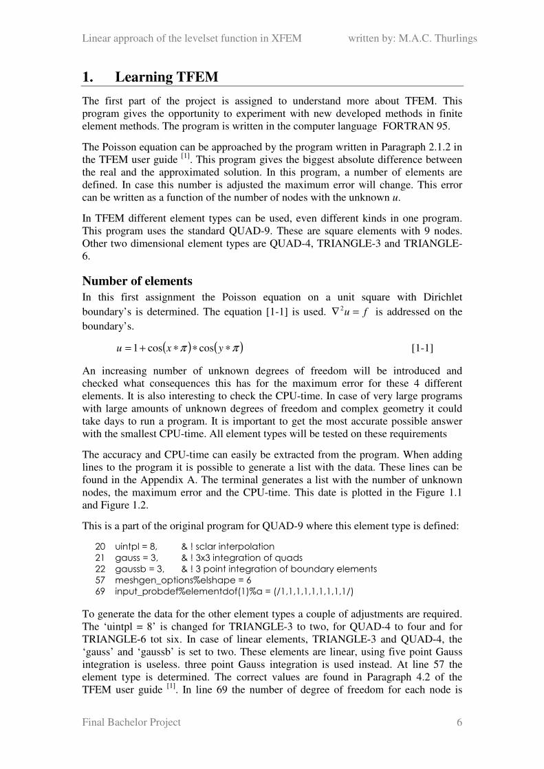
The accuracy and CPU-time can easily be extracted from the program. When adding

lines to the program it is possible to generate a list with the data. These lines can be

found in the Appendix A. The terminal generates a list with the number of unknown

nodes, the maximum error and the CPU-time. This date is plotted in the Figure 1.1

and Figure 1.2.

This is a part of the original program for QUAD-9 where this element type is defined:

20 uintpl = 8, & ! sclar interpolation

21 gauss = 3, & ! 3x3 integration of quads

22 gaussb = 3, & ! 3 point integration of boundary elements

57 meshgen_options%elshape = 6

69 input_probdef%elementdof(1)%a = (/1,1,1,1,1,1,1,1,1/)

To generate the data for the other element types a couple of adjustments are required.

The ‘uintpl = 8’ is changed for TRIANGLE-3 to two, for QUAD-4 to four and for

TRIANGLE-6 tot six. In case of linear elements, TRIANGLE-3 and QUAD-4, the

‘gauss’ and ‘gaussb’ is set to two. These elements are linear, using five point Gauss

integration is useless. three point Gauss integration is used instead. At line 57 the

element type is determined. The correct values are found in Paragraph 4.2 of the

TFEM user guide [1]

. In line 69 the number of degree of freedom for each node is



determined. This is ‘one’ for all nodes of an element type. For TRIANGLE-3 there

are three ones required and so on. The data for these other three element types are

plotted in the Figure 1.1 and Figure 1.2.

1,00E-11

1,00E-10

1,00E-09

1,00E-08

1,00E-07

1,00E-06

1,00E-05

1,00E-04

1,00E-03

1,00E-02

1,00E-01

10 100 1000 10000 100000 1000000

#dof

Err

or

Triangle, 3 nodes Triangle, 6 nodes Quad, 4 nodes Quad, 9 nodes

Figure 1.1 Error versus number of unknown dof

As show in Figure 1.1, the quadratic elements give more accurate results than the

linear elements. The Poisson equation gives a nonlinear solution. For this reason the

quadratic elements give much better results. The QUAD elements give better results

than the TRIANGLE shape elements, because the unknown nodes in QUAD’s are

calculated with more known nodes. Figure 1.1 shows that the error drops wit a first

order for linear elements and second order for quadratic elements.

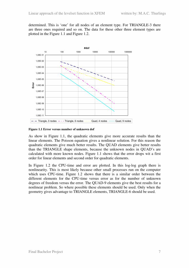
In Figure 1.2 the CPU-time and error are plotted. In this log-log graph there is

nonlinearity. This is most likely because other small processes run on the computer

which uses CPU-time. Figure 1.2 shows that there is a similar order between the

different elements for the CPU-time versus error as for the number of unknown

degrees of freedom versus the error. The QUAD-9 elements give the best results for a

nonlinear problem. So where possible these elements should be used. Only when the

geometry gives advantage to TRIANGLE elements, TRIANGLE-6 should be used.



1,00E-11

1,00E-10

1,00E-09

1,00E-08

1,00E-07

1,00E-06

1,00E-05

1,00E-04

1,00E-03

1,00E-02

1,00E-01

1,00E+00

1,00E-03 1,00E-02 1,00E-01 1,00E+00 1,00E+01

CPU_time

Err

or

Triangle, 3 nodes Triangle, 6 nodes Quad, 4 nodes Quad, 9 nodes

Figure 1.2 CPU-time versus error

Changing the geometry

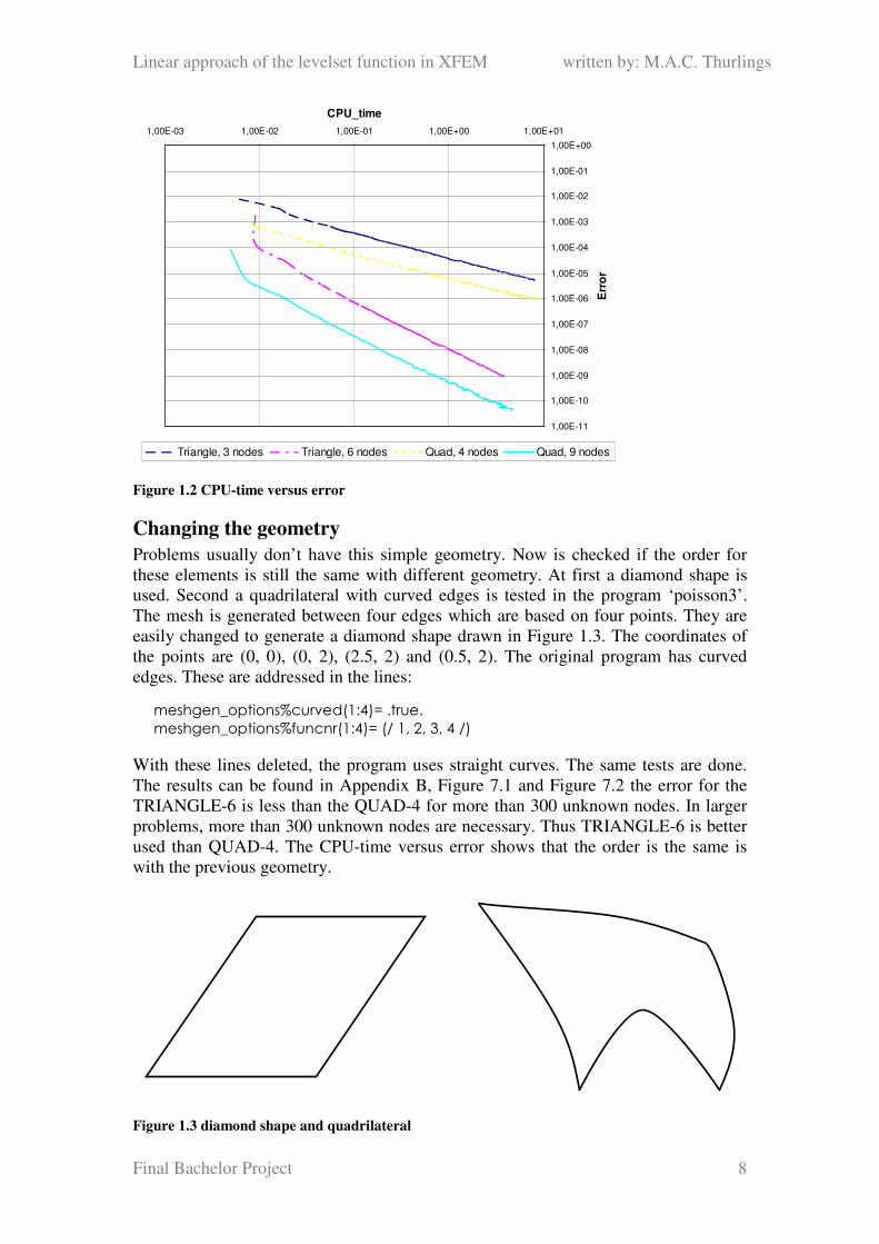
Problems usually don’t have this simple geometry. Now is checked if the order for

these elements is still the same with different geometry. At first a diamond shape is

used. Second a quadrilateral with curved edges is tested in the program ‘poisson3’.

The mesh is generated between four edges which are based on four points. They are

easily changed to generate a diamond shape drawn in Figure 1.3. The coordinates of

the points are (0, 0), (0, 2), (2.5, 2) and (0.5, 2). The original program has curved

edges. These are addressed in the lines:

meshgen_options%curved(1:4)= .true.

meshgen_options%funcnr(1:4)= (/ 1, 2, 3, 4 /)

With these lines deleted, the program uses straight curves. The same tests are done.

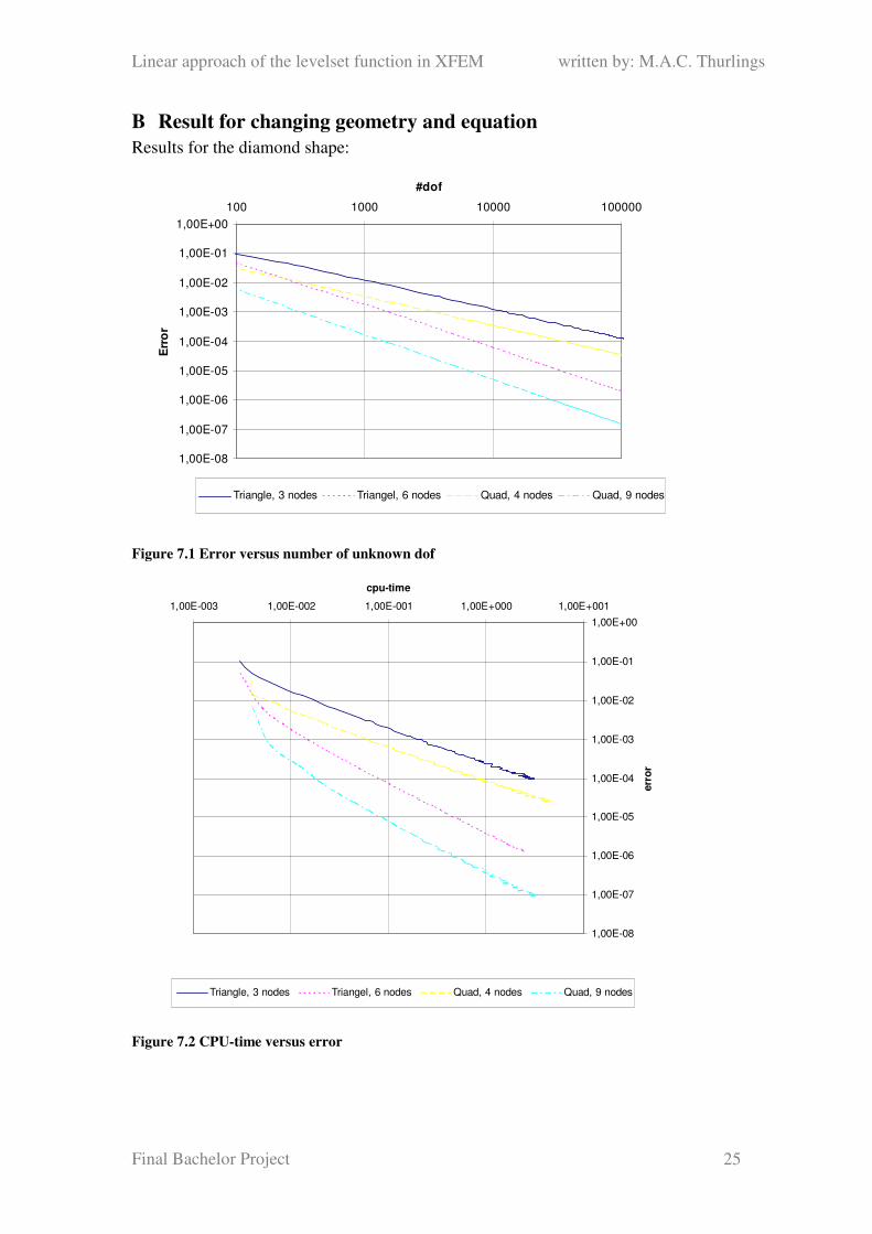
The results can be found in Appendix B, Figure 7.1 and Figure 7.2 the error for the

TRIANGLE-6 is less than the QUAD-4 for more than 300 unknown nodes. In larger

problems, more than 300 unknown nodes are necessary. Thus TRIANGLE-6 is better

used than QUAD-4. The CPU-time versus error shows that the order is the same is

with the previous geometry.

Figure 1.3 diamond shape and quadrilateral



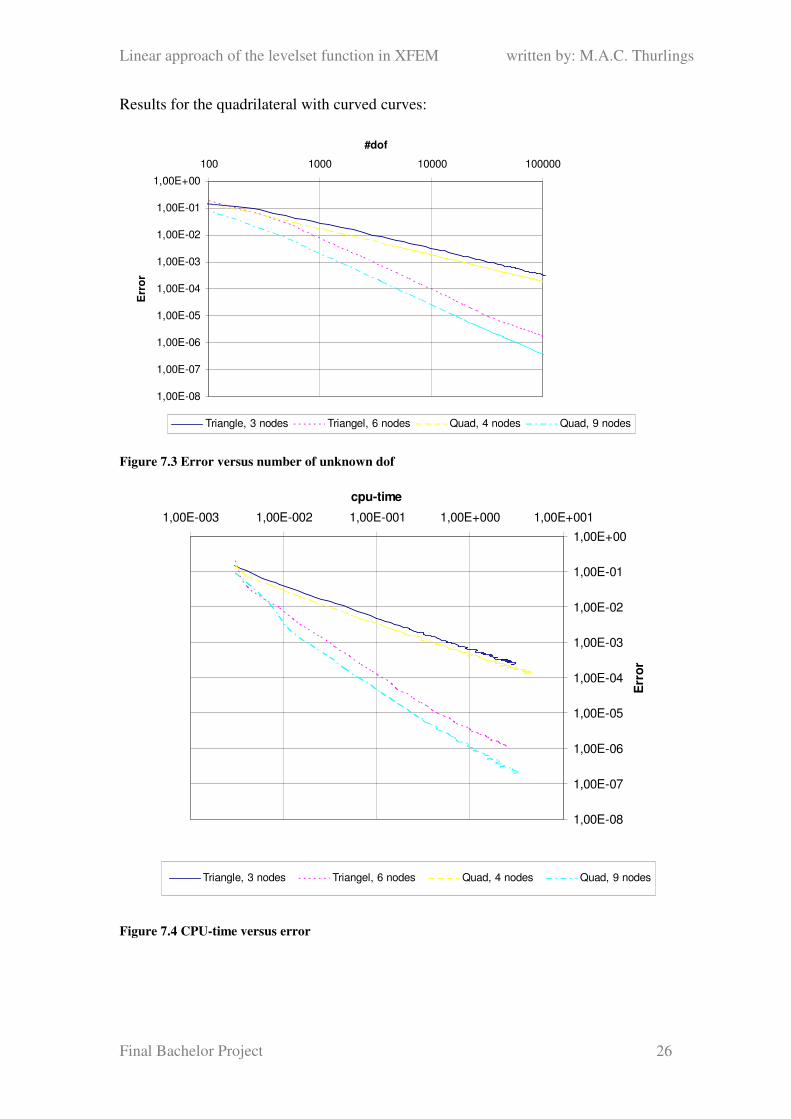
Now the two lines deleted before are placed back. The four edges are now curved, so

the form is a quadrilateral drawn in Figure 1.3. The results are found in Appendix B,

Figure 7.3 and Figure 7.4. The order of the results is the same as before but there is a

difference. In the previous test the difference between the quadratic elements was

about one decade for the error versus number of unknown dof and CPU-time versus

error. But for this problem the lines lie twice as close to each other on the logarithmic

scale. Also the lines of the linear elements lie twice as close to each other. This effect

might be caused by the integration which could be slower for QUAD-elements for this

geometry.

Changing the equation

In the first two parts the equation [1-1] is solved. Now a different equation [1-2] in

introduced and checked what influence it has on the tests. The second order deviation

is applied on the boundaries which is [1-3]

( ) ( )ππ ∗∗∗∗∗+= yxu 4sin4sin1 . [1-2]

( ) ( )πππ ∗∗∗∗∗∗=∇− yxu 4sin4sin32 22 [1-3]

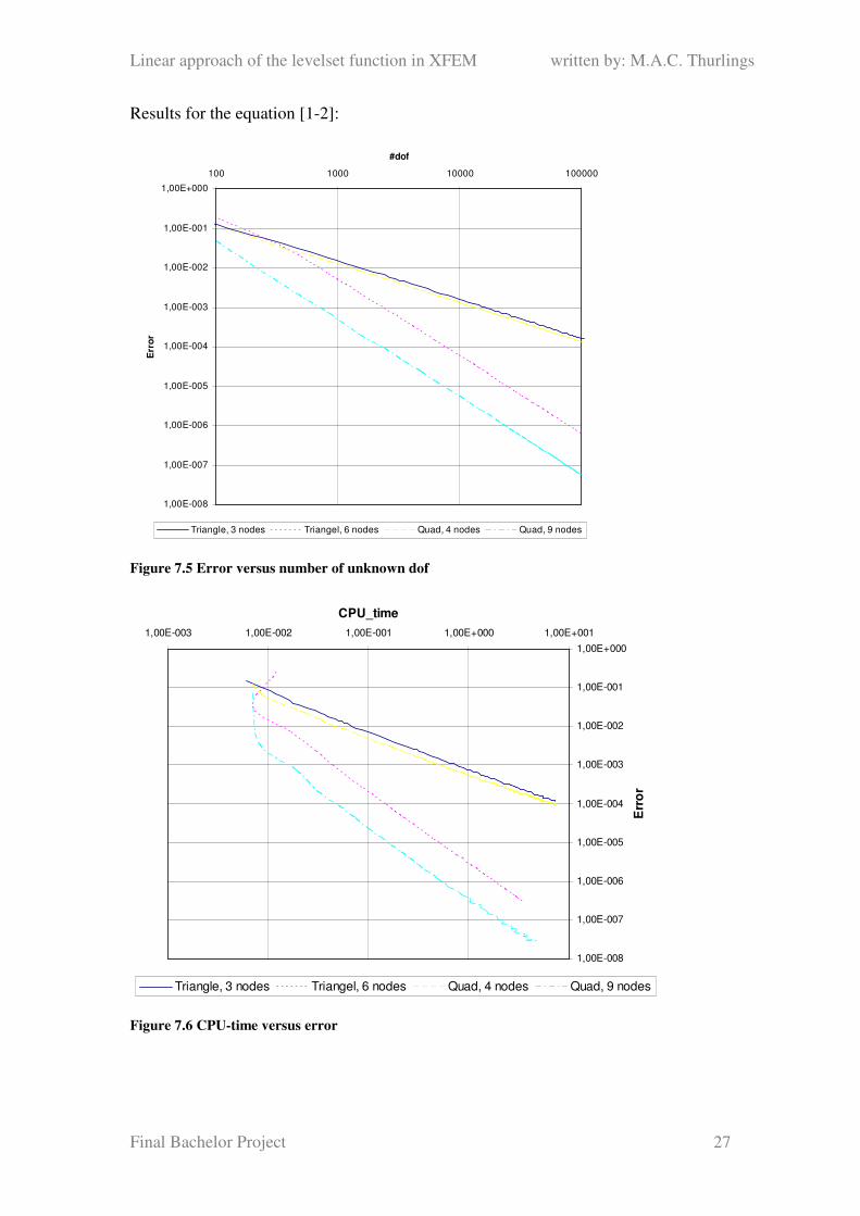
The results of this equation are found in Appendix B, Figure 7.5 and Figure 7.6. They

are similar to the other problems. Other equations have little influence on which

element is best used.



2. First version of the linear approach in 2D

A linear approach for a two dimensional problem will be developed. This is expected

to be less complicated to develop than a quadratic approach. Developing this approach

consist of two main parts. At first the method to determine the sign will be developed.

Second a way to determine the distance is developed. It would be useful if this

program is easily adjustable for 3D problems.

The sign

On the internet [2]

and in the TFEM user guide [1]

three ways to determine the sign

were found.

1) From a point in the mesh, a line to infinite or in case of FEM, to the end of the

mesh is determined. This line will cross the object interface an even or odd

time. If it is even, the point is outside the object, and if it is odd, the point is

inside the object. The risk of this method is on nodes, where two lines come

together. When not well defined, the program will count two crossings at the

nodes.

2) When a function ( )0xr

φ is given, with values on a finite number of points,

interpolation can be used to approach the value of ( )0xr

φ on unknown points.

This method is not useful because the values on the points are not given.

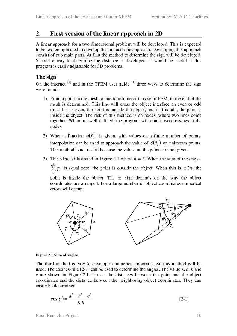
3) This idea is illustrated in Figure 2.1 where n = 5. When the sum of the angles

∑=

n

i

i

1

ϕ is equal zero, the point is outside the object. When this is π2± the

point is inside the object. The ± sign depends on the way the object

coordinates are arranged. For a large number of object coordinates numerical

errors will occur.

Figure 2.1 Sum of angles

The third method is easy to develop in numerical programs. So this method will be

used. The cosines-rule [2-1] can be used to determine the angles. The value’s, a, b and

c are shown in Figure 2.1. It uses the distances between the point and the object

coordinates and the distance between the neighboring object coordinates. They can

easily be determined.

( )ab

cba

2cos

222 −+=α [2-1]

2ϕ

1ϕ 3ϕ

4ϕ

5ϕ

1ϕ

2ϕ

3ϕ

4ϕ

5ϕ

a

b

c



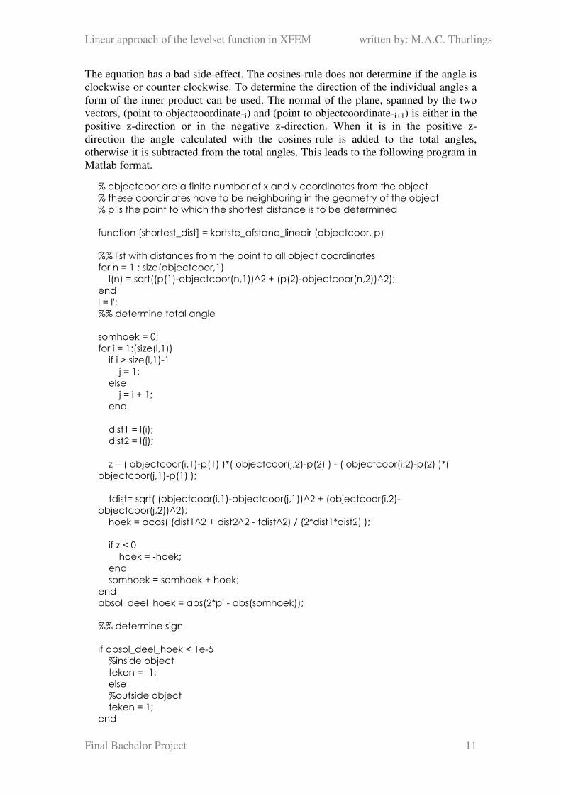
The equation has a bad side-effect. The cosines-rule does not determine if the angle is

clockwise or counter clockwise. To determine the direction of the individual angles a

form of the inner product can be used. The normal of the plane, spanned by the two

vectors, (point to objectcoordinate-i) and (point to objectcoordinate-i+1) is either in the

positive z-direction or in the negative z-direction. When it is in the positive z-

direction the angle calculated with the cosines-rule is added to the total angles,

otherwise it is subtracted from the total angles. This leads to the following program in

Matlab format.

% objectcoor are a finite number of x and y coordinates from the object

% these coordinates have to be neighboring in the geometry of the object

% p is the point to which the shortest distance is to be determined

function [shortest_dist] = kortste_afstand_lineair (objectcoor, p)

%% list with distances from the point to all object coordinates

for n = 1 : size(objectcoor,1)

l(n) = sqrt((p(1)-objectcoor(n,1))^2 + (p(2)-objectcoor(n,2))^2);

end

l = l';

%% determine total angle

somhoek = 0;

for i = 1:(size(l,1))

if i > size(l,1)-1

j = 1;

else

j = i + 1;

end

dist1 = l(i);

dist2 = l(j);

z = ( objectcoor(i,1)-p(1) )*( objectcoor(j,2)-p(2) ) - ( objectcoor(i,2)-p(2) )*(

objectcoor(j,1)-p(1) );

tdist= sqrt( (objectcoor(i,1)-objectcoor(j,1))^2 + (objectcoor(i,2)-

objectcoor(j,2))^2);

hoek = acos( (dist1^2 + dist2^2 - tdist^2) / (2*dist1*dist2) );

if z < 0

hoek = -hoek;

end

somhoek = somhoek + hoek;

end

absol_deel_hoek = abs(2*pi - abs(somhoek));

%% determine sign

if absol_deel_hoek < 1e-5

%inside object

teken = -1;

else

%outside object

teken = 1;

end



The program continuous, at this part the sign can be determined. Depending on the

position of the point and the objects geometry there is a small error in the results.

Thus if the ‘absol_deel_hoek < 1e-5’ the sign is negative, if not the sign is positive.

The distance

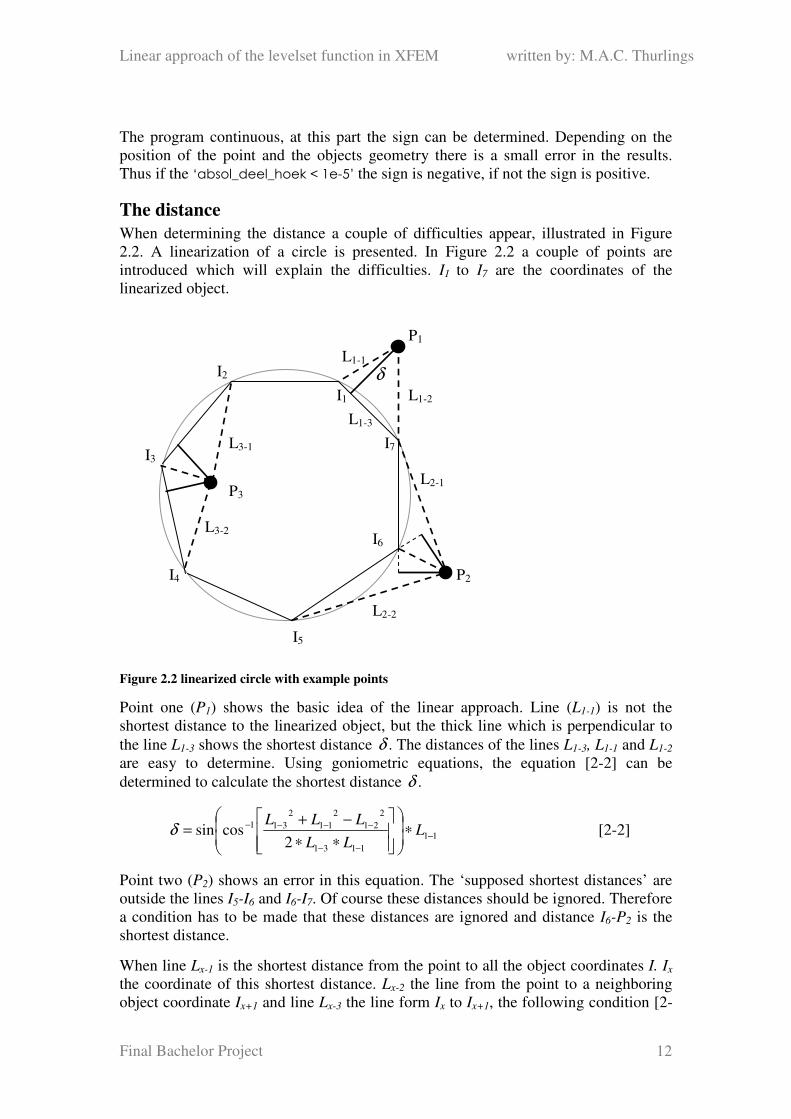
When determining the distance a couple of difficulties appear, illustrated in Figure

2.2. A linearization of a circle is presented. In Figure 2.2 a couple of points are

introduced which will explain the difficulties. I1 to I7 are the coordinates of the

linearized object.

Figure 2.2 linearized circle with example points

Point one (P1) shows the basic idea of the linear approach. Line (L1-1) is not the

shortest distance to the linearized object, but the thick line which is perpendicular to

the line L1-3 shows the shortest distance δ . The distances of the lines L1-3, L1-1 and L1-2

are easy to determine. Using goniometric equations, the equation [2-2] can be

determined to calculate the shortest distance δ .

11

1131

2

21

2

11

2

311

2cossin −

−−

−−−− ∗

∗∗

−+= L

LL

LLLδ [2-2]

Point two (P2) shows an error in this equation. The ‘supposed shortest distances’ are

outside the lines I5-I6 and I6-I7. Of course these distances should be ignored. Therefore

a condition has to be made that these distances are ignored and distance I6-P2 is the

shortest distance.

When line Lx-1 is the shortest distance from the point to all the object coordinates I. Ix

the coordinate of this shortest distance. Lx-2 the line from the point to a neighboring

object coordinate Ix+1 and line Lx-3 the line form Ix to Ix+1, the following condition [2-

P2

I3

P3

P1

L3-1

L3-2

L1-2

L1-1

L2-2

L2-1

I6

I7

I1

I2

I4

I5

L1-3

δ



3] can be made. If this condition is true, the distance δ should be calculated. Else it

should be ignored.

2

2

2

3

2

1 −−− ≤+ xxx LLL [2-3]

Point three (P3) shows the next issue. In some cases it is not directly clear if the

distance to the object coordinate, the perpendicular line before or after this coordinate

is the shortest distance. All three distances should be calculated and the distance

closest to zero is the shortest distance δ .

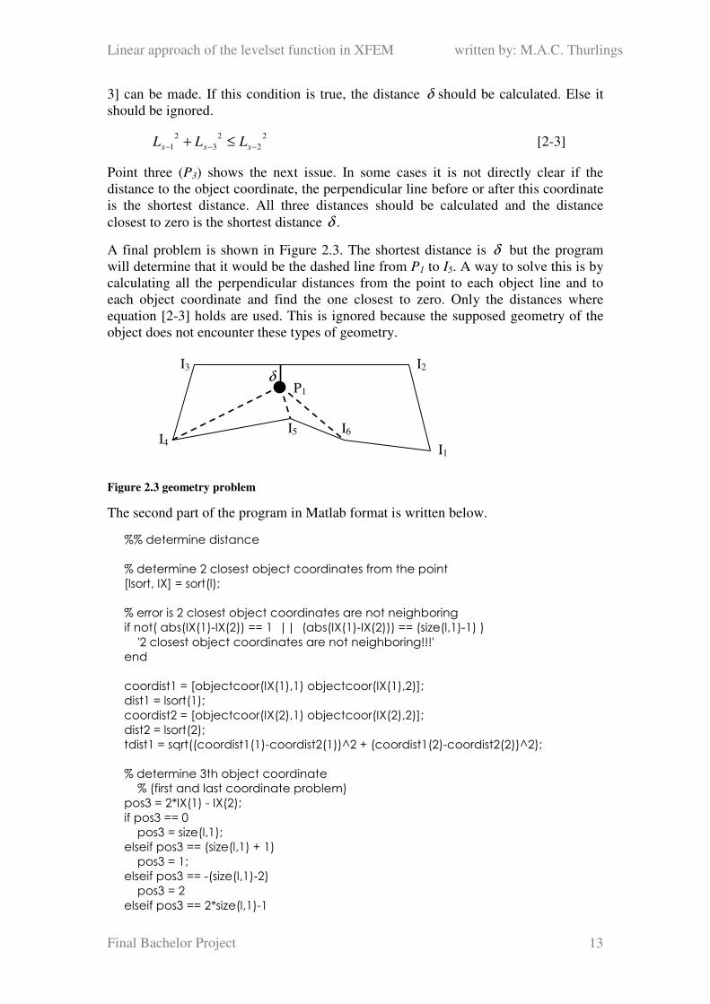
A final problem is shown in Figure 2.3. The shortest distance is δ but the program

will determine that it would be the dashed line from P1 to I5. A way to solve this is by

calculating all the perpendicular distances from the point to each object line and to

each object coordinate and find the one closest to zero. Only the distances where

equation [2-3] holds are used. This is ignored because the supposed geometry of the

object does not encounter these types of geometry.

Figure 2.3 geometry problem

The second part of the program in Matlab format is written below.

%% determine distance

% determine 2 closest object coordinates from the point

[lsort, IX] = sort(l);

% error is 2 closest object coordinates are not neighboring

if not( abs(IX(1)-IX(2)) == 1 || (abs(IX(1)-IX(2))) == (size(l,1)-1) )

'2 closest object coordinates are not neighboring!!!'

end

coordist1 = [objectcoor(IX(1),1) objectcoor(IX(1),2)];

dist1 = lsort(1);

coordist2 = [objectcoor(IX(2),1) objectcoor(IX(2),2)];

dist2 = lsort(2);

tdist1 = sqrt((coordist1(1)-coordist2(1))^2 + (coordist1(2)-coordist2(2))^2);

% determine 3th object coordinate

% (first and last coordinate problem)

pos3 = 2*IX(1) - IX(2);

if pos3 == 0

pos3 = size(l,1);

elseif pos3 == (size(l,1) + 1)

pos3 = 1;

elseif pos3 == -(size(l,1)-2)

pos3 = 2

elseif pos3 == 2*size(l,1)-1

P1

δ

I2 I3

I1

I4

I5 I6



pos3 = size(l,1) - 1

end

coordist3 = [objectcoor(pos3,1) objectcoor(pos3,2)];

dist3 = l(pos3);

tdist2 = sqrt((coordist1(1)-coordist3(1))^2 + (coordist1(2)-coordist3(2))^2);

% shortest distance

SHORTEST_DIST = [];

SHORTEST_DIST = [SHORTEST_DIST; dist1];

if sqrt(tdist1^2 + dist1^2) <= dist2

shortest_dist1 = dist1;

else

shortest_dist1 = sin(acos((dist2^2+tdist1^2-dist1^2)/(2*dist2*tdist1)))*dist2;

end

SHORTEST_DIST = [SHORTEST_DIST; shortest_dist1];

if sqrt(tdist2^2 + dist1^2) <= dist3

shortest_dist2 = dist1;

else

shortest_dist2 = sin(acos((dist3^2+tdist2^2-dist1^2)/(2*dist3*tdist1)))*dist3;

end

SHORTEST_DIST = [SHORTEST_DIST; shortest_dist2];

shortest_dist_zonder_teken = min(SHORTEST_DIST);

%% sign * distance

shortest_dist = teken * shortest_dist_zonder_teken;

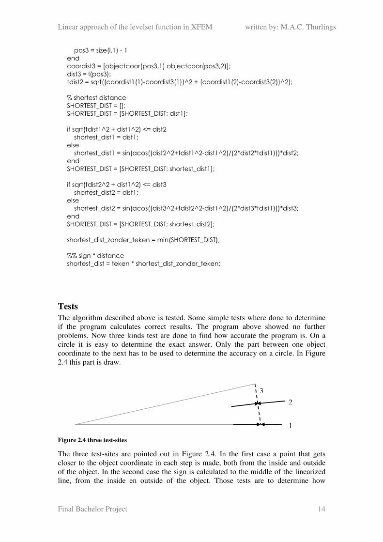
Tests

The algorithm described above is tested. Some simple tests where done to determine

if the program calculates correct results. The program above showed no further

problems. Now three kinds test are done to find how accurate the program is. On a

circle it is easy to determine the exact answer. Only the part between one object

coordinate to the next has to be used to determine the accuracy on a circle. In Figure

2.4 this part is draw.

Figure 2.4 three test-sites

The three test-sites are pointed out in Figure 2.4. In the first case a point that gets

closer to the object coordinate in each step is made, both from the inside and outside

of the object. In the second case the sign is calculated to the middle of the linearized

line, from the inside en outside of the object. Those tests are to determine how

1

2

3



accurate the sign is calculated. In the third case the maximum error on the linearized

line (the dashed line) is determined.

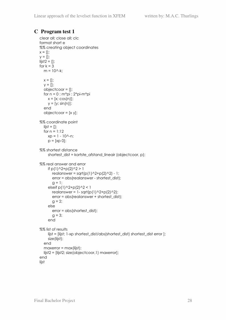
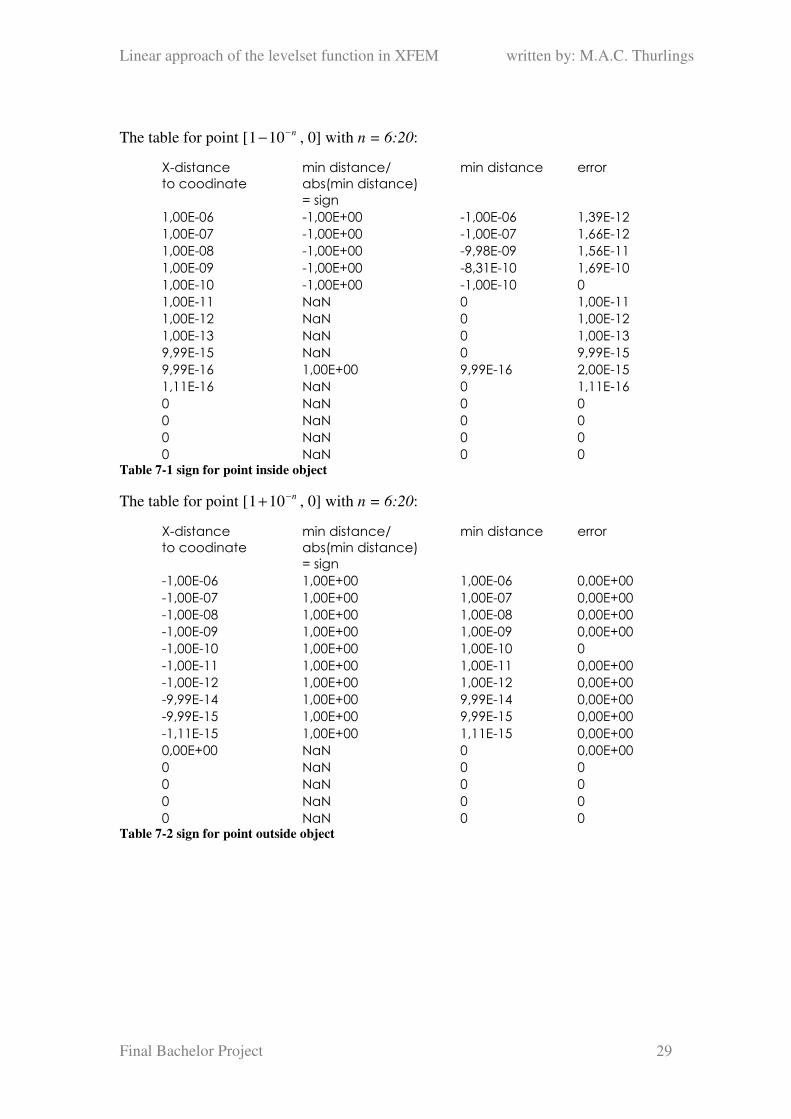
1) The program for this test is found in Appendix C. The object is described with

2000 object coordinates. The exact distance between the point and the

coordinate is n−10 with n = 6:20. At first the point is inside the object. The

sign stays -1 till the exact distance is 1010− as shown in Table 7-1. The table

produced by Matlab shows that the calculated distance for 1110− is exactly

zero. No sign can be calculated. When the point is outside the object only the

x-coordinate of the point has to be adjusted to n−+101 . For n = 6:20, Table 7-2

show that the sign is correct till n = 15. When n is getting smaller, the real

distance is so close to the machε number (machine number) that errors are

inevitable.

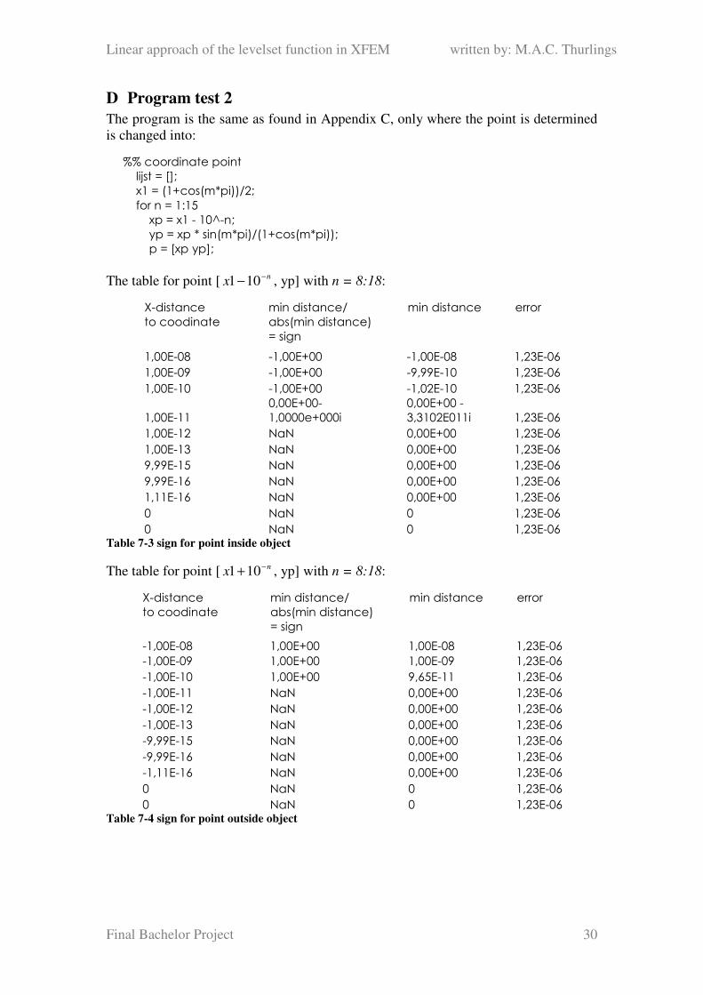
2) This test is almost the same as the previous test but the points are positioned at

a different place. In Appendix D is found how these points are determined.

The point starting from the inside of the object give the correct sign till n = 10.

When n = 11 the distance is imaginary shown in Table 7-3. This is most likely

a numerical error. This might give a problem in the actual XFEM program. It

is not known yet what will happen if an imaginary distance is introduced.

When the points is outside the object, the program gives the expected answer

till n = 10. When n > 10 the distance is zero, the sign can’t be calculated. This

is shown in Table 7-4.

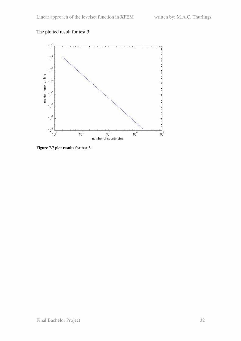
3) In this test the maximum error is determined with a different amount of object

coordinates. It will show how the error decreases for more object coordinates.

The error should decrease with a second order. This program is found in

Appendix E. Figure 7.7 shows the results of the program. This plot shows that

the maximum error changes with the second order which is expected.

In conclusion it shows that the results are acceptable to work with. There are only

errors within 1010− of the line. These errors are acceptable. There is only one other

problem that didn’t show from the results in the test but was discovered when running

the third test. A large cpu-time was required to calculate the minimum distance for a

large amount of object coordinates. A faster method has to be developed. This

program also does not seem easy to adapt for a 3D problem.



3. Improved linear approach in 2D

The idea behind the improved version is to prevent the roots, cosinus, sinus and any

other expensive calculations. The use of vectors may be faster. Vectors will give

advantage in 3D problems.

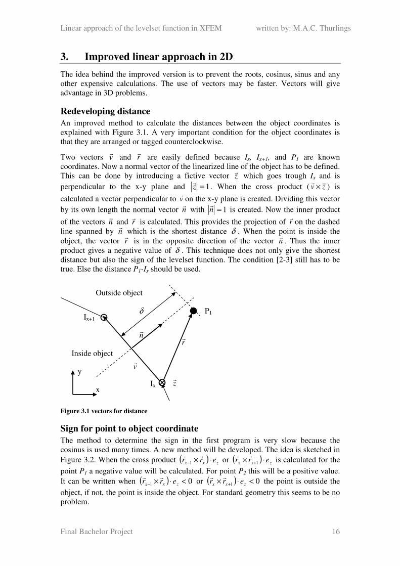
Redeveloping distance

An improved method to calculate the distances between the object coordinates is

explained with Figure 3.1. A very important condition for the object coordinates is

that they are arranged or tagged counterclockwise.

Two vectors vr

and rr

are easily defined because Ix, Ix+1, and P1 are known

coordinates. Now a normal vector of the linearized line of the object has to be defined.

This can be done by introducing a fictive vector zr

which goes trough Ix and is

perpendicular to the x-y plane and 1=zr

. When the cross product ( zvrr

× ) is

calculated a vector perpendicular to vr

on the x-y plane is created. Dividing this vector

by its own length the normal vector nr

with 1=nr

is created. Now the inner product

of the vectors nr

and rr

is calculated. This provides the projection of rr

on the dashed

line spanned by nr

which is the shortest distance δ . When the point is inside the

object, the vector rr

is in the opposite direction of the vector nr

. Thus the inner

product gives a negative value of δ . This technique does not only give the shortest

distance but also the sign of the levelset function. The condition [2-3] still has to be

true. Else the distance P1-Ix should be used.

Figure 3.1 vectors for distance

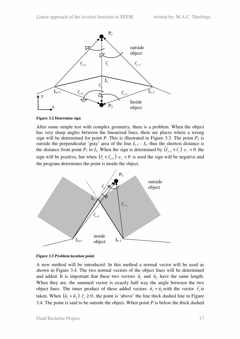
Sign for point to object coordinate

The method to determine the sign in the first program is very slow because the

cosinus is used many times. A new method will be developed. The idea is sketched in

Figure 3.2. When the cross product ( ) zxx err ⋅×−

rr1 or ( ) zxx err ⋅× +1

rr is calculated for the

point P1 a negative value will be calculated. For point P2 this will be a positive value.

It can be written when ( ) 01 <⋅×− zxx errrr

or ( ) 01 <⋅× + zxx errrr

the point is outside the

object, if not, the point is inside the object. For standard geometry this seems to be no

problem.

P1

Outside object

Ix

Ix+1

δ

rr

vr

nr

Inside object

zr

y

x



Figure 3.2 Determine sign

After some simple test with complex geometry, there is a problem. When the object

has very sharp angles between the linearized lines, there are places where a wrong

sign will be determined for point P. This is illustrated in Figure 3.3. The point P1 is

outside the perpendicular ‘gray’ area of the line Ix-1 - Ix, thus the shortest distance is

the distance from point P1 to Ix. When the sign is determined by ( ) 01 <⋅×− zxx errrr

the

sign will be positive, but when ( ) 01 <⋅× + zxx errrr

is used the sign will be negative and

the program determines the point is inside the object.

Figure 3.3 Problem location point

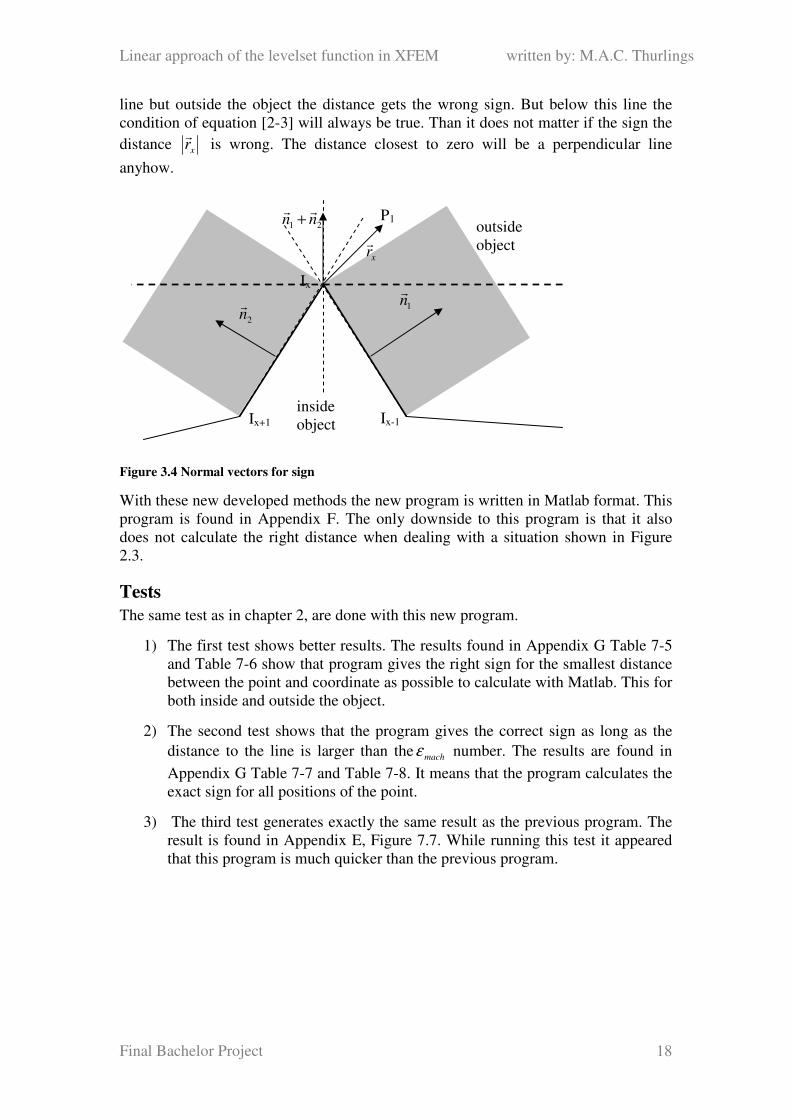
A new method will be introduced. In this method a normal vector will be used as

shown in Figure 3.4. The two normal vectors of the object lines will be determined

and added. It is important that these two vectors 1nr

and 2nr

have the same length.

When they are, the summed vector is exactly half way the angle between the two

object lines. The inner product of these added vectors 21 nnrr

+ with the vector xrr

is

taken. When ( ) 021 ≥⋅+ xrnnrrr

, the point is ‘above’ the line thick dashed line in Figure

3.4. The point is said to be outside the object. When point P is below the thick dashed

P2

P1

Ix

Ix-1 Ix+1

outside

object

Inside

object

1−xrr

xrr

1+xr

r

1+xrr

xrr

1−xrr

y

x

P1

Ix

Ix-1 Ix+1

outside

object

inside

object

1−xrr

xrr

1+xrr



line but outside the object the distance gets the wrong sign. But below this line the

condition of equation [2-3] will always be true. Than it does not matter if the sign the

distance xrr

is wrong. The distance closest to zero will be a perpendicular line

anyhow.

Figure 3.4 Normal vectors for sign

With these new developed methods the new program is written in Matlab format. This

program is found in Appendix F. The only downside to this program is that it also

does not calculate the right distance when dealing with a situation shown in Figure

2.3.

Tests

The same test as in chapter 2, are done with this new program.

1) The first test shows better results. The results found in Appendix G Table 7-5

and Table 7-6 show that program gives the right sign for the smallest distance

between the point and coordinate as possible to calculate with Matlab. This for

both inside and outside the object.

2) The second test shows that the program gives the correct sign as long as the

distance to the line is larger than the machε number. The results are found in

Appendix G Table 7-7 and Table 7-8. It means that the program calculates the

exact sign for all positions of the point.

3) The third test generates exactly the same result as the previous program. The

result is found in Appendix E, Figure 7.7. While running this test it appeared

that this program is much quicker than the previous program.

P1

Ix

Ix-1 Ix+1

outside

object

inside

object

1nr

xrr

2nr

21 nnrr

+



4. XFEM

The next step is to implement the algorithm in the existing xfem program and test if it

will generate acceptable results. The programs xfem1 and xfem2 are available. The

xfem2 is a more accurate program. This program divides the last elements into

triangle elements which gives a much more accurate approach of the object. In the

original program the geometry of the object is already created. This is done in the next

part of the program:

! create mesh for particle boundary

nelem = 4 * nx * radius / lx

call mesh_skeleton ( mesh_particle, nnodes=2*nelem, nelem=nelem, elshape=2,

&

ndim=2 )

rp = radius ! radius of the circular object

xpc = center ! initial position of the center of the object

call objectscoor ( 1, mesh_particle%coor )

do elem = 1, mesh_particle%nelem

mesh_particle%topology(1)%a(:,elem) = (/ 2*elem-1, 2*elem, 2*elem + 1 /)

end do

mesh_particle%topology(1)%a(3,mesh_particle%nelem) = 1 ! close circle

! one object

call add_to_mesh ( mesh, object='mesh', objectmesh=mesh_particle, &

topology=.true., intrule=2, nsubint=nsubinto )

The object coordinates are created in the subroutine ‘objectscoor’. This subroutine is

in the file subs1.f90. These coordinates can be used to make a linearized object. This

data is not transferred to the module ‘functions_xf2_m’ before the levelset function is

determined. This is done by the line:

lmesh => mesh ! supply mesh to mapcoor for mapping coordinates

This line is copied to a line before the levelset function is determined. Now the object

coordinates generated can be used in the function ‘levelset function’. The part where

the levelset function is determined is replaced by the program found in Appendix H.

Increasing object coordinates

It appears that the results of the xfem programs are very depended on the number of

object elements. When the object crosses just a very small percentage of an original

element the dividing does not work correct. To prevent this, the original mesh is

deformed, but in some cases this may not be enough. Other programs have a solution

for this problem but they are not used here. The amounts of object elements are

changed in the program line below by changing the value k. This will sometimes

prevent or create the described problem. It also provides more object coordinates.

With the original k = 4 there are only forty elements and eighty object coordinates.

When increasing k this number of coordinates also increases. The Lagrange



multipliers increase with the increasing elements. In future tests the number of

elements should not be increased but only the number of coordinates.

nelem = k * nx * radius / lx

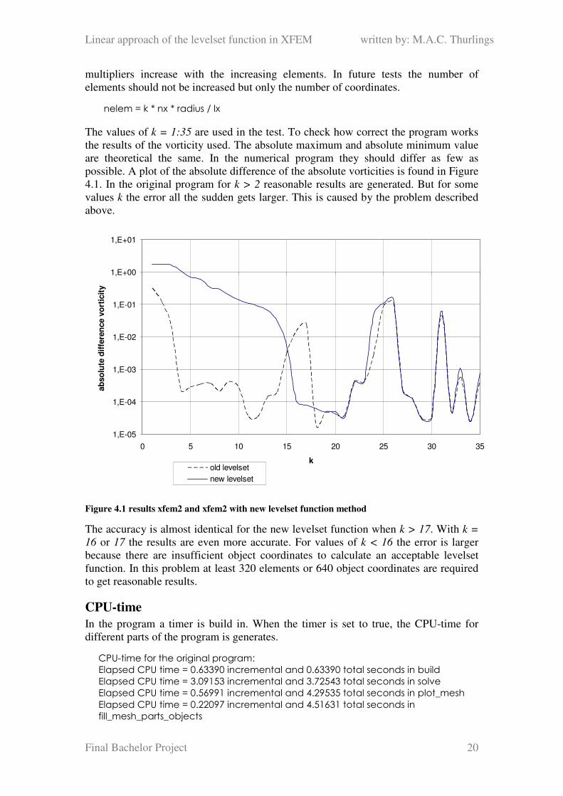
The values of k = 1:35 are used in the test. To check how correct the program works

the results of the vorticity used. The absolute maximum and absolute minimum value

are theoretical the same. In the numerical program they should differ as few as

possible. A plot of the absolute difference of the absolute vorticities is found in Figure

4.1. In the original program for k > 2 reasonable results are generated. But for some

values k the error all the sudden gets larger. This is caused by the problem described

above.

1,E-05

1,E-04

1,E-03

1,E-02

1,E-01

1,E+00

1,E+01

0 5 10 15 20 25 30 35

k

ab

so

lute

dif

fere

nce v

ort

icit

y

old levelset

new levelset

Figure 4.1 results xfem2 and xfem2 with new levelset function method

The accuracy is almost identical for the new levelset function when k > 17. With k =

16 or 17 the results are even more accurate. For values of k < 16 the error is larger

because there are insufficient object coordinates to calculate an acceptable levelset

function. In this problem at least 320 elements or 640 object coordinates are required

to get reasonable results.

CPU-time

In the program a timer is build in. When the timer is set to true, the CPU-time for

different parts of the program is generates.

CPU-time for the original program:

Elapsed CPU time = 0.63390 incremental and 0.63390 total seconds in build

Elapsed CPU time = 3.09153 incremental and 3.72543 total seconds in solve

Elapsed CPU time = 0.56991 incremental and 4.29535 total seconds in plot_mesh

Elapsed CPU time = 0.22097 incremental and 4.51631 total seconds in

fill_mesh_parts_objects



Elapsed CPU time = 0.33095 incremental and 4.84726 total seconds in fill_sample

CPU-time for the adjusted program

Elapsed CPU time = 0.67490 incremental and 0.67490 total seconds in build

Elapsed CPU time = 3.11353 incremental and 3.78842 total seconds in solve

Elapsed CPU time = 0.59991 incremental and 4.38833 total seconds in plot_mesh

Elapsed CPU time = 0.22297 incremental and 4.61130 total seconds in

fill_mesh_parts_objects

Elapsed CPU time = 0.32795 incremental and 4.93925 total seconds in fill_sample

These CPU-times are a bit variable when different processes are running but

reasonably constant to show the differences. The part were the levelset function is

determined is in the build part. Logically the CPU-time increases in this part. In this

case it is just an increase of 6%. The difference between the total time is even only

2% Other parts appear to be a bit faster. It is not clear if this is the result of the new

levelset function function. This increase in time is acceptable

Other shapes

The basic idea to introduce this new algorithm in xfem was to be able to introduce

other than standard geometries. Because of the problem with dividing elements which

are crosses by a small percentage, it will be difficult to introduce other shapes in

xfem2.

A simple adjustment to the original program would be to introduce an ellipse. This is

easily done by changing the lines where the coordinates are generated in the

subprogram subs1.f90. The 2-coordinates will be multiplied by 0,75.

coor(:,2) = rp * 0,75_dp * cos(p) + xpc(2)

This gives an ellipse, stretched in the 1-direction. When the value k is set to 20 the

program gives the following results for the voritcity.

max vorticity min voriticity abs diffence

4,5182377E+00 -4,5187312E+00 4,9344487E-04

Thus also for other shapes a very accurate absolute difference between the vorticities

can be determined. For other values of k with this shape the program is not as

consistent as it was for the cylinder.



5. Conclusion and recommendation

With the results of the first chapter can be concluded that QUAD-9 elements should

be used. These are much more accurate and faster. There are geometrical examples

where TRIANGLE-9 elements have there benefits. But it is also possible to combine

these two quadratic element types. Linear elements should only be used with

nonlinear problems.

The linear approach of the levelset function is best calculated without cosinuses and

roots. These are expensive operators and less accurate. Only the lengths and vectors of

the objects and points are used. When using these, an extra condition for the object

coordinates is introduced. The object coordinates have to be arranged or tagged

counterclockwise. When this is implemented the results are optimal. There is of

coarse still an error between the exact levelset function and the linear approach. This

error decreases with second order when the number of object coordinates is increased.

The result of the algorithm implemented in the original xfem2 program showed when

a minimum object coordinates is reached the program generates similar results as the

old program. The algorithm can easily be changed for 3D problems. Instead of the

fictive vector zr

a second vector of the object element can be used to determine the

normal vector.

There is a ‘topology’ generated and added to the object. This is a list which contains

nodal numbers. The first row of the ‘topology’ contains the nodal numbers to which

the first element is connected and so on. It is possible to generate a list that works the

other way around, called the ‘nodelem’. That list is not jet generated. When an object

changed for instance in time, nodes can be added. This will break the clockwise

sequence of the nodes. Then it is not possible to use the previous and next number of

the node as done in the existing program. Instead the ‘topology’ and ‘nodelem’ should

be used. This ‘nodelem’ is not generated in the program and there for not

implemented in the program.

The program cannot deal with situations explained with Figure 2.3. This can be

changed by introducing a brute force method which calculates the distance to all

linearized lines excluding those were condition [2-3] is false. In stead of using

condition [2-3] it might be possible to use the local coordinate system of the elements

connecting the object coordinates. When the position of the point is outside the

perpendicular area described in local coordinates with 1−<ξ or 1>ξ , condition [2-

3] is false and the distance to the line should be ignored.



6. Literature

[1] TFEM user guide. A toolkit for finite element method. By: Martien A. Hulsen.

Version 25th

June, 2009

[2] http://gathering.tweakers.net/forum/list_messages/1228505



7. Appendix

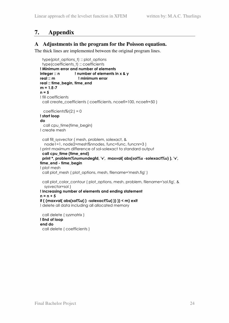
A Adjustments in the program for the Poisson equation.

The thick lines are implemented between the original program lines.

type(plot_options_t) :: plot_options

type(coefficients_t) :: coefficients

! Minimum error and number of elements

integer :: n ! number of elements in x & y

real :: m ! minimum error

real :: time_begin, time_end

m = 1.E-7

n = 5

! fill coefficients

call create_coefficients ( coefficients, ncoefi=100, ncoefr=50 )

coefficients%r(2:) = 0

! start loop

do

call cpu_time(time_begin)

! create mesh

call fill_sysvector ( mesh, problem, solexact, &

node1=1, node2=mesh%nnodes, func=func, funcnr=3 )

! print maximum difference of sol-solexact to standard output

call cpu_time (time_end)

print *, problem%numundegfd, 'v', maxval( abs(sol%u -solexact%u) ), 'v',

time_end - time_begin

! plot mesh

call plot_mesh ( plot_options, mesh, filename='mesh.fig' )

call plot_color_contour ( plot_options, mesh, problem, filename='sol.fig', &

sysvector=sol )

! Increasing number of elements and ending statement

n = n + 5

if ( (maxval( abs(sol%u(:) -solexact%u(:)) )) < m) exit

! delete all data including all allocated memory

call delete ( sysmatrix )

! End of loop

end do

call delete ( coefficients )



B Result for changing geometry and equation

Results for the diamond shape:

1,00E-08

1,00E-07

1,00E-06

1,00E-05

1,00E-04

1,00E-03

1,00E-02

1,00E-01

1,00E+00

100 1000 10000 100000

#dof

Err

or

Triangle, 3 nodes Triangel, 6 nodes Quad, 4 nodes Quad, 9 nodes


1,00E-08

1,00E-07

1,00E-06

1,00E-05

1,00E-04

1,00E-03

1,00E-02

1,00E-01

1,00E+00

1,00E-003 1,00E-002 1,00E-001 1,00E+000 1,00E+001

cpu-time

err

or





Results for the quadrilateral with curved curves:

1,00E-08

1,00E-07

1,00E-06

1,00E-05

1,00E-04

1,00E-03

1,00E-02

1,00E-01

1,00E+00

100 1000 10000 100000

#dofE

rro

r



1,00E-08

1,00E-07

1,00E-06

1,00E-05

1,00E-04

1,00E-03

1,00E-02

1,00E-01

1,00E+00

1,00E-003 1,00E-002 1,00E-001 1,00E+000 1,00E+001

cpu-time

Err

or





Results for the equation [1-2]:

1,00E-008

1,00E-007

1,00E-006

1,00E-005

1,00E-004

1,00E-003

1,00E-002

1,00E-001

1,00E+000

100 1000 10000 100000

#dofE

rro

r



1,00E-008

1,00E-007

1,00E-006

1,00E-005

1,00E-004

1,00E-003

1,00E-002

1,00E-001

1,00E+000

1,00E-003 1,00E-002 1,00E-001 1,00E+000 1,00E+001

CPU_time

Err

or





C Program test 1

clear all; close all; clc

format short e

%% creating object coordinates

x = [];

y = [];

lijst2 = [];

for k = 3

m = 10^-k;

x = [];

y = [];

objectcoor = [];

for n = 0 : m*pi : 2*pi-m*pi

x = [x; cos(n)];

y = [y; sin(n)];

end

objectcoor = [x y];

%% coordinate point

lijst = [];

for n = 1:12

xp = 1 - 10^-n;

p = [xp 0];

%% shortest distance

shortest_dist = kortste_afstand_lineair (objectcoor, p);

%% real answer and error

if p(1)^2+p(2)^2 > 1

realanswer = sqrt(p(1)^2+p(2)^2) - 1;

error = abs(realanswer - shortest_dist);

g = 1;

elseif p(1)^2+p(2)^2 < 1

realanswer = 1- sqrt(p(1)^2+p(2)^2);

error = abs(realanswer + shortest_dist);

g = 2;

else

error = abs(shortest_dist);

g = 3;

end

%% list of results

lijst = [lijst; 1-xp shortest_dist/abs(shortest_dist) shortest_dist error ];

size(lijst);

end

maxerror = max(lijst);

lijst2 = [lijst2; size(objectcoor,1) maxerror];

end

lijst



The table for point [ n−−101 , 0] with n = 6:20:

X-distance

to coodinate

min distance/

abs(min distance)

= sign

min distance error

1,00E-06 -1,00E+00 -1,00E-06 1,39E-12

1,00E-07 -1,00E+00 -1,00E-07 1,66E-12

1,00E-08 -1,00E+00 -9,98E-09 1,56E-11

1,00E-09 -1,00E+00 -8,31E-10 1,69E-10

1,00E-10 -1,00E+00 -1,00E-10 0

1,00E-11 NaN 0 1,00E-11

1,00E-12 NaN 0 1,00E-12

1,00E-13 NaN 0 1,00E-13

9,99E-15 NaN 0 9,99E-15

9,99E-16 1,00E+00 9,99E-16 2,00E-15

1,11E-16 NaN 0 1,11E-16

0 NaN 0 0

0 NaN 0 0

0 NaN 0 0

0 NaN 0 0 Table 7-1 sign for point inside object

The table for point [ n−+101 , 0] with n = 6:20:

X-distance

to coodinate

min distance/

abs(min distance)

= sign

min distance error

-1,00E-06 1,00E+00 1,00E-06 0,00E+00

-1,00E-07 1,00E+00 1,00E-07 0,00E+00

-1,00E-08 1,00E+00 1,00E-08 0,00E+00

-1,00E-09 1,00E+00 1,00E-09 0,00E+00

-1,00E-10 1,00E+00 1,00E-10 0

-1,00E-11 1,00E+00 1,00E-11 0,00E+00

-1,00E-12 1,00E+00 1,00E-12 0,00E+00

-9,99E-14 1,00E+00 9,99E-14 0,00E+00

-9,99E-15 1,00E+00 9,99E-15 0,00E+00

-1,11E-15 1,00E+00 1,11E-15 0,00E+00

0,00E+00 NaN 0 0,00E+00

0 NaN 0 0

0 NaN 0 0

0 NaN 0 0

0 NaN 0 0 Table 7-2 sign for point outside object



D Program test 2

The program is the same as found in Appendix C, only where the point is determined

is changed into:

%% coordinate point

lijst = [];

x1 = (1+cos(m*pi))/2;

for n = 1:15

xp = x1 - 10^-n;

yp = xp * sin(m*pi)/(1+cos(m*pi));

p = [xp yp];

The table for point [ nx

−−101 , yp] with n = 8:18:

X-distance

to coodinate

min distance/

abs(min distance)

= sign

min distance error

1,00E-08 -1,00E+00 -1,00E-08 1,23E-06

1,00E-09 -1,00E+00 -9,99E-10 1,23E-06

1,00E-10 -1,00E+00 -1,02E-10 1,23E-06

1,00E-11

0,00E+00-

1,0000e+000i

0,00E+00 -

3,3102E011i 1,23E-06

1,00E-12 NaN 0,00E+00 1,23E-06

1,00E-13 NaN 0,00E+00 1,23E-06

9,99E-15 NaN 0,00E+00 1,23E-06

9,99E-16 NaN 0,00E+00 1,23E-06

1,11E-16 NaN 0,00E+00 1,23E-06

0 NaN 0 1,23E-06

0 NaN 0 1,23E-06 Table 7-3 sign for point inside object

The table for point [ nx

−+101 , yp] with n = 8:18:

X-distance

to coodinate

min distance/

abs(min distance)

= sign

min distance error

-1,00E-08 1,00E+00 1,00E-08 1,23E-06

-1,00E-09 1,00E+00 1,00E-09 1,23E-06

-1,00E-10 1,00E+00 9,65E-11 1,23E-06

-1,00E-11 NaN 0,00E+00 1,23E-06

-1,00E-12 NaN 0,00E+00 1,23E-06

-1,00E-13 NaN 0,00E+00 1,23E-06

-9,99E-15 NaN 0,00E+00 1,23E-06

-9,99E-16 NaN 0,00E+00 1,23E-06

-1,11E-16 NaN 0,00E+00 1,23E-06

0 NaN 0 1,23E-06

0 NaN 0 1,23E-06 Table 7-4 sign for point outside object



E Program test 3

clear all; close all; clc

format short e

%% creating object coordinates

x = [];

y = [];

lijst2 = [];

for k = 1:4

m = 10^-k

x = [];

y = [];

objectcoor = [];

for n = 0 : m*pi : 2*pi-m*pi

x = [x; cos(n)];

y = [y; sin(n)];

end

objectcoor = [x y];

%% coordinate point

lijst = [];

for xp = cos(m*pi): (1-cos(m*pi))/99 : 1

yp = -sin(m*pi)/(1-cos(m*pi))*xp + sin(m*pi)/(1-cos(m*pi));

p = [xp yp];

%% shcortest distance

shortest_dist = kortste_afstand_lineair (objectcoor, p);

%% exact answer and error

if p(1)^2+p(2)^2 > 1

realanswer = sqrt(p(1)^2+p(2)^2) - 1;

error = abs(realanswer - shortest_dist);

g = 1;

elseif p(1)^2+p(2)^2 < 1

realanswer = 1- sqrt(p(1)^2+p(2)^2);

error = abs(realanswer + shortest_dist);

g = 2;

else

error = abs(shortest_dist);

g = 3;

end

%% list of result of all points

lijst = [lijst; error ];

size(lijst)

end

maxerror = max(lijst);

lijst2 = [lijst2; size(objectcoor,1) maxerror];

end

%% plot results

loglog(lijst2(:,1),lijst2(:,2))

xlabel('number of coordinates')

ylabel('maxiam error on line')



The plotted result for test 3:

Figure 7.7 plot results for test 3



F Improved program

% objectcoor are a finite number of x and y coordinates from the object

% These coodinates have to be neighboring in the geometry of the object

% p is the point to which the shortest distance is to be determinated

% shortest_dist is the shortest distance to the boundary of the object

% positive: the point lays outside the object

% negative: the point lays inside the object

function [shortest_dist] = kortste_afstand_lineair_3 (objectcoor,p)

%% list of quadratic distances from point to all object coordintes

l(1,:) = (p(1)-objectcoor(:,1)).^2 + (p(2)-objectcoor(:,2)).^2;

l = l';

%% determine 3 points

% determine closest objectcoordinate

[lsort, IX] = sort(l);

% determine first point

pos1 = IX(1);

% determine second point

pos2 = IX(1) + 1;

if pos2 == size(l,1) + 1

pos2 = 1;

end

% determine third point

pos3 = IX(1) - 1;

if pos3 == 0

pos3 = size(l,1);

end

%% determine if object line participates and determine the distances

a_kwad = (objectcoor(pos2,1) - objectcoor(pos1,1) )^2 + (objectcoor(pos2,2) -

objectcoor(pos1,2))^2;

b_kwad = (objectcoor(pos3,1) - objectcoor(pos1,1) )^2 + (objectcoor(pos3,2) -

objectcoor(pos1,2))^2;

d = Inf;

d1 = d;

d2 = d;

if a_kwad + l(pos1) > l(pos2)

% determine normal vector v*z = n

n1 = ( objectcoor(pos2,2) - objectcoor(pos1,2) );

n2 = -( objectcoor(pos2,1) - objectcoor(pos1,1) );

% vector from pos1 to point = r

r1 = ( p(1) - objectcoor(pos1,1) );


% inproduct / abs(n)

d1 = (r1*n1 + r2*n2)/sqrt(n1^2+n2^2);

else

d= sqrt( l(pos1) );

end



if b_kwad + l(pos1) > l(pos3)

% determine normal vector v*z = n



% vector from pos1 to point = r



% inproduct / abs(n)

d2 = (r1*n1 + r2*n2)/sqrt(n1^2+n2^2);

else

d =sqrt( l(pos1) );

end

%% sign for d



ln1 = sqrt(n11^2 + n12^2);



ln2 = sqrt(n21^2 + n22^2);

n1 = n11/ln1 + n21/ln2;

n2 = n12/ln1 + n22/ln2;



value = (r1*n1 + r2*n2);

if value <= 0

d = -d;

end

%% kortste afstand

D = [d; d1; d2];

[dsort,I] = sort(abs(D));

shortest_dist = D( I(1) );



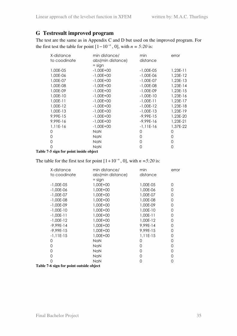
G Testresult improved program

The test are the same as in Appendix C and D but used on the improved program. For

the first test the table for point [ n−−101 , 0], with n = 5:20 is:

X-distance

to coodinate

min distance/

abs(min distance)

= sign

min

distance

error

1,00E-05 -1,00E+00 -1,00E-05 1,23E-11

1,00E-06 -1,00E+00 -1,00E-06 1,23E-12

1,00E-07 -1,00E+00 -1,00E-07 1,23E-13

1,00E-08 -1,00E+00 -1,00E-08 1,23E-14

1,00E-09 -1,00E+00 -1,00E-09 1,23E-15

1,00E-10 -1,00E+00 -1,00E-10 1,23E-16

1,00E-11 -1,00E+00 -1,00E-11 1,23E-17

1,00E-12 -1,00E+00 -1,00E-12 1,23E-18

1,00E-13 -1,00E+00 -1,00E-13 1,23E-19

9,99E-15 -1,00E+00 -9,99E-15 1,23E-20

9,99E-16 -1,00E+00 -9,99E-16 1,23E-21

1,11E-16 -1,00E+00 -1,11E-16 1,37E-22

0 NaN 0 0

0 NaN 0 0

0 NaN 0 0

0 NaN 0 0 Table 7-5 sign for point inside object

The table for the first test for point [ n−+101 , 0], with n =5:20 is:

X-distance

to coodinate

min distance/

abs(min distance)

= sign

min

distance

error

-1,00E-05 1,00E+00 1,00E-05 0

-1,00E-06 1,00E+00 1,00E-06 0

-1,00E-07 1,00E+00 1,00E-07 0

-1,00E-08 1,00E+00 1,00E-08 0

-1,00E-09 1,00E+00 1,00E-09 0

-1,00E-10 1,00E+00 1,00E-10 0

-1,00E-11 1,00E+00 1,00E-11 0

-1,00E-12 1,00E+00 1,00E-12 0

-9,99E-14 1,00E+00 9,99E-14 0

-9,99E-15 1,00E+00 9,99E-15 0

-1,11E-15 1,00E+00 1,11E-15 0

0 NaN 0 0

0 NaN 0 0

0 NaN 0 0

0 NaN 0 0

0 NaN 0 0 Table 7-6 sign for point outside object



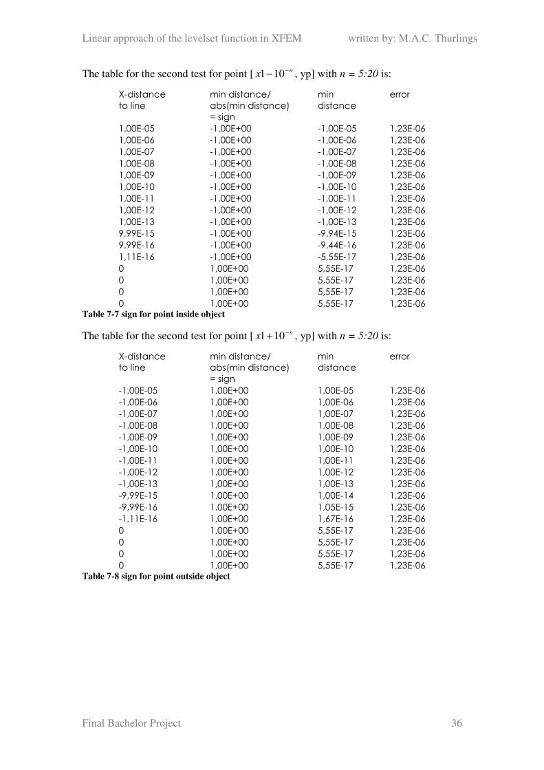
The table for the second test for point [ nx

−−101 , yp] with n = 5:20 is:

X-distance

to line

min distance/

abs(min distance)

= sign

min

distance

error

1,00E-05 -1,00E+00 -1,00E-05 1,23E-06

1,00E-06 -1,00E+00 -1,00E-06 1,23E-06

1,00E-07 -1,00E+00 -1,00E-07 1,23E-06

1,00E-08 -1,00E+00 -1,00E-08 1,23E-06

1,00E-09 -1,00E+00 -1,00E-09 1,23E-06

1,00E-10 -1,00E+00 -1,00E-10 1,23E-06

1,00E-11 -1,00E+00 -1,00E-11 1,23E-06

1,00E-12 -1,00E+00 -1,00E-12 1,23E-06

1,00E-13 -1,00E+00 -1,00E-13 1,23E-06

9,99E-15 -1,00E+00 -9,94E-15 1,23E-06

9,99E-16 -1,00E+00 -9,44E-16 1,23E-06

1,11E-16 -1,00E+00 -5,55E-17 1,23E-06

0 1,00E+00 5,55E-17 1,23E-06

0 1,00E+00 5,55E-17 1,23E-06

0 1,00E+00 5,55E-17 1,23E-06

0 1,00E+00 5,55E-17 1,23E-06 Table 7-7 sign for point inside object

The table for the second test for point [ nx

−+101 , yp] with n = 5:20 is:

X-distance

to line

min distance/

abs(min distance)

= sign

min

distance

error

-1,00E-05 1,00E+00 1,00E-05 1,23E-06

-1,00E-06 1,00E+00 1,00E-06 1,23E-06

-1,00E-07 1,00E+00 1,00E-07 1,23E-06

-1,00E-08 1,00E+00 1,00E-08 1,23E-06

-1,00E-09 1,00E+00 1,00E-09 1,23E-06

-1,00E-10 1,00E+00 1,00E-10 1,23E-06

-1,00E-11 1,00E+00 1,00E-11 1,23E-06

-1,00E-12 1,00E+00 1,00E-12 1,23E-06

-1,00E-13 1,00E+00 1,00E-13 1,23E-06

-9,99E-15 1,00E+00 1,00E-14 1,23E-06

-9,99E-16 1,00E+00 1,05E-15 1,23E-06

-1,11E-16 1,00E+00 1,67E-16 1,23E-06

0 1,00E+00 5,55E-17 1,23E-06

0 1,00E+00 5,55E-17 1,23E-06

0 1,00E+00 5,55E-17 1,23E-06

0 1,00E+00 5,55E-17 1,23E-06 Table 7-8 sign for point outside object



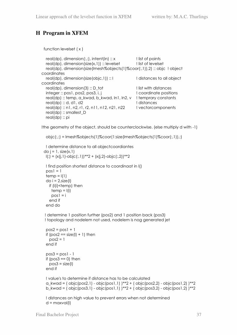
H Program in XFEM

function levelset ( x )

real(dp), dimension(:,:), intent(in) :: x ! list of points

real(dp), dimension(size(x,1)) :: levelset ! list of levelset

real(dp), dimension(size(lmesh%objects(1)%coor(:,1)),2) :: objc ! object

coordinates

real(dp), dimension(size(objc,1)) :: l ! distances to all object

coordinates

real(dp), dimension(3) :: D_tot ! list with distances

integer :: pos1, pos2, pos3, i, j ! coordinate positions

real(dp) :: temp, a_kwad, b_kwad, ln1, ln2, v ! temprary constants

real(dp) :: d, d1, d2 ! distances

real(dp) :: n1, n2, r1, r2, n11, n12, n21, n22 ! vectorcomponents

real(dp) :: smallest_D

real(dp) :: pi

!the geometry of the object, should be counterclockwise. (else multiply d with -1)

objc(:,:) = lmesh%objects(1)%coor(1:size(lmesh%objects(1)%coor(:,1)),:)

! determine distance to all objectcoordiantes

do j = 1, size(x,1)

l(:) = (x(j,1)-objc(:,1))**2 + (x(j,2)-objc(:,2))**2

! find position shortest distance to coordinaat in l()

pos1 = 1

temp = l(1)

do i = 2,size(l)

if (l(i)<temp) then

temp = l(i)

pos1 = i

end if

end do

! determine 1 position further (pos2) and 1 position back (pos3)

! topology and nodelem not used, nodelem is nog generated jet

pos2 = pos1 + 1

if (pos2 == size(l) + 1) then

pos2 = 1

end if

pos3 = pos1 - 1

if (pos3 == 0) then

pos3 = size(l)

end if

! value's to determine if distance has to be calculated

a_kwad = ( objc(pos2,1) - objc(pos1,1) )**2 + ( objc(pos2,2) - objc(pos1,2) )**2

b_kwad = ( objc(pos3,1) - objc(pos1,1) )**2 + ( objc(pos3,2) - objc(pos1,2) )**2

! distances on high value to prevent errors when not determined

d = maxval(l)



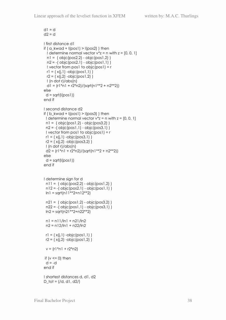
d1 = d

d2 = d

! first distance d1

if ( a_kwad + l(pos1) > l(pos2) ) then

! determine normal vector v*z = n with z = [0, 0, 1]

n1 = ( objc(pos2,2) - objc(pos1,2) )

n2 = -( objc(pos2,1) - objc(pos1,1) )

! vector from pos1 to objc(pos1) = r

r1 = ( x(j,1) -objc(pos1,1) )

r2 = ( x(j,2) -objc(pos1,2) )

! (n dot r)/abs(n)

d1 = (r1*n1 + r2*n2)/(sqrt(n1**2 + n2**2))

else

d = sqrt(l(pos1))

end if

! second distance d2

if ( b_kwad + l(pos1) > l(pos3) ) then

! determine normal vector v*z = n with z = [0, 0, 1]



! vector from pos1 to objc(pos1) = r

r1 = ( x(j,1) -objc(pos3,1) )

r2 = ( x(j,2) -objc(pos3,2) )

! (n dot r)/abs(n)

d2 = (r1*n1 + r2*n2)/(sqrt(n1**2 + n2**2))

else

d = sqrt(l(pos1))

end if

! determine sign for d



ln1 = sqrt(n11**2+n12**2)



ln2 = sqrt(n21**2+n22**2)

n1 = n11/ln1 + n21/ln2

n2 = n12/ln1 + n22/ln2

r1 = ( x(j,1) -objc(pos1,1) )

r2 = ( x(j,2) -objc(pos1,2) )

v = (r1*n1 + r2*n2)

if (v <= 0) then

d = -d

end if

! shortest distances d, d1, d2

D_tot = (/d, d1, d2/)



smallest_D = D_tot(1)

if ( abs(D_tot(2)) < abs(smallest_D) ) then


end if

if ( abs(D_tot(3)) < abs(smallest_D) ) then


end if

levelset(j) = -1 * smallest_D ! clockwise, multiply with * -1

end do

end function levelset

Documents

Linear approach of the levelset function in XFEM · Linear approach of the levelset function in XFEM written by: M.A.C. Thurlings Final Bachelor Project 2 Foreword This report is