Embed Size (px)
Citation preview
SIPCom8-1: Information Theory and Coding
Linear Binary Codes
Ingmar Land
Ingmar Land, SIPCom8-1: Information Theory and Coding (2006 Spring) – p.1
Overview
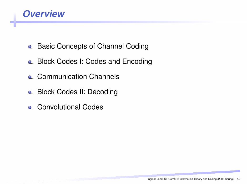
Basic Concepts of Channel Coding
Block Codes I: Codes and Encoding
Communication Channels
Block Codes II: Decoding
Convolutional Codes
Ingmar Land, SIPCom8-1: Information Theory and Coding (2006 Spring) – p.2
Basic Concepts of Channel Coding
System Model
Examples
Ingmar Land, SIPCom8-1: Information Theory and Coding (2006 Spring) – p.3
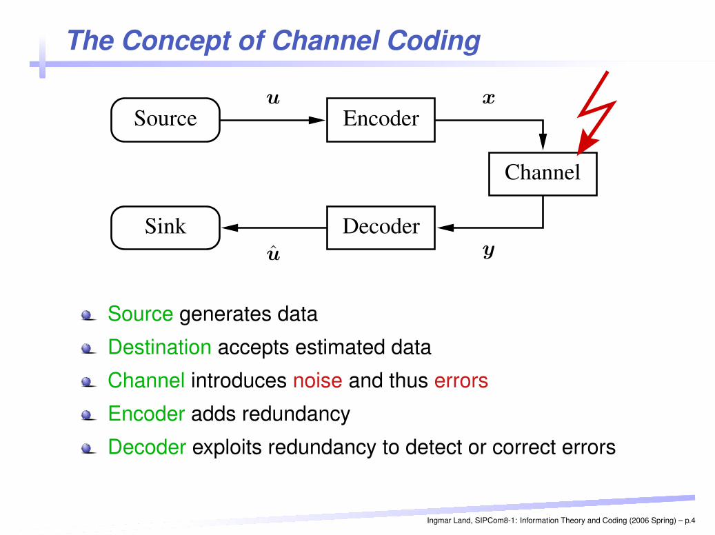
The Concept of Channel Coding
Source
Channel
Encoder
DecoderSink
PSfrag replacements
u x
yu
Source generates data
Destination accepts estimated data
Channel introduces noise and thus errors
Encoder adds redundancy
Decoder exploits redundancy to detect or correct errors
Ingmar Land, SIPCom8-1: Information Theory and Coding (2006 Spring) – p.4
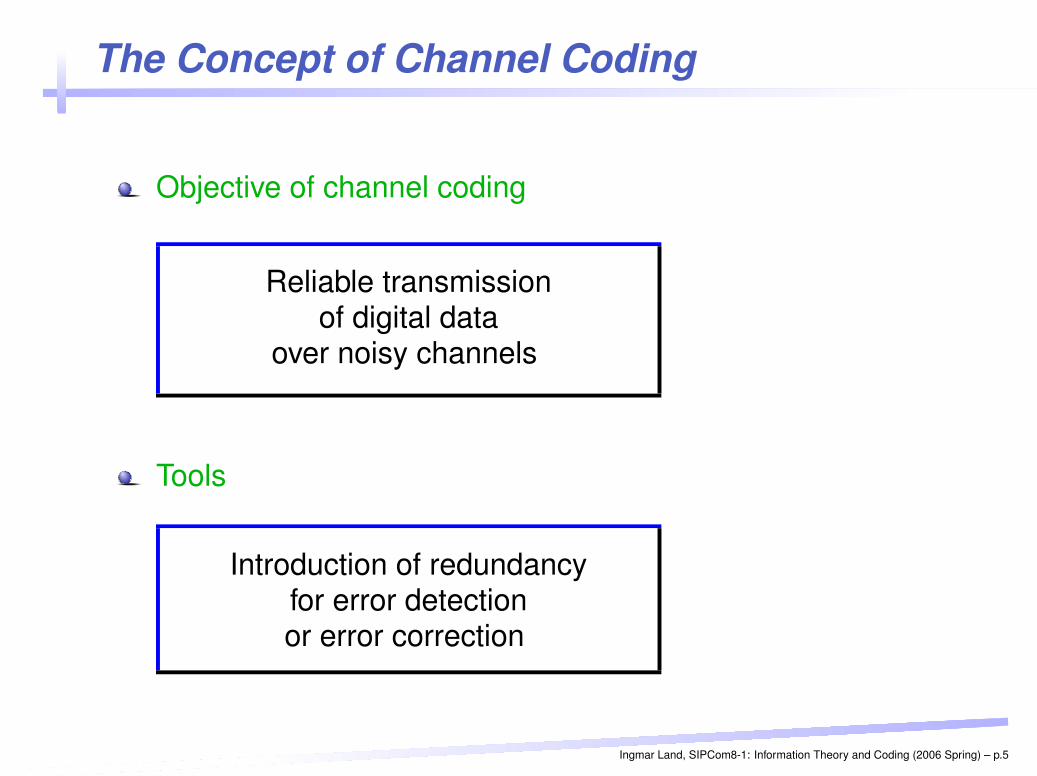
The Concept of Channel Coding
Objective of channel coding
Reliable transmissionof digital data
over noisy channels
Tools
Introduction of redundancyfor error detectionor error correction
Ingmar Land, SIPCom8-1: Information Theory and Coding (2006 Spring) – p.5
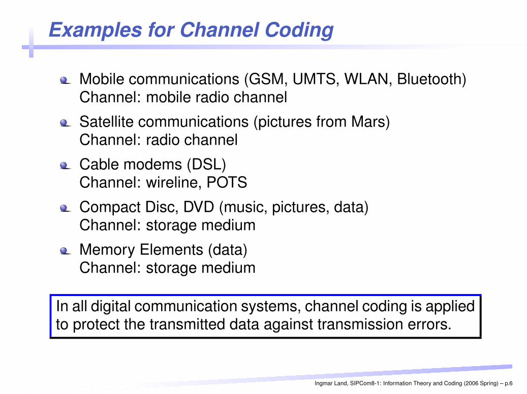
Examples for Channel Coding
Mobile communications (GSM, UMTS, WLAN, Bluetooth)Channel: mobile radio channel
Satellite communications (pictures from Mars)Channel: radio channel
Cable modems (DSL)Channel: wireline, POTS
Compact Disc, DVD (music, pictures, data)Channel: storage medium
Memory Elements (data)Channel: storage medium
In all digital communication systems, channel coding is appliedto protect the transmitted data against transmission errors.
Ingmar Land, SIPCom8-1: Information Theory and Coding (2006 Spring) – p.6
System Model for Channel Coding I
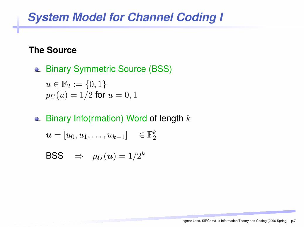
The Source
Binary Symmetric Source (BSS)
u ∈ F2 := {0, 1}pU (u) = 1/2 for u = 0, 1
Binary Info(rmation) Word of length k
u = [u0, u1, . . . , uk−1] ∈ Fk2
BSS ⇒ pU (u) = 1/2k
Ingmar Land, SIPCom8-1: Information Theory and Coding (2006 Spring) – p.7
System Model for Channel Coding II
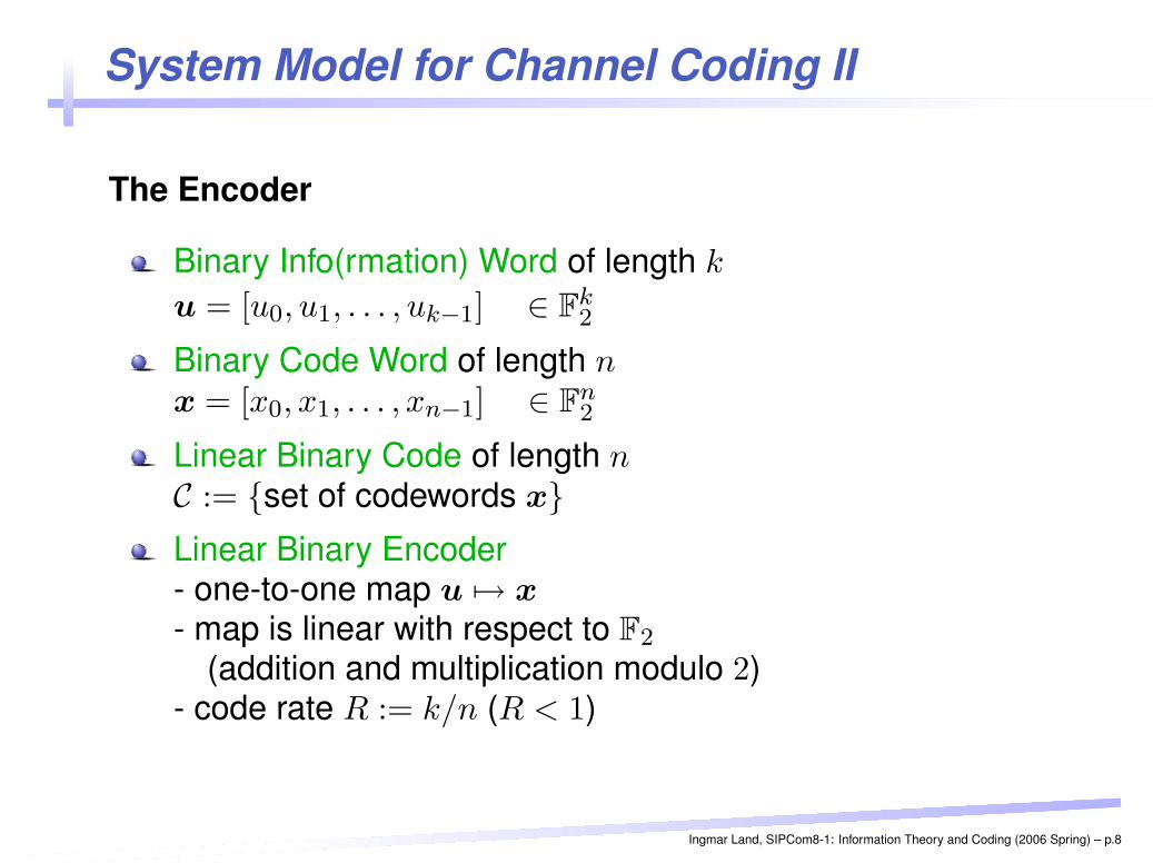
The Encoder
Binary Info(rmation) Word of length k
u = [u0, u1, . . . , uk−1] ∈ Fk2
Binary Code Word of length nx = [x0, x1, . . . , xn−1] ∈ F
n2
Linear Binary Code of length nC := {set of codewords x}Linear Binary Encoder- one-to-one map u 7→ x
- map is linear with respect to F2
(addition and multiplication modulo 2)- code rate R := k/n (R < 1)
Ingmar Land, SIPCom8-1: Information Theory and Coding (2006 Spring) – p.8
Examples for Binary Linear Codes
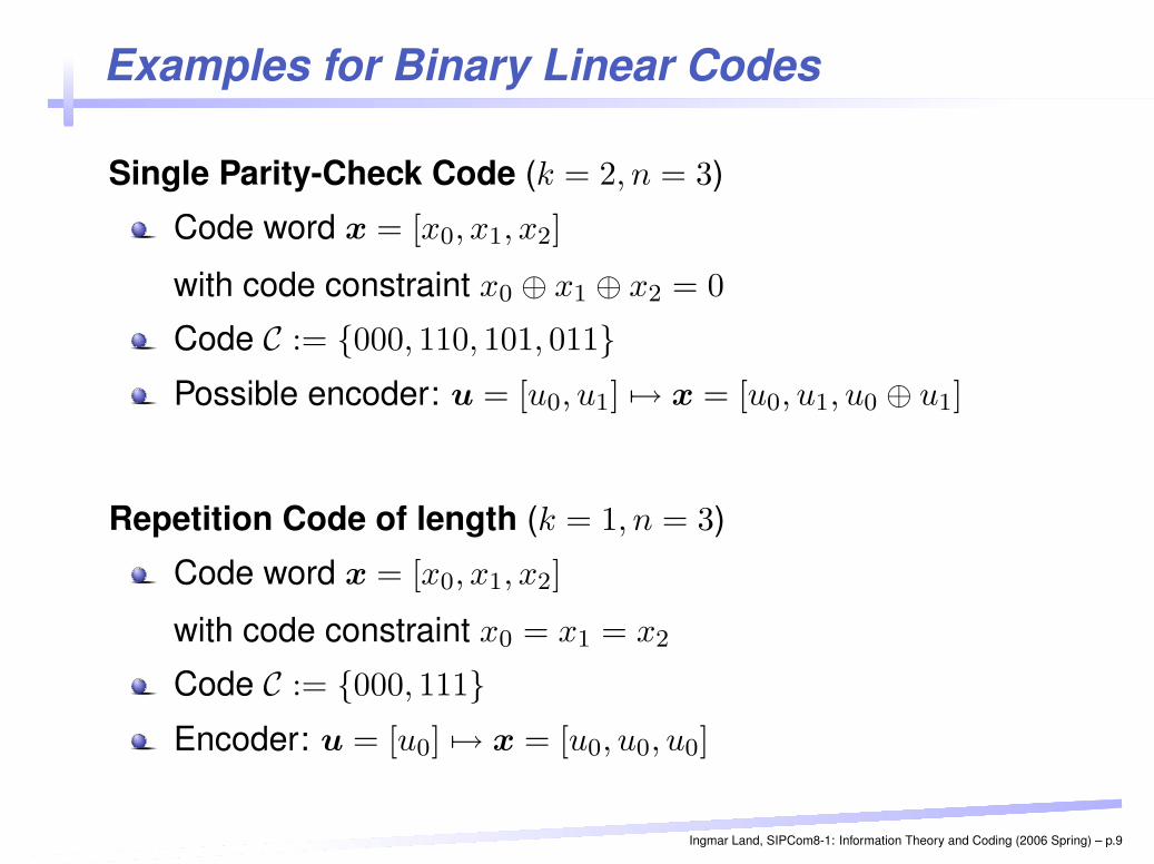
Single Parity-Check Code (k = 2, n = 3)
Code word x = [x0, x1, x2]
with code constraint x0 ⊕ x1 ⊕ x2 = 0
Code C := {000, 110, 101, 011}Possible encoder: u = [u0, u1] 7→ x = [u0, u1, u0 ⊕ u1]
Repetition Code of length (k = 1, n = 3)
Code word x = [x0, x1, x2]
with code constraint x0 = x1 = x2
Code C := {000, 111}Encoder: u = [u0] 7→ x = [u0, u0, u0]
Ingmar Land, SIPCom8-1: Information Theory and Coding (2006 Spring) – p.9
System Model for Channel Coding III
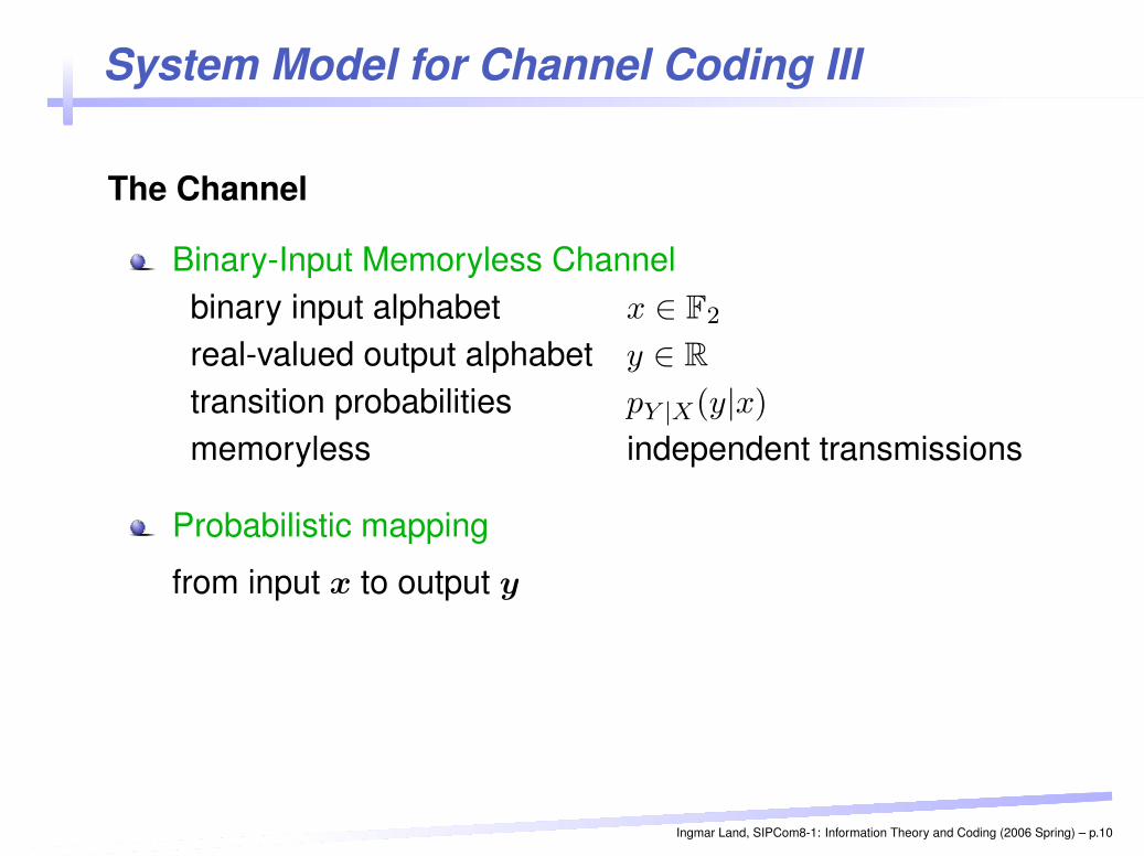
The Channel
Binary-Input Memoryless Channelbinary input alphabet x ∈ F2
real-valued output alphabet y ∈ R
transition probabilities pY |X(y|x)
memoryless independent transmissions
Probabilistic mapping
from input x to output y
Ingmar Land, SIPCom8-1: Information Theory and Coding (2006 Spring) – p.10
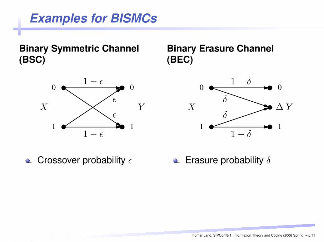
Examples for BISMCs
Binary Symmetric Channel(BSC)
0 0
11
PSfrag replacements
X Yε
ε
1 − ε
1 − ε
Crossover probability ε
Binary Erasure Channel(BEC)
0
1 1
0
PSfrag replacements
X Y∆δ
δ
1 − δ
1 − δ
Erasure probability δ
Ingmar Land, SIPCom8-1: Information Theory and Coding (2006 Spring) – p.11
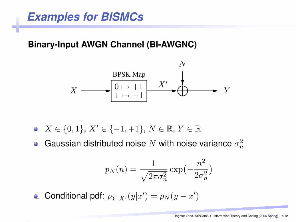
Examples for BISMCs
Binary-Input AWGN Channel (BI-AWGNC)
BPSK Map
PSfrag replacements
XX ′
Y
N
0 7→ +11 7→ −1
X ∈ {0, 1}, X ′ ∈ {−1, +1}, N ∈ R, Y ∈ R
Gaussian distributed noise N with noise variance σ2n
pN (n) =1
√
2πσ2n
exp(− n2
2σ2n
)
Conditional pdf: pY |X′(y|x′) = pN (y − x′)
Ingmar Land, SIPCom8-1: Information Theory and Coding (2006 Spring) – p.12
System Model for Channel Coding IV
The Decoder
Received Word of length ny = [y0, y1, . . . , yn−1] ∈ R
n
Decoder- error correction or error detection- estimation of the transmitted info word or code word
Estimated Info Word of length k
u = [u0, u1, . . . , uk−1] ∈ Fk2
Ingmar Land, SIPCom8-1: Information Theory and Coding (2006 Spring) – p.13
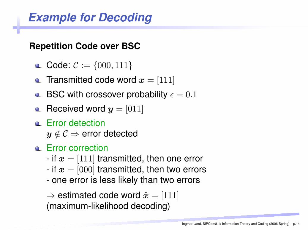
Example for Decoding
Repetition Code over BSC
Code: C := {000, 111}Transmitted code word x = [111]
BSC with crossover probability ε = 0.1
Received word y = [011]
Error detectiony /∈ C ⇒ error detected
Error correction- if x = [111] transmitted, then one error- if x = [000] transmitted, then two errors- one error is less likely than two errors
⇒ estimated code word x = [111](maximum-likelihood decoding)
Ingmar Land, SIPCom8-1: Information Theory and Coding (2006 Spring) – p.14
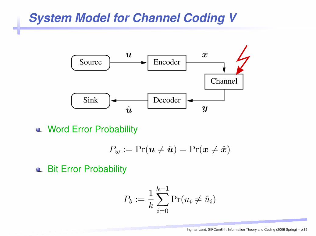
System Model for Channel Coding V
Source
Channel
Encoder
DecoderSink
PSfrag replacementsu x
yu
Word Error Probability
Pw := Pr(u 6= u) = Pr(x 6= x)
Bit Error Probability
Pb :=1
k
k−1∑
i=0
Pr(ui 6= ui)
Ingmar Land, SIPCom8-1: Information Theory and Coding (2006 Spring) – p.15
Problems in Channel Coding
Construction of good codes
Construction of low-complexity decoders
Existence of codes with certain parameters
(Singleton bound, Hamming bound, Gilbert bound,Varshamov bound)
Highest code rate for a given channel such thattransmission is error-free when codelength tends to infinity
(Channel Coding Theorem)
Ingmar Land, SIPCom8-1: Information Theory and Coding (2006 Spring) – p.16
Block Codes I: Codes and Encoding
Properties of Codes and Encoders
Hamming Distances and Hamming Weights
Generator Matrix and Parity-Check Matrix
Examples of Codes
Ingmar Land, SIPCom8-1: Information Theory and Coding (2006 Spring) – p.17
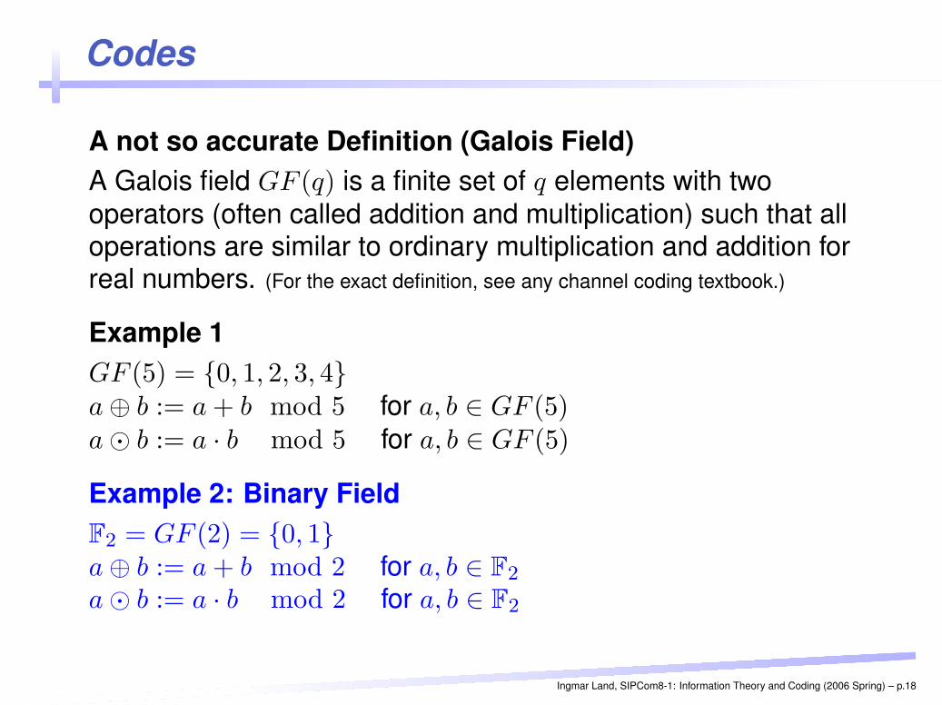
Codes
A not so accurate Definition (Galois Field)A Galois field GF (q) is a finite set of q elements with twooperators (often called addition and multiplication) such that alloperations are similar to ordinary multiplication and addition forreal numbers. (For the exact definition, see any channel coding textbook.)
Example 1GF (5) = {0, 1, 2, 3, 4}a ⊕ b := a + b mod 5 for a, b ∈ GF (5)a � b := a · b mod 5 for a, b ∈ GF (5)
Example 2: Binary FieldF2 = GF (2) = {0, 1}a ⊕ b := a + b mod 2 for a, b ∈ F2
a � b := a · b mod 2 for a, b ∈ F2
Ingmar Land, SIPCom8-1: Information Theory and Coding (2006 Spring) – p.18
Codes
Definition (Hamming distance)The Hamming distance between two vectors a and b (of thesame length) is defined as the number of positions in which theydiffer, and it is denoted by dH(a, b).
Examplea = [0111], b = [1100], dH(a, b) = 3
Ingmar Land, SIPCom8-1: Information Theory and Coding (2006 Spring) – p.19
Codes
Definition (Linear Binary Block Code)A binary linear (n, k, dmin) block code C is a subset of F
n with2k vectors that have the following properties:
Minimum Distance The minimum Hamming distancebetween pairs of distinct vectors in C is dmin, i.e.,
dmin := mina,b∈Ca6=b
dH(a, b)
Linearity Any sum of two vectors in C is again a vectorin C, i.e.,
a ⊕ b ∈ C for all a, b ∈ C.
The ratio of k and n is called the code rate R = k/n.
Ingmar Land, SIPCom8-1: Information Theory and Coding (2006 Spring) – p.20
Codes
CodewordThe elements x of a code are called codewords, and they arewritten as
x = [x0, x1, . . . , xn−1].
The elements xi of a codeword are called code symbols.
InfowordEach codeword x may be associated with a binary vector oflength k. These vectors u are called infowords (informationwords), and they are written as
u = [u0, u1, . . . , uk−1].
The elements ui of an infoword are called info symbols(information symbols).
Ingmar Land, SIPCom8-1: Information Theory and Coding (2006 Spring) – p.21
Codes
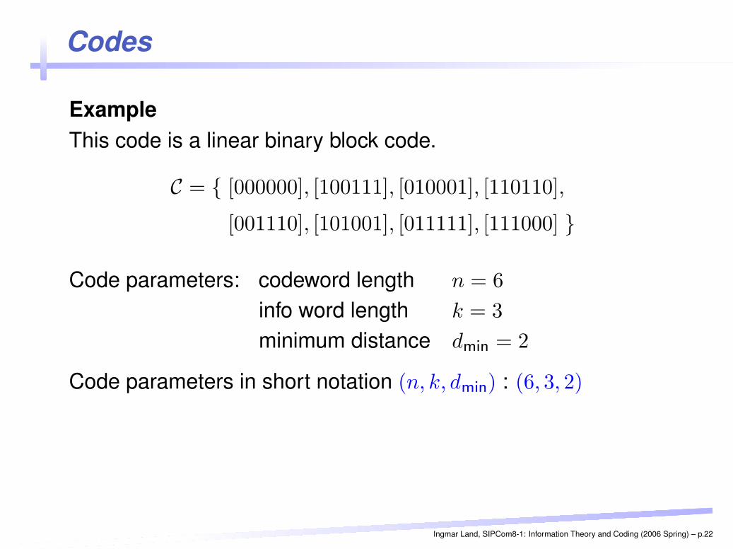
ExampleThis code is a linear binary block code.
C = { [000000], [100111], [010001], [110110],
[001110], [101001], [011111], [111000] }
Code parameters: codeword length n = 6
info word length k = 3
minimum distance dmin = 2
Code parameters in short notation (n, k, dmin) : (6, 3, 2)
Ingmar Land, SIPCom8-1: Information Theory and Coding (2006 Spring) – p.22
Encoding
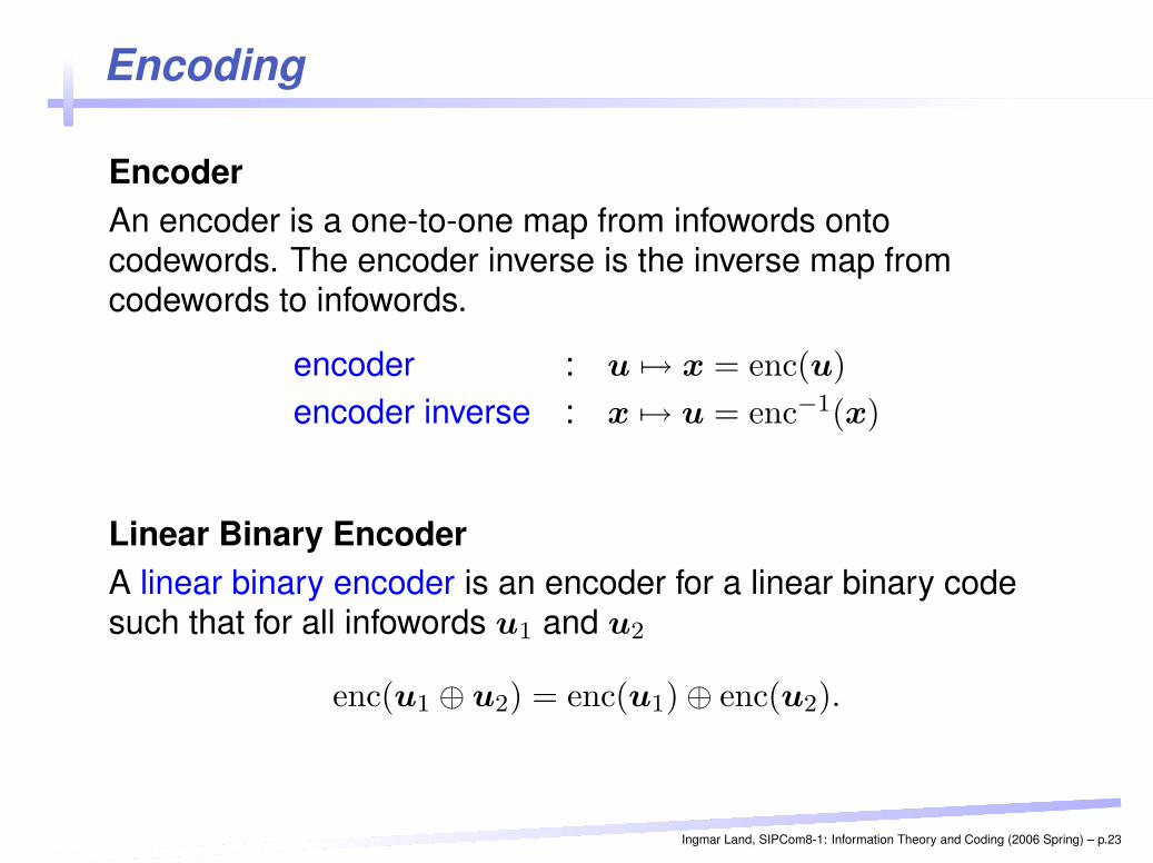
EncoderAn encoder is a one-to-one map from infowords ontocodewords. The encoder inverse is the inverse map fromcodewords to infowords.
encoder : u 7→ x = enc(u)
encoder inverse : x 7→ u = enc−1(x)
Linear Binary EncoderA linear binary encoder is an encoder for a linear binary codesuch that for all infowords u1 and u2
enc(u1 ⊕ u2) = enc(u1) ⊕ enc(u2).
Ingmar Land, SIPCom8-1: Information Theory and Coding (2006 Spring) – p.23

Encoding
Remark 1Also the device implementing the encoding may be called anencoder.
Remark 2An encoder is a linear map over F2.A code is a linear vector subspace over F2.
(Compare to ordinary linear algebra over real numbers.)
Ingmar Land, SIPCom8-1: Information Theory and Coding (2006 Spring) – p.24
Encoding
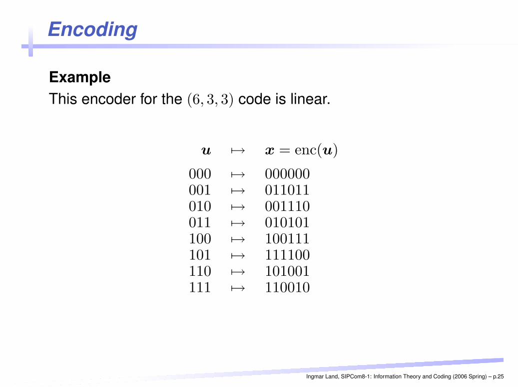
ExampleThis encoder for the (6, 3, 3) code is linear.
u 7→ x = enc(u)
000 7→ 000000001 7→ 011011010 7→ 001110011 7→ 010101100 7→ 100111101 7→ 111100110 7→ 101001111 7→ 110010
Ingmar Land, SIPCom8-1: Information Theory and Coding (2006 Spring) – p.25
Encoding
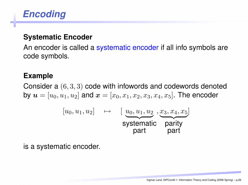
Systematic EncoderAn encoder is called a systematic encoder if all info symbols arecode symbols.
ExampleConsider a (6, 3, 3) code with infowords and codewords denotedby u = [u0, u1, u2] and x = [x0, x1, x2, x3, x4, x5]. The encoder
[u0, u1, u2] 7→ [ u0, u1, u2︸ ︷︷ ︸
systematicpart
, x3, x4, x5︸ ︷︷ ︸
paritypart
]
is a systematic encoder.
Ingmar Land, SIPCom8-1: Information Theory and Coding (2006 Spring) – p.26
Distances and Weights
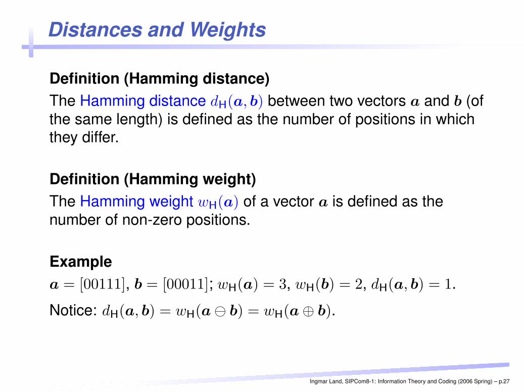
Definition (Hamming distance)The Hamming distance dH(a, b) between two vectors a and b (ofthe same length) is defined as the number of positions in whichthey differ.
Definition (Hamming weight)The Hamming weight wH(a) of a vector a is defined as thenumber of non-zero positions.
Examplea = [00111], b = [00011]; wH(a) = 3, wH(b) = 2, dH(a, b) = 1.
Notice: dH(a, b) = wH(a b) = wH(a ⊕ b).
Ingmar Land, SIPCom8-1: Information Theory and Coding (2006 Spring) – p.27
Distances and Weights
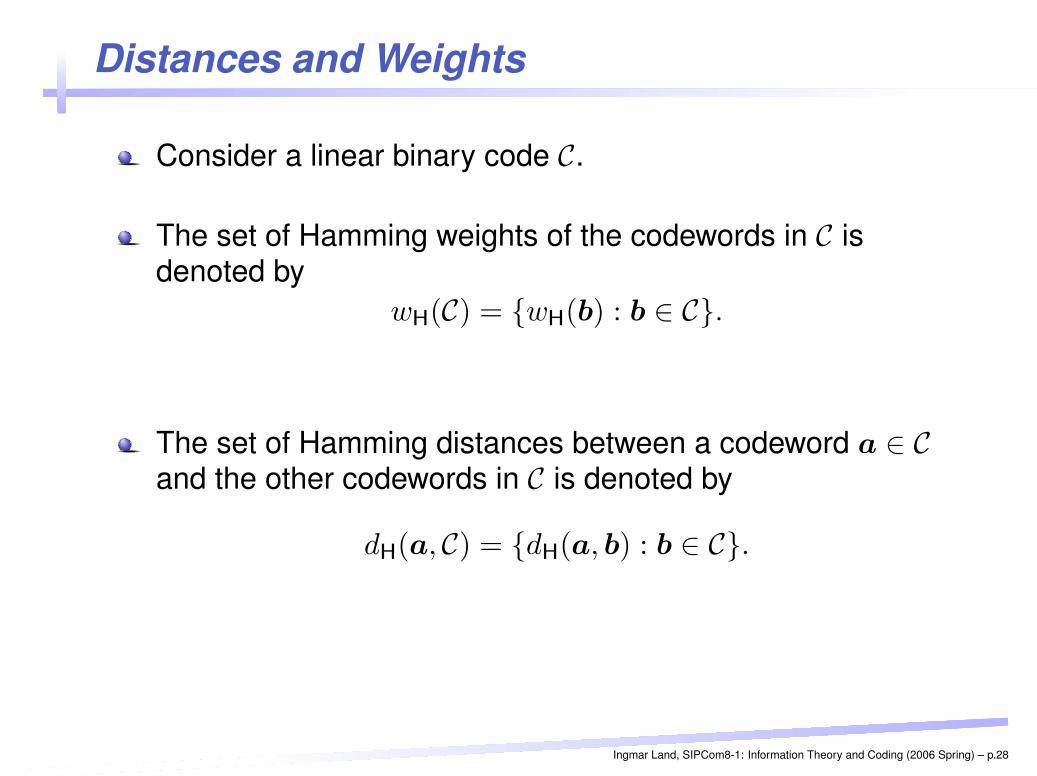
Consider a linear binary code C.
The set of Hamming weights of the codewords in C isdenoted by
wH(C) = {wH(b) : b ∈ C}.
The set of Hamming distances between a codeword a ∈ Cand the other codewords in C is denoted by
dH(a, C) = {dH(a, b) : b ∈ C}.
Ingmar Land, SIPCom8-1: Information Theory and Coding (2006 Spring) – p.28
Distances and Weights
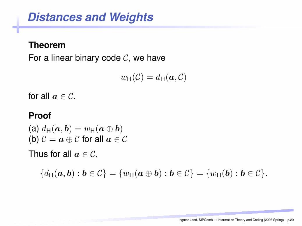
TheoremFor a linear binary code C, we have
wH(C) = dH(a, C)
for all a ∈ C.
Proof(a) dH(a, b) = wH(a ⊕ b)(b) C = a ⊕ C for all a ∈ CThus for all a ∈ C,
{dH(a, b) : b ∈ C} = {wH(a ⊕ b) : b ∈ C} = {wH(b) : b ∈ C}.
Ingmar Land, SIPCom8-1: Information Theory and Coding (2006 Spring) – p.29
Distances and Weights
The Hamming distances between codewords are closelyrelated to the error correction/detection capabilities of thecode.
The set of Hamming distances is identical to the set ofHamming weights.
IdeaA code should not only be described by the parameters(n, k, dmin), but also by the distribution of the codewordweights.
Ingmar Land, SIPCom8-1: Information Theory and Coding (2006 Spring) – p.30
Distances and Weights
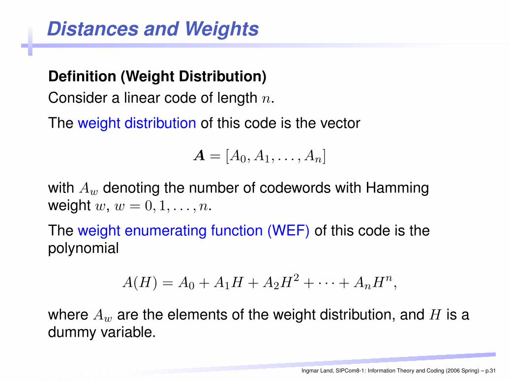
Definition (Weight Distribution)Consider a linear code of length n.
The weight distribution of this code is the vector
A = [A0, A1, . . . , An]
with Aw denoting the number of codewords with Hammingweight w, w = 0, 1, . . . , n.
The weight enumerating function (WEF) of this code is thepolynomial
A(H) = A0 + A1H + A2H2 + · · · + AnHn,
where Aw are the elements of the weight distribution, and H is adummy variable.
Ingmar Land, SIPCom8-1: Information Theory and Coding (2006 Spring) – p.31
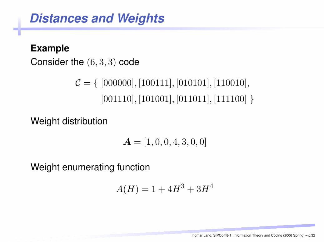
Distances and Weights
ExampleConsider the (6, 3, 3) code
C = { [000000], [100111], [010101], [110010],
[001110], [101001], [011011], [111100] }
Weight distribution
A = [1, 0, 0, 4, 3, 0, 0]
Weight enumerating function
A(H) = 1 + 4H3 + 3H4
Ingmar Land, SIPCom8-1: Information Theory and Coding (2006 Spring) – p.32
Generator Matrix and Parity-Check Matrix
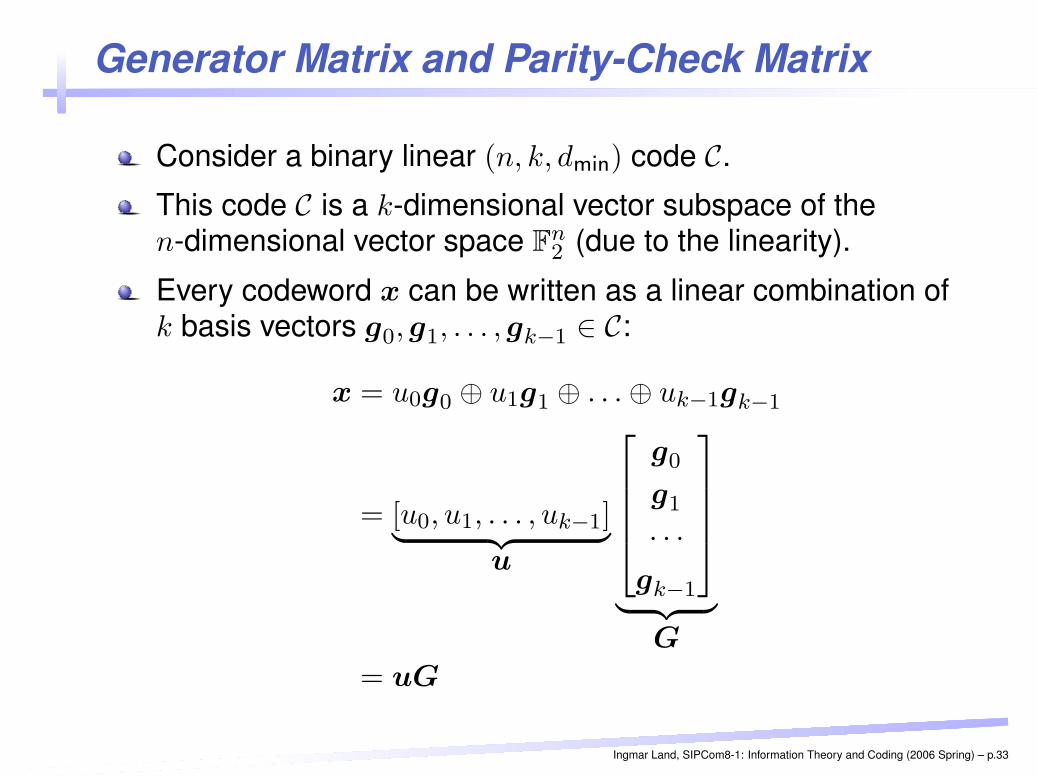
Consider a binary linear (n, k, dmin) code C.
This code C is a k-dimensional vector subspace of then-dimensional vector space F
n2 (due to the linearity).
Every codeword x can be written as a linear combination ofk basis vectors g0, g1, . . . , gk−1 ∈ C:
x = u0g0 ⊕ u1g1 ⊕ . . . ⊕ uk−1gk−1
= [u0, u1, . . . , uk−1]︸ ︷︷ ︸
u
g0
g1
· · ·gk−1
︸ ︷︷ ︸
G
= uG
Ingmar Land, SIPCom8-1: Information Theory and Coding (2006 Spring) – p.33

Generator Matrix and Parity-Check Matrix
Definition (Generator Matrix)Consider a binary linear (n, k, dmin) code C.A matrix G ∈ F
k×n2 is called a generator matrix of C if the set of
“generated” words is equal to the code, i.e., if
C = {x = uG : u ∈ Fk2}.
Remarks
The rows of G are codewords.
The rank of G is equal to k.
The generator matrix defines an encoder:
x = enc(u) := uG.
Ingmar Land, SIPCom8-1: Information Theory and Coding (2006 Spring) – p.34

Generator Matrix and Parity-Check Matrix
ExampleConsider the (6, 3, 3) code
C = { [000000], [100111], [010101], [110010],
[001110], [101001], [011011], [111100] }
A generator matrix of this code is
G =
1 0 0 1 1 1
0 1 0 1 0 1
0 0 1 1 1 0
Ingmar Land, SIPCom8-1: Information Theory and Coding (2006 Spring) – p.35
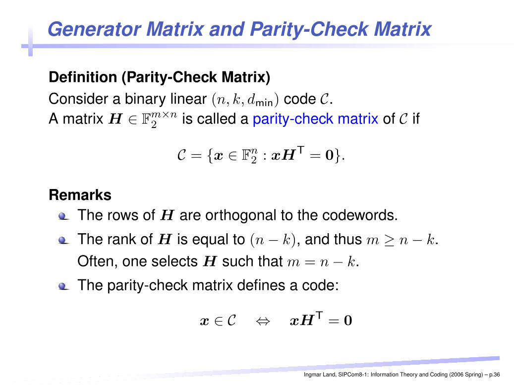
Generator Matrix and Parity-Check Matrix
Definition (Parity-Check Matrix)Consider a binary linear (n, k, dmin) code C.A matrix H ∈ F
m×n2 is called a parity-check matrix of C if
C = {x ∈ Fn2 : xHT = 0}.
RemarksThe rows of H are orthogonal to the codewords.
The rank of H is equal to (n − k), and thus m ≥ n − k.Often, one selects H such that m = n − k.
The parity-check matrix defines a code:
x ∈ C ⇔ xHT = 0
Ingmar Land, SIPCom8-1: Information Theory and Coding (2006 Spring) – p.36
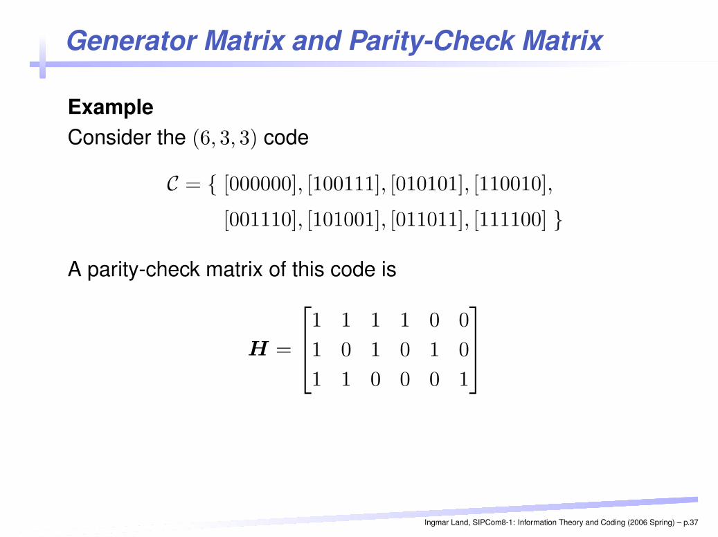
Generator Matrix and Parity-Check Matrix
ExampleConsider the (6, 3, 3) code
C = { [000000], [100111], [010101], [110010],
[001110], [101001], [011011], [111100] }
A parity-check matrix of this code is
H =
1 1 1 1 0 0
1 0 1 0 1 0
1 1 0 0 0 1
Ingmar Land, SIPCom8-1: Information Theory and Coding (2006 Spring) – p.37
Generator Matrix and Parity-Check Matrix
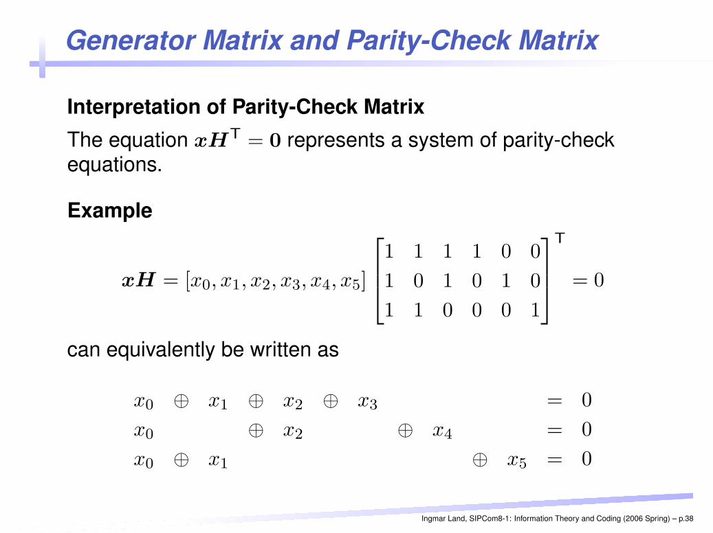
Interpretation of Parity-Check MatrixThe equation xHT = 0 represents a system of parity-checkequations.
Example
xH = [x0, x1, x2, x3, x4, x5]
1 1 1 1 0 0
1 0 1 0 1 0
1 1 0 0 0 1
T
= 0
can equivalently be written as
x0 ⊕ x1 ⊕ x2 ⊕ x3 = 0
x0 ⊕ x2 ⊕ x4 = 0
x0 ⊕ x1 ⊕ x5 = 0
Ingmar Land, SIPCom8-1: Information Theory and Coding (2006 Spring) – p.38
Generator Matrix and Parity-Check Matrix
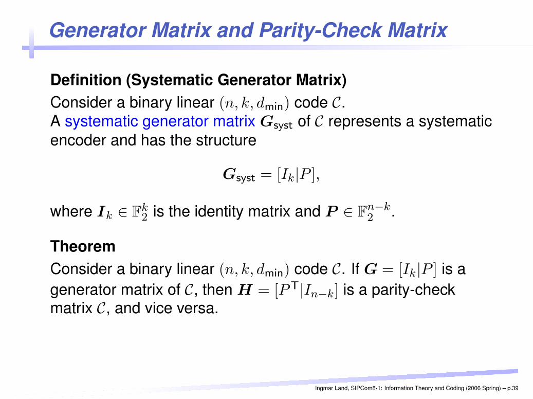
Definition (Systematic Generator Matrix)Consider a binary linear (n, k, dmin) code C.A systematic generator matrix Gsyst of C represents a systematicencoder and has the structure
Gsyst = [Ik|P ],
where Ik ∈ Fk2 is the identity matrix and P ∈ F
n−k2 .
TheoremConsider a binary linear (n, k, dmin) code C. If G = [Ik|P ] is agenerator matrix of C, then H = [P T|In−k] is a parity-checkmatrix C, and vice versa.
Ingmar Land, SIPCom8-1: Information Theory and Coding (2006 Spring) – p.39
Generator Matrix and Parity-Check Matrix
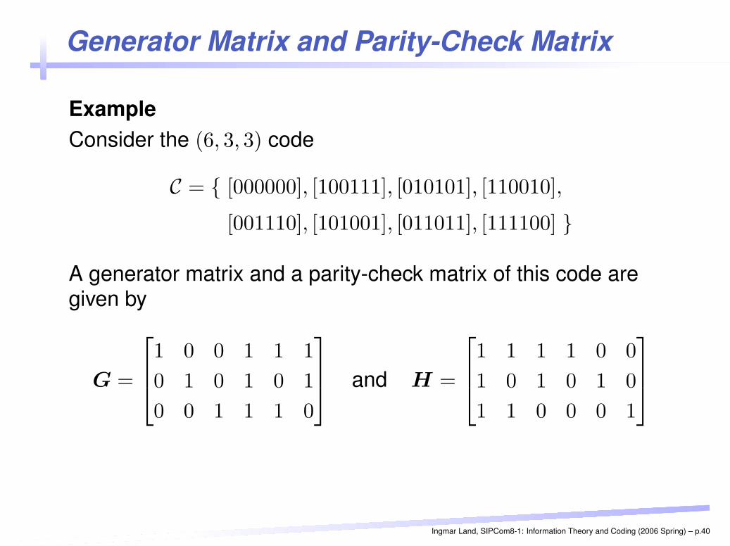
ExampleConsider the (6, 3, 3) code
C = { [000000], [100111], [010101], [110010],
[001110], [101001], [011011], [111100] }
A generator matrix and a parity-check matrix of this code aregiven by
G =
1 0 0 1 1 1
0 1 0 1 0 1
0 0 1 1 1 0
and H =
1 1 1 1 0 0
1 0 1 0 1 0
1 1 0 0 0 1
Ingmar Land, SIPCom8-1: Information Theory and Coding (2006 Spring) – p.40
Generator Matrix and Parity-Check Matrix
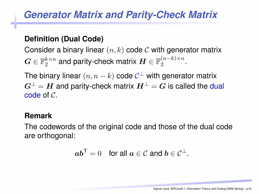
Definition (Dual Code)Consider a binary linear (n, k) code C with generator matrixG ∈ F
k×n2 and parity-check matrix H ∈ F
(n−k)×n2 .
The binary linear (n, n − k) code C⊥ with generator matrixG⊥ = H and parity-check matrix H⊥ = G is called the dualcode of C.
RemarkThe codewords of the original code and those of the dual codeare orthogonal:
abT = 0 for all a ∈ C and b ∈ C⊥.
Ingmar Land, SIPCom8-1: Information Theory and Coding (2006 Spring) – p.41
Examples of Codes
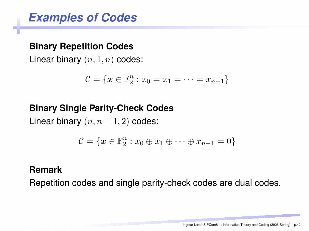
Binary Repetition CodesLinear binary (n, 1, n) codes:
C = {x ∈ Fn2 : x0 = x1 = · · · = xn−1}
Binary Single Parity-Check CodesLinear binary (n, n − 1, 2) codes:
C = {x ∈ Fn2 : x0 ⊕ x1 ⊕ · · · ⊕ xn−1 = 0}
RemarkRepetition codes and single parity-check codes are dual codes.
Ingmar Land, SIPCom8-1: Information Theory and Coding (2006 Spring) – p.42
Examples of Codes
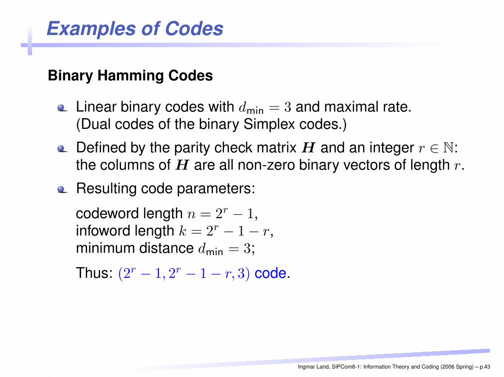
Binary Hamming Codes
Linear binary codes with dmin = 3 and maximal rate.(Dual codes of the binary Simplex codes.)
Defined by the parity check matrix H and an integer r ∈ N:the columns of H are all non-zero binary vectors of length r.
Resulting code parameters:
codeword length n = 2r − 1,infoword length k = 2r − 1 − r,minimum distance dmin = 3;
Thus: (2r − 1, 2r − 1 − r, 3) code.
Ingmar Land, SIPCom8-1: Information Theory and Coding (2006 Spring) – p.43
Examples of Codes
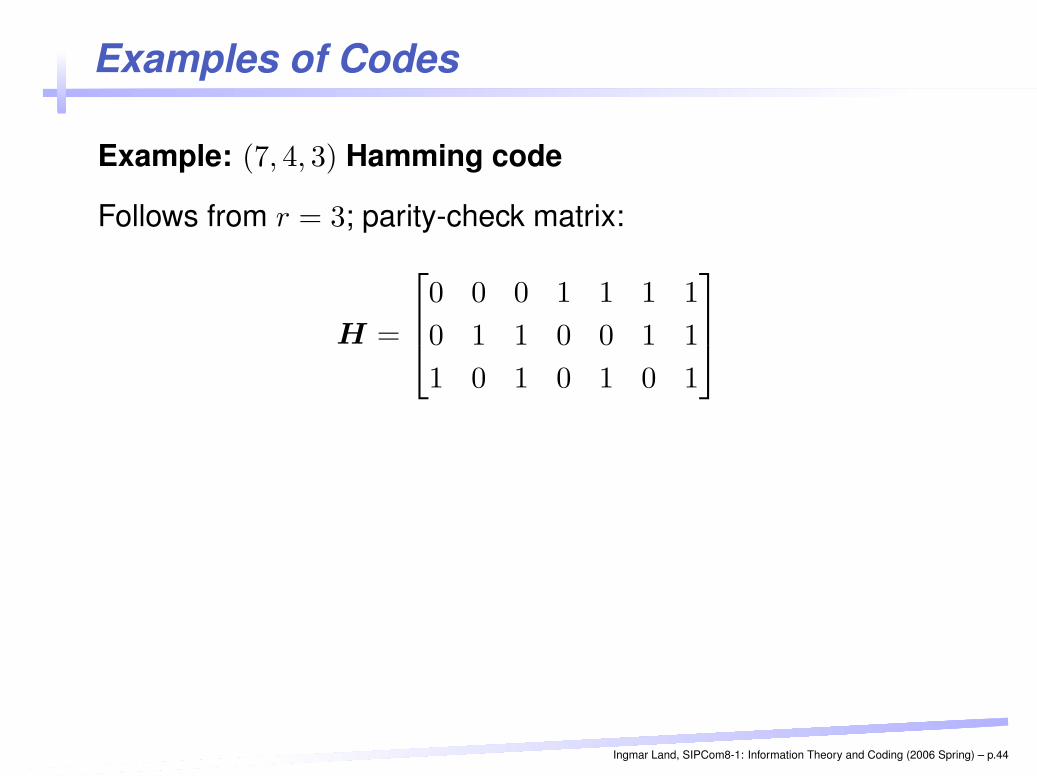
Example: (7, 4, 3) Hamming code
Follows from r = 3; parity-check matrix:
H =
0 0 0 1 1 1 1
0 1 1 0 0 1 1
1 0 1 0 1 0 1
Ingmar Land, SIPCom8-1: Information Theory and Coding (2006 Spring) – p.44
Examples of Codes
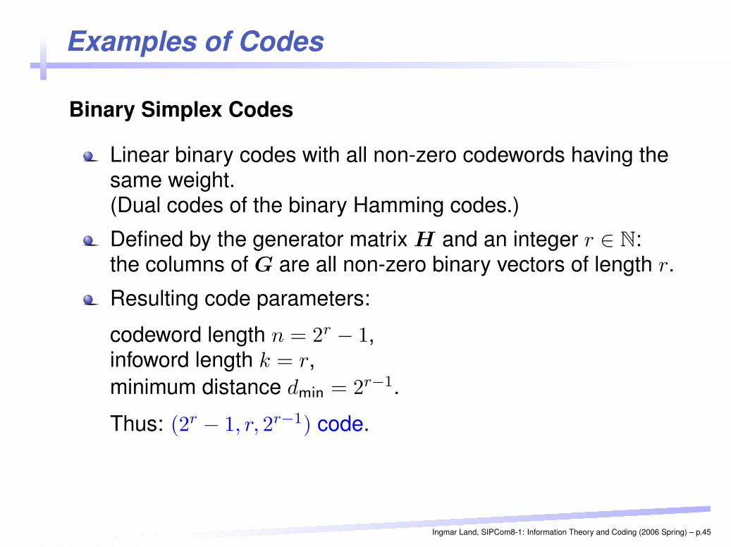
Binary Simplex Codes
Linear binary codes with all non-zero codewords having thesame weight.(Dual codes of the binary Hamming codes.)
Defined by the generator matrix H and an integer r ∈ N:the columns of G are all non-zero binary vectors of length r.
Resulting code parameters:
codeword length n = 2r − 1,infoword length k = r,minimum distance dmin = 2r−1.
Thus: (2r − 1, r, 2r−1) code.
Ingmar Land, SIPCom8-1: Information Theory and Coding (2006 Spring) – p.45
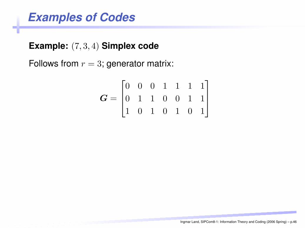
Examples of Codes
Example: (7, 3, 4) Simplex code
Follows from r = 3; generator matrix:
G =
0 0 0 1 1 1 1
0 1 1 0 0 1 1
1 0 1 0 1 0 1
Ingmar Land, SIPCom8-1: Information Theory and Coding (2006 Spring) – p.46
Examples of Codes
Repetition codes
Single parity-check codes
Hamming codes
Simplex codes
Golay codes
Reed-Muller codes
BCH codes
Reed-Solomon codes
Low-density parity-check codes
Concatenated codes (turbo codes)
Ingmar Land, SIPCom8-1: Information Theory and Coding (2006 Spring) – p.47
Summary
Linear Binary (n, k, dmin) Code
Linear (Systematic) Encoder
Weight distribution
(Systematic) Generator matrix
Parity-check matrix
Dual code
Ingmar Land, SIPCom8-1: Information Theory and Coding (2006 Spring) – p.48
Communication Channels
Binary Symmetric Channel
Binary Erasure Channel
Binary Symmetric Erasure Channel
Binary-Input AWGN Channel
Ingmar Land, SIPCom8-1: Information Theory and Coding (2006 Spring) – p.49
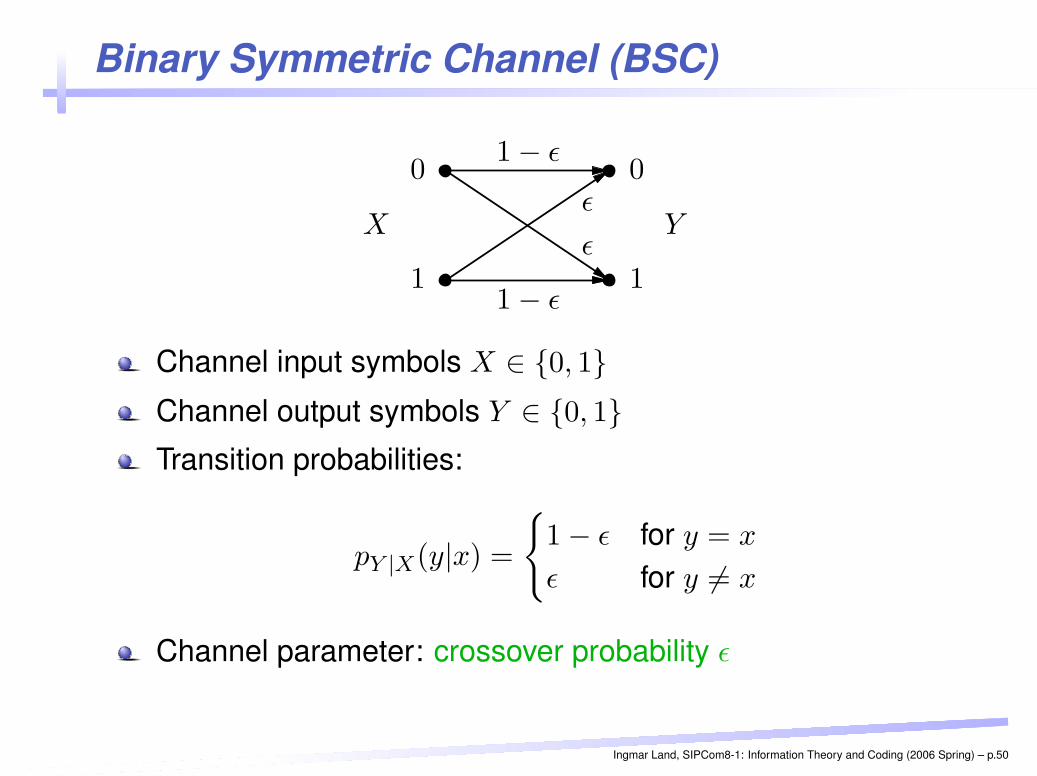
Binary Symmetric Channel (BSC)PSfrag replacements
00
1 1
X Yε
ε
1 − ε
1 − ε
Channel input symbols X ∈ {0, 1}Channel output symbols Y ∈ {0, 1}Transition probabilities:
pY |X(y|x) =
{
1 − ε for y = x
ε for y 6= x
Channel parameter: crossover probability ε
Ingmar Land, SIPCom8-1: Information Theory and Coding (2006 Spring) – p.50
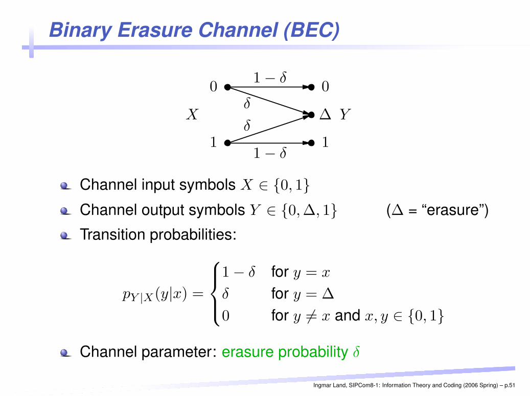
Binary Erasure Channel (BEC)PSfrag replacements
00
11
∆X Yδ
δ
1 − δ
1 − δ
Channel input symbols X ∈ {0, 1}Channel output symbols Y ∈ {0, ∆, 1} (∆ = “erasure”)
Transition probabilities:
pY |X(y|x) =
1 − δ for y = x
δ for y = ∆
0 for y 6= x and x, y ∈ {0, 1}
Channel parameter: erasure probability δ
Ingmar Land, SIPCom8-1: Information Theory and Coding (2006 Spring) – p.51
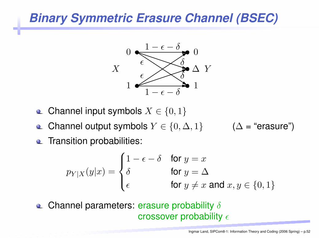
Binary Symmetric Erasure Channel (BSEC)PSfrag replacements
00
11
X Y∆ε
ε
δ
δ
1 − ε − δ
1 − ε − δ
Channel input symbols X ∈ {0, 1}Channel output symbols Y ∈ {0, ∆, 1} (∆ = “erasure”)
Transition probabilities:
pY |X(y|x) =
1 − ε − δ for y = x
δ for y = ∆
ε for y 6= x and x, y ∈ {0, 1}
Channel parameters: erasure probability δcrossover probability ε
Ingmar Land, SIPCom8-1: Information Theory and Coding (2006 Spring) – p.52
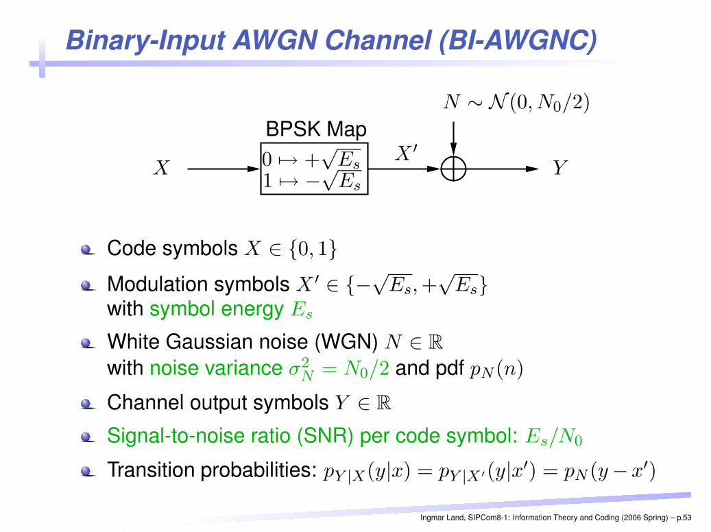
Binary-Input AWGN Channel (BI-AWGNC)PSfrag replacements
BPSK Map
XX ′
Y
N ∼ N (0, N0/2)
0 7→ +√
Es1 7→ −√
Es
Code symbols X ∈ {0, 1}Modulation symbols X ′ ∈ {−√
Es, +√
Es}with symbol energy Es
White Gaussian noise (WGN) N ∈ R
with noise variance σ2N = N0/2 and pdf pN (n)
Channel output symbols Y ∈ R
Signal-to-noise ratio (SNR) per code symbol: Es/N0
Transition probabilities: pY |X(y|x) = pY |X′(y|x′) = pN (y−x′)
Ingmar Land, SIPCom8-1: Information Theory and Coding (2006 Spring) – p.53
Binary-Input AWGN Channel (BI-AWGNC)
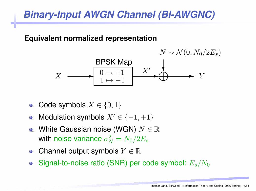
Equivalent normalized representation
PSfrag replacements
BPSK Map
XX ′
Y
N ∼ N (0, N0/2Es)
0 7→ +11 7→ −1
Code symbols X ∈ {0, 1}Modulation symbols X ′ ∈ {−1, +1}White Gaussian noise (WGN) N ∈ R
with noise variance σ2N = N0/2Es
Channel output symbols Y ∈ R
Signal-to-noise ratio (SNR) per code symbol: Es/N0
Ingmar Land, SIPCom8-1: Information Theory and Coding (2006 Spring) – p.54
Binary-Input AWGN Channel (BI-AWGNC)
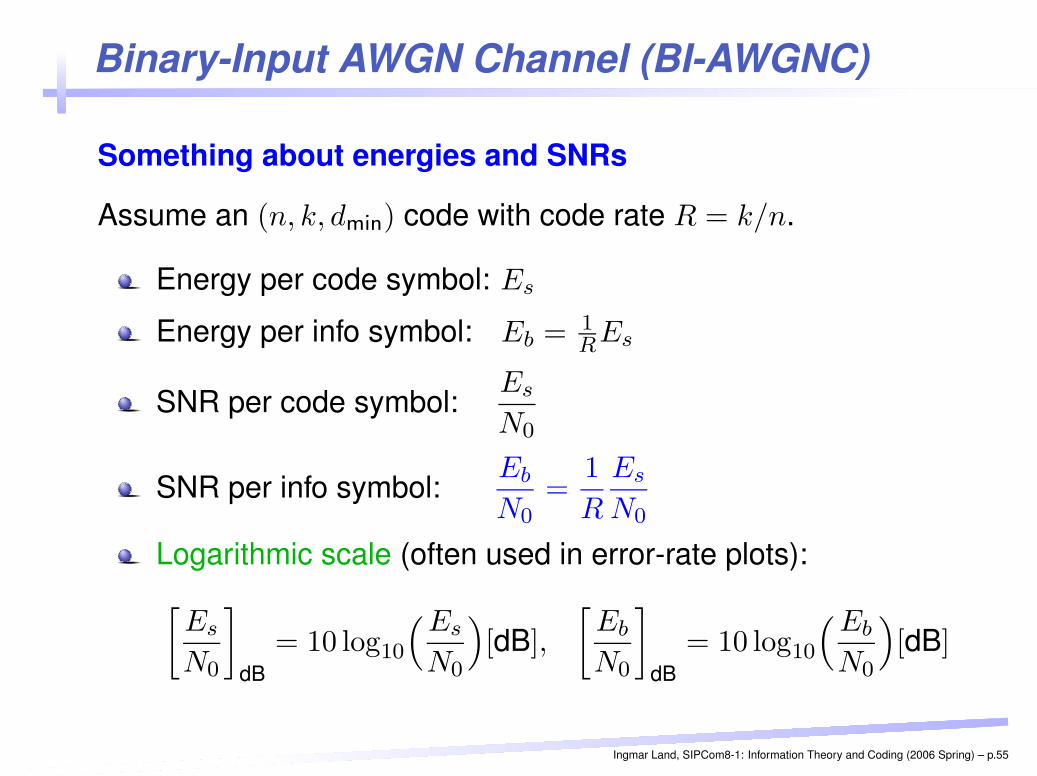
Something about energies and SNRs
Assume an (n, k, dmin) code with code rate R = k/n.
Energy per code symbol: Es
Energy per info symbol: Eb = 1REs
SNR per code symbol:Es
N0
SNR per info symbol:Eb
N0=
1
R
Es
N0
Logarithmic scale (often used in error-rate plots):[
Es
N0
]
dB= 10 log10
(Es
N0
)
[dB],
[Eb
N0
]
dB= 10 log10
( Eb
N0
)
[dB]
Ingmar Land, SIPCom8-1: Information Theory and Coding (2006 Spring) – p.55
Binary-Input AWGN Channel (BI-AWGNC)
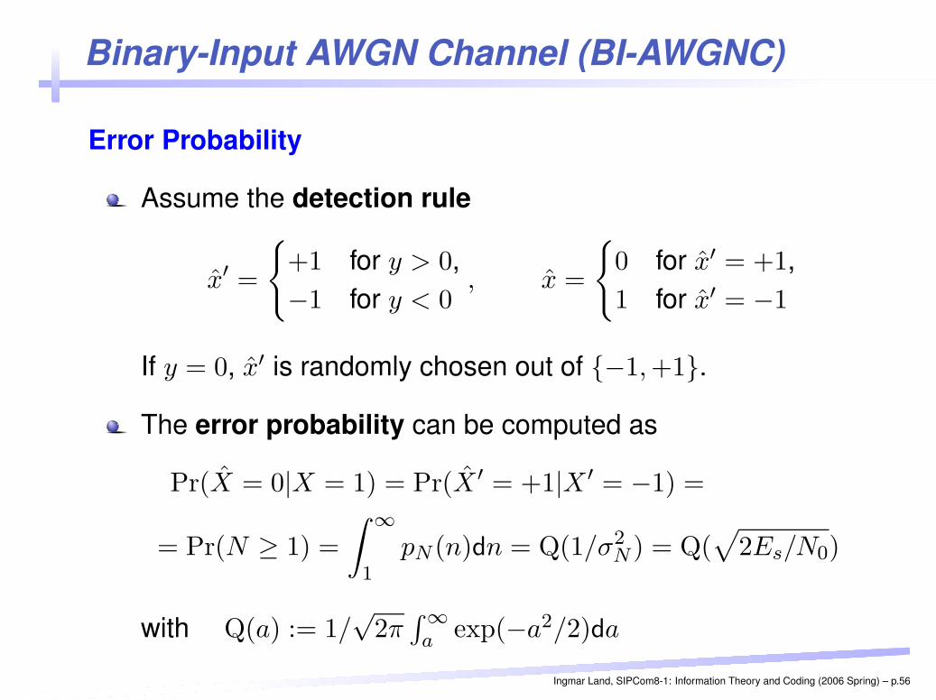
Error Probability
Assume the detection rule
x′ =
{
+1 for y > 0,−1 for y < 0
, x =
{
0 for x′ = +1,1 for x′ = −1
If y = 0, x′ is randomly chosen out of {−1, +1}.
The error probability can be computed as
Pr(X = 0|X = 1) = Pr(X ′ = +1|X ′ = −1) =
= Pr(N ≥ 1) =
∫ ∞
1pN (n)dn = Q(1/σ2
N ) = Q(√
2Es/N0)
with Q(a) := 1/√
2π∫ ∞a exp(−a2/2)da
Ingmar Land, SIPCom8-1: Information Theory and Coding (2006 Spring) – p.56
Binary-Input AWGN Channel (BI-AWGNC)
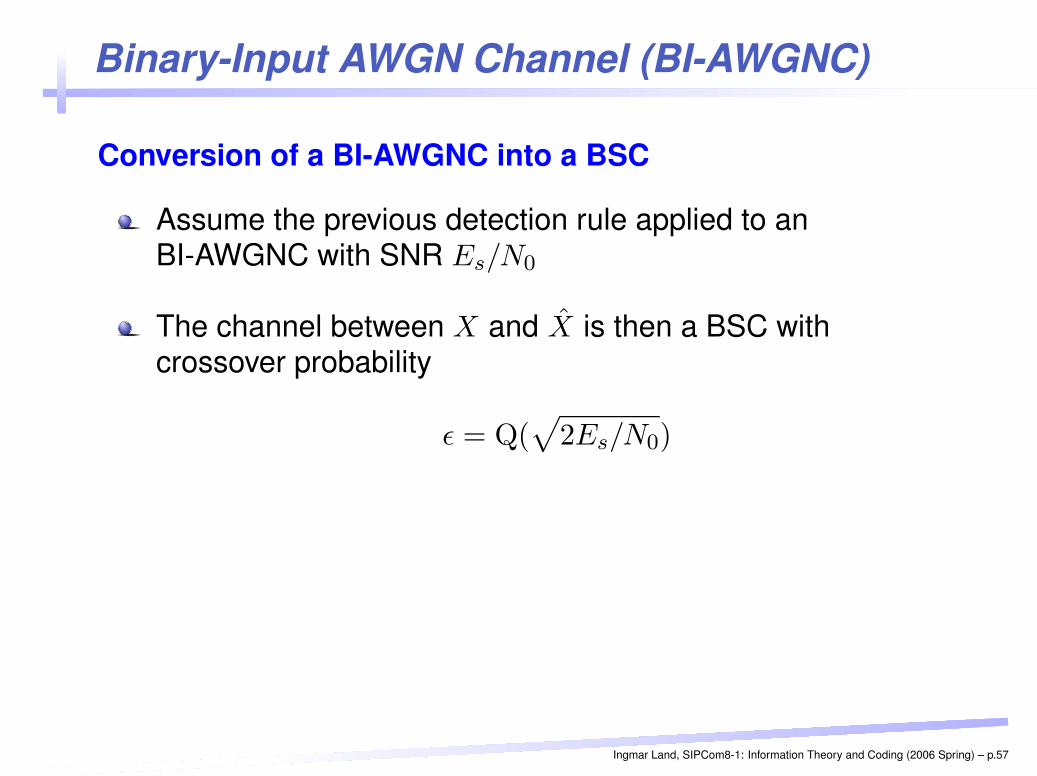
Conversion of a BI-AWGNC into a BSC
Assume the previous detection rule applied to anBI-AWGNC with SNR Es/N0
The channel between X and X is then a BSC withcrossover probability
ε = Q(√
2Es/N0)
Ingmar Land, SIPCom8-1: Information Theory and Coding (2006 Spring) – p.57
Block Codes II: Decoding
The Tasks
Decoding Principles
Guaranteed Performance
Performance Bounds
Ingmar Land, SIPCom8-1: Information Theory and Coding (2006 Spring) – p.58
The Tasks of Decoding
Objective of error correction
Given a received word,estimate the most likely (or at least a likely)
transmitted infoword or codeword
Objective of error detection
Given a received word,detect transmission errors
Problem
Decoding complexity
Ingmar Land, SIPCom8-1: Information Theory and Coding (2006 Spring) – p.59
Decoding Principles
Optimum Word-wise Decoding⇒ minimization of word-error probability
Maximum-a-posteriori (MAP) word-estimation
Maximum-likelihood (ML) word-estimation
Optimum Symbol-wise Decoding⇒ minimization of symbol-error probability
Maximum-a-posteriori (MAP) symbol-estimation
Maximum-likelihood (ML) symbol-estimation
Remarks:Word-wise estimation is also called sequence estimation.Symbol-wise estimation is also called symbol-by-symbol estimation
Ingmar Land, SIPCom8-1: Information Theory and Coding (2006 Spring) – p.60
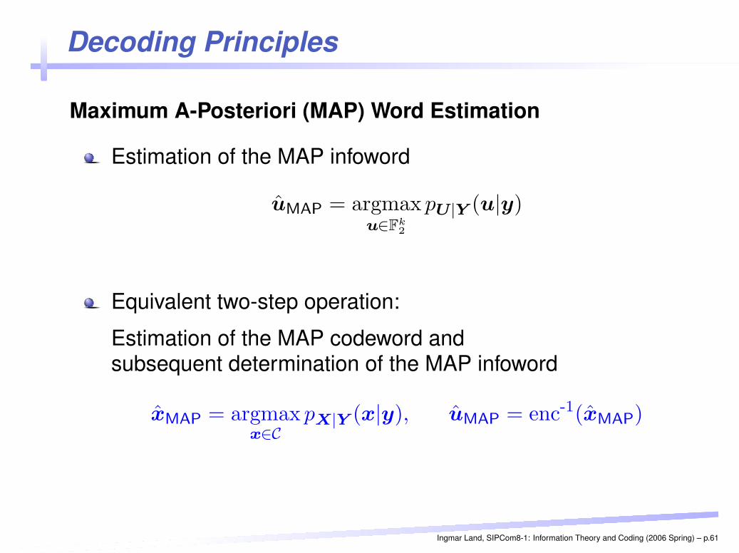
Decoding Principles
Maximum A-Posteriori (MAP) Word Estimation
Estimation of the MAP infoword
uMAP = argmaxu∈F
k2
pU |Y (u|y)
Equivalent two-step operation:
Estimation of the MAP codeword andsubsequent determination of the MAP infoword
xMAP = argmaxx∈C
pX|Y (x|y), uMAP = enc-1(xMAP)
Ingmar Land, SIPCom8-1: Information Theory and Coding (2006 Spring) – p.61
Decoding Principles
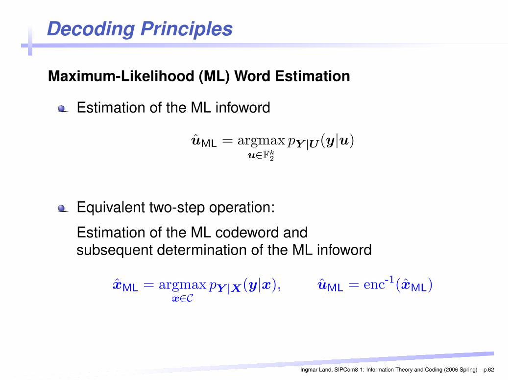
Maximum-Likelihood (ML) Word Estimation
Estimation of the ML infoword
uML = argmaxu∈F
k2
pY |U (y|u)
Equivalent two-step operation:
Estimation of the ML codeword andsubsequent determination of the ML infoword
xML = argmaxx∈C
pY |X(y|x), uML = enc-1(xML)
Ingmar Land, SIPCom8-1: Information Theory and Coding (2006 Spring) – p.62
Decoding Principles
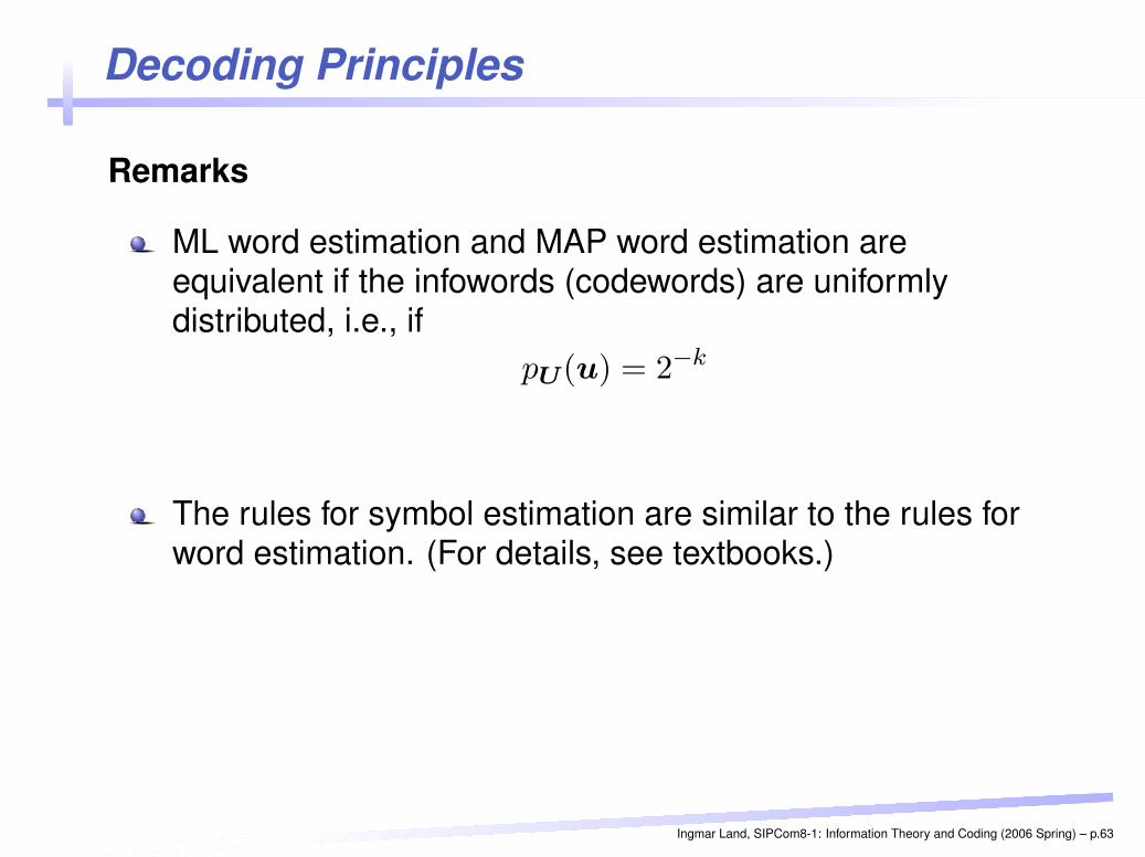
Remarks
ML word estimation and MAP word estimation areequivalent if the infowords (codewords) are uniformlydistributed, i.e., if
pU (u) = 2−k
The rules for symbol estimation are similar to the rules forword estimation. (For details, see textbooks.)
Ingmar Land, SIPCom8-1: Information Theory and Coding (2006 Spring) – p.63
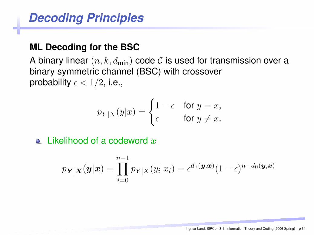
Decoding Principles
ML Decoding for the BSCA binary linear (n, k, dmin) code C is used for transmission over abinary symmetric channel (BSC) with crossoverprobability ε < 1/2, i.e.,
pY |X(y|x) =
{
1 − ε for y = x,ε for y 6= x.
Likelihood of a codeword x
pY |X(y|x) =
n−1∏
i=0
pY |X(yi|xi) = εdH(y,x)(1 − ε)n−dH(y,x)
Ingmar Land, SIPCom8-1: Information Theory and Coding (2006 Spring) – p.64
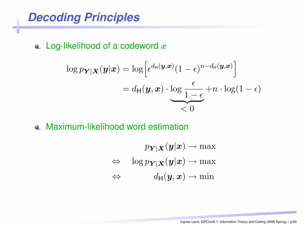
Decoding Principles
Log-likelihood of a codeword x
log pY |X(y|x) = log[
εdH(y,x)(1 − ε)n−dH(y,x)]
= dH(y, x) · logε
1 − ε︸ ︷︷ ︸
< 0
+n · log(1 − ε)
Maximum-likelihood word estimation
pY |X(y|x) → max
⇔ log pY |X(y|x) → max
⇔ dH(y, x) → min
Ingmar Land, SIPCom8-1: Information Theory and Coding (2006 Spring) – p.65
Decoding Principles
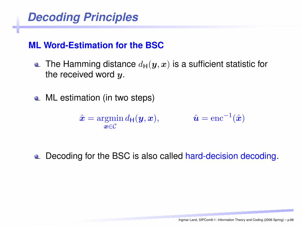
ML Word-Estimation for the BSC
The Hamming distance dH(y, x) is a sufficient statistic forthe received word y.
ML estimation (in two steps)
x = argminx∈C
dH(y, x), u = enc−1(x)
Decoding for the BSC is also called hard-decision decoding.
Ingmar Land, SIPCom8-1: Information Theory and Coding (2006 Spring) – p.66
Decoding Principles
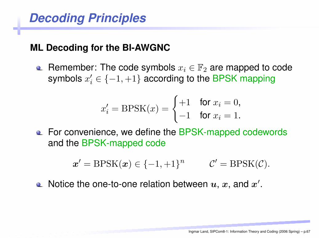
ML Decoding for the BI-AWGNC
Remember: The code symbols xi ∈ F2 are mapped to codesymbols x′
i ∈ {−1, +1} according to the BPSK mapping
x′i = BPSK(x) =
{
+1 for xi = 0,−1 for xi = 1.
For convenience, we define the BPSK-mapped codewordsand the BPSK-mapped code
x′ = BPSK(x) ∈ {−1, +1}n C′ = BPSK(C).
Notice the one-to-one relation between u, x, and x′.
Ingmar Land, SIPCom8-1: Information Theory and Coding (2006 Spring) – p.67
Decoding Principles
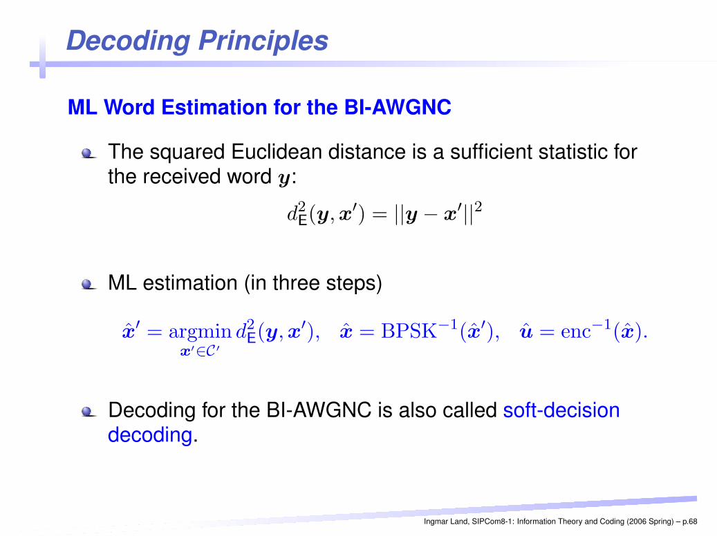
ML Word Estimation for the BI-AWGNC
The squared Euclidean distance is a sufficient statistic forthe received word y:
d2E(y, x′) = ||y − x′||2
ML estimation (in three steps)
x′ = argminx′∈C′
d2E(y, x′), x = BPSK−1(x′), u = enc−1(x).
Decoding for the BI-AWGNC is also called soft-decisiondecoding.
Ingmar Land, SIPCom8-1: Information Theory and Coding (2006 Spring) – p.68
Guaranteed Performance
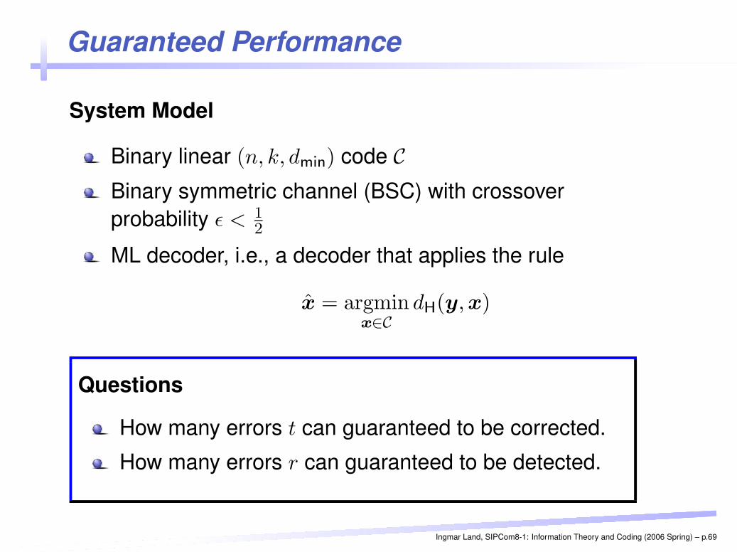
System Model
Binary linear (n, k, dmin) code CBinary symmetric channel (BSC) with crossoverprobability ε < 1
2
ML decoder, i.e., a decoder that applies the rule
x = argminx∈C
dH(y, x)
Questions
How many errors t can guaranteed to be corrected.
How many errors r can guaranteed to be detected.
Ingmar Land, SIPCom8-1: Information Theory and Coding (2006 Spring) – p.69
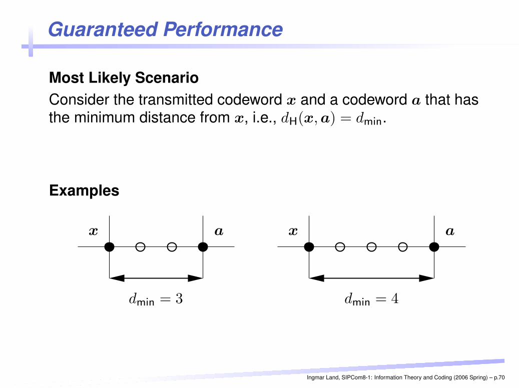
Guaranteed Performance
Most Likely ScenarioConsider the transmitted codeword x and a codeword a that hasthe minimum distance from x, i.e., dH(x, a) = dmin.
Examples
PSfrag replacements x a
dmin = 3
PSfrag replacements x a
dmin = 4
Ingmar Land, SIPCom8-1: Information Theory and Coding (2006 Spring) – p.70
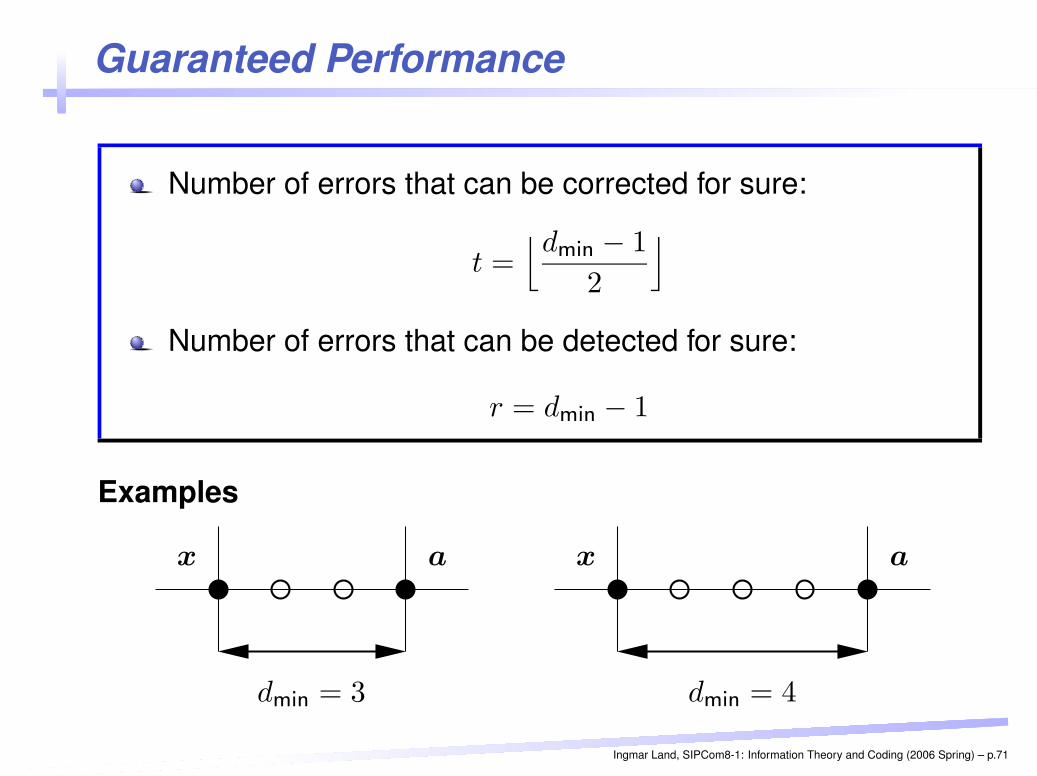
Guaranteed Performance
Number of errors that can be corrected for sure:
t =⌊dmin − 1
2
⌋
Number of errors that can be detected for sure:
r = dmin − 1
Examples
PSfrag replacements x a
dmin = 3
PSfrag replacements x a
dmin = 4
Ingmar Land, SIPCom8-1: Information Theory and Coding (2006 Spring) – p.71
Decoding Principles
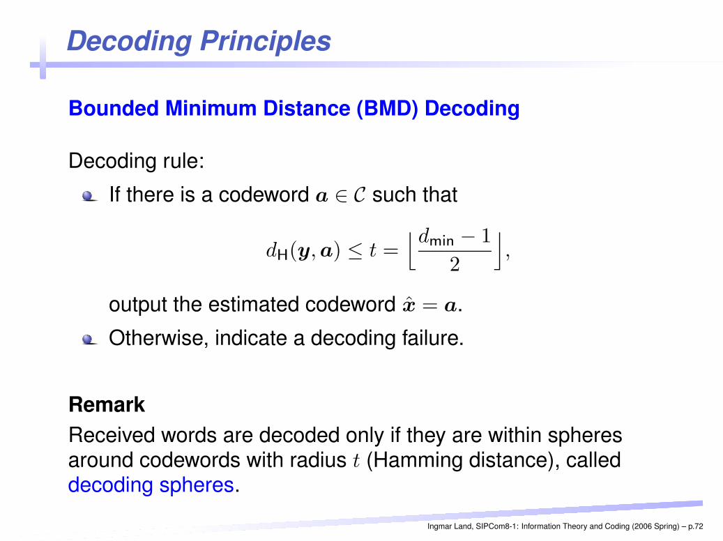
Bounded Minimum Distance (BMD) Decoding
Decoding rule:
If there is a codeword a ∈ C such that
dH(y, a) ≤ t =⌊dmin − 1
2
⌋
,
output the estimated codeword x = a.
Otherwise, indicate a decoding failure.
RemarkReceived words are decoded only if they are within spheresaround codewords with radius t (Hamming distance), calleddecoding spheres.
Ingmar Land, SIPCom8-1: Information Theory and Coding (2006 Spring) – p.72
Performance Bounds
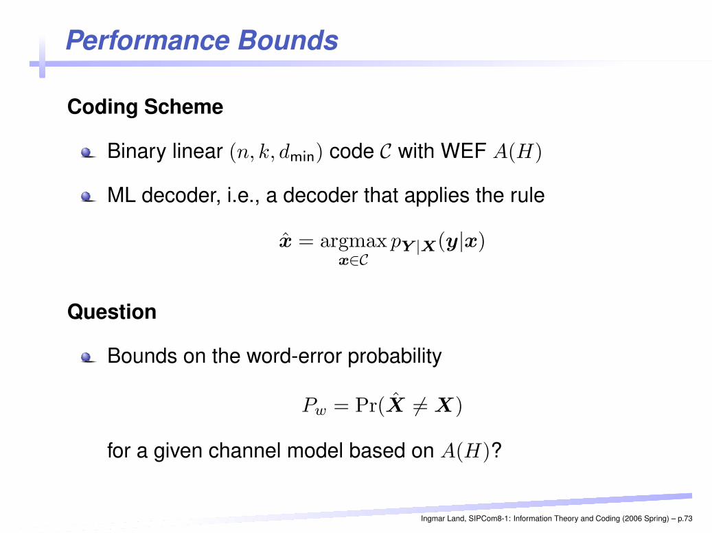
Coding Scheme
Binary linear (n, k, dmin) code C with WEF A(H)
ML decoder, i.e., a decoder that applies the rule
x = argmaxx∈C
pY |X(y|x)
Question
Bounds on the word-error probability
Pw = Pr(X 6= X)
for a given channel model based on A(H)?
Ingmar Land, SIPCom8-1: Information Theory and Coding (2006 Spring) – p.73
Performance Bounds
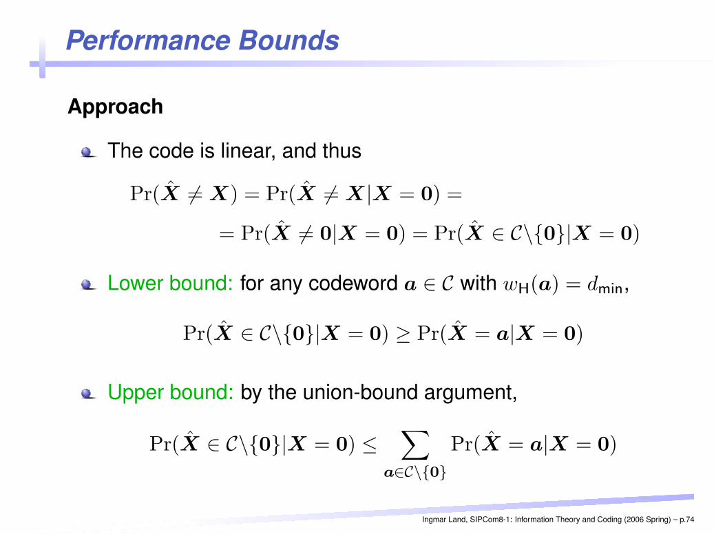
Approach
The code is linear, and thus
Pr(X 6= X) = Pr(X 6= X|X = 0) =
= Pr(X 6= 0|X = 0) = Pr(X ∈ C\{0}|X = 0)
Lower bound: for any codeword a ∈ C with wH(a) = dmin,
Pr(X ∈ C\{0}|X = 0) ≥ Pr(X = a|X = 0)
Upper bound: by the union-bound argument,
Pr(X ∈ C\{0}|X = 0) ≤∑
a∈C\{0}
Pr(X = a|X = 0)
Ingmar Land, SIPCom8-1: Information Theory and Coding (2006 Spring) – p.74
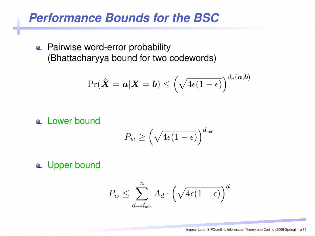
Performance Bounds for the BSC
Pairwise word-error probability(Bhattacharyya bound for two codewords)
Pr(X = a|X = b) ≤(√
4ε(1 − ε))dH(a,b)
Lower bound
Pw ≥(√
4ε(1 − ε))dmin
Upper bound
Pw ≤n∑
d=dmin
Ad ·(√
4ε(1 − ε))d
Ingmar Land, SIPCom8-1: Information Theory and Coding (2006 Spring) – p.75
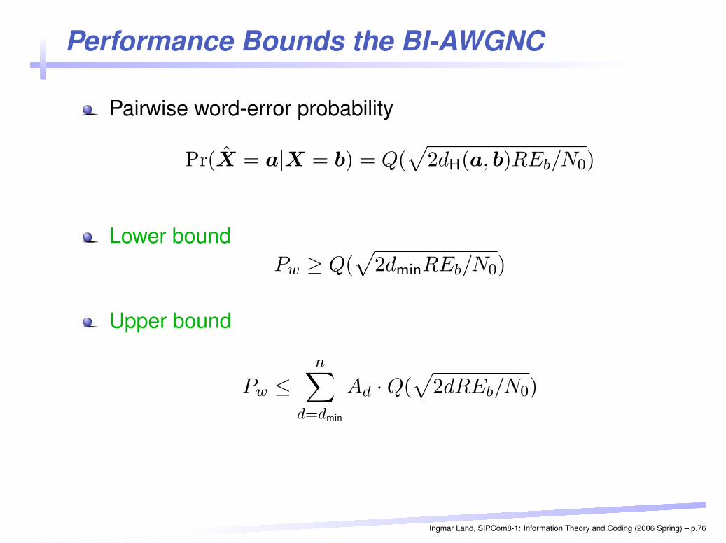
Performance Bounds the BI-AWGNC
Pairwise word-error probability
Pr(X = a|X = b) = Q(√
2dH(a, b)REb/N0)
Lower boundPw ≥ Q(
√
2dminREb/N0)
Upper bound
Pw ≤n∑
d=dmin
Ad · Q(√
2dREb/N0)
Ingmar Land, SIPCom8-1: Information Theory and Coding (2006 Spring) – p.76
Performance Bounds
For improving channel quality, the gap between the lowerbound and the upper bound becomes very small. (ForAdmin
= 1, it vanishes.)
Improving channel quality meansfor the BSC: ε → 1
for the BI-AWGNC: Eb /N0 → ∞
Ingmar Land, SIPCom8-1: Information Theory and Coding (2006 Spring) – p.77
Asymptotic Coding-Gain for the BI-AWGNC
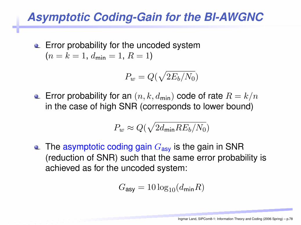
Error probability for the uncoded system(n = k = 1, dmin = 1, R = 1)
Pw = Q(√
2Eb/N0)
Error probability for an (n, k, dmin) code of rate R = k/nin the case of high SNR (corresponds to lower bound)
Pw ≈ Q(√
2dminREb/N0)
The asymptotic coding gain Gasy is the gain in SNR(reduction of SNR) such that the same error probability isachieved as for the uncoded system:
Gasy = 10 log10(dminR)
Ingmar Land, SIPCom8-1: Information Theory and Coding (2006 Spring) – p.78
Summary
Guaranteed PerformanceNumber of errors that can guaranteed to be correctedNumber of errors that can guaranteed to be detected
Maximum-likelihood decodingBSC (“hard-decision decoding”): Hamming distanceBI-AWGNC (“soft-decision decoding”): squaredEuclidean distance
Performance boundsbased on the weight enumerating functionasymptotic coding gain for the BI-AWGNC
Ingmar Land, SIPCom8-1: Information Theory and Coding (2006 Spring) – p.79
Convolutional Codes
General Properties
EncodingConvolutional EncoderState Transition DiagramTrellis Diagram
DecodingML Sequence DecodingViterbi Algorithm
Ingmar Land, SIPCom8-1: Information Theory and Coding (2006 Spring) – p.80
Convolutional Codes
General Properties
Continuous encoding of info symbols to code symbols
Generated code symbols depend on current info symboland previously encoded info symbols
Convolutional encoder is a finite state machine (withmemory)
Certain decoders allow continuous decoding of receivedsequence
⇒ Convolutional codes enable continuous transmission,whereas block codes allow only blocked transmission.
Ingmar Land, SIPCom8-1: Information Theory and Coding (2006 Spring) – p.81
Convolutional Encoder
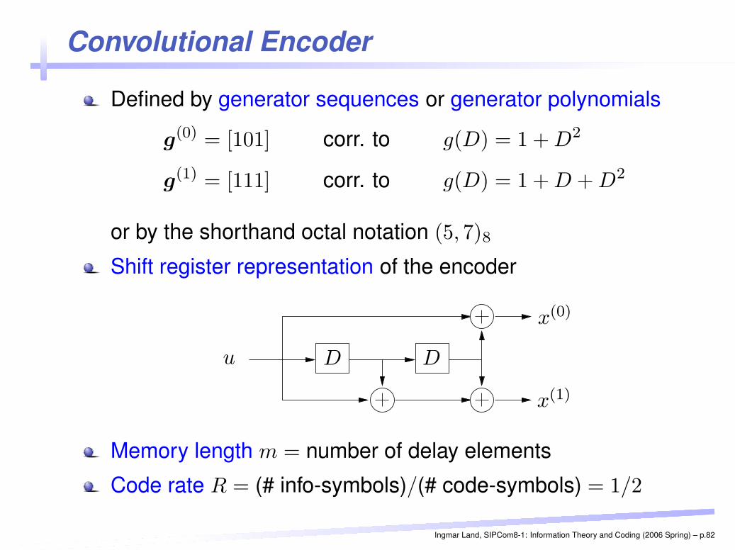
Defined by generator sequences or generator polynomials
g(0) = [101] corr. to g(D) = 1 + D2
g(1) = [111] corr. to g(D) = 1 + D + D2
or by the shorthand octal notation (5, 7)8
Shift register representation of the encoderPSfrag replacements
u
x(0)
x(1)
D D
Memory length m = number of delay elements
Code rate R = (# info-symbols)/(# code-symbols) = 1/2
Ingmar Land, SIPCom8-1: Information Theory and Coding (2006 Spring) – p.82
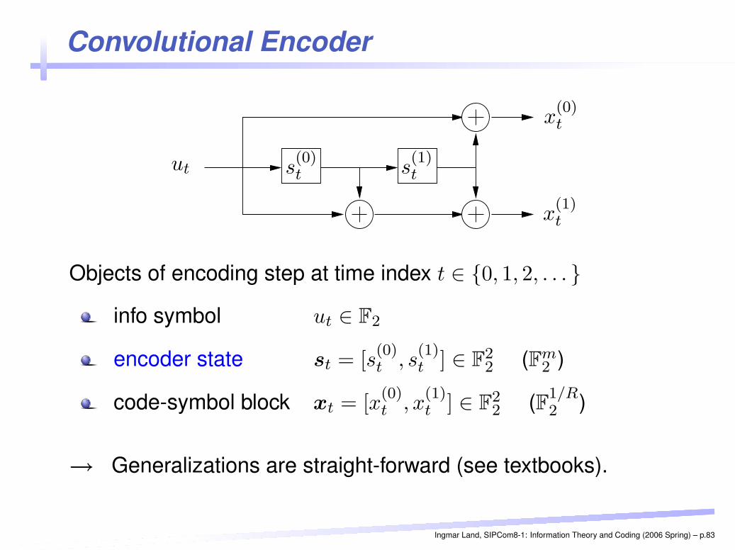
Convolutional EncoderPSfrag replacements
ut
x(0)t
x(1)t
s(0)t s
(1)t
Objects of encoding step at time index t ∈ {0, 1, 2, . . . }
info symbol ut ∈ F2
encoder state st = [s(0)t , s
(1)t ] ∈ F
22 (Fm
2 )
code-symbol block xt = [x(0)t , x
(1)t ] ∈ F
22 (F1/R
2 )
→ Generalizations are straight-forward (see textbooks).
Ingmar Land, SIPCom8-1: Information Theory and Coding (2006 Spring) – p.83
State Transition Diagram
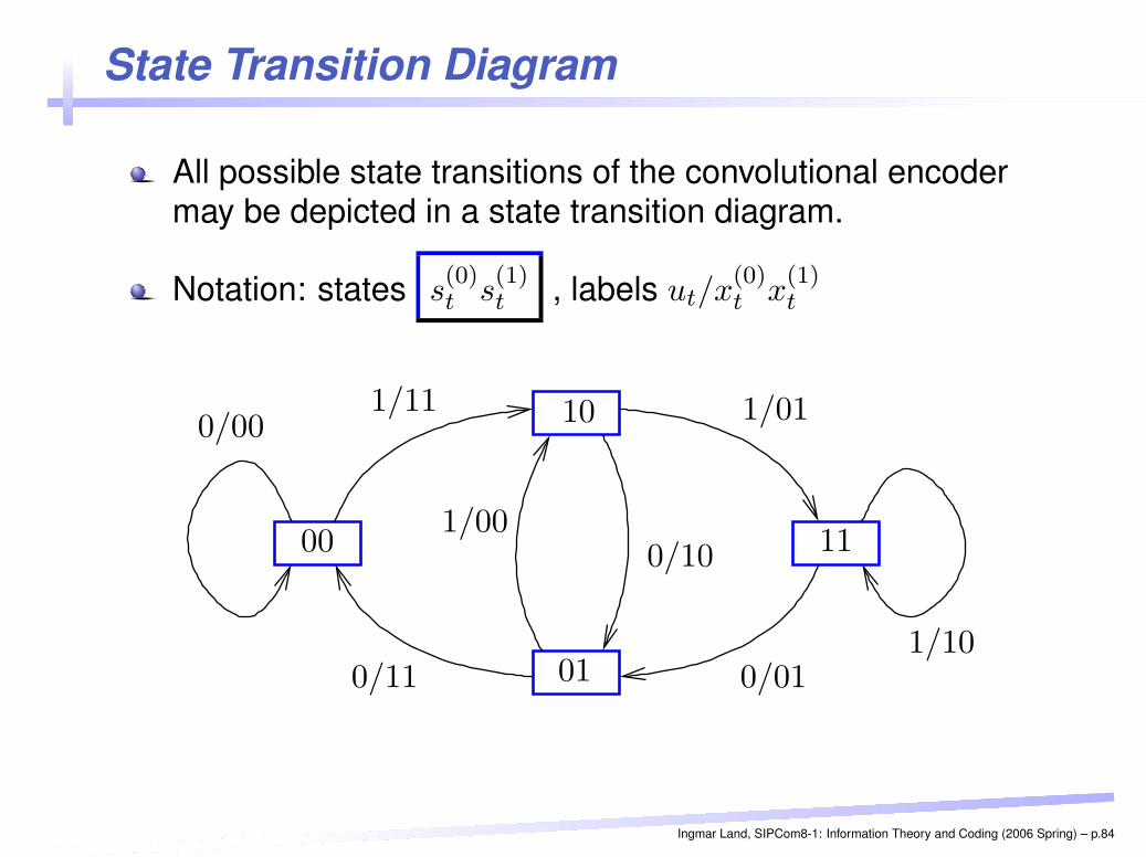
All possible state transitions of the convolutional encodermay be depicted in a state transition diagram.
Notation: states s(0)t s
(1)t , labels ut/x
(0)t x
(1)t
PSfrag replacements
00
01
10
11
0/00
0/01
0/10
0/11
1/00
1/01
1/10
1/11
Ingmar Land, SIPCom8-1: Information Theory and Coding (2006 Spring) – p.84
Trellis Diagram
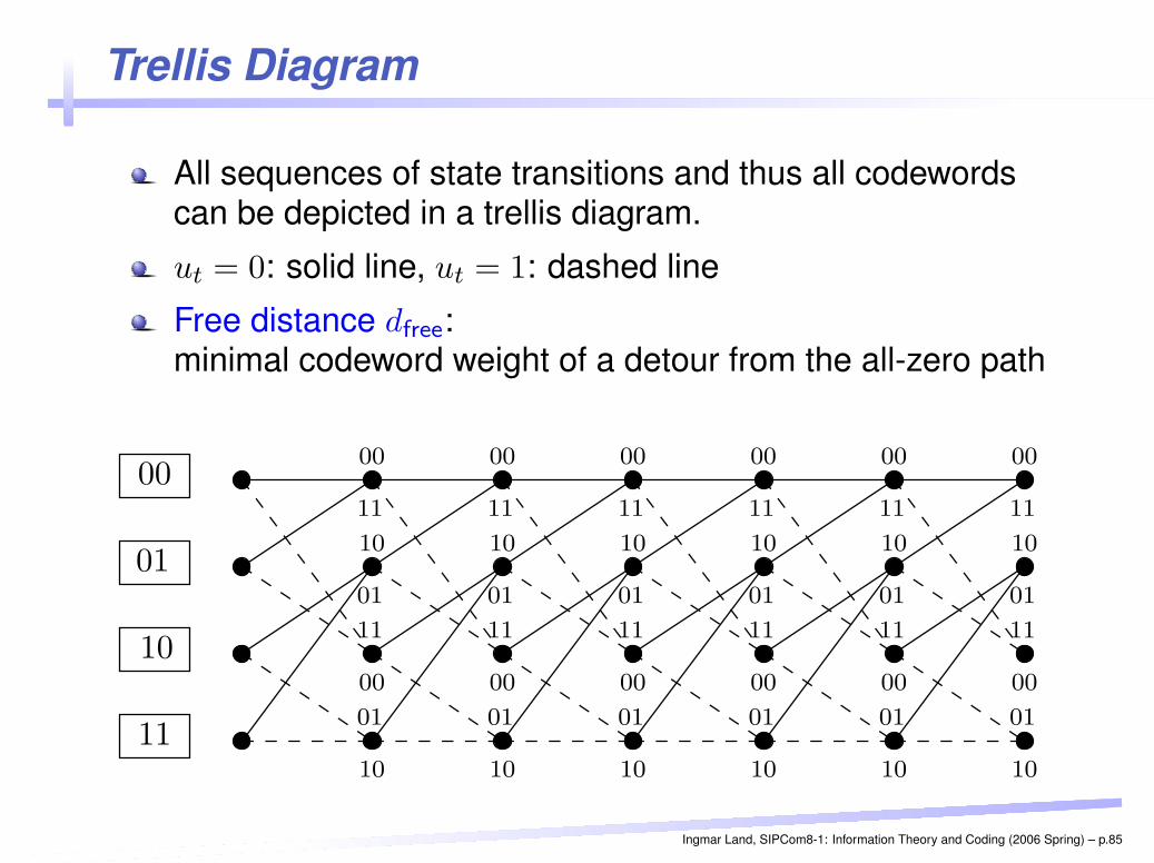
All sequences of state transitions and thus all codewordscan be depicted in a trellis diagram.
ut = 0: solid line, ut = 1: dashed line
Free distance dfree:minimal codeword weight of a detour from the all-zero path
PSfrag replacements00
01
10
11
00
00
00
00
00
00
00
00
00
00
00
00
01
01
01
01
01
01
01
01
01
01
01
01
10
10
10
10
10
10
10
10
10
10
10
10
11
11
11
11
11
11
11
11
11
11
11
11
Ingmar Land, SIPCom8-1: Information Theory and Coding (2006 Spring) – p.85
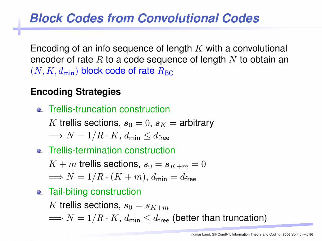
Block Codes from Convolutional Codes
Encoding of an info sequence of length K with a convolutionalencoder of rate R to a code sequence of length N to obtain an(N, K, dmin) block code of rate RBC
Encoding Strategies
Trellis-truncation constructionK trellis sections, s0 = 0, sK = arbitrary=⇒ N = 1/R · K, dmin ≤ dfree
Trellis-termination constructionK + m trellis sections, s0 = sK+m = 0
=⇒ N = 1/R · (K + m), dmin = dfree
Tail-biting constructionK trellis sections, s0 = sK+m
=⇒ N = 1/R · K, dmin ≤ dfree (better than truncation)
Ingmar Land, SIPCom8-1: Information Theory and Coding (2006 Spring) – p.86
Decoding of Convolutional Codes
Goal: ML word estimation
x = argmaxx∈C
pY |X(y|x)
Possible evaluation:
Compute pY |X(y|x) for all x ∈ C and determine thecodeword x with the largest likelihood
Problem: computational complexity
Solution: Viterbi algorithm
Ingmar Land, SIPCom8-1: Information Theory and Coding (2006 Spring) – p.87
Branches, Paths, and Metrics
Branch in the trellis: one state transition
s[t,t+1] = [st, st+1]
Block of code symbols associated to a branch and block ofobservations corresponding to these code symbols:
x(s[t,t+1]) = xt = [x(0)t , x
(1)t ] yt = [y
(0)t , y
(1)t ]
Path “through” the trellis: sequence of state transitions
s[t1,t2+1] = [st1 , st1+1, . . . , st2 , st2+1]
Partial code word associated to a path:
x(s[t1,t2+1]) = [xt1 , xt1+1, . . . , xt2−1, xt2 ]
Ingmar Land, SIPCom8-1: Information Theory and Coding (2006 Spring) – p.88

Branches, Paths, and Metrics
Branch metric: distance measure between code-symbolblock and observations block,e.g. Hamming distance for the BSC:
µ(s[t,t+1]) = dH(yt, xt)
Path metric: distance measure between code-symbolsequence and sequence of observations:
µ(s[t1,t2+1]) = dH
(
[yt1 , . . . , yt2 ], [xt1 , . . . , xt2 ])
,
The metric should be an additive metric to allow for arecursive computation of the path metric:
µ(s[0,t+1])︸ ︷︷ ︸
path metric
= µ(s[0,t])︸ ︷︷ ︸
path metric
+ µ(st,t+1)︸ ︷︷ ︸
branch metricIngmar Land, SIPCom8-1: Information Theory and Coding (2006 Spring) – p.89
Decoding of Convolutional Codes
Consider a convolutional code with T trellis sections.
ML decoding rule
Search for the path with the smallest metricand determine the associated codeword:
s0,T = argmins0,T∈ trellis
µ(s0,T )
x = x(s0,T )
Viterbi algorithm (VA)trellis-based search algorithmrecursive evaluation of the decoding rule in the trellismost efficient way to implement ML decoding
Ingmar Land, SIPCom8-1: Information Theory and Coding (2006 Spring) – p.90
Viterbi Algorithm
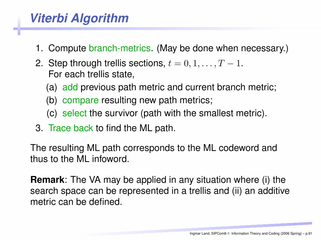
1. Compute branch-metrics. (May be done when necessary.)
2. Step through trellis sections, t = 0, 1, . . . , T − 1.For each trellis state,(a) add previous path metric and current branch metric;(b) compare resulting new path metrics;(c) select the survivor (path with the smallest metric).
3. Trace back to find the ML path.
The resulting ML path corresponds to the ML codeword andthus to the ML infoword.
Remark: The VA may be applied in any situation where (i) thesearch space can be represented in a trellis and (ii) an additivemetric can be defined.
Ingmar Land, SIPCom8-1: Information Theory and Coding (2006 Spring) – p.91
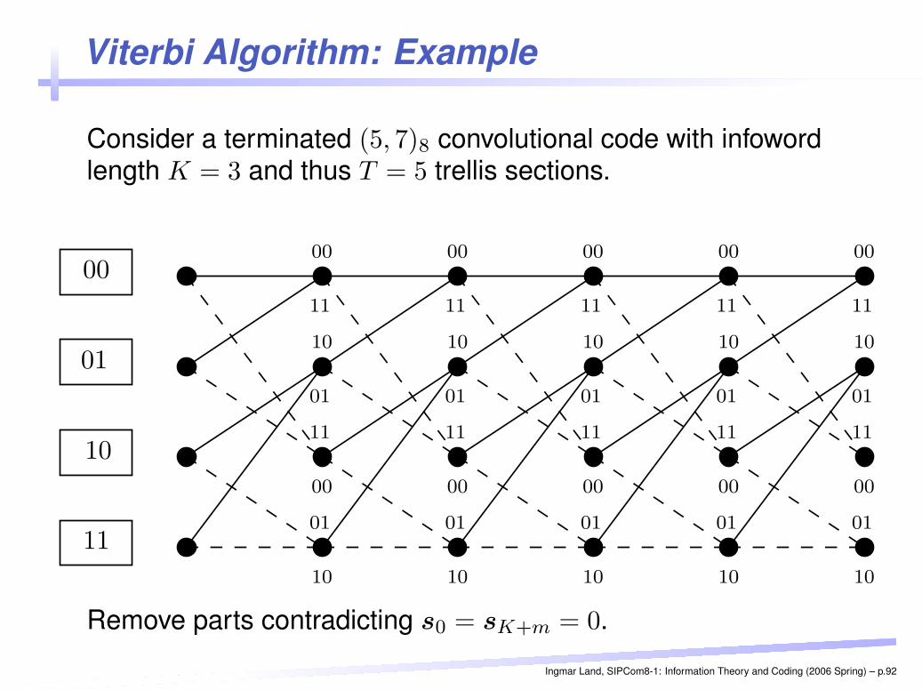
Viterbi Algorithm: Example
Consider a terminated (5, 7)8 convolutional code with infowordlength K = 3 and thus T = 5 trellis sections.
PSfrag replacements
00
01
10
11
00
00
00
00
00
00
00
00
00
00
01
01
01
01
01
01
01
01
01
01
10
10
10
10
10
10
10
10
10
10
11
11
11
11
11
11
11
11
11
11
Remove parts contradicting s0 = sK+m = 0.
Ingmar Land, SIPCom8-1: Information Theory and Coding (2006 Spring) – p.92
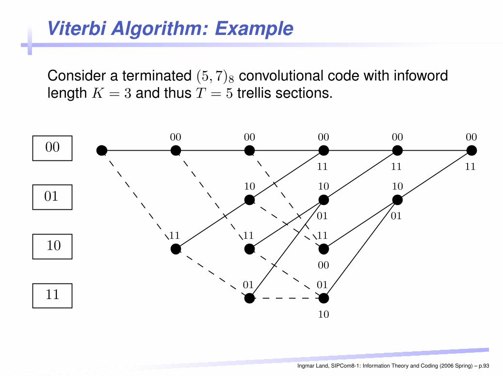
Viterbi Algorithm: Example
Consider a terminated (5, 7)8 convolutional code with infowordlength K = 3 and thus T = 5 trellis sections.
PSfrag replacements
00
01
10
11
0000
00
000000
01
01
01
01
10
10
1010
1111
11
11
1111
Ingmar Land, SIPCom8-1: Information Theory and Coding (2006 Spring) – p.93
Summary
Convolutional encoder
State transition diagram
Trellis diagram
Path metrics and branch metrics
Viterbi algorithm
Ingmar Land, SIPCom8-1: Information Theory and Coding (2006 Spring) – p.94