Embed Size (px)
Citation preview

LINEAR FIRST ORDER Ordinary Differential Equations

Topics Covered
• General and Standard Forms of linear first-order ordinary differential equations.
• Theory of solving these ODE’s.
• Direct Method of solving linear first-order ODE’s.
• Examples.

Definition
𝑎1 𝑥 .𝑑𝑦
𝑑𝑥+ 𝑎0 𝑥 . 𝑦 = 𝑔(𝑥)
• It is linear, so there are no functions of 𝑦 or any of its derivatives.
• The highest order is 𝑑𝑦
𝑑𝑥.
• There is a function of 𝑥 represented by 𝑔(𝑥), though this function may also be equal to 0.

General and Standard Form
• The general form of a linear first-order ODE is
𝒂𝟏 𝒙 .𝒅𝒚
𝒅𝒙+ 𝒂𝟎 𝒙 . 𝒚 = 𝒈(𝒙)
• In this equation,
if 𝑎1 𝑥 = 0, it is no longer an differential equation and so 𝑎1 𝑥 cannot be 0; and if 𝑎0 𝑥 = 0, it is a variable separated ODE and can easily be solved by integration, thus in this chapter 𝑎0 𝑥 cannot be 0. If 𝑔 𝑥 = 0, it is called a Homogenous Equation, and can easily be solved by separating the variables, thus in this chapter g(𝑥) is generally not 0. If 𝑔(𝑥) ≠ 0 it is a non-homogenous equation.

Standard Form
By dividing both sides of this general form by 𝑎1(𝑥) we get the standard form, which is much more useful for solving it:
𝒅𝒚
𝒅𝒙+ 𝑷 𝒙 𝒚 = 𝒇(𝒙)
where 𝑃 𝑥 = 𝑎0 𝑥 /𝑎1 𝑥 and f 𝑥 = 𝑔 𝑥 /𝑎1 𝑥
There is a very important theory behind the solution of differential equations which is covered in the next few slides. For a review of the direct method to solve linear first-order differential equations, jump ahead to the direct method on slide 14.

The Property
• Solving differential equations is based on the property that the solution 𝑦(𝑥) can be represented as 𝑦𝑐 𝑥 + 𝑦𝑝(𝑥), where
𝑦𝑐 𝑥 is the solution of the homogenous equation 𝑑𝑦
𝑑𝑥+
𝑃 𝑥 𝑦 = 0 and 𝑦𝑝(𝑥) is a particular solution of the entire
non-homogenous equation 𝑑𝑦
𝑑𝑥+ 𝑃 𝑥 𝑦 = 𝑓 𝑥 .

NOTE
• There are 2 important points to note:
1. Clearly, if the original problem is a homogenous equation, 𝑦𝑝 𝑥 = 0 and the solution is 𝑦 = 𝑦𝑐 𝑥 .
2. We can see that 𝑦𝑐 𝑥 = 0 is always valid. However this is known as the trivial solution and we are only interested in finding out all non-trivial solutions.

To find 𝑦𝑐(𝑥)
The equation 𝑑𝑦
𝑑𝑥+ 𝑃 𝑥 𝑦 = 0 can be re-written as
𝑑𝑦
𝑦=
− 𝑃 𝑥 𝑑𝑥 with simple algebra. Integrating both sides,
ln 𝑦 = − 𝑃 𝑥 𝑑𝑥
∴ 𝑦 = 𝑒− 𝑃 𝑥 𝑑𝑥+𝑐
Where c is the constant of integration.

To find 𝑦𝑐 𝑥 contd.
We can rewrite this expression for 𝑦𝑐 𝑥 as
𝑦𝑐 = 𝑐𝑒− 𝑃 𝑥 𝑑𝑥 = 𝑐𝑦1
where 𝑐 is the parameter which can have any real value, and all the obtained functions will be solutions of the associated homogenous equation of the original differential equation; and
𝑦1 = 𝑒− 𝑃 𝑥 𝑑𝑥

Example of 𝑦𝑐 𝑥
Let us consider the homogenous equation 3𝑦′ + sin 𝑥 + 3𝑒𝑎𝑥 𝑦 = 0
where a is a constant. The equation can be re-written as: 𝑦′
𝑦= −
1
3sin 𝑥 + 3𝑒𝑎𝑥
Integrating both sides with respect to x, we get
ln 𝑦 = −1
3 sin 𝑥 𝑑𝑥 + 3𝑒𝑎𝑥𝑑𝑥 =
cos 𝑥
3−𝑒𝑎𝑥
𝑎+ 𝑐1
∴ 𝑦 = 𝑐𝑒cos 𝑥3 −
𝑒𝑎𝑥
𝑎 = 𝑦𝑐
Where 𝑐 is any arbitrarily chosen parameter. Alternatively, this answer for 𝑦𝑐 𝑥 can be obtained from the formula on the previous slide.

To find 𝑦𝑝(𝑥)
To find 𝑦𝑝(𝑥) we use the method of Variation of Parameters and make
the assumption that it is of the form 𝑢(𝑥)𝑦1(𝑥) where 𝑢(𝑥) is an
unknown function and 𝑦1 = 𝑒− 𝑃 𝑥 𝑑𝑥. Substituting this form of
𝑦𝑝(𝑥) into the Standard form of the equation, we get
𝑢𝑦1′ + 𝑦1𝑢
′ + 𝑃 𝑥 𝑢𝑦1 = 𝑓(𝑥)
Rearranging and substituting 𝑑𝑦1
𝑑𝑥+ 𝑃 𝑥 𝑦1 = 0, we get 𝑢 =
𝑓(𝑥)
𝑦1(𝑥)𝑑𝑥
and therefore
𝑦𝑝 𝑥 = 𝑢 𝑥 𝑦1 𝑥 = 𝑒− 𝑃 𝑥 𝑑𝑥 𝑒 𝑃 𝑥 𝑑𝑥𝑓(𝑥)𝑑𝑥

Putting it together for 𝑦(𝑥)
Going back to the original equation 𝑦 𝑥 = 𝑦𝑐 𝑥 + 𝑦𝑝(𝑥) we
substitute and get
𝑦 𝑥 = 𝑒− 𝑃 𝑥 𝑑𝑥(𝑐 + 𝑒 𝑃 𝑥 𝑑𝑥𝑓 𝑥 𝑑𝑥)
Which is the entire solution for the differential equation that we started with.
Using this equation we can now derive an easier method to solve linear first-order differential equation.

The previous equation can be re-written as:
𝑦 𝑥 𝑒 𝑃 𝑥 𝑑𝑥 = 𝑐 + 𝑒 𝑃 𝑥 𝑑𝑥𝑓 𝑥 𝑑𝑥
Differentiating both sides, we get
𝑦′𝑒 𝑃 𝑥 𝑑𝑥 + 𝑃 𝑥 𝑦𝑒 𝑃 𝑥 𝑑𝑥 = 𝑒 𝑃 𝑥 𝑑𝑥𝑓 𝑥
Which is clearly the Standard Form multiplied with 𝑒 𝑃 𝑥 𝑑𝑥. Thus we can clearly see following these steps in reverse, we get an easy way to solve these differential equations.

Direct Method
The trick is to represent the left side of the Standard Form of the equation in the form of the product rule, while the right side is some function of the independent variable (𝑥). To do so, we multiply the entire differential equation with the Integrating
Factor 𝑒 𝑃 𝑥 𝑑𝑥 to get the equation: 𝑑𝑦
𝑑𝑥𝑒 𝑃 𝑥 𝑑𝑥 + 𝑃 𝑥 𝑦𝑒 𝑃 𝑥 𝑑𝑥 = 𝑒 𝑃 𝑥 𝑑𝑥𝑓 𝑥

Direct Method (contd.)
We can see that the left side is in the form of the product rule: 𝑑
𝑑𝑥𝑦 𝑥 . 𝑒 𝑃 𝑥 𝑑𝑥 = 𝑒 𝑃 𝑥 𝑑𝑥𝑓 𝑥
Integrating this equation with respect to 𝑥, we get
𝑦 𝑥 . 𝑒 𝑃 𝑥 𝑑𝑥 = 𝑒 𝑃 𝑥 𝑑𝑥𝑓 𝑥 𝑑𝑥 + 𝑐
Which can then easily be solved for 𝑦(𝑥).
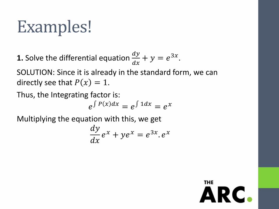
Examples!
1. Solve the differential equation 𝑑𝑦
𝑑𝑥+ 𝑦 = 𝑒3𝑥.
SOLUTION: Since it is already in the standard form, we can directly see that 𝑃 𝑥 = 1.
Thus, the Integrating factor is:
𝑒 𝑃 𝑥 𝑑𝑥 = 𝑒 1𝑑𝑥 = 𝑒𝑥
Multiplying the equation with this, we get 𝑑𝑦
𝑑𝑥𝑒𝑥 + 𝑦𝑒𝑥 = 𝑒3𝑥 . 𝑒𝑥

∴𝑑
𝑑𝑥𝑦. 𝑒𝑥 = 𝑒4𝑥
Integrating this equation with respect to 𝑥,
y. 𝑒𝑥 = 𝑒4𝑥𝑑𝑥 =𝑒4𝑥
4+ 𝑐
∴ 𝑦 =𝑒3𝑥
4+ 𝑐𝑒−𝑥
Which is the desired solution for the differential equation. Here, 𝑐 is any arbitrary real number.

2. Solve: cos2 𝑥 sin 𝑥𝑑𝑦
𝑑𝑥+ cos3 𝑥 𝑦 = 1
SOLUTION: We first change it from the General Form to the Standard Form.
𝑑𝑦
𝑑𝑥+cos (𝑥)
sin (𝑥)𝑦 =
1
cos2 𝑥 sin 𝑥
The integrating factor is
𝑒 cos (𝑥)sin (𝑥)
𝑑𝑥= 𝑒ln |sin (𝑥)| = sin (𝑥)
Multiplying the standard form with sin (𝑥), we get:
sin (𝑥)𝑑𝑦
𝑑𝑥+ cos (𝑥)𝑦 =
1
cos2 𝑥

∴𝑑
𝑑𝑥𝑦. sin 𝑥 =
1
cos2(𝑥)
∴ 𝑦. sin 𝑥 = sec2 𝑥 𝑑𝑥 = tan 𝑥 + 𝑐
∴ 𝑦 𝑥 =1
cos (𝑥)+
𝑐
sin (𝑥)
Alternatively we can write:
∴ 𝑦 𝑥 = sec 𝑥 + 𝑐. csc (𝑥)
which is the desired solution.

3. Solve: 𝑦𝑑𝑥
𝑑𝑦− 𝑥 = 2𝑦2 ; 𝑦 1 = 5
SOLUTION: This sum covers 2 important new ideas. Firstly, as can be seen from the given ODE, 𝑥 is the dependent variable and not 𝑦. Secondly, an Initial Value of 𝑦 = 5 when 𝑥 = 1 is given to find a specific value of the arbitrary parameter 𝑐. Keeping in mind that x is dependent and so we will integrate with respect to y, we convert to Standard Form as:
𝑑𝑥
𝑑𝑦−1
𝑦𝑥 = 2𝑦
The integrating factor is
𝑒 −1𝑦𝑑𝑦= 𝑒−ln |𝑦| =
1
𝑦
Multiplying the standard form with 1
𝑦, we get:
1
𝑦
𝑑𝑥
𝑑𝑦−1
𝑦2𝑥 = 2
∴𝑑
𝑑𝑦
1
𝑦. 𝑥 = 2
Integrating with respect to 𝑦; 1
𝑦. 𝑥 = 2𝑦 + 𝑐
∴ 𝑥 = 2𝑦2 + 𝑐𝑦

This equation is the solution of the ODE that we started off with. However we are not done yet. We will now use the given Initial Value to solve for a particular value of 𝑐 for this problem.
Substituting 𝑦 = 5 and 𝑥 = 1 into the solution 𝑥 = 2𝑦2 + 𝑐𝑦, we get: 1 = 2. 52 + 𝑐. 5 ∴ 1 − 50 = 5𝑐
∴ 𝑐 = −49
5
Substituting this value for 𝑐 back into the solution equation, we get our complete final solution:
𝑥 = 2𝑦2 −49
5𝑦

4. Solve 𝑑𝑇
𝑑𝑡= 𝑘(𝑇 − 𝑇𝑚) ; 𝑇 0 = 𝑇0 where 𝑘, 𝑇𝑚 and 𝑇0 are
constants.
SOLUTION: Rewriting in standard form: 𝑑𝑇
𝑑𝑡− 𝑘𝑇 = −𝑘𝑇𝑚
Integrating Factor: 𝑒 −𝑘𝑑𝑡 = 𝑒−𝑘𝑡.
Multiplying with the Integrating Factor,
𝑒−𝑘𝑡𝑑𝑇
𝑑𝑡− 𝑘𝑒−𝑘𝑡𝑇 = −𝑘𝑒−𝑘𝑡𝑇𝑚
∴𝑑
𝑑𝑡𝑇. 𝑒−𝑘𝑡 = −𝑘𝑒−𝑘𝑡𝑇𝑚
∴ 𝑇. 𝑒−𝑘𝑡 = 𝑇𝑚𝑒−𝑘𝑡 + 𝑐
∴ 𝑇 = 𝑇𝑚 + 𝑐𝑒𝑘𝑡
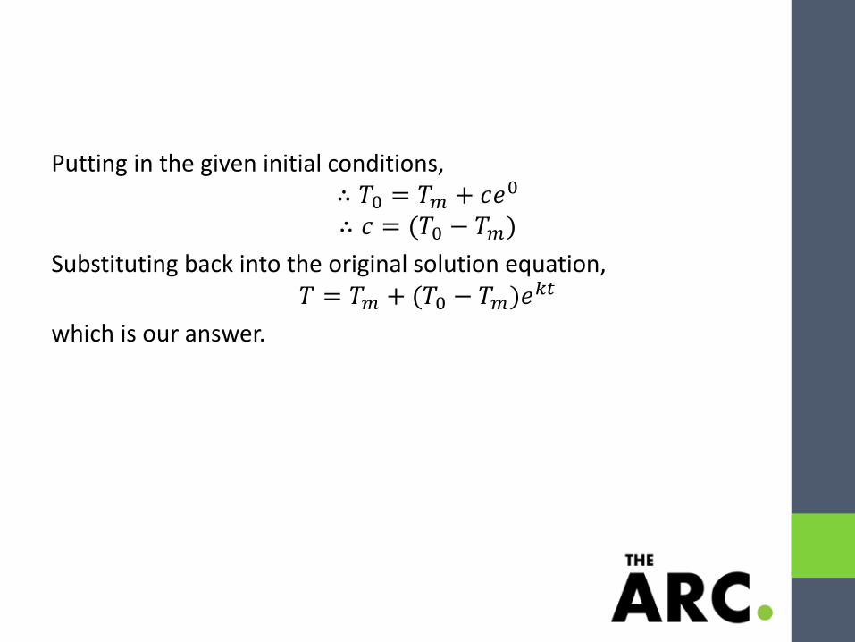
Putting in the given initial conditions, ∴ 𝑇0 = 𝑇𝑚 + 𝑐𝑒
0 ∴ 𝑐 = (𝑇0 − 𝑇𝑚)
Substituting back into the original solution equation, 𝑇 = 𝑇𝑚 + (𝑇0 − 𝑇𝑚)𝑒
𝑘𝑡
which is our answer.

5. Solve 𝑦′ + (tan 𝑥)𝑦 = cos2𝑥
SOLUTION: Integrating Factor is
𝑒 (tan 𝑥)𝑑𝑥 = sec 𝑥
Multiplying, we get (sec 𝑥)𝑦′ + (sec 𝑥 tan 𝑥)𝑦 = cos 𝑥
∴𝑑
𝑑𝑥[𝑦. sec 𝑥] = cos 𝑥
Integrating, we get ∴ 𝑦. sec 𝑥 = sin 𝑥 + 𝑐
∴ 𝑦 = sin 𝑥 cos 𝑥 + 𝑐. cos 𝑥

References
•A First Course in Differential Equations with Modeling Applications
David G.Zill
•Rohit Agarwal – Math Tutor at Academic Resource
Center
Illinois Institute of Technology
Made Spring 2012