Linear Prediction Coding (LPC)• History: Originally developed to compress (code) speech

• Broader Implications– Models the harmonic resonances of the vocal tract– Provide features useful for speech recognition– Part of speech synthesis algorithms– IIR Filter, to eliminate noise from a signal

• Concept– Predict samples with linear combinations of previous

values to create a LPC signal– The residue or error is the difference between the signal

and the prediction

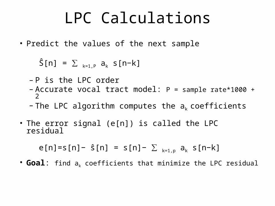
LPC Calculations

• Predict the values of the next sample

Ŝ[n] = ∑ k=1,P ak s[n−k]

– P is the LPC order– Accurate vocal tract model: P = sample rate*1000 + 2– The LPC algorithm computes the ak coefficients

• The error signal (e[n]) is called the LPC residual

e[n]=s[n]− ŝ[n] = s[n]− ∑ k=1,p ak s[n−k]

• Goal: find ak coefficients that minimize the LPC residual

Linear Predictive Compression (LPC)

Concept

• For a frame of the signal, find the optimal coefficients, predicting the next values using sets of previous values

• Instead of outputting the actual data, output the residual, plus the coefficients

• Less bits are needed, which results in compression

Pseudo Code

WHILE not EOF READ frame of signal

x = prediction(frame) error = x – s[n]

WRITE LPC coefficientsWRITE error

Linear Algebra Background

• N linear independent equations; P unknowns

• If N<P, ∞ number of potential solutionsx + y = 5 // one equation, two unknowns

Solutions are along the line y = 5-x

• If N=P, there is at most one unique solutionx + y = 5 and x – y = 3, solution x=4, y=1

• If N>P, there are no solutions No solutions for: x+y = 4, x – y = 3, 2x + 7 = 7

The best we can do is find the closes fit

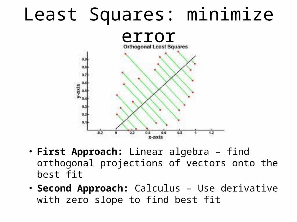
Least Squares: minimize error

• First Approach: Linear algebra – find orthogonal projections of vectors onto the best fit

• Second Approach: Calculus – Use derivative with zero slope to find best fit

Solving n equations and n unknownsNumerical Algorithms

•Gaussian Elimination – Complexity: O(n3)

•Successive Iteration– Complexity varies

•Cholskey Decomposition– More efficient, still O(n3)

•Levenson-Durbin– Complexity: O(n2)– Symmetric Toeplitz

matrices

Definitions for any matrix, ATranspose (AT): Replace all aij by aji Symmetric: AT = AToeplitz: Descending diagonals to the right have equal valuesLower/Upper triangular: No non zero values above/below diagonal

Symmetric Toeplitz Matrices

• Flipping rows and columns produces the same matrix• Every diagonal to the right contains the same value

Example

Levinson Durbin Algorithm

Verify results by plugging a41, a42, a43, a44 back into the equations

6/5(1) + 0(2) + (0)3 + 1/5(4) = 2, 6/5(2) + 0(1) + 0(2) + 1/5(3) = 36/5(3) + 0(2) + 0(1) + 1/5(2) = 4, 6/5(4) + 0(3) + 0(2) + 1/5(1) = 5

Step 0 E0 = 1 [r0 Initial Value]

Step 1 E1 = -3 [ (1-k12)E0] k1 = 2 [r1/E0]

Step 2 E2 = -8/3 [ (1-k22)E1] k2 = 1/3 [(r2 – a11r1)/E1]

Step 3 E3 = -5/2 [(1-k32)E2 k3 = 1/4 [(r3 – a21r2 – a22r1)/E2]

Step 4 E4 = -12/5 [(1-k42) E3] k4 = 1/5 [r4 – a31r3 – a32r2 – a33r1)/E3]

a11=2 [k1]

a21=4/3 [a11-k2a11] a22=1/3[k2]

a31=5/4 [a21-k3a22] a32=0 [a22-k3a21] a33=1/4 [k3]

a41=6/5 [a31-k4a33] a42=0 [a32-k4a32] a43=0[a33-k4a31] a44=1/5[k4]

or

Levinson-Durbin Pseudo Code

E0 = r0

FOR step = 1 TO Pkstep = ri

FOR i = 1 TO step-1 THEN kstep -= ai-1,i * rstep-i

kstep /= Estep-1

Estep = (1 – k2step)Estep-1

astep,step = kstep-1

For i = 1 TO step-1 THEN astep,i = astep-1,I – kstep*astep-1, step-i

Note: ri are the row 1 matrix coefficients

Cholesky Decomposition• Requirements:

– Symmetric (same matrix if flip rows and columns)– Positive definite matrix

Matrix A is real positive definite if and only if for all x ≠ 0, xTAx > 0 • Solution

– Factor matrix A into: A = LLT where L is lower triangular– Perform forward substitution to solve: L(LT[ak]) = [bk]

– Use the resulting vector, [xi], in the above step to perform a backward substitution to solve for LT[ak] = [xi]

• Complexity– Factoring step: O(n3/3) – Forward and Backward substitution: O(n2)

Cholesky Factorization

Result:

Cholesky Factorization Pseudo Code

• Column index: k• Row index: j• Elements of matrix A: aij

• Elements of matrix L: l

FOR k=1 TO n-1 lkk = a½

kk

FOR j = k+1 TO n ljk = ajk/ lkk

FOR j = k+1 TO nFOR i = j TO n aij = aij – lik ljk

lnn = ann

{1, 2, 3, 4, 5, 6, 7, 8, 9, 10, 11, 12, 13, 14, 15, 16}

Illustration: Linear Prediction

Goal: Estimate yn using the three previous valuesyn ≈ a1 yn-1 + a2 yn-2 + a3 yn-3

Three ak coefficients, Frame size of 16Thirteen equations and three unknowns

LPC Basics• Predict x[n] from x[n-1], … , x[n-P]

– en = yn - ∑k=1,P ak yn-k

– en is the error between the projection and the actual value

– The goal is to find the coefficients that produce the smallest en value

• Concept– Square the error– Take the partial derivative with respect to each ak

– Optimize (The minimum slope has a derivative of zero)– Result: P equations and P unknowns– Solve using either the Cholesky or Levinson-Durbin algorithms

LPC Derivation• One linear prediction equation: en = yn - ∑k=1,P ak yn-k

Over a whole frame we have n equations and k unknowns• Sum en over the entire frame: E = ∑n=0,N-1(yn - ∑k=1,P ak yn-k)

• Square the total error: E2 = ∑n=0,N-1 (yn - ∑k=1,P ak yn-k)2

• Partial derivative with respect to each aj; generates P equations (Ej)

Like a regular derivative treating only aj as a variable

2Ej = 2(∑n=0,N-1 (yn - ∑k=1,P akyn-k)yn-j)

Calculus Chain Rule: if y = y(u(x)) then dy/dx = dy/du * du/dx• Set each Ej to zero (zero derivative) to find the minimum P errors

for j = 1 to P then 0 = ∑n=0,N-1 (yn - ∑k=1,P akyn-k)yn-j (j indicates the equation)

• Rearrange terms: for each j of the P equations, ∑n=0,N-1 ynyn-j = ∑n=0,N-1∑k=1,Pakyn-kyn-j = ∑k=1,P∑n=1,Nakyn-kyn-j

• Yule Walker equations: IF φ(j,0)= ∑n=0,N-1 ynyn-j, THEN φ(j,0) = ∑k=1,Pakφ(j,k)

• Result: P equations and P unknowns (ak), one solution for the best prediction

LPC: the Covariance Method• Result from previous: φ(j,k) = ∑k=1,P∑n=0,N-1yn-kyn-j

• Equation j: φ(j,0)=∑k=1,Pakφ(j,k)

• Now we have P equations and P unknowns• Because φ(j,k) = φ(k,j), the matrix is symmetric• Solution requires O(n3) iterations (ex: Cholskey’s decomposition)• Why covariance? It’s not probabilistic, but the matrix looks similar

Covariance Example

• Signal: { … , 3, 2, -1, -3, -5, -2, 0, 1, 2, 4, 3, 1, 0, -1, -2, -4, -1, 0, 3, 1, 0, … }• Frame: {-5, -2, 0, 1, 2, 4, 3, 1}, Number of coefficients: 3• φ(1,1) = -3*-3 +-5*-5 + -2*-2 + 0*0 + 1*1 + 2*2 + 4*4 + 3*3 = 68 • φ(2,1) = -1*-3 +-3*-5 + -5*-2 + -2*0 + 0*1 + 1*2 + 2*4 + 4*3 = 50 • φ(3,1) = 2*-3 +-1*-5 + -3*-2 + -5*0 + -2*1 + 0*2 + 1*4 + 2*3 = 13 • φ(1,2) = -3*-1 +-5*-3 + -2*-5 + 0*-2 + 1*0 + 2*1 + 4*2 + 3*4 = 50 • φ(2,2) = -1*-1 +-3*-3 + -5*-5 + -2*-2 + 0*0 + 1*1 + 2*2 + 4*4 = 60 • φ(3,2) = 2*-1 +-1*-3 + -3*-5 + -5*-2 + -2*0 + 0*1 + 1*2 + 2*4 = 36 • φ(1,3) = -3*2 +-5*-1 + -2*-3 + 0*-5 + 1*-2 + 2*0 + 4*1 + 3*2 = 13 • φ(2,3) = -1*2 +-3*-1 + -5*-3 + -2*-5 + 0*-2 + 1*0 + 2*1 + 4*2 = 36 • φ(3,3) = 2*2 +-1*-1 + -3*-3 + -5*-5 + -2*-2 + 0*0 + 1*1 + 2*2 = 48 • φ(1,0) = -3*-5 +-5*-2 + -2*0 + 0*1 + 1*2 + 2*4 + 4*3 + 3*1 = 50 • φ(2,0) = -1*-5 +-3*-2 + -5*0 + -2*1 + 0*2 + 1*4 + 2*3 + 4*1 = 23 • φ(3,0) = 2*-5 +-1*-2 + -3*0 + -5*1 + -2*2 + 0*4 + 1*3 + 2*1 = -12

Recall: φ(j,k) = ∑n=start,start+N-1 yn-kyn-j Where equation j is: φ(j,0) = ∑k=1,Pakφ(j,k)

Auto-Correlation Method• Assume: all signal values outside of the frame (0<j<N-1) assumed zero

• Correlate from -∞ to ∞ (most values are 0)• The LPC formula for φ becomes: φ(j,k)=∑n=0,N-1-(j-k) ynyn+(j-k)=R(j-k)

• The Matrix is now in the Toplitz format– The Levinson Durbin algorithm applies – Implementation complexity: O(n2)

Auto Correlation Example

• Signal: {…, 3, 2, -1, -3, -5, -2, 0, 1, 2, 4, 3, 1, 0, -1, -2, -4, -1, 0, 3, 1, 0, …}• Frame: {-5, -2, 0, 1, 2, 4, 3, 1}, Number of coefficients: 3

• R(0) = -5*-5 + -2*-2 + 0*0 + 1*1 + 2*2 + 4*4 + 3*3 + 1*1 = 60• R(1) = -5*-2 + -2*0 + 0*1 + 1*2 + 2*4 + 4*3 + 3*1 = 35• R(2) = -5*0 + -2*1 + 0*2 + 1*4 + 2*3 + 4*1 = 12• R(3) = -5*1 + -2*2 + 0*4 + 1*3 + 2*1 = -4

Recall: φ(j,k)=∑n=0,N-1-(j-k) ynyn+(j-k)=R(j-k)Where equation j is: R(j) = ∑k=1,P R(j-k)ak

LPC Transfer Function• Predict the values of the next sample

Ŝ[n] = ∑ k=1,p ak s[n−k]

• The error signal (e[n]), is the LPC residuale[n]=s[n]− ŝ[n] = s[n]− ∑ k=1,p ak s[n−k]

• Perform a Z-transform of both sidesE(z)=S(z)− ∑k=1,pak S(z)z−k

• Factor S(z)E(z) = S(z)[ 1−∑k=1,p ak z−k ]=S(z)A(z)

• Compute the transfer function: S(z) = E(z)/A(z)

• Conclusion: LPC is an all pole IIR filter

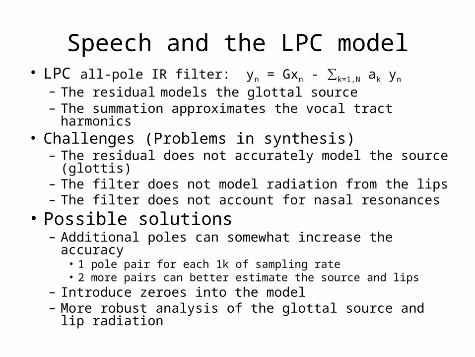
Speech and the LPC model• LPC all-pole IR filter: yn = Gxn - ∑k=1,N ak yn

– The residual models the glottal source– The summation approximates the vocal tract harmonics

• Challenges (Problems in synthesis)– The residual does not accurately model the source (glottis) – The filter does not model radiation from the lips– The filter does not account for nasal resonances

• Possible solutions– Additional poles can somewhat increase the accuracy

• 1 pole pair for each 1k of sampling rate• 2 more pairs can better estimate the source and lips

– Introduce zeroes into the model– More robust analysis of the glottal source and lip radiation

Vocal Tract Tube Model• Series of short uniform tubes

connected in series– Each slice has a fixed area– Add slices for the model to

become more continuous

• Analysis– Using physics of gas flow through

pipes– LPC turns out to be equivalent to

this model– Equations exist to compute pipe

diameters using LPC coefficients

The LPC Spectrum

1. Perform a LPC analysis2. Find the poles3. Plot the spectrum around

the z-Plane unit circle

What do we find concerning the LPC spectrum?1.Adding poles better matches speech up to about 18 for a 16k sampling rate2.The peaks tend to be overly sharp (“spiky”) because small radius changesgreatly alters pole skirt widths