Embed Size (px)
Citation preview

Linear Programming
Lecture 13: Sensitivity Analysis
Lecture 13: Sensitivity Analysis Linear Programming 1 / 62
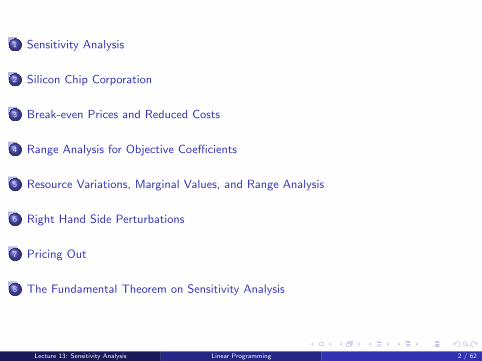
1 Sensitivity Analysis
2 Silicon Chip Corporation
3 Break-even Prices and Reduced Costs
4 Range Analysis for Objective Coefficients
5 Resource Variations, Marginal Values, and Range Analysis
6 Right Hand Side Perturbations
7 Pricing Out
8 The Fundamental Theorem on Sensitivity Analysis
Lecture 13: Sensitivity Analysis Linear Programming 2 / 62

Sensitivity Analysis
We now study general questions involving the sensitivity of the solution to an LP underchanges to its input data.
As it turns out LP solutions can be extremely sensitive to such changes and this has veryimportant practical consequences for the use of LP technology in applications.
For this reason it is very important to have tools for assessing the sensitivity of a solutionto an LP. Without an understanding of this sensitivity, the solution to the LP may beworse than useless. Indeed, it may be dangerous.
We begin our study of sensitivity analysis with a concrete toy example.
Lecture 13: Sensitivity Analysis Linear Programming 3 / 62

SILICON CHIP CORPORATION
A Silicon Valley firm specializes in making four types of silicon chips for personal computers.Each chip must go through four stages of processing before completion. First the basic siliconwafers are manufactured, second the wafers are laser etched with a micro circuit, next the circuitis laminated onto the chip, and finally the chip is tested and packaged for shipping. Theproduction manager desires to maximize profits during the next month. During the next 30 daysshe has enough raw material to produce 4000 silicon wafers. Moreover, she has 600 hours ofetching time, 900 hours of lamination time, and 700 hours of testing time. Taking into accountdepreciated capital investment, maintenance costs, and the cost of labor, each raw silicon waferis worth $1, each hour of etching time costs $40, each hour of lamination time costs $60, andeach hour of inspection time costs $10.
The production manager has formulated her problem as a profit maximization
Lecture 13: Sensitivity Analysis Linear Programming 4 / 62

SILICON CHIP CORPORATION
Initial Tableau:
x1 x2 x3 x4 x5 x6 x7 x8 b
raw wafers 100 100 100 100 1 0 0 0 4000etching 10 10 20 20 0 1 0 0 600lamination 20 20 30 20 0 0 1 0 900testing 20 10 30 30 0 0 0 1 700
2000 3000 5000 4000 0 0 0 0 0
x1, x2, x3, x4 represent the number of 100 chip batches of the four types of chips.The objective row coefficients correspond to dollars profit per 100 chip batch.
Lecture 13: Sensitivity Analysis Linear Programming 5 / 62

SILICON CHIP CORPORATION
Initial Tableau:
x1 x2 x3 x4 x5 x6 x7 x8 b
raw wafers 100 100 100 100 1 0 0 0 4000etching 10 10 20 20 0 1 0 0 600lamination 20 20 30 20 0 0 1 0 900testing 20 10 30 30 0 0 0 1 700
2000 3000 5000 4000 0 0 0 0 0
x1, x2, x3, x4 represent the number of 100 chip batches of the four types of chips.
The objective row coefficients correspond to dollars profit per 100 chip batch.
Lecture 13: Sensitivity Analysis Linear Programming 5 / 62

SILICON CHIP CORPORATION
Initial Tableau:
x1 x2 x3 x4 x5 x6 x7 x8 b
raw wafers 100 100 100 100 1 0 0 0 4000etching 10 10 20 20 0 1 0 0 600lamination 20 20 30 20 0 0 1 0 900testing 20 10 30 30 0 0 0 1 700
2000 3000 5000 4000 0 0 0 0 0
x1, x2, x3, x4 represent the number of 100 chip batches of the four types of chips.The objective row coefficients correspond to dollars profit per 100 chip batch.
Lecture 13: Sensitivity Analysis Linear Programming 5 / 62

SILICON CHIP CORPORATION
Optimal tableau:
x1 x2 x3 x4 x5 x6 x7 x8 b
0.5 1 0 0 .015 0 0 −.05 25−5 0 0 0 −.05 1 0 −.5 50
0 0 1 0 −.02 0 .1 0 100.5 0 0 1 .015 0 −.1 .05 5
−1500 0 0 0 −5 0 −100 −50 −145, 000
The optimal production schedule is
(x1, x2, x3, x4) = (0, 25, 10, 5),
and the optimal value is $145, 000.
Lecture 13: Sensitivity Analysis Linear Programming 6 / 62

Break-even Prices and Reduced Costs
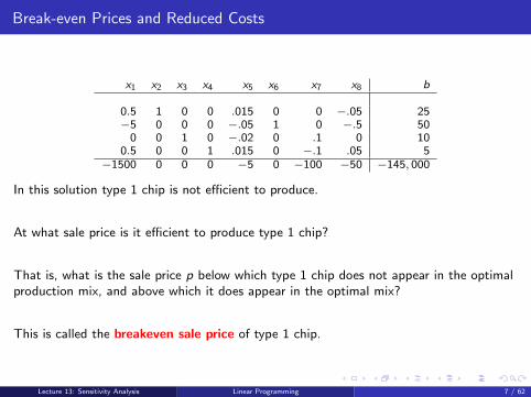
x1 x2 x3 x4 x5 x6 x7 x8 b
0.5 1 0 0 .015 0 0 −.05 25−5 0 0 0 −.05 1 0 −.5 50
0 0 1 0 −.02 0 .1 0 100.5 0 0 1 .015 0 −.1 .05 5
−1500 0 0 0 −5 0 −100 −50 −145, 000
In this solution type 1 chip is not efficient to produce.
At what sale price is it efficient to produce type 1 chip?
That is, what is the sale price p below which type 1 chip does not appear in the optimalproduction mix, and above which it does appear in the optimal mix?
This is called the breakeven sale price of type 1 chip.
Lecture 13: Sensitivity Analysis Linear Programming 7 / 62

Break-even Prices and Reduced Costs
x1 x2 x3 x4 x5 x6 x7 x8 b
0.5 1 0 0 .015 0 0 −.05 25−5 0 0 0 −.05 1 0 −.5 50
0 0 1 0 −.02 0 .1 0 100.5 0 0 1 .015 0 −.1 .05 5
−1500 0 0 0 −5 0 −100 −50 −145, 000
In this solution type 1 chip is not efficient to produce.
At what sale price is it efficient to produce type 1 chip?
That is, what is the sale price p below which type 1 chip does not appear in the optimalproduction mix, and above which it does appear in the optimal mix?
This is called the breakeven sale price of type 1 chip.
Lecture 13: Sensitivity Analysis Linear Programming 7 / 62

Break-even Prices and Reduced Costs
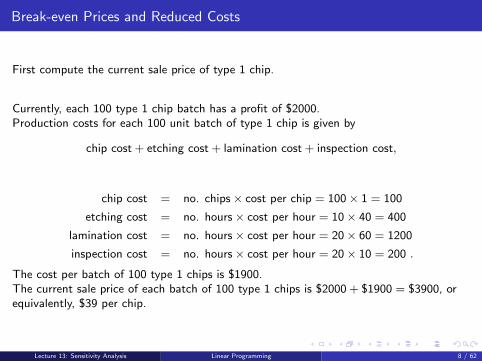
First compute the current sale price of type 1 chip.
Currently, each 100 type 1 chip batch has a profit of $2000.Production costs for each 100 unit batch of type 1 chip is given by
chip cost + etching cost + lamination cost + inspection cost,
chip cost = no. chips× cost per chip = 100× 1 = 100
etching cost = no. hours× cost per hour = 10× 40 = 400
lamination cost = no. hours× cost per hour = 20× 60 = 1200
inspection cost = no. hours× cost per hour = 20× 10 = 200 .
The cost per batch of 100 type 1 chips is $1900.The current sale price of each batch of 100 type 1 chips is $2000 + $1900 = $3900, orequivalently, $39 per chip.
Lecture 13: Sensitivity Analysis Linear Programming 8 / 62

Break-even Prices and Reduced Costs
First compute the current sale price of type 1 chip.
Currently, each 100 type 1 chip batch has a profit of $2000.
Production costs for each 100 unit batch of type 1 chip is given by
chip cost + etching cost + lamination cost + inspection cost,
chip cost = no. chips× cost per chip = 100× 1 = 100
etching cost = no. hours× cost per hour = 10× 40 = 400
lamination cost = no. hours× cost per hour = 20× 60 = 1200
inspection cost = no. hours× cost per hour = 20× 10 = 200 .
The cost per batch of 100 type 1 chips is $1900.The current sale price of each batch of 100 type 1 chips is $2000 + $1900 = $3900, orequivalently, $39 per chip.
Lecture 13: Sensitivity Analysis Linear Programming 8 / 62

Break-even Prices and Reduced Costs
First compute the current sale price of type 1 chip.
Currently, each 100 type 1 chip batch has a profit of $2000.Production costs for each 100 unit batch of type 1 chip is given by
chip cost + etching cost + lamination cost + inspection cost,
chip cost = no. chips× cost per chip = 100× 1 = 100
etching cost = no. hours× cost per hour = 10× 40 = 400
lamination cost = no. hours× cost per hour = 20× 60 = 1200
inspection cost = no. hours× cost per hour = 20× 10 = 200 .
The cost per batch of 100 type 1 chips is $1900.The current sale price of each batch of 100 type 1 chips is $2000 + $1900 = $3900, orequivalently, $39 per chip.
Lecture 13: Sensitivity Analysis Linear Programming 8 / 62

Break-even Prices and Reduced Costs
First compute the current sale price of type 1 chip.
Currently, each 100 type 1 chip batch has a profit of $2000.Production costs for each 100 unit batch of type 1 chip is given by
chip cost + etching cost + lamination cost + inspection cost,
chip cost = no. chips× cost per chip = 100× 1 = 100
etching cost = no. hours× cost per hour = 10× 40 = 400
lamination cost = no. hours× cost per hour = 20× 60 = 1200
inspection cost = no. hours× cost per hour = 20× 10 = 200 .
The cost per batch of 100 type 1 chips is $1900.
The current sale price of each batch of 100 type 1 chips is $2000 + $1900 = $3900, orequivalently, $39 per chip.
Lecture 13: Sensitivity Analysis Linear Programming 8 / 62
Break-even Prices and Reduced Costs
First compute the current sale price of type 1 chip.
Currently, each 100 type 1 chip batch has a profit of $2000.Production costs for each 100 unit batch of type 1 chip is given by
chip cost + etching cost + lamination cost + inspection cost,
chip cost = no. chips× cost per chip = 100× 1 = 100
etching cost = no. hours× cost per hour = 10× 40 = 400
lamination cost = no. hours× cost per hour = 20× 60 = 1200
inspection cost = no. hours× cost per hour = 20× 10 = 200 .
The cost per batch of 100 type 1 chips is $1900.The current sale price of each batch of 100 type 1 chips is $2000 + $1900 = $3900, orequivalently, $39 per chip.
Lecture 13: Sensitivity Analysis Linear Programming 8 / 62
Break-even Prices and Reduced Costs
We do not produce type 1 chip in our optimal production mix, so the breakeven sale pricemust be greater than $39 per chip.
Let θ denote the increase in sale price of type 1 chip needed for it to enter the optimalproduction mix.
Lecture 13: Sensitivity Analysis Linear Programming 9 / 62

Break-even Prices and Reduced Costs
With this change to the sale price of type 1 chip the initial tableau for the LP becomes
x1 x2 x3 x4 x5 x6 x7 x8 b
raw wafers 100 100 100 100 1 0 0 0 4000etching 10 10 20 20 0 1 0 0 600lamination 20 20 30 20 0 0 1 0 900testing 20 10 30 30 0 0 0 1 700
2000 + θ 3000 5000 4000 0 0 0 0 0
.
Suppose we repeat on this tableau all of the pivots that led to the previously optimaltableau.What will the new tableau look like? That is, how does θ appear in this new tableau?
Lecture 13: Sensitivity Analysis Linear Programming 10 / 62

Break-even Prices and Reduced Costs
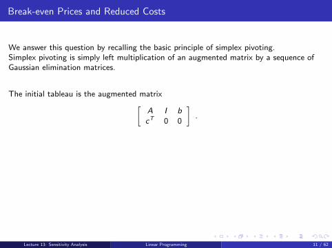
We answer this question by recalling the basic principle of simplex pivoting.
Simplex pivoting is simply left multiplication of an augmented matrix by a sequence ofGaussian elimination matrices.
The initial tableau is the augmented matrix[A I bcT 0 0
].
Pivoting to an optimal tableau corresponds to left multiplication by a matrix of the form
G =
[R 0−yT 1
].
The nonsingular matrix R is called the record matrix.
Lecture 13: Sensitivity Analysis Linear Programming 11 / 62
Break-even Prices and Reduced Costs
We answer this question by recalling the basic principle of simplex pivoting.Simplex pivoting is simply left multiplication of an augmented matrix by a sequence ofGaussian elimination matrices.
The initial tableau is the augmented matrix[A I bcT 0 0
].
Pivoting to an optimal tableau corresponds to left multiplication by a matrix of the form
G =
[R 0−yT 1
].
The nonsingular matrix R is called the record matrix.
Lecture 13: Sensitivity Analysis Linear Programming 11 / 62
Break-even Prices and Reduced Costs
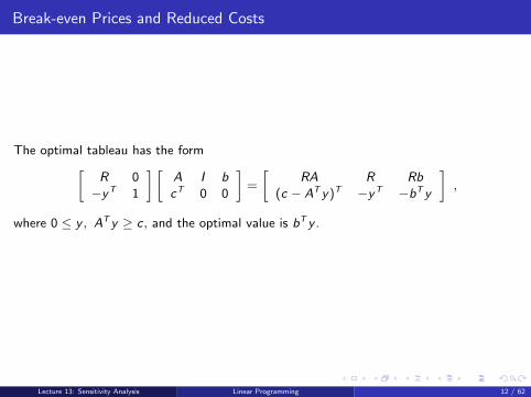
The optimal tableau has the form[R 0−yT 1
] [A I bcT 0 0
]=
[RA R Rb
(c − AT y)T −yT −bT y
],
where 0 ≤ y , AT y ≥ c, and the optimal value is bT y .
Lecture 13: Sensitivity Analysis Linear Programming 12 / 62

Break-even Prices and Reduced Costs
Changing the value of one (or more) of the objective coefficients c corresponds toreplacing c by a vector of the form c + ∆c.
The corresponding new initial tableau is[A I b
(c + ∆c)T 0 0
].
Lecture 13: Sensitivity Analysis Linear Programming 13 / 62

Break-even Prices and Reduced Costs
Changing the value of one (or more) of the objective coefficients c corresponds toreplacing c by a vector of the form c + ∆c.
The corresponding new initial tableau is[A I b
(c + ∆c)T 0 0
].
Lecture 13: Sensitivity Analysis Linear Programming 13 / 62

Break-even Prices and Reduced Costs
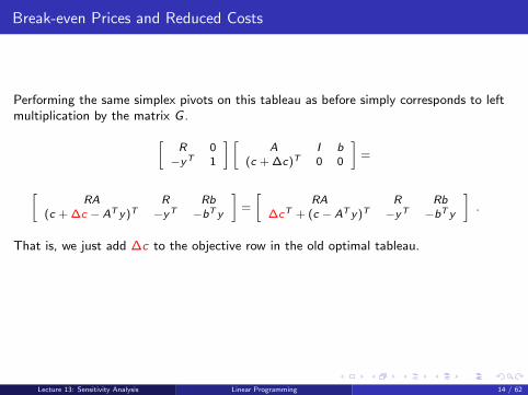
Performing the same simplex pivots on this tableau as before simply corresponds to leftmultiplication by the matrix G .
[R 0
−yT 1
] [A I b
(c + ∆c)T 0 0
]=
[RA R Rb
(c + ∆c − AT y)T −yT −bT y
]=
[RA R Rb
∆cT + (c − AT y)T −yT −bT y
].
That is, we just add ∆c to the objective row in the old optimal tableau.
Lecture 13: Sensitivity Analysis Linear Programming 14 / 62

Break-even Prices and Reduced Costs
Performing the same simplex pivots on this tableau as before simply corresponds to leftmultiplication by the matrix G .
[R 0
−yT 1
] [A I b
(c + ∆c)T 0 0
]=
[RA R Rb
(c + ∆c − AT y)T −yT −bT y
]=
[RA R Rb
∆cT + (c − AT y)T −yT −bT y
].
That is, we just add ∆c to the objective row in the old optimal tableau.
Lecture 13: Sensitivity Analysis Linear Programming 14 / 62

Break-even Prices and Reduced Costs
T =
[RA R Rb
∆cT + (c − AT y)T −yT −bT y
]If T is a tableau, then T remains optimal if and only if
∆c + (c − AT y) ≤ 0
or equivalently,∆c ≤ −(c − AT y) .
These inequalities place restrictions on how large the entries of ∆c can be before onemust pivot to obtain the new optimal tableau.
Lecture 13: Sensitivity Analysis Linear Programming 15 / 62

Break-even Prices and Reduced Costs
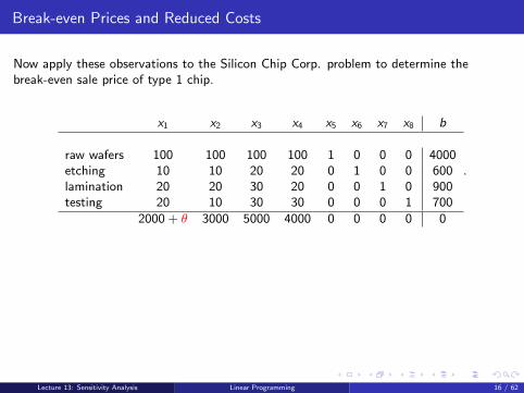
Now apply these observations to the Silicon Chip Corp. problem to determine thebreak-even sale price of type 1 chip.
x1 x2 x3 x4 x5 x6 x7 x8 b
raw wafers 100 100 100 100 1 0 0 0 4000etching 10 10 20 20 0 1 0 0 600lamination 20 20 30 20 0 0 1 0 900testing 20 10 30 30 0 0 0 1 700
2000 + θ 3000 5000 4000 0 0 0 0 0
.
c =
2000300050004000
, ∆c =
θ000
= θe1, c + ∆c =
2000 + θ
300050004000
= c + θe1
Lecture 13: Sensitivity Analysis Linear Programming 16 / 62
Break-even Prices and Reduced Costs
Now apply these observations to the Silicon Chip Corp. problem to determine thebreak-even sale price of type 1 chip.
x1 x2 x3 x4 x5 x6 x7 x8 b
raw wafers 100 100 100 100 1 0 0 0 4000etching 10 10 20 20 0 1 0 0 600lamination 20 20 30 20 0 0 1 0 900testing 20 10 30 30 0 0 0 1 700
2000 + θ 3000 5000 4000 0 0 0 0 0
.
c =
2000300050004000
, ∆c =
θ000
= θe1, c + ∆c =
2000 + θ
300050004000
= c + θe1
Lecture 13: Sensitivity Analysis Linear Programming 16 / 62

Break-even Prices and Reduced Costs
[RA R Rb
(c − AT y)T −yT −bT y
]=
x1 x2 x3 x4 x5 x6 x7 x8 b
0.5 1 0 0 .015 0 0 −.05 25−5 0 0 0 −.05 1 0 −.5 50
0 0 1 0 −.02 0 .1 0 100.5 0 0 1 .015 0 −.1 .05 5
−1500 0 0 0 −5 0 −100 −50 −145, 000
∆c + (c − AT y) = θe1 + (c − AT y) =
θ000
−
1500000
=
θ − 1500
000
Lecture 13: Sensitivity Analysis Linear Programming 17 / 62

Break-even Prices and Reduced Costs
∆c + (c − AT y) =
θ − 1500
000
,
x1 x2 x3 x4 x5 x6 x7 x8 b
0.5 1 0 0 .015 0 0 −.05 25−5 0 0 0 −.05 1 0 −.5 50
0 0 1 0 −.02 0 .1 0 100.5 0 0 1 .015 0 −.1 .05 5
θ − 1500 0 0 0 −5 0 −100 −50 −145, 000
Thus, to preserve optimality, we need θ ≤ 1500.
Lecture 13: Sensitivity Analysis Linear Programming 18 / 62

Break-even Prices and Reduced Costs
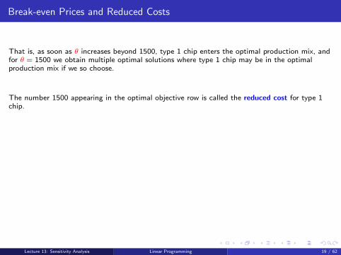
That is, as soon as θ increases beyond 1500, type 1 chip enters the optimal production mix, andfor θ = 1500 we obtain multiple optimal solutions where type 1 chip may be in the optimalproduction mix if we so choose.
The number 1500 appearing in the optimal objective row is called the reduced cost for type 1chip.
In general, the negative of the objective row coefficient for decision variables in the optimaltableau are the reduced costs of these variables.The reduced cost of a decision variable is the needed increase in its objective row coefficient inorder for it to be included in the optimal solution.For non-basic variables the break-even sale price can be read off from the reduced costs in theoptimal tableau.
break-even price = current price + reduced cost = $39 + $15 = $54 .
Lecture 13: Sensitivity Analysis Linear Programming 19 / 62
Break-even Prices and Reduced Costs
That is, as soon as θ increases beyond 1500, type 1 chip enters the optimal production mix, andfor θ = 1500 we obtain multiple optimal solutions where type 1 chip may be in the optimalproduction mix if we so choose.
The number 1500 appearing in the optimal objective row is called the reduced cost for type 1chip.
In general, the negative of the objective row coefficient for decision variables in the optimaltableau are the reduced costs of these variables.The reduced cost of a decision variable is the needed increase in its objective row coefficient inorder for it to be included in the optimal solution.For non-basic variables the break-even sale price can be read off from the reduced costs in theoptimal tableau.
break-even price = current price + reduced cost = $39 + $15 = $54 .
Lecture 13: Sensitivity Analysis Linear Programming 19 / 62

Break-even Prices and Reduced Costs
That is, as soon as θ increases beyond 1500, type 1 chip enters the optimal production mix, andfor θ = 1500 we obtain multiple optimal solutions where type 1 chip may be in the optimalproduction mix if we so choose.
The number 1500 appearing in the optimal objective row is called the reduced cost for type 1chip.
In general, the negative of the objective row coefficient for decision variables in the optimaltableau are the reduced costs of these variables.
The reduced cost of a decision variable is the needed increase in its objective row coefficient inorder for it to be included in the optimal solution.For non-basic variables the break-even sale price can be read off from the reduced costs in theoptimal tableau.
break-even price = current price + reduced cost = $39 + $15 = $54 .
Lecture 13: Sensitivity Analysis Linear Programming 19 / 62

Break-even Prices and Reduced Costs
That is, as soon as θ increases beyond 1500, type 1 chip enters the optimal production mix, andfor θ = 1500 we obtain multiple optimal solutions where type 1 chip may be in the optimalproduction mix if we so choose.
The number 1500 appearing in the optimal objective row is called the reduced cost for type 1chip.
In general, the negative of the objective row coefficient for decision variables in the optimaltableau are the reduced costs of these variables.The reduced cost of a decision variable is the needed increase in its objective row coefficient inorder for it to be included in the optimal solution.
For non-basic variables the break-even sale price can be read off from the reduced costs in theoptimal tableau.
break-even price = current price + reduced cost = $39 + $15 = $54 .
Lecture 13: Sensitivity Analysis Linear Programming 19 / 62

Break-even Prices and Reduced Costs
That is, as soon as θ increases beyond 1500, type 1 chip enters the optimal production mix, andfor θ = 1500 we obtain multiple optimal solutions where type 1 chip may be in the optimalproduction mix if we so choose.
The number 1500 appearing in the optimal objective row is called the reduced cost for type 1chip.
In general, the negative of the objective row coefficient for decision variables in the optimaltableau are the reduced costs of these variables.The reduced cost of a decision variable is the needed increase in its objective row coefficient inorder for it to be included in the optimal solution.For non-basic variables the break-even sale price can be read off from the reduced costs in theoptimal tableau.
break-even price = current price + reduced cost = $39 + $15 = $54 .
Lecture 13: Sensitivity Analysis Linear Programming 19 / 62

Break-even Prices and Reduced Costs
That is, as soon as θ increases beyond 1500, type 1 chip enters the optimal production mix, andfor θ = 1500 we obtain multiple optimal solutions where type 1 chip may be in the optimalproduction mix if we so choose.
The number 1500 appearing in the optimal objective row is called the reduced cost for type 1chip.
In general, the negative of the objective row coefficient for decision variables in the optimaltableau are the reduced costs of these variables.The reduced cost of a decision variable is the needed increase in its objective row coefficient inorder for it to be included in the optimal solution.For non-basic variables the break-even sale price can be read off from the reduced costs in theoptimal tableau.
break-even price = current price + reduced cost = $39 + $15 = $54 .
Lecture 13: Sensitivity Analysis Linear Programming 19 / 62

Break-even Prices and Reduced Costs
Now consider a more intuitive and simpler explanation of break-even sale prices.
One way to determine these prices, is to determine by how much our profit is reduced ifwe produce one batch of these chips.
Recall that the objective row coefficients in the optimal tableau correspond to thefollowing expression for the objective variable z :
z = 145000− 1500x1 − 5x5 − 100x7 − 50x8.
Hence, if we make one batch of type 1 chip, we reduce our optimal value by $1500.Thus, to recoup this loss we must charge $1500 more for these chips yielding abreak-even sale price of $39 + $15 = $54 per chip.
Lecture 13: Sensitivity Analysis Linear Programming 20 / 62

Range Analysis for Objective Coefficients
Range analysis is a tool for understanding the effects of both objective coefficientvariations as well as resource availability variations.
We now examine objective coefficient variations.
Lecture 13: Sensitivity Analysis Linear Programming 21 / 62
Range Analysis for Objective Coefficients
Range analysis is a tool for understanding the effects of both objective coefficientvariations as well as resource availability variations.
We now examine objective coefficient variations.
Lecture 13: Sensitivity Analysis Linear Programming 21 / 62
Range Analysis for Objective Coefficients
Recall that to compute a breakeven price one needs to determine the change in theassociated objective coefficient that make it efficient to introduce this activity into theoptimal production mix, or equivalently, to determine the smallest change in the objectivecoefficient of this currently non-basic decision variable that requires one to bring it intothe basis in order to maintain optimality.
A related question is what is the range of variation of a given objective coefficient thatpreserves the current basis as optimal?
The answer to this question is an interval, possibly unbounded, on the real line withinwhich a given objective coefficient can vary but these variations do not effect thecurrently optimal basis.
Lecture 13: Sensitivity Analysis Linear Programming 22 / 62

SILICON CHIP CORPORATION
Initial Tableau x1 x2 x3 x4 x5 x6 x7 x8 b
raw wafers 100 100 100 100 1 0 0 0 4000etching 10 10 20 20 0 1 0 0 600lamination 20 20 30 20 0 0 1 0 900testing 20 10 30 30 0 0 0 1 700
2000 3000 5000 4000 0 0 0 0 0
Opt. Tableau x1 x2 x3 x4 x5 x6 x7 x8 b
0.5 1 0 0 .015 0 0 −.05 25−5 0 0 0 −.05 1 0 −.5 50
0 0 1 0 −.02 0 .1 0 100.5 0 0 1 .015 0 −.1 .05 5
−1500 0 0 0 −5 0 −100 −50 −145, 000
Lecture 13: Sensitivity Analysis Linear Programming 23 / 62

Range Analysis for Objective Coefficients
Silicon Chip Corp optimal tableau.
x1 x2 x3 x4 x5 x6 x7 x8 b0.5 1 0 0 .015 0 0 −.05 25−5 0 0 0 −.05 1 0 −.5 500 0 1 0 −.02 0 .1 0 10
0.5 0 0 1 .015 0 −.1 .05 5−1500 0 0 0 −5 0 −100 −50 −145, 000
In the Silicon Chip Corp problem the decision variable x3 associated with type 3 chips isin the optimal basis.
For what range of variations in c3 = 5000 does the current optimal basis {x2, x3, x4, x6}remain optimal?
Lecture 13: Sensitivity Analysis Linear Programming 24 / 62

Range Analysis for Objective Coefficients
To answer this question we perturb the objective coef. of type 3 chip and writec3 = 5000 + θ.
The resulting change to the optimal tableau is
x1 x2 x3 x4 x5 x6 x7 x8 b0.5 1 0 0 .015 0 0 −.05 25−5 0 0 0 −.05 1 0 −.5 500 0 1 0 −.02 0 .1 0 10
0.5 0 0 1 .015 0 −.1 .05 5−1500 0 θ 0 −5 0 −100 −50 −145, 000
This is no-longer a simplex tableau. To recover a tableau we must pivot on the x3 column.
Lecture 13: Sensitivity Analysis Linear Programming 25 / 62

x1 x2 x3 x4 x5 x6 x7 x8 b0.5 1 0 0 .015 0 0 −.05 25−5 0 0 0 −.05 1 0 −.5 500 0 1 0 −.02 0 .1 0 10
0.5 0 0 1 .015 0 −.1 .05 5−1500 0 θ 0 −5 0 −100 −50 −145, 000
To recover a proper simplex tableau we must eliminate θ from the objective row entryunder x3.
Multiply the 3rd row by −θ and add it to the objective row to eliminate θ.
Lecture 13: Sensitivity Analysis Linear Programming 26 / 62

x1 x2 x3 x4 x5 x6 x7 x8 b0.5 1 0 0 .015 0 0 −.05 25−5 0 0 0 −.05 1 0 −.5 500 0 1 0 −.02 0 .1 0 10
0.5 0 0 1 .015 0 −.1 .05 5−1500 0 0 0 −5 + 0.02θ 0 −100 − 0.1 θ −50 −145, 000 − 10θ
.
To remain optimal the objective row must remain non-positive.
−5 + 0.02θ ≤ 0, or equivalently, θ ≤ 250−100− 0.1θ ≤ 0, or equivalently, −1000 ≤ θ .
which implies4000 ≤ c3 ≤ 5250.
since originally c3 = 5000.
Lecture 13: Sensitivity Analysis Linear Programming 27 / 62

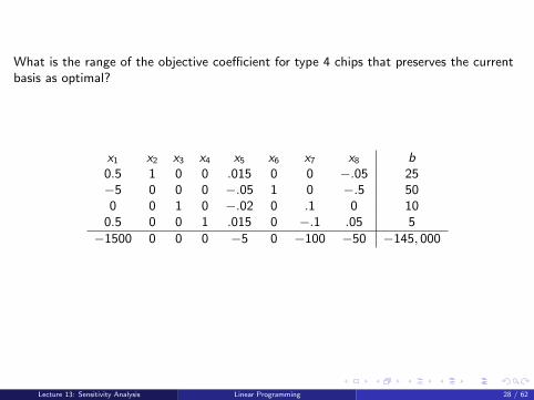
What is the range of the objective coefficient for type 4 chips that preserves the currentbasis as optimal?
x1 x2 x3 x4 x5 x6 x7 x8 b0.5 1 0 0 .015 0 0 −.05 25−5 0 0 0 −.05 1 0 −.5 500 0 1 0 −.02 0 .1 0 10
0.5 0 0 1 .015 0 −.1 .05 5−1500 0 0 0 −5 0 −100 −50 −145, 000
Lecture 13: Sensitivity Analysis Linear Programming 28 / 62

x1 x2 x3 x4 x5 x6 x7 x8 b0.5 1 0 0 .015 0 0 −.05 25−5 0 0 0 −.05 1 0 −.5 500 0 1 0 −.02 0 .1 0 10
0.5 0 0 1 .015 0 −.1 .05 5−1500 0 0 θ −5 0 −100 −50 −145, 000
0.5 1 0 0 .015 0 0 −.05 25− 5 0 0 0 −.05 1 0 −.5 500 0 1 0 −.02 0 .1 0 10
0.5 0 0 1 .015 0 −.1 .05 5− 1500 − 0.5θ 0 0 0 −5 − 0.015θ 0 −100 + 0.1θ −50 − 0.05θ −145, 000 − 5θ
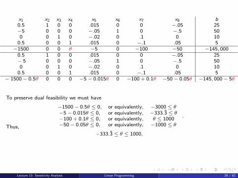
To preserve dual feasibility we must have
−1500 − 0.5θ ≤ 0, or equivalently, −3000 ≤ θ−5 − 0.015θ ≤ 0, or equivalently, −333.3̄ ≤ θ−100 + 0.1θ ≤ 0, or equivalently, θ ≤ 1000−50 − 0.05θ ≤ 0, or equivalently, −1000 ≤ θ
.
Thus,
−333.3̄ ≤ θ ≤ 1000,and the range for c4 is
3666.6̄ ≤ c4 ≤ 5000since originally c4 = 4000.
Lecture 13: Sensitivity Analysis Linear Programming 29 / 62

x1 x2 x3 x4 x5 x6 x7 x8 b0.5 1 0 0 .015 0 0 −.05 25−5 0 0 0 −.05 1 0 −.5 500 0 1 0 −.02 0 .1 0 10
0.5 0 0 1 .015 0 −.1 .05 5−1500 0 0 θ −5 0 −100 −50 −145, 000
0.5 1 0 0 .015 0 0 −.05 25− 5 0 0 0 −.05 1 0 −.5 500 0 1 0 −.02 0 .1 0 10
0.5 0 0 1 .015 0 −.1 .05 5− 1500 − 0.5θ 0 0 0 −5 − 0.015θ 0 −100 + 0.1θ −50 − 0.05θ −145, 000 − 5θ
To preserve dual feasibility we must have
−1500 − 0.5θ ≤ 0, or equivalently, −3000 ≤ θ−5 − 0.015θ ≤ 0, or equivalently, −333.3̄ ≤ θ−100 + 0.1θ ≤ 0, or equivalently, θ ≤ 1000−50 − 0.05θ ≤ 0, or equivalently, −1000 ≤ θ
.
Thus,
−333.3̄ ≤ θ ≤ 1000,and the range for c4 is
3666.6̄ ≤ c4 ≤ 5000since originally c4 = 4000.
Lecture 13: Sensitivity Analysis Linear Programming 29 / 62
x1 x2 x3 x4 x5 x6 x7 x8 b0.5 1 0 0 .015 0 0 −.05 25−5 0 0 0 −.05 1 0 −.5 500 0 1 0 −.02 0 .1 0 10
0.5 0 0 1 .015 0 −.1 .05 5−1500 0 0 θ −5 0 −100 −50 −145, 000
0.5 1 0 0 .015 0 0 −.05 25− 5 0 0 0 −.05 1 0 −.5 500 0 1 0 −.02 0 .1 0 10
0.5 0 0 1 .015 0 −.1 .05 5− 1500 − 0.5θ 0 0 0 −5 − 0.015θ 0 −100 + 0.1θ −50 − 0.05θ −145, 000 − 5θ
To preserve dual feasibility we must have
−1500 − 0.5θ ≤ 0, or equivalently, −3000 ≤ θ−5 − 0.015θ ≤ 0, or equivalently, −333.3̄ ≤ θ−100 + 0.1θ ≤ 0, or equivalently, θ ≤ 1000−50 − 0.05θ ≤ 0, or equivalently, −1000 ≤ θ
.
Thus,
−333.3̄ ≤ θ ≤ 1000,
and the range for c4 is
3666.6̄ ≤ c4 ≤ 5000since originally c4 = 4000.
Lecture 13: Sensitivity Analysis Linear Programming 29 / 62

x1 x2 x3 x4 x5 x6 x7 x8 b0.5 1 0 0 .015 0 0 −.05 25−5 0 0 0 −.05 1 0 −.5 500 0 1 0 −.02 0 .1 0 10
0.5 0 0 1 .015 0 −.1 .05 5−1500 0 0 θ −5 0 −100 −50 −145, 000
0.5 1 0 0 .015 0 0 −.05 25− 5 0 0 0 −.05 1 0 −.5 500 0 1 0 −.02 0 .1 0 10
0.5 0 0 1 .015 0 −.1 .05 5− 1500 − 0.5θ 0 0 0 −5 − 0.015θ 0 −100 + 0.1θ −50 − 0.05θ −145, 000 − 5θ
To preserve dual feasibility we must have
−1500 − 0.5θ ≤ 0, or equivalently, −3000 ≤ θ−5 − 0.015θ ≤ 0, or equivalently, −333.3̄ ≤ θ−100 + 0.1θ ≤ 0, or equivalently, θ ≤ 1000−50 − 0.05θ ≤ 0, or equivalently, −1000 ≤ θ
.
Thus,
−333.3̄ ≤ θ ≤ 1000,and the range for c4 is
3666.6̄ ≤ c4 ≤ 5000since originally c4 = 4000.
Lecture 13: Sensitivity Analysis Linear Programming 29 / 62

What is the range for the objective coefficient for x2?
x1 x2 x3 x4 x5 x6 x7 x8 b0.5 1 0 0 .015 0 0 −.05 25−5 0 0 0 −.05 1 0 −.5 500 0 1 0 −.02 0 .1 0 10
0.5 0 0 1 .015 0 −.1 .05 5−1500 0 0 0 −5 0 −100 −50 −145, 000
−333.3̄ ≤ θ ≤ 1000
and1666.6̄ ≤ c2 ≤ 3000
Lecture 13: Sensitivity Analysis Linear Programming 30 / 62

Resource Variations, Marginal Values, and Range Analysis
We now consider questions concerning the effect of resource variations on the optimalsolution.
We begin with standard questions for the Silicon Chip Corp.
Suppose we wish to purchase more silicon wafers this month. Before doing so, we needto answer three obvious questions.
How many should we purchase?
What is the most that we should pay for them?
After the purchase, what is the new optimal production schedule?
Lecture 13: Sensitivity Analysis Linear Programming 31 / 62

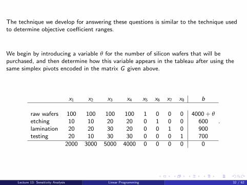
The technique we develop for answering these questions is similar to the technique usedto determine objective coefficient ranges.
We begin by introducing a variable θ for the number of silicon wafers that will bepurchased, and then determine how this variable appears in the tableau after using thesame simplex pivots encoded in the matrix G given above.
x1 x2 x3 x4 x5 x6 x7 x8 b
raw wafers 100 100 100 100 1 0 0 0 4000 + θetching 10 10 20 20 0 1 0 0 600lamination 20 20 30 20 0 0 1 0 900testing 20 10 30 30 0 0 0 1 700
2000 3000 5000 4000 0 0 0 0 0
.
Lecture 13: Sensitivity Analysis Linear Programming 32 / 62

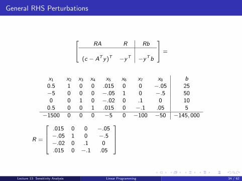
General RHS Perturbations
To effect the same simplex pivots we multiply the perturbed initial tableau by theelimination matrx G .
[R 0−yT 1
] [A I b + ∆bcT 0 0
]
=
[RA R Rb + R∆b
(c − AT y)T −yT −yTb − yT∆b
].
The new tableau is dual feasible.This tableau is optimal if it is primal feasible.That is, the new tableau is optimal as long as
0 ≤ Rb + R∆b ⇔ −Rb ≤ R∆b .
Lecture 13: Sensitivity Analysis Linear Programming 33 / 62

General RHS Perturbations
To effect the same simplex pivots we multiply the perturbed initial tableau by theelimination matrx G . [
R 0−yT 1
] [A I b + ∆bcT 0 0
]
=
[RA R Rb + R∆b
(c − AT y)T −yT −yTb − yT∆b
].
The new tableau is dual feasible.
This tableau is optimal if it is primal feasible.That is, the new tableau is optimal as long as
0 ≤ Rb + R∆b ⇔ −Rb ≤ R∆b .
Lecture 13: Sensitivity Analysis Linear Programming 33 / 62

General RHS Perturbations
To effect the same simplex pivots we multiply the perturbed initial tableau by theelimination matrx G . [
R 0−yT 1
] [A I b + ∆bcT 0 0
]
=
[RA R Rb + R∆b
(c − AT y)T −yT −yTb − yT∆b
].
The new tableau is dual feasible.This tableau is optimal if it is primal feasible.
That is, the new tableau is optimal as long as
0 ≤ Rb + R∆b ⇔ −Rb ≤ R∆b .
Lecture 13: Sensitivity Analysis Linear Programming 33 / 62

General RHS Perturbations
To effect the same simplex pivots we multiply the perturbed initial tableau by theelimination matrx G . [
R 0−yT 1
] [A I b + ∆bcT 0 0
]
=
[RA R Rb + R∆b
(c − AT y)T −yT −yTb − yT∆b
].
The new tableau is dual feasible.This tableau is optimal if it is primal feasible.That is, the new tableau is optimal as long as
0 ≤ Rb + R∆b ⇔ −Rb ≤ R∆b .
Lecture 13: Sensitivity Analysis Linear Programming 33 / 62

General RHS Perturbations
RA R Rb
(c − AT y)T −yT −yTb
=
x1 x2 x3 x4 x5 x6 x7 x8 b0.5 1 0 0 .015 0 0 −.05 25−5 0 0 0 −.05 1 0 −.5 500 0 1 0 −.02 0 .1 0 10
0.5 0 0 1 .015 0 −.1 .05 5−1500 0 0 0 −5 0 −100 −50 −145, 000
R =
.015 0 0 −.05−.05 1 0 −.5−.02 0 .1 0.015 0 −.1 .05
y =
50
10050
Rb =
2550105
Lecture 13: Sensitivity Analysis Linear Programming 34 / 62

General RHS Perturbations
How do variations the raw wafer resource effect the optimal tableau?
x1 x2 x3 x4 x5 x6 x7 x8 b
raw wafers 100 100 100 100 1 0 0 0 4000 + θetching 10 10 20 20 0 1 0 0 600lamination 20 20 30 20 0 0 1 0 900testing 20 10 30 30 0 0 0 1 700
2000 3000 5000 4000 0 0 0 0 0
.
b + ∆b = b + θe1 =
4000600900700
+ θ
1000
Lecture 13: Sensitivity Analysis Linear Programming 35 / 62

General RHS Perturbations
RA R Rb + R∆b
(c − AT y)T −yT −yTb − yT∆b
=
x1 x2 x3 x4 x5 x6 x7 x8 b0.5 1 0 0 .015 0 0 −.05 25−5 0 0 0 −.05 1 0 −.5 500 0 1 0 −.02 0 .1 0 10 +R∆b
0.5 0 0 1 .015 0 −.1 .05 5
−1500 0 0 0 −5 0 −100 −50 −145, 000 −yT∆b
0 ≤ Rb + R∆b = Rb + θRe1 =
2550105
+ θ
0.015−0.05−0.020.015
=
25 + θ 0.01550− θ 0.0510− θ 0.025 + θ 0.015
Lecture 13: Sensitivity Analysis Linear Programming 36 / 62

General RHS Perturbations
RA R Rb + R∆b
(c − AT y)T −yT −yTb − yT∆b
=
x1 x2 x3 x4 x5 x6 x7 x8 b0.5 1 0 0 .015 0 0 −.05 25−5 0 0 0 −.05 1 0 −.5 500 0 1 0 −.02 0 .1 0 10 +R∆b
0.5 0 0 1 .015 0 −.1 .05 5
−1500 0 0 0 −5 0 −100 −50 −145, 000 −yT∆b
0 ≤
Rb + R∆b = Rb + θRe1 =
2550105
+ θ
0.015−0.05−0.020.015
=
25 + θ 0.01550− θ 0.0510− θ 0.025 + θ 0.015
Lecture 13: Sensitivity Analysis Linear Programming 36 / 62

General RHS Perturbations
RA R Rb + R∆b
(c − AT y)T −yT −yTb − yT∆b
=
x1 x2 x3 x4 x5 x6 x7 x8 b0.5 1 0 0 .015 0 0 −.05 25−5 0 0 0 −.05 1 0 −.5 500 0 1 0 −.02 0 .1 0 10 +R∆b
0.5 0 0 1 .015 0 −.1 .05 5
−1500 0 0 0 −5 0 −100 −50 −145, 000 −yT∆b
0 ≤ Rb + R∆b = Rb + θRe1 =
2550105
+ θ
0.015−0.05−0.020.015
=
25 + θ 0.01550− θ 0.0510− θ 0.025 + θ 0.015
Lecture 13: Sensitivity Analysis Linear Programming 36 / 62

General RHS Perturbations
To preserve primal feasibility we need −Rb ≤ θR∆b, i.e.
−
2550105
≤ θ
0.015−0.05−0.020.015
,
or equivalently,−25 ≤ .015θ implies θ ≥ −5000/3−50 ≤ −.05θ implies θ ≤ 1000−10 ≤ −.02θ implies θ ≤ 500−5 ≤ .015θ implies θ ≥ −1000/3
This reduces to the simple inequality
−1000
3≤ θ ≤ 500.
The interval 3666.6̄ ≤ b1 ≤ 4500 is called the range of the raw chip resource in theoptimal solution.
Lecture 13: Sensitivity Analysis Linear Programming 37 / 62

General RHS Perturbations
If − 10003≤ θ ≤ 500, then the optimal solution is given by
x2
x6
x3
x4
= Rb + R∆b =
25 + .015θ50− .05θ10− .02θ5 + .015θ
with optimal value
yTb + yT∆b = 145000 + 5θ.
Lecture 13: Sensitivity Analysis Linear Programming 38 / 62
General RHS Perturbations
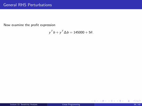
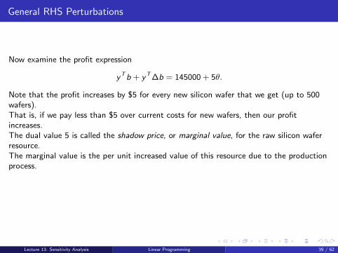
Now examine the profit expression
yTb + yT∆b = 145000 + 5θ.
Note that the profit increases by $5 for every new silicon wafer that we get (up to 500wafers).That is, if we pay less than $5 over current costs for new wafers, then our profitincreases.The dual value 5 is called the shadow price, or marginal value, for the raw silicon waferresource.The marginal value is the per unit increased value of this resource due to the productionprocess.Since we currently pay $1 per wafer. If another vendor sells them at $2.50 per wafer,then we should buy them since our unit increase in profit with this purchase price is$5− $1.5 = $3.5 since $2.5 is $1.5 greater than the $1 we now pay.
Lecture 13: Sensitivity Analysis Linear Programming 39 / 62

General RHS Perturbations
Now examine the profit expression
yTb + yT∆b = 145000 + 5θ.
Note that the profit increases by $5 for every new silicon wafer that we get (up to 500wafers).
That is, if we pay less than $5 over current costs for new wafers, then our profitincreases.The dual value 5 is called the shadow price, or marginal value, for the raw silicon waferresource.The marginal value is the per unit increased value of this resource due to the productionprocess.Since we currently pay $1 per wafer. If another vendor sells them at $2.50 per wafer,then we should buy them since our unit increase in profit with this purchase price is$5− $1.5 = $3.5 since $2.5 is $1.5 greater than the $1 we now pay.
Lecture 13: Sensitivity Analysis Linear Programming 39 / 62

General RHS Perturbations
Now examine the profit expression
yTb + yT∆b = 145000 + 5θ.
Note that the profit increases by $5 for every new silicon wafer that we get (up to 500wafers).That is, if we pay less than $5 over current costs for new wafers, then our profitincreases.
The dual value 5 is called the shadow price, or marginal value, for the raw silicon waferresource.The marginal value is the per unit increased value of this resource due to the productionprocess.Since we currently pay $1 per wafer. If another vendor sells them at $2.50 per wafer,then we should buy them since our unit increase in profit with this purchase price is$5− $1.5 = $3.5 since $2.5 is $1.5 greater than the $1 we now pay.
Lecture 13: Sensitivity Analysis Linear Programming 39 / 62

General RHS Perturbations
Now examine the profit expression
yTb + yT∆b = 145000 + 5θ.
Note that the profit increases by $5 for every new silicon wafer that we get (up to 500wafers).That is, if we pay less than $5 over current costs for new wafers, then our profitincreases.The dual value 5 is called the shadow price, or marginal value, for the raw silicon waferresource.
The marginal value is the per unit increased value of this resource due to the productionprocess.Since we currently pay $1 per wafer. If another vendor sells them at $2.50 per wafer,then we should buy them since our unit increase in profit with this purchase price is$5− $1.5 = $3.5 since $2.5 is $1.5 greater than the $1 we now pay.
Lecture 13: Sensitivity Analysis Linear Programming 39 / 62
General RHS Perturbations
Now examine the profit expression
yTb + yT∆b = 145000 + 5θ.
Note that the profit increases by $5 for every new silicon wafer that we get (up to 500wafers).That is, if we pay less than $5 over current costs for new wafers, then our profitincreases.The dual value 5 is called the shadow price, or marginal value, for the raw silicon waferresource.The marginal value is the per unit increased value of this resource due to the productionprocess.
Since we currently pay $1 per wafer. If another vendor sells them at $2.50 per wafer,then we should buy them since our unit increase in profit with this purchase price is$5− $1.5 = $3.5 since $2.5 is $1.5 greater than the $1 we now pay.
Lecture 13: Sensitivity Analysis Linear Programming 39 / 62

General RHS Perturbations
Now examine the profit expression
yTb + yT∆b = 145000 + 5θ.
Note that the profit increases by $5 for every new silicon wafer that we get (up to 500wafers).That is, if we pay less than $5 over current costs for new wafers, then our profitincreases.The dual value 5 is called the shadow price, or marginal value, for the raw silicon waferresource.The marginal value is the per unit increased value of this resource due to the productionprocess.Since we currently pay $1 per wafer. If another vendor sells them at $2.50 per wafer,then we should buy them since our unit increase in profit with this purchase price is$5− $1.5 = $3.5 since $2.5 is $1.5 greater than the $1 we now pay.
Lecture 13: Sensitivity Analysis Linear Programming 39 / 62

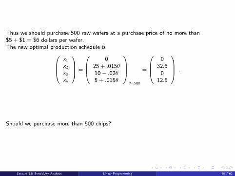
Thus we should purchase 500 raw wafers at a purchase price of no more than$5 + $1 = $6 dollars per wafer.
The new optimal production schedule isx1
x2
x3
x4
=
0
25 + .015θ10− .02θ5 + .015θ
θ=500
=
0
32.50
12.5
.
Should we purchase more than 500 chips?
Lecture 13: Sensitivity Analysis Linear Programming 40 / 62

Thus we should purchase 500 raw wafers at a purchase price of no more than$5 + $1 = $6 dollars per wafer.The new optimal production schedule is
x1
x2
x3
x4
=
0
25 + .015θ10− .02θ5 + .015θ
θ=500
=
0
32.50
12.5
.
Should we purchase more than 500 chips?
Lecture 13: Sensitivity Analysis Linear Programming 40 / 62

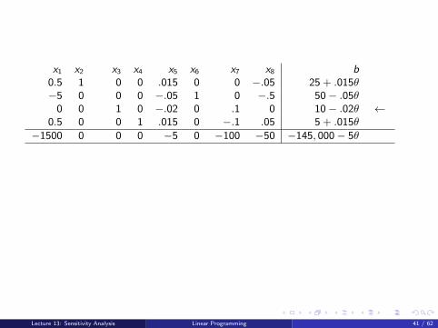
x1 x2 x3 x4 x5 x6 x7 x8 b0.5 1 0 0 .015 0 0 −.05 25 + .015θ−5 0 0 0 −.05 1 0 −.5 50− .05θ
0 0 1 0 −.02 0 .1 0 10− .02θ
←
0.5 0 0 1 .015 0 −.1 .05 5 + .015θ−1500 0 0 0 −5 0 −100 −50 −145, 000− 5θ
0.5 1 .75 0 0 0 .075 −.05 32.5−5 0 −2.5 0 0 1 −.25 −.5 25
0 0 −50 0 1 0 −5 0 −500 + θ0.5 0 .75 1 0 0 −.025 .05 12.5
−1500 0 −250 0 0 0 −125 −50 −147500
Do not purchase more than 500 since the wafer resource becomes slack.
Lecture 13: Sensitivity Analysis Linear Programming 41 / 62
x1 x2 x3 x4 x5 x6 x7 x8 b0.5 1 0 0 .015 0 0 −.05 25 + .015θ−5 0 0 0 −.05 1 0 −.5 50− .05θ
0 0 1 0 −.02 0 .1 0 10− .02θ ←0.5 0 0 1 .015 0 −.1 .05 5 + .015θ
−1500 0 0 0 −5 0 −100 −50 −145, 000− 5θ
0.5 1 .75 0 0 0 .075 −.05 32.5−5 0 −2.5 0 0 1 −.25 −.5 25
0 0 −50 0 1 0 −5 0 −500 + θ0.5 0 .75 1 0 0 −.025 .05 12.5
−1500 0 −250 0 0 0 −125 −50 −147500
Do not purchase more than 500 since the wafer resource becomes slack.
Lecture 13: Sensitivity Analysis Linear Programming 41 / 62

RHS Range Analysis: Etching Time
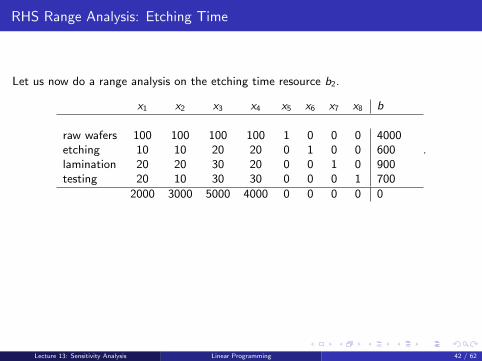
Let us now do a range analysis on the etching time resource b2.
x1 x2 x3 x4 x5 x6 x7 x8 b
raw wafers 100 100 100 100 1 0 0 0 4000etching 10 10 20 20 0 1 0 0 600
+ θ
lamination 20 20 30 20 0 0 1 0 900testing 20 10 30 30 0 0 0 1 700
2000 3000 5000 4000 0 0 0 0 0
.
b + ∆b = b + θe2 =
4000600900700
+ θ
0100
The new rhs in the opt. tableau is Rb + θRe2 since ∆b = θe2.
Lecture 13: Sensitivity Analysis Linear Programming 42 / 62
RHS Range Analysis: Etching Time
Let us now do a range analysis on the etching time resource b2.
x1 x2 x3 x4 x5 x6 x7 x8 b
raw wafers 100 100 100 100 1 0 0 0 4000etching 10 10 20 20 0 1 0 0 600
+ θ
lamination 20 20 30 20 0 0 1 0 900testing 20 10 30 30 0 0 0 1 700
2000 3000 5000 4000 0 0 0 0 0
.
b + ∆b = b + θe2 =
4000600900700
+ θ
0100
The new rhs in the opt. tableau is Rb + θRe2 since ∆b = θe2.
Lecture 13: Sensitivity Analysis Linear Programming 42 / 62

RHS Range Analysis: Etching Time
Let us now do a range analysis on the etching time resource b2.
x1 x2 x3 x4 x5 x6 x7 x8 b
raw wafers 100 100 100 100 1 0 0 0 4000etching 10 10 20 20 0 1 0 0 600 + θlamination 20 20 30 20 0 0 1 0 900testing 20 10 30 30 0 0 0 1 700
2000 3000 5000 4000 0 0 0 0 0
.
b + ∆b = b + θe2 =
4000600900700
+ θ
0100
The new rhs in the opt. tableau is Rb + θRe2 since ∆b = θe2.
Lecture 13: Sensitivity Analysis Linear Programming 42 / 62

RHS Range Analysis: Etching Time
0 ≤
Rb + R∆b =
25
50 + θ105
To preserve primal feasibility we only require
0 ≤ 50 + θ,
or equivalently,−50 ≤ θ.
Therefore, the range for b2 is[550, +∞) .
Lecture 13: Sensitivity Analysis Linear Programming 43 / 62

RHS Range Analysis: Etching Time
0 ≤ Rb + R∆b =
25
50 + θ105
To preserve primal feasibility we only require
0 ≤ 50 + θ,
or equivalently,−50 ≤ θ.
Therefore, the range for b2 is[550, +∞) .
Lecture 13: Sensitivity Analysis Linear Programming 43 / 62

RHS Range Analysis: Etching Time
0 ≤ Rb + R∆b =
25
50 + θ105
To preserve primal feasibility we only require
0 ≤ 50 + θ,
or equivalently,−50 ≤ θ.
Therefore, the range for b2 is[550, +∞) .
Lecture 13: Sensitivity Analysis Linear Programming 43 / 62

RHS Range Analysis: Etching Time
0 ≤ Rb + R∆b =
25
50 + θ105
To preserve primal feasibility we only require
0 ≤ 50 + θ,
or equivalently,−50 ≤ θ.
Therefore, the range for b2 is[550, +∞) .
Lecture 13: Sensitivity Analysis Linear Programming 43 / 62

RHS Range Analysis: Etching Time
What is the shadow price for etching, and what does it mean?
x1 x2 x3 x4 x5 x6 x7 x8 b0.5 1 0 0 .015 0 0 −.05 25−5 0 0 0 −.05 1 0 −.5 50
0 0 1 0 −.02 0 .1 0 100.5 0 0 1 .015 0 −.1 .05 5
−1500 0 0 0 −5 0 −100 −50 −145, 000
The shadow price, or marginal value, is 0 since we have surplus etching time in theoptimal solution.Additional hours of etching time do not change current profit levels.
Lecture 13: Sensitivity Analysis Linear Programming 44 / 62

RHS Range Analysis: Etching Time
What is the shadow price for etching, and what does it mean?
x1 x2 x3 x4 x5 x6 x7 x8 b0.5 1 0 0 .015 0 0 −.05 25−5 0 0 0 −.05 1 0 −.5 50
0 0 1 0 −.02 0 .1 0 100.5 0 0 1 .015 0 −.1 .05 5
−1500 0 0 0 −5 0 −100 −50 −145, 000
The shadow price, or marginal value, is 0 since we have surplus etching time in theoptimal solution.
Additional hours of etching time do not change current profit levels.
Lecture 13: Sensitivity Analysis Linear Programming 44 / 62

RHS Range Analysis: Etching Time
What is the shadow price for etching, and what does it mean?
x1 x2 x3 x4 x5 x6 x7 x8 b0.5 1 0 0 .015 0 0 −.05 25−5 0 0 0 −.05 1 0 −.5 50
0 0 1 0 −.02 0 .1 0 100.5 0 0 1 .015 0 −.1 .05 5
−1500 0 0 0 −5 0 −100 −50 −145, 000
The shadow price, or marginal value, is 0 since we have surplus etching time in theoptimal solution.Additional hours of etching time do not change current profit levels.
Lecture 13: Sensitivity Analysis Linear Programming 44 / 62

RHS Range Analysis: Lamination Time
What is the range for lamination time, and what is its marginal value?
x1 x2 x3 x4 x5 x6 x7 x8 b0.5 1 0 0 .015 0 0 −.05 25−5 0 0 0 −.05 1 0 −.5 50
0 0 1 0 −.02 0 .1 0 100.5 0 0 1 .015 0 −.1 .05 5
−1500 0 0 0 −5 0 −100 −50 −145, 000
Lecture 13: Sensitivity Analysis Linear Programming 45 / 62

RHS Range Analysis: Lamination Time
x1 x2 x3 x4 x5 x6 x7 x8 b0.5 1 0 0 .015 0 0 −.05 25−5 0 0 0 −.05 1 0 −.5 50
0 0 1 0 −.02 0 .1 0 100.5 0 0 1 .015 0 −.1 .05 5
−1500 0 0 0 −5 0 −100 −50 −145, 000
0 ≤ Rb + R∆b =
2550
10 + 0.1θ5− 0.1θ
0 ≤ 10 + 0.1θ, or equivalently, −100 ≤ θ0 ≤ 5− 0.1θ, or equivalently, θ ≤ 50
.
Therefore,800 ≤ b3 ≤ 950 .
Lecture 13: Sensitivity Analysis Linear Programming 46 / 62

RHS Range Analysis: Lamination Time
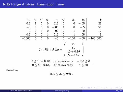
x1 x2 x3 x4 x5 x6 x7 x8 b0.5 1 0 0 .015 0 0 −.05 25−5 0 0 0 −.05 1 0 −.5 50
0 0 1 0 −.02 0 .1 0 100.5 0 0 1 .015 0 −.1 .05 5
−1500 0 0 0 −5 0 −100 −50 −145, 000
0 ≤ Rb + R∆b =
2550
10 + 0.1θ5− 0.1θ
0 ≤ 10 + 0.1θ, or equivalently, −100 ≤ θ0 ≤ 5− 0.1θ, or equivalently, θ ≤ 50
.
Therefore,800 ≤ b3 ≤ 950 .
Lecture 13: Sensitivity Analysis Linear Programming 46 / 62
RHS Range Analysis: Lamination Time
x1 x2 x3 x4 x5 x6 x7 x8 b0.5 1 0 0 .015 0 0 −.05 25−5 0 0 0 −.05 1 0 −.5 50
0 0 1 0 −.02 0 .1 0 100.5 0 0 1 .015 0 −.1 .05 5
−1500 0 0 0 −5 0 −100 −50 −145, 000
The shadow price, or marginal value, for lamination time is $100.
Each additional hour of lamination time improves profitability by $100.
If we are able to obtain 50 additional hours of lamination time this month, how muchwould we be willing to pay for it beyond what we currently pay?
$5,000
Lecture 13: Sensitivity Analysis Linear Programming 47 / 62

RHS Range Analysis: Lamination Time
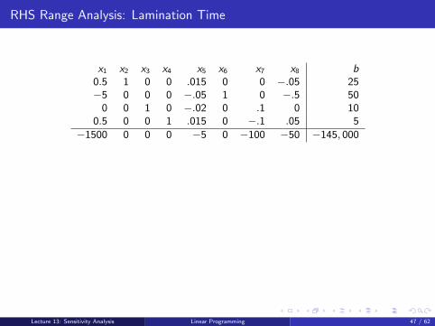
x1 x2 x3 x4 x5 x6 x7 x8 b0.5 1 0 0 .015 0 0 −.05 25−5 0 0 0 −.05 1 0 −.5 50
0 0 1 0 −.02 0 .1 0 100.5 0 0 1 .015 0 −.1 .05 5
−1500 0 0 0 −5 0 −100 −50 −145, 000
The shadow price, or marginal value, for lamination time is $100.
Each additional hour of lamination time improves profitability by $100.
If we are able to obtain 50 additional hours of lamination time this month, how muchwould we be willing to pay for it beyond what we currently pay?
$5,000
Lecture 13: Sensitivity Analysis Linear Programming 47 / 62

Pricing Out New Products
We now consider the problem of adding a new product to our product line.
Consider a new chip that requires ten hours each of etching, lamination, and testing timeper 100 chip batch.
Suppose it can be sold for $ 33.10 per chip.
(a) Is it efficient to produce?
(b) If it is efficient to produce, what is the new optimal production schedule?
Lecture 13: Sensitivity Analysis Linear Programming 48 / 62

Pricing Out New Products
We analyze this problem in the same way that we analyzed the two previous problems.
First, determine how this new chip changes the initial tableau.
Second, determine how the change to the initial tableau propagates through to theoptimal tableau.
This propagation is determined by multiplying the new initial tableau through by thepivot matrix G .
Lecture 13: Sensitivity Analysis Linear Programming 49 / 62
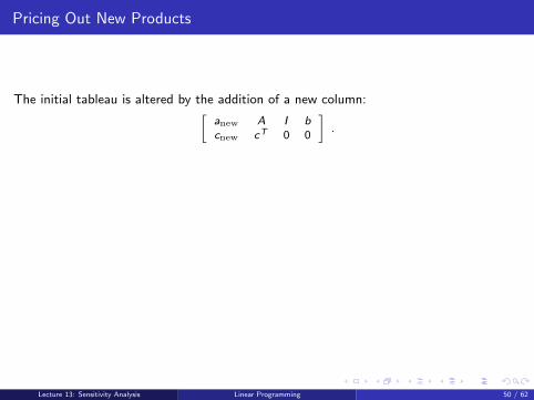
Pricing Out New Products
The initial tableau is altered by the addition of a new column:[anew A I bcnew cT 0 0
].
Multiplying on the left by the matrix G gives[R 0
−yT 1
] [anew A I bcnew cT 0 0
]=[
Ranew RA R Rbcnew − aTnewy (c − AT y)T −yT −yTb
].
The expression (cnew − aTnewy) determines whether this new tableau is optimal or not.If 0 < (cnew − aTnewy), then the new tableau is not optimal. In this case the new productis efficient to produce.
Lecture 13: Sensitivity Analysis Linear Programming 50 / 62

Pricing Out New Products
The initial tableau is altered by the addition of a new column:[anew A I bcnew cT 0 0
].
Multiplying on the left by the matrix G gives[R 0
−yT 1
] [anew A I bcnew cT 0 0
]=[
Ranew RA R Rbcnew − aTnewy (c − AT y)T −yT −yTb
].
The expression (cnew − aTnewy) determines whether this new tableau is optimal or not.
If 0 < (cnew − aTnewy), then the new tableau is not optimal. In this case the new productis efficient to produce.
Lecture 13: Sensitivity Analysis Linear Programming 50 / 62

Pricing Out New Products
The initial tableau is altered by the addition of a new column:[anew A I bcnew cT 0 0
].
Multiplying on the left by the matrix G gives[R 0
−yT 1
] [anew A I bcnew cT 0 0
]=[
Ranew RA R Rbcnew − aTnewy (c − AT y)T −yT −yTb
].
The expression (cnew − aTnewy) determines whether this new tableau is optimal or not.If 0 < (cnew − aTnewy), then the new tableau is not optimal. In this case the new productis efficient to produce.
Lecture 13: Sensitivity Analysis Linear Programming 50 / 62
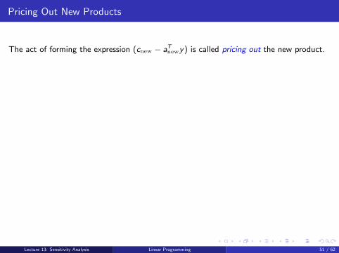
Pricing Out New Products
The act of forming the expression (cnew − aTnewy) is called pricing out the new product.
If (cnew − aTnewy) < 0, then the new product does not price out, and we do not produceit since in this case the new tableau is optimal with the new product non-basic.
If(cnew − aTnewy) > 0, then we say that the new product does price out and it should beintroduced into the optimal production mix.
The value aTnewy represents the increase in value of the resources consumed by one unit ofthis activity due to the current production schedule. If this value exceeds the profitabilityof this activity, then it is not efficient to introduce this activity into the production mix.
The new optimal production mix is found by applying the standard primal simplexalgorithm to the tableau since this tableau is primal feasible but not dual feasible.
Lecture 13: Sensitivity Analysis Linear Programming 51 / 62

Pricing Out New Products
Returning to the Silicon Chip Corp. problem, the new chip under consideration has
anew =
100101010
.
We need to compute cnew.
The stated sale price or revenue for each 100 chip batch of the new chip is $3310, so
cnew = 3310−
1
406010
T
100101010
= 3310− 1200 = 2110.
We need to subtract from this number the cost of producing each 100 chip batch.
Lecture 13: Sensitivity Analysis Linear Programming 52 / 62
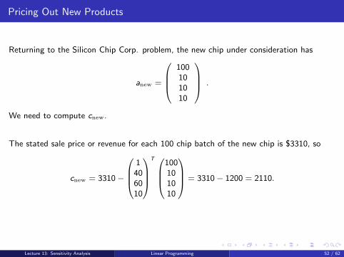

Pricing Out New Products
We have that each raw silicon wafer is worth $1, each hour of etching time costs $40,each hour of lamination time costs $60, and each hour of inspection time costs $10.
Therefore, the cost of producing each 100 chip batch of these new chips is
100× 1 (cost of the raw wafers)+ 10× 40 (cost of etching time)+ 10× 60 (cost of lamination time)+ 10× 10 (cost of testing time)
—–1200 (total cost)
.
Hence the profit on each 100 chip batch of these new chips is $3310− $1200 = $2110, or$21.10 per chip, and so
cnew = 2110.
Lecture 13: Sensitivity Analysis Linear Programming 53 / 62

Pricing Out New Products
We have that each raw silicon wafer is worth $1, each hour of etching time costs $40,each hour of lamination time costs $60, and each hour of inspection time costs $10.Therefore, the cost of producing each 100 chip batch of these new chips is
100× 1 (cost of the raw wafers)
+ 10× 40 (cost of etching time)+ 10× 60 (cost of lamination time)+ 10× 10 (cost of testing time)
—–1200 (total cost)
.
Hence the profit on each 100 chip batch of these new chips is $3310− $1200 = $2110, or$21.10 per chip, and so
cnew = 2110.
Lecture 13: Sensitivity Analysis Linear Programming 53 / 62

Pricing Out New Products
We have that each raw silicon wafer is worth $1, each hour of etching time costs $40,each hour of lamination time costs $60, and each hour of inspection time costs $10.Therefore, the cost of producing each 100 chip batch of these new chips is
100× 1 (cost of the raw wafers)+ 10× 40 (cost of etching time)
+ 10× 60 (cost of lamination time)+ 10× 10 (cost of testing time)
—–1200 (total cost)
.
Hence the profit on each 100 chip batch of these new chips is $3310− $1200 = $2110, or$21.10 per chip, and so
cnew = 2110.
Lecture 13: Sensitivity Analysis Linear Programming 53 / 62

Pricing Out New Products
We have that each raw silicon wafer is worth $1, each hour of etching time costs $40,each hour of lamination time costs $60, and each hour of inspection time costs $10.Therefore, the cost of producing each 100 chip batch of these new chips is
100× 1 (cost of the raw wafers)+ 10× 40 (cost of etching time)+ 10× 60 (cost of lamination time)
+ 10× 10 (cost of testing time)—–
1200 (total cost)
.
Hence the profit on each 100 chip batch of these new chips is $3310− $1200 = $2110, or$21.10 per chip, and so
cnew = 2110.
Lecture 13: Sensitivity Analysis Linear Programming 53 / 62

Pricing Out New Products
We have that each raw silicon wafer is worth $1, each hour of etching time costs $40,each hour of lamination time costs $60, and each hour of inspection time costs $10.Therefore, the cost of producing each 100 chip batch of these new chips is
100× 1 (cost of the raw wafers)+ 10× 40 (cost of etching time)+ 10× 60 (cost of lamination time)+ 10× 10 (cost of testing time)
—–1200 (total cost)
.
Hence the profit on each 100 chip batch of these new chips is $3310− $1200 = $2110, or$21.10 per chip, and so
cnew = 2110.
Lecture 13: Sensitivity Analysis Linear Programming 53 / 62
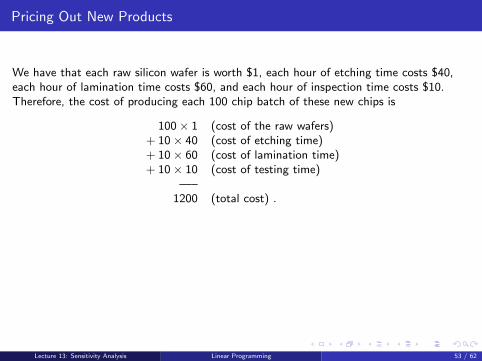
Pricing Out New Products
We have that each raw silicon wafer is worth $1, each hour of etching time costs $40,each hour of lamination time costs $60, and each hour of inspection time costs $10.Therefore, the cost of producing each 100 chip batch of these new chips is
100× 1 (cost of the raw wafers)+ 10× 40 (cost of etching time)+ 10× 60 (cost of lamination time)+ 10× 10 (cost of testing time)
—–1200 (total cost) .
Hence the profit on each 100 chip batch of these new chips is $3310− $1200 = $2110, or$21.10 per chip, and so
cnew = 2110.
Lecture 13: Sensitivity Analysis Linear Programming 53 / 62

Pricing Out New Products
Pricing out the new chip gives
cnew − aTnewy = 2110−
100101010
T
50
10050
= 2110− 2000 = 110 .
The new chip prices out positive, and so it will be efficient to produce.
The new column in the tableau associated with this chip is
(Ranew
cnew − aTnewy
)=
10−11
110
.
Lecture 13: Sensitivity Analysis Linear Programming 54 / 62

Pricing Out New Products
xnew x1 x2 x3 x4 x5 x6 x7 x8 b1 0.5 1 0 0 .015 0 0 −.05 250 −5 0 0 0 −.05 1 0 −.5 50
−1 0 0 1 0 −.02 0 .1 0 101 0.5 0 0 1 .015 0 −.1 .05 5
110 −1500 0 0 0 −5 0 −100 −50 −145, 000
0 0 1 0 −1 0 0 .1 −.1 200 −5 0 0 0 −.05 1 0 −.5 500 .5 0 1 1 −.005 0 0 .05 151 0.5 0 0 1 .015 0 −.1 .05 50 −1555 0 0 −110 −6.65 0 −88.9 −55.5 −145550
The new optimal solution is (xnew, x1, x2, x3, x4) = (5, 0, 20, 15, 0) .
The new shadow prices are (y1, y2, y3, y4) = (6.65, 0, 89.9, 55.5) .
Lecture 13: Sensitivity Analysis Linear Programming 55 / 62

Pricing Out New Products
xnew x1 x2 x3 x4 x5 x6 x7 x8 b1 0.5 1 0 0 .015 0 0 −.05 250 −5 0 0 0 −.05 1 0 −.5 50
−1 0 0 1 0 −.02 0 .1 0 101 0.5 0 0 1 .015 0 −.1 .05 5
110 −1500 0 0 0 −5 0 −100 −50 −145, 0000 0 1 0 −1 0 0 .1 −.1 200 −5 0 0 0 −.05 1 0 −.5 500 .5 0 1 1 −.005 0 0 .05 151 0.5 0 0 1 .015 0 −.1 .05 50 −1555 0 0 −110 −6.65 0 −88.9 −55.5 −145550
The new optimal solution is (xnew, x1, x2, x3, x4) = (5, 0, 20, 15, 0) .
The new shadow prices are (y1, y2, y3, y4) = (6.65, 0, 89.9, 55.5) .
Lecture 13: Sensitivity Analysis Linear Programming 55 / 62

Pricing Out New Products
Consider a different new chip.
This chip requires 15 hours each of etching and testing, and 30 hours of lamination timeper 100 chip batch.
What is the breakeven sale price of this new chip?
x1 x2 x3 x4 x5 x6 x7 x8 b0.5 1 0 0 .015 0 0 −.05 25−5 0 0 0 −.05 1 0 −.5 50
0 0 1 0 −.02 0 .1 0 100.5 0 0 1 .015 0 −.1 .05 5
−1500 0 0 0 −5 0 −100 −50 −145, 000
Lecture 13: Sensitivity Analysis Linear Programming 56 / 62
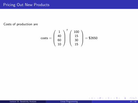
Pricing Out New Products
Costs of production are
costs =
1
406010
T
100153015
= $2650
Marginal costs are
marginal costs = yTanew =
50
10050
T
100153015
= $4250
Breakeven sale price = $2650 + $4250 = $6900. Or equivalently, $69 per chip.
Lecture 13: Sensitivity Analysis Linear Programming 57 / 62
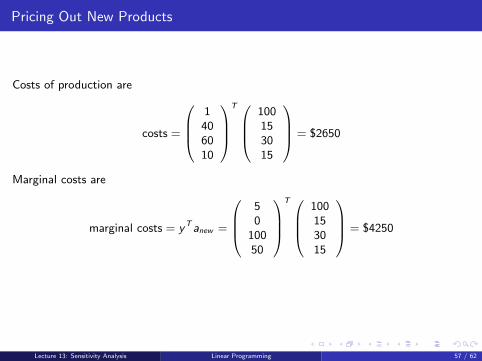
Pricing Out New Products
Costs of production are
costs =
1
406010
T
100153015
= $2650
Marginal costs are
marginal costs = yTanew =
50
10050
T
100153015
= $4250
Breakeven sale price = $2650 + $4250 = $6900. Or equivalently, $69 per chip.
Lecture 13: Sensitivity Analysis Linear Programming 57 / 62

Pricing Out New Products
Costs of production are
costs =
1
406010
T
100153015
= $2650
Marginal costs are
marginal costs = yTanew =
50
10050
T
100153015
= $4250
Breakeven sale price = $2650 + $4250 = $6900. Or equivalently, $69 per chip.
Lecture 13: Sensitivity Analysis Linear Programming 57 / 62

Pricing Out New Products
It is decided that we can sell the new chip for $70 each.
We now wish to simultaneously determine if either or both of the new chips are efficientto produce.
How do we determine this and how do we determine the new optimal production mix?
[R 0
−yT 1
] [anew1 anew2 A I bcnew1 cnew2 cT 0 0
]=
[Ranew1 Ranew2 RA R Rb
cnew1 − aTnew1y cnew2 − aTnew2y (c − AT y)T −yT −yTb
]
Then pivot to optimality.
Lecture 13: Sensitivity Analysis Linear Programming 58 / 62

Pricing Out New Products
It is decided that we can sell the new chip for $70 each.
We now wish to simultaneously determine if either or both of the new chips are efficientto produce.
How do we determine this and how do we determine the new optimal production mix?
[R 0
−yT 1
] [anew1 anew2 A I bcnew1 cnew2 cT 0 0
]
=
[Ranew1 Ranew2 RA R Rb
cnew1 − aTnew1y cnew2 − aTnew2y (c − AT y)T −yT −yTb
]
Then pivot to optimality.
Lecture 13: Sensitivity Analysis Linear Programming 58 / 62
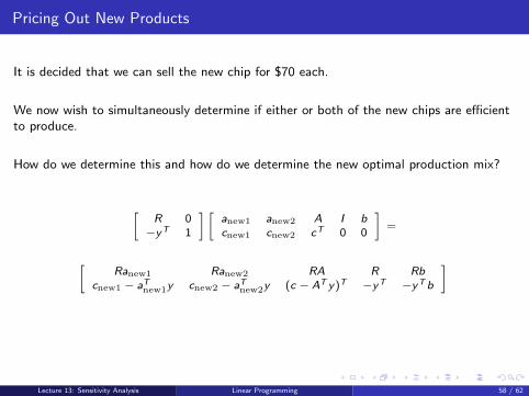
Pricing Out New Products
It is decided that we can sell the new chip for $70 each.
We now wish to simultaneously determine if either or both of the new chips are efficientto produce.
How do we determine this and how do we determine the new optimal production mix?
[R 0
−yT 1
] [anew1 anew2 A I bcnew1 cnew2 cT 0 0
]=
[Ranew1 Ranew2 RA R Rb
cnew1 − aTnew1y cnew2 − aTnew2y (c − AT y)T −yT −yTb
]
Then pivot to optimality.
Lecture 13: Sensitivity Analysis Linear Programming 58 / 62

Pricing Out New Products
It is decided that we can sell the new chip for $70 each.
We now wish to simultaneously determine if either or both of the new chips are efficientto produce.
How do we determine this and how do we determine the new optimal production mix?
[R 0
−yT 1
] [anew1 anew2 A I bcnew1 cnew2 cT 0 0
]=
[Ranew1 Ranew2 RA R Rb
cnew1 − aTnew1y cnew2 − aTnew2y (c − AT y)T −yT −yTb
]
Then pivot to optimality.
Lecture 13: Sensitivity Analysis Linear Programming 58 / 62

The Fundamental Theorem on Sensitivity Analysis
Let A ∈ Rm×n, b ∈ Rm, and c ∈ Rn.
P maximize cT xsubject to Ax ≤ b, 0 ≤ x .
We associate to P the optimal value function V : Rm → R ∪ {±∞} defined by
V (u) = maximize cT xsubject to Ax ≤ b + u, 0 ≤ x
for all u ∈ Rm.
LetF(u) = {x ∈ Rn |Ax ≤ b + u, 0 ≤ x }
denote the feasible region for the LP associated with value V (u).
If F(u) = ∅ for some u ∈ Rm, we define V (u) = −∞.
Lecture 13: Sensitivity Analysis Linear Programming 59 / 62
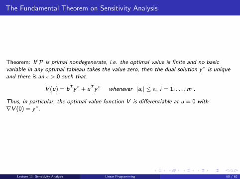
The Fundamental Theorem on Sensitivity Analysis
Theorem: If P is primal nondegenerate, i.e. the optimal value is finite and no basicvariable in any optimal tableau takes the value zero, then the dual solution y∗ is uniqueand there is an ε > 0 such that
V (u) = bT y∗ + uT y∗ whenever |ui | ≤ ε, i = 1, . . . ,m .
Thus, in particular, the optimal value function V is differentiable at u = 0 with∇V (0) = y∗.
Lecture 13: Sensitivity Analysis Linear Programming 60 / 62

The Fundamental Theorem on Sensitivity Analysis: Proof
[R 0−yT 1
] [A I bcT 0 0
]=
[RA R Rb
(c − AT y∗)T −(y∗)T −bT y∗
]
[R 0−yT 1
][A I b + ucT 0 0
]=
[RA R Rb + Ru
(c − AT y∗)T −(y∗)T −bT y∗ − uT y∗
]
Lecture 13: Sensitivity Analysis Linear Programming 61 / 62

The Fundamental Theorem on Sensitivity Analysis: Proof
[R 0−yT 1
] [A I bcT 0 0
]=
[RA R Rb
(c − AT y∗)T −(y∗)T −bT y∗
]
[R 0−yT 1
][A I b + ucT 0 0
]
=
[RA R Rb + Ru
(c − AT y∗)T −(y∗)T −bT y∗ − uT y∗
]
Lecture 13: Sensitivity Analysis Linear Programming 61 / 62

The Fundamental Theorem on Sensitivity Analysis: Proof
[R 0−yT 1
] [A I bcT 0 0
]=
[RA R Rb
(c − AT y∗)T −(y∗)T −bT y∗
]
[R 0−yT 1
][A I b + ucT 0 0
]=
[RA R Rb + Ru
(c − AT y∗)T −(y∗)T −bT y∗ − uT y∗
]
Lecture 13: Sensitivity Analysis Linear Programming 61 / 62

The Fundamental Theorem on Sensitivity Analysis: Proof
[RA R Rb + Ru
(c − AT y∗)T −(y∗)T −bT y∗ − uT y∗
]
Non-degeneracy implies that Rb > 0 so there is an ε > 0 such that
Rb > ε1 .
By continuity, there is a δ > 0 such that
|(Ru)i | ≤ ε whenever |ui | ≤ δ ∀ i = 1, 2, . . . , n.
Hence Rb + Ru > 0 whenever |ui | ≤ δ ∀ i = 1, 2, . . . , n.
Lecture 13: Sensitivity Analysis Linear Programming 62 / 62
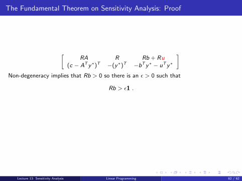
The Fundamental Theorem on Sensitivity Analysis: Proof
[RA R Rb + Ru
(c − AT y∗)T −(y∗)T −bT y∗ − uT y∗
]Non-degeneracy implies that Rb > 0 so there is an ε > 0 such that
Rb > ε1 .
By continuity, there is a δ > 0 such that
|(Ru)i | ≤ ε whenever |ui | ≤ δ ∀ i = 1, 2, . . . , n.
Hence Rb + Ru > 0 whenever |ui | ≤ δ ∀ i = 1, 2, . . . , n.
Lecture 13: Sensitivity Analysis Linear Programming 62 / 62