1

Linear Quadratic Gaussian Control of a Quarter-Car Suspension

Mohamed M. ElMadany* & Zuhair S. Abduljabbar**

* Professor ** Associate Professor

Mechanical Engineering Department King Saud University

P.O. Box 800, Riyadh 11421 Saudi Arabia

Fax: 966 1 4676652 Email: mmadany@ksu.edu

SUMMARY

This paper presents a method for designing linear multivariable controllers

in the frequency-domain for an intelligent controlled suspension system for a

quarter-car model. The design methodology uses singular value inequalities and

optimal control theory. The vehicle system is augmented with additional

dynamics in the form of an integrator to affect the loop shapes of the system. The

measurements are assumed to be obtained in a noisy state, and the optimal control

gain and the Kalman filter gain are derived using system dynamics and noise

statistics. A combination of singular value analysis, eigenvalue analysis, time

response, and power spectral densities of random response is used to describe the

performance of the active suspension systems.

Keywords: Active suspension design, Intelligent controlled suspensions, LQG

control of vehicles.

2

INTRODUCTION

The development of design techniques for the synthesis of active vehicle

suspension systems has been an active area of research over the last two decades

[1-8]. In particular, the development of robust controllers in order to improve the

well known trade-offs between ride comfort, controllability and road safety has

been pursued in Refs. [9-14]. Two major problems are encountered in applying

linear quadratic regulator (LQR) theory to the design of vehicle suspensions. The

first problem occurs when some of the feedback states are not available, which

may be deduced from an estimator (filter). However, the guaranteed gain and

phase margin results of the LQR [15] may decrease markedly when the estimator

is included. References [15-19] discuss some of the techniques used to solve this

problem, and show that the proper choice of the estimator gains allows the

guaranteed gain and phase results of the full state feedback LQR to be obtained

asymptotically.

The second problem arises from the fact that the actively controlled

system does not have zero steady-state axle to body deflection in response to

external body force due to payload variations, braking, accelerating or cornering

forces. In order to overcome this limitation, Davis and Thompson [9] and

ElMadany [10, 11], assuming full state feedback, derived optimal suspension

systems using multivariable integral control. The control law consists of two

parts. The first is an integral controller acting on suspension deflection to ensure

zero steady-state offset due to body and maneuvering forces as well as due to road

3

ramp inputs. The second part is a state variable feedback controller for vibration

control and performance improvements. By introducing integral compensation in

the state space, a controllable state space is chosen so that all of the states that are

used in the LQR problem have a zero steady-state equilibrium. With this state

space, the infinite time quadratic performance index is well behaved, the

robustness properties for the full state feedback regulator apply, and the resulting

controller will have zero steady-state errors in the presence of parameter

uncertainty, [16]. Further development and investigation of the integral

compensation problem, however, is needed.

In this work, as opposed to earlier studies [9-11], measurement errors are

taken into consideration. The case of incomplete and noisy measurements is

treated and the optimal state observer is derived. A design method is proposed for

designing linear multivariable integral controllers for an intelligent controlled

suspension system. The method is based on a frequency-domain design

methodology using singular value inequalities and optimal control theory.

In what follows, the vehicle suspension problem is described, and the

design methodology to synthesize the compensator and estimator gains is

presented along with an analysis of the performance and robustness

characteristics. The compensator allows set point control with command

following. The estimator design is performed in the framework of the Kalman

filter formalism. Loop transfer recovery is used to try to recover the desired

degree of robustness to uncertainty. The technique is applied to design the

controller for the state augmented vehicle suspension system with limited state

4

feedback and noisy measurements. The system performance is computed and

compared with passive and fully active with and without integral control systems

by numerical simulation.

VEHICLE SUSPENSION PROBLEM

The quarter-car model is often adequate in preliminary studies of vehicle

ride dynamics [1-4]. Despite its simplicity, it captures the most basic features of

the real vehicle problem, leads to a basic understanding of the limitations to

suspension performance, and allows to set the line of thinking in the design of

suspensions which accords with experience. However, when a detailed study of

the motion of the vehicle is required, and when the features which are implicitly

omitted from the quarter-car model need to be assessed, more elaborate models

(two-or-three-dimensional models) should be considered.

A two-degree-of-freedom vehicle suspension representing a quarter-car is

shown in Fig. 1. The sprung and unsprung masses are denoted by m1 and m2,

respectively. The suspension spring stiffness and damping coefficients are given

by k and c respectively, while the tire is modelled as a linear spring with stiffness

kt. The variable u denotes an active control force applied between the body and

axle.

The vehicle is assumed to travel at a constant forward speed over a

random road surface, which is approximated by an integrated white noise input

[20]. Hence, the vertical road velocity disturbance, vi, is modelled as a white-

noise input and it is specified by

5

(1a) [ ]E v ti ( ) = 0

(1b) ( ) ( )[ ] (E v t v t V t ti i1 2 1 2= −δ )

where E[.] denotes the expectation operator and δ(.) is the Dirac delta function.

The states are selected as x1 being the distance between the sprung and

unsprung masses (suspension travel), x2 being the distance between the unsprung

mass and the road surface (tire deflection), x3 being the sprung mass absolute

velocity, and x4 being the unsprung mass absolute velocity.

The state space representation of the system is

DvBuAxx ++=& (2a)

y = Cx (2b)

z = Hx + Γη (2c)

The dependence of variables on time t is suppressed in the interest of brevity,

where

A km

cm

cm

km

km

cm

cm

t

=

−

−−

− −

⎡

⎣

⎢⎢⎢⎢⎢⎢⎢

⎤

⎦

⎥⎥⎥⎥⎥⎥⎥

0 0 1 1

0 0 0 1

01 1

2 2 2 2

1,

Bm m

T=

−⎡

⎣⎢

⎤

⎦⎥0 0 1 1

1 2,

, [ ] [ ]D CT= =0 1 0 0 1 0 0 0,

[ ] [ ]H = =1 0 0 0 1 0 0 0, Γ

η is a zero mean random process with normal distribution with intensity Rη, i.e.,

6

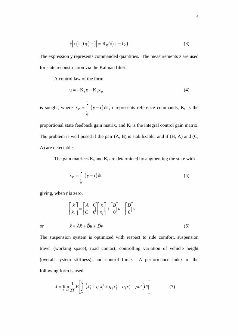
( ) ( )[ ] ( )E t t R t tη η δη1 2 1 2= − (3)

The expression y represents commanded quantities. The measurements z are used

for state reconstruction via the Kalman filter.

A control law of the form

u K x K xs i e= − − (4)

is sought, where , r represents reference commands, K( )x y reo

t= −∫ dt

dt

s is the

proportional state feedback gain matrix, and Ki is the integral control gain matrix.

The problem is well posed if the pair (A, B) is stabilizable, and if (H, A) and (C,

A) are detectable.

The gain matrices Ks and Ki are determined by augmenting the state with

(5) ( )x y reo

t= −∫

giving, when r is zero,

vD

uB

xx

CA

xx

ee⎥⎦

⎤⎢⎣

⎡+⎥

⎦

⎤⎢⎣

⎡+⎥

⎦

⎤⎢⎣

⎡⎥⎦

⎤⎢⎣

⎡=⎥

⎦

⎤⎢⎣

⎡000

0&

&

or (6) vDuBxAx ˆˆˆˆˆ ++=&

The suspension system is optimized with respect to ride comfort, suspension

travel (working space), road contact, controlling variation of vehicle height

(overall system stiffness), and control force. A performance index of the

following form is used

( ) ⎥⎦

⎤⎢⎣

⎡++++= ∫∞→

dtuxqxqxqxET

J e

T

oT

223

222

211

232

1lim ρ& (7)

7

where q1, q2, q3, and ρ are the weights on working space, road contact (tire

deflection), overall system stiffness, and control force, respectively. They govern

the relative importance attached to the various components of the optimality

criterion.

In matrix form, the performance index is given by

[ ] ⎥⎦

⎤⎢⎣

⎡⎥⎦

⎤⎢⎣

⎡⎥⎦

⎤⎢⎣

⎡= ∫∞→

dtux

RNNQ

uxET

Jc

TTT

T

oT

ˆˆ

21lim (8)

with Q, Rc are symmetric, Rc is positive definite, Q is positive semi-definite, and

N is a constant matrix.

where

Qm

k q m kc kc

q m

kc c c

kc c c

q m

=

+ −

− −

−

⎡

⎣

⎢⎢⎢⎢⎢⎢⎢⎢

⎤

⎦

⎥⎥⎥⎥⎥⎥⎥⎥

1

0 0

0 0 0

0 0

0 0

0 0 0 0

12

21 1

2

2 12

2 2

2 2

3 12

0

[ ]Nm

k c c T= −1 0 012 ,

Rm

c = +1

12 ρ

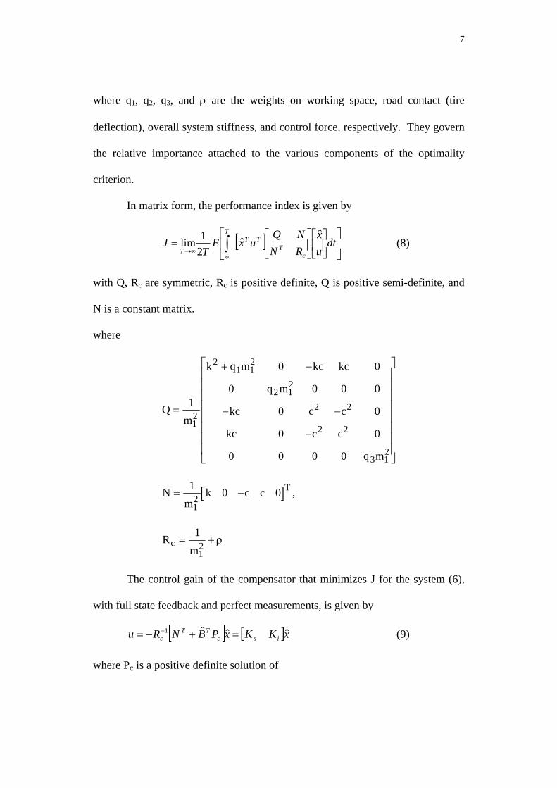
The control gain of the compensator that minimizes J for the system (6),

with full state feedback and perfect measurements, is given by

[ ] [ ]xKKxPBNRu iscTT

c ˆˆˆ1 =+−= − (9)

where Pc is a positive definite solution of

8

(10) 0ˆ 1 =+−+ −ncccc

Tnnc QPRBPPAAP

where A A BR N Q Q N R Nn cT

n cT= − = − ≥− −$ $ ,1 1 0 .

The design of the compensator reduces to the selection of the matrices Qn

and Rc satisfying the performance and robustness constraints prescribed for the

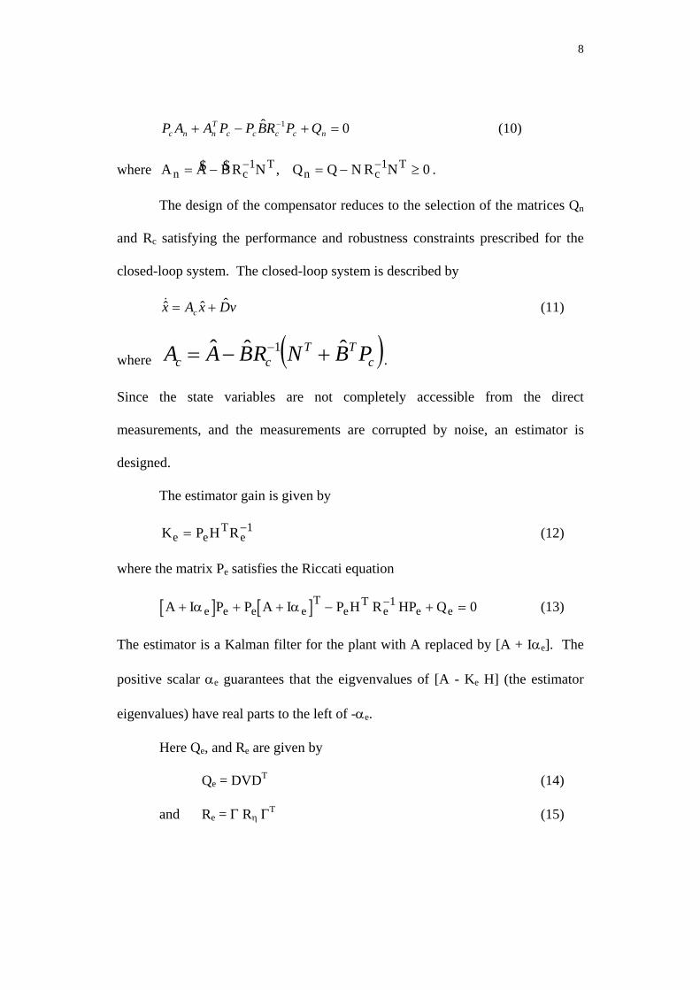
closed-loop system. The closed-loop system is described by

(11) vDxAx cˆˆˆ +=&

where ( )cTT

cc PBNRBAA ˆˆˆ 1 +−= −.

Since the state variables are not completely accessible from the direct

measurements, and the measurements are corrupted by noise, an estimator is

designed.

The estimator gain is given by

(12) K P H Re eT

e= −1

where the matrix Pe satisfies the Riccati equation

(13) [ ] [ ]A I P P A I P H R HP Qe e e eT

eT

e e e+ + + − +−α α 1 0=

The estimator is a Kalman filter for the plant with A replaced by [A + Iαe]. The

positive scalar αe guarantees that the eigvenvalues of [A - Ke H] (the estimator

eigenvalues) have real parts to the left of -αe.

Here Qe, and Re are given by

Qe = DVDT (14)

and Re = Γ Rη ΓT (15)

9

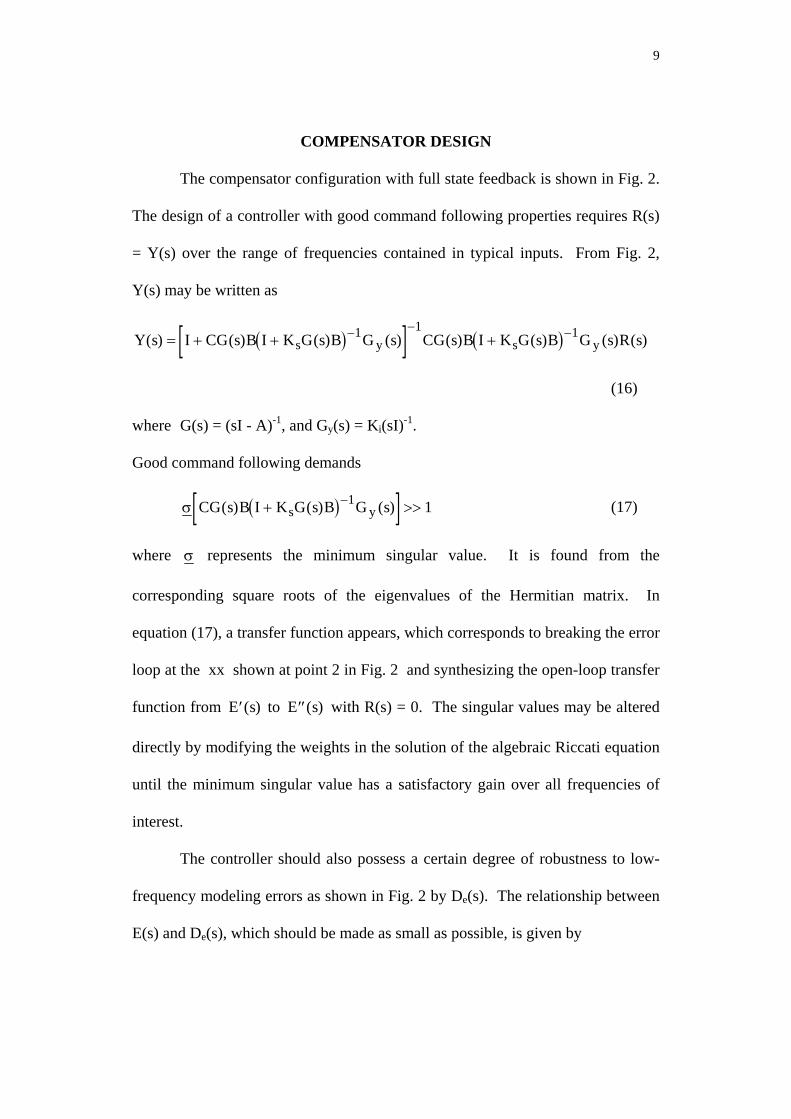
COMPENSATOR DESIGN

The compensator configuration with full state feedback is shown in Fig. 2.

The design of a controller with good command following properties requires R(s)

= Y(s) over the range of frequencies contained in typical inputs. From Fig. 2,

Y(s) may be written as

( )[ ] ( )Y s I CG s B I K G s B G s CG s B I K G s B G s R ss y s y( ) ( ) ( ) ( ) ( ) ( ) ( ) ( )= + + +− − −1 1 1

(16)

where G(s) = (sI - A)-1, and Gy(s) = Ki(sI)-1.

Good command following demands

( )[σ CG s B I K G s B G ss y( ) ( ) ( )+ −1 1] >> (17)

where σ represents the minimum singular value. It is found from the

corresponding square roots of the eigenvalues of the Hermitian matrix. In

equation (17), a transfer function appears, which corresponds to breaking the error

loop at the xx shown at point 2 in Fig. 2 and synthesizing the open-loop transfer

function from ′E s( ) to with R(s) = 0. The singular values may be altered

directly by modifying the weights in the solution of the algebraic Riccati equation

until the minimum singular value has a satisfactory gain over all frequencies of

interest.

′′E s( )

The controller should also possess a certain degree of robustness to low-

frequency modeling errors as shown in Fig. 2 by De(s). The relationship between

E(s) and De(s), which should be made as small as possible, is given by

10

( )[ ]E s I CG s B I K G s B G s D ss y( ) ( ) ( ) ( ) ( )= − + + −e

−1 1 (18)

which illustrates that the condition specified in Eq. (17) for good command

following is sufficient to guarantee disturbance rejection resulting from low-

frequency modeling errors.

The impact of modeling errors reflected at the plant input and sensor noise

may be minimized by considering the control input equation

(19) [U s I K G s B G s C G s B D ss y( ) ( ) ( ) ( ) ( )= + +−1] m

where Dm(s) represents both plant uncertainties and noise disturbances.

Equation (19) shows that disturbance rejection at the input corresponds to

selecting the regulator weights such that

[σ K G s B G s CG s Bs y( ) ( ) ( )+ 1] >> (20)

over the frequencies where Dm(s) has the majority of its energy. The transfer

function in Eq. (20) may result from breaking the loop at point 1 and synthesizing

the relation from to with R(s) = 0, in Fig. 2. ′U s( ) ′′U s( )

Therefore, based on the above analysis, the singular values of two

different transfer functions, (17) and (20), must be designed simultaneously, in

order to obtain a controller with good command following and robustness to

modelling errors and plant disturbances.

ESTIMATOR DESIGN

11

Since all plant states are not measurable, a Kalman filter may be used to

realize the full state feedback controller. From Fig. 3, the transfer function from

η(s) to E(s) with R(s) = 0 is

E s CG s B I G s CG s B K I G s K H G s B K HG s B

I G s CG s B K G s K s

y s e e

y s e

( ) ( ) [ ( ) ( ) ] { ( ) ( )( ( ) )

[ ( ) ( ) ] } ( ) ( )

= + + + +

+

−

− −

1

1 1 η

×

(21)

The impact of sensor noise on the error can be minimized by making

σ( ( ) [ ( ) ( ) ] { ( ) ( )( ( ) )

( ( ) ( ) ] } ( ) )

CG s B I G s CG s B K I G s K H G s B K HG s B

I G s CG s B K G s K

y s e e

y s e

+ + + +

× + <<

−

− −

1

1 1 1

(22)

over frequencies where η(s) has its energy.

For recovery, the estimator gain Ke is chosen such that A - KeH is stable,

and the performance of the combined regulator/estimator matches that of full state

feedback design.

In the design method of loop transfer recovery (LTR), the linear quadratic

regulator (LQR) transfer properties are asymptotically recovered in the linear

quadratic Gaussian (LQG) system for systems with minimum phase transmission

zeros [18]. Typically, when the loop transfer recovery (LTR) technique is

applied, the Kalman filter is synthesized by setting D = B, Rη = I and V = q.

Change q until the return ratio at the input of the compensated plant has

converged sufficiently closely to -Kc(sI-A)-1B over a sufficiently large range of

frequencies, and at the same time the resulting Kalman filter gain Ke satisfies Eq.

12

(22). However, for the problem in hand, D was not set equal to B, and therefore

full recovery was not possible.

RESULTS AND DISCUSSIONS

This paper develops a design method suited to the purpose of controller

synthesis for an intelligent active suspension system. The controller must provide

zero steady-state suspension deflection for external forces and road ramp input,

perform well over a variety of road conditions, be multi-objective, and be

insensitive to modelling errors.

The baseline values for the parameters of the quarter-car model used in the

numerical calculations are given below [9].

Sprung mass, m1 = 288.9 kg

Unsprung mass, m2 = 28.58 kg

Tire spring rate, kt = 155900 N/m

Suspension spring rate for passive system (baseline), k = 19960 N/m

Suspension damping rate for passive system (baseline), c = 1300 Ns/m

Suspension spring rate for active system, k = 10, 000 N/m

Suspension damping rate for active system, c = 850 Ns/m.

The inclusion of passive elements together with active elements would serve two

purposes: provide some degree of reliability, and reduce the power demand

needed for the operation of active elements. The passive elements are selected to

13

provide a minimal level of performance and safety; then the active elements can

be designed to further improve the performance.

It is well known that, for both active and passive suspension systems, the

constraint placed on the damping ratio of the wheel-hop mode limits the extent to

which the sprung mass acceleration can be reduced. For very lightly damped

wheel motion, however, the road-holding ability is degraded. Ref. [6] suggested a

damping ratio of 0.2 as the lower limit for the damping of the wheel-hop mode.

The first step in the design of the active suspension is the synthesis of the

controller using regulator theory. The eigenvalues for the vehicle incorporating

passive system (Pa) and a number of optimal active suspension systems obtained

by varying the weighting factors in the performance index are shown in Table 1.

The eigenvalues for the active suspensions are for state variable feedback

controller (P) and integral plus state variable feedback controllers (PI-1 and PI-2).

The wheel-hop damping ratio has the value of 0.3 in all cases considered.

Table 1 Eigenvalues of suspension systems.

Type ρ q1 q2 q3 Eigenvalues, rad/s Passive (Pa) - - - - -1.80 ± j 7.0 (ξs = 0.23)

-23.19 ± j 73.85 (ξw = 0.30)

State variable feedback (P)

1 108 7×109 -2.87 ± j 5.76 (ξs = .45) -24.19 ± j 76.59 (ξw = .30)

Integral plus state variable feedback (PI) Case 1 (PI-1)

1

108

7×109

109

-2.89 ± j 5.96 (ξs = .44) -24.19 ± j 76.59 (ξw = .30) -2.11

Case 2 (PI-2) 1 108 7×109 1010 -3.16 ± j 6.90 (ξs = 0.42) -24.20 ± j 76.59 (ξw = .30) -5.08

14

The results of the full state feedback design of the integral plus state

variable feedback controller are shown in Figs. 4 and 5. The curves of the

singular values provide a measure of the robustness in the controller. The

weighting parameters q1, q2, q3 and ρ must be chosen to satisfy Eqs. (17) and (20)

over a specified frequency range. The effect of selecting ρ = 1, q1 = 108, q2 =

7×109 and three values of q3 on the minimum singular values of the closed-loop

system with loop broken at point 2 is shown in Fig. 4. By selecting q3 =1010, Eq.

(17) is satisfied up to 1 rad/s. Fig. 5 shows singular values of the closed-loop

system with loop broken at point 1, which illustrates that Eq. (20) is satisfied over

a broad range of frequencies for robustness. It is clear that the higher the value of

the weighting parameter q3, the most robust the controller will be.

The selection of z = x1 for state reconstruction results in an invertible

realization {A, B, H}. The objective of the nominal design of the estimator is to

choose αe, Qe = DVDT, and Re = ΓRηΓT such that Eq. (22) is satisfied over all

frequencies. A nominal design using αe = 2, V = 2π(20×10-6), and Rη = 10-10

gave the singular value plots for sensor noise rejection shown in Fig. 6. However,

Fig. 5 shows that the introduction of the estimator leads to lowering the minimum

singular value of Eq. (20), indicating degradation in the robustness of the

controller.

The responses of the different vehicle suspension designs to an applied

step force of 1000 N are shown in Fig. 7. Full state feedback is assumed for the

actively suspended vehicles. It can be seen that the PI controller provides a zero

steady-state offset, and the actively controller system reacts quickly to the applied

15

load with increasing the weighting q3. It can also be seen that the body

acceleration oscillation dies quickly for the PI controllers compared to the P

controller. A control force of 1000 N is generated to counteract the applied force.

While the system with P controller requires almost exclusively dissipation of

energy, the system with PI controller calls for supply of power in part of the

response time. The peak power demand for the P controller is larger than the one

for PI controller.

Figure 8 shows the time responses of the passively and actively controlled

suspensions to a unit step velocity, which is equivalent to a unit ramp

displacement input at the tire-road interface. The results are obtained for full state

feedback and perfect measurements. The suspension deflection for the actively

suspended vehicle with P controller exhibits a steady-state offset, while the use of

PI controller give zero steady-state error. Increasing q3 in PI controller design

results in reduction in the overshoot of the suspension deflection. The body

acceleration is well damped for the actively controlled vehicles compared with the

passively suspended vehicle. Large values of initial control force and power are

demanded for the PI controller compared with the counterparts for P controller.

However, no steady-state control force is required for PI controller, while a

constant force of about 500 N is needed for P controller. The behaviour of the

curves representing tire deflection (not shown here) is very much similar to the

corresponding ones for body acceleration.

The effect of the design of the estimator on the performance of the vehicle

system with PI controller Case 1 is shown in Figures 9 and 10. The nominal

16

design values of αe=2 and V = 2π(20×10-6) together with two values of Rη of 10-7

and 10-10 are used. In general, in comparison with full state feedback and perfect

measurements, delay and degradation in the responses of the system incorporating

state estimator may be seen. Larger control forces and more control power

(dissipated and added) are needed for the system with state estimator. By

increasing Rη, the performance is worsened in terms of maximum amplitudes and

settling times. It is found that changing V from 2π(20×10-6) to 2π(20×10-8) will

have similar effect on performance as changing Rη from 10-10 to 10-7.

Figure 11 shows the response spectra for the passive and actively

controlled suspensions with full state feedback. The sprung mass acceleration

spectra for the actively suspended vehicle are attenuated well in the frequency

range of 0.8 to 3 Hz with negligible compromise of isolation at frequencies higher

than the wheel-hop frequency. The PI controller shows a less damped peak

associated with the sprung mass mode. The power spectra of the suspension

deflection show attenuation of peak near body frequency for controlled

suspensions, accompanied with an increase in low frequency stroke response.

The introduction of the PI controller limits the low frequency suspension

response, but it is still higher than the passive system. It can be seen that the tire

deflection is largely improved by the controlled suspension over the frequency

range up to the wheel resonance frequency. The power spectral densities for the

control force show that, in the low frequency range 0.1 to 0.8 Hz, the control

force demand using PI controller is larger than the P controller, while the opposite

is true in the frequency range of 0.8 to 12 Hz.

17

In Fig. 12 is shown a comparison of the power spectra of vehicle response

for the PI-1 controller. The results are obtained for full state feedback with

perfect measurement and state-controlled vehicle system with an estimator. As

can be seen from Fig. 12, the results are deteriorated by the introduction of the

estimator particularly at the body natural frequency. However, some

improvements in suspension deflection at low frequencies is noticed.

Figure 13 shows the rms body accelerations contained in successive one-

third octave bands. The results are obtained for the vehicle employing the PI-1

controller with and without an estimator. The ISO 4- and 8-h riding comfort

criteria are also shown in Fig. 13. The results presented in the figure show clearly

that the active suspension systems are able to meet the performance specifications

for the vehicle traveling at 20 m/s over such a quality of road as that under

investigation.

CONCLUSIONS

This study presents a frequency-domain design method using singular

value inequalities and optimal control theory for the design of controllers for

active suspension systems. Singular value analysis is used to evaluate the

command following and robustness to low-frequency modeling errors and noise

disturbances. The synthesis methodology provides a systematic procedure for

trading-off performance versus robustness in the linear quadratic Gaussian based

multivariable control design. The design method is applied to control the motion

of a quarter-car model subjected to both deterministic and stochastic environment.

18

The compensators allow command following with set point control that is

necessary to control the variation of vehicle height and the attitude change of the

vehicle. The results obtained demonstrate the effectiveness of the design method

and show the trade-off between robustness and sensor noise rejection in the

compensator. Therefore, a balance between robustness and sensor noise rejection

should be reached based on the anticipated operating environment.

The performance of the different vehicle suspension designs is evaluated

in the frequency and time domains showing good potential for the state variable

feedback plus integral controller in providing excellent attitude control without

sacrificing the good ride comfort offered by the state variable feedback

controllers. In general, moderate degradation in performance is noticed with the

introduction of the estimator designed using linear quadratic Gaussian theory.

Linear quadratic Gaussian and loop transfer recovery (LQG/LTR) technique has

been applied to recover the required degree of robustness to uncertainty reflected

at the plant input. However, because the command (suspension deflection

variable) was used for state reconstruction, i.e., the measurement variable was the

command variable, and because the excitation distribution matrix was not set

equal to the control distribution matrix, full recovery was not possible. This

limitation could be relaxed if a number of sensors such as suspension deflection,

body velocity, and wheel velocity are available for feedback. Command

variables, sensor set and measurement accuracy are issues that warrant further

investigation.

19

ACKNOWLEDGMENT

The authors would like to thank the Research Center, King Saud

University, for supporting this research.

REFERENCES

1.Hac, A.: Suspension optimization of a 2-dof vehicle model using a stochastic

optimal control technique. Journal of Sound and Vibration. 100(3), (1985),

pp 343-357.

2.Wilson, D.A., Sharp, R.S., and Hassan, S.A.: Application of linear optimal

control theory to design of active automotive suspensions. Vehicle System

Dynamics, 15, 2, (1986), pp 103-118.

3.Hrovat, D., and Hubbard, M.: A comparison between jerk optimal and

acceleration optimal vibration isolation. Journal of Sound & Vibration,

112(2) (1987), pp 201-210.

4.Sharp, R.S., and Crolla, D.A.: Road vehicle suspension design - a review.

Vehicle System Dynamics, 16 (1987), pp 167-192.

5.Yue, C., Butsuen T., and Hedrick, J.K.: Alternative control laws for automotive

active suspensions, ASME, Journal of Dynamic Systems, Measurement and

Control, 111 (1989), pp 286-291.

6.Chalasani, R.M.: Ride performance potential of active suspension systems - Part

I: Simplified analysis based on a quarter-car model. ASME Monograph,

AMD - vol. 80, DSC - vol. 2, (1986), pp 206-234.

20

7.Hac, A., Youn, I., and Chen, H.H.: Control of suspension for vehicles with

flexible bodies - Part I: active suspensions. ASME, Journal of Dynamic

Systems, Measurement and Control, 118 (1996), pp 508-517.

8.Rutledge, D.C., Hubbard, M., and Hrovat, D.: A two dof model for jerk optimal

vehicle suspensions. Vehicle System Dynamics, 25(1996), pp. 113-136.

9.Davis, B.R., and Thompson, A.G.: Optimal linear active suspension with

integral constraint. Vehicle System Dynamics 17(1988), pp 193-210.

10.ElMadany, M.M.: Optimal linear active suspensions with multivariable

integral control. Vehicle System Dynamics 19 (1990), pp 313-329.

11.ElMadany, M.M.: Integral and state variable feedback controllers for improved

performance in automotive vehicles. Computers & Structures, Vol. 42, No. 2

(1992), pp 237-244.

12.Kiriczi, S.B., and Kashani, R.: Robust control of active car suspension with

model uncertainty using H∞ methods, Advanced Automotive Technologies.

Velinsky et al. Eds. DE-vol. 40, The ASME Bk#H00719 (1991), pp 375-390.

13.Kashani, R., and Kiriczi, S.: Robust stability analysis of LQG-controlled active

suspension with model uncertainty using structured singular value, μ,

method. Vehicle System Dynamics, 21 (1992), pp 361-384.

14.ElMadany, M.M., and Yigit, A.S.: Robust control of linear active suspensions.

Journal of Canadian Society of Mechanical Engineers, Vol. 17, No. 4B,

(1993), pp. 759-773.

21

15.Safonov, M.G., and Athans, M.: Gain and phase margin for multiloop LQG

regulators. IEEE Transactions on Automatic Control, AC-22 (1977), pp 173-

179.

16. Lehtomaki, N., Sandell, N., and Athans, M.: Robustness results in linear-

quadratic Gaussian based multivariable control design. IEEE Transactions

on Automatic Control, AC-26 (1981), pp 47-65.

17. Doyle, J., and Stein, G,: Multivariable feedback design: concepts for a

classical/ modern synthesis. IEEE Transactions on Automatic Control, AC-

26 (1981), pp 4-16.

18. Stein, G., and Athans, M.: The LQG/LTR procedure for multivariable

feedback control design. IEEE Transactions on Automatic Control, AC-32

(1987).

19. Maciejowski, J.M.: Multivariable Feedback Design. Addison Wesley,

Essex, 1989.

20. Wong, Y.J.: Theory of Ground Vehicles. New York, Wiley-Interscience,

1978.

22

List of Figures

Fig. 1 Linear quarter-car model. Fig. 2 Compensator with full state feedback. Fig. 3 Compensator with Kalman filter. Fig. 4 Minimum singular values of closed-loop system with loop broken at point

2. Fig. 5 Singular values of closed-loop system with loop broken at point 1. Fig. 6 Maximum singular values for sensor noise rejection. Fig. 7 Response of passively and actively suspended vehicles, full state feedback

for active systems- step body force of 1000 N. [Key: ___ Pa; P; PI-1; PI-2]. Fig. 8 Response of passively and actively suspended vehicles, full state feedback

for active systems - unit step velocity input. [Key: ___ Pa; P; PI-1; PI-2]. Fig. 9 Effect of estimator design on responses of vehicle with PI-1 controller-

step body force of 1000 N. [Key: ___ full state feedback; with estimator Rη = 10-7; with estimator, Rη = 10-10].

Fig. 10 Effect of estimator design on responses of vehicle with PI-1 controller-unit

step velocity input. [Key: ___ full state feedback; --- with estimator Rη = 10-7; with estimator, Rη = 10-10].

Fig. 11 Response power spectra for passively and actively suspended vehicles -

full state feedback for active systems. [Key: ___ Pa; P; PI-1; PI-2]. Fig. 12 Effect of estimator design on response power spectra for vehicle with PI-1

controller. [Key: ___ φυλλ στατε φεεδβαχκ; ωιτη εστιμτορ, Ρη = 10-7]. Fig. 13 One-third octave band rms body acceleration for vehicle with PI-1

controller.