Embed Size (px)
Citation preview
1Daniel Baur / Numerical Methods for Chemical Engineers / Linear Regression
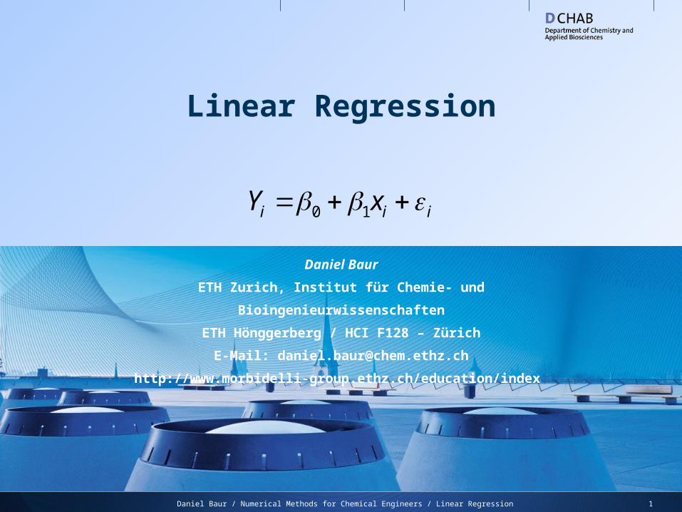
Linear Regression
0 1i i iY x
Daniel Baur
ETH Zurich, Institut für Chemie- und Bioingenieurwissenschaften
ETH Hönggerberg / HCI F128 – Zürich
E-Mail: [email protected]
http://www.morbidelli-group.ethz.ch/education/index
2
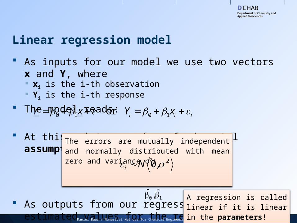
Linear regression model
As inputs for our model we use two vectors x and Y, where xi is the i-th observation Yi is the i-th response
The model reads:
At this point, we make a fundamental assumption:
As outputs from our regression we get estimated values for the regression parameters:
Daniel Baur / Numerical Methods for Chemical Engineers / Linear Regression
0 1 0 1or i i iY x Y x
The errors are mutually independent and normally distributed with mean zero and variance σ2:
20,i N
0 1ˆ ˆ, A regression is called linear if
it is linear in the parameters!
3Daniel Baur / Numerical Methods for Chemical Engineers / Linear Regression
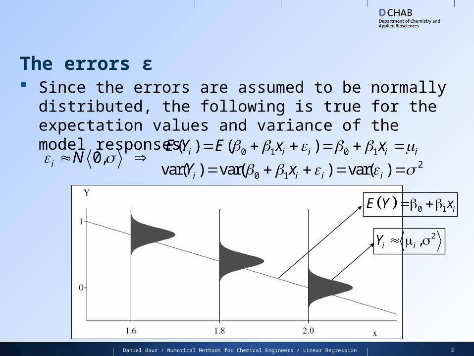
The errors ε Since the errors are assumed to be normally distributed,
the following is true for the expectation values and variance of the model responses
0 1 0 12
0 1
( ) ( )0,
var( ) var( ) var( )i i i i i
ii i i i
E Y E x xN
Y x
0 1 iE Y x
2,i iY

4Daniel Baur / Numerical Methods for Chemical Engineers / Linear Regression
Example: Boiling Temperature and Pressure

5Daniel Baur / Numerical Methods for Chemical Engineers / Linear Regression
Parameter estimation
1 11
,
1obs obsN N
x Y
X Y
x Y
a = confidence interval
6Daniel Baur / Numerical Methods for Chemical Engineers / Linear Regression
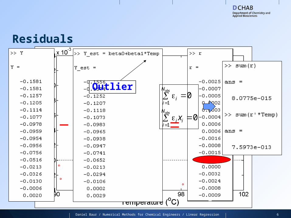
Residuals
1
1
0
0
obs
obs
N
ii
N
i ii
x
Outlier

7Daniel Baur / Numerical Methods for Chemical Engineers / Linear Regression
Removing the Outlier
8Daniel Baur / Numerical Methods for Chemical Engineers / Linear Regression
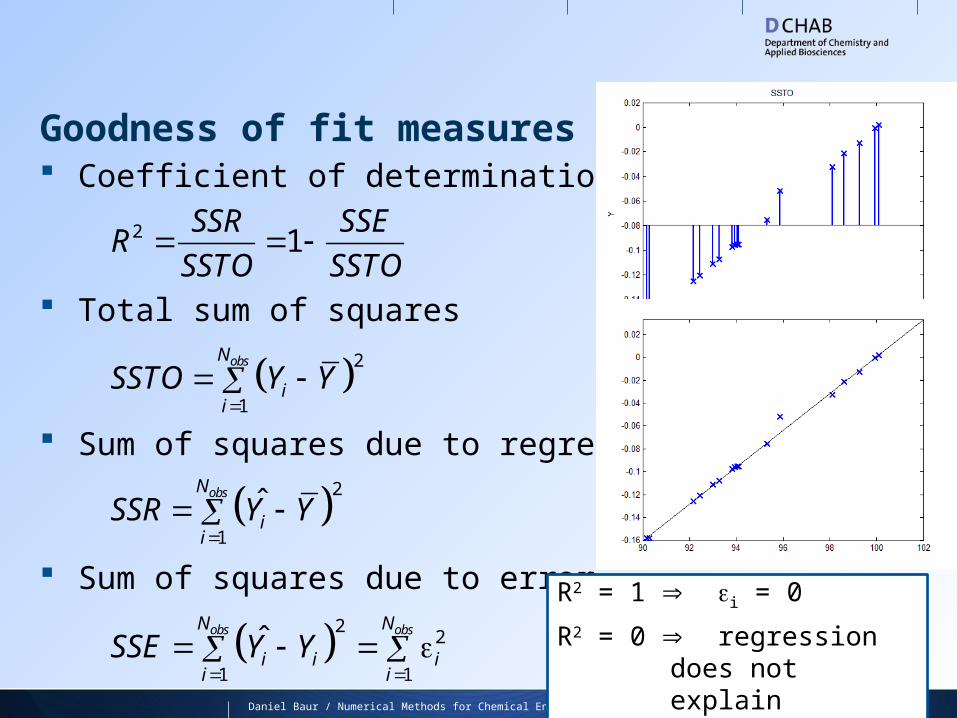
Goodness of fit measures Coefficient of determination
Total sum of squares
Sum of squares due to regression
Sum of squares due to error
2
1
obsN
ii
SSTO Y Y
2
1
ˆobsN
ii
SSR Y Y
22
1 1
ˆobs obsN N
i i ii i
SSE Y Y
R2 = 1 i = 0
R2 = 0 regression does not explain variation of Y
2 1SSR SSE
RSSTO SSTO
9Daniel Baur / Numerical Methods for Chemical Engineers / Linear Regression
The LinearModel and dataset classes
Matlab 2012 features two classes that are designed specifically for statistical analysis and linear regression
dataset creates an object that holds data and meta-data like variable names,
options for inclusion / exclusion of data points, etc.
LinearModel is constructed from datasets or X, Y pairs (as with the regress
function) and a model description automatically does linear regression and holds all important
regression outputs like parameter estimates, residuals, confidence intervals etc.
includes several useful functions like plots, residual analysis, exclusion of parameters etc.
10Daniel Baur / Numerical Methods for Chemical Engineers / Linear Regression
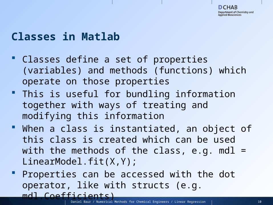
Classes in Matlab
Classes define a set of properties (variables) and methods (functions) which operate on those properties
This is useful for bundling information together with ways of treating and modifying this information
When a class is instantiated, an object of this class is created which can be used with the methods of the class, e.g. mdl = LinearModel.fit(X,Y);
Properties can be accessed with the dot operator, like with structs (e.g. mdl.Coefficients)
Methods can be called either with the dot operator, or by having an object of the class as first input argument (e.g. plot(mdl) or mdl.plot())
11Daniel Baur / Numerical Methods for Chemical Engineers / Linear Regression
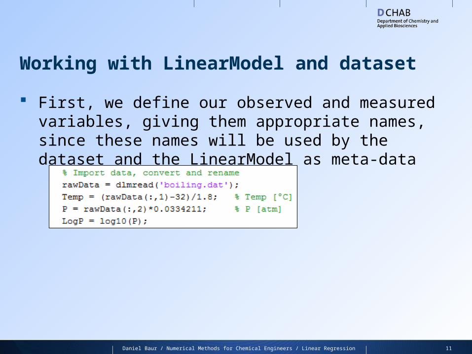
Working with LinearModel and dataset
First, we define our observed and measured variables, giving them appropriate names, since these names will be used by the dataset and the LinearModel as meta-data

12Daniel Baur / Numerical Methods for Chemical Engineers / Linear Regression
Working with LinearModel and dataset
Next, we construct the dataset from our variables
13Daniel Baur / Numerical Methods for Chemical Engineers / Linear Regression
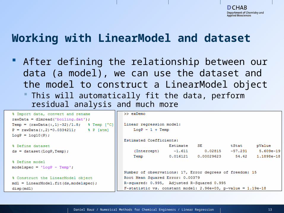
Working with LinearModel and dataset
After defining the relationship between our data (a model), we can use the dataset and the model to construct a LinearModel object This will automatically fit the data, perform residual analysis and
much more
14Daniel Baur / Numerical Methods for Chemical Engineers / Linear Regression
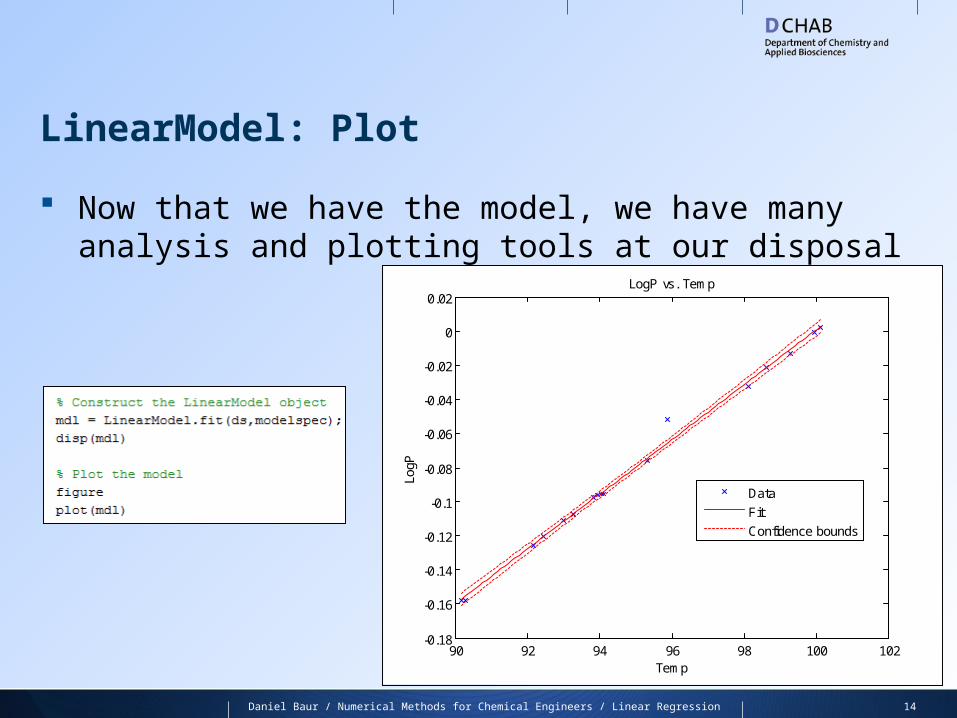
LinearModel: Plot
Now that we have the model, we have many analysis and plotting tools at our disposal
90 92 94 96 98 100 102-0.18
-0.16
-0.14
-0.12
-0.1
-0.08
-0.06
-0.04
-0.02
0
0.02LogP vs. Temp
Temp
LogP
Data
Fit
Confidence bounds
15Daniel Baur / Numerical Methods for Chemical Engineers / Linear Regression
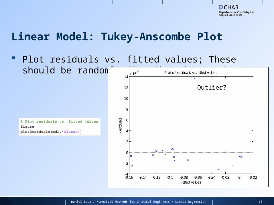
Linear Model: Tukey-Anscombe Plot
Plot residuals vs. fitted values; These should be randomly distributed around 0
-0.16 -0.14 -0.12 -0.1 -0.08 -0.06 -0.04 -0.02 0 0.02-4
-2
0
2
4
6
8
10
12
14x 10
-3
Fitted values
Res
idua
ls
Plot of residuals vs. fitted values
Outlier?
16Daniel Baur / Numerical Methods for Chemical Engineers / Linear Regression
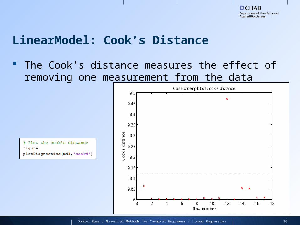
LinearModel: Cook’s Distance
The Cook’s distance measures the effect of removing one measurement from the data
0 2 4 6 8 10 12 14 16 180
0.05
0.1
0.15
0.2
0.25
0.3
0.35
0.4
0.45
0.5
Row number
Coo
k's
dist
ance
Case order plot of Cook's distance
17Daniel Baur / Numerical Methods for Chemical Engineers / Linear Regression
90 92 94 96 98 100 102-0.16
-0.14
-0.12
-0.1
-0.08
-0.06
-0.04
-0.02
0
0.02LogP vs. Temp
Temp
LogP
Data
Fit
Confidence bounds
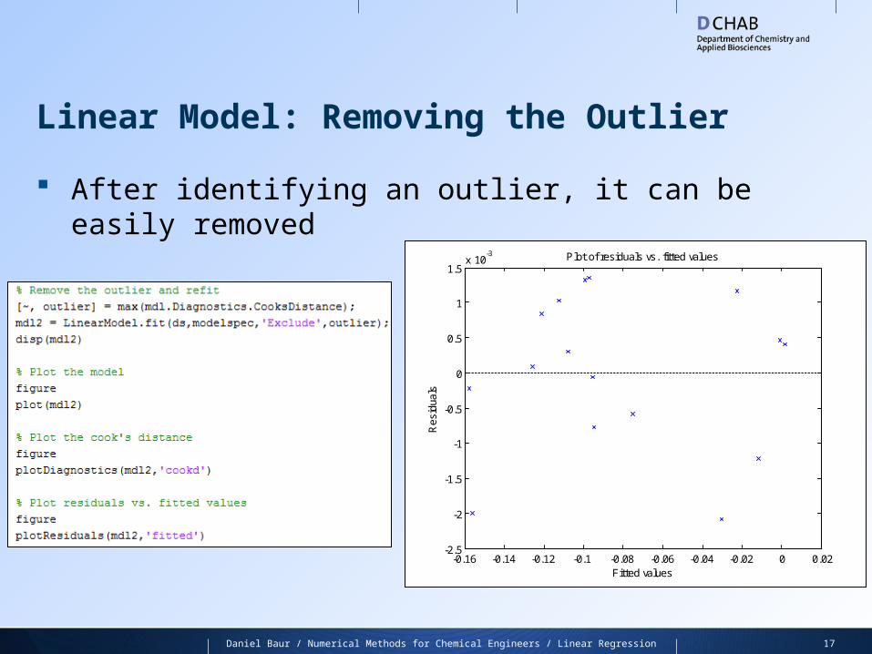
Linear Model: Removing the Outlier
After identifying an outlier, it can be easily removed
0 2 4 6 8 10 12 14 16 180
0.05
0.1
0.15
0.2
0.25
0.3
0.35
0.4
0.45
0.5
Row number
Coo
k's
dist
ance
Case order plot of Cook's distance
-0.16 -0.14 -0.12 -0.1 -0.08 -0.06 -0.04 -0.02 0 0.02-2.5
-2
-1.5
-1
-0.5
0
0.5
1
1.5x 10
-3
Fitted values
Res
idua
ls
Plot of residuals vs. fitted values
18Daniel Baur / Numerical Methods for Chemical Engineers / Linear Regression
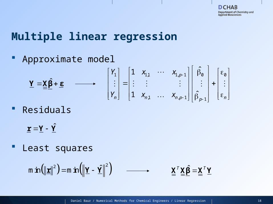
Multiple linear regression
Approximate model
Residuals
Least squares
ˆ Y Xβ ε1 1,1 1, 1 0 0
,1 , 1 1
ˆ1
ˆ1
p
n n n p np
Y x x
Y x x
ˆ r Y Y
22 ˆmin min r Y Y ˆT TX Xβ X Y
19Daniel Baur / Numerical Methods for Chemical Engineers / Linear Regression
Exercise
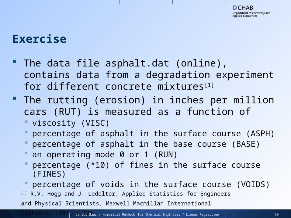
The data file asphalt.dat (online), contains data from a degradation experiment for different concrete mixtures[1]
The rutting (erosion) in inches per million cars (RUT) is measured as a function of viscosity (VISC) percentage of asphalt in the surface course (ASPH) percentage of asphalt in the base course (BASE) an operating mode 0 or 1 (RUN) percentage (*10) of fines in the surface course (FINES) percentage of voids in the surface course (VOIDS)
[1] R.V. Hogg and J. Ledolter, Applied Statistics for Engineers and Physical
Scientists, Maxwell Macmillan International Editions, 1992, p.393.
20Daniel Baur / Numerical Methods for Chemical Engineers / Linear Regression
Assignment
The LinearModel class only exists in Matlab 2012 or newer There are two versions of the assignment, one for Matlab
2012 and one for older versions, do one of the two
21Daniel Baur / Numerical Methods for Chemical Engineers / Linear Regression
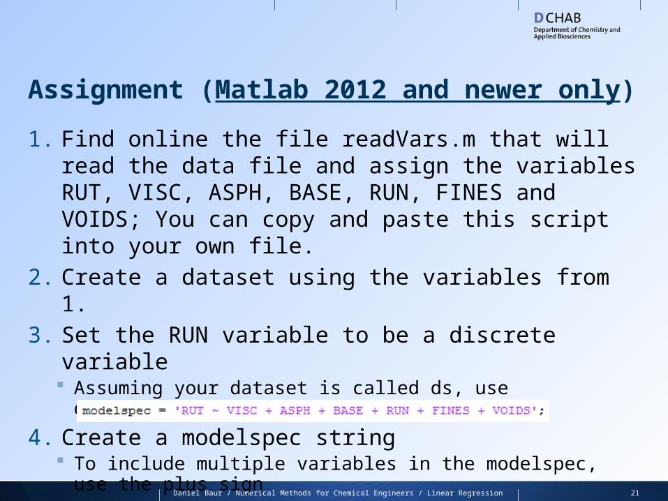
Assignment (Matlab 2012 and newer only)
1. Find online the file readVars.m that will read the data file and assign the variables RUT, VISC, ASPH, BASE, RUN, FINES and VOIDS; You can copy and paste this script into your own file.
2. Create a dataset using the variables from 1.
3. Set the RUN variable to be a discrete variable Assuming your dataset is called ds, useds.RUN = nominal(ds.RUN);
4. Create a modelspec string To include multiple variables in the modelspec, use the plus sign
5. Fit your model using LinearModel.fit, display the model output and plot the model.
22Daniel Baur / Numerical Methods for Chemical Engineers / Linear Regression
Assignment (Continued)
6. Which variables most likely have the largest influence?
7. Generate the Tukey-Anscombe plot. Is there any indication of nonlinearity, non-constant variance or of a skewed distribution of residuals?
8. Plot the adjusted responses for each variable, using the plotAllResponses function you can find online
9. The variables seem to show a rather random response, except for VISC which seems to mostly lie on one of the axes. Try and transform the system by defining logRUT = log10(RUT); logVISC = log10(VISC);
10.Define a new dataset and modelspec using the transformed variables.
23Daniel Baur / Numerical Methods for Chemical Engineers / Linear Regression
Assignment (Continued)
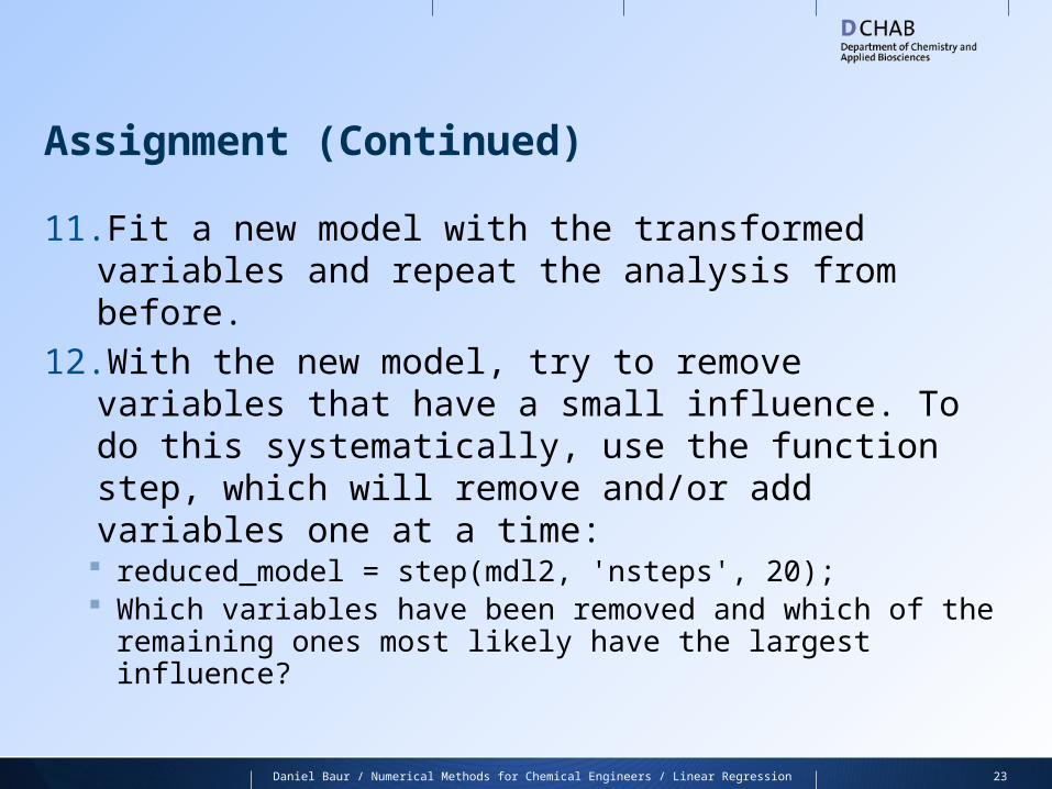
11. Fit a new model with the transformed variables and repeat the analysis from before.
12.With the new model, try to remove variables that have a small influence. To do this systematically, use the function step, which will remove and/or add variables one at a time: reduced_model = step(mdl2, 'nsteps', 20); Which variables have been removed and which of the remaining
ones most likely have the largest influence?
24Daniel Baur / Numerical Methods for Chemical Engineers / Linear Regression
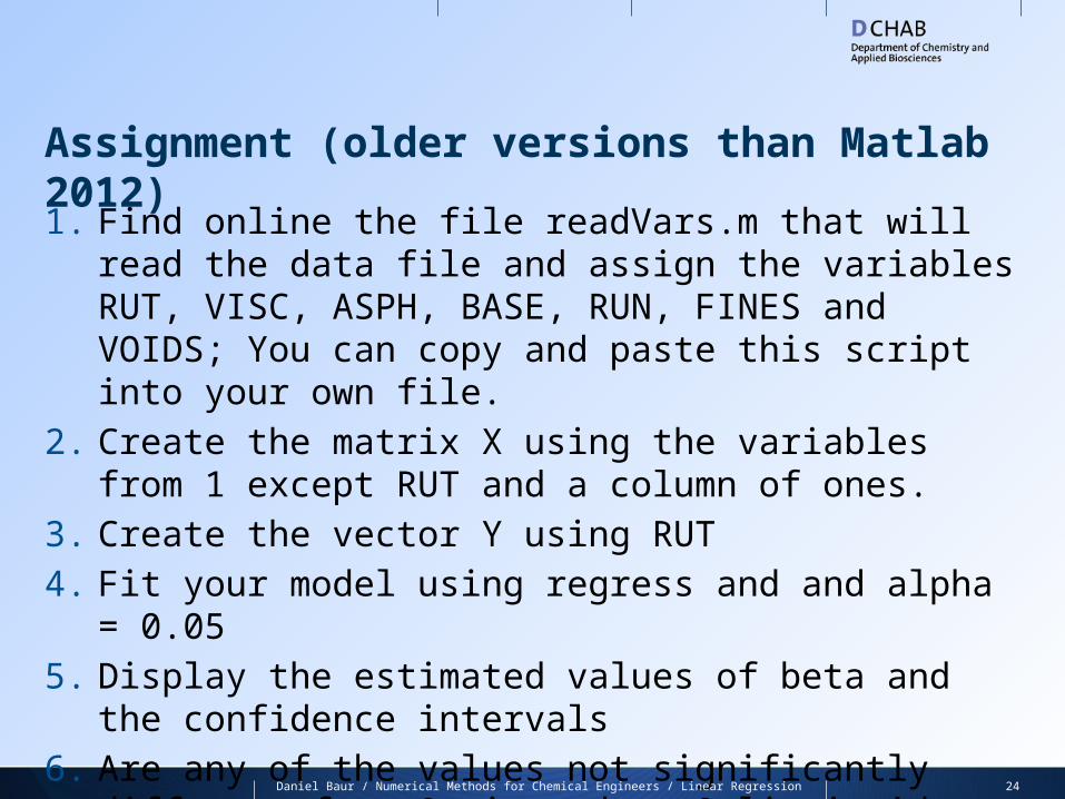
Assignment (older versions than Matlab 2012)
1. Find online the file readVars.m that will read the data file and assign the variables RUT, VISC, ASPH, BASE, RUN, FINES and VOIDS; You can copy and paste this script into your own file.
2. Create the matrix X using the variables from 1 except RUT and a column of ones.
3. Create the vector Y using RUT
4. Fit your model using regress and and alpha = 0.05
5. Display the estimated values of beta and the confidence intervals
6. Are any of the values not significantly different from 0, i.e. does 0 lie inside the confidence interval?
25Daniel Baur / Numerical Methods for Chemical Engineers / Linear Regression
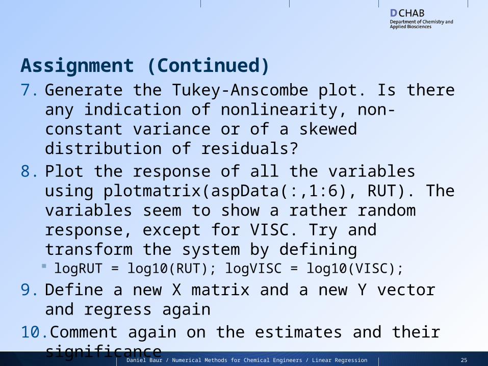
Assignment (Continued)7. Generate the Tukey-Anscombe plot. Is there any
indication of nonlinearity, non-constant variance or of a skewed distribution of residuals?
8. Plot the response of all the variables using plotmatrix(aspData(:,1:6), RUT). The variables seem to show a rather random response, except for VISC. Try and transform the system by defining logRUT = log10(RUT); logVISC = log10(VISC);
9. Define a new X matrix and a new Y vector and regress again
10.Comment again on the estimates and their significance
11. Reproduce the Tukey-Anscombe plot. Did anything change?


![Erwin Baur or Carl Correns: Who Really Created the …brusso/BaurCorrens[32,33]sortof.pdf · Erwin Baur or Carl Correns: Who Really Created the Theory of ... that Baur alone deserves](https://img.pdfslide.net/doc/110x75/5b9f1e0209d3f2d7748d761f/erwin-baur-or-carl-correns-who-really-created-the-brussobaurcorrens3233-.jpg)