Embed Size (px)
Citation preview
LINEAR STATE-SPACECONTROL SYSTEMS
Robert L. Williams II
Douglas A. LawrenceOhio University
JOHN WILEY & SONS, INC.
Linear State-Space Control Systems. Robert L. Williams II and Douglas A. LawrenceCopyright 2007 John Wiley & Sons, Inc. ISBN: 978-0-471-73555-7
Copyright 2007 by John Wiley & Sons, Inc. All rights reserved
Published by John Wiley & Sons, Inc., Hoboken, New JerseyPublished simultaneously in Canada.
No part of this publication may be reproduced, stored in a retrieval system, or transmitted in anyform or by any means, electronic, mechanical, photocopying, recording, scanning, or otherwise,except as permitted under Section 107 or 108 of the 1976 United States Copyright Act, withouteither the prior written permission of the Publisher, or authorization through payment of theappropriate per-copy fee to the Copyright Clearance Center, Inc., 222 Rosewood Drive, Danvers,MA 01923, (978) 750-8400, fax (978) 750-4470, or on the web at www.copyright.com. Requeststo the Publisher for permission should be addressed to the Permissions Department, John Wiley &Sons, Inc., 111 River Street, Hoboken, NJ 07030, (201) 748-6011, fax (201) 748-6008, or online athttp://www.wiley.com/go/permission.
Limit of Liability/Disclaimer of Warranty: While the publisher and author have used their bestefforts in preparing this book, they make no representations or warranties with respect to theaccuracy or completeness of the contents of this book and specifically disclaim any impliedwarranties of merchantability or fitness for a particular purpose. No warranty may be created orextended by sales representatives or written sales materials. The advice and strategies containedherein may not be suitable for your situation. You should consult with a professional whereappropriate. Neither the publisher nor author shall be liable for any loss of profit or any othercommercial damages, including but not limited to special, incidental, consequential, or otherdamages.
For general information on our other products and services or for technical support, please contactour Customer Care Department within the United States at (800) 762-2974, outside the UnitedStates at (317) 572-3993 or fax (317) 572-4002.
Wiley also publishes its books in a variety of electronic formats. Some content that appears in printmay not be available in electronic formats. For more information about Wiley products, visit ourweb site at www.wiley.com.
Library of Congress Cataloging-in-Publication Data:
Williams, Robert L., 1962-Linear state-space control systems / Robert L. Williams II and Douglas A.
Lawrence.p. cm.
Includes bibliographical references.ISBN 0-471-73555-8 (cloth)
1. Linear systems. 2. State-space methods. 3. Control theory. I.Lawrence, Douglas A. II. Title.
QA402.W547 2007629.8′32—dc22
2006016111
Printed in the United States of America
10 9 8 7 6 5 4 3 2 1

To Lisa, Zack, and especially Sam, an aspiring author.—R.L.W.
To Traci, Jessica, and Abby.—D.A.L.
CONTENTS
Preface ix
1 Introduction 1
1.1 Historical Perspective and Scope / 11.2 State Equations / 31.3 Examples / 51.4 Linearization of Nonlinear Systems / 171.5 Control System Analysis and Design using
MATLAB / 241.6 Continuing Examples / 321.7 Homework Exercises / 39
2 State-Space Fundamentals 482.1 State Equation Solution / 492.2 Impulse Response / 632.3 Laplace Domain Representation / 632.4 State-Space Realizations Revisited / 702.5 Coordinate Transformations / 722.6 MATLAB for Simulation and Coordinate
Transformations / 782.7 Continuing Examples for Simulation
and Coordinate Transformations / 842.8 Homework Exercises / 92
v
vi CONTENTS
3 Controllability 108
3.1 Fundamental Results / 1093.2 Controllability Examples / 1153.3 Coordinate Transformations
and Controllability / 1193.4 Popov-Belevitch-Hautus Tests for
Controllability / 1333.5 MATLAB for Controllability and Controller Canonical
Form / 1383.6 Continuing Examples for Controllability
and Controller Canonical Form / 1413.7 Homework Exercises / 144
4 Observability 149
4.1 Fundamental Results / 1504.2 Observability Examples / 1584.3 Duality / 1634.4 Coordinate Transformations and Observability / 1654.5 Popov-Belevitch-Hautus Tests for Observability / 1734.6 MATLAB for Observability and Observer Canonical
Form / 1744.7 Continuing Examples for Observability and Observer
Canonical Form / 1774.8 Homework Exercises / 180
5 Minimal Realizations 185
5.1 Minimality of Single-Input, Single OutputRealizations / 186
5.2 Minimality of Multiple-Input, Multiple OutputRealizations / 192
5.3 MATLAB for Minimal Realizations / 1945.4 Homework Exercises / 196
6 Stability 198
6.1 Internal Stability / 1996.2 Bounded-Input, Bounded-Output Stability / 2186.3 Bounded-Input, Bounded-Output Stability Versus
Asymptotic Stability / 2206.4 MATLAB for Stability Analysis / 225
CONTENTS vii
6.5 Continuing Examples: Stability Analysis / 2276.6 Homework Exercises / 230
7 Design of Linear State Feedback Control Laws 234
7.1 State Feedback Control Law / 2357.2 Shaping the Dynamic Response / 2367.3 Closed-Loop Eigenvalue Placement via State
Feedback / 2507.4 Stabilizability / 2637.5 Steady-State Tracking / 2687.6 MATLAB for State Feedback Control Law Design / 2787.7 Continuing Examples: Shaping Dynamic Response
and Control Law Design / 2837.8 Homework Exercises / 293
8 Observers and Observer-Based Compensators 300
8.1 Observers / 3018.2 Detectability / 3128.3 Reduced-Order Observers / 3168.4 Observer-Based Compensators and the Separation
Property / 3238.5 Steady-State Tracking with Observer-Based
Compensators / 3378.6 MATLAB for Observer Design / 3438.7 Continuing Examples: Design of State
Observers / 3488.8 Homework Exercises / 351
9 Introduction to Optimal Control 357
9.1 Optimal Control Problems / 3589.2 An Overview of Variational Calculus / 3609.3 Minimum Energy Control / 3719.4 The Linear Quadratic Regulator / 3779.5 MATLAB for Optimal Control / 3979.6 Continuing Example 1: Linear Quadratic
Regulator / 3999.7 Homework Exercises / 403
viii CONTENTS
Appendix A Matrix Introduction 407
A.1 Basics / 407A.2 Matrix Arithmetic / 409A.3 Determinants / 412A.4 Matrix Inversion / 414
Appendix B Linear Algebra 417
B.1 Vector Spaces / 417B.2 Subspaces / 419B.3 Standard Basis / 421B.4 Change of Basis / 422B.5 Orthogonality and Orthogonal Complements / 424B.6 Linear Transformations / 426B.7 Range and Null Space / 430B.8 Eigenvalues, Eigenvectors, and Related Topics / 435B.9 Norms for Vectors and Matrices / 444
Appendix C Continuing MATLAB Example m-file 447
References 456
Index 459
PREFACE
This textbook is intended for use in an advanced undergraduate or first-year graduate-level course that introduces state-space methods for theanalysis and design of linear control systems. It is also intended to servepracticing engineers and researchers seeking either an introduction to ora reference source for this material. This book grew out of separate lec-ture notes for courses in mechanical and electrical engineering at OhioUniversity. The only assumed prerequisites are undergraduate courses inlinear signals and systems and control systems. Beyond the traditionalundergraduate mathematics preparation, including calculus, differentialequations, and basic matrix computations, a prior or concurrent coursein linear algebra is beneficial but not essential.
This book strives to provide both a rigorously established foundationto prepare students for advanced study in systems and control theory anda comprehensive overview, with an emphasis on practical aspects, forgraduate students specializing in other areas. The reader will find rigor-ous mathematical treatment of the fundamental concepts and theoreticalresults that are illustrated through an ample supply of academic examples.In addition, to reflect the complexity of real-world applications, a majortheme of this book is the inclusion of continuing examples and exercises.Here, practical problems are introduced in the first chapter and revisited insubsequent chapters. The hope is that the student will find it easier to applynew concepts to familiar systems. To support the nontrivial computationsassociated with these problems, the book provides a chapter-by-chapter
ix
x PREFACE
tutorial on the use of the popular software package MATLAB and the associ-ated Control Systems Toolbox for computer-aided control system analysisand design. The salient features of MATLAB are illustrated in each chapterthrough a continuing MATLAB example and a pair of continuing examples.
This textbook consists of nine chapters and three appendices organizedas follows. Chapter 1 introduces the state-space representation for lin-ear time-invariant systems. Chapter 2 is concerned primarily with thestate equation solution and connections with fundamental linear systemsconcepts along with several other basic results to be used in subsequentchapters. Chapters 3 and 4 present thorough introductions to the impor-tant topics of controllability and observability, which reveal the power ofstate-space methods: The complex behavior of dynamic systems can becharacterized by algebraic relationships derived from the state-space sys-tem description. Chapter 5 addresses the concept of minimality associatedwith state-space realizations of linear time-invariant systems. Chapter 6deals with system stability from both internal and external (input-output)viewpoints and relationships between them. Chapter 7 presents strate-gies for dynamic response shaping and introduces state feedback controllaws. Chapter 8 presents asymptotic observers and dynamic observer-based compensators. Chapter 9 gives an introduction to optimal control,focusing on the linear quadratic regulator. Appendix A provides a sum-mary of basic matrix computations. Appendix B provides an overview ofbasic concepts from linear algebra used throughout the book. AppendixC provides the complete MATLAB program for the Continuing MATLAB
Example.Each chapter concludes with a set of exercises intended to aid
the student in his or her quest for mastery of the subject matter.Exercises will be grouped into four categories: Numerical Exercises,Analytical Exercises, Continuing MATLAB Exercises, and ContinuingExercises. Numerical Exercises are intended to be straightforwardproblems involving numeric data that reinforce important computations.Solutions should be based on hand calculations, although students arestrongly encouraged to use MATLAB to check their results. AnalyticalExercises are intended to require nontrivial derivations or proofs of factseither asserted without proof in the chapter or extensions thereof. Theseexercises are by nature more challenging than the Numerical Exercises.Continuing MATLAB Exercises will revisit the state equations introducedin Chapter 1. Students will be called on to develop MATLAB m-filesincrementally for each exercise that implement computations associatedwith topics in each chapter. Continuing Exercises are also cumulativeand are patterned after the Continuing Examples introduced in Chapter1. These exercises are based on physical systems, so the initial task will

PREFACE xi
be to derive linear state equation representations from the given physicaldescriptions. The use of MATLAB also will be required over the course ofworking these exercises, and the experience gained from the ContinuingMATLAB Exercises will come in handy .
1
INTRODUCTION
This chapter introduces the state-space representation for linear time-invariant systems. We begin with a brief overview of the origins ofstate-space methods to provide a context for the focus of this book. Fol-lowing that, we define the state equation format and provide examples toshow how state equations can be derived from physical system descrip-tions and from transfer-function representations. In addition, we showhow linear state equations arise from the linearization of a nonlinear stateequation about a nominal trajectory or equilibrium condition.
This chapter also initiates our use of the MATLAB software packagefor computer-aided analysis and design of linear state-space control sys-tems. Beginning here and continuing throughout the book, features ofMATLAB and the accompanying Control Systems Toolbox that support eachchapter’s subject matter will be presented and illustrated using a Continu-ing MATLAB Example. In addition, we introduce two Continuing Examplesthat we also will revisit in subsequent chapters.
1.1 HISTORICAL PERSPECTIVE AND SCOPE
Any scholarly account of the history of control engineering would haveto span several millennia because there are many examples throughout
1
Linear State-Space Control Systems. Robert L. Williams II and Douglas A. LawrenceCopyright 2007 John Wiley & Sons, Inc. ISBN: 978-0-471-73555-7
2 INTRODUCTION
ancient history, the industrial revolution, and into the early twentiethcentury of ingeniously designed systems that employed feedback mech-anisms in various forms. Ancient water clocks, south-pointing chariots,Watt’s flyball governor for steam engine speed regulation, and mecha-nisms for ship steering, gun pointing, and vacuum tube amplifier stabiliza-tion are but a few. Here we are content to survey important developmentsin the theory and practice of control engineering since the mid-1900s inorder to provide some perspective for the material that is the focus of thisbook in relation to topics covered in most undergraduate controls coursesand in more advanced graduate-level courses.
In the so-called classical control era of the 1940s and 1950s, systemswere represented in the frequency domain by transfer functions. In addi-tion, performance and robustness specifications were either cast directly inor translated into the frequency domain. For example, transient responsespecifications were converted into desired closed-loop pole locations ordesired open-loop and/or closed-loop frequency-response characteristics.Analysis techniques involving Evans root locus plots, Bode plots, Nyquistplots, and Nichol’s charts were limited primarily to single-input, single-output systems, and compensation schemes were fairly simple, e.g., asingle feedback loop with cascade compensation. Moreover, the designprocess was iterative, involving an initial design based on various sim-plifying assumptions followed by parameter tuning on a trial-and-errorbasis. Ultimately, the final design was not guaranteed to be optimal inany sense.
The 1960s and 1970s witnessed a fundamental paradigm shift from thefrequency domain to the time domain. Systems were represented in thetime domain by a type of differential equation called a state equation.Performance and robustness specifications also were specified in the timedomain, often in the form of a quadratic performance index. Key advan-tages of the state-space approach were that a time-domain formulationexploited the advances in digital computer technology and the analysisand design methods were well-suited to multiple-input, multiple-outputsystems. Moreover, feedback control laws were calculated using analyticalformulas, often directly optimizing a particular performance index.
The 1980’s and 1990’s were characterized by a merging of frequency-domain and time-domain viewpoints. Specifically, frequency-domain per-formance and robustness specifications once again were favored, coupledwith important theoretical breakthroughs that yielded tools for handlingmultiple-input, multiple-output systems in the frequency domain. Furtheradvances yielded state-space time-domain techniques for controller syn-thesis. In the end, the best features of the preceding decades were mergedinto a powerful, unified framework.
STATE EQUATIONS 3
The chronological development summarized in the preceding para-graphs correlates with traditional controls textbooks and academic curric-ula as follows. Classical control typically is the focus at the undergraduatelevel, perhaps along with an introduction to state-space methods. An in-depth exposure to the state-space approach then follows at the advancedundergraduate/first-year graduate level and is the focus of this book. This,in turn, serves as the foundation for more advanced treatments reflectingrecent developments in control theory, including those alluded to in thepreceding paragraph, as well as extensions to time-varying and nonlinearsystems.
We assume that the reader is familiar with the traditional undergrad-uate treatment of linear systems that introduces basic system propertiessuch as system dimension, causality, linearity, and time invariance. Thisbook is concerned with the analysis, simulation, and control of finite-dimensional, causal, linear, time-invariant, continuous-time dynamic sys-tems using state-space techniques. From now on, we will refer to membersof this system class as linear time-invariant systems.
The techniques developed in this book are applicable to various types ofengineering (even nonengineering) systems, such as aerospace, mechani-cal, electrical, electromechanical, fluid, thermal, biological, and economicsystems. This is so because such systems can be modeled mathematicallyby the same types of governing equations. We do not formally addressthe modeling issue in this book, and the point of departure is a lineartime-invariant state-equation model of the physical system under study.With mathematics as the unifying language, the fundamental results andmethods presented here are amenable to translation into the applicationdomain of interest.
1.2 STATE EQUATIONS
A state-space representation for a linear time-invariant system has thegeneral form
x(t) = Ax(t) + Bu(t)
y(t) = Cx(t) + Du(t)x(t0) = x0 (1.1)
in which x(t) is the n-dimensional state vector
x(t) =
x1(t)
x2(t)...
xn(t)
4 INTRODUCTION
whose n scalar components are called state variables. Similarly, them-dimensional input vector and p-dimensional output vector are given,respectively, as
u(t) =
u1(t)
u2(t)...
um(t)
y(t) =
y1(t)
y2(t)...
yp(t)
Since differentiation with respect to time of a time-varying vector quan-tity is performed component-wise, the time-derivative on the left-hand sideof Equation (1.1) represents
x(t) =
x1(t)
x2(t)...
xn(t)
Finally, for a specified initial time t0, the initial state x(t0) = x0 is aspecified, constant n-dimensional vector.
The state vector x(t) is composed of a minimum set of system variablesthat uniquely describes the future response of the system given the currentstate, the input, and the dynamic equations. The input vector u(t) containsvariables used to actuate the system, the output vector y(t) contains themeasurable quantities, and the state vector x(t) contains internal systemvariables.
Using the notational convention M = [mij ] to represent the matrixwhose element in the ith row and j th column is mij , the coefficientmatrices in Equation (1.1) can be specified via
A = [aij ] B = [bij ] C = [cij ]D = [dij ]
having dimensions n × n, n × m, p × n, and p × m, respectively. Withthese definitions in place, we see that the state equation (1.1) is a compactrepresentation of n scalar first-order ordinary differential equations, that is,
xi(t) = ai1x1(t) + ai2x2(t) + · · · + ainxn(t)
+ bi1u1(t) + bi2u2(t) + · · · + bimum(t)
for i = 1, 2, . . . , n, together with p scalar linear algebraic equations
yj (t) = cj1x1(t) + cj2x2(t) + · · · + cjnxn(t)
+ dj1u1(t) + dj2u2(t) + · · · + djmum(t)
EXAMPLES 5
+
++ +
A
CB
D
u(t) y(t)x(t) x(t)
x0
∫
FIGURE 1.1 State-equation block diagram.
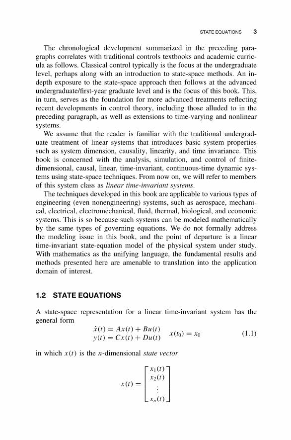
for j = 1, 2, . . . , p. From this point on the vector notation (1.1) willbe preferred over these scalar decompositions. The state-space descrip-tion consists of the state differential equation x(t) = Ax(t) + Bu(t) andthe algebraic output equation y(t) = Cx(t) + Du(t) from Equation (1.1).Figure 1.1 shows the block diagram for the state-space representation ofgeneral multiple-input, multiple-output linear time-invariant systems.
One motivation for the state-space formulation is to convert a cou-pled system of higher-order ordinary differential equations, for example,those representing the dynamics of a mechanical system, to a coupledset of first-order differential equations. In the single-input, single-outputcase, the state-space representation converts a single nth-order differen-tial equation into a system of n coupled first-order differential equations.In the multiple-input, multiple-output case, in which all equations are ofthe same order n, one can convert the system of k nth-order differentialequations into a system of kn coupled first-order differential equations.
1.3 EXAMPLES
In this section we present a series of examples that illustrate the construc-tion of linear state equations. The first four examples begin with first-principles modeling of physical systems. In each case we adopt the strat-egy of associating state variables with the energy storage elements in thesystem. This facilitates derivation of the required differential and algebraicequations in the state-equation format. The last two examples begin withtransfer-function descriptions, hence establishing a link between transferfunctions and state equations that will be pursued in greater detail in laterchapters.
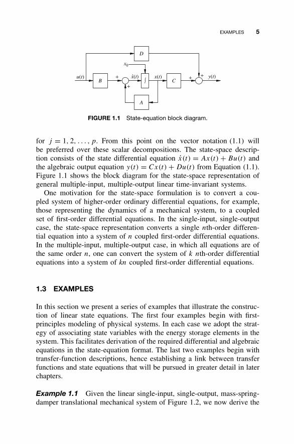
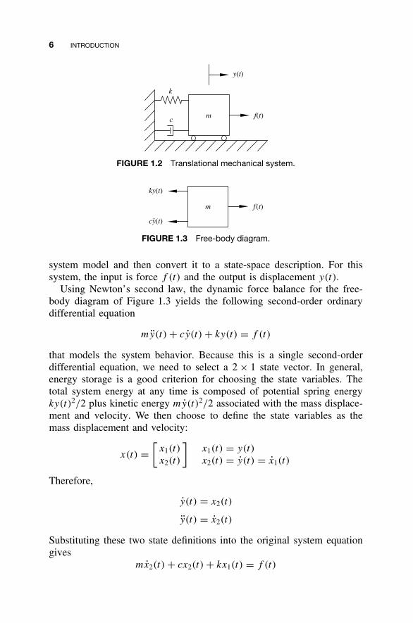
Example 1.1 Given the linear single-input, single-output, mass-spring-damper translational mechanical system of Figure 1.2, we now derive the
6 INTRODUCTION
y(t)
f(t)
k
c m
FIGURE 1.2 Translational mechanical system.
ky(t)
cy(t)
f (t)m
FIGURE 1.3 Free-body diagram.
system model and then convert it to a state-space description. For thissystem, the input is force f (t) and the output is displacement y(t).
Using Newton’s second law, the dynamic force balance for the free-body diagram of Figure 1.3 yields the following second-order ordinarydifferential equation
my(t) + cy(t) + ky(t) = f (t)
that models the system behavior. Because this is a single second-orderdifferential equation, we need to select a 2 × 1 state vector. In general,energy storage is a good criterion for choosing the state variables. Thetotal system energy at any time is composed of potential spring energyky(t)2/2 plus kinetic energy my(t)2/2 associated with the mass displace-ment and velocity. We then choose to define the state variables as themass displacement and velocity:
x(t) =[
x1(t)
x2(t)
]x1(t) = y(t)
x2(t) = y(t) = x1(t)
Therefore,
y(t) = x2(t)
y(t) = x2(t)
Substituting these two state definitions into the original system equationgives
mx2(t) + cx2(t) + kx1(t) = f (t)
EXAMPLES 7
The original single second-order differential equation can be written asa coupled system of two first-order differential equations, that is,
x1(t) = x2(t)
x2(t) = − c
mx2(t) − k
mx1(t) + 1
mf (t)
The output is the mass displacement
y(t) = x1(t)
The generic variable name for input vectors is u(t), so we define:
u(t) = f (t)
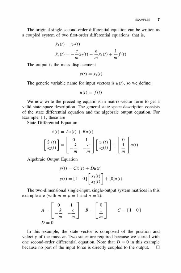
We now write the preceding equations in matrix-vector form to get avalid state-space description. The general state-space description consistsof the state differential equation and the algebraic output equation. ForExample 1.1, these are
State Differential Equation
x(t) = Ax(t) + Bu(t)
[x1(t)
x2(t)
]=
0 1
− k
m− c
m
[
x1(t)
x2(t)
]+
0
1
m
u(t)
Algebraic Output Equation
y(t) = Cx(t) + Du(t)
y(t) = [ 1 0 ]
[x1(t)
x2(t)
]+ [0]u(t)
The two-dimensional single-input, single-output system matrices in thisexample are (with m = p = 1 and n = 2):
A = 0 1
− k
m− c
m
B =
0
1
m
C = [ 1 0 ]
D = 0
In this example, the state vector is composed of the position andvelocity of the mass m. Two states are required because we started withone second-order differential equation. Note that D = 0 in this examplebecause no part of the input force is directly coupled to the output. �
8 INTRODUCTION
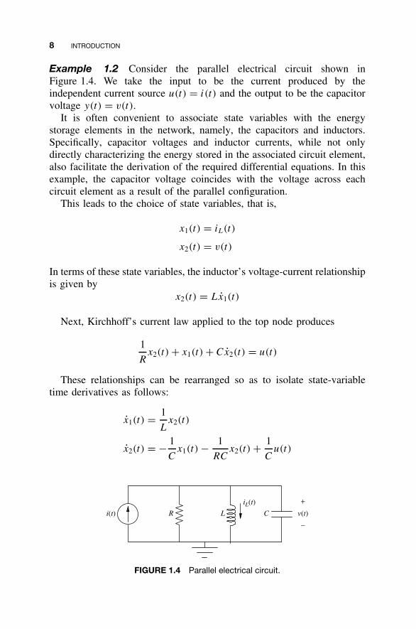
Example 1.2 Consider the parallel electrical circuit shown inFigure 1.4. We take the input to be the current produced by theindependent current source u(t) = i(t) and the output to be the capacitorvoltage y(t) = v(t).
It is often convenient to associate state variables with the energystorage elements in the network, namely, the capacitors and inductors.Specifically, capacitor voltages and inductor currents, while not onlydirectly characterizing the energy stored in the associated circuit element,also facilitate the derivation of the required differential equations. In thisexample, the capacitor voltage coincides with the voltage across eachcircuit element as a result of the parallel configuration.
This leads to the choice of state variables, that is,
x1(t) = iL(t)
x2(t) = v(t)
In terms of these state variables, the inductor’s voltage-current relationshipis given by
x2(t) = Lx1(t)
Next, Kirchhoff’s current law applied to the top node produces
1
Rx2(t) + x1(t) + Cx2(t) = u(t)
These relationships can be rearranged so as to isolate state-variabletime derivatives as follows:
x1(t) = 1
Lx2(t)
x2(t) = − 1
Cx1(t) − 1
RCx2(t) + 1
Cu(t)
i(t) R L C v(t)
+
−
iL(t)
FIGURE 1.4 Parallel electrical circuit.
EXAMPLES 9
This pair of coupled first-order differential equations, along with theoutput definition y(t) = x2(t), yields the following state-space descriptionfor this electrical circuit:
State Differential Equation
[x1(t)
x2(t)
]=
0
1
L
− 1
C− 1
RC
[x1(t)
x2(t)
]+
0
1
C
u(t)
Algebraic Output Equation
y(t) = [ 0 1 ]
[x1(t)
x2(t)
]+ [0]u(t)
from which the coefficient matrices A, B, C, and D are found by inspec-tion, that is,
A = 0
1
L
− 1
C− 1
RC
B =
0
1
C
C = [ 0 1 ]
D = 0
Note that D = 0 in this example because there is no direct couplingbetween the current source and the capacitor voltage. �
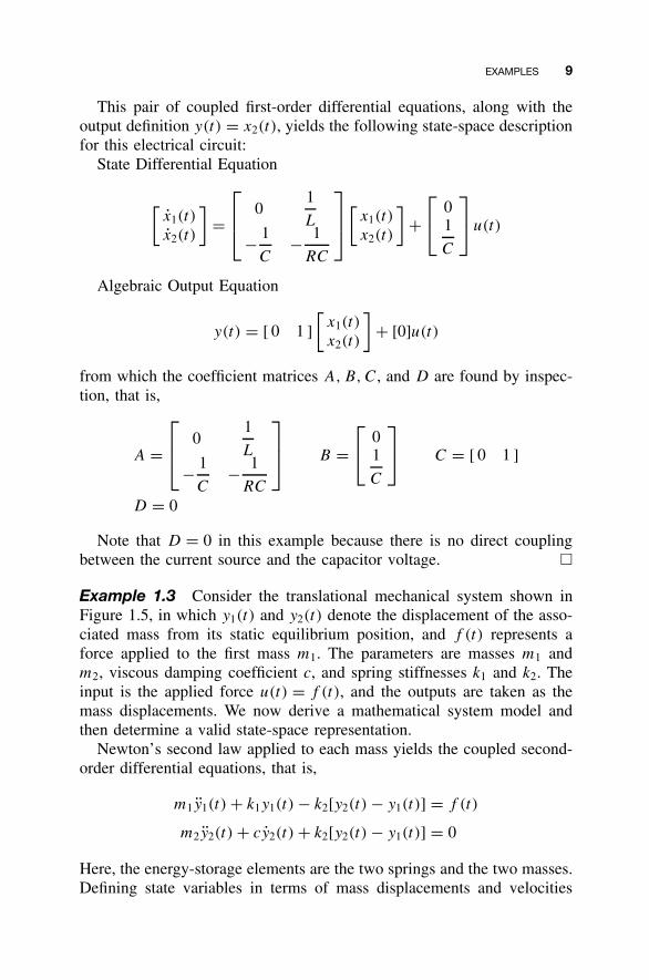
Example 1.3 Consider the translational mechanical system shown inFigure 1.5, in which y1(t) and y2(t) denote the displacement of the asso-ciated mass from its static equilibrium position, and f (t) represents aforce applied to the first mass m1. The parameters are masses m1 andm2, viscous damping coefficient c, and spring stiffnesses k1 and k2. Theinput is the applied force u(t) = f (t), and the outputs are taken as themass displacements. We now derive a mathematical system model andthen determine a valid state-space representation.
Newton’s second law applied to each mass yields the coupled second-order differential equations, that is,
m1y1(t) + k1y1(t) − k2[y2(t) − y1(t)] = f (t)
m2y2(t) + cy2(t) + k2[y2(t) − y1(t)] = 0
Here, the energy-storage elements are the two springs and the two masses.Defining state variables in terms of mass displacements and velocities
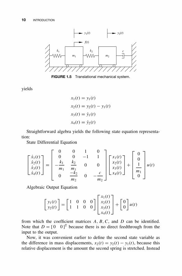
10 INTRODUCTION
y1(t)
f(t)
y2(t)
m1 m2
k1 k2 c
FIGURE 1.5 Translational mechanical system.
yields
x1(t) = y1(t)
x2(t) = y2(t) − y1(t)
x3(t) = y1(t)
x4(t) = y2(t)
Straightforward algebra yields the following state equation representa-tion:
State Differential Equation
x1(t)
x2(t)
x3(t)
x4(t)
=
0 0 1 00 0 −1 1
− k1
m1
k2
m10 0
0−k2
m20 − c
m2
x1(t)
x2(t)
x3(t)
x4(t)
+
001
m10
u(t)
Algebraic Output Equation
[y1(t)
y2(t)
]=
[1 0 0 01 1 0 0
]
x1(t)
x2(t)
x3(t)
x4(t)
+
[00
]u(t)
from which the coefficient matrices A, B,C, and D can be identified.Note that D = [ 0 0 ]T because there is no direct feedthrough from theinput to the output.
Now, it was convenient earlier to define the second state variable asthe difference in mass displacements, x2(t) = y2(t) − y1(t), because thisrelative displacement is the amount the second spring is stretched. Instead
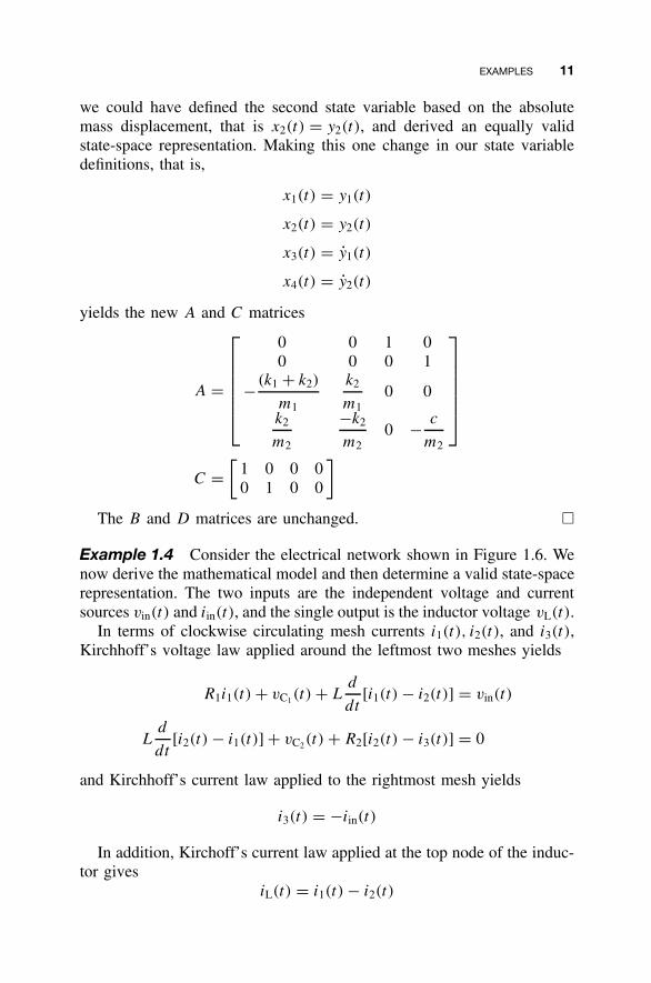
EXAMPLES 11
we could have defined the second state variable based on the absolutemass displacement, that is x2(t) = y2(t), and derived an equally validstate-space representation. Making this one change in our state variabledefinitions, that is,
x1(t) = y1(t)
x2(t) = y2(t)
x3(t) = y1(t)
x4(t) = y2(t)
yields the new A and C matrices
A =
0 0 1 00 0 0 1
−(k1 + k2)
m1
k2
m10 0
k2
m2
−k2
m20 − c
m2
C =[
1 0 0 00 1 0 0
]
The B and D matrices are unchanged. �
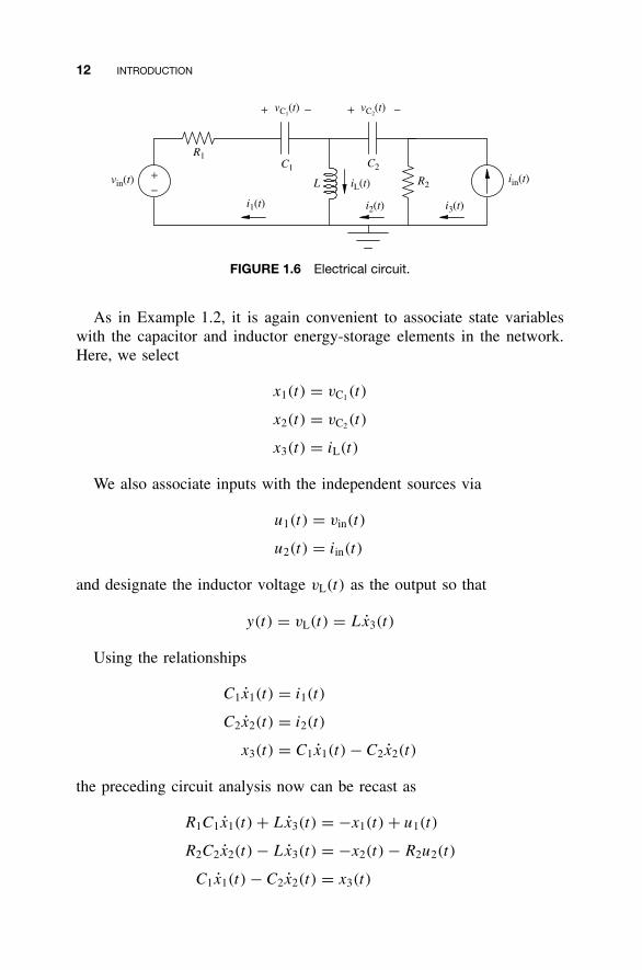
Example 1.4 Consider the electrical network shown in Figure 1.6. Wenow derive the mathematical model and then determine a valid state-spacerepresentation. The two inputs are the independent voltage and currentsources vin(t) and iin(t), and the single output is the inductor voltage vL(t).
In terms of clockwise circulating mesh currents i1(t), i2(t), and i3(t),Kirchhoff’s voltage law applied around the leftmost two meshes yields
R1i1(t) + vC1(t) + Ld
dt[i1(t) − i2(t)] = vin(t)
Ld
dt[i2(t) − i1(t)] + vC2(t) + R2[i2(t) − i3(t)] = 0
and Kirchhoff’s current law applied to the rightmost mesh yields
i3(t) = −iin(t)
In addition, Kirchoff’s current law applied at the top node of the induc-tor gives
iL(t) = i1(t) − i2(t)
12 INTRODUCTION
+ −
+−
R1
vin(t) iin(t)R2
C1 C2
L iL(t)
vC1(t) vC2
(t)+ −
i1(t) i2(t) i3(t)
FIGURE 1.6 Electrical circuit.
As in Example 1.2, it is again convenient to associate state variableswith the capacitor and inductor energy-storage elements in the network.Here, we select
x1(t) = vC1(t)
x2(t) = vC2(t)
x3(t) = iL(t)
We also associate inputs with the independent sources via
u1(t) = vin(t)
u2(t) = iin(t)
and designate the inductor voltage vL(t) as the output so that
y(t) = vL(t) = Lx3(t)
Using the relationships
C1x1(t) = i1(t)
C2x2(t) = i2(t)
x3(t) = C1x1(t) − C2x2(t)
the preceding circuit analysis now can be recast as
R1C1x1(t) + Lx3(t) = −x1(t) + u1(t)
R2C2x2(t) − Lx3(t) = −x2(t) − R2u2(t)
C1x1(t) − C2x2(t) = x3(t)
EXAMPLES 13
Packaging these equations in matrix form and isolating the state-variabletime derivatives gives
x1(t)
x2(t)
x3(t)
=
R1C1 0 L
0 R2C2 −L
C1 −C2 0
−1
−1 0 0
0 −1 00 0 0
x1(t)
x2(t)
x3(t)
+
1 0
0 −R2
0 0
[u1(t)
u2(t)
]
Calculating and multiplying through by the inverse and yields the statedifferential equation, that is,
x1(t)
x2(t)
x3(t)
=
1
(R1 + R2)C1
−1
(R1 + R2)C1
R2
(R1 + R2)C1
−1
(R1 + R2)C2
−1
(R1 + R2)C2
−R1
(R1 + R2)C2
−R2
(R1 + R2)L
R1
(R1 + R2)L
−R1R2
(R1 + R2)L
x1(t)
x2(t)
x3(t)
+
1
(R1 + R2)C1
−R2
(R1 + R2)C1
1
(R1 + R2)C2
−R2
(R1 + R2)C2
R2
(R1 + R2)L
R1R2
(R1 + R2)L
[u1(t)
u2(t)
]
which is in the required format from which coefficient matrices A and B
can be identified. In addition, the associated output equation y(t) = Lx3(t)
can be expanded to the algebraic output equation as follows
y(t) =[ −R2
(R1 + R2)
R1
(R1 + R2)
−R1R2
(R1 + R2)
] x1(t)
x2(t)
x3(t)
+[
R2
(R1 + R2)
R1R2
(R1 + R2)
] [u1(t)
u2(t)
]
from which coefficient matrices C and D can be identified.Note that in this example, there is direct coupling between the indepen-
dent voltage and current source inputs vin(t) and iin(t) and the inductorvoltage output vL(t), and hence the coefficient matrix D is nonzero. �
14 INTRODUCTION
Example 1.5 This example derives a valid state-space description fora general third-order differential equation of the form
¨y(t) + a2y(t) + a1y(t) + a0y(t) = b0u(t)
The associated transfer function definition is
H(s) = b0
s3 + a2s2 + a1s + a0
Define the following state variables:
x(t) = x1(t)
x2(t)
x3(t)
x1(t) = y(t)
x2(t) = y(t) = x1(t)
x3(t) = y(t) = x1(t) = x2(t)
Substituting these state-variable definitions into the original differentialequation yields the following:
x3(t) = −a0x1(t) − a1x2(t) − a2x3(t) + b0u(t)
The state differential and algebraic output equations are then
State Differential Equation
x1(t)
x2(t)
x3(t)
=
0 1 0
0 0 1−a0 −a1 −a2
x1(t)
x2(t)
x3(t)
+
0
0b0
u(t)
Algebraic Output Equation
y(t) = [ 1 0 0 ]
x1(t)
x2(t)
x3(t)
+ [0]u(t)
from which the coefficient matrices A, B,C, and D can be identified.D = 0 in this example because there is no direct coupling between theinput and output.
This example may be generalized easily to the nth-order ordinary dif-ferential equation
dny(t)
dtn+ an−1
dn−1y(t)
dtn−1+ · · · + a2
d2y(t)
dt2+ a1
dy(t)
dt+ a0y(t) = b0u(t)
(1.2)
EXAMPLES 15
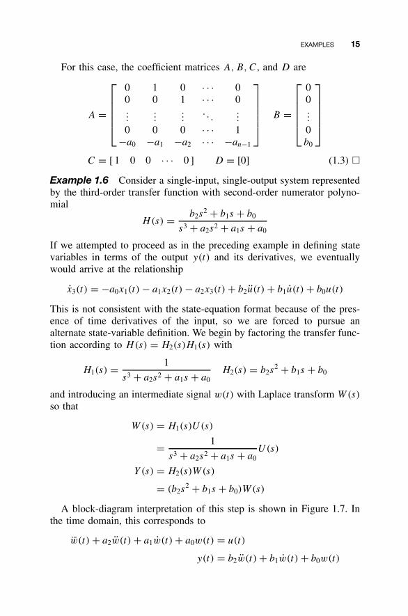
For this case, the coefficient matrices A, B, C, and D are
A =
0 1 0 · · · 00 0 1 · · · 0...
......
. . ....
0 0 0 · · · 1−a0 −a1 −a2 · · · −an−1
B =
00...
0b0
C = [ 1 0 0 · · · 0 ] D = [0] (1.3) �
Example 1.6 Consider a single-input, single-output system representedby the third-order transfer function with second-order numerator polyno-mial
H(s) = b2s2 + b1s + b0
s3 + a2s2 + a1s + a0
If we attempted to proceed as in the preceding example in defining statevariables in terms of the output y(t) and its derivatives, we eventuallywould arrive at the relationship
x3(t) = −a0x1(t) − a1x2(t) − a2x3(t) + b2u(t) + b1u(t) + b0u(t)
This is not consistent with the state-equation format because of the pres-ence of time derivatives of the input, so we are forced to pursue analternate state-variable definition. We begin by factoring the transfer func-tion according to H(s) = H2(s)H1(s) with
H1(s) = 1
s3 + a2s2 + a1s + a0H2(s) = b2s
2 + b1s + b0
and introducing an intermediate signal w(t) with Laplace transform W(s)
so that
W(s) = H1(s)U(s)
= 1
s3 + a2s2 + a1s + a0U(s)
Y (s) = H2(s)W(s)
= (b2s2 + b1s + b0)W(s)
A block-diagram interpretation of this step is shown in Figure 1.7. Inthe time domain, this corresponds to
¨w(t) + a2w(t) + a1w(t) + a0w(t) = u(t)
y(t) = b2w(t) + b1w(t) + b0w(t)
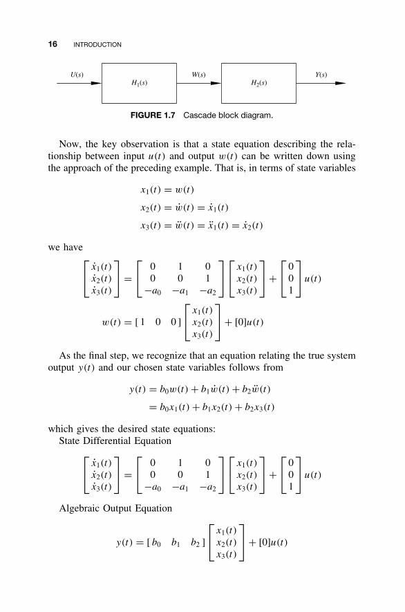
16 INTRODUCTION
U(s) W(s) Y(s)H1(s) H2(s)
FIGURE 1.7 Cascade block diagram.
Now, the key observation is that a state equation describing the rela-tionship between input u(t) and output w(t) can be written down usingthe approach of the preceding example. That is, in terms of state variables
x1(t) = w(t)
x2(t) = w(t) = x1(t)
x3(t) = w(t) = x1(t) = x2(t)
we have x1(t)
x2(t)
x3(t)
=
0 1 0
0 0 1−a0 −a1 −a2
x1(t)
x2(t)
x3(t)
+
0
01
u(t)
w(t) = [ 1 0 0 ]
x1(t)
x2(t)
x3(t)
+ [0]u(t)
As the final step, we recognize that an equation relating the true systemoutput y(t) and our chosen state variables follows from
y(t) = b0w(t) + b1w(t) + b2w(t)
= b0x1(t) + b1x2(t) + b2x3(t)
which gives the desired state equations:State Differential Equation
x1(t)
x2(t)
x3(t)
=
0 1 0
0 0 1−a0 −a1 −a2
x1(t)
x2(t)
x3(t)
+
0
01
u(t)
Algebraic Output Equation
y(t) = [ b0 b1 b2 ]
x1(t)
x2(t)
x3(t)
+ [0]u(t)
LINEARIZATION OF NONLINEAR SYSTEMS 17
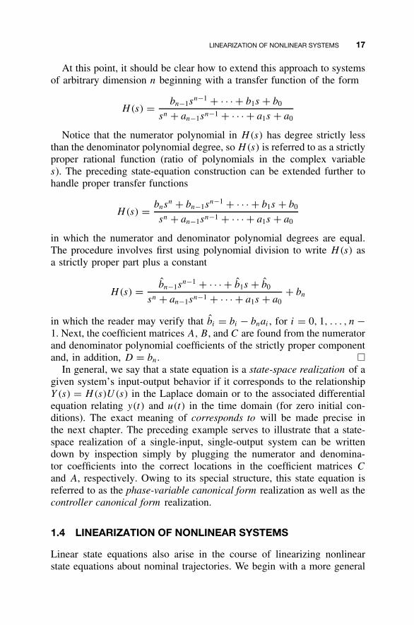
At this point, it should be clear how to extend this approach to systemsof arbitrary dimension n beginning with a transfer function of the form
H(s) = bn−1sn−1 + · · · + b1s + b0
sn + an−1sn−1 + · · · + a1s + a0
Notice that the numerator polynomial in H(s) has degree strictly lessthan the denominator polynomial degree, so H(s) is referred to as a strictlyproper rational function (ratio of polynomials in the complex variables). The preceding state-equation construction can be extended further tohandle proper transfer functions
H(s) = bnsn + bn−1s
n−1 + · · · + b1s + b0
sn + an−1sn−1 + · · · + a1s + a0
in which the numerator and denominator polynomial degrees are equal.The procedure involves first using polynomial division to write H(s) asa strictly proper part plus a constant
H(s) = bn−1sn−1 + · · · + b1s + b0
sn + an−1sn−1 + · · · + a1s + a0+ bn
in which the reader may verify that bi = bi − bnai , for i = 0, 1, . . . , n −1. Next, the coefficient matrices A, B, and C are found from the numeratorand denominator polynomial coefficients of the strictly proper componentand, in addition, D = bn. �
In general, we say that a state equation is a state-space realization of agiven system’s input-output behavior if it corresponds to the relationshipY(s) = H(s)U(s) in the Laplace domain or to the associated differentialequation relating y(t) and u(t) in the time domain (for zero initial con-ditions). The exact meaning of corresponds to will be made precise inthe next chapter. The preceding example serves to illustrate that a state-space realization of a single-input, single-output system can be writtendown by inspection simply by plugging the numerator and denomina-tor coefficients into the correct locations in the coefficient matrices C
and A, respectively. Owing to its special structure, this state equation isreferred to as the phase-variable canonical form realization as well as thecontroller canonical form realization.
1.4 LINEARIZATION OF NONLINEAR SYSTEMS
Linear state equations also arise in the course of linearizing nonlinearstate equations about nominal trajectories. We begin with a more general
18 INTRODUCTION
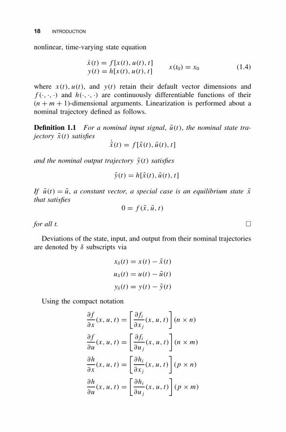
nonlinear, time-varying state equation
x(t) = f [x(t), u(t), t]y(t) = h[x(t), u(t), t]
x(t0) = x0 (1.4)
where x(t), u(t), and y(t) retain their default vector dimensions andf (·, ·, ·) and h(·, ·, ·) are continuously differentiable functions of their(n + m + 1)-dimensional arguments. Linearization is performed about anominal trajectory defined as follows.
Definition 1.1 For a nominal input signal, u(t), the nominal state tra-jectory x(t) satisfies ˙x(t) = f [x(t), u(t), t]
and the nominal output trajectory y(t) satisfies
y(t) = h[x(t), u(t), t]
If u(t) = u, a constant vector, a special case is an equilibrium state x
that satisfies0 = f (x, u, t)
for all t. �
Deviations of the state, input, and output from their nominal trajectoriesare denoted by δ subscripts via
xδ(t) = x(t) − x(t)
uδ(t) = u(t) − u(t)
yδ(t) = y(t) − y(t)
Using the compact notation
∂f
∂x(x, u, t) =
[∂fi
∂xj
(x, u, t)
](n × n)
∂f
∂u(x, u, t) =
[∂fi
∂uj
(x, u, t)
](n × m)
∂h
∂x(x, u, t) =
[∂hi
∂xj
(x, u, t)
](p × n)
∂h
∂u(x, u, t) =
[∂hi
∂uj
(x, u, t)
](p × m)
LINEARIZATION OF NONLINEAR SYSTEMS 19
and expanding the nonlinear maps in Equation (1.4) in a multivariateTaylor series about [x(t), u(t), t] we obtain
x(t) = f [x(t), u(t), t]
= f [x(t), u(t), t] + ∂f
∂x[x(t), u(t), t][x(t) − x(t)]
+ ∂f
∂u[x(t), u(t), t][u(t) − u(t)] + higher-order terms
y(t) = h[x(t), u(t), t]
= h[x(t), u(t), t] + ∂h
∂x[x(t), u(t), t][x(t) − x(t)]
+ ∂h
∂u[x(t), u(t), t][u(t) − u(t)] + higher-order terms
On defining coefficient matrices
A(t) = ∂f
∂x(x(t), u(t), t)
B(t) = ∂f
∂u(x(t), u(t), t)
C(t) = ∂h
∂x(x(t), u(t), t)
D(t) = ∂h
∂u(x(t), u(t), t)
rearranging slightly, and substituting deviation variables [recognizing thatxδ(t) = x(t) − ˙x(t)] we have
xδ(t) = A(t)xδ(t) + B(t)uδ(t) + higher-order terms
yδ(t) = C(t)xδ(t) + D(t)uδ(t) + higher-order terms
Under the assumption that the state, input, and output remain close totheir respective nominal trajectories, the high-order terms can be neglected,yielding the linear state equation
xδ(t) = A(t)xδ(t) + B(t)uδ(t)
yδ(t) = C(t)xδ(t) + D(t)uδ(t) (1.5)
which constitutes the linearization of the nonlinear state equation (1.4)about the specified nominal trajectory. The linearized state equation
20 INTRODUCTION
approximates the behavior of the nonlinear state equation provided that thedeviation variables remain small in norm so that omitting the higher-orderterms is justified.
If the nonlinear maps in Equation (1.4) do not explicitly depend on t ,and the nominal trajectory is an equilibrium condition for a constant nom-inal input, then the coefficient matrices in the linearized state equation areconstant; i.e., the linearization yields a time-invariant linear state equation.
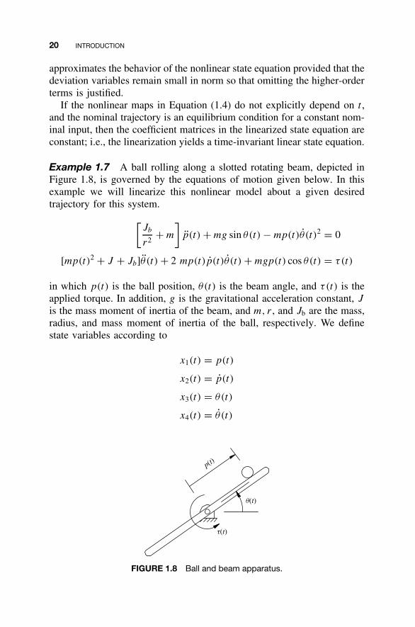
Example 1.7 A ball rolling along a slotted rotating beam, depicted inFigure 1.8, is governed by the equations of motion given below. In thisexample we will linearize this nonlinear model about a given desiredtrajectory for this system.
[Jb
r2+ m
]p(t) + mg sin θ(t) − mp(t)θ(t)2 = 0
[mp(t)2 + J + Jb]θ (t) + 2 mp(t)p(t)θ(t) + mgp(t) cos θ(t) = τ(t)
in which p(t) is the ball position, θ(t) is the beam angle, and τ(t) is theapplied torque. In addition, g is the gravitational acceleration constant, J
is the mass moment of inertia of the beam, and m, r , and Jb are the mass,radius, and mass moment of inertia of the ball, respectively. We definestate variables according to
x1(t) = p(t)
x2(t) = p(t)
x3(t) = θ(t)
x4(t) = θ (t)
p(t)
q(t)
t(t)
FIGURE 1.8 Ball and beam apparatus.
LINEARIZATION OF NONLINEAR SYSTEMS 21
In addition, we take the input to be the applied torque τ(t) and theoutput to be the ball position p(t), so
u(t) = τ(t)
y(t) = p(t)
The resulting nonlinear state equation plus the output equation then are
x1(t) = x2(t)
x2(t) = b[x1(t)x4(t)2 − g sin x3(t)]
x3(t) = x4(t)
x4(t) = −2mx1(t)x2(t)x4(t) − mgx1(t) cos x3(t) + u(t)
mx1(t)2 + J + Jb
y(t) = x1(t)
in which b = m/[(Jb/r2) + m].We consider nominal trajectories corresponding to a steady and level
beam and constant-velocity ball position responses. In terms of an initialball position p0 at the initial time t0 and a constant ball velocity v0, we take
x1(t) = p(t) = v0(t − t0) + p0
x2(t) = ˙p(t) = v0
x3(t) = θ (t) = 0
x4(t) = ˙θ(t) = 0
u(t) = τ (t) = mgx1(t)
for which it remains to verify that Definition 1.1 is satisfied. Comparing
˙x1(t) = v0
˙x2(t) = 0
˙x3(t) = 0
˙x4(t) = 0
withx2(t) = v0
b(x1(t)x4(t)2 − g sin x3(t)) = b(0 − g sin(0)) = 0
x4(t) = 0
22 INTRODUCTION
−2mx1(t)x2(t)x4(t)−mgx1(t) cos x3(t) + u(t)
mx1(t)2 + J + Jb= 0 − mgx1(t) cos(0) + mgx1(t)
mx1(t)2 + J + Jb= 0
we see that x(t) is a valid nominal state trajectory for the nominal inputu(t). As an immediate consequence, the nominal output is y(t) = x1(t) =p(t). It follows directly that deviation variables are specified by
xδ(t) =
p(t) − p(t)
p(t) − ˙p(t)
θ(t) − 0θ (t) − 0
uδ(t) = τ(t) − mgp(t)
yδ(t) = p(t) − p(t)
With
f (x, u) =
f1(x1, x2, x3, x4, u)
f2(x1, x2, x3, x4, u)
f3(x1, x2, x3, x4, u)
f4(x1, x2, x3, x4, u)
=
x2
b(x1x42 − g sin x3)
x4−2mx1x2x4 − mgx1 cos x3 + u
mx12 + J + Jb
partial differentiation yields
∂f
∂x(x, u) =
0 1 0 0bx4
2 0 −bg cos x3 2bx1x4
0 0 0 1∂f4
∂x1
−2mx1x4
mx12 + J + Jb
mgx1 sin x3
mx12 + J + Jb
−2mx1x2
mx12 + J + Jb
where
∂f4
∂x1=
[(−2mx2x4 − mg cos x3)(mx12 + J + Jb)]−
[(−2mx1x2x4 − mgx1 cos x3 + u)(2mx1)]
(mx12 + J + Jb)2
∂f
∂u(x, u) =
0001
mx12 + J + Jb
LINEARIZATION OF NONLINEAR SYSTEMS 23
∂h
∂x(x, u) = [ 1 0 0 0 ]
∂h
∂u(x, u) = 0
Evaluating at the nominal trajectory gives
A(t) = ∂f
∂x[x(t), u(t)]
=
0 1 0 00 0 −bg 00 0 0 1
−mg
mp(t)2 + J + Jb0 0
−2mp(t)v0
mp(t)2 + J + Jb
B(t) = ∂f
∂u[x(t), u(t)] =
0001
mp(t)2 + J + Jb
C(t) = ∂h
∂x[x(t), u(t)] = [ 1 0 0 0 ]
D(t) = ∂h
∂u[x(t), u(t)] = 0 (1.6)
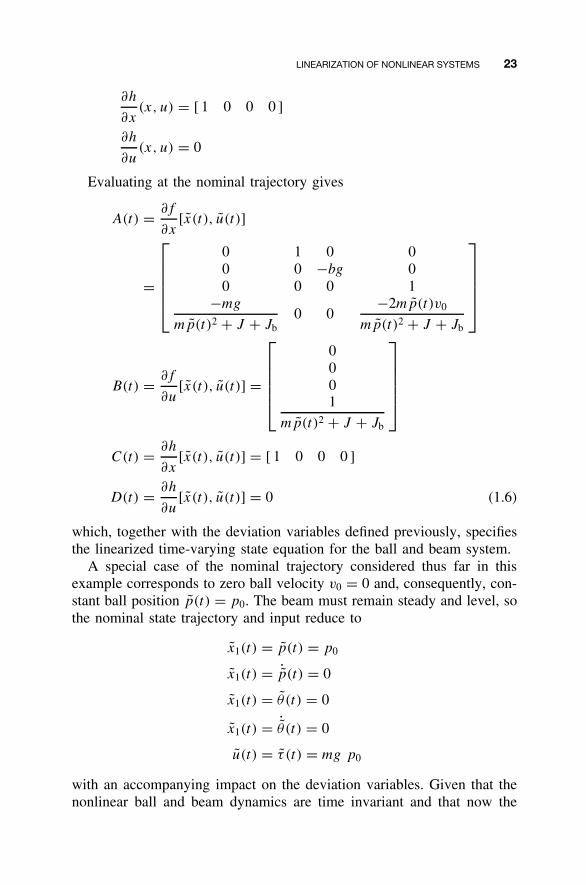
which, together with the deviation variables defined previously, specifiesthe linearized time-varying state equation for the ball and beam system.
A special case of the nominal trajectory considered thus far in thisexample corresponds to zero ball velocity v0 = 0 and, consequently, con-stant ball position p(t) = p0. The beam must remain steady and level, sothe nominal state trajectory and input reduce to
x1(t) = p(t) = p0
x1(t) = ˙p(t) = 0
x1(t) = θ (t) = 0
x1(t) = ˙θ(t) = 0
u(t) = τ (t) = mg p0
with an accompanying impact on the deviation variables. Given that thenonlinear ball and beam dynamics are time invariant and that now the
24 INTRODUCTION
nominal state trajectory and input are constant and characterize an equi-librium condition for these dynamics, the linearization process yields atime-invariant linear state equation. The associated coefficient matricesare obtained by making the appropriate substitutions in Equation (1.6)to obtain
A = ∂f
∂x(x, u) =
0 1 0 00 0 −bg 00 0 0 1
−mg
m p20 + J + Jb
0 0 0
B = ∂f
∂u(x, u) =
0001
m p20 + J + Jb
C = ∂h
∂x(x, u) = [ 1 0 0 0 ]
D = ∂h
∂u(x, u) = 0 �
1.5 CONTROL SYSTEM ANALYSIS AND DESIGN USING MATLAB
In each chapter we include a section to identify and explain the useof MATLAB software and MATLAB functions for state-space analysis anddesign methods. We use a continuing example to demonstrate the use ofMATLAB throughout; this is a single-input, single-output two–dimensionalrotational mechanical system that will allow the student to perform alloperations by hand to compare with MATLAB results. We assume that theControl Systems Toolbox is installed with MATLAB.
MATLAB: General, Data Entry, and Display
In this section we present general MATLAB commands, and we start theContinuing MATLAB Example. We highly recommend the use of MATLAB
m-files, which are scripts and functions containing MATLAB commandsthat can be created and modified in the MATLAB Editor and then executed.Throughout the MATLAB examples, bold Courier New font indicates MAT-
LAB function names, user inputs, and variable names; this is given foremphasis only. Some useful MATLAB statements are listed below to helpthe novice get started.

CONTROL SYSTEM ANALYSIS AND DESIGN USING MATLAB 25
General MATLAB Commands:
help Provides a list of topics for which you canget online help.
help fname Provides online help for MATLAB functionfname .
% The % symbol at any point in the codeindicates a comment; text beyond the % isignored by MATLAB and is highlighted ingreen .
; The semicolon used at the end of a linesuppresses display of the line’s result tothe MATLAB workspace.
clear This command clears the MATLAB
workspace, i.e., erases any previoususer-defined variables.
clc Clears the cursor.figure(n) Creates an empty figure window (numbered
n) for graphics.who Displays a list of all user-created variable
names.whos Same as who but additionally gives the
dimension of each variable.size(name) Responds with the dimension of the matrix
name .length(name) Responds with the length of the vector
name .eye(n) Creates an n × n identity matrix In.zeros(m,n) Creates a m × n array of zeros.ones(m,n) Creates a m × n array of ones.t = t0:dt:tf Creates an evenly spaced time array starting
from initial time t0 and ending at finaltime tf , with steps of dt .
disp(‘string’) Print the text string to the screen.name = input(‘string’) The input command displays a text
string to the user, prompting for input;the entered data then are written to thevariable name .
In the MATLAB Editor (not in this book), comments appear in green,text strings appear in red, and logical operators and other reserved pro-gramming words appear in blue.
26 INTRODUCTION
MATLAB for State-Space Description
MATLAB uses a data-structure format to describe linear time-invariant sys-tems. There are three primary ways to describe a linear time-invariantsystem in MATLAB: (1) state-space realizations specified by coefficientmatrices A, B, C, and D (ss); (2) transfer functions with (num, den),where num is the array of polynomial coefficients for the transfer-functionnumerator and den is the array of polynomial coefficients for the transfer-function denominator (tf); and (3) transfer functions with (z, p, k), wherez is the array of numerator polynomial roots (the zeros), p is the arrayof denominator polynomial roots (the poles), and k is the system gain.There is a fourth method, frequency response data (frd), which will notbe considered in this book. The three methods to define a continuous-timelinear time-invariant system in MATLAB are summarized below:
SysName = ss(A,B,C,D);SysName = tf(num,den);SysName = zpk(z,p,k);
In the first statement (ss), a scalar 0 in the D argument position willbe interpreted as a zero matrix D of appropriate dimensions. Each ofthese three statements (ss, tf, zpk) may be used to define a systemas above or to convert between state-space, transfer-function, and zero-pole-gain descriptions of an existing system. Alternatively, once the lineartime-invariant system SysName is defined, the parameters for each systemdescription may be extracted using the following statements:
[num,den] = tfdata(SysName);[z,p,k] = zpkdata(SysName);[A,B,C,D] = ssdata(SysName);
In the first two statements above, if we have a single-input, single-output system, we can use the switch 'v': tfdata(SysName,'v') andzpkdata(SysName,'v'). There are three methods to access data fromthe defined linear time-invariant SysName: set
/get commands, direct
structure referencing, and data-retrieval commands. The latter approach isgiven above; the first two are:
set(SysName,PropName,PropValue);PropValue = get(SysName,PropName);SysName.PropName = PropValue;% equivalent to ‘set’ command
CONTROL SYSTEM ANALYSIS AND DESIGN USING MATLAB 27
PropValue = SysName.PropName;% equivalent to ‘get’ command
In the preceding, SysName is set by the user as the desired name forthe defined linear time-invariant system. PropName (property name) rep-resents the valid properties the user can modify, which include A, B, C, Dfor ss, num, den, variable (the default is ‘s ’ for a continuous systemLaplace variable) for tf, and z, p, k, variable (again, the default is‘s ’) for zpk. The command set(SysName) displays the list of proper-ties for each data type. The command get(SysName) displays the valuecurrently stored for each property. PropValue (property value) indicatesthe value that the user assigns to the property at hand. In previous MATLAB
versions, many functions required the linear time-invariant system inputdata (A, B, C, D for state space, num, den for transfer function, and z, p,k for zero-pole-gain notation); although these still should work, MATLAB’spreferred mode of operation is to pass functions the SysName linear time-invariant data structure. For more information, type help ltimodels andhelp ltiprops at the MATLAB command prompt.
Continuing MATLAB Example
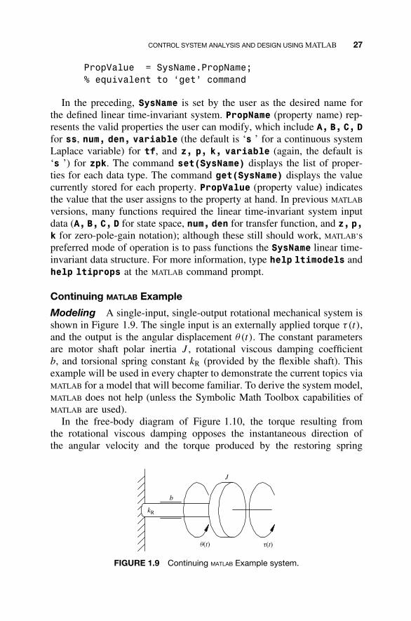
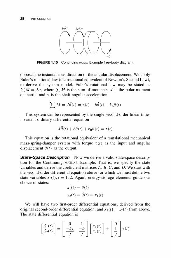
Modeling A single-input, single-output rotational mechanical system isshown in Figure 1.9. The single input is an externally applied torque τ(t),and the output is the angular displacement θ(t). The constant parametersare motor shaft polar inertia J , rotational viscous damping coefficientb, and torsional spring constant kR (provided by the flexible shaft). Thisexample will be used in every chapter to demonstrate the current topics viaMATLAB for a model that will become familiar. To derive the system model,MATLAB does not help (unless the Symbolic Math Toolbox capabilities ofMATLAB are used).
In the free-body diagram of Figure 1.10, the torque resulting fromthe rotational viscous damping opposes the instantaneous direction ofthe angular velocity and the torque produced by the restoring spring
J
b
kR
q(t) t(t)
FIGURE 1.9 Continuing MATLAB Example system.
28 INTRODUCTION
kRq(t)b q(t)
t(t)
FIGURE 1.10 Continuing MATLAB Example free-body diagram.
opposes the instantaneous direction of the angular displacement. We applyEuler’s rotational law (the rotational equivalent of Newton’s Second Law),to derive the system model. Euler’s rotational law may be stated as∑
M = Jα, where∑
M is the sum of moments, J is the polar momentof inertia, and α is the shaft angular acceleration.
∑M = J θ(t) = τ(t) − bθ(t) − kRθ(t)
This system can be represented by the single second-order linear time-invariant ordinary differential equation
J θ(t) + bθ(t) + kRθ(t) = τ(t)
This equation is the rotational equivalent of a translational mechanicalmass-spring-damper system with torque τ(t) as the input and angulardisplacement θ(t) as the output.
State-Space Description Now we derive a valid state-space descrip-tion for the Continuing MATLAB Example. That is, we specify the statevariables and derive the coefficient matrices A, B, C, and D. We start withthe second-order differential equation above for which we must define twostate variables xi(t), i = 1, 2. Again, energy-storage elements guide ourchoice of states:
x1(t) = θ(t)
x2(t) = θ (t) = x1(t)
We will have two first-order differential equations, derived from theoriginal second-order differential equation, and x1(t) = x2(t) from above.The state differential equation is
[x1(t)
x2(t)
]=
0 1
−kR
J
−b
J
[x1(t)
x2(t)
]+
0
1
J
τ(t)
CONTROL SYSTEM ANALYSIS AND DESIGN USING MATLAB 29
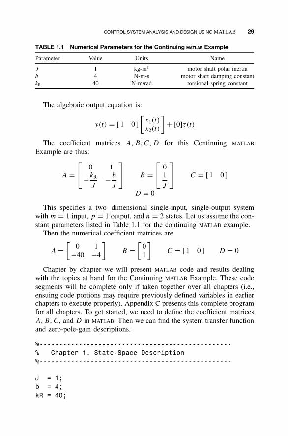
TABLE 1.1 Numerical Parameters for the Continuing MATLAB Example
Parameter Value Units Name
J 1 kg-m2 motor shaft polar inertiab 4 N-m-s motor shaft damping constantkR 40 N-m/rad torsional spring constant
The algebraic output equation is:
y(t) = [ 1 0 ]
[x1(t)
x2(t)
]+ [0]τ(t)
The coefficient matrices A, B,C, D for this Continuing MATLAB
Example are thus:
A = 0 1
−kR
J− b
J
B =
0
1
J
C = [ 1 0 ]
D = 0
This specifies a two–dimensional single-input, single-output systemwith m = 1 input, p = 1 output, and n = 2 states. Let us assume the con-stant parameters listed in Table 1.1 for the continuing MATLAB example.
Then the numerical coefficient matrices are
A =[
0 1−40 −4
]B =
[01
]C = [ 1 0 ] D = 0
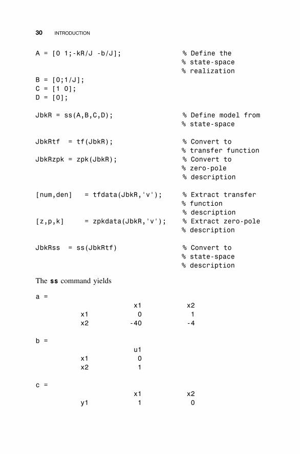
Chapter by chapter we will present MATLAB code and results dealingwith the topics at hand for the Continuing MATLAB Example. These codesegments will be complete only if taken together over all chapters (i.e.,ensuing code portions may require previously defined variables in earlierchapters to execute properly). Appendix C presents this complete programfor all chapters. To get started, we need to define the coefficient matricesA, B, C, and D in MATLAB. Then we can find the system transfer functionand zero-pole-gain descriptions.
%-------------------------------------------------% Chapter 1. State-Space Description%-------------------------------------------------
J = 1;b = 4;kR = 40;
30 INTRODUCTION
A = [0 1;-kR/J -b/J]; % Define the% state-space% realization
B = [0;1/J];C = [1 0];D = [0];
JbkR = ss(A,B,C,D); % Define model from% state-space
JbkRtf = tf(JbkR); % Convert to% transfer function
JbkRzpk = zpk(JbkR); % Convert to% zero-pole% description
[num,den] = tfdata(JbkR,'v'); % Extract transfer% function% description
[z,p,k] = zpkdata(JbkR,'v'); % Extract zero-pole% description
JbkRss = ss(JbkRtf) % Convert to% state-space% description
The ss command yields
a =x1 x2
x1 0 1x2 -40 -4
b =u1
x1 0x2 1
c =x1 x2
y1 1 0
CONTROL SYSTEM ANALYSIS AND DESIGN USING MATLAB 31
d =u1
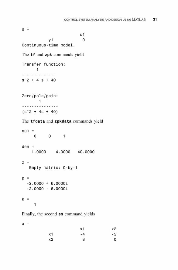
y1 0Continuous-time model.
The tf and zpk commands yield
Transfer function:1
--------------s^2 + 4 s + 40
Zero/pole/gain:1
---------------(s^2 + 4s + 40)
The tfdata and zpkdata commands yield
num =0 0 1
den =1.0000 4.0000 40.0000
z =Empty matrix: 0-by-1
p =-2.0000 + 6.0000i-2.0000 - 6.0000i
k =1
Finally, the second ss command yields
a =x1 x2
x1 -4 -5x2 8 0
32 INTRODUCTION
b =u1
x1 0.25x2 0
c =x1 x2
y1 0 0.5
d =u1
y1 0
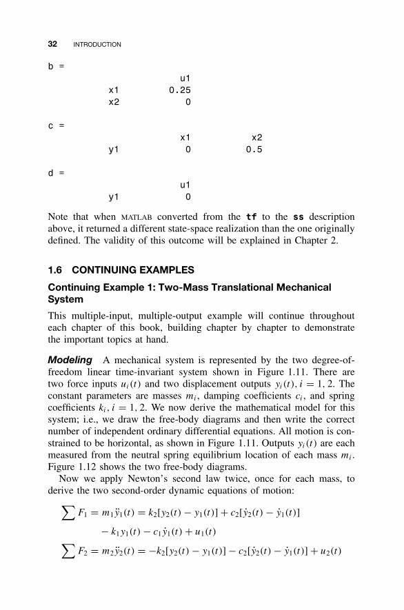
Note that when MATLAB converted from the tf to the ss descriptionabove, it returned a different state-space realization than the one originallydefined. The validity of this outcome will be explained in Chapter 2.
1.6 CONTINUING EXAMPLES
Continuing Example 1: Two-Mass Translational MechanicalSystem
This multiple-input, multiple-output example will continue throughouteach chapter of this book, building chapter by chapter to demonstratethe important topics at hand.
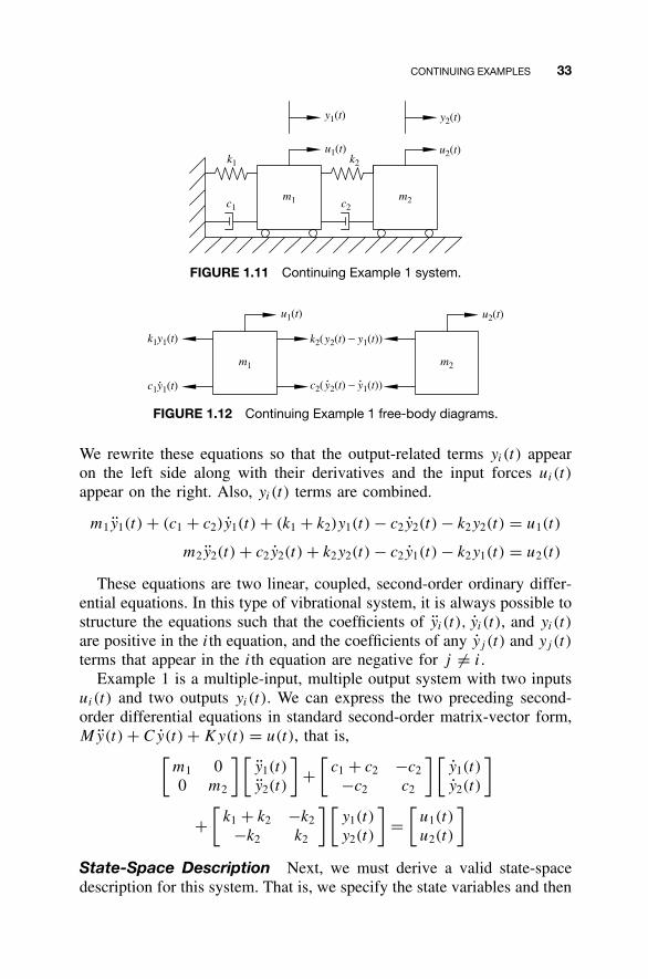
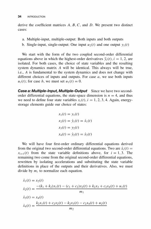
Modeling A mechanical system is represented by the two degree-of-freedom linear time-invariant system shown in Figure 1.11. There aretwo force inputs ui(t) and two displacement outputs yi(t), i = 1, 2. Theconstant parameters are masses mi , damping coefficients ci , and springcoefficients ki, i = 1, 2. We now derive the mathematical model for thissystem; i.e., we draw the free-body diagrams and then write the correctnumber of independent ordinary differential equations. All motion is con-strained to be horizontal, as shown in Figure 1.11. Outputs yi(t) are eachmeasured from the neutral spring equilibrium location of each mass mi .Figure 1.12 shows the two free-body diagrams.
Now we apply Newton’s second law twice, once for each mass, toderive the two second-order dynamic equations of motion:∑
F1 = m1y1(t) = k2[y2(t) − y1(t)] + c2[y2(t) − y1(t)]
− k1y1(t) − c1y1(t) + u1(t)∑F2 = m2y2(t) = −k2[y2(t) − y1(t)] − c2[y2(t) − y1(t)] + u2(t)
CONTINUING EXAMPLES 33
m2
y1(t) y2(t)
u1(t) u2(t)
m1 c2c1
k2k1
FIGURE 1.11 Continuing Example 1 system.
m1 m2
u1(t) u2(t)
k1y1(t)
c1y1(t)
k2(y2(t) − y1(t))
c2(y2(t) − y1(t))
FIGURE 1.12 Continuing Example 1 free-body diagrams.
We rewrite these equations so that the output-related terms yi(t) appearon the left side along with their derivatives and the input forces ui(t)
appear on the right. Also, yi(t) terms are combined.
m1y1(t) + (c1 + c2)y1(t) + (k1 + k2)y1(t) − c2y2(t) − k2y2(t) = u1(t)
m2y2(t) + c2y2(t) + k2y2(t) − c2y1(t) − k2y1(t) = u2(t)
These equations are two linear, coupled, second-order ordinary differ-ential equations. In this type of vibrational system, it is always possible tostructure the equations such that the coefficients of yi(t), yi(t), and yi(t)
are positive in the ith equation, and the coefficients of any yj (t) and yj (t)
terms that appear in the ith equation are negative for j �= i.Example 1 is a multiple-input, multiple output system with two inputs
ui(t) and two outputs yi(t). We can express the two preceding second-order differential equations in standard second-order matrix-vector form,My(t) + Cy(t) + Ky(t) = u(t), that is,[
m1 00 m2
] [y1(t)
y2(t)
]+
[c1 + c2 −c2
−c2 c2
] [y1(t)
y2(t)
]
+[
k1 + k2 −k2
−k2 k2
] [y1(t)
y2(t)
]=
[u1(t)
u2(t)
]
State-Space Description Next, we must derive a valid state-spacedescription for this system. That is, we specify the state variables and then
34 INTRODUCTION
derive the coefficient matrices A, B, C, and D. We present two distinctcases:
a. Multiple-input, multiple-output: Both inputs and both outputs
b. Single-input, single-output: One input u2(t) and one output y1(t)
We start with the form of the two coupled second-order differentialequations above in which the highest-order derivatives yi(t), i = 1, 2, areisolated. For both cases, the choice of state variables and the resultingsystem dynamics matrix A will be identical. This always will be true,i.e., A is fundamental to the system dynamics and does not change withdifferent choices of inputs and outputs. For case a, we use both inputsui(t); for case b, we must set u1(t) = 0.
Case a: Multiple-Input, Multiple-Output Since we have two second-order differential equations, the state-space dimension is n = 4, and thuswe need to define four state variables xi(t), i = 1, 2, 3, 4. Again, energy-storage elements guide our choice of states:
x1(t) = y1(t)
x2(t) = y1(t) = x1(t)
x3(t) = y2(t)
x4(t) = y2(t) = x3(t)
We will have four first-order ordinary differential equations derivedfrom the original two second-order differential equations. Two are xi(t) =xi+1(t) from the state variable definitions above, for i = 1, 3. Theremaining two come from the original second-order differential equations,rewritten by isolating accelerations and substituting the state variabledefinitions in place of the outputs and their derivatives. Also, we mustdivide by mi to normalize each equation.
x1(t) = x2(t)
x2(t) = −(k1 + k2)x1(t) − (c1 + c2)x2(t) + k2x3 + c2x4(t) + u1(t)
m1
x3(t) = x4(t)
x4(t) = k2x1(t) + c2x2(t) − k2x3(t) − c2x4(t) + u2(t)
m2
CONTINUING EXAMPLES 35
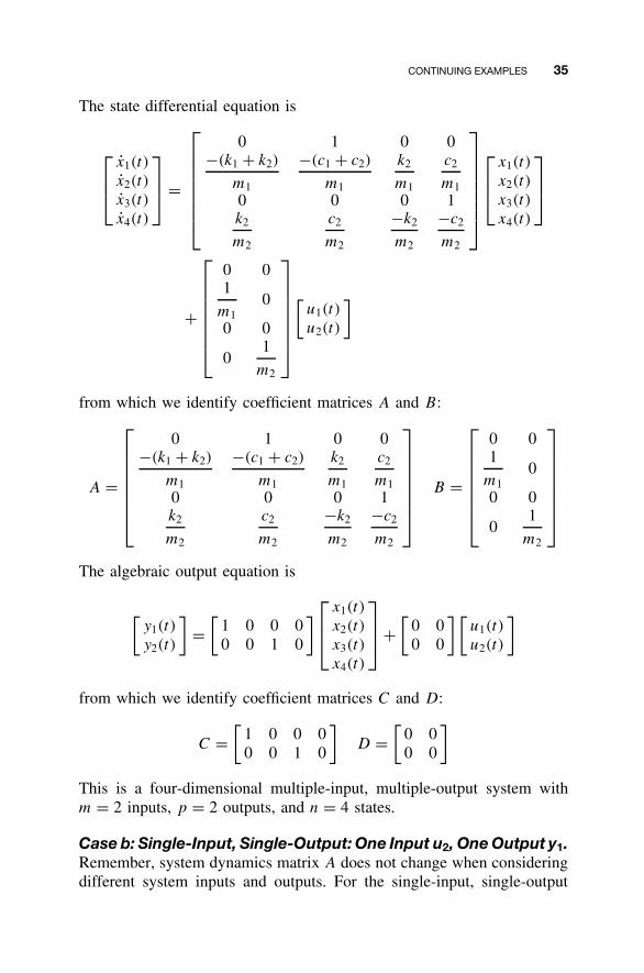
The state differential equation is
x1(t)
x2(t)
x3(t)
x4(t)
=
0 1 0 0−(k1 + k2)
m1
−(c1 + c2)
m1
k2
m1
c2
m10 0 0 1k2
m2
c2
m2
−k2
m2
−c2
m2
x1(t)
x2(t)
x3(t)
x4(t)
+
0 01
m10
0 0
01
m2
[u1(t)
u2(t)
]
from which we identify coefficient matrices A and B:
A =
0 1 0 0−(k1 + k2)
m1
−(c1 + c2)
m1
k2
m1
c2
m10 0 0 1k2
m2
c2
m2
−k2
m2
−c2
m2
B =
0 01
m10
0 0
01
m2
The algebraic output equation is
[y1(t)
y2(t)
]=
[1 0 0 00 0 1 0
]
x1(t)
x2(t)
x3(t)
x4(t)
+
[0 00 0
] [u1(t)
u2(t)
]
from which we identify coefficient matrices C and D:
C =[
1 0 0 00 0 1 0
]D =
[0 00 0
]
This is a four-dimensional multiple-input, multiple-output system withm = 2 inputs, p = 2 outputs, and n = 4 states.
Case b: Single-Input, Single-Output: One Input u2, One Output y1.Remember, system dynamics matrix A does not change when consideringdifferent system inputs and outputs. For the single-input, single-output
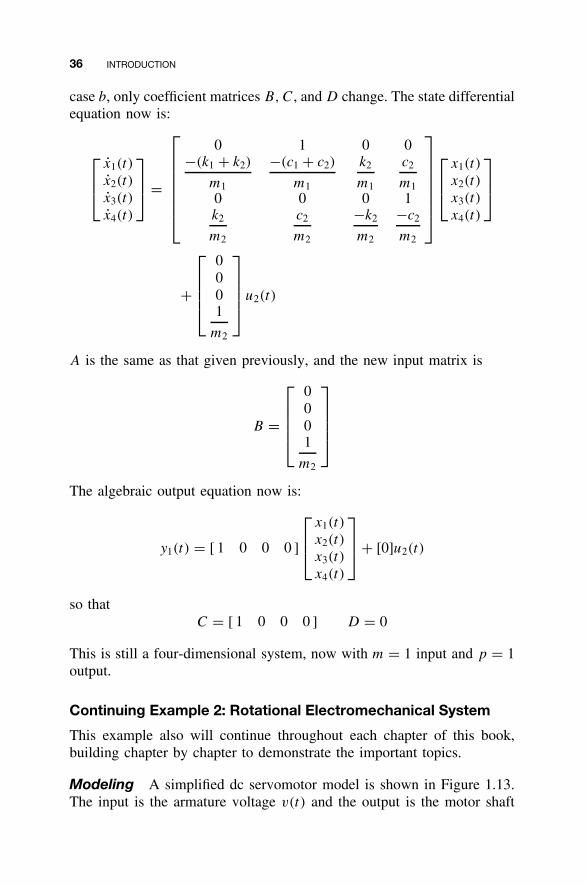
36 INTRODUCTION
case b, only coefficient matrices B,C, and D change. The state differentialequation now is:
x1(t)
x2(t)
x3(t)
x4(t)
=
0 1 0 0−(k1 + k2)
m1
−(c1 + c2)
m1
k2
m1
c2
m10 0 0 1k2
m2
c2
m2
−k2
m2
−c2
m2
x1(t)
x2(t)
x3(t)
x4(t)
+
0001
m2
u2(t)
A is the same as that given previously, and the new input matrix is
B =
0001
m2
The algebraic output equation now is:
y1(t) = [ 1 0 0 0 ]
x1(t)
x2(t)
x3(t)
x4(t)
+ [0]u2(t)
so thatC = [ 1 0 0 0 ] D = 0
This is still a four-dimensional system, now with m = 1 input and p = 1output.
Continuing Example 2: Rotational Electromechanical System
This example also will continue throughout each chapter of this book,building chapter by chapter to demonstrate the important topics.
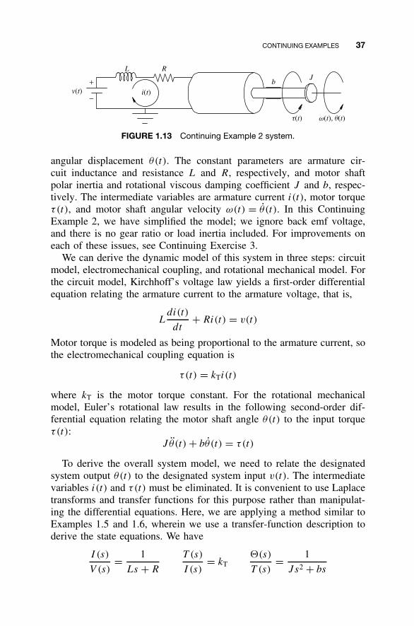
Modeling A simplified dc servomotor model is shown in Figure 1.13.The input is the armature voltage v(t) and the output is the motor shaft
CONTINUING EXAMPLES 37
J
i(t)
L R
bv(t)
+
−
t(t) w(t), q(t)
FIGURE 1.13 Continuing Example 2 system.
angular displacement θ(t). The constant parameters are armature cir-cuit inductance and resistance L and R, respectively, and motor shaftpolar inertia and rotational viscous damping coefficient J and b, respec-tively. The intermediate variables are armature current i(t), motor torqueτ(t), and motor shaft angular velocity ω(t) = θ (t). In this ContinuingExample 2, we have simplified the model; we ignore back emf voltage,and there is no gear ratio or load inertia included. For improvements oneach of these issues, see Continuing Exercise 3.
We can derive the dynamic model of this system in three steps: circuitmodel, electromechanical coupling, and rotational mechanical model. Forthe circuit model, Kirchhoff’s voltage law yields a first-order differentialequation relating the armature current to the armature voltage, that is,
Ldi(t)
dt+ Ri(t) = v(t)
Motor torque is modeled as being proportional to the armature current, sothe electromechanical coupling equation is
τ(t) = kTi(t)
where kT is the motor torque constant. For the rotational mechanicalmodel, Euler’s rotational law results in the following second-order dif-ferential equation relating the motor shaft angle θ(t) to the input torqueτ(t):
J θ(t) + bθ(t) = τ(t)
To derive the overall system model, we need to relate the designatedsystem output θ(t) to the designated system input v(t). The intermediatevariables i(t) and τ(t) must be eliminated. It is convenient to use Laplacetransforms and transfer functions for this purpose rather than manipulat-ing the differential equations. Here, we are applying a method similar toExamples 1.5 and 1.6, wherein we use a transfer-function description toderive the state equations. We have
I (s)
V (s)= 1
Ls + R
T (s)
I (s)= kT
�(s)
T (s)= 1
J s2 + bs
38 INTRODUCTION
Multiplying these transfer functions together, we eliminate the intermedi-ate variables to generate the overall transfer function:
�(s)
V (s)= kT
(Ls + R)(J s2 + bs)
Simplifying, cross-multiplying, and taking the inverse Laplace transformyields the following third-order linear time-invariant ordinary differentialequation:
LJ ¨θ(t) + (Lb + RJ)θ(t) + Rbθ(t) = kTv(t)
This equation is the mathematical model for the system of Figure 1.13.Note that there is no rotational mechanical spring term in this equation,i.e., the coefficient of the θ(t) term is zero.
State-Space Description Now we derive a valid state-space descrip-tion for Continuing Example 2. That is, we specify the state variablesand derive the coefficient matrices A, B, C, and D. The results then arewritten in matrix-vector form. Since we have a third-order differentialequation, the state-space dimension is n = 3, and thus we need to definethree state variables xi(t), i = 1, 2, 3. We choose
x1(t) = θ(t)
x2(t) = θ (t) = x1(t)
x3(t) = θ (t) = x2(t)
We will have three first-order differential equations, derived from theoriginal third-order differential equation. Two are xi(t) = xi+1(t) from thestate variable definitions above, for i = 1, 2. The remaining first-order dif-ferential equation comes from the original third-order differential equation,rewritten by isolating the highest derivative ¨θ(t) and substituting the state-variable definitions in place of output θ(t) and its derivatives. Also, wedivide the third equation by LJ :
x1(t) = x2(t)
x2(t) = x3(t)
x3(t) = −(Lb + RJ)
LJx3(t) − Rb
LJx2(t) + kT
LJv(t)
HOMEWORK EXERCISES 39
The state differential equation is
x1(t)
x2(t)
x3(t)
=
0 1 00 0 1
0−Rb
LJ
−(Lb + RJ)
LJ
x1(t)
x2(t)
x3(t)
+
00kT
LJ
v(t)
from which we identify coefficient matrices A and B:
A =
0 1 00 0 1
0−Rb
LJ
−(Lb + RJ)
LJ
B =
00kT
LJ
The algebraic output equation is
y(t) = [ 1 0 0 ]
x1(t)
x2(t)
x3(t)
+ [0]v(t)
from which we identify coefficient matrices C and D:
C = [ 1 0 0 ] D = 0
This is a three-dimensional single-input, single-output system with m = 1input, p = 1 output, and n = 3 states.
1.7 HOMEWORK EXERCISES
We refer the reader to the Preface for a description of the four classes ofexercises that will conclude each chapter: Numerical Exercises, AnalyticalExercises, Continuing MATLAB Exercises, and Continuing Exercises.
Numerical Exercises
NE1.1 For the following systems described by the given transfer func-tions, derive valid state-space realizations (define the state vari-ables and derive the coefficient matrices A, B, C, and D).
a. G(s) = Y(s)
U(s)= 1
s2 + 2s + 6
b. G(s) = Y(s)
U(s)= s + 3
s2 + 2s + 6
40 INTRODUCTION
c. G(s) = Y(s)
U(s)= 10
s3 + 4s2 + 8s + 6
d. G(s) = Y(s)
U(s)= s2 + 4s + 6
s4 + 10s3 + 11s2 + 44s + 66
NE1.2 Given the following differential equations (or systems of differ-ential equations), derive valid state-space realizations (define thestate variables and derive the coefficient matrices A, B,C, and D).a. y(t) + 2y(t) = u(t)
b. y(t) + 3y(t) + 10y(t) = u(t)
c. ¨y(t) + 2y(t) + 3y(t) + 5y(t) = u(t)
d. y1(t) + 5y1(t) − 10[y2(t) − y1(t)] = u1(t)
2y2(t) + y2(t) + 10[y2(t) − y1(t)] = u2(t)
Analytical Exercises
AE1.1 Suppose that A is n × m and H is p × q. Specify dimensions forthe remaining matrices so that the following expression is valid.
[A B
C D
] [E F
G H
]=
[AE + BG AF + BH
CE + DG CF + DH
]
AE1.2 Suppose that A and B are square matrices, not necessarily of thesame dimension. Show that∣∣∣∣A 0
0 B
∣∣∣∣ = |A| · |B|
AE1.3 Continuing AE1.2, show that
∣∣∣∣ A 0C B
∣∣∣∣ = |A| · |B|AE1.4 Continuing AE1.3, show that if A is nonsingular,
∣∣∣∣ A D
C B
∣∣∣∣ = |A| · |B − CA−1D|
AE1.5 Suppose that X is n × m and Y is m × n. With Ik denoting thek × k identity matrix for any integer k > 0, show that
|In − XY | = |Im − YX|
HOMEWORK EXERCISES 41
Explain the significance of this result when m = 1. Hint: ApplyAE1.4 to [
Im Y
X In
]and
[In X
Y Im
]
AE1.6 Show that the determinant of a square upper triangular matrix(zeros everywhere below the main diagonal) equals the productif its diagonal entries.
AE1.7 Suppose that A and C are nonsingular n × n and m × m matrices,respectively. Verify that
[A + BCD]−1 = A−1 − A−1B[C−1 + DA−1B]−1DA−1
What does this formula reduce to when m = 1 and C = 1?
AE1.8 Suppose that X is n × m and Y is m × n. With Ik denoting thek × k identity matrix for any integer k > 0, show that
(In − XY)−1X = X(Im − YX)−1
when the indicated inverses exist.
AE1.9 Suppose that A and B are nonsingular matrices, not necessarilyof the same dimension. Show that[
A 00 B
]−1
=[
A−1 00 B−1
]
AE1.10 Continuing AE1.8, derive expressions for[
A 0C B
]−1
and
[A D
0 B
]−1
AE1.11 Suppose that A is nonsingular and show that[
A D
C B
]−1
=[
A−1 + E�−1F −E�−1
−�−1F �−1
]
in which � = B − CA−1D, E = A−1D, and F = CA−1.
AE1.12 Compute the inverse of the k × k Jordan block matrix
Jk(λ) =
λ 1 0 · · · 00 λ 1 · · · 0
0 0 λ. . . 0
......
.... . . 1
0 0 0 · · · λ
42 INTRODUCTION
AE1.13 Suppose that A : Rn → R
m is a linear transformation and S is asubspace of R
m. Verify that the set
A−1S = {x ∈ R
n|Ax ∈ S}is a subspace of R
n. This subspace is referred to as the inverseimage of the subspace S under the linear transformation A.
AE1.14 Show that for conformably dimensioned matrices A and B, anyinduced matrix norm satisfies
||AB|| ≤ ||A||||B||AE1.15 Show that for A nonsingular, any induced matrix norm satisfies
||A−1|| ≥ 1
||A||AE1.16 Show that for any square matrix A, any induced matrix norm
satisfies||A|| ≥ ρ(A)
where ρ(A) � maxλi∈σ(A) |λi | is the spectral radius of A.
Continuing MATLAB Exercises
CME1.1 Given the following open-loop single-input, single-outputtwo–dimensional linear time-invariant state equations, namely,[
x1(t)
x2(t)
]=
[ −1 00 −2
] [x1(t)
x2(t)
]+
[1√2
]u(t)
y(t) = [ 1 −√2/2 ]
[x1(t)
x2(t)
]+ [0]u(t)
find the associated open-loop transfer function H(s).
CME1.2 Given the following open-loop single-input, single-outputthree–dimensional linear time-invariant state equations, namely
x1(t)
x2(t)
x3(t)
=
0 1 0
0 0 1−52 −30 −4
x1(t)
x2(t)
x3(t)
+
0
01
u(t)
y(t) = [ 20 1 0 ]
x1(t)
x2(t)
x3(t)
+ [0]u(t)
find the associated open-loop transfer function H(s).
HOMEWORK EXERCISES 43
CME1.3 Given the following open-loop single-input, single-outputfourth–order linear time-invariant state equations, namely,
x1(t)
x2(t)
x3(t)
x4(t)
=
0 1 0 00 0 1 00 0 0 1
−962 −126 −67 −4
x1(t)
x2(t)
x3(t)
x4(t)
+
0001
u(t)
y(t) = [300 0 0 0 ]
x1(t)
x2(t)
x3(t)
x4(t)
+ [0]u(t)
find the associated open-loop transfer function H(s).
CME1.4 Given the following open-loop single-input, single-outputfour–dimensional linear time-invariant state equations, namely,
x1(t)
x2(t)
x3(t)
x4(t)
=
0 1 0 00 0 1 00 0 0 1
−680 −176 −86 −6
x1(t)
x2(t)
x3(t)
x4(t)
+
0001
u(t)
y(t) = [ 100 20 10 0 ]
x1(t)
x2(t)
x3(t)
x4(t)
+ [0]u(t)
find the associated open-loop transfer function H(s).
Continuing Exercises
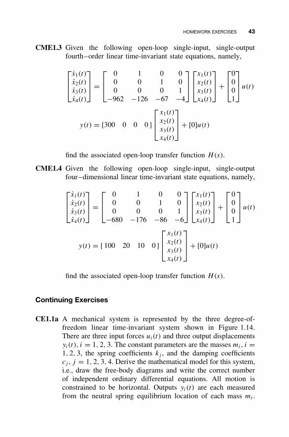
CE1.1a A mechanical system is represented by the three degree-of-freedom linear time-invariant system shown in Figure 1.14.There are three input forces ui(t) and three output displacementsyi(t), i = 1, 2, 3. The constant parameters are the masses mi, i =1, 2, 3, the spring coefficients kj , and the damping coefficientscj , j = 1, 2, 3, 4. Derive the mathematical model for this system,i.e., draw the free-body diagrams and write the correct numberof independent ordinary differential equations. All motion isconstrained to be horizontal. Outputs yi(t) are each measuredfrom the neutral spring equilibrium location of each mass mi .
44 INTRODUCTION
y1(t)
m1 m2 m3
k1 k2 k3
c1 c2 c3
k4
c4
y2(t) y3(t)
u1(t) u2(t) u3(t)
FIGURE 1.14 Diagram for Continuing Exercise 1.
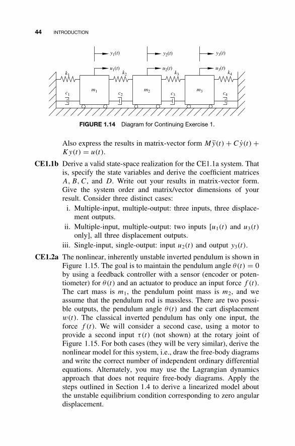
Also express the results in matrix-vector form My(t) + Cy(t) +Ky(t) = u(t).
CE1.1b Derive a valid state-space realization for the CE1.1a system. Thatis, specify the state variables and derive the coefficient matricesA, B, C, and D. Write out your results in matrix-vector form.Give the system order and matrix/vector dimensions of yourresult. Consider three distinct cases:
i. Multiple-input, multiple-output: three inputs, three displace-ment outputs.
ii. Multiple-input, multiple-output: two inputs [u1(t) and u3(t)
only], all three displacement outputs.iii. Single-input, single-output: input u2(t) and output y3(t).
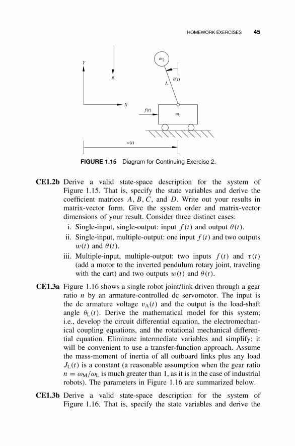
CE1.2a The nonlinear, inherently unstable inverted pendulum is shown inFigure 1.15. The goal is to maintain the pendulum angle θ(t) = 0by using a feedback controller with a sensor (encoder or poten-tiometer) for θ(t) and an actuator to produce an input force f (t).The cart mass is m1, the pendulum point mass is m2, and weassume that the pendulum rod is massless. There are two possi-ble outputs, the pendulum angle θ(t) and the cart displacementw(t). The classical inverted pendulum has only one input, theforce f (t). We will consider a second case, using a motor toprovide a second input τ(t) (not shown) at the rotary joint ofFigure 1.15. For both cases (they will be very similar), derive thenonlinear model for this system, i.e., draw the free-body diagramsand write the correct number of independent ordinary differentialequations. Alternately, you may use the Lagrangian dynamicsapproach that does not require free-body diagrams. Apply thesteps outlined in Section 1.4 to derive a linearized model aboutthe unstable equilibrium condition corresponding to zero angulardisplacement.
HOMEWORK EXERCISES 45
Y
f (t)X
gL
m1
w(t)
m2
q(t)
FIGURE 1.15 Diagram for Continuing Exercise 2.
CE1.2b Derive a valid state-space description for the system ofFigure 1.15. That is, specify the state variables and derive thecoefficient matrices A, B, C, and D. Write out your results inmatrix-vector form. Give the system order and matrix-vectordimensions of your result. Consider three distinct cases:
i. Single-input, single-output: input f (t) and output θ(t).ii. Single-input, multiple-output: one input f (t) and two outputs
w(t) and θ(t).iii. Multiple-input, multiple-output: two inputs f (t) and τ(t)
(add a motor to the inverted pendulum rotary joint, travelingwith the cart) and two outputs w(t) and θ(t).
CE1.3a Figure 1.16 shows a single robot joint/link driven through a gearratio n by an armature-controlled dc servomotor. The input isthe dc armature voltage vA(t) and the output is the load-shaftangle θL(t). Derive the mathematical model for this system;i.e., develop the circuit differential equation, the electromechan-ical coupling equations, and the rotational mechanical differen-tial equation. Eliminate intermediate variables and simplify; itwill be convenient to use a transfer-function approach. Assumethe mass-moment of inertia of all outboard links plus any loadJL(t) is a constant (a reasonable assumption when the gear ration = ωM/ωL is much greater than 1, as it is in the case of industrialrobots). The parameters in Figure 1.16 are summarized below.
CE1.3b Derive a valid state-space description for the system ofFigure 1.16. That is, specify the state variables and derive the
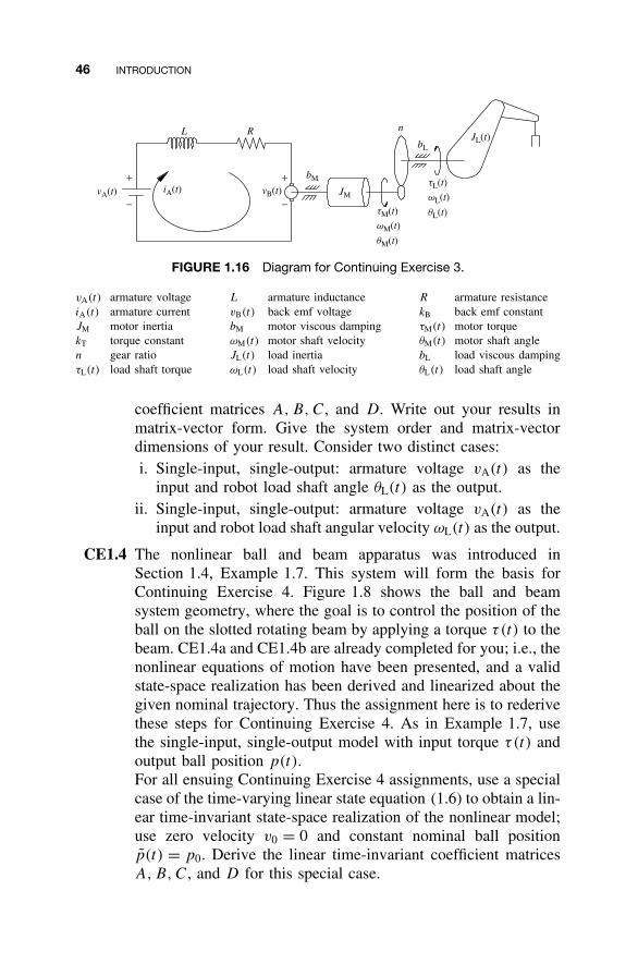
46 INTRODUCTION
L R nJL(t)
bL
vA(t) JM
bM+
−vB(t)
+
−iA(t)
qM(t)
wM(t)
tM(t) qL(t)
wL(t)
tL(t)
FIGURE 1.16 Diagram for Continuing Exercise 3.
vA(t) armature voltage L armature inductance R armature resistanceiA(t) armature current vB(t) back emf voltage kB back emf constantJM motor inertia bM motor viscous damping τM(t) motor torquekT torque constant ωM(t) motor shaft velocity θM(t) motor shaft anglen gear ratio JL(t) load inertia bL load viscous dampingτL(t) load shaft torque ωL(t) load shaft velocity θL(t) load shaft angle
coefficient matrices A, B, C, and D. Write out your results inmatrix-vector form. Give the system order and matrix-vectordimensions of your result. Consider two distinct cases:i. Single-input, single-output: armature voltage vA(t) as the
input and robot load shaft angle θL(t) as the output.ii. Single-input, single-output: armature voltage vA(t) as the
input and robot load shaft angular velocity ωL(t) as the output.
CE1.4 The nonlinear ball and beam apparatus was introduced inSection 1.4, Example 1.7. This system will form the basis forContinuing Exercise 4. Figure 1.8 shows the ball and beamsystem geometry, where the goal is to control the position of theball on the slotted rotating beam by applying a torque τ(t) to thebeam. CE1.4a and CE1.4b are already completed for you; i.e., thenonlinear equations of motion have been presented, and a validstate-space realization has been derived and linearized about thegiven nominal trajectory. Thus the assignment here is to rederivethese steps for Continuing Exercise 4. As in Example 1.7, usethe single-input, single-output model with input torque τ(t) andoutput ball position p(t).For all ensuing Continuing Exercise 4 assignments, use a specialcase of the time-varying linear state equation (1.6) to obtain a lin-ear time-invariant state-space realization of the nonlinear model;use zero velocity v0 = 0 and constant nominal ball positionp(t) = p0. Derive the linear time-invariant coefficient matricesA, B, C, and D for this special case.
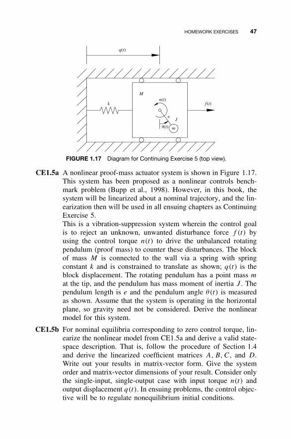
HOMEWORK EXERCISES 47
m
J
k
M
e
f (t)
q(t)
n(t)
q(t)
FIGURE 1.17 Diagram for Continuing Exercise 5 (top view).
CE1.5a A nonlinear proof-mass actuator system is shown in Figure 1.17.This system has been proposed as a nonlinear controls bench-mark problem (Bupp et al., 1998). However, in this book, thesystem will be linearized about a nominal trajectory, and the lin-earization then will be used in all ensuing chapters as ContinuingExercise 5.This is a vibration-suppression system wherein the control goalis to reject an unknown, unwanted disturbance force f (t) byusing the control torque n(t) to drive the unbalanced rotatingpendulum (proof mass) to counter these disturbances. The blockof mass M is connected to the wall via a spring with springconstant k and is constrained to translate as shown; q(t) is theblock displacement. The rotating pendulum has a point mass m
at the tip, and the pendulum has mass moment of inertia J . Thependulum length is e and the pendulum angle θ(t) is measuredas shown. Assume that the system is operating in the horizontalplane, so gravity need not be considered. Derive the nonlinearmodel for this system.
CE1.5b For nominal equilibria corresponding to zero control torque, lin-earize the nonlinear model from CE1.5a and derive a valid state-space description. That is, follow the procedure of Section 1.4and derive the linearized coefficient matrices A, B,C, and D.Write out your results in matrix-vector form. Give the systemorder and matrix-vector dimensions of your result. Consider onlythe single-input, single-output case with input torque n(t) andoutput displacement q(t). In ensuing problems, the control objec-tive will be to regulate nonequilibrium initial conditions.
2
STATE-SPACEFUNDAMENTALS
Chapter 1 presented the state-space description for linear time-invariantsystems. This chapter establishes several fundamental results that followfrom this representation, beginning with a derivation of the state equationsolution. In the course of this analysis we encounter the matrix exponen-tial, so named because of many similarities with the scalar exponentialfunction. In terms of the state-equation solution, we revisit several famil-iar topics from linear systems analysis, including decomposition of thecomplete response into zero-input and zero-state response components,characterizing the system impulse response that permits the zero-stateresponse to be cast as the convolution of the impulse response with theinput signal, and the utility of the Laplace transform in computing thestate-equation solution and defining the system transfer function.
The chapter continues with a more formal treatment of the state-spacerealization issue and an introduction to the important topic of state coor-dinate transformations. As we will see, a linear transformation of the statevector yields a different state equation that also realizes the system’s input-output behavior represented by either the associated impulse response ortransfer function. This has the interesting consequence that state-spacerealizations are not unique; beginning with one state-space realization,other realizations of the same system may be derived via a state coor-dinate transformation. We will see that many topics in the remainder of
48
Linear State-Space Control Systems. Robert L. Williams II and Douglas A. LawrenceCopyright 2007 John Wiley & Sons, Inc. ISBN: 978-0-471-73555-7
STATE EQUATION SOLUTION 49
this book are facilitated by the flexibility afforded by this nonuniqueness.For instance, in this chapter we introduce the so-called diagonal canon-ical form that specifies a set of decoupled, scalar, first-order ordinarydifferential equations that may be solved independently.
This chapter also illustrates the use of MATLAB in supporting the compu-tations encountered earlier. As in all chapters, these demonstrations willrevisit the MATLAB Continuing Example along with Continuing Examples 1and 2.
2.1 STATE EQUATION SOLUTION
From Chapter 1, our basic mathematical model for a linear time-invariantsystem consists of the state differential equation and the algebraic outputequation:
x(t) = Ax(t) + Bu(t) x(t0) = x0
y(t) = Cx(t) + Du(t) (2.1)
where we assume that the n × n system dynamics matrix A, the n × m
input matrix B, the p × n output matrix C, and the p × m direct transmis-sion matrix D are known constant matrices. The first equation compactlyrepresents a set of n coupled first-order differential equations that must besolved for the state vector x(t) given the initial state x(t0) = x0 and inputvector u(t). The second equation characterizes a static or instantaneousdependence of the output on the state and input. As we shall see, the realwork lies in deriving a solution expression for the state vector. With thatin hand, a direct substitution into the second equation yields an expressionfor the output.
Prior to deriving a closed-form solution of Equation (2.1) for the n–di-mensional case as outlined above, we first review the solution of scalarfirst-order differential equations.
Solution of Scalar First-Order Differential Equations
Consider the one–dimensional system represented by the scalar differen-tial equation
x(t) = ax(t) + bu(t) x(t0) = x0 (2.2)
in which a and b are scalar constants, and u(t) is a given scalar inputsignal. A traditional approach for deriving a solution formula for the scalar
50 STATE-SPACE FUNDAMENTALS
state x(t) is to multiply both sides of the differential equation by theintegrating factor e−a(t−t0) to yield
d
d t(e−a(t−t0)x(t)) = e−a(t−t0)x(t) − e−a(t−t0)ax(t)
= e−a(t−t0)bu(t)
We next integrate from t0 to t and invoke the fundamental theorem ofcalculus to obtain
e−a(t−t0)x(t) − e−a(t−t0)x(t0) =∫ t
t0
d
d t(e−a(τ−t0)x(τ )) dτ
=∫ t
t0
e−a(τ−t0)bu(τ) dτ.
After multiplying through by ea(t−t0) and some manipulation, we get
x(t) = ea(t−t0)x0 +∫ t
t0
ea(t−τ )bu(τ) dτ (2.3)
which expresses the state response x(t) as a sum of terms, the first owingto the given initial state x(t0) = x0 and the second owing to the specifiedinput signal u(t). Notice that the first component characterizes the stateresponse when the input signal is identically zero. We therefore refer tothe first term as the zero-input response component. Similarly, the sec-ond component characterizes the state response for zero initial state. Wetherefore refer to the second term as the zero-state response component.
The Laplace transform furnishes an alternate solution strategy. For this,we assume without loss of generality that t0 = 0 and transform the differ-ential equation, using linearity and time-differentiation properties of theLaplace transform, into
sX(s) − x0 = aX(s) + bU(s)
in which X(s) and U(s) are the Laplace transforms of x(t) and u(t),respectively. Straightforward algebra yields
X(s) = 1
s − ax0 + b
s − aU(s)
STATE EQUATION SOLUTION 51
From the convolution property of the Laplace transform, we obtain
x(t) = eatx0 + eat ∗ bu(t)
= eatx0 +∫ t
0ea(t−τ )bu(τ) dτ
which agrees with the solution (2.3) derived earlier for t0 = 0.If our first-order system had an associated scalar output signal y(t)
defined by the algebraic relationship
y(t) = cx(t) + d u(t) (2.4)
then by simply substituting the state response we obtain
y(t) = ceatx0 +∫ t
0cea(t−τ )bu(τ) dτ + du(t)
which also admits a decomposition into zero-input and zero-state responsecomponents. In the Laplace domain, we also have
Y(s) = c
s − ax0 + cb
s − aU(s)
We recall that the impulse response of a linear time-invariant system isthe system’s response to an impulsive input u(t) = δ(t) when the systemis initially at rest, which in this setting corresponds to zero initial statex0 = 0. By interpreting the initial time as t0 = 0−, just prior to whenthe impulse occurs, the zero-state response component of y(t) yields thesystem’s impulse response, that is,
h(t) =∫ t
0−cea(t−τ )bδ(τ ) dτ + dδ(t)
= ceatb + dδ(t)
(2.5)
where we have used the sifting property of the impulse to evaluate the inte-gral. Now, for any input signal u(t), the zero-input response componentof y(t) can be expressed as
∫ t
0−cea(t−τ )bu(τ) dτ + du(t) =
∫ t
0−[cea(t−τ )b + dδ(t − τ)]u(τ) dτ
=∫ t
0−h(t − τ)u(τ) dτ
= h(t) ∗ u(t)
52 STATE-SPACE FUNDAMENTALS
which should look familiar to the reader. Alternatively, in the Laplacedomain, the system’s transfer function H(s) is, by definition,
H(s) = Y(s)
U(s)
∣∣∣∣zero initial state
=(
cb
s − a+ d
)
and so the impulse response h(t) and transfer function H(s) form aLaplace transform pair, as we should expect.
Our approach to deriving state-equation solution formulas for the n-dimensional case and discussing various systems-related implications inboth the time and Laplace domains is patterned after the preceding devel-opment, but greater care is necessary to tackle the underlying matrix-vector computations correctly. Before proceeding, the reader is encouragedto ponder, however briefly, the matrix-vector extensions of the precedingcomputations.
State Equation Solution
In this subsection we derive a closed-form solution to the n-dimensionallinear time invariant state equation (2.1) given a specified initial statex(t0) = x0 and input vector u(t).
Homogeneous Case We begin with a related homogeneous matrixdifferential equation
X(t) = AX(t) X(t0) = I (2.6)
where I is the n × n identity matrix. We assume an infinite power seriesform for the solution
X(t) =∞∑
k=0
Xk(t − t0)k (2.7)
Each term in the sum involves an n × n matrix Xk to be determined anddepends only on the elapsed time t − t0, reflecting the time-invariance ofthe state equation. The initial condition for Equation (2.6) yields X(t0) =X0 = I . Substituting Equation (2.7) into Equation (2.6), formally differ-entiating term by term with respect to time, and shifting the summation
STATE EQUATION SOLUTION 53
index gives
∞∑k=0
(k + 1)Xk+1(t − t0)k = A
( ∞∑k=0
Xk(t − t0)k
)
=∞∑
k=0
A Xk(t − t0)k
By equating like powers of t − t0, we obtain the recursive relationship
Xk+1 = 1
k + 1AXk k ≥ 0
which, when initialized with X0 = I , leads to
Xk = 1
k!Ak k ≥ 0
Substituting this result into the power series (2.7) yields
X(t) =∞∑
k=0
1
k!Ak(t − t0)
k
We note here that the infinite power series (2.7) has the requisite con-vergence properties so that the infinite power series resulting from term-by-term differentiation converges to X(t), and Equation (2.6) is satisfied.
Recall that the scalar exponential function is defined by the followinginfinite power series
eat = 1 + at + 12a2t2 + 1
6a3t3 + · · ·
=∞∑
k=0
1
k!aktk
Motivated by this, we define the so-called matrix exponential via
eAt = I + At + 12A2t2 + 1
6A3t3 + · · ·
=∞∑
k=0
1
k!Aktk
(2.8)
54 STATE-SPACE FUNDAMENTALS
from which the solution to the homogeneous matrix differentialequation (2.6) can be expressed compactly as
X(t) = eA(t−t0)
It is important to point out that eAt is merely notation used to representthe power series in Equation (2.8). Beyond the scalar case, the matrixexponential never equals the matrix of scalar exponentials correspondingto the individual elements in the matrix A. That is,
eAt �= [eaij t ]
Properties that are satisfied by the matrix exponential are collected inthe following proposition.
Proposition 2.1 For any real n × n matrix A, the matrix exponential eAt
has the following properties:
1. eAt is the unique matrix satisfying
d
d teAt = AeAt eAt
∣∣t=0
= In
2. For any t1 and t2 , eA(t1 +t2 ) = eAt1 eAt2 . As a direct consequence, forany t
I = eA(0 ) = eA(t−t) = eAte−At
Thus eAt is invertible (nonsingular) for all t with inverse
[eAt
]−1 = e−At
3. A and eAt commute with respect to matrix multiplication, that is,AeAt = eAtA for all t .
4. [eAt ]T = eAT t for all t.5. For any real n × n matrix B, e(A+B)t = eAteBt for all t if and onlyif AB = BA, that is, A and B commute with respect to matrix multipli-cation. �
The first property asserts the uniqueness of X(t) = eA(t−t0) as a solutionto Equation (2.6). This property is useful in situations where we must ver-ify whether a given time–dependent matrix X(t) is the matrix exponential
STATE EQUATION SOLUTION 55
for an associated matrix A. To resolve this issue, it is not necessary com-pute eAt from scratch via some means. Rather, it suffices to check whetherX(t) = AX(t) and X(0) = I . If a candidate for the matrix exponential isnot provided, then it must be computed directly. The defining power seriesis, except in special cases, not especially useful in this regard. However,there are special cases in which closed-form solutions can be deduced, asshown in the following two examples.
Example 2.1 Consider the 4 × 4 matrix with ones above the main diag-onal and zeros elsewhere:
A =
0 1 0 00 0 1 00 0 0 10 0 0 0
As called for by the power series (2.8), we compute powers of A:
A2 =
0 0 1 00 0 0 10 0 0 00 0 0 0
A3 =
0 0 0 10 0 0 00 0 0 00 0 0 0
A4 =
0 0 0 00 0 0 00 0 0 00 0 0 0
from which it follows that Ak = 0, for k ≥ 4, and consequently, the powerseries (2.8) contains only a finite number of nonzero terms:
eAt = I + At + 12A
2t2 + 16A3t3
=
1 0 0 00 1 0 00 0 1 00 0 0 1
+
0 t 0 00 0 t 00 0 0 t
0 0 0 0
+
0 0 12 t
2 00 0 0 1
2 t2
0 0 0 00 0 0 0
+
0 0 0 16 t
3
0 0 0 00 0 0 00 0 0 0
=
1 t 12 t
2 16 t
3
0 1 t 12 t
2
0 0 1 t
0 0 0 1
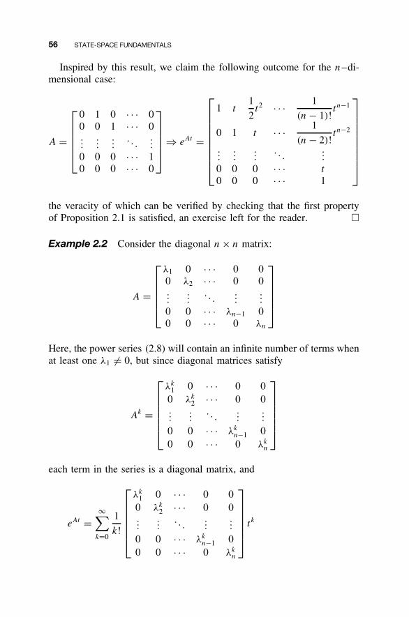
56 STATE-SPACE FUNDAMENTALS
Inspired by this result, we claim the following outcome for the n–di-mensional case:
A =
0 1 0 · · · 00 0 1 · · · 0...
......
. . ....
0 0 0 · · · 10 0 0 · · · 0
⇒ eAt =
1 t1
2t2 · · · 1
(n − 1)!tn−1
0 1 t · · · 1
(n − 2)!tn−2
......
.... . .
...
0 0 0 · · · t
0 0 0 · · · 1
the veracity of which can be verified by checking that the first propertyof Proposition 2.1 is satisfied, an exercise left for the reader. �
Example 2.2 Consider the diagonal n × n matrix:
A =
λ1 0 · · · 0 00 λ2 · · · 0 0...
.... . .
......
0 0 · · · λn−1 00 0 · · · 0 λn
Here, the power series (2.8) will contain an infinite number of terms whenat least one λ1 �= 0, but since diagonal matrices satisfy
Ak =
λk1 0 · · · 0 0
0 λk2 · · · 0 0
......
. . ....
...
0 0 · · · λkn−1 0
0 0 · · · 0 λkn
each term in the series is a diagonal matrix, and
eAt =∞∑
k=0
1
k!
λk1 0 · · · 0 0
0 λk2 · · · 0 0
......
. . ....
...
0 0 · · · λkn−1 0
0 0 · · · 0 λkn
t k
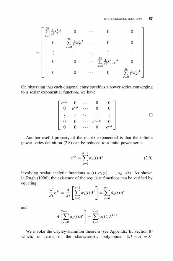
STATE EQUATION SOLUTION 57
=
∞∑k=0
1k!λ
k1t
k 0 · · · 0 0
0∞∑
k=0
1k!λ
k2t
k · · · 0 0
......
. . ....
...
0 0 · · ·∞∑
k=0
1k!λ
kn−1t
k 0
0 0 · · · 0∞∑
k=0
1k!λ
knt
k
On observing that each diagonal entry specifies a power series convergingto a scalar exponential function, we have
eλ1t 0 · · · 0 00 eλ2t · · · 0 0...
.... . .
......
0 0 · · · eλn−1t 00 0 · · · 0 eλnt
�
Another useful property of the matrix exponential is that the infinitepower series definition (2.8) can be reduced to a finite power series
eAt =n−1∑k=0
αk(t)Ak (2.9)
involving scalar analytic functions α0(t), α1(t), . . . , αn−1(t). As shownin Rugh (1996), the existence of the requisite functions can be verified byequating
d
d teAt = d
d t
[n−1∑k=0
αk(t)Ak
]=
n−1∑k=0
αk(t)Ak
and
A
[n−1∑k=0
αk(t)Ak
]=
n−1∑k=0
αk(t)Ak+1
We invoke the Cayley-Hamilton theorem (see Appendix B, Section 8)which, in terms of the characteristic polynomial |λI − A| = λn
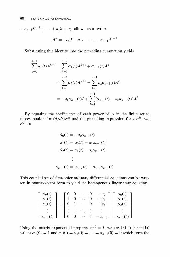
58 STATE-SPACE FUNDAMENTALS
+ an−1λn−1 + · · · + a1λ + a0, allows us to write
An = −a0I − a1A − · · · − an−1An−1
Substituting this identity into the preceding summation yields
n−1∑k=0
αk(t)Ak+1 =
n−2∑k=0
αk(t)Ak+1 + αn−1(t)A
n
=n−2∑k=0
αk(t)Ak+1 −
n−1∑k=0
akαn−1(t)Ak
= −a0αn−1(t)I +n−1∑k=1
[αk−1(t) − akαn−1(t)]Ak
By equating the coefficients of each power of A in the finite seriesrepresentation for (d/dt)eAt and the preceding expression for AeAt , weobtain
α0(t) = −a0αn−1(t)
α1(t) = α0(t) − a1αn−1(t)
α2(t) = α1(t) − a2αn−1(t)
...
αn−1(t) = αn−2(t) − an−1αn−1(t)
This coupled set of first-order ordinary differential equations can be writ-ten in matrix-vector form to yield the homogenous linear state equation
α0(t)
α1(t)
α2(t)...
αn−1(t)
=
0 0 · · · 0 −a0
1 0 · · · 0 −a1
0 1 · · · 0 −a2...
.... . .
......
0 0 · · · 1 −an−1
α0(t)
α1(t)
α2(t)...
αn−1(t)
Using the matrix exponential property eA·0 = I , we are led to the initialvalues α0(0) = 1 and α1(0) = α2(0) = · · · = αn−1(0) = 0 which form the
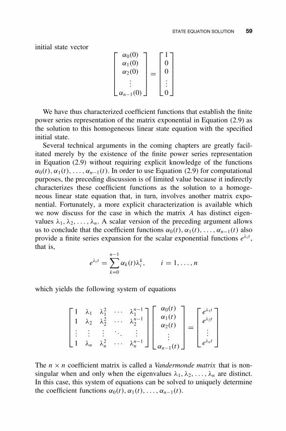
STATE EQUATION SOLUTION 59
initial state vector
α0(0)
α1(0)
α2(0)...
αn−1(0)
=
100...
0
We have thus characterized coefficient functions that establish the finitepower series representation of the matrix exponential in Equation (2.9) asthe solution to this homogeneous linear state equation with the specifiedinitial state.
Several technical arguments in the coming chapters are greatly facil-itated merely by the existence of the finite power series representationin Equation (2.9) without requiring explicit knowledge of the functionsα0(t), α1(t), . . . , αn−1(t). In order to use Equation (2.9) for computationalpurposes, the preceding discussion is of limited value because it indirectlycharacterizes these coefficient functions as the solution to a homoge-neous linear state equation that, in turn, involves another matrix expo-nential. Fortunately, a more explicit characterization is available whichwe now discuss for the case in which the matrix A has distinct eigen-values λ1, λ2, . . . , λn. A scalar version of the preceding argument allowsus to conclude that the coefficient functions α0(t), α1(t), . . . , αn−1(t) alsoprovide a finite series expansion for the scalar exponential functions eλit ,that is,
eλit =n−1∑k=0
αk(t)λki , i = 1, . . . , n
which yields the following system of equations
1 λ1 λ21 · · · λn−1
1
1 λ2 λ22 · · · λn−1
2...
......
. . ....
1 λn λ2n · · · λn−1
n
α0(t)
α1(t)
α2(t)...
αn−1(t)
=
eλ1t
eλ2t
...
eλnt
The n × n coefficient matrix is called a Vandermonde matrix that is non-singular when and only when the eigenvalues λ1, λ2, . . . , λn are distinct.In this case, this system of equations can be solved to uniquely determinethe coefficient functions α0(t), α1(t), . . . , αn−1(t).
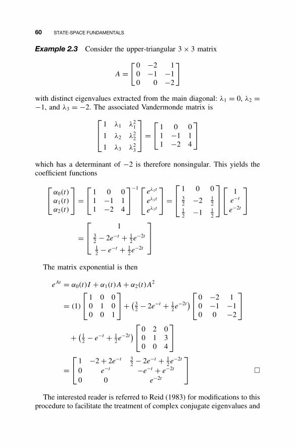
60 STATE-SPACE FUNDAMENTALS
Example 2.3 Consider the upper-triangular 3 × 3 matrix
A =[ 0 −2 1
0 −1 −10 0 −2
]
with distinct eigenvalues extracted from the main diagonal: λ1 = 0, λ2 =−1, and λ3 = −2. The associated Vandermonde matrix is
1 λ1 λ21
1 λ2 λ22
1 λ3 λ23
=
1 0 0
1 −1 11 −2 4
which has a determinant of −2 is therefore nonsingular. This yields thecoefficient functions
α0(t)
α1(t)
α2(t)
=
1 0 0
1 −1 11 −2 4
−1 eλ1t
eλ1t
eλ1t
=
1 0 032 −2 1
212 −1 1
2
1
e−t
e−2t
=
132 − 2e−t + 1
2e−2t
12 − e−t + 1
2e−2t
The matrix exponential is then
eAt = α0(t)I + α1(t)A + α2(t)A2
= (1)
1 0 0
0 1 00 0 1
+ (
32 − 2e−t + 1
2e−2t
) 0 −2 1
0 −1 −10 0 −2
+ (12 − e−t + 1
2e−2t
) 0 2 0
0 1 30 0 4
= 1 −2 + 2e−t 3
2 − 2e−t + 12e−2t
0 e−t −e−t + e−2t
0 0 e−2t
�
The interested reader is referred to Reid (1983) for modifications to thisprocedure to facilitate the treatment of complex conjugate eigenvalues and
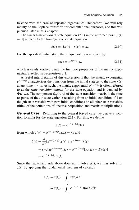
STATE EQUATION SOLUTION 61
to cope with the case of repeated eigenvalues. Henceforth, we will relymainly on the Laplace transform for computational purposes, and this willpursued later in this chapter.
The linear time-invariant state equation (2.1) in the unforced case [u(t)
≡ 0] reduces to the homogeneous state equation
x(t) = Ax(t) x(t0) = x0 (2.10)
For the specified initial state, the unique solution is given by
x(t) = eA(t−t0)x0 (2.11)
which is easily verified using the first two properties of the matrix expo-nential asserted in Proposition 2.1.
A useful interpretation of this expression is that the matrix exponentialeA(t−t0) characterizes the transition from the initial state x0 to the state x(t)
at any time t ≥ t0. As such, the matrix exponential eA(t−t0) is often referredto as the state-transition matrix for the state equation and is denoted by�(t, t0). The component φij (t, t0) of the state-transition matrix is the timeresponse of the ith state variable resulting from an initial condition of 1 onthe j th state variable with zero initial conditions on all other state variables(think of the definitions of linear superposition and matrix multiplication).
General Case Returning to the general forced case, we derive a solu-tion formula for the state equation (2.1). For this, we define
z(t) = e−A(t−t0)x(t)
from which z(t0) = e−A(t0−t0)x(t0) = x0 and
z(t) = d
d t[e−A(t−t0)]x(t) + e−A(t−t0)x(t)
= (−A)e−A(t−t0)x(t) + e−A(t−t0)[Ax(t) + Bu(t)]
= e−A(t−t0)Bu(t)
Since the right-hand side above does not involve z(t), we may solve forz(t) by applying the fundamental theorem of calculus
z(t) = z(t0) +∫ t
t0
z(τ )dτ
= z(t0) +∫ t
t0
e−A(τ−t0)Bu(τ)dτ
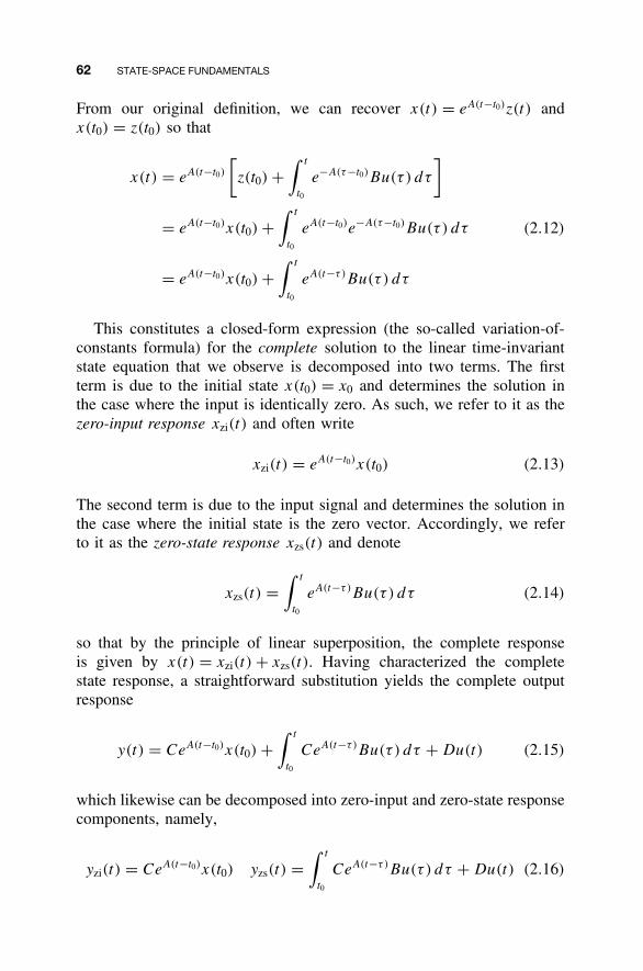
62 STATE-SPACE FUNDAMENTALS
From our original definition, we can recover x(t) = eA(t−t0)z(t) andx(t0) = z(t0) so that
x(t) = eA(t−t0)
[z(t0) +
∫ t
t0
e−A(τ−t0)Bu(τ) dτ
]
= eA(t−t0)x(t0) +∫ t
t0
eA(t−t0)e−A(τ−t0)Bu(τ) dτ
= eA(t−t0)x(t0) +∫ t
t0
eA(t−τ )Bu(τ) dτ
(2.12)
This constitutes a closed-form expression (the so-called variation-of-constants formula) for the complete solution to the linear time-invariantstate equation that we observe is decomposed into two terms. The firstterm is due to the initial state x(t0) = x0 and determines the solution inthe case where the input is identically zero. As such, we refer to it as thezero-input response xzi(t) and often write
xzi(t) = eA(t−t0)x(t0) (2.13)
The second term is due to the input signal and determines the solution inthe case where the initial state is the zero vector. Accordingly, we referto it as the zero-state response xzs(t) and denote
xzs(t) =∫ t
t0
eA(t−τ )Bu(τ) dτ (2.14)
so that by the principle of linear superposition, the complete responseis given by x(t) = xzi(t) + xzs(t). Having characterized the completestate response, a straightforward substitution yields the complete outputresponse
y(t) = CeA(t−t0)x(t0) +∫ t
t0
CeA(t−τ )Bu(τ) dτ + Du(t) (2.15)
which likewise can be decomposed into zero-input and zero-state responsecomponents, namely,
yzi(t) = CeA(t−t0)x(t0) yzs(t) =∫ t
t0
CeA(t−τ )Bu(τ) dτ + Du(t) (2.16)
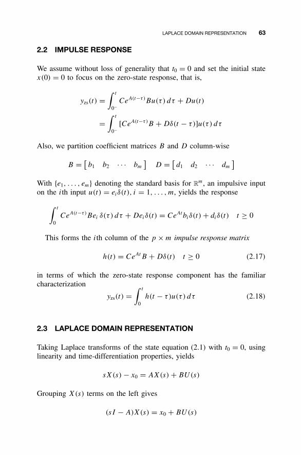
LAPLACE DOMAIN REPRESENTATION 63
2.2 IMPULSE RESPONSE
We assume without loss of generality that t0 = 0 and set the initial statex(0) = 0 to focus on the zero-state response, that is,
yzs(t) =∫ t
0−CeA(t−τ )Bu(τ) dτ + Du(t)
=∫ t
0−[CeA(t−τ )B + Dδ(t − τ)]u(τ) dτ
Also, we partition coefficient matrices B and D column-wise
B = [b1 b2 · · · bm
]D = [
d1 d2 · · · dm
]
With {e1, . . . , em} denoting the standard basis for Rm, an impulsive input
on the ith input u(t) = eiδ(t), i = 1, . . . , m, yields the response
∫ t
0CeA(t−τ )Bei δ(τ ) dτ + Deiδ(t) = CeAtbiδ(t) + diδ(t) t ≥ 0
This forms the ith column of the p × m impulse response matrix
h(t) = CeAtB + Dδ(t) t ≥ 0 (2.17)
in terms of which the zero-state response component has the familiarcharacterization
yzs(t) =∫ t
0h(t − τ)u(τ) dτ (2.18)
2.3 LAPLACE DOMAIN REPRESENTATION
Taking Laplace transforms of the state equation (2.1) with t0 = 0, usinglinearity and time-differentiation properties, yields
sX(s) − x0 = AX(s) + BU(s)
Grouping X(s) terms on the left gives
(sI − A)X(s) = x0 + BU(s)
64 STATE-SPACE FUNDAMENTALS
Now, from basic linear algebra, the determinant |sI − A| is a degree-nmonic polynomial (i.e., the coefficient of sn is 1), and so it is not thezero polynomial. Also, the adjoint of (sI − A) is an n × n matrix ofpolynomials having degree at most n − 1. Consequently,
(sI − A)−1 = adj(sI − A)
|sI − A|
is an n × n matrix of rational functions in the complex variable s. More-over, each element of (sI − A)−1 has numerator degree that is guaranteedto be strictly less than its denominator degree and therefore is a strictlyproper rational function.
The preceding equation now can be solved for X(s) to obtain
X(s) = (sI − A)−1x0 + (sI − A)−1BU(s) (2.19)
As in the time domain, we can decompose X(s) into zero-input andzero-state response components X(s) = Xzi(s) + Xzs(s) in which
Xzi(s) = (sI − A)−1x0 Xzs(s) = (sI − A)−1BU(s) (2.20)
Denoting a Laplace transform pair by f (t) ↔ F(s), we see that since
xzi(t) = eAtx0 ↔ Xzi(s) = (sI − A)−1x0
holds for any initial state, we can conclude that
eAt ↔ (sI − A)−1 (2.21)
This relationship suggests an approach for computing the matrix exponen-tial by first forming the matrix inverse (sI − A)−1, whose elements areguaranteed to be rational functions in the complex variable s, and thenapplying partial fraction expansion element by element to determine theinverse Laplace transform that yields eAt .
Taking Laplace transforms through the output equation and substitutingfor X(s) yields
Y(s) = CX(s) + DU(s)
= C(sI − A)−1x0 + [C(sI − A)−1B + D]U(s)(2.22)
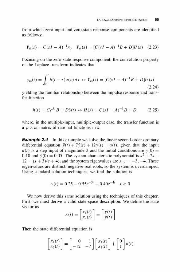
LAPLACE DOMAIN REPRESENTATION 65
from which zero-input and zero-state response components are identifiedas follows:
Yzi(s) = C(sI − A)−1x0 Yzs(s) = [C(sI − A)−1B + D]U(s) (2.23)
Focusing on the zero-state response component, the convolution propertyof the Laplace transform indicates that
yzs(t) =∫ t
0h(t − τ)u(τ) dτ ↔ Yzs(s) = [C(sI − A)−1B + D]U(s)
(2.24)
yielding the familiar relationship between the impulse response and trans-fer function
h(t) = CeAtB + Dδ(t) ↔ H(s) = C(sI − A)−1B + D (2.25)
where, in the multiple-input, multiple-output case, the transfer function isa p × m matrix of rational functions in s.
Example 2.4 In this example we solve the linear second-order ordinarydifferential equation y(t) + 7y(t) + 12y(t) = u(t), given that the inputu(t) is a step input of magnitude 3 and the initial conditions are y(0) =0.10 and y(0) = 0.05. The system characteristic polynomial is s2 + 7s +12 = (s + 3)(s + 4), and the system eigenvalues are s1,2 = −3, −4. Theseeigenvalues are distinct, negative real roots, so the system is overdamped.Using standard solution techniques, we find the solution is
y(t) = 0.25 − 0.55e−3t + 0.40e−4t t ≥ 0
We now derive this same solution using the techniques of this chapter.First, we must derive a valid state-space description. We define the statevector as
x(t) =[
x1(t)
x2(t)
]=
[y(t)
y(t)
]
Then the state differential equation is
[x1(t)
x2(t)
]=
[0 1
−12 −7
] [x1(t)
x2(t)
]+
[01
]u(t)
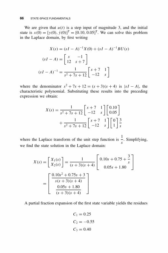
66 STATE-SPACE FUNDAMENTALS
We are given that u(t) is a step input of magnitude 3, and the initialstate is x(0) = [y(0), y(0)]T = [0.10, 0.05]T. We can solve this problemin the Laplace domain, by first writing
X(s) = (sI − A)−1X(0) + (sI − A)−1BU(s)
(sI − A) =[
s −112 s + 7
]
(sI − A)−1 = 1
s2 + 7s + 12
[s + 7 1−12 s
]
where the denominator s2 + 7s + 12 = (s + 3)(s + 4) is |sI − A|, thecharacteristic polynomial. Substituting these results into the precedingexpression we obtain:
X(s) = 1
s2 + 7s + 12
[s + 7 1−12 s
] [0.100.05
]
+ 1
s2 + 7s + 12
[s + 7 1−12 s
] [01
]3
s
where the Laplace transform of the unit step function is1
s. Simplifying,
we find the state solution in the Laplace domain:
X(s) =[
X1(s)
X2(s)
]= 1
(s + 3)(s + 4)
0.10s + 0.75 + 3
s
0.05s + 1.80
=
0.10s2 + 0.75s + 3
s(s + 3)(s + 4)
0.05s + 1.80
(s + 3)(s + 4)
A partial fraction expansion of the first state variable yields the residues
C1 = 0.25
C2 = −0.55
C3 = 0.40
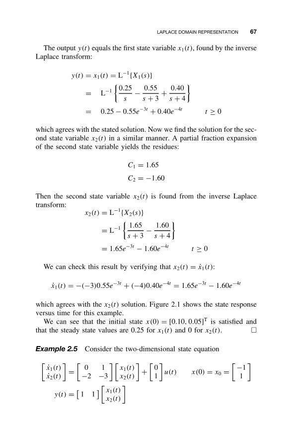
LAPLACE DOMAIN REPRESENTATION 67
The output y(t) equals the first state variable x1(t), found by the inverseLaplace transform:
y(t) = x1(t) = L−1{X1(s)}
= L−1
{0.25
s− 0.55
s + 3+ 0.40
s + 4
}
= 0.25 − 0.55e−3t + 0.40e−4t t ≥ 0
which agrees with the stated solution. Now we find the solution for the sec-ond state variable x2(t) in a similar manner. A partial fraction expansionof the second state variable yields the residues:
C1 = 1.65
C2 = −1.60
Then the second state variable x2(t) is found from the inverse Laplacetransform:
x2(t) = L−1{X2(s)}
= L−1
{1.65
s + 3− 1.60
s + 4
}
= 1.65e−3t − 1.60e−4t t ≥ 0
We can check this result by verifying that x2(t) = x1(t):
x1(t) = −(−3)0.55e−3t + (−4)0.40e−4t = 1.65e−3t − 1.60e−4t
which agrees with the x2(t) solution. Figure 2.1 shows the state responseversus time for this example.
We can see that the initial state x(0) = [0.10, 0.05]T is satisfied andthat the steady state values are 0.25 for x1(t) and 0 for x2(t). �
Example 2.5 Consider the two-dimensional state equation
[x1(t)
x2(t)
]=
[0 1
−2 −3
] [x1(t)
x2(t)
]+
[01
]u(t) x(0) = x0 =
[ −11
]
y(t) = [1 1
] [x1(t)
x2(t)
]
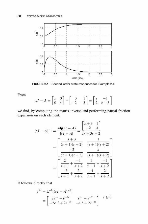
68 STATE-SPACE FUNDAMENTALS
0 0.5 1 1.5 2 2.5 30
0.1
0.2
0 0.5 1 1.5 2 2.5 30
0.1
0.2
time (sec)
x 2(t
)x 1
(t)
FIGURE 2.1 Second-order state responses for Example 2.4.
From
sI − A =[
s 00 s
]−
[0 1
−2 −3
]=
[s −12 s + 3
]
we find, by computing the matrix inverse and performing partial fractionexpansion on each element,
(sI − A)−1 = adj(sI − A)
|sI − A| =
[s + 3 1−2 s
]
s2 + 3s + 2
=
s + 3
(s + 1)(s + 2)
1
(s + 1)(s + 2)
−2
(s + 1)(s + 2)
s
(s + 1)(s + 2)
=
2
s + 1+ −1
s + 2
1
s + 1+ −1
s + 2−2
s + 1+ 2
s + 2
−1
s + 1+ 2
s + 2
It follows directly that
eAt = L−1[(sI − A)−1]
=[
2e−t − e−2t e−t − e−2t
−2e−t + 2e−2t −e−t + 2e−2t
]t ≥ 0
LAPLACE DOMAIN REPRESENTATION 69
For the specified initial state, the zero-input response component of thestate and output are
xzi(t) = eAtx0 =[ −e−t
e−t
]yzi(t) = CeAtx0 = Cxzi(t) = 0 t ≥ 0
For a unit-step input signal, the Laplace domain representation of thezero-state components of the state and output response are
Xzs(s) = (sI − A)−1BU(s)
=
[s + 3 1−2 s
]
s2 + 3s + 2
[01
]1
s
=
1
(s + 1)(s + 2)
s
(s + 1)(s + 2)
1
s
=
1
s(s + 1)(s + 2)
1
(s + 1)(s + 2)
=
1/2
s− 1
s + 1+ 1/2
s + 21
s + 1− 1
s + 2
Yzs(s) = CXzs(s) + DU(s)
= [1 1
]
1/2
s− 1
s + 1+ 1/2
s + 21
s + 1− 1
s + 2
+ [0]
1
s
= 1/2
s− 1/2
s + 2
from which
xzs(t) =[
1/2 − e−t + 1/2e−2t
e−t − e−2t
]yzs(t) = 1
2(1 − e−2t ) t ≥ 0
70 STATE-SPACE FUNDAMENTALS
and complete state and output responses then are
x(t) =[
1/2 − 2e−t + 1/2e−2t
2e−t − e−2t
]y(t) = 1
2(1 − e−2t ) t ≥ 0
Finally, the transfer function is given as
H(s) = C(sI − A)−1B + D
= [1 1
][
s + 3 1−2 s
]
s2 + 3s + 2
[01
]+ 0
= s + 1
s2 + 3s + 2= s + 1
(s + 1)(s + 2)= 1
s + 2
with associated impulse response
h(t) = e−2t t ≥ 0 �
2.4 STATE-SPACE REALIZATIONS REVISITED
Recall that at the conclusion of Section 1.3 we called a state equation astate-space realization of a linear time-invariant system’s input-outputbehavior if, loosely speaking, it corresponds to the Laplace domainrelationship Y(s) = H(s)U(s) involving the system’s transfer function.Since this pertains to the zero-state response component, we see thatEquation (2.25) implies that a state-space realization is required to satisfy
C(sI − A)−1B + D = H(s)
or, equivalently, in terms of the impulse response in the time domain,
CeAtB + Dδ(t) = h(t)
Example 2.6 Here we extend to arbitrary dimensions the state-spacerealization analysis conducted for the three–dimensional system ofExample 1.6. Namely, we show that the single-input, single-outputn–dimensional strictly proper transfer function
H(s) = b(s)
a(s)= bn−1s
n−1 + · · · + b1s + b0
sn + an−1sn−1 + · · · + a1s + a0(2.26)
STATE-SPACE REALIZATIONS REVISITED 71
has a state-space realization specified by coefficient matrices
A =
0 1 0 · · · 0 00 0 1 · · · 0 0...
......
. . ....
...
0 0 0 · · · 1 00 0 0 · · · 0 1
−a0 −a1 −a2 · · · −an−2 −an−1
B =
00...
001
C = [ b0 b1 b2 · · · bn−2 bn−1 ] D = 0
(2.27)
Moreover, by judiciously ordering the calculations, we avoid theunpleasant prospect of symbolically rendering (sI − A)−1, which isseemingly at the heart of the identity we must verify. First, observe that
(sI − A)
1s
s2
...
sn−2
sn−1
=
s −1 0 · · · 0 00 s −1 · · · 0 0...
......
. . ....
...0 0 0 · · · −1 00 0 0 · · · s −1a0 a1 a2 · · · an−2 s + an−1
1s
s2
...
sn−2
sn−1
=
s · 1 + (−1) · s
s · s + (−1) · s2
...
s · sn−3 + (−1) · sn−2
s · sn−2 + (−1) · sn−1
a0 · 1 + a1 · s + a2 · s2 + · · · + an−2 · sn−2 + (s + an−1)sn−1
=
00...00
sn + an−1sn−1 + · · · + a1s + a0
= Ba(s)
72 STATE-SPACE FUNDAMENTALS
Rearranging to solve for (sI − A)−1B and substituting intoC(sI − A)−1B + D yields
C(sI − A)−1B + D = [b0 b1 b2 · · · bn−2 bn−1
]
1s
s2
...
sn−2
sn−1
a(s)+ 0
= b0 · 1 + b1 · s + b2 · s2 + · · · + bn−2 · sn−2 + bn−1sn−1
a(s)
= b(s)
a(s)= H(s)
as required. �
2.5 COORDINATE TRANSFORMATIONS
Here we introduce the concept of a state coordinate transformation andstudy the impact that such a transformation has on the state equation itself,as well as various derived quantities. Especially noteworthy is what does notchange with the application of a state coordinate transformation. The readeris referred to Appendix B (Sections B.4 and B.6) for an overview of linearalgebra topics (change of basis and linear transformations) that underpin ourdevelopment here. Once having discussed state coordinate transformationsin general terms, we consider a particular application: transforming a givenstate equation into the so-called diagonal canonical form.
General Coordinate Transformations
For the n-dimensional linear time-invariant state equation (2.1), any non-singular n × n matrix T defines a coordinate transformation via
x(t) = T z(t) z(t) = T −1x(t) (2.28)
Associated with the transformed state vector z(t) is the transformed stateequation
z(t) = T −1x(t)
= T −1[Ax(t) + Bu(t)]
= T −1AT z(t) + T −1Bu(t)
y(t) = CT z(t) + Du(t)
COORDINATE TRANSFORMATIONS 73
That is, the coefficient matrices are transformed according to
A = T −1AT B = T −1B C = CT D = D (2.29)
and we henceforth write
z(t) = Az(t) + Bu(t)
y(t) = Cz(t) + Du(t)z(t0) = z0 (2.30)
where, in addition, the initial state is transformed via z(t0) = T −1x(t0) .For the system dynamics matrix, the coordinate transformation yields
A = T −1AT . This is called a similarity transformation, so the new systemdynamics matrix A has the same characteristic polynomial and eigenval-ues as A. However, the eigenvectors are different but are linked by thecoordinate transformation.
The impact that state coordinate transformations have on various quan-tities associated with linear time-invariant state equations is summarizedin the following proposition.
Proposition 2.2 For the linear time-invariant state equation (2.1) andcoordinate transformation (2.28):
1. |sI − A| = |sI − A|2. (sI − A)−1 = T −1(sI − A)−1 T
3. eAt = T −1eAtT
4. C(sI − A)−1B + D = C(sI − A)−1B + D
5. CeAt B + Dδ(t) = CeAtB + Dδ(t) �
Item 1 states that the system characteristic polynomial and thus the sys-tem eigenvalues are invariant under the coordinate transformation (2.28).This proposition is proved using determinant properties as follows:
|sI − A| = |sI − T −1AT |= |sT −1T − T −1AT |= |T −1(sI − A)T |= |T −1||sI − A||T |= |T −1||T ||sI − A|= |sI − A|
74 STATE-SPACE FUNDAMENTALS
where the last step follows from |T −1||T | = |T −1T | = |I | = 1. Therefore,since a nonsingular matrix and its inverse have reciprocal determinants,A and A have the same characteristic polynomial and eigenvalues.
Items 4 and 5 indicate that the transfer function and impulse responseare unaffected by (or invariant with respect to) any state coordinate trans-formation. Consequently, given one state-space realization of a transferfunction or impulse response, there are infinitely many others (of thesame dimension) because there are infinitely many ways to specify a statecoordinate transformation.
Diagonal Canonical Form
There are some special realizations that can be obtained by applying thestate coordinate transformation (2.28) to a given linear state equation. Inthis subsection we present the diagonal canonical form for the single-input,single-output case.
Diagonal canonical form is also called modal form because it yieldsa decoupled set of n first-order ordinary differential equations. This isclearly convenient because in this form, n scalar first-order differentialequation solutions may be formulated independently, instead of using cou-pled system solution methods. Any state-space realization with a diagonal-izable A matrix can be transformed to diagonal canonical form (DCF) by
x(t) = TDCF z(t)
where the diagonal canonical form coordinate transformation matrix TDCF
= [ v1 v2 · · · vn ] consists of eigenvectors vi of A arranged column-wise (see Appendix B, Section B.8 for an overview of eigenvalues andeigenvectors). Because A is assumed to be diagonalizable, the n eigenvec-tors are linearly independent, yielding a nonsingular TDCF. The diagonalcanonical form is characterized by a diagonal A matrix with eigenvaluesappearing on the diagonal, where eigenvalue λi is associated with theeigenvector vi, i = 1, 2, . . . , n:
ADCF = T −1DCFATDCF =
λ1 0 0 · · · 00 λ2 0 · · · 00 0 λ3 · · · 0...
......
. . ....
0 0 0 0 λn
(2.31)
BDCF = T −1DCFB,CDCF = CTDCF, and DDCF = D have no particular form.
COORDINATE TRANSFORMATIONS 75
Example 2.7 We now compute the diagonal canonical form via a statecoordinate transformation for the linear time-invariant state equation inExample 2.5. For this example, the state coordinate transformation (2.28)given by
TDCF =[
1 −1−1 2
]T −1
DCF =[
2 11 1
]
yields transformed coefficient matrices
ADCF = T −1DCFATDCF
=[
2 11 1
] [0 1
−2 −3
] [1 −1
−1 2
]
=[ −1 0
0 −2
]
BDCF = T −1DCFB
=[
2 11 1
] [01
]
=[
11
]
CDCF = CTDCF
= [1 1
] [1 −1
−1 2
]
= [0 1
]DDCF
DDCF = D = 0
Note that this yields a diagonal ADCF matrix so that the diagonal canonicalform represents two decoupled first-order ordinary differential equations,that is,
z1(t) = −z1(t) + u(t) z2(t) = −2z2(t) + u(t)
which therefore can be solved independently to yield complete solutions
z1(t) = e−t z1(0) +∫ t
0e−(t−τ )u(τ ) dτ
z2(t) = e−t z2(0) +∫ t
0e−2(t−τ )u(τ ) dτ
We also must transform the initial state given in Example 2.5 using z(0) =T −1
DCFx(0): [z1(0)
z2(0)
]=
[2 11 1
] [ −11
]=
[ −10
]
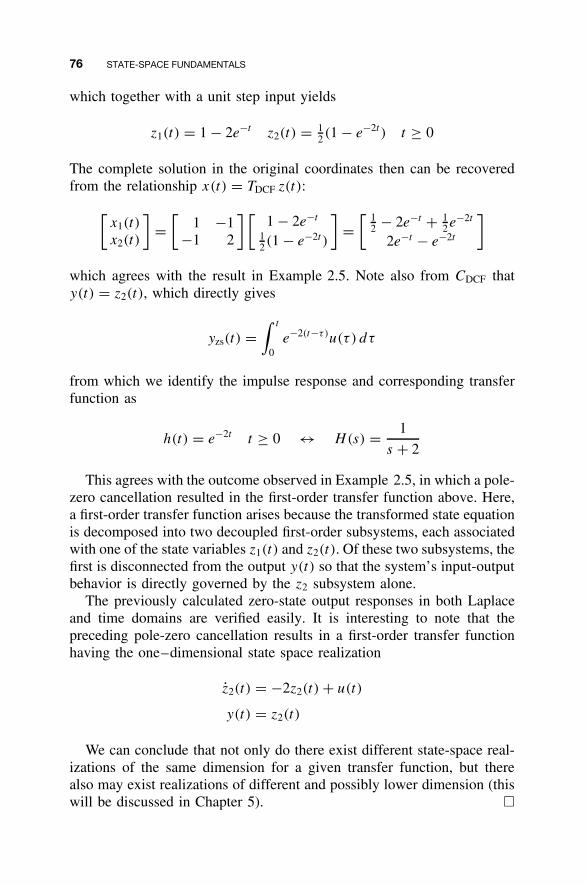
76 STATE-SPACE FUNDAMENTALS
which together with a unit step input yields
z1(t) = 1 − 2e−t z2(t) = 12(1 − e−2t ) t ≥ 0
The complete solution in the original coordinates then can be recoveredfrom the relationship x(t) = TDCF z(t):
[x1(t)
x2(t)
]=
[1 −1
−1 2
] [1 − 2e−t
12(1 − e−2t )
]=
[ 12 − 2e−t + 1
2e−2t
2e−t − e−2t
]
which agrees with the result in Example 2.5. Note also from CDCF thaty(t) = z2(t), which directly gives
yzs(t) =∫ t
0e−2(t−τ )u(τ ) dτ
from which we identify the impulse response and corresponding transferfunction as
h(t) = e−2t t ≥ 0 ↔ H(s) = 1
s + 2
This agrees with the outcome observed in Example 2.5, in which a pole-zero cancellation resulted in the first-order transfer function above. Here,a first-order transfer function arises because the transformed state equationis decomposed into two decoupled first-order subsystems, each associatedwith one of the state variables z1(t) and z2(t). Of these two subsystems, thefirst is disconnected from the output y(t) so that the system’s input-outputbehavior is directly governed by the z2 subsystem alone.
The previously calculated zero-state output responses in both Laplaceand time domains are verified easily. It is interesting to note that thepreceding pole-zero cancellation results in a first-order transfer functionhaving the one–dimensional state space realization
z2(t) = −2z2(t) + u(t)
y(t) = z2(t)
We can conclude that not only do there exist different state-space real-izations of the same dimension for a given transfer function, but therealso may exist realizations of different and possibly lower dimension (thiswill be discussed in Chapter 5). �
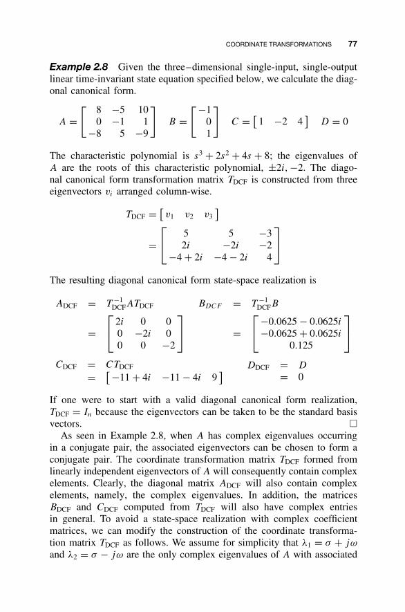
COORDINATE TRANSFORMATIONS 77
Example 2.8 Given the three–dimensional single-input, single-outputlinear time-invariant state equation specified below, we calculate the diag-onal canonical form.
A =[ 8 −5 10
0 −1 1−8 5 −9
]B =
[−101
]C = [
1 −2 4]
D = 0
The characteristic polynomial is s3 + 2s2 + 4s + 8; the eigenvalues ofA are the roots of this characteristic polynomial, ±2i, −2. The diago-nal canonical form transformation matrix TDCF is constructed from threeeigenvectors vi arranged column-wise.
TDCF = [v1 v2 v3
]
= 5 5 −3
2i −2i −2−4 + 2i −4 − 2i 4
The resulting diagonal canonical form state-space realization is
ADCF = T −1DCFATDCF
= 2i 0 0
0 −2i 00 0 −2
BDCF = T −1DCFB
= −0.0625 − 0.0625i
−0.0625 + 0.0625i
0.125
CDCF = CTDCF
= [ −11 + 4i −11 − 4i 9] DDCF = D
= 0
If one were to start with a valid diagonal canonical form realization,TDCF = In because the eigenvectors can be taken to be the standard basisvectors. �
As seen in Example 2.8, when A has complex eigenvalues occurringin a conjugate pair, the associated eigenvectors can be chosen to form aconjugate pair. The coordinate transformation matrix TDCF formed fromlinearly independent eigenvectors of A will consequently contain complexelements. Clearly, the diagonal matrix ADCF will also contain complexelements, namely, the complex eigenvalues. In addition, the matricesBDCF and CDCF computed from TDCF will also have complex entriesin general. To avoid a state-space realization with complex coefficientmatrices, we can modify the construction of the coordinate transforma-tion matrix TDCF as follows. We assume for simplicity that λ1 = σ + jω
and λ2 = σ − jω are the only complex eigenvalues of A with associated
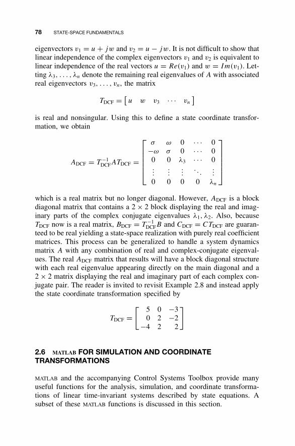
78 STATE-SPACE FUNDAMENTALS
eigenvectors v1 = u + jw and v2 = u − jw. It is not difficult to show thatlinear independence of the complex eigenvectors v1 and v2 is equivalent tolinear independence of the real vectors u = Re(v1) and w = Im(v1). Let-ting λ3, . . . , λn denote the remaining real eigenvalues of A with associatedreal eigenvectors v3, . . . , vn, the matrix
TDCF = [u w v3 · · · vn
]
is real and nonsingular. Using this to define a state coordinate transfor-mation, we obtain
ADCF = T −1DCFATDCF =
σ ω 0 · · · 0−ω σ 0 · · · 00 0 λ3 · · · 0...
......
. . ....
0 0 0 0 λn
which is a real matrix but no longer diagonal. However, ADCF is a blockdiagonal matrix that contains a 2 × 2 block displaying the real and imag-inary parts of the complex conjugate eigenvalues λ1, λ2. Also, becauseTDCF now is a real matrix, BDCF = T −1
DCFB and CDCF = CTDCF are guaran-teed to be real yielding a state-space realization with purely real coefficientmatrices. This process can be generalized to handle a system dynamicsmatrix A with any combination of real and complex-conjugate eigenval-ues. The real ADCF matrix that results will have a block diagonal structurewith each real eigenvalue appearing directly on the main diagonal and a2 × 2 matrix displaying the real and imaginary part of each complex con-jugate pair. The reader is invited to revisit Example 2.8 and instead applythe state coordinate transformation specified by
TDCF =[ 5 0 −3
0 2 −2−4 2 2
]
2.6 MATLAB FOR SIMULATION AND COORDINATETRANSFORMATIONS
MATLAB and the accompanying Control Systems Toolbox provide manyuseful functions for the analysis, simulation, and coordinate transforma-tions of linear time-invariant systems described by state equations. Asubset of these MATLAB functions is discussed in this section.
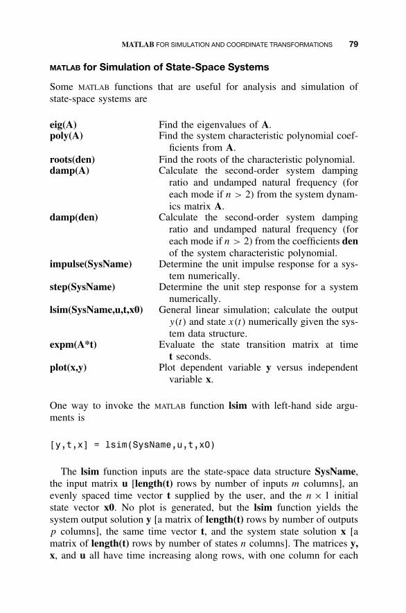
MATLAB FOR SIMULATION AND COORDINATE TRANSFORMATIONS 79
MATLAB for Simulation of State-Space Systems
Some MATLAB functions that are useful for analysis and simulation ofstate-space systems are
eig(A) Find the eigenvalues of A.poly(A) Find the system characteristic polynomial coef-
ficients from A.roots(den) Find the roots of the characteristic polynomial.damp(A) Calculate the second-order system damping
ratio and undamped natural frequency (foreach mode if n > 2) from the system dynam-ics matrix A.
damp(den) Calculate the second-order system dampingratio and undamped natural frequency (foreach mode if n > 2) from the coefficients denof the system characteristic polynomial.
impulse(SysName) Determine the unit impulse response for a sys-tem numerically.
step(SysName) Determine the unit step response for a systemnumerically.
lsim(SysName,u,t,x0) General linear simulation; calculate the outputy(t) and state x(t) numerically given the sys-tem data structure.
expm(A*t) Evaluate the state transition matrix at timet seconds.
plot(x,y) Plot dependent variable y versus independentvariable x.
One way to invoke the MATLAB function lsim with left-hand side argu-ments is
[y,t,x] = lsim(SysName,u,t,x0)
The lsim function inputs are the state-space data structure SysName,the input matrix u [length(t) rows by number of inputs m columns], anevenly spaced time vector t supplied by the user, and the n × 1 initialstate vector x0. No plot is generated, but the lsim function yields thesystem output solution y [a matrix of length(t) rows by number of outputsp columns], the same time vector t, and the system state solution x [amatrix of length(t) rows by number of states n columns]. The matrices y,x, and u all have time increasing along rows, with one column for each
80 STATE-SPACE FUNDAMENTALS
component, in order. The user then can plot the desired output and statecomponents versus time after the lsim command has been executed.
MATLAB for Coordinate Transformations and DiagonalCanonical Form
Some MATLAB functions that are useful for coordinate transformations andthe diagonal canonical form realization are
canon MATLAB function for canonical forms (use the modal switch fordiagonal canonical form)
ss2ss Coordinate transformation of one state-space realization toanother.
The canon function with the modal switch handles complex conjugateeigenvalues using the approach described following Example 2.8 andreturns a states-space realization with purely real coefficient matrices.
Continuing MATLAB Example
State-Space Simulation For the Continuing MATLAB Example [single-input, single-output rotational mechanical system with input torque τ (t)and output angular displacement θ (t)], we now simulate the open-loopsystem response given zero input torque τ (t) and initial state x(0) =[0.4, 0.2]T. We invoke the lsim command which numerically solves forthe state vector x(t) from x(t) = Ax(t) + Bu(t) given the zero input u(t)
and the initial state x(0). Then lsim also yields the output y(t) from y(t) =Cx(t) + Du(t). The following MATLAB code, in combination with that inChapter 1, performs the open-loop system simulation for this example.Appendix C summarizes the entire Continuing MATLAB Example m-file.
%-----------------------------------------------% Chapter 2. Simulation of State-Space Systems%-----------------------------------------------t = [0:.01:4]; % Define array of time
% valuesU = [zeros(size(t))]; % Zero single input of
% proper size to go with tx0 = [0.4; 0.2]; % Define initial state
% vector [x10; x20]
CharPoly = poly(A) % Find characteristic% polynomial from A
MATLAB FOR SIMULATION AND COORDINATE TRANSFORMATIONS 81
Poles = roots(CharPoly) % Find the system poles
EigsO = eig(A); % Calculate open-loop% system eigenvalues
damp(A); % Calculate eigenvalues,% zeta, and wn from ABCD
[Yo,t,Xo] = lsim(JbkR,U,t,x0);% Open-loop response% (zero input, given ICs)
Xo(101,:); % State vector value at% t=1 sec
X1 = expm(A*1)*X0; % Compare with state% transition matrix% method
figure; % Open-loop State Plotssubplot(211), plot(t,Xo(:,1)); grid;
axis([0 4 -0.2 0.5]);set(gca,'FontSize',18);ylabel('{\itx}−1 (\itrad)')subplot(212), plot(t,Xo(:,2)); grid; axis([0 4 -2 1]);set(gca,'FontSize',18);xlabel('\ittime (sec)'); ylabel('{\itx}−2 (\itrad/s)');
This m-file, combined with the m-file from Chapter 1, generates thefollowing results for the open-loop characteristic polynomial, poles, eigen-values, damping ratio ξ and undamped natural frequency ωn, and the valueof the state vector at 1 second. The eigenvalues of A agree with those fromthe damp command, and also with roots applied to the characteristicpolynomial.
CharPoly =1.0000 4.0000 40.0000
Poles =-2.0000 + 6.0000i-2.0000 - 6.0000i
EigsO =-2.0000 + 6.0000i-2.0000 - 6.0000i
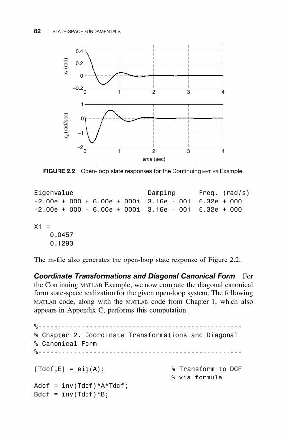
82 STATE-SPACE FUNDAMENTALS
0 1 2 3 4−0.2
0
0.2
0.4
0 1 2 3 4−2
−1
0
1
time (sec)
x 1(r
ad)
x 2(r
ad/s
ec)
FIGURE 2.2 Open-loop state responses for the Continuing MATLAB Example.
Eigenvalue Damping Freq. (rad/s)-2.00e + 000 + 6.00e + 000i 3.16e - 001 6.32e + 000-2.00e + 000 - 6.00e + 000i 3.16e - 001 6.32e + 000
X1 =0.04570.1293
The m-file also generates the open-loop state response of Figure 2.2.
Coordinate Transformations and Diagonal Canonical Form Forthe Continuing MATLAB Example, we now compute the diagonal canonicalform state-space realization for the given open-loop system. The followingMATLAB code, along with the MATLAB code from Chapter 1, which alsoappears in Appendix C, performs this computation.
%----------------------------------------------------% Chapter 2. Coordinate Transformations and Diagonal% Canonical Form%----------------------------------------------------
[Tdcf,E] = eig(A); % Transform to DCF% via formula
Adcf = inv(Tdcf)*A*Tdcf;Bdcf = inv(Tdcf)*B;
MATLAB FOR SIMULATION AND COORDINATE TRANSFORMATIONS 83
Cdcf = C*Tdcf;Ddcf = D;
[JbkRm,Tm] = canon(JbkR,'modal'); % Calculate DCF% using MATLAB canon
Am = JbkRm.aBm = JbkRm.bCm = JbkRm.cDm = JbkRm.d
This m-file, combined with the Chapter 1 m-file, produces the diagonalcanonical form realization for the Continuing MATLAB Example:
Tdcf =-0.0494 - 0.1482i -0.0494 + 0.1482i0.9877 0.9877
Adcf =-2.0000 + 6.0000i 0 - 0.0000i0.0000 - 0.0000i -2.0000 - 6.0000i
Bdcf =0.5062 + 0.1687i0.5062 - 0.1687i
Cdcf =-0.0494 - 0.1482i -0.0494 + 0.1482i
Ddcf =0
Tm =0 1.0124-6.7495 -0.3375
Am =-2.0000 6.0000-6.0000 -2.0000
Bm =1.0124-0.3375
84 STATE-SPACE FUNDAMENTALS
Cm =-0.0494 -0.1482
Dm =0
We observe that Am is a real 2 × 2 matrix that displays the real andimaginary parts of the complex conjugate eigenvalues −2 ± 6i. The MAT-
LAB modal transformation matrix Tm above is actually the inverse of ourcoordinate transformation matrix given in Equation (2.28). Therefore, theinverse of this matrix, for use in our coordinate transformation, is
inv(Tm) =-0.0494 -0.14820.9877 0
The first column of inv(Tm) is the real part of the first column of Tdcf,which is an eigenvector corresponding to the eigenvalue −2 + 6i. Thesecond column of inv(Tm) is the imaginary part of this eigenvector.
2.7 CONTINUING EXAMPLES FOR SIMULATIONAND COORDINATE TRANSFORMATIONS
Continuing Example 1: Two-Mass Translational MechanicalSystem
Simulation The constant parameters in Table 2.1 are given for Contin-uing Example 1 (two-mass translational mechanical system):
For case a, we simulate the open-loop system response given zeroinitial state and step inputs of magnitudes 20 and 10 N, respectively, foru1(t) and u2(t).
For case b, we simulate the open-loop system response given zero inputu2(t) and initial state x(0) = [0.1, 0, 0.2, 0]T [initial displacements ofy1(0) = 0.1 and y2(0) = 0.2 m, with zero initial velocities].
TABLE 2.1 Numerical Parameters for ContinuingExample 1
i mi (kg) ci (Ns/m) ki (N/m)
1 40 20 4002 20 10 200
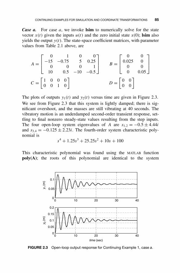
CONTINUING EXAMPLES FOR SIMULATION AND COORDINATE TRANSFORMATIONS 85
Case a. For case a, we invoke lsim to numerically solve for the statevector x(t) given the inputs u(t) and the zero initial state x(0); lsim alsoyields the output y(t). The state-space coefficient matrices, with parametervalues from Table 2.1 above, are
A =
0 1 0 0−15 −0.75 5 0.25
0 0 0 110 0.5 −10 −0.5
B =
0 00.025 0
0 00 0.05
C =[
1 0 0 00 0 1 0
]D =
[0 00 0
]
The plots of outputs y1(t) and y2(t) versus time are given in Figure 2.3.We see from Figure 2.3 that this system is lightly damped; there is sig-nificant overshoot, and the masses are still vibrating at 40 seconds. Thevibratory motion is an underdamped second-order transient response, set-tling to final nonzero steady-state values resulting from the step inputs.The four open-loop system eigenvalues of A are s1,2 = −0.5 ± 4.44i
and s3,4 = −0.125 ± 2.23i. The fourth-order system characteristic poly-nomial is
s4 + 1.25s3 + 25.25s2 + 10s + 100
This characteristic polynomial was found using the MATLAB functionpoly(A); the roots of this polynomial are identical to the system
0 10 20 30 400
0.05
0.1
0 10 20 30 400
0.05
0.1
0.15
0.2
time (sec)
y 2(m
)y 1
(m)
FIGURE 2.3 Open-loop output response for Continuing Example 1, case a.
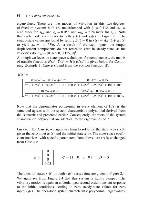
86 STATE-SPACE FUNDAMENTALS
eigenvalues. There are two modes of vibration in this two-degrees-of-freedom system; both are underdamped with ξ1 = 0.112 and ωn1 =4.48 rad/s for s1,2 and ξ2 = 0.056 and ωn2 = 2.24 rad/s for s3,4. Notethat each mode contributes to both y1(t) and y2(t) in Figure 2.3. Thesteady-state values are found by setting x(t) = 0 in x(t) = Ax(t) + Bu(t)
to yield xss = −A−1Bu. As a result of the step inputs, the outputdisplacement components do not return to zero in steady-state, as thevelocities do: xss = [0.075, 0, 0.125, 0]T.Although we focus on state-space techniques, for completeness, the matrixof transfer functions H(s) [Y(s) = H(s)U(s)] is given below for Contin-uing Example 1, Case a (found from the MATLAB function tf):
H(s) =
0.025s2 + 0.0125s + 0.25
s4 + 1.25s3 + 25.25s2 + 10s + 100
0.0125s + 0.25
s4 + 1.25s3 + 25.25s2 + 10s + 100
0.0125s + 0.25
s4 + 1.25s3 + 25.25s2 + 10s + 100
0.05s2 + 0.0375s + 0.75
s4 + 1.25s3 + 25.25s2 + 10s + 100
Note that the denominator polynomial in every element of H(s) is thesame and agrees with the system characteristic polynomial derived fromthe A matrix and presented earlier. Consequently, the roots of the systemcharacteristic polynomial are identical to the eigenvalues of A.
Case b. For Case b, we again use lsim to solve for the state vector x(t)
given the zero input u2(t) and the initial state x(0). The state-space coeffi-cient matrices, with specific parameters from above, are (A is unchangedfrom Case a):
B =
000
0.05
C = [ 1 0 0 0 ] D = 0
The plots for states x1(t) through x4(t) versus time are given in Figure 2.4.We again see from Figure 2.4 that this system is lightly damped. Thevibratory motion is again an underdamped second-order transient responseto the initial conditions, settling to zero steady-state values for zeroinput u2(t). The open-loop system characteristic polynomial, eigenvalues,
CONTINUING EXAMPLES FOR SIMULATION AND COORDINATE TRANSFORMATIONS 87
0 10 20 30 40−0.1
0
0.1
0 10 20 30 40−0.2
0
0.2
0 10 20 30 40−0.2
0
0.2
0 10 20 30 40−0.5
0
0.5
time (sec)
x 4(m
/sec
)x 3
(m)
x 1(m
)x 2
(m/s
ec)
FIGURE 2.4 Open-loop state response for Continuing Example 1, case b.
damping ratios, and undamped natural frequencies are all identical to theCase a results.In Figure 2.4, we see that states x1(t) and x3(t) start from the given initialdisplacement values of 0.1 and 0.2, respectively. The given initial veloci-ties are both zero. Note that in this Case b example, the final values are allzero because after the transient response has died out, each spring returnsto its equilibrium position referenced as zero displacement.When focusing on the zero-input response, we can calculate the statevector at any desired time by using the state transition matrix �(t, t0) =eA(t−t0). For instance, at time t = 20 sec:
x(20) = �(20, 0)x(0)
= eA(20)x(0)
=
0.0067
−0.0114
0.0134
−0.0228
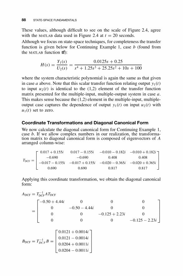
88 STATE-SPACE FUNDAMENTALS
These values, although difficult to see on the scale of Figure 2.4, agreewith the MATLAB data used in Figure 2.4 at t = 20 seconds.Although we focus on state-space techniques, for completeness the transferfunction is given below for Continuing Example 1, case b (found fromthe MATLAB function tf):
H(s) = Y1(s)
U2(s)= 0.0125s + 0.25
s4 + 1.25s3 + 25.25s2 + 10s + 100
where the system characteristic polynomial is again the same as that givenin case a above. Note that this scalar transfer function relating output y1(t)
to input u2(t) is identical to the (1,2) element of the transfer functionmatrix presented for the multiple-input, multiple-output system in case a.This makes sense because the (1,2) element in the multiple-input, multiple-output case captures the dependence of output y1(t) on input u2(t) withu1(t) set to zero.
Coordinate Transformations and Diagonal Canonical FormWe now calculate the diagonal canonical form for Continuing Example 1,case b. If we allow complex numbers in our realization, the transforma-tion matrix to diagonal canonical form is composed of eigenvectors of Aarranged column-wise:
TDCF =
0.017 + 0.155i 0.017 − 0.155i −0.010 − 0.182i −0.010 + 0.182i
−0.690 −0.690 0.408 0.408
−0.017 − 0.155i −0.017 + 0.155i −0.020 − 0.365i −0.020 + 0.365i
0.690 0.690 0.817 0.817
Applying this coordinate transformation, we obtain the diagonal canonicalform:
ADCF = T −1DCFATDCF
=
−0.50 + 4.44i 0 0 0
0 −0.50 − 4.44i 0 0
0 0 −0.125 + 2.23i 0
0 0 0 −0.125 − 2.23i
BDCF = T −1DCF B =
0.0121 + 0.0014i
0.0121 − 0.0014i
0.0204 + 0.0011i
0.0204 − 0.0011i
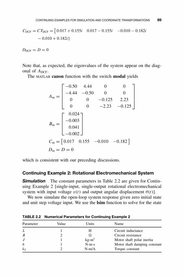
CONTINUING EXAMPLES FOR SIMULATION AND COORDINATE TRANSFORMATIONS 89
CDCF = CTDCF = [0.017 + 0.155i 0.017 − 0.155i −0.010 − 0.182i
− 0.010 + 0.182i]
DDCF = D = 0
Note that, as expected, the eigenvalues of the system appear on the diag-onal of ADCF.
The MATLAB canon function with the switch modal yields
Am =
−0.50 4.44 0 0
−4.44 −0.50 0 0
0 0 −0.125 2.23
0 0 −2.23 −0.125
Bm =
0.024
−0.003
0.041
−0.002
Cm = [0.017 0.155 −0.010 −0.182
]Dm = D = 0
which is consistent with our preceding discussions.
Continuing Example 2: Rotational Electromechanical System
Simulation The constant parameters in Table 2.2 are given for Contin-uing Example 2 [single-input, single-output rotational electromechanicalsystem with input voltage v(t) and output angular displacement θ (t)].
We now simulate the open-loop system response given zero initial stateand unit step voltage input. We use the lsim function to solve for the state
TABLE 2.2 Numerical Parameters for Continuing Example 2
Parameter Value Units Name
L 1 H Circuit inductanceR 2 � Circuit resistanceJ 1 kg-m2 Motor shaft polar inertiab 1 N-m-s Motor shaft damping constantkT 2 N-m/A Torque constant
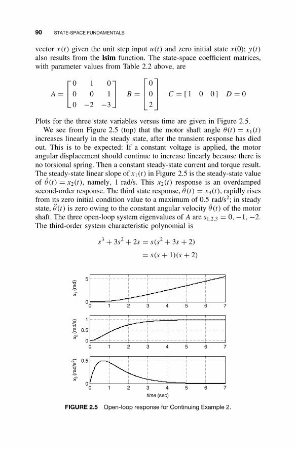
90 STATE-SPACE FUNDAMENTALS
vector x(t) given the unit step input u(t) and zero initial state x(0); y(t)
also results from the lsim function. The state-space coefficient matrices,with parameter values from Table 2.2 above, are
A =
0 1 0
0 0 1
0 −2 −3
B =
0
0
2
C = [ 1 0 0 ] D = 0
Plots for the three state variables versus time are given in Figure 2.5.We see from Figure 2.5 (top) that the motor shaft angle θ (t) = x1(t)
increases linearly in the steady state, after the transient response has diedout. This is to be expected: If a constant voltage is applied, the motorangular displacement should continue to increase linearly because there isno torsional spring. Then a constant steady-state current and torque result.The steady-state linear slope of x1(t) in Figure 2.5 is the steady-state valueof θ (t) = x2(t), namely, 1 rad/s. This x2(t) response is an overdampedsecond-order response. The third state response, θ (t) = x3(t), rapidly risesfrom its zero initial condition value to a maximum of 0.5 rad/s2; in steadystate, θ (t) is zero owing to the constant angular velocity θ (t) of the motorshaft. The three open-loop system eigenvalues of A are s1,2,3 = 0, −1, −2.The third-order system characteristic polynomial is
s3 + 3s2 + 2s = s(s2 + 3s + 2)
= s(s + 1)(s + 2)
0 1 2 3 4 5 6 70
5
0 1 2 3 4 5 6 70
0.5
1
0 1 2 3 4 5 6 70
0.5
time (sec)
x 3(r
ad/s
2 )x 2
(rad
/s)
x 1(r
ad)
FIGURE 2.5 Open-loop response for Continuing Example 2.
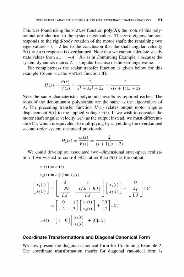
CONTINUING EXAMPLES FOR SIMULATION AND COORDINATE TRANSFORMATIONS 91
This was found using the MATLAB function poly(A); the roots of this poly-nomial are identical to the system eigenvalues. The zero eigenvalue cor-responds to the rigid-body rotation of the motor shaft; the remaining twoeigenvalues −1, −2 led to the conclusion that the shaft angular velocityθ (t) = ω(t) response is overdamped. Note that we cannot calculate steadystate values from xss = −A−1Bu as in Continuing Example 1 because thesystem dynamics matrix A is singular because of the zero eigenvalue.
For completeness the scalar transfer function is given below for thisexample (found via the MATLAB function tf):
H(s) = θ(s)
V (s)= 2
s3 + 3s2 + 2s= 2
s(s + 1)(s + 2)
Note the same characteristic polynomial results as reported earlier. Theroots of the denominator polynomial are the same as the eigenvalues ofA. The preceding transfer function H(s) relates output motor angulardisplacement θ (t) to the applied voltage v(t). If we wish to consider themotor shaft angular velocity ω(t) as the output instead, we must differenti-ate θ (t), which is equivalent to multiplying by s, yielding the overdampedsecond-order system discussed previously:
H2(s) = ω(s)
V (s)= 2
(s + 1)(s + 2)
We could develop an associated two–dimensional state-space realiza-tion if we wished to control ω(t) rather than θ (t) as the output:
x1(t) = ω(t)
x2(t) = ω(t) = x1(t)
[x1(t)
x2(t)
]=
0 1
−Rb
LJ
−(Lb + RJ)
LJ
[
x1(t)
x2(t)
]+
0
kT
LJ
v(t)
=[
0 1
−2 −3
] [x1(t)
x2(t)
]+
[0
2
]v(t)
ω(t) = [1 0
] [x1(t)
x2(t)
]+ [0]v(t)
Coordinate Transformations and Diagonal Canonical Form
We now present the diagonal canonical form for Continuing Example 2.The coordinate transformation matrix for diagonal canonical form is
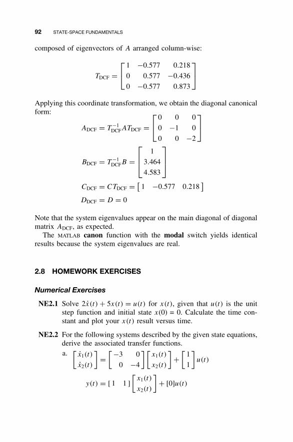
92 STATE-SPACE FUNDAMENTALS
composed of eigenvectors of A arranged column-wise:
TDCF =
1 −0.577 0.218
0 0.577 −0.436
0 −0.577 0.873
Applying this coordinate transformation, we obtain the diagonal canonicalform:
ADCF = T −1DCFATDCF =
0 0 0
0 −1 0
0 0 −2
BDCF = T −1DCFB =
1
3.464
4.583
CDCF = CTDCF = [1 −0.577 0.218
]DDCF = D = 0
Note that the system eigenvalues appear on the main diagonal of diagonalmatrix ADCF, as expected.
The MATLAB canon function with the modal switch yields identicalresults because the system eigenvalues are real.
2.8 HOMEWORK EXERCISES
Numerical Exercises
NE2.1 Solve 2x(t) + 5x(t) = u(t) for x(t), given that u(t) is the unitstep function and initial state x(0) = 0. Calculate the time con-stant and plot your x(t) result versus time.
NE2.2 For the following systems described by the given state equations,derive the associated transfer functions.a. [
x1(t)
x2(t)
]=
[ −3 0
0 −4
] [x1(t)
x2(t)
]+
[1
1
]u(t)
y(t) = [ 1 1 ]
[x1(t)
x2(t)
]+ [0]u(t)
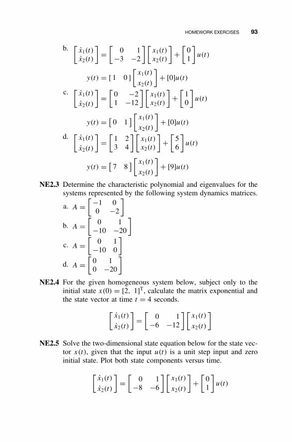
HOMEWORK EXERCISES 93
b. [x1(t)
x2(t)
]=
[0 1
−3 −2
] [x1(t)
x2(t)
]+
[01
]u(t)
y(t) = [ 1 0 ]
[x1(t)
x2(t)
]+ [0]u(t)
c. [x1(t)
x2(t)
]=
[0 −21 −12
] [x1(t)
x2(t)
]+
[10
]u(t)
y(t) = [0 1
] [x1(t)
x2(t)
]+ [0]u(t)
d. [x1(t)
x2(t)
]=
[1 23 4
] [x1(t)
x2(t)
]+
[56
]u(t)
y(t) = [7 8
] [x1(t)
x2(t)
]+ [9]u(t)
NE2.3 Determine the characteristic polynomial and eigenvalues for thesystems represented by the following system dynamics matrices.
a. A =[ −1 0
0 −2
]
b. A =[
0 1−10 −20
]
c. A =[
0 1−10 0
]
d. A =[
0 10 −20
]
NE2.4 For the given homogeneous system below, subject only to theinitial state x(0) = [2, 1]T, calculate the matrix exponential andthe state vector at time t = 4 seconds.
[x1(t)
x2(t)
]=
[0 1
−6 −12
] [x1(t)
x2(t)
]
NE2.5 Solve the two-dimensional state equation below for the state vec-tor x(t), given that the input u(t) is a unit step input and zeroinitial state. Plot both state components versus time.
[x1(t)
x2(t)
]=
[0 1
−8 −6
] [x1(t)
x2(t)
]+
[01
]u(t)
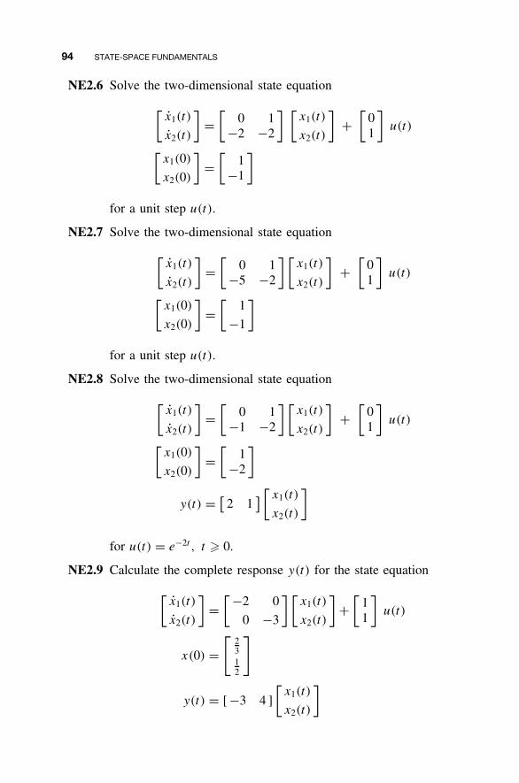
94 STATE-SPACE FUNDAMENTALS
NE2.6 Solve the two-dimensional state equation
[x1(t)
x2(t)
]=
[0 1
−2 −2
] [x1(t)
x2(t)
]+
[01
]u(t)
[x1(0)
x2(0)
]=
[1
−1
]
for a unit step u(t).
NE2.7 Solve the two-dimensional state equation
[x1(t)
x2(t)
]=
[0 1
−5 −2
] [x1(t)
x2(t)
]+
[01
]u(t)
[x1(0)
x2(0)
]=
[1
−1
]
for a unit step u(t).
NE2.8 Solve the two-dimensional state equation
[x1(t)
x2(t)
]=
[0 1
−1 −2
] [x1(t)
x2(t)
]+
[01
]u(t)
[x1(0)
x2(0)
]=
[1
−2
]
y(t) = [2 1
] [x1(t)
x2(t)
]
for u(t) = e−2t , t � 0.
NE2.9 Calculate the complete response y(t) for the state equation
[x1(t)
x2(t)
]=
[ −2 0
0 −3
] [x1(t)
x2(t)
]+
[11
]u(t)
x(0) =[
2312
]
y(t) = [ −3 4 ]
[x1(t)
x2(t)
]
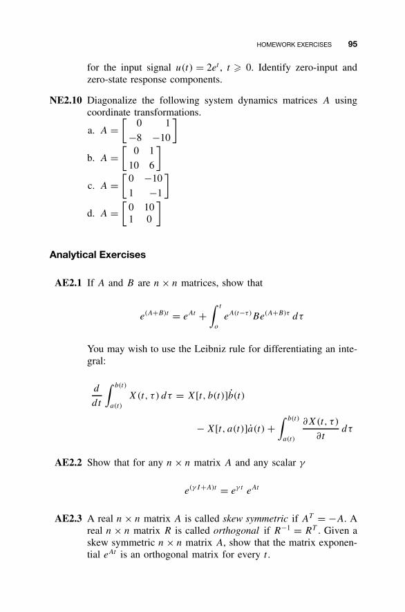
HOMEWORK EXERCISES 95
for the input signal u(t) = 2et , t � 0. Identify zero-input andzero-state response components.
NE2.10 Diagonalize the following system dynamics matrices A usingcoordinate transformations.
a. A =[
0 1
−8 −10
]
b. A =[
0 1
10 6
]
c. A =[
0 −10
1 −1
]
d. A =[
0 101 0
]
Analytical Exercises
AE2.1 If A and B are n × n matrices, show that
e(A+B)t = eAt +∫ t
o
eA(t−τ )Be(A+B)τ dτ
You may wish to use the Leibniz rule for differentiating an inte-gral:
d
d t
∫ b(t)
a(t)
X(t, τ ) dτ = X[t, b(t)]b(t)
− X[t, a(t)]a(t) +∫ b(t)
a(t)
∂X(t, τ )
∂tdτ
AE2.2 Show that for any n × n matrix A and any scalar γ
e(γ I+A)t = eγ t eAt
AE2.3 A real n × n matrix A is called skew symmetric if AT = −A. Areal n × n matrix R is called orthogonal if R−1 = RT . Given askew symmetric n × n matrix A, show that the matrix exponen-tial eAt is an orthogonal matrix for every t .
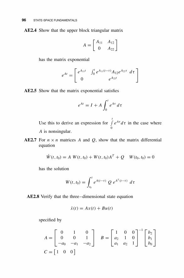
96 STATE-SPACE FUNDAMENTALS
AE2.4 Show that the upper block triangular matrix
A =[
A11 A12
0 A22
]
has the matrix exponential
eAt =[
eA11t∫ t
0 eA11(t−τ )A12eA22τ dτ
0 eA22t
]
AE2.5 Show that the matrix exponential satisfies
eAt = I + A
∫ t
0eAτ dτ
Use this to derive an expression fort∫
0eAτ dτ in the case where
A is nonsingular.
AE2.7 For n × n matrices A and Q, show that the matrix differentialequation
W (t, t0) = A W(t, t0) + W(t, t0)AT + Q W(t0, t0) = 0
has the solution
W(t, t0) =∫ t
t0
eA(t−τ ) Q eAT (t−τ ) dτ
AE2.8 Verify that the three–dimensional state equation
x(t) = Ax(t) + Bu(t)
specified by
A = 0 1 0
0 0 1−a0 −a1 −a2
B =
1 0 0
a2 1 0a1 a2 1
−1 b2
b1
b0
C = [1 0 0
]
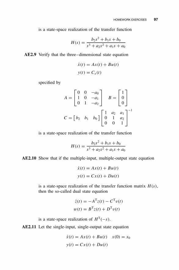
HOMEWORK EXERCISES 97
is a state-space realization of the transfer function
H(s) = b2s2 + b1s + b0
s3 + a2s2 + a1s + a0
AE2.9 Verify that the three–dimensional state equation
x(t) = Ax(t) + Bu(t)
y(t) = Cx(t)
specified by
A = 0 0 −a0
1 0 −a1
0 1 −a2
B =
1
00
C = [b2 b1 b0
] 1 a2 a1
0 1 a2
0 0 1
−1
is a state-space realization of the transfer function
H(s) = b2s2 + b1s + b0
s3 + a2s2 + a1s + a0
AE2.10 Show that if the multiple-input, multiple-output state equation
x(t) = Ax(t) + Bu(t)
y(t) = Cx(t) + Du(t)
is a state-space realization of the transfer function matrix H(s),then the so-called dual state equation
z(t) = −ATz(t) − CTv(t)
w(t) = BTz(t) + DTv(t)
is a state-space realization of H T(−s).
AE2.11 Let the single-input, single-output state equation
x(t) = Ax(t) + Bu(t) x(0) = x0
y(t) = Cx(t) + Du(t)
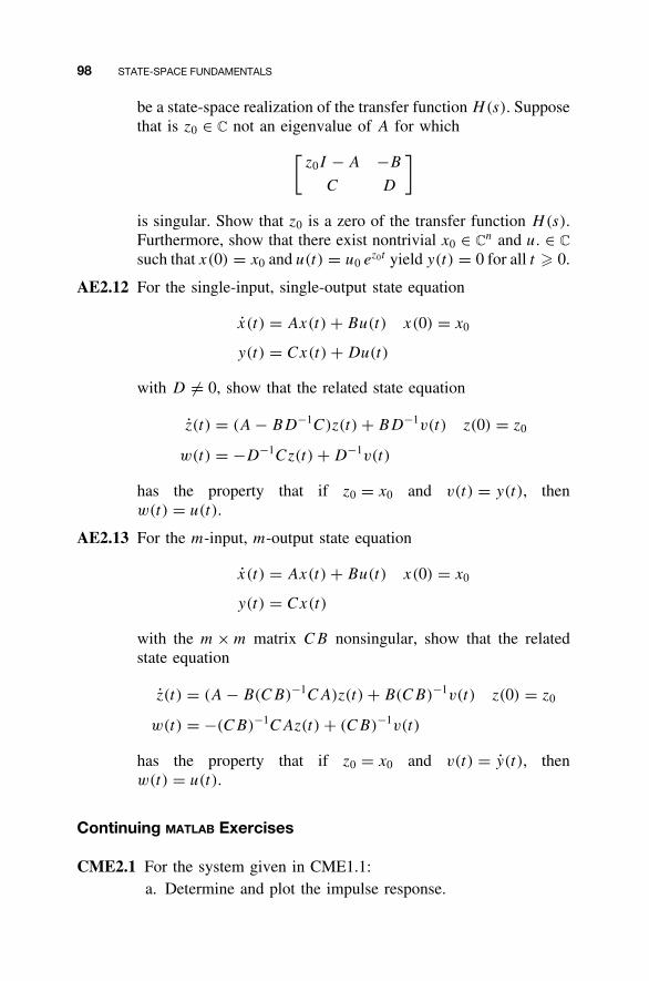
98 STATE-SPACE FUNDAMENTALS
be a state-space realization of the transfer function H(s). Supposethat is z0 ∈ C not an eigenvalue of A for which
[z0I − A −B
C D
]
is singular. Show that z0 is a zero of the transfer function H(s).Furthermore, show that there exist nontrivial x0 ∈ C
n and u. ∈ C
such that x(0) = x0 and u(t) = u0 ez0t yield y(t) = 0 for all t � 0.
AE2.12 For the single-input, single-output state equation
x(t) = Ax(t) + Bu(t) x(0) = x0
y(t) = Cx(t) + Du(t)
with D �= 0, show that the related state equation
z(t) = (A − BD−1C)z(t) + BD−1v(t) z(0) = z0
w(t) = −D−1Cz(t) + D−1v(t)
has the property that if z0 = x0 and v(t) = y(t), thenw(t) = u(t).
AE2.13 For the m-input, m-output state equation
x(t) = Ax(t) + Bu(t) x(0) = x0
y(t) = Cx(t)
with the m × m matrix CB nonsingular, show that the relatedstate equation
z(t) = (A − B(CB)−1CA)z(t) + B(CB)−1v(t) z(0) = z0
w(t) = −(CB)−1CAz(t) + (CB)−1v(t)
has the property that if z0 = x0 and v(t) = y(t), thenw(t) = u(t).
Continuing MATLAB Exercises
CME2.1 For the system given in CME1.1:a. Determine and plot the impulse response.
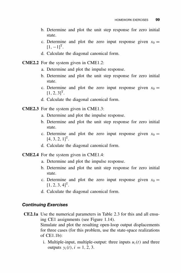
HOMEWORK EXERCISES 99
b. Determine and plot the unit step response for zero initialstate.
c. Determine and plot the zero input response given x0 =[1, −1]T.
d. Calculate the diagonal canonical form.
CME2.2 For the system given in CME1.2:
a. Determine and plot the impulse response.
b. Determine and plot the unit step response for zero initialstate.
c. Determine and plot the zero input response given x0 =[1, 2, 3]T.
d. Calculate the diagonal canonical form.
CME2.3 For the system given in CME1.3:
a. Determine and plot the impulse response.
b. Determine and plot the unit step response for zero initialstate.
c. Determine and plot the zero input response given x0 =[4, 3, 2, 1]T.
d. Calculate the diagonal canonical form.
CME2.4 For the system given in CME1.4:
a. Determine and plot the impulse response.
b. Determine and plot the unit step response for zero initialstate.
c. Determine and plot the zero input response given x0 =[1, 2, 3, 4]T.
d. Calculate the diagonal canonical form.
Continuing Exercises
CE2.1a Use the numerical parameters in Table 2.3 for this and all ensu-ing CE1 assignments (see Figure 1.14).Simulate and plot the resulting open-loop output displacementsfor three cases (for this problem, use the state-space realizationsof CE1.1b):
i. Multiple-input, multiple-output: three inputs ui(t) and threeoutputs yi(t), i = 1, 2, 3.
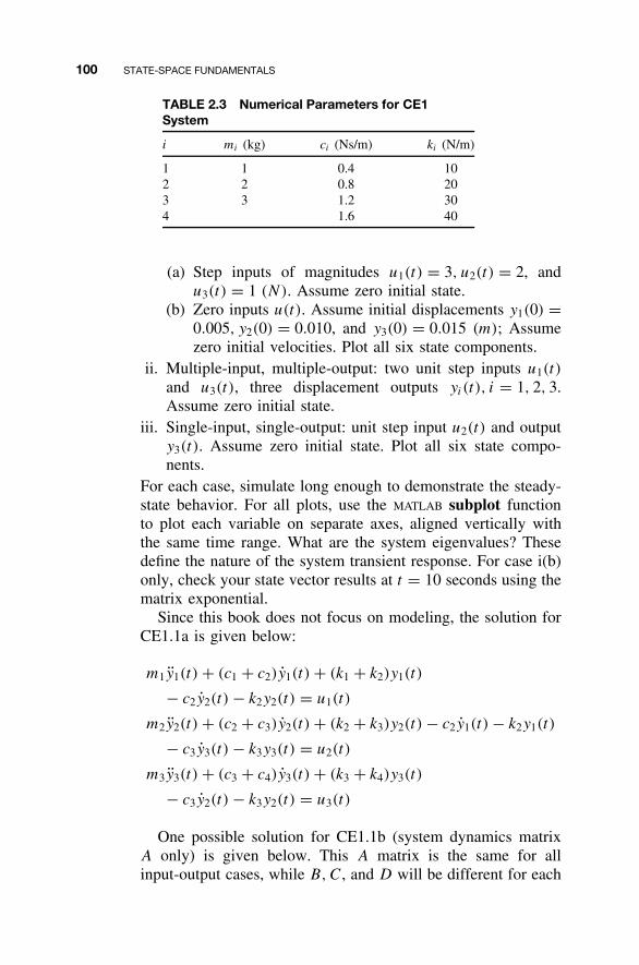
100 STATE-SPACE FUNDAMENTALS
TABLE 2.3 Numerical Parameters for CE1System
i mi (kg) ci (Ns/m) ki (N/m)
1 1 0.4 102 2 0.8 203 3 1.2 304 1.6 40
(a) Step inputs of magnitudes u1(t) = 3, u2(t) = 2, andu3(t) = 1 (N). Assume zero initial state.
(b) Zero inputs u(t). Assume initial displacements y1(0) =0.005, y2(0) = 0.010, and y3(0) = 0.015 (m); Assumezero initial velocities. Plot all six state components.
ii. Multiple-input, multiple-output: two unit step inputs u1(t)
and u3(t), three displacement outputs yi(t), i = 1, 2, 3.Assume zero initial state.
iii. Single-input, single-output: unit step input u2(t) and outputy3(t). Assume zero initial state. Plot all six state compo-nents.
For each case, simulate long enough to demonstrate the steady-state behavior. For all plots, use the MATLAB subplot functionto plot each variable on separate axes, aligned vertically withthe same time range. What are the system eigenvalues? Thesedefine the nature of the system transient response. For case i(b)only, check your state vector results at t = 10 seconds using thematrix exponential.
Since this book does not focus on modeling, the solution forCE1.1a is given below:
m1y1(t) + (c1 + c2)y1(t) + (k1 + k2)y1(t)
− c2y2(t) − k2y2(t) = u1(t)
m2y2(t) + (c2 + c3)y2(t) + (k2 + k3)y2(t) − c2y1(t) − k2y1(t)
− c3y3(t) − k3y3(t) = u2(t)
m3y3(t) + (c3 + c4)y3(t) + (k3 + k4)y3(t)
− c3y2(t) − k3y2(t) = u3(t)
One possible solution for CE1.1b (system dynamics matrixA only) is given below. This A matrix is the same for allinput-output cases, while B, C, and D will be different for each
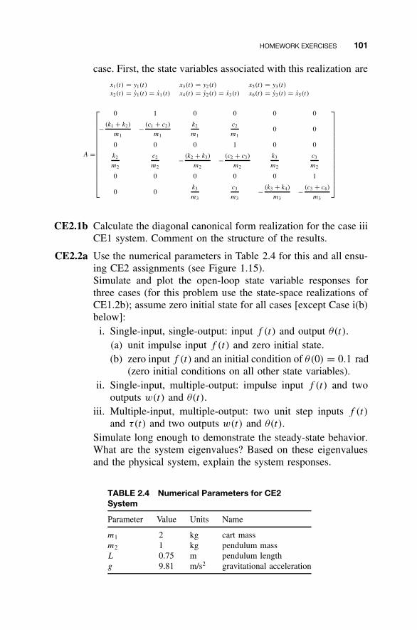
HOMEWORK EXERCISES 101
case. First, the state variables associated with this realization are
x1(t) = y1(t)
x2(t) = y1(t) = x1(t)
x3(t) = y2(t)
x4(t) = y2(t) = x3(t)
x5(t) = y3(t)
x6(t) = y3(t) = x5(t)
A =
0 1 0 0 0 0
− (k1 + k2)
m1− (c1 + c2)
m1
k2
m1
c2
m10 0
0 0 0 1 0 0
k2
m2
c2
m2− (k2 + k3)
m2− (c2 + c3)
m2
k3
m2
c3
m2
0 0 0 0 0 1
0 0k3
m3
c3
m3− (k3 + k4)
m3− (c3 + c4)
m3
CE2.1b Calculate the diagonal canonical form realization for the case iiiCE1 system. Comment on the structure of the results.
CE2.2a Use the numerical parameters in Table 2.4 for this and all ensu-ing CE2 assignments (see Figure 1.15).Simulate and plot the open-loop state variable responses forthree cases (for this problem use the state-space realizations ofCE1.2b); assume zero initial state for all cases [except Case i(b)below]:
i. Single-input, single-output: input f (t) and output θ (t).(a) unit impulse input f (t) and zero initial state.(b) zero input f (t) and an initial condition of θ(0) = 0.1 rad
(zero initial conditions on all other state variables).ii. Single-input, multiple-output: impulse input f (t) and two
outputs w(t) and θ (t).iii. Multiple-input, multiple-output: two unit step inputs f (t)
and τ (t) and two outputs w(t) and θ (t).Simulate long enough to demonstrate the steady-state behavior.What are the system eigenvalues? Based on these eigenvaluesand the physical system, explain the system responses.
TABLE 2.4 Numerical Parameters for CE2System
Parameter Value Units Name
m1 2 kg cart massm2 1 kg pendulum massL 0.75 m pendulum lengthg 9.81 m/s2 gravitational acceleration
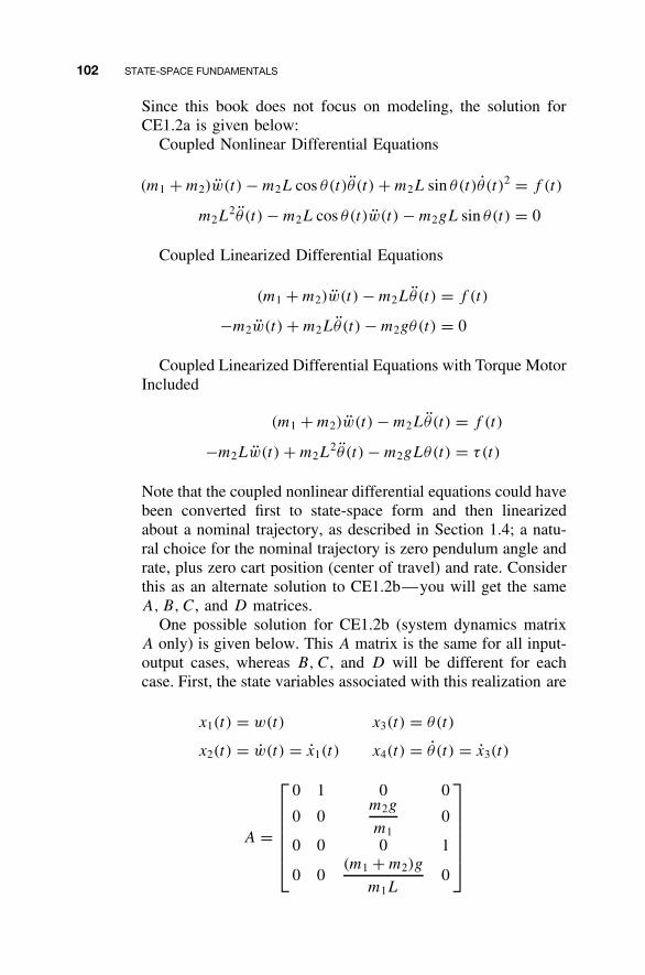
102 STATE-SPACE FUNDAMENTALS
Since this book does not focus on modeling, the solution forCE1.2a is given below:
Coupled Nonlinear Differential Equations
(m1 + m2)w(t) − m2L cos θ(t)θ(t) + m2L sin θ(t)θ(t)2 = f (t)
m2L2θ (t) − m2L cos θ(t)w(t) − m2gL sin θ(t) = 0
Coupled Linearized Differential Equations
(m1 + m2)w(t) − m2Lθ(t) = f (t)
−m2w(t) + m2Lθ(t) − m2gθ(t) = 0
Coupled Linearized Differential Equations with Torque MotorIncluded
(m1 + m2)w(t) − m2Lθ(t) = f (t)
−m2Lw(t) + m2L2θ (t) − m2gLθ(t) = τ(t)
Note that the coupled nonlinear differential equations could havebeen converted first to state-space form and then linearizedabout a nominal trajectory, as described in Section 1.4; a natu-ral choice for the nominal trajectory is zero pendulum angle andrate, plus zero cart position (center of travel) and rate. Considerthis as an alternate solution to CE1.2b—you will get the sameA, B, C, and D matrices.
One possible solution for CE1.2b (system dynamics matrixA only) is given below. This A matrix is the same for all input-output cases, whereas B, C, and D will be different for eachcase. First, the state variables associated with this realization are
x1(t) = w(t) x3(t) = θ(t)
x2(t) = w(t) = x1(t) x4(t) = θ (t) = x3(t)
A =
0 1 0 0
0 0m2g
m10
0 0 0 1
0 0(m1 + m2)g
m1L0
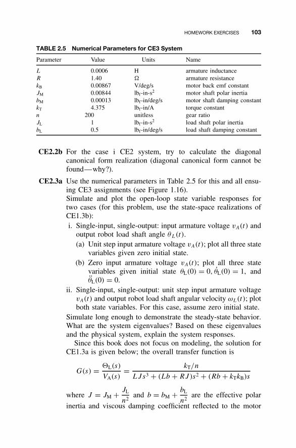
HOMEWORK EXERCISES 103
TABLE 2.5 Numerical Parameters for CE3 System
Parameter Value Units Name
L 0.0006 H armature inductanceR 1.40 � armature resistancekB 0.00867 V/deg/s motor back emf constantJM 0.00844 lbf-in-s2 motor shaft polar inertiabM 0.00013 lbf-in/deg/s motor shaft damping constantkT 4.375 lbf-in/A torque constantn 200 unitless gear ratioJL 1 lbf-in-s2 load shaft polar inertiabL 0.5 lbf-in/deg/s load shaft damping constant
CE2.2b For the case i CE2 system, try to calculate the diagonalcanonical form realization (diagonal canonical form cannot befound—why?).
CE2.3a Use the numerical parameters in Table 2.5 for this and all ensu-ing CE3 assignments (see Figure 1.16).Simulate and plot the open-loop state variable responses fortwo cases (for this problem, use the state-space realizations ofCE1.3b):i. Single-input, single-output: input armature voltage vA(t) and
output robot load shaft angle θL(t).(a) Unit step input armature voltage vA(t); plot all three state
variables given zero initial state.(b) Zero input armature voltage vA(t); plot all three state
variables given initial state θL(0) = 0, θL(0) = 1, andθL(0) = 0.
ii. Single-input, single-output: unit step input armature voltagevA(t) and output robot load shaft angular velocity ωL(t); plotboth state variables. For this case, assume zero initial state.
Simulate long enough to demonstrate the steady-state behavior.What are the system eigenvalues? Based on these eigenvaluesand the physical system, explain the system responses.
Since this book does not focus on modeling, the solution forCE1.3a is given below; the overall transfer function is
G(s) = �L(s)
VA(s)= kT/n
LJs3 + (Lb + RJ)s2 + (Rb + kTkB)s
where J = JM + JL
n2and b = bM + bL
n2are the effective polar
inertia and viscous damping coefficient reflected to the motor
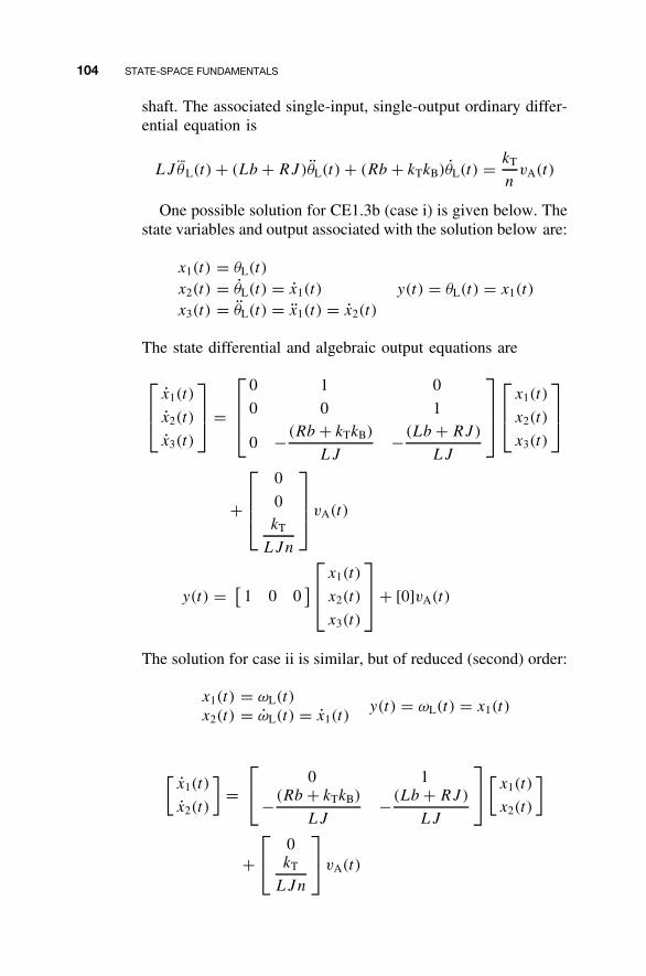
104 STATE-SPACE FUNDAMENTALS
shaft. The associated single-input, single-output ordinary differ-ential equation is
LJ ¨θL(t) + (Lb + RJ)θL(t) + (Rb + kTkB)θL(t) = kT
nvA(t)
One possible solution for CE1.3b (case i) is given below. Thestate variables and output associated with the solution below are:
x1(t) = θL(t)
x2(t) = θL(t) = x1(t)
x3(t) = θL(t) = x1(t) = x2(t)
y(t) = θL(t) = x1(t)
The state differential and algebraic output equations are
x1(t)
x2(t)
x3(t)
=
0 1 0
0 0 1
0 −(Rb + kTkB)
LJ−(Lb + RJ)
LJ
x1(t)
x2(t)
x3(t)
+
0
0kT
LJn
vA(t)
y(t) = [1 0 0
]
x1(t)
x2(t)
x3(t)
+ [0]vA(t)
The solution for case ii is similar, but of reduced (second) order:
x1(t) = ωL(t)
x2(t) = ωL(t) = x1(t)y(t) = ωL(t) = x1(t)
[x1(t)
x2(t)
]=
0 1
−(Rb + kTkB)
LJ−(Lb + RJ)
LJ
[x1(t)
x2(t)
]
+ 0
kT
LJn
vA(t)
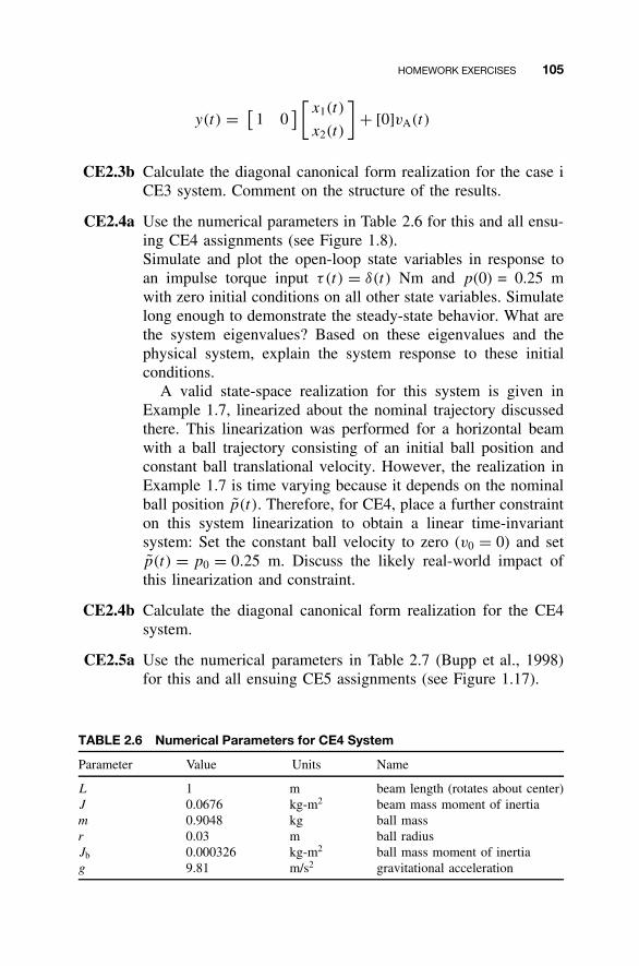
HOMEWORK EXERCISES 105
y(t) = [1 0
] [x1(t)
x2(t)
]+ [0]vA(t)
CE2.3b Calculate the diagonal canonical form realization for the case iCE3 system. Comment on the structure of the results.
CE2.4a Use the numerical parameters in Table 2.6 for this and all ensu-ing CE4 assignments (see Figure 1.8).Simulate and plot the open-loop state variables in response toan impulse torque input τ(t) = δ(t) Nm and p(0) = 0.25 mwith zero initial conditions on all other state variables. Simulatelong enough to demonstrate the steady-state behavior. What arethe system eigenvalues? Based on these eigenvalues and thephysical system, explain the system response to these initialconditions.
A valid state-space realization for this system is given inExample 1.7, linearized about the nominal trajectory discussedthere. This linearization was performed for a horizontal beamwith a ball trajectory consisting of an initial ball position andconstant ball translational velocity. However, the realization inExample 1.7 is time varying because it depends on the nominalball position p(t). Therefore, for CE4, place a further constrainton this system linearization to obtain a linear time-invariantsystem: Set the constant ball velocity to zero (v0 = 0) and setp(t) = p0 = 0.25 m. Discuss the likely real-world impact ofthis linearization and constraint.
CE2.4b Calculate the diagonal canonical form realization for the CE4system.
CE2.5a Use the numerical parameters in Table 2.7 (Bupp et al., 1998)for this and all ensuing CE5 assignments (see Figure 1.17).
TABLE 2.6 Numerical Parameters for CE4 System
Parameter Value Units Name
L 1 m beam length (rotates about center)J 0.0676 kg-m2 beam mass moment of inertiam 0.9048 kg ball massr 0.03 m ball radiusJb 0.000326 kg-m2 ball mass moment of inertiag 9.81 m/s2 gravitational acceleration
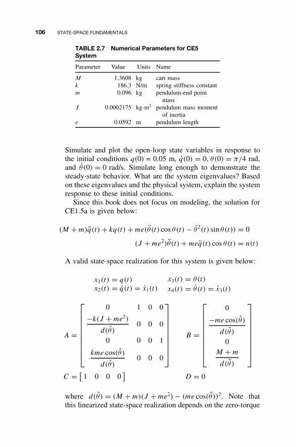
106 STATE-SPACE FUNDAMENTALS
TABLE 2.7 Numerical Parameters for CE5System
Parameter Value Units Name
M 1.3608 kg cart massk 186.3 N/m spring stiffness constantm 0.096 kg pendulum-end point
massJ 0.0002175 kg-m2 pendulum mass moment
of inertiae 0.0592 m pendulum length
Simulate and plot the open-loop state variables in response tothe initial conditions q(0) = 0.05 m, q(0) = 0, θ(0) = π/4 rad,and θ (0) = 0 rad/s. Simulate long enough to demonstrate thesteady-state behavior. What are the system eigenvalues? Basedon these eigenvalues and the physical system, explain the systemresponse to these initial conditions.
Since this book does not focus on modeling, the solution forCE1.5a is given below:
(M + m)q(t) + kq(t) + me(θ(t) cos θ(t) − θ2(t) sin θ(t)) = 0
(J + me2)θ(t) + meq(t) cos θ(t) = n(t)
A valid state-space realization for this system is given below:
x1(t) = q(t)
x2(t) = q(t) = x1(t)
x3(t) = θ(t)
x4(t) = θ (t) = x3(t)
A =
0 1 0 0
−k(J + me2)
d(θ )0 0 0
0 0 0 1
kme cos(θ)
d(θ )0 0 0
B =
0
−me cos(θ )
d(θ )
0M + m
d(θ )
C = [1 0 0 0
]D = 0
where d(θ) = (M + m)(J + me2) − (me cos(θ ))2. Note thatthis linearized state-space realization depends on the zero-torque
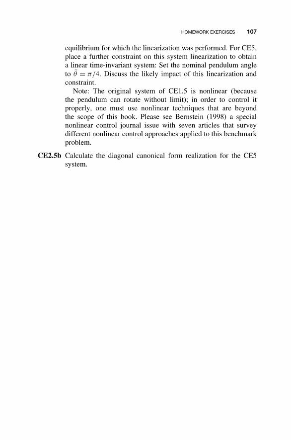
HOMEWORK EXERCISES 107
equilibrium for which the linearization was performed. For CE5,place a further constraint on this system linearization to obtaina linear time-invariant system: Set the nominal pendulum angleto θ = π/4. Discuss the likely impact of this linearization andconstraint.
Note: The original system of CE1.5 is nonlinear (becausethe pendulum can rotate without limit); in order to control itproperly, one must use nonlinear techniques that are beyondthe scope of this book. Please see Bernstein (1998) a specialnonlinear control journal issue with seven articles that surveydifferent nonlinear control approaches applied to this benchmarkproblem.
CE2.5b Calculate the diagonal canonical form realization for the CE5system.
3
CONTROLLABILITY
In this chapter we explore the input-to-state interaction of the n-dimen-sional linear time-invariant state equation, seeking to characterize theextent to which state trajectories can be controlled by the input signal.Specifically, we derive conditions under which, starting anywhere in thestate space, the state trajectory can be driven to the origin by piecewisecontinuous input signals over a finite time interval. More generally, itturns out that if it is possible to do this, then it is also possible to steer thestate trajectory to any final state in finite time via a suitable input signal.
While the controllability analysis presented in this chapter has a decid-edly open-loop flavor involving input signals that have a prescribed effecton the state trajectory without any mention of feedback, there is also animportant connection between controllability and the design of feedback-control laws that will be pursued in Chapter 7.
This chapter initiates a strategy that will recur throughout the remainderof this book. Specifically, our aim is to characterize important propertiesof dynamic systems described by our state-space model via analysis of thestate-equation data, namely the coefficient matrices A, B, C, and D. Fun-damental questions pertaining to the complex interaction of input, state,and output can be answered using the tools of linear algebra. Much of whatwe present in what follows either originated with or was inspired by thepioneering work of R. E. Kalman, unquestionably the father of state-space
108
Linear State-Space Control Systems. Robert L. Williams II and Douglas A. LawrenceCopyright 2007 John Wiley & Sons, Inc. ISBN: 978-0-471-73555-7
FUNDAMENTAL RESULTS 109
methods in linear systems and control theory. In our investigation ofcontrollability, we identify connections between input-to-state behavior,as characterized by the state-equation solution derived in Chapter 2, andlinear algebraic properties of the state equation’s coefficient matrices.
Once the basic notion of controllability is defined, analyzed, and illus-trated with several examples, we study the relationship between controlla-bility and state coordinate transformations and present additional algebraiccharacterizations of controllability that are of utility not only in the anal-ysis of particular systems but also in establishing further general results.We also illustrate the use of MATLAB for controllability analysis and onceagain return to the MATLAB Continuing Example along with ContinuingExamples 1 and 2.
3.1 FUNDAMENTAL RESULTS
We consider the linear time-invariant state differential equation
x(t) = Ax(t) + Bu(t) x(t0) = x0 (3.1)
in which the algebraic output equation has been omitted because it willplay no role in the ensuing analysis. Our point of departure is the followingdefinition.
Definition 3.1 A state x ∈ Rn is controllable to the origin if for a given
initial time t0 there exists a finite final time tf > t0 and a piecewise con-tinuous input signal u(·) defined on [t0, tf ] such that with initial statex(t0) = x, the final state satisfies
x(tf ) = eA(tf −t0)x +∫ tf
t0
eA(tf −τ )Bu(τ)dτ
= 0 ∈ Rn
The state equation (3.1) is controllable if every state x ∈ Rn is controllable
to the origin.Based on this definition alone, determining whether or not a particularstate equation is controllable appears to be a daunting task because it isnot immediately clear how to characterize input signals that have the pre-scribed effect on the state trajectory. Our immediate goal is to overcomethis difficulty by translating this controllability property of state equationsinto an equivalent linear algebraic property of the state equation’s coeffi-cient matrices A and B.
110 CONTROLLABILITY
Theorem 3.2 The linear state equation (3.1) is controllable if andonly if
rank[ B AB A2B · · · An−1B ] = n
We refer to this matrix as the controllability matrix and often denote itby P to save considerable writing. We note that this controllability matrixis constructed directly from the state equation’s coefficient matrices A andB. The theorem asserts that controllability of the state equation (3.1) isequivalent to P having full-row rank, thereby yielding a linear algebraictest for controllability. This equivalence affords us a measure of pithinessbecause we will henceforth take controllability of a matrix pair (A, B) tomean controllability of the linear state equation with coefficient matricesA and B.
For the general multiple-input case, we see that P consists of n matrixblocks B, AB, A2B, . . . , An−1B, each with dimension n × m, stacked sideby side. Thus P has dimension n × (n m) and therefore has more columnsthan rows in the multiple-input case. Furthermore, the rank condition inthe theorem requires that the n rows of P are linearly independent whenviewed as row vectors of dimension 1 × (nm). Consequently, P satisfyingthe preceding rank condition is frequently referred to as having full-rowrank. An alternative interpretation of the rank condition is that of the n m
columns of P written out as
P = [ b1 b2 · · · bm | Ab1 Ab2 · · · Abm |· · · |An−1b1 An−1b2 · · · An−1bm ]
there must be at least one way to select n linearly independent columns.For the single-input case, B consists of a single column, as do AB, A2B,
. . . , An−1B, yielding a square n × n controllability matrix P . Therefore,a single-input linear state equation is controllable if and only if theassociated controllability matrix is nonsingular. We can check that P isnonsingular by verifying that P has a nonzero determinant.
In order to prove Theorem 3.2, we introduce the so-called controllabil-ity Gramian, defined as follows for any initial time t0 and any finite finaltime tf > t0:
W(t0, tf ) =∫ tf
t0
eA(t0−τ )BBTeAT(t0−τ )dτ
The controllability Gramian is a square n × n matrix. Also, it isstraightforward to check that it is a symmetric matrix, that is, W(t0, tf ) =WT (t0, tf ). Finally, it is a positive semidefinite matrix because the
FUNDAMENTAL RESULTS 111
associated real-valued quadratic form xT W(t0, tf )x satisfies the followingfor all vectors x ∈ R
n
xT W(t0, tf )x = xT
∫ tf
t0
eA(t0−τ )BBTeAT(t0−τ )dτ x
=∫ tf
t0
∣∣∣∣BT eAT (t0−τ )x∣∣∣∣2
dτ
≥ 0
The asserted inequality follows from the fact that integrating a nonnegativeintegral forward in time from t0 to tf must produce a nonnegative result.
�Lemma 3.3
rank[ B AB A2B · · · An−1B ] = n
if and only if for any initial time t0 and any finite final time tf > t0, thecontrollability Gramian W(t0, tf ) is nonsingular.
Proof. The lemma involves two implications:If rank P = n, then W(t0, tf ) is nonsingular for any t0 and any finite
tf > t0.If W(t0, tf ) is nonsingular for any t0 and any finite tf > t0, then rank
P = n.We begin with a proof of the contrapositive of the first implication:
If W(t0, tf ) is singular for some t0 and finite tf > t0, then rank P < n.Assuming that W(t0, tf ) is singular for some t0 and tf > t0, there
exists a nonzero vector x ∈ Rn for which W(t0, tf )x = 0 ∈ R
n and there-fore xT W(t0, tf )x = 0 ∈ R. Using the controllability Gramian definition,we have
0 = xT
∫ tf
t0
eA(t0−τ )BBTeAT(t0−τ )dτ x
=∫ tf
t0
∣∣∣∣BT eAT (t0−τ )x∣∣∣∣2
dτ
The integrand in this expression involves the Euclidean norm of them × 1 vector quantity BT eAT (t0−τ )x which we view as an analytic func-tion of the integration variable τ ∈ [t0, tf ]. Since this integrand can neverbe negative, the only way the integral over a positive time interval canevaluate to zero is if the integrand is identically zero for all τ ∈ [t0, tf ].
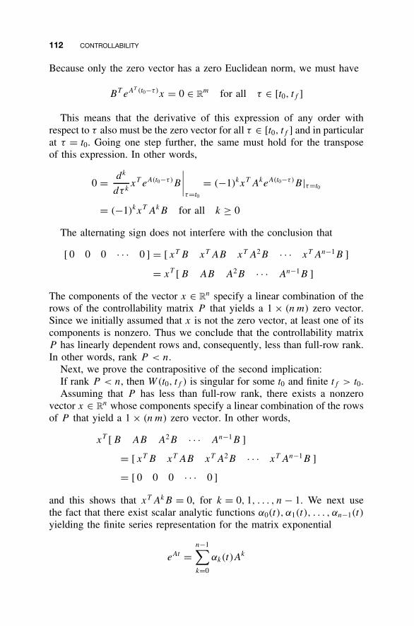
112 CONTROLLABILITY
Because only the zero vector has a zero Euclidean norm, we must have
BT eAT (t0−τ )x = 0 ∈ Rm for all τ ∈ [t0, tf ]
This means that the derivative of this expression of any order withrespect to τ also must be the zero vector for all τ ∈ [t0, tf ] and in particularat τ = t0. Going one step further, the same must hold for the transposeof this expression. In other words,
0 = dk
dτ kxT eA(t0−τ )B
∣∣∣∣τ=t0
= (−1)kxT AkeA(t0−τ )B|τ=t0
= (−1)kxT AkB for all k ≥ 0
The alternating sign does not interfere with the conclusion that
[ 0 0 0 · · · 0 ] = [ xT B xT AB xT A2B · · · xT An−1B ]
= xT [ B AB A2B · · · An−1B ]
The components of the vector x ∈ Rn specify a linear combination of the
rows of the controllability matrix P that yields a 1 × (nm) zero vector.Since we initially assumed that x is not the zero vector, at least one of itscomponents is nonzero. Thus we conclude that the controllability matrixP has linearly dependent rows and, consequently, less than full-row rank.In other words, rank P < n.
Next, we prove the contrapositive of the second implication:If rank P < n, then W(t0, tf ) is singular for some t0 and finite tf > t0.Assuming that P has less than full-row rank, there exists a nonzero
vector x ∈ Rn whose components specify a linear combination of the rows
of P that yield a 1 × (n m) zero vector. In other words,
xT [ B AB A2B · · · An−1B ]
= [ xT B xT AB xT A2B · · · xT An−1B ]
= [ 0 0 0 · · · 0 ]
and this shows that xT AkB = 0, for k = 0, 1, . . . , n − 1. We next usethe fact that there exist scalar analytic functions α0(t), α1(t), . . . , αn−1(t)
yielding the finite series representation for the matrix exponential
eAt =n−1∑k=0
αk(t)Ak
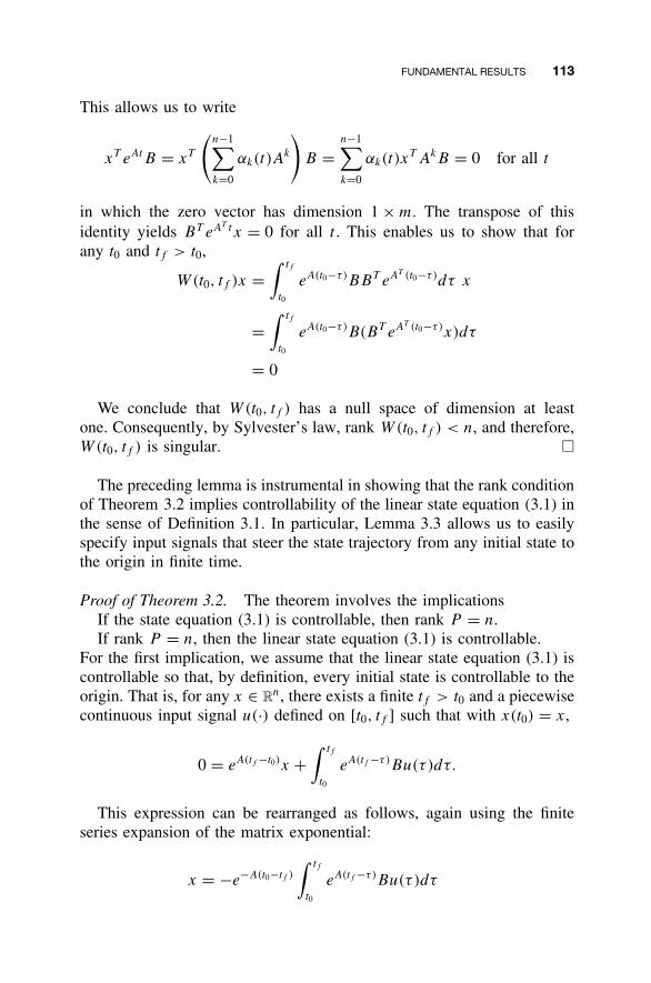
FUNDAMENTAL RESULTS 113
This allows us to write
xT eAtB = xT
(n−1∑k=0
αk(t)Ak
)B =
n−1∑k=0
αk(t)xT AkB = 0 for all t
in which the zero vector has dimension 1 × m. The transpose of thisidentity yields BT eAT tx = 0 for all t . This enables us to show that forany t0 and tf > t0,
W(t0, tf )x =∫ tf
t0
eA(t0−τ )BBT eAT (t0−τ )dτ x
=∫ tf
t0
eA(t0−τ )B(BT eAT (t0−τ )x)dτ
= 0
We conclude that W(t0, tf ) has a null space of dimension at leastone. Consequently, by Sylvester’s law, rank W(t0, tf ) < n, and therefore,W(t0, tf ) is singular. �
The preceding lemma is instrumental in showing that the rank conditionof Theorem 3.2 implies controllability of the linear state equation (3.1) inthe sense of Definition 3.1. In particular, Lemma 3.3 allows us to easilyspecify input signals that steer the state trajectory from any initial state tothe origin in finite time.
Proof of Theorem 3.2. The theorem involves the implicationsIf the state equation (3.1) is controllable, then rank P = n.If rank P = n, then the linear state equation (3.1) is controllable.
For the first implication, we assume that the linear state equation (3.1) iscontrollable so that, by definition, every initial state is controllable to theorigin. That is, for any x ∈ R
n, there exists a finite tf > t0 and a piecewisecontinuous input signal u(·) defined on [t0, tf ] such that with x(t0) = x,
0 = eA(tf −t0)x +∫ tf
t0
eA(tf −τ )Bu(τ)dτ.
This expression can be rearranged as follows, again using the finiteseries expansion of the matrix exponential:
x = −e−A(t0−tf )
∫ tf
t0
eA(tf −τ )Bu(τ)dτ
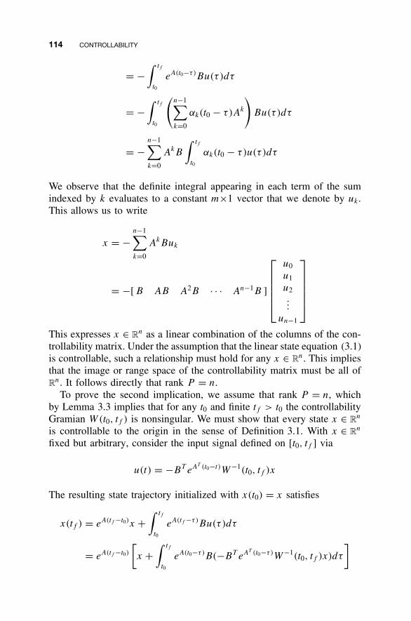
114 CONTROLLABILITY
= −∫ tf
t0
eA(t0−τ )Bu(τ)dτ
= −∫ tf
t0
(n−1∑k=0
αk(t0 − τ)Ak
)Bu(τ)dτ
= −n−1∑k=0
AkB
∫ tf
t0
αk(t0 − τ)u(τ)dτ
We observe that the definite integral appearing in each term of the sumindexed by k evaluates to a constant m×1 vector that we denote by uk.This allows us to write
x = −n−1∑k=0
AkBuk
= −[ B AB A2B · · · An−1B ]
u0
u1
u2...
un−1
This expresses x ∈ Rn as a linear combination of the columns of the con-
trollability matrix. Under the assumption that the linear state equation (3.1)is controllable, such a relationship must hold for any x ∈ R
n. This impliesthat the image or range space of the controllability matrix must be all ofR
n. It follows directly that rank P = n.To prove the second implication, we assume that rank P = n, which
by Lemma 3.3 implies that for any t0 and finite tf > t0 the controllabilityGramian W(t0, tf ) is nonsingular. We must show that every state x ∈ R
n
is controllable to the origin in the sense of Definition 3.1. With x ∈ Rn
fixed but arbitrary, consider the input signal defined on [t0, tf ] via
u(t) = −BT eAT (t0−t)W−1(t0, tf )x
The resulting state trajectory initialized with x(t0) = x satisfies
x(tf ) = eA(tf −t0)x +∫ tf
t0
eA(tf −τ )Bu(τ)dτ
= eA(tf −t0)
[x +
∫ tf
t0
eA(t0−τ )B(−BT eAT (t0−τ )W−1(t0, tf )x)dτ
]
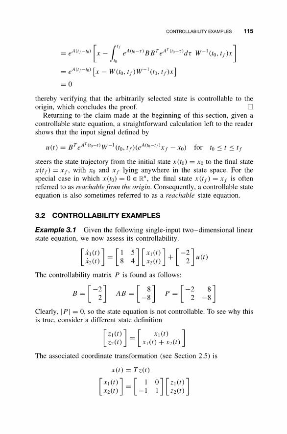
CONTROLLABILITY EXAMPLES 115
= eA(tf −t0)
[x −
∫ tf
t0
eA(t0−τ )BBT eAT (t0−τ )dτ W−1(t0, tf )x
]
= eA(tf −t0)[x − W(t0, tf )W−1(t0, tf )x
]= 0
thereby verifying that the arbitrarily selected state is controllable to theorigin, which concludes the proof. �
Returning to the claim made at the beginning of this section, given acontrollable state equation, a straightforward calculation left to the readershows that the input signal defined by
u(t) = BT eAT (t0−t)W−1(t0, tf )(eA(t0−tf )xf − x0) for t0 ≤ t ≤ tf
steers the state trajectory from the initial state x(t0) = x0 to the final statex(tf ) = xf , with x0 and xf lying anywhere in the state space. For thespecial case in which x(t0) = 0 ∈ R
n, the final state x(tf ) = xf is oftenreferred to as reachable from the origin. Consequently, a controllable stateequation is also sometimes referred to as a reachable state equation.
3.2 CONTROLLABILITY EXAMPLES
Example 3.1 Given the following single-input two–dimensional linearstate equation, we now assess its controllability.[
x1(t)
x2(t)
]=
[1 58 4
][x1(t)
x2(t)
]+
[ −22
]u(t)
The controllability matrix P is found as follows:
B =[ −2
2
]AB =
[8
−8
]P =
[ −2 82 −8
]
Clearly, |P | = 0, so the state equation is not controllable. To see why thisis true, consider a different state definition[
z1(t)
z2(t)
]=
[x1(t)
x1(t) + x2(t)
]
The associated coordinate transformation (see Section 2.5) is
x(t) = T z(t)[x1(t)
x2(t)
]=
[1 0
−1 1
] [z1(t)
z2(t)
]
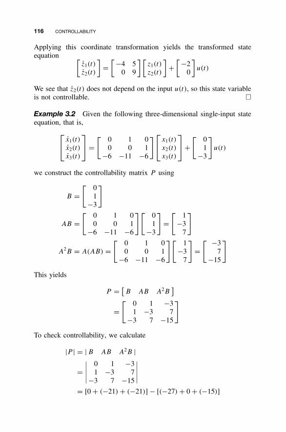
116 CONTROLLABILITY
Applying this coordinate transformation yields the transformed stateequation [
z1(t)
z2(t)
]=
[ −4 50 9
] [z1(t)
z2(t)
]+
[ −20
]u(t)
We see that z2(t) does not depend on the input u(t), so this state variableis not controllable. �
Example 3.2 Given the following three-dimensional single-input stateequation, that is,
x1(t)
x2(t)
x3(t)
=
[ 0 1 00 0 1
−6 −11 −6
] x1(t)
x2(t)
x3(t)
+
[ 01
−3
]u(t)
we construct the controllability matrix P using
B =[ 0
1−3
]
AB =[ 0 1 0
0 0 1−6 −11 −6
][ 01
−3
]=
[ 1−3
7
]
A2B = A(AB) =[ 0 1 0
0 0 1−6 −11 −6
][ 1−3
7
]=
[ −37
−15
]
This yields
P = [B AB A2B
]
=[ 0 1 −3
1 −3 7−3 7 −15
]
To check controllability, we calculate
|P | = | B AB A2B |
=∣∣∣∣∣
0 1 −31 −3 7
−3 7 −15
∣∣∣∣∣= [0 + (−21) + (−21)] − [(−27) + 0 + (−15)]
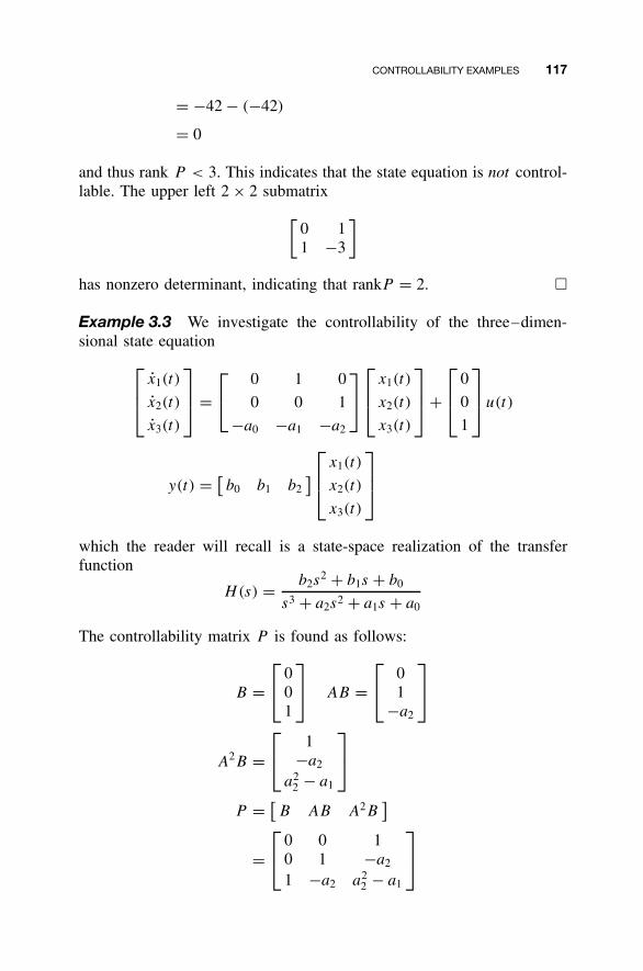
CONTROLLABILITY EXAMPLES 117
= −42 − (−42)
= 0
and thus rank P < 3. This indicates that the state equation is not control-lable. The upper left 2 × 2 submatrix
[0 11 −3
]
has nonzero determinant, indicating that rankP = 2. �
Example 3.3 We investigate the controllability of the three–dimen-sional state equation
x1(t)
x2(t)
x3(t)
=
0 1 0
0 0 1
−a0 −a1 −a2
x1(t)
x2(t)
x3(t)
+
0
0
1
u(t)
y(t) = [b0 b1 b2
]
x1(t)
x2(t)
x3(t)
which the reader will recall is a state-space realization of the transferfunction
H(s) = b2s2 + b1s + b0
s3 + a2s2 + a1s + a0
The controllability matrix P is found as follows:
B = 0
01
AB =
0
1−a2
A2B = 1
−a2
a22 − a1
P = [B AB A2B
]
= 0 0 1
0 1 −a2
1 −a2 a22 − a1
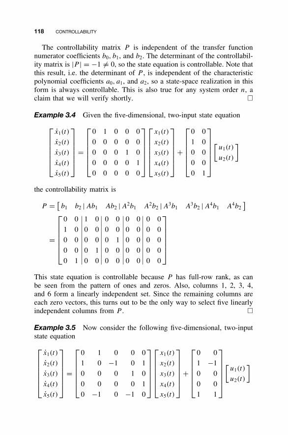
118 CONTROLLABILITY
The controllability matrix P is independent of the transfer functionnumerator coefficients b0, b1, and b2. The determinant of the controllabil-ity matrix is |P | = −1 �= 0, so the state equation is controllable. Note thatthis result, i.e. the determinant of P , is independent of the characteristicpolynomial coefficients a0, a1, and a2, so a state-space realization in thisform is always controllable. This is also true for any system order n, aclaim that we will verify shortly. �
Example 3.4 Given the five-dimensional, two-input state equation
x1(t)
x2(t)
x3(t)
x4(t)
x5(t)
=
0 1 0 0 0
0 0 0 0 0
0 0 0 1 0
0 0 0 0 1
0 0 0 0 0
x1(t)
x2(t)
x3(t)
x4(t)
x5(t)
+
0 0
1 0
0 0
0 0
0 1
[u1(t)
u2(t)
]
the controllability matrix is
P = [b1 b2 | Ab1 Ab2 | A2b1 A2b2 | A3b1 A3b2 |A4b1 A4b2
]
=
0 0
1 0
0 0
0 0
0 1
∣∣∣∣∣∣∣∣∣∣∣
1 0
0 0
0 0
0 1
0 0
∣∣∣∣∣∣∣∣∣∣∣
0 0
0 0
0 1
0 0
0 0
∣∣∣∣∣∣∣∣∣∣∣
0 0
0 0
0 0
0 0
0 0
∣∣∣∣∣∣∣∣∣∣∣
0 0
0 0
0 0
0 0
0 0
This state equation is controllable because P has full-row rank, as canbe seen from the pattern of ones and zeros. Also, columns 1, 2, 3, 4,and 6 form a linearly independent set. Since the remaining columns areeach zero vectors, this turns out to be the only way to select five linearlyindependent columns from P . �
Example 3.5 Now consider the following five-dimensional, two-inputstate equation
x1(t)
x2(t)
x3(t)
x4(t)
x5(t)
=
0 1 0 0 0
1 0 −1 0 1
0 0 0 1 0
0 0 0 0 1
0 −1 0 −1 0
x1(t)
x2(t)
x3(t)
x4(t)
x5(t)
+
0 0
1 −1
0 0
0 0
1 1
[u1(t)
u2(t)
]
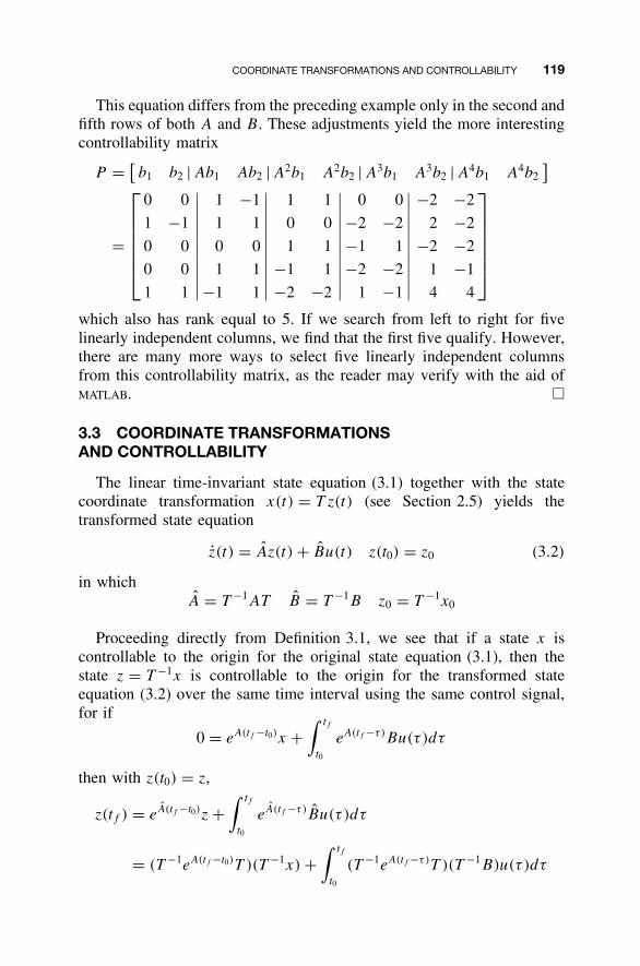
COORDINATE TRANSFORMATIONS AND CONTROLLABILITY 119
This equation differs from the preceding example only in the second andfifth rows of both A and B. These adjustments yield the more interestingcontrollability matrix
P = [b1 b2 | Ab1 Ab2 | A2b1 A2b2 | A3b1 A3b2 |A4b1 A4b2
]
=
0 0
1 −1
0 0
0 0
1 1
∣∣∣∣∣∣∣∣∣∣∣
1 −1
1 1
0 0
1 1
−1 1
∣∣∣∣∣∣∣∣∣∣∣
1 1
0 0
1 1
−1 1
−2 −2
∣∣∣∣∣∣∣∣∣∣∣
0 0
−2 −2
−1 1
−2 −2
1 −1
∣∣∣∣∣∣∣∣∣∣∣
−2 −2
2 −2
−2 −2
1 −1
4 4
which also has rank equal to 5. If we search from left to right for fivelinearly independent columns, we find that the first five qualify. However,there are many more ways to select five linearly independent columnsfrom this controllability matrix, as the reader may verify with the aid ofMATLAB. �
3.3 COORDINATE TRANSFORMATIONSAND CONTROLLABILITY
The linear time-invariant state equation (3.1) together with the statecoordinate transformation x(t) = T z(t) (see Section 2.5) yields thetransformed state equation
z(t) = Az(t) + Bu(t) z(t0) = z0 (3.2)
in whichA = T −1AT B = T −1B z0 = T −1x0
Proceeding directly from Definition 3.1, we see that if a state x iscontrollable to the origin for the original state equation (3.1), then thestate z = T −1x is controllable to the origin for the transformed stateequation (3.2) over the same time interval using the same control signal,for if
0 = eA(tf −t0)x +∫ tf
t0
eA(tf −τ )Bu(τ)dτ
then with z(t0) = z,
z(tf ) = eA(tf −t0)z +∫ tf
t0
eA(tf −τ )Bu(τ)dτ
= (T −1eA(tf −t0)T )(T −1x) +∫ tf
t0
(T −1eA(tf −τ )T )(T −1B)u(τ)dτ
120 CONTROLLABILITY
= T −1
[eA(tf −t0)x +
∫ tf
t0
eA(tf −τ )Bu(τ)dτ
]
= 0
Conversely, if a state z is controllable to the origin for the stateequation (3.2), then the state x = T z is controllable to the origin for thestate equation (3.1). We immediately conclude that the transformed stateequation (3.2) is controllable if and only if the original state equation (3.1)is controllable. In short, we say that controllability is invariant with respectto state coordinate transformations.
Any equivalent characterization of controllability must reflect this out-come. For instance, we expect that the rank test for controllability providedby Theorem 3.2 should yield consistent results across all state equationsrelated by a coordinate transformation. To see this, we relate the control-lability matrix for the state equation (3.2) to the controllability matrix forthe state equation (3.1). Using the fact that Ak = T −1AkT for any positiveinteger k, we have
P = [B AB · · · An−1B
]= [
T −1B|(T −1AT )(T −1B)| · · · |(T −1An−1T )(T −1B)]
= [T −1B |T −1AB| · · · |T −1An−1B
]= T −1
[B AB · · · An−1B
]= T −1P
Since either pre- or post-multiplication by a square nonsingular matrixdoes not affect matrix rank, we see that
rank P = rank P
In addition, the n × n controllability Gramians for Equations (3.2) and(3.1) are related according to
W (t0, tf ) =∫ tf
t0
eA(t0−τ )BBTeAT(t0−τ )dτ
=∫ tf
t0
(T −1eA(t0−τ )T )(T −1B)(T −1B)T(T −1eA(t0−τ )T )Tdτ
= T −1∫ tf
t0
eA(t0−τ )BBTeA(t0−τ )dτT −T
= T −1W(t0, tf )T −T
COORDINATE TRANSFORMATIONS AND CONTROLLABILITY 121
where T −T is shorthand notation for (T −1)T = (T T)−1. We conclude thatW (t0, tf ) is nonsingular for some initial time t0 and finite final time tf > t0if and only if W(t0, tf ) is nonsingular for the same t0 and tf .
Various system properties are often revealed by a judiciously chosenstate-space realization. Here we examine the role that the diagonal canon-ical form plays in controllability analysis. To do so, we assume thatthe state equation (3.1) has a single input and a diagonalizable systemdynamics matrix A. As discussed in Chapter 2, this ensures that the stateequation (3.1) can be transformed into diagonal canonical form. Using theidentity:
AkDCFBDCF =
λk1 0 · · · 0
0 λk2 · · · 0
......
. . ....
0 0 · · · λkn
b1
b2
...
bn
=
λk1b1
λk2b2
...
λknbn
for any integer k ≥ 0, we see that the controllability matrix for the diag-onal canonical form is given by
PDCF =
b1 λ1b1 λ21b1 · · · λn−1
1 b1
b2 λ2b2 λ22b2 · · · λn−1
2 b2
......
.... . .
...
bn λnbn λ2nbn · · · λn−1
n bn
=
b1 0 · · · 0
0 b2 · · · 0...
.... . .
...
0 0 · · · bn
1 λ1 λ21 · · · λn−1
1
1 λ2 λ22 · · · λn−1
2
......
.... . .
...
1 λn λ2n · · · λn−1
n
which is nonsingular if and only if each factor on the right-hand is nonsin-gular. The diagonal left factor is nonsingular if and only if every elementof BDCF is nonzero. The right factor is the Vandermonde matrix encoun-tered in Chapter 2, which is nonsingular if and only if the eigenvaluesλ1, λ2, . . . , λn are distinct. Since controllability is invariant with respectto state coordinate transformations, we conclude that controllability of asingle-input state equation can be assessed by inspection of its diagonalcanonical form (when it exists). Specifically, a necessary and sufficientcondition for controllability is that the eigenvalues of A displayed on the
122 CONTROLLABILITY
diagonal of ADCF must be distinct and every element of BDCF must benonzero.
The condition on BDCF is relatively easy to interpret; because of thedecoupled nature of the diagonal canonical form, if any component ofBDCF is zero, the corresponding state variable is disconnected from theinput signal, and therefore cannot be steered between prescribed initialand final values. The eigenvalue condition is a bit more subtle. Supposethat A has a repeated eigenvalue, say, λi = λj = λ. Given zero initialconditions on the corresponding state variables xi(t) and xj (t), and anyinput signal u(t), we have
bjxi(t) = bj
[∫ t
0eλ(t−τ )biu(τ)dτ
]=
∫ t
0eλ(t−τ )(bjbi)u(τ)dτ
= bi
[∫ t
0eλ(t−τ )bju(τ)dτ
]= bixj (t)
for all t ≥ 0. That these state variable responses are constrained to satisfythis relationship regardless of the input signal indicates that not everystate can be reached from the origin in finite time. Hence when A has arepeated eigenvalue, the state equation in diagonal canonical form is notcontrollable, implying the same for the original state equation.
This section concludes with three results that, in different ways, relatecoordinate transformations and controllability. The first two apply onlyto the single-input, single-output case. The third holds in the generalmultiple-input, multiple-output case.
Controllable Realizations of the Same Transfer Function
Consider two single-input, single-output state equations
x1(t) = A1x1(t) + B1u(t) x2(t) = A2x2(t) + B2u(t)
y(t) = C1x1(t) + D1u(t) y(t) = C2x2(t) + D2u(t) (3.3)
that are both n-dimensional realizations of the same transfer function. Weshow that when both realizations are controllable, they are related by auniquely and explicitly defined coordinate transformation.
Lemma 3.4 Two controllable n-dimensional single-input, single-outputrealizations (3.3) of the same transfer function are related by the unique
COORDINATE TRANSFORMATIONS AND CONTROLLABILITY 123
state coordinate transformation x1(t) = T x2(t), where
T = [B1 A1B1 · · · An−1
1 B1
] [B2 A2B2 · · · An−1
2 B2
]−1
= P1P−12
Proof. We must verify the identities
A2 = T −1A1T B2 = T −1B1 C2 = C1T
The first identity can be recast as
[B2 A2B2 · · · An−1
2 B2
]−1A2
[B2 A2B2 · · · An−1
2 B2
]= [
B1 A1B1 · · · An−11 B1
]−1A1
[B1 A1B1 · · · An−1
1 B1
](3.4)
Now, for any matrix pair (A, B) describing a controllable state equationwith |sI − A| = sn + an−1s
n−1 + · · · + a1s + a0, the Cayley-Hamiltontheorem gives
[B AB · · · An−1B
]−1A
[B AB · · · An−1B
]
= [B AB · · · An−1B
]−1 [AB A2B · · · AnB
]
= [B AB · · · An−1B
]−1
× [AB A2B · · · (−a0B − a1AB − · · · − an−1A
n−1B)]
=
0 0 · · · 0 0 −a0
1 0 · · · 0 0 −a1
0 1 · · · 0 0 −a2
......
. . ....
......
0 0 · · · 1 0 −an−2
0 0 · · · 0 1 −an−1
Since the state equations (3.3) are each n-dimensional realizations of thesame transfer function H(s) = b(s)/a(s) with deg a(s) = n, we nec-essarily have |sI − A1| = |sI − A2|. Thus both matrix pairs (A1, B1)
and (A2, B2) satisfy an identity analogous to the preceding one, withan identical outcome in each case. Hence Equation (3.4) holds, yieldingA2 = T −1A1T .
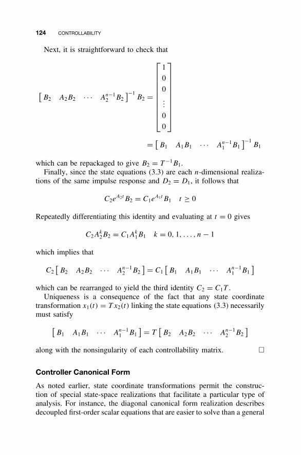
124 CONTROLLABILITY
Next, it is straightforward to check that
[B2 A2B2 · · · An−1
2 B2
]−1B2 =
1
0
0...
0
0
= [B1 A1B1 · · · An−1
1 B1
]−1B1
which can be repackaged to give B2 = T −1B1.Finally, since the state equations (3.3) are each n-dimensional realiza-
tions of the same impulse response and D2 = D1, it follows that
C2eA2tB2 = C1e
A1tB1 t ≥ 0
Repeatedly differentiating this identity and evaluating at t = 0 gives
C2Ak2B2 = C1A
k1B1 k = 0, 1, . . . , n − 1
which implies that
C2[B2 A2B2 · · · An−1
2 B2
] = C1[B1 A1B1 · · · An−1
1 B1
]
which can be rearranged to yield the third identity C2 = C1T .Uniqueness is a consequence of the fact that any state coordinate
transformation x1(t) = T x2(t) linking the state equations (3.3) necessarilymust satisfy
[B1 A1B1 · · · An−1
1 B1
] = T[B2 A2B2 · · · An−1
2 B2
]
along with the nonsingularity of each controllability matrix. �
Controller Canonical Form
As noted earlier, state coordinate transformations permit the construc-tion of special state-space realizations that facilitate a particular type ofanalysis. For instance, the diagonal canonical form realization describesdecoupled first-order scalar equations that are easier to solve than a general
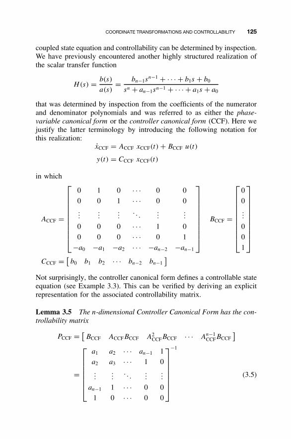
COORDINATE TRANSFORMATIONS AND CONTROLLABILITY 125
coupled state equation and controllability can be determined by inspection.We have previously encountered another highly structured realization ofthe scalar transfer function
H(s) = b(s)
a(s)= bn−1s
n−1 + · · · + b1s + b0
sn + an−1sn−1 + · · · + a1s + a0
that was determined by inspection from the coefficients of the numeratorand denominator polynomials and was referred to as either the phase-variable canonical form or the controller canonical form (CCF). Here wejustify the latter terminology by introducing the following notation forthis realization:
xCCF = ACCF xCCF(t) + BCCF u(t)
y(t) = CCCF xCCF(t)
in which
ACCF =
0 1 0 · · · 0 0
0 0 1 · · · 0 0...
......
. . ....
...
0 0 0 · · · 1 0
0 0 0 · · · 0 1
−a0 −a1 −a2 · · · −an−2 −an−1
BCCF =
0
0...
0
0
1
CCCF = [b0 b1 b2 · · · bn−2 bn−1
]Not surprisingly, the controller canonical form defines a controllable stateequation (see Example 3.3). This can be verified by deriving an explicitrepresentation for the associated controllability matrix.
Lemma 3.5 The n-dimensional Controller Canonical Form has the con-trollability matrix
PCCF = [BCCF ACCFBCCF A2
CCFBCCF · · · An−1CCFBCCF
]
=
a1 a2 · · · an−1 1
a2 a3 · · · 1 0...
.... . .
......
an−1 1 · · · 0 0
1 0 · · · 0 0
−1
(3.5)
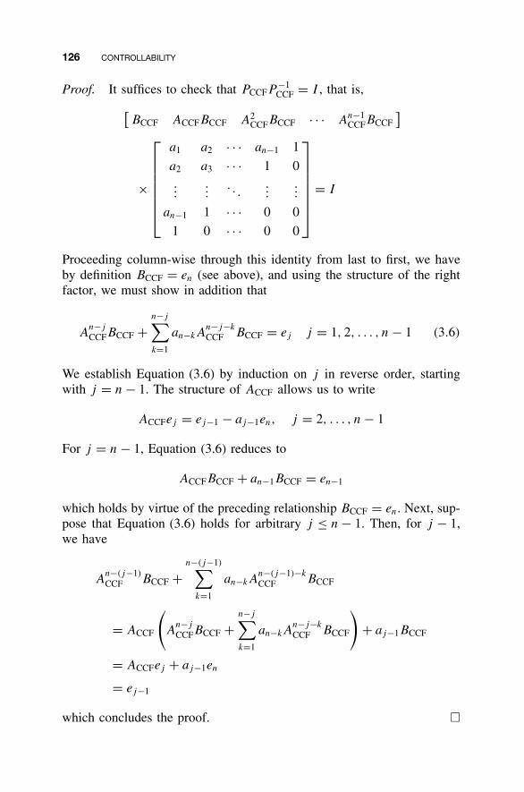
126 CONTROLLABILITY
Proof. It suffices to check that PCCFP−1CCF = I , that is,
[BCCF ACCFBCCF A2
CCFBCCF · · · An−1CCFBCCF
]
×
a1 a2 · · · an−1 1
a2 a3 · · · 1 0...
.... . .
......
an−1 1 · · · 0 0
1 0 · · · 0 0
= I
Proceeding column-wise through this identity from last to first, we haveby definition BCCF = en (see above), and using the structure of the rightfactor, we must show in addition that
An−j
CCFBCCF +n−j∑k=1
an−kAn−j−k
CCF BCCF = ej j = 1, 2, . . . , n − 1 (3.6)
We establish Equation (3.6) by induction on j in reverse order, startingwith j = n − 1. The structure of ACCF allows us to write
ACCFej = ej−1 − aj−1en, j = 2, . . . , n − 1
For j = n − 1, Equation (3.6) reduces to
ACCFBCCF + an−1BCCF = en−1
which holds by virtue of the preceding relationship BCCF = en. Next, sup-pose that Equation (3.6) holds for arbitrary j ≤ n − 1. Then, for j − 1,we have
An−(j−1)
CCF BCCF +n−(j−1)∑
k=1
an−kAn−(j−1)−k
CCF BCCF
= ACCF
(A
n−j
CCFBCCF +n−j∑k=1
an−kAn−j−k
CCF BCCF
)+ aj−1BCCF
= ACCFej + aj−1en
= ej−1
which concludes the proof. �
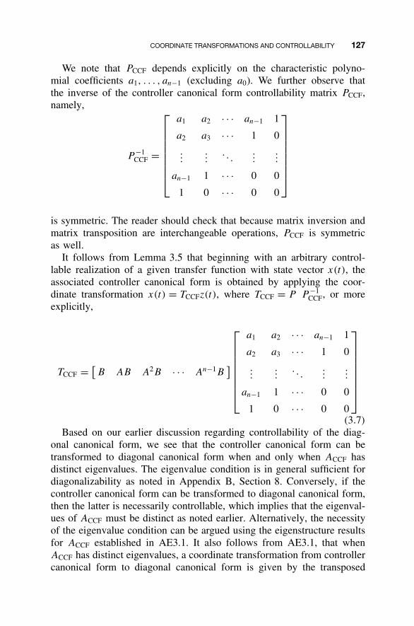
COORDINATE TRANSFORMATIONS AND CONTROLLABILITY 127
We note that PCCF depends explicitly on the characteristic polyno-mial coefficients a1, . . . , an−1 (excluding a0). We further observe thatthe inverse of the controller canonical form controllability matrix PCCF,namely,
P −1CCF =
a1 a2 · · · an−1 1
a2 a3 · · · 1 0
......
. . ....
...
an−1 1 · · · 0 0
1 0 · · · 0 0
is symmetric. The reader should check that because matrix inversion andmatrix transposition are interchangeable operations, PCCF is symmetricas well.
It follows from Lemma 3.5 that beginning with an arbitrary control-lable realization of a given transfer function with state vector x(t), theassociated controller canonical form is obtained by applying the coor-dinate transformation x(t) = TCCFz(t), where TCCF = P P −1
CCF, or moreexplicitly,
TCCF = [B AB A2B · · · An−1B
]
a1 a2 · · · an−1 1
a2 a3 · · · 1 0
......
. . ....
...
an−1 1 · · · 0 0
1 0 · · · 0 0
(3.7)
Based on our earlier discussion regarding controllability of the diag-onal canonical form, we see that the controller canonical form can betransformed to diagonal canonical form when and only when ACCF hasdistinct eigenvalues. The eigenvalue condition is in general sufficient fordiagonalizability as noted in Appendix B, Section 8. Conversely, if thecontroller canonical form can be transformed to diagonal canonical form,then the latter is necessarily controllable, which implies that the eigenval-ues of ACCF must be distinct as noted earlier. Alternatively, the necessityof the eigenvalue condition can be argued using the eigenstructure resultsfor ACCF established in AE3.1. It also follows from AE3.1, that whenACCF has distinct eigenvalues, a coordinate transformation from controllercanonical form to diagonal canonical form is given by the transposed
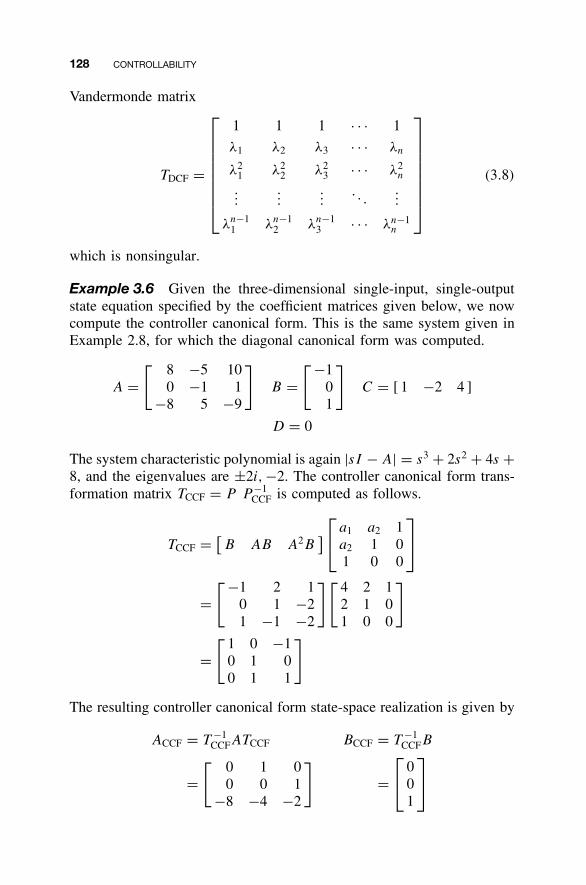
128 CONTROLLABILITY
Vandermonde matrix
TDCF =
1 1 1 · · · 1
λ1 λ2 λ3 · · · λn
λ21 λ2
2 λ23 · · · λ2
n
......
.... . .
...
λn−11 λn−1
2 λn−13 · · · λn−1
n
(3.8)
which is nonsingular.
Example 3.6 Given the three-dimensional single-input, single-outputstate equation specified by the coefficient matrices given below, we nowcompute the controller canonical form. This is the same system given inExample 2.8, for which the diagonal canonical form was computed.
A =[ 8 −5 10
0 −1 1−8 5 −9
]B =
[−101
]C = [ 1 −2 4 ]
D = 0
The system characteristic polynomial is again |sI − A| = s3 + 2s2 + 4s +8, and the eigenvalues are ±2i,−2. The controller canonical form trans-formation matrix TCCF = P P −1
CCF is computed as follows.
TCCF = [B AB A2B
] a1 a2 1
a2 1 01 0 0
=[−1 2 1
0 1 −21 −1 −2
][ 4 2 12 1 01 0 0
]
=[ 1 0 −1
0 1 00 1 1
]
The resulting controller canonical form state-space realization is given by
ACCF = T −1CCFATCCF BCCF = T −1
CCFB
=[ 0 1 0
0 0 1−8 −4 −2
]=
0
01
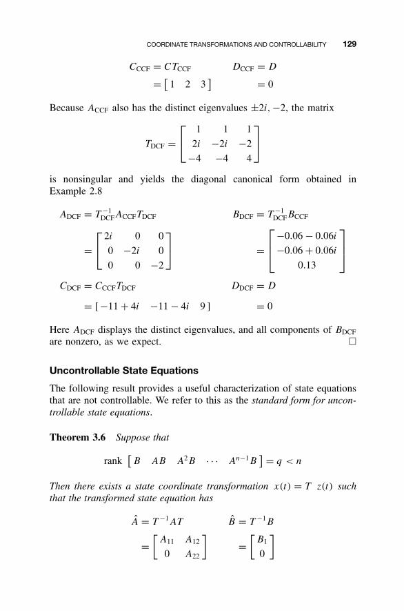
COORDINATE TRANSFORMATIONS AND CONTROLLABILITY 129
CCCF = CTCCF DCCF = D
= [1 2 3
] = 0
Because ACCF also has the distinct eigenvalues ±2i, −2, the matrix
TDCF =
1 1 1
2i −2i −2
−4 −4 4
is nonsingular and yields the diagonal canonical form obtained inExample 2.8
ADCF = T −1DCFACCFTDCF BDCF = T −1
DCFBCCF
=
2i 0 0
0 −2i 0
0 0 −2
=
−0.06 − 0.06i
−0.06 + 0.06i
0.13
CDCF = CCCFTDCF DDCF = D
= [ −11 + 4i −11 − 4i 9 ] = 0
Here ADCF displays the distinct eigenvalues, and all components of BDCF
are nonzero, as we expect. �
Uncontrollable State Equations
The following result provides a useful characterization of state equationsthat are not controllable. We refer to this as the standard form for uncon-trollable state equations.
Theorem 3.6 Suppose that
rank[B AB A2B · · · An−1B
] = q < n
Then there exists a state coordinate transformation x(t) = T z(t) suchthat the transformed state equation has
A = T −1AT B = T −1B
=[
A11 A12
0 A22
]=
[B1
0
]
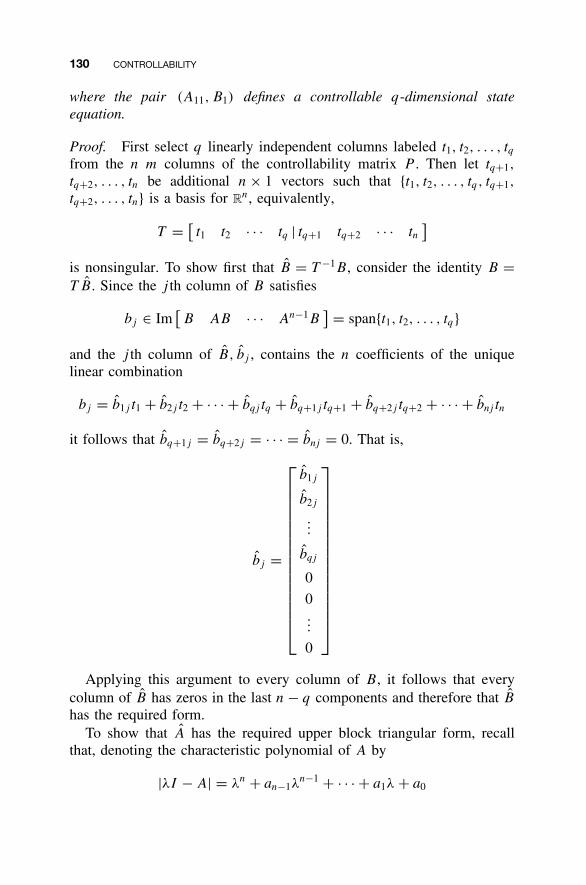
130 CONTROLLABILITY
where the pair (A11, B1) defines a controllable q-dimensional stateequation.
Proof. First select q linearly independent columns labeled t1, t2, . . . , tqfrom the n m columns of the controllability matrix P . Then let tq+1,
tq+2, . . . , tn be additional n × 1 vectors such that {t1, t2, . . . , tq, tq+1,
tq+2, . . . , tn} is a basis for Rn, equivalently,
T = [t1 t2 · · · tq | tq+1 tq+2 · · · tn
]
is nonsingular. To show first that B = T −1B, consider the identity B =T B. Since the j th column of B satisfies
bj ∈ Im[B AB · · · An−1B
] = span{t1, t2, . . . , tq}
and the j th column of B, bj , contains the n coefficients of the uniquelinear combination
bj = b1j t1 + b2j t2 + · · · + bqj tq + bq+1j tq+1 + bq+2j tq+2 + · · · + bnj tn
it follows that bq+1j = bq+2j = · · · = bnj = 0. That is,
bj =
b1j
b2j
...
bqj
0
0...
0
Applying this argument to every column of B, it follows that everycolumn of B has zeros in the last n − q components and therefore that B
has the required form.To show that A has the required upper block triangular form, recall
that, denoting the characteristic polynomial of A by
|λI − A| = λn + an−1λn−1 + · · · + a1λ + a0
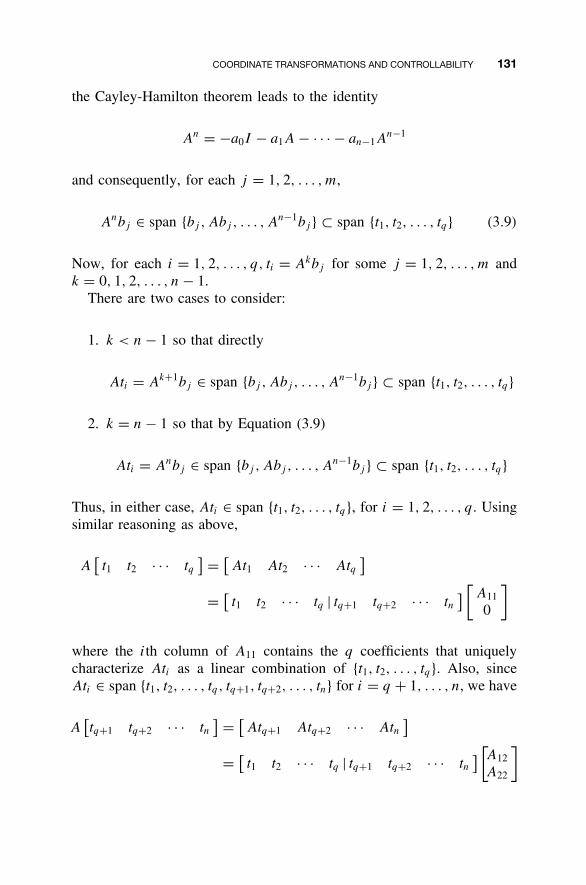
COORDINATE TRANSFORMATIONS AND CONTROLLABILITY 131
the Cayley-Hamilton theorem leads to the identity
An = −a0I − a1A − · · · − an−1An−1
and consequently, for each j = 1, 2, . . . , m,
Anbj ∈ span {bj , Abj , . . . , An−1bj } ⊂ span {t1, t2, . . . , tq} (3.9)
Now, for each i = 1, 2, . . . , q, ti = Akbj for some j = 1, 2, . . . , m andk = 0, 1, 2, . . . , n − 1.
There are two cases to consider:
1. k < n − 1 so that directly
Ati = Ak+1bj ∈ span {bj , Abj , . . . , An−1bj } ⊂ span {t1, t2, . . . , tq}
2. k = n − 1 so that by Equation (3.9)
Ati = Anbj ∈ span {bj , Abj , . . . , An−1bj } ⊂ span {t1, t2, . . . , tq}
Thus, in either case, Ati ∈ span {t1, t2, . . . , tq}, for i = 1, 2, . . . , q. Usingsimilar reasoning as above,
A[t1 t2 · · · tq
] = [At1 At2 · · · Atq
]
= [t1 t2 · · · tq | tq+1 tq+2 · · · tn
] [A11
0
]
where the ith column of A11 contains the q coefficients that uniquelycharacterize Ati as a linear combination of {t1, t2, . . . , tq}. Also, sinceAti ∈ span {t1, t2, . . . , tq, tq+1, tq+2, . . . , tn} for i = q + 1, . . . , n, we have
A[tq+1 tq+2 · · · tn
] = [Atq+1 Atq+2 · · · Atn
]
= [t1 t2 · · · tq | tq+1 tq+2 · · · tn
] [A12
A22
]
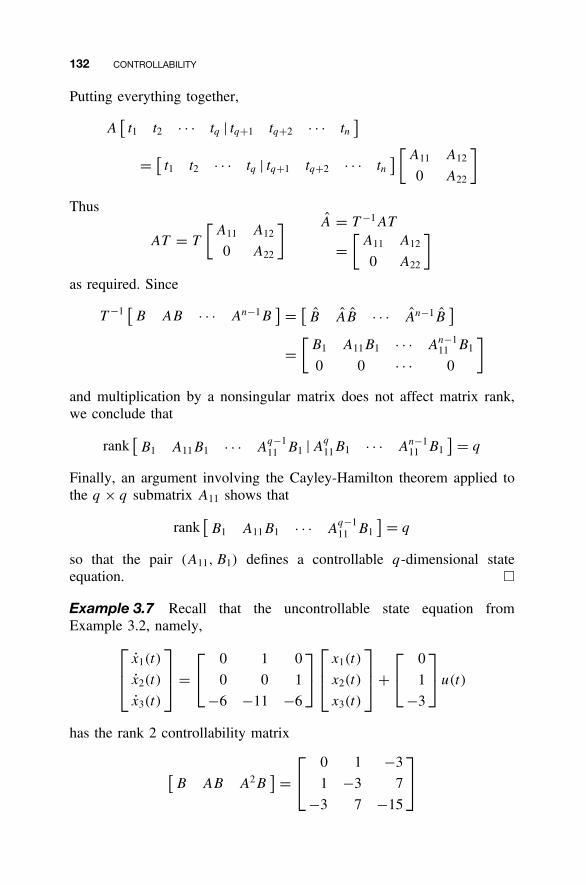
132 CONTROLLABILITY
Putting everything together,
A[t1 t2 · · · tq | tq+1 tq+2 · · · tn
]
= [t1 t2 · · · tq | tq+1 tq+2 · · · tn
] [A11 A12
0 A22
]
Thus
AT = T
[A11 A12
0 A22
] A = T −1AT
=[
A11 A12
0 A22
]
as required. Since
T −1[B AB · · · An−1B
] = [B AB · · · An−1B
]
=[
B1 A11B1 · · · An−111 B1
0 0 · · · 0
]
and multiplication by a nonsingular matrix does not affect matrix rank,we conclude that
rank[B1 A11B1 · · · A
q−111 B1 |Aq
11B1 · · · An−111 B1
] = q
Finally, an argument involving the Cayley-Hamilton theorem applied tothe q × q submatrix A11 shows that
rank[B1 A11B1 · · · A
q−111 B1
] = q
so that the pair (A11, B1) defines a controllable q-dimensional stateequation. �
Example 3.7 Recall that the uncontrollable state equation fromExample 3.2, namely,
x1(t)
x2(t)
x3(t)
=
0 1 0
0 0 1
−6 −11 −6
x1(t)
x2(t)
x3(t)
+
0
1
−3
u(t)
has the rank 2 controllability matrix
[B AB A2B
] =
0 1 −3
1 −3 7
−3 7 −15

POPOV-BELEVITCH-HAUTUS TESTS FOR CONTROLLABILITY 133
in which the first two columns are linearly independent. Appending tothese column vectors the third standard basis vector gives
T =[ 0 1 0
1 −3 0−3 7 1
]
which is nonsingular, as can be verified with a straightforward determinantcomputation. A direct calculation shows that
A = T −1AT B = T −1B
=
0 −2 | 1|1 −3 | 0||0 0 | −3
=
10
0
which is in the standard form for an uncontrollable state equation becausethe q = two-dimensional state equation specified by
A11 =[
0 −21 −3
]B1 =
[10
]
is easily seen to be controllable. �
3.4 POPOV-BELEVITCH-HAUTUS TESTS FORCONTROLLABILITY
Checking the rank of the controllability matrix provides an algebraic testfor controllability. Here we present two others, referred to as the Popov-Belevitch-Hautus eigenvector and rank tests, respectively.
Theorem 3.7 (Popov-Belevitch-Hautus Eigenvector Test for Controlla-bility). The state equation specified by the pair (A, B) is controllable ifand only if there exists no left eigenvector of A orthogonal to the columnsof B.
Proof. We must prove two implications:If the state equation specified by the pair (A, B) is controllable, then
there exists no left eigenvector of A orthogonal to the columns of B.If there exists no left eigenvector of A orthogonal to the columns of
B, then the state equation specified by the pair (A, B) is controllable.
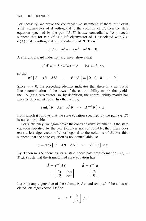
134 CONTROLLABILITY
For necessity, we prove the contrapositive statement: If there does exista left eigenvector of A orthogonal to the columns of B, then the stateequation specified by the pair (A, B) is not controllable. To proceed,suppose that for w ∈ C
n is a left eigenvector of A associated with λ ∈σ(A) that is orthogonal to the columns of B. Then
w �= 0 w∗A = λw∗ w∗B = 0.
A straightforward induction argument shows that
w∗AkB = λk(w∗B) = 0 for all k ≥ 0
so thatw∗ [
B AB A2B · · · An−1B] = [
0 0 0 · · · 0]
Since w �= 0, the preceding identity indicates that there is a nontriviallinear combination of the rows of the controllability matrix that yieldsthe 1 × (nm) zero vector, so, by definition, the controllability matrix haslinearly dependent rows. In other words,
rank[B AB A2B · · · An−1B
]< n
from which it follows that the state equation specified by the pair (A, B)
is not controllable.For sufficiency, we again prove the contrapositive statement: If the state
equation specified by the pair (A, B) is not controllable, then there doesexist a left eigenvector of A orthogonal to the columns of B. For this,suppose that the state equation is not controllable, so
q = rank[B AB A2B · · · An−1B
]< n
By Theorem 3.6, there exists a state coordinate transformation x(t) =T z(t) such that the transformed state equation has
A = T −1AT B = T −1B
=[
A11 A12
0 A22
]=
[B1
0
]
Let λ be any eigenvalue of the submatrix A22 and w2 ∈ Cn−q be an asso-
ciated left eigenvector. Define
w = T −T
[0w2
]�= 0
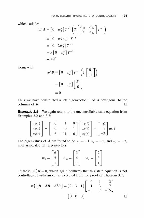
POPOV-BELEVITCH-HAUTUS TESTS FOR CONTROLLABILITY 135
which satisfies
w∗A = [0 w∗
2
]T −1
(T
[A11 A12
0 A22
]T −1
)
= [0 w∗
2A22]T −1
= [0 λw∗
2
]T −1
= λ[
0 w∗2
]T −1
= λw∗
along with
w∗B = [0 w∗
2
]T −1
(T
[B1
0
])
= [0 w∗
2
] [B1
0
]
= 0
Thus we have constructed a left eigenvector w of A orthogonal to thecolumns of B. �
Example 3.8 We again return to the uncontrollable state equation fromExamples 3.2 and 3.7:
x1(t)
x2(t)
x3(t)
=
0 1 0
0 0 1
−6 −11 −6
x1(t)
x2(t)
x3(t)
+
0
1−3
u(t)
The eigenvalues of A are found to be λ1 = −1, λ2 = −2, and λ3 = −3,with associated left eigenvectors
w1 =
6
5
1
w2 =
3
4
1
w3 =
2
3
1
Of these, wT3 B = 0, which again confirms that this state equation is not
controllable. Furthermore, as expected from the proof of Theorem 3.7,
wT3
[B AB A2B
] = [ 2 3 1 ]
[ 0 1 −31 −3 7
−3 7 −15
]
= [0 0 0
]�
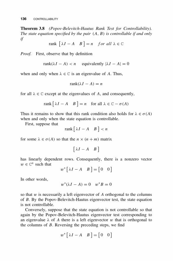
136 CONTROLLABILITY
Theorem 3.8 (Popov-Belevitch-Hautus Rank Test for Controllability).The state equation specified by the pair (A, B) is controllable if and onlyif
rank[λI − A B
] = n f or all λ ∈ C
Proof. First, observe that by definition
rank(λI − A) < n equivalently |λI − A| = 0
when and only when λ ∈ C is an eigenvalue of A. Thus,
rank(λI − A) = n
for all λ ∈ C except at the eigenvalues of A, and consequently,
rank[λI − A B
] = n for all λ ∈ C − σ(A)
Thus it remains to show that this rank condition also holds for λ ∈ σ(A)
when and only when the state equation is controllable.First, suppose that
rank[λI − A B
]< n
for some λ ∈ σ(A) so that the n × (n + m) matrix
[λI − A B
]
has linearly dependent rows. Consequently, there is a nonzero vectorw ∈ C
n such thatw∗ [
λI − A B] = [
0 0]
In other words,w∗(λI − A) = 0 w∗B = 0
so that w is necessarily a left eigenvector of A orthogonal to the columnsof B. By the Popov-Belevitch-Hautus eigenvector test, the state equationis not controllable.
Conversely, suppose that the state equation is not controllable so thatagain by the Popov-Belevitch-Hautus eigenvector test corresponding toan eigenvalue λ of A there is a left eigenvector w that is orthogonal tothe columns of B. Reversing the preceding steps, we find
w∗ [λI − A B
] = [0 0
]
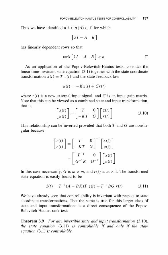
POPOV-BELEVITCH-HAUTUS TESTS FOR CONTROLLABILITY 137
Thus we have identified a λ ∈ σ(A) ⊂ C for which
[λI − A B
]
has linearly dependent rows so that
rank[λI − A B
]< n �
As an application of the Popov-Belevitch-Hautus tests, consider thelinear time-invariant state equation (3.1) together with the state coordinatetransformation x(t) = T z(t) and the state feedback law
u(t) = −Kx(t) + Gr(t)
where r(t) is a new external input signal, and G is an input gain matrix.Note that this can be viewed as a combined state and input transformation,that is, [
x(t)
u(t)
]=
[T 0
−KT G
] [z(t)
r(t)
](3.10)
This relationship can be inverted provided that both T and G are nonsin-gular because
[z(t)
r(t)
]=
[T 0
−KT G
]−1 [x(t)
u(t)
]
=[
T −1 0
G−1K G−1
][x(t)
u(t)
]
In this case necessarily, G is m × m, and r(t) is m × 1. The transformedstate equation is easily found to be
z(t) = T −1(A − BK)T z(t) + T −1BG r(t) (3.11)
We have already seen that controllability is invariant with respect to statecoordinate transformations. That the same is true for this larger class ofstate and input transformations is a direct consequence of the Popov-Belevitch-Hautus rank test.
Theorem 3.9 For any invertible state and input transformation (3.10),the state equation (3.11) is controllable if and only if the stateequation (3.1) is controllable.
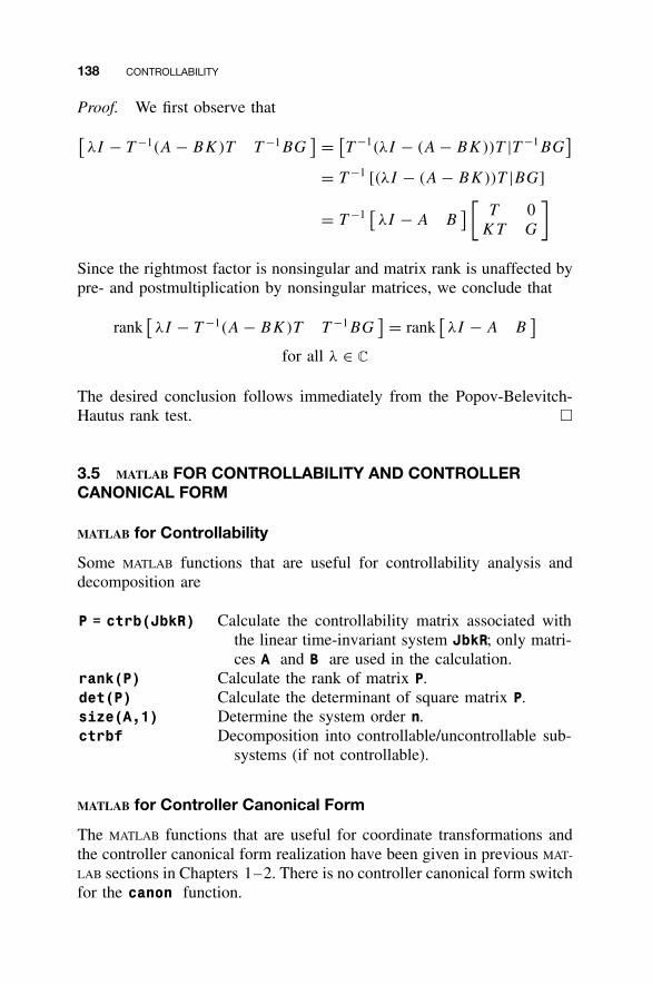
138 CONTROLLABILITY
Proof. We first observe that
[λI − T −1(A − BK)T T −1BG
] = [T −1(λI − (A − BK))T |T −1BG
]= T −1 [(λI − (A − BK))T |BG]
= T −1[λI − A B
] [T 0
KT G
]
Since the rightmost factor is nonsingular and matrix rank is unaffected bypre- and postmultiplication by nonsingular matrices, we conclude that
rank[λI − T −1(A − BK)T T −1BG
] = rank[λI − A B
]for all λ ∈ C
The desired conclusion follows immediately from the Popov-Belevitch-Hautus rank test. �
3.5 MATLAB FOR CONTROLLABILITY AND CONTROLLERCANONICAL FORM
MATLAB for Controllability
Some MATLAB functions that are useful for controllability analysis anddecomposition are
P = ctrb(JbkR) Calculate the controllability matrix associated withthe linear time-invariant system JbkR; only matri-ces A and B are used in the calculation.
rank(P) Calculate the rank of matrix P.det(P) Calculate the determinant of square matrix P.size(A,1) Determine the system order n.ctrbf Decomposition into controllable/uncontrollable sub-
systems (if not controllable).
MATLAB for Controller Canonical Form
The MATLAB functions that are useful for coordinate transformations andthe controller canonical form realization have been given in previous MAT-
LAB sections in Chapters 1–2. There is no controller canonical form switchfor the canon function.
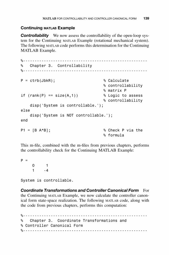
MATLAB FOR CONTROLLABILITY AND CONTROLLER CANONICAL FORM 139
Continuing MATLAB Example
Controllability We now assess the controllability of the open-loop sys-tem for the Continuing MATLAB Example (rotational mechanical system).The following MATLAB code performs this determination for the ContinuingMATLAB Example.
%------------------------------------------------------% Chapter 3. Controllability%------------------------------------------------------
P = ctrb(JbkR); % Calculate% controllability% matrix P
if (rank(P) == size(A,1)) % Logic to assess% controllability
disp('System is controllable.');else
disp('System is NOT controllable.');end
P1 = [B A*B]; % Check P via the% formula
This m-file, combined with the m-files from previous chapters, performsthe controllability check for the Continuing MATLAB Example:
P =0 11 -4
System is controllable.
Coordinate Transformations and Controller Canonical Form Forthe Continuing MATLAB Example, we now calculate the controller canon-ical form state-space realization. The following MATLAB code, along withthe code from previous chapters, performs this computation:
%------------------------------------------------------% Chapter 3. Coordinate Transformations and% Controller Canonical Form%------------------------------------------------------
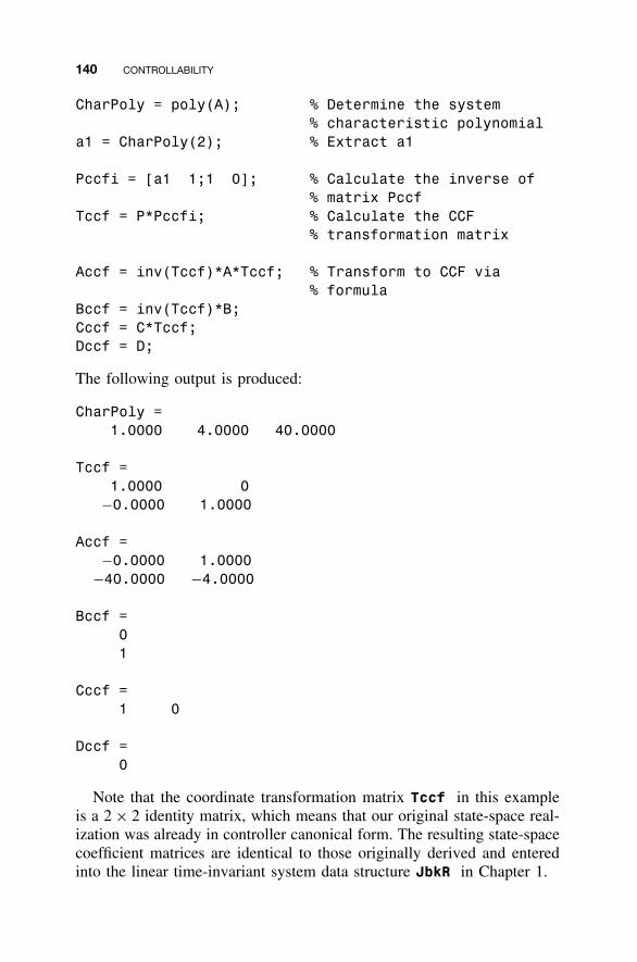
140 CONTROLLABILITY
CharPoly = poly(A); % Determine the system% characteristic polynomial
a1 = CharPoly(2); % Extract a1
Pccfi = [a1 1;1 0]; % Calculate the inverse of% matrix Pccf
Tccf = P*Pccfi; % Calculate the CCF% transformation matrix
Accf = inv(Tccf)*A*Tccf; % Transform to CCF via% formula
Bccf = inv(Tccf)*B;Cccf = C*Tccf;Dccf = D;
The following output is produced:
CharPoly =1.0000 4.0000 40.0000
Tccf =1.0000 0
−0.0000 1.0000
Accf =−0.0000 1.0000
−40.0000 −4.0000
Bccf =01
Cccf =1 0
Dccf =0
Note that the coordinate transformation matrix Tccf in this exampleis a 2 × 2 identity matrix, which means that our original state-space real-ization was already in controller canonical form. The resulting state-spacecoefficient matrices are identical to those originally derived and enteredinto the linear time-invariant system data structure JbkR in Chapter 1.
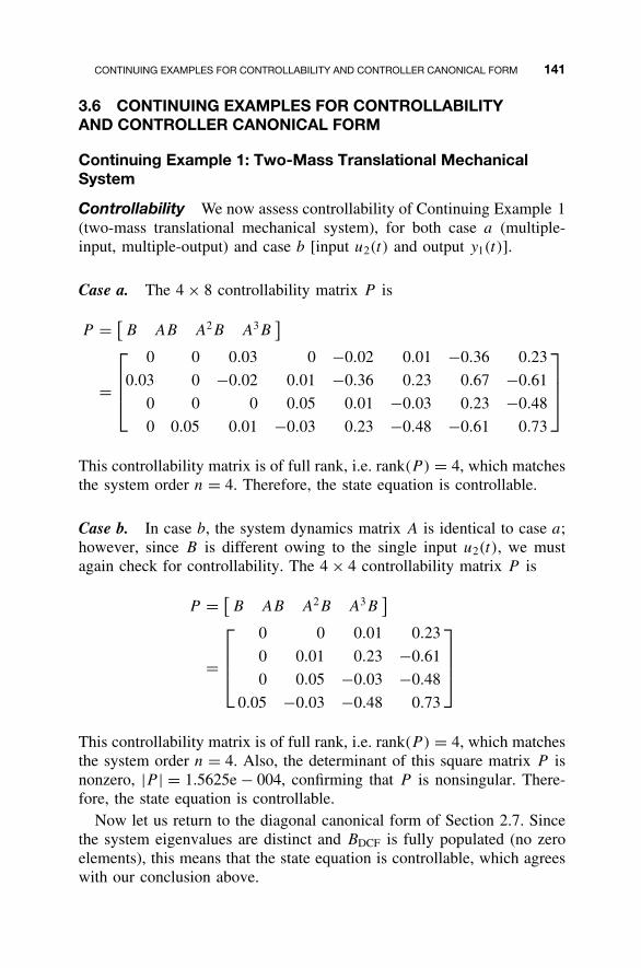
CONTINUING EXAMPLES FOR CONTROLLABILITY AND CONTROLLER CANONICAL FORM 141
3.6 CONTINUING EXAMPLES FOR CONTROLLABILITYAND CONTROLLER CANONICAL FORM
Continuing Example 1: Two-Mass Translational MechanicalSystem
Controllability We now assess controllability of Continuing Example 1(two-mass translational mechanical system), for both case a (multiple-input, multiple-output) and case b [input u2(t) and output y1(t)].
Case a. The 4 × 8 controllability matrix P is
P = [B AB A2B A3B
]
=
0 0 0.03 0 −0.02 0.01 −0.36 0.23
0.03 0 −0.02 0.01 −0.36 0.23 0.67 −0.61
0 0 0 0.05 0.01 −0.03 0.23 −0.48
0 0.05 0.01 −0.03 0.23 −0.48 −0.61 0.73
This controllability matrix is of full rank, i.e. rank(P ) = 4, which matchesthe system order n = 4. Therefore, the state equation is controllable.
Case b. In case b, the system dynamics matrix A is identical to case a;however, since B is different owing to the single input u2(t), we mustagain check for controllability. The 4 × 4 controllability matrix P is
P = [B AB A2B A3B
]
=
0 0 0.01 0.23
0 0.01 0.23 −0.61
0 0.05 −0.03 −0.48
0.05 −0.03 −0.48 0.73
This controllability matrix is of full rank, i.e. rank(P ) = 4, which matchesthe system order n = 4. Also, the determinant of this square matrix P isnonzero, |P | = 1.5625e − 004, confirming that P is nonsingular. There-fore, the state equation is controllable.
Now let us return to the diagonal canonical form of Section 2.7. Sincethe system eigenvalues are distinct and BDCF is fully populated (no zeroelements), this means that the state equation is controllable, which agreeswith our conclusion above.
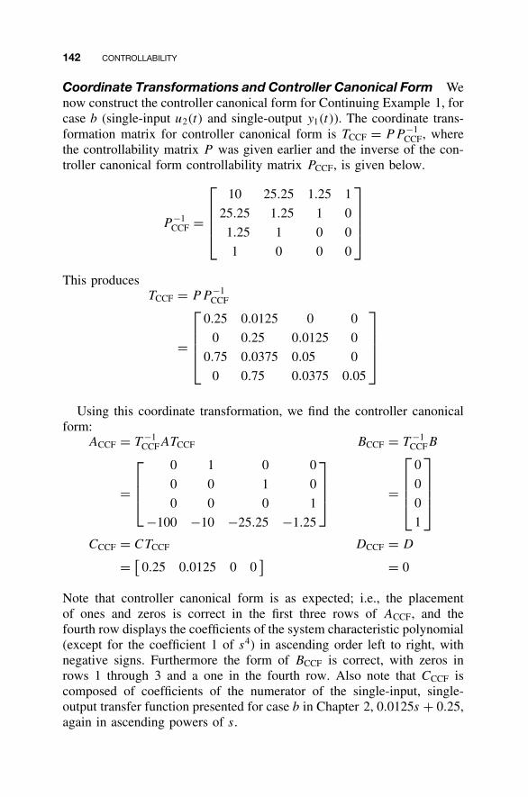
142 CONTROLLABILITY
Coordinate Transformations and Controller Canonical Form Wenow construct the controller canonical form for Continuing Example 1, forcase b (single-input u2(t) and single-output y1(t)). The coordinate trans-formation matrix for controller canonical form is TCCF = PP −1
CCF, wherethe controllability matrix P was given earlier and the inverse of the con-troller canonical form controllability matrix PCCF, is given below.
P −1CCF =
10 25.25 1.25 1
25.25 1.25 1 0
1.25 1 0 0
1 0 0 0
This producesTCCF = PP −1
CCF
=
0.25 0.0125 0 0
0 0.25 0.0125 0
0.75 0.0375 0.05 0
0 0.75 0.0375 0.05
Using this coordinate transformation, we find the controller canonicalform:
ACCF = T −1CCFATCCF BCCF = T −1
CCFB
=
0 1 0 0
0 0 1 0
0 0 0 1
−100 −10 −25.25 −1.25
=
0
0
0
1
CCCF = CTCCF DCCF = D
= [0.25 0.0125 0 0
] = 0
Note that controller canonical form is as expected; i.e., the placementof ones and zeros is correct in the first three rows of ACCF, and thefourth row displays the coefficients of the system characteristic polynomial(except for the coefficient 1 of s4) in ascending order left to right, withnegative signs. Furthermore the form of BCCF is correct, with zeros inrows 1 through 3 and a one in the fourth row. Also note that CCCF iscomposed of coefficients of the numerator of the single-input, single-output transfer function presented for case b in Chapter 2, 0.0125s + 0.25,again in ascending powers of s.
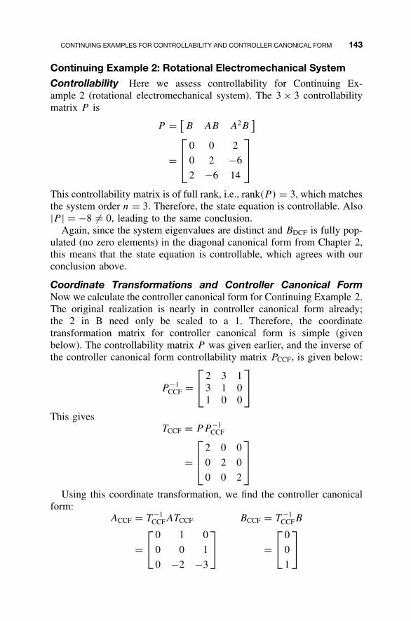
CONTINUING EXAMPLES FOR CONTROLLABILITY AND CONTROLLER CANONICAL FORM 143
Continuing Example 2: Rotational Electromechanical System
Controllability Here we assess controllability for Continuing Ex-ample 2 (rotational electromechanical system). The 3 × 3 controllabilitymatrix P is
P = [B AB A2B
]
=
0 0 2
0 2 −6
2 −6 14
This controllability matrix is of full rank, i.e., rank(P ) = 3, which matchesthe system order n = 3. Therefore, the state equation is controllable. Also|P | = −8 �= 0, leading to the same conclusion.
Again, since the system eigenvalues are distinct and BDCF is fully pop-ulated (no zero elements) in the diagonal canonical form from Chapter 2,this means that the state equation is controllable, which agrees with ourconclusion above.
Coordinate Transformations and Controller Canonical FormNow we calculate the controller canonical form for Continuing Example 2.The original realization is nearly in controller canonical form already;the 2 in B need only be scaled to a 1. Therefore, the coordinatetransformation matrix for controller canonical form is simple (givenbelow). The controllability matrix P was given earlier, and the inverse ofthe controller canonical form controllability matrix PCCF, is given below:
P −1CCF =
2 3 1
3 1 01 0 0
This givesTCCF = PP −1
CCF
=
2 0 0
0 2 0
0 0 2
Using this coordinate transformation, we find the controller canonicalform:
ACCF = T −1CCFATCCF BCCF = T −1
CCFB
=
0 1 0
0 0 1
0 −2 −3
=
0
0
1
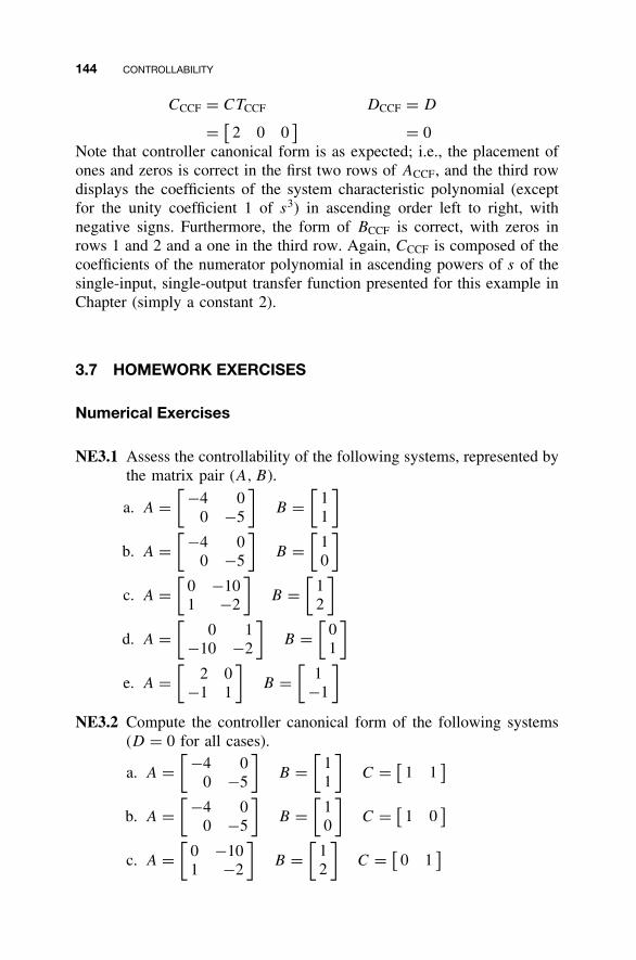
144 CONTROLLABILITY
CCCF = CTCCF DCCF = D
= [2 0 0
] = 0Note that controller canonical form is as expected; i.e., the placement ofones and zeros is correct in the first two rows of ACCF, and the third rowdisplays the coefficients of the system characteristic polynomial (exceptfor the unity coefficient 1 of s3) in ascending order left to right, withnegative signs. Furthermore, the form of BCCF is correct, with zeros inrows 1 and 2 and a one in the third row. Again, CCCF is composed of thecoefficients of the numerator polynomial in ascending powers of s of thesingle-input, single-output transfer function presented for this example inChapter (simply a constant 2).
3.7 HOMEWORK EXERCISES
Numerical Exercises
NE3.1 Assess the controllability of the following systems, represented bythe matrix pair (A, B).
a. A =[ −4 0
0 −5
]B =
[11
]
b. A =[ −4 0
0 −5
]B =
[10
]
c. A =[
0 −101 −2
]B =
[12
]
d. A =[
0 1−10 −2
]B =
[01
]
e. A =[
2 0−1 1
]B =
[1
−1
]
NE3.2 Compute the controller canonical form of the following systems(D = 0 for all cases).
a. A =[ −4 0
0 −5
]B =
[11
]C = [
1 1]
b. A =[ −4 0
0 −5
]B =
[10
]C = [
1 0]
c. A =[
0 −101 −2
]B =
[12
]C = [
0 1]
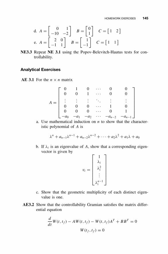
HOMEWORK EXERCISES 145
d. A =[
0 1−10 −2
]B =
[01
]C = [
1 2]
e. A =[
2 0−1 1
]B =
[1
−1
]C = [
1 1]
NE3.3 Repeat NE 3.1 using the Popov-Belevitch-Hautus tests for con-trollability.
Analytical Exercises
AE 3.1 For the n × n matrix
A =
0 1 0 · · · 0 00 0 1 · · · 0 0...
......
. . ....
...
0 0 0 · · · 1 00 0 0 · · · 0 1
−a0 −a1 −a2 · · · −an−2 −an−1
a. Use mathematical induction on n to show that the character-istic polynomial of A is
λn + an−1λn−1 + an−2λ
n−2 + · · · + a2λ2 + a1λ + a0
b. If λi is an eigenvalue of A, show that a corresponding eigen-vector is given by
vi =
1λi
λ2i...
λn−1i
c. Show that the geometric multiplicity of each distinct eigen-value is one.
AE3.2 Show that the controllability Gramian satisfies the matrix differ-ential equation
d
dtW(t, tf ) − AW(t, tf ) − W(t, tf )AT + BBT = 0
W(tf , tf ) = 0
146 CONTROLLABILITY
AE3.3 Show that the matrix exponential for[A BBT
0 −AT
]
is given by [eAt eAtW(0, t)
0 e−AT t
]
AE 3.4 Consider the reachability Gramian, defined as follows for anyinitial time t0 and any finite final time tf > t0:
WR(t0, tf ) =∫ tf
t0
eA(tf −τ )BBT eAT (tf −τ )dτ
Show that WR(t0, tf ) is nonsingular for any t0 and tf > t0 if andonly if the pair (A, B) is controllable. Assuming that (A, B)
is controllable, use the reachability Gramian to construct, forany xf ∈ R
n, an input signal on [t0, tf ] such that x(t0) = 0 andx(tf ) = xf .
AE 3.5 Suppose that a single-input n-dimensional state equation has
q � rank[B AB A2B · · · An−1B
] ≤ n
Show that the first q columns {B, AB, A2B, . . . , Aq−1B} are lin-early independent.
AE 3.6 Show that the single-input state equation characterized by
A =
µ 1 0 · · · 00 µ 1 · · · 0...
......
. . ....
0 0 0 · · · 10 0 0 · · · µ
B =
b1
b2...
bn−1
bn
is controllable if and only if bn �= 0.
AE 3.7 For the controllable system with two separate scalar outputs
x(t) = Ax(t) + Bu(t)
y1(t) = C1x(t)
y2(t) = C2x(t)
show that the related impulse responses h1(t) and h2(t) are iden-tical if and only if C1 = C2.
HOMEWORK EXERCISES 147
AE3.8 Suppose that H1(s) and H2(s) are two strictly proper single-input, single-output transfer functions with controllable state-space realizations (A1, B1, C1) and (A2, B2, C2), respectively.Construct a state-space realization for the parallel interconnectionH1(s) + H2(s), and use the Popov-Belevitch-Hautus eigenvectortest to show that the parallel realization is controllable if andonly if A1 and A2 have no common eigenvalues.
AE3.9 Suppose that H1(s) and H2(s) are two strictly proper single-input,single-output transfer functions with controllable state-space real-izations (A1, B1, C1) and (A2, B2, C2), respectively. Construct astate-space realization for the series interconnection H1(s)H2(s),and show that this realization is controllable if and only if noeigenvalue of A2 is a zero of H1(s).
AE3.10 Show that the pair (A, B) is controllable if and only if the onlysquare matrix X that satisfies
AX = XA XB = 0
is X = 0.
Continuing MATLAB Exercises
CME3.1 For the CME1.1 system:a. Assess the system controllability.b. Compute the controller canonical form.
CME3.2 For the CME1.2 system:a. Assess the system controllability.b. Compute the controller canonical form.
CME3.3 For the CME1.3 system:a. Assess the system controllability.b. Compute the controller canonical form.
CME3.4 For the CME1.4 system:a. Assess the system controllability.b. Compute the controller canonical form.
Continuing Exercises
CE3.1a Determine if the CE1 system is controllable for all three cases(cases from CE1.1b and numeric parameters from CE2.1a). Give
148 CONTROLLABILITY
the mathematical details to justify your answers; explain yourresults in all cases by looking at the physical problem.
CE3.1b Compute the controller canonical form for the CE1 system, caseiii only. Comment on the structure of your results. Determine thesystem controllability by looking at the diagonal canonical formrealization of CE 2.1b; compare to your controllability resultsfrom CE3.1a.
CE3.2a Determine if the CE2 system is controllable for all three cases(cases from CE1.2b and numeric parameters from CE2.2a). Givethe mathematical details to justify your answers; explain yourresults in all cases by looking at the physical problem.
CE3.2b Compute the controller canonical form for the CE2 system, Casei only. Comment on the structure of your results.
CE3.3a Determine if the CE3 system is controllable for both cases (casesfrom CE1.3b and numeric parameters from CE2.3a). Give themathematical details to justify your answers; explain your resultsin all cases by looking at the physical problem.
CE3.3b Compute the controller canonical form for the CE3 system forboth cases. Comment on the structure of your results. Determinethe system controllability by looking at the diagonal canonicalform realization from CE 2.3b for case i; compare to your resultsfrom CE3.3a.
CE3.4a Determine if the CE4 system is controllable (for the CE1.4bsingle-input, single-output case with the numeric parameters fromCE2.4a). Give the mathematical details to justify your answers;explain your results by looking at the physical problem.
CE3.4b Compute the controller canonical form for the CE4 system. Com-ment on the structure of your results. Determine the systemcontrollability by looking at the diagonal canonical form real-ization from CE 2.4b; compare with your results from CE3.4a.
CE3.5a Determine if the CE5 system is controllable (for the CE1.5bsingle-input, single-output case with the numeric parameters fromCE2.5a). Give the mathematical details to justify your answers;explain your results by looking at the physical problem.
CE3.5b Compute the controller canonical form for the CE5 system. Com-ment on the structure of your results. Determine the systemcontrollability by looking at the diagonal canonical form real-ization from CE 2.5b; compare with your results from CE3.5a.
4
OBSERVABILITY
In our state-space description of linear time-invariant systems, the statevector constitutes an internal quantity that is influenced by the input sig-nal and, in turn, affects the output signal. We have seen in our examplesand it is generally true in practice that the dimension of the state vector,equivalently the dimension of the system modeled by the state equation,is greater than the number of input signals or output signals. This reflectsthe fact that the complexity of real-world systems precludes the abil-ity to directly actuate or sense each state variable. Nevertheless, we areoften interested in somehow estimating the state vector because it char-acterizes the system’s complex inner workings and, as we shall see inChapters 7 and 8, figures prominently in state-space methods of controlsystem design.
The fundamental question we address in this chapter is whether or notmeasurements of the input and output signals of our linear state equationover a finite time interval can be processed in order to uniquely deter-mine the initial state. If so, knowledge of the initial state and the inputsignal allows the entire state trajectory to be reconstructed according tothe state equation solution formula. This, in essence, characterizes thesystem property of observability. As with our treatment of controllabilityin Chapter 3, our aim is to establish algebraic criteria for observabilityexpressed in terms of the state-equation coefficient matrices.
149
Linear State-Space Control Systems. Robert L. Williams II and Douglas A. LawrenceCopyright 2007 John Wiley & Sons, Inc. ISBN: 978-0-471-73555-7
150 OBSERVABILITY
We begin the chapter with an analysis of observability patterned afterour introduction to controllability. This suggests a duality that existsbetween controllability and observability that we develop in detail. Thispays immediate dividends in that various observability-related results canbe established with modest effort by referring to the corresponding resultfor controllability and invoking duality. In particular, we investigate rela-tionships between observability and state coordinate transformations aswell as formulate Popov-Belevich-Hautus tests for observability. We con-clude the chapter by illustrating the use of MATLAB for observabilityanalysis and revisit the MATLAB Continuing Example as well as ContinuingExamples 1 and 2.
4.1 FUNDAMENTAL RESULTS
For the n–dimensional linear time-invariant state equation
x(t) = Ax(t) + Bu(t)
y(t) = Cx(t) + Du(t)x(t0) = x0 (4.1)
we assume that the input signal u(t) and the output signal y(t) can bemeasured over a finite time interval and seek to deduce the initial statex(t0) = x0 by processing this information in some way. As noted ear-lier, if the initial state can be uniquely determined, then this, along withknowledge of the input signal, yields the entire state trajectory via
x(t) = eA(t−t0)x0 +∫ t
t0
eA(t−τ )Bu(τ) dτ for t ≥ t0
Since u(t) is assumed to be known, the zero-state response can beextracted from the complete response y(t), also known, in order to isolatethe zero-input response component via
y(t) −[∫ t
t0
CeA(t−τ )Bu(τ)dτ + Du(t)
]= CeA(t−t0)x0
which depends directly on the unknown initial state. Consequently, we canassume without loss of generality that u(t) ≡ 0 for all t ≥ t0 and insteadconsider the homogeneous state equation
x(t) = Ax(t)
y(t) = Cx(t)x(t0) = x0 (4.2)
which directly produces the zero-input response component of Equ-ation (4.1).
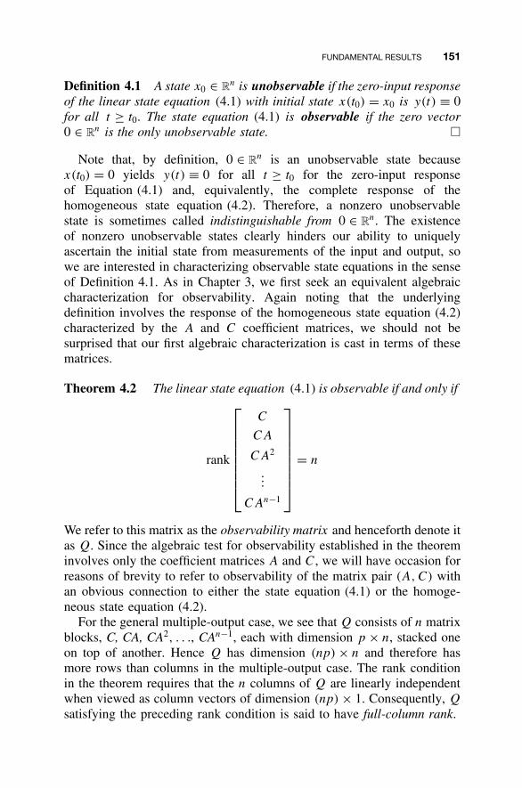
FUNDAMENTAL RESULTS 151
Definition 4.1 A state x0 ∈ Rn is unobservable if the zero-input response
of the linear state equation (4.1) with initial state x(t0) = x0 is y(t) ≡ 0for all t ≥ t0. The state equation (4.1) is observable if the zero vector0 ∈ R
n is the only unobservable state. �
Note that, by definition, 0 ∈ Rn is an unobservable state because
x(t0) = 0 yields y(t) ≡ 0 for all t ≥ t0 for the zero-input responseof Equation (4.1) and, equivalently, the complete response of thehomogeneous state equation (4.2). Therefore, a nonzero unobservablestate is sometimes called indistinguishable from 0 ∈ R
n. The existenceof nonzero unobservable states clearly hinders our ability to uniquelyascertain the initial state from measurements of the input and output, sowe are interested in characterizing observable state equations in the senseof Definition 4.1. As in Chapter 3, we first seek an equivalent algebraiccharacterization for observability. Again noting that the underlyingdefinition involves the response of the homogeneous state equation (4.2)characterized by the A and C coefficient matrices, we should not besurprised that our first algebraic characterization is cast in terms of thesematrices.
Theorem 4.2 The linear state equation (4.1) is observable if and only if
rank
C
CA
CA2
...
CAn−1
= n
We refer to this matrix as the observability matrix and henceforth denote itas Q. Since the algebraic test for observability established in the theoreminvolves only the coefficient matrices A and C, we will have occasion forreasons of brevity to refer to observability of the matrix pair (A, C) withan obvious connection to either the state equation (4.1) or the homoge-neous state equation (4.2).
For the general multiple-output case, we see that Q consists of n matrixblocks, C, CA, CA2, . . ., CAn−1, each with dimension p × n, stacked oneon top of another. Hence Q has dimension (np) × n and therefore hasmore rows than columns in the multiple-output case. The rank conditionin the theorem requires that the n columns of Q are linearly independentwhen viewed as column vectors of dimension (np) × 1. Consequently, Q
satisfying the preceding rank condition is said to have full-column rank.
152 OBSERVABILITY
Alternatively, this rank condition means that out of the np rows of Q
written as
c1
c1
...
cp
c1A
c2A
...
cpA
...
c1An−1
c2An−1
...
cpAn−1
there must be at least one way to select n linearly independent rows.For the single-output case, C consists of a single row, and Q is a square
n × n matrix. Hence a single-output linear state equation is observable ifand only if the observability matrix is nonsingular. We can check that Q
is nonsingular by verifying that it has a nonzero determinant.
Proof of Theorem 4.2. The theorem involves two implications:If the state equation (4.1) is observable, then rankQ = n.If rankQ = n, then the state equation (4.1) is observable.
We begin by proving the contrapositive of the first implication: If rankQ < n, then the state equation (4.1) is not observable. Assuming rankQ < n, Q has linearly dependent columns, so there exists a nontriviallinear combination of the columns of Q that yields an (np) × 1 zerovector. Stacking the coefficients of this linear combination into a nonzeron × 1 vector x0, we have
C
CA
CA2
...
CAn−1
x0 =
000...
0
FUNDAMENTAL RESULTS 153
Another way to arrive at this is to observe that rankQ < n implies, bySylvester’s law of nullity, that nullityQ ≥ 1. The vector x0 just introducedis a nonzero n × 1 vector lying in the null space of Q. In any case, thepreceding identity can be divided up into
Cx0 = CAx0 = CA2x0 = · · · = CAn−1x0 = 0 ∈ Rp
Using the finite series expansion
eAt =n−1∑k=0
αk(t)Ak
for scalar functions α0(t), α1(t), . . . , αn−1(t), we see that the response ofthe homogeneous system (4.2) with initial state x(t0) = x0 satisfies
y(t) = CeA(t−t0)x0
= C
[n−1∑k=0
αk(t − t0)Ak
]x0
=n−1∑k=0
αk(t − t0)(CAkx0)
≡ 0 for all t ≥ t0
Thus x0 is an unobservable state. Since x0 was taken initially to be anonzero vector, we have, as a consequence of Definition 4.1, that thelinear state equation (4.1) is not observable.
We next prove the contrapositive of the second implication: If the linearstate equation (4.1) is not observable, then rankQ < n. Assuming that thelinear state equation (4.1) is not observable, there exists by Definition 4.1a nonzero unobservable state. That is, there exists a nonzero n × 1 vectorx0 for which CeA(t−t0)x0 ≡ 0 for all t ≥ t0. We can repeatedly differentiatethis identity with respect to t and evaluate at t = t0 to obtain
0 = dk
dtk(CeA(t−t0)x0)
∣∣∣∣t=t0
= CAkeA(t−t0)x0
∣∣∣∣t=t0
= CAkx0 for k = 0, 1, . . . , n − 1
154 OBSERVABILITY
These identities can be repackaged into
0
0
0...
0
=
Cx0
CAx0
CA2x0
...
CAn−1x0
=
C
CA
CA2
...
CAn−1
x0
which indicates that the unobservable state x0 lies in the null space of Q.In terms of the components of x0, the preceding identity specifies a linearcombination of the columns of Q that yields the zero vector. Since x0 wastaken initially to be a nonzero vector, we conclude that Q has linearlydependent columns and hence less than full column rank n. Alternatively,we have that nullity Q ≥ 1, so an appeal to Sylvester’s law of nullityyields rank Q < n. �
We conclude this section by answering the fundamental question posedat the outset: It is possible to uniquely determine the initial state by pro-cessing measurements of the input and output signals over a finite timeinterval if and only if the linear state equation (4.1) is observable. To arguethe necessity of observability, suppose that x(t0) = x0 is a nonzero unob-servable initial state that yields, by definition, yzi(t) = CeA(t−t0)x0 ≡ 0for all t ≥ t0. Thus x(t0) = x0 is indistinguishable from the zero initialstate, and it is not possible to resolve this ambiguity by processing thezero-input response. To show that observability is sufficient to uniquelyrecover the initial state from the input and output signals as above, wefirst show that observability also be can characterized by an observabilityGramian defined as follows for any initial time t0 and any finite final timetf > t0:
M(t0, tf ) =∫ tf
t0
eAT(τ−t0)CTCeA(τ−t0) dτ
As with the controllability Gramian introduced in Chapter 3, theobservability Gramian is a square n × n symmetric matrix that is alsopositive semidefinite because the associated real-valued quadratic formxT M(t0, tf )x satisfies the following for all vectors x ∈ R
n
xT M(t0, tf )x = xT
∫ tf
t0
eAT(τ−t0)CTCeA(τ−t0) dτ x

FUNDAMENTAL RESULTS 155
=∫ tf
t0
||CeA(τ−t0)x||2 dτ
≥ 0
Lemma 4.3
rank
C
CA
CA2
...
CAn−1
= n
if and only if for any initial time t0 and any finite final time tf > t0 theobservability Gramian M(t0, tf ) is nonsingular.
Proof. This proof is very similar to the proof of Lemma 3.3 from theprevious chapter, and so the reader is encouraged to independently adaptthat proof to the case at hand and then compare the result with whatfollows.
Lemma 4.3 involves two implications:
If rank Q = n, then M(t0, tf ) is nonsingular for any t0 and any finitetf > t0.If M(t0, tf ) is nonsingular for any t0 and any finite tf > t0, then rankQ = n.
To begin, we prove the contrapositive of the first implication: If M(t0, tf )
is singular for some t0 and finite tf > t0, then rankQ < n. If we assumethat M(t0, tf ) is singular for some t0 and finite tf > t0, then there existsa nonzero vector x0 ∈ R
n for which M(t0, tf )x0 = 0 ∈ Rn and conse-
quently xT0 M(t0, tf )x0 = 0 ∈ R. Using the observability Gramian defini-
tion, we have
0 = xT0 M(t0, tf )x0
= xT0
∫ tf
t0
eAT(τ−t0)CTCeA(τ−t0)dτ x0
=∫ tf
t0
||CeA(τ−t0)x0||2 dτ
156 OBSERVABILITY
The integrand in this expression involves the Euclidean norm of the p × 1vector quantity CeA(τ−t0)x0, which we view as an analytic function of theintegration variable τ ∈ [t0, tf ]. Since this integrand never can be negative,the only way the integral over a positive time interval can evaluate to zerois if the integrand is identically zero for all τ ∈ [t0, tf ]. Because only thezero vector has zero Euclidean norm, we must have
CeA(τ−t0)x0 = 0 ∈ Rp for all τ ∈ [t0, tf ]
This means that the derivative of this expression of any order with respectto τ also must be the zero vector for all τ ∈ [t0, tf ] and in particular atτ = t0. That is,
0 = dk
dtkCeA(τ−t0)x0
∣∣∣∣τ=t0
= CAkeA(τ−t0)x0
∣∣∣∣τ=t0
= CAkx0 for all k ≥ 0
We conclude that
C
CA
CA2
...
CAn−1
x0 =
Cx0
CAx0
CA2x0
...
CAn−1x0
=
0
0
0...
0
which implies, since x0 ∈ Rn is a nonzero vector, that Q has less than
full-column rank, or rankQ < n.We next prove the contrapositive of the second implication: If rankQ <
n, then M(t0, tf ) is singular for some t0 and finite tf > t0. Assuming thatQ has less than full column rank, there exists a nonzero vector x0 ∈ R
n
whose components specify a linear combination of the columns of Q thatyield an (np) × 1 zero vector. That is,
C
CA
CA2
...
CAn−1
x0 =
Cx0
CAx0
CA2x0
...
CAn−1x0
=
0
0
0...
0
FUNDAMENTAL RESULTS 157
which shows that CAkx0 = 0 for k = 0, 1, . . . , n − 1. The finite seriesexpansion
eAt =n−1∑k=0
αk(t)Ak
for scalar functions α0(t), α1(t), . . . , αn−1(t) now gives
CeAtx0 = C
[n−1∑k=0
αk(t)Ak
]x0 =
n−1∑k=0
αk(t)(CAkx0) = 0 for all t
It follows from this that for any t0 and finite tf > t0,
M(t0, tf )x0 =∫ tf
t0
eAT(τ−t0)CTCeA(τ−t0) dτ x0
=∫ tf
t0
eAT(τ−t0)CT(CeA(τ−t0)x0) dτ
= 0
which implies, since x0 ∈ Rn is a nonzero vector, that M(t0, tf ) is singular.
�As a consequence of Lemma 4.3, an observable state equation has, for
any initial time t0 and finite final time tf > t0, a nonsingular observabilityGramian. This can be used to process input and output measurementsu(t), y(t) on the interval [t0, tf ] to yield the initial state x(t0) = x0 asfollows: We first form the zero-input response component
yzi(t) = y(t) −[∫ t
t0
CeA(t−τ )Bu(τ) dτ + Du(t)
]
= CeA(t−t0)x0
Then we process the zero-input response according to
M−1(t0, tf )
∫ tf
t0
eAT(τ−t0)CTyzi(τ ) dτ
= M−1(t0, tf )
∫ tf
0eAT(τ−t0)CTCeA(τ−t0)x0 dσ
= M−1(t0, tf )
∫ tf
0eAT(τ−t0)CTCeA(τ−t0)dτ x0
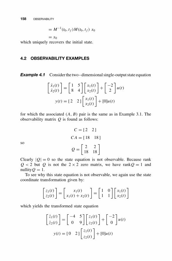
158 OBSERVABILITY
= M−1(t0, tf )M(t0, tf ) x0
= x0
which uniquely recovers the initial state.
4.2 OBSERVABILITY EXAMPLES
Example 4.1 Consider the two–dimensional single-output state equation
[x1(t)
x2(t)
]=
[1 58 4
] [x1(t)
x2(t)
]+
[ −22
]u(t)
y(t) = [ 2 2 ]
[x1(t)
x2(t)
]+ [0]u(t)
for which the associated (A, B) pair is the same as in Example 3.1. Theobservability matrix Q is found as follows:
C = [ 2 2 ]
CA = [ 18 18 ]so
Q =[
2 218 18
]
Clearly |Q| = 0 so the state equation is not observable. Because rankQ < 2 but Q is not the 2 × 2 zero matrix, we have rankQ = 1 andnullityQ = 1.
To see why this state equation is not observable, we again use the statecoordinate transformation given by:
[z1(t)
z2(t)
]=
[x1(t)
x1(t) + x2(t)
]=
[1 01 1
] [x1(t)
x2(t)
]
which yields the transformed state equation
[z1(t)
z2(t)
]=
[ −4 5
0 9
] [z1(t)
z2(t)
]+
[ −2
0
]u(t)
y(t) = [ 0 2 ]
[z1(t)
z2(t)
]+ [0]u(t)
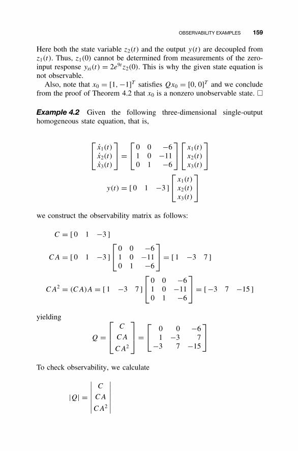
OBSERVABILITY EXAMPLES 159
Here both the state variable z2(t) and the output y(t) are decoupled fromz1(t). Thus, z1(0) cannot be determined from measurements of the zero-input response yzi(t) = 2e9t z2(0). This is why the given state equation isnot observable.
Also, note that x0 = [1, −1]T satisfies Qx0 = [0, 0]T and we concludefrom the proof of Theorem 4.2 that x0 is a nonzero unobservable state. �
Example 4.2 Given the following three-dimensional single-outputhomogeneous state equation, that is,
x1(t)
x2(t)
x3(t)
=
0 0 −6
1 0 −110 1 −6
x1(t)
x2(t)
x3(t)
y(t) = [ 0 1 −3 ]
x1(t)
x2(t)
x3(t)
we construct the observability matrix as follows:
C = [ 0 1 −3 ]
CA = [ 0 1 −3 ]
0 0 −6
1 0 −110 1 −6
= [ 1 −3 7 ]
CA2 = (CA)A = [ 1 −3 7 ]
0 0 −6
1 0 −110 1 −6
= [ −3 7 −15 ]
yielding
Q =
C
CA
CA2
=
0 0 −6
1 −3 7−3 7 −15
To check observability, we calculate
|Q| =
∣∣∣∣∣∣∣C
CA
CA2
∣∣∣∣∣∣∣
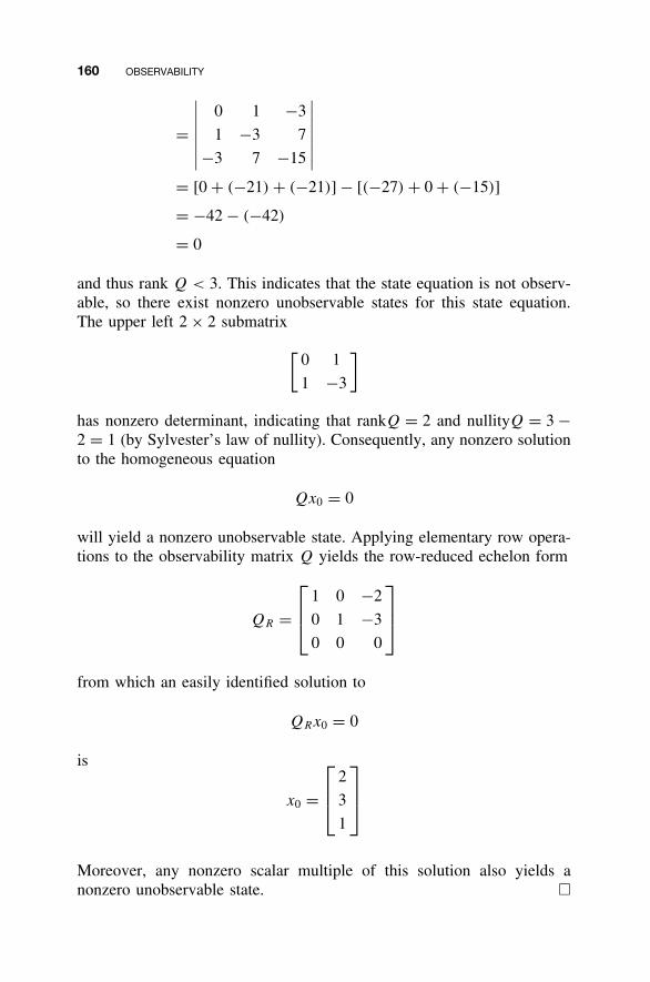
160 OBSERVABILITY
=
∣∣∣∣∣∣∣0 1 −3
1 −3 7
−3 7 −15
∣∣∣∣∣∣∣= [0 + (−21) + (−21)] − [(−27) + 0 + (−15)]
= −42 − (−42)
= 0
and thus rank Q < 3. This indicates that the state equation is not observ-able, so there exist nonzero unobservable states for this state equation.The upper left 2 × 2 submatrix
[0 1
1 −3
]
has nonzero determinant, indicating that rankQ = 2 and nullityQ = 3 −2 = 1 (by Sylvester’s law of nullity). Consequently, any nonzero solutionto the homogeneous equation
Qx0 = 0
will yield a nonzero unobservable state. Applying elementary row opera-tions to the observability matrix Q yields the row-reduced echelon form
QR =
1 0 −2
0 1 −3
0 0 0
from which an easily identified solution to
QRx0 = 0
is
x0 =
2
3
1
Moreover, any nonzero scalar multiple of this solution also yields anonzero unobservable state. �
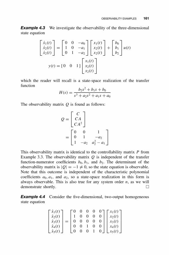
OBSERVABILITY EXAMPLES 161
Example 4.3 We investigate the observability of the three-dimensionalstate equation
x1(t)
x2(t)
x2(t)
=
0 0 −a0
1 0 −a1
0 1 −a2
x1(t)
x2(t)
x2(t)
+
b0
b1
b2
u(t)
y(t) = [ 0 0 1 ]
x1(t)
x2(t)
x2(t)
which the reader will recall is a state-space realization of the transferfunction
H(s) = b2s2 + b1s + b0
s3 + a2s2 + a1s + a0
The observability matrix Q is found as follows:
Q = C
CA
CA2
= 0 0 1
0 1 −a2
1 −a2 a22 − a1
This observability matrix is identical to the controllability matrix P fromExample 3.3. The observability matrix Q is independent of the transferfunction-numerator coefficients b0, b1, and b2. The determinant of theobservability matrix is |Q| = −1 �= 0, so the state equation is observable.Note that this outcome is independent of the characteristic polynomialcoefficients a0, a1, and a2, so a state-space realization in this form isalways observable. This is also true for any system order n, as we willdemonstrate shortly. �
Example 4.4 Consider the five-dimensional, two-output homogeneousstate equation
x1(t)
x2(t)
x3(t)
x4(t)
x5(t)
=
0 0 0 0 01 0 0 0 00 0 0 0 00 0 1 0 00 0 0 1 0
x1(t)
x2(t)
x3(t)
x4(t)
x5(t)
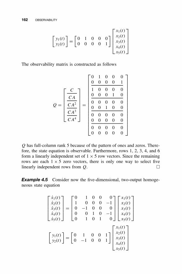
162 OBSERVABILITY
[y1(t)
y2(t)
]=
[0 1 0 0 00 0 0 0 1
]
x1(t)
x2(t)
x3(t)
x4(t)
x5(t)
The observability matrix is constructed as follows
Q =
C
CA
CA2
CA3
CA4
=
0 1 0 0 00 0 0 0 1
1 0 0 0 00 0 0 1 0
0 0 0 0 00 0 1 0 0
0 0 0 0 00 0 0 0 0
0 0 0 0 00 0 0 0 0
Q has full-column rank 5 because of the pattern of ones and zeros. There-fore, the state equation is observable. Furthermore, rows 1, 2, 3, 4, and 6form a linearly independent set of 1 × 5 row vectors. Since the remainingrows are each 1 × 5 zero vectors, there is only one way to select fivelinearly independent rows from Q. �
Example 4.5 Consider now the five-dimensional, two-output homoge-neous state equation
x1(t)
x2(t)
x3(t)
x4(t)
x5(t)
=
0 1 0 0 01 0 0 0 −10 −1 0 0 00 0 1 0 −10 1 0 1 0
x1(t)
x2(t)
x3(t)
x4(t)
x5(t)
[y1(t)
y2(t)
]=
[0 1 0 0 10 −1 0 0 1
]
x1(t)
x2(t)
x3(t)
x4(t)
x5(t)
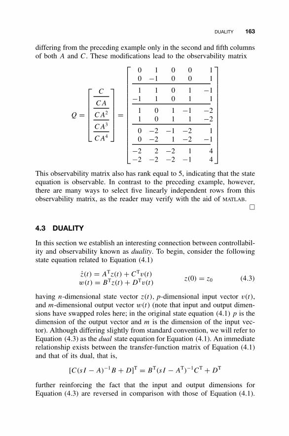
DUALITY 163
differing from the preceding example only in the second and fifth columnsof both A and C. These modifications lead to the observability matrix
Q =
C
CA
CA2
CA3
CA4
=
0 1 0 0 10 −1 0 0 1
1 1 0 1 −1−1 1 0 1 1
1 0 1 −1 −21 0 1 1 −2
0 −2 −1 −2 10 −2 1 −2 −1
−2 2 −2 1 4−2 −2 −2 −1 4
This observability matrix also has rank equal to 5, indicating that the stateequation is observable. In contrast to the preceding example, however,there are many ways to select five linearly independent rows from thisobservability matrix, as the reader may verify with the aid of MATLAB.
�
4.3 DUALITY
In this section we establish an interesting connection between controllabil-ity and observability known as duality. To begin, consider the followingstate equation related to Equation (4.1)
z(t) = ATz(t) + CTv(t)
w(t) = BTz(t) + DTv(t)z(0) = z0 (4.3)
having n-dimensional state vector z(t), p-dimensional input vector v(t),and m-dimensional output vector w(t) (note that input and output dimen-sions have swapped roles here; in the original state equation (4.1) p is thedimension of the output vector and m is the dimension of the input vec-tor). Although differing slightly from standard convention, we will refer toEquation (4.3) as the dual state equation for Equation (4.1). An immediaterelationship exists between the transfer-function matrix of Equation (4.1)and that of its dual, that is,
[C(sI − A)−1B + D]T = BT(sI − AT)−1CT + DT
further reinforcing the fact that the input and output dimensions forEquation (4.3) are reversed in comparison with those of Equation (4.1).
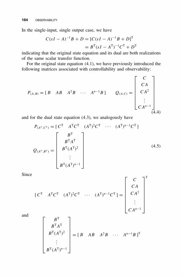
164 OBSERVABILITY
In the single-input, single output case, we have
C(sI − A)−1B + D = [C(sI − A)−1B + D]T
= BT(sI − AT)−1CT + DT
indicating that the original state equation and its dual are both realizationsof the same scalar transfer function.
For the original state equation (4.1), we have previously introduced thefollowing matrices associated with controllability and observability:
P(A,B) = [ B AB A2B · · · An−1B ] Q(A,C) =
C
CA
CA2
...
CAn−1
(4.4)
and for the dual state equation (4.3), we analogously have
P(AT ,CT ) = [ CT ATCT (AT)2CT · · · (AT)n−1CT ]
Q(AT ,BT ) =
BT
BTAT
BT(AT)2
...
BT(AT)n−1
(4.5)
Since
[ CT ATCT (AT)2CT · · · (AT)n−1CT ] =
C
CA
CA2
...
CAn−1
T
and
BT
BTAT
BT(AT)2
...
BT(AT)n−1
= [ B AB A2B · · · An−1B ]T
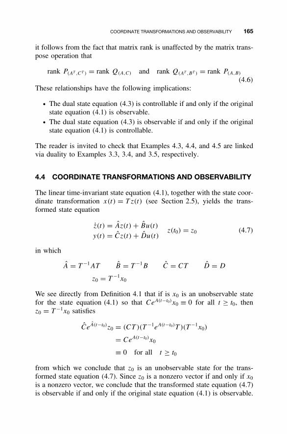
COORDINATE TRANSFORMATIONS AND OBSERVABILITY 165
it follows from the fact that matrix rank is unaffected by the matrix trans-pose operation that
rank P(AT ,CT ) = rank Q(A,C) and rank Q(AT ,BT ) = rank P(A,B)
(4.6)
These relationships have the following implications:
• The dual state equation (4.3) is controllable if and only if the originalstate equation (4.1) is observable.
• The dual state equation (4.3) is observable if and only if the originalstate equation (4.1) is controllable.
The reader is invited to check that Examples 4.3, 4.4, and 4.5 are linkedvia duality to Examples 3.3, 3.4, and 3.5, respectively.
4.4 COORDINATE TRANSFORMATIONS AND OBSERVABILITY
The linear time-invariant state equation (4.1), together with the state coor-dinate transformation x(t) = T z(t) (see Section 2.5), yields the trans-formed state equation
z(t) = Az(t) + Bu(t)
y(t) = Cz(t) + Du(t)z(t0) = z0 (4.7)
in which
A = T −1AT B = T −1B C = CT D = D
z0 = T −1x0
We see directly from Definition 4.1 that if is x0 is an unobservable statefor the state equation (4.1) so that CeA(t−t0)x0 ≡ 0 for all t ≥ t0, thenz0 = T −1x0 satisfies
CeA(t−t0)z0 = (CT )(T −1eA(t−t0)T )(T −1x0)
= CeA(t−t0)x0
≡ 0 for all t ≥ t0
from which we conclude that z0 is an unobservable state for the trans-formed state equation (4.7). Since z0 is a nonzero vector if and only if x0
is a nonzero vector, we conclude that the transformed state equation (4.7)is observable if and only if the original state equation (4.1) is observable.
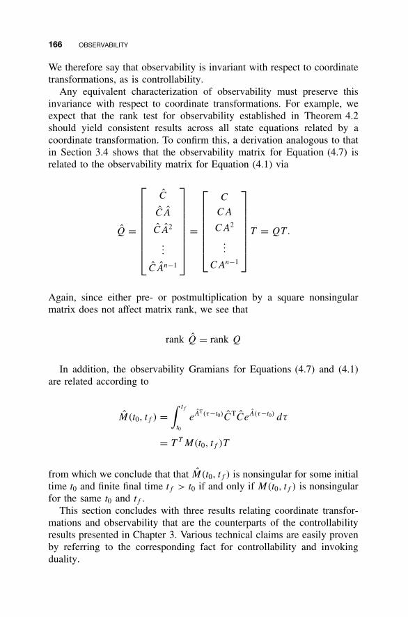
166 OBSERVABILITY
We therefore say that observability is invariant with respect to coordinatetransformations, as is controllability.
Any equivalent characterization of observability must preserve thisinvariance with respect to coordinate transformations. For example, weexpect that the rank test for observability established in Theorem 4.2should yield consistent results across all state equations related by acoordinate transformation. To confirm this, a derivation analogous to thatin Section 3.4 shows that the observability matrix for Equation (4.7) isrelated to the observability matrix for Equation (4.1) via
Q =
C
CA
CA2
...
CAn−1
=
C
CA
CA2
...
CAn−1
T = QT.
Again, since either pre- or postmultiplication by a square nonsingularmatrix does not affect matrix rank, we see that
rank Q = rank Q
In addition, the observability Gramians for Equations (4.7) and (4.1)are related according to
M(t0, tf ) =∫ tf
t0
eAT(τ−t0)CTCeA(τ−t0) dτ
= T T M(t0, tf )T
from which we conclude that that M(t0, tf ) is nonsingular for some initialtime t0 and finite final time tf > t0 if and only if M(t0, tf ) is nonsingularfor the same t0 and tf .
This section concludes with three results relating coordinate transfor-mations and observability that are the counterparts of the controllabilityresults presented in Chapter 3. Various technical claims are easily provenby referring to the corresponding fact for controllability and invokingduality.
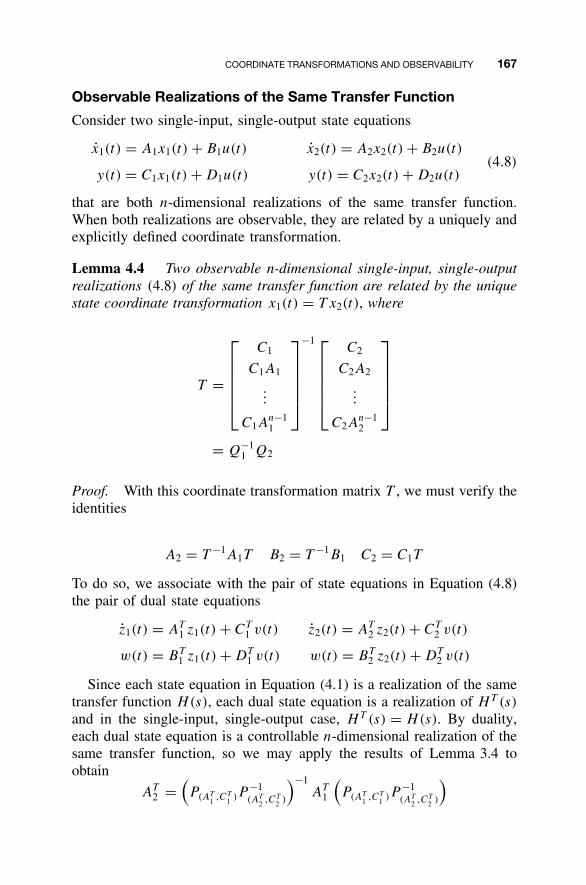
COORDINATE TRANSFORMATIONS AND OBSERVABILITY 167
Observable Realizations of the Same Transfer Function
Consider two single-input, single-output state equations
x1(t) = A1x1(t) + B1u(t) x2(t) = A2x2(t) + B2u(t)
y(t) = C1x1(t) + D1u(t) y(t) = C2x2(t) + D2u(t)(4.8)
that are both n-dimensional realizations of the same transfer function.When both realizations are observable, they are related by a uniquely andexplicitly defined coordinate transformation.
Lemma 4.4 Two observable n-dimensional single-input, single-outputrealizations (4.8) of the same transfer function are related by the uniquestate coordinate transformation x1(t) = T x2(t), where
T =
C1
C1A1
...
C1An−11
−1
C2
C2A2
...
C2An−12
= Q−11 Q2
Proof. With this coordinate transformation matrix T , we must verify theidentities
A2 = T −1A1T B2 = T −1B1 C2 = C1T
To do so, we associate with the pair of state equations in Equation (4.8)the pair of dual state equations
z1(t) = AT1 z1(t) + CT
1 v(t) z2(t) = AT2 z2(t) + CT
2 v(t)
w(t) = BT1 z1(t) + DT
1 v(t) w(t) = BT2 z2(t) + DT
2 v(t)
Since each state equation in Equation (4.1) is a realization of the sametransfer function H(s), each dual state equation is a realization of HT (s)
and in the single-input, single-output case, HT (s) = H(s). By duality,each dual state equation is a controllable n-dimensional realization of thesame transfer function, so we may apply the results of Lemma 3.4 toobtain
AT2 =
(P(AT
1 ,CT1 )P
−1(AT
2 ,CT2 )
)−1AT
1
(P(AT
1 ,CT1 )P
−1(AT
2 ,CT2 )
)
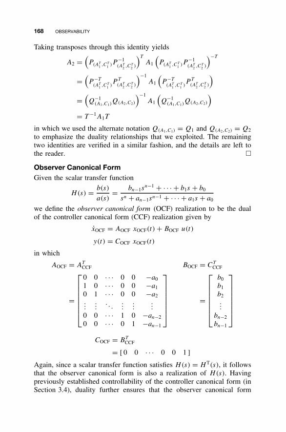
168 OBSERVABILITY
Taking transposes through this identity yields
A2 =(P(AT
1 ,CT1 )P
−1(AT
2 ,CT2 )
)T
A1
(P(AT
1 ,CT1 )P
−1(AT
2 ,CT2 )
)−T
=(P −T
(AT1 ,CT
1 )P T
(AT2 ,CT
2 )
)−1A1
(P −T
(AT1 ,CT
1 )P T
(AT2 ,CT
2 )
)
=(Q−1
(A1,C1)Q(A2,C2)
)−1A1
(Q−1
(A1,C1)Q(A2,C2)
)
= T −1A1T
in which we used the alternate notation Q(A1,C1) = Q1 and Q(A2,C2) = Q2
to emphasize the duality relationships that we exploited. The remainingtwo identities are verified in a similar fashion, and the details are left tothe reader. �
Observer Canonical FormGiven the scalar transfer function
H(s) = b(s)
a(s)= bn−1s
n−1 + · · · + b1s + b0
sn + an−1sn−1 + · · · + a1s + a0
we define the observer canonical form (OCF) realization to be the dualof the controller canonical form (CCF) realization given by
xOCF = AOCF xOCF(t) + BOCF u(t)
y(t) = COCF xOCF(t)
in which
AOCF = ATCCF BOCF = CT
CCF
=
0 0 · · · 0 0 −a0
1 0 · · · 0 0 −a1
0 1 · · · 0 0 −a2...
.... . .
......
...
0 0 · · · 1 0 −an−2
0 0 · · · 0 1 −an−1
=
b0
b1
b2...
bn−2
bn−1
COCF = BTCCF
= [ 0 0 · · · 0 0 1 ]
Again, since a scalar transfer function satisfies H(s) = H T(s), it followsthat the observer canonical form is also a realization of H(s). Havingpreviously established controllability of the controller canonical form (inSection 3.4), duality further ensures that the observer canonical form
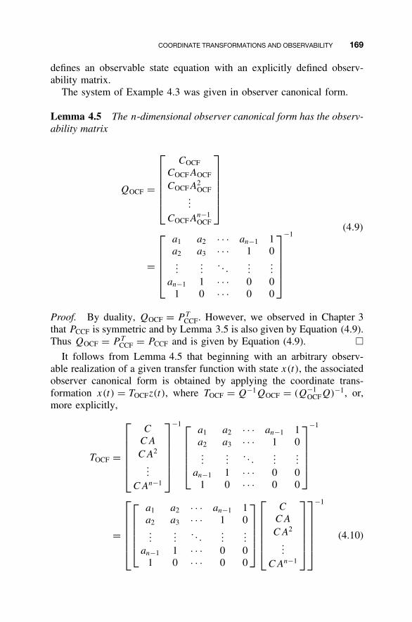
COORDINATE TRANSFORMATIONS AND OBSERVABILITY 169
defines an observable state equation with an explicitly defined observ-ability matrix.
The system of Example 4.3 was given in observer canonical form.
Lemma 4.5 The n-dimensional observer canonical form has the observ-ability matrix
QOCF =
COCF
COCFAOCF
COCFA2OCF
...
COCFAn−1OCF
=
a1 a2 · · · an−1 1a2 a3 · · · 1 0...
.... . .
......
an−1 1 · · · 0 01 0 · · · 0 0
−1(4.9)
Proof. By duality, QOCF = P TCCF. However, we observed in Chapter 3
that PCCF is symmetric and by Lemma 3.5 is also given by Equation (4.9).Thus QOCF = P T
CCF = PCCF and is given by Equation (4.9). �It follows from Lemma 4.5 that beginning with an arbitrary observ-
able realization of a given transfer function with state x(t), the associatedobserver canonical form is obtained by applying the coordinate trans-formation x(t) = TOCFz(t), where TOCF = Q−1QOCF = (Q−1
OCFQ)−1, or,more explicitly,
TOCF =
C
CA
CA2
...
CAn−1
−1
a1 a2 · · · an−1 1a2 a3 · · · 1 0...
.... . .
......
an−1 1 · · · 0 01 0 · · · 0 0
−1
=
a1 a2 · · · an−1 1a2 a3 · · · 1 0...
.... . .
......
an−1 1 · · · 0 01 0 · · · 0 0
C
CA
CA2
...
CAn−1
−1
(4.10)
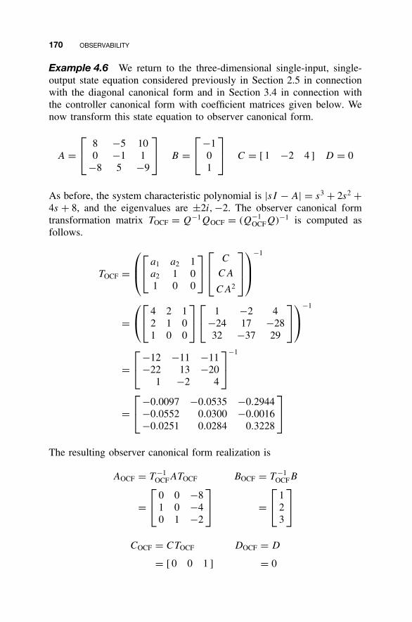
170 OBSERVABILITY
Example 4.6 We return to the three-dimensional single-input, single-output state equation considered previously in Section 2.5 in connectionwith the diagonal canonical form and in Section 3.4 in connection withthe controller canonical form with coefficient matrices given below. Wenow transform this state equation to observer canonical form.
A = 8 −5 10
0 −1 1−8 5 −9
B =
−1
01
C = [ 1 −2 4 ] D = 0
As before, the system characteristic polynomial is |sI − A| = s3 + 2s2 +4s + 8, and the eigenvalues are ±2i,−2. The observer canonical formtransformation matrix TOCF = Q−1QOCF = (Q−1
OCFQ)−1 is computed asfollows.
TOCF =
a1 a2 1
a2 1 01 0 0
C
CA
CA2
−1
=
4 2 1
2 1 01 0 0
1 −2 4
−24 17 −2832 −37 29
−1
= −12 −11 −11
−22 13 −201 −2 4
−1
= −0.0097 −0.0535 −0.2944
−0.0552 0.0300 −0.0016−0.0251 0.0284 0.3228
The resulting observer canonical form realization is
AOCF = T −1OCFATOCF BOCF = T −1
OCFB
= 0 0 −8
1 0 −40 1 −2
=
1
23
COCF = CTOCF DOCF = D
= [ 0 0 1 ] = 0
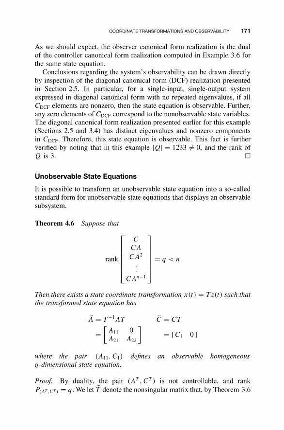
COORDINATE TRANSFORMATIONS AND OBSERVABILITY 171
As we should expect, the observer canonical form realization is the dualof the controller canonical form realization computed in Example 3.6 forthe same state equation.
Conclusions regarding the system’s observability can be drawn directlyby inspection of the diagonal canonical form (DCF) realization presentedin Section 2.5. In particular, for a single-input, single-output systemexpressed in diagonal canonical form with no repeated eigenvalues, if allCDCF elements are nonzero, then the state equation is observable. Further,any zero elements of CDCF correspond to the nonobservable state variables.The diagonal canonical form realization presented earlier for this example(Sections 2.5 and 3.4) has distinct eigenvalues and nonzero componentsin CDCF. Therefore, this state equation is observable. This fact is furtherverified by noting that in this example |Q| = 1233 �= 0, and the rank ofQ is 3. �
Unobservable State Equations
It is possible to transform an unobservable state equation into a so-calledstandard form for unobservable state equations that displays an observablesubsystem.
Theorem 4.6 Suppose that
rank
C
CA
CA2
...
CAn−1
= q < n
Then there exists a state coordinate transformation x(t) = T z(t) such thatthe transformed state equation has
A = T −1AT C = CT
=[
A11 0A21 A22
]= [ C1 0 ]
where the pair (A11, C1) defines an observable homogeneousq-dimensional state equation.
Proof. By duality, the pair (AT , CT ) is not controllable, and rankP(AT ,CT ) = q. We let T denote the nonsingular matrix that, by Theorem 3.6
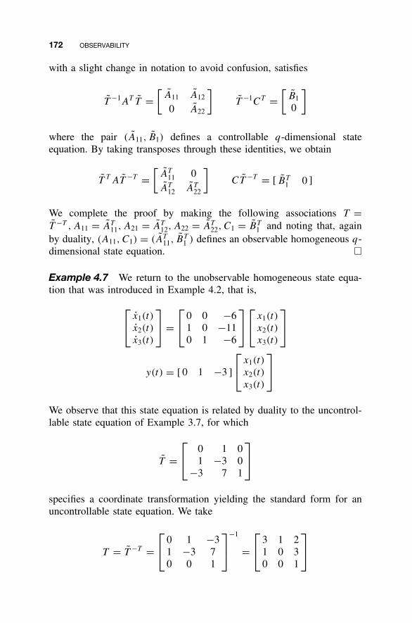
172 OBSERVABILITY
with a slight change in notation to avoid confusion, satisfies
T −1AT T =[
A11 A12
0 A22
]T −1CT =
[B1
0
]
where the pair (A11, B1) defines a controllable q-dimensional stateequation. By taking transposes through these identities, we obtain
T T AT −T =[
AT11 0
AT12 AT
22
]CT −T = [ BT
1 0 ]
We complete the proof by making the following associations T =T −T , A11 = AT
11, A21 = AT12, A22 = AT
22, C1 = BT1 and noting that, again
by duality, (A11, C1) = (AT11, B
T1 ) defines an observable homogeneous q-
dimensional state equation. �
Example 4.7 We return to the unobservable homogeneous state equa-tion that was introduced in Example 4.2, that is,
x1(t)
x2(t)
x3(t)
=
0 0 −6
1 0 −110 1 −6
x1(t)
x2(t)
x3(t)
y(t) = [ 0 1 −3 ]
x1(t)
x2(t)
x3(t)
We observe that this state equation is related by duality to the uncontrol-lable state equation of Example 3.7, for which
T = 0 1 0
1 −3 0−3 7 1
specifies a coordinate transformation yielding the standard form for anuncontrollable state equation. We take
T = T −T = 0 1 −3
1 −3 70 0 1
−1
= 3 1 2
1 0 30 0 1
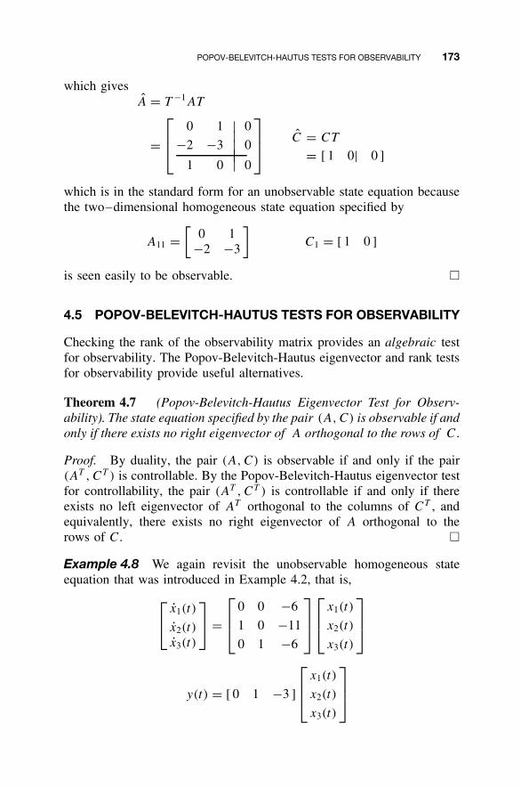
POPOV-BELEVITCH-HAUTUS TESTS FOR OBSERVABILITY 173
which givesA = T −1AT
=
0 1 | 0|−2 −3 | 0||1 0 | 0
C = CT
= [ 1 0| 0 ]
which is in the standard form for an unobservable state equation becausethe two–dimensional homogeneous state equation specified by
A11 =[
0 1−2 −3
]C1 = [ 1 0 ]
is seen easily to be observable. �
4.5 POPOV-BELEVITCH-HAUTUS TESTS FOR OBSERVABILITY
Checking the rank of the observability matrix provides an algebraic testfor observability. The Popov-Belevitch-Hautus eigenvector and rank testsfor observability provide useful alternatives.
Theorem 4.7 (Popov-Belevitch-Hautus Eigenvector Test for Observ-ability). The state equation specified by the pair (A, C) is observable if andonly if there exists no right eigenvector of A orthogonal to the rows of C.
Proof. By duality, the pair (A, C) is observable if and only if the pair(AT , CT ) is controllable. By the Popov-Belevitch-Hautus eigenvector testfor controllability, the pair (AT , CT ) is controllable if and only if thereexists no left eigenvector of AT orthogonal to the columns of CT , andequivalently, there exists no right eigenvector of A orthogonal to therows of C. �
Example 4.8 We again revisit the unobservable homogeneous stateequation that was introduced in Example 4.2, that is,
x1(t)
x2(t)
x3(t)
=
0 0 −6
1 0 −11
0 1 −6
x1(t)
x2(t)
x3(t)
y(t) = [ 0 1 −3 ]
x1(t)
x2(t)
x3(t)
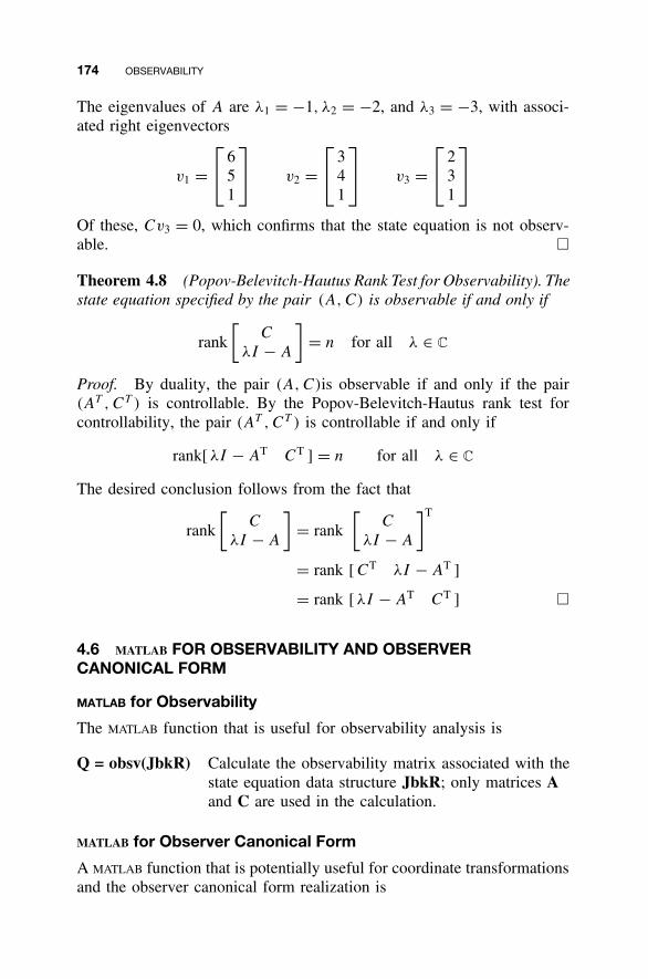
174 OBSERVABILITY
The eigenvalues of A are λ1 = −1, λ2 = −2, and λ3 = −3, with associ-ated right eigenvectors
v1 = 6
51
v2 =
3
41
v3 =
2
31
Of these, Cv3 = 0, which confirms that the state equation is not observ-able. �
Theorem 4.8 (Popov-Belevitch-Hautus Rank Test for Observability). Thestate equation specified by the pair (A, C) is observable if and only if
rank
[C
λI − A
]= n for all λ ∈ C
Proof. By duality, the pair (A, C)is observable if and only if the pair(AT , CT ) is controllable. By the Popov-Belevitch-Hautus rank test forcontrollability, the pair (AT ,CT ) is controllable if and only if
rank[ λI − AT CT ] = n for all λ ∈ C
The desired conclusion follows from the fact that
rank
[C
λI − A
]= rank
[C
λI − A
]T
= rank [ CT λI − AT ]
= rank [ λI − AT CT ] �
4.6 MATLAB FOR OBSERVABILITY AND OBSERVERCANONICAL FORM
MATLAB for Observability
The MATLAB function that is useful for observability analysis is
Q = obsv(JbkR) Calculate the observability matrix associated with thestate equation data structure JbkR; only matrices Aand C are used in the calculation.
MATLAB for Observer Canonical Form
A MATLAB function that is potentially useful for coordinate transformationsand the observer canonical form realization is
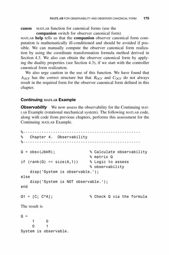
MATLAB FOR OBSERVABILITY AND OBSERVER CANONICAL FORM 175
canon MATLAB function for canonical forms (use thecompanion switch for observer canonical form)
MATLAB help tells us that the companion observer canonical form com-putation is mathematically ill-conditioned and should be avoided if pos-sible. We can manually compute the observer canonical form realiza-tion by using the coordinate transformation formula method derived inSection 4.3. We also can obtain the observer canonical form by apply-ing the duality properties (see Section 4.3), if we start with the controllercanonical form realization.
We also urge caution in the use of this function. We have found thatAOCF has the correct structure but that BOCF and COCF do not alwaysresult in the required form for the observer canonical form defined in thischapter.
Continuing MATLAB Example
Observability We now assess the observability for the Continuing MAT-
LAB Example (rotational mechanical system). The following MATLAB code,along with code from previous chapters, performs this assessment for theContinuing MATLAB Example.
%---------------------------------------------------% Chapter 4. Observability%---------------------------------------------------
Q = obsv(JbkR); % Calculate observability% matrix Q
if (rank(Q) == size(A,1)) % Logic to assess% observability
disp(’System is observable.’);else
disp(’System is NOT observable.’);end
Q1 = [C; C*A]; % Check Q via the formula
The result is
Q =1 00 1
System is observable.
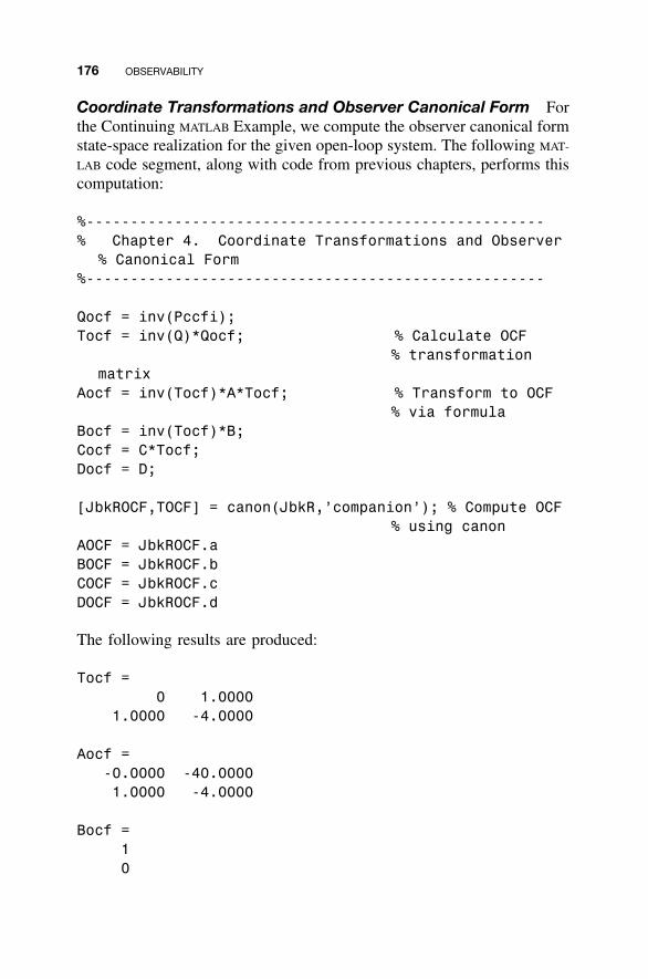
176 OBSERVABILITY
Coordinate Transformations and Observer Canonical Form Forthe Continuing MATLAB Example, we compute the observer canonical formstate-space realization for the given open-loop system. The following MAT-
LAB code segment, along with code from previous chapters, performs thiscomputation:
%----------------------------------------------------% Chapter 4. Coordinate Transformations and Observer
% Canonical Form%----------------------------------------------------
Qocf = inv(Pccfi);Tocf = inv(Q)*Qocf; % Calculate OCF
% transformationmatrix
Aocf = inv(Tocf)*A*Tocf; % Transform to OCF% via formula
Bocf = inv(Tocf)*B;Cocf = C*Tocf;Docf = D;
[JbkROCF,TOCF] = canon(JbkR,’companion’); % Compute OCF% using canon
AOCF = JbkROCF.aBOCF = JbkROCF.bCOCF = JbkROCF.cDOCF = JbkROCF.d
The following results are produced:
Tocf =0 1.0000
1.0000 -4.0000
Aocf =-0.0000 -40.00001.0000 -4.0000
Bocf =10
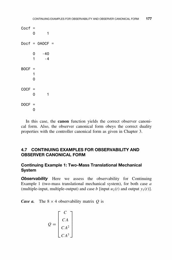
CONTINUING EXAMPLES FOR OBSERVABILITY AND OBSERVER CANONICAL FORM 177
Cocf =0 1
Docf = 0AOCF =
0 -401 -4
BOCF =10
COCF =0 1
DOCF =0
In this case, the canon function yields the correct observer canoni-cal form. Also, the observer canonical form obeys the correct dualityproperties with the controller canonical form as given in Chapter 3.
4.7 CONTINUING EXAMPLES FOR OBSERVABILITY ANDOBSERVER CANONICAL FORM
Continuing Example 1: Two-Mass Translational MechanicalSystem
Observability Here we assess the observability for ContinuingExample 1 (two-mass translational mechanical system), for both case a
(multiple-input, multiple-output) and case b [input u2(t) and output y1(t)].
Case a. The 8 × 4 observability matrix Q is
Q =
C
CA
CA2
CA3
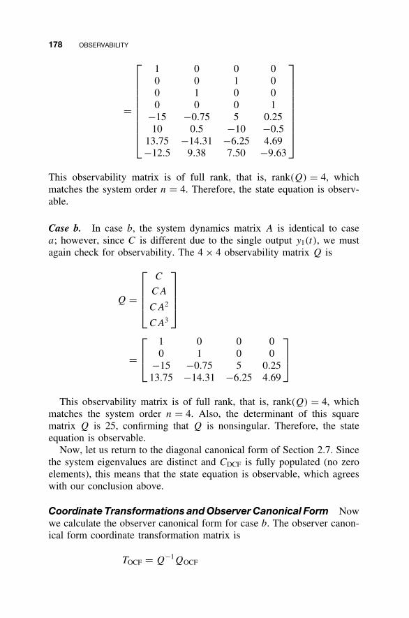
178 OBSERVABILITY
=
1 0 0 00 0 1 00 1 0 00 0 0 1
−15 −0.75 5 0.2510 0.5 −10 −0.5
13.75 −14.31 −6.25 4.69−12.5 9.38 7.50 −9.63
This observability matrix is of full rank, that is, rank(Q) = 4, whichmatches the system order n = 4. Therefore, the state equation is observ-able.
Case b. In case b, the system dynamics matrix A is identical to casea; however, since C is different due to the single output y1(t), we mustagain check for observability. The 4 × 4 observability matrix Q is
Q =
C
CA
CA2
CA3
=
1 0 0 00 1 0 0
−15 −0.75 5 0.2513.75 −14.31 −6.25 4.69
This observability matrix is of full rank, that is, rank(Q) = 4, whichmatches the system order n = 4. Also, the determinant of this squarematrix Q is 25, confirming that Q is nonsingular. Therefore, the stateequation is observable.
Now, let us return to the diagonal canonical form of Section 2.7. Sincethe system eigenvalues are distinct and CDCF is fully populated (no zeroelements), this means that the state equation is observable, which agreeswith our conclusion above.
Coordinate Transformations and Observer Canonical Form Nowwe calculate the observer canonical form for case b. The observer canon-ical form coordinate transformation matrix is
TOCF = Q−1QOCF
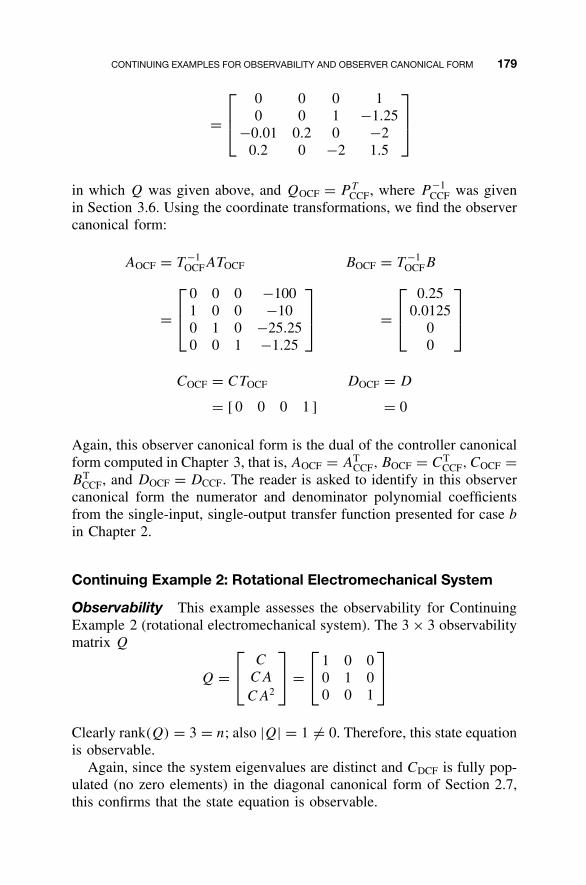
CONTINUING EXAMPLES FOR OBSERVABILITY AND OBSERVER CANONICAL FORM 179
=
0 0 0 10 0 1 −1.25
−0.01 0.2 0 −20.2 0 −2 1.5
in which Q was given above, and QOCF = P TCCF, where P −1
CCF was givenin Section 3.6. Using the coordinate transformations, we find the observercanonical form:
AOCF = T −1OCFATOCF BOCF = T −1
OCFB
=
0 0 0 −1001 0 0 −100 1 0 −25.250 0 1 −1.25
=
0.250.0125
00
COCF = CTOCF DOCF = D
= [ 0 0 0 1 ] = 0
Again, this observer canonical form is the dual of the controller canonicalform computed in Chapter 3, that is, AOCF = AT
CCF, BOCF = CTCCF, COCF =
BTCCF, and DOCF = DCCF. The reader is asked to identify in this observer
canonical form the numerator and denominator polynomial coefficientsfrom the single-input, single-output transfer function presented for case b
in Chapter 2.
Continuing Example 2: Rotational Electromechanical System
Observability This example assesses the observability for ContinuingExample 2 (rotational electromechanical system). The 3 × 3 observabilitymatrix Q
Q = C
CA
CA2
=
1 0 0
0 1 00 0 1
Clearly rank(Q) = 3 = n; also |Q| = 1 �= 0. Therefore, this state equationis observable.
Again, since the system eigenvalues are distinct and CDCF is fully pop-ulated (no zero elements) in the diagonal canonical form of Section 2.7,this confirms that the state equation is observable.
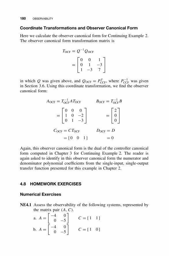
180 OBSERVABILITY
Coordinate Transformations and Observer Canonical Form
Here we calculate the observer canonical form for Continuing Example 2.The observer canonical form transformation matrix is
TOCF = Q−1QOCF
= 0 0 1
0 1 −31 −3 7
in which Q was given above, and QOCF = P TCCF, where P −1
CCF was givenin Section 3.6. Using this coordinate transformation, we find the observercanonical form:
AOCF = T −1OCFATOCF BOCF = T −1
OCFB
= 0 0 0
1 0 −20 1 −3
=
2
00
COCF = CTOCF DOCF = D
= [ 0 0 1 ] = 0
Again, this observer canonical form is the dual of the controller canonicalform computed in Chapter 3 for Continuing Example 2. The reader isagain asked to identify in this observer canonical form the numerator anddenominator polynomial coefficients from the single-input, single-outputtransfer function presented for this example in Chapter 2.
4.8 HOMEWORK EXERCISES
Numerical Exercises
NE4.1 Assess the observability of the following systems, represented bythe matrix pair (A, C).
a. A =[ −4 0
0 −5
]C = [ 1 1 ]
b. A =[ −4 0
0 −5
]C = [ 1 0 ]
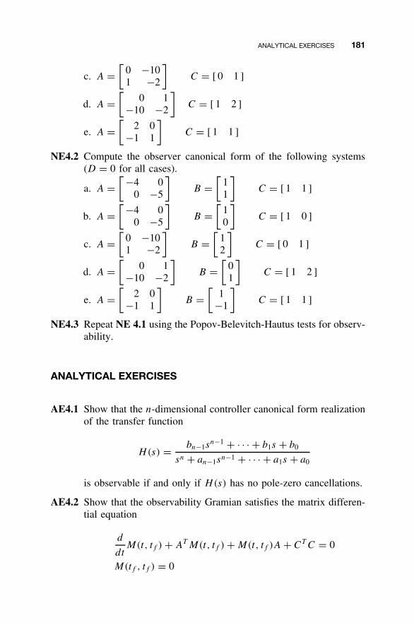
ANALYTICAL EXERCISES 181
c. A =[
0 −101 −2
]C = [ 0 1 ]
d. A =[
0 1−10 −2
]C = [ 1 2 ]
e. A =[
2 0−1 1
]C = [ 1 1 ]
NE4.2 Compute the observer canonical form of the following systems(D = 0 for all cases).
a. A =[ −4 0
0 −5
]B =
[11
]C = [ 1 1 ]
b. A =[ −4 0
0 −5
]B =
[10
]C = [ 1 0 ]
c. A =[
0 −101 −2
]B =
[12
]C = [ 0 1 ]
d. A =[
0 1−10 −2
]B =
[01
]C = [ 1 2 ]
e. A =[
2 0−1 1
]B =
[1
−1
]C = [ 1 1 ]
NE4.3 Repeat NE 4.1 using the Popov-Belevitch-Hautus tests for observ-ability.
ANALYTICAL EXERCISES
AE4.1 Show that the n-dimensional controller canonical form realizationof the transfer function
H(s) = bn−1sn−1 + · · · + b1s + b0
sn + an−1sn−1 + · · · + a1s + a0
is observable if and only if H(s) has no pole-zero cancellations.
AE4.2 Show that the observability Gramian satisfies the matrix differen-tial equation
d
dtM(t, tf ) + AT M(t, tf ) + M(t, tf )A + CT C = 0
M(tf , tf ) = 0
182 OBSERVABILITY
AE4.3 Show that the matrix exponential for[A 0
−CT C −AT
]
is given by [eAt 0
−e−AT tM(0, t) e−AT t
]
AE4.4 Show that the homogeneous single-output state equation charac-terized by
A =
µ 1 0 · · · 00 µ 1 · · · 0...
......
. . ....
0 0 0 · · · 10 0 0 · · · µ
C = [ c1 c2 · · · cn−1 cn ]
is observable if and only if c1 �= 0.
AE4.5 Show that the pair (A, C) is observable if and only if the onlysquare matrix X that satisfies
AX = XA CX = 0is X = 0.
AE4.6 Show that the pair (A, C) is observable if and only if the pair(A − LC, HC) is observable for any n × p matrix L and anynonsingular p × p matrix H .
AE4.7 Show that the homogeneous multiple-output system[x1(t)
x2(t)
]=
[A11 A12
A21 A22
] [x1(t)
x2(t)
]
y(t) = [C1 0
] [x1(t)
x2(t)
]
with C1 nonsingular is observable if and only if the homogeneoussystem
x2(t) = A22x2(t)
y2(t) = A12x2(t)
is observable.
ANALYTICAL EXERCISES 183
Continuing MATLAB Exercises
CME4.1 For the CME1.1 system:a. Assess the system observability.b. Compute the observer canonical form. Compare with the
controller canonical form from CME3.1b.
CME4.2 For the CME1.2 system:a. Assess the system observability.b. Compute the observer canonical form. Compare with the
controller canonical form from CME3.2b.
CME4.3 For the CME1.3 system:a. Assess the system observability.b. Compute the observer canonical form. Compare with the
controller canonical form from CME3.3b.
CME4.4 For the CME1.4 system:a. Assess the system observability.b. Compute the observer canonical form. Compare with the
controller canonical form from CME3.4b.
Continuing Exercises
CE4.1a Determine if the CE1 system is observable for all three cases(cases from CE1.1b and numeric parameters from CE2.1a).
CE4.1b Calculate the observer canonical form realization numerically forthe CE1 system, case iii only. Demonstrate the duality relation-ship between controller canonical form (CE3.1b) and observercanonical form. Assess the system observability by looking atthe diagonal canonical form realization of CE2.1b; compare withyour results from CE4.1a.
CE4.2a Determine if the CE2 system is observable for all three cases(cases from CE1.2b and numeric parameters from CE2.2a).
CE4.2b Calculate the observer canonical form realization numerically forthe CE2 system, case i only. Demonstrate the duality relation-ship between controller canonical form (CE3.2b) and observercanonical form.
CE4.3a Determine if the CE3 system is observable for both cases (casesfrom CE1.3b and numeric parameters from CE2.3a).
184 OBSERVABILITY
CE4.3b Calculate the observer canonical form realization numerically forthe CE3 system for both cases. Demonstrate the duality relation-ship between controller canonical form (CE3.3b) and observercanonical form. Assess the system observability by looking atthe diagonal canonical form realization of CE2.3b; compare withyour results from CE4.3a.
CE4.4a Determine if the CE4 system is observable (for the CE1.4bsingle-input, single-output case and with the numeric parametersfrom CE2.4a).
CE4.4b Calculate the observer canonical form realization numerically forthe CE4 system. Assess the system observability by looking atthe diagonal canonical form realization from CE 2.4b; comparewith your results from CE4.4a.
CE4.5a Determine if the CE5 system is observable (for the CE1.5bsingle-input, single-output case and with the numeric parametersfrom CE2.5a).
CE4.5b Calculate the observer canonical form realization numerically forthe CE5 system. Assess the system observability by looking atthe diagonal canonical form realization from CE2.5b; comparewith your results from CE4.5a.
5
MINIMAL REALIZATIONS
We have observed that a specified transfer function has more than onestate-space realization because, starting with a particular realization, anyvalid coordinate transformation yields another state-space realization withthe same dimension. Moreover, we have seen in a previous example thata given transfer function may have realizations of different dimension.This motivates the notion of a minimal realization of a particular trans-fer function, namely, a realization of least dimension out of all possiblerealizations.
It is clearly impractical to assess the minimality of a particular realiza-tion by comparing its dimension against that of all others. We thereforeare interested in verifiable conditions for minimality. In this chapter wedevelop such conditions, first for single-input, single-output state equationshaving scalar transfer functions. In this case, there is an immediate linkbetween minimality of a realization and possible pole-zero cancellationsin the associated transfer function. Aided by this fact, along with theability to write down state-space realizations by inspection of the trans-fer function, we strike an interesting connection between minimality of astate-space realization and its controllability and observability properties.
This analysis cannot be extended readily to multiple-input, multiple-output state equations because of several complications arising from thefact that the associated transfer functions are matrices of rational functions.
185
Linear State-Space Control Systems. Robert L. Williams II and Douglas A. LawrenceCopyright 2007 John Wiley & Sons, Inc. ISBN: 978-0-471-73555-7
186 MINIMAL REALIZATIONS
First, it is not immediately clear how to extend the notions of polesand zeros to the multiple-input, multiple-output case. Another reason isthat the process of constructing a state-space realization from a transfer-function matrix is not nearly as straightforward as in the single-input,single-output case. Nevertheless, we derive the same result obtained in thesingle-input, single-output case for multiple-input, multiple-output stateequations, albeit by different means.
Often in real-world problems, systems are modeled in the least possiblesize, and there are no pole/zero cancellations. Therefore, most of ourcontinuing examples and exercises are already in minimal form, and hencethere is nothing to present for these in this chapter. We present a MATLAB
section to demonstrate the computation of minimal realizations.
5.1 MINIMALITY OF SINGLE-INPUT, SINGLE OUTPUTREALIZATIONS
Recall that the linear time-invariant state equation
x(t) = Ax(t) + Bu(t)
y(t) = Cx(t) + Du(t) (5.1)
is a state-space realization of a linear time-invariant system’s input-outputbehavior if, given the associated transfer function H(s), the coefficientmatrices satisfy
C(sI − A)−1B + D = H(s)
We consider a single-input, single-output system with scalar transferfunction
H(s) = b(s)
a(s)= bn−1s
n−1 + · · · + b1s + b0
sn + an−1sn−1 + · · · + a1s + a0(5.2)
in which n defines the degree of the denominator polynomial a(s) andhence the order of the transfer function. Also note that we have specifieda strictly proper transfer function. This is essentially for convenience anddoes not affect any of the conclusions drawn in this section (as the readermay check). We call H(s) irreducible if it has no pole-zero cancellations,and equivalently, its numerator and denominator polynomials have nocommon roots/factors.
Suppose that we have an n–dimensional realization of H(s). Now itis clear that if the nth-order transfer function has one or more pole-zero
MINIMALITY OF SINGLE-INPUT, SINGLE OUTPUT REALIZATIONS 187
cancellations, then, on canceling the corresponding factors in a(s) andb(s), we can write
H(s) = b(s)
a(s)
with n = degree a(s) < n. It is clear that there is a state-space realiza-tion of H(s) with dimension n [say either controller canonical formor observer canonical form written down by inspection from the coef-ficients of a(s) and b(s)], so the original n–dimensional realization is notminimal.
Conversely, suppose that we have an n–dimensional realization of thenth–order transfer function H(s) that is not minimal, so there existsanother realization of strictly lower dimension. Let (A, B, C) denote thecoefficient matrices for this realization and n denote its dimension. Since,by definition of the matrix adjoint, adj(sI − A) is an n × n matrix ofpolynomials of degree strictly less than n, it follows that
b(s) = C adj(sI − A)B
is a scalar polynomial of degree strictly less than n. This along with
a(s) = |sI − A|allows us to write
H(s) = C(sI − A)−1B
= C adj(sI − A)B
|sI − A|
= b(s)
a(s)
We then conclude from the fact that degree a(s) = n < n that a(s) andb(s) must have at least one common factor and that H(s) is therefore notirreducible. The preceding argument can be summarized as follows.
Theorem 5.1 Given the transfer function H(s) in Equation (5.2) withn = degree a(s), an n–dimensional realization of H(s) is minimal if andonly if H(s) is irreducible.
Toward relating minimality of a realization to its controllability andobservability properties, we consider the following example.
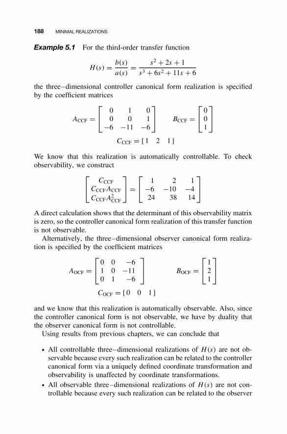
188 MINIMAL REALIZATIONS
Example 5.1 For the third-order transfer function
H(s) = b(s)
a(s)= s2 + 2s + 1
s3 + 6s2 + 11s + 6
the three–dimensional controller canonical form realization is specifiedby the coefficient matrices
ACCF = 0 1 0
0 0 1−6 −11 −6
BCCF =
0
01
CCCF = [ 1 2 1 ]
We know that this realization is automatically controllable. To checkobservability, we construct
CCCF
CCCFACCF
CCCFA2CCF
=
1 2 1
−6 −10 −424 38 14
A direct calculation shows that the determinant of this observability matrixis zero, so the controller canonical form realization of this transfer functionis not observable.
Alternatively, the three–dimensional observer canonical form realiza-tion is specified by the coefficient matrices
AOCF = 0 0 −6
1 0 −110 1 −6
BOCF =
1
21
COCF = [ 0 0 1 ]
and we know that this realization is automatically observable. Also, sincethe controller canonical form is not observable, we have by duality thatthe observer canonical form is not controllable.
Using results from previous chapters, we can conclude that
• All controllable three–dimensional realizations of H(s) are not ob-servable because every such realization can be related to the controllercanonical form via a uniquely defined coordinate transformation andobservability is unaffected by coordinate transformations.
• All observable three–dimensional realizations of H(s) are not con-trollable because every such realization can be related to the observer
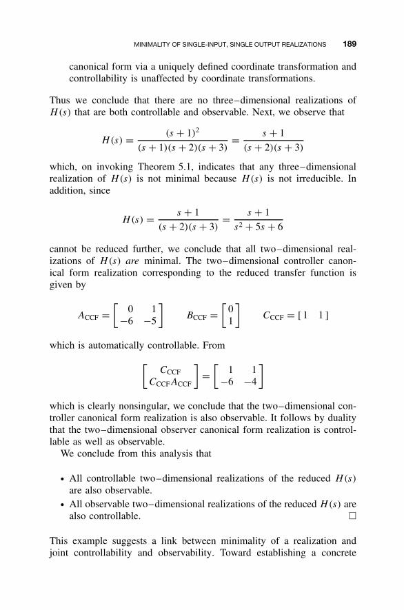
MINIMALITY OF SINGLE-INPUT, SINGLE OUTPUT REALIZATIONS 189
canonical form via a uniquely defined coordinate transformation andcontrollability is unaffected by coordinate transformations.
Thus we conclude that there are no three–dimensional realizations ofH(s) that are both controllable and observable. Next, we observe that
H(s) = (s + 1)2
(s + 1)(s + 2)(s + 3)= s + 1
(s + 2)(s + 3)
which, on invoking Theorem 5.1, indicates that any three–dimensionalrealization of H(s) is not minimal because H(s) is not irreducible. Inaddition, since
H(s) = s + 1
(s + 2)(s + 3)= s + 1
s2 + 5s + 6
cannot be reduced further, we conclude that all two–dimensional real-izations of H(s) are minimal. The two–dimensional controller canon-ical form realization corresponding to the reduced transfer function isgiven by
ACCF =[
0 1−6 −5
]BCCF =
[01
]CCCF = [ 1 1 ]
which is automatically controllable. From
[CCCF
CCCFACCF
]=
[1 1
−6 −4
]
which is clearly nonsingular, we conclude that the two–dimensional con-troller canonical form realization is also observable. It follows by dualitythat the two–dimensional observer canonical form realization is control-lable as well as observable.
We conclude from this analysis that
• All controllable two–dimensional realizations of the reduced H(s)
are also observable.• All observable two–dimensional realizations of the reduced H(s) are
also controllable. �
This example suggests a link between minimality of a realization andjoint controllability and observability. Toward establishing a concrete
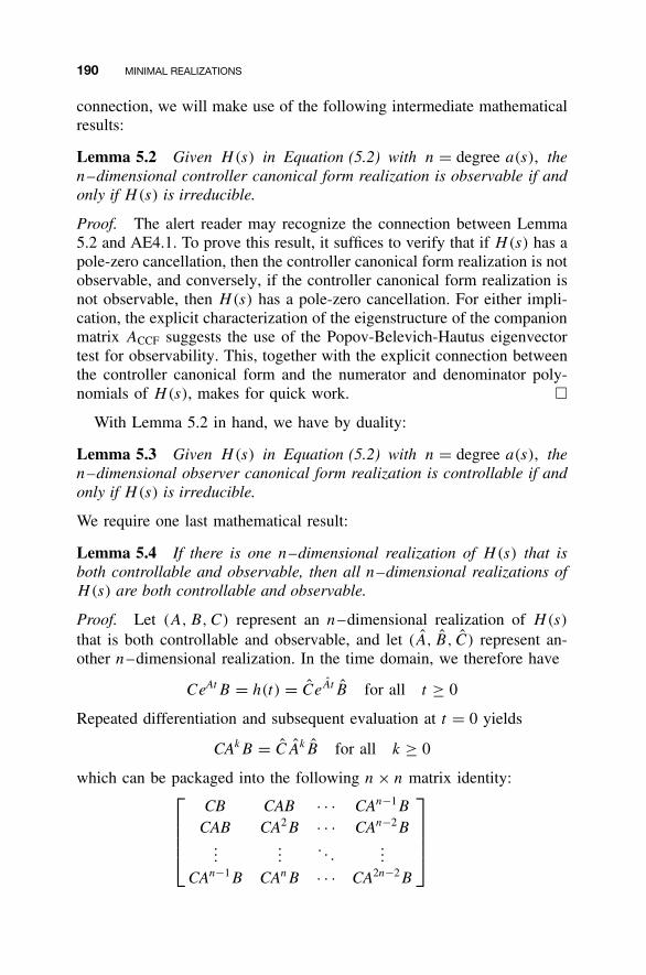
190 MINIMAL REALIZATIONS
connection, we will make use of the following intermediate mathematicalresults:
Lemma 5.2 Given H(s) in Equation (5.2) with n = degree a(s), then–dimensional controller canonical form realization is observable if andonly if H(s) is irreducible.
Proof. The alert reader may recognize the connection between Lemma5.2 and AE4.1. To prove this result, it suffices to verify that if H(s) has apole-zero cancellation, then the controller canonical form realization is notobservable, and conversely, if the controller canonical form realization isnot observable, then H(s) has a pole-zero cancellation. For either impli-cation, the explicit characterization of the eigenstructure of the companionmatrix ACCF suggests the use of the Popov-Belevich-Hautus eigenvectortest for observability. This, together with the explicit connection betweenthe controller canonical form and the numerator and denominator poly-nomials of H(s), makes for quick work. �
With Lemma 5.2 in hand, we have by duality:
Lemma 5.3 Given H(s) in Equation (5.2) with n = degree a(s), then–dimensional observer canonical form realization is controllable if andonly if H(s) is irreducible.
We require one last mathematical result:
Lemma 5.4 If there is one n–dimensional realization of H(s) that isboth controllable and observable, then all n–dimensional realizations ofH(s) are both controllable and observable.
Proof. Let (A, B, C) represent an n–dimensional realization of H(s)
that is both controllable and observable, and let (A, B, C) represent an-other n–dimensional realization. In the time domain, we therefore have
CeAtB = h(t) = CeAt B for all t ≥ 0
Repeated differentiation and subsequent evaluation at t = 0 yields
CAkB = CAkB for all k ≥ 0
which can be packaged into the following n × n matrix identity:
CB CAB · · · CAn−1B
CAB CA2B · · · CAn−2B...
.... . .
...
CAn−1B CAnB · · · CA2n−2B
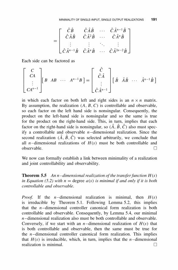
MINIMALITY OF SINGLE-INPUT, SINGLE OUTPUT REALIZATIONS 191
=
CB CAB · · · CAn−1B
CAB CA2B · · · CAnB...
.... . .
...
CAn−1B CAnB · · · CA2n−2B
Each side can be factored as
C
CA...
CAn−1
[B AB · · · An−1B
] =
C
CA...
CAn−1
[B AB · · · An−1B
]
in which each factor on both left and right sides is an n × n matrix.By assumption, the realization (A, B, C) is controllable and observable,so each factor on the left hand side is nonsingular. Consequently, theproduct on the left-hand side is nonsingular and so the same is truefor the product on the right-hand side. This, in turn, implies that eachfactor on the right-hand side is nonsingular, so (A, B, C) also must spec-ify a controllable and observable n–dimensional realization. Since thesecond realization (A, B, C) was selected arbitrarily, we conclude thatall n–dimensional realizations of H(s) must be both controllable andobservable. �
We now can formally establish a link between minimality of a realizationand joint controllability and observability.
Theorem 5.5 An n–dimensional realization of the transfer function H(s)
in Equation (5.2) with n = degree a(s) is minimal if and only if it is bothcontrollable and observable.
Proof. If the n–dimensional realization is minimal, then H(s)
is irreducible by Theorem 5.1. Following Lemma 5.2, this impliesthat the n–dimensional controller canonical form realization is bothcontrollable and observable. Consequently, by Lemma 5.4, our minimaln–dimensional realization also must be both controllable and observable.Conversely, if we start with an n–dimensional realization of H(s) thatis both controllable and observable, then the same must be true forthe n–dimensional controller canonical form realization. This impliesthat H(s) is irreducible, which, in turn, implies that the n–dimensionalrealization is minimal. �
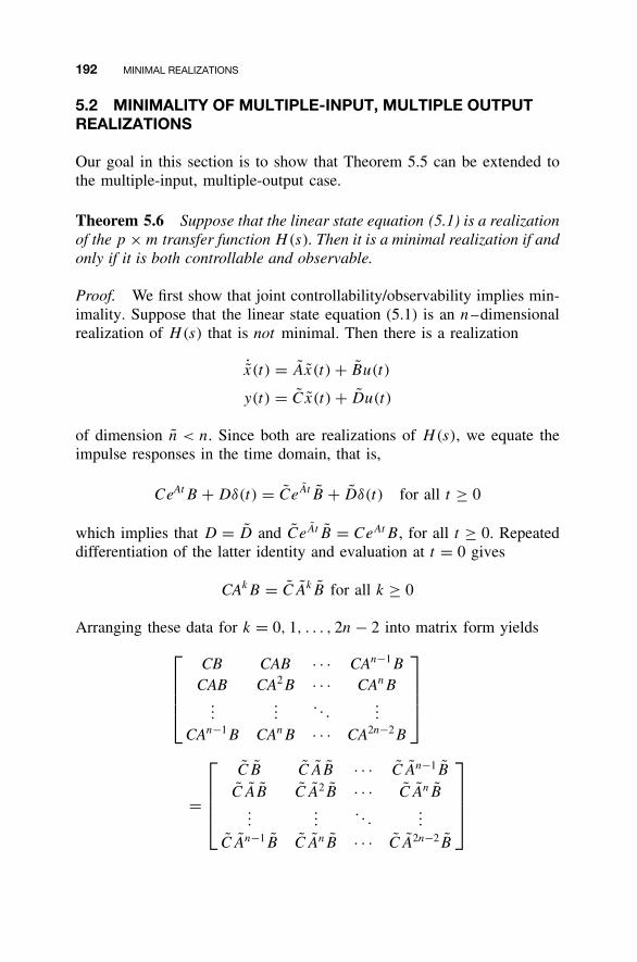
192 MINIMAL REALIZATIONS
5.2 MINIMALITY OF MULTIPLE-INPUT, MULTIPLE OUTPUTREALIZATIONS
Our goal in this section is to show that Theorem 5.5 can be extended tothe multiple-input, multiple-output case.
Theorem 5.6 Suppose that the linear state equation (5.1) is a realizationof the p × m transfer function H(s). Then it is a minimal realization if andonly if it is both controllable and observable.
Proof. We first show that joint controllability/observability implies min-imality. Suppose that the linear state equation (5.1) is an n–dimensionalrealization of H(s) that is not minimal. Then there is a realization
˙x(t) = Ax(t) + Bu(t)
y(t) = Cx(t) + Du(t)
of dimension n < n. Since both are realizations of H(s), we equate theimpulse responses in the time domain, that is,
CeAtB + Dδ(t) = CeAt B + Dδ(t) for all t ≥ 0
which implies that D = D and CeAt B = CeAtB, for all t ≥ 0. Repeateddifferentiation of the latter identity and evaluation at t = 0 gives
CAkB = CAkB for all k ≥ 0
Arranging these data for k = 0, 1, . . . , 2n − 2 into matrix form yields
CB CAB · · · CAn−1B
CAB CA2B · · · CAnB...
.... . .
...
CAn−1B CAnB · · · CA2n−2B
=
CB CAB · · · CAn−1B
CAB CA2B · · · CAnB...
.... . .
...
CAn−1B CAnB · · · CA2n−2B
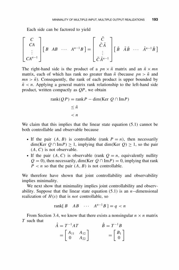
MINIMALITY OF MULTIPLE-INPUT, MULTIPLE OUTPUT REALIZATIONS 193
Each side can be factored to yield
C
CA...
CAn−1
[B AB · · · An−1B
] =
C
CA...
CAn−1
[B AB · · · An−1B
]
The right-hand side is the product of a pn × n matrix and an n × mn
matrix, each of which has rank no greater than n (because pn > n andmn > n). Consequently, the rank of each product is upper bounded byn < n. Applying a general matrix rank relationship to the left-hand sideproduct, written compactly as QP , we obtain
rank(QP ) = rankP − dim(Ker Q ∩ ImP)
≤ n
< n
We claim that this implies that the linear state equation (5.1) cannot beboth controllable and observable because
• If the pair (A, B) is controllable (rank P = n), then necessarilydim(Ker Q ∩ ImP) ≥ 1, implying that dim(Ker Q) ≥ 1, so the pair(A, C) is not observable.
• If the pair (A, C) is observable (rank Q = n, equivalently nullityQ = 0), then necessarily, dim(Ker Q ∩ ImP) = 0, implying that rankP < n so that the pair (A, B) is not controllable.
We therefore have shown that joint controllability and observabilityimplies minimality.
We next show that minimality implies joint controllability and observ-ability. Suppose that the linear state equation (5.1) is an n–dimensionalrealization of H(s) that is not controllable, so
rank[ B AB · · · An−1B ] = q < n
From Section 3.4, we know that there exists a nonsingular n × n matrixT such that
A = T −1AT B = T −1B
=[
A11 A12
0 A22
]=
[B1
0
]
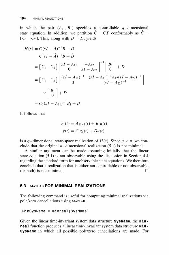
194 MINIMAL REALIZATIONS
in which the pair (A11, B1) specifies a controllable q –dimensionalstate equation. In addition, we partition C = CT conformably as C =[ C1 C2 ]. This, along with D = D, yields
H(s) = C(sI − A)−1B + D
= C(sI − A)−1B + D
= [C1 C2
] [sI − A11 −A12
0 sI − A22
]−1 [B1
0
]+ D
= [C1 C2
] [(sI − A11)
−1 (sI − A11)−1A12(sI − A22)
−1
0 (sI − A22)−1
]
×[
B1
0
]+ D
= C1(sI − A11)−1B1 + D
It follows that
z1(t) = A11z1(t) + B1u(t)
y(t) = C1z1(t) + Du(t)
is a q –dimensional state-space realization of H(s). Since q < n, we con-clude that the original n–dimensional realization (5.1) is not minimal.
A similar argument can be made assuming initially that the linearstate equation (5.1) is not observable using the discussion in Section 4.4regarding the standard form for unobservable state equations. We thereforeconclude that a realization that is either not controllable or not observable(or both) is not minimal. �
5.3 MATLAB FOR MINIMAL REALIZATIONS
The following command is useful for computing minimal realizations viapole/zero cancellations using MATLAB.
MinSysName = minreal(SysName)
Given the linear time-invariant system data structure SysName, the min-real function produces a linear time-invariant system data structure Min-SysName in which all possible pole/zero cancellations are made. For
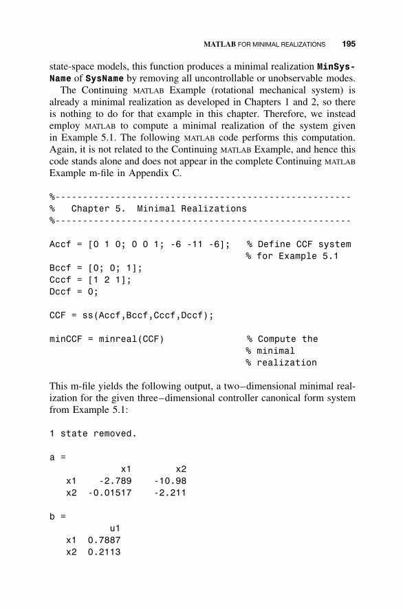
MATLAB FOR MINIMAL REALIZATIONS 195
state-space models, this function produces a minimal realization MinSys-Name of SysName by removing all uncontrollable or unobservable modes.
The Continuing MATLAB Example (rotational mechanical system) isalready a minimal realization as developed in Chapters 1 and 2, so thereis nothing to do for that example in this chapter. Therefore, we insteademploy MATLAB to compute a minimal realization of the system givenin Example 5.1. The following MATLAB code performs this computation.Again, it is not related to the Continuing MATLAB Example, and hence thiscode stands alone and does not appear in the complete Continuing MATLAB
Example m-file in Appendix C.
%------------------------------------------------------% Chapter 5. Minimal Realizations%------------------------------------------------------
Accf = [0 1 0; 0 0 1; -6 -11 -6]; % Define CCF system% for Example 5.1
Bccf = [0; 0; 1];Cccf = [1 2 1];Dccf = 0;
CCF = ss(Accf,Bccf,Cccf,Dccf);
minCCF = minreal(CCF) % Compute the% minimal% realization
This m-file yields the following output, a two–dimensional minimal real-ization for the given three–dimensional controller canonical form systemfrom Example 5.1:
1 state removed.
a =x1 x2
x1 -2.789 -10.98x2 -0.01517 -2.211
b =u1
x1 0.7887x2 0.2113
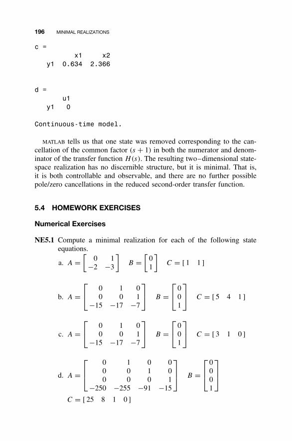
196 MINIMAL REALIZATIONS
c =x1 x2
y1 0.634 2.366
d =u1
y1 0
Continuous-time model.
MATLAB tells us that one state was removed corresponding to the can-cellation of the common factor (s + 1) in both the numerator and denom-inator of the transfer function H(s). The resulting two–dimensional state-space realization has no discernible structure, but it is minimal. That is,it is both controllable and observable, and there are no further possiblepole/zero cancellations in the reduced second-order transfer function.
5.4 HOMEWORK EXERCISES
Numerical Exercises
NE5.1 Compute a minimal realization for each of the following stateequations.
a. A =[
0 1−2 −3
]B =
[01
]C = [ 1 1 ]
b. A = 0 1 0
0 0 1−15 −17 −7
B =
0
01
C = [ 5 4 1 ]
c. A = 0 1 0
0 0 1−15 −17 −7
B =
0
01
C = [ 3 1 0 ]
d. A =
0 1 0 00 0 1 00 0 0 1
−250 −255 −91 −15
B =
0001
C = [ 25 8 1 0 ]
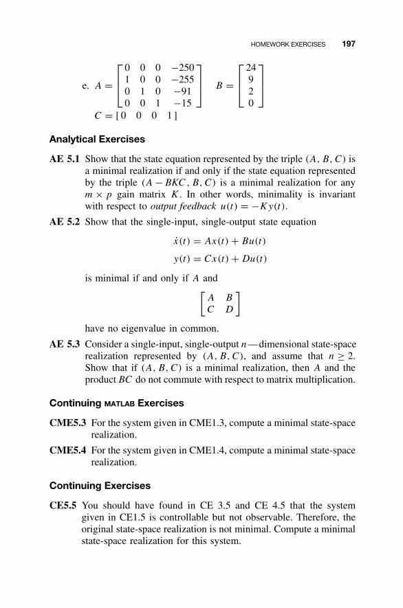
HOMEWORK EXERCISES 197
e. A =
0 0 0 −2501 0 0 −2550 1 0 −910 0 1 −15
B =
24920
C = [ 0 0 0 1 ]
Analytical Exercises
AE 5.1 Show that the state equation represented by the triple (A, B, C) isa minimal realization if and only if the state equation representedby the triple (A − BKC , B, C) is a minimal realization for anym × p gain matrix K . In other words, minimality is invariantwith respect to output feedback u(t) = −Ky(t).
AE 5.2 Show that the single-input, single-output state equation
x(t) = Ax(t) + Bu(t)
y(t) = Cx(t) + Du(t)
is minimal if and only if A and[A B
C D
]
have no eigenvalue in common.
AE 5.3 Consider a single-input, single-output n—dimensional state-spacerealization represented by (A, B, C), and assume that n ≥ 2.Show that if (A, B,C) is a minimal realization, then A and theproduct BC do not commute with respect to matrix multiplication.
Continuing MATLAB Exercises
CME5.3 For the system given in CME1.3, compute a minimal state-spacerealization.
CME5.4 For the system given in CME1.4, compute a minimal state-spacerealization.
Continuing Exercises
CE5.5 You should have found in CE 3.5 and CE 4.5 that the systemgiven in CE1.5 is controllable but not observable. Therefore, theoriginal state-space realization is not minimal. Compute a minimalstate-space realization for this system.
6
STABILITY
For the linear time-invariant state equation
x(t) = Ax(t) + Bu(t)
y(t) = Cx(t) + Du(t)x(0) = x0 (6.1)
we consider two types of stability in this chapter. The first is an internalnotion of stability and involves the qualitative behavior of the zero-inputstate response, i.e., the response of a related homogeneous state equationthat depends solely on the initial state. We introduce the fundamentalconcepts in a more general setting involving homogeneous nonlinear stateequations but specialize to the linear case for which explicit stabilitycriteria are available that involve the eigenvalues of the system dynamicsmatrix A. We also present an energy-based stability analysis that has itsorigins in the work of the Russian mathematician A. M. Lyapunov morethan a century ago. The power of Lyapunov stability theory lies in itsapplicability to nonlinear systems; however, we focus on its specializationto linear systems.
The second type of stability we study in this chapter focuses on external,or input-output, behavior. In particular, we characterize state equationsfor which the zero-state output response is a bounded signal for every
198
Linear State-Space Control Systems. Robert L. Williams II and Douglas A. LawrenceCopyright 2007 John Wiley & Sons, Inc. ISBN: 978-0-471-73555-7
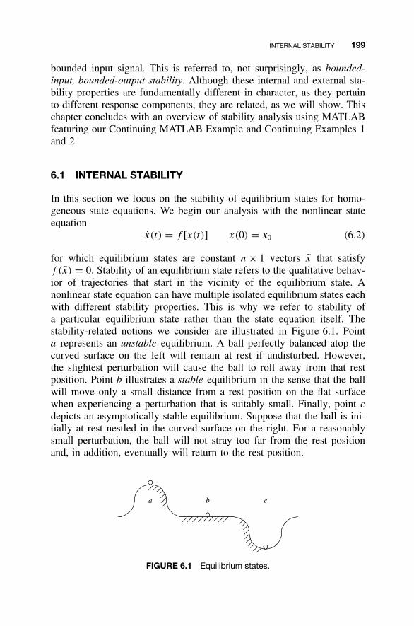
INTERNAL STABILITY 199
bounded input signal. This is referred to, not surprisingly, as bounded-input, bounded-output stability. Although these internal and external sta-bility properties are fundamentally different in character, as they pertainto different response components, they are related, as we will show. Thischapter concludes with an overview of stability analysis using MATLABfeaturing our Continuing MATLAB Example and Continuing Examples 1and 2.
6.1 INTERNAL STABILITY
In this section we focus on the stability of equilibrium states for homo-geneous state equations. We begin our analysis with the nonlinear stateequation
x(t) = f [x(t)] x(0) = x0 (6.2)
for which equilibrium states are constant n × 1 vectors x that satisfyf (x) = 0. Stability of an equilibrium state refers to the qualitative behav-ior of trajectories that start in the vicinity of the equilibrium state. Anonlinear state equation can have multiple isolated equilibrium states eachwith different stability properties. This is why we refer to stability ofa particular equilibrium state rather than the state equation itself. Thestability-related notions we consider are illustrated in Figure 6.1. Pointa represents an unstable equilibrium. A ball perfectly balanced atop thecurved surface on the left will remain at rest if undisturbed. However,the slightest perturbation will cause the ball to roll away from that restposition. Point b illustrates a stable equilibrium in the sense that the ballwill move only a small distance from a rest position on the flat surfacewhen experiencing a perturbation that is suitably small. Finally, point c
depicts an asymptotically stable equilibrium. Suppose that the ball is ini-tially at rest nestled in the curved surface on the right. For a reasonablysmall perturbation, the ball will not stray too far from the rest positionand, in addition, eventually will return to the rest position.
cba
FIGURE 6.1 Equilibrium states.
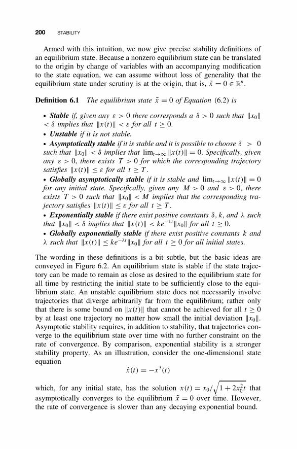
200 STABILITY
Armed with this intuition, we now give precise stability definitions ofan equilibrium state. Because a nonzero equilibrium state can be translatedto the origin by change of variables with an accompanying modificationto the state equation, we can assume without loss of generality that theequilibrium state under scrutiny is at the origin, that is, x = 0 ∈ R
n.
Definition 6.1 The equilibrium state x = 0 of Equation (6.2) is
• Stable if, given any ε > 0 there corresponds a δ > 0 such that ||x0||< δ implies that ||x(t)|| < ε for all t ≥ 0.• Unstable if it is not stable.• Asymptotically stable if it is stable and it is possible to choose δ > 0such that ||x0|| < δ implies that limt→∞ ||x(t)|| = 0. Specifically, givenany ε > 0, there exists T > 0 for which the corresponding trajectorysatisfies ||x(t)|| ≤ ε for all t ≥ T .• Globally asymptotically stable if it is stable and limt→∞ ||x(t)|| = 0for any initial state. Specifically, given any M > 0 and ε > 0, thereexists T > 0 such that ||x0|| < M implies that the corresponding tra-jectory satisfies ||x(t)|| ≤ ε for all t ≥ T .• Exponentially stable if there exist positive constants δ, k, and λ suchthat ||x0|| < δ implies that ||x(t)|| < ke−λt ||x0|| for all t ≥ 0.• Globally exponentially stable if there exist positive constants k andλ such that ||x(t)|| ≤ ke−λt ||x0|| for all t ≥ 0 for all initial states.
The wording in these definitions is a bit subtle, but the basic ideas areconveyed in Figure 6.2. An equilibrium state is stable if the state trajec-tory can be made to remain as close as desired to the equilibrium state forall time by restricting the initial state to be sufficiently close to the equi-librium state. An unstable equilibrium state does not necessarily involvetrajectories that diverge arbitrarily far from the equilibrium; rather onlythat there is some bound on ||x(t)|| that cannot be achieved for all t ≥ 0by at least one trajectory no matter how small the initial deviation ||x0||.Asymptotic stability requires, in addition to stability, that trajectories con-verge to the equilibrium state over time with no further constraint on therate of convergence. By comparison, exponential stability is a strongerstability property. As an illustration, consider the one-dimensional stateequation
x(t) = −x3(t)
which, for any initial state, has the solution x(t) = x0/
√1 + 2x2
0 t thatasymptotically converges to the equilibrium x = 0 over time. However,the rate of convergence is slower than any decaying exponential bound.
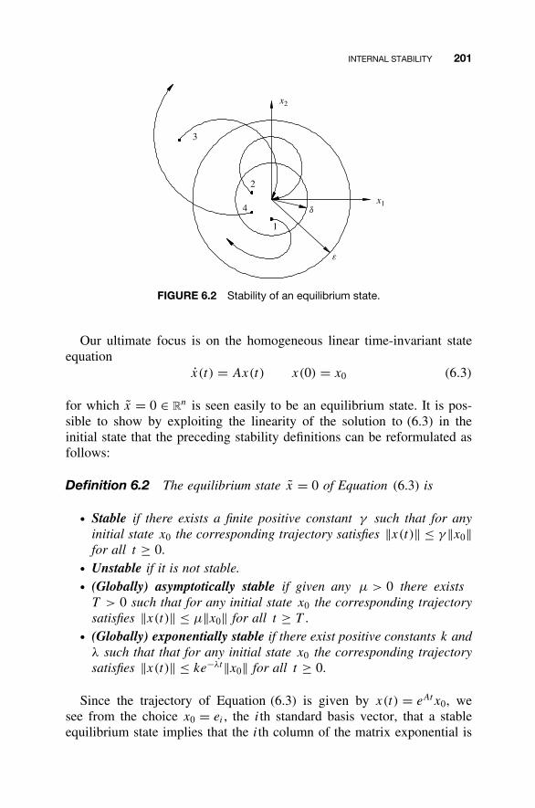
INTERNAL STABILITY 201
x1
x2
1
2
4
e
d
3
FIGURE 6.2 Stability of an equilibrium state.
Our ultimate focus is on the homogeneous linear time-invariant stateequation
x(t) = Ax(t) x(0) = x0 (6.3)
for which x = 0 ∈ Rn is seen easily to be an equilibrium state. It is pos-
sible to show by exploiting the linearity of the solution to (6.3) in theinitial state that the preceding stability definitions can be reformulated asfollows:
Definition 6.2 The equilibrium state x = 0 of Equation (6.3) is
• Stable if there exists a finite positive constant γ such that for anyinitial state x0 the corresponding trajectory satisfies ||x(t)|| ≤ γ ||x0||for all t ≥ 0.
• Unstable if it is not stable.• (Globally) asymptotically stable if given any µ > 0 there exists
T > 0 such that for any initial state x0 the corresponding trajectorysatisfies ||x(t)|| ≤ µ||x0|| for all t ≥ T .
• (Globally) exponentially stable if there exist positive constants k andλ such that that for any initial state x0 the corresponding trajectorysatisfies ||x(t)|| ≤ ke−λt ||x0|| for all t ≥ 0.
Since the trajectory of Equation (6.3) is given by x(t) = eAtx0, wesee from the choice x0 = ei , the ith standard basis vector, that a stableequilibrium state implies that the ith column of the matrix exponential is
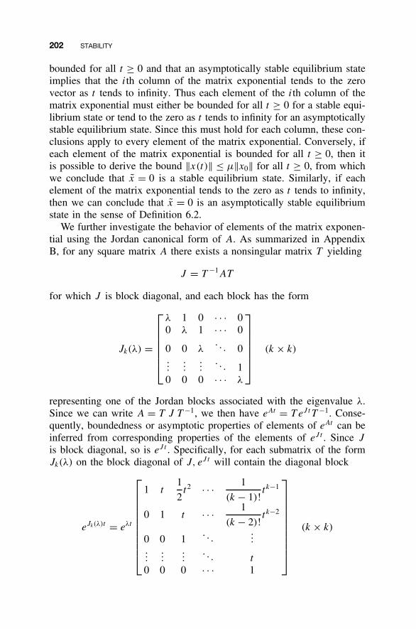
202 STABILITY
bounded for all t ≥ 0 and that an asymptotically stable equilibrium stateimplies that the ith column of the matrix exponential tends to the zerovector as t tends to infinity. Thus each element of the ith column of thematrix exponential must either be bounded for all t ≥ 0 for a stable equi-librium state or tend to the zero as t tends to infinity for an asymptoticallystable equilibrium state. Since this must hold for each column, these con-clusions apply to every element of the matrix exponential. Conversely, ifeach element of the matrix exponential is bounded for all t ≥ 0, then itis possible to derive the bound ||x(t)|| ≤ µ||x0|| for all t ≥ 0, from whichwe conclude that x = 0 is a stable equilibrium state. Similarly, if eachelement of the matrix exponential tends to the zero as t tends to infinity,then we can conclude that x = 0 is an asymptotically stable equilibriumstate in the sense of Definition 6.2.
We further investigate the behavior of elements of the matrix exponen-tial using the Jordan canonical form of A. As summarized in AppendixB, for any square matrix A there exists a nonsingular matrix T yielding
J = T −1AT
for which J is block diagonal, and each block has the form
Jk(λ) =
λ 1 0 · · · 00 λ 1 · · · 0
0 0 λ. . . 0
......
.... . . 1
0 0 0 · · · λ
(k × k)
representing one of the Jordan blocks associated with the eigenvalue λ.Since we can write A = T J T −1, we then have eAt = T eJ tT −1. Conse-quently, boundedness or asymptotic properties of elements of eAt can beinferred from corresponding properties of the elements of eJ t . Since J
is block diagonal, so is eJ t . Specifically, for each submatrix of the formJk(λ) on the block diagonal of J, eJ t will contain the diagonal block
eJk(λ)t = eλt
1 t1
2t2 · · · 1
(k − 1)!t k−1
0 1 t · · · 1
(k − 2)!t k−2
0 0 1. . .
......
......
. . . t
0 0 0 · · · 1
(k × k)
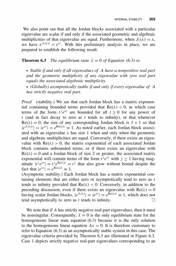
INTERNAL STABILITY 203
We also point out that all the Jordan blocks associated with a particulareigenvalue are scalar if and only if the associated geometric and algebraicmultiplicities of that eigenvalue are equal. Furthermore, when J1(λ) = λ,we have eJ1(λ)t = eλt . With this preliminary analysis in place, we areprepared to establish the following result:
Theorem 6.3 The equilibrium state x = 0 of Equation (6.3) is:
• Stable if and only if all eigenvalues of A have a nonpositive real partand the geometric multiplicity of any eigenvalue with zero real partequals the associated algebraic multiplicity.• (Globally) asymptotically stable if and only if every eigenvalue of A
has strictly negative real part.
Proof (stability.) We see that each Jordan block has a matrix exponen-tial containing bounded terms provided that Re(λ) < 0, in which caseterms of the form t j eλt are bounded for all t ≥ 0 for any power oft (and in fact decay to zero as t tends to infinity), or that wheneverRe(λ) = 0, the size of any corresponding Jordan block is 1 × 1 so that|eJ1(λ)t | = |eλt | = eRe(λ)t ≡ 1. As noted earlier, each Jordan block associ-ated with an eigenvalue λ has size 1 when and only when the geometricand algebraic multiplicities are equal. Conversely, if there exists an eigen-value with Re(λ) > 0, the matrix exponential of each associated Jordanblock contains unbounded terms, or if there exists an eigenvalue withRe(λ) = 0 and a Jordan block of size 2 or greater, the associated matrixexponential will contain terms of the form t j eλt with j ≥ 1 having mag-nitude |t j eλt | = t j eRe(λ)t = t j that also grow without bound despite thefact that |eλt | = eRe(λ)t ≡ 1.(Asymptotic stability.) Each Jordan block has a matrix exponential con-taining elements that are either zero or asymptotically tend to zero as t
tends to infinity provided that Re(λ) < 0. Conversely, in addition to thepreceding discussion, even if there exists an eigenvalue with Re(λ) = 0having scalar Jordan blocks, |eJ1(λ)| = |eλt | = eRe(λ)t ≡ 1, which does nottend asymptotically to zero as t tends to infinity. �
We note that if A has strictly negative real-part eigenvalues, then it mustbe nonsingular. Consequently, x = 0 is the only equilibrium state for thehomogeneous linear state equation (6.3) because it is the only solutionto the homogeneous linear equation Ax = 0. It is therefore customary torefer to Equation (6.3) as an asymptotically stable system in this case. Theeigenvalue criteria provided by Theorem 6.3 are illustrated in Figure 6.3.Case 1 depicts strictly negative real-part eigenvalues corresponding to an
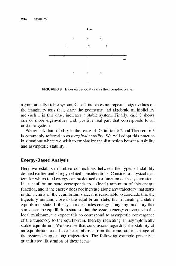
204 STABILITY
+Re
Im
1
+
++ +
2 3
FIGURE 6.3 Eigenvalue locations in the complex plane.
asymptotically stable system. Case 2 indicates nonrepeated eigenvalues onthe imaginary axis that, since the geometric and algebraic multiplicitiesare each 1 in this case, indicates a stable system. Finally, case 3 showsone or more eigenvalues with positive real-part that corresponds to anunstable system.
We remark that stability in the sense of Definition 6.2 and Theorem 6.3is commonly referred to as marginal stability. We will adopt this practicein situations where we wish to emphasize the distinction between stabilityand asymptotic stability.
Energy-Based Analysis
Here we establish intuitive connections between the types of stabilitydefined earlier and energy-related considerations. Consider a physical sys-tem for which total energy can be defined as a function of the system state.If an equilibrium state corresponds to a (local) minimum of this energyfunction, and if the energy does not increase along any trajectory that startsin the vicinity of the equilibrium state, it is reasonable to conclude that thetrajectory remains close to the equilibrium state, thus indicating a stableequilibrium state. If the system dissipates energy along any trajectory thatstarts near the equilibrium state so that the system energy converges to thelocal minimum, we expect this to correspond to asymptotic convergenceof the trajectory to the equilibrium, thereby indicating an asymptoticallystable equilibrium. We observe that conclusions regarding the stability ofan equilibrium state have been inferred from the time rate of change ofthe system energy along trajectories. The following example presents aquantitative illustration of these ideas.
INTERNAL STABILITY 205
Example 6.1 We consider the second-order linear translational mechan-ical system that was introduced in Example 1.1, which for zero externalapplied force is governed by
m y(t) + cy(t) + ky(t) = 0
in which y(t) represents the displacement of both the mass and springfrom rest. The state variables were chosen previously as the mass/springdisplacement x1(t) = y(t) and the mass velocity x2(t) = y(t), yieldingthe homogeneous state equation
[x1(t)
x2(t)
]=
0 1
− k
m− c
m
[
x1(t)
x2(t)
]
We recall that these state variables are related to energy stored in thissystem. The spring displacement characterizes the potential energy storedin the spring, and the mass velocity characterizes the kinetic energy storedin the mass. We therefore can express the total energy stored in the systemby the function
E(x1, x2) = 1
2kx2
1 + 1
2mx2
2
We observe that the system energy is positive whenever [x1, x2]T �=[0, 0]T and attains the minimum value of zero at the equilibrium state[x1, x2]T = [0, 0]T .
On evaluating the energy function along a system trajectory, we cancompute the time derivative
d
dtE[x1(t), x2(t)] = d
dt
[1
2kx2
1(t) + 1
2mx2
2(t)
]
= kx1(t)x1(t) + mx2(t)x2(t)
= kx1(t)
[x2(t)
]+ mx2(t)
[− k
mx1(t) − c
mx2(t)
]
= −cx22(t)
where we have invoked the chain rule and have used the state equationto substitute for the state-variable derivatives.
For zero damping (c = 0) we have dE/dt ≡ 0, so the total systemenergy is constant along any trajectory. This corresponds to a perpetualexchange between the potential energy stored in the spring and the kinetic
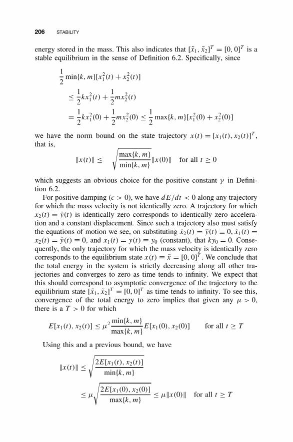
206 STABILITY
energy stored in the mass. This also indicates that [x1, x2]T = [0, 0]T is astable equilibrium in the sense of Definition 6.2. Specifically, since
1
2min{k, m}[x2
1(t) + x22(t)]
≤ 1
2kx2
1(t) + 1
2mx2
2(t)
= 1
2kx2
1(0) + 1
2mx2
2(0) ≤ 1
2max{k, m}[x2
1(0) + x22(0)]
we have the norm bound on the state trajectory x(t) = [x1(t), x2(t)]T ,that is,
||x(t)|| ≤√
max{k, m}min{k, m} ||x(0)|| for all t ≥ 0
which suggests an obvious choice for the positive constant γ in Defini-tion 6.2.
For positive damping (c > 0), we have dE/dt < 0 along any trajectoryfor which the mass velocity is not identically zero. A trajectory for whichx2(t) = y(t) is identically zero corresponds to identically zero accelera-tion and a constant displacement. Since such a trajectory also must satisfythe equations of motion we see, on substituting x2(t) = y(t) ≡ 0, x1(t) =x2(t) = y(t) ≡ 0, and x1(t) = y(t) ≡ y0 (constant), that ky0 = 0. Conse-quently, the only trajectory for which the mass velocity is identically zerocorresponds to the equilibrium state x(t) ≡ x = [0, 0]T . We conclude thatthe total energy in the system is strictly decreasing along all other tra-jectories and converges to zero as time tends to infinity. We expect thatthis should correspond to asymptotic convergence of the trajectory to theequilibrium state [x1, x2]T = [0, 0]T as time tends to infinity. To see this,convergence of the total energy to zero implies that given any µ > 0,there is a T > 0 for which
E[x1(t), x2(t)] ≤ µ2 min{k, m}max{k, m}E[x1(0), x2(0)] for all t ≥ T
Using this and a previous bound, we have
||x(t)|| ≤√
2E[x1(t), x2(t)]
min{k, m}
≤ µ
√2E[x1(0), x2(0)]
max{k, m} ≤ µ||x(0)|| for all t ≥ T
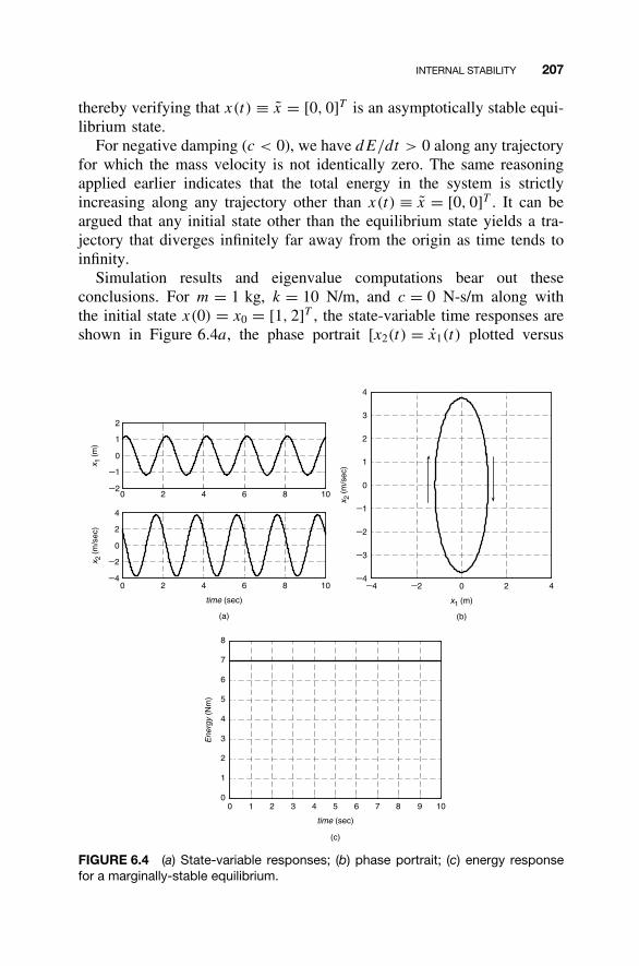
INTERNAL STABILITY 207
thereby verifying that x(t) ≡ x = [0, 0]T is an asymptotically stable equi-librium state.
For negative damping (c < 0), we have dE/dt > 0 along any trajectoryfor which the mass velocity is not identically zero. The same reasoningapplied earlier indicates that the total energy in the system is strictlyincreasing along any trajectory other than x(t) ≡ x = [0, 0]T . It can beargued that any initial state other than the equilibrium state yields a tra-jectory that diverges infinitely far away from the origin as time tends toinfinity.
Simulation results and eigenvalue computations bear out theseconclusions. For m = 1 kg, k = 10 N/m, and c = 0 N-s/m along withthe initial state x(0) = x0 = [1, 2]T , the state-variable time responses areshown in Figure 6.4a, the phase portrait [x2(t) = x1(t) plotted versus
x 2(m
/sec
)
−4 −2 0 2 4−4
−3
−2
−1
0
1
2
3
4
x1 (m)
(b)
0 2 4 6 8 10−2
−1
0
1
2
0 2 4 6 8 10−4
−2
0
2
4
time (sec)
x 2(m
/sec
)x 1
(m)
(a)
(c)
0 1 2 3 4 5 6 7 8 9 100
1
2
3
4
5
6
7
8
time (sec)
Ene
rgy
(Nm
)
FIGURE 6.4 (a) State-variable responses; (b) phase portrait; (c) energy responsefor a marginally-stable equilibrium.
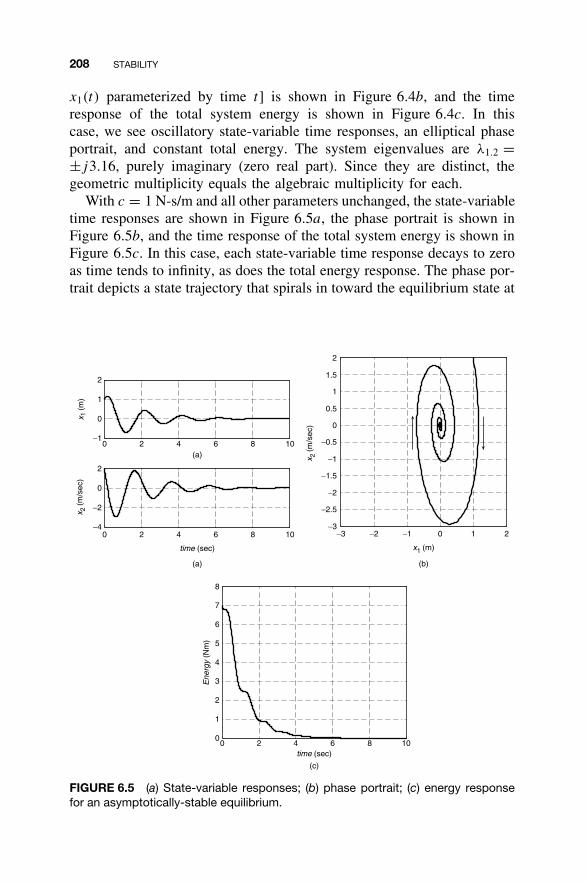
208 STABILITY
x1(t) parameterized by time t] is shown in Figure 6.4b, and the timeresponse of the total system energy is shown in Figure 6.4c. In thiscase, we see oscillatory state-variable time responses, an elliptical phaseportrait, and constant total energy. The system eigenvalues are λ1.2 =±j3.16, purely imaginary (zero real part). Since they are distinct, thegeometric multiplicity equals the algebraic multiplicity for each.
With c = 1 N-s/m and all other parameters unchanged, the state-variabletime responses are shown in Figure 6.5a, the phase portrait is shown inFigure 6.5b, and the time response of the total system energy is shown inFigure 6.5c. In this case, each state-variable time response decays to zeroas time tends to infinity, as does the total energy response. The phase por-trait depicts a state trajectory that spirals in toward the equilibrium state at
(c)
0 2 4 6 8 100
1
2
3
4
5
6
7
8
time (sec)
Ene
rgy
(Nm
)
(b)
−3 −2 −1 0 1 2−3
−2.5
−2
−1.5
−1
−0.5
0
0.5
1
1.5
2
x1 (m)
x 2(m
/sec
)
0 2 4 6(a)
(a)
8 10−1
0
1
2
x 1(m
)
0 2 4 6 8 10−4
−2
0
2
time (sec)
x 2(m
/sec
)
FIGURE 6.5 (a) State-variable responses; (b) phase portrait; (c) energy responsefor an asymptotically-stable equilibrium.
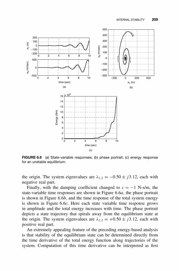
INTERNAL STABILITY 209
(b)
−200 0 200 400−300
−200
−100
0
100
200
300
400
500
x1 (m)
x 2(m
/sec
)
0 2 4 6 8 10−200
−100
0
100
200
x 1(m
)
0 2 4 6 8 10−500
0
500
time (sec)
(a)
x 2(m
/sec
)
(c)
0 2 4 6 8 100
2
4
6
8
10
12
14
16 x 104
time (sec)
Ene
rgy
(Nm
)
FIGURE 6.6 (a) State-variable responses; (b) phase portrait; (c) energy responsefor an unstable equilibrium.
the origin. The system eigenvalues are λ1,2 = −0.50 ± j3.12, each withnegative real part.
Finally, with the damping coefficient changed to c = −1 N-s/m, thestate-variable time responses are shown in Figure 6.6a, the phase portraitis shown in Figure 6.6b, and the time response of the total system energyis shown in Figure 6.6c. Here each state variable time response growsin amplitude and the total energy increases with time. The phase portraitdepicts a state trajectory that spirals away from the equilibrium state atthe origin. The system eigenvalues are λ1,2 = +0.50 ± j3.12, each withpositive real part.
An extremely appealing feature of the preceding energy-based analysisis that stability of the equilibrium state can be determined directly fromthe time derivative of the total energy function along trajectories of thesystem. Computation of this time derivative can be interpreted as first
210 STABILITY
computing the following function of the state variables
E(x1, x2) � ∂E
∂x1(x1, x2)x1 + ∂E
∂x2(x1, x2)x2
= (kx1)x1 + (mx2)x2
= (kx1)(x2) + (mx2)
(− k
mx1 − c
mx2
)
= −cx22
followed by evaluating along a system trajectory x(t) = [x1(t), x2(t)]T toobtain
E[x1(t), x2(t)] = −cx22(t) = d
dtE[x1(t), x2(t)]
In addition, properties of the total energy time derivative along all sys-tem trajectories and accompanying stability implications can be deducedfrom properties of the function E(x1, x2) over the entire state space. Animportant consequence is that explicit knowledge of the trajectories them-selves is not required.
Lyapunov Stability Analysis
The Russian mathematician A. M. Lyapunov (1857–1918) observedthat conclusions regarding stability of an equilibrium state can bedrawn from a more general class of energy-like functions. For thenonlinear state equation (6.2), we consider real-valued functions V (x) =V (x1, x2, . . . , xn) with continuous partial derivatives in each state variablethat are positive definite, meaning that V (0) = 0 and V (x) > 0 for allx �= 0 at least in a neighborhood of the origin. This generalizes theproperty that the total energy function has a local minimum at theequilibrium. To analyze the time derivative of the function V (x) alongtrajectories of Equation (6.2), we define
V (x) = ∂V
∂x1(x)x1 + ∂V
∂x2(x)x2 + · · · + ∂V
∂xn
(x)xn
=[
∂V
∂x1(x)
∂V
∂x2(x) · · · ∂V
∂x2(x)
]
x1
x2...
xn
= ∂V
∂x(x)f (x)
INTERNAL STABILITY 211
Thus V (x) is formed from the inner product of the gradient of V (x) andthe nonlinear map f (x) that defines the system dynamics. The fundamen-tal discovery of Lyapunov is that the equilibrium x = 0 is
• Stable if V (x) is negative semidefinite; that is, V (x) ≤ 0 for all x ina neighborhood of the origin.
• Asymptotically stable if V (x) is negative definite; that is, V (x) < 0for all x �= 0 in a neighborhood of the origin.
A positive-definite function V (x) for which V (x) is at least negativesemidefinite is called a Lyapunov function. The preceding result isextremely powerful because stability of an equilibrium can be determineddirectly from the system dynamics without explicit knowledge of systemtrajectories. Consequently, this approach is referred to as Lyapunov’sdirect method. This is extremely important in the context of nonlinearsystems because system trajectories, i.e., solutions to the nonlinear stateequation (6.2), in general are not available in closed form.
We observe that Lyapunov’s direct method only provides a sufficientcondition for (asymptotic) stability of an equilibrium in terms of anunspecified Lyapunov function for which, in general, there are no system-atic ways to construct. As a consequence, if a particular positive-definitefunction V (x) fails to have V (x) negative semidefinite, we cannot con-clude immediately that the origin is unstable. Similarly, if, for a Lyapunovfunction V (x), V (x) fails to be negative definite, we cannot rule outasymptotic stability of the origin. On the other hand, a so-called conversetheorem exists for asymptotic stability that, under additional hypotheses,guarantees the existence of a Lyapunov function with a negative-definiteV (x). For a thorough treatment of Lyapunov stability analysis, we referthe interested reader to Khalil (2002).
For the linear state equation (6.3), Lyapunov stability analysis can bemade much more explicit. First, we can focus on energy-like functionsthat are quadratic forms given by
V (x) = xT Px =n∑
i,j=1
pijxixj (6.4)
in which the associated matrix P = [pij ] is symmetric without loss ofgenerality so that its elements satisfy pij = pji . We note here that P
does not refer to the controllability matrix introduced in Chapter 3. Aquadratic form is a positive-definite function over all of R
n if and only ifP is a positive-definite symmetric matrix. A symmetric n × n matrix P ispositive definite if and only if every eigenvalue of P is real and positive.
212 STABILITY
Consequently, the eigenvalues of a symmetric positive-definite matrix canbe ordered via
0 < λmin(P ) = λ1 ≤ λ2 ≤ · · · ≤ λn = λmax(P )
and the associated quadratic form satisfies the so-called Rayleigh-Ritzinequality
λmin(P )xT x ≤ xT Px ≤ λmax(P )xT x for all x ∈ Rn
Another useful characterization of positive definiteness of a symmetricn × n matrix P = [pij ] is that its n leading principal minors defined asthe submatrix determinants
p11
∣∣∣∣ p11 p12
p12 p22
∣∣∣∣∣∣∣∣∣∣p11 p12 p13
p12 p22 p23
p13 p23 p33
∣∣∣∣∣∣ · · ·
∣∣∣∣∣∣∣∣
p11 p12 · · · p1n
p12 p22 · · · p2n
......
. . ....
p1n p2n · · · pnn
∣∣∣∣∣∣∣∣are all positive. This is referred to as Sylvester’s criterion. It followsdirectly that a quadratic form xT Px and associated symmetric matrix P
are negative definite if and only if −P is a positive-definite matrix.The gradient of the quadratic form V (x) = xT Px is (∂V/∂x)(x) =
2xT P , as can be verified from the summation in Equation (6.4). Usingthis and the linear dynamics in Equation (6.3), we can compute V (x)
according to
V (x) = ∂V
∂x(x)f (x)
= (2xT P )(Ax)
= xT AT Px + xT PAx
= xT [AT P + PA]x
in which we also have used the fact that xT AT Px = xT PAx becausethese are scalar quantities related by the transpose operation. We observethat V (x) is also a quadratic form expressed in terms of the symmet-ric matrix AT P + PA. Therefore, a sufficient condition for asymptoticstability of the equilibrium state x = 0 is the existence of a symmetricpositive-definite matrix P for which AT P + PA is negative definite. Thefollowing result links the existence of such a matrix to the eigenvaluecondition for asymptotic stability established in Theorem 6.3.
INTERNAL STABILITY 213
Theorem 6.4 For any symmetric positive definite matrix Q, the Lya-punov matrix equation
AT P + PA = −Q (6.5)
has a unique symmetric positive definite solution P if and only if everyeigenvalue of A has strictly negative real part.
Proof. For necessity, suppose that, given a symmetric positive-definitematrix Q, there exists a unique symmetric positive-definite solution P tothe Lyapunov matrix equation (6.5). Let λ be any eigenvalue of A and v ∈R
n be a corresponding (right) eigenvector. Premultiplying Equation (6.5)by v∗ and postmultiplying by v yields
−v∗Qv = v∗[AT P + PA]v
= v∗AT Pv + v∗PAv
= λv∗Pv + λv∗Pv
= (λ + λ)v∗Pv
= 2 Re(λ)v∗Pv
Since v �= 0 (because it is an eigenvector) and P and Q are positivedefinite matrices, these quadratic forms satisfy v∗Pv > 0 and v∗Qv > 0.This gives
Re(λ) = −1
2
v∗Qv
v∗Pv< 0
from which we conclude that every eigenvalue of A necessarily has astrictly negative real part.
For sufficiency, suppose that every eigenvalue of A has a strictly nega-tive real part and consider, for any symmetric positive definite matrix Q,
P =∫ ∞
0eAT t
QeAtdt
Since elements of eAt are sums of terms of the form M tk−1eRe(λ)t cos(Im(λ)t + θ) that decay to zero exponentially fast, this improper integralconverges to a finite limit, so P is well defined. Also, P is symmetric byinspection. Next, for any x ∈ R
n,
xT P x =∫ ∞
0(eAtx)T Q(eAtx)dt ≥ 0
because the integrand is nonnegative for all t ≥ 0. Moreover, equalityholds when and only when the integrand is identically zero which, by
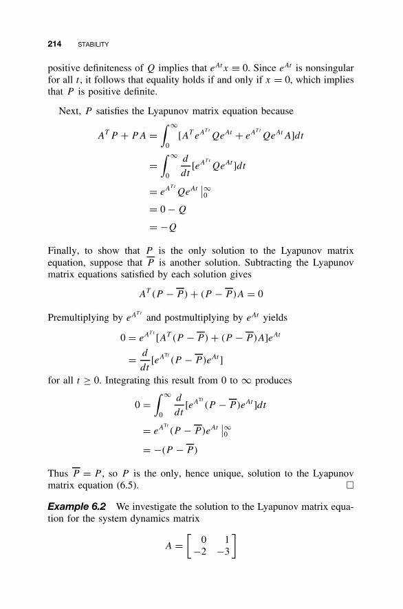
214 STABILITY
positive definiteness of Q implies that eAtx ≡ 0. Since eAt is nonsingularfor all t , it follows that equality holds if and only if x = 0, which impliesthat P is positive definite.
Next, P satisfies the Lyapunov matrix equation because
AT P + PA =∫ ∞
0[AT eAT t
QeAt + eAT t
QeAtA]dt
=∫ ∞
0
d
dt[eAT t
QeAt ]dt
= eAT t
QeAt∣∣∞0
= 0 − Q
= −Q
Finally, to show that P is the only solution to the Lyapunov matrixequation, suppose that P is another solution. Subtracting the Lyapunovmatrix equations satisfied by each solution gives
AT (P − P) + (P − P)A = 0
Premultiplying by eAT t
and postmultiplying by eAt yields
0 = eAT t
[AT (P − P) + (P − P)A]eAt
= d
dt[eATt
(P − P)eAt ]
for all t ≥ 0. Integrating this result from 0 to ∞ produces
0 =∫ ∞
0
d
dt[eATt
(P − P)eAt ]dt
= eATt
(P − P)eAt∣∣∞0
= −(P − P)
Thus P = P , so P is the only, hence unique, solution to the Lyapunovmatrix equation (6.5). �
Example 6.2 We investigate the solution to the Lyapunov matrix equa-tion for the system dynamics matrix
A =[
0 1−2 −3
]
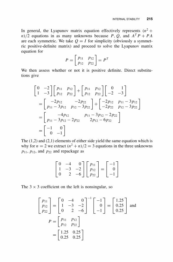
INTERNAL STABILITY 215
In general, the Lyapunov matrix equation effectively represents (n2 +n)/2 equations in as many unknowns because P, Q, and AT P + PA
are each symmetric. We take Q = I for simplicity (obviously a symmet-ric positive-definite matrix) and proceed to solve the Lyapunov matrixequation for
P =[
p11 p12
p12 p22
]= P T
We then assess whether or not it is positive definite. Direct substitu-tions give
[0 −21 −3
] [p11 p12
p12 p22
]+
[p11 p12
p12 p22
] [0 1
−2 −3
]
=[ −2p12 −2p22
p11 − 3p12 p12 − 3p22
]+
[ −2p12 p11 − 3p12
−2p22 p12 − 3p22
]
=[ −4p12 p11 − 3p12 − 2p22
p11 − 3p12 − 2p22 2p12 − 6p22
]
=[ −1 0
0 −1
]
The (1,2) and (2,1) elements of either side yield the same equation which iswhy for n = 2 we extract (n2 + n)/2 = 3 equations in the three unknownsp11, p12, and p22 and repackage as
0 −4 0
1 −3 −20 2 −6
p11
p12
p22
=
−1
0−1
The 3 × 3 coefficient on the left is nonsingular, so
p11
p12
p22
=
0 −4 0
1 −3 −20 2 −6
−1 −1
0−1
=
1.25
0.250.25
and
P =[
p11 p12
p12 p22
]
=[
1.25 0.250.25 0.25
]
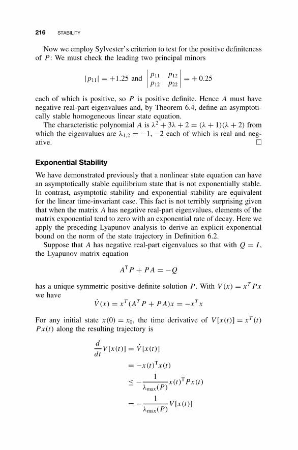
216 STABILITY
Now we employ Sylvester’s criterion to test for the positive definitenessof P : We must check the leading two principal minors
|p11| = +1.25 and
∣∣∣∣ p11 p12
p12 p22
∣∣∣∣ = + 0.25
each of which is positive, so P is positive definite. Hence A must havenegative real-part eigenvalues and, by Theorem 6.4, define an asymptoti-cally stable homogeneous linear state equation.
The characteristic polynomial A is λ2 + 3λ + 2 = (λ + 1)(λ + 2) fromwhich the eigenvalues are λ1,2 = −1, −2 each of which is real and neg-ative. �
Exponential Stability
We have demonstrated previously that a nonlinear state equation can havean asymptotically stable equilibrium state that is not exponentially stable.In contrast, asymptotic stability and exponential stability are equivalentfor the linear time-invariant case. This fact is not terribly surprising giventhat when the matrix A has negative real-part eigenvalues, elements of thematrix exponential tend to zero with an exponential rate of decay. Here weapply the preceding Lyapunov analysis to derive an explicit exponentialbound on the norm of the state trajectory in Definition 6.2.
Suppose that A has negative real-part eigenvalues so that with Q = I ,the Lyapunov matrix equation
ATP + PA = −Q
has a unique symmetric positive-definite solution P . With V (x) = xT Px
we haveV (x) = xT (AT P + PA)x = −xT x
For any initial state x(0) = x0, the time derivative of V [x(t)] = xT (t)
P x(t) along the resulting trajectory is
d
dtV [x(t)] = V [x(t)]
= −x(t)Tx(t)
≤ − 1
λmax(P )x(t)TPx(t)
= − 1
λmax(P )V [x(t)]
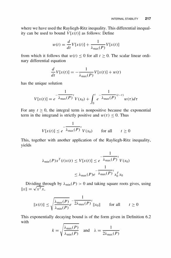
INTERNAL STABILITY 217
where we have used the Rayliegh-Ritz inequality. This differential inequal-ity can be used to bound V [x(t)] as follows: Define
w(t) = d
dtV [x(t)] + 1
λmax(P )V [x(t)]
from which it follows that w(t) ≤ 0 for all t ≥ 0. The scalar linear ordi-nary differential equation
d
dtV [x(t)] = − 1
λmax(P )V [x(t)] + w(t)
has the unique solution
V [x(t)] = e−
1
λmax(P )t
V (x0) +∫ t
0e−
1
λmax(P )(t−τ )
w(τ)dτ
For any t ≥ 0, the integral term is nonpositive because the exponentialterm in the integrand is strictly positive and w(τ) ≤ 0. Thus
V [x(t)] ≤ e−
1
λmax(P )t
V (x0) for all t ≥ 0
This, together with another application of the Rayliegh-Ritz inequality,yields
λmin(P )xT (t)x(t) ≤ V [x(t)] ≤ e−
1
λmax(P )t
V (x0)
≤ λmax(P )e−
1
λmax(P )t
xT0 x0
Dividing through by λmin(P ) > 0 and taking square roots gives, using||x|| = √
xT x,
||x(t)|| ≤√
λmax(P )
λmin(P )e−
1
2λmax(P )t
||x0|| for all t ≥ 0
This exponentially decaying bound is of the form given in Definition 6.2with
k =√
λmax(P )
λmin(P )and λ = 1
2λmax(P )
218 STABILITY
6.2 BOUNDED-INPUT, BOUNDED-OUTPUT STABILITY
Thus far in this chapter, we have been concerned with internal stabil-ity. This section discusses a type of external stability called bounded-input, bounded-output stability. As mentioned at the outset, bounded-input,bounded-output stability pertains to the zero-state output response. In thissection we study bounded-input, bounded-output stability, and in the nextsection we relate asymptotic and bounded-input, bounded-output stability.
A vector-valued signal u(t) is bounded if there is a finite, positiveconstant ν for which
||u(t)|| ≤ ν for all t ≥ 0
If such an upper bound exits, we denote the least upper bound, or supre-mum, by
supt≥0||u(t)||When ||u(t)|| cannot be bounded above in this way, we write
supt≥0||u(t)|| = ∞The supremum of ||u(t)|| over the infinite interval [0, ∞) is in generaldifferent from a maximum value because the latter must be achieved atsome t ∈ [0, ∞) and therefore may not exist. For example, consider thebounded scalar signal u(t) = 1 − e−t , for which
supt≥0||u(t)|| = supt≥0(1 − e−t ) = 1
but a maximum value for ||u(t)|| is never attained on t ∈ [0, ∞).
Definition 6.5 The linear state equation (6.1) is called bounded-input,bounded-output stable if there exists a finite constant η such that for anyinput u(t) the zero-state output response satisfies
supt≥0||y(t)|| ≤ η supt≥0||u(t)||
This definition is not terribly useful as a test for bounded-input,bounded-output stability because it requires an exhaustive search overall bounded input signals, which is, of course, impossible. The next resultis of interest because it establishes a necessary and sufficient test forbounded-input, bounded-output stability involving the system’s impulseresponse that in principle requires a single computation. The theorem iscast in the multiple-input, multiple-output context and, as such, involves
BOUNDED-INPUT, BOUNDED-OUTPUT STABILITY 219
a choice of vector norm for both the input space Rm and the output space
Rp and a corresponding induced matrix norm on the set of p × m matrices
(see Appendix B, Section 9).
Theorem 6.6 The linear state equation (6.1) is bounded-input, bounded-output stable if and only if the impulse response matrix H(t) = CeAtB+Dδ(t) satisfies ∫ ∞
0||H(τ)||dτ < ∞
Proof. To show sufficiency, suppose that this integral is finite, and set
η =∫ ∞
0||H(τ)||dτ
Then, for all t ≥ 0, the zero-state output response satisfies
||y(t)|| = ||∫ t
0H(τ)u(t − τ)dτ ||
≤∫ t
0||H(τ)u(t − τ)||dτ
≤∫ t
0||H(τ)||||u(t − τ)||dτ
≤∫ t
0||H(τ)||dτ sup0≤σ≤t ||u(σ)||
≤∫ ∞
0||H(τ)||dτ supt≥0||u(t)||
= ηsupt≥0||u(t)||from which the bound in Definition 6.5 follows from the definition ofsupremum. Since the input signal was arbitrary, we conclude that thesystem (6.1) is bounded-input, bounded-output stable.
To show that bounded-input, bounded-output stability implies∫ ∞
0||H(τ)||dτ < ∞
we prove the contrapositive. Assume that for any finite η > 0 there existsa T > 0 such that ∫ T
0||H(τ)||dτ > η
220 STABILITY
It follows that there exists an element Hij (τ ) of H(τ) and a Tij > 0 suchthat ∫ Tij
0
∣∣Hij (τ )∣∣ dτ > η
Consider the bounded input defined by u(t) ≡ 0 ∈ R� for all t > Tij , and
on the interval [0, Tij ] every component of u(t) is zero except for uj (t),which is set to
uj (t) =
−1 Hij (Tij − t) > 0
0 Hij (Tij − t) = 0
1 Hij (Tij − t) < 0
Then ||u(t)|| ≤ 1 for all t ≥ 0, but the ith component of the zero-stateoutput response satisfies
yi(Tij ) =∫ Tij
0Hij (Tij − σ)uj (σ )dσ
=∫ Tij
0|Hij (Tij − σ)|dσ
=∫ Tij
0|Hij (τ )|dτ
> η
≥ ηsupt≥0||u(t)||
Since ||y(Tij )|| ≥ |yi(Tij )| and η was arbitrary, we conclude that the sys-tem (6.1) is not bounded-input, bounded-output stable. �
6.3 BOUNDED-INPUT, BOUNDED-OUTPUT STABILITYVERSUS ASYMPTOTIC STABILITY
It is reasonable to expect, since elements of the impulse-response matrixinvolve linear combinations of elements of the matrix exponential viapremultiplication by C and postmultiplication by B, that asymptotic sta-bility implies bounded-input, bounded-output stability. This indeed is true.However, the converse in general is not true as illustrated by the followingexample.
BOUNDED-INPUT, BOUNDED-OUTPUT STABILITY VERSUS ASYMPTOTIC STABILITY 221
Example 6.3 Consider the following two-dimensional state equation:[x1(t)
x2(t)
]=
[0 11 0
][x1(t)
x2(t)
]+
[ −11
]u(t)
y(t) = [ 0 1 ]
[x1(t)
x2(t)
]
The characteristic polynomial is
|sI − A| =∣∣∣∣ s −1−1 s
∣∣∣∣= s2 − 1
= (s + 1)(s − 1)
indicating that the eigenvalues of A are λ1,2 = −1, +1 and according toTheorem 6.3, the state equation is not asymptotically stable as a result.This can be seen by inspection of the matrix exponential
eAt =
1
2(et + e−t )
1
2(et − e−t )
1
2(et − e−t )
1
2(et + e−t )
The growing exponential term et associated with the positive eigenvaluecauses every element of eAt to diverge as t increases. The transfer func-tion is
H(s) = C(sI − A)−1B
= [ 0 1 ]
[s −1
−1 s
]−1 [ −11
]
= [ 0 1 ]
[s 11 s
]
s2 − 1
[ −11
]
= s − 1
(s + 1)(s − 1)
= 1
(s + 1)
from which the impulse response h(t) = e−t , t ≥ 0, satisfies∫ ∞
0|h(τ)|dτ = 1
222 STABILITY
so, by Theorem 6.6, the system is bounded-input, bounded-outputstable.
In this example, we observe that the state equation is not minimal(it is observable but not controllable). Thus the transfer function H(s)
necessarily must have a pole-zero cancellation. In this case, the unsta-ble pole at s = 1 is canceled by a zero at the same location, yieldinga first-order transfer function with a stable pole at s = −1. In the timedomain, the unstable exponential term et that appears in the matrix expo-nential is missing from the impulse response. This unstable pole-zerocancellation therefore leads to a bounded-input, bounded-output-stablestate equation that is not asymptotically stable. If we are concerned onlywith input-output behavior, we might be tempted to think that bounded-input, bounded-output stability is good enough. The problem lies in thefact that bounded-input, bounded-output stability characterizes only thezero-state response, and it may happen that an initial state yields a zero-input response component resulting in a complete output response thatdoes not remain bounded. For this example, the initial state x(0) = [1, 1]T
yields the zero-input response component yzi(t) = et , so for, say, a unitstep input, the complete response is
y(t) = yzi(t) + yzs(t)
= et + (1 − e−t )t ≥ 0
that, despite the bounded zero-state response component, diverges withincreasing t . �
In the single-input, single-output case, we see that the situation encoun-tered in the preceding example can be avoided by disallowing pole-zerocancellations of any type, i.e., by requiring an irreducible transfer func-tion associated with the given state equation. This, as we have seen,is equivalent to minimality of the realization. It turns out that whilethe transfer-function interpretation is difficult to extend to the multiple-input, multiple-output case, the minimality condition remains sufficientfor bounded-input, bounded-output stability to imply asymptotic stability.
Theorem 6.7 For the linear state equation (6.1):
1. Asymptotic stability always implies bounded-input, bounded-outputstability.2. If Equation (6.1) is minimal, then bounded-input, bounded-output
stability implies asymptotic stability.
Proof. As argued previously, asymptotic stability is equivalent to expo-nential stability. Thus there exist finite positive constants k and λ such
BOUNDED-INPUT, BOUNDED-OUTPUT STABILITY VERSUS ASYMPTOTIC STABILITY 223
that||eAtx(0)|| ≤ ke−λt ||x(0)|| for all x(0) ∈ R
n
Thus, for any x(0) �= 0,||eAtx(0)||||x(0)|| ≤ ke−λt
thereby establishing an upper bound on the left-hand-side ratio for eacht ≥ 0. By definition of supremum, the induced matrix norm therefore hasthe bound
||eAt || = supx(0) �=0||eAtx(0)||||x(0)|| ≤ ke−λt for all t ≥ 0
Using this, familiar bounding arguments give
∫ ∞
0||H(τ)||dτ ≤
∫ ∞
0
[||CeAτB|| + ||Dδ(t)||] dτ
≤ ||C||||B||∫ ∞
0ke−λτdτ + ||D||
= k||C||||B||λ
+ ||D||≤ ∞
and so state equation (6.1) is bounded-input, bounded-output stable byTheorem 6.6.
Next, we show via a contradiction argument that under the minimalityhypothesis, bounded-input, bounded-output stability implies asymptoticstability. Suppose that Equation (6.1) is bounded-input, bounded-outputstable and yet there is an eigenvalue λi of A with Re(λi) ≥ 0. Let mi
denote the associated algebraic multiplicity so that, based on the partialfraction expansion of (sI − A)−1, we see that eAt will contain terms ofthe form
Ri1eλit + Ri2te
λit + · · · + Rimi
tmi−1
(mi − 1)!eλit
in which Rimi�= 0 because of the assumed algebraic multiplicity, along
with similar terms associated with the other distinct eigenvalues of A.Bounded-input, bounded-output stability implies, via Theorem 6.6, that
limt→∞ CeAtB = 0 ∈ R
p×m
224 STABILITY
and since exponential time functions associated with distinct eigenvaluesare linearly independent, the only way the nondecaying terms in eAt willbe absent in CeAtB is if
CRijB = 0 j = 1, 2, . . . , mi
In particular,0 = CRimi
B
= C[(s − λi)mi (sI − A)−1]|s=λi
B
= [(s − λi)miC(sI − A)−1B]|s=λi
This allows us to conclude that[
C
λiI − A
]Rimi
[ B λiI − A ]
=[
C
sI − A
][(s − λi)
mi (sI − A)−1][ B sI − A ]
∣∣∣∣s=λi
=[
(s − λi)mi C(sI − A)−1B (s − λi)
miC
(s − λi)miB (s − λi)
mi (sI − A)
]∣∣∣∣s=λi
=[
0 00 0
]
Now, minimality of the linear state equation (6.1) implies that the leftmostfactor has full-column rank n by virtue of the Popov-Belevich-Hautusrank rest for observability. Consequently, it is possible to select n lin-early independent rows from the leftmost factor to give a nonsingularmatrix MO . Similarly, that the rightmost factor has full-row rank n by thePopov-Belevich-Hautus rank rest for controllability, and it is possible toselect n linearly independent columns from the rightmost factor to yielda nonsingular matrix MC . This corresponds to selecting n rows and n
columns from the left-hand-side product. An identical selection from theright hand side yields the identity
MORimiMC = 0
which, because of the nonsingularity of MO and MC , implies that Rimi=
0. This contradicts Rimi�= 0, which enables us to conclude that under the
minimality hypothesis, bounded-input, bounded-output stability impliesasymptotic stability. �

MATLAB FOR STABILITY ANALYSIS 225
6.4 MATLAB FOR STABILITY ANALYSIS
The following MATLAB function is useful for Lyapunov stability analysis:lyap(A',Q) Solve A'P+PA=-Q for matrix P, given a positive-definite
matrix Q.Note that the MATLAB function lyap directly solves the problemAP+PA'=-Q, so we must give the transpose of matrix A (that is, A') as aninput to this function.
We now assess the stability of the Continuing MATLAB Example (rota-tional mechanical system) via Lyapunov stability analysis. The followingMATLAB code segment performs this computation and logic:
%------------------------------------------------------% Chapter 6. Lyapunov Stability Analysis%------------------------------------------------------
if (real(Poles(1))==0 | real(Poles(2))==0) % lyap% will fail
if (real(Poles(1)) < =0 | real(Poles(2)) < =0)disp('System is marginally stable.');elsedisp('System is unstable.');end
else % lyap will succeedQ = eye(2); % Given positive definite
% matrixP = lyap(A',Q); % Solve for Ppm1 = det(P(1,1)); % Sylvester's method to see
% if P is positive definitepm2 = det(P(1:2,1:2));if (pm1>0 & pm2>0) % Logic to assess stability
% conditiondisp('System is asymptotically stable.');elsedisp('System is unstable.');end
end
figure; % Plot phase portraits to% enforce stability analysis
plot(Xo(:,1),Xo(:,2),'k'); grid; axis('square');axis([-1.5 1.5 -2 1]);
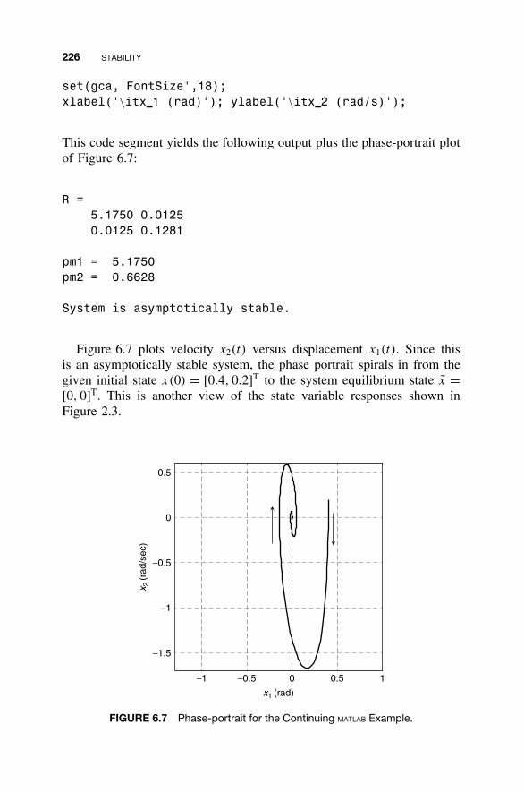
226 STABILITY
set(gca,'FontSize',18);xlabel('\itx 1 (rad)'); ylabel('\itx 2 (rad/s)');
This code segment yields the following output plus the phase-portrait plotof Figure 6.7:
R =5.1750 0.01250.0125 0.1281
pm1 = 5.1750pm2 = 0.6628
System is asymptotically stable.
Figure 6.7 plots velocity x2(t) versus displacement x1(t). Since thisis an asymptotically stable system, the phase portrait spirals in from thegiven initial state x(0) = [0.4, 0.2]T to the system equilibrium state x =[0, 0]T. This is another view of the state variable responses shown inFigure 2.3.
−1 −0.5 0 0.5 1
−1.5
−1
−0.5
0
0.5
x1 (rad)
x 2(r
ad/s
ec)
FIGURE 6.7 Phase-portrait for the Continuing MATLAB Example.
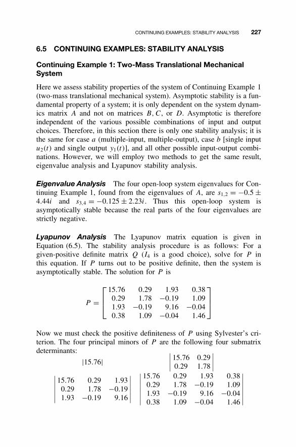
CONTINUING EXAMPLES: STABILITY ANALYSIS 227
6.5 CONTINUING EXAMPLES: STABILITY ANALYSIS
Continuing Example 1: Two-Mass Translational MechanicalSystem
Here we assess stability properties of the system of Continuing Example 1(two-mass translational mechanical system). Asymptotic stability is a fun-damental property of a system; it is only dependent on the system dynam-ics matrix A and not on matrices B,C, or D. Asymptotic is thereforeindependent of the various possible combinations of input and outputchoices. Therefore, in this section there is only one stability analysis; it isthe same for case a (multiple-input, multiple-output), case b [single inputu2(t) and single output y1(t)], and all other possible input-output combi-nations. However, we will employ two methods to get the same result,eigenvalue analysis and Lyapunov stability analysis.
Eigenvalue Analysis The four open-loop system eigenvalues for Con-tinuing Example 1, found from the eigenvalues of A, are s1,2 = −0.5 ±4.44i and s3,4 = −0.125 ± 2.23i. Thus this open-loop system isasymptotically stable because the real parts of the four eigenvalues arestrictly negative.
Lyapunov Analysis The Lyapunov matrix equation is given inEquation (6.5). The stability analysis procedure is as follows: For agiven-positive definite matrix Q (I4 is a good choice), solve for P inthis equation. If P turns out to be positive definite, then the system isasymptotically stable. The solution for P is
P =
15.76 0.29 1.93 0.380.29 1.78 −0.19 1.091.93 −0.19 9.16 −0.040.38 1.09 −0.04 1.46
Now we must check the positive definiteness of P using Sylvester’s cri-terion. The four principal minors of P are the following four submatrixdeterminants:
|15.76|∣∣∣∣ 15.76 0.29
0.29 1.78
∣∣∣∣∣∣∣∣∣∣15.76 0.29 1.93
0.29 1.78 −0.191.93 −0.19 9.16
∣∣∣∣∣∣
∣∣∣∣∣∣∣15.76 0.29 1.93 0.380.29 1.78 −0.19 1.091.93 −0.19 9.16 −0.040.38 1.09 −0.04 1.46
∣∣∣∣∣∣∣
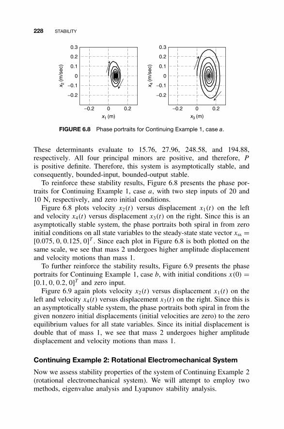
228 STABILITY
−0.2 0 0.2
−0.2
−0.1
0
0.1
0.2
0.3
x1 (m)
x 2(m
/sec
)
−0.2 0 0.2
−0.2
−0.1
0
0.1
0.2
0.3
x3 (m)
x 4(m
/sec
)
FIGURE 6.8 Phase portraits for Continuing Example 1, case a.
These determinants evaluate to 15.76, 27.96, 248.58, and 194.88,respectively. All four principal minors are positive, and therefore, P
is positive definite. Therefore, this system is asymptotically stable, andconsequently, bounded-input, bounded-output stable.
To reinforce these stability results, Figure 6.8 presents the phase por-traits for Continuing Example 1, case a, with two step inputs of 20 and10 N, respectively, and zero initial conditions.
Figure 6.8 plots velocity x2(t) versus displacement x1(t) on the leftand velocity x4(t) versus displacement x3(t) on the right. Since this is anasymptotically stable system, the phase portraits both spiral in from zeroinitial conditions on all state variables to the steady-state state vector xss =[0.075, 0, 0.125, 0]T . Since each plot in Figure 6.8 is both plotted on thesame scale, we see that mass 2 undergoes higher amplitude displacementand velocity motions than mass 1.
To further reinforce the stability results, Figure 6.9 presents the phaseportraits for Continuing Example 1, case b, with initial conditions x(0) =[0.1, 0, 0.2, 0]T and zero input.
Figure 6.9 again plots velocity x2(t) versus displacement x1(t) on theleft and velocity x4(t) versus displacement x3(t) on the right. Since this isan asymptotically stable system, the phase portraits both spiral in from thegiven nonzero initial displacements (initial velocities are zero) to the zeroequilibrium values for all state variables. Since its initial displacement isdouble that of mass 1, we see that mass 2 undergoes higher amplitudedisplacement and velocity motions than mass 1.
Continuing Example 2: Rotational Electromechanical System
Now we assess stability properties of the system of Continuing Example 2(rotational electromechanical system). We will attempt to employ twomethods, eigenvalue analysis and Lyapunov stability analysis.
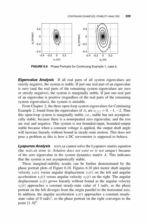
CONTINUING EXAMPLES: STABILITY ANALYSIS 229
−0.4 −0.2 0 0.2−0.4
−0.2
0
0.2
x1 (m)
x 2(m
/sec
)
−0.4 −0.2 0 0.2
−0.4
−0.2
0
0.2
x3 (m)
x 4(m
/sec
)
FIGURE 6.9 Phase Portraits for Continuing Example 1, case b.
Eigenvalue Analysis If all real parts of all system eigenvalues arestrictly negative, the system is stable. If just one real part of an eigenvalueis zero (and the real parts of the remaining system eigenvalues are zeroor strictly negative), the system is marginally stable. If just one real partof an eigenvalue is positive (regardless of the real parts of the remainingsystem eigenvalues), the system is unstable.
From Chapter 2, the three open-loop system eigenvalues for ContinuingExample 2, found from the eigenvalues of A, are s1,2,3 = 0, −1, −2. Thusthis open-loop system is marginally stable, i.e., stable but not asymptoti-cally stable, because there is a nonrepeated zero eigenvalue, and the restare real and negative. This system is not bounded-input, bounded-outputstable because when a constant voltage is applied, the output shaft anglewill increase linearly without bound in steady-state motion. This does notpose a problem as this is how a DC servomotor is supposed to behave.
Lyapunov Analysis MATLAB cannot solve the Lyapunov matrix equation(the MATLAB error is: Solution does not exist or is not unique) becauseof the zero eigenvalue in the system dynamics matrix A. This indicatesthat the system is not asymptotically stable.
These marginal-stability results can be further demonstrated by thephase portrait plots of Figure 6.10. Figures 6.10 plot motor shaft angularvelocity x2(t) versus angular displacement x1(t) on the left and angularacceleration x3(t) versus angular velocity x2(t) on the right. The angulardisplacement x1(t) grows linearly without bound as the angular velocityx2(t) approaches a constant steady-state value of 1 rad/s, so the phaseportrait on the left diverges from the origin parallel to the horizontal axis.In addition, the angular acceleration x3(t) approaches a constant steady-state value of 0 rad/s2, so the phase portrait on the right converges to thepoint [1, 0]T .
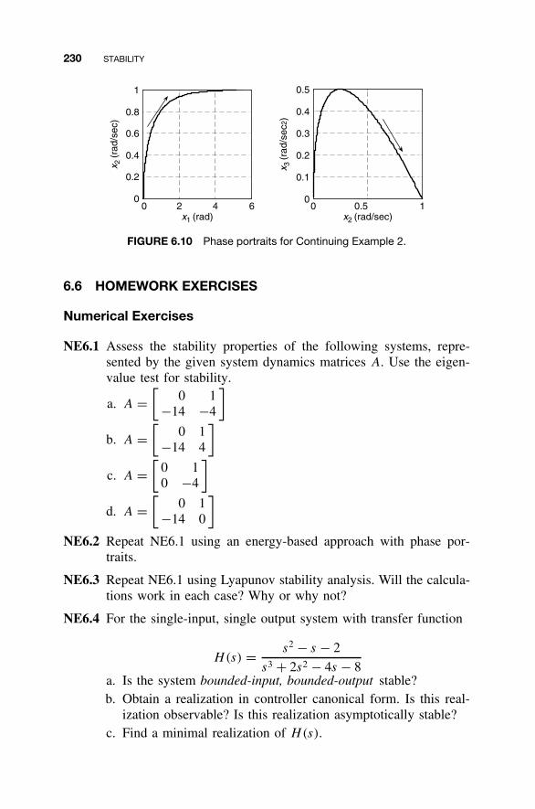
230 STABILITY
0 2 4 60
0.2
0.4
0.6
0.8
1
x1 (rad)
x 2(r
ad/s
ec)
0 0.5 10
0.1
0.2
0.3
0.4
0.5
x2 (rad/sec)
x 3(r
ad/s
ec2)
FIGURE 6.10 Phase portraits for Continuing Example 2.
6.6 HOMEWORK EXERCISES
Numerical Exercises
NE6.1 Assess the stability properties of the following systems, repre-sented by the given system dynamics matrices A. Use the eigen-value test for stability.
a. A =[
0 1−14 −4
]
b. A =[
0 1−14 4
]
c. A =[
0 10 −4
]
d. A =[
0 1−14 0
]
NE6.2 Repeat NE6.1 using an energy-based approach with phase por-traits.
NE6.3 Repeat NE6.1 using Lyapunov stability analysis. Will the calcula-tions work in each case? Why or why not?
NE6.4 For the single-input, single output system with transfer function
H(s) = s2 − s − 2
s3 + 2s2 − 4s − 8a. Is the system bounded-input, bounded-output stable?b. Obtain a realization in controller canonical form. Is this real-
ization observable? Is this realization asymptotically stable?c. Find a minimal realization of H(s).
HOMEWORK EXERCISES 231
NE6.5 For the single-input, single output system with transfer function
H(s) = s2 + s − 2
s3 + 2s2 − 4s − 8a. Is the system bounded-input, bounded-output stable?b. Obtain a realization in observer canonical form. Is this realiza-
tion controllable? Is this realization asymptotically stable?c. Find a minimal realization of H(s).
Analytical Exercises
AE6.1 If A = −AT , show that the homogeneous linear state equation
x(t) = Ax(t)
is stable but not asymptotically stable.
AE6.2 Given matrices A and Q, let P satisfy the Lyapunov matrixequation
ATP + PA = −Q
Show that for all t ≥ 0,
P = eAT t
QeAt +∫ t
0eAT τ
QeAτdτ
AE6.3 Show that the eigenvalues of A have real part less than −µ if andonly if for every symmetric positive-definite matrix Q there existsa unique symmetric positive-definite solution to
AT P + PA + 2µP = −Q
AE6.4 Suppose that A has negative real-part eigenvalues, and let P
denote the unique symmetric-positive definite solution to the Lya-punov matrix equation
AT P + PA = −I
Show that the perturbed homogeneous linear state equation
x(t) = (A + �A)x(t)
is asymptotically stable if the perturbation matrix satisfies the spec-tral norm bound
||�A|| <1
2λmax(P )
232 STABILITY
AE6.5 Suppose that the pair (A, B) is controllable and that A has negativereal-part eigenvalues. Show that the Lyapunov matrix equation
AW + WA = −BBT
has a symmetric positive definite solution W .
AE6.6 Suppose that the pair (A, B) is controllable and that the Lyapunovmatrix equation
AW + WA = −BBT
has a symmetric positive-definite solution W . Show that A hasnegative real-part eigenvalues.
AE6.7 Consider a bounded-input, bounded-output stable single-input,single-output state equation with transfer function H(s). Forpositive constants λ and µ, show that the zero-state response y(t)
to the input u(t) = e−λt , t ≥ 0 satisfies
∫ ∞
0y(t)e−µtdt = 1
λ + µH(µ)
Under what conditions can this relationship hold if the stateequation is not bounded-input, bounded-output stable?
Continuing MATLAB Exercises
CME6.1 For the system given in CME1.1:a. Assess system stability using Lyapunov analysis. Compare
this result with eigenvalue analysis.b. Plot phase portraits to reinforce your stability results.
CME6.2 For the system given in CME1.2:a. Assess system stability using Lyapunov analysis. Compare
this result with eigenvalue analysis.b. Plot phase portraits to reinforce your stability results.
CME6.3 For the system given in CME1.3:a. Assess system stability condition using Lyapunov analysis.
Compare this result with eigenvalue analysis.b. Plot phase portraits to reinforce your stability results.
CME6.4 For the system given in CME1.4:
HOMEWORK EXERCISES 233
a. Assess system stability condition using Lyapunov analysis.Compare this result with eigenvalue analysis.
b. Plot phase portraits to reinforce your stability results.
Continuing Exercises
CE6.1 Using Lyapunov analysis, assess the stability properties of theCE1 system; any case will do—since the A matrix is identicalfor all input/output cases, the stability condition does not change.Check your results via eigenvalue analysis. Plot phase portraits toreinforce your results.
CE6.2 Using Lyapunov analysis, assess the stability properties of theCE2 system; any case will do—because the A matrix is identicalfor all input-output cases, stability does not change. Lyapunovstability analysis will not succeed (why?); therefore, assess systemstability via eigenvalue analysis. Plot phase portraits to reinforceyour results.
CE6.3 Using Lyapunov analysis, assess the stability properties of theCE3 system; either case will do—since the A matrix is identicalfor all input-output cases, stability does not change. Lyapunovstability analysis will not succeed (why?); therefore, assess systemstability via eigenvalue analysis. Plot phase portraits to reinforceyour results.
CE6.4 Using Lyapunov analysis, assess the stability properties of the CE4system. Lyapunov stability analysis will not succeed (why?); there-fore, assess system stability via eigenvalue analysis. Plot phaseportraits to reinforce your results.
CE6.5 Using Lyapunov analysis, assess the stability properties of the CE5system. Lyapunov stability analysis will not succeed (why?); there-fore, assess system stability via eigenvalue analysis. Plot phaseportraits to reinforce your results.
7
DESIGN OF LINEAR STATEFEEDBACK CONTROL LAWS
Previous chapters, by introducing fundamental state-space concepts andanalysis tools, have now set the stage for our initial foray into state-space methods for control system design. In this chapter, our focus ison the design of state feedback control laws that yield desirable closed-loop performance in terms of both transient and steady-state responsecharacteristics. The fundamental result that underpins much of this chapteris that controllability of the open-loop state equation is both necessary andsufficient to achieve arbitrary closed-loop eigenvalue placement via statefeedback. Furthermore, explicit feedback gain formulas for eigenvalueplacement are available in the single-input case. To support the design ofstate feedback control laws, we discuss important relationship between theeigenvalue locations of a linear state equation and its dynamic responsecharacteristics.
For state equations that are not controllable and so arbitrary eigen-value placement via state feedback is not possible, we investigate whetherstate feedback can be used to at least stabilize the closed-loop stateequation. This leads to the concept of stabilizability. Following that, wediscuss techniques for improving steady-state performance first by intro-ducing an additional gain parameter in the state feedback law, followed bythe incorporation of integral-error compensation into our state feedbackstructure.
234
Linear State-Space Control Systems. Robert L. Williams II and Douglas A. LawrenceCopyright 2007 John Wiley & Sons, Inc. ISBN: 978-0-471-73555-7
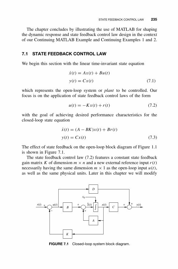
STATE FEEDBACK CONTROL LAW 235
The chapter concludes by illustrating the use of MATLAB for shapingthe dynamic response and state feedback control law design in the contextof our Continuing MATLAB Example and Continuing Examples 1 and 2.
7.1 STATE FEEDBACK CONTROL LAW
We begin this section with the linear time-invariant state equation
x(t) = Ax(t) + Bu(t)
y(t) = Cx(t) (7.1)
which represents the open-loop system or plant to be controlled. Ourfocus is on the application of state feedback control laws of the form
u(t) = −Kx(t) + r(t) (7.2)
with the goal of achieving desired performance characteristics for theclosed-loop state equation
x(t) = (A − BK )x(t) + Br(t)
y(t) = Cx(t) (7.3)
The effect of state feedback on the open-loop block diagram of Figure 1.1is shown in Figure 7.1.
The state feedback control law (7.2) features a constant state feedbackgain matrix K of dimension m × n and a new external reference input r(t)
necessarily having the same dimension m × 1 as the open-loop input u(t),as well as the same physical units. Later in this chapter we will modify
+ + + +
+−
A
CB
D
K
r(t) u(t) x(t) x(t) y(t)
x0
•
FIGURE 7.1 Closed-loop system block diagram.
236 DESIGN OF LINEAR STATE FEEDBACK CONTROL LAWS
the state feedback control law to include a gain matrix multiplying thereference input. The state feedback control law can be written in terms ofscalar components as
u1(t)
u2(t)...
um(t)
= −
k11 k12 · · · k1n
k21 k22 · · · k2n
......
. . ....
km1 km2 · · · kmn
x1(t)
x2(t)...
xn(t)
+
r1(t)
r2(t)...
rm(t)
For the single-input, single-output case, the feedback gain K is a 1 ×n row vector, the reference input r(t) is a scalar signal, and the statefeedback control law has the form
u(t) = − [k1 k2 · · · kn
]
x1(t)
x2(t)...
x2(t)
+ r(t)
= −k1x1(t) − k2x2(t) − · · · − knxn(t) + r(t)
If the external reference input is absent, the state feedback control law iscalled a regulator that is designed to deliver desirable transient responsefor nonzero initial conditions and/or attenuate disturbances to maintainthe equilibrium state x = 0.
7.2 SHAPING THE DYNAMIC RESPONSE
In addition to closed-loop asymptotic stability (see Chapter 6), whichrequires that the closed-loop system dynamics matrix A − BK havestrictly negative real-part eigenvalues, we are often interested in othercharacteristics of the closed-loop transient response, such as rise time,peak time, percent overshoot, and settling time of the step response. Beforewe investigate the extent to which state feedback can influence the closed-loop eigenvalues, we first review topics associated with transient responseperformance of feedback control systems that are typically introducedin an undergraduate course emphasizing classical control theory. Inour state-space context, we seek to translate desired transient responsecharacteristics into specifications on system eigenvalues, which are closelyrelated to transfer function poles. Specifying desired closed-loop systembehavior via eigenvalue selection is called shaping the dynamic response.Control system engineers often use dominant first- and second-order
SHAPING THE DYNAMIC RESPONSE 237
subsystems as approximations in the design process, along with criteriathat justify such approximations for higher-order systems. Our discussionfollows this approach.
Eigenvalue Selection for First-Order Systems
Figure 7.2 shows unit step responses of typical of first- through fourth-order systems.
For a first-order system, we can achieve desired transient behavior viaspecifying a single eigenvalue. Figure 7.2 (top left) shows a standard first-order system step response. All stable first-order systems driven by unitstep inputs behave this way, with transient response governed by a singledecaying exponential involving the time constant τ . After three time con-stants, the first-order unit step response is within 95 percent of its steady-state value. A smaller time constant responds more quickly, whereas alarger time constant responds more slowly. On specifying a desired timeconstant, the associated characteristic polynomial and eigenvalue are
λ + 1
τand λ1 = −1
τ
0 5 100
0.5
1
time (sec)
time (sec) time (sec)
time (sec)
y 1 y 2y 4y 3
0 5 100
0.5
1
1.5
2
0 5 100
0. 5
1
0 5 10−1
0
1
2
3
FIGURE 7.2 First- through fourth-order system unit step responses.
238 DESIGN OF LINEAR STATE FEEDBACK CONTROL LAWS
Eigenvalue Selection for Second-Order Systems
For a second-order system, we can achieve desired transient behaviorvia specifying a pair of eigenvalues. To illustrate, we consider the lin-ear translational mechanical system of Example 1.1 (see Figure 1.2) withapplied force f (t) as the input and mass displacement y(t) as the out-put. We identify this with a standard second-order system by redefin-ing the input via u(t) = f (t)/k. The new input u(t) can be interpretedas a commanded displacement. This will normalize steady-state valueof the unit step response to 1.0. With this change, the state equationbecomes
[x1(t)
x2(t)
]=
0 1
− k
m− c
m
[x1(t)
x2(t)
]+
0
k
m
u(t)
y(t) = [1 0
] [x1(t)
x2(t)
]
with associated transfer function
H(s) =km
s2 + cms + k
m
We compare this with the standard second-order transfer function, namely,
ω2n
s2 + 2ξωn + ω2n
in which ξ is the unitless damping ratio, and ωn is the undamped naturalfrequency in radians per second. This leads to the relationships
ξ = c
2√
kmand ωn =
√k
m
The characteristic polynomial is
λ2 + c
mλ + k
m= λ2 + 2ξωnλ + ω2
n
from which the eigenvalues are
λ1,2 = −ξωn ± ωn
√ξ 2 − 1
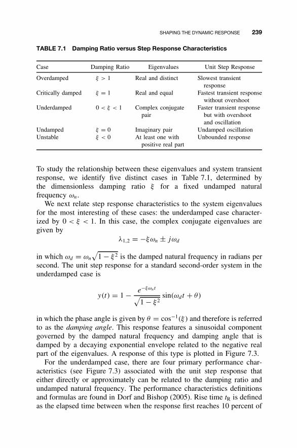
SHAPING THE DYNAMIC RESPONSE 239
TABLE 7.1 Damping Ratio versus Step Response Characteristics
Case Damping Ratio Eigenvalues Unit Step Response
Overdamped ξ > 1 Real and distinct Slowest transientresponse
Critically damped ξ = 1 Real and equal Fastest transient responsewithout overshoot
Underdamped 0 < ξ < 1 Complex conjugatepair
Faster transient responsebut with overshootand oscillation
Undamped ξ = 0 Imaginary pair Undamped oscillationUnstable ξ < 0 At least one with
positive real partUnbounded response
To study the relationship between these eigenvalues and system transientresponse, we identify five distinct cases in Table 7.1, determined bythe dimensionless damping ratio ξ for a fixed undamped naturalfrequency ωn.
We next relate step response characteristics to the system eigenvaluesfor the most interesting of these cases: the underdamped case character-ized by 0 < ξ < 1. In this case, the complex conjugate eigenvalues aregiven by
λ1,2 = −ξωn ± jωd
in which ωd = ωn
√1 − ξ 2 is the damped natural frequency in radians per
second. The unit step response for a standard second-order system in theunderdamped case is
y(t) = 1 − e−ξωnt√1 − ξ 2
sin(ωdt + θ)
in which the phase angle is given by θ = cos−1(ξ) and therefore is referredto as the damping angle. This response features a sinusoidal componentgoverned by the damped natural frequency and damping angle that isdamped by a decaying exponential envelope related to the negative realpart of the eigenvalues. A response of this type is plotted in Figure 7.3.
For the underdamped case, there are four primary performance char-acteristics (see Figure 7.3) associated with the unit step response thateither directly or approximately can be related to the damping ratio andundamped natural frequency. The performance characteristics definitionsand formulas are found in Dorf and Bishop (2005). Rise time tR is definedas the elapsed time between when the response first reaches 10 percent of
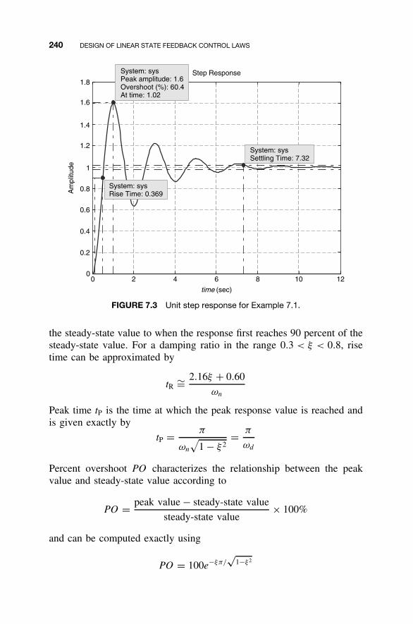
240 DESIGN OF LINEAR STATE FEEDBACK CONTROL LAWS
Step Response
time (sec)
0 2 4 6 8 10 120
0.2
0.4
0.6
0.8
1
1.2
1.4
1.6
1.8
System: sysPeak amplitude: 1.6Overshoot (%): 60.4At time: 1.02
System: sysRise Time: 0.369
System: sysSettling Time: 7.32
Am
plitu
de
FIGURE 7.3 Unit step response for Example 7.1.
the steady-state value to when the response first reaches 90 percent of thesteady-state value. For a damping ratio in the range 0.3 < ξ < 0.8, risetime can be approximated by
tR ∼= 2.16ξ + 0.60
ωn
Peak time tP is the time at which the peak response value is reached andis given exactly by
tP = π
ωn
√1 − ξ 2
= π
ωd
Percent overshoot PO characterizes the relationship between the peakvalue and steady-state value according to
PO = peak value − steady-state value
steady-state value× 100%
and can be computed exactly using
PO = 100e−ξπ/√
1−ξ 2
SHAPING THE DYNAMIC RESPONSE 241
Settling time tS is typically defined to be the time at which the responseenters and remains within a ±2 percent band about the steady-state valueand can be approximated by
tS ∼= 4
ξωn
The swiftness of the response is related to the rise time and peak time;the deviation between the response and its steady-state value is related tothe percent overshoot and settling time.
Example 7.1 We return to the linear translational mechanical systemfor the parameter values m = 1 kg, c = 1 N-s/m, and k = 10 N/m. Theundamped natural frequency and dimensionless damping ratio are
ωn =√
k
m=
√10
1= 3.16 rad/s
ξ = c
2√
km= 1
2√
10(1)= 0.158
and the damped natural frequency is
ωd = ωn
√1 − ξ 2 = 3.12 rad/s
The characteristic polynomial is
λ2 + 2ξωnλ + ω2n = λ2 + λ + 10
yielding the complex conjugate eigenvalues
λ1,2 = −0.5 ± 3.12i
The unit step response is given by
y(t) = 1 − 1.01e−0.5t sin(3.12t + 80.9◦)
We calculate directly from ξ and ωn the step response characteristics:tR = 0.30 s (because ξ < 0.3 this estimate may be somewhat inaccurate),tP = 1.01 s, PO = 60.5 percent, and tS = 8 s.
A plot of the unit step response is given is Figure 7.3, with rise time,peak time, percent overshoot, and settling time displayed. This plot wasobtained from MATLAB using the step command and right-clicking in the
242 DESIGN OF LINEAR STATE FEEDBACK CONTROL LAWS
resulting figure window to add the performance specifications (Charac-teristics → choose Peak Response, Settling Time, Rise Time, and SteadyState in turn. MATLAB will mark the response with a dot, which the usermay click to display the numerical values). We see that with the exceptionof rise time (0.30 s estimated versus 0.37 s from the plot), the formulavalues agree well with the MATLAB results values labeled on Figure 7.3(settling time is also inaccurate, 8 s from the equation versus 7.32 s asmeasured from the MATLAB generated response). �
Example 7.2 The unit step response in Figure 7.3 is typical of lightlydamped systems such as large-scale space structures. We consider theapplication of a proportional-derivative (PD) control law given by
u(t) = −kPy(t) − kDy(t) + Gr(t)
= − [kP kD
] [x1(t)
x2(t)
]+ Gr(t)
which, as shown, also has the form of a state feedback control law. Theclosed-loop system that results is given by
[x1(t)
x2(t)
]=
0 1
−(
k
m+ kP
)−
( c
m+ kD
)[
x1(t)
x2(t)
]+
0
k
m
Gr(t)
y(t) = [1 0
] [x1(t)
x2(t)
]
Our objective is to improve the step response characteristics by reducingthe percent overshoot and settling time via adjusting the proportional andderivative gains kP and kD. In particular, we specify a desired percentovershoot of 4 percent and a settling time of 2 s. The gain G will bechosen so that the closed-loop unit step response will have the samesteady-state value as the open-loop unit step response.
In terms of these performance specifications, we calculate thedesired closed-loop damping ratio ξ ′ from the percent-overshoot formulaaccording to
ξ ′ =
∣∣∣∣ln(
PO
100
)∣∣∣∣√π2 +
[ln
(PO
100
)]2=
∣∣∣∣ln(
4
100
)∣∣∣∣√π2 +
[ln
(4
100
)]2= 0.716
SHAPING THE DYNAMIC RESPONSE 243
Using this, we calculate the desired closed-loop undamped naturalfrequency from the settling-time formula via
ω′n = 4
ξ ′tS= 2.79 rad/s
The desired closed-loop damped natural frequency is
ω′d = ω′
n
√1 − (ξ ′)2 = 1.95 rad/s
The proportional and derivative gains then can be determined by com-paring the closed-loop characteristic polynomial of the closed-loop stateequation with the desired closed-loop characteristic polynomial:
λ2 + (2ξωn + kD)λ + (ω2n + kP) = λ2 + 2ξ ′ω′
nλ + ω′n
2 = λ2 + 4λ + 7.81
which leads to
kP = ω′n
2 − ω2n = −2.20 kD = 2ξ ′ω′
n − 2ξωn = 3.00
The input gain G is determined from the relationship
G = ω′n
2
ω2n
= 0.781
which yields the closed-loop transfer function
kmG
s2 + ( cm
+ kD)s + ( km
+ kP)= ω2
nG
s2 + (2ξωn + kD)s + (ω2n + kP)
= ω′n
2
s2 + 2ξ ′ω′ns + ω
′2n
= 7.81
s2 + 4s + 7.81
The closed-loop eigenvalues then are:
λ1,2 = −2 ± j1.95
and the closed-loop unit step response is
y(t) = 1 − 1.43e−2t sin(1.95t + 44.3◦)
The MATLAB step command gives us the four performance specifica-tions: tR = 0.78 s, tP = 1.60 s, PO = 4 percent, and tS = 2.12 s. Theactual settling time differs slightly from the desired settling time becauseof the approximation in the settling-time formula. Figure 7.4 shows a
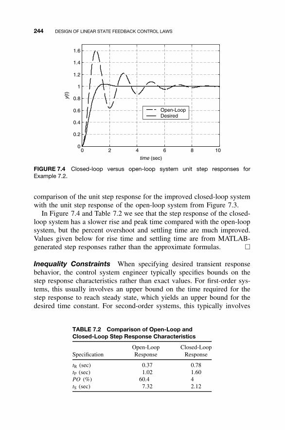
244 DESIGN OF LINEAR STATE FEEDBACK CONTROL LAWS
0 2 4 6 8 100
0.2
0.4
0.6
0.8
1
1.2
1.4
1.6
time (sec)
y(t)
Open-LoopDesired
FIGURE 7.4 Closed-loop versus open-loop system unit step responses forExample 7.2.
comparison of the unit step response for the improved closed-loop systemwith the unit step response of the open-loop system from Figure 7.3.
In Figure 7.4 and Table 7.2 we see that the step response of the closed-loop system has a slower rise and peak time compared with the open-loopsystem, but the percent overshoot and settling time are much improved.Values given below for rise time and settling time are from MATLAB-generated step responses rather than the approximate formulas. �
Inequality Constraints When specifying desired transient responsebehavior, the control system engineer typically specifies bounds on thestep response characteristics rather than exact values. For first-order sys-tems, this usually involves an upper bound on the time required for thestep response to reach steady state, which yields an upper bound for thedesired time constant. For second-order systems, this typically involves
TABLE 7.2 Comparison of Open-Loop andClosed-Loop Step Response Characteristics
Open-Loop Closed-LoopSpecification Response Response
tR (sec) 0.37 0.78tP (sec) 1.02 1.60PO (%) 60.4 4tS (sec) 7.32 2.12
SHAPING THE DYNAMIC RESPONSE 245
any combination of upper bounds the on rise time, peak time, percentovershoot, and settling time of the step response. This yields bounds onthe desired damping ratio and undamped natural frequency that, in turn,can be translated into regions in the complex plane that specify desiredeigenvalue locations. This more general viewpoint will be demonstratedin the following example for the second-order case.
Example 7.3 In this example we characterize acceptable eigenvaluelocations in the complex plane so that the following second-order per-formance specifications are satisfied:
PO ≤ 4% tS ≤ 2 s tP ≤ 0.5 s
The formula for percent overshoot indicates that percent overshootdecreases as damping ratio increases. Therefore, an upper bound onpercent overshoot PO ≤ POmax corresponds to a lower bound on dampingratio ξ ≥ ξmin. From Example 7.2, we know that a damping ratio ofξmin = 0.716 will yield a percent overshoot equal to POmax = 4 percent.Therefore, in order to achieve a percent overshoot less than 4 percent,we require a damping ratio greater than 0.716. We previously defined thedamping angle θ = cos−1(ξ), which appeared in the expression for the unitstep response of the standard underdamped second-order system. From thisrelationship, we see that a lower bound on the damping ratio correspondsto an upper bound on the damping angle θ ≤ θmax = cos−1(ξmin). To relatethis to allowable eigenvalue locations, we see from basic trigonometry that
tan(θ) =√
1 − ξ 2
ξ= ωn
√1 − ξ 2
ξωn
= ωd
ξωn
Recalling that eigenvalues of an underdamped second-order system areλ1,2 = −ξωn ± jωd , in which ωd = ωn
√1 − ξ 2 is the damped natural
frequency, we therefore interpret the damping angle θ as the angle madeby the radial line from the origin in the complex plane passing throughthe eigenvalue λ1 = −ξωn + jωd measured with respect to the negativereal axis. By symmetry, −θ is the angle made by the radial line fromthe origin in the complex plane passing through the conjugate eigenvalueλ2 = −ξωn − jωd , also measured with respect to the negative real axis.An upper bound on the damping angle characterizes a sector in the left halfof the complex plane bounded by the pair of radial lines correspondingto the maximum allowable damping angle. In this example, a minimumallowable damping ratio of 0.716 corresponds to a maximum allowabledamping angle of cos−1(0.716) = 44.3◦. The associated sector specifying
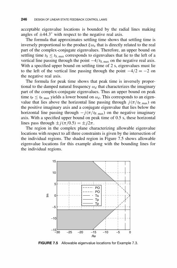
246 DESIGN OF LINEAR STATE FEEDBACK CONTROL LAWS
acceptable eigenvalue locations is bounded by the radial lines makingangles of ±44.3◦ with respect to the negative real axis.
The formula that approximates settling time shows that settling time isinversely proportional to the product ξωn that is directly related to the realpart of the complex-conjugate eigenvalues. Therefore, an upper bound onsettling time tS ≤ tS, max corresponds to eigenvalues that lie to the left of avertical line passing through the point −4/tS, max on the negative real axis.With a specified upper bound on settling time of 2 s, eigenvalues must lieto the left of the vertical line passing through the point −4/2 = −2 onthe negative real axis.
The formula for peak time shows that peak time is inversely propor-tional to the damped natural frequency ωd that characterizes the imaginarypart of the complex-conjugate eigenvalues. Thus an upper bound on peaktime tP ≤ tP, max yields a lower bound on ωd . This corresponds to an eigen-value that lies above the horizontal line passing through j (π/tP, max) onthe positive imaginary axis and a conjugate eigenvalue that lies below thehorizontal line passing through −j (π/tP, max) on the negative imaginaryaxis. With a specified upper bound on peak time of 0.5 s, these horizontallines pass through ±j (π/0.5) = ±j2π .
The region in the complex plane characterizing allowable eigenvaluelocations with respect to all three constraints is given by the intersection ofthe individual regions. The shaded region in Figure 7.5 shows allowableeigenvalue locations for this example along with the bounding lines forthe individual regions.
−30 −25 −20 −15 −10 −5 0−15
−10
−5
0
5
10
15
Re
POPOTsTpTp
Im
FIGURE 7.5 Allowable eigenvalue locations for Example 7.3.
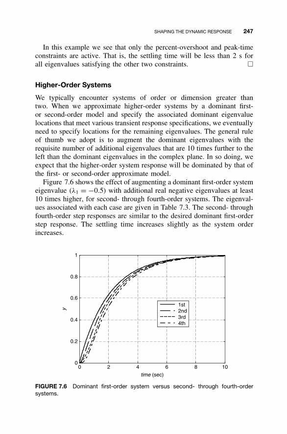
SHAPING THE DYNAMIC RESPONSE 247
In this example we see that only the percent-overshoot and peak-timeconstraints are active. That is, the settling time will be less than 2 s forall eigenvalues satisfying the other two constraints. �
Higher-Order Systems
We typically encounter systems of order or dimension greater thantwo. When we approximate higher-order systems by a dominant first-or second-order model and specify the associated dominant eigenvaluelocations that meet various transient response specifications, we eventuallyneed to specify locations for the remaining eigenvalues. The general ruleof thumb we adopt is to augment the dominant eigenvalues with therequisite number of additional eigenvalues that are 10 times further to theleft than the dominant eigenvalues in the complex plane. In so doing, weexpect that the higher-order system response will be dominated by that ofthe first- or second-order approximate model.
Figure 7.6 shows the effect of augmenting a dominant first-order systemeigenvalue (λ1 = −0.5) with additional real negative eigenvalues at least10 times higher, for second- through fourth-order systems. The eigenval-ues associated with each case are given in Table 7.3. The second- throughfourth-order step responses are similar to the desired dominant first-orderstep response. The settling time increases slightly as the system orderincreases.
0 2 4 6 8 100
0.2
0.4
0.6
0.8
1
y
1st2nd3rd4th
time (sec)
FIGURE 7.6 Dominant first-order system versus second- through fourth-ordersystems.
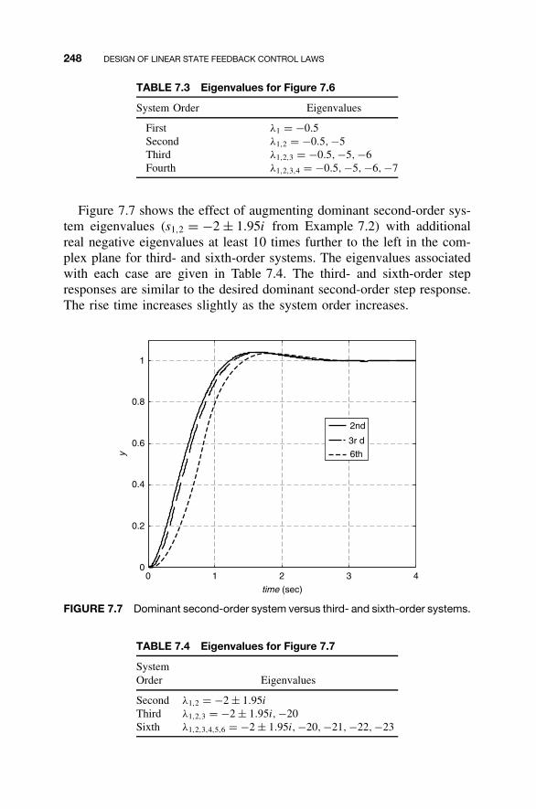
248 DESIGN OF LINEAR STATE FEEDBACK CONTROL LAWS
TABLE 7.3 Eigenvalues for Figure 7.6
System Order Eigenvalues
First λ1 = −0.5Second λ1,2 = −0.5,−5Third λ1,2,3 = −0.5,−5,−6Fourth λ1,2,3,4 = −0.5,−5,−6,−7
Figure 7.7 shows the effect of augmenting dominant second-order sys-tem eigenvalues (s1,2 = −2 ± 1.95i from Example 7.2) with additionalreal negative eigenvalues at least 10 times further to the left in the com-plex plane for third- and sixth-order systems. The eigenvalues associatedwith each case are given in Table 7.4. The third- and sixth-order stepresponses are similar to the desired dominant second-order step response.The rise time increases slightly as the system order increases.
0 1 2
time (sec)
3 40
0.2
0.4
0.6
y
0.8
1
2nd
3r d
6th
FIGURE 7.7 Dominant second-order system versus third- and sixth-order systems.
TABLE 7.4 Eigenvalues for Figure 7.7
SystemOrder Eigenvalues
Second λ1,2 = −2 ± 1.95i
Third λ1,2,3 = −2 ± 1.95i,−20Sixth λ1,2,3,4,5,6 = −2 ± 1.95i,−20,−21,−22,−23
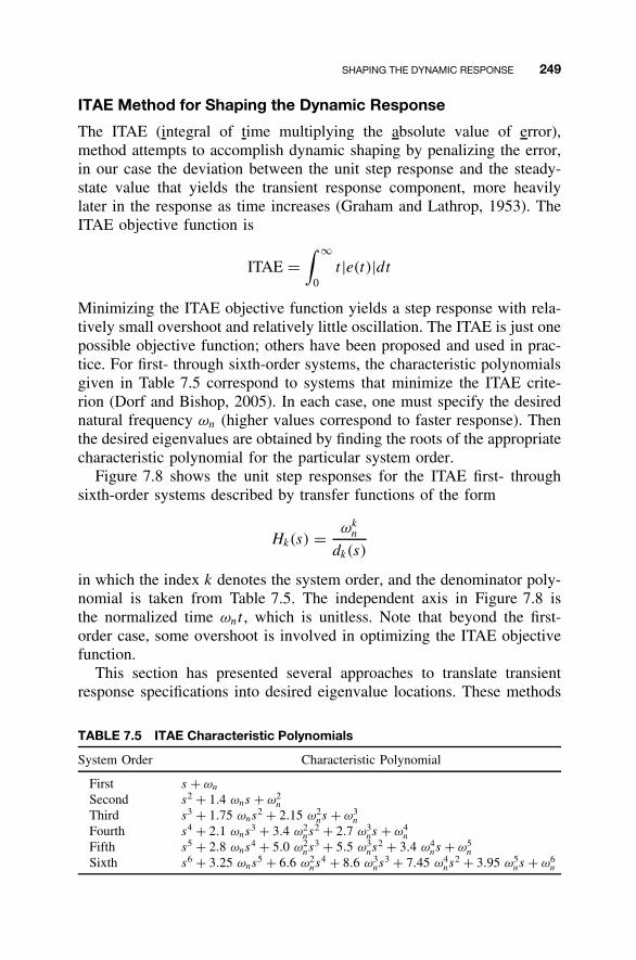
SHAPING THE DYNAMIC RESPONSE 249
ITAE Method for Shaping the Dynamic Response
The ITAE (integral of time multiplying the absolute value of error),method attempts to accomplish dynamic shaping by penalizing the error,in our case the deviation between the unit step response and the steady-state value that yields the transient response component, more heavilylater in the response as time increases (Graham and Lathrop, 1953). TheITAE objective function is
ITAE =∫ ∞
0t |e(t)|dt
Minimizing the ITAE objective function yields a step response with rela-tively small overshoot and relatively little oscillation. The ITAE is just onepossible objective function; others have been proposed and used in prac-tice. For first- through sixth-order systems, the characteristic polynomialsgiven in Table 7.5 correspond to systems that minimize the ITAE crite-rion (Dorf and Bishop, 2005). In each case, one must specify the desirednatural frequency ωn (higher values correspond to faster response). Thenthe desired eigenvalues are obtained by finding the roots of the appropriatecharacteristic polynomial for the particular system order.
Figure 7.8 shows the unit step responses for the ITAE first- throughsixth-order systems described by transfer functions of the form
Hk(s) = ωkn
dk(s)
in which the index k denotes the system order, and the denominator poly-nomial is taken from Table 7.5. The independent axis in Figure 7.8 isthe normalized time ωnt , which is unitless. Note that beyond the first-order case, some overshoot is involved in optimizing the ITAE objectivefunction.
This section has presented several approaches to translate transientresponse specifications into desired eigenvalue locations. These methods
TABLE 7.5 ITAE Characteristic Polynomials
System Order Characteristic Polynomial
First s + ωn
Second s2 + 1.4 ωns + ω2n
Third s3 + 1.75 ωns2 + 2.15 ω2
ns + ω3n
Fourth s4 + 2.1 ωns3 + 3.4 ω2
ns2 + 2.7 ω3
ns + ω4n
Fifth s5 + 2.8 ωns4 + 5.0 ω2
ns3 + 5.5 ω3
ns2 + 3.4 ω4
ns + ω5n
Sixth s6 + 3.25 ωns5 + 6.6 ω2
ns4 + 8.6 ω3
ns3 + 7.45 ω4
ns2 + 3.95 ω5
ns + ω6n
250 DESIGN OF LINEAR STATE FEEDBACK CONTROL LAWS
0 2 4 6 8 10 120
0.2
0.4
0.6
0.8
1
1st2nd3rd
5th4th
6th
wnt
y IT
AE(w
nt)
FIGURE 7.8 ITAE unit step responses.
have focused on so-called all-pole system models. It is well known fromclassical control that the presence of zeros (roots of the transfer func-tion numerator polynomial) will change the system’s transient behavior.One approach to remedy this is to use a prefilter to reduce the effect ofthese zeros.
7.3 CLOSED-LOOP EIGENVALUE PLACEMENT VIA STATEFEEDBACK
The following result establishes a connection between the ability to arbi-trarily place the closed-loop eigenvalues by proper choice of the statefeedback gain matrix K and controllability of the open-loop state equation,i.e., the pair (A, B).
Theorem 7.1 For any symmetric set of n complex numbers {µ1 , µ2 , . . . ,
µn}, there exists a state feedback gain matrix K such that σ(A − BK ) ={µ1 , µ2 , . . . , µn} if and only if the pair (A, B) is controllable.
Proof. Here we prove that controllability of the pair (A, B) is necessaryfor arbitrary eigenvalue placement via state feedback. That controllabil-ity of the pair (A, B) is sufficient for arbitrary eigenvalue placement viastate feedback will be established constructively in the single-input caseby deriving formulas for the requisite state feedback gain vector. The
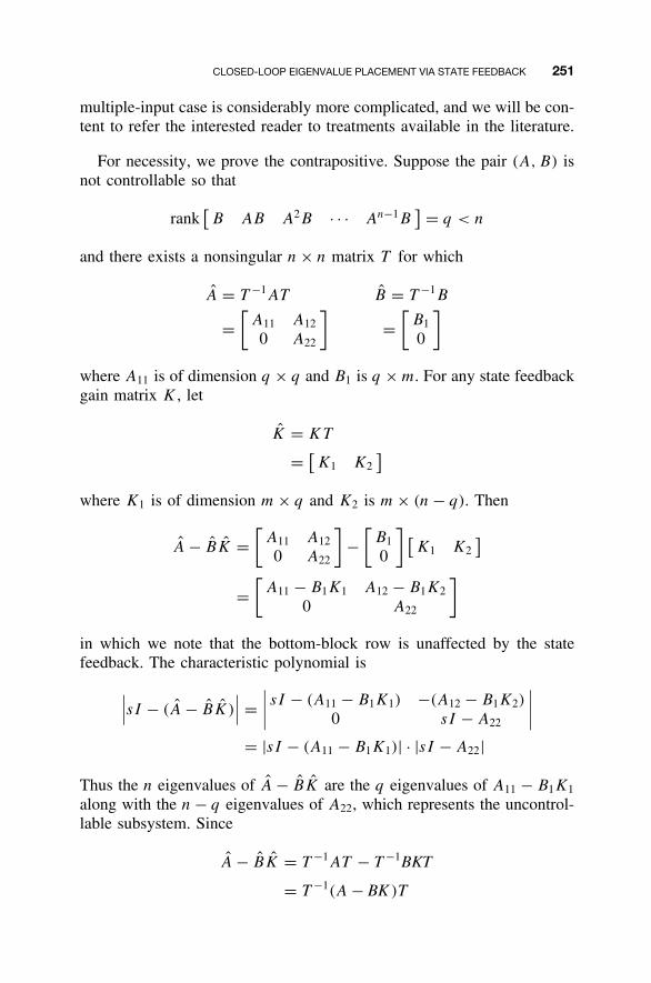
CLOSED-LOOP EIGENVALUE PLACEMENT VIA STATE FEEDBACK 251
multiple-input case is considerably more complicated, and we will be con-tent to refer the interested reader to treatments available in the literature.
For necessity, we prove the contrapositive. Suppose the pair (A, B) isnot controllable so that
rank[B AB A2B · · · An−1B
] = q < n
and there exists a nonsingular n × n matrix T for which
A = T −1AT B = T −1B
=[
A11 A12
0 A22
]=
[B1
0
]
where A11 is of dimension q × q and B1 is q × m. For any state feedbackgain matrix K , let
K = KT
= [K1 K2
]
where K1 is of dimension m × q and K2 is m × (n − q). Then
A − BK =[
A11 A12
0 A22
]−
[B1
0
] [K1 K2
]
=[
A11 − B1K1 A12 − B1K2
0 A22
]
in which we note that the bottom-block row is unaffected by the statefeedback. The characteristic polynomial is
∣∣∣sI − (A − BK)
∣∣∣ =∣∣∣∣ sI − (A11 − B1K1) −(A12 − B1K2)
0 sI − A22
∣∣∣∣= |sI − (A11 − B1K1)| · |sI − A22|
Thus the n eigenvalues of A − BK are the q eigenvalues of A11 − B1K1
along with the n − q eigenvalues of A22, which represents the uncontrol-lable subsystem. Since
A − BK = T −1AT − T −1BKT
= T −1(A − BK )T
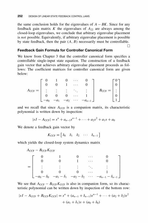
252 DESIGN OF LINEAR STATE FEEDBACK CONTROL LAWS
the same conclusion holds for the eigenvalues of A − BK . Since for anyfeedback gain matrix K the eigenvalues of A22 are always among theclosed-loop eigenvalues, we conclude that arbitrary eigenvalue placementis not possible. Equivalently, if arbitrary eigenvalue placement is possibleby state feedback, then the pair (A, B) necessarily must be controllable.
�Feedback Gain Formula for Controller Canonical Form
We know from Chapter 3 that the controller canonical form specifies acontrollable single-input state equation. The construction of a feedbackgain vector that achieves arbitrary eigenvalue placement proceeds as fol-lows: The coefficient matrices for controller canonical form are givenbelow:
ACCF =
0 1 0 · · · 00 0 1 · · · 0...
......
. . ....
0 0 0 · · · 1−a0 −a1 −a2 · · · −an−1
BCCF =
00...
01
and we recall that since ACCF is a companion matrix, its characteristicpolynomial is written down by inspection:
|sI − ACCF| = sn + an−1sn−1 + · · · + a2s
2 + a1s + a0
We denote a feedback gain vector by
KCCF = [δ0 δ1 δ2 · · · δn−1
]which yields the closed-loop system dynamics matrix
ACCF − BCCFKCCF
=
0 1 0 · · · 00 0 1 · · · 0...
......
. . ....
0 0 0 · · · 1−a0 − δ0 −a1 − δ1 −a2 − δ2 · · · −an−1 − δn−1
We see that ACCF − BCCFKCCF is also in companion form, so its charac-teristic polynomial can be written down by inspection of the bottom row:
|sI − ACCF + BCCFKCCF| = sn + (an−1 + δn−1)sn−1 + · · · + (a2 + δ2)s
2
+ (a1 + δ1)s + (a0 + δ0)
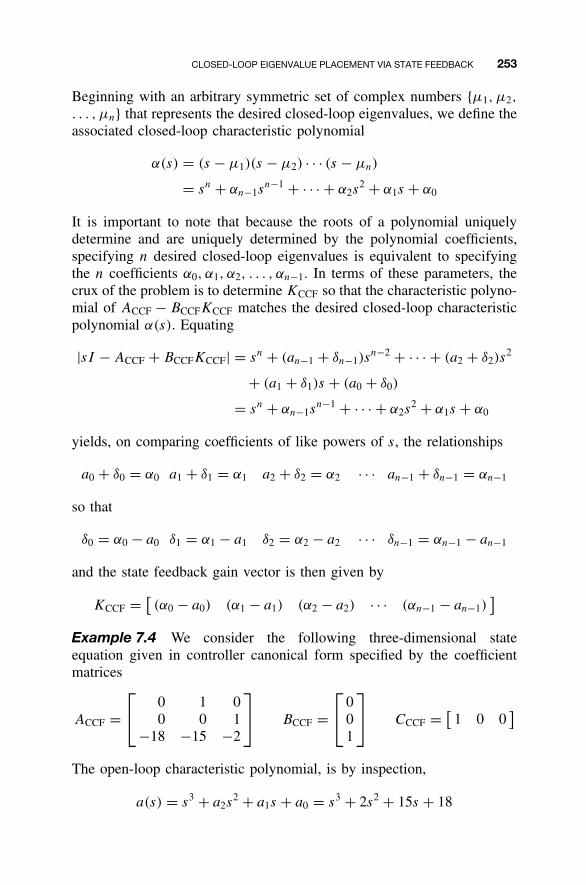
CLOSED-LOOP EIGENVALUE PLACEMENT VIA STATE FEEDBACK 253
Beginning with an arbitrary symmetric set of complex numbers {µ1, µ2,
. . . , µn} that represents the desired closed-loop eigenvalues, we define theassociated closed-loop characteristic polynomial
α(s) = (s − µ1)(s − µ2) · · · (s − µn)
= sn + αn−1sn−1 + · · · + α2s
2 + α1s + α0
It is important to note that because the roots of a polynomial uniquelydetermine and are uniquely determined by the polynomial coefficients,specifying n desired closed-loop eigenvalues is equivalent to specifyingthe n coefficients α0, α1, α2, . . . , αn−1. In terms of these parameters, thecrux of the problem is to determine KCCF so that the characteristic polyno-mial of ACCF − BCCFKCCF matches the desired closed-loop characteristicpolynomial α(s). Equating
|sI − ACCF + BCCFKCCF| = sn + (an−1 + δn−1)sn−2 + · · · + (a2 + δ2)s
2
+ (a1 + δ1)s + (a0 + δ0)
= sn + αn−1sn−1 + · · · + α2s
2 + α1s + α0
yields, on comparing coefficients of like powers of s, the relationships
a0 + δ0 = α0 a1 + δ1 = α1 a2 + δ2 = α2 · · · an−1 + δn−1 = αn−1
so that
δ0 = α0 − a0 δ1 = α1 − a1 δ2 = α2 − a2 · · · δn−1 = αn−1 − an−1
and the state feedback gain vector is then given by
KCCF = [(α0 − a0) (α1 − a1) (α2 − a2) · · · (αn−1 − an−1)
]
Example 7.4 We consider the following three-dimensional stateequation given in controller canonical form specified by the coefficientmatrices
ACCF = 0 1 0
0 0 1−18 −15 −2
BCCF =
0
01
CCCF = [
1 0 0]
The open-loop characteristic polynomial, is by inspection,
a(s) = s3 + a2s2 + a1s + a0 = s3 + 2s2 + 15s + 18
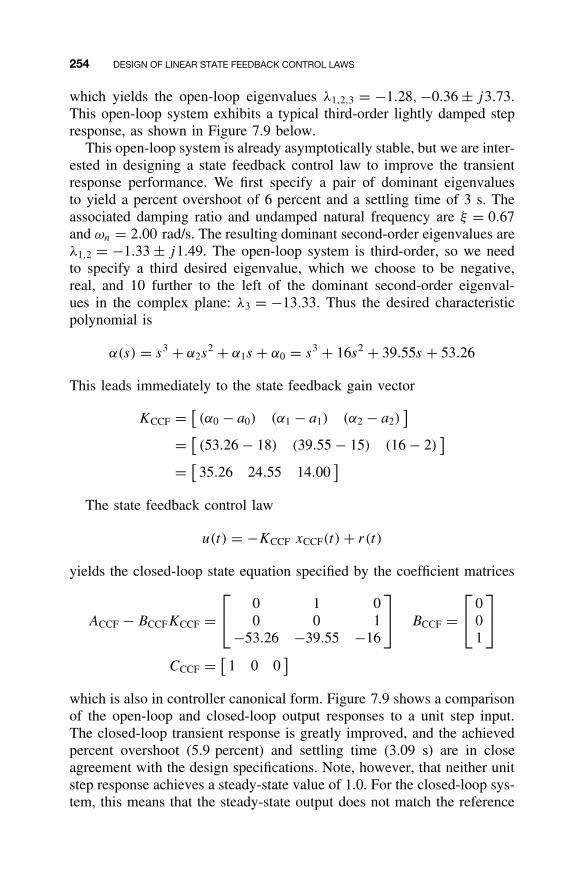
254 DESIGN OF LINEAR STATE FEEDBACK CONTROL LAWS
which yields the open-loop eigenvalues λ1,2,3 = −1.28, −0.36 ± j3.73.This open-loop system exhibits a typical third-order lightly damped stepresponse, as shown in Figure 7.9 below.
This open-loop system is already asymptotically stable, but we are inter-ested in designing a state feedback control law to improve the transientresponse performance. We first specify a pair of dominant eigenvaluesto yield a percent overshoot of 6 percent and a settling time of 3 s. Theassociated damping ratio and undamped natural frequency are ξ = 0.67and ωn = 2.00 rad/s. The resulting dominant second-order eigenvalues areλ1,2 = −1.33 ± j1.49. The open-loop system is third-order, so we needto specify a third desired eigenvalue, which we choose to be negative,real, and 10 further to the left of the dominant second-order eigenval-ues in the complex plane: λ3 = −13.33. Thus the desired characteristicpolynomial is
α(s) = s3 + α2s2 + α1s + α0 = s3 + 16s2 + 39.55s + 53.26
This leads immediately to the state feedback gain vector
KCCF = [(α0 − a0) (α1 − a1) (α2 − a2)
]= [
(53.26 − 18) (39.55 − 15) (16 − 2)]
= [35.26 24.55 14.00
]
The state feedback control law
u(t) = −KCCF xCCF(t) + r(t)
yields the closed-loop state equation specified by the coefficient matrices
ACCF − BCCFKCCF = 0 1 0
0 0 1−53.26 −39.55 −16
BCCF =
0
01
CCCF = [1 0 0
]
which is also in controller canonical form. Figure 7.9 shows a comparisonof the open-loop and closed-loop output responses to a unit step input.The closed-loop transient response is greatly improved, and the achievedpercent overshoot (5.9 percent) and settling time (3.09 s) are in closeagreement with the design specifications. Note, however, that neither unitstep response achieves a steady-state value of 1.0. For the closed-loop sys-tem, this means that the steady-state output does not match the reference
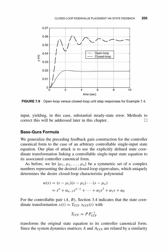
CLOSED-LOOP EIGENVALUE PLACEMENT VIA STATE FEEDBACK 255
0 2 4 6 8 100
0.01
0.02
0.03
0.04
0.05
0.06
0.07
Open-loopClosed-loop
y(m
)
time (sec)
FIGURE 7.9 Open-loop versus closed-loop unit step responses for Example 7.4.
input, yielding, in this case, substantial steady-state error. Methods tocorrect this will be addressed later in this chapter. �
Bass-Gura Formula
We generalize the preceding feedback gain construction for the controllercanonical form to the case of an arbitrary controllable single-input stateequation. Our plan of attack is to use the explicitly defined state coor-dinate transformation linking a controllable single-input state equation toits associated controller canonical form.
As before, we let {µ1, µ2, . . . , µn} be a symmetric set of n complexnumbers representing the desired closed-loop eigenvalues, which uniquelydetermines the desire closed-loop characteristic polynomial
α(s) = (s − µ1)(s − µ2) · · · (s − µn)
= sn + αn−1sn−1 + · · · + α2s
2 + α1s + α0
For the controllable pair (A, B), Section 3.4 indicates that the state coor-dinate transformation x(t) = TCCF xCCF(t) with
TCCF = PP −1CCF
transforms the original state equation to its controller canonical form.Since the system dynamics matrices A and ACCF are related by a similarity
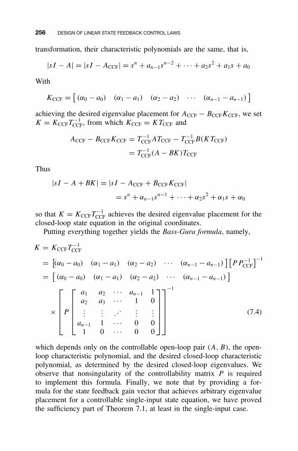
256 DESIGN OF LINEAR STATE FEEDBACK CONTROL LAWS
transformation, their characteristic polynomials are the same, that is,
|sI − A| = |sI − ACCF| = sn + an−1sn−2 + · · · + a2s
2 + a1s + a0
With
KCCF = [(α0 − a0) (α1 − a1) (α2 − a2) · · · (αn−1 − an−1)
]achieving the desired eigenvalue placement for ACCF − BCCFKCCF, we setK = KCCFT
−1CCF, from which KCCF = KTCCF and
ACCF − BCCFKCCF = T −1CCFATCCF − T −1
CCFB(KTCCF)
= T −1CCF(A − BK )TCCF
Thus
|sI − A + BK | = |sI − ACCF + BCCFKCCF|= sn + αn−1s
n−1 + · · · + α2s2 + α1s + α0
so that K = KCCFT−1
CCF achieves the desired eigenvalue placement for theclosed-loop state equation in the original coordinates.
Putting everything together yields the Bass-Gura formula, namely,
K = KCCFT−1
CCF
= [(α0 − a0) (α1 − a1) (α2 − a2) · · · (αn−1 − an−1)
] [PP −1
CCF
]−1
= [(α0 − a0) (α1 − a1) (α2 − a2) · · · (αn−1 − an−1)
]
×
P
a1 a2 · · · an−1 1a2 a3 · · · 1 0...
... . .....
...
an−1 1 · · · 0 01 0 · · · 0 0
−1
(7.4)
which depends only on the controllable open-loop pair (A, B), the open-loop characteristic polynomial, and the desired closed-loop characteristicpolynomial, as determined by the desired closed-loop eigenvalues. Weobserve that nonsingularity of the controllability matrix P is requiredto implement this formula. Finally, we note that by providing a for-mula for the state feedback gain vector that achieves arbitrary eigenvalueplacement for a controllable single-input state equation, we have provedthe sufficiency part of Theorem 7.1, at least in the single-input case.
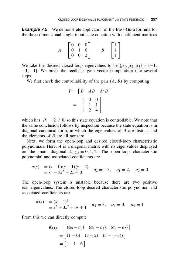
CLOSED-LOOP EIGENVALUE PLACEMENT VIA STATE FEEDBACK 257
Example 7.5 We demonstrate application of the Bass-Gura formula forthe three-dimensional single-input state equation with coefficient matrices
A = 0 0 0
0 1 00 0 2
B =
1
11
We take the desired closed-loop eigenvalues to be {µ1, µ2, µ3} = {−1,
−1, −1}. We break the feedback gain vector computation into severalsteps.
We first check the controllability of the pair (A, B) by computing
P = [B AB A2B
]
= 1 0 0
1 1 11 2 4
which has |P | = 2 = 0, so this state equation is controllable. We note thatthe same conclusion follows by inspection because the state equation is indiagonal canonical form, in which the eigenvalues of A are distinct andthe elements of B are all nonzero.
Next, we form the open-loop and desired closed-loop characteristicpolynomials. Here, A is a diagonal matrix with its eigenvalues displayedon the main diagonal λ1,2,3 = 0, 1, 2. The open-loop characteristicpolynomial and associated coefficients are
a(s) = (s − 0)(s − 1)(s − 2)
= s3 − 3s2 + 2s + 0a2 = −3, a1 = 2, a0 = 0
The open-loop system is unstable because there are two positivereal eigenvalues. The closed-loop desired characteristic polynomial andassociated coefficients are
α(s) = (s + 1)3
= s3 + 3s2 + 3s + 1α2 = 3, α1 = 3, α0 = 1
From this we can directly compute
KCCF = [(α0 − a0) (α1 − a1) (α2 − a2)
]= [
(1 − 0) (3 − 2) (3 − (−3))]
= [1 1 6
]
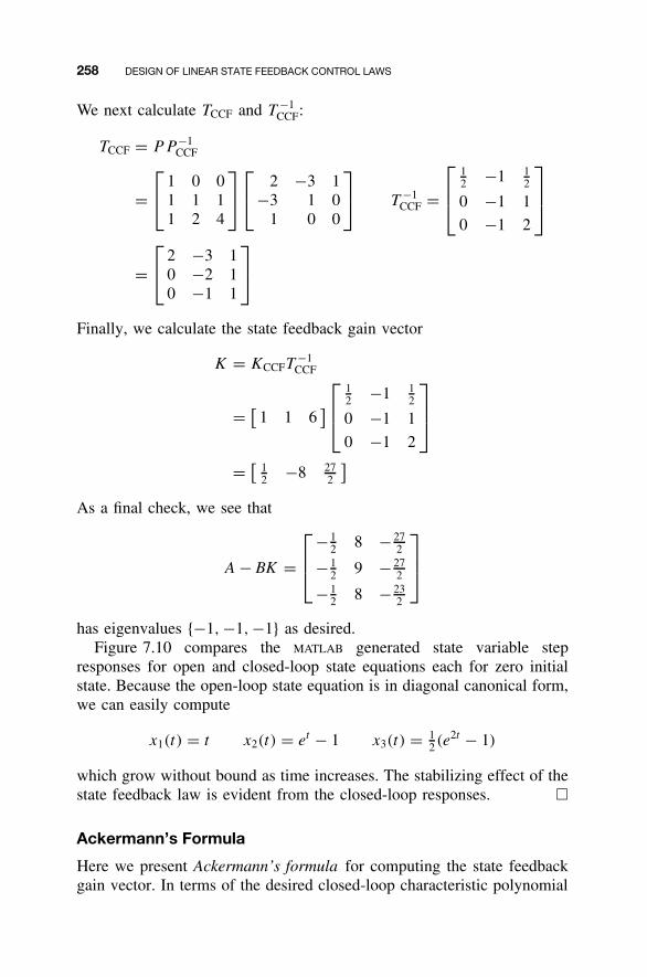
258 DESIGN OF LINEAR STATE FEEDBACK CONTROL LAWS
We next calculate TCCF and T −1CCF:
TCCF = PP −1CCF
= 1 0 0
1 1 11 2 4
2 −3 1
−3 1 01 0 0
T −1
CCF =
12 −1 1
2
0 −1 1
0 −1 2
= 2 −3 1
0 −2 10 −1 1
Finally, we calculate the state feedback gain vector
K = KCCFT−1
CCF
= [1 1 6
]
12 −1 1
2
0 −1 1
0 −1 2
= [12 −8 27
2
]As a final check, we see that
A − BK =
− 12 8 − 27
2
− 12 9 − 27
2
− 12 8 − 23
2
has eigenvalues {−1, −1, −1} as desired.Figure 7.10 compares the MATLAB generated state variable step
responses for open and closed-loop state equations each for zero initialstate. Because the open-loop state equation is in diagonal canonical form,we can easily compute
x1(t) = t x2(t) = et − 1 x3(t) = 12(e2t − 1)
which grow without bound as time increases. The stabilizing effect of thestate feedback law is evident from the closed-loop responses. �
Ackermann’s Formula
Here we present Ackermann’s formula for computing the state feedbackgain vector. In terms of the desired closed-loop characteristic polynomial
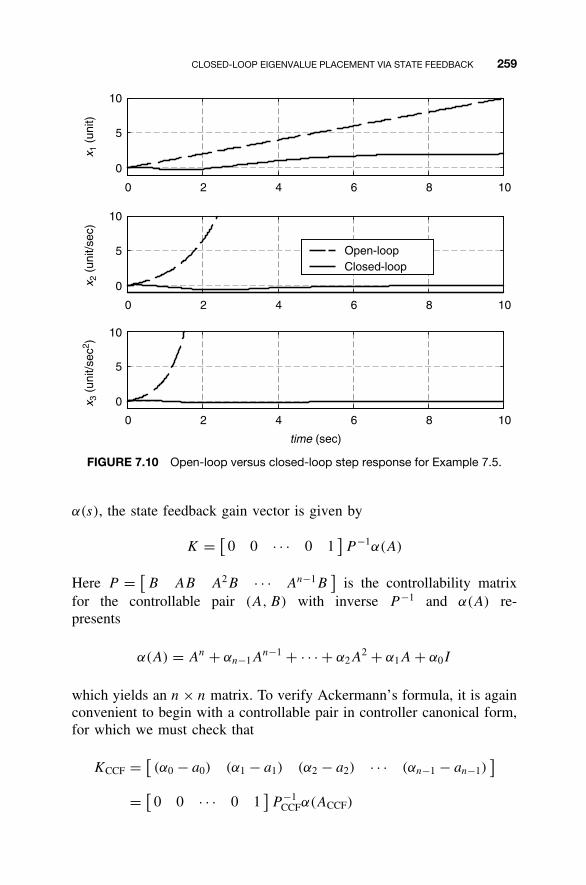
CLOSED-LOOP EIGENVALUE PLACEMENT VIA STATE FEEDBACK 259
0
5
10
Open-loopClosed-loop
0 2 4 6 8 10
0 2 4 6 8 10
0 2 4 6 8 10
x 1 (
unit)
0
5
10
x 2 (
unit/
sec)
0
5
10
x 3 (
unit/
sec2 )
time (sec)
FIGURE 7.10 Open-loop versus closed-loop step response for Example 7.5.
α(s), the state feedback gain vector is given by
K = [0 0 · · · 0 1
]P −1α(A)
Here P = [B AB A2B · · · An−1B
]is the controllability matrix
for the controllable pair (A, B) with inverse P −1 and α(A) re-presents
α(A) = An + αn−1An−1 + · · · + α2A
2 + α1A + α0I
which yields an n × n matrix. To verify Ackermann’s formula, it is againconvenient to begin with a controllable pair in controller canonical form,for which we must check that
KCCF = [(α0 − a0) (α1 − a1) (α2 − a2) · · · (αn−1 − an−1)
]
= [0 0 · · · 0 1
]P −1
CCFα(ACCF)
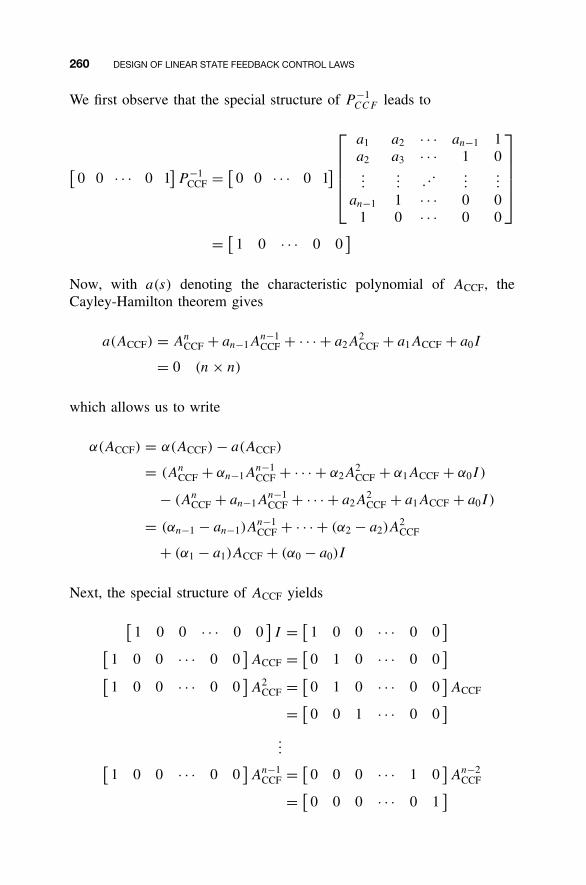
260 DESIGN OF LINEAR STATE FEEDBACK CONTROL LAWS
We first observe that the special structure of P −1CCF leads to
[0 0 · · · 0 1
]P −1
CCF = [0 0 · · · 0 1
]
a1 a2 · · · an−1 1a2 a3 · · · 1 0...
... . .....
...
an−1 1 · · · 0 01 0 · · · 0 0
= [1 0 · · · 0 0
]
Now, with a(s) denoting the characteristic polynomial of ACCF, theCayley-Hamilton theorem gives
a(ACCF) = AnCCF + an−1A
n−1CCF + · · · + a2A
2CCF + a1ACCF + a0I
= 0 (n × n)
which allows us to write
α(ACCF) = α(ACCF) − a(ACCF)
= (AnCCF + αn−1A
n−1CCF + · · · + α2A
2CCF + α1ACCF + α0I )
− (AnCCF + an−1A
n−1CCF + · · · + a2A
2CCF + a1ACCF + a0I )
= (αn−1 − an−1)An−1CCF + · · · + (α2 − a2)A
2CCF
+ (α1 − a1)ACCF + (α0 − a0)I
Next, the special structure of ACCF yields
[1 0 0 · · · 0 0
]I = [
1 0 0 · · · 0 0]
[1 0 0 · · · 0 0
]ACCF = [
0 1 0 · · · 0 0]
[1 0 0 · · · 0 0
]A2
CCF = [0 1 0 · · · 0 0
]ACCF
= [0 0 1 · · · 0 0
]...[
1 0 0 · · · 0 0]An−1
CCF = [0 0 0 · · · 1 0
]An−2
CCF
= [0 0 0 · · · 0 1
]
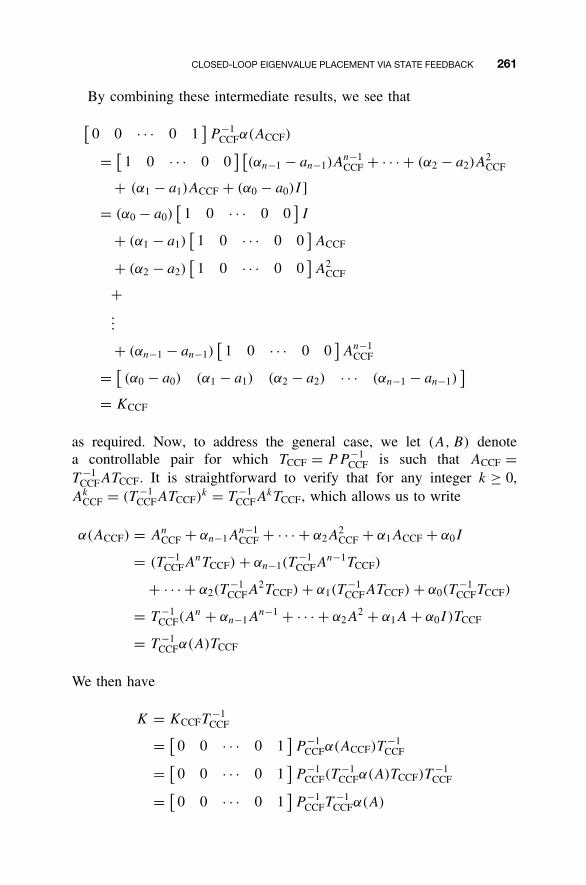
CLOSED-LOOP EIGENVALUE PLACEMENT VIA STATE FEEDBACK 261
By combining these intermediate results, we see that
[0 0 · · · 0 1
]P −1
CCFα(ACCF)
= [1 0 · · · 0 0
] [(αn−1 − an−1)A
n−1CCF + · · · + (α2 − a2)A
2CCF
+ (α1 − a1)ACCF + (α0 − a0)I ]
= (α0 − a0)[
1 0 · · · 0 0]I
+ (α1 − a1)[
1 0 · · · 0 0]ACCF
+ (α2 − a2)[
1 0 · · · 0 0]A2
CCF
+...
+ (αn−1 − an−1)[
1 0 · · · 0 0]An−1
CCF
= [(α0 − a0) (α1 − a1) (α2 − a2) · · · (αn−1 − an−1)
]= KCCF
as required. Now, to address the general case, we let (A, B) denotea controllable pair for which TCCF = PP −1
CCF is such that ACCF =T −1
CCFATCCF. It is straightforward to verify that for any integer k ≥ 0,Ak
CCF = (T −1CCFATCCF)
k = T −1CCFA
kTCCF, which allows us to write
α(ACCF) = AnCCF + αn−1A
n−1CCF + · · · + α2A
2CCF + α1ACCF + α0I
= (T −1CCFA
nTCCF) + αn−1(T−1
CCFAn−1TCCF)
+ · · · + α2(T−1
CCFA2TCCF) + α1(T
−1CCFATCCF) + α0(T
−1CCFTCCF)
= T −1CCF(A
n + αn−1An−1 + · · · + α2A
2 + α1A + α0I )TCCF
= T −1CCFα(A)TCCF
We then have
K = KCCFT−1
CCF
= [0 0 · · · 0 1
]P −1
CCFα(ACCF)T−1
CCF
= [0 0 · · · 0 1
]P −1
CCF(T−1
CCFα(A)TCCF)T−1
CCF
= [0 0 · · · 0 1
]P −1
CCFT−1
CCFα(A)
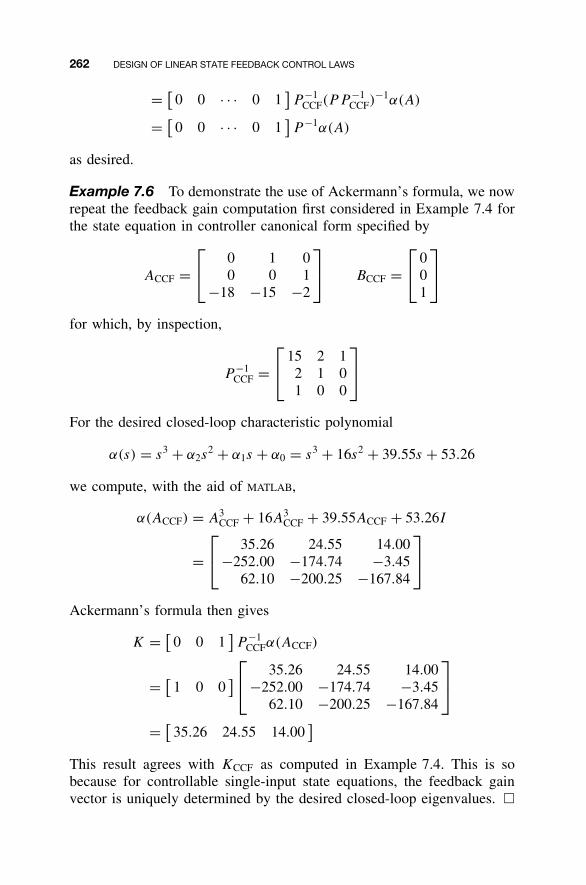
262 DESIGN OF LINEAR STATE FEEDBACK CONTROL LAWS
= [0 0 · · · 0 1
]P −1
CCF(PP −1CCF)
−1α(A)
= [0 0 · · · 0 1
]P −1α(A)
as desired.
Example 7.6 To demonstrate the use of Ackermann’s formula, we nowrepeat the feedback gain computation first considered in Example 7.4 forthe state equation in controller canonical form specified by
ACCF = 0 1 0
0 0 1−18 −15 −2
BCCF =
0
01
for which, by inspection,
P −1CCF =
15 2 1
2 1 01 0 0
For the desired closed-loop characteristic polynomial
α(s) = s3 + α2s2 + α1s + α0 = s3 + 16s2 + 39.55s + 53.26
we compute, with the aid of MATLAB,
α(ACCF) = A3CCF + 16A3
CCF + 39.55ACCF + 53.26I
= 35.26 24.55 14.00
−252.00 −174.74 −3.4562.10 −200.25 −167.84
Ackermann’s formula then gives
K = [0 0 1
]P −1
CCFα(ACCF)
= [1 0 0
] 35.26 24.55 14.00
−252.00 −174.74 −3.4562.10 −200.25 −167.84
= [35.26 24.55 14.00
]This result agrees with KCCF as computed in Example 7.4. This is sobecause for controllable single-input state equations, the feedback gainvector is uniquely determined by the desired closed-loop eigenvalues. �
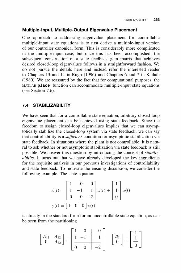
STABILIZABILITY 263
Multiple-Input, Multiple-Output Eigenvalue Placement
One approach to addressing eigenvalue placement for controllablemultiple-input state equations is to first derive a multiple-input versionof our controller canonical form. This is considerably more complicatedin the multiple-input case, but once this has been accomplished, thesubsequent construction of a state feedback gain matrix that achievesdesired closed-loop eigenvalues follows in a straightforward fashion. Wedo not pursue the details here and instead refer the interested readerto Chapters 13 and 14 in Rugh (1996) and Chapters 6 and 7 in Kailath(1980). We are reassured by the fact that for computational purposes, theMATLAB place function can accommodate multiple-input state equations(see Section 7.6).
7.4 STABILIZABILITY
We have seen that for a controllable state equation, arbitrary closed-loopeigenvalue placement can be achieved using state feedback. Since thefreedom to assign closed-loop eigenvalues implies that we can asymp-totically stabilize the closed-loop system via state feedback, we can saythat controllability is a sufficient condition for asymptotic stabilization viastate feedback. In situations where the plant is not controllable, it is natu-ral to ask whether or not asymptotic stabilization via state feedback is stillpossible. We answer this question by introducing the concept of stabiliz-ability. It turns out that we have already developed the key ingredientsfor the requisite analysis in our previous investigations of controllabilityand state feedback. To motivate the ensuing discussion, we consider thefollowing example. The state equation
x(t) =
1 0 0
1 −1 1
0 0 −2
x(t) +
1
1
0
u(t)
y(t) = [1 0 0
]x(t)
is already in the standard form for an uncontrollable state equation, as canbe seen from the partitioning
[A11 A12
0 A22
]=
1 0 | 0|1 −1 | 1||0 0 | −2
[B1
0
]=
1
1
0
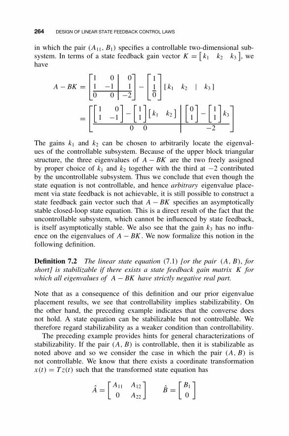
264 DESIGN OF LINEAR STATE FEEDBACK CONTROL LAWS
in which the pair (A11, B1) specifies a controllable two-dimensional sub-system. In terms of a state feedback gain vector K = [
k1 k2 k3], we
have
A − BK =1 0 0
1 −1 10 0 −2
−
1
10
[ k1 k2 | k3 ]
=
[1 01 −1
]−
[11
] [k1 k2
] [01
]−
[11
]k3
0 0 −2
The gains k1 and k2 can be chosen to arbitrarily locate the eigenval-ues of the controllable subsystem. Because of the upper block triangularstructure, the three eigenvalues of A − BK are the two freely assignedby proper choice of k1 and k2 together with the third at −2 contributedby the uncontrollable subsystem. Thus we conclude that even though thestate equation is not controllable, and hence arbitrary eigenvalue place-ment via state feedback is not achievable, it is still possible to construct astate feedback gain vector such that A − BK specifies an asymptoticallystable closed-loop state equation. This is a direct result of the fact that theuncontrollable subsystem, which cannot be influenced by state feedback,is itself asymptotically stable. We also see that the gain k3 has no influ-ence on the eigenvalues of A − BK . We now formalize this notion in thefollowing definition.
Definition 7.2 The linear state equation (7.1) [or the pair (A, B), forshort] is stabilizable if there exists a state feedback gain matrix K forwhich all eigenvalues of A − BK have strictly negative real part.
Note that as a consequence of this definition and our prior eigenvalueplacement results, we see that controllability implies stabilizability. Onthe other hand, the preceding example indicates that the converse doesnot hold. A state equation can be stabilizable but not controllable. Wetherefore regard stabilizability as a weaker condition than controllability.
The preceding example provides hints for general characterizations ofstabilizability. If the pair (A, B) is controllable, then it is stabilizable asnoted above and so we consider the case in which the pair (A, B) isnot controllable. We know that there exists a coordinate transformationx(t) = T z(t) such that the transformed state equation has
A =[
A11 A12
0 A22
]B =
[B1
0
]
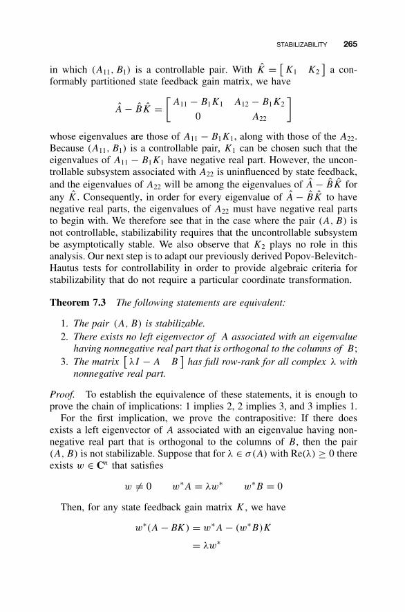
STABILIZABILITY 265
in which (A11, B1) is a controllable pair. With K = [K1 K2
]a con-
formably partitioned state feedback gain matrix, we have
A − BK =[
A11 − B1K1 A12 − B1K2
0 A22
]
whose eigenvalues are those of A11 − B1K1, along with those of the A22.Because (A11, B1) is a controllable pair, K1 can be chosen such that theeigenvalues of A11 − B1K1 have negative real part. However, the uncon-trollable subsystem associated with A22 is uninfluenced by state feedback,and the eigenvalues of A22 will be among the eigenvalues of A − BK forany K . Consequently, in order for every eigenvalue of A − BK to havenegative real parts, the eigenvalues of A22 must have negative real partsto begin with. We therefore see that in the case where the pair (A, B) isnot controllable, stabilizability requires that the uncontrollable subsystembe asymptotically stable. We also observe that K2 plays no role in thisanalysis. Our next step is to adapt our previously derived Popov-Belevitch-Hautus tests for controllability in order to provide algebraic criteria forstabilizability that do not require a particular coordinate transformation.
Theorem 7.3 The following statements are equivalent:
1. The pair (A, B) is stabilizable.2. There exists no left eigenvector of A associated with an eigenvalue
having nonnegative real part that is orthogonal to the columns of B;3. The matrix
[λI − A B
]has full row-rank for all complex λ with
nonnegative real part.
Proof. To establish the equivalence of these statements, it is enough toprove the chain of implications: 1 implies 2, 2 implies 3, and 3 implies 1.
For the first implication, we prove the contrapositive: If there doesexists a left eigenvector of A associated with an eigenvalue having non-negative real part that is orthogonal to the columns of B, then the pair(A, B) is not stabilizable. Suppose that for λ ∈ σ(A) with Re(λ) ≥ 0 thereexists w ∈ Cn that satisfies
w = 0 w∗A = λw∗ w∗B = 0
Then, for any state feedback gain matrix K , we have
w∗(A − BK ) = w∗A − (w∗B)K
= λw∗
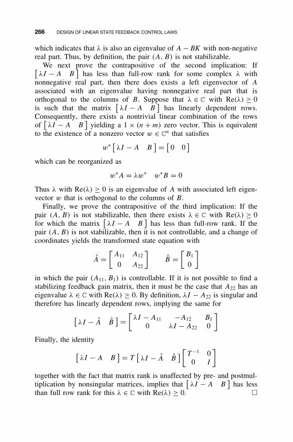
266 DESIGN OF LINEAR STATE FEEDBACK CONTROL LAWS
which indicates that λ is also an eigenvalue of A − BK with non-negativereal part. Thus, by definition, the pair (A, B) is not stabilizable.
We next prove the contrapositive of the second implication: If[λI − A B
]has less than full-row rank for some complex λ with
nonnegative real part, then there does exists a left eigenvector of A
associated with an eigenvalue having nonnegative real part that isorthogonal to the columns of B. Suppose that λ ∈ C with Re(λ) ≥ 0is such that the matrix
[λI − A B
]has linearly dependent rows.
Consequently, there exists a nontrivial linear combination of the rowsof
[λI − A B
]yielding a 1 × (n + m) zero vector. This is equivalent
to the existence of a nonzero vector w ∈ Cn that satisfies
w∗ [λI − A B
] = [0 0
]which can be reorganized as
w∗A = λw∗ w∗B = 0
Thus λ with Re(λ) ≥ 0 is an eigenvalue of A with associated left eigen-vector w that is orthogonal to the columns of B.
Finally, we prove the contrapositive of the third implication: If thepair (A, B) is not stabilizable, then there exists λ ∈ C with Re(λ) ≥ 0for which the matrix
[λI − A B
]has less than full-row rank. If the
pair (A, B) is not stabilizable, then it is not controllable, and a change ofcoordinates yields the transformed state equation with
A =[
A11 A12
0 A22
]B =
[B1
0
]
in which the pair (A11, B1) is controllable. If it is not possible to find astabilizing feedback gain matrix, then it must be the case that A22 has aneigenvalue λ ∈ C with Re(λ) ≥ 0. By definition, λI − A22 is singular andtherefore has linearly dependent rows, implying the same for
[λI − A B
] =[
λI − A11 −A12 B1
0 λI − A22 0
]
Finally, the identity
[λI − A B
] = T[λI − A B
] [T −1 0
0 I
]
together with the fact that matrix rank is unaffected by pre- and postmul-tiplication by nonsingular matrices, implies that
[λI − A B
]has less
than full row rank for this λ ∈ C with Re(λ) ≥ 0. �
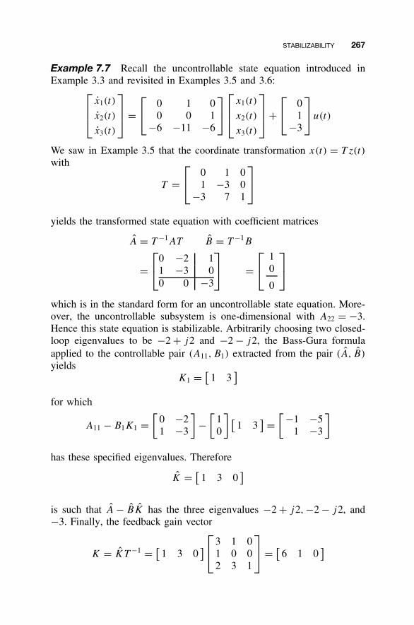
STABILIZABILITY 267
Example 7.7 Recall the uncontrollable state equation introduced inExample 3.3 and revisited in Examples 3.5 and 3.6:
x1(t)
x2(t)
x3(t)
=
0 1 0
0 0 1−6 −11 −6
x1(t)
x2(t)
x3(t)
+
0
1−3
u(t)
We saw in Example 3.5 that the coordinate transformation x(t) = T z(t)
with
T = 0 1 0
1 −3 0−3 7 1
yields the transformed state equation with coefficient matrices
A = T −1AT B = T −1B
=0 −2 1
1 −3 00 0 −3
=
1
0
0
which is in the standard form for an uncontrollable state equation. More-over, the uncontrollable subsystem is one-dimensional with A22 = −3.Hence this state equation is stabilizable. Arbitrarily choosing two closed-loop eigenvalues to be −2 + j2 and −2 − j2, the Bass-Gura formulaapplied to the controllable pair (A11, B1) extracted from the pair (A, B)
yieldsK1 = [
1 3]
for which
A11 − B1K1 =[
0 −21 −3
]−
[10
] [1 3
] =[ −1 −5
1 −3
]
has these specified eigenvalues. Therefore
K = [1 3 0
]
is such that A − BK has the three eigenvalues −2 + j2, −2 − j2, and−3. Finally, the feedback gain vector
K = KT −1 = [1 3 0
] 3 1 0
1 0 02 3 1
= [
6 1 0]
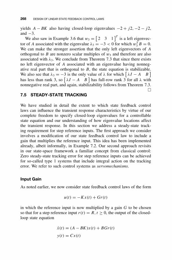
268 DESIGN OF LINEAR STATE FEEDBACK CONTROL LAWS
yields A − BK also having closed-loop eigenvalues −2 + j2, −2 − j2,and −3.
We also saw in Example 3.6 that w3 = [2 3 1
]Tis a left eigenvec-
tor of A associated with the eigenvalue λ3 = −3 < 0 for which wT3 B = 0.
We can make the stronger assertion that the only left eigenvectors of A
orthogonal to B are nonzero scalar multiples of w3 and therefore are alsoassociated with λ3. We conclude from Theorem 7.3 that since there existsno left eigenvector of A associated with an eigenvalue having nonneg-ative real part that is orthogonal to B, the state equation is stabilizable.We also see that λ3 = −3 is the only value of λ for which
[λI − A B
]has less than rank 3, so
[λI − A B
]has full-row rank 3 for all λ with
nonnegative real part, and again, stabilizability follows from Theorem 7.3.�
7.5 STEADY-STATE TRACKING
We have studied in detail the extent to which state feedback controllaws can influence the transient response characteristics by virtue of ourcomplete freedom to specify closed-loop eigenvalues for a controllablestate equation and our understanding of how eigenvalue locations affectthe transient response. In this section we address a steady-state track-ing requirement for step reference inputs. The first approach we considerinvolves a modification of our state feedback control law to include again that multiplies the reference input. This idea has been implementedalready, albeit informally, in Example 7.2. Our second approach revisitsin our state-space framework a familiar concept from classical control:Zero steady-state tracking error for step reference inputs can be achievedfor so-called type 1 systems that include integral action on the trackingerror. We refer to such control systems as servomechanisms.
Input Gain
As noted earlier, we now consider state feedback control laws of the form
u(t) = −Kx(t) + Gr(t)
in which the reference input is now multiplied by a gain G to be chosenso that for a step reference input r(t) = R, t ≥ 0, the output of the closed-loop state equation
x(t) = (A − BK )x(t) + BGr(t)
y(t) = Cx(t)
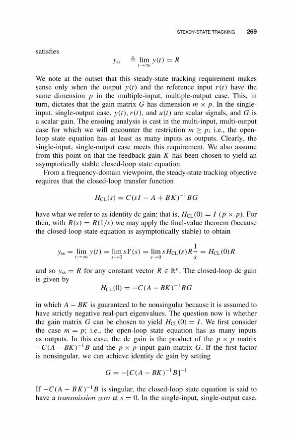
STEADY-STATE TRACKING 269
satisfiesyss � lim
t→∞ y(t) = R
We note at the outset that this steady-state tracking requirement makessense only when the output y(t) and the reference input r(t) have thesame dimension p in the multiple-input, multiple-output case. This, inturn, dictates that the gain matrix G has dimension m × p. In the single-input, single-output case, y(t), r(t), and u(t) are scalar signals, and G isa scalar gain. The ensuing analysis is cast in the multi-input, multi-outputcase for which we will encounter the restriction m ≥ p; i.e., the open-loop state equation has at least as many inputs as outputs. Clearly, thesingle-input, single-output case meets this requirement. We also assumefrom this point on that the feedback gain K has been chosen to yield anasymptotically stable closed-loop state equation.
From a frequency-domain viewpoint, the steady-state tracking objectiverequires that the closed-loop transfer function
HCL(s) = C(sI − A + BK)−1BG
have what we refer to as identity dc gain; that is, HCL(0) = I (p × p). Forthen, with R(s) = R(1/s) we may apply the final-value theorem (becausethe closed-loop state equation is asymptotically stable) to obtain
yss = limt→∞ y(t) = lim
s→0sY (s) = lim
s→0sHCL(s)R
1
s= HCL(0)R
and so yss = R for any constant vector R ∈ Rp. The closed-loop dc gain
is given byHCL(0) = −C(A − BK )−1BG
in which A − BK is guaranteed to be nonsingular because it is assumed tohave strictly negative real-part eigenvalues. The question now is whetherthe gain matrix G can be chosen to yield HCL(0) = I . We first considerthe case m = p; i.e., the open-loop state equation has as many inputsas outputs. In this case, the dc gain is the product of the p × p matrix−C(A − BK )−1B and the p × p input gain matrix G. If the first factoris nonsingular, we can achieve identity dc gain by setting
G = −[C(A − BK )−1B]−1
If −C(A − BK)−1B is singular, the closed-loop state equation is said tohave a transmission zero at s = 0. In the single-input, single-output case,
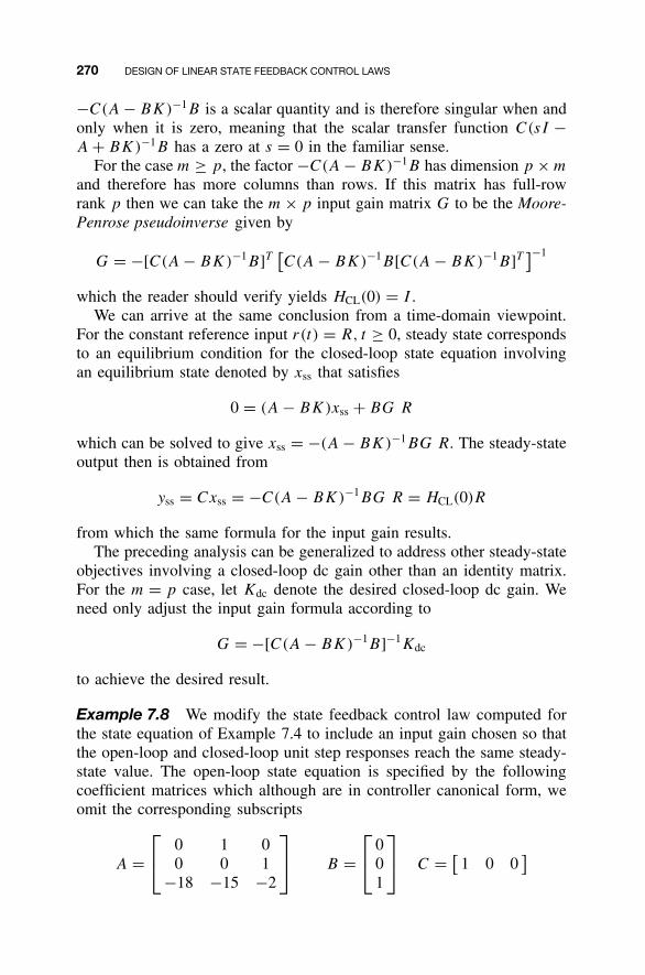
270 DESIGN OF LINEAR STATE FEEDBACK CONTROL LAWS
−C(A − BK)−1B is a scalar quantity and is therefore singular when andonly when it is zero, meaning that the scalar transfer function C(sI −A + BK)−1B has a zero at s = 0 in the familiar sense.
For the case m ≥ p, the factor −C(A − BK)−1B has dimension p × m
and therefore has more columns than rows. If this matrix has full-rowrank p then we can take the m × p input gain matrix G to be the Moore-Penrose pseudoinverse given by
G = −[C(A − BK)−1B]T[C(A − BK)−1B[C(A − BK)−1B]T
]−1
which the reader should verify yields HCL(0) = I .We can arrive at the same conclusion from a time-domain viewpoint.
For the constant reference input r(t) = R, t ≥ 0, steady state correspondsto an equilibrium condition for the closed-loop state equation involvingan equilibrium state denoted by xss that satisfies
0 = (A − BK)xss + BG R
which can be solved to give xss = −(A − BK)−1BG R. The steady-stateoutput then is obtained from
yss = Cxss = −C(A − BK)−1BG R = HCL(0)R
from which the same formula for the input gain results.The preceding analysis can be generalized to address other steady-state
objectives involving a closed-loop dc gain other than an identity matrix.For the m = p case, let Kdc denote the desired closed-loop dc gain. Weneed only adjust the input gain formula according to
G = −[C(A − BK)−1B]−1Kdc
to achieve the desired result.
Example 7.8 We modify the state feedback control law computed forthe state equation of Example 7.4 to include an input gain chosen so thatthe open-loop and closed-loop unit step responses reach the same steady-state value. The open-loop state equation is specified by the followingcoefficient matrices which although are in controller canonical form, weomit the corresponding subscripts
A = 0 1 0
0 0 1−18 −15 −2
B =
0
01
C = [
1 0 0]
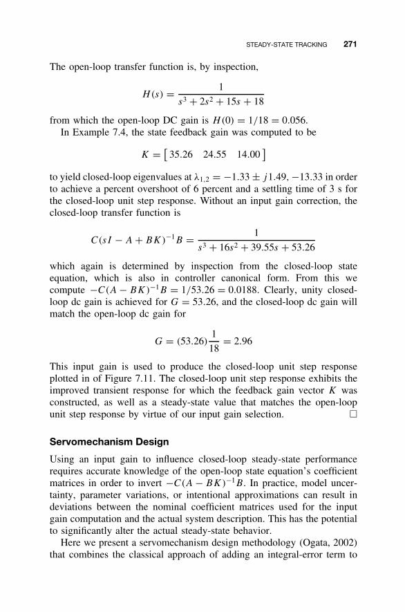
STEADY-STATE TRACKING 271
The open-loop transfer function is, by inspection,
H(s) = 1
s3 + 2s2 + 15s + 18
from which the open-loop DC gain is H(0) = 1/18 = 0.056.In Example 7.4, the state feedback gain was computed to be
K = [35.26 24.55 14.00
]to yield closed-loop eigenvalues at λ1,2 = −1.33 ± j1.49, −13.33 in orderto achieve a percent overshoot of 6 percent and a settling time of 3 s forthe closed-loop unit step response. Without an input gain correction, theclosed-loop transfer function is
C(sI − A + BK)−1B = 1
s3 + 16s2 + 39.55s + 53.26
which again is determined by inspection from the closed-loop stateequation, which is also in controller canonical form. From this wecompute −C(A − BK)−1B = 1/53.26 = 0.0188. Clearly, unity closed-loop dc gain is achieved for G = 53.26, and the closed-loop dc gain willmatch the open-loop dc gain for
G = (53.26)1
18= 2.96
This input gain is used to produce the closed-loop unit step responseplotted in of Figure 7.11. The closed-loop unit step response exhibits theimproved transient response for which the feedback gain vector K wasconstructed, as well as a steady-state value that matches the open-loopunit step response by virtue of our input gain selection. �
Servomechanism Design
Using an input gain to influence closed-loop steady-state performancerequires accurate knowledge of the open-loop state equation’s coefficientmatrices in order to invert −C(A − BK)−1B. In practice, model uncer-tainty, parameter variations, or intentional approximations can result indeviations between the nominal coefficient matrices used for the inputgain computation and the actual system description. This has the potentialto significantly alter the actual steady-state behavior.
Here we present a servomechanism design methodology (Ogata, 2002)that combines the classical approach of adding an integral-error term to
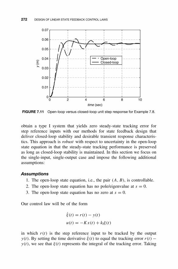
272 DESIGN OF LINEAR STATE FEEDBACK CONTROL LAWS
0 2 4 6 8 100
0.01
0.02
0.03
0.04
0.05
0.06
0.07
Open-loopClosed-loop
y (m
)
time (sec)
FIGURE 7.11 Open-loop versus closed-loop unit step response for Example 7.8.
obtain a type I system that yields zero steady-state tracking error forstep reference inputs with our methods for state feedback design thatdeliver closed-loop stability and desirable transient response characteris-tics. This approach is robust with respect to uncertainty in the open-loopstate equation in that the steady-state tracking performance is preservedas long as closed-loop stability is maintained. In this section we focus onthe single-input, single-output case and impose the following additionalassumptions:
Assumptions1. The open-loop state equation, i.e., the pair (A, B), is controllable.2. The open-loop state equation has no pole/eigenvalue at s = 0.3. The open-loop state equation has no zero at s = 0.
Our control law will be of the form
ξ (t) = r(t) − y(t)
u(t) = −Kx(t) + kIξ(t)
in which r(t) is the step reference input to be tracked by the outputy(t). By setting the time derivative ξ (t) to equal the tracking error r(t) −y(t), we see that ξ(t) represents the integral of the tracking error. Taking
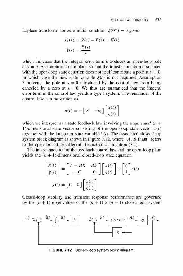
STEADY-STATE TRACKING 273
Laplace transforms for zero initial condition ξ(0−) = 0 gives
sξ(s) = R(s) − Y(s) = E(s)
ξ(s) = E(s)
s
which indicates that the integral error term introduces an open-loop poleat s = 0. Assumption 2 is in place so that the transfer function associatedwith the open-loop state equation does not itself contribute a pole at s = 0,in which case the new state variable ξ(t) is not required. Assumption3 prevents the pole at s = 0 introduced by the control law from beingcanceled by a zero at s = 0. We thus are guaranteed that the integralerror term in the control law yields a type I system. The remainder of thecontrol law can be written as
u(t) = − [K −kI
] [x(t)
ξ(t)
]
which we interpret as a state feedback law involving the augmented (n +1)-dimensional state vector consisting of the open-loop state vector x(t)
together with the integrator state variable ξ(t). The associated closed-loopsystem block diagram is shown in Figure 7.12, where “A, B Plant” refersto the open-loop state differential equation in Equation (7.1).
The interconnection of the feedback control law and the open-loop plantyields the (n + 1)-dimensional closed-loop state equation:
[x(t)
ξ (t)
]=
[A − BK BkI
−C 0
] [x(t)
ξ(t)
]+
[01
]r(t)
y(t) = [C 0
] [x(t)
ξ(t)
]
Closed-loop stability and transient response performance are governedby the (n + 1) eigenvalues of the (n + 1) × (n + 1) closed-loop system
+•
−k1
K
r(t) +
−
u(t) x(t) y(t)A,B Plant
x(t) x(t)C
FIGURE 7.12 Closed-loop system block diagram.
274 DESIGN OF LINEAR STATE FEEDBACK CONTROL LAWS
dynamics matrix[A − BK BkI
−C 0
]=
[A 0
−C 0
]−
[B
0
] [K −kI
]
In order to arbitrarily place these closed-loop eigenvalues we require([A 0
−C 0
],
[B
0
])
to be a controllable pair, which we have not yet explicitly assumed. Byassumption 2, the open-loop system dynamics matrix A is nonsingular,and hence |A| = 0 because a zero eigenvalue has been disallowed. Next,assumption 3 implies that
H(0) = C(sI − A)−1B|s=0 = −CA−1B = 0
For nonsingular A, the block determinant formula∣∣∣∣ A B
−C 0
∣∣∣∣ = ∣∣CA−1B∣∣ |A|
= CA−1B|A|shows that as a consequence of assumptions 2 and 3,[
A B
−C 0
]
is a nonsingular (n + 1) × (n + 1) matrix. Analytical Exercise 7.1 assertsthat controllability of the open-loop pair (A, B) as per assumption 1,along with nonsingularity of the preceding matrix, are necessary and suf-ficient for ([
A 0−C 0
],
[B
0
])
to be a controllable pair. Consequently, under assumptions 1, 2, and 3, the(n + 1) closed-loop eigenvalues can be placed arbitrarily by appropriatechoice of the augmented feedback gain vector
[K −kI
]For instance, we can apply either the Bass-Gura formula or Ackermann’sformula, as well as the MATLAB place function. Assuming from thispoint on that the gains have been chosen to yield an asymptotically stableclosed-loop state equation, we must show next that for step reference input
STEADY-STATE TRACKING 275
r(t) = R, t ≥ 0, we have
yss = limt→∞ y(t) = R
This involves checking that the closed-loop state equation has anequilibrium condition involving constant xss, ξss, uss, along with yss = R.Using the relationship uss = −Kxss + kI ξss leads to
[00
]=
[A − BK BkI
−C 0
] [xss
ξss
]+
[01
]R
=[
A 0−C 0
] [xss
ξss
]+
[B
0
]uss +
[01
]R
=[
A B
−C 0
] [xss
uss
]+
[01
]R
With A nonsingular and H(0) = −CA−1B = 0, a block matrix inverseformula gives
[A B
−C 0
]−1
=[A−1 − A−1B(CA−1B)−1CA−1 −A−1B(CA−1B)−1
(CA−1B)−1CA−1 (CA−1B)−1
]
which allows us to solve for [xTss, uss]T to obtain
[xss
uss
]= −
[A B
−C 0
]−1 [0R
]
=[
A−1B(CA−1B)−1R
−(CA−1B)−1R
]
in which, from before, −(CA−1B)−1 = H−1(0), the inverse of the open-loop dc gain. We may now solve for ξss, that is,
ξss = 1
kI[uss + Kxss]
= 1
kI
[1 − KA−1B
]H−1(0)R
We observe that kI = 0, for otherwise we would have a closed-loop eigen-value at λ = 0.
276 DESIGN OF LINEAR STATE FEEDBACK CONTROL LAWS
Finally,yss = Cxss
= C[A−1B(CA−1B)−1R]
= (CA−1B)(CA−1B)−1R
= R
We therefore have achieved the desired steady-state tracking objective.All that is required is that the augmented feedback gain vector
[K −kI
]stabilize the closed-loop state equation, thereby ensuring an asymptoticallystable equilibrium for any constant reference input. This does not requireperfect knowledge of the open-loop state equation. At this equilibrium,ξ(t) = ξss implies that 0 = ξ (t) = R − yss, so yss = R is assured.
Example 7.9 We design a type I servomechanism for the state equationof Example 7.4 so that closed-loop unit step response reaches a steady-state value of 1 corresponding to zero steady-state error between thereference input r(t) and the system output y(t). We begin by checkingthat the three assumptions are satisfied. The state equation is in controllercanonical form and is therefore controllable. We see from the associatedtransfer function given in Example 7.8 that there is neither a pole nor azero at s = 0.
We may then proceed with the construction of a state feedback gainvector for the controllable pair
[A 0
−C 0
]=
0 1 0 00 0 1 0
−18 −15 −2 0−1 0 0 0
[B
0
]=
001
0
We select eigenvalues based on the ITAE criterion presented in Section 7.2using an undamped natural frequency of ωn = 2 rad/s. This yields thedesired fourth-order characteristic polynomial
s4 + 2.1 ωns3 + 3.4 ω2
ns2 + 2.7 ω3
ns + ω4n
= s4 + 4.2s3 + 13.6s2 + 21.6s + 16
and associated eigenvalues
λ1,2 = −0.848 ± j2.53 λ3,4 = −1.25 ± j0.828
We observe that, although we started with a state equation in controllercanonical form, the four-dimensional controllable pair is not in controller
STEADY-STATE TRACKING 277
canonical form, so we must use our general purpose formulas tocompute the state feedback gain vector. Either the Bass-Gura formulaor Ackermann’s formula yields
[K −kI
] = [3.6 −1.4 2.2 −16
]and the associated control law is given by
ξ (t) = r(t) − y(t)
u(t) = − [3.6 −1.4 2.2
]
x1(t)
x2(t)
x3(t)
+ 16ξ(t)
The resulting closed-loop state equation is
x1(t)
x2(t)
x3(t)
ξ (t)
=
0 1 0 00 0 1 0
−21.6 −13.6 −4.2 16−1 0 0 0
x1(t)
x2(t)
x3(t)
ξ(t)
+
000
1
r(t)
y(t) = [1 0 0 | 0
]
x1(t)
x2(t)
x3(t)
ξ(t)
To illustrate the robustness properties of type 1 servomechanisms, weconsider a perturbation to the original system dynamics matrix that yields
A = 0 1 0
0 0 1−16 −16 −1
having eigenvalues −1, ±j4, indicating a marginally stable system. Usingthe same control law designed based on the nominal system dynamicsmatrix now yields the closed-loop system dynamics matrix
[A − BK BkI
−C 0
]=
0 1 0 00 0 1 0
−19.6 −14.6 −3.2 16−1 0 0 0
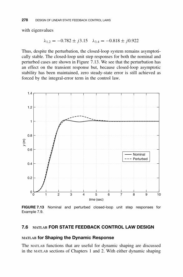
278 DESIGN OF LINEAR STATE FEEDBACK CONTROL LAWS
with eigenvalues
λ1,2 = −0.782 ± j3.15 λ3,4 = −0.818 ± j0.922
Thus, despite the perturbation, the closed-loop system remains asymptoti-cally stable. The closed-loop unit step responses for both the nominal andperturbed cases are shown in Figure 7.13. We see that the perturbation hasan effect on the transient response but, because closed-loop asymptoticstability has been maintained, zero steady-state error is still achieved asforced by the integral-error term in the control law.
1.4
1.2
1
0.8
0.6
0.4
0.2
00 1 2 3 4 5 6 7 8 9 10
NominalPerturbed
time (sec)
y(m
)
FIGURE 7.13 Nominal and perturbed closed-loop unit step responses forExample 7.9.
7.6 MATLAB FOR STATE FEEDBACK CONTROL LAW DESIGN
MATLAB for Shaping the Dynamic Response
The MATLAB functions that are useful for dynamic shaping are discussedin the MATLAB sections of Chapters 1 and 2. With either dynamic shaping
MATLAB FOR STATE FEEDBACK CONTROL LAW DESIGN 279
method (dominant/augmented eigenvalues or ITAE eigenvalues), a usefulMATLAB capability is provided in conjunction with the step function:
figure;DesSys = tf(numDes,denDes);step(DesSys);
where denDes contains the n + 1 coefficients of the nth-order desiredclosed-loop characteristic polynomial (found based on dominant-plus-augmented eigenvalues or ITAE eigenvalues), and numDes is the constantdesired behavior numerator, chosen to normalize the steady-state unitstep response value to 1.0. After executing the step function with thedesired system, one can right-click in the figure window, as describedearlier, to display the performance measures on the plot (rise time, peaktime, percent overshoot, and settling time). MATLAB calculates these valuesnumerically from the response data by applying the definition for each per-formance measure; i.e, they should be accurate even for non-second-ordersystems.
MATLAB for Control Law Design and Evaluation
The following MATLAB functions are useful for design of linear state feed-back control laws:
K=place(A,B,DesEig) Solve for state feedback gain matrix K to placethe desired eigenvalues DesEig of the closed-loop system dynamics matrix A−BK .
K=acker(A,B,DesEig) Solve for state feedback gain matrix K to placethe desired eigenvalues DesEig of the closed-loop system dynamics matrix A − BK usingAckermann’s formula (for single-input, single-output systems only).
conv Multiply polynomial factors to obtain a poly-nomial product.
Continuing MATLAB Example
Shaping the Dynamic Response For the Continuing MATLAB
Example (rotational mechanical system), we compute two desiredeigenvalues for control law design to improve the performance relativeto the open-loop responses of Figure 2.2. We use a desired percentovershoot and settling time of 3 percent and 0.7 s, respectively, to find the
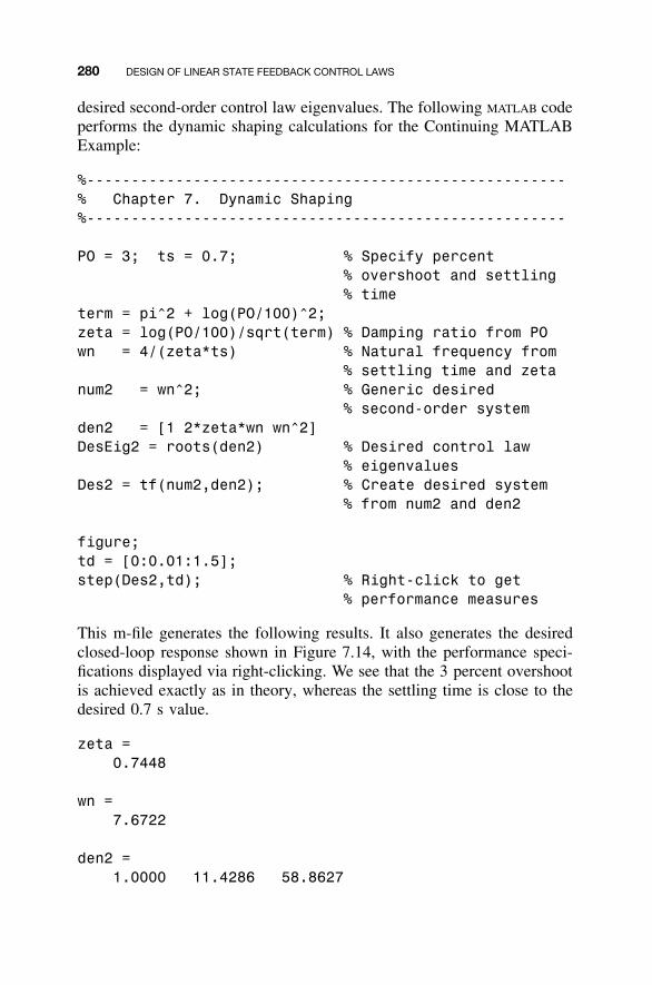
280 DESIGN OF LINEAR STATE FEEDBACK CONTROL LAWS
desired second-order control law eigenvalues. The following MATLAB codeperforms the dynamic shaping calculations for the Continuing MATLABExample:
%------------------------------------------------------% Chapter 7. Dynamic Shaping%------------------------------------------------------
PO = 3; ts = 0.7; % Specify percent% overshoot and settling% time
term = pi^2 + log(PO/100)^2;zeta = log(PO/100)/sqrt(term) % Damping ratio from POwn = 4/(zeta*ts) % Natural frequency from
% settling time and zetanum2 = wn^2; % Generic desired
% second-order systemden2 = [1 2*zeta*wn wn^2]DesEig2 = roots(den2) % Desired control law
% eigenvaluesDes2 = tf(num2,den2); % Create desired system
% from num2 and den2
figure;td = [0:0.01:1.5];step(Des2,td); % Right-click to get
% performance measures
This m-file generates the following results. It also generates the desiredclosed-loop response shown in Figure 7.14, with the performance speci-fications displayed via right-clicking. We see that the 3 percent overshootis achieved exactly as in theory, whereas the settling time is close to thedesired 0.7 s value.
zeta =0.7448
wn =7.6722
den2 =1.0000 11.4286 58.8627
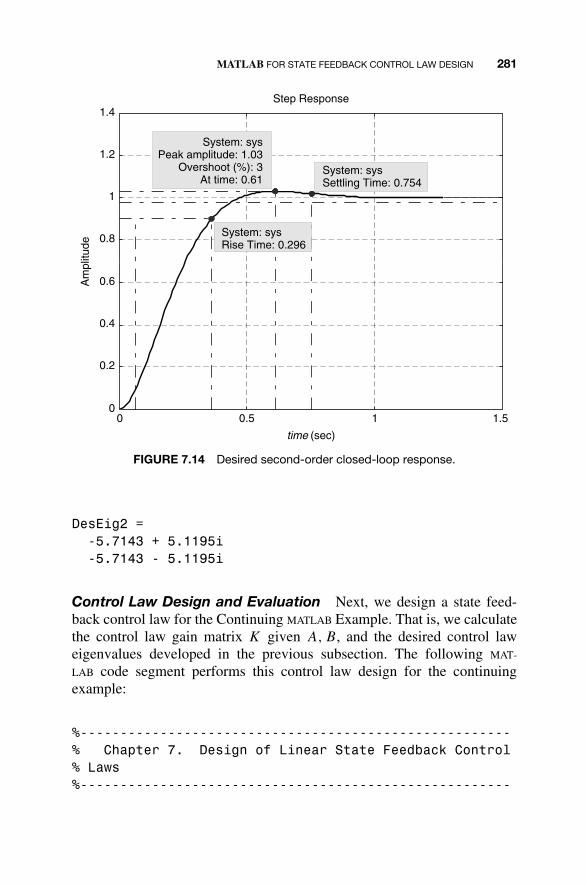
MATLAB FOR STATE FEEDBACK CONTROL LAW DESIGN 281
0 0.5 1 1.50
0.2
0.4
0.6
0.8
1
1.2
1.4
System: sysSettling Time: 0.754
Am
plitu
de
time (sec)
Step Response
System: sysPeak amplitude: 1.03
Overshoot (%): 3 At time: 0.61
System: sysRise Time: 0.296
FIGURE 7.14 Desired second-order closed-loop response.
DesEig2 =-5.7143 + 5.1195i-5.7143 - 5.1195i
Control Law Design and Evaluation Next, we design a state feed-back control law for the Continuing MATLAB Example. That is, we calculatethe control law gain matrix K given A, B, and the desired control laweigenvalues developed in the previous subsection. The following MAT-
LAB code segment performs this control law design for the continuingexample:
%------------------------------------------------------% Chapter 7. Design of Linear State Feedback Control% Laws%------------------------------------------------------
282 DESIGN OF LINEAR STATE FEEDBACK CONTROL LAWS
K = place(A,B,DesEig2) % Compute state% feedback gain matrix% K
Kack = acker(A,B, DesEig2); % Check K via% Ackermann’s formula
Ac = A-B*K; Bc = B; % Compute closed-loop% state feedback system
Cc = C; Dc = D;JbkRc = ss(Ac,Bc,Cc,Dc); % Create the
% closed-loop% state-space system
[Yc,t,Xc] = lsim(JbkRc,U,t,X0); % Compare open-loop and% closed-loop responses
figure;subplot(211), plot(t,Xo(:,1),’r’,t,Xc(:,1),’g’); grid;axis([0 4 -0.2 0.5]);set(gca,’FontSize’,18);legend(’Open-loop’,’Closed-loop’);ylabel(’ \itx 1’)subplot(212), plot(t,Xo(:,2),’r’,t,Xc(:,2),’g’); grid;axis([0 4 -2 1]);set(gca,’FontSize’,18);xlabel(’\ittime (sec)’); ylabel(’\itx 2’);
This m-file, combined with the previous chapter m-files, yields thefollowing output, plus the comparison of open- versus closed-loop stateresponses shown in Figure 7.15.
K =18.86 7.43
Figure 7.15 shows that the simulated closed-loop system performs bet-ter than the open-loop system in terms of reduced overshoot and faster riseand settling times. There is less vibration with the closed-loop responses,and the steady-state zero values are obtained sooner than in the open-loop case.
Closed-loop system simulation also can be performed using MATLAB’sSimulink. Again, a detailed treatment of Simulink is beyond the scope of

CONTINUING EXAMPLES: SHAPING DYNAMIC RESPONSE AND CONTROL LAW DESIGN 283
0 1 2 3 4−0.2
0
0.2
0.4x 1
(ra
d)
0 1 2 3 4−2
−1
0
1
time (sec)
x 2(r
ad/s
ec)
Open-loopClosed-loop
FIGURE 7.15 Open- versus closed-loop state responses for the Continuing MAT-
LAB Example.
this book. The reader is encouraged to explore this powerful MATLABtoolbox on her or his own.
7.7 CONTINUING EXAMPLES: SHAPING DYNAMIC RESPONSEAND CONTROL LAW DESIGN
Continuing Example 1: Two-Mass Translational MechanicalSystem
Shaping the Dynamic Response For control law design, we needto specify desired eigenvalues that would improve the open-loop systemperformance. There are infinite possibilities; in this example we will usethe two methods discussed in Section 7.2 to be applied later in controllaw design for Continuing Example 1.
We will use a dominant second-order system for desired eigenvalues toachieve a 5 percent overshoot and a 2 s settling time. These two eigenval-ues must be augmented with two additional nondominant eigenvalues (weneed 4 desired eigenvalues for our fourth-order system): real, negative,and at least 10 times farther to the left in the complex plane. We willuse this specification of eigenvalues for multiple-input, multiple-outputcase a.
We also will use a fourth-order ITAE approach for desired eigenval-ues, with the same undamped natural frequency ωn as case a for easy
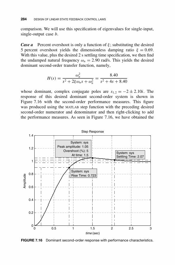
284 DESIGN OF LINEAR STATE FEEDBACK CONTROL LAWS
comparison. We will use this specification of eigenvalues for single-input,single-output case b.
Case a Percent overshoot is only a function of ξ ; substituting the desired5 percent overshoot yields the dimensionless damping ratio ξ = 0.69.With this value, plus the desired 2 s settling time specification, we then findthe undamped natural frequency ωn = 2.90 rad/s. This yields the desireddominant second-order transfer function, namely,
H(s) = ω2n
s2 + 2ξωns + ω2n
= 8.40
s2 + 4s + 8.40
whose dominant, complex conjugate poles are s1,2 = −2 ± 2.10i. Theresponse of this desired dominant second-order system is shown inFigure 7.16 with the second-order performance measures. This figurewas produced using the MATLAB step function with the preceding desiredsecond-order numerator and denominator and then right-clicking to addthe performance measures. As seen in Figure 7.16, we have obtained the
Step Response
time (sec)
Am
plitu
de
0 0.5 1 1.5 2 2.5 30
0.2
0.4
0.6
0.8
1
1.2
1.4
System: sysPeak amplitude: 1.05
Overshoot (%): 5At time: 1.5
System: sysSettling Time: 2.07
System: sysRise Time: 0.723
FIGURE 7.16 Dominant second-order response with performance characteristics.
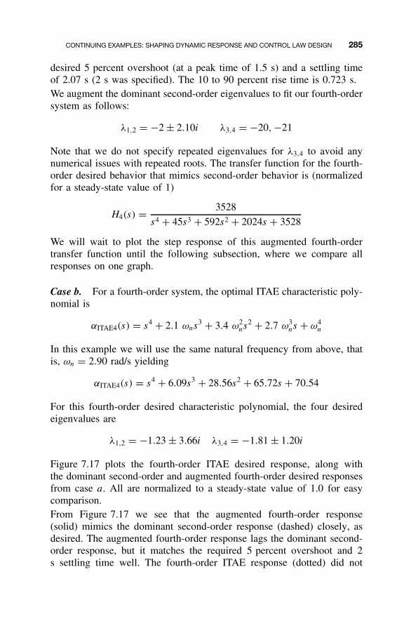
CONTINUING EXAMPLES: SHAPING DYNAMIC RESPONSE AND CONTROL LAW DESIGN 285
desired 5 percent overshoot (at a peak time of 1.5 s) and a settling timeof 2.07 s (2 s was specified). The 10 to 90 percent rise time is 0.723 s.We augment the dominant second-order eigenvalues to fit our fourth-ordersystem as follows:
λ1,2 = −2 ± 2.10i λ3,4 = −20, −21
Note that we do not specify repeated eigenvalues for λ3,4 to avoid anynumerical issues with repeated roots. The transfer function for the fourth-order desired behavior that mimics second-order behavior is (normalizedfor a steady-state value of 1)
H4(s) = 3528
s4 + 45s3 + 592s2 + 2024s + 3528
We will wait to plot the step response of this augmented fourth-ordertransfer function until the following subsection, where we compare allresponses on one graph.
Case b. For a fourth-order system, the optimal ITAE characteristic poly-nomial is
αITAE4(s) = s4 + 2.1 ωns3 + 3.4 ω2
ns2 + 2.7 ω3
ns + ω4n
In this example we will use the same natural frequency from above, thatis, ωn = 2.90 rad/s yielding
αITAE4(s) = s4 + 6.09s3 + 28.56s2 + 65.72s + 70.54
For this fourth-order desired characteristic polynomial, the four desiredeigenvalues are
λ1,2 = −1.23 ± 3.66i λ3,4 = −1.81 ± 1.20i
Figure 7.17 plots the fourth-order ITAE desired response, along withthe dominant second-order and augmented fourth-order desired responsesfrom case a. All are normalized to a steady-state value of 1.0 for easycomparison.From Figure 7.17 we see that the augmented fourth-order response(solid) mimics the dominant second-order response (dashed) closely, asdesired. The augmented fourth-order response lags the dominant second-order response, but it matches the required 5 percent overshoot and 2s settling time well. The fourth-order ITAE response (dotted) did not
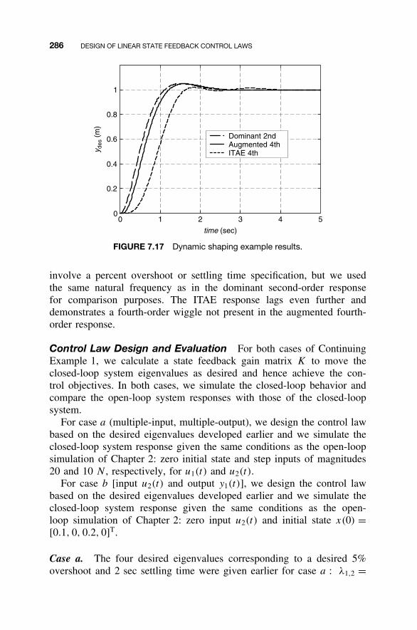
286 DESIGN OF LINEAR STATE FEEDBACK CONTROL LAWS
0 1 2 3 4 50
0.2
0.4
0.6
0.8
1
Dominant 2ndAugmented 4thITAE 4th
time (sec)
y des
(m
)
FIGURE 7.17 Dynamic shaping example results.
involve a percent overshoot or settling time specification, but we usedthe same natural frequency as in the dominant second-order responsefor comparison purposes. The ITAE response lags even further anddemonstrates a fourth-order wiggle not present in the augmented fourth-order response.
Control Law Design and Evaluation For both cases of ContinuingExample 1, we calculate a state feedback gain matrix K to move theclosed-loop system eigenvalues as desired and hence achieve the con-trol objectives. In both cases, we simulate the closed-loop behavior andcompare the open-loop system responses with those of the closed-loopsystem.
For case a (multiple-input, multiple-output), we design the control lawbased on the desired eigenvalues developed earlier and we simulate theclosed-loop system response given the same conditions as the open-loopsimulation of Chapter 2: zero initial state and step inputs of magnitudes20 and 10 N , respectively, for u1(t) and u2(t).
For case b [input u2(t) and output y1(t)], we design the control lawbased on the desired eigenvalues developed earlier and we simulate theclosed-loop system response given the same conditions as the open-loop simulation of Chapter 2: zero input u2(t) and initial state x(0) =[0.1, 0, 0.2, 0]T.
Case a. The four desired eigenvalues corresponding to a desired 5%overshoot and 2 sec settling time were given earlier for case a : λ1,2 =
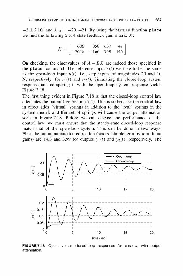
CONTINUING EXAMPLES: SHAPING DYNAMIC RESPONSE AND CONTROL LAW DESIGN 287
−2 ± 2.10i and λ3,4 = −20, −21. By using the MATLAB function placewe find the following 2 × 4 state feedback gain matrix K:
K =[
606 858 637 47−3616 −166 759 446
]
On checking, the eigenvalues of A − BK are indeed those specified inthe place command. The reference input r(t) we take to be the sameas the open-loop input u(t), i.e., step inputs of magnitudes 20 and 10N, respectively, for r1(t) and r2(t). Simulating the closed-loop systemresponse and comparing it with the open-loop system response yieldsFigure 7.18.The first thing evident in Figure 7.18 is that the closed-loop control lawattenuates the output (see Section 7.4). This is so because the control lawin effect adds “virtual” springs in addition to the “real” springs in thesystem model; a stiffer set of springs will cause the output attenuationseen in Figure 7.18. Before we can discuss the performance of thecontrol law, we must ensure that the steady-state closed-loop responsematch that of the open-loop system. This can be done in two ways:First, the output attenuation correction factors (simple term-by-term inputgains) are 14.3 and 3.99 for outputs y1(t) and y2(t), respectively. The
0 5 10 15 200
0.05
0.1
y 1(m
)
Open-loopClosed-loop
0 5 10 15 200
0.05
0.1
0.15
0.2
time (sec)
y 2(m
)
FIGURE 7.18 Open- versus closed-loop responses for case a, with outputattenuation.
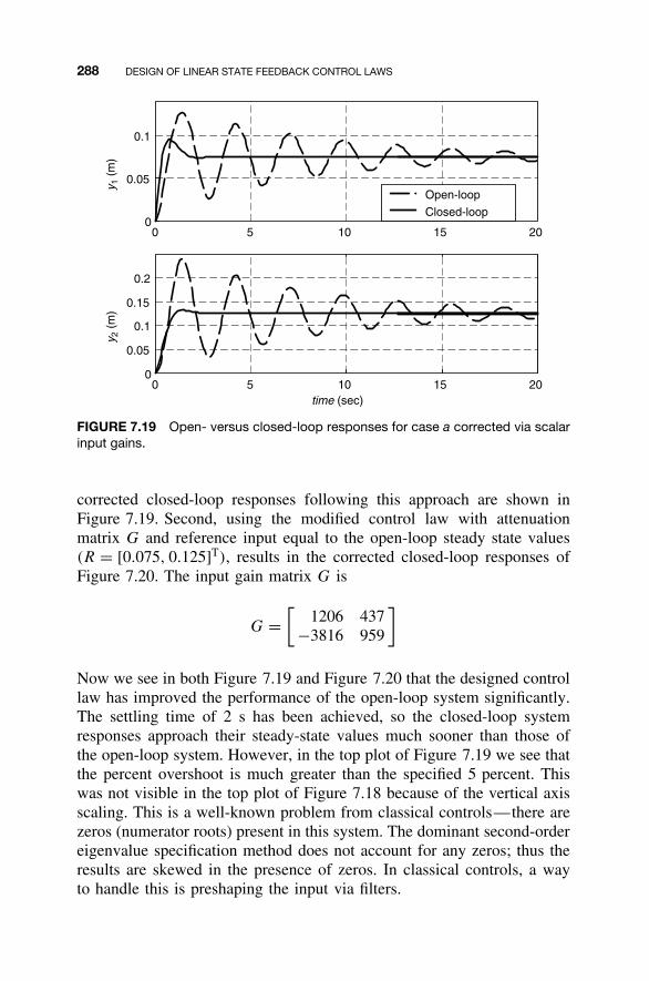
288 DESIGN OF LINEAR STATE FEEDBACK CONTROL LAWS
0 5 10 15 200
0.05
0.1
y 1(m
)
0 5 10 15 200
0.05
0.1
0.15
0.2
time (sec)
y 2(m
)
Open-loop
Closed-loop
FIGURE 7.19 Open- versus closed-loop responses for case a corrected via scalarinput gains.
corrected closed-loop responses following this approach are shown inFigure 7.19. Second, using the modified control law with attenuationmatrix G and reference input equal to the open-loop steady state values(R = [0.075, 0.125]T), results in the corrected closed-loop responses ofFigure 7.20. The input gain matrix G is
G =[
1206 437−3816 959
]
Now we see in both Figure 7.19 and Figure 7.20 that the designed controllaw has improved the performance of the open-loop system significantly.The settling time of 2 s has been achieved, so the closed-loop systemresponses approach their steady-state values much sooner than those ofthe open-loop system. However, in the top plot of Figure 7.19 we see thatthe percent overshoot is much greater than the specified 5 percent. Thiswas not visible in the top plot of Figure 7.18 because of the vertical axisscaling. This is a well-known problem from classical controls—there arezeros (numerator roots) present in this system. The dominant second-ordereigenvalue specification method does not account for any zeros; thus theresults are skewed in the presence of zeros. In classical controls, a wayto handle this is preshaping the input via filters.
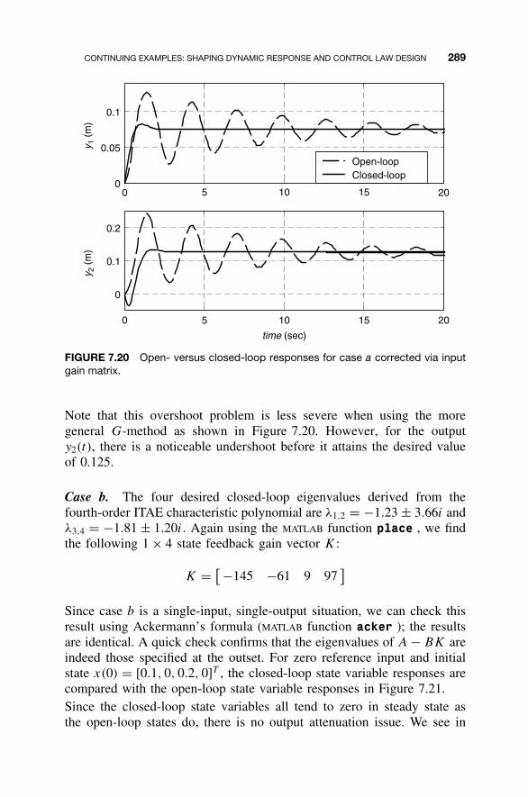
CONTINUING EXAMPLES: SHAPING DYNAMIC RESPONSE AND CONTROL LAW DESIGN 289
0 5 10 15 200
0.05
0.1
y 1 (
m)
0 5 10 15 20
0
0.1
0.2
time (sec)
y 2 (
m)
Open-loopClosed-loop
FIGURE 7.20 Open- versus closed-loop responses for case a corrected via inputgain matrix.
Note that this overshoot problem is less severe when using the moregeneral G-method as shown in Figure 7.20. However, for the outputy2(t), there is a noticeable undershoot before it attains the desired valueof 0.125.
Case b. The four desired closed-loop eigenvalues derived from thefourth-order ITAE characteristic polynomial are λ1,2 = −1.23 ± 3.66i andλ3,4 = −1.81 ± 1.20i. Again using the MATLAB function place , we findthe following 1 × 4 state feedback gain vector K:
K = [ −145 −61 9 97]
Since case b is a single-input, single-output situation, we can check thisresult using Ackermann’s formula (MATLAB function acker ); the resultsare identical. A quick check confirms that the eigenvalues of A − BK areindeed those specified at the outset. For zero reference input and initialstate x(0) = [0.1, 0, 0.2, 0]T , the closed-loop state variable responses arecompared with the open-loop state variable responses in Figure 7.21.Since the closed-loop state variables all tend to zero in steady state asthe open-loop states do, there is no output attenuation issue. We see in
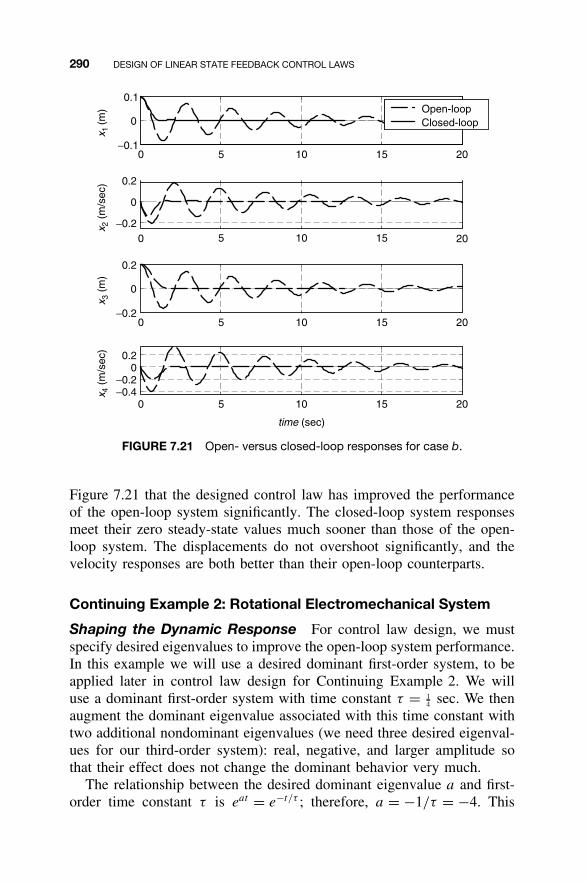
290 DESIGN OF LINEAR STATE FEEDBACK CONTROL LAWS
0 5 10 15−0.1
0
0.1x 1
(m)
0 5 10 15 20
20
−0.2
0
0.2
x 2 (
m/s
ec)
0 5 10 15 20−0.2
0
0.2
x 3 (
m)
0 5 10 15 20−0.4−0.2
00.2
time (sec)
x 4 (
m/s
ec)
Open-loopClosed-loop
FIGURE 7.21 Open- versus closed-loop responses for case b.
Figure 7.21 that the designed control law has improved the performanceof the open-loop system significantly. The closed-loop system responsesmeet their zero steady-state values much sooner than those of the open-loop system. The displacements do not overshoot significantly, and thevelocity responses are both better than their open-loop counterparts.
Continuing Example 2: Rotational Electromechanical System
Shaping the Dynamic Response For control law design, we mustspecify desired eigenvalues to improve the open-loop system performance.In this example we will use a desired dominant first-order system, to beapplied later in control law design for Continuing Example 2. We willuse a dominant first-order system with time constant τ = 1
4 sec. We thenaugment the dominant eigenvalue associated with this time constant withtwo additional nondominant eigenvalues (we need three desired eigenval-ues for our third-order system): real, negative, and larger amplitude sothat their effect does not change the dominant behavior very much.
The relationship between the desired dominant eigenvalue a and first-order time constant τ is eat = e−t/τ ; therefore, a = −1/τ = −4. This
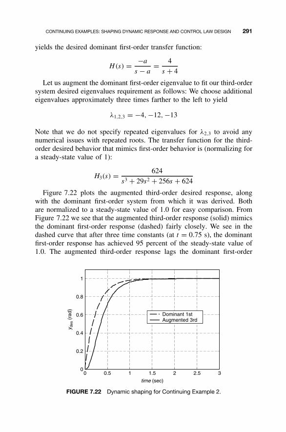
CONTINUING EXAMPLES: SHAPING DYNAMIC RESPONSE AND CONTROL LAW DESIGN 291
yields the desired dominant first-order transfer function:
H(s) = −a
s − a= 4
s + 4
Let us augment the dominant first-order eigenvalue to fit our third-ordersystem desired eigenvalues requirement as follows: We choose additionaleigenvalues approximately three times farther to the left to yield
λ1,2,3 = −4, −12, −13
Note that we do not specify repeated eigenvalues for λ2,3 to avoid anynumerical issues with repeated roots. The transfer function for the third-order desired behavior that mimics first-order behavior is (normalizing fora steady-state value of 1):
H3(s) = 624
s3 + 29s2 + 256s + 624
Figure 7.22 plots the augmented third-order desired response, alongwith the dominant first-order system from which it was derived. Bothare normalized to a steady-state value of 1.0 for easy comparison. FromFigure 7.22 we see that the augmented third-order response (solid) mimicsthe dominant first-order response (dashed) fairly closely. We see in thedashed curve that after three time constants (at t = 0.75 s), the dominantfirst-order response has achieved 95 percent of the steady-state value of1.0. The augmented third-order response lags the dominant first-order
0 0.5 1 1.5 2 2.5 30
0.2
0.4
0.6
0.8
1
time (sec)
y des
(ra
d) Dominant 1stAugmented 3rd
FIGURE 7.22 Dynamic shaping for Continuing Example 2.
292 DESIGN OF LINEAR STATE FEEDBACK CONTROL LAWS
response; we can make this arbitrarily close to the dashed curve by movingthe augmented eigenvalues even farther to the left. However, this maylead to large numerical values for control gains, which is generally to beavoided. This could potentially require large actuator amplitudes, perhapsexceeding physical limits.
Control Law Design and Evaluation
For Continuing Example 2, we compute a state feedback gain matrix K tomove the closed-loop system eigenvalues where desired and hence achievethe control objectives. Then we simulate the closed-loop behavior andcompare the open-loop system responses with those of the closed-loopsystem.
We design the control law based on the desired eigenvalues devel-oped in the preceding subsection, and we simulate the closed-loop sys-tem response given the same conditions as the open-loop simulation ofChapter 2 [zero initial state and a unit step input in voltage v(t)].
The three desired eigenvalues for this case, λ1,2,3 = −4, −12, −13,were specified by a dominant first-order eigenvalue augmented by twomore real, negative eigenvalues farther to the left by a factor of three. Byusing MATLAB functions place or acker we find the following 1 × 3state feedback gain matrix K:
K = [312 127 13
]The eigenvalues of A − BK are indeed those that were specified, as thereader may verify. Simulating the closed-loop system response for zeroinitial state and unit step reference input and comparing with the open-loopunit step response yields Figure 7.23.
There is no output attenuation issue because the open-loop responseincreases linearly after the transient response has died out; this is asexpected because there is no torsional spring in the system model. How-ever, we could use the input gain matrix method to achieve any desiredsteady-state angular displacement for the closed-loop system.
The closed-loop angular displacement x1(t) in Figure 7.23 (top plot)was artificially scaled to achieve a steady-state value of 0.5 rad. Com-paring the open- and closed-loop angular displacement, we see that thestate feedback control law has effectively added a virtual spring wherebywe can servo to commanded angles rather than having the shaft angleincrease linearly without bound as in the open-loop case. In Figure 7.23,the closed-loop angular velocity and acceleration both experience a tran-sient and then tend to zero steady-state values. The open-loop values arethe same as those plotted in Figure 2.5.
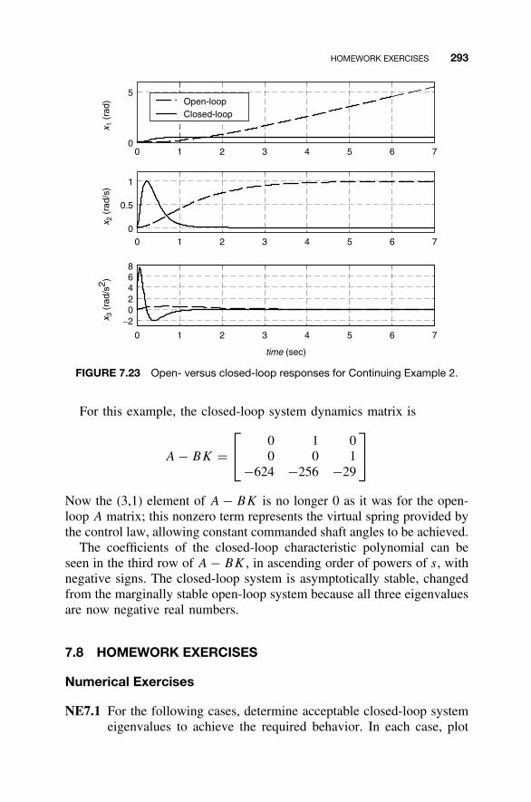
HOMEWORK EXERCISES 293
0 1 2 3 4 5 6 70
5x 1
(ra
d)
0 1 2 3 4 5 6 70
0.5
1
x 2 (
rad/
s)
0 1 2 3 4 5 6 7
−202468
time (sec)
x 3 (
rad/
s2 )Open-loopClosed-loop
FIGURE 7.23 Open- versus closed-loop responses for Continuing Example 2.
For this example, the closed-loop system dynamics matrix is
A − BK = 0 1 0
0 0 1−624 −256 −29
Now the (3,1) element of A − BK is no longer 0 as it was for the open-loop A matrix; this nonzero term represents the virtual spring provided bythe control law, allowing constant commanded shaft angles to be achieved.
The coefficients of the closed-loop characteristic polynomial can beseen in the third row of A − BK , in ascending order of powers of s, withnegative signs. The closed-loop system is asymptotically stable, changedfrom the marginally stable open-loop system because all three eigenvaluesare now negative real numbers.
7.8 HOMEWORK EXERCISES
Numerical Exercises
NE7.1 For the following cases, determine acceptable closed-loop systemeigenvalues to achieve the required behavior. In each case, plot
294 DESIGN OF LINEAR STATE FEEDBACK CONTROL LAWS
the unit step response to demonstrate that the desired behavior isapproximately satisfied.a. Determine acceptable eigenvalues for a second-, third-, and
fourth-order system to approximate a first-order system with atime constant of 0.5 s.
b. Determine acceptable eigenvalues for a second-, third-, andfourth- order system to approximate a second-order system witha percent overshoot of 6 percent and a settling time of 4 s.
c. Co-plot the desired ITAE responses for second-, third-, andfourth- order systems assuming ωn = 5 rad/s. Discuss yourresults.
NE7.2 For each (A, B) pair below, use the Bass-Gura formula to calculatethe state feedback gain vector K to place the given eigenvaluesof the closed-loop system dynamics matrix A − BK . Check yourresults.
a. A =[ −1 0
0 −4
]B =
[1
1
]λ1,2 = −2 ± 3i
b. A =[
0 1
−6 −8
]B =
[0
1
]λ1,2 = −4, −5
c. A =[
0 1
−6 0
]B =
[0
1
]λ1,2 = −4, −5
d. A =[
0 8
1 10
]B =
[1
0
]λ1,2 = −1 ± i
NE7.3 Repeat NE 7.2 using Ackermann’s Formula.
Analytical Exercises
AE7.1 Show that the (n + 1)-dimensional single-input, single-output stateequation
[x(t)
ξ (t)
]=
[A 0
C 0
] [x(t)
ξ(t)
]+
[B
0
]u(t)
with output ξ(t) is controllable if and only if the n-dimensionalsingle-input, single-output state equation represented by (A, B,C)
is controllable and the (n + 1) × (n + 1) matrix[
A B
C 0
]
HOMEWORK EXERCISES 295
is nonsingular. What is the interpretation of the state variable ξ(t)?
AE7.2 Suppose that the pair (A, B) is controllable, and for any finite tf >
0, consider the state feedback gain matrix K = −BT W−1(0, tf ).Show that the closed-loop state equation
x(t) = (A − BK)x(t)
is asymptotically stable. Hint: Recall AE6.5.
AE7.3 Suppose that given the symmetric positive definite matrix Q, theRiccati matrix equation
AT P + PA − PBBT P + Q = 0
has a symmetric positive-definite solution P . Show that the statefeedback law u(t) = −K x(t) with K = −BT P yields the closed-loop state equation
x(t) = (A − BK)x(t)
that is asymptotically stable, thereby implying that the pair (A, B)
is stabilizable.
AE7.4 For the linear state equation (7.1) and state feedback law (7.4), showthat the open- and closed-loop transfer functions are related by
HCL(s) = H(s)[I + K(sI − A)−1B]−1G
This indicates that the same closed-loop input-output behavior canbe achieved using a dynamic precompensator instead of state feed-back. Hint: Use AE1.8.
Continuing MATLAB Exercises
CME7.1 For the system given in CME1.1:a. Determine the desired eigenvalues for a generic second-order
system to obtain 1 percent overshoot and a 1-s settling time.Plot the unit step response for this desired behavior and dis-cuss your results.
b. Design a state feedback control law to achieve the eigen-value placement of part a. Compare open- and closed-loopresponses to a unit step input, assuming zero initial condi-tions. Normalize the closed-loop output level to match that of
296 DESIGN OF LINEAR STATE FEEDBACK CONTROL LAWS
the open-loop system for easy comparison. Were your controllaw design goals met?
c. Design a state feedback servomechanism to achieve theeigenvalue placement of part a and a steady-state outputvalue of 1. Compare open- and closed-loop responses to aunit step input. In this case, normalize the open-loop outputlevel to 1 for easy comparison. Were your control law designgoals met?
CME7.2 For the system given in CME1.2:
a. Determine the desired eigenvalues for a first-order systemwith a time constant of 1 s, augmented by two additionalreal, negative eigenvalues (the first exactly 10 times the dom-inant eigenvalue, the third one less than the second). Plot theunit step response for this desired behavior, and discuss yourresults.
b. Design a state feedback control law to achieve the eigen-value placement of part a. Compare open- and closed-loopresponses to a unit step input. Normalize the closed-loopoutput level to match that of the open-loop system for easycomparison. Were your control law design goals met?
c. Design a state feedback servomechanism to achieve theeigenvalue placement of part a and a steady-state outputvalue of 1. Compare open- and closed-loop responses to aunit step input. In this case, normalize the open-loop outputlevel to 1 for easy comparison. Were your control law designgoals met?
CME7.3 For the system given in CME1.3:
a. Determine the desired eigenvalues for a fourth–order ITAEsystem with ωn = 2 rad/s. Plot the unit step response for thisdesired behavior, and discuss your results.
b. Design a state feedback control law to achieve the eigen-value placement of part a. Compare open- and closed-loopresponses to a unit step input. Normalize the closed-loopoutput level to match that of the open-loop system for easycomparison. Were your control law design goals met?
c. Design a state feedback servomechanism to achieve theeigenvalue placement of part a and a steady-state outputvalue of 1. Compare open- and closed-loop responses to aunit step input. In this case normalize, the open-loop output
HOMEWORK EXERCISES 297
level to 1 for easy comparison. Were your control law designgoals met?
CME7.4 For the system given in CME1.4:a) Determine the desired eigenvalues for a generic second-order
system to obtain 2 percent overshoot and a 2-s settling time.Plot the unit step response for this desired behavior and dis-cuss your results.
b) Design a state feedback control law to achieve the eigen-value placement of part a. Compare open- and closed-loopresponses to a unit step input. Normalize the closed-loopoutput level to match that of the open-loop system for easycomparison. Were your control law design goals met?
c) Design a state feedback servomechanism to achieve theeigenvalue placement of part a and a steady-state outputvalue of 1. Compare open- and closed-loop responses to aunit step input. In this case, normalize the open-loop outputlevel to 1 for easy comparison. Were your control law designgoals met?
Continuing Exercises
CE7.1a Given control law design criteria of 3 percent overshoot and a3-s settling time: (i) Calculate the undamped natural frequencyand damping ratio required for a standard generic second-ordersystem to achieve this (assuming a unit step input). What are theassociated system eigenvalues? Plot the unit step response for theresult and demonstrate how well the design criteria are met (nor-malize your output to ensure the final value is 1.0). Display theresulting rise time, peak time, settling time, and percent over-shoot on your graph. (ii) Augment these desired second-ordersystem eigenvalues for control law design in CE1; since thisis a sixth-order system you, will need four additional eigenval-ues (real, negative, approximately 10 times farther to the left).Choose the first additional eigenvalue to be exactly ten timesthe real part of the dominant second-order system eigenvalues.For the remaining three, successively subtract one from the firstadditional eigenvalue (to avoid repeated eigenvalues). (iii) Alsocompute the optimal ITAE sixth-order coefficients and eigenval-ues using an undamped natural frequency twice that from thedominant second-order approach. Plot both the sixth-order ITAE
298 DESIGN OF LINEAR STATE FEEDBACK CONTROL LAWS
and the augmented sixth-order desired step responses with thedominant second-order step response of part (i) (normalize toensure steady-state values of 1.0); compare and discuss.
CE7.1b For the desired closed-loop eigenvalues from CE7.1a, designstate feedback control laws (i.e., calculate K) for all three casesfrom CE2.1. For cases (i) and (ii), use the augmented sixth-ordereigenvalues based on dominant second-order behavior; for case(iii), use the sixth-order ITAE eigenvalues. In each case, evaluateyour results: Plot and compare the simulated open- versus closed-loop output responses for the same input cases as in CE2.1a; useoutput attenuation correction so that the closed-loop steady-statevalues match the open-loop steady-state values for easy compar-isons.
CE7.2a Since this is a fourth-order system, we will need four desiredeigenvalues for future control law design in CE2. Use a fourth-order ITAE approach with undamped natural frequency ωn =3 rad/s to generate the four desired eigenvalues. Plot the desiredsystem impulse response.
CE7.2b For the desired closed-loop eigenvalues from CE7.2a, designstate feedback control laws (i.e., calculate K) for all three casesfrom CE2.2. In each case, evaluate your results: Plot and com-pare the simulated open- versus closed-loop output responses forthe same input cases as in CE2.2a. Be sure to scale the verticalaxes so that the closed-loop responses are clearly visible.
CE7.3a Use a dominant first-order system with time constant τ = 0.5 s.What is the associated desired eigenvalue? Augment this desiredfirst-order eigenvalue for future control law design in CE3; sincethis is a third-order system, you will need two additional eigen-values (real, negative, approximately 10 times farther to the left).Choose the first additional eigenvalue to be exactly 10 timesthe dominant first-order eigenvalue. For the remaining eigen-value, subtract one from the first additional eigenvalue (to avoidrepeated eigenvalues). Plot this augmented third-order desiredstep response versus the dominant first-order step response (nor-malize to ensure steady-state values of 1.0); compare and discuss.
CE7.3b For the desired closed-loop eigenvalues from CE7.3a, designstate feedback control laws (i.e., calculate K) for both cases fromCE2.3. In each case, evaluate your results: Plot and compare thesimulated open- versus closed-loop output responses for the same
HOMEWORK EXERCISES 299
input cases as in CE2.3a [for case (ii), use output attenuationcorrection so that the closed-loop steady-state values match theopen-loop steady-state values for easy comparison].
CE7.4a Based on your knowledge of the CE4 system and the methods ofthis chapter, calculate a good set of desired closed-loop eigenval-ues to be used as input to the control law design problem. Plotthe responses using appropriate input signals, and discuss yourresults.
CE7.4b For your desired closed-loop eigenvalues from CE7.4a, designa state feedback control law (i.e., calculate K). Evaluate yourresults: Plot and compare the simulated open- versus closed-loopoutput responses for a unit impulse input and zero initial condi-tions as in CE2.4a.
CE7.5 In Chapter 5 we found that the CE1.5 system was not minimal.However, since the open-loop system is controllable, for thisproblem, use the fourth-order system for control law design, i.e.,do not use the minimal second-order system. In this way you canpreserve the physical interpretation of the four state variables.
CE7.5a Based on your knowledge of the CE5 system and the methods ofthis chapter, compute a good set of desired closed-loop eigenval-ues to be used as input to the control law design problem. Plotthe responses using appropriate input signals, and discuss yourresults.
CE7.5b For your desired closed-loop eigenvalues from CE7.5a, designa state feedback control law (i.e., calculate K). Evaluate yourresults: Plot and compare the simulated open- versus closed-loopoutput responses for the initial conditions given in CE2.5a.
8OBSERVERS AND
OBSERVER-BASEDCOMPENSATORS
For the linear time-invariant state equation
x(t) = Ax(t) + Bu(t)
y(t) = Cx(t)x(0) = x0 (8.1)
we know from Chapter 7 that if the pair (A, B) is controllable then, astate feedback control law can be constructed to arbitrarily locate theclosed-loop eigenvalues. While this is an extremely powerful result, thereis one serious drawback. As we noted in Chapter 4, it is unreasonable toexpect in real-world applications that every state variable is measurable,which jeopardizes are ability to implement a state feedback control law.This fact motivated our pursuit of an estimate of the state vector derivedfrom measurements of the input and output and led us to the concept ofobservability. In particular, we established the fundamental result that theinitial state can be uniquely determined (and therefore, the state trajectorycan be reconstructed) from input and output measurements when andonly when the state equation is observable. Unfortunately, the schemeproposed for computing the initial state is not directly amenable to real-time control.
In this chapter we present the linear state observer, also known as theLuenberger observer, named after D. G. Luenberger, who did much of the
300
Linear State-Space Control Systems. Robert L. Williams II and Douglas A. LawrenceCopyright 2007 John Wiley & Sons, Inc. ISBN: 978-0-471-73555-7
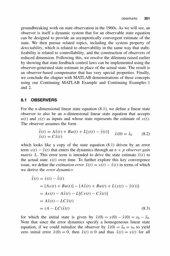
OBSERVERS 301
groundbreaking work on state observation in the 1960s. As we will see, anobserver is itself a dynamic system that for an observable state equationcan be designed to provide an asymptotically convergent estimate of thestate. We then pursue related topics, including the system property ofdetectability, which is related to observability in the same way that stabi-lizability is related to controllability, and the construction of observers ofreduced dimension. Following this, we resolve the dilemma raised earlierby showing that state feedback control laws can be implemented using theobserver-generated state estimate in place of the actual state. The result isan observer-based compensator that has very special properties. Finally,we conclude the chapter with MATLAB demonstrations of these conceptsusing our Continuing MATLAB Example and Continuing Examples 1and 2.
8.1 OBSERVERS
For the n-dimensional linear state equation (8.1), we define a linear stateobserver to also be an n-dimensional linear state equation that acceptsu(t) and y(t) as inputs and whose state represents the estimate of x(t).The observer assumes the form
˙x(t) = Ax(t) + Bu(t) + L[y(t) − y(t)]y(t) = Cx(t)
x(0) = x0 (8.2)
which looks like a copy of the state equation (8.1) driven by an errorterm y(t) − y(t) that enters the dynamics through an n × p observer gainmatrix L. This error term is intended to drive the state estimate x(t) tothe actual state x(t) over time. To further explore this key convergenceissue, we define the estimation error x(t) = x(t) − x(t) in terms of whichwe derive the error dynamics
˙x(t) = x(t) − ˙x(t)
= [Ax(t) + Bu(t)] − {Ax(t) + Bu(t) + L(y(t) − y(t))}= Ax(t) − Ax(t) − L[Cx(t) − Cx(t)]
= Ax(t) − LCx(t)
= (A − LC)x(t) (8.3)
for which the initial state is given by x(0) = x(0) − x(0) = x0 − x0.Note that since the error dynamics specify a homogeneous linear stateequation, if we could initialize the observer by x(0) = x0 = x0 to yieldzero initial error x(0) = 0, then x(t) ≡ 0 and thus x(t) = x(t) for all
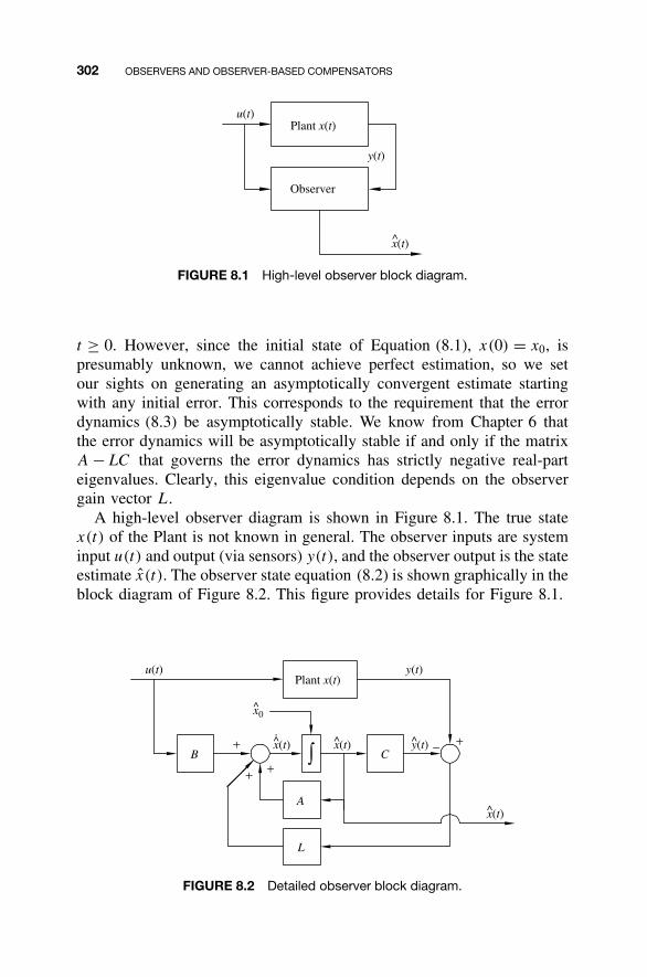
302 OBSERVERS AND OBSERVER-BASED COMPENSATORS
u(t)
y(t)
x(t)^
Plant x(t)
Observer
FIGURE 8.1 High-level observer block diagram.
t ≥ 0. However, since the initial state of Equation (8.1), x(0) = x0, ispresumably unknown, we cannot achieve perfect estimation, so we setour sights on generating an asymptotically convergent estimate startingwith any initial error. This corresponds to the requirement that the errordynamics (8.3) be asymptotically stable. We know from Chapter 6 thatthe error dynamics will be asymptotically stable if and only if the matrixA − LC that governs the error dynamics has strictly negative real-parteigenvalues. Clearly, this eigenvalue condition depends on the observergain vector L.
A high-level observer diagram is shown in Figure 8.1. The true statex(t) of the Plant is not known in general. The observer inputs are systeminput u(t) and output (via sensors) y(t), and the observer output is the stateestimate x(t). The observer state equation (8.2) is shown graphically in theblock diagram of Figure 8.2. This figure provides details for Figure 8.1.
y(t)
+
+−
+
+
Plant x(t)u(t) y(t)
L
A
B Cx(t)^x(t)
x0^
x(t)^
FIGURE 8.2 Detailed observer block diagram.
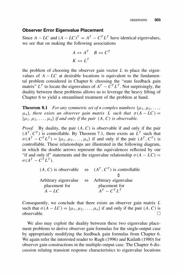
OBSERVERS 303
Observer Error Eigenvalue Placement
Since A − LC and (A − LC )T = AT − CT LT have identical eigenvalues,we see that on making the following associations
A ↔ AT B ↔ CT
K ↔ LT
the problem of choosing the observer gain vector L to place the eigen-values of A − LC at desirable locations is equivalent to the fundamen-tal problem considered in Chapter 6: choosing the “state feedback gainmatrix” LT to locate the eigenvalues of AT − CT LT . Not surprisingly, theduality between these problems allows us to leverage the heavy lifting ofChapter 6 to yield a streamlined treatment of the problem at hand.
Theorem 8.1 For any symmetric set of n complex numbers {µ1, µ2, . . . ,
µn}, there exists an observer gain matrix L such that σ(A − LC ) ={µ1, µ2, . . . , µn} if and only if the pair (A, C) is observable.
Proof. By duality, the pair (A, C) is observable if and only if the pair(AT , CT ) is controllable. By Theorem 7.1, there exists an LT such thatσ(AT − CT LT ) = {µ1, µ2, . . . , µn} if and only if the pair (AT , CT ) iscontrollable. These relationships are illustrated in the following diagram,in which the double arrows represent the equivalences reflected by our“if and only if” statements and the eigenvalue relationship σ(A − LC) =σ(AT − CT LT ).
(A, C) is observable ⇔ (AT , CT ) is controllable�
Arbitrary eigenvalueplacement forA − LC
⇔ Arbitrary eigenvalueplacement forAT − CT LT
Consequently, we conclude that there exists an observer gain matrix L
such that σ(A − LC ) = {µ1, µ2, . . . , µn} if and only if the pair (A, C) isobservable. �
We also may exploit the duality between these two eigenvalue place-ment problems to derive observer gain formulas for the single-output caseby appropriately modifying the feedback gain formulas from Chapter 6.We again refer the interested reader to Rugh (1996) and Kailath (1980) forobserver gain constructions in the multiple-output case. The Chapter 6 dis-cussion relating transient response characteristics to eigenvalue locations
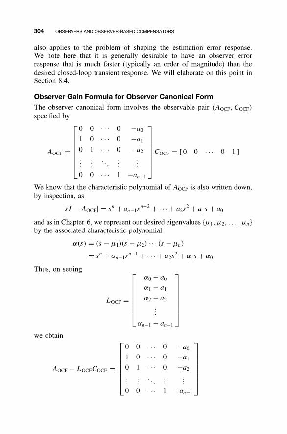
304 OBSERVERS AND OBSERVER-BASED COMPENSATORS
also applies to the problem of shaping the estimation error response.We note here that it is generally desirable to have an observer errorresponse that is much faster (typically an order of magnitude) than thedesired closed-loop transient response. We will elaborate on this point inSection 8.4.
Observer Gain Formula for Observer Canonical Form
The observer canonical form involves the observable pair (AOCF, COCF)
specified by
AOCF =
0 0 · · · 0 −a0
1 0 · · · 0 −a1
0 1 · · · 0 −a2
......
. . ....
...
0 0 · · · 1 −an−1
COCF = [ 0 0 · · · 0 1 ]
We know that the characteristic polynomial of AOCF is also written down,by inspection, as
|sI − AOCF| = sn + an−1sn−2 + · · · + a2s
2 + a1s + a0
and as in Chapter 6, we represent our desired eigenvalues {µ1, µ2, . . . , µn}by the associated characteristic polynomial
α(s) = (s − µ1)(s − µ2) · · · (s − µn)
= sn + αn−1sn−1 + · · · + α2s
2 + α1s + α0
Thus, on setting
LOCF =
α0 − a0
α1 − a1
α2 − a2
...
αn−1 − an−1
we obtain
AOCF − LOCFCOCF =
0 0 · · · 0 −a0
1 0 · · · 0 −a1
0 1 · · · 0 −a2
......
. . ....
...
0 0 · · · 1 −an−1
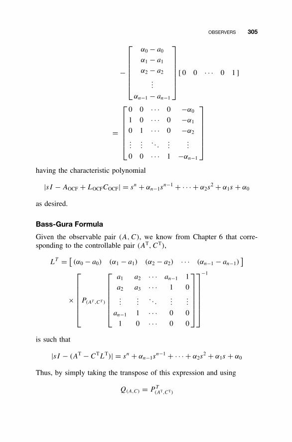
OBSERVERS 305
−
α0 − a0
α1 − a1
α2 − a2
...
αn−1 − an−1
[ 0 0 · · · 0 1 ]
=
0 0 · · · 0 −α0
1 0 · · · 0 −α1
0 1 · · · 0 −α2
......
. . ....
...
0 0 · · · 1 −αn−1
having the characteristic polynomial
|sI − AOCF + LOCFCOCF| = sn + αn−1sn−1 + · · · + α2s
2 + α1s + α0
as desired.
Bass-Gura Formula
Given the observable pair (A, C), we know from Chapter 6 that corre-sponding to the controllable pair (AT, CT),
LT = [(α0 − a0) (α1 − a1) (α2 − a2) · · · (αn−1 − an−1)
]
×
P(AT ,CT )
a1 a2 · · · an−1 1
a2 a3 · · · 1 0...
.... . .
......
an−1 1 · · · 0 0
1 0 · · · 0 0
−1
is such that
|sI − (AT − CTLT)| = sn + αn−1sn−1 + · · · + α2s
2 + α1s + α0
Thus, by simply taking the transpose of this expression and using
Q(A,C) = P T(AT,CT)
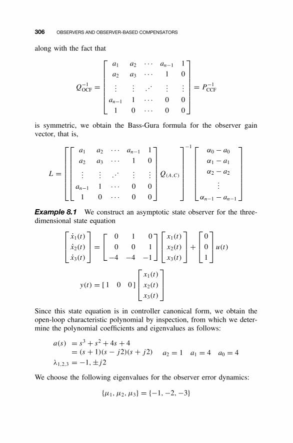
306 OBSERVERS AND OBSERVER-BASED COMPENSATORS
along with the fact that
Q−1OCF =
a1 a2 · · · an−1 1
a2 a3 · · · 1 0...
... . .....
...
an−1 1 · · · 0 0
1 0 · · · 0 0
= P −1CCF
is symmetric, we obtain the Bass-Gura formula for the observer gainvector, that is,
L =
a1 a2 · · · an−1 1
a2 a3 · · · 1 0...
... . .....
...
an−1 1 · · · 0 0
1 0 · · · 0 0
Q(A,C)
−1
α0 − a0
α1 − a1
α2 − a2
...
αn−1 − an−1
Example 8.1 We construct an asymptotic state observer for the three-dimensional state equation
x1(t)
x2(t)
x3(t)
=
0 1 0
0 0 1
−4 −4 −1
x1(t)
x2(t)
x3(t)
+
0
0
1
u(t)
y(t) = [ 1 0 0 ]
x1(t)
x2(t)
x3(t)
Since this state equation is in controller canonical form, we obtain theopen-loop characteristic polynomial by inspection, from which we deter-mine the polynomial coefficients and eigenvalues as follows:
a(s) = s3 + s2 + 4s + 4= (s + 1)(s − j2)(s + j2)
λ1,2,3 = −1, ±j2a2 = 1 a1 = 4 a0 = 4
We choose the following eigenvalues for the observer error dynamics:
{µ1, µ2, µ3} = {−1, −2, −3}
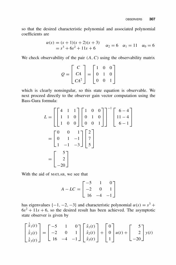
OBSERVERS 307
so that the desired characteristic polynomial and associated polynomialcoefficients are
α(s) = (s + 1)(s + 2)(s + 3)
= s3 + 6s2 + 11s + 6α2 = 6 α1 = 11 α0 = 6
We check observability of the pair (A, C) using the observability matrix
Q =
C
CA
CA2
=
1 0 0
0 1 0
0 0 1
which is clearly nonsingular, so this state equation is observable. Wenext proceed directly to the observer gain vector computation using theBass-Gura formula:
L =
4 1 1
1 1 0
1 0 0
1 0 0
0 1 0
0 0 1
−1
6 − 4
11 − 4
6 − 1
=
0 0 1
0 1 −1
1 −1 −3
2
7
5
=
5
2
−20
With the aid of MATLAB, we see that
A − LC =
−5 1 0
−2 0 1
16 −4 −1
has eigenvalues {−1, −2, −3} and characteristic polynomial α(s) = s3 +6s2 + 11s + 6, so the desired result has been achieved. The asymptoticstate observer is given by
˙x1(t)
˙x2(t)
˙x3(t)
=
−5 1 0
−2 0 1
16 −4 −1
x1(t)
x2(t)
x3(t)
+
0
0
1
u(t) +
5
2
−20
y(t)
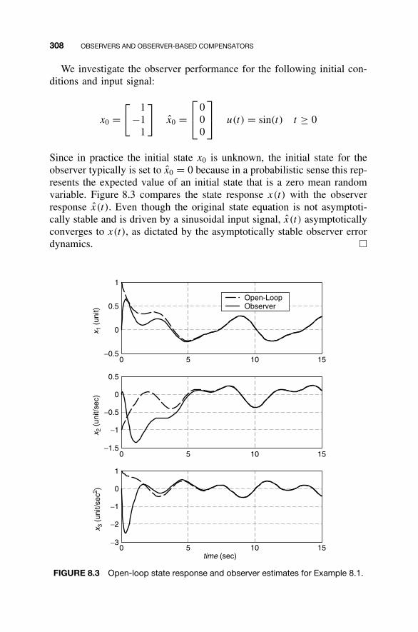
308 OBSERVERS AND OBSERVER-BASED COMPENSATORS
We investigate the observer performance for the following initial con-ditions and input signal:
x0 =[ 1
−11
]x0 =
0
00
u(t) = sin(t) t ≥ 0
Since in practice the initial state x0 is unknown, the initial state for theobserver typically is set to x0 = 0 because in a probabilistic sense this rep-resents the expected value of an initial state that is a zero mean randomvariable. Figure 8.3 compares the state response x(t) with the observerresponse x(t). Even though the original state equation is not asymptoti-cally stable and is driven by a sinusoidal input signal, x(t) asymptoticallyconverges to x(t), as dictated by the asymptotically stable observer errordynamics. �
x 1(u
nit)
x 2(u
nit/s
ec)
x 3(u
nit/s
ec2 )
time (sec)
0 5 10 15−0.5
0
0.5
1
Open-LoopObserver
0 5 10 15−1.5
−1
−0.5
0
0.5
0 5 10 15−3
−2
−1
0
1
FIGURE 8.3 Open-loop state response and observer estimates for Example 8.1.
OBSERVERS 309
Example 8.2 In this example we design an observer for the state equa-tion appearing in Example 7.4, which we repeat here for convenience.Thus
x1(t)
x2(t)
x3(t)
=
0 1 0
0 0 1
−18 −15 −2
x1(t)
x2(t)
x3(t)
+
0
0
1
u(t)
y(t) = [ 1 0 0 ]
x1(t)
x2(t)
x3(t)
which, as we recall, is in controller canonical form. Therefore, we seeby inspection that the characteristic polynomial and polynomial coeffi-cients are
a(s) = s3 + 2s2 + 15s + 18 a2 = 2 a1 = 15 a0 = 18
In Example 7.4 we specified desired closed-loop eigenvalues to beµ1,2,3 = −1.33 ± j1.49, −13.3 to achieve a percent overshoot of 6percent and a settling time of 3 s for the closed-loop step response. Weselect eigenvalues for the observer error dynamics by scaling the precedingeigenvalues by 10 to give µ1,2,3 = −13.3 ± j14.9, −133.3. The desiredcharacteristic polynomial for the observer error dynamics then becomes
α(s) = s3 + 160s2 + 3955s + 53260
α2 = 160 α1 = 3955 α0 = 53260
Note that when comparing this characteristic polynomial for the ob-server error dynamics with s3 + 16s2 + 39.55s + 53.26 associated withthe eigenvalues achieved by state feedback in Example 7.4, we see that160/16 = 10, 3955/39.55 = 100, and 53260/53.26 = 1000 as a result ofthe factor of 10 relating the respective eigenvalues.
We next check observability of the pair (A, C) via
Q =
C
CA
CA2
=
1 0 0
0 1 0
0 0 1
which is obviously nonsingular, so the state equation is observable. Wethen proceed to compute the observer gain vector using the Bass-Gura
310 OBSERVERS AND OBSERVER-BASED COMPENSATORS
formula, that is,
L =
15 2 1
2 1 0
1 0 0
1 0 0
0 1 0
0 0 1
−1
(53260 − 18)
(3955 − 15)
(160 − 2)
=
0 0 1
0 1 −2
1 −2 −11
53242
3940
158
=
158
3624
43624
We conclude the example by verifying that
A − LC = 0 1 0
0 0 1
−18 −15 −2
−
158
3624
43624
[ 1 0 0 ]
=
−158 1 0
−3624 0 1
−43642 −15 −2
has eigenvalues λ1,2,3 = −13.3 ± j14.9, −133.3 as required. We observethat the “fast” observer eigenvalues we specified resulted in large observergains that may be impractical. Therefore, we may need to trade off therapid convergence of the observer error with practical limitations onachievable observer gains. �
Ackermann’s Formula
Given the observable pair (A, C), again, our strategy is to first apply ourChapter 6 result to the controllable pair (AT, CT) to write
LT = [ 0 0 · · · 0 1 ]P −1(AT ,CT )
α(AT )
Using
α(AT ) = (AT )n + αn−1(AT )n−1 + · · · + α2(A
T )2 + α1AT + α0I
= (An)T + αn−1(An−1)T + · · · + α2(A
2)T + α1AT + α0I
= [α(A)]T
OBSERVERS 311
we obtain [α(AT )]T = α(A), which along with
[P −1(AT ,CT )
]T = [P T(AT ,CT )]
−1 = Q−1(A,C)
gives
L = α(A)Q−1(A,C)
0
0...
0
1
Example 8.3 We demonstrate the use of Ackermann’s formula for thestate equation given in Example 8.1. We have previously computed
Q =
C
CA
CA2
=
1 0 0
0 1 0
0 0 1
In terms of the desired characteristic polynomial α(s) = s3 + 6s2 + 11s +6, we construct
α(A) = A3 + 6A2 + 11A + 6I
=
−4 −4 −1
4 0 −3
12 16 3
+ 6
0 0 1
−4 −4 −1
4 0 −2
+ 11
0 1 0
0 0 1
−4 −4 −1
+ 6
1 0 0
0 1 0
0 0 1
=
2 7 5
−20 −18 2
−8 −28 −20
so that
L =
2 7 5
−20 −18 2
−8 −28 −20
1 0 0
0 1 0
0 0 1
−1
0
0
1
=
5
2
−20
which agrees with the previously-derived result. �
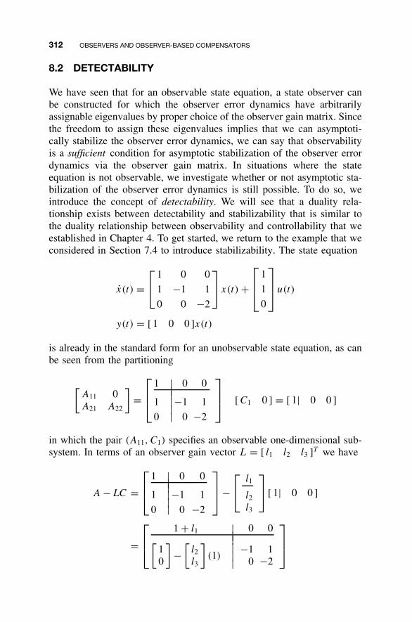
312 OBSERVERS AND OBSERVER-BASED COMPENSATORS
8.2 DETECTABILITY
We have seen that for an observable state equation, a state observer canbe constructed for which the observer error dynamics have arbitrarilyassignable eigenvalues by proper choice of the observer gain matrix. Sincethe freedom to assign these eigenvalues implies that we can asymptoti-cally stabilize the observer error dynamics, we can say that observabilityis a sufficient condition for asymptotic stabilization of the observer errordynamics via the observer gain matrix. In situations where the stateequation is not observable, we investigate whether or not asymptotic sta-bilization of the observer error dynamics is still possible. To do so, weintroduce the concept of detectability. We will see that a duality rela-tionship exists between detectability and stabilizability that is similar tothe duality relationship between observability and controllability that weestablished in Chapter 4. To get started, we return to the example that weconsidered in Section 7.4 to introduce stabilizability. The state equation
x(t) =
1 0 0
1 −1 1
0 0 −2
x(t) +
1
1
0
u(t)
y(t) = [ 1 0 0 ]x(t)
is already in the standard form for an unobservable state equation, as canbe seen from the partitioning
[A11 0A21 A22
]=
1 | 0 0||1 |−1 1|0 | 0 −2
[ C1 0 ] = [ 1| 0 0 ]
in which the pair (A11, C1) specifies an observable one-dimensional sub-system. In terms of an observer gain vector L = [ l1 l2 l3 ]T we have
A − LC =
1 | 0 0||1 |−1 1|0 | 0 −2
−
l1
l2l3
[ 1| 0 0 ]
=
1 + l1 | 0 0|||[10
]−
[l2l3
](1) | −1 1
0 −2|
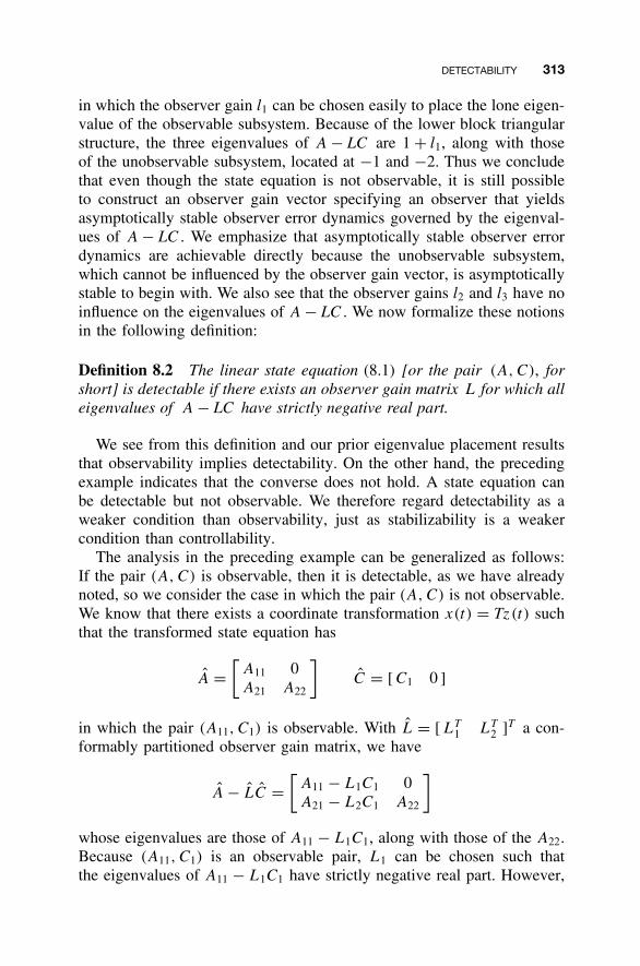
DETECTABILITY 313
in which the observer gain l1 can be chosen easily to place the lone eigen-value of the observable subsystem. Because of the lower block triangularstructure, the three eigenvalues of A − LC are 1 + l1, along with thoseof the unobservable subsystem, located at −1 and −2. Thus we concludethat even though the state equation is not observable, it is still possibleto construct an observer gain vector specifying an observer that yieldsasymptotically stable observer error dynamics governed by the eigenval-ues of A − LC . We emphasize that asymptotically stable observer errordynamics are achievable directly because the unobservable subsystem,which cannot be influenced by the observer gain vector, is asymptoticallystable to begin with. We also see that the observer gains l2 and l3 have noinfluence on the eigenvalues of A − LC . We now formalize these notionsin the following definition:
Definition 8.2 The linear state equation (8.1) [or the pair (A, C), forshort] is detectable if there exists an observer gain matrix L for which alleigenvalues of A − LC have strictly negative real part.
We see from this definition and our prior eigenvalue placement resultsthat observability implies detectability. On the other hand, the precedingexample indicates that the converse does not hold. A state equation canbe detectable but not observable. We therefore regard detectability as aweaker condition than observability, just as stabilizability is a weakercondition than controllability.
The analysis in the preceding example can be generalized as follows:If the pair (A, C) is observable, then it is detectable, as we have alreadynoted, so we consider the case in which the pair (A, C) is not observable.We know that there exists a coordinate transformation x(t) = Tz (t) suchthat the transformed state equation has
A =[
A11 0A21 A22
]C = [ C1 0 ]
in which the pair (A11, C1) is observable. With L = [ LT1 LT
2 ]T a con-formably partitioned observer gain matrix, we have
A − LC =[
A11 − L1C1 0A21 − L2C1 A22
]
whose eigenvalues are those of A11 − L1C1, along with those of the A22.Because (A11, C1) is an observable pair, L1 can be chosen such thatthe eigenvalues of A11 − L1C1 have strictly negative real part. However,
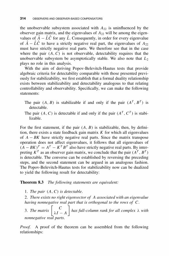
314 OBSERVERS AND OBSERVER-BASED COMPENSATORS
the unobservable subsystem associated with A22 is uninfluenced by theobserver gain matrix, and the eigenvalues of A22 will be among the eigen-values of A − LC for any L. Consequently, in order for every eigenvalueof A − LC to have a strictly negative real part, the eigenvalues of A22
must have strictly negative real parts. We therefore see that in the casewhere the pair (A, C) is not observable, detectability requires that theunobservable subsystem be asymptotically stable. We also note that L2
plays no role in this analysis.With the aim of deriving Popov-Belevitch-Hautus tests that provide
algebraic criteria for detectability comparable with those presented previ-ously for stabilizability, we first establish that a formal duality relationshipexists between stabilizability and detectability analogous to that relatingcontrollability and observability. Specifically, we can make the followingstatements:
The pair (A, B) is stabilizable if and only if the pair (AT , BT ) isdetectable.
The pair (A, C) is detectable if and only if the pair (AT , CT ) is stabi-lizable.
For the first statement, if the pair (A, B) is stabilizable, then, by defini-tion, there exists a state feedback gain matrix K for which all eigenvaluesof A − BK have strictly negative real parts. Since the matrix transposeoperation does not affect eigenvalues, it follows that all eigenvalues of(A − BK )T = AT − KT BT also have strictly negative real parts. By inter-preting KT as an observer gain matrix, we conclude that the pair (AT ,BT )
is detectable. The converse can be established by reversing the precedingsteps, and the second statement can be argued in an analogous fashion.The Popov-Belevitch-Hautus tests for stabilizability now can be dualizedto yield the following result for detectability:
Theorem 8.3 The following statements are equivalent:
1. The pair (A, C) is detectable.2. There exists no right eigenvector of A associated with an eigenvaluehaving nonnegative real part that is orthogonal to the rows of C.
3. The matrix
[C
λI − A
]has full-column rank for all complex λ with
nonnegative real parts.
Proof. A proof of the theorem can be assembled from the followingrelationships:
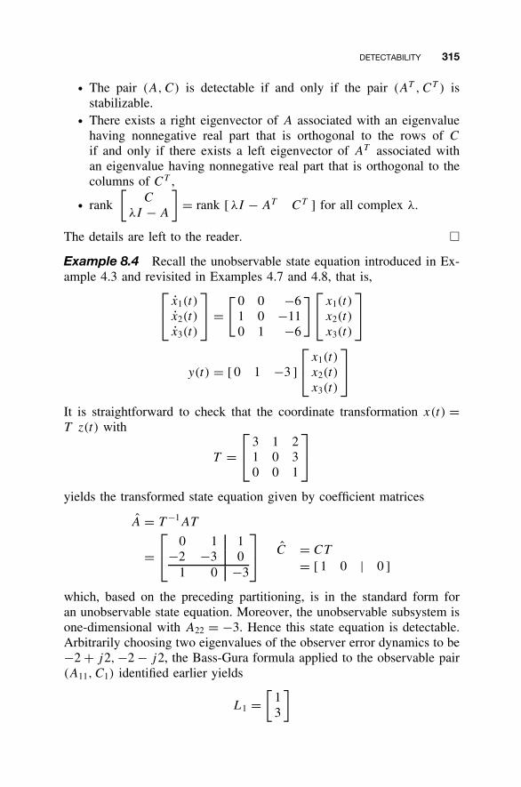
DETECTABILITY 315
• The pair (A, C) is detectable if and only if the pair (AT , CT ) isstabilizable.
• There exists a right eigenvector of A associated with an eigenvaluehaving nonnegative real part that is orthogonal to the rows of C
if and only if there exists a left eigenvector of AT associated withan eigenvalue having nonnegative real part that is orthogonal to thecolumns of CT ,
• rank
[C
λI − A
]= rank [ λI − AT CT ] for all complex λ.
The details are left to the reader. �
Example 8.4 Recall the unobservable state equation introduced in Ex-ample 4.3 and revisited in Examples 4.7 and 4.8, that is,
x1(t)
x2(t)
x3(t)
=
[ 0 0 −61 0 −110 1 −6
] x1(t)
x2(t)
x3(t)
y(t) = [ 0 1 −3 ]
x1(t)
x2(t)
x3(t)
It is straightforward to check that the coordinate transformation x(t) =T z(t) with
T = 3 1 2
1 0 30 0 1
yields the transformed state equation given by coefficient matrices
A = T −1AT
= 0 1 1
−2 −3 01 0 −3
C = CT
= [ 1 0 | 0 ]
which, based on the preceding partitioning, is in the standard form foran unobservable state equation. Moreover, the unobservable subsystem isone-dimensional with A22 = −3. Hence this state equation is detectable.Arbitrarily choosing two eigenvalues of the observer error dynamics to be−2 + j2, −2 − j2, the Bass-Gura formula applied to the observable pair(A11, C1) identified earlier yields
L1 =[
13
]
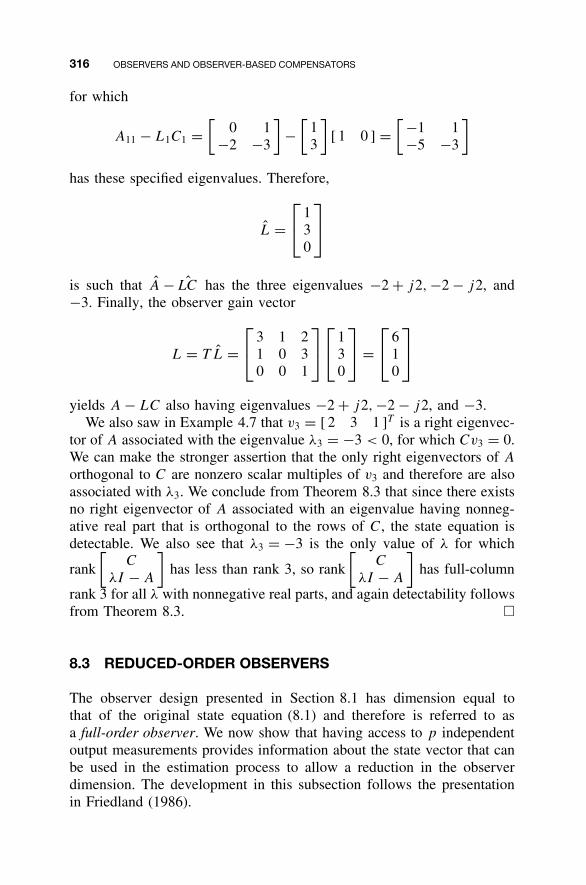
316 OBSERVERS AND OBSERVER-BASED COMPENSATORS
for which
A11 − L1C1 =[
0 1−2 −3
]−
[13
][ 1 0 ] =
[ −1 1−5 −3
]
has these specified eigenvalues. Therefore,
L = 1
30
is such that A − ˆLC has the three eigenvalues −2 + j2, −2 − j2, and−3. Finally, the observer gain vector
L = T L = 3 1 2
1 0 30 0 1
1
30
=
6
10
yields A − LC also having eigenvalues −2 + j2, −2 − j2, and −3.We also saw in Example 4.7 that v3 = [ 2 3 1 ]T is a right eigenvec-
tor of A associated with the eigenvalue λ3 = −3 < 0, for which Cv3 = 0.We can make the stronger assertion that the only right eigenvectors of A
orthogonal to C are nonzero scalar multiples of v3 and therefore are alsoassociated with λ3. We conclude from Theorem 8.3 that since there existsno right eigenvector of A associated with an eigenvalue having nonneg-ative real part that is orthogonal to the rows of C, the state equation isdetectable. We also see that λ3 = −3 is the only value of λ for which
rank
[C
λI − A
]has less than rank 3, so rank
[C
λI − A
]has full-column
rank 3 for all λ with nonnegative real parts, and again detectability followsfrom Theorem 8.3. �
8.3 REDUCED-ORDER OBSERVERS
The observer design presented in Section 8.1 has dimension equal tothat of the original state equation (8.1) and therefore is referred to asa full-order observer. We now show that having access to p independentoutput measurements provides information about the state vector that canbe used in the estimation process to allow a reduction in the observerdimension. The development in this subsection follows the presentationin Friedland (1986).
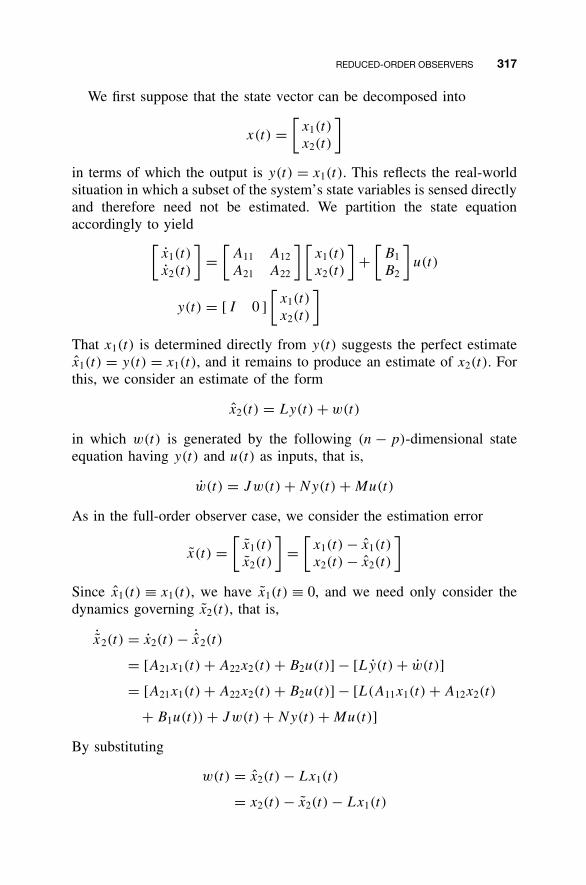
REDUCED-ORDER OBSERVERS 317
We first suppose that the state vector can be decomposed into
x(t) =[
x1(t)
x2(t)
]
in terms of which the output is y(t) = x1(t). This reflects the real-worldsituation in which a subset of the system’s state variables is sensed directlyand therefore need not be estimated. We partition the state equationaccordingly to yield[
x1(t)
x2(t)
]=
[A11 A12
A21 A22
] [x1(t)
x2(t)
]+
[B1
B2
]u(t)
y(t) = [ I 0 ]
[x1(t)
x2(t)
]
That x1(t) is determined directly from y(t) suggests the perfect estimatex1(t) = y(t) = x1(t), and it remains to produce an estimate of x2(t). Forthis, we consider an estimate of the form
x2(t) = Ly(t) + w(t)
in which w(t) is generated by the following (n − p)-dimensional stateequation having y(t) and u(t) as inputs, that is,
w(t) = Jw(t) + Ny(t) + Mu(t)
As in the full-order observer case, we consider the estimation error
x(t) =[
x1(t)
x2(t)
]=
[x1(t) − x1(t)
x2(t) − x2(t)
]
Since x1(t) ≡ x1(t), we have x1(t) ≡ 0, and we need only consider thedynamics governing x2(t), that is,
˙x2(t) = x2(t) − ˙x2(t)
= [A21x1(t) + A22x2(t) + B2u(t)] − [Ly(t) + w(t)]
= [A21x1(t) + A22x2(t) + B2u(t)] − [L(A11x1(t) + A12x2(t)
+ B1u(t)) + Jw(t) + Ny(t) + Mu(t)]
By substituting
w(t) = x2(t) − Lx1(t)
= x2(t) − x2(t) − Lx1(t)
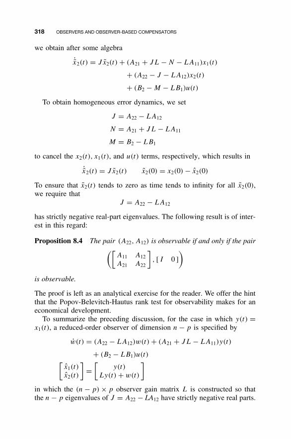
318 OBSERVERS AND OBSERVER-BASED COMPENSATORS
we obtain after some algebra
˙x2(t) = J x2(t) + (A21 + JL − N − LA11)x1(t)
+ (A22 − J − LA12)x2(t)
+ (B2 − M − LB1)u(t)
To obtain homogeneous error dynamics, we set
J = A22 − LA12
N = A21 + JL − LA11
M = B2 − LB1
to cancel the x2(t), x1(t), and u(t) terms, respectively, which results in
˙x2(t) = J x2(t) x2(0) = x2(0) − x2(0)
To ensure that x2(t) tends to zero as time tends to infinity for all x2(0),we require that
J = A22 − LA12
has strictly negative real-part eigenvalues. The following result is of inter-est in this regard:
Proposition 8.4 The pair (A22, A12) is observable if and only if the pair([A11 A12
A21 A22
], [ I 0 ]
)
is observable.
The proof is left as an analytical exercise for the reader. We offer the hintthat the Popov-Belevitch-Hautus rank test for observability makes for aneconomical development.
To summarize the preceding discussion, for the case in which y(t) =x1(t), a reduced-order observer of dimension n − p is specified by
w(t) = (A22 − LA12)w(t) + (A21 + JL − LA11)y(t)
+ (B2 − LB1)u(t)[x1(t)
x2(t)
]=
[y(t)
Ly(t) + w(t)
]
in which the (n − p) × p observer gain matrix L is constructed so thatthe n − p eigenvalues of J = A22 − LA12 have strictly negative real parts.
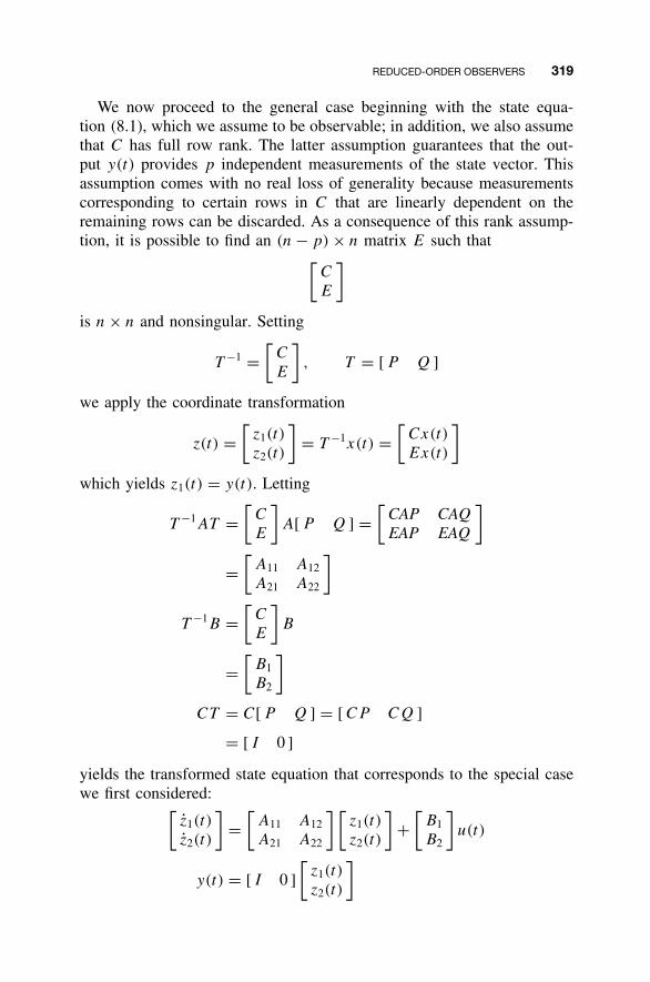
REDUCED-ORDER OBSERVERS 319
We now proceed to the general case beginning with the state equa-tion (8.1), which we assume to be observable; in addition, we also assumethat C has full row rank. The latter assumption guarantees that the out-put y(t) provides p independent measurements of the state vector. Thisassumption comes with no real loss of generality because measurementscorresponding to certain rows in C that are linearly dependent on theremaining rows can be discarded. As a consequence of this rank assump-tion, it is possible to find an (n − p) × n matrix E such that[
C
E
]
is n × n and nonsingular. Setting
T −1 =[
C
E
], T = [ P Q ]
we apply the coordinate transformation
z(t) =[
z1(t)
z2(t)
]= T −1x(t) =
[Cx(t)
Ex(t)
]
which yields z1(t) = y(t). Letting
T −1AT =[
C
E
]A[ P Q ] =
[CAP CAQEAP EAQ
]
=[
A11 A12
A21 A22
]
T −1B =[
C
E
]B
=[
B1
B2
]
CT = C[ P Q ] = [ CP CQ ]
= [ I 0 ]
yields the transformed state equation that corresponds to the special casewe first considered:[
z1(t)
z2(t)
]=
[A11 A12
A21 A22
] [z1(t)
z2(t)
]+
[B1
B2
]u(t)
y(t) = [ I 0 ]
[z1(t)
z2(t)
]
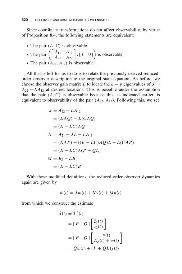
320 OBSERVERS AND OBSERVER-BASED COMPENSATORS
Since coordinate transformations do not affect observability, by virtueof Proposition 8.4, the following statements are equivalent:
• The pair (A, C) is observable.
• The pair
([A11 A12
A21 A22
], [ I 0 ]
)is observable.
• The pair (A22, A12) is observable.
All that is left for us to do is to relate the previously derived reduced-order observer description to the original state equation. As before, wechoose the observer gain matrix L to locate the n − p eigenvalues of J =A22 − LA12 at desired locations. This is possible under the assumptionthat the pair (A, C) is observable because this, as indicated earlier, isequivalent to observability of the pair (A22, A12). Following this, we set
J = A22 − LA12
= (EAQ) − L(CAQ)
= (E − LC)AQ
N = A21 + JL − LA11
= (EAP) + ((E − LC)AQ)L − L(CAP)
= (E − LC)A(P + QL)
M = B2 − LB1
= (E − LC)B
With these modified definitions, the reduced-order observer dynamicsagain are given by
w(t) = Jw(t) + Ny(t) + Mu(t)
from which we construct the estimate
x(t) = T z(t)
= [ P Q ]
[z1(t)
z2(t)
]
= [ P Q ]
[y(t)
Ly(t) + w(t)
]
= Qw(t) + (P + QL)y(t)
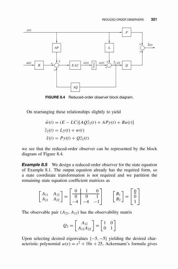
REDUCED-ORDER OBSERVERS 321
w(t)+E-LC
AQ
u(t)Q
y(t)
x(t)^
B
AP
w(t)
L
z2 (t)^+
++
+
P
+
+
FIGURE 8.4 Reduced-order observer block diagram.
On rearranging these relationships slightly to yield
w(t) = (E − LC)[AQz2(t) + APy(t) + Bu(t)]
z2(t) = Ly(t) + w(t)
x(t) = Py(t) + Qz2(t)
we see that the reduced-order observer can be represented by the blockdiagram of Figure 8.4.
Example 8.5 We design a reduced-order observer for the state equationof Example 8.1. The output equation already has the required form, soa state coordinate transformation is not required and we partition theremaining state equation coefficient matrices as
[A11 A12
A21 A22
]=
0 1 0
0 0 1−4 −4 −1
[
B1
B2
]=
0
01
The observable pair (A22, A12) has the observability matrix
Q2 =[
A12
A12A22
]=
[1 00 1
]
Upon selecting desired eigenvalues {−5, −5} yielding the desired char-acteristic polynomial α(s) = s2 + 10s + 25, Ackermann’s formula gives
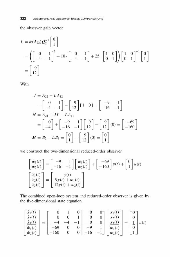
322 OBSERVERS AND OBSERVER-BASED COMPENSATORS
the observer gain vector
L = α(A22)Q−12
[01
]
=([
0 1−4 −1
]2
+ 10 ·[
0 1−4 −1
]+ 25 ·
[1 00 1
]) [1 00 1
]−1 [01
]
=[
912
]
With
J = A22 − LA12
=[
0 1−4 −1
]−
[9
12
][ 1 0 ] =
[ −9 1−16 −1
]
N = A21 + JL − LA11
=[
0−4
]+
[ −9 1−16 −1
] [9
12
]−
[9
12
](0) =
[ −69−160
]
M = B2 − LB1 =[
01
]−
[9
12
](0) =
[01
]
we construct the two-dimensional reduced-order observer
[w1(t)
w2(t)
]=
[ −9 1−16 −1
] [w1(t)
w2(t)
]+
[ −69−160
]y(t) +
[01
]u(t)
x1(t)
x2(t)
x3(t)
=
y(t)
9y(t) + w1(t)
12y(t) + w2(t)
The combined open-loop system and reduced-order observer is given bythe five-dimensional state equation
x1(t)
x2(t)
x3(t)
w1(t)
w2(t)
=
0 1 0 0 00 0 1 0 0
−4 −4 −1 0 0−69 0 0 −9 1
−160 0 0 −16 −1
x1(t)
x2(t)
x3(t)
w1(t)
w2(t)
+
00101
u(t)
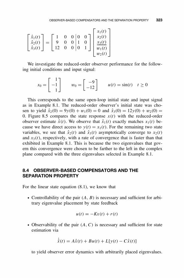
OBSERVER-BASED COMPENSATORS AND THE SEPARATION PROPERTY 323
x1(t)
x2(t)
x3(t)
=
1 0 0
9 0 012 0 0
∣∣∣∣∣∣0 01 00 1
x1(t)
x2(t)
x3(t)
w1(t)
w2(t)
We investigate the reduced-order observer performance for the follow-ing initial conditions and input signal:
x0 =[ 1
−11
]w0 =
[ −9−12
]u(t) = sin(t) t ≥ 0
This corresponds to the same open-loop initial state and input signalas in Example 8.1. The reduced-order observer’s initial state was cho-sen to yield x2(0) = 9y(0) + w1(0) = 0 and x3(0) = 12y(0) + w2(0) =0. Figure 8.5 compares the state response x(t) with the reduced-orderobserver estimate x(t). We observe that x1(t) exactly matches x1(t) be-cause we have direct access to y(t) = x1(t). For the remaining two statevariables, we see that x2(t) and x3(t) asymptotically converge to x2(t)
and x3(t), respectively, with a rate of convergence that is faster than thatexhibited in Example 8.1. This is because the two eigenvalues that gov-ern this convergence were chosen to be farther to the left in the complexplane compared with the three eigenvalues selected in Example 8.1.
8.4 OBSERVER-BASED COMPENSATORS AND THESEPARATION PROPERTY
For the linear state equation (8.1), we know that
• Controllability of the pair (A, B) is necessary and sufficient for arbi-trary eigenvalue placement by state feedback
u(t) = −Kx(t) + r(t)
• Observability of the pair (A, C) is necessary and sufficient for stateestimation via
˙x(t) = Ax(t) + Bu(t) + L[y(t) − Cx(t)]
to yield observer error dynamics with arbitrarily placed eigenvalues.
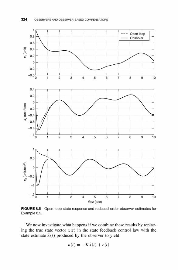
324 OBSERVERS AND OBSERVER-BASED COMPENSATORS
1
0.5
0
−0.5
−1
−1.50 1 2 3 4 5 6 7 8 9 10
time (sec)
x 3 (
unit
/sec
2 )
0.4
0.2
0
−0.2
−0.4
−0.6
−0.8
−10 1 2 3 4 5 6 7 8 9 10
x 2 (
unit
/sec
)
1
0.8
0.6
0.4
0.2
0
−0.2
−0.50 1 2 3 4 5 6 7 8 9 10
x 1 (
unit)
Open-loopObserver
FIGURE 8.5 Open-loop state response and reduced-order observer estimates forExample 8.5.
We now investigate what happens if we combine these results by replac-ing the true state vector x(t) in the state feedback control law with thestate estimate x(t) produced by the observer to yield
u(t) = −Kx(t) + r(t)
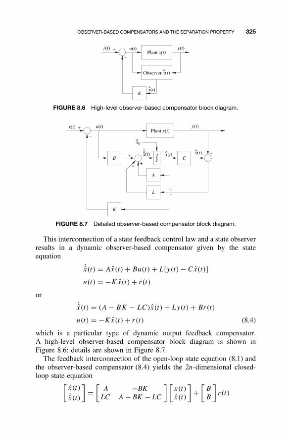
OBSERVER-BASED COMPENSATORS AND THE SEPARATION PROPERTY 325
+−
r(t) u(t)Plant x(t)
Observer x(t)
y(t)
K
^
x(t)^
FIGURE 8.6 High-level observer-based compensator block diagram.
+
+−
+
−
+
+
Plant x(t)r(t)
x(t)
u(t) y(t)
K
L
A
B C^x(t) y(t)
x0^
FIGURE 8.7 Detailed observer-based compensator block diagram.
This interconnection of a state feedback control law and a state observerresults in a dynamic observer-based compensator given by the stateequation
˙x(t) = Ax(t) + Bu(t) + L[y(t) − Cx(t)]
u(t) = −Kx(t) + r(t)
or
˙x(t) = (A − BK − LC)x(t) + Ly(t) + Br(t)
u(t) = −Kx(t) + r(t) (8.4)
which is a particular type of dynamic output feedback compensator.A high-level observer-based compensator block diagram is shown inFigure 8.6; details are shown in Figure 8.7.
The feedback interconnection of the open-loop state equation (8.1) andthe observer-based compensator (8.4) yields the 2n-dimensional closed-loop state equation[
x(t)˙x(t)
]=
[A −BK
LC A − BK − LC
] [x(t)
x(t)
]+
[B
B
]r(t)
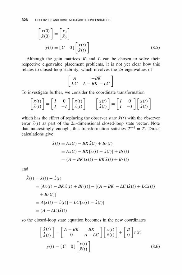
326 OBSERVERS AND OBSERVER-BASED COMPENSATORS
[x(0)
x(0)
]=
[x0
x0
]
y(t) = [ C 0 ]
[x(t)
x(t)
](8.5)
Although the gain matrices K and L can be chosen to solve theirrespective eigenvalue placement problems, it is not yet clear how thisrelates to closed-loop stability, which involves the 2n eigenvalues of[
A −BKLC A − BK − LC
]
To investigate further, we consider the coordinate transformation[x(t)
x(t)
]=
[I 0I −I
] [x(t)
x(t)
] [x(t)
x(t)
]=
[I 0I −I
] [x(t)
x(t)
]
which has the effect of replacing the observer state x(t) with the observererror x(t) as part of the 2n-dimensional closed-loop state vector. Notethat interestingly enough, this transformation satisfies T −1 = T . Directcalculations give
x(t) = Ax(t) − BK x(t) + Br(t)
= Ax(t) − BK [x(t) − x(t)] + Br(t)
= (A − BK )x(t) − BK x(t) + Br(t)
and
˙x(t) = x(t) − ˙x(t)
= [Ax (t) − BK x(t) + Br(t)] − [(A − BK − LC )x(t) + LCx(t)
+ Br(t)]
= A[x(t) − x(t)] − LC [x(t) − x(t)]
= (A − LC )x(t)
so the closed-loop state equation becomes in the new coordinates[
x(t)˙x(t)
]=
[A − BK BK
0 A − LC
] [x(t)
x(t)
]+
[B
0
]r(t)
y(t) = [ C 0 ]
[x(t)
x(t)
](8.6)
OBSERVER-BASED COMPENSATORS AND THE SEPARATION PROPERTY 327
Because of the block triangular structure of the transformed closed-loopsystem dynamics matrix, we see that the 2n closed-loop eigenvalues aregiven by
σ
([A − BK BK
0 A − LC
])= σ(A − BK ) ∪ σ(A − LC )
Because state coordinate transformations do not affect eigenvalues, weconclude that
σ
([A −BK
LC A − BK − LC
])= σ(A − BK ) ∪ σ(A − LC )
This indicates that the 2n closed-loop eigenvalues can be placed by sep-arately and independently locating eigenvalues of A − BK and A − LCvia choice of the gain matrices K and L, respectively. We refer to this asthe separation property of observer-based compensators.
We generally require the observer error to converge faster than thedesired closed-loop transient response dynamics. Therefore, we choosethe eigenvalues of A − LC to be about 10 times farther to the left in thecomplex plane than the (dominant) eigenvalues of A − BK .
Example 8.6 We return to the open-loop state equation in Example 8.1.The open-loop characteristic polynomial is a(s) = s3 + s3 + 4s + 4. Theopen-loop the eigenvalues λ1,2,3 = −1, ±j2 indicate that this is amarginally stable state equation because of the nonrepeated zero-real-parteigenvalues. This state equation is not bounded-input, bounded outputstable since the bounded input u(t) = sin(2t) creates a resonance withthe imaginary eigenvalues and an unbounded zero-state response results.We therefore seek to design an observer-based compensator by combiningthe observer designed previously with a state feedback control law.
Given the following eigenvalues to be placed by state feedback, namely,
µ1,2,3 = − 12 ± j
√3
2 , −1
the desired characteristic polynomial is α(s) = s3 + 2s2 + 2s + 1. Sincethe open-loop state equation is in controller canonical form we easilycompute state feedback gain vector to be
K = KCCF
= [( α0 − a0) (α1 − a1) (α2 − a2) ]
= [ (1 − 4) (2 − 4) (2 − 1) ]
= [ −3 −2 1 ]
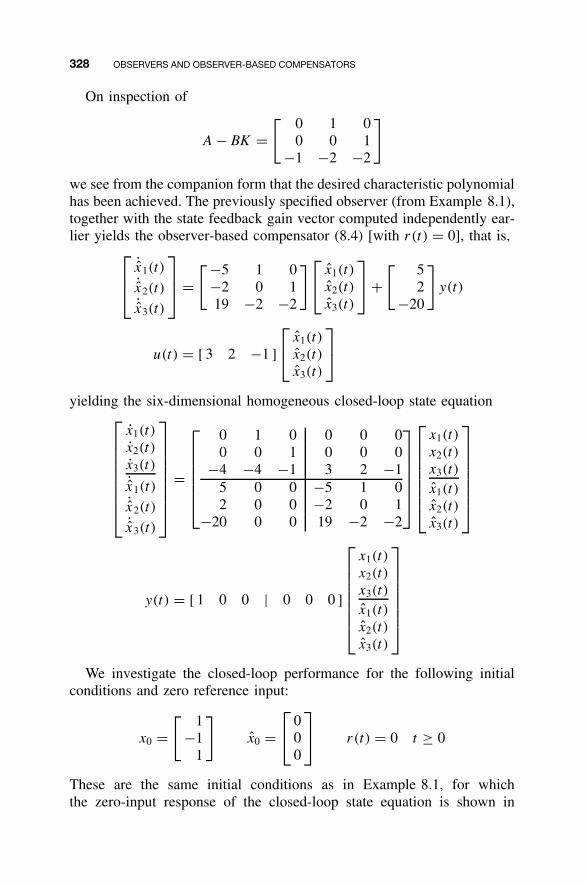
328 OBSERVERS AND OBSERVER-BASED COMPENSATORS
On inspection of
A − BK =[ 0 1 0
0 0 1−1 −2 −2
]
we see from the companion form that the desired characteristic polynomialhas been achieved. The previously specified observer (from Example 8.1),together with the state feedback gain vector computed independently ear-lier yields the observer-based compensator (8.4) [with r(t) = 0], that is,
˙x1(t)˙x2(t)˙x3(t)
=
[−5 1 0−2 0 119 −2 −2
] x1(t)
x2(t)
x3(t)
+
[ 52
−20
]y(t)
u(t) = [ 3 2 −1 ]
x1(t)
x2(t)
x3(t)
yielding the six-dimensional homogeneous closed-loop state equation
x1(t)
x2(t)
x3(t)
˙x1(t)˙x2(t)˙x3(t)
=
0 1 0 0 0 00 0 1 0 0 0
−4 −4 −1 3 2 −15 0 0 −5 1 02 0 0 −2 0 1
−20 0 0 19 −2 −2
x1(t)
x2(t)
x3(t)
x1(t)
x2(t)
x3(t)
y(t) = [ 1 0 0 | 0 0 0 ]
x1(t)
x2(t)
x3(t)
x1(t)
x2(t)
x3(t)
We investigate the closed-loop performance for the following initialconditions and zero reference input:
x0 =[ 1
−11
]x0 =
0
00
r(t) = 0 t ≥ 0
These are the same initial conditions as in Example 8.1, for whichthe zero-input response of the closed-loop state equation is shown in
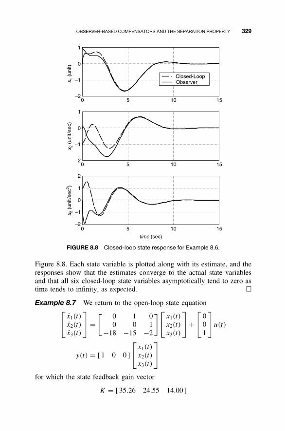
OBSERVER-BASED COMPENSATORS AND THE SEPARATION PROPERTY 329
0 5 10 15−2
−1
0
1
Closed-LoopObserver
0 5 10 15−2
−1
0
1
time (sec)
0 5 10 15−2
−1
0
2
1
x 3 (
unit
/sec
2 )x 2
(un
it/s
ec)
x 1 (
unit)
FIGURE 8.8 Closed-loop state response for Example 8.6.
Figure 8.8. Each state variable is plotted along with its estimate, and theresponses show that the estimates converge to the actual state variablesand that all six closed-loop state variables asymptotically tend to zero astime tends to infinity, as expected. �
Example 8.7 We return to the open-loop state equation x1(t)
x2(t)
x3(t)
=
[ 0 1 00 0 1
−18 −15 −2
] x1(t)
x2(t)
x3(t)
+
0
01
u(t)
y(t) = [ 1 0 0 ]
x1(t)
x2(t)
x3(t)
for which the state feedback gain vector
K = [ 35.26 24.55 14.00 ]
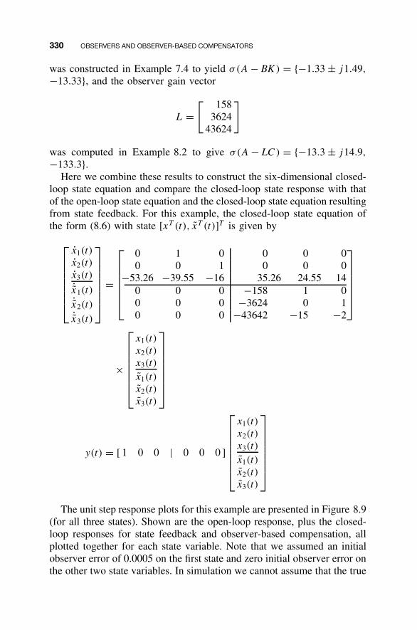
330 OBSERVERS AND OBSERVER-BASED COMPENSATORS
was constructed in Example 7.4 to yield σ(A − BK ) = {−1.33 ± j1.49,
−13.33}, and the observer gain vector
L =[ 158
362443624
]
was computed in Example 8.2 to give σ(A − LC ) = {−13.3 ± j14.9,
−133.3}.Here we combine these results to construct the six-dimensional closed-
loop state equation and compare the closed-loop state response with thatof the open-loop state equation and the closed-loop state equation resultingfrom state feedback. For this example, the closed-loop state equation ofthe form (8.6) with state [xT (t), xT (t)]T is given by
x1(t)
x2(t)
x3(t)
˙x1(t)˙x2(t)˙x3(t)
=
0 1 0 0 0 00 0 1 0 0 0
−53.26 −39.55 −16 35.26 24.55 140 0 0 −158 1 00 0 0 −3624 0 10 0 0 −43642 −15 −2
×
x1(t)
x2(t)
x3(t)
x1(t)
x2(t)
x3(t)
y(t) = [ 1 0 0 | 0 0 0 ]
x1(t)
x2(t)
x3(t)
x1(t)
x2(t)
x3(t)
The unit step response plots for this example are presented in Figure 8.9(for all three states). Shown are the open-loop response, plus the closed-loop responses for state feedback and observer-based compensation, allplotted together for each state variable. Note that we assumed an initialobserver error of 0.0005 on the first state and zero initial observer error onthe other two state variables. In simulation we cannot assume that the true
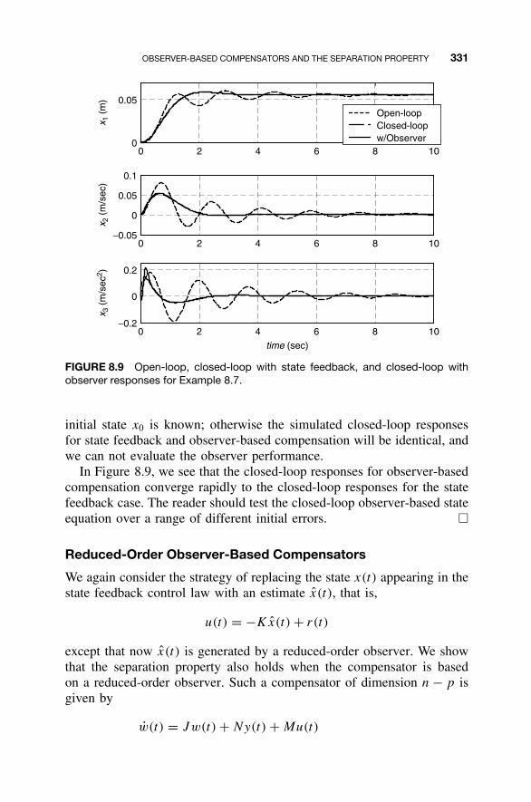
OBSERVER-BASED COMPENSATORS AND THE SEPARATION PROPERTY 331
0
0.05
0 2 4 6 8 10
0 2 4 6 8 10−0.05
0
0.05
0.1
0 2 4 6 8 10−0.2
0
0.2
time (sec)
x 3 (
m/s
ec2 )
x 2 (
m/s
ec)
x 1 (
m)
Open-loopClosed-loopw/Observer
FIGURE 8.9 Open-loop, closed-loop with state feedback, and closed-loop withobserver responses for Example 8.7.
initial state x0 is known; otherwise the simulated closed-loop responsesfor state feedback and observer-based compensation will be identical, andwe can not evaluate the observer performance.
In Figure 8.9, we see that the closed-loop responses for observer-basedcompensation converge rapidly to the closed-loop responses for the statefeedback case. The reader should test the closed-loop observer-based stateequation over a range of different initial errors. �
Reduced-Order Observer-Based Compensators
We again consider the strategy of replacing the state x(t) appearing in thestate feedback control law with an estimate x(t), that is,
u(t) = −Kx(t) + r(t)
except that now x(t) is generated by a reduced-order observer. We showthat the separation property also holds when the compensator is basedon a reduced-order observer. Such a compensator of dimension n − p isgiven by
w(t) = Jw(t) + Ny(t) + Mu(t)
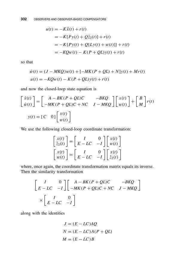
332 OBSERVERS AND OBSERVER-BASED COMPENSATORS
u(t) = −Kx(t) + r(t)
= −K[Py(t) + Qz2(t)] + r(t)
= −K{Py(t) + Q[Ly(t) + w(t)]} + r(t)
= −KQw(t) − K(P + QL)y(t) + r(t)
so that
w(t) = (J − MKQ)w(t) + [−MK (P + QL) + N ]y(t) + Mr(t)
u(t) = −KQw(t) − K(P + QL)y(t) + r(t)
and now the closed-loop state equation is[
x(t)
w(t)
]=
[A − BK (P + QL)C −BKQ
−MK (P + QL)C + NC J − MKQ
] [x(t)
w(t)
]+
[B
M
]r(t)
y(t) = [ C 0 ]
[x(t)
w(t)
]
We use the following closed-loop coordinate transformation:[
x(t)
z2(t)
]=
[I 0
E − LC −I
] [x(t)
w(t)
]
[x(t)
w(t)
]=
[I 0
E − LC −I
] [x(t)
z2(t)
]
where, once again, the coordinate transformation matrix equals its inverse.Then the similarity transformation
[I 0
E − LC −I
] [A − BK (P + QL)C −BKQ
−MK (P + QL)C + NC J − MKQ
]
×[
I 0E − LC −I
]
along with the identities
J = (E − LC )AQ
N = (E − LC )A(P + QL)
M = (E − LC )B
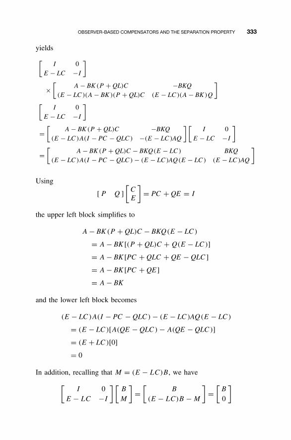
OBSERVER-BASED COMPENSATORS AND THE SEPARATION PROPERTY 333
yields
[I 0
E − LC −I
]
×[
A − BK (P + QL)C −BKQ(E − LC )(A − BK )(P + QL)C (E − LC )(A − BK )Q
]
[I 0
E − LC −I
]
=[
A − BK (P + QL)C −BKQ(E − LC )A(I − PC − QLC ) −(E − LC )AQ
] [I 0
E − LC −I
]
=[
A − BK (P + QL)C − BKQ(E − LC ) BKQ(E − LC )A(I − PC − QLC ) − (E − LC )AQ(E − LC ) (E − LC )AQ
]
Using
[ P Q ]
[C
E
]= PC + QE = I
the upper left block simplifies to
A − BK (P + QL)C − BKQ(E − LC )
= A − BK [(P + QL)C + Q(E − LC )]
= A − BK [PC + QLC + QE − QLC ]
= A − BK [PC + QE ]
= A − BK
and the lower left block becomes
(E − LC )A(I − PC − QLC ) − (E − LC )AQ(E − LC )
= (E − LC )[A(QE − QLC ) − A(QE − QLC )]
= (E + LC )[0]
= 0
In addition, recalling that M = (E − LC)B, we have
[I 0
E − LC −I
] [B
M
]=
[B
(E − LC)B − M
]=
[B
0
]
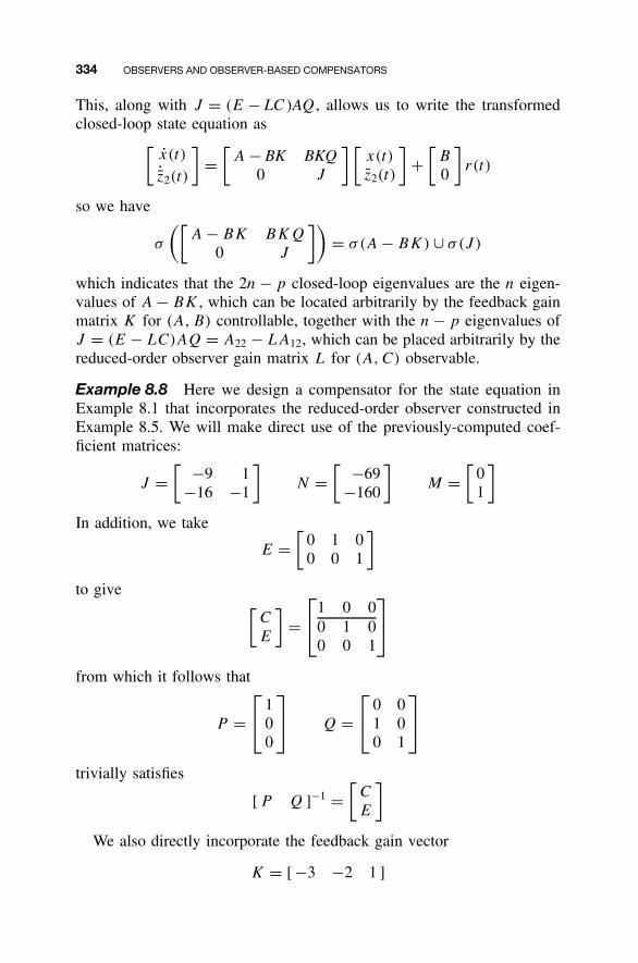
334 OBSERVERS AND OBSERVER-BASED COMPENSATORS
This, along with J = (E − LC )AQ , allows us to write the transformedclosed-loop state equation as[
x(t)˙z2(t)
]=
[A − BK BKQ
0 J
] [x(t)
z2(t)
]+
[B
0
]r(t)
so we have
σ
([A − BK BKQ
0 J
])= σ(A − BK) ∪ σ(J )
which indicates that the 2n − p closed-loop eigenvalues are the n eigen-values of A − BK , which can be located arbitrarily by the feedback gainmatrix K for (A, B) controllable, together with the n − p eigenvalues ofJ = (E − LC)AQ = A22 − LA12, which can be placed arbitrarily by thereduced-order observer gain matrix L for (A, C) observable.
Example 8.8 Here we design a compensator for the state equation inExample 8.1 that incorporates the reduced-order observer constructed inExample 8.5. We will make direct use of the previously-computed coef-ficient matrices:
J =[ −9 1
−16 −1
]N =
[ −69−160
]M =
[01
]
In addition, we take
E =[
0 1 00 0 1
]
to give [C
E
]=
1 0 0
0 1 00 0 1
from which it follows that
P = 1
00
Q =
0 0
1 00 1
trivially satisfies
[ P Q ]−1 =[
C
E
]
We also directly incorporate the feedback gain vector
K = [ −3 −2 1 ]
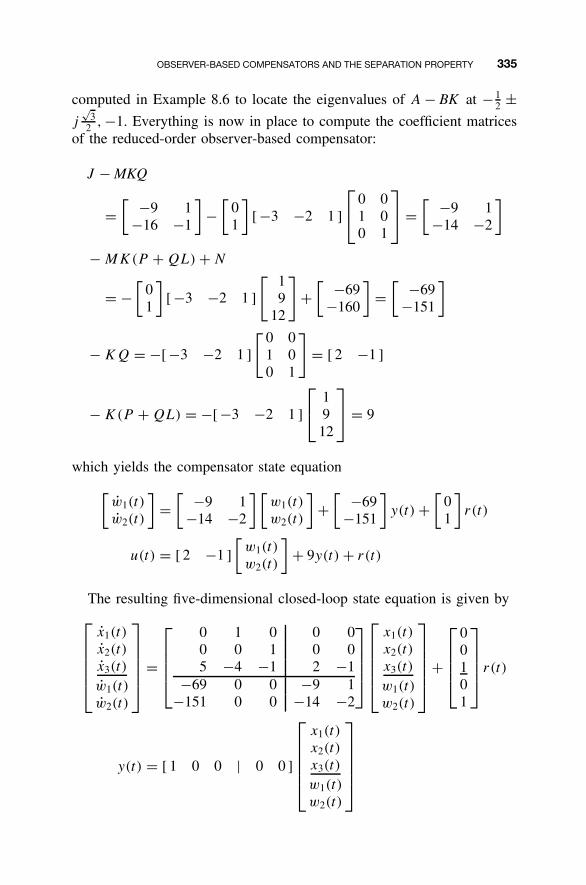
OBSERVER-BASED COMPENSATORS AND THE SEPARATION PROPERTY 335
computed in Example 8.6 to locate the eigenvalues of A − BK at − 12 ±
j√
32 , −1. Everything is now in place to compute the coefficient matrices
of the reduced-order observer-based compensator:
J − MKQ
=[ −9 1
−16 −1
]−
[01
][ −3 −2 1 ]
0 0
1 00 1
=
[ −9 1−14 −2
]
− MK(P + QL) + N
= −[
01
][ −3 −2 1 ]
[ 19
12
]+
[ −69−160
]=
[ −69−151
]
− KQ = −[ −3 −2 1 ]
[ 0 01 00 1
]= [ 2 −1 ]
− K(P + QL) = −[ −3 −2 1 ]
1
912
= 9
which yields the compensator state equation
[w1(t)
w2(t)
]=
[ −9 1−14 −2
] [w1(t)
w2(t)
]+
[ −69−151
]y(t) +
[01
]r(t)
u(t) = [ 2 −1 ]
[w1(t)
w2(t)
]+ 9y(t) + r(t)
The resulting five-dimensional closed-loop state equation is given by
x1(t)
x2(t)
x3(t)
w1(t)
w2(t)
=
0 1 0 0 00 0 1 0 05 −4 −1 2 −1
−69 0 0 −9 1−151 0 0 −14 −2
x1(t)
x2(t)
x3(t)
w1(t)
w2(t)
+
00101
r(t)
y(t) = [ 1 0 0 | 0 0 ]
x1(t)
x2(t)
x3(t)
w1(t)
w2(t)
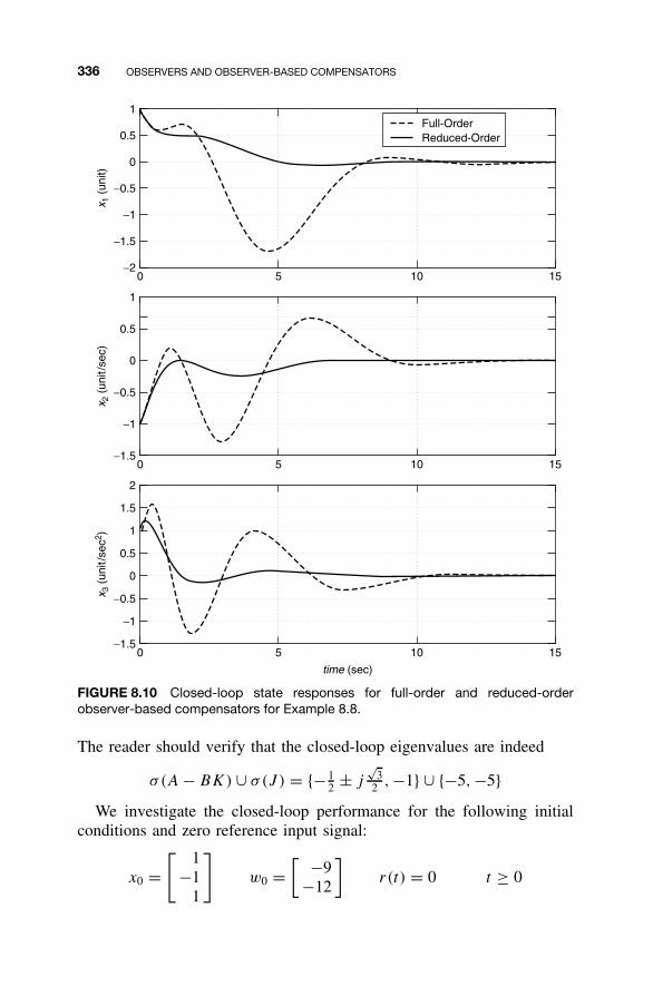
336 OBSERVERS AND OBSERVER-BASED COMPENSATORS
2
1.5
1
0.5
0
−0.5
−1
−1.50 5 10
5 10
5 10
15
time (sec)
x 3 (
unit
/sec
2 )
1
0.5
0
−0.5
−1
−1.50 15
x 2 (
unit
/sec
)1
0.5
0
−1.5
−2
−0.5
−1
0 15
x 1 (
unit)
Full-OrderReduced-Order
FIGURE 8.10 Closed-loop state responses for full-order and reduced-orderobserver-based compensators for Example 8.8.
The reader should verify that the closed-loop eigenvalues are indeed
σ(A − BK) ∪ σ(J ) = {− 12 ± j
√3
2 , −1} ∪ {−5, −5}We investigate the closed-loop performance for the following initial
conditions and zero reference input signal:
x0 =[ 1
−11
]w0 =
[ −9−12
]r(t) = 0 t ≥ 0
STEADY-STATE TRACKING WITH OBSERVER-BASED COMPENSATORS 337
Figure 8.10 compares the closed-loop state response x(t) for the full-orderobserver-based compensator constructed in Example 8.6 with the closed-loop state response x(t) for the reduced-order observer-based compensatorconstructed here. The difference between theses responses again can beattributed to the different eigenvalue specifications for the observer errordynamics for the full-order and reduced-order cases.
8.5 STEADY-STATE TRACKING WITH OBSERVER-BASEDCOMPENSATORS
Input Gain with Observers
We begin by observing that the structure of the closed-loop state equation(8.6) with state [xT (t), xT (t)] easily allows us to compute the closed-looptransfer function
HCL(s) = [ C 0 ]
[sI − A + BK −BK
0 sI − A + LC
]−1 [B
0
]
= [ C 0 ]
×[
(sI − A + BK)−1 (sI − A + BK)−1BK(sI − A + LC)−1
0 (sI − A + LC)−1
]
×[
B
0
]
= C(sI − A + BK)−1B
which is exactly the same closed-loop transfer function that results from adirect application of state feedback. Of course, the same conclusion holdsfor the closed-loop state equation (8.5) with state [xT (t), xT (t)] becausethe two state equations are related by a state coordinate transformation thatdoes not affect the transfer function. One interpretation of this outcomeis the following: Transfer functions in general characterize input-outputbehavior for zero initial state. Initializing [xT (0), xT (0)] = [0, 0] neces-sarily yields x(t) ≡ 0 for all t ≥ 0, so the observer produces a perfectestimate of x(t), and thus we should expect the closed-loop input-outputbehavior with an observer-based compensator to exactly match closed-loop input-output behavior with state feedback.
As a consequence, the input gain required to achieve identity closed-loop dc gain is identical to that derived in Chapter 7:
G = −[C(A − BK)−1B]−1
338 OBSERVERS AND OBSERVER-BASED COMPENSATORS
Observer-Based Servomechanism Design
In Section 7.5 we presented a servomechanism design methodology fea-turing integral error compensation together with state feedback that yieldedasymptotic tracking of reference step inputs. This design was robust in thesense that accurate knowledge of the open-loop state equation coefficientmatrices was not required to achieve zero steady-state error. This sectionextends that work by incorporating an observer to provide an estimate ofthe state feedback for direct substitution into the state feedback portionof the compensator. As with the servomechanism design based on statefeedback presented in Section 7.5, this section follows the developmentin Ogata (2002).
For the open-loop state equation (8.1), we have the same objectives asin Section 7.5; i.e., we must achieve asymptotic stability for the closed-loop state equation and asymptotic tracking of step reference inputs withzero steady-state error. We adopt essentially the same assumptions as inSection 7.5 but also add observability of the open-loop state equation toassumption 1.
Assumptions
1. The open-loop state equation (8.1) is controllable and observable.2. The open-loop state equation has no pole/eigenvalue at s = 0.3. The open-loop state equation has no zero at s = 0.
Our observer-based compensator is of the form
ξ (t) = r(t) − y(t)
˙x(t) = (A − LC)x(t) + Bu(t) + Ly(t)
u(t) = −Kx(t) + kIξ(t)
which we can repackage as the (n + 1)-dimensional state equation[ξ (t)˙x(t)
]=
[0 0
BkI A − BK − LC
][ξ(t)
x(t)
]+
[10
]r(t) +
[ −1L
]y(t)
u(t) = [ kI −K ]
[ξ(t)
x(t)
]
This, along with the open-loop state equation (8.1), yields the (2n + 1)-dimensional closed-loop state equation
x(t)
ξ (t)˙x(t)
=
A BkI −BK
−C 0 0LC BkI A − BK − LC
x(t)
ξ(t)
x(t)
+
0
10
r(t)
STEADY-STATE TRACKING WITH OBSERVER-BASED COMPENSATORS 339
y(t) = [ C 0 0 ]
x(t)
ξ(t)
x(t)
Our first design objective is to achieve closed-loop asymptotic stability,for which we require that the (2n + 1) eigenvalues of the (2n + 1) ×(2n + 1) closed-loop system dynamics matrix have strictly negative realparts. It is not obvious how to proceed with the closed-loop state equationas written above, so we once again replace the observer state x(t) with theobserver error x(t) = x(t) − x(t). As always, the observer error dynamicsare given by
˙x(t) = (A − LC)x(t)
and this leads to
x(t)
ξ (t)˙x(t)
=
A − BK Bk I BK
−C 0 00 0 A − LC
x(t)
ξ(t)
x(t)
+
0
10
r(t)
y(t) = [ C 0 0 ]
x(t)
ξ(t)
x(t)
Again, the block triangular structure of this closed-loop system dynamicsmatrix indicates that the (2n + 1) closed-loop eigenvalues are the (n + 1)
eigenvalues of [A − BK BkI
−C 0
]
which we know from Chapter 7 that under our assumptions can be freelyassigned by proper choice of the augmented state feedback gain vector[K − kI] together with n eigenvalues of (A − LC), which, by virtue of ouradded observability assumption, can be arbitrarily located by the observergain vector L.
To check that the steady-state tracking requirement has been met, wecharacterize the closed-loop equilibrium condition resulting from the con-stant reference input r(t) = R, t ≥ 0. Using the relationship
uss = −K(xss − xss) + kIξss
= −K xss + Kxss + kIξss
340 OBSERVERS AND OBSERVER-BASED COMPENSATORS
we see that 0
00
=
A − BK BkI BK
−C 0 00 0 A − LC
xss
ξss
xss
+
0
10
R
= A B 0
−C 0 00 0 A − LC
xss
uss
xss
+
0
10
R
which corresponds to the decoupled equations
(A − LC)xss = 0
[00
]=
[A B
−C 0
] [xss
uss
]+
[01
]R
the first of which, since A − LC is necessarily nonsingular, forces xss = 0.The second equation we observe is exactly has encountered in Chapter 7from which we conclude that
[xss
uss
]= −
[A B
−C 0
]−1 [0R
]
=[
A−1B(CA−1B)−1R
−(CA−1B)−1R
]
ξss = 1
kI[uss + Kxss]
= 1
kI[1 − KA−1B]H−1(0)R
and
yss = Cxss
= C(A−1B(CA−1B)−1R)
= (CA−1B)(CA−1B)−1R
= R
as desired.The observer-based servomechanism block diagram is shown in
Figure 8.11. Note that this block diagram is very similar to Figure 7.12,except that rather than directly applying the state feedback gain to thestate x(t), the state estimate x(t) produced by the Observer block is used
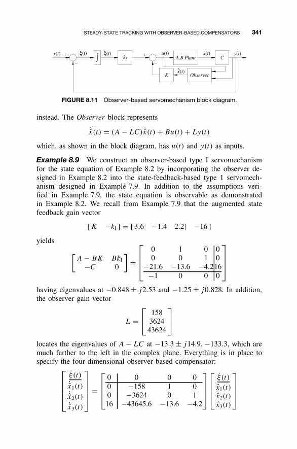
STEADY-STATE TRACKING WITH OBSERVER-BASED COMPENSATORS 341
+−
kI A,B Plant
K
r(t) ξ(t)ξ(t) u(t)+−
x(t)C
y(t)
Observerx(t)^
.
FIGURE 8.11 Observer-based servomechanism block diagram.
instead. The Observer block represents
˙x(t) = (A − LC)x(t) + Bu(t) + Ly(t)
which, as shown in the block diagram, has u(t) and y(t) as inputs.
Example 8.9 We construct an observer-based type I servomechanismfor the state equation of Example 8.2 by incorporating the observer de-signed in Example 8.2 into the state-feedback-based type 1 servomech-anism designed in Example 7.9. In addition to the assumptions veri-fied in Example 7.9, the state equation is observable as demonstratedin Example 8.2. We recall from Example 7.9 that the augmented statefeedback gain vector
[ K −kI ] = [ 3.6 −1.4 2.2| −16 ]
yields
[A − BK BkI
−C 0
]=
0 1 0 00 0 1 0
−21.6 −13.6 −4.216−1 0 0 0
having eigenvalues at −0.848 ± j2.53 and −1.25 ± j0.828. In addition,the observer gain vector
L = 158
362443624
locates the eigenvalues of A − LC at −13.3 ± j14.9, −133.3, which aremuch farther to the left in the complex plane. Everything is in place tospecify the four-dimensional observer-based compensator:
ξ (t)
˙x1(t)˙x2(t)˙x3(t)
=
0 0 0 00 −158 1 00 −3624 0 116 −43645.6 −13.6 −4.2
ξ (t)
x1(t)
x2(t)
x3(t)
342 OBSERVERS AND OBSERVER-BASED COMPENSATORS
+
1000
r(t) +
−1158
362443624
y(t)
u(t) = [ 16 | − 3.6 1.4 −2.2 ]
ξ (t)
x1(t)
x2(t)
x3(t)
The resulting seven-dimensional closed-loop state equation is:
x1(t)
x2(t)
x3(t)
ξ (t)
˙x1(t)˙x2(t)˙x3(t)
=
0 1 0 0 0 0 00 0 1 0 0 0 0
−18 −15 −2 16 −3.6 1.4 −2.2−1 0 0 0 0 0 0158 0 0 0 −158 1 03624 0 0 0 −3624 0 1
43624 0 0 16 −43645.6 −13.6 −4.2
×
x1(t)
x2(t)
x3(t)
ξ(t)
x1(t)
x2(t)
x3(t)
+
0001000
r(t)
y(t) = [ 1 0 0 |0| 0 0 0 ]
x1(t)
x2(t)
x3(t)
ξ(t)
x1(t)
x2(t)
x3(t)
The closed-loop unit step response for zero initial conditions is shownin Figure 8.12. Note that because in this case x0 = x0 = 0, the observerstate x(t) response exactly matches x(t), so the output response exactlymatches the nominal output response shown in Figure 7.13 for the state-feedback-based type 1 servomechanism design of Example 7.9. To see theeffect of the observer, the closed-loop response for the following initial
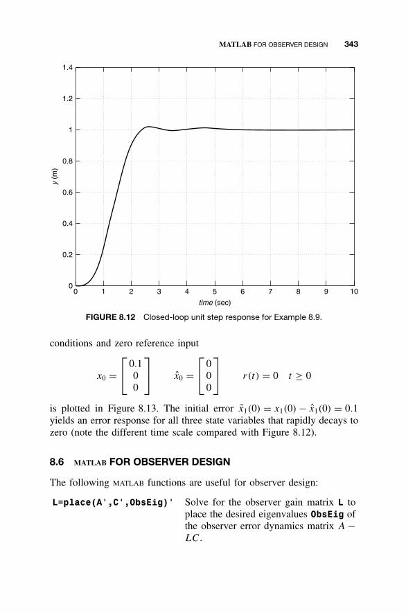
MATLAB FOR OBSERVER DESIGN 343
1.4
1.2
1
0.8
0.6
0.4
0.2
00 1 2 3 4 5 6 7 8 9 10
time (sec)
y (m
)
FIGURE 8.12 Closed-loop unit step response for Example 8.9.
conditions and zero reference input
x0 = 0.1
00
x0 =
0
00
r(t) = 0 t ≥ 0
is plotted in Figure 8.13. The initial error x1(0) = x1(0) − x1(0) = 0.1yields an error response for all three state variables that rapidly decays tozero (note the different time scale compared with Figure 8.12).
8.6 MATLAB FOR OBSERVER DESIGN
The following MATLAB functions are useful for observer design:
L=place(A',C',ObsEig)' Solve for the observer gain matrix L toplace the desired eigenvalues ObsEig ofthe observer error dynamics matrix A −LC.
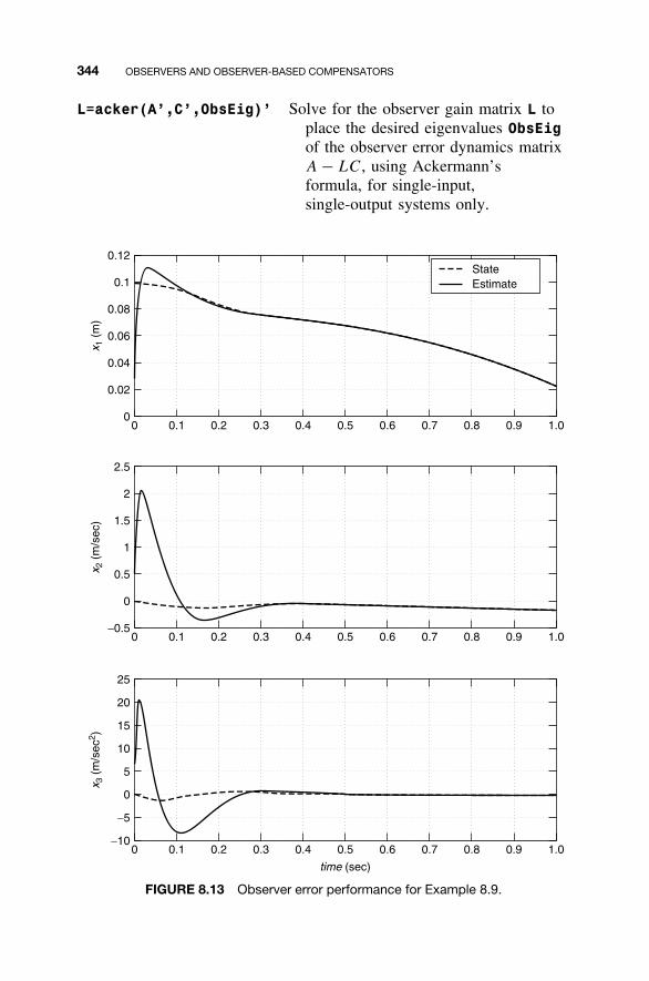
344 OBSERVERS AND OBSERVER-BASED COMPENSATORS
L=acker(A’,C’,ObsEig)’ Solve for the observer gain matrix L toplace the desired eigenvalues ObsEigof the observer error dynamics matrixA − LC, using Ackermann’sformula, for single-input,single-output systems only.
25
15
20
10
5
0
−5
−100 0.1 0.2 0.3 0.4 0.5 0.6 0.7 0.8 0.9 1.0
0 0.1 0.2 0.3 0.4 0.5 0.6 0.7 0.8 0.9 1.0
0 0.1 0.2 0.3 0.4 0.5 0.6 0.7 0.8 0.9 1.0
time (sec)
x 3 (
m/s
ec2 )
2.5
2
1.5
1
0.5
0
−0.5
x 2 (
m/s
ec)
0.12
0.1
0.08
0.06
0.04
0.02
0
x 1 (
m)
StateEstimate
FIGURE 8.13 Observer error performance for Example 8.9.
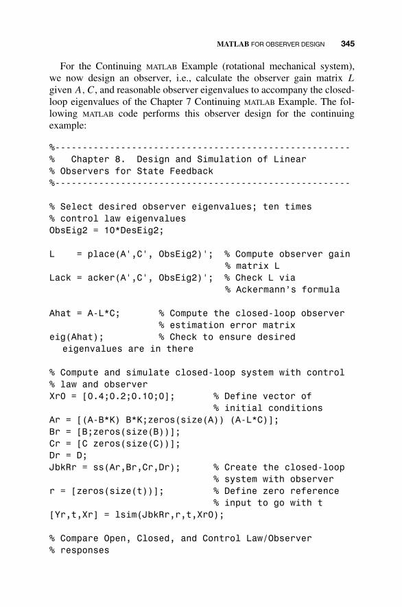
MATLAB FOR OBSERVER DESIGN 345
For the Continuing MATLAB Example (rotational mechanical system),we now design an observer, i.e., calculate the observer gain matrix L
given A, C, and reasonable observer eigenvalues to accompany the closed-loop eigenvalues of the Chapter 7 Continuing MATLAB Example. The fol-lowing MATLAB code performs this observer design for the continuingexample:
%------------------------------------------------------% Chapter 8. Design and Simulation of Linear% Observers for State Feedback%------------------------------------------------------
% Select desired observer eigenvalues; ten times% control law eigenvaluesObsEig2 = 10*DesEig2;
L = place(A',C', ObsEig2)'; % Compute observer gain% matrix L
Lack = acker(A',C', ObsEig2)'; % Check L via% Ackermann’s formula
Ahat = A-L*C; % Compute the closed-loop observer% estimation error matrix
eig(Ahat); % Check to ensure desiredeigenvalues are in there
% Compute and simulate closed-loop system with control% law and observerXr0 = [0.4;0.2;0.10;0]; % Define vector of
% initial conditionsAr = [(A-B*K) B*K;zeros(size(A)) (A-L*C)];Br = [B;zeros(size(B))];Cr = [C zeros(size(C))];Dr = D;JbkRr = ss(Ar,Br,Cr,Dr); % Create the closed-loop
% system with observerr = [zeros(size(t))]; % Define zero reference
% input to go with t[Yr,t,Xr] = lsim(JbkRr,r,t,Xr0);
% Compare Open, Closed, and Control Law/Observer% responses
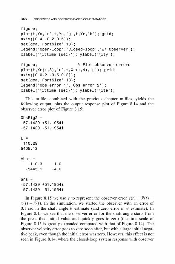
346 OBSERVERS AND OBSERVER-BASED COMPENSATORS
figure;plot(t,Yo,'r',t,Yc,'g',t,Yr,'b'); grid;axis([0 4 -0.2 0.5]);set(gca,'FontSize',18);legend('Open-loop','Closed-loop','w/ Observer');xlabel('\ittime (sec)'); ylabel('\ity');
figure; % Plot observer errorsplot(t,Xr(:,3),'r',t,Xr(:,4),'g'); grid;axis([0 0.2 -3.5 0.2]);set(gca,'FontSize',18);legend('Obs error 1','Obs error 2');xlabel('\ittime (sec)'); ylabel(’\ite’);
This m-file, combined with the previous chapter m-files, yields thefollowing output, plus the output response plot of Figure 8.14 and theobserver error plot of Figure 8.15:
ObsEig2 =-57.1429 +51.1954i-57.1429 -51.1954i
L =110.29
5405.13
Ahat =-110.3 1.0-5445.1 -4.0
ans =-57.1429 +51.1954i-57.1429 -51.1954i
In Figure 8.15 we use e to represent the observer error e(t) = x(t) =x(t) − x(t). In the simulation, we started the observer with an error of0.1 rad in the shaft angle θ estimate (and zero error in θ estimate). InFigure 8.15 we see that the observer error for the shaft angle starts fromthe prescribed initial value and quickly goes to zero (the time scale ofFigure 8.15 is greatly expanded compared with that of Figure 8.14). Theobserver velocity error goes to zero soon after, but with a large initial nega-tive peak, even though the initial error was zero. However, this effect is notseen in Figure 8.14, where the closed-loop system response with observer
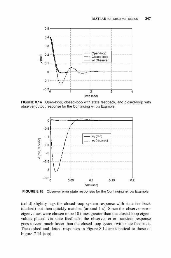
MATLAB FOR OBSERVER DESIGN 347
0 1 2 3 4−0.2
−0.1
0
0.1
0.2
0.3
0.4
0.5
time (sec)
y(r
ad) Open-loop
Closed-loopw/ Observer
FIGURE 8.14 Open-loop, closed-loop with state feedback, and closed-loop withobserver output response for the Continuing MATLAB Example.
0 0.05 0.1 0.15 0.2−3.5
−3
−2.5
−2
−1.5
−1
−0.5
0
time (sec)
e1 (rad)e2 (rad/sec)
e (r
ad, r
ad/s
ec)
FIGURE 8.15 Observer error state responses for the Continuing MATLAB Example.
(solid) slightly lags the closed-loop system response with state feedback(dashed) but then quickly matches (around 1 s). Since the observer erroreigenvalues were chosen to be 10 times greater than the closed-loop eigen-values placed via state feedback, the observer error transient responsegoes to zero much faster than the closed-loop system with state feedback.The dashed and dotted responses in Figure 8.14 are identical to those ofFigure 7.14 (top).
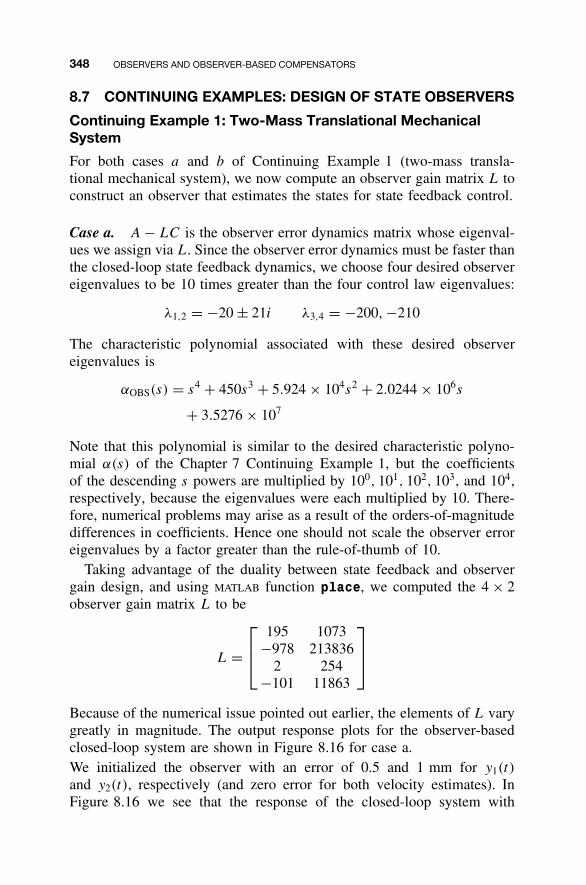
348 OBSERVERS AND OBSERVER-BASED COMPENSATORS
8.7 CONTINUING EXAMPLES: DESIGN OF STATE OBSERVERS
Continuing Example 1: Two-Mass Translational MechanicalSystem
For both cases a and b of Continuing Example 1 (two-mass transla-tional mechanical system), we now compute an observer gain matrix L toconstruct an observer that estimates the states for state feedback control.
Case a. A − LC is the observer error dynamics matrix whose eigenval-ues we assign via L. Since the observer error dynamics must be faster thanthe closed-loop state feedback dynamics, we choose four desired observereigenvalues to be 10 times greater than the four control law eigenvalues:
λ1,2 = −20 ± 21i λ3,4 = −200, −210
The characteristic polynomial associated with these desired observereigenvalues is
αOBS(s) = s4 + 450s3 + 5.924 × 10⁴s2 + 2.0244 × 10⁶s
+ 3.5276 × 10⁷
Note that this polynomial is similar to the desired characteristic polyno-mial α(s) of the Chapter 7 Continuing Example 1, but the coefficientsof the descending s powers are multiplied by 100, 101, 102, 103, and 104,respectively, because the eigenvalues were each multiplied by 10. There-fore, numerical problems may arise as a result of the orders-of-magnitudedifferences in coefficients. Hence one should not scale the observer erroreigenvalues by a factor greater than the rule-of-thumb of 10.
Taking advantage of the duality between state feedback and observergain design, and using MATLAB function place, we computed the 4 × 2observer gain matrix L to be
L =
195 1073−978 213836
2 254−101 11863
Because of the numerical issue pointed out earlier, the elements of L varygreatly in magnitude. The output response plots for the observer-basedclosed-loop system are shown in Figure 8.16 for case a.We initialized the observer with an error of 0.5 and 1 mm for y1(t)
and y2(t), respectively (and zero error for both velocity estimates). InFigure 8.16 we see that the response of the closed-loop system with
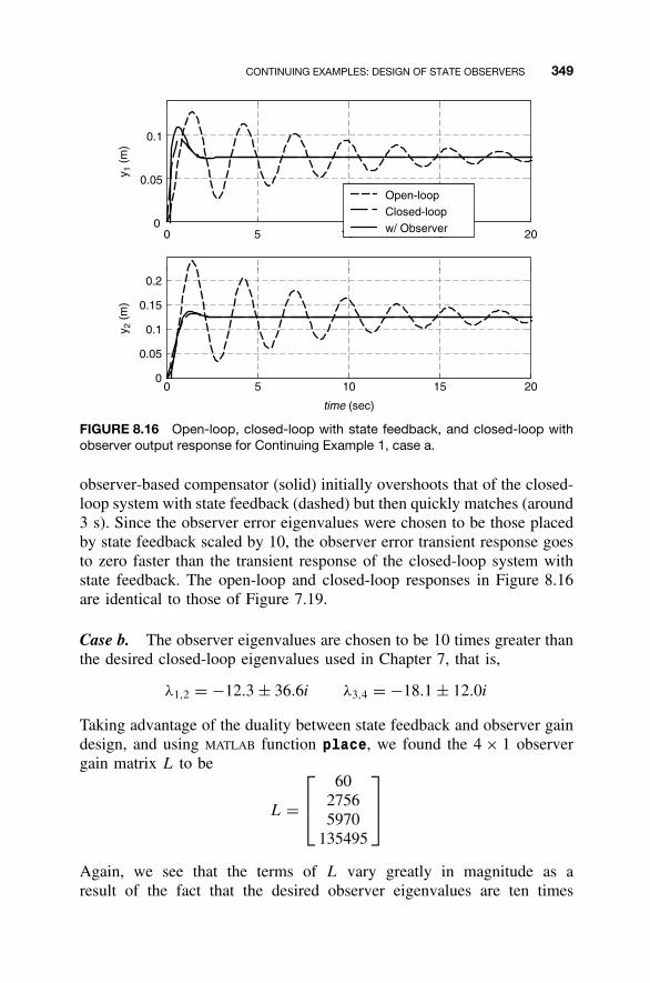
CONTINUING EXAMPLES: DESIGN OF STATE OBSERVERS 349
0 5 10 15 200
0.05
0.1
Open-loopClosed-loopw/ Observer
0 5 10 15 200
0.05
0.1
0.15
0.2
time (sec)
y 2 (
m)
y 1 (
m)
FIGURE 8.16 Open-loop, closed-loop with state feedback, and closed-loop withobserver output response for Continuing Example 1, case a.
observer-based compensator (solid) initially overshoots that of the closed-loop system with state feedback (dashed) but then quickly matches (around3 s). Since the observer error eigenvalues were chosen to be those placedby state feedback scaled by 10, the observer error transient response goesto zero faster than the transient response of the closed-loop system withstate feedback. The open-loop and closed-loop responses in Figure 8.16are identical to those of Figure 7.19.
Case b. The observer eigenvalues are chosen to be 10 times greater thanthe desired closed-loop eigenvalues used in Chapter 7, that is,
λ1,2 = −12.3 ± 36.6i λ3,4 = −18.1 ± 12.0i
Taking advantage of the duality between state feedback and observer gaindesign, and using MATLAB function place, we found the 4 × 1 observergain matrix L to be
L =
6027565970
135495
Again, we see that the terms of L vary greatly in magnitude as aresult of the fact that the desired observer eigenvalues are ten times
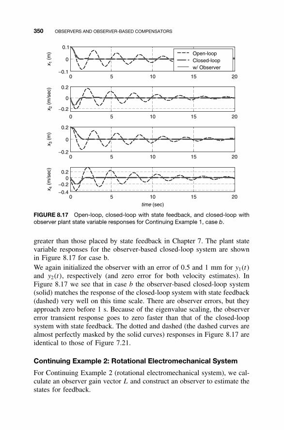
350 OBSERVERS AND OBSERVER-BASED COMPENSATORS
0 5 10 15 20−0.1
0
0.1x 1
(m
) Open-loopClosed-loopw/ Observer
0 5 10 15 20
−0.2
0
0.2
x 2 (
m/s
ec)
0 5 10 15 20−0.2
0
0.2
x 3 (
m)
0 5 10 15 20−0.4
−0.20
0.2
time (sec)
x 4 (
m/s
ec)
FIGURE 8.17 Open-loop, closed-loop with state feedback, and closed-loop withobserver plant state variable responses for Continuing Example 1, case b.
greater than those placed by state feedback in Chapter 7. The plant statevariable responses for the observer-based closed-loop system are shownin Figure 8.17 for case b.We again initialized the observer with an error of 0.5 and 1 mm for y1(t)
and y2(t), respectively (and zero error for both velocity estimates). InFigure 8.17 we see that in case b the observer-based closed-loop system(solid) matches the response of the closed-loop system with state feedback(dashed) very well on this time scale. There are observer errors, but theyapproach zero before 1 s. Because of the eigenvalue scaling, the observererror transient response goes to zero faster than that of the closed-loopsystem with state feedback. The dotted and dashed (the dashed curves arealmost perfectly masked by the solid curves) responses in Figure 8.17 areidentical to those of Figure 7.21.
Continuing Example 2: Rotational Electromechanical System
For Continuing Example 2 (rotational electromechanical system), we cal-culate an observer gain vector L and construct an observer to estimate thestates for feedback.
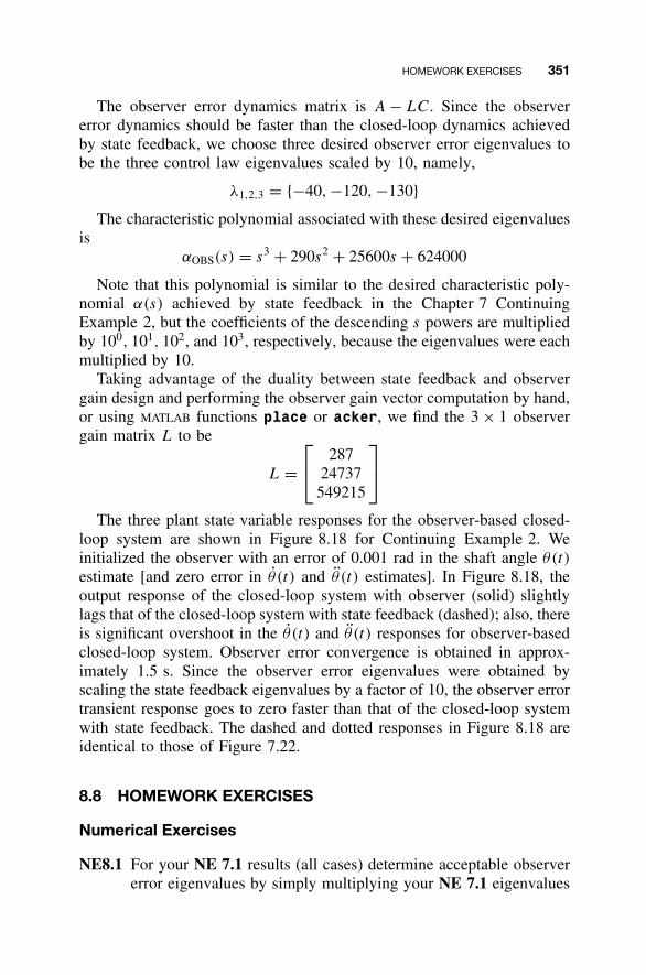
HOMEWORK EXERCISES 351
The observer error dynamics matrix is A − LC. Since the observererror dynamics should be faster than the closed-loop dynamics achievedby state feedback, we choose three desired observer error eigenvalues tobe the three control law eigenvalues scaled by 10, namely,
λ1,2,3 = {−40, −120, −130}The characteristic polynomial associated with these desired eigenvalues
isαOBS(s) = s3 + 290s2 + 25600s + 624000
Note that this polynomial is similar to the desired characteristic poly-nomial α(s) achieved by state feedback in the Chapter 7 ContinuingExample 2, but the coefficients of the descending s powers are multipliedby 100, 101, 102, and 103, respectively, because the eigenvalues were eachmultiplied by 10.
Taking advantage of the duality between state feedback and observergain design and performing the observer gain vector computation by hand,or using MATLAB functions place or acker, we find the 3 × 1 observergain matrix L to be
L = 287
24737549215
The three plant state variable responses for the observer-based closed-loop system are shown in Figure 8.18 for Continuing Example 2. Weinitialized the observer with an error of 0.001 rad in the shaft angle θ(t)
estimate [and zero error in θ (t) and θ (t) estimates]. In Figure 8.18, theoutput response of the closed-loop system with observer (solid) slightlylags that of the closed-loop system with state feedback (dashed); also, thereis significant overshoot in the θ (t) and θ (t) responses for observer-basedclosed-loop system. Observer error convergence is obtained in approx-imately 1.5 s. Since the observer error eigenvalues were obtained byscaling the state feedback eigenvalues by a factor of 10, the observer errortransient response goes to zero faster than that of the closed-loop systemwith state feedback. The dashed and dotted responses in Figure 8.18 areidentical to those of Figure 7.22.
8.8 HOMEWORK EXERCISES
Numerical Exercises
NE8.1 For your NE 7.1 results (all cases) determine acceptable observererror eigenvalues by simply multiplying your NE 7.1 eigenvalues
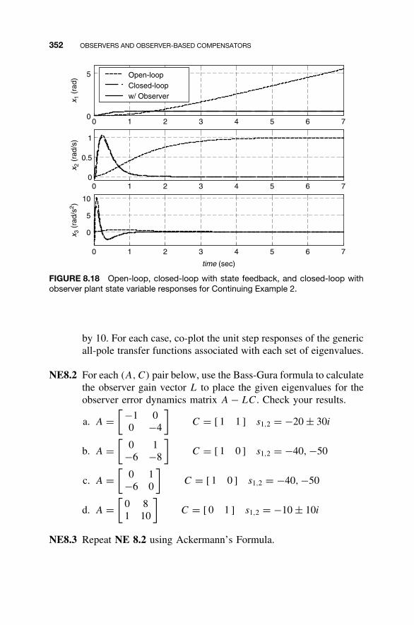
352 OBSERVERS AND OBSERVER-BASED COMPENSATORS
0 1 2 3 4 5 6 70
5
0 1 2 3 4 5 6 70
0.5
1
0 1 2 3 4 5 6 7
0
5
10
time (sec)
x 3 (
rad/
s2 )x 2
(ra
d/s)
x 1 (
rad)
Open-loopClosed-loopw/ Observer
FIGURE 8.18 Open-loop, closed-loop with state feedback, and closed-loop withobserver plant state variable responses for Continuing Example 2.
by 10. For each case, co-plot the unit step responses of the genericall-pole transfer functions associated with each set of eigenvalues.
NE8.2 For each (A, C) pair below, use the Bass-Gura formula to calculatethe observer gain vector L to place the given eigenvalues for theobserver error dynamics matrix A − LC. Check your results.
a. A =[ −1 0
0 −4
]C = [ 1 1 ] s1,2 = −20 ± 30i
b. A =[
0 1−6 −8
]C = [ 1 0 ] s1,2 = −40, −50
c. A =[
0 1−6 0
]C = [ 1 0 ] s1,2 = −40, −50
d. A =[
0 81 10
]C = [ 0 1 ] s1,2 = −10 ± 10i
NE8.3 Repeat NE 8.2 using Ackermann’s Formula.
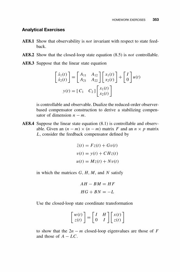
HOMEWORK EXERCISES 353
Analytical Exercises
AE8.1 Show that observability is not invariant with respect to state feed-back.
AE8.2 Show that the closed-loop state equation (8.5) is not controllable.
AE8.3 Suppose that the linear state equation
[x1(t)
x2(t)
]=
[A11 A12
A21 A22
] [x1(t)
x2(t)
]+
[I
0
]u(t)
y(t) = [ C1 C2 ]
[x1(t)
x2(t)
]
is controllable and observable. Dualize the reduced-order observer-based compensator construction to derive a stabilizing compen-sator of dimension n − m.
AE8.4 Suppose the linear state equation (8.1) is controllable and observ-able. Given an (n − m) × (n − m) matrix F and an n × p matrixL, consider the feedback compensator defined by
z(t) = Fz(t) + Gv(t)
v(t) = y(t) + CHz(t)
u(t) = Mz(t) + Nv(t)
in which the matrices G, H, M , and N satisfy
AH − BM = HF
HG + BN = −L
Use the closed-loop state coordinate transformation
[w(t)
z(t)
]=
[I H
0 I
] [x(t)
z(t)
]
to show that the 2n − m closed-loop eigenvalues are those of F
and those of A − LC.
354 OBSERVERS AND OBSERVER-BASED COMPENSATORS
AE 8.5 Suppose that H1(s) and H2(s) are two strictly proper transferfunctions with observable state-space realizations (A1, B1, C1) and(A2, B2, C2), respectively. Show that
[x1(t)
x2(t)
]=
[A1 00 A2
] [x1(t)
x2(t)
]+
[B1
B2
]u(t)
y(t) = [ C1 C2 ]
[x1(t)
x2(t)
]
is a state-space realization of the parallel interconnection H1(s) +H2(s) and that this realization is observable if and only if A1 andA2 have no common eigenvalues.
Continuing MATLAB Exercises
CME8.1 For the system given in CME1.1:a. Design an observer-based compensator using the control law
of CME7.1b. Use observer error eigenvalues that are thedesired state feedback eigenvalues of CME7.1a scaled by10. Compare open-loop, closed-loop with state feedback,and closed-loop with observer responses to a unit step input.Introduce an initial observer error, otherwise, the closed-loopwith state feedback and closed-loop with observer responseswill be identical.
b. Design and evaluate in simulation an observer for the ser-vomechanism of CME7.1c.
CME8.2 For the system given in CME1.2:a. Design an observer-based compensator using the control law
of CME7.2b. Use observer error eigenvalues that are thedesired state feedback eigenvalues of CME7.2a scaled by10. Compare open-loop, closed-loop with state feedback,and closed-loop with observer responses to a unit step input.Introduce an initial observer error, otherwise, the closed-loopwith state feedback and closed-loop with observer responseswill be identical.
b. Design and evaluate in simulation an observer for the ser-vomechanism of CME7.2c.
CME8.3 For the system given in CME1.3:
HOMEWORK EXERCISES 355
a. Design an observer-based compensator using the control lawof CME7.3b. Use observer error eigenvalues that are thedesired control law eigenvalues of CME7.3a scaled by 10.Compare open-loop, closed-loop with state feedback, andclosed-loop with observer responses to a unit step input.Introduce an initial observer error, otherwise, the closed-loopwith state feedback and closed-loop with observer responseswill be identical.
b. Design and evaluate in simulation an observer for the ser-vomechanism of CME7.3c.
CME8.4 For the system given in CME1.4:a. Design an observer-based compensator using the control law
of CME7.4b. Use observer error eigenvalues that are thedesired state feedback eigenvalues of CME7.4a scaled by10. Compare open-loop, closed-loop with state feedback,and closed-loop with observer responses to a unit step input.Introduce an initial observer error, otherwise, the closed-loopwith state feedback and closed-loop with observer responseswill be identical.
b. Design and evaluate in simulation an observer for the ser-vomechanism of CME7.4c.
Continuing Exercises
CE8.1 For the control laws designed in CE7.1b, design observer-basedcompensators for all three cases. Use observer error eigenvaluesthat are the desired state feedback eigenvalues scaled by 10 (forcase iii, a factor of 2 works better because of numerical condi-tioning). In each case, evaluate your results: Plot and compare thesimulated open-loop, closed-loop with state feedback, and closed-loop with observer output responses for the same cases as inCE2.1; use the same correction factors from CE7.1b. Introduce aninitial observer error, otherwise, the closed-loop with state feed-back and closed-loop with observer responses will be identical.
CE8.2 For the control laws designed in CE7.2b, design observer-basedcompensators for all three cases (this is possible only for theobservable cases). Use observer error eigenvalues that are thedesired state feedback eigenvalues scaled by 10. In each case,evaluate your results: Plot and compare the simulated open-loop,closed-loop with state feedback, and closed-loop with observer
356 OBSERVERS AND OBSERVER-BASED COMPENSATORS
output responses for the same cases as in CE2.2; use the same cor-rection factors from CE7.2b. Introduce an initial observer error,otherwise, the closed-loop with state feedback and closed-loopwith observer responses will be identical.
CE8.3 For the control laws designed in CE7.3b, design observer-basedcompensators for both cases. Use observer error eigenvalues thatare the desired state feedback eigenvalues scaled by 10. In eachcase, evaluate your results: Plot and compare the simulated open-loop, closed-loop with state feedback, and closed-loop with ob-server output responses for the same cases as in CE2.3 (for caseii, use the same correction factor from CE7.3b). Introduce an initialobserver error, otherwise, the closed-loop with state feedback andclosed-loop with observer responses will be identical.
CE8.4 Design an observer-based compensator for the control law de-signed in CE7.4b. Use observer error eigenvalues that areyour desired state feedback eigenvalues scaled by 10. Evaluateyour results: Plot and compare the simulated open-loop, closed-loop with state feedback, and closed-loop with observer outputresponses for the same case (impulse input, zero initial conditions)as in CE2.4. Introduce an initial observer error, otherwise, theclosed-loop with state feedback and closed-loop with observerresponses will be identical.
CE8.5 CE4.5 results should indicate that the original system is not observ-able. Therefore, add a second output: Make θ(t) an output inaddition to q(t); check observability again and proceed. For thecontrol law designed in CE7.5b, design an observer-based com-pensator for this modified system with two outputs. Use observererror eigenvalues that are your desired state feedback eigenvaluesscaled by 10. Evaluate your results: Plot and compare the simu-lated open-loop, closed-loop with state feedback, and closed-loopwith observer output responses for the same case (given initialconditions) as in CE2.5. Introduce an initial observer error; oth-erwise, the closed-loop with state feedback and closed-loop withobserver responses will be identical.
9
INTRODUCTION TOOPTIMAL CONTROL
As we noted in Chapter 1, the ability to formulate and solve optimalcontrol problems was the primary catalyst in the emergence of state-spacemethods in the late 1950s and early 1960s. It is therefore fitting that weconclude this text with an introduction to the fundamental discoveries ofthis era that have shaped the theory and practice of control engineeringover the past five decades.
We begin by formulating the linear quadratic regulator problem, whichis the optimal control problem that is the central focus of this chapter.This is followed by a tutorial on the key mathematical tool that we willemploy to solve this problem: the calculus of variations, or variationalcalculus. Variational calculus can be thought of as a generalization ofcertain results from multivariable calculus, so we include a brief reviewof the latter for motivation. We first apply variational calculus to solvethe so-called minimum energy control problem before proceeding to thesolution of the linear quadratic regulator problem. Since all but the mosttrivial examples are best solved with the aid of a computer, we nextturn our attention to MATLAB functionality that supports the solution tothe linear quadratic regulator problem. These tools are applied to theContinuing MATLAB Example and Continuing Example 1.
We must emphasize that this chapter merely scratches the surface ofa vast body of basic and applied research on optimal control. For more
357
Linear State-Space Control Systems. Robert L. Williams II and Douglas A. LawrenceCopyright 2007 John Wiley & Sons, Inc. ISBN: 978-0-471-73555-7
358 INTRODUCTION TO OPTIMAL CONTROL
in depth study, we refer the interested reader to the many excellent textson the subject including but by no means limited to Anderson and Moore(1971), Bryson and Ho (1975), Dorato, et al. (1995), Kwakernaak andSivan (1972), Lewis (1992), and Zhou (1995).
9.1 OPTIMAL CONTROL PROBLEMS
We begin with a somewhat general optimal control problem formulationin order to provide a broader context for the special cases we consider inthis chapter. We consider the nonlinear state equation
x(t) = f [x(t), u(t), t] x(t0) = x0
and introduce the performance index, cost function, or objective functionto be minimized:
J =∫ tf
t0
L[x(t), u(t), t]dt + ϕ[x(tf ), tf ]
Here L(x, u, t) is called the loss function that assigns a penalty to thestate and input in a possibly t-dependent way, and the function ϕ(x, t)
characterizes the terminal cost on the state. The optimization problem athand is to determine an optimal state trajectory and input signal denotedby [x∗(t), u∗(t)] that minimizes the performance index subject to the con-straints imposed by the state equation and the specified initial state. Thisis, by nature, a regulation problem because the goal is to maintain thestate trajectory “close” to the equilibrium at the origin while expending“moderate” control effort. For a particular problem, the performance indexquantifies these qualitative notions and further serves to capture the fun-damental design tradeoff between the conflicting objectives of regulationperformance and control effort.
Additional constraints might be imposed on the state trajectory andinput signal of the form
C[x(t), u(t), t] = 0 or C[x(t), u(t), t] ≤ 0 for all t ∈ (t0, tf )
In addition, the problem formulation might involve explicit constraints onthe terminal state instead of or in addition to the terminal cost term in theperformance index.
Necessary conditions in the form of optimality equations that must besatisfied by the optimal solution [x∗(t), u∗(t)] have been derived using the
OPTIMAL CONTROL PROBLEMS 359
tools of variational calculus and dynamic programming. However, theseequations in general are difficult to solve. Furthermore, by only satisfyinga necessary condition for optimality, there is no guarantee that a solutionto these equations is in fact optimal. Verifying this may require furthernontrivial analysis.
In this chapter we consider the linear time-invariant state equation
x(t) = Ax(t) + Bu(t) x(t0) = x0 (9.1)
and seek to minimize the quadratic performance index
J = 12
∫ tf
t0
[xT (t)Qx(t) + uT (t)Ru(t)
]dt + 1
2xT (tf )Sx(tf ) (9.2)
in which the loss function
L(x, u) = 12(x
T Qx + uT Ru)
= 12
[xT uT
] [Q 00 R
][x
u
]
and terminal cost function ϕ(x) = 12x
T Sx are quadratic forms. We assumethat the weighting matrices Q, R, and S are each symmetric, with Q andS positive semidefinite and R positive definite. Regulator design for alinear time-invariant state equation with the goal of minimizing a quadraticperformance index naturally is referred to as the linear quadratic regulator(LQR) problem. In contrast to the challenges that arise in the generalnonlinear optimal control problem, the linear quadratic regulator problemadmits an analytical solution that we will derive in the sequel.
Here we explicitly see the manner in which the quadratic performanceindex captures a tradeoff between regulation performance and controleffort. In particular, if the quadratic terms involving the state are “large”compared with the quadratic term involving the input, then the optimalstate trajectory will exhibit “good” regulation performance in that theresponse to a nonzero initial state will return rapidly to the equilibriumstate at the origin, but this may come at the expense of “large” controlenergy. Conversely, if the input is penalized more heavily than the state,then the optimal control signal may not require a great deal of energy, butthe regulation performance may not be acceptable. In essence, the under-lying design problem is to translate given performance specifications intochoices for the weighting matrices in such a way that the optimal solu-tion meets these specifications. This issue has received a great deal of
360 INTRODUCTION TO OPTIMAL CONTROL
attention since the linear quadratic regulator problem was introduced inthe late 1950s and yet remains something of an art.
9.2 AN OVERVIEW OF VARIATIONAL CALCULUS
We first consider optimization problems on the d-dimensional Euclideanspace R
d . As noted earlier, this material should come as a review to thereader and is included here to motivate the elements of variational calculusthat we require to solve the optimal control problems posed in this chapter.We consider real-valued functions f : R
d → R and seek to minimize f (z)
over all z ∈ Rd . We avoid many mathematical technicalities by assuming
throughout this chapter that all functions defined on Euclidean spaces havecontinuous partial derivatives in all arguments over the entire domain.Furthermore, we will only consider optimization problems that have globalsolutions.
We first derive a necessary condition for z∗ ∈ Rd to minimize f (z).
If z∗ minimizes f (z), then f (z∗ + v) > f (z∗) for any nonzero vectorv ∈ R
d . This implies that the directional derivative of f (z) at z∗ in thedirection v, written in terms of the gradient ∇f (z) as ∇f (z∗) · v, must bezero. To see this, for any ε > 0 we also must have f (z∗ ± εv) > f (z∗)from which
∇f (z∗) · v = limε→0+
f (z∗+εv)−f (z∗)ε
≥ 0
∇f (z∗) · (−v) = limε→0+
f (z∗−εv)−f (z∗)ε
≥ 0
Since ∇f (z∗) · (−v) = −∇f (z∗) · v, the only way both these inequalitiescan hold is if ∇f (z∗) · v = 0 as claimed. Since the directional derivativemust vanish at z∗ for any direction v ∈ R
d , we conclude that the gradientof f (z) at z∗ must be the zero vector. In this case we call z∗ a critical pointof f (z), and we have argued that if z∗ minimizes f (z), then necessarily,z∗ is a critical point of f (z).
The converse statement does not hold in general. Namely, a criticalpoint of f (z) is not necessarily a minimum. For example, on R
2,f (z) = − 1
2(z21 + z2
2) has ∇f (z) = −[z1, z2], for which the critical pointz∗ = (0, 0) corresponds to the maximum of f (z). Also, f (z) = 1
2(z21 − z2
2)
has ∇f (z) = [z1, −z2], for which the critical point z∗ = (0, 0) is a saddlepoint. Often, second-derivative information is used to classify criticalpoints as being a minimum, maximum, or saddle point. Here we consideran approach that is better suited to the objectives of this chapter.
AN OVERVIEW OF VARIATIONAL CALCULUS 361
A real-valued function f : Rd → R is convex if
f (z + v) − f (z) ≥ ∇f (z) · v for all z, v ∈ Rd
and strictly convex if equality holds above when and only when v = 0 ∈R
d . It is easy to see that a critical point of a strictly convex function is aminimum point. For if z∗ satisfies ∇f (z∗) = 0, then
f (z∗ + v) − f (z∗) > ∇f (z∗) · v = 0 for all v �= 0 ∈ Rd
from which f (z∗ + v) > f (z∗) for all nonzero v ∈ Rd .
We next turn our attention to the problem of minimizing a real-valuedfunction f (z) over all z ∈ R
d that satisfy equality constraints of the form
gi(z) = 0 i = 1, . . . , n
or in vector form
G(z) =
g1(z)
g2(z)...
gn(z)
=
00...
0
We assume that there are fewer constraints n than the Euclidean spacedimension d so as not to over constrain the problem. We attack thisproblem using the method of Lagrange multipliers. The first step is toadjoin the constraints to the original function f (z) using the n × 1 vectorof Lagrange multipliers
λ =
λ1
λ2...
λn
to form the real-valued function
f (z) = f (z) + λ1g1(z) + λ2g2(z) + · · · + λngn(z)
= f (z) + λT G(z)
We observe that if z∗ minimizes the augmented function f (z) over Rd
so thatf (z) > f (z∗) for all z �= z∗
362 INTRODUCTION TO OPTIMAL CONTROL
then, in particular, for any z �= z∗ that satisfies G(z) = G(z∗), we havefor any Lagrange multiplier vector λ ∈ R
n
f (z) − f (z∗) = f (z) − f (z∗) + λT [G(z) − G(z∗)]
= [f (z) + λT G(z)] − [f (z∗) + λT G(z∗)]
= f (z) − f (z∗)
> 0
We conclude that z∗ minimizes the original function f (z) over all z ∈ Rd
that satisfy G(z) = G(z∗). Now, if f (z) is strictly convex (and this ingeneral depends on λ ∈ R
n), then the minimum of f (z) is characterizedby ∇f (z∗) = 0. This, along with the constraint equation G(z∗) = 0, yieldsd + n equations that, in principle, can be solved for the d + n unknownsgiven by the components of z∗ and λ.
Note that once z∗ and λ have been determined, we must verify that f (z)
is strictly convex for this λ in order to conclude that the critical point z∗minimizes f (z) and, in turn, minimizes f (z) over all z ∈ R
d that satisfyG(z) = G(z∗) = 0 as desired. One situation in which the strict convexityof f (z) is assured for any Lagrange multiplier vector is when the originalfunction f (z) is strictly convex and the equality constraint is given by thelinear equation Cz = d so that
G(z) = Cz − d
To see this, we use
∇f (z) = ∇f (z) + λT ∂G∂z
(z)
= ∇f (z) + λT C
together with the strict convexity of f (z) to write
f (z + v) − f (z) ={f (z + v) + λT [C(z + v) − d]}−[f (z) + λT (Cz − d)]
= [f (z + v) − f (z)] + λT Cv
≥ ∇f (z) · v + λT Cv
= [∇f (z) + λT C] · v
= ∇f (z) · v
for all z, v ∈ Rd with equality when and only when v = 0, thereby char-
acterizing strict convexity of f (z).
AN OVERVIEW OF VARIATIONAL CALCULUS 363
To illustrate these ideas, we consider the problem of minimizing thequadratic form
f (z) = 12z
T Qz
subject to the equality constraint Cz = d. We assume that the d × d matrixQ is symmetric and positive definite and that the n × d matrix C has full-row rank n. We can easily check that f (z) is strictly convex. Using thegradient ∇f (z) = zT Q, we have for all z, v ∈ R
d
f (z + v) − f (z) = 12(z + v)T Q(z + v) − 1
2zT Qz
= zT Qv + 12vT Qv
= ∇f (z) · v + 12v
T Qv
≥ ∇f (z) · v
with equality when and only when v = 0 because of the assumed positivedefiniteness of Q. From the preceding discussion, we conclude that
f (z) = 12z
T Qz + λT (Cz − d)
is strictly convex as well. We therefore minimize f (z) and, in turn, min-imize f (z) over all z ∈ R
d that satisfy Cz = d by solving
∇f (z) = zT Q + λT C = 0 and Cz = d
for z = z∗ ∈ Rd and λ ∈ R
n. This leads to the system of equations
[C 0Q CT
] [z
λ
]=
[d
0
]
Since Q is positive definite, it is nonsingular, which givesz∗ = −Q−1CT λ. On substituting into the constraint equation, we find−CQ−1CT λ = d. Since, in addition, C is assumed to have full-row rankn, the symmetric n × n matrix CQ−1CT can be shown to be positivedefinite and hence nonsingular. This ultimately yields the optimal solution
λ = −(CQ−1CT )−1d and z∗ = Q−1CT (CQ−1CT )−1d
We now generalize the preceding discussion for optimization on theEuclidean space R
d to optimization on the space of d-dimensional vector-valued functions z(t) defined on the interval [t0, tf ] having a continuous
364 INTRODUCTION TO OPTIMAL CONTROL
derivative z(t). We denote this space of functions by C1[t0, tf ], in whichthe dimension of z(t), i.e. the number of component functions of z(t), isleft as understood from the context. We remark that C1[t0, tf ] satisfies thedefinition of a linear vector space given in Appendix B for vector additionand scalar multiplication of (vector-valued) functions defined pointwisein t .
Our discussion will focus on the minimization of real-valued integralfunctions of the form
F(z) =∫ tf
t0
f [t, z(t), z(t)] dt
over elements of C1[t0, tf ] that, in addition, are assumed to satisfy one ofthe following possible boundary conditions:
• z(t0) = z0 is specified.• z(tf ) = zf is specified.• both z(t0) = z0 and z(tf ) = zf are specified.
We note that other boundary conditions are possible involving specificcomponents of z(t) at t = t0 and t = tf .
To generalize the previous analysis on Rd , we first need to generalize
the notion of a directional derivative that will enable us to establish anecessary condition for minimizing the integral function F(z) and furthercharacterize the requisite convexity property under which the necessarycondition becomes sufficient as well. This leads us to consider the Gateauxvariation of the integral function F(z) at z(t) in the direction v(t) ∈C1[t0, tf ], defined as
δF (z; v) = limε→0
F(z + εv) − F(z)
ε
If we assume that the integrand function f (t, z, z) has continuous partialderivatives with respect to the second and third d-dimensional argumentson the entire domain R × R
d × Rd , we can then compute the Gateaux
variation using the chain rule as follows:
δF (z; v) = ∂
∂εF (z + εv)|ε=0
=∫ tf
t0
∂
∂εf [t, z(t) + εv(t), z(t) + εv(t)] dt
∣∣∣∣ε=0
AN OVERVIEW OF VARIATIONAL CALCULUS 365
=∫ tf
t0
[∂f
∂z[t, z + εv(t), z(t) + εv(t)]v(t)
+ ∂f
∂z[t, z(t) + εv(t), z(t) + εv(t)]v(t)
]dt
∣∣∣∣ε=0
=∫ tf
t0
{∂f
∂z[t, z(t), z(t)]v(t) + ∂f
∂z[t, z(t), z(t)]v(t)
}dt (9.3)
Example 9.1 We consider the integral function F(z) for scalar z(t)
with integrand function f (t, z, z) = tz + 12 z
2. The partial derivatives
∂f
∂z(t, z, z) = t
∂f
∂z(t, z, z) = z
yield the Gateaux variation
δF (z; v) =∫ tf
t0
[tv(t) + z(t)v(t)] dt �
Next, we derive a necessary condition for z∗(t) ∈ C1[t0, tf ] to minimizeF(z) over all z(t) ∈ C1[t0, tf ] that satisfy one of the three boundaryconditions. If z∗(t) is such a minimizer, then F(z∗ + v) ≥ F(z∗) for allv(t) ∈ C1[t0, tf ] such that z∗(t) + v(t) also satisfies the specified bound-ary condition. This requirement characterizes the so-called admissibledirections:
• If z(t0) = z0 is specified, then v(t0) = 0 ∈ Rd .
• If z(tf ) = zf is specified, then v(tf ) = 0 ∈ Rd .
• If both z(t0) = z0 and z(tf ) = zf are specified, then v(t0) = v(tf ) =0 ∈ R
d .
Now, if F(z∗ + v) ≥ F(z∗) for all admissible directions, we see that forany ε > 0, F(z∗ ± εv) ≥ F(z∗) for all admissible directions, from whichwe obtain
δF (z∗; v) = limε→0+
F(z∗ + εv) − F(z∗)ε
≥ 0,
δF (z∗; −v) = limε→0+
F(z∗ − εv) − F(z∗)ε
≥ 0
Moreover since, as with the directional derivative on Rd , the Gateaux
variation satisfies δF (z, −v) = −δF (z; v), we see that the only way both
366 INTRODUCTION TO OPTIMAL CONTROL
inequalities can be satisfied is if δF (z∗; v) = 0 for all admissible direc-tions. Thus, having δF (z∗; v) = 0 for all admissible directions is a nec-essary condition for z∗(t) to minimize F(z).
For the integral function F(z), one way to guarantee that the Gateauxvariation (9.3) satisfies δF (z; v) = 0 for all admissible directions is to firstrequire
d
dt
∂f
∂z[t, z(t), z(t)] = ∂f
∂z[t, z(t), z(t)] for all t ∈ (t0, tf ) (9.4)
This is the well-known Euler-Lagrange equation whose solutions arecalled stationary functions. Evaluating the Gateaux variation at a station-ary function yields
δF (z; v) =∫ tf
t0
{∂f
∂z[t, z(t), z(t)]v(t) + ∂f
∂z[t, z(t), z(t)]v(t)
}dt
=∫ tf
t0
({d
dt
∂f
∂z[t, z(t), z(t)]
}v(t) + ∂f
∂z[t, z(t), z(t)]v(t)
)dt
=∫ tf
t0
d
dt
{∂f
∂z[t, z(t), z(t)]v(t)
}dt
= ∂f
∂z[tf , z(tf ), z(tf )]v(tf ) − ∂f
∂z[t0, z(t0), z(t0)]v(t0)
Now, we see that the manner in which to achieve δF (z; v) = 0 for alladmissible directions depends on the originally specified boundary condi-tions. If z(t0) = z0 is specified but z(tf ) is free, then v(t) is only requiredto satisfy v(t0) = 0, and in order to achieve δF (z; v) = 0 for all suchdirections, we must further impose the natural boundary condition
∂f
∂z[tf , z(tf ), z(tf )] = 0
Similarly, if z(tf ) = zf is specified but z(t0) is free, then v(t) is onlyrequired to satisfy v(tf ) = 0, which leads to the natural boundary condi-tion
∂f
∂z[t0, z(t0), z(t0)] = 0
Finally, if both z(t0) = z0 and z(tf ) = zf are specified, then admissibledirections must satisfy v(t0) = v(tf ) = 0, from which we obtainδF (z; v) = 0 without imposing any further conditions. Now we have
AN OVERVIEW OF VARIATIONAL CALCULUS 367
argued that satisfying the Euler-Lagrange equation together with theappropriate combination of original and natural boundary conditions isone way to achieve δF (z; v) = 0 for all admissible directions. It can beshown using standard calculus results that this is the only way. �
Example 9.2 For the integral function of Example 9.1, the Euler-Lagrange equation on the interval [0, 1] is
d
dt[z(t)] = z(t) = t for all t ∈ (0, 1)
Integrating twice yields z(t) = 16 t
3 + c1t + c0, where the coefficients c0
and c1 are determined by the boundary conditions. If we specify z(0) = 0but leave z(1) free, the associated natural boundary condition is z(1) = 0,which yields c0 = 0 and c1 = − 1
2 . If we specify z(1) = 0 but leave z(0)
free, the associated natural boundary condition is z(0) = 0, which yieldsc0 = − 1
6 and c1 = 0. Finally, if we specify z(0) = z(1) = 0, we obtainc0 = 0 and c1 = − 1
6 . �We next extend the notion of convexity to integral functions defined
on the space C1[t0, tf ] using the Gateaux variation as a generalization ofthe directional derivative on Euclidean space. The integral function F(z)
is convex if
F(z + v) − F(z) ≥ δF (z; v) for all z ∈ C1[t0, tf ] and admissible
v ∈ C1[t0, tf ]
and strictly convex if equality holds above when and only when theonly admissible direction is v(t) ≡ 0 on [t0, tf ]. It is easy to see thatif δF (z∗; v) = 0 for all admissible directions, i.e., z∗(t) is a stationaryfunction that satisfies the appropriate combination of original and natu-ral boundary conditions, then z∗(t) minimizes the strictly convex integralfunction F(z).
Example 9.3 For the integral function in the preceding examples, adirect calculation gives
F(z + v) − F(z) =∫ 1
0
{t[z(t) + v(t)] + 1
2 [z(t) + v(t)]2}
dt
−∫ 1
0[tz(t) + 1
2 z2(t)] dt
=∫ 1
0[tv(t) + z(t)v(t)] dt +
∫ 1
0
12 v2(t) dt
368 INTRODUCTION TO OPTIMAL CONTROL
= δF (z; v) +∫ 1
0
12 v
2(t) dt
≥ δF (z; v)
for all z ∈ C1[0, 1] and admissible v ∈ C1[0, 1] with respect to each ofthe possible boundary conditions we have considered. We conclude thatF(z) is convex. We also see that equality holds when and only whenv(t) ≡ 0, so v(t) is constant on the interval [0, 1]. For any one of thethree boundary conditions, we have either v(1) = 0, v(0) = 0, or both.We conclude, because a constant function on [0, 1] that vanishes at asingle point is identically zero on [0, 1], that F(z) is strictly convex andthat z∗(t) = 1
6 t3 + c1t + c0 minimizes F(z) for the coefficients determined
in Example 9.2 for the particular boundary condition. �We conclude our overview of variational calculus by incorporating into
the problem constraints of the form
gi[t, z(t), z(t)] = 0 for all t ∈ [t0, tf ] i = 1, 2, . . . , n
or in vector form
G[t, z(t), z(t)] =
g1[t, z(t), z(t)]g2[t, z(t), z(t)]
...
gn[t, z(t), z(t)]
=
00...
0
Following our discussion on constrained minimization on Euclidean space,we introduce a Lagrange multiplier vector that, because the constraintshere are imposed pointwise in t , we allow to be a function of t of theform
λ(t) =
λ1(t)
λ2(t)...
λn(t)
where, for simplicity, we assume that the Lagrange multiplier functionsare also continuously differentiable on the interval [t0, tf ]. From this, wedefine
f (t, z, z) = f (t, z, z) + λ1(t)g1(t, z, z) + λ2(t)g2(t, z, z) + · · ·+ λn(t)gn(t, z, z)
= f (t, z, z) + λT (t)G(t, z, z)
AN OVERVIEW OF VARIATIONAL CALCULUS 369
Now suppose that z∗(t) minimizes the augmented integral function
F (z) =∫ tf
t0
f [t, z(t), z(t)] dt
over all z(t) ∈ C1[t0, tf ] that satisfy the specified boundary conditions sothat
F (z) > F (z∗)
for all such z(t) �= z∗(t). In particular, if z(t) in addition satisfiesG[t, z(t), z(t)] = G[t, z∗(t), z∗(t)] for all t ∈ [t0, tf ], then for anyLagrange multiplier vector λ(t),
F(z) − F(z∗) = F(z) − F(z∗)
+∫ tf
t0
λT (t){G[t, z(t), z(t)] − G[t, z∗(t), z∗(t)]
}dt
={F(z) +
∫ tf
t0
λT (t)G[t, z(t), z(t)] dt
}
−{F(z∗) +
∫ tf
t0
λT (t)G[t, z∗(t), z∗(t)] dt
}
= F (z) − F (z∗)
> 0
We conclude that z∗(t) minimizes F(z) over all z(t) ∈ C1[t0, tf ]that satisfy the specified boundary conditions and G[t, z(t), z(t)] =G[t, z∗(t), z∗(t)] for all t ∈ [t0, tf ]. If F (z) is strictly convex [which ingeneral depends on λ(t)], then the minimum of F (z) is characterized byδF (z∗; v) = 0 for all admissible directions as determined by the boundaryconditions. We can then characterize z∗(t) as the solution to the Euler-Lagrange equation
d
dt
∂f
∂z[t, z(t), z(t)] = ∂f
∂z[t, z(t), z(t)] for all t ∈ (t0, tf ) (9.5)
with the accompanying combination of originally specified boundary con-ditions and natural boundary conditions that now involve (∂f /∂z)[t, z(t),z(t)] at t = t0 and/or t = tf .
Our hope is that this, along with the constraint equation G[t, z(t), z(t)]= 0, enables us to determine z∗(t) and λ(t) and, furthermore, for λ(t) so
370 INTRODUCTION TO OPTIMAL CONTROL
obtained that F (z) is strictly convex. We then can conclude that z∗(t) min-imizes F(z) over all z(t) ∈ C1[t0, tf ] that satisfy the specified boundaryconditions and the constraint G[t, z(t), z(t)] = 0 for all t ∈ [t0, tf ].
One situation in which strict convexity of F (z) is assured for anyLagrange multiplier vector is when F(z) is strictly convex and z(t) isconstrained to satisfy the linear ordinary differential equation
E(t)z(t) = C(t)z(t) + d(t)
This leads to a constraint equation of the form
G(t, z(t), z(t)) = C(t)z(t) + d(t) − E(t)z(t) = 0
In this case, we have
∂f
∂z(t, z, z) = ∂f
∂z(t, z, z) + λT (t)
∂G
∂z(t, z, z) = ∂f
∂z(t, z, z) + λT (t)C(t)
∂f
∂z(t, z, z) = ∂f
∂z(t, z, z) + λT (t)
∂G
∂z(t, z, z) = ∂f
∂z(t, z, z) − λT (t)E(t)
which gives
δF (z; v) =∫ tf
t0
{∂f
∂z[t, z(t), z(t)]v(t) + ∂f
∂z[t, z(t), z(t)]v(t)
}dt
=∫ tf
t0
({∂f
∂z[t, z(t), z(t)] + λT (t)C(t)
}v(t)
+{
∂f
∂z[t, z(t), z(t)] − λT (t)E(t)
}v(t)
)dt
= δF (z; v) +∫ tf
t0
λT (t)[C(t)v(t) − E(t)v(t)] dt
This allows us to conclude that for any λ(t),
F (z + v) − F (z) =(
F(z + v) +∫ tf
t0
λT (t){C(t)[z(t) + v(t)] + d(t)
− E(t)[z(t) + v(t)]} dt
)
−{F(z) +
∫ tf
t0
λT (t)[C(t)z(t) + d(t) − E(t)z(t)] dt
}
MINIMUM ENERGY CONTROL 371
= F(z + v) − F(z) +∫ tf
t0
λT (t)[C(t)v(t) − E(t)v(t)] dt
≥ δF (z; v) +∫ tf
t0
λT (t)[C(t)v(t) − E(t)v(t)] dt
= δF (z; v)
for all admissible directions with equality when and only when the onlyadmissible direction is v(t) ≡ 0 on [t0, tf ]. Thus, for this class of con-straints, (strict) convexity of F(z) implies (strict) convexity of F (z) forany Lagrange multiplier vector λ(t).
It is important to note that strict convexity of F (z) is sufficient butnot necessary for this process to yield the minimizer of F(z) subject tothe specified boundary conditions and equality constraints. We will seethat for the optimal control problems of this chapter, strict convexity failsto hold, and yet direct problem-specific arguments allow us to reach thedesired conclusions nonetheless.
9.3 MINIMUM ENERGY CONTROL
Before attacking the linear quadratic regulator problem, we first investi-gate a related optimal control problem that involves computing the inputsignal of minimum energy among those that transfer the state trajectoryfrom a specified initial state to a specified final state. This has practicalsignificance in vehicle trajectory planning problems, such as launch vehi-cle ascent or satellite orbit transfer, in which minimizing control energycan be related to minimizing fuel consumption.
We begin under the assumption that the state equation (9.1) is control-lable. The objective is to minimize the control “energy”
J = 12
∫ tf
t0
||u(t)||2dt (9.6)
over all control signals u(t) on the time interval [t0, tf ] that meet thefollowing boundary conditions:
x(t0) = x0 x(tf ) = xf (9.7)
for specified initial state x0 and final state xf . We observe that eventhough the objective function (9.6) does not directly involve the state, asolution to this problem consists of the minimum energy control signaland the associated state trajectory because the two are linked by the state
372 INTRODUCTION TO OPTIMAL CONTROL
equation (9.1). In other words, we seek to minimize Equation (9.6) overall z(t) = [xT (t), uT (t)]T that satisfy the boundary conditions (9.7) andthe equality constraint
G[t, z(t), z(t)] = Ax(t) + Bu(t) − x(t)
= [A B
] [x(t)
u(t)
]− [
I 0] [
x(t)
u(t)
]
= 0 (9.8)
Adapting the methodology of Section 9.2 to the problem at hand, wefirst characterize admissible directions associated with the boundary condi-tion (9.7) as v(t) = [ξT (t), µT (t)]T with ξ(t0) = ξ(tf ) = 0, and becauseu(t0) and u(tf ) are unconstrained, µ(t0) and µ(tf ) are free. We adjointhe constraint (9.8) to the original objective function using the vector ofLagrange multipliers
λ(t) =
λ1(t)
λ2(t)...
λn(t)
to form the augmented objective function
J (z) =∫ tf
t0
{12 ||u(t)||2 + λT (t)[Ax(t) + Bu(t) − x(t)]
}dt
We directly check the convexity of the augmented objective function.On identifying
f (t, z, z) = 12 ||u||2 + λT (t)(Ax + Bu − x)
we have
∂f
∂z(t, z, z) =
[∂f
∂x(t, z, z)
∂f
∂u(t, z, z)
]
= [λT (t)A uT + λT (t)B
]and
∂f
∂z(t, z, z) =
[∂f
∂x(t, z, z)
∂f
∂u(t, z, z)
]
= [−λT (t) 0]
MINIMUM ENERGY CONTROL 373
which yields the Gateaux variation
δJ (z; v) =∫ tf
t0
{[λT (t)A uT (t) + λT (t)B
] [ξ(t)
µ(t)
]
+ [−λT (t) 0] [
ξ (t)
µ(t)
]}dt
=∫ tf
t0
{[uT (t) + λT (t)B]µ(t) + λT (t)[Aξ(t) − ξ (t)]
}dt
In terms of this, we find
J (z + v) − J (z)
=(∫ tf
t0
12 ||u(t) + µ(t)||2 + λT (t) {A[x(t) + ξ(t)]
+ B[u(t) + µ(t)] − [x(t) + ξ (t)]}dt
)
−{∫ tf
t0
12 ||u(t)||2 + λT (t)[A(t)x(t) + Bu(t) − x(t)]dt
}
= δJ (z; v) +∫ tf
t0
12 ||µ(t)||2dt
≥ δJ (z; v)
from which we conclude that J (z) is convex. Unfortunately, we can-not conclude that J (z) is strictly convex because equality holds for anyadmissible direction of the form v(t) = [ξT (t), 0]T . However, we canargue directly that if equality holds above for z(t) and v(t) = [ξT (t), 0]T
in which ξ(t0) = ξ(tf ) = 0, and if both z(t) and z(t) + v(t) satisfy theconstraint (9.8), equivalently, the linear state equation (9.1), we must thenhave ξ(t) ≡ 0. For if z(t) = [xT (t), uT (t)]T satisfies
x(t) = Ax(t) + Bu(t)
and z(t) + v(t) = [(x(t) + ξ(t))T , uT (t)
]Tsatisfies
x(t) + ξ (t) = A[x(t) + ξ(t)] + Bu(t)
then subtracting these identities yields the homogeneous linear stateequation
ξ (t) = Aξ(t)
374 INTRODUCTION TO OPTIMAL CONTROL
from which either the initial condition ξ(t0) = 0 or the final conditionξ(tf ) = 0 is enough to force ξ(t) ≡ 0 on [t0, tf ] as claimed. We thereforeconclude that if z∗(t) satisfies δJ (z; v) = 0 for all admissible directionsalong with the constraint (9.8), then z∗(t) minimizes J (z) over all z(t)
that satisfy the boundary conditions (9.7) and the constraint (9.8), therebydetermining the minimum energy control signal and corresponding statetrajectory.
We now turn our attention to the Euler-Lagrange equation (9.5), whichtakes the form
d
dt
[ −λT (t) 0] = [
λT (t)A uT (t) + λT (t)B]
and can be reformulated as
λ(t) = −AT λ(t)
u(t) = −BT λ(t) (9.9)
We note that the natural boundary conditions associated withEquation (9.7) are
∂f
∂u(t, z(t0), z(t0)) = 0 and
∂f
∂u(t, z(tf ), z(tf )) = 0
which are automatically satisfied because f (t, z, z) is independent of u.The homogeneous linear state equation in Equation (9.9) implies
that for any ta ∈ [t0, tf ], on specifying λ(ta) = λa, λ(t) = e−AT (t−ta)λa
is uniquely determined. Here we choose ta = t0, which, in terms ofλ(t0) = λ0, yields
λ(t) = e−AT (t−t0)λ0 = eAT (t0−t)λ0 and u(t) = −BT eAT (t0−t)λ0
This input signal uniquely determines the state trajectory x(t) given thespecified initial state x(t0) = x0, and it remains to choose λ0 so that
x(tf ) = eA(tf −t0)x0 +∫ tf
t0
eA(tf −τ )Bu(τ)dτ
= x0 −∫ tf
t0
eA(tf −τ )BBT eAT (t0−τ )dτλ0
= eA(tf −t0)
[x0 −
∫ tf
t0
eA(t0−τ )BBT eAT (t0−τ )dτλ0
]
= xf
MINIMUM ENERGY CONTROL 375
We recall from Chapter 3 that the controllability Gramian
W(t0, tf ) =∫ tf
t0
eA(t0−τ )BBT eAT (t0−τ )dτ
is nonsingular for any tf > t0 because the state equation (9.1) is assumedto be controllable. We then can solve for λ0 to obtain
λ0 = W−1(t0, tf )(x0 − eA(t0−tf )xf
)
which, in turn, now completely specifies the minimum energy controlsignal
u∗(t) = −BT eAT (t0−t)W−1(t0, tf )(x0 − eA(t0−tf )xf
)(9.10)
We observe that this is precisely the input signal used in Chapter 3 todemonstrate that the trajectory of a controllable state equation can besteered between any initial and final states over a finite time interval.Also, the reader is invited to verify that the minimum energy control signalalso can be expressed in terms of the reachability Gramian introduced inAE3.4, that is,
WR(t0, tf ) =∫ tf
t0
eA(tf −τ )BBT eAT (tf −τ )dτ
asu∗(t) = BT eAT (tf −t)W−1
R (t0, tf )(xf − eA(tf −t0)x0
)
We can compute the minimum energy value achieved by this controlsignal via
J ∗ = 12
∫ tf
t0
||u∗(t)||2dt
= 12
∫ tf
t0
[−BT eAT (t0−t)W−1(t0, tf )
(x0 − eA(t0−tf )xf
)]T
×[−BT eAT (t0−t)W−1(t0, tf )
(x0 − eA(t0−tf )xf
)]dt
= 12
(x0 − eA(t0−tf )xf
)TW−1(t0, tf )
(∫ tf
t0
eA(t0−t)BBT eAT (t0−t)dt
)
× W−1(t0, tf )(x0 − eA(t0−tf )xf
)
376 INTRODUCTION TO OPTIMAL CONTROL
= 12
(x0 − eA(t0−tf )xf
)TW−1(t0, tf )W(t0, tf )
× W−1(t0, tf )(x0 − eA(t0−tf )xf
)= 1
2
(x0 − eA(t0−tf )xf
)TW−1(t0, tf )
(x0 − eA(t0−tf )xf
)
Alternatively, the minimum energy can be represented in terms of thereachability Gramian as
J ∗ = 12
(xf − eA(tf −t0)x0
)TW−1
R (t0, tf )(xf − eA(tf −t0)x0
)
Example 9.4 In this example we solve the minimum energy controlproblem for the controllable state equation
[x1(t)
x2(t)
]=
[0 10 0
] [x1(t)
x2(t)
]+
[01
]u(t)
that describes a double integrator. The associated matrix exponential is
eAt =[
1 t
0 1
]
in terms of which we compute the controllability Gramian
W(t0, tf ) =∫ tf
t0
[1 t0 − τ
0 1
] [01
] [0 1
] [1 0
t0 − τ 1
]dτ
=[
13(tf − t0)
3 − 12(tf − t0)
2
− 12(tf − t0)
2 (tf − t0)
]
as well as the reachability gramian
WR(t0, tf ) =∫ tf
t0
[1 tf − τ
0 1
] [01
] [0 1
] [1 0
tf − τ 1
]dτ
=[
13(tf − t0)
3 12(tf − t0)
2
12(tf − t0)
2 (tf − t0)
]
For t0 = 0, tf = 1, and
x0 =[
00
]xf =
[11
]
THE LINEAR QUADRATIC REGULATOR 377
the minimum energy control signal given by Equation (9.10) is
u∗(t) = − [0 1
] [1 0−t 1
] [ 13 − 1
2− 1
2 1
]−1 ([00
]−
[1 −10 1
] [11
])
= [t −1
] [12 66 4
] [0
−1
]
= 4 − 6t
The reader is invited to check that the alternate formula in terms of thereachability Gramian yields the same result. The associated state trajectoryis given by
x∗(t) =∫ t
0eA(t−τ )Bu∗(τ )dτ
=∫ t
0
[1 t − τ
0 1
] [01
](4 − 6τ)dτ
=[ −t3 + 2t2
−3t2 + 4t
]
Note that x∗2 (t) = ∫ t
0 u∗(τ )dτ and x∗1 (t) = ∫ t
0 x∗2 (τ )dτ as required for
this double integrator system. The minimum achievable control energy,expressed in terms of the reachability Gramian, is
J ∗ = 12
([11
]−
[1 10 1
] [00
])T [ 13
12
12 1
]−1 ([11
]−
[1 10 1
] [00
])
= 12
[1 1
] [12 −6−6 4
] [11
]
= 2
The minimum control input u∗(t) is plotted versus time in Figure 9.1,and the state trajectory is plotted versus time in Figure 9.2. In addition,the phase portrait [x2(t) versus x1(t)] is shown in Figure 9.3. �
9.4 THE LINEAR QUADRATIC REGULATOR
We now return to the linear quadratic regulator problem formulated at thebeginning of the chapter. As with the minimum energy control problem
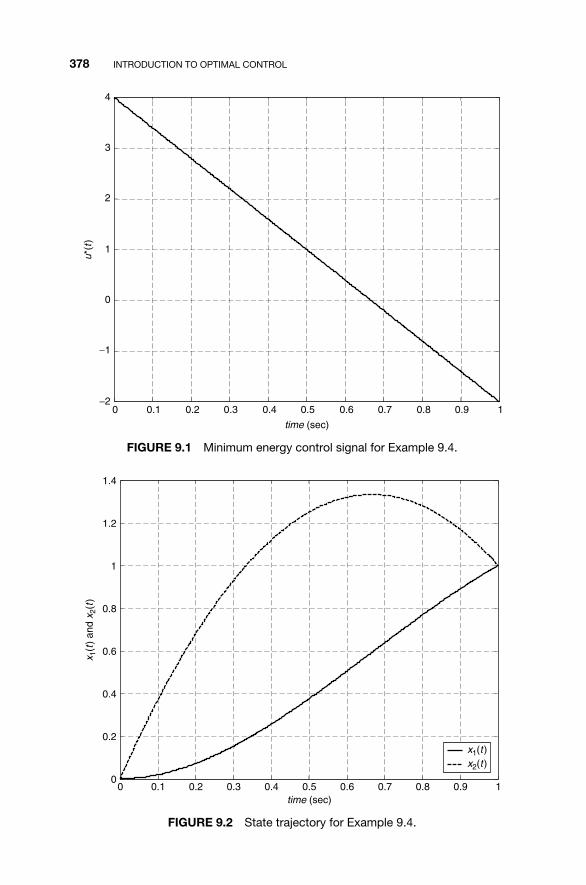
378 INTRODUCTION TO OPTIMAL CONTROL
0 0.1 0.2 0.3 0.4 0.5 0.6 0.7 0.8 0.9 1−2
−1
0
1
2
3
4u*
(t)
time (sec)
FIGURE 9.1 Minimum energy control signal for Example 9.4.
0 0.1 0.2 0.3 0.4 0.5 0.6 0.7 0.8 0.9 10
0.2
0.4
0.6
0.8
1
1.2
1.4
time (sec)
x 1(t
) an
d x 2
(t)
x1(t )x2(t )
FIGURE 9.2 State trajectory for Example 9.4.
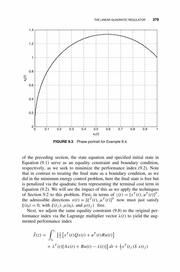
THE LINEAR QUADRATIC REGULATOR 379
0 0.1 0.2 0.3 0.4 0.5 0.6 0.7 0.8 0.9 10
0.2
0.4
0.6
0.8
1
1.2
1.4
x 2(t
)
x1(t )
FIGURE 9.3 Phase portrait for Example 9.4.
of the preceding section, the state equation and specified initial state inEquation (9.1) serve as an equality constraint and boundary condition,respectively, as we seek to minimize the performance index (9.2). Notethat in contrast to treating the final state as a boundary condition, as wedid in the minimum energy control problem, here the final state is free butis penalized via the quadratic form representing the terminal cost term inEquation (9.2). We will see the impact of this as we apply the techniquesof Section 9.2 to this problem. First, in terms of z(t) = [xT (t), uT (t)]T ,the admissible directions v(t) = [ξT (t), µT (t)]T now must just satisfyξ(t0) = 0, with ξ(tf ), µ(t0), and µ(tf ) free.
Next, we adjoin the same equality constraint (9.8) to the original per-formance index via the Lagrange multiplier vector λ(t) to yield the aug-mented performance index
J (z) =∫ tf
t0
{12
[xT (t)Qx(t) + uT (t)Ru(t)
]
+ λT (t)[Ax(t) + Bu(t) − x(t)]}dt + 1
2xT (tf )S x(tf )
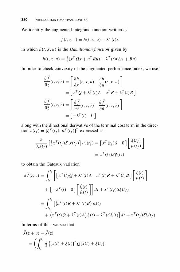
380 INTRODUCTION TO OPTIMAL CONTROL
We identify the augmented integrand function written as
f (t, z, z) = h(t, x, u) − λT (t)x
in which h(t, x, u) is the Hamiltonian function given by
h(t, x, u) = 12(x
T Qx + uT Ru) + λT (t)(Ax + Bu)
In order to check convexity of the augmented performance index, we use
∂f
∂z(t, z, z) =
[∂h
∂x(t, x, u)
∂h
∂u(t, x, u)
]
= [xT Q + λT (t)A uT R + λT (t)B
]∂f
∂z(t, z, z) =
[∂f
∂x(t, z, z)
∂f
∂u(t, z, z)
]
= [ −λT (t) 0]
along with the directional derivative of the terminal cost term in the direc-tion v(tf ) = [ξT (tf ), µT (tf )]T expressed as
∂
∂z(tf )
[12x
T (tf )S x(tf )] · v(tf ) = [
xT (tf )S 0] [
ξ(tf )
µ(tf )
]
= xT (tf )Sξ(tf )
to obtain the Gateaux variation
δJ (z; v) =∫ tf
t0
[[xT (t)Q + λT (t)A uT (t)R + λT (t)B
] [ξ(t)
µ(t)
]
+ [−λT (t) 0] [
ξ (t)
µ(t)
]]dt + xT (tf )Sξ(tf )
=∫ tf
t0
[(uT (t)R + λT (t)B
)µ(t)
+ (xT (t)Q + λT (t)A
)ξ(t) − λT (t)ξ (t)
]dt + xT (tf )Sξ(tf )
In terms of this, we see that
J (z + v) − J (z)
=(∫ tf
t0
12
{[x(t) + ξ(t)]T Q[x(t) + ξ(t)]
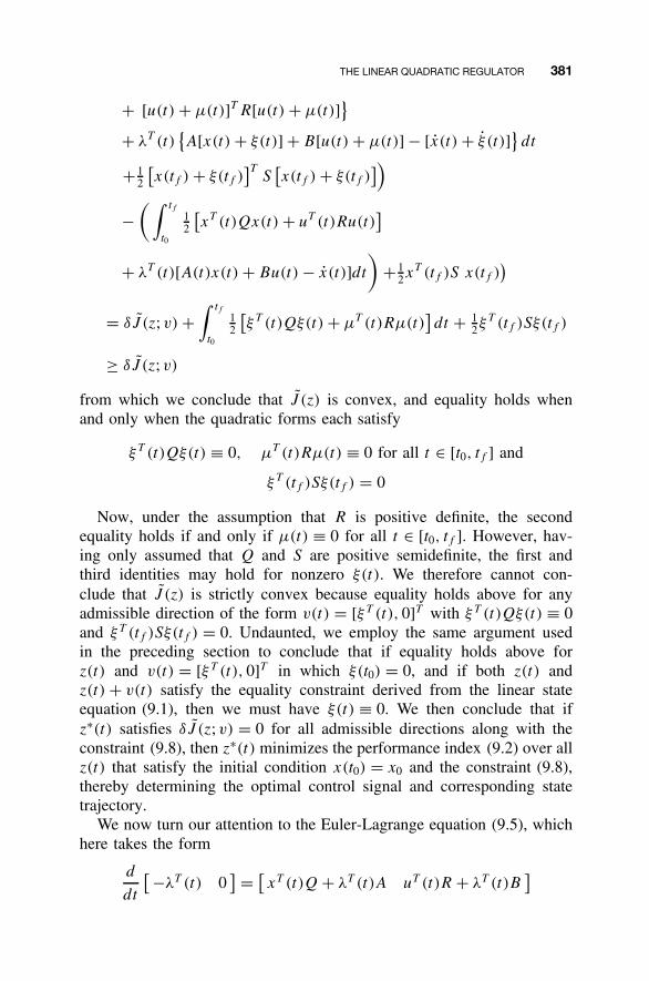
THE LINEAR QUADRATIC REGULATOR 381
+ [u(t) + µ(t)]T R[u(t) + µ(t)]}
+ λT (t){A[x(t) + ξ(t)] + B[u(t) + µ(t)] − [x(t) + ξ (t)]
}dt
+ 12
[x(tf ) + ξ(tf )
]TS
[x(tf ) + ξ(tf )
])
−(∫ tf
t0
12
[xT (t)Qx(t) + uT (t)Ru(t)
]
+ λT (t)[A(t)x(t) + Bu(t) − x(t)]dt
)+ 1
2xT (tf )S x(tf )
)
= δJ (z; v) +∫ tf
t0
12
[ξT (t)Qξ(t) + µT (t)Rµ(t)
]dt + 1
2ξT (tf )Sξ(tf )
≥ δJ (z; v)
from which we conclude that J (z) is convex, and equality holds whenand only when the quadratic forms each satisfy
ξT (t)Qξ(t) ≡ 0, µT (t)Rµ(t) ≡ 0 for all t ∈ [t0, tf ] and
ξT (tf )Sξ(tf ) = 0
Now, under the assumption that R is positive definite, the secondequality holds if and only if µ(t) ≡ 0 for all t ∈ [t0, tf ]. However, hav-ing only assumed that Q and S are positive semidefinite, the first andthird identities may hold for nonzero ξ(t). We therefore cannot con-clude that J (z) is strictly convex because equality holds above for anyadmissible direction of the form v(t) = [ξT (t), 0]T with ξT (t)Qξ(t) ≡ 0and ξT (tf )Sξ(tf ) = 0. Undaunted, we employ the same argument usedin the preceding section to conclude that if equality holds above forz(t) and v(t) = [ξT (t), 0]T in which ξ(t0) = 0, and if both z(t) andz(t) + v(t) satisfy the equality constraint derived from the linear stateequation (9.1), then we must have ξ(t) ≡ 0. We then conclude that ifz∗(t) satisfies δJ (z; v) = 0 for all admissible directions along with theconstraint (9.8), then z∗(t) minimizes the performance index (9.2) over allz(t) that satisfy the initial condition x(t0) = x0 and the constraint (9.8),thereby determining the optimal control signal and corresponding statetrajectory.
We now turn our attention to the Euler-Lagrange equation (9.5), whichhere takes the form
d
dt
[ −λT (t) 0] = [
xT (t)Q + λT (t)A uT (t)R + λT (t)B]
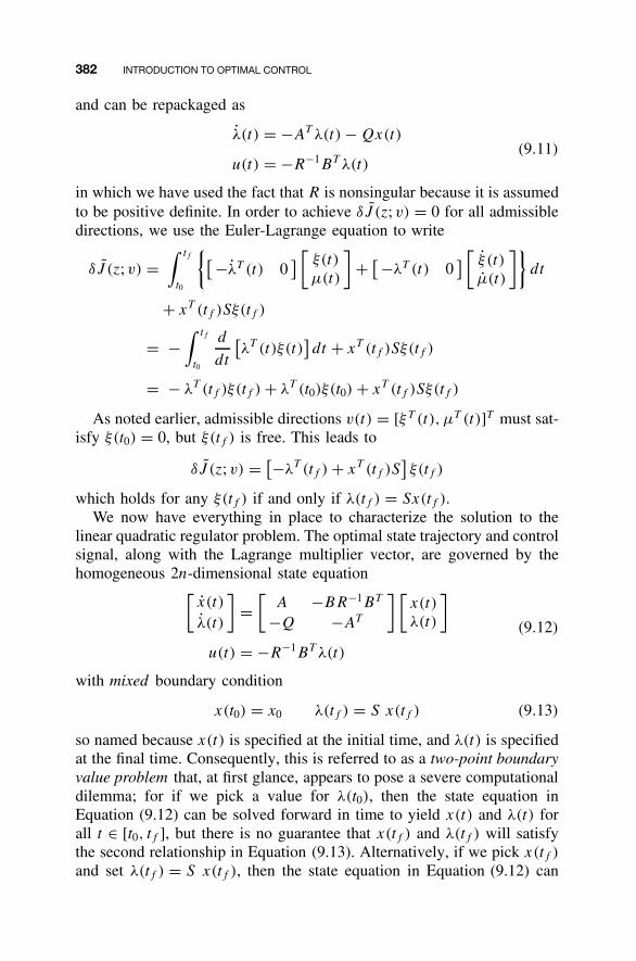
382 INTRODUCTION TO OPTIMAL CONTROL
and can be repackaged as
λ(t) = −AT λ(t) − Qx(t)
u(t) = −R−1BT λ(t)(9.11)
in which we have used the fact that R is nonsingular because it is assumedto be positive definite. In order to achieve δJ (z; v) = 0 for all admissibledirections, we use the Euler-Lagrange equation to write
δJ (z; v) =∫ tf
t0
{[ −λT (t) 0] [
ξ(t)
µ(t)
]+ [−λT (t) 0
] [ξ (t)
µ(t)
]}dt
+ xT (tf )Sξ(tf )
= −∫ tf
t0
d
dt
[λT (t)ξ(t)
]dt + xT (tf )Sξ(tf )
= − λT (tf )ξ(tf ) + λT (t0)ξ(t0) + xT (tf )Sξ(tf )
As noted earlier, admissible directions v(t) = [ξT (t), µT (t)]T must sat-isfy ξ(t0) = 0, but ξ(tf ) is free. This leads to
δJ (z; v) = [−λT (tf ) + xT (tf )S]ξ(tf )
which holds for any ξ(tf ) if and only if λ(tf ) = Sx(tf ).We now have everything in place to characterize the solution to the
linear quadratic regulator problem. The optimal state trajectory and controlsignal, along with the Lagrange multiplier vector, are governed by thehomogeneous 2n-dimensional state equation[
x(t)
λ(t)
]=
[A −BR−1BT
−Q −AT
] [x(t)
λ(t)
]
u(t) = −R−1BT λ(t)
(9.12)
with mixed boundary condition
x(t0) = x0 λ(tf ) = S x(tf ) (9.13)
so named because x(t) is specified at the initial time, and λ(t) is specifiedat the final time. Consequently, this is referred to as a two-point boundaryvalue problem that, at first glance, appears to pose a severe computationaldilemma; for if we pick a value for λ(t0), then the state equation inEquation (9.12) can be solved forward in time to yield x(t) and λ(t) forall t ∈ [t0, tf ], but there is no guarantee that x(tf ) and λ(tf ) will satisfythe second relationship in Equation (9.13). Alternatively, if we pick x(tf )
and set λ(tf ) = S x(tf ), then the state equation in Equation (9.12) can
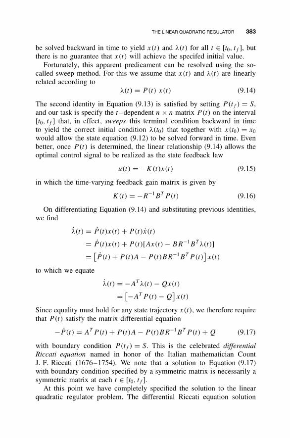
THE LINEAR QUADRATIC REGULATOR 383
be solved backward in time to yield x(t) and λ(t) for all t ∈ [t0, tf ], butthere is no guarantee that x(t) will achieve the specifed initial value.
Fortunately, this apparent predicament can be resolved using the so-called sweep method. For this we assume that x(t) and λ(t) are linearlyrelated according to
λ(t) = P(t) x(t) (9.14)
The second identity in Equation (9.13) is satisfied by setting P(tf ) = S,and our task is specify the t –dependent n × n matrix P(t) on the interval[t0, tf ] that, in effect, sweeps this terminal condition backward in timeto yield the correct initial condition λ(t0) that together with x(t0) = x0
would allow the state equation (9.12) to be solved forward in time. Evenbetter, once P(t) is determined, the linear relationship (9.14) allows theoptimal control signal to be realized as the state feedback law
u(t) = −K(t)x(t) (9.15)
in which the time-varying feedback gain matrix is given by
K(t) = −R−1BT P (t) (9.16)
On differentiating Equation (9.14) and substituting previous identities,we find
λ(t) = P (t)x(t) + P(t)x(t)
= P (t)x(t) + P(t)[Ax(t) − BR−1BT λ(t)]
= [P (t) + P(t)A − P(t)BR−1BT P (t)
]x(t)
to which we equate
λ(t) = −AT λ(t) − Qx(t)
= [−AT P (t) − Q]x(t)
Since equality must hold for any state trajectory x(t), we therefore requirethat P(t) satisfy the matrix differential equation
−P (t) = AT P (t) + P(t)A − P(t)BR−1BT P (t) + Q (9.17)
with boundary condition P(tf ) = S. This is the celebrated differentialRiccati equation named in honor of the Italian mathematician CountJ. F. Riccati (1676–1754). We note that a solution to Equation (9.17)with boundary condition specified by a symmetric matrix is necessarily asymmetric matrix at each t ∈ [t0, tf ].
At this point we have completely specified the solution to the linearquadratic regulator problem. The differential Riccati equation solution
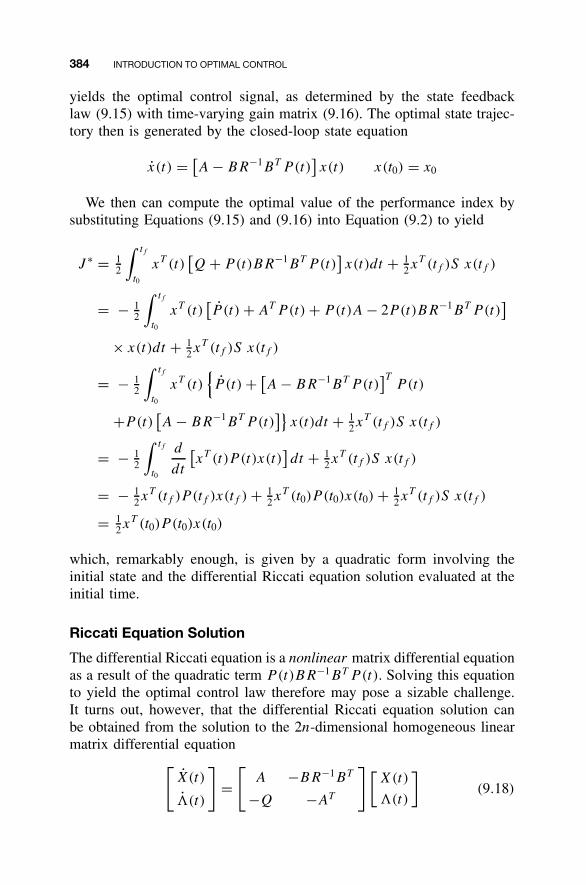
384 INTRODUCTION TO OPTIMAL CONTROL
yields the optimal control signal, as determined by the state feedbacklaw (9.15) with time-varying gain matrix (9.16). The optimal state trajec-tory then is generated by the closed-loop state equation
x(t) = [A − BR−1BT P (t)
]x(t) x(t0) = x0
We then can compute the optimal value of the performance index bysubstituting Equations (9.15) and (9.16) into Equation (9.2) to yield
J ∗ = 12
∫ tf
t0
xT (t)[Q + P(t)BR−1BT P (t)
]x(t)dt + 1
2xT (tf )S x(tf )
= − 12
∫ tf
t0
xT (t)[P (t) + AT P (t) + P(t)A − 2P(t)BR−1BT P (t)
]
× x(t)dt + 12x
T (tf )S x(tf )
= − 12
∫ tf
t0
xT (t){P (t) + [
A − BR−1BT P (t)]T
P (t)
+P(t)[A − BR−1BT P (t)
]}x(t)dt + 1
2xT (tf )S x(tf )
= − 12
∫ tf
t0
d
dt
[xT (t)P (t)x(t)
]dt + 1
2xT (tf )S x(tf )
= − 12x
T (tf )P (tf )x(tf ) + 12x
T (t0)P (t0)x(t0) + 12x
T (tf )S x(tf )
= 12x
T (t0)P (t0)x(t0)
which, remarkably enough, is given by a quadratic form involving theinitial state and the differential Riccati equation solution evaluated at theinitial time.
Riccati Equation Solution
The differential Riccati equation is a nonlinear matrix differential equationas a result of the quadratic term P(t)BR−1BT P (t). Solving this equationto yield the optimal control law therefore may pose a sizable challenge.It turns out, however, that the differential Riccati equation solution canbe obtained from the solution to the 2n-dimensional homogeneous linearmatrix differential equation
[X(t)
�(t)
]=
[A −BR−1BT
−Q −AT
][X(t)
�(t)
](9.18)
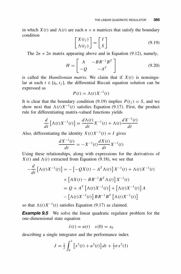
THE LINEAR QUADRATIC REGULATOR 385
in which X(t) and �(t) are each n × n matrices that satisfy the boundarycondition [
X(tf )
�(tf )
]=
[I
S
](9.19)
The 2n × 2n matrix appearing above and in Equation (9.12), namely,
H =[
A −BR−1BT
−Q −AT
](9.20)
is called the Hamiltonian matrix. We claim that if X(t) is nonsingu-lar at each t ∈ [t0, tf ], the differential Riccati equation solution can beexpressed as
P(t) = �(t)X−1(t)
It is clear that the boundary condition (9.19) implies P(tf ) = S, and weshow next that �(t)X−1(t) satisfies Equation (9.17). First, the productrule for differentiating matrix-valued functions yields
d
dt
[�(t)X−1(t)
] = d�(t)
dtX−1(t) + �(t)
dX−1(t)
dt
Also, differentiating the identity X(t)X−1(t) = I gives
dX−1(t)
dt= −X−1(t)
dX(t)
dtX−1(t)
Using these relationships, along with expressions for the derivatives ofX(t) and �(t) extracted from Equation (9.18), we see that
− d
dt
[�(t)X−1(t)
] = − [−QX(t) − AT �(t)]X−1(t) + �(t)X−1(t)
× [AX(t) − BR−1BT �(t)
]X−1(t)
= Q + AT[�(t)X−1(t)
] + [�(t)X−1(t)
]A
− [�(t)X−1(t)
]BR−1BT
[�(t)X−1(t)
]so that �(t)X−1(t) satisfies Equation (9.17) as claimed.
Example 9.5 We solve the linear quadratic regulator problem for theone-dimensional state equation
x(t) = u(t) x(0) = x0
describing a single integrator and the performance index
J = 12
∫ 1
0
[x2(t) + u2(t)
]dt + 1
2σx2(1)
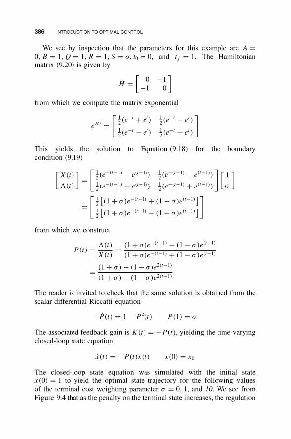
386 INTRODUCTION TO OPTIMAL CONTROL
We see by inspection that the parameters for this example are A =0, B = 1, Q = 1, R = 1, S = σ, t0 = 0, and tf = 1. The Hamiltonianmatrix (9.20) is given by
H =[
0 −1−1 0
]
from which we compute the matrix exponential
eHt =[
12(e
−t + et ) 12(e−t − et )
12(e
−t − et ) 12(e−t + et )
]
This yields the solution to Equation (9.18) for the boundarycondition (9.19)
[X(t)
�(t)
]=
[12(e−(t−1) + e(t−1)) 1
2(e−(t−1) − e(t−1))
12(e−(t−1) − e(t−1)) 1
2(e−(t−1) + e(t−1))
][1
σ
]
=[
12
[(1 + σ)e−(t−1) + (1 − σ)e(t−1)
]12
[(1 + σ)e−(t−1) − (1 − σ)e(t−1)
]]
from which we construct
P(t) = �(t)
X(t)= (1 + σ)e−(t−1) − (1 − σ)e(t−1)
(1 + σ)e−(t−1) + (1 − σ)e(t−1)
= (1 + σ) − (1 − σ)e2(t−1)
(1 + σ) + (1 − σ)e2(t−1)
The reader is invited to check that the same solution is obtained from thescalar differential Riccatti equation
−P (t) = 1 − P 2(t) P (1) = σ
The associated feedback gain is K(t) = −P(t), yielding the time-varyingclosed-loop state equation
x(t) = −P(t)x(t) x(0) = x0
The closed-loop state equation was simulated with the initial statex(0) = 1 to yield the optimal state trajectory for the following valuesof the terminal cost weighting parameter σ = 0, 1, and 10. We see fromFigure 9.4 that as the penalty on the terminal state increases, the regulation
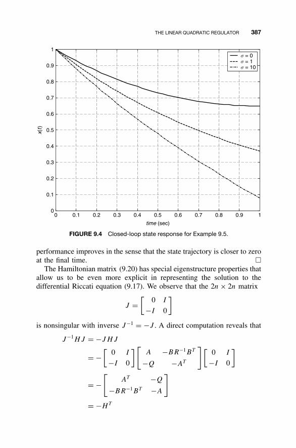
THE LINEAR QUADRATIC REGULATOR 387
0 0.1 0.2 0.3 0.4 0.5 0.6 0.7 0.8 0.9 10
0.1
0.2
0.3
0.4
0.5
0.6
0.7
0.8
0.9
1
x(t)
time (sec)
s = 0s = 1s = 10
FIGURE 9.4 Closed-loop state response for Example 9.5.
performance improves in the sense that the state trajectory is closer to zeroat the final time. �
The Hamiltonian matrix (9.20) has special eigenstructure properties thatallow us to be even more explicit in representing the solution to thedifferential Riccati equation (9.17). We observe that the 2n × 2n matrix
J =[
0 I
−I 0
]
is nonsingular with inverse J−1 = −J . A direct computation reveals that
J−1HJ = −JHJ
= −[
0 I
−I 0
] [A −BR−1BT
−Q −AT
][0 I
−I 0
]
= −[
AT −Q
−BR−1BT −A
]
= −HT
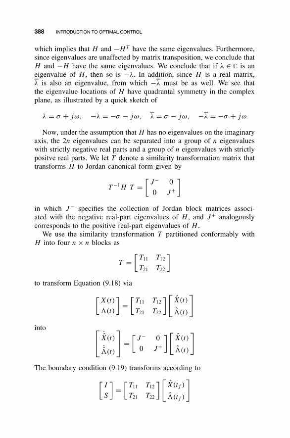
388 INTRODUCTION TO OPTIMAL CONTROL
which implies that H and −HT have the same eigenvalues. Furthermore,since eigenvalues are unaffected by matrix transposition, we conclude thatH and −H have the same eigenvalues. We conclude that if λ ∈ C is aneigenvalue of H , then so is −λ. In addition, since H is a real matrix,λ is also an eigenvalue, from which −λ must be as well. We see thatthe eigenvalue locations of H have quadrantal symmetry in the complexplane, as illustrated by a quick sketch of
λ = σ + jω, −λ = −σ − jω, λ = σ − jω, −λ = −σ + jω
Now, under the assumption that H has no eigenvalues on the imaginaryaxis, the 2n eigenvalues can be separated into a group of n eigenvalueswith strictly negative real parts and a group of n eigenvalues with strictlypositve real parts. We let T denote a similarity transformation matrix thattransforms H to Jordan canonical form given by
T −1H T =[
J− 0
0 J+
]
in which J− specifies the collection of Jordan block matrices associ-ated with the negative real-part eigenvalues of H , and J+ analogouslycorresponds to the positive real-part eigenvalues of H .
We use the similarity transformation T partitioned conformably withH into four n × n blocks as
T =[
T11 T12
T21 T22
]
to transform Equation (9.18) via
[X(t)
�(t)
]=
[T11 T12
T21 T22
] [X(t)
�(t)
]
into ˙
X(t)
˙�(t)
=
[J− 0
0 J+
][X(t)
�(t)
]
The boundary condition (9.19) transforms according to
[I
S
]=
[T11 T12
T21 T22
] [X(tf )
�(tf )
]
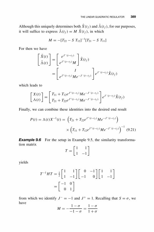
THE LINEAR QUADRATIC REGULATOR 389
Although this uniquely determines both X(tf ) and �(tf ), for our purposes,it will suffice to express �(tf ) = M X(tf ), in which
M = −[T22 − S T12]−1[T21 − S T11]
For then we have[X(t)
�(t)
]=
[eJ−(t−tf )
eJ+(t−tf )M
]X(tf )
=[
I
eJ+(t−tf )Me−J−(t−tf )
]eJ−(t−tf )X(tf )
which leads to
[X(t)
�(t)
]=
[T11 + T12e
J+(t−tf )Me−J−(t−tf )
T21 + T22eJ+(t−tf )Me−J−(t−tf )
]eJ−(t−tf )X(tf )
Finally, we can combine these identities into the desired end result
P(t) = �(t)X−1(t) =(T21 + T22e
J+(t−tf )Me−J−(t−tf ))
×(T11 + T12e
J+(t−tf )Me−J−(t−tf ))−1
(9.21)
Example 9.6 For the setup in Example 9.5, the similarity transforma-tion matrix
T =[
1 1
1 −1
]
yields
T −1HT = 12
[1 1
1 −1
] [0 −1
−1 0
] [1 1
1 −1
]
=[ −1 0
0 1
]
from which we identify J− = −1 and J+ = 1. Recalling that S = σ , wehave
M = − 1 − σ
−1 − σ= 1 − σ
1 + σ
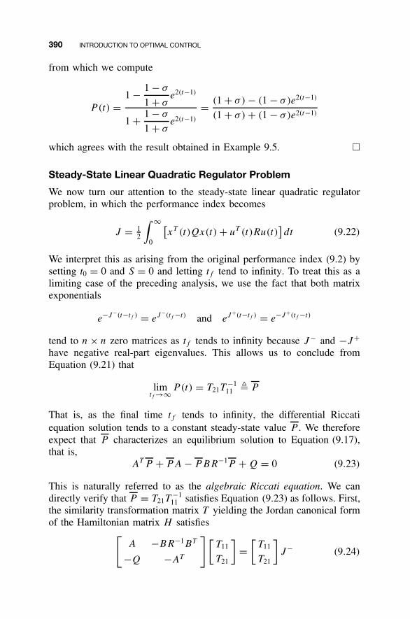
390 INTRODUCTION TO OPTIMAL CONTROL
from which we compute
P(t) =1 − 1 − σ
1 + σe2(t−1)
1 + 1 − σ
1 + σe2(t−1)
= (1 + σ) − (1 − σ)e2(t−1)
(1 + σ) + (1 − σ)e2(t−1)
which agrees with the result obtained in Example 9.5. �
Steady-State Linear Quadratic Regulator Problem
We now turn our attention to the steady-state linear quadratic regulatorproblem, in which the performance index becomes
J = 12
∫ ∞
0
[xT (t)Qx(t) + uT (t)Ru(t)
]dt (9.22)
We interpret this as arising from the original performance index (9.2) bysetting t0 = 0 and S = 0 and letting tf tend to infinity. To treat this as alimiting case of the preceding analysis, we use the fact that both matrixexponentials
e−J−(t−tf ) = eJ−(tf −t) and eJ+(t−tf ) = e−J+(tf −t)
tend to n × n zero matrices as tf tends to infinity because J− and −J+have negative real-part eigenvalues. This allows us to conclude fromEquation (9.21) that
limtf →∞ P(t) = T21T
−111 � P
That is, as the final time tf tends to infinity, the differential Riccatiequation solution tends to a constant steady-state value P . We thereforeexpect that P characterizes an equilibrium solution to Equation (9.17),that is,
AT P + PA − PBR−1P + Q = 0 (9.23)
This is naturally referred to as the algebraic Riccati equation. We candirectly verify that P = T21T
−111 satisfies Equation (9.23) as follows. First,
the similarity transformation matrix T yielding the Jordan canonical formof the Hamiltonian matrix H satisfies[
A −BR−1BT
−Q −AT
][T11
T21
]=
[T11
T21
]J− (9.24)
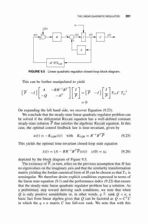
THE LINEAR QUADRATIC REGULATOR 391
+
++
+
A
Bx(t) y(t)u(t)
C
−R−1BTKLQR
d(t)
x(t)
x0
∫
FIGURE 9.5 Linear quadratic regulator closed-loop block diagram.
This can be further manipulated to yield
[P −I
] [A −BR−1BT
−Q −AT
] [I
P
]= [
P −I] [
I
P
]T11J
−T −111
= 0
On expanding the left hand side, we recover Equation (9.23).We conclude that the steady-state linear quadratic regulator problem can
be solved if the differential Riccati equation has a well-defined constantsteady-state solution P that satisfies the algebraic Riccati equation. In thiscase, the optimal control feedback law is time-invariant, given by
u(t) = −KLQRx(t) with KLQR = R−1BT P (9.25)
This yields the optimal time-invariant closed-loop state equation
x(t) = (A − BR−1BT P )x(t) x(0) = x0 (9.26)
depicted by the block diagram of Figure 9.5.The existence of P , in turn, relies on the previous assumption that H has
no eigenvalues on the imaginary axis and that the similarity transformationmatrix yielding the Jordan canonical form of H can be chosen so that T11 isnonsingular. We therefore desire explicit conditions expressed in terms ofthe linear state equation (9.1) and the performance index (9.22) that ensurethat the steady-state linear quadratic regulator problem has a solution. Asa preliminary step toward deriving such conditions, we note that whenQ is only positive semidefinite or, in other words, q � rank Q < n, abasic fact from linear algebra gives that Q can be factored as Q = CT C
in which the q × n matrix C has full-row rank. We note that with this
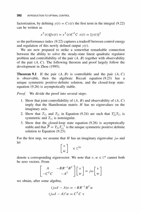
392 INTRODUCTION TO OPTIMAL CONTROL
factorization, by defining y(t) = Cx(t) the first term in the integral (9.22)can be written as
xT (t)Qx(t) = xT (t)CT C x(t) = ||y(t)||2
so the performance index (9.22) captures a tradeoff between control energyand regulation of this newly defined output y(t).
We are now prepared to strike a somewhat remarkable connectionbetween the ability to solve the steady-state linear quadratic regulatorproblem and controllability of the pair (A, B) together with observabilityof the pair (A, C). The following theorem and proof largely follow thedevelopment in Zhou (1995).
Theorem 9.1 If the pair (A, B) is controllable and the pair (A, C)
is observable, then the algebraic Riccati equation (9.23) has aunique symmetric positive-definite solution, and the closed-loop state-equation (9.26) is asymptotically stable.
Proof. We divide the proof into several steps:
1. Show that joint controllability of (A, B) and observability of (A, C)
imply that the Hamiltonian matrix H has no eigenvalues on theimaginary axis.
2. Show that T11 and T21 in Equation (9.24) are such that T ∗21T11 is
symmetric and T11 is nonsingular.3. Show that the closed-loop state equation (9.26) is asymptotically
stable and that P = T21T−1
11 is the unique symmetric positive definitesolution to Equation (9.23).
For the first step, we assume that H has an imaginary eigenvalue jω andlet [
v
w
]∈ C
2n
denote a corresponding eigenvector. We note that v, w ∈ Cn cannot both
be zero vectors. From[A −BR−1BT
−CT C −AT
][v
w
]= jω
[v
w
]
we obtain, after some algebra,
(jωI − A)v = −BR−1BT w
(jωI − A)∗w = CT C v
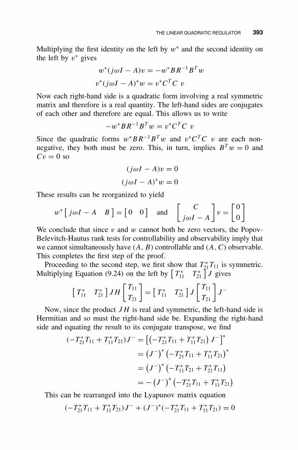
THE LINEAR QUADRATIC REGULATOR 393
Multiplying the first identity on the left by w∗ and the second identity onthe left by v∗ gives
w∗(jωI − A)v = −w∗BR−1BT w
v∗(jωI − A)∗w = v∗CT C v
Now each right-hand side is a quadratic form involving a real symmetricmatrix and therefore is a real quantity. The left-hand sides are conjugatesof each other and therefore are equal. This allows us to write
−w∗BR−1BT w = v∗CT C v
Since the quadratic forms w∗BR−1BT w and v∗CT C v are each non-negative, they both must be zero. This, in turn, implies BT w = 0 andCv = 0 so
(jωI − A)v = 0
(jωI − A)∗w = 0
These results can be reorganized to yield
w∗ [jωI − A B
] = [0 0
]and
[C
jωI − A
]v =
[0
0
]
We conclude that since v and w cannot both be zero vectors, the Popov-Belevitch-Hautus rank tests for controllability and observability imply thatwe cannot simultaneously have (A, B) controllable and (A, C) observable.This completes the first step of the proof.
Proceeding to the second step, we first show that T ∗21T11 is symmetric.
Multiplying Equation (9.24) on the left by[T ∗
11 T ∗21
]J gives
[T ∗
11 T ∗21
]JH
[T11
T21
]= [
T ∗11 T ∗
21
]J
[T11
T21
]J−
Now, since the product JH is real and symmetric, the left-hand side isHermitian and so must the right-hand side be. Expanding the right-handside and equating the result to its conjugate transpose, we find
(−T ∗21T11 + T ∗
11T21)J− = [(−T ∗
21T11 + T ∗11T21
)J−]∗
= (J−)∗ (−T ∗
21T11 + T ∗11T21
)∗
= (J−)∗ (−T ∗
11T21 + T ∗21T11
)= − (
J−)∗ (−T ∗21T11 + T ∗
11T21)
This can be rearranged into the Lyapunov matrix equation
(−T ∗21T11 + T ∗
11T21)J− + (J−)∗(−T ∗
21T11 + T ∗11T21) = 0
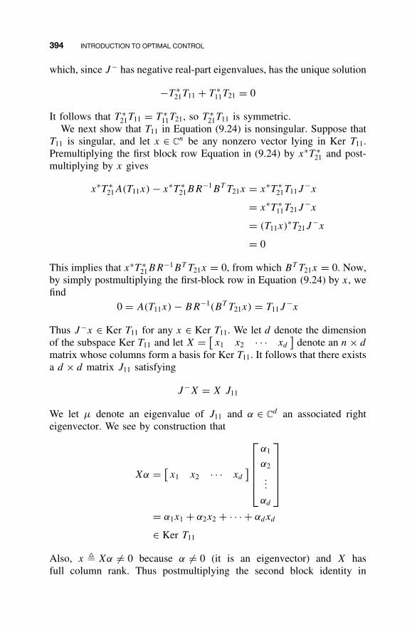
394 INTRODUCTION TO OPTIMAL CONTROL
which, since J− has negative real-part eigenvalues, has the unique solution
−T ∗21T11 + T ∗
11T21 = 0
It follows that T ∗21T11 = T ∗
11T21, so T ∗21T11 is symmetric.
We next show that T11 in Equation (9.24) is nonsingular. Suppose thatT11 is singular, and let x ∈ C
n be any nonzero vector lying in Ker T11.Premultiplying the first block row Equation in (9.24) by x∗T ∗
21 and post-multiplying by x gives
x∗T ∗21A(T11x) − x∗T ∗
21BR−1BT T21x = x∗T ∗21T11J
−x
= x∗T ∗11T21J
−x
= (T11x)∗T21J−x
= 0
This implies that x∗T ∗21BR−1BT T21x = 0, from which BT T21x = 0. Now,
by simply postmultiplying the first-block row in Equation (9.24) by x, wefind
0 = A(T11x) − BR−1(BT T21x) = T11J−x
Thus J−x ∈ Ker T11 for any x ∈ Ker T11. We let d denote the dimensionof the subspace Ker T11 and let X = [
x1 x2 · · · xd
]denote an n × d
matrix whose columns form a basis for Ker T11. It follows that there existsa d × d matrix J11 satisfying
J−X = X J11
We let µ denote an eigenvalue of J11 and α ∈ Cd an associated right
eigenvector. We see by construction that
Xα = [x1 x2 · · · xd
]
α1
α2
...
αd
= α1x1 + α2x2 + · · · + αdxd
∈ Ker T11
Also, x � Xα �= 0 because α �= 0 (it is an eigenvector) and X hasfull column rank. Thus postmultiplying the second block identity in
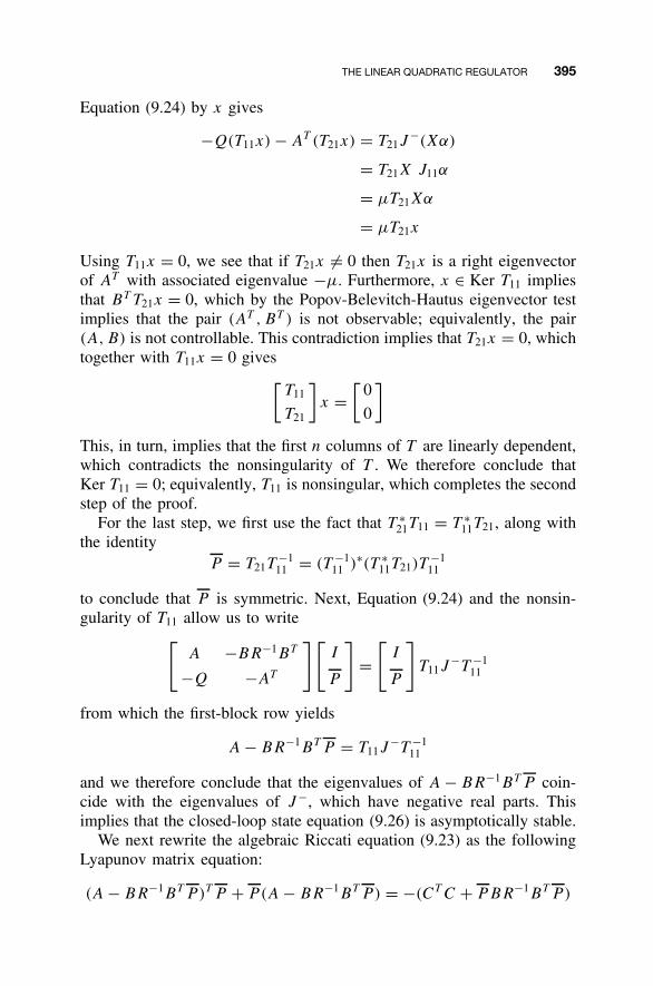
THE LINEAR QUADRATIC REGULATOR 395
Equation (9.24) by x gives
−Q(T11x) − AT (T21x) = T21J−(Xα)
= T21X J11α
= µT21Xα
= µT21x
Using T11x = 0, we see that if T21x �= 0 then T21x is a right eigenvectorof AT with associated eigenvalue −µ. Furthermore, x ∈ Ker T11 impliesthat BT T21x = 0, which by the Popov-Belevitch-Hautus eigenvector testimplies that the pair (AT , BT ) is not observable; equivalently, the pair(A, B) is not controllable. This contradiction implies that T21x = 0, whichtogether with T11x = 0 gives
[T11
T21
]x =
[0
0
]
This, in turn, implies that the first n columns of T are linearly dependent,which contradicts the nonsingularity of T . We therefore conclude thatKer T11 = 0; equivalently, T11 is nonsingular, which completes the secondstep of the proof.
For the last step, we first use the fact that T ∗21T11 = T ∗
11T21, along withthe identity
P = T21T−1
11 = (T −111 )∗(T ∗
11T21)T−1
11
to conclude that P is symmetric. Next, Equation (9.24) and the nonsin-gularity of T11 allow us to write[
A −BR−1BT
−Q −AT
] [I
P
]=
[I
P
]T11J
−T −111
from which the first-block row yields
A − BR−1BT P = T11J−T −1
11
and we therefore conclude that the eigenvalues of A − BR−1BT P coin-cide with the eigenvalues of J−, which have negative real parts. Thisimplies that the closed-loop state equation (9.26) is asymptotically stable.
We next rewrite the algebraic Riccati equation (9.23) as the followingLyapunov matrix equation:
(A − BR−1BT P )T P + P(A − BR−1BT P ) = −(CT C + PBR−1BT P )
396 INTRODUCTION TO OPTIMAL CONTROL
from which P can be represented as
P =∫ ∞
0e(A−BR−1BT P )T t (CT C + PBR−1BT P )e(A−BR−1BT P )tdt
This indicates that P is positive semidefinite because CT C + PBR−1P
is positive semidefinite. To argue that P is in fact positive definite, wetake any x0 ∈ Ker P and write
xT0 Px0 = xT
0
∫ ∞
0e(A−BR−1BT P )T t (CT C + PBR−1BT P )e(A−BR−1BT P )tdt x0
= xT0
∫ ∞
0e(A−BR−1BT P )T tCT Ce(A−BR−1BT P )tdt x0
+ xT0
∫ ∞
0e(A−BR−1BT P )T tPBR−1BT Pe(A−BR−1BT P )tdt x0
= 0
Since each term is nonnegative, both must vanish. From the second term,we conclude that
R−1BT Pe(A−BR−1BT P )t ≡ 0 for all t ≥ 0
which, using a matrix exponential identity, allows us to write
e(A−BR−1BT P )tx0 = eAtx0 −∫ t
0eA(t−τ )BR−1BT Pe(A−BR−1BT P )τ x0dτ
= eAtx0
From the first term, we see that
CeAtx0 = Ce(A−BR−1BT P )tx0 ≡ 0 for all t ≥ 0
Now, by definition, if x0 �= 0, then (A, C) is an unobservable pair. Thusthe only x0 ∈ Ker P is x0 = 0, from which P is nonsingular and hencepositive definite. Finally, uniqueness can be argued by showing that P =T21T
−111 is the only solution to the algebraic Riccati equation from which
a stabilizing state feedback gain matrix (9.25) can be constructed. This ispursued in AE9.1. �
Example 9.7 We again return to the scalar state equation ofExample 9.5, now with the performance index
J = 12
∫ ∞
0
[x2(t) + u2(t)
]dt
MATLAB FOR OPTIMAL CONTROL 397
The solution of the differential Riccati equation for arbitrary final time tfand terminal cost weight σ is easily adapted from previous computations:
P(t) =1 − 1 − σ
1 + σe2(t−tf )
1 + 1 − σ
1 + σe2(t−tf )
= (1 + σ) − (1 − σ)e2(t−tf )
(1 + σ) + (1 − σ)e2(t−tf )
Since e2(t−tf ) = e−2(tf −t) tends to zero as tf tends to infinity, P(t)
approaches the steady-state value
P = 1 + σ
1 + σ= 1
which is independent of σ .With A = 0 and B = 1, the pair (A, B) is controllable, and for C =√Q = 1, the pair (A, C) is observable. The algebraic Riccati equation
1 − P 2 = 0
has two solutions, P = ±1. Of these, only P = 1 is positive (definite) forwhich the state feedback gain KLQR = 1 yields the asymptotically stableclosed-loop state equation
x(t) = −x(t) �
9.5 MATLAB FOR OPTIMAL CONTROL
MATLAB Functions for Linear Quadratic Regulator Design
The following MATLAB functions are useful for design of state feedbackcontrol laws that solve the linear quadratic regulator problem:
Pbar = are(A,BB,Q) Returns the positive definite (stabilizing) solutionto the algebraic Riccati equation, given the sys-tem dynamics matrix A, the coefficient matrixof the quadratic term BB = B*inv(R)*B’, andweighting matrix Q.
Klqr = lqr(A,B,Q,R) Directly calculates the optimal linear quadraticregulator gain matrix Klqr, given the systemdynamics matrix A, the input matrix B, and theweighting matrices Q and R.
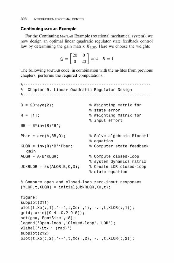
398 INTRODUCTION TO OPTIMAL CONTROL
Continuing MATLAB Example
For the Continuing MATLAB Example (rotational mechanical system), wenow design an optimal linear quadratic regulator state feedback controllaw by determining the gain matrix KLQR. Here we choose the weights
Q =[
20 0
0 20
]and R = 1
The following MATLAB code, in combination with the m-files from previouschapters, performs the required computations:
%------------------------------------------------------% Chapter 9. Linear Quadratic Regulator Design%------------------------------------------------------
Q = 20*eye(2); % Weighting matrix for% state error
R = [1]; % Weighting matrix for% input effort
BB = B*inv(R)*B’;
Pbar = are(A,BB,Q); % Solve algebraic Riccati% equation
KLQR = inv(R)*B’*Pbar; % Computer state feedbackgain
ALQR = A-B*KLQR; % Compute closed-loop% system dynamics matrix
JbkRLQR = ss(ALQR,B,C,D); % Create LQR closed-loop% state equation
% Compare open and closed-loop zero-input responses[YLQR,t,XLQR] = initial(JbkRLQR,X0,t);
figure;subplot(211)plot(t,Xo(:,1),'--',t,Xc(:,1),'-.',t,XLQR(:,1));grid; axis([0 4 -0.2 0.5]);set(gca,'FontSize',18);legend('Open-loop','Closed-loop','LQR');ylabel('\itx 1 (rad)')subplot(212)plot(t,Xo(:,2),'--',t,Xc(:,2),'-.',t,XLQR(:,2));
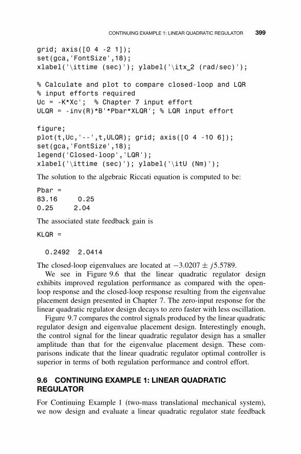
CONTINUING EXAMPLE 1: LINEAR QUADRATIC REGULATOR 399
grid; axis([0 4 -2 1]);set(gca,'FontSize',18);xlabel('\ittime (sec)'); ylabel('\itx 2 (rad/sec)');
% Calculate and plot to compare closed-loop and LQR% input efforts requiredUc = -K*Xc'; % Chapter 7 input effortULQR = -inv(R)*B'*Pbar*XLQR'; % LQR input effort
figure;plot(t,Uc,'--',t,ULQR); grid; axis([0 4 -10 6]);set(gca,'FontSize',18);legend('Closed-loop','LQR');xlabel('\ittime (sec)'); ylabel('\itU (Nm)');
The solution to the algebraic Riccati equation is computed to be:
Pbar =83.16 0.250.25 2.04
The associated state feedback gain is
KLQR =
0.2492 2.0414
The closed-loop eigenvalues are located at −3.0207 ± j5.5789.We see in Figure 9.6 that the linear quadratic regulator design
exhibits improved regulation performance as compared with the open-loop response and the closed-loop response resulting from the eigenvalueplacement design presented in Chapter 7. The zero-input response for thelinear quadratic regulator design decays to zero faster with less oscillation.
Figure 9.7 compares the control signals produced by the linear quadraticregulator design and eigenvalue placement design. Interestingly enough,the control signal for the linear quadratic regulator design has a smalleramplitude than that for the eigenvalue placement design. These com-parisons indicate that the linear quadratic regulator optimal controller issuperior in terms of both regulation performance and control effort.
9.6 CONTINUING EXAMPLE 1: LINEAR QUADRATICREGULATOR
For Continuing Example 1 (two-mass translational mechanical system),we now design and evaluate a linear quadratic regulator state feedback
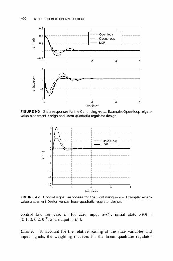
400 INTRODUCTION TO OPTIMAL CONTROL
0 1 2 3 4−0.2
0
0.2
0.4
0.6
x 1 (
rad)
Open-loopClosed-loopLQR
0 1 2 3 4−2
−1
0
1
time (sec)
x 2 (
rad/
sec)
FIGURE 9.6 State responses for the Continuing MATLAB Example: Open-loop, eigen-value placement design and linear quadratic regulator design.
0 1 2 3 4−10
−8
−6
−4
−2
0
2
4
6
time (sec)
U(N
m)
Closed-loopLQR
FIGURE 9.7 Control signal responses for the Continuing MATLAB Example: eigen-value placement Design versus linear quadratic regulator design.
control law for case b [for zero input u2(t), initial state x(0) =[0.1, 0, 0.2, 0]T, and output y1(t)].
Case b. To account for the relative scaling of the state variables andinput signals, the weighting matrices for the linear quadratic regulator
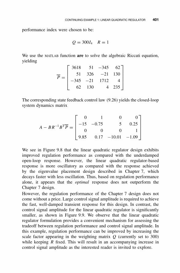
CONTINUING EXAMPLE 1: LINEAR QUADRATIC REGULATOR 401
performance index were chosen to be:
Q = 300I4 R = 1
We use the MATLAB function are to solve the algebraic Riccati equation,yielding
P =
3618 51 −345 62
51 326 −21 130
−345 −21 1712 4
62 130 4 235
The corresponding state feedback control law (9.26) yields the closed-loopsystem dynamics matrix
A − BR−1BTP =
0 1 0 0
−15 −0.75 5 0.25
0 0 0 1
9.85 0.17 −10.01 −1.09
We see in Figure 9.8 that the linear quadratic regulator design exhibitsimproved regulation performance as compared with the underdampedopen-loop response. However, the linear quadratic regulator-basedresponse is more oscillatory as compared with the response achievedby the eigenvalue placement design described in Chapter 7, whichdecays faster with less oscillation. Thus, based on regulation performancealone, it appears that the optimal response does not outperform theChapter 7 design.However, the regulation performance of the Chapter 7 design does notcome without a price. Large control signal amplitude is required to achievethe fast, well-damped transient response for this design. In contrast, thecontrol signal amplitude for the linear quadratic regulator is significantlysmaller, as shown in Figure 9.9. We observe that the linear quadraticregulator formulation provides a convenient mechanism for assessing thetradeoff between regulation performance and control signal amplitude. Inthis example, regulation performance can be improved by increasing thescale factor appearing in the weighting matrix Q (currently set to 300)while keeping R fixed. This will result in an accompanying increase incontrol signal amplitude as the interested reader is invited to explore.
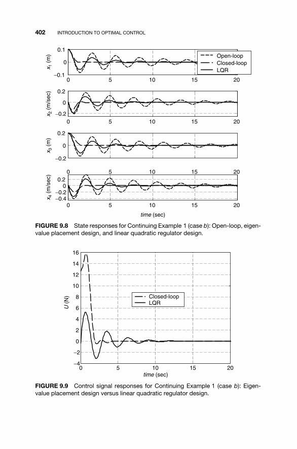
402 INTRODUCTION TO OPTIMAL CONTROL
0 5 10 15 20−0.1
0
0.1Open-loopClosed-loopLQR
0 5 10 15 20−0.2
0
0.2
0 5 10 15 20
−0.2
0
0.2
0 5 10 15 20−0.4−0.2
00.2
time (sec)
x 1 (
m)
x 2 (
m/s
ec)
x 3 (
m)
x 4 (
m/s
ec)
FIGURE 9.8 State responses for Continuing Example 1 (case b): Open-loop, eigen-value placement design, and linear quadratic regulator design.
0 5 10 15 20−4
−2
0
2
4
6
8
10
12
14
16
time (sec)
U(N
) Closed-loopLQR
FIGURE 9.9 Control signal responses for Continuing Example 1 (case b): Eigen-value placement design versus linear quadratic regulator design.
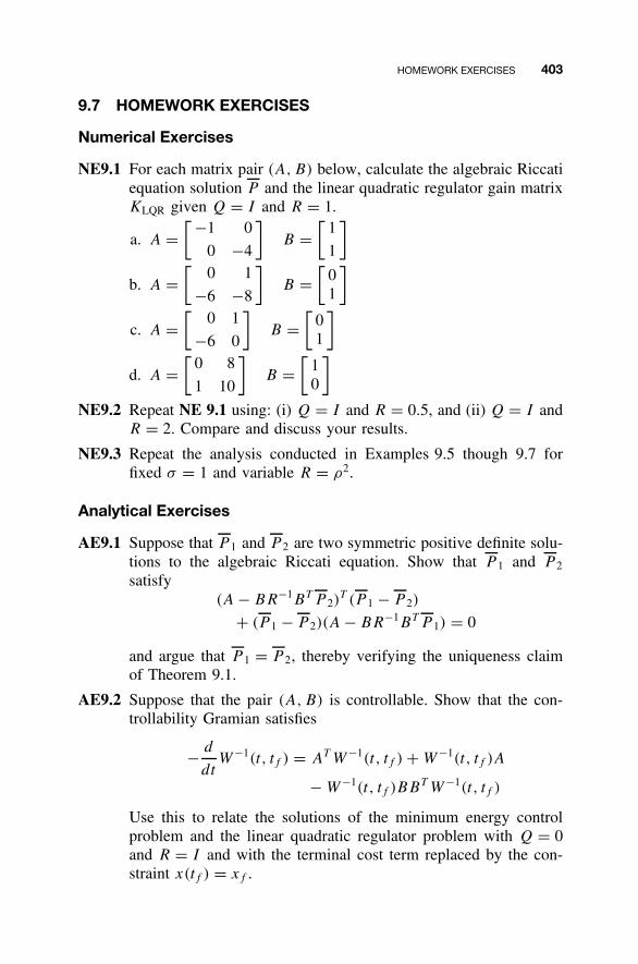
HOMEWORK EXERCISES 403
9.7 HOMEWORK EXERCISES
Numerical Exercises
NE9.1 For each matrix pair (A, B) below, calculate the algebraic Riccatiequation solution P and the linear quadratic regulator gain matrixKLQR given Q = I and R = 1.
a. A =[ −1 0
0 −4
]B =
[1
1
]
b. A =[
0 1
−6 −8
]B =
[01
]
c. A =[
0 1
−6 0
]B =
[01
]
d. A =[
0 8
1 10
]B =
[10
]
NE9.2 Repeat NE 9.1 using: (i) Q = I and R = 0.5, and (ii) Q = I andR = 2. Compare and discuss your results.
NE9.3 Repeat the analysis conducted in Examples 9.5 though 9.7 forfixed σ = 1 and variable R = ρ2.
Analytical Exercises
AE9.1 Suppose that P 1 and P 2 are two symmetric positive definite solu-tions to the algebraic Riccati equation. Show that P 1 and P 2
satisfy(A − BR−1BT P 2)
T (P 1 − P 2)
+ (P 1 − P 2)(A − BR−1BT P 1) = 0
and argue that P 1 = P 2, thereby verifying the uniqueness claimof Theorem 9.1.
AE9.2 Suppose that the pair (A, B) is controllable. Show that the con-trollability Gramian satisfies
− d
dtW−1(t, tf ) = AT W−1(t, tf ) + W−1(t, tf )A
− W−1(t, tf )BBT W−1(t, tf )
Use this to relate the solutions of the minimum energy controlproblem and the linear quadratic regulator problem with Q = 0and R = I and with the terminal cost term replaced by the con-straint x(tf ) = xf .
404 INTRODUCTION TO OPTIMAL CONTROL
AE9.3 Suppose that the algebraic Riccati equation has a unique symmet-ric positive-definite solution P . Determine the n × n matrix X forwhich
T =[
I 0
P I
]
satisfies
T −1H T =[
A − BR−1BT P X
0 −(A − BR−1BT P )T
]
Use this to relate the eigenvalues of H to the eigenvalues of theclosed-loop state equation (9.26).
AE9.4 Derive a solution to the optimal control problem involving theweighted performance index
Jα = 12
∫ ∞
0[xT (t)Qx(t) + uT (t)Ru(t)]e2αtdt
and show that the associated closed-loop eigenvalues have realparts less than −α.
AE9.5 For the single-input, single-output case, show that
|1 + KLQR(jω − A)−1B| ≥ 1 for all − ∞ < ω < ∞As a result, show that the Nyquist plot of KLQR(sI − A)−1B neverenters the circle of radius one centered at −1 + j0 in the complexplane. Argue that the linear quadratic regulator achieves infinitegain margin and a phase margin of at least 60◦.
Continuing MATLAB Exercises
CME9.1 For the CME1.1 system, design and evaluate an optimal linearquadratic regulator with equal weighting for the state and input.Plot the output response to a unit step input, and compare on thesame graph the open-loop and closed-loop responses obtained inCME7.1b and the linear quadratic regulator responses (assumingzero initial conditions). Also plot the associated control sig-nals for the CME7.1b design and the linear quadratic regulatordesign.
CME9.2 For the CME1.2 system, design and evaluate an optimal linearquadratic regulator with the state weighting ten times greater
HOMEWORK EXERCISES 405
than the input weighting. Plot the output response to a unit stepinput, and compare on the same graph the open-loop and closed-loop responses obtained in CME7.2b and the linear quadraticregulator responses (assuming zero initial conditions). Also plotthe associated control signals for the CME7.2b design and thelinear quadratic regulator design.
CME9.3 For the CME1.3 system, design and evaluate an optimal linearquadratic regulator with the state weighting 300 times greaterthan the input weighting. Plot the output response to a unitstep input and compare on the same graph the open-loop andthe closed-loop response obtained in CME7.3b and the linearquadratic regulator responses (assuming zero initial conditions).Also plot the associated control signals for the CME7.3b designand the linear quadratic regulator design.
CME9.4 For the CME1.4 system, design and evaluate an optimal linearquadratic regulator with the state weighting 100 times greaterthan the input weighting. Plot the output response to a unitstep input and compare on the same graph the open-loop andthe closed-loop response obtained in CME7.4b and the linearquadratic regulator responses (assuming zero initial conditions).Also plot the associated control signals for the CME7.4b designand the linear quadratic regulator design.
Continuing Exercises
CE9.1 Design and evaluate a linear quadratic regulator for the CE2.1.i.bsystem. Use equal weighting on the state and input. In addition toplotting the open-loop and closed-loop linear quadratic regulatorstate responses, separately plot the input signals. Compare withthe CE7.1 results.
CE9.2 Design and evaluate a linear quadratic regulator for the CE2.2.i.bsystem. Use equal weighting on the state and input. In addition toplotting the open-loop and closed-loop linear quadratic regulatorstate responses, separately plot the input signals. Compare withthe CE7.2 results.
CE9.3 Design and evaluate a linear quadratic regulator for the CE2.3.i.bsystem. Use equal weighting on the state and input. In addition toplotting the open-loop and closed-loop linear quadratic regulatorstate responses, separately plot the input signals. Compare withthe CE7.3 results.

406 INTRODUCTION TO OPTIMAL CONTROL
CE9.4 Design and evaluate a linear quadratic regulator for the CE2.4system. Weight the state twice as much as the input. In addition toplotting the open-loop and closed-loop linear quadratic regulatorstate responses, separately plot the input signals. Compare withthe CE7.4 results.
APPENDIX AMATRIX INTRODUCTION
This appendix presents a matrix introduction to support the material ofthe textbook. Topics covered are matrix basics, matrix arithmetic, matrixdeterminants, and matrix inversion.
A.1 BASICS
A matrix is a two-dimensional array of real or complex numbers. Here afew examples:
[2 0 −1
1 5 3
]
−1 + j2 3
0 −j
2 − j 1
1 + j3 0
[−3 12 −4
][ 0 2 4 ]
−10
−27
The number of rows and columns specify the dimension of the matrix.That is, a matrix with m rows and n columns is said to have dimensionm × n or is referred to as an m × n matrix. The preceding matrices havedimension 2 × 3, 4 × 2, 2 × 2, 1 × 3, and 4 × 1, respectively. Note that arow vector can be regarded as a matrix with a single row, and a columnvector can be regarded a matrix with a single column. Matrices with thesame number of rows and columns are called square.
407
Linear State-Space Control Systems. Robert L. Williams II and Douglas A. LawrenceCopyright 2007 John Wiley & Sons, Inc. ISBN: 978-0-471-73555-7
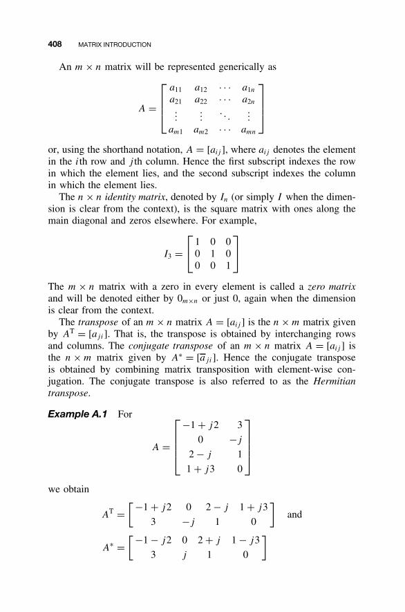
408 MATRIX INTRODUCTION
An m × n matrix will be represented generically as
A =
a11 a12 · · · a1n
a21 a22 · · · a2n
......
. . ....
am1 am2 · · · amn
or, using the shorthand notation, A = [aij ], where aij denotes the elementin the ith row and j th column. Hence the first subscript indexes the rowin which the element lies, and the second subscript indexes the columnin which the element lies.
The n × n identity matrix, denoted by In (or simply I when the dimen-sion is clear from the context), is the square matrix with ones along themain diagonal and zeros elsewhere. For example,
I3 = 1 0 0
0 1 00 0 1
The m × n matrix with a zero in every element is called a zero matrixand will be denoted either by 0m×n or just 0, again when the dimensionis clear from the context.
The transpose of an m × n matrix A = [aij ] is the n × m matrix givenby AT = [aji]. That is, the transpose is obtained by interchanging rowsand columns. The conjugate transpose of an m × n matrix A = [aij ] isthe n × m matrix given by A∗ = [aji]. Hence the conjugate transposeis obtained by combining matrix transposition with element-wise con-jugation. The conjugate transpose is also referred to as the Hermitiantranspose.
Example A.1 For
A =
−1 + j2 3
0 −j
2 − j 1
1 + j3 0
we obtain
AT =[ −1 + j2 0 2 − j 1 + j3
3 −j 1 0
]and
A∗ =[ −1 − j2 0 2 + j 1 − j3
3 j 1 0
]
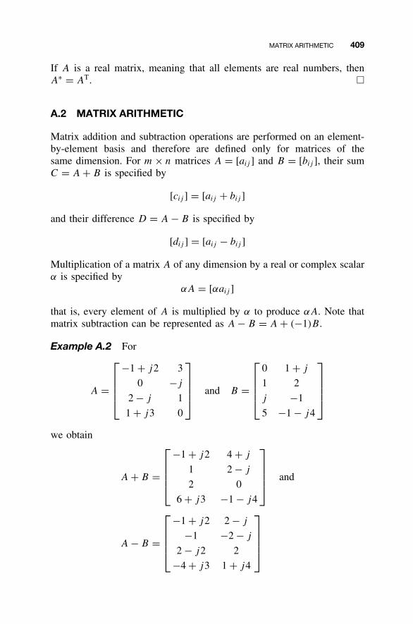
MATRIX ARITHMETIC 409
If A is a real matrix, meaning that all elements are real numbers, thenA∗ = AT. �
A.2 MATRIX ARITHMETIC
Matrix addition and subtraction operations are performed on an element-by-element basis and therefore are defined only for matrices of thesame dimension. For m × n matrices A = [aij ] and B = [bij ], their sumC = A + B is specified by
[cij ] = [aij + bij ]
and their difference D = A − B is specified by
[dij ] = [aij − bij ]
Multiplication of a matrix A of any dimension by a real or complex scalarα is specified by
αA = [αaij ]
that is, every element of A is multiplied by α to produce αA. Note thatmatrix subtraction can be represented as A − B = A + (−1)B.
Example A.2 For
A =
−1 + j2 3
0 −j
2 − j 1
1 + j3 0
and B =
0 1 + j
1 2
j −1
5 −1 − j4
we obtain
A + B =
−1 + j2 4 + j
1 2 − j
2 0
6 + j3 −1 − j4
and
A − B =
−1 + j2 2 − j
−1 −2 − j
2 − j2 2
−4 + j3 1 + j4
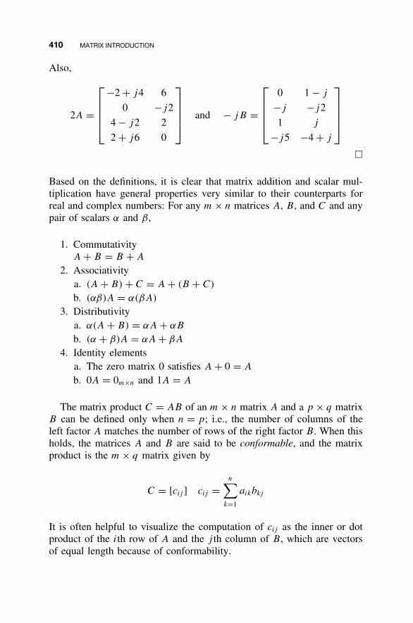
410 MATRIX INTRODUCTION
Also,
2A =
−2 + j4 6
0 −j2
4 − j2 2
2 + j6 0
and − jB =
0 1 − j
−j −j2
1 j
−j5 −4 + j
�
Based on the definitions, it is clear that matrix addition and scalar mul-tiplication have general properties very similar to their counterparts forreal and complex numbers: For any m × n matrices A, B, and C and anypair of scalars α and β,
1. CommutativityA + B = B + A
2. Associativitya. (A + B) + C = A + (B + C)
b. (αβ)A = α(βA)
3. Distributivitya. α(A + B) = αA + αB
b. (α + β)A = αA + βA
4. Identity elementsa. The zero matrix 0 satisfies A + 0 = A
b. 0A = 0m×n and 1A = A
The matrix product C = AB of an m × n matrix A and a p × q matrixB can be defined only when n = p; i.e., the number of columns of theleft factor A matches the number of rows of the right factor B. When thisholds, the matrices A and B are said to be conformable, and the matrixproduct is the m × q matrix given by
C = [cij ] cij =n∑
k=1
aikbkj
It is often helpful to visualize the computation of cij as the inner or dotproduct of the ith row of A and the j th column of B, which are vectorsof equal length because of conformability.
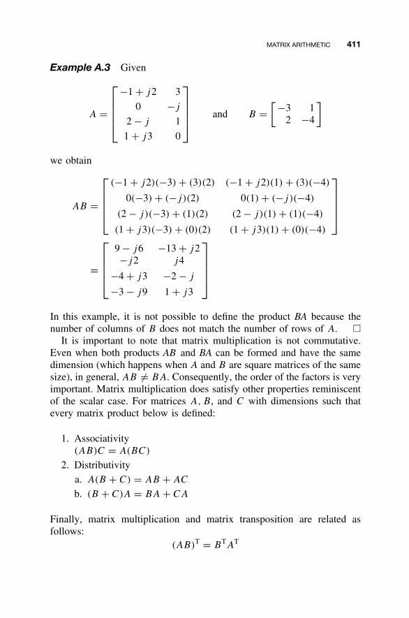
MATRIX ARITHMETIC 411
Example A.3 Given
A =
−1 + j2 3
0 −j
2 − j 1
1 + j3 0
and B =
[ −3 12 −4
]
we obtain
AB =
(−1 + j2)(−3) + (3)(2) (−1 + j2)(1) + (3)(−4)
0(−3) + (−j)(2) 0(1) + (−j)(−4)
(2 − j)(−3) + (1)(2) (2 − j)(1) + (1)(−4)
(1 + j3)(−3) + (0)(2) (1 + j3)(1) + (0)(−4)
=
9 − j6 −13 + j2−j2 j4
−4 + j3 −2 − j
−3 − j9 1 + j3
In this example, it is not possible to define the product BA because thenumber of columns of B does not match the number of rows of A. �
It is important to note that matrix multiplication is not commutative.Even when both products AB and BA can be formed and have the samedimension (which happens when A and B are square matrices of the samesize), in general, AB �= BA. Consequently, the order of the factors is veryimportant. Matrix multiplication does satisfy other properties reminiscentof the scalar case. For matrices A, B, and C with dimensions such thatevery matrix product below is defined:
1. Associativity(AB)C = A(BC)
2. Distributivitya. A(B + C) = AB + AC
b. (B + C)A = BA + CA
Finally, matrix multiplication and matrix transposition are related asfollows:
(AB)T = BTAT
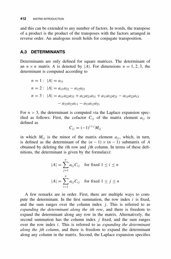
412 MATRIX INTRODUCTION
and this can be extended to any number of factors. In words, the transposeof a product is the product of the transposes with the factors arranged inreverse order. An analogous result holds for conjugate transposition.
A.3 DETERMINANTS
Determinants are only defined for square matrices. The determinant ofan n × n matrix A is denoted by |A|. For dimensions n = 1, 2, 3, thedeterminant is computed according to
n = 1 : |A| = a11
n = 2 : |A| = a11a22 − a12a21
n = 3 : |A| = a11a22a33 + a12a23a31 + a13a32a21 − a31a22a13
− a32a23a11 − a33a12a21
For n > 3, the determinant is computed via the Laplace expansion spec-ified as follows: First, the cofactor Cij of the matrix element aij isdefined as
Cij = (−1)i+jMij
in which Mij is the minor of the matrix element aij , which, in turn,is defined as the determinant of the (n − 1) × (n − 1) submatrix of A
obtained by deleting the ith row and j th column. In terms of these defi-nitions, the determinant is given by the formula(s):
|A| =n∑
j=1
aijCij for fixed 1 ≤ i ≤ n
|A| =n∑
i=1
aijCij for fixed 1 ≤ j ≤ n
A few remarks are in order. First, there are multiple ways to com-pute the determinant. In the first summation, the row index i is fixed,and the sum ranges over the column index j . This is referred to asexpanding the determinant along the ith row, and there is freedom toexpand the determinant along any row in the matrix. Alternatively, thesecond summation has the column index j fixed, and the sum rangesover the row index i. This is referred to as expanding the determinantalong the jth column, and there is freedom to expand the determinantalong any column in the matrix. Second, the Laplace expansion specifies
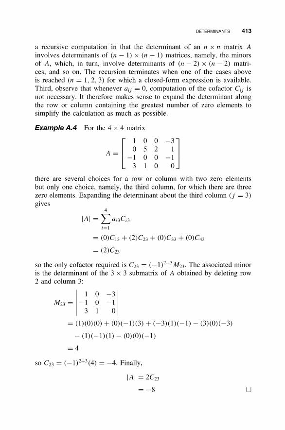
DETERMINANTS 413
a recursive computation in that the determinant of an n × n matrix A
involves determinants of (n − 1) × (n − 1) matrices, namely, the minorsof A, which, in turn, involve determinants of (n − 2) × (n − 2) matri-ces, and so on. The recursion terminates when one of the cases aboveis reached (n = 1, 2, 3) for which a closed-form expression is available.Third, observe that whenever aij = 0, computation of the cofactor Cij isnot necessary. It therefore makes sense to expand the determinant alongthe row or column containing the greatest number of zero elements tosimplify the calculation as much as possible.
Example A.4 For the 4 × 4 matrix
A =
1 0 0 −30 5 2 1
−1 0 0 −13 1 0 0
there are several choices for a row or column with two zero elementsbut only one choice, namely, the third column, for which there are threezero elements. Expanding the determinant about the third column (j = 3)
gives
|A| =4∑
i=1
ai3Ci3
= (0)C13 + (2)C23 + (0)C33 + (0)C43
= (2)C23
so the only cofactor required is C23 = (−1)2+3M23. The associated minoris the determinant of the 3 × 3 submatrix of A obtained by deleting row2 and column 3:
M23 =∣∣∣∣∣∣
1 0 −3−1 0 −1
3 1 0
∣∣∣∣∣∣= (1)(0)(0) + (0)(−1)(3) + (−3)(1)(−1) − (3)(0)(−3)
− (1)(−1)(1) − (0)(0)(−1)
= 4
so C23 = (−1)2+3(4) = −4. Finally,
|A| = 2C23
= −8 �
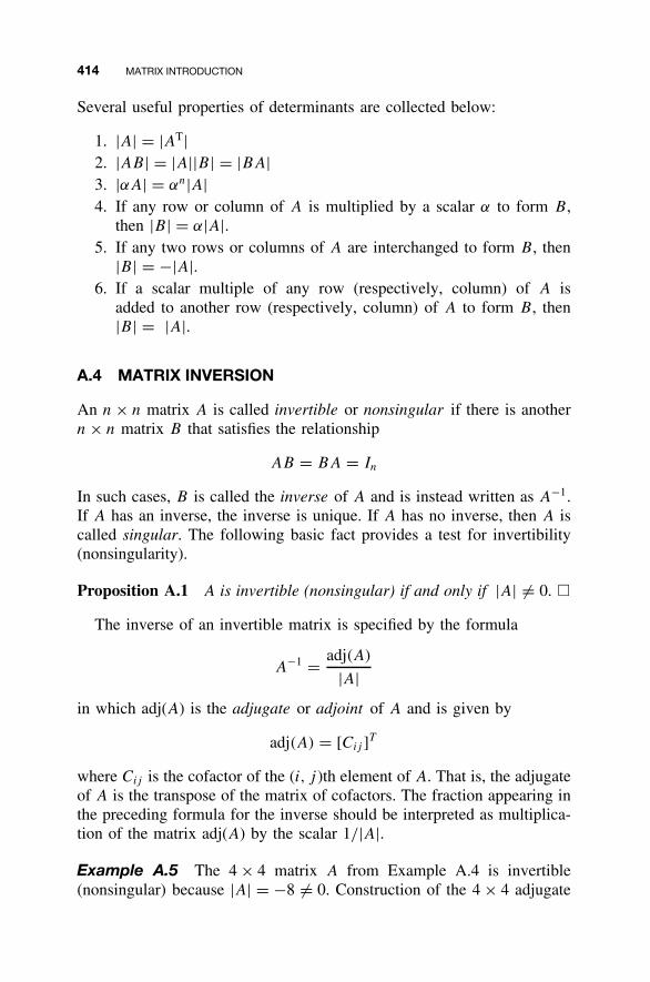
414 MATRIX INTRODUCTION
Several useful properties of determinants are collected below:
1. |A| = |AT|2. |AB| = |A||B| = |BA|3. |αA| = αn|A|4. If any row or column of A is multiplied by a scalar α to form B,
then |B| = α|A|.5. If any two rows or columns of A are interchanged to form B, then
|B| = −|A|.6. If a scalar multiple of any row (respectively, column) of A is
added to another row (respectively, column) of A to form B, then|B| = |A|.
A.4 MATRIX INVERSION
An n × n matrix A is called invertible or nonsingular if there is anothern × n matrix B that satisfies the relationship
AB = BA = In
In such cases, B is called the inverse of A and is instead written as A−1.If A has an inverse, the inverse is unique. If A has no inverse, then A iscalled singular. The following basic fact provides a test for invertibility(nonsingularity).
Proposition A.1 A is invertible (nonsingular) if and only if |A| �= 0. �
The inverse of an invertible matrix is specified by the formula
A−1 = adj(A)
|A|in which adj(A) is the adjugate or adjoint of A and is given by
adj(A) = [Cij ]T
where Cij is the cofactor of the (i, j )th element of A. That is, the adjugateof A is the transpose of the matrix of cofactors. The fraction appearing inthe preceding formula for the inverse should be interpreted as multiplica-tion of the matrix adj(A) by the scalar 1/|A|.Example A.5 The 4 × 4 matrix A from Example A.4 is invertible(nonsingular) because |A| = −8 �= 0. Construction of the 4 × 4 adjugate
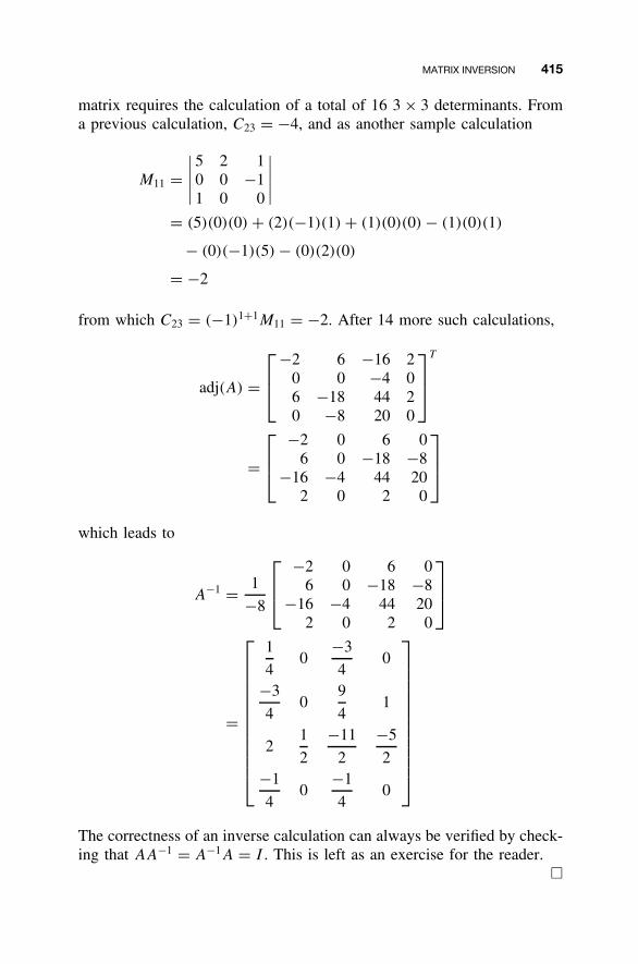
MATRIX INVERSION 415
matrix requires the calculation of a total of 16 3 × 3 determinants. Froma previous calculation, C23 = −4, and as another sample calculation
M11 =∣∣∣∣∣5 2 10 0 −11 0 0
∣∣∣∣∣= (5)(0)(0) + (2)(−1)(1) + (1)(0)(0) − (1)(0)(1)
− (0)(−1)(5) − (0)(2)(0)
= −2
from which C23 = (−1)1+1M11 = −2. After 14 more such calculations,
adj(A) =
−2 6 −16 20 0 −4 06 −18 44 20 −8 20 0
T
=
−2 0 6 06 0 −18 −8
−16 −4 44 202 0 2 0
which leads to
A−1 = 1
−8
−2 0 6 06 0 −18 −8
−16 −4 44 202 0 2 0
=
1
40
−3
40
−3
40
9
41
21
2
−11
2
−5
2−1
40
−1
40
The correctness of an inverse calculation can always be verified by check-ing that AA−1 = A−1A = I . This is left as an exercise for the reader.
�
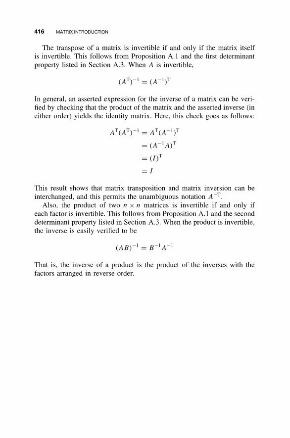
416 MATRIX INTRODUCTION
The transpose of a matrix is invertible if and only if the matrix itselfis invertible. This follows from Proposition A.1 and the first determinantproperty listed in Section A.3. When A is invertible,
(AT)−1 = (A−1)T
In general, an asserted expression for the inverse of a matrix can be veri-fied by checking that the product of the matrix and the asserted inverse (ineither order) yields the identity matrix. Here, this check goes as follows:
AT(AT)−1 = AT(A−1)T
= (A−1A)T
= (I )T
= I
This result shows that matrix transposition and matrix inversion can beinterchanged, and this permits the unambiguous notation A−T.
Also, the product of two n × n matrices is invertible if and only ifeach factor is invertible. This follows from Proposition A.1 and the seconddeterminant property listed in Section A.3. When the product is invertible,the inverse is easily verified to be
(AB)−1 = B−1A−1
That is, the inverse of a product is the product of the inverses with thefactors arranged in reverse order.
APPENDIX BLINEAR ALGEBRA
This appendix presents an overview of selected topics from linear algebrathat support state-space methods for linear control systems.
B.1 VECTOR SPACES
Definition B.1 A linear vector space X over a field of scalars F is aset of elements (called vectors) that is closed under two operations: vectoraddition and scalar multiplication. That is,
x1 + x2 ∈ X for all x1, x2 ∈ X
andαx ∈ X for all x ∈ X and for all α ∈ F
In addition, the following axioms are satisfied for all x, x1, x2, x3 ∈ X andfor all α, α1, α2 ∈ F:
1. Commutativityx1 + x2 = x2 + x1
2. Associativitya. (x1 + x2) + x3 = x1 + (x2 + x3)
b. (α1α2)x = α1(α2x)
3. Distributivitya. α(x1 + x2) = αx1 + αx2
b. (α1 + α2)x = α1x + α2x
417
Linear State-Space Control Systems. Robert L. Williams II and Douglas A. LawrenceCopyright 2007 John Wiley & Sons, Inc. ISBN: 978-0-471-73555-7
418 LINEAR ALGEBRA
4. Identity elementsa. There is a zero vector 0 ∈ X such that x + 0 = x
b. For additive and multiplicative identity elements in F, denoted 0and 1, respectively,
0x = 0 and 1x = x �
Example B.1
Fn = {x = (x1, x2, . . . , xn), xi ∈ F, i = 1, . . . , n}
i.e., the set of all n-tuples with elements in F. When F is either the real fieldR or the complex field C, R
n and Cn denote real and complex Euclidean
space, respectively. �
Example B.2
Fm×n = {A = [aij ], aij ∈ F, i = 1, . . . , m, j = 1, . . . , n}
i.e., the set of all m × n matrices with elements in F. Again, typicallyF is either R or C, yielding the set of real or complex m × n matrices,respectively. That C
m×n is a vector space over C is a direct consequenceof the discussion in Section A.2. Note that by stacking columns of anm × n matrix on top of one another to form a vector, we can identifyF
m×n with Fmn. �
Example B.3 C[a, b], the set of continuous functions f : [a, b] → F,with vector addition and scalar multiplication defined in a pointwise senseas follows:
(f + g)(x) := f (x) + g(x) (αf )(x) := αf (x) for all x ∈ [a, b]
for all f, g ∈ C[a, b] and α ∈ F. �
Definition B.2 Let x1, x2, . . . , xk be vectors in X. Their span isdefined as
span{x1, x2, . . . , xk} := {x = α1x1 + α2x2 + · · · + αkxk, αi ∈ F}
i.e., the set of all linear combinations of x1, x2, . . . , xk . �
SUBSPACES 419
Definition B.3 A set of vectors {x1, x2, . . . , xk} is linearly independentif the relation
α1x1 + α2x2 + · · · + αkxk = 0
implies that α1 = α2 = · · · = αk = 0. �
Lemma B.4 If {x1, x2, . . . , xk} is a linearly independent set of vectorsand x ∈ span{x1, x2, . . . , xk}, then the relation
x = α1x1 + α2x2 + · · · + αkxk
is unique.
Proof. Suppose that x = β1x1 + β2x2 + · · · + βkxk is another represen-tation with βi �= αi for at least one i ∈ {1, . . . , k}. Then
0 = x − x
= (α1x1 + α2x2 + · · · + αkxk) − (β1x1 + β2x2 + · · · + βkxk)
= (α1 − β1)x1 + (α2 − β2)x2 + · · · + (αk − βk)xk
By assumption, αi − βi �= 0 for some i, which contradicts the linear inde-pendence hypothesis. �
B.2 SUBSPACES
Definition B.5 A linear subspace S of a linear vector space X is asubset of X that is itself a linear vector space under the vector additionand scalar multiplication defined on X. �
Definition B.6 A basis for a linear subspace S is a linearly independentset of vectors {x1, x2, . . . , xk} such that
S = span{x1, x2, . . . , xk} �
A basis for S is not unique; however, all bases for S have the samenumber of elements, which defines the dimension of the linear subspaceS. Since a linear vector space X can be viewed as a subspace of itself, theconcepts of basis and dimension apply to X as well.
420 LINEAR ALGEBRA
On R3:
1. {0} is a zero-dimensional subspace called the zero subspace.2. Any line through the origin is a one-dimensional subspace, and any
nonzero vector on the line is a valid basis.3. Any plane through the origin is a two-dimensional subspace, and
any two noncollinear vectors in the plane form a valid basis.4. R
3 is a three-dimensional subspace of itself, and any three noncopla-nar vectors form a valid basis.
Example B.4 The set of all 2 × 2 real matrices R2×2 is a four-
dimensional vector space, and a valid basis is
{[1 00 0
],
[0 10 0
],
[0 01 0
],
[0 00 1
]}
because
A =[
a11 a12
a21 a22
]
= a11
[1 00 0
]+ a12
[0 10 0
]+ a21
[0 01 0
]+ a22
[0 00 1
]
The subset of all upper triangular matrices
A =[
a11 a12
0 a22
]
is a three-dimensional subspace, and a valid basis is obtained by omitting
[0 01 0
]
in the basis for R2×2 given above.
The subset of symmetric matrices A = AT (so that a12 = a21) is athree-dimensional subspace, and a valid basis is
{[1 00 0
],
[0 11 0
],
[0 00 1
]}�
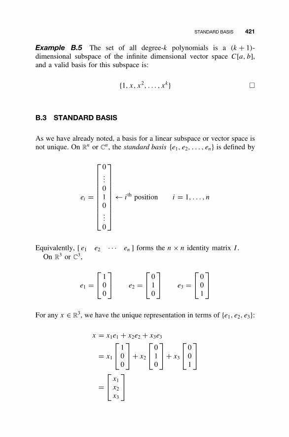
STANDARD BASIS 421
Example B.5 The set of all degree-k polynomials is a (k + 1)-dimensional subspace of the infinite dimensional vector space C[a, b],and a valid basis for this subspace is:
{1, x, x2, . . . , xk} �
B.3 STANDARD BASIS
As we have already noted, a basis for a linear subspace or vector space isnot unique. On R
n or Cn, the standard basis {e1, e2, . . . , en} is defined by
ei =
0...
010...
0
← i th position i = 1, . . . , n
Equivalently, [ e1 e2 · · · en ] forms the n × n identity matrix I .On R
3 or C3,
e1 = 1
00
e2 =
0
10
e3 =
0
01
For any x ∈ R3, we have the unique representation in terms of {e1, e2, e3}:
x = x1e1 + x2e2 + x3e3
= x1
1
00
+ x2
0
10
+ x3
0
01
= x1
x2
x3
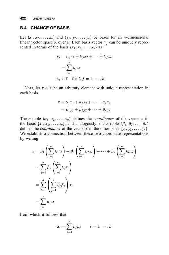
422 LINEAR ALGEBRA
B.4 CHANGE OF BASIS
Let {x1, x2, . . . , xn} and {y1, y2, . . . , yn} be bases for an n-dimensionallinear vector space X over F. Each basis vector yj can be uniquely repre-sented in terms of the basis {x1, x2, . . . , xn} as
yj = t1j x1 + t2j x2 + · · · + tnjxn
=n∑
i=1
tij xi
tij ∈ F for i, j = 1, · · · , nNext, let x ∈ X be an arbitrary element with unique representation in
each basis
x = α1x1 + α2x2 + · · · + αnxn
= β1y1 + β2y2 + · · · + βnyn
The n-tuple (α1, α2, . . . , αn) defines the coordinates of the vector x inthe basis {x1, x2, . . . , xn}, and analogously, the n-tuple (β1, β2, . . . , βn)
defines the coordinates of the vector x in the other basis {y1, y2, . . . , yn}.We establish a connection between these two coordinate representationsby writing
x = β1
(n∑
i=1
ti1xi
)+ β2
(n∑
i=1
ti2xi
)+ · · · + βn
(n∑
i=1
tinxi
)
=n∑
j=1
βj
(n∑
i=1
tij xi
)
=n∑
i=1
n∑
j=1
tijβj
xi
=n∑
i=1
αixi
from which it follows that
αi =n∑
j=1
tijβj i = 1, · · · , n
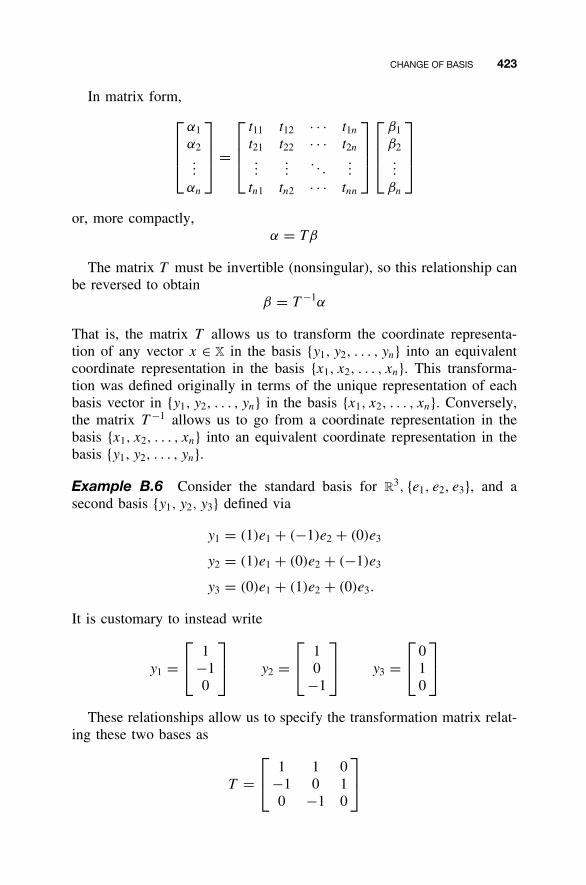
CHANGE OF BASIS 423
In matrix form,
α1
α2...
αn
=
t11 t12 · · · t1n
t21 t22 · · · t2n
......
. . ....
tn1 tn2 · · · tnn
β1
β2...
βn
or, more compactly,α = Tβ
The matrix T must be invertible (nonsingular), so this relationship canbe reversed to obtain
β = T −1α
That is, the matrix T allows us to transform the coordinate representa-tion of any vector x ∈ X in the basis {y1, y2, . . . , yn} into an equivalentcoordinate representation in the basis {x1, x2, . . . , xn}. This transforma-tion was defined originally in terms of the unique representation of eachbasis vector in {y1, y2, . . . , yn} in the basis {x1, x2, . . . , xn}. Conversely,the matrix T −1 allows us to go from a coordinate representation in thebasis {x1, x2, . . . , xn} into an equivalent coordinate representation in thebasis {y1, y2, . . . , yn}.Example B.6 Consider the standard basis for R
3, {e1, e2, e3}, and asecond basis {y1, y2, y3} defined via
y1 = (1)e1 + (−1)e2 + (0)e3
y2 = (1)e1 + (0)e2 + (−1)e3
y3 = (0)e1 + (1)e2 + (0)e3.
It is customary to instead write
y1 = 1
−10
y2 =
1
0−1
y3 =
0
10
These relationships allow us to specify the transformation matrix relat-ing these two bases as
T = 1 1 0
−1 0 10 −1 0
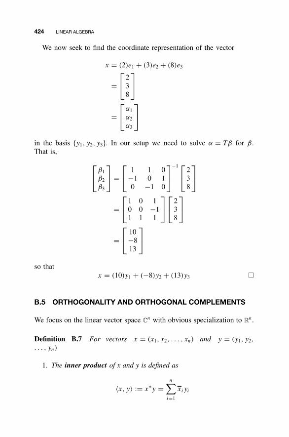
424 LINEAR ALGEBRA
We now seek to find the coordinate representation of the vector
x = (2)e1 + (3)e2 + (8)e3
= 2
38
=α1
α2
α3
in the basis {y1, y2, y3}. In our setup we need to solve α = Tβ for β.That is,
β1
β2
β3
=
1 1 0
−1 0 10 −1 0
−1 2
38
= 1 0 1
0 0 −11 1 1
2
38
= 10
−813
so thatx = (10)y1 + (−8)y2 + (13)y3 �
B.5 ORTHOGONALITY AND ORTHOGONAL COMPLEMENTS
We focus on the linear vector space Cn with obvious specialization to R
n.
Definition B.7 For vectors x = (x1, x2, . . . , xn) and y = (y1, y2,
. . . , yn)
1. The inner product of x and y is defined as
〈x, y〉 := x∗y =n∑
i=1
xiyi
ORTHOGONALITY AND ORTHOGONAL COMPLEMENTS 425
where the ∗-superscript denotes conjugate transpose. Note that
〈y, x〉 = y∗x = (x∗y)∗ = 〈x, y〉∗. For x, y ∈ Rn, 〈x, y〉 := xT y
= yT x = 〈y, x〉.
2. Vectors x, y ∈ Cn are orthogonal if 〈x, y〉 = 0.
3. The Euclidian norm of x ∈ Cn is given by
||x|| = 〈x, x〉 12 =
(n∑
i=1
|xi |2) 1
2
4. A set of vectors {x1, x2, . . . , xk} is orthogonal if 〈xi, xj 〉 = 0 fori �= j and orthonormal if, in addition, ||xi || = 1, i = 1, . . . , k.
For a subspace S ⊂ Cn
1. A set of vectors {x1, x2, · · · , xk} is called an orthonormal basis forS if it is an orthonormal set and is a basis for S.
2. The orthogonal complement of S is defined as
S⊥ = {y ∈ C
n|〈y, x〉 = 0 ∀x ∈ S} �
It follows from the definition that S⊥ is also a subspace of C
n. Moreover,if {x1, x2, . . . , xk} is a basis for S, then an equivalent though simplercharacterization of S
⊥ is
S⊥ = {y ∈ C
n|〈y, xi〉 = 0; i = 1, . . . , k}
It also can be shown that dim(S⊥) = dim(Cn) − dim(S) = n − k and
S⊥ = span{y1, y2, . . . , yn−k}
for any linearly independent set of vectors {y1, y2, . . . , yn−k} that satisfy
〈yj , xi〉 = 0 i = 1, . . . , k j = 1, . . . , n − k
426 LINEAR ALGEBRA
Example B.7 On R3,
1. Suppose that S = span{x1} with
x1 = 1
0−1
Then S⊥ = span{y1, y2} with
y1 = 1
01
y2 =
0
10
2. Suppose that S = span{x1, x2} with
x1 = 1
11
x2 =
0
11
Then S⊥ = span{y1} with
y1 = 0
−11
�
B.6 LINEAR TRANSFORMATIONS
Definition B.8 Let X and Y be linear vector spaces over the same fieldF. A transformation A : X → Y is linear if
A(α1x1 + α2x2) = α1Ax1 + α2Ax2 f or all x1, x2 ∈ X
and for all α1, α2 ∈ F �
Suppose that X = Cn and Y ∈ C
m. A linear transformation A : Cn → C
m
is specified in terms of its action on a basis for Cn, represented in terms
of a basis for Cm.
Let {x1, x2, . . . , xn} be a basis for Cn and {y1, y2, . . . , ym} be a basis
for Cm. Then Axj ∈ C
m, j = 1, . . . , n, has the unique representation
Axj = a1j y1 + a2j y2 + · · · + amjym
LINEAR TRANSFORMATIONS 427
As we have seen previously, the m-tuple (a1j , a2j , . . . , amj ) defines thecoordinates of Axj in the basis {y1, y2, . . . , ym}.
Next, for every x ∈ Cn and y := Ax, we have the unique representation
in the appropriate basis
x = α1x1 + α2x2 + · · · + αnxn
y = β1y1 + β2y2 + · · · + βmym
Again, the n-tuple (α1, α2, . . . , αn) defines the coordinates of the vector x
in the basis {x1, x2, . . . , xn} and the m-tuple (β1, β2, . . . , βm) defines thecoordinates of the vector y in the basis {y1, y2, . . . , ym}.Putting everything together and using linearity of the transformation A,leads to
y = Ax
= A
n∑
j=1
αjxj
=n∑
j=1
αjAxj
=n∑
j=1
αj
(m∑
i=1
aijyi
)
=m∑
i=1
n∑
j=1
aijαj
yi
Comparing this with the unique representation for y = Ax given previ-ously, we therefore require
βi =n∑
j=1
aijαj i = 1, · · · , m
or more compactly, in matrix notation,
β1
β2...
βm
=
a11 a12 · · · a1n
a21 a22 · · · a2n
......
. . ....
am1 am2 · · · amn
α1
α2...
αn
428 LINEAR ALGEBRA
Thus, with respect to the basis {x1, x2, . . . , xn} for Cn and the basis
{y1, y2, . . . , ym} for Cm, the linear transformation A : C
n → Cm has the
m × n matrix representation
A =
a11 a12 · · · a1n
a21 a22 · · · a2n
......
. . ....
am1 am2 · · · amn
.
If different bases are used for Cn and/or C
m, the same linear transformationwill have a different matrix representation. Often a matrix is used torepresent a linear transformation with the implicit understanding that thestandard bases for C
n and Cm are being used.
Example B.8 Let A : R3 → R
2 be the linear transformation having thematrix representation with respect to the standard bases for R
3 and R2
given by
A =[
1 2 34 5 6
]
That is,
A
1
00
=
[14
]= (1)
[10
]+ (4)
[01
]
A
0
10
=
[25
]= (2)
[10
]+ (5)
[01
]
A
0
01
=
[36
]= (3)
[10
]+ (6)
[01
].
Suppose instead that we consider the following basis for R3:
x1 =
1
11
, x2 =
0
22
, x3 =
0
03
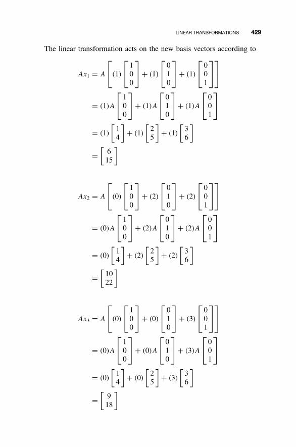
LINEAR TRANSFORMATIONS 429
The linear transformation acts on the new basis vectors according to
Ax1 = A
(1)
1
00
+ (1)
0
10
+ (1)
0
01
= (1)A
1
00
+ (1)A
0
10
+ (1)A
0
01
= (1)
[14
]+ (1)
[25
]+ (1)
[36
]
=[
615
]
Ax2 = A
(0)
1
00
+ (2)
0
10
+ (2)
0
01
= (0)A
1
00
+ (2)A
0
10
+ (2)A
0
01
= (0)
[14
]+ (2)
[25
]+ (2)
[36
]
=[
1022
]
Ax3 = A
(0)
1
00
+ (0)
0
10
+ (3)
0
01
= (0)A
1
00
+ (0)A
0
10
+ (3)A
0
01
= (0)
[14
]+ (0)
[25
]+ (3)
[36
]
=[
918
]
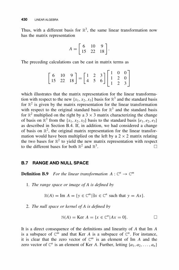
430 LINEAR ALGEBRA
Thus, with a different basis for R3, the same linear transformation now
has the matrix representation
A =[
6 10 915 22 18
].
The preceding calculations can be cast in matrix terms as
[6 10 9
15 22 18
]=
[1 2 34 5 6
] 1 0 0
1 2 01 2 3
which illustrates that the matrix representation for the linear transforma-tion with respect to the new {x1, x2, x3} basis for R
3 and the standard basisfor R
2 is given by the matrix representation for the linear transformationwith respect to the original standard basis for R
3 and the standard basisfor R
2 multiplied on the right by a 3 × 3 matrix characterizing the changeof basis on R
3 from the {x1, x2, x3} basis to the standard basis {e1, e2, e3}as described in Section B.4. If, in addition, we had considered a changeof basis on R
2, the original matrix representation for the linear transfor-mation would have been multiplied on the left by a 2 × 2 matrix relatingthe two bases for R
2 to yield the new matrix representation with respectto the different bases for both R
2 and R3. �
B.7 RANGE AND NULL SPACE
Definition B.9 For the linear transformation A : Cn → C
m
1. The range space or image of A is defined by
R(A) = Im A = {y ∈ Cm|∃x ∈ C
n such that y = Ax}.
2. The null space or kernel of A is defined by
N(A) = Ker A = {x ∈ Cn|Ax = 0}. �
It is a direct consequence of the definitions and linearity of A that Im A
is a subspace of Cm and that Ker A is a subspace of C
n. For instance,it is clear that the zero vector of C
m is an element of Im A and thezero vector of C
n is an element of Ker A. Further, letting {a1, a2, . . . , an}
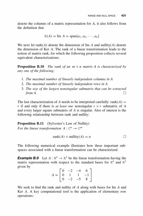
RANGE AND NULL SPACE 431
denote the columns of a matrix representation for A, it also follows fromthe definition that
R(A) = Im A = span{a1, a2, · · · , an}
We next let rank(A) denote the dimension of Im A and nullity(A) denotethe dimension of Ker A. The rank of a linear transformation leads to thenotion of matrix rank, for which the following proposition collects severalequivalent characterizations:
Proposition B.10 The rank of an m × n matrix A is characterized byany one of the following:
1. The maximal number of linearly independent columns in A2. The maximal number of linearly independent rows in A3. The size of the largest nonsingular submatrix that can be extracted
from A �
The last characterization of A needs to be interpreted carefully: rank(A) =r if and only if there is at least one nonsingular r × r submatrix of A
and every larger square submatrix of A is singular. Also of interest is thefollowing relationship between rank and nullity:
Proposition B.11 (Sylvester’s Law of Nullity)For the linear transformation A : C
n → Cm
rank(A) + nullity(A) = n �
The following numerical example illustrates how these important sub-spaces associated with a linear transformation can be characterized.
Example B.9 Let A : R4 → R
3 be the linear transformation having thematrix representation with respect to the standard bases for R
4 and R3
given by
A = 0 −2 −4 6
0 1 1 −10 −2 −5 8
We seek to find the rank and nullity of A along with bases for Im A andKer A. A key computational tool is the application of elementary rowoperations:
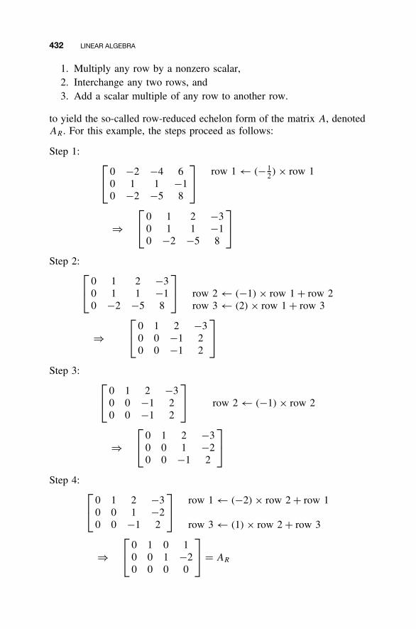
432 LINEAR ALGEBRA
1. Multiply any row by a nonzero scalar,2. Interchange any two rows, and3. Add a scalar multiple of any row to another row.
to yield the so-called row-reduced echelon form of the matrix A, denotedAR. For this example, the steps proceed as follows:
Step 1: 0 −2 −4 6
0 1 1 −10 −2 −5 8
row 1 ← (− 1
2) × row 1
⇒ 0 1 2 −3
0 1 1 −10 −2 −5 8
Step 2: 0 1 2 −3
0 1 1 −10 −2 −5 8
row 2 ← (−1) × row 1 + row 2
row 3 ← (2) × row 1 + row 3
⇒ 0 1 2 −3
0 0 −1 20 0 −1 2
Step 3: 0 1 2 −3
0 0 −1 20 0 −1 2
row 2 ← (−1) × row 2
⇒ 0 1 2 −3
0 0 1 −20 0 −1 2
Step 4: 0 1 2 −3
0 0 1 −20 0 −1 2
row 1 ← (−2) × row 2 + row 1
row 3 ← (1) × row 2 + row 3
⇒ 0 1 0 1
0 0 1 −20 0 0 0
= AR
RANGE AND NULL SPACE 433
We then have
rank(A) = the number of linearly independent columns in A or AR
= the number of linearly independent rows in A or AR
= the number of nonzero rows in AR
= 2
By Sylvester’s law of nullity:
nullity(A) = n − rank(A)
= 4 − 2
= 2
A basis for Im A can be formed by any rank(A) = 2 linearly inde-pendent columns of A. (AR cannot be used here because elementary rowoperations affect the image.) Possible choices are
−2
1−2
,
−4
1−5
−2
1−2
,
6
−18
,
−4
1−5
,
6
−18
Linear independence of each vector pair can be verified by checking thatthe associated 3 × 2 matrix has a nonsingular 2 × 2 submatrix.
A basis for Ker A can be formed by any nullity(A) = 2 linearly inde-pendent solutions to the homogeneous matrix equation Ax = 0. Sincethe solution space in not affected by elementary row operations, insteadwe may seek to characterize linearly independent solutions to ARx = 0.Writing
0 1 0 1
0 0 1 −20 0 0 0
x1
x2
x3
x4
=
x2 + x4
x3 − 2x4
0
=
0
00
we must satisfy x2 = −x4 and x3 = 2x4, with x1 and x4 treated as freeparameters. The combination x1 = 1, x4 = 0 yields x2 = x3 = 0, and we
434 LINEAR ALGEBRA
readily see that
1000
∈ Ker A
The combination x1 = 0, x4 = 1 yields x2 = −1, x3 = 2 which gives
0−121
∈ Ker A
The set
1000
,
0−121
is clearly linearly independent by virtue of our choices for x1 and x4
because the associated 4 × 2 matrix has the 2 × 2 identity matrix as thesubmatrix obtained by extracting the first and fourth rows. This set there-fore qualifies as a basis for Ker A. �
Lemma B.12 For the linear transformation A : Cn → C
m
1. [Im A]⊥ = Ker A∗
2. [Ker A]⊥ = Im A∗ �
It is a worthwhile exercise to prove the first part of Lemma B.12, whichasserts the equality of two subspaces. In general, the equality of twosubspaces S = T can be verified by demonstrating the pair of containmentsS ⊂ T and T ⊂ S. To show a containment relationship, say, S ⊂ T, it isenough to show that an arbitrary element of S is also an element of T.
We first show that [Im A]⊥ ⊂ Ker A∗. Let y be an arbitrary element of[Im A]⊥ so that, by definition, 〈y, z〉 = 0 for all z ∈ Im A. Consequently〈y, Ax〉 = 0 for all x ∈ C
n, from which we conclude that
〈A∗y, x〉 = (A∗y)∗x = y∗Ax = 〈y, Ax〉 = 0
Since the only vector orthogonal to every x ∈ Cn is the zero vector,
we must have A∗y = 0, that is, y ∈ Ker A∗. The desired containment[Im A]⊥ ⊂ Ker A∗ follows because y ∈ [Im A]⊥ was arbitrary.
EIGENVALUES, EIGENVECTORS, AND RELATED TOPICS 435
We next show that Ker A∗ ⊂ [Im A]⊥. Let y be an arbitrary elementof Ker A∗ so that A∗y = 0. Since the zero vector is orthogonal to everyvector in C
n, 〈A∗y, x〉 = 0, for all x ∈ Cn, from which we conclude that
〈y, Ax〉 = y∗Ax = (A∗y)∗x = 〈A∗y, x〉 = 0
Since for every z ∈ Im A, there must exist some x ∈ Cn such that z = Ax,
it follows that 〈y, z〉 = 0, that is, y ∈ [Im A]⊥. The desired containmentKer A∗ ⊂ [Im A]⊥ follows because y ∈ Ker A∗ was arbitrary. Havingestablished the required subspace containments, we may conclude that[Im A]⊥ = Ker A∗. �
Note that since the orthogonal complements satisfy S = T if and only ifS
⊥ = T⊥ and (S⊥)⊥ = S, the second subspace identity in Proposition B.4
is equivalent to [ImA∗]⊥ = Ker A. This, in turn, follows by applyingthe first subspace identity in Proposition B.4 to the linear transformationA∗ : C
m → Cn.
B.8 EIGENVALUES, EIGENVECTORS, AND RELATED TOPICS
Eigenvalues and Eigenvectors
Definition B.13 For a matrix A ∈ Cn×n
1. The characteristic polynomial of A is defined as
|λI − A| = λn + an−1λn−1 + · · · + a1λ + a0
2. The eigenvalues of A are the n roots1 of the characteristic equation
|λI − A| = 0
3. The spectrum of A is its set of eigenvalues, denoted
σ(A) = {λ1, λ2, . . . , λn}4. For each λi ∈ σ(A), any nonzero vector v ∈ C
n that satisfies
(λiI − A)v = 0 equivalently Av = λiv
is called a right eigenvector of A associated with the eigenvalue λi .
1As indicated, the characteristic polynomial of an n × n matrix is guaranteed to be amonic degree-n polynomial that, by the fundamental theorem of algebra, must have n
roots. If A is real, the roots still may be complex but must occur in conjugate pairs.
436 LINEAR ALGEBRA
5. For each λi ∈ σ(A), any nonzero vector w ∈ Cn that satisfies
w∗(λiI − A) = 0 equivalently w∗A = λiw∗
is called a left eigenvector of A associated with the eigenvalue λi .
For each eigenvalue λi of A, by definition, |λiI − A| = 0, so that λiI −A is a singular matrix and therefore has a nontrivial null space. Righteigenvectors, viewed as nontrivial solutions to the homogeneous equation(λiI − A)v = 0 are therefore nonzero vectors lying in Ker(λiI − A). Assuch, if v is an eigenvector of A associated the eigenvalue λi , then so isany nonzero scalar multiple of v.
By taking the conjugate transpose of either identity defining a lefteigenvector w associated with the eigenvalue λi , we see that w can beinterpreted as a right eigenvector of A∗ associated with the conjugateeigenvalue λi .
Example B.10 For
A = 1 0 0
2 3 −12 2 1
1. The characteristic polynomial of A can be obtained by expanding|λI − A| about the first row to yield
|λI − A| = λ − 1 0 0
−2 λ − 3 1−2 −2 λ − 1
= (λ − 1)[(λ − 3)(λ − 1) − (−2)(1)]
= (λ − 1)[λ2 − 4λ + 5]
= λ3 − 5λ2 + 9λ − 5
2. Factoring the characteristic polynomial
|λI − A| = (λ − 1)(λ − 2 − j)(λ − 2 + j)
indicates that the eigenvalues of A are λ1 = 1, λ2 = 2 + j , and λ3 =2 − j . Note that λ2 and λ3 are complex but form a conjugate pair.
3. The spectrum of A is simply
σ(A) = {λ1, λ2, λ3} = {1, 2 + j, 2 − j}
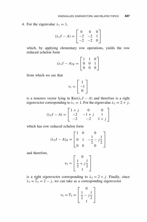
EIGENVALUES, EIGENVECTORS, AND RELATED TOPICS 437
4. For the eigenvalue λ1 = 1,
(λ1I − A) = 0 0 0
−2 −2 1−2 −2 0
which, by applying elementary row operations, yields the rowreduced echelon form
(λ1I − A)R = 1 1 0
0 0 10 0 0
from which we see that
v1 = 1
−10
is a nonzero vector lying in Ker(λ1I − A) and therefore is a righteigenvector corresponding to λ1 = 1. For the eigenvalue λ2 = 2 + j ,
(λ2I − A) = 1 + j 0 0
−2 −1 + j 1−2 −2 1 + j
which has row reduced echelon form
(λ2I − A)R =
1 0 0
0 1 −1
2− j
1
20 0 0
and therefore,
v2 =
01
2+ j
1
21
is a right eigenvector corresponding to λ2 = 2 + j . Finally, sinceλ3 = λ2 = 2 − j , we can take as a corresponding eigenvector
v3 = v2 =
01
2− j
1
21
438 LINEAR ALGEBRA
5. Proceeding in an analogous fashion for AT and, λ1 = λ1, λ2 = λ3,and λ3 = λ2, we see that associated left eigenvectors are given by
w1 = 1
00
w2 =
1
1− 1
2 − j 12
w3 = w2 = 1
1− 1
2 + j 12
�
Interesting situations arise in the search for eigenvectors when thematrix A has nondistinct or repeated eigenvalues. To explore further, wefirst require
Definition B.14 Let d ≤ n denote the number of distinct eigenvalues ofA, denoted {λ1, λ2, . . . , λd}. Upon factoring the characteristic polynomialof A accordingly,
det(λiI − A) = (λ − λ1)m1(λ − λ2)
m2 · · · (λ − λd)md
mi denotes the algebraic multiplicity of the eigenvalue λi for i = 1, . . . , d.The geometric multiplicity of the eigenvalue λi is defined as
ni = nullity(λiI − A) = dim Ker(λiI − A)
for i = 1, . . . , d. �As a consequence, for each distinct eigenvalue λi , i = 1, . . . , d, there areni linearly independent solutions to the homogeneous equation (λiI −A)v = 0, which we denote by {vi
1, vi2, . . . , v
ini}. This set of vectors, in turn,
forms a so-called eigenbasis for the eigenspace Ker(λiI − A) associatedwith the eigenvalue λi .
The following facts establish some useful relationships.
Proposition B.15 For i = 1, . . . , d, 1 ≤ ni ≤ mi �
Proposition B.16 Eigenbases associated with different eigenvalues arelinearly independent. �We conclude this subsection with an illustrative example.
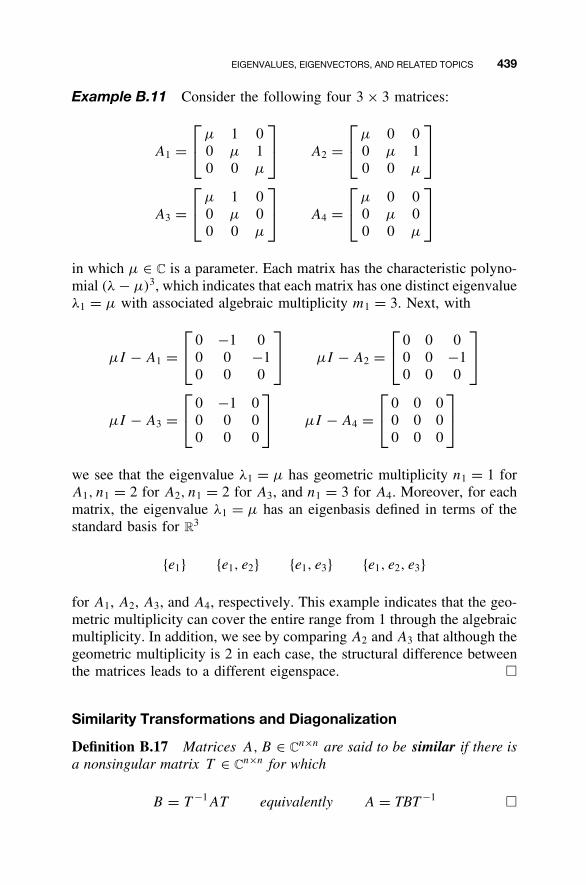
EIGENVALUES, EIGENVECTORS, AND RELATED TOPICS 439
Example B.11 Consider the following four 3 × 3 matrices:
A1 =µ 1 0
0 µ 10 0 µ
A2 =
µ 0 0
0 µ 10 0 µ
A3 =µ 1 0
0 µ 00 0 µ
A4 =
µ 0 0
0 µ 00 0 µ
in which µ ∈ C is a parameter. Each matrix has the characteristic polyno-mial (λ − µ)3, which indicates that each matrix has one distinct eigenvalueλ1 = µ with associated algebraic multiplicity m1 = 3. Next, with
µI − A1 = 0 −1 0
0 0 −10 0 0
µI − A2 =
0 0 0
0 0 −10 0 0
µI − A3 = 0 −1 0
0 0 00 0 0
µI − A4 =
0 0 0
0 0 00 0 0
we see that the eigenvalue λ1 = µ has geometric multiplicity n1 = 1 forA1, n1 = 2 for A2, n1 = 2 for A3, and n1 = 3 for A4. Moreover, for eachmatrix, the eigenvalue λ1 = µ has an eigenbasis defined in terms of thestandard basis for R
3
{e1} {e1, e2} {e1, e3} {e1, e2, e3}
for A1, A2, A3, and A4, respectively. This example indicates that the geo-metric multiplicity can cover the entire range from 1 through the algebraicmultiplicity. In addition, we see by comparing A2 and A3 that although thegeometric multiplicity is 2 in each case, the structural difference betweenthe matrices leads to a different eigenspace. �
Similarity Transformations and Diagonalization
Definition B.17 Matrices A, B ∈ Cn×n are said to be similar if there is
a nonsingular matrix T ∈ Cn×n for which
B = T −1AT equivalently A = TBT −1 �

440 LINEAR ALGEBRA
In this case, T is called a similarity transformation. A fundamental rela-tionship between similar matrices is the following.
Proposition B.18 If A and B are similar matrices, then they have thesame eigenvalues. �This result is proven by using determinant properties to show that similarmatrices have identical characteristic polynomials.
A diagonal matrix necessarily displays its eigenvalues on the maindiagonal. For a general matrix A, diagonalization refers to the process ofconstructing a similarity transformation yielding a diagonal matrix that,by virtue of the preceding proposition, displays the eigenvalues of A. Theability to diagonalize the matrix A via similarity transformation is closelyconnected to its underlying eigenstructure.
To investigate further, note that, by definition, the distinct eigenvaluesof A ∈ C
n×n have associated algebraic multiplicities that satisfy
m1 + m2 + · · · + md = n
because the characteristic polynomial of A has degree n. On the otherhand, the geometric multiplicities indicate that we can find a total ofn1 + n2 + · · · + nd eigenvectors associated with the distinct eigenvalues{λ1, λ2, . . . , λd}, written
{v11, v
12, . . . , v
1n1
, v21, v
22, . . . , v
2n2
, · · · , vd1 , vd
2 , . . . , vdnd
}
By Proposition B.16, this is a linearly independent set. The relationshipsAv
j
i = λivj
i , for i = 1, . . . , d and j = 1, . . . , ni , can be packaged into
AT = T �
in which T is the n × (n1 + n2 + · · · + nd) matrix whose columns are thecomplete set of eigenvectors, and � is a diagonal (n1 + n2 + · · · + nd) ×(n1 + n2 + · · · + nd) matrix given by
� = diag
λ1, · · · , λ1︸ ︷︷ ︸
n1times
, λ2, · · · , λ2︸ ︷︷ ︸n2times
, · · · λd, · · · , λd︸ ︷︷ ︸nd times
In the event that
n1 + n2 + · · · + nd = m1 + m2 + · · · + md = n
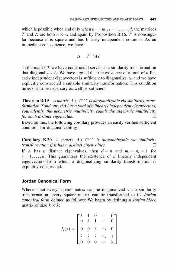
EIGENVALUES, EIGENVECTORS, AND RELATED TOPICS 441
which is possible when and only when ni = mi, i = 1, . . . , d, the matricesT and � are both n × n, and again by Proposition B.16, T is nonsingu-lar because it is square and has linearly independent columns. As animmediate consequence, we have
� = T −1AT
so the matrix T we have constructed serves as a similarity transformationthat diagonalizes A. We have argued that the existence of a total of n lin-early independent eigenvectors is sufficient to diagonalize A, and we haveexplicitly constructed a suitable similarity transformation. This conditionturns out to be necessary as well as sufficient.
Theorem B.19 A matrix A ∈ Cn×n is diagonalizable via similarity trans-
formation if and only if A has a total of n linearly independent eigenvectors,equivalently, the geometric multiplicity equals the algebraic multiplicityfor each distinct eigenvalue. �Based on this, the following corollary provides an easily verified sufficientcondition for diagonalizability:
Corollary B.20 A matrix A ∈ Cn×n is diagonalizable via similarity
transformation if it has n distinct eigenvalues. �If A has n distinct eigenvalues, then d = n and mi = ni = 1 fori = 1, . . . , n. This guarantees the existence of n linearly independenteigenvectors from which a diagonalizing similarity transformation isexplicitly constructed.
Jordan Canonical Form
Whereas not every square matrix can be diagonalized via a similaritytransformation, every square matrix can be transformed to its Jordancanonical form defined as follows: We begin by defining a Jordan blockmatrix of size k × k:
Jk(λ) =
λ 1 0 · · · 00 λ 1 · · · 0
0 0 λ. . . 0
......
.... . . 1
0 0 0 · · · λ
442 LINEAR ALGEBRA
displaying the parameter λ on the main diagonal and 1s on the first super-diagonal. An n × n Jordan matrix is a block diagonal matrix constructedfrom Jordan block matrices:
J =
Jk1(λ1) 0 · · · 00 Jk2(λ2) · · · 0...
.... . .
0 0 · · · Jkr(λr)
with k1 + k2 + · · · + kr = n
Note that if each ki = 1 and r = n, then J is a diagonal matrix.
Proposition B.21 Let A ∈ Cn×n have d distinct eigenvalues λ1, λ2, . . . ,
λd with associated algebraic and geometric multiplicities m1, m2, . . .,md and n1, n2, . . . , nd , respectively. There exists a similarity trans-formation T yielding a Jordan matrix
J = T −1AT
in which there are ni Jordan blocks associated with the eigenvalue λi , andthe sum of the sizes of these blocks equals the algebraic multiplicity mi ,for i = 1, . . . , d. The matrix J is unique up to a reordering of the Jordanblocks and defines the Jordan canonical form of A. �Note that the algebraic and geometric multiplicities alone do notcompletely determine the Jordan canonical form. For example, the Jordanmatrices
J1 =
λ 1 00 λ 10 0 λ
0 0 00 0 0
∣∣∣∣∣∣∣∣∣∣
0 00 00 0
λ 10 λ
J2 =
λ 1 0 00 λ 1 00 0 λ 10 0 0 λ
0 0 0 0
∣∣∣∣∣∣∣∣∣∣
0000
λ
each could represent the Jordan canonical form of a matrix having asingle distinct eigenvalue λ with algebraic multiplicity 5 and geometricmultiplicity 2. An interesting special case occurs when the geometricmultiplicity equals the algebraic multiplicity for a particular eigenvalue.In this case, each of the Jordan blocks associated with this eigenvalue isscalar. Conversely, if each of the Jordan blocks associated with a particular
EIGENVALUES, EIGENVECTORS, AND RELATED TOPICS 443
eigenvalue is scalar, then the geometric and algebraic multiplicities for thiseigenvalue must be equal. If the geometric multiplicity equals the algebraicmultiplicity for each distinct eigenvalue, then the Jordan canonical formis diagonal. This is consistent with Theorem B.19.
Cayley-Hamilton Theorem
Theorem B.22 For any matrix A ∈ Cn×n with characteristic polynomial
|λI − A| = λn + an−1λn−1 + · · · + a1λ + a0
there holds
An + an−1An−1 + · · · + a1A + a0I = 0 (n × n) �
By definition, eigenvalues of A are roots of the associated (scalar) charac-teristic equation. Loosely speaking, the Cayley-Hamilton theorem assertsthat the matrix A is itself a root of a matrix version of its characteristicequation. This is not difficult to verify when A is diagonalizable, althoughthe result still holds for nondiagonalizable matrices.
Example B.12 For the matrix A studied in Example B.10, the charac-teristic polynomial was found to be
λ3 − 5λ2 + 9λ − 5
Then
A3 − 5A2 + 9A − 5I = 1 0 0
12 13 −1122 22 −9
− 5 ·
1 0 0
6 7 −48 8 −1
+ 9 · 1 0 0
2 3 −12 2 1
− 5 ·
1 0 0
0 1 00 0 1
= 0 0 0
0 0 00 0 0
�
444 LINEAR ALGEBRA
B.9 NORMS FOR VECTORS AND MATRICES
Definition B.23 A vector norm on Cn is any real-valued function || · ||
that satisfies
Positive Definiteness: ||x|| ≥ 0 for all x ∈ Cn and ||x|| = 0 if and
only if x = 0 ∈ Cn
Triangle Inequality: ||x + y|| ≤ ||x|| + ||y|| for all x, y ∈ Cn
Homogeneity: ||αx|| = |α|||x|| for all x ∈ Cn and α ∈ C
�
A special class of norms, called p− norms, is defined by
||x||p = (|x1|p + |x2|p + · · · + |xn|p)1p for all p ∈ [1, ∞)
||x||∞ = max1≤i≤n
|xi |
Most common of these are || · ||1, || · ||∞, and
||x||2 = (|x1|2 + |x2|2 + · · · + |xn|2)12
= (x∗x)12
which is the familiar Euclidean norm. These p− norms satisfy the so-called Holder inequality
|x∗y| ≤ ||x||p||y||q for all x, y ∈ Cn and for all p, q
such that1
p+ 1
q= 1
The special case p = q = 2 yields the familiar Cauchy-Schwarzinequality:
|x∗y| ≤ ||x||2||y||2 for all x, y ∈ Cn
For a linear transformation A : Cn → C
m represented by a matrix A ∈C
m×n, we define:
NORMS FOR VECTORS AND MATRICES 445
Definition B.24 A matrix norm on Cn×m is any real-valued function || · ||
that satisfies
Positive Definiteness: ||A|| ≥ 0 for all A ∈ Cm×n and ||A|| = 0 if
and only if A = 0 ∈ Cm×n
Triangle Inequality: ||A + B|| ≤ ||A|| + ||B|| for all A, B ∈ Cm×n
Homogeneity: ||αA|| = |α|||A|| for all A ∈ Cm×n and α ∈ C
�
Corresponding to any pair of vector norms on Cn and C
m, respectively,we define an associated induced matrix norm according to
||A|| = supx �=0
||Ax||||x||
in which sup stands for supremum, or least upper bound, here taken overall nonzero vectors in C
n. It can be shown that this definition is equiva-lent to
||A|| = max||x||=1
||Ax||
As a direct consequence of the definition, any induced matrix norm sat-isfies
||Ax|| ≤ ||A||||x|| for all x ∈ Cn
The class of p− norms for vectors define a class of induced p− normsfor matrices via the preceding definition. For p = 1, 2, ∞, the inducedmatrix norms can be computed using
||A||1 = max1≤j≤n
m∑i=1
|aij |
||A||2 = (λmax(AT A))
12
||A||∞ = max1≤i≤m
n∑j=1
|aij |
The induced matrix 2− norm is often referred to as the spectral norm.
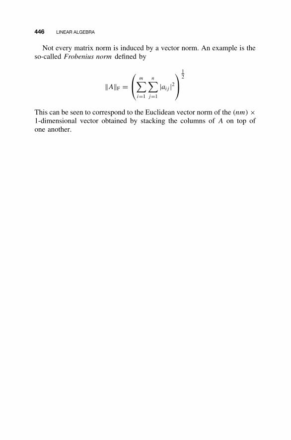
446 LINEAR ALGEBRA
Not every matrix norm is induced by a vector norm. An example is theso-called Frobenius norm defined by
||A||F = m∑
i=1
n∑j=1
|aij |2
12
This can be seen to correspond to the Euclidean vector norm of the (nm) ×1-dimensional vector obtained by stacking the columns of A on top ofone another.
APPENDIX CCONTINUING MATLAB
EXAMPLE M-FILE
Chapter 1 introduced the Continuing MATLAB Example, based on thesingle-input, single-output rotational mechanical system of Figure 1.9. Theinput is torque τ(t), and the output is the angular displacement θ(t). Thisexample was revisited each chapter, illustrating the important topics inthe context of one familiar example for which most computations can bedone by hand to check the MATLAB results. MATLAB code segmentswere presented in each chapter to demonstrate important calculations; ingeneral, each chapter’s code did not stand alone but required MATLABcode from previous chapters to execute properly.
This appendix presents the entire m-file for the Continuing MATLABExample, from Chapter 1 through Chapter 9. No new code is given; rather,the complete code is listed here for the convenience of the student.
%------------------------------------------------------% Continuing MATLAB Example m-file% Chapter 1 through Chapter 9% Dr. Bob Williams
%------------------------------------------------------% Chapter 1. State-Space Description%------------------------------------------------------
J = 1;b = 4;kR = 40;
447
Linear State-Space Control Systems. Robert L. Williams II and Douglas A. LawrenceCopyright 2007 John Wiley & Sons, Inc. ISBN: 978-0-471-73555-7
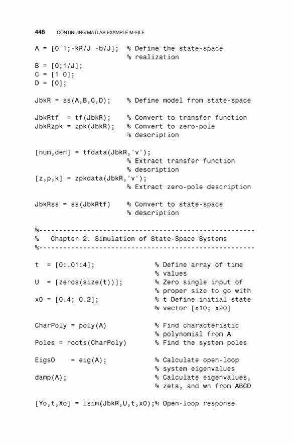
448 CONTINUING MATLAB EXAMPLE M-FILE
A = [0 1;-kR/J -b/J]; % Define the state-space% realization
B = [0;1/J];C = [1 0];D = [0];
JbkR = ss(A,B,C,D); % Define model from state-space
JbkRtf = tf(JbkR); % Convert to transfer functionJbkRzpk = zpk(JbkR); % Convert to zero-pole
% description
[num,den] = tfdata(JbkR,'v');% Extract transfer function% description
[z,p,k] = zpkdata(JbkR,'v');% Extract zero-pole description
JbkRss = ss(JbkRtf) % Convert to state-space% description
%------------------------------------------------------% Chapter 2. Simulation of State-Space Systems%------------------------------------------------------
t = [0:.01:4]; % Define array of time% values
U = [zeros(size(t))]; % Zero single input of% proper size to go with
x0 = [0.4; 0.2]; % t Define initial state% vector [x10; x20]
CharPoly = poly(A) % Find characteristic% polynomial from A
Poles = roots(CharPoly) % Find the system poles
EigsO = eig(A); % Calculate open-loop% system eigenvalues
damp(A); % Calculate eigenvalues,% zeta, and wn from ABCD
[Yo,t,Xo] = lsim(JbkR,U,t,x0);% Open-loop response
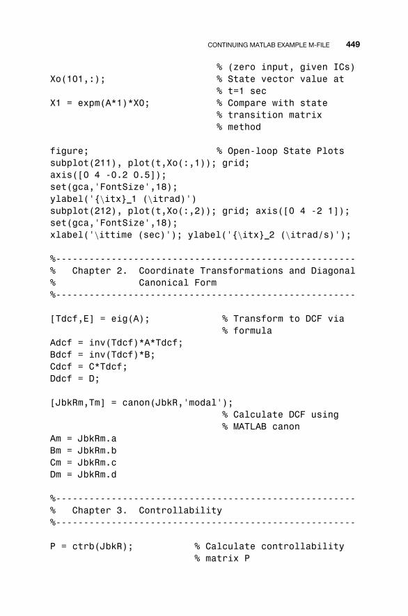
CONTINUING MATLAB EXAMPLE M-FILE 449
% (zero input, given ICs)Xo(101,:); % State vector value at
% t=1 secX1 = expm(A*1)*X0; % Compare with state
% transition matrix% method
figure; % Open-loop State Plotssubplot(211), plot(t,Xo(:,1)); grid;axis([0 4 -0.2 0.5]);set(gca,'FontSize',18);ylabel('{\itx} 1 (\itrad)')subplot(212), plot(t,Xo(:,2)); grid; axis([0 4 -2 1]);set(gca,'FontSize',18);xlabel('\ittime (sec)'); ylabel('{\itx} 2 (\itrad/s)');
%------------------------------------------------------% Chapter 2. Coordinate Transformations and Diagonal% Canonical Form%------------------------------------------------------
[Tdcf,E] = eig(A); % Transform to DCF via% formula
Adcf = inv(Tdcf)*A*Tdcf;Bdcf = inv(Tdcf)*B;Cdcf = C*Tdcf;Ddcf = D;
[JbkRm,Tm] = canon(JbkR,'modal');% Calculate DCF using% MATLAB canon
Am = JbkRm.aBm = JbkRm.bCm = JbkRm.cDm = JbkRm.d
%------------------------------------------------------% Chapter 3. Controllability%------------------------------------------------------
P = ctrb(JbkR); % Calculate controllability% matrix P
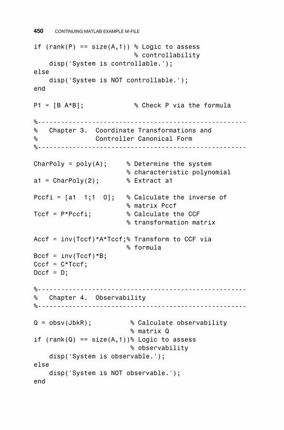
450 CONTINUING MATLAB EXAMPLE M-FILE
if (rank(P) == size(A,1)) % Logic to assess% controllability
disp('System is controllable.');else
disp('System is NOT controllable.');end
P1 = [B A*B]; % Check P via the formula
%------------------------------------------------------% Chapter 3. Coordinate Transformations and% Controller Canonical Form%------------------------------------------------------
CharPoly = poly(A); % Determine the system% characteristic polynomial
a1 = CharPoly(2); % Extract a1
Pccfi = [a1 1;1 0]; % Calculate the inverse of% matrix Pccf
Tccf = P*Pccfi; % Calculate the CCF% transformation matrix
Accf = inv(Tccf)*A*Tccf;% Transform to CCF via% formula
Bccf = inv(Tccf)*B;Cccf = C*Tccf;Dccf = D;
%------------------------------------------------------% Chapter 4. Observability%------------------------------------------------------
Q = obsv(JbkR); % Calculate observability% matrix Q
if (rank(Q) == size(A,1))% Logic to assess% observability
disp('System is observable.');else
disp('System is NOT observable.');end

CONTINUING MATLAB EXAMPLE M-FILE 451
Q1 = [C; C*A]; % Check Q via the formula
%------------------------------------------------------% Chapter 4. Coordinate Transformations and Observer% Canonical Form%------------------------------------------------------
Qocf = inv(Pccfi);Tocf = inv(Q)*Qocf; % Calculate OCF transformation
% matrixAocf = inv(Tocf)*A*Tocf; % Transform to OCF via formulaBocf = inv(Tocf)*B;Cocf = C*Tocf;Docf = D;
[JbkROCF,TOCF] = canon(JbkR,'companion');% Compute OCF using canon
AOCF = JbkROCF.aBOCF = JbkROCF.bCOCF = JbkROCF.cDOCF = JbkROCF.d
%------------------------------------------------------% Chapter 5. Minimal Realizations% The Continuing Matlab Example is already minimal;% hence, there is nothing to do here. The student% may verify this with MATLAB function minreal.%------------------------------------------------------
%------------------------------------------------------% Chapter 6. Lyapunov Stability Analysis%------------------------------------------------------
if (real(Poles(1))==0 | real(Poles(2))==0) % lyap willfailif (real(Poles(1))<=0 | real(Poles(2))<=0)
disp('System is marginally stable.');else
disp('System is unstable.');end
else % lyap will% succeed
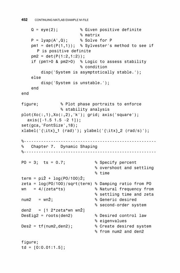
452 CONTINUING MATLAB EXAMPLE M-FILE
Q = eye(2); % Given positive definite% matrix
P = lyap(A',Q); % Solve for Ppm1 = det(P(1,1)); % Sylvester's method to see if
P is positive definitepm2 = det(P(1:2,1:2));if (pm1>0 & pm2>0) % Logic to assess stability
% conditiondisp('System is asymptotically stable.');
elsedisp('System is unstable.');
endend
figure; % Plot phase portraits to enforce% stability analysis
plot(Xo(:,1),Xo(:,2),'k'); grid; axis('square');axis([-1.5 1.5 -2 1]);
set(gca,'FontSize',18);xlabel('{\itx} 1 (rad)'); ylabel('{\itx} 2 (rad/s)');
%------------------------------------------------------% Chapter 7. Dynamic Shaping%------------------------------------------------------
PO = 3; ts = 0.7; % Specify percent% overshoot and settling% time
term = pi2 + log(PO/100)2;zeta = log(PO/100)/sqrt(term) % Damping ratio from POwn = 4/(zeta*ts) % Natural frequency from
% settling time and zetanum2 = wn2; % Generic desired
% second-order systemden2 = [1 2*zeta*wn wn2]DesEig2 = roots(den2) % Desired control law
% eigenvaluesDes2 = tf(num2,den2); % Create desired system
% from num2 and den2
figure;td = [0:0.01:1.5];
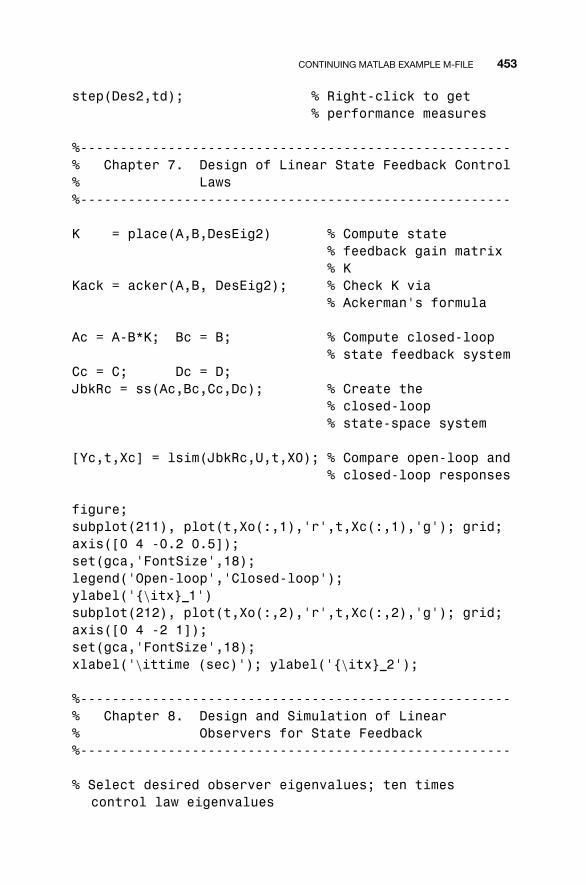
CONTINUING MATLAB EXAMPLE M-FILE 453
step(Des2,td); % Right-click to get% performance measures
%------------------------------------------------------% Chapter 7. Design of Linear State Feedback Control% Laws%------------------------------------------------------
K = place(A,B,DesEig2) % Compute state% feedback gain matrix% K
Kack = acker(A,B, DesEig2); % Check K via% Ackerman's formula
Ac = A-B*K; Bc = B; % Compute closed-loop% state feedback system
Cc = C; Dc = D;JbkRc = ss(Ac,Bc,Cc,Dc); % Create the
% closed-loop% state-space system
[Yc,t,Xc] = lsim(JbkRc,U,t,X0); % Compare open-loop and% closed-loop responses
figure;subplot(211), plot(t,Xo(:,1),'r',t,Xc(:,1),'g'); grid;axis([0 4 -0.2 0.5]);set(gca,'FontSize',18);legend('Open-loop','Closed-loop');ylabel('{\itx} 1')subplot(212), plot(t,Xo(:,2),'r',t,Xc(:,2),'g'); grid;axis([0 4 -2 1]);set(gca,'FontSize',18);xlabel('\ittime (sec)'); ylabel('{\itx} 2');
%------------------------------------------------------% Chapter 8. Design and Simulation of Linear% Observers for State Feedback%------------------------------------------------------
% Select desired observer eigenvalues; ten timescontrol law eigenvalues
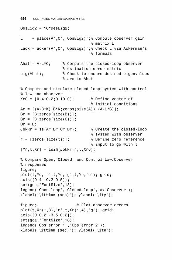
454 CONTINUING MATLAB EXAMPLE M-FILE
ObsEig2 = 10*DesEig2;
L = place(A',C', ObsEig2)';% Compute observer gain% matrix L
Lack = acker(A',C', ObsEig2)';% Check L via Ackerman's% formula
Ahat = A-L*C; % Compute the closed-loop observer% estimation error matrix
eig(Ahat); % Check to ensure desired eigenvalues% are in Ahat
% Compute and simulate closed-loop system with control% law and observerXr0 = [0.4;0.2;0.10;0]; % Define vector of
% initial conditionsAr = [(A-B*K) B*K;zeros(size(A)) (A-L*C)];Br = [B;zeros(size(B))];Cr = [C zeros(size(C))];Dr = D;JbkRr = ss(Ar,Br,Cr,Dr); % Create the closed-loop
% system with observerr = [zeros(size(t))]; % Define zero reference
% input to go with t[Yr,t,Xr] = lsim(JbkRr,r,t,Xr0);
% Compare Open, Closed, and Control Law/Observer% responsesfigure;plot(t,Yo,'r',t,Yc,'g',t,Yr,'b'); grid;axis([0 4 -0.2 0.5]);set(gca,'FontSize',18);legend('Open-loop','Closed-loop','w/ Observer');xlabel('\ittime (sec)'); ylabel('\ity');
figure; % Plot observer errorsplot(t,Xr(:,3),'r',t,Xr(:,4),'g'); grid;axis([0 0.2 -3.5 0.2]);set(gca,'FontSize',18);legend('Obs error 1','Obs error 2');xlabel('\ittime (sec)'); ylabel('\ite');
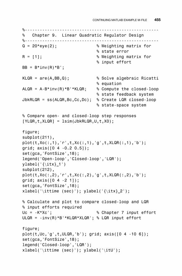
CONTINUING MATLAB EXAMPLE M-FILE 455
%------------------------------------------------------% Chapter 9. Linear Quadratic Regulator Design%------------------------------------------------------Q = 20*eye(2); % Weighting matrix for
% state errorR = [1]; % Weighting matrix for
% input effortBB = B*inv(R)*B';
KLQR = are(A,BB,Q); % Solve algebraic Ricatti% equation
ALQR = A-B*inv(R)*B'*KLQR; % Compute the closed-loop% state feedback system
JbkRLQR = ss(ALQR,Bc,Cc,Dc); % Create LQR closed-loop% state-space system
% Compare open- and closed-loop step responses[YLQR,t,XLQR] = lsim(JbkRLQR,U,t,X0);
figure;subplot(211),plot(t,Xo(:,1),'r',t,Xc(:,1),'g',t,XLQR(:,1),'b');grid; axis([0 4 -0.2 0.5]);set(gca,'FontSize',18);legend('Open-loop','Closed-loop','LQR');ylabel('{\itx} 1')subplot(212),plot(t,Xo(:,2),'r',t,Xc(:,2),'g',t,XLQR(:,2),'b');grid; axis([0 4 -2 1]);set(gca,'FontSize',18);xlabel('\ittime (sec)'); ylabel('{\itx} 2');
% Calculate and plot to compare closed-loop and LQR% input efforts requiredUc = -K*Xc'; % Chapter 7 input effortULQR = -inv(R)*B'*KLQR*XLQR'; % LQR input effort
figure;plot(t,Uc,'g',t,ULQR,'b'); grid; axis([0 4 -10 6]);set(gca,'FontSize',18);legend('Closed-loop','LQR');xlabel('\ittime (sec)'); ylabel('\itU');
REFERENCES
Anderson, B. D. O., and J. B. Moore, 1971, Linear Optimal Control, Prentice-Hall, Englewood Cliffs, NJ.
Bupp, R. T., D. S. Bernstein, and V. T. Coppola, 1998, “A Benchmark Problemfor Nonlinear Control Design”, International Journal of Robust and NonlinearControl, 8: 307–310.
Bernstein, D. S., editor, 1998, Special Issue: A Nonlinear Benchmark Problem,International Journal of Robust and Nonlinear Control 8(4–5): 305–461.
Bryson, A. E., Jr., and Y.-C. Ho, 1975, Applied Optimal Control, Hemisphere:Optimization, Estimation, and Control, Hemisphere, Washington, DC.
Chen, C. T., 1984, Linear System Theory and Design, Holt, Rinehart, and Win-ston, New York.
Dorato, P., C. Abdallah, and V. Cerone, 1995, Linear Quadratic Control: AnIntroduction, Prentice-Hall, Englewood Cliffs, NJ.
Dorf, R. C., and R. H. Bishop, 2005, Modern Control Systems, 10th ed., Prentice-Hall, Upper Saddle River, NJ.
Friedland, B., 1986, Control System Design: An Introduction to State-Space Meth-ods, McGraw-Hill, New York.
Graham, D., and R. C. Lathrop, 1953, “The Synthesis of Optimum Response:Criteria and Standard Forms, Part 2,” Transactions of the AIEE 72: 273–288.
Kailath, T., 1980, Linear Systems, Prentice Hall, Upper Saddle River, NJ.
456
Linear State-Space Control Systems. Robert L. Williams II and Douglas A. LawrenceCopyright 2007 John Wiley & Sons, Inc. ISBN: 978-0-471-73555-7
REFERENCES 457
Khalil, H. K., 2002, Nonlinear Systems, 3rd ed., Prentice-Hall, Upper SaddleRiver, NJ.
Kwakernaak, H., and R. Sivan, 1972, Linear Optimal Control Systems, JohnWiley & Sons, Inc.
Lewis, F. L., 1992, Applied Optimal Control and Estimation, Prentice-Hall,Englewood-Cliffs, NJ.
Ogata, K., 2002, Modern Control Engineering, 4th ed., Prentice Hall, Upper Sad-dle River, NJ.
Reid, J. G., 1983, Linear System Fundamentals: Continuous and Discrete, Classicand Modern, McGraw-Hill.
Rugh, W. J., 1996, Linear System Theory, 2nd ed., Prentice-Hall, Upper SaddleRiver, NJ.
Zhou, K., 1995, Robust and Optimal Control, Prentice-Hall, Upper Saddle River,NJ.

INDEX
Ackermann’s formula, 258, 262, 274, 277,279, 282, 289, 294, 310–311, 321,394–395, 352
Adjoint, 64, 187, 414Adjugate, 414Algebraic output equation, 5, 7, 9–10,
13–14, 16, 29, 35–36, 39, 49, 104,109
Algebraic Riccati equation, 390–392,395–399, 401, 403–404
Asymptotic Stability, 200, 203–204,211–212, 216, 220, 222–224, 227,236, 278, 338–339
Asymptotic stabilization, 263, 312Asymptotically stable
equilibrium, 199–204, 207–208, 211,216, 276
error dynamics, 302, 308, 313state equation, 216, 221–222, 231, 264,
269, 274, 295, 392, 395, 397(sub)system, 203–204, 225–231, 254,
265, 278, 293, 314
Ball and beam system, 20–24, 46, 105,148, 183, 233, 298, 355, 405
Basis, 130, 394, 419–430, 433–434change of, see Change of basis
orthonormal, see Orthonormal basisstandard, see Standard basis
Bass-Gura formula, 255–257, 267, 274,277, 294, 305–310, 315, 352
Bounded-input, bounded-output stability,198, 218–224, 228–231
Canonical formcontroller, see Controller canonical
formdiagonal, see Diagonal canonical formobserver, see Observer canonical formphase-variable, see Phase-variable
canonical formCauchy-Schwarz inequality, 445Cayley-Hamilton theorem, 57, 123,
131–132, 260, 443Change of basis, 72, 422, 430Characteristic
equation, 436, 443polynomial, 57, 65–66, 73–74, 77,
79–81, 85–88, 90–91, 93, 118,127–128, 131, 140, 142, 144–145,161, 170, 216, 221, 237–238, 241,243, 249, 251–258, 260, 262, 276,279, 285, 289, 293, 304–307, 309,311, 321, 327–328, 348, 351,435–437, 439–441, 444
459
Linear State-Space Control Systems. Robert L. Williams II and Douglas A. LawrenceCopyright 2007 John Wiley & Sons, Inc. ISBN: 978-0-471-73555-7
460 INDEX
Closed-loopeigenvalue(s), 236, 243, 250, 252–253,
255–257, 262–263, 267–268, 271,274–275, 289, 292–293, 298–299,309, 327, 334, 336, 339, 345, 347,349, 353, 399, 404
state equation, 234–235, 254, 256, 264,268–270, 273–277, 295, 325–326,328, 330, 332, 334–335, 337–339,342, 353, 384, 386, 391–392, 395,397, 404
system, 236, 242–244, 254, 263, 273,278, 282, 286–288, 292–293,347–351
stability, 236, 272–273, 278, 326,339
transfer function, 243, 269, 271, 295,337
Cofactor, 412–414Conjugate transpose, 393, 408, 425, 436Control law, 234, 287Controllability, 108–109, 119–120, 133,
138, 141, 149–150, 163, 166, 168,185, 187–193, 234, 250, 263–264,274, 301, 312–314, 323, 392
Gramian, 110–111, 114, 120, 145, 154,375–376, 403
matrix, 110, 112, 114–121, 125, 130,132–134, 138, 141–143, 161, 211,256, 259
rank condition, 110, 113Controllable
pair, 110, 123, 130, 133, 136, 146–147,193, 232, 250–252, 255–256, 259,261, 264–265, 267, 272, 274, 295,300, 392, 397, 403
state, 109realization, 122, 127, 147, 188–192state equation, 109, 115, 123, 125, 263,
268, 375–376Controller canonical form, 17, 124–125,
127–128, 138–144, 147–148, 168,170–171, 175, 179, 181, 183–184,187–191, 195, 230, 252–255, 259,262–263, 270–271, 276–277, 306,309, 327
Coordinate transformation, 72–75, 77–78,80, 82, 88, 91, 109, 119–124, 127,129, 134, 137–140, 142–143, 150,165–172, 174, 176, 178–180, 185,188, 255, 264–265, 267, 313, 315,319–320, 326–327, 332, 337,353
Cost function, 358
dc gain, 269–271, 275, 337Damping ratio, 79, 81, 87, 238–242, 245,
254, 284, 297Detectability, 301, 312–316Determinant, 41, 60, 64, 73, 110,
117–118, 138, 152, 160–161, 178,188, 212, 227, 274, 407, 412–414,416, 440
Diagonalization, 440Diagonal canonical form, 49, 72, 74–75,
77, 80, 82–83, 88, 91–92, 99, 101,103, 105, 107, 121–122, 127, 129,141, 143, 170–171, 178–179,183–184, 257–258
Differential Riccati equation, 383–385,387, 390–391, 397
Dimension, 3, 17, 25, 34, 38, 74, 76, 110,113, 149, 151, 163, 185, 187, 192,247, 269–270, 301, 316, 318, 331,353, 361, 407–409, 411, 419, 431
Direct transmission matrix, 49Dual state equation, 163–165, 167Duality, 150, 163, 165–169, 171–175,
183–184, 188–189, 190, 303, 312,314, 348–349, 351
Eigenbasis, 439–440Eigenstructure, 127, 190, 387, 440Eigenvalue, 59–61, 65, 73–74, 77–82,
84–87, 89–92, 121–122, 127–129,134–136, 141, 143, 145, 147,170–171, 174, 178–179, 197, 198,202–205, 208–209, 211–213, 216,221, 223–224, 227–229, 231–232,236, 243, 250, 252–257, 262–263,267–268, 271, 274–275, 289,292–293, 298–299, 309, 327, 334,336, 339, 345, 347, 349, 353, 399,404, 435–443
Eigenvalue placement, 234, 250–252,256, 263–264, 303, 313, 323, 326,399, 401
Eigenvector, 73–74, 77–78, 84, 88, 92,145, 213, 392, 441–442
left, 133–136, 173, 265–266, 268, 315,436, 438
right, 173–174, 213, 314–316,394–395, 436–438
Elementary row operations, 160,431–434, 437
Energy, 5–6, 8–9, 12, 28, 34, 198,204–211, 359, 392
Equilibrium condition, 1, 20, 24, 44, 270,275, 339
INDEX 461
Equilibrium state, 18, 199–201, 236asymptotically stable, see
Asymptotically stable equilibriumexponentially stable, 200–201, 216stable, 199–201unstable, see Unstable equilibrium
Error dynamics, 301–302, 306, 308–309,312–313, 315, 318, 323, 337, 339,343–344, 348, 351–352
Estimation error, 301, 304, 317Euclidean norm, 111–112, 156, 425,
445–446Euclidean space, 360–361, 363, 367–368,
418Euler-Lagrange equation, 366–367, 369,
374, 381Exponential stability, 200–201, 216, 222
Feedback,state, see State feedbackoutput, see Output feedback
Frobenius norm, 446
Gateaux variation, 364–367, 373, 380Gramian
controllability, see Controllabilitygramian
observability, see Observability gramianreachability, see Reachability gramian
Hamiltonianfunction, 380matrix, 385–387, 390, 392
Holder inequality, 445Homogeneous state equation, 52, 59, 61,
150–151, 153, 159, 161–162,171–173, 182, 198–199, 201, 203,205, 231, 301, 318, 328, 373–374,382, 384
Identity matrix, 25, 40–41, 52, 140, 270,408, 416, 421, 434
Image, 42, 114, 430, 433Impulse response, 48, 51–52, 63, 65, 70,
74, 76, 79, 98–99, 124, 146, 192,218–222, 298–299
Inner product, 211, 424Input
gain, 137, 243, 268–271, 288, 292, 337matrix, 4, 36, 49, 397vector, 4, 7, 49, 52, 163
Input-output behavior, 17, 48, 70, 76, 186,198, 222, 295, 337
Internal stability, 198–199, 218Inverted pendulum, 44–45, 101–103, 148,
183, 233, 298, 355, 404–405ITAE criteria, 249–250, 276, 279, 283,
285–286, 289, 294, 296–298
Jordan canonical form, 202, 388,390–391, 442–443
Jordan block matrix, 41, 202–203, 388,442–443
Kalman, R. E., 108Kernel, 430
Lagrange multiplier, 361–362, 368–372,379, 382
Laplace domain, 17, 51–52, 63, 66,69–70
Laplace transform, 15, 37, 48, 50–52, 61,63–67, 273
Linear dependence, 112, 134, 136–137,152, 154, 266, 319, 395
Linear independence, 74, 77, 110,118–119, 130, 133, 146, 151–152,162–163, 224, 419, 425, 431,433–434, 439, 441–442
Linear quadratic regulator, 357, 359–360,377, 382–383, 385, 403
steady-state, 390–392, 404–406MATLAB, 397–402
Linear time-invariantstate equation, 20, 24, 42–43, 61–62,
72–73, 75, 77, 119, 137, 150, 165,270, 198, 201, 235, 300, 359
system, 1, 3, 5, 26–27, 32, 48–49, 51,70, 78, 105, 107, 149, 186
Linear transformation, 41, 48, 72, 426,428–431, 434–435, 445
Linearization, 1, 17–20, 44, 46–47, 102,105–107
Luenberger, D. G., 300Lyapunov, A. M., 198, 210–211Lyapunov
function, 211matrix equation, 213–216, 227, 229,
231–232, 393, 395
Marginal stability, 204, 229, 277, 293, 327MATLAB,
controllability, 138controller canonical form, 138diagonal canonical form, 80introduction, 24
462 INDEX
MATLAB, (continued )m-files for Continuing MATLAB
Example, 447minimal realizations, 194observability, 174observer canonical form, 174observer design, 343optimal control, 397shaping the dynamic response, 278stability analysis, 225simulation, 79state feedback control law design, 279state-space description, 26
Matrix arithmetic, 409–412Matrix exponential, 48, 53–55, 57–61,
64, 93, 95–96, 100, 113, 146, 182,201–203, 216, 220–222, 376, 386,390, 396
Matrix inverse, 13, 41, 54, 64, 68, 74, 84,127, 142–143, 259, 275, 332, 387,414–416
Matrix norm, 42, 219, 223, 231, 445–446Minor, 412–413Minimal realization, 185–187, 189,
191–197, 222, 230–231, 299Minimum energy control, 357, 371,
374–377, 379, 403
Natural frequencydamped, 239, 241, 243, 245–246undamped, 79, 81, 238–239, 241, 243,
245, 249, 254, 276, 283–286,297–298
Negative (semi)definite, 211–212Nominal trajectory, 1, 17–24, 46–47, 102,
105Nonlinear state equation, 1, 18–21, 44,
46–47, 102Null space, 113, 153–154, 430, 436Nullity, 153–154, 158, 160, 193, 431,
433, 439
Objective function, 249, 358, 371–372Observability, 149–151, 154, 159, 161,
163–166, 171, 173, 175, 177,179–180, 183–184, 185, 187–189,191–193, 300–301, 307, 309,312–314, 320, 323, 338–339, 353,356, 392
Gramian, 154–157, 166, 181matrix, 151–152, 158–163, 166, 169,
174, 177–179, 188, 307, 321rank condition, 151–152
Observablepair, 151, 171, 173–174, 182, 193,
303–305, 310, 312–313, 318,320–321, 323, 392, 397
realization, 167, 169, 188–190, 354state equation, 151, 157, 169, 301, 312
Observer, 300–302, 306–309, 312–313,324–325, 327–328, 338,341–343,345–346, 348, 350
reduced-order, 316, 318, 320–323, 331,334
Observer-basedcompensator, 301, 323, 325, 327–328,
330–331, 335, 337–338, 341, 349,353–356
servomechanism, 338, 340–341,354–355
Observer canonical form, 168–171,174–181, 183–184, 187–190, 231,304
Observer error, 310, 326–327, 330, 339,346, 354–356
dynamics, 301–302, 306, 308–309,312–313, 315, 318, 323, 337, 339,343–344, 348, 351–352
Observer gain, 301–304, 306–307, 310,312–314, 316, 318, 322, 330, 334,339, 341, 343, 345, 348–351, 352
Optimal control, 357–360, 371, 397, 404Orthogonal
matrix, 95complement, 425, 435vectors, 133–136, 173, 265–266, 268,
314–316, 425, 435Orthonormal basis, 425Output
feedback, 197, 325matrix, 49vector, 4, 163
Peak time, 236, 240–241, 244–247, 279,284, 297
Percent overshoot, 236, 240–242, 244,247, 254, 271, 279–280, 283–286,288, 294–297, 309
Performance index, 2, 358–359, 379–381,384–385, 390–392, 396, 401, 404
Phase portrait, 207–209, 226, 229, 337Phase-variable canonical form, 17, 125Pole, 2, 26, 29, 76, 181, 185–186, 190,
194, 196, 222, 234, 272–273, 276,338
Popov-Belevitch-Hautuseigenvector test for controllability, 133,
136, 145, 147, 173, 265
INDEX 463
eigenvector test for detectability, 314eigenvector test for observability, 150,
173, 181, 190, 395eigenvector test for stabilizability, 265,
314rank test for controllability, 136,
137–138, 145, 174, 224, 265, 393rank test for detectability, 314rank test for observability, 150, 174,
181, 224, 318, 393rank test for stabilizability, 265, 314
Positive definite, 210–216, 225, 227–228,231–232, 295, 359, 363, 381–382,392, 396–397, 403–404
Positive semidefinite, 110, 154, 359, 391,396
Proof-mass actuator system, 47, 105, 148,184, 197, 233, 299, 356
Quadratic form, 111, 154, 211–213, 359,363, 379, 381, 384, 393
Range space, 114, 430Rank, 431, 433Reachability Gramian, 146, 375–377Reachable
state, 115state equation, 115
Reduced-order observer, 316, 318,320–323, 331, 334
Reference input, 137, 235–236, 255,268–270, 272, 274, 276, 287–289,292, 328, 336, 338–339, 343
Riccati, J. F., 383Riccati matrix equation, 295Rise time, 236, 239–245, 248, 279, 285,
297Robot joint/link, 46, 103, 148, 183, 233,
298, 356, 405Rotational mechanical system, 27, 80,
139, 175, 225, 279, 345, 398Rotational electromechanical system, 36,
89, 143, 179, 228, 290, 350Row-reduced echelon form, 160, 432,
437–438
Separation property, 327, 331Servomechanism,
observer-based, 338, 340–341,354–355
state feedback, 271, 276, 296–297Settling time, 236, 241–247, 254, 271,
279–280, 282–286, 288, 294–295,297, 309
Similarity transformation, 73, 255, 332,388–391, 440–442
Span, 130–131, 418–419, 426, 431Spectral norm, 231, 446Spectral radius, 42Spectrum, 436–437Stability,
asymptotic, see Asymptotic stabilitybounded-input, bounded-output, see
Bounded-input, bounded-outputstability
closed-loop, see Closed-loop stabilityexponential, see Exponential stabilityinternal, see Internal stabilitymarginal, see Marginal stability
Stabilizability, 234, 263–265, 295, 301,312–315
Standard basis, 63, 77, 133, 201, 421, 423,428, 430, 440
Statedifferential equation, 5, 7, 9–10,
13–14, 16, 28, 35–36, 39, 49, 65,104, 109, 273
equation solution, 48–49, 52, 61–62,109, 149, 201
estimate, 300–302, 317, 320, 323–324,331, 338, 34
feedback (control law), 137, 234–236,242, 250–252, 254, 263–265, 268,270, 272–273, 279, 281, 292,295–299, 300–301, 309, 323–325,327, 330–331, 337–338, 341,347–351, 353–356, 383–384, 391,397–399, 401
feedback gain matrix/vector, 234–236,250–259, 262–267, 269, 271, 274,276–277, 279, 281, 287, 289, 292,294–295, 303, 314, 327–329, 334,339–341, 383, 386, 391, 396–397,399
feedback-based servomechanism, 271,276, 296–297, 338, 341–342
variables, 4–6, 8–10, 12, 14, 16, 20,28, 34, 38–40, 44–46, 61, 66–67,76, 90, 101–102, 104, 116, 122,149, 159, 171, 205, 210, 273, 295,300, 317
vector, 3–4, 6–7, 48–49, 65, 72, 127,149, 163, 273, 300, 317, 324, 326
transition matrix, 61, 79, 87State-space realization, 17, 26, 32, 39–40,
44–46, 48, 70–71, 74, 76–78, 80, 91,96–98, 117–118, 122–124, 127, 147,161, 164, 167, 169, 186, 354
464 INDEX
State-space realization, (continued )minimal, see Minimal realization
Stationary function, 366–367Steady-state tracking, 268–269, 272, 276,
337, 339–340Subspace, 41–42, 394, 419–421, 425,
430–431, 435Supremum, 218–219, 223, 445Symmetric matrix, 110, 127, 154, 169,
211–213, 215–216, 231–232, 295,306, 359, 363, 383, 392–395,403–404, 420
System dynamics matrix, 34, 49, 73,78–79, 91, 93, 95, 100, 102, 121,198, 214, 227, 229–230, 236, 252,255, 273–274, 277, 279, 293–294,327, 339, 397, 401
Taylor series, 19Time constant, 92, 237, 244, 290–291,
294, 296, 298Transfer function, 2, 5, 14–15, 17, 26–27,
29, 37–39, 42–43, 45, 48, 52, 65, 70,74, 76, 86, 88, 91, 92, 96–98, 103,117, 122–123, 125, 127, 142, 144,147, 161, 163–164, 167–169,179–181, 185–190, 192, 196,221–222, 230–232, 238, 249,284–285, 291, 352, 354
closed-loop, 243, 269, 271, 295, 337open-loop, 271, 273, 276, 295
Transpose, 112–113, 165, 168, 172, 212,225, 305, 314, 408, 411, 414, 416
conjugate (Hermitian), 393, 408, 425,436
Two-mass translational mechanical system,32, 84, 141, 177, 227, 283, 348, 399
Two-point boundary value problem, 382Three-mass translational mechanical
system, 44, 99, 147, 183, 233, 297,355, 405
Uncontrollable state equation, 129, 132,135, 172, 263, 267, 193
Unobservable state, 151, 153–154, 159,160, 165
Unobservable state equation, 171–172,194, 312, 315
Unstableequilibrium, 44, 199–201, 209, 211system, 204, 239, 257
Vandermonde matrix, 59–60, 121, 128Variational calculus, 357, 359–360, 368Vector norm, 219, 444–445
bound, 206, 216Euclidean, 111–112, 156, 425,
445–446Vector space, 364, 417–422, 424
Zero-input response, 48, 50–51, 62,64–65, 69, 87, 95, 150–151, 157,159, 198, 222, 328, 399
Zero-state response, 48, 50–51, 62–65,69–70, 76, 95, 150, 198, 218–220,222, 232, 327
Zero, 26, 29, 76, 181, 185–186, 190, 194,196, 222, 250, 272–273, 276, 338