Linear system solvers for boundary value ODEs

Journal of Computational and Applied Mathematics 45 (1993) 103-117 North-Holland

103

CAM 1286

Linear system solvers for boundary value ODES

Lixin Liu and Robert D. Russell

Department of Mathematics and Statistics, Simon Fraser University, Bumaby, B.C., Canada

Received 11 November 1991 Revised 28 January 1992

Abstract

Liu, L. and R.D. Russell, Linear system solvers for boundary value ODES, Journal of Computational and Applied Mathematics 45 (1993) 103-117.

We investigate the stability properties of several linear system solvers for solving boundary value ODES. We consider the compactification algorithm, Gaussian elimination with row partial pivoting, and a QR algorithm applied to linear systems arising from solving BVPs for which the matrix is block-bidiagonal except for bordering along the last n rows and columns. We will particularly compare AUTO’s original linear solver (an LU decomposition with partial pivoting) and our implementation of the analogous QR algorithm to AUTO. Two other factors (the underlying continuation strategy and mesh selection strategy) may affect the stability of the linear system solver for ODE continuation codes as well and are also discussed in our numerical investigations.

Keywords: Boundary value problems; continuation; multiple shooting; finite difference; collocation; compactification; Gaussian elimination; QR factorization; stability.

1. Introduction

Most of the widely-used methods for solving boundary value problems (BVPs) for ordinary differential equations (ODES) involve solving block-bidiagonal linear systems of equations. Both the efficiency and the stability of the linear system solvers are crucial in developing BVP codes. Since these nN linear systems have only n2N nonzero elements, the solution method should minimize fill-in in order to reduce the storage requirements and CPU-time. At the same time, the solvers should to the extent possible also avoid potential instabilities, and recently several methods have been developed with this in mind, viz., Gaussian elimination with complete row pivoting implemented in the code SOLVEBLOK [6], alternate row and column

Correspondence to: Prof. R.D. Russell, Department of Mathematics and Statistics, Simon Fraser University, Burnaby, B.C., Canada V5A lS6.

0377-0427/93/$06.00 0 1993 - Elsevier Science Publishers B.V. All rights reserved

104 L. Liu, R.D. Russell / Stability of methods for BWs

elimination implemented in [7], the DECOMP and SOLVE routines from the code PASVA [13] and a stable block factorization [15,16]. The latter ones incorporate nonseparated boundary conditions which destroy the block-bidiagonal structure.

For BVP continuation codes (involving boundary value problems with at least one parameter), one computes a series of solutions on one or several branches rather than one particular solution of a BVP, and in this context an efficient linear system solver becomes even more important. For this type of problem, the discrete system involves a matrix with block-bidiagonal structure ,except for nonzero blocks bordering the matrix in the last rows and columns. Stable block factorizations for this type of system have recently been investigated in [15,16]. The system solution is only one of several important factors that affect the stability of a method. Moreover, stability of the solver can be strongly influenced by some other factors, e.g., the mesh selection strategy and the continuation strategy. This will be demonstrated here. One of our main objectives is to analyze and improve the stability properties of the linear system solver for the code AUTO [8,9], popular mathematical software for performing bifurcation analysis. AUTO uses a restricted pivoting strategy when solving the linear systems arising from a collocation method. While the emphasis is on the special features of AUTO, our analysis also applies if the fast solvers considered here were used for other continuation codes, such as COLCON [4].

2. Background

In this section, we briefly review some methods for solving the linear two-point boundary value problem

Y’ =A(t)y +4(t), (1)

&y(a) +&y(b) = d, (2)

where t E [a, b], y, q(t), d E R” and A(t), B,, B, E Wx”. The widely-used methods which have been developed for solving (1) and (2) are the

multiple-shooting method, the finite-difference method and the collocation method. All these methods lead to a similar linear system of equations.

2.1. Multiple-shooting method

Given a mesh a = t, < t, < . * * < tN+l = b, we compute a fundamental solution y:,(t) E RnXn

and a particular solution v,(t) E R” on each mesh interval [ti, tj+ll, 1 < i <N, such that

yi’ =A(t)Y,, y(tJ =l$ (3)

Vf=A(t)Yi-t-q(t), LQtJ =ei. (4)

We then find a vector si E KY, 1 < i <N, such that

y(t)=y(t)s,+ui(t), tE[ti, ti+I], i=l,..,, N. (5)

L. Liu, R.D. Russell / Stability of methods for BVPs 10.5

For the standard multiple shooting, we choose Fi = I and ei = 0. By satisfying the continuity conditions at the mesh-points and the boundary conditions to the endpoints, we obtain

W3) --I

I yN-itN) -I Ba 4

Sl

s2

SN-I

SN

=

-dt2)

- ~z(t3)

-‘N-l@,)

d

(f-9

The conditioning of the coefficient matrix has been discussed, for example, in [2,12]. It is well conditioned when N is large enough, its condition number being the same order as the conditioning constants of the BVP itself.

2.2. Finite-difference method

We consider a one-step finite-difference method, choosing the mesh as in the multiple-shooting method. Letting hi = ti+l - tj and ti+1,2 = ti + ihi, the BVP can be approximated by

S, R1 Yl 41

s2 R2 Y2 42

= .

s, RN Y; 4,

> (7)

_B, 47 __ yN+l d

where Si, R, are IZ X n matrices. For the trapezoidal scheme,

Si = -h,‘I - iA( Ri = -h,‘I - $4(ti+,), 4i= $&+1> +4(4>], (8)

and for the midpoint scheme,

Si = Rj = -!z:~I- $4(ti+l,2), 4i = 4(4+1,2). (9)

2.3. Collocation method

Since our main purpose is to examine the code AUTO, we only discuss the collocation method as it is implemented therein with Lagrange basis functions. We try to find

PjCt) = 5 wji(t>Yj+i/m~ (10) i=O

where

tj+i/m = tj + i(t,+, - tj), (11)

such that

Pi(zji) =A(zji)Pj(Zji) + 4('ji)Y (12) B,YI +B~YN+I =d, (13)


with zji, 1 < i < m, the Gauss points on the interval [ti, tj+l], 1 <j < N. The above formulation results in (mN + 1)n linear equations. By using the condensation method, we can eliminate the unknowns at non-mesh-points, and the linear system is reduced to

Yl 41

Y2 42 = .

c, r, 4;

4__ YNfl d

(14)

2.4. Solution of linear systems

The three linear system (6), (7) and (14) have similar almost block-bidiagonal structure. The conditioning of the systems (7) and (14) is quite similar to that for the multiple-shooting case when N is large [2]. Thus (14) can be reliably solved with a standard linear system solver such as Gaussian elimination with partial pivoting or the QR factorization. However, to preserve the sparsity of the system, special linear system solvers are used. We discuss several of these below.

Compactification The compactification algorithm is a well-known but unstable method for solving block-bidi-

agonal linear systems formed when solving the two-point boundary value problem. To study this method, we consider the linear system generated by the multiple-shooting method. We compute a discrete fundamental solution (@J/!!’ and particular solution {p$?T by

Pi+1 = @iPi + Ui(ti+l), @i+l = K(ti+l)@iY i=l ,***, N,

with the initial condition

PI = 0, @,=I,

and form

si=Qisl+pi, i=2 ,..., N,

where s1 satisfies

LB, +&@N+I]% =d-hPN+v

The compactification algorithm, like the single-shooting method, suffers from instability because the fastest growing (fundamental solution) mode dominates the others. A similar cornpacification technique can be applied for other methods by using

Yi+l = g -2&, ii = C-lq, ii = C-l& i=l ,***, N,

to eliminate all the interior mesh-point unknowns y,, . . . , y, and reduce the linear system to a 2n x 2n dense system in the unknowns y1 and yN+r.

L U decomposition Gaussian elimination with various pivoting strategies has been used for solving the linear

system (14). Although it is well known that the complete row pivoting Gaussian elimination

L. Liu, R.D. Russell / Stability of methods for BW’s 107

method is stable in practice, it is also known that the worst-case error growth is 0(2(N+1)“). For the separated boundary conditions case, the linear system is block-bidiagonal and Gaussian elimination with row pivoting can be used to efficiently solve the system

4 Al Cl

A,

Yl

Y2

CN Y,

BtJ _ YN+l

=

da 41

* .

qN

4 _

(15)

This method has been widely used (e.g., software SOLVEBLOK [6] used in COLSYS [l] and COLNEW [3]), and it is generally very stable. In fact the worst-case error growth is exponential only in the bandwidth [5]. However, the nonseparated boundary condition case is more delicate and more important to us because our purpose is to modify AUTO’s linear system solver. The well-conditioned BVP has ordinary or exponential dichotomy. For the latter, the pivoting strategy should properly “decouple” the exponentially increasing and exponentially decreasing modes of the fundamental solution. With this idea in mind, Mattheij [15,16] develops a stable block LU decomposition based on Gaussian elimination with row partial pivoting. However, this method is not always practical, because it requires knowing the exact number of increasing modes, and this may not be realistic to assume. Recently, Wright [19] considers applying Gaussian elimination to the columns of the reordered system

Cl Al Y2 41

A2 c2 42

YN = : .

A, cN yN+l qN

4 Ba__y,_ _ _ d

(16)

The serial version of this method starts to use Gaussian elimination with row pivoting for the first 2n rows of (16) such that

J%Pi,, * * . ~l,24,2L%[ 3 = [ 3

where P,,i E R2” X2n, i = 1,. . . , n, are permutation matrices, L,,i E R2nx2n, i = 1,. . .,n, are Gauss transformations, and U, is upper triangular. The transformed coefficient matrix of (16) becomes

E2

c3

AN CN

BN

(17)

108 L. Liu, R.D. Russell / Stability of methods for BVPs

If we apply a similar process to the blocks [,$+,I for k = 2, 3,. . . , N - 1, we obtain the coefficient matrix

-4 El Gl - u2 E2 G2

u N-1 EN-1 GN-1 EN A, Biv Bo

(18)

It is then easy to solve for yi, i = 1,. . . , N + 1, from the above formulation. Wright [19] proves that under certain assumptions this method is equivalent to Mattheij’s block LU decomposition and that it is stable. However, it is not clear how often the required assumptions are satisfied. In fact, if no pivoting occurs between the blocks Ci and AI~+~, then this method is equivalent to the compactification algorithm. The worst-case error growth 0(2(N+1)n) can happen.

QR fat toriza tion Wright [18] also proposes applying a Householder QR decomposition procedure to solve the

above linear system (16). The process is similar; instead of applying LU decompositions, we use QR decompositions to obtain the coefficient matrix (18). Wright has proved the stability of this algorithm. The serial version of the LU decomposition is about twice as fast as the QR decomposition, but both the LU decomposition and the QR decomposition have the advantage that they can be easily parallelized [l&19].

To compare the stability properties of these methods, we now study two examples. In our numerical results, the multiple-shooting method uses the ODE initial-value code DVERK from netlib and the tolerance in this routine is set to lo-“; the finite-difference code uses the midpoint scheme.

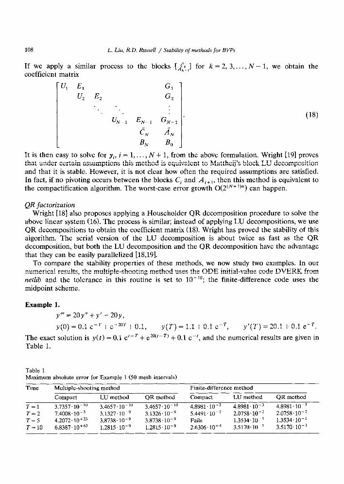
Example 1.

y”’ = 2Oy” + y’ - 2oy,

y(0) = 0.1 e-r+ ew20T + 0.1, y(T) = 1.1 + 0.1 e-r, y’(T) = 20.1 + 0.1 e-r.

The exact solution is y(t) = 0.1 et-r + e 20(t-T) + 0.1 e-‘, and the numerical results are given in Table 1.

Table 1 Maximum absolute error for Example 1 (50 mesh intervals)

Time Multiple-shooting method Finite-difference method

Compact LU method QR method Compact LU method QR method

T=l 3.7357.10-10 3.4657. lo-” 3.4657.10-10 4.8981. lo-’ 4.8981.10-3 4.8981.10-3 T=2 7.4008.10-3 3.1327.10-’ 3.1326.10-9 5.4491.10-2 2.0758.10-’ 2.0758.10-’ T=5 4.2072.10tz3 3.8738.10-9 3.8738*10-’ Fails 1.3534.10-r 1.3534.10-r T=lO 6.8387.10+63 1.2815.10-’ 1.2815.10-9 2.6306.10+4 3.5170.10-r 3.5170.10-l

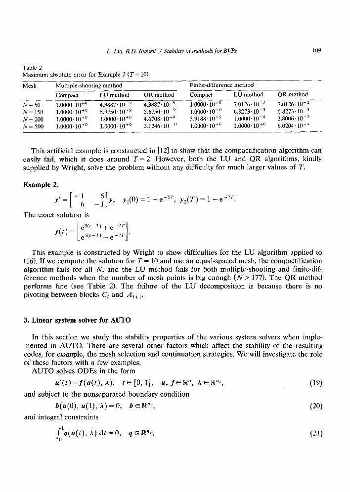
L. Liu, R.D. Russell / Stability of methods for BWs 109

Table 2 Maximum absolute error for Example 2 (T = 10)

Mesh Multiple-shooting method

Compact LU method QR method

N=SO l.oooo~lo+” 4.3887’10-9 4.3887.10-9

N=150 l.oooo~lo+” 5.9750.10-9 5.6750.10-9

N=200 l.oooo~lo+” l.oooo~lo+” 4.6708.10P9

N=500 l.OOOO~lO+O l.oooo~lo+O 3.1246.10W”

Finite-difference method

Compact LU method QR method

l.oooo~lo+O 7.0126.10-’ 7.0126.10-’ l.oooo~lo+O 6.8273.10-3 6.8273.10-3 3.9188.10+5 l.OOOO~lO+O 3.8006.10-3 l.oooo~lo+O l.oooo~lo+” 6.0204.10-4

This artificial example is constructed in [12] to show that the compactification algorithm can easily fail, which it does around T = 2. However, both the LU and QR algorithms, kindly supplied by Wright, solve the problem without any difficulty for much larger values of T.

Example 2.

The exact solution is

y(t) = e5(r-T) + e-7T 1 e5(t-T) _ e-7T *

This example is constructed by Wright to show difficulties for the LU algorithm applied to (16). If we compute the solution for T = 10 and use an equal-spaced mesh, the compactification algorithm fails for all N, and the LU method fails for both multiple-shooting and finite-difference methods when the number of mesh points is big enough (N > 177). The QR method performs fine (see Table 2). The failure of the LU decomposition is because there is no pivoting between blocks Ci and Ai+ 1.

3. Linear system solver for AUTO

In this section we study the stability properties of the various system solvers when implemented in AUTO. There are several other factors which affect the stability of the resulting codes, for example, the mesh selection and continuation strategies. We will investigate the role of these factors with a few examples.

AUTO solves ODES in the form

u’(t) =f@(t), A), t E [O, 11, u, fE R”, A E BP,

and subject to the nonseparated boundary condition

b@(O), u(l), A) = 0, b E Iw”“,

and integral constraints

(19)

(20)

j)(u(t), A) dt = 0, 4 E Rnq, (21)

110 L. Liy R.D. Russell / Stability of methods for BVPs

where nh = nb + nq - n + 1. The continuation strategy in AUTO uses the pseudo-arclength continuation equation [ 1 l]

e,z/l(u(t)-u,(t))‘zi,(t) dt+0,2(A-h0)Th0(t)--s=0, 0

(22)

where (uo, A,) is the previously computed point on the solution branch, (li,, i,> is the normalized direction of the branch at that point, 6s is the continuation stepsize, and 8, and 8, are user-defined scaling parameters. The system of ODES is approximated in AUTO with spline collocation using m Gauss points per subinterval and Lagrange basis polynomials as we discussed in the previous section. The differential equations are approximated by

pj(zji) =f(pj(zji), A), i = l,..., m, j= l,..., IV+ 1; (23)

the boundary conditions become

b(u,, uN+l, A) = 0; (24)

the integral equations are approximated by a Gaussian quadrature

5 E Wjiq(Uj+i/m, A) ~0; (25) j=li=O

and the discretization of the pseudo-arclength equation becomes

- (“o)j+i/m]T(tiO)i+i/m + e;(A - Ao)Ti - 6s = 0. (26)

j=l i-0

The above discretization gives mnN + nb + n4 + 1 nonlinear algebraic equations which are then solved by a Newton iteration. When solving the linearized system, all of the local variables are eliminated by a condensation of parameters algorithm, which leaves a linear system of the following form:

Al Cl Dl - u1 -

A2 c2 4 u2

=

A, C, d, * uN+1

B, B, * * * BN_1 BN E - A -

41

42

qN+l

qA

(27)

where Ai, Ci E Wx”, Bi E R”rx”, Di E Wx”~, E E R”rx”*, n, = nb + n4 + 1. This linear system is solved in AUTO by a Gaussian elimination with (row) partial pivoting

algorithm similar to Wright’s LU decomposition. The pivoting is only applied to the first nN equations and the blocks of B,, 1 G k G N - 1, are eliminated without any pivoting. One advantage of this linear system solver is that the Floquet multipliers of the periodic solutions can be obtained with little extra work. However as we have seen, this type of linear solver has potential instability. An alternative is to modify Wright’s QR algorithm to replace the current linear system solver. It is also easy to perform partial pivoting during the condensation of parameters. While we have experimented extensively with this modification to the condensation process, it is usually not critical, and not important to us here, so we will not discuss it further.

L. Liu, R.D. Russell / Stability of methods for B?Ts 111

We now give a brief description of our implementation of Wright’s Householder QR algorithm. Let the Householder transformation Q, E R2nx2n satisfy

hT G, RI F, HI

a 2 I c2 fi2 ’

where R, E Wx” is upper triangular. If I, E (WMXM where M = (N - 2)n + it,, then

G, R, F, H1

QA = $’

’ Ii

A= 22 c’2 62

I

M 4 c3 4 *

. .

Similarly, let di E [W2nx2n satisfy

& Ai Ayll ci+l DT = i! r - -1 [ z+1 r+l

Ri $11 fij , If1 1

where 1 < i < N - 1 and Ri is upper triangular. Let

(28)

(29)

(30)

Qi= , i=l,..., N-l, (31)

where IM, and IM are (i-l)nX(i-1)n and (N-i-l)n+n,X(N-i-l)n+n, identity matrices. Applying’these Householder transformations to A, we obtain

G, R1 F, H1

G2 R2 F2 H2

Q;_, -a- Q;A= G:_ N 1 RN11 FN-1 Hi-1 ’

(32)

AN CN 0,

B, B, *. + * * * BN_1 BN E

After eliminating blocks B,, B,, . . . , BN_l, we obtain the same coefficient matrix structure as does AUTO’s original linear system solver. For a period& so_lution, it has been shown that the Floquet multipliers are the eigenvalues of the matrix -C; ‘AN 1141.

The original linear system solver in AUTO is virtually the same as the LU algorithm we discussed in the previous section and will thus be referred to below as simply the LU method. As previously mentioned, in the serial version, which is all that has been implemented in AUTO, the QR method roughly doubles the cost of the LU method. In practice, however, because the condensation of parameters takes most of the CPU-time, the actual increase is not very significant. It is worth noting that modification of AUTO’s system solver was a nontrivial undertaking, as the code’s construction is far from structured, and it is a major undertaking to replace its linear system solver.


Table 3 Maximum absolute error for Example 1 (NTST = 50, NCOL = 2)

Time

T=l T=2 T=5 T=lO

AUTO without adaptive mesh (IAD = 200)

LU decomposition QR factorization

4.9434.10-s 4.9434.10-s 5.9528.10-4 5.9528~10-~ 1.0737.10-2 1.0737.10-z 5.8607.10-’ 5.8607.10-*

AUTO with adaptive mesh (IAD = 1)


2.6954.10-6 2.6954’10-6 1.1513.10-4 1.1513.10-4 1.6647.10-4 1.6647.10-4 6.2498.10F4 6.2498.10-4

To analyze the stability of the linear system solvers, we first test them on Examples 1 and 2 from the previous section. Somewhat surprisingly, not only the QR solver but also the LU solver computes the solutions without any difficulty (see Tables 3 and 4). In these tests, we use both fixed and adaptive meshes. One possible explanation for the success of AUTO (with the LU solver) for Example 2 is that the addition of the continuation parameter equation appears to help stabilize the problem.

In order to further challenge the LU method for AUTO, we extend Example 2 to the following example.

Example 3.

-1 6

,,r= 6 -1 -1 8 ” 8 -1

I

y,(O) = 1 + eh5r, y,(T) = 1 - ee7r, ~~(0) = 1 + ee7r, y,(T) = 1 - ee9r.

The exact solution is

e5(t-T) + e-7t

Y= e5(t-T) _ e-7t

I 1 e7(t-T) + e-9t *

e7(t-T) _ e-9t

Not surprisingly, using the multiple-shooting and finite-difference methods as in Example 2, the only stable linear system solver is the QR decomposition method (see Table 5). We also run

Table 4 Maximum absolute error for Example 2 CT = 10, NCOL = 2)

Mesh AUTO without adaptive mesh (IAD = 50) AUTO with adaptive mesh (IAD = 1)

LU decomposition QR factorization LU decomposition QR factorization

NTST = 50 3.7409.10-3 3.7409.10-s 9.6359.10-5 9.6359.10-5

NTST = 150 8.7258.10-5 8.7258+10-5 2.1765*10-6 2.1765.10+

NTST = 200 3.0056.10-5 3.0056.10-5 1.0281 .10-6 1.0704.10-6

NTST = 500 8.9945.10-7 8.9945.10-7 1.0833.10-7 1.0833.10-7


Table 5 Maximum absolute error for Example 3 (multiple-shooting and finite-difference methods, N = 300)

Time Multiple-shooting method Finite-difference method

Compact LU method QR method Compact LU method QR method

T=2 7.1638.10-” 5.0653. lo- lo 2.1455.10-i3 1.1039~10-4 1.1039.10-4 1.1039.10-4 T=5 4.1914.10-2 1.3137.10-l 4.6527.10-” 7.1832.10-2 1.3137.10-i 6.9059.10-4 T=8 l.oooo~lo+O l.oooo~lo+” 6.6350. lo- lo 1.1553.10+s 2.3920.10+’ 1.7756.10-3 T=lO l.oooo~lo+O l.oooo~lo+O 2.1705.10-9 1.3333.10+i4 1.2665.10+’ 2.7725.10-’

AUTO, using T as the continuation parameter and starting to compute the solution from T = 1. As before, we turn off the adaptive mesh selection (this is done by setting the parameter IAD to a large number). AUTO successfully computes the solution for at least T = 20 when using a small number of mesh intervals. However, when we increase the mesh number (parameter NTST) to 300, AUTO fails when T = 8.9893. On the other hand, the QR solver is successful in all cases at least until T = 20 (see Table 6). This seems to demonstrate that the continuation parameter equation in AUTO helps to stabilize the problem when there is only one increasing mode, but with two increasing modes, instability can occur.

Interestingly, when we turn on the mesh selection, then in all of the above cases, AUTO successfully computes the solution with the LU method. This shows how a good mesh selection strategy can help to stabilize the problem. Presumably, this stabilizing effect of the adaptive mesh selection would carry over for many other BVP solvers.

Finally, we give a practical example to show how the QR solver can succeed when the LU solver fails.

Example 4 ( Kuramoto-Siuashinsky equation [lo]).

au a4u a2u au -$+4--$+cu s+zlz =o, (X,t)E~X~+Y

[ I u(x, t) = u(x + 2Tr, f), u(x, t) = -u(2n-x, t).

Following [17], we use a spectral method to discretize in x, use a traditional Gale&n method to form a system of ODES for the resulting series coefficients, and solve these resulting ODES for periodic solutions with AUTO. The resulting bifurcation analysis of this problem has

Table 6 Maximum absolute error for Example 3 (use AUTO, NTST = 300, NCOL = 2)

Time

T=2 T=5 T=8 T=lO

AUTO without adaptive mesh (IAD = 50)


4.7525.1O-8 4.7525.10-’ 1.1764.1O-‘j 1.1764.10K6 7.2077.10V6 7.2077.1O-‘j Fails at T = 8.9893 1.6817. 1O-5

AUTO with adaptive mesh (IAD = 1)


3.9444.10-s 3.9444.10-S 5.8461.10-9 5.8461.10-9 1.0866.10-s 1.0866.10-s 3.1209.10-’ 3.1209.10-’


1. I I I I I I I

30. 31. 32. 33. 3.. 35. 36. 37

1

Fig. 1. Use of the LU method for solving the KS equation.

been discussed by many authors [10,17]. There is a Hopf bifurcation point around (Y = 30.345 22 which lies on a secondary steady-state solution branch (the upper curve in Figs. 1 and 3). We use a 1Zmode traditional Galerkin method with ten mesh intervals and four collocation points per interval to follow the periodic branch starting from this Hopf bifurcation point (the middle curve). Both the LU and QR methods fail after 115 continuation steps when cx = 35.97086. After increasing the number of mesh intervals to 40 and restart from (Y = 35.37104, the LU method fails again after only 39 continuation steps when it reaches the turning point at a! = 36.199 39. With the QR decomposition method, AUTO continues following this branch for

L2-liorm

3.50

3.25

2.15

2.50

2.25

1

I I.50

O.7C-t..

1.50 I I I , I I

35.00 35.25 35.50 35.75 36.00 36.7.5 3,

Fig. 2. Use of the LU method for solving the KS equation (blowup).

L. Liy R.D. Russell / Stability of methods for BWs 115

1. I 1 I I , I I

30. 31. 32. 33. 36. 35. 36. 3

Fig. 3. Use of the QR method for solving the KS equation.

LZ-NorIn

3.50 I

3.25

3.00

2.75

2.50

2.25

2.00

1.75

1.50 I I I I I

35.00 35.25 35.50 35.75 36.00 36.25 36.50

P.Jxm9t.r

Fig. 4. Use of the QR method for solving the KS equation (blowup).

another 305 steps without any difficulties (see Figs. l-4). In these figures, the lower curve is another steady-state solution branch which is not important to our discussion here.

4. Conclusion

The linear system of equations generated by the multiple-shooting method, the finite-difference method and the collocation method for solving boundary value problems of ODES can have a similar structure and conditioning. Specifically, this linear system is well-conditioned if the BVP is well-conditioned and if the number of mesh intervals N is large enough. However,


instability can arise from the linear system solver. Compactification is one of the well-known examples of an unstable linear solver of this type. When applying Gaussian elimination with partial pivoting to solve this linear system, it is generally stable if the pivoting starts in blocks associated with the boundary conditions at the left endpoint, but instability can more easily happen if the boundary conditions are not involved in the pivoting process until the end. This type of linear solver is used in AUTO in order to obtain the Floquet multipliers of the periodic solution without significant extra cost. In the continuation code, the equations for the continuation parameters can help stabilize the linear solver, but the potential instability still exists, as we have shown in Example 3. To overcome the instability problems of Gaussian elimination and still preserve the structure of the Jacobian in AUTO to obtain the Floquet multipliers with little extra cost, we have used a QR factorization to replace the current LU decomposition algorithm in AUTO. The extra cost of the QR factorization versus the LU decomposition is not very significant in AUTO, since the linear solver usually takes less than 15% of the total CPU-time in the serial version. A good mesh selection strategy can also help to stabilize the linear system solver. Investigations into why the continuation and mesh selection strategies can stabilize the linear system solvers will be carried out in the future.

References

[l] U. Ascher, J. Christiansen and R.D. Russell, Collocation software for boundary value ODE’s, ACM. Trans. Math. Software 7 (1981) 209-222.

[2] U. Ascher, R.M.M. Mattheij and R.D. Russell, Numerical Solution of Boundary Value Problems for Ordinary Differential Equations (Prentice-Hall, Englewood Cliffs, NJ, 1988).

[3] G. Bader and U. Ascher, A new basis implementation for a mixed order boundary value solver, SIAM J. Sci. Statist. Comput. 8 (1987) 483-500.

[4] G. Bader and P. Kunkel, Continuation and collocation for parameter-dependent boundary value problems, SLAMS. Sci. Statist. Comput. 10 (1989) 72-88.

[5] Z. Bohte, Bounds for rounding errors in Gaussian elimination for band systems, J. Inst. Math. Appl. 16 (1975) 790-805.

[6] C. de Boor and R. Weiss, SOLVEBLOK: A package for solving almost block diagonal linear systems, ACM Trans. Math. Software 6 (1980) 80-87.

[7] J.C. Diaz, G. Fairweather and P. Keast, FORTRAN packages for solving certain almost block diagonal linear systems by modified alternate row and column elimination, ACM Trans. Math. Software 9 (1983) 358-375.

[8] E.J. Doedel, AUTO: a program for the automatic bifurcation analysis of autonomous systems, Congr. Numer. 30 (1981) 265-284.

[9] E.J. Doedel and J.P. Kernevez, AUTO: software for continuation and bifurcation problems in ordinary differential equations, Technical Report, Appl. Math., California Inst. Techn., Pasadena, CA, 1986.

[lo] M.S. Jolly, I.G. Kevrekidis and ES. Titi, Approximate inertial manifolds for the Kuramoto-Sivashinsky equation: analysis and computations, Phys. D 44 (1990) 38-60.

[ll] H.B. Keller, Numerical solution of bifurcation and nonlinear eigenvalue problems, in: P.H. Rabinowitz, Ed., Proc. Applications of Bifurcations Theory (Academic Press, New York, 19771359-384.

[12] M. Lentini, M.R. Osborne and R.D. Russell, The close relationships between methods for solving two-point boundary value problems, SIAM J. Numer. Anal. 22 (1985) 280-309.

[13] M. Lentini and V. Pereyra, An adaptive finite difference solver for nonlinear two-point boundary value problems with mild boundary layers, SLAM .Z. Numer. Anal. 14 (19771 91-111.

[14] L. Liu and R.D. Russell, Boundary value ODE algorithms for bifurcation analysis, in: R. Vichnevetsky and J.J.H. Miller, Eds., Proc. 13th ZMACS World Congress on Comput. Appl. Math., Dublin, Ireland, 1991 (BAIL Publishers, Dublin) 302-303.


[15] R.M.M. Mattheij, Stability of block LU-decomposition of matrices arising from BVP, SLAMI. Algebraic Discrete Methods 5 (1984) 314-331.

[16] R.M.M. Mattheij, Decoupling and stability of algorithms for boundary value problems, SIAM Rev. 27 (1985) l-44.

[17] R.D. Russell, D.M. Sloan and M.R. Trummer, Some numerical aspects of computing inertial manifolds, SLAM J. Sci. Statist. Comput., to appear.

[18] S.J. Wright, Stable parallel algorithms for two-point boundary value problems, SIAM1 Sci. Statist. Comput. 13 (1991) 742-764.

[19] S.J. Wright, Stable parallel elimination for boundary value ODE’s, SHMJ. Sci. Statist. Comput., to appear. [20] S.J. Wright, A collection of problems for which Gaussian elimination with partial pivoting is unstable, SZAM J.

Sci. Statist. Comput., to appear.

Documents

Linear system solvers for boundary value ODEs