Embed Size (px)
Citation preview
A-1100 Wien, Ettenreichgasse 45a, Tel.: 01/606 68 77, Fax: 01/606 68 77 109
DIPLOMARBEIT
Linear System Theory and Design
E-Learning Implementation
ausgeführt am
Fachhochschul-Studiengang Technisches Projekt- und Prozessmanagement
unter der Leitung von
Ao.Univ.Prof. Dipl.-Ing. Dr.techn. Alireza Baghai-Wadji
durch
Robin Michael Berrer
0110079003
Ich versichere,
• dass ich die Diplomarbeit selbstständig verfasst, andere als die angegebenen Quellen und Hilfsmittel nicht benutzt und mich auch sonst keiner unerlaubten Hilfe bedient habe,
• dass ich dieses Diplomarbeitsthema bisher weder im In- noch im Ausland in irgend einer Form als Prüfungsarbeit vorgelegt habe.
Wien, am 01.06.2004

Abstract This paper introduces a possible design of a training system that can be used at educational institutions. The employment of the training system can increase the temporal flexibility and the effectiveness of the learning process. In the first part of this thesis, linear time-invariant system theory is described by discussing notions, mathematical descriptions, stability conditions, state-space solutions and realizations. In the second part, the technical and mathematical content of the first part is implemented in a designed E-Learning programme considering didactic aspects. The process of E-Learning implementation is discussed in terms of an exemplarily chosen semi-virtual lecture. Structuring of computer-based training programmes is introduced consecutively. Finally, the evaluation of the semi-virtual lecture is carried out.
i
Kurzfassung Diese Arbeit beschreibt die Struktur und den Aufbau eines Trainingsystems, welches an Bildungsinstituten eingesetzt werden kann. Die Verwendung des Systems ermöglicht zeitliche Flexibilität und kann die Effizienz des Lernprozesses der Studierenden erhöhen. Im ersten Teil dieser Diplomarbeit erfolgt eine Beschreibung der Theorie linearer, zeitinvarianter Systeme, indem Begriffserklärungen, mathematische Beschreibungen, Stabilitätsbedingungen, Lösungen und Umsetzungen von Zustandsraumgleichungen erörtert werden. Im zweiten Teil dieser Arbeit wird der technische und mathematische Inhalt des ersten Teils unter Berücksichtigung didaktischer Aspekte in ein E-Learning Programm eingearbeitet. Es werden Grundprinzipien und Implementierungs-Kriterien von E-Learning Anwendungen anhand eines konkreten Beispiels (Semi-virtuelle Vorlesung) vorgestellt. Erstellungsrichtlinien für Computer-Based-Training Programme werden im Anschluss daran beschrieben. Abschließend erfolgt eine Evaluierung der vorgestellten E-Learning Anwendungen.
ii

Acknowledgements Primarily and above all I’d like to thank my wife Gabi. Only by her patience and by her constant support - on the one hand with technical assistance and on the other hand by the physical support (this resulted in some additional body weight) - a completion of my studies at the FH Campus Wien has been made. Also I would like to thank my next of kin (particularly mother, father, Mutti and Peter) for their understanding. That is how I overcame so many hours of abstinence of shared identity to my family without ever being reproached. Finally, I would like to thank my teaching staff for their untiring attention and for their outstanding support. My special thanks go to Ao.Univ.Prof. Dipl.-Ing. Dr.techn. Alireza Baghai-Wadji, who invested many hours in making necessary material (described in this paper) more accessible in such a patient way. Learning with him was a pleasure for me. I not only benefited from his competent explanations, but also have received much for my future path. Further, I would like to thank Mr. DI Thomas Fischer for the professional support in creating and transforming the technical part of this thesis into an E-Learning programme. And last but not least, I would like to thank Mrs. Mag. Ulrike Alker. Only with her commitment is it possible that English-experienced readers can work through this thesis without getting a face distorted by pain!
iii

List of abbreviations ADC Analog Digital Converter ASTD American Society for Training and Development BIBO Bounded Input Bounded Output CAI Computer-Assisted Instruction CAL Computer-Aided Learning CBT Computer-Based Training/Teaching CD-ROM Compact Disc Read Only Memory DAC Digital Analog Converter DSP Digital Signal Processing DVD Digital Versatile Disc DVR Digital Video Recorder E-Learning Electronic Learning HTML Hypertext Markup Language LHS Left-Hand-Side LTI Linear Time-Invariant LTD Linear Time-Invariant Discrete-Time MIMO Multiple-Input Multiple-Output MISO Multiple-Input Single-Output MPEG Moving Pictures Experts Group MSB Master Storyboard Op-amp Operational Amplifier PC Personal Computer RHS Right-Hand-Side ROC Region of Convergence SISO Single-Input Single-Output SIMO Single-Input Multiple-Output SVL Semi-Virtual Lecture TPPM Technical Project and Process Management
iv

Contents
Abstract................................................................................... i Kurzfassung............................................................................ii Acknowledgements................................................................ iii List of abbreviations...............................................................iv
1. INTRODUCTION.............................................................................. 1
1.1 Overview......................................................................................................2
1.2 The Conception of “System”.....................................................................2
1.3 The Conception of “Model” .......................................................................3
1.4 Classification of Signals ............................................................................4 1.4.1 Deterministic versus Stochastic Signals ....................................... 5 1.4.2 Continuous-Time versus Discrete-Time Signals ........................... 5 1.4.3 Value-Continuous versus Value-Discrete Signals......................... 5
1.5 Test Signals ................................................................................................6 1.5.1 Dirac Impulse ................................................................................ 6 1.5.2 Heaviside Function ....................................................................... 7 1.5.3 Discrete-Time Test Signals ........................................................... 8
2. MATHEMATICAL DESCRIPTION........................................................ 9
2.1 System Properties ......................................................................................9 2.1.1 Time-Invariance ............................................................................ 9 2.1.2 Linearity ...................................................................................... 10 2.1.3 Causality ..................................................................................... 10
2.2 Description of LTI-Systems .....................................................................11 2.2.1 System Response....................................................................... 11 2.2.2 State-space Description of LTI-Systems..................................... 12 2.2.3 Convolution Integral (External Description)................................. 15 2.2.4 Laplace Transform...................................................................... 21 2.2.5 Transfer Function........................................................................ 23
2.3 Description of LTD-Systems....................................................................26 2.3.1 Discrete-Time Signal................................................................... 26 2.3.2 Properties of LTD-Systems......................................................... 29 2.3.3 Discrete Convolution................................................................... 29 2.3.4 State-space Description of LTD-Systems ................................... 33 2.3.5 z-Transform................................................................................. 33 2.3.6 Discrete Transfer Function.......................................................... 35 2.3.7 Difference Equation of LTD-Systems.......................................... 38
3. STABILITY CONDITION ................................................................. 42
3.1 BIBO Stability of LTI-Systems .................................................................42 3.1.1 BIBO Stability of MIMO LTI-Systems .......................................... 46
v
3.2 BIBO Stability of LTD-Systems ...............................................................46 3.2.1 BIBO Stability of MIMO LTD-Systems ........................................ 50
3.3 Internal Stability of LTI-Systems .............................................................50
3.4 Internal Stability of LTD-Systems............................................................51
4. STATE-SPACE SOLUTIONS........................................................... 53
4.1 Solution of the External Description.......................................................53
4.2 Solution of LTI-State Equations ..............................................................54
4.3 Solution of LTD-State Equations.............................................................57
5. STATE-SPACE REALIZATIONS ...................................................... 60
5.1 Realizations...............................................................................................60
5.2 Controllability and Observability.............................................................62 5.2.1 Controllability .............................................................................. 62 5.2.2 Observability ............................................................................... 64
5.3 Minimal Realizations ................................................................................65
5.4 Operational Amplifier Implementation....................................................66 5.4.1 Basic Op-amp Circuit Elements .................................................. 66 5.4.2 Solving Ordinary Differential Equations ...................................... 67 5.4.3 State-space Implementation ....................................................... 68
6. E-LEARNING FUNDAMENTALS ...................................................... 71
6.1 Blended Learning .....................................................................................71 6.1.1 Economical Origin of Blended Learning...................................... 71 6.1.2 Blended Learning Background.................................................... 72
6.2 E-Learning.................................................................................................73 6.2.1 E-Learning Variants .................................................................... 73 6.2.2 E-Learning Requirements ........................................................... 75
6.3 Integration of Blended Learning..............................................................77 6.3.1 Theories of Learning ................................................................... 77 6.3.2 Instruction and Construction ....................................................... 79 6.3.3 Integration by Blended Learning ................................................. 79
7. CRITERIA FOR E-LEARNING IMPLEMENTATION ............................... 82
7.1 Didactical Concept ...................................................................................82 7.1.1 Targets and Contents ................................................................. 82 7.1.2 Expected Benefit......................................................................... 84 7.1.3 Media, Methods and Pedagogic Concept ................................... 85 7.1.4 Course of Events ........................................................................ 88
8. CBT REALIZATION...................................................................... 90
vi
8.1 Notional-Systematic Basics.....................................................................90 8.1.1 CBT – Computer-Based Training................................................ 90 8.1.2 Multimedia .................................................................................. 91 8.1.3 Authoring Systems...................................................................... 92
8.2 Computer Learning Programmes............................................................94 8.2.1 Tutorial Forms............................................................................. 95 8.2.2 Non-Tutorial Forms ..................................................................... 95
8.3 CBT Development.....................................................................................96 8.3.1 Pre-Planning Phase .................................................................... 96 8.3.2 Conception Phase....................................................................... 99 8.3.3 Realization Phase ..................................................................... 107 8.3.4 Evaluation Phase ...................................................................... 109
9. CONCLUDING REMARKS ............................................................ 110
9.1 Evaluation Method..................................................................................110
9.2 Evaluation of the CBT Programme........................................................111
9.3 Evaluation of the Semi-Virtual Lecture .................................................113 9.3.1 Problem-Orientated Task.......................................................... 113 9.3.2 Traditional Lecture .................................................................... 114
9.4 Closing Words ........................................................................................115 9.4.1 The Future of E-Learning.......................................................... 117
APPENDIX/ADDITIONAL INFORMATION............................................... 119
Table of Figures: ..................................................................................... 119 Table of Tables: ...................................................................................... 120 References:............................................................................................. 121 Index: ...................................................................................................... 124
vii
Linear System Theory Introduction
1. INTRODUCTION
Present educational methods tend toward Blended Learning. Blended Learning is basically a combination of traditional classroom training and E-Learning (e. g. Computer-Based Training (CBT)). This tendency is observable both in internal company training and school education. In order to conduct a study for working people, an implementation of tele-learning lessons, for example in form of a CBT, is advantageous if it is adjusted to the corresponding classroom training, which provides more flexibility and reduces classroom attendance of the students. Technical colleges especially do not presently meet this demand extensively enough. The content of this thesis basically concerns the topic “Linear System Theory and Design” and designing and establishing a CBT programme considering the latest didactic principles for E-Learning construction. Therefore, the primary objective of this thesis is to achieve more flexibility and possible improvement in efficiency for students in learning a specific topic. To be more precise, the improvement should be achieved in “Linear System Theory and Design”. The documented approach of the E-Learning realization – the steps to establish a CBT – can be applied to other subjects likewise, whether or not it is used for technical applications. This thesis can be roughly divided into two parts. In the first part, the reader finds the technical and mathematical description of Linear System Theory. It should be pointed out that only linear time-invariant systems (for detailed description of the terminology refer to Section 2.1) are treated in this work. Any given examples (in the following chapters) for a better understanding mainly cover network theory and control engineering, as these areas address most of the readers. In the second part, the theoretical knowledge of Part 1 is implemented into an E-Learning programme. Before that all steps for the design of the programme are shown in a structured way, some special didactic aspects for E-Learning establishment are introduced. Parallel to the work presented in this thesis, a CBT-programme has been developed. Existing source code of the programme is not included and is therefore not described in any way. But flow charts, for example for solving special problems, are shown.
1

Linear System Theory Introduction
1.1 Overview
The motivation for this thesis and the limits of its subject area have been detailed in Chapter 1. The following subsections introduce the terms “model” and “system” and thus demonstrate the difference between them. Basics of signals are introduced additionally. A mathematical description of linear time-invariant (LTI) and linear time-invariant discrete-time (LTD) systems is carried out in Chapter 2. Therefore, a brief introduction of LTI-system attributes is inserted at the beginning of that section. Because of the importance of LTI-system stability conditions these matters are discussed in a separate section, Chapter 3, although major characteristics of LTI-systems are discussed already in the previous one. Solutions of state-space equations, which are treated in Section 2, are introduced in Chapter 4. The last section of the technical part (linear system theory) is introduced in Chapter 5, in which a discussion of state-space realizations is described. Chapter 6 is dedicated to the introduction of E-Learning fundamentals. These basics are required for discussing the E-Learning implementation in the form of a semi-virtual lecture, which is introduced in Chapter 7. The semi-virtual lecture is composed of traditional classroom training, online training and offline training, the latter of which comprises a computer-based training programme, introduced in Chapter 8. Chapter 9 concludes this thesis with evaluating the individual learning parts of the semi-virtual lecture.
1.2 The Conception of “System”
In technical science and especially in modern electronics the term “system” is a fundamental idea for scientific thinking and research, but it is certainly of a very general nature. Therefore, an exact definition of a system is hardly possible. A system is, for instance, an amplifier circuit or simply a resistor. But a system can also be an entire construction for transmissions, a computer, a microphone, etc. “System” is not only used in connection with technical features or plants, but also with traffic systems, organic systems and industrial production systems. In a most simple consideration the above-mentioned systems all share the following common schematic characterization (causal behaviour):
o An input signal (which can be a voltage, mechanical movement, etc.) affects the input of a transmission system (motor, microphone, circuit) whereby at the output of this transmission system an output signal (mechanic movement, voltage, etc.) is caused. For a possible graphical system representation see Figure 1.1.
2

Linear System Theory Introduction
Systemu y
Figure 1.1: Symbolic system representation
In the system representation of Figure 1.1, systems are presented in form of blocks, which have input (u) and output (y) signals. The direction of signals is indicated by arrows. Systems can be subdivided into single-variable (single-input single-output (SISO) system) or multivariable ones. Input and output signals vary in kind and shape, therefore, it makes sense to classify a set of possible input and output signals. The appearance of a specified input signal exists in choosing the appropriate type of signal included in the mentioned set of input and output signals. This is equally true of output signals. Thus, a system procures a picture between the elements of the input signals and the elements of the corresponding output signals. System theory is therefore logically seen as identical to the set theory (see [Wun69]).
1.3 The Conception of “Model”
In former days it was impossible for inventors to calculate any system response of their existing work, because system theory had not yet been introduced. Thus it happened that many people died, or a lot of money was wasted during the trial period of the inventions. The design relied heavily on past experience and was carried out by trial and error. But empirical methods may often become impractical if physical systems are too dangerous or too expensive to be experimented on. That is the reason for building a model of a system. The derived model is used for system analysis and synthesis. Therefore, a possible definition of the term “model” could be:
o A model is a mathematical description of the behaviour of a real system. Ideally it generates the same output signal as the real system if it is excited by the same concrete input signal. An exact congruence between a real system and its model is in most cases impossible. But possible deviations may be tolerated if they remain within a specific range.
In this context the model of a system is for example a capacitor or any other electronic device but operating limits have to be observed otherwise the model might be destroyed or invalidated. During system analysis attention has to be paid to the operating range in order to keep used devices alive and to achieve the wanted effects (e. g. maintain linearity). Different models can describe the
3

Linear System Theory Introduction
same physical system. For instance a low pass of first order can be modelled with a resistor combined with a capacitor or an inductor (see [Che99]). On the one hand the distinction between a physical system and the corresponding model is important and basic in engineering, on the other hand, the modelling of physical systems is a separate field of knowledge and is thus not treated in this thesis. It should be pointed out that a “system” is a model of a physical system. From now on “system” is used to indicate a model (of a physical system) in this paper.
1.4 Classification of Signals
Representations of messages or information by means of physical dimension, which arise in connection with systems, are called signals. For the distinction of signals a multiplicity of criteria exists. The criteria specified in this section represent only one possible selection. For general classification of signals see Table 1.1. QUANTIZATION OF INFORMATION
no yes analog, continuous-time value-discrete, continuous-time
no
x(t)
t
x(t)
t
x(t)
t
x(t)
t
analog, discrete-time value-discrete, discrete-time
QU
AN
TIZA
TIO
N O
F TI
ME
yes
x[nT]
nT
x[nT]
nT
x[nT]
nT
x[nT]
n
x[nT]
nT
Table 1.1: Classification of signals
Due to the loss of information during the quantization process digital signals are not as accurate as analog signals. This context is shown in Table 1.2.
4

Linear System Theory Introduction
ANALOG ⇒ DIGITAL
quantization ⇒ value-discrete value-continuous
sampling depth ↔ amount of bits per sample
sampling ⇒ discrete-time continuous-time
sampling rate ↔ amount of samples per time unit
Table 1.2: Accuracy of digital signals
1.4.1 Deterministic versus Stochastic Signals
This distinction is based on the origin of the signals in question. A deterministic signal is predictable and can be described by mathematical functions. On the other hand, only stochastic1 characteristics can be indicated for stochastic signals. Real systems always contain a stochastic signal portion but for reasons of simplification this is ignored in the course of this paper.
1.4.2 Continuous-Time versus Discrete-Time Signals
Regarding its definition range the signal is continuous (infinite number of values) or discrete (finite number of values) along the time axis (see Table 1.1). If a system accepts discrete-time signals as its input and generates discrete-time signals as its output, it is called a discrete-time system.2 On the other hand, a system is called a continuous-time system if it accepts continuous-time signals as its input and generates continuous-time signals as its output.
1.4.3 Value-Continuous versus Value-Discrete Signals
A signal is value-continuous, if it can assume arbitrary values. Otherwise the signal is called value-discrete. In this context, a time and value-discrete signal is called a digital signal, and a time and value-continuous signal is called an analog signal (see Table 1.1, Table 1.2 and [Dig03]).
1 A signal is called to be stochastic if it is unpredictable. A stochastic process is also called a random process. 2 All discrete-time signals in the linear time-invariant discrete-time system are assumed to have the same sampling period T.
5

Linear System Theory Introduction
1.5 Test Signals
Beside standard harmonic wave forms (sine and cosine), some other specialized test signals are used for analysing systems. The Dirac (delta) impulse and the Heaviside jump (function) are the most common ones and are introduced in this section.
1.5.1 Dirac Impulse
In order to explain the characteristics of a Dirac impulse more descriptively, it is derived on the basis of a pulse as shown in Figure 1.2 (left picture). The pulse δ∆(t) has ∆ width and 1/∆ height. Now if ∆ approaches zero, the width reaches also zero value but the height becomes infinite. But exactly that is the definition of the Dirac impulse and it is easily understandable that its area is 1 because 1/∆ multiplied by ∆ is 1 (see Figure 1.2).
∆
δ∆(t)
t
∆1
∆
δ∆(t)
t
∆1
0
δ(t)
t
+4∆ → 0
0
δ(t)
t
+4∆ → 0
Figure 1.2: Pulse δ∆(t) turns into Dirac impulse δ(t)
The mathematical representation of these findings can be shown as
( )0, tif0, tif
0,,
tδ≠=
∞
= (1.1)
and
( ) 1 tδdt =∫+∞
∞−
. (1.2)
The Dirac impulse has a sifting property, which can be expressed as follows:
6

Linear System Theory Introduction
( ) ( ) ( 00 tx txttδdt =−∫+∞
∞−
) (1.3)
This means that any signal x(t) multiplied by a Dirac impulse δ(t-t0) results in the value of the signal at the location of the Dirac impulse (if x(t) is continuous at time t0), because the Dirac impulse is only unequal to zero at its time instant.3 This property is used to generate discrete signals in theory (signal sampling) but practically it is not possible to generate a Dirac impulse, therefore, a sample and hold device is used to perform a quantization of time and a subsequent ADC (analog / digital converter) performs the quantization of information (see [Tie02]). If a system is excited by a Dirac impulse the corresponding system response is called impulse response (see also Chapter 2.2.3). A linear time-invariant system is uniquely characterized by its impulse response.
1.5.2 Heaviside Function
If a system is excited by a Heaviside function, the corresponding system response is called step response. A system is not characterized by its impulse response only, but also by its step response. The step response of a system can be obtained by calculating the integral over the impulse response (inversely the Dirac impulse is expressed by the derivation of the Heaviside function).
1
t
σ(t)
1
t
σ(t)
Figure 1.3: Heaviside function σ(t)
Figure 1.3 shows the Heaviside function, which can be expressed as
( )0. tif0, tif
0,,1
t≤>
=σ (1.4)
3 The time instant t0 denotes a time shift to the right, thus the Dirac impulse δ(t-t0) is delayed by t0.
7
Linear System Theory Introduction
1.5.3 Discrete-Time Test Signals
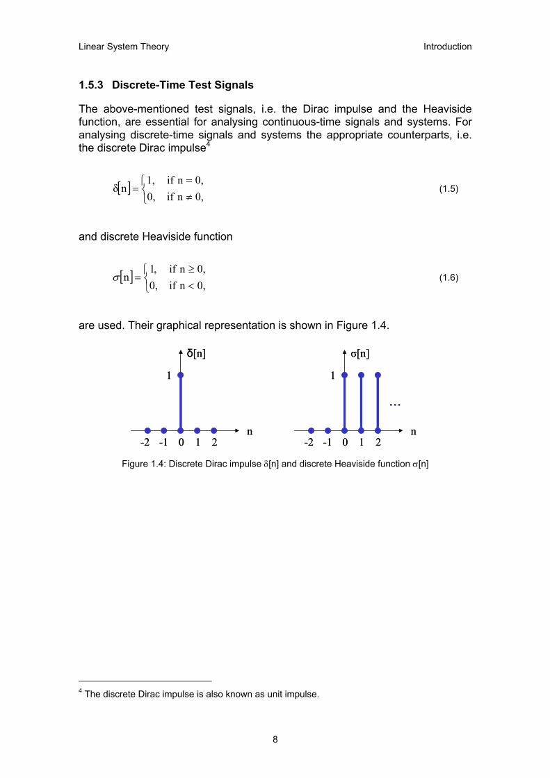
The above-mentioned test signals, i.e. the Dirac impulse and the Heaviside function, are essential for analysing continuous-time signals and systems. For analysing discrete-time signals and systems the appropriate counterparts, i.e. the discrete Dirac impulse4
[ ]0,n if0,n if
0,1,
nδ≠=
= (1.5)
and discrete Heaviside function
[ ]0,n if0,n if
0,,1
n<≥
=σ (1.6)
are used. Their graphical representation is shown in Figure 1.4.
0
δ[n]
n1 2-1-2
1
0
δ[n]
n1 2-1-2
1
0
σ[n]
n1 2-1-2
1
...
0
σ[n]
n1 2-1-2
1
...
Figure 1.4: Discrete Dirac impulse δ[n] and discrete Heaviside function σ[n]
4 The discrete Dirac impulse is also known as unit impulse.
8
Linear System Theory Mathematical Description
2. MATHEMATICAL DESCRIPTION
In this chapter important system properties are introduced. Additionally, methods that describe a system mathematically are shown. This leads to a possible derivative of the convolution integral without any strict line of argument. For the description of the transfer function of a system the Laplace transform (for continuous-time systems) and the z-transform (for discrete-time systems) are introduced. These transforms are used to describe a system mathematically with least possible effort. Principle characteristics of Fourier transform, Laplace transform and z-transform are not dealt with in this text in more detail (recommendation for further reading [Mil95]), i.e. only the most necessary context is stated.
2.1 System Properties
For describing LTI-systems it is necessary to know about vital system properties like linearity and time-invariance (and still some more are discussed in this section). Stability is also an important system property, therefore, it is treated in more detail in Chapter 3. Statements about LTI-system properties are in most cases directly applicable to LTD-systems. However, worthwhile mathematical formulations of LTD-system properties are introduced in Section 2.3.2 additionally.
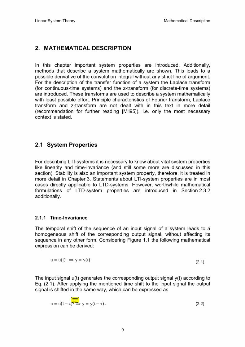
2.1.1 Time-Invariance
The temporal shift of the sequence of an input signal of a system leads to a homogeneous shift of the corresponding output signal, without affecting its sequence in any other form. Considering Figure 1.1 the following mathematical expression can be derived:
y(t)y u(t)u =⇒= (2.1)
The input signal u(t) generates the corresponding output signal y(t) according to Eq. (2.1). After applying the mentioned time shift to the input signal the output signal is shifted in the same way, which can be expressed as
τ)y(ty τ)u(tu −=⇒−= . (2.2)
9

Linear System Theory Mathematical Description
The form of the reaction of a system is thus independent of the time instant at which the signal arrives.
2.1.2 Linearity
If a system for two elementary input signals (u1(t), u2(t)) supplies determined output signals (y1(t), y2(t)),
(t)y (t)u 11 ⇒ and (2.3) , (t)y (t)u 22 ⇒
the overlay of the two input signals leads to the similar overlay of the corresponding output signals
(t)y(t)y (t)u (t)u 2121 +⇒+ . (2.4)
A system fulfils the additivity property if Eq. (2.4) is satisfied. If an input signal of a system is multiplied by a real constant and the corresponding system output (amplitude) is scaled by the same amount, the system fulfils the homogeneity property, which can be expressed as follows:
Rα (t)αy (t)αu 11 ∈⇒ (2.5)
If a system fulfils both the additivity and the homogeneity property, it also fulfils the superposition property
Rα,α (t)yα(t)yα (t)uα(t)uα 2122112211 ∈+⇒+ . (2.6)
A system is called a linear system only if the superposition property (Eq. (2.6)) holds.
2.1.3 Causality
Assume that a network consists of resistors only, thus it has no memory modules such as capacitors or inductors. We refer to a system, which has no memory modules at all as a memory-less system. The output y(t0) of such a system depends only on the input applied at t0, that means the system output is independent of the input applied before or after t0. In other words, the current
10

Linear System Theory Mathematical Description
output of a memory-less system depends only on current input and therefore it is independent of past and future inputs (see [Che99]). The causal (or non-anticipatory) system does not have predictive character. A change of the output signal arises only after any change of the input signal. It should be noted that no physical system can predict or anticipate what will be applied in the future, therefore, every physically realizable system is causal and this text studies only causal systems. A possible mathematical expression of causality could read:
00 tttt 0y(t) 0u(t) << =⇒= (2.7) Eq. (2.7) could be interpreted also in such a way that the current output of a system depends on past and current inputs but not on future input. Due to this characteristic of causal systems the following statements are valid:
o The impulse response of a causal system is zero for t < 0.
o The step response of a causal system is zero for t < 0.
2.2 Description of LTI-Systems
In this section the state of a system and the input-output or external description5 are introduced. This leads us to the state-space equations (called the internal description of a system) and to the convolution integral. The Laplace transform is introduced in order to calculate the transfer function of a system.
2.2.1 System Response
The system response of every linear system can be obtained by adding the zero-state response and the zero-input response (superposition property). The state of a system represents the status at a specific time t0. This stands for what happened before t0 (described by the state x(t0)) and what will happen after t0 (caused by the input u(t)) to the system. Thus, the output y(t) for all t ≥ t0 can be made up of the state of a system x(t0) together with the input u(t) for t ≥ t0. In other words, if we know the state of a system at t0, there is no more need to know the input u(t) applied before t0 in determining the output y(t) after t0 (see [Che99]). This context can be expressed as
5 The external description shows the relationship between the input and the output of a system.
11

Linear System Theory Mathematical Description
00
0 t ty(t),t tu(t),
)x(t≥→
≥. (2.8)
A system is in the zero-state if all state variables are zero. The sequence of the output signal as reaction to a given input signal outgoing from the zero state of the system is the associated zero-state response (see Eq. (2.9)). The zero-state response yzs of a system can be defined as follows:
0zs0
0 t t(t),yt tu(t),0)x(t
≥→
≥=
(2.9)
Beginning at a certain time t0 and keeping the input of a system zero (realized with a short circuit for example) the zero-input response can be derived:
0zi0
0 t t(t),yt t0,u(t)
)x(t≥→
≥= (2.10)
A system is not in the zero-state initially. The sequence of the output signal as reaction to a given input signal outgoing from the state of the system is the associated zero-input response if, during the whole procedure, the input is kept zero (see Eq. (2.10)). Consider, for example, a network with memory modules. If at a specific time instant t0 no more input is applied (to the system – in this case a network), the output only depends on the state of the memory modules. To be more specific, the state of the memory modules is composed of charges in this context. It should be stressed that the entire system response, which comes off by addition of the zero-state response and the zero-input response,
(t)y(t)y(t)y zszisys += , (2.11)
applies to linear systems only.
2.2.2 State-space Description of LTI-Systems
A LTI-system is lumped, if its number of state variables (n) is finite or its state is describable by a finite vector ( ( )0txv ). If we introduce a positive finite whole number M, the state of a system can be expressed as
12
Linear System Theory Mathematical Description
( )
( )( )
( )
M n
tx
txtx
tx
0n
02
01
0 ≤
=M
v (2.12)
A lumped LTI-system can be described by a set of equations, which are also called state-space equations or the internal description of a system, of the form
( ) ( ) tuBtxAtx vv&v ⋅+⋅= ( ) (2.13)
and
( ) ( ) ( )tuDtxCty vvv ⋅+⋅= , (2.14)
where differentiation with respect to time is denoted by a dot: . If a system has p inputs and q outputs,
( ) /dtxdtx v&v =uv is a 1p × vector and yv is a q vector. 1× xv
is a n vector because the system has n state variables (see Eq. (2.12)). A, B, C and D are, respectively,
1×nn × , pn × , nq × , and pq × constant matrices in
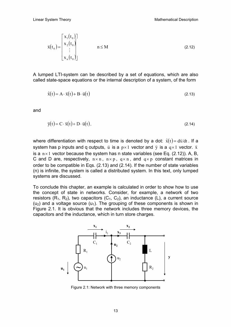
order to be compatible in Eqs. (2.13) and (2.14). If the number of state variables (n) is infinite, the system is called a distributed system. In this text, only lumped systems are discussed. To conclude this chapter, an example is calculated in order to show how to use the concept of state in networks. Consider, for example, a network of two resistors (R1, R2), two capacitors (C1, C2), an inductance (L), a current source (u2) and a voltage source (u1). The grouping of these components is shown in Figure 2.1. It is obvious that the network includes three memory devices, the capacitors and the inductance, which in turn store charges.
~
R1 L
R2u1
u2
u2
u1
C1 C2
x1 x2
x3
y
i1
Figure 2.1: Network with three memory components
13

Linear System Theory Mathematical Description
The state, or the vector x of the network (or system), could therefore be expressed as
( )( )( )( )
=
txtxtx
tx
03
02
01
0v
. (2.15)
Now, as we know the state variables of the system, the next step is the application of Kirchhoff’s current and voltage laws in order to establish the state-space equations (mathematical expressions according to Eqs. (2.13) and (2.14)):
2
32223
1
231211213
111
Cx
xxCx
Cux
xuxCuix
xCi
=⇒=
−=⇒+=+=
=
&&
&&
&
(2.16)
Eqs. (2.16) represent the application of Kirchhoff’s current law which results in
and . Now, if Kirchhoff’s voltage law is applied to the system, this can be expressed as follows:
1x& 2x&
( ) 233211231 RxLxxxRuxu ++++−= &
( )
( )2113121
2321132121
233
211321213
uRuxRxxy RxuRuxRRxx
RxLxy
LuRuxRRxx
x
++−−−=++++−−−=
+=
+++−−−=
&
&
(2.17)
The underlined results in Eqs. (2.16) and (2.17) can be brought to the state-space form by transferring them into matrices. The state-space equations for this example network can be represented as follows:
14
Linear System Theory Mathematical Description
( )
[ ] [ ]
⋅+
⋅−−−=
⋅
−
+
⋅
+−−−
=
2
11
3
2
1
1
2
1
1
1
3
2
1
21
2
1
3
2
1
uu
R1xxx
R11y
uu
LR
L1
00
C10
xxx
LRR
L1
L1
C100
C100
xxx
&
&
&
(2.18)
2.2.3 Convolution Integral (External Description)
The external description describes only zero-state responses, thus, systems are implicitly assumed to be relaxed or equivalently their initial conditions are assumed to be zero. In this chapter we use a special function, which is called the analysing function δ∆(t), to describe and approximate an arbitrary signal. After deriving the corresponding mathematical expression, it is shown that it can easily be transferred to the convolution integral. The analysing function6 used, which is defined as
( )
elsewhere, , 0
∆,t0 if ,1
tδ
≤≤∆
=∆ (2.19)
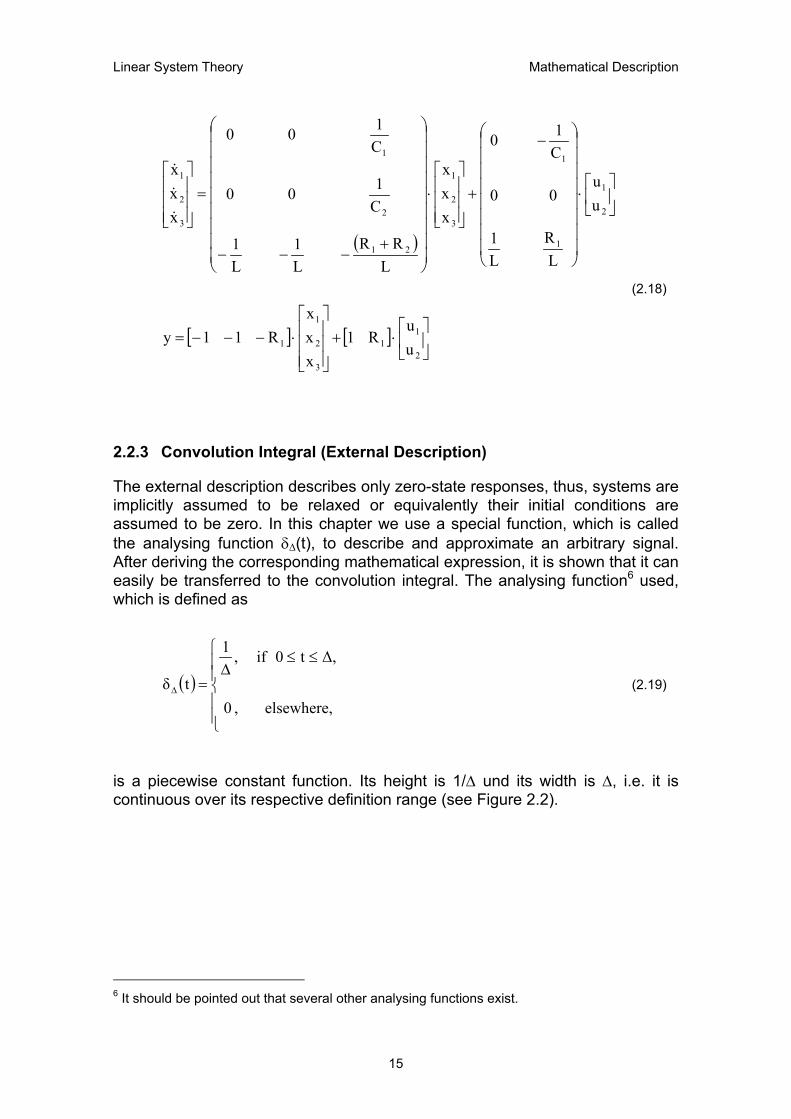
is a piecewise constant function. Its height is 1/∆ und its width is ∆, i.e. it is continuous over its respective definition range (see Figure 2.2).
6 It should be pointed out that several other analysing functions exist.
15
Linear System Theory Mathematical Description
δ∆(t)
t0 ∆
1/∆
Figure 2.2: Analysing function δ∆(t)
To develop the mathematical external description7, the output is excited by the input signal only and the initial state of the system is assumed to be zero. For further consideration let
( )
elsewhere, 0,
∆,t t tif ,1
ttδii
i
+≤≤∆
=−∆ (2.20)
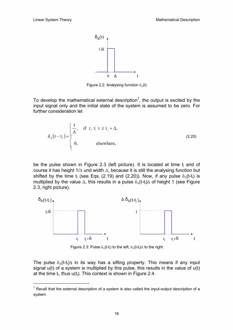
be the pulse shown in Figure 2.3 (left picture). It is located at time ti and of course it has height 1/∆ und width ∆, because it is still the analysing function but shifted by the time ti (see Eqs. (2.19) and (2.20)). Now, if any pulse δ∆(t-ti) is multiplied by the value ∆, this results in a pulse δ∆(t-ti)∆ of height 1 (see Figure 2.3, right picture).
δ ∆ (t - t i )
tt i t i + ∆
1/ ∆
∆ δ∆(t-ti )
tti t i + ∆
1
Figure 2.3: Pulse δ∆(t-ti) to the left, δ∆(t-ti)∆ to the right
The pulse δ∆
(t-ti)∆ in its way has a sifting property. This means if any input signal u(t) of a system is multiplied by this pulse, this results in the value of u(t) at the time ti, thus u(ti). This context is shown in Figure 2.4.
7 Recall that the external description of a system is also called the input-output description of a system.
16
Linear System Theory Mathematical Description
u(t)
tt1 t2 t3··· ···
u(t1)
u(t3)
…
1
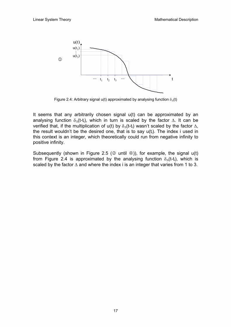
Figure 2.4: Arbitrary signal u(t) approximated by analysing function δ∆(t)
It seems that any arbitrarily chosen signal u(t) can be approximated by an analysing function δ∆(t-ti), which in turn is scaled by the factor ∆. It can be verified that, if the multiplication of u(t) by δ∆(t-ti) wasn’t scaled by the factor ∆, the result wouldn’t be the desired one, that is to say u(ti). The index i used in this context is an integer, which theoretically could run from negative infinity to positive infinity. Subsequently (shown in Figure 2.5 (2 until )), for example, the signal u(t) from Figure 2.4 is approximated by the analysing function δ∆(t-ti), which is scaled by the factor ∆ and where the index i is an integer that varies from 1 to 3.
17

Linear System Theory Mathematical Description
u(t1)δ∆(t-t1)∆
tt1 t1+∆
u(t1)
2
u(t2)δ∆(t-t2)∆
tt2 t2+∆
u(t2)
3
u(t3)δ∆(t-t3)∆
tt3 t3+∆
u(t3)4
tt1 t2 t3
u(t1)
u(t3)
…
5
t3+∆
∑=
−≈3
1ii∆i )∆t(t)δu(tu(t)
Figure 2.5: Approximation of signal
Due to the above-mentioned facts, the input signal u(t) of a system can be expressed by summing up the previously accomplished multiplications, thus resulting in stepwise constant functions. Such a process (for three time instances t1, t2 and t3) can be viewed in Figure 2.5 (2 to 5). In general the equation given in Figure 2.5 (5) can be extended to the form
18

Linear System Theory Mathematical Description
∑ −≈i
i∆i )∆t(t)δu(tu(t) , (2.21)
which is an approximate representation of the input signal u(t). An input signal generates a corresponding output signal. If the input signal of a LTI-system is the pulse of Figure 2.3 (left picture), the output signal will be g∆(t-ti) for example, which can be expressed as
)t(tg)t(tδ i∆i∆ −→− . (2.22)
Now, if the input signal is scaled by a factor (in this case by u(ti)∆), the corresponding system output is scaled by the same factor likewise (if the homogeneity property holds, see Eq. (2.5)):
)∆)u(tt(tg)∆)u(tt(tδ ii∆ii∆ −→− (2.23)
In the next step, all values corresponding to the various i are added and fed to the system input. If the additivity property (Eq. (2.4)) holds, this yields
∆))u(tt(tg)∆)u(tt(tδi i
ii∆ii∆∑ ∑ −→− (2.24)
because the system output consists of the summation of the corresponding system responses to the individual input signals. The above stated mappings finally show that if the input signal of a LTI-system is u(t) the corresponding system output y(t) can be approximated by
∑ −≈i
i∆i )∆t(t)gu(ty(t) . (2.25)
It should be pointed out that the superposition property (homogeneity and additivity, see Eqs. (2.23) and (2.24)) must be fulfilled, otherwise the observed system is a non-linear system and Eq. (2.25) is invalid. The approximation in Eq. (2.25) becomes an equation if ∆ approaches zero. Now if ∆ approaches zero, the pulse δ∆(t-ti) becomes an impulse at ti, denoted by δ(t-ti), and the corresponding output is denoted by g(t-ti). Moreover the summation becomes an integration, the discrete ti becomes a continuum and can be replaced by τ, and ∆ can be written as dτ. This process yields
19

Linear System Theory Mathematical Description
( ) ( )∫+∞
∞−
−= τtgτu dτy(t) , (2.26)
which is also called convolution integral. In Eq. (2.26) g(t-τ) is called the impulse response, because it is the response to an impulse excitation. Thus, the output y(t) of every linear system, whether an electrical system, a mechanical system, or any other system, can be calculated if the input signal u(t) is convoluted with the impulse response g(t) of the system. The convolution is commutative. This can be shown if t-τ of Eq. (2.26) is substituted by any variable, in the following by v:
( ) ( ) ( )
( ) ( ) ( ) ( ) ( ) ( )vtuvg dvvtuvg dvty
dvdτconstant) a is(t vt τ vτt
τuτtg dτtyτ
τ
−=−−=
−=−=→=−
−=
∫∫
∫
∞+
∞−
∞−
∞+
+∞=
−∞=
(2.27)
The dummy8 variable v can be replaced by any other variable in this integral. In the following, τ is used instead of v. Therefore, we obtain:
( ) ( ) ( ) ( ) ( ) τtgτu dττtuτg dτty −=−= ∫∫+∞
∞−
+∞
∞−
(2.28)
Because the condition for a linear time-invariant system to be causal is g(t) = 0 for all t < 0 (see Section 2.1.3) the lower boundary of the convolution integral can be set to zero. Thus, Eq. (2.28) reduces to
( ) ( ) ( ) ( ) ( )τtgτu dττtuτg dτty00
−=−= ∫∫+∞+∞
. (2.29)
If a LTI-system has p input terminals and q output terminals, Eq. (2.29) can be extended to
8 That means that the denomination of this variable is insignificant.
20
Linear System Theory Mathematical Description
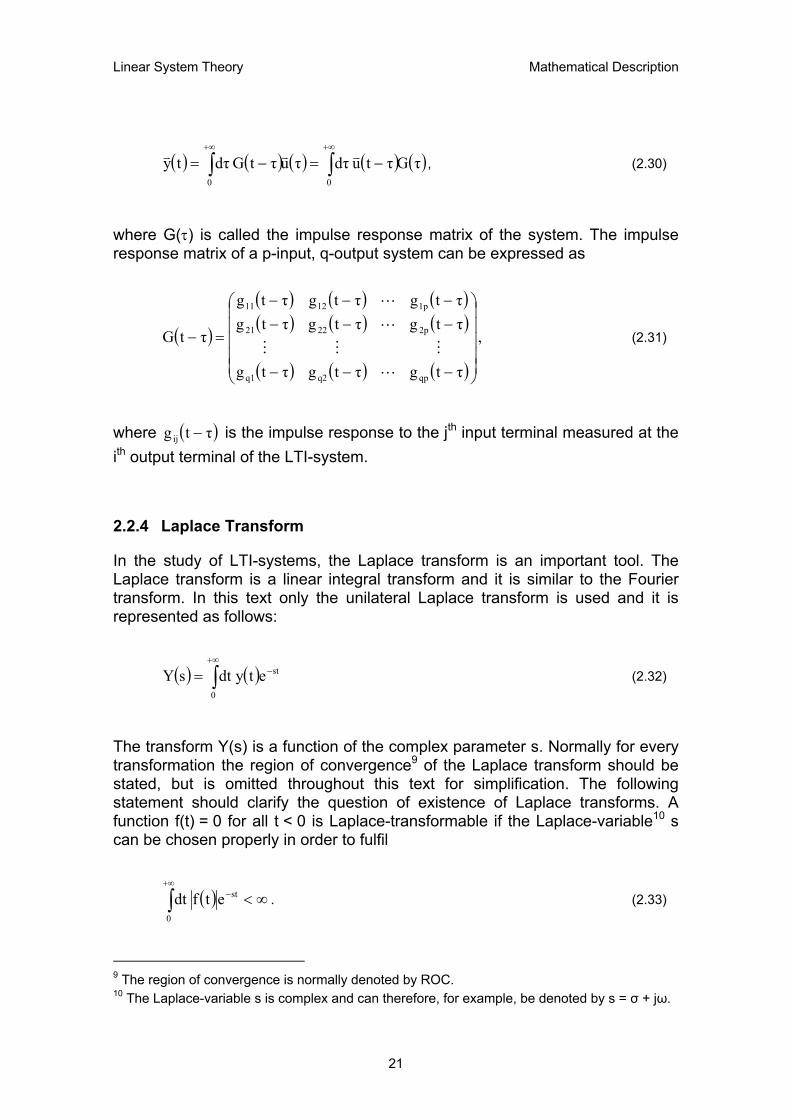
( ) ( ) ( ) ( ) ( )τGτtu dττuτtG dτty00∫∫
+∞+∞
−=−= vvv, (2.30)
where G(τ) is called the impulse response matrix of the system. The impulse response matrix of a p-input, q-output system can be expressed as
( )
( ) ( ) ( )( ) ( ) ( )
( ) ( ) ( )
,
τtgτtgτtg
τtgτtgτtgτtgτtgτtg
τtG
qpq2q1
2p2221
1p1211
−−−
−−−−−−
=−
L
MMM
L
L
(2.31)
where is the impulse response to the j( τtg ij − ) th input terminal measured at the ith output terminal of the LTI-system.
2.2.4 Laplace Transform
In the study of LTI-systems, the Laplace transform is an important tool. The Laplace transform is a linear integral transform and it is similar to the Fourier transform. In this text only the unilateral Laplace transform is used and it is represented as follows:
( ) ( )∫+∞
−=0
stetydt sY (2.32)
The transform Y(s) is a function of the complex parameter s. Normally for every transformation the region of convergence9 of the Laplace transform should be stated, but is omitted throughout this text for simplification. The following statement should clarify the question of existence of Laplace transforms. A function f(t) = 0 for all t < 0 is Laplace-transformable if the Laplace-variable10 s can be chosen properly in order to fulfil
( )∫+∞
− ∞<0
stetfdt . (2.33)
9 The region of convergence is normally denoted by ROC. 10 The Laplace-variable s is complex and can therefore, for example, be denoted by s = σ + jω.
21

Linear System Theory Mathematical Description
In other words, the complex Laplace-variable s has to be chosen in a way such that the Laplace integral is absolutely integrable. If the Laplace transform is applied to any signal x(t), this signal is transformed from the time-domain into the Laplace-domain or s-domain and is denoted by X(s) i.e. capital letters with parameter s. Now, if the Laplace transform is applied to the convolution integral (external description of a LTI-system, see Section 2.2.3), this results in a major property and advantage of this transform i.e.: A convolution in the time-domain – which is in fact the external system description – corresponds to a multiplication in the Laplace-domain (details of the derivation are shown in Section 2.2.5) and conversely, a convolution in the Laplace-domain corresponds to a multiplication in the time-domain. This context can be expressed as follows:11
( ) ( ) ( ) txtxty 21 ∗= ( ) ( ) ( ) sXsXsY 21= (2.34)
( ) ( ) ( )sXsXsY 21 ∗= ( ) ( ) ( ) txtxty 21= (2.35)
This explains the reason for transforming signals into the Laplace-domain: Complex calculations in the time-domain (such as differential equations or the convolution integral) can be replaced by considerably simpler arithmetic equations. This is guaranteed by another important property of the Laplace transform, the linearity property. The superposition property, which is stated in Eq. (2.6), applied to the Laplace transform yields
( ) ( ) ( )thαtgαtf 21 += ( ) ( ) ( )sHαsGαsF 21 += , (2.36)
whereby α1 and α2 are real. The theorem of derivative, which can be expressed as
( ) ( )tf n ( ) ( ) ( ) ( ) ( ) ( ) ( )0f0sf...0fs0fssF 1n2n2n1nn −−−− −−−′−−s , (2.37)
is used for solving differential equations. Because of the definition range of the Laplace transform, which lasts from zero to positive infinity (Eq. (2.32)), the function f(t) is required to be zero for all t < 0. This can be achieved by multiplying f(t) by the Heaviside function σ(t), which is shown in Figure 1.3 (see [Mil95]).
11 The convolution operand is denoted by the ∗ -symbol.
22

Linear System Theory Mathematical Description
If the initial condition f(0) equals zero, Eq. (2.37) can be reduced by the terms that include f(0). In other words, the memories of a system are zero at t = 0 or the state of the system x(0) = 0. A system is called relaxed if its initial state is zero. Thus, the theorem of derivative reduces to
( ) ( )tf n s . (2.38) ( )sFn
The inverse Laplace transform (transformation from the Laplace-domain into the time-domain) can be calculated numerically (recommendation for further reading [Wun69]) or alternatively for standard signals by using a Laplace transform table.
2.2.5 Transfer Function
In this section the transfer function is derived and defined. In this text the transfer function of a system is a rational function of the complex Laplace-variable s, because only lumped LTI-systems are discussed. Rational Laplace-transformations are very important in practice, because many signals just have rational Laplace-transformations and therefore can be transformed easily into the time-domain in most cases. In the following, it is shown that a convolution in the time-domain is equal to a multiplication in the Laplace-domain. Therefore, the Laplace-integral (Eq. (2.32)) is applied to the external system description (the convolution integral, see Eq. (2.29)), which yields
( ) ( ) ( )
( )
st
0
ty
0
eτtuτg dτdtsY −∞ ∞
∫ ∫
−=44 344 21
. (2.39)
Under certain conditions, the order of integrations may be interchanged (for further reading see [Sti99]). If the order of integrations is interchanged Eq. (2.39) becomes
( ) ( ) ( )∫ ∫∞ ∞
−
−=
0 0
steτtudt τg dτsY . (2.40)
Now, if the parameter t-τ in Eq. (2.40) is substituted by the parameter v, for example, we obtain:
23

Linear System Theory Mathematical Description
( ) ( ) ( ) ( )
( ) ( ) sτ
0 τ-
sv
0 τ-
τvs
eevu dvτg dτ
evu dvτg dτsY
τtv
−∞ ∞
−
∞ ∞+−
∫ ∫
∫ ∫
=
=
−=
(2.41)
Considering the causality condition, the lower integration boundary of the integral inside the parentheses can be changed to zero. Additionally, it is to be observed that this integral becomes independent of the integration variable τ of the “outer” integral. Thus, the double integrations become
( ) ( ) ( )
( )
( )
( )
( )
( ) ( ).sUsG etudt etgdt
evu dv eτg dτsY
sU
0
st
sG
st
0
0
svsτ
0
==
==
∫∫
∫∫∞
−−∞
∞−−
∞
4342143421
(2.42)
The dummy variables τ and v of Eq. (2.42) can be replaced by t. The convolution in the time-domain y(t) = g(t)∗ u(t) results in an easier multiplication in the Laplace-domain, that is to say Y(s) = G(s)U(s) (see Eq. (2.34)). G(s) is called the transfer function of the system. Thus, the transfer function of a system is the Laplace transform of the impulse response g(t) and, conversely, the impulse response g(t) is the inverse Laplace transform of the transfer function G(s). If a LTI-system has p input terminals and q output terminals, Eq. (2.42) can be extended to
( )( )
( )
( ) ( ) ( )( ) ( ) ( )
( ) ( ) ( )
( )( )
( )
=
sU
sUsU
sGsGsG
sGsGsGsGsGsG
sY
sYsY
p
2
1
qpq2q1
2p2221
1p1211
q
2
1
M
L
MMM
L
L
M (2.43)
or
( ) ( ) ( )sUssYvv
G= , (2.44)
24

Linear System Theory Mathematical Description
respectively, where G(s)12 is called the transfer-function matrix of the system. Gij(s) is the transfer function from the jth input to the ith output of the LTI-system. If a system has an infinite number of state variables, thus being a distributed system, its transfer function is an irrational function of the Laplace-variable s. The transfer function of a system, which can be expressed as
( ) ( )( ) n
n10
mm10
sb...sbbsa...saa
sUsY sG
++++++
== , (2.45)
is a rational function of s, if the LTI-system is lumped. In this text transfer functions with real coefficients (ai and bj with i = 0…m, j = 0…n, see Eq. (2.45)) are treated only. The numerator and denominator polynomials of equation Eq. (2.45)) can be factorised into the products of the roots of the respective polynomials. The numerator polynomial Y(s) has m zeros, which are denoted as z1, z2, …, zm. The n roots of the denominator polynomial U(s) are denoted as p1, p2, …, pn, because U(s) has poles at these points, that is G(s) becomes infinite. In terms of poles and zeros, the transfer function G(s) can be expressed as
( ) ( )( ) ( )( )( ) ( )n21
m21
n
m
pspspszszszs
ba sG
−−−−−−
=L
L, (2.46)
which is called the zero-pole-gain form. The following statements are valid for transfer functions, which are treated in this text:
o The transfer function G(s) is a rational function of s.
o The degree of the numerator polynomial of G(s) is less than or equal to the degree of the denominator polynomial of G(s). In this case G(s) is said to be proper.
o If the degree of the numerator polynomial of G(s) is less than the degree of the denominator polynomial of G(s), the transfer function is said to be strictly proper.
The following concluding statements are valid for the transfer-function matrix G(s) of LTI-systems, which are treated in this text:
o Every entry Gij(s) of the transfer-function matrix G(s) is a rational function of the complex Laplace-variable s.
12 Transformed matrices in the Laplace-, z-, or frequency-domain are denoted by bold type capital letters.
25
Linear System Theory Mathematical Description
o The degree of the numerator polynomial of every entry Gij(s) is less than or equal to the degree of the denominator polynomial of Gij(s). In this case G(s) is said to be proper.
o If the degree of the numerator polynomial of every Gij(s) is less than the degree of its denominator polynomial, the transfer-function matrix is said to be strictly proper.
2.3 Description of LTD-Systems
This section can be seen as the discrete counterpart of the previous Section 2.2. A possible definition of a discrete-time signal is introduced. This leads us to the state-space equations (called the internal description of a system) and to the discrete convolution integral. The z-transform is introduced in order to calculate the discrete transfer function of a system.
2.3.1 Discrete-Time Signal
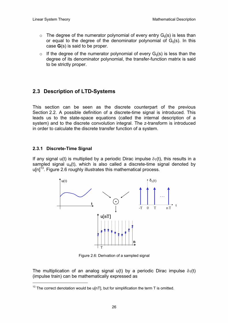
If any signal u(t) is multiplied by a periodic Dirac impulse δT(t), this results in a sampled signal ua(t), which is also called a discrete-time signal denoted by u[n]13. Figure 2.6 roughly illustrates this mathematical process.
t t
u(t)
··
δT(t)
t n T
· · ·
T-T 0 u[nT]
nT
u[nT]
nT
Figure 2.6: Derivation of a sampled signal
The multiplication of an analog signal u(t) by a periodic Dirac impulse δT(t) (impulse train) can be mathematically expressed as 13 The correct denotation would be u[nT], but for simplification the term T is omitted.
26
Linear System Theory Mathematical Description
[ ] [ ] ( ) ∈=
==N,nwhereby
elsewhere,0, nT for t ,tu
nunTu (2.47)
and
( ) ( ) ( ) ( ) ( ) ( ) ( )∑∑+∞
−∞=
+∞
−∞=
−=−==nn
Ta nTtδnTunTtδtutδtutu , (2.48)
whereby T represents the sampling period. For the mathematical description of discrete-time signals the discrete Dirac impulse (see Figure 1.4) can be used, too. A discrete-time signal u[n] can be described by the sum of weighted (by u[i]) discrete Dirac impulses, which are time shifted by i sampling periods, that is,
[ ] [ ] [ ]∑+∞
−∞=
−=i
inδiunu . (2.49)
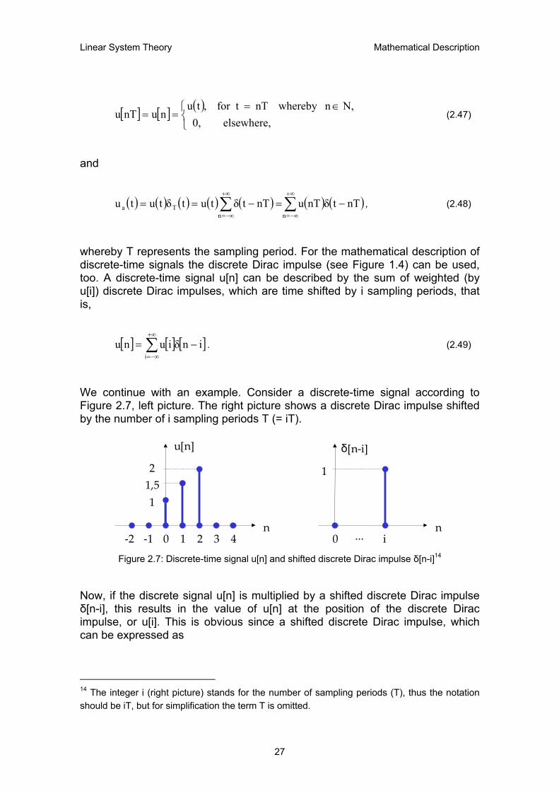
We continue with an example. Consider a discrete-time signal according to Figure 2.7, left picture. The right picture shows a discrete Dirac impulse shifted by the number of i sampling periods T (= iT).
0n
1 2 - 1 - 2 3 4
1
1,5
2
u[n]
δ[n-i]
n i
1
0 ··· Figure 2.7: Discrete-time signal u[n] and shifted discrete Dirac impulse δ[n-i]14
Now, if the discrete signal u[n] is multiplied by a shifted discrete Dirac impulse δ[n-i], this results in the value of u[n] at the position of the discrete Dirac impulse, or u[i]. This is obvious since a shifted discrete Dirac impulse, which can be expressed as
14 The integer i (right picture) stands for the number of sampling periods (T), thus the notation should be iT, but for simplification the term T is omitted.
27

Linear System Theory Mathematical Description
[ ]i,n ifi,n if
0,1,
inδ≠=
=− (2.50)
is different from zero at its time instant only. Figure 2.8 shows the graphical representation of Eq. (2.49) referred to our example of Figure 2.7.
0
u[0]δ[n-0]
n1 2-1-2 3 4
1
0n
1 2-1-2 3 4
1,5
u[1]δ[n-1]
0n
1 2-1-2 3 4
2
u[2]δ[n-2]
Figure 2.8: Discrete-time signal u[n] multiplied by discrete Dirac impulse δ[n-i]
If the individual constituents are added they result in u[n], which can be expressed as
[ ] [ ] [ ] [ ] [ ] [ ] [ ] [ ] [ ]∑=
−=−+−+−=2
0iinδiu 2nδ2u1nδ1u0nδ0unu , (2.51)
where the integer i varies only from 0 to 2, because u[n] is equal to zero anywhere else.
28

Linear System Theory Mathematical Description
2.3.2 Properties of LTD-Systems
This section briefly introduces some important mathematical formulations of LTD-system properties. For additional information about system properties of linear time-invariant systems refer to Section 2.1. Stability conditions of LTD-systems are discussed in greater detail in Chapter 3. The property of linearity is treated first. An input sequence u[n] causes the output sequence y[n]. Now, if input sequences are scaled by factors ki, corresponding output sequences are scaled by the same factors, too. Considering the superposition property according to Eq. (2.6) this leads to:
[ ] [ ] [ ] [ ]
[ ] [ ] [ ] [ ] [ ] [ ]nyknyknynuknuknu
nynu and nynu
22112211
2211
+=→+=
→→ (2.52)
The property of time-invariance is treated next. If an input signal is delayed (shifted) by, say, i sampling periods, the output waveform is simply delayed by i sampling periods and unchanged otherwise. Thus, the output signal from a time-invariant discrete-time system merely shifts forward or backward in time as the input signal is shifted forward or backward in time. This can be expressed as
[ ] [ ]inyinu −→− . (2.53)
Finally a discrete-time system is said to be causal if the nth element of an output sequence y, i.e. y[n], does not depend on future inputs u[n+1], u[n+2], u[n+3], etc.
2.3.3 Discrete Convolution
This section represents the discrete counterpart of continuous-time systems (Section 2.2.3). The discrete convolution describes only zero-state responses. It has to be assumed that the input u[n] and the output y[n] of every discrete-time system have the same sampling period T. Most concepts in continuous-time systems can be applied directly to discrete-time systems. The following considerations are only valid for LTD (linear time-invariant discrete-time) systems. The output signal y[n] of a LTD-system is equal to the input signal u[n] convoluted by the impulse response sequence g[n] of the system. The following steps underline this statement:
29
Linear System Theory Mathematical Description
1. The discrete Dirac impulse δ[n] generates the impulse response sequence g[n], because y[n] = g[n] if the system input u[n] = δ[n].
2. Due to the system property of time-invariance, a shifted (by i sampling periods) impulse δ[n-i] also generates a shifted (by i sampling periods) impulse response sequence g[n-i].
3. If the shifted impulse δ[n-i] is multiplied by the sampled value u[i] – thus, the impulse is weighted – the shifted and weighted impulse u[i]δ[n-i] generates the output u[i]g[n-i] due to the system property of linearity.
4. Also due to the system property of linearity an input signal
generates the output . [ ] [ ] [ ]∑+∞
−∞=
−=i
inδiunu [ ] [ ] [ ]∑+∞
−∞=
−=i
ingiuny
The last step leads to the definition of the discrete convolution. The output of a LTD-system is equal to the input signal convoluted by the impulse response sequence of the system. The discrete convolution is also commutative and can be expressed as
[ ] [ ] [ ] [ ] [ ]∑∑+∞
−∞=
+∞
−∞=
−=−=ii
iginuingiuny . (2.54)
The fact that the discrete convolution is commutative, can facilitate many calculations in the time-domain. The characteristic that the discrete convolution (Eq. (2.54) is commutative can be readily obtained by substituting the parameter n-i by another variable l, for example. Therefore, we obtain:
[ ] [ ] [ ]
boundary upper"" inl
boundary lower"" inlinl
ingiuny
i
i
i
−∞=−=
+∞=−=
−=
−=
+∞=
−∞=
+∞
−∞=∑
(2.55)
Eq. (2.55) shows the process of substitution, where the variable n is a constant and the variable i is a dummy variable. Now, if the new boundaries, which arise from the substitution, are replaced this leads to
[ ] [ ] [ ] [ ] [ ]∑∑+∞
−∞=
−∞=
+∞=
−=−=l
l
llglnulglnuny . (2.56)
30
Linear System Theory Mathematical Description
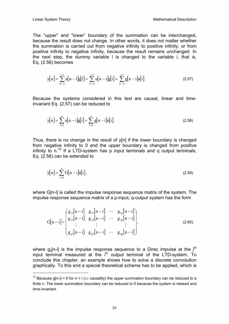
The “upper” and “lower” boundary of the summation can be interchanged, because the result does not change. In other words, it does not matter whether the summation is carried out from negative infinity to positive infinity, or from positive infinity to negative infinity, because the result remains unchanged. In the next step, the dummy variable l is changed to the variable i, that is, Eq. (2.56) becomes
[ ] [ ] [ ] [ ] [ ] [ ] [∑∑∑+∞
−∞=
+∞
−∞=
+∞
−∞=
−=−=−=iil
iuingiginulglnuny ]. (2.57)
Because the systems considered in this text are causal, linear and time-invariant Eq. (2.57) can be reduced to
[ ] [ ] [ ] [ ] [ ]∑∑==
−=−=n
0i
n
0iiuingiginuny . (2.58)
Thus, there is no change in the result of y[n] if the lower boundary is changed from negative infinity to 0 and the upper boundary is changed from positive infinity to n.15 If a LTD-system has p input terminals and q output terminals, Eq. (2.58) can be extended to
[ ] [ ] [ ]∑=
−=n
0iiuinGny vv
, (2.59)
where G[n-i] is called the impulse response sequence matrix of the system. The impulse response sequence matrix of a p-input, q-output system has the form
[ ]
[ ] [ ] [ ][ ] [ ] [ ]
[ ] [ ] [ ]
,
inginging
inginginginginging
inG
qpq2q1
2p2221
1p1211
−−−
−−−−−−
=−
L
MMM
L
L
(2.60)
where gij[n-i] is the impulse response sequence to a Dirac impulse at the jth input terminal measured at the ith output terminal of the LTD-system. To conclude this chapter, an example shows how to solve a discrete convolution graphically. To this end a special theoretical scheme has to be applied, which is 15 Because g[n-i] = 0 for n < i (⇔ causality) the upper summation boundary can be reduced to a finite n. The lower summation boundary can be reduced to 0 because the system is relaxed and time-invariant.
31

Linear System Theory Mathematical Description
indicated in Table 2.1. This process can be seen as graphical execution of Eq. (2.54). Step Signal-status Comment
u[n]
n1 2 - 1 - 2 3 4
1
0- 1
0
g[n]
n1 2-1-2 3 4
11,52
signal data
1 u[i]
i1 2 - 1 - 2 3 4
1
0- 1
0
g[i]
i1 2-1-2 3 4
11,52
the time variable n is changed to the
variable i
2
0
g[-i]
i1 2- 1 - 2 3 4
1 1,5 2
one of the two signals is flipped with respect to the vertical axis16
3
0
g[n2-i]
i1 2-1-2 3 4
1
1,5
2
the flipped signal is shifted by n = n2
sampling periods to the right17
4 0
u[i]g[n2-i]
i1 2-1-2 3 4
1,5
-1
for every sampling period i u[i] is
multiplied by g[n2-i] resulting in u[i]g[n2-i]
5
y[n]
nn2
y[n2] = 0,5
summing up all results of u[i]g[n2-i] this results in y[n2]
6
y[n]
n0 1 2-1-2 3 4
1
the steps 3 to 5 have to be repeated in
order to obtain the entire convoluted
signal y[n]
Table 2.1: How to perform a discrete convolution graphically 16 Because the convolution is commutative the choice of the signal (u or g) is arbitrary. 17 The variable n2 is an integer and varies from negative infinity to positive infinity. In this diagram the parameter n2 is chosen to be 1 for clarity of illustration.
32
Linear System Theory Mathematical Description
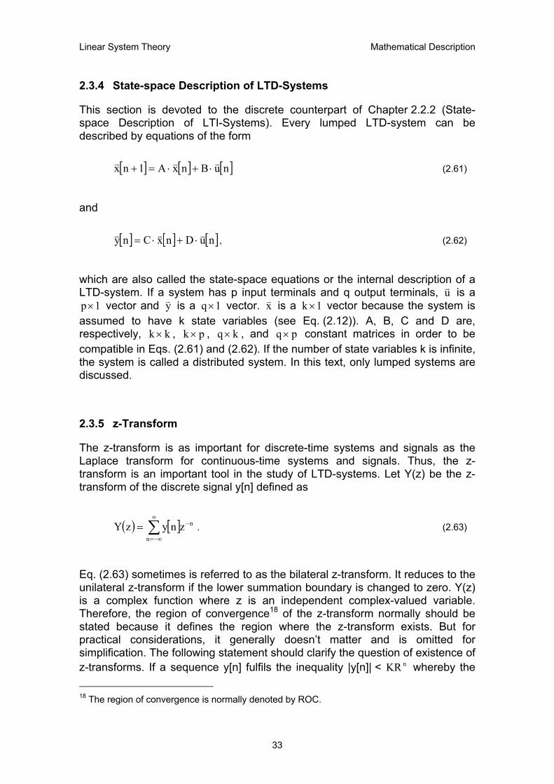
2.3.4 State-space Description of LTD-Systems
This section is devoted to the discrete counterpart of Chapter 2.2.2 (State-space Description of LTI-Systems). Every lumped LTD-system can be described by equations of the form
[ ] [ ] [ ]nuBnxA1nx vvv ⋅+⋅=+ (2.61)
and
[ ] [ ] nuDnxCny vvv ⋅+⋅= [ ], (2.62)
which are also called the state-space equations or the internal description of a LTD-system. If a system has p input terminals and q output terminals, uv is a
vector and 1p × yv is a vector. 1q × xv is a 1k × vector because the system is assumed to have k state variables (see Eq. (2.12)). A, B, C and D are, respectively, kk × , , , and p qk × k× pq × constant matrices in order to be compatible in Eqs. (2.61) and (2.62). If the number of state variables k is infinite, the system is called a distributed system. In this text, only lumped systems are discussed.
2.3.5 z-Transform
The z-transform is as important for discrete-time systems and signals as the Laplace transform for continuous-time systems and signals. Thus, the z-transform is an important tool in the study of LTD-systems. Let Y(z) be the z-transform of the discrete signal y[n] defined as
( ) [ ]∑∞
−∞=
−=n
nznyzY . (2.63)
Eq. (2.63) sometimes is referred to as the bilateral z-transform. It reduces to the unilateral z-transform if the lower summation boundary is changed to zero. Y(z) is a complex function where z is an independent complex-valued variable. Therefore, the region of convergence18 of the z-transform normally should be stated because it defines the region where the z-transform exists. But for practical considerations, it generally doesn’t matter and is omitted for simplification. The following statement should clarify the question of existence of z-transforms. If a sequence y[n] fulfils the inequality |y[n]| < K nR whereby the 18 The region of convergence is normally denoted by ROC.
33
Linear System Theory Mathematical Description
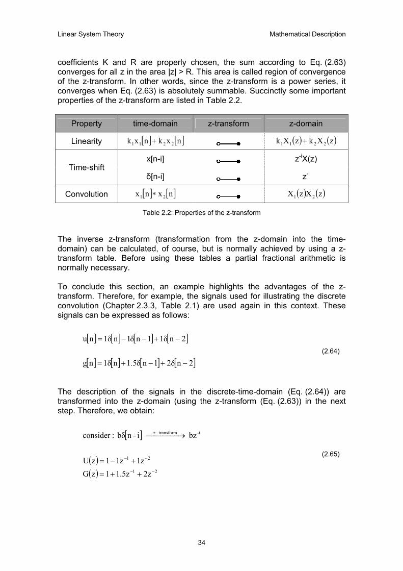
coefficients K and R are properly chosen, the sum according to Eq. (2.63) converges for all z in the area |z| > R. This area is called region of convergence of the z-transform. In other words, since the z-transform is a power series, it converges when Eq. (2.63) is absolutely summable. Succinctly some important properties of the z-transform are listed in Table 2.2.
Property time-domain z-transform z-domain
Linearity [ ] [ ]nxknxk 2211 + ( ) ( )zXkzXk 2211 +
x[n-i] z-iX(z) Time-shift
δ[n-i] z-i
Convolution [ ] [ ]nxnx 21 ∗ ( ) ( )zXzX 21
Table 2.2: Properties of the z-transform
The inverse z-transform (transformation from the z-domain into the time-domain) can be calculated, of course, but is normally achieved by using a z-transform table. Before using these tables a partial fractional arithmetic is normally necessary. To conclude this section, an example highlights the advantages of the z-transform. Therefore, for example, the signals used for illustrating the discrete convolution (Chapter 2.3.3, Table 2.1) are used again in this context. These signals can be expressed as follows:
[ ] [ ] [ ] [ ]
[ ] [ ] [ ] [ ]2n2δ1nδ5.1n1δng
2n1δ1nδ1n1δnu
−+−+=
−+−−= (2.64)
The description of the signals in the discrete-time-domain (Eq. (2.64)) are transformed into the z-domain (using the z-transform (Eq. (2.63)) in the next step. Therefore, we obtain:
[ ]
( )( ) 21
21
-itransformz
2zz5.11zG1z1z1zU
bz i-nbδ :consider
−−
−−
−
++=
+−=
→
(2.65)
34
Linear System Theory Mathematical Description
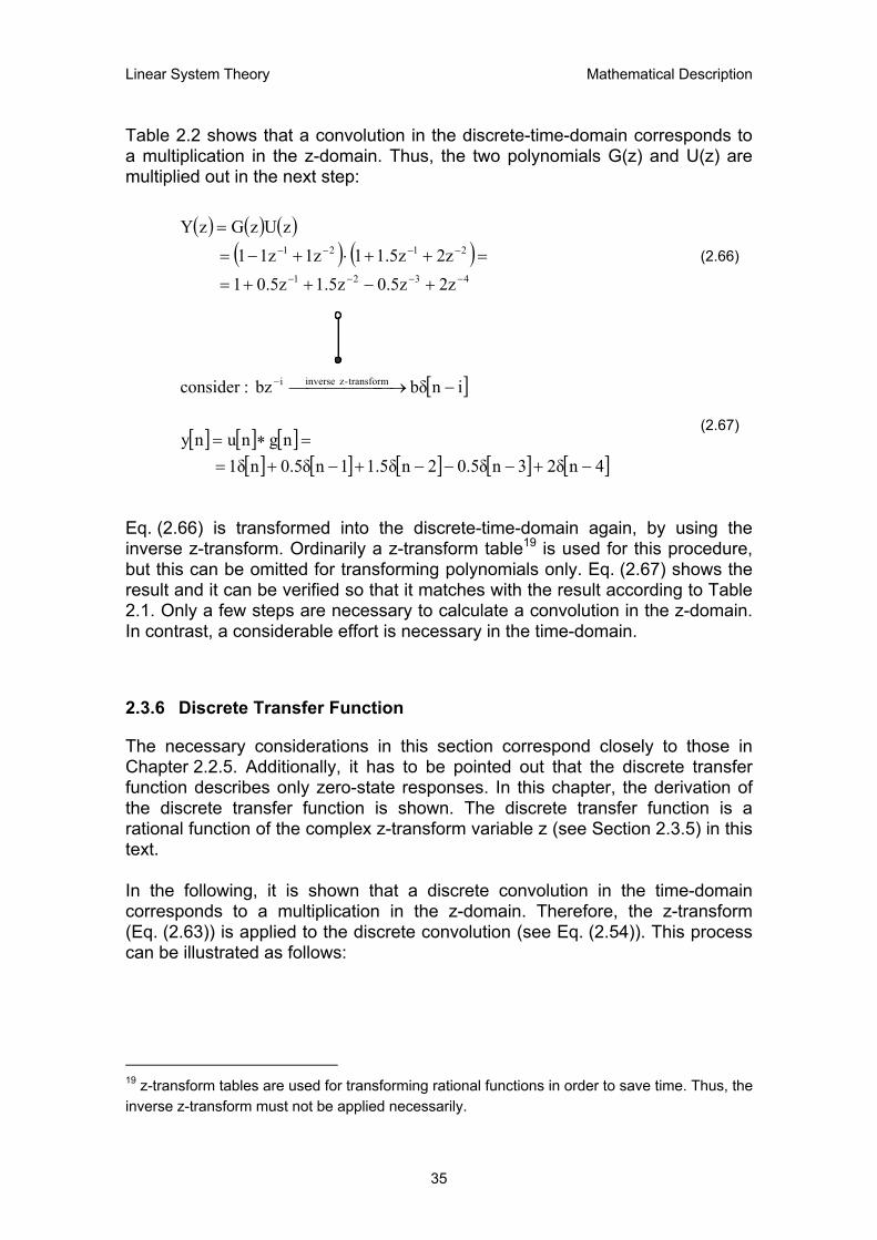
Table 2.2 shows that a convolution in the discrete-time-domain corresponds to a multiplication in the z-domain. Thus, the two polynomials G(z) and U(z) are multiplied out in the next step:
( ) ( ) ( )( ) (
4321
2121
2zz5.0z5.1z5.01 2zz5.111z1z1
zUzGzY
−−−−
−−−− )+−++=
=++⋅+−=
=
(2.66)
[ ]
[ ] [ ] [ ][ ] [ ] [ ] [ ] [ ]4nδ23nδ5.02n1.5δ1nδ5.0n1δ
ngnuny
inbδ bz :consider transform-z inversei
−+−−−+−+==∗=
− →−
(2.67)
Eq. (2.66) is transformed into the discrete-time-domain again, by using the inverse z-transform. Ordinarily a z-transform table19 is used for this procedure, but this can be omitted for transforming polynomials only. Eq. (2.67) shows the result and it can be verified so that it matches with the result according to Table 2.1. Only a few steps are necessary to calculate a convolution in the z-domain. In contrast, a considerable effort is necessary in the time-domain.
2.3.6 Discrete Transfer Function
The necessary considerations in this section correspond closely to those in Chapter 2.2.5. Additionally, it has to be pointed out that the discrete transfer function describes only zero-state responses. In this chapter, the derivation of the discrete transfer function is shown. The discrete transfer function is a rational function of the complex z-transform variable z (see Section 2.3.5) in this text. In the following, it is shown that a discrete convolution in the time-domain corresponds to a multiplication in the z-domain. Therefore, the z-transform (Eq. (2.63)) is applied to the discrete convolution (see Eq. (2.54)). This process can be illustrated as follows:
19 z-transform tables are used for transforming rational functions in order to save time. Thus, the inverse z-transform must not be applied necessarily.
35
Linear System Theory Mathematical Description
( ) [ ] [ ][ ]
[ ] [ ][ ]
( )43421
4434421
4434421
nz
ini
n
ny
i
n
n
ny
i
zzingix
zingixzY
−
−−−∞+
−∞=
∞+
−∞=
∞+
−∞=
−∞+
−∞=
∑ ∑
∑ ∑
−=
−=
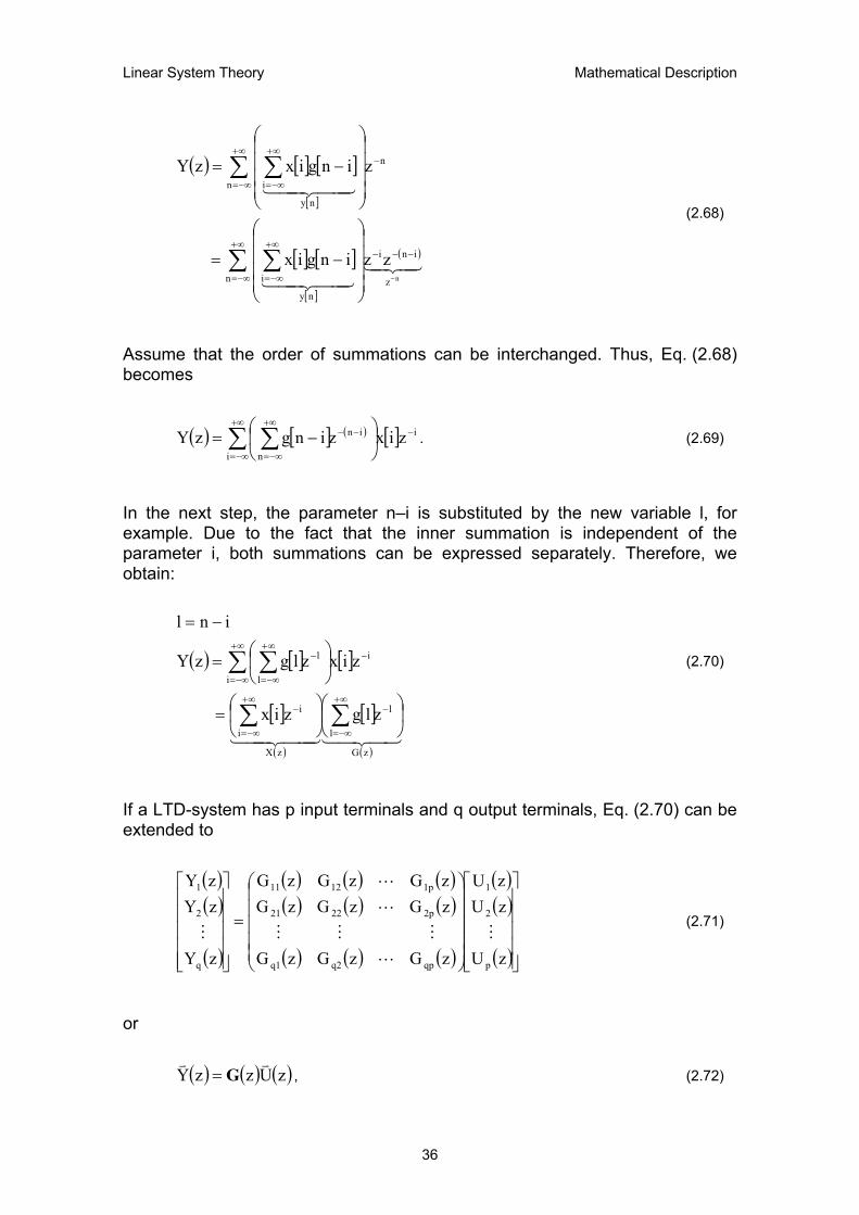
(2.68)
Assume that the order of summations can be interchanged. Thus, Eq. (2.68) becomes
( ) [ ] ( ) [ ] i
i
in
nzixzingzY −
+∞
−∞=
−−+∞
−∞=∑ ∑
−= . (2.69)
In the next step, the parameter n–i is substituted by the new variable l, for example. Due to the fact that the inner summation is independent of the parameter i, both summations can be expressed separately. Therefore, we obtain:
( ) [ ] [ ]
[ ]( )
[ ]( )434214434421
zG
l
l
zX
i
i
i
i
l
l
zlg zix
zixzlgzY
inl
=
=
−=
−∞+
−∞=
∞+
−∞=
−
−∞+
−∞=
−∞+
−∞=
∑∑
∑ ∑ (2.70)
If a LTD-system has p input terminals and q output terminals, Eq. (2.70) can be extended to
( )( )
( )
( ) ( ) ( )( ) ( ) ( )
( ) ( ) ( )
( )( )
( )
=
zU
zUzU
zGzGzG
zGzGzGzGzGzG
zY
zYzY
p
2
1
qpq2q1
2p2221
1p1211
q
2
1
M
L
MMM
L
L
M (2.71)
or
( ) ( ) ( )zUzzYvv
G= , (2.72)
36

Linear System Theory Mathematical Description
respectively, where G(z)20 is called the discrete transfer-function matrix of the system. Gij(z) is the discrete transfer function from the jth input to the ith output of the LTD-system. The function G(z) is therefore the z-transform of the impulse response sequence g[n] and is called the discrete transfer function, which can be expressed as
( ) ( )( ) ,
zb...zbbza...zaa
zUzY zG n
n10
mm10
++++++
== (2.73)
conversely, the discrete impulse response is the inverse z-transform of the discrete transfer function. It is a rational function of the complex z-transform variable z. It can be observed that, similar to the transfer function of continuous-time systems, in the z-domain a multiplication is applied instead of a discrete convolution in the discrete-time-domain. In this text, only discrete transfer functions with real coefficients (ai and bj with i = 0…m, j = 0…n, see Eq. (2.73)) are treated. The numerator and denominator polynomials of equation Eq. (2.73)) can be factorised into products of roots. The numerator polynomial Y(z) has m zeros, which are denoted as z1, z2, …, zm. The n roots of the denominator polynomial U(z) are denoted as p1, p2, …, pn, because U(z) has poles at these points, that is G(z) becomes infinite. In terms of poles and zeros, the discrete transfer function G(z) can be expressed as
( ) ( )( ) ( )( )( ) ( )n21
m21
n
m
pzpzpzzzzzzz
ba
zG−−−−−−
=L
L (2.74)
and is called the zero-pole-gain form. The following concluding statements are valid for discrete transfer functions, which are treated in this text:
o The discrete transfer function G(z) is a rational function of z.
o The degree of the numerator polynomial of G(z) is less than or equal to the degree of the denominator polynomial of G(z). In this case G(z) is said to be proper.
o If the degree of the numerator polynomial of G(z) is less than the degree of the denominator polynomial of G(z), the discrete transfer function is said to be strictly proper.
20 Recall that transformed matrices in the Laplace-, z-, or frequency-domain are denoted by bold type capital letters.
37

Linear System Theory Mathematical Description
2.3.7 Difference Equation of LTD-Systems
Proper representation of the input/output relationship to a given LTD-system is important. A linear constant-coefficient difference equation21 serves as a way of expressing just this relationship. Thus, it is a very useful tool in describing and calculating the output of a discrete-time system. It is called nth order, if the highest order of the occurring differences is equal to n. In other words, the order of a difference equation depends on the highest degree of the contained polynomials. LTD-systems can be designed of three basic elements in general:
o Adder – the output of the adder-component is made up of added input signals.
o Multiplier – the input signal is multiplied by a constant, which is denoted by a.
o Unit-time delay – the discrete input of the unit-time delay is delayed by one sampling period.
The basic LTD-system components are shown symbolically in Figure 2.9.
+
u1[n]
u2[n]
y[n] = u1[n] + u2[n]
y[n]
au[n]
y[n] = a u[n]
y[n]
Tu[n]
y[n] = u[n-1]
y[n]
Figure 2.9: Basic elements of LTD-systems
Basic devices of LTD-systems can be easily programmed on digital signal processors (DSP). A LTD-system is described by its difference equation, impulse response sequence or by the discrete convolution (of its impulse response sequence by the discrete input signal). The difference equation of a LTD-system can be expressed as
[ ] [∑∑==
−=−N
0jj
M
0ii jnubinya ]
. (2.75)
If the coefficient a0 = 1 or if the Eq. (2.75) is properly standardised it becomes
21 A difference equation is a mathematical formulation corresponding to a discrete-time model. It describes a relation between consecutive elements of a sequence.
38
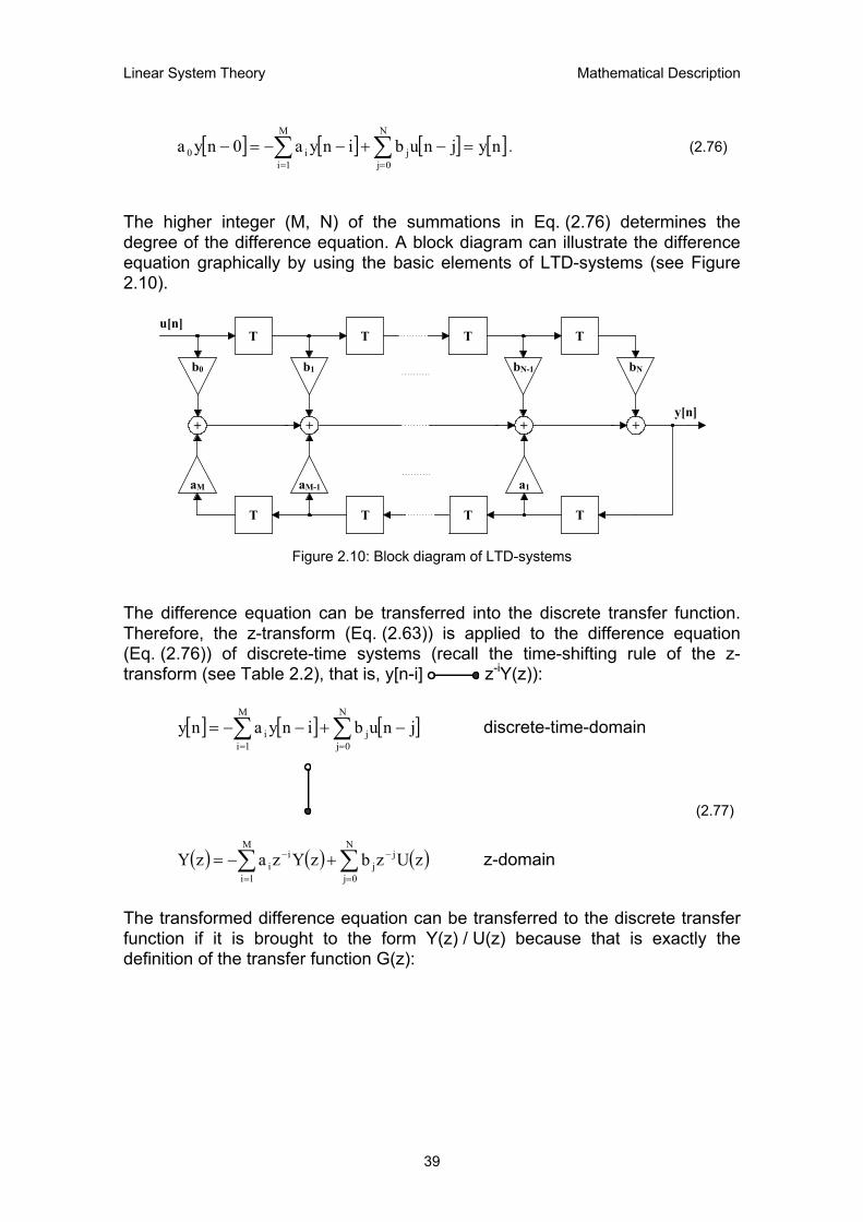
Linear System Theory Mathematical Description
[ ] [ ] [ ] [nyjnubinya0nyaN
0jj
M
1ii0 =−+−−=− ∑∑
==
] . (2.76)
The higher integer (M, N) of the summations in Eq. (2.76) determines the degree of the difference equation. A block diagram can illustrate the difference equation graphically by using the basic elements of LTD-systems (see Figure 2.10).
T T T T
bNbN-1b1b0
u[n]
TTTT
aM aM-1 a1
+ + + +y[n]
Figure 2.10: Block diagram of LTD-systems
The difference equation can be transferred into the discrete transfer function. Therefore, the z-transform (Eq. (2.63)) is applied to the difference equation (Eq. (2.76)) of discrete-time systems (recall the time-shifting rule of the z-transform (see Table 2.2), that is, y[n-i] z-iY(z)):
[ ] [ ] [ ]∑∑==
−+−−=N
0jj
M
1ii jnubinyany discrete-time-domain
(2.77)
( ) ( ) ( )∑∑=
−
=
− +−=N
0j
jj
M
1i
ii zUzbzYzazY z-domain
The transformed difference equation can be transferred to the discrete transfer function if it is brought to the form Y(z) / U(z) because that is exactly the definition of the transfer function G(z):
39

Linear System Theory Mathematical Description
( ) ( )
( ) ( )( ) M
M1
1
NN
110
M
1i
ii
N
0j
jj
N
0j
jj
M
1i
ii
za...za1zb...zbb
za1
zb
zUzYzG
zUzbza1zY
−−
−−
=
−
=
−
=
−
=
−
++++++
=+
==
=
+
∑
∑
∑∑
(2.78)
If Eq. (2.78) is compared with Eq. (2.73) it is obvious that both equations are equal, because a0 = 1. Remember that the impulse response sequence of a LTD-system is the inverse z-transform of the discrete transfer function G(z). In the following, it is shown that the impulse response sequence can also be obtained by using the difference equation. Consider, for example, the LTD-system, which is shown in Figure 2.11.
T T
b1b0
u[n]
+
u[n-1]T
b3b2
+ +y[n]
u[n-2] u[n-3]
Figure 2.11: Block diagram of a non-recursive LTD-system
First of all, the difference equation describing the LTD-system is derived. In the example depicted in Figure 2.11 this is simple because it is a non-recursive system, that is to say, it has no reversed transfer. The delayed input signal u[n-i] has to be multiplied by the corresponding factors bi and summed up subsequently, this yields
[ ] [ ] [ ] [ ] [ ]3nub2nub1nubnubny 3210 −+−+−+= . (2.79)
Now, if the input signal is the discrete Dirac impulse, the output of the system is the impulse response sequence g[n]. Thus, Eq. (2.79) becomes
[ ] [ ] [ ] [ ]
[ ] [ ] [ ] [ ] [ ]. 3nδb2nδb1nδbnδbng
ngny
3210
nδnu
−+−+−+=
= = (2.80)
To show the result graphically the coefficients are chosen as follows: b0 = b3 = 1, b1 = 1.5 and b2 = 2. The shifted discrete Dirac impulses δ[n-i] are scaled by the corresponding coefficients bi (Figure 2.12).
40
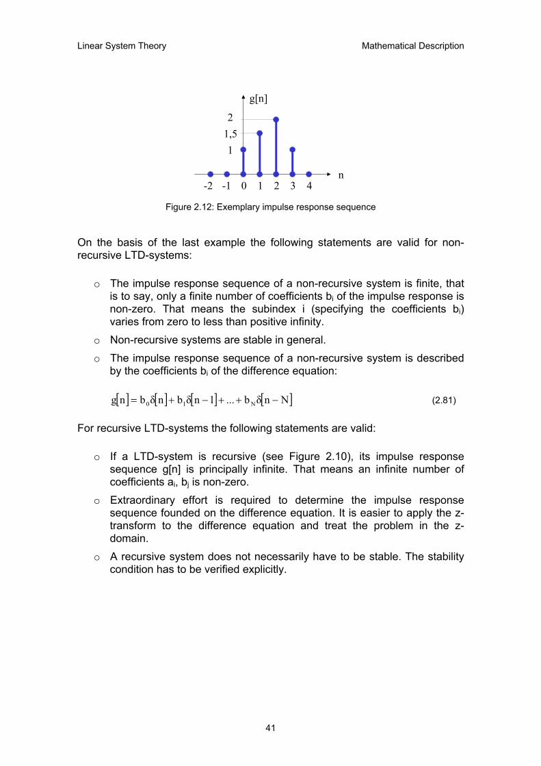
Linear System Theory Mathematical Description
0
g[n]
n1 2-1-2 3 4
11,52
Figure 2.12: Exemplary impulse response sequence
On the basis of the last example the following statements are valid for non-recursive LTD-systems:
o The impulse response sequence of a non-recursive system is finite, that is to say, only a finite number of coefficients bi of the impulse response is non-zero. That means the subindex i (specifying the coefficients bi) varies from zero to less than positive infinity.
o Non-recursive systems are stable in general.
o The impulse response sequence of a non-recursive system is described by the coefficients bi of the difference equation:
[ ] [ ] [ ] [ ]Nnδb...1nδbnδbng N10 −++−+= (2.81)
For recursive LTD-systems the following statements are valid:
o If a LTD-system is recursive (see Figure 2.10), its impulse response sequence g[n] is principally infinite. That means an infinite number of coefficients ai, bj is non-zero.
o Extraordinary effort is required to determine the impulse response sequence founded on the difference equation. It is easier to apply the z-transform to the difference equation and treat the problem in the z-domain.
o A recursive system does not necessarily have to be stable. The stability condition has to be verified explicitly.
41

Linear System Theory Stability Condition
3. STABILITY CONDITION
Stability is the most important system specification, because if a system is not stable, it could be destroyed, or it might be saturated when a finite signal is applied. Therefore, a stable system is important in practice not only to save money but also to achieve the desired results of the used model (see also Section 1.3). Thus, stability is a basic requirement for all systems. There are many definitions for stability depending upon the kind of system or one’s point of view. This section is limited to a consideration of the stability condition of LTI and LTD-systems. The response of such systems is set up by the zero-state response and the zero-input response (see also Section 2.2.1). The study of the stability condition of these two system responses is performed separately. The introduction of the BIBO (bounded-input bounded-output) stability for the zero-state response of a system is carried out first. Afterwards marginal and asymptotic stabilities are introduced for the zero-input response.
3.1 BIBO Stability of LTI-Systems
The BIBO stability is only defined for the zero-state response of a system. Thus, the system has to be initially relaxed at t = 0. A signal u(t) is said to be bounded if u(t) does not grow to positive or negative infinity (see [Che99]). More precisely, u(t) is bounded if a (signal) constant Mu exists, so that
( ) ∞<≤ uMtu (3.1)
is fulfilled for all t ≥ 0. Now, if every bounded input signal u(t) excites a bounded output signal y(t), this system is said to be BIBO stable. As already mentioned in Section 2.2.3 the zero-state response of a system can be described by the convolution integral (external description, see Eq. (2.29)). The external description of a system means that an arbitrary input signal u(t), which is convoluted by the impulse response of the system g(t) results in the system output y(t). If the input signal is bounded, which is a requirement for defining the BIBO stability, the impulse response of the system has to be absolutely integrable from zero to a point less than positive infinity, in other words, in the interval [0,∞[ in order to guarantee BIBO stability for the system (see [Mil95]):
( ) ∞<∫∞
0
tgdt (3.2)
42
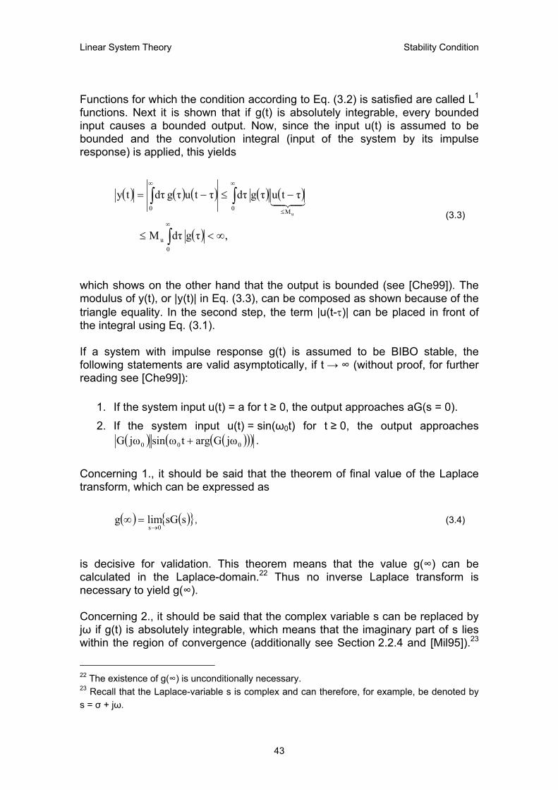
Linear System Theory Stability Condition
Functions for which the condition according to Eq. (3.2) is satisfied are called L1 functions. Next it is shown that if g(t) is absolutely integrable, every bounded input causes a bounded output. Now, since the input u(t) is assumed to be bounded and the convolution integral (input of the system by its impulse response) is applied, this yields
( ) ( ) ( ) ( ) ( )
( ) ,τg dτM
τtuτg dττtuτg dτty
0u
0 M0u
∞<≤
−≤−=
∫
∫∫∞
∞
≤
∞
43421 (3.3)
which shows on the other hand that the output is bounded (see [Che99]). The modulus of y(t), or |y(t)| in Eq. (3.3), can be composed as shown because of the triangle equality. In the second step, the term |u(t-τ)| can be placed in front of the integral using Eq. (3.1). If a system with impulse response g(t) is assumed to be BIBO stable, the following statements are valid asymptotically, if t → ∞ (without proof, for further reading see [Che99]):
1. If the system input u(t) = a for t ≥ 0, the output approaches aG(s = 0).
2. If the system input u(t) = sin(ω0t) for t ≥ 0, the output approaches ( ) ( )( )( )000 jωGargtωsinjωG + .
Concerning 1., it should be said that the theorem of final value of the Laplace transform, which can be expressed as
( ) ( ) ssGlimg0s→
=∞
, (3.4)
is decisive for validation. This theorem means that the value g(∞) can be calculated in the Laplace-domain.22 Thus no inverse Laplace transform is necessary to yield g(∞). Concerning 2., it should be said that the complex variable s can be replaced by jω if g(t) is absolutely integrable, which means that the imaginary part of s lies within the region of convergence (additionally see Section 2.2.4 and [Mil95]).23
22 The existence of g(∞) is unconditionally necessary. 23 Recall that the Laplace-variable s is complex and can therefore, for example, be denoted by s = σ + jω.
43
Linear System Theory Stability Condition
From this it follows that G(s) = G(jω), whereby G(jω) is complex and its argument can be retrieved by calculating
( )( ) ( ) ( )
=
jωGRejωGImtanjωGarg . (3.5)
Thus, the argument of a complex function is the tangent of its imaginary part divided by its real part. The BIBO stability condition can also be stated in terms of proper rational transfer functions. A system with a proper (for definition see Section 2.2.5) rational transfer function G(s) is BIBO stable only if every pole of G(s) has a negative real part. In other words, every pole lies inside the left half of the complex s-plane24. Now, if the rational transfer function of a system25 has pole pi with multiplicity mi, its partial fraction expansion contains the following factors:
( ) ( ) imi
2ii ps
1 ..., ,ps1 ,
ps1
−−− (3.6)
As already mentioned, the impulse response g(t) of a system has to be absolutely integrable in order to guarantee the BIBO stability condition for a LTI-system. However, the inverse Laplace transform of G(s) is just the impulse response g(t). Therefore, every such term of Eq. (3.6) has to be absolutely integrable after the inverse Laplace transform has been applied. Using a Laplace table for inverse transform yields
( )( ) tp1m transformLaplace inverse
mi
ii
ie t
ps1 − →
−. (3.7)
Such a term is absolutely integrable if and only if pi has a negative real part. This fact can be expressed as
24 The s-plane is a complex plane with an imaginary and real axis referring to the complex-valued variable s. 25 In this context SISO systems are treated only.
44

Linear System Theory Stability Condition
( ) ( ) ( )
( )
else,
0, xif
,
,tedt
etdt etdt 0
1mtx
0
tjyx1m
0
tp1m
i
iii
<
∞==
∫∫∫
∞−−
∞+−
∞− (3.8)
whereby x denotes the real part of pole pi and y the imaginary part of pi.26 For better illustration, pole-zero patterns are introduced where the abscissa describes the real axis and the ordinate describes the imaginary axis of the complex Laplace-variable s. Now, as one marks zeros in the complex s-plane with circles, and poles with crosses, then the pole-zero pattern of G(s) is retrieved. It describes the associated rational function G(s) with the exception of a constant factor am / bn (see Eq. (2.46)). If the concerned rational function has only real coefficients am, bn, which are treated in this text exclusively, poles and zeros exist either on the real axis or as complex conjugate pairs. The correctness of these statements is shown by an example of a pole-zero pattern according to Figure 3.1. In this diagram three zeros z1 = 2, z2 = -1+j and z3 = -1-j and three poles p1 = -2, p2 = 1+j and p3 = 1-j are recorded.
Im s
Re s
+j
-j
-1-2 1 2
+
+
+
Figure 3.1: Exemplary pole-zero pattern of G(s)
According to Eq. (2.46) this pole-zero pattern is equal to
( ) ( )( )(( )( )(
))
,42ss42ssK
j1sj1s2sj1sj1s2sK sG
3
3
+−−−
=
+−−−+++−+−
= (3.9)
26 The calculation was performed with Derive 5.
45
Linear System Theory Stability Condition
whereby the constant K is equal to am / bn. In the second step the denominator and the numerator of G(s) are multiplied out. We recognize that if products of complex conjugate poles and zeros respectively are multiplied out, these result in polynomials of 2nd degree with real coefficients. Thus, polynomials with real coefficients are developed collectively. On closer examination the following considerations are applied. If
and a defines a pair of complex conjugate poles or zeros, the product
jβαa += jβα −=∗
( )( )∗−− asas results in a polynomial with real coefficients if it is multiplied out:
( )( ) 222 βα2sαsasas ++−=−− ∗ (3.10) From the pole-zero pattern, the region of divergence of the corresponding Laplace transformation can also be retrieved. It is limited to the left by the furthest to the right lying pole. In other words, the limiting parameter (to the left) is the pole with the largest real part (see [Mil95]).
3.1.1 BIBO Stability of MIMO LTI-Systems
A system is called a multivariable system if it has more than one input and more than one output, that is to say it is a MIMO-system. Now, for multivariable systems, the following statements are valid (see [Che99]):
o A MIMO-system with impulse response matrix G(t) according to Eq. (2.31) is said to be BIBO stable if and only if every entry gij(t) of G(t) is absolutely integrable in [0,∞[.
o A MIMO-system with a proper rational transfer matrix G(s) according to Eqs. (2.43) and (2.44) is said to be BIBO stable if and only if every pole of every entry Gij(s) has a negative real part.
3.2 BIBO Stability of LTD-Systems
This section is devoted to the BIBO stability condition of LTD-systems. Thus, this chapter is the discrete counterpart of the previous one and therefore many similarities can be observed. The BIBO stability is defined for the zero-state response of a LTD-system and is only applicable if the system is initially relaxed. Remember Eq. (2.54), which represents the discrete convolution, whereby the impulse response sequence is denoted by g[n]. The impulse
46
Linear System Theory Stability Condition
response sequence is the output sequence excited by an impulse sequence applied at n = 0. A discrete input signal u[n] is said to be bounded if it does not grow to negative or positive infinity. More precisely, u[n] is bounded if a signal-dependent constant Mu exists, so that
[ ] ∞<≤ uMnu (3.11)
is fulfilled (for n = 0, 1, 2, …). Now, if every bounded discrete input signal u[n] excites a bounded output signal y[n], this LTD-system is said to be BIBO stable. As already mentioned in Chapter 2.3.3 a zero-state response of a LTD-system can be described by the discrete convolution integral (see Eq. (2.54)). Thus, the description of a discrete-time system y[n] is achieved by convoluting an arbitrary input signal u[n] with the impulse response sequence g[n] of the system. If the input signal is bounded, that is critically necessary for defining the BIBO stability, the impulse response sequence of the system has to be absolutely summable from zero to a number less than positive infinity, that is to say in the interval [0,∞[ in order to guarantee BIBO stability for the system (see [Mil95] and [Che99]):
[ ] ∞<∑∞
=0nng (3.12)
Discrete functions satisfying the condition according to Eq. (3.12) are called l1 functions. A LTD-system is said to be BIBO stable if and only if its impulse response sequence g[n] is absolutely summable. The proof of this context is shown succinctly. First, we assume a real-valued impulse response sequence denoted by g[n]. Now, since the input sequence u[n] is bounded and the discrete convolution (input of the system by its impulse response sequence) is applied, this results in
[ ] [ ] [ ] [ ] [ ]
[ ] . igM
inuiginuigny
0iu
0i0i
∞<≤
−≤−=
∑
∑∑∞
=
∞
=
∞
= (3.13)
Because the sum is less than positive infinity this implies that the system output y[n] is also bounded. If we assume a system with impulse response sequence g[n] to be BIBO stable, the following statements are asymptotically valid, if n → ∞ (without proof, for further reading see [Che99]):
47
Linear System Theory Stability Condition
1. If the system input sequence u[n] = a for n ≥ 0, the output approaches aG(z = 1).
2. If the system input sequence u[n] = sin(ω n) for n ≥ 0, the output approaches
0
( ) ( )( )( )00 jω0
jω eGargnωsineG + .
Concerning 1., it is to be said that the theorem of final value (see Eq. (3.14)) of the z-transform, which can be expressed as
[ ] ( ) ( ) zG1zlimg1z
−=∞→
, (3.14)
is decisive for validation. This theorem means that the value g[∞] can be calculated in the z-domain.27 Thus, no inverse z-transform is necessary to yield g[∞] in the discrete-time-domain. The BIBO stability condition for LTD-systems can also be stated in terms of discrete proper rational transfer functions. A system with a discrete proper (for definition see Section 2.3.6) rational transfer function G(z) is BIBO stable if and only if every pole of G(z) has a magnitude less than 1. In other words, every pole lies inside the unit circle on the complex z-plane28. Now, if the rational discrete transfer function of a system29 has pole pi with multiplicity mi, its partial fraction expansion contains the following factors:
( ) ( ) imi
2ii pz
1 ..., ,pz
1 ,pz
1−−−
(3.15)
As already mentioned, the impulse response sequence g[n] of a system has to be absolutely summable in order to guarantee the BIBO stability condition for a LTD-system. However, the inverse z-transform of G(z) is just the impulse response sequence g[n]. Therefore, every such term of Eq. (3.15) has to be absolutely summable after the inverse z-transform has been carried out. Using a z-transform table for inverse transform yields
( )( ) n
i1mtransform-z inverse
mi
pn pz1 i
i
− →−
. (3.16)
27 The existence of g[∞] is unconditionally necessary. 28 “The z-plane is a complex plane with an imaginary and real axis referring to the complex-valued variable z, [Fit03]”. 29 In this context SISO systems are treated only.
48

Linear System Theory Stability Condition
Such a term is absolutely summable if and only if pi has a magnitude less than 1 (without proof). Pole-zero patterns are used for better illustration whereby the abscissa describes the real axis and the ordinate describes the imaginary axis of the complex z-variable z. Now, as one marks zeros in the complex z-plane with circles, and poles with crosses, then the pole-zero pattern of G(z) is retrieved. It describes the associated discrete rational function G(z) with the exception of a constant factor am / bn (see Eq. (2.74)). If the concerned rational function has only real coefficients am, bn, which are treated in this text exclusively, poles and zeros exist either on the real axis or as complex conjugate pairs. For better illustration, an example is shown. Consider a pole-zero pattern according to Figure 3.2. In this diagram three poles p1 = -0.5, p2 = 0.5+0.5j and p3 = 0.5-0.5j and one zero z1 = 2 (outside the unit circle) are recorded.
Im z
Re z
+j
-j
-1 -0.5 1 20.5
0.5j
-0.5j
|z| = 1
+
+
+
Figure 3.2: Exemplary pole-zero pattern of G(z)
According to Eq. (2.74) this pole-zero pattern is equal to
( ) ( )( )( )( )
( )( ) , 12z2z0.250.5z
2-zK0.250.5zz
2-zK
0.5j0.5z0.5j0.5z0.5z2zK zG
223 +−+=
+−=
+−−−+−
= (3.17)
whereby the constant K is equal to am / bn. In the second step, the denominator of G(z) is multiplied out. Similar to the example of the previous chapter (BIBO Stability of LTI-Systems) it is observable that if products of complex conjugate poles and zeros respectively are multiplied out, these result in polynomials of 2nd degree with real coefficients. Thus, polynomials with real coefficients are developed collectively.
49
Linear System Theory Stability Condition
From the pole-zero pattern also the region of convergence of the discrete transfer function G(z) can be retrieved. The ROC of G(z) lies beyond a circle around the origin where the radius is defined by the pole, which is furthermost from the origin. In other words, the limiting parameter is the pole with the highest absolute value (see [Mil95]).
3.2.1 BIBO Stability of MIMO LTD-Systems
A system is called a multivariable discrete-time system if it has more than one input and more than one output, or rather a MIMO discrete-time system. Now, for multivariable discrete-time systems the following statements are valid without proof (see [Che99]):
o A MIMO discrete-time system with impulse response sequence matrix G[n] according to Eq. (2.60) is said to be BIBO stable if and only if every entry gij[n] of G[n] is absolutely summable.
o A MIMO discrete-time system with a discrete proper rational transfer matrix G(z) according to Eqs.(2.71) and (2.72) is said to be BIBO stable if and only if every pole of every entry Gij(z) has a magnitude less than 1.
3.3 Internal Stability of LTI-Systems
In previous subsections of Chapter 3 the stability conditions were defined for zero-state responses only. Thus, the BIBO stability is defined for the zero-state response only. In this section the stability of the zero-input response is studied. Remember the state-space equations (see Eqs. (2.13) and (2.14)), now, if no input is applied Eq. (2.13) reduces to
( ) ( )txAtx v&v ⋅= , (3.18)
whereby ( )tx&v and xv are n vectors because the considered system has n state variables (see Eq. (2.12)) and A is a
1×nn × constant matrix. The internal
stability of LTI-systems can be defined as follows: “The zero-input response of Eqs. (2.13) and (2.14) or the Eq. (3.18) is marginally stable or stable in the sense of Lyapunov if every finite initial state
0xv excites a bounded response. It is asymptotically stable if every finite initial
50

Linear System Theory Stability Condition
state excites a bounded response, which, in addition, approaches 0v
as ∞→t , [Che99]”.
xv
)A−det
Before some supplemental statements about the internal stability are introduced, first the terms "eigenvalue" and "minimal polynomial" of a n-by-n real matrix A are explained briefly:
o λ is called an eigenvalue of A if there exists a nonzero vector such that xλxA vv =⋅ is fulfilled.30 The eigenvalues of A can be determined by
calculating the roots of the characteristic polynomial ( ) (λIλ∆ = of A because every root of ( )λ∆ is an eigenvalue of A.31
o The minimal polynomial of A is defined as the monic32 polynomial p(λ) of least degree such that p(A) is equal to the n-by-n zero matrix. In other words, the minimal polynomial is irreducible and is a factor of the characteristic polynomial of A. Every linear factor of ( )λ∆ has to occur in p(λ).
Now, as we discussed some necessary algebraic terms the following statements about the internal stability condition of LTI-systems can be introduced according to [Che99]:
1. Eq. (3.18) is marginally stable if and only if all eigenvalues of the matrix A have zero or negative real parts. The eigenvalues with zero real part have to be simple roots of the minimal polynomial of A.
2. Eq. (3.18) is asymptotically stable if and only if all eigenvalues of the matrix A have negative real parts.
3.4 Internal Stability of LTD-Systems
This section represents the counterpart to the previous one (Internal Stability of LTI-Systems). The BIBO stability condition of LTD-systems was defined for zero-state responses only. In this section, the stability condition of the zero-input response of LTD-systems is studied. Thus, the study of the internal stability of discrete-time systems is restricted to
[ ] [nxA1nx rr ]⋅=+ , (3.19)
30 Any nonzero vector xv satisfying xλxA vv =⋅ is called an eigenvector of A. 31 I denotes the n-by-n identity matrix of A. 32 A polynomial with leading coefficient 1 is called to be monic.
51

Linear System Theory Stability Condition
whereby and [ 1nx +v ] xv are k-by-1 vectors because the considered discrete-time system has k state variables (see Eq. (2.12)) and A is a k-by-k constant matrix. Eq. (3.19) can be seen as the discrete counterpart of Eq. (3.18). The internal stability of LTD-systems can be defined as follows: “Eq. (3.19) is said to be marginally stable or stable in the sense of Lyapunov if every finite initial state 0xv excites a bounded response. It is asymptotically stable if every finite initial state excites a bounded response, which, in addition, approaches 0
v as , [Che99]”. ∞→n
Additionally, the following statements about the internal stability condition of LTD-systems are valid according to [Che99]:
1. Eq. (3.19) is marginally stable if and only if all eigenvalues of the matrix A have magnitudes less than or equal to 1. The eigenvalues with magnitude 1 have to be simple roots of the minimal polynomial of A.
2. Eq. (3.19) is asymptotically stable if and only if all eigenvalues of the matrix A have magnitudes less than 1.
52

Linear System Theory State-Space Solutions
4. STATE-SPACE SOLUTIONS
In Chapter 2 we showed that linear systems can be described by convolutions (external description) and, if the system is lumped, by state-space equations. In this section the solutions of the above-mentioned system descriptions are discussed briefly.
4.1 Solution of the External Description
As derived in Section 2.2.3 the convolution integral equals the external or input-output description of a linear system. However, there is no simple analytical way of computing the convolution (see Eq. (2.26)). For computation on a digital computer it is necessary to discretize the convolution integral. Basically this results in the discrete convolution, which was described in Section 2.3.3. Convolutions of LTI-systems can be transformed into the Laplace-domain and therefore Y(s) = G(s)U(s) can be used to compute the solution. On the other hand, discrete convolutions of LTD-systems can be transformed into the z-domain and therefore Y(z) = G(z)U(z) can be used to get the desired result. The functions G(s) and G(z) are rational functions if the corresponding system is lumped (see Sections 2.2.5 and 2.3.6). The solution y(t) can be obtained by taking the inverse Laplace transform of G(s)U(s) and discrete signals y[n] are calculated by the inverse z-transform of G(z)U(z). Because both G(z) and G(s) are rational functions it is necessary to carry out partial fraction expansions in most cases, and then using transform tables for inverse transformation (see [Che99]). However, a better method for computation is to transform the transfer function into state-space equations and then compute the solutions. Therefore, solutions of state-space equations are shown next.
53

Linear System Theory State-Space Solutions
4.2 Solution of LTI-State Equations
In this section a possible solution of the LTI-state differential equations is shown. Therefore, the state equations are transformed into the Laplace-domain where the solution can be determined algebraically (instead of solving differential equations in the continuous-time-domain). After derivation of the solution in the Laplace-domain the inverse Laplace transform is applied to yield the solution in the time-domain.33 Consider the following continuous-time state-space representation of a system with p inputs, q outputs and n state variables:
( ) ( ) ( )tuBtxAtxdtxd vv&vv
⋅+⋅== (4.1)
( ) ( ) ( )tuDtxCty vvv ⋅+⋅= (4.2)
where A, B, C and D are, respectively, n-by-n, n-by-p, q-by-n, and q-by-p constant matrices (see also Section 2.2.2). First we have a look at the zero-input solution of the system. Remember, u(t) denotes the input, thus the terms including u(t) can be omitted for this approach, that is, Eq. (4.1) reduces to
( ) ( )txAtx v&v ⋅= . (4.3)
Now, taking the Laplace transform (see also Section 2.2.4) of Eq. (4.3) yields
( ) ( ) ( )sXA0xsXsvvv
⋅=− (4.4)
where is equal to at time t = 0. If Eq. (4.4) is reformulated, this results in
( )0xv ( )txv
( ) ( ) ( )
( ) ( ) ( ) , 0xAsIsX
or0xsXAsI
1 vv
vv
⋅−=
=⋅−
−
(4.5)
33 This is also called Laplace approach.
54
Linear System Theory State-Space Solutions
where I is the n-by-n identity matrix with n being the rank of A. Taking the inverse Laplace transform of Eq. (4.5) yields
( ) ( )
( ) ( ) ( ) ( ) ( ) ( ) , 0xtΦtx0xAsIsX
tΦAsI :consider
transformLaplace inverse1
transformLaplace inverse1
vvvv⋅= →⋅−=
→−
−
−
(4.6)
where Φ(t) is also known as the “State Transition Matrix”. Next we consider the case where there is an input, that means ( ) 0tu
vv ≠ . Thus, the Laplace transform of Eq. (4.1) yields
( ) ( ) ( ) ( ) ( ) ( ) sUBsXA0xsXstuBtxAtx transformLaplace ( )vvvvvv&v ⋅+⋅=− →⋅+⋅= . (4.7)
Eq. (4.7) also means that,
( ) ( ) ( ) ( ) ( )sUBAsI0xAsIsX 11 vvv⋅⋅−+⋅−= −− . (4.8)
Now, if Eq. (4.2) is transformed into the Laplace-domain and ( )sX
v is substituted
by the result of Eq. (4.8), this yields
( ) ( ) ( ) ( ) ( ) ( )sUDsUBAsIC0xAsICsY 11 vvvv⋅+⋅⋅−⋅+⋅−⋅= −− . (4.9)
The inverse Laplace transform applied to Eq. (4.8) yields
( ) ( ) ( ) ( ) ( )
( ) ( )
, τuBτtΦ dτ0xtΦtx
solution state-zero|
tuBby t ofn convolutio
t
0solutioninput -zero 444 3444 21
v43421vv
v⋅Φ
⋅⋅−+⋅= ∫ (4.10)
whereby Φ(t) is the inverse Laplace transform of the matrix (sI-A)-1. Eq. (4.10) shows finally that the solution is composed of the zero-input solution and of the zero-state solution. Next, Eq. (4.10) is substituted into Eq. (4.2) and this yields the solution of Eq. (4.2) as
55

Linear System Theory State-Space Solutions
( ) ( ) ( ) ( ) ( ) ( )tuDτuBτtΦ dτC0xtΦCtyt
0
vvvv ⋅+⋅⋅−+⋅⋅= ∫ . (4.11)
For better illustration of the state transition matrix Φ(t), an example is calculated. To this end consider the following equation:
( ) ( ) ( )tu10
tx0213
tx
A
vv
43421
&v ⋅
+⋅
−−
= (4.12)
For this system the matrix (sI-A) is calculated next (recall that the matrix I is the n-by-n identity matrix with n being the rank of A, here 2):
( ) s213s
0213
1001
sAsI
−+=
−−
−
=− (4.13)
The fact that Φ(t) is the inverse Laplace transform of (sI-A)-1 implies that Φ(s) is equal to (sI-A)-1. Therefore, the inverse of (sI-A)-1 is calculated next and can be expressed as
( ) ( )( ) ( ) ( ) .c
AsIdet1
AsIdetAsIAdjAsI T
ij1
−=
−−
=− − (4.14)
The number cij is the cofactor corresponding to aij (consider (sI-A) = (aij), thus aij are the entries of the matrix (sI-A)) and equals (-1)i+jdet(Mij), where Mij is the (n-1)-by-(n-1) submatrix (minor) of the matrix (sI-A) by deleting its ith row and jth column (see [Che99]). This context is used to calculate the inverse of Eq. (4.13). Therefore, we obtain:
( ) ( ) ( )( )
( )
( ) ( )( )
+−++
=−
+−
=
+
−=−
++=++=−
−
3s21s
2s1s1AsI
3s21s
3s12s
AsIAdj
2s1s23ssAsIdet
1
T
(4.15)
56

Linear System Theory State-Space Solutions
Now, if Eq. (4.15) is multiplied out and a partial fraction expansion is carried out afterwards, this results in
( )
+−
+++
++
−
+−
+++
++
−
=− −
2s1
1s2
2s2
1s2
2s1
1s1
2s2
1s1
AsI 1 . (4.16)
Recall that Φ(t) is the inverse Laplace transform of (sI-A)-1. Thus, if the inverse Laplace transform is applied to every entry of (sI-A)-1 by using a Laplace transform table, this yields
( ) .e2e2e2e
ee2eetΦ
2tt2t2t
2tt2tt
−+−
−+−=
−−−−
−−−−
(4.17)
4.3 Solution of LTD-State Equations
Every lumped LTD-system with p input terminals, q output terminals and k state variables can be described by a set of equations of the form
[ ] [ ] [ ]nuBnxA1nx vvv ⋅+⋅=+ (4.18)
and
[ ] [ ] nuDnxCny vvv ⋅+⋅= [ ], (4.19)
where A, B, C and D are, respectively, k-by-k, k-by-p, q-by-k, and q-by-p constant matrices (see also Section 2.3.4). A solution can be found if the descriptive series of x[n] is derived. Therefore, consider
[ ] [ ] [ ][ ] [ ] [ ] [ ] [ ] [ ]1uB0xBA0xA1uB1xA2x
0uB0xA1x2 vvvvvv
vvv
⋅+⋅⋅+⋅=⋅+⋅=
⋅+⋅= (4.20)
57

Linear System Theory State-Space Solutions
and proceeding forward this yields
[ ] [ ] ( ) [ ]∑−
=
−− ⋅⋅+⋅=1n
0i
i1nn iuBA0xAnx vvv (4.21)
and
[ ] [ ] ( ) [ ] [ ], nuDiuBAC0xACny1n
0i
i1nn vvvv ⋅+⋅⋅⋅+⋅⋅= ∑−
=
−− (4.22)
for n > 0. The solution of (see Eq. (4.22)) results from substituting the solution of (see Eq. (4.21)) into
[ ]nyv
[ ]nxv [ ]nyv . In these equations we use the definition A0 = I. Concluding this chapter, the transformation of the LTD-state-space equations into the z-domain is shown. Consider, therefore, the z-transform of [ ]1nx +v which is derived as follows:
[ ] [ ] [ ] ( )
[ ] [ ] [ ]
( ) [ ]( )0xzXz
0x0xzlxz
z1nxzz1nx1nx
l
1l
1n
0n
n
0n
transformz
vv
vvv
vvv
−=
=
−+=
=+=+ →+
−∞
=
+−∞
=
−∞
=
−=
∑
∑∑
(4.23)
Considering the result of Eq. (4.23) the application of the z-transform to the LTD-state-space equations (Eqs. (4.18) and (4.19)) yields
( ) [ ] ( ) ( )zUBzXA0xzzXzvvvv
⋅+⋅=− (4.24)
and
( ) ( ) zUDzXCzY ( )vvv
⋅+⋅= . (4.25)
Eq. (4.24) can also be expressed as
( ) ( ) [ ] ( ) ( )zUBAzI0xzAzIzX 11 vvv⋅⋅−+⋅−= −−
(4.26)
58

Linear System Theory State-Space Solutions
and inserted into Eq. (4.25) this leads to
( ) ( ) [ ] ( ) ( ) ( )zUDzUBAzIC0xzAzICzY 11 vvvv⋅+⋅⋅−⋅+⋅−⋅= −− , (4.27)
where I represents the k-by-k identity matrix with k being the rank of A. Eq. (4.26) can be seen as the discrete counterpart of Eq. (4.8).
59

Linear System Theory State-Space Realizations
5. STATE-SPACE REALIZATIONS
The central problem of realization theory is one of construction for a given external description of the system, an internal description in the form of state-space equations. This section shows how to find the state-space equations from a given transfer matrix first. This is called the realization of a system, because it is possible to realize a LTI-system on basis of the state-space equations by implementing an operational amplifier circuit. Now, if a transfer function is realizable, it has infinitely many realizations, not necessarily of the same dimension. One may conclude from this, that realizations with the smallest possible dimension are called minimal realizations, which is briefly discussed next. Finally, this chapter closes illustrating the concept of operational amplifier circuit implementation.
5.1 Realizations
Recall that every lumped LTI-system can be described by the internal or external system description. The external system description also referred to as the input-output description is expressed in Eq. (2.44). On the other hand, the internal description also referred to as the state-space description of a system is represented in Eqs. (2.13) and (2.14). Now, if the state-space description is known, the transfer-function matrix G(s) can be computed as ( ) ( ) ( )sU/sYs
vv=G .
Considering Eqs. (4.8) and (4.9) this yields,
( ) ( ) DBAsICs 1 +⋅−⋅= −G (5.1)
if the initial state ( )0xv is assumed to be zero. It is to be stressed that the system has to be lumped, because a distributed system cannot be described by a finite-dimensional state-space equation. A transfer-function matrix G(s) of a LTI-system is realizable only if G(s) is a proper rational matrix (see Section 2.2.5, for further details refer to [Che99]). Thus, the state-space model of Eqs. (2.13) and (2.14) is called a realization of a given transfer-function matrix G(s) if it satisfies Eq. (5.1). In other words, a realization exists if the transfer-function matrix of the state-space model (A, B, C, D) is identical to the given transfer function. A proper transfer-function matrix G(s) can be composed of a constant matrix G(∞) and a strictly proper rational matrix Gsp(s) as follows:
60

Linear System Theory State-Space Realizations
( ) ( )( ) ( )
∞
− +⋅−⋅= s
1 D BAsICssp
GG
G 44 344 21 (5.2)
The strictly proper part Gsp(s) of a p-input and q-output LTI-system can be expressed as
( ) ( )( )( )r
1rr1r
2r2
1r1sp NsNsNsN
sd1sG ++++= −−
−−− K (5.3)
where Ni are q-by-p constant matrices and the polynomial d(s), which can be expressed as
( ) ( )r
1rr1r
1r1
r αsαsαssd ++++= −−−
− K , (5.4)
denotes the monic least common denominator of all entries of Gsp(s). Now, a realization of G(s), the so-called “controllable canonical form”, can be obtained by substituting the above-mentioned context, that is, the matrices Ni of Eq. (5.3), the coefficients αi of Eq. (5.4) and G(∞) of Eq. (5.2), into
u
I
x
I
II
IαIαIαIα
x
p
A
p
p
p
prp1rp2p1
v
M
v
4444444 34444444 21L
MMMM
L
L
L
&v ⋅
+⋅
−−−−
=
−
0
00
000
000000
(5.5)
and
( ) ( ) uxNNNNy r1r21vv
Lv ⋅∞+⋅= − G . (5.6)
The matrix Ip of Eq. (5.5) is the p-by-p identity matrix and every 0 stands for a p-by-p zero matrix. The matrix A consists of r rows and r columns of p-by-p matrices, thus A has order rp-by-rp. Additionally, A is said to be in block companion form (see [Che99]).
61

Linear System Theory State-Space Realizations
For better illustration a simple realization for SISO systems (according to [Rud04]) is shown regarding to “controllable canonical form” as shown in Eqs. (5.5) and (5.6). Therefore, consider for instance a given transfer function
( )n
1n1
nn
1n1
a...sasb...sb sG+++
++= −
−
, (5.7)
which corresponds to:
( )xb,b,,b,by
u
0
001
x
0100
00100001aaaa
x
n1-n21
n1n21
vL
M
v
L
MMMM
L
L
L
&v
=
+⋅
−−−−
=
−
(5.8)
5.2 Controllability and Observability
Controllability and observability are basic properties of state models and so these concepts are introduced in this section. Controllability and observability play an essential role in defining a minimal realization of a system (see Section 5.3) and these concepts are also essential in discussing the internal structure of linear systems. Because the following statements can easily be extended to LTD-systems, only the continuous-time case (LTI-systems) is treated.
5.2.1 Controllability
Controllability deals with whether or not the state of a state-space equation can be controlled from the input. For a n-dimensional p-input system consider the following state equation,
uBxAx vv&v ⋅+⋅= , (5.9)
62
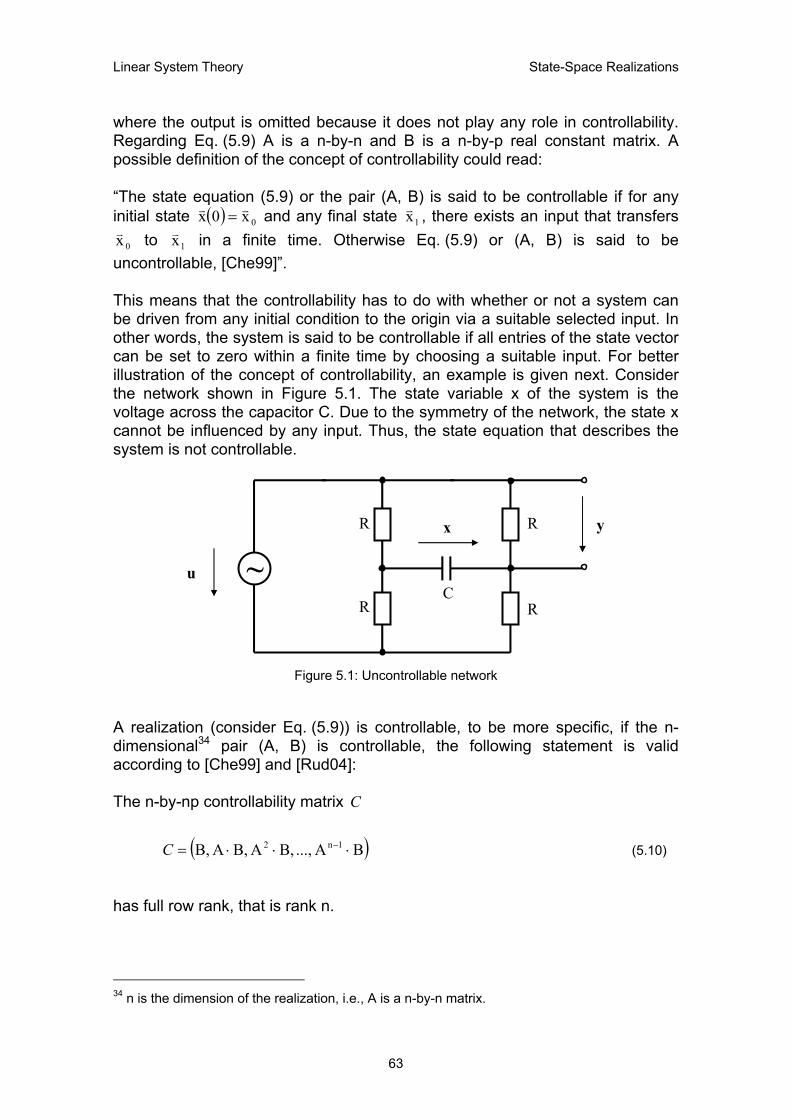
Linear System Theory State-Space Realizations
where the output is omitted because it does not play any role in controllability. Regarding Eq. (5.9) A is a n-by-n and B is a n-by-p real constant matrix. A possible definition of the concept of controllability could read: “The state equation (5.9) or the pair (A, B) is said to be controllable if for any initial state ( ) 0x0x vv = and any final state 1xv , there exists an input that transfers
0xv to in a finite time. Otherwise Eq. (5.9) or (A, B) is said to be uncontrollable, [Che99]”.
1xv
This means that the controllability has to do with whether or not a system can be driven from any initial condition to the origin via a suitable selected input. In other words, the system is said to be controllable if all entries of the state vector can be set to zero within a finite time by choosing a suitable input. For better illustration of the concept of controllability, an example is given next. Consider the network shown in Figure 5.1. The state variable x of the system is the voltage across the capacitor C. Due to the symmetry of the network, the state x cannot be influenced by any input. Thus, the state equation that describes the system is not controllable.
~R
R
u
x yR
RC
Figure 5.1: Uncontrollable network
A realization (consider Eq. (5.9)) is controllable, to be more specific, if the n-dimensional34 pair (A, B) is controllable, the following statement is valid according to [Che99] and [Rud04]: The n-by-np controllability matrix C
( )BA ..,. B,A B,A B, 1n2 ⋅⋅⋅= −C (5.10)
has full row rank, that is rank n.
34 n is the dimension of the realization, i.e., A is a n-by-n matrix.
63

Linear System Theory State-Space Realizations
5.2.2 Observability
Observability deals with whether or not the initial state can be observed from the output. In other words, observability studies the possibility of estimating the state from the output. For a n-dimensional p-input q-output system consider following state equations:
uDxCy
uBxAx
vvv
vv&v
⋅+⋅=
⋅+⋅= (5.11)
where A, B, C and D are, respectively, n-by-n, n-by-p, q-by-n, and q-by-p constant matrices. A possible definition of the concept of observability could read: “The state equation (5.11) is said to be observable if for any unknown initial state , there exists a finite t( )0xv 1 > 0 such that the knowledge of the input uv and the output yv over the interval [0, t1] suffices to determine the initial state ( )0xv uniquely. Otherwise Eq. (5.11) is said to be unobservable, [Che99]”. In other words, observability has to do with whether or not the value of the state vector can be determined by “listening” to the output sufficiently long (see [Rud04]). For better illustration of the concept of observability, an example is given next. Consider the network shown in Figure 5.2. The state variable x of the system is the voltage across the capacitor C. Now, if the input u is zero, the output y is also zero, no matter what the initial state (voltage across the capacitor) is. This means, due to the symmetry of the network the state x cannot be determined by observing the input u and output y. Thus, the state equation that describes the system is not observable (see [Che99]).
~R
R
u
x
y
R
RC
Figure 5.2: Unobservable network
64

Linear System Theory State-Space Realizations
A realization (consider Eq. (5.11)) is observable, to be more specific, if the n-dimensional35 pair (A, C) is observable, the following statements are valid according to [Che99] and [Rud04]:
1. The nq-by-n observability matrix O
⋅
⋅=
−qnAC
ACC
MO (5.12)
has full row rank, that is rank n.
2. The controllable canonical form of Eq. (5.8), which represents the
internal description of SISO LTI-systems is observable if and only if the nominator- and the denominator polynomial of G(s) are coprime36 (see Eq. (5.7)).
5.3 Minimal Realizations
This section briefly introduces the idea of minimal realization of systems. It is shown that there exist several reasons for considering the problem of realization in practice. However, due to space limitation an introduction to algorithms for solving the minimal realization problem for given system parameters is omitted (recommendation for further reading [Che99] and [DeS00]). Recall that for a given realizable transfer function G(s) there are always infinitely many realizations. In general, the minimal state-space realization problem for LTI-systems can be formulated as follows: If there are certain given data specifying an LTI-system, a state-space description of minimal size has to be found that describes the given data. The corresponding data are, for example, the impulse response of a system, the step response, input-output measurements, or more generally frequency measurements (see [DeS00]). The definition of a minimal realization of an LTI-system (according to Eqs. (4.1) and (4.2)) reads as follows: A realization (A, B, C, D) is said to be minimal if and only if it is controllable and observable (see [Che99] and [DeS00]).
35 n is the dimension of the realization, i.e., A is a n-by-n matrix. 36 “Two polynomials are said to be coprime if they have no common factor of degree at least 1, [Che99]”. Computing of coprime fractions is not simple by hand and will therefore be omitted in this text.
65

Linear System Theory State-Space Realizations
According to [DeS00] there are several reasons why the minimal state-space realization problem for LTI-systems deserves to be studied:
o The realization problem is one of the most fundamental problems in system theory. The solution of the minimal state-space realization problem can be seen as reconciliation towards problems such as model reduction and identification, which are of important interest.
o For system analysis it is advantageous to have a compact description of the system.
o Since the minimal realization is both controllable and observable, it is a good basis for designing an observer and a state feedback controller.37
o The minimal state-space realization problem can be solved using linear matrix algebra methods, which can be implemented straightforwardly and in a numerically stable way.
Furthermore, the minimal state-space realization methods can be classified into two main groups:
o Methods that start with a non-minimal realization and then reduce it in order to get a minimal realization, that is, where the realization is both controllable and observable, belong to group one.
o Methods that start with the impulse response of the system and obtain the minimal realization directly belong to group two.
5.4 Operational Amplifier Implementation
Operational amplifier (op-amp) circuits can be used for solving differential equations. As every linear time-invariant state-space equation can be described in terms of differential equations, it is possible to use operational amplifier circuits for implementation. This section introduces an approach showing how to implement state-space equations via op-amp circuits.
5.4.1 Basic Op-amp Circuit Elements
In this section two basic op-amp circuit elements are introduced, that is to say the adder and the integrator. All inputs, denoted by xi, are connected, through resistors, to the inverting terminal, and the positive input (non-inverting terminal) 37 The design of an observer and a state feedback controller is not treated in this text.
66
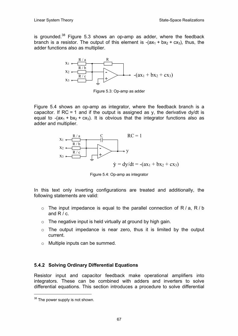
Linear System Theory State-Space Realizations
is grounded.38 Figure 5.3 shows an op-amp as adder, where the feedback branch is a resistor. The output of this element is -(ax1 + bx2 + cx3), thus, the adder functions also as multiplier.
-(ax1 + bx2 + cx3)
x1
-+
x2
x3
R / a
R / b
R / c
R
Figure 5.3: Op-amp as adder
Figure 5.4 shows an op-amp as integrator, where the feedback branch is a capacitor. If RC = 1 and if the output is assigned as y, the derivative dy/dt is equal to -(ax1 + bx2 + cx3). It is obvious that the integrator functions also as adder and multiplier.
= dy/dt = -(ax1 + bx2 + cx3)
x1
-+
x2
x3
R / a
R / b
R / c
C RC = 1
y
Figure 5.4: Op-amp as integrator
In this text only inverting configurations are treated and additionally, the following statements are valid:
o The input impedance is equal to the parallel connection of R / a, R / b and R / c.
o The negative input is held virtually at ground by high gain.
o The output impedance is near zero, thus it is limited by the output current.
o Multiple inputs can be summed.
5.4.2 Solving Ordinary Differential Equations
Resistor input and capacitor feedback make operational amplifiers into integrators. These can be combined with adders and inverters to solve differential equations. This section introduces a procedure to solve differential 38 The power supply is not shown.
67

Linear System Theory State-Space Realizations
equations by using op-amp circuits. A possible approach could be stated as follows (according to [Soh01]):
1. Solve the differential equation for the highest order derivative.
2. Use successive integrators to create lower order terms.
3. Compute the terms on the right side of the equation and sum them into the first integrator.
The scaling of the problem to get measurable signal levels39 is disregarded in this text. For better illustration, consider an example according to Figure 5.5. The capacitors C1 and C2 are both chosen to be 1 F and the resistor R has the value 1 Ω. This arrangement of op-amps solves the equation
( ) ( ) ( ) 4t3utu2tu ++= &&& for the voltage u(t).
-+
+4 V
R / 3
R
R
C2
-+
R
C1
u(t)
2RR
Figure 5.5: Op-amp solution of differential equation
5.4.3 State-space Implementation
This section illustrates the state-space implementation of an example-network by using an op-amp circuit. Consider the network according to Figure 5.6. It consists of two memory modules that are the inductance L and the capacitor C. Thus, this network has two state variables, which are denoted in the sequel by x1 and x2. The current passing through the inductance is x1 and the voltage across the capacitor is x2.
39 If any signal grows beyond the admissible range, the circuit might be saturated or burn out.
68
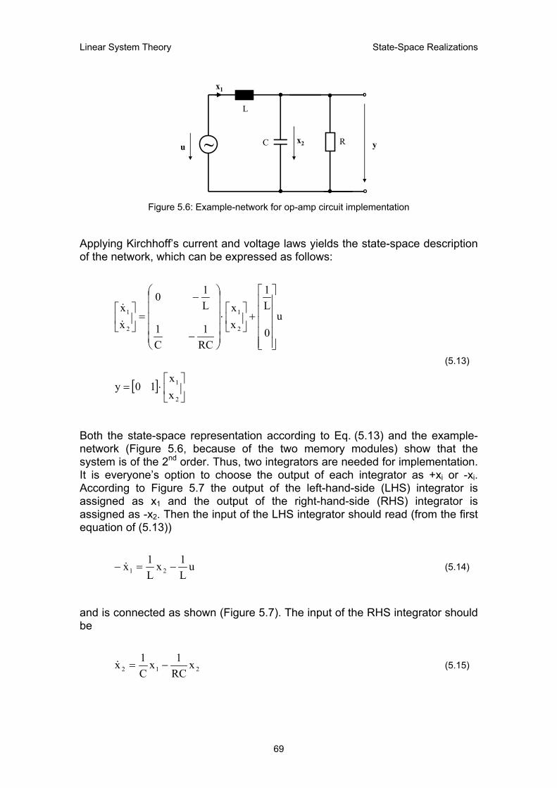
Linear System Theory State-Space Realizations
~ Ru
x1
y
L
C x2
Figure 5.6: Example-network for op-amp circuit implementation
Applying Kirchhoff’s current and voltage laws yields the state-space description of the network, which can be expressed as follows:
[ ] xx
10y
u0
L1
xx
RC1
C1
L10
xx
2
1
2
1
2
1
⋅=
+
⋅
−
−
=
&
&
(5.13)
Both the state-space representation according to Eq. (5.13) and the example-network (Figure 5.6, because of the two memory modules) show that the system is of the 2nd order. Thus, two integrators are needed for implementation. It is everyone’s option to choose the output of each integrator as +xi or -xi. According to Figure 5.7 the output of the left-hand-side (LHS) integrator is assigned as x1 and the output of the right-hand-side (RHS) integrator is assigned as -x2. Then the input of the LHS integrator should read (from the first equation of (5.13))
uL1x
L1x 21 −=− & (5.14)
and is connected as shown (Figure 5.7). The input of the RHS integrator should be
212 xRC1x
C1x −=& (5.15)
69

Linear System Theory State-Space Realizations
and is connected as shown (Figure 5.7). Because the output is equal to x2, the output of the RHS integrator has to be inverted only, in order to retrieve y. Thus, the state equation in Eq. (5.13) can be implemented as shown in Figure 5.7. It has to be noted that there are many alternative ways to implement the same equation. For example, if the outputs of the two integrators in Figure 5.7 are assigned as x1 and +x2, instead of x1 and -x2, a different implementation is obtained.
-+
uR
C
-+
RL
x1-u
R
RLC
-+
R2C
-x2
RC
x2
-+
R
R
y
Figure 5.7: Op-amp implementation of Eq. (5.13)
70

Linear System Theory E-Learning Fundamentals
6. E-LEARNING FUNDAMENTALS
Blended Learning, according to [Rei03], will stimulate didactic innovations and have a lasting effect on developments in technical colleges. This section introduces the concepts of E-Learning (electronic learning) and Blended Learning. Also a brief theoretical introduction of essential concepts of learning (media based teaching and learning methods) is given. This section is mainly based on [Rei03] and [Lee04].
6.1 Blended Learning
Blended Learning is without any doubt one of the many new buzzwords in the field of electronics. Therefore, it is necessary to discuss its concept in order to get a basis for evaluation. In this section the history of Blended Learning and its definition are discussed.
6.1.1 Economical Origin of Blended Learning
We live in a fast-moving time particularly concerning conceptions of economics. Just after the key word Blended Learning (and the idea of E-Learning concomitantly) had been accepted in universities and technical colleges, E-Learning-hype had already disappeared in the business because of disappointments regarding virtual continual professional education. It was realized that E-Learning could not replace methods of conventional extended training (e.g. classroom training), instead the realization of a hybrid learning method was in demand, such as a combined method of face-to-face training courses and electronic learning. Thus, Blended Learning is a mixed learning method, whereby one could draw a descriptive comparison to blended whiskey, where different sorts are favourably mixed. The concept of Blended Learning goes back to a controversy between classical coaches and technology-oriented tele-coaches, who met with the world’s largest coaching association ASTD (American Society for Training and Development) in Florida. Through Blended Learning, both parties should become reconciled. New methods of E-Learning as well as conventional face-to-face-Learning/Teaching should be seen as equivalent learning methods. More and more authors see the future in creating learning environments as an intelligent composition of E-Learning-offerings and classical forms of learning.
71
Linear System Theory E-Learning Fundamentals
6.1.2 Blended Learning Background
In the Anglo-American world Blended Learning is also called Distributed Learning, Integrated Learning, Flexible Learning and Hybrid Teaching. Each of these names reflects another characteristic of Blended Learning:
o Distributed Learning and Integrated Learning refer to the fact that the contents of learning and teaching are distributed among several media (Distributed Learning). However, these methods are not simply stringed together (technically and methodically), but one or the other is co-ordinated between different levels and is therefore interconnected in a common concept (Integrated Learning).
o Flexible Learning draws attention to the fact that with the basic idea of media and method-mix this kind of learning (and instructing) makes it particularly easy to adapt to different conditions in context (e.g. teaching targets, teaching contents, target groups, resources). Thus, Flexible Learning allows reacting flexibly to current conditions and situations.
o Hybrid Teaching comprises courses in which significant portions of the learning activities have been moved online, with a combination of traditional classroom and Internet instruction methods. The goal of hybrid courses is to combine the best features of in-class teaching and online learning to promote active, independent learning and reduce class time, thus, time traditionally spent in the classroom is reduced but not eliminated.
Blended Learning is a new form of E-Learning and a possible definition depends upon one’s perspective. Three of the primary perspectives in a learning setting are: that of the learner, of the designer or teacher, and that of the administrator (see [Ora04]).
o The learner’s perspective of Blended Learning focuses on his/her ability to choose from all available facilities, technology, media and materials matching those that apply to the prior knowledge and style of learning (of the learner) as he/she deems appropriate to achieve an instructional goal.
o The designer’s or teacher’s perspective of Blended Learning focuses on the organization and distribution of all available facilities, technology, media and materials to achieve an instructional goal even when many of these facilities, tools, and methodologies may overlap.
o The administrator’s perspective of Blended Learning focuses on the organization and distribution of as many cost effective facilities, technology, media and materials as economically viable as possible to achieve an instructional goal even when many of these may overlap.
72

Linear System Theory E-Learning Fundamentals
6.2 E-Learning
There are several variants of E-Learning, which however demand different requirements of the involved persons. Therefore, first different variants of E-Learning are discussed in this section and different requirements of E-Learning are introduced.
6.2.1 E-Learning Variants
E-Learning comprises learning processes that are guided, controlled or supported electronically in any form. To be more specific, electronically means all kinds of media-based learning methods (e.g. web based learning, videos, computer-based training). Thus, a possible definition of E-Learning could read: “E-Learning is the effective learning process created by combining digitally delivered contents with (learning) support and services, [Wil01]”. This definition includes some important words and notions, which should be interpreted as follows:
o “Effective” implies that there are many types of learning processes.
o “Combining” means that the combination makes the difference, not the individual parts themselves – although each part is perfectly valid on its own.
o “Digitally delivered content” excludes, for instance, paper based materials that, although still a perfectly valid medium for learning, are not E-Learning.
o “Support” – theoretically, a CD-ROM based programme can be run anywhere and anytime, but it is often not supported by tutors, though naturally, it could be.
E-Learning applies the didactical potential of the new media40 (e.g. Internet, computer, handhelds). New media allow a hypermedial representation of the teaching-contents as well as support of self-controlled and collaborated forms of learning. This is possible due to three substantial characteristics of new information and communication technologies (see [Seu01]):
1. Multimedia allows an integration of different media (also old ones) thus systems of different symbols can be combined.
40 New media in this context means the integration of computers, computer networking, and multimedia. For a detailed description of the term “multimedia” refer to Section 8.1.2.
73
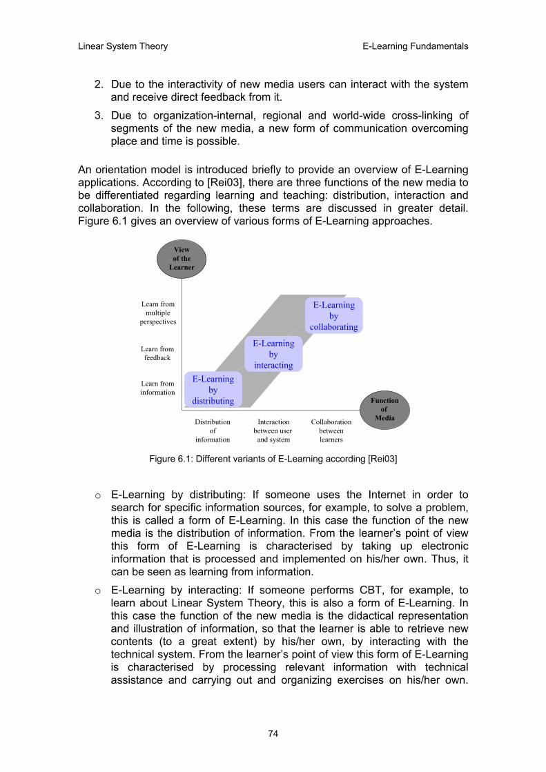
Linear System Theory E-Learning Fundamentals
2. Due to the interactivity of new media users can interact with the system and receive direct feedback from it.
3. Due to organization-internal, regional and world-wide cross-linking of segments of the new media, a new form of communication overcoming place and time is possible.
An orientation model is introduced briefly to provide an overview of E-Learning applications. According to [Rei03], there are three functions of the new media to be differentiated regarding learning and teaching: distribution, interaction and collaboration. In the following, these terms are discussed in greater detail. Figure 6.1 gives an overview of various forms of E-Learning approaches.
Functionof
Media
Viewof the
Learner
Learn frommultiple
perspectives
Learn fromfeedback
Learn frominformation
Distributionof
information
Interactionbetween user
and system
Collaborationbetweenlearners
E-Learningby
collaborating
E-Learningby
interactingE-Learning
bydistributing
Figure 6.1: Different variants of E-Learning according [Rei03]
o E-Learning by distributing: If someone uses the Internet in order to
search for specific information sources, for example, to solve a problem, this is called a form of E-Learning. In this case the function of the new media is the distribution of information. From the learner’s point of view this form of E-Learning is characterised by taking up electronic information that is processed and implemented on his/her own. Thus, it can be seen as learning from information.
o E-Learning by interacting: If someone performs CBT, for example, to learn about Linear System Theory, this is also a form of E-Learning. In this case the function of the new media is the didactical representation and illustration of information, so that the learner is able to retrieve new contents (to a great extent) by his/her own, by interacting with the technical system. From the learner’s point of view this form of E-Learning is characterised by processing relevant information with technical assistance and carrying out and organizing exercises on his/her own.
74

Linear System Theory E-Learning Fundamentals
Thus, it is a form of learning through feedback. An instructor is not necessary for learning from feedback, but the introduction of a learning advisor is possible, if not necessary.
o E-Learning by collaborating: If someone, for example, attends an online seminar and processes exercises within virtual groups, that is to say together with other learners via a network, this is also a form of E-Learning. In this case the function of the new media is to connect learners with each other and encourage them to arrive at common solution. From the learner’s point of view this form of E-Learning is characterised by generating relatively independent knowledge so to solve social problems within the learning environment. In other words, this is also called learning from different perspectives. For moderation of learning processes an instructor, or a coach for solving virtual problems, respectively, is obligatory.
6.2.2 E-Learning Requirements
E-Learning by distribution, E-Learning by interacting and E-Learning by collaborating are three variants of learning involving new media. Each of these variants demands special requirements, namely on the one hand the design of an E-Learning environment with the abilities of the media-designer and the instructors, and on the other hand the learning processes and therewith the requirements which have to be met by the learners. In the following, these aspects are discussed in more detail.
o Requirements of E-Learning by distributing: If new media are used for distributing information, a successful learning process is guaranteed only if the structure of information is well-designed and if the potential of multimedia is exploited and used correctly; in other words, if the design of text and picture, as well as the structure and preparation of the information is correct. The demands on the learner with this form of E-Learning are high. Certainly the information to be learned is available, but the incentive to read, understand and use it has to develop on its own and this presupposes motivation and usually also foreknowledge. The abilities for self-control and self-determination as well as being able to deal with new media are prerequisites for successful E-Learning by distributing.
o Requirements of E-Learning by interacting: If new media are used for interaction between users and systems, a professional design of instructions, exercises and feedback has to be added to a well-designed presentation of information also. The demands on the learner with this form of E-Learning are rather low. Not only well-prepared information, but also necessary technical facilities like CBTs and WBTs (web based
75
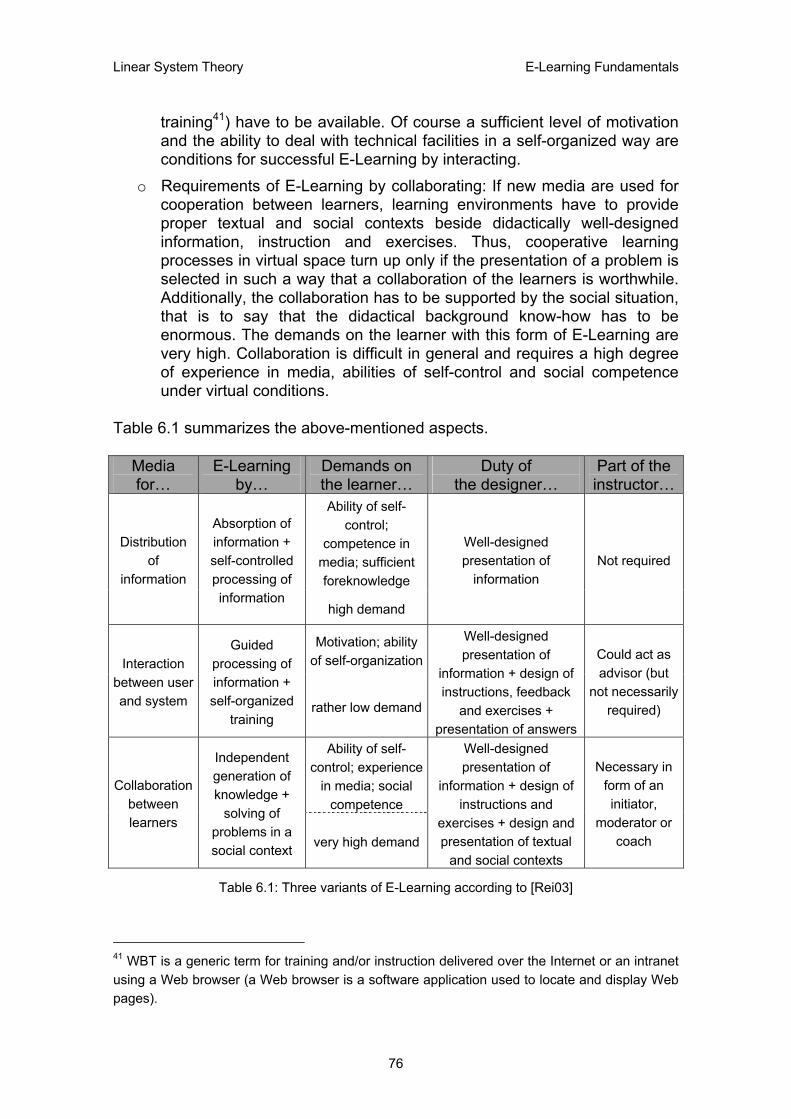
Linear System Theory E-Learning Fundamentals
training41) have to be available. Of course a sufficient level of motivation and the ability to deal with technical facilities in a self-organized way are conditions for successful E-Learning by interacting.
o Requirements of E-Learning by collaborating: If new media are used for cooperation between learners, learning environments have to provide proper textual and social contexts beside didactically well-designed information, instruction and exercises. Thus, cooperative learning processes in virtual space turn up only if the presentation of a problem is selected in such a way that a collaboration of the learners is worthwhile. Additionally, the collaboration has to be supported by the social situation, that is to say that the didactical background know-how has to be enormous. The demands on the learner with this form of E-Learning are very high. Collaboration is difficult in general and requires a high degree of experience in media, abilities of self-control and social competence under virtual conditions.
Table 6.1 summarizes the above-mentioned aspects.
Media for…
E-Learning by…
Demands on the learner…
Duty of the designer…
Part of the instructor…
Ability of self-control;
competence in media; sufficient foreknowledge
Distribution of
information
Absorption of information + self-controlled processing of information
high demand
Well-designed presentation of
information Not required
Motivation; ability of self-organizationInteraction
between user and system
Guided processing of information + self-organized
training rather low demand
Well-designed presentation of
information + design of instructions, feedback
and exercises + presentation of answers
Could act as advisor (but
not necessarily required)
Ability of self-control; experience
in media; social competence
Collaboration between learners
Independent generation of knowledge +
solving of problems in a social context very high demand
Well-designed presentation of
information + design of instructions and
exercises + design and presentation of textual
and social contexts
Necessary in form of an initiator,
moderator or coach
Table 6.1: Three variants of E-Learning according to [Rei03]
41 WBT is a generic term for training and/or instruction delivered over the Internet or an intranet using a Web browser (a Web browser is a software application used to locate and display Web pages).
76
Linear System Theory E-Learning Fundamentals
6.3 Integration of Blended Learning
Blended Learning is a form of E-Learning and therefore it uses the above-mentioned variants of learning by combining old and new media contents. Both an advanced impartation (or communication) of information and therewith a form of receptive learning as well as stimulation of active generation of knowledge is fulfilled. This section briefly introduces different theories of learning and shows that Blended Learning integrates such theories.
6.3.1 Theories of Learning
Of course, no unambiguous theory of learning (which could describe all changes of knowledge and skills) exists and most probably will never exist. However, we can identify three fundamentally different ideas about the nature of learning and what the nature of knowledge is. In other words, the approaches not only include a view of how learning occurs, but also a view of what knowledge actually is. These three basic approaches or psychological theories are referred to as behaviourism, cognitivism and constructivism and are discussed briefly as follows. The overviews concentrate on the main differences between the theoretical positions and are very general. Note that there is a lot more to these "fields" than what is presented in the following text.
o Behaviourism is a theory of animal and human learning that only focuses on objectively observable behaviour and discounts mental activities. Learning is defined as nothing more than the acquisition of new behaviour. Many of the early behaviouristic experiments were carried out with animals focusing on reflexive behaviour of an organism exposed to certain stimuli. This theory is relatively easy to understand because it relies on observable behaviour only and describes several universal laws of behaviour (e.g. behaviourism often is used by teachers, who reward or punish student behaviour). In other words, the theory of behaviourism tries to explain without referring to mental processes.42 Although there is a lack of expressiveness, the behaviouristic theories have been generalized to many higher-level functions as well (see [Psy98]).
o Cognitivism is a theory from the field of psychology that models an individual’s mental perceptions and internal rules, which form his or her decision-making processes. The cognitive viewpoint focuses on mental processes, stresses objectivity in research and builds models of mental processes and interactions with information systems. Psychology can be explained by the use of experiments, measurements and the scientific
42 Note the famous "Dog-Salivation-Experiment" by Ivan Petrovich Pavlov where he made dogs salivate at the sound of a bell.
77

Linear System Theory E-Learning Fundamentals
methods in a cognitivistic way. Individual components of mental function can be identified and meaningfully understood. Mental function could also be understood in terms of information processing or mathematical models. Thus, the theory of cognitivism makes mental processes the primary object of study and tries to discover and model the mental processes on the part of the learner during the learning-process (see [Psy98]).
o Constructivism is a theory of learning founded on the premise that, by reflecting on our experiences, we construct our own understanding of the world we live in. All of us generate our own "rules" and "mental models", which we use in order to make sense of our experiences. Learning, therefore, is simply the process of adjusting our mental models to integrate new experiences. Next, we have a look at the impact of constructivism on learning. Educators focus on making connections between facts and fostering new understanding in students. Instructors tailor their teaching strategies to student responses and encourage students to analyse, interpret, and predict information. Teachers also rely heavily on open-ended questions and promote extensive dialogue among students. Constructivism calls for the elimination of grades and standardized testing. Instead, assessment becomes part of the learning process so that students play a larger role in judging their own progress.
Table 6.2 shows the keywords about the three different learning theories, which is incomplete but gives a concluding overview.
Theory Comments
Behaviourism Is based on behavioural changes. Focuses on a new behavioural pattern being repeated until it becomes automatic.
Cognitivism Is based on the thought process behind behaviour. Changes in behaviour are observed, but only as an indicator to what is going on in the learner's
head.
Constructivism Is based on the premise that we all construct our own perspective of the world, based on individual experiences and schemata. Focuses on preparing the learner to solve problems in ambiguous situations.
Table 6.2: Keywords about different learning theories
78
Linear System Theory E-Learning Fundamentals
6.3.2 Instruction and Construction
Behaviourism, cognitivism and constructivism influence situations of learning and teaching differently. On the one hand the selection and composition of teaching methods and therewith activities of the instructor – thus the instruction – could be in the foreground. On the other hand motivation, foreknowledge, processes of understanding as well as the structure and the use of knowledge on the learner’s part – thus the construction – could be the focus of attention. Teacher-centred instruction is characterized by methods, activities, and techniques where the teacher decides what is to be learned, what is to be tested, and how the class is to be run. Often teachers are in the centre of the classroom giving instruction with little input from their students. The teacher decides the goals of the class based on some outside criteria. This form of instruction creates passive learners and therefore it is hardly possible to generate competence in media, social competence and competence in learning (see [Esl02]). Student-centred and/or learner-centred instruction is characterized by language activities, techniques, methods where the focus is on students/learners and the teacher plays only a peripheral role. Students are allowed to have some control over the activity or to give some input into the curriculum. These activities encourage student creativity. Group work is one kind of student-centred activity. If students design their own test, this is another learner-centred activity. Individual styles and needs of the learners are taken into account. Learner-centred education is thought to be intrinsically43 motivating and thus beneficial. This can be put in contrast to teacher-centred learning. But this form of instruction can also cause theoretical, empirical and practical problems. Central difficulties are cognitive overwork by too little guided learning processes as well as learning processes that do not lead to the aspired learning results because the ability of self-control is lacking (see [Esl02]).
6.3.3 Integration by Blended Learning
If one refers back to the above-mentioned terms (see Section 6.3.2), an integrative view of teaching and learning consists of connecting teacher-centred instruction with the learner-oriented support of generating knowledge. This should be performed in such a manner that it is helpful both for meeting the targets (both learning and teaching) and for the learner. The instructor takes over multiple functions that vary from presenting, structuring, guiding and explaining to stimulating, advising and collaborating. Certainly the instructor is still responsible for the content of teaching, but the student is expected to take
43 Intrinsic in this context means motivation in learning that comes from a sense of empowerment in being able to do something. Doing something for the sake of doing it without thought of rewards such as praise, grades, candy, or money (see [Esl02]).
79
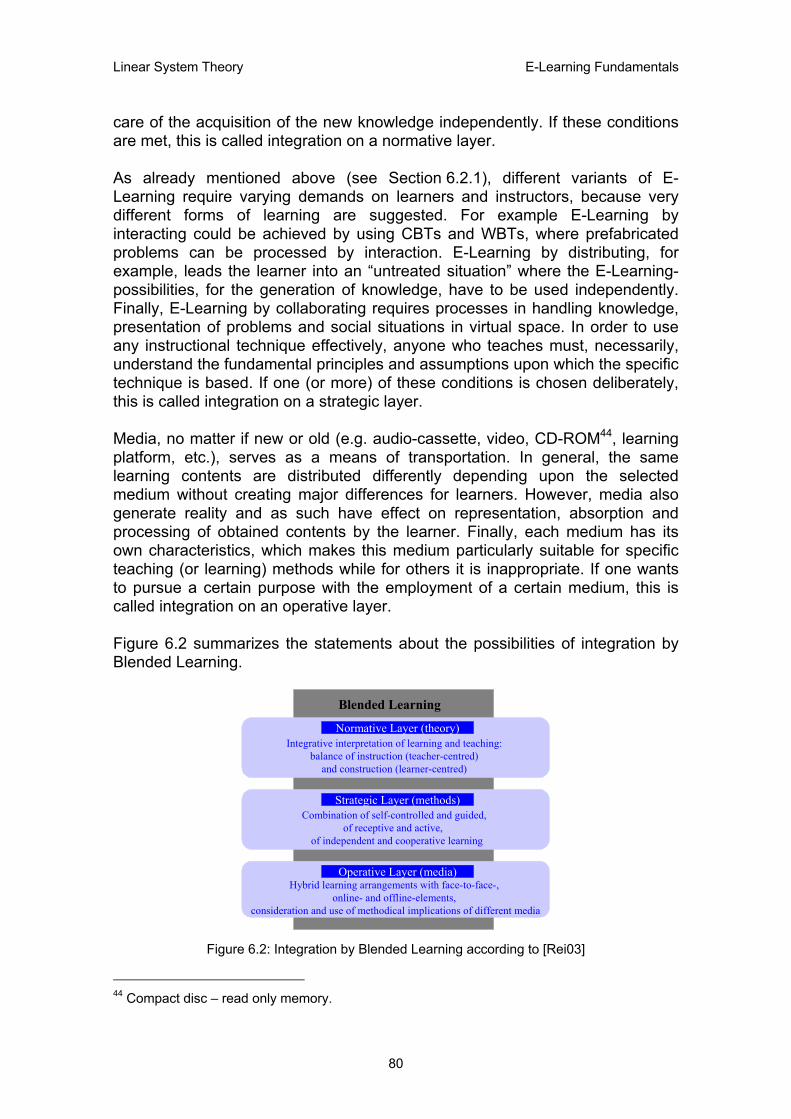
Linear System Theory E-Learning Fundamentals
care of the acquisition of the new knowledge independently. If these conditions are met, this is called integration on a normative layer. As already mentioned above (see Section 6.2.1), different variants of E-Learning require varying demands on learners and instructors, because very different forms of learning are suggested. For example E-Learning by interacting could be achieved by using CBTs and WBTs, where prefabricated problems can be processed by interaction. E-Learning by distributing, for example, leads the learner into an “untreated situation” where the E-Learning-possibilities, for the generation of knowledge, have to be used independently. Finally, E-Learning by collaborating requires processes in handling knowledge, presentation of problems and social situations in virtual space. In order to use any instructional technique effectively, anyone who teaches must, necessarily, understand the fundamental principles and assumptions upon which the specific technique is based. If one (or more) of these conditions is chosen deliberately, this is called integration on a strategic layer. Media, no matter if new or old (e.g. audio-cassette, video, CD-ROM44, learning platform, etc.), serves as a means of transportation. In general, the same learning contents are distributed differently depending upon the selected medium without creating major differences for learners. However, media also generate reality and as such have effect on representation, absorption and processing of obtained contents by the learner. Finally, each medium has its own characteristics, which makes this medium particularly suitable for specific teaching (or learning) methods while for others it is inappropriate. If one wants to pursue a certain purpose with the employment of a certain medium, this is called integration on an operative layer. Figure 6.2 summarizes the statements about the possibilities of integration by Blended Learning.
Blended Learning
Integrative interpretation of learning and teaching: balance of instruction (teacher-centred)
and construction (learner-centred)
Normative Layer (theory)
Combination of self-controlled and guided, of receptive and active,
of independent and cooperative learning
Strategic Layer (methods)
Hybrid learning arrangements with face-to-face-, online- and offline-elements,
consideration and use of methodical implications of different media
Operative Layer (media)
Figure 6.2: Integration by Blended Learning according to [Rei03]
44 Compact disc – read only memory.
80
Linear System Theory E-Learning Fundamentals
That Blended Learning fulfils both an inductive and a deductive psychological approach is shown next. Therefore, these definitions are discussed briefly. Inferences, for example, are made when a person (or machine) goes beyond available evidence to form a conclusion (see [Cog04]):
o An inductive inference is one that is likely to be true because of the state of the world. Unlike deductive inferences, inductive inferences do yield conclusions that increase the semantic information over and above that found in the initial premises. However, in the case of inductive inferences, we cannot be sure that our conclusion is a logical result of the premises, but we may be able to assign a likelihood to each conclusion.
o A deductive inference is one where this conclusion always follows the stated premises. In other words, if the premises are true, the conclusion is valid. Studies of human efficiency in deductive inference involve conditional reasoning problems which follow the "if A, then B" format.
In the history of the beginnings of Blended Learning, discontent, disappointment and cost problems led to hybrid learning arrangements that are based on traditional forms of teaching (learning). Therefore, initially Blended Learning was developed inductively from experiences and requirements of practice. Furthermore, a short analysis of different learning theories and views about learning and teaching showed that a mix of methods and media not only justifies theoretical levels, but can also be postulated. Thus, Blended Learning fulfils both an inductive and a deductive psychological approach.
81

Linear System Theory Criteria for E-Learning Implementation
7. CRITERIA FOR E-LEARNING IMPLEMENTATION
The previous section introduced basics of electronic learning and especially of Blended Learning. This chapter describes a possible approach for using Blended Learning at technical colleges. Therefore, didactic concepts including targets and contents, media and methods are stated by introducing a sample lecture, which is called SVL (semi-virtual lecture). This section should thus reflect a concrete illustration of a Blended Learning arrangement. It is obvious that the selected topic for the SVL mostly coincides with the topic of this thesis, because linear system theory is the basis for many technical applications, too. This chapter is mainly based on [Rei03] and [Lee04].
7.1 Didactical Concept
In the following, it is shown how the SVL is methodically and technically (media) structured and additionally a possible way of implementation is discussed. One could say that this section introduces a general idea about the possibilities of Blended Learning at technical colleges.
7.1.1 Targets and Contents
The title of the SVL is “Linear System Theory and Design”. It is dealt with in many technical subjects, which cover theoretical as well as practical aspects. The structure of the SVL predominantly adheres to those chosen above (see also Chapter 1 to 5):
1. In the block “Introduction” the notions and the basics of “System”, “Model” and “Signal” are discussed.
2. In the block “Mathematical Description”, a description of important LTI-system properties, internal and external system relationships, transfer functions and helpful calculation methods is carried out. This block covers the continuous-time case as well as the discrete-time case.
3. The block “Stability Condition” introduces the BIBO (bounded-input bounded-output) stability for the zero-state response of a LTI-system and marginal and asymptotic stabilities are introduced for the zero-input response. This block covers the continuous-time case as well as the discrete-time case.
4. The block “State-Space Solutions” describes the solutions of the internal description, which was derived in block 2 (mathematical description), of
82
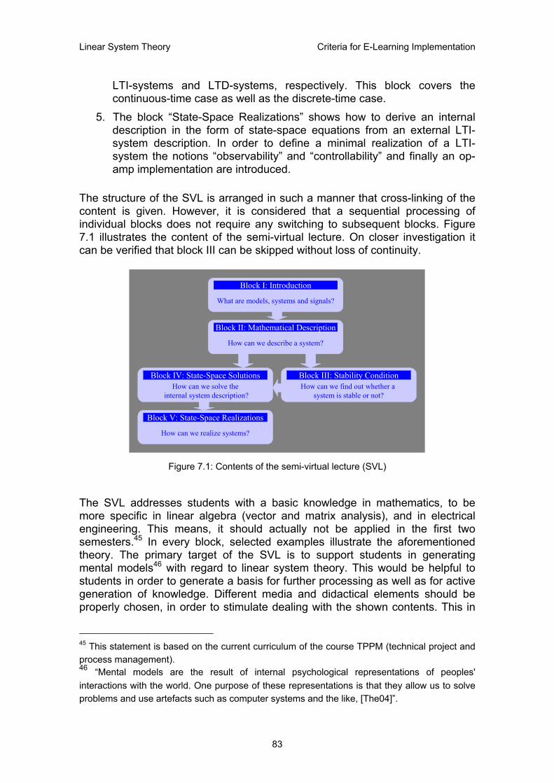
Linear System Theory Criteria for E-Learning Implementation
LTI-systems and LTD-systems, respectively. This block covers the continuous-time case as well as the discrete-time case.
5. The block “State-Space Realizations” shows how to derive an internal description in the form of state-space equations from an external LTI-system description. In order to define a minimal realization of a LTI-system the notions “observability” and “controllability” and finally an op-amp implementation are introduced.
The structure of the SVL is arranged in such a manner that cross-linking of the content is given. However, it is considered that a sequential processing of individual blocks does not require any switching to subsequent blocks. Figure 7.1 illustrates the content of the semi-virtual lecture. On closer investigation it can be verified that block III can be skipped without loss of continuity.
What are models, systems and signals?
Block I: Introduction
How can we describe a system?
Block II: Mathematical Description
How can we find out whether a system is stable or not?
Block III: Stability Condition
How can we realize systems?
Block V: State-Space Realizations
How can we solve theinternal system description?
Block IV: State-Space Solutions
Figure 7.1: Contents of the semi-virtual lecture (SVL)
The SVL addresses students with a basic knowledge in mathematics, to be more specific in linear algebra (vector and matrix analysis), and in electrical engineering. This means, it should actually not be applied in the first two semesters.45 In every block, selected examples illustrate the aforementioned theory. The primary target of the SVL is to support students in generating mental models46 with regard to linear system theory. This would be helpful to students in order to generate a basis for further processing as well as for active generation of knowledge. Different media and didactical elements should be properly chosen, in order to stimulate dealing with the shown contents. This in
45 This statement is based on the current curriculum of the course TPPM (technical project and process management). 46 “Mental models are the result of internal psychological representations of peoples' interactions with the world. One purpose of these representations is that they allow us to solve problems and use artefacts such as computer systems and the like, [The04]”.
83

Linear System Theory Criteria for E-Learning Implementation
fact would allow the development of mental models. Beside the building of mental models, transfer processes should also be stimulated during learning. This can be accomplished by problem-orientated exercises at the end of each block. It is also necessary and inevitable that students become confident in dealing with new media, to develop competence in working with media. Typical phenomena, which are associated with the classic lecture, like passiveness, control of and isolation during learning should be avoided if possible. In principal considerable time is required for preparing the structure and content of the SVL. For one page, for example, of the CBT-programme (including programming of animations) the time involved is about one hour. This effort is necessary because only a well-prepared and structured lecture causes an increase in value of an educational offer. A professional technique and design is important to learners. Shortcomings could cause a negative impact to the learning process. It should be noted that thoughtless as well as poorly structured contents of learning cannot be compensated by the use of hard- and software. During the phase of editing, the appropriate contents of the SVL were modelled on the above-mentioned aims, so that focus was on general graphs, clear, manageable modules47, clear and audible articulation, and a clear structure. The CD-ROM, which in fact represents the CBT, is recorded with logical graphs, animations, videos and definitions that should stimulate the process of building mental models. During the lecture (phase of presence) there should be a discussion of derivations and corresponding mathematical background information for illustrating necessary equations. If one compares the content of the CBT with the traditional lecture, on the one hand the CBT partly overlaps with the traditional lecture, and on the other hand it offers more detailed information than the lecture.
7.1.2 Expected Benefit
Nowadays, when E-Learning products are rapidly increasing in number, it is important to think about the benefits of a Blended Learning scenario like the SVL. Questions, such as the requirements to be met, or the problems to be solved in a more efficient way, should be answered before the SVL is outlined and held. In the following, three major expectations are stated:
1. It is to be expected that the learning style is active, motivated and efficient. The learners have to process the shown information actively because every block of information has at least one integrated exercise. Work in groups and competition between groups heightens the motivation of students, thus it is higher than in traditional lectures. Processing of periodical exercises allows students a continuous and distributed learning process and thus a term-concomitant self-evaluation in contrast to a single exercise. Particularly distributed learning causes
47 A module denotes an information unit.
84
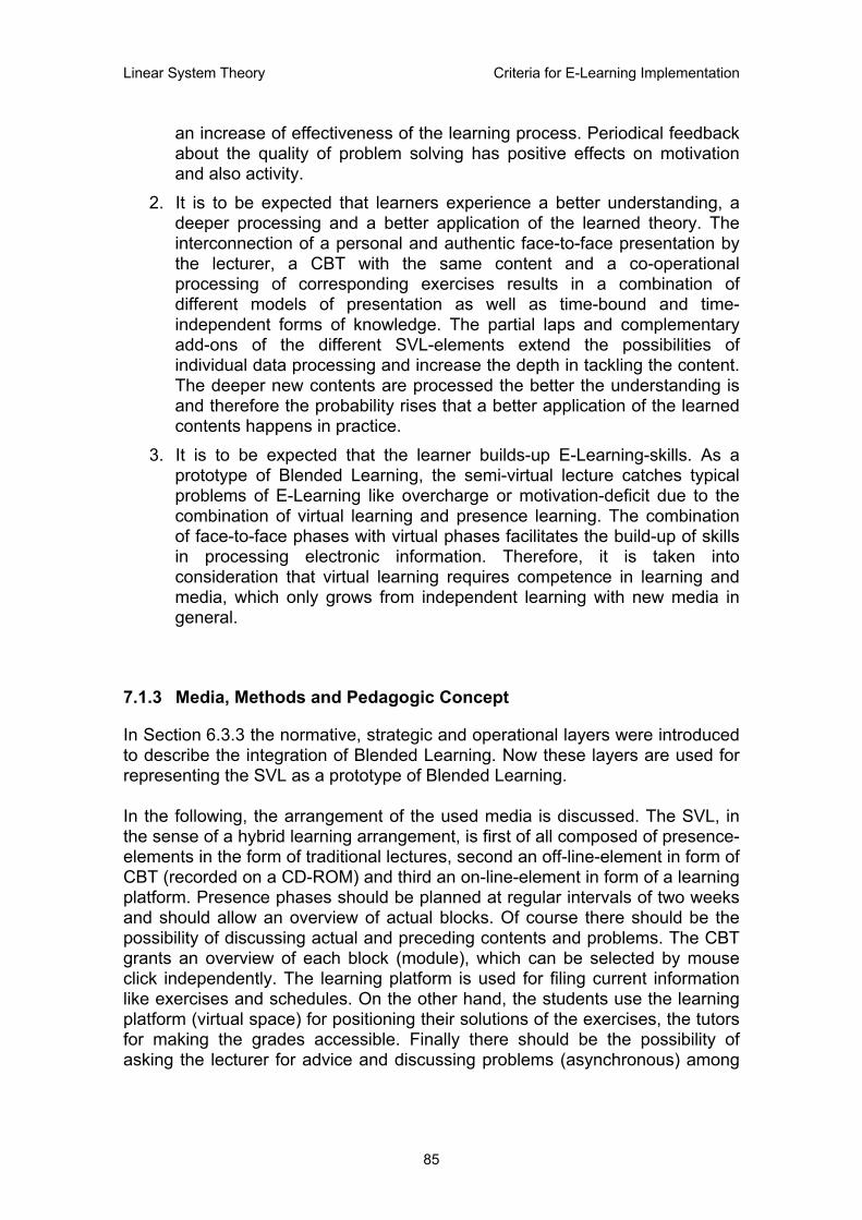
Linear System Theory Criteria for E-Learning Implementation
an increase of effectiveness of the learning process. Periodical feedback about the quality of problem solving has positive effects on motivation and also activity.
2. It is to be expected that learners experience a better understanding, a deeper processing and a better application of the learned theory. The interconnection of a personal and authentic face-to-face presentation by the lecturer, a CBT with the same content and a co-operational processing of corresponding exercises results in a combination of different models of presentation as well as time-bound and time-independent forms of knowledge. The partial laps and complementary add-ons of the different SVL-elements extend the possibilities of individual data processing and increase the depth in tackling the content. The deeper new contents are processed the better the understanding is and therefore the probability rises that a better application of the learned contents happens in practice.
3. It is to be expected that the learner builds-up E-Learning-skills. As a prototype of Blended Learning, the semi-virtual lecture catches typical problems of E-Learning like overcharge or motivation-deficit due to the combination of virtual learning and presence learning. The combination of face-to-face phases with virtual phases facilitates the build-up of skills in processing electronic information. Therefore, it is taken into consideration that virtual learning requires competence in learning and media, which only grows from independent learning with new media in general.
7.1.3 Media, Methods and Pedagogic Concept
In Section 6.3.3 the normative, strategic and operational layers were introduced to describe the integration of Blended Learning. Now these layers are used for representing the SVL as a prototype of Blended Learning. In the following, the arrangement of the used media is discussed. The SVL, in the sense of a hybrid learning arrangement, is first of all composed of presence-elements in the form of traditional lectures, second an off-line-element in form of CBT (recorded on a CD-ROM) and third an on-line-element in form of a learning platform. Presence phases should be planned at regular intervals of two weeks and should allow an overview of actual blocks. Of course there should be the possibility of discussing actual and preceding contents and problems. The CBT grants an overview of each block (module), which can be selected by mouse click independently. The learning platform is used for filing current information like exercises and schedules. On the other hand, the students use the learning platform (virtual space) for positioning their solutions of the exercises, the tutors for making the grades accessible. Finally there should be the possibility of asking the lecturer for advice and discussing problems (asynchronous) among
85
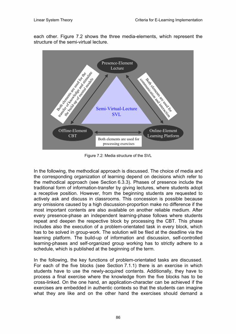
Linear System Theory Criteria for E-Learning Implementation
each other. Figure 7.2 shows the three media-elements, which represent the structure of the semi-virtual lecture.
Presence-ElementLecture
Online-ElementLearning Platform
Offline-ElementCBT
Semi-Virtual-LectureSVL
Both el
emen
ts are
used
for t
he
trans
ferof
know
ledge
and s
timula
te
the bu
ild-u
p of m
ental
mod
els
Both elements are used for processing exercises
Both elements are used for
communication and interaction
Figure 7.2: Media structure of the SVL
In the following, the methodical approach is discussed. The choice of media and the corresponding organization of learning depend on decisions which refer to the methodical approach (see Section 6.3.3). Phases of presence include the traditional form of information-transfer by giving lectures, where students adopt a receptive position. However, from the beginning students are requested to actively ask and discuss in classrooms. This concession is possible because any omissions caused by a high discussion-proportion make no difference if the most important contents are also available on another reliable medium. After every presence-phase an independent learning-phase follows where students repeat and deepen the respective block by processing the CBT. This phase includes also the execution of a problem-orientated task in every block, which has to be solved in group-work. The solution will be filed at the deadline via the learning platform. The build-up of information and discussion, self-controlled learning-phases and self-organized group working has to strictly adhere to a schedule, which is published at the beginning of the term. In the following, the key functions of problem-orientated tasks are discussed. For each of the five blocks (see Section 7.1.1) there is an exercise in which students have to use the newly-acquired contents. Additionally, they have to process a final exercise where the knowledge from the five blocks has to be cross-linked. On the one hand, an application-character can be achieved if the exercises are embedded in authentic contexts so that the students can imagine what they are like and on the other hand the exercises should demand a
86

Linear System Theory Criteria for E-Learning Implementation
practical processing within the authentic contexts. In other words, the more the problem-orientated task is related to practice, the better the understanding of the students will be. The problem-orientated tasks of the SVL should fulfil the following functions at the same time:
o They activate in a cognitive way, because processing of exercises is only meaningful if the offered information is understood.
o They activate in an emotionally-motivational way, because students have personal reference to demanded contents. The on-line publication of solutions and grades causes a positive competition, which is motivating.
o They activate in a socially interactive way, because exercises are processed in group work and are compared with other group solutions.
o They show a safeguard character with regard to application, because processing of exercises (realistic presentation of a problem) requires a paper-pencil transfer of newly-obtained contents.
o They show a safeguard character with regard to practice, because exercises are an additional (not the only one) element for the generation of knowledge and cause repeated confrontation with the contents.
o They show a safeguard character with regard to examination, because the solutions of exercises are graded and the processing of all exercises replaces a final exam.
SafeguardingActivation
Problem-orientated Tasks
Cognitive(processing of exercises requires understanding)
Application(authentic presentation
of problems)
Emotional-Motivational(personal relationand competition)
Practice(exercises as additional
elements)
Examination(grading of exercises andreplacement of exams)
Social Interaction(group work and
comparison of solutions)
Figure 7.3: Problem-orientated tasks as central didactic element
Figure 7.3 summarizes the functions of the problem-orientated tasks of the semi-virtual lecture. The pedagogic concept is discussed next.
87

Linear System Theory Criteria for E-Learning Implementation
The pedagogic concept of the SVL, which the mentioned methodical approach and the chosen media-arrangement is based on, corresponds to a moderate constructive view in which learning is active-constructive, self-controlled and a social process. The characteristics of this process can be described as follows:
o Students do not only grasp the offered pedagogic contents, but also build mental models actively and constructively with regard to individual blocks, or extend and change existing models.
o Students acquire contents largely in an independent and self-controlled way while being supported in evaluating their knowledge independently.
o Besides individual learning, students also practice social and cooperative learning by processing exercises in group working.
o Students first recognise application-orientated anchors by processing exercises that show a possible application of the learned contents.
The underlying moderate constructive view is characterised by offering the learner tasks and tools for solving problems in contrast to radical constructive approaches, which favour complete open learning environments. Additionally, the selected position rather integrates instructional guidance and support, whereby (for open learning environments necessary) competence in self-learning could be developed.
7.1.4 Course of Events
In the following, it is illustrated what to expect from the operational sequence of the semi-virtual lecture. During the first lecture an introduction of contents and methodology of the seminar, as well as an introduction to the learning platform if students are not familiar with it, will be given. In the following week a CD-ROM will be distributed and an e-mail address administration should be arranged, or if it already exists, should be brought up to date. Additionally, groups should be organized that will perform a cooperative processing of the subsequent exercises, and a ratio formula for evaluation will be predetermined. Subsequently, face-to-face lectures (traditional lectures) will take place at regular intervals of two weeks. Between two lectures virtual learning phases are integrated including cooperative processing of exercises. Statements and questions regarding the last block may be given and asked, respectively, after each self-controlled and cooperative phase. Exercises have to be processed between two presence phases (traditional lectures). Each group files their solution on the learning platform within a predetermined time frame. Group-solutions are transparent for anyone and can be examined at any time by using the learning platform. Nevertheless, inconspicuous copying is hardly possible because the date when the solution was placed on the learning platform appears visibly to all. After the expiration of the deadline, every solution will be
88
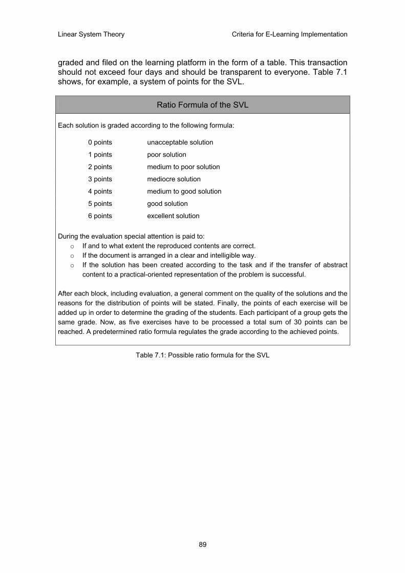
Linear System Theory Criteria for E-Learning Implementation
graded and filed on the learning platform in the form of a table. This transaction should not exceed four days and should be transparent to everyone. Table 7.1 shows, for example, a system of points for the SVL.
Ratio Formula of the SVL
Each solution is graded according to the following formula:
0 points unacceptable solution
1 points poor solution
2 points medium to poor solution
3 points mediocre solution
4 points medium to good solution
5 points good solution
6 points excellent solution During the evaluation special attention is paid to:
o If and to what extent the reproduced contents are correct. o If the document is arranged in a clear and intelligible way. o If the solution has been created according to the task and if the transfer of abstract
content to a practical-oriented representation of the problem is successful. After each block, including evaluation, a general comment on the quality of the solutions and the reasons for the distribution of points will be stated. Finally, the points of each exercise will be added up in order to determine the grading of the students. Each participant of a group gets the same grade. Now, as five exercises have to be processed a total sum of 30 points can be reached. A predetermined ratio formula regulates the grade according to the achieved points.
Table 7.1: Possible ratio formula for the SVL
89

Linear System Theory CBT Realization
8. CBT REALIZATION
These days, knowledge and information are essential factors of success in order to survive on the national and international markets. On the one hand the availability of information increases rapidly, on the other hand its validity periods are getting shorter and shorter. Consequently, education and advanced education have to be adjusted to the given situations. In order to meet this requirement the implementation of new teaching methods in combination with old teaching methods (substantial conclusions and statements regarding this problematic were already made in Chapter 7) must be considered. The method of programmed instruction (or learning) is a form of learning which allows individual learning, independent of place and time. For implementing this method, media of written documentation were used initially. Teaching machines, which consisted of tape recorders, still-picture projectors, etc., were first developed in the 60’s. Only two buttons for answering the questions were available to the students most of the time. Very soon the computer replaced the learning automatons. It makes the use of multimedia computer-aided teaching programmes in operational as well as school training possible. This section discusses the conceptual fundamentals first. After the introduction of varying types of learning programmes and the criteria for their utilization a brief description of the design of the “Linear System Theory and Design”-CBT is carried out.
8.1 Notional-Systematic Basics
In order to provide more detailed information about learning programmes, which are computer-based, it is necessary to discuss notional basics briefly. Therefore, this section introduces frequently and globally used notions.
8.1.1 CBT – Computer-Based Training
Several concepts are used in connection with learning on the computer. For example, Computer-Based Teaching (CBT), Computer-Assisted Instruction (CAI) or Computer-Aided Learning (CAL). In this text the notion Computer-Based Training is used as a synonym for computer-aided learning.
90
Linear System Theory CBT Realization
CBT is a method of learning, which should impart both computer-dependent and computer-independent learning contents. The computer is used as a tool and as a medium, respectively. Thus, it does not become an end in itself but it supports (computer-based training) learning. The target of this method is acquisition of new experiences (computer-based training). However, the computer should only be used where its use provides certain advantages. Another definition has to be introduced at this point: The concept “computer learning programme” used in this text does not mean an integration of the computer in educational programmes, but certain soft- and teaching-ware respectively. “Computer learning programme” means tutorial or non-tutorial dialogue respectively between a computer system and a learner by imparting facts and intellectual skills by using multimedia objects and interaction. Beside interactivity, individuality and adaptability are essential characteristics of computer learning programmes.
8.1.2 Multimedia
Nowadays everyone is talking about multimedia. The word multimedia has an effect on selling points and on purchasing points likewise. Besides, its development potential is not yet fully exhausted. Research projects, for example, try to find new techniques that should interact with other human senses beside the senses of hearing and seeing. In the CBT sector, the use of multimedia computer learning programmes has provided new possibilities in the transfer of knowledge, too. “The term multimedia describes a number of diverse technologies that allow visual and audio media to be combined in new ways for the purpose of communicating. Applications include entertainment, education and advertising. Multimedia often refers to computer technologies. Nearly every PC built today is capable of multimedia applications because they include a CD-ROM or DVD drive, and a sophisticated sound and video card (often built into the motherboard). But the term multimedia also describes a number of dedicated media appliances, such as digital video recorders (DVRs), interactive television, MP348 players, advanced wireless devices and public video displays, [Mul04]“. According to [Bol95] multimedia applications can be characterised as networks consisting of nodes and arcs. While nodes represent the media objects (audiovisual media), the arcs describe the relationship between various kinds of media. Media objects are subdivided into output media objects (text, animation, video, audio, diagram) and interaction media objects (projected buttons, menus or text 48 Is the file extension for MPEG, audio Layer 3. Layer 3 is one of three coding schemes (Layer 1, Layer 2 and Layer 3) for the compression of audio signals (see [Web04]).
91

Linear System Theory CBT Realization
fields onto user interface). Now, if different types of media objects appear, they can be referred to as multimedia objects. According to the type of cause (trigger) and impact different types of relations can be distinguished, which are discussed next:
o Temporal relations result from temporal triggers – Start of a media object – with temporal impact – End of media object.
o Creative relations result from creative triggers – creative change of a media object (colour scheme, size, position on monitor) – with creative impact.
o In mixed relations the type of trigger differs from the type of impact, e.g. termination of a video due to the position change of a graphic object.
o Interaction relations are characterized by triggers, called interaction media objects. If impacts are of temporal nature the interaction is said to be navigational (navigational interaction), on the other hand, if impacts are of creative nature this is called creative interaction.
8.1.3 Authoring Systems49
Today there are three different groups of tools that can be used for developing learning programmes, which are: programming languages50, authoring languages51 and authoring systems. Conventional programming languages have high flexibility but require extensive knowledge in programming. Authoring languages are programming languages with additional instructions for functions, which are very supportive for developing learning programmes. Functions, for example motioned graphics, animations, can be called via subroutines, so that programming compared to programming languages is easier. Authoring systems do not require any knowledge in programming in the stricter sense. They make the creation of learning programmes by menu guidance only possible. While authoring languages require fairly long settling-in periods due to the required knowledge in programming, but have high function-potential, authoring systems are relatively easy to operate but have low function-potential. Literature shows different possibilities of differentiating between authoring tools. Authoring tools are also known as author-ware, a programme that helps you write hypertext or multimedia applications. They usually enable you to create a
49 Software for assembling multimedia applications is called authoring system. 50 A list of vocabulary and set of grammatical rules for instructing a computer to perform specific tasks. The term programming language usually refers to high-level languages, such as BASIC, C, C++, COBOL, FORTRAN, Ada, and Pascal. Each language has a unique set of keywords (words that it understands) and a special syntax for organizing programme instructions (see [Web04]). 51 Software that can be used to develop interactive computer programmes without the technically demanding task of computer programming is called authoring language.
92
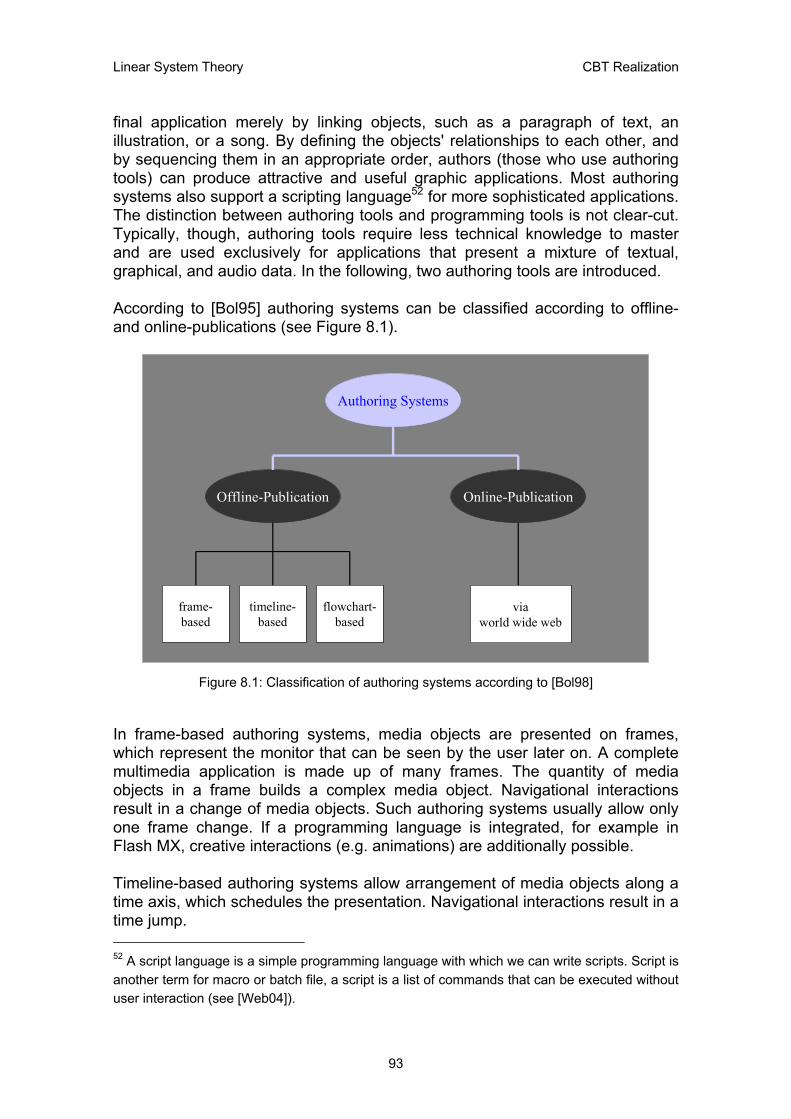
Linear System Theory CBT Realization
final application merely by linking objects, such as a paragraph of text, an illustration, or a song. By defining the objects' relationships to each other, and by sequencing them in an appropriate order, authors (those who use authoring tools) can produce attractive and useful graphic applications. Most authoring systems also support a scripting language52 for more sophisticated applications. The distinction between authoring tools and programming tools is not clear-cut. Typically, though, authoring tools require less technical knowledge to master and are used exclusively for applications that present a mixture of textual, graphical, and audio data. In the following, two authoring tools are introduced. According to [Bol95] authoring systems can be classified according to offline- and online-publications (see Figure 8.1).
Online-PublicationOffline-Publication
frame-based
Authoring Systems
flowchart-based
timeline-based
viaworld wide web
Figure 8.1: Classification of authoring systems according to [Bol98]
In frame-based authoring systems, media objects are presented on frames, which represent the monitor that can be seen by the user later on. A complete multimedia application is made up of many frames. The quantity of media objects in a frame builds a complex media object. Navigational interactions result in a change of media objects. Such authoring systems usually allow only one frame change. If a programming language is integrated, for example in Flash MX, creative interactions (e.g. animations) are additionally possible. Timeline-based authoring systems allow arrangement of media objects along a time axis, which schedules the presentation. Navigational interactions result in a time jump. 52 A script language is a simple programming language with which we can write scripts. Script is another term for macro or batch file, a script is a list of commands that can be executed without user interaction (see [Web04]).
93

Linear System Theory CBT Realization
In flowchart-based authoring systems media objects are shown as symbols, which are connected through arcs in diagrams. Navigational interactions of the user (at a later stage) determine the arcs, which will be processed. Authoring systems for electronic online publications are called HTML53-editors usually, because learner-controlled learning environments are still predominantly implemented by using hypertext-systems.
8.2 Computer Learning Programmes
This section introduces different types of computer learning programmes. The differentiation is carried out according to [Rat98] which used tutorial components for the demarcation of computer learning programmes. Figure 8.2 shows various forms of computer-based learning programmes according to [Rat98].
Non-Tutorial CBTTutorial CBT
drill & practicesystems
tutorialsystems
traditional
Computer-based Learning Programmes
intelligent
simulationslearner-
controlledsystems
learningenviron-
ments
arrange-ments
Figure 8.2: Forms of computer-based learning programmes
53 Short for HyperText Markup Language, the authoring language used to create documents on the World Wide Web. HTML defines the structure and layout of a Web document by using a variety of tags and attributes (see [Web04]).
94
Linear System Theory CBT Realization
8.2.1 Tutorial Forms
With tutorial teach-ware a computer controls or regulates the activities of the learners like a tutor or instructor. The tutorial component results from pre-programmed linear- or divided learning-algorithms. The target of drill and practice programmes is to consolidate available knowledge and to impart cognitive knowledge. These types of learning programmes are suitable for learning by heart, e.g. vocabulary training. Such systems consist of text and graphic frames and exercises, which are presented and processed in a fixed sequence. The process of learning is reduced to a simple stimulus-reaction-scheme and is rather often based on simple trial-and-error concepts. The learner has to answer (react) given exercises (stimuli). Afterwards the answers are evaluated by the programme and corresponding feedback is given. Another form of teach-ware are tutorial systems that aim at imparting new knowledge. These types of learning programmes try to simulate the interaction between learner and instructor by transferring knowledge, giving feedback and checking the progress of learning. After the presentation of information in form of text, graphics or video-scenes and the subsequent answering of logical questions, the answers are analysed. Depending on the result of the analysis the learning programme will select the succeeding module, thus it controls the sequence of learning. Intellectual tutorial programmes make different presentations of learning matters depending on the results of the learner possible. Such systems try to coach the learner individually by providing effectual learning techniques regarding the existing problem. The content of learning is compared to the evaluated knowledge of the learner and therefore it is possible to control the learning progress. In practice this could mean, for example, that due to a placement test the learners are advised to skip particular modules because of their high level of knowledge.
8.2.2 Non-Tutorial Forms
With non-tutorial forms of computer-based learning programmes the tutorial component is pushed into the background or is missing entirely. Such systems could be simulations, experimental games or learner-controlled systems. A simulation is the process of imitating a real phenomenon with a set of mathematical formulas. Advanced computer programmes can simulate, for example, weather conditions, operating methods of a motor, atomic reactions, and even biological processes. In theory, any phenomena or physical systems that can be reduced to mathematical data and equations can be simulated on a computer. In practice, however, simulation is extremely difficult because most
95

Linear System Theory CBT Realization
natural phenomena are subject to an almost infinite number of influences (see [Web04]). Because of the playful processing of simulations, the learner is motivated. Such learning programmes make the transfer of knowledge like concentration, skill, staying power or thinking in a general perspective possible, which is normally impossible by written and/or verbal learning matters. The processing of problem-orientated tasks (during the simulation) confronts the learners with the consequences of their decisions. To experiment with an arbitrary amount of strategies without any risk results in “learning by doing”, or individual development of problem-solving strategies until the optimal result is achieved. Learner-controlled systems allow absolutely free navigation through modules. Such systems try to adjust to the human behaviour during the processing of exercises. The learner is in a deficit-situation first, because he/she has a demand for knowledge. This is comparable to a workman who manages any job by choosing proper equipment. Thus, by creating the right working environment first the learners will create their learning environment. The learners will choose a system, which includes all relevant topics. The worker will not use every tool during workmanship, but only suitable ones, and so the learner will get significant information only. Thus, the learners establish their own learning environment. This theory can be put into practice by using hypertext systems where cross-references to other information are especially marked. If other media in form of videos, music or animations are used beside text format this is called hypermedia. An arrangement of learner-controlled systems is set up of several media, which can be accessed via media databases or media servers.
8.3 CBT Development
This section introduces each step of the development of the “Linear System Theory and Design” computer-based training software. [Ris02] and [Lee04] played a decisive role in designing and structuring this section.
8.3.1 Pre-Planning Phase
The pre-planning phase of a CBT development can be composed of the phases target-setting and production run. At the beginning of each and every multimedia production, the target is set. If and only if the production target is clearly defined and visualised can the actual product development be started. Starting from a basic idea of developing a learning programme, a definition of the production subject has to be done first. This involves the definition of the focus group (technical college) and fixing the most suitable distribution medium
96
Linear System Theory CBT Realization
(CD-ROM) and targeted platform (Windows). Such factors should be considered as soon as possible. Also information about the focus group should be collected in order to prevent a waste of resources. Furthermore, the following general conditions should be considered in the pre-planning phase:
o Financial and personnel resources: Within the scope of this thesis both resources are limited. Therefore, no simulations are programmed and animations are only applied sporadically.
o Data complexity: The CBT programme requires a lot of memory because of animations and videos that are not compressed effectively. Thus, presently the programme is not suitable for WBT.
o Updating of data and contents: Certainly updating of data and contents is possible, but it should be considered that the effort involved is disproportionately high because every CD-ROM has to be updated.
o Copies of the production: It can be expected from the students to make a copy of the CD-ROM on their own. Therefore, the number of copies can be reduced to five (on the assumption that each of four groups and the administration gets a copy).
o Backup material: Lecture notes should be provided additionally. Once form, structure and function of the application are defined, the outline of the production run can be designed. Normally, necessary talents of the developing team, technical conditions, time and sufficient budget have to be considered in order to achieve a proper preparation of the concept. But since the scope of this thesis is limited, these facts are considered only partially. A possible production run for the “Linear System Theory and Design” CBT is illustrated in Figure 8.3.
97
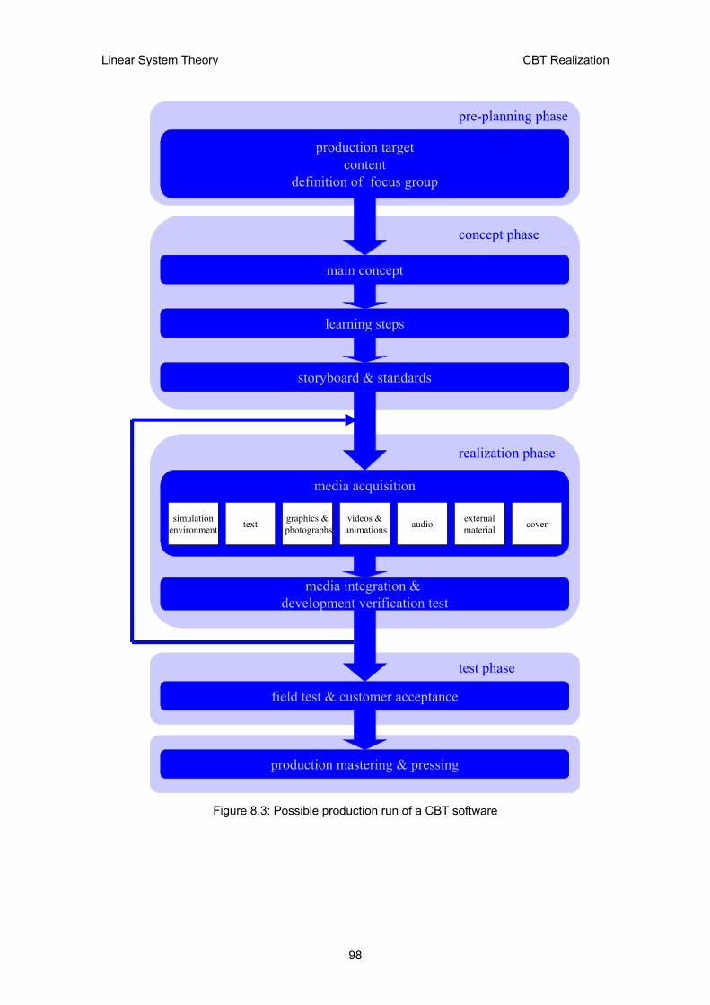
Linear System Theory CBT Realization
Cbt production run
media acquisition
simulationenvironment text graphics &
photographsvideos &
animations audio externalmaterial cover
media integration & development verification test
realization phase
storyboard & standards
concept phase
learning steps
main concept
pre-planning phase
production targetcontent
definition of focus group
test phase
field test & customer acceptance
production mastering & pressing
Figure 8.3: Possible production run of a CBT software
98

Linear System Theory CBT Realization
8.3.2 Conception Phase
The pre-planning phase is followed by the conception phase, which contains the outline of the concept, planning of learning steps and fixing the storyboard54. The sketching of conception (coarse concept) can be initiated by a form of brainstorming in which all ideas of instances that are required for the production are collected and documented. Representatives of the following fields (instances) should be present: production, project management, editing, didactics, media psychology, text and graphic design as well as information technology. The information retrieved from this meeting is used for developing a main concept, which can be used as performance specification likewise. The items that should be covered are shown in the left column of Table 8.1, Table 8.2 and Table 8.3.
Step General “Linear System Theory and Design” CBT
1 Project content
Target-setting: Brief introduction to linear system theory, collateral to lecture notes, including definition of notions, important system properties, mathematical description of systems (internal and external, continuous-time and discrete-time), stability condition of systems, state-space solutions and state-space realizations. The CBT shall represent a repetition and partial add-on of the lecture. Duration and scope of the project: The CBT programme comprises approximately 350 frames where each frame requires about one hour of programming time on average.
Table 8.1: Main concept of the CBT programme
54 “A storyboard is a series of illustrations that represent a process, such as the steps of interacting with a computer or website. Storyboards are useful for presentations, such as with focus groups, and for checking that the steps of a process make sense once the details are sketched, [The04]”.
99

Linear System Theory CBT Realization
Step General “Linear System Theory and Design” CBT
2 General guidelines and
standards
Screen mask: The screen mask remains unchanged throughout the CBT programme. It consists of two types of entities: the screen headers and the screen details (screen fields). Screen headers are used for labelling the frame according to the current progress. Screen details show specific information like definitions, animations, graphics, videos or equations. Colour standard: The colour standard remains unchanged throughout the CBT programme. Navigation: Navigation facilities (buttons like previous or next frame, repeat, menu) remain unchanged throughout the CBT programme. If animations are available, upon pressing any mouse button over a defined field (additionally the mouse pointer is changing to hand-symbol), this is indicated by text.
3 Guideline for the design
of frames
Text design: The used font is Times New Roman, size 2055 and colour Light-Grey (#D0D0D056). Sub-headers are decreased by size 2. Screen headers are presented on a blue (#000099) background and screen details are presented on a grey (#666666) background. Equations should be imported as symbols57 in order to prevent font mismatch. Graphic design: Graphics should be designed by using Flash MX in order to minimize size and save memory. If graphics are imported they should be converted to Flash-symbols in order to save memory. Graphics are shown in screen fields therefore, it should be considered that the background is grey (see screen details above). General design steps are:
o Definition of background and texture as well as a collection of colour combinations.
o Definition of fonts and logos. o Definition of size and shape of buttons and icons,
respectively. o Check of the screen layout system (compound). o Fixing of hypertext markings. o Integration of dynamic media in order to stimulate
the user. o Restriction of interactivity. o Test of the design by test personnel (omitted).
Table 8.2: Main concept of the CBT programme, cont’d
55 Size-specification according to Flash MX. 56 Colour-specification according to Flash MX. 57 A symbol, in this context, is a special graphic format used in Flash MX.
100

Linear System Theory CBT Realization
Step General “Linear System Theory and Design” CBT
4 Coarse target of
interaction possibilities and types
Navigation: Standard navigation according to step 2. Additional information: If deemed necessary the user can select animations, graphics or examples. Multiple-choice: every section is closed with a multiple choice and/or drag and drop test, which provides self-control of the learning progress of the user.
5
Production scheduling and assignment of
activities of development teams
Activities: Strict separation of duties has to be executed in regard to the attending experts. Schedule: On the basis of this thesis the period for programming the CBT covers approximately three months.
6 Coarse structure of
contents
1. Introduction 2. Mathematical description 3. Stability condition 4. State-space solutions 5. State-space realizations
Each section will start with an overview of contents followed by a descriptive main part and finished by a multiple-choice test.
7 Structure of the way of learning and check of
learning objectives
Principally the degree of freedom (of navigating through the CBT) should be adjusted to the users foreknowledge. This CBT is designated for students of a technical college. The user (student) can select a module of his/her own choice. Nevertheless, there is a recommended sequence, which is entered if the user processes from the first module to the last by “next frame navigation”. Evaluation of tests: In order to minimize programming-effort the evaluation of tests is omitted.
Table 8.3: Main concept of the CBT programme, cont’d
Next the planning of learning steps is discussed. This phase is of elementary importance and requires a conscientious preparation. The rough outline of the project (see Table 8.1, Table 8.2 and Table 8.3) is described in more detail in this phase. For each point at each step a target is defined, which determines further preparation and depth of imparting knowledge. Thus, a coarse planning of learning steps has already been performed in Table 8.1, Table 8.2 and Table 8.3 (right column). A detailed planning of learning steps is not carried out in this text. Each point should be processed by stating technical terms and key words. During this phase in the development of learning programmes, the final distribution and allocation of subject matters is fixed. The distribution and consistency of subject matters in learning steps, modules and sections are once again checked. Any weaknesses of logic structure are recognised and corrected
101
Linear System Theory CBT Realization
accordingly. These corrections could have effects on the content of the outline of the main concept, which should be completed accordingly. During the planning of learning steps, the learning programme is pre-structured. Final formulation and fixing of frame design is carried out in the next step, that is, during the phase of refined conception. Technical terms of the learning step plan are formulated and didactically prepared. The learning text is enriched with graphics, interactions and animations and is distributed on frames. The whole application can be visualised by a master storyboard (MSB). The MSB is used within the development team mainly for communicating and also to uncover inconsistencies. In addition, the MSB is informative regarding the following questions:
o Are links to other frames logical and useful?
o Are technical terms and used media identifiable?
o Can programmers and designers fulfil their tasks? Figure 8.4, for example, shows a detail of the MSB: the module 1.2 Introduction of the CBT programme “Linear System Theory and Design”.
102

Linear System Theory CBT Realization
Figure 8.4: Detail of MSB, module 1.2 Introduction
A few comments on the MSB according to Figure 8.4 are given next. Text in the upper half of the squares usually denotes the reference number of the frame. The numbering should be performed according to the structure of the CBT. The lower half of the square roughly shows the subject matter of the frame. Table 8.4 shows the coding of the MSB (according to Figure 8.4) in more detail.
103
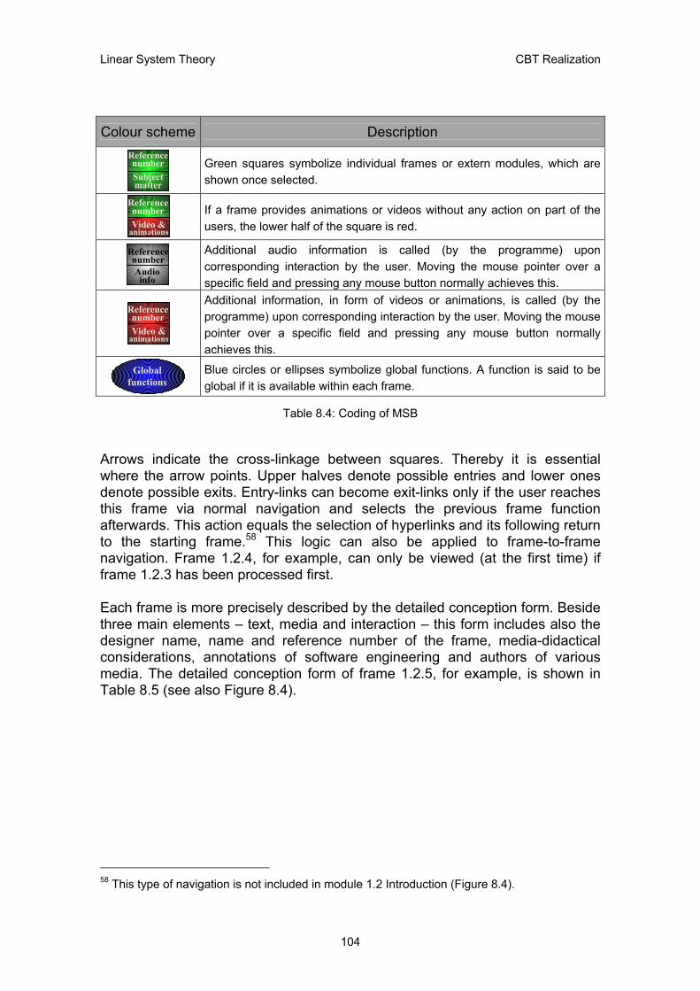
Linear System Theory CBT Realization
Colour scheme Description ReferencenumberSubjectmatter
Green squares symbolize individual frames or extern modules, which are shown once selected.
ReferencenumberVideo &
animations
If a frame provides animations or videos without any action on part of the users, the lower half of the square is red.
ReferencenumberAudioinfo
Additional audio information is called (by the programme) upon corresponding interaction by the user. Moving the mouse pointer over a specific field and pressing any mouse button normally achieves this.
ReferencenumberVideo &
animations
Additional information, in form of videos or animations, is called (by the programme) upon corresponding interaction by the user. Moving the mouse pointer over a specific field and pressing any mouse button normally achieves this.
Globalfunctions
Blue circles or ellipses symbolize global functions. A function is said to be global if it is available within each frame.
Table 8.4: Coding of MSB
Arrows indicate the cross-linkage between squares. Thereby it is essential where the arrow points. Upper halves denote possible entries and lower ones denote possible exits. Entry-links can become exit-links only if the user reaches this frame via normal navigation and selects the previous frame function afterwards. This action equals the selection of hyperlinks and its following return to the starting frame.58 This logic can also be applied to frame-to-frame navigation. Frame 1.2.4, for example, can only be viewed (at the first time) if frame 1.2.3 has been processed first. Each frame is more precisely described by the detailed conception form. Beside three main elements – text, media and interaction – this form includes also the designer name, name and reference number of the frame, media-didactical considerations, annotations of software engineering and authors of various media. The detailed conception form of frame 1.2.5, for example, is shown in Table 8.5 (see also Figure 8.4).
58 This type of navigation is not included in module 1.2 Introduction (Figure 8.4).
104
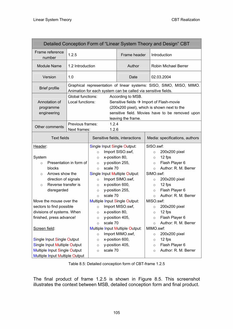
Linear System Theory CBT Realization
Detailed Conception Form of “Linear System Theory and Design” CBT
Frame reference number
1.2.5 Frame header Introduction
Module Name 1.2 Introduction Author Robin Michael Berrer
Version 1.0 Date 02.03.2004
Brief profile Graphical representation of linear systems: SISO, SIMO, MISO, MIMO. Animation for each system can be called via sensitive fields.
Annotation of programme engineering
Global functions: According to MSB. Local functions: Sensitive fields Import of Flash-movie (200x200 pixel), which is shown next to the sensitive field. Movies have to be removed upon leaving the frame.
Other comments Previous frames: 1.2.4 Next frames: 1.2.6
Text fields Sensitive fields, interactions Media: specifications, authors
Header: System
o Presentation in form of blocks
o Arrows show the direction of signals
o Reverse transfer is disregarded
Move the mouse over the sectors to find possible divisions of systems. When finished, press advance! Screen field: Single Input Single Output Single Input Multiple Output Multiple Input Single Output Multiple Input Multiple Output
Single Input Single Output: o Import SISO.swf, o x-position 80, o y-position 255, o scale 70
Single Input Multiple Output: o Import SIMO.swf, o x-position 600, o y-position 255, o scale 70
Multiple Input Single Output: o Import MISO.swf, o x-position 80, o y-position 405, o scale 70
Multiple Input Multiple Output: o Import MIMO.swf, o x-position 600, o y-position 405, o scale 70
SISO.swf: o 200x200 pixel o 12 fps o Flash Player 6 o Author: R. M. Berrer
SIMO.swf: o 200x200 pixel o 12 fps o Flash Player 6 o Author: R. M. Berrer
MISO.swf: o 200x200 pixel o 12 fps o Flash Player 6 o Author: R. M. Berrer
MIMO.swf: o 200x200 pixel o 12 fps o Flash Player 6 o Author: R. M. Berrer
Table 8.5: Detailed conception form of CBT-frame 1.2.5
The final product of frame 1.2.5 is shown in Figure 8.5. This screenshot illustrates the context between MSB, detailed conception form and final product.
105
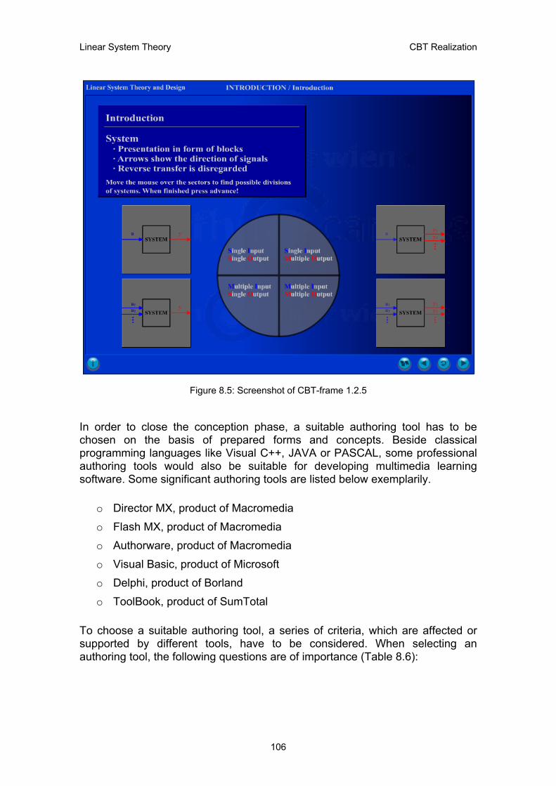
Linear System Theory CBT Realization
Figure 8.5: Screenshot of CBT-frame 1.2.5
In order to close the conception phase, a suitable authoring tool has to be chosen on the basis of prepared forms and concepts. Beside classical programming languages like Visual C++, JAVA or PASCAL, some professional authoring tools would also be suitable for developing multimedia learning software. Some significant authoring tools are listed below exemplarily.
o Director MX, product of Macromedia
o Flash MX, product of Macromedia
o Authorware, product of Macromedia
o Visual Basic, product of Microsoft
o Delphi, product of Borland
o ToolBook, product of SumTotal To choose a suitable authoring tool, a series of criteria, which are affected or supported by different tools, have to be considered. When selecting an authoring tool, the following questions are of importance (Table 8.6):
106
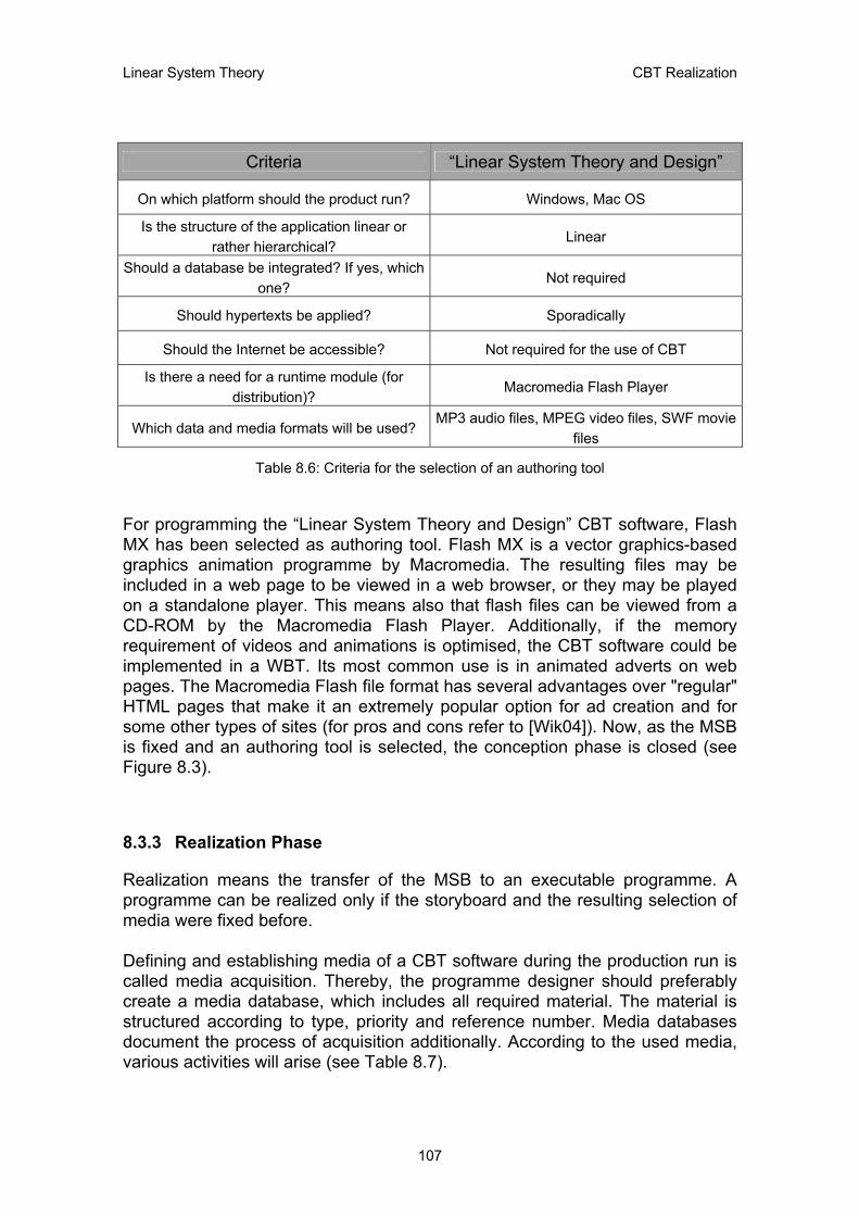
Linear System Theory CBT Realization
Criteria “Linear System Theory and Design”
On which platform should the product run? Windows, Mac OS
Is the structure of the application linear or rather hierarchical?
Linear
Should a database be integrated? If yes, which one?
Not required
Should hypertexts be applied? Sporadically
Should the Internet be accessible? Not required for the use of CBT
Is there a need for a runtime module (for distribution)?
Macromedia Flash Player
Which data and media formats will be used? MP3 audio files, MPEG video files, SWF movie
files
Table 8.6: Criteria for the selection of an authoring tool
For programming the “Linear System Theory and Design” CBT software, Flash MX has been selected as authoring tool. Flash MX is a vector graphics-based graphics animation programme by Macromedia. The resulting files may be included in a web page to be viewed in a web browser, or they may be played on a standalone player. This means also that flash files can be viewed from a CD-ROM by the Macromedia Flash Player. Additionally, if the memory requirement of videos and animations is optimised, the CBT software could be implemented in a WBT. Its most common use is in animated adverts on web pages. The Macromedia Flash file format has several advantages over "regular" HTML pages that make it an extremely popular option for ad creation and for some other types of sites (for pros and cons refer to [Wik04]). Now, as the MSB is fixed and an authoring tool is selected, the conception phase is closed (see Figure 8.3).
8.3.3 Realization Phase
Realization means the transfer of the MSB to an executable programme. A programme can be realized only if the storyboard and the resulting selection of media were fixed before. Defining and establishing media of a CBT software during the production run is called media acquisition. Thereby, the programme designer should preferably create a media database, which includes all required material. The material is structured according to type, priority and reference number. Media databases document the process of acquisition additionally. According to the used media, various activities will arise (see Table 8.7).
107
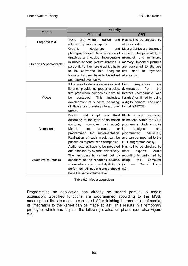
Linear System Theory CBT Realization
Activity Media General CBT
Prepared text Texts are written, edited and released by various experts.
Has still to be checked by other experts.
Graphics & photographs
Graphic designers and photographers create a selection of drawings and copies. Investigating in miscellaneous picture libraries is part of it. Furthermore graphics have to be converted into adequate formats. Pictures have to be edited and packed eventually.
Most graphics are designed in Flash. This prevents type mismatch and minimizes memory. Imported pictures are converted to Bitmaps first and to symbols afterwards.
Videos
If the use of videos is necessary and libraries provide no proper articles, film production companies have to be contacted. This includes: development of a script, shooting, digitizing, compressing into a proper format.
Film sequences are downloaded from the Internet (comparable with libraries) or filmed by using a digital camera. The used format is MPEG.
Animations
Design and script are fixed according to the type of animation (cartoon, computer animation). Models are recreated or programmed for implementation. Realization of such media can be passed on to production companies.
Flash movies represent animations within the CBT programme. Such a movie is designed and programmed individually and can be imported to the CBT programme easily.
Audio (voice, music)
Audio lectures have to be prepared and checked by experts didactically. The recording is carried out by speakers at the recording studios, where also copying and digitizing is performed. All audio signals should have the same volume level.
Has still to be checked by other experts. Audio recording is performed by using the computer (software: Sound Forge 6.0).
Table 8.7: Media acquisition
Programming an application can already be started parallel to media acquisition. Specified functions are programmed according to the MSB, meaning that links to media are created. After finishing the production of media, its integration to the kernel can be made at last. This results in a temporary prototype, which has to pass the following evaluation phase (see also Figure 8.3).
108

Linear System Theory CBT Realization
8.3.4 Evaluation Phase
During programming it is the task of software developers to check the application for correct functionality. Frequently sources of error are overlooked, which are only detected by an expanded field test. The following listing shows possible technical sources of error that could occur:
o The main memory is not clear (enabled) and the application locks soon.
o The installation routine is faulty.
o The programme cannot be run under another screen resolution. Graphics are overlapping or are not displayed.
o Possible print operation is missing. Printing of frames is fussy or is not possible at all.
o Unsatisfying or unwanted circulating links that make it difficult for the learner to navigate.
o System responses take a long time. Users do not get any information about the system condition (e.g. loading of data).
o Keying errors (of user) are not caught sufficiently. At this point verification of technical terms is carried out by the responsible experts (depending on the area of expertise), who have to consider the following aspects:
o Do targets and subject matters correspond to defined conceptions according to the MSB?
o Are didactical reasons sufficient?
o Is the used voice (text and audio) understandable and adjusted to audience?
o Is the subject matter correct and well-structured?
o Is it possible to achieve learning objectives?
o Is navigation through the programme manageable and adequate? It should be pointed out that this phase has been omitted (“Linear System Theory and Design” CBT programming) due to lack of resources. However, the following (concluding) chapter comprises a self-evaluation of the CBT programme and of the SVL that was described in Chapter 7.
109

Linear System Theory Concluding Remarks
9. CONCLUDING REMARKS
The first part of this thesis (Chapter 1 to 5) has provided information on fundamentals of linear system theory and design. Basic ideas and notions like system, model and test signals have been described and a mathematical description of linear time-invariant systems (discrete-time and continuous-time) and its essential properties have been carried out. After pointing out these important characteristics of LTI-systems, the second part of this thesis introduced fundamentals of E-Learning environments. It has been attempted to provide a basis for implementing the theoretical part (system theory) into an E-Learning environment. By means of the semi-virtual lecture, a concept has been introduced that should make an optimisation of E-Learning benefit possible. The development of a CBT programme, which is related to the SVL, was introduced next. In the following, a method is introduced, which makes a clear and understandable evaluation of learning concepts possible. The above-mentioned learning elements, on the one hand the CBT programme and on the other the SVL, are evaluated by means of this evaluation method afterwards.
9.1 Evaluation Method
This section introduces a graphical evaluation method that makes looking at learning and teaching situations from different angles possible. This chapter is mainly based on [Bau99] and [Fis02]. Figure 9.1 shows this evaluation method according to [Bau99].
110

Linear System Theory Concluding Remarks
context- free facts
context & rules
problemsolving
design& model
complexsituation Teaching/Learning
Layer
KnowledgeAccess
information& presentation
drill & tests
tutor systems
parametricsimulation
freesimulation
Social OrganizationLayer
teaching & explaining (teacher)
observing & helping (tutor)collaborating (coach)
Figure 9.1: Evaluation model according to [Bau99]
Figure 9.1 illustrates that every learning process should aim at a level where complex situations are solved by free simulation and collaboration. In other words, every learning process should reach a constructivistic level or standard. In the following, teaching aids, like the CBT programme and the SVL (as a whole, including the CBT), are evaluated by means of the introduced model.
9.2 Evaluation of the CBT Programme
The time delay between the end of a scheduled class and the students' first opportunity to use their knowledge results in a reduction of retained knowledge. A standalone CBT course allows the students to take the course when deemed necessary and to put the new knowledge to work immediately. This results in reinforcement of the learned content and greatly increases long-term retention. This implicates imparting context-free facts, context & rules but precludes problem solving. Studies show that students typically retain twice as much information from a CBT course that covers the same material as an instructor-led course. This is explained through the intense interaction inherent in the CBT format, the ability to move through the material at the student's own pace and the ability to review material as many times as required. However, the CBT, used in this context, does not observe the learning progress, neither does it help the learner to solve
111
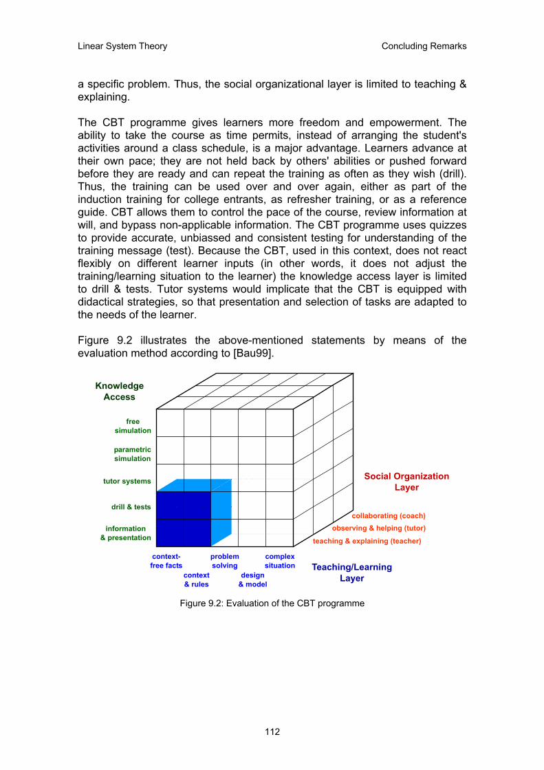
Linear System Theory Concluding Remarks
a specific problem. Thus, the social organizational layer is limited to teaching & explaining. The CBT programme gives learners more freedom and empowerment. The ability to take the course as time permits, instead of arranging the student's activities around a class schedule, is a major advantage. Learners advance at their own pace; they are not held back by others' abilities or pushed forward before they are ready and can repeat the training as often as they wish (drill). Thus, the training can be used over and over again, either as part of the induction training for college entrants, as refresher training, or as a reference guide. CBT allows them to control the pace of the course, review information at will, and bypass non-applicable information. The CBT programme uses quizzes to provide accurate, unbiassed and consistent testing for understanding of the training message (test). Because the CBT, used in this context, does not react flexibly on different learner inputs (in other words, it does not adjust the training/learning situation to the learner) the knowledge access layer is limited to drill & tests. Tutor systems would implicate that the CBT is equipped with didactical strategies, so that presentation and selection of tasks are adapted to the needs of the learner. Figure 9.2 illustrates the above-mentioned statements by means of the evaluation method according to [Bau99].
context- free facts
context & rules
problemsolving
design& model
complexsituation Teaching/Learning
Layer
KnowledgeAccess
information& presentation
drill & tests
tutor systems
parametricsimulation
freesimulation
Social OrganizationLayer
teaching & explaining (teacher)
observing & helping (tutor)collaborating (coach)
Figure 9.2: Evaluation of the CBT programme
112
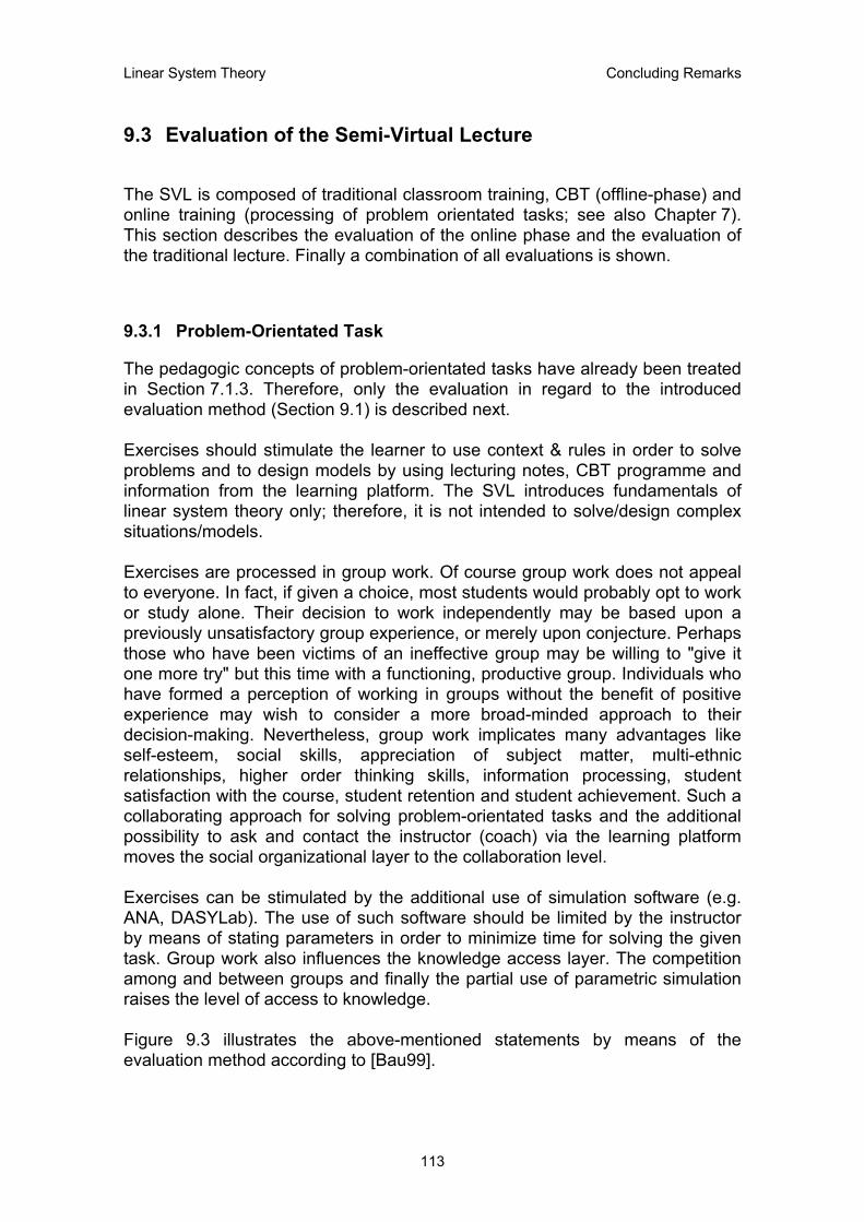
Linear System Theory Concluding Remarks
9.3 Evaluation of the Semi-Virtual Lecture
The SVL is composed of traditional classroom training, CBT (offline-phase) and online training (processing of problem orientated tasks; see also Chapter 7). This section describes the evaluation of the online phase and the evaluation of the traditional lecture. Finally a combination of all evaluations is shown.
9.3.1 Problem-Orientated Task
The pedagogic concepts of problem-orientated tasks have already been treated in Section 7.1.3. Therefore, only the evaluation in regard to the introduced evaluation method (Section 9.1) is described next. Exercises should stimulate the learner to use context & rules in order to solve problems and to design models by using lecturing notes, CBT programme and information from the learning platform. The SVL introduces fundamentals of linear system theory only; therefore, it is not intended to solve/design complex situations/models. Exercises are processed in group work. Of course group work does not appeal to everyone. In fact, if given a choice, most students would probably opt to work or study alone. Their decision to work independently may be based upon a previously unsatisfactory group experience, or merely upon conjecture. Perhaps those who have been victims of an ineffective group may be willing to "give it one more try" but this time with a functioning, productive group. Individuals who have formed a perception of working in groups without the benefit of positive experience may wish to consider a more broad-minded approach to their decision-making. Nevertheless, group work implicates many advantages like self-esteem, social skills, appreciation of subject matter, multi-ethnic relationships, higher order thinking skills, information processing, student satisfaction with the course, student retention and student achievement. Such a collaborating approach for solving problem-orientated tasks and the additional possibility to ask and contact the instructor (coach) via the learning platform moves the social organizational layer to the collaboration level. Exercises can be stimulated by the additional use of simulation software (e.g. ANA, DASYLab). The use of such software should be limited by the instructor by means of stating parameters in order to minimize time for solving the given task. Group work also influences the knowledge access layer. The competition among and between groups and finally the partial use of parametric simulation raises the level of access to knowledge. Figure 9.3 illustrates the above-mentioned statements by means of the evaluation method according to [Bau99].
113
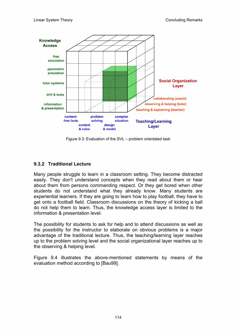
Linear System Theory Concluding Remarks
Figure 9.3: Evaluation of the SVL – problem orientated task
9.3.2 Traditional Lecture
Many people struggle to learn in a classroom setting. They become distracted easily. They don't understand concepts when they read about them or hear about them from persons commanding respect. Or they get bored when other students do not understand what they already know. Many students are experiential learners. If they are going to learn how to play football, they have to get onto a football field. Classroom discussions on the theory of kicking a ball do not help them to learn. Thus, the knowledge access layer is limited to the information & presentation level. The possibility for students to ask for help and to attend discussions as well as the possibility for the instructor to elaborate on obvious problems is a major advantage of the traditional lecture. Thus, the teaching/learning layer reaches up to the problem solving level and the social organizational layer reaches up to the observing & helping level. Figure 9.4 illustrates the above-mentioned statements by means of the evaluation method according to [Bau99].
114
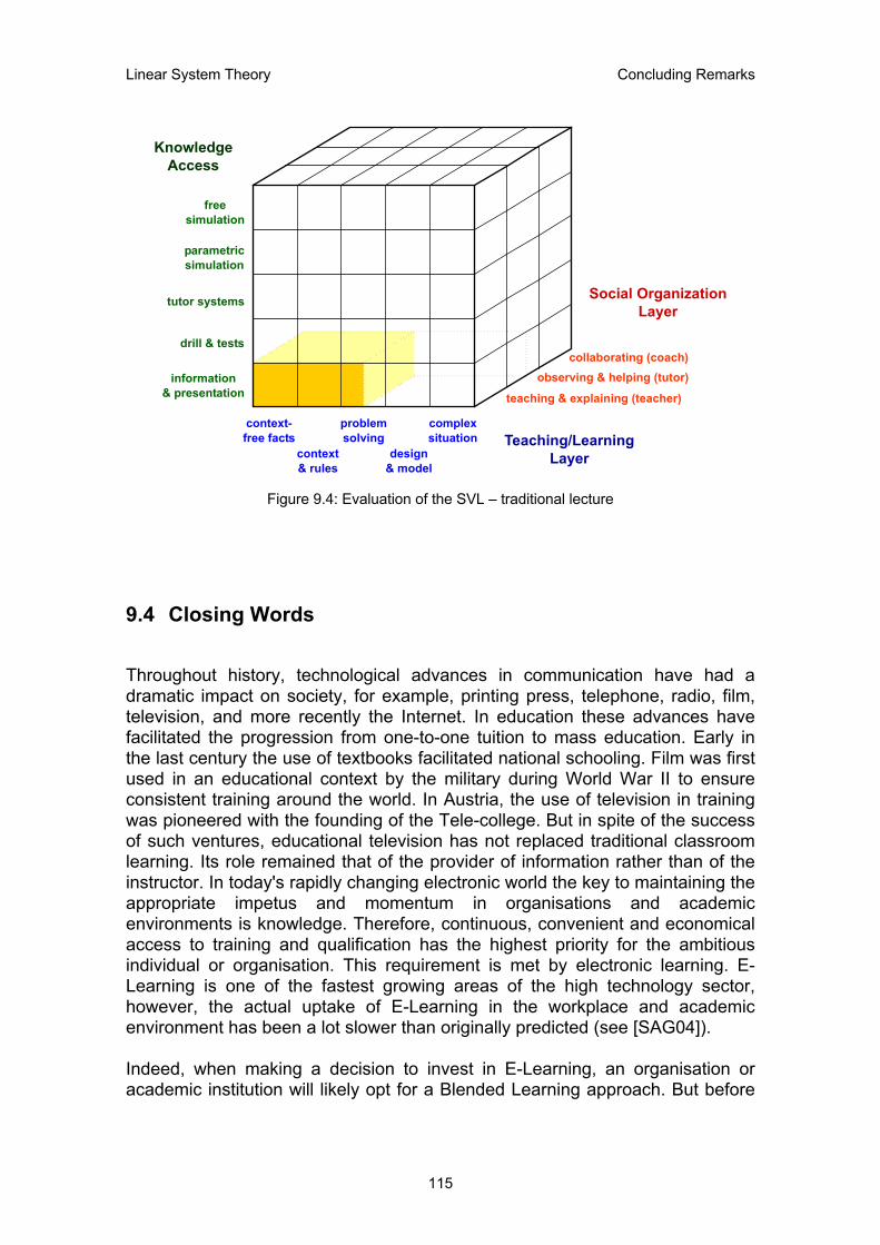
Linear System Theory Concluding Remarks
context- free facts
context & rules
problemsolving
design& model
complexsituation Teaching/Learning
Layer
KnowledgeAccess
information& presentation
drill & tests
tutor systems
parametricsimulation
freesimulation
Social OrganizationLayer
teaching & explaining (teacher)
observing & helping (tutor)collaborating (coach)
Figure 9.4: Evaluation of the SVL – traditional lecture
9.4 Closing Words
Throughout history, technological advances in communication have had a dramatic impact on society, for example, printing press, telephone, radio, film, television, and more recently the Internet. In education these advances have facilitated the progression from one-to-one tuition to mass education. Early in the last century the use of textbooks facilitated national schooling. Film was first used in an educational context by the military during World War II to ensure consistent training around the world. In Austria, the use of television in training was pioneered with the founding of the Tele-college. But in spite of the success of such ventures, educational television has not replaced traditional classroom learning. Its role remained that of the provider of information rather than of the instructor. In today's rapidly changing electronic world the key to maintaining the appropriate impetus and momentum in organisations and academic environments is knowledge. Therefore, continuous, convenient and economical access to training and qualification has the highest priority for the ambitious individual or organisation. This requirement is met by electronic learning. E-Learning is one of the fastest growing areas of the high technology sector, however, the actual uptake of E-Learning in the workplace and academic environment has been a lot slower than originally predicted (see [SAG04]). Indeed, when making a decision to invest in E-Learning, an organisation or academic institution will likely opt for a Blended Learning approach. But before
115
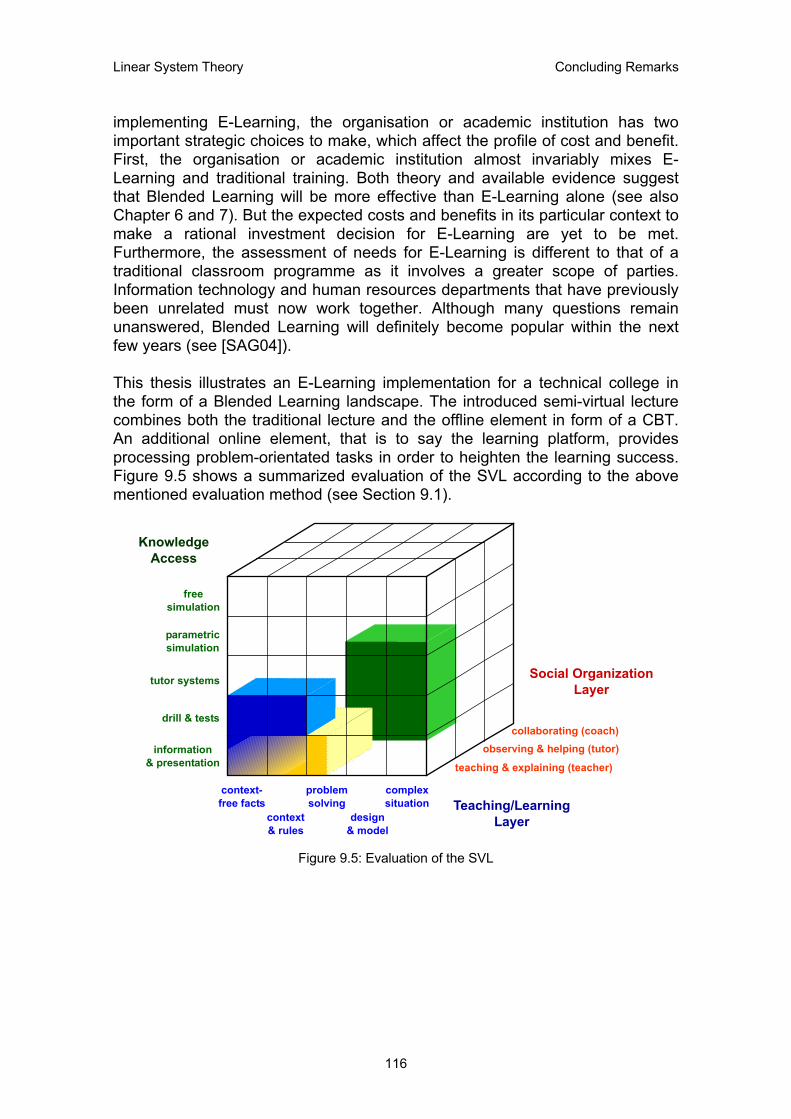
Linear System Theory Concluding Remarks
implementing E-Learning, the organisation or academic institution has two important strategic choices to make, which affect the profile of cost and benefit. First, the organisation or academic institution almost invariably mixes E-Learning and traditional training. Both theory and available evidence suggest that Blended Learning will be more effective than E-Learning alone (see also Chapter 6 and 7). But the expected costs and benefits in its particular context to make a rational investment decision for E-Learning are yet to be met. Furthermore, the assessment of needs for E-Learning is different to that of a traditional classroom programme as it involves a greater scope of parties. Information technology and human resources departments that have previously been unrelated must now work together. Although many questions remain unanswered, Blended Learning will definitely become popular within the next few years (see [SAG04]). This thesis illustrates an E-Learning implementation for a technical college in the form of a Blended Learning landscape. The introduced semi-virtual lecture combines both the traditional lecture and the offline element in form of a CBT. An additional online element, that is to say the learning platform, provides processing problem-orientated tasks in order to heighten the learning success. Figure 9.5 shows a summarized evaluation of the SVL according to the above mentioned evaluation method (see Section 9.1).
context- free facts
context & rules
problemsolving
design& model
complexsituation Teaching/Learning
Layer
KnowledgeAccess
information& presentation
drill & tests
tutor systems
parametricsimulation
freesimulation
Social OrganizationLayer
teaching & explaining (teacher)
observing & helping (tutor)collaborating (coach)
Figure 9.5: Evaluation of the SVL
116

Linear System Theory Concluding Remarks
9.4.1 The Future of E-Learning
This section closes this thesis by looking at the future of E-Learning and possible changes of its environment. The following statements are based on [Fut04]. Now, what is the future of E-Learning? Most probably nobody has the exact answer to this question, but it is important to think about it. To start out, it is important to look at many of the trends related to learning that are already taking hold in our world. Knowledge is expanding at a tremendous rate. The class graduating college in the year 2004 will be exposed to more new information in one year than their grandparents were in a lifetime. Memorizing facts will have a much lower value, while utilizing information for analysis and decision-making will be an essential skill. The typical worker will have many distinct careers in his or her lifetime, due to the rise and fall of companies in this fast moving time. Each of these careers will require new knowledge and skills and implies new challenges. Lifelong learning will be something that any successful person must do to compete. “It will no longer be worthwhile to learn something with the hope that it will be useful at some unknown time. Just-In-Time learning that meets the needs of individuals as they occur, makes learning more meaningful and effective, [Fut04]”. Educational facilities, companies and careers of the future will utilize technologies that cannot even be imagined today. These technologies will require a whole new set of skills from the workforce or student. Learning to use the new technology will be important, and so will using those technologies to learn. The world indeed seems to be shrinking rapidly. The Internet has brought millions of people together in ways that nobody would have expected. One can now attend a college half way around the world, with students from any country with Internet access (e.g. Fernuniversität Hagen). People will telecommute to their jobs more in the future, while their companies compete globally. In order to meet the needs of the changing world noted above, future learning must take on more of the following qualities:
o Time flexible
o Geographically independent
o Competitive in cost / value
o Learner-centred
o Technology-embracing
o Ethnically diverse
117

Linear System Theory Concluding Remarks
Organizations that deliver learning (colleges, universities, companies, etc.) will need to consider these issues and:
o Realize what kind of market they serve
o Be responsive to learner needs
o Prove their value to learners
o Listen closely to the needs of business
o Remove some of the massive burdens on instructors
o Look for partnerships with other complementary organizations
o Find creative ways to certify learning credentials
o Be prepared to compete globally with a variety of learning providers The importance of E-Learning and its application will strongly grow in the future. New media will be discovered for developing E-Learning applications and new challenges will arise for each of us. We will have to face these facts with an open mind in order to keep track of a fast moving environment.
118
Linear System Theory Appendix/Additional Information
Appendix/Additional Information
TABLE OF FIGURES:
Figure 1.1: Symbolic system representation ...................................................... 3 Figure 1.2: Pulse δ (t) turns into Dirac impulse δ(t)∆ ............................................ 6 Figure 1.3: Heaviside function σ(t) ..................................................................... 7 Figure 1.4: Discrete Dirac impulse δ[n] and discrete Heaviside function σ[n] ..... 8 Figure 2.1: Network with three memory components ....................................... 13 Figure 2.2: Analysing function δ∆(t)................................................................... 16 Figure 2.3: Pulse δ (t-ti) to the left, δ (t-ti)∆ to the right ..................................... 16 ∆ ∆
Figure 2.4: Arbitrary signal u(t) approximated by analysing function δ (t)∆ ........ 17 Figure 2.5: Approximation of signal .................................................................. 18 Figure 2.6: Derivation of a sampled signal ....................................................... 26 Figure 2.7: Discrete-time signal u[n] and shifted discrete Dirac impulse δ[n-i] . 27 Figure 2.8: Discrete-time signal u[n] multiplied by discrete Dirac impulse δ[n-i]28 Figure 2.9: Basic elements of LTD-systems..................................................... 38 Figure 2.10: Block diagram of LTD-systems..................................................... 39 Figure 2.11: Block diagram of a non-recursive LTD-system............................. 40 Figure 2.12: Exemplary impulse response sequence....................................... 41 Figure 3.1: Exemplary pole-zero pattern of G(s) .............................................. 45 Figure 3.2: Exemplary pole-zero pattern of G(z) .............................................. 49 Figure 5.1: Uncontrollable network................................................................... 63 Figure 5.2: Unobservable network.................................................................... 64 Figure 5.3: Op-amp as adder ........................................................................... 67 Figure 5.4: Op-amp as integrator ..................................................................... 67 Figure 5.5: Op-amp solution of differential equation......................................... 68 Figure 5.6: Example-network for op-amp circuit implementation...................... 69 Figure 5.7: Op-amp implementation of Eq. (5.13) ............................................ 70 Figure 6.1: Different variants of E-Learning according [Rei03] ......................... 74 Figure 6.2: Integration by Blended Learning according to [Rei03].................... 80 Figure 7.1: Contents of the semi-virtual lecture (SVL)...................................... 83 Figure 7.2: Media structure of the SVL............................................................. 86 Figure 7.3: Problem-orientated tasks as central didactic element .................... 87 Figure 8.1: Classification of authoring systems according to [Bol98]................ 93 Figure 8.2: Forms of computer-based learning programmes............................ 94 Figure 8.3: Possible production run of a CBT software .................................... 98 Figure 8.4: Detail of MSB, module 1.2 Introduction ........................................ 103 Figure 8.5: Screenshot of CBT-frame 1.2.5.................................................... 106 Figure 9.1: Evaluation model according to [Bau99] ........................................ 111 Figure 9.2: Evaluation of the CBT programme ............................................... 112 Figure 9.3: Evaluation of the SVL – problem orientated task ......................... 114 Figure 9.4: Evaluation of the SVL – traditional lecture.................................... 115 Figure 9.5: Evaluation of the SVL................................................................... 116
119
Linear System Theory Appendix/Additional Information
TABLE OF TABLES:
Table 1.1: Classification of signals ..................................................................... 4 Table 1.2: Accuracy of digital signals ................................................................. 5 Table 2.1: How to perform a discrete convolution graphically .......................... 32 Table 2.2: Properties of the z-transform ........................................................... 34 Table 6.1: Three variants of E-Learning according to [Rei03] .......................... 76 Table 6.2: Keywords about different learning theories ..................................... 78 Table 7.1: Possible ratio formula for the SVL ................................................... 89 Table 8.1: Main concept of the CBT programme.............................................. 99 Table 8.2: Main concept of the CBT programme, cont’d ................................ 100 Table 8.3: Main concept of the CBT programme, cont’d ................................ 101 Table 8.4: Coding of MSB .............................................................................. 104 Table 8.5: Detailed conception form of CBT-frame 1.2.5 ............................... 105 Table 8.6: Criteria for the selection of an authoring tool ................................. 107 Table 8.7: Media acquisition........................................................................... 108
120
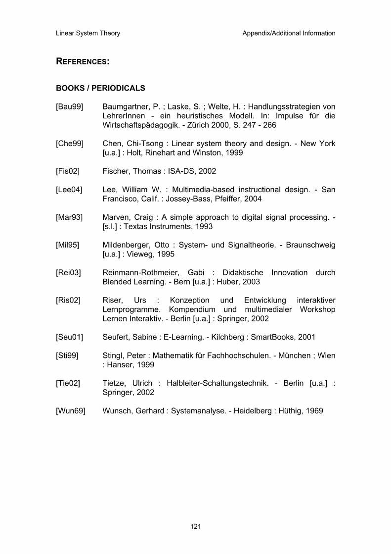
Linear System Theory Appendix/Additional Information
REFERENCES:
BOOKS / PERIODICALS [Bau99] Baumgartner, P. ; Laske, S. ; Welte, H. : Handlungsstrategien von
LehrerInnen - ein heuristisches Modell. In: Impulse für die Wirtschaftspädagogik. - Zürich 2000, S. 247 - 266
[Che99] Chen, Chi-Tsong : Linear system theory and design. - New York
[u.a.] : Holt, Rinehart and Winston, 1999 [Fis02] Fischer, Thomas : ISA-DS, 2002 [Lee04] Lee, William W. : Multimedia-based instructional design. - San
Francisco, Calif. : Jossey-Bass, Pfeiffer, 2004 [Mar93] Marven, Craig : A simple approach to digital signal processing. -
[s.l.] : Textas Instruments, 1993 [Mil95] Mildenberger, Otto : System- und Signaltheorie. - Braunschweig
[u.a.] : Vieweg, 1995 [Rei03] Reinmann-Rothmeier, Gabi : Didaktische Innovation durch
Blended Learning. - Bern [u.a.] : Huber, 2003 [Ris02] Riser, Urs : Konzeption und Entwicklung interaktiver
Lernprogramme. Kompendium und multimedialer Workshop Lernen Interaktiv. - Berlin [u.a.] : Springer, 2002
[Seu01] Seufert, Sabine : E-Learning. - Kilchberg : SmartBooks, 2001 [Sti99] Stingl, Peter : Mathematik für Fachhochschulen. - München ; Wien
: Hanser, 1999 [Tie02] Tietze, Ulrich : Halbleiter-Schaltungstechnik. - Berlin [u.a.] :
Springer, 2002 [Wun69] Wunsch, Gerhard : Systemanalyse. - Heidelberg : Hüthig, 1969
121
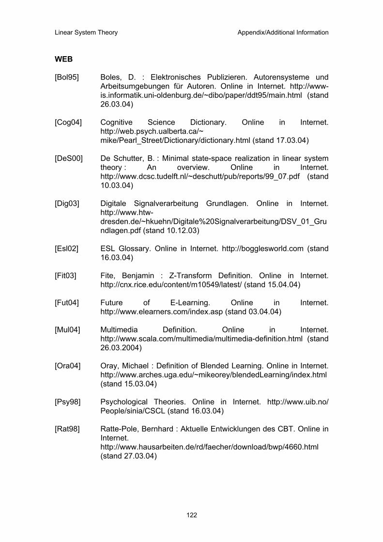
Linear System Theory Appendix/Additional Information
WEB [Bol95] Boles, D. : Elektronisches Publizieren. Autorensysteme und
Arbeitsumgebungen für Autoren. Online in Internet. http://www-is.informatik.uni-oldenburg.de/~dibo/paper/ddt95/main.html (stand 26.03.04)
[Cog04] Cognitive Science Dictionary. Online in Internet.
http://web.psych.ualberta.ca/~ mike/Pearl_Street/Dictionary/dictionary.html (stand 17.03.04)
[DeS00] De Schutter, B. : Minimal state-space realization in linear system
theory : An overview. Online in Internet. http://www.dcsc.tudelft.nl/~deschutt/pub/reports/99_07.pdf (stand 10.03.04)
[Dig03] Digitale Signalverarbeitung Grundlagen. Online in Internet.
http://www.htw-dresden.de/~hkuehn/Digitale%20Signalverarbeitung/DSV_01_Grundlagen.pdf (stand 10.12.03)
[Esl02] ESL Glossary. Online in Internet. http://bogglesworld.com (stand
16.03.04) [Fit03] Fite, Benjamin : Z-Transform Definition. Online in Internet.
http://cnx.rice.edu/content/m10549/latest/ (stand 15.04.04) [Fut04] Future of E-Learning. Online in Internet.
http://www.elearners.com/index.asp (stand 03.04.04) [Mul04] Multimedia Definition. Online in Internet.
http://www.scala.com/multimedia/multimedia-definition.html (stand 26.03.2004)
[Ora04] Oray, Michael : Definition of Blended Learning. Online in Internet.
http://www.arches.uga.edu/~mikeorey/blendedLearning/index.html (stand 15.03.04)
[Psy98] Psychological Theories. Online in Internet. http://www.uib.no/
People/sinia/CSCL (stand 16.03.04) [Rat98] Ratte-Pole, Bernhard : Aktuelle Entwicklungen des CBT. Online in
Internet. http://www.hausarbeiten.de/rd/faecher/download/bwp/4660.html (stand 27.03.04)
122
Linear System Theory Appendix/Additional Information
[Rud04] Rudiments of state-space control. Online in Internet. http://www.ece.umn.edu/users/georgiou/courses/4231/week13.pdf (stand 08.03.04)
[SAG04] Shoniregun A., Charles; Gray, Sarah-Jane : Is E-learning Really
the Future or a Risk?. Online in Internet. http://www.acm.org/ubiquity/views/c_shoniregun_3.pdf (stand 03.04.04)
[Soh01] Sohl, G. : Analog Electronics. Using Operational Amplifiers. Online
in Internet. http://engr.smu.edu/ee/SrDesign/AnalogOA.pdf (stand 11.03.04)
[The04] The Usability Company. Online in Internet.
http://www.theusabilitycompany.com/index.html (stand 17.03.04) [Web04] Webopedia. The Online Dictionary. Online in Internet.
http://www.pcwebopedia.com/ (stand 27.03.04) [Wik04] Wikipedia The Free Encyclopedia. Online in Internet.
http://en.wikipedia.org/wiki/Main_Page (stand 01.04.04) [Wil01] Wilson, Jim : A Definition for E-Learning. Online in Internet.
http://www.baol.co.uk/PDF/OLT/Issue%2058/wilson.pdf (stand 15.03.04)
123

Linear System Theory Appendix/Additional Information
INDEX:
Adder................................................................................................................ 67 Additivity property............................................................................................. 10 Authoring system.............................................................................................. 92
flowchart-based ............................................................................................ 94 frame-based.................................................................................................. 93 timeline-based .............................................................................................. 93
Behaviourism.................................................................................................... 77 BIBO stability.................................................................................................... 42 Blended Learning ............................................................................................. 71
Distributed Learning...................................................................................... 72 Flexible Learning .......................................................................................... 72 Hybrid Teaching............................................................................................ 72
Causality .................................................................................................... 10, 29 CBT .................................................................................................................. 90
non-tutorial forms.......................................................................................... 95 tutorial forms ................................................................................................. 95
CBT programme............................................................................................... 96 conception phase.......................................................................................... 99 evaluation ................................................................................................... 111 evaluation phase......................................................................................... 109 pre-planning phase ....................................................................................... 96 production run............................................................................................... 98 realization phase......................................................................................... 107 storyboard................................................................................................... 103
Characteristic polynomial ................................................................................. 51 Cognitivism....................................................................................................... 77 Constructivism.................................................................................................. 78 Controllability.................................................................................................... 62
matrix ............................................................................................................ 63 Controllable canonical form.............................................................................. 61 Convolution integral.......................................................................................... 15
analysing function ......................................................................................... 15 Difference equation .......................................................................................... 38 Discrete convolution ......................................................................................... 29 Eigenvalue........................................................................................................ 51 E-Learning........................................................................................................ 73
by collaborating............................................................................................. 75 by distributing................................................................................................ 74 by interacting ................................................................................................ 74 future .......................................................................................................... 117 implementation ............................................................................................. 82 requirements................................................................................................. 75
Homogeneity property ...................................................................................... 10 Impulse response ............................................................................................... 7
124

Linear System Theory Appendix/Additional Information
matrix ............................................................................................................ 21 sequence ...................................................................................................... 30
Inference .......................................................................................................... 81 deductive ...................................................................................................... 81 inductive........................................................................................................ 81
Instruction student-centred............................................................................................. 79 teacher-centred............................................................................................. 79
Integrator .......................................................................................................... 67 Laplace transform............................................................................................. 21
linearity property ........................................................................................... 22 theorem of derivative .................................................................................... 22 theorem of final value ................................................................................... 43
Learning theories.............................................................................................. 77 behaviourism ................................................................................................ 77 cognitivism.................................................................................................... 77 constructivism ............................................................................................... 78
Linearity...................................................................................................... 10, 29 Minimal polynomial........................................................................................... 51 Minimal realization............................................................................................ 65 Model ................................................................................................................. 3 Observability..................................................................................................... 64
matrix ............................................................................................................ 65 Operational amplifier ........................................................................................ 66
adder ............................................................................................................ 66 implementation ............................................................................................. 68 integrator....................................................................................................... 66
Pole ............................................................................................................ 25, 37 Pole-zero pattern.............................................................................................. 45 Realization........................................................................................................ 60
minimal ......................................................................................................... 65 Semi-virtual lecture........................................................................................... 82
evaluation ................................................................................................... 113 media............................................................................................................ 86 pedagogic concept........................................................................................ 88 problem-orientated tasks .............................................................................. 87 ratio formula.................................................................................................. 89
Signal ................................................................................................................. 4 bounded.................................................................................................. 42, 47 deterministic.................................................................................................... 5 Dirac impulse .................................................................................................. 6 discrete-time signal....................................................................................... 26 Heaviside function .......................................................................................... 7 stochastic........................................................................................................ 5
Stability............................................................................................................. 42 asymptotic..................................................................................................... 50 BIBO stability of LTD-systems ...................................................................... 46
125
Linear System Theory Appendix/Additional Information
BIBO stability of LTI-systems........................................................................ 42 in the sense of Lyapunov.............................................................................. 50 internal stability ............................................................................................. 51
State transition matrix....................................................................................... 55 State-space description.............................................................................. 12, 33
state.............................................................................................................. 12 state-space equations................................................................................... 13
Superposition property ..................................................................................... 10 System ............................................................................................................... 2
causal ..................................................................................................... 11, 29 distributed ..................................................................................................... 13 linear ....................................................................................................... 10, 29 lumped.......................................................................................................... 12 memory-less ................................................................................................. 11 MIMO............................................................................................................ 46 multivariable.................................................................................................. 46 SISO ............................................................................................................... 3 time-invariant ................................................................................................ 29
Time-invariance............................................................................................ 9, 29 Transfer function .............................................................................................. 23
discrete ......................................................................................................... 37 pole............................................................................................................... 25 transfer-function matrix ................................................................................. 25 zero............................................................................................................... 25
Zero............................................................................................................ 25, 37 Zero-input response ......................................................................................... 11 Zero-state response ......................................................................................... 11 z-transform ....................................................................................................... 33
theorem of final value ................................................................................... 48
126