Linear Systems - Electrical and Computer Engineering | UC

1

Digital Image Processing, 2nd ed.Digital Image Processing, 2nd ed.www.imageprocessingbook.com

© 2001 R. C. Gonzalez & R. E. Woods

ObjectiveObjectiveTo provide background material in support of topics in Digital Image Processing that are based on linear system theory.

Review

Linear SystemsReview

Linear Systems

2



Review: Linear SystemsReview: Linear Systems

Some DefinitionsSome Definitions

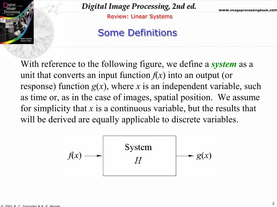
With reference to the following figure, we define a system as a unit that converts an input function f(x) into an output (or response) function g(x), where x is an independent variable, such as time or, as in the case of images, spatial position. We assume for simplicity that x is a continuous variable, but the results that will be derived are equally applicable to discrete variables.

3




Some Definitions (Con�t)Some Definitions (Con�t)

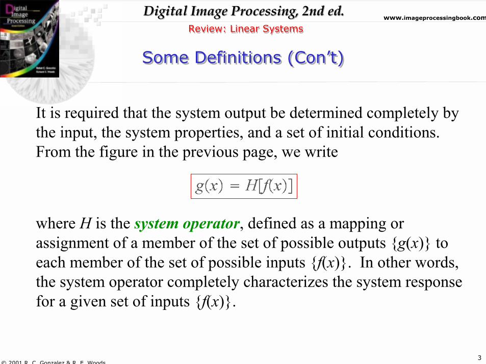
It is required that the system output be determined completely by the input, the system properties, and a set of initial conditions. From the figure in the previous page, we write

where H is the system operator, defined as a mapping or assignment of a member of the set of possible outputs {g(x)} to each member of the set of possible inputs {f(x)}. In other words, the system operator completely characterizes the system responsefor a given set of inputs {f(x)}.

4





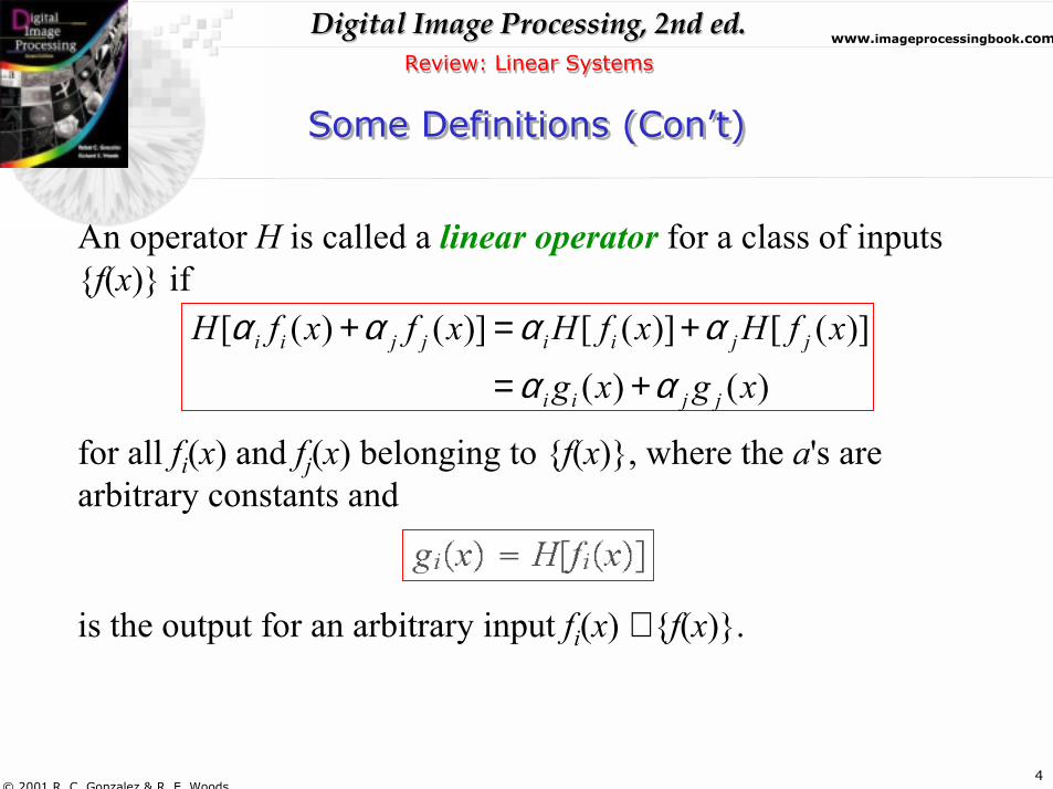
An operator H is called a linear operator for a class of inputs {f(x)} if

for all fi(x) and fj(x) belonging to {f(x)}, where the a's are arbitrary constants and

is the output for an arbitrary input fi(x) ∈ {f(x)}.

[ ( ) ( )] [ ( )] [ ( )]( ) ( )

i i j j i i j j

i i j j

H f x f x H f x H f xg x g x

α α α αα α

+ = +

= +

5





The system described by a linear operator is called a linear system (with respect to the same class of inputs as the operator). The property that performing a linear process on the sum of inputs is the same that performing the operations individually and then summing the results is called the property of additivity. The property that the response of a linear system to a constant times an input is the same as the response to the original inputmultiplied by a constant is called the property of homogeneity.

6





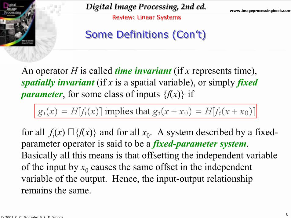
An operator H is called time invariant (if x represents time), spatially invariant (if x is a spatial variable), or simply fixed parameter, for some class of inputs {f(x)} if

for all fi(x) ∈ {f(x)} and for all x0. A system described by a fixed-parameter operator is said to be a fixed-parameter system. Basically all this means is that offsetting the independent variable of the input by x0 causes the same offset in the independent variable of the output. Hence, the input-output relationship remains the same.

7





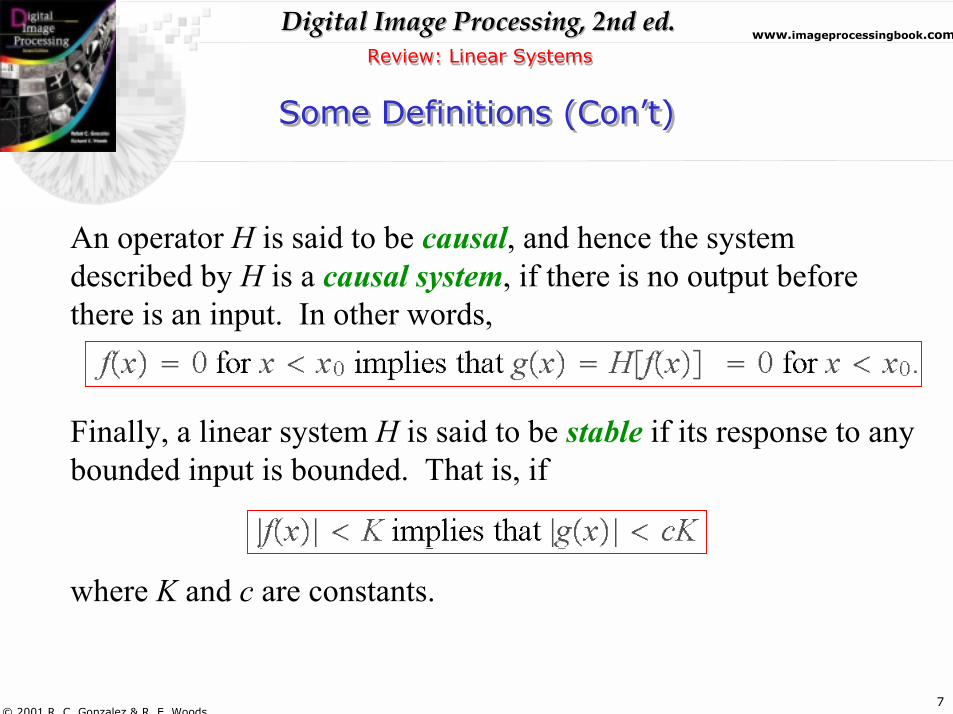
An operator H is said to be causal, and hence the system described by H is a causal system, if there is no output before there is an input. In other words,

Finally, a linear system H is said to be stable if its response to any bounded input is bounded. That is, if

where K and c are constants.

8





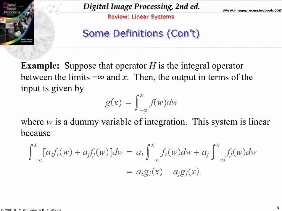
Example: Suppose that operator H is the integral operator between the limits −∞ and x. Then, the output in terms of the input is given by

where w is a dummy variable of integration. This system is linear because

9





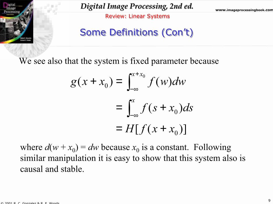
We see also that the system is fixed parameter because

where d(w + x0) = dw because x0 is a constant. Following similar manipulation it is easy to show that this system also iscausal and stable.

0

0

0

0

( ) ( )

( )

[ ( )]

x x

x

g x x f w dw

f s x ds

H f x x

+

−∞

−∞

+ =

= +

= +

∫∫

10





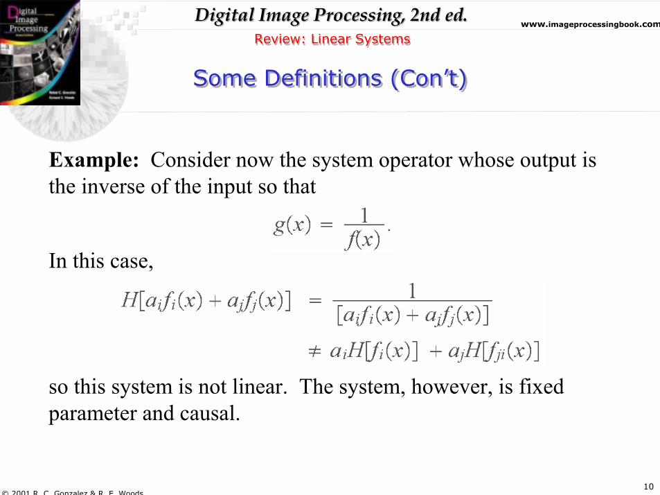
Example: Consider now the system operator whose output is the inverse of the input so that

In this case,

so this system is not linear. The system, however, is fixed parameter and causal.

11




Linear System Characterization-ConvolutionLinear System Characterization-Convolution

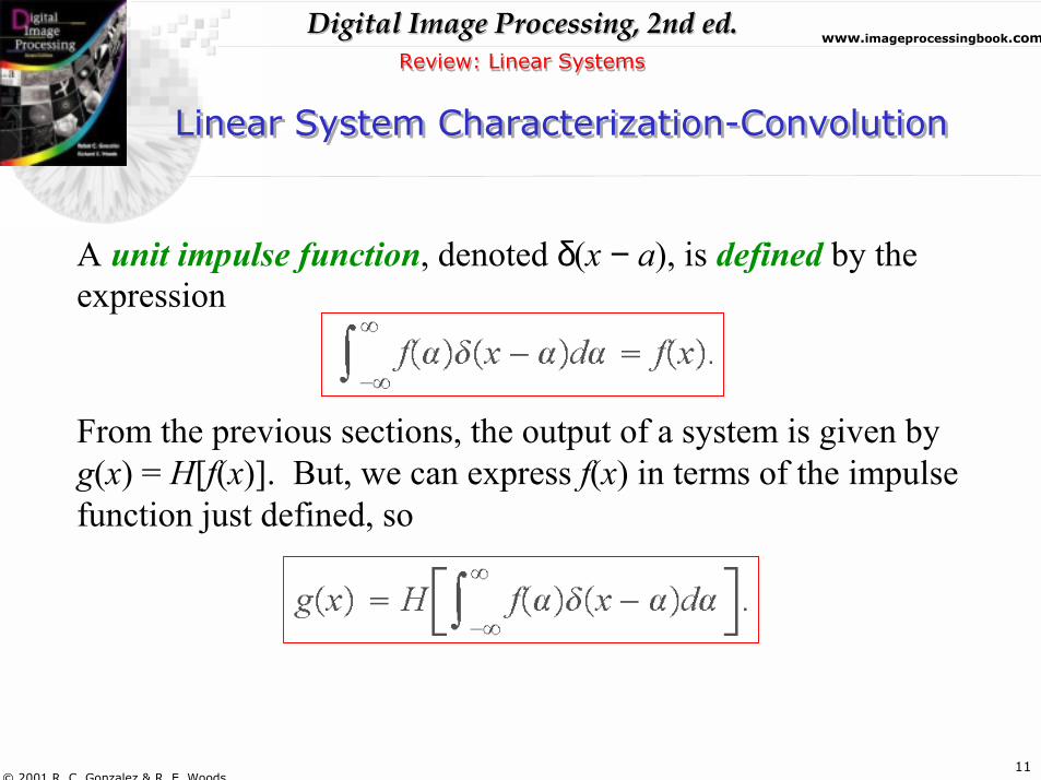
A unit impulse function, denoted δ(x − a), is defined by the expression

From the previous sections, the output of a system is given by g(x) = H[f(x)]. But, we can express f(x) in terms of the impulse function just defined, so

12




System Characterization (Con�t)System Characterization (Con�t)

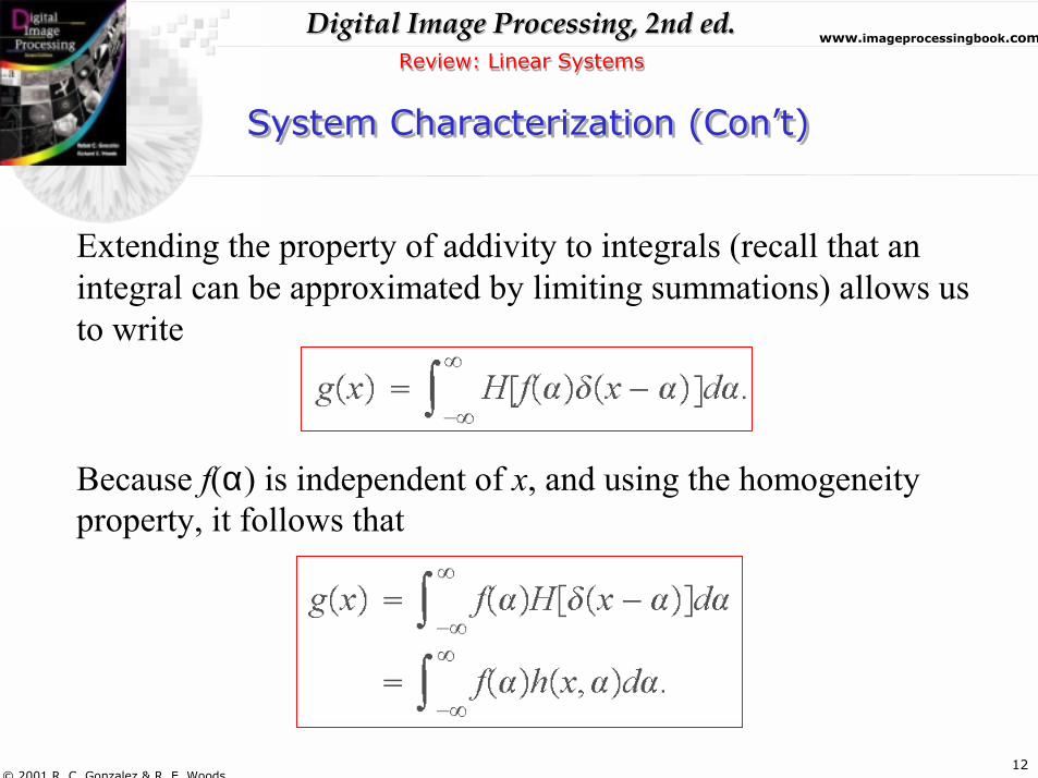
Extending the property of addivity to integrals (recall that an integral can be approximated by limiting summations) allows us to write

Because f(α) is independent of x, and using the homogeneity property, it follows that

13





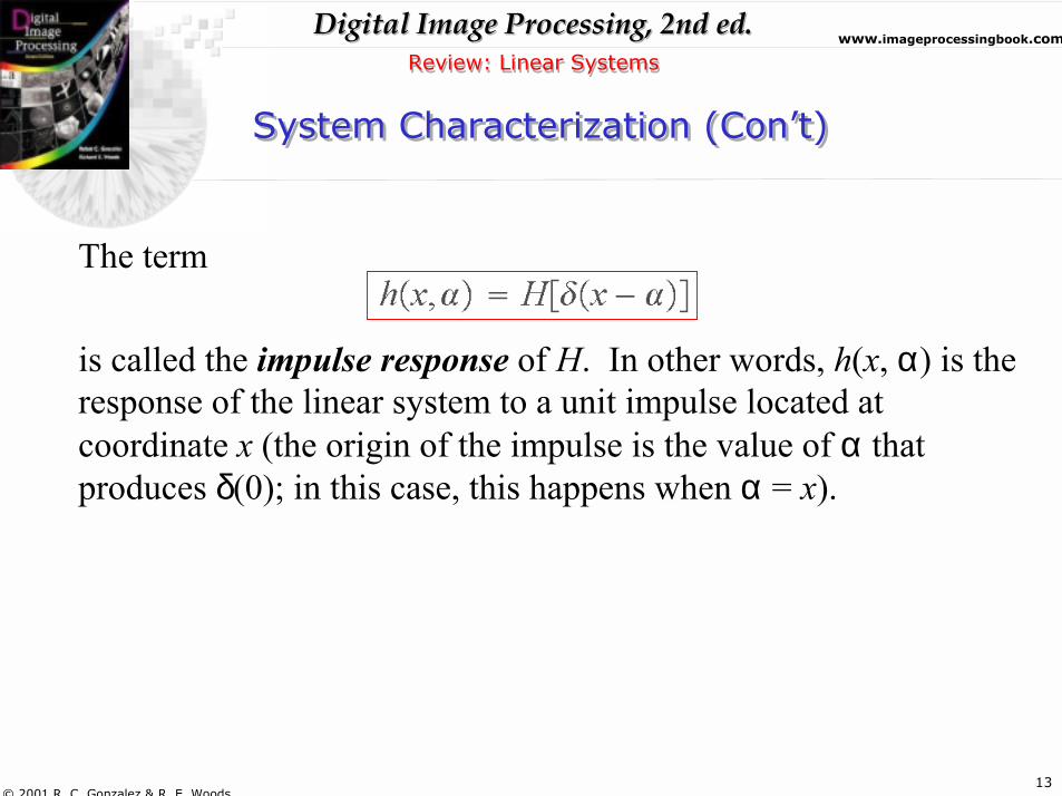
The term

is called the impulse response of H. In other words, h(x, α) is the response of the linear system to a unit impulse located at coordinate x (the origin of the impulse is the value of α that produces δ(0); in this case, this happens when α = x).

14





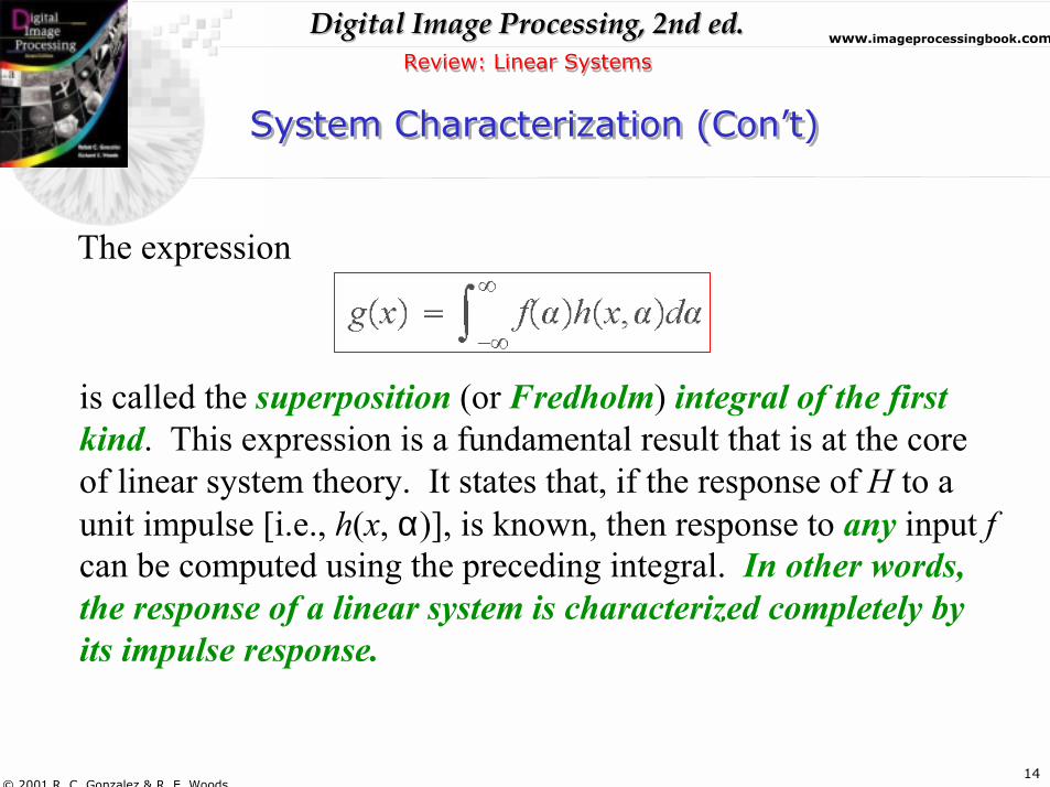
The expression

is called the superposition (or Fredholm) integral of the first kind. This expression is a fundamental result that is at the core of linear system theory. It states that, if the response of H to a unit impulse [i.e., h(x, α)], is known, then response to any input fcan be computed using the preceding integral. In other words, the response of a linear system is characterized completely by its impulse response.

15





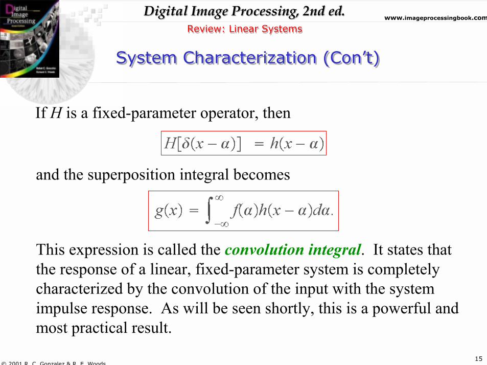
If H is a fixed-parameter operator, then

and the superposition integral becomes

This expression is called the convolution integral. It states that the response of a linear, fixed-parameter system is completely characterized by the convolution of the input with the system impulse response. As will be seen shortly, this is a powerful and most practical result.

16





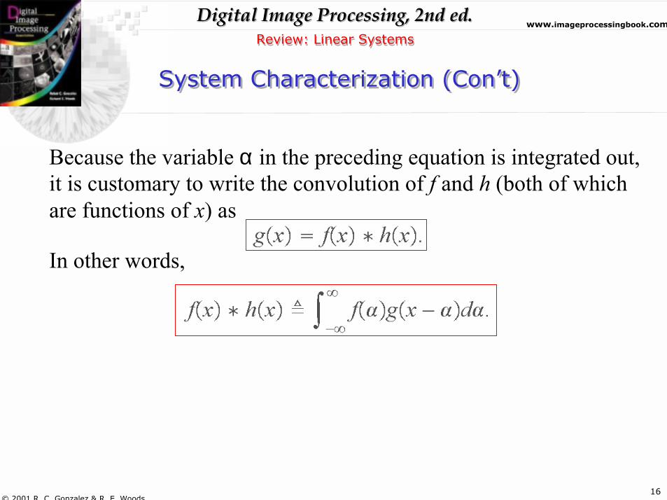
Because the variable α in the preceding equation is integrated out, it is customary to write the convolution of f and h (both of which are functions of x) as

In other words,

17





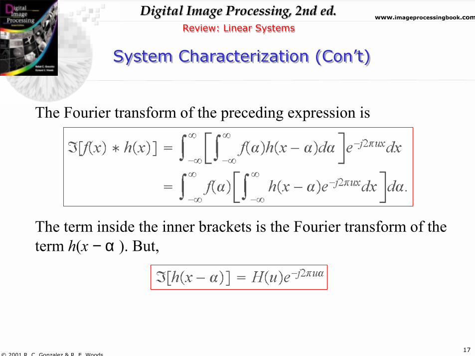
The Fourier transform of the preceding expression is

The term inside the inner brackets is the Fourier transform of the term h(x − α ). But,

18





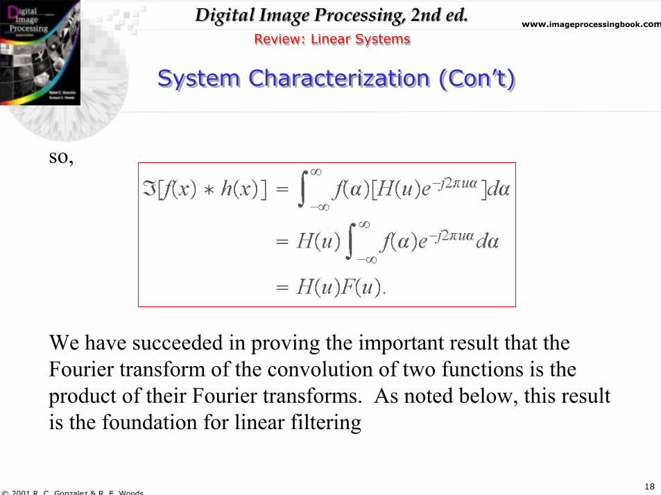
so,

We have succeeded in proving the important result that the Fourier transform of the convolution of two functions is the product of their Fourier transforms. As noted below, this result is the foundation for linear filtering

19





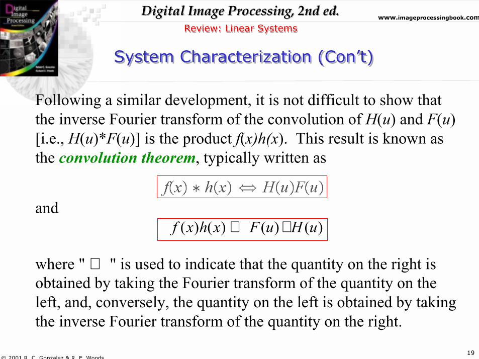
Following a similar development, it is not difficult to show that the inverse Fourier transform of the convolution of H(u) and F(u) [i.e., H(u)*F(u)] is the product f(x)h(x). This result is known as the convolution theorem, typically written as

and

where " ⇔ " is used to indicate that the quantity on the right is obtained by taking the Fourier transform of the quantity on the left, and, conversely, the quantity on the left is obtained by taking the inverse Fourier transform of the quantity on the right.

( ) ( ) ( ) ( )f x h x F u H u⇔ ∗

20





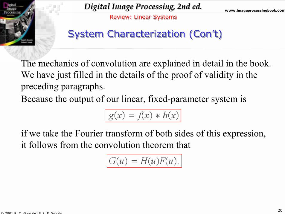
The mechanics of convolution are explained in detail in the book. We have just filled in the details of the proof of validity in the preceding paragraphs.Because the output of our linear, fixed-parameter system is

if we take the Fourier transform of both sides of this expression, it follows from the convolution theorem that

21





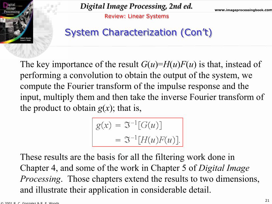
The key importance of the result G(u)=H(u)F(u) is that, instead of performing a convolution to obtain the output of the system, we compute the Fourier transform of the impulse response and the input, multiply them and then take the inverse Fourier transform of the product to obtain g(x); that is,

These results are the basis for all the filtering work done in Chapter 4, and some of the work in Chapter 5 of Digital Image Processing. Those chapters extend the results to two dimensions, and illustrate their application in considerable detail.

Documents

Linear Systems - Electrical and Computer Engineering | UC