Embed Size (px)
Citation preview
LING 438/538Computational Linguistics
Sandiway Fong
Lecture 19: 11/6
Administrivia
• Reminder– Britney Spears Homework due Thursday
– Excel trouble?– See references.xls on course homepage
download for an example on how to do table lookups
– Alternative: Perl also accepted
Today’s Topics
• Background: General Introduction to Probability Concepts
• Sample Space• Events• Counting• Event Probability• Entropy
• Application to Language: N-gram language models– cf. Google talk– background reading– textbook chapter 6: N-grams
Introduction to Probability
• some definitions– sample space
• the set of all possible outcomes of a statistical experiment is called the sample space (S)
• finite or infinite (also discrete or continuous)
– example• coin toss experiment• possible outcomes: {heads, tails}
– example• die toss experiment• possible outcomes: {1,2,3,4,5,6}
QuickTime™ and aTIFF (Uncompressed) decompressor
are needed to see this picture.
QuickTime™ and aTIFF (Uncompressed) decompressor
are needed to see this picture.
Introduction to Probability
• some definitions– sample space
• the set of all possible outcomes of a statistical experiment is called the sample space (S)
• finite or infinite (also discrete or continuous)
– example• die toss experiment for whether the number is even or odd• possible outcomes: {even,odd} • not {1,2,3,4,5,6}
QuickTime™ and aTIFF (Uncompressed) decompressor
are needed to see this picture.
Introduction to Probability
• some definitions– events
• an event is a subset of sample space
• simple and compound events
– example• die toss experiment • let A represent the
event such that the outcome of the die toss experiment is divisible by 3
• A = {3,6} • a subset of the sample
space {1,2,3,4,5,6}
Introduction to Probability
• some definitions– events
• an event is a subset of sample space
• simple and compound events
QuickTime™ and aTIFF (Uncompressed) decompressorare needed to see this picture.
QuickTime™ and aTIFF (Uncompressed) decompressorare needed to see this picture.
– example• deck of cards draw
experiment
• suppose sample space S = {heart,spade,club,diamond} (four suits)
• let A represent the event of drawing a heart
• let B represent the event of drawing a red card
• A = {heart} (simple event)
• B = {heart} {diamond} = ∪{heart,diamond} (compound event)
– a compound event can be expressed as a set union of simple events
– example• alternative sample space S
= set of 52 cards• A and B would both be
compound events
Introduction to Probability
• some definitions– events
• an event is a subset of sample space
• null space {} (or )• intersection of two events
A and B is the event containing all elements common to A and B
• union of two events A and B is the event containing all elements belonging to A or B or both
– example• die toss experiment, sample
space S = {1,2,3,4,5,6}
• let A represent the event such that the outcome of the experiment is divisible by 3
• let B represent the event such that the outcome of the experiment is divisible by 2
• intersection of events A and B is {6} (simple event)
• union of events A and B is the compound event {2,3,4,6}
Introduction to Probability
• some definitions– rule of counting
• suppose operation oi can be performed in ni ways, a sequence of k operations o1o2...ok can be performed in
n1 n2 ... nk ways QuickTime™ and a
TIFF (Uncompressed) decompressorare needed to see this picture.
– example• die toss experiment, 6
possible outcomes• two dice are thrown at the
same time• number of sample points in
sample space = 6 6 = 36
Introduction to Probability
• some definitions– permutations
• a permutation is an arrangement of all or part of a set of objects
• the number of permutations of n distinct objects is n!
• (n! is read as n factorial)
– Definition:• n! = n x (n-1) ... x 2 x 1
• n! = n x (n-1)!• 1!=1 • 0!=1
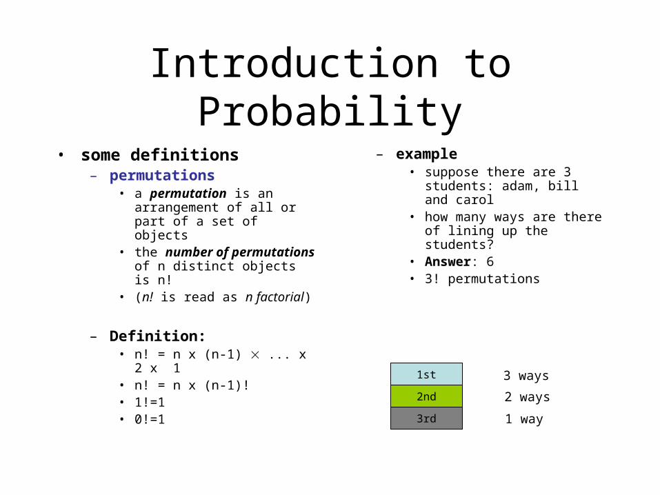
1st
2nd
3rd
3 ways
2 ways
1 way
– example• suppose there are 3 students:
adam, bill and carol• how many ways are there of
lining up the students? • Answer: 6• 3! permutations
Introduction to Probability
• some definitions– permutations
• a permutation is an arrangement of all or part of a set of objects
• the number of permutations of n distinct objects taken r at a time is n!/(n-r)!
QuickTime™ and aTIFF (Uncompressed) decompressor
are needed to see this picture.
– example• a first and a second prize raffle
ticket is drawn from a book of 425 tickets
• Total number of sample points = 425!/(425-2)!
• = 425!/423!• = 425 x 424 = 180,200
possibilities• instance of sample space
calculation
Introduction to Probability
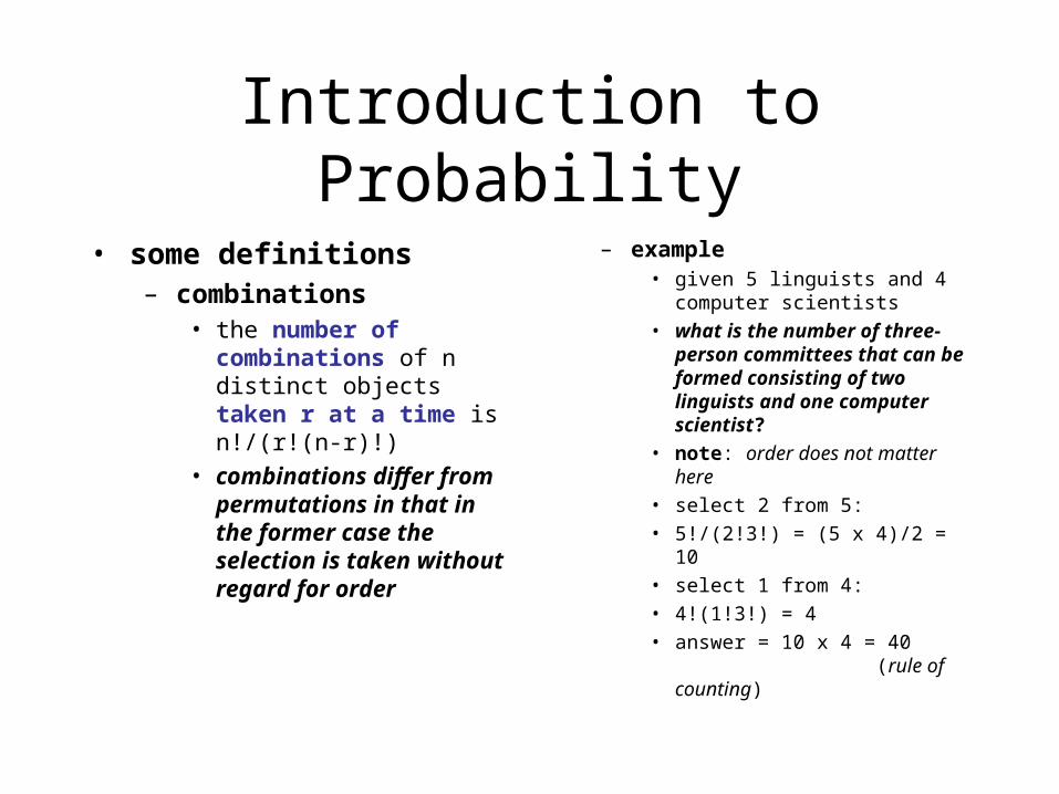
• some definitions– combinations
• the number of combinations of n distinct objects taken r at a time is n!/(r!(n-r)!)
• combinations differ from permutations in that in the former case the selection is taken without regard for order
– example• given 5 linguists and 4
computer scientists
• what is the number of three-person committees that can be formed consisting of two linguists and one computer scientist?
• note: order does not matter here
• select 2 from 5:
• 5!/(2!3!) = (5 x 4)/2 = 10
• select 1 from 4:
• 4!(1!3!) = 4
• answer = 10 x 4 = 40 (rule of counting)
Introduction to Probability
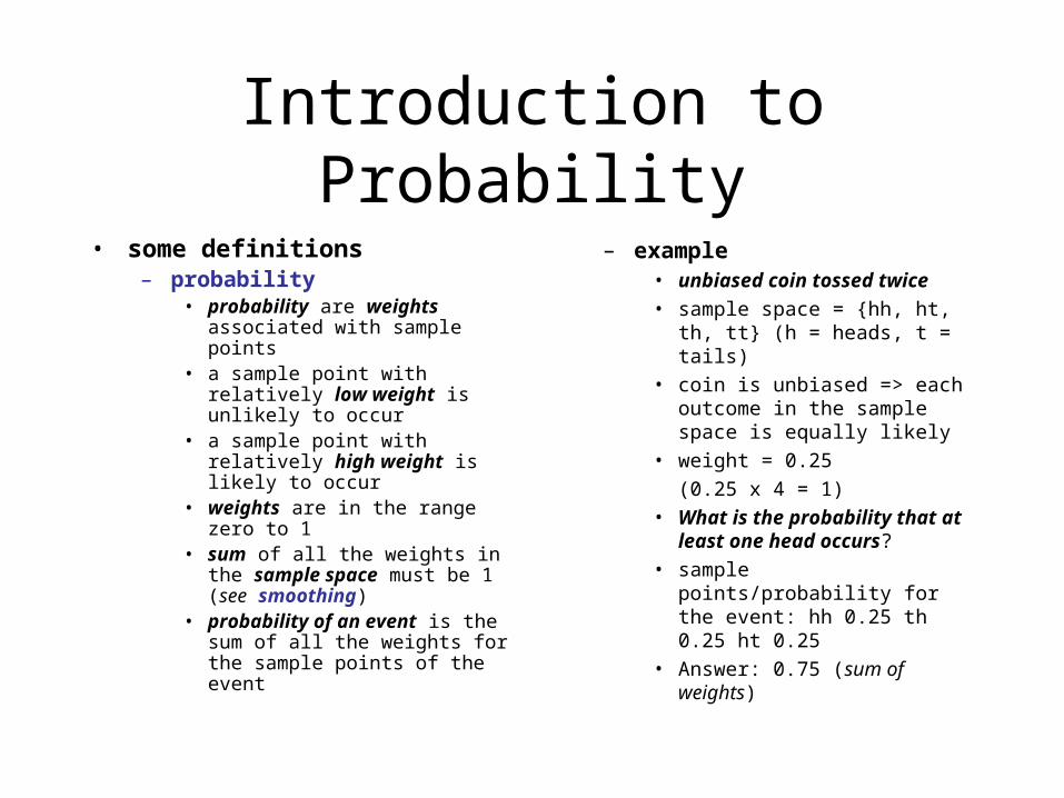
• some definitions– probability
• probability are weights associated with sample points
• a sample point with relatively low weight is unlikely to occur
• a sample point with relatively high weight is likely to occur
• weights are in the range zero to 1
• sum of all the weights in the sample space must be 1
(see smoothing)
• probability of an event is the sum of all the weights for the sample points of the event
– example• unbiased coin tossed twice
• sample space = {hh, ht, th, tt} (h = heads, t = tails)
• coin is unbiased => each outcome in the sample space is equally likely
• weight = 0.25
(0.25 x 4 = 1)
• What is the probability that at least one head occurs?
• sample points/probability for the event: hh 0.25 th 0.25 ht 0.25
• Answer: 0.75 (sum of weights)
Introduction to Probability
• some definitions– probability
• probability are weights associated with sample points
• a sample point with relatively low weight is unlikely to occur
• a sample point with relatively high weight is likely to occur
• weights are in the range zero to 1
• sum of all the weights in the sample space must be 1
• probability of an event is the sum of all the weights for the sample points of the event
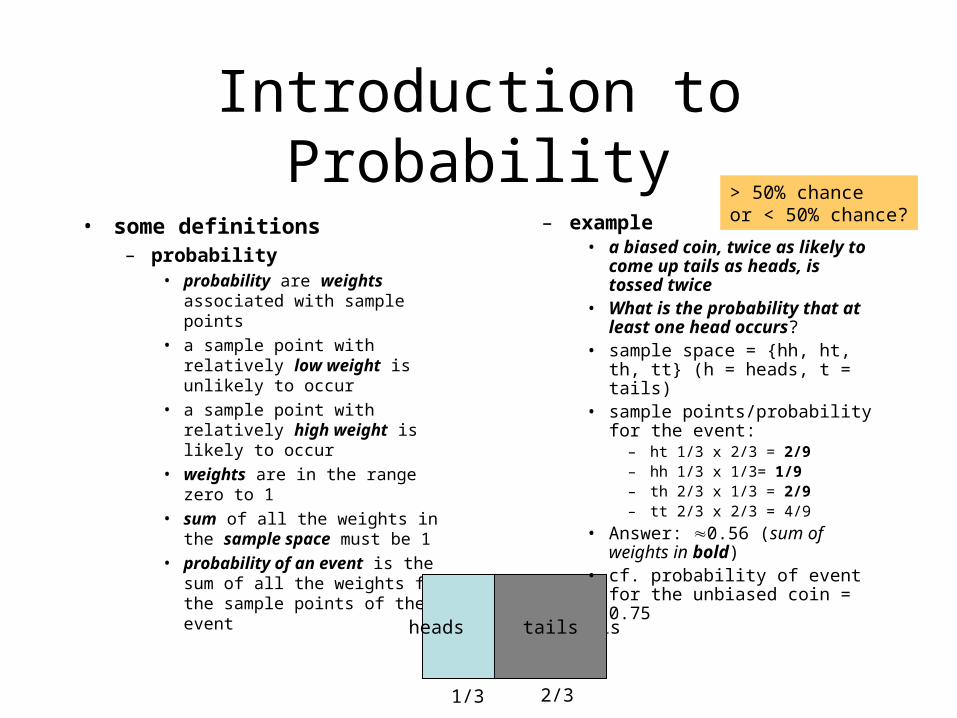
heads and tailstails
1/3 2/3
– example• a biased coin, twice as likely
to come up tails as heads, is tossed twice
• What is the probability that at least one head occurs?
• sample space = {hh, ht, th, tt} (h = heads, t = tails)
• sample points/probability for the event:
– ht 1/3 x 2/3 = 2/9– hh 1/3 x 1/3= 1/9– th 2/3 x 1/3 = 2/9– tt 2/3 x 2/3 = 4/9
• Answer: 0.56 (sum of weights in bold)
• cf. probability of event for the unbiased coin = 0.75
> 50% chanceor < 50% chance?
QuickTime™ and aTIFF (Uncompressed) decompressor
are needed to see this picture.
S
Introduction to Probability
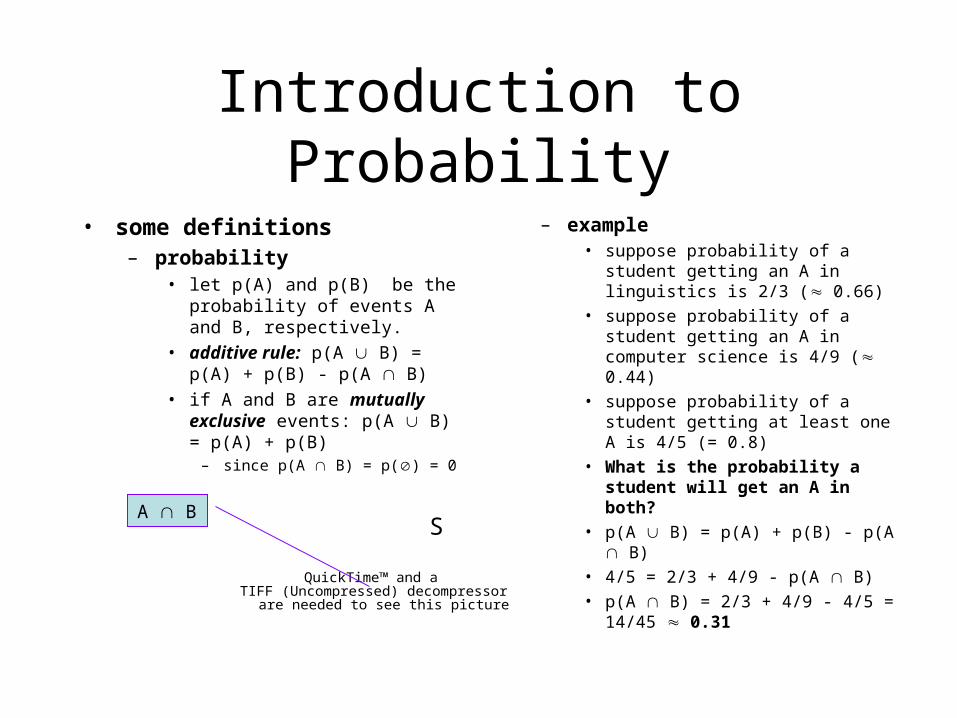
• some definitions– probability
• let p(A) and p(B) be the probability of events A and B, respectively.
• additive rule: p(A B) = p(A) + p(B) - p(A B)
• if A and B are mutually exclusive events: p(A B) = p(A) + p(B)
– since p(A B) = p() = 0
A B
– example• suppose probability of a student
getting an A in linguistics is 2/3 ( 0.66)
• suppose probability of a student getting an A in computer science is 4/9 ( 0.44)
• suppose probability of a student getting at least one A is 4/5 (= 0.8)
• What is the probability a student will get an A in both?
• p(A B) = p(A) + p(B) - p(A B)
• 4/5 = 2/3 + 4/9 - p(A B)
• p(A B) = 2/3 + 4/9 - 4/5 = 14/45 0.31
QuickTime™ and aTIFF (Uncompressed) decompressor
are needed to see this picture.
S
Introduction to Probability
• some definitions– conditional probability
• let A and B be events• p(B|A) = the probability of event B occurring given event A occurs• definition: p(B|A) = p(A B) / p(A) provided p(A)>0
– used an awful lot in language processing• (context-independent)• probability of a word occurring in a corpus
• (context-dependent)• probability of a word occurring given
the previous word
Entropy
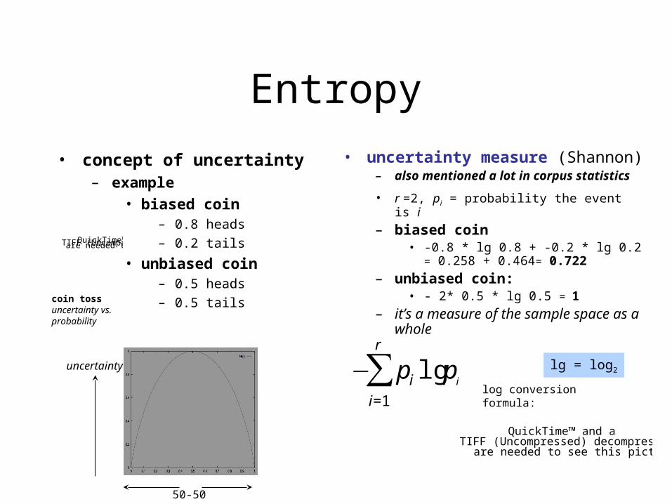
• concept of uncertainty– example
• biased coin– 0.8 heads
– 0.2 tails
• unbiased coin– 0.5 heads
– 0.5 tails
QuickTime™ and aTIFF (Uncompressed) decompressorare needed to see this picture.
€
− pi lg pi
i=1
r
∑QuickTime™ and a
TIFF (Uncompressed) decompressorare needed to see this picture.
log conversionformula:
lg = log2
coin tossuncertainty vs.probability
• uncertainty measure (Shannon)– also mentioned a lot in corpus
statistics
• r =2, pi = probability the event is i
– biased coin• -0.8 * lg 0.8 + -0.2 * lg 0.2 = 0.258 +
0.464= 0.722
– unbiased coin: • - 2* 0.5 * lg 0.5 = 1
– it’s a measure of the sample space as a whole
uncertainty
50-50
Entropy
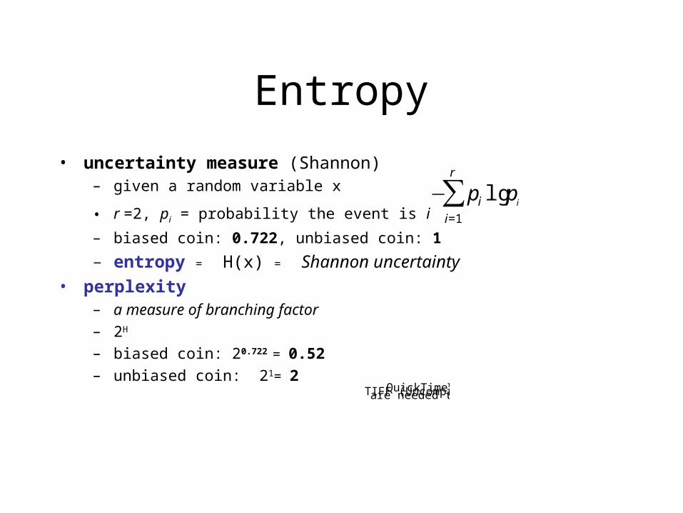
• uncertainty measure (Shannon)– given a random variable x
• r =2, pi = probability the event is i
– biased coin: 0.722, unbiased coin: 1
– entropy = H(x) = Shannon uncertainty
• perplexity– a measure of branching factor– 2H
– biased coin: 20.722 = 0.52– unbiased coin: 21= 2
€
− pi lg pi
i=1
r
∑
QuickTime™ and aTIFF (Uncompressed) decompressorare needed to see this picture.
Application to Language
N-grams: Unigrams
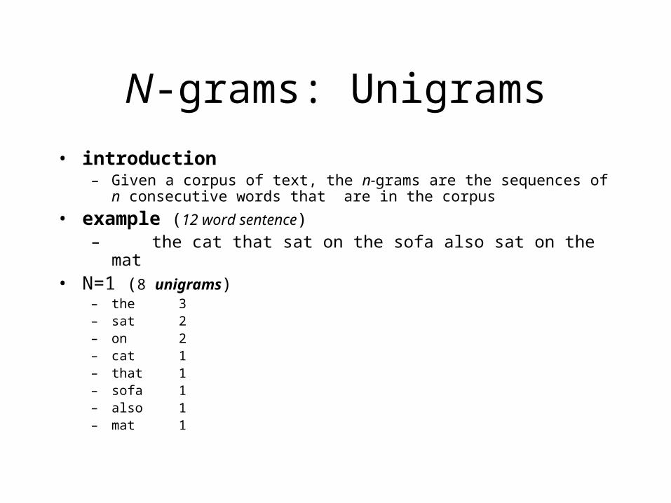
• introduction– Given a corpus of text, the n-grams are the sequences of n consecutive
words that are in the corpus
• example (12 word sentence)– the cat that sat on the sofa also sat on the mat
• N=1 (8 unigrams)– the 3– sat 2– on 2 – cat 1– that 1– sofa 1– also 1– mat 1
N-grams: Bigrams
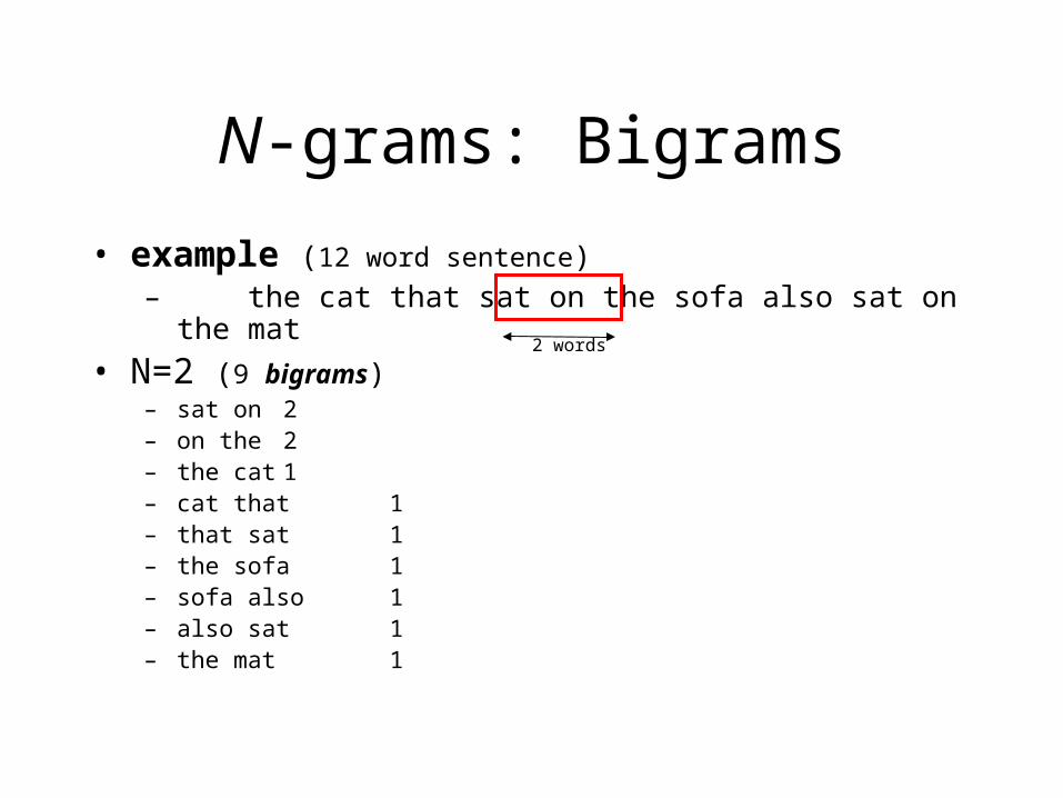
• example (12 word sentence)– the cat that sat on the sofa also sat on the mat
• N=2 (9 bigrams)– sat on 2– on the 2 – the cat 1– cat that 1– that sat 1 – the sofa 1– sofa also 1– also sat 1– the mat 1
2 words
N-grams: Trigrams
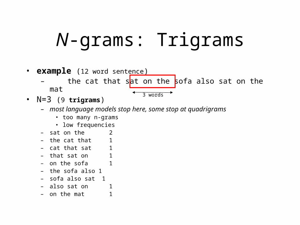
• example (12 word sentence)– the cat that sat on the sofa also sat on the mat
• N=3 (9 trigrams) – most language models stop here, some stop at quadrigrams
• too many n-grams• low frequencies
– sat on the 2 – the cat that 1– cat that sat 1– that sat on 1– on the sofa 1– the sofa also 1– sofa also sat 1– also sat on 1– on the mat 1
3 words
N-grams: Quadrigrams
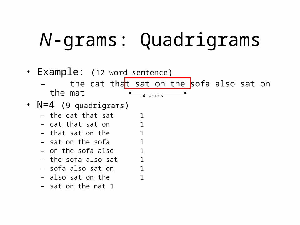
• Example: (12 word sentence)– the cat that sat on the sofa also sat on the mat
• N=4 (9 quadrigrams) – the cat that sat 1– cat that sat on 1– that sat on the 1– sat on the sofa 1– on the sofa also 1– the sofa also sat 1– sofa also sat on 1– also sat on the 1– sat on the mat 1
4 words
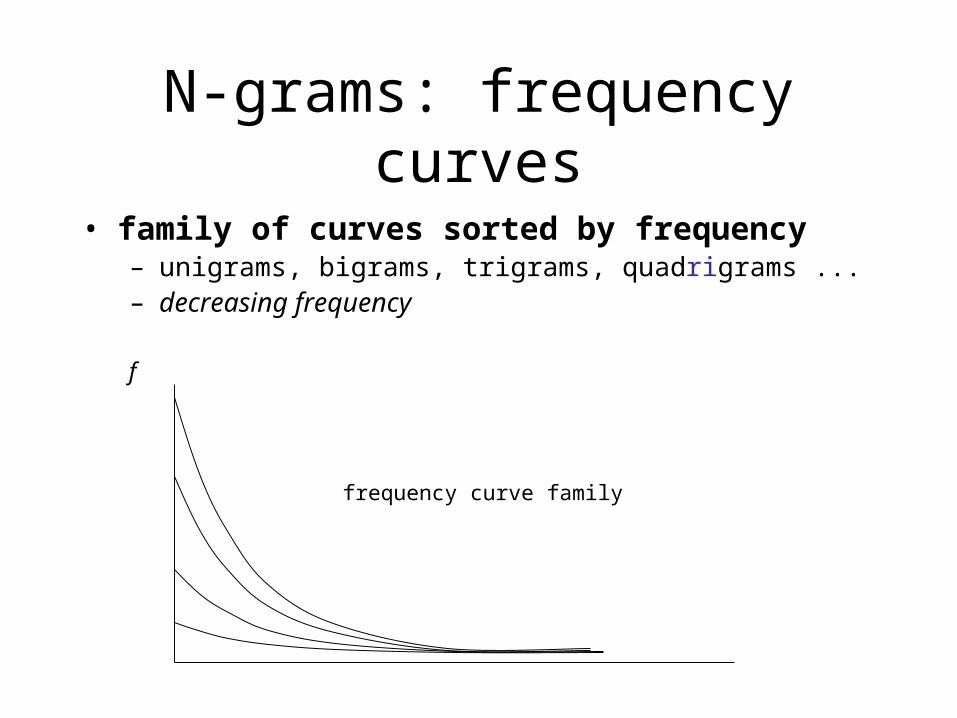
N-grams: frequency curves
• family of curves sorted by frequency– unigrams, bigrams, trigrams, quadrigrams ...– decreasing frequency
f
frequency curve family
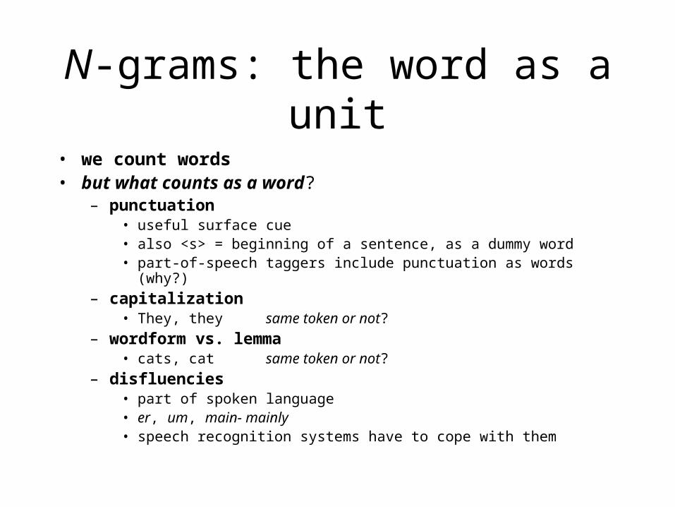
N-grams: the word as a unit
• we count words• but what counts as a word?
– punctuation• useful surface cue• also <s> = beginning of a sentence, as a dummy word• part-of-speech taggers include punctuation as words (why?)
– capitalization• They, they same token or not?
– wordform vs. lemma• cats, cat same token or not?
– disfluencies• part of spoken language• er, um, main- mainly• speech recognition systems have to cope with them
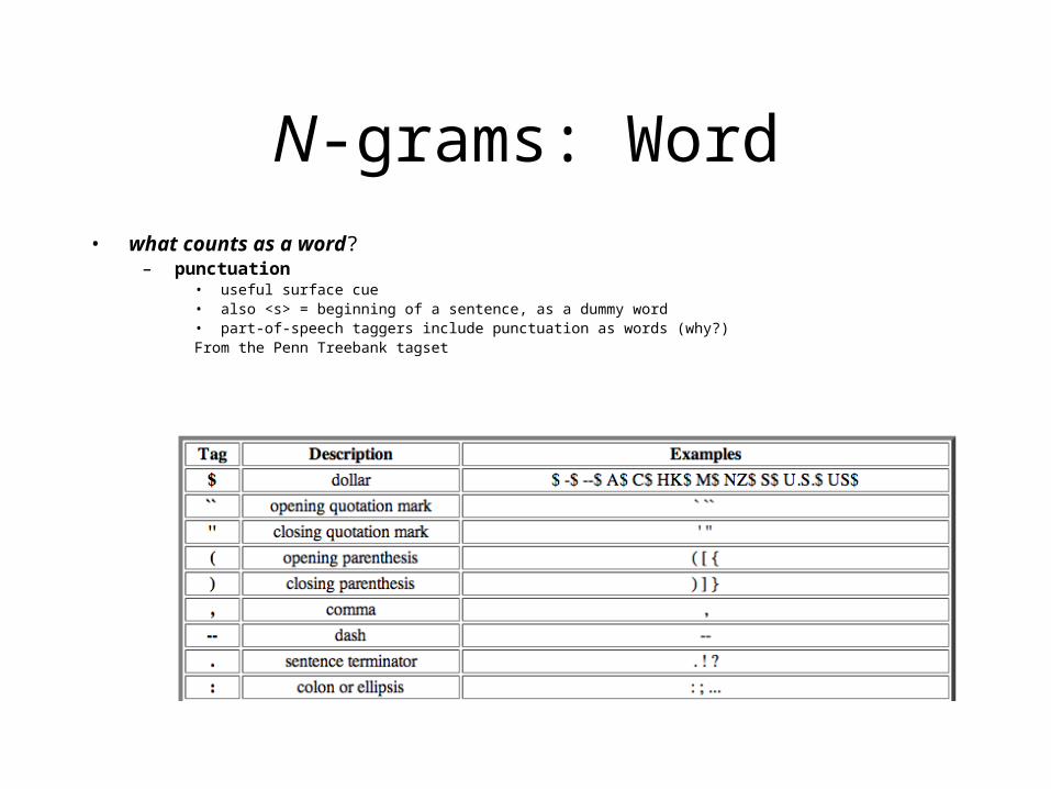
N-grams: Word• what counts as a word?
– punctuation• useful surface cue• also <s> = beginning of a sentence, as a dummy word• part-of-speech taggers include punctuation as words (why?)From the Penn Treebank tagset
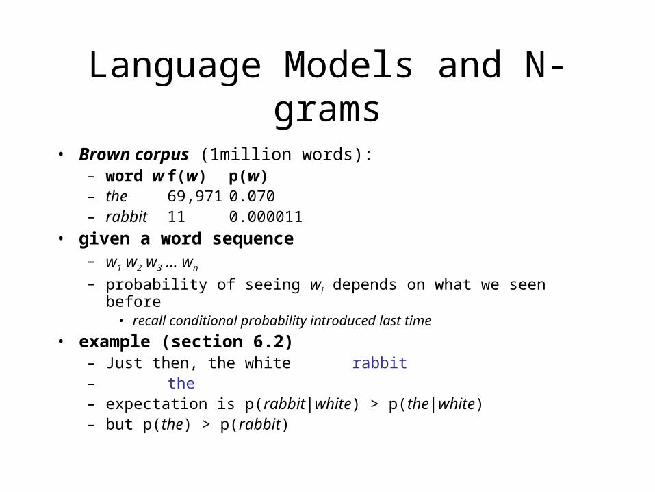
Language Models and N-grams
• Brown corpus (1million words):– word w f(w) p(w)– the 69,971 0.070– rabbit 11 0.000011
• given a word sequence – w1 w2 w3 ... wn
– probability of seeing wi depends on what we seen before• recall conditional probability introduced last time
• example (section 6.2)– Just then, the white rabbit– the– expectation is p(rabbit|white) > p(the|white)– but p(the) > p(rabbit)
Language Models and N-grams
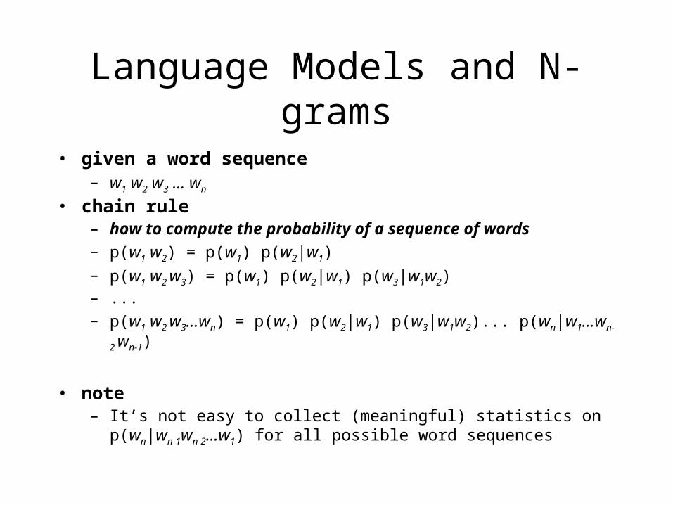
• given a word sequence– w1 w2 w3 ... wn
• chain rule– how to compute the probability of a sequence of words– p(w1 w2) = p(w1) p(w2|w1) – p(w1 w2 w3) = p(w1) p(w2|w1) p(w3|w1w2) – ...– p(w1 w2 w3...wn) = p(w1) p(w2|w1) p(w3|w1w2)... p(wn|w1...wn-2 wn-1)
• note– It’s not easy to collect (meaningful) statistics on p(wn|wn-1wn-2...w1)
for all possible word sequences
Language Models and N-grams
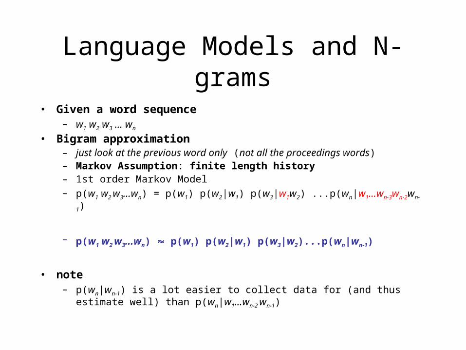
• Given a word sequence– w1 w2 w3 ... wn
• Bigram approximation– just look at the previous word only (not all the proceedings words) – Markov Assumption: finite length history– 1st order Markov Model– p(w1 w2 w3...wn) = p(w1) p(w2|w1) p(w3|w1w2) ...p(wn|w1...wn-3wn-2wn-1)
– p(w1 w2 w3...wn) p(w1) p(w2|w1) p(w3|w2)...p(wn|wn-1)
• note– p(wn|wn-1) is a lot easier to collect data for (and thus estimate well) than p(wn|
w1...wn-2 wn-1)
Language Models and N-grams
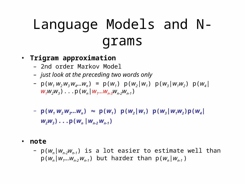
• Trigram approximation – 2nd order Markov Model– just look at the preceding two words only– p(w1 w2 w3 w4...wn) = p(w1) p(w2|w1) p(w3|w1w2) p(w4|w1w2w3)...p(wn|
w1...wn-3wn-2wn-1)
– p(w1 w2 w3...wn) p(w1) p(w2|w1) p(w3|w1w2)p(w4|w2w3)...p(wn |wn-2
wn-1)
• note– p(wn|wn-2wn-1) is a lot easier to estimate well than p(wn|w1...wn-2 wn-1)
but harder than p(wn|wn-1 )