link.springer.com · Transp Porous Med (2015) 110:369–408 DOI 10.1007/s11242-015-0554-1 Pressure Transient Behavior of Horizontal Wells Intersecting Multiple Hydraulic Fractures

Transp Porous Med (2015) 110:369–408DOI 10.1007/s11242-015-0554-1

Pressure Transient Behavior of Horizontal WellsIntersecting Multiple Hydraulic Fractures in NaturallyFractured Reservoirs

Denis Biryukov1 · Fikri J. Kuchuk1

Received: 1 February 2015 / Accepted: 27 July 2015 / Published online: 7 September 2015© The Author(s) 2015. This article is published with open access at Springerlink.com

Abstract In this study, we present a mesh-free semi-analytical technique for modeling pres-sure transient behavior of continuously and discretely hydraulically and naturally fracturedreservoirs for a single-phase fluid. In our model, we consider a 3D reservoir, where eachfracture is explicitly modeled without any upscaling or homogenization as required for dual-porosity media. Fractures can have finite or infinite conductivities, and the formation (matrix)is assumed to have a finite permeability. Our approach is based on the boundary elementmethod. The method has advantages such as the absence of grids and reduced dimension-ality. It provides continuous rather than discrete solutions. The uniform-pressure boundarycondition over the wellbore is used in our mathematical model. This is the true physicalboundary condition for any type of well, whether fractured or not, provided that the frictionpressure drop in the wellbore is small and the fluid is Newtonian. The method is sufficientlygeneral to be applied to many different well geometries and reservoir geological settings,where the spatial domain may include arbitrary fracture and/or fault distribution, a num-ber of horizontal wells with and without hydraulic fractures, and different types of outerboundaries. The model also applies to multistage hydraulically fractured horizontal wells inhomogenous reservoirs. More specifically, it is applied to investigate the pressure transientbehavior of horizontal wells in continuously and discretely naturally fractured reservoirs,including multistage hydraulically fractured horizontal wells. A number of solutions havebeen published in the literature for horizontal wells in naturally fractured reservoirs usingthe conventional dual-porosity models that are not applicable to many of these reservoirsthat contain horizontal wells with multiple fractures. Most published solutions for fracturedhorizontal wells in homogenous and naturally fractured reservoirs ignore the presence ofthe wellbore and the contribution to flow from the formation directly into the unfracturedhorizontal sections of the wellbore. Therefore, some of the flow regimes from these solutionsare incorrect or do not exist, such as fracture-radial flow regime. In our solutions, all or someof multistage hydraulic fractures may intersect the natural fractures, which is very importantfor shale gas and oil reservoir production. The number and type of fractures (hydraulic or

B Fikri J. [email protected]

1 1 rue Henri Becquerel, 92142 Clamart Cedex, France

123

http://crossmark.crossref.org/dialog/?doi=10.1007/s11242-015-0554-1&domain=pdf

370 D. Biryukov, F. J. Kuchuk

natural) intersecting the wellbore and with each other are not limited in both homogeneousand naturally fractured reservoirs. Our solutions are compared with a number of existingsolutions published in the literature. Example diagnostic derivative plots are presented fora variety of horizontal wells with multiple fractures in homogenous and naturally fracturedreservoirs.

Keywords Naturally fractured reservoirs · Pressure transient well testing · Pressuretransient behavior of horizontal wells · Multistage hydraulic fractures · Boundary elementmethod

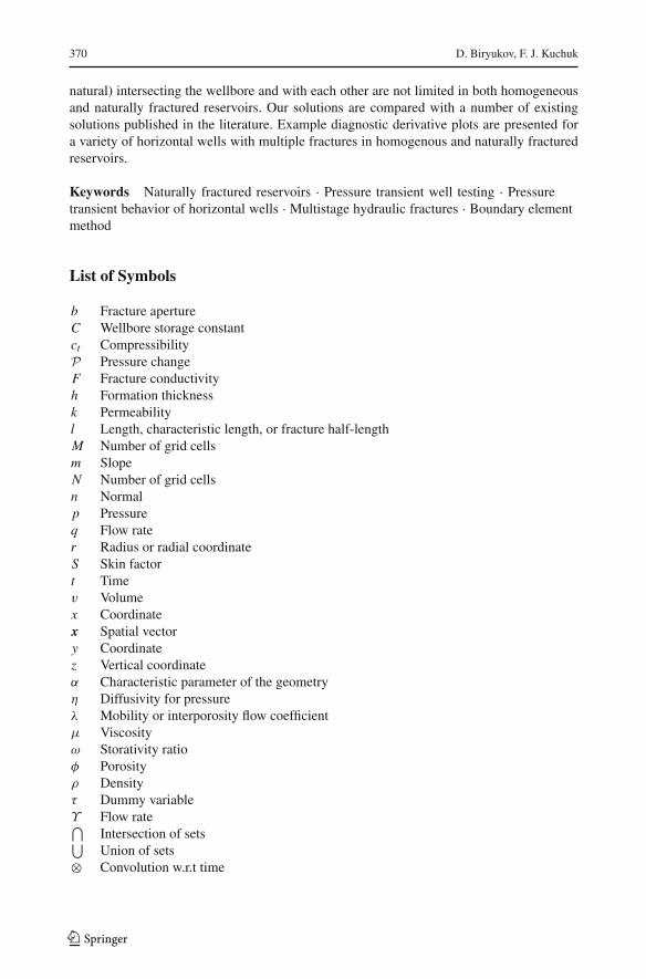
List of Symbols

b Fracture apertureC Wellbore storage constantct CompressibilityP Pressure changeF Fracture conductivityh Formation thicknessk Permeabilityl Length, characteristic length, or fracture half-lengthM Number of grid cellsm SlopeN Number of grid cellsn Normalp Pressureq Flow rater Radius or radial coordinateS Skin factort Timev Volumex Coordinatex Spatial vectory Coordinatez Vertical coordinateα Characteristic parameter of the geometryη Diffusivity for pressureλ Mobility or interporosity flow coefficientμ Viscosityω Storativity ratioφ Porosityρ Densityτ Dummy variableΥ Flow rate⋂

Intersection of sets⋃Union of sets

⊗ Convolution w.r.t time

123

Pressure Transient Behavior of Horizontal Wells Intersecting. . . 371

Subscripts

D Dimensionlessf Fracturef i Quantity related to the i th fractureh Horizontalhi Quantity related to the i th horizontal well sectionm Matrix or matrix blockma Matrix or matrix blocko Initial or originalu Uniformt TotalV Volumev Vertical or volumew Wellbore

1 Introduction

Shale gas developments, particularly in the USA, have increased applications of horizontalwells with multistage hydraulic fracturing. Drilling horizontal wells to accelerate produc-tion and increase recovery efficiency of oil and gas are now common. With the increasingnumber of wells, pressure transient well tests have been conducted in different geologicalsettings, particularly in carbonate and shale reservoirs. Natural fractures are common fea-tures of these reservoirs. In many naturally fractured carbonate reservoirs, faults often havehigh-permeability zones and are connected to many fractures with varying conductivities. Inthese naturally fractured reservoirs, faults and fractures can be discrete (i.e., not a connectedfracture network system). In this paper, we present a number of solutions for horizontal wellswith multiple fractures in naturally fractured and homogenous nonfractured (do not containfractures) reservoirs. These solutions are applicable to finite- and infinite-conductivity trans-verse and longitudinal fractures in hydraulically and naturally fractured reservoirs, wherethe horizontal wellbore can intersect multiple hydraulic and natural fractures. In this paper,fractures denote both fractures and faults, unless differentiation is necessary.

Most of the published solutions on horizontal wells with multiple fractures in bothfractured and nonfractured homogeneous reservoirs do not include the wellbore in the math-ematical model. For transverse fractures, the effect of the horizontal wellbore cannot beignored if the fracture conductivity is finite because the wellbore is perforated in single ormultiple locations for the fracture initiation, as well as providing access for the fluid flowinto the wellbore. In other words, perforation channels provide hydraulic communicationbetween the wellbore, fractures, and formation if the well is not completed barefoot.

In this paper, the formation (matrix) is assumed to be transversely isotropic (kmh =kmx = kmy) and vertically anisotropic with horizontal and vertical permeabilities, kmh andkmv , respectively, whereas fractures are assumed to be isotropic. Each fracture may have adifferent permeability (k f ), length (l), and aperture (b). A nominal dimensionless fracture

conductivity is defined as FD = k f bkmhlc

, where lc is a nominal fracture half-length that isconsidered to be used as a reference or characteristic length, provided it is not much smalleror bigger than the mean fracture length. The dimensionless fracture conductivity for eachfracture will be FDi .

123


Al-Kobaisi et al. (2006) provided an extensive list of references anddiscussions concerningthe pressure transient behavior of a single horizontal well intersectingmultiple transverse ver-tical hydraulic fractures. They also discussed a number of flow regimes that can be observedduring pressure transient tests. In general, the pressure transient behavior of a single horizon-tal well intersecting multiple transverse vertical hydraulic or natural fractures lies betweentwo limits. First, for high fracture conductivities (FD), the horizontal wellbore effect is neg-ligible at early times, and the fractures dominate the behavior of the system in homogenousreservoirs. But at late times, there will be a significant contribution to flow from the forma-tion directly into the horizontal sections of the wellbore. Second, as FD becomes smaller(FD � ∞), the unfractured horizontal sections of the wellbore start to contribute to flow. ForFD < 1, the flow contributions frommultiple fractures become negligible, and the horizontalwell dominates the behavior of the system; it is therefore extremely important to include thewellbore and the unfractured horizontal sections of the well. As we stated previously, mostof the published solutions did not include the wellbore and the unfractured horizontal sec-tions; consequently, some of the flow regimes observed from these solutions are incorrect,or simply they do not exist.

The inner boundary condition for a horizontal well with multiple transverse fracturesis considered to be of the mixed type. In a mixed boundary value problem (MBVP), wehave both the Neumann and Dirichlet boundary conditions imposed on the inner boundarywellbore surface. Furthermore, as stated above, except for openhole completions, hydraulicor natural fractures communicate with the wellbore through perforation tunnels, some ofwhich may not be 100% efficient (i.e., they are not cleaned up properly and totally debrisfree).

The majority of the published solutions do not specify where the wellbore pressure, whichis uniform over the inner wall of the wellbore (sandface), is evaluated. This inner bound-ary condition over the wellbore is called the uniform-pressure condition. In addition to theuniform-pressure condition, the wellbore pressure is approximated at the middle point of thefracture–well intersection in the literature. In general, the middle point wellbore pressureapproximation is crude and often incorrect when the pressure diffusion reaches any bound-aries (i.e., top, bottom, faults, fractures, etc.); see Tables 2 and 3 of Biryukov and Kuchuk(2012b). For most single-fractured wellbore, the wellbore pressure is also approximated atan appropriate equivalent-pressure point (Gringarten and Ramey 1975). For some cases,particularly, horizontal wells and fractures, the wellbore pressure is also approximated byaveraging over the flowing surface (Biryukov and Kuchuk 2012b; Kuchuk 1994; Kuchukand Wilkinson 1991; Ozkan and Raghavan 1991; Streltsova 1979; Wilkinson and Hammond1990; Yildiz and Bassiouni 1990).

The published solutions for the pressure transient behavior of a single horizontal wellintersecting multiple transverse vertical hydraulic or natural fractures can be divided intofour categories as follows:

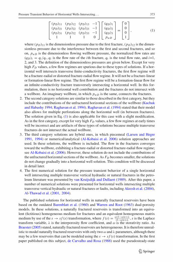
1. The first category solutions for multiple transverse fractures are generated using thesuperposition theorem in space and the pressure distribution solution for a single verticalfracture. Chen and Raghavan (1997), Guo et al. (1994), Horne and Temeng (1995),Raghavan et al. (1994), Zhou et al. (2013) used this approach to derive their solutions,in which the same flowing wellbore pressure is used for all fractures without a wellbore,and it is assumed that the uniform-flux or infinite-conductivity rectangular fractures fullypenetrate the formation. For example, the dimensionless wellbore solution (pwD) for areservoir with three vertical fractures (Horne and Temeng 1995) can be written as

123


⎡

⎢⎢⎣

(pD)11 (pD)12 (pD)13 −1(pD)21 (pD)22 (pD)23 −1(pD)31 (pD)32 (pD)33 −1

1 1 1 0

⎤

⎥⎥⎦

⎡

⎢⎢⎣

(qD)1(qD)2(qD)3pwD

⎤

⎥⎥⎦ =

⎡

⎢⎢⎣

0001

⎤

⎥⎥⎦ , (1)

where (pD)11 is the dimensionless pressure due to the first fracture, (pD)12 is the dimen-sionless pressure due to the interference between the first and second fractures, and soon, pwD is the dimensionless flowing wellbore pressure, the normalized flow rates are(qD)i = qi/qt , qi is the flow rate of the i th fracture, qt is the total flow rate, and i=1,2, and 3. The definition of the dimensionless pressures are given below. Except for veryhigh FD values, a few flow regimes are spurious due to these types of solutions. If a hor-izontal well intersects transverse finite-conductivity fractures, the first flow regime willbe a fracture-radial or distorted fracture-radial flow regime. It will not be a fracture-linearor formation-linear flow regime. The first flow regime will be a formation-linear flow foran infinite-conductivity fracture transversely intersecting a horizontal well. In this for-mulation, there is no horizontal well contribution and the fractures do not intersect witha wellbore. An imaginary wellbore, in which pwD is the same, connects the fractures.

2. The second category solutions are similar to those described in the first category, but theyinclude the contributions of the unfractured horizontal sections of the wellbore (Kuchukand Habashy 1994; Raghavan et al. 1994). Raghavan et al. (1994) stated that their modelalso allows for multiple perforations along the horizontal well (in between fractures).The solution given in Eq. (1) is also applicable for this case with a slight modification.As in the first category, except for very high FD values, a few flow regimes at early timeswill be incorrect and are artifacts of these types of solutions because multiple transversefractures do not intersect the actual wellbore.

3. The third category solutions are hybrid ones, in which piecemeal (Larsen and Hegre1991, 1994) or numerical/analytical (Al-Kobaisi et al. 2006) solution approaches areused. In these solutions, the wellbore is included. The flow in the fractures convergestoward the wellbore, exhibiting a fracture-radial or distorted fracture-radial flow regime;see Al-Kobaisi et al. (2006). However, these solution do not include the contributions ofthe unfractured horizontal sections of the wellbore. As FD becomes smaller, the solutionsdo not change gradually into a horizontal well solution. This condition will be discussedin detail later.

4. The first numerical solution for the pressure transient behavior of a single horizontalwell intersecting multiple transverse vertical hydraulic or natural fractures in the petro-leum literature was presented by van Kruijsdijk and Dullaert (1989). After this paper, anumber of numerical solutions were presented for horizontal wells intersecting multipletransverse vertical hydraulic or natural fractures or faults, including Akresh et al. (2004),Al-Thawad et al. (2001, 2004).

The published solutions for horizontal wells in naturally fractured reservoirs have beenbased on the outdated Barenblatt et al. (1960) and Warren and Root (1963) dual-porositymodels. In these solutions, a naturally fractured reservoirs is transformed into an equiva-lent (fictitious) homogeneous medium for fractures and an equivalent homogeneous matrixmedium by use of the s → s f (s) transformation, where f (s) = ω(1−ω)s+λ

(1−ω)s+λ, s is the Laplace

transform variable, λ is the interporosity flow coefficient, and ω is the storativity ratio. AsBraester (2005) stated, naturally fractured reservoirs are heterogeneous. It is therefore unreal-istic to model naturally fractured reservoirs with only twoω and λ parameters, although theremay be a few reservoirs that can be modeled using the s → s f (s) transformation. In the firstpaper published on this subject, de Carvalho and Rosa (1988) used the pseudosteady-state

123


flow conditions in matrix blocks with the s → s f (s) transformation to derive the pressuretransient solution for a horizontal well in a naturally fractured reservoir. After the de Car-valho and Rosa (1988) solution, many more solutions have been published in the petroleumliterature using the→ s f (s) transformation, while varying thematrix block shape andmatrixblock flow condition, and adding the interporosity skin factor for the matrix (Aguilera andNg 1991; Du and Stewart 1992; Williams and Kikani 1990), in addition to the more recentpapers by Abdulal et al. (2011), Brohi et al. (2011), Guo et al. (2012), Ketineni and Ertekin(2012), Lu et al. (2009), Medeiros et al. (2007, 2008, 2010), Nie et al. (2012a, b), Torcuket al. (2013).

As reported by Kuchuk et al. (2014), if the permeabilities of the fracture segments area few orders of magnitude larger than those of the matrix blocks, but not km � k f , then amacroscopic representative elementary volume can be constructed (i.e., dual-porositymodelscan therefore be used for continuously fractured reservoirs). If km � k f , then a macroscopicrepresentative elementary volume (REV) cannot be constructed. Thus, analytical or numeri-cal techniques should be used to model the pressure transient behavior of fractured reservoirswithout fracture-segment homogenization or upscaling (i.e., fractures have to be modeledexplicitly). In general, dual-porosity models should not be used for discretely fractured reser-voirs (Kuchuk et al. 2014).

Kuchuk et al. (2014) also showed that the resistance interface condition used byBarenblattet al. (1960) and Warren and Root (1963) to specify fluid transport between the equivalentmatrix and fractured media, dominates the dual-porosity model pressure transient behavior,irrespective of whether it is a vertical or horizontal well. The pseudosteady-state flow inthe equivalent matrix medium that we observe in the Warren and Root (1963) model is aconsequence of the resistance interface condition. This is not the actual pseudosteady-stateflow that takes place after the transient flow in the equivalent matrix medium. The resistanceinterface condition for pseudosteady-state flow and the interporosity skin with transient flowin the matrix are of a nonphysical nature. The inclusion of these two nonphysical phenomenain the dual-porosity models introduces serious nonuniqueness problems for interpretation,significantly distorts flow regimes, and creates a naturally fractured reservoir look-alikepressure behavior but without any physical meaning of the parameters.

In a naturally fractured reservoir, a horizontalwell usually intersects hundreds or thousandsof fractures and several conductive and/or nonconductive faults [see Fig. 1.10 of the Nurmiet al. (1995) and Fig. 1 of the Kuchuk and Biryukov (2015) papers], particularly in carbonateformations (Al-Thawad et al. 2001, 2004). It was reported by Kuchuk and Biryukov (2015)and Kuchuk et al. (2014) that wellbore-intersecting fractures dominate the pressure transientbehavior of both continuously and discretely naturally fractured reservoirs.

Next, we present the mesh-free semi-analytical technique for modeling the pressure tran-sient behavior of hydraulically and naturally fractured horizontal wells in continuously anddiscretely 3D fractured and nonfractured reservoirs.

2 Mathematical Model

In this section, we present new semi-analytical solutions in the real-time domain for horizon-tal wells in reservoirs bounded at the top and bottom by the no-flow horizontal boundaries.Let us consider a single-phase slightly compressible fluid flow in an infinite reservoir witha no-flow condition on the top and bottom boundaries. The reservoir is naturally fracturedand consists of fractures and the formation (matrix). In this model, the formation betweenthe fractures becomes the matrix without predetermined shapes, and it can easily deal with

123


fracture properties that exhibit power-law distributions or other type distributions, such aslog-normal. The formation thickness h, porosity φm , total isothermal compressibility (ct )m ,horizontal and vertical permeabilities kmh and kmv , and fluid viscosity μ are assumed to beconstant, and time and pressure invariant. The fluid is assumed to be Newtonian. The fractureporosity φ f , total isothermal compressibility (ct ) f , and permeability k f are also assumed tobe constant, and time and pressure invariant. The model also applies to multistage hydrauli-cally fractured horizontal wells in homogenous (unconventional oil and gas) reservoirs.

The origin of the global Cartesian coordinates {x = 0, y = 0, z = 0} is in the center ofthe reservoir, and the top and bottom boundary planes are at z = ± h

2 , respectively. For thissystem, the pressure diffusion equation can be written as

kmh

μ

∂2P∂x2

+ kmh

μ

∂2P∂y2

+ kmv

μ

∂2P∂z2

= φm(ct )m∂P∂t

, (2)

P(x, y, z, 0) = 0, (3)

∂P∂z

(

x, y,±h

2, t

)

= 0, (4)

where P(x, y, z, t) = p0 − p(x, y, z, t) is reservoir pressure change, and po and p denotethe initial and reservoir pressures, respectively.

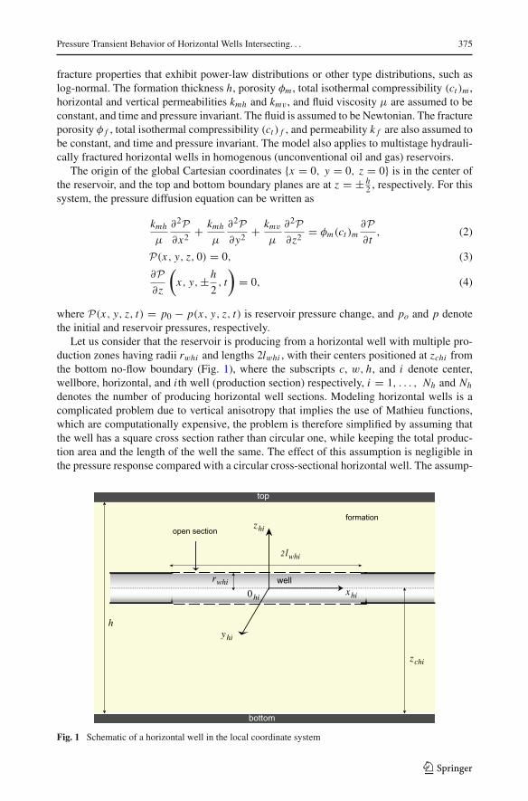
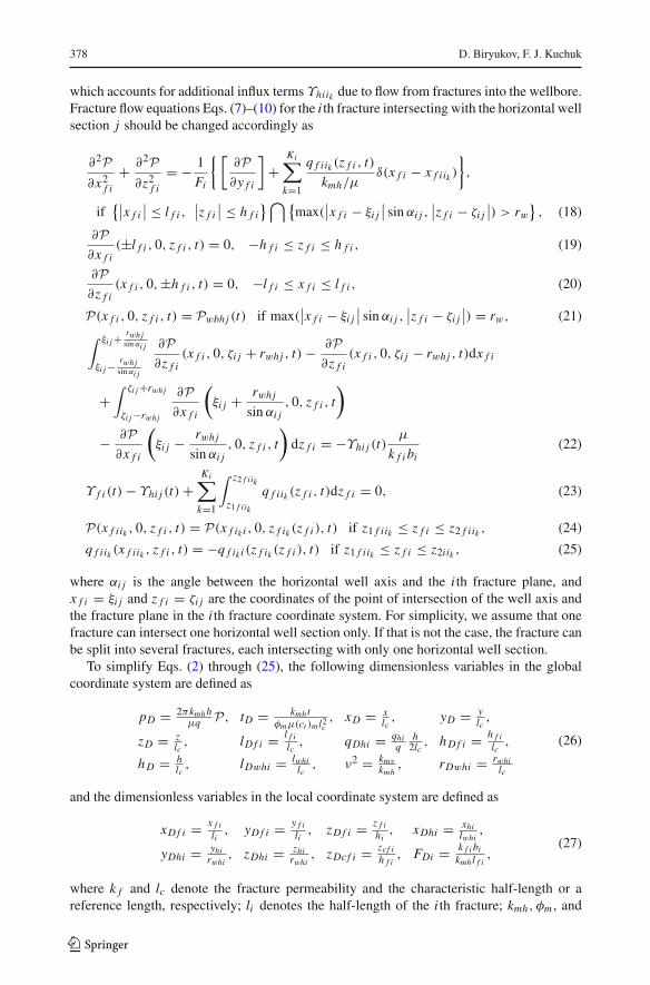
Let us consider that the reservoir is producing from a horizontal well with multiple pro-duction zones having radii rwhi and lengths 2lwhi , with their centers positioned at zchi fromthe bottom no-flow boundary (Fig. 1), where the subscripts c, w, h, and i denote center,wellbore, horizontal, and i th well (production section) respectively, i = 1, . . . , Nh and Nh

denotes the number of producing horizontal well sections. Modeling horizontal wells is acomplicated problem due to vertical anisotropy that implies the use of Mathieu functions,which are computationally expensive, the problem is therefore simplified by assuming thatthe well has a square cross section rather than circular one, while keeping the total produc-tion area and the length of the well the same. The effect of this assumption is negligible inthe pressure response compared with a circular cross-sectional horizontal well. The assump-

bottom

top

h

zchi

xhi0hi

zhi

yhi

rwhi

2lwhi

formation

open section

well

Fig. 1 Schematic of a horizontal well in the local coordinate system

123


tion of a square cross-sectional wellbore is considered to be a fair trade-off in exchange forsimplifying derivations. For a square cross-sectional horizontal well, the governing partialdifferential equation given by Eq. (2), and the initial condition given by Eq. (3) should becompleted with the following conditions; see Fig. 1:

P(xhi , yhi , zhi , t) = Pwbhi (t), if |xhi | < lwhi and max(|yhi | , |zhi |) = rwhi , (5)

Υwbhi (t) ≡ kmh

μ

(∫ rwhi

−rwhi

∫ lwhi

−lwhi

∂P∂yhi

(xhi , rwhi , zhi , t)

− ∂P∂yhi

(xhi ,−rwhi , zhi , t)dxhidzhi

)

+ kmv

μ

(∫ rwhi

−rwhi

∫ lwhi

−lwhi

∂P∂zhi

(xhi , yhi , rwhi , t)

− ∂P∂zhi

(xhi , yhi ,−rwhi , t)dxhidyhi

)

= −qhi (t), (6)

where Υwbhi is the flow rate entering the horizontal well from the reservoir.Becausewe are going to use different coordinate systems, it is assumed for the simplicity of

notations that all functions are being expressed in the coordinate systems corresponding to thesubscripts of their arguments (i.e., we omit the transformation signs from a local coordinatesystem xi , yi , zi to a global system of x, y, z: f (xi , yi , zi ) ≡ f [x(xi , yi , zi ), y(xi , yi , zi ),

z(xi , yi , zi )]).Let us also consider a number of discrete fractures in the reservoir. For the sake of simpli-

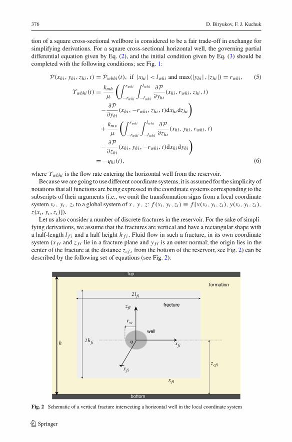
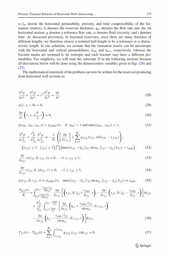
fying derivations, we assume that the fractures are vertical and have a rectangular shape witha half-length l f i and a half height h f i . Fluid flow in such a fracture, in its own coordinatesystem (x f i and z f i lie in a fracture plane and y f i is an outer normal; the origin lies in thecenter of the fracture at the distance zc f i from the bottom of the reservoir, see Fig. 2) can bedescribed by the following set of equations (see Fig. 2):

xfi

zfi

o

rw

y fi

well

fracture

formation

bottom

top

2h fi

zcfi

xfi

2lfi

h

Fig. 2 Schematic of a vertical fracture intersecting a horizontal well in the local coordinate system

123


∂2P∂x2f i

+ ∂2P∂z2f i

= − 1

Fi

[∂P∂y f i

]

, −l f i ≤ x f i ≤ l f i and − h f i ≤ z f i ≤ h f i , (7)

∂P∂x f i

(±l f i , 0, z f i , t) = 0, −h f i ≤ z f i ≤ h f i , (8)

∂P∂z f i

(x f i , 0,±h f i , t) = 0, −l f i ≤ x f i ≤ l f i , (9)

Υ f i (t) = −kmh

μ

∫ l f i

−l f i

∫ h f i

−h f i

[∂P∂y f i

]

(x f i , 0, z f i , t)dz f idx f i = 0, (10)

where, i = 1, 2, 3, . . . , N f , and N f is the total number of fractures in the reservoir, Fi = k f i bikmh

is the i th fracture conductivity, bi is i th fracture aperture, k f i is i th fracture permeability,[∂P∂y f i

]= ∂P

∂y f i

∣∣∣y f i →+0

− ∂P∂y f i

∣∣∣y f i →−0

is the pressure derivative jump across the fracture,

and Υ f i is the flow rate entering the fracture from the reservoir. Note that in Eq. (10), weassume an incompressible fluid flow in fractures (i.e., we do not consider any effects offluid compressibility in the fracture). Biryukov and Kuchuk (2012a) showed (see Fig. 10 oftheir paper) that a compressible fluid flow in the fractures has almost no impact on wellborepressure response.

Equations (7)–(10) are only valid for an isolated fracture that is not intersecting anythingelse.When the i th fracture intersects a number of ik fractures, where k = 1, . . . , Ki along thelines x f i = x f iik , z1 f i ik ≤ z f i ≤ z2 f i ik , we should replace Eqs. (7)–(10) with the following:

∂2P∂x2f i

+ ∂2P∂z2f i

= − 1

Fi

⎛

⎝[

∂P∂y f i

]

+Ki∑

k=1

q f iik (z f i , t)

kmh/μδ(x f i − x f iik )

⎞

⎠ ,

∣∣x f i

∣∣ ≤ l f i ,

∣∣z f i

∣∣ ≤ h f i , (11)

∂P∂x f i


∂P∂z f i


Υ f i (t) +Ki∑

k=1

∫ z2 f i ik

z1 f i ik

qiik (z f i , t)dz f i = 0, (14)

P(x f iik , 0, z f i , t) = P(x f ik i , 0, z f ik (z f i ), t) if z1 f i ik ≤ z f i ≤ z2 f i ik , (15)

q f iik (z f i , t) = −q f ik i (z f ik (z f i ), t) if z1 f i ik ≤ z f i ≤ z2 f i ik , (16)

where Eqs. (15) and (16) correspond respectively to pressure and the flux density continuityconditions at the intersection line, while Eq. (14) indicates the total flux conservation in thesystem of intersecting fractures. The term q f iik corresponds to the flux density exchangebetween the i th and ik th fractures. Note that if the intersection line lies on the edge of thefracture, then the corresponding portion of the boundary condition in Eq. (12) is “overwritten”by Eqs. (15) and (16).

When the horizontal well intersects a number of fractures, Eq. (6) is no longer valid, andthen the following equation should be used instead:

Υwbhi (t) +jk=i∑

j

Υhj jk (t) = −qhi , (17)

123


which accounts for additional influx terms Υhiik due to flow from fractures into the wellbore.Fracture flow equations Eqs. (7)–(10) for the i th fracture intersecting with the horizontal wellsection j should be changed accordingly as

∂2P∂x2f i

+ ∂2P∂z2f i

= − 1

Fi

{[∂P∂y f i

]

+Ki∑

k=1

q f iik (z f i , t)

kmh/μδ(x f i − x f iik )

}

,

if{∣∣x f i

∣∣ ≤ l f i ,

∣∣z f i

∣∣ ≤ h f i

}⋂{max(

∣∣x f i − ξi j

∣∣ sin αi j ,

∣∣z f i − ζi j

∣∣) > rw

}, (18)

∂P∂x f i


∂P∂z f i


P(x f i , 0, z f i , t) = Pwbhj (t) if max(∣∣x f i − ξi j

∣∣ sin αi j ,


∣∣) = rw, (21)

∫ ξi j + rwhjsin αi j

ξi j − rwhjsin αi j

∂P∂z f i

(x f i , 0, ζi j + rwhj , t) − ∂P∂z f i

(x f i , 0, ζi j − rwhj , t)dx f i

+∫ ζi j +rwhj

ζi j −rwhj

∂P∂x f i

(

ξi j + rwhj

sin αi j, 0, z f i , t

)

− ∂P∂x f i

(

ξi j − rwhj


)

dz f i = −Υhi j (t)μ

k f i bi(22)

Υ f i (t) − Υhi j (t) +Ki∑

k=1

∫ z2 f i ik

z1 f i ik

q f iik (z f i , t)dz f i = 0, (23)

P(x f iik , 0, z f i , t) = P(x f ik i , 0, z f ik (z f i ), t) if z1 f i ik ≤ z f i ≤ z2 f i ik , (24)

q f iik (x f iik , z f i , t) = −q f ik i (z f ik (z f i ), t) if z1 f i ik ≤ z f i ≤ z2i ik , (25)

where αi j is the angle between the horizontal well axis and the i th fracture plane, andx f i = ξi j and z f i = ζi j are the coordinates of the point of intersection of the well axis andthe fracture plane in the i th fracture coordinate system. For simplicity, we assume that onefracture can intersect one horizontal well section only. If that is not the case, the fracture canbe split into several fractures, each intersecting with only one horizontal well section.

To simplify Eqs. (2) through (25), the following dimensionless variables in the globalcoordinate system are defined as

pD = 2πkmh hμq P, tD = kmh t

φmμ(ct )ml2c, xD = x

lc, yD = y

lc,

zD = zlc

, lD f i = l f ilc

, qDhi = qhiq

h2lc

, h D f i = h f ilc

,

h D = hlc

, lDwhi = lwhilc

, ν2 = kmv

kmh, rDwhi = rwhi

lc

(26)

and the dimensionless variables in the local coordinate system are defined as

xD f i = x f ili

, yD f i = y f ili

, zD f i = z f ihi

, xDhi = xhilwhi

,

yDhi = yhirwhi

, zDhi = zhirwhi

, zDc f i = zc f ih f i

, FDi = k f i bikmhl f i

,(27)

where k f and lc denote the fracture permeability and the characteristic half-length or areference length, respectively; li denotes the half-length of the i th fracture; kmh, φm , and

123


(ct )m denote the horizontal permeability, porosity, and total compressibility of the for-mation (matrix); h denotes the reservoir thickness; qhi denotes the flow rate into the i thhorizontal section; q denotes a reference flow rate; μ denotes fluid viscosity; and t denotestime. As discussed previously, in fractured reservoirs, since there are many fractures ofdifferent lengths; we therefore choose a nominal half-length to be a reference or a charac-teristic length. In our solutions, we assume that the formation matrix can be anisotropicwith the horizontal and vertical permeabilities, kmh and kmv , respectively, whereas thefracture media are assumed to be isotropic and each fracture may have a different per-meability. For simplicity, we will omit the subscript D in the following sections becauseall derivations below will be done using the dimensionless variables given in Eqs. (26) and(27).

Themathematical statement of the problem can now bewritten for the reservoir producingfrom horizontal well sections as

∂2 p

∂x2+ ∂2 p

∂y2+ ν2

∂2 p

∂z2= ∂p

∂t, (28)

p(x, y, z, 0) = 0, (29)

∂p

∂z

(

x, y, ±h

2, t

)

= 0, (30)

p(xhi , yhi , zhi , t) = pwbhi (t), if |xhi | < 1 and max(|yhi | , |zhi |) = 1, (31)

∂2 p

∂x2f i

+l2f i

h2f i

∂2 p

∂z2f i

= − 1

Fi

⎛

⎝[

∂p

∂y f i

]

+Ki∑

k=1

q f iik (z f i , t)δ(x f i − x f iik )

⎞

⎠ ,

{∣∣x f i

∣∣ ≤ 1,

∣∣z f i

∣∣ ≤ 1

}⋂{max(

∣∣x f i − ξi j

∣∣ l f i sin αi ,


∣∣ h f i ) > rwhi

}, (32)

∂p

∂x f i(±l f i , 0, z f i , t) = 0, −1 ≤ z f i ≤ 1, (33)

∂p

∂z f i(x f i , 0, ±h f i , t) = 0, −1 ≤ x f i ≤ 1, (34)

p(x f i , 0, z f i , t) = pwbhi (t), max(∣∣x f i − ξi j

∣∣ l f i sin αi j ,


∣∣ h f i ) = rwhi , (35)

Υhi j (t)

Fi=

∫ ξi j − rwhi / l f isin αi j

ξi j+rwhi / l f isin αi j

∂p

∂z f i

[(

x f i , 0, ζi j + rwhi

h f i, t

)

− ∂p

∂z f i

(

x f i , 0, ζi j − rwhi

h f i, t

)]

dx f i

+h2f i

l2f i

∫ ζi j − rwhih f i

ζi j + rwhih f i

[∂p

∂x f i

(

ξi j + rwhi / l f i


)

− ∂p

∂x f i

(

ξi j − rwhi / l f i


)]

dz f i , (36)

Υ f i (t) − Υhi j (t) +Ki∑

k=1

∫ z2 f i ik

z1 f i ik

q f iik (z f i , t)dz f i = 0, (37)

123


rwhi Υwbhi (t) +lk=i∑

l

h f lΥhllk (t) = 4πqhi , (38)

p(x f iik , 0, z f i , t) = p(x f ik i , 0, z f ik (z f i ), t) if z1 f i ik ≤ z f i ≤ z2 f i ik , (39)

q f iik (z f i , t) = −q f ik i (z f ik (z f i ), t) if z1 f i ik ≤ z f i ≤ z2 f i ik , (40)

Υwbhi (t) =∫ 1

−1

∫ 1

−1

∂p

∂yhi(xhi , 1, zhi , t) − ∂p

∂yhi(xhi , −1, zhi , t)dxhidzhi

+ ν2l2whi

r2whi

∫ 1

−1

∫ 1

−1

∂p

∂zhi(xhi , yhi , 1, t) − ∂p

∂zhi(xhi , yhi ,−1, t)dxhidyhi . (41)

Finally, the system should be completed by imposing conditions at each horizontal wellboresection on the flow rates qhj and pressure change pwbhj that are not independent. For example,if we assume that all horizontal production zones are part of one well and are hydraulicallyconnected and produce with a constant flow rate q , we should add the following closureequations:

pwbhi (t) = pwb(t), i = 1, . . . , Nh, (42)

Nh∑

j=1

qhj = h/2. (43)

3 Transient Solution

In this section, we will describe a solution technique that is used for solving Eqs. (28)–(43).Let us first build an expansion for a flux density distribution on fractures. We consider a gridin the form−1 = x1f i < x2f i < · · · < xm

f i < · · · < x Mi +1f i = 1 and−1 = z1f i < z2f i < · · · <

znf i < · · · < zNi +1

f i = 1, and we also define �xmf i = xm+1

f i − xmf i and �zn

f i = zn+1f i − zn

f i ,where Mi and Ni are the number of grid cells in the x and z directions, respectively.

Now, let us assume that the flux density can be approximated as

q f i (x f i , z f i , t) ≡ 1

2

[∂p

∂y f i

]

≈Mi∑

m=1

Ni∑

n=1

4πcmnf i (t)

h2f i l f i

ω(

x f i , xmf i , xm+1

f i

)ω

(z f i , zn

f i , zn+1f i

),

(44)where ω denotes the boundary element in the form

ω(x, xn, xn+1) ={

1xn+1−xn if xn ≤ x ≤ xn+1

0, otherwise.(45)

Although we could use Chebyshev polynomials as we did in the 2D case (Biryukov andKuchuk 2012a), we did not find them to be efficient for approximating the flux densitydistribution near the point of intersection with the horizontal well. On the other hand, withboundary elements ω, we can easily vary the local grid size in order to achieve the desiredprecision. Therefore, we decided to increase the grid density near the edges of the fractureand near the horizontal wellbore intersection (if there is one). The question of gridding willbe discussed in detail in “Appendix 1.”

123


The flux density distribution defined by Eq. (44) will induce the following pressure changein the reservoir:

p f i (x f i , y f i , z f i , t) =Mi∑

m=1

Ni∑

n=1

c f imn(t) ⊗ Gmn

f i (x f i , y f i , z f i , t), (46)

where ⊗ denotes the time convolution operation, and

Gmnf i (x f i , y f i , z f i , t) = e− y2f i

4t

Ξ(

x f i , t/ l2f i , u)∣∣∣xm+1

f i

xmf i

�xmf i l f i

Λ(

z f i ,ν2th f i

,zc f ih f i

, hh f i

, u)∣∣∣zn+1

f i

znf i

th2f i�zn

f i

,

(47)

Ξ(x, t, u) =√

π

2erf

(u − x

2√

t

)

, (48)

Λ(z, t, z0, h, u) =∞∑

j=−∞

{

erf

(z − u + 2 jh

2√

t

)

+ erf

(z + u + 2z0 + 2 jh

2√

t

)}

. (49)

The evaluation of Λ and the time integrals given in Eq. (46) are discussed in detail in“Appendix 1.” We also consider a grid along the fracture intersection lines in the form

z1 f i ik = z1f i ik< z2f i ik

< . . . < znf iik

< . . . < zN f iik +1

f i ik= z2 f i ik , and assume that the

interfracture flow exchange terms can be expressed as

q f iik (z f i , t) = 4π

N f iik∑

n=1

qnf iik

h2f i

ω(

z f i , znf iik

, zn+1f i ik

), (50)

where it is assumed that z f i (znf ik i ) = zn

f iik.

For the horizontal well, we define a grid in the form −1 = x1hi < x2hi < · · · < xnhi <

· · · < x Nhi +1hi = 1 along the well and −1 = y1hi < y2hi < · · · < ym

hi < · · · < yMhi /4+1hi = 1

at zhi = ±1 and −1 = z1hi < z2hi < · · · < zmhi < · · · < zMhi /4+1

hi = 1 at yhi = ±1 in thetransverse direction, where Nhi and Mhi are the number of grid cells in the x and z directions,respectively

Let us also consider the following point source distribution on the wellbore:

qwhi (xhi , yhi , 1, t) =Mhi /4∑

m=1

Nhi∑

n=1

4πcmnhi (t)

r2whi lwhiω

(yhi , ym

hi , ym+1hi

)ω

(xhi , xn

hi , xn+1hi

), (51)

qwhi (xhi , yhi ,−1, t) =Mhi /2∑

m=Mhi /4+1

Nhi∑

n=1

4πcmnhi (t)

r2whi lwhiω

(yhi , ym−Mhi /4

hi , ym−Mhi /4+1hi

)

× ω(

xhi , xnhi , xn+1

hi

), (52)

qwhi (xhi , 1, zhi , t) =3Mhi /4∑

m=Mhi /2+1

Nhi∑

n=1

4πcmnhi (t)

r2whi lwhiω

(zhi , zm−Mhi /2

hi , zm−Mhi /2+1hi

)

× ω(

xhi , xnhi , xn+1

hi

), (53)

123


qwhi (xhi ,−1, zhi , t) =Mhi∑

m=3Mhi /4+1

Nhi∑

n=1

4πcmnhi (t)

r2whi lwhiω

(zhi , zm−3Mhi /4

hi , zm−3Mhi /4+1hi

)

× ω(

xhi , xnhi , xn+1

hi

). (54)

The pressure change in the reservoir induced by this source distribution can be expressed bythe following equation as

phi (xhi , yhi , zhi , t) =Mhi∑

m=1

Nhi∑

n=1

cmnhi (t) ⊗ Gmn

hi (xhi , yhi , zhi , t), (55)

where

Gmnhi (xhi , yhi , zhi , t) =

Ωm(

yhi , zhi ,t

r2whi,

zchirwhi

, hrwhi

)

r2whi

Ξ(xhi , t/ l2whi , u

)∣∣xn+1

hixn

hi

t�xmhi lwhi

(56)

Ωm(yhi , zhi , zchi , h, t) =

⎧⎪⎪⎪⎪⎪⎪⎪⎪⎪⎪⎪⎪⎪⎪⎪⎪⎪⎨

⎪⎪⎪⎪⎪⎪⎪⎪⎪⎪⎪⎪⎪⎪⎪⎪⎪⎩

Z(zhi ,zchi ,h,ν2t,1)ν

Ξ(yhi ,t,u)|ym+1hi

ymhi

�ym−Mhi /4hi

, 1 ≤ m ≤ Mhi4 ,

Z(zhi ,zchi ,h,ν2t,−1)ν

Ξ(yhi ,t,u)|ym−Mhi /4+1hi

ym−Mhi /4hi

�ym−Mhi /4hi

, 1 + Mhi4 ≤ m ≤ Mhi

2 ,

e− (1−yhi )2

4t

Λ(zhi ,ν2t,zchi ,h,u)

∣∣zm−Mhi /2+1hi

zm−Mhi /2hi

�zm−Mhi /2hi

, 1 + Mhi2 ≤ m ≤ 3Mhi

4 ,

e− (1+yhi )2

4t

Λ(zhi ,ν2t,zchi ,h,u)

∣∣zm−3Mhi /4+1hi

zm−3Mhi /4hi

�zm−3Mhi /4hi

, 1 + 3Mhi4 ≤ m ≤ Mhi ,

(57)

with Ξ being defined by Eq. (48), and

Z(zhi , zchi , h, t, u) =∞∑

j=−∞

(

e− (u−zhi +2 jh)2

4t + e− (u+zhi +2zchi +2 jh)2

4t

)

. (58)

The total flow rate over the i th producing horizontal section due to the pressure change isobtained by substituting phi from Eq. (55) into Eq. (41) as

Υwbhi (t) = 2π

rwhi

⎡

⎣2Mhi∑

m=1

Nhi∑

n=1

cmnhi (t) ⊗ Υ mn

whi (t) +Mhi∑

m=1

Nhi∑

n=1

cmnhi (t)

⎤

⎦ , (59)

where

Υ mnwhi (t) =

√tπ

2W m

s

(t/r2whi

) W (t/ l2whi , u)∣∣xn+1

hixn

hi

�xmhi

, (60)

W (t, u) = (1 − u)erf

(1 − u

2√

t

)

− (1 + u)erf

(1 + u

2√

t

)

+ 2

√t

π

(

e− (1−u)24t − e− (1+u)2

4t

)

, (61)

123


W ms (t)

=

⎧⎪⎪⎪⎪⎪⎪⎪⎪⎪⎪⎪⎪⎪⎪⎪⎪⎪⎪⎪⎪⎪⎪⎨

⎪⎪⎪⎪⎪⎪⎪⎪⎪⎪⎪⎪⎪⎪⎪⎪⎪⎪⎪⎪⎪⎪⎩

1�ym

hi

{

R(t, u)erf(

1ν√

t

)+ W (t, u) e

− 14tν2

νt

}∣∣∣∣∣

ym+1hi

ymhi

, 1 ≤ m ≤ Mhi4 ,

1

�ym− Mhi

4hi

{

R(t, u)erf(

1ν√

t

)+ W (t, u) e

− 14tν2

νt

}∣∣∣∣∣

ym+1− Mhi

4hi

ym− Mhi

4hi

, 1 + Mhi4 ≤ m ≤ Mhi

2 ,

ν

�zm− Mhi

2hi

{

R(ν2t, u)erf(

1ν√

t

)+ W (ν2t, u) e

− 14tν2

νt

}∣∣∣∣∣

zm+1− Mhi

2hi

zm− Mhi

2hi

, 1 + Mhi2 ≤ m ≤ 3Mhi

4 ,

ν

�zm− 3Mhi

4hi

{

R(ν2t, u)erf(

1ν√

t

)+ W (ν2t, u) e

− 14tν2

νt

}∣∣∣∣∣

zm+1− 3Mhi

4hi

zm− 3Mhi

4hi

, 1 + 3Mhi4 ≤ m ≤ Mhi ,

(62)

and

R(t, u) = e− (1+u)24t − e− (1−u)2

4t . (63)

Next, we seek the solution of Eqs. (28)–(43) in the following form:

p(x, y, z, t) =Kh∑

i=1

phi (x, y, z, t) +N f∑

i=1

p f i (x, y, z, t). (64)

It can be observed that Eqs. (28)–(30) are satisfied automatically. The remaining equationscannot be satisfied everywhere because we have restricted ourselves to a limited number ofexpansion functions in phi and p f i . We therefore choose a number of collocation points onevery fracture and well segment (must correspond to the number of expansion functions) andconsider these equations only on this set. We suggest taking a point in the middle of everygrid cell to construct our expansion functions as

xmf i = xm

f i + xm+1f i

2, m = 1, . . . , M f i , zn

f i = znf i + zn+1

f i

2,

n = 1, . . . , N f i , on fracture i, (65)

umhi =

⎧⎪⎪⎪⎪⎪⎪⎪⎪⎪⎪⎪⎪⎪⎪⎪⎪⎪⎨

⎪⎪⎪⎪⎪⎪⎪⎪⎪⎪⎪⎪⎪⎪⎪⎪⎪⎩

(ym

hi +ym+1hi

2 , 1

)

, m = 1, . . . , Mhi4 ,

⎛

⎝ ym− Mhi

4hi +y

m− Mhi4 +1

hi2 ,−1

⎞

⎠ , m = Mhi4 + 1, . . . , Mhi

2 ,

⎛

⎝1,z

m− Mhi2

hi +zm− Mhi

2 +1hi

2

⎞

⎠ , m = Mhi2 + 1, . . . , 3Mhi

4 ,

⎛

⎝−1,z

m− 3Mhi4

hi +zm− 3Mhi

4hi

2

⎞

⎠ , m = 3Mhi4 + 1, . . . , Mhi ,

(66)

xnhi = xn

hi + xn+1hi

2, n = 1, . . . , Nhi , on the i th horizontal wellbore section.

123


The quantities M f i , Mhi , N f i , and Nhi are the numbers of collocation points and/or gridcells in corresponding directions for fractures and horizontal wells, respectively. N f iik is thenumber of collocation points and grid cells along the intersection line of i th and ik fractures.Their values should be chosen based upon the desired accuracy and the computational timepreferences. This procedure is discussed in “Appendix 1.” In the samemanner, the collocationpoints on the fracture intersection lines can be defined as

znf i ik

= znf iik

+ zn+1f i ik

2, n = 1, . . . , N f iik , on the intersection of the

i th and the ik th fractures. (67)

Considering Eqs. (30)–(43) only on these collocation points, we can obtain the followingsystem of equations for the unknown variable coefficients cmn

f i (t) and cmnhi (t):

No∑

[i]

M[i]∑

m=1

N[i]∑

n=1

cmn[i] (t) ⊗ Gmn

[i](

x ph j , u

qhj , t

)= pwbhj (t), (68)

No∑

[i]

M[i]∑

m=1

N[i]∑

n=1

cmn[i] (t)⊗Gmn

[i](

x pf j , 0, zq

f j , t)

= p f j (t) − 1

Fj

⎛

⎝M f j∑

m

N f j∑

n

cmnf j (t)Ψ mn

j

(x p

f j , zqf j

)

+K j∑

k=1

N f j jk∑

n=1

q f j jk (t)ψnj jk

(x p

f j , zqf j

)⎞

⎠ , j = 1, . . . , N f , (69)

1

2

Mhj∑

m=1

Nhj∑

n=1

cmnhj (t) +

Mhj∑

m=1

Nhj∑

n=1

cmnhj (t) ⊗ Υ mn

whj (t) +∑

lk= j

Υhllk (t) = qhj , 1 ≤ j ≤ Nh, (70)

M f j∑

m=1

N f j∑

n=1

cmnf j (t) +

K j∑

k=1

N f j jk∑

n=1

q f j jk (t) −K jh∑

k=1

Υhj jk (t) = 0, 1 ≤ j ≤ N f , (71)

p f j (t) = pwbhk(t), if the j th fracture intersects the kth horizontall well, (72)

p f j (t) − 1

Fj

⎛

⎝M f j∑

m

N f j∑

n

cmnf j (t)Ψ mn

j

(x f j jl , zq

f j jl

)+

K j∑

k=1

N f j jk∑

n=1

qnf j jk (t)ψ

nj jk

(x f j jl , zq

f j jl

)⎞

⎠

= p f jl (t) − 1

Fjl

⎛

⎝

M f jl∑

m

N f jl∑

n

cmnf jl (t)Ψ

mnjl

(x f jl j , zq

f jl j

)

+K jl∑

k=1

N f jl jk∑

n=1

qnf jl jlk (t)ψ

njl jlk

(x f jl j , zq

f jl j

)⎞

⎠ , (73)

qnj jk (t) = qn

jk j (t), if the j th fracture intersects the jk th, (74)

pwbhi (t) = pwb(t), i = 1, . . . , Nh, (75)

Nh∑

i=1

qhi (t) = h/2. (76)

Equations (68) and (69) correspond to the pressure conditions that are prescribed on thewell segments and fractures, i.e., to Eqs. (31) and (32), respectively. Equations (70) and (71)

123


correspond to the flow rate conditions imposed on the horizontal well sections and fractures,i.e., to Eqs. (37) and (38), respectively. Equations (72) and (73) correspond to the pressurecontinuity condition on the fractured horizontal well section and the fracture-fracture inter-section lines, i.e., to Eqs. (35) and (39), respectively. Finally, Eq. (74) indicates the fluxcontinuity along the intersection line of two fractures (see Eq. 40), while Eqs. (75) and (76)correspond to the closer conditions imposed on the wellbore pressure and flow rates. Notethat the equations corresponding to the fracture collocations points situated in the horizontalwell cross section, as well as the coefficients cmn

f i corresponding to the same grid cells shouldbe removed. Also, for simplicity of notation, we used a superindex [i] = { f i, hi}, whereNo = Nh + N f is the total number of “objects” in the reservoir and

Ψ mnj (x, z)

=

⎧⎪⎨

⎪⎩

2πΦ(

x, z, xmf j , xm+1

f j , znf j , zn+1

f j ,l f jh f j

), if the j th fracture does not intersect hor. well,

2π E(

x, z, xmf j , xm+1

f j , znf j , zn+1

f j ,l f jh f j

, ξ jk , ζ jk ,rwhk

l f j sin α jk,

rwhkh f j

), otherwise,

(77)

ψnj jk (x, z)

=⎧⎨

⎩

2πϕ(

x, z, x j jk , znj jk

, zn+1j jk

,l f jh f j

), if the j th fracture does not intersect hor. well,

2πε(

x, z, x j jk , znj jk

, zn+1j jk

,l f jh f j

, ξ jk , ζ jk ,rwhk

l f j sin α jk,

rwhkh f j

), otherwise,

(78)

where Φ(x, z, x1, x2, z1, z2, ν) is defined as the solution of the following problem:

∂2Φ

∂x2+ ν2

∂2Φ

∂z2= ω(x, x1, x2)ω(z, z1, z2) − 1, |x | < 1, |z| < 1, (79)

∂Φ

∂x(±1, z) = 0, −1 ≤ z ≤ 1, (80)

∂Φ

∂z(x,±1) = 0, −1 ≤ x ≤ 1. (81)

E(x, z, x1, x2, z1, z2, ν, ξ, ζ, α, β) is defined as the solution of the following problem:

∂2E

∂x2+ ν2

∂2E

∂z2= ω(x, x1, x2)ω(z, z1, z2),

{|x | < 1, |z| < 1}⋂

{max(|x − ξ |/α, |z − ζ |/β) > 1}, (82)

∂ E

∂x(±1, z) = 0, −1 ≤ z ≤ 1, (83)

∂ E

∂z(x,±1) = 0, −1 ≤ x ≤ 1, (84)

E(x, z) = 0, if max(|x − ξ |/α, |z − ζ |/β) = 1, (85)

ϕ(x, z, x0, z1, z2, ν) is defined as the solution of the following problem:

∂2ϕ

∂x2+ ν2

∂2ϕ

∂z2= ω(z, z1, z2)δ(x − x0) − 1, |x | < 1, |z| < 1, (86)

∂ϕ

∂x(±1, z) = 0, −1 ≤ z ≤ 1, (87)

123


∂ϕ

∂z(x,±1) = 0, −1 ≤ x ≤ 1. (88)

ε(x, z, x0, z1, z2, ν, ξ, ζ, α, β) is defined as the solution of the following problem:

∂2ε

∂x2+ ν2

∂2ε

∂z2= ω(z, z1, z2)δ(x − x0),

{|x | < 1, |z| < 1}⋂{

max

( |x − ξ |α

,|z − ζ |

β

)

> 1

}

, (89)

∂ε

∂x(±1, z) = 0, −1 ≤ z ≤ 1, (90)

∂ε

∂z(x,±1) = 0, −1 ≤ x ≤ 1, (91)

ε(x, z) = 0, if max(|x − ξ |/α, |z − ζ |/β) = 1. (92)

These mixed boundary value problems are time independent and relatively simple; therefore,they can be solved by a variety of methods. In “Appendix 2,” we describe one possibleapproach based on the analytical elements method. Now, let us return to the system definedbyEqs. (68)–(76). To solve this system,we need to discretize it over time. The systemcontainsthe convolution operation, which is only convenient for discretizing on a fixed-step-size grid.At the same time, we would like to be able to increase the step size as time grows (due tothe logarithmic behavior of pressure response). So, we suggest considering the followingtime grid: t s

l = l × 2s, l = 0, 1, 2, 3, 4 and s = s1, . . . , s2, which effectively consists ofoverlapping fixed-step subgrids (with steps of 2s). In our computations, we use s1 = −35 ands2 = 8, which covers the dimensionless time range from 2−35 ≈ 2 × 10−11 to 210 ≈ 1000,which is sufficient for the most cases. Let us also define a discrete convolution operation ⊗on this time grid as

G(t)⊗c(t)∣∣ts1l

=l∑

v=0

Gs1v c

(t s1l−v

), l = 1, . . . , 4, (93)

c(

t s1+11

)= c

(t s11

) + c(t s12

)

2, c

(t s1+12

)= c

(t s13

) + c(t s14 )

2, (94)

Gs1+11 = Gs1

1 + Gs12 , Gs1+1

2 = Gs13 + Gs1

4 , (95)

G(t)⊗c(t)∣∣t sl

=l∑

v=0

Gsvc

(t sl−v

), l = 3, 4, s > s1, (96)

c(

t s+11

)= c

(t s1

) + c(t s2

)

2, c

(t s+12

)= c

(t s3

) + c(t s4

)

2, s > s1, (97)

Gs+11 = Gs

1 + Gs2, Gs+1

2 = Gs3 + Gs

4, s > s1, (98)

where Gsv = ∫ t s

v+1t sv

G(τ )dτ . Now, the discretized version of the system defined by Eqs. (68)–(76) can be obtained by simply replacing the continuous convolution with one that is discrete,and the continuous time with discrete time values from the time grid. The values for the timepoints that are not in the grid can be obtained by interpolation.

123


The dimensionless wellbore pressure (pwD) with the wellbore storage (CD) and skin (S)effects can be obtained using the superposition theorem that is given as an integro-differentialequation of a convolution type, namely:

pwD(tD) =∫ tD

0

[

1 − CDdpwD(τ )

dτ

]dpD(tD − τ)

dtDdτ + S

[

1 − CDdpwD(tD)

dtD

]

, (99)

where pD is the dimensionless constant-rate wellbore pressure (solutions are given above)and the dimensionless wellbore storage, which is defined as

CD = C

2πφm(ct )mhl2c. (100)

The above integro-differential equation can be easily solved numerically using a variety ofmethods. The most straightforward method consists of replacing the integral with its sumrepresentation and derivatives with finite differences, which reduces the problem to a set oflinear equations (Kucuk 1986).

4 Comparison of the Results

In these examples, we investigate the pressure transient behavior of a single horizontal wellintersecting a number of vertical hydraulic and natural fractures in fractured and nonfracturedreservoirs.

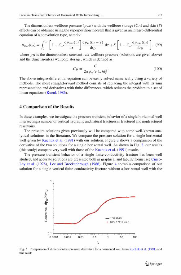
The pressure solutions given previously will be compared with some well-known ana-lytical solutions in the literature. We compare the pressure solution for a single horizontalwell given by Kuchuk et al. (1991) with our solution. Figure 3 shows a comparison of thederivative of the two solutions for a single horizontal well. As shown in Fig. 3, our results(this study) compare very well with those of the Kuchuk et al. (1991) results.

The pressure transient behavior of a single finite-conductivity fracture has been wellstudied, and accurate solutions are presented both in graphical and tabular forms; see Cinco-Ley et al. (1978), Lee and Brockenbrough (1986). Figure 4 shows a comparison of oursolution for a single vertical finite-conductivity fracture without a horizontal well with the

0.1

1

Der

ivat

ive,

dpD

/dln

t D

0.0001 0.001 0.01 0.1 1 10 100

tD

This study SPE 17413 Ex. 1

Fig. 3 Comparison of dimensionless pressure derivative for a horizontal well from Kuchuk et al. (1991) andthis work

123


0.1

1

p D

0.001 0.01 0.1 1 10 100 1000

tD

FD = 0.2 π (Cinco)FD = π (Cinco)FD = 2π (Cinco)FD = 10 π (Cinco)FD = 20 π (Cinco)FD = 0.2 π (this study)FD = π (this study)FD = 2π (this study)FD = 10 π (this study)FD = 20 π (this study)

Fig. 4 Comparison of dimensionless pressure for a single finite-conductivity vertical fracture with varyingconductivities from Cinco-Ley et al. (1978) and this work

Table 1 Formation, fluid, and fracture properties for a single fracture example

φm Fraction 0.1 (ct )m psi−1 3×10−6 μ cp 0.6 kmh = kmv mD 0.1

qo STB/D 25 B0 RB/STB 1.273 po psi 4200 h ft 50

lw ft 500 FD 10,000 l f (x f ) ft 210 rw ft 0.354

po initial reservoir pressurel f (x f ) fracture half-lengthFD dimensionless fracture conductivity

Cinco-Ley andSamaniego (1981) solution for various FD values. Riley et al. (2007) presentedone of the most accurate solutions available in the petroleum literature. Riley et al. (2007)obtained the dimensionless pressure for a vertical fracture with finite conductivity, wherethe fracture is assumed to have an elliptical cross section, the flow within the fracture to beincompressible, and the reservoir to be infinite. Their solution is a line-source solution, fromwhich they computed the wellbore pressure by using an equivalent wellbore radius. This isa reasonable approximation for the uniform-wellbore-pressure condition if the time is notvery small. The Riley et al. (2007) results, as can be observed from Table 1 of Biryukovand Kuchuk (2012a), are approximately 1% higher than the Biryukov and Kuchuk (2012a)results. This difference might be due to the use of an equivalent wellbore radius with a line-source solution by Riley et al. (2007), whereas Biryukov and Kuchuk (2012a) used a finite(actual) wellbore radius (in the dimensionless form rDw = 10−3) with the uniform-pressureboundary condition, which is the true boundary condition at the wellbore.

For transverse fractures, the effect of the horizontal wellbore cannot be ignored if thewell is either entirely completed barefoot (openhole) or cased and perforated over the entirewellbore. The flow contribution from the formation directly into the unfractured horizon-tal sections of the wellbore is negligible for high-conductivity fractures if the wellbore iscased and perforated in clusters over small sections, and hydraulically fractured. This is acommon practice in horizontal wells in shale formations. The next example will illustratethe importance of inclusion of the wellbore in the solutions. As we stated previously, mostpublished solutions on horizontal wells with multiple fractures in fractured and nonfractured(homogenous) reservoirs do not include the wellbore effect in the solution.

For this case, we will use the example given in one of the most recent articles publishedby Zhou et al. (2013). For this single-rectangular-fracture case, fracture, formation, and fluid

123


0.001

0.01

0.1

1

Der

ivat

ive,

dp D

/dln

t D

10-6 10-5 10-4 10-3 10-2 10-1 100 101 102

tD

m = 1/2Horizontal well radial

m = 1/2

m = 1/3

m = 0

without well with wellbore with horizontal well

only horizontal well

Fig. 5 Comparison of dimensionless pressure derivatives of a single vertical fracture with and without awellbore and a horizontal well

properties are given in Table 1 of Zhou et al. (2013) and in Table 1 of this paper with a fewadditions: a horizontal well and FD = 10,000 instead of 20. The reservoir is homogenousand infinite, the center of the well is located at {0, 0, 0} (in the middle of the formation fromthe top and bottom), and the transverse vertical fracture intersects the 1000-ft horizontal at{0, 0, 0} and penetrates the entire formation. We will investigate the behavior of three cases:(1) a single vertical fracture (denoted without well in Fig. 5), (2) a single vertical fracturewith the horizontal wellbore (denoted with wellbore) without the flow contribution from theformation into the horizontal section of the wellbore, and (3) a single vertical fracture withthe wellbore and the flow contribution from the formation into the horizontal section of thewellbore (denoted with horizontal well).

As shown in Fig. 5, the single vertical fracture derivatives with and without wellbore areexactly the same because as discussed previously for high fracture conductivities (FD), thehorizontal wellbore effect without the noncontributing horizontal section is negligible at earlytimes, and the fractures dominate the behavior of the system in homogenous reservoirs. Asexpected, the derivatives exhibit a formation-linear flow regime (m = 1/2) until about tD of30, after which an infinite-acting pseudoradial flow regime is observed. The same figure alsopresents the derivative of the horizontal well without the fracture in a homogenous reservoiras a bench mark. The horizontal well derivative exhibits a first radial flow regime aroundthe well and then an intermediate horizontal well linear flow regime from tD of 0.02 to 0.4before a horizontal well infinite-acting pseudoradial flow regime. The derivative (denotedwith horizontal well in Fig. 5) of the single vertical fracture with the contributing horizontalwell section over its entire length also exhibits a formation-linear flow regime (m = 1/2)until about tD of 3 × 10−5, after which it deviates from the formation-linear flow regimeuntil about tD of 0.02, after which the horizontal well dominates the derivative behavior, asshown by the “only horizontal well’ derivative in Fig. 5.

Figure 6 presents the dimensional derivatives to give an idea about the observability ofthese flow regimes. The formation-linear flow regime of the derivatives with and withoutwellbore last about 3h before the start of an infinite-acting pseudoradial flow regime. Theformation-linear flow regime of the derivative of the single vertical fracture with the con-tributing horizontal well lasts about 0.008h (less than 1min). Even without skin and wellborestorage effects, this flow regime would not be observable. Note that the derivative for thiscase exhibits a trilinear flow regime from 0.1 to 10h, perhaps a look-alike one. It exhibits anintermediate horizontal well linear flow regime from 10 to 20h. The infinite-acting pseudo-

123


0.1

1

10

100

Der

ivat

ive,

psi

10-4 10-3 10-2 10-1 100 101 102 103 104

Time, hr

m = 1/2Horizontal well radial

m = 1/2

m = 1/3

m = 0



Fig. 6 Comparison of dimensional pressure derivatives of a single vertical fracturewith andwithout awellboreand a horizontal well

1200

1000

800

600

400

200

0

Pre

ssur

e ch

ange

, Δp,

psi

300025002000150010005000

Time, hr

400 psi



Fig. 7 Comparison of pressure changes in a single vertical fracture with and without a wellbore and ahorizontal well

radial flow regime starts for all derivatives about 5000h, which is unlikely to be achieved fora reasonable well test duration.

Figure 7 presents the pressure changes for the three fracture cases and a single horizontalwell. A very large pressure change difference is observed between the fracture with andwithout wellbore cases and the fracture with the horizontal well contribution case. Figure 8presents the percentage differences for pressure changes and derivatives for the fracture with-out wellbore cases and the fracture with the horizontal well contribution case. As shown inthese plots, more than one hundred percent difference in pressure changes and derivativesare observed. Note also that the difference in derivatives goes down after 10h, and eventuallywill be small when all derivatives reach the infinite-acting pseudoradial flow regime at about5000h.

As shown here, the solutions (discussed above) without wellbore or the horizontal wellcontribution may have serious consequences for model identification and history matching,whichmay lead to serious inaccuracies in estimatingwell, fracture, and formation parametersfrom transientwell test data. This large difference in the pressure changes particularly for longtimes, as shown in Fig. 8, will have a very large impact on the rate behavior of the reservoir.

We compare our solution with the one given by Al-Kobaisi et al. (2006) shown in Fig. 9.This horizontal well example is given in Fig. 16 of the (Ozkan 2014) paper. As we discussed

123


150

100

50Diff

eren

ce, %

100806040200

Time, hr

pressure derivative

Fig. 8 Differences (%) in pressure changes and derivatives for a single vertical fracture without wellbore andwith a horizontal well

10-4

10-3

10-2

10-1

100

Der

ivat

ive,

dpD

/dln

t D

10-7 10-6 10-5 10-4 10-3 10-2 10-1 100 101

t D

m = 1/2

m = 0

m = 0

FD = 1 FD = 10 FD = 100 FD = 1000 FD = 1 SPE 92040 FD = 10 SPE 92040 FD = 100 SPE 92040 FD = 1000 SPE 92040

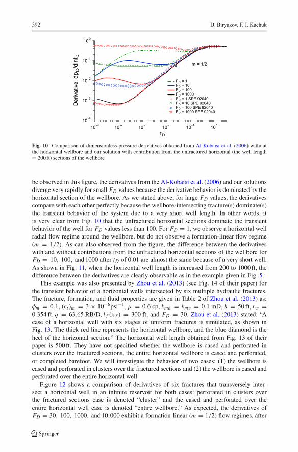
Fig. 9 Comparison of dimensionless pressure derivatives obtained from Al-Kobaisi et al. (2006) and oursolution without the unfractured horizontal (the well length = 200 ft) sections of the wellbore

above, the Al-Kobaisi et al. (2006) solution does not include the contributions of the unfrac-tured horizontal sections of the wellbore, but, unlike most other solutions, it does include thewellbore in the fracture plane. Therefore, as can be observed in Fig. 9, the derivative curvesfirst exhibit a fracture-radial flow regime (m = 0) and then a formation-linear flow regime(m = 1/2). Our results compare remarkably well with those of Al-Kobaisi et al. (2006) if weexclude the flow contributions from the unfractured horizontal sections of the wellbore. Aslight difference can be observed between the derivatives of the two solutions due to our exacttreatment of the uniform-wellbore-pressure condition. For low-finite-conductivity fractures,the duration of the fracture-radial flow regime becomes longer, and the formation-linear flowregime becomes shorter. The derivatives for FD = 1 do not exhibit a formation-linear flowregime. The derivatives for FD = 100 exhibit a very short fracture-radial flow regime, whichcannot be observed in real pressure transient well tests. As we said above, our solutions nor-mally include the flow contributions from the unfractured horizontal sections of the wellbore,but for this case we did not include them.

Figure 10 compares our solution that includes the flow contributions from the unfracturedhorizontal sections of the wellbore with the Al-Kobaisi et al. (2006) solution given in Fig. 16of their paper.We assume that the horizontalwell length in this case is 200 ft,which is the sameas the fracture length (see Table 1 of Al-Kobaisi et al. 2006) and is a very short well. As can

123


10-4

10-3

10-2

10-1

100

Der

ivat

ive,

dpD/d

lnt D

10-9 10-7 10-5 10-3 10-1 101

tD

m = 1/2


Fig. 10 Comparison of dimensionless pressure derivatives obtained from Al-Kobaisi et al. (2006) withoutthe horizontal wellbore and our solution with contribution from the unfractured horizontal (the well length= 200 ft) sections of the wellbore

be observed in this figure, the derivatives from the Al-Kobaisi et al. (2006) and our solutionsdiverge very rapidly for small FD values because the derivative behavior is dominated by thehorizontal section of the wellbore. As we stated above, for large FD values, the derivativescompare with each other perfectly because the wellbore-intersecting fracture(s) dominate(s)the transient behavior of the system due to a very short well length. In other words, itis very clear from Fig. 10 that the unfractured horizontal sections dominate the transientbehavior of the well for FD values less than 100. For FD = 1, we observe a horizontal wellradial flow regime around the wellbore, but do not observe a formation-linear flow regime(m = 1/2). As can also observed from the figure, the difference between the derivativeswith and without contributions from the unfractured horizontal sections of the wellbore forFD = 10, 100, and 1000 after tD of 0.01 are almost the same because of a very short well.As shown in Fig. 11, when the horizontal well length is increased from 200 to 1000 ft, thedifference between the derivatives are clearly observable as in the example given in Fig. 5.

This example was also presented by Zhou et al. (2013) (see Fig. 14 of their paper) forthe transient behavior of a horizontal wells intersected by six multiple hydraulic fractures.The fracture, formation, and fluid properties are given in Table 2 of Zhou et al. (2013) as:φm = 0.1, (ct )m = 3 × 10−6psi−1, μ = 0.6 cp, kmh = kmv = 0.1 mD, h = 50 ft, rw =0.354 ft, q = 63.65 RB/D, l f (x f ) = 300 ft, and FD = 30. Zhou et al. (2013) stated: “Acase of a horizontal well with six stages of uniform fractures is simulated, as shown inFig. 13. The thick red line represents the horizontal wellbore, and the blue diamond is theheel of the horizontal section.” The horizontal well length obtained from Fig. 13 of theirpaper is 500 ft. They have not specified whether the wellbore is cased and perforated inclusters over the fractured sections, the entire horizontal wellbore is cased and perforated,or completed barefoot. We will investigate the behavior of two cases: (1) the wellbore iscased and perforated in clusters over the fractured sections and (2) the wellbore is cased andperforated over the entire horizontal well.

Figure 12 shows a comparison of derivatives of six fractures that transversely inter-sect a horizontal well in an infinite reservoir for both cases: perforated in clusters overthe fractured sections case is denoted “cluster” and the cased and perforated over theentire horizontal well case is denoted “entire wellbore.” As expected, the derivatives ofFD = 30, 100, 1000, and 10,000 exhibit a formation-linear (m = 1/2) flow regimes, after

123


10-4

10-3

10-2

10-1

100

Der

ivat

ive,

dpD/d

lnt D

10-7 10-6 10-5 10-4 10-3 10-2 10-1 100 101

tD

m = 1/2

m = 0

m = 0

m = 0 m = 1/2


Fig. 11 Comparison of dimensionless pressure derivatives obtained from Al-Kobaisi et al. (2006) withoutthe horizontal wellbore and our solution with contribution from the unfractured horizontal (the well length= 1000 ft) sections of the wellbore

1

10

100

Der

ivat

ive,

psi

0.0001 0.001 0.01 0.1 1 10 100 1000 Time, hr

m = 1/4

m = 1/2

m ≈ 1

m = 0

m = 0

FD = 1 cluster FD = 10 cluster FD = 30 cluster FD = 100 cluster FD = 1000 cluster FD = 10000 cluster

FD = 1 entire wellbore FD = 10 entire wellbore FD = 30 entire wellbore FD = 100 entire wellbore FD = 1000 entire wellbore FD = 10000 entire wellbore

Fig. 12 Comparison of derivatives from the six fracture solutions with cluster perforations and perforationsover the entire horizontal wellbore

0.01

0.1

1

10

100

Diff

eren

ce, %

0.0001 0.001 0.01 0.1 1 10

Time, hr

F D = 1 F D = 10 F D = 30 F D = 100 F D = 1000 F D = 10000

Fig. 13 Difference (%) in pressure changes in cluster perforations and perforations over the entire horizontalwellbore cases

123


1

10

100

Der

ivat

ive,

psi

0.01 0.1 1 10 100 1000 Time, hr

m = 1/2

m = 1/4

m = 0

FD = 1without - this study FD = 1 without - SPE 157367 FD = 10without - this study FD = 10 without - SPE 157367 FD = 30 without - this study FD = 30 without - SPE 157367

FD = 1 entire wellbore FD = 10 entire wellbore FD = 30 entire wellbore

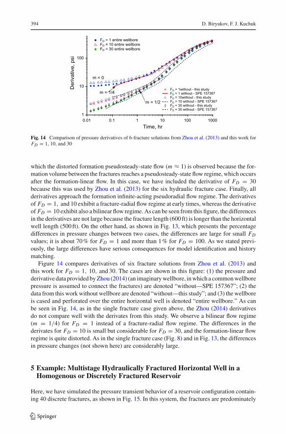
Fig. 14 Comparison of pressure derivatives of 6-fracture solutions from Zhou et al. (2013) and this work forFD = 1, 10, and 30

which the distorted formation pseudosteady-state flow (m ≈ 1) is observed because the for-mation volume between the fractures reaches a pseudosteady-state flow regime, which occursafter the formation-linear flow. In this case, we have included the derivative of FD = 30because this was used by Zhou et al. (2013) for the six hydraulic fracture case. Finally, allderivatives approach the formation infinite-acting pseudoradial flow regime. The derivativesof FD = 1, and 10 exhibit a fracture-radial flow regime at early times, whereas the derivativeof FD = 10 exhibit also a bilinear flow regime.As can be seen from this figure, the differencesin the derivatives are not large because the fracture length (600 ft) is longer than the horizontalwell length (500 ft). On the other hand, as shown in Fig. 13, which presents the percentagedifferences in pressure changes between two cases, the differences are large for small FD

values; it is about 70% for FD = 1 and more than 1% for FD = 100. As we stated previ-ously, the large differences have serious consequences for model identification and historymatching.

Figure 14 compares derivatives of six fracture solutions from Zhou et al. (2013) andthis work for FD = 1, 10, and 30. The cases are shown in this figure: (1) the pressure andderivative data provided byZhou (2014) (an imaginarywellbore, inwhich a commonwellborepressure is assumed to connect the fractures) are denoted “without—SPE 157367”; (2) thedata from this work without wellbore are denoted “without—this study”; and (3) the wellboreis cased and perforated over the entire horizontal well is denoted “entire wellbore.” As canbe seen in Fig. 14, as in the single fracture case given above, the Zhou (2014) derivativesdo not compare well with the derivates from this study. We observe a bilinear flow regime(m = 1/4) for FD = 1 instead of a fracture-radial flow regime. The differences in thederivates for FD = 10 is small but considerable for FD = 30, and the formation-linear flowregime is quite distorted. As in the single fracture case (Fig. 8) and in Fig. 13, the differencesin pressure changes (not shown here) are considerably large.

5 Example: Multistage Hydraulically Fractured Horizontal Well in aHomogenous or Discretely Fractured Reservoir

Here, we have simulated the pressure transient behavior of a reservoir configuration contain-ing 40 discrete fractures, as shown in Fig. 15. In this system, the fractures are predominately

123


-5

-4

-3

-2

-1

0

1

2

3

4

5

yD c

oord

inat

e

-5 -4 -3 -2 -1 0 1 2 3 4 5

xD coordinate

0.00

0.00

well

natural fractures

hydraulic fractures

NORTH

EAST

Fig. 15 Distributions of fractures in a discretely fractured reservoir, and a horizontal well intersected by 40vertical hydraulic fractures, where the well is located at {0, 0, 0}

Fig. 16 Schematic of a horizontal well intersected by vertical hydraulic fractures

in the northeast direction, fully penetrate the formation, and are vertical and disjointed.Let us consider a 1000-ft horizontal well in the x direction completed in the reservoir,where the center of the well is located at {0, 0, 0}, and the well is hydraulically frac-tured, as shown in Figs. 15 and 16. We will investigate the behavior of these threecases: (1) a horizontal well with only hydraulic fractures in a homogenous (nonfractured)reservoir; (2) a horizontal well in a naturally fractured reservoir without any hydraulicfractures; and (3) a horizontal well in a naturally fractured reservoir with 40 hydraulicfractures (Fig. 15) for FD = 0.01, 0.1, 1, 10, 100, 1000, and 10,0000. For the exampleof the horizontal well in a naturally fractured reservoir with hydraulic fracture, forma-tion, and fluid properties are given in Table 2. In this system, each transverse hydraulicfracture intersects the horizontal well every 20 ft and extends 400 ft (the half fracturelength l f ) in the y direction. The total number of hydraulic fractures in the x directionis 40.

For each run, the dimensionless conductivity of 40 fractures remains the same, but is variedfrom 10−2 to 10,0000 to compute dimensionless pressures and derivatives. For the first case,

123


Table 2 Formation, fluid, and fracture properties for a horizontal well in a homogenous or discretely fracturedreservoirs with hydraulic fractures

φm Fraction 0.2 (ct )m psi−1 1.5×10−5 μ cp 1.0 q B/D 5000

kmh = kmv mD 1 k f mD 106 h ft 100 rw ft 0.354

lw ft 500 l f ft 400 b mm 2 (0.0066 ft) zw ft 50

b fracture aperturezw distance from the wellbore to the bottom boundary

10-5

10-4

10-3

10-2

10-1

Der

ivat

ive,

dp D

/dln

t D

10-7

10-5

10-3

10-1

101

103

tD

m = 1/2

m = 1

horizontal well radial

FD = 0.01

FD = 0.1

FD = 1

FD = 10

FD = 100

FD = 1000

FD = 10000

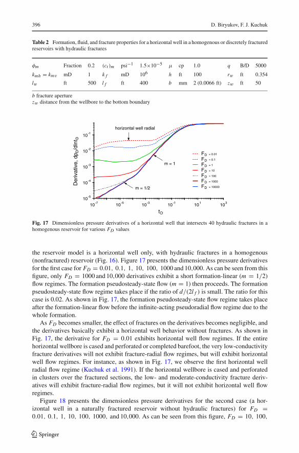
Fig. 17 Dimensionless pressure derivatives of a horizontal well that intersects 40 hydraulic fractures in ahomogenous reservoir for various FD values

the reservoir model is a horizontal well only, with hydraulic fractures in a homogenous(nonfractured) reservoir (Fig. 16). Figure 17 presents the dimensionless pressure derivativesfor the first case for FD = 0.01, 0.1, 1, 10, 100, 1000 and 10,000. As can be seen from thisfigure, only FD = 1000 and 10,000 derivatives exhibit a short formation-linear (m = 1/2)flow regimes. The formation pseudosteady-state flow (m = 1) then proceeds. The formationpseudosteady-state flow regime takes place if the ratio of d/(2l f ) is small. The ratio for thiscase is 0.02. As shown in Fig. 17, the formation pseudosteady-state flow regime takes placeafter the formation-linear flow before the infinite-acting pseudoradial flow regime due to thewhole formation.

As FD becomes smaller, the effect of fractures on the derivatives becomes negligible, andthe derivatives basically exhibit a horizontal well behavior without fractures. As shown inFig. 17, the derivative for FD = 0.01 exhibits horizontal well flow regimes. If the entirehorizontal wellbore is cased and perforated or completed barefoot, the very low-conductivityfracture derivatives will not exhibit fracture-radial flow regimes, but will exhibit horizontalwell flow regimes. For instance, as shown in Fig. 17, we observe the first horizontal wellradial flow regime (Kuchuk et al. 1991). If the horizontal wellbore is cased and perforatedin clusters over the fractured sections, the low- and moderate-conductivity fracture deriv-atives will exhibit fracture-radial flow regimes, but it will not exhibit horizontal well flowregimes.

Figure 18 presents the dimensionless pressure derivatives for the second case (a hor-izontal well in a naturally fractured reservoir without hydraulic fractures) for FD =0.01, 0.1, 1, 10, 100, 1000, and 10,000. As can be seen from this figure, FD = 10, 100,

123


10-4

10-3

10-2

10-1

Der

ivat

ive,

dp D

/dln

t D

10-7

10-5

10-3

10-1

101

103

tD

m = 1/2

m = 1/4


FD = 0.01

FD = 0.1

FD = 1

FD = 10

FD = 100

FD = 1000

FD = 10000

Fig. 18 Dimensionless pressure derivatives of a horizontal well in a naturally fractured reservoir for variousFD values

10-5

10-4

10-3

10-2

10-1

Der

ivat

ive,

dp D

/dln

t D

10-7 10-5 10-3 10-1 101 103

t D

m = 1/2

m = 1


FD = 0.01

FD = 0.1

FD = 1

FD = 10

FD = 100

FD = 1000

FD = 10000

Fig. 19 Dimensionless pressure derivatives of a horizontal well that intersects 40 hydraulic fractures in anaturally fractured reservoir for various FD values

1000, and 10,000 derivatives exhibit a very long formation-linear (m = 1/2) flow regimecompared to the linear flow regime observed in Fig. 17. For this case, eight natural fractureswith different lengths intersect the horizontal well and extend from the well center into theformation that is 4.5 times thewell length. Therefore, the formation-linear flow regime is verylong. The derivative FD = 10 exhibits a 1/4-slope bilinear flow regime at early times mostlikely after a fracture-radial flow regime. This radial flow regime cannot be the formation-radial flow regime around the horizontal well because the derivative value (slope) is small. Aswith the first case, the effect of natural fractures on the derivatives becomes negligible, and thederivatives basically exhibit a horizontal well behavior without fractures for small FD values.It should be noted that a formation pseudosteady-state flow regime is absent for this case.

Figure 19 presents the dimensionless pressure derivatives for the third case (a horizon-tal well in a naturally fractured reservoir with hydraulic fractures, as shown in Fig. 15) forFD = 0.01, 0.1, 1, 10, 100, 1000, and 10,000.As can be seen from this figure, the behaviorin this case is very similar to that of the first case as shown in Fig. 17 because the wellbore-intersecting 40 hydraulic fractures and eight natural fractures dominate the behavior of thesystem.

123


6 Conclusions

In this paper, we have presented solutions for the pressure transient behavior of horizontalwells intersected by multiple hydraulic and/or natural fractures in homogenous (nonfrac-tured) and naturally fractured reservoirs. A mesh-free semi-analytical technique was usedfor obtaining pressure transient solutions to multistage fractured horizontal wells in continu-ously and discretely naturally fractured and homogenous reservoirs. Our solution techniqueis based on the boundary element method, which has advantages such as the absence ofgrids, reduced dimensionality, and the ability to obtain continuous rather than discrete solu-tions. This technique is sufficiently general and can be applied to many different reservoirgeological settings and well geometries.

In our solutions, naturally fractured reservoirs can contain periodically or arbitrarily dis-tributed finite- and/or infinite-conductivity fractures with different lengths and orientations.There are many factors, including fracture conductivities, lengths, and distributions as well aswhether or not fractures intersect the wellbore, that dominate the pressure transient behaviorof horizontal wells intersected by multiple hydraulic fractures in naturally fractured reser-voirs.

Our solutions are compared with a number of existing solutions published in the literature.It has been shown that most of the published solutions ignore the contribution to flow fromthe formation directly into the unfractured horizontal sections of the wellbore. With oneexception, the published solutions did not include the wellbore in the fracture plane. Some ofthe flow regimes from these solutions are therefore incorrect and superfluous. Our solutionincludes the effects of the wellbore in the fracture plane and the unfractured horizontalsections of the wellbore. In addition, our solutions are also given for horizontal wells withmultistage hydraulic fractures in continuously and discretely naturally fractured reservoirswithout using the no-fracture containing Warren and Root dual-porosity type models. In oursolutions, all or some of the multistage hydraulic fractures may intersect the natural fractures,which is very important for shale gas and oil reservoir production.

It is shown that the solutions without the wellbore and the unfractured sections cannotcapture the true early-time response, such as fracture-radial flow.More than one hundred per-cent difference in pressure changes and derivatives are observed among these solutions withand without the unfractured sections. This large difference will have serious consequencesfor model identification and history matching, which may lead to serious inaccuracies inestimating well, fracture, and formation parameters from transient well test data.

The exact treatment of the uniform-wellbore-pressure condition and the inclusion of thewellbore and the unfractured sections of the horizontal well result in the identification of newflow regimes that were not apparent from most of the published solutions.

Diagnostic derivative plots have been presented for a variety of horizontal wells withmultiple fractures in homogenous and naturally fractured reservoirs. It has been shown thatthese reservoirs exhibit many different flow regimes.

Acknowledgments The authors are grateful to Schlumberger for permission to publish this paper. Wewould like to thank Professor Erdal Ozkan, Petroleum Engineering Department, Colorado School of Mines,and Wentao Zhou, Schlumberger, for providing tables for the graphical data given in the Al-Kobaisi et al.(2006) and Zhou et al. (2013) papers, respectively. We also would like to thank Kirsty Morton and TonyFitzpatrick, Schlumberger, for valuable discussions.

Open Access This article is distributed under the terms of the Creative Commons Attribution 4.0 Inter-national License (http://creativecommons.org/licenses/by/4.0/), which permits unrestricted use, distribution,and reproduction in any medium, provided you give appropriate credit to the original author(s) and the source,provide a link to the Creative Commons license, and indicate if changes were made.

123

http://creativecommons.org/licenses/by/4.0/


Appendices

Appendix 1: Evaluating Functions Λ and Z: Computing Time Integrals—GridGeneration

In this appendix, we will present some aspects of evaluating the functions Λ(z, t, z0, h, u)

defined by Eq. (49) and Z(z, t, z0, h, u) defined by Eq. (58). The computations might presentsome difficulties because they are expressed in terms of an infinite series. For large andmoderate h2/t values, these series converge very fast; thus, the only problem that may ariseis for small h2/t . Using the Poisson summation formula, these series can be rewritten as

Λ(z, t, z0, h, u) = 2u

h+

∞∑

j=1

2

π je− π2 j2 t

h2

{

sin

(

(u − z)jπ

h

)

+ sin

(

(u + z + 2z0 − h)jπ

h

)}

, (101)

Z(z, t, z0, h, u) = 2√

π t

h+

√π t

h

∞∑

j=1

2

π je− π2 j2 t

h2

{

cos

(

(u − z)jπ

h

)

+ cos

(

(u + z + 2z0 − h)jπ

h

)}

. (102)

It can be seen that these series converge very fast for small values of h2/t .

Now, let us discuss the evaluation of integrals of the type Gmns[i]v = ∫ t s

v+1t sv

Gmn[i] (. . . , t)dt .

On interval [t sv , t s

v+1], the function Gmn[i] can be approximated as

Gmn[i] (. . . , t) ≈ Ctαe−β/t , (103)

and thus, the integral can be rewritten in the following form:

Gmns[i]v ≈ C(t s

v+1)α+1

∫ 1

tsvtsv+1

uαe− β

tsv+1

(1u −1

)

du. (104)

Note that t sv

t sv+1

can take only a finite number of values on the time grid that we built. On every

interval[

t sv

t sv+1

, 1], we can use the following approximation:

1

u− 1 ≈ av + bv ln u, (105)

where a and b can be determined in advance by means of an optimization method and thenstored. Finally, we can obtain the following approximate expression for Gmns

[i]v :

Gmns[i]v ≈ Ce

− βavtsv+1 (t s

v+1)α+1

∫ 1

tsvtsv+1

uα− βbv

tsv+1 du

≈

⎧⎪⎨

⎪⎩

Gmn[i] (...,t sv+1)t

sv+1−Gmn[i] (...,t s

v )t sv

α+1− βbvtsv+1

, if α − βbv

t sv+1

+ 1 = 0,

Gmn[i] (. . . , t s

v+1)tsv+1 ln

t sv+1t sv

, otherwise.(106)

123


The last point that we will present is the grid construction. For the fractures that do notintersect any producing horizontal well sections or along the axis of the horizontal well, wesuggest using Chebyshev grids as follows:

xmf i = − cos

(π(n − 1)

M f i

)

, m = 1, . . . , M f i + 1, (107)

znf i = − cos

(π(m − 1)

N f i

)

, n = 1, . . . , N f i + 1, (108)

xnhi = − cos

(π(n − 1)

Nhi

)

, n = 1, . . . , Nhi + 1 (109)

because they have very good approximation and convergence properties and allows us toeasily account for flux singularities near the edges of the fracture or the producing horizontalwell sections. On the other hand, a simple uniform grid in the normal cross sections of thehorizontal well in the form

zmhi = ym

hi = −1 + 2m

Mhi/4 + 1, m = 1, . . . , Mhi/4 + 1, (110)

appears to be sufficient. Particularly, we find that N[i] = M[i] = 16 provides very goodaccuracy and computational speed. Also, as the distance from the wellbore to the fracturesincreases, the number of grid cells N f i and M f i can be safely reduced without impactingthe accuracy of the production well pressure response. If the fracture intersects the hori-zontal well, we suggest choosing a grid that consists of Chebyshev nodes near the fractureedges and becomes logarithmic near the wellbore, which would allow us to account for bothflux singularities (i.e., near the fracture edges and near the wellbore, respectively). In ourcomputations, we used the following grid:

xmf i =

⎧⎪⎪⎪⎪⎪⎪⎪⎪⎪⎪⎪⎪⎪⎪⎨

⎪⎪⎪⎪⎪⎪⎪⎪⎪⎪⎪⎪⎪⎪⎩

ξi j − (1 + ξi j ) cos(

π(m−1)M f i /2+3

), m = 1, . . . , M f i/4 + 1,

ξi j − rwxi

(ξi j −x

M f i /4+1

f irwxi

) M f i /2−mM f i /4−1

, m = M f i/4 + 2, . . . , M f i/2,

ξi j , m = M f i/2 + 1,

ξi j + rwxi

(x3M f i /4+1

f i −ξi j

rwxi

)m−M f i /2−2M f i /4−1

, m = M f i/2 + 2, . . . , 3M f i/4,

ξi j + (1 − ξi j ) cos(

π(M f i +1−m)

M f i /2+3

), m = 3M f i/4 + 1, . . . , M f i + 1,

(111)

znf i =

⎧⎪⎪⎪⎪⎪⎪⎪⎪⎪⎪⎪⎪⎪⎪⎨

⎪⎪⎪⎪⎪⎪⎪⎪⎪⎪⎪⎪⎪⎪⎩

ζi j − (1 + ζi j ) cos(

π(n−1)N f i /2+3

), n = 1, . . . , N f i/4 + 1,

ζi j − rwzi

(ζi j −z

N f i /4+1

f irwzi

) N f i /2−nN f i /4−1

, n = N f i/4 + 2, . . . , N f i/2,

ζi j , N = N f i/2 + 1,

ζi j + rwzi

(x3N f i /4+1

f i −ζi j

rwzi

) N−N f i /2−2N f i /4−1

, N = N f i/2 + 2, . . . , 3N f i/4,

ζi j + (1 − ζi j ) cos(

π(N f i +1−N )

N f i /2+3

), N = 3N f i/4 + 1, . . . , N f i + 1,

(112)

123


where rwxi = rwhjsin αi j l f i

and rwzi = rwhjh f i

. Four cells contained inside of the well cross section

and the corresponding coefficients cmnf i should be discarded from the systems in Eqs. (68)–

(76).

Appendix 2: Evaluating Functions Φ, ϕ, E and ε

In this appendix, we will describe a possible approach for evaluating functions Φ,ϕ, E , andε. First, let us begin by solving a problem specified by Eqs. (79)–(81) to obtain the functionΦ(x, z, x1, x2, z1, z2, ν). Generally, it is possible to solve this problem exactly by usingthe standard Fourier series decomposition technique, but we will provide a semi-analyticalapproach that is faster and has better convergence properties. Let us assume for simplicitythat x1+x2

2 ≥ 0 and z1+z22 ≥ 0; i.e., that the center of the right-hand side source term lies

in the first coordinate quadrant (otherwise, we can rotate the coordinate system in order toachieve identical configuration). Let us also extend the domain to−1 < x < 3, −1 < z < 3(see Fig. 20) (to improve convergence properties). In the extended domain, our problem willbe as follows:

∂2Φ

∂x2+ ν2

∂2Φ

∂z2=

1∑

i=0

1∑

j=0

ω(x, xi1, xi

2)ω(z, z j1, z j

2) − 1, (113)

∂Φ

∂x(x, z) = 0, |x − 1| = 2, −1 ≤ z ≤ 3, (114)

∂Φ

∂z(x, z) = 0, −1 ≤ x ≤ 3, |z − 1| = 2, (115)

where xik = 2i + (−1)i xk and z j

k = 2 j + (−1) j zk . Now, let us assume that we have a sourcedistribution along the boundaries of the extended domain in the following form:

(x1, z2)

2β

(x1, z1)

(x2, z2)

(x2, z1)

(1,1)

x

z

0

2α

(ξ, ζ)

(3,1)

(-1,1)

(-1,-1)

(1,-1)

(3,-1)

(3,3)

Fig. 20 Extended domain problem (Eqs. 113–115)

123


q1(x) =N∑

n=1

anT2n

( x−12

)

√1 − (1 − x)2/4

, |z − 1| = 2, −1 < x < 3, (116)

q2(z) =N∑

n=1

bnT2n

( z−12

)

√1 − (1 − z)2/4

, |x − 1| = 2, −1 < z < 3. (117)

Note that we used only even polynomials and the same expansion coefficients on oppositesides due to the symmetry of the problem. Now, Φ can be written as

Φ(x, z) =N∑

n=1

an

{

S2n

(

−1 − x

2, ν

1 + z

2, 2

)

+ S2n

(

−1 − x

2, ν

3 − z

2, 2

)}

+N∑

n=1

bn

{

S2n

(

−1 − z

2,1 + x

2ν, 2ν

)

+ S2n

(

−1 − z

2,3 − x

2ν, 2ν

)}

+1∑

l=0

1∑

k=0

(−1)k+l

⎧⎨

⎩

1∑

i=0

1∑

j=0

F(

x − xik, ν(z − z j

l ))

ν(x2 − x1)(z2 − z1)

− F(x − (−1)k, ν(z − (−1)l)

)

4ν

}

, (118)

where

S2n(x, z, r) = 1

2π

∫ π

0ln

(r2(x − cos θ)2 + y2

)cos(2nθ)dθ, (119)

F(x, y) = 1

2π

∫ ∫

ln((x − ξ)2 + (z − ζ )2)dξdζ

= 1

2π

[xy(ln(x2 + y2) − 3) + x2atan(y/x) + y2atan(x/y)

]. (120)

Using the table of integrals from Prudnikov et al. (1981) we can evaluate Sn in closed form:

S0(x, z, r) ={

(−Re ln(Z2 + √Z2 − 1) + ln(2r)), if |Z | ≤ 1,

(−Re ln(Z2 − √Z2 − 1) + ln(2r)), if |Z | > 1,

(121)

Sn(x, z, r) ={

− 12nRe(Z2 + √

Z2 − 1)2n, if |Z | ≤ 1,

− 12nRe(Z2 − √

Z2 − 1)2n, if |Z | > 1,(122)

where Z = |x |+i |z|. The unknown coefficients an and bn can be obtained from the conditionof no-flow on the outer boundaries:

∂Φ

∂z(xm,−1) = 0, m = 1, . . . , N , (123)

∂Φ

∂x(−1, zm) = 0, m = 1, . . . , N , (124)

where zm = xm = 2 cos(

π(m−0.5)2N

)− 1 is a set of shifted Chebyshev nodes. Due to the

excellent convergence properties of Chebyshev Polynomials, a small number of equationsis sufficient. In particular, we found N = 10 (thus, 20 equations) to provide a sufficientaccuracy. Similarly, we can find the solution for the problem defined by Eqs. (86)–(88).Again, we assume that x0 > 0, z1+z2

2 > 0, and to improve the convergence properties of the

123


solution, we suggest solving it in the extended domain −1 < x < 3,−1 < z < 3 where itwill take the following form:

∂2ϕ

∂x2+ ν2

∂2ϕ

∂z2=

1∑

i=0

1∑

j=0

ω(x, z j1, z j

2)δ(xi0) − 1, (125)

∂ϕ

∂x(x, z) = 0, |x − 1| = 2, −1 ≤ z ≤ 3, (126)

∂ϕ

∂z(x, z) = 0, −1 ≤ x ≤ 3, |z − 1| = 2, (127)

where xi0 = 2i+(−1)i x0.Again,we assume that the source distribution on the boundaries can

be written in the form given by Eqs. (116)–(117). Thus, we obtain the following expressionfor ϕ:

ϕ(x, z) =N∑

n=1

an

{

S2n

(

−1 − x

2, ν

1 + z

2, 2

)

+ S2n

(

−1 − x

2, ν

3 − z

2, 2

)}

+N∑

n=1

bn

{

S2n

(

−1 − z

2,1 + x

2ν, 2ν

)

+ S2n

(

−1 − z

2,3 − x

2ν, 2ν

)}

+1∑

l=0

(−1)l

⎧⎨

⎩

1∑

i=0

1∑

j=0

f(ν(z − z j

l ), x − xi0

)

ν(z2 − z1)

−1∑

k=0

(−1)k F(x − (−1)k, ν(z − (−1)l)

)

4ν

}

,

(128)

where

f (x, y) = 1

2π

∫

ln((x − ξ)2 + y2)dξ = 2

π

[x ln(x2 + y2) − 2x + 2yatan(x/y)

]. (129)

The unknown coefficients an and bn can be obtained from the condition of no-flow on theouter boundaries:

∂ϕ

∂z(xm,−1) = 0, m = 1, . . . , N , (130)

∂ϕ

∂x(−1, zm) = 0, m = 1, . . . , N . (131)

Note that due to domain extension, the problem can be solved correctly even if the line sourceis situated exactly at the original domain boundary (x0 = 1).

Now, let us solve the problem defined by Eqs. (82)–(85). We assume that the source centeris positioned in the first coordinate quadrant and similarly to the previous cases, we extendthe domain of the problem as follows:

∂2E

∂x2+ ν2

∂2E

∂z2=

1∑

i=0

1∑

j=0

ω(x, xi1, xi

2)ω(z, z j1, z j

2),

{|x − 1| < 1, |z − 1| < 1} and2⋂

i=1

2⋂

j=1

{

max(|x − ξi |

α,|z − ζ j |

β) > 1

}

, (132)

123


∂ E

∂x(x, z) = 0, |x − 1| = 2, −1 ≤ z ≤ 3, (133)

∂ E

∂z(x, z) = 0, −1 ≤ x ≤ 3, |z − 1| = 2, (134)

E(x, z) = 0, if max(|x − ξi |/α, |z − ζ j |/β) = 1, i = 1, 2, j = 1, 2 (135)∫ α

−α

∂ E

∂z(x, ζ j + β) − ∂ E

∂z(x, ζ j − β)dx +

∫ β

−β

∂ E

∂x(ξi + α, z) − ∂ E

∂x(ξi − α, z)dz = 1.

(136)

We assume that the source distribution over the outer boundaries can be represented as it isin Eqs. (116) and (117), and in the following form:

qw1 (x) =

Nw∑

n=1

c1nω(

x, xni , xn+1

i

), |x − ξi | < α, z = ζ j + β, (137)

qw2 (x) =

Nw∑

n=1

c2nω(

x, xni , xn+1

i

), |x − ξi | < α, z = ζ j − β, (138)

qw3 (z) =

Nw∑

n=1

c3nω(

z, znj , zn+1

j

), x = ξi + α, |z − ζ j | < β, (139)

qw4 (z) =

Nw∑

n=1

c4nω(

z, znj , zn+1

j

), x = ξi − α, |z − ζ j | < β, (140)

on inner boundaries, where zni = ζi + β cos

(πnNw

)is the Chebyshev grid and xn

i = ξi +α cos

(πnNw

). Note that the source distribution is the same on all inner boundaries due to

symmetry (see Fig. 21).Now, we obtain the following expression for E(x, z):

E(x, z) =N∑

n=1

an

{

S2n

(

−1 − x

2, ν

1 + z

2, 2

)

+ S2n

(

−1 − x

2,3 − z

2, 2

)}

+N∑

n=1

bn

{

S2n

(

−1 − z

2,1 + x

2ν, 2ν

)

+ S2n

(

−1 − z

2,3 − x

2ν, 2ν

)}

+2∑

k=1

Nw∑

n=1

ckn

1∑

l=0

(−1)l1∑

i=0

1∑

j=0

f(

x − xn+li , ν(z − ζ j + (−1)kβ)

)

xn+1i − xn

i

+4∑

k=3

Nw∑

n=1

ckn

1∑

l=0

(−1)l1∑

i=0

1∑

j=0

f(ν(

z − zn+lj

), (x − ξi + (−1)kα)

)

ν(

zn+1i − zn

i

)

+1∑

l=0

1∑

k=0

(−1)k+l1∑

i=0

1∑

j=0

F(

x − xik, ν

(z − z j

l

))

ν(x2 − x1)(z2 − z1).

(141)

123


(x1, z2)

(x1, z1)

(x2, z2)

(x2, z1)

(1,1)

x

z

0

(3,1)

(-1,1)

(-1,-1)

(1,-1)

(3,-1)

(3,3)

Fig. 21 Extended domain problem (Eqs. 132–136)

The unknown coefficients an, bn , and ckn can be obtained from the conditions imposed on the

outer and inner boundaries:

∂ E

∂z(xm,−1) = 0, m = 1, . . . , N , (142)

∂ E

∂x(−1, zm) = 0, m = 1, . . . , N , (143)

E(xm1 , ζ ± β

) = 0, m = 1, . . . , Nw, (144)

E(ξ ± α, zm

1

) = 0, m = 1, . . . , Nw, (145)

where xm1 = (xm+1

1 + xm1 )/2 and zm

1 = (zm+11 + zm

1 )/2 is a set of “quasi-Chebyshev”collocation nodes. A modest number of Nw = N = 10 (i.e., 60 equations in total) yieldsvery good accuracy.

Finally, similar technique can be used to find the solution of Eqs. (89)–(92) in the followingform:

ε(x, z) =N∑

n=1

an

{

S2n

(

−1 − x

2, ν

1 + z

2, 2

)

+ S2n

(

−1 − x

2,3 − z

2, 2

)}

+N∑

n=1

bn

{

S2n

(

−1 − z

2, ν

1 + x

2ν, 2ν

)

+ S2n

(

−1 − z

2,3 − x

2ν, 2ν

)}

+2∑

k=1

Nw∑

n=1

ckn

1∑

l=0

(−1)l1∑

i=0

1∑

j=0

f(

x − xn+li , ν(z − ζ j + (−1)kβ)

)

xn+1i − xn

i

123


+4∑

k=3

Nw∑

n=1

ckn

1∑

l=0

(−1)l1∑

i=0

1∑

j=0

f(ν(

z − zn+lj

), (x − ξi + (−1)kα)

)

ν(

zn+1i − zn

i

)

+1∑

l=0

(−1)l1∑

i=0

1∑

j=0

f(ν(

z − z jl

), x − xi

0

)

ν(z2 − z1). (146)

The unknown coefficients are obtained from the following boundary conditions given as

∂ε

∂z(xm,−1) = 0, m = 1, . . . , N , (147)

∂ε

∂x(−1, zm) = 0, m = 1, . . . , N , (148)

ε(xm1 , ζ ± β

) = 0, m = 1, . . . , Nw, (149)

ε(ξ ± α, zm

1

) = 0, m = 1, . . . , Nw. (150)

References

Abdulal, H.J., Samandarli, O., Wattenbarger, B.A.: New type curves for shale gas wells with dual porositymodel. In: Paper SPE-149367-MS, Canadian Unconventional Resources Conference, 15–17 November,Alberta, Canada (2011)

Aguilera, R., Ng, M.: Transient pressure analysis of horizontal wells in anisotropic naturally fractured reser-voirs. SPE Form. Eval. 6(1), 95–100 (1991)

Akresh, S.B., Al-Obaid, R., Al-Ajaji, A.: Inter-reservoir communication detection via pressure transient analy-sis: integrated approach. In: Paper SPE-88678-MS, Abu Dhabi International Conference and Exhibition,10–13 October, Abu Dhabi, United Arab Emirates (2004)

Al-Kobaisi, M., Ozkan, E., Kazemi, H.: A hybrid numerical/analytical model of a finite-conductivity verticalfracture intercepted by a horizontal well. SPE Reserv. Eval. Eng. 9(4), 345–355 (2006)

Al-Thawad, F., Agyapong, D., Banerjee, R., Issaka, M.: Pressure transient analysis of horizontal wells in afractured reservoir; gridding between art and science. In: Paper SPE 87013, SPE Asia Pacific Conferenceon Integrated Modelling for Asset Management, Kuala Lumpur, Malaysia, 29–30 March (2004)

Al-Thawad, F., Bin-Akresh, S., Al-Obaid, R.: Characterization of fractures/faults network from well tests;synergistic approach. In: Paper SPE 71578, SPE Annual Technical Conference and Exhibition, NewOrleans, Louisiana, 30 September–3 October (2001)

Barenblatt, G.I., Zeltov, Y.P., Kochina, I.: Basic concepts in the theory of seepage of homogeneous liquids infissured rocks. J. Sov. Appl. Math. Mech. 24(5), 1286–1303 (1960)

Biryukov, D., Kuchuk, F.: Transient pressure behavior of reservoirs with discrete conductive faults and frac-tures. Transp. Porous Media 95, 239–268 (2012a). doi:10.1007/s11242-012-0041-x

Biryukov, D., Kuchuk, F.J.: Pressure transient solutions to mixed boundary value problems for partially openwellbore geometries in porous media. J. Pet. Sci. Eng. 96–97, 162–175 (2012b)

Braester, C.: Groundwater flow through fractured rocks. In: Silveira, L., Usunoff, E.J. (eds.) Groundwater,vol. II, 1st edn, pp. 22–42. EOLSS/UNESCO, Oxford (2005)

Brohi, I.G., Pooladi-Darvish,M., Aguilera, R.:Modeling fractured horizontal wells as dual porosity compositereservoirs—application to tight gas, shale gas and tight oil cases. In: Paper SPE-144057-MS, SPEWesternNorth American Region Meeting, 7–11 May, Anchorage, Alaska (2011)

Chen, C., Raghavan, R.: A multiply fractured horizontal well in a rectangular drainage region. SPE J. 2(4),455–465 (1997)

Cinco-Ley, H., Samaniego, V.F.: Transient pressure analysis for fractured wells. J. Pet. Technol. 33(9), 1749–1766 (1981)

Cinco-Ley, H., Samaniego, V.F., Dominguez, A.N.: Transient pressure behavior for a well with a finite-conductivity vertical fracture. Soc. Pet. Eng. J. 18(4), 253–264 (1978)

de Carvalho, R., Rosa, A.: Transient pressure behavior for horizontal wells in naturally fractured reservoir. In:Paper SPE-18302-MS, SPE Annual Technical Conference and Exhibition, 2–5 October, Houston, Texas(1988)

123

http://dx.doi.org/10.1007/s11242-012-0041-x


Du, K.-F., Stewart, G.: Transient pressure response of horizontal wells in layered and naturally fractured reser-voirswith dual-porosity behavior. In: SPE-24682-MS, SPEAnnual Technical Conference andExhibition,4–7 October, Washington, D.C. (1992)

Gringarten, A.C., Ramey, H.J.J.: An approximate infinite conductivity solution for a partially penetratingline-source well. Trans. AIME 259, 140–148 (1975)

Guo, G., Evans, R., Chang, M.M.: Pressure-transient behavior for a horizontal well intersecting multiplerandom discrete fractures. In: Paper SPE-28390-MS, SPE Annual Technical Conference and Exhibition,25–28 September, New Orleans, Louisiana (1994)

Guo, J.-C., Nie, R.-S., Jia, Y.-L.: Dual permeability flow behavior for modeling horizontal well production infractured-vuggy carbonate reservoirs. J. Hydrol. 464–465, 281–293 (2012)

Horne, R., Temeng, K.: Relative productivities and pressure transient modeling of horizontal wells withmultiple fractures. In: Paper SPE 29891, the SPE Middle East Oil Show, Bahrain,11–14 March (1995)

Ketineni, S.P., Ertekin, T.: Analysis of production decline characteristics of amultistage hydraulically fracturedhorizontal well in a naturally fractured reservoir. In: Paper SPE-161016-MS, SPE Eastern RegionalMeeting, 3–5 October, Lexington, Kentucky (2012)

Kuchuk, F.: Pressure behavior of MDT packer module and DST in crossflow-multilayer reservoirs. J. Pet. Sci.Eng. 11(2), 123–135 (1994)

Kuchuk, F., Biryukov, D.: Pressure-transient tests and flow regimes in fractured reservoirs. SPE Reserv. Eval.Eng. 18(1), 187–204 (2015)

Kuchuk, F., Biryukov, D., Fitzpatrick, T.: Fractured reservoirs modeling and interpretation. In: Paper IPTC18194-MS, International Petroleum Technology Conference, Kuala Lumpur, Malaysia, 1–12 December(2014)

Kuchuk, F., Goode, P.A.,Wilkinson, D.J., Thambynayagam, R.K.M.: Pressure-transient behavior of horizontalwells with and without gas cap or aquifer. SPE Form. Eval. 6(1), 86–94 (1991)

Kuchuk, F., Habashy, T.: Pressure behavior of horizontal wells with multiple fractures. In: Paper SPE 27971,University of Tulsa Centennial Petroleum Engineering Symposium, 29–31 August, Tulsa, Oklahoma(1994)

Kuchuk, F.J., Wilkinson, D.: Pressure behavior of commingled reservoirs. SPE Form. Eval. 6(1), 111–120(1991)

Kucuk, F.: Generalized transient pressure solutions with wellbore storage. In: Paper SPE-15671, Unsolicited,Society of Petroleum Engineers (1986)

Larsen, L., Hegre, T.: Pressure-transient behavior of horizontal wells with finite-conductivity vertical fractures.In: Paper SPE 22076-MS, International Arctic Technology Conference, 29–31 May, Anchorage, Alaska(1991)

Larsen, L., Hegre, T.: Pressure transient analysis of multifractured horizontal wells. In: Paper SPE 28389-MS,SPE Annual Technical Conference and Exhibition, 25–28 September, New Orleans, Louisiana (1994)

Lee, S.-T., Brockenbrough, J.R.: A new approximate analytic solution for finite-conductivity vertical fractures.SPE Form. Eval. 1(1), 75–88 (1986)

Lu, J., Zhu, T., Tiab, D.: Pressure behavior of horizontal wells in dual-porosity, dual-permeability naturallyfractured reservoirs. In: Paper SPE-120103-MS, SPE Middle East Oil and Gas Show and Conference,15–18 March, Bahrain, Bahrain (2009)

Medeiros, F., Kurtoglu, B., Ozkan, E., Kazemi, H.: Pressure–transient performances of hydraulically fracturedhorizontal wells in locally and globally naturally fractured formation. In: Paper IPTC-11781-MS, MSInternational Petroleum Technology Conference, 4–6 December, Dubai, U.A.E. (2007)

Medeiros, F., Ozkan, E., Kazemi, H.: Productivity and drainage area of fractured horizontal wells in tight gasreservoirs. SPE Reserv. Eval. Eng. 11(5), 902–911 (2008)

Medeiros, F., Ozkan, E., Kazemi, H.: A semianalytical approach to model pressure transients in heterogeneousreservoirs. SPE Reserv. Eval. Eng. 13(2), 341–358 (2010)

Nie, R., Jia,Y.-L.,Meng,Y.-F.,Wang,Y.-H.,Yuan, J.-M.,Xu,W.-F.:New type curves formodeling productivityof horizontal well with negative skin factors. J. SPE Reserv. Eval. Eng. 15, 486–497 (2012a)

Nie, R.-S., Meng, Y.-F., Jia, Y.-L., Zhang, F.-X., Yang, X.-T., Niu, X.-N.: Dual porosity and dual permeabilitymodeling of horizontal well in naturally fractured reservoir. Transp. Porous Media 92, 213–235 (2012b)

Nurmi, R., Kuchuk, F., Cassell, B., Chardac, J.-L., Maguet, L.: Horizontal highlights. Schlumberger MiddleEast Well Eval. Rev. 16, 6–25 (1995)

Ozkan, E.: Providing Data for Fig. 16 of SPE-92040-PA. Personal Communication (2014)Ozkan, E., Raghavan, R.: New solutions for well-test-analysis problems: part 1—analytical considerations.

SPE Form. Eval. 6(3), 359–368 (1991)Prudnikov, A., Brychkov, Y., Marichev, O.I.: Integrali i ryadi. Elementarnie funkcii. Nauka, Moscow (1981).

(in Russian)

123


Raghavan, R., Chen, C.C., Agarwal, B.: An analysis of horizontal wells intersected by multiple fractures. In:Paper HWC94-39, the Canadian SPE/CIM/CANMET International Conference on Recent Advances inHorizontal Well Applications, Calgary (1994)

Riley, M., Brigham,W., Horne, R.: Analytic solutions for elliptical finite-conductivity fractures. In: Paper SPE22656, SPE Annual Technical Conference and Exhibition, 6–9 October, Richardson, Texas (2007)

Streltsova, T.D.: Pressure drawdown in a well with limited flow entry. J. Pet. Technol. 31(11), 1469–1476(1979)

Torcuk, M.A., Kurtoglu, B., Fakcharoenphol, P., Kazemi, H.: Theory and application of pressure and ratetransient analysis in unconventional reservoirs. In: SPE-166147-MS, SPE Annual Technical Conferenceand Exhibition, 30 September–2 October, New Orleans, Louisiana (2013)

van Kruijsdijk, C., Dullaert, G.: A boundary solution to the transient pressure response of multiply frac-tured horizontal wells. In: ECMOR I, 2nd European Conference on the Mathematics of Oil Recovery,Cambridge, UK (1989)

Warren, J.E., Root, P.J.: The behavior of naturally fractured reservoirs. SPE J. 3(3), 245–255 (1963)Wilkinson, D., Hammond, P.: A perturbation method for mixed boundary-value problems in pressure transient

testing. Trans. Porous Media 5, 609–636 (1990)Williams, E., Kikani, J.: Pressure transient analysis of horizontal wells in a naturally fractured reservoir.

In: Paper SPE 20612-MS, SPE Annual Technical Conference and Exhibition, 23–26 September, NewOrleans, Louisiana (1990)

Yildiz, T., Bassiouni, Z.: Transient pressure analysis in partially-penetrating wells. In: Paper SPE-21551-MS,CIM/SPE International Technical Meeting, 10–13 June, Calgary, Alberta, Canada (1990)

Zhou, W.: Providing Data for Fig. 14 of SPE-57367-PA. Personal Communication (2014)Zhou, W., Banerjee, R., Poe, B.D., Spath, J., Thambynayagam, M.: Semianalytical production simulation of

complex hydraulic-fracture networks. SPE J. 19(1), 6–18 (2013)

123

Documents

link.springer.com · Transp Porous Med (2015) 110:369–408 DOI 10.1007/s11242-015-0554-1 Pressure Transient Behavior of Horizontal Wells Intersecting Multiple Hydraulic Fractures