Linking Atmospheric Rivers and Warm Conveyor Belt Airflows

H. F. DACRE

Department of Meteorology, University of Reading, Reading, United Kingdom

O. MARTÍNEZ-ALVARADO

National Centre for Atmospheric Sciences, Reading, United Kingdom

C. O. MBENGUE

Department of Atmospheric, Oceanic and Planetary Physics, University of Oxford, Oxford, United Kingdom

(Manuscript received 16 August 2018, in final form 31 March 2019)

ABSTRACT

Extreme precipitation associated with extratropical cyclones can lead to flooding if cyclones track over

land. However, the dynamical mechanisms by which moist air is transported into cyclones is poorly un-

derstood. In this paper we analyze airflows within a climatology of cyclones in order to understand how

cyclones redistribute moisture stored in the atmosphere. This analysis shows that within a cyclone’s warm

sector the cyclone-relative airflow is rearwards relative to the cyclone propagation direction. This low-level

airflow (termed the feeder airstream) slows down when it reaches the cold front, resulting in moisture flux

convergence and the formation of a band of high moisture content. One branch of the feeder airstream turns

toward the cyclone center, supplying moisture to the base of the warm conveyor belt where it ascends and

precipitation forms. The other branch turns away from the cyclone center exporting moisture from the cy-

clone. As the cyclone travels, this export results in a filament of highmoisture contentmarking the track of the

cyclone (often used to identify atmospheric rivers). We find that both cyclone precipitation and water vapor

transport increase when moisture in the feeder airstream increases, thus explaining the link between atmo-

spheric rivers and the precipitation associated with warm conveyor belt ascent. Atmospheric moisture bud-

gets calculated as cyclones pass over fixed domains relative to the cyclone tracks show that continuous

evaporation of moisture in the precyclone environment moistens the feeder airstream. Evaporation behind

the cold front acts to moisten the atmosphere in the wake of the cyclone passage, potentially preconditioning

the environment for subsequent cyclone development.

1. Introduction

Intense extratropical cyclones are a major weather

hazard in the midlatitudes. They can cause huge eco-

nomic losses due to heavy precipitation and flooding

(e.g., Pfahl and Wernli 2012; Catto and Pfahl 2013). A

good understanding of the physical processes that de-

termine the persistence of precipitation features is im-

portant for predicting precipitation totals and assessing

the risk of subsequent flooding. The aim of this paper is

to determine how moisture is redistributed by cyclone

airflows into regions of convergence and ascent and thus

to illustrate the relationship between warm conveyor

belts and atmospheric rivers.

There is some debate in the literature regarding the

relationship between warm conveyor belts and atmo-

spheric rivers. To avoid confusion in this paper, we first

clarify what we understand by these terms. An atmo-

spheric river is a long, narrow, and transient corridor of

strong horizontal water vapor transport (Ralph et al.

2017). They are identified using a threshold of vertically

integrated vapor transport (IVT) and are typically lo-

cated ahead of the cold front in extratropical cyclones,

where both the specific humidity and horizontal wind

speeds are relatively large throughout the depth of the

lower troposphere. A warm conveyor belt is a cyclone-

relative airflow that ascends from within the boundary

Denotes content that is immediately available upon publica-

tion as open access.

Corresponding author: H. F. Dacre, h.f.dacre@reading.ac.uk

JUNE 2019 DACRE ET AL . 1183

DOI: 10.1175/JHM-D-18-0175.1

� 2019 American Meteorological Society. For information regarding reuse of this content and general copyright information, consult the AMS CopyrightPolicy (www.ametsoc.org/PUBSReuseLicenses).

Unauthenticated | Downloaded 12/08/21 12:17 AM UTC

layer to the upper troposphere along a vertically sloping

isentropic surface (Carlson 1980). Since, in the absence

of nonconservative forces, air parcels travel along isen-

tropic surfaces, Harrold (1973), Browning and Roberts

(1994), and others identify the warm conveyor belt

airflow using cyclone-relative streamlines on a warm

wet-bulb potential temperature surface. Cyclone-relative

isentropic streamlines are lines tangential to the instanta-

neous cyclone-relative velocity of air parcels at every point

on an isentropic surface. At low levels these streamlines

are typically located ahead of the cold front, in the warm

sector of an extratropical cyclone. The warm conveyor

belt airstream then ascends from the top of the boundary

layer to the upper-troposphere along the vertically

sloping isentropic surface. Cyclone-relative isentropic

streamlines can also be used to represent trajectories,

assuming that the vertical velocity of the isentropic

surface is small. Therefore, Wernli (1997), Madonna

et al. (2014), and others alternatively define the warm

conveyor belt as a set of trajectories that meet a criterion

based on net ascent (e.g., a pressure decrease exceeding

600 hPa in the vicinity of cyclones).

Unlike an atmospheric river, a warm conveyor belt is

not an Earth-relative airflow but a cyclone-relative air-

flow. That is, warm conveyor belts are defined in a frame

of reference that moves with the cyclone. This makes it

difficult to define the relationship between atmospheric

rivers and warm conveyor belts. Spatial overlap between

atmospheric rivers and warm conveyor belt features

often exists (Knippertz et al. 2018). However, it is also

possible for atmospheric rivers to exist without the

presence of cyclone airflows because an atmospheric

river can remain quasi-stationary while the cyclone air-

flows travel with the poleward propagating cyclone. It is

also possible for new cyclones to form in the presence

of a preexisting atmospheric river, at which time the

atmospheric river can be enhanced by the new cyclone

airflows. In the literature it is often stated that the moist

air in an atmospheric river feeds directly into the warm

conveyor belt airstream (Ralph et al. 2004; Neiman et al.

2008). However, this can only occur if the cyclone

propagation velocity is equal to or slower than the pre-

cold-front wind velocities, which is often not the case for

developing cyclones.

Dacre et al. (2015) analyzed 200 North Atlantic cy-

clones and their associated moisture budgets in a cyclone-

relative frame of reference. They showed that moisture

flux convergence along the cold front was due to the cold

front sweeping upmoisture in the cyclones’ warm sector.

Since the cyclone typically propagates faster than the

background flow field during the cyclones developing

stage (Hoskins and Hodges 2002), this moisture can

actually be transported away from the cyclone center.

They hypothesized that this export results in filaments of

high total column water vapor (TCWV) being left be-

hind as cyclones travel poleward from the subtropics,

thus atmospheric rivers represent the footprint of a cy-

clone’s path. In this paper we test this hypothesis by

quantitatively evaluating the relationship between

extratropical cyclone precipitation, IVT, and back-

ground moisture fields.

The degree to which surface fluxes affect cyclone

evolution and precipitation is likely to depend on the

location and timing of these fluxes relative to the cyclone

passage. For example, Vannière et al. (2017) showed

that low-level temperature gradients in the atmosphere

are restored rapidly by the strong surface fluxes in the

cold sector of cyclones. Reed and Albright (1986) also

hypothesized that large moisture fluxes in the precyclone

environment could precondition the near-surface envi-

ronment and lead to explosive deepening of cyclones. In

idealized baroclinic life cycle experiments, Boutle et al.

(2011) showed that moisture evaporated from the sea

surface ahead of their cyclones was transported within

the boundary layer, supplying moisture to the base of

the warm conveyor belt airflow. This rearward traveling

airflow is consistent with that described in Houze et al.

(1976), Hoskins and West (1979), Carlson (1980),

McBean and Stewart (1991), and Browning and Roberts

(1994), who found that the moist low-level inflow orig-

inates in relatively easterly flow at low latitudes with air

turning northward to flow approximately parallel to the

cold front. In this paper we will reexamine this low-level

cyclone airflow and establish its relationship to local sur-

face fluxes in order to determine the contribution of local

moisture sources to the poleward transport of moisture.

2. Method

a. Cyclone identification and compositing

Following Dacre et al. (2012), we identify and track

the position of the 200 most intense cyclones in 20 years

of the ERA-Interim dataset (1989–2009) using the

tracking algorithm of Hodges (1995). Tracks are identified

using 6-hourly 850-hPa relative vorticity, truncated to T42

resolution to emphasize the synoptic scales. The 850-hPa

relative vorticity features are filtered to remove stationary

or short-lived features that are not associated with ex-

tratropical cyclones. The 200 most intense, in terms of

the T42 vorticity, winter cyclone tracks with maximum

intensity in the NorthAtlantic (708–108W, 308–908N) are

used in this study. The required fields are extracted from

the ERA-Interim dataset along the tracks of the selected

cyclones within a 158 radius surrounding the cyclone cen-

ter. For example, Fig. 1a shows the 925-hPa wind velocity

1184 JOURNAL OF HYDROMETEOROLOGY VOLUME 20

Unauthenticated | Downloaded 12/08/21 12:17 AM UTC

field for a randomly chosen cyclone. The cyclone-

relative wind velocity field for this cyclone at this time

is calculated by subtracting the cyclone propagation

velocity from the Earth-relative wind, as shown in

Fig. 1b. Following Catto et al. (2010), the fields are ro-

tated according to the direction of travel of each cyclone

such that the direction of travel becomes the same for all

cyclones (Fig. 1c). The composites are produced by

identifying the required offset time relative to the time

of maximum intensity of each cyclone and the corre-

sponding fields on the radial grid averaged over all cy-

clones. For the remainder of this paper the time of

maximum intensity is denoted max, and times 24 and

48h prior to maximum intensity are denoted max 224

and max 248, respectively. Since the cyclones have

quite different propagation directions, performing the

rotation ensures that mesoscale features such as warm

and cold fronts are approximately aligned and so not

smoothed out by the compositing. As this method

assumes that the cyclones all intensify and decay at

the same rate only the 200 most intense cyclones are

included in the composite. Limiting the number of cy-

clones produces a more homogeneous group in terms of

their evolution but will bias the mean fields to be typical

of the most intense cyclones.

b. Sensitivity to moisture sources

The extent to which the background moisture con-

tributes to the cyclone’s precipitation and domain in-

tegrated IVT totals is quantified by calculating the

sensitivity of a cyclone’s domain integrated total pre-

cipitation (TP) and IVT at a given time to the 10-day

bandpass filtered TCWV field 24h earlier (hereafter

background TCWV). The filtered TCWV field repre-

sents the background moisture availability rather than

themoisture field influencedby the presence of the cyclone

itself. The sensitivity is calculated at all grid points within

158 of the cyclone center yielding two-dimensional sensi-

tivity maps. Following the ensemble sensitivity method of

Garcies andHomar (2009) andDacre andGray (2013) a

linear regression is calculated at each spatial grid point

(i, j), between the values of the response function Jij(here we use TP or IVT) and the difference x of the

precursor field (here we use background TCWV) from

its mean value over all 200 cyclones. This yields a re-

gression coefficient for the slope mij given by

mij5

�›J

›x

�ij

. (1)

The linear regression uses normalized TCWV, TP, and

IVT (calculated by subtracting the mean and dividing by

the standard deviation), which gives a dimensionless

slope. This slope mij is multiplied by the standard de-

viation sij of the background TCWV field at each grid

point to give the sensitivity Sij:

Sij5m

ijsij. (2)

Multiplication of the regression coefficient by the stan-

dard deviation means that the units of Sij are the same as

those of TP (kgm22) and IVT (kgm21 s21), respec-

tively. The resulting sensitivity at a grid point can then

be interpreted as the change in TP or IVT associated

with a one standard deviation increase in the back-

ground TCWV field at that grid point. Here TP and IVT

are described as being sensitive to the background

TCWV, but note that mathematically only an associa-

tion is found and the inference of sensitivity relies on a

postulated dynamical mechanism.

FIG. 1. Cyclone-centered 925-hPawind speed for an individual cyclone, overlaid with wind vectors. (a) Earth-relative wind, (b) cyclone-

relative wind, (c) rotated cyclone-relative wind. The cyclone propagation velocity is shown in (a). The cyclone propagation direction

before and after rotation is shown in (b) and (c), respectively.

JUNE 2019 DACRE ET AL . 1185

Unauthenticated | Downloaded 12/08/21 12:17 AM UTC

We use the false detection rate (FDR) method pro-

posed by Wilks (2016) to test for statistical significance.

The method limits the number of false null hypothesis

rejections in an ensemble of statistical significance tests

by reducing the critical p value used to reject an indi-

vidual null hypothesis [see Wilks (2016) for a validation

of this method]. The method determines the new critical

p value (pFDR) by first placing all p values in ascending

order and then setting pFDR to the largest p value that

satisfies the inequality pn # na/N, where a, which is set

to 0.1 in this study, is the statistical significance level, pn

is the nth smallest p value, and N is the total number of

hypothesis tests. Note that pFDR 5a when n5N, hence

pFDR reduces to pa for a single hypothesis test. All

p values less than pFDR are considered to be statistically

significant and are stippled in white.

c. Eulerian moisture budgets

To quantify the importance of local surface moisture

fluxes to the poleward transport ofmoisture we calculate

Eulerian moisture budgets for 4 days in fixed domains as

the cyclones pass overhead. The domains correspond to

positions along to the cyclone tracks. For example, for a

given cyclone position at max 248, the budget is calcu-

lated in a fixed domain of 158 radius centered at that

position. The budget time series is centered on the time

that the cyclone center is coincident with the center of

the fixed domain, thus allowing us to evaluate changes in

the budget as cyclones pass overhead. The budgets for

all cyclones are then composited at different stages of

the cyclone evolution. This is important as the balance of

terms in the cyclone-relative moisture budgets evolve as

the cyclones develop (Dacre et al. 2015). Note that the

cyclones will evolve as they travel across the fixed

domains.

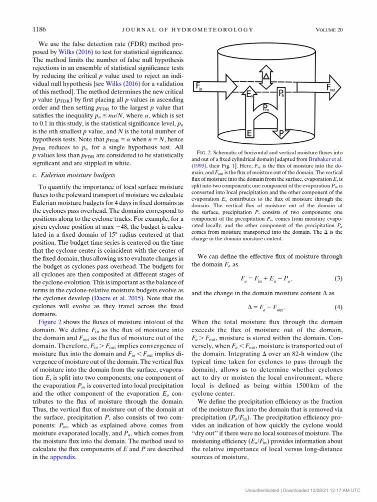
Figure 2 shows the fluxes of moisture into/out of the

domain. We define Fin as the flux of moisture into

the domain and Fout as the flux of moisture out of the

domain. Therefore, Fin .Fout implies convergence of

moisture flux into the domain and Fin ,Fout implies di-

vergence ofmoisture out of the domain. The vertical flux

of moisture into the domain from the surface, evapora-

tion E, is split into two components; one component of

the evaporation Pm is converted into local precipitation

and the other component of the evaporation Ea con-

tributes to the flux of moisture through the domain.

Thus, the vertical flux of moisture out of the domain at

the surface, precipitation P, also consists of two com-

ponents: Pm, which as explained above comes from

moisture evaporated locally, and Pa, which comes from

the moisture flux into the domain. The method used to

calculate the flux components of E and P are described

in the appendix.

We can define the effective flux of moisture through

the domain Fa as

Fa5F

in1E

a2P

a, (3)

and the change in the domain moisture content D as

D5Fa2F

out. (4)

When the total moisture flux through the domain

exceeds the flux of moisture out of the domain,

Fa .Fout, moisture is stored within the domain. Con-

versely, when Fa ,Fout, moisture is transported out of

the domain. Integrating D over an 82-h window (the

typical time taken for cyclones to pass through the

domain), allows us to determine whether cyclones

act to dry or moisten the local environment, where

local is defined as being within 1500 km of the

cyclone center.

We define the precipitation efficiency as the fraction

of the moisture flux into the domain that is removed via

precipitation (Pa/Fin). The precipitation efficiency pro-

vides an indication of how quickly the cyclone would

‘‘dry out’’ if there were no local sources of moisture. The

moistening efficiency (Ea/Fin) provides information about

the relative importance of local versus long-distance

sources of moisture,

FIG. 2. Schematic of horizontal and vertical moisture fluxes into

and out of a fixed cylindrical domain [adapted from Brubaker et al.

(1993), their Fig. 1]. Here, Fin is the flux of moisture into the do-

main, andFout is the flux ofmoisture out of the domain. The vertical

flux of moisture into the domain from the surface, evaporationE, is

split into two components; one component of the evaporation Pm is

converted into local precipitation and the other component of the

evaporation Ea contributes to the flux of moisture through the

domain. The vertical flux of moisture out of the domain at

the surface, precipitation P, consists of two components; one

component of the precipitation Pm comes from moisture evapo-

rated locally, and the other component of the precipitation Pa

comes from moisture transported into the domain. The D is the

change in the domain moisture content.

1186 JOURNAL OF HYDROMETEOROLOGY VOLUME 20

Unauthenticated | Downloaded 12/08/21 12:17 AM UTC

3. Results

a. Cyclone composites

To describe the basic structure and evolution of the

200 cyclones studied, we first compute horizontal and

vertical composites of cyclone structure during their

developing phase. In each composite field the cyclones

are located at the center of the 158 radial grid and the

cyclones are rotated so that they all travel from left

to right.

Figure 3a shows composite cyclone-centered fields at

max248. At this early stage in the cyclones development

the cyclones typically exhibit an openwave structure in the

925-hPa equivalent potential temperature. High values of

TCWV (.20kgm22) are confined between the surface

cold and warm fronts. Maximum precipitation occurs

ahead of the cyclone center above the warm front.

Figure 3b shows a circular cross section taken 5.58 fromthe cyclone center (anticlockwise around the arrow in

Fig. 3a). Moist air (.80% relative humidity) ascends

along the sloping isentropic surfaces of the warm front

with maximum vertical velocities typically occurring

between 700 and 500hPa. Near the surface, the cyclone-

relative wind fields produce convergence ahead of the

surface cold front.

Figures 3c and 3d show composite cyclone-centered

fields at max 224. In this rapidly intensifying stage of

development the 925-hPa equivalent potential temper-

ature wave has amplified and the warm sector area has

decreased. The highest values of TCWV are now found

in a band ahead of the surface cold front. Maximum

precipitation has approximately doubled compared to

24h earlier, and there is a region of maximum evapo-

ration located in the cold air behind the surface cold

front. At 925hPa the cyclone-relative wind fields pro-

duce increased convergence at the cold front, compared

to 24h earlier, leading to the accumulation of moisture

and the formation of the band of high TCWV (often

used as a proxy for identifying atmospheric rivers).

Figures 3e and 3f show composite cyclone-centered

fields at max. By this mature stage of development the

925-hPa equivalent potential temperature frontal gra-

dients have started to weaken and the accumulated

precipitation has decreased. The 925-hPa cyclone-relative

wind field convergence at the cold front occurs further

from the cyclone center due to frontal fracture and the

band of TCWV has also decreased in magnitude.

To illustrate the 3D structure of airflows within extra-

tropical cyclones, cyclone-relative isentropic analysis has

been performed for each cyclone. Figures 4a and 4c

show composite specific humidity and cyclone-relative

flow along the 285-K isentropic surface at max 248 and

max 224, respectively, and Fig. 4e shows composite

cyclone-relative specific humidity and flow along the

275-K isentropic surface at max. A cooler isentropic

surface is shown at max to illustrate the boundary layer

flow, since typically the cyclones have propagated

farther north by their mature stage of development.

Figures 4a, 4c, and 4e show that within the warm sector

the cyclone-relative airflow is easterly, at constant

pressure (1000–900hPa), and relatively moist (specific

humidity . 5 g kg21). At the cold front, the low-level

flow diverges with one branch traveling away from the

cyclone center parallel to the cold front, and another

branch traveling toward the cyclone center. This is

consistent with the 925-hPa cyclone-relative winds

shown in Figs. 3a, 3c, and 3e. This low-level cyclone

airflow (referred to in this paper as the feeder airstream)

is responsible for supplying moist air to the base of the

warm conveyor belt where it then ascends, condenses

into cloud, and forms precipitation. The feeder air-

stream is also responsible for the formation of filaments

of high TCWV seen extending along the cyclone’s cold

front and for exporting moisture from the cyclone. The

branch of the feeder airstream traveling away from the

cyclone center is weaker at max compared to the de-

veloping stages of cyclone evolution as the cyclones

begin to slow down as they reach their mature stage. To

the west of the cyclone center a relatively dry (specific

humidity , 3kg21), descending cyclone airflow also di-

verges when it reaches the cold front with the strongest

branch turning clockwise away from the cyclone center.

At low levels during the cyclone’s developing phase the

dry intrusion airflow and the feeder airstream form a

deformation pattern, which acts to strengthen the fron-

tal temperature gradient.

Figures 4b and 4d show the composite specific hu-

midity and cyclone-relative flow along the 300-K isen-

tropic surface at max 248 and max 224, respectively,

and Fig. 4f shows the composite specific humidity and

cyclone-relative flow along the 285-K isentropic surface

at max. To the south of the cyclone center, this surface is

located at approximately 800 hPa sloping up to 400 hPa

to the north of the cyclone. To the east of the cyclone

center air ascends along this sloped surface rising to

400 hPa. The strength of this ascending cyclone airflow

increases as the cyclone intensifies. This cyclone airflow,

the warm conveyor belt, is responsible for transporting

warm moist air from the boundary layer to the upper

troposphere. A compensating descending cyclone air-

flow occurs to the west of the cyclone center. This cy-

clone airflow, the dry intrusion, transports dry air from

the upper troposphere to the lower troposphere.

Despite the inherent smoothing associated with the

compositing methodology, coherent airstreams have

JUNE 2019 DACRE ET AL . 1187

Unauthenticated | Downloaded 12/08/21 12:17 AM UTC

FIG. 3. Composite cyclone-centered fields at (a),(b) max 248; (c),(d) max 224; and (e),(f) max. (left) The

6-hourly accumulated precipitation (blue contours every 1.5mm), 6-hourly accumulated evaporation (orange

contours every 1.5mm), TCWV (filled contours at 16, 20, and 24 kgm22), 925-hPa equivalent potential tempera-

ture (black dashed contours at 290, 300, and 310K), and 925-hPa cyclone-relative wind vectors. Gray arrows show

the location of the 3608 vertical cross sections shown in (b), (d), and (f) 5.58 from the cyclone center. (right) Equivalent

potential temperature (black dashed contours), omega (black solid contours at 21.5, 23.0, and 24.5 hPa s21), and

relative humidity (blue dotted contours at 80% and 90%).

1188 JOURNAL OF HYDROMETEOROLOGY VOLUME 20

Unauthenticated | Downloaded 12/08/21 12:17 AM UTC

FIG. 4. Composite cyclone-centered fields at (top) max 248; (middle) max 224; and (bottom) max.

(a),(c),(f) Pressure (hPa; contours), specific humidity (filled contours), and cyclone-relative flow (arrows)

on the 285-K potential temperature surface. (e) Pressure, specific humidity, and cyclone-relative flow on

the 275-K potential temperature surface. (b),(d) Pressure, specific humidity, and cyclone-relative flow on

the 300-K potential temperature surface.

JUNE 2019 DACRE ET AL . 1189

Unauthenticated | Downloaded 12/08/21 12:17 AM UTC

been identified in the composites. In this cyclone-relative

framework, it is found that as the cyclone propagates

through the background moisture field, accumulation of

moisture occurring along the cold front is largely re-

sponsible for creating the band of high TCWV. The

extent to which the background moisture contributes to

the cyclone’s domain integrated TP and IVT is the focus

of the next section.

b. Sensitivity to background moisture

In this section we investigate the sensitivity of a cy-

clone’s TP and IVT to the background TCWV field 24h

earlier by performing lagged linear regression. Figures 5a

and 5c show the composite background TCWV at

max 248 for 117 cyclones. This is a subset of the total

200 cyclones, since only 117 cyclones have a track that

extends 48h back from their time of maximum intensity.

The composite background TCWV field shows a meridi-

onal gradient of TCWV with high values (.17kgm22) to

the south and low values (,8 kgm22) to the north. The

orientation of the contours is fairly zonal as typically the

cyclone propagate eastward during this early stage in

their development and the cyclones are developing in a

region where the climatological TCWV contours are

also zonal (not shown). Figures 5b and 5d show the

background TCWVatmax224 for the 181 cyclones that

have a track that extends 24 h back from their time of

maximum intensity. The meridional gradient is similar

to that 24 h earlier, but the orientation of the contours is

not as zonal as typically the cyclones propagate in a

more northeastward direction as they reach their mature

stage, and the cyclones are typically developing in a

region where the climatological TCWV contours are

tilted southwest–northeast.

Figure 5a also shows the sensitivity of TP at max 224

to the background TCWV field 24h earlier. The maxi-

mum sensitivities are found to the right of the cyclone

center (in the precyclone environment). The sensitivity

is such that enhanced background TCWV in this pre-

cyclone region is associated with cyclones that pre-

cipitate more 24 h later. An increase of one standard

deviation in background TCWV leads to an increase in

total precipitation of up to 0.75 kgm22 (approximately

12% increase in the mean TP). Therefore cyclones that

propagate into regions with higher TCWV are more

likely to produce more precipitation than cyclones that

propagate into dry regions. Figure 5b shows the sensi-

tivity of TP at max to the background TCWV field at

max224. As for the developing cyclones, the maximum

sensitivity is found in the precyclone environment sug-

gesting that cyclones’ precipitation is controlled by the

background moisture content downstream not upstream.

At this mature stage of their evolution however, the

sensitivity is weaker and located farther from the cy-

clone center. This is likely due to the fact that both the

TP and feeder airstream wind speeds reduce between

max 224 and max (Figs. 4c and 4e, respectively).

Comparing Figs. 5a and 5b with the composite

cyclone-relative flow fields at max 248 and max 224,

respectively (Figs. 3a and 3c), the region of maximum

sensitivity is located in a region where the 925-hPa

cyclone-relative winds are easterly and approximately

15–20m s21. Thus, assuming a constant cyclone propa-

gation velocity, it will take approximately 21–28 h for the

center of the cyclone to reach the region of maximum

sensitivity, that is, the background moisture in the pre-

cyclone environment is swept up by the propagating

cyclone and converted into precipitation due to rapid

ascent in the warm conveyor belt. Since the cyclone-

relative flow into the cyclone center at low levels is from

the precyclone environment we conclude that the

moisture advected into the region from tropical/sub-

tropical latitudes does not play an important role in the

formation of high TP. Of course, we have only examined

very intense, oceanic cyclones, and this conclusion

will be tested for other subsets of cyclones as part of

future work.

Figure 5c shows the sensitivity of domain integrated

IVT at max 224 to the background TCWV field 24h

earlier. Significant sensitivities are again found in the

warm sector region of the cyclone, with maximum sen-

sitivity in the bottom-right quadrant [similar to the TP

sensitivity maximum (Fig. 5a)]. Thus, enhanced back-

ground TCWV in the precyclone region is associated

with cyclones with higher IVT 24h later. An increase of

one standard deviation in background TCWV leads to

an increase in total precipitation of up to 150kgm21 s21

(approximately 20% increase in the mean domain in-

tegrated IVT). Therefore, cyclones that propagate into

regions with higher TCWV are more likely to have

stronger IVT. There is also some significant sensitivity

to background TCWV in the postcyclone environment

(bottom-left quadrant). This sensitivity is approxi-

mately one-third as large as that in the precyclone

environment and is likely to be due to high spatial

correlations in the TCWV field since the composite

mean winds in this region are directed away from the

cyclone center.

Finally, Fig. 5d shows the sensitivity of domain in-

tegrated IVT at max to the background TCWV field at

max 224. At this mature stage of the cyclones’ evolu-

tion, the sensitivity is located downstream from the cy-

clone center only. This is likely to be due to the fact that

the structure of the cyclone evolves between max 224

andmax. Many of the cyclones undergo frontal fracture,

with the cold front moving away from the cyclone

1190 JOURNAL OF HYDROMETEOROLOGY VOLUME 20

Unauthenticated | Downloaded 12/08/21 12:17 AM UTC

center, perpendicular to the warm front (Fig. 3e). Since

the region of sensitivity is likely to be bounded by the

cold front (i.e., air does not travel across the frontal

boundary), this results in a region of sensitivity that is

confined to the bottom-right quadrant of the domain at

max, but which can extend into the bottom-left quadrant

at max 224. We do not have a proposed dynamical ex-

planation for high sensitivity in this region since they are

not consistent with the magnitude and direction of the

isentropic moisture fluxes shown in Fig. 4. Regions of

statistically significant sensitivities exist outside the area

shown. However, it is likely that these occur due to high

spatial correlations in the background TCWV field

shown in Fig. 4.

In summary, maximum sensitivity values are found in

the precyclone environment for both TP and IVT and

during the developing and mature phases of cyclone

evolution. This suggests that the same mechanism is

responsible for creating cyclones with higher TP and

IVT. We combine this statistical sensitivity with our

composite analysis of cyclones to infer that the mag-

nitude of TCWV at the entrance of the feeder air-

stream is important for determining TP and IVT at a

later stage in the cyclone evolution. This relationship

occurs because the background moisture in the pre-

cyclone environment is swept up by the propagating

cyclone and is either converted into precipitation in

the warm conveyor belt or converged into a band of

FIG. 5. Cyclone sensitivity fields (shaded; stippling denotes statistically significant sensitivities), overlaid

with composite background TCWV (gray contours). (a) Sensitivity of TP at max224 to the background TCWV at

max 248. (b) Sensitivity of TP at max to the background TCWV at max 224. A sensitivity value of 0.5 kgm22

signifies that for one standard deviation increase in the background TCWV there is a corresponding increase in TP

of 0.5 kgm22. (c) Sensitivity of domain integrated IVT at max 224 to the background TCWV at max 248.

(d) Sensitivity of domain integrated IVT at max to the background TCWV at max 224. A sensitivity value of

100 kgm21 s21 signifies that for one standard deviation increase in the background TCWV there is a corresponding

increase in total IVT of 100 kgm21 s21.

JUNE 2019 DACRE ET AL . 1191

Unauthenticated | Downloaded 12/08/21 12:17 AM UTC

high TCWV and left behind as the cyclone propagates

poleward.

c. Eulerian moisture budgets

In this section we aim to quantify the relative contri-

butions of horizontal and surface moisture fluxes to the

overall moisture transport by the cyclones.

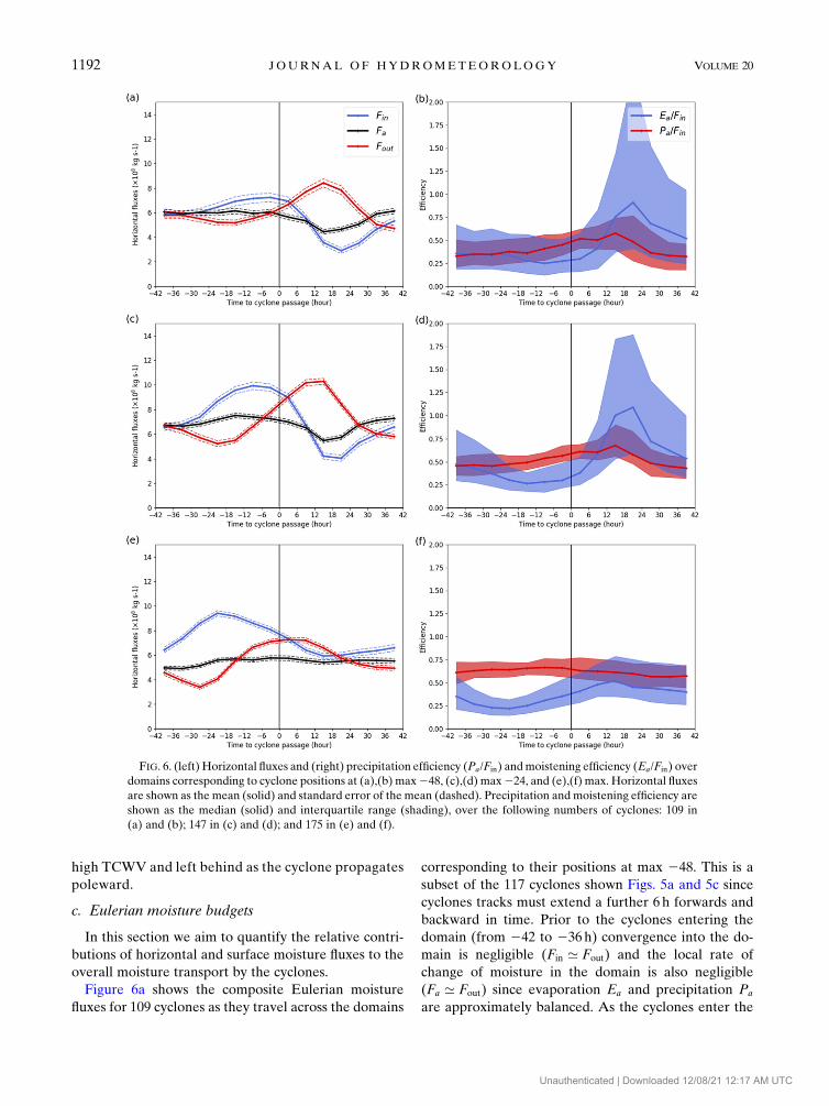
Figure 6a shows the composite Eulerian moisture

fluxes for 109 cyclones as they travel across the domains

corresponding to their positions at max 248. This is a

subset of the 117 cyclones shown Figs. 5a and 5c since

cyclones tracks must extend a further 6 h forwards and

backward in time. Prior to the cyclones entering the

domain (from 242 to 236h) convergence into the do-

main is negligible (Fin ’ Fout) and the local rate of

change of moisture in the domain is also negligible

(Fa ’ Fout) since evaporation Ea and precipitation Pa

are approximately balanced. As the cyclones enter the

FIG. 6. (left) Horizontal fluxes and (right) precipitation efficiency (Pa/Fin) andmoistening efficiency (Ea/Fin) over

domains corresponding to cyclone positions at (a),(b) max248, (c),(d) max224, and (e),(f) max. Horizontal fluxes

are shown as the mean (solid) and standard error of the mean (dashed). Precipitation and moistening efficiency are

shown as the median (solid) and interquartile range (shading), over the following numbers of cyclones: 109 in

(a) and (b); 147 in (c) and (d); and 175 in (e) and (f).

1192 JOURNAL OF HYDROMETEOROLOGY VOLUME 20

Unauthenticated | Downloaded 12/08/21 12:17 AM UTC

domain (from 230 to 0 h) moisture flux convergence is

positive (Fin .Fout) due to the horizontal flux of mois-

ture into the domain by the propagating cyclone. How-

ever the rate of change of moisture in the domain is

smaller than the total due to moisture flux convergence

becausemuch of themoisture transported into the domain

is removed via precipitation. For example, at 212h, on

average 50% of the horizontal moisture transported into

the domain is removed via precipitation (Pa/Fin ’ 0:5;

Fig. 6b). This loss of moisture is offset by local evapo-

ration (Ea/Fin ’ 0:3) ensuring that the cyclones do not

dry out quickly. As the cyclone exits the domain

(from 16 to 130h), moisture flux convergence is neg-

ative (Fin ,Fout). At the same time, evaporation in the

domain increases, largely due to enhanced evaporation

behind the cyclone cold front (Fig. 3c). At 124h, the

average moistening efficiency (70%) exceeds the pre-

cipitation efficiency (45%) (Fig. 6b), although it should

be noted that the variability in moistening efficiency

between cyclones is large at this point. This moisture is

transported out of the domain and moistens the atmo-

sphere in the wake of the cyclone, potentially pre-

conditioning it for subsequent cyclone development. Over

the entire cyclone passage the moisture transported away

from the local environment is on average213 Pg (where 1

Pg5 13 1015 g), calculated by integrating D over an 82-h

window. Thus, in the early stage of the cyclone devel-

opment the cyclone can be said to ‘‘store’’ moisture that

is evaporated locally and transport it poleward as it

travels. Within the boundary layer this transport is

slower than the cyclone propagation velocity (Fig. 4a) so

while the moisture transport remains poleward, relative

to the cyclone center it is left behind.

Figure 6c shows the composite Eulerian moisture

fluxes for 147 cyclones as they travel across the domains

corresponding to their positions at max 224. This is a

subset of the 181 cyclones shown Figs. 5b and 5d since

cyclones tracks must extend a further 6 h forwards and

backward in time. As the cyclones enter the domain

(from 236 to 0 h) the moisture flux convergence is

positive (Fin .Fout). The moisture flux convergence is

greater than 24h earlier due to the increased moisture

storedwithin the cyclones themselves.On average between

45% and 60% of this moisture is lost via precipitation

(Fig. 6d). This loss is offset by local evaporation (moist-

ening efficiency’30%). Thus, there is a continuous cycle

of evaporation and moisture flux convergence in the

vicinity of cyclones which acts to replenish the water

vapor lost via precipitation. The resulting moisture is

stored within the domain (Fa .Fout). As the cyclones

leave the domain the situation is reversed. Moisture is

transported out of the domain and transported poleward

by the propagating cyclone. The moisture transported

away from the local environment is on average 211 Pg,

thus the cyclone continues to pull in moisture from the

local environment and transports it poleward.

Figure 6e shows the Eulerian horizontal moisture

fluxes for 175 cyclones as they travel across the domains

corresponding to their positions at max. Unlike the early

and intensifying stages of cyclone life cycle, theprecipitation

and evaporation fluxes (Ea and Pa) do not balance initially.

The precipitation efficiency is on average .60% at 242h

whereas the moistening efficiency is on average,40%. At

this mature stage of the cyclone development the

evaporation in the domain is not large enough to re-

plenish the moisture lost via precipitation and as a result

the cyclones rapidly dry out. Thus, the moisture di-

verging out of the domain is significantly smaller than

that entering the domain for almost the entire time

period. The moisture transported away from the local

environment is smaller than during the developing and

intensifying stages of the cyclone life cycle (21 Pg).

Therefore, in the mature stage of the cyclone develop-

ment the cyclone ‘‘empties’’ of moisture and the pole-

ward transport of moisture decreases as the cyclone

begins to decay.

In summary, since precipitation and moistening effi-

ciencies are nonzero we can conclude that, even if

Fin 5Fout, the same moisture that enters the domain

does not leave the domain. That is, moisture lost via

precipitation is replenished by a combination of local

evaporation and moisture from the local environment

(where local is within 1500km of the cyclone center).

As a result the local environment is drier following the

passage of a cyclone during its developing and mature

stages. The contribution of local evaporation to the

horizontal moisture flux is calculated using Ea/Fin aver-

aged over the developing stages of cyclone evolution

(max 248 and max224). Between 242 and 0h local

evaporation contributes approximately 30% to the

horizontal moisture flux, providing a continuous source

of moisture to the feeder airstream airflow in the pre-

cyclone environment. Between 0 and 142h local evapo-

ration contributes approximately 70% to the horizontal

moisture flux in the postcyclone environment (although

the variability between cyclones is large), potentially pre-

conditioning it for subsequent cyclone development.

4. Discussion and conclusions

Figure 7 shows a schematic of the cyclone-relative

airflows and their relation to Eulerian features such as

the surface fronts and regions of high precipitation and

TCWV. The feeder airstream is a low-level flow of moist

air that travels rearwards, relative to the cyclone prop-

agation direction. At the cold front the feeder airstream

JUNE 2019 DACRE ET AL . 1193

Unauthenticated | Downloaded 12/08/21 12:17 AM UTC

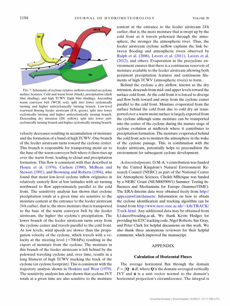
velocity decreases resulting in accumulation of moisture

and the formation of a band of high TCWV. One branch

of the feeder airstream turns toward the cyclone center.

This branch is responsible for transporting moist air to

the base of the warm conveyor belt where it then rises up

over the warm front, leading to cloud and precipitation

formation. This flow is consistent with that described in

Houze et al. (1976), Carlson (1980), McBean and

Stewart (1991), and Browning and Roberts (1994), who

found that moist low-level cyclone inflow originates in

relatively easterly flow at low latitudes with air turning

northward to flow approximately parallel to the cold

front. The sensitivity analysis has shown that cyclone

precipitation totals at a given time are sensitive to the

moisture content at the entrance to the feeder airstream

24h earlier, that is, themoremoisture that is transported

to the base of the warm conveyor belt by the feeder

airstream, the higher the cyclone’s precipitation. The

lower branch of the feeder airstream turns away from

the cyclone center and travels parallel to the cold front.

At low levels, wind speeds are slower than the propa-

gation velocity of the cyclone, which travels with a ve-

locity at the steering level (’700 hPa) resulting in the

export of moisture from the cyclone. The moisture in

this branch of the feeder airstream is left behind by the

poleward traveling cyclone and, over time, results in a

long filament of high TCWV marking the track of the

cyclone (or cyclone footprint). This is consistent with the

trajectory analysis shown in Hoskins and West (1979).

The sensitivity analysis has also shown that cyclone IVT

totals at a given time are also sensitive to the moisture

content at the entrance to the feeder airstream 24h

earlier, that is, the more moisture that is swept up by the

cold front as it travels poleward through the atmo-

sphere, the stronger the atmospheric river. Thus, the

feeder airstream cyclone airflow explains the link be-

tween flooding and atmospheric rivers observed by

Ralph et al. (2006), Lavers et al. (2011), Lavers et al.

(2012), and others. Evaporation in the precyclone en-

vironment ensures that there is a continuous reservoir of

moisture available to the feeder airstream allowing both

persistent precipitation features and continuous fila-

ments of high TCWV (atmospheric rivers) to form.

Behind the cyclone a dry airflow, known as the dry

intrusion, descends frommid- and upper levels toward the

surface cold front. At the cold front it is forced to diverge

and flow both toward and away from the cyclone center

parallel to the cold front. Moisture evaporated from the

surface behind the cold front due to cold dry air trans-

ported over a warmmoist surface is largely exported from

the cyclone although some moisture can be transported

into the center of the cyclone during the mature stage of

cyclone evolution at midlevels where it contributes to

precipitation formation. The moisture evaporated behind

the cold front acts to moisten the atmosphere in the wake

of the cyclone passage. This, in combination with the

feeder airstream, potentially helps to precondition the

environment for subsequent cyclone development.

Acknowledgments.O.M-A.’s contribution was funded

by the United Kingdom’s Natural Environment Re-

search Council (NERC) as part of the National Centre

for Atmospheric Sciences. Cheikh MBengue was funded

by a NERC Grant (NE/M005909/1) Summer: Testing In-

fluences and Mechanisms for Europe (SummerTIME).

The ERA-Interim data were obtained freely from http://

apps.ecmwf.int/datasets/. Information on how to obtain

the cyclone identification and tracking algorithm can be

found from http://www.nerc-essc.ac.uk/;kih/TRACK/

Track.html. Any additional data may be obtained from

h.f.dacre@reading.ac.uk. We thank Kevin Hodges for

providing his ETC tracking code,NigelRoberts, SueGray,

and Peter Clark for helpful discussions on this work. We

also thank three anonymous reviewers for their helpful

comments, which improved the manuscript.

APPENDIX

Calculation of Horizontal Fluxes

The average horizontal flux through the domain

F5ÐQ � n̂dl, whereQ is the domain-averaged vertically

IVT and n̂ is a unit vector normal to the domain’s

horizontal projection’s circumference. The integral is

FIG. 7. Schematic of cyclone-relative airflows overlaid on cyclone

surface features. Cold and warm front (black), precipitation (dark

blue shading), and high TCWV (light blue shading). Ascending

warm conveyor belt (WCB; red), split into lower cyclonically

turning and higher anticyclonically turning branch. Low-level

rearward flowing feeder airstream (FA; green), split into lower

cyclonically turning and higher anticyclonically turning branch.

Descending dry intrusion (DI; yellow), split into lower anti-

cyclonically turning branch and higher cyclonically turning branch.

1194 JOURNAL OF HYDROMETEOROLOGY VOLUME 20

Unauthenticated | Downloaded 12/08/21 12:17 AM UTC

computed over half of this circumference to find

F5 2rQ, where Q is the magnitude of Q and r is the

domain’s radius. Following Trenberth (1999) (see also

Brubaker et al. 1993),

F51

2(F

in1F

out) . (A1)

Furthermore, the domain-integrated moisture flux

convergence C5Fin 2Fout. Thus, Fin 5F1C/2 and

Fout 5F2C/2.

The change in the domain’s moisture content D is

given by

D5Fin2F

out1E2P . (A2)

We assume that precipitation can be split into two parts,

one due tomoisture flux into the domainPa, and another

due to local evaporation converted into precipitation

Pm, that is,

P5Pa1P

m. (A3)

Using (A2) and (A3) to rewrite (A1), we get

F5Fin11

2(E2P

m2P

a)2

1

2D , (A4)

which can also be split into two parts, one due to the

moisture flux into the domain Qa 5Fin 2 1/2Pa 2 1/2D,and another due to evaporated moisture Qm 51/2(E2Pm). Following Brubaker et al. (1993) and

Trenberth (1999), we assume that the ratio Pa/Pm is

equal to the ratio Qa/Qm, from which we find that

Pa

Pm

52F

in2D

E. (A5)

Using (A4) and (A5) in (A3) yields

Pm5P

�E

2F1P

�. (A6)

REFERENCES

Boutle, I., S. Belcher, and R. Plant, 2011: Moisture transport in

midlatitude cyclones. Quart. J. Roy. Meteor. Soc., 137, 360–

373, https://doi.org/10.1002/qj.783.

Browning, K., and N. Roberts, 1994: Structure of a frontal cyclone.

Quart. J. Roy. Meteor. Soc., 120, 1535–1557, https://doi.org/

10.1002/qj.49712052006.

Brubaker, K. L., D. Entekhabi, and P. Eagleson, 1993: Estimation

of continental precipitation recycling. J. Climate, 6, 1077–1089,

https://doi.org/10.1175/1520-0442(1993)006,1077:EOCPR.2.0.CO;2.

Carlson, T. N., 1980: Airflow through midlatitude cyclones and

the comma cloud pattern. Mon. Wea. Rev., 108, 1498–1509,

https://doi.org/10.1175/1520-0493(1980)108,1498:ATMCAT.2.0.CO;2.

Catto, J. L., and S. Pfahl, 2013: The importance of fronts for ex-

treme precipitation. J. Geophys. Res. Atmos., 118, 10 791–

10 801, https://doi.org/10.1002/jgrd.50852.

——, L. C. Shaffrey, and K. I. Hodges, 2010: Can climate models

capture the structure of extratropical cyclones? J. Climate, 23,

1621–1635, https://doi.org/10.1175/2009JCLI3318.1.

Dacre, H. F., and S. L. Gray, 2013: Quantifying the climatological

relationship between extratropical cyclone intensity and at-

mospheric precursors. Geophys. Res. Lett., 40, 2322–2327,

https://doi.org/10.1002/grl.50105.

——, M. Hawcroft, M. Stringer, and K. Hodges, 2012: An extra-

tropical cyclone atlas: A tool for illustrating cyclone structure

and evolution characteristics. Bull. Amer. Meteor. Soc., 93,

1497–1502, https://doi.org/10.1175/BAMS-D-11-00164.1.

——, P. A. Clark, O.Martinez-Alvarado,M. A. Stringer, andD. A.

Lavers, 2015: How do atmospheric rivers form? Bull. Amer.

Meteor. Soc., 96, 1243–1255, https://doi.org/10.1175/BAMS-D-

14-00031.1.

Garcies, L., and V. Homar, 2009: Ensemble sensitivities of the real at-

mosphere: application to Mediterranean intense cyclones. Tellus,

61A, 394–406, https://doi.org/10.1111/j.1600-0870.2009.00392.x.

Harrold, T., 1973: Mechanisms influencing the distribution of

precipitation within baroclinic disturbances. Quart. J. Roy.

Meteor. Soc., 99, 232–251, https://doi.org/10.1002/qj.49709942003.

Hodges, K., 1995: Feature tracking on the unit sphere. Mon. Wea.

Rev., 123, 3458–3465, https://doi.org/10.1175/1520-0493(1995)

123,3458:FTOTUS.2.0.CO;2.

Hoskins, B. J., and N. V. West, 1979: Baroclinic waves and front-

ogenesis. Part II: Uniformpotential vorticity jet flows-cold and

warm fronts. J. Atmos. Sci., 36, 1663–1680, https://doi.org/

10.1175/1520-0469(1979)036,1663:BWAFPI.2.0.CO;2.

——, and K. I. Hodges, 2002: New perspectives on the Northern

Hemisphere winter storm tracks. J. Atmos. Sci., 59, 1041–1061,

https://doi.org/10.1175/1520-0469(2002)059,1041:NPOTNH.2.0.CO;2.

Houze, R. A., Jr., J. D. Locatelli, and P. V. Hobbs, 1976: Dynamics

and cloudmicrophysics of the rainbands in an occluded frontal

system1. J. Atmos. Sci., 33, 1921–1936, https://doi.org/10.1175/

1520-0469(1976)033,1921:DACMOT.2.0.CO;2.

Knippertz, P., F. Pantillon, and A. H. Fink, 2018: The devil in the

detail of storms.Environ. Res. Lett., 13, 044002, https://doi.org/

10.1088/1748-9326/aabd3e.

Lavers, D.A., R. P.Allan, E. F.Wood,G.Villarini, D. J. Brayshaw,

and A. J. Wade, 2011: Winter floods in Britain are connected

to atmospheric rivers.Geophys. Res. Lett., 38, L23803, https://

doi.org/10.1029/2011GL049783.

——, G. Villarini, R. P. Allan, E. F. Wood, and A. J. Wade, 2012:

The detection of atmospheric rivers in atmospheric reanalyses

and their links to British winter floods and the large-scale

climatic circulation. J. Geophys. Res., 117, D20106, https://

doi.org/10.1029/2012JD018027.

Madonna, E., H. Wernli, H. Joos, and O. Martius, 2014: Warm

conveyor belts in the ERA-Interim dataset (1979–2010). Part

I: Climatology and potential vorticity evolution. J. Climate, 27,

3–26, https://doi.org/10.1175/JCLI-D-12-00720.1.

McBean, G. A., and R. E. Stewart, 1991: Structure of a frontal

system over the northeast Pacific Ocean.Mon. Wea. Rev., 119,

997–1013, https://doi.org/10.1175/1520-0493(1991)119,0997:

SOAFSO.2.0.CO;2.

Neiman, P. J., F. M. Ralph, G. A. Wick, J. D. Lundquist, andM. D.

Dettinger, 2008: Meteorological characteristics and overland

JUNE 2019 DACRE ET AL . 1195

Unauthenticated | Downloaded 12/08/21 12:17 AM UTC

precipitation impacts of atmospheric rivers affecting the west

coast of North America based on eight years of SSM/I satellite

observations. J. Hydrometeor., 9, 22–47, https://doi.org/10.1175/

2007JHM855.1.

Pfahl, S., and H. Wernli, 2012: Quantifying the relevance of cy-

clones for precipitation extremes. J. Climate, 25, 6770–6780,

https://doi.org/10.1175/JCLI-D-11-00705.1.

Ralph, F. M., P. J. Neiman, and G. A. Wick, 2004: Satellite and

CALJET aircraft observations of atmospheric rivers over the

eastern North Pacific Ocean during the winter of 1997/98.

Mon. Wea. Rev., 132, 1721–1745, https://doi.org/10.1175/1520-

0493(2004)132,1721:SACAOO.2.0.CO;2.

——, ——, ——, S. I. Gutman, M. D. Dettinger, D. R. Cayan, and

A. B. White, 2006: Flooding on California’s Russian River:

Role of atmospheric rivers. Geophys. Res. Lett., 33, L13801,https://doi.org/10.1029/2006GL026689.

——, and Coauthors, 2017: Atmospheric rivers emerge as a global

science and applications focus. Bull. Amer. Meteor. Soc., 98,

1969–1973, https://doi.org/10.1175/BAMS-D-16-0262.1.

Reed, R. J., and M. D. Albright, 1986: A case study of explosive

cyclogenesis in the eastern Pacific. Mon. Wea. Rev., 114,

2297–2319, https://doi.org/10.1175/1520-0493(1986)114,2297:

ACSOEC.2.0.CO;2.

Trenberth, K. E., 1999: Atmospheric moisture recycling: Role of

advection and local evaporation. J. Climate, 12, 1368–1381,

https://doi.org/10.1175/1520-0442(1999)012,1368:AMRROA.2.0.CO;2.

Vannière, B., A. Czaja, and H. F. Dacre, 2017: Contribution of the

cold sector of extratropical cyclones to mean state features

over the Gulf Stream in winter. Quart. J. Roy. Meteor. Soc.,

143, 1990–2000, https://doi.org/10.1002/qj.3058.Wernli, H., 1997: A Lagrangian-based analysis of extratropical

cyclones. II: A detailed case-study.Quart. J. Roy.Meteor. Soc.,

123, 1677–1706, https://doi.org/10.1002/qj.49712354211.Wilks, D. S., 2016: ‘‘The stippling shows statistically significant grid

points’’: How research results are routinely overstated and

overinterpreted, and what to do about it. Bull. Amer. Meteor.

Soc., 97, 2263–2273, https://doi.org/10.1175/BAMS-D-15-00267.1.

1196 JOURNAL OF HYDROMETEOROLOGY VOLUME 20

Unauthenticated | Downloaded 12/08/21 12:17 AM UTC