Linking Words in Economic Discourse: Implications for … · Linking Words in Economic Discourse: Implications for Macroeconomic Forecasts J. Daniel Arom March 19, 2018 Abstract Word

Linking Words in Economic Discourse: Implications for

Macroeconomic Forecasts

J. Daniel Aromı

March 19, 2018

Abstract

Word vector representations are trained to construct quantitative indicators ofunstructured information in the press. Vectors are trained using the GloVe model(Pennington et al. 2014) and a corpus covering 90 years of press content. Therepresentations are shown to learn meaningful associations in economic context.These links are exploited to develop indicators of relevant subjective states in presscontent. In-sample and out-of-sample forecasting exercises show that the indicatorscontain valuable information regarding future economic activity. The combinationof information from indices associated to different subjective states allows for gainsin prediction accuracy. This forecasting performance cannot be reproduced usingalternative text analysis techniques previously proposed in the literature.

1 Introduction

A large quantity of unstructured economic data is generated and disseminated every-day through multiple channels. For example, this type of data is found in corporateand government documents, expert reports, mass media and social media. Improve-ments in data availability and processing capacity have allowed for studies thatextract information and evaluate its forecasting ability. These contributions typi-cally compute interpretable indicators that are based on a small set of keywords orpredefined dictionaries. These works have shown positive results in macroeconomicand financial contexts (Tetlock 2007, Loughran & MacDonald 2011, Baker et al.2016, Aromi 2017a 2017c, Nyman et al. 2018). One relevant question is whethermachine learning techniques can attain informational gains and, at the same time,allow for straightforward interpretations.

This work tackles this question through word vector representations, a tool thathas been successfully tested in natural language processing applications (Collobertet al. 2011, Mikolov et al. 2013, Pennington et al. 2014). Word vector repre-sentations are trained to learn meaning in economic context using a large corpusof information in the press. The resulting structure of meaning allows for indica-tors with a straightforward interpretation. Following Pennington (2014), the GloVe(global vectors) model is used to compute the representations. The links betweenwords, as indicated by their vector representations, are used to generate quantitative

1

indicators of information in the press.

Mutiple evaluations of the resulting vectors show that they are able to learnmeaning in economic context. Vectors are shown to resolve ambiguities, recognizerelationships between entities and understand similarities between words. As a re-sult, instead of using a predefined dictionary, quantitative indicators can be derivedselecting words closely associated to relevant keywords.

In response to the prominent role assigned to the concept of uncertainty in theanalysis of business cycles (see for example Jurado et al. 2015, Baker et al. 2016,Rossi & Sekhposyan 2015), in the first set of exercises, indices approximating mani-festations of uncertainty are evaluated. In-sample, the indicators are shown to pro-vide information on future levels of employment, industrial production, investmentand GDP. Out-of-sample exercises are implemented using bayesian model averaging(BMA) to learn about convenient specifications of indicators from the press. Theseexercises show positive results on the predictive ability of the indicators that exploitword vector representations.

Beyond indicators approximating uncertainty, complementary explorations con-sider indices capturing manifestations of different subjective states that are conjec-tured to be relevant. These indices summarize manifestations linked to pessimism,fear and anxiety. Out of sample forecast exercises show that these alternative in-dices contain additional information that can be combined to attain higher accuracy.

The approach proposed in this work is compared to four alternative text analysismethodologies as proposed by Baker et al. (2016), Loughram & McDonald(2011),Tetlock (2007) and The Economist.1 In Baker et al. (2016) and Economist’s R-wordindex small sets of words are selected to generate indices of press content. In Tetlock(2007) and Loughran & MacDonald (2011) the indices are based on large lists builtusing expert judgment. Forecasting exercises show that the performance of indicesbased on word vector representations compares favorably with that verified underalternative techniques previously proposed in the literature.

The rest of the paper is organized as follows. The next section presents themethodology and the data. The properties of trained word vectors are preliminaryexplored in section 3. Forecasting exercises associated to the metric of uncertaintyare presented in section 4. The next section evaluates indices approximating alter-native subjective states. In section 6, comparisons with other methodologies arepresented. Section 7 concludes.

2 Methodology and data

The exercises presented in this work involve two steps. In the first step, word vec-tor representations are trained using a corpus covering ninety years. In this way, astructure of meaning is built. In the second step, indicators that summarize eco-nomic information in the press are computed using the previously computed word

1”The R-word” (2001, Apr, 5th), The Economist. Retrieved from http://www.economist.com/

2

vector representations as a key input. More specifically, having selected a relevantkeyword or set of keywords (e.g. uncertainty), closely associated words are identifiedcomputing the distance between their respective word vector representations. Theindicator is given by the frequency of these closely associated words. In forecastingexercises, this index is computed using a second corpus. In this section the method-ology is outlined in more detail and a description of the training corpus is provided.

2.1 Word vector representations

As previously indicated, the first step involves representing words through vectorsusing the GloVe model (Pennington et al. 2014). This type of representation hasbeen shown to efficiently summarize word semantic (and syntactic) information (Col-lobert et al. 2011, Mikolov et al. 2013, Pennington et al. 2014). As suggested by theauthors, it can be understood as a linear structure of meaning. This quantitativerepresentation can be used to assess relatedness between different words by com-puting the distance between the respective vectors. Also, information provided bymultiple words can be combined through simple algebraic operations. While GloVeis not the only method that computes vector representations of words, it has beenshown to perform better than alternative methods in multiple natural language pro-cessing tasks (see Pennington 2014).

In the GloVe model, word vectors are trained to capture information on wordco-occurrences in the training corpus. The method is global in the sense that allvectors are computed in a single optimization exercise. Let W denote a dictionaryand let Xij denote the number of times word i occurs in the context of word j. Theloss function of the GloVe model is given by:∑

i

∑j

f(Xij)[vi · vj + bi + bj − log(Xij)

]2Where vi and vj are word vectors, f(Xij) is a weighting function and bi and bj are

word biases.2 This is a log-bilinear regression model. The weighting function f(Xij)is increasing and concave.3 The vector representations are trained using stochasticgradient descent (Duchi et al. 2011). More details can be found in Pennington etal. (2014).

Following parameter values that are in line with those used in the natural lan-guage representation literature, the vector dimensionality is 100 and the windowsize used to compute term co-occurrence is 5. The vocabulary used in the im-plementation is given by words with a frequency of 100 or higher in the trainingcorpus. Robustness analyses indicate that the results are not sensible to variationsin the value of this parameters. Vector representations of words are computed usingpackage text2vec in platform R. The same package was used in other related com-

2The vector representations used in applications are typically given by the sum of the two word vector(vi and vj). This practice is followed in this study.

3More specifically, following Pennington et al. (2014), the weighting function equals f(x) = (x/100)α

if x < 100, otherwise f(x) = 1.

3

putations (e.g. tokenization, term co-occurrence matrix).

2.2 Quantitative indicators

In the second step, word vector representations are used to construct quantitativeindicators of information in the press. The intention is to generate indicators thatexploit knowledge captured by word vectors and can be interpreted in a straight-forward manner. The procedure involves, first, identifying a keyword representing afeature of interest. Next, the set of K most closely related terms are found based onthe cosine distance between the respective vectors. Finally, the indicator is definedby the frequency of selected words.

More formally, given keyword k ∈ W the set of K closest words is identified

computing the cosine distance:vw · vj||vw||||vj ||

. This results in a set of words K ⊂ W .

The index computed for a selected set of text C is given by:

IkC =

∑w∈K cw∑w∈W cw

where cw indicates the number of times word w is observed in the selected setof text C. The set of selected text in the exercises below is given by economic presscontent over a specific time window.

The selection of the keyword is a function of the rationale behind the text analy-sis exercise. In macroeconomic forecasting context the choice will reflect conjecturesregarding which are the aspects that are more likely to be informative regardingfuture business cycle dynamics. Given the high level of attention placed on the con-cept of uncertainty (see for example Jurado et al. 2015, Baker et al. 2016, Rossi &Sekhposyan 2015) a natural choice for a keyword is given by ”uncertainty”. In thefollowing section, the results associated to this choice, are reported.

2.3 Data

The corpus used to train the vectors is given by a selection of text published inthe Wall Street Journal between 1900 and 1989. The selected text corresponds tothe content of a public webpage.4 For each article published in the newspaper, thiswebsite provides access to the headline, the lead and a fraction of the body. To avoidconcerns regarding forward looking biases, the training corpus is constructed usinga time period that predates the period of forecasting exercises that are presented inthe next section. Table 1 shows information on the corpus used to train the wordvector representations and the corpus used to compute the indicators.

4The text was extracted from: http://pqasb.pqarchiver.com/djreprints/.

4

Following common practice, numbers and punctuation marks are deleted fromthe text. Also, all text is converted to lower case and stop words are filtered.5 Af-ter applying the minimum frequency filter, the dictionary of the training dataset isgiven by 28296 words. This is the number of 100 dimensional vectors computed inthe GloVe model implementation.

The training corpus is relatively small compared to databases used in the fieldof natural language processing.6. On the other hand, the training corpus is focusedon economic discussions and can be conjectured to follow a relatively stable naturallanguage. Additionally, the corpus used to compute the indices, the test corpus,shares the theme and style of the training corpus. As a result, there are reasonsto remain optimistic regarding the present implementation’s ability to learn wordmeaning in economic context.

Beyond text, a second set of data used in this study is given by real-time eco-nomic activity indicators for years 1966 through 2017. Four variables were selected:employment (Nonfarm Payroll Employment), industrial production (Industrial Pro-duction Index: Manufacturing), investment (Nonresidential Real Gross Private Do-mestic Investment) and GDP (Real Gross Domestic Product)7 The information isfrom the Federal Reserve Bank of Philadelphia’s Real-Time Data Research Cen-ter.8 The database built for the exercises below, preserves the real time natureof the original data. More specifically, for each quarterly observation t, the valuesof the economic activity indicators, latest figures and lagged values, correspond toinformation available at the time data for quarter t is first released.

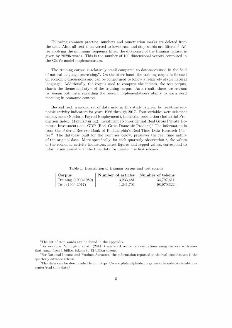
Table 1: Description of training corpus and test corpus

Corpus Number of articles Number of tokensTraining (1900-1989) 3,233,481 134,797,611Test (1990-2017) 1,241,706 98,979,322

5The list of stop words can be found in the appendix.6For example Pennington et al. (2014) train word vector representations using corpora with sizes

that range from 1 billion tokens to 42 billion tokens.7For National Income and Product Accounts, the information reported in the real-time dataset is the

quarterly advance release.8The data can be downloaded from: https://www.philadelphiafed.org/research-and-data/real-time-

center/real-time-data/

5

Table 2: Descriptive statistics - Quarterly growth rates

Activity Indicator Mean St. Dev. Min MaxEmployment 0.0039 0.0051 -0.0202 0.0166Industrial Production 0.0060 0.0186 -0.1098 0.0598Investment 0.0085 0.0228 -0.1190 0.0531GDP 0.0061 0.0074 -0.0274 0.0264

Note: Figures correspond to first releases. Sample period is 1966-2017.

3 Preliminary analysis of trained word vectors

Before proceeding to the forecasting exercise, preliminary evaluations of the infor-mation captured by word vectors are presented. First, some selected associationsbetween word vectors will be used to demonstrate that trained vectors are able tolearn word meaning in economic contexts. Second, an indicator that intends tocapture manifestations of ”uncertainty” will be evaluated in terms of its contempo-raneous association with relevant macroeconomic events.

3.1 Vectors and meaning in economic context

The extent to which vectors capture meaning is naturally an empirical matter thatdepends on the informativeness of the training corpus and the efficiency of thelearning model. One reason for concern is that, as previously indicated, the trainingcorpus is relatively small compared to corpora typically used in the field of naturallanguage processing. A variety of tasks can be used to evaluate trained vectors.The evaluations are based on associations between trained vectors. Three tasks areconsidered below: resolution of ambiguity in word meaning, entity identificationthrough vector composition and identification of words indicative of tone or topic.The last task is the most relevant for the exercises carried out in the next sections.

Ambiguous words are a common challenge in natural language processing appli-cations. In particular, it is a problem for indicators based on predefined dictionaries.For example, Tetlock (2017), Garcia (2013) and Aromi (2017a 2017c) have shownthat words in the negative category of Harvard IV dictionary can be used to antic-ipate financial and macroeconomic dynamics. Nevertheless, this category includesambiguous words such as ”capital”, ”tire” and ”vice”. In economic contexts, thesewords are not likely to carry negative information. The presence of the word ”capi-tal” typically reflects discussions regarding financial issues, not discussions regardingthe death penalty. Similarly, the word ”tire” typically refers to the manufacturingof rings of rubber, not the need of rest or sleep. In the case of ”vice” the mostlikely use is linked to the title of a corporate or bureaucratic position (e.g. vicechairman). The use of the word to refer to immoral or wicked behavior can be con-jectured to be less likely. These examples are suggestive of potential efficiency gainsassociated to the use of unsupervised learning algorithms in word classification tasks.

6

Table 3 shows, for each of the mentioned ambiguous terms, the set of words withthe closest vectors. The selected words suggest that word vectors are able to identifythe most likely meaning. A final example of an ambiguous word is given by ”de-fault”. The identity of the closest neighbours suggests that the identified meaningpoints to failures to fulfill an obligation not to preselected options.

Word vector representations have been shown to learn relationships betweenwords. For example, in natural language processing tasks, computed vectors havebeen shown to learn associations such as: ”king”-”male”+”female”=”queen”. Thistype of associations can be used to identify related entities in economic settings. Acouple of examples are shown in table 3. The results suggest that vectors trainedusing economic press content learn to identify relationships between government en-tities and manufacturing corporations.

Finally, and more relevant for the current analysis, vectors are shown to identifygroups of words related to the tone or the topic in a collection of texts. For example,as shown in table 3, the word ”uncertainty” is identified as close to other words thatreflect concern over future contingencies. This evidence suggest that related wordscan be used to construct an indicator that approximates uncertainty as communi-cated by economic press content. At the same time, it must be observed that theserelated words are not synonyms of uncertainty. In other words, the links point toclosely related states that tend to co-occur with the manifestation of uncertainty.These observations are relevant for a more informed interpretation of the index.Finally, showing that word vector representations can be used to identify topics, itis observed that vectors learn to identify words related to ”debt”.

Table 3: Sample evidence on word meaning captured by word vector representation

Selected vector 5 closest word vectors

Ambiguous word vectors:tire goodyear, firestone, akron, tires, rubbercapital par, authorized, outstanding, shares, commonvice executive, president, elected, director, managerdefault payment, debt, obligations, overdue, waiver

Vector compositions:bundesbank-germany+us fed, regulators, intervention, analysts, agencygm-cars+planes boeing, northrop, lockheed, aircraft, fighter

Tone/topic keywords:uncertainty confusion, nervousness, apprehension, uneasiness, anxietydebt funding, longterm, financing, subordinated, restructure

Note: distance computed using cosine distance. closest words do not include words ofthe selected vector and words with the same root.

7

3.2 An indicator of uncertainty

In this subsection, an indicator of uncertainty is presented. As previously indicated, theconcept of uncertainty has received substantial attention in the analysis of business cycles(Jurado et al. 2015, Baker et al. 2016, Rossi & Sekhposyan 2015). Choosing ”uncertainty”as a keyword is a natural choice given this related literature. An additional rationale isgiven by a study that exploits word vector representations to construct an uncertainty in-dex that is shown to anticipate changes in expected stock market volatility (Aromi 2017b).In the first step of the computation, the vectors associated to the words ”uncertainty”,”uncertain” and ”uncertainties” are added to compute a new vector wU . The distancebetween this new vector and all words in the vocabulary W is computed. As previouslydescribed, K words whose vectors are closest to wU are selected. Finally, the index is givenby the frequency of these K words.

The collection of texts used in the first step of the exercise corresponds to the samesource of Wall Street Journal content already mentioned in the previous subsection. Theindices are computed forming a second corpus that covers material published betweenJanuary 1990 and February 2017. This second dataset contains approximately 98 milliontokens.

Figure 1 shows the values of three uncertainty indicator computed using different setsof selected words. Increments in the indices can be observed in the three recessions thattook place during the sample period. This increment is particularly clear in the case ofthe recession linked to the 2008 Global Financial Crisis. Interestingly, in the case of the2008-2009 recession, the indices show increments several months before the start of therecession in December 2007. Additionally, spikes in the indices are observed around threewell-known crisis episodes: the Asian Crisis of 1997, the Russian Crisis of 1998 and the 2011Debt-ceiling crisis. These associations suggest that meaningful information is captured bythe index. Its ability to anticipate economic activity is evaluated in the next sections.

8

Figure 1: Uncertainty Indices.

0

0.002

0.004

0.006

0.008

0.01

0.012

0.014

0.016

1990

0119

9012

1991

1219

9212

1993

1219

9411

1995

1119

9611

1997

1119

9811

1999

1020

0010

2001

1020

0210

2003

1020

0408

2005

0520

0602

2006

1120

0707

2008

0320

0811

2009

0820

1004

2011

0120

1109

2012

0520

1302

2013

1020

1407

2015

0320

1601

2016

11

Unc-25Unc-50Unc-100

Russian-LTCM crisisAsian crisis

Debt-ceiling crisis

Notes: the figure shows the average of the indices for 90 day moving windows. Hori-zontal bars indicate recessions.

4 Macroeconomic forecasts

In this section, the indicator of uncertainty described above is evaluated in forecastingtasks. The forecasting model is given by an autoregressive specification complementedwith an indicator of lagged press content. The growth rate of each economic activity in-dicator over the following h quarters is modeled as a function of lagged quarterly growthrates. The number of lags is selected minimizing the Bayesian Information Criterion.

More formally, let at be the value of an economic indicator in quarter t. The growth ratecomputed on quarter t is given by ∆at = log(at)−log(at−1). Let ∆hat represent the growthrate computed on quarter t for a window of size ”h”, that is ∆hat = log(at) − log(at−h).The baseline autoregressive model satisfies:

9

∆hat+h = α+

p∑s=0

βs∆at−s + ut (1)

To evaluate the predictive ability of indicators based on press content, this baselinemodel is modified incorporating as predictor an indicator of press content. Let It representthe value of indicator of press content corresponding to quarter t. Then, the forecastingmodel is given by the following equation:

∆hat+h = α+

p∑s=0

βs∆at−s + βIIt + ut (2)

The parameter of interest is βI . Also, the relative metric of model fit, as indicated bydifferences in adjusted R2’s, will be analyzed to assess the in-sample forecasting perfor-mance of the indicator. The models are estimated for the period 1990-2017. In this way,trained vectors using press content ending in 1989, do not contain any forward lookinginformation.

In this section, the indicator of press content is associated to the 100 words most closelyassociated to uncertainty. That is, the index is given by lagged quarterly frequency of thisset of words. While the optimal specification of the indicator is unknown, this specificationis used to generate the first set of evidence associated to macroeconomic forecasts. In out-of-sample exercises developed below, a bayesian model averaging framework will be usedto acknowledge uncertainty regarding the optimal specification of press content indicators.

The forecasting exercise has been carefully designed taking into account the scheduleof economic data release. For each observation t, most recent and lagged information isas available at the time of the first release. The indicator of information in the press Itsummarizes lagged press content up 90 days before the release of the respective economicactivity indicator. In other words, the forecasting exercise evaluates the predictive value ofindicators of press content, right after having incorporated the news proceeding from thefirst release of quarterly economic activity data.

In the case of industrial production, the release dates are as reported by the Boardof Governors of the Federal Reserve System is used.9 In the case of payrolls, new databecomes available in the first days after the end of the month on which data is reported forthe first time. In a cautious approach, the index is based on information published duringor before the month for which the latest information is available. In the case of NationalIncome and Product Accounts, release dates starting from 1996 are available from the Bu-reau of Economic Analysis webpage.10 For earlier dates, release dates are not available.The 28th day of the month of the release, the average day observed in the subsequent years,was used as the release date.

Table 4 shows evidence on the information content of the selected indicator. Fourforecast horizons are considered: h ∈ {1, 2, 4, 8}. Adjusted R2’s show important gains inexplanatory ability. This is specially noticeable in the case of longer forecasting horizons.

9The list can be found visiting https://www.federalreserve.gov/releases/g17/10https://www.bea.gov/newsreleases/releasearchive.htm

10

For example, in the case of one-year ahead GDP forecasting models, the adjusted R2 in-creases from 0.113 to 0.239 as the press content indicator is incorporated as a predictor.

In all cases, the estimated coefficient is negative. The estimated models point to aconsistent economically significant association. A one standard deviation change in theinformation metric anticipates a mean change in economic growth that ranges from 0.18to 0.40. standard deviations. For short forecast horizon models, statistically significantassociations are observed. As forecast horizon grows, the number of statistically significantassociations decreases. The indicator of press content is seen to be consistently informativein the case of GDP forecasts. In contrast, when industrial production forecasts are con-sidered, the associated parameter is statistically significant only in the case of the shortestforecast horizon.

This preliminary evidence suggests that indices that exploit word vector representa-tions have information regarding future levels of economic activity. In particular, this canbe inferred from increments in adjusted R2’s as these indices are incorporated in the fore-casting models. At the same, it is observed that the estimated association is not alwaysstatistically consistent. This is could be the result of inefficient specification of the indexreflecting information in the press. This issue is dealt with in out of sample exercises shownbelow.

11

Table 4: Estimated forecast models

h=1 h=2 h=4 h=8

Employment

βI -0.263*** -0.342** -0.408** -0.389t-stat. [2.24] [2.25] [2.05] [1.29]Adj. R2 0.710 0.659 0.523 0.315Baseline adj. R2 0.666 0.583 0.412 0.214

Industrial Production

βI -0.280* -0.341 -0.298 -0.180t-stat. [1.68] [1.40] [0.77] [0.43]Adj. R2 0.414 0.290 0.155 0.029Baseline adj. R2 0.352 0.194 0.084 0.009

Investment

βI -0.342*** -0.396** -0.354 -0.297t-stat. [2.96] [2.00] [1.23] [0.94]Adj. R2 0.328 0.358 0.287 0.114Baseline adj. R2 0.230 0.225 0.180 0.041

GDP

βI -0.320*** -0.387*** -0.387*** -0.370**t-stat [3.85] [3.01] [2.44] [2.06]Adj. R2 0.299 0.280 0.239 0.151Baseline adj. R2 0.217 0.156 0.113 0.035

Notes: significance levels: “*” 0.10, “**” 0.05 and “***” 0.01. Standard errors are es-timated following Newey & West (1987, 1994). Parameter estimates are standardized;absolute t-statistics in brackets.

4.1 Out of sample exercises

The previous evidence on in-sample predictive ability is complemented with a set of out-of-sample forecast exercises. Forecasts are generated using models fitted with real-time data.Four different forecast horizons are considered: h ∈ {1, 2, 4, 8}. The test sample starts inyear 1990. Models are trained using expanding windows that begin in 1966 and end hquarters before the date in which the respective prediction exercise is implemented.

The analysis implements forecast combinations to acknowledge uncertainty regardingoptimal specification of indicators summarizing information in the press. First, it must benoted that the choice of 100 words used in the previous forecasting exercises was arbitrary.It is reasonable to conjecture that a more efficient approach would allow for a data drivenselection of the weights assigned to related words. Also, optimal indicators would weightmore heavily more recent information flows. Considering these concerns, indices associatedto different number of words and alternative lags are incorporated in the exercise. The

12

forecasts associated to each of those indices are combined using bayesian model averaging(BMA) techniques. In this way, forecasts combinations are used as a strategy to deal withrisks associated to unknown models (Timmermann 2006).

Baseline forecasts correspond to those generated by the autoregressive model. As inthe previous exercises, the number of lags is selected to minimize the bayesian informa-tion criterion. The associated forecasts are compared to the combination of forecasts thatresult from incorporating information from the press and BMA. To contemplate variationin the informativeness of more closely related words, indices with different number of re-lated words are considered. The number of words considered are: 100, 50 and 25. Also,considering that more recent news flows might be more informative, two window sizes areconsidered. In addition to the previously proposed 90 day window specification, indicesbased on 30 day windows are considered. These alternative specifications result in sixindicators of information in the press. Let {Iit}6i=1 represent the indices computed thealternative specifications. Then, given a variable measuring economic activity at and aforecast horizon h, each indicator of uncertainty defines a forecasting model given by:

∆hat+h = αi +

p∑s=0

βis∆sat + βiII

it + uit (3)

Where uit is normally distributed with mean 0 and variance σ2i . The BMA exer-

cise incorporates an additional model given by the baseline autoregressive specification.Under BMA, forecast combinations involve computing weighted averages of the forecastsgenerated under each model. The weights are given by the posterior probability that thecorresponding model is the true model. The current implementation follows the specifica-tion proposed in Faust et al. (2012).

More formally, let {Mi}i∈N be a collection of models. Also, let θi represent the parame-ters {αi, βi1, ..., βip, βiI , σ2

i }, and let D be the observed data. Then, the posterior probabilityis given by:

P (Mi|D) =P (D|Mi)P (Mi)∑j∈N P (D|Mj)P (Mj)

(4)

where

P (D|Mi) =

∫P (D|θi,Mi)P (θi|Mi)dθi (5)

is the marginal likelihood of the i-th model; p(θi|Mi) is the prior density of the param-eter vector θi and P (D|θi,MI) is the likelihood function. Following usual practice, it isoriginally assumed that prior probabilities are the same for all models. Also, it is assumedthat the prior density of the parameters {αi, βi1, βip, βiI , σ2

i } is uninformative and propor-tional to 1/σi. The prior for parameter βiI follows Zellner (1986) g-prior specification:βiI ∼ N(0, φσ2

i (I ′iIi)−1). The parameter φ > 0 controls the strength of the prior. Following

previous literature, this parameter value is φ = 4.11 After computing the forecasts associ-ated to each model, ait+h, and updating beliefs, the forecast combination is given by:

11See for example Fernandez et al. (2001) and Faust et al. (2012). The results are not sensible tochanges in this parameter. These robustness exercises are available from the author upon request.

13

∆hat+h =

N∑i=0

P (Mi|D)∆hait+h (6)

Table 5 shows the information on the relative performance of the forecast that incorpo-rate information from the press.12 P-values are based on bootstrap methods as implementedin Faust et al. (2013). Gains in forecast accuracy are observed for most activity indicatorsand forecast horizons. For short forecast horizons (h=1 and h=2), gains in accuracy arestatistically significant with a p-value below 0.01. The case of GDP forecasts presents themost consistent improvements associated to lagged information from the press. In contrast,in the case of industrial production, one-year-ahead and two-year-ahead forecasts are notseen to improve when compared to baseline forecasts. These differences in performanceassociated to different indicators of economic activity are consistent with the results ob-served in previously reported in-sample prediction exercises.

Table 5: Out-of-sample predictive accuracy

h=1 h=2 h=4 h=8

Employment 0.921 0.907 0.967 0.996[0.00] [0.00] [0.08] [0.44]

Industrial Production 0.941 0.954 1.004 1.011[0.00] [0.00] [0.39] [0.59]

Investment 0.943 0.939 0.911 0.945[0.00] [0.00] [0.00] [0.07]

GDP 0.945 0.936 0.925 0.875[0.00] [0.00] [0.00] [0.02]

NOTE: Relative RMSPEs; bootstrapped p-values for the test of the null hypothesis thatthe ratio of the RMSPEs is equal to one are reported in square brackets.

5 Indices measuring other subjective states

So far the analysis has focused on indicators that capture expressions associated to uncer-tainty. Forecasting exercises shown above indicate that these indices contain informationregarding the future evolution of the business cycle. The choice of uncertainty related in-dices is a natural choice given the theoretical and empirical contributions that have focusedon this concept on the context of business cycle studies (Jurado et al. 2015, Baker et al.2016, Rossi & Sekhposyan 2015). Also, previous work showed that this type of uncertaintymetric is able to anticipate stock market implied volatility (Aromi 2017b). On the otherhand, the evaluation of indicators associated to alternative concepts is a logical extension

12The BMA implementation was estimated using R’s package BMS.

14

of the previous exercise. It is likely that the uncertainty proxy does not capture all relevantfactors in an appropriate manner. Hence, increases in accuracy can result from a combi-nation of forecast using proxies of different manifestations of subjective states in the press.In the exploratory exercises shown below, three complementary indicators are incorporated.

As in the case of uncertainty, the choice of relevant additional concepts is guided byprevious literature and informed conjectures regarding subjective states that are likely toanticipate business cycle dynamics. While it would be desirable to have a more systematicapproach for feature selection, this is beyond the scope of the current exercise and is leftfor future explorations.

First, considering the current prediction task associated to macroeconomic outcomes,manifestations in the press related to ”pessimism”, that is, expectations of negative sce-narios, can be conjectured to be relevant. Hence, this concept is used to construct newindicators. Second, pointing to a very prominent emotion, expressions related to ”fear” areused as another potentially informative indicator. In this direction, it can be observed thatthe intensity of web searches related to ”fear” were shown to have predictive value regardinginvestment decisions and stock market volatility (Da et al. 2014). Finally, in Nyman et al.(2018) it is suggested that expressions related to ”anxiety” capture important informationregarding subjective states and associated behaviors. Following this perspective, indicesassociated to this concept are evaluated below. 13

Words most closely related to the selected keywords are shown in table 6. It is observedthat related words are, for the most part, consistent with expected associations. In otherwords, these associations suggest that negative words allow for the construction of indicesthat can be interpreted in a straightforward manner. This exploratory evidence also showsthat these concepts are closely linked. For example, words such as uncertainty, uneasinessand anxiety appear in table 6 in multiple occasions. As a result, indices associated tothese concepts are expected to have an important common component. At the same time,differences in these closely related indices might allow for complementarities in forecastingtasks. This possibility is evaluated in the exercises below.

13In related explorations, indices associated to positive words such as optimism and excitement wereevaluated. No predictive value was observed in this case. This can be linked to the ”Pollyanna Hypothe-sis”, according to which positive words are used more diversely and do not carry as much information asnegative words. Negative words are used in a more discriminatory manner (Bouchard & Osgood 1969,Garcia et al. 2012). Relatedly, Tetlock (2007) and Aromi(2017a) observe that, in contrast to negativewords, positive words do not provide any information regarding future stock market returns.

15

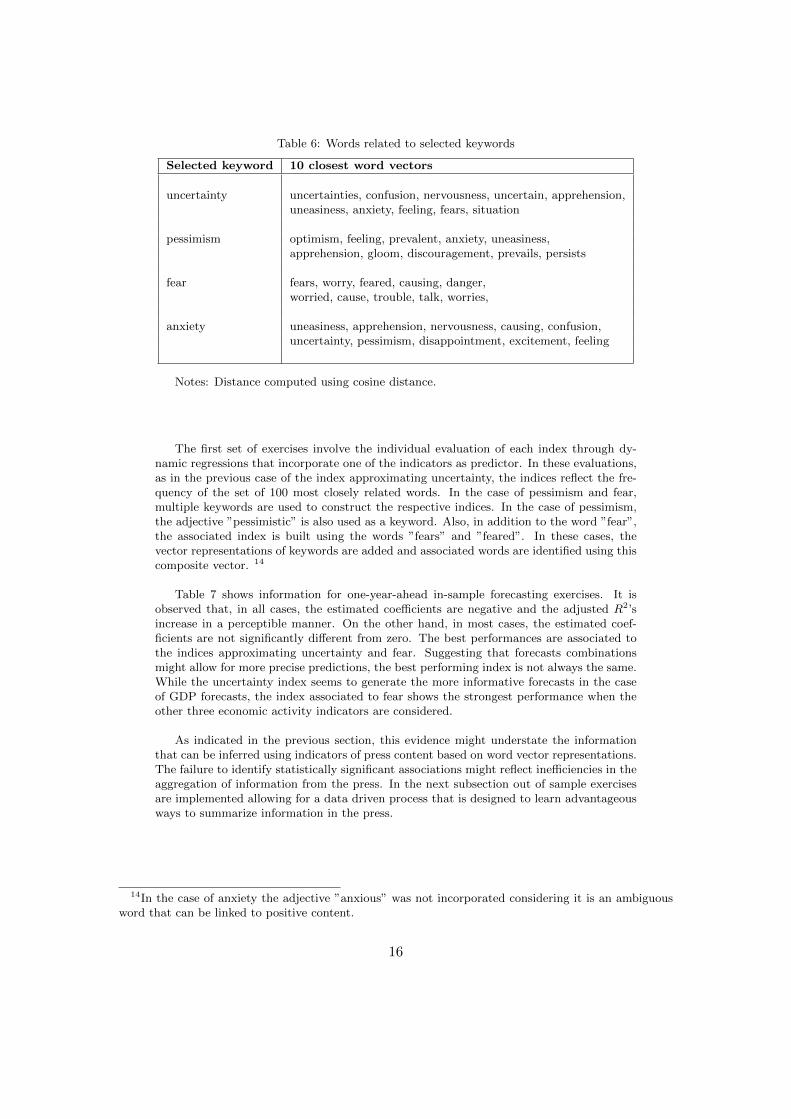
Table 6: Words related to selected keywords

Selected keyword 10 closest word vectors

uncertainty uncertainties, confusion, nervousness, uncertain, apprehension,uneasiness, anxiety, feeling, fears, situation

pessimism optimism, feeling, prevalent, anxiety, uneasiness,apprehension, gloom, discouragement, prevails, persists

fear fears, worry, feared, causing, danger,worried, cause, trouble, talk, worries,

anxiety uneasiness, apprehension, nervousness, causing, confusion,uncertainty, pessimism, disappointment, excitement, feeling

Notes: Distance computed using cosine distance.

The first set of exercises involve the individual evaluation of each index through dy-namic regressions that incorporate one of the indicators as predictor. In these evaluations,as in the previous case of the index approximating uncertainty, the indices reflect the fre-quency of the set of 100 most closely related words. In the case of pessimism and fear,multiple keywords are used to construct the respective indices. In the case of pessimism,the adjective ”pessimistic” is also used as a keyword. Also, in addition to the word ”fear”,the associated index is built using the words ”fears” and ”feared”. In these cases, thevector representations of keywords are added and associated words are identified using thiscomposite vector. 14

Table 7 shows information for one-year-ahead in-sample forecasting exercises. It isobserved that, in all cases, the estimated coefficients are negative and the adjusted R2’sincrease in a perceptible manner. On the other hand, in most cases, the estimated coef-ficients are not significantly different from zero. The best performances are associated tothe indices approximating uncertainty and fear. Suggesting that forecasts combinationsmight allow for more precise predictions, the best performing index is not always the same.While the uncertainty index seems to generate the more informative forecasts in the caseof GDP forecasts, the index associated to fear shows the strongest performance when theother three economic activity indicators are considered.

As indicated in the previous section, this evidence might understate the informationthat can be inferred using indicators of press content based on word vector representations.The failure to identify statistically significant associations might reflect inefficiencies in theaggregation of information from the press. In the next subsection out of sample exercisesare implemented allowing for a data driven process that is designed to learn advantageousways to summarize information in the press.

14In the case of anxiety the adjective ”anxious” was not incorporated considering it is an ambiguousword that can be linked to positive content.

16

Table 7: Estimated forecast models - h=4

Uncertainty Fear Pessimism Anxiety

Employment (baseline adj. R2 =0.412)

βI -0.408** -0.480** -0.322* -0.298t-stat. [2.05] [2.52] [1.69] [1.36]Adj. R2 0.523 0.570 0.488 0.485

Ind. Prod. (baseline adj. R2 =0.084)

βI -0.298 -0.356 -0.259 -0.250t-stat. [1.40] [1.09] [1.18] [1.36]Adj. R2 0.155 0.184 0.139 0.138

Investment (baseline adj. R2 =0.180)

βI -0.354 -0.408 -0.236 -0.234t-stat. [1.29] [1.36] [0.85] [0.76]Adj. R2 0.287 0.320 0.225 0.227

GDP (baseline adj. R2 =0.113)

βI -0.387** -0.342 -0.231 -0.304t-stat [2.00] [1.53] [1.01] [1.40]Adj. R2 0.239 0.217 0.157 0.197


17

5.1 Out of sample forecasts

The methodology implemented in this subsection is the same as that implemented in thecase of the indicators capturing manifestations of uncertainty. Forecast combinations basedon BMA are evaluated against the baseline autoregressive model. Associated to each con-cept, six indices are constructed. As in the previously reported out-of-sample exercises, thealternative specifications correspond to different number of related words (100, 50 and 25)and different periods (30 day and 90 day windows). As a result, the BMA exercise involves25 models. One model is the baseline model and 24 models correspond to autoregressivemodels that incorporate one of the 24 indices reflecting information in the press.

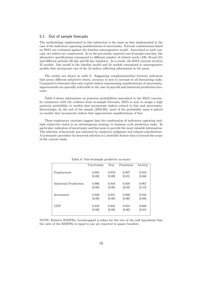
The results are shown in table 8. Suggesting complementarities between indicatorsthat proxy different subjective states, accuracy is seen to increase in all forecasting tasks.Compared to forecasts that only exploit indices summarizing manifestations of uncertainty,improvements are specially noticeable in the case of payrolls and industrial production fore-casts.

Table 9 shows information on posterior probabilities associated to the BMA exercise.In consistence with the evidence from in-sample forecasts, BMA is seen to assign a highposterior probability to models that incorporate indices related to fear and uncertainty.Interestingly, by the end of the sample (2016-III), most of the probability mass is placedon models that incorporate indices that approximate manifestations of fear.

These exploratory exercises suggest that the combination of indicators capturing mul-tiple subjective states is an advantageous strategy in business cycle prediction tasks. Inparticular, indicators of uncertainty and fear seem to provide the most valuable information.The selection of keywords was informed by subjective judgment and related contributions.A systematic procedure for keyword selection is a desirable feature that is beyond the scopeof the current study.

Table 8: Out-of-sample predictive accuracy

Uncertainty Fear Pessimism Anxiety

Employment 0.885 0.859 0.897 0.919[0.00] [0.00] [0.01] [0.06]


Investment 0.928 0.931 0.886 0.934[0.00] [0.00] [0.00] [0.06]

GDP 0.935 0.924 0.910 0.860[0.00] [0.00] [0.00] [0.01]


18

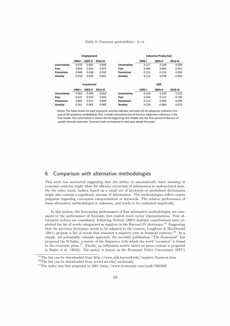
Table 9: Posterior probabilities - h=4.

1990-I 2003-II 2016-III 1990-I 2003-II 2016-IIIUncertainty 0.076 0.055 0.006 Uncertainty 0.217 0.148 0.039Fear 0.854 0.654 0.977 Fear 0.494 0.604 0.952Pessimism 0.044 0.248 0.010 Pessimism 0.111 0.124 0.004Anxiety 0.018 0.035 0.001 Anxiety 0.113 0.078 0.0030.992 0.992 0.994 0.935 0.954 0.998

1990-I 2003-II 2016-III 1990-I 2003-II 2016-IIIUncertainty 0.402 0.390 0.054 Uncertainty 0.254 0.250 0.223Fear 0.421 0.533 0.945 Fear 0.446 0.519 0.730Pessimism 0.081 0.013 0.000 Pessimism 0.113 0.094 0.009Anxiety 0.061 0.003 0.000 Anxiety 0.125 0.084 0.013

GDP

Industrial ProductionEmployment

Investment

Notes: The table shows for each economic activity indicator and each set of subjective indicators the sum of the posterior probabilities that a model associated one of the four subjective indicators is the true model. This information is shown for the beginning, the middle and the final period of the out-of-sample forecast exercises. Forecast tasks correspond to one-year-ahead forecasts.

6 Comparison with alternative methodologies

This work was motivated suggesting that the ability to automatically learn meaning ineconomic contexts might allow for efficient extraction of information in unstructured data.On the other hand, indices based on a small set of keywords or predefined dictionariesmight also contain a significant amount of information. The methodologies reflect expertjudgment regarding convenient categorizations or keywords. The relative performance ofthese alternative methodologies is unknown, and needs to be evaluated empirically.

In this section, the forecasting performance of four alternative methodologies are com-pared to the performance of forecasts that exploit word vector representations. Four al-ternative indices are considered. Following Tetlock (2007) multiple contributions have ex-ploited the list of words categorized as negative in the Harvard IV dictionary.15 Suggestingthat the previous dictionary needs to be adapted to the context, Loughran & MacDonald(2011) propose a list of words that transmit a negative tone in financial contexts.16. In asimple, yet potentially valuable approach, the monthly publication ”The Economist” hasproposed the R-Index, a metric of the frequency with which the word ”recession” is foundin the economic press.17. Finally, an influential metric based on press content is proposedin Baker et al. (2016). The metric is known as the Economic Policy Uncertainty (EPU)

15The list can be downloaded from http://www.wjh.harvard.edu/ inquirer/homecat.htm.16The list can be downloaded from www3.nd.edu/ mcdonald/17The index was first proposed in 2001 (http://www.economist.com/node/566293)

19

index. This index computes the fraction of news articles that refer to economic policy anduncertainty.18 These articles are identified using a small set of words.19

The performance of the uncertainty metric based on word vector representation iscompared to the performance of indices associated to the previously described alternativemethods. In the case of the first three alternative methods, the indices are computed usingthe test corpus of WSJ content used in this contribution. In the case of the Economic Pol-icy Uncertainty index, the index was downloaded from the website created by the authors.The EPU is based on text content for a large collection of publications. This elementshould be considered when evaluating relative forecast performance.

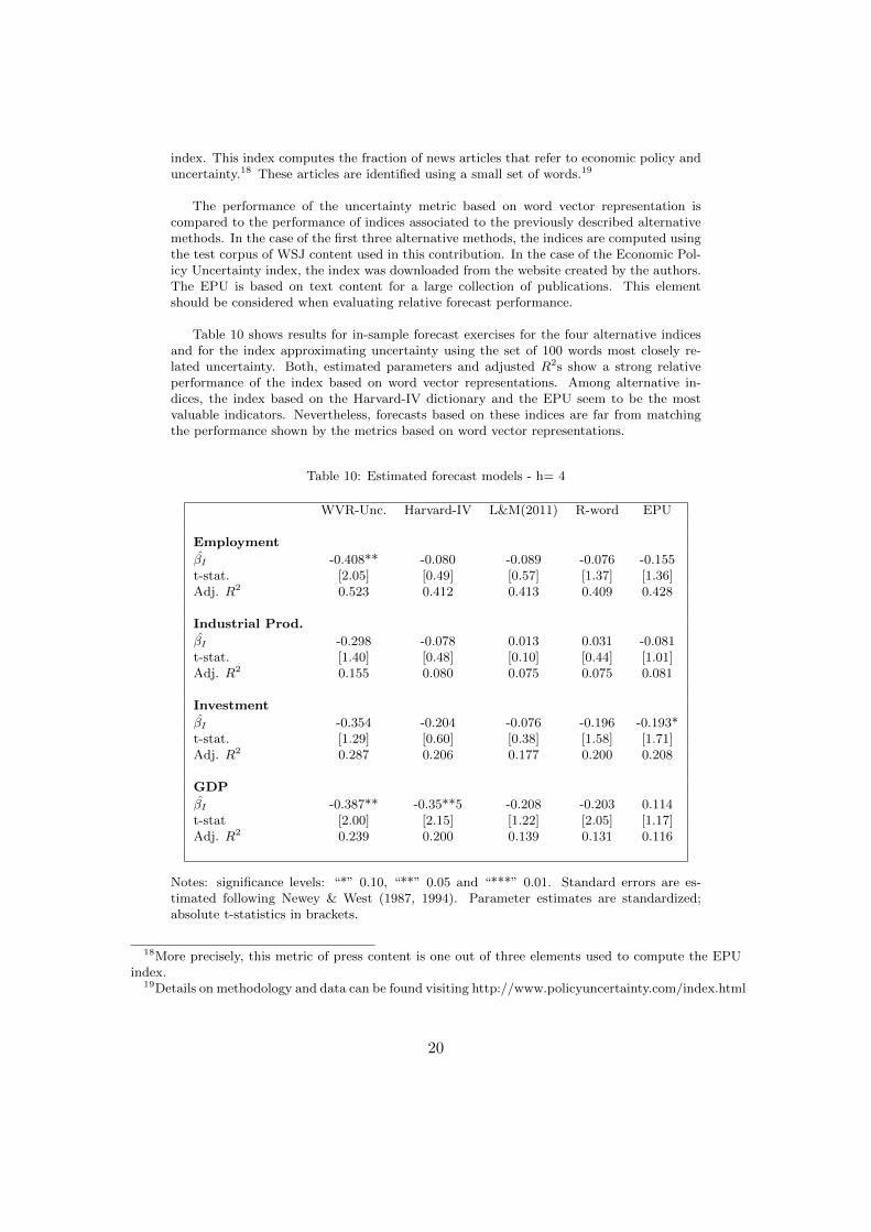
Table 10 shows results for in-sample forecast exercises for the four alternative indicesand for the index approximating uncertainty using the set of 100 words most closely re-lated uncertainty. Both, estimated parameters and adjusted R2s show a strong relativeperformance of the index based on word vector representations. Among alternative in-dices, the index based on the Harvard-IV dictionary and the EPU seem to be the mostvaluable indicators. Nevertheless, forecasts based on these indices are far from matchingthe performance shown by the metrics based on word vector representations.

Table 10: Estimated forecast models - h= 4

WVR-Unc. Harvard-IV L&M(2011) R-word EPU

Employment

βI -0.408** -0.080 -0.089 -0.076 -0.155t-stat. [2.05] [0.49] [0.57] [1.37] [1.36]Adj. R2 0.523 0.412 0.413 0.409 0.428

Industrial Prod.

βI -0.298 -0.078 0.013 0.031 -0.081t-stat. [1.40] [0.48] [0.10] [0.44] [1.01]Adj. R2 0.155 0.080 0.075 0.075 0.081

Investment

βI -0.354 -0.204 -0.076 -0.196 -0.193*t-stat. [1.29] [0.60] [0.38] [1.58] [1.71]Adj. R2 0.287 0.206 0.177 0.200 0.208

GDP

βI -0.387** -0.35**5 -0.208 -0.203 0.114t-stat [2.00] [2.15] [1.22] [2.05] [1.17]Adj. R2 0.239 0.200 0.139 0.131 0.116


18More precisely, this metric of press content is one out of three elements used to compute the EPUindex.

19Details on methodology and data can be found visiting http://www.policyuncertainty.com/index.html

20

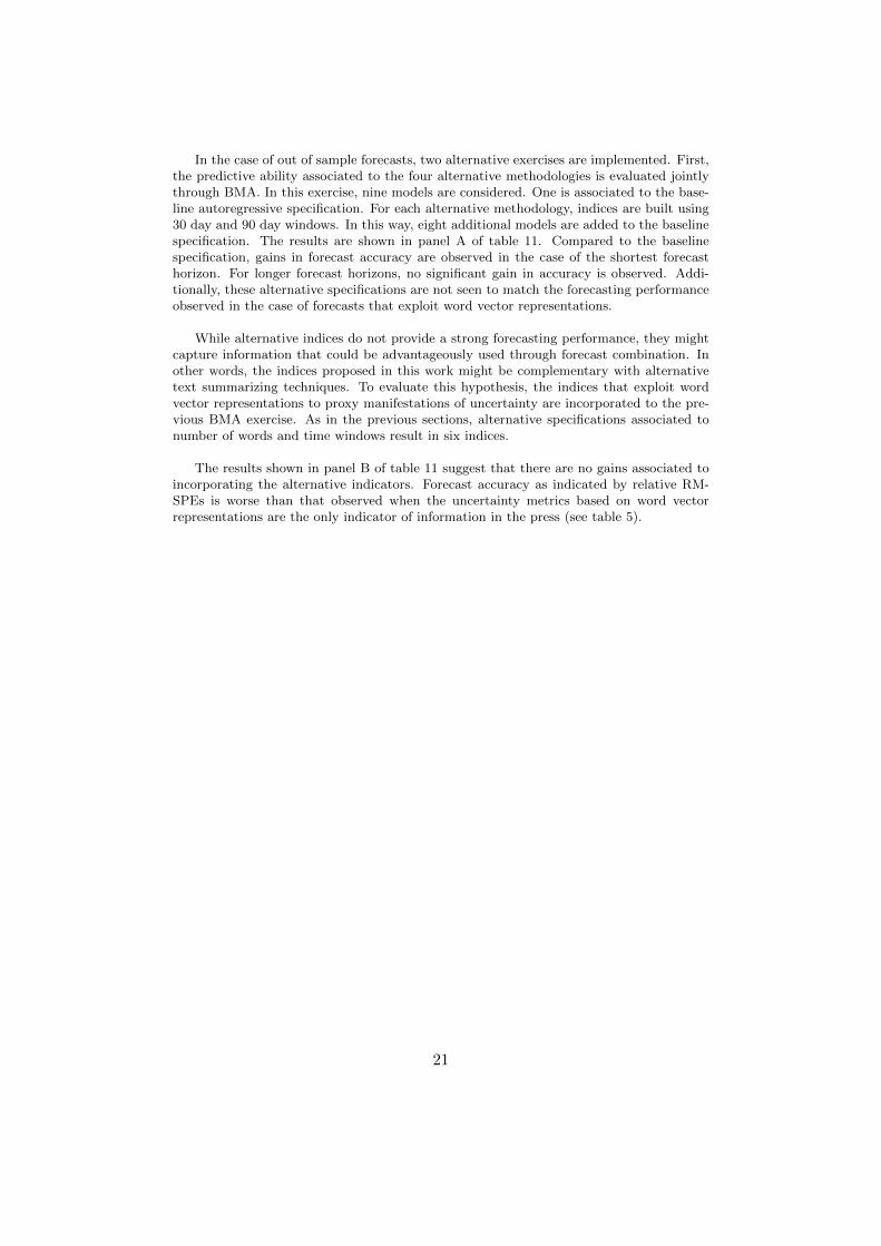
In the case of out of sample forecasts, two alternative exercises are implemented. First,the predictive ability associated to the four alternative methodologies is evaluated jointlythrough BMA. In this exercise, nine models are considered. One is associated to the base-line autoregressive specification. For each alternative methodology, indices are built using30 day and 90 day windows. In this way, eight additional models are added to the baselinespecification. The results are shown in panel A of table 11. Compared to the baselinespecification, gains in forecast accuracy are observed in the case of the shortest forecasthorizon. For longer forecast horizons, no significant gain in accuracy is observed. Addi-tionally, these alternative specifications are not seen to match the forecasting performanceobserved in the case of forecasts that exploit word vector representations.

While alternative indices do not provide a strong forecasting performance, they mightcapture information that could be advantageously used through forecast combination. Inother words, the indices proposed in this work might be complementary with alternativetext summarizing techniques. To evaluate this hypothesis, the indices that exploit wordvector representations to proxy manifestations of uncertainty are incorporated to the pre-vious BMA exercise. As in the previous sections, alternative specifications associated tonumber of words and time windows result in six indices.

The results shown in panel B of table 11 suggest that there are no gains associated toincorporating the alternative indicators. Forecast accuracy as indicated by relative RM-SPEs is worse than that observed when the uncertainty metrics based on word vectorrepresentations are the only indicator of information in the press (see table 5).

21

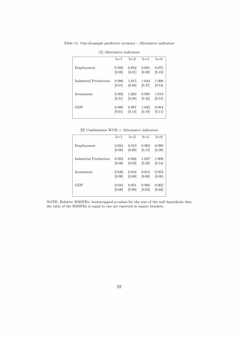
Table 11: Out-of-sample predictive accuracy - Alternative indicators

[A] Alternative indicators

h=1 h=2 h=4 h=8

Employment 0.950 0.952 0.991 0.975[0.00] [0.01] [0.20] [0.18]


Investment 0.992 1.003 0.989 1.019[0.31] [0.88] [0.42] [0.54]

GDP 0.980 0.987 1.032 0.954[0.01] [0.14] [0.19] [0.11]

[B] Combination WVR + Alternative indicators

h=1 h=2 h=4 h=8

Employment 0.924 0.913 0.982 0.990[0.00] [0.00] [0.15] [0.30]


Investment 0.946 0.944 0.914 0.953[0.00] [0.00] [0.00] [0.08]

GDP 0.944 0.951 0.960 0.902[0.00] [0.00] [0.03] [0.02]


22

7 Conclusions

This study proposes a method for the quantification of unstructured information in thepress. It it is based on word vector representations, a tool developed in the field of naturallanguage processing. It is shown that trained representations learn meaningful relationshipsbetween words in economic contexts. These associations are exploited to build indicatorsof subjective states in press content.

The resulting indicators can be interpreted in a straightforward manner. Using real-time data on economic activity, the indices are shown to anticipate business cycles dynam-ics. Bayesian model averaging exercises show that there are benefits associated to com-bining information from indices linked to different subjective states. Also, the forecastingperformance compares favorably to results under alternative text processing techniquesconsidered in previous literature. In this way, this work shows how novel machine learningtools can generate interpretable and informative indicators that can be used in macroeco-nomic forecasting applications.

The are several directions in which the current work can be extended. A natural pathis associated to implementations based on larger training and testing corpora. Automatedmethods for the selection of relevant keywords can also be explored. In the field of naturallanguage processing, word vector representations are used as inputs in neural network ap-plications (Kim 2014). Hence, while the property of straightforward interpretation wouldbe lost, another possible extension involves exploring nonlinear forecasting models.

23

References:

Ardia, D., Bluteau, K., & Boudt, K. (2017). Aggregating the Panel of Daily TextualSentiment for Sparse Forecasting of Economic Growth.

Aromı, J. D. (2017a). Conventional views and asset prices: What to expect after timesof extreme opinions?. Journal of Applied Economics, 20(1), 49-73.

Aromı, J. D. (2017b). Measuring uncertainty through word vector representations.Economica, 63(1), 135-156.

Aromı, J. D., (2017c), GDP growth forecasts and information flows: is there evidenceof overreaction?, International Finance,-(-), -.

Baker, S. R., Bloom, N., & Davis, S. J. (2016). Measuring economic policy uncertainty.The Quarterly Journal of Economics, 131(4), 1593-1636.

Bernanke, B. S., Gertler, M., & Gilchrist, S. (1999). The financial accelerator in aquantitative business cycle framework. Handbook of macroeconomics, 1, 1341-1393.

Boucher, J., & Osgood, C. E. (1969). The pollyanna hypothesis. Journal of VerbalLearning and Verbal Behavior, 8(1), 1-8.

Chen, H., De, P., Hu, Y. J., & Hwang, B. H. (2014). Wisdom of crowds: The value ofstock opinions transmitted through social media. The Review of Financial Studies, 27(5),1367-1403.

Collobert, R., Weston, J., Bottou, L., Karlen, M., Kavukcuoglu, K., & Kuksa, P.(2011). Natural language processing (almost) from scratch. Journal of Machine LearningResearch, 12(Aug), 2493-2537.

Corsi, F. (2009). A simple approximate long-memory model of realized volatility. Jour-nal of Financial Econometrics, 7(2), 174-196.

Diebold, F. (2015). Comparing Predictive Accuracy, Twenty Years Later: A PersonalPerspective on the Use and Abuse of Diebold-Mariano Test, Journal of Business and Eco-nomic Statistics, Vol 33, 1.

Duchi, J., Hazan, E., & Singer, Y. (2011). Adaptive subgradient methods for onlinelearning and stochastic optimization. Journal of Machine Learning Research, 12(Jul), 2121-2159.

Faust, J., Gilchrist, S., Wright, J. H., & Zakrajssek, E. (2013). Credit spreads as pre-dictors of real-time economic activity: a Bayesian model-averaging approach. Review ofEconomics and Statistics, 95(5), 1501-1519.

Fernandez, C., Ley, E., & Steel, M. F. (2001). Benchmark priors for Bayesian model

24

averaging. Journal of Econometrics, 100(2), 381-427.

Garcia, D. (2013). Sentiment during recessions. The Journal of Finance, 68(3), 1267-1300.

Garcia, D., Garas, A., & Schweitzer, F. (2012). Positive words carry less informationthan negative words. EPJ Data Science, 1(1), 3.

Gilchrist, S., & Zakrajsek, E. (2012). Credit spreads and business cycle fluctuations.American Economic Review, 102(4), 1692-1720.

Jermann, U., & Quadrini, V. (2012). Macroeconomic effects of financial shocks. Amer-ican Economic Review, 102(1), 238-71.

Jurado, K., Ludvigson, S. C., & Ng, S. (2015). Measuring uncertainty. American Eco-nomic Review, 105(3), 1177-1216.

Kim, Y. (2014). Convolutional neural networks for sentence classification. arXivpreprint arXiv:1408.5882.

Loughran, T., & McDonald, B. (2011). When is a liability not a liability? Textualanalysis, dictionaries, and 10-Ks. The Journal of Finance, 66(1), 35-65.

Mikolov, T., Sutskever, I., Chen, K., Corrado, G. S., & Dean, J. (2013). Distributedrepresentations of words and phrases and their compositionality. In Advances in neuralinformation processing systems (pp. 3111-3119).

Newey WK & West KD (1987), A Simple, Positive Semi-Definite, Heteroskedasticityand Autocorrelation Consistent Covariance Matrix. Econometrica, 55,pp. 703-708.

Newey WK & West KD (1994), Automatic Lag Selection in Covariance Matrix Esti-mation. Review of Economic Studies, 61,pp. 631-653.

Nyman, R. & Kapadia, S., Tuckett, D., Gregory, D., Ormerod, P. and Smith, R.(2018).News and Narratives in Financial Systems: Exploiting Big Data for Systemic Risk Assess-ment. Bank of England Working Paper No. 704.

Pennington, J., Socher, R., & Manning, C. D. (2014). Glove: Global vectors for wordrepresentation. In EMNLP (Vol. 14, pp 1532-1543).

Rossi, B., & Sekhposyan, T. (2015). Macroeconomic uncertainty indices based on now-cast and forecast error distributions. American Economic Review, 105(5), 650-55.

Schularick, M., & Taylor, A. M. (2012). Credit booms gone bust: Monetary policy,leverage cycles, and financial crises, 1870-2008. American Economic Review, 102(2), 1029-61.

25

Tetlock, P. C. (2007). Giving content to investor sentiment: The role of media in thestock market. The Journal of finance, 62(3), 1139-1168.

Timmermann, A. (2006). Forecast combinations. Handbook of economic forecasting,1, 135-196.

Zellner, A. (1986). On assessing prior distributions and Bayesian regression analysiswith g-prior distributions. Bayesian inference and decision techniques, ed. by P.K. Goel &A. Zellner, Amsterdam, The Netherlands: North-Holland, 233-243.

26

Appendix A: List of stop wordsa, an, and, at, are, been, by, between, by, can, could, for, has, have, is, in, of, on, or, since,that, the, these, this, those, to, was, were, will, with, without.

27

Documents

Linking Words in Economic Discourse: Implications for … · Linking Words in Economic Discourse: Implications for Macroeconomic Forecasts J. Daniel Arom March 19, 2018 Abstract Word