Superfluidity in Liquid 4He

Masatsugu Sei Suzuki

Department of Physics, SUNY at Binghamton

(Date: November 14, 2018)

______________________________________________________________________________

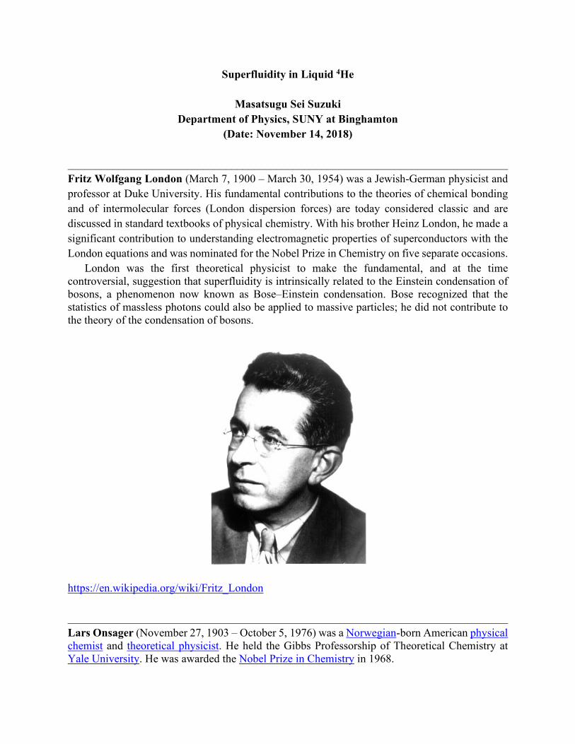
Fritz Wolfgang London (March 7, 1900 – March 30, 1954) was a Jewish-German physicist and

professor at Duke University. His fundamental contributions to the theories of chemical bonding

and of intermolecular forces (London dispersion forces) are today considered classic and are

discussed in standard textbooks of physical chemistry. With his brother Heinz London, he made a

significant contribution to understanding electromagnetic properties of superconductors with the

London equations and was nominated for the Nobel Prize in Chemistry on five separate occasions.

London was the first theoretical physicist to make the fundamental, and at the time controversial, suggestion that superfluidity is intrinsically related to the Einstein condensation of bosons, a phenomenon now known as Bose–Einstein condensation. Bose recognized that the statistics of massless photons could also be applied to massive particles; he did not contribute to the theory of the condensation of bosons.

https://en.wikipedia.org/wiki/Fritz_London

______________________________________________________________________________

Lars Onsager (November 27, 1903 – October 5, 1976) was a Norwegian-born American physical chemist and theoretical physicist. He held the Gibbs Professorship of Theoretical Chemistry at Yale University. He was awarded the Nobel Prize in Chemistry in 1968.

https://en.wikipedia.org/wiki/Lars_Onsager

1. Properties of liquid He

Helium exists in two stable isotropic forms, 4He and 3He. The phase diagram of 4He is shown

below. The normal boiling point is 4.2 K and the critical temperature is 5.19 K (1,718 Torr = 2.26

atm). Liquid He exists in two phases, He I and He II, separated by a phase boundary commonly

called the lambda-line. At T = 2.172 K, which is termed the -point. There is no latent heat

associated with this transformation. The specific heat at saturated vapor pressure, becomes large

as the -point is approached from either side. One of the most remarkable properties of He II is its

ability to flow through very small capillaries or narrow channels without any friction at all.

Fig. Phase diagram of liquid 4He. He I (normal liquid) and He II (superfluid)

Fig. Specific heat of liquid 4He (point) in comparison with the theoretical curve for an ideal

Bose gas with the parameters of liquid He (dashed line).

Fig. Temperature dependence of the viscosity of He II as determined from flow experiments

with thin capillaries.

2. Historical overview on the research on superfluid Helium 4.

In 1908, Kammerlingh Onnes succeeded for the first time in liquefying helium in Leiden. In 1938

Allen and Misener, and Kapitza independently discovered that it exhibited a superfluid behavior. Fritz

London put forth his theory that superfluidity could be related to the Bose-Einstein condensation. Tisza

suggested that the superfluid phase of the liquid could be described by a two-fluid model, the normal fluid

and the superfluid. In 1941 Landau suggested that superfluidity can be understood in terms of the special

nature of the thermally excited states of the liquid: the well-known phonons and rotons. This theory also

led Landau to the two-fluid model. Experimentally the two-fluid model was supported by the experiment

of the experiment of Andronikashvili and the discovery of second sound.

In 1946, Onsager put forth his idea of quantized circulation in superfluid helium. The well-

known invariant called the hydrodynamic circulation is quantized. The quantum of circulation is

mh / , where m is the exact mass of the bare helium atom. This is a surprising result in itself

considering how strongly coupled atoms in a liquid really are. Feynman was working on the same

problem and came to a somewhat different conclusion. He showed that the excitation spectrum

postulated by Landau can be derived within a quantum-mechanical description. He considered

that the vortices in the superfluid might take the form of a vortex filament with a core of atomic

dimensions, truly a line vortex. In this picture, the multiple connectivity of a vortex arises because

the superfluid is somehow excluded from the core and circulates about the core in quantized

fashion. The quantization of circulation was experimentally confirmed by Hall and Vinen with the direct

observation in a macroscopic scale. This work led to an appreciation for the first time of the full significance

of London’s “quantum mechanism on a macroscopic scale”, and of the underlying importance of Bose-

Einstein condensation in superfluidity.

Here the superfluidity of He II is discussed in association with the statistical mechanics and quantum

mechanics.

3 Two component fluid model (Tisza, Landau)

Fig. Density of the superfluid and normal-fluid component in He II as a function of

temperature.

The two-fluid model of liquid helium (Landau) postulates that He II behaves as if it were a

mixture of two fluids freely intermingling with each other without any viscous interaction. There

two fluids are termed the normal fluid and have densities n and s such that

sn

where is the ordinary density of liquid He. The normal density n is a function of temperature,

and increases from zero at T = 0 K, to the value at the lambda point. Conversely, the superfluid

density s is zero at the lambda point and increases to the value at T = 0 K. The model

postulates that the superfluid carries zero entropy, and experiences no resistance whaever to its

flow, that is, it exhibits neither viscosity nor turbulence. This condition is specified by stipulating

that the viscosity of the superfluid is zero, and that its velocity sv satisfies the relation

0 sv (irrotational).

On the other hand, the normal fluid has a viscosity, the so-called normal viscosity n , and an

entropy nS equal to the entropy of liquid He.

We now derive equations of motion for the two fluids of the model. Let j denotes the

momentum of unit volume of liquid He, and nv and sv the velocities of the two fluids. Then we

have

ssnn vvj

The flow j is also related to the density of liquid He by the equation of continuity

0

t

j

4. Probability current density (London) in quantum mechanics in Macroscopic scale

A superfluid has the special property of having phase, given by the wave function. The order

parameter (wave function) for the BEC phase is given by

)(

0)( rr

ie

where 0 is independent of the position vector r and the phase ( ) r is a real-valued function of

r. The probability current density is

*

*

* *

Re[ ]

Re[ ]

( )2

m

mi

im

pj

ℏ

ℏ

Suppose that ( )0

ie r

2 2

0 0 sm j vℏ

with the velocity

sm

vℏ

The velocity sv of the superfluid is proportional to the gradient of the phase.

)(rv m

s

ℏ

We not that

0)( rvw m

s

ℏ

In 1941, Landau suggested a test of this assumption in experiments with He II in a rotating vessel.

Even before such experiments were conducted, Onsager speculated whether the assumption of

0s v is generally valid and suspected the occurrence of vortices in rotating He II.

Fig. Vortex line and vortex ring.

6. Quantization of angular momentum

Fig. Quantum vortex with 2 r

q

, where q = 6 and 12. is the wavelength.

The angular momentum is quantized. We note that

(2 )

sd m d

m dm

q

p l v l

lℏ

ℏ

� �

�

where q is integer. The momentum p is

(2 )

2

q qp

r r

ℏ ℏ

The kinetic energy is

2 2 2

22 2

p q

m mr

ℏ

The velocity is

s

p qv

m mr

ℏ.

The circulation:

(2 )s

hqd d q

m m m v l l

ℏ ℏ

� �

The angular momentum:

2 2 ( ) 2 ( ) 2s s zm d rp r mv mv r L p l�

leading to

2z s

mL mv r

7. Quantization of circulation

The circulation around any closed loop in the superfluid is zero, if the region enclosed is simply

connected. The superfluid is thought to be irrotational (no rotation),

( ) 0s s

A L

d d v a v l� � (Stoke’s theorem).

However, if the enclosed region actually contains a smaller region with an absence of superfluid

(the singularity), the circulation around a doubly connected system is

qmm

dm

dCC

s 2)(ℏℏℏ

lrlv (Stoke’s theorem)

where q is integer.

81.58769 104m u

ℏ ℏ

m2/s

m is the mass of He4 .

Fig. Circulating sv in a doubly connected system. Circulation around a hole.

((Note))

Simply connected superfluid and multiply connected superfluid.

Fig. (a) Simply-connected superfluid. (b) Multiply-connected superfluid.

___________________________________________________________________________

For the velocity vs, we have

(2 ) 2sv r qm

ℏ

, 2sv

r

or

z sL mv r q ℏ

which means that the angular momentum is quantized.

The circulation around the path C is either zero or a multiple of the quantum of circulation ,

qmm

hq ℏ

2

For 0q , the velocity around the singularity decreases to zero at infinity.

r , 0v ,

0r , v ,

The sign of q determines the direction of the flow. q is called the charge of the vortex.

If sn is the superfluid number density, the kinetic energy is (for q = 1),

2

2 2

2

12

2

ln

ln( )4

b

s

a

s

s

qE n m rdrl

mr

q l bn

m a

l b

a

ℏ

ℏ

where l is the depth of liquid, ss mn is the superfluid density, a is the core radius of the vortex,

b is the radius of the bucket, or the mean distance between vortices. The line energy per unit length

is given by

2 ln( )4

sE bl

l a

Feynman conjectured how the vortex line might be arranged. First, note that since the

circulation enters squared in the energy, doubly quantized vortex line would have four times

the energy of a singly quantized line, and would likely be unstable to break up into four separate

lines. The creation of many vortices with q = 1 is energetically more favorable than the creation

of a smaller number of vortices with correspondingly higher circulation.

The angular momentum zL per unit length associated with a single vortex is given by

0

2

0

0

2

(2 )

22

2

R

s s

R

s

R

s

s

Lrv r dr

l

r drr

rdr

R

where

2svr

We note that

2

2 2

ln( ) ln( )4

2

2

s

s

b b

E a a

RL R

We assume that

21122

c

c

c

IE

L I

Thus we have

2 2

ln( )ln( )c

b

hq ba

R m R a

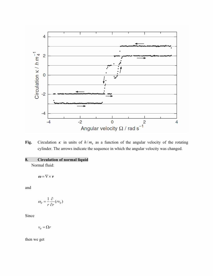
Fig. Circulation in units of 4/ mh as a function of the angular velocity of the rotating

cylinder. The arrows indicate the sequence in which the angular velocity was changed.

8. Circulation of normal liquid

Normal fluid:

vω

and

)(1

rvrr

Since

rv

then we get

221

)(1 2 r

rr

rr : solid body rotation

The velocity v is proportional to r in the normal phase.

\

Fig. (i) qmr

vℏ

(q: integer). (ii) rv for the normal fluid.

9. Second London equation

Since

)(rv m

s

ℏ

we have

0)]([ rv m

s

ℏ.

or

0 sv (the second London equation)

The superfluid is irrotational.

Here note that using the Stokes theorem we have

r

v

i

ii

qm

dd s

C

s 2)(ℏ

avlv

where da is the areal vector of the surface element (inside the closed loop C). This result leads to

the expression of around the singularity as

zs ervω )(2

)(2 r is the two-dimensional Dirac delta function. So svω is zero (the flow is irrotational)

except at the origin (singularity).

Fig. Radial (r) dependence of vs around the singularity (origin).

10. Anderson-Josephson evolution relation (time dependent Schrödinger equation)

We start with the time-dependent Schrödinger equation

Ht

i ℏ .

We assume that the wave function is given by

ie0

The phase angle is dependent on t and r. Thus we have

iii eH

tee

ti

ti 000

ℏℏℏ

or

Ht

ℏ .

As regards the time derivative, we replace the Hamiltonian with the chemical potential .

dt

dℏ (Anderson-Josephson phase evolution relation).

Since m

vs

ℏ, we have

)()(tmt

mt

vm s

ℏℏ

11. The Gibbs-Duhem relation (thermodynamics)

The Gibbs free energy is given by

PVSTEPVFNG

leading to the differential form

VdPPdVTdSSdTdENddNdG

or

VdPPdVTdSSdTdNPdVTdSNddN

or

VdPSdTNd

So we get the relation

dTN

SdP

N

Vd (Gibbs-Duhem relation)

Here N is the number of particles, V is the volume, S is the entropy, is the pressure and T is the

temperature. The chemical potential can be written as follows.

)( dTdP

mmdTdPm

dTN

SdP

N

Vd

m

N

M

M

V

N

V , mm

Nm

S

N

S

The Gibbs-Duhem can be rewritten as

)1

( TPm

,

where is the entropy per unit mass and is the density.

12. The first London equation

We consider the Bernoulli effect for a system in dynamic flow. The pressure P is replaced by

2

2

1svPP

Fig. The principle based on the Bernoulli equation (derived from the work energy theorem for

fluid). const2

1 2 vghP .

Then we have

TvPm

s

)2

1(

11 2

The time evolution of sv is

TPv

TvP

mt

s

s

s

1

2

1

)2

1(

1

1

2

2

v

or

TPvt

ss

1

2

1 2v. (The first London equation)

13. Heat flux density

The heat flux density (erg/cm2 s) is expressed by

nvTq

The amount of heat per unit mass

TQ

where is the entropy per unit mass. Once equilibrium has been established, the heat flow may

be expressed in terms of the entropy, average temperature T, and flow rate as

nvTq ɺɺ

14. Fountain effect (mechanocaloric effect)

In a nearly blocked porous plug only the superfluid can flow while the heat flow is blocked.

This is enough to lift the superfluid against gravity and force it out at the top of vessel. It is an

unusual example of osmosis. Both the superfluid and normal fluid components carry particle

current, but only the normal component carries heat current.

We assume a steady state.

TPt

vs

1

0

or

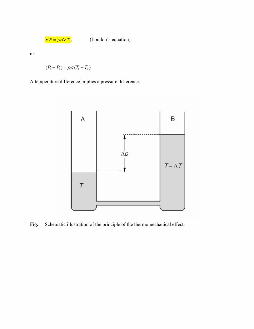
TP , (London’s equation)

or

)()( 2121 TTPP

A temperature difference implies a pressure difference.

Fig. Schematic illustration of the principle of the thermomechanical effect.

Fig Demonstration of the fountain effect. A capillary tube is “closed” at one end by a superleak

and is placed into a bath of superfluid helium and then heated. The helium flows up through

the tube and squirts like a fountain.

15. Quantum vortices in the rotating He II

Fig. Electrometer signal as a function of angular velocity. The velocity of rotation of He II was

increased steadily in this experiment

Fig. Schematic illustration of vortices in a rotating vessel containing He II.

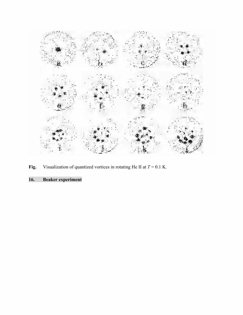
Fig. Visualization of quantized vortices in rotating He II at T = 0.1 K.

16. Beaker experiment

Fig. Schematic illustration of beaker experiments. Pioneering film flow experiments of Daunt

and Mendelssohn. (a) Beaker filling through the film. (b) Beaker emptying through the

film. (c) Drops forming on the bottom of the beaker.

17. Andronikashivili experiment

A schematic drawing of the specially designed torsion oscillator that Andronikashvili used in 1948 to determine the normal-fluid density n is shown in Fig. The complete normal-fluid

component n , but not the superfluid component s , was dragged with the discs above and below

the lambda point.

Fig. Schematic drawing of the apparatus used by Andronikashivili to determine the normal-

fluid density n of He II.

Fig. Temperature dependence of the normal-fluid density n normalized to the density at

T . The data were obtained with two different methods: ○ Andronikashvili viscometer,

and ● second-sound measurements.

18. First sound, second sound, and third sound

Fig. Velocity of second sound in He II as a function of temperature. The solid line shows the

theoretical prediction.

19. Critical velocity

Concept of the critical velocity

p 'MvMv (Momentum conservation)

pvv 22 '2

1

2

1MM (Energy conservation)

Using the relation

Mvv

p'

we have

pp pvp

vp

vv M

MM

MM22

1)(

2

1

2

1 2222

or

ppvp

M2

2

We assume that M is so large that the M2

2p

can be neglected. If is the angle between p and v, we

then have

vpvp cospvp

Thus the condition

pv

p

must be satisfied for excitation to be created. Thus the critical velocity is given by

min

pvc

p

The superfluidity can therefore occur if

0cv

a condition which is known as the Landau criterion for superfluidity.

The energy dispersion relation was determined using inelastic neutron scattering. The energy

spectrum of the rotons is described by

20*)(

2

1pp

m

where *m denotes the effective mass of a helium atom.

Fig. Dispersion curve of He II as determined experimentally (inelastic neutron scattering)

Fig. Phonon-roton spectrum in comparison with free 4He atoms. The two dashed lines are

tangents to the dispersion curve and reflect the critical velocities of phonons and rotons.

At T = 1 K, one finds that

67.8

Bk K, 94.10

ℏ

p Å-1, 4

* 15.0 mm

We note that the critical velocity is evaluated as

8 .580

p

vc 5 m/s (roton).

((Mathematica))

((Ion mobility and the Landau critical velocity))

An direct measurement of significance is the study of ions in liquid helium. In this type of

experiment, ions are injected into the liquid by applying a high voltage to a fine metal tip. The ion

motion to a collector electrode can be controlled and studied with suitably arranged grids set at

specific potential.

Clear "Global` " ;

rule1 kB 1.3806504 1016,

1.054571628 1027, 10

8, THz 10

12,

7.2973525376 103, m 10

2;

vc8.67 kB

1.94 1 m. rule1

58.5093

The measurement of negative ion mobility provides an experimental verification of the critical

velocity. There is virtually no dissipation seen until the Landau critical velocity is reached. This

a direct measurement of the critical velocity, and the magnitude agrees remarkably well with that

calculated from the dispersion relation.

Fig. The critical velocity determined experimentally. T = 0.35 K.

20. DC and AC Josephson effect

Here we consider two vessels containing He II that are connected by a weak link. Suppoe that

there is a difference in the chemical potential such that

.12

Let 1 and 2 be the probability amplitude of macroscopic wave function on either side of the

aperture. We can write for the Schrödinger equation for the two vessels,

2111

tiℏ , 122

2

tiℏ

or

2

1

2

1

2

1

tiℏ

where represents the coupling across the weak link.

Let

,1

1 i

e 2

2 i

e

where

2

1 , 2

2

where 1 and 2 are the phases of the two wave functions. We solve the problem using

Mathematica.

______________________________________________________________________

((Mathematica))

______________________________________________________________________

Then we have

0222 11 iei ɺℏɺℏ (1)

0222 22 iei ɺℏɺℏ (2)

where the phase difference is defined by

12 .

Now equate the real and imaginary parts of Eqs.(1) and (2),

sin2

ℏɺ (3)

and

0cos11 ɺℏ

0cos22 ɺℏ

leading to

ℏℏ

ɺ 1)(

112 (4)

For =0 we have a constant phase difference 12 that results in a stationary mass flow

without any pressure applied. This phenomenon is called the dc Josephson effect. For 0 we

find an oscillating mass flow with frequency

tJ 1

ℏ

This phenomenon is called the ac Josephson effect.

21. Experiment on Josephson effect in liquid He II

Phys. Rev. Letts. 106, 055302 (2011)

Quantum Coherence in a Superfluid Josephson Junction

by S. Narayana and Y. Sato

Fig.1 Experimental apparatus. A flexible diaphragm (D) and a rigid electrode (E) form an

electrostatic pressure pump. The diaphragm also forms the input element of a sensitive

displacement sensor through a nearby pickup coil (P) connected to a dc- SQUID (not

shown). A heater (R) is used to induce quantum phase gradients across an aperture array

(A).

The experimental apparatus is schematically shown in Fig.1. Unshaded regions are filled with

superfluid 4He, and the entire apparatus is immersed in a temperature regulated 4He bath. Two

reservoirs of superfluid 4He are coupled through an array of apertures (A). In an ideal weak

coupling limit, the mass current )(tI across the junction driven by a chemical potential difference

is governed by the Josephson current-phase relation

sin0II ,

where 0I is the junction critical current, and is the quantum phase difference across the junction.

The phase difference evolves in time according to the Anderson phase evolution equation

ℏ

ɺ

.

A constant chemical potential difference counterintuitively leads to oscillatory mass current

at the junction

tItIℏ

sin)( 0 (AC Josephson effect).

To observe such Josephson phenomena, a ‘‘weak’’ coupling must be established between two

quantum fluids. This is achieved by using an aperture whose size matches the superfluid healing

length 4 . Near the superfluid transition temperature ,17.2 KT the correlation length 4

diverges as

67.04 )1(4.0

T

T, (nm).

Because of this property, various Josephson phenomena emerge at temperatures roughly 1 – 10

mK away from T if the aperture size is 50 nm. A Josephson mass current signal from a single

≈50 nm aperture is on the order of 1610 kg/sec, too small to detect. Furthermore, large thermally

induced fluctuations in superfluid order parameter phase at 2 K are expected to destroy the

Josephson effect even if one had the capability to detect such a small signal.

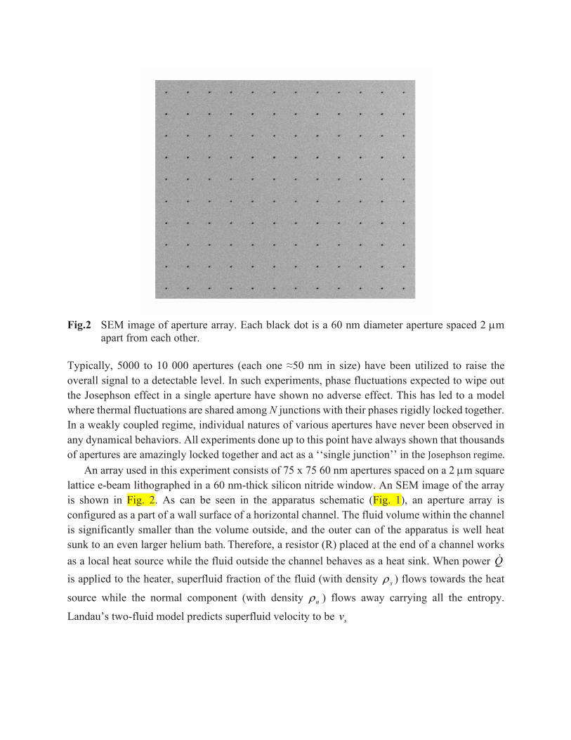
Fig.2 SEM image of aperture array. Each black dot is a 60 nm diameter aperture spaced 2 m

apart from each other.

Typically, 5000 to 10 000 apertures (each one ≈50 nm in size) have been utilized to raise the

overall signal to a detectable level. In such experiments, phase fluctuations expected to wipe out

the Josephson effect in a single aperture have shown no adverse effect. This has led to a model

where thermal fluctuations are shared among N junctions with their phases rigidly locked together.

In a weakly coupled regime, individual natures of various apertures have never been observed in

any dynamical behaviors. All experiments done up to this point have always shown that thousands

of apertures are amazingly locked together and act as a ‘‘single junction’’ in the Josephson regime.

An array used in this experiment consists of 75 x 75 60 nm apertures spaced on a 2 m square

lattice e-beam lithographed in a 60 nm-thick silicon nitride window. An SEM image of the array

is shown in Fig. 2. As can be seen in the apparatus schematic (Fig. 1), an aperture array is

configured as a part of a wall surface of a horizontal channel. The fluid volume within the channel

is significantly smaller than the volume outside, and the outer can of the apparatus is well heat

sunk to an even larger helium bath. Therefore, a resistor (R) placed at the end of a channel works

as a local heat source while the fluid outside the channel behaves as a heat sink. When power Qɺ

is applied to the heater, superfluid fraction of the fluid (with density s ) flows towards the heat

source while the normal component (with density n ) flows away carrying all the entropy.

Landau’s two-fluid model predicts superfluid velocity to be sv

Qɺɺ

Tm

vs

ns

4

where is the total fluid density, is the specific entropy, and T is the temperature. London’s

wave function view of the condensate leads to superfluid velocity related to quantum phase

gradient by

4m

vs

ℏ.

A phase gradient is then induced along the channel (and along the aperture array):

Qɺℏ

ɺ

Ts

n1 . (1)

This apparatus configuration allows us to directly apply finite phase gradient along the array of

apertures, giving us an unique opportunity to probe their collective dynamics. In operation, we

apply a pressure difference (and hence a chemical potential difference) across the aperture array

by pulling a diaphragm [labeled (D) in Fig. 1] towards a nearby electrode (E). In response, the

array exhibits Josephson mass current oscillation. The diaphragm motion (indicating fluid flow

through the array) is detected using a dc-SQUID based displacement transducer. We record the

overall mass current oscillation amplitude while applying finite external phase gradient [Eq. (1)]

along the array in an attempt to unlock their phases and reveal their individuality.

In Fig. 3, we plot the overall mass current oscillation amplitude as a function of heat input in

the channel for three different temperatures. If all the apertures are indeed phase locked due to

strong coupling or interactions, the oscillation amplitude from the array should remain constant.

However, as the heater power is increased, we find that the oscillation amplitude varies. The

surprisingly smooth and nonchaotic behavior implies that different apertures maintain temporal

coherence of Josephson oscillations with a well-defined frequency of h/ in the background of

externally applied phase gradients.

Fig.3 Oscillation amplitude as a function of heater power. The solid lines are fits. At power levels higher than what is shown here, turbulence sets in, rendering the oscillation amplitude measurement difficult

((Note))

0 ssnn vv ɺɺ (from 0t

j).

)(44 s

n

sn vsTmvsTmQ ɺɺɺ

(the normal component has the entropy)

QsTm

vs

ns

ɺɺ

4

______________________________________________________________________________

REFERENCES

P. Kapitza, Nature 141, 74 (1938).

L. Tisza, Nature 141, 913 (1938).

J.F. Allen and A.D. Misener, Nature 141, 75 (1938).

F. London, Nature 141, 643 (1938).

L. Onsager, Nuovo Cimento Suppl. 6, 249 (1949).

R.P. Feyman, Phys. Rev. 90, 1116 (1953).

F. London, Superfluids, Vol. II (Wiley, 1954).

R.P. Feynman, Application of quantum mechanics to liquid helium, in Progress in Low

Temperature Physics I, edited by C.J. Gorter (North-Holland, 1955).

W.F. Vinen, The Physics of Superfluid Helium

(https://cds.cern.ch/record/808382/files/p363.pdf).

K.R. Atkins, Liquid Helium (Cambridge, 1959).

R.J. Donnelly, Experimental Superfluidity (University of Chicago, 1967).

R.P. Feynman, Statistical Mechanics: A Set of Lectures (Benjamin/Cummings) (1982).

J. Wilks and D.S. Betts, second edition, Introduction to Liquid Helium (Oxford, 1987).

D.R. Tilley and J. Tilley, Superfluidity and Superconductivity, 3rd edition (Institute of Physics,

1990).

D.J. Thouless, Topological Quantum Numbers in Nonrelativistic Physics (World Scientific, 1998).

I.M. Khlatnikov, An Introduction to the Theory of Superfluidity (Westview 2000).

J.F. Annett, Superconductivity, Superfluids and Condensates (Oxford, 2004)

C. Enss and S. Hunklinger, Low-Temperature Physics (Springer, 2005).

C.F. Barenghi, A Primer on Quantum Fluids (Springer, 2016).

L. D. Landau and E. M. Lifshitz, Fluid Mechanics, vol. 6 (Pergamon Press 2nd ed. July 1987).

T. Geunault, Basic Superfluids (Taylor & Francis, 2003).

P.V.E. MvClintock and D.J. Meredith, and J.K. Wigmore, Matter at Low Temperatures (A Wiley-

Interscience, 1984).

APPENDIX Fraunhofer diffraction pattern

((Mathematica))

0 100 200 300 400 500 600

0

100

200

300

400

500

600

APPENDIX-II Important equations equations

0 100 200 300 400 500 600

0

100

200

300

400

500

600

0 100 200 300 400 500 600

0.1

0.2

0.3

0.4

0.5

0.6

0

t

j (equation of continuity) (1)

0

Ptj (Euler equation) (2)

Usual hydrodynamic equation of continuity for the liquid as whole and has the effect of ensuring

conservation of mass.

ssnn vvj (3)

sn (4)

PTt

s

1v (5)

0)()(

t

nv (6)

Conservation of entropy on the assumption that viscous effects are negligible.

(i) Pt

2

2

2

(7)

((Proof))

From Eqs.(1) and (2)

Ptt

2

2

2

j

(ii)

ts

sn

)( vv (8)

((Proof))

t

t

t

n

nsn

nnns

ssnssns

v

v

vv

vvvv

)(

)(

)(

since

0)(

t

ssnn

vv

or

0

t

ssnn

vv

from Eq.(2). Then we get

ts

n

s

sn

1

)( vvv (a)

For Eq.(6), we have

)()( t

n

v

or

ttn

1

v (b)

From (a) and (b), we get

tt ss

sn

1

)( vv

When 0

t

, we have

ts

sn

)( vv

(iii)

Tt

snn

2)(

vv (9)

((Proof))

From Eqs.(5) and (2)

ssnn

ssnn

s

T

tT

tT

PT

vv

vv

j

v

ɺɺ

ɺ

)(

or

ssnnssn T vvv ɺɺɺ )(

Thus we have

Tsnn )( vv ɺɺ

and

Tsnn

2)( vv ɺɺ

(iv)

Tt n

s 22

2

2

((Proof))

From Eq.(8)

ts

sn

)( vv (8)

From Eq.(9),

Tt n

sn

2)(

vv (9)

Thus we have

Ttt ns

2][

If

s

is independent of t,

Tt n

s 22

2

2

APPENDIX III

svt

m

)1

( Tpm

nvTmQ ɺɺ

Since

0 ssnn vv ɺɺ

we get

s

n

ss

n

s vTm

vTmQ ɺɺɺ

)(

or

QTm

vs

ns

ɺɺ

_________________________________________________________________