Journal of Banking & Finance 45 (2014) 140–151

Contents lists available at ScienceDirect

Journal of Banking & Finance

journal homepage: www.elsevier .com/locate / jbf

Liquidity provision and stock return predictability

http://dx.doi.org/10.1016/j.jbankfin.2013.12.0210378-4266/� 2014 Elsevier B.V. All rights reserved.

⇑ Corresponding author. Tel.: +852 15109317531; fax: +852 23587666.E-mail addresses: hender@haas.berkeley.edu (T. Hendershott), Mark.Seasholes@

gmail.com (M.S. Seasholes).1 Rather than repeatedly refer to the differences in between position levels and

changes in positions, we will often say stocks heavily bought or sold by liquidityproviders. For competing market makers we exactly measure stocks bought and sold.Unless otherwise noted, for specialists we mean those stocks with the largest (mostpositive) inventories and smallest (most negative) inventories, respectively.

2 Campbell et al. (1993), Jegadeesh and Sheridan (1995), Llorente et aPastor and Stambaugh (2003) and Avramov et al. (2006) provide indirect evliquidity providers inducing negative autocorrelation in price changes. Henand Seasholes (2007) provide direct evidence using trading data byproviders.

Terrence Hendershott, Mark S. Seasholes ⇑Haas School of Business, University of California, Berkeley, United StatesHKUST, Clear Water Bay, Hong Kong

a r t i c l e i n f o a b s t r a c t

Article history:Received 16 August 2012Accepted 23 December 2013Available online 15 January 2014

JEL classification:G12G14D53

Keywords:LiquidityMarket makersMarket efficiencyInventoryLiquidity provision

This paper examines the trading behavior of two groups of liquidity providers (specialists and competingmarket makers) using a six-year panel of NYSE data. Trades of each group are negatively correlated withcontemporaneous price changes. To test for return predictability, we sort stocks into quintiles based oneach group’s past trades and then form long-short portfolios. Stocks most heavily bought have signifi-cantly higher returns than stocks most heavily sold over the two weeks following a sort. Cross-sectionalanalysis shows smaller, more volatile, less actively traded, and less liquid stocks more often appear in theextreme quintiles. Time series analysis shows the long-short portfolio returns are positively correlatedwith a market-wide measure of liquidity. A double sort using past trades of specialists and competingmarket makers produces a long-short portfolio that earns 88 basis points per week (act as complements).Finally, we identify a ‘‘chain’’ of liquidity provision. Designated market makers (NYSE specialists) initiallytrade against order flows and prices changes. Specialists later mean revert their inventories by tradingwith competing market makers who appear to spread trades over a number of days. Alternatively, spe-cialists may trade with competing market makers who arrive to market with delay.

� 2014 Elsevier B.V. All rights reserved.

1. Introduction different manners? How long do the designated market makers

Stock returns can have a temporary and predictable short-runcomponent in order to compensate liquidity providers for tradingwith less patient investors. What is the magnitude of this predict-able component? What is its duration? Which types of stocks aremost heavily traded by liquidity providers? This paper addressesthese questions by employing six years of daily and weekly tradingdata from the New York Stock Exchange (NYSE). Our data containrecords for two types of market makers: designated NYSE marketmakers (called ‘‘specialists’’) and competing market makers (some-time referred to as ‘‘CMMs’’ in this paper). Our data allow us toexamine the specialists’ inventory positions and the net trades ofcompeting market makers.1

Studying two groups of investors who are linked to liquidityprovision allows us to address a rich set of questions: Do the tradesof different liquidity providers forecast stock returns in similar or

hold their positions before reverting inventories back to target lev-els? Do liquidity providers always trade together? Or, is there a‘‘chain of liquidity provision’’ as initial positions are later trans-ferred between members of these groups?

This paper provides an in-depth study of liquidity providertrading at daily and weekly frequencies.2 As mentioned above,liquidity providers profit from trading with less patient investors.Such trading requires a liquidity provider to hold a suboptimal port-folio—suboptimal at efficient prices, but not at the transactionprices—until the position can be unwound. The liquidity providerprofits from buying a stock below its efficient price and later sellingas the price mean-reverts upward. Alternatively, the liquidity pro-vider can sell (short) above the efficient price and later buy shares(to cover the short) as the price mean-reverts downward. Tradingprofits compensate a liquidity provider for risk, effort, and costs ofcapital.

From the financial econometrician’s perspective, the act of pro-viding liquidity (being compensated for providing a service) is

l. (2002),idence ofdershottliquidity

T. Hendershott, M.S. Seasholes / Journal of Banking & Finance 45 (2014) 140–151 141

linked to predictability in price changes: when prices fall due todemands of sellers, prices will subsequently rise. Similarly, whenprices rise due demands of buyers, prices will subsequently fall.3

This predictability forms a bound around efficient prices and repre-sents an empirical measure of the compensation required by liquid-ity providers for their services. The bound can also be thought of as alimit to arbitrage—the limit is due to risk-bearing capacity andliquidity provision.

Jagadeesh (1990) and Lehmann (1990) first observed short-horizon return reversals.4 These reversals have been attributed toboth investor overreaction and liquidity provider inventoryeffects—see Subrahmanyam (2005) for a discussion of this point. Ifthere is no trading, there is no channel for inventory effects. In amarket with trading, overreaction and inventory effects can workin concert. If investors trade heavily in one direction and the marketfor liquidity provision is less than perfectly competitive, then pricescan overshoot fundamental values and subsequently reverse. Wetake no position on whether the source of shocks that our liquidityproviders accommodate is rational or not. Instead, we show thatthe trading of liquidity providers is linked to subsequent pricechanges. Thus, we establish that liquidity providers and inventoryeffects play a significant role in short-run price reversion.

For both types of liquidity providers studied in this paper (spe-cialists and competing market makers) we find their trades arenegatively correlated with contemporaneous returns. The findingis consistent with liquidity providers temporarily accommodatingbuying and selling pressure. We sort stocks into quintiles basedon each group’s trading. Quintile 1 represents stocks most heavilybought and Quintile 5 represents stocks most heavily sold. Wethen form value-weighted, long-short portfolios using stocks inquintiles one and five (there are two different long-short portfoliosbased on sorting the trading of both liquidity providers). At a one-day horizon, the long-short portfolios have returns of 20 basispoints and 13 basis points when sorting by the trades of specialistsand competing market makers respectively.5 To eliminate bid-askbounce, all returns are calculated using the midpoint of closingbid-ask quotes. The cumulative weekly returns of the long-shortportfolios are 41 basis points and 36 basis points and are statisticallysignificant. The cumulative two week returns are 52 basis points and40 basis points for specialists and competing market makers. Aftertwo weeks, the incremental returns of the long-short portfolios areno longer statistically different from zero consistent with prices hav-ing mean-reverted back to near-efficient levels.

The second part of our analysis investigates the characteristicsof stocks most likely to be in the liquidity providers’ highest orlowest trading quintiles. The more frequently a stock appears inQuintile 1 or Quintile 5, the more often the stock contributes tothe long-short portfolio returns discussed above. We calculatethe frequency with which each stock appears in the two extremeportfolios and then rank stocks by this frequency. In general, smal-ler, more volatile, less actively traded, and less liquid stocks appearmore often in the extreme portfolios. Consistent with results in

3 Reversals can occur at intraday horizons due to market makers buying at the bidand selling at the ask. For examples, see Stoll (1978), Amihud and Mendelson (1980),Ho and Stoll (1981), and Roll (1984). Over longer horizons, liquidity providers whotake on positions have assumed risk which can lead to reversals—see Grossman andMiller (1988). These longer-term, inventory-induced reversals are empirically similarto, but on a larger and market-wide scale, than reversals following block trades—seeKraus and Stoll (1972).

4 Conrad et al. (1994), Ball et al. (1995), Cooper (1999), Avramov et al. (2006), andothers also study short-run reversal strategies and their profitability.

5 The price reversals are also consistent with inventory models where a liquidityprovider offers attractive prices to induce order flow on one side of the market toreduce his inventory position. For example, if other investors have been buying fromthe specialist, prices have been rising, and the specialist has built up a short position.The specialist then raises his quotes to the point where investors begin to sell and thisselling leads to prices subsequently falling.

Amihud and Mendelson (1986), we find that stocks’ average dailyreturns increase with the frequency they appear in the extremeportfolios. In other words, less liquid stocks appear to have higherreturns.

Time series regressions show the returns of the long-short port-folios are related to a time series measure of effective bid-askspreads in the market. This finding complements the cross-sec-tional evidence that less liquidity stocks are more often in an ex-treme portfolio. Taken together, the sort results, cross-sectionalanalysis, and time series regressions provide strong evidence thatshort-run return predictability is related to liquidity provision.

We employ Fama–MacBeth style regressions to show tradesfrom one group do not drive out the predictability of trades fromother groups. Trades also predict future returns above and beyondthe predictability contained in only past returns. We also sortstocks into market capitalization terciles before repeating theregressions. Our results show that trades by competing marketmakers have the best ability to predict the returns of small stocksafter controlling for specialists’ inventories and past returns. Spe-cialist inventories have the best ability to predict the returns oflarge stocks. The size/predictability results suggest the two groupsof traders do not normally provide liquidity in the same stocks atthe same time. We hypothesize that observing two groups contem-poraneously providing liquidity for the same stock indicates a timeof exceptionally high liquidity demand. To test this hypothesis, wedouble-sort stocks based on the trades of specialists and competingmarket makers and form a long-short portfolio. The return of thelong-short portfolio is 88 basis points (on average) over the weekfollowing the double sort.

Our data allow us to better understand the inventory controlbehavior specialists and competing market makers. Both types ofliquidity providers lean against the wind—they trade in the oppo-site direct as contemporaneous returns—a characteristic of bothcontrarian investing and liquidity provision. Both contrarianinvesting and liquidity provision involve buying temporarilyunderpriced securities and selling temporarily overpriced securi-ties. Models of market making, however, predict that liquidity pro-viders hold their positions for brief periods of time. Brief holdingperiods help manage inventory and control risk. Thus, trades ofliquidity providers’ should be negatively autocorrelated as inMadhavan and Smidt (1993).

We find evidence of inventory control behavior for the NYSEspecialists only. They buy stocks with falling prices (sell stocks withrising prices) and revert their positions over the next few days. Thehalf-life of the average specialist position is about 1.8 days which isfar shorter than the 7.3 days reported by Madhavan and Smidt(1993) using data from fifteen years earlier. Furthermore, the neg-ative autocorrelation is stronger (mean-reversion is faster) the lar-ger the specialist’s inventory position. We do not find evidence ofcompeting market makers managing their inventory over shorthorizons as the autocorrelations of their net trades are positivefor at least 10 daily lags. The positive autocorrelations may resultfrom competing market makers having longer holding periods thanspecialists. Or, the positive autocorrelations may result from datathat are aggregated across many different types of competing mar-ket makers. If some competing market makers provide liquidityover short horizons and others continue trading in the directionof original price movements, then detecting mean reversion inaggregate trading data becomes difficult.

It is possible the autocorrelated CMM trades result from limita-tions of our data and point to avenues for future research. Forexample, we do not currently have access to the competing marketmakers’ portfolios (as we do for the NYSE specialists.) It is possiblethat the CMMs trade on the NYSE to hedge positions built up fromtrading on other venues. Hedging their positions may entail tradingover a number of days, thus leading to positively autocorrelated

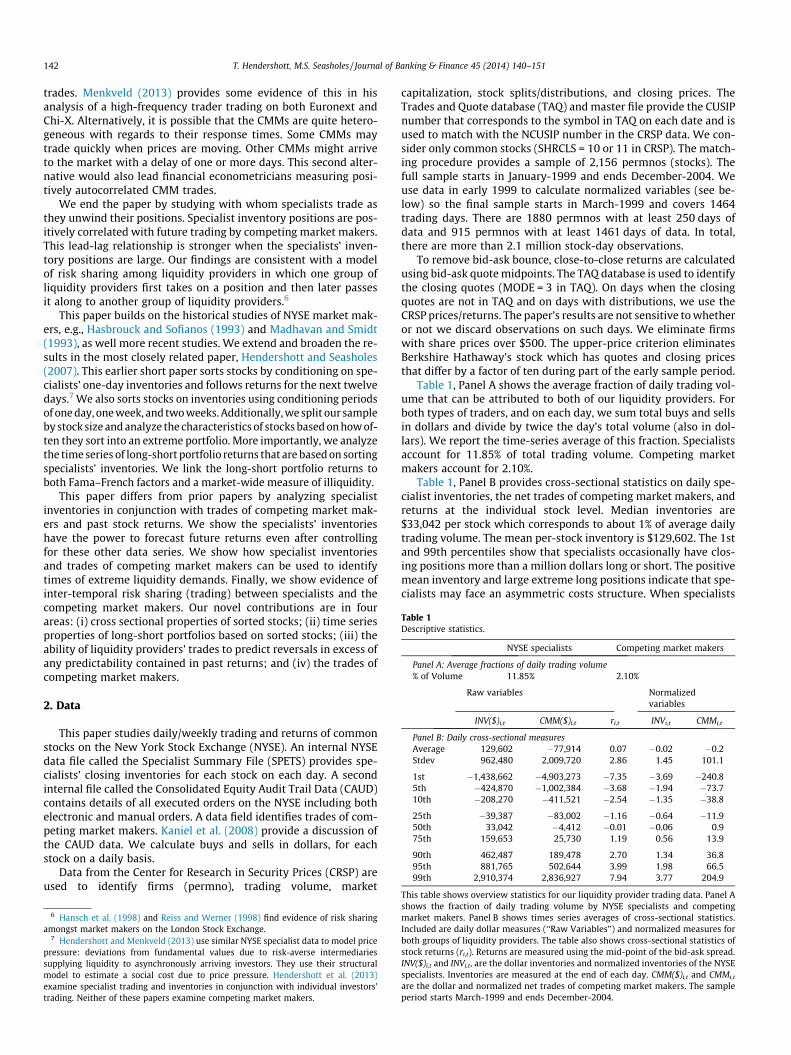
Table 1Descriptive statistics.

NYSE specialists Competing market makers

Panel A: Average fractions of daily trading volume% of Volume 11.85% 2.10%

Raw variables Normalizedvariables

INV($)i,t CMM($)i,t ri,t INVi,t CMMi,t

Panel B: Daily cross-sectional measuresAverage 129,602 �77,914 0.07 �0.02 �0.2Stdev 962,480 2,009,720 2.86 1.45 101.1

1st �1,438,662 �4,903,273 �7.35 �3.69 �240.85th �424,870 �1,002,384 �3.68 �1.94 �73.710th �208,270 �411,521 �2.54 �1.35 �38.8

25th �39,387 �83,002 �1.16 �0.64 �11.950th 33,042 �4,412 �0.01 �0.06 0.975th 159,653 25,730 1.19 0.56 13.9

90th 462,487 189,478 2.70 1.34 36.895th 881,765 502,644 3.99 1.98 66.599th 2,910,374 2,836,927 7.94 3.77 204.9

142 T. Hendershott, M.S. Seasholes / Journal of Banking & Finance 45 (2014) 140–151

trades. Menkveld (2013) provides some evidence of this in hisanalysis of a high-frequency trader trading on both Euronext andChi-X. Alternatively, it is possible that the CMMs are quite hetero-geneous with regards to their response times. Some CMMs maytrade quickly when prices are moving. Other CMMs might arriveto the market with a delay of one or more days. This second alter-native would also lead financial econometricians measuring posi-tively autocorrelated CMM trades.

We end the paper by studying with whom specialists trade asthey unwind their positions. Specialist inventory positions are pos-itively correlated with future trading by competing market makers.This lead-lag relationship is stronger when the specialists’ inven-tory positions are large. Our findings are consistent with a modelof risk sharing among liquidity providers in which one group ofliquidity providers first takes on a position and then later passesit along to another group of liquidity providers.6

This paper builds on the historical studies of NYSE market mak-ers, e.g., Hasbrouck and Sofianos (1993) and Madhavan and Smidt(1993), as well more recent studies. We extend and broaden the re-sults in the most closely related paper, Hendershott and Seasholes(2007). This earlier short paper sorts stocks by conditioning on spe-cialists’ one-day inventories and follows returns for the next twelvedays.7 We also sorts stocks on inventories using conditioning periodsof one day, one week, and two weeks. Additionally, we split our sampleby stock size and analyze the characteristics of stocks based on how of-ten they sort into an extreme portfolio. More importantly, we analyzethe time series of long-short portfolio returns that are based on sortingspecialists’ inventories. We link the long-short portfolio returns toboth Fama–French factors and a market-wide measure of illiquidity.

This paper differs from prior papers by analyzing specialistinventories in conjunction with trades of competing market mak-ers and past stock returns. We show the specialists’ inventorieshave the power to forecast future returns even after controllingfor these other data series. We show how specialist inventoriesand trades of competing market makers can be used to identifytimes of extreme liquidity demands. Finally, we show evidence ofinter-temporal risk sharing (trading) between specialists and thecompeting market makers. Our novel contributions are in fourareas: (i) cross sectional properties of sorted stocks; (ii) time seriesproperties of long-short portfolios based on sorted stocks; (iii) theability of liquidity providers’ trades to predict reversals in excess ofany predictability contained in past returns; and (iv) the trades ofcompeting market makers.

2. Data

This paper studies daily/weekly trading and returns of commonstocks on the New York Stock Exchange (NYSE). An internal NYSEdata file called the Specialist Summary File (SPETS) provides spe-cialists’ closing inventories for each stock on each day. A secondinternal file called the Consolidated Equity Audit Trail Data (CAUD)contains details of all executed orders on the NYSE including bothelectronic and manual orders. A data field identifies trades of com-peting market makers. Kaniel et al. (2008) provide a discussion ofthe CAUD data. We calculate buys and sells in dollars, for eachstock on a daily basis.

Data from the Center for Research in Security Prices (CRSP) areused to identify firms (permno), trading volume, market

6 Hansch et al. (1998) and Reiss and Werner (1998) find evidence of risk sharingamongst market makers on the London Stock Exchange.

7 Hendershott and Menkveld (2013) use similar NYSE specialist data to model pricepressure: deviations from fundamental values due to risk-averse intermediariessupplying liquidity to asynchronously arriving investors. They use their structuralmodel to estimate a social cost due to price pressure. Hendershott et al. (2013)examine specialist trading and inventories in conjunction with individual investors’trading. Neither of these papers examine competing market makers.

capitalization, stock splits/distributions, and closing prices. TheTrades and Quote database (TAQ) and master file provide the CUSIPnumber that corresponds to the symbol in TAQ on each date and isused to match with the NCUSIP number in the CRSP data. We con-sider only common stocks (SHRCLS = 10 or 11 in CRSP). The match-ing procedure provides a sample of 2,156 permnos (stocks). Thefull sample starts in January-1999 and ends December-2004. Weuse data in early 1999 to calculate normalized variables (see be-low) so the final sample starts in March-1999 and covers 1464trading days. There are 1880 permnos with at least 250 days ofdata and 915 permnos with at least 1461 days of data. In total,there are more than 2.1 million stock-day observations.

To remove bid-ask bounce, close-to-close returns are calculatedusing bid-ask quote midpoints. The TAQ database is used to identifythe closing quotes (MODE = 3 in TAQ). On days when the closingquotes are not in TAQ and on days with distributions, we use theCRSP prices/returns. The paper’s results are not sensitive to whetheror not we discard observations on such days. We eliminate firmswith share prices over $500. The upper-price criterion eliminatesBerkshire Hathaway’s stock which has quotes and closing pricesthat differ by a factor of ten during part of the early sample period.

Table 1, Panel A shows the average fraction of daily trading vol-ume that can be attributed to both of our liquidity providers. Forboth types of traders, and on each day, we sum total buys and sellsin dollars and divide by twice the day’s total volume (also in dol-lars). We report the time-series average of this fraction. Specialistsaccount for 11.85% of total trading volume. Competing marketmakers account for 2.10%.

Table 1, Panel B provides cross-sectional statistics on daily spe-cialist inventories, the net trades of competing market makers, andreturns at the individual stock level. Median inventories are$33,042 per stock which corresponds to about 1% of average dailytrading volume. The mean per-stock inventory is $129,602. The 1stand 99th percentiles show that specialists occasionally have clos-ing positions more than a million dollars long or short. The positivemean inventory and large extreme long positions indicate that spe-cialists may face an asymmetric costs structure. When specialists

This table shows overview statistics for our liquidity provider trading data. Panel Ashows the fraction of daily trading volume by NYSE specialists and competingmarket makers. Panel B shows times series averages of cross-sectional statistics.Included are daily dollar measures (‘‘Raw Variables’’) and normalized measures forboth groups of liquidity providers. The table also shows cross-sectional statistics ofstock returns (ri,t). Returns are measured using the mid-point of the bid-ask spread.INV($)i,t and INVi,t, are the dollar inventories and normalized inventories of the NYSEspecialists. Inventories are measured at the end of each day. CMM($)i,t and CMMi,t

are the dollar and normalized net trades of competing market makers. The sampleperiod starts March-1999 and ends December-2004.

Table 2Contemporaneous correlations.

Raw Variables Normalized

INV($)i,t CMM($)i,t ri,t INVi,t

CMM($)i,t 0.066(0.24)

ri,t -0.306 -0.144(0.00) (0.17)

INVi,t 0.783 0.059 -0.320(0.00) (0.23) (0.00)

CMMi,t 0.070 0.849 -0.152 0.074(0.20) (0.00) (0.16) (0.19)

This table shows the contemporaneous correlations of daily liquidity providertrading variables and stock returns. We consider NYSE specialist inventories (INV)and competing market makers (CMM). Correlations are first calculated for eachstock in our sample. The table reports cross-sectional averages. Below each corre-lation is the fraction of stocks with a correlation of opposite sign from that of theaverage. Returns are measured using the mid-point of the bid-ask spread. Inven-tories are measured at the end of each day. We consider dollar values ($) andnormalized variables as described in the text. The sample period starts March-1999and ends December-2004.

T. Hendershott, M.S. Seasholes / Journal of Banking & Finance 45 (2014) 140–151 143

are short they need to be a buyer to return their inventory to its de-sired level, requiring other traders to be sellers. If some traders faceshort-sale constraints, the specialist can anticipate that unwindinglarge short positions is more difficult than unwinding large longpositions. A related short-sale constraint explanation is that theNYSE up-tick rule effectively forces short sellers to provide liquid-ity via limit orders.

While we measure inventory levels for the NYSE specialist, ourdata only allow us to measure changes in holding levels, or nettrades, for the CMMs. The average net trades of competing marketmakers (on a per-stock basis) are �$77,914. This negative valueindicates that, in aggregate, either the CMMs have been reducingpositions during the sample period or the CMMs use the NYSE to‘‘lay off’’ positions built up from trading on other venues. Althoughcompeting market makers represent about two percent of totaltrading, the group experiences large variances in their net trading.At the 1st and 99th percentiles, the net trades of competing marketmakers are �$4,903,273 and $2,836,927.

2.1. Normalized variables

To aid cross-sectional comparisons we create normalized trad-ing measures for each of the three liquidity providers. For NYSEspecialist inventories, we follow Hendershott and Seasholes(2007) and subtract a moving average of stock i’s past dollar inven-tory levels from day t’s dollar inventory and divide by the standarddeviation of past dollar inventory levels. The moving average andstandard deviation consider lagged inventories from a three monthperiod using trading days from t � 70 to t � 11:

Normalized : INVi;t

�Inventoryð$Þi;t �MAfInventoryð$Þi;½t¼�70;t¼�11�g

StdevfInventoryð$Þi;½t¼�70;t¼�11�g

For the net trades of competing market makers, we follow the pro-cedure Kaniel et al. (2008) use for individuals in CAUD and to iden-tify periods of intense buying or selling. We divide net dollarvolume by the stock’s average dollar volume over the previous year.We then subtract a moving average of this measure. For competingmarket makers, the expression is:

Xi;t ¼Buy Volumeð$ÞCMM

i;t � Sell Volumeð$ÞCMMi;t

Average Volumeð$ÞOver Previous Yeari;t

Normalized : CMMi;t � Xi;t �MAfXi;½t�70;t�11�g

Table 1, Panel B also provides daily cross-sectional statistics forthe two normalized variables used in this paper. Normalizedinventories (INVi,t) are �3.69 and +3.77 at the 1st and 99th percen-tiles. The average 1st and 99th percentiles values of the net tradingvariables (CMMi,t) are much larger. Normalized net trades of com-peting market makers have average values of �240.8 and +204.9 atthe 1st and 99th percentiles. Unless otherwise noted, the results inthis paper use the normalized variables.

2.2. Leaning against the wind

We test whether our liquidity provision variables are negativelycorrelated with contemporaneous returns. For each of the 915stocks in our sample with at least 1461 days of data, we measurethe contemporaneous correlation of liquidity provision variablesand returns. We report a cross-sectional average of these time-ser-ies correlations.8

8 Results are qualitatively similar if we consider the 1880 permnos (stocks) with atleast 250 days of data and available from authors upon request.

Table 2 shows that a NYSE specialist’s inventory levels (in dol-lars) and returns have a �0.306 correlation. To gauge significance,we record the fraction of stocks with a correlation that is oppositein sign to the average. In the case of inventories and returns, lessthan 1% of stocks have a positive correlation. The net trades ofcompeting market makers have a �0.144 correlation with returns.However, 17% of the respective correlations using net trades arepositive. The 17% provides evidence consistent with the two previ-ously-mentioned phenomena (CMMs either lay-off positions builtup on other venues or CMMs are heterogeneous in the responsetime to price movements.) Correlations using our normalized vari-ables give qualitatively similar results.

Table 2 also highlights some positive correlation among thetrades of liquidity providers. When NYSE specialists are long stock,competing market makers tend to be buying. The correlation ofINV($)i,t and CMM($)i,t is 0.066. Note that the positive correlationof 0.066 indicates the two groups do buy together but the relation-ship is not too strong. Similar results hold when using normalizedvariables.

3. Liquidity provision and stock return predictability

3.1. Single-sort procedure

We sort stocks into quintiles based on the daily trades of liquid-ity providers in order to quantify the economic magnitude of returnpredictability. For completeness, we consider sorting stocks basedon current values of a liquidity provision variable (day t = 0), thepast week’s values [t � 4, t = 0], and the past two week’s values[t � 9, t = 0]. We form value-weighted long-short portfolios usingstocks in Quintile 1 and Quintile 5. The portfolios buy stocks thatliquidity providers have been buying and sell stocks that liquidityproviders have been selling. Throughout the paper, we focus onthe returns of these long-short portfolios which are measured ondays t + 1, t + 2, . . ., t + 5, and t + 10. We also measure cumulative re-turn over one week [t + 1, t + 5] and over two weeks [t + 1, t + 10].

Table 3, Panel A sorts using the normalized measure of NYSEspecialist inventories (INVi,t). Sorting by only day t’s inventoriespredicts returns of 17 bp after one day, 33 bp over one week(cumulative), and 42 bp over two weeks (cumulative). Sortingusing the average inventory level over the past week [t � 4, t = 0]predicts returns of 20 bp after one day, 41 bp over one week(cumulative), and 52 bp over two weeks (cumulative). T-statisticsare shown in parentheses below the returns of the long-short

144 T. Hendershott, M.S. Seasholes / Journal of Banking & Finance 45 (2014) 140–151

portfolios and are based on Newey–West standard errors. Notethat the incremental return on day t + 10 only is no longer statisti-cally significant and T-statistics range from 0.56 to 1.29.

Table 3, Panel B sorts using the normalized measure of nettrades by competing market makers (CMMi,t). Based on sorting over[t � 4, t = 0], predictable returns are 36 bp and 40 bp after one andtwo weeks respectively.

To compare our results to related work on return reversals suchas Jagadeesh (1990) and Lehmann (1990), and others, we endTable 3 with return sorts. Long-short portfolios based on returnssorts are long stocks in the low (negative) return quintile and shortstocks in the high (positive) return quintile. Sorting using returnsover the past week [t � 4, t = 0] predicts returns of 15 bp afterone day, 57 bp over one week (cumulative), and 77 bp over twoweeks (cumulative). The magnitude of the return-sort predictabil-ity is smaller than those shown in Lehmann (1990) because ourportfolios use value-weighted returns whereas the earlier paperemploys portfolios weights based on the absolute value of returns.

To gain insight into the return predictability of large and smallstocks, we sort our sample of stocks into market capitalization ter-ciles each day. To avoid confounding returns and size, we use mar-ket capitalization lagged by eleven days. For each size tercile, weperform a similar sorting procedure as the one shown in Table 3except we limit ourselves to sorting by the past week’s variables,[t � 4, t = 0], only. Fig. 1 graphs the returns, net of the market, forthe long-short portfolio over the two-week period following thesort (i.e., [t + 1, t + 10]).

Fig. 1, Panel A shows results based on inventory sorts. We graphonly the large and small terciles (by market capitalization). Forlarge stocks with high past inventories over the period[t � 4, t = 0], prices rise for four days before leveling off. For largestocks with low (negative) inventories, prices fall over the nexttwo weeks. Small stocks may have predictability beyond twoweeks—the high portfolio rises and the low (negative) portfoliofalls throughout the two week holding period shown in the figure.

Fig. 1, Panel B shows predictability using the net trades of com-peting market makers. Most of the return predictability followsperiods of buying (not selling) by competing market makers. This

Table 3Single sort results.

Sorting ; Period Returns of long-short portfolios over the following periods

t + 1 t + 2 t + 3 t + 4

Panel A: Sort by Specialists’ Inventories (INV)t = 0 0.17 0.09 0.07 0.04

(3.21) (3.49) (1.63) (1.40)[t � 4, t = 0] 0.20 0.06 0.15 0.03

(2.79) (1.64) (3.77) (0.66)[t � 9, t = 0] 0.14 0.03 0.10 0.02

(2.93) (0.89) (2.81) (0.43)

Panel B: Sort by net trades of Competing Market Makers (CMM)t = 0 0.16 0.05 0.04 0.05

(2.41) (1.24) (0.80) (1.10)[t � 4, t = 0] 0.13 0.07 0.07 0.07

(1.99) (1.31) (1.45) (1.24)[t � 9, t = 0] 0.07 0.00 0.04 0.05

(2.02) (0.11) (0.91) (0.88)

Panel C: Sort by returns (r)t = 0 0.03 0.12 0.09 �0.01

(0.64) (2.41) (1.85) (�0.17)[t � 4, t = 0] 0.15 0.18 0.22 0.03

(1.93) (2.00) (3.09) (0.48)[t � 9, t = 0] 0.26 0.11 0.22 0.10

(3.57) (2.29) (3.27) (1.57)

This table shows results of three single sorting procedures. Sort variables include NYSEreturns (ri,t). For each quintile, we form a portfolio of stocks and measure the value-weighof long-short portfolios using Quintiles 1 and 5. Cumulative long-short portfolio returnT-statistics are shown in parentheses and are based on Newey–West standard errors.

fact may be related to the CMMs selling, on average, throughoutour sample period. If some competing market makers are ran-domly selling from time to time, the sorting procedure may notwell identify the stocks where aggregate selling by this group isassociated with liquidity provision versus selling for other reasons.Alternatively, the CMMs may buy in the NYSE to cover shortpositions built up in other markets. Large stocks revert by approx-imately 40 bp over two weeks—the amount of large-stock rever-sion can be roughly seen as the distance between the ‘‘Large-Hi’’and ‘‘Large-Lo’’ graph lines.

Fig. 1, Panel C shows predictability using stock returns. Largestocks have noticeably more predictability than small stocks. Largestocks with low (negative) returns over the period [t � 4, t = 0],tend to go up 32 bp (basis points) over the following week. Largestocks with high (positive) returns over the period [t � 4, t = 0],tend to go down 28 bp (basis points) over the following week.The net difference for the large stocks is 60 bp over the week. Thisis slightly more than the 57 bp shown in Table 3, Panel C for allstocks. The difference is due to small stocks having lower predict-ability over the one week horizon.

The single-sort results in Table 3 and Fig. 1 provoke a number ofquestions which we address in the following sub-sections: (3.2)What types of stocks tend to sort into the extreme portfolios(Quintile 1 and Quintile 5)? Do the three sorting strategies shownin Table 3 tend to put similar or different type of stocks in the ex-treme portfolios? (3.3) What are the time series properties of thereturns on the long-short portfolios based on liquidity providertrading? Are the returns correlated with Fama–French factors ormeasures of liquidity? (3.4) Do the returns of the three sorting pro-cedures represent a single predictability phenomenon or, is therean incremental ability to forecast returns using our liquidity sup-plier variables? (3.5) Can trades of two liquidity providers be usedto predict times of extreme illiquidity?

3.2. Characteristics of reversal stocks

To examine stock characteristics, we employ a sequence of twosingle-sort procedures. We start with a typical single-sort

t + 5 t + 10 [t + 1, t + 5] [t + 1, t + 10]

�0.03 0.05 0.33 0.42(�0.87) (1.29) (4.79) (3.47)�0.02 0.05 0.41 0.52(�0.54) (1.09) (3.84) (3.05)0.01 �0.02 0.30 0.30(0.36) (�0.56) (2.64) (1.39)

0.03 0.08 0.33 0.55(0.64) (1.64) (4.29) (3.75)0.03 �0.02 0.36 0.40(0.79) (�0.69) (2.67) (2.08)0.01 0.01 0.17 0.20(0.35) (0.21) (1.92) (1.01)

�0.03 0.11 0.21 0.51(�0.64) (2.17) (2.50) (2.71)0.00 �0.10 0.57 0.77(�0.04) (�1.33) (3.92) (4.25)�0.09 �0.03 0.60 0.74(�1.14) (�0.33) (3.91) (2.36)

specialist inventories (INVi,t), net trades of competing market makers (CMMi,t), andted return over following ten days (t + 1, t + 2, . . ., t + 10). The tables show the returnss over the following week [t + 1, t + 5] and two weeks [t + 1, t + 10] are also shown.

Panel A: Sort Based on Inventories ( INVi,t ) Panel B: Sort Based on CMMi,t

-0.50

-0.30

-0.10

0.10

0.30

0.50

1 2 3 4 5 6 7 8 9 10

Large-Hi

Large-Lo

Small-Hi

Small-Lo

Panel C: Sort Based on Returns ( ri,t )

-0.50

-0.30

-0.10

0.10

0.30

0.50

1 2 3 4 5 6 7 8 9 10

Large-Hi

Large-Lo

Small-Hi

Small-Lo

-0.50

-0.30

-0.10

0.10

0.30

0.50

1 2 3 4 5 6 7 8 9 10

Large-Hi

Large-Lo

Small-Hi

Small-Lo

Fig. 1. Single sort results. This figure shows results of three single sorting procedure based NYSE specialist inventories (INVi), net trades of competing market makers (CMMi),and returns (ri). Before sorting, stocks are divided into terciles by size (market capitalization) on day t � 11. ‘‘Large’’ indicates stocks in the top size tercile and ‘‘Small’’indicates stocks in the lowest size tercile. We sort stocks into quintiles based on variable values over the past five days [t � 4, t = 0]. For each quintile, we form a portfolio ofstocks, value-weight returns, and show cumulative returns, net of the market, over the following week two weeks [t + 1, t + 10].

T. Hendershott, M.S. Seasholes / Journal of Banking & Finance 45 (2014) 140–151 145

methodology based on the past week of NYSE inventories, the nettrades of competing market makers, or returns. For each of the 915stocks with at least 1461 days of data, we calculate the fraction ofweeks the stock is in an extreme sort portfolio (Quintile 1 or Quin-tile 5). We then rank (re-sort) stocks by this fraction from lowest(stocks that least often in an extreme portfolio) to highest (stocksthat are most often in an extreme portfolio). Table 4 summarizesthe results. Note that in a purely random world, each stock shouldspend 0.200 of the days in each quintile and 0.400 of the days ineither of the two extreme quintiles.

Table 4, Panel A shows results for stocks that have first beensorted by NYSE specialist inventory over the past week[t � 4, t = 0]. Based on the frequency in an extreme portfolio, thelower 20% of stocks spends an average of 0.262 of the time in an

Table 4Characteristics of sorted stocks.

Fraction of days inan extreme portfolio

MktCap$ billion

ReturnStdev (%)

Panel A: Sort by Specialists’ Inventories (INV)Least Often 0.262 18.05 2.51

0.303 11.25 2.490.343 5.77 2.650.403 2.18 2.81

Most Often 0.513 7.12 2.76

Panel B: Sort by net trades of Competing Market Makers (CMM)Least Often 0.119 12.02 2.29

0.229 9.74 2.480.326 11.73 2.620.443 9.32 2.80

Most Often 0.624 1.56 3.04

Panel C: Sort by returns (r)Least Often 0.213 9.39 1.74

0.295 14.72 2.090.364 11.99 2.450.448 4.20 2.92

Most Often 0.573 4.07 4.02

This table shows characteristics of sorted stocks. We first perform a single sort procedportfolio. Stocks labeled ‘‘least often’’ sort least frequently into Quintiles 1 or 5. Stocksrecord its average market capitalization over the sample period, standard deviation of reilliquidity (‘‘Illiq.’’), and average daily return.

extreme portfolio. The upper 20% of stocks spends an average of0.513 of the time an extreme portfolio. It is the latter group ofstocks that most heavily influences the returns of the long-shortportfolios shown in Table 3 and Fig. 1. Inventory sorts tend to placemedium sized stocks in extreme portfolios and the average marketcapitalization of these stocks is $7.12 billion. These stocks areslightly more volatile than average with r(r) = 2.76%, have lowerturnover of 0.44%, larger spreads of 0.28%, higher values of theAmihud (2002) illiquidity measure of 4.83%, and slightly higherthan average returns of 0.08%.

Table 4, Panel B shows results for stocks that have first beensorted by CMMi,t over the past week [t � 4, t = 0]. These CMM-sortstend to put small, illiquid stocks in the extreme portfolios. Theaverage market capitalization of stocks most likely to sort into an

Averageturn (%)

Spreads(%)

Illiq.(%)

Averagereturn (%)

0.57 0.11 0.34 0.060.60 0.11 0.32 0.070.57 0.16 0.96 0.080.58 0.21 2.13 0.090.44 0.28 4.83 0.08

0.61 0.08 0.10 0.060.59 0.11 0.26 0.070.60 0.13 0.59 0.080.54 0.19 1.37 0.080.42 0.35 6.27 0.09

0.34 0.11 0.50 0.060.44 0.12 0.88 0.060.52 0.14 0.96 0.070.65 0.19 2.10 0.090.81 0.31 4.14 0.10

ure. We next rank (re-sort) stocks by the fraction of days it is in an extreme sortlabeled ‘‘most often’’ sort most frequently into Quintiles 1 or 5. For each stock, weturns, average daily turnover, average effective spread, average Amihud measure of

0.00

0.50

1.00

1.50

2.00

2.50

3.00

3.50

4.00

4.50

5.00

Mar

-99

Jul-

99

Nov

-99

Mar

-00

Jul-

00

Nov

-00

Mar

-01

Jul-

01

Nov

-01

Mar

-02

Jul-

02

Nov

-02

Mar

-03

Jul-

03

Nov

-03

Mar

-04

Jul-

04

Nov

-04

r

INV

CMM

Fig. 2. Cumulative strategy returns. This table shows the cumulative returns of three long-short portfolios that result from three single sorting procedures. Sort variables includeNYSE specialist inventories (INVi,t), net trades of competing market makers (CMMi,t), and returns (ri,t). We sort stocks using data over the past week [t � 4, t = 0]. Portfolios are heldfor the following week [t + 1, t + 5]. The returns of a long-short portfolio is equal to the difference between the returns of extreme sort portfolios (Quintiles 1 and 5).

146 T. Hendershott, M.S. Seasholes / Journal of Banking & Finance 45 (2014) 140–151

extreme portfolio is $1.56 billion, the volatility of returns is 3.04%,turnover is 0.42%, spreads are 0.35%, the Amihud (2002) value ofilliquidity is 6.27%, and the average return is 0.09%. The tablemakes it clear that sorting by CMMi,t puts small, illiquid stocks inextreme quintiles. These stocks are used to form the long-shortportfolios shown in Table 3, Panel B.

Panel C shows that sorting by returns, ri,t, puts medium tosmall-sized firms in the extreme quintiles. Due to the fact thatportfolios are formed on the basis of past returns, it is not surpris-ing that stocks in the extreme portfolios have an average returnvolatility of 4.02%. Interestingly, these stocks also have high turn-over of 0.81%, and high average returns of 0.10%.

To summarize, sorting procedures that predict short-horizon re-turns based on liquidity provider trading tend to place small, illiq-uid stocks in extreme portfolios. The prevalence of small stocks inextreme portfolios is particularly noticeable when sorting by thenet trades of competing market makers. In the latter case, stockswith an average market capitalization of only $1.56 billion spendan average of 0.624 of the days in extreme portfolios.

3.3. Time series properties of sorted portfolios

We examine the time-series properties of the long-short portfo-lios shown in Table 3. We focus on portfolios formed by sortingover the past [t � 4, t = 0] interval and holding stocks over thefuture [t + 1, t + 5] interval. Fig. 2 graphs the cumulative returnsbased on sorting by NYSE specialist inventories, net trades ofcompeting market makers, and past returns. As shown in Table 3,sorting by past returns gives the largest returns.

The returns of the three long-short portfolios are positively corre-lated. For example, the correlation of returns from the inventory long-short portfolio is 0.3697 with the returns from the CMM long-shortportfolio. Also, the correlation of returns from the inventory long-short portfolio is 0.3126 with the return-sorted long-short portfolio.

We test whether the returns of the three long-short portfoliosare correlated with Fama–French and momentum factors. We alsotest whether returns are correlated with a market-wide measure ofliquidity—the effective spread.9 Table 5 presents our results.

9 We calculate each stock’s effective spread each day by volume weightingtransactions throughout the day—see Comerton-Forde et al. (2010) for a completeexplanation of spread calculations. We equal-weight spreads each day to obtain amarket-wide measure.

Results using the long-short portfolio returns based on NYSEspecialist inventory sorts are shown in Regression #1a and #1b.In Regression #1a, notice that returns load negatively on SMB witha �13.26 coefficient and �2.07 T-statistic. Throughout the table,coefficients have been multiplied by 100. The long-short portfolioreturns load positively on UMD with an 8.71 coefficient and a2.20 T-statistic. Regression #1b adds market-wide spreads and atime trend to the regression. The coefficient on SMB is no longerstatistically significant while the coefficient on UMD remains so.

The most important feature of Table 5 is the positive loading onour market-wide measure of liquidity as shown in Regression #1b.The coefficient on effective spreads is 85.34 with a 2.89 T-statistic.This result indicates that liquidity providers earn higher returns attimes when average spreads are wider and lower return at timeswhen average spreads are narrower. The result, however, is notdriven by spreads themselves as returns in our paper use bid-askquote midpoints.

The returns of a long-short portfolio based on CMM sorts areshown in Regression #2a and #2b and are not significantly corre-lated with any factor. Finally, the returns of a return-based long-short portfolio, in Regressions #4a and #4b, show no correlationwith Fama–French factors, momentum factors, nor with spreads.

To summarize, strategies based on mimicking the trades ofNYSE specialists are more profitable at times when market-widespreads are wider. This result provides further evidence that thereturn predictability documented in this paper is linked to liquidityprovision. Interestingly, the strategies are also more profitable attimes the momentum portfolio (UMD) exhibits higher returns.Understanding the relation between the UMD returns (formed onthe basis of six-month momentum sorts) and the returns of along-short portfolio (formed on the basis of a one-week reversalsort) is a topic for future research. Sadka (2006) has initiated re-search along this line.

3.4. Fama–Macbeth regressions

We use Fama–Macbeth regressions to test whether NYSE inven-tories and/or the net trades of competing market makers predict fu-ture returns in excess of the predictability contained in past returnsalone. In other words, we test whether specialists’ inventories andcompeting market makers net trades acts as complements or substi-tutes when it comes to predicting reversals. The dependent regres-sion variable is the return of stock i over the time period

Table 5Time-series regressions from single sorts.

Long-short portfolio based on INV sort Long-short portfolio based on CMM sort Long-short portfolio based on ret sort

Reg #1a Reg #1b Reg #2a Reg #2b Reg #3a Reg #3b

Dependent variable: Returns from a long-short portfoliorm � rf 0.65 0.88 7.05 7.41 12.68 13.06

(0.16) (0.23) (1.08) (1.12) (1.56) (1.58)SMB �13.26. �11.48 �14.14 �12.53 �17.14 �15.11

(�2.07) (�1.79) (�1.70) (�1.36) (�1.27) (�1.10)HML �7.31 �6.89 10.10 10.68 1.60 2.24

(�1.13) (�1.10) (1.43) (1.54) (0.12) (0.17)UMD 8.71 8.66 14.25 14.05 �6.80 �6.98

(2.20) (2.15) (2.13) (1.98) (�0.80) (�0.79)Spreads 85.34 75.22 95.64

(2.89) (1.55) (1.48)Time Trend 0.00 0.00 0.00

(1.82) (0.77) (0.81)Constant 0.43 �1.35 0.34 �1.10 0.62 �1.27

(5.59) (�1.89) (3.13) (�0.96) (4.24) (�0.83)

This table shows time series regressions based on three single sort results. The dependent variables are the returns, in percentage, of the three long-short portfolios shown inTable 3. Independent variables include the market excess return (rm � rf), Fama–French size factor (SMBt), Fama–French size factor (HMLt), momentum factor (UMDt), equal-weighted measure of effective spreads in our sample (Spreadst), and a time trend variable. T-statistics are shown in parentheses and are based on Newey–West standarderrors.

T. Hendershott, M.S. Seasholes / Journal of Banking & Finance 45 (2014) 140–151 147

[t + 1, t + 5]. The independent variables consists of a series of indica-tors. We set the first indicator equal to one if stock i is in the highestinventory quintile measured over the [t � 4, t = 0] interval. We setthe second indicator equal to one if stock i is in the lowest inventoryquintile over the same interval. We set the third (fourth) indicatorequal to one if stock i is in its highest (lowest) CMM quintile overthe time period [t � 4, t = 0], respectively. Finally, we set the fifth(sixth) indicator equal to one if stock i is in its highest (lowest) returnquintile over the time period [t � 4, t = 0], respectively. The regres-sions have the advantage that many predictor variables can betested simultaneously. The methodology avoids sorting stocks alongmultiple dimensions which results in sparsely populated bins.

Table 6 shows time-series averages of weekly estimated coeffi-cients. In order to increase comparability with the sorting results,we report the difference in pairs of estimated coefficients (highminus low) for INV and CMM. For returns, we report the differenceof low minus high.

Table 6, Regression 1 shows an inventory high minus low differ-ence of 23 bp per week with a 5.16 T-statistic. This high minus lowvalue differs from the 41 bp shown in Table 3 due to the fact thatFama–Macbeth regressions treat each stock (over the same week)as an equal observation. In other words, the earlier table reportsvalue-weighted portfolio returns while the Fama–Macbethregressions effectively report equal-weighted portfolio returns.Fig. 1, Panel A confirms that a value-weighted portfolio should out-perform an equal-weighted portfolio. Over the [t + 1, t + 5] horizon

Table 6Fama Macbeth regressions.

Reg #1 Reg #2 Reg #3

Dependent variable: Return of Stock i over days [t + 1, t + 5]INVi,t Hi � Lo 0.23

(5.16)CMMi,t Hi � Lo 0.30

(4.71)ri,t Hi � Lo 0.26

(3.11)Const 0.34 0.28 0.30

(2.40) (1.97) (2.31)

This table shows results of Fama–Macbeth cross-sectional regressions. Each week, the reWe include variables indicating whether stock i sorts into a ‘‘Hi’’ portfolio (Quintile 1) or atrades of competing market makers (CMMi,t), and returns (ri,t). We report is the differencWe report ‘‘Lo � Hi’’ for returns (r). The right hand side of the table repeats Regression #parentheses and are based on Newey–West standard errors.

following an inventory sort, the figure shows that large stocks out-perform small stocks.

The effect of size becomes particularly apparent when looking atthe return difference (low minus high) in Table 6, Regression 3. Thereturn difference is only 26 bp with at 3.11 T-statistic. Again, theFama–Macbeth regressions are akin to equal-weighted sort method-ology and Fig. 1, Panel C shows that equal-weighted return sorts donot have nearly the predictive power as value-weighted return sorts.

Table 6, Regression 4 tests for significance of indicator differ-ences when all three sorting variables are included in the regres-sion. The difference in the inventory high minus low indicatorvariables is 14 bp with a 3.20 T-statistic. For CMMs, the differenceis 30 bp with a 3.82 T-statistic. Finally, for returns, the difference is18 bp with a 2.14 T-statistic. Most importantly, Regression 4 showsthat the trades of both liquidity providers help predict returnsabove and beyond the predictability contained in past returns.

To understand/confirm the role of stock market capitalization inreturn predictability, we divide our sample into size terciles andthen repeat the Fama–Macbeth regressions. Inventories have anincreasing ability to predict reversals as we move from small tolarge stocks (Table 6, Regressions 5 to Regression 7). CMMs exhibitthe largest marginal ability to predict the returns of small stocks.By marginal, we mean after ‘‘controlling’’ for the predictability ofspecialist inventories and past returns. The ability of returns topredict reversals is highest for large stocks. Following a return sort,the difference between low and high indicator variables is 0.21 for

Reg #4 Reg #5 Small Reg #6 Medium Reg #7 Large

0.14 0.11 0.18 0.23(3.20) (1.51) (2.04) (3.81)0.30 0.29 0.11 0.09(3.82) (4.32) (1.40) (0.93)0.18 0.21 0.14 0.36(2.14) (1.71) (1.62) (3.44)0.23 0.22 0.28 0.20(1.62) (0.95) (1.97) (1.69)

turns of stock i over days [t + 1, t + 5] are regressed on a series of indicator variables.‘‘Lo’’ portfolio (Quintile 5). Sorts are based on NYSE specialist inventories (INVi,t), nete between the estimated values of indicator variables (‘‘Hi � Lo’’) for INV and CMM.4 for stocks in the small, medium, and large size terciles. T-statistics are shown in

148 T. Hendershott, M.S. Seasholes / Journal of Banking & Finance 45 (2014) 140–151

small stocks, 0.14 for medium stocks, and 0.36 with a 3.44 T-statis-tic for large stocks.

3.5. Double sorts

We test whether the trading behavior of liquidity providers canbe used to identify periods of large return predictability. In partic-ular, we are interested in whether the net trades can be used toconstruct a strategy with average returns greater than or equalto the 57 bp per week obtained by the single return sort (shownin Table 3, Panel C).

We independently double sort stocks into quintiles based onliquidity provision variables from days [t � 4, t = 0]. After sorting,we form value-weighted portfolios of stocks in each of the 25 binsand measure returns over the next week [t + 1, t + 5].

Table 7, Panel A reports the results of a double sort using special-ists’ inventories and the net trades of competing market makers.We report the average return of all 25 bins (portfolios). Returns overthe next week increase as we move from the top-left to the bottom-right of the table. We also report return differentials while keepingone sort variable constant. Using the top row as an example, a port-folio that is long Hi-CMM & Lo-INV stocks and short Lo-CMM & Lo-INV stocks earns 26 bp over the next week and this return has a1.23 T-statistic. Using the first column as a second example, a port-folio that is long Hi-INV & Lo-CMM stocks and short Lo-INV & Lo-CMM stocks earns 49 bp over the next week with a 2.95 T-statistic.

Table 7, Panel A also reports the average return of the portfoliowe expect to exhibit the largest reversals—labeled the ‘‘Extreme

Table 7Double sort results.

Panel A: Double Sort by Inventories ( INVi,t ) and Net Trades of CompeReturns Over [t+1,t+5] Shown

Net Trades of CMMs

Lo (-) 2 3 4

Lo (-) -0.32 0.05 0.11 0.33

2 -0.13 0.06 0.01 0.41

INV 3 0.04 -0.01 0.17 0.05

4 0.08 0.02 0.06 0.22

Hi (+) 0.17 0.22 0.36 0.36

INV Effect 0.49 0.17 0.24 0.03

(2.95) (0.74) (1.55) (0.17)

Panel B: Overview of Double Sorts*

Sort Sort

#1 #2 Long Portfolio Short Portfolio

INVi,t ri,t Hi-INV & Lo-Ret Lo-INV & Hi-Ret

CMMi,t ri,t Hi-CMM & Lo-Ret Lo-CMM & Hi-Ret

CMMi,t INVi,t Hi-CMM & Hi-INV Lo-CMM & Lo-INV

* The details of the third double sort are shown in Panel A directly above.

This table shows results of double sorting procedures. Sort variables include NYSE specia(ri,t). We sort variables using values over the past week [t � 4, t = 0]. For each of the 25 bfollowing week [t + 1, t + 5]. Panel A shows average returns for each of the 25 bins basemarket makers (CMM). Panel B summarizes the return of the extreme reversal portfolio oshown in parentheses and are based on Newey–West standard errors.

Reversal Portfolio’’. In the case of an INV-CMM double sort, the ex-treme reversal portfolio is long Hi-INV & Hi-CMM stocks and isshort Lo-INV & Lo-CMM stocks. This portfolio earns 88 bp per weekand has a 4.73 T-statistic. The standard deviation of the extremereversal portfolio’s returns is 2.79% per week which leads to anannualized Sharpe Ratio of approximately 2.28. More importantly,the extreme reversal portfolio produces average returns that areboth economically and statistically greater than the long-shortportfolio based on only a return sort (see the 57 bp return in Ta-ble 3, Panel C). The return difference between the extreme reversalportfolio and the single return-sort portfolio is 31 bp per week andhas a 2.12 T-statistic.

Table 7, Panel B summarizes the results of three other doublesorts with a focus on the returns of the extreme reversal portfolios.The third double sort in Panel B repeats the results shown in PanelA directly above. In the first row of Panel B, we see that a portfoliothat is long Hi-INV & Lo-Ret stocks and short Lo-INV & Hi-Ret stocksearns 85 bp per week with a 5.08 T-statistic.

To conclude, our double sort results show that using the NYSEspecialist inventories and the net trades of competing marketmakers can be used to predict returns of 88 bp per week. Thismagnitude of predicted returns is significantly greater than usingonly past returns (or any other single variable) as a conditioningvariable. When both types of traders are providing liquidity, we be-lieve liquidity demands are particularly high. During such times,the compensation for providing liquidity is also high. The highcompensation can be measured by the 88 bp per week average re-turn of the extreme reversal portfolio.

ting Market Makers ( CMMi,t )

Hi (+) CMM Effect

-0.07 0.26 (1.23)

0.42 0.55 (2.70)

0.27 0.23 (1.38)

0.33 0.25 (1.49)

0.56 0.39 (2.70)

Extreme

0.62 0.88 Reversal

(2.51) (4.73) Portfolio

Return Over

[ t+1, t+5 ] (T-Stat)

0.85 (5.08)

0.76 (3.66)

0.88 (4.73)

list inventories (INVi,t), net trades of competing market makers (CMMi,t), and returnsins, we form a portfolio of stocks and measure the value-weighted return over the

d on a double sort using NYSE specialist inventories (INV) and trades of competingver the following week [t + 1, t + 5] from three different double sorts. T-statistics are

Table 8Cross-sectional averages of auto-correlation coefficients.

Raw variables Normalized variables

INV($)i,t DINV($)i,t CMM($)i,t ri,t INVi,t CMMi,t

AR(1) 0.542 �0.322 0.252 �0.004 0.473 0.261(0.00) (0.00) (0.01) (0.50) (0.00) (0.00)

AR(2) 0.417 �0.069 0.164 �0.016 0.349 0.178(0.01) (0.08) (0.04) (0.32) (0.00) (0.02)

AR(3) 0.352 �0.026 0.136 0.003 0.285 0.149(0.01) (0.28) (0.04) (0.48) (0.00) (0.02)

AR(4) 0.308 �0.020 0.120 �0.003 0.240 0.132(0.02) (0.34) (0.06) (0.46) (0.01) (0.03)

AR(5) 0.278 �0.012 0.109 �0.010 0.207 0.121(0.03) (0.37) (0.06) (0.36) (0.02) (0.03)

AR(6) 0.256 �0.007 0.100 �0.011 0.183 0.110(0.03) (0.44) (0.08) (0.37) (0.03) (0.04)

AR(7) 0.238 �0.007 0.091 �0.011 0.161 0.099(0.03) (0.43) (0.09) (0.37) (0.03) (0.06)

AR(8) 0.224 �0.007 0.085 0.003 0.144 0.092(0.04) (0.42) (0.10) (0.46) (0.04) (0.06)

AR(9) 0.213 �0.003 0.081 �0.004 0.127 0.086(0.06) (0.48) (0.11) (0.44) (0.05) (0.07)

AR(10) 0.204 �0.005 0.079 �0.008 0.110 0.080(0.06) (0.46) (0.12) (0.38) (0.06) (0.08)

This table shows auto-correlation coefficients. We first calculate the coefficients foreach stock in our sample. The table shows cross-sectional averages. Below eachauto-correlation is the fraction of stocks with an auto-correlation of opposite signfrom the average. Returns are measured using the mid-point of the bid-ask spread.Inventories are measured at the end of each day. Normalized variables are descri-bed in the text. T-statistics are shown in parentheses. The sample period startsMarch-1999 and ends December-2004.

T. Hendershott, M.S. Seasholes / Journal of Banking & Finance 45 (2014) 140–151 149

4. The trading behavior of liquidity providers

4.1. Inventory control

We begin the section by analyzing the trading behavior of twogroups of liquidity provider at the individual stock-level. Table 8reports tests of whether NYSE specialists and/or competing marketmakers have mean reverting trades. In order to compare net tradesacross trader types, we calculate the daily change of specialists’inventories and label this measure DINVi,t. For each of the 915stocks with at least 1461 days of data, we calculate the first tendaily auto-correlation coefficients. We then report the cross-sec-tional average of each auto-correlation coefficient. Table 8 showsthat inventories levels, INV($), are highly auto-correlated with a0.542 first-order coefficient. The net trades of NYSE specialists,DINV($)i,t, show strong mean-reversion. The first three auto-corre-lation coefficients are �0.322, �0.069, and �0.026 respectively. Togauge significance, we record the fraction of stocks with a correla-tion that is opposite in sign to the average. We find 0% of stockshave a positive AR(1) coefficient when looking at DINV($)i,t. Com-bined with earlier results from Table 2, the mean-reversion indi-cates NYSE specialists behave in a manner consistent withtheoretical models of market making. They initially buy as pricesare falling or they initially sell as prices are rising. After buildinga position, specialists quickly undo their trades and mean-revertinventories towards target levels.

The autocorrelation coefficients shown in Table 8 indicate spe-cialists revert their inventories back towards target levels at a fas-ter rate than previously reported in the literature. Madhavan andSmidt (1993) report half-life of inventory positions on the orderof 49 trading days. After correcting for shifts in desired target lev-els, their estimated half-life falls to 7.3 days. For our variableDINV($)i,t, an AR(1) coefficient of �0.322 indicates a half-life of1.78 days. A slightly shorter half-life is obtained when consideringall ten autoregression coefficients. The difference between our re-

sults and those in the earlier paper most likely stems from differ-ences in sample periods. Madhavan and Smidt (1993) examinedata from February 1, 1987 to December 31, 1987. Our data aregenerated approximately fifteen years later and trading conditionshave undoubtedly evolved.

Table 8 shows the net trades of competing market makers donot mean-revert. Instead, the trades of CMMs are positively andsignificantly auto-correlated with AR(1) coefficients of 0.252. Aftera week/five days, the AR(5) coefficients is 0.109. The normalizedmeasures also display high levels of positive auto-correlation. Asdiscussed earlier, the positive autocorrelation for CMMs’ tradingcould be due to the aggregate nature of the data or due to longerholding periods.

Table 2 shows both groups of liquidity providers trade againstcontemporaneous price movements—they buy as prices fall andsell as prices rise. The differences in auto-correlations shown inTable 8 suggest that the liquidity providers may trade with eachother following a significant rise or fall in prices.

4.2. Cross auto-correlations of liquidity providers net trades

To better understand trading between groups of liquidity pro-viders we calculate the cross auto-correlation of net trades. We di-vide stock-days into those when NYSE specialist inventories areneither high nor low (i.e., in Quintiles 2, 3, or 4) and stock-dayswhen inventories are more extreme (in Quintile 1 or Quintile 5).For each of the 915 stocks with at least 1461 days of data, we thenmeasure the correlation of INVi,t, DINVi,t+1, CMMi,t+1, DINVi,[t+1,t+5],and CMMi,[t+1,t+5]. Table 9 reports the cross-sectional average ofthe correlation coefficients.

Table 9, Panel A considers stocks-days when inventories areneither high nor low. NYSE specialists still mean revert their inven-tories as the �0.255 correlation between INVi,t and DINVi,t+1 shows.The mean reversion continues over days [t + 1, t + 5] as the �0.318correlation between INVi,t and DINVi,[t+1,t+5] shows. These results areconsistent with the AR(p) coefficients shown in Table 8. The nettrades of all three liquidity providers are slightly positively corre-lated: Corr(DINVi,t+1,CMMi,t+1) = 0.052. Below each average coeffi-cient we calculate the fraction of stocks with correlation ofopposite sign as the average.

The results in Table 9 change noticeably if a stock’s inventory isin Quintile 1 or Quintile 5 on day t. Panel B shows the meanreversion increases to �0.565 between INVi,t and DINVi,t+1. The nettrades of the liquidity providers become negatively correlated. Forexample, Corr(DINVi,t+1,CMMi,t+1) = �0.006. The negative correlationbecomes stronger over the following week: Corr(DINVi,[t+1,t+5],CMMi,[t+1,t+5]) = �0.033.

In summary, Tables 8 and 9 provide evidence of a ‘‘chain ofliquidity provision’’. NYSE specialists and competing market mak-ers each buy as prices fall and sell as prices rise. The buying behav-ior is stronger for specialists though we do see evidence of CMMsalso buying. NYSE specialists unwind their positions quickly whilethe CMMs continue a trend of buying or selling. The net result isthat, following a large and positive build up of inventory, special-ists sell to competing market makers. Following large short inven-tory positions, specialists buy shares back from competing marketmakers.

The results from Table 9 are the likely result of heterogeneityCMMs. Some CMMs buy (sell) when the specialists buy (sell). How-ever, there are other CMMs that want to buy (sell), but appear toarrive late to market. Having some CMMs respond slowly to stockprice movements is also consistent with the autocorrelation pat-ters seen in Table 8.

The results in Tables 8 and 9 also suggest that conditioning onthe trades of two or more liquidity providers help identify timeswhen large amount of liquidity has been provided. It is during

Table 9Correlations of inventories and future trading variables.

INVi,t DINVi,t+1 DINVi,[t+1,t+5] CMMi,t+1 CMMi,[t+1, t+5]

Panel A: Using data from ‘‘Middle’’ quintiles (2, 3, and/or 4)INVi,t 1.0 �0.255 �0.318 0.016 0.024

(0.00) (0.00) (0.40) (0.39)DINVi,t+1 1.0 0.217 0.052 0.039

(0.00) (0.28) (0.24)DINVi,[t+1,t+5] 1.0 0.003 0.033

(0.48) (0.35)

Panel B: Using data from ‘‘Extreme’’ quintiles (1 and/or 5)INVi,t 1.0 �0.565 �0.713 0.062 0.077

(0.00) (0.00) (0.26) (0.25)DINVi,t+1 1.0 0.559 �0.006 �0.015

(0.00) (0.48) (0.39)DINVi,[t+1,t+5] 1.0 �0.045 �0.033

(0.27) (0.31)

This table shows the correlations of inventories on day t and future trading vari-ables. The future variables are measured over day t + 1 and over the interval[t + 1, t + 5]. Correlations are first calculated for each stock in our sample. The tableshows cross-sectional averages. Below each correlation is the fraction of stocks withcorrelation of opposite sign as the average.

150 T. Hendershott, M.S. Seasholes / Journal of Banking & Finance 45 (2014) 140–151

these times that return predictability may be particularly large.Our earlier double sort results (Table 7) show this to be the case.

10 For a detailed examination of this point see Avramov et al. (2006).11 See Hasbrouck and Sofianos (1993) for a spectral decomposition of liquidity

provider profitability. This methodology enables identification of the horizon ofprofitability for liquidity providers.

5. Conclusion

We examine the role of liquidity providers and their impact onshort run stock returns. Liquidity providers buy stocks with fallingprices and sell stocks with increasing prices in order to accommo-date others’ demand to trade immediately. We study two types ofliquidity providers: designated market makers (NYSE specialists)and competing market makers both of whose trades are identifiedin proprietary NYSE data. Our results find a subtle process ofliquidity provision—one that depends both on horizon and stockcharacteristics. Today’s trades of NYSE specialists and competingmarket makers both predict returns over day t + 1. Portfolios ofstock sorted by today’s returns, however, have no predictabilityfor returns over day t + 1.

Portfolios of stocks sorted by specialists’ inventories, CMMs’ nettrades, and/or returns over the past week or two weeks also predictreturns on day t + 1. Both NYSE specialist inventories and pastreturns help predict returns of large stocks better than smallstocks—specialist predictability is strongest over the [t + 1, t + 5]horizon while return predictability is strongest over the[t + 2, t + 5] horizon. The net trades of competing market makershelp to predict returns of smaller stocks (after controlling for theability of specialist inventories and returns to predict returns.)

A Fama–Macbeth regression of future returns on indicator vari-ables shows extreme trading in each of the three groups helps fore-cast returns. The trades of one group are not ‘‘driven out’’ by tradesfrom other groups, nor by returns. It is not surprising that usingtrades of both NYSE specialists and competing market makershelps predict significant returns—we show 88 bp per week of pre-dictability. Since the aggregated data from our two groups appearto be generated at different frequencies, using trades from bothhelps identify times when liquidity has been most provided.

Our data also highlight the difference between designated mar-ket makers and competing market makers on the NYSE. Specialistsbuy as prices are falling (sell as prices are rising), accumulateinventory positions, and then quickly mean-revert their positionstowards target levels. The half-life of their holdings is estimatedto be 1.78 days. Competing market makers also buy as prices arefalling (sell as prices are risking) but do not reverse their tradeswithin a two-week window. Instead, the CMMs engage in highlyauto-correlated buying or selling runs. They end up trading with

NYSE specialists as the specialists work to reduce their inventorypositions.

Deviations from efficient prices may not represent profitabletrading opportunities for a liquidity demanding trader for severalreasons. First, the trading data on market makers is not publicallyavailable. Second, transactions costs are likely incurred on bothwhen opening and closing a position. The fact that seemingly largepredictability in returns may not yield profitable trading opportu-nity makes carefully defining market efficiency important for workclaiming to uncover violations of efficiency.10

The return predictability from liquidity provision is a form oflimits to arbitrage. Further study of liquidity provider risks, re-turns, and strategies is warranted. In addition, the implicit gainsthat arise from the correlation between future returns and liquidityproviders past trading may be offset by losses incurred when accu-mulating positions.11 Such loses could be substantial.

Acknowledgements

We thank the New York Stock Exchange (NYSE) for providingdata and participants at the Gerzensee Summer Session 2007,HKUST, INSEAD, and IMD. Part of this research was conductedwhile Hendershott was the visiting economist at the NYSE. Seas-holes acknowledges support of the Hong Kong Research GrantCouncil and Grant #642509 and #644611.

References

Amihud, Yakov, 2002. Illiquidity and stock returns: cross-section and time-serieseffects. Journal of Financial Markets 5, 31–56.

Amihud, Yakov, Mendelson, Haim, 1980. Dealership market: market making withinventory. Journal of Financial Economics 8, 31–53.

Amihud, Yakov, Mendelson, Haim, 1986. Asset pricing and the bid-ask spread.Journal of Financial Economics 17, 223–249.

Avramov, Doron, Goyal, Amit, Chordia, Tarun, 2006. Liquidity and autocorrelationsin individual stock returns. Journal of Finance 61, 2365–2394.

Ball, Ray, Kothari, S.P., Shanken, Jay, 1995. Problems in measuring portfolioperformance: an application to contrarian investment strategies. Journal ofFinancial Economics 38, 79–107.

Campbell, John, Grossman, Sanford, Wang, Jiang, 1993. Trading volume and serialcorrelation in stocks returns. Quarterly Journal of Economics 108, 905–939.

Comerton-Forde, Carole, Hendershott, Terrence, Jones, Charles, Moulton, Pamela,Seasholes, Mark S., 2010. Time variation in liquidity: the role of market makerinventories and revenues. Journal of Finance 65 (1), 295–331.

Conrad, Jennifer, Hameed, Allaudeen, Niden, Cathy, 1994. Volume andautocovariances in short-horizon individual security returns. Journal ofFinance 49, 1305–1329.

Cooper, Michael, 1999. Filter rules based on price and volume in individual securityoverreaction. Review of Financial Studies 12, 901–935.

Grossman, Sanford, Miller, Merton, 1988. Liquidity and market structure. Journal ofFinance 43, 617–633.

Hansch, Oliver, Naik, Narayan, Viswanathan, S., 1998. Do inventories matter indealership markets? Evidence from the London Stock Exchange. Journal ofFinance 53, 1623–1655.

Hasbrouck, Joel, Sofianos, George, 1993. The trades of market makers: an empiricalanalysis. Journal of Finance 48 (5), 1565–1593.

Hendershott, Terrence, Seasholes, Mark, 2007. Market maker inventories and stockprices. American Economic Review 97, 210–214.

Hendershott, Terrence, Menkveld, Albert J., 2013. Price pressures. Journal ofFinancial Economics (forthcoming).

Hendershott, Terrence, Li, Sunny X., Menkveld, Albert J., Seasholes, Mark S., 2013.Asset Price Dynamics with Limited Attention, Working Paper UC Berkeley.

Ho, Thomas, Stoll, Hans, 1981. Optimal dealer pricing under transactions and returnuncertainty. Journal of Financial Economics 9, 47–73.

Jagadeesh, Narasimhan, 1990. Evidence of predictable behavior of security returns.Journal of Finance 45, 881–898.

Kaniel, Ron, Saar, Gideon, Titman, Sheridan, 2008. Individual investor trading andstock returns. Journal of Finance 63 (1), 273–310.

Kraus, Alan, Stoll, Hans, 1972. Price impacts of block trading on the New York StockExchange. Journal of Finance 27, 569–588.

T. Hendershott, M.S. Seasholes / Journal of Banking & Finance 45 (2014) 140–151 151

Lehmann, Bruce, 1990. Fads, martingales, and market efficiency. Quarterly Journalof Economics 105, 1–28.

Llorente, Guillermo, Michaely, Roni, Saar, Gideon, Wang, Jiang, 2002. Dynamicvolume-return relation of individual stocks. Review of Financial Studies 15,1005–1047.

Madhavan, Ananth, Smidt, Seymour, 1993. An analysis of daily changes in specialistinventories and quotations. Journal of Finance 48, 1595–1628.

Menkveld, Albert, 2013. High-frequency trading and the new-market makers.Journal of Financial Markets 16, 712–740.

Pastor, Lubos, Stambaugh, Robert, 2003. Liquidity risk and expected stock returns.Journal of Political Economy 111, 642–685.

Reiss, Peter, Werner, Ingrid, 1998. Does risk sharing motivate inter-dealer trading?Journal of Finance 53, 1657–1704.

Roll, Richard, 1984. A simple implicit measure of the effective bid-ask spread in anefficient market. Journal of Finance 39, 1127–1139.

Sadka, Ronnie, 2006. Momentum and post-earnings-announcement driftanomalies: the role of liquidity risk. Journal of Financial Economics 80, 309–349.

Stoll, Hans, 1978. The supply of dealer services in security markets. Journal ofFinance 33, 1133–1151.

Subrahmanyam, Avanidhar, 2005. Distinguishing between rationales for short-horizon predictability of stock returns. The Financial Review 40, 11–35.