The Use of Health Economic Methods in

the Development of New Interventions for

Systemic Lupus Erythematosus

Penelope Rose Watson

BA, MSc.

Thesis for the degree of

Doctor of Philosophy

School of Health and Related Research, University of Sheffield

Submitted August 2013

i

ABSTRACT

The objective of this thesis is to investigate how health economic evaluation methods could

be applied to optimise clinical trial designs. The study focuses on trial design during the

development of new drugs in the pharmaceutical industry. The methods developed account

for many of the motivations, constraints, and uncertainties faced by a pharmaceutical

company that have not been factored in to previous Expected Net Benefit of Sampling

(ENBS) methods.

The study focussed on Systemic Lupus Erythematosus (SLE) because it is a disease area

with a history of failed clinical trials, attributed to poor trial design. Almost no health

economic modelling studies had been published in this area. The work in this PhD made

substantial contributions to developments in the economic modelling for SLE.

In chapter 2, I systematically reviewed previous clinical trials in SLE and extracted and

summarised their design features. In chapter 3, I identified health economic methods that

have been used to design clinical trials and which methods would be adopted. In chapter 4, I

reviewed observational cohort studies for SLE to develop (i) a conceptual model of SLE (ii)

identify quantitative estimates of the natural history of the disease. I found that there was

insufficient data from the published literature to describe the natural history of SLE

according to the conceptual model so I undertook statistical analysis of an SLE registry. The

analysis produces statistical models to extrapolate disease activity, steroid dose, organ

damage incidence and mortality over the short and long term. In chapters 6 and 7, I

described a Bayesian Clinical Trial Simulation for a Phase III SLE trial to evaluate the value

of alternative research designs and a cost-effectiveness model for SLE. In chapter 8, I

compared six trial designs for an SLE Phase III RCT using an ENBS approach adapted to

the pharmaceutical perspective. For each simulated trial the expected profits were calculated

conditional on expected regulatory and reimbursement approval. The study found that the

analysis was extremely time consuming and is currently not feasible with individual patient

simulation models. However, the framework for evaluating trial designs from a

pharmaceutical perspective use value-based pricing can be applied to trial designs in simple

decision problems.

ii

ACKNOWLEDGEMENTS

I thank the Economic and Social research Council for funding this research and who

provided me with a wonderful opportunity to pursue my PhD.

I am extremely grateful to my supervisor, Professor Alan Brennan, for all his support,

guidance and contributions to this work. His enthusiasm for the project have been

motivating and inspiring throughout the PhD.

I would like to thank my second supervisor Jeremy Oakley for his technical support and for

comments on my thesis. I would like to acknowledge the help and assistance provided by the

staff in ScHARR during the course of this study. I would like to extend particular thanks to

Mark Strong for providing technical support throughout the PhD and who provided

invaluable support in using Iceberg.

All through my PhD I have been fortunate to have worked alongside PhD students who have

provided a brilliant support and friendship network. I would like to extend particular thanks

to Jenny Willson, Carl Tilling, Will Sullivan, Kiera Bartlett, Brian Reddy, and Paul

Richards, for creating a helpful, amusing and positive work environment.

I would also like to thank all my friends and family for their continuing love and assistance.

I thank my sister Naomi for her support and advice. I must acknowledge the invaluable

emotional support, contribution, and proof-reading from my father Peter, and my partner

Jonathan. In sadness I thank and remember my mother Jan, whose love and encouragement

have always been the greatest inspiration to me.

iii

CONTENTS

ABSTRACT.............................................................................................................................II

ACKNOWLEDGEMENTS..................................................................................................III

LIST OF ABBREVIATIONS............................................................................................XIV

1 CHAPTER 1: INTRODUCTION....................................................................................1

1.1 Drug Development Processes......................................................................................1

1.2 What are Decision Theoretic Methods?.....................................................................3

1.2.1 Bayesian Statistics.......................................................................................................3

1.2.2 Decision-Making.........................................................................................................4

1.2.3 Health Economic Decision-Making.............................................................................4

1.2.4 Value of Information...................................................................................................7

1.2.5 Summary......................................................................................................................8

1.3 What is Systemic Lupus Erythematosus (SLE)?......................................................8

1.3.1 Aetiology.....................................................................................................................8

1.3.2 Incidence and Prevalence.............................................................................................8

1.3.3 Symptoms and Consequences......................................................................................9

1.3.4 Treatment...................................................................................................................11

1.4 Hypothesis...................................................................................................................12

1.5 Overview of Methods Used in This Thesis...............................................................12

1.6 Outline of this PHD Study.........................................................................................14

iv

2 CHAPTER 2: A REVIEW OF RANDOMISED CONTROLLED TRIALS

IN SLE.....................................................................................................................................18

2.1 Method........................................................................................................................18

2.1.1 Search Strategy..........................................................................................................18

2.1.2 Data Extraction..........................................................................................................20

2.2 Clinical Trials in SLE Results...................................................................................20

2.2.1 Trial Duration............................................................................................................23

2.2.2 Sample Size...............................................................................................................24

2.2.3 Concomitant Medications..........................................................................................24

2.2.4 Inclusion Criteria.......................................................................................................24

2.2.5 Trial Endpoints..........................................................................................................27

2.2.6 Adverse Events..........................................................................................................30

2.3 Discussion...................................................................................................................31

2.3.1 Duration of Follow-up...............................................................................................31

2.3.2 Sample Size...............................................................................................................32

2.3.3 Concommitant Medications.......................................................................................33

2.3.4 Inclusion Criteria.......................................................................................................33

2.3.5 Definition of Endpoints..............................................................................................34

2.3.6 Adverse Events..........................................................................................................34

2.4 Conclusions.................................................................................................................34

3 CHAPTER 3: MODELLING METHODS LITERATURE REVIEW......................36

v

3.1 Chilcott et al. (2003)...................................................................................................36

3.1.1 Expected Value of Information..................................................................................37

3.1.2 The ‘Payback’ of Research........................................................................................38

3.1.3 Conclusions................................................................................................................39

3.2 Literature Search and Review Methods..................................................................40

3.2.1 Inclusion Exclusion....................................................................................................40

3.2.2 Search Strategy..........................................................................................................41

3.2.3 Data Extraction..........................................................................................................41

3.3 Literature Search and Review Results.....................................................................42

3.3.1 ENBS assuming Net Benefit is Normally Distributed...............................................44

3.3.2 ENBS assuming Conjugate Priors.............................................................................46

3.3.3 ENBS With Non-Conjugate Priors............................................................................48

3.3.4 Behavioural Bayesian Approaches to Clinical Trial Design......................................49

3.3.5 Probability of success Approaches to Clinical Trial Design......................................52

3.3.6 Other approaches.......................................................................................................53

3.3.7 Subsequent Published Literature................................................................................54

3.4 Discussion...................................................................................................................54

3.4.1 Literature Review Methodology................................................................................54

3.4.2 Merits of the Approaches to Valuing Clinical Trials.................................................55

3.4.3 Methods for Sampling Trial Outcomes......................................................................57

3.4.4 Problems with Computational Burden.......................................................................58

vi

3.4.5 Using VOI in Reimbursement Decision-Making.......................................................58

3.5 Conclusion..................................................................................................................58

4 CHAPTER 4: NATURAL HISTORY OF SLE LITERATURE REVIEW...............60

4.1 Method........................................................................................................................60

4.1.1 Search Strategy..........................................................................................................60

4.1.2 Data Extraction..........................................................................................................62

4.2 Results.........................................................................................................................64

4.2.1 Conceptual Map and Conceptual Model....................................................................64

4.2.2 Disease Activity.........................................................................................................67

4.2.3 Mortality....................................................................................................................69

4.2.4 Organ Damage...........................................................................................................73

4.2.5 Organ Damage by Organ System...............................................................................77

4.3 Discussion...................................................................................................................88

4.3.1 The Formulation of a Conceptual Model for SLE.....................................................88

4.3.2 Justification for further Data Analysis.......................................................................88

4.3.3 Identification of Large Observational Cohorts...........................................................89

4.4 Conclusion..................................................................................................................90

5 CHAPTER 5: DEVELOPING A MODEL FOR THE NATURAL

HISTORY OF SLE................................................................................................................91

5.1 Methods.......................................................................................................................92

5.1.1 Patient Population......................................................................................................92

vii

5.1.2 Analysis Plan.............................................................................................................92

5.1.3 SPecification of the Dependent Variables..................................................................94

5.1.4 Covariate Measures....................................................................................................97

5.1.5 Statistical Models.....................................................................................................101

5.1.6 Statistical Model Validation.....................................................................................105

5.2 Results.......................................................................................................................105

5.2.1 Baseline characteristics............................................................................................105

5.2.2 Results of Analysis of SLEDAI Items and Steroid dose..........................................106

5.2.3 Results of Average SLEDAI and Average Steroid dose..........................................111

5.2.4 Results of Mortality and Organ Damage.................................................................114

5.3 Simulation Validation Exercises.............................................................................121

5.3.1 Validation of Longitudinal SLEDAI Scores Against Hopkins Lupus COhort.........121

5.3.2 Validation of Organ Damage Accrual Against Hopkins Lupus Cohort and the

Toronto Lupus Cohort.............................................................................................................123

5.4 Discussion.................................................................................................................124

5.4.1 Summary of the Key Findings of the SLEDAI Item and Steroid Model, Annual

Disease Activity and Steroid Models and Organ damage and Mortality Models....................124

5.4.2 Describing Disease Activity With the SLEDAI.......................................................125

5.4.3 The Validity of the Natural History Model..............................................................126

5.4.4 Limitations of the Statistical Methods.....................................................................126

5.5 Conclusion................................................................................................................127

viii

6 CHAPTER 6: THE DEVELOPMENT OF A BAYESIAN CLINICAL

TRIAL SIMULATION FOR SLE PHASE III TRIALS..................................................128

6.1 Model Structure.......................................................................................................128

6.2 Simulation Process...................................................................................................129

6.2.1 Overview of the Simulation.....................................................................................129

6.2.2 Generate Population Process....................................................................................130

6.2.3 The Bayesian Clinical Trial Simulation Process......................................................134

6.2.4 Treatment Efficacy..................................................................................................139

6.3 Elicitation of Uncertainty in Long-term treatment effects on disease Activity,

Organ Damage and Mortality...........................................................................................140

6.3.1 Elicitation Introduction............................................................................................140

6.3.2 Elicitation Methods..................................................................................................141

6.3.3 Results......................................................................................................................150

6.3.4 Summary..................................................................................................................156

6.4 BCTS Outcomes.......................................................................................................158

6.4.1 BCTS Validation of Predicted Outcomes................................................................158

6.4.2 Computation Time...................................................................................................159

6.5 Discussion.................................................................................................................159

6.5.1 Generating an SLE population.................................................................................159

6.5.2 Flexibility to Simulate Multiple Design Specifications...........................................160

6.5.3 Simulating Disease Activity with One Disease Activity Index................................160

6.5.4 The Exclusion of Adverse Events............................................................................161ix

6.6 Conclusions...............................................................................................................161

7 CHAPTER 7: COST-EFFECTIVENESS ANALYSIS..............................................163

7.1 CE Model Structure.................................................................................................163

7.2 Simulation Process and Parameter Inputs............................................................165

7.2.1 Generate Population.................................................................................................166

7.2.2 The Cost-Effectiveness Model.................................................................................166

7.2.3 Discounting..............................................................................................................176

7.2.4 Reducing Simulation Error......................................................................................177

7.3 CE Model Outcomes................................................................................................177

7.3.1 Health Outcomes and Costs.....................................................................................177

7.3.2 Parameter Sensitivity Analysis................................................................................178

7.4 RESULTS.................................................................................................................178

7.4.1 CE Model Outcomes................................................................................................178

7.4.2 Drug Price Analysis.................................................................................................181

7.4.3 Parameter Sensitivity...............................................................................................183

7.4.4 Computation Burden................................................................................................185

7.5 Discussion.................................................................................................................187

7.6 The Cost-Effectiveness of New Treatments in SLE..............................................187

7.6.1 How can CE models be used in Drug Development?..............................................187

7.6.2 Computation Burden................................................................................................188

7.6.3 Conclusions..............................................................................................................189x

8 CHAPTER 8: VALUE OF TRIALS ANALYSIS.......................................................190

8.1 Bayesian Statistical Methods in Planning SLE Clinical Trials............................190

8.2 The Prior Parameter Distributions........................................................................192

8.3 Data Simulation........................................................................................................192

8.3.1 Clinical Trial Characteristics...................................................................................193

8.3.2 Modified Clinical Trial Settings..............................................................................195

8.4 Bayesian Updating of Probability Density.............................................................199

8.4.1 Markov Chain Monte Carlo (MCMC) Methods......................................................200

8.4.2 Brennan and Karroubi Bayesian Approximation.....................................................201

8.5 Valuation of Clinical Trials In Industry................................................................211

8.5.1 Assurance Based Valuation of Trials.......................................................................211

8.5.2 Value Based Pricing Valuation of Trials.................................................................212

8.5.3 Expected Commercial Net Benefit of Sampling (ECNBS)......................................213

8.5.4 Number of Patients Who Will Benefit From Treatment..........................................214

8.6 Results.......................................................................................................................216

8.6.1 Assurance.................................................................................................................216

8.6.2 Expected Value-Based Price and Expected Commercial Net Benefit of Sampling

Results 217

8.6.3 VOI Analysis Convergence.....................................................................................221

8.7 Discussion.................................................................................................................224

8.7.1 Value-Based Pricing and the Threshold...................................................................224

xi

8.7.2 Computation Burden................................................................................................225

8.7.3 CE model Accuracy versus number of BCTS iterations..........................................226

8.7.4 Generalisability of Computation Problems..............................................................227

8.7.5 Conclusions..............................................................................................................227

9 CHAPTER 9: DISCUSSION........................................................................................229

9.1 The results of the valuation of SLE Phase III trials.............................................229

9.2 What is new about this research.............................................................................231

9.2.1 Systemic Lupus Erythematosus...............................................................................231

9.2.2 Value of Information Analysis.................................................................................233

9.2.3 The Pharmaceutical Perspective..............................................................................234

9.3 Limitations................................................................................................................237

9.4 Further Research and Development......................................................................239

9.5 Implications of Research.........................................................................................241

9.6 Conclusions...............................................................................................................251

10 REFERENCES..............................................................................................................252

APPENDIX 1: SYSTEMIC LUPUS ERYTHEMATOSUS DISEASE

INDICES...............................................................................................................................268

APPENDIX 2: RANDOMISED CONTROLLED TRIAL PIPELINE

SEARCH...............................................................................................................................271

APPENDIX 3: RCT SEARCH STRATEGIES...............................................................272

xii

APPENDIX 4: OBSERVATION STUDIES SEARCH STRATEGIES.......................273

APPENDIX 5: OBSERVATION STUDIES RESULTS.................................................274

APPENDIX 6: CHARACTERISTICS OF PATIENTS EXCLUDED FROM

ANALYSIS...........................................................................................................................277

APPENDIX 7: RESULTS OF UNIVARIATE STATISTICAL ANALYSIS

OF ORGAN DAMAGE......................................................................................................278

APPENDIX 8: ORGAN DAMAGE FRAILTY SURVIVAL ANALYSIS..................279

APPENDIX 9: VALIDATION OF AN INDIVIDUAL PATIENT LEVEL

SIMULATION OF THE NATURAL HISTORY OF SYSTEMIC LUPUS

ERYTHEMATOSUS AGAINST AN ALTERNATIVE LONGITUDINAL

COHORT.............................................................................................................................281

APPENDIX 10: AGE AND DISEASE DURATION PARAMETER

DISTRIBUTIONS...............................................................................................................286

APPENDIX 11: SIMULATION PARAMETER DISTRIBUTIONS...........................287

APPENDIX 12 : SLEDAI RANDOM EFFECTS CORRELATION MATRIX

303

APPENDIX 13: ELICITATION LITERATURE SEARCH.........................................304

APPENDIX 14: ELICITATION PRE-READING..........................................................306

APPENDIX 15: CLINICAL TRIAL VALIDATION.....................................................310

APPENDIX 16: CE MODEL PARAMETER DISTRIBUTIONS................................318

APPENDIX 17: HEALTH STATE UTILITY SEARCH...............................................325

xiii

APPENDIX 18: LOG-LIKELIHOOD FUNCTIONS FOR TRIAL DATA................328

APPENDIX 19: WINBUGS SPECIFICATIONS............................................................328

APPENDIX 20: TESTING MAXIMUM LIKELIHOOD WITH

INDEPENDENT REGRESSION MODELS...................................................................328

LIST OF ABBREVIATIONS

ACR American College of RheumatologyANA Anti-nucleus antibodiesAUC Area under the curveBCTS Bayesian Clinical Trial SimulationBeBay Behavioural Bayes.B&K Brennan and Kharroubi CE Cost-EffectivenessENBS Expected Net Benefit of SamplingEMEA European Medicines AgencyEULAR European League Against RheumatologyEVPI Expected Value of Perfect InformationEVPPI Expected Value of Parameter Perfect InformationEVSI Expected Value of Sample InformationFDA Food and Drugs AdministrationGSK GlaxoSmithKlineHR Hazard ratioHRQOL Health Related Quality of LifeHTA Health Technology AssessmentINB Incremental Net BenefitMCMC Markov Chain Monte CarloNICE National Institute for Health and Care ExcellenceOR Odds RatioOMERACT Outcomes Measure in Rheumatoid Arthritis Clinical TrialsPAD Persistently Active DiseasePGA Physician’s Global AssessmentPSA Probabilistic Sensitivity AnalysisQALY Quality Adjusted Life YearRCT Randomised Controlled TrialSELENA Safety of Estrogen in Lupus Erythematosus National AssessmentSLE Systemic Lupus ErythematosusSLEDAI Systemic Lupus Erythematosus Disease Activity IndexSLICC/ACR Systemic Lupus International Collaborating Centres/American College of

RheumatologyUK United KingdomVOI Value of Information

xiv

1 CHAPTER 1: INTRODUCTION(1)

The objective of this thesis is to investigate how health economic evaluation methods could

be applied during the development of new drugs in the pharmaceutical industry to optimise

trial design. The study has a particular focus on Systemic Lupus Erythematosus (SLE)

because it is a disease area with a history of failed clinical trials, attributed to poor trial

design. SLE is a disease with numerous manifestations and presented an interesting set of

methodological challenges, particularly because almost no health economic modelling

studies had been published in this area.

In this introduction I cover the background of how drug development processes work

globally, how decision analytic methods are used in health care resource allocation, and

describe SLE. In the final section I present the research hypothesis and a summary of the

work presented in the thesis.

1.1 DRUG DEVELOPMENT PROCESSES

Before new drugs can be prescribed to a patient it is necessary to obtain a license from

government agencies such as the FDA (1), or the EMA (2). Both regulators produce clear

guidance for industry on what evidence is required to obtain market approval (3;4). Under

both the EMA and the FDA, the drug development process includes preclinical testing;

clinical trials with phase 1, 2, and 3 testing; and a final approval procedure.

Market approval from either the FDA or EMA does not guarantee the reimbursement of new

treatments in the United States (US) or Europe. Systems of reimbursement are highly

variable between national settings (5). In the United Kingdom (UK), the National Institute

for Health and Care Excellence (NICE) can mandate reimbursement of new treatments (6).

NICE does not list all prescription drugs that are eligible for reimbursement, and technology

appraisals are selected according to prioritisation criteria (7). Reimbursement decisions not

covered by NICE, or rejected by NICE, are made by local commissioners. However, local

commissioners are required to reimburse NICE approved technologies. In the US, private

health insurance system reimbursement is not centrally regulated. Health insurers are free to

determine the insurance formulary (8). Most insurers offer open formularies or allow co-

payments for off-formulary prescriptions. However, Medicare drug coverage allows a closed

formulary of generics and therapeutic substitutes.

1

To aid the narrative of this PhD I propose to define a simple structure for a drug

development programme. The rationale behind the regulator's intervention is dual: to

guarantee and improve patient health and safety and to limit expenditures on drugs. The

system of drug regulation and reimbursement was loosely based on the United Kingdom;

however it does not include many of the details and intricacies of pharmaceutical market

access. From the pharmaceutical perspective a drug development programme comprises

three phases prior to market approval (9). Phase I trials aim to test the safety of the treatment

in a small sample of humans. Phase II trials establish if the drug is effective. Phase III trials

confirm the effectiveness and safety of the treatment in a large sample of patients sufficient

to demonstrate statistically significant benefits compared with alternative treatment options.

After market approval phase IV trials are conducted to determine the real-life value of the

treatment and collect data on long-term safety. For simplicity it is assumed that all phases of

research are funded by a single pharmaceutical company who is responsible for the drug

development. Market restrictions comprise two stages. Firstly, the new treatment must apply

for a license for use of the drug for a particular indication. For the purposes of this thesis this

body will be referred to as the license regulator. A license is granted based on evidence from

all trials up to Phase III and is extremely unlikely to be approved without data from a Phase

III trial. Secondly, a separate institution evaluates whether the treatment will be funded by

the healthcare provider. For the purposes of this thesis this body will be referred to as the

reimbursement authority. The drug is assumed to be reimbursed if the treatment is licensed

and can demonstrate cost-effectiveness from a Phase IV trial or evidence for long term costs

and benefits from modelling studies.

From the perspective of the pharmaceutical company there are two outcomes from a drug

development programme: success or failure. The drug is a success if it reaches the market

due to a successful application for license and reimbursement. The drug is a failure if it is

not granted a license or does not achieve reimbursement.

Within the public sector, the regulation of pharmaceutical markets involves many different

organisations at the local (GP consortia), national (6), and supra-national level (2). It is

difficult to define a typical process or generalise the processes of drug development.

However, it is useful to do so to help contextualise the problems addressed in this PhD and

standardise terminology. Whilst I acknowledge that there are limitations to the structure I

believe that it captures the main hurdles involved in drug development. This structure is

useful because it simplifies regulatory and reimbursement decision criteria, which helps to

define the outcome of a drug development programme in terms of success and failure.

2

1.2 WHAT ARE DECISION THEORETIC METHODS?

1.2.1 BAYESIAN STATISTICS

The use of Bayesian statistics in decision-making is a significant area of active research and

have been applied to great effect in healthcare decision-making (10). Bayesian statistics

formalises the process in which we learn from research that has been conducted previously

and update our knowledge with new data. In Bayesian statistics, inference of unknown

parameters can be conducted using subjective probabilities combined with new data (11).

Subjective probabilities express probability statements for an event even if the event is non-

repeatable. By incorporating subjective probabilities Bayesian analysis enables probability

statements to be made about parameters, whereas frequentist theory does not allow this (12).

With Bayesian statistics it is possible to express a probability distribution for the outcomes

of a decision problem based on all available evidence. This enables the health economics

analyst to express the probability that one treatment is more cost-effective than another at

the willingness to pay threshold, λ. This method is particularly useful for decision analysis in

healthcare because it has been argued that decisions should be based on the expected value

of the decision and it’s uncertainty (13).

In Bayesian statistics it is necessary to express the current knowledge of unknown

parameters as a prior probability distribution before observing the new data x. The prior

distribution should be expressed in the form of a probability distribution of the parametersθ.

The information from the new data x is synthesised with the prior distribution to estimate the

posterior distribution of parametersθ, which describes our updated knowledge of new and

existing information. Bayes theorem describes how to derive the posterior density function

for the unknown parameters after data x have been collected.

f (θ|x )=f (θ ) f (x∨θ)

f (x)(

1.1

)

The prior distribution is described byf (θ ), the model for the data conditional on the

parameters is expressed byf (x∨θ), which is known as the likelihood function. The

denominator,f (x), is a normalising constant to ensure that the posterior distribution

integrates to 1.

3

The posterior distribution is used in Bayesian statistics to draw inference (12). Therefore, the

probability interval is influenced by the prior and data. The posterior distribution can be

estimated in a number of ways. Firstly, if the prior probability distribution and data, x,

follow a compatible pair of distributions the posterior distribution can be computed

explicitly through conjugate analysis. Conjugate distributions exist when the posterior

distribution is from the same family of distributions as the prior (10). If the distributions are

not conjugate the estimation of the prior is more computationally expensive and is most

often estimated using Markov Chain Monte Carlo (MCMC) methods (10). MCMC enables

sampling from the posterior distribution even if the posterior does not have a known

algebraic form (10). MCMC enables the adoption of Bayesian techniques in more complex

models than would be possible with algebraic solutions (12). Complex MCMC problems

require specialist software, such as WinBUGS, to sample from the posterior distributions

(14).

1.2.2 DECISION-MAKING

The use of Bayesian analyses in decision-making is a growing field of research (10).

Decision theory is concerned with identifying the value of two or more competing decision

options and identifying the optimal decision. Each option is associated with some value or

utility from the consequences of the decision. If the decision-maker had perfect information

decision-theory recommends that the optimal decision would be that which maximised

utility. However, in most practical applications the value of the decision is uncertain, and

there is a risk that a sub-optimal decision will be made. In this situation the consequences of

the decision must be assigned probability distributions to reflect uncertainty in future

outcomes. The optimal decision is that which maximises the expected utility (15).

Decision-maker using a health economics framework have adopted Bayesian statistics and

Bayesian decision theory as an important component of health technology appraisal (11).

Methods for handling of uncertainty in health technology assessment have promoted a

Bayesian approach to describing uncertainty in prior parameter inputs (16).

1.2.3 HEALTH ECONOMIC DECISION-MAKING

Decision theory has been applied to resource allocation in healthcare sectors (15).

Healthcare policy makers are interested in observing the expected utility of resource

allocation decisions under conditions of uncertainty. Decisions will be made with some

4

uncertainty, and if a wrong decision is made there is an opportunity cost estimated at the

value of the best alternative forgone (17).

Economic evaluation is a branch of health economics concerned with issues related to

resource allocation within a health service. The economic perspective in resource allocation

incorporates the concept of opportunity cost, which describes the value of opportunity

foregone as a result of engaging resources in a particular activity. In health economic terms,

the opportunity cost of investing in a given healthcare policy is measured by the health

benefits that could have been achieved had the money been spent on the next best policy

(17). Efficiency is a key objective of an economic approach to resource allocation and is

achieved when health benefits are maximised and opportunity costs are minimised.

The normative foundations of economic evaluation derive from welfare economics, in which

social welfare is a function of individual welfare, as judged by the individual’s preferences

between states of the world (18). Under welfarism individual utility is a function of the

consumption goods and services from the productive economy. In practice resource

allocation according to welfare economics implies a cost-benefit approach. The objective in

a cost-benefit analysis is to compare healthcare interventions on two dimensions; cost and

consequences, in which the costs and benefits of the policy are measured in monetary units

(19). A resource allocation decision is determined through an evaluation of the expected net

benefit of a given policy (20).

More recently, some health economists have preferred an “Extra-Welfarist” normative

foundation to economic evaluation, which incorporates non-good characteristics into the

social welfare function and is founded on the principles of Amatryr Sen (21). The rejection

of traditional welfare economics in favour of non-welfarist approaches has coincided with

the development of decision maker approaches and cost-effectiveness analysis (22;23).

Within a cost-effectiveness analysis the benefits are measured in terms of health output,

rather than in monetary units (19). In order to employ a cost-effectiveness analysis

framework it is necessary to specify a threshold at which society is willing to pay for a unit

of health. Policies whose incremental cost-effectiveness ratio is above the threshold are

viewed as being poor value for money in contrast to the opportunity cost of alternative

resource allocations (24).

Cost-effectiveness analysis has been viewed as a deviation from traditional welfare

economics and is inconsistent with welfare economic objectives (25). Nonetheless, a cost-

utility framework enables the decision-maker to focus on the maximisation of health as the

5

objective of policy decision-making. The practicalities of the approach, and the adoption of a

cost per QALY method by the National Institute of Health and Care Excellence, have been

instrumental in promoting cost-effectiveness methods in health economics (26).

Economic evaluations can compare multiple intervention optionsDi which can be

pharmaceuticals or programmes of care, and can include existing or new innovations in

treatment. The value of each intervention can be expressed as the monetary net benefit of the

treatment.

NB ( D i )=λ e i−ci (

1.2

)

Where e denotes the benefits of the intervention, measured in Quality Adjusted Life Years

(QALYs) (the general approach taken in the United Kingdom, Canada and elsewhere), and c

is the total cost of the intervention. The term λ describes the societal willingness to pay

threshold for health benefits. It has been reported that NICE have used a threshold range

between £20,000 and £30,000 per QALY gained (24). For the purpose of this thesis I

assume that λ is fixed at £30,000 per QALY due to the absence of alternative effective

treatments for SLE (27).

The costs and QALYs for each treatment can be estimated alongside the clinical trial to

report a within trial analysis (28). However, this type of assessment only considers the costs

and outcomes observed during trial follow-up. A longer time perspective is needed for

chronic diseases such as SLE where important health implications occur after the trial

follow-up (29). Cost-effectiveness (CE) modelling is frequently adopted in economic

evaluation to extrapolate cost and QALY gains beyond trial follow-up (28).

Cost-effectiveness models can be used to evaluate the long term consequences of treatment

and have been recommended in a number of review articles (22;24). One advantage of this

approach is that the patient outcomes can be extrapolated beyond the period of trial follow-

up. Decision-analytic models can be used to synthesise clinical evidence from randomised

controlled trials, with epidemiology data, cost-of illness studies and utility estimates. This

approach is the most appropriate for use in evaluating SLE treatments because it is a chronic

disease. There are several types of modelling structures and the choice of modelling

structure should relate to the role of expected values, patient heterogeneity and time (30).

6

A CE model comprises a set of input parameters, θ, to express estimates of treatment

effectiveness, disease natural history, costs and utilities. CE models synthesise data from

randomised controlled trials, epidemiology data, cost-of illness studies and utility estimates,

from which the CE model generates the lifetime costs and QALYs for each intervention.

I considered a CE model comparing two treatment options to be consistent with the decision

problem faced by the Pharmaceutical Company developing a new treatment for SLE. The

existing intervention, i=1 would be compared with a new intervention, i=2. The decision

whether to adopt the new treatment is made based on the incremental net benefit it provides

compared with the existing technology. The CE model can be used to estimate the

incremental mean effectiveness and incremental mean costs to give the mean incremental

net benefit (INB).

INB= λ (E [e2∨θ ]−E [e1∨θ ] )−( E [c2∨θ ]−E [c1∨θ ] )=λ (∆e)−( ∆c ) (

1.3

)

where the expectations of e and c are functions of θ. Incremental net benefit describes the

gains or losses, in monetary terms, of selecting treatment 2 rather than treatment 1.

CE models account for uncertainty in the input parameters θ, by drawing samples from the

probability distribution of the parameter (31). This approach accounts for the decision

maker’s imperfect knowledge of the population parameters. Probabilistic sensitivity analysis

(PSA) is used to characterise the input parameter uncertainty surrounding the costs and

outcomes of the economic evaluation (13). Probability distributions are assigned to the

parameter inputs of the CE model and multiple CE model outcomes are estimated using

Monte Carlo (MC) Simulation (32). For each iteration of the PSA s=1, … S, a set of values

for θs are sampled and INB∨θs evaluated. This generates a distribution of CE model

outcomes and describes uncertainty in the INB.

1.2.4 VALUE OF INFORMATION

Decision theory can also be applied to the decision of whether to invest in further research to

help inform our decision whether treatment 1 or treatment 2 is optimal. If we are uncertain

of the optimal treatment there may be value in collecting further research to reduce the risk

that we make a sub-optimal decision. The value of information expresses the amount that the

decision maker would be willing to pay for information to reduce the uncertainty in their

7

decision (33). If we have a current posterior for which E [ INB|θs ]>0, but there is

uncertainty in INB, there may be some values of θ for which the incremental net benefit is

negative. We can calculate the value of collected further information by sampling values of

θ to estimate the expected benefits lost when a wrong decision is made.

In a commercial setting the value of information must be quantified in terms of the expected

profits for the company. The process of valuing information must also assess the chances of

regulatory approval, reimbursement and future market competition (10). This leads to a

situation where a wrong decision to invest in a trial could lead to zero benefits if the

treatment is not granted regulatory approval. In pharmaceutical drug development the risk of

failure is important because 19%-30% of compounds that undergo clinical testing are

abandoned without obtaining marketing approval (34)

1.2.5 SUMMARY

In Bayesian statistics, probabilities are expressions of uncertainty and have been adopted in

health economics to evaluate the uncertainty for a decision-maker. Health economic models

often incorporate probabilistic sensitivity analysis to evaluate the probability that treatment 2

is optimal compared with treatment 1 given some decision maker’s criteria. More recently

health economists have explored the value of data collection for decision-makers if the

uncertainty in the cost-effectiveness model indicates that there is a high risk of making a

sub-optimal decision.

1.3 WHAT IS SYSTEMIC LUPUS ERYTHEMATOSUS (SLE)?

Systemic lupus erythematosus (SLE) is a multi-system autoimmune disorder with variable

manifestations. SLE can affect almost any organ in the body and has a broad spectrum of

immunological manifestations. It is characterised by periods of disease activity and

remission (35). Periods of active disease are often associated with reversible impairment

however; active disease can cause permanent organ damage and mortality (36).

1.3.1 AETIOLOGY

The pathogenesis of SLE involves a complex mix of genetic (37), environmental factors and

the immune system (38). Genetic polymorphisms, epigenetic modifications to DNA,

influence risk and environmental triggers are believed to induce the disease.

8

1.3.2 INCIDENCE AND PREVALENCE

Studies of the prevalence of SLE in the UK estimate it to be 27.7/100,000 (95% confidence

interval 24.2-31.2/100,000) in the population and 206/100,000 in Afro-Caribbean females

(39). SLE has a higher prevalence among women, with estimates ranging between 80 to

90% of cases (40). SLE diagnosis can range from 2 years to 80 years. However, disease

onset is most commonly observed in women of childbearing age (41). A large multicentre

European cohort study of 1,000 patients from 7 European countries reported a mean age of

diagnosis to be 31 years (42). It is believed that ethnicity plays an important role in the

incidence of cases (43).

1.3.3 SYMPTOMS AND CONSEQUENCES

Diagnosis

Most people with SLE test positive for antinuclear antibodies following a blood test.

Another antibody, anti-double-stranded DNA (anti-dsDNA) is often present in people with

SLE. Various other antibodies are also associated with SLE. However, they can also occur in

well people who do not have SLE. Typical symptoms combined with high levels of certain

antibodies are used in diagnosis.

Criteria for the classification and diagnosis of SLE were published by the American College

of Rheumatology (ACR) in 1982 with amendments published in 1997 (44). The diagnosis of

SLE is based on clinical and laboratory tests when patients meet four of the eleven criteria.

The most common criteria satisfied at diagnosis were Anti-nuclear Antibody (ANA) positive

(96%), other serological abnormalities (92%), arthritis (62%), and haematological

abnormalities (56%), malar rash (43%) and photosensitivity (35%) (45).

Disease Activity

It is extremely difficult to describe a typical disease path for SLE patients because they

experience periods of active disease of varying length, affecting one or more organ systems

(45). A number of indices have been developed to monitor disease severity in observational

studies. The most commonly used are the Systemic Lupus Erythematosus Disease Activity

Index (SLEDAI), and the British Isles Lupus Assessment Group (BILAG) index. These

indices record symptoms in the neuropsychiatric, cardiovascular, peripheral vascular,

musculoskeletal, mucocutaneous, ocular, renal, respiratory, and gastrointestinal systems.

9

The SLEDAI focuses on symptoms experienced in the past 10 days. Disease activity can

range between 0-105 and patients with a score of >20 would be considered very severe (46).

Twenty-four features that are attributed to lupus are listed in Table 1, with a weighted score

given to any one that is present.

10

Table 1: SLEDAI score attributes

Weight Descriptor Weight Descriptor Weight Descriptor8 Seizure 4 Arthritis 2 New rash8 Psychosis 4 Myositis 2 Alopecia8 Organic Brain

Syndrome4 Urinary Casts 2 Mucosal Ulcers

8 Visual Disturbance 4 Hematuria 2 Pleurisy8 Cranial Nerve

Disorder4 Proteinuria 2 Pericarditis

8 Lupus Headache 4 Pyuria 2 Low Complement8 CVA 2 Increased DNA

binding8 Vasculitis 1 Fever

1 Thrombocytopenia1 Leukopenia

The more serious manifestations (such as renal, neurologic, and vasculitis) are weighted

more than others (such as cutaneous manifestations). The SLEDAI records immunology

results such as anti-dsDNA antibodies and complement. A limitation of the SLEDAI is that,

unlike the BILAG, it does not rate the severity of symptoms. Since the publication of the

original SLEDAI several modifications of the SLEDAI have been made to how items are

defined such as the Safety of Estrogen in Lupus Erythematosus National Assessment

(SELENA) (47) and the SLEDAI-2k (48). Each version of the SLEDAI maintains the same

24 items and weighting system so they are very similar; however the classification of events

is slightly different.

The BILAG score was developed based on a physician intention-to-treat basis (49). The

index assesses eight organ systems over the past month. It includes haematological and renal

tests, but unlike the SLEDAI does not require immunological tests. A composite score can

be generated by the BILAG, but it is more commonly used to generate organ system severity

scores. The BILAG index is the only index that records whether the symptoms are new,

worsening or improving, rather than present or absent (50). Details of the SLEDAI and

BILAG indices can be found in Appendix 1.

Organ Damage

Organ damage can occur in nine organ systems as a result of SLE (Cardiovascular, renal,

musculoskeletal, neuropsychiatric, pulmonary, peripheral vascular, gastrointestinal, ocular

and skin). The SLICC/ACR Damage Index is a validated instrument developed to measure

irreversible organ damage in patients with SLE (51-53). The index has 41 items. It includes

items relating to the disease and complications arising from toxicity from treatments, such as

cataracts due to steroids. Items are recorded on the SLICC/ACR Damage Index if they have

11

been present for more than 6 months to distinguish between disease activity and permanent

damage. The definitions and determinants of the SLICC/ACR Damage Index are based on

clinical grounds or widely available investigations, such as chest X-ray, so that it can be

completed in centres without access to more expensive imaging techniques (54). Details on

the SLICC/ACR Damage Index can be found in Appendix 1.

1.3.4 TREATMENT

SLE treatments aim to minimise symptoms, reduce inflammation, and maintain normal

bodily functions. Treatment choices often depend on organ involvement, and the severity of

activity. The European League Against Rheumatism (EULAR) guidelines on the

management of SLE recommend non-steroidal anti-inflammatories, anti-malarials,

cytotoxics/immunosuppressants and steroids (55). More recently biologic drugs, such as

rituximab, have been used in patients with severe disease (56). However, there are numerous

problems associated with the effectiveness, and side effects of the traditional treatment

options for SLE. Infection and permanent organ damage have been attributed to steroid

exposure and cytotoxic treatments (57).

Despite the apparent need for new treatments, no license indications for SLE were granted

before 2011. SLE is a complex autoimmune disease that poses considerable challenges in

the development of drugs and design of clinical trials. Eisenberg (2009) identified six

reasons for the lack of new treatments in SLE (58).

1. SLE is a complex and only partially understood disease.

2. SLE patients have extremely heterogeneous symptoms. This complicates inclusion

criteria, subgroup analysis, and outcome measures.

3. Although there are many useful mouse models for SLE, the findings of studies in

murine disease do not correspond with the findings in humans.

4. There are few reliable biomarkers for SLE, and none that have been validated for

use in clinical trials.

5. SLE patients respond to new treatments differently to other patient populations.

6. The history of failed trials in SLE discourages companies developing drugs for this

disease.

In the past decade there has been an increasing number of clinical trials conducted in SLE,

which has generated much excitement in the field for the prospects of new effective

therapies (59). A detailed review of clinical trials in SLE will be presented in Chapter 2.

12

A search of the online clinical trials database (www.clinicaltrials.gov) on the 7th April 2010

revealed that there was an abundant pipeline of at least 17 trials recruiting SLE patients

(Appendix 2). Rituximab and epratzumab are B-cell depleting therapies that target B-

lymphocyte surface markers CD20 and CD22 respectively. Belimumab and ataticept target

the cytokines that regulate the maturation, proliferation and survival of B-cells (60).

However, the success of recent clinical trials has been mixed, with many trials failing to

meet their primary endpoint. Two phase III studies for rituximab and one trial for abatacept

failed to meet their primary endpoint (61;62). In 2011 Belimumab reported success in two

large phase III clinical trials and received a license from the FDA and EMEA.

In summary, there is currently considerable demand for new effective treatments for SLE

due to the paucity of licensed treatments. Much excitement has been expressed for the

potential of biologics to provide effective treatment for SLE (59). However, after several

years of research there are considerable barriers for patients to access biologic treatment, and

the challenges in designing clinical trials have contributed to the restricted access to new

treatments. Clinical trial design impacts on the strength of evidence for efficacy and safety

required by the regulator, and the long-term effectiveness and cost-effectiveness over the

patient’s lifetime.

1.4 HYPOTHESIS

I hypothesize that Health Economic analyses can improve clinical trial design in the

pharmaceutical industry by prioritising trial design features that optimise future profits for

the pharmaceutical company.

1.5 OVERVIEW OF METHODS USED IN THIS THESIS

New treatments for SLE require CE models to demonstrate the incremental benefits of new

treatment compared with standard care. The work in this PhD has made substantial

contribution to the development of a CE model for SLE. This PhD aimed to explore whether

the cost-effectiveness model could also be used early in the drug development process to

improve the design of clinical trials.

I believe that the CE model has two main uses for a Pharmaceutical company during drug

development. Firstly, it is important to develop a good quality model to present the most

reliable estimates of the cost-effectiveness of SLE. This can be informative throughout the

13

stages of drug development to estimate the expected cost-effectiveness results based on

current or projected information. This may help inform the pharmaceutical company on

whether to proceed with the drug development and data collection process. Secondly, the

decision model can be used to characterise the uncertainty in the parameter estimates, and

use value of information techniques to consider if data collection is valuable. By considering

the costs together with the expected value of future research it is possible to analyse the cost-

effectiveness of future research. In this thesis I present a novel method for evaluating the

value of alternative trial designs from a pharmaceutical perspective where profits are

maximised according to the price achieved after data collection. The profits are conditional

on the constraints of regulatory approval and acceptable prices implied by value-based

pricing.

The review of Health Economic methods for trial design identified that Bayesian Value of

Information methods were an appropriate method to value trial designs. Within this method

prior parameters for a cost-effectiveness evaluation can be updated with multiple simulated

datasets to evaluate the reduction in uncertainty from data collection.

In summary, the method uses Bayes theorem to update the parameters of a CE model with

new data from a simulated clinical trial. Therefore, the method draws upon health economic

methods to develop CE analyses to estimate total costs and QALYs. In this example the CE

analyses will be generated from a CE model, which includes uncertain input parameters,θ.

The clinical trial would provide additional data Xθ I on all or a subset of the CE model

parametersθ I. The complement set of CE model parameters, θ IC , may not updated with trial

data. The prior joint probability density p(θ I) was updated, via Bayesian updating, to derive

the posterior density p(θ∨Xθ I) for each hypothetical data set sampled. The CE model could

then be re-run with the posterior density p(θ∨Xθ I) and p(θ¿¿ IC )¿to estimate the CE

outcomes given the simulated trial data.

Bayesian Clinical Trial Simulation (BCTS) can be used to simulate Phase III datasets for

complex design options. Within the VOI framework multiple simulated datasets are

generated for each trial design to predict many possible outcomes of the Phase III trial. The

BCTS provided a flexible method for simulating a broad range of trial specifications.

Clinical trial designs can be evaluated by simulating trial data and updating CE model

parameters with the information gathered. For each simulated dataset the prior and

likelihood of the data are synthesised to generate the posterior distribution of the parameters

and evaluate the CE model outcomes. 14

The simulation process used within this thesis is illustrated in Figure 1.

Figure 1: The four stage simulation process to evaluate alternative trial designs

Generate SLE population

1. Generate 50,000 patients with baseline characteristics

2. Set baseline SLEDAI score (Repeat SLEDAI probability

calculations 3 times to stabilise SLEDAI score)

3. Estimate Prednisone dose

4. Set baseline organ damage score

Clinical trial Simulation1. Sample the parameters of from their distributions

3. Run natural history model

3.1 Determine major events3.2 Determine withdrawal3.3 Estimate SLEDAI3.4 Estimate Prednisone dose

2. Recruit patients

4. Estimate outcomes of trial

Bayesian Updating

1. Specify the prior distribution of CE model

2. Extract data from trial outcomes related to CE model parameters

3. Estimate the posterior distribution of the parameters used in the CE model

Cost-effectiveness model1. Sample the parameters from their distributions

3. Run natural history model

4. Estimate total costs and QALYs for simulation run

3.1 Determine major events3.2 Estimate change in SLEDAI3.3 Estimate Prednisone dose3.4 Collect costs and QALYs

2. Recrutit patients

PSA

First, a population of SLE patients are generated reflecting the disease characteristics of

patients in the Hopkins Lupus Cohort. Secondly, a SLE Phase III clinical trial is simulated to

generate a single sample dataset. In stage three, this dataset is combined with the prior

distributions of the CE model to get the posterior distributions. In the final stage, the CE

model is evaluated given the posterior parameters and the results are recorded. The

simulation returns to stage 2 to simulate another clinical trial dataset, and the process is

repeated until sufficient trial results have been iterated to draw a conclusion about the value

of chosen trial designs. The whole process is repeated for each alternative trial design of

interest, thus enabling comparison of the relative value of different designs.

1.6 OUTLINE OF THIS PHD STUDY

I have provided a background to the main themes of this thesis. I have described a stylised

description of the drug development process and pathway to regulatory and reimbursement

approval. I have introduced the main principles of health economic methods and Bayesian

statistics. Finally, I have summarised the signs and symptoms of SLE, and provided a

background to the pipeline of new biologic treatments that are under development.

The thesis comprises four Phases of research. The Phases of research, and the impact each

chapter had on subsequent research developments are illustrated in Figure 2. In Phase I

reviewed current literature on clinical trials in SLE, and health economic methods for trial

design. Following the outcome of the methods review I identified a need to describe the

natural history of SLE to enable the simulation of patient outcomes in a Bayesian Clinical

15

Trial Simulation and CE model. In Phase 2 I developed a conceptual model for the natural

history of SLE, which informed the analysis plan for statistical analyses of a SLE registry

cohort. The statistical models describing the natural history of SLE were used to develop a

Bayesian Clinical Trial Simulation and cost-effectiveness model. These are described as the

simulation modelling Phase of the research. The design of the Bayesian Clinical Trial

Simulation incorporated data and findings from the Clinical trials review. Finally, in Phase 4

I implemented the methods identified in the methods review to develop an analysis to value

six trial designs. The Bayesian Clinical Trial Simulation and CE model were combined in

Chapter 8 to simulate clinical trial datasets, and evaluate cost-effectiveness outcomes for

each simulated dataset. This enabled calculation of the Net Commercial benefit of a

proposed trial design.

Figure 2: Illustration of the Phases of research

Phase 1: Reviewing

Phase 2: Natural History

Phase 3: Simulation modelling

Phase 4: Bayesian Updating

Chapter 2: Clinical trials review

Chapter 3: Methods review

Chapter 4: Conceptual model

development

Chapter 5: Natural History Statistical

Analysis

Chapter 6: Bayesian Clinical Trial Simulation

Chapter 7: Cost-effectiveness model

Chapter 8: Expected Net Commercial

Benefit

In Chapter 2, I conducted a literature review to describe the established characteristics of

SLE clinical trials, and identify what trial design features could be improved. Clinical trials

can be very difficult to design particularly if disease outcomes in the population recruited

into the trial are unpredictable. Previous successful clinical trials set a strong precedent for

clinical trial designs. However, there are inevitably cases where more difficult choices arise,

such as in SLE where very few clinical trials have been successful and outcomes are often

negative.

16

In Chapter 3, a review was needed to identify a suitable methodological framework for

evaluating clinical trials for drug development programmes. Analytical methods for

designing clinical trials may be preferable to informal decision-making or evaluation of

study design through pilot studies. Analytic methods can incorporate data from multiple data

sources and consider multiple research objectives. For example, many new treatments have

to demonstrate the health economic consequences of the interventions in order to improve

their prospects of being approved by reimbursement authorities.

Chapter 4 and 5 focussed on the development of a natural history model for SLE. In Chapter

4, I developed a conceptual model to describe the natural history of SLE based on a

literature review of observational studies in SLE. The review also established that there was

insufficient data from the existing literature to inform the natural history of SLE as defined

by the conceptual model. In Chapter 5, I describe a statistical analysis of the Hopkins Lupus

Cohort, which generated statistical models to describe the short and long-term natural

history of SLE. The development of the natural history model for SLE present a novel

method for simulating individual patient outcomes across disease activity, treatment

exposure, organ damage and mortality.

Based on the analysis described in Figure 1 it was necessary to develop two simulation

models. In Chapter 6 a Bayesian Clinical Trial Simulation was described adopting methods

identified in the methods review (63). The simulation predicted individual patient disease

progression across multiple organ systems over 3 monthly cycles to estimate outcomes from

future clinical trials. The simulation was based on some of the statistical analyses described

in Chapter 5 and data from previous SLE trials. Unknown parameters in the simulation were

elicited from Clinical experts in SLE through an elicitation study.

Chapter 7 describes a cost-effectiveness model to evaluate new pharmaceutical products for

SLE. The CE model described was developed for the purpose of this thesis.

GlaxoSmithKline developed a CE model concurrently, but independently, from my work

using the statistical analyses I produced. The simulation was based on the statistical analyses

described in Chapter 5 and data from a cost-effectiveness model developed for belimumab.

Chapter 8 describes the evaluation of six Phase III trial designs using a novel framework for

Expected Net Benefit of Sampling from a pharmaceutical perspective. I describe an analytic

method to compare SLE Phase III RCTs with variable sample size and duration of follow-

up. The VOI analysis utilised the BCTS described in Chapter 6 and the CE model described

in Chapter 7. The method for Bayesian Updating adopted an existing Bayesian

17

Approximation technique. The Bayesian Approximation method had not previously been

applied to an individual patient CE model. The analysis from Chapter 8 illustrates that

Health Economic analyses can be incorporated into clinical trial design process. However,

the methods are computationally intensive and may not be feasible for complex individual

patient simulation models.

Chapter 9 summarizes the findings of the thesis and discusses their practical application in

the pharmaceutical industry. This Chapter highlights the limitations of the method and

reflects on areas of further research that are needed.

18

2 CHAPTER 2: A REVIEW OF RANDOMISED CONTROLLED

TRIALS IN SLE 2.

The purpose of this chapter is to review clinical trials in Systemic Lupus Erythematosus

(SLE) and their design features.

Very few SLE clinical trials have been successful. It was important to learn from the design

choices and outcomes of previous trials. I decided to conduct a literature review of previous

clinical trials and clinical trial guidelines in SLE. The literature review would help to define

the main characteristics of an SLE trial by observing the approximate sample size, duration

of follow-up, inclusion criteria, primary endpoints, protocol for concomitant medications

and adverse events in previous trials, and discussion of these features in guidelines. I hoped

to identify what aspects of clinical trials in SLE could be varied to improve data collection,

and could be evaluated with an analytical model.

Section 2.1 describes methods for literature identification and data extraction. Section 2.2

reports the results of the literature review, broken down into clinical trial features. The

discussion in Section 2.3 considers what clinical trial features are most relevant to

investigate in this thesis. In the conclusion, Section 2.4, possible analyses for the PhD were

identified.

2.1 METHOD

2.1.1 SEARCH STRATEGY

A literature search was performed using Medline, an online database of clinical articles, to

identify randomised controlled trial (RCTs) in SLE. Professor David Isenberg, from

University College London, United Kingdom specialising in SLE, was consulted (December

2009) before and after the literature search to assist with the design of the search strategy

and check that important SLE trials had been identified. Embase, and other online databases,

were not searched in this review because the coverage of the search in Medline identified the

most recent large multi-centre trials.

Search terms included a combination of free-text and MeSH terms. Details of the search

strategies are reported in Appendix 3. Only studies that were published from January 1995 to

19

January 2010 were included in the search. Professor Isenberg (December 2009) did not think

that excluding studies prior to 1995 would exclude any good quality RCTs in SLE that

would contribute additional information that had not already been incorporated into the

guidelines for trial design. The search was repeated on the 21st February 2012 to update the

literature review with more recent RCTs. All references were exported to Reference

Manager 11.0 for application of the inclusion/exclusion criteria.

Identification of citations was based on title and abstract review according to the pre-defined

selection criteria. The final inclusion criteria for the studies were as follows.

Study design. Randomised controlled trials

Patients. An American College of Rheumatology (ACR) diagnosis of SLE, adults.

Interventions. Pharmacological interventions for SLE.

Outcome measures. Outcomes of interest were disease activity indices (i.e.

SLEDAI, BILAG), SLICC/ACR Damage Index, Physicians Global Assessment,

Response, remission, flare, Anti-DNA, anti-dsDNA, serum creatinine, proteinuria.

Other autoantibodies, genetic, and immunological outcomes were excluded from the

review.

Language. Full-published reports in English were considered.

Studies of autoantibodies, genetics, and immunological outcomes were excluded for

pragmatic reasons due to the breadth of outcomes that have been associated with SLE

without clear causation (59). Therefore, it was not feasible to include all of these

physiological processes into the study.

Full text reports were obtained for the abstracts that met the inclusion criteria. I decided to

exclude articles that described clinical trials in Lupus Nephritis or Cutaneous Lupus patients.

It was clear from the full text reports that the design of these trials was different to an SLE

population because the primary endpoints observe response criteria within individual organ

systems. In contrast, an SLE trial aims to observe treatment effect across multiple organ

systems.

A separate search was conducted to identify guidelines for clinical trials in SLE. Guidelines

published by national and international agencies were included in the review. A free text

search in Medline using the search terms ((“recommendation” OR “Endpoints” OR

“guidelines” OR “EULAR” OR “ACR” OR “OMERACT”) AND “Clinical trials” AND

“Systemic Lupus Erythematosus”) was conducted to identify guidelines. Additional grey

20

literature searches were conducted by searching the United States Food and Drugs

Administration (FDA), the European Medicines Agency (EMA), and the American College

of Rheumatology (ACR) websites.

2.1.2 DATA EXTRACTION

For each published clinical trial, trial inclusion criteria, sample size and power calculations,

interventions, primary endpoints, length of follow-up, and results were extracted and

recorded onto a data extraction form. Serious adverse events, infections and discontinuation

data were extracted.

A description of SLE sample size, duration of follow-up, inclusion criteria, concomitant

medications, endpoints, and adverse events was extracted based on findings from the RCT

search and guidelines.

2.2 CLINICAL TRIALS IN SLE RESULTS

In the initial search a total of ninety-nine records were identified in Medline. These ninety-

nine records were screened and twenty-three studies reported the results of an RCT in an

adult population. Ten studies were included in the review, whereas the other thirteen

reported the results of RCTs in Lupus Nephritis or Cutaneous Lupus. The updated search

conducted on 21 February 2012 identified a further twenty-three studies. Fourteen were

found to report the results of an RCT in patients with SLE of which eight were excluded

because they studied a Lupus Nephritis population. A total of sixteen articles in an SLE

population were identified describing fifteen RCTs. Figure 3 details the process of

identifying the literature.

21

Figure 3: CONSORT diagram for identification of RCT trials in SLE

99 articles identified 31/03/2010

76 studies did not meet the inclusion

criteria

13 studies were in Lupus Nephritis or Cutaneous Lupus

16 studies included in the review

23 articles identified 21/02/2012

9 studies did not meet the inclusion

criteria

8 studies were in Lupus Nephritis or Cutaneous Lupus

10 studies included 6 studies included

The trial characteristics are summarised in Table 2. The search identified clinical trials from

different stages of treatment development. Four of the studies were Phase III, one Phase

II/III, and three Phase II trials. Eight were exploratory studies with small sample sizes.

22

Table 2: Summary of trial design in disease activity trials

Author Date Funding Phase Treatments Inclusion criteria Primary endpoint Conmeds Sample size

Duration

Hackshaw(64)

1995 Pharma I ZileutonPlacebo

Age ≥18, ACR diagnosis SLAM Acetaminophen allowed 40(20; 20)

2 months

Carneiro(65)

1999 Public N/A MethotrexatePlacebo

ACR diagnosis, low dose prednisone. SLEDAI Prednisone dose stable for 1 month 41(20; 21)

6 months

Kalunian(66)

2002 Pharma I IDEC 131Placebo

Age ≥18, ACR diagnosis Mean change in SELENA SLEDAI None stated 85(65; 20)

5 months

Petri (67)

2004 Pharma PrasteronePlacebo

Age ≥18, ACR diagnosis Response (SLEDAI+ SLAM Quality of life)

Conmed doses remained stable from baseline

191(127; 64)

12 months

Tam (68)

2004 Public N/A LeflunomidePlacebo

ACR diagnosis, SLEDAI ≥6, low dose prednisone

Mean change in SLEDAI Prednisone tapered. Antimalarials and NSAIDs allowed

12(6; 6)

2.5 months

Fortin(69)

2008 Public N/A MethotrexatePlacebo

Age ≥18, ACR diagnosis, SLAM≥8, Mean change in SLAM None stated 86(41; 45)

12 months

Abdou(70)

2008 Pharma I Fulvestrant groupPlacebo

ACR diagnosis Change in SLEDAI from baseline None stated 20(10; 10)

12 months

Uppal(71)

2009 Public N/A InfliximabPlacebo

ACR diagnosis None specified1 Standard treatments allowed 27(9; 18)

 Variable

Wallace/ Furie(72;73)

2009 Pharma II Belimumab (3 doses)Placebo

Age ≥18, ACR diagnosis, SELENA SLEDAI ≥4, history of autoantibodies, stable prednisone.

Mean change in SELENA SLEDAI Changes in other therapy permitted as indicated

449(336; 113)

12 months

Merril (61)

2010 Pharma IIb AbataceptPlacebo

Age ≥16, ACR diagnosis, ANA+, BILAG A or 2 B score, 1 immunosuppressant.

New BILAG A or 2 B scores Prednisone was given for one month then tapered

175(118;57)

12 months

Griffiths(46)

2010 Public N/A CiclosporinAzathioprine

ACR diagnosis, severe disease defined by 15mg prednisone, stable dose.

Absolute mean change in prednisone HCQ permitted but held stable over trial. NSAIDs avoided.

89(47;42)

12 months

Merril (62)

2010 Pharma IIb RituximabPlacebo

Age ≥18, ACR diagnosis, msk, skin or serositis manifestation, BILAG A or B score

BILAG response Prednisone was added for all patients then tapered

227(169;88)

12 months

Navarra(74)

2011 Pharma III Belimumab 1mgBelimumab 10mgPlacebo

Age ≥18, ACR diagnosis, SELENA SLEDAI ≥6, ANA+, stable prednisone or immunosuppressants.

SLE Responder Index: ≥4 decrease in SSLEDAI, no new BILAG, no worsening in PGA

Immunosuppressant dose increases allowed. Unrestricted steroid dose up to week 24.

865(288;290;287)

12 months

Furie(75)

2011 Pharma III Belimumab 1mgBelimumab 10mgPlacebo

Age ≥18, ACR diagnosis, SELENA SLEDAI ≥6, ANA+, stable prednisone or immunosuppressants.

SLE Responder Index: ≥4 decrease in SSLEDAI, no new BILAG, no worsening in PGA

Immunosuppressant dose increases allowed. Unrestricted steroid dose up to week 24.

819(275;271;273)

18 months

Merrill(76)

2011 Pharma I SifalimumabPlacebo

Age ≥18, ACR diagnosis SLE Responder Index: ≥4 decrease in SSLEDAI, no new BILAG, no worsening in PGA

Other treatments were permitted if the regimen was unchanged during the 28 days before randomisation.

50(33:17)

3 months

ACR=American College of Rheumatology; SLE= Systemic Lupus Erythematosus. 1 assumed to be mean change in SLEDAI. AZA azathioprine; SLAM Systemic Lupus Activity Measure records disease activity in 11 organ systems and 8 laboratory tests in the last month. Each symptom is weighted by severity.

23

Eight clinical trial guidelines for SLE were identified using the search strategy described in

Section 2.1.1. Table 3 describes the title and organisations responsible for the guidelines.

The guidelines varied in scope of clinical trial design features. Most covered a broad range

of design features, whereas others focussed on trial endpoints only (77-80).

Table 3: Summary of SLE clinical trial guidelines

Name of Organisation Date Title of guidelines Reference

Food and Drugs

Administration

2010 Guidance for Industry: Systemic Lupus Erythematosus -

Developing Drugs for Treatment

(81)

The European Medicines

Agency

2009 Concept paper on the need for a guideline on the clinical

investigation of medical products intended for treatment of

systemic and cutaneous lupus erythematosus.

(82)

The European League

Against Rheumatism

(EULAR)

2008 Clinical trials in systemic lupus erythematosus (SLE): lessons

from the past as we proceed to the future--the EULAR

recommendations for the management of SLE and the use of

endpoints in clinical trials

(77)

The European League

Against Rheumatism

(EULAR)

2009 EULAR points to consider for conducting clinical trials in

systemic lupus erythematosus: literature based evidence for

the selection of endpoints

(79)

The European League

Against Rheumatism

(EULAR)

2009 EULAR points to consider for conducting clinical trials in

systemic lupus erythematosus

(83)

Outcomes Measure in

Rheumatoid Arthritis

Clinical Trials

2000 Endpoints: consensus recommendations from OMERACT IV.

Outcome Measures in Rheumatology

(78)

American College of

Rheumatology

2004 The American College of Rheumatology response criteria for

systemic lupus erythematosus clinical trials: measures of

overall disease activity

(80)

American College of

Rheumatology

2006 Endpoints: consensus recommendations from OMERACT IV.

Outcome Measures in Rheumatology

(84)

2.2.1 TRIAL DURATION

The FDA states that clinical trials in SLE should be at least 1 year in duration to observe

sustained clinical benefit (81). The EULAR guidelines stipulate that the trial should be of

sufficient duration that immunosuppressive drugs to be tapered during the study. Nine trials

followed patients for at least 12 months (Table 2). The shortest trial duration was 2 months,

and the longest 18 months.

24

2.2.2 SAMPLE SIZE

The sample sizes from the clinical trials are reported in Table 2. Six out of fifteen of the

trials could be considered very small with less than 50 patients. Six of the trials had a large

sample size (greater than 100 patients in total). Six studies reported a sample size calculation

based on 80% power (46;62;69;72;74;75).

2.2.3 CONCOMITANT MEDICATIONS

The FDA guidelines recommend that patients are not denied essential treatment during an

SLE clinical trial (81). It would be unethical to restrict patient access to effective treatment

because SLE flares can be severe, and can cause permanent damage and even mortality.

None of the guidelines make specific recommendations on how concomitant medications

should be regulated in a clinical trial.

Details of the concomitant medication protocols are reported in Table 2. Three articles did

not report the protocol for concomitant medications. The concomitant medications that are

listed are consistent with standard treatments for SLE described in Section 1.3.4 of Chapter

1.

Four trials employed a strategy to reduce steroid dose during the study to observe the steroid

sparing effects of treatment (65;68;69;85). The belimumab Phase III trials allowed steroid

dose changes during the trial as clinically indicated (74;75). In the rituximab Phase II/III

trials a high dose pulse methylprednisone dose was administered with every infusion of

rituximab (62). This is a high dose intravenous steroid injection intended to treat acute flares

in disease activity. The authors reflected that the pulse methylprednisone dose may have

masked the effect of rituximab because it is believed to be an effective method of controlling

disease activity.

2.2.4 INCLUSION CRITERIA

The FDA and EULAR guidelines recommend that patients recruited into the clinical trials

match with the patients who would reasonably be considered for this treatment. However, no

other recommendations are made for the inclusion criteria.

25

Eight studies set inclusion criteria to recruit patients with disease activity index scores above

a threshold ranging from very mild to moderate activity. One study required disease activity

to be present in the musculoskeletal system, skin system or serositis. Table 4 details the

participant characteristics of the trials. The majority of subjects enrolled in the trials were

women, which was consistent with the population demographics. The mean age of patients

was between 30 and 45 years. The mean disease duration tends to be over 5 years,

suggesting that the trials have not targeted a newly diagnosed patient group.

Early trial analyses have identified patient sub-groups for whom the treatment may be more

effective (67;73). The Phase II trial for belimumab and Phase III trial for prasterone

identified a subgroup of patients based on disease severity for which a statistically

significant result was attained. As a consequence, the Phase III belimumab studies require

that patients test positive for antinuclear antibodies (ANA+). The ANA+ is a test for SLE

and reflects a more stringent requirement for SLE diagnosis than the ACR diagnostic

criteria. A statistically significant result in the prasterone trial was observed in patients with

a SLEDAI score >2 at baseline (67). These findings highlight that inclusion criteria can

influence the outcomes if a sub-group of patients are more likely to respond. It suggests that

patients with disease activity, at baseline were a good target population for new treatments.

26

Table 4: Results from all organ clinical trials

Author Date Treatment arm Sample size

Duration age (mean years)

female (%)

disease duration (mean years)

Trial endpoint (1) Outcome p-value Trial endpoint (2) Outcome p-value

Hackshaw(64)

1995 zileutonPlacebo

40(20; 20)

2 months 46.642

90%85%

Change in SLAM -2.1-2.3

0.048†

Carneiro(65)

1999 methotrexatePlacebo

41(20; 21)

6 months 32.230.3

90%100%

7.16.7

Difference in SLEDAI score at 6 months

NR 0.05† Proportion with 50% reduction in steroid dose

72.2%5%

<0.0001†

Kalunian(66)

2002 IDEC 2.5IDEC 5IDEC 10Placebo

85(65; 20)

5 months 43.145.443.841.7

100%100%92%95%

9.229.539.499.78

Change in SLEDAI from baseline

-2.6-2.2-1.8-2

0.003‡0.001‡0.054‡0.034‡

Petri (67)

2004 PrasteronePlacebo

191(127; 64)

12 months 43.844.4

Response in SLAM, SLEDAI and HRQOL

51.3%42.2%

0.074†

Tam (68)

2004 leflunomideplacebo

12(6; 6)

24 weeks 40.642.3

83%100%

8.28.7

Change in SLEDAI from baseline

114.5

0.026†

Fortin(69)

2008 methotrexatePlacebo

86(41; 45)

12 months 40.240.2

90%91%

5.74.5

Difference in SLAM during trial

-0.86 0.039

Abdou(70)

2008 fulvestrantplacebo

20(10; 10)

12 months 3938

100%100%

11.39.75

Change in SLEDAI from baseline

4.50.87

0.006‡0.87‡

Difference in SLEDAI at 12 months

3.257

0.0591†

Uppal(71)

2009 infliximabplacebo

27(9; 18)

 Variable 2322.5

100%60%

7.154.79

Change in SLEDAI from baseline

-27.7-13.3

0.035†

Wallace(72)

2009 belimumabPlacebo

449(336; 113)

12 months 42.142.2

94%90%

98.1

Change in SLEDAI from baseline

-47.80% NS†

Merril (61)

2010 AbataceptPlacebo

175(118;57)

12 months 39.137.6

88.196.5

7.26.5

Proportion of patients with a new flare

79.7%82.5%

NS†

Griffiths(46)

2010 CiclosporinAzathioprine

89(47;42)

12 months 3339

9688

24

Corticosteroid sparing effect

-9.010.7

NS†

Merril (62)

2010 RituximabPlacebo

227(169;88)

12 months 40.240.5

89.993.2

8.58.7

Major clinical response 12.4%15.90%

NS† Partial clinical response 17.2%12.5%

NS†

Navarra(74)

2011 Belimumab 1mgBelimumab 10mgPlacebo

865(288;290;287)

12 months 35.436.235.0

97%94%94%

5.05.95.0

SRI Responder Index 51%58%44%

0.013†0.0006†

Furie(75)

2011 Belimumab 1mgBelimumab 10mgPlacebo

819(275;271;273)

12 months 40.040.540.0

93.494.991.6

7.97.27.4

SRI Responder Index 40.6%43.2%33.5%

0.089†0.017†

Merrill(76)

2011 SifalimumabPlacebo

50(33:17)

84 days 4448

9788

4.97.8

SRI Responder Index 26%15%

NS†

† compared with placebo; ‡ compared with baseline; NR Not Reported; SLAM Systemic Lupus Activity Measure records disease activity in11 organ systems and 8 laboratory tests in the last month. Each symptom is weighted by severity.

27

2.2.5 TRIAL ENDPOINTS

2.2.5.1 GUIDELINE RECOMMENTATIONS ON TRIAL ENDPOINTS

There has been discussion about trial endpoints in the guidelines, however very few specific

recommendations are provided. The FDA report makes several suggestions for possible

endpoints for SLE clinical trials, but does not impose a single criteria (81). Gordon et al.

explain that they cannot make any firm recommendations due to the lack of quality

randomised trials on which to base their report (83). The guidelines propose a number of

alternative ways of assessing therapeutic benefit. Table 5 documents a summary of

comments from the guidelines relating to general comments about endpoints, disease

activity, steroid dose, health related quality of life (HRQL), and organ damage.

The major clinical outcomes in SLE are problematic to measure in a clinical trial because

they include mortality, end-stage renal disease (ESRD) and other organ failures listed in the

SLICC/ACR Damage Index. These are not realistic primary endpoints in clinical trials

because they are rare events that would require large sample size or long duration of follow-

up to power the study. The ACR report that the main problem with the SLICC/ACR Damage

Index was that a clinical trial would need a long period of follow-up to detect treatment

effects on organ damage. However, the actual duration of follow-up needed is not discussed.

The EULAR review concluded that there was no validated intermediate outcome measure to

act as a surrogate marker for the mortality, end-stage renal disease or organ failure (79).

Disease activity indices were the predominant measure of efficacy recommended by the

guidelines. The ACR express reservations about using composite disease activity scores and

suggest that they should be used in conjunction with organ specific measures (80). The FDA

recommends that HRQL measures are studied in all trials of SLE to ensure that

improvement in disease activity was not accompanied by a worsening in quality of life.

However, they also state that improvement in HRQL alone would not be sufficient for

approval (81). This sentiment was reiterated by the SLE taskforce who recommend that

health status and quality of life be collected as secondary endpoints in clinical trials (77).

28

Table 5: Discussion of clinical endpoints in SLE trials

General Disease Activity Steroid Dose Quality of life Organ damageFDA (81) "Clinical trials in SLE generally are

expected to collect information about disease activity at all sites* , irreversible damage due to SLE and its treatment, and valid HRQL measures"

"In a randomized clinical trial, the SELENA SLEDAI, the SLAM, the BILAG, the ECLAM, or other established index could be used to measure disease activity" "We recommend using methods that assess the activity of disease over the duration of the study in conjunction with methods that measure disease activity at the beginning and end."

"The Agency recommends that HRQL be studied in all trials of SLE" "It is important that (trials) demonstrate no or minimal worsening in measures of HRQL"

"The SLICC/ACR Damage Index can be used as an endpoint, but we recommend discussing this with the appropriate reviewing division before beginning trials"

EULAR (83) "The efficacy of a drug can be described in a number of possible ways depending on the endpoints used. These include 1) reduction in lupus disease activity… 2) prevention of disease flare… 3) prevention of the onset of damage or the progression of damage ... 4) improvement or stabilisation of health status and quality of life ... 5) reduction in steroid dose.”

"Although not validated for use in clinical trials, the SLE Task Force agreed that standardised disease activity indices are preferable to completely untested outcome measures for capturing disease activity" "It is anticipated that more than one measure of disease activity may be used in a trial to capture changes in the manifestations of lupus present at baseline and the development of any new features of lupus during the trial"

"Any trial assessing disease activity as an endpoint will need to ensure that the use of immunosuppressive drugs that influence disease activity is controlled during a study."

"At present we recommend that health status and quality of life should remain secondary endpoints in a clinical trial"

"Accumulated multisystem chronic damage… is only definitely suitable as an endpoint in studies using newly or recently diagnosed patients without pre-existing damage and in studies with sufficient duration of follow-up for damage to occur"

OMERACT (78)

"The randomized controlled trials discussion group recommended that disease activity, health related quality of life, adverse events and damage be included as core outcome domains, in that order of preference"

"Although there is no consensus as to which one is preferable, six disease activity measures have been validated compared with physician global assessment, and against change in treatment, and against each other"

"Yearly assessment is appropriate, or at the initiation and completion of a clinical trial, and the SDI can be used to stratify patients at entry into a protocol"

EMEA (82) "A successful treatment of patients with SLE may:- improve signs and symptoms - prevent subsequent flares- decrease cumulative steroid dose- prevent long-term relapse and damage"

"There are several validated indices in SLE… the choice of disease activity indices in SLE requires further discussion"

"a choice of disease-specific or general quality of life measures should be discussed"

"A damage index, such as SLICC/ACR might be of interest"

ACR (80) “The committee recommended that controlled trials of therapy in SLE should use organ-specific measures, with response criteria that are defined a priori, and valid reliable composite instruments for calculating overall disease activity”

“Composite indices … by their nature, mask worsening and responding organ systems”

* sites refers to the different organ systems that are assessed to identify disease activity in SLE

29

2.2.5.2 TRIAL ENDPOINTS USED IN REPORTED CLINICAL TRIALS

All trials have used a disease activity index or steroid sparing effects to measure efficacy.

There was very little consistency in the endpoints employed. The trials used the SLEDAI ,

BILAG or SLAM for the primary endpoint. Two trials used multiple response criteria. A

response criteria using outcomes from disease activity indices and HRQOL scores was

employed in a trial for prasterone (67). In the belimumab Phase III trials (74;75) a SLE

Response Index (SRI) was used,

≥ 4 point reduction in the SELENA-SLEDAI,

no new BILAG A or no more than 1 new BILAG B domain score1,

no deterioration from baseline physicians global assessment by ≥ 0.3 points (86).

In 2009 the SRI was developed using exploratory analysis of the Phase II trial for

belimumab (73). The index is defined above and meets the specification from the FDA that

an index should measure improvement in disease activity without ignoring worsening in the

overall condition of the patient. However, this responder index does not include a measure

of HRQL, which was recommended by the FDA, EULAR and OMERACT. The two Phase

III trials for belimumab were the only trials of large sample size to achieve their primary

endpoint (74;75). It is likely that the SRI will be used in future SLE trials by other

companies with new biologic agents now that there is a precedent for success.

In the rituximab trial the primary endpoint was extremely strict (62). It classed patients as

treatment failure if they experience 1 new BILAG B flare, which meant a mild/moderate

flare in at least one organ system, in the second 6 months of the trial. Rituximab failed to

meet the primary endpoint, which was unexpected given the positive outcomes that have

been observed in open-label trials (56). It has been observed that rituximab had a biological

effect on an important serological marker for SLE, despite not meeting the primary endpoint

(62).

The Phase II trial for abatacept observed considerable discordance between flare assessed by

the BILAG and the treating physician’s opinion (61). They concluded that the primary

endpoint based on the proportion of patients with new BILAG A or two BILAG B after the

steroid taper was a good trial endpoint. Subsequent analysis of the trial data investigated an

alternative definition of treatment failure that only included the more severe BILAG A

flares, which showed better fit to the physician’s assessment of improvement in outcomes.

1 A is very active disease, B is moderate activity30

2.2.6 ADVERSE EVENTS

No recommendations were made in the guidelines on data collection for adverse events. The

clinical trials with smaller sample size tended to have less detailed reporting of adverse

events. The difference in the proportion of patients with severe adverse events between arms

of the trial was small and not statistically significant, indicating a good safety profile for the

drugs investigated. Infections tended to be more common in the treatment group than the

control arm, with exceptions in the rituximab and sifalimumab trials (62;76).

Discontinuation due to adverse events, lack of efficacy, and other causes were similar

between the treatment arms. Table 6: Summary of adverse events and withdrawal rates from SLE clinical trials

Author Date Treatment arm Sample size

Severe AE (%)

Infection (%)

Discontinue AE ( %)

Discontinue Efficacy (%)

Discontinue Other (%)

Hackshaw(64)

1995 zileutonPlacebo

40(20; 20)

0.10

NA 0.10

NA NA

Carneiro(65)

1999 methotrexatePlacebo

41(20; 21)

NA NA NA NA NA

Kalunian(66)

2002 IDEC 2.5IDEC 5IDEC 10Placebo

85(65; 20)

NA NA NA NA NA

Petri (67)

2004 PrasteronePlacebo

191(127; 64)

0.71.5

NA 5.35.0

NA NA

Tam (68)

2004 leflunomideplacebo

12(6; 6)

NA NA NA NA NA

Fortin(69)

2008 methotrexatePlacebo

86(41; 45)

NA 4.92.2

12.20

17.122.2

4.44.9

Abdou(70)

2008 fulvestrantplacebo

20(10; 10)

NA NA NA NA NA

Uppal(71)

2009 infliximabplacebo

27(9; 18)

NA NA NA NA NA

Wallace(72)

2009 belimumabPlacebo

449(336; 113)

16.119.5

5.13.5

6.04.4

0.010.01

12.512.4

Merril (61)

2010 AbataceptPlacebo

175(118;57)

5.83.4

2.51.7

5.81.7

17.821.1

7.515.8

Griffiths(46)

2010 CiclosporinAzathioprine

89(47;42)

21.320.9

NA 17.016.3

4.311.6

10.69.3

Merril (62)

2010 RituximabPlacebo

227(169;88)

37.936.4

9.517.0

11.214.7

NA 17.712.5

31

Navarra(74)

2011 Belimumab 1mgBelimumab 10mgPlacebo

865(288;290;287)

16.014.013.0

8.04.06.0

5.55.26.6

4.24.15.6

6.97.69.1

Furie(75)

2011 Belimumab 1mgBelimumab 10mgPlacebo

819(275;271;273)

18.919.818.8

7.07.35.3

6.68.48.4

4.46.27.3

15.415.417.4

Merrill(76)

2011 SifalimumabPlacebo

50(33:17)

3.012.0

39.041.0

00

01.0

02.0

NA not reported or not reported in sufficient detail

2.3 DISCUSSION

In this discussion I aimed to summarise the findings of the review of clinical trial designs. I

reflected on the areas of SLE trial design that could be evaluated. I considered which aspects

of trial design have affected past trial outcomes and which aspects of trial designs are likely

to impact on cost-effectiveness outcomes.

2.3.1 DURATION OF FOLLOW-UP

Longer follow-up collects more data about the long-term effectiveness of treatment. Longer

follow-up would generate stronger evidence on the effectiveness of treatment in reducing

disease activity. For example, the benefits of steroid treatment may not have expired within

the 1-year time-horizon in the rituximab (62) and abatacept (61) trials. A longer follow-up

might have demonstrated a longer time to flare on biologic treatment after steroid benefits

have worn off in the placebo arm. Longer follow-up would provide more evidence for the

durability of benefits for those receiving treatment.

Longer follow-up trials are more likely to collect useful evidence about the effectiveness of

treatment in preventing organ damage. None of the 15 RCTs described in this literature

review report a reduction in the risk of organ damage. Most of the trials used at least 12

month duration in line with the FDA guidelines. Relating this back to the discussion of cost-

effectiveness analysis, evidence of a reduction in organ damage events would substantially

reduce uncertainty in the INB of a CE model because organ damage is associated with high

costs and substantial quality of life decrements. A 12 month trial will record fewer organ

damage events than longer term trials so will be less likely to observe the effect of treatment

in reducing organ damage. The impact will have to be estimated indirectly through an

intermediate marker by estimating the impact of disease activity levels of the probability of

damage.

32

There are many reasons why a longer duration of follow-up might not be adopted by

pharmaceutical companies. Firstly, they would be more costly. Secondly, a longer trial will

delay the launch of the new treatment and may increase the likelihood of launch into a

competitive market. Thirdly, it would be unethical to maintain patients on an ineffective

treatment if the trial had identified a better treatment option in the first 18 months. Finally, it

may not be possible to retain patients in the trial long enough to collect the required data.

Approximately 30% of patients in the belimumab Phase III trials withdrew from follow-up

before the 52 week primary endpoint of the trial (74;75).

Although the adoption of longer trials might be fraught with difficulties, it is undoubtedly an

interesting question which is also relevant for many other chronic diseases. Longer trials will

collect better evidence for the effect of treatment on disease activity, but it is not known how

much longer the trial would need to be. This would depend on the incidence of organ

damage events and the severity of the population, which is difficult to gauge without

statistical analysis of longitudinal datasets. Health Economic modelling techniques proposed

in this study could be used to predict incidence and assess the benefit of a longer trial.

2.3.2 SAMPLE SIZE

Traditional sample size calculations do not recommend trial sample sizes that will maximise

the probability of market success. They are used to ensure that trial is powered to detect the

clinical trial primary endpoint. The power of a statistical test is the probability that the test

will reject the null hypothesis when the null hypothesis is false. Clinical trial endpoints are

very rarely designed to account for the precision of the CE outcome and the decision criteria

of the reimbursement authority. The larger trials in this review used frequentist sample size

calculations. Smaller trials did not report explicit methods for estimating sample sizes. The

outcomes from the belimumab trials suggest that traditional sample size calculations were

adequate to power the study for a statistically significant SRI endpoint. However, the

treatment was not reimbursed in Canada or the United Kingdom. Alternative methods for

deciding sample size with consideration of CE outcomes may be of interest to

pharmaceutical companies. However, the pharmaceutical perspective is complicated by two

main factors. Firstly, price is not fixed early in drug development. Secondly, drug companies

often design multi-national trials which inform multiple reimbursement submissions to local

authorities. Therefore, there is not a single CE outcome to target in CE based sample size

calculation.

33

Larger sample sizes will inevitably lead to more precise estimates for the parameters of the

CE model. Sample sizes are a very important aspect of trial design, and complement the

exploration of the duration of follow-up. Both features impact on the magnitude of data

collected in the clinical trial. Longer follow-up may be financially viable if it were possible

to trade-off the sample size against duration of follow-up to optimise the usefulness of the

data collected. There may also be limits to the sample size due to problems with patient

recruitment, which may mean that a balance must be struck between sample size and

duration of follow-up.

2.3.3 CONCOMMITANT MEDICATIONS

The protocol for concomitant medications has affected trial outcomes in SLE because it is

believed that steroid doses have masked the effectiveness of new treatments in previous

trials (62). It is not currently an important area of research for SLE clinical trials. There is

evidence that concomitant medications can impact on outcomes of SLE RCTs. The

concomitant medications protocol in the rituximab trial was thought to be detrimental

whereas the belimumab Phase III trial concomitant medications protocol was successful. A

reduction in disease activity was observed and a lower dose of steroids was used in the

belimumab treatment arms (74;75). Future trials will most likely learn from the rituximab

concomitant medication protocol in favour of a more flexible approach like the belimumab

trials.

Estimating the interactions between concomitant medications and treatment effect would be

challenging. Firstly, the analysis would need to account for variability of prescribing

behaviours between trial centres (87). Secondly, changes to the use of concomitant

medications in a trial would require consideration of the ethical implications for trial

subjects. Thirdly, interactions between steroid treatment effects and new treatment effects

will be complex and difficult to estimate. As a consequence, it was considered an

impractical design feature to evaluate.

2.3.4 INCLUSION CRITERIA

I have identified from the systematic review that inclusion criteria can be strategically used

to identify patients who are more likely to respond to treatment, to increase the likelihood of

trial success. There was a tendency for trials to recruit severe patients using disease activity

34

thresholds. Patients with higher disease activity scores have a greater capacity to benefit

from treatment, and may be refractory to conventional treatment. Inclusion criteria could be

used to target trials towards particular organ systems where there is a rationale for greater

efficacy. For example, early trial evidence might show greater treatment effect in the renal

organ systems.

Inclusion criteria may improve the probability of demonstrating treatment benefit. There

may be unintended consequences for future profits if the criteria result in a restrictive

treatment licence. It may be useful to compare the value of a trial in a small patient sub-

group against a trial in a broader population of patients. There is a potential trade-off of a

higher probability of meeting the primary endpoint with a smaller eligible population at

marketing versus a lower probability of trial success but with larger eligible population.

Health Economic modelling techniques proposed in this study could be used to predict

future profits for sub-populations of SLE patients.

2.3.5 DEFINITION OF ENDPOINTS

The review indicates that there is evidence that the trial endpoint affects the likelihood of a

successful trial. Variation in the choice of disease activity index and definition of the

endpoint may explain some of the variation in trial outcomes. The belimumab trials used the

SLEDAI and BILAG scores to measure disease activity, and were successful. The rituximab

Phase II/III trial employed a stringent response criteria based only on the BILAG score, and

was not successful (62). Other unsuccessful trials, such as the abatacept trial did not meet

their primary endpoint using the BILAG score, but observed positive outcomes on the

physician’s assessment (61).

Investigators planning an SLE trial will inevitably be interested in identifying suitable

endpoints (73). Post-hoc analysis of the belimumab Phase II trial was used to develop a

composite responder index for the Phase III trial. Mathematical modelling could be

employed to assess the sensitivity of the endpoints in observing differences between the

arms of the trial.

2.3.6 ADVERSE EVENTS

Infections and other major adverse events are monitored during trials and often lead to

participants withdrawing from the trial. I decided not to consider alternative options for the

design of trials in relation to adverse event protocols because there are strict guidelines on

35

the monitoring of adverse events. The FDA require that the safety database is consistent with

the recommendations made in the ICH guidance for industry (88).

2.4 CONCLUSIONS

In conclusion, the literature review was informative in defining what characteristics are

commonly found in an SLE clinical trial. The standard trial design for a large drug

development included 100-800 patients with moderate/severe disease who were followed for

1-1.5 years. Efficacy is evaluated by monitoring disease activity. Concomitant medications

are allowed but are likely to be regulated. I identified that sample size, duration of follow-

up, definition of primary endpoint, and inclusion criteria were potential design features to

vary in future SLE clinical trials. Concomitant medications and adverse events were not

suitable design features to evaluate.

Having identified trial design features that could be changed in future SLE trials it was

necessary to identify a suitable method to evaluate an optimal trial design. As a

consequence, I reviewed the literature to include in my analysis plan.

36

3 CHAPTER 3: MODELLING METHODS LITERATURE

REVIEW3.

The aim of this literature review was to identify health economic methods that have been

used to design clinical trials.

The literature review would be used to inform the methodological approach to evaluating

alternative trial designs for a Phase III SLE trial. Health economic analyses are more

commonly used to evaluate treatments after data collection. However, there is also interest in

using health economic methods to plan clinical trials. A comprehensive literature search

reviewing modelling methods in clinical trial design was reported in 2003 (89). These

findings were used as an introduction to trial design methods and to guide further literature

searching. Chilcott et al. (2003) identified the Value of Information (VOI) approach to

planning future clinical trials that uses Bayesian methods to plan and prioritise trials (89). In

this chapter, I focus on the Expected Net Benefit of Sampling(ENBS), which has been used

by health economists to inform the design of clinical trials.

Section 3.1 describes the findings from Chilcott et al. 2003. Section 3.2 describes the search

strategy for the updated literature review. Section 3.3 describes the methods adopted in the

studies identified in the literature. Section 3.4 discusses the advantages and limitations of the

methods identified and whether they can be applied in this case study. Section 3.5

summarises how the literature review was used to select the methods used in this thesis to

evaluate the value of Phase III RCTs in SLE.

3.1 CHILCOTT ET AL. (2003)

A comprehensive review of the role of modelling in prioritising and planning clinical trials

was published as a Health Technology Assessment Methodology report (89). Chilcott et al.

(2003) identified a number of modelling approaches for the planning and prioritising of

clinical trials (89). The review concluded that these can be useful in identifying parameters

for which further data collection would be beneficial. They find that methods have been

developed to evaluate the benefit of alternative trial designs. In the following sections I

summarise the findings from Chapters 6-8 from Chilcott et al. (2003).

37

3.1.1 EXPECTED VALUE OF INFORMATION

In decision theory, the expected value of information described the monetary value that the

decision-maker would be willing to pay in order to reduce the uncertainty in the decision

problem. Uncertainty for the decision maker is expressed as the uncertainty in the

incremental net benefit. This is a function of the uncertainty in model inputs θ.

The distribution of the prior parameters of the CE model can be updated with new data using

Bayes theorem. This will increase the precision of the CE model input parameters and in

turn reduce the uncertainty in INB. Reimbursement decision-makers are adverse to

uncertainty because it increases the probability that a sub-optimal treatment is chosen. For

this reason it may be preferable to collect more data to support the decision, rather than

make a decision based on current information.

VOI assigns a monetary value to the uncertainty in the CE model to reflect the opportunity

cost of choosing the less cost-effective treatment. The opportunity cost is estimated from the

lost net benefit if the wrong decision were made. Reducing the uncertainty of the INB

reduces the opportunity costs to the decision-maker because there is a lower risk of an

incorrect decision. The VOI approach assumes that data collection can be predicted and

valued to help decide whether to conduct the research and compare the value of alternative

research designs. The VOI framework broadly calculates the expected reduction in

uncertainty after the collection of new data, and thereby assigns a value to new research.

Chilcott et al. identified three types of analysis within the VOI framework. Expected Value

of Perfect Information (EVPI) calculates the potential value of research if all uncertainty

were eliminated from the CE model. EVPI for specific parameters in the CE model was

often referred to as partial Expected Value of Perfect Information (EVPPI). This estimates

the value of perfect information for an individual, or a set of parameters.

The Expected Value of Sample Information (EVSI) values a reduction in CE model

uncertainty through the collection of data from a finite sample. Given that the elimination of

uncertainty is an impossible target, EVSI has a more practical application in the design of

future trials. Therefore, the EVSI calculation is more useful in assessing the value of trials

with realistic sample sizes. EVSI estimates the difference between the expected value of a

decision made after the proposed research and the expected value of a decision made with

prior knowledge.

38

EVSI=EX [maxD

Eθ∨X NB(D ,θ)]−maxD

Eθ NB (D , θ) (

3.1

)

Where D represents two or more treatment options, θ, the parameters of a CE model, and X,

the new data collected.

The EVSI simulates possible results from the data collection exercise, takes the average

outcome over possible results from the proposed data collection exercise, and values the

reduction in uncertainty the additional data provides.

Collecting further information is costly, and the value of sample information must be

balanced against the cost of data collection. Expected net benefit of sample information

(ENBS) is the difference between the EVSI and the expected costs of the trial.

ENBS=EVSI−Cost of sampling (

3.2

)

Therefore, the trial design with the greatest expected net benefit of sampling generates the

greatest payoff to further research. EVSI has previously been applied to the medical decision

making context to determine optimal sample size in randomised controlled trials (33;90).

EVSI is not limited to assessing the value of future research into the clinical data from

RCTs. Other research designs, such as epidemiology, cost of illness, and quality of life

studies can also be evaluated as part of this process. Different combinations of study type,

endpoints, and sample size can all be compared based on the ENBS. However, the costs of

collecting the data must be accounted for to avoid unbounded research design.

3.1.2 THE ‘PAYBACK’ OF RESEARCH

Seven studies identified by Chilcott et al. (2003) use a cost-benefit framework to assess the

Payback of research (89). The Payback to research approach is based on an input-output

model to evaluate the return to investment in research. The approach aims to assess whether

or not to commission the research by estimating the impact of research outcomes on current

practise, and the benefits to society of the change in policy.

39

The studies included both prospective and retrospective designs. The approach required the

specification of discrete trial outcomes of a study. The number of outcomes considered

varied between studies. The CE outcomes for each delta result were calculated. The methods

for estimating health outcomes depended on the trial type but were broadly consistent with

CE modelling used for health technology assessment. The probability of each outcome

tended to be arbitrary. The benefits of the research were measured in terms of the health

outcomes, future uptake of the treatment, and each study made assumptions of the impact on

trial results on changes in treatment.

3.1.3 CONCLUSIONS

Chilcott et al. found that the payback method was intuitive in the questions it answers, and

how the method was applied. However, they discussed a few problems with how this

methodology was applied. Firstly, the results were dependent on what delta values were

assumed. There were no clear guidelines or consistency in how delta should be specified.

Secondly, the probabilities assigned to the outcomes were arbitrary in some cases, and none

used data specific to the trial being assessed. Misspecification of these probabilities was

likely to lead to misleading recommendations from the analysis. Thirdly, they identify

variability in the complexity of the uptake assumptions for the new technology. Fourthly, the

expected lifetime of a new treatment was difficult to predict.

Uncertainty can be addressed to some extent with sensitivity analyses on the delta result,

health outcomes and future uptake inputs in the Payback approach. However, Chilcott et al.

believed that specifying prior uncertainty on the model parameters was difficult within this

framework and does not explicitly make use of Bayesian methods (89). Furthermore, the

methods used in the case studies were of limited use in evaluating alternative designs of the

future trial. Chilcott et al. suggest that stochastic sensitivity analysis should be implemented

into the payback method, which essentially moves this approach towards a VOI calculation

(89).

The reviewers identify several advantages to using the VOI approach in the design of

clinical trials. Firstly, the research was valued using the same metric and methods as the

treatment. Secondly, the method does not require discrete trial outcomes and their

probabilities, because the trial outcomes were expressed as uncertain parameters based on

prior knowledge. Thirdly, it does not require a pre-specified research design. In a separate

review of VOI methods Eckermann et al. (2010) conclude that EVPI and EVPPI are not

sufficient conditions to inform policy because they do not consider the net gains of sampling

40

(91). They also conclude that estimating EVSI, expected costs and expected net gain of

research designs can be useful to guide research programmes.

The main limitation of EVSI is the computation time of the analysis and that the

specification of how many patients benefit from treatment in the future can be arbitrary in

comparison to the methods used to predict trial outcomes. Other criticisms include that the

assumptions of the impact of the research are often over-estimated (92) and the usefulness of

the method is conditional on whether the model for predicting outcomes is accurate (10).

Nevertheless, I followed the recommendations from Chilcott et al and decided that a VOI

approach of valuing clinical trials according to the expected reduction in uncertainty should

be seriously considered (89). The method integrates prior knowledge of the treatment into

the CE model and the costs of the trial to weigh up the benefits of further research. This

helped to finalise the focus of the updated methods literature search and review.

3.2 LITERATURE SEARCH AND REVIEW METHODS

3.2.1 INCLUSION EXCLUSION

I updated the literature review reported in Chilcott et al. (89) and modified the scope of the

search to identify recent developments in health economic applications of VOI. The review

focussed on EVSI methods, excluded EVPI studies, and was broadened to identify other

Bayesian methods of trial design using a Net Benefit approach. EVPI studies were excluded

because the methods required to estimate the value of perfect information are less

burdensome than EVSI, and less likely to be adopted in this study.

I designed a literature review to identify studies that had used Bayesian methods to design

clinical trials. I knew that Bayesian methods to calculate sample size in clinical trials were

an active area of research amongst clinical trial statisticians. Articles describing Bayesian

methods for clinical trial design were only included in the review if they used a net benefit

approach to valuing the trial or used simulation techniques to combine prior parameters for

multiple outcomes to maintain the focus of the PhD on health economic methods. Studies

were included if they met the following criteria:

A comparison of two or more clinical trial design options

Probabilistic analysis to reflect input parameter uncertainty

The value of trials is expressed in health economic terms (Costs, QALYs etc…)

41

The search excluded the following types of papers because they would not contribute to the

methods used in this study for the design of a Phase III efficacy trial:

Discussion or review papers

Sample size calculations for CE trials

Pay back to research methods

EVPI or EVPPI studies

3.2.2 SEARCH STRATEGY

There are many challenges involved in using systematic searching approaches to identify

methodology papers (89). Subject searches yield large number of citations of which only a

small proportion were relevant, study selection criteria were difficult to define, and data

extraction needs to be problem specific. As a consequence the search strategy was designed

to adopt the ‘pearl growing’ methods recommended in Chilcott et al. (2003). The search

started with the identification of key publications that met the inclusion criteria. A citation

search was conducted using the online database Web of Knowledge to identify related

articles (93). Articles were screened to meet the inclusion criteria and these were then

included in a second round of literature searching. In the second round the reference lists and

citation lists were searched for relevant articles.

Three references from Chilcott et al. were selected as the starting point of the search strategy

and whose reference lists and citation lists were screened to identify studies meeting the

inclusion and exclusion criteria (33;94;95). The full text articles were sought. The reference

and citation search was conducted in Web of Knowledge in January 2010 and updated in

January 2012.

3.2.3 DATA EXTRACTION

The strategy for data extraction was designed to identify how Bayesian methods have been

used to design clinical trials. A traditional systematic review approach to data extraction was

not suitable. The methodologies were variable and required a narrative style to accommodate

different reporting styles. The review aimed to identify common approaches, and group the

articles accordingly. A checklist of questions was developed to characterise and categorise

the methods used in the papers. Once the studies were grouped according to categories it

was possible to summarise key methods within the study categories. The checklist was

developed after an initial read of some of the papers identified in the search.

42

1. Does the study value the trial from a societal perspective using EVSI?

2. Does the study assume that the net benefit is normally distributed?

3. Does the study use conjugate distributions to estimate the posterior?

4. Does the study use Markov Chain Monte Carlo methods to sample from the

posterior?

5. Does the study sample more than one outcome from the trial?

6. Does the study estimate the probability of license or reimbursement?

7. Does the study simulate outcomes of the clinical trial?

3.3 LITERATURE SEARCH AND REVIEW RESULTS

Chilcott et al. (2003) identified three articles that described ENBS methods to predict

outcomes of future trials (33;94;95). The three articles are listed in Table 7 with Karl

Claxton first author on two and Simon Thompson the first author on the other. These 3

papers provided a background in the fundamental concepts of using CE models to design

clinical trials, and formed the foundations for subsequent work in this area. Citation searches

on these three articles identified 349 references, after duplicate articles were removed. Of

these 19 met the inclusion criteria. The second round of searching in the reference lists and

citations related to the 19 articles identified 461 references. The second round of searching

identified 15 articles that met the inclusion criteria. A total of 37 articles were therefore

included in the methods literature review. Details of the articles and the responses to the

questions used for categorising the articles are reported in Table 7.

43

Table 7: Full list of papers included in the review and the findings to questions 1-7 in section 3.2.3

First Author Title 1 2 3 4 5 6 7Halpern 2001(96) The sample size for a clinical trial: a bayesian-decision theoretic approach Y Y Y YKoerkamp 2008 (97)

Value of information analysis used to determine the necessity of additional research: MR imaging in acute knee trauma as an example

Y Y Y Y

Koerkamp 2010 (98)

Value of information analyses of economic RCTs: the treatment of intermittent claudication

Y Y Y Y

Claxton 1996 (33) An economic approach to clinical trial design and research priority setting Y Y YClaxton 1999 (94) The irrelevance of inference: a decision-making approach to the stochastic

evaluation of health care technologiesY Y Y

Claxton 2001 (99) A dynamic programming approach to the efficient design of clinical trials Y Y YWillan 2005 (100) The value of information and optimal clinical trial design Y Y YWillan 2007 (101) Clinical decision making and the expected value of information Y Y YWillan 2008 (102) Determining optimal sample sizes for multi-stage randomized clinical trials using

value of information methodsY Y Y

Eckermann 2008(103)

The option value of delay in health technology assessment Y Y Y

Eckermann 2009(104)

Globally optimal trial design for local decision making Y Y Y

Willan 2010 (105) Optimal clinical trial design using value of information methods with imperfect implementation

Y Y Y

Eckermann 2007 (106)

Expected value of information and decision making in HTA Y Y Y

Eckermann 2008 (107)

Time and expected value of sample information Y Y Y

Ades 2004 (108) Expected value of sample information calculations in medical decision modelling Y Y YConti 2009 (109) Dimensions of design space: a decision-theoretic approach to optimal research

designY Y Y

Stevenson 2009 (110)

Vitamin k to prevent fractures in older women: systematic review and economic evaluation

Y Y Y

Stevenson 2009(111)

The cost-effectiveness of an RCT to establish whether 5 or 10 years of bisphosphonate treatment is the better duration for women with a prior fracture

Y Y Y

McKenna 2011(112)

Addressing adoption and research design decisions simultaneously: the role of value of sample information analysis

Y Y Y

Stevenson 2011 (113)

The cost-effectiveness of an RCT to establish the relative efficacy of vitamin k(1) compared with alendronate

Y Y Y

Kharroubi 2011 (114)

Estimating expected value of sample information for incomplete data models using bayesian approximation

Y Y Y

Brennan 2007 (115)

Expected value of sample information for weibull survival data Y Y

Brennan 2007 (116)

Efficient computation of partial expected value of sample information using bayesian approximation

Y Y

Thompson 1981 (95)

Decision-analytic determination of study size: the case of electronic fetal monitoring (EFM)

Y

Shavit 2005 (117) It’s time to choose the study design! Net benefit analysis of alternative study designs to acquire information for evaluation of health technologies

Y

Kikuchi 2009 (118) A bebayes method to determine the sample size of a clinical trial considering efficacy and safety

Y Y Y Y Y

Kikuchi 2011 (119) A behavioural bayesian approach to the determination of sample size for clinical trials considering efficacy and safety: imbalanced sample size in treatment groups

Y Y Y Y Y

Kikuchi 2010 (120) A bebayes approach to sample size determination in cluster RCTs Y Y Y Y YKikuchi 2008 (121) A cost-benefit approach to the amount of experimentation in clinical trials Y Y Y YWillan 2008 (122) Optimal sample size determinations from an industry perspective based on the

expected value of informationY Y Y

Pezeshk 2002 (123) A fully bayesian approach to calculating sample sizes for clinical trials with binary responses

Y Y Y

Gittens 2000 (124) How large should a clinical trial be? Y Y YGittens 2000 (125) A behavioural bayes method for determining the size of a clinical trial Y Y YO'Hagan 2005(126) Assurance in clinical trial design Y Y Y YNixon 2009 (63) The rheumatoid arthritis drug development model: a case study in bayesian

clinical trial simulationY Y Y Y

Girling 2007 (127) Sample-size calculations for trials that inform individual treatment decisions: a ‘true-choice’ approach

Y

Patel 2007 (128) A bayesian approach for incorporating economic factors in sample size design for clinical trials of individual drugs and portfolios of drugs

Y Y

44

3.3.1 ENBS ASSUMING NET BENEFIT IS NORMALLY DISTRIBUTED

Four ENBS studies assumed that the incremental net benefit was normally distributed, which

enables the expected net benefit of future research to be estimated with analytic procedures

(33;94;100;101). In these studies sample size is chosen to maximise the difference between

the costs of a trial and the expected value of the results. If the expected Net Benefit is

normally distributed then analytic solutions can be used to estimate the posterior

distribution. Full details of the analytic solution are described elsewhere (100). The analytic

solution is easy to compute relative to other methodologies identified in the review. As such

many of the case studies have used this method to test and demonstrate other theoretical

principles in decision-making. The case studies consider a decision maker choosing whether

to adopt a new treatment, adopt and run a trial, or delay a decision until a trial was complete

(106). The impacts of alternative assumptions about the context of the decision and the

options available to the decision-maker have been evaluated using the normally distributed

Net Benefit assumption.

Eckermann and Willan extend this analysis to consider the costs of reversing a decision to

adopt if further data were collected (103). They find that the cost of reversing the decision

impacts on the value of an “adopt and run a trial” decision in HTA.

Eckermann and Willan consider the effect on ENBS calculations of including patients

outside of the clinical trial, who potentially receive sub-optimal treatment whilst a trial is

being conducted. This increases the opportunity cost of the trial compared to a decision to

adopt immediately (107).

Willan and Eckermann relax the assumption of perfect implementation of new treatments,

and suggest that the probability that a patient receives the new treatment increases linearly

with time (105). They demonstrate that imperfect implementation impacts on the value of

further research and the optimum sample size of a trial. The study proposes that the

implementation rate be a function of the incremental benefit of the new treatment, however

no recommendations on how this can be estimated were provided.

Complex decision problems including a number of different trial options have been

evaluated by adopting normally distributed Net Benefit assumptions. Dynamic programming

was used to evaluate clinical decision problems that have a sequence of contingent decisions

(99). The analysis identified a portfolio of research, where optimal sample sizes were

balanced between stages of the research. Willan and Kowgier (2008) consider multi-stage

45

adaptive design trials using ENBS to evaluate a sequence of trial designs (102). They use

ENBS methods to identify the optimum sample size and proportion of patients that should

be recruited into two stages of the trial. They demonstrate that multi-stage adaptive design

trials have substantial expected net gains over a single stage trial.

Eckermann and Willan consider the difference between local and global optimal decisions

and trial designs. They show that where information was exchangeable between

jurisdictions, the globally optimal trial design conveys greater benefits than individual

locally optimal decisions (104).

Koerkamp et al. (2008,2010) conduct a partial EVSI on some of the parameters of the net

benefit function (97;98). They consider a clinical trial that would collect data on the

parameters of interestθ I. They disaggregate the Net Benefit into two calculations for the

parameters of interestθ I, and the parameters not of interest θ IC , with correlation ρ. They

updated the Net Benefit for the parameters of interest from sampled data, and update the net

benefit for the parameters of no interest using the correlation parameter. Revised total

benefit is calculated as the sum of the two Net Benefit estimates. This method could not be

used to evaluate a study of QALYs only, or treatment effectiveness if each subset of the

parameters does not estimate Net Benefit.

The studies assumed that the between patient variance was known. The method is most

appropriate to determine sample size for cost-effectiveness trials where Net Benefit is

calculated from within trial data. In this case there is a clear relationship between trial

sample size and Net Benefit uncertainty. Previous trials, or pilot studies, could provide

estimates of between patient variance. However, CE models are used to synthesise data from

multiple data sources to extrapolate the benefits over a lifetime. The Phase III trial only

collects data for a sub-section of the parameters of the CE model, such as the effectiveness

of treatment in an RCT. The impact of individual CE model parameters on Net Benefit is

difficult to estimate. This approach to Bayesian updating enabled other assumptions in

ENBS calculations to be tested and explore more complex decision problems.

In summary, studies that assume that Net Benefit was normally distributed have made a

major contribution in introducing ENBS as a method to estimate the optimum sample size.

The simplifying assumptions have allowed the method to be applied in real-world examples,

and more complex decision problems. However, the limitations of the approach arise if Net

Benefit is not normally distributed, or if the variance in Net Benefit is not known.

46

3.3.2 ENBS ASSUMING CONJUGATE PRIORS

If Net Benefit cannot be assumed to be normally distributed it is possible to use conjugate

distributions to simplify the estimation of the Bayesian posterior distribution. Ades et al.

(2004) describe extensions to normally distributed Net Benefit methods to deal with model

parameter uncertainty (108). It is a pivotal publication in the field of VOI for health

economics and provides many useful methodological guidelines.

They assumed that net benefit for treatment D was a function of θ parameters, NB (θ , D).

Future data collection obtains data for a subset of parametersθ I, but not the complement

parameters θ ICthat were not updated with new information and were assumed to be

independent. Firstly, they describe guidelines on how to update Net Benefit after data

collection.

1. If NB (θ , D) is linear or multi-linear in θ I and θ IC then evaluate CE outcomes with

the posterior mean for θ I and prior mean for θ IC.

2. If NB (θ , D) is linear in θ I, but non-linear in θ IC, carry out a nested Monte Carlo

integration over θ IC using samples from the prior distribution, and fix θ I at the

posterior mean.

3. If NB (θ , D) is non-linear in θ I, but linear in θ IC , carry out a nested Monte Carlo

integration over θ I using samples from the prior distribution, and fix θ IC at the prior

mean.

4. If NB (θ , D) is non-linear in both, carry out Monte Carlo integration over θ I and θ IC

using samples from the posterior and prior distributions respectively.

They present alternative methods to estimate the posterior distribution for non-normally

distributed data with unknown variance. This includes the Beta-Binomial conjugate

relationship for probabilities, Gamma-Poisson for rates, and Normal with unknown variance

for other parameters. They also identify transformations of data and parameters to the

normal distribution so that the posterior distribution can be estimated on the transformed

scale. The article discusses situations where the decision problem includes probabilities of

an event for two treatment options θ1 andθ2. These could be expressed as two probabilities,

but are commonly described by the standard of case baseline probability θ1 and a relative

risk, or odds ratio for the new treatment from which we can estimateθ2. Ades et al. (2004)

47

demonstrate that the baseline risk does not have to be updated with the new trial data,

providing that the relative risk is used because this can be assumed to be independent of

baseline risk.

Conti and Claxton (2009) use these methods to develop an optimisation procedure to

identify a portfolio of research designs with optimum sample size. The log odds ratios were

modelled via a normal approximation to binomial likelihoods. This simplifies the calculation

of the net benefit function for a given set of parameters. McKenna and Claxton (2011)

explore some of the issues involved with an “adopt and research decision” for institutions

such as NICE (112). They demonstrate a practical example of ENBS and highlight that it

was important to consider all groups of patients, whether in the trial, or out of the trial and

how the data collection affects them.

The literature review identified three practical ENBS case studies in which individual or

groups of parameters would be updated in a future clinical trial using analytical methods to

estimate the posterior distribution (110;111;113). In all three studies the parameters

collected in the data collection were assumed to be normal or log-normal, which allowed a

conjugate relationship to be used. The posterior distribution of the sampled parameters were

then used in an inner-level Monte Carlo (MC) sampling of a CE model to estimate the

expected net benefit after the data sampling.

The problem with the computational burden of the inner-loop MC calculation was raised in

these studies. For each probabilistic sample from the trial outcomes it is necessary to run a

complete PSA analysis to evaluate whether the trial will change the reimbursement decision.

PSA analyses can be time consuming, so repeating the process for many data samples will

escalate the computation time. In one study the authors note that they adopt a relatively

simple CE model for osteoporosis because of the computational burden of EVSI analysis

(111). They claim that the simple CE model was unlikely to affect the decision

recommendation compared with the more detailed model. However no comparisons between

the simple and complex CE model were presented to support this assumption. In the studies

of Vitamin K a meta-model based on the outputs of an individual patient model to predict

costs and QALYs for the efficacy of a treatment was used to simplify the inner-loop MC

process (110;113). This method had been calibrated against a more complex CE model

(110).

The assumption of conjugate distributions will simplify the process of Bayesian updating but

does not eliminate the computational burden of an EVSI analysis. The evaluation of the

48

inner level Monte Carlo Sampling can still be very time consuming with complex CE

models. Conjugate methods cannot be applied if there is correlation between the parameters

to be updated, and the complement set of parameter not updated with trial data. Conjugate

methods cannot be used if the parameters of the CE model cannot be described by conjugate

distributions.

In summary, studies that utilise conjugate distributions to update parameters of a CE model

have demonstrated practical examples in which simple CE models have informed the design

of clinical trials.

3.3.3 ENBS WITH NON-CONJUGATE PRIORS

Not all statistical distributions used in CE models can be updated using conjugate

distributions. In this situation, Bayesian updating can be undertaken using MCMC methods

(10). Bayesian software, such as WinBUGS, can be used to specify the prior distribution, the

model for the data, and data. WinBUGS samples values from the posterior distribution of the

parameters which can then be used in the CE model. The process can be computationally

expensive, because the data sampling and nested Monte Carlo are both time consuming,

which restricts the use of EVSI to simple CE models.

Brennan and Karroubi (2007) developed a method of Bayesian approximation (B&K

approximation) that can be used in EVSI calculations (116). The B&K approximation

formula estimates the posterior expectation of a Net Benefit function given data collected for

a subset of parameters. In the article the B&K approximation formula was shown to estimate

similar expected Net Benefit to the MCMC sampling method. The methods have also been

demonstrated to work with Weibull survival data where the data and prior distribution were

not conjugate (115). The method offers substantial efficiency gains over conventional

MCMC Bayesian updating in two ways. Firstly, the Bayesian updating was faster to

compute than MCMC sampling. Secondly, it avoids the need to perform a nested Monte

Carlo sample of Net Benefit given the posterior estimates of the subset of parameters. The

approximation method requires 2d+1 evaluations of net benefit, where d is the number of

uncertain parameters in the Net Benefit function. In contrast, MCMC sampling would

require substantially more evaluations of Net Benefit for the sampled posterior distributions

of θ to get accurate estimates of Net Benefit.

A recent development from Karroubi et al. (2011) has demonstrated that the method can be

used to evaluate research programmes of different size. The previous B&K approximation

49

studies assumed that the same amount of data was collected for all parameters of interest.

The authors refer to this as a “balanced” case. The study design would be “unbalanced” if,

for example, the samples for the efficacy parameter were larger than that of utility data. In

the example, the prior distribution was updated sequentially with six sets of data of different

size. This study demonstrates that the multivariate normal prior can be analysed

independently within the B&K approximation method if it needs to be divided into smaller

sub-groups of parameters.

In summary, the Brennan and Karroubi (B&K) approximation provides an efficient method

to calculate EVSI if the data collected would not be conjugate with the prior or from

imbalanced datasets. This method reduces the computational burden of conducting MCMC

sampling in these situations and opens up the possibility of conducting EVSI in more

complex CE models where MCMC sampling could not be completed within a reasonable

time-frame.

3.3.4 BEHAVIOURAL BAYESIAN APPROACHES TO CLINICAL TRIAL

DESIGN

A series of articles have considered methods to determine sample size based on the

assumption that the number of subsequent patients receiving the intervention was a function

of the distribution of the standardised difference between the treatments. Therefore, the

greater the difference and the smaller the variance the more likely it was that patients would

switch. The method is referred to in the literature as the Behavioural Bayesian (BeBay)

approach to sample size determination (124). The articles present methods relevant for the

public health perspective and the industry perspective. This review focuses on the method

developed from the industry perspective.

The authors utilising the BeBay approach assumed that the difference between two

treatments has a mean δ and variance σ 2 (124). The prior distribution for δ was normally

distributed N (µ, τ2). In the basic case the variance σ 2 was assumed known. The number of

users of the new treatment depends on the posterior distribution of δ contingent on the prior

distribution and data collected. The benefit of the trial is measured in terms of the number of

patients who will switch to the treatment after the data is collected multiplied by the profits

from that patient. This benefit is offset by the costs of the trial. The analyses seek to

maximise expected Net Benefit of the trial for varying sample sizes. The method assumes

that the cost of the trial and variance in the treatment effect were known. Halpern (2001)

50

develop a programme to identify the optimum sample size for a clinical trial with a binary

outcome (96). They assume a bivariate normal distribution for the probability of success on

an experimental treatment, P2 and standard treatment P1 to reduce calculation time. The

authors subsequently showed the method can be used with Normal data, Binary data,

Poisson data, and survival analysis assuming that the central limit theorem to justify the

assumption of normality (124).

In this framework the commercial Net Benefit of the trial depends on the number of

subsequent users of the treatment. They assume that patients were more likely to adopt the

new treatment if the posterior estimate for δ was large and the standard deviation was small.

They define two parameters A and B that represent threshold at which some patients will

switch to the new treatment and all patients will switch to the new treatment respectively

(Figure 4). The method allows for partial adoption of the new treatment.

Figure 4: Number of subsequent users

A B δ

m

Several extensions to the fundamental structure have been published. Pezeshk and Gittens

(2002) introduced a method of estimating sample size for binary data when the central limit

theorem does not provide an accurate approximation (123). Kikuchi and Gittens (2008)

update the weight function illustrated in Figure 4 to describe the probability that patients

adopt the new treatment between the thresholds A and B described by logistic weight

function. The logistic regression approximates the linear gradient used in previous studies.

The authors use Monte Carlo simulation to calculate sample size and relax the assumption

that variance is known (121). Other extensions of the approach were to determine sample

size calculations for cluster randomized controlled trials (120), and trials with imbalanced

sample sizes between trial arms (119).

In recent adaptations of the method Kikuchi and Gittens (2010) have introduced the

behaviour of licensing authorities on the trial size calculations. The licence regulator’s 51

decision was based on classical theory and requires a statistically significant result inδ . This

decision has an impact on the result if the minimum probability of success required by the

regulator was greater than the lower threshold that would motivate subsequent users to

switch treatments (125). The license regulator would prevent access to treatment for a

proportion of patients who would otherwise have switched based on the evidence.

Recent BeBay publications have incorporated costs of the treatment to the health authority

introducing a health economics framework for treatment access. This has primarily included

the costs of adverse events into the methodology (118). The adverse reactions were

simulated to occur at a Poisson rate, and the prior expectation for the rate was expressed by

the gamma distribution to allow conjugate updating. The cost of adverse events was

included in the cost of the clinical trial and the incremental cost of treating subsequent

patients. Kikuchi and Gittens adopt Monte Carlo simulation in this approach to estimating

the dependence of expected Net Benefit on sample size (118). The probability of subsequent

users adopting the new treatment was calculated by logistic regression accounting for the

magnitude ofδ , and the difference in adverse events between the treatments. They include

the costs and benefits from the perspective of the health authority, but they exclude the costs

of the treatment. The authors argue that this approach allows the company to consider what

treatment costs would be considered reasonable for the health authority. Although, the

authors discuss the possibility of investigating the potential prices that could be charged by

the company, given the expected evidence, they do not explore further.

Willan (2008) adopts the BeBay approach to specify that the value of additional information

relates to the increase in expected profit resulting from an increase in the probability of

reimbursement approval (122). This article is the first explicit connection made between the

Health Economics EVSI methods and the BeBay approach. The expected profit was

formulated as a function of profit per patient, p, the annual incidence of treatable patients, k,

the time horizon of treatment, h, market share s, and the probability of reimbursement

approval as a function of the strength of evidence, g(z1).

Expected Profit=p k hs g( z1) (

3.3

)

The probability of reimbursement approval is estimated using a simple step function

according to the z-statistic. They specify a lower and upper threshold for the z-statistic at

which the drug would be firmly accepted or rejected. The probability between these 52

thresholds can take a value between 0 and 1.The z-statistic was estimated from the mean and

variance of the sample data combined with prior estimates using the using the algorithms for

the normal distribution. In the case where the upper and lower thresholds for z were the

same. This was equivalent to assuming a threshold for statistical significance. The

limitations to this method are that it relies on the outcome of the trial to be normally

distributed with known population variance.

Patel et al. (2007) develop a similar method for selecting sample size to optimise the

expected profit for the company (128). However, they consider the situation where the

pharmaceutical company has a fixed budget to be assigned to a portfolio of drug

development options. This approach would be useful for pharmaceutical companies to

decide research priorities.

In summary, a substantial number of studies have adopted a BeBay approach to trial design.

The foundations of the methods are very similar to those employed in health economic

studies. In recent applications the objectives of the regulators have focussed on cost-

effectiveness criteria. However, the formula for estimating cost-effectiveness outcomes is

not complex.

3.3.5 PROBABILITY OF SUCCESS APPROACHES TO CLINICAL TRIAL

DESIGN

Assurance in trial design describes the unconditional probability that the trial ends with a

desired outcome. The desired outcome can be set to any result observed in the trial, but

usually concerns a statistically significant difference between treatments. The assurance is

often described as the expected power of a trial, but is estimated by averaging over the prior

distribution of the trial outcomes. The probability of reimbursement approval g(z1)

described in Willan (2008) was a form of assurance calculated under the condition of a one-

sided test where data were normally distributed with known variance, and where a conjugate

normal prior distribution was assumed for the unknown treatment effect (122).

O’Hagan et al. demonstrate that the approach can be generalised to a wide range of trial

outcomes to include: two sided superiority trials; non-inferiority trial; equivalence trials;

normal data with unknown variance; and binary data (126). They identify mathematical

expressions for assurances for simple problems and introduce a general purpose technique

for calculating assurance using simulation. They demonstrate that assurances can be

calculated for normal data with unknown variance and binary data using Bayesian Clinical

53

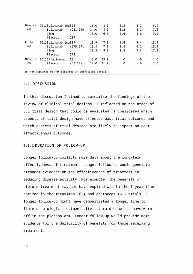
Trial Simulation (BCTS). This process involves the following process as described by

O’Hagan et al. where θ represents the prior distributions for the outcome variables (126).

1. Define counters I for iteration and T 1 , T 2 , …, T k for the assurances, and set all

counters to 0.

2. Sample θ from the prior distribution

3. Sample the sufficient statistics using the model and the sampled value of θ.

4. For j=1,2 ,… k increment T k if the outcome A j has occurred.

5. IncrementI . IfI ≤ N , go to step 2.

6. For j=1,2 ,… k, estimate assurance γ j=P ( A j )by T j/ N .

A simulation approach to calculating assurance was adopted in a separate paper to evaluate a

sequential series of Phase IIb and Phase III trials for a new drug for Rheumatoid Arthritis

using the Rheumatoid Arthritis Drug Development Model (RADDM) (63). The RADDM

model estimates the probability of license regulatory approval for different trial designs.

Disease duration of the target population, sample sizes, doses of the experimental treatment,

choice of comparator, duration of the Phase IIb clinical trial, the primary efficacy outcome

and decision criteria for proceeding to Phase III based on the results at Phase IIa were all

varied. The simulation was flexible to address many design decisions that extend beyond

sample size. The study does not present the impact of the results on cost-effectiveness

analyses but the authors acknowledge in their discussion that the simulation can be linked to

a CE model or commercial value model.

3.3.6 OTHER APPROACHES

Shavit et al. (2005) develop a CE model to compare the costs and incremental benefits for

two research designs (117). They compare a Randomised Controlled Trial (RCT) with a

retrospective observational study design. They measure the benefits of the studies in terms

of the expected bias in the information gained. They assessed estimates of information bias

for the designs that were evaluated and assign probabilistic distributions to these.

The study provides a framework to compare RCTs with observational studies, however

many of the practicalities involved in their method are not explored in detail. The authors

specified informative priors for the bias, but do not give a detailed description on how they

were derived. The sample size of the designs were reported to be calculated using EVSI,

however they do not explicitly state how the EVSI calculation was performed. The authors

recommend that the information from the studies should be valued according to a threshold 54

for the organization financing the research’s willingness to pay for a unit of effectiveness

observed. This method could be applied from a societal perspective in terms of willingness

to pay for health gain, or from an industry perspective of increased profit per unit

effectiveness.

3.3.7 SUBSEQUENT PUBLISHED LITERATURE

Since my review was completed I have identified two further publications that are relevant

for conducting Value of Information analyses from the pharmaceutical perspective. These

were not incorporated into the review because whilst they were relevant to the review, they

did not use methods that were absent from the review. From a methodological perspective

these studies utilise an assumption that Net Benefit is normally distributed. However, one

article considers decision-making when the pharmaceutical company and the reimbursement

authority differ in their valuation of the drug (129). The second article develops on previous

work in which multiple stage trial designs are considered from a pharmaceutical perspective

(130). Both studies assume that the company has an option to submit for reimbursement with

current evidence. The analysis of multi-stage trial designs conducts sensitivity analysis for

different prices but in discrete analyses.

Willan and Eckermann (2012) investigated price setting and the trade-off between pricing

and evidence when a pharmaceutical company is applying for reimbursement from a societal

decision-maker of whether to approve healthcare interventions (129). They consider what

actions should be taken when the pharmaceutical company controls the prospective research

and the decision maker the reimbursement within a jurisdiction. For a given level of

evidence, they described a maximum threshold price ‘acceptable’ to the societal decision

maker. The expected net gain for conducting another trial will be positive above this price.

The pharmaceutical company will act according to their expected value of research and cost

of research and current evidence. For a given level of evidence, the company will have a

minimum threshold price ‘acceptable’. Prices below the threshold will generate a positive

expected net gain from further research. The company should submit to the reimbursement

authority if they have negative expected net gain for all sample sizes for this price, but

perform another trial if there is a sample size with positive net gain

3.4 DISCUSSION

3.4.1 LITERATURE REVIEW METHODOLOGY

55

I adopted the recommended Pearl Growing approach to study identification in which

references were identified from the reference list and citation list of relevant articles. The

literature review was designed to efficiently identify Bayesian methodologies utilising health

economic methods or mathematical modelling to inform design decisions in clinical trials.

Chilcott et al. (2003) had found that traditional systematic review methods using search

terms and online databases were not a suitable method for identifying health economic

methodologies. Traditional systematic reviewing identified a large number of references, of

which only a small yield of articles were relevant (89).

I decided not to continue with the search beyond two rounds of searching because the

subsequent yield of articles was very low and would be time consuming to complete. Two

assessments were made to support this decision. Firstly, the reference lists of the 15 articles

identified in the second round of the review were screened to identify papers that used

methodologies not already described above or from authors not included in the review.

Secondly, the reference list was compared against that of a fellow PhD student who had

independently developed a literature review to identify ENBS studies. These checks did not

indicate that an important body of literature had been excluded from the review.

3.4.2 MERITS OF THE APPROACHES TO VALUING CLINICAL TRIALS

The three main approaches to valuing clinical trials in the literature review were ENBS,

BeBay and assurance. There are many similarities between the ENBS and Bebay

approaches. The assurance methodology is quite different because it generates estimates of

the probability of success but does not value the outcome in monetary terms. ENBS has been

more commonly used in a societal framework, whereas BeBay and assurance have a

stronger focus on pharmaceutical company trials. ENBS values the reduction in uncertainty

in Net Benefit, after data collection, in monetary terms. The BeBay approach links trial

results to the uptake of new treatments conditional on trial sample size.

ENBS studies have developed many useful methodologies but none that are sufficient for the

requirements of this research question. The main limitation arises from the adoption of a

pharmaceutical perspective. I concluded that an assumption of normally distributed Net

Benefit was not applicable in this study. It would be unreasonable to assume that Net Benefit

was normally distributed in the absence of a CE analyses in SLE to support this assumption.

Furthermore, a CE model for SLE was likely to require inputs from multiple sources and it

was more useful to focus on acquiring data on a sub-set of parameters that are used to

calculate Net Benefit. I believe that the assumption of a normally distributed Net Benefit is

56

best applied to within trial CE evaluations where Net Benefit and the variance in Net Benefit

are directly measured. ENBS has been applied to within trial CE evaluation, and CE models

of variable structure and complexity. As a consequence, several methodological

developments have been made to improve the efficiency of calculations for more complex

analyses.

The main limitation of the ENBS approach is that it does not reflect the incentives and

objectives of a pharmaceutical company. The main focus of the ENBS studies has been to

assist with reimbursement decision making from a societal perspective. In very simple terms

a pharmaceutical company invest in an RCT to optimise the profitability of that drug. They

are not mandated to consider the health of society in this decision. However, the

pharmaceutical company should not design their trials without consideration for the health

economics regulations. Their expected profits would be conditional on the license regulators

requirements of efficacy, safety, and reimbursement requirements for cost-effectiveness.

I would argue that adaptations of ENBS to the pharmaceutical perspective have not

addressed all of the factors that would be important during the drug development process.

Previous methods have assumed that the profit per patient treated is known by the company

before they start the trial. The analysis is therefore conditional on the price that is assumed.

However, the price of new treatments will not be fixed in the early stages of the drug

development and the price may be dependent on the strength of evidence collected in the

Phase III trial. It would be more appropriate to relax the assumption that price is fixed.

The BeBay literature introduced a useful method for valuing trials from a pharmaceutical

perspective. Many of the studies from the BeBay literature have focussed on the

implications of the trial meeting a primary endpoint to determine market access. Health

economics and cost-effectiveness modelling are not central to their methods. However, they

have developed a useful method for specifying the value of treatment from the

pharmaceutical company perspective in terms of profit per patient and market coverage. In a

more recent analysis they considered factors affecting reimbursement such as costs and

adverse events. However, the methods for estimating the future costs and health outcomes

are simple compared with most CE models. In recent studies the BeBay approach has

integrated the motivations of the pharmaceutical company to maximise profits with the

requirements of license regulators and reimbursement authorities, without specifying the

price of the new treatment. It will be useful to adopt their specifications of the objectives of

the pharmaceutical company into the valuation of trial designs.

57

3.4.3 METHODS FOR SAMPLING TRIAL OUTCOMES

The ENBS and BeBay studies use the prior distribution of the parameter of interest to

sample a new dataset. In a drug development programme the prior distribution could be

reliably estimated from the Phase II trial. However, there are several scenarios where this

may not be satisfactory to address innovative trial design features.

I have identified three situations that would present challenges to defining the prior

distribution. Firstly, the inclusion criteria may not be compatible between previous and

potential future trials. The impact of alternative inclusion criteria on the data collected may

be difficult to predict. For example, the new trial may target a sub-group of individuals from

the Phase II, or if the Phase II trial did not have a representative sample of the target

population. In either case it might be beneficial to pool evidence from multiple sources of

data that can describe the expected natural history of patients in the target population.

Secondly, gaps in the data exist if the duration of follow-up in the Phase II trial is shorter

than the new trial. Prior distributions for long-term treatment effect can be assumed but it

may be more difficult to factor in the impact of other factors such as withdrawal into what

treatment effects are observed. Thirdly, the trial investigators may wish to collect clinical

outcomes that were not included in the Phase II trial, or change the way it is measured. In

this situation sampling from Phase II trial outcomes would either limit the scope of the EVSI

or rely on other means to estimate prior parameters, such as elicitation (131). It may be

difficult for experts to translate outcomes from one primary endpoint to another. The

outcomes will be correlated, but the response index provides very little information to

estimate the mean difference.

The RADDM study illustrates the advantages of building more complex CE models to

estimate the impact of multiple design decisions. This would be advantageous in the SLE

study where multiple disease outcomes can be observed. Data from observational cohort

studies could be used to populate the BCTS. Patient registry data would be a less subjective

source of information than elicitation. Data analysis facilitates detailed description of

dependencies and correlation between clinical outcomes, which would be challenging to

elicit from clinical experts. Assurance calculations in the RADDM case study by Nixon et

al. (2009) were useful in identifying optimal research designs across a range of design

features using BCTS (63).

58

3.4.4 PROBLEMS WITH COMPUTATIONAL BURDEN

Computation burden was identified in the discussion section of some articles as a potential

problem for Value of Information analyses (108;111;113;115;116). Due to the complexity of

SLE this is likely to pose additional challenges because a CE model must describe multiple

disease processes. Several methods have been identified to speed up analyses. There are

several methods that have been proposed to deal with computational burden in evaluating

clinical trial designs. The assumption of a normally distributed net benefit as the outcome of

the clinical trial would be useful to reduce CE model complexity. Two alternative methods

to minimise computation time were identified as potentially useful: the use of conjugate

distributions and the B&K approximation of Net Benefit. However, neither method has been

tested with a complex CE model developed for reimbursement submission for a new SLE

treatment.

3.4.5 USING VOI IN REIMBURSEMENT DECISION-MAKING

It is noted that the health economic literature identified in this review (103;106;107;112) has

sought to apply VOI methods to aid reimbursement decision-making. It has been argued that

a binary “approve” versus “do not approve” decision criteria is too restrictive, particularly if

the decision is irreversible. Therefore, reimbursement authorities should evaluate the option

value of delaying decision-making to allow collection of further evidence (103). Although

consideration of options to delay a decision and gather more evidence would provide a more

consistent application of the VOI method on the side of the pharmaceutical company and the

reimbursement decision-maker, I decided not to incorporate this process into the methods. It

would add considerable additional complexity that was not necessary to demonstrate the

feasibility of VOI in pharmaceutical drug development.

3.5 CONCLUSION

This literature review identified thirty-seven studies that have used Bayesian and specifically

VOI methods to evaluate the value of alternative trial designs. I identified methodologies

from the BeBay, ENSB and assurance literature that could be used to evaluate SLE trials.

The literature review identified some limitations in the application of EVSI methods to the

pharmaceutical perspective. A study from the BeBay literature suggested that price can be

59

treated as an outcome of the analysis rather than a fixed parameter. This approach was not

fully explored in their article, and price was not reported as an outcome of their analysis.

Nonetheless, I identified that this approach could be used to relax some of the problematic

assumptions that have been imposed when adapting ENBS to a pharmaceutical perspective.

I planned to develop a CE model for SLE that would be suitable for submission to

reimbursement authorities. The Bayesian methods for updating parameters from a CE model

would be taken from the ENSB literature. In this study I will develop a BCTS to increase the

flexibility of the simulation tool to compare a large selection of clinical trial designs, to

allow the assessment of assurance based on multiple trial outcomes, and use longitudinal

datasets to estimate trial outcomes that would not be collected in Phase II trials. BCTS has

been used to generate assurance estimates for clinical trials with a broad range of design

features. I decided that a BCTS would be useful to simulate flexible trial designs to evaluate

a broad range of trial designs. In particular this would enable trial data to be simulated for

outcomes that would not have been observed in the Phase II clinical trial.

In Chapter 4 I describe the process of conceptualising SLE and designing a natural history

model to describe the important outcomes in SLE. Health economic modelling must estimate

the lifetime costs and health outcomes for two or more treatment options. Lifetime costs and

health outcomes can be estimated in CE model by predicting what disease outcomes are

expected for each treatment option. It is necessary to develop a simplified description of

SLE that includes disease outcomes that may impact on the lifetime costs and health

outcomes and includes all major costs and health outcomes that could be modified by new

treatments.

60

4 CHAPTER 4: NATURAL HISTORY OF SLE LITERATURE

REVIEW4.

The purpose of this chapter is to develop a conceptual model of SLE and identify

quantitative estimates to populate the modelling framework.

The National Institute for Health and Care Excellence (NICE) reference case requires that

CE models include the costs and QALYs over a lifetime horizon (29). This is particularly

important for a chronic disease such as SLE where treatments can impact on long term

outcomes and mortality. All outcomes and comorbidities can potentially be included in CE

models, but it is sensible to only include outcomes that will impact on decision-making to

reduce CE model complexity. Defining what long term outcomes to include in the

conceptual model is an important stage of CE model development. It is important to identify

intermediate markers to relate clinical trial outcomes to long term outcomes and mortality.

Once the conceptual map is decided it is also necessary to identify evidence to describe the

relationships associations between disease outcomes.

Section 4.1 provides a detailed description of the methods used in the literature search.

Section 4.2.1 describe the results of the conceptual map of literature and how this was used

to develop a conceptual model for SLE. Section 4.2.2 provides a detailed description of the

studies describing disease activity. Section 4.2.3 describes the studies of mortality. Sections

4.2.4 and 4.2.5 report the results for the literature review for organ damage by composite

score and organ system respectively. The discussion in Section 4.3 considers whether the

published data is sufficient to meet the requirements of the conceptual model. The

conclusion, in Section 4.4 outlines the data requirements from the conceptual model for

further statistical analyses to be completed in this PhD.

4.1 METHOD

4.1.1 SEARCH STRATEGY

Given the breadth of epidemiological research in SLE, SLE associated symptoms, and co-

morbidities, it was impractical to perform an exhaustive systematic literature search.

Therefore, the literature search was designed to identify a sufficient number of quality

epidemiology studies of adult SLE published in major SLE related journals. The online

61

database Medline was used to conduct the search. Other databases were not searched in this

review because the breadth of coverage of the search in Medline covered the main journals

for SLE research suggested by Professor David Isenberg, a clinician and researcher from

University College London (December 2009).

Search terms included a combination of free-text and MeSH terms. The review only

included studies published after 1995. Only studies published after this date were reviewed

because a number of important publications relating to the classification and definition of the

disease were published at this time including: an update of the criteria for classification of

SLE in 1997 (44); the definition of the SLICC/ACR Damage Index in 1996 (52); the

definition of the SLEDAI score in 1992 (132); the definition of the BILAG score in 1993

(133). Furthermore, discussions with Professor Isenberg (December,2009) indicated that

treatment practices changed at this time. Studies of patients before this period may be less

representative of current SLE patients. Details of the search strategies are reported in

Appendix 4.

The final inclusion criteria for the studies were as follows.

Study design. Prospective observational cohort studies to reduce confounding and

selection bias

Patients. Patients diagnosed with SLE

Outcome measures. Outcomes of interest were symptoms, clinical events, co-

morbidities, and mortality.

Language. Full published reports in English were considered.

The title and abstract for each citation were reviewed to determine whether they met the pre-

defined selection criteria. Full text reports were obtained for the articles where the abstracts

met the inclusion criteria. Only full published reports were considered, letters and abstracts

were excluded. Retrospective design studies were excluded from the search because they are

more likely to encounter problems with confounding and selection bias. Furthermore,

disease activity and organ damage scores of interest are less likely to be available in

retrospective data because they are not routinely collected in clinical practice. Nonetheless,

the abstracts of all the retrospective studies identified in the search were reviewed to identify

any important findings.

62

4.1.2 DATA EXTRACTION

4.1.2.1 CATALOGUE COHORT STUDIES

The first part of the review aimed to identify important cohorts with multiple publications,

and record the key themes explored in the studies. The full reports were reviewed and the

following information was extracted.

Sample size

Population description

Cohort name

Primary theme

4.1.2.2 THE CONCEPTUAL MODEL

The second stage of the review aimed to build a conceptual description of the disease to

understand the relationships between short term disease measures and long term

consequences. The abstracts of the articles were reviewed to identify statistically significant

associations between disease characteristics and co-morbidities to develop a conceptual

disease map. The references were included in the map to illustrate the evidence base

supporting the relationships to help prioritise disease outcomes. The conceptual disease map

illustrated the strength of evidence for relationships between clinical events and disease

characteristics. The conceptual map was discussed with Professor Isenberg to determine if

the main features of the disease were accounted for.

The conceptual map includes symptoms and outcomes of the disease. For simplicity, I

decided to exclude the following from the diagram and the data extraction process:-

1. Fibromyalgia as a comorbidity to SLE

2. Health Related Quality of Life outcomes

3. Psychosocial risk factors such as wealth or health perception

4. Genetic risk factors

Some outcomes were grouped according to organ system to simplify the visual presentation

of the map. For example, avascular necrosis and osteoporosis were combined into

musculoskeletal damage, and seizure and stroke were included in neuropsychiatric damage.

63

The conceptual map was discussed with a Prof. David Isenberg, clinical expert in SLE, to

address the following questions:

1. Are there any important outcomes, symptoms or events associated with the disease

that are missing?

2. Are there any important relationships missing from the disease map?

3. Are there any important studies or research that has not been identified in this map?

4.1.2.3 QUANTITATIVE DATA EXTRACTION

The outcomes of the conceptual disease model informed the third stage of the review which

aimed to extract quantitative data from the epidemiological studies relating to features of the

disease that would be included in the natural history model. I developed the list of items to

be extracted based on prior understanding of epidemiology study outcomes.

The following data extraction criteria were used for articles exploring disease activity in

SLE.

Rate of flare/organ involvement at fixed intervals

Disease activity scores

Predictors of changes in disease activity or flare

The following data extraction criteria were used for articles exploring mortality in SLE.

Survival analysis/event rates at fixed intervals

Standardised mortality ratios

Predictors of mortality (univariate and multivariate analysis)

Studies of organ damage either employed the SLICC/ACR Damage Index composite score

or looked at individual events. The following data extraction criteria were used for articles

exploring organ damage in SLE and were chosen based on what statistics were commonly

reported.

Time to damage.

Mean SLICC score over time.

Organ system involvement.

Event rates at fixed intervals

Predictors of damage (univariate and multivariate analysis).

64

4.2 RESULTS

The search strategy identified 142 articles reporting the results of a prospective

observational cohort study. The key details of each of these individual articles are

summarised in Appendix 5.

4.2.1 CONCEPTUAL MAP AND CONCEPTUAL MODEL

The conceptual map of SLE can be found in Figure 5. The rounded shapes define important

symptoms, outcomes or clinical markers identified in the review. Arrows represent

associations that have been identified between clinical factors due to statistically significant

test results. The boxes list the articles discussing the causal links between two clinical

factors. The conceptual disease map illustrates the breadth of research that has been

identified on all aspects of the disease. The map illustrates that there is a strong evidence

base for a causal relationship between disease activity, organ damage and mortality.

Prof. Isenberg did not think that any major events were missing; however he did suggest that

the disease could be broken down into organ systems. He identified some well known

relationships between the disease characteristics that had not been identified in the literature.

These have been added to the map, indicated by a white box. The relationship between the

incidence of diabetes, cardiovascular damage and renal damage were absent. He discussed

the need to control for well-known risk factors for cardiovascular damage such as obesity,

diet and physical activity. These were unlikely to be identified in the review because they

are common risk factors in non-SLE patients rather than being particular risk factors to SLE.

He expected inflammation in skin activity to lead to permanent skin damage. It is possible

that this association is less likely to be studies because it has a clear causal pathway. He

noted that anti-malarials were not sufficiently represented in the map as these should have a

protective effect on more outcomes. He referred to a recent systematic review of anti-

malarials in SLE (134).

65

Figure 5: Conceptual map of SLE from the published literature

Disease Activity Mortality

DamageAlarcon ’01Andrade ’07Bertoli ’06

Calvo-Allen ’03Santo s’09

Peschken ’09Toloza ’04

Alarcon ‘04

Alarcon ’01Cardoso ’08Manger ’02

Mok ’03Mok ’05

Nived ’02Nossent ’07Rahman ’01

Gladman ‘00

Alarcon ’01Alarcon ’04

Becker-Merok ’06Gilboe ’01Ibanez ’05Ibanez ’07Mok ’03Stoll ’04

Toloza ’04Peschken ‘09

Alarcon ’01Becker-Merok ’06

Abu-Shakra ’95Cook ’00

Ibanez ’03Nossent ’07

Fernandez ’07Ibanez ’07

Kasitanon ’02Xie ‘98

Cardiovascular damage

Renal

ESRD

Alarcon ’01Abu-Shakra ’95

Cardoso ’08Carvera ’03

Kasitanon ’02Manger ’02

Campbell ‘08

Alarcon ’01Becker-Merok ’09

Bjornadal ’04Manger ’02

Mok ’05Ward ‘95

Previous damage

Alarcon ’04Stoll ’00Mok ‘00

Steroids/ Cytotoxic treatment

Alarcon ’04Gladman ’03

Ibanez ’05Mok ’00Mok ’03

Santos ’09Thamer ’09

Alarcon ‘06

Disease activity

Allen ’06Bujan ’03

Nikpour ‘09

Anti-phospholipid

antibodies

Bastian ‘02

Anti-dsDNA

Bastian ‘02

Becker-Merok ’09Ibanez ’07Apte ‘08

Pulmonary damage

Abu-Shakra ’95Cardoso ‘08

Anemia

Allen ’06Bertoli ‘08

Bertoli ‘07

Pnumonitis

Infection

Bosch ’06Jeong ’09Noel ’01

Zonana-Nacach ‘01

Bosch ’06Gladman ’02

Noel ’01Zonana-

Nacach ‘01

Peripheral Vascular damage

Calvo-Allen ’05Becker-Merok ‘09

Calvo-Allen ‘05

Musculoskeletal damage

Calvo-Allen ’06Gladman ’01

Zonana-Nacach ’00Prasad ‘07

Malignancy

Chun ’05Ward ‘95

Duran ‘08

Fauschou ‘06

Premature gonadal failure

Gonzalez ‘08

Gonzalez ‘08

Neuro-psychiatric

damage

Gonzalez ’09Mikdashi ’04

Mok ’06Andrade ’08Mikdashi ‘05Mikdashi ’07Andrade ‘08

Serum creatinine

Fauschou ‘06

Mikdashi ’04Mok ’06

Appenzeller ’04McLaurin ’05

Bujan ‘03

Infection

Mok ’05Nossent ’07

Ward ’05Chambers ‘09

Santos ‘09Ruiz-Irastorza ‘04

Ethnicity/ gender/ late

onset /hypertension

Ocular damage

Skin damage

Clinical opinion

Age/smoking

Bertoli ’09Calvo-A. ’05Toloza ’04

Manger ‘02

Bertoli ‘09

Fatigue

Burgos‘09

EthnicityFever

Young age , ethnicity,

hypertension/ gender

Gonzalez ’09Ramsey-G. ’08Mikdashi ’07Mikdashi ‘05

Diabetes

Pons-Estel ’09Apte ’08

Ibanez ’05Toloza ‘04

Age/gender/smoking

Age/ethnicity

Age/gender/ethnicity

Campbell ’08Ibanez ’07Doria ‘06

Gonzalez ‘09

Clinical opinion

Andrade ’07Ibanez ’07Ibanez ‘05

Age

Lupus anticoagulant

Doria ‘06

Steroids

Mok ’06McLaurin ‘05

Lupus anticoagulant

Calvo-A.’05Manger ‘02

Anemia

Toloza ‘04

Bujan ‘03

ethnicity

Steroids

Alarcon ’01Mok ’00Xie ‘98

hypertension

Mikdashi ‘07

hypertension

Font ‘01

Zonana-N. ‘00

Zonana-N. ‘01

Hypertension

Rahman ‘00

Amit ‘99

66

Having reviewed the conceptual map, and supplemented it with clinical opinion, I reduced

the conceptual map into higher level groups and defined a conceptual model of SLE (Figure

6). The boxes within the diagram refer to characteristics and outcomes to be included in the

conceptual model and the arrows describe causal relationships between them. The

conceptual model accounted for patient characteristics that impact on the risk and incidence

of disease outcomes. These included demographic characteristics of gender, ethnicity and

age. It also included medical characteristics such as cholesterol, hypertension, anticardiolipin

syndrome, obesity, and lupus anticoagulant. The conceptual model describes the associations

between disease activity, steroid dose, organ damage and mortality. Within the conceptual

model higher disease activity and steroid dose increase the risk of organ damage outcomes

and mortality. I decided to separate organ damage by organ system because some organ

damage is caused by disease activity, steroids, or a combination of both. Furthermore, the

costs and health implications of damage in different organ systems are variable. Renal

damage is likely to be more costly than skin damage, and musculoskeletal damage is likely

to impact more on quality of life than ocular damage, which can be reversible. The organ

systems will also have differential risk factors for mortality.

Figure 6: Conceptual model of SLE

Patient Characteristics

Mortality

Disease Activity

Prednisone Dose

Ocular damage

Gastrointestinal damage

Peripheral vascular damage

Pulmonary damage

Neuropsychiatric damage

Musculoskeletal damage

Skin damage

Renal damage

Cardiovascular damage

Diabetes

Malignancy

Gonadal Failure

67

4.2.2 DISEASE ACTIVITY

The search identified ten articles that study disease activity in SLE. Some interesting

observations about the patterns of disease activity have been made.

One study estimated an annual flare incidence to be 3 per patient year using the

BILAG index (135).

Flares are more commonly observed in the musculoskeletal, skin, and

haematological systems. (135)

Seventy percent of flares involved only one organ system and 30% of flares

manifest in two or more body systems at a time (135).

Remission is uncommon in SLE, the incidence density is 0.028 cases of remission

per person year. The mean duration of remission was 4.6 years (SD 3.6). The mean

time to remission was 5.8 years. (35).

The disease remains active in many patients beyond 10 years duration (136).

4.2.2.1 PREDICTORS OF DISEASE ACTIVITY

A few studies of disease activity used statistical techniques to identify predictors of future

disease activity. The results of these studies are reported in Table 8

68

Table 8: Predictors of disease activity outcomes in SLE

Author name Date Sample Cohort Measure of disease activity

Description of predictors Estimated hazard ratio

Bujan (137) 2003 239 Barcelona Haematological activity

Haematological activity 4.52 (1.27-16.7)

Bujan (137) 2003 239 Barcelona Cardiac activity Cardiac activity 5.07 (1.23-20.9)Bujan (137) 2003 239 Barcelona Neurological

activityNeurological activity 4.97 (2.34-10.52)

Bujan (137) 2003 239 Barcelona Neurological activity

Anticardiolipid antibodies 3.81 (1.75-8.30)

Bujan (137) 2003 239 Barcelona Renal activity Renal activity 7.89 (4.04-15.04)Allen (138) 2006 411 Birmingham Mucocutaneous

activityMucocutaneous activity 1.98 (1.35-2.90)

Allen (138) 2006 411 Birmingham Mucocutaneous activity

Renal activity 0.38 (0.19-0.75)

Allen (138) 2006 411 Birmingham Mucocutaneous activity

Disease duration 0.86 (0.81-0.91)

Allen (138) 2006 411 Birmingham Renal activity Renal activity 9.43 (4.27-20.79)Allen (138) 2006 411 Birmingham Renal activity Renal damage 3.39 (2.12-5.44)Allen (138) 2006 411 Birmingham Renal activity Musculoskeletal activity 0.58 (0.39-0.87)Allen (138) 2006 411 Birmingham Musculoskeletal

activityMusculoskeletal activity 3.28 (1.60-6.73)

Allen (138) 2006 411 Birmingham Musculoskeletal activity

Renal activity 0.649 (0.471-0.894)

Allen (138) 2006 411 Birmingham Musculoskeletal activity

Disease duration 0.923 (0.865-0.985)

Bertoli (139) 2006 287 LUMINA Low level disease activity

Social support 1.21 (1.06-1.38)

Bertoli (139) 2006 287 LUMINA Low level disease activity

No. ACR diagnostic criteria 0.77 (0.63-0.93)

Bertoli (139) 2006 287 LUMINA Low level disease activity

SLICC/ACR DI 0.85 (0.74-0.97)

Nikpour (140)

2009 202 Toronto Persistent active disease

SLEDAI-2K 1.34 (1.20–1.51)

Nikpour (140)

2009 202 Toronto Persistent active disease

Cutaneous activity 2.37 (1.17–4.81)

ACR American College of Rheumatology; DI Damage Index

4.2.2.2 MEASURES OF LONG TERM DISEASE ACTIVITY

Studies of disease activity have employed different methods of measuring the severity of

disease activity in patients. The approach to describing long term burden of disease activity

is of interest when observing long term outcomes that are affected by a burden of disease

activity. The magnitude of burden has often been calculated as the area under the curve

(AUC) of a disease activity index. However, Barr et al. (141) argue the nature of the disease

activity is lost using this method. A patient with a short period of severe disease activity and

a patient with long term mild disease activity will have equivalent AUC scores despite

substantial differences in the nature of the disease. Consequently, Barr et al. (141) argue that

the pattern of disease activity should be studied more closely. They identify three patterns of

SLE disease activity: relapsing/remitting; long quiescent; persistently active disease (PAD).

PAD is more common than relapsing remitting but also because periods of chronically active

69

disease were more likely to be moderate or severe. More recently, Nikpour et al. (140) study

the importance of PAD in SLE and find that PAD is more common than short periods of

disease flare. They argue against using flares as endpoints in clinical trials because it

excludes the important assessment of treatment on PAD.

Although, Barr et al. (141) and Nikpour et al. (140) presented an account of the patterns of

disease activity Ibanez et al. (2003) argue that they do not provide an objective measure of

disease activity that can be used routinely in studies (142). Ibanez et al. developed a method

of calculating Adjusted Mean SLEDAI (AMS) as a measure of disease activity burden over

time. The continuous spectrum allows comparisons to be made between patients. AMS

offers a pragmatic way to relate disease activity to organ damage and mortality.

Furthermore, AMS is a strong predictor of mortality, damage, and coronary artery disease

(142;143). From these studies, they concluded that AMS is a reproducible measure of

disease activity over time because it is a good measure of persistently active disease and can

be affected by flares in the disease.

4.2.3 MORTALITY

SLE can lead to premature death. A standardized mortality ratio quantifies the increase or

decrease in mortality of a study cohort relative to the general population. Bernatsky et al.

report a standardised mortality ratio of 2.4 (95% CI 2.3-2.5) from a large cohort of 9547

patients (144). Other estimates have reported similar results of 2.3 and 2.4 (145;146). An

earlier study, published in 1995, report a SMR of 4.9 (147). The risk for SLE patients is

significantly higher than that observed in the general population. The search strategy

identified 27 studies that investigated mortality in a cohort of SLE patients.

4.2.3.1 RATES OF MORTALITY

The survival rates of SLE patients are reported in Table 9

. Two studies Ward et al. (148) and Xie et al. (149) report substantially lower survival than

the other studies. Differences in survival estimates across studies may be due to the time

periods in which patients were recruited because survival estimates have improved in recent

years (146;149;150).

70

Table 9: Survival estimates in SLE

Author name Date Sample Size Survival (proportion)1 year 5 year 10 year 15 year

Campbell (151) 2008

265 - 0.90 - -

Doria (152) 2006

207 - 0.96 0.93 0.76

Kasitanon (153) 2006

1378 - 0.95 0.91 0.85

Ruiz-Irastorza (154) 2004

202 - 0.95 0.91 0.86

Cervera (155) 2003

1000 -  - 0.92 -

Nived (156) 2002

80 - 1.00 0.91  -

Manger (145) 2002

338 - 0.97 0.90 -

Kasitanon (157) 2002

349 - 0.84 0.75 -

Alarcon (158) 2001

288 - 0.87  -  -

Rahman (159) 2001

190 (No damage) -  - 0.93 -

Rahman (159) 2001

73 (Early damage) - - 0.75 -

Mok (160) 2000

163 - 0.93  - -

Cervera (161) 1999

1000 - 0.95  -  -

Xie (149) 1998

566 - 0.79 0.70 -

Abu-Shakra (147) 1995

665 0.98 0.93 0.85 0.79

Ward (148) 1995

408 - 0.82 0.71 0.63

4.2.3.2 PREDICTORS OF MORTALITY

Table 10 reports results from regression analyses of mortality. Eight studies included disease

activity as a covariate in regression analyses and all but one found it to be a predictor of

mortality. Becker-Merok et al. found that patients with a weighted average SLEDAI score of

greater than 3 over time have a 242% greater risk of mortality than those with average

SLEDAI less than 3 (162). Fernandez et al. found that a unit increase in SLAM-R score at

baseline increases mortality risk by 10% (163). Cook et al. estimate that patients with a

SLEDAI score of between 6 and 10 points increase their risk of mortality by almost 300%

(164). Urowitz et al. (146) and Ibanez et al. (142) use a unit increase in the adjusted mean

SLEDAI increases risk of mortality by 15%. Finally, Alarcon (2001) reports an odds ratio of

1.09 for a unit increase in the SLAM at enrolment (158). Therefore, there is strong evidence

that disease activity increases the risk of mortality.

71

Renal involvement was found to be statistically significant in five studies

(145;151;154;165;166). However, Kasitanon and Abu-Shakra found that renal disease was

not a significant predictor of mortality (147;153). Pulmonary manifestations were

statistically significant in Cardoso et al. (166) but with wide confidence intervals.

Organ damage, measured by the SLICC/ACR Damage index has been found to be a

statistically significant predictor of mortality. Five of the studies estimated similar risk ratios

from different cohorts of patient (146;158;163;166;167). One study did not find organ

damage to be predictive of mortality (162). This came from a relatively small sample of 157

patients. Cardoso et al. found that a unit increase in the SLICC/ACR Damage Index score

increases the risk of mortality by 34% (166). Fernandez and Alarcon et al. looked at the

relationship between organ damage at baseline and mortality from the LUMINA cohort

(158;168). A unit increase in damage score increased mortality risk by 20% and 45%

respectively. Chambers et al. related the last available SLICC/ACR Damage Index score to

mortality and found that damage predicted a 40% increase in mortality risk (167).

The variation in study risk associations could be due to three factors. Firstly, variation in

covariate selection could lead to some confounding variables being omitted in the analyses.

Secondly, geographical variations in cohorts may lead to different risk associations. Thirdly,

the choice of disease activity measure and definition of risk (average or threshold0 will

impact on estimates.

72

Table 10: Predictors of mortality from multivariate analysis

Cox regression (Hazard ratio)Author Date Sample Renal

involvementPrevious cardio-vascular events

Disease Activity Organ damage Age Pulmonary damage Thrombotic event

Disease duration

Kasitanon (153) 2006 1378 Not significant Not significant 5.9 (2.5-14.4) Not significantCardoso (166) 2008 105 4.14

(1.47-11.71)1.34 (1.14-1.58) 3.38 (1.2-9.51)

Ruiz-Irastorza (154) 2004 202 4.4 (1.4-14.0) 1.07 (1.03-1.1)Becker-Merok (162) 2006 158 2.4 (1.19-4.42) Not significant 5.57 (2.44-12.7)Fernandez (168) 2007 552 1.1 (1.06-1.16) 1.20 (1.00-1.44) 1.03 (1.01-1.05)Mok (160) 2000 163 38.2 (1.2-124)Chambers (167) 2009 232 1.4 (1.14-1.72)Bernatsky (144) 2006 9547 6.4 (5.5-7.5) 7.7 (5.9-10.2)Cook (164) 2000 806 2.98 (1.06-8.38)Urowitz (146) 2008 1241 1.52 (1.02-2.26) 1.15 (1.11-1.20) 1.24 (1.14-1.35)Ward (165) 1996 408 2.38 (1.63-3.48)Campbell (151) 2008 265 2.5 (1.1-5.5)Manger (145) 2002 338 1.6 (1.1-2.4) 1.5 (1.0-2.4)Ibanez (142) 2003 575 1.15 (1.09-1.20) 1.05 (1.03-1.06)Abu-Shakra (147) 1995 665 Not significant 2.02 (1.34-3.04) 1.71 (1.18-2.49)Logistic regression (Odds ratio at 5 years)Alarcon (158) 2001 288 1.09 (1.01-1.17) 1.45 (1.19-1.91)    

73

4.2.4 ORGAN DAMAGE

4.2.4.1 SLICC/ACR DAMAGE INDEX

Organ damage has been widely studied using the SLICC/ACR Damage Index and within

individual organ systems. Details of the SLICC/ACR Damage Index are provided in

Appendix 1. In these observational studies the SLICC/ACR Damage Index is recorded by

the rheumatologist to monitor a patient’s accumulation of organ damage. The search

identified eighteen studies investigating organ damage using the composite index.

Mean SLICC/ACR Damage Index scores for a group of cohorts are summarised in Table 11.

It has been reported that the mean SLICC/ACR Damage Index score accumulates linearly

over time (169). Figure 7 illustrates how the mean organ damage score changed in time in

three studies. The results illustrate a linear trend in the accumulation of organ damage

(167;169;170). The rate of accumulation is faster in the Baltimore cohort (170) than the

London Clinic (167), this is likely due to differences in the ethnic profile of these regions.

Table 11: Damage accrual over time

Mean SLICC/ACR Damage Index score over time from diagnosisAuthor Date Sample size Year 1 Year 5 Year 10 Year 15Chambers (167) 2009 232 0.11 0.42 0.77 1.01Gladman (169) 2003 73 0.33 0.81 1.19 1.9Ruiz-Irastorza (154)

2004 202 1.00a 2a

Petri (170) 1995 407 0.45 0.9 1.6Mean SLICC/ACR Damage Index score over time from enrolmentAuthor Date Sample size Time = 0 Time = 5

yearsAlarcon (171) 2004 352 1.3 2.4Stoll (172) 2004 141 1.2 1.6a median SLICC/ACR Damage Index

74

Figure 7: Rate of organ damage accumulation over time

0

0.2

0.4

0.6

0.8

1

1.2

1.4

1.6

1.8

2

0 1 2 3 4 5 6 7 8 9 10 11 12 13 14 15

SLIC

C/AC

R DI

Years

SLICC/ACR DI from diagnosis

Chambers

Gladman

Petri

4.2.4.2 TIME TO INITIAL DAMAGE

Three studies have reported time from cohort entry to the first damage event. The results

from these studies are summarised in Table 12. The summary suggests that there is

substantial variation in time to initial damage between the studies reported here. Chambers

and Becker-Merok report slower time to damage than Ruiz-Irastroza. Toloza et al. (173)

report time to initial damage across different ethnic groups in a survival curve. After 5 years

of the disease approximately 50% of Hispanic and African Americans are damage free,

whereas 67% of Caucasians have not accrued damage. Ethnicity and environmental factors

are important determinants of damage accrual. Ruiz-Irastroza studies a Spanish population

whereas the other two studies are from mainly North European populations. Differences in

the ethnicity profile of cohorts may explain some of the variation.

Table 12: Time to initial damage

Author Year Sample size Proportions of patients damage free at the time point1 year 5 year 10 year

Becker-Merok (162) 2006 158 0.97 0.58Chambers (167) 2009 232 0.90 0.67 0.49Ruiz-Irastorza (154) 2004 202 0.65 0.46

4.2.4.3 PREDICTORS OF ORGAN DAMAGE

Twelve studies use Cox-regression ad logistic regression analysis to identify predictors of

organ damage. The results are reported in Table 13. In summary, three studies identified

steroids and other treatment as predictors of organ damage (171;174-176). Thamer et al. do

75

not find a statistically results, but do identify a trend towards an association that is robust to

sensitivity analyses (175). Four studies associated baseline disease activity with organ

damage (171-173;177). Three studies with disease activity as a covariate (162;172;176) use

an average score for disease activity.

Only three studies reported hazard ratios for the independent risks of disease activity and

treatments. Ibanez et al. (176) found disease activity and steroid use to be statistically

significant predictors of organ damage. A one unit increase in the SLEDAI score increased

the risk of damage by 4%. The use of steroids increased the risk of damage by 80%. Mok et

al. found the number of major flares and cyclophosphamide to be independent predictors of

organ damage (178). Finally, Alarcon et al. found that disease activity at baseline and

maximum steroid dose are significant predictors of a change in damage score (171). These

findings suggested that that disease activity and steroids are independent predictors of organ

damage.

76

Table 13: Predictors of organ damage from multivariate analysis

Predictors of organ damage from logistic regression (Odds ratio)Author name Date Sample

sizeAge Initial disease

activityAverage disease activity

Prior damage score

Steroids APL antibodies Cyclophosphamide Myocarditis

Alarcon (171) 2004 352 1.02 (1.00-1.03)

1.07 (1.05-1.10) 1.07 (1.04-1.10) 1.63 (1.16-2.29)

Santos (174) 2009 221 1.05 (1.02-1.07)

6.04 (1.60-25.21) 3.05 (1.17-7.94)

Gilboe (177) 2001 93 Not significant 1.14 (1.00-1.28) 1.52 (1.02-2.27)Ruiz-Irastorza (154)

2004 202 1.94 (1.01-3.73)

Stoll (179) 2000 141 Not significant Not significant 1.46 (1.04-2.05)Stoll (172) 2004 141 1.62 (1.22-2.16)Mok (178) 2003 242 1.63 (1.15-2.32) 1.54 (1.10-2.15)Predictors of organ damage from Cox regression (Hazard ratios)Author name Date Sample

sizeAge Initial disease

activityAverage disease activity

Prior damage score

Steroids APL antibodies Cyclophosphamide Myocarditis

Becker-Merok (162)

2006 158 3.45 (1.63-7.33)

Not significant 2.34 (1.13-4.81)

Toloza (173) 2004 158 1.09 (1.04-1.15) 2.53 (1.15-5.55)Ibanez (176) 2005 575 1.02 (1.01-

1.03) Not significant 1.04 (1.01-1.06) 1.80 (1.27-2.55)Thamer (175) 2008 525 Not significantPredictors of organ damage from Poisson regression (regression coefficient)Apte (180) 2008 636 0.01 (0.00-

0.03)0.09 (0.05-0.13) 0.97 (0.83-1.12) 0.48 (0.00-

0.95)

77

4.2.5 ORGAN DAMAGE BY ORGAN SYSTEM

Twenty studies studied organ damage in individual organ systems. Table 14 details the

prevalence of organ damage by organ system reported in eight of these studies. The

proportion of patients with system organ damage is variable between cohorts. There is

evidence that some organ systems are more susceptible to organ damage at different points

of the disease. Two studies report the prevalence of damage by organ system over time.

Figure 8 illustrates that musculoskeletal, cardiovascular and ocular damage are the most

prevalent damage events. Cardiovascular and neuropsychiatric damage occur early in

disease onset. Figure 9 illustrates a lower rate of damage accumulation. Neuropsychiatric,

renal and musculoskeletal damage have the highest incidence.

Figure 8: Organ damage by system (169)

0

10

20

30

40

50

60

1 2 3 4 5 6 7 8 9 10 11 12 13 14 15

% o

f pati

ents

Time (years)

Proportion of patients with system damage reported in Gladman (2003)

neuropsychiatric

ocular

renal

pulmonary

cardiovascular

peripheral vascular

gastrointestinal

musculoskeletal

skin

78

Figure 9: Organ damage by system (167)

0

2

4

6

8

10

12

14

16

1 2 3 4 5 6 7 8 9 10

% o

f pati

ents

Time (years)

Proportion of patients with organ damage reported in Chambers (2009)

neuropsychiatric

ocular

renal

pulmonary

cardiovascular

peripheral vascular

gastrointestinal

musculoskeletal

skin

79

Table 14: Prevalence of damage by organ system in cross-sectional studies at various stages of disease duration

Author name Date Sample size

Musculo-skeletal

Cardio-vascular

Neuro-psychiatric

Peripheral vascular

Ocular Renal Pulmonary GI Skin Gonad failure

Diabetes Malignancy

Becker-Merok (162)

2006 158 22.2% 17.8% 15.2% 11.4%  - -  -  - - - - -

Santos (174) 2009 221 14% 10% 14% 4% 13% 7% 6% 5% 5% 3% 4% 4%

Zonana-Nacach (181)

2000 539 22% 9% 20% 6% 13% 15% 7% 4% 8% 2% 6% 3%

Appenzeller (182) 2008 560 16% 11% 20% 5% 16% 8% 8% 5% 16% 4% 4% 4%

Chambers (167) 2009 232 12.1% 4.7% 14.7% 4.7% 1.3% 12.9% 3.4% 3.4% 5.2% 0.4% 0.4% 2.2%

Gilboe (177) 2001 93 37% 23% 28% 8% 11% 8% 20% 5% 11% 4% 2% 5%

Gladman (169) 2003 73 54.7% 28.7% 20.5% 4.1% 31.5% 5.4% 2.8% 12.4% 13.7% 1.4% 2.7% 1.4%

Mok (178) 2003 242 26.5% 12.4% 18.4% - - 15.1% - - - - - -

Guarize (183) 2007 60 8.3% 10% 18.3% 16.6% 15% 23.3% 8.3% 3% 35% 1.7% - -

80

In the next sections I summarise the prevalence and risk factors for each of the organ

systems included in the SLICC/ACR Damage Index. Quantitative estimates of risk factors

for organ damage by organ systems were needed to refine the causal links of the conceptual

model.

4.2.5.1 OCULAR ORGAN SYSTEM

The SLICC/ACR Damage Index includes the following events for the Ocular Organ System

Any cataract ever

Retinal change or optic atrophy

Studies have found a relatively high prevalence of ocular damage in SLE cohorts. Patients

are at lower risk of ocular damage in the early stages of the disease and at higher risk as

disease duration extends beyond 15 years. This may be due to cumulative doses of steroids

over time. However, I identified no studies to quantify this effect.

4.2.5.2 NEUROPSYCHIATRIC ORGAN SYSTEM

The SLICC/ACR Damage Index includes the following events for the Neuropsychiatric Organ System

Cognitive Impairment

Seizures requiring therapy for 6 months

Cerebrovascular accident

Cranial or peripheral neuropathy

Transverse myelitis

Mikdashi et al. report that cerebrovascular damage is a common cause of damage and was

observed in 27.3% of patients with neuropsychiatric damage. Polyneuropathy was observed

in 25.7% of patients and psychosis in 18.2%. Other damage included seizures and transverse

myelitis with 7.6% and 6.1% respectively (184). Mok et al. found a higher proportion of

damage was due to seizures (20%) (185). Table 15 reports results from studies of

neuropsychiatric damage to describe risk associations from Cox-regression and logistic

analysis.

81

Table 15: Odds ratios and hazard ratios with confidence intervals estimated for risk factors for neuropsychiatric damage

Author name Date Damage outcome Disease Activity Ethnicity anticardiolipids Organ damage Steroid Anti-malarials Diabetes Age Hypertension

Mikdashi (184) 2004 Neuropsychiatric

damage (OR)

2.7 (1.0-6.7) 3.0 (1.0-19.5) 4.8 (1.0-23.0)

Mok (185) 2006 Neuropsychiatric

damage (HR)

1.28 (1.29-1.31) 1.16 (1.10-1.23)

Gonzalez (186) 2009 Neuropsychiatric

damage (HR)

1.16 (1.12–1.21) 1.87 (1.22–2.87) 0.56 (0.35–0.92) 0.58 (0.36–0.93) 3.47 (1.44–8.38)

Mikdashi (187) 2005 Seizures(OR) 2.29 (1.01-1.12) 2.23 (1.01–4.67)

Andrade (188) 2008 Seizures (HR) 1.10 (1.04- 1.15) 2.7 (1.3–5.7) 0.35 (0.15- 0.80) 1.04 (1.00-1.08)

Ramsey-

Goldman (189)

2008 Seizure (HR) 1.0 (0.9–1.0)

Mikdashi (190) 2007 Stroke (HR) 1.31 (0.40-4.31) 1.11 (0.43–2.84) 1.00 (0.98–1.03) 2.31 (1.15–4.65)

HR Hazard ratios, OR Odds ratios; aCL anticardiolipin antibodies

82

4.2.5.3 PULMONARY ORGAN SYSTEM

The SLICC/ACR Damage Index includes the following events for the Pulmonary Organ System

Pulmonary hypertension

Pulmonary fibrosis

Shrinking lung

Pleural fibrosis

Pulmonary Infarction

A smaller proportion of patients are affected by damage to the pulmonary system. Bertoli et

al. report a slow rate of pulmonary damage accumulation. In this study 92.4% of patients

had no damage in the pulmonary system after 5 years of follow-up; after 10 years it was

88.4%. However, this is a slightly faster rate of damage accumulation than is found in

Gladman et al. (169) and Chambers et al. (167).

In univariate regression reported in Bertoli et al. (2007) average disease activity was

predictive of organ damage (HR 1.1 95% CI 1.04-1.17). Age, overall damage and steroids

were not statistically significant. In the multivariate analysis the results were quite different;

disease activity was no longer statistically significant and age became significant (HR 1.03

95% CI 1.01-1.06) (191).

4.2.5.4 CARDIOVASCULAR ORGAN SYSTEM

The SLICC/ACR Damage Index includes the following events for the Cardiovascular Organ System

Angina or coronary artery bypass

Myocardial infarction

Cardiomyopathy

Valvular disease

Pericarditis for 6 months or pericardiectomy

SLE patients are known to be at higher risk of atherosclerotic heart disease, particularly

myocardial infarction (192). Traditional risk factors for heart disease such as diabetes,

hypertension, tobacco use and sedentary lifestyle are common in SLE patients (193).

However, it is believed that these factors do not completely explain the increased risk (194).

Table 16 reports the odds ratios, or hazard ratios, from logistic regression and Cox-

regression for studies of cardiovascular damage and related events.

83

Table 16: Hazard ratios and odds ratios with confidence intervals estimated for risk factors for Cardiovascular damage

First Author name

Date Damage outcome Disease

Activity

Steroids Age Gender Organ

damage

Anticardiolipin

s

Anti-malarials Immuno-

suppressant

Cholesterol Smoking

Toloza

(195)

2004 Vascular events

(HR)

4.72 (1.68-

13.16)

Pons-Estel

(196)

2009 Cardiovascular

damage (OR)

1.06 (1.03-

1.09)

3.57 (1.35-

9.09)

1.28 (1.09-

1.5)

Becker-

Merok (197)

2009 Antherothrombotic

damage (OR)

0.3 (0.12-

0.75)

3.33 (1.36-

8.12)

0.19 (0.08-

0.47)

0.39 (0.15-0.99) 0.77 (0.70-

0.85)

Zonana-

Nacach

(181)

2000 Coronary artery

disease (RR)

1.7 (1.1-1.4)

Ibanez (176) 2005 Coronary artery

disease (HR)

1.04 (1.01-

1.06)

1.80 (1.27-

2.55)

1.02 (1.01-

1.03)

0.81 (0.56-

1.16)

0.81 (0.64-

1.01)

2.21 (1.73-2.82)

Rahman

(159)

2000 Vascular event

(OR)

6.9 (2.4-24.8)

HR Hazard ratios, RR Relative risk; OR Odds ratios; aCL anticardiolipin antibodies

84

4.2.5.5 SKIN ORGAN SYSTEM

The SLICC/ACR Damage Index includes the following events for the Skin Organ System

Scarring chronic alopecia

Extensive scarring or panniculum other than scalp and pulp space

Skin ulceration for more than 6 months

Skin involvement, such as malar rash and ulcers, are the most frequent complaints among

SLE patients. However, damage relating to the skin is relatively uncommon. Guarise et al.

(183) found that 35% of patients had accrued damage to the skin early in the disease. This is

in sharp contrast to Gladman et al. and Chambers et al. who report rates of only 8.2% and

3.9% after 5 years of the disease. This may be due to increased sun exposure in the Brazilian

population they studied.

4.2.5.6 PERIPHERAL VASCULAR ORGAN SYSTEM

The SLICC/ACR Damage Index includes the following events for the Peripheral Vascular Organ System

Claudication for 6 months

Minor tissue loss

Significant tissue loss ever

Venous Thrombosis

Peripheral vascular damage is relatively uncommon in SLE. Gladman et al. (169) and

Chambers et al. (167) report a constant rate of damage accumulation for peripheral damage

over time. Table 17 reports the risk factors identified for events associated with peripheral

vascular disease from Cox-regression and logistic regression.

85

Table 17: Hazard ratios and odds ratios with confidence intervals estimated for risk factors for Peripheral vascular damage

First Author name

Date Damage outcome Disease Activity Smoking Lupus Anticoagulant

Hypertension aCL Hydroxycholoriquine

Calvo-Allen (198)

2005 Venous thrombosis (HR)

2.49 (1.22-5.06) 1.11 (1.01-1.21) 2.29 (1.2-5.12)

Toloza (195) 2004 Vascular events (HR)

4.72 (1.68-13.16)

Manger (145) 2002 Thromboembolic event (HR)

1.6 (0.8-3.1)

Becker-Merok(197)

2009 Venous thrombotic event (OR)

4.8 (0.99-23.19) 0.08 (0.02-0.38) 0.26 (0.06-1.12)

HR Hazard ratios, RR Relative risk; OR Odds ratios; aCL anticardiolipin antibodies

86

4.2.5.7 GASTROINTESTINAL ORGAN SYSTEM

The SLICC/ACR Damage Index includes the following events for the Gastrointestinal Organ System

Infarction or resection of bowel below duodenum

Mesenteric insufficiency

Chronic peritonitis

Stricture or upper gastrointestinal tract surgery ever

The evidence from Table 14 suggests that gastrointestinal damage occurs in a very small

proportion of SLE patients. Figure 8 and Figure 9 show that gastrointestinal system damage

occurs early in the disease. The rate of damage accrual after the first year of the disease is

relatively low.

4.2.5.8 MUSCULOSKELETAL ORGAN SYSTEM

The SLICC/ACR Damage Index includes the following events for the Musculsoskeletal Organ System

Muscle atrophy or weakness

Deforming or erosive arthritis

Osteoperosis with fracture or vertebral collapse

Avascular Necrosis

Osteomyelitis

Table 14 illustrates that damage in the musculoskeletal system is common in SLE patients.

Petri et al. (170) find that avascular necrosis (osteonecrosis) as the most common

musculoskeletal complication in SLE patients affecting 14.5% of patients.

reports the odds ratios for logistic regression for musculoskeletal damage and related

events.

Table 18: Odds ratios with confidence intervals estimated for risk factors for musculoskeletal damage

First Author name

Date Damage outcome Disease Activity

Age Steroids Immunosuppressants Arthritis

Stoll (179) 2001

Musculoskeletal damage (OR)

2.26 (0.65–10.32)

0.885 (0.78–1.00)

Gladman (199)

2001

Osteonecrosis (OR)

18.5(3.2-359.6)

2.7 (1.02-8.8)

4.2 (1.6-13.7)

Calvo-Allen (200)

2006

Osteonecrosis (OR)

1.03 (1.00-1.05)

3.04 (1.02 -9.04)

OR Odds ratios

87

4.2.5.9 RENAL ORGAN SYSTEM

The SLICC/ACR Damage Index includes the following events for the Renal Organ System

Estimated or measured glomerular filtration rate <50%

Proteinuria or End stage renal disease

Results from Table 14 suggest that renal damage is not common among SLE patients. Table

19 reports the survival rates for time to end-stage renal failure after 10 years of follow-up in

different population of SLE patients.

Table 19: Renal survival over time

Author Date Sample size Renal Survival Overall survival10 years 10 years

Farschou (201) 2006 91 0.83Moroni (202) 2007 93 0.97 0.83Chen (203) 2008 37 0.94a 0.95a

Chen (203) 2008 21 0.45b 0.76b

Chen (203) 2008 28 0.19c 0.41c

Korbet (204) 2000 37 0.95a

Korbet (204) 2000 49 0.31c

a Survival of patients with complete remission; b survival of patients with partial remission; c survival of patients with no remission

.

Several studies have utilised univariate and multivariate statistical techniques to identify

variables associated with end stage renal disease. The results are detailed in Table 20.

Table 20: Predictors of end stage renal disease

Author Year Outcome Disease Activity

Age Serum creatinine

anti-Ro antibodies

No remission

Alarcon (205)

2006

Renal disease (HR)

0.96 (0.92-0.99)

Korbet (204)

2000

ESRD (HR) 2 (1.4-2.9) 3 (1.4-6.4) 8.2 (2.6-25.6)

Bastian (206)

2002

Lupus Nephritis (OR)

1.11 (1.02-1.19)

HR Hazard ratios; OR Odds ratios

4.2.5.10 GONADAL FAILURE

Gonadal failure is among the least commonly reported damage type recorded by the

SLICC/ACR Damage Index. Table 14 reports a prevalence of between 0.43-4%. Gonzalez et

al. (207) studied the occurrence of gonadal failure in SLE. They identified age (HR 1.07

95% CI 1.00-1.41), average disease activity (HR 1.29 95% CI 1.19-1.39), and cumulative

88

cyclophosphamide (HR 3.63 95% CI 1.81-7.27) to be statistically significant predictors of

gonadal failure in univariate analysis. In multivariate analysis age, average disease activity

and cyclophosphamide were significantly associated with gonadal failure. The association

between cyclophosphamide and gonadal failure is reported elsewhere in the literature (208).

4.2.5.11 DIABETES

No studies were identified investigating diabetes comorbid to SLE.

4.2.5.12 MALIGNANCY

There is some contradictory evidence in the literature as to whether SLE patients have an

increased risk of cancer compared with the general population. Chun (2005) compared the

rates of cancer in a Korean population. The incidence of malignancy was not different

between the populations. Ramsey-Goldman et al. (209) estimate a statistically significant

standardised incidence ratio of 2.0 (95% CI 1.4, 2.9) for all malignancies in the United

States.

4.3 DISCUSSION

4.3.1 THE FORMULATION OF A CONCEPTUAL MODEL FOR SLE

The conceptual model identified a number of very important associations between disease

features and co-morbidities that arise with SLE. The relationship between the short term

features of the disease, such as disease activity and steroids, and the long term outcomes,

organ damage and mortality, are of particular interest because the short term outcomes will

be measured in short clinical trials, whereas organ damage and mortality are not. The

literature shows that both disease activity and steroid dose are likely to be risk factors for

organ damage and mortality. Previous analyses of individual organ damage systems suggest

that the relationships will vary between different organ systems. Disease activity and steroid

dose are also inevitably correlated as one is used to treat the other. It is important that the

natural history model estimates the independent effects on long term outcomes to estimate

the total benefit of reducing disease activity and steroid exposure.

4.3.2 JUSTIFICATION FOR FURTHER DATA ANALYSIS

89

There was not sufficient evidence from the literature to build a CE model and BCTS. There

are three reasons for this. Firstly, the statistical analyses that have been employed cannot be

easily translated into probabilities of organ damage events for the BCTS and CE model. The

Cox-regression model estimates hazard ratios for risk factors, but not the baseline hazard.

Secondly, there are several gaps in the literature for certain outcomes, for example skin,

gastrointestinal and ocular damage are under-represented in the literature. Most studies have

used the SLICC/ACR Damage Index composite score as the outcome of interest, which may

not be appropriate for use in the CE model. The severity, aetiology and rate of damage

accrual for each organ system are highly variable. Furthermore, the costs and health

outcomes for damage events will vary so it is appropriate to consider the organ systems

separately. Finally, only a small number of studies have reported multivariate analyses that

included covariates for disease activity and steroid exposure. These covariates can both be

risk factors for long term outcomes so it is necessary to try and estimate the independent

contribution of each in a survival model.

4.3.3 IDENTIFICATION OF LARGE OBSERVATIONAL COHORTS

There have been many observational studies in SLE. Three cohorts have contributed a large

body of research due to their size and duration of follow-up.

The Lupus in Minority Populations: Nature vs. Nurture (LUMINA) cohort is a

comprehensive database of approximately 600 patients from the University of Alabama at

Birmingham, the University of Texas Health Science Centre at Houston, and the University

of Texas Medical Branch at Galveston (210).

The John Hopkins lupus cohort is a decade long prospective study based in Baltimore in

which patients with SLE are seen on a quarterly basis for measurement of disease activity,

laboratory tests, and assessment of morbidity and quality of life (36). The study measures

disease activity using the Physicians Global Assessment and the SLEDAI, damage is

measured by the SLICC/ACR Damage Index. Kasitanon et al. report analyses from the

cohort with a sample size of 1378 (153). The cohort is large and a rich source of data on the

natural history of lupus.

Patients attending the University of Toronto Lupus Clinic are seen every 2 to 6 months. At

each visit clinical and laboratory details are entered in a database. There are over 1000

patients registered at the clinic and data has been collected prospectively on patients since

1970.

90

It was beneficial to access the data from at least one of these cohorts that represent the

diverse nature of SLE and are followed at regular, frequent intervals followed over time.

Soon after the literature review was completed an opportunity arose for the School of Health

and Related Research (ScHARR) to collaborate with GlaxoSmithKline (GSK) in the

development of their CE model for belimumab, a new treatment for SLE that had recently

passed its Phase III endpoint. GSK had access to the Hopkins Lupus Cohort and were

looking to run statistical analyses to use in their CE model. I was responsible for the

development of a natural history model for SLE on behalf of ScHARR, and Pharmerit would

execute the CE model using the natural history model for SLE. This arrangement enabled

me to access a large observational cohort and develop a new set of statistical analyses as part

of this PhD programme.

4.4 CONCLUSION

The conceptual model developed here has identified that disease activity, steroids, organ

damage and mortality were important outcomes to include in a natural history model for

SLE. Disease activity and steroid dose were associated with organ damage and mortality.

These associations can be used to relate treatment effects in short term studies to long-term

outcomes.

The epidemiology studies did not report sufficient data to inform a detailed natural history

model for SLE. The findings of the literature review of observational studies suggested that

future statistical analyses should address the following data gaps. Firstly, that the statistical

analyses would predict all disease outcomes included in the conceptual model. Secondly, the

confounding effects of disease activity and steroid dose should be described in the statistical

models where both factors are associated with the outcome. Thirdly, the statistical models

should report sufficient data to estimate the probability of organ damage in each system and

mortality. The opportunity arose, through collaboration with GSK, to develop a new set of

statistical analyses to estimate parameters for the BCTS and CE model with these data

requirements in mind using the John Hopkins Cohort.

91

5 CHAPTER 5: DEVELOPING A MODEL FOR THE NATURAL

HISTORY OF SLE5.

This chapter describes the statistical analysis of the Hopkins Lupus Cohort to estimate SLE

natural history for a BCTS and CE model.

The statistical analyses built upon the findings from the literature review described in

Chapter 4. The conceptual model was used to design the statistical analysis. The conceptual

model informed the choice of covariates and outcomes that were included in the analysis.

The final analysis included forty independent statistical models that could be combined to

predict disease outcomes in a BCTS or CE model conditional of patient characteristics.

The Hopkins Lupus Cohort has collected data on the SLEDAI, steroid dose, SLICC/ACR

Damage Index and mortality since 1987. The dataset includes a measure of the Physicians

Global Assessment, but no other measures of disease activity, such as the BILAG.

Collaboration with GlaxoSmithKline (GSK) was important to gaining access to the Hopkins

Lupus Cohort. GSK wanted to use the dataset to develop a CE model for belimumab. An

arrangement was made for The School of Health and Related Research, Sheffield University

(ScHARR) to take responsibility for the natural history modelling, and an external

consultancy company were commissioned to build a CE model. I was the main researcher on

the natural history model project with advisory contributions from Professor Alan Brennan

and Professor Mike Campbell from ScHARR. I was responsible for the design and

implementation of the analysis plan and undertook all the analysis described in this Chapter.

In Section 5.1 the methods of data analysis are described with details on how the outcomes

are specified, covariates selected and what statistical methods were used. Section 5.2.1

describes the characteristics of the Hopkins Lupus Cohort. Section 5.2.2 describes the

models predicting SLEDAI and steroid dose conditional on patient and clinical

characteristics. Section 5.2.3 describes the results of the models predicting long term

SLEDAI and steroid dose conditional of patient and clinical characteristics. Section 5.2.4

describes the results of the models predicting organ damage and mortality outcomes

conditional on patient and clinical characteristics. Section 5.3 summarises the results of a

validation of short and long term simulated outcomes. Section 5.4 discusses the limitations

of the statistical analyses and their validity to predict SLE disease outcomes. Section 5.5

92

concluded that the statistical analyses are the best source of information to describe the

natural history of SLE in the BCTS and CE models.

5.1 METHODS

5.1.1 PATIENT POPULATION

The Hopkins Lupus Cohort contains data on a large population of SLE patients from

Baltimore, Maryland, USA. The Hopkins Lupus Cohort represents one of the largest SLE

cohorts identified in the literature search with a substantial duration of follow-up of the

patients. Patients in the Hopkins cohort visit the clinic every 3 months from cohort entry.

The current analysis was based on all data extracted from the database in early 2010 for a

total of 2047 patients. Patients with more than two years of follow-up were included in the

final analysis to isolate the analysis to patients with sufficient duration of follow-up to

contribute to all of the statistical models. All of the analyses were conducted on the same

population to simplify the description of the population in submissions to reimbursement

authorities.

Some data cleaning was required to get the data in the correct form for the analyses. There

was a very small proportion of missing data in the cohort, approximately 0.5% for SLEDAI

score items. Missing data from clinic visits was imputed using a last observation carried

forward. Given the low proportion of missing data for SLEDAI score, this method is

unlikely to have affected the model outcomes if compared with other imputation methods. If

the precise date of an event were not recorded in the dataset, it was assumed that the event

occurred on the 15th day of the month.

5.1.2 ANALYSIS PLAN

The analysis was designed to produce two complete natural history models for the BCTS

and CE model. I decided that a more complex simulation model would be required for the

BCTS to describe short term changes in disease activity. In the BCTS it would be beneficial

to monitor disease activity by organ system to enable simulation of interventions with

differential effects across organ systems. This level of detail would not be necessary for the

CE model so a different structure would be necessary to simulate patients. The CE model is

required to simulate outcomes over the lifetime of a patient so disease activity was

simplified to enable more efficient computation of patient outcomes. The analysis of the

Hopkins Lupus Cohort can be grouped into three stages. The first examined SLEDAI score 93

items and steroid dose at each quarterly clinic visit. The second estimated mean SLEDAI

and steroid dose over annual periods. The third estimated the risk of organ damage. Figure

10 illustrates the three types of analysis that were used in the natural history models.

Figure 10: Diagram illustrating the three sets of statistical models that were analysed

Y1Y0 Y2 Y3 Yn-1 Yn

Analysis 2: Annual mean SLEDAI and mean Steroid dose

Analysis 3: Time to damage and mortality event

MSK

CNS

renalCV

Analysis 1: Quarterly SLEDAI items and Steroid dose

2:1S 3:2S nnS :1ˆ

25.0S 5.0S 75.0S 1S 25.1S 5.1S 75.1S 2S 25.2S 5.2S 75.2S 3S

In Figure 10, Analysis 1 predicted twenty-four SLEDAI items and steroid dose in three

month intervals. These models were used to predict outcomes in a BCTS. It was important to

record SLEDAI items and discrete changes in SLEDAI score to estimate trial endpoints.

Analysis 1 is used to simulate disease activity and steroid dose in the BCTS model.

Analysis 2 predicted annual mean SLEDAI scores and steroid doses. The composite

SLEDAI scores observed at 3 monthly visits were averaged to reflect the burden of the

disease over annual periods of observation. This analysis aims to investigate how disease

activity evolves over longer intervals and what information can be used to predict the long

term severity of the disease. These two regression models would be used in the CE model to

extrapolate average scores over the patient’s lifetime. Analysis 2 is used to simulate disease

activity and steroid dose in the CE model.

Analysis 3 estimates the time to organ damage and mortality. The analysis identified risk

factors for these outcomes and quantified the effect they have on the probability of the

outcome occurring at any stage of the disease. Analysis 3 is used to simulate organ damage

in the BCTS and CE model.94

5.1.3 SPECIFICATION OF THE DEPENDENT VARIABLES

5.1.3.1 DEPENDENT VARIABLES FOR SLEDAI ITEMS AND STEROID DOSE

Disease activity was measured using the SLEDAI in all of the analyses. The SLEDAI was

used in the simulation because it is an objective assessment of disease activity and provides

a good description of organ involvement. The 24 items of the SLEDAI were the outcome

measures of the first analysis. Each item is a binary variable taking the value of 1 if the

symptom was present at that visit. The SLEDAI is a weighted measure of the 24 items of the

SLEDAI (Table 21).

Table 21: SLEDAI items and weighting system

Organ System SLEDAI Item Weight Organ System SLEDAI Item WeightNeuropsychiatric Seizure 8 Musculoskeletal Arthritis 4

Psychosis 8 Myositis 4Organic Brain Syndrome

8 Skin Rash 2

Visual Disturbance

8 Alopecia 2

Cranial Nerve Disorder

8 Mucosal Ulcers 2

Lupus Headache 8 Serositis Pleurisy 2Cerebrovascular accident

8 Pericarditis 2

Vascular Vasculitis 8 Immunological Low Complement 2Renal Urinary Casts 4 Increased DNA

binding2

Hematuria 4 Haematological Thrombocytopenia 1Proteinuria 4 Leukopenia 1Pyuria 4 Constitution Fever 1

Figure 11 reports a histogram of SLEDAI scores taken from all visits in the Hopkins Lupus

Cohort. There were a large number of observations where the SLEDAI score was zero, and

the scores cluster around even numbers because of the weighting system. For this reason,

and to enable organ involvement to be recorded in the simulation, the analysis of individual

items of the SLEDAI was favoured.

95

Figure 11: A histogram for SLEDAI scores from the Hopkins Lupus Cohort

010

2030

40P

erce

nt

0 5 10 15 20 25 30SLEDAI score

Steroid dose was measured in the Hopkins Lupus Cohort in mg/day. Figure 12 reports a

histogram of steroid doses (mg per day). The histogram illustrates that there were a large

number of zero observations. The distribution of positive steroid doses clustered around

certain doses.

Figure 12: A histogram for Steroid dose from the Hopkins Lupus Cohort

010

2030

4050

Per

cent

0 10 20 30 40 50 60 70 80Prednisone dose

96

5.1.3.2 DEPENDENT VARIABLES FOR AVERAGE SLEDAI AND STEROID

DOSE

SLEDAI score and steroid dose were averaged over annual intervals for the second analysis.

The annual mean SLEDAI and steroid dose was adjusted for time between visits using the

Adjusted Mean SLEDAI (AMS) calculation (142).

∑i=2

n ( X i+X i−1

2 ) t i

∑i=2

n

t i

(

5.1

)

where Xi is the measure of interest, t i is the time interval between visit i- 1 and i. The long

term disease activity regression model estimated the change in mean SLEDAI score between

annual intervals of observation. Change in average SLEDAI score appears normally

distributed (Figure 13). Steroid dose (mg per day) was estimated as a total score rather than a

change in dose because it was found to have a better fit to the data. A histogram for steroid

dose is reported in Figure 14.

Figure 13: A histogram for change in mean SLEDAI score from the Hopkins Lupus Cohort

010

2030

40P

erce

nt

-15 -10 -5 0 5 10 15Change in SLEDAI

97

Figure 14: A histogram for average steroid dose from the Hopkins Lupus Cohort

010

2030

40P

erce

nt

0 10 20 30 40 50 60 70 80Average Prednisone dose

5.1.3.3 DEPENDENT VARIABLES FOR ORGAN DAMAGE AND MORTALITY

The SLICC/ACR Damage Index was used to measure irreversible damage. The items of the

SLICC/ACR Damage Index were grouped into twelve categories as follows: nine organ

systems: cardiovascular, renal, musculoskeletal, pulmonary, peripheral vascular,

gastrointestinal, ocular, skin and neuropsychiatric, and three co-morbidities; diabetes,

gonadal failure and malignancy. Mortality and organ damage events were only included in

the analysis if the patient had a clinic visit within 2 years of the event. If the gap in the data

were greater than this the event would not be able to reliably contribute to the relationship

between disease activity and the long term events because the most recent periods of activity

or remission would not be described in the AMS.

5.1.4 COVARIATE MEASURES

5.1.4.1 COVARIATE SELECTION FOR SLEDAI ITEMS AND STEROID DOSE

Demographic characteristics were included in the analyses because ethnicity and gender

have previously been associated with disease severity. Disease activity declines in older

patients so a covariate for log of age was included. The logged transformation was used

because a non-linear relationship between age and disease outcomes was preferred so that

older patients’ outcomes were not dominated by the age coefficient. Hypertension was

included in the vasculitis regression models following a discussion with an SLE clinical

98

expert, Dr Ian Bruce from the University of Manchester. It was shown to have good

statistical fit to the data.

Disease activity can be persistent, so previous disease activity will predict subsequent

activity. A lagged dependent variable was included in the SLEDAI item regression models.

The lagged dependent variable described whether the SLEDAI item was present at the

previous clinic visit. The lagged dependent variable was not included in the cerebrovascular

accident and urinary casts models where symptoms were present in fewer than 5

observations. Research from other authors suggests that there are correlations between

disease activity items across organ systems (138).

In total twenty-seven covariates were considered for inclusion in each SLEDAI item model.

Relationships between lagged variables across SLEDAI items were examined using

univariate logistic regressions. Statistically significant associations (p<0.05) were carried

into the multiple covariate analyses. In the multiple covariate model patient characteristics

and lagged SLEDAI items were selected by backward stepwise elimination. A full model

specification was estimated and the covariate with the highest p-value was eliminated until

all covariates were statistically significant. Therefore, the method of model selection did not

take a Bayesian approach in order that the methods were consistent with previous

epidemiology studies.

The SLEDAI items were assumed to determine steroid dose. A simple description of steroid

dose was used in the statistical analyses so that the estimates could be easily validated or

amended by clinical experts at a later date. The use of steroid is variable between clinicians

and geographical regions so the regression model would be difficult to generalise to other

settings. Two-way tables were used to identify SLEDAI items that were associated with the

use of steroid. The Fishers Exact test was employed to test the significance of the

association. Fisher's Exact test is a statistical significance test used in the analysis of

contingency tables (211).The mean steroid dose was also estimated for all visits with each

SLEDAI item and without to identify a univariate statistically significant relationship.

SLEDAI items were selected by backward stepwise elimination for the final regression

model specification.

5.1.4.2 COVARIATE SELECTION FOR AVERAGE SLEDAI AND STEROIDS

The change in average SLEDAI regression model included covariates for patient

characteristics and medical history. Patient characteristics included gender, age, and African

99

American ethnicity. Haematological, renal, neurological, skin involvement and anaemia

have been associated with disease activity (137;138;140). Disease activity in each of these

systems in the previous year was included in the regression model as binary variables.

Increased anti-dsDNA and low complement, important antibodies in SLE, were included in

the regression model to identify serologically active patients. Previous SLEDAI score was

included into the regression model to reflect the observation that higher scores will have a

larger magnitude of change than low scores.

An alternative model specification was tested to observe the impact of treatment on change

in SLEDAI score. In these regression models, covariates for steroid dose, a binary variable

for treatment with immunosuppressants, and a binary variable for treatment with anti-

malarials were also included in the analysis.

The steroid dose regression model included average SLEDAI score observed in the

corresponding annual period. Demographic characteristics, such as age, gender, and African

American ethnicity, were included in the regression model.

5.1.4.3 COVARIATE SELECTION FOR ORGAN DAMAGE AND MORTALITY

Baseline patient characteristics included gender, African American ethnicity, obesity, age at

diagnosis, and whether the patient was a smoker at cohort entry or in the past. Age at

diagnosis was an important covariate to include in the regression model because the organ’s

affected by damage with late onset SLE has been observed to be different to the organs

affected by damage in younger cohorts (212). The analyses controlled for non-lupus risk

factors including, cholesterol, hypertension, smoking, and obesity. Antiphospholipid

syndrome, measured by three anticardiolipin antibodies, and lupus anticoagulant, measured

by the Russels Viper Venom test, are associated with SLE and may be an important cause of

some damage events and mortality (172;174;176).

Age and disease duration have important relationships with organ damage and mortality.

Mortality and some damage events were associated with older age, so a covariate for age

should be included to adjust for the aging effect on baseline risk. However, in some cases

disease duration was a more appropriate covariate if combined with age at diagnosis. Age

and disease duration were both implemented into the regression models as log-

transformations. This transformation allows the regression model to estimate a non-linear

relationship between the time trend and the outcome of interest. This was done for pragmatic

reasons to induce a diminishing impact of time trends on the hazard of outcome.

100

AMS is a measure of long term burden of the disease (142). It was calculated as the sum of

the average score observed between two visits weighted by time.

∑i=2

n ( X i+X baseline

2 ) ti

∑i=2

n

t i

(5.2)

AMS was included as a time-varying measure of disease activity and was calculated using

equation (5.2) from cohort entry to each clinic visit.

Binary variables to SLEDAI items in organ systems at each clinic visit were included in the

regression models to identify relationships between activity in a particular system and organ

damage or mortality. Neuropsychiatric involvement in disease activity was defined by

seizure, psychosis, organic brain syndrome, visual disturbance, cranial nerve disorder, lupus

headache, or cerebrovascular accidents reported on the SLEDAI. Renal involvement in

disease activity was defined by urinary casts, haematuria, proteinuria, pyuria on the

SLEDAI, or if the 24 hour urine protein or urine protein: creatinine ratio was greater than

0.5g/24 hours, or urinalysis protein greater than or equal to 3+. Skin involvement in disease

activity was defined by new rash, alopecia, or mucosal ulcers on the SLEDAI. Serositis in

disease activity was defined by pleurisy or pericarditis on the SLEDAI. Haematological

involvement in disease activity was defined by thrombocytopenia or leukopenia on the

SLEDAI.

The variable cumulative average monthly steroid dose was calculated by dividing the

cumulative steroid dose by the months of follow-up to get a monthly average score in

mg/month to measure steroid exposure. History of immunosuppressive treatment and

antimalarials were included as binary indicators based on whether they were prescribed at

any given clinic visit.

Previous organ damage has been shown to be a predictor of further damage. As such, the

SLICC/ACR Damage Index was tested as a covariate in organ damage regression models.

The twelve individual organ system scores were included in the mortality regression model

to identify the specific organ systems that increase the mortality risk in SLE patients.

Two model specifications were generated for each of the organ damage and mortality

models. The first included all covariates described above that were considered eligible for

101

inclusion in the model. The second model specification excluded the binary organ

involvement parameters, and non-steroid treatment parameters from the model specification.

The second model specification was intended for use in the CE model, in which organ

involvement and other treatments would not be included in the natural history model to

reduce model complexity and the number of parameter inputs.

5.1.5 STATISTICAL MODELS

5.1.5.1 STATISTICAL ANALYSIS FOR SLEDAI ITEMS AND STEROID DOSE

Logistic regression is used in statistical analyses of binary outcomes to estimate the

probability of an event occurring as a function of relevant risk factors (213). The logistic

analyses were performed with patient specific random intercept to account for within patient

correlation,ζ j.

Pr ( y¿=1|x¿ , ζ i )=exp ( x¿ β+ζ i)

1+exp (x¿ β+ζ i)(

5.3

)

with t indicating clinic visit and i the patient. The equation uses ( y¿ , x¿¿, which were

observed in the data and β were parameters estimated from the data where ζ i N (0 , ψ )and

ζ iwere independent across patients i. The random intercept acts to capture the combined

effect of patient specific time constant effects.

For each regression model the Wald Chi-squared statistic and the interclass correlation

coefficient were reported. The Wald test assesses the overall fit of a regression model. The

intraclass correlation coefficient was measured on a scale between 0 and 1 to describe the

percentage of variation in the dependent variable that can be attributed to the patient specific

random intercept and can be used to assess whether the random effects was necessary.

Steroid dose was analysed as count data to impose restrictions against negative outcomes.

Steroid is mainly prescribed in SLE patients when patients have a severe flare in disease

activity that threatens organ function. The data included a large proportion of observations

with zero steroid dose. Consequently, standard approaches to count data such as Poisson or

Negative Binomial regression model did not fit well with the distribution of the data. Two

part extensions to standard count data regression models can be used to model participation

and count in separate stages (214). Zero inflated Poisson regression model, zero inflated

102

Negative Binomial regression model, and Hurdle Models are all two stage models that could

be applied in this setting.

A Hurdle Model was selected because it employs a zero-truncated form of the Poisson and

Negative Binomial regression models so that if participation was positive the Poisson or

Negative Binomial function cannot take the value of zero. The two step process starts with a

binomial process to determine whether the patient receives steroids or not.

Pr (Y = y )= π1−π

y=0y>0

(

5.4

)

The zero-truncated Poisson process has a probability mass function

Pr (Y= y∨Y ≠ 0)=λy e−λ

(1−e− λ) y !,

0 ,

y>0,

otherwise

(

5.5

)

The unconditional probability mass function for Y is

Pr (Y = y )=,

¿ π y=0¿ ¿

y>0

(

5.6

)

The two regression models that comprise the Hurdle model can be estimated independently.

The logit function was used for the first stage of the regression model and both poisson and

negative binomial regression models were tested for the second stage.

The likelihood ratio test for over dispersion was used to choose between the Poisson and

Negative Binomial models. The pseudo R2 was reported to indicate the goodness of fit of the

regression models. Goodness of fit was assessed in all models with a single measure or test

statistics to avoid conflicting guidance for the inclusion or exclusion of covariates. The

Hosmer-Lemehsow test was not used to assess goodness of fit for the logistic models.

Simulated outcomes were compared with the Hopkins Lupus Cohort data to observe the fit

of the regression models to the data.

5.1.5.2 STATISTICAL ANALYSIS FOR AVERAGE SLEDAI AND STEROIDS

103

The regression for change in average SLEDAI score and average steroid dose were assumed

to be normally distributed and estimated as linear regression models. Ordinary Least Squares

(OLS) and panel data regression techniques were considered to estimate the population

average to adjust for individual patient characteristics. Random intercept regression models

were adopted to allow for dependence among within patient observations in the cohort. The

random effects regression model controls for repeated measures of patients and provides

estimates of within–patient effects of covariates. Whereas the OLS assumes that all

observations are uncorrelated.

The one-way random effects regression model can be written as

y¿=x¿ βk+ζ i+ϵ ¿ , ϵ ¿∨ζ i N (0 , θ ) ζ i N (0 , φ) (

5.7

)

where x¿ is a 1xk vector of variables that vary over individual and time, and βk is the k ×1

vector of coefficients on x¿, ζ i are realisations of the random effects parameter, and є is the

disturbance term (215). The ζ i are uncorrelated with the regressors in xi. The combined

ζ i+є¿ are often referred to as the composite-error term. As such, the individual effect was

equivalent to a random draw. The random effects regression model identifies the population

parameter that describes the individual level heterogeneity in disease severity.

R2 was used to describe the goodness of fit of the regression model by expressing the

variation in the outcome of the regression model that was described by the covariates in the

Ordinary Least Squares (OLS) regression model. Overall R2 was reported for the random

effects regression model to express the variation in outcome that was described by the

covariate and random effects parameter. These statistics can be used to assess the relative

merit of alternative covariate specifications.

5.1.5.3 STATISTICAL ANALYSIS FOR ORGAN DAMAGE AND MORTALITY

Organ damage and mortality were analysed using parametric survival regression with time-

dependent covariates. The exponential, Weibull, Gompertz and Loglogistic parametric

regression models were considered to describe the parametric form for these analyses. The

Log-Normal and Gamma were not considered for the analysis at the request of

GlaxoSmithKline to avoid added complexity in simulating the events.

104

The likelihood function for all of the parametric survival regression models can be written as

L(βx , Θ)=∏i=1

n S (t i∨β0+xi βx ,Θ)S (t 0 i∨β0+ xi βx ,Θ)

h (t i∨β0+x i β x , Θ )δi(

5.8

)

S( ) describes the survival function for the model and h() is the hazard function with i the

patient. The likelihood uses time in the current period t i , time in the previous period t 0 i ,

covariates x i, and an indicator variable for censoring δ i, which were observed in the data.

The baseline hazard β0, log-hazard ratios, βx, and additional shape parameters required for

some functional forms , Θ , were parameters estimated from the data. The first part of the

likelihood expresses the probability of survival from t 0 i untilt i. It should be noted that when

t 0 i=0 , S (t0 i|x i β x , Θ )=1 the likelihood corresponds to the time-constant covariate form.

The last part contributes the hazard if the time span t 0 i tot i ends in a failure, δ i=1, and one

if the span was censored. Table details the forms of the hazard and survivor functions for

each of the parametric models.

Frailty models can be employed in survival analysis to describe heterogeneity in individual’s

propensity for organ damage (216). This method was tested but not included in the final

model specification. Details on the results of these analyses can be found in Appendix 8.

All covariates, other than age and disease duration, are assumed to be linearly related to the

risk of the event. For most outcomes this assumption was considered reasonable, although

very little information was available from the literature. The linear relationship between

Adjusted Mean SLEDAI and mortality fit better than a logged transformation. However,

given the weights of the SLEDAI it is possible that a non-linear association exists between

Adjusted Mean SLEDAI and mortality, however it was challenging to specify a clinically

relevant functional form.

Table 22: The functional form of the parametric models (216)

Survival curve Survivor function Hazard function Parameter 1 Parameter 2

Exponential exp (−λt ) λ λ=exp ( X ' β ) n/a

Weibull exp (− λ tγ ) λγ t γ−1 λ=exp ( X ' β ) γ

Gompertzexp( λ

γ(1−eγt)) λ eγt λ=exp ( X ' β ) γ

105

LogLogistic 11+ λtθ

λθ tθ−1

1+ λ tθ

λ=exp (−X ' β ) θ=1γ

Two methods were used to evaluate the alternative specification of the parametric model,

Akaike Information Criterion and Cos-Snell Residuals. The parametric form of each

regression model was selected using the Akaike Information Criterion (AIC), which

identifies the best regression model as that with the lowest value of AIC (217). The AIC is

defined as,

AIC=−2 ln ( L )+2(k+c ) (

5.9

)

where k is the number of regression model covariates, c is number of regression model

specific distributional parameters and L is the likelihood. The Bayesian Information

Criterion was not used to avoid conflicting guidance regarding model specification during

the model selection. The AIC was favoured because it applies a lower penalty to multiple

parameters. The overall regression model fit was assessed using Cox-Snell residuals. The

analysis was conducted in STATA 11.

5.1.6 STATISTICAL MODEL VALIDATION

Two simulation models were developed to evaluate whether the statistical models could re-

produce the data from the Hopkins Lupus Cohort. These analyses were used to test the

internal validity of the statistical models. In each simulation baseline characteristics from the

Hopkins Lupus Cohort were sampled in the simulation model to produce a large cohort of

individuals. The statistical models were used to estimate the longitudinal changes in disease

outcomes over time. The aggregated statistics for the simulated cohorts were compared with

the Hopkins Lupus Cohort.

I obtained limited access to summary statistics of organ damage mortality in the Toronto

cohort. This enabled an evaluation of the external validity of the organ damage simulation

model.

5.2 RESULTS

106

5.2.1 BASELINE CHARACTERISTICS

A total of 1354 patients were included in the analysis. The baseline characteristics of this

cohort of patients are described in Table 23. The characteristics of these 639 patients that

were not included in the analysis are reported in Appendix 6.

107

Table 23: Summary data for patients in the Hopkins cohort with >24 months follow-up and clinic visits

between 1987-2010 (N=1354)

Mean/% of cohort

Standard deviation

Median

Female 92.91%African American 38.77%Caucasian 52.44%Age at diagnosis 32.93 13.05 30.69Age at cohort entry 37.76 12.85 35.90Disease duration at cohort entry 4.83 6.30 2.61Disease duration <1 year at cohort entry 39.88%SLEDAI score at first visit 3.71 4.06 2.00Mean SLEDAI in first year 3.01 2.59 2.48Mean SLEDAI in last year of follow-up 2.15 2.59 1.57Steroid dose at first visit (mg per day) 10.49 16.19 5.00Patient visits with immunosuppressants prescribed 43.23%Patient visits with anti-malarials prescribed 62.06%Duration of follow-up in years 8.13 5.02 6.93Days between clinic visits 98.40 164.11 91Days between clinic visits greater than 93 days 36.82%Days between clinic visits greater than 365 days 2.09%

% of patients with organ damage over timeOrgan damage accrual Cohort

entry5 year 10 year 15 year

n 1354 938 459 175Cardiovascular damage 1.16 1.71 2.10 2.51Renal damage 6.4% 10.5% 13.7% 16.0%Musculoskeletal damage 7.9% 10.2% 10.7% 10.3%CNS damage 15.2% 23.5% 31.8% 40.6%Pulmonary damage 16.8% 21.8% 25.7% 28.0%Peripheral Vascular damage 7.5% 11.7% 16.6% 17.1%Gastrointestinal damage 4.3% 5.6% 6.5% 7.4%Ocular damage 11.4% 15.4% 13.5% 12.6%Skin damage 10.0% 14.7% 18.7% 24.0%Diabetes 6.3% 7.4% 9.4% 14.9%Malignancy 4.5% 6.8% 8.7% 9.1%Gonadal failure 4.4% 7.0% 8.7% 13.7%Mortality 0.0% 2.5% 5.0% 6.4%

5.2.2 RESULTS OF ANALYSIS OF SLEDAI ITEMS AND STEROID DOSE

In the following section each logistic regression for the twenty-four items of the SLEDAI

are reported, grouped by organ system. In all tables the coefficients are reported in which a

positive coefficient indicates that the covariate increases the risk of disease activity and a

negative is associated with lower risk of activity.

The analysis of seven neuropsychiatric items of the SLEDAI is reported in Table 24. In all

regression models, except cerebrovascular accident, the presence of the symptom in the

previous period was significantly associated with current status of the symptom. African

American ethnicity was significantly associated with seizure. Lupus headache was

negatively associated with age. No covariates were included in the final cerebrovascular

regression model. The regression models identified statistically significant cross-item lagged

variables from renal, musculoskeletal, haematological involvement and immunological

108

items. The Wald Chi-squared statistics were statistically significant in all analyses

suggesting that the overall fit of the regression models was good. The intraclass correlation

was high (>0.1) in all regression models.

Table 24: Coefficient estimates from random effects logistic regression for neuropsychiatric items

Neuropsychiatric involvementSeizure Psychosis OBS Visual

DisturbanceCranial nerve disorder

Lupus Headache

CVA

African American ethnicity

0.9866 (0.4917)

Log of age -1.7834 (0.5030)

Seizure in last period 1.8503 (0.4870)

Psychosis in last period 5.1913 (0.9328)

OBS in last period 2.0323 (0.8917)

1.8502 (0.3341)

Visual disturbance 3.0167 (0.3618)

Cranial nerve disorder 1.1543 (0.3786)

Lupus Headache 2.2125 (0.9146)

2.4789 (0.3307)

Proteinuria 1.0859 (0.3136)

Hematuria 0.9151 (0.3737)

Myositis 1.4969 (0.7632)

Low complement 1.3484 (0.3881)

Increased DNA binding 0.7687 (0.2521)

Leukopenia 0.6346 (0.3450)

Constant -9.6643 (0.8062)

-7.7533 (0.6156)

-7.9324 (0.4741)

-7.3223 (0.3588)

-6.6201 (0.2485)

-0.5371 (1.7155)

-8.1021 (0.9598)

Sigma 2.2579 (0.3531)

1.0351 (0.5509)

2.3633 (0.2703)

1.5614 (0.2294)

1.5511 (0.1708)

1.9511 (0.2402)

1.6053 (1.6053)

Intraclass correlation 0.608 0.25 0.63 0.43 0.42 0.54 0.44Wald Chi2 45.57 77.52 47.64 90.22 9.30 152.5 5.67OBS Organic Brain Syndrome; CVA cerebrovascular accident; ( ) standard error

The results of the analysis of vasculitis, renal and musculoskeletal items are reported in

Table 25. The lagged dependent variables were statistically significant in all regression

models. All regression models except vasculitis and myositis were negatively associated

with age. Males have a lower risk of developing Pyuria and arthritis. Renal and

musculoskeletal involvement was associated with African American ethnicity. Low

complement and/or increased DNA binding increased the risk of vasculitis, some renal items

and arthritis. There were strong associations between the four renal items. Hypertension was

statistically significant in the vasculitis regression model. The Wald Chi-squared statistics

109

were statistically significant in all analyses suggesting that the overall fit of the regression

models were good. The intraclass correlation was high in all regression models.

Table 25: Coefficient estimates from random effects logistic regression for vasculitis, renal and

musculoskeletal items

Vascular Renal Involvement Musculoskeletal Vasculitis Urinary

castsHematuria Proteinuria Pyuria Arthritis Myositis

log of age -3.8345 (1.2023)

-0.8761 (0.1888)

-1.2822 (0.2251)

-0.5705 (0.1850)

-0.5538 (0.1762)

Male gender -0.9511 (0.2790)

-0.5446 (0.2401)

African American ethnicity

0.4786 (0.1182)

1.1880 (0.1463)

0.3593 (0.1141)

0.6110 (0.1201)

1.4161 (0.3015)

Hypertension 0.3714 (0.1706)

OBS 1.9362 (0.7501)

Vasculitis in last period 2.3860 (0.1833)

0.6443 (0.2620)

Hematuria 1.4368 (0.1032)

0.4256 (0.1172)

0.5652 (0.1365)

-0.4111 (0.1647)

Proteinuria 0.7178 (0.1095)

1.6980 (0.0891)

0.7220 (0.1308)

Pyuria 0.6817 (0.1361)

0.4206 (0.1487)

1.7547 (0.1255)

Arthritis 1.5619 (0.0701)

Myositis 3.0996 (0.3656)

Rash 0.4948 (0.1796)

Mucosal ulcers 0.6046 (0.2502)

Pleurisy 0.5578 (0.1986)

Low complement 0.7225 (0.1676)

0.4442 (0.0935)

0.3212 (0.0933)

0.3680 (0.0989)

Increased DNA binding 0.3795 (0.1772)

0.4201 (0.0983)

0.2813 (0.0952)

0.2533 (0.0827)

Constant -6.7457 (0.2743)

2.9133 (4.0053)

-1.3595 (0.6772)

0.0779 (0.7979)

-2.6291 (0.6702)

-1.7828 (0.6421)

-7.7148 (0.4217)

Sigma 1.7860 (0.1594)

2.4996 (0.6041)

1.1637 (0.0754)

1.6332 (0.0957)

0.9441 (0.0828)

1.4882 (0.0750)

1.6066 (0.2485)

Intraclass correlation 0.49 0.66 0.29 0.45 0.21 0.40 0.44Wald Chi2 252.5 10.17 609.17 975.84 488.19 620.43 121.75OBS Organic Brain Syndrome; () Standard error

The results of the analysis for skin, serositis and immunological items are reported in Table

26. The lagged dependent variables were statistically significant in all regression models. All

regression models except Mucosal Ulcers and Alopecia were negatively associated with age.

Alopecia, mucosal ulcers and increased DNA binding were associated with African

American ethnicity. Males have a lower risk of developing alopecia, mucosal ulcers and

pleurisy. There were several associations between different items of the SLEDAI identified

110

in the analysis of skin, serositis and immunological items. The Wald Chi-squared statistics

were statistically significant in all analyses suggesting that the overall fit of the regression

models were good. The intraclass correlation was high in all regression models.

Table 26: Coefficient estimates from random effects logistic regression for skin, serologic and immunology

Skin Involvement Serositis ImmunologyRash Alopecia Mucosal

ulcersPleurisy Pericarditis Low

complementIncreased DNA binding

Log of age -0.3967 (0.1545)

0.4423 (0.2101)

-0.9881 (0.2178)

-1.3246 (0.3818)

-1.4403 (0.2025)

-1.0218 (0.2220)

African American ethnicity

1.6742 (0.1314)

-0.8985 (0.1195)

0.5394 (0.1455)

Male gender -2.0594 (0.3505)

-0.8893 (0.2487)

-0.9720 (0.2834)

Vasculitis in last period 0.4151 (0.1800)

0.5606 (0.2321)

1.0966 (0.2834)

Hematuria -0.4657 (0.2115)

0.3866 (0.1149)

Rash 1.5691 (0.0679)

0.3868 (0.1083)

0.2628 (0.0845)

0.3663 (0.0905)

Alopecia 0.2171 (0.0989)

1.9743 (0.0726)

0.5381 (0.1182)

Mucosal ulcers 0.5527 (0.1182)

1.1187 (0.1000)

Pleurisy 1.6638 (0.1392)

1.1127 (0.2745)

Pericarditis 0.5985 (0.2340)

1.7390 (0.2938)

0.5782 (0.2863)

Low complement 0.1715 (0.0865)

2.0155 (0.0530)

0.4953 (0.0671)

Increased DNA binding 0.2991 (0.0749)

0.7016 (0.1215)

0.8106 (0.2158)

0.4732 (0.0651)

2.2122 (0.0574)

Thrombocytopenia 0.2322 (0.1393)

Leukopenia 0.3096 (0.1026)

0.3501 (0.1126)

Constant -2.0789 (0.5762)

-6.6136 (0.7784)

-3.6001 (0.0816)

-1.3521 (0.8021)

-2.0823 (1.3909)

2.7720 (0.7240)

0.6760 (0.7999)

Sigma 1.3707 (0.0649)

1.4942 (0.0777)

1.1404 (0.0678)

1.3585 (0.1044)

1.6273 (0.1846)

1.9255 (0.0772)

2.1041 (0.0896)

Intraclass correlation 0.36 0.40 0.28 0.36 0.45 0.53 0.57Wald Chi2 641.45 1439.49 271.63 276.86 120.38 2048.62 1979.80() Standard error

The results of the analysis for haematological items, fever and infection are reported in

Table 27. Haematological involvement in the previous period was a statistically significant

predictor of future haematological involvement. The risk of haematological involvement and

fever declines with age. Males were more likely to develop infection and African American

patients are more likely to develop leukopenia and fever. The Wald Chi-squared statistics

were statistically significant in all analyses suggesting that the overall fit of the regression

models were good. The intraclass correlation was high in all regression models.

111

Table 27: Coefficient estimates from random effects logistic regression for haematological items and fever

Thrombocytopenia Leukopenia Fever InfectionLog of age -0.8898 (0.2996) -1.8866 (0.3798) -0.2604 (0.1156)African American ethnicity 1.1418 (0.1953) 0.5150 (0.2339)Male gender -0.3217 (0.1502)Steroid dose 0.0235 (0.1156)Low complement 0.3725 (0.1025)Increased DNA binding 0.4243 (0.1445) 0.2522 (0.1057)Thrombocytopenia 2.6837 (0.1305) 0.5988 (0.1795)Leukopenia 0.4472 (0.1851) 1.5806 (0.0873)Constant -6.4382 (0.2739) -2.1578 (1.0729) 0.5940 (1.3047) -2.2568 (0.4319)Sigma 2.3409 (0.1854) 2.1958 (0.1243) 1.4468 (0.1670) 0.7949 (0.0451)Intraclass correlation 0.62 0.59 0.39 0.16Wald Chi2 445.83 658.16 60.01 75.51LH Lupus Headache ; () Standard error

Table 28 reports the results of the steroid dose regression models. Patients were more likely

to receive steroid if they were of African American ethnicity or male, and less likely to

receive steroid if they were older. Seizure, psychosis and urinary casts were important

predictors of steroid prescription. Many of the SLEDAI items increase the likelihood of

receiving steroid.

The log-likelihood for the zero-truncated negative binomial regression model was larger

than the zero-truncated Poisson indicating the superiority of this approach. The outcomes of

the likelihood ratio test for alpha=0 was statistically significant which indicates that there

was over-dispersion in the data. Therefore, the zero-truncated negative Binomial has better

fit to the data.

The coefficients in Table 28 describe the coefficients of the analyses in which values greater

that zero indicate a greater likelihood of steroid or greater dosage. In the steroid dose

regression model, log-transformed age was negatively associated with steroid dose. African

American patients were more likely to receive higher doses of steroid than Caucasian

patients. Neuropsychiatric items, vasculitis, thrombocytopenia, renal items and myositis

were significant predictors of higher steroid doses with larger coefficients. The pseudo R2

was low in all regression models suggesting that the profile of disease activity is not a good

predictor of steroid use and dosage.

112

Table 28: Estimated coefficients for the incidence of prescribing steroid and the dose

Logit Model Truncated Poisson Truncated Negative Binomial

p(Y=1) Y>0 Y>0African American 0.7621 (0.0258) 0.1504 (0.0053) 0.1520 (0.0112)Male 0.4582 (0.0468) -0.0289 (0.0094)Log of age -0.3188 (0.0422) -0.3736 (0.0088) -0.3841 (0.0190)Seizure 1.8275 (0.5394) 0.3119 (0.0370) 0.3846 (0.0969)Psychosis 0.9608 (0.4608) 0.3931 (0.0472) 0.4189 (0.1230)OBS 2.1515 (0.3569) 0.4918 (0.0256) 0.5302 (0.0689)Visual Disturbance 0.6709 (0.2370) 0.3966 (0.0301) 0.4384 (0.0762)Lupus Headache 1.4146 (0.2402) 0.3456 (0.0216) 0.3701 (0.0556)CVA 0.6783 (0.0735) 0.6579 (0.2427)Vasculitis 0.7990 (0.1400) 0.4896 (0.0154) 0.5238 (0.0410)Urinary casts 0.2870 (0.0735)Hematuria 0.5233 (0.0778) 0.2555 (0.0099) 0.2536 (0.0244)Proteinuria 1.1074 (0.0713) 0.2872 (0.0080) 0.3030 (0.0195)Pyuria 0.2421 (0.0880) 0.1414 (0.0123) 0.1625 (0.0297)Arthritis 0.8485 (0.0502)Myositis 0.4942 (0.2171) 0.4208 (0.0253) 0.4739 (0.0673)Rash 0.2243 (0.0459) 0.1530 (0.0079) 0.1625 (0.0181)Pleurisy 0.6791 (0.0756) 0.1811 (0.0128) 0.2025 (0.0300)Pericarditis 0.5821 (0.0548)Low complement 0.5731 (0.0309) 0.0741 (0.0057) 0.0770 (0.0124)Increase DNA binding 0.4657 (0.0318) 0.0435 (0.0058) 0.0424 (0.0127)Thrombocytopenia 0.5378 (0.0955) 0.3337 (0.0108) 0.3507 (0.0262)Leukopenia -0.3042 (0.0548)Fever 0.5298 (0.2370) 0.0660 (0.0276)Constant 0.5818 (0.1596) 3.4150 (0.0323) 3.428 (0.0704)Pseudo R2 0.0901 0.0889 0.0258Log likelihood -66375.75 -48937.03Alpha 0.3582 (0.0057)CND Cranial Nerve Disorder; OBS Organic Brain Syndrome; Y steroid dose; () Standard error

5.2.3 RESULTS OF AVERAGE SLEDAI AND AVERAGE STEROID DOSE

Six different statistical models were developed to estimate changes in SLEDAI score over

time as a function of previously observed disease outcomes and patient characteristics

(Table 29). Table 29 reports the coefficient estimates for six model specifications for

average SLEDAI. The table also reports the variance in the between patient random effects

parameter ui, and the proportion of between-patient and within-patient variance that is

explained by the model. The intra-class correlation statistic describes the proportion of the

variance which is due to differences across panels. Models 1, 2 and 3 report the ordinary

least squares analysis and 4, 5 and 6 the random effects regression models. In all regression

models the negative relationship between previous SLEDAI and change in SLEDAI

suggests a tendency for disease activity to subside over time. Ethnicity has a significant

113

impact in this regression model and suggests that African American patients have a tendency

to larger increases in disease activity. Model 2 reports that immunosuppressants and anti-

malarials were not statistically significant predictors of a change in average SLEDAI score.

The coefficient for steroid dose was positive suggesting that higher average dose this year

will increase SLEDAI score in the next year. This relationship does not indicate that

aggressive treatment reduces SLEDAI score over time, but these causal relationships may

not be observed over an annual period. Model 3 describes a reduced form of the regression

model where treatments and disease features were removed. The R2 of the regression model

was slightly reduced in model 3.

The random effects regression models reported in models 4, 5 and 6 demonstrate that the

coefficient estimates were very similar to the ordinary least squares form of the regression

models and the intraclass correlation was very low, which indicates that the random effects

regression models were not required to estimate change in average SLEDAI over annual

intervals.

The R2 statistics across all models indicate that the covariates explain a very small

proportion of the variance in average SLEDAI. This is not surprising given the

heterogeneous and unpredictable nature of the disease. However, it does highlight that the

model is a poor fit to the data.

114

Table 29: Coefficient results for the regression model predicting change in SLEDAI

Model 1 Model 2 Model 3 Model 4 Model 5 Model 6

Expanded model Expanded model with

treatments

Reduced model without

lagged covariates

Expanded model with

Random effects

Expanded model with

treatments with

Random effects

Reduced model without

lagged covariates, with

random effects

Coefficient SE Coefficient SE Coefficient SE Coefficient SE Coefficient SE Coefficient SE

SLEDAI score in previous period -0.4020 0.0172 -0.4110 0.0175 -0.3344 0.0120 -0.4594 0.0148 -0.4163 0.0150 -0.4071 0.0083

African American ethnicity 0.3173 0.0369 0.2899 0.0394 0.2691 0.0364 0.3839 0.0464 0.2959 0.0424 0.3494 0.0445

Lagged Increase DNA binding 0.2793 0.0493 0.2676 0.0508 0.2745 0.0515 0.2675 0.0512

Lagged low complement 0.4903 0.0480 0.4850 0.0494 0.4834 0.4834 0.4853 0.0487

Log of age -0.1528 0.0594 -0.1145 0.0604 -0.2583 0.0601 -0.2428 0.0721 -0.1207 0.0657 -0.3708 0.0705

Lagged Haematological involvement 0.0978 0.0568 0.0881 0.0573 0.1031 0.0606 0.0882 0.0558

Lagged anaemia 0.1656 0.0468 0.1625 0.0482 0.1553 0.0481 0.1620 0.1620

Lagged renal involvement -0.3044 0.0542 -0.3468 0.0573 -0.3033 0.0524 -0.3473 0.0525

Lagged mean steroid dose 0.0144 0.0042 0.0146 0.0373

Lagged treatment with anti-malarials -0.0101 0.0373 -0.0138 0.0393

Lagged treatment with

immunosuppressants

-0.0065 0.0432 -0.0081 0.0453

Constant 1.0189 0.2285 0.8414 0.2339 1.5348 0.2321 1.4889 0.2787 0.8777 0.2551 2.1102 0.2685

Sigma ui 0.3858 0.0983 0.4043

Within R2 0.3525 0.3512 0.3610

Overall R2 0.1963 0.2019 0.1699 0.1957 0.2019 0.1699

Intraclass correlation 0.0609 0.004 0.0662

log = Natural logarithm; SE Standard error

115

5.2.3.1 MEAN ANNUAL STEROID DOSE MODEL

Table 30 details the results of three regression models that have developed to estimate

steroid dose. Average annual SLEDAI score increases the average annual steroid dose in the

same year. Gender and African American ethnicity increase steroid dose. Most of the

individual items of the SLEDAI were statistically significant predictors of steroid dose

independent of the composite SLEDAI scores in Model 1. Model 3 reports the results of a

reduced regression model where only the composite SLEDAI score was included. The R2

values are very low for all models, suggesting that the covariates only explain a small

proportion of the variation in steroid dose.

Table 30: Results of the steroid dose regression models

Model 1 Random effects organ involvement

Model 2 Random effects reduced model

Model 3 Random effects reduced model with demographics

Coefficient SE Coefficient SE Coefficient SEAverage SLEDAI score 0.3792 0.0743 0.7769 0.0546 .6980 .0550CNS involvement 2.0839 0.4281Vasculitis 2.7900 .6037Renal involvement 2.3081 0.2178Musculoskeletal involvement

0.5491 0.2033

Increased DNA binding 0.9744 0.2046Low complementSkin involvement 0.0041 0.1518Serositis 1.0848 0.2776HematologyAfrican American Ethnicity 2.1032 0.3108Male 1.1249 0.6537Log age -4.4497 0.5366Constant 3.2854 0.1751 3.4753 0.1783 19.2511 2.0197R2 0.1702 0.1389 0.1532SE standard error

5.2.4 RESULTS OF MORTALITY AND ORGAN DAMAGE

5.2.4.1 MORTALITY

Individual univariate analyses were conducted for each of the covariates described in the

Methods section. The univariate analysis was run using an exponential survival curve. The

results of the univariate regressions can be found in column 1 of Table 31. Most of the

variables found to be statistically significant in the univariate analysis were included in the

multivariate stepwise covariate selection process. Log-transformed age was not included in 116

favour of age at diagnosis and log of disease duration. The results of the multivariate

survival model with an exponential distribution can be found in Table 31 in column 2. The

choice of parametric survival distribution affects the underlying hazard rate and can

introduce time dependency into the survival model. The parametric distribution was selected

based on AIC goodness of fit criteria. The Weibull distribution was found to have the lowest

AIC according to this criterion. The results of the Weibull survival model are reported in

column 3.

Analysis of the African American ethnicity and age at diagnosis were found to be

independent predictors of mortality in the Weibull survival model. Adjusted mean SLEDAI

has a relative large and statistically significant impact on mortality. Each increase in the

adjusted mean SLEDAI score increases the risk of mortality by 24.6%, suggesting a strong

relationship between disease activity and mortality. Haematological involvement has an

independent impact on the risk of mortality in addition to the increase in risk found with the

SLEDAI, such that the presence of haematological involvement increases the risk of

mortality by 234%.

A number of variables were included in the survival model to account for the effects of

organ damage on risk of mortality. Cardiovascular damage was only statistically significant

in the exponential survival model so was excluded from the analysis. However, renal

damage, musculoskeletal damage, gastrointestinal, and peripheral vascular damage all

increase the risk of mortality. Diabetes and malignancy were also associated with mortality.

Finally, infection events were known to be a cause of mortality in SLE patients and the

covariate suggests that infection increases the risk of mortality by 279%.

The covariate for disease duration was not statistically significant; however the size of the

parametric distribution parameter indicates that the baseline hazard increases over time. In

column 4 haematological involvement and anti-malarials were removed from the survival

model. Model 4 can be used in a less complex simulation in which the natural history of

haematological involvement and anti-malarials were not included.

117

Table 31: Results of the Mortality analysis with log baseline hazard, hazard ratios, distribution

parameters, and standard errors in brackets

1 2 3 4Univariate analysis Covariate selection Distribution

selectedReduced analysis for CE model

Exponential Exponential Weibull WeibullHazard ratio Hazard ratio Hazard ratio Hazard ratio

Male 1.736*African American ethnicity 2.243*** 2.4386 (0.6093) 2.1041 (0.5281) 2.2889 (0.5761)Age at diagnosis 1.029*** 1.0370 (0.0095) 1.0344 (0.0090) 1.0347 (0.0091)Past smoker at baseline 1.802***Cholesterol at last visit 1.005*** 1.0037 (0.0015) 1.0041 (0.0015) 1.0048 (0.0014)Hypertension at last visit 3.148***Obese at baseline 1.126Anticardiolipid antibody positive at last visit 0.000Lupus Anticoagulant positive at last visit 1.696*Log of age 9.827***Log of disease duration 1.933*** 1.5391 (0.2537)Adjusted Mean SLEDAI at last visit 1.216*** 1.1898 (0.0545) 1.2462 (0.0678) 1.3064 (0.0671)Cumulative average steroid dose at last visit 1.001***Cytotoxic treatment at last visit 1.904***Anti-malarials treatment at last visit 0.592** 0.6142 (0.1414) 0.5721 (0.1321)Neuropsychiatric involvement at last visit 2.140Musculoskeletal involvement at last visit 0.956Renal involvement at last visit 2.628*** 1.7534 (0.4991)Skin involvement at last visit 0.831Vasculitis at last visit 1.872Haematological involvement at last visit 2.410*** 2.1904 (0.6544) 2.3247 (0.6979)Serositis involvement at last visit 1.344DNA binding at last visit 1.348Low complement at last visit 1.383SLICC/ACR DI score at last visit 1.465***Cardiovascular damage score at last visit 2.432*** 1.4003 (0.2200) 1.4020 (0.2234) 1.5275 (0.2399)Renal damage score at last visit 2.758*** 2.0529 (0.4931) 1.7408 (0.4240) 2.0039 (0.4672)Neuropsychiatric damage score at last visit 1.743***Musculoskeletal damage score at last visit 2.167*** 1.3991 (0.1824) 1.3801 (0.1767) 1.2860 (0.1672)Ocular damage score at last visit 2.421***Pulmonary damage score at last visit 1.536**Peripheral vascular damage at last visit 3.134*** 2.5151 (0.5945) 2.4659 (0.5676) 2.1982 (0.5024)Gastrointestinal damage score at last visit 2.191*** 1.7632 (0.4066) 1.9663 (0.4425) 1.8861 (0.4238)Skin damage score at last visit 1.938***Diabetes score at last visit 3.753***Gonadal failure score at last visit 1.045Malignancy score 2.940*** 3.0724 (0.8095) 2.7104 (0.7117) 2.9774 (0.7751)Any infection at last visit 2.916*** 2.7215 (0.9647) 2.7912 (0.9900) 2.6101 (0.9247)Log baseline hazard -9.3321 (0.7101) -10.4149 (0.7379) -10.6985 (0.7252)Parametric distribution parameter 1.8143 (0.1620) 1.7507 (0.0907)Chi-squared 154.93*** 150.8*** 132.87***AIC 490.40 487.24 499.21* p<0.1, **p<0.05, *** p<0.01

5.2.4.2 ORGAN DAMAGE ANALYSES

Univariate analyses were run to identify covariates that were associated with the 12 organ

systems from the SLICC/ACR Damage Index. The results of the univariate analyses are

reported in Appendix 6. The statistically significant variables in the univariate analysis were

implemented into a process of backward induction to derive a suitable multivariate survival

model. The AIC statistics were compared to find an appropriate parametric distribution for

the survival model. The results of the multivariate analyses with individual organ systems

variable, such as skin involvement or renal involvement, cytotoxic treatment and treatment

118

with anti-malarials as covariates are reported in Table 32. These survival models can be used

in a BCTS where data on the organs involved were simulated in the SLEDAI.

The functional forms of the survival model vary between organ systems. The exponential

survival model is used to describe peripheral vascular, gastrointestinal, diabetes, malignancy

and gonadal failure. The Weibull distribution was selected for musculoskeletal,

neuropsychiatric and ocular damage. The Gompertz was only selected for cardiovascular

damage. The Loglogistic form was selected for pulmonary, skin and renal damage because

the AIC indicated that the loglogistic form fit the data better than exponential, Weibull or

Gompertz.

The statistical analyses identified several risk factors for organ damage. In these analyses

traditional risk factors for cardiovascular events such as age at diagnosis, log of disease

duration, hypertension, and cholesterol were found to be significant risk factors in the SLE

population. AMS and serositis involvement were strong, statistically significant predictors of

cardiovascular damage. A weak relationship was identified for average steroid dose

increasing cardiovascular damage.

AMS and renal involvement had a significant effect in increasing the risk of renal damage.

For musculoskeletal damage significant increased hazard was associated with average

steroid dose, a history of immunosupressive treatment, log of age, and previous damage.

Neuropsychiatric involvement on the SLEDAI, cholesterol, hypertension, log of age and

average prednisone dose were associated with neuropsychiatric damage. The analyses for

pulmonary damage found that serositis, increased DNA binding and renal involvement were

all significant risk factors. Average steroid dose and anticardiolipin were also associated

with a higher risk of damage in the pulmonary system. Smoking, cholesterol and lupus

anticoagulant were found to be significantly related to peripheral vascular damage. Average

prednisone dose and vasculitis were associated with gastrointestinal damage. Log of age was

a strong and significant predictor of ocular damage. Average corticosteroid dose and

neuropsychiatric involvement were also retained in the ocular survival model. The analysis

found that African American ethnicity, smoking, and skin involvement was associated with

shorter time to skin damage, whereas anti-malarials increases time to skin damage. Log of

age, African American ethnicity, prednisone dose and renal involvement were associated

with diabetes. High cholesterol, log of disease duration, age at diagnosis, history of cytotoxic

treatment, and previous damage were predictors of malignancy. Cholesterol, steroid and

cytotoxic treatment predicted gonadal failure.

119

Similar results were identified in the less complex risk models reported in Table 33.

However, skin damage and pulmonary damage include a covariate for adjusted mean

SLEDAI.

In summary, the statistical analyses generated 14 detailed statistical models from which

time-varying probabilities of organ damage and mortality can be generated. I also report 14

statistical models which did not include disease activity organ system as covariates for use in

a CE model where organ involvement for disease activity and non-steroid treatment were not

simulated.

120

Table 32: Results of the multiple covariate analyses for time to occurrence of organ damage with organ involvement disease activity covariates

Cardio. Renal MSK Neuro. Pulmonary P. Vascular Gastro. Ocular Skin Diabetes Malignancy Gonadal Gompertz Loglogistic Weibull Weibull Loglogistic Exponential Exponential Weibull Loglogistic Exponential Exponential Exponential

African American ethnicity 0.0874 (0.0671)

2.0703 (0.5885)

Age at diagnosis 1.0479 (0.0080)

1.0259 (0.0077)

Past smoker at baseline 1.9814 (0.5732)

0.1584 (0.1058)

Cholesterol at last visit 1.0027 (0.0013)

0.9922 (0.0037)

1.0034 (0.0012)

1.0049 (0.0014)

0.9906 (0.0024)

1.0044 (0.0017)

Hypertension at last visit 2.2692 (0.5408)

1.8038 (0.2974)

2.2216 (0.7229)

1.4793 (0.2597)

Anticardiolipid antibody positive at last visit 0.2918 (0.1249)

Lupus Anticoagulant positive at last visit 2.2758 (0.7800)

Log of age 2.6446 (0.5583)

2.4353 (0.6385)

0.1824 (0.0743)

9.7554 (2.8792)

9.8192 (4.9752)

Log of disease duration 1.8532 (0.2646)

1.3486 (0.1867)

Adjusted Mean SLEDAI at last visit 1.1585 (0.0454)

0.8190 (0.0658)

Cumulative average steroid dose at last visit 1.0012 (0.0004)

1.0012 (0.0002)

1.0004 (0.0026)

1.0008 (0.0004)

1.0013 (0.0002)

1.0012 (0.0004)

1.0017 (0.0004)

Cytotoxic treatment at last visit 1.2955 (0.1624)

2.3074 (0.9870)

Anti-malarials treatment at last visit 4.4640 (2.6656)

0.3896 (0.1604)

Neuropsychiatric involvement at last visit 7.9842 (1.7761)

2.1807 (0.8494)

Renal involvement at last visit 0.0257 (0.0226)

0.4234 (0.1178)

2.4083 (0.0812)

Skin involvement at last visit 0.0866 (0.0595)

Vasculitis at last visit 5.2815 (2.7295)

Serositis involvement at last visit 3.0638 (1.2134)

0.1062 (0.0431)

DNA binding at last visit 0.6176 (0.1410)

SLICC/ACR DI score at last visit 1.1084 (0.0308)

0.8542 (0.0477)

1.2014 (1.2014)

Baseline hazard -8.8971 (0.5605)

10.2576 (1.6567)

-7.4545 (0.8019)

-8.0924 (0.9883)

11.5193 (1.6366)

-7.3112 (0.4140)

-5.0532 (0.1526)

-12.814 (1.1373)

9.1549 (1.8185)

-14.672 (2.0155)

-4.8090 (0.6016)

-7.2658 (0.5077)

Parametric distribution parameter -0.04446 (0.0253)

1.4942 (0.2951)

0.8544 (0.0483)

0.8254 (0.0546)

1.1486 (0.0845)

0.8027 (0.0566)

1.4128 (0.3422)

Chi-squared 117.62 101.06 101.32 110.17 86.79 27.95 10.83 108.27 35.15 39.86 58.34 43.80

121

Table 33: Results of the multivariate analyses for each time to occurrence of organ damage with AMS forced into the survival models and anti-malarials and cytotoxic

treatments removed

Cardio. Renal MSK Neuro. Pulmonary P. Vascular Gastro. Ocular Skin Diabetes Malignancy Gonadal Gompertz Loglogistic Weibull Weibull Loglogistic Exponential Exponential Weibull Loglogistic Exponential Exponential Exponential

African American ethnicity 0.2224 (0.1687)

2.1836 (0.6173)

Age at diagnosis 1.0468 (0.0080)

1.0259 (0.0077)

Past smoker at baseline 1.9814 (0.5732)

0.1959 (0.1473)

Cholesterol at last visit 1.0026 (0.0013)

0.9842 (0.0062)

1.0034 (0.0012)

1.0049 (0.0014)

0.9906 (0.0024)

1.0053 (0.0017)

Hypertension at last visit 2.2594 (0.5382)

1.7831 (0.2936)

2.2216 (0.7229)

1.4783 (0.2594)

Anticardiolipid antibody positive at last visit 0.248 (0.1148)

Lupus Anticoagulant positive at last visit 2.2758 (0.7800)

Log of age 2.5906 (0.5476)

2.4556 (0.6379)

0.2313 (0.0992)

9.7085 (2.8599)

9.0274 (4.5989)

Log of disease duration 1.8157 (0.2587)

1.3486 (0.1867)

Adjusted Mean SLEDAI at last visit 1.1688 (0.0458)

0.6361 (0.0701)

0.8906 (0.0404)

0.8115 (0.0805)

Cumulative average steroid dose at last visit 1.0011 (0.0004)

1.0013 (0.0002)

1.0006 (0.0003)

1.00084 (0.0004)

1.0013 (0.0002)

1.0015 (0.0004)

1.0020 (0.0004)

SLICC/ACR DI score at last visit 1.1158 (0.0307)

0.8564 (0.0509)

Diabetes score at last visit 1.2014 (0.0481)

Baseline hazard -8.7642 (0.5548)

12.228 (2.5711)

-7.3413 (0.8012)

-8.0130 (0.9809)

10.4723 (1.7603)

-7.3111 (0.4140)

-5.0300 (0.1512)

-12.778 (1.1349)

9.7465 (1.9013)

-14.296 (2.0218)

-4.8090 (0.6016)

-7.4845 (0.3877)

Parametric distribution parameter -0.04475 (0.0254)

1.7293 (0.2385)

0.8758 (0.0474)

0.8134 (0.0541)

1.1136 (0.1092)

0.8006 (0.0566)

1.4414 (0.3533)

Chi-squared 115.35 54.1 97.03 55.73 47.62 27.95 4.17 105.06 22.25 33.82 58.34 34.27

122

5.3 SIMULATION VALIDATION EXERCISES

5.3.1 VALIDATION OF LONGITUDINAL SLEDAI SCORES AGAINST

HOPKINS LUPUS COHORT

The simulation replicates most of the outcomes from the Hopkins Lupus Cohort with good

accuracy. The proportion of patients with each SLEDAI item was recorded at every visit for

five years and compared with those observed in the first five years of the Hopkins lupus

Cohort. Graphical plots indicated that the simulated outcomes were close to the Hopkins

data and that most of the Hopkins observations fell within the 95% percentile plots to

indicate the upper and lower limits of the simulation (results not reported here). The

simulation demonstrated that the proportion of patients with any of the SLEDAI items

declined over time. This trend was observed in the Hopkins cohort. Table 34 reports

summary results for statistical tests on the difference between the simulated proportion at

each time point and the observed Hopkins data. In eighteen of the items of the SLEDAI the

proportion of simulated outcomes that were statistically significantly different from the

Hopkins data was less than 5%. Two items of the SLEDAI had more than 10% of simulated

outcomes that were statistically significantly different. Table 34: Simulation results for the SLEDAI items and proportion of simulated outcomes within the 95%

confidence interval of Hopkins results up to 5 years

SLEDAI Item Proportion of events in Hopkins Lupus Cohort across all observations

Average simulated proportions of events across all observations

Proportion of simulated observations significantly different from Cohort

Seizure 0.002 0.003 0.017Psychosis 0.001 0.002 0.014Organic Brain Syndrome 0.004 0.006 0.030Visual Disturbance 0.004 0.004 0.017Cranial Nerve Disorder 0.005 0.004 0.005Lupus Headache 0.009 0.010 0.029CVA 0.001 0.009 0.029Vasculitis 0.013 0.015 0.026Arthritis 0.098 0.079 0.217*Myositis 0.006 0.006 0.040Urinary Casts 0.001 0.001 0.005Hematuria 0.048 0.049 0.034Proteinuria 0.076 0.087 0.084*Pyuria 0.029 0.027 0.019New rash 0.089 0.089 0.023Alopecia 0.072 0.060 0.051*Mucosal Ulcers 0.043 0.041 0.018Pleurisy 0.029 0.024 0.071*Pericarditis 0.008 0.008 0.012Low Complement 0.298 0.281 0.027Increased DNA binding 0.283 0.266 0.044Fever 0.036 0.022 0.016Thrombocytopenia 0.067 0.054 0.212*Leukopenia 0.006 0.008 0.079** Proportion of simulation runs statistically significantly different (5% significant level)123

Figure 15 illustrates a histogram of SLEDAI scores generated in the simulation and

compares this with a histogram of observed SLEDAI score from the Hopkins cohort. The

diagram shows that the simulation produces a very similar distribution of SLEDAI score to

those observed in the Hopkins Lupus Cohort.

Figure 15: A histogram of SLEDAI scores from the Simulation and Hopkins cohort

Distirbution of SLEDAI scores from simulation

SLEDAI score

Den

sity

0 5 10 15 20 25 30

0.0

0.2

0.4

Distribution of SLEDAI scores from Hopkins

SLEDAI score

Den

sity

0 5 10 15 20 25 30

0.0

0.2

Figure 16 illustrates a histogram of steroid doses generated in the simulation and compares

this with a histogram of observed steroid dose in the Hopkins cohort. The simulation

accurately simulates the proportion of patients with zero steroid dose. The distribution of

positive steroid doses in the simulation is much smoother than those observed in the

Hopkins Cohort. The real-life observations cluster around certain values is difficult to

replicate in a simulation.

124

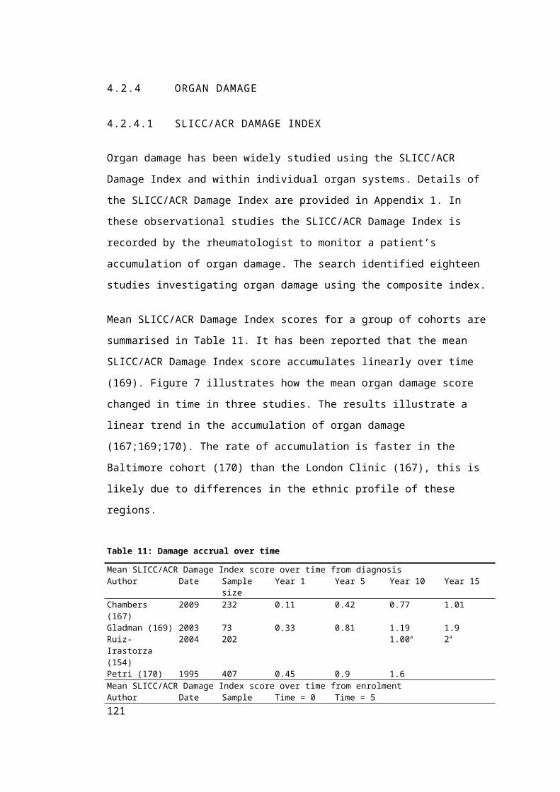
Figure 16: A histogram of steroid (prednisone) dose from the Simulation and Hopkins cohort

5.3.2 VALIDATION OF ORGAN DAMAGE ACCRUAL AGAINST HOPKINS

LUPUS COHORT AND THE TORONTO LUPUS COHORT

I presented a conference paper at the 2012 Operational Research Society Simulation

Workshop 2012, describing the internal and external validity of the natural history model.

The paper is provided in Appendix 9 for reference. Figure 17 illustrates the incidence of

organ damage by organ system for the Hopkins Lupus cohort, and the simulated outcomes.

Figure 18 illustrates the incidence of organ damage by organ system for the Toronto Lupus

cohort, and the simulated outcomes. The simulation fits better to the Hopkins cohort data,

than the Toronto data. Skin damage and pulmonary damage are the most inaccurate

outcomes from the simulation compared with the Toronto data.

125

Figure 17: Simulated organ damage accrual compared with the Hopkins Lupus Cohort

0

0.005

0.01

0.015

0.02

0.025

0.03

0.035M

orta

lity

Card

io

Rena

l

MSK

Neur

o.

Pulm

onar

y

Vasc

ular

Gast

ro

Ocu

lar

Skin

Diab

etes

Mal

igna

ncy

G.Fa

ilure

Incid

ence

Incidence of Organ Damage per patient year of observation for the Hopkins Cohort

Simulation

Hopkins

Figure 18: Simulated organ damage accrual compared with the Toronto Lupus Cohort

0

0.005

0.01

0.015

0.02

0.025

0.03

0.035

Mor

talit

y

Card

io

Rena

l

MSK

Neur

o.

Pulm

onar

y

Vasc

ular

Gast

ro

Ocu

lar

Skin

Diab

etes

Mal

igna

ncy

G.Fa

ilure

Incid

ence

Incidence of Organ Damage per patient year of observation for the Toronto Cohort

Simulation

Toronto

5.4 DISCUSSION

5.4.1 SUMMARY OF THE KEY FINDINGS OF THE SLEDAI ITEM AND

STEROID MODEL, ANNUAL DISEASE ACTIVITY AND STEROID

MODELS AND ORGAN DAMAGE AND MORTALITY MODELS

In this chapter I reported the results of statistical models to predict quarterly incidence of 24

SLEDAI items, and used a hurdle model to estimate steroid dose at quarterly intervals.

Analyses found that age, gender and ethnicity impact on the probability of disease activity.

The findings of the statistical models predicting SLEDAI items are consistent with other 126

analyses in the literature (139). A previous study that found that previous renal involvement

predicted renal involvement, and previous musculoskeletal involvement predicted

musculoskeletal involvement (138). This study also identified that individuals with a history

of renal involvement were less likely to develop musculoskeletal or skin involvement. The

results were consistent with the findings of this analysis which identified that if a SLEDAI

item was present in the previous period it was a strong predictor of future involvement.

Although, I did not find that previous renal involvement was negatively associated with

musculoskeletal involvement, there was a negative association between haematuria and

Mucosal ulcers.

Higher adjusted mean SLEDAI and cumulative average SLEDAI predicted a shorter time to

mortality and organ damage events. As previously discussed in Chapter 5, many

epidemiology studies in SLE have identified that average SLEDAI score and steroid dose

are associated with organ damage and mortality (142;153;162;175;175;176;176;191). In

these analyses we have also estimated the independent effects of adjusted mean SLEDAI

and disease activity within an organ system on the time to organ damage and mortality.

5.4.2 DESCRIBING DISEASE ACTIVITY WITH THE SLEDAI

Two methods for predicting SLEDAI scores were developed in this chapter. A detailed

method to generate SLEDAI scores was developed for the BCTS and a longer term average

SLEDAI score was estimated for the CE model. The BCTS needed statistical models to

predict short-term changes in disease activity, whilst retaining information about which

organ system was involved. Whereas this detail was not necessary in the CE model and

would have increased computation time. Therefore, an alternative modelling approach was

taken to generate average SLEDAI scores over the long term.

The SLEDAI score was estimated using 24 independent statistical models to enable an

accurate and detailed description of the disease. It was challenging to find a distribution to

fit the pattern of the SLEDAI score because it is a weighted measure of the 24 SLEDAI

items. Figure 11 reports a histogram of SLEDAI scores taken from all visits in the Hopkins

Lupus Cohort. There were a large number of observations where the SLEDAI score was

zero, and the scores cluster around even numbers because of the weighting system. For this

reason, and to enable organ involvement to be recorded in the simulation, the more

comprehensive analysis of individual items of the SLEDAI was favoured. The CE model has

a longer time horizon, which was incompatible with a detailed simulation of the disease.

127

5.4.3 THE VALIDITY OF THE NATURAL HISTORY MODEL

The validity of the combined statistical models in predicting short and long-term patient

outcomes have been assessed. The first validation simulation combined the statistical models

to predict SLEDAI items and steroid dose. The second validation simulation combined the

statistical models to predict long term disease, steroid dose, mortality, and damage systems

as described in the SLICC/ACR Damage Index. The simulation was used to validate the

accuracy of the statistical models in predicting long-term outcomes, when all the

independencies within the individuals were incorporated. The simulation reproduced organ

damage events with reasonable accuracy. The fit of the simulation to an external dataset was

reasonable, but highlighted important differences in the predicted incidence of skin and

pulmonary outcomes. I decided not to make any adjustments to the predictive models for

pulmonary and skin damage because it was not necessary given the research objectives of

this project. However, future applications of the natural history models should consider

adjustments to reflect local incidence rates of organ damage.

5.4.4 LIMITATIONS OF THE STATISTICAL METHODS

Designing statistical analyses of longitudinal disease processes was challenging because the

data was susceptible to correlation and confounding that were known to cause problems with

traditional regression techniques. I have tested and selected a series of appropriate methods

to deal with these problems. Random effects regression models have been employed where

repeated measures caused correlation between observations. Frailty survival models were

assessed for the organ damage and mortality survival models, but were not adopted in the

final analysis because within patient effects were small, and had an almost negligible effect

on the coefficients (Appendix 8).

There are several limitations to the work undertaken here. Time-varying confounding was

not fully adjusted for in these analyses. Time-varying covariates are used in the organ

damage and mortality survival models but do not adjust for the causal relationships between

covariates. A confounding variable is one that is associated with both the exposure of

interest and the response, and if it were ignored could result in biased estimates. An

intermediate variable is on the causal pathway from the exposure of interest to outcome. The

challenge in analysing longitudinal studies arises because variables can be both a

confounders and intermediate variables. In this context steroids can be conceived as both a

confounder and intermediate variable for the relationship between disease activity and long

128

term outcomes. The problem may lead to bias in the estimates for the disease activity

coefficient.

One potential approach to deal with this is marginal structural models (218). However, this

method would be difficult to apply in this setting because I was also interested in estimating

the causal affects of cytotoxic drugs and steroid on organ damage, which were confounded

by disease activity. Exploratory analyses indicated several problems with the distribution of

the stabilised probability weights required for marginal structural models. It was decided that

the methods should not be adopted at this time, because the complexity of the bi-directional

confounding variables would require advanced application of marginal structural methods.

Further, research into the use of marginal structural models in longitudinal studies of SLE

would be a good idea.

Secondly, the regression models were analysed independently, which may underestimate

correlation between outcomes of the disease. Joint modelling techniques have been used in

other contexts to account for a single repeated measure predicting a single event outcome

(219). The CE model requires repeated measures for SLEDAI and steroids which predict

thirteen possible event outcomes, which would require considerable programming to

implement in a single analysis.

5.5 CONCLUSION

I have presented forty statistical models to predict individual SLEDAI items at three

monthly clinic visits and steroid doses at three monthly visits. A separate set of analyses

developed regression models to predict average SLEDAI scores and steroid doses over

annual intervals. Survival models for organ damage and mortality have been reported. Two

sets of organ damage and mortality are presented with different choices of covariates to be

compatible with a BCTS and CE model. The BCTS model includes covariates for organ

involvement, whereas the CE model does not. Despite some limitations the statistical

analyses provide a complete set of parameters to enable prediction of individual patient

outcomes in a BCTS or for a CE model.

In the next chapter I describe in detail how the twenty-four SLEDAI item models, steroid

hurdle model and the detailed organ damage and mortality models are incorporated into the

BCTS. I will describe how these are used to simulate data collection for clinical trials. In

Chapter 7, I describe how the long-term average SLEDAI, average steroid dose, and less

complex organ damage and mortality models are used in the CE model.129

6 CHAPTER 6: THE DEVELOPMENT OF A BAYESIAN

CLINICAL TRIAL SIMULATION FOR SLE PHASE III TRIALS6.

In this chapter I describe a Bayesian Clinical Trial Simulation (BCTS) for a Phase III SLE

trial to evaluate the value of alternative research designs.

The BCTS was developed to generate clinical trial datasets for a range of clinical trial

designs. The BCTS was designed to simulate clinical trials for a hypothetical new biologic

treatment for SLE, with no similar comparator on the market. Phase II trial data from

belimumab was used to describe the effectiveness of the new treatment, therefore the

hypothetical drug is assumed to have a similar profile to belimumab. An individual patient

simulation model was used to reflect the substantial heterogeneity in outcomes observed in

SLE trials. Individual patient outcomes in the trials were predicted from the natural history

model described in Chapter 5. Additional published literature was sought to estimate

treatment withdrawal from the trial and efficacy data. The long term efficacy of biologic

treatment in SLE is unknown and so an elicitation was used to quantify uncertain prior

distributions for the long-term effectiveness of treatment.

The BCTS was developed independently from the GSK collaboration and I undertook all of

the work described in this Chapter.

The BCTS structure is described in Section 6.1 and a detailed description of the simulation

process is given in Section 6.2. Section 6.3 describes the efficacy assumptions assumed for

the hypothetical treatment including an elicitation exercise. A discussion of the outcomes of

the simulation is provided in Section 6.4. The discussion in Section 6.5 reflects on the

strengths and weakness of the BCTS.

6.1 MODEL STRUCTURE

An individual patient simulation was built to model patient outcomes over the duration of

follow-up of an SLE clinical trial. The patient population entering the BCTS were randomly

allocated between two treatment arms in the trial. The clinical trial compared a new

hypothetical biologic treatment with Standard of Care (SoC). The BCTS estimated patient’s

disease course in three monthly cycles to reflect regular clinic visits scheduled in an RCT.

At every three monthly visit the patient’s disease status is updated for a number of trial 130

outcomes to include: visit attendance; SLEDAI items; steroid dose; organ damage;

mortality. The BCTS accounts for uncertainty in trial outcomes by simulating one thousand

possible realisations of the trial, each of which has a different trial result.

6.2 SIMULATION PROCESS

6.2.1 OVERVIEW OF THE SIMULATION

The BCTS relies on two simulation processes developed in R software (220). A summary of

the two simulation processes is described in Figure 19. The first generates a SLE population

with sufficient information about the patients’ characteristics and disease profile to enable

modelling of their future disease outcomes. The patients vary in disease severity and organ

damage involvement to reflect the heterogeneity of the disease.

In the second process the outcomes of the clinical trial are generated. The recruitment

process selected patients if they met the inclusion criteria until the sample size for the

clinical trial was reached. The eligible patients were randomised between the two treatment

arms of the trial using a simple randomisation process. The BCTS monitors patients over

time to estimate their outcomes during the clinical trial follow-up. At the end of the clinical

trial follow-up the endpoints were estimated and recorded. The natural history described in

the BCTS is based on the conceptual model for SLE described in Section 4.2.1 of Chapter 4.

The BCTS is repeated many times to estimate a range of possible trial outcomes with

different sampled parameter inputs. The parameters of the Generate SLE Population were

not varied between BCTS runs. However, the parameters for the regression models for

disease activity, steroid dose, organ damage, mortality, and withdrawal were all sampled

from their probability distributions. Each BCTS run uses a different set of input values that

are sampled from parametric distributions. This Bayesian approach captures the uncertainty

of the parameters inputs to estimate the uncertainty in trial outcomes. The BCTS was run

1000 times with sampled input parameters.

131

Figure 19: Summary of the simulation process used in the BCTS

Generate SLE population

1. Generate 50,000 patients with baseline characteristics

2. Set baseline SLEDAI score (Repeat SLEDAI probability

calculations 3 times to stabilise SLEDAI score)

3. Estimate Prednisone dose

4. Set baseline organ damage score

Clinical trial Simulation1. Sample the parameters from their distributions

3. Run natural history model

3.1 Determine major events3.2 Determine withdrawal3.3 Estimate SLEDAI3.4 Estimate Prednisone dose

2. Recruit n patients

4. Estimate outcomes of trial

The simulation generated detailed disease status information for each simulated patient at

every 3 monthly clinic visit in the trial. The model had the flexibility to report a range of

trial outcomes relating the SLEDAI score, steroid dose, organ damage, mortality, and

withdrawal.

6.2.2 GENERATE POPULATION PROCESS

6.2.2.1 PATIENT CHARACTERISTICS

The patient characteristics were randomly drawn from statistical distributions to generate an

individual patient profile for each person in the SLE population. All statistical distributions

were estimated from the Hopkins Lupus Cohort to reproduce the baseline characteristics of

this population in an SLE population matrix. Sampling characteristics from probability

distributions, rather the raw data, were used to broaden the combinations of characteristics

that could be sampled in the simulation.

Table 35 details summary statistics for the characteristics of patients in the hypothetical SLE population, previously described in

132

, and the statistical distributions used to simulate patient characteristics. Column D of this

table details the statistical distribution used to represent variations in each characteristic. All

patient characteristics, except disease activity, were sampled independently. An alternative

approach would have been to bootstrap individuals from the Hopkins Lupus Cohort. This

method would have ensured correlation between baseline characteristics of patients was

maintained. However, Bootstrapping was not used. The simulation needed to be flexible to

simulate patients with mild, moderate or severe SLE or by specific organ type. Therefore

sampling characteristics from distributions was preferred to increase the possible

combinations of patients included in the simulation that may not be represented in the

Hopkins Lupus Cohort. Disease activity score generation is described in more detail in

section 6.2.2.2. Multinomial distributions were used to draw a person’s age at diagnosis and

disease duration. The probabilities of a patient entering the cohort with a particular age and

disease duration are reported in the Appendix 10. Organ damage score at baseline was drawn

from a multinomial distribution using probabilities outlined in Table 35.

Table 35: Baseline characteristics of patients in the simulated trial based on Hopkins cohort at baseline

(n=1354)

A B C D E FPatient Characteristics Mean/

% of cohort

Standard deviation

Median Distribution Parameter A

Parameter B

Male 8.0% BERNOULLI 0.08Black 43.0% BERNOULLI 0.20Smoker 43.0% BERNOULLI 0.50Hypertension 53.0% BERNOULLI 0.50Anticardiolipin antibody positive 4.0% BERNOULLI 0.20Lupus Anticoagulant 13.0% BERNOULLI 0.10Cholesterol 187 44 LOGNORMAL 187 44Age at diagnosis 32.9 13.05 30.69 MULTINOMIAL NAPlaquenil 62.1% BERNOULLIImmunosuppressants 43.2% BERNOULLIDisease duration at cohort entry 4.83 6.3 2.61 MULTINOMIAL NASLICC damage item Score 0 Score 1 Score 2 Score

3Score 4 Distribution

Cardiovascular 94.6% 4.8% 0.5% 0.1% 0.0% MULTINOMIALDiabetes 97.1% 2.9% 0.0% 0.0% 0.0% MULTINOMIALGastrointestinal 95.4% 4.5% 0.1% 0.0% 0.0% MULTINOMIALMalignancy 99.3% 0.7% 0.0% 0.0% 0.0% MULTINOMIALMusculoskeletal 85.6% 10.0% 3.6% 0.6% 0.2% MULTINOMIALNeuropsychiatric 87.9% 9.5% 2.3% 0.3% 0.0% MULTINOMIALOcular 93.3% 6.6% 0.1% 0.0% 0.0% MULTINOMIALPeripheral vascular 95.7% 3.7% 0.3% 0.3% 0.0% MULTINOMIALPremature gonadal failure 98.1% 1.9% 0.0% 0.0% 0.0% MULTINOMIALPulmonary 97.3% 2.4% 0.3% 0.0% 0.0% MULTINOMIALRenal 97.8% 2.2% 0.0% 0.0% 0.0% MULTINOMIALSkin 92.8% 6.7% 0.4% 0.2% 0.0% MULTINOMIAL

133

6.2.2.2 BASELINE SLEDAI SCORE

Patient SLEDAI scores are assigned using the SLEDAI regression models described in

Section 5.2.2 of Chapter 5. Each item of the SLEDAI is estimated to describe the severity

and organ involvement of disease activity. The regression models estimate the patient’s

probability of SLEDAI involvement at each three monthly clinic visit based on demographic

characteristics and previously observed SLEDAI items. These statistical models were used

to predict the probability that a symptom is present at a clinical visit. Logit models were

used to predict dichotomous responses on the SLEDAI.

Pr ( yij=1|x ij , ζ i )=exp (x ij β+ζ i)

1+exp (x ij β+ζ i)(6.1)

where i is a patient identifier, and j indicates the period of observation. A binary indicator

for each of the 24 items of the SLEDAI is described by y, x contains a vector of k covariate

details for the patients at each time period, and β is a k dimensional vector of coefficients,

and ζ j are time constant latent risk parameter for each patient and varies for each SLEDAI

item. The mean estimates for β1 ,…, βk for each SLEDAI item are reported in Section 5.2.2

of Chapter 5. The variance-covariance matrices were extracted for each statistical model so

that parameter estimates could be drawn from the joint distribution for each PSA run of the

BCTS. The variance-covariance matrices are reported in the Appendix 11.

The inclusion of a time constant latent risk parameter, ζ i , is useful to ensure that unobserved

heterogeneity between patients is incorporated in the estimation of the SLEDAI. Excluding

the latent risk parameters would underestimate patient heterogeneity because all

probabilities would be based on the population mean risk, conditional on a few patient

characteristics. The latent risk parameters allows correlation in a simulated patient’s latent

risk of SLEDAI involvement across items. In practical terms this means that patients with a

propensity for musculoskeletal involvement are more likely to have a propensity for skin

involvement. The latent risk parameter is assumed to be multivariate normally distributed

Ζ N (Μ ,Σ). Where Ζ is a vector of latent risk parameters ζ i for the items of the SLEDAI,

Μ is a vector of zeros to express the mean latent risk, and Σ describes the covariance matrix

of latent risk. Realisations of the latent risk parameter were assigned to each patient in the

Generate Population process to reflect the unobserved heterogeneity of the SLE population.

The covariance matrix could not be directly estimated from the data because the regression

models were estimated independently. However, data from the Hopkins cohort were used to

134

approximate covariance between latent risks for items of the SLEDAI. A correlation matrix

was generated from the Hopkins Lupus Cohort to express the associations between items if

they were observed in a patient at any time during follow-up (Appendix 12). This shows that

most of the items of the SLEDAI are positively correlated with the other items and that there

are stronger correlations within organ systems. The standard deviation of latent risk

parameters were estimated from the regression and were reported in section 5.2.2 of Chapter

5. The correlation matrix was multiplied by the standard deviations for the latent risk

parameters for each item of the SLEDAI to approximate a covariance matrix for latent risk

parameters.

Determining baseline SLEDAI required an iterative burn-in process. The twenty-four binary

indicator variables for the SLEDAI were simultaneously determined based on the probability

generated by equation (6.1) and a random number draw. The probability of SLEDAI

involvement is conditional on the profile of SLEDAI items present in the previous period.

Therefore, the process of estimating SLEDAI score for all twenty-four items was repeated

three times to allow patient’s disease status to stabilise conditional on the previous SLEDAI

score.

6.2.2.3 BASELINE STEROID DOSE

Baseline steroid dose is assigned to patients conditional on their baseline SLEDAI score.

Baseline steroid dose was calculated using a two stage hurdle model described in section

5.2.2 of Chapter 5. The first stage of the statistical model estimates the probability that a

patient was prescribed steroid, given their profile of SLEDAI items, using the same

statistical model described in equation (6.1). The probability was used in a Bernoulli trial to

determine if a simulated patient receives steroids. If a patient was prescribed steroid, the

second stage of the Hurdle model estimated what dose of steroid would be prescribed from

the truncated Negative Binomial model. The coefficients of the zero-truncated Negative

Binomial model described in Chapter 5, were used to estimate the first parameter of the

zero-truncated Negative Binomial distributionμi.

μi=exp (x i β ) (6.2)

The dispersion parameter of the Negative Binomial distribution vi is sampled from a gamma

distribution with mean 1 and variance α based on estimates reported in section 5.2.2 of

Chapter 5. The dose was estimated from the Poisson function.

135

p (Y= y|y>0 , x )=( vi μi )

y e−( vi μi)

y !

(6.3)

6.2.3 THE BAYESIAN CLINICAL TRIAL SIMULATION PROCESS

6.2.3.1 INCLUSION CRITERIA

The BCTS randomly samples patients from the simulated SLE population. A screening

process was used to identify eligible patients who meet the inclusion/exclusion criteria of the

trial. The inclusion criteria are modifiable to observe the effects of different patient profiles

on the trial outcomes. The screening process shuffled the order of patients in the SLE

population matrix to capture variation in the profile of SLE patients recruited for different

BCTS runs.

Patients were recruited into the trial if they meet the following criteria:

1. SLEDAI score ≥ 4

2. ≥ 18 years old

3. No neuropsychiatric involvement

4. No severe renal involvement

5. Immunologically positive test for either increased anti-dsDNA or low complement

These inclusion criteria were developed in consultation with Dr M. Akil, a clinical expert in

SLE based in Sheffield (October 2011).

6.2.3.2 QUARTERLY DISEASE ACTIVITY SCORE SIMULATED DURING

FOLLOW-UP

The SLEDAI score was updated every 3 months in the BCTS to monitor changes in disease

severity during the trial. The logit regression model described in equation (6.1) was adapted

to estimate the risk of SLEDAI items being present during the clinical trial. The equation is

amended by the inclusion of a treatment effect coefficient here denoted Di.

Pr ( yij=1|x ij , ζ i )=exp (x ij βk+Di βk +1+ζ i)

1+exp (x ij βk+Di βk+1+ζ i)(

6.4

)

136

where y represents each of the 24 items of the SLEDAI, x contains the profile of

characteristics for each patient including activity in last period, and β are the coefficients of

the regression models, and ζ i are the time constant underlying risk parameter for each

patient. An additional coefficient, βk−1 is appended to the logit model, to modify the risk of

the symptom being present in patients who are treated with the new treatment (Di=1). The

patient specific random intercept ζ i are time-constant and independent across patients.

6.2.3.3 ORGAN DAMAGE ACCRUAL

The probability that organ damage occurred between each 3 monthly visits was estimated

using the parametric survival models described in section 5.2.4.2 of Chapter 5. The

parametric survival models were used to generate estimates of the cumulative hazard in the

current and previous period. From which the probability of organ damage being diagnosed

was estimated.

p (Organ Damage )=1−exp (H ( t )−H ( t−1 )) (6.5)

The functional form for the organ damage survival models included exponential, Weibull,

Gompertz, and LogLogistic and cumulative hazard functions for each distribution are

outlined in Table 36.

Table 36: Cumulative Hazard function for exponential, Weibull, Gompertz and Loglogistic functions

Survival curve Cumulative Hazard Parameter 1 Parameter 2

Exponential λ t i λ=exp ( β0+X βk+βk+1 D ) n/a

Weibull λ t γ λ=exp ( β0+X βk+βk+1 D ) γ

Gompertz λγ(eγt−1) λ=exp ( β0+X βk+βk+1 D ) γ

LogLogistic 1+λ t θ λ=exp¿ θ=1γ

Parameter 1 is estimated from the baseline hazard β0 and the covariate effects for the organ

damage survival model described in the natural history modelβK . An additional coefficient

for treatment was appended onto each of the organ damage survival models to modify the

risk of organ damage in treated patients (D=1). The shape parameter (parameter 2 in Table

36) of the organ damage survival models was assumed to be unchanged by treatment.

137

Table 32 of Chapter 5 reported the estimates for the organ damage survival model

parameters β1 ,…, βk used in the BCTS. The variance-covariance matrix for the organ

damage survival models can be found in the Appendix 11. These organ damage risk

regressions were chosen because they included organ involvement covariates, such as skin

involvement to increase the risk of developing skin damage.

The propensity of organ damage was assumed to be independent across organ systems. In

contrast to SLEDAI items I did not impose a correlated latent risk to reflect unobserved

propensity for organ damage. Frailty survival models tested as part of the statistical analysis

described in Chapter 5 found that latent factors were not important in the organ damage

survival models, and their inclusion would have increased the complexity of the BCTS

(Appendix 8). Furthermore, disease activity and other patient characteristics will induce

some correlation in the risk of organ damage.

A constraint was imposed in the BCTS to avoid over-estimation of organ damage. The

simulation allows patients to accrue multiple damage events in those organ systems where

more than one damage type is listed in the SLICC/ACR Damage Index. However, if patients

reach the maximum number of events in that organ system the patients did not record any

further damage in the simulation. For example, there are only two types of ocular damage; if

a patient has a SLICC/ACR Damage Index score of 2 for ocular damage additional ocular

damage events are not recorded in the simulation.

6.2.3.4 MORTALITY

Mortality is a rare event during a clinical trial of SLE, but must be simulated to give a

complete description of the natural history of the disease. A Weibull survival distribution

was used to assess the probability of death. The probability of a patient dying in each period

of the BCTS was estimated using the same method described in equation (6.5) for organ

damage. The proportional hazards Weibull model assumed that the covariates were

multiplicatively related to the hazard. The cumulative hazard for the Weibull distribution can

be expressed as a two parameter survival model.

H (t )=λ t γ (6.6)

λ=exp (β0+ β1 : 11 X ij+ β12 D) (6.7)

138

where λ describes the scale of the distribution and γ is the shape parameter of the survival

model. The scale of the distribution is estimated from the baseline hazard β0 and eleven

covariate effects described in Table 31 in Chapter 5 β1 :11. An additional coefficient for

treatment can be appended onto the mortality survival model to modify the risk of mortality

in treated patients (D=1). The shape parameter of the Weibull survival model is assumed to

be unchanged by treatment and the impact of treatment is made on the scale parameter

through the proportional hazards assumption.

Section 5.2.4.1 of Chapter 5 reports the estimates for mortality survival model parameters

β1 , …, β11 used in the BCTS. The survival models with haematological organ involvement,

and plaquenil covariates were used to predict organ damage and mortality events in the

BCTS. This was possible because the BCTS simulates a detailed description of the SLEDAI

score. The variance-covariance matrix for the mortality survival models can be found in the

Appendix 11. At every 3 month cycle of the simulation a probability for mortality is

calculated and events were sampled from the Bernoulli distribution.

6.2.3.5 CONCOMMITANT MEDICATIONS

The list of concomitant medications permitted in an SLE clinical trial is extensive because of

the breadth of organ systems involved in the SLE and the high prevalence of co-morbid

conditions. Treatment regimens vary between geographical locations due to paucity of

licensed treatments and evidenced based recommendations from large scale clinical trials.

Consequently, it is not feasible to simulate a comprehensive list of concomitant medications

for SLE patients. Discussion with Professor Michelle Petri from the Hopkins Lupus Cohort

identified three classes of drugs that affect the risk of long term outcomes in SLE;

corticosteroids, immunosuppressants, and anti-malarials (March 2010). Broadly speaking

corticosteroids and immunosuppressants increase the risk of organ damage and anti-

malarials are protective against organ damage. These are simulated in the BCTS to describe

concomitant medications.

The regression model to predict steroid dose is the same as that described in Section 6.2.2.3.

The Hurdle models estimate steroid in two stages, the first regression model determines the

probability that the patient is prescribed steroid (equation (6.2)). The second stage estimates

steroid dose from the Negative Binomial distribution (equation (6.3)).

Treatment with immunosuppressants and anti-malarials are indicated with binary indicators.

Patients are assumed to remain on these treatments during the clinical trials. Patients’ 139

immunosuppressant and anti-malarial status is determined at baseline, based on the

characteristics of the Hopkins Lupus Cohort described in Chapter 5. The simulation assumes

a strict concomitant medications protocol in which no patients can initiate new treatments,

other than steroids.

6.2.3.6 ADVERSE EVENTS

Adverse events are recorded during a trial to understand the safety profile of a new

treatment. It can be justifiable to exclude them from a CE model if there is no difference

observed between the treatment arms. In this situation the adverse events would not impact

on the economic evaluation outcomes. Evidence from previous clinical trials suggests that

the differences between the proportions of adverse events between the treatment arms in

previous studies were very small and not statistically significant (74;75). The focus of this

research is to investigate how CE analyses can help to design future trial design. Simulating

adverse events would add to the complexity of the BCTS and it was decided that they could

be excluded from this BCTS if it was assumed that the hypothetical new treatment did not

cause more adverse events than standard care.

6.2.3.7 PATIENT WITHDRAWAL FROM THE TRIAL

In the BCTS, patients could withdraw from the trial at any clinic visit for both treatment

arms. The risk of withdrawal from the clinical trial was modelled using the exponential

distribution and a coefficient for treatment arm was included. The hazard rate for the

exponential distribution can be estimated as a function of the log-baseline hazard rate plus

the log hazard ratio for treatment.

λ=exp ( β0+β1 D ) (

6.8

)

where λ describes the hazard, β0 is the log-baseline hazard, β1 is the log hazard ratio for

treatment and D indicates whether the patient was randomised to receive treatment. These

beta parameters were assumed to be normally distributed and independent. The estimated

hazard rate was converted into a probability using the following conversion:

140

p=1−exp (−λt ) (

6.9

)

In a real-life scenario it is likely that the rate of withdrawal would be based on data from a

Phase II clinical trial for the new treatment. In this hypothetical case there is an absence of

data from a Phase II trial to provide this data. Withdrawal rates are estimated from previous

clinical trials in SLE (Trials identified in Chapter 2). The rates of withdrawal in placebo

controlled arms and activity treatment arms were extracted from data from previous clinical

trials. Table 37 reports the proportion of patients withdrawn from the clinical trials for the

placebo and new treatment arms. A weighted average withdrawal rate and variance was

calculated for the placebo arm based on trial sample size. The differences between the

placebo and treatment arms were used to estimate the log hazard ratio for treatment effect

using the same weights.

Table 37: Withdrawal rates for simulation calculated from published clinical trials in SLE patients

Author Year Sample size

New treatment Proportion of patients withdrawn from the trial after 12 months

Placebo Treatment DifferenceFortin 2008 86 Methotrexate 0.2667 0.3415 -0.0748

Wallace 2009 449 Belimumab 0.1786 0.1935 -0.0149

Merril 2010 175 Abatacept 0.2456 0.3136 -0.068

Merril 2010 227 Rituximab 0.2727 0.2899 -0.0172

Navarra 2011 865 Belimumab 0.2125 0.1678 0.0447

Furie 2011 819 Belimumab 0.3260 0.2821 0.0439

Weighted Mean 0.2514 0.2339 0.0178Log hazard parameter mean -1.4061 -0.079

Log hazard parameter standard error 0.0206 0.0106

6.2.4 TREATMENT EFFICACY

6.2.4.1 EFFICACY AT 12 MONTHS

Estimating treatment effect for the first 12 months was complicated by the absence of a

Phase II trial. In a real-life case study statistical analysis of the Phase II data would be used

to estimate the treatment effect parameters. However, in this study the new treatment was a

hypothetical new biologic drug. The distribution of the log odds ratio for treatment βk+1 in

reducing the odds of SLEDAI items was estimated from summary trial rather than estimated

individual patient data. As such, data from two articles describing a Phase II trial for a new 141

biologic was sought (72;73). This Phase II trial reported the efficacy of belimumab after 12

months of treatment.

The odds ratio for response was divided between the 24 items of the SLEDAI, weighted by

the prevalence of each item. The published data showed that there was evidence that the

treatment effect varied between organ systems and the simulation was adjusted to reflect the

data reported the article (73). The method of distributing the odds ratio between the SLEDAI

items is crude due to the absence of Phase II trial outcomes that are compatible with the

natural history model. In a future ‘real world’ application one would utilise phase II trial

evidence for the new product of interest rather than going back to previously published trials

of other products.

6.2.4.2 EFFICACY BEYOND 12 MONTHS

The Phase II data is an useful source of evidence for the existing uncertainty in the efficacy

of treatment in reducing disease activity scores up to 12 months follow-up. However, the

Phase II trial cannot be used to estimate efficacy beyond 12 months, or estimate the

treatment effect in reducing organ damage and mortality. There is therefore an evidence gap

when considering how uncertain we might be about efficacy beyond 12 months.

Consultation with clinical experts can be used to elicit the scale of uncertainty for such data

gaps.

6.3 ELICITATION OF UNCERTAINTY IN LONG-TERM TREATMENT

EFFECTS ON DISEASE ACTIVITY, ORGAN DAMAGE AND

MORTALITY

6.3.1 ELICITATION INTRODUCTION

Elicitation is the appropriate method by which to formulate judgements from people (221).

Estimation of efficacy parameters for the BCTS required the estimation of the frequency of

an event for a treated population. The elicitation also needs to quantify the expert’s

uncertainty using a probability distribution. This enables the uncertainty of the experts to be

incorporated into probabilistic sensitivity analysis. Elicitation of a probability density

function f (X ) from a non-statistician raises several challenges.

142

Tversky and Kahneman (1974) identified three well known types of heuristics: availability;

representiveness; and anchoring and adjusting. These are often adopted to help people solve

problems, make decisions, or form judgements. Heuristics can lead to biases in people’s

judgements of probabilities. Availability describes the impact of recent or personal

experience of the clinician that may affect the expert’s perceptions. For example, if the

expert saw a patient in their clinic before the interview, this patient may have a

disproportionate impact on their estimates. Representativeness relates to the judgement of

similarities and differences between two groups to estimate the probability. This can mean

that if two groups have similar characteristics on attribute A the expert assumes that they

will have similar attributes on the elicited attribute B. Anchoring and Adjusting suggests that

people use an anchor value and then adjust upwards or downwards. This can lead to bias if

the respondent has a tendency to stay close to the anchor. These potential sources of bias

must be considered when designing the elicitation exercise to minimise their impact.

As a consequence, the design of the elicitation exercise was informed by a detailed

consultation of the literature on eliciting probability density functions. O’Hagan et al. (2006)

provided a broad introduction to elicitation and supplied useful guidelines to the process that

take account of the problems of heuristics. This was supplemented with a review of

elicitation studies in CE models. These findings of this review are summarised in the

Appendix 13.

6.3.2 ELICITATION METHODS

6.3.2.1 DEFINING THE AIMS

The aims of this elicitation were to inform the parameters of a BCTS that cannot be

estimated from other data sources. Elicitation is only required to estimate the difference in

the long-term outcomes with the new treatment compared with the Hopkins regression

model predictions.

A clear specification of what parameters were needed was important to ensure that the data

was compatible with the BCTS and CE model (221). Consequently, the elicitation was

planned after the simulation was developed. The following quantities for the BCTS are

unknown and will need to be informed by elicitation:

A. The probability of SLEDAI items being present whilst receiving treatment after 12

months.

143

B. The risk of mortality for patients receiving treatment independent of the effects of

SLEDAI.

C. The risk of organ damage for patients receiving treatment independent of the

reduction in average SLEDAI score and other treatment effects.

The probability of SLEDAI items (A)

The effectiveness of treatment in reducing SLEDAI involvement beyond the 12 months

needed to be elicited from clinical experts. The elicitation needed to identify parameter

distributions for 22 βk+1 log-odds coefficients to be used in the models estimating the

probability of 22 items of the SLEDAI. Vasculitis and fever were not included in the

elicitation; these are very rare events that could not be grouped with other items of the

SLEDAI.

The risk of long term outcomes (B and C)

The new treatment may modify the rate of damage accumulation and the risk of mortality.

Treatment has an indirect effect on these outcomes through Adjusted Mean SLEDAI and

cumulative average prednisone dose. The elicitation aimed to estimate clinical experts’

beliefs and uncertainty about the direct effect, i.e. the effect over and above that mediated by

adjusted mean SLEDAI and steroid dose, of biologic treatment on long-term outcomes. A

treatment coefficient was added to the survival models as described in Table 36 for each of

the twelve organ damage models and equation (6.7) for mortality. Therefore, the elicitation

needed to identify distributions for 13 βk+1 coefficients.

6.3.2.2 DEFINING THE OBJECT TO ELICIT

It would have been difficult for the clinical experts to express distributions for the quantities

βk+1, or their corresponding odds ratios, hazard ratios, and time ratios. These are non-

observable quantities and experts would be likely to draw on heuristics to aid their estimates

(221). As such the questions were rephrased to elicit observable quantities from the clinical

experts, which were transformed to reveal the parameters of interest.

O’Hagan et al. (2006) recommend framing questions to clinical experts in terms of the

proportion of a cohort of patients (221). Respondents can conceptualise a cohort of patients

and estimate difference in the number of the cohort who experience an event. These

proportions can be interpreted as an expression of the probability of an event. Therefore, in

144

each elicitation questions the experts were presented with the number of individuals out of a

cohort of 1,000 patients who had an event at time t in the baseline scenario. They were asked

to estimate how many fewer, or more, patients they would expect to experience an event

whilst on treatment compared with the baseline estimate.

It was recommended to elicit independent parameters, rather than conditional parameters,

because it is challenging to elicit correlations or associations between parameters (221). The

proportion of patients in the treatment arm with a particular SLE symptom is not an

independent parameter. The elicited proportions were conditional on whatever baseline

value for standard of care that the expert considered at the time. The difference between the

two arms expresses the treatment effect and can be assumed to be independent of the

baseline value.

The experts were asked to consider the treatment effect of a hypothetical biologic treatment

with efficacy and safety characteristics from a Phase II trial similar to those observed from

belimumab. They were presented with hypothetical data to describe the effectiveness of the

treatment from a Phase II trial. The experts were asked to elicit clinically plausible treatment

effects in reducing the number of clinical events. This may have been challenging given that

they did not have personal experience with the treatment. However, their experience of

treating patients with other drugs would allow them to consider what magnitude of benefits

or harm would be possible.

The experts were asked to describeΔ, the distribution for the difference in the proportion of

individuals with a characteristic receiving SoC and treatment at a single point in time.

pr ( y=1|D1 )= pr ( y=1∨D0 )+Δ (

6.10

)

The proportion of the patients receiving the new treatment that demonstrate this disease

feature, y=1, is a function of the proportion of the cohort that demonstrate this disease

feature in SoC plus an adjustment parameter Δ. The difference between SoC and treatment

was assumed to be independent of the SoC risk. The distribution for Δ is assumed to be

normal Δ~N(μ,σ2) allowing improvements and worsening in outcomes for the new treatment.

6.3.2.3 SIMPLIFYING THE INTERVIEW

145

The elicitation needed to estimate 35 parameters for the BCTS. To simplify the elicitation

task and reduce the workload for the clinicians the coefficients were grouped into ten

categories. Discussion with Dr Akil in the pilot elicitation helped to develop a grouping

system (March 2011). Items of the SLEDAI were grouped according to organ system, organ

damage outcomes were grouped according to the main risk factors identified in the natural

history model. Low complement and increased DNA binding were elicited individually

because they have a high incidence in the Hopkins Cohort. Grouping the outcomes reduced

the burden of the elicitation interview to 13 questions. For the purposes of notation I will

refer to the 13 elicitation estimates as Δv, where v indicates the 13 elicitation questions, and

δw describe the difference in proportion assigned to the 35 individual outcomes w.

146

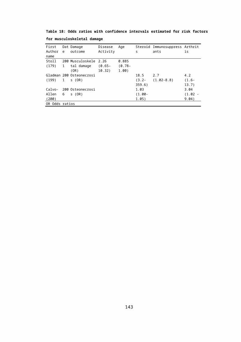
Table 38: Details of how model outcomes were grouped in the elicitation questions

Elicitation Questions (v) Disease Outcomes Covered (w)

Neuropsychiatric SLEDAI Seizure Psychosis Organic Brain Syndrome

Visual Disturbance Cranial Nerve Disorder Lupus Headache

Cerebrovascular event

Renal SLEDAI Urinary Casts Hematuria Proteinuria

Pyuria

Musculoskeletal SLEDAI Arthritis Myositis

Skin SLEDAI Rash Alopecia Mucosal Ulcers

Serositis SLEDAI Pleurisy Pericarditis

Haematological SLEDAI Thrombocytopenia Leukopenia

Low Complement Low Complement

Increased DNA Binding Increased DNA Binding

Disease Activity induced damage Renal damage Skin damage Peripheral Vasculitis

Pulmonary damage

Steroid induced damage Musculoskeletal damage Ocular damage Diabetes

Disease Activity and steroid

induced damage

Cardiovascular damage Neuropsychiatric damage Gastrointestinal damage

Other damage Malignancy Gonadal Failure

Mortality Mortality

6.3.2.4 STATISTICAL TRANSFORMATION FROM ELICITED VALUES TO

REGRESSION MODEL COEFFICIENTS

The elicited quantities were transformed into coefficient parameters through a two stage

transformation process. The first stage estimates the difference in proportions for the

individual outcomes from the elicited quantities. The transformation fromΔv into coefficient

estimates for 35 outcomes required additional assumptions to be made about the distribution

of treatment effect within the groups. It is reasonable to assume that the treatment effect is

distributed between the outcomes More common outcomes should be allocated a larger

proportion of the difference. Incidence rates for each of the outcomes were used to estimate

weights for the outcomes according to their occurrence, ω. The weights ω were estimated

from the incidence of SLEDAI items observed in the Hopkins Cohort. The Δv estimates

were segmented intoδw.

147

δ w=ωw Δv (

6.11

)

For example, a normal distribution was fitted to the renal involvement elicitation responses

to give the mean and standard deviation for the distribution ΔRenal N (−10.74,41.46). This

estimate was distributed between the four renal items according to the prevalence of each, as

reported from the Hopkins Lupus Cohort data.

Table 39: Exemplar distribution of elicited quantities between renal items

Weight Delta mean Delta Standard deviation

Urinary casts 0.0039 -0.0421 0.0253Hematuria 0.3174 -3.4084 2.0439Proteinuria 0.4671 -5.0161 3.0080Pyuria 0.2115 -2.2715 1.3621

The second stage of the transformation estimated individual coefficient parameters for the

statistical models based on the elicited differences. The transformations of δw into

coefficients for the statistical models differed according to the differing functional forms of

the statistical model. For the logit models the coefficient is the difference between the log

odds of disease activity with delta minus the log odds of disease activity without delta. Mean

estimates of the SoC risk of SLEDAI involvement were used to estimate βwk+1.

βwk+1=log( pr ( yw=1 )+δw

1−pr ( yw=1 )+δw )−log( pr ( y w=1 )1−pr ( yw=1 ) )

(

6.12

)

The elicitation method for survival parameters was based on a PhD thesis completed at the

time of designing this elicitation (222).The elicitation presented respondents with the

proportion of patients with an attribute at a given timeS ( t ). The survival estimates for an

exponential survival function can be used to generateλ1, the baseline hazard.

148

λ1=−log (S ( t ))

t ,(

6.13

)

The elicited quantity can be incorporated into the baseline hazard for treatment to calculate

the coefficient,

βk+1=log(−log (S (t )+δ )t )−log (−log (S (t ))

t ) (

6.14

)

The Weibull, Gompertz and Loglogistic parametric survival models have two parameters.

For these survival models it is assumed that parameter 2, as detailed in Table 36, is held

constant so that the treatment does not affect parameter 2. Using this assumption, the

coefficient can be estimated using the same method described above for the exponential

distribution. The calculation for the Weibull distribution was used to estimate mortality,

musculoskeletal damage, neuropsychiatric damage, and ocular damage. The estimation of

the Weibull parameter is described in equation (6.15),

λ i=−log (S (t ))

t γ

(6.15)

The Gompertz distribution was used to estimate cardiovascular damage and the calculation

for the Gompertz distribution is described in equation (6.16),

λ i=γlog (S (t ))

1−eγt

(6.16)

The loglogistic distribution was used to estimate renal, pulmonary, and skin damage. The

calculation for the loglogistic distribution is described in equation (6.17).

λ i=−log ( 1S (t ) t γ −

1t γ ) (6.17)

6.3.2.5 ELICITATION TECHNIQUE

Many techniques can be used to describe the distribution of uncertain parameters in an

elicitation. The histogram elicitation technique was used in three of the elicitation studies

identified in the literature search (112;131;223). The technique is easy to use and it provides

the expert with an immediate visual representation of their estimate. The clinical experts

149

were allowed 21 x’s to assign in a 21x21 grid in which the x-axis described fixed intervals

for possible responses (223). Two examples of the grid and possible responses are illustrated

below. The limits of the grid were pre-specified, but the expert could change the axis if

needed.

They were advised to assign more x’s to those estimates which they believed to be more

likely. A normal distribution was fitted to their histogram using mean and variance estimated

from the histogram. The fitted normal distribution and other summary statistics were

immediately fed back to the clinical experts so that they could scrutinise the implications of

their estimates. If the clinical expert was unhappy with the fitted distribution they could

return to the grid to amend their estimate. Although a flat beta prior would fit responses

illustrated in example 2 better than a normal flat prior, a normal distribution was used to

enable pooling between responses.

Example1 Example 2

x

x

x x x

x x x

x x x x

x x x x x x x x x x x x x x x x x x x x x x x x x x x x x x

-15 -14 -13 -12 -11 -10 -9 -8 -7 -6 -5 -4 -3 -2 -1 0 1 2 3 4 5 -15 -14 -13 -12 -11 -10 -9 -8 -7 -6 -5 -4 -3 -2 -1 0 1 2 3 4 5

6.3.2.6 COMPUTER SOFTWARE

An elicitation programme was designed for this study using Microsoft Excel 2010. The

software was programmed to give immediate feedback to the clinical experts on the

implications of their responses. The software was designed so that their responses to early

150

questions were integrated into the predicted baseline risk estimate presented to the same

clinical experts later in the interview. For example, the elicited long term treatment effect on

disease activity was used in the estimate of the impact of AMS on organ damage later in the

elicitation. The software was designed to be user friendly and operable without assistance

from the interviewer so that the exercise could be completed after the meeting, if the

interview overran.

6.3.2.7 TRAINING

It is important that clinical experts should receive training in preparation for the interview

(221). In this study the training constituted background reading, an oral presentation and

practice exercises to complete before the elicitation. A background document was emailed

prior to the interview and the clinical experts were asked to read this before the face-to-face

meeting. This document included the following information and an example copy can be

found in the Appendix 14.

A concise definition of elicitation

An explanation of the purpose of the interview

An explanation of proportions and probabilities

An illustration of a probability density function and how this describes uncertainty

A description of the hypothetical Phase II trial

A list of questions asked in the elicitation and how the answer would be used in the

BCTS.

At the face-to-face meeting I gave a short presentation, to reiterate the information provided

in the background reading. The details of the presentation were planned before the elicitation

to reduce the risk that the information provided to the experts would bias their responses.

The clinical experts were encouraged to ask questions about the elicitation exercise. Two

example elicitation questions were presented to the clinicians before commencing the

elicitation to demonstrate how to use the software.

6.3.2.8 PILOT STUDY

The elicitation exercise was piloted with Dr Akil, a Rheumatologist at Sheffield Hallamshire

Hospital (March 2011). A number of suggestions for improvements to the elicitation

programme were made and incorporated into the final version.

151

The inclusion criteria for patients into the hypothetical cohort were changed to better

reflect a clinical trial population. Patients were required to be either anti-dsDNA

positive or positive for low complement on entry to the simulation. All patients with

neuropsychiatric involvement, proteinuria and haematuria at baseline were excluded

from the cohort because these patients would be considered too severe to enter a

clinical trial.

The training exercise was improved to more closely reflect the wording and

structure of the elicitation questions. A second training exercise was developed for

the elicitation of the organ damage and mortality survival models.

The elicitation quantities were grouped to reduce the interview time.

6.3.2.9 SYNTHESIS OF EVIDENCE

The elicitation interviews were conducted with four individual clinical experts rather than a

panel discussion. A panel discussion would have been preferable to individual estimates, as

specified in the guidance (221). Initial discussions with the experts highlighted difficulties in

identifying times to meet with the clinicians. In two cases it was necessary to schedule the

meeting more than two months in advance to identify a two hour interval in their diary.

Consequently, it is necessary to mathematically synthesise the results of the individual

interviews. A simple mathematical approach to synthesising the results of the elicitation

exercises is by linear opinion pooling. An alternative would have been to use logarithmic

opinion pooling, in which the consensus distribution is obtained by taking a weighted

geometric mean. These two methods are likely to produce different results. O’Hagan et al.

recommend that logarithmic pooling should be used if both experts are good judges based on

the information available to them, but they have different sources of information (221).

Linear pooling is more representative of the full range of values reported by the experts. In

this study linear pooling was considered more appropriate because the experts were all

presented with the same data about the hypothetical new treatment and none of the experts

had practical experience with the treatment so it was preferable to reflect the full range of

their responses.

Weighting experts’ responses can be challenging and requires appropriate methods to

identify the quality of an expert’s response. Previous studies suggest that adopting weighted

estimates can impact on the parameter estimates (131). However, the methodology for

generating weights requires further development (223). In this example, none of the clinical

experts had experience with the hypothetical drug described to them. As a consequence, it

was challenging to formulate an appropriate test question to evaluate the reliability of 152

clinical experts’ responses to questions about a hypothetical treatment. Therefore, the

experts’ responses Δvwere weighted equally.

6.3.2.10 SELECTION OF EXPERTS

The elicitation guidance states that the expert must have knowledge of the uncertain quantity

of interest (221). This condition posed challenges for the objectives of the elicitation to

estimate long-term treatment effects for a new drug whose long term benefits have not been

established. Therefore, it was important that the experts had experience with treating the

long-term outcomes of SLE but also experience with biologic treatments such as belimumab

and rituximab. SLE can affect multiple organs therefore patients can be treated by

physicians in various different departments. However, the most common primary physician

would be based in Rheumatology. It was anticipated that these clinicians might also be able

to draw from experiences of biologics in other rheumatic diseases. The natural history model

was based on SLE specific indices such as the SLEDAI and SLICC/ACR Damage Index.

These scoring systems are not often used in routine clinical practice; therefore the experts

needed to have experience in observational cohort studies or RCTs where the indices are

used.

The interviews were designed to be conducted face-to-face. Therefore, SLE specialists based

in the UK were the primary target of the elicitation. I attended the American College of

Rheumatology 2011 conference in Chicago, which presented an opportunity to conduct

interviews with SLE specialists from the US and Canada who had collaborated in the

development of the natural history models. Dr Petri, Dr Gladman, and Dr Urowitz were

invited to participate in the interviews during this conference, but all declined due to busy

schedules.

There are several SLE specialists in the UK who are part of a research collaboration called

the BILAG group. The BILAG group includes experienced SLE specialists with an interest

in clinical research. Following the Pilot study with Dr Akil, he agreed to introduce my

elicitation study at a BILAG meeting and encourage its members to participate. Following

this meeting six members communicated an interest in the study, however only three were

available to complete the interview. Together with Dr Akil (November 2011), Dr Bruce

(December 2011), Dr Griffiths (February 2012) and Professor Isenberg (May 2012) were

recruited into the study.

6.3.3 RESULTS

153

The results of the elicitation are reported in Table 40. Graphical representations of the

aggregated distributions elicited from the experts are presented in column 2. A brief

summary of the individual experts beliefs are reported in column 3. Expert 4 consistently

expressed a high degree of uncertainty in his responses to almost all of the questions. He

strongly believed that it was impossible to predict the effectiveness of treatment beyond the

period for which data had been collected. Experts 1, 2 and 3 were generally in agreement for

the disease activity questions, but reported very different distributions for the organ damage

questions. All experts stated that they were fairly certain that treatment was unlikely to

modify malignancy and gonadal failure rates in SLE patients.

154

Table 40: Graphical illustrations of the clinical expert’s responses in dotted lines and the pooled estimate in a bold solid line

Elicitation question Histograms of aggregated replies and fitted

distribution

Comments

1 After 24 months of follow-up what difference do you

think there could be in the number of patients with

neuropsychiatric involvement on the SLEDAI score

between standard of care and the new drug?

0

0.05

0.1

0.15

0.2

0.25

0.3

0.35

-14 -13 -11 -10 -9 -7 -6 -5 -4 -2 -1 0 2 3 4 6 7 8 10 11 12Difference from SoC risk (per 1000 patient)

Expert responses and fitted distribution for neuropsychiatric involvement

Experts 1, 2 and 3 believed that the benefits

of treatment in reducing neuropsychiatric

involvement would be sustained over the long

term. Expert 4 was very uncertain about the

long term effects of treatment on

neuropsychiatric involvement.

2 After 24 months of follow-up what difference do you

think there could be in the number of patients with

renal involvement on the SLEDAI score between

standard of care and the new drug?

0

0.05

0.1

0.15

0.2

0.25

0.3

-43 -40 -36 -33 -29 -26 -23 -19 -16 -13 -9 -6 -3 1 4 8 11 14 18 21 24Difference from SoC risk (per 1000 patient)

Expert responses and fitted distribution for renal involvement

Experts 1, 2 and 3 believed that the benefits

of treatment in reducing renal involvement

would be sustained over the long term. Expert

4 was very uncertain about the long term

effects of treatment on renal involvement.

155

3 After 24 months of follow-up what difference do you

think there could be in the number of patients with

musculoskeletal involvement on the SLEDAI score

between standard of care and the new drug?

0

0.05

0.1

0.15

0.2

0.25

-47 -44 -40 -37 -34 -30 -27 -23 -20 -17 -13 -10 -6 -3 0 4 7 10 14 17 21Difference from SoC risk (per 1000 patient)

Expert responses and fitted distribution for musuloskeletal involvement

Experts 1, 2 and 3 believed that the benefits

of treatment in reducing musculoskeletal

involvement would be sustained over the long

term. Expert 4 was very uncertain about the

long term effects of treatment on

musculoskeletal involvement.

4 After 24 months of follow-up what difference do you

think there could be in the number of patients with

skin involvement on the SLEDAI score between

standard of care and the new drug?

0

0.05

0.1

0.15

0.2

0.25

-60 -55 -50 -45 -40 -35 -30 -25 -20 -15 -10 -5 0 5 10 15 20 25 30 35 40Difference from SoC risk (per 1000 patient)

Expert responses and fitted distribution for Skin involvement Experts 1, 2 and 3 believed that the benefits

of treatment in reducing skin involvement

would be sustained over the long term. Expert

4 was very uncertain about the long term

effects of treatment on skin involvement.

5 After 24 months of follow-up what difference do you

think there could be in the number of patients with

increased DNA binding between standard of care and

the new drug?

00.005

0.010.015

0.020.025

0.030.035

0.040.045

0.05

Difference from SoC risk (per 1000 patient)

Expert responses and fitted distribution for Increased DNA Binding All experts believed that the benefits of

treatment in reducing low complement would

be sustained in the long term. The

uncertainties in these estimates were less than

for other SLEDAI items.

6 After 24 months of follow-up what difference do you

think there could be in the number of patients with

All experts believed that the benefits of

treatment in reducing low complement would

156

low complement between standard of care and the

new drug?

00.005

0.010.015

0.020.025

0.030.035

0.040.045

0.05

Difference from SoC risk (per 1000 patient)

Expert responses and fitted distribution for low complement be sustained in the long term. The

uncertainties in these estimates were quite

low.

7 After 24 months of follow-up what difference do you

think there could be in the number of patients with

serositis on the SLEDAI between standard of care and

the new drug?

0

0.05

0.1

0.15

0.2

0.25

0.3

0.35

0.4

-15 -14 -12 -11 -10 -8 -7 -6 -4 -3 -2 0 1 2 4 5 6 7 9 10 11Difference from SoC risk (per 1000 patient)

Expert responses and fitted distribution for serositis Experts 1, 2 and 3 believed that the benefits

of treatment would be sustained with a small

risk of no different from standard of care.

Expert 4 was very uncertain of the long term

outcomes for patients receiving treatment.

8 After 24 months of follow-up what difference do you

think there could be in the number of patients with

haematological involvement on the SLEDAI between

standard of care and the new drug?

00.05

0.10.15

0.20.25

0.30.35

0.40.45

0.5

-15 -14 -13 -11 -10 -9 -8 -6 -5 -4 -2 -1 0 1 3 4 5 7 8 9 10Difference from SoC risk (per 1000 patient)

Expert responses and fitted distribution for haematological involvement

Experts 1, 2 and 3 believed that the benefits

of treatment would be sustained. Expert 4

was very uncertain of the long term outcomes

for patients receiving treatment. Expert 4 was

very uncertain of the long term outcomes for

patients receiving treatment.

157

9 What difference do you think there could be in the

number of patients who have cardiovascular,

neuropsychiatric, or gastrointestinal damage after 5

years of biologic treatment compared with the natural

history predictions.

In this question reductions in damage risk due to

lower disease activity scores and steroid dose have

been adjusted for.

0

0.1

0.2

0.3

0.4

0.5

0.6

0.7

-22 -21 -19 -17 -16 -14 -12 -11 -9 -7 -6 -4 -2 -1 1 2 4 6 7 9 11Difference from SoC risk (per 1000 patient)

Expert responses and fitted distribution for CVD, CNS, and GI damage

Expert 1 did not believe that additional

benefit to damage would be observed. Expert

2 was uncertain about the effect of treatment.

Expert 3 expected large reductions in organ

damage, but expressed uncertainty in the

magnitude. Expert 4 was very uncertain of

the long term outcomes for patients receiving

treatment.

10 What difference do you think there could be in the

number of patients who have renal, pulmonary or

vascular damage after 5 years of biologic treatment

compared with the natural history predictions.

In this question reductions in damage risk due to

lower disease activity scores and steroid dose have

been adjusted for.

0

0.05

0.1

0.15

0.2

0.25

0.3

-17 -16 -14 -13 -12 -10 -9 -7 -6 -4 -3 -1 0 1 3 4 6 7 9 10 12Difference from SoC risk (per 1000 patient)

Expert responses and fitted distribution for Renal, Pulmonary and Vascular damage

Expert 1 did not believe that additional

benefit to damage would be observed. Expert

2 believed that fewer patients would develop

disease activity related damage. Expert 3

expected improvements in disease activity

related organ damage. Expert 4 was uncertain

of the effect of treatment on damage.

11 What difference do you think there could be in the

number of patients who have musculoskeletal

damage, ocular damage or diabetes after 5 years of

biologic treatment compared with the natural history

predictions.

In this question reductions in damage risk due to

lower steroid dose have been adjusted for.

0

0.05

0.1

0.15

0.2

0.25

0.3

-23 -22 -20 -18 -16 -14 -12 -11 -9 -7 -5 -3 -2 0 2 4 6 7 9 11 13Difference from SoC risk (per 1000 patient)

Expert responses and fitted distribution for Musculoskeletal, Ocular and Diabetes

Expert 1 believed that additional benefit to

damage caused by steroids would be

observed. Expert 2 believed that treatment

was less likely to improve outcomes than the

predictions. Expert 3 was very uncertain of

the effects of treatment on steroid related

damage. Expert 4 was uncertain of the effect

of treatment on damage.

158

12 What difference do you think there could be in the

number of patients who have gonadal failure or

malignancy after 5 years of biologic treatment

compared with the natural history predictions.

In this question reductions in damage risk due to

lower steroid dose have been adjusted for.0

0.5

1

1.5

2

2.5

3

3.5

4

4.5

-2.97 -2.23 -1.48 -0.74 0.00 0.74 1.48 2.23 2.97Difference from SoC risk (per 1000 patient)

Expert responses and fitted distribution for Malignancy and Gonadal Failure

Expert 1 was confident that additional benefit

would not be observed. Expert 2 did not

expect treatment to improve these outcomes

but was uncertain. Expert 3 was confident

that treatment would not modify these

outcomes. Expert 4 was confident of no

additional benefit for these outcomes.

13 What difference do you think there could be in the

number of patients who have died after 5 years of

biologic treatment compared with the natural history

predictions.

In this question reductions in mortality risk due to

lower disease activity scores have been adjusted for.0

0.05

0.1

0.15

0.2

0.25

0.3

0.35

0.4

-14 -13 -12 -10 -9 -8 -6 -5 -4 -3 -1 0 1 3 4 5 6 8 9 10 12Difference from SoC risk (per 1000 patient)

Expert responses and fitted distribution for Mortality Expert 1 was confident that additional benefit

would not be observed. Expert 2 believed that

there was a higher probability of

improvements in mortality. Expert 3 expected

additional improvements in mortality rates.

Expert 4 was uncertain of the effect of

treatment on mortality.

159

The distributions for the coefficients of the SLEDAI logit models, organ damage survival

models and mortality survival models are summarised in Table 41.

Table 41: Coefficient estimates for treatment effect estimated from the elicitation

Mean Standard Deviation

Mean Standard deviation

Treatment effect coefficients for disease activity1. Seizure -0.2223 1.6937 12. Arthritis -0.2090 0.3614

2. Psychosis -0.1743 1.4697 13. Myositis -0.1051 0.2406

3. Organic Brain Syndrome -0.0148 0.1595 14. Rash -0.0658 0.1475

4. Visual Disturbance -0.0243 0.1901 15. Alopecia -0.2140 0.3953

5. Cranial Nerve Disorder -0.0200 0.2058 16. Mucosal Ulcers -0.1204 0.2547

6. Lupus Headache -0.0602 0.3025 17. Pleurisy -0.1977 0.4631

7. Cerebrovascular event -0.0043 0.0556 18. Pericarditis -0.0864 0.2817

8. Urinary Casts -0.0023 0.0212 19. Thrombocytopenia -0.1297 0.3057

9. Hematuria -0.2738 0.4354 20. Leukopenia -0.0389 0.1255

10. Proteinuria -0.1255 0.2516 21. Increased DNA Binding -0.1056 0.0363

11. Pyuria -0.3009 0.4983 22. Low Complement -0.1074 0.0343

Treatment effect coefficients for Disease Activity induced damage1. Renal damage 0.0105 0.0300 3. Skin damage 0.0127 0.04142. Peripheral Vasculitis -0.0854 0.3049 4. Pulmonary damage 0.0204 0.0565Treatment effect coefficients for Steroid induced damage5. Musculoskeletal damage -0.0469 0.0727 7. Ocular damage -0.0461 0.06636. Diabetes -0.0454 0.0721Treatment effect coefficients for Disease Activity and Steroid induced damage8. Cardiovascular damage -0.0435 0.0665 10. Neuropsychiatric damage -0.0440 0.06669. Gastrointestinal damage -0.0432 0.0663Treatment effect coefficient for mortality11. Mortality -0.3854 1.3754

6.3.4 SUMMARY

The elicitation successfully estimated prior parameters for the uncertainty in the long term

effectiveness of a new treatment. Four clinical experts were recruited into the study. The study

would have been strengthened from a larger sample of clinical experts. However the experts that

were recruited into the study were all senior SLE specialists, with research experience. It would

have been useful to have recruited specialists from other countries, but this was found to be very

difficult to organise.

The interviews were all conducted within 2 hours. In order to meet this short time-scale the

elicitation interview was adapted to reduce the number of questions asked. Only two out of four

of the experts had read the pre-reading before the interview, which increased the time spent in

160

the training exercise. However, the experts were not rushed to complete the questions within the

allocated time.

All of the experts responded well to the training exercise and reported that they were

comfortable using the software. Three out of four of the experts actively engaged with the

feedback page in the software to review their responses at some point. However, the use of this

page tended to decline during the course of the interview, particularly towards the end of the

interview when response fatigue may have distracted the experts.

The elicitation concerned a hypothetical new treatment. It is understandable that the experts

would find it difficult to complete the elicitation. Nonetheless, the experts were advised that the

new treatment was similar to belimumab, and although the experts did not have experience with

the hypothetical treatment, they were presented with Phase II trial data. The elicitation would

have been difficult and may not have elicited accurate estimates of treatment effect. However,

the experts all had extensive experience that they could draw upon to consider what treatment

effects would be clinically plausible. In the absence of observed data I believe that the

clinician’s estimates are valuable.

Only one of the experts found the purpose of the exercise particularly challenging and was

reluctant to propose answers for many of the questions. He did not believe that it was

appropriate to predict treatment effects that had not been observed in follow-up trials or

observational studies. After a long discussion he decided to respond by allocating the x values

in a flat line across all outcomes. I considered whether to exclude his responses from the study

because it is possible that his responses are not a true representation of his judgement about new

treatments. However, I decided that it was more appropriate to include his survey to represent

his statement that the effectiveness of new treatments is uncertain until data have been collected.

A more detailed discussion about the treatment effect on malignancy and gonadal failure with

Dr Akil and Dr Bruce revealed that the clinical mechanisms through which these outcomes

occur are not related to the factors that a new treatment would modify. Malignancy and gonadal

failure are known co morbidities for SLE, and cytotoxic treatments for SLE are known to

increase the incidence of these events in SLE patients. However, the physiological mechanism

of a new biologic drug for SLE is unlikely to impact on the incidence of malignancy and

gonadal failure. Dr Bruce and Dr Akil suggested that the treatment parameter was unnecessary.

It was necessary to decide whether to use the elicited values to reflect the clinicians perspective

that there is unlikely to be a treatment effect or to exclude the treatment effect parameter

161

completely because it was not clinically plausible. I decided that the elicited values should not

be used to modify the risk of malignancy and gonadal failure for treated patients.

6.4 BCTS OUTCOMES

6.4.1 BCTS VALIDATION OF PREDICTED OUTCOMES

Outcomes from the BCTS were generated to observe whether the simulation results were

compatible with those observed in real data. Full details of the validation exercise are reported

in the Appendix 15. The validation exercise compared simulation outcome with data from the

Hopkins Lupus Cohort, and three published RCTs for belimumab (72;74;75). Figure 20

illustrates the simulation output as a histogram compared with the distributions reported in two

Phase III trials for belimumab (74;75).

Figure 20: Distribution of proportion of patients with a ≥ 4 unit reduction in SLEDAI for simulated trials (red

bars) and estimate distribution of Phase III results (Blue line) for placebo and treatment arm

The simulation generates clinical trial endpoints that are similar to those that have been

observed in large SLE clinical trials. Overall the validation process has illustrated that the

simulation outcomes are not substantially different from real-life patient outcomes observed in

162

clinical trials and the Hopkins Lupus Cohort. Therefore, the simulation can be useful in

predicting outcomes from clinical trial endpoints.

The simulated trial indicates that 40% of those in the placebo arm were expected to meet the

response criteria. Whereas 45% of individuals receiving treatment were expected to meet the

response criteria. These proportions can vary from approximately 30% to 60% in the treatment

arm. The trial was expected to demonstrate an odds ratio of treatment benefit greater than 1. The

average change in SLEDAI score at 12 months between the two arms was -0.363 (standard error

0.4296). However, there was a 15% chance that the odds ratio will be less than 1 showing that

the new treatment is less effective than standard care. Therefore, there was considerable

uncertainty prior to the Phase III trial about the treatment effectiveness at 12 months.

6.4.2 COMPUTATION TIME

Computation time is an important consideration in the BCTS because the simulation process

must be repeated multiple times to reflect uncertainty in clinical trial outcomes. The BCTS is

relatively complex compared with the Rheumatoid Arthritis Drug Development Model (63)

because multiple patient outcomes are generated at every visit. A single iteration of a trial with

1000 patients for 12 months took 4.4 seconds to complete. The BCTS was run for 1000

iterations, which took 74 minutes to compute on a desktop PC.

6.5 DISCUSSION

6.5.1 GENERATING AN SLE POPULATION

The process of simulating baseline characteristics was chosen to represent a broad range of

baseline characteristics. The baseline characteristics were sampled independently of one another

in the Generate Population process. It is likely that correlation exists between baseline

characteristics, however, due to the number of baseline characteristics, and the different

distributions used to generate them, it was considered too complex to add correlation in the

baseline characteristics. An alternative method of bootstrapping from the Hopkins Lupus Cohort

was considered but was believed to be too restrictive. Firstly, the simulation would be limited to

patients with the combinations of disease attributes that are observed in the cohort. Even though

it is a large sample it is unlikely to include an exhaustive mix of age, gender, ethnicity and the

24 items of the SLEDAI. Secondly, the current approach has the advantage that it is relatively

simple and flexible for the user to specify alternative population profiles. This is advantageous

if the user wishes to consider trials in a particular population that has attributes not well 163

represented in the Hopkins Lupus Cohort. For example, a trial of patients with musculoskeletal

involvement in a predominantly white population would need to bootstrap from a small sample

of 336 patients from the Hopkins Lupus Cohort. This would require duplication of patient

characteristics within the trial and may underestimate the variability in trial outcomes based on

heterogeneous sampled populations.

6.5.2 FLEXIBILITY TO SIMULATE MULTIPLE DESIGN SPECIFICATIONS

It was important that the BCTS was flexible to simulate many different trial design

specifications. The BCTS is flexible to estimate any trial outcome relating to responses to the

SLEDAI, steroid dose, organ damage, mortality or withdrawal from the trial. The use of

longitudinal cohort data and elicitation enables the simulation of trial outcomes that have not

been observed in the Phase II trial. For example, it would be possible to predict the difference in

organ damage events between new treatment and standard of care after two, or more, years of

follow-up.

As an individual patient simulation it is very easy to specify alternative inclusion criteria to

modify the profile of patients recruited into the trial. The adjusted mean SLEDAI and organ

damage incidence are automatically updated in the BCTS for alternative patient populations.

6.5.3 SIMULATING DISEASE ACTIVITY WITH ONE DISEASE ACTIVITY

INDEX

The SLEDAI is not an exhaustive measure of disease activity, and it is believed that two or

more disease activity indices could be employed in clinical trials to more sensitively capture

variations in the disease (73). Furie et al. (2009) used data from the Phase II trial to develop an

appropriate composite endpoint for the belimumab Phase III trials that defined responders by an

improvement in the SLEDAI and no worsening in the BILAG or PGA (73). This is a strict

requirement for response because the other indices are sensitive to symptoms not captured in the

SLEDAI. The inclusion of only one disease activity measure is a limitation of the simulation,

and consequently the simulations were not able to test combined primary endpoint definitions.

There were three main reasons why I did not include more than one disease activity measure in

the BCTS. Firstly, the Hopkins Lupus Cohort use the SLEDAI to measure disease activity so

another data source would be required to implement multiple disease activity measurements.

Secondly, there would be strong correlation between the SLEDAI and other disease activity

scores both at the aggregate and organ level. This correlation would have to be accurately

164

represented in the BCTS. This poses considerable methodological challenges in both the

analysis of the data and development of the simulation. Thirdly, the analysis natural history

model for SLE only includes SLEDAI as a measure of disease activity. There is currently no

evidence to relate the BILAG to long-term outcomes independent of the SLEDAI effect.

Consequently, the clinical trial endpoint was defined only using the SLEDAI. Further research

to incorporate multiple disease scores within the framework would be interesting.

6.5.4 THE EXCLUSION OF ADVERSE EVENTS

The absence of adverse events in the BCTS is a simplifying assumption that may need to be

amended in future applications. The expected trial outcomes, positive or negative, would be

affected by the risk that the new treatment causes more severe adverse events than SoC. By

excluding adverse events from the BCTS the uncertainty in trial outcomes could be

underestimated. However, if the Phase II trial was reasonably large, as was the case with

belimumab, the risk of the Phase III trial failing due to safety concerns will be low. The

inclusion of adverse events into the BCTS could be integrated in future versions of the

simulation with relative ease. However, they would increase the computational burden of the

BCTS and CE model, and consequently the time it would take to generate outcomes.

6.6 CONCLUSIONS

The BCTS produced detailed descriptions of patient disease outcomes over a time horizon

suitable for a clinical trial. The natural history model describes some of the inter-dependencies

between disease outcomes observed in the Hopkins Lupus Cohort. These, together with the

elicitation of clinical experts, and a literature review of withdrawal rates, were used in the BCTS

to predict numerous outcomes from a clinical trial relating to disease activity in specific organ

systems, organ damage, and mortality. This Chapter demonstrated that patient registry data can

be used to simulate clinical trial outcomes for patients with SLE with reasonable accuracy when

compared with observed trials. The BCTS described here is able to simulate trial outcomes

across multiple disease outcomes and incorporated correlations in treatment effects across these

outcomes. The validation exercise demonstrates that the uncertainty in trial outcomes has been

incorporated into the simulation and the simulation produces a range of final trial outcomes.

The BCTS model described in this chapter is flexible to evaluate a broad range of clinical trial

designs. The choice of an individual patient simulation enables the analyst to select a large

number of different inclusion criteria and clinical trial endpoints. Multiple decision criteria for

a license regulator can be applied to these outcomes to determine whether the treatment would 165

be granted a license given the trial data. SLEDAI score, steroid dose, organ damage and

mortality are all simulated in the BCTS and could be used to determine the effectiveness of the

new treatment. The BCTS can be used to estimate the assurance for alternative trial designs and

license regulators decision criteria. Some analyses of alternative trial designs are undertaken in

Chapter 8.However, the BCTS on its own cannot predict whether the treatment would be

approved by a reimbursement authority. The simulated trial data must be input into a CE model

to evaluate the long-term costs and QALYs. The development of a long-term CE model to

assess the probability of reimbursement given proposed trial designs and their possible results is

the topic of Chapter 7.

166

7 CHAPTER 7: COST-EFFECTIVENESS ANALYSIS7.

The aim of this chapter is to describe a cost-effectiveness (CE) model for Systemic Lupus

Erythematosus (SLE) and demonstrate how the analyses can be used in early stage drug

development by a pharmaceutical company.

The CE model was developed to evaluate the lifetime costs and health outcomes for SLE

patients in an individual patient simulation. The CE model combined data from the natural

history model, described in section 5.2 of Chapter 5, with costs, QALYS, hypothetical treatment

data to develop a CE model for SLE. The structure, inputs and assumptions used in the CE

model are described in this chapter. The outcomes from the CE model include an assessment of

the value-based price of treatment given society’s willingness to pay for a QALY.

The CE model described in this Chapter was developed independently from the GSK

collaboration and I undertook all of the work described in this Chapter. At the same time

Pharmerit, a GSK contractor, adopted my statistical models to develop a CE model for

belimumab. The Pharmerit model was used in GSK manufacturer’s submission to NICE (224).

This chapter is structured to describe and report outcomes from the CE model. Section 7.1

introduces the structure of the CE model. Section 7.2 describes the simulation process, and how

each disease outcome is calculated. Section 7.3 describe how the outcomes of the CE model

were generated. Section 7.4 presents the results of the CE model. Finally, Section 7.5 reflects on

the important issues raised in this chapter and summarises the differences between the CE

model and the GSK manufacturer submission model.

7.1 CE MODEL STRUCTURE

The model was designed to evaluate the cost-effectiveness of a new hypothetical drug for SLE

in order for the Pharmaceutical Company to demonstrate the benefits of the new treatment to

institutions like NICE. SLE is a heterogeneous and complex disease and it has been necessary to

develop a relatively detailed CE model. The previous chapters identified disease activity, steroid

exposure, organ damage and mortality to be key characteristics of SLE. The CE model

estimates each patient’s disease course in annual cycles and records their disease activity,

steroid exposure, and organ damage progression until their death. A microsimulation CE model

was built to reflect a detailed account of the costs and health implications of individual SLE

patient’s lifetime according to the organ systems that are affected.

167

The CE model is designed to compare two treatment options for SLE. Due to the absence of

approved treatments for SLE it is not possible to identify a single comparator. Belimumab has

recently received a licence but was rejected by NICE (225). The CE model is designed to

compare a new hypothetical biologic treatment with standard of care (SoC). As such the new

treatment is assumed to be added on to SoC therapies and the treatment costs for SoC are not

considered in the CE model. If the new treatment increases life expectancy the overall SoC

costs will be greater in the new treatment arm. However, given that SoC treatments for SLE are

cheap and generic the cost impact was assumed to be very small compared with the overall

treatment costs of the new biologic.

The structure of the natural history model is detailed in Figure 21. The relationships between

patient disease profiles and the long term consequences of the disease quantified using the

statistical analyses described in Chapter 5. Fifteen-thousand patients in the simulation have

individual characteristics at baseline described in the box in the top left-hand corner in Figure

21. These characteristics impact on the estimation of a patient’s natural history. Disease activity

score determines current steroid dose. Patient characteristics, disease activity score and steroid

dose influence the probability of organ damage. Organ damage events have been grouped

according to organ system. Patient characteristics, disease activity and organ damage influence

the risk of mortality.

Probabilistic sensitivity analysis, in which costs, utilities, regression parameters and treatment

withdrawal rates are sampled at random from parametric distributions, is used to generate the

results based on 10,000 iterations of input parameters in order to describe uncertainty in the CE

model outcomes.

168

Figure 21: Diagram for the annual cycles for the CE natural history model structure

Patient CharacteristicsAge at diagnosis [ ]

Disease duration [ ]Sex [ ]

Ethnicity [ ]Cholesterol [ ]

Hypertension [ ]Antiphospholipin antibodies [ ]

Infection [ ]

Mortality

Disease Activity

Prednisone Dose

Ocular damage

Gastrointestinal damage

Peripheral vascular damage

Pulmonary damage

Neuropsychiatric damage

Musculoskeletal damage

Skin damage

Renal damage

Cardiovascular damage

Diabetes

Malignancy

Gonadal Failure

7.2 SIMULATION PROCESS AND PARAMETER INPUTS

The CE model relies on two simulation processes. The first generates an SLE population with

variable characteristics and disease severity. The second process selects a sample of SLE

patients from the population to populate the CE model and simulates their disease. A summary

of the two simulation processes is described in Figure 22. The simulation was developed using

R software (220).

169

Figure 22: Summary of simulation process

Generate SLE population

1. Generate 50,000 patients with baseline characteristics

2. Set baseline SLEDAI score a(Repeat SLEDAI probability

calculations 3 times to stabilise SLEDAI score)

3. Estimate Prednisone dose

4. Set baseline organ damage score

Cost-effectiveness model1. Sample the parameters of the cost-effectiveness model from their distributions

2. Run natural history model

3. Estimate total costs and QALYs for simulation run

2.1 Determine major events2.2 Estimate change in SLEDAI2.3 Estimate Prednisone dose2.4 Collect costs and QALYs

7.2.1 GENERATE POPULATION

The Generate SLE population process described in section 6.2.1 of Chapter 6 is also used in the

CE model to sample a large population of SLE patients that are representative of the

characteristics observed in the Hopkins Lupus Cohort. The input parameters for the Generate

SLE population simulation process are described in section 6.2.1 of Chapter 6.

7.2.2 THE COST-EFFECTIVENESS MODEL

At the start of the PSA a sample of patients were selected from the SLE population until the

sample size for the CE model of fifteen thousand patients had been reached. The recruited

patients were cloned to generate an identical sample in the treatment and SoC arm to reduce

random error in the results of the analysis. The CE analysis was repeated 5,000 times to

estimate a range of possible CE outcomes for the PSA. At the start of every iteration the CE

model input parameters are sampled from their probability distributions. During the simulation

the CE model monitors patients in annual intervals to record disease severity, treatment burden,

and important events such as organ damage and mortality. Each annual interval generates an

estimate of the cost of their disease and the QALY gained in that year. For each PSA iteration

the expected direct healthcare costs, expected QALYs, and expected years on new treatment

were recorded.

170

7.2.2.1 AVERAGE CHANGE IN SLEDAI SCORE

A regression model to predict annual changes in mean SLEDAI was used to update the average

SLEDAI score for each annual interval. The composite SLEDAI score was used to avoid having

to simulate disease activity organ involvement which would add substantial complexity to the

CE model and was not considered necessary because the CE model must simulation outcomes

over the patient’s lifetime. Simulated changes in SLEDAI were given by,

ΔSLEDAI ij=β0+black ij β1+ log (age)ij β2+ L.SLEDAI ij β3+Dij β4+ζ i (

7.1

)

where i indexes the patients observed, j indicates the annual time period of the observation.

Change in SLEDAI is calculated as a linear function of covariates, where L.SLEDAI represents

SLEDAI observed in the previous period, Dijindicates whether patient i was receiving treatment

at time period j, and ζ i indicates the patient’s latent propensity for disease activity. The

coefficients of the regression model were taken from Model 3 of Table 29 in Chapter 5. The β

coefficients and the covariance matrix for the regression are reported in Appendix 16.

Three modifications were made in implementing the regression in the simulation. Firstly the

intercept was increased because clinical trial populations are likely to have higher SLEDAI

scores over time than the Hopkins Lupus Cohort because they would be recruited into the trial

to represent a moderate/severe population. In the CE model the intercept term for the change in

SLEDAI regression was modified to adjust for differences between the Hopkins Lupus cohort

and patient group that would be eligible for more intensive treatment. Without an adjustment the

average SLEDAI regression model would underestimate long-term SLEDAI scores. This

adjustment was implemented and validated by GSK’s contractors in their submission to NICE

using long-term SLEDAI scores observed from the follow-up of Phase II patients. In the GSK

submission the mean intercept was adjusted from 1.53 to 3 (224). The same assumption was

applied in this CE model. The mean intercept was increased, but the uncertainty in the

parameter was maintained.

Secondly, a coefficient for the treatment effect was added to the equation. This covariate is

appended on to the original average SLEDAI regression model specification to accommodate

the effect of treatment on SLEDAI score in the CE model. The coefficient for treated patients

171

β4 was assumed to be -0.363 (standard error 0.4296). The treatment effect parameter was

generated from simulations of the BCTS, described in Section 6.4.1 of Chapter 6. In a real-life

case study β4 would be most likely estimated from the Phase II trial for the treatment.

Thirdly, a latent propensity parameter for disease activity is included in the simulation to ensure

patient heterogeneity is described. Disease heterogeneity is simulated in the CE model by

assigning each patient a disease activity propensity parameter at baseline. The propensity

parameter is generated in the Generate SLE population process. Heterogeneity in disease

outcomes is an important characteristic in SLE. Without a latent propensity parameter the

average SLEDAI regression model would induce SLEDAI scores to converge over time to

mean estimates, and the CE model would not reflect unobservable heterogeneity between

patients over the long term. It has been shown that if there is a non-linear relationship between a

patient characteristic, such as SLEDAI score, and the CE model output, it is necessary to

account for variability (226). The relationship between SLEDAI score and Net Benefit is a

complex function of the relationships between steroid, mortality, and organ damage and is

unlikely to be linearly related to Net Benefit.

7.2.2.2 STEROID USE

The random effects regression analysis to predict average steroid dose as a function of average

SLEDAI score in the corresponding year is used to estimate the expected steroid dose in the CE

model. This relatively simple statistical model describes the expected average steroid dose for

given average SLEDAI. In the CE model average steroid dose is estimated as,

Steroidij=β0+SLEDAI ij β1(

7.2

)

where i indexes the patients observed, j indicates the time period of the observation. The

coefficients of the regression model are described byβ , which were estimated in Model 2 of

Table 30 of Section 5. The estimates of the mean and covariance matrix are reported in

Appendix 16.

7.2.2.3 ORGAN DAMAGE DEVELOPMENT

The natural history model was used to estimate the probability of organ damage for each

simulated year. This approach to modelling separate organ systems allows the CE model to

172

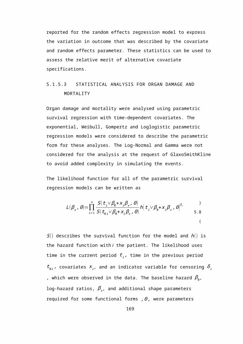
record differential costs and utility implications of organ damage in different organ systems.

The hazards for each organ system were estimated independently in the CE model. However,

some correlation in the risk of events across organ systems would be captured by the covariate

adjustment in the statistical models. For example, a high disease activity score increase the

probability of organ damage in multiple organ systems.

At every year of the simulation a probability of damage for each organ system is calculated for

the individual patients, which was used in a Bernoulli trial to determine whether damage

occurred for that patient in that period. The probabilities of a patient developing organ damage

in each period of the CE model were estimated as the difference between the cumulative

hazards in the current period minus the cumulative hazards in the previous periodH ( t−1 ). This

is converted into a probability with the following formula.

p (event )ij=1−exp (H (t )ij−H (t−1 )ij) (7.3)

where i indexes the patients observed, j indicates the time period of the observation.

The functional form for the parametric survival models on time to damage event included

Exponential, Weibull, Gompertz, and LogLogistic. The cumulative hazard functions for each

distribution are described in used to estimate annual probabilities are outlined in Table 42.

Table 42: Cumulative Hazard function for exponential, Weibull, Gompertz and Loglogistic functions

Survival curve Cumulative Hazard Parameter 1 Parameter 2

Exponential λt λ=exp ( Xβ ) n/a

Weibull λ t γ λ=exp ( Xβ ) p

Gompertz λγ(eγt−1) λ=exp ( Xβ ) γ

LogLogistic1+λ t

1γ λ=exp (−Xβ ) θ

The parameters labelled Parameter 1 in Table 42 were estimated from the baseline hazard β0

and the covariate effects for the organ damage survival model described in the natural history

modelβK .

173

Xβ ij=β0+ βk X ij+βk+1 Dij (

7.4

)

where i indexes the patients observed, j indicates the time period of the observation, k indicates

the number of covariates in the survival model. The parameter estimates for the organ damage

survival models are based on the analyses described in Table 33 of Chapter 5 and the mean and

their covariance matrices are reported in Appendix 16. An additional coefficient for treatment

βk+1 was appended onto each of the organ damage survival models to modify the risk of organ

damage in treated patients (D=1). They are included in this survival model to reflect clinicians’

beliefs that new biologic treatments will modify organ damage accumulation rates. The

coefficients were estimated from the elicitation exercise described in Chapter 6.

The simulation allowed patients to accrue multiple damage events in those organ systems where

more than one damage type is listed in the SLICC/ACR Damage Index. However, if a patient

reached the maximum number of events in that organ system the patients did not record any

further damage in the simulation. For example, there are two types of ocular damage; if a

patient has a SLICC/ACR Damage Index score of 2 for ocular damage they not experience

additional ocular damage events.

7.2.2.4 TREATMENT DISCONTINUATION

In the CE model it is assumed that patients withdraw from treatment at a constant rate. The

exponential distribution is used to estimate the rate of withdrawal

H ( t )ij= λij t (

7.5

)

where i indexes the patients observed, j indicates the time period of the observation. The

parameter λ ij describes the scale parameter for individual i at time j.

λ ij=exp (β0+β1 Dij) (

7.6

)

174

Therefore, the baseline risk of withdrawal is estimated from β0 with an additional coefficient for

treatment β1, according to patient’s treatment status at time j. The estimates of the intercept and

treatment coefficient are estimated from previous clinical trials reported in Section 6.2 of

Chapter 6. Clinical trial withdrawal was assumed to be an appropriate estimate of real-world

discontinuation given an absence of real-world data on biologic treatment withdrawal in SLE

patients. The probability of withdrawal is derived from cumulative hazard for current and

previous cycle as specified in equation (7.3). Alternative time-dependent distributions for

withdrawal could be fitted to Phase II trial data to account for greater rates of withdrawal in the

early stages of the trial.

When patients discontinue from treatment their natural history continues to be monitored in the

simulation and their costs and health outcomes recorded. The effect of treatment in the change

in mean SLEDAI score is removed immediately, i.e. no tapering in the treatment effect

assumed.

7.2.2.5 MORTALITY

The Weibull survival distribution was used to model the probability of death. The probability of

a patient dying in each period of the CE model from the cumulative hazard as described in

equation (7.3). The Cumulative Hazard for the Weibull distribution can be expressed as a two

parameter survival model.

H ( t )ij= λij tγ (

7.7

)

where i indexes the patients observed, j indicates the time period of the observation. The

parameter λ ij describes the scale parameter for individual i at time j, and γ is the shape

parameter of the Weibull survival model. The scale of the distribution is estimated from the

baseline hazard β0 and eleven covariate effects described in the natural history model β1 :11. An

additional coefficient for treatment can be appended onto the mortality survival model to

modify the risk of mortality in treated patients (D=1).

175

λ ij=exp (β0+βk X ij+ βk+1 Dij ) (

7.8

)

where i indexes the patients observed, j indicates the time period of the observation, k indicates

the number of covariates in the survival model. The mean parameter estimates for the mortality

survival model are reported in Table 31 of Chapter 5. At every year of the simulation a

probability for mortality is calculated and an event is sampled from the Bernoulli distribution.

Applying the mortality survival model to estimate the probability of death was found to

underestimate the risk of mortality in the elderly. The mean age at entry into the Hopkins cohort

is 38 years and a maximum follow-up of 22 years. Only 27 patients in the cohort were followed

to an age 75 or older. As a consequence, the increased rate of mortality in elderly patients would

not have been captured in the mortality survival model. In order to avoid an underestimation of

mortality in the CE model a correction was required to increase mortality risk at older ages

using mortality estimates for the general population.

Life tables for the UK were obtained to express age related mortality for the general population

(227). The general population mortality rate is reported in column 2 of Table 43. The general

population mortality rate would underestimate the mortality risk for SLE patients with active

disease. It is necessary to inflate the general population risk with an SLE risk ratio. For that

reason, risk estimates were generated for SLE patients with zero AMS score and no organ

damage for all ages using the mortality survival model (Column 3 of Table 43). The risk ratio

for SLE patients compared with the general population was calculated for all ages (Column 4 of

Table 43). The analysis showed that the predicted mortality risk for an SLE patient with no

disease symptoms is higher than the general population up to the age of 62. For ages greater

than 62 the general population has a higher risk, so an adjustment is made to ensure that the

simulated mortality risk increases in line with the general population in old age (Column 5 of

Table 43). The risk adjusted mortality rate for SLE patients and the subsequent probability are

reported in Columns 6 and 7. The risk ratio was not subject to PSA.

Table 43: Mortality adjustment for older SLE patients

1 2 3 4 5 6 7Age General

population mortality risk

Estimated remission

mortality rate

Risk ratio estimate

Risk ratio applied

Risk adjusted mortality

Annual probability

50 0.00260 0.00527 0.49476 1.00000 0.00527 0.0052751 0.00285 0.00546 0.52312 1.00000 0.00546 0.0054652 0.00311 0.00565 0.55254 1.00000 0.00565 0.00565

176

53 0.00340 0.00585 0.58357 1.00000 0.00585 0.0058554 0.00372 0.00605 0.61681 1.00000 0.00605 0.0060555 0.00407 0.00625 0.65237 1.00000 0.00625 0.0062556 0.00445 0.00646 0.69071 1.00000 0.00646 0.0064657 0.00487 0.00667 0.73304 1.00000 0.00667 0.0066758 0.00535 0.00688 0.77973 1.00000 0.00688 0.0068859 0.00587 0.00710 0.83039 1.00000 0.00710 0.0071060 0.00645 0.00731 0.88522 1.00000 0.00731 0.0073161 0.00709 0.00754 0.94458 1.00000 0.00754 0.0075462 0.00780 0.00776 1.00885 1.00885 0.00783 0.0078063 0.00858 0.00799 1.07846 1.07846 0.00861 0.0085864 0.00945 0.00822 1.15451 1.15451 0.00949 0.0094465 0.01042 0.00845 1.23827 1.23827 0.01046 0.0104166 0.01151 0.00868 1.33125 1.33125 0.01156 0.0114967 0.01275 0.00892 1.43582 1.43582 0.01281 0.0127368 0.01418 0.00916 1.55407 1.55407 0.01424 0.0141469 0.01581 0.00941 1.68789 1.68789 0.01588 0.0157670 0.01768 0.00966 1.83963 1.83963 0.01776 0.0176171 0.01983 0.00991 2.01188 2.01188 0.01993 0.0197372 0.02230 0.01016 2.20660 2.20660 0.02242 0.0221773 0.02507 0.01041 2.41977 2.41977 0.02520 0.0248974 0.02809 0.01067 2.64627 2.64627 0.02824 0.0278575 0.03138 0.01093 2.88568 2.88568 0.03155 0.0310676 0.03494 0.01120 3.13788 3.13788 0.03514 0.0345377 0.03879 0.01147 3.40206 3.40206 0.03901 0.0382678 0.04292 0.01174 3.67899 3.67899 0.04318 0.0422679 0.04754 0.01201 3.98299 3.98299 0.04783 0.0467080 0.05287 0.01228 4.33026 4.33026 0.05319 0.05180

7.2.2.6 HEALTH RELATED QUALITY OF LIFE

A literature review of quality of life studies in SLE was conducted to identify appropriate utility

values for the health states of the CE model. The full detail of the utility literature search is

described in the Appendix 17. An initial review using the exclusion criteria found only six

articles that were related to health utilities (163;228-232). Unfortunately, none of these provided

sufficient data for utilities in SLE to populate the CE model.

More recently the results of the belimumab Phase III trials have been published and as part of

the belimumab NICE submission analysis of the EQ-5D scores collected in the trials (224). A

linear regression was fitted by GSK contractors to explore the relation between utility values

and SLEDAI score, organ damage items and patient characteristics (224). The results are

presented in Table 44.

177

Table 44 Linear regression explaining utility value based on BLISS trial data

Parameter Coefficient p-valueConstant 1.275 0.0000Log-transformed age -0.140 0.0000Black Ethnicity -0.036 0.0418SELENA-SLEDAI score -0.009 0.0000Ocular Damage 0.062 0.0011NP Damage -0.071 0.0000MSK Damage -0.047 0.0005Diabetes -0.065 0.0187

On average, a person’s utility value decreases by 0.009 per unit SLEDAI score. In addition, age,

ethnicity, ocular damage, NP damage, MSK damage and Diabetes had a significant relation

with quality of life. Ocular damage has a positive association with quality of life which is an

unusual finding and unlikely to be externally valid. The prevalence of organ damage was low in

the BLISS trials, which makes it more difficult to infer the effects of organ damage on EQ-5D

from this data. Not all organ damage items were found to be associated with poorer quality of

life. However, the patients in the BLISS trials tended to have low organ damage scores at

baseline and are not representative of patients at all stages of the disease.

In the CE model the regression analysis from Table 45 was used to determine a patient’s

baseline utility without considering their organ damage:

U ij=1.275−0.140∗log ( AGE ij )−0.036∗BLACK i−0.009∗S ij (

7.9

)

where i indexes the patients observed, j indicates the time period of the observation. The utility

score of patient i at time period j is predicted by age, ethnicity and SLEDAI score, S. The linear

regression does not predict utility values greater than 0.9 so does not exceed the upper bound for

utilities of 1.

Organ damage coefficients reported in Table 44 were not used to describe the utility impact of

organ damage in the CE model. Organ damage disutilities were applied to the baseline utility as

a multiplicative factor, rather than an absolute reduction as recommended in recent guidelines

from the NICE Decision Support Unit (233). The values for the disutility factors were taken

from a review of damage event disutilities reported in the GSK NICE submission (224). The

disutilities for organ systems were estimated as weighted averages from the multiple types of

178

events within each organ system. The disutility multipliers used for the first and subsequent year

with damage to an organ system are detailed in Table 45.

Table 45 Disutility multipliers for damage to a specific organ system.

Year 1 Year 2 onwardsCardiovascular 0.72 0.76Diabetes 0.91 0.91Gastrointestinal 0.79 0.91Malignancy 0.92 0.92Musculoskeletal 0.67 0.74Neuropsychiatric 0.68 0.71Ocular 0.97 0.99Peripheral vascular 0.86 0.92Premature gonadal failure 1.00 1.00Pulmonary 0.69 0.69Renal 0.89 0.89Skin 0.94 0.94

The baseline utility was multiplied with the greatest disutility from the organ damage systems a

patient had developed. When patients developed more than one damage event within an organ

system the two year onwards disutility was raised to the power of the number of events.

The utility decrements are assumed to be independent parameters in the CE model following the

Beta distribution. The parameters of the Beta distribution (α , β ) were approximated from the

estimates for mean, μ, and variance, s2, identified in the literature review using the method of

moments approach (22).

(α +β )=μ (1−μ )s2 −1

(

7.10

)

α=μ(α+β ) (

7.11

)

β=α (1−μ)μ

(

7.12

)

In most cases the standard errors were not reported in which case it was assumed to be 10% of

the mean.

179

7.2.2.7 COST INPUTS

The model was designed to evaluate the cost-effectiveness of a new hypothetical drug for SLE

in order for the Pharmaceutical Company to demonstrate the benefits of the new treatment to

institutions like NICE. As such the analysis is evaluated from the NHS/PSS Cost perspective in

line with the NICE reference case (29).

The CE model included parameters to describe the annual costs associated with disease activity,

organ damage mainly identified from Health Technology Appraisals related to each event.

Indirect were not included in the CE model and the cost of the new technology was not pre-

fixed. The costs of disease activity included a fixed and variable cost, where incremental

increases in the average SLEDAI score increase the cost of the patient. This method of relating

disease activity to costs may not produce reliable estimates of total costs because organ damage

and other co morbid conditions were not incorporated into the analysis. Furthermore, SLEDAI

score may not be a reliable estimate of costs because the types of clinical events included in the

SLEDAI will be extremely variable in terms of their costs. Nevertheless, no alternative sources

of evidence for SLE patients according to disease activity were found. Organ damage costs

included a cost associated with the event in the first year of its incidence, and subsequent annual

costs of treating patients with a history of the event.

Costs were assumed to follow the Gamma distribution and the parameters of the Gamma

distribution (α , β ) were approximated from the estimates for mean, μ, and variance, s2,

identified in the literature review using the method of moments approach (22).

α= μ2

s2

(

7.13

)

β= s2

μ(

7.14

)

In most cases the standard deviations were not reported in which case it was assumed to be 10%

of the mean.

180

The costs associated with disease activity were based on the GSK manufacturer’s submission in

which the baseline yearly cost of SLE is £1,152 (224). This increases with higher SLEDAI

scores assuming a linear relationship of £55.6 per SLEDAI score.

Organ damage has a substantial effect on the cost of managing SLE patients. The impact is

variable across organ systems. In the GSK submission a literature review identified the costs

associated with organ damage events, and averaged within organ systems (224). Each organ

system estimates the cost for the first year of the event and subsequent years. The costs

associated with each organ system are reported in Table 46.

Table 46 Costs for organ damage in the first and subsequent year

Year 1 2Cardiovascular £3,402 £500Diabetes £2,313 £2,313Gastrointestinal £2,678 £0Malignancy £6,056 £0Musculoskeletal £5,372 £1,882Neuropsychiatric £3,659 £1,144Ocular £1,518 £17Peripheral vascular £2,955 £591Premature gonadal failure £0 £0Pulmonary £9,678 £9,603Renal £1,746 £2,426Skin £0 £0

TREATMENT COSTS

The costs of the new treatment were not explicitly modelled in the simulation. The price of

treatment is assumed to be an exogenous variable in the CE model so it does not impact on the

other parameters of the CE model. It is possible to vary the price of treatment after the PSA has

run with little computational expense. The total cost of treatment is a function of price and the

number of courses of treatment administered. The discounted duration of treatment is recorded

in the CE model so to enable a post hoc analysis of price after the simulation has run.

7.2.3 DISCOUNTING

The costs and QALY were discounted in the CE model at a rate of 3.5% (29).

7.2.4 REDUCING SIMULATION ERROR

181

Simulation error can cause estimates from individual patient simulation models to produce

different outcomes depending on the random numbers used in the simulation. Simulation error

describes the variation in estimated CE model outcomes conditional on the same parameter

inputs because the CE model outcomes were subject to random variation. Increasing the number

of patients simulated in the CE model is an effective way to reduce simulation error. However,

this can substantially increase the time it takes to compute the analysis if the sample size

required is large. The simulation error was more than 5% of incremental Net Benefit in the CE

model so the following modifications to the simulation were made to reduce simulation error.

1. The patients included in the CE model were cloned across the two treatment arms so

that the patients had identical baseline characteristics.

2. The same patients were selected from the Generate Population process so that the

baseline characteristics were identical between iterations of the CE model.

3. All patients were assigned a vector of random numbers for each organ damage,

mortality, and withdrawal outcome so that the same random numbers would be used at

each time point of the CE model.

7.3 CE MODEL OUTCOMES

7.3.1 HEALTH OUTCOMES AND COSTS

The outcomes of CE models are usually presented as either incremental cost-effectiveness ratios

(ICER) or incremental net benefit (INB). Both measures are derived from the total costs, and

QALYs associated with the SoC and new treatments. Net benefit also requires that a willingness

to pay for a QALY is specified. The ICER summarises the cost of an additional QALY with the

new treatment. INB expresses the additional gains, in monetary terms, of switching to the new

treatment. The overall cost-effectiveness of a new treatment will be influenced by the

acquisition costs of the new treatment and other administration costs associated with it. At an

early stage of drug development these costs may be unknown or uncertain. For this reason, I

assumed that pharmaceutical companies would be less interested in a single ICER or INB

statistic based on a single price.

The value-based price represents the maximum price for the treatment given a pre-specified

willingness to pay per QALY threshold (234). In all of the analyses the willingness to pay

threshold is assumed to be £30,000 (29). I believe that pharmaceutical companies will be

interested in observing this statistic and its uncertainty at an early development stage to observe

the potential profitability of the treatment and the probability distribution of value-based price.

182

This measure will illustrate the level of risk involved in pursing the treatment into a Phase III

trial.

VBP=λ (QD2

−QD1 )+CD 1−CD2

T

(

7.15

)

where Di indicates the treatment option, discounted Costs and QALYs are indicated by C and Q

respectively, λ indicates the willingness to pay for a QALY threshold and T indicates the

average discounted treatment years of the new biologic treatment. The value-based price will be

estimated for all iterations of the PSA so that it is possible to estimate the expected value-based

price and the distribution of simulated value-based Price arising out of the PSA.

7.3.2 PARAMETER SENSITIVITY ANALYSIS

Traditional Expected Value of Perfect Parameter Information was not conducted because it

requires that a fixed treatment cost is assumed. This is incompatible with the objectives of our

analysis to investigate the impact of parameters on the uncertainty in value-based price.

Parameter sensitivity analyses are conducted to identify which parameters contribute most to the

overall uncertainty in CE model outcomes. This analysis can be used to identify CE model

parameters that should be prioritised in future data collection exercises. The parameter

sensitivity analysis was conducted using analysis of covariance methods (ANCOVA) to

summarise the proportion of the variance in the value-based price that is explained by the

variation in the input parameters. The first ANCOVA used value-based price as the output

parameter, so that price did not have to be specified.

7.4 RESULTS

In this section I report the results of a CE analysis comparison of the hypothetical new treatment

versus standard of care (SoC) under the assumptions about the effectiveness of the new

treatment based on the prior distributions obtained from the phase II belimumab trial (72)

elicitation exercise described in Chapter 6.

7.4.1 CE MODEL OUTCOMES

183

The expected age at death was higher in the new treatment arm than the SoC arm and there was

more life years gained. The undiscounted and discounted QALYs accumulated in the new

treatment arms are higher than the SoC arm. In the simulation patients receiving the new

treatment live longer by 0.57 life years and are therefore at risk of incurring organ damage for a

longer time.

Table 47: Summary of mean CE model outcomes (standard deviation)

Standard of care New treatment DifferenceAge at Death 70.56 (2.568) 71.13 (3.050) 0.57 (1.711)Life Years 29.26 (2.566) 29.86 (3.048) 0.57 (1.711)QALYS (undiscounted) 13.380 (2.532) 13.700 (2.671) 0.318 (0.759)QALYS (discounted) 8.208 (1.433) 8.349 (1.493) 0.141 (0.389)

Table 48 reports the proportion of patients who experienced organ damage up to the time of

death for the SoC and treatment arms. A lower proportion of patients receiving the new

treatment had accumulated organ damage in the cardiovascular, renal, ocular, and skin organ

systems. More patients with the new treatment died with damage in the neuropsychiatric

system, peripheral vascular system, malignancy, and diabetes. Overall there were very small

differences in the accumulation of damage between the two treatment arms. However, patients

receiving treatment live longer, so have a longer time at risk of damage accumulation.

Table 48: Mean proportion of patients with organ damage at death (standard deviation)

Standard of care New treatment DifferenceCardiovascular 0.434 (0.075) 0.420 (0.077) -0.014 (0.022)Renal 0.154 (0.049) 0.146 (0.048) -0.007 (0.011)Musculoskeletal 0.636(0.044) 0.637(0.051) 0.001 (0.027)Neuropsychiatric 0.476(0.040) 0.477(0.044) 0.001 (0.018)Pulmonary 0.399(0.047) 0.397(0.050) -0.002 (0.021)Peripheral Vascular 0.158(0.018) 0.159(0.021) 0.001 (0.011)Gastrointestinal 0.243(0.025) 0.243(0.028) 0.0003 (0.011)Ocular 0.484(0.050) 0.487(0.054) 0.002 (0.024)Skin 0.154(0.044) 0.151 (0.043) -0.003 (0.007)Malignancy 0.396 (0.059) 0.401(0.059) 0.005 (0.023)Diabetes 0.252(0.043) 0.255(0.046) 0.003 (0.016)Gonadal Failure 0.089(0.014) 0.089(0.015) 0.001 (0.004)

The mean discounted costs incurred by patients in the simulation are reported in Table 49.

Overall the new treatment has a marginal reduction in the costs associated with SLE. However,

many costs are increased, which is most likely because patients live longer and spend longer at

risk of organ damage. Organ systems that reported lower incidence of damage, also were found

to incur lower costs in the simulation. Overall the cost differences between the two arms are

184

small relative to the overall cost and suggest that there are almost no cost-savings from the new

treatment.

Table 49: Summary of mean discounted costs broken down by cause (standard deviation)

Standard of care New Treatment DifferenceDisease activity related costs £19,950 (1006) £20,280 (1340) £330Organ damage costCardiovascular £3,164 (627) £3069 (639) -£95Renal £3,136 (1003) £3,070 (994) -£66Musculoskeletal £20880 (2,487) £21,040 (2,752) £160Neuropsychiatric £7,742 (823) £7,822 (969) £80Pulmonary £39,820 (6,486) £39,840 (6,761) £20Peripheral vascular £1,036 (142) £1,094 (185) £58Gastrointestinal £346 (46) £343 (49) -£3Ocular £607 (84) £607 (90) £0Skin £0 £0 £0Malignancy £615 (102) £622 (109) £7Diabetes £821(165) £822 (174) £1Gonadal Failure £0 £0Sum of organ damage costs £78,187 £78,329 £142Total costs £98,137 £98,609 £472

The uncertainty in the CE model is illustrated in Figure 23 assuming that the cost of the new

treatment is zero. This demonstrates the extent of uncertainty in the CE model.

185

Figure 23: A cost-effectiveness plane for the PSA outcomes assuming price is zero

CE plane describing incremental cost and incremental QALY outcomes from the PSA

incremental QALYs

incr

emen

tal C

osts

-3 -2 -1 0 1 2 3

-600

00-3

0000

3000

060

000

7.4.2 DRUG PRICE ANALYSIS

A fixed price is not assumed in these analyses to allow the pharmaceutical company to observe

how price affects the cost-effectiveness of the treatment and the probability of reimbursement.

Figure 24 illustrates how incremental net benefit decreases with price on the left-hand axis. The

graph illustrates that with current evidence a price of more than £900 per year yields a marginal

positive Net Benefit. In other words, any price below £900 per year would result in an

incremental CE ratio below £30,000 per QALY gained.

186

Figure 24: Drug Price Analysis. Impact on Incremental Net Benefit and Probability Cost-Effective

0 200 400 600 800 1000

-100

00

1000

2000

3000

4000

Variation in Incremental Net Benefit for a change in Drug Price

Annual Drug Price

Incr

emen

tal N

et B

enef

it

Figure 25 illustrates a histogram of the distribution of value-based price estimate for all

iterations of the PSA. The graph demonstrates that model simulations estimate value-based

price between -£5000 and £5000. The most probable outcomes would be a price in the range of

0-£1000. A proportion of iterations generate a negative value-based price indicating how often

the treatment is less beneficial than SoC at a threshold of £30,000 per QALY. The distribution

of value-based price is not symmetric with some model iterations producing very favourable

outcomes where QALY gains were greater than 1.

187

Figure 25: Variation in Expected Value-Based Price from Probabilistic Sensitivity Analysis

Histogram of Value Based Price estimates

Value Based Price

Freq

uenc

y

010

020

030

040

0

-10000 -5000 0 5000 10000

7.4.3 PARAMETER SENSITIVITY

An ANCOVA sensitivity analysis was used to identify important parameters in the CE model.

The disadvantage of using the ANCOVA method was that it imposes an assumption that all

parameters are linearly associated with value-based price. The large residual identified in this

analysis indicates that this condition does not hold for a large proportion of the variables

included in the analysis. However, the ANOVA method is relatively simple to use and does not

require advanced training in statistics. Therefore, the method is accessible to many analysts and

can easily be incorporated into analyses during drug development. Figure 26 illustrates how the

variation in other CE model parameters impacts on the variation in value-based price.

188

Variability in the statistical models for mean change in SLEDAI, musculoskeletal damage,

mortality, neuropsychiatric damage and pulmonary damage explain the greatest variation in

value-based price in the CE model. The costs associated with organ damage and utility did not

contribute much to the variance of value-based price. The residual demonstrates the proportion

of variance in value-base price not explained by the inputs.

Figure 26: ANCOVA results for % variability in Value-Based Price explained by model inputs

Cardio CostRenal CostMSK CostCNS CostPulm CostVasc Cost

Gastro CostOular CostSkin Cost

Diabetes CostMalignancy Cost

SLEDAI CostCardio utilRenal utilMSK utilCNS utilPulm utilVasc util

GI utilOcular util

Skin utilMalignancy util

Diabetes utilUtility

SteroidsGonadal

MalignancySLEDAIMortality

CardiovascularRenal

MusculoskeletalNeuropsychiatric

PulmonaryVascular

Gastro.Ocular

SkinDiabetes

WithdrawalResidual

Proportion of variation in VBP explained by inputs

Percentage

0.0 0.1 0.2 0.3 0.4 0.5

189

7.4.4 COMPUTATION BURDEN

The CE model was developed to be an individual patient simulation of 15,000 duplicated

patients whose disease status is updated every year until death. A single iteration of the CE

model takes approximately 41 seconds to complete the analysis, and 12 hours to generate 1000

iterations of the PSA. Figure 27 illustrates how the expected value-based price converges to a

stable estimate for increasing PSA iterations. After 5,000 iterations the CE outcome is relatively

stable. The CE model is unlikely to generate reliable results for runs of fewer than 3,000

iterations. Consequently, the computation time to generate PSA results from the CE model is 36

hours at a minimum.

190

Figure 27: The Expected Value-Based Price for increasing PSA iterations

0

2000

4000

6000

8000

1000

0-500

0

500

1000

Convergence of VBP with PSA iterations

Number of iterations

Val

ue B

ased

Pric

e

191

7.5 DISCUSSION

7.6 THE COST-EFFECTIVENESS OF NEW TREATMENTS IN SLE

The CE model developed in this chapter estimates modest long term health benefits and cost

savings from the hypothetical new biologic treatments given the elicited uncertainty in its

additional effect over and above standard care. The CE model demonstrated how a new

treatment that modifies disease activity has the potential to increase life expectancy. The

differences in the proportion of patients developing organ damage were less notable. However,

this is at least in part due to greater damage accrual in patients living longer on the new

treatment. The reduction in healthcare costs for the new treatment was marginal.

This chapter has developed a CE model for SLE and demonstrates the challenges involved in

demonstrating cost-effectiveness from 12 month RCT evidence. The analysis of drug price

indicates that a new treatment with efficacy evidence similar to that described above will not be

able to charge high prices if the reimbursement authority imposes a willingness to pay threshold

of £30,000. In this chapter I examined the expected value-based price for the treatment based on

prior information about the CE model inputs. This data was implicitly information that might be

available after a Phase II trial. The incremental Net Benefit was low at all prices and negligible

at £5,000. This means that in the absence of stronger evidence companies would have to choose

between limited access to health care markets at a high price, and broader access at lower

prices. However, if a Phase III trial were undertaken and if the results showed superior

effectiveness to the prior means the prospects for reimbursement would be more favourable.

A recent example from the belimumab Phase III trials illustrates the limitations of trial design.

The drug was assessed in two Phase III clinical trials each of sample size of approximately 800.

The follow-up of the clinical trials were 12 and 18 months. The drug was approved by the FDA

and EMEA, however the drug has not been approved by NICE or CADTH based on CE

evidence. This suggests that more evidence is needed to ensure comprehensive market access

for new treatments in SLE.

7.6.1 HOW CAN CE MODELS BE USED IN DRUG DEVELOPMENT?

Preliminary analyses early in drug development could be used to aid a pharmaceutical

company’s decision to continue data collection for the new treatment. The CE analysis could be

used to decide whether to proceed with the drug development programme. If the expected CE

192

outcomes suggest that the value-based price is substantially lower than the pharmaceutical

company’s expectations it may not be worth investing in further trials. Multi-way parameter

sensitivity analyses could be employed to evaluate what combination of parameter estimates

would be necessary to achieve higher prices and whether these parameter estimates are realistic.

Parameter sensitivity analysis can be helpful in identifying which parameters contribute to the

variance in value-based price and treatment Net Benefit. It may be beneficial to target data

collection towards those parameters whose variability contributes the most to the variance in CE

model outcomes.

From a societal perspective EVPPI can be used to value a complete reduction in the uncertainty

for individual parameters of the model. EVPPI was not employed in this analysis because it is

conditional on a fixed price for the treatment, which I am assuming has not been set by the

pharmaceutical company. The ANCOVA analysis did not require price to be fixed, but is more

limited than EVPPI because does not value a reduction in CE model outcome uncertainty. The

ANCOVA method is sufficient as a guide to the pharmaceutical company on which parameters

are more important and is quick and easy to generate.

7.6.2 COMPUTATION BURDEN

The computation burden of the CE model is considerable. The main reason for this is because

every annual cycle the model evaluates if the individual has experienced fourteen different

organ damage and mortality events. The model is an individual patient simulation so the

outcomes must be updated for every individual. It could have been beneficial to make

simplifications to the CE model to reduce the time taken to generate analyses. I considered two

methods to simplify the CE model.

Firstly, I investigated whether a Markov cohort CE model could be employed to simulate SLE.

However, a Markov cohort CE model was considered incompatible with a structure that

included interactions between disease activity, steroid exposure, organ damage development

and mortality. Recording the many combinations of disease feature would require a large

number of tunnel states in a Markov CE model, and the Markov framework would become large

and inefficient.

Secondly, I considered modifying the structure of the CE model to combine or exclude organ

damage outcomes with less impact, such as diabetes, gonadal failure and malignancy. However,

simplifications would weaken the CE model in terms of its robustness and flexibility. Organ

193

damage impacts on the risk of future events like mortality, pulmonary damage and

musculoskeletal damage, which have been identified as important inputs in the CE model in the

ANCOVA analysis. Modelling a subset of organ damage events would underestimate the

burden of organ damage. The more detailed CE model can accommodate more patient

population sub-group analyses if the pharmaceutical company were interested in analysing

possible different inclusion criteria. Simplifications would reduce the generalisability of the CE

model to different treatments for SLE. Simplifications could be potentially more appropriately

made in a real-life setting where more information was available about the new treatment to

inform the decisions. However, for the reasons of robustness and flexibility I decided not to

make simplifications to the CE model.

7.6.3 CONCLUSIONS

In this chapter I have described a CE model to evaluate long-term costs and QALYs for SLE.

The CE model can be used to generate useful analyses of the CE outcomes during the early

stages of drug development. Probabilistic sensitivity analysis and parameter sensitivity analysis

can be used to describe the uncertainty in the CE model outcomes and indicate where more

precise parameter estimates are needed. However, in order to evaluate the value of data

collection the CE model and BCTS must be combined to predict possible trial outcomes and

how they would impact on the expected price of the new treatment.

In Chapter 8 of the thesis I move on to combine the BCTS and CE model in a single simulation

to evaluate the value of alternative SLE trial designs.

194

8 CHAPTER 8: VALUE OF TRIALS ANALYSIS8.

In this chapter I compare trial designs for an SLE Phase III RCT using a modified version of the

Health Economic VOI methods to consider the pharmaceutical perspective.

I describe an analytic method to compare SLE Phase III RCTs with variable sample size and

duration of follow-up. The VOI analysis utilised the BCTS described in Chapter 6 and the CE

model described in Chapter 7. The BCTS was used to simulate trial datasets given a particular

design specification. The trial data were combined with prior parameters of the CE model to

estimate posterior densities for the CE model inputs and update the outcomes of the CE model.

Initially Bayesian updating was completed using a traditional calculation using Markov Chain

Monte Carlo Simulation (MCMC) in WinBUGS. However, this method would take years to

generate results. An approximation method was used to speed up analysis time. In the results

section I present the outcomes of the analysis from 1,600 BCTS iterations.

In Chapter 3, I discussed the limitations of using the ENBS method from the pharmaceutical

perspective. In this chapter I present an alternative method to value drug development trials

based on the uncertainty in value-based price that aligns with the priorities and information

constraints of a pharmaceutical company. As such, this chapter describes a novel method for

evaluating the value of trials from a pharmaceutical perspective and illustrates the limitations of

adopting value of information methods alongside a CE model for a complex disease.

Section 8.1 describes an overview of the process of Bayesian updating of prior data. Sections

8.2, 8.4, and 8.5 describe the methods used in the analysis. Section 8.2 specifies the prior

parameters of the CE model to be updated. Section 8.3 describes the trial design specifications

for the BCTS. The process of Bayesian updating is described in detail in Section 8.4. Section

8.5 introduces a novel method for valuing alternative trial designs from the pharmaceutical

perspective. The results of the analysis are presented in Section 8.6 with a discussion of the

method in Section 8.7.

8.1 BAYESIAN STATISTICAL METHODS IN PLANNING SLE CLINICAL

TRIALS

The CE model described in Chapter 7 defined a model to estimate total costs and QALYs

conditional on uncertain input parameters,θ. The Phase III trial would provide additional data

195

Xθ I on a subset of the CE model parametersθ I. The complement set of CE model parameters, θ I

C

, were not updated with trial data. The prior joint probability density p(θ I) was updated, via

Bayesian updating, to derive the posterior density p(θ∨Xθ I) for each hypothetical data set

sampled. The CE model was re-run with the posterior density p(θ∨Xθ I) and p(θ¿¿ IC )¿to

estimate the CE outcomes given the simulated trial data.

The BCTS described in Chapter 6 can be used to simulate Phase III data generated from

alternative trial designs. Multiple simulated datasets are generated for each trial design to

predict many possible outcomes of the Phase III trial. Alternative clinical trial designs can be

evaluated by simulating trial data and updating CE model parameters with the information

gathered. For each simulated dataset the prior and likelihood of the data are synthesised to

generate the posterior distribution of the parameters and evaluate the CE model outcomes. The

CE model parameters described in Chapter 7 are analogous to the pharmaceutical company’s

prior belief of the CE model inputs before they collect Phase III data.

The simulation process is illustrated in Figure 28.

Figure 28: The four stage simulation process to evaluate alternative trial designs

Generate SLE population

1. Generate 50,000 patients with baseline characteristics

2. Set baseline SLEDAI score (Repeat SLEDAI probability

calculations 3 times to stabilise SLEDAI score)

3. Estimate Prednisone dose

4. Set baseline organ damage score

Clinical trial Simulation1. Sample the parameters of from their distributions

3. Run natural history model

3.1 Determine major events3.2 Determine withdrawal3.3 Estimate SLEDAI3.4 Estimate Prednisone dose

2. Recruit patients

4. Estimate outcomes of trial

Bayesian Updating

1. Specify the prior distribution of CE model

2. Extract data from trial outcomes related to CE model parameters

3. Estimate the posterior distribution of the parameters used in the CE model

Cost-effectiveness model1. Sample the parameters from their distributions

3. Run natural history model

4. Estimate total costs and QALYs for simulation run

3.1 Determine major events3.2 Estimate change in SLEDAI3.3 Estimate Prednisone dose3.4 Collect costs and QALYs

2. Recrutit patients

PSA

In the first stage, a population of SLE patients are generated reflecting the disease

characteristics of patients in the Hopkins Lupus Cohort. Secondly, a chosen trial design a SLE

Phase III clinical trial is simulated to generate a single sample dataset. In stage three, this

dataset is combined with the prior distributions of the CE model to get the posterior

distributions. In the final stage, the CE model is evaluated given the posterior parameters and

the results are recorded. The simulation returns to stage 2 to simulate another clinical trial

dataset, and the process is repeated until sufficient trial results have been iterated to draw a

196

conclusion about the value of chosen trial designs. The whole process is repeated for each

alternative trial design of interest, thus enabling comparison of the relative value of different

designs.

8.2 THE PRIOR PARAMETER DISTRIBUTIONS

The prior distributions of the CE model were introduced and discussed in more detail in Chapter

7. The full list of the prior distributions of all the CE model parameters can be found in

Appendix 16. In this example, the natural history data was taken from a longitudinal cohort

study, the treatment specific data from a Phase II trials, costs and QALYs from published

literature, and unknown data from elicitation of experts.

8.3 DATA SIMULATION

The BCTS described in Chapter 6 was used to simulate data collected in future Phase III SLE

trials. The simulation describes a comprehensive set of disease outcomes, but only records those

outcomes that will be used to update parameters of the CE model. Phase III trials are most

commonly used to estimate treatment effect and treatment withdrawal, and these data were

collected in the BCTS. Costs, utilities, prednisone dose, malignancy and gonadal failure were

not recorded in the simulation. The parameter sensitivity analysis, described in Chapter 7,

indicated that the health economic outcomes were not sensitive to these parameters. For this

reason they were excluded from Bayesian Updating. In a real life setting steroid dose,

malignancy and gonadal failure events could be monitored in a Phase III trial. It was important

to balance the inclusion of parameters in the Bayesian Updating against the time burden of the

subsequent analysis.

In Chapter 2 I identified four trial design features that might be modified in a Phase III trial for

SLE including sample size, duration of follow-up, inclusion criteria, and trial endpoint. I

decided to focus the analysis on sample size and duration of follow-up.

Sample size and trial duration were identified as the two design features that should be

investigated further. Larger sample sizes and duration of follow-up would increase the precision

of CE model parameters, particularly those relating to treatment effect. Duration of follow-up

was of particular interest because longer trials will collect more evidence for the effect of

treatment on organ damage and mortality. The prior parameters for the organ damage and

mortality survival models were found to have an important impact on the variance of value-

197

based price. Longer follow-up in the Phase III trials should collect more precise estimates for

the treatment effect on organ damage because it takes time to confirm a diagnosis of organ

damage. In addition the sample size may improve the probability of observing a statistically

significant difference in organ damage. However, both designs would increase the cost of the

RCT. I therefore decided to focus my research on investigating whether longer follow-up of

patients or larger sample sizes increase the prospects of reimbursement sufficiently to justify the

additional costs in SLE trials.

I decided not to evaluate inclusion criteria in this hypothetical analysis because in the absence of

a real case study the specification of sub-groups of patients for whom the treatment may be

more effective was arbitrary and unlikely to produce generalisable results. Furthermore, the

analysis would require accurate market forecasting to consider uptake of treatment in different

sub-groups. This data was not readily available. I decided not to focus on multiple disease

activity measures. The main reason being that it was not possible to simulate multiple disease

activity indices in the BCTS because the statistical analysis only included SLEDAI to describe

disease activity. The definition of primary endpoint was not investigated due to data limitations

describing the impact of the BILAG index on long term outcomes. The definition of primary

endpoint can impact on the probability of regulatory approval, but given the SLEDAI based

structure of the CE model would not impact on the quality of data collected for CE analysis.

8.3.1 CLINICAL TRIAL CHARACTERISTICS

8.3.1.1 INCLUSION CRITERIA

The specifications for inclusion criteria were fixed to reflect a realistic design decision based on

the available information on SLE clinical trials. The review of clinical trials highlighted that age

and SLE diagnosis are the most common inclusion criteria in SLE trials. Disease severity and

organ involvement have been used to define clinical trial populations. Recent successful trials

have used disease activity scores at baseline as inclusion criteria, and this approach is adopted in

the BCTS. A meeting with Dr Akil, a clinical expert in SLE from the Hallamshire Hospital

Sheffield, (March 2011) highlighted the importance of excluding patients with severe renal

involvement and neuropsychiatric involvement. It may be unsafe to recruit patients with

neuropsychiatric or severe renal involvement into a clinical trial if their symptoms are life

threatening. Furthermore, he suggested that the inclusion criteria would include the

identification of immunological indicators for disease activity such as anti-dsDNA or low

complement on entry into the trial.

198

In this BCTS the inclusion criteria specified that patients were,

(aged 18-70) AND (SLEDAI>4) AND (DNA binding OR Low complement).

Patients were excluded if they had proteinuria, haematuria or neuropsychiatric involvement at

baseline.

8.3.1.2 CONCOMITANT MEDICATIONS

The BCTS included variables to monitor patient’s history of immunosuppressant treatment,

plaquenil prescribed at any time and steroid dose. It was assumed that patient’s history of

immunosuppressants did not change during the trial, which is consistent with a concomitant

medication restriction that new immunosuppressants cannot be initiated during the trial. Patients

receiving plaquenil on entry into the trial continue to receive this treatment, however it was

assumed that patients did not initiate plaquenil during the trial. Steroid treatment was allowed to

vary over the course of the clinical trial according to the Hurdle model described in Chapter 5.

8.3.1.3 TREATMENT COMPARATORS

The BCTS was simulated with two treatment arms. The first treatment arm reflected current

Standard of Care (SoC) given to SLE patients. The second treatment arm included SoC

combined with a new hypothetical biologic treatment. The patients were randomised to either

biologic treatment or SoC only with equal weights to generate an even distribution of patients

across each treatment arm.

8.3.1.4 TRIAL ENDPOINTS

The simulations will collect data for three clinical trial endpoints. These endpoints reflect three

methods of describing the effectiveness of a new treatment.

The first endpoint aimed to demonstrate efficacy. This approach is similar to that taken in the

belimumab trials to observe a statistically significant difference in the proportion of patients

who respond to treatment. Treatment efficacy was determined using a responder analysis. The

patient was classified as having responded to treatment if the SLEDAI score declined period by

more than 4 SLEDAI points after 52-week. This trial endpoint was described as the Efficacy

Trial Endpoint from herein.

199

The second endpoint was based on the SLEDAI score measure and focused on the scale of the

effect of treatment in reducing disease activity. The measure of effectiveness will be based on

the reduction in average SLEDAI scores over the entire period of follow-up. This statistic will

be applied to the long-term disease activity regression model to estimate the reduction in long

term SLEDAI with treatment. This endpoint is more relevant for the CE analysis because it

assesses if the reduction in SLEDAI score is sustained over time. This endpoint will be referred

to as the Disease Activity Trial Endpoint.

The third endpoint observed the reduction in organ damage accrual measured by the

SLICC/ACR damage index over the entire period of follow-up. Organ damage events are

relatively rare events and a small proportion of patients were expected to record an event during

the BCTS. However, organ damage is a key component of the CE model because it is costly and

impacts on quality of life. This endpoint will be referred to as the Organ Damage Trial

Endpoint.

8.3.2 MODIFIED CLINICAL TRIAL SETTINGS

8.3.2.1 SAMPLE SIZE SELECTION

Three sample sizes will be considered representing small, moderate and large sample sizes. The

sample sizes were determined using frequentist sample size calculations according to the three

endpoints of the trial. The endpoints were chosen to reflect different trial objectives. The sample

size calculations assumed that the duration of follow-up in the trial is 12 months. In the analysis

the duration of follow-up will vary, but the sample sizes calculations were not changed for the

alternative durations.

The first sample size was determined with an aim to demonstrate short term efficacy. Response

is defined as a reduction in disease activity scores according to the efficacy trial endpoint. The

middle sample size was powered to observe a statistically significant reduction in average

SLEDAI scores. This sample size will be calculated based on a statistically significant reduction

in the disease activity trial endpoint. The large sample size was powered to observe a

statistically significant reduction in organ damage accrual. Organ damage events are relatively

rare events and a small proportion of patients will be expected to record an event over the 12

months of the clinical trial. Therefore, the sample size is likely to be very large. The sample size

was calculated to observe a significant reduction in the Organ Damage trial endpoint.

200

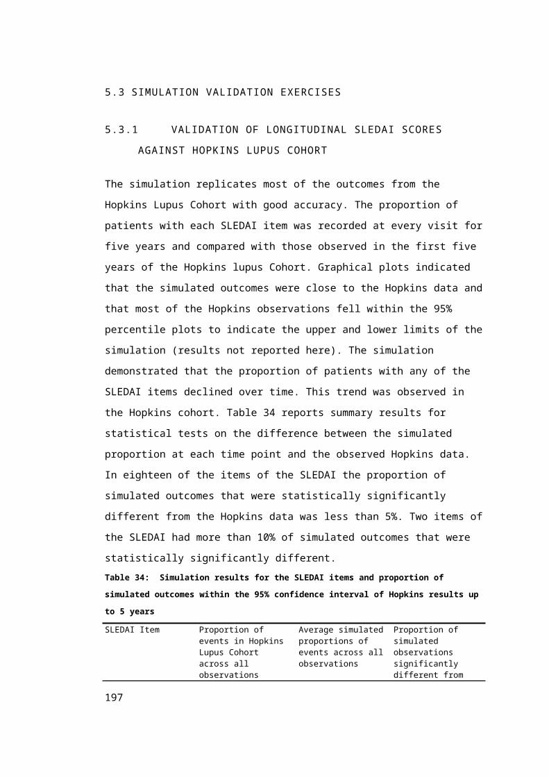
Frequentist sample size calculations are a more widely used method to determine sample size

and have been adopted in previous trials for SLE. It may be counter-intuitive to adopt a

frequentist sample size calculation alongside a Bayesian analysis of trial designs. However, the

computation time of the analysis was too long to evaluate small incremental increases in sample

size. I adopted a pragmatic method to adopt in order to quickly generate three sample size

calculations for three trial endpoints. All sample size calculations were estimated in STATA 11

(235).

8.3.2.1.1 SAMPLE SIZE ESTIMATION FOR THE EFFICACY TRIAL ENDPOINT

The Efficacy Trial endpoint measures the proportion of responders to treatments in each arm of

the trial (π1, π2). The proportions are estimated from the counts of binary data from participants

defined as either responders or non-responders at the end of the trial. The hypotheses for the test

are

H 0 :π 1−π 2=0 , H1 : π1−π2 ≠0

The general formula for calculating the sample size for binary data is expressed by,

n≈π2 (1−π 2 )+π 1(1−π1)

(π ¿¿2−π1)2{Φ−1 ( β )+Φ−1( α

2 )}2

¿

(

8.1

)

where α is the probability of a false positive error and β is the probability of a false negative

error (236). A single simulation of the BCTS provided estimates p1, p2 to approximate the

response rates for the two arms of the trial. The new treatment arm is expected to have a

response rate 0.54, and the standard of care arm 0.4. The α and β are set to 5% and 20%

respectively so that the trial has an 80% power to detect a clinically meaningful difference. The

estimated sample size is 426, which should be inflated to account for an estimated 24%

withdrawal rate, to give a final sample size of 529 patients.

8.3.2.1.2 SAMPLE SIZE ESTIMATION FOR THE DISEASE ACTIVITY TRIAL

ENDPOINT

The Disease Activity Trial Endpoint measures the change in average SLEDAI score over a year

(µ1, µ2). In a one year trial it is not possible to collect data on the average SLEDAI score for the

year before entry into the trial, therefore the SLEDAI score at baseline will act as a proxy for

the previous year. The primary endpoint of the trial aims to observe a statistically significant

201

difference in the change in SLEDAI score between the two arms of the trial. The hypotheses for

the test are

H 0 :µ1−µ2=δ=0 , H 1: µ1−µ2=δ ≠0

The general formula for calculating the sample size for continuous data is expressed by,

n ≈ 2σ 2

¿¿(

8.2

)

where α is the probability of a false positive error and β is the probability of a false negative

error (236). A single simulation of the BCTS provided estimates x1, x2 to approximate the

difference between the two arms of the trial, and an estimate of the variance σ 2. The average

change in SLEDAI for standard of care was 1.525. The change in SLEDAI for treatment was

estimated to be 1.8832. These estimates were derived from the BCTS described in Chapter 6.

The respective standard deviations were 2.44 and 2.43. The α and β are set to 5% and 20%

respectively so that the trial has an 80% power to detect a clinically meaningful difference. The

estimated sample size is 1,946, which should be inflated to account for an estimated 24%

withdrawal rate, to give a final sample size of 2413 patients. The withdrawal rate was estimated

from previous SLE trials as described in Section 6.2.3.7 of Chapter 6.

8.3.2.1.3 SAMPLE SIZE ESTIMATION FOR THE ORGAN DAMAGE TRIAL

ENDPOINT

The organ damage trial endpoint measures the reduction in the accumulation of organ damage.

The primary endpoint of the trial observes the difference in the rate of organ damage accrual on

the SLICC/ACR Damage Index between by comparing the hazard rates in the two arms of the

trial to get the log of the hazard ratio for treatment. The hypotheses for the test are

H 0 : ln ( λ¿¿1)−ln (λ2)=ln (Δ)=0 ,H 1: ln (λ¿¿1)−ln (λ2)=ln (Δ)≠ 0¿¿

To estimate the sample size for the difference between two hazard rates we must assume an

exponential survivor function for the control group. This assumption gives more flexible study

designs and accounts for the duration of follow-up and how these impacts on the number of

events observed given the baseline hazard rate. The method also accounts for an exponential

hazard for loss of follow-up of patients. The method assumes that the rate of organ damage

follows an exponential survival distribution with hazard rates in the control and treatment arms 202

λ1 and λ2 respectively (216). The natural history model for organ damage included exponential,

Weibull, Gompertz and loglogistic functional forms. Whereas, for the sample size calculation a

single function form was needed and the exponential was chosen for simplicity,

I used the Hopkins Lupus Cohort to estimate the baseline hazard,λ, of composite SLICC/ACR

Damage Index progression to be 0.1225. The elicitation exercise estimated hazard ratios for

treatment effect on groups of organ systems of the index. These were pooled by weighted

average, according to the prevalence of organ damage, to give a mean hazard ratio of 0.8043.

The estimated sample size, accounting for withdrawal of patients is 6350.

8.3.2.2 DURATION OF FOLLOW-UP SELECTION

The BCTS compared alternative duration of follow-ups. The baseline specification followed

patients for 12 months, because this design specification had been adopted in previous clinical

trials and is required by the FDA (81). I hypothesised that longer duration of follow-up would

be beneficial to the pharmaceutical companies because it would collect data on the long term

benefits of treatment. Therefore, duration of 2 years and 5 years was simulated. The 5 year trial

is considered to be an extreme value to illustrate the maximum possible follow-up that could be

considered.

8.3.2.3 FINAL SPECIFICATION OF THE TRIAL DESIGNS

To consider the trade-off between sample size and follow-up I specified six trial design

scenarios. The trial designs considered in these analyses will include 3 sample sizes and 3

duration of follow-up. The combinations of possible trial design settings are illustrated in Figure

29. Three other trial designs with large sample size and long duration of follow-up were not

included in the analysis. This was primarily to reduce computation time in the simulation. The

largest trial design specifications were excluded because these were less likely to be feasible for

a pharmaceutical company. The excluded trials would be more costly to conduct that the trial

designs that have been selected, but they would collect more information on the effectiveness of

the new treatments. However, the trial specifications described below is sufficient to consider

the trade-off between sample size and follow-up.

203

Figure 29: Trial design options to be simulated

Trial An= 529

f= 1 year

Trial Bn= 2413f= 1 year

Trial Cn= 6350f= 1 year

Trial Dn= 529

f= 2 year

Trial En= 2413f= 2 year

Trial Fn= 6350f= 2 year

Trial Fn= 529

f= 5 year

Trial Hn= 2413f= 5 year

Trial In= 6350f= 5 year

The six clinical trial design choices reflect a wide range of clinical trial designs. Whilst Trial A

may be sufficient to meet the requirements of a license regulator, the design does not aim to

collect data that will demonstrate that the drug is cost-effective.

Trials B through to F reflect changes to the trial design to increase the amount of data collected

in the clinical trial. The designs reflect several options to increase data. The analysis is designed

to observe the value of increasing the sample size, duration of follow-up or a combination of

both.

8.4 BAYESIAN UPDATING OF PROBABILITY DENSITY

The log-likelihood for each model was specified so that the prior could be updated with the data

from the simulated trial. The log likelihood for the change in average SLEDAI score model can

be written as,

ln ( L )=−0.5 n log (2π )−0.5 n log ( σ )−( y−βX )T ( y−βX )2 σ

where n is the number of time-points observed, σ is the variance, y is the change in SLEDAI, β

the coefficients and X the patient characteristics. The natural history model included 12

statistical models, which were updated simultaneously. The 12 models were assumed to be

204

independent, but the parameters within a model were multivariate normal. The likelihood for the

parametric survival models can be written as,

L(βx , Θ)=∏j=1

n S (t j∨β0+x j βx ,Θ)S (t 0 j∨β0+x j βx ,Θ)

h (t j∨β0+x j β x , Θ )δ j

S( ) describes the survival function for the model and h() is the hazard function. A detailed list

of the log-likelihood functions for the regression models is provided in Appendix 18.

8.4.1 MARKOV CHAIN MONTE CARLO (MCMC) METHODS

Many of the EVSI studies identified in the Methodology literature review in Chapter 3 used

conjugate distributions to update the prior distributions with data. The risk of withdrawal, organ

damage and mortality models use parametric survival analysis. The prior distribution θ I is

characterised by a multivariate normal distribution. However, the distribution of the trial data,

Xθ I, are not conjugate with the prior, because their form is generated by the exponential,

Weibull, Gompertz or loglogistic forms that were used to generate them. If the prior and

simulated data are not conjugate then the standard approach is to estimate the posterior using

Markov Chain Monte Carlo (MCMC) methods (92).

MCMC techniques are based on the construction of a Markov chain that eventually “converges”

to the target distribution which describes the posterior density p(θ∨Xθ I). Simulated samples

from the posterior probability distribution can be obtained using WinBUGS (Windows Bayesian

Inference Using Gibbs Sampling) software (14). In WinBUGS a Gibbs sampling algorithm is an

iterative procedure where every step generates instances from the distribution of each variable

conditional on the current values of the other variables.

MCMC Bayesian updating of the regression model parameters was implemented in WinBUGS.

The MCMC method was developed to sample parameter values from the posterior density of θ I

in the CE model. Two WinBUGs processes were set up to analyse firstly the survival models,

including organ damage mortality and withdrawal rates, and secondly the average change in

SLEDAI regression. Details of the specification of the WinBUGS model and illustrative results

from the mortality survival model are reported in Appendix 19. The MCMC successfully

sampled parameter values from the posterior distribution. However, this method could not be

used in the final analysis because it was prohibitively time-consuming.

205

8.4.1.1 COMPUTATION TIME ISSUES FOR IMPLEMENTING MCMC

The computation time of MCMC raised considerable methodological challenges. In order to

achieve convergence it was necessary to specify a burn-in of 15,000 and a large degree of

thinning (1 in 100) to deal with considerable autocorrelation. As a consequence it was necessary

to generate a very large number of posterior iterations which, in turn, generate the set of results

after thinning.

The full analysis process was completed for all regression parameters with a small simulated

dataset of 529 patients followed for 1 year. The analysis took 69,443 seconds, approximately 19

hours, to generate 1000 parameters samples for the CE model. The larger trial designs would

require even longer analysis time because of the increased size of the data. In Chapter 7, I

concluded that the CE model required a minimum of 3,000 PSA iterations to generate stable CE

results. This would increase the computation of the posterior distribution for a single trial

dataset to 57 hours. In addition to the WinBUGS analysis time it is necessary to evaluate the

posterior samples in the CE model, which added an additional 12 hours to estimate the nested

inner-loop CE outcomes. This process would need to be repeated many times to reflect

uncertainty in trial outcomes for each trial design. For example, a BCTS of 6 trial designs each

with 1,000 simulated trial results and fed through the MCMC and CE model PSA process would

take 6*1000*(12+57)=414,000 hours=17,250 days=47 years computation time.

I explored the possibility of using a High Performance Computer (HPC) cluster to generate the

analysis to moderate the impact of the substantial computation time of the analysis. The

University of Sheffield Linux based HPC, known as Iceberg, has the facility to run the MCMC

Bayesian updating described above using R linked to OpenBUGS (237). The HPC allows

several simulations to be run in parallel on separate nodes increasing the number of analyses

that can be generated within a fixed time-frame. However, the analysis was too time consuming

because the HPC imposes a maximum simulation time of 129 hours for each iteration of the

prior parameters. I would not be able to evaluate more than 2 trial datasets in that time. In

summary, I concluded that implementation of an MCMC updating process nested with the

BCTS and alongside running the patient level CE model with PSA was not feasible in terms of

computation time.

8.4.2 BRENNAN AND KARROUBI BAYESIAN APPROXIMATION

Brennan and Karroubi (2007) developed a set of formulae for generating posterior expectations

for EVSI analysis (115), building on work from Sweeting and Karroubi (2003), whose methods

206

introduced the approximation of a number of Bayesian quantities (238). Sweeting and

Karroubi’s method was adapted to incorporate the prior into the likelihood functions to allow

the posterior net benefit to be estimated. The method was found to be more efficient in EVSI

calculations because it avoided the MCMC updating process to generate a posterior probability

distribution. It also reduces computation time because it does not require PSA inner loop

evaluations of CE outcomes for each simulated dataset. Their case study using the Weibull

distribution would have taken 36.5 days to complete the analysis using MCMC in WinBUGS,

whereas the B&K approximation could produce the same result in 3.1 days (115). Based on this

estimate I anticipated that the B&K approximation could facilitate the evaluation of multiple

trial designs.

8.4.2.1 B&K APPROXIMATION NOTATION

The approximation is comprised of a series of calculations described below, for which the

following notation will be used.

X A dataset of trial data with n independent and identically distributed observations,

θ vector of d parameters (θ=(θ1 , θ2 , …,θd),

v (θ) a function or CE model with parameter inputs θ,

p( X∨θ) the probability of X given the vector of d parameters (θ=(θ1, θ2 , …,θd) or

likelihood,

p(θ) the prior probability density describes the prior expectations of parametersθ,

π (θ∨X ) the posterior density of θ given X

l (θ ) the log-posterior density,

li=δl(θ)δ θ i the first partial derivatives of the log-posterior density function

j (θ )=−δ2 l(θ)δ θ2 the matrix of second order derivative of the log-posterior density function,

J= j ( θ ) the matrix for second order derivatives for the maximum likelihood estimate θ.

207

The approximation includes a number of calculations on partitions of the parameters.

θi=(θ1 , …,θi ) a vector of the first i components of θ,

θi=(θi+1 , …, θd ) a vectors of the remaining components of θ from i+1 to d .

The approximation method includes a step that defines the maximum likelihood estimators for a

partition of the parameters θi conditional on a fixed set of remaining parameter. Such that,

θi(θ i−1) the maximum likelihood estimate of θi conditional on the first parameters θ(i−1 ).

For any function g(θ), when i<d we use the short-hand gi(θ) to denote g(θ i , θ( i+1)(θ i)) which

describe the function at the parameter values θi from 1 to i and θ( i+1 )(θ i) for values (i+1) to d.

8.4.2.2 BRENNAN AND KARROUBI METHOD

Brennan and Karroubi (2007) introduce their method based on the asymptotic theory of signed-

root log-density ratio transformation described in Sweeting and Karroubi (2003) (238).

ri (θi )=sign {θi−θi(θi−1)}[2 {l (θ i−1 )−l(θi)}]12 , i=1 , …, d

(

8.3

)

Brennan and Karroubi (2007) modify the method to incorporate the prior into the likelihood

function to create the probability density. The method maximises the probability density in

order to calculate the posterior expectation of a function.

E {v (θ )|X }≅ v (θ )+∑i=1

d

¿¿(

8.4

)

The first term of the equation v (θ) expresses the CE model outcome estimated at the posterior

mode,θ. The second term describes a correction term based on d summations, each of which

evaluates the function v (θ) with 2d+1 specifications of the CE model parameter inputs θ, ¿,

where θ−¿¿and θ+¿ ¿are weighted by α i−¿¿ and α i

+¿¿.

208

A maximum likelihood procedure is used to identify the posterior mode, or the values of

(θ1 , θ2 , …,θd) that maximise the posterior density function given the data X. Brennan and

Karroubi (2007) use the Newton-Raphson technique to estimate the minimum of the negative

log posterior density function, which is performed as an algorithm in a package from R (220).

θ+¿ ¿ and θ−¿¿ are (dxd) matrices with each row of the matrix containing a vector θi+¿ ¿ or θi

−¿¿

with values for each of the parameters of the CE model. The matrix θ+¿ ¿ follows the structure

illustrated below, and the matrix θ−¿¿ follows an identical structure with a different specification

for the diagonal.

¿ (

8.5

)

The off diagonal elements to the left and below the diagonal are the posterior mode for the first

i−1 parameters of vectorθ. The diagonal elements for i=1 , …, d are estimated by

θi+¿=θi+(k i)−12 , ¿ (

8.6

)

where k i is derived from the submatrix of j(θ) at i, ji(θ).

J=−(δ2 l(θ)δ (θ1)2

δ 2l(θ)δ (θ1)δ(θ2)

δ2 l(θ)δ (θ2)δ (θ1)

δ 2l(θ)δ (θ2)2

δ2 l(θ)δ(θ1)2

δ 2 l(θ)δ(θ1)δ(θ2)

¿⋱

δ 2 l(θ)δ (θ2)2

δ2 l(θ)δ (θ1)2

δ 2l(θ)δ (θ1)δ(θ2)

δ2 l(θ)δ (θ2)δ (θ1)

δ 2l(θ)δ (θ2)2

J i=[ δ 2l(θ)δ(θi)2 ¿⋱] )

(

8.7

)

Where the sub-matrix J i is inverted, and k i is the first element of the inverted matrix [ J i ]−1.

209

Finally, the weights α+¿¿ and α−¿¿ are calculated from partial derivative of the log-likelihood

density li(θi±), and the function υi (θi

±).

υi (θi±)=| ji+1(θi

±)|−12

The weights α+¿¿ and α−¿¿ are estimated from

α i−¿=( τ i )−1¿¿

τ i=¿

Brennan and Karroubi (2007) estimate the partial derivative analytically. νi ¿ was obtained

using the hessian j(θ) matrix, and obtaining the sub-matrix j ( i+1 )(θ), when θ=θi+¿ . ¿

Brennan and Karroubi (2007) introduce a Health Economics case study to evaluate Net Benefit

and let v (θ )=NB (t , θ) so that the Net Benefit of treatment D can be evaluated given

parameters θ. They demonstrated that the inner expectation of the net benefit for data X can be

approximated by

NB ( D , θ )+∑i=1

d

¿¿(

8.8

)

If the net benefit function is linear, the CE model parameters are independent and the

probability distributions are symmetric then the first term of the equation will be accurate.

However, if these conditions cannot be assumed then the second correction term will be

required. Each approximation requires the net benefit to be estimated 2 d+1 times, because

θi+¿ ,∧θi

−¿ ¿¿ each required d evaluations of net benefit and a single evaluation is required for θ.

This can be included in the EVSI formula.

EVSI ≅ EX θI

maxt

¿¿ (

8.9

)

210

Brennan and Karroubi test the feasibility and accuracy of the approach has been demonstrated

with two case studies. The case studies illustrate that the method can be used with a conjugate

multivariate normal distribution and a non-conjugate Weibull distribution for survival data.

8.4.2.3 APPLICATION OF THE B&K METHOD TO THE SLE STUDY

I adopted the second-order B&K method to approximate posterior CE model outcomes for SLE

clinical trials to reduce the computational burden of the MCMC method. The SLE VOI analysis

provided a case study to evaluate and help to progress methods for future applications of B&K

in ENBS studies. The SLE case study is very complex and applies the B&K method in an

individual patient simulation with a large number of input parameters. The method would be

faster and more straightforward if applied to a cohort model with fewer parameters. The CE

model includes 144 parameters, of which 82 would be updated with trial information. The CE

model includes exponential, Gompertz, Log-logistic and linear regression which have not

previously been used in the B&K method. The log-likelihoods can be found in Appendix 18.

The SLE VOI analysis raised several challenges to implement the process. As a consequence,

adaptations to the original R code used in the B&K Weibull case study were made (115). In the

following sections I describe four critical issues that were raised with the SLE case study and

what measures were taken to overcome them.

8.4.2.3.1 EXCLUDING CE MODEL PARAMETERS

I decided to include a subset of the CE model parameters in the B&K approximation. This

differs from the previous B&K approaches in which all CE model parameters were included

whether they were updated or not. The SLE CE model included three linear regression models,

four Weibull survival models, five exponential survival models, two Gompertz survival models,

three log-logistic survival models, and forty eight single parameters for costs and utilities. The

CE model parameters can be combined into a single multivariate normal prior distribution.

However, only a sub-set of these parameters will be updated with data from the clinical trial.

The speed of the approximation is conditional on the number of parameters in the prior (2 d+1)

, because this determines the number of θi−¿¿ and θi

+¿ ¿ that are calculated to make the second-

order approximation. There were substantial efficiency benefits to be gained from excluding

those parameters for which data would not be collected in the clinical trial. In the final

specification of the B&K approximation it was estimated that each parameter contributed

approximately 68 seconds to the process. Therefore, including the 63 parameters of the CE

model that were not updated with trial data would add at least an hour to the calculation time of

each B&K approximation.

211

The mean values for the prior distributions of the excluded parameters were used to calculate

the posterior health economic outcomes from the CE model. This was equivalent to assuming

that they are uncorrelated with other parameters and have symmetrical distribution. Whilst this

may not be a true reflection of the prior information on parameters it is justifiable if the

parameters have a linear relationship with the health economic outcomes of the CE model. The

ANCOVA investigation of the CE model described in section 7.4.3 showed that the parameters

contribute a small amount to the variation in value-based price and Net Benefit.

After the 63 parameters were excluded from the approximation the remaining prior consisted of

a multivariate normal distribution with d=82 dimensionsθ, mean μ and variance matrixΣƩ.

Prior p (θ )= 1

√ (2π )d|Σ|exp (−0.5 (θ−µ )T Σ−1 (θ−µ )) (

8.10

)

8.4.2.3.2 BAYESIAN UPDATING REGRESSION MODELS INDEPENDENTLY

The log-likelihood for the data is very complex because it is the sum of individual likelihood

functions for the regression models of the natural history model. The maximisation process on

the log-posterior density was problematic using R optim function from the standard stats

package. The function required more than 100,000 iterations to complete the process correctly,

with very small values for the step and gradient tolerance (0.00001). The process was run for

20 minutes and had not achieved convergence. Appendix 20 reports results of the optim

maximisation with only five regression models. When the process is repeated with eight

regression models the function does not identify a suitable solution within the number of

iterations permitted (max iterations=10000). It was impractical to increase the number of

iterations further to allow maximisation to occur, as a consequence an alternative method was

sought.

The alternative method developed took advantage of the considerable computational

efficiencies gained from segmenting the maximisation processes by regression model. The 14

statistical models were assumed to be independent in the natural history model. This assumption

is carried forward in the B&K approximation. Each group of parameters is part of a single

statistical model, and does not appear in the likelihood function for any other statistical model.

Consequently, the analytical specification of the log-posterior density, its partial derivatives and

second order derivatives, could be broken down into component parts because parameters from

one regression model are independent of other regression models. The tests are reported in

212

Appendix 20 and illustrate that the assumption of independence between the natural history

statistical models does not impact on the estimation of the B&K approximation.

In summary, the maximisation of the log-posterior density function was simplified to enable

maximisation of a large log-likelihood function and reduce computation time. It has been

demonstrated that there are considerable difficulties in maximising a large log-posterior density

function using optim in R. However, segmenting the calculation into individual maximisation

process for each statistical model using optim is efficient and reliable in producing estimates.

8.4.2.3.3 COMPUTATIONAL ESTIMATION OF PARTIAL DIFFERENTIATION

A modification of the B&K method aimed to make the method more accessible to non-

mathematicians. In the estimation of α i+¿¿ and α i

−¿¿ it is necessary to calculate the partial

differential and second order differential. Brennan and Karroubi (2007) use analytical methods

to estimate the partial differential and numerical methods to estimate the second-order

differentiation. Analytical methods are quicker to compute than the numerical methods;

however they require the analyst to be confident and competent in partial differentiation. In the

SLE case study we use the Gompertz and Log-logistic functions, which were more challenging

to differentiate. I do not have a strong background in mathematics and it was time consuming to

complete. Many checks needed to be made on the calculations because there was a risk that

small errors could have be made. It was felt that this approach was onerous and that the method

would be more accessible to non-statisticians if it were possible to use numerical methods to

estimate both the first order and second order differentials. This would mean that the modeller

would only need to specify an equation for the log-posterior density.

The numDeriv package in R was identified, with methods to numerically estimate the first

derivative and second derivative for a given function (239). The function grad was used to

calculate a numerical approximation of the first derivative of the log-posterior density for each

row of θi−¿¿ andθi

+¿ ¿. The calculation is done using a simple epsilon difference. The function

hessian was used to calculate a numerical approximation of the dxd matrix of second

derivatives of the log-posterior density. The utilisation of these functions has simplified the

method and made it more accessible to health economists.

8.4.2.3.4 SELECTION OF NUMBER OF PATIENTS TO RUN THROUGH THE INDIVIDUAL LEVEL SIMULATION FOR CE MODEL

213

Simulation error describes the random variation in the results from individual level simulation

type CE models, and is analogous to sampling error in statistics. Each time the individual level

CE model is run, patient outcomes vary slightly, which creates “noise” in the Monte Carlo

estimate of the true mean. Increasing the number of patients in the individual patient simulation

reduces the simulation error and increases the accuracy of the outcomes estimated.

The B&K method evaluates the health economic outcomes of the SLE CE model at the

posterior mode of the input parameters, i.e. the patient level simulation is run with θ. The

second order estimate evaluates the health economic outcomes of the SLE CE model at values

of each of the parameters above and below the posterior mode, i.e. the patient level simulation is

run with θ−¿¿ and θ+¿ ¿. The precision of each evaluation of the CE model is critical in

determining the overall accuracy of the B&K approximation. Analysis has shown that in this

case study the method was very sensitive to the effects of simulation error. The B&K method

identifies the posterior mode for the density of θ, and the upper and lower estimate θ−¿¿, θ+¿ ¿.

The value-based price is evaluated at these three values for θ and these estimates are used to

estimate the posterior treatment value-based price using the equation below.

VBP (t , θ )+∑i=1

d

¿¿(

8.11

)

Figure 30 illustrates how the B&K method estimates posterior health economic outcomes in a

simple one parameter CE model. The dotted line represents the posterior density of θ, and the

linear line describes the relationship between θ and treatment value-based price, VBP (t , θ).The

simulation error is depicted in the graph as error bars around the three estimated value-based

price. If the simulation error is large the posterior value-based price which is a weighted average

of the three simulation model runs could be inaccurate. This will impact on the second order

correction term. This is most likely to occur in the SLE CE model for parameters that have very

little impact on the Health Economic outcomes because the gradient of the slope depicted in

Figure 30 will be shallow, and those with very precise estimates. It turns out in practice that

both of these characteristics are observed for many of the CE model prior parameters for this

case study.

214

Figure 30: An illustration of the B&K method to estimate Health Economic outcomes in a simple one

parameter model

0

1

2

3

4

5

6

7

8

9

6 7 8 9 10 11 12 13 14

Expe

cted

QAL

Y fo

r tre

atm

ent

theta

B&K evaluation of Expected QALYs for treatment given parameter theta

Simulation error can be reduced by increasing the number of patients included in the simulation.

Figure 31 illustrates how simulation error in expected QALYs for treatment vary with sample

size.

215

Figure 31: An illustration of simulation error at increasing individual patient sizes

7

7.5

8

8.5

9

9.5

10

0 2000 4000 6000 8000 10000 12000 14000 16000 18000 20000

Expe

cted

QAL

Ys (t

reat

men

t)

Number of Patients

Simulation error and the number of simulated patients

n=100

n=1000

n=10000

n=20000

This shows that there is only a small reduction in simulation error between sample sizes of

10,000 and 20,000. The analysis where n=10,000 took 81 minutes to run, whereas n=20,000

takes 198 minutes. There are clear diminishing returns from larger sample sizes. The MC error

where n=10,000 was 0.057 and n=20,000 was 0.039. In order to ensure that the MC error was

less than 0.05 QALYs in the final analysis the sample was fixed at 15,000 patients. A similar

finding was observed for other model outcomes such as the Incremental Net Benefit. Greater

accuracy in B&K estimates from large CE model samples sizes would come at a substantial

computational cost.

8.4.2.4 COMPUTATION TIME FOR B&K METHOD

Although considerable efforts were made to reduce the computation time of the B&K analysis,

VOI analysis of the SLE CE model remains a very time consuming process. Each stage of the

simulation is detailed in Table 50. The most time-consuming stage of the process occurs when

the weights for α i−¿¿and α i

+¿¿ are calculated. The simulation process in which expected CE

outcomes were generated for all six trial designs took 5 days to calculate.

216

Table 50: Simulation processes and estimated computation times

Simulation process Computation time (minutes)Simulate trial data 0.444

Small sample (529) Large sample (6350)Estimate θ 1.00 minute 2.5 minutes

Estimate θ−¿¿ and θ+¿ ¿ 2.88 minutes 38.22 minutes

Estimate α i−¿¿and α i

+¿¿ 76.99 minutes 934.8 minutes

Evaluate E {v (θ )|X } 130.00 minutes 135.2 minutes

Total 3.5 hours 18.5 hours

8.5 VALUATION OF CLINICAL TRIALS IN INDUSTRY

The EVSI for each trial design would be estimated as the difference between the expected value

of a decision from the trial and the current expected value of the decision.

EVSI=EXθ I[maxD

{E(θIC , θI∨X θI

)[ NB(D , θ I ,θ IC )]}]−max

D{Eθ [NB(D , θ)] } (

8.12

)

where θ IC is the complement set of parameters of θ that are not collected in the clinical trial.

However, traditional EVSI methods are not compatible with the decision problem facing

pharmaceutical companies designing their Phase III trials for three reasons:

1. The pharmaceutical company do not directly seek to maximise the health benefits of the

population subject to resource constraints.

2. The pharmaceutical company are very unlikely to get regulatory approval based on their

Phase II data so the expected value to the company of current information is zero.

3. The pharmaceutical company do not have a fixed price for the new treatment.

In the following sections I describe an alternative method that I have adapted from considering

how Commercial Net Benefit and value-based pricing can be used to compare and value clinical

trials from a pharmaceutical perspective. I have applied this new method to the SLE case study

to demonstrate how a pharmaceutical company might use the analysis to maximise expected

profits conditional on trial design.

8.5.1 ASSURANCE BASED VALUATION OF TRIALS

217

Willan (2008) formulated a function for Expected Profit for a pharmaceutical company’s

product. This is renamed in this thesis to be the Profit Forecast (PF).

PF=π kh s g(z ) (8.13)

where π is the profit per treated patient, k is the annual disease incidence in SLE, h is the time

horizon of sales for the new treatment. The market share of the new treatment is given by s and

the probability of reimbursement approvalg ( z ) conditional on the strength of evidence from the

trial z. The estimate for g ( z ) is analogous to an assurance calculation. I generated assurance

calculations for multiple endpoints of a trial to describe different strengths of evidence.

Firstly, the BCTS reported the assurance calculations for the Efficacy Trial endpoint, the

Disease Activity Trial endpoint, and Organ Damage Trial endpoint.

The assurance calculation for a successful CE model outcome, with a positive incremental net

benefit is more challenging to estimate. CE model success can only be estimated if the price of

the new treatment were known. Within this framework it would be necessary to assume a target

price for the treatment and calculate the Profit Forecast. It may be useful to evaluate Profit

Forecasts for a range of prices to observe the trade-off between increasing profit per patient

treated as price increasing and decreasing the probability that the treatment will be approved.

However, the pharmaceutical company will not have to make a decision about the price at this

stage in the drug development and the final decision for price will be conditional on trial results.

Price scenario analyses may be difficult to interpret for decision-making for trial designs. I

considered how the method proposed by Willan (2008) could be adapted to account for an

evaluation of trial designs with variable price.

8.5.2 VALUE BASED PRICING VALUATION OF TRIALS

I proposed that Willan’s formula should be revised so that the probability of reimbursement

approval was removed from the equation and the profit per patient was variable and conditional

on the CE outcomes after data collection. Equation (8.13) has been modified to account for the

variable profit per patient, π (θ I ,θ IC ) .

PF=π (θI , θ IC )k h s−c (

8.14

)

218

where c is the cost of production, k is the annual disease incidence in SLE, h is the time horizon

of sales for the new treatment. The profit per patient can be estimated from the CE outcomes

assuming that the drug company are willing to set their price according to the willingness to pay

threshold of the reimbursement authority. The value-based price of the new treatment can be

expressed as an outcome of the CE model. It describes the maximum price that the drug

company can charge given the decision criteria of the reimbursement authority. A simple

example would be the willingness to pay per QALY threshold. Prior to the Phase III trial, the

expected value-based price for the treatment conditional on new data will be uncertain due to

the variability in possible data outcomes from the trial. In designing the Phase III trial

pharmaceutical companies will want to maximise the expected value-based price and reduce the

risk that the treatment fails to reach the market. Different trial designs will have a differential

effect on the expected value-based price and trial assurance.

I specified an alternative formula for determining profit per patient. In Section 1.1 of Chapter 1

I proposed that drug success is defined by two factors: a successful licence application and a

successful reimbursement application. These two conditions are required in order to achieve

profits for the new treatment. The treatment license is granted if the primary endpoint of the trial

is statistically significant. The primary endpoint of the trial is expressed by Δ and the

significance test z ( Δ). Reimbursement is granted if the annual price of treatment is less than or

equal to the value-based price. It assumed that the pharmaceutical company have a minimum

price m at which they would agree to market the treatment, this may be related to the cost of

producing the drug c, but may be influenced by other factors. For example, price expectations

may vary if the pharmaceutical company knows of, or anticipate, other drug indications. In the

formulation of expected profits, patients are assumed to receive treatment for t years, which can

be estimated from the mean treatment years across all BCTS evaluations.

π (θX )={ 0 (VBP<Pmin∨z ( Δ)<1.96)VBP(θI , θC)t (VBP≥ Pmin∧z ( Δ )>1.96)} (8.15)

If the new treatment has generated a value-based price less than the minimum, Pmin , or, if the

efficacy of the treatment is not statistically significant then the profit per patient is zero.

However, if the value-based price is greater than the pharmaceutical companies minimum price

Pmin, and efficacy is statistically significant, the pharmaceutical company will adopt the value-

based price and profit per patient will equal value-based price minus the cost of treatment

production.

219

8.5.3 EXPECTED COMMERCIAL NET BENEFIT OF SAMPLING (ECNBS)

The Expected Profit for each trial design was estimated from the expectation over all iterations

of the Profit Forecasts. A profit forecast was made for each simulated dataset. With some trial

results having zero profit implication and others achieving regulatory approval, reimbursement

at the value-based price, the expected profit forecast is simply the average of all these.

EPF X θI

=EXθ I[ PF(θ I∨X ,θC)] (

8.16

)

The decision criteria for selecting the optimal trial design required the specification of the

maximum Expected Commercial Net Benefit of Sampling (ECNBS). ECNBS expressed the

difference in the total value of the trial design and the cost of the trial design.

ECNBSX θI

=EPF Xθ I

−cost∨n ,d (

8.17

)

The costs of the clinical trial depend on the specification of the trial design because increased

sample size, n, and duration of follow-up, d, will increase the cost of the trial. Consequently, the

ECNBS will weigh up whether the increased benefit of a longer trial is justified by the increased

cost of data collection.

The literature view of previous Bayesian analyses of trial design identified that most studies

used a fixed and variable cost of the clinical trials in their evaluations. In most cases the

estimation of trial cost was crude and very few studies conducted a detailed analysis of clinical

trial costs to justify their choice. Since this case study concerns a hypothetical new drug, and in

the absence of a detailed specification of the clinical research a similar approach to estimate the

costs of the clinical trial was adopted. A fixed cost of £1,000,000 is assumed with a variable

cost of £1,000 per patient in the first year of observation and £500 for subsequent years. The

additional costs of monitoring patients in subsequent years are incurred, even if they have

withdrawn from the study. This is a simplifying assumption and may over-estimate the cost of

longer trials, but this may be justified by the costs of chasing up patients who are lost to follow-

up. The cost of producing the drug was assumed to be £200 per patient treated. No costing

studies for SLE trials were identified in the literature.

8.5.4 NUMBER OF PATIENTS WHO WILL BENEFIT FROM TREATMENT220

Estimation of the Profit Forecast relies on an estimation of the number of patients who will

receive treatment. The estimate is determined by the annual incidence of SLE k, the current time

horizon of the treatment h, and the market share of the new treatment s. These three parameters

can be challenging to estimate, particularly for a hypothetical new treatment. Given the

complexity of the Bayesian updating it was necessary to adopted relatively simple assumptions

regarding these parameters. However, in a real-life case study it would be necessary to refine

these estimates or to conduct sensitivity analyses to test the impact of the assumptions.

I used published literature to generate an estimate of the incidence of SLE over an annual period

from Birmingham, UK to reflect a population with a broad ethnic mix. The study reports a point

estimate of the incidence to be 3.8/100,000/year (39). The analysis described above has been

presented using a simple description of UK regulation and reimbursement. However, the value

of the Phase III trial is not restricted to the projected sales in the UK market. Therefore, the

incidence rate was applied to the current population statistics for the OECD countries. The most

recent population statistics were from 2009 and reported a total population of 1,221,410,000. In

line with the methods used in the Birmingham study children aged less than 18 were excluded

from the population base. The OECD reported a population of 309,388,240 who were less than

19 years of age (240). This estimate was considered sufficient to exclude juveniles from the

population base despite the small discrepancy between the use of 18 and 19 years of age. This

gave a final population base of 912,021,760, and an annual incidence of 34,657 diagnoses of

SLE per year. By estimating an incidence for the OECD countries it is implicitly assumed that

the £30,000 cost-effectiveness threshold is used to set prices across all multiple national

markets. Whilst this is not a realistic assumption the threshold can be used to approximate

prices in other jurisdictions and is sufficient to demonstrate the method and meet the objectives

of this study. Further adaptations of the method to incorporate multiple market settings are

explored further in Chapter 9.

The time horizon of the treatment was assumed to be 10 years. This describes the time until the

treatment would be replaced by more effective alternatives. The value is relatively arbitrary but

is consistent with estimates from other ENBS studies (111).

It has been stated earlier in the thesis that there are very few licensed treatments available for

SLE, which would indicate a potential for a large market share to be exploited. However, given

the heterogeneous nature of the disease it is likely that a percentage of patients with an SLE

diagnosis would not require a new biologic treatment because their symptoms can be managed

with cheaper and less intensive treatments. The market share parameter in this analysis was used

to moderate the proportion of SLE patients who would be considered eligible to receive a new 221

treatment. It is assumed that the market share for a new treatment is 43.2% of SLE patients,

which was estimated from the proportion of patients in the Hopkins Lupus Cohort who had a

history of immunosuppressant treatment, in Table 23 of Chapter 6. Initiation of

immunosuppressants is indicative of a severe flare in the disease.

8.6 RESULTS

8.6.1 ASSURANCE

The analysis identified that sample size and duration of follow-up impact on the assurance for

the three endpoints of the trials. Table 51 reports the proportion of simulation runs in which the

simulated trial results produced a statistically significant difference between the treatment arms

for each of the three trial endpoints. The efficacy endpoint describes the responder index, the

disease activity endpoint describes the difference in average SLEDAI score, and the organ

damage endpoint described the difference in SLICC/ACR Damage Index. Larger datasets

increased the likelihood that the effect size will be significant because the standard errors for the

difference between arms are decreased.

The efficacy endpoint reports the highest probabilities for a successful trial. Probabilities fall in

the range 0.74-0.92 for all trial designs. This indicates that there is a strong likelihood of

achieving this endpoint for all trial designs. The assurance can be used to represent the power of

a trial. RCT power calculations are often based on estimates of between 80-90%. In this respect

the simulated trials have reasonable power, with slight under-powering observed in the small

sample size trial. Increasing the duration of follow-up does not impact on the responder index

because it records the difference in the proportion of responders after 52 weeks of treatment.

Table 51 demonstrates that sample size improves the likelihood of success on the efficacy

endpoint. However, modest gains in the probability of success are achieved for relatively large

increases in sample size. It is also shown that the gains are diminishing with larger sample sizes.

An increase in sample size of approximately 1800 subjects, from 529 subjects, increased the

222

probability by a factor of 14%. Whereas increasing the sample size by 3937, to 6350, subjects

increased the probability by a factor of only 8%.

The assurance for the disease activity endpoint is lower than the responder index efficacy

endpoint. The disease activity endpoint reports the largest variation in probabilities across the

trial designs. A small trial with short follow-up has a less than 50% probability of meeting the

primary endpoint. Whereas, increasing the sample size or duration of follow-up will tip the

likelihood over this threshold. The greatest gains in the probability of meeting the disease

activity endpoint were for sample size increases, rather than duration of follow-up. However, a

combined increase in both produces favourable results.

The organ damage endpoint has the lowest probability of success of the three endpoints. None

of the trials exceeded a probability of success greater than 50%. Increasing the sample size of a

1 year trial has a very modest impact on the probability of success. Increasing the duration of

follow-up to 2 years is a much more effective strategy to increase the likelihood that the

endpoint is met. On the other hand, increasing the duration of follow-up to 5 years has almost

no effect on the probability of success. This is most likely due to the high rates of withdrawal

from the trials (approximately 25% in the first year), which substantially reduces the amount of

data collected in the later stages of the trial.

Table 51: Probability that the clinical trials will demonstrate a statistically significant effect size

Efficacy endpoint (SLEDAI) Disease Activity (SLEDAI) Organ damage (SLICC/ACR DI)

1 year 2 years 5 years 1 year 2 years 5 years 1 year 2 years 5 years

n= 529 0.743 0.743 0.743 0.431 0.596 0.695 0.069 0.138 0.135

n=2413 0.884 0.884 0.777 0.809 0.070 0.201

n=6350 0.921 0.882 0.081

SLEDAI = SLE Disease Activity Index; SLICC/ACR DI = SLICC/ACR Damage Index

8.6.2 EXPECTED VALUE-BASED PRICE AND EXPECTED COMMERCIAL

NET BENEFIT OF SAMPLING RESULTS

Figure 32 illustrates the proportion of simulated trials for each trial design that met the

reimbursement criteria. In some trial designs the most likely reason for not achieving

reimbursement was due to the low proportion of trials meeting the primary endpoint, as

observed for the trials with lower sample size. Whereas the larger sample size trials tended not

to achieve reimbursement because the value-based price was lower than the minimum price.

223

Figure 32: Proportion of simulated trials with meeting the criteria for success from 1,600 simulations for six

trial designs

n=529,d=1 n=2413,d=1 n=6350,d=1 n=529,d=2 n=529,d=5 n=2413,d=2

The proportion of sucessful trials for each trial design

Designs

Pro

porti

on o

f suc

essf

ul tr

ials

0.0

0.2

0.4

0.6

0.8

1.0

efficacy endpointP>Pminreimbursement

Table 52 reports the expected financial outcomes of the trial after regulatory approval and

reimbursement for each of the simulated trial designs. The results are based on 1,600 simulated

datasets for each trial design generated from the BCTS. Each simulated dataset was used to

update the CE model parameters to estimate value-based price, and averaged over all

simulations to estimated expected Commercial Net Benefit of Sampling.

Table 52: Probability of reimbursement, expected value-based price, expected sales volume, expected costs and

expected Net profits from sampling

Probability of

reimbursement

Expected

revenue per

patient year for

trials meeting

Expected

Profit per

Patient

Expected

Sales

Volume

Expected sales

value

(million £)

Trial Cost

(million £)

Expected

Commercial

Net Benefit of

Sampling

224

reimbursement

criteria(million £)

n= 529

1 year0.692

£2132

(891)

£9774.8

(7354.2)

103,586

(69149)£1463 (1101) £2.06 £1440 (108.8)

n= 529

2 years0.646 £1715 (968)

£7920.9

(6516.7)

96,661

(71636)£1186 (976) £2.85 £1164 (96.3)

n= 529

5 years0.669 £821.2 (2618)

£8543.5

(6679.4)

100,217

(70455)£1279 (1000) £5.23 £1254 (98.7)

n= 2413

1 year0.700 £1371 (1005)

£7520.4

(5549.3)

104,803

(68631)£1126 (831) £5.83 £1099 (81.9)

n=2413

2 years0.471 £1860 (903)

£4868.4

(13286.2)

70,461

(74753)£729 (1989) £9.45 £705 (198.3)

n= 6350

1 year0.486 £731 (1979)

£4820.1

(8103.0)

72,800

(74854)£722 (1213) £13.70 £693 (120.4)

Reimbursement criteria = probability of a significant reduction on SLEDAI AND estimated VBP VBP>Pmin (minimum price

acceptable to company); () standard deviation

In the first column of Table 52 the probability of reimbursement is reported for each trial design

conditional on a statistically significant difference in the efficacy endpoint (> 4 point reduction

in SLEDAI at 52 weeks) and a value-based price greater than £900. Those trial simulations

which achieved the reimbursement criteria used the value-based price generated from the CE

model to estimate profit forecast.

In the second column I report the expected value-based price for trial designs with that meet the

reimbursement criteria. The expected value-based price for trials achieving the reimbursement

criteria were variable across the trial designs.

Column three contains the expected profit per patient estimated from all trials. As described in

equation (8.15), trial simulations that did not meet the reimbursement criteria were assigned a

profit forecast of zero. Those that did meet the criteria were expected to achieve a profit equal to

the expected value-based price multiplied by the treatment duration, minus the costs of

production.

In the fourth column the sales volume described the expected number of sales of the treatment

given the reimbursement status, SLE incidence, market share and the time horizon of the

treatment. As such the sales volumes are higher in trial designs that report a higher probability

of reimbursement.

225

Column five shows the trial costs based on the sample size and duration of follow-up of the

trial.

In the sixth column, the overall commercial net benefit of sampling is reported. The expected

profit per patient (column 3) was multiplied by the sales volume to estimate the expected total

profits. Expected total profits minus the trial costs gave the expected commercial net benefit.

The results reported in Table 52 imply that the trial design with small sample size and short

follow-up has the greatest commercial net profits owing to the good probability of

reimbursement, high expected value-based price and low trial costs. However, there are strong

indications from the data that these estimates are influenced by simulation error due to only

1,600 BCTS trial datasets being sampled.

The patterns in the standard deviations for reimbursement value-based prices, in column 2, have

a tendency to increase with larger sample size and duration of follow-up. This pattern is

consistent with the principles of Bayesian updating. As the datasets increase in size there will be

greater variation in the expected value-based price because the data dominates the prior in the

estimation of the posterior density. Smaller datasets will tend to produce estimates closer to the

prior mean, and will subsequently report less variability. The implication is that larger sample

sizes are more likely to generate large profits when the treatment effect is sampled to be large.

The prior distribution will be stronger for small sample sizes so it is less likely that the new data

will yield prices greater than the price at the prior mean.

226

Figure 33 illustrates the differences in the expected Commercial Net Benefit for each trial

design. Commercial Net Benefit describes the difference between the expected profit

forecast and the total costs of the trial. The trial design with the highest commercial net

benefit is considered the most efficient design because it is expected to yield the highest

revenue after accounting for the costs of the trial. The current estimated mean for 1,600

simulations suggest that a small trial design is optimal, and the additional costs of larger trial

designs are not justified.

Figure 33: The expected Commercial Net Benefit of six trial designs from a sample of 1,600 simulations

n=529 n=2413 n=6350 n=529 n=2413 n=529

Commerical Net Benefit of Trial Design

Trial design

Net

Ben

efit

mill

ions

£

-200

0-1

000

010

0020

0030

00

d=1d=2d=5

8.6.3 VOI ANALYSIS CONVERGENCE

227

There is strong evidence from the results that there is insufficient stability in the model

outcomes from 1600 trial simulations to draw firm conclusion regarding the Commercial

Net Benefit of treatments. Value-based price estimates are highly variable across trial design

specifications. The differences have a substantial impact on Net Benefit and it is not possible

to correct for the bias in the results without running additional simulations.

Two patterns in the expected value-based price were anticipated in the results. Firstly, the

mean of the expected value-based price should be equal across trial designs of equal

duration because they are derived from the same prior distribution. Secondly, the standard

deviation should increase for larger datasets because the data will dominate the prior

distribution. Equal mean expected value-based price have not been observed, which poses

considerable problems. Since the appropriate pattern in standard deviations is present it is

most likely that the differences in mean expected value-based price are due to insufficient

simulation runs. Each simulation run represents a random draw from the distribution of

expected value-based price. Figure 34 illustrates a boxplot diagram for the expected value-

based price across the six trial designs. At convergence we would expect to see considerably

greater alignment in the median reported in Figure 34. Increasing the number of simulation

runs will minimise the impact of extreme samples and the results will converge to a common

mean estimate.

228

Figure 34: A Boxplot demonstrating the variability in value-based price across six trial designs

The analysis produced large variations in the expected value-based prices for each trial

design. Investigation of the posterior estimates for the CE model parameters indicated that

the analysis had not converged to a stable estimate with 1,600 trial simulations. The

variability in mean estimates for CE model parameters indicates that many more trial

simulations were needed. However, given that these 1,600 trial simulations took two months

to generate using a High Performance Computing Cluster it was not feasible to continue the

analysis due to computation time.

229

8.7 DISCUSSION

In this chapter I have described how the SLE BCTS and CE model were combined to

evaluate alternative trial designs for SLE. I have presented a method for valuing the trials

from the pharmaceutical perspective by evaluating the value-based price from the CE

models assuming a threshold of £30,000. The computation time of the analyses was

considerable and several interesting findings emerged from the process of reducing

computation time. The analysis time could potentially extend to 12 months using the High

Performance Computer. I decided that there was only a small advantage to pursuing further

simulations given the overall objectives of the PhD. Further research to test, develop and

implement further computation time saving methods would be useful and would be needed

to draw a firm conclusion on the optimal trial design in this case study.

In the discussion chapter I reflect on some of the issues raised in this study around the

potential for value-based pricing, the problems of computation time, and the balance

between the number of trial datasets simulated and the accuracy of the CE model in

optimising computation time.

8.7.1 VALUE-BASED PRICING AND THE THRESHOLD

Value-based pricing assumes that a threshold has been set to determine the maximum price

that society is willing to pay for the benefits of the new treatment. In this study the threshold

reflected the money that society is willing to pay for a QALY gain. In the UK it is often

cited that the standard QALY threshold used by NICE is between £20,000-30,000 per

QALY (241). For this reason the value-based price in this study was determined assuming a

threshold of £30,000 per QALY.

In reality the value-based price for new treatments is more difficult to specify. Determining

the value of a QALY has been an active area of research in Health Economics (242). There

are ongoing debates whether there should be a single QALY value, or whether the QALY

should be weighted according to the characteristics of who is gaining them (243).

Furthermore, research has shown that decisions at NICE are influenced by the burden of

disease and uncertainty in INB (244). As a consequence, the £30,000 threshold to determine

the value-based price in this analysis may not incorporate other important factors that may

influence reimbursement authority’s decisions. If these other factors are truly used in the

reimbursement decision process it will affect the accuracy by which the analysis that I have

presented here predicts the expected value-based price of the new treatment. Explicit 230

decision criteria for these multiple factors are not currently specified for the UK and other

national reimbursement authorities. In order to apply this method to a real-life case study it

would be necessary to make assumptions for the threshold QALY and other decision

criteria. The reliability of the VOI method will depend on the validity of the value-based

pricing decision criteria assumptions.

The threshold used here has the advantage that it is recognisable as a well defined threshold

in health economics decision-making. It is extensively discussed in the literature and used in

practice, which means that it is not an arbitrary figure. However, it is not currently used in

the UK to determine prices. Future changes to UK pricing policy will clarify the

mechanisms for how prices will be set using value-based pricing. These should be

incorporated into the function within the CE model to calculate the value-based price.

8.7.2 COMPUTATION BURDEN

The PhD study has identified several improvements in efficient computation of posterior CE

outcomes within the context of a complex individual level simulation model. However, even

with those efficiency improvements the computational burden remains substantial and

prohibitive. Computation time has driven many of the decisions that were made when

implementing the analysis. The complexity of the CE model is the most important

contributing factor to computation time in this analysis. The complexity of the CE model

impacts on the time it takes to evaluate the impact of a simulated dataset and the number of

parameters impacts on the B&K process. The B&K method was applied to reduce the

computation time and was substantially quicker than MCMC updating. Within the B&K

method I excluded CE model parameters not updated with trial data and assumed that the

regression models describing the natural history of the disease were independent. Testing of

the posterior density maximum likelihood indicated that this was unlikely to impact on

outcomes.

Despite efficiency gains from the approximation methods used, the analysis could not

generate useful results within a reasonable time-frame for a pharmaceutical drug

development programme. The final analysis took over a month to compute using a High

Performance Computer (HPC), and a much longer period to develop the BCTS and CE

model. There are many contexts in which a HPC facility would not be available and it might

not be feasible within the timelines of a pharmaceutical company drug development

programme. A considerable proportion of time was spent on the development and

modifications of the simulation structure. Once the simulation is built a large proportion of

231

the investment of time would not have to be repeated, apart from small modifications to

design specifications. However, it is unlikely that the process could be repeated in a real

world setting for a disease of comparable complexity.

8.7.3 CE MODEL ACCURACY VERSUS NUMBER OF BCTS ITERATIONS

In this analysis there are two sources of random error in the reported results. The first arises

from the estimation of CE model outcomes in the B&K approximation. An important

consequence of an individual patient simulation is that one must accept that the results

include some degree of simulation error. Simulation error must be reduced by increasing

number of individuals simulated in the CE model, but larger numbers will increase the

computation time of the analysis. In the final analysis the CE model sampled 15,000

patients. The modeller must make a judgement about what level of error can be tolerated.

The second source of random error arises from the sampling of BCTS trial data. It will take

time for the outcomes of the simulation to converge to the true posterior mean, as each

sample represents a single draw from the distribution. Both sources of error can be resolved

by larger samples. However, larger samples will increase the computation time, so a trade-

off must be made.

An analogous problem arises when sampling multiple CE model runs in a PSA using an

individual patient simulation. Time constraints often mean that precision in an individual CE

model run must be sacrificed to allow more PSA runs to be completed. Analytic methods

using analysis of variance techniques to balance the number of individuals in the sample and

the number of PSA runs have been described (245). The method investigates the variance in

individual outcomes and the variance between PSA outcomes to optimise the specification

of the two sample sizes. By adopting the B&K approximation it was not necessary to run

PSA on the CE model, further research would be useful to develop these kinds of methods to

balance individuals in a CE model against trial simulations.

A similar analysis of variance method to optimise the number of individuals and the number

of runs could theoretically have been applied to this decision problem. However, the large

number of input parameters included in both the BCTS and CE model was prohibitive in

adopting this approach. As a consequence, it was necessary to use normative judgements to

decide the two numbers. The sample sizes were selected by investigating the accuracy of CE

model outcomes rather than arbitrarily selection. I decided to adopt a two step process of

investigating the number of individuals required to obtain reliable CE model outcomes, and

232

allow the number of BCTS trial simulations to vary. This meant that the accuracy of the

overall analysis would have to be evaluated after the analysis was completed.

The number of patients included in the CE model was fixed for two reasons. Firstly, it was

much quicker to evaluate the accuracy of the CE estimates in the B&K approximation.

Secondly, it would be possible to increase the number of BCTS samples after the analysis

was completed, whereas the whole analysis would need to be repeated if the CE model

sample size was not sufficient.

Analysis of the accuracy of CE model outcomes in a B&K approximation identified that

there were modest gains in simulation accuracy when moving from a sample of 10,000

patients in the CE model to 20,000 patients. In contrast, the time to complete the analysis is

more than doubled. The final sample size was selected so that the MC simulation error in

expected QALYs was less than 0.05. I settled on a sample size of 15,000 for the individual

level simulation CE model.

8.7.4 GENERALISABILITY OF COMPUTATION PROBLEMS

Although the analysis of trials in SLE was not feasible within this study the problem of

computational burden would be unlikely to arise in all future applications of the method. The

computational burden identified in this example arises due to three features of the model.

Firstly, the model describes here is an individual patient simulation. Cohort simulation

models require substantially less computation time than individual patient simulations.

Therefore, a simple cohort model might have generated results within a shorter time-frame.

Secondly, the SLE CE model included fourteen regression models to describe the treatment

effect of the new treatment, and therefore 88 parameters of the CE model needed to be

updated with trial information. In contrast, other CE models may only need to update one or

two CE model parameters, which would substantially reduce computation time.

The method for evaluating trial designs for a pharmaceutical company can be generalisable

to other decision problems. However, the SLE case study has highlighted that the method

cannot be universally applied to all models, and complex CE models are more likely to pose

computational challenges.

8.7.5 CONCLUSIONS

233

The CE model for SLE is complex and requires an individual level simulation with a

substantial computation burden. I have developed a BCTS in order to simulate trial results

for a Phase III trial for a hypothetical drug. I have used the BCTS to investigate assurance in

terms of regulatory approval and have linked the trial outcomes to the CE model to estimate

the assurance of reimbursement approval. Prior to a Phase III trial the price of the treatment

has not been decided. I have developed a framework to use the ideas of value-based pricing

to quantify the expected commercial Net Benefit of Sampling. This enables comparison

between alternative trial design specifications.

Substantial computation time problems were faced when using traditional methods for

Bayesian Updating in this model. I have developed and adapted the Brennan and Karroubi

(2007) approximation method and show that it is possible to compare the expected value-

based price and expected commercial Net Benefit of sampling between trial designs. Whilst

demonstrating that this analysis is possible in principle, the substantial computational burden

means that there remain some issues with the interpretation of the results. Running more

simulations would be needed to improve the accuracy of the hypothetical results presented,

but are not necessary to demonstrate the theory or principles of the PhD. The framework has

been tested and developed using a very challenging and complex disease. The principles and

methods should be able to be utilised in much simpler disease contexts where the

computational burden is less challenging.

234

9 CHAPTER 9: DISCUSSION

9.1 THE RESULTS OF THE VALUATION OF SLE PHASE III TRIALS

I hypothesize that Health Economic analyses can improve clinical trial design in the

pharmaceutical industry by prioritising trial design features that optimise future profits for

the pharmaceutical company.

In this thesis I have demonstrated how value of information (VOI) analyses could be used to

prioritise SLE clinical trials during pharmaceutical drug development programmes. I have

developed a conceptual model to describe the health implications of SLE and used it to

develop a natural history model for SLE. The natural history model was implemented in a

BCTS and CE model to describe the effectiveness and cost-effectiveness of new treatments

for SLE. I have integrated the CE model and BCTS to sample clinical trial data, and evaluate

clinical trials using VOI methods. I have demonstrated that there are some limitations to

applying the methods in complex diseases; therefore the method will only improve clinical

trial design if the analyses can be completed within a reasonable time-frame.

I was motivated to investigate whether alternative designs could be evaluated using health

economic techniques. I identified several new biologic treatments for SLE in drug

development approaching Phase III assessment so information about the optimal trial

designs would have practical value. Very few large trials in SLE have been successful,

which leaves many questions about the optimal trial design unanswered. SLE provided an

interesting case study because CE studies in SLE were very rare at the start of this project

and there would be considerable challenges in developing a conceptual model. VOI has the

potential to improve clinical trial design in a case study like SLE, because there is a paucity

of existing data and testing alternative trial designs with real patients can be very expensive

and inefficient. I selected SLE as a case study following a series of unsuccessful clinical

trials, and reimbursement applications for new treatments.

The BCTS and CE models were complex because they were individual patient simulation

models with multiple disease outcomes. The CE model developed here could be used in a

reimbursement submission because the conceptual model and statistical analysis were

developed with GlaxoSmithKline and were subsequently submitted to NICE. Therefore, the

statistical analysis underpinning the CE model has been confirmed to meet the requirements

of a pharmaceutical company and the NICE Evidence Review Group was happy with the

235

statistical analyses of the Hopkins Lupus Cohort. I decided to adopt a complex CE model in

the VOI analysis because it was more relevant to the decision problem of the pharmaceutical

company to use the CE model that they would use for reimbursement. A simpler CE model

would have reduced the computation time, but would only approximate the impact of the

trial on the more complex CE model.

An elicitation study was designed to estimate log odds ratios and survival analysis

parameters for the long term efficacy of treatment. This study was undertaken because some

data would not be estimated from Phase I and Phase II studies. The elicitation exercise was

relatively complex because it elicited multiple unobservable quantities for logistic and

survival models. The elicitation was designed within a month, each interview took 2 hours to

complete, and the analysis of the results took approximately one week to generate and

present in an acceptable form. I believe that this time frame could be reasonably

accommodated within a pharmaceutical companies drug development programme.

I developed a VOI analysis to investigate whether longer follow-up or large sample size

would improve the expected value-based price of the treatment. All strategies would

increase the amount of data available for the new treatment and increase precision in the CE

outcomes. However, the VOI analysis could determine whether more investment in the trial

was a cost-effective design strategy. I have adapted the traditional method of EVSI to reflect

the uncertainties and motivations of a pharmaceutical company when planning a Phase III

trial. Importantly I allowed price to vary according to the outcomes of the CE model, which

can be used to estimate the value-based price at a willingness to pay threshold of £30,000

(29). Each trial design was simulated 1,600 times to estimate their impact on the expected

value-base price that would be imposed by the reimbursement authority.

The VOI analysis did not produce conclusive results for the SLE clinical trial design.

Unfortunately, one thousand BCTS iterations were not sufficient for the VOI analysis to

produce stable results from which it is reasonable to compare between trial designs. There

remains considerable simulation error that masks the true benefits of the alternative

treatments. I decided that it was not practical to increase the number of BCTS iterations

above one thousand. The analysis is time consuming to run because the CE model is

complex and includes non-conjugate distributions. However, the main driver of

computation time comes from the number of CE model parameters that needed to be

updated.

236

9.2 WHAT IS NEW ABOUT THIS RESEARCH

This PhD undertook new research in three main topics. Firstly, this study has contributed to

the development of cost-effectiveness modelling in SLE to enable future economic

evaluations. This required the development of conceptual and statistical modelling of SLE

outcomes for a BCTS and CE model. Secondly, since SLE is a complex disease, a complex

simulation process was undertaken to generate VOI outcomes. Thirdly, modifications of the

traditional EVSI approach were studied to enable the uncertainties and motivations of the

pharmaceutical company to be integrated into the process.

9.2.1 SYSTEMIC LUPUS ERYTHEMATOSUS

The analysis presented in this thesis has contributed original research to the field of SLE

with substantial practical value. The analysis of the Hopkins Lupus Cohort presents a set of

statistical models from a single, large cohort of patients that describe a broad range of

outcomes of SLE. The statistical models can be used as a natural history model for SLE to

describe the disease outcomes for SLE patients that match to the characteristics of the

Hopkins Lupus Cohort. The natural history model is structured to allow the

interdependencies between the disease outcomes to be emulated in a simulation.

There were several limitation and data gaps identified from the published literature. The

review of SLE epidemiology studies identified a large number of analyses that had

investigated risk factors associated with mortality, organ damage and disease activity

described in Section 4.2. These studies predominantly used Cox-regression methods, and

logistic regression. These methods are commonly used in epidemiology studies, and are

useful in identifying risk factors for disease outcomes. These statistical models enable an

understanding of which covariates such as age, sex, disease activity, affect the risk of

damage or mortality. For example, Ibanez et al. developed the Adjusted Mean SLEDAI

measure and have demonstrated that high AMS is associated with organ damage and

mortality (142;176). Cox-regression models estimate the relative effects of risk factors on

survival without making assumptions regarding the shape of the survival curves and the time

to an event. However, to predict organ damage and mortality in a simulation it is necessary

to model the shape of the survival curve. Parametric survival models overcome these

limitations and can be used to predict the time and probability of events.

Previous epidemiological analyses of SLE have focussed their research questions on specific

aspects of the disease. Studies have investigated mortality (150), organ damage (171), 237

treatment (181) and disease activity (176) separately. Organ damage has been modelled in

various ways ranging from grouping events according to the SLICC/ACR Damage Index

(162) to modelling individual events such as seizures (187). As such, there were some organ

damage events that had not been studied. Other data gaps arose for organ systems in which

disease activity and steroid exposure contribute to damage accumulation, whereas only one

risk factor was included in the statistical model. I have developed statistical models for

gastrointestinal, ocular, and skin damage. This approach found that vasculitis and prednisone

predicted gastrointestinal damage, prednisone predicted ocular damage, and skin

involvement predicted skin damage.

The magnitudes of the risk factors for mortality and organ damage are broadly consistent

with previous studies. Comparisons with analyses of the Toronto cohort are most relevant

because they are estimated from a similar size cohort, and collected over a similar time-

horizon with Adjusted Mean SLEDAI as the measure of disease activity. Analysis of the

Toronto Lupus Cohort identified that a unit increase in the Adjusted Mean SLEDAI

increased the risk of mortality by 20% (142), and the results from the Hopkins cohort were

23%. Analysis from the Toronto group investigated the relationship between AMS and

composite organ damage and reported a hazard ratio of 1.09 (176). In the Hopkins analysis

the SLICC/ACR Damage Index was split by organ system, and we identify larger risk ratios

but only in three organ systems, across all organ systems the average would be much closer

to 1.09.

Complex natural history models have been adopted in other disease areas such as Diabetes,

in which analyses of the UKPDS trial cohort were used to generate the UKPDS Outcomes

model (246). The UKPDS Outcomes model is a simulation model for Type 2 diabetes that

can be used to estimate the likely occurrence of major diabetes-related complications over a

lifetime. The UKPDS Outcomes model comprises seven Weibull survival models for key

complications, three mortality survival models with logistic and gompertz functional forms,

and four linear regression models to describe the long term trajectories of important risk

factors. The UKPDS model has been used in Health Technology Assessment for Diabetes

interventions (247). The SLE natural history model developed here is similar in that it

includes statistical models to describe linear process over time and survival analysis to

predict future events. Covariates within the statistical models ensure that inter-dependencies

between disease outcomes are described in the simulation.

My analysis of the Hopkins Lupus Cohort has made two main contributions to the literature.

Firstly, it has provided a detailed description of the longitudinal outcomes of SLE for 238

multiple disease outcomes from a single observational cohort. Previous studies have

focussed on mortality or individual organ damage outcomes, such as cardiovascular events.

Therefore, we have identified risk relationships for organ damage outcomes that have not

been extensively studied, such as skin, ocular and gastrointestinal damage. Secondly, I have

used statistical methods that can be easily implemented in a simulation model because they

assume a distribution for the survivor function.

9.2.2 VALUE OF INFORMATION ANALYSIS

The BCTS and CE model developed for VOI analysis are relatively complex compared with

other EVSI studies. Many studies had assumed that Net Benefit was normally distributed,

and calculated EVSI analytically (33;94;100;101;106;129). Even when existing CE models

have been used VOI analyses have evaluated future trial designs whose outcomes can be

sampled from a single probability distribution (111;113). This approach could not be taken

because the SLE trial would update multiple CE model parameters and the correlation

between these parameters was unknown. It was not possible to update the treatment effect

parameters independent from the organ damage and mortality survival models because the

parameter is nested within the regression models. Adjusted Mean SLEDAI and cumulative

average steroid dose describe some of the difference in treatment effect. The correlation

between these coefficients and the treatment coefficient was unknown.

Assuming conjugate distributions for CE model parameters is an efficient method to update

the prior with new data. However, many of the prior distributions of the CE model were

non-conjugate. The survival models to describe the risk of organ damage and mortality have

Weibull, log-logistic and Gompertz survival functions. These distributions do not have

conjugate priors.

In order to increase the efficiency of the EVSI I adopted the Brennan and Kharroubi (B&K)

Bayesian approximation technique (115;116). The B&K Approximation was introduced in

2007 with two case study examples. Since then the method has been adapted to evaluate

unbalanced datasets if multiple studies are planned (114). I applied the method to a complex

reimbursement individual patient simulation model with 144 parameters, of which 82 were

updated with trial data. The SLE CE model I have developed was more complex than the

previous applications of B&K, and has more parameters to update than most CE models. As

such, it can be viewed as an extreme test of the method. Brennan and Kharroubi (2007)

stated that the method can be extended to more complex CE models where the greatest

efficiency gains can be made (116). In this thesis I tested this claim and applied the method

239

to a CE model with 144 parameters, which includes fourteen independent regression models

and many costs and utility estimates. I found that the method can be extended to more

complex CE model and has considerable efficiency savings compared with MCMC

methods.

Several modifications were made to the original B&K code accompanying the Weibull

example (115), written in the programme package R, to adapt the method to this case study,

make the method more accessible to health economists, and decrease the calculation time.

The modifications were necessary to enable me to reduce computation time compared with

MCMC methods. As a consequence, it was possible to generate posterior expected value-

based prices for six clinical trial designs using the University of Sheffield High Performance

Computer (237). However, despite many efforts to reduce computation time the method was

still very time consuming to run and would require longer analysis time, or faster computers

to generate in a real-world setting.

The B&K method successfully reduced computation time because it substituted the MCMC

sampling with a quicker algorithm, and substituted the nested PSA to evaluate CE outcomes

by approximating the expected CE outcomes. The B&K approximation requires fewer

evaluations of the CE model than a PSA (165 vs. ≈5,000). As a consequence, I had not

anticipated that additional simplifications would be required. Two EVSI studies with large

CE models adopted simplifying assumptions when using conjugate distributions to reduce

the computation burden of the nested inner PSA evaluation (111;113). One study used meta-

modelling to approximate the CE outcomes (113). The second developed an alternative

simple CE model of fewer than 20 parameters to evaluate the cost-effectiveness results

(111). These approaches could be utilised to speed up the computation time of the SLE CE

model. This would enable evaluations of Phase III trial designs to be completed within a

reasonable time-frame and would generate sufficient BCTS iterations to generate stable

results to help guide decision-making. Future extensions to this work, or real life application

of the method would likely consider adapting the CE model and extensive analysis would be

required to ensure that the simple CE model accurately predicted the results of the larger

reimbursement CE model.

9.2.3 THE PHARMACEUTICAL PERSPECTIVE

EVSI literature has focussed on decision problems within the public sector, which does not

reflect the balance of investment made into clinical trials in the private sector. Drug

development trials are almost exclusively designed and funded within the pharmaceutical

240

industry, and as such the VOI must be modified to reflect their interests. I have applied VOI

analyses to the design of a Phase III trial from the perspective of a pharmaceutical company.

There are obvious differences between how trials are planned and designed between the

public and private sector. Most importantly, the drug company is not expected to design the

trial to maximise societal health, so the way that the trial information is valued must reflect a

commercial setting. However, other differences must be considered such as information

available from early trials, the choice of comparator, and the choice of inclusion criteria.

The only published attempts of applying EVSI to private sector trials have been described in

two main publications (122;129). Willan (2008) introduced a formula for evaluating the

benefits of trial information in terms of the probability of reimbursement approval, duration

of license, market share, disease incidence and profit per patient (122). I adopted many of

the principles recommended in that article for evaluating the benefits of a pharmaceutical

company clinical trial, but believed that the assumption that there was a fixed profit per

patient known at the time of planning a clinical trial was unrealistic. Before a Phase III trial

the final price may not have been determined and is more likely to be conditional on the

outcomes of the Phase III trial. The optimal trial design may vary according to the price

chosen, creating a more complex decision-problem than that described by Willan (2008).

A more recent paper investigated optimal pricing behaviour of pharmaceutical companies

when faced with a reimbursement threshold (100). They describe the maximum threshold

that the societal decision maker will accept the new treatment given current evidence. They

also assume that the pharmaceutical company have a minimum threshold at which it will be

worth entering the market. If the two thresholds are incompatible, the pharmaceutical

company may consider it worth investing in more research if the expected net gains from the

research are positive. The article provides a useful framework to formalise decision making

for a pharmaceutical company at the stage of reimbursement and I adopted the assumption

that the pharmaceutical company has a minimum threshold for price. However, these papers

assumed that the pharmaceutical company has sufficient evidence to apply for licensing. The

majority of trials in pharmaceutical companies are conducted before this stage.

I concluded that Willan (2008) had not fully adapted the method to the requirements of a

pharmaceutical company (122). The BeBay methodology was more aligned with the

pharmaceutical perspective and the authors had considered a simple case where the costs and

benefits to the reimbursement authority were accounted for in the decision criteria (118).

The methods of calculating costs and benefits were not as complex as those in most CE

models. However, they identified that if the costs and benefits from the societal perspective 241

could be estimated it would be possible to estimate what price the reimbursement authority

would be willing to pay. In Health Economics this calculation is often referred to as the

value-based price, given a willingness to pay for a QALY.

Value-based pricing is implicitly stated if a reimbursement authority report a willingness to

pay threshold or in the case of NICE a threshold range. In the UK from January 2014 value

based pricing is expected to be explicitly incorporated into price-setting in the NHS. At the

time of writing details of how value-based pricing will be used have not been specified.

However, the Department of Health have stated that it will include a wide assessment of

benefit which entails: the improvement in health measured in QALYs; the burden of illness

and unmet need; and wider societal benefits (248).

A recent taxonomy of the approaches to value-based pricing identified five dimensions for

implementing value-based price. First, what is identified as being of value? Second, how are

the elements measured? Third, how are the elements valued? Fourth, how are the elements

aggregated? Fifth, how to determine the price? (234). In contrast to the issues raised in the

taxonomy the method used estimate the value-based price in this thesis is relatively crude.

Only QALYs are values and are measured using standard preference based measures of

utility such as the EQ-5D. Since I only considered QALYs there were no problems with

aggregating the elements and price is estimated from a single threshold value. However,

given the DoH objectives to incorporate wider benefits this approach is too simplistic and

would need to be adapted. The taxonomy emphasises the challenges involved in using value-

based pricing. The SLE analysis described here could be modified to incorporate more

complex criteria, such as weighted QALYs or MCDA, to determine the price. It will be

important that the methods are transparent to avoid controversy in price setting. An explicit

process is needed to ensure that prices are fair, consistent and benefit the pharmaceutical

companies in estimating expected prices. The adaptation of VOI through value-based prices

will be more relevant once this policy is implemented.

In the SLE VOI analysis, uncertainty in the posterior expected incremental net benefit was

not factored into the price setting criteria. It is considered that NICE currently consider

uncertainty as part of the deliberation process and are less willing to accept treatments with

very uncertain outcomes (27). Reimbursement decision-making based on point estimates for

net benefit have been criticised because they do not account for the uncertainty in the

decision (112). A treatment may fall below the reimbursement authority’s threshold, but

with a large probability of error. Even in the absence of value-based pricing it is

recommended that the reimbursement authority should consider whether it is worth 242

collecting more evidence to reduce the decision uncertainty (112). However, these

considerations could be more important within a value-based pricing system because the

price is more likely to be set close to, or actually at, the threshold. Consequently, it is

recommended that uncertainty is factored into value-based price criteria. Furthermore, it has

been argued in a recent report, that reimbursement decisions should maintain “only in

research” and “approval with research” conditions, to ensure that irrecoverable costs of

pricing and reimbursement decisions are not burdensome (249). Greater flexibility in the

nature and timing of the value-based pricing decision will add complexity to the analysis

described here.

It is worth noting that the B&K approximation demonstrated here approximated the

expected value-based price and did not estimate the variance of that quantity. The B&K

algorithm can be used to estimate the posterior expectation of the CE model outcomes, but

does not report the uncertainty in the results. It could not be used in its current form to

estimate value-based price conditional on uncertainty in the costs and QALY estimates. If

greater uncertainty was penalised with lower value-based price setting it would impact on

which trial design was believed to be optimal. The value of larger trials is likely to be

underestimated with the current point estimate method. Therefore, alternative methods

would be required to correct for this bias. Other methods of Bayesian updating such as

conjugate distributions and MCMC simulation would not share these problems because CE

model outcomes would be evaluated with a nested PSA. The B&K is much more

computationally efficient than alternative methods, because it is not necessary to run PSA

for every simulated trial. If uncertainty were a criterion for setting value-based prices, this

would exacerbate the need for simple CE models for trial design evaluation, because

efficient computation methods could not be used.

9.3 LIMITATIONS

There are several limitations with the BCTS, CE models and the VOI analysis. The most

important relates the computation time taken to generate the analyses reported here. The

analysis took 8 weeks to generate using a High Performance Cluster. It was not possible to

draw a conclusion over which trial design is optimum with the 1600 BCTS iterations that

were generated. This suggests that the analysis is not feasible even with superior computing

facilities. Even if the pharmaceutical company had an additional 12 weeks to run analyses, it

is not reasonable to assume that analysts would have access to a suitable computer facility.

My overall conclusion is that the analyses cannot currently be performed in a real-world

243

setting. Computer processing continues to improve and it is not implausible to look ahead to

a time when these analyses will be workable within a trial development programme.

Six designs of clinical trials in SLE were simulated with varying sample size and duration of

follow-up. The six trials represent a selection of trial designs that could be tested using the

BCTS described in Chapter 6. It would be advantageous if the analysis could produce a

more granular evaluation of sample size, and duration of follow- up increments. There may

be sample sizes between 500-2000 that are optimum, or the duration of follow-up of 2.5

years would be sufficient to gather data on organ damage. The analysis of six trials does not

provide an exhaustive answer to the question “How SLE Phase III trials should be

designed?” The BCTS has the capacity to consider inclusion criteria, health economic

outcomes data collection, and could simulate adaptive trial designs with some small

modifications. The computation time of the analysis was an important limitation to the

number of questions that can be asked about trial design. The implications are that the

principle investigator would need to prioritise the most informative trial specifications

before starting the simulation.

The simulation includes the SLEDAI as a measure of disease activity, which precluded the

evaluation of alternative disease activity indices. The definition of clinical trial endpoints

have been challenging and have been attributed to the failure of at least one major drug

development trial. The BILAG and PGA indices have not been associated with organ

damage and mortality in multivariate analyses alongside the SLEDAI, and are not included

in the natural history model for SLE because the data were not available. In these analyses,

the BCTS is more focused on sampling data collected in a trial to update the CE model. In

the future it may be possible to structure CE models in SLE based on multiple disease

activity indices. It should be noted that this would add substantial complexity to the CE

model and was impractical given the computation time of the analysis.

The analysis of SLE trials was conducted for a hypothetical new biologic treatment.

Consequently, the simulations were developed based on hypothetical treatment effects that

may not reflect the true effectiveness of biologic treatment for SLE. Where possible

treatment effectiveness has been calibrated against trial results for belimumab. This project

would have benefited from a Phase II clinical trial dataset. In a real-life setting this would

provide most of the information needed to develop the BCTS and the prior distributions for

the parameters of the CE model. In the absence of this information the BCTS was developed

using longitudinal data from the Hopkins Lupus Cohort. This approach was sufficient for the

244

purposes of this research, but the main disadvantage is that it reflects a less severe

population from clinical practice.

9.4 FURTHER RESEARCH AND DEVELOPMENT

Simplicity will lend advantage in the simulation of SLE to evaluate clinical trial designs.

Further research should consider methods to reduce the computation burden of sensitivity

analyses on the CE model. I have identified two possible means to reducing the computation

burden. Firstly, to re-structure the CE model to reduce the number of parameters. Secondly,

to develop a meta-model to approximate the outcomes of the CE model.

A CE model with fewer parameters would be beneficial if the simplifications do not impact

on the decisions taken. Model simplifications could be validated against the more complex

CE model and should remove parameters that have the least impact on the CE outcomes. It

is likely that some organ damage systems have a greater impact on the CE model outcomes

than others. These could be combined or removed without impacting on the decision

whether to reimburse a new treatment. Similarly, the natural history model includes

parameters such as ethnicity, hypertension and cholesterol that describe the effect of patient

characteristics on the long term outcomes Adjusting for confounders was necessary to

reduce the bias in the estimates of the effect of disease activity, steroid and damage on long

term outcomes. However, alternative use of these parameters in the CE model could simplify

the model structure. The natural history model was developed to be flexible to evaluate

treatment effects for different subgroups of patients and with differential treatment effects

across organ systems. An advantage of the complex CE model is that it captures many

disease outcomes and can accommodate treatment effects in a wide range of organ systems.

Simplifying the CE model may reduce this flexibility. I would recommend that

simplifications in the future are undertaken and tailored for specific treatments when more

data is available about the attributes of the treatment.

Meta-modelling involves the use of statistical regression to describe the model input-output

relationship (111). Meta-models can be used to facilitate extensive and repeated sensitivity

analyses alongside computationally expensive CE models. This could take the form of a

simple emulator; in which the cost and QALY results of the individual patient model are

predicted using multivariate linear regression. The disadvantage of this approach is that it

requires assumptions to be made about the relationships between the inputs and outputs of

the model. Alternatively Gaussian Process Modelling is a non-parametric technique (250).

245

The Gaussian technique described enabled an accurate approximation of the CE output from

an individual patient model to be generated almost instantaneously. Gaussian process

modelling techniques have been demonstrated to accurately approximate the outcomes of an

individual patient CE model (250)

The natural history model for SLE and the CE model are the first attempts to model the

disease with a view to collect cost and health outcomes data for alternative treatments. The

models could be refined and developed in a number of ways. The statistical analyses used in

the natural history model extrapolate the long term pathway of disease activity and the

incidence of important events such as organ damage and mortality. The statistical methods

used here enabled the development of the BCTS and CE models. With this in mind, there are

many challenges involved in analysing longitudinal data, particularly when trying to

describe complex associations between disease characteristics within patients. There are

potential sources of bias in the model estimates. In this study it was necessary to analyse

multiple disease processes, which are likely to be correlated and include many time-varying

confounders. Advanced statistical modelling methods, such as joint modelling (219) and

marginal structural modelling (251), might be adopted to develop a more sophisticated

natural history model for SLE. These methods could not be easily applied to the SLE data

because of the multiple outcomes included in the conceptual model. It was not possible to

pursue the statistical analyses further without compromising the time available to develop

the simulation models needed for the VOI analyses.

The final analysis assumes that the total profits of the new treatment can be predicted by a

reimbursement decision rule for estimating value-based price. In this analysis, the UK

willingness to pay threshold was used, but this is not representative of decision making in

other jurisdictions. Nonetheless the analysis may be useful because although the UK market

is small it is known to be influential in other markets (252). Furthermore, decisions between

national payers are likely to be correlated; selecting a single decision criterion is likely to act

as a proxy for most budget constrained healthcare markets. An alternative approach would

be to adapt the value-based price criteria to different jurisdiction settings. Once the overall

architecture of the BCTS, CE model and Bayesian updating are in place other changes will

be relatively straightforward. A more complex algorithm could be integrated into the

analysis, with relatively little computational burden to reflect a more diverse range of

reimbursement decision. The formulation in equation (8.15) assumes a very simplistic

market in which the reimbursement authority has universal control over access to treatment.

In reality the pharmaceutical company may only have partial access to the market at their

246

minimum price. In this analysis it is assumed that the reimbursement decision is universal so

that either all eligible patients or no patients have access to the treatment. The function can

be adapted to incorporate partial access to the market through a proportion of patients

receiving treatment conditional on treatment effectiveness,g (θ I ,θC ).

π (θ I ,θ IC )={ 0 VBP≤ 0

(g (θ I , θC ) m) t 0<VBP<m

(VBP (θI , θC )−c ) t VBP≥ m }(9)

The probability that patients, and local commissioners will be willing to pay for the

treatment will depend on the strength of evidence for the treatment, and how close the cost-

effective threshold the treatment was. In this scenario the methods developed by Kikuchi,

Pezeshk, and Gittens (2008) to estimate the proportion of patients who would adopt the

treatment could be applied (121). The profit per patient would be calculated from the

proportion of patients receiving the treatment and minimum acceptable price to the

pharmaceutical company. Elsewhere in the health economic literature analyses have

incorporated changes in the price of treatments after the initial stage of the products lifecycle

to reflect uncertainty for the reimbursement authority on future costs (253). More complex

simulation of uncertain changes in price after the value-based price has been approved could

be incorporated into the method.

9.5 IMPLICATIONS OF RESEARCH

The contributions made in this PhD are of interest to a wide range of researchers. SLE

clinicians and epidemiologists will be interested in the relationships between disease

activity, steroids, organ damage and mortality that were identified in the Hopkins cohort. I

have demonstrated that composite disease activity scores increase the risk of mortality,

cardiovascular disease, renal disease and pulmonary disease. Disease activity in certain

organ systems increases the risk of most organ damage outcomes with the exception of

musculoskeletal damage, diabetes, malignancy and gonadal failure. Cumulative steroid

exposure increases the risk of musculoskeletal, neuropsychiatric, ocular, skin and

gastrointestinal damage. All of these identified relationships can be used to estimate the

indirect effect of new treatments on the important outcomes of SLE. If new treatments can

demonstrate a reduction in the disease activity or cumulative steroids it will be possible to

estimate the long term implications of treatment. In this respect the analyses are flexible to

accommodate several types of trial outcomes and can be generalised to treatments that focus

on particular organ systems.247

The statistical analyses are useful methods for predicting disease outcomes for a SLE

population like the Hopkins Lupus cohort. The natural history model is likely to predict

accurate disease projects for very different patient populations. SLE is a heterogeneous

disease and it is known to be affected by ethnic, social and geographical factors.

Generalising the statistical models to a clinical trial population recruited based on high

disease activity scores, may produce biased estimates if the relationships between disease

activity and organ damage are more or less pronounced in this population. Generalising the

relationships to other national settings is also challenging, particularly since the underlying

rate of mortality and organ damage is highly variable between the studies identified in the

literature (Chapter 4). There are currently no alternative disease registries with comparable

follow-up to the Hopkins cohort that would resolve this problem. A multi-national SLE

inception cohort was initiated and currently has approximately 10 years of follow-up.

Further research should focus on this cohort to estimate between site variations in the rate of

events.

The research presented in this thesis has several practical applications for health economists

based within the pharmaceutical industry with an interest in SLE. The natural history model

for SLE has been used in reimbursement submissions for a new biologic therapy in the UK

and Canada. The analyses are likely to be adopted by other pharmaceutical companies as

more treatments complete their drug development programmes. I have developed a generic

CE model for SLE treatments that could easily be adapted for use by a pharmaceutical

company in their submission. The elicitation of UK clinical experts has added additional

data to previous CE models to describe the expected additional long-term benefits of

biologics in addition to indirect effects through disease activity. The experts reported

favourable estimates for biologics that may add to reimbursement arguments for new

treatments.

At a more general level the methods developed to run a BCTS and VOI analysis to design

clinical trials would be of interest to health economists in the pharmaceutical industry

working in other disease areas. I have demonstrated that health economics methods can be

used to design clinical trials using value-based pricing to estimate the expected profits. As

described in Section 8.7.4 of Chapter 8, the computation burden problems identified in this

study are not generalisable to all future applications. This case study highlights that

computation burden can prohibit the evaluation of trial designs if the CE model is an

individual patient simulation and need to update many model parameters. However, trials

could be evaluated within a reasonable time-frame if the CE model is less complex.

248

Therefore, analysts in the future should consider the complexity of their CE model before

embarking on this type of analysis.

9.6 CONCLUSIONS

This thesis has developed a method to evaluate the trial designs for SLE Phase III trials from

the pharmaceutical perspective. Complex CE models present considerable computation

challenges that were not completely resolved even after applying the B&K approximation

method. While it was not currently feasible to complete a comprehensive analysis of

multiple design specifications using a CE model of the level of complexity of the SLE model

described in Chapter 7, the work of this thesis developed practical tools to assist future drug

development and reimbursement applications for SLE. VOI analyses can be applied to

smaller CE models and the use of value-based pricing to reflect variable pricing based on

Phase III evidence provides a useful development in the VOI methods designed for the

pharmaceutical industry.

Application of these methods during drug development trial design should be considered in

the future particularly with advances in the capabilities of computers and software. There

remain obstacles to overcome. Firstly, I have found that the method was limited by the

number of parameters and non-conjugate distributions. Secondly, training and

familiarisation of the knowledge and skills amongst the health economists in the industry

would be required and would enhance its application. Thirdly, communication of the value

and utility of the methods to non health economists within the pharmaceutical industry is

needed to encourage adoption in real trial design decision-making. This is most likely to be

demonstrated through a real life case study with a less complex decision-model.

249

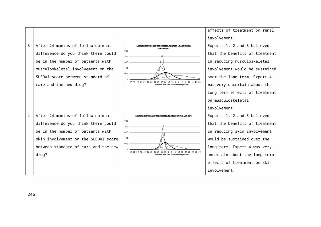
10 REFERENCES

(1) U S Food and Drug Administration 2013Available from: URL: http://www.fda.gov/

(2) What we do. European Medicines Agency 2013Available from: URL: http://www.ema.europa.eu/ema/index.jsp?curl=pages/about_us/general/general_content_000091.jsp&mid=WC0b01ac0580028a42

(3) US Food and Drug Administration. Guidance for Industry Q8(R2) Pharmaceutical Development. 2004.

(4) European Commission. European Commission Directive 2001/20/EC. Clinical trial directive. Brussels, Belgium; 2013.

(5) Gress S, Niebuhr D, May U, Wasem J. Reform of prescription drug reimbursement and pricing in the German social health insurance market: a comparison of three scenarios. Pharmacoeconomics 2007;25(6):443-54.

(6) National Institute for Health and Clinical Excellenc 2013Available from: URL: http://www.nice.org.uk/

(7) National Institute for Health and Clinical Excellence. Updated prioritisation criteria for referral of Technology Appraisal topics to NICE . Centre for Health Technology Evaluation ; 2010.

(8) Peters CP. Fundamentals of the prescription drug market. Washington DC.: National Health Policy Forum; 2004.

(9) The FDA's Drug Review Process: Ensuring Drugs Are Safe and Effective: Stages of Drug Development and Review. US Food and Drug Administration 2012Available from: URL: http://www.fda.gov/drugs/resourcesforyou/consumers/ucm143534.htm )

(10) Spiegelhalter DJ, Abrams KR, Myles JP. Bayesian Approaches to Clinical Trials and Health Care Evaluation. Chicester: John Wiley and Sons Ltd.; 2004.

(11) Luce BR, Shih YC, Claxton K. Introduction. Bayesian approaches to technology assessment and decision making. Int J Technol Assess Health Care 2001;17(1):1-5.

(12) O'Hagan A, Luce BR. A Primer on Bayesian Statistics in Health Economics. Sheffield: Centre for Bayesian Statistics in Health Economics; 2003.

(13) Claxton K, Sculpher M, McCabe C, Briggs A, Akehurst R, Buxton M, et al. Probabilistic sensitivity analysis for NICE technology assessment: not an optional extra. Health Econ 2005 Apr;14(4):339-47.

(14) WInBUGS User Manual: Version1.4. Cambridge, UK: MRC Biostatistics Unit [computer program]. 2001.

(15) Parmigiani G. Modeling in Medical Decision Making: a Bayesian Approach. Chichester: 2002.

(16) Briggs AH. Handling uncertainty in cost-effectiveness models. Pharmacoeconomics 2000 May;17(5):479-500.

(17) Palmer S, Raftery J. Economic Notes: opportunity cost. BMJ 1999 Jun 5;318(7197):1551-2.

(18) Culyer AJ. The Economics of health care finance and provision. Oxford Review of Economic Policy 1989;5(1):34-58.

(19) Drummond MF, Sculpher M, Torrance GW, O'Brien BJ, Stoddart GL. Methods for the Economic Evaluation of Health Care Programmes. Third Edition ed. Oxford: Oxford University Press; 2005.

(20) Morris S, Devlin N, Parkin D. Economic Analysis in Health Care. Chichester: John Wiley and Sons; 2009.

250

(21) Sen A. Social choice theory; a re-examination. Econometrica 1977;45(1):53-89.

(22) Briggs A, Sculpher M, Claxton K. Decision Modelling for Health Economic Evaluation. first edition ed. Oxford: Oxford University Press; 2006.

(23) Brouwer WB, Koopmanschap MA. On the economic foundations of CEA. Ladies and gentlemen, take your positions! J Health Econ 2000 Jul;19(4):439-59.

(24) McCabe C, Claxton K, Culyer AJ. The NICE cost-effectiveness threshold: what it is and what that means. Pharmacoeconomics 2008;26(9):733-44.

(25) Birch S, Gafni A. Cost effectiveness/utility analyses. Do current decision rules lead us to where we want to be? J Health Econ 1992 Oct;11(3):279-96.

(26) Coast J, Smith RD, Lorgelly P. Welfarism, extra-welfarism and capability: the spread of ideas in health economics. Soc Sci Med 2008 Oct;67(7):1190-8.

(27) Devlin N, Parkin D. Does NICE have a cost-effectiveness threshold and what other factors influence its decisions? A binary choice analysis. Health Econ 2004 May;13(5):437-52.

(28) Buxton MJ, Drummond MF, Van Hout BA, Prince RL, Sheldon TA, Szucs T, et al. Modelling in economic evaluation: an unavoidable fact of life. Health Econ 1997 May;6(3):217-27.

(29) National Institute for Health and Care Excellence. Guide to the methods of technology appraisal 2013. London: National Institute for Health and Care Excellence; 2013.

(30) Brennan A, Chick SE, Davies R. A taxonomy of model structures for economic evaluation of health technologies. Health Econ 2006 Dec;15(12):1295-310.

(31) Briggs AH. A Bayesian approach to stochastic cost-effectiveness analysis. Health Econ 1999 May;8(3):257-61.

(32) Sonnenberg FA, Beck JR. Markov models in medical decision making: a practical guide. Med Decis Making 1993 Oct;13(4):322-38.

(33) Claxton K, Posnett J. An economic approach to clinical trial design and research priority-setting. Health Econ 1996 Nov;5(6):513-24.

(34) Dimasi JA. Risks in new drug development: approval success rates for investigational drugs. Clin Pharmacol Ther 2001 May;69(5):297-307.

(35) Drenkard C, Villa AR, Garcia-Padilla C, Perez-Vazquez ME, Alarcon-Segovia D. Remission of systematic lupus erythematosus. Medicine (Baltimore) 1996 Mar;75(2):88-98.

(36) Petri M. Lupus in Baltimore: evidence-based 'clinical pearls' from the Hopkins Lupus Cohort. Lupus 2005;14(12):970-3.

(37) Ardoin SP, Pisetsky DS. Developments in the scientific understanding of lupus. Arthritis Res Ther 2008;10(5):218.

(38) Mason JA, Bossingham D. The clinical characterisation of systemic lupus erythematosus in a Far North Queensland Indigenous kindred. Lupus 2009 Feb;18(2):144-8.

(39) Johnson AE, Gordon C, Palmer RG, Bacon PA. The prevalence and incidence of systemic lupus erythematosus in Birmingham, England. Relationship to ethnicity and country of birth. Arthritis Rheum 1995 Apr;38(4):551-8.

(40) Siegel M, Lee SL. The epidemiology of systemic lupus erythematosus. Semin Arthritis Rheum 1973;3(1):1-54.

(41) Danchenko N, Satia JA, Anthony MS. Epidemiology of systemic lupus erythematosus: a comparison of worldwide disease burden. Lupus 2006;15(5):308-18.

251

(42) Cervera R, Khamashta MA, Hughes GR. The Euro-lupus project: epidemiology of systemic lupus erythematosus in Europe. Lupus 2009 Sep;18(10):869-74.

(43) Reveille JD, Moulds JM, Ahn C, Friedman AW, Baethge B, Roseman J, et al. Systemic lupus erythematosus in three ethnic groups: I. The effects of HLA class II, C4, and CR1 alleles, socioeconomic factors, and ethnicity at disease onset. LUMINA Study Group. Lupus in minority populations, nature versus nurture. Arthritis Rheum 1998 Jul;41(7):1161-72.

(44) Hochberg MC. Updating the American College of Rheumatology revised criteria for the classification of systemic lupus erythematosus. Arthritis Rheum 1997 Sep;40(9):1725.

(45) Jacobsen S, Petersen J, Ullman S, Junker P, Voss A, Rasmussen JM, et al. A multicentre study of 513 Danish patients with systemic lupus erythematosus. I. Disease manifestations and analyses of clinical subsets. Clin Rheumatol 1998;17(6):468-77.

(46) Griffiths B, Mosca M, Gordon C. Assessment of patients with systemic lupus erythematosus and the use of lupus disease activity indices. Best Pract Res Clin Rheumatol 2005 Oct;19(5):685-708.

(47) Petri M, Kim MY, Kalunian KC, Grossman J, Hahn BH, Sammaritano LR, et al. Combined oral contraceptives in women with systemic lupus erythematosus. N Engl J Med 2005 Dec 15;353(24):2550-8.

(48) Gladman DD, Ibanez D, Urowitz MB. Systemic lupus erythematosus disease activity index 2000. J Rheumatol 2002 Feb;29(2):288-91.

(49) Isenberg DA, Rahman A, Allen E, Farewell V, Akil M, Bruce IN, et al. BILAG 2004. Development and initial validation of an updated version of the British Isles Lupus Assessment Group's disease activity index for patients with systemic lupus erythematosus. Rheumatology (Oxford) 2005 Jul;44(7):902-6.

(50) Isenberg DA. BILAG, SLEDAI, SIS, ECLAM, WAM, SLAM .... thank you MAM. Lupus 2007;16(11):849-51.

(51) Gladman DD, Goldsmith CH, Urowitz MB, Bacon P, Fortin P, Ginzler E, et al. The Systemic Lupus International Collaborating Clinics/American College of Rheumatology (SLICC/ACR) Damage Index for Systemic Lupus Erythematosus International Comparison. J Rheumatol 2000 Feb;27(2):373-6.

(52) Gladman D, Ginzler E, Goldsmith C, Fortin P, Liang M, Urowitz M, et al. The development and initial validation of the Systemic Lupus International Collaborating Clinics/American College of Rheumatology damage index for systemic lupus erythematosus. Arthritis Rheum 1996 Mar;39(3):363-9.

(53) Gladman DD, Urowitz MB, Goldsmith CH, Fortin P, Ginzler E, Gordon C, et al. The reliability of the Systemic Lupus International Collaborating Clinics/American College of Rheumatology Damage Index in patients with systemic lupus erythematosus. Arthritis Rheum 1997 May;40(5):809-13.

(54) Dayal NA, Gordon C, Tucker L, Isenberg DA. The SLICC damage index: past, present and future. Lupus 2002;11(4):261-5.

(55) Bertsias G, Ioannidis JP, Boletis J, Bombardieri S, Cervera R, Dostal C, et al. EULAR recommendations for the management of systemic lupus erythematosus. Report of a Task Force of the EULAR Standing Committee for International Clinical Studies Including Therapeutics. Ann Rheum Dis 2008 Feb;67(2):195-205.

(56) Murray E, Perry M. Off-label use of rituximab in systemic lupus erythematosus: a systematic review. Clin Rheumatol 2010 Feb 13.

(57) Kang I, Park SH. Infectious complications in SLE after immunosuppressive therapies. Curr Opin Rheumatol 2003 Sep;15(5):528-34.

(58) Eisenberg R. Why can't we find a new treatment for SLE? J Autoimmun 2009 May;32(3-4):223-30.

252

(59) Sousa E, Isenberg D. Treating lupus: from serendipity to sense, the rise of the new biologicals and other emerging therapies. Best Pract Res Clin Rheumatol 2009 Aug;23(4):563-74.

(60) Sousa E, Isenberg D. Treating lupus: from serendipity to sense, the rise of the new biologicals and other emerging therapies. Best Pract Res Clin Rheumatol 2009 Aug;23(4):563-74.

(61) Merrill JT, et al. Activity of Abatacept in SLE: Results of a 12 month Phase II Exploratory Study. Ann Rheum Dis 2009 68(suppl3):70 . 2009. Ref Type: Abstract

(62) Merrill JT, Neuwelt CM, Wallace DJ, Shanahan JC, Latinis KM, Oates JC, et al. Efficacy and safety of rituximab in moderately-to-severely active systemic lupus erythematosus: the randomized, double-blind, phase II/III systemic lupus erythematosus evaluation of rituximab trial. Arthritis Rheum 2010 Jan;62(1):222-33.

(63) Nixon RM, O'Hagan A, Oakley J, Madan J, Stevens JW, Bansback N, et al. The Rheumatoid Arthritis Drug Development Model: a case study in Bayesian clinical trial simulation. Pharm Stat 2009 Oct;8(4):371-89.

(64) Hackshaw KV, Shi Y, Brandwein SR, Jones K, Westcott JY. A pilot study of zileuton, a novel selective 5-lipoxygenase inhibitor, in patients with systemic lupus-erythematosus. Journal of Rheumatology 1994; 22(3)(pp 462-468), 1995;1995.

(65) Carneiro JRM, Sato EI. Double blind, randomized, placebo controlled clinical trial of methotrexate in systemic lupus erythematosus. Journal of Rheumatology 1994; 26(6)(pp 1275-1279), 1999;1999.

(66) Kalunian KC, Davis JC, Jr., Merrill JT, Totoritis MC, Wofsy D. Treatment of systemic lupus erythematosus by inhibition of T cell costimulation with anti-CD154: a randomized, double-blind, placebo-controlled trial. Arthritis Rheum 2002 Dec;46(12):3251-8.

(67) Petri MA, Mease PJ, Merrill JT, Lahita RG, Iannini MJ, Yocum DE, et al. Effects of prasterone on disease activity and symptoms in women with active systemic lupus erythematosus. Arthritis Rheum 2004 Sep;50(9):2858-68.

(68) Tam L-S, Li EK, Wong C-K, Lam CWK, Szeto C-C. Double-blind, randomized, placebo-controlled pilot study of leflunomide in systemic lupus erythematosus. Lupus 1994; 13(8)(pp 601-604), 2004;2004.

(69) Fortin PR, Abrahamowicz M, Ferland D, Lacaille D, Smith CD, Zummer M. Steroid-sparing effects of methotrexate in systemic lupus erythematosus: A double-blind, randomized, placebo-controlled trial. Arthritis Care and Research 1994; 59(12)(pp 1796-1804), 2008;15.

(70) Abdou NI, Rider V, Greenwell C, Li X, Kimler BF. Fulvestrant (Faslodex), an estrogen selective receptor downregulator, in therapy of women with systemic lupus erythematosus. clinical, serologic, bone density, and T cell activation marker studies: a double-blind placebo-controlled trial. J Rheumatol 2008 May;35(5):797.

(71) Uppal SS, Hayat SJ, Raghupathy R. Efficacy and safety of infliximab in active SLE: a pilot study. Lupus 2009 Jul;18(8):690-7.

(72) Wallace DJ, Stohl W, Furie RA, Lisse JR, McKay JD, Merrill JT, et al. A phase II, randomized, double-blind, placebo-controlled, dose-ranging study of belimumab in patients with active systemic lupus erythematosus. Arthritis Rheum 2009 Sep 15;61(9):1168-78.

(73) Furie RA, Petri MA, Wallace DJ, Ginzler EM, Merrill JT, Stohl W, et al. Novel evidence-based systemic lupus erythematosus responder index. Arthritis Rheum 2009 Sep 15;61(9):1143-51.

(74) Navarra SV, Guzman RM, Gallacher AE, Hall S, Levy RA, Jimenez RE, et al. Efficacy and safety of belimumab in patients with active systemic lupus erythematosus: a randomised, placebo-controlled, phase 3 trial. Lancet 2011 Feb 26;377(9767):721-31.

253

(75) Furie R, Petri M, Zamani O, Cervera R, Wallace DJ, Tegzova D, et al. A phase III, randomized, placebo-controlled study of belimumab, a monoclonal antibody that inhibits B lymphocyte stimulator, in patients with systemic lupus erythematosus. Arthritis Rheum 2011 Dec;63(12):3918-30.

(76) Merrill JT, Wallace DJ, Petri M, Kirou KA, Yao Y, White WI, et al. Safety profile and clinical activity of sifalimumab, a fully human anti-interferon alpha monoclonal antibody, in systemic lupus erythematosus: a phase I, multicentre, double-blind randomised study. Ann Rheum Dis 2011 Nov;70(11):1905-13.

(77) Bertsias G, Gordon C, Boumpas DT. Clinical trials in systemic lupus erythematosus (SLE): lessons from the past as we proceed to the future--the EULAR recommendations for the management of SLE and the use of end-points in clinical trials. Lupus 2008;17(5):437-42.

(78) Strand V, Gladman D, Isenberg D, Petri M, Smolen J, Tugwell P. Endpoints: consensus recommendations from OMERACT IV. Outcome Measures in Rheumatology. Lupus 2000;9(5):322-7.

(79) Bertsias GK, Ioannidis JP, Boletis J, Bombardieri S, Cervera R, Dostal C, et al. EULAR points to consider for conducting clinical trials in systemic lupus erythematosus: literature based evidence for the selection of endpoints. Ann Rheum Dis 2009 Apr;68(4):477-83.

(80) American College of Rheumatology. The American College of Rheumatology response criteria for systemic lupus erythematosus clinical trials: measures of overall disease activity. Arthritis Rheum 2004 Nov;50(11):3418-26.

(81) US Department of Health and Human Services Food and Drug Administration. Guidance for Industry: Systemic Lupus Erythematosus - Developing Drugs for Treatment. 2010.

(82) Concept paper on the need for a guideline on the clinical investigation of medical products intended for treatment of systemic and cutaneous lupus erythematosus. European Medicines Agency 2009Available from: URL: http://www.ema.europa.eu/pdfs/human/ewp/60404009en.pdf

(83) Gordon C, Bertsias G, Ioannidis JP, Boletis J, Bombardieri S, Cervera R, et al. EULAR points to consider for conducting clinical trials in systemic lupus erythematosus. Ann Rheum Dis 2009 Apr;68(4):470-6.

(84) American College of Rheumatology. The American College of Rheumatology response criteria for proliferative and membranous renal disease in systemic lupus erythematosus clinical trials. Arthritis Rheum 2006 Feb;54(2):421-32.

(85) Li EK, Tam LS, Zhu TY, Li M, Kwok CL, Li TK, et al. Is combination rituximab with cyclophosphamide better than rituximab alone in the treatment of lupus nephritis? Rheumatology (Oxford) 2009 Aug;48(8):892-8.

(86) Navarra S, et al. Belimumab, a BLyS-Specific Inhibitor, Reduced Disease Activity, Flares and Prednisone Use in PAtients with Active SLE: Efficacy and Safety Results From the Phase 3 BLISS-52 Study. Arthritis and Rheumatism 2009 (S10):60 . 2010. Ref Type: Abstract

(87) Brunner HI, Klein-Gitelman MS, Ying J, Tucker LB, Silverman ED. Corticosteroid use in childhood-onset systemic lupus erythematosus-practice patterns at four pediatric rheumatology centers. Clin Exp Rheumatol 2009 Jan;27(1):155-62.

(88) ICH. The Extent of Population Exposure to Assess Clinical Safety for Drugs Intended for Long-Term Treatment of Non-Life Threatening Conditions. http://www ich org/products/guidelines/efficacy/efficacy-single/article/the-extent-of-population-exposure-to-assess-clinical-safety-for-drugs-intended-for-long-term-treatme html 2012Available from: URL: http://www.ich.org/products/guidelines/efficacy/efficacy-single/article/the-extent-of-population-exposure-to-assess-clinical-safety-for-drugs-intended-for-long-term-treatme.html

(89) Chilcott J, Brennan A, Booth A, Karnon J, Tappenden P. The role of modelling in prioritising and planning clinical trials. Health Technol Assess 2003;7(23):iii, 1-iii125.

254

(90) Claxton K, Neumann PJ, Araki S, Weinstein MC. Bayesian value-of-information analysis. An application to a policy model of Alzheimer's disease. Int J Technol Assess Health Care 2001;17(1):38-55.

(91) Eckermann S, Karnon J, Willan AR. The value of value of information: best informing research design and prioritization using current methods. Pharmacoeconomics 2010;28(9):699-709.

(92) Spiegelhalter DJ, Myles JP, Jones DR, Abrams KR. Bayesian methods in health technology assessment: a review. Health Technol Assess 2000;4(38):1-130.

(93) Web of Knowledge 2013Available from: URL: http://apps.webofknowledge.com/UA_GeneralSearch_input.do?product=UA&search_mode=GeneralSearch&SID=W1OdbeobKOEanf4EaMp&preferencesSaved=

(94) Claxton K. The irrelevance of inference: a decision-making approach to the stochastic evaluation of health care technologies. Journal of Health Economics 1999;18(3):341-64.

(95) Thompson MS. Decision-analytic determination of study size. The case of electronic fetal monitoring. Med Decis Making 1981;1(2):165-79.

(96) Halpern J, Brown BW, Hornberger J. The sample size for a clinical trial: A Bayesian-decision theoretic approach. Statistics in Medicine 2001;20(6):841-58.

(97) Koerkamp BG, Nikken JJ, Oei EH, Stijnen T, Ginai AZ, Hunink M. Value of information analysis used to determine the necessity of additional research: MR imaging in acute knee trauma as an example. Radiology 2008;246(2):420-5.

(98) Koerkamp BG, Spronk S, Stijnen T, Hunink M. Value of Information Analyses of Economic Randomized Controlled Trials: The Treatment of Intermittent Claudication. Value in Health 2010;13(2):242-50.

(99) Claxton K, Thompson KM. A dynamic programming approach to the efficient design of clinical trials. Journal of Health Economics 2001;20(5):797-822.

(100) Willan AR, Pinto EM. The value of information and optimal clinical trial design. Statistics in Medicine 2005;24(12):1791-806.

(101) Willan AR. Clinical decision making and the expected value of information. Clinical Trials 2007;4(3):279-85.

(102) Willan A, Kowgier M. Determining optimal sample sizes for multi-stage randomized clinical trials using value of information methods. Clinical Trials 2008;5(4):289-300.

(103) Eckermann S, Willan AR. The option value of delay in health technology assessment. Medical Decision Making 2008;28(3):300-5.

(104) Eckermann S, Willan AR. Globally Optimal Trial Design for Local Decision Making. Health Economics 2009;18(2):203-16.

(105) Willan AR, Eckermann S. Optimal Clinical Trial Design Using Value of Information Methods with Imperfect Implementation. Health Economics 2010;19(5):549-61.

(106) Eckermann S, Willan AR. Expected value of information and decision making in HTA. Health Economics 2007;16(2):195-209.

(107) Eckermann S, Willan AR. Time and expected value of sample information wait for no patient. Value in Health 2008;11(3):522-6.

(108) Ades AE, Lu G, Claxton K. Expected value of sample information calculations in medical decision modeling. Medical Decision Making 2004;24(2):207-27.

255

(109) Conti S, Claxton K. Dimensions of Design Space: A Decision-Theoretic Approach to Optimal Research Design. Medical Decision Making 2009;29(6):643-60.

(110) Stevenson M, Lloyd-Jones M, Papaioannou D. Vitamin K to prevent fractures in older women: systematic review and economic evaluation. Health Technology Assessment 2009;13(45):1-+.

(111) Stevenson MD, Oakley JE, Jones ML, Brennan A, Compston JE, McCloskey EV, et al. The Cost-Effectiveness of an RCT to Establish Whether 5 or 10 Years of Bisphosphonate Treatment Is the Better Duration for Women With a Prior Fracture. Medical Decision Making 2009;29(6):678-89.

(112) McKenna C, Claxton K. Addressing Adoption and Research Design Decisions Simultaneously: The Role of Value of Sample Information Analysis. Medical Decision Making 2011;31(6):853-65.

(113) Stevenson MD, Jones ML. The Cost Effectiveness of a Randomized Controlled Trial to Establish the Relative Efficacy of Vitamin K(1) Compared with Alendronate. Medical Decision Making 2011;31(1):43-52.

(114) Kharroubi SA, Brennan A, Strong M. Estimating Expected Value of Sample Information for Incomplete Data Models Using Bayesian Approximation. Medical Decision Making 2011;31(6):839-52.

(115) Brennan A, Kharroubi SA. Expected value of sample information for Weibull survival data. Health Economics 2007;16(11):1205-25.

(116) Brennan A, Kharroubi SA. Efficient computation of partial expected value of sample information using Bayesian approximation. Journal of Health Economics 2007;26(1):122-48.

(117) Shavit O, Leshno M, Goldberger A, Shmueli A, Hoffman A. It's time to choose the study design! Net benefit analysis of alternative study designs to acquire information for evaluation of health technologies. Pharmacoeconomics 2007;25(11):903-11.

(118) Kikuchi T, Gittins J. A behavioral Bayes method to determine the sample size of a clinical trial considering efficacy and safety. Statistics in Medicine 2009;28(18):2293-306.

(119) Kikuchi T, Gittins J. A behavioural Bayes approach to the determination of sample size for clinical trials considering efficacy and safety: imbalanced sample size in treatment groups. Stat Methods Med Res 2011 Aug;20(4):389-400.

(120) Kikuchi T, Gittins J. A behavioural Bayes approach for sample size determination in cluster randomized clinical trials. Journal of the Royal Statistical Society Series C-Applied Statistics 2010;59:875-88.

(121) Kikuchi T, Pezeshk H, Gittins J. A Bayesian cost-benefit approach to the determination of sample size in clinical trials. Stat Med 2008 Jan 15;27(1):68-82.

(122) Willan AR. Optimal sample size determinations from an industry perspective based on the expected value of information. Clinical Trials 2008;5(6):587-94.

(123) Pezeshk H, Gittins J. A fully Bayesian Approach to Calculating Sample Sizes for Clinical Trials with Binary Responses. Drug Information Journal 2002;36:143-50.

(124) Gittins J, Pezeshk H. How large should a trial be? Journal of the Royal Statistical Society Seies D 2000;49(2):177-87.

(125) Gittins J, Pezeshk H. A behavioral bayes method for determining the size of a clinical trial. Drug Information Journal 2000;34(2):355-63.

(126) O'Hagan A, Stevens J, Campbell M. Assurance in Clinical Trial Design. Pharmaceutical Statistics 2005;4:187-204.

(127) Girling AJ, Lilford RJ, Braunholtz DA, Gillett WR. Sample-size calculations for trials that inform individual treatment decisions: a 'true-choice' approach. Clinical Trials 2007;4(1):15-24.

256

(128) Patel M, Clarke AM, Bruce IN, Symmons DP. The prevalence and incidence of biopsy-proven lupus nephritis in the UK: Evidence of an ethnic gradient. Arthritis Rheum 2006 Sep;54(9):2963-9.

(129) Willan AR, Eckermann S. Value of information and pricing new healthcare interventions. Pharmacoeconomics 2012 Jun 1;30(6):447-59.

(130) Chen MH, Willan AR. Determining optimal sample sizes for multistage adaptive randomized clinical trials from an industry perspective using value of information methods. Clin Trials 2013 Feb;10(1):54-62.

(131) Bojke L, Claxton K, Bravo-Vergel Y, Sculpher M, Palmer S, Abrams K. Eliciting distributions to populate decision analytic models. Value Health 2010 Aug;13(5):557-64.

(132) Bombardier C, Gladman DD, Urowitz MB, Caron D, Chang CH. Derivation of the SLEDAI. A disease activity index for lupus patients. The Committee on Prognosis Studies in SLE. Arthritis Rheum 1992 Jun;35(6):630-40.

(133) Hay EM, Bacon PA, Gordon C, Isenberg DA, Maddison P, Snaith ML, et al. The BILAG index: a reliable and valid instrument for measuring clinical disease activity in systemic lupus erythematosus. Q J Med 1993 Jul;86(7):447-58.

(134) Ruiz-Irastorza G, Ramos-Casals M, Brito-Zeron P, Khamashta MA. Clinical efficacy and side effects of antimalarials in systemic lupus erythematosus: a systematic review. Ann Rheum Dis 2010 Jan;69(1):20-8.

(135) Ehrenstein MR, Conroy SE, Heath J, Latchman DS, Isenberg DA. The occurrence, nature and distribution of flares in a cohort of patients with systemic lupus erythematosus: a rheumatological view. Br J Rheumatol 1995 Mar;34(3):257-60.

(136) Swaak AJ, van den Brink HG, Smeenk RJ, Manger K, Kalden JR, Tosi S, et al. Systemic lupus erythematosus. Disease outcome in patients with a disease duration of at least 10 years: second evaluation. Lupus 2001;10(1):51-8.

(137) Bujan S, Ordi-Ros J, Paredes J, Mauri M, Matas L, Cortes J, et al. Contribution of the initial features of systemic lupus erythematosus to the clinical evolution and survival of a cohort of Mediterranean patients. Ann Rheum Dis 2003 Sep;62(9):859-65.

(138) Allen E, Farewell VT, Isenberg DA, Gordon C. A statistical analysis of the interrelationships between disease activity in different systems in systemic lupus erythematosus. Rheumatology (Oxford) 2006 Mar;45(3):308-13.

(139) Bertoli AM, Alarcon GS, McGwin G, Jr., Fernandez M, Bastian HM, Fessler BJ, et al. Systemic lupus erythematosus in a multiethnic U.S. cohort (LUMINA) XXVII: factors predictive of a decline to low levels of disease activity. Lupus 2006;15(1):13-8.

(140) Nikpour M, Urowitz MB, Ibanez D, Gladman DD. Frequency and determinants of flare and persistently active disease in systemic lupus erythematosus. Arthritis Rheum 2009 Sep 15;61(9):1152-8.

(141) Barr SG, Zonana-Nacach A, Magder LS, Petri M. Patterns of disease activity in systemic lupus erythematosus. Arthritis Rheum 1999 Dec;42(12):2682-8.

(142) Ibanez D, Urowitz MB, Gladman DD. Summarizing disease features over time: I. Adjusted mean SLEDAI derivation and application to an index of disease activity in lupus. J Rheumatol 2003 Sep;30(9):1977-82.

(143) Ibanez D, Gladman D, Urowitz M. Summarizing disease features over time: II. Variability measures of SLEDAI-2K. J Rheumatol 2007 Feb;34(2):336-40.

(144) Bernatsky S, Boivin JF, Joseph L, Manzi S, Ginzler E, Gladman DD, et al. Mortality in systemic lupus erythematosus. Arthritis Rheum 2006 Aug;54(8):2550-7.

257

(145) Manger K, Manger B, Repp R, Geisselbrecht M, Geiger A, Pfahlberg A, et al. Definition of risk factors for death, end stage renal disease, and thromboembolic events in a monocentric cohort of 338 patients with systemic lupus erythematosus. Ann Rheum Dis 2002 Dec;61(12):1065-70.

(146) Urowitz MB, Gladman DD, Tom BD, Ibanez D, Farewell VT. Changing patterns in mortality and disease outcomes for patients with systemic lupus erythematosus. J Rheumatol 2008 Nov;35(11):2152-8.

(147) Abu-Shakra M, Urowitz MB, Gladman DD, Gough J. Mortality studies in systemic lupus erythematosus. Results from a single center. II. Predictor variables for mortality. J Rheumatol 1995 Jul;22(7):1265-70.

(148) Ward MM, Pyun E, Studenski S. Long-term survival in systemic lupus erythematosus. Patient characteristics associated with poorer outcomes. Arthritis Rheum 1995 Feb;38(2):274-83.

(149) Xie SK, Feng SF, Fu H. Long term follow-up of patients with systemic lupus erythematosus. J Dermatol 1998 Jun;25(6):367-73.

(150) Urowitz MB, Gladman DD, bu-Shakra M, Farewell VT. Mortality studies in systemic lupus erythematosus. Results from a single center. III. Improved survival over 24 years. J Rheumatol 1997 Jun;24(6):1061-5.

(151) Campbell R, Jr., Cooper GS, Gilkeson GS. Two aspects of the clinical and humanistic burden of systemic lupus erythematosus: mortality risk and quality of life early in the course of disease. Arthritis Rheum 2008 Apr 15;59(4):458-64.

(152) Doria A, Iaccarino L, Ghirardello A, Zampieri S, Arienti S, Sarzi-Puttini P, et al. Long-term prognosis and causes of death in systemic lupus erythematosus. Am J Med 2006 Aug;119(8):700-6.

(153) Kasitanon N, Magder LS, Petri M. Predictors of survival in systemic lupus erythematosus. Medicine (Baltimore) 2006 May;85(3):147-56.

(154) Ruiz-Irastorza G, Egurbide MV, Ugalde J, Aguirre C. High impact of antiphospholipid syndrome on irreversible organ damage and survival of patients with systemic lupus erythematosus. Arch Intern Med 2004 Jan 12;164(1):77-82.

(155) Cervera R, Khamashta MA, Font J, Sebastiani GD, Gil A, Lavilla P, et al. Morbidity and mortality in systemic lupus erythematosus during a 10-year period: a comparison of early and late manifestations in a cohort of 1,000 patients. Medicine (Baltimore) 2003 Sep;82(5):299-308.

(156) Nived O, Jonsen A, Bengtsson AA, Bengtsson C, Sturfelt G. High predictive value of the Systemic Lupus International Collaborating Clinics/American College of Rheumatology damage index for survival in systemic lupus erythematosus. J Rheumatol 2002 Jul;29(7):1398-400.

(157) Kasitanon N, Louthrenoo W, Sukitawut W, Vichainun R. Causes of death and prognostic factors in Thai patients with systemic lupus erythematosus. Asian Pac J Allergy Immunol 2002 Jun;20(2):85-91.

(158) Alarcon GS, McGwin G, Jr., Bastian HM, Roseman J, Lisse J, Fessler BJ, et al. Systemic lupus erythematosus in three ethnic groups. VII [correction of VIII]. Predictors of early mortality in the LUMINA cohort. LUMINA Study Group. Arthritis Rheum 2001 Apr;45(2):191-202.

(159) Rahman P, Gladman DD, Urowitz MB, Hallett D, Tam LS. Early damage as measured by the SLICC/ACR damage index is a predictor of mortality in systemic lupus erythematosus. Lupus 2001;10(2):93-6.

(160) Mok CC, Lee KW, Ho CT, Lau CS, Wong RW. A prospective study of survival and prognostic indicators of systemic lupus erythematosus in a southern Chinese population. Rheumatology (Oxford) 2000 Apr;39(4):399-406.

(161) Cervera R, Khamashta MA, Font J, Sebastiani GD, Gil A, Lavilla P, et al. Morbidity and mortality in systemic lupus erythematosus during a 5-year period. A multicenter prospective study of 1,000 patients. European Working Party on Systemic Lupus Erythematosus. Medicine (Baltimore) 1999 May;78(3):167-75.

258

(162) Becker-Merok A, Nossent HC. Damage accumulation in systemic lupus erythematosus and its relation to disease activity and mortality. J Rheumatol 2006 Aug;33(8):1570-7.

(163) Fernandez M, Alarcon GS, McGwin G, Jr., Sanchez ML, Apte M, Vila LM, et al. Using the Short Form 6D, as an overall measure of health, to predict damage accrual and mortality in patients with systemic lupus erythematosus: XLVII, results from a multiethnic US cohort. Arthritis Rheum 2007 Aug 15;57(6):986-92.

(164) Cook RJ, Gladman DD, Pericak D, Urowitz MB. Prediction of short term mortality in systemic lupus erythematosus with time dependent measures of disease activity. J Rheumatol 2000 Aug;27(8):1892-5.

(165) Ward MM, Pyun E, Studenski S. Mortality risks associated with specific clinical manifestations of systemic lupus erythematosus. Arch Intern Med 1996 Jun 24;156(12):1337-44.

(166) Cardoso CR, Signorelli FV, Papi JA, Salles GF. Initial and accrued damage as predictors of mortality in Brazilian patients with systemic lupus erythematosus: a cohort study. Lupus 2008 Nov;17(11):1042-8.

(167) Chambers SA, Allen E, Rahman A, Isenberg D. Damage and mortality in a group of British patients with systemic lupus erythematosus followed up for over 10 years. Rheumatology (Oxford) 2009 Jun;48(6):673-5.

(168) Fernandez M, Alarcon GS, Calvo-Alen J, Andrade R, McGwin G, Jr., Vila LM, et al. A multiethnic, multicenter cohort of patients with systemic lupus erythematosus (SLE) as a model for the study of ethnic disparities in SLE. Arthritis Rheum 2007 May 15;57(4):576-84.

(169) Gladman DD, Urowitz MB, Rahman P, Ibanez D, Tam LS. Accrual of organ damage over time in patients with systemic lupus erythematosus. J Rheumatol 2003 Sep;30(9):1955-9.

(170) Petri M. Musculoskeletal complications of systemic lupus erythematosus in the Hopkins Lupus Cohort: an update. Arthritis Care Res 1995 Sep;8(3):137-45.

(171) Alarcon GS, Roseman JM, McGwin G, Jr., Uribe A, Bastian HM, Fessler BJ, et al. Systemic lupus erythematosus in three ethnic groups. XX. Damage as a predictor of further damage. Rheumatology (Oxford) 2004 Feb;43(2):202-5.

(172) Stoll T, Sutcliffe N, Mach J, Klaghofer R, Isenberg DA. Analysis of the relationship between disease activity and damage in patients with systemic lupus erythematosus--a 5-yr prospective study. Rheumatology (Oxford) 2004 Aug;43(8):1039-44.

(173) Toloza SM, Roseman JM, Alarcon GS, McGwin G, Jr., Uribe AG, Fessler BJ, et al. Systemic lupus erythematosus in a multiethnic US cohort (LUMINA): XXII. Predictors of time to the occurrence of initial damage. Arthritis Rheum 2004 Oct;50(10):3177-86.

(174) Santos MJ, Vinagre F, Nero P, Barcelos F, Barcelos A, Rodrigues AM, et al. Predictors of damage progression in Portuguese patients with systemic lupus erythematosus. Ann N Y Acad Sci 2009 Sep;1173:822-8.:822-8.

(175) Thamer M, Hernan MA, Zhang Y, Cotter D, Petri M. Prednisone, lupus activity, and permanent organ damage. J Rheumatol 2009 Mar;36(3):560-4.

(176) Ibanez D, Gladman DD, Urowitz MB. Adjusted mean Systemic Lupus Erythematosus Disease Activity Index-2K is a predictor of outcome in SLE. J Rheumatol 2005 May;32(5):824-7.

(177) Gilboe IM, Kvien TK, Husby G. Disease course in systemic lupus erythematosus: changes in health status, disease activity, and organ damage after 2 years. J Rheumatol 2001 Feb;28(2):266-74.

(178) Mok CC, Ho CT, Wong RW, Lau CS. Damage accrual in southern Chinese patients with systemic lupus erythematosus. J Rheumatol 2003 Jul;30(7):1513-9.

(179) Stoll T, Sutcliffe N, Klaghofer R, Isenberg DA. Do present damage and health perception in patients with systemic lupus erythematosus predict extent of future damage?: a prospective study. Ann Rheum Dis 2000 Oct;59(10):832-5.

259

(180) Apte M, McGwin G, Jr., Vila LM, Kaslow RA, Alarcon GS, Reveille JD. Associated factors and impact of myocarditis in patients with SLE from LUMINA, a multiethnic US cohort (LV). [corrected]. Rheumatology (Oxford) 2008 Mar;47(3):362-7.

(181) Zonana-Nacach A, Barr SG, Magder LS, Petri M. Damage in systemic lupus erythematosus and its association with corticosteroids. Arthritis Rheum 2000 Aug;43(8):1801-8.

(182) Appenzeller S, Pereira DA, Costallat LT. Greater accrual damage in late-onset systemic lupus erythematosus: a long-term follow-up study. Lupus 2008 Nov;17(11):1023-8.

(183) Guarize J, Appenzeller S, Costallat LT. Skin damage occurs early in systemic lupus erythematosus and independently of disease duration in Brazilian patients. Rheumatol Int 2007 Mar;27(5):483-7.

(184) Mikdashi J, Handwerger B. Predictors of neuropsychiatric damage in systemic lupus erythematosus: data from the Maryland lupus cohort. Rheumatology (Oxford) 2004 Dec;43(12):1555-60.

(185) Mok CC, To CH, Mak A. Neuropsychiatric damage in Southern Chinese patients with systemic lupus erythematosus. Medicine (Baltimore) 2006 Jul;85(4):221-8.

(186) Gonzalez LA, Pons-Estel GJ, Zhang J, Vila LM, Reveille JD, Alarcon GS. Time to neuropsychiatric damage occurrence in LUMINA (LXVI): a multi-ethnic lupus cohort. Lupus 2009 Aug;18(9):822-30.

(187) Mikdashi J, Krumholz A, Handwerger B. Factors at diagnosis predict subsequent occurrence of seizures in systemic lupus erythematosus. Neurology 2005 Jun 28;64(12):2102-7.

(188) Andrade RM, Alarcon GS, Gonzalez LA, Fernandez M, Apte M, Vila LM, et al. Seizures in patients with systemic lupus erythematosus: data from LUMINA, a multiethnic cohort (LUMINA LIV). Ann Rheum Dis 2008 Jun;67(6):829-34.

(189) Ramsey-Goldman R, Alarcon GS, McGwin G, Petri M, Vila LM, Edberg JC, et al. Time to seizure occurrence and damage in PROFILE, a multi-ethnic systemic lupus erythematosus cohort. Lupus 2008;17(3):177-84.

(190) Mikdashi J, Handwerger B, Langenberg P, Miller M, Kittner S. Baseline disease activity, hyperlipidemia, and hypertension are predictive factors for ischemic stroke and stroke severity in systemic lupus erythematosus. Stroke 2007 Feb;38(2):281-5.

(191) Bertoli AM, Vila LM, Apte M, Fessler BJ, Bastian HM, Reveille JD, et al. Systemic lupus erythematosus in a multiethnic US Cohort LUMINA XLVIII: factors predictive of pulmonary damage. Lupus 2007;16(6):410-7.

(192) Manzi S, Meilahn EN, Rairie JE, Conte CG, Medsger TA, Jr., Jansen-McWilliams L, et al. Age-specific incidence rates of myocardial infarction and angina in women with systemic lupus erythematosus: comparison with the Framingham Study. Am J Epidemiol 1997 Mar 1;145(5):408-15.

(193) Petri M, Spence D, Bone LR, Hochberg MC. Coronary artery disease risk factors in the Johns Hopkins Lupus Cohort: prevalence, recognition by patients, and preventive practices. Medicine (Baltimore) 1992 Sep;71(5):291-302.

(194) Bessant R, Hingorani A, Patel L, MacGregor A, Isenberg DA, Rahman A. Risk of coronary heart disease and stroke in a large British cohort of patients with systemic lupus erythematosus. Rheumatology (Oxford) 2004 Jul;43(7):924-9.

(195) Toloza SM, Uribe AG, McGwin G, Jr., Alarcon GS, Fessler BJ, Bastian HM, et al. Systemic lupus erythematosus in a multiethnic US cohort (LUMINA). XXIII. Baseline predictors of vascular events. Arthritis Rheum 2004 Dec;50(12):3947-57.

(196) Pons-Estel GJ, Gonzalez LA, Zhang J, Burgos PI, Reveille JD, Vila LM, et al. Predictors of cardiovascular damage in patients with systemic lupus erythematosus: data from LUMINA (LXVIII), a multiethnic US cohort. Rheumatology (Oxford) 2009 Jul;48(7):817-22.

(197) Becker-Merok A, Nossent J. Prevalence, predictors and outcome of vascular damage in systemic lupus erythematosus. Lupus 2009 May;18(6):508-15.

260

(198) Calvo-Alen J, Toloza SM, Fernandez M, Bastian HM, Fessler BJ, Roseman JM, et al. Systemic lupus erythematosus in a multiethnic US cohort (LUMINA). XXV. Smoking, older age, disease activity, lupus anticoagulant, and glucocorticoid dose as risk factors for the occurrence of venous thrombosis in lupus patients. Arthritis Rheum 2005 Jul;52(7):2060-8.

(199) Gladman DD, Urowitz MB, Chaudhry-Ahluwalia V, Hallet DC, Cook RJ. Predictive factors for symptomatic osteonecrosis in patients with systemic lupus erythematosus. J Rheumatol 2001 Apr;28(4):761-5.

(200) Calvo-Alen J, McGwin G, Toloza S, Fernandez M, Roseman JM, Bastian HM, et al. Systemic lupus erythematosus in a multiethnic US cohort (LUMINA): XXIV. Cytotoxic treatment is an additional risk factor for the development of symptomatic osteonecrosis in lupus patients: results of a nested matched case-control study. Ann Rheum Dis 2006 Jun;65(6):785-90.

(201) Faurschou M, Starklint H, Halberg P, Jacobsen S. Prognostic factors in lupus nephritis: diagnostic and therapeutic delay increases the risk of terminal renal failure. J Rheumatol 2006 Aug;33(8):1563-9.

(202) Moroni G, Quaglini S, Gallelli B, Banfi G, Messa P, Ponticelli C. The long-term outcome of 93 patients with proliferative lupus nephritis. Nephrol Dial Transplant 2007 Sep;22(9):2531-9.

(203) Chen YE, Korbet SM, Katz RS, Schwartz MM, Lewis EJ. Value of a complete or partial remission in severe lupus nephritis. Clin J Am Soc Nephrol 2008 Jan;3(1):46-53.

(204) Korbet SM, Lewis EJ, Schwartz MM, Reichlin M, Evans J, Rohde RD. Factors predictive of outcome in severe lupus nephritis. Lupus Nephritis Collaborative Study Group. Am J Kidney Dis 2000 May;35(5):904-14.

(205) Alarcon GS, McGwin G, Jr., Petri M, Ramsey-Goldman R, Fessler BJ, Vila LM, et al. Time to renal disease and end-stage renal disease in PROFILE: a multiethnic lupus cohort. PLoS Med 2006 Oct;3(10):e396.

(206) Bastian HM, Roseman JM, McGwin G, Jr., Alarcon GS, Friedman AW, Fessler BJ, et al. Systemic lupus erythematosus in three ethnic groups. XII. Risk factors for lupus nephritis after diagnosis. Lupus 2002;11(3):152-60.

(207) Gonzalez LA, McGwin G, Jr., Duran S, Pons-Estel GJ, Apte M, Vila LM, et al. Predictors of premature gonadal failure in patients with systemic lupus erythematosus. Results from LUMINA, a multiethnic US cohort (LUMINA LVIII). Ann Rheum Dis 2008 Aug;67(8):1170-3.

(208) Mok CC, Lau CS, Wong RW. Risk factors for ovarian failure in patients with systemic lupus erythematosus receiving cyclophosphamide therapy. Arthritis Rheum 1998 May;41(5):831-7.

(209) Ramsey-Goldman R, Mattai SA, Schilling E, Chiu YL, Alo CJ, Howe HL, et al. Increased risk of malignancy in patients with systemic lupus erythematosus. J Investig Med 1998 Jun;46(5):217-22.

(210) Fernandez M, Alarcon GS, Apte M, Andrade RM, Vila LM, Reveille JD. Systemic lupus erythematosus in a multiethnic US cohort: XLIII. The significance of thrombocytopenia as a prognostic factor. Arthritis Rheum 2007 Feb;56(2):614-21.

(211) Allen E, Farewell VT, Isenberg DA, Gordon C. A statistical analysis of the interrelationships between disease activity in different systems in systemic lupus erythematosus. Rheumatology (Oxford) 2006 Mar;45(3):308-13.

(212) Bertoli AM, Alarcon GS, Calvo-Alen J, Fernandez M, Vila LM, Reveille JD. Systemic lupus erythematosus in a multiethnic US cohort. XXXIII. Clinical [corrected] features, course, and outcome in patients with late-onset disease. Arthritis Rheum 2006 May;54(5):1580-7.

(213) McCullagh P, Nelder J. Generalized Linear Models. London: Chapman and Hall; 1989.

(214) McDowell A. From the help desk: Hurdle models. The STATA Journal 2003;3(2):178-84.

(215) Baum C. An introduction to Modern Econometrics using STATA. College Station: Stata press; 2006.

261

(216) Cleves M, Gould W, Gutierrez R, Marachenko Y. An Introduction to Surival Analysis using Stata. Second Edition ed. College Station: Stata press; 2008.

(217) Akaike H. A new look at the statistical model identification. IEEE Transaction on Automated Control 1974;19:716-23.

(218) Robins JM, Hernan MA, Brumback B. Marginal structural models and causal inference in epidemiology. Epidemiology 2000 Sep;11(5):550-60.

(219) Williamson PR, Kolamunnage-Dona R, Philipson P, Marson AG. Joint modelling of longitudinal and competing risks data. Stat Med 2008 Dec 30;27(30):6426-38.

(220) R: A Language and Environment for Statistical Computing [computer program]. Vienna, Austria: R Foundation for Statistical Computing; 2012.

(221) O'Hagan A.et al. Uncertain Judements: Eliciting Experts' Probabilities. Chichester: John Wiley & Sons; 2006.

(222) Ren S. Using Prior Information in Clinical Trial Design University of Sheffield; 2011.

(223) Soares MO, Bojke L, Dumville J, Iglesias C, Cullum N, Claxton K. Methods to elicit experts' beliefs over uncertain quantities: application to a cost effectiveness transition model of negative pressure wound therapy for severe pressure ulceration. Stat Med 2011 Aug 30;30(19):2363-80.

(224) GlaxoSmithKline. Single Technology Appraisal. Belimumab for the treatment of active autoantibody-positive systemic lupus eythematosus. Specification for manufacturer/sponsor submission of evidence . National Institue for Health and Clinical Excellence (NICE) 2011Available from: URL: http://www.nice.org.uk/nicemedia/live/13307/56490/56490.pdf

(225) Systemic lupus erythematosus (active) - belimumab: appraisal consultation document. National Institute for Health and Clinical Excellence 2013 MarchAvailable from: URL: http://guidance.nice.org.uk/TAG/273/Consultation/DraftGuidance

(226) Griffin S, Claxton K, Hawkins N, Sculpher M. Probabilistic analysis and computationally expensive models: Necessary and required? Value Health 2006 Jul;9(4):244-52.

(227) Decennial Life Tables - England (2000-02). Office of National statistics 2009Available from: URL: http://www.ons.gov.uk/ons/publications/re-reference-tables.html?edition=tcm%3A77-224936

(228) Aggarwal R, Wilke CT, Pickard AS, Vats V, Mikolaitis R, Fogg L, et al. Psychometric properties of the EuroQol-5D and Short Form-6D in patients with systemic lupus erythematosus. J Rheumatol 2009 Jun;36(6):1209-16.

(229) Ariza-Ariza R, Hernandez-Cruz B, Navarro-Sarabia F. EuroQol is a useful instrument for assessing the health-related quality of life of the patients with systemic lupus erythematosus. Lupus 2005;14(4):334-5.

(230) Sanchez ML, McGwin G, Jr., Duran S, Fernandez M, Reveille JD, Vila LM, et al. Factors predictive of overall health over the course of the disease in patients with systemic lupus erythematosus from the LUMINA cohort (LXII): use of the SF-6D. Clin Exp Rheumatol 2009 Jan;27(1):67-71.

(231) Wang C, Mayo NE, Fortin PR. The relationship between health related quality of life and disease activity and damage in systemic lupus erythematosus. J Rheumatol 2001 Mar;28(3):525-32.

(232) Moore AD, Clarke AE, Danoff DS, Joseph L, Belisle P, Neville C, et al. Can health utility measures be used in lupus research? A comparative validation and reliability study of 4 utility indices. J Rheumatol 1999 Jun;26(6):1285-90.

(233) Ara R, Wailoo A. Nice DSU Technical Support Document 12:The Use Of Health State Utility Values In Decision Models. NICE Decision Support Unit 2011Available from: URL: http://www.nicedsu.org.uk/Utilities-TSD-series(2391676).htm

262

(234) Sussex J, Towse A, Devlin N. Operationalizing value-based pricing of medicines : a taxonomy of approaches. Pharmacoeconomics 2013 Jan;31(1):1-10.

(235) Stata Statistical Software: Release 11 [computer program]. College Station, TX: StataCorp LP; 2009.

(236) Campbell MJ, Julious SA, Altman DG. Estimating sample sizes for binary, ordered categorical, and continuous outcomes in two group comparisons. BMJ 1995 Oct 28;311(7013):1145-8.

(237) Iceberg HPC Cluster. University of Sheffield 2012Available from: URL: http://www.shef.ac.uk/wrgrid/iceberg

(238) Sweeting T, Karroubi SA. Some new formulae for posterior expectations and bartlett corrections. Test 2003;12:497-521.

(239) Gilbert P, Varadhan R. numDeriv: accurate numerical derivatives. CRAN R project 2013Available from: URL: http://cran.r-project.org/web/packages/numDeriv/index.html

(240) OECD population statistics. 2012. Ref Type: Internet Communication

(241) Rawlins MD, Culyer AJ. National Institute for Clinical Excellence and its value judgments. BMJ 2004 Jul 24;329(7459):224-7.

(242) Claxton K, Martin S, Soares M, Rice N, Spackman E, Hinde S, et al. Methods for the Estimation of the NICE Cost Effectiveness Threshold . CHE Discussion Papers 2013;81.

(243) Baker R, Bateman I, Donaldson C, Jones-Lee M, Lancsar E, Loomes G, et al. Weighting and valuing quality-adjusted life-years using stated preference methods: preliminary results from the Social Value of a QALY Project. Health Technol Assess 2010 May;14(27):1-162.

(244) O'Hagan A, Stevenson M, Madan J. Monte Carlo probabilistic sensitivity analysis for patient level simulation models: efficient estimation of mean and variance using ANOVA. Health Econ 2007 Oct;16(10):1009-23.

(245) O'Hagan A, Stevenson M, Madan J. Monte Carlo probabilistic sensitivity analysis for patient level simulation models: efficient estimation of mean and variance using ANOVA. Health Econ 2007 Oct;16(10):1009-23.

(246) Clarke PM, Gray AM, Briggs A, Farmer AJ, Fenn P, Stevens RJ, et al. A model to estimate the lifetime health outcomes of patients with type 2 diabetes: the United Kingdom Prospective Diabetes Study (UKPDS) Outcomes Model (UKPDS no. 68). Diabetologia 2004 Oct;47(10):1747-59.

(247) Waugh N, Cummins E, Royle P, Clar C, Marien M, Richter B, et al. Newer agents for blood glucose control in type 2 diabetes: systematic review and economic evaluation. Health Technol Assess 2010 Jul;14(36):1-248.

(248) Department of Health. A new value-based approach to the pricing of branded medicines: a consultation. London: Department of Health; 2010.

(249) Claxton K, Palmer S, Longworth L, Bojke L, Griffin S, McKenna C, et al. Informing a decision framework for when NICE should recommend the use of health technologies only in the context of an appropriately designed programme of evidence development. Health Technol Assess 2012;16(46):1-323.

(250) Stevenson MD, Oakley J, Chilcott JB. Gaussian process modeling in conjunction with individual patient simulation modeling: a case study describing the calculation of cost-effectiveness ratios for the treatment of established osteoporosis. Med Decis Making 2004 Jan;24(1):89-100.

(251) Diggle P, Heagerty P, Liang K, Zeger S. Analysis of Longitudinal Data. Second edition ed. Oxford: Oxford Univerisity Press; 2002.

263

(252) Hughes DA. Value-based pricing: incentive for innovation or zero net benefit? Pharmacoeconomics 2011 Sep;29(9):731-5.

(253) Palmer S, Smith PC. Incorporating option values into the economic evaluation of health care technologies. J Health Econ 2000 Sep;19(5):755-66.

(254) Watson et al. P. (Submitted to Journal) The Natural History and Predictive Factors of Long Term Outcomes in Systemic Lupus Erythematosus: Analysis from the Hopkins Lupus Cohort. 2011.

(255) Lau AH, Leong TY. PROBES: a framework for probability elicitation from experts. Proc AMIA Symp 1999;301-5.

(256) Garthwaite PH, Chilcott JB, Jenkinson DJ, Tappenden P. Use of expert knowledge in evaluating costs and benefits of alternative service provisions: a case study. Int J Technol Assess Health Care 2008;24(3):350-7.

(257) Leal J, Wordsworth S, Legood R, Blair E. Eliciting expert opinion for economic models: an applied example. Value Health 2007 May;10(3):195-203.

(258) Harmanec D, Leong TY, Sundaresh S, Poh KL, Yeo TT, Ng I, et al. Decision analytic approach to severe head injury management. Proc AMIA Symp 1999;271-5.

264

APPENDIX 1: SYSTEMIC LUPUS ERYTHEMATOSUS DISEASE

INDICESTable 53: The SLEDAI index

Weight Descriptor Definition8 Seizure Recent onset. Exclude metabolic, infectious or drug cause.8 Psychosis Altered ability to function in normal activity due to severe disturbance in the

perception of reality. Include hallucinations, incoherence, marked loose associations, impoverished thought content, marked illogical thinking bizarre, disorganised, or catatonic behaviour. Excluded uraemia and drug causes.

8 Organic Brain Syndrome

Altered mental function with impaired orientation memory or other intelligent function, with rapid onset fluctuating clinical features. Include clouding of consciousness with reduced capacity to focus, and inability to sustain attention to environment, plus at least two of the following: perceptual disturbance, incoherent speech, insomnia, or daytime drowsiness, or increased or decreased psychomotor activity. Exclude metabolic, infectious or drug causes.

8 Visual Disturbance Retinal changes of SLE. Include cytoid bodies, retinal haemorrhages, serious exodate or haemorrhages in the choroids, or optic neuritis. Exclude hypertension, infection or drug causes.

8 Cranial Nerve Disorder

New onset of sensory or motor neuropathy involving cranial nerves.

8 Lupus Headache Severe persistent headache: may be migrainous, but must be non-responsive to narcotic analgesia.

8 CVA New onset cerebrovascular accident(s). Exclude arteriosclerosis.8 Vasculitis Ulcerating, gangrene, tender finger nodules, periungual, infarction, splinter

haemorrhages, or biopsy or angiogram proof of vasculitis.4 Arthritis More than 2 joints with pain and signs of inflammation (i.e. tenderness,

swelling, or effusion)4 Myositis Proximal muscle aching/weakness associated with elevated creatinine

phosphokinase/adolase or electromyogram changes or a biopsy showing myositis.

4 Urinary Casts Heme-granular or red blood cell casts.4 Hematuria >5 red blood cells/high power field. Exclude stone, infection or other cause.4 Proteinuria >0.5gm/24 hours. New onset or recent increase of more than 0.5gm/24 hours.4 Pyuria >5 white blood cells/high power field. Exclude stone, infection or other cause.2 New rash New onset or recurrence of inflammatory type rash.2 Alopecia New onset or recurrence of abnormal, patchy or diffuse loss of hair.2 Mucosal Ulcers New onset or recurrence or oral or nasal ulcerations. 2 Pleurisy Pleuritic chest pain with pleural rub or effusion, or pleural thickening.2 Pericarditis Pericardinal pain with at least 1 of the following: rub, effusion, or,

electrocardiogram confirmation.2 Low Complement Decrease in CH50, C3 or C4 below the lower limit of normal for testing

laboratory.2 Increased DNA

binding>25% binding by Far assay or above normal range for testing laboratory

1 Fever >38 C. Exclude infectious cause1 Thrombocytopenia <100,000 platelets/mm31 Leukopenia <3,000 White blood cell/mm3. Exclude drug causes.

265

Table 54: The BILAG Index

General (Answer 1) Improving 2) Same 3) Worse 4) New) 44. Arthralgia

1. Pyrexia (documented) 45. Myalgia

2. Weight loss – unintentional >5% 46. Tendon contractures and fixed deformity

3. Lymphadenopathy/splenomeagaly 47. Aseptic necrosis

4. Fatigue/malaise/lethargy Cardio and Resp (Answer 1) Improving 2) Same 3) Worse 4)

New)

5. Anorexia/nausea/vomiting 48. Pleuropericardial pain

Mucocutaneous (Answer 1) Improving 2) Same 3) Worse 4)

New)

49. Dyspnoea

6. Maculopapular rash – severe, active 50. Cardiac failure

7. Maculopapular eruption – mild 51. Friction rub

8. Active discoid lesions – generalised extensive 52. Effusion (pericardial or pleural)

9. Active discoid lesions – local inc. lupus profundus 53. Mild or intermittent chest pain

10. Alopecia – severe, active 54. Progressive CXR changes – lungs

11. Alopeica – mild 55. Progressive CXR changes – heart

12. Severe panniculitis 56. ECG evidence or pericarditis or myocarditis

13. Abgio-oedema 57. Cardiac arrhythmias including tachycardia

14. Extensive mucosal ulceration 58. Pulmonary function fall by >20%

15. Small muscocal ulcers 59. Cyto-histological evidence of inflammatory lung disease

16. Malar erythema Vascilitis (Answer 1) Improving 2) Same 3) Worse 4) New)

17. Subcutaneous nodules 60. Major cutaneous vascilitis including ulcers

18. Perniotic skin lesions 61. Major abdominal crisis due to vasculitis

19. Peri-ungual erythema 62. Recurrent thromboembolism

20. Swollen fingers 63. Raynaud’s

21. Sclerodactyly 64. Livedo reticularis

22. Calcinosis 65. Superficial phlebitis

23. Telengiectasia 66. Minor cutaneous vasculitis

Neurological (Answer 1) Improving 2) Same 3) Worse 4) New) 67. Thromboembolism

24. Deteriorating level of consciousness Renal (Answer with number value or Y/N)

25. Acutepsychosis or delirium or confusional state 68. Systolic BP mmHg

26. Seizures 69. Diastolic BP (5th phase)

27. Stroke or stroke syndrome 70. Accelerated hypertension

28. Aseptic meningitis 71. Dipstick (-=1,++=2,+++=3)

29. Mononeuritis multiplex 72. 24 h urine protein (g)

30. Ascending or transverse myelitis 73. Newly documented proteinuria of >1 g/24 h

31. Peripheral or cranial neuropathy 74. Nephrotic syndrome

32. Disc swelling/cytoid bodies 75. Creatinine (plasma/serum)

33. Chorea 76. Creatinine clearance/GFR (ml/min)

34. Cerebellar ataxia 77. Active urinary sediment

35. Headaches – severe unremitting 78. Histological evidence of active nephritis

36. Organic depressive illness Hematology (Answer with number (value) or Y/N)

37. Organic brain syndrome inc. pseudotumour cerebri 79. Haemoglobin (g/dl)

38. Episodic migrainous headaches 80. Total white cell count x109/l

Musculoskeletal (Answer 1) Improving 2) Same 3) Worse 4) 81. Neutrophils x109/l

266

New)

39. Definite myositis 82. Lymphocytes x 109/l

40. Severe polyarthritis – with loss of function 83. Platelets x 109/l

41. Arthritis 84. Evidence of active haemolysis

42. Tendonitis 85. Coombs test positive

43. Mild chronic myositis 86. Evidence of circulating anticoagulant

Table 55: The SLICC/ACR Damage Index

OcularAny cataract ever 1Retinal change or optic atrophy 1NeuropsychiatricCognitive impairment (e.g. memory deficit, difficulty with calculation, poor concentration, difficulty in spoken or written language, impaired performance levels) or major psychosis

1

Seizures requiring therapy for 6 months 1Cerebrovascular accident ever (score 2>1) 1 (2)Cranial or peripheral neuropathy (excluding optic) 1Transverse myelitis 1RenalEstimated or measured glomerular filtration <50% 1Proteinuria ≥3.5 gm/24hours 1OR End stage renal disease (regardless of dialysis or transplantation) 3PulmonaryPulmonary hypertension (right ventricular prominence or loud P2) 1Pulmonary fibrosis (physical and radiograph) 1Shrinking lung (radiograph) 1Pleural fibrosis (radiograph) 1Pulmonary infarction (radiograph) 1CardiovascularAngina or coronary artery bypass 1Myocardial infarction ever (score 2 if >1) 1 (2)Cardiomyopathy (ventricular dysfunction) 1Valvular disease (diastolic murmur, or systolic murmur >3/6) 1Peripheral VascularClaudication for 6 months 1Minor tissue loss (pulp space) 1Significant tissue loss ever (e.g. loss of digit or limb (score 2 if >1 site) 1 (2)Venous thrombosis with swelling, ulceration, or venous stasis 1GastrointestinalInfarction or resection of bowel below duodenum spleen, liver, or gall bladder ever, for cause an (score 2 if >1 site)

1 (2)

Mesenteric insufficiency 1Chronic peritonitis 1Stricture of upper gastrointestinal tract surgery 1MusculoskeletalMuscle atrophy or weakness 1Deforming or erosive arthritis (including reducible deformities) 1Osteoporosis with fracture or vertebral collapse (excluding avascular necrosis) 1Avascular necrosis (score 2 if >1) 1 (2)Osteomyelitis 1SkinScarring chronic alopecia 1Extensive scarring or panniculum other than scalp and pulp space 1Skin ulceration (sxcluding thrombosis) for >6 months 1Premature gonadal failure 1Diabetes (regardless of treatment) 1Malignancy (exclude dysplasia) (score 2 if >1 site) 1 (2)

267

268

APPENDIX 2: RANDOMISED CONTROLLED TRIAL PIPELINE

SEARCH

A search was conducted on the website www.clinicaltrials.gov to identify ongoing trials in

SLE.

The search was conducted on 7th April 2010 using the search terms Systemic Lupus

Erythematosus. The search was restricted to studies registered in the last 2 years.

Studies were included in the review if they met the following inclusion criteria:

ACR SLE diagnosis used in the inclusion criteria Prospective studies of an pharmacological intervention

The exclusion criteria were as follows:

Studies in animals Terminated studies Nutritional supplements Continuation studies

The search identified 69 studies. Of these studies 18 met the inclusion criteria and are

summarised below.

Interventions Comparators Duration Sample Phase Status Expected completion date

AMG 557 placebo not stated 32 Phase I Recruiting Jan 2011

AMG 811 placebo 5 months 48 Phase I Recruiting May 2011

NNC 0152-0000-0001

placebo not stated 56 Phase I Recruiting Feb 2011

SBI-087 none 12 months 24 Phase I Recruiting Sept 2010

CDP7657 placebo 4 months 44 Phase I Recruiting Mar 2012

N-acetylcysteine placebo 4 months 80 Phase I/II Recruiting Dec 2012

IFN-K placebo 3 months 28 Phase I/II Recruiting soon Jan 2011

CC-10004 none 3 months 10 Phase I/II Recruiting Jun 2009

paquinimod none 1 month 20 Phase II Recruiting Dec 2010

MEDI-545 none 12 months 20 Phase II Recruiting Jan2011

rontalizumab none 6 months 210 Phase II Recruiting Sep 2012

belimumab placebo 12 months 449 Phase II Not recruiting Aug 2012

Sifalimumab none 36 months 260 Phase II Recruiting soon Jan 2014

Epratuzumab placebo 3 months 175 Phase II Recruiting Jan 2014

Rapamycin placebo 12 months 80 Phase II Recruiting Oct 2012

MEDI-545 placebo 6 months 80 Phase II Not recruiting Jun 2010

abatacept placebo 6 months 100 Phase II Recruiting Oct 2014

269

etanercept none 5 months 20 Phase II Recruiting Oct 2009

APPENDIX 3: RCT SEARCH STRATEGIES

The RCT search strategy and citation results of the search conducted in 2010 and updated in 2012 are reported in Table 56 and Table 57.

Table 56: Medline search conducted on 31st March 2010

#1 Systemic Lupus Erythematosus [MESH] 40154#2 Disease Activity Index 17545#3 SLEDAI 745#4 British Isles lupus assessment group 91#5 BILAG 113#6 Lupus Activity Measure 519#7 SLAM 1351#8 ECLAM 98#9 Damage Index 11654#10 SLICC/ACR 120#11 Physicians Global Assessment 640#12 PGA 2340#13 Response 1396283#14 Remission 90482#15 Flare 5567#16 anti-dsDNA 1994#17 Serum Creatinine 34192#18 Proteinuria 39716#19 #2 OR …OR #21 1557944#20 #1 AND #22 7585#21 Limits RCT, English, Human, >1995 99Free text unless otherwise statedTable 57 Medline search conducted on 21st February 2012

#1 Systemic Lupus Erythematosus [MESH] 2435#2 Disease Activity Index 3639#3 SLEDAI 219#4 British Isles lupus assessment group 29#5 BILAG 31#6 Lupus Activity Measure 64#7 SLAM 145#8 ECLAM 10#9 Damage Index 1965#10 SLICC/ACR 12#11 Physicians Global Assessment 130#12 PGA 374#13 Response 156713#14 Remission 8814#15 Flare 766#16 anti-dsDNA 234#17 Serum Creatinine 4430#18 Proteinuria 3711#19 #2 OR …OR #21 175269#20 #1 AND #22 799#21 Limits RCT, English, Human, >1995 23Free text unless otherwise stated

270

271

APPENDIX 4: OBSERVATION STUDIES SEARCH STRATEGIES

The observational studies search strategy and citation results are reported in Table 58.

Table 58: Medline search conducted on 12th January 2010

#1 Systemic Lupus Erythematosus (MeSH) 39759#2 Disease activity 193927#3 Flare 5453#4 Remission 89277#5 Damage 286943#6 Mortality 624995#7 Survival 952202#8 Steroid 689452#9 Corticosteroid 310116#10 prednisone 39388#11 Infection 965838#12 Disease outcome 224863#13 Cardiovascular 1118072#14 #2 OR … #10 3962665#15 Cohort studies 649584#17 Observational 39886#18 Longitudinal 121618#19 Survival analysis 229159#20 #12 OR … #21 1002955#21 #1 AND #14 AND #19 2199#22 Limits (Humans, english, last 15 years) 1421Free text unless otherwise stated

272

APPENDIX 5: OBSERVATION STUDIES RESULTSFirst Author Date Sample Population description Study name/ Location Key theme

Bujan 2003 239 Systemic Lupus Erythematosus Barcelona Disease activity

Font 2004 533 Systemic Lupus Erythematosus Barcelona Disease features

Font 2001 431 Lupus Nephritis Barcelona System damage

Yee 2009 347 Systemic Lupus Erythematosus BILAG 2004 Disease activity

Allen 2006 440 Systemic Lupus Erythematosus Birmingham cohort Disease activity

Ruiz-Irastorza 2004 202 Systemic Lupus Erythematosus Bizkaia Damage

Erhenstein 1995 114 Systemic Lupus Erythematosus Bloomsbury Rheumatology Unit Disease activity

Cardoso 2008 105 Systemic Lupus Erythematosus Brazil Mortality

Tayer 2001 81 Systemic Lupus Erythematosus California Fatigue

Campbell 2008 265 Systemic Lupus Erythematosus Carolina Lupus Study Mortality

Kasitanon 2002 91 Neuropsychiatric SLE Chiang Mai University NP events

Kasitanon 2002 349 Systemic Lupus Erythematosus Chiang Mai University Mortality

Ramsey-Goldman 1998 616 Systemic Lupus Erythematosus Chicago Lupus Cohort Malignancy

Korbet 2000 86 Lupus Nephritis Clinical trial extension System damage

Chen 2008 86 Lupus Nephritis Collaborative Study Group System damage

Faurschou 2006 91 Lupus Nephritis Copenhagen System damage

Erdozain 2006 232 Systemic Lupus Erythematosus De Cruces Infection

Gilboe 2001 93 Systemic Lupus Erythematosus Diakondjemmet Hospital Damage

Al-Saleh 2008 151 Systemic Lupus Erythematosus Dubai Prevalence

Ward 1996 408 Systemic Lupus Erythematosus Duke University Mortality

Ward 1995 408 Systemic Lupus Erythematosus Duke University Mortality

Ward 1995 408 Systemic Lupus Erythematosus Duke University Mortality

Manger 2002 338 Systemic Lupus Erythematosus Erlangen Mortality

Nossent 2007 2500 Systemic Lupus Erythematosus EULAR Mortality

Cervera 2003 1000 Systemic Lupus Erythematosus Euro-Lupus cohort Mortality

Cervera 1999 1000 Systemic Lupus Erythematosus Euro-Lupus cohort Mortality

Swaak 2001 187 Systemic Lupus Erythematosus Multicentre Europe Disease activity

Garcia 2005 1214 Systemic Lupus Erythematosus GLADEL cohort Gender

Bono 1999 110 Lupus Nephritis Guys Hospital System damage

Hanly 2009 209 Systemic Lupus Erythematosus Halifax, Canada NP events

Chun 2005 466 Systemic Lupus Erythematosus Hangyang Malignancy

Mok 2009 155 Systemic Lupus Erythematosus Hong Kong Quality of Life

Mok 2008 442 Systemic Lupus Erythematosus Hong Kong Mortality

Mok 2005 285 Systemic Lupus Erythematosus Hong Kong Late onset

Mok 2006 282 Systemic Lupus Erythematosus Hong Kong System damage

Mok 2003 242 Systemic Lupus Erythematosus Hong Kong Damage

Mok 2000 163 Systemic Lupus Erythematosus Hong Kong Mortality

Barr 1999 204 Systemic Lupus Erythematosus Hopkins Lupus Cohort Disease activity

Petri 2000 800 Systemic Lupus Erythematosus Hopkins Lupus Cohort Review

Petri 1996 407 Systemic Lupus Erythematosus Hopkins Lupus Cohort System damage

Petri 1995 407 Systemic Lupus Erythematosus Hopkins Lupus Cohort System damage

273

First Author Date Sample Population description Study name/ Location Key theme

Thamer 2009 525 Systemic Lupus Erythematosus Hopkins Lupus Cohort Damage

Zonana-Nacach 2000 539 Systemic Lupus Erythematosus Hopkins Lupus Cohort Damage

Kasitanon 2006 1378 Systemic Lupus Erythematosus Hopkins Lupus Cohort Mortality

Petri 2008 190 Recently diagnosed SLE Hopkins Lupus Cohort NP events

Xie 1998 566 Systemic Lupus Erythematosus Huashan Hospital Mortality

Santos 2009 221 Systemic Lupus Erythematosus Lisbon Damage

Stoll 2004 141 Systemic Lupus Erythematosus London Damage

Stoll 2000 141 Systemic Lupus Erythematosus London Damage

Alarcon 2006 229 Lupus Nephritis LUMINA System damage

Alarcon 2004 202 Systemic Lupus Erythematosus LUMINA Wealth

Alarcon 2004 352 Systemic Lupus Erythematosus LUMINA Damage

Alarcon 2001 288 Systemic Lupus Erythematosus LUMINA Mortality

Alarcon 2001 258 Systemic Lupus Erythematosus LUMINA Ethnicity

Andrade 2008 600 Systemic Lupus Erythematosus LUMINA System damage

Andrade 2007 63 Systemic Lupus Erythematosus LUMINA Gender

Apte 2008 496 Systemic Lupus Erythematosus LUMINA System damage

Bastian 2002 353 Lupus Nephritis LUMINA System damage

Bertoli 2007 613 Systemic Lupus Erythematosus LUMINA Haematology

Bertoli 2007 632 Systemic Lupus Erythematosus LUMINA System damage

Bertoli 2006 217 Systemic Lupus Erythematosus LUMINA Late onset

Bertoli 2006 287 Systemic Lupus Erythematosus LUMINA Disease activity

Burgos 2009 515 Systemic Lupus Erythematosus LUMINA Fatigue

Calvo alen 2006 571 Systemic Lupus Erythematosus LUMINA System damage

Calvo alen 2005 570 Systemic Lupus Erythematosus LUMINA System damage

Chaiamnuay 2007 379 Systemic Lupus Erythematosus LUMINA Hypertension

Duran 2008 628 Systemic Lupus Erythematosus LUMINA Haematology

Fernandez 2007 72 Postmenopausal SLE LUMINA System damage

Fernandez 2007 552 Systemic Lupus Erythematosus LUMINA Damage

Fernandez 2007 617 Systemic Lupus Erythematosus LUMINA Ethnicity

Fernandez 2007 616 Systemic Lupus Erythematosus LUMINA Haematology

Fernandez 2005 518 Systemic Lupus Erythematosus LUMINA Menopause

Friedman 2003 363 Systemic Lupus Erythematosus LUMINA Fibromyalgia

Gonzalez 2009 632 Systemic Lupus Erythematosus LUMINA System damage

Gonzalez 2008 316 Systemic Lupus Erythematosus LUMINA System damage

Pons-Estel 2009 637 Systemic Lupus Erythematosus LUMINA System damage

Sanchez 2009 588 Systemic Lupus Erythematosus LUMINA Quality of life

Toloza 2004 546 Systemic Lupus Erythematosus LUMINA System damage

Toloza 2004 158 Systemic Lupus Erythematosus LUMINA Damage

Zonana-Nacach 2000 223 Systemic Lupus Erythematosus LUMINA Fatigue

Nived 2002 80 Systemic Lupus Erythematosus Lund Mortality

Jonsen 2002 117 Systemic Lupus Erythematosus Lund-Orup NP events

Chang 2006 426 Systemic Lupus Erythematosus McGill University System damage

274

First Author Date Sample Population description Study name/ Location Key theme

Drenkard 1996 667 Systemic Lupus Erythematosus Mexico Remission

Zonana-Nacach 2001 200 Systemic Lupus Erythematosus Mexico Infection

Gonzalez-Duarte 2008 1200 Systemic Lupus Erythematosus Mexico System damage

Vergara-Fernandez 2009 73 Systemic Lupus Erythematosus Mexico Abdominal pain

Moroni 2007 93 Lupus Nephritis Milan System damage

Fortin 1998 96 Systemic Lupus Erythematosus Montreal general hospital Quality of life

Pineau 2006 151 Systemic Lupus Erythematosus Montreal general hospital Damage

Bernatsky 2006 2688 Systemic Lupus Erythematosus Multicentre Canadian Cohort Mortality

Peschken 2009 1000 Systemic Lupus Erythematosus Multicentre Canadian Cohort Ethnicity

Bernatsky 2005 9547 Systemic Lupus Erythematosus Multicentre International Malignancy

Bernatsky 2006 9547 Systemic Lupus Erythematosus Multicentre International Mortality

Gladman 2000 1297 Systemic Lupus Erythematosus Multicentre International Damage

Ghosh 2009 70 Systemic Lupus Erythematosus Mumbai Infection

Chen 2003 152 Lupus Nephritis

Nanjing University School of

Medicine System damage

Rovin 2005 92 Systemic Lupus Erythematosus Ohio SLE Fever

Doria 2006 207 Systemic Lupus Erythematosus Padua Mortality

Bertoli 2009 1333 Systemic Lupus Erythematosus PROFILE System damage

Ramsey-Goldman 2008 1295 Systemic Lupus Erythematosus PROFILE System damage

McLaurin 2005 123 Systemic Lupus Erythematosus SALUD System damage

Jeong 2009 110 Systemic Lupus Erythematosus Seoul Infection

Hanly 2008 890 Systemic Lupus Erythematosus SLICC inception cohort Neuropsychiatric

Hanly 2007 572 Systemic Lupus Erythematosus SLICC inception cohort Neuropsychiatric

Urrowitz 2008 278 Systemic Lupus Erythematosus SLICC inception cohort System damage

Bosch 2006 100 Systemic Lupus Erythematosus Spain Infection

Calvo alen 2003 80 Systemic Lupus Erythematosus Spain/LUMINA Ethnicity

Appenzeller 2008 560 Systemic Lupus Erythematosus State University of Campinas Damage

Appenzeller 2004 519 Systemic Lupus Erythematosus State University of Campinas System damage

Guarize 2007 60 Systemic Lupus Erythematosus State University of Campinas Damage

Bjornadal 2004 4737 Systemic Lupus Erythematosus Swedish register System damage

Bessant 2004 64 Systemic Lupus Erythematosus University College London System damage

Chambers 2009 232 Systemic Lupus Erythematosus University College London Damage

Padovan 2007 255 Caucasian SLE University of Ferrara Late onset

Jump 2005 127 Systemic Lupus Erythematosus University of Florida Fatigue

Mikdashi 2007 238 Systemic Lupus Erythematosus University of Maryland Lupus cohort System damage

Mikdashi 2005 195 Systemic Lupus Erythematosus University of Maryland Lupus cohort System damage

Mikdashi 2004 130 Systemic Lupus Erythematosus University of Maryland Lupus cohort System damage

Abu-Shakra 1995 665 Systemic Lupus Erythematosus University of Toronto Lupus Clinic Mortality

Abu-Shakra 1995 665 Systemic Lupus Erythematosus University of Toronto Lupus Clinic Mortality

Bruce 1999 81 Systemic Lupus Erythematosus University of Toronto Lupus Clinic Fatigue

Cook 2000 806 Systemic Lupus Erythematosus University of Toronto Lupus Clinic Mortality

Gladman 2003 73 Systemic Lupus Erythematosus University of Toronto Lupus Clinic Damage

275

First Author Date Sample Population description Study name/ Location Key theme

Gladman 2002 960 Systemic Lupus Erythematosus University of Toronto Lupus Clinic Disease activity

Gladman 2002 363 Systemic Lupus Erythematosus University of Toronto Lupus Clinic Infection

Gladman 2001 744 Systemic Lupus Erythematosus University of Toronto Lupus Clinic System damage

Gladman 2001 140 Systemic Lupus Erythematosus University of Toronto Lupus Clinic System damage

Ibanez 2007 575 Systemic Lupus Erythematosus University of Toronto Lupus Clinic Disease activity

Ibanez 2005 575 Systemic Lupus Erythematosus University of Toronto Lupus Clinic Damage

Ibanez 2003 575 Systemic Lupus Erythematosus University of Toronto Lupus Clinic Disease activity

Johnson 2006 1017 Systemic Lupus Erythematosus University of Toronto Lupus Clinic Ethnicity

Nikpour 2009 417 Systemic Lupus Erythematosus University of Toronto Lupus Clinic Disease activity

Prasad 2007 570 Systemic Lupus Erythematosus University of Toronto Lupus Clinic System damage

Rahman 2001 263 Systemic Lupus Erythematosus University of Toronto Lupus Clinic Mortality

Rahman 2000 150 Systemic Lupus Erythematosus University of Toronto Lupus Clinic Hypertension

Urrowitz 2008 1241 Systemic Lupus Erythematosus University of Toronto Lupus Clinic Mortality

Urrowitz 1997 720 Systemic Lupus Erythematosus University of Toronto Lupus Clinic Mortality

Becker-Merok 2009 158 Systemic Lupus Erythematosus Tromso cohort System damage

Becker-Merok 2006 158 Systemic Lupus Erythematosus Tromso cohort Damage

Amit 1999 148 Systemic Lupus Erythematosus Zerifin Headache

276

APPENDIX 6: CHARACTERISTICS OF PATIENTS EXCLUDED FROM

ANALYSISTable 59: Characteristics of patients excluded from the analysis n=639

Mean/

% of cohort

Standard deviation

Median

Female 92.56%African American 31.16%Caucasian 49.51%Age at diagnosis 31.84 12.50 29.02Age at cohort entry 36.95 12.76 34.98Disease duration at cohort entry 5.10 6.48 2.61Disease duration <1 year at cohort entry 36.96%SLEDAI score at first visit 3.22 4.06 2.00Steroid dose at first visit (mg per day) 10.44 15.95 4.00Patient visits with immunosuppressants prescribed

30.26%

Patient visits with anti-malarials prescribed 58.02%Duration of follow-up in years 1.02 0.56 1.07

APPENDIX 7: RESULTS OF UNIVARIATE STATISTICAL ANALYSIS OF ORGAN DAMAGETable 60: Results of the univariate analyses for each organ system

1 2 3 4 5 6 7 8 9 10 11 12Cardio. Renal MSK Neuro. Pulmonary Peripheral

vascularGastro. Ocular Skin Diabetes Malignancy Gonadal

FailureMale 1.4326 1.9380* 1.0091 1.1554 0.7193 0.7693 0.7993 0.7874 0.3419 0.6593 1.9177** 0.0000African American ethnicity 1.2880 1.9139** 1.1299 1.2030 1.0741 1.4891 0.8477 0.9407 4.7997*** 2.2263*** 0.9733 1.0302Age at diagnosis 1.0287*** 0.9833 1.0137*** 1.0213*** 1.0298*** 1.0149 1.0058 1.0415*** 0.9997 1.0340*** 1.0237*** 0.9621**Past smoker at baseline 1.6302*** 1.0175 1.0812 1.2071 0.9877 2.1376*** 1.2516 1.2773* 3.2611*** 1.0339*** 1.0523 1.7742Cholesterol at last visit 1.0055*** 1.0072*** 1.0033*** 1.3344*** 1.0005 1.0058*** 1.0005 1.0035*** 0.9990 1.0060*** 1.5200** 1.0070***Hypertension at last visit 3.1118*** 2.6810*** 1.4597*** 2.2090*** 1.3240* 2.7058*** 1.2424 2.2105*** 0.7864 1.9494** 0.9928*** 1.7679Obese at baseline 1.4366** 1.2686 1.32340** 0.8760** 1.3032 0.8896 1.1593 1.2956* 1.2042 1.7280* 1.2796 1.0560Anticardiolipid antibody positive at last visit 0.8497 0.4553 0.5487 1.1161 2.5759*** 1.8554 0.7403 0.9901 0.0000 1.0399 0.2698 0.0000Lupus Anticoagulant positive at last visit 1.3139 0.5555 0.8301 1.0048 1.2072 2.3753** 0.8059 1.0021 0.2400 0.6278 1.1443 0.2787Log of age 4.9119*** 0.3670** 2.1580*** 2.6685*** 3.4128*** 3.1271** 1.0895 7.7358*** 0.7558 5.0099*** 5.2973*** 0.2024***Log of disease duration 1.1397*** 0.7687** 1.0369 .8943 0.9486 1.3013 0.9364 0.9602 0.9699 0.9281 1.3883*** 0.8279Adjusted Mean SLEDAI at last visit 1.1976*** 1.4106*** 1.1005*** 1.0835** 1.0788** 1.1301* 1.0093 1.0690* 1.2438*** 1.0045 1.0911**Cumulative average steroid dose at last visit 1.0011*** 1.0021*** 1.0013*** 1.0008*** 1.0003 1.0010** 1.0008** 1.0011*** 1.0012** 1.0011*** 1.0003 1.0023***Cytotoxic treatment at last visit 1.164 2.516** 1.645*** 1.1273 1.3550* 0.8635 1.7985** 1.4431** 1.5746 1.0543 1.5755** 3.4201***Anti-malarials treatment at last visit 0.701** 0.2979*** 0.9244 .9845 1.3410* 0.6562 0.8709 1.1290 0.4655** 0.6156* 1.0811 0.3576***Neuropsychiatric involvement at last visit 1.4326 0.000 2.4116*** 8.7535*** 0.8364 0.0000 0.8323 2.6596** 5.9423*** 1.1592 0.6118 4.4676***Musculoskeletal involvement at last visit 1.9818*** 0.3823 1.5936*** 1.1510 1.3335 0.5006 0.7978 1.3353 2.8457** 0.6573 0.5782 1.2664Renal involvement at last visit 1.8721*** 14.795*** 1.0064 1.3576 1.9120*** 1.8173 0.6693 0.9250 1.9791 2.6379*** 1.3311 5.0869***Skin involvement at last visit 0.6892 0.5362 0.7950 .6970* 1.1519 1.2477 1.1000 0.9630 3.8781*** 1.0397 0.8812 0.3026Vasculitis at last visit 0.6194 1.3958 0.8090 1.2792 2.8064** 3.5777* 4.5541*** 1.4694 2.4628 0.0000 1.6237 0.0000Haematological involvement at last visit 0.8162 1.0031 1.1800 1.0087 1.0613 0.7647 0.4652 1.0176 1.9141 0.8915 1.3410 4.7953***Serositis involvement at last visit 2.8107*** 1.3089 1.4566 .4037 4.8941*** 0.0000 1.0475 0.9360 0.0000 1.4685 0.0000 1.3550DNA binding at last visit 1.8484*** 2.4724*** 1.0812 1.2097 1.4028** 0.9744 1.1651 0.9702 1.0187 0.7276 1.1231 2.1690**Low complement at last visit 1.1596 1.4037 1.0725 1.2340 1.1416 1.0654 0.7924 0.8362 1.5247 0.8762 1.0943 1.1023SLICC/ACR score at last visit 1.2506*** 0.9718 1.0725*** 1.1340*** 1.1493*** 1.1183* 1.0718 1.1449*** 1.0059 1.0531 1.2547*** 1.0498Renal damage score at last visit 1.6088**Diabetes score at last visit 2.9019*** 1.4486 1.8774****** statistically significant at p<0.001; ** statistically significant at p<0.05; * statistically significant at P<0.1; AIC Akaike Information Criterion

APPENDIX 8: ORGAN DAMAGE FRAILTY SURVIVAL ANALYSISTable 61: Regression results for organ damage risk models with frailty (Clinical trial analysis)

Cardio. Renal MSK Neuro. Pulmonary P. Vascular Gastro. Ocular Skin Diabetes Malignancy Gonadal Gompertz Loglogistic Weibull Weibull Loglogistic Exponential Exponential Weibull Loglogistic Exponential Exponential Exponential

African American ethnicity 0.0829 (0.0663)

2.0703 (0.5885)

Age at diagnosis 1.0481 (0.0081)

1.0259 (0.0077)

Past smoker at baseline 2.0054 (0.6155)

0.1553 (0.1098)

Cholesterol at last visit 1.0027 (0.0013)

0.9922 (0.0037)

1.0035 (0.0012)

1.0058 (0.0020)

0.9906 (0.0024)

1.0044 (0.0017)

Hypertension at last visit 2.2665 (0.5414)

1.8043 (0.2990)

2.2430 (0.7481)

Anticardiolipid antibody positive at last visit 0.3133 (0.1387)

Lupus Anticoagulant positive at last visit 2.2758 (0.7800)

Log of age 2.6446 (0.5583)

2.4330 (0.6504)

0.1723 (0.0738)

9.8192 (4.9752)

Log of disease duration 1.8593 (0.2675)

1.3486 (0.1867)

Adjusted Mean SLEDAI at last visit 1.1597 (0.0463)

0.8190 (0.0658)

Cumulative average steroid dose at last visit 1.0012 (0.0004)

1.0012 (0.0002)

1.0004 (0.0027)

1.0008 (0.0004)

1.0012 (0.0004)

1.0017 (0.0004)

Cytotoxic treatment at last visit 1.2955 (0.1624)

2.3074 (0.9870)

Plaquenil treatment at last visit 5.0263 (3.2089)

0.3896 (0.1604)

Neuropsychiatric involvement at last visit 8.0571 (1.8171)

Renal involvement at last visit 0.0257 (0.0226)

0.4120 (0.1173)

2.4083 (0.0812)

Skin involvement at last visit 0.0851 (0.0608)

Vasculitis at last visit 5.2827 (2.7295)

Serositis involvement at last visit 3.0610 (1.2160)

0.1194 (0.0495)

DNA binding at last visit 0.6129 (0.1444)

SLICC/ACR score at last visit 1.1084 (0.0308)

0.8776 (0.0526)

1.2014 (1.2014)

Baseline hazard -8.9072 (0.5679)

10.2551 (1.6553)

-7.4545 (0.8019)

-8.1285 (1.0017)

11.5193 (1.6366)

-7.5132 (0.5073)

-5.0532 (0.1526)

10.3180 (1.5288)

-14.672 (2.0155)

-4.8090 (0.6016)

-7.2659 (0.5077)

Parametric distribution parameter -0.04446 (0.0253)

1.4937 (0.2949)

0.8544 (0.0483)

0.8254 (0.0546)

1.1402 (0.0845)

1.6042 (0.2449)

Frailty Parameter (theta) 0.0820 (0.2705) 0.0000 (0.0007) 0.0000 (0.0002) 0.1171 (0.2286) 0.8849 (0.4080) 2.2502 (1.6640) 0.0000 (0.0027) 2.6719 (1.8938) 0.0000 (0.0006) 0.2068 (0.4335) 0.0000 (0.0027)Chi-squared 112.10 101.06 99.72 110.17 72.65 27.39 10.83 35.15 39.86 58.34 43.80

280

Table 62: Regression results for organ damage risk models with frailty (CE model analysis)

Cardio. Renal MSK Neuro. Pulmonary P. Vascular Gastro. Ocular Skin Diabetes Malignancy Gonadal Gompertz Loglogistic Weibull Weibull Loglogistic Exponential Exponential Weibull Loglogistic Exponential Exponential Exponential

African American ethnicity 0.1953 (0.1728)

2.1837 (0.6174)

Age at diagnosis 1.0469 (0.0081)

1.0264 (0.0077)

Past smoker at baseline 2.0054 (0.6155)

0.1836 (0.1605)

Cholesterol at last visit 1.0025 (0.0013)

0.9842 (0.0062)

1.0034 (0.0012)

1.0058 (0.0020)

0.9905 (0.0024)

1.0053 (0.0017)

Hypertension at last visit 2.2563 (0.5389)

1.7816 (0.2951)

2.2430 (0.7481)

Anticardiolipid antibody positive at last visit 0.2674 (0.1268)

Lupus Anticoagulant positive at last visit 2.3511 (0.8452)

Log of age 2.5907 (0.5476)

2.4621 (0.6469)

0.2275 (0.1011)

9.0296 (4.5999)

Log of disease duration 1.8234 (0.2621)

1.3578 (0.1906)

Adjusted Mean SLEDAI at last visit 1.1703 (0.0468)

0.6361 (0.0701)

0.8883 (0.0421)

0.8305 (0.0975)

Cumulative average steroid dose at last visit 1.0011 (0.0004)

1.0014 (0.0002)

1.0006 (0.0003)

1.00084 (0.0004)

1.0015 (0.0004)

1.0020 (0.0004)

SLICC/ACR score at last visit 1.1157 (0.0307)

0.8685 (0.0545)

Diabetes score at last visit 1.1995 (0.0491)

Baseline hazard -8.7768 (0.5635)

12.229 (2.5710)

-7.3413 (0.8012)

-8.0321 (0.9938)

10.4957 (1.8234)

-7.5132 (0.5073)

-5.0300 (0.1512)

10.2414 (2.1835)

-14.2973 (2.0218)

-4.8219 (0.6068)

-7.4850 (0.3877)

Parametric distribution parameter -0.04437 (0.0254)

1.7293 (0.2385)

0.8758 (0.0474)

0.8114 (0.0541)

1.1059 (0.1108)

1.5666 (0.3533)

Frailty Parameter (theta) 0.0942 (0.27422)

0.0000 (0.0052)

0.0000 (0.0001)

0.1489 (0.2412)

0.6898 (0.4097)

2.2502 (1.6640)

0.0000 (0.0025)

5.2215 (3.5448)

0.0000 (0.0006)

0.2068 (0.4335)

0.0000 (0.0027)

Chi-squared 106.18 54.1 95.43 54.15 38.66 27.95 4.17 15.64 33.82 56.75 34.27

281

APPENDIX 9: VALIDATION OF AN INDIVIDUAL PATIENT LEVEL

SIMULATION OF THE NATURAL HISTORY OF SYSTEMIC LUPUS

ERYTHEMATOSUS AGAINST AN ALTERNATIVE LONGITUDINAL

COHORT

METHODS

Model description

An individual patient simulation with Markov structure was used to model the natural history of

the cohort of patients in Simul8®. A hypothetical cohort of 100,000 patients is modelled in the

simulation and each patient’s disease status is monitored in annual cycles.

When patients enter the simulation they are allocated a profile of demographic characteristics and

a profile of their disease status. Demographic details include sex, ethnicity, and smoking status.

Their health status is described by their age of diagnosis, disease duration, cholesterol, whether

they have hypertension, antiphospholipid syndrome, or an infection. Their SLE Disease Activity

Index (SLEDAI) score and prednisone dose are set and binary variables indicate which organ

systems are currently active. Patients may enter the simulation with permanent organ damage to

each organ system listed in the Systemic Lupus International Collaborating Centres/American

College of Rheumatology Damage Index (SLICC/ACR DI). Independent sampling of the baseline

characteristics was used but may not account for correlations between patient characteristics. Due

to the number of characteristics and distribution types it was too complex to incorporate

correlation and bootstrapping the Hopkins cohort would not be useful in validating the models

against other cohorts with different baseline characteristics.

The pathway of disease progression for each individual in the simulation is determined by a set of

statistical models, which are used to estimate SLEDAI score, mean prednisone dose, organ

damage and mortality. The statistical models were analysed independently and are applied in the

simulation as independent calculations (254).

Figure 35 illustrates the interdependencies present in the statistical models and illustrates how

disease activity and prednisone dose affect the risk of organ damage and mortality.

282

Patient CharacteristicsAge at diagnosis [ ]

Disease duration [ ]Sex [ ]

Ethnicity [ ]Cholesterol [ ]

Hypertension [ ]Antiphospholipin antibodies [ ]

Infection [ ]

Mortality

Disease Activity

Prednisone Dose

Ocular damage

Gastrointestinal damage

Peripheral vascular damage

Pulmonary damage

Neuropsychiatric damage

Musculoskeletal damage

Skin damage

Renal damage

Cardiovascular damage

Diabetes

Malignancy

Gonadal Failure

Figure 35: Diagram of the interdependencies in the simulation

There are a number of disease specific indices that have been developed to measure disease

activity and organ damage in SLE. The Selena SLE Disease Activity Index (SSLEDAI) is a

modified version of the SLEDAI and was used to measure disease activity in the Hopkins cohort

(47). It measures a range of symptoms and immunology results experienced by patients. Ibanez et

al. developed the Adjusted Mean SLEDAI (AMS) to measure disease severity over time using

responses on the SLEDAI. AMS is calculated as the area under the curve of disease activity

measurements, divided by the duration of follow-up. The Systemic Lupus International

Collaborating Centres/American College of Rheumatology Damage Index (SLICC/ACR DI)

measures irreversible organ damage across 12 organ systems. Evidence of damage must be

present for at least 6 months to distinguish permanent from reversible organ damage. In the

statistical analyses the SLICC/ACR DI was split into individual organ systems and each was

modelled separately.

In each cycle of the model the patient’s disease status is re-estimated. Average SSLEDAI score is

calculated using the change in SSLEDAI score equation. Average prednisone dose is calculated

using an algorithm which describes the relationship between disease activity and prednisone dose.

Details of which organs were active in each annual period were generated at random using the

Bernoulli distribution and are calculated independently of medical history or other characteristics.

In order to simplify the simulation disease characteristics such as cholesterol, hypertension,

anticardiolipin antibodies, and lupus anti-coagulant were held constant from the baseline values in

the model.

At each annual interval of the model the cumulative hazard of mortality, cardiovascular damage,

renal damage, musculoskeletal damage, neuropsychiatric damage, pulmonary damage, peripheral 283

vascular damage, gastrointestinal damage, ocular damage and skin damage are calculated

independently for each individual patient using the exponential, Weibull, gompertz and

loglogistic distributions. The probability that the event occurred over the previous year are

estimated as,

p (e vent )=1−exp ¿)

A set of random numbers are sampled from a uniform distribution and compared with the

probabilities of the events to determine the outcomes for that period. Many of the SLICC/ACR DI

organ systems include more than one damage event that may occur. Therefore, the patients remain

at risk of further damage to each organ system after they have accrued damage to that organ

system. However, if a patient dies they are withdrawn from the model permanently.

In order to reproduce the different duration of follow-up in two cohorts it is necessary to simulate

censoring. The time to censoring is assigned to all patients in the simulation at baseline and the

patients withdraw from the model when time exceeds their follow-up.

Patient population

The Hopkins Lupus Cohort collects demographic details about the patients and their past medical

history before cohort entry. Patients in the Hopkins Lupus cohort visit the clinic at least every 3

months. Data from the Hopkins Lupus Cohort collected between 1987 and 2010 were used in the

statistical analysis. The data on these patients are used to generate baseline characteristics and

withdrawal rates in the Hopkins simulation.

Table 63: Summary data for patients in the longitudinal cohorts with >24 months follow-up

Hopkins Cohort (N=1354) Toronto Cohort (N=911)

Simulation inputs (mean ±SD)

Male 7.1% 12.0%

Black 38.8% 10.2%

Age at diagnosis 32.93 ± 13.05 30.35 ± 13.05

Disease duration at cohort entry 4.83 ± 6.3 5.53 ± 5.23

SLEDAI score at first visit 3.71 ± 4.06 9.09 ± 7.54

Prednisone dose at first visit 10.5 ± 16.19 8.16 ± 15.5

Duration of follow-up in cohort 8.13 ± 5.02 13.24 ± 8.89

External validation cohort

284

The Toronto Lupus Cohort is a longitudinal study of SLE patients attending the Toronto Lupus

Clinic. The cohort consists of 911 patients followed between 1980 and 2010 who have more than

24 months of follow-up in the cohort. Disease activity is measured using the SLEDAI-2k revision

of the SLEDAI score (48). Collaboration with the Toronto Lupus Cohort facilitated statistical

analyses of the dataset.

Summary data for the Toronto cohort is reported in Table 63. There is a higher proportion of

black patients in the Hopkins Cohort and a lower proportion of males. The age at diagnosis is

slightly lower in the Toronto cohort and the disease duration at cohort entry is higher in the

Hopkins cohort. The SLEDAI score on entry into the Toronto cohort is higher and the average

prednisone dose is lower than the Hopkins cohort.

In the validation of the natural history model it is necessary to generate a population of patients

similar to the Toronto cohort to see how well the models predict the long term outcomes of a

different cohort using the statistical analyses from the Hopkins cohort. Firstly, the summary

statistics for the Toronto cohort detailed in Table 63 were used to generate an alternative set of

parameters. Secondly, the duration of follow-up in the Toronto cohort is longer than the Hopkins

cohort so it was necessary to alter the time to withdrawal parameters. Thirdly, the distributions of

damage scores at baseline were updated.

RESULTS

Baseline summary statistics generated from the simulation of the Hopkins cohort and Toronto

cohort are reported in Table 64. The results show that the simulation generates similar baseline

scores to the respective cohorts. However, prednisone dose at first visit differs slightly between

the Toronto cohort and simulation.

Table 64: Results of the simulations

HopkinsSimulated cohort (N=100,000)

Toronto Simulated cohort (N=100,000)

Simulation Output (mean ±SD)Male 7.3% 12.6%Black 38.2% 10.1%Age at diagnosis 32.71 ± 12.98 30.36 ± 13.46Disease duration at cohort entry 4.89 ± 6.59 3.59 ± 5.35SLEDAI score at first visit 3.03 ± 2.59 9.03 ± 7.52Prednisone dose at first visit 10.45 ± 16.20 9.98 ± 15.34Duration of follow-up in cohort 8.61 ±4.53 13.46 ±4.53

285

Table 65: Incidence of organ damage per patient year of observation

Hopkins Cohort Toronto CohortSimulation Data Simulation Data

Patient years 862294 11018 1118394 12065Mortality 0.008 0.009 0.014 0.009Cardiovascular 0.015 0.013 0.017 0.011Renal 0.005 0.006 0.008 0.008Musculoskeletal 0.031 0.030 0.029 0.030Neuropsychiatric 0.023 0.019 0.020 0.013Pulmonary 0.013 0.015 0.012 0.003Peripheral Vascular 0.003 0.005 0.004 0.005Gastrointestinal 0.009 0.007 0.009 0.004Ocular 0.015 0.017 0.014 0.018Skin 0.002 0.003 0.001 0.007Diabetes 0.007 0.005 0.006 0.004Malignancy 0.011 0.010 0.012 0.004Gonadal Failure 0.003 0.003 0.003 0.002

Error: Reference source not found reports the rate of organ damage accrual during the

observational period for the Hopkins cohort and Toronto cohort with their respective simulations

results. Visual appraisal of the data suggests that the overall fit is good for the Hopkins cohort.

There is more variation between the Toronto cohort and simulation data.

286

APPENDIX 10: AGE AND DISEASE DURATION PARAMETER

DISTRIBUTIONS

Multinomial distribution for Age at diagnosis and Disease Duration are reported in Table 66.Table 66: Multinomial parameters used to sample Age at Diagnosis and Disease Duration

Sampled value Age at diagnosis Disease Duration0 0 0.270777 52 0.010761 01 0 0.173143 53 0.009608 02 0 0.112501 54 0.008537 03 0 0.083025 55 0.00755 04 0 0.064551 56 0.006649 05 0 0.051642 57 0.005831 06 0 0.042068 58 0.005096 07 0 0.034699 59 0.00444 08 0 0.028883 60 0.003859 09 0 0.02421 61 0.003348 010 0 0.020406 62 0.002902 011 0.007803 0.017275 63 0.002516 012 0.008812 0.014679 64 0.002185 013 0.009905 0.012511 65 0.001901 014 0.011078 0.010692 66 0.001661 015 0.012327 0.009158 67 0.001459 016 0.013644 0.007859 68 0.00129 017 0.01502 0.006757 69 0.00115 018 0.016444 0.005817 70 0.001034 019 0.017901 0.005016 71 0.00094 020 0.019377 0.00433 72 0.000863 021 0.020855 0 73 0.000801 022 0.022315 0 74 0.000751 023 0.023738 0 75 0.000711 024 0.025104 0 76 0.00068 025 0.026392 0 77 0.000655 026 0.027582 0 78 0.000636 027 0.028655 0 79 0.000621 028 0.029592 0 80 0.000609 029 0.030378 0 81 0 030 0.030998 0 82 0 031 0.031442 0 83 0 032 0.031701 0 84 0 033 0.031771 0 85 0 034 0.031651 0 86 0 035 0.031342 0 87 0 036 0.030851 0 88 0 037 0.030186 0 89 0 038 0.029359 0 90 0 039 0.028384 0 91 0 040 0.027279 0 92 0 041 0.026061 0 93 0 042 0.02475 0 94 0 043 0.023367 0 95 0 044 0.021932 0 96 0 045 0.020466 0 97 0 046 0.018987 0 98 0 047 0.017514 0 99 0 048 0.016064 0 100 0 049 0.014652 050 0.01329 051 0.01199 0

287

APPENDIX 11: SIMULATION PARAMETER DISTRIBUTIONS

SLEDAI Item Models

Table 67: Seizure model parameter details

Parameter name Mean Estimate

Covariance Matrix Distribution

African American coefficient 0.9866 0.2418 Multivariate Normal

Lag Seizure coefficient 1.8503 -0.0205 0.2371 Multivariate Normal

Lag Low Complement coefficient 1.3484 0.0023 -0.0160 0.1506

Multivariate Normal

Intercept -9.6643 -0.2030 0.0879 -0.1039 0.6499 Multivariate Normal

Table 68: Psychosis model parameter details

Parameter name Mean Estimate

Covariance Matrix Distribution

Lag Psychosis coefficient 5.1913 0.8702 Multivariate Normal

Lag OBS coefficient 2.0323 -0.4546 0.7952 Multivariate Normal

Lag Lupus Headache coefficient 2.2125 0.0123 -0.0223 0.8364

Multivariate Normal

Intercept -7.7534 0.3881 -0.2563 -0.0668 0.3790 Multivariate Normal

OBS Organic Brain Syndrome

Table 69: Organic Brain Syndrome model parameter details

Parameter name Mean Estimate

Covariance Matrix Distribution

Lag OBS coefficient 1.8502 0.111611 Multivariate Normal

Lag Myositis coefficient 1.4969 0.001876 0.582429 Multivariate Normal

Intercept -7.9324 0.034591 -0.02099 0.22473855 Multivariate Normal

OBS Organic Brain Syndrome

Table 70: Visual Disturbance model parameter details

Parameter name Mean Estimate

Covariance Matrix Distribution

Lag visual disturbance coefficient 3.0167 0.130866

Multivariate Normal

Lag Haematuria coefficient 0.9151 3.44E-06 0.139665 Multivariate Normal

Lag Increase DNA coefficient 0.7687 -0.00478 -0.0119 0.063534 Multivariate Normal

Intercept -7.3223 0.045662 -0.02129 -0.03117 0.12872 Multivariate Normal

288

Table 71: Cranial Nerve Disorder model parameter details

Parameter name Mean Estimate

Covariance Matrix Distribution

Lag cranial nerve disorder coefficient 1.1543 1.43E-01

Multivariate Normal

Intercept -6.6201 0.020961 0.061768 Multivariate Normal

Table 72: Lupus Headache model parameter details

Parameter name Mean Estimate

Covariance Matrix Distribution

log transformed age coefficient -1.7834 0.25302

Multivariate Normal

Lag Lupus Headache coefficient 2.4789 0.025441 0.109346

Multivariate Normal

Lag Proteinuria coefficient 1.0859 0.00605 -0.00596 0.098322 Multivariate Normal

Lag Leukopenia coefficient 0.6346 0.007633 0.006188 -0.00508 0.119032 Multivariate Normal

Intercept -0.5371 -0.84103 -0.04795 -0.05538 -0.03683 2.942823 Multivariate Normal

Table 73: Cerebrovascular event model parameter details

Parameter name Mean Estimate

Covariance Matrix Distribution

Intercept -8.1021 0.92113082 Normal

Table 74: Vasculitis model parameter details

Parameter name Mean Estimate

Covariance Matrix Distribution

Hypertension coefficient 0.3714 0.0291 Multivariate Normal

Lag vasculitis coefficient 2.3860 -0.0028 0.03359 Multivariate Normal

Lag New rash coefficient 0.4948 0.00059 -0.0002 0.03226 Multivariate Normal

Lag Mucosal ulcers 0.6046 -0.0003 -0.0031 -0.0036 0.06259 Multivariate Normal

Lag Low complement coefficient 0.7225 0.00069 -0.0009 -0.0023 -0.0006 0.02809

Multivariate Normal

Lag Increased DNA coefficient 0.3795 -0.0011 -0.0013 -0.0021 0.00079 -0.0079 0.03141

Multivariate Normal

Intercept -6.7457 -0.0175 0.01268 0.00167 -0.0034 -0.0112 -0.0099 0.07526 Multivariate Normal

Table 75: Urinary Casts model parameter details

Parameter name Mean Estimate

Covariance Matrix Distribution

Log transformed age coefficient -3.8345 1.445433

Multivariate Normal

Intercept 2.9133 -4.61044 16.04229 Multivariate Normal

289

Table 76: Haematuria model parameter details

Parameter name Mean Estimate

Covariance Matrix Distribution

Log transformed age coefficient -0.8761 0.0356

Multivariate Normal

African America coefficient 0.4786 0.0002 0.0140

Multivariate Normal

Lag haematuria coefficient 1.4368 0.0015 -0.001 0.0106 Multivariate Normal

Lag Proteinuria coefficient 0.7178 0.001 -0.001 -0.002 0.012 Multivariate Normal

Lag Pyuria coefficient 0.6817 0.0005 -0.0002 -0.0027 -0.0012 0.01853 Multivariate Normal

Lag low complement coefficient 0.4442 0.00126 0.00014 -0.0005 -0.0005 -2.5e-05 0.00874

Multivariate Normal

Lag Increased DNA coefficient 0.4201 0.0013 -0.0005 -0.0005 -0.0004 -0.0005 -0.0027 0.00967

Multivariate Normal

Intercept -1.3595 -0.1257 -0.0077 -0.0038 -0.0039 -0.0021 -0.0075 -0.0073 0.45861 Multivariate Normal

Table 77: Proteinuria model parameter details

Parameter name Mean Estimate

Covariance Matrix Distribution

Log transformed age coefficient -1.2822 0.0507

Multivariate Normal

African America coefficient 1.1880 -0.002 0.0214

Multivariate Normal

Lag vasculitis coefficient 0.6421 -0.0003 0.0006 0.06864 Multivariate Normal

Lag haematuria coefficient 0.4226 0.00081 -8e-05 0.00075 0.01373 Multivariate Normal

Lag Proteinuria coefficient 1.6980 0.00131 -0.0017 -0.0007 -0.0016 0.00793 Multivariate Normal

Lag Pyuria coefficient 0.4206 0.00056 -9.7e-05 -0.0002 -0.0034 -0.0008 0.02212 Multivariate Normal

Lag low complement coefficient 0.3212 0.00172 2.5e-05

-

0.00133 -0.0006 -4e-05 -0.0001 0.00870Multivariate Normal

Lag Increased DNA coefficient 0.2813 0.00087 -0.0004 -0.0002 -0.0007 -0.0002 -0.0007 -0.0022 0.00907

Multivariate Normal

Intercept 0.0779 -0.1768 -0.0051 -0.0015 -0.0031 -0.0032 -0.0024 -0.0085 -0.0053 0.63659 Multivariate Normal

Table 78: Pyuria model parameter details

Parameter name Mean Estimate

Covariance Matrix Distribution

Log transformed age coefficient -0.5705 0.03428

Multivariate Normal

Male coefficient -0.9511 -0.0006 0.07781 Multivariate Normal

African America coefficient 0.3593 0.00069 0.00029 0.01302

Multivariate Normal

Lag haematuria coefficient 0.5652 0.00123 -0.0002 -0.0004 0.01864 Multivariate Normal

290

Lag Proteinuria coefficient 0.7220 0.00109 -0.0012 -0.0012 -0.0037 0.01712 Multivariate Normal

Lag Pyuria coefficient 1.7547 0.0015 0.00175 -0.0009 -0.0036 -0.0013 0.01574 Multivariate Normal

Lag Pleurisy coefficient 0.5578 0.00169 0.00067 -0.0004 0.00019 -0.0004 -0.0001 0.03943 Multivariate Normal

Lag low complement coefficient 0.3680 0.00233 0.00012 0.00012 -0.0011 -0.0012 -0.002 -0.0003 0.00978

Multivariate Normal

Intercept -2.6291 -0.1217 1.8e-05 -0.0090 -0.0045 -0.0059 -0.0031 -0.0077 -0.0122 0.44923 Multivariate Normal

Table 79: Arthritis model parameter details

Parameter name Mean Estimate

Covariance Matrix Distribution

Log transformed age coefficient -0.5538 0.0310

Multivariate Normal

Male coefficient -0.5446 -0.0006 0.0577 Multivariate Normal

African America coefficient 0.6110 -0.0010 0.0007 0.0144

Multivariate Normal

Lag haematuria coefficient -0.4111 0.0008 -0.0002 -0.0004 0.0271 Multivariate Normal

Lag arthritis coefficient 1.5619 0.0020 0.0002 -0.0006 -0.0004 0.0049 Multivariate Normal

Lag Increased DNA coefficient 0.2533 0.0016 -0.0002 -0.0004 -0.0007 -0.0002 0.0068

Multivariate Normal

Intercept -1.7828 -0.1118 -0.0015 -0.0033 -0.0037 -0.0070 -0.0077 0.4123 Multivariate Normal

Table 80: Myositis model parameter details

Parameter name Mean Estimate

Covariance Matrix Distribution

African America coefficient 1.4161 0.090905 Multivariate Normal

Lag OBS 1.9362 0.004198 0.562678 Multivariate Normal

Lag myositis coefficient 3.0996 -0.02311 4.42E-05 0.133655 Multivariate Normal

Intercept -7.7148 -0.0831 -0.02067 0.071568 0.177861 Multivariate Normal

OBS Organic Brain Syndrome

Table 81: New rash model parameter details

Parameter name Mean Estimate

Covariance Matrix Distribution

Log transformed age coefficient -0.3967 0.02388

Multivariate Normal

Lag vasculitis coefficient 0.4151 0.000219 0.03240 Multivariate Normal

Lag New rash coefficient 1.5691 -3.85e-06 -0.0003 0.00461 Multivariate Normal

Lag Alopecia coefficient 0.2171 -0.00088 -0.0006 -0.0005 0.00978 Multivariate Normal

Lag Mucosal ulcers coefficient 0.5527 -0.00029 -0.0011 -0.0004 -0.0009 0.01398

Multivariate Normal

Lag low complement coefficient 0.2991 0.001909 -0.0006 -0.0003 -0.0001 -3 e-05 0.00560

Multivariate Normal

Intercept -2.0789 -0.08834 -0.0008 0.00011 0.00248 0.00028 -0.0088 0.33198 Multivariate Normal

291

Table 82: Alopecia model parameter details

Parameter name Mean Estimate

Covariance Matrix Distribution

Log transformed age coefficient 0.4423 0.044155

Multivariate Normal

Male coefficient -2.0594 0.000359 0.122862 Multivariate Normal

African America coefficient 1.6742 0.002028 -0.0013 0.017269

Multivariate Normal

Lag Alopecia coefficient 1.9743 -0.00029 0.001506 -0.00143 0.005268 Multivariate Normal

Lag low complement coefficient 0.1715 0.002112 -0.00053 0.000386 -0.00038 0.007485

Multivariate Normal

Intercept -6.6136 -0.00023 -4.6e-05 9.90e-06 -3.9e-05 2.05e-05 6.38e-06 Multivariate Normal

Table 83: Mucosal Ulcers model parameter details

Parameter name Mean Estimate

Covariance Matrix Distribution

Male coefficient -0.8893 0.061848 Multivariate Normal

African American coefficient -0.8985 0.000803 0.014272

Multivariate Normal

Lag vasculitis coefficient 0.5606 -0.00025 -0.00056 0.053881 Multivariate Normal

Lag Haematuria coefficient -0.4957 -0.00067 -0.00064 -8.4e-05 0.044718

Multivariate Normal

Lag new rash coefficient 0.3868 1.01E-05 0.000314 -0.00245 -0.00044 0.011732 Multivariate Normal

Lag alopecia coefficient 0.5381 0.001223 -0.00254 -0.00044 -0.00081 -0.00094 0.013954 Multivariate Normal

Lag mucosal ulcers coefficient 1.1187 0.000542 0.000959 -0.0014 6.52e-05 -0.00087 -0.00091 0.009996

Multivariate Normal

Intercept -3.6001 -0.00343 -0.00376 -0.00068 -0.00095 -0.00143 -0.00054 0.000246 0.006666 Multivariate Normal

Table 84: Pleurisy model parameter details

Parameter name Mean Estimate

Covariance Matrix Distribution

Log transformed age coefficient -0.9881 0.047419

Multivariate Normal

Male coefficient -0.9720 -0.00141 0.119924 Multivariate Normal

Lag vasculitis coefficient 1.0966 -1.6E-05 -0.00053 0.080291 Multivariate Normal

Lag pleurisy coefficient 1.6638 0.001438 0.00234 -0.00119 0.019384 Multivariate Normal

Lag pericarditis coefficient 0.5985 0.001379 -0.00047 -0.0013 -0.00711 0.064501 Multivariate Normal

Lag Increased DNA 0.7016 0.003798 -0.0012 -0.00107 -0.00033 -0.00127 0.01476 Multivariate Normal

292

coefficient

Intercept -1.3521 -0.17249 0.002391 -0.00352 -0.0024 -0.00388 -0.01939 0.643315 Multivariate Normal

Table 85: Pericarditis model parameter details

Parameter name Mean Estimate

Covariance Matrix Distribution

log transformed age coefficient -1.3246 0.145772

Multivariate Normal

Lag Pleurisy coefficient 1.1127 0.004071 0.07535 Multivariate Normal

Lag Pericarditis coefficient 1.7390 0.006683 -0.02539 0.086328 Multivariate Normal

Lag Increased DNA coefficient 0.8106 0.01133 -0.00374 -0.00383 0.04659

Multivariate Normal

Intercept -2.0822 -0.51971 -0.01428 -0.00143 -0.06483 1.934583 Multivariate Normal

Table 86: Thrombocytopenia model parameter details

Parameter name Mean Estimate

Covariance Matrix Distribution

Lag thrombocytopenia coefficient 2.6837 0.017036

Multivariate Normal

Lag Leukopenia coefficient 0.4472 -0.00182 0.034244 Multivariate Normal

Lag Increased DNA coefficient 0.4243 0.000272 -0.00035 0.020893

Multivariate Normal

Intercept -6.4382 0.009644 -0.00313 -0.00809 0.075015 Multivariate Normal

Table 87: Leukopenia model parameter details

Parameter name Mean Estimate

Covariance Matrix Distribution

Log transformed coefficient -0.8898 0.089755

Multivariate Normal

African America coefficient 1.1418 -0.00013 0.038149

Multivariate Normal

Lag thrombocytopenia coefficient 0.5988 -2.9E-05 0.00019 0.032204

Multivariate Normal

Lag Leukopenia coefficient 1.5806 0.000493 -0.00161 -0.00078 0.007618

Multivariate Normal

Lag low complement coefficient 0.3725 0.002367 -4.6E-05 -0.00054 -0.00034 0.010509

Multivariate Normal

Lag Increased DNA coefficient 0.2522 0.001409 -0.0002 0.000213 -0.00021 -0.002 0.011167

Multivariate Normal

Intercept -2.1578 -0.31586 -0.02283 -0.00073 0.000628 -0.01105 -0.00851 1.151025 Multivariate Normal

293

Table 88: Low Complement model parameter details

Parameter name Mean Estimate

Covariance Matrix Distribution

Log transformed coefficient -1.4403 0.04100

Multivariate Normal

Lag New rash coefficient 0.2628 0.00011 0.00714 Multivariate Normal

Lag thrombocytopenia coefficient 0.2322 0.00027 -0.00043 0.01941

Multivariate Normal

Lag Leukopenia coefficient 0.3096 0.00017 0.00014 -0.00087 0.01053

Multivariate Normal

Lag low complement coefficient 2.0156 0.00070 -0.00024 -0.00019 -0.00017 0.00281

Multivariate Normal

Lag Increased DNA coefficient 0.4732 0.00072 -0.00019 -0.00001 0.00000 -0.00038 0.00424

Multivariate Normal

Intercept 2.7720 -0.14574 -0.00101 -0.00133 -0.00137 -0.00307 -0.00365 0.524126 Multivariate Normal

Table 89: Increased DNA binding model parameter details

Parameter name Mean Estimate

Covariance Matrix Distribution

Log transformed age coefficient -1.0218 0.0493

Multivariate Normal

Male coefficient 0.5394 0.0005 0.0212 Multivariate Normal

Lag haematuria coefficient 0.3866 0.0009 -0.0003 0.0132 Multivariate Normal

Lag arthritis coefficient 0.3663 0.0002 0.0003 -0.0002 0.0082 Multivariate Normal

Lag pericarditis coefficient 0.5782 0.0009 -0.0003 -0.0003 0.0000 0.0820 Multivariate Normal

Lag leukopenia coefficient 0.3501 0.0001 -0.0007 0.0002 0.0002 -0.0001 0.0127

Multivariate Normal

Lag low complement coefficient 0.4953 0.0010 0.0000 -0.0004 -0.0004 -0.0002 -0.0004 0.0045

Multivariate Normal

Lag increased DNA coefficient 2.2122 0.0003 -0.0003 -0.0002 -0.0001 0.0000 0.0000 -0.0004 0.0033

Multivariate Normal

Intercept 0.6760 -0.176 -0.0107 -0.0038 -0.0014 -0.0039 -0.0012 -0.0047 -0.0015 0.6399 Multivariate Normal

Table 90: Fever model parameter details

Parameter name Mean Estimate

Covariance Matrix Distribution

Log transformed age -1.8866 0.144231 Multivariate Normal

294

coefficientAfrican American coefficient 0.5150 -0.00157 0.05473 Multivariate Normal

Intercept 0.5940 -0.48382 -2.47E-02 1.702157 Multivariate Normal

Table 91: Infection model parameter details

Parameter name Mean Estimate

Covariance Matrix Distribution

Steroid dose coefficient 0.0235 9.36E-06 Multivariate Normal

Lag male coefficient -0.3217 -2.20E-06 0.02257 Multivariate Normal

Log transformed age coefficient -0.2604 5.32E-05 -0.00054 0.013368

Multivariate Normal

Intercept -2.2568 -0.00026 0.000566 -0.04962 0.186536 Multivariate Normal

295

Table 92: Probability of steroid prescription model parameter details

Parameter name Mean Estimate

Covariance Matrix Distribution

A. American coefficient0.7621

0.00067 Multivariate Normal

Male coefficient0.4582

8.43e-05 0.00219 Multivariate Normal

Log transformed age coefficient -0.3189

-2e-05 -4.8e-05 1.78e-03 Multivariate Normal

Lag seizure coefficient1.8275

-2.1e-05 -2e-05 2.87e-05 2.91e-01 Multivariate Normal

Lag psychosis coefficient0.9608

-0.00017 5.32e-05 8.33e-05 0.00021 0.21937 Multivariate Normal

Lag OBS coefficient2.1515

8.53e-05 0.00011 -0.0001 -0.00093 -0.00636 0.12739

Lag VD coefficient0.6709

-4.4e-05

-3.98e-

07 -6.9e-05 0.00016 0.00021 -0.00037 5.62e-02 Multivariate Normal

Lag LH coefficient1.4146

2. 7e-05 0.00014 0.00035 0.00017 -0.00058 -0.00049 -0.00012 0.05769 Multivariate Normal

Lag vasculitis coefficient 0.79904.95e-06 7.22e-05 -1.1E-05 5.32e-05 0.00014 -0.00012 8.29e-05 -0.00018 1.96e-02 Multivariate Normal

Lag arthritis coefficient0.8485

-4.3E-05 0.00011 -0.00013 3.98e-05 -0.00017 4.18e-05 8.94e-06 -0.00016 -4.9e-06 0.00252 Multivariate Normal

Lag myositis coefficient0.4942

-0.0002 -0.00016 3.40e-06 0.00016 0.00016 -0.00021 0.00017 3.24e-05 -1.3e-05 5.02e-06 0.04713 Multivariate Normal

Lag Haematuria coefficient 0.5233

-2.8e-05 -5.9e-05 0.00011 0.00015 0.00011 7.03e-05 2.6e-05 0.00017 3.4e-05 5.16e-05 6.34e-05 0.00604 Multivariate Normal

Lag proteinuria coefficient1.1074

-0.00011 -2.5e-05 0.0002 -1.9e-05 7.54e-05 1.05e-05 9.04e-06 -0.00017 -3.8e-05 4.38e-05 -7.9E-05 -0.00057 0.00508 Multivariate Normal

Lag pyuria coefficient0.2421

-3.9e-05 0.00012 3.71e-05 -6e-05 -0.00023 4.61e-05 -0.00015 -0.00011 -7.1e-05 -1.9e-05 0.00013 -0.0012 -0.00019 0.00774 Multivariate Normal

Lag new rash coefficient0.2243

2.e8e-05 -6.0e-06 7.7e-05 -2e-05 0.00016 -0.00017 8.43e-05 -3.9e-06 -0.00048 -3.7e-05 -0.0001 -1.5E-05 3.81e-05 -6.1e-06 0.00210 Multivariate Normal

Lag thrombocytopenia coefficient 0.5379

5.24e-05 -0.00012 -1.3e-05 0.00010 0.00011 2.79e-05 0.00014 -0.00024 3.58e-06 7.54e-05 -0.00015 -3.3e-05 -3.7e-05 -2.8e-05 -5.9e-06 0.00572 Multivariate Normal

Lag leukopenia coefficient-0.3042

-0.00014 -5e-05 8.41e-05 7.09e06 0.00016 3.29e-06 -4.6e-05 -9.6e-05 4.96e-05 -6.6e-06 5.65e-05 6.02e-05 -0.0001 5.6E-05 -8.8e-06 -0.00039 0.00300 Multivariate Normal

Lag pleurisy coefficient 0.67912.32e-05 9.56e-05 0.00015 -6.1e-05 0.00017 2.67e-05 6.59e-05 1.78e-05 -2e-05 -7.3e-05 -3.8e-05 4.85e-05 4.41e-05 -0.00012 -2.5E-05 8.19e-05 1.64e-05 0.00913 Multivariate Normal

Lag pericarditis coefficient0.5821

2.04e-05 5.39e-05 0.00011 0.00014 0.00011 0.00010 0.00014 -8e-05 3.39e-05 -5.7e-05 -0.00012 -1.7e-05 -2.9e-05 1.25e-05 1.12e-05 -6.2e-05 -1.3e-05 -0.00282 0.03636 Multivariate Normal

Lag low complement coefficient 0.5731

5.58e-05 3.91e-05 0.00011 -0.00023 -1.1e-06 1.61e-05 5.91e-06 -2.3e-06 -0.00012 3.01e-05 8.00e-06 -3.3e-05 -2.5e-05 -2.1e-05 -6.4e-05 -0.00012 -0.0002 2.52e-05 -1.6e-05 0.00096 Multivariate Normal

Lag increased DNA 0.4657 -1.1e-05 -2.2e-06 9.41e-05 0.00011 0.00010 0.00011 -8e-05 3.31e-05 -1.2e-05 -3e-05 5.61e-07 -7.2e-05 -4.1e-05 -4.9e-05 -9.e-06 -3.9e-06 -2.7e-05 -8.2e-05 -3.7e-05 -0.00029 0.00101 Multivariate Normal

296

coefficient

Lag constitutional coefficient 0.5298

-1.8e-05 7.5e-05 0.00028 -2.5e-05 -0.00169 0.00022 -0.00047 -0.00148 -0.00025 -0.00027 -0.00067 -2.8e-06 4.95e-05 -2.5E-05 -0.00025 2.37e-05 -0.00027 -0.00041 -9.6e-05 -8.2e-05 3.17e-05 0.05616

Intercept 0.5818-0.0002 -3.9e-05 -0.00668 -0.00023 -0.00043 0.00016 0.00013 -0.00147 -5.3e-05 0.00032 -6.9E-05 -0.00049 -0.00082 -0.00024 -0.00044 -7.7e-05 -0.00036 -0.00072 -0.0005 -0.00061 -0.00049 -0.00112 0.02546

OBS Organic Brain Syndrome; VD Visual Disturbance; LH Lupus Headache

297

Table 93: Negtaive Binomial steroid prescription model parameter details

Parameter name Mean Estimate

Covariance Matrix Distribution

A. American coefficient 0.1520 0.000125 Multivariate Normal

Log transformed age coefficient

-0.3841 7.26E-06 0.00036 Multivariate Normal

Lag seizure coefficient 0.3846 -2E-05 9.93E-06 0.009393 Multivariate Normal

Lag psychosis coefficient 0.4189 -3E-05 -2.56E-05 5.47E-05 0.015118 Multivariate Normal

Lag OBS coefficient 0.5302 2.45E-06 -2.2E-05 -1.40E-04 -8.12E-04 0.004751 Multivariate Normal

Lag VD coefficient 0.4384 -1.7E-05 -7.19E-06 3.63E-05 4.73E-05 -5.9E-05 5.81E-03 Multivariate Normal

Lag LH coefficient 0.3701 1.08E-05 5.51E-05 3.95E-05 -5.7E-05 -9.3E-05 -5.5E-05 0.003091 Multivariate Normal

Lag Cerebro. coefficient 0.6579 -3.8E-05 -1.17E-05 9.22E-05 0.00044 -0.00231 6.37E-05 8.50E-05 5.89E-02

Lag vasculitis coefficient 0.5239 -4.88E-06 -1.5E-05 1.87E-05 3.36E-05 -1.7E-05 1.02E-05 -4.4E-05 -0.00018 0.001678 Multivariate Normal

Lag myositis coefficient 0.4739 -4.42E-05 -9.92E-06 4.21E-05 -6.9E-05 -5.5E-05 3.77E-05 -1.1E-05 7.89E-05 -2.00E-05 0.004535 Multivariate Normal

Lag Haematuria coefficient 0.2536 -1.39E-06 2.7E-05 2.68E-05 -1.4E-05 8.14E-06 -7.59E-07 2.25E-05 -2.4E-05 2.13E-05 1.65E-05 0.000597 Multivariate Normal

Lag proteinuria coefficient 0.3030 -2.1E-05 2.39E-05 -7.68E-06 -2.27E-07 8.60E-06 4.50E-06 -9.82E-06 -4.4E-05 3.41E-06 -1.6E-05 -9E-05 0.000378 Multivariate Normal

Lag pyuria coefficient 0.1625 -8.89E-07 1.84E-05 -3.7E-05 3.18E-05 -1E-05 -1.7E-05 -1.8E-05 3.69E-05 -1.7E-05 2.05E-05 -0.00013 -3.6E-05 0.00088 Multivariate Normal

Lag new rash coefficient 0.1710 6.37E-06 2.16E-05 1.74E-05 1.38E-05 -2.7E-05 1.32E-05 1.35E-05 1.79E-05 -6.9E-05 -2E-05 -1.63E-06 6.59E-06 5.41E-07 0.000327 Multivariate Normal

Lag thrombocytopenia coefficient

0.3507 2.56E-06 -5.62E-06 -2.4E-05 3.13E-05 7.67E-06 2.56E-05 -6E-05 1.6E-05 1.72E-05 1.89E-05 -1.1E-05 -5.47E-06 9.01E-06 -5.77E-06 0.000688 Multivariate Normal

Lag pleurisy coefficient 0.2025 -3.49E-06 3.31E-05 -1.2E-05 2.39E-05 1.56E-05 1.11E-05 -4.47E-06 1.46E-05 -8.03E-06 1.08E-05 1.41E-05 1.18E-05 -3.2E-05 -5.33E-06 1.72E-05 0.000903 Multivariate Normal

Lag low complement coefficient

0.0770 3.09E-06 2.2E-05 -4.6E-05 -4.85E-06 4.56E-07 -1.60E-06 8.91E-06 2.56E-05 -1.95E-05 -9.00E-06 -1.2E-05 -7.31E-06 -7.56E-06 -1.5E-05 -3.1E-05 9.83E-06 0.000154 Multivariate Normal

Lag increased DNA coefficient

0.0424 -9.26E-06 1.77E-05 3.24E-06 9.30E-06 1.39E-05 -3.90E-06 1.59E-05 3.62E-05 -6.78E-06 5.29E-06 -1.8E-05 -8.38E-06 -1.5E-05 1.56E-08 -2.34E-06 -3.1E-05 -5.1E-05 0.000162 Multivariate Normal

Intercept 3.4285 -7.9E-05 -0.00132 -5.2E-05 7.35E-05 3.44E-05 -9.05E-07 -0.00026 1.26E-05 3.68E-05 1.84E-05 -0.00011 -0.00012 -7.5E-05 -0.0001 6.07E-06 -0.00015 -0.00012 -9.8E-05 0.0005 Multivariate Normal

OBS Organic Brain Syndrome; VD Visual Disturbance; LH Lupus Headache

298

299

Table 94: Mortality model for BCTS parameter details

Parameter name Mean Estimate

Covariance Matrix Distribution

A. American coefficient 0.7439 0.062994 Multivariate Normal

Age at diagnosis coefficient 0.0339 0.000248 7.64e-05 Multivariate Normal

Cholesterol coefficient 0.0041 -1.4e-05 -2.8e-07 2.15e-06 Multivariate Normal

AMS coefficient 0.2201 -0.00055 0.000114 -1e-05 0.002954 Multivariate Normal

Plaquenil coefficient -0.5584 0.001796 -4.2e-05 4.89e-05 0.000345 0.053345 Multivariate Normal

Renal involvement coefficient 0.5616 -0.00778 -9.4e-05 -5.9e-05 -0.0045 0.001896 0.081009 Multivariate Normal

Haematology involvement coefficient

0.8436 -0.00131 -1.7e-05 6.03e-05 -0.00154 0.00785 0.000285 0.09012 Multivariate Normal

Cardio. damage coefficient 0.3379 -0.00277 -0.00036 -1.5e-06 -0.00034 0.002466 0.000389 -0.00758 0.025392 Multivariate Normal

Renal damage coefficient 0.5543 0.010524 5.21e-05 -4.3e-06 0.000298 0.004583 -0.015 2.63E-05 -0.00052 0.059317 Multivariate Normal

MSK damage coefficient 0.3221 -0.00096 8.16e-06 1.92e-06 -0.00118 -0.00183 0.002388 0.003523 -0.004 0.000316 0.016401 Multivariate Normal

P.vascular damage coefficient 0.9025 0.005532 2.04e-05 1.38e-05 -0.00149 -0.00184 0.001616 0.009895 -0.00454 0.004615 0.00013 0.052979 Multivariate Normal

GI damage coefficient 0.6762 0.010126 -0.00019 1.42e-05 -0.00082 -0.00066 0.001948 0.003848 0.000476 -0.00308 -0.00514 0.00232 0.050647 Multivariate Normal

Malignancy coefficient 0.9971 0.015873 -0.0003 1.73e-05 0.000782 0.004116 -0.00228 -0.00235 -0.0064 0.000765 0.002143 0.000277 0.004341 0.068949 Multivariate Normal

Infection coefficient 1.0265 -0.00203 0.000146 1.37e-05 -0.00038 -0.00234 0.002299 0.003036 -0.00141 0.001902 0.001342 6.73E-05 -0.00118 0.001448 0.125797 Multivariate Normal

Intercept -10.4149 -0.03556 -0.00371 -0.00046 -0.0176 -0.03077 0.011064 -0.0323 0.014284 -0.01487 0.002676 -0.00443 -0.01556 -0.01229 -0.02106 0.5445 Multivariate Normal

Gamma 0.5957 -0.00341 0.00014 9.40e-06 0.00157 -0.00159 0.00153 0.001251 -0.00082 -0.00145 -0.0018 -0.00218 0.000922 -0.0023 0.000239 -0.0429 0.0080 Multivariate Normal

Treatment coefficient -0.1935 0.0000 0.0000 0.0000 0.0000 0.0000 0.0000 0.0000 0.0000 0.0000 0.0000 0.0000 0.0000 0.0000 0.0000 0.0000 0.0000 1.1426 Multivariate Normal

Cardio. Cardiovascular; MSK Musculoskeletal; P. vascular Peripheral Vascular; GI Gastrointestinal

300

Table 95: Cardiovascular model for BCTS parameter details

Parameter name Mean Estimate

Covariance Matrix Distribution

Age at diagnosis coefficient

0.0468 5.89E-05 Multivariate Normal

Cholesterol coefficient 0.0027 -9.01E-07 1.59E-06 Multivariate Normal

Hypertension coefficient 0.8194 -0.00046 -1.5E-05 0.056786 Multivariate Normal

Log transformed disease duration coefficient

0.6169 0.000442 -2.4E-05 -0.00565 0.020379 Multivariate Normal

AMS coefficient 0.1471 4.34E-05 -7.55E-06 -0.00043 -0.00025 0.001537 Multivariate Normal

Steroid coefficient 0.0012 8.51E-07 -1.01E-07 -1E-05 1.32E-05 -5.39E-06 1.41E-07 Multivariate Normal

Serositis coefficient 1.1197 0.000233 2.85E-05 0.000963 0.004441 -0.00192 7.36E-06 0.156853 Multivariate Normal

Intercept -8.8971 -0.00307 -0.0002 -0.00661 -0.0471 -0.00421 -5.5E-05 -0.02954 0.314196 Multivariate Normal

Gamma -0.0445 -4.25E-06 3.82E-06 -0.00023 -0.00155 0.000166 3.73E-07 6.72E-05 -0.00109 0.000641 Multivariate Normal

Treatment coefficient -0.0483 0.0000 0.0000 0.0000 0.0000 0.0000 0.0000 0.0000 0.0000 0.0000 0.1479 Multivariate Normal

OBS Organic Brain Syndrome; VD Visual Disturbance; LH Lupus Headache

301

Table 96: Renal model parameter details

Parameter name Mean Estimate

Covariance Matrix Distribution

Cholesterol coefficient -0.0078 1.37E-05 Multivariate Normal

AMS coefficient -0.1997 -1.5E-05 0.006455 Multivariate Normal

Renal involvement coefficient -3.6604 7.19E-04 -7.70E-03 0.774814

Multivariate Normal

Intercept 10.2576 -0.00429 -0.03418 -1.04132 2.744691 Multivariate Normal

Gamma 0.4016 -0.00029 -0.0028 -0.1361 0.288369 0.039009 Multivariate Normal

Treatment coefficient 0.0009 0.0000 0.0000 0.0000 0.0000 0.0000 0.0355 Multivariate Normal

Table 97: Musculoskeletal model parameter details

Parameter name Mean Estimate

Covariance Matrix Distribution

Log transformed age coefficient 0.9725 0.044565

Multivariate Normal

Average steroid coefficient 0.0012 9.32E-06 3.74E-08

Multivariate Normal

Immunosuppressant coefficient 0.2589 1.18E-03 -7.47e-06 0.015713

Multivariate Normal

SLICC/ACR coefficient 0.1029 -0.00197 -8.50e-07 -0.0004 0.000773 Multivariate Normal

Intercept -7.4545 -0.16643 -4.9E-05 -0.00703 0.006717 0.643058 Multivariate Normal

Gamma -0.1573 -0.00061 4.47E-06 -0.00152 -0.00032 -0.00348 3.19E-03 Multivariate Normal

Treatment coefficient -0.0532 0.0000 0.0000 0.0000 0.0000 0.0000 0.0000 0.1622 Multivariate Normal

Table 98: Neuropsychiatric model parameter details

Parameter name Mean Estimate

Covariance Matrix Distribution

Cholesterol coefficient 0.0034 1.4e-06 Multivariate Normal

Hypertension coefficient 0.5899 -1.7e-05 0.02718 Multivariate Normal

Log transformed age coefficient 0.8901 -3e-05 -1.2e-02 0.06875

Multivariate Normal

Average steroid coefficient 0.0004 -8e-08 -6.6e-06 1.8e-05 7e-08

Multivariate Normal

CNS involvement coefficient 2.0775 3.6-06 5.7e-04 -0.0002 -1e-05 0.04948

Multivariate Normal

Intercept -8.0923 -0.0002 0.03339 -0.2478 -0.0001 -0.005 9.8e-01 Multivariate Normal

Gamma -0.1919 6.7e-06 -0.001 -0.0018 3.5e-06 0.00073 -0.0025 0.00437 Multivariate Normal

Treatment coefficient -0.0488 0.0000 0.0000 0.0000 0.0000 0.0000 0.0000 0.0000 0.1484 Multivariate Normal

302

Table 99: Pulmonary model parameter details

Parameter name Mean Estimate

Covariance Matrix Distribution

Anti-cardiolipin coefficient -1.2317 1.83e-01

Multivariate Normal

Log transformed age coefficient -1.7013 0.00743 0.16576

Multivariate Normal

Renal involvement coefficient -0.8595 8.85e-03 2.38e-02 0.07746

Multivariate Normal

Serositis coefficient -2.2426 1.33e-02 3.59e-02 0.00477 1.65e-01 Multivariate Normal

Increased DNA coefficient -0.4820 -2.7e-03 1.80e-02 -0.0030 -3.8e-04 0.05212

Multivariate Normal

SLICC/ACR coefficient -0.1576 0.00211 -0.0031 -0.0004 0.00360 0.0008 3.12e-03

Intercept 11.5193 -5.9e-02 -0.6574 -0.1084 -1.8e-01 -0.0885 0.00211 2.67855 Multivariate Normal

Gamma 0.1385 -0.0066 -0.0110 -0.0029 -0.0095 -0.0018 -0.0014 0.05780 0.00541 Multivariate Normal

Treatment coefficient 0.0216 0.000 0.000 0.000 0.000 0.000 0.000 0.000 0.000 0.0721 Multivariate Normal

Table 100: Peripheral vascular model parameter details

Parameter name Mean Estimate

Covariance Matrix Distribution

Smoking coefficient 0.6838 8.37E-02 Multivariate Normal

Cholesterol coefficient 0.0048 -3.1E-05 2.02E-06 Multivariate Normal

Hypertension coefficient 0.7982 -7.49E-03 -4.84E-05 0.105866 Multivariate Normal

Lupus anticoagulant coefficient 0.8223 7.11E-03 -2.45E-05 -0.00878 1.17E-01

Multivariate Normal

Intercept -7.3112 -4.03E-02 -3.65E-04 -0.06221 -1.79E-02 0.171403 Multivariate Normal

Treatment coefficient -0.0724 0.0000 0.0000 0.0000 0.0000 0.0000 0.3384 Multivariate Normal

Table 101: Gastrointestinal model parameter details

Parameter name Mean Estimate

Covariance Matrix Distribution

Average steroid coefficient 0.0008 1.48E-07

Multivariate Normal

Vasculitis coefficient 1.6642 -2.3E-05 2.67E-01 Multivariate Normal

Intercept -5.0533 -3.80E-05 -7.60E-03 0.023291 Multivariate Normal

Treatment coefficient -0.048 0.0000 0.0000 0.0000 0.1474 Multivariate Normal

Table 102: Ocular model parameter details

Parameter name Mean Estimate

Covariance Matrix Distribution

303

Hypertension coefficient 0.3916 3.08E-02 Multivariate Normal

Log transformed age 2.2778 -0.01535 8.71E-02 Multivariate Normal

Average steroid coefficient 0.0013 -6.47E-06 1.57E-05 5.54E-08

Multivariate Normal

CNS coefficient 0.7796 1.79E-04 1.35E-03 -9.83E-06 1.52E-01 Multivariate Normal

Intercept -12.8137 4.16E-02 -3.30E-01 -8.3E-05 -9.91E-03 1.293529 Multivariate Normal

\Gamma -0.2197 -0.00116 -0.0009 6.12E-06 0.000771 -0.00619 0.004978 Multivariate Normal

Treatment coefficient -0.0524 0.0000 0.0000 0.0000 0.0000 0.0000 0.0000 0.1613

Table 103: Skin model parameter details

Parameter name Mean Estimate

Covariance Matrix Distribution

African American coefficient -2.4375 0.589015

Multivariate Normal

Smoking coefficient -1.8429 0.115711 0.446497 Multivariate Normal

Plaquenil coefficient 1.4960 -0.07469 -0.06114 0.356567 Multivariate Normal

Skin involvement coefficient -2.4463 0.159855 0.132284 -0.13111 0.472578

Multivariate Normal

Intercept 10.2613 -0.84749 -0.63616 0.122218 -0.62516 2.27986 Multivariate Normal

Gamma 0.4647 -0.06173 -0.04659 0.02514 -0.05834 0.199223 0.023273 Multivariate Normal

Treatment coefficient 0.0105 0.0000 0.0000 0.0000 0.0000 0.0000 0.0000 0.0481 Multivariate Normal

Table 104: Diabetes model parameter details

Parameter name Mean Estimate

Covariance Matrix Distribution

African American coefficient 0.7277 0.080798

Multivariate Normal

Log transformed coefficient 2.2843 0.004441 0.256724

Multivariate Normal

Average steroid coefficient 0.0012 -1.2E-05 5.51E-05 2.01E-07

Multivariate Normal

Renal involvement coefficient 0.8789 -0.00882 0.012947 -3.5E-05 0.110694

Multivariate Normal

Intercept -14.6725 -0.0631 -1.01357 -0.00026 -0.06031 4.062102 Multivariate Normal

Treatment coefficient -0.0518 0.0000 0.0000 0.0000 0.0000 0.0000 0.1605 Multivariate Normal

Table 105: Malignancy model parameter details

Parameter name Mean Estimate

Covariance Matrix Distribution

Age at diagnosis coefficient 0.0256 5.66E-05

Multivariate Normal

Cholesterol coefficient -0.0094 -1.81E-06 5.94E-06 Multivariate Normal

304

Log transformed disease duration coefficient 0.2991 4.11E-04 -1.13E-05 1.92E-02

Multivariate Normal

SLICC coefficient 0.1835 -1.00E-04 -3.29E-06 -0.00207 1.60E-03 Multivariate Normal

Intercept -4.8090 -0.00239 -0.00093 -5.09E-02 0.004454 0.36187 Multivariate Normal

Table 106: Gonadal failure model parameter details

Parameter name Mean Estimate

Covariance Matrix Distribution

Cholesterol coefficient 0.0044 2.87E-06 Multivariate Normal

Average steroid coefficient 0.0017 -2.54E-07 1.68E-07

Multivariate Normal

Immunosupressant coefficient 0.8361 -5.4E-05 -3.5E-05 0.18296

Multivariate Normal

Plaquenil coefficient -0.9426 8.39E-05 2.66E-05 -0.00397 0.169468 Multivariate Normal

Interecept -7.2658 -0.00052 -9.48E-06 -0.10216 -0.08109 0.25771 Multivariate Normal

305

APPENDIX 12 : SLEDAI RANDOM EFFECTS CORRELATION MATRIXcns1 cns2 cns3 cns4 cns5 cns6 cns7 vasc1 ms1 ms2 renal1 renal2 renal3 renal4 skin1 skin2 skin3 heme1 heme2 sero1 sero2 imm1 imm2 cons1

cns1 1 0.0599 0.1592 0.0826 0.0254 0.0609 0.0392 0.0255 0.0421 0.0241 -0.0135 0.0181 0.047 0.0193 0.0225 -0.0234 0.0237 0.0379 0.0544 0.0771 0.0912 0.0119 0.0438 0.0297cns2 0.0599 1 0.2413 0.0196 0.0477 0.0381 0.0462 0.0392 0.0287 0.0108 0.0546 -0.0016 0.0163 0.0222 -0.0149 0.031 0.0131 -0.0235 -0.0229 -0.0091 0.038 0.028 0.0175 0.0418cns3 0.1592 0.2413 1 0.0035 0.0877 0.0871 0.1007 0.0813 0.0808 0.0728 -0.0185 0.0277 0.0658 0.0194 0.0648 0.046 0.0331 0.039 0.0244 0.0227 0.1466 0.0543 0.0217 0.0781cns4 0.0826 0.0196 0.0035 1 0.0332 0.0679 -0.0064 0.038 0.0807 0.0476 0.018 0.0718 0.0745 0.1347 0.0316 0.0459 0.0785 0.0484 0.0326 0.0622 0.0407 0.0665 0.0331 0.0374

cns5 0.0254 0.0477 0.0877 0.0332 1 0.0694 0.0298 -0.0072 0.0186 0.0445 -0.0263 -0.0543 -0.084 -0.0162 0.0366 0.0577 0.0706 0.0418 0.0537 0.0289 0.0643 0.0271-

0.0353 0.0444cns6 0.0609 0.0381 0.0871 0.0679 0.0694 1 0.1393 0.0676 0.1391 0.0746 -0.0047 0.0177 0.1147 0.0604 0.1471 0.0084 0.0259 0.0937 0.0478 0.0888 0.1466 0.105 0.063 0.2563

cns7 0.0392 0.0462 0.1007 -0.0064 0.0298 0.1393 1 0.0356 0.0434 -0.0268 -0.009 0.0182 -0.0117 0.0268 0.0536 0.0458 0.0189 0.0166 -0.0042 0.0348 0.0298 0.0416 0.0104-

0.0026vasc1 0.0255 0.0392 0.0813 0.038 -0.0072 0.0676 0.0356 1 0.1111 0.0155 -0.0063 0.1124 0.1412 0.0602 0.2128 0.104 0.0788 0.1425 0.1022 0.0406 0.0899 0.142 0.1434 0.111ms1 0.0421 0.0287 0.0808 0.0807 0.0186 0.1391 0.0434 0.1111 1 0.041 -0.0185 0.0864 0.0743 0.1295 0.1344 0.1638 0.1144 0.2001 0.1406 0.0202 0.0918 0.1068 0.1533 0.147ms2 0.0241 0.0108 0.0728 0.0476 0.0445 0.0746 -0.0268 0.0155 0.041 1 0.0654 0.0773 0.0786 0.0842 0.0412 0.0879 0.034 0.1065 0.1451 0.0479 0.1029 0.0751 0.0756 0.0519renal1 -0.0135 0.0546 -0.0185 0.018 -0.0263 -0.0047 -0.009 -0.0063 -0.0185 0.0654 1 0.0836 0.0786 0.0836 0.0031 0.0086 -0.0069 0.0107 0.0643 -0.0135 0.057 0.039 0.0474 0.0832renal2 0.0181 -0.0016 0.0277 0.0718 -0.0543 0.0177 0.0182 0.1124 0.0864 0.0773 0.0836 1 0.4255 0.4362 0.093 0.1428 0.0116 0.0919 0.1035 0.1346 0.1022 0.2107 0.2594 0.092renal3 0.047 0.0163 0.0658 0.0745 -0.084 0.1147 -0.0117 0.1412 0.0743 0.0786 0.0786 0.4255 1 0.3215 0.0545 0.0801 -0.0714 0.0628 0.0851 0.1319 0.1592 0.2476 0.2937 0.0813renal4 0.0193 0.0222 0.0194 0.1347 -0.0162 0.0604 0.0268 0.0602 0.1295 0.0842 0.0836 0.4362 0.3215 1 0.0607 0.1657 0.073 0.1392 0.147 0.0856 0.1176 0.1596 0.1869 0.0834skin1 0.0225 -0.0149 0.0648 0.0316 0.0366 0.1471 0.0536 0.2128 0.1344 0.0412 0.0031 0.093 0.0545 0.0607 1 0.1378 0.1935 0.0801 0.0919 0.092 0.1157 0.1196 0.0653 0.1544skin2 -0.0234 0.031 0.046 0.0459 0.0577 0.0084 0.0458 0.104 0.1638 0.0879 0.0086 0.1428 0.0801 0.1657 0.1378 1 0.0921 0.0885 0.0747 0.0179 0.1041 0.0486 0.0356 0.0665

skin3 0.0237 0.0131 0.0331 0.0785 0.0706 0.0259 0.0189 0.0788 0.1144 0.034 -0.0069 0.0116 -0.0714 0.073 0.1935 0.0921 1 0.1663 0.1043 0.0025 0.0059 -0.0119-

0.0622 0.0279heme1 0.0379 -0.0235 0.039 0.0484 0.0418 0.0937 0.0166 0.1425 0.2001 0.1065 0.0107 0.0919 0.0628 0.1392 0.0801 0.0885 0.1663 1 0.376 0.0186 0.0628 0.0994 0.1106 0.1312heme2 0.0544 -0.0229 0.0244 0.0326 0.0537 0.0478 -0.0042 0.1022 0.1406 0.1451 0.0643 0.1035 0.0851 0.147 0.0919 0.0747 0.1043 0.376 1 0.0235 0.0987 0.0983 0.0902 0.1349sero1 0.0771 -0.0091 0.0227 0.0622 0.0289 0.0888 0.0348 0.0406 0.0202 0.0479 -0.0135 0.1346 0.1319 0.0856 0.092 0.0179 0.0025 0.0186 0.0235 1 0.2599 0.1529 0.1224 0.148sero2 0.0912 0.038 0.1466 0.0407 0.0643 0.1466 0.0298 0.0899 0.0918 0.1029 0.057 0.1022 0.1592 0.1176 0.1157 0.1041 0.0059 0.0628 0.0987 0.2599 1 0.2644 0.1573 0.2129imm1 0.0119 0.028 0.0543 0.0665 0.0271 0.105 0.0416 0.142 0.1068 0.0751 0.039 0.2107 0.2476 0.1596 0.1196 0.0486 -0.0119 0.0994 0.0983 0.1529 0.2644 1 0.4039 0.1554imm2 0.0438 0.0175 0.0217 0.0331 -0.0353 0.063 0.0104 0.1434 0.1533 0.0756 0.0474 0.2594 0.2937 0.1869 0.0653 0.0356 -0.0622 0.1106 0.0902 0.1224 0.1573 0.4039 1 0.084cons1 0.0297 0.0418 0.0781 0.0374 0.0444 0.2563 -0.0026 0.111 0.147 0.0519 0.0832 0.092 0.0813 0.0834 0.1544 0.0665 0.0279 0.1312 0.1349 0.148 0.2129 0.1554 0.084 1

306

APPENDIX 13: ELICITATION LITERATURE SEARCH

Articles describing elicitation in health economic models were identified using search terms

for Elicitation AND [health economic OR cost effectiveness OR decision analytic OR cost

utility OR economic evaluation]. The search was conducted on 26th August 2011 and

identified 146 articles. Of these articles seven were found to describe an elicitation study for

a health economic model. The titles and references for these articles are reported in the table

below.

First Author

(year)

Title reference

Lau (1999) PROBES: a framework for probability elicitation from experts (255)

Bojke (2010) Eliciting distributions to populate decision analytic models (131)

McKenna (2011) Addressing Adoption and Research Design Decisions Simultaneously: The

Role of Value of Sample Information Analysis

(112)

Garthwaite

(2008)

Use of expert knowledge in evaluating costs and benefits of alternative

service provisions: a case study

(256)

Leal (2007) Eliciting expert opinion for economic models: an applied example (257)

Harmanec

(1999)

Decision analytic approach to severe head injury management (258)

Soares2011) Methods to elicit experts' beliefs over uncertain quantities:

application to a cost effectiveness transition model of negative

pressure wound therapy for severe pressure ulceration

(223)

307

Table 107: Summary of elicitation methods used

Study Selection of participants Number of participants

Survey or face to face

Pre-elicitation training of participants

Elicitation technique Synthesis

Soares (2010)

Nurses with knowledge and experience of patient management

23 Group face to face

A talk on the concepts and questions covered in the exercise and example exercises.

Histogram with discrete numerical scale. Respondents used 21 crosses to express distribution.

Linear pooling with equal weights.

Harmanec (1999)

Doctors Not reported Not reported Not reported Doctors reported point estimate probabilities

Not reported

Garthwaite (2008)

Medical experts with experience in a range of issues in the decision model

4 Face to face An outline of the questions to be asked, and consultation on what covariates to include.

Median and quartile selection with covariates.

The model uses one response from an expert and uncertainty in increased if other experts have different responses.

Leal (2007) Genetic experts and cardiologists. Experts were selected from different geographic locations in the UK

7 Questionnaire and face to face

An email explaining the goal of the questionnaire.

Four complimentary intervals. Linear pooling with equal weights.

McKenna (2010)

Experience and clinical knowledge in the UK.

5 Questionnaire Not reported Frequency chart. Respondents used 20 crosses to express distribution.

Linear pool with equal weights.

Boike (2009)

Senior rheumatologist with experience of disease activity index used in the model.

5 Questionnaire Not reported Histogram with a discrete numerical scale. Respondents used 20 crosses to express distribution.

Linear pool with weights derived calibration questions and random effects meta-analysis.

Lau (1999) Physicians. 2 Face to face Document outlining the objectives, description of cognitive heuristics and biases and other relevant issues was read by expert.

Techniques include sample distribution, the betting and the likelihood method.

Not reported

308

APPENDIX 14: ELICITATION PRE-READINGClinical Experts Briefing Document

What is Elicitation?Elicitation is the appropriate method by which to formulate judgements from people. The purpose of elicitation is to construct a quantitative judgement that represents the experts’ knowledge and uncertainty of an unknown quantity. This exercise is particularly challenging because the questions relate to clinical outcomes which have not been observed by the experts or anyone else. However, the experts can draw on their knowledge and experiences to characterise their uncertainty and judge the probability of different outcomes occurring.What I want to elicit and whyI have developed a computer simulation that predicts individual patients’ disease pathway and how it develops and evolves over their lifetime. The simulation is based on a set of statistical equations which predict the probability of each of the SLEDAI items being present, prednisone dose, organ damage, and mortality every 3 months. These models can be used to simulate future clinical trials and estimate the probability that the trial will be successful. I want to compare a 12 month trial with a trial with 3 to 5 years of follow-up to assess the value of longer trials in SLE for drug reimbursement decision makers. I am therefore interested in testing this method in a hypothetical scenario where a new treatment for SLE has just finished its 12 month long Phase II trial with positive results. I am proposing to use my simulation in the planning stages for the Phase III trial to decide what duration of follow-up should be used. However, we do not have all the data necessary to populate the simulation. There are two stages to the questioning. The first set of questions relates to the reduction in disease activity from the new treatment. The second asks about the impact of the new drug on organ damage and mortality. Full details of the questions are detailed on the other side of the page.Probability and proportionsIn this exercise I will ask questions about several disease outcomes in SLE, such as whether patients have renal involvement, a cardiovascular event, or die before their next clinic visit. In my simulation I need estimates for the probability that events will happen. If I had a large set of data I could use the proportion of patients who experience the event to estimate the proportion. In the elicitation I use the hypothetical future sample method to ask the proportion of patients who they would expect to experience the event out of a sample of 1000 patients. By estimating the proportion of a sample that experiences an event I can extrapolate the probability of the event. Expressing uncertaintyMany of the questions in this exercise relate to the treatment effect of a new hypothetical drug for SLE. We need to ask clinical experts because we have no data. Consequently, the questions may be difficult to answer and it is reasonable to assume that they may be uncertain about their answers. Furthermore, it is very important that the elicitation captures experts’ uncertainty because this will be very important in the simulation because greater uncertainty about the new treatment indicates that there are greater risks in conducting the Phase III trial.Figure 36: probability mass function for X

In the elicitation uncertainty can be expressed as a probability distribution function in a histogram illustrated in Figure 36. The X axis represents the quantity that is being estimated. The probability of observing that quantity is expressed by the height of the bar.

309

0

0.05

0.1

0.15

0.2

0.25

0.3

1 2 3 4 5 6 7 8 9 10

P(X)

X

Hypothetical Phase IINew therapies in SLE are more targeted due to the improved understanding of the immunogenesis of the disease. The treatments have been developed to target selective components of the immune system. The clinical trial simulation is designed to be a non treatment specific tool that can be applied to different new treatments in SLE. Therefore, in this study the treatment will be a hypothetical new biologic drug for SLE.The study will focus of the design of a phase III trial. It is therefore necessary to assume that the drug has completed a hypothetical Phase II trial to indicate that the treatment is effective. In recent years several Phase II trials for new lupus treatments have been unsuccessful; however the phase II trial for belimumab found a sub-group of antinuclear antibody positive patients in whom the treatment was effective. Therefore, the hypothetical Phase II trial is based on the outcomes of the Phase II belimumab trial as this represents reasonable outcomes of a biologic treatment using the SELENA SLEDAI. The sample size, duration of follow-up and SELENA SLEDAI outcomes of the hypothetical trial are taken from the belimumab trial and are detailed below.

Standard of care Treatmentn 86 235number of patients with a ≥4 improvement in the SELENA SLEDAI

34 116

% patients with a ≥4 improvement in the SELENA SLEDAI

39.6% 49.4%

Relative risk of response to treatment after 12 months*

1.25

* Response to treatment ≥4 improvement in the SELENA SLEDAI after 12 months

Phase III simulationI have developed a computer simulation which generates a cohort of SLE patients and can predict SELENA SLEDAI scores and the incidence of organ damage and mortality over time. The estimates are based on statistical analyses of the Hopkins Lupus Cohort. The predicted outcomes from the Hopkins natural history model will be used to estimate the outcomes for standard of care patients.The effectiveness of the new treatment in reducing SELENA SLEDAI scores after 12 months is taken from the hypothetical phase II trial. However, the simulation will consider the value of running a Phase III trial for longer than 12 months therefore we need a plausible estimate of treatment effect after 12 months. The longer trial may also capture treatment effects on the reduction of long term outcomes of organ damage and mortality. In this situation the designers of the Phase III trial would not have data available to estimate the effectiveness of treatment on SELENA SLEDAI, organ damage or mortality. However, we need plausible estimates for the simulation to reflect the most likely estimates for the effect and the uncertainty in those estimates. We have developed a formal elicitation exercise to help clinical experts to express their best estimates for the treatment effect and their uncertainty about how effective the treatment may be.The elicitation will ask you to consider a sample of 2000 patients who meet the criteria detailed below:

Inclusion/Exclusion criteria1. Diagnosis of SLE2. SELENA SLEDAI score ≥4 at baseline3. No neuropsychiatric involvement at baseline4. No proteinuria or haematuria at baseline

The questions will present data extracted from the simulation to indicate the proportion of the cohort who have the attribute in question, such as

“After 24 months of standard of care 21 patients have an infection”The elicitation will ask whether you believe that the treatment arm of the cohort will have a different number of patients with infection and estimate the magnitude of the difference. We will

310

ask you to reflect your uncertainty in your estimate by identifying 1 or more estimates and weighting the likelihood of the estimates with the size of the bars.The table below details the list of questions we would like to address in the elicitation.

311

Section A: Disease Activity QuestionsQuestion asked Role in Clinical trial Simulation

1. After 24 months of follow-up what difference do you think there could be in the number of patients with neuropsychiatric involvement on the SLEDAI score between standard of care and the new drug?

Informs the relative risk of neuropsychiatric involvement beyond 12 months.

2. After 24 months of follow-up what difference do you think there could be in the number of patients with renal involvement on the SLEDAI score between standard of care and the new drug?

Informs the relative risk of renal involvement beyond 12 months.

3. After 24 months of follow-up what difference do you think there could be in the number of patients with musculoskeletal involvement on the SLEDAI score between standard of care and the new drug?

Informs the relative risk of ms involvement beyond 12 months.

4. After 24 months of follow-up what difference do you think there could be in the number of patients with skin involvement on the SLEDAI score between standard of care and the new drug?

Informs the relative risk of skin involvement beyond 12 months.

5. After 24 months of follow-up what difference do you think there could be in the number of patients with increased DNA binding between standard of care and the new drug?

Informs the relative risk of increased DNA binding beyond 12 months.

6. After 24 months of follow-up what difference do you think there could be in the number of patients with low complement between standard of care and the new drug?

Informs the relative risk of low complement beyond 12 months.

7. After 24 months of follow-up what difference do you think there could be in the number of patients with serositis on the SLEDAI between standard of care and the new drug?

Informs the relative risk of serositis beyond 12 months.

8. After 24 months of follow-up what difference do you think there could be in the number of patients with haematological involvement on the SLEDAI between standard of care and the new drug?

Informs the relative risk of haematological involvement beyond 12 months.

Section B: Organ Damage and Mortality Questions8. What difference do you think there could be in the number of patients who have

cardiovascular, neuropsychiatric, or gastrointestinal damage after 5 years of biologic treatment compared with the natural history predictions. In this question reductions in damage risk due to lower disease activity scores and prednisone dose have been adjusted for.

Informs the relative risk of cardiovascular, neuropsychiatric, or gastrointestinal damage for patients receiving the new treatment.

9. What difference do you think there could be in the number of patients who have either renal, skin, peripheral vascular, or pulmonary damage after 5 years of biologic treatment compared with the natural history predictions. In this question reductions in damage risk due to lower disease activity scores have been adjusted for.

Informs the relative risk of renal, skin, peripheral vascular and pulmonary damage for patients receiving the new treatment.

10. What difference do you think there could be in the number of patients who have musculoskeletal damage, ocular damage or diabetes after 5 years of biologic treatment compared with the natural history predictions. In this question reductions in damage risk due to lower prednisone dose have been adjusted for.

Informs the relative risk of musculoskeletal or ocular damage for patients receiving the new treatment.

11. What difference do you think there could be in the number of patients who have gonadal failure or malignancy after 5 years of biologic treatment compared with the natural history predictions. In this question reductions in damage risk due to lower prednisone dose have been adjusted for.

Informs the relative risk of gonadal failure or malignancy for patients receiving the new treatment.

12. What difference do you think there could be in the number of patients who have died after 5 years of biologic treatment compared with the natural history predictions. In this question reductions in mortality risk due to lower disease activity scores have been adjusted for.

Informs the relative risk of mortality for patients receiving the new treatment.

312

APPENDIX 15: CLINICAL TRIAL VALIDATION

METHOD

A validation of the SLE BCTS was performed to evaluate whether the simulation predicts

realistic SLE outcomes. The validity of the simulation can be assessed by comparing the

outcomes of the simulation against real life observations from observational data and clinical

trials. The simulation output was compared against the Hopkins Lupus cohort, and three

successful clinical trials reporting outcomes using a SLEDAI index.

The validation exercise aimed to observe whether the BCTS meets the following

assessments, which were used to indicate how well the simulation fits to reality.

1. The proportion of simulated observations where the proportion of patients were

outside the 95% Confidence Interval of the respective time point in the Hopkins

Lupus Cohort data.

2. The distribution of simulated SLEDAI scores and steroid doses should have a

similar distribution to the Hopkins data.

3. Observed clinical trial endpoints should fall within the distribution of simulated trial

endpoints.

The criteria were assessed with the following analyses from three simulation runs, each of

1000 iterations. The accumulation of organ damage and mortality events was not tested in

this analysis.

Simulation 1- The Hopkins Lupus Cohort

The simulation was run to reproduce outcomes from the Hopkins Lupus cohort for the first 5

years of individual’s follow-up. The SLE population used in this simulation was based on

the baseline characteristics of the Hopkins SLE population. Summary statistics for the

baseline profile of patients are reported in Table 108. The analysis was only conducted on

placebo patients to compare the natural history outcomes for patients without treatment.

Statistical tests at each observation period were performed and the proportion of observation

more extreme than the observed data was evaluated.

Simulation 2 – The Phase II Clinical Trial

313

The simulation was set up to run a 1 year clinical trial of 321 patients. The baseline

characteristics of the patients were designed to match with the demographic profile of the

belimumab Phase II trial (73). Treatment efficacy was estimated from summary statistics

reported in Furie et al. (2009). Summary statistics for the baseline profile of patients is

reported in Table 108. The mean percentage change in SELENA SLEDAI score from

baseline to week 52, and the percentage of patients who experienced a change in SELENA

SLEDAI score of 4 units or more in each treatment arms, were reported for each simulation

run. The odds ratio for treatment effect was estimated. The simulated outcomes are

compared with the published trial outcomes from Wallace and Furie et al (72;73).

Simulation 3 – The Phase III Clinical Trial

The simulation was set up to run a 1 year clinical trial of 800 patients. The baseline

characteristics of the patients were designed to match with the demographic profiles of the

belimumab Phase III trials (74;75). Prior estimates for treatment efficacy were estimated

from summary statistics reported the Phase II trial (72;73). The percentage of patients who

experienced a change in SELENA SLEDAI score of 4 units or more in the treatment and

placebo arms were reported for each simulation run. The odds ratio for treatment effect was

calculated. Summary statistics for the baseline profile of patients is reported in Table 108.

Table 108: Baseline characteristic of patients for each simulation

Hopkins Simulation Phase II Simulation Phase III simulation

Number of patients 1354 321 842

Age mean (sd) 37.8 (13.05) 40.6 (11.0) 37.8 (11.8)

Disease duration mean (sd) 4.83 (6.3) 8.98 (8.1) 6.37 (6.2)

Women % 92.9 95.2 94.0

Black % 38.8 26.2 9.0

RESULTS

The Hopkins Lupus Cohort

The simulation replicates most of the outcomes from the Hopkins Lupus Cohort with good

accuracy. The proportion of patients with each SLEDAI item was recorded at every visit for

five years and compared with those observed in the first five years of the Hopkins lupus

Cohort. Graphical plots indicated that the simulated outcomes were close to the Hopkins

data and that most of the Hopkins observations fell within the 95% percentile plots to

314

indicate the upper and lower limits of the simulation (results not reported here). Table 109

reports summary results for statistical tests on the difference between the simulated

proportion at each time point and the observed Hopkins data. In eighteen of the items of the

SLEDAI the proportion of simulated outcomes that were statistically significantly different

from the Hopkins data was less than 5%. Two items of the SLEDAI had more than 10% of

simulated outcomes that were statistically significantly different.

Table 109: Simulation results for the SLEDAI items and proportion of simulated outcomes within the 95%

confidence interval of Hopkins results

SLEDAI Item Proportion of events in

Hopkins Lupus Cohort

across all observations up

to 5 years

Average simulated

proportions of events

across all observations up

to 5 years

Proportion of simulated

observations significantly

different from Cohort

Seizure 0.002 0.003 0.017

Psychosis 0.001 0.002 0.014

Organic Brain Syndrome 0.004 0.006 0.030

Visual Disturbance 0.004 0.004 0.017

Cranial Nerve Disorder 0.005 0.004 0.005

Lupus Headache 0.009 0.010 0.029

CVA 0.001 0.009 0.029

Vasculitis 0.013 0.015 0.026

Arthritis 0.098 0.079 0.217*

Myositis 0.006 0.006 0.040

Urinary Casts 0.001 0.001 0.005

Hematuria 0.048 0.049 0.034

Proteinuria 0.076 0.087 0.084*

Pyuria 0.029 0.027 0.019

New rash 0.089 0.089 0.023

Alopecia 0.072 0.060 0.051*

Mucosal Ulcers 0.043 0.041 0.018

Pleurisy 0.029 0.024 0.071*

Pericarditis 0.008 0.008 0.012

Low Complement 0.298 0.281 0.027

Increased DNA binding 0.283 0.266 0.044

Fever 0.036 0.022 0.016

Thrombocytopenia 0.067 0.054 0.212*

Leukopenia 0.006 0.008 0.079*

* Proportion of simulation runs considered extreme (statistically significantly different 5% significant level) in

comparison with Hopkins Cohort

315

Figure 15 illustrates a histogram of SLEDAI scores generated in the simulation and

compared this with a histogram of observed SLEDAI score from the Hopkins cohort. The

diagram shows that the simulation produces a very similar distribution of SLEDAI score to

those observed in the Hopkins Lupus Cohort.

Figure 37: A histogram of SLEDAI scores from the Simulation and Hopkins cohort

Distirbution of SLEDAI scores from simulation

SLEDAI score

Den

sity

0 5 10 15 20 25 30

0.0

0.2

0.4

Distribution of SLEDAI scores from Hopkins

SLEDAI score

Den

sity

0 5 10 15 20 25 30

0.0

0.2

Figure 16 illustrates a histogram of Steroid doses generated in the simulation and compares

this with a histogram of observed Steroid dose in the Hopkins cohort. The simulation

accurately simulated the proportion of patients with zero Steroid dose. The distribution of

positive steroid doses in the simulation is much smoother than those observed in the

Hopkins Cohort. The real-life observations cluster around certain values, which is difficult

to replicate in a simulation. Steroid dose in the first year of the simulation is significantly

lower than that observed in the Hopkins cohort (results not reported here). This is due to the

aggressive treatment of patient’s when they are referred to doctors at the Hopkins cohort.

316

Figure 38: A histogram of Steroid dose from the Simulation and Hopkins cohort

Phase II trial results

Figure 39 reports the percentage change in SLEDAI score from baseline to week 52 reported

in the belimumab Phase II trial and the Phase II simulation model. The thin line depicts a

normal distribution fitted to summary statistics reported in Wallace et al. (2009) (72). The

bars indicate the distribution of 1000 simulated trial results. The two graphs describe the

outcomes for placebo and treatment. In both diagrams the simulation tends to produce lower

percentage change in SLEDAI scores than those observed in the Phase II trial. However, the

Phase II results are within the simulated range of possible trial outcomes.

317

Figure 39: Distribution of percentage change in SLEDAI for simulated trials (red bars) and estimate

distribution of Phase II results (Blue line) for placebo and treatment arm

Figure 40 reports the proportion of patients who achieve a 4 unit reduction in the SLEDAI

score in the Phase II trial. The mean difference in the proportion of responders and the odds

ratio of response are also illustrated. The thin line represents a normal distribution fitted to

the summary statistics of responders reported in Furie et al. (2009) (73) and the bars

represents the distribution of simulated outcomes. The graphs show that the simulation tends

to predict greater proportions of responders than those observed in the Phase II trial.

However, the difference between placebo and treatment and odds ratio have the same

distribution as that fitted to the Phase II trial summary statistics.

318

Figure 40: Distribution of proportion of patients with a ≥4 unit reduction in SLEDAI for simulated trials

(red bars) and estimate distribution of Phase II results (Blue line) for placebo and treatment arm

Histogram of placebo response

Placebo responders

Freq

uenc

y

0.2 0.3 0.4 0.5 0.6

010

0

Histogram of treatment response

Treatment responders

Freq

uenc

y

0.3 0.4 0.5 0.6 0.7

010

0

Histogram of treatment response

Difference in responders

Freq

uenc

y

-0.1 0.0 0.1 0.2 0.3

050

150

Histogram with odds ratio

Odds ratio for response

Freq

uenc

y

0.5 1.0 1.5 2.0 2.5 3.0

010

020

0

Phase III belimumab trial

The Phase III belimumab trial and simulation results are illustrated below. The thin line

represents a normal distribution fitted to relevant summary statistics from two Phase III trials

(74;75). The bars represent the distribution of simulated observations. The simulation output

fits well with the summary statistics for the Phase III trial. The simulation tends to predict

slightly lower proportions of responding patients than that observed in the Phase III trial.

319

Figure 41: Distribution of proportion of patients with a ≥4 unit reduction in SLEDAI for simulated trials

(red bars) and estimate distribution of Phase III results (Blue line) for placebo and treatment arm

320

APPENDIX 16: CE MODEL PARAMETER DISTRIBUTIONSTable 110: Parameter distributions for costs

Parameter name Mean Standard Deviation

Alpha Beta Distribution

SLEDAI score fixed cost 1152.44 115.24 100 11.52 GammaSLEDAI score variable cost 55.4 5.4 100 0.54 GammaCardiovascular y1 3440 344 100 34.4 GammaCardiovascular y>1 505 50.5 100 5.05 GammaRenal y1 1765 176.5 100 17.65 GammaRenal y>1 2453 245.3 100 24.53 GammaMusculoskeletal y1 5431 543.1 100 54.31 GammaMusculoskeletal y>1 1903 190.3 100 19.03 GammaNeuropsychiatric y1 3660 366 100 36.6 GammaNeuropsychiatric y>1 1144 114.4 100 11.44 GammaPulmonary y1 9679 967.9 100 96.79 GammaPulmonary y>1 9603 960.3 100 96.03 GammaPeripheral vascular y1 2988 298.8 100 29.88 GammaPeripheral vascular y>1 598 59.8 100 5.98 GammaGastrointestinal y1 2708 270.8 100 27.08 GammaOcular y1 1535 153.5 100 15.35 GammaOcular y>1 17 1.7 100 0.17 GammaDiabetes y1 2338 233.8 100 23.38 GammaDiabetes y>1 2338 233.8 100 23.38 GammaMalignancy y1 6123 612.3 100 61.23 Gamma

Table 111: Parameter distribution for baseline utility regression

Parameter name Mean Estimate

Covariance Matrix Distribution

African American coefficient -0.036 0.0004 Multivariate NormalLog transformed age -0.14 -1.01e05 0.0004 Multivariate NormalSLEDAI coefficient -0.0009 1.27e-09 4.06e07 3.87e-07 Multivariate NormalIntercept 1.275 -2.69e-06 -0.0014 -4.17e-06 0.0052 Multivariate Normal

Table 112: Parameter distribution for organ damage disutilities

Parameter name Mean Standard Deviation

Alpha Beta Distribution

Cardiovascular y1 0.72 0.072 2799.28 1088.61 BetaCardiovascular y>1 0.76 0.076 1299.13 194.12 BetaRenal y1 0.87 0.087 3299.33 1625.04 BetaRenal y>1 0.87 0.087 3199.32 1505.56 BetaMusculoskeletal y1 0.67 0.067 3099.31 1392.44 BetaMusculoskeletal y>1 0.74 0.074 1399.14 227.77 BetaNeuropsychiatric y1 0.68 0.068 2099.21 558.02 BetaNeuropsychiatric y>1 0.71 0.071 299.03 9.25 BetaPulmonary y1 0.69 0.069 599.06 38.24 BetaPulmonary y>1 0.69 0.069 899.09 88.92 BetaPeripheral vascular y1 0.86 0.086 799.08 69.49 BetaPeripheral vascular y>1 0.92 0.092 2399.24 757.65 BetaGastrointestinal y1 0.79 0.079 1299.13 194.12 BetaGastrointestinal y>1 0.91 0.091 2599.26 913.25 BetaOcular y1 0.97 0.097 2899.29 1184.22 BetaOcular y>1 0.99 0.099 3099.31 1392.44 BetaSkin y1 0.94 0.094 799.08 69.49 BetaSkin y>1 0.94 0.094 899.09 88.92 BetaDiabetes y1 0.92 0.092 9999.01 101.00 BetaDiabetes y>1 0.92 0.092 599.06 38.24 Beta

321

Malignancy y1 0.91 0.091 899.09 88.92 BetaMalignancy y>1 0.91 0.091 799.08 69.49 Beta

Table 113: Parameter distribution for Steroid dose model

Parameter name Mean Estimate Covariance Matrix DistributionSLEDAI coefficient 0.777 0.0030 Multivariate NormalIntercept 3.475 -0.0058 0.0318 Multivariate Normal

Table 114: Parameter distribution for Change in average SLEDAI regression

Parameter name Mean Estimate

Covariance Matrix Distribution

Lagged SLEDAI Score coefficient -0.3344 0.0001

Multivariate Normal

African American coefficient 0.2691 -0.0001 0.0013 Multivariate Normallog-transformed age -0.2583 0.0001 -0.0001 0.0036 Multivariate NormalTreatment coefficient -0.3737 0.0000 0.0000 0.0000 0.1845 Multivariate NormalIntercept 3.0000 -0.0007 -0.0002 -0.0139 0.0000 0.0539 Multivariate Normal

Table 115: Parameter distribution for Malignancy risk model

Parameter name Mean Estimate

Covariance Matrix Distribution

Age at diagnosis coefficient 0.0256 5.66e-05 Multivariate NormalCholesterol coefficient -0.0094 -1.81e-06 5.94e-06 Multivariate NormalLog transformed disease duration 0.2991 0.0004 -1.13e-05 0.0192

Multivariate Normal

SLICC/ACR DI coefficient 0.1835 -0.0001 -3.29e-06 -0.0021 0.0016 Multivariate NormalIntercept -4.8090 -0.0024 -0.0009 -0.0509 0.0045 0.3619 Multivariate Normal

Table 116: Parameter distribution for Gonadal Failure risk model

Parameter name Mean Estimate

Covariance Matrix Distribution

Cholesterol coefficient 0.0053 2.70e-06 Multivariate NormalPrednisone coefficient 0.0020 -2.73e-07 1.40e-07 Multivariate NormalIntercept -7.4845 -0.0005 -8.85e-06 0.1503 Multivariate Normal

322

Table 117: Parameter distribution details for Mortality risk model

Parameter name Mean Estimate

Covariance Matrix Distribution

African American coefficient

0.8281 0.0633 Multivariate Normal

Age at diagnosis coefficient

0.0342 2.46e-04 7.79e-05 Multivariate Normal

Cholesterol coefficient

0.0047 -1.28e-05 -3.23e-07 2.09e-06 Multivariate Normal

AMS coefficient 0.2673 -0.0012 1.16e-04 -1.5e-05 2.64e-03 Multivariate Normal

Cardio. damage coefficient

0.4236 -0.0023 -3.43e-04 -3.42e-06 8.96e-06 0.0247 Multivariate Normal

Renal damage coefficient

0.6951 0.01003 8.06e-05 -1.9e-05 -0.00062 0.0002 0.0544 Multivariate Normal

MSK.damage coefficient

0.2515 -7e-05 -5.7e-05 4.01e-06 -0.00102 -0.0041 -0.0002 0.0173 Multivariate Normal

Vascular damage coefficient

0.7877 0.00553 -2e-05 1.46e-05 -0.0013 -0.0054 0.0044 -0.0003 0.0522 Multivariate Normal

Gastro. damage coefficient

0.6345 0.01253 -0.0001 1.92e-05 -0.0010 -0.0002 -0.0039 -0.0052 0.0029 0.0505 Multivariate Normal

Malignancy coefficient

1.0910 0.01593 -0.0002 4.44e-06 0.0008 -0.0056 0.0024 0.0020 0.0014 0.0050 0.0678 Multivariate Normal

Infection 0.9594 -0.00183 0.0002 1.1e-05 -0.0003 -0.0018 0.0017 0.0011 -0.0010 -0.0022 0.0004 0.1255 Multivariate Normal

Intercept -10.6985 -0.03573 -0.0039 -0.00042 -0.0167 0.0104 -0.0096 0.0062 -0.0026 -0.0159 -0.0156 -0.0192 0.5259 Multivariate Normal

Log(Gamma) 0.5600 -0.0037 0.0002 1.4e-05 0.0017 -0.0003 -0.0015 -0.0025 -0.0021 0.0004 -0.0019 -9.8e-05 -0.0450 0.0082 Multivariate Normal

Treatment coefficient

-0.1935 0.0000 0.0000 0.0000 0.0000 0.0000 0.0000 0.0000 0.0000 0.0000 0.0000 0.0000 0.0000 0.0000 1.3055 Multivariate Normal

323

Table 118: Parameter distribution details for Cardiovascular risk model

Parameter name Mean Estimate

Covariance Matrix Distribution

Age at diagnosis coefficient 0.0457 5.87e-05 Multivariate Normal

Cholesterol coefficient 0.0026 -9.45e-07 1.59e-06 Multivariate Normal

Hypertension coefficient 0.8151 -4.62e-04 -1.53e-05 5.67e-02 Multivariate Normal

Log transformed disease duration coefficient 0.5965 0.0004 -2.42e-05 -0.0056 2.03e-02

Multivariate Normal

AMS coefficient 0.1560 4.57e-05 -7.44e-06 -4.11e-04 -2.53e-04 0.0015 Multivariate Normal

Steroid exposure coefficient 0.0011 8.35e-07 -1.02e-07 -1e-05 1.3e-05 -5.47e-06 1.41e-07 Multivariate Normal

Intercept -8.7642 -0.0030 -0.0002 -6.62e-03 -0.0461 -0.0044 -5.3e-05 0.3078 Multivariate Normal

Gamma -0.0448 -4.96e-06 3.91e-06 -2.34e-04 -0.0016 0.0002 3.55e-07 -0.0011 0.0006 Multivariate Normal

Treatment coefficient -0.0483 0.0000 0.0000 0.0000 0.0000 0.0000 0.0000 0.0000 0.0000 0.0219 Multivariate Normal

324

Table 119: Parameter distribution details for Renal risk model

Parameter name Mean Estimate

Covariance Matrix Distribution

Cholesterol coefficient -0.0160 3.98e-05 Multivariate Normal

AMS coefficient -0.4524 0.0003 0.0121 Multivariate Normal

Intercept 12.2281 -0.0145 -0.2036 6.6107 Multivariate Normal

Log(Gamma) 0.5477 -0.0011 -0.0189 0.5631 5.69e-02 Multivariate NormalTreatment coefficient 0.0093 0.0000 0.0000 0.0000 0.0000 0.0013 Multivariate Normal

Table 120: Parameter distribution details for Musculoskeletal risk model

Parameter name Mean Estimate

Covariance Matrix Distribution

Log transformed age coefficient 0.9519 0.0447

Multivariate Normal

Steroid exposure coefficient 0.0014 9.83e-06 3.28e-08 Multivariate NormalSLICC/ACR DI coefficient 0.1095 -0.0020 -1.03e-06 0.0008 Multivariate NormalIntercept -7.3412 -0.1666 -5.2e-05 0.0067 0.6420 Multivariate NormalLog(Gamma) -0.1326 -0.0005 3.73e-06 -0.0004 -0.0041 0.0029 Multivariate NormalTreatment coefficient -0.0532 0.0000 0.0000 0.0000 0.0000 0.0000 0.0263 Multivariate Normal

Table 121: Parameter distribution details for Neuropsychiatric risk model

Parameter name Mean Estimate

Covariance Matrix Distribution

Cholesterol coefficient 0.0034 1.3e-06 Multivariate Normal

Hypertension coefficient 0.5784 -1.6e-05 0.0271 Multivariate Normal

Log transformed age coefficient 0.8984 -2.4e-05 -0.0118 0.06748

Multivariate Normal

Steroid exposure coefficient0.0006

-7.27e-

08

-6.33e-

06 1.75e-05 6.55e-08

Intercept -8.0130 -0.00015 0.03253 -0.2441 -7e-05 0.96226 Multivariate Normal

Log(Gamma) -0.2064 6.89e-06 -0.00099 -0.00188 3e9e-06 -0.0024 0.00442 Multivariate Normal

Treatment coefficient -0.0488 0 0 0 0 0 0 0.02203 Multivariate Normal

Table 122: Parameter distribution details for Pulmonary risk model

Parameter name Mean Estimate

Covariance Matrix Distribution

Anticardiolipin antibodies coefficient -1.3923 0.2134

Multivariate Normal

Log transformed age coefficient -1.4642 0.0214 0.1841

Multivariate Normal

AMS coefficient -0.1159 0.0002 0.0052 0.0021

SLICC/ACR DI coefficient -0.1550 0.0034 -0.0024 -0.0001 0.0035 Multivariate Normal

Intercept 10.4723 -0.1272 -0.7436 -0.0266 -0.0026 3.0987 Multivariate Normal

325

Log(Gamma) 0.10762 -0.0135 -0.0172 -0.0003 -0.0025 0.0902 0.0096 Multivariate Normal

Treatment coefficient 0.02162 0.0000 0.0000 0.0000 0.0000 0.0000 0.0000 0.0052 Multivariate Normal

Table 123: Parameter distribution details for Peripheral Vascular risk model

Parameter name Mean Estimate

Covariance Matrix Distribution

Smoking coefficient 0.6838 8.37e-02 Multivariate NormalCholesterol coefficient 0.0048 -3.1e-05 2.02e-06 Multivariate NormalHypertension coefficient 0.7982 -7.49e-03 -4.84e-05 0.1059 Multivariate NormalLupus anticoagulant coefficient 0.8223 7.11e-03 -2.45e-05 -0.0088 1.17e-01

Multivariate Normal

Intercept -7.3112 -4.03e-02 -3.65e-04 -0.0622 -1.79e-02 0.1714 Multivariate NormalTreatment coefficient -0.0724 0.0000 0.0000 0.0000 0.0000 0.0000 0.1145 Multivariate Normal

Table 124: Parameter distribution details for Gastrointestinal risk model

Parameter name Mean Estimate

Covariance Matrix Distribution

Steroid exposure coefficient 0.0008 1.43e-07 Multivariate NormalIntercept -5.0299 -3.8e-05 0.0229 Multivariate NormalTreatment coefficient -0.0480 0.0000 0.0000 0.0217 Multivariate Normal

Table 125: Parameter distribution details for Ocular risk model

Parameter name Mean Estimate

Covariance Matrix Distribution

Hypertension coefficient 0.3909 0.0357 Multivariate NormalLog-transformed age coefficient 2.2730 -0.0190 0.1050

Multivariate Normal

Steroid exposure coefficient 0.0013 -6.06e-06 2.11e-05 9.78e-08 Multivariate NormalIntercept -12.7782 -4.84e-04 0.002 -5.56e-06 0.0017 Multivariate NormalLog(Gamma) -0.2226 0.0510 -0.4062 -8.71e-05 -0.0111 1.6062 Multivariate NormalTreatment coefficient -0.0524 0.0000 0.0000 0.0000 0.0000 0.0000 0.0260 Multivariate Normal

Table 126: Parameter distribution details for Skin risk model

Parameter name Mean Estimate

Covariance Matrix Distribution

Hypertension coefficient -1.5034 0.5753 Multivariate NormalLog-transformed age coefficient -1.6300 0.1624 0.5656

Multivariate Normal

Steroid exposure coefficient -0.2088 0.0007 0.0062 0.0099 Multivariate NormalIntercept 9.7465 -0.9870 -0.9973 -0.0654 3.6148 Multivariate NormalLog(Gamma) 0.3656 -1.07e-01 -0.1057 -0.0047 0.4303 0.0601 Multivariate NormalTreatment coefficient 0.0105 0.0000 0.0000 0.0000 0.0000 0.0000 0.0023 Multivariate Normal

326

Table 127: Parameter distribution details for Diabetes risk model

Parameter name Mean Estimate

Covariance Matrix Distribution

African American coefficient 0.7810 0.0799 Multivariate NormalSteroid exposure coefficient 0.0015 -1.4e-05 1.84e-07 Multivariate NormalLog transformed age coefficient 2.2003 0.0047 5.83e-05 0.2595

Multivariate Normal

Intercept -14.2964 -0.0650 -0.0003 -1.0224 4.0876 Multivariate NormalTreatment coefficient -0.0518 0.0000 0.0000 0.0000 0.0000 0.0257 Multivariate Normal

Table 128: Parameter distribution details for Withdrawal risk model

Parameter name Mean Estimate

Covariance Matrix Distribution

Intercept -1.4061 0.0505 Multivariate Normal

Treatment coefficient -0.0798 0.0000 0.0260 Multivariate Normal

327

APPENDIX 17: HEALTH STATE UTILITY SEARCH

A systematic literature search was performed to identify studies of utility in SLE. The online

database PubMed (Medline) was searched. Search terms included a combination of free-text

and MeSH terms. Only studies that were published from 1995 to 26th March 2010 were

considered. All references were exported to Reference Manager 11.0 for application of the

inclusion/exclusion criteria. The selection of citations from the databases was based on title

and abstract review according to the pre defined selection criteria. The final inclusion

criteria for the studies were as follows.

o Patients. An American College of Rheumatology diagnosis systemic lupus erythematosus, adults.

o Outcome measures. Outcomes of interest were utility measures (EQ-5D, SF-6D, HUI-2, HUI-3, Time-trade Off, standard gamble),

o Language. Full-published reports in English were considered.

Only full-published reports were considered in the initial search. Full text reports were

obtained for the abstracts that met the inclusion criteria.

DATA EXTRACTION

For each included study, summary statistics relating health utility to disease status were

extracted. A descriptive summary of the results is presented.

RESULTS

The results of the search strategy are reported in Table 129.

Table 129: Search strategy and results

#1 Systemic Lupus Erythematosus [MeSH] 40072#2 Utility 78211#3 Utilities 2688#4 QALY 5958#5 Quality Adjusted Life Years 6466#6 EQ-5D 1269#7 Euroqol 1162#8 SF-6D 171#9 Short form 30477#10 HUI-3 33#11 HUI-III 7#12 TTO 400#13 Time Trade Off 1729#14 Standard Gamble 776#15 #2 OR …#14 117353#16 #1 AND #15 271#17 Limits: Humans and English 249The search identified 249 articles. Process of exclusion is illustrated in Figure 42.

328

Figure 42: Article identification

Search identified 249 articles

Title search identified37 articles

212 articles rejected for unrelated subject

31 articles rejected for incorrect outcomes

Abstract searchidentified 6 articles

An initial review using the exclusion criteria found only seven articles that were related to

health utilities. Of the excluded articles 30 were related to health related quality of life but

did not use validated utility instruments.

Summary data on each study can be found in Table 130. The studies have used a number of

different measurement instruments for utility.

Table 130: Summary of selected articles

Author Objective Sample size

Utility instrument

Study design

Wang (2001) (231)

Evaluate relationship between QOL and disease activity, damage, impairment, disability and handicap.

54 EQ-5D Cross sectional

Moore (1999) (232)

To assess the validity and reliability of 4 utility indices

25 VAS; Standard gamble, TTO, HUI-2

Repeated interviews

Ariza-Ariza (2005) (229)

Test the EuroQol as an instrument for quality of life

35 EQ-5D Cross sectional

Fernandez (2007) (163)

Assess whether SF-6D is associated with damage and mortality

552 SF-6D Longitudinal

Sanchez (2009) (230)

Measure health related quality of life using the SF-6D

588 SF-6D Longitudinal

Aggarwal (2009) (228)

Evaluate the psychometric properties of HRQOL measures

167 EQ-5D; SF-6D

Longitudinal

VAS-Visual Analogue Scale; SG-Standard Gamble; TTO-Time trade Off; HUI-Health Utilities Index

Only a few studies have assessed and reported utility scores in a population of SLE patients.

To date no new treatments for SLE have been granted a licence. Consequently, there has

been very little interest in the measurement of utilities for SLE for market access

applications. Most of the studies identified in this search have investigated the use of utility

instruments to measure quality of life in SLE. The studies suggest that patients with SLE

329

have low health related quality of life with a mean score of between 0.65-0.81. The large

variation in reported outcomes is likely due to the different instruments used.

The studies suggest that there is considerable variability in patient’s utility with SLE.

Disease activity is consistently found to be a significant predictor of utility in cross-sectional

studies. However, in longitudinal studies utility is insensitive to changes in disease activity

scores. Whilst the studies have assessed the relationship between disease activity, damage

and utility only one has reported the impact of disease severity on utility. In this study a

significant difference in utility between disease activity states measured with both the SF-6D

and EQ-5D was observed. A trend to significance in utility between organ damage states

was found with the EQ-5D, and a statistically significant difference with the SF-6D.

Difficulties with usual activities, pain and anxiety/depression were the most commonly

reported problems reported in the EQ-5D in SLE patients.

330

APPENDIX 18: LOG-LIKELIHOOD FUNCTIONS FOR TRIAL DATATable 131: The log-likelihood functions for the individual regression models

Parameters Log-likelihoodSLEDAI θk=θ1 , …,θ5

σ 2=θ6

−n2

ln (2 π )−n2

ln ( σ2 )−12∑❑

n [ ( y i−x iθk)2

σ2 ]Mortality θk=θ7 , …,θ18 , θ20

γ=eθ19

∑i=1

n

δi {x iθk+ ln (γ )}+( γ−1 )∑i=1

n

δi log ( ti )−∑i=1

n

ex i θk t iγ+∑

i=1

n

ex i θk t i−1γ

Cardiovascular θk=θ21 ,…, θ27 , θ29

γ=θ28

∑i=1

n

δi log {ex i θk eγ ti }+¿∑i=1

n ex i θk

γ(1−eγ t i)−∑

i=1

n ex i θk

γ(1−eγ ti−1)¿

Renal θk=θ30 ,… ,θ32 ,θ34

γ=eθ33 ∑i=1

n

δi log { e−x i θk( 1

γ )ti

( 1γ−1 )

γ [1+(e− x iθk ti )( 1

γ )] }+∑i=1

n

log { 1

1+(e−x iθk t i )(1

γ ) }−∑i=1

n

lo g { 1

1+(e− xi θk ti−1)( 1

γ )}Musculoskeletal θk=θ35 ,…, θ38 , θ40

γ=eθ39

∑i=1

n

δi {x iθk+ ln (γ )}+( γ−1 )∑i=1

n

δi log ( ti )−∑i=1

n

ex i θk t iγ+∑

i=1

n

ex i θk t i−1γ

Neuropsychiatric θk=θ41 ,…,θ45 , θ47

γ=eθ46

∑i=1

n

δi {x iθk+ ln (γ )}+( γ−1 )∑i=1

n

δi log ( ti )−∑i=1

n

ex i θk t iγ+∑

i=1

n

ex i θk t i−1γ

Pulmonary θk=θ48 ,…,θ52 , θ54

γ=eθ53

∑i=1

n

δi log {ex i θk eγ ti }+¿∑i=1

n ex i θk

γ(1−eγ t i)−∑

i=1

n ex i θk

γ(1−eγ ti−1)¿

P. Vascular θk=θ55 ,…, θ60 ∑i=1

n

δi xi θk−¿∑i=1

n

{e xi θk ti }+∑i=1

n

{ex i θk t i−1}¿

Gastrointestinal θk=θ61 ,…, θ63 ∑i=1

n

δi xi θk−¿∑i=1

n

{e xi θk ti }+∑i=1

n

{ex i θk t i−1}¿

Ocular θk=θ64 ,…,θ67 , θ69

γ=eθ68

∑i=1

n

δi {x iθk+ ln (γ )}+( γ−1 )∑i=1

n

δi log ( ti )−∑i=1

n

ex i θk t iγ+∑

i=1

n

ex i θk t i−1γ v

Skin θk=θ70 ,… ,θ73 , θ75

γ=eθ74 ∑i=1

n

δi log { e−x i θk( 1

γ )ti

( 1γ−1 )

γ [1+(e− x iθk ti )( 1

γ )] }+∑i=1

n

log { 1

1+(e−x iθk t i )(1

γ ) }−∑i=1

n

log{ 1

1+(e− xi θk ti−1)( 1

γ )}Diabetes θk=θ76 , …,θ79 ∑

i=1

n

δi xi θk−¿∑i=1

n

{e xi θk ti }+∑i=1

n

{ex i θk t i−1}¿

Withdrawal θk=θ81 ,θ82 ∑i=1

n

δi xi θk−¿∑i=1

n

{e xi θk ti }+∑i=1

n

{ex i θk t i−1}¿

331

332

APPENDIX 19: WINBUGS SPECIFICATIONS

The parametric survival models were programmed into WinBUGs using the ones trick to

specify a sampling distribution not included in the WinBUGS list of standard distributions.

The ones trick supposes that the data is a set of 1’s assumed to be result of Bernoulli trials

with probabilities p[i]. Each p[i] is estimated to be proportional to the Likelihood L[i] via a

scaling constant C. An example of the code used for the mortality model with the ones trick

is reported below.

C <- 10000000for (i in 1:N) {

mones[i] <- 1mp[i] <- mL[i] / Cmones[i] ~ dbern(mp[i])}

THE DATA

The simulated data was input into WinBUGS as a matrix which contained each period of

observation for the patients within the trial as a separate row of data. The matrix included

patient characteristics that were used as covariate adjustments in the regression models as

well as data indicating when an event occurred and the time of the event.

INITIAL VALUES

The mean estimates from the prior distributions were used for the initial values for the

posterior parameters. To test burn in a second list of initial values were used in which all

parameters were set to zero.

BURN-IN

The initial iterations of the MCMC were discarded in order that remaining samples are

drawn from the posterior distribution. The size of burn in for the MCMC was evaluated

using the Gelman-Rubin Statistic (14). Winbugs automatically generates graphical

representation of the statistic if multiple chains starting at over-dispersed initial values are

specified. The MCMC process is said to be converged when the ratio of within- and

between-chain variability, R, is stable at 1. The graph also illustrates the within and between

chain variability, and these should be stable at the point of convergence.

333

The two sets of initial values described above were used for this assessment. Using the

model, simulated data, and initial values described above 30,000 iterations were conducted

to evaluate convergence. Example graphics to represent convergence using two parameters

from the analysis are reported below. The risk model analysis included a total of 77

parameters and it is not necessary to present them all here. The Baseline hazard and shape

parameter of the mortality model are given below as illustrations. In both graphs the upper

line in the graph represents the ratio R, and the lower lines depict the within and between

variability.

Figure 43: The Gelman Rubin statistic of 30,000 burn-in for Mortality Baseline Hazard

mbeta[12] chains 1:2

start-iteration

4131 10000 15000

0.0 0.5 1.0 1.5 2.0

Figure 44: The Gelman Rubin statistic of 30,000 burn-in for Mortality Shape parameter

mbeta[13] chains 1:2

start-iteration

4131 10000 15000

0.0 0.5

1.0 1.5

The graphs illustrate that the upper line is reasonably stable at 1 after 6,000 iterations and

there is less instability in the lower lines of the graph. However, the lines continue to make

small fluctuations beyond 6000 iterations. A similar pattern of convergence was observed

for all of the risk models assessed. A burn-in of 15,000 iterations was used in the final

analysis.

EVALUATION OF AUTOCORRELATION

Using the prior point estimates for the initial values and 15,000 iterations for the burn-in it

was possible to assess autocorrelation in the results. Autocorrelation was assessed by

reviewing the graphical plots provided by WinBUGs. High autocorrelation was identified in

many of the parameters indicated by the shallow decline in the bars of the plots. A graphical

334

illustration of the mortality baseline hazard parameter and shape parameter are given below.

The summary data for the mortality parameters are reported in Table 132.

Figure 45: The autocorrelation plot for Mortality Baseline hazard

mbeta[12]

lag

0 20 40

-1.0 -0.5 0.0 0.5 1.0

Figure 46: The autocorrelation plot for Mortality Shape parameter

Table 132: Mortality model posterior density estimates without thinning

Node Mean SD MC error 2.5% Median 97.5% Start SampleAfrican American 0.7928 0.2429 0.0105 0.3186 0.7859 1.281 15001 10000Age at Diagnosis 0.0302 0.0091 0.0007 0.0124 0.0301 0.0469 15001 10000Cholesterol 0.0042 0.0015 0.0001 0.0014 0.0043 0.0071 15001 10000AMS 0.2907 0.0508 0.0033 0.1939 0.2913 0.3916 15001 10000Cardio damage 0.471 0.1594 0.0051 0.1507 0.475 0.7802 15001 10000Renal damage 0.6729 0.2291 0.0071 0.2194 0.6767 1.124 15001 10000MSK damage 0.245 0.1334 0.0043 -0.0143 0.2434 0.5117 15001 10000P. Vascular damage 0.7538 0.2343 0.0059 0.2921 0.7577 1.209 15001 10000GI damage 0.5796 0.2221 0.0064 0.1453 0.5819 1.014 15001 10000Malignancy 1.077 0.259 0.0074 0.5592 1.08 1.589 15001 10000Infection 0.8932 0.3485 0.0083 0.2213 0.8833 1.608 15001 10000Intercept -9.999 0.733 0.0652 -11.46 -10.06 -8.62 15001 10000Gamma 0.4493 0.0773 0.0056 0.2976 0.4514 0.5952 15001 10000Treatment -0.9588 1.095 0.0308 -3.257 -0.8971 0.9143 15001 10000

WinBUGs includes an option to thin the sample such that every kth iteration will be stored in

the sampled output. Thinning the data would not have removed autocorrelation from the

analysis but should have reduced the risk that the sampled data are not representative of the

posterior density. This is particularly important when only a small sample of parameter

iterations will be implemented in the CE model. The sample of parameter estimates must be

representative of the posterior distribution. The final analysis would have required a

minimum of 3000 iterations from the posterior density to use in the PSA. Therefore, 3000

parameter iterations were generated and due to the high level of autocorrelation in some

335

parameters, k was set to 100. The autocorrelation plots are reported in Figure 47 and Figure

48.

Figure 47: Final autocorrelation plot for Mortality Baseline hazard

mbeta[12]

lag

0 20 40

-1.0 -0.5 0.0 0.5 1.0

Figure 48: The autocorrelation plot for Mortality Shape parameter

mbeta[13]

lag

0 20 40

-1.0 -0.5 0.0 0.5 1.0

The thinning technique substantially reduced the problem of autocorrelation in the sampled

values of the parameters.

Table 133: Mortality model posterior density estimates with thinning

Node Mean SD MC error 2.5% Median 97.5% Start SampleAfrican American 0.7934 0.2539 0.0081 0.3063 0.783 1.304 15001 3000Age at Diagnosis 0.032 0.0087 0.0003 0.0134 0.032 0.0487 15001 3000Cholesterol 0.0043 0.0015 0.0004 0.0014 0.0044 0.0072 15001 3000AMS 0.302 0.0487 0.0019 0.2071 0.3045 0.3995 15001 3000Cardio damage 0.4703 0.1586 0.0051 0.1472 0.4754 0.7738 15001 3000Renal damage 0.6701 0.227 0.0051 0.2227 0.6793 1.123 15001 3000MSK damage 0.2435 0.1351 0.0042 -0.0273 0.2407 0.514 15001 3000P. Vascular damage 0.7337 0.234 0.0073 0.2711 0.7402 1.193 15001 3000GI damage 0.5671 0.2229 0.0073 0.1856 0.5714 1.004 15001 3000Malignancy 1.077 0.2717 0.0092 0.5212 1.085 1.611 15001 3000Infection 0.8937 0.3557 0.0094 0.1856 0.8908 1.586 15001 3000Intercept -10.18 0.6795 0.0324 -11.52 -10.2 -8.818 15001 3000Gamma 0.4643 0.0759 0.0035 0.3107 0.4645 0.6182 15001 3000Treatment -0.9391 1.049 0.0297 -3.196 -0.8539 0.902 15001 3000

336

APPENDIX 20: TESTING MAXIMUM LIKELIHOOD WITH

INDEPENDENT REGRESSION MODELS

The Problem with the full log-likelihood function

I observed that the full log-likelihood function was not deviating from the prior despite using

a large number of iterations in the optim procedure and small gradient tolerance. Table 134

reports the prior parameter means in the first column to indicate how the analysis updates the

estimates from the starting values. The time it takes to compute the analysis, the number of

iterations reported by the optim function, and the log-likelihood estimate are reported at the

bottom of the table.

Column A reports the posterior mode for a combined log-posterior model with 6 of the

models included in the log-likelihood function. The estimates are different from the starting

values, the minimum estimate is 1535, and the estimate takes 159 minutes. The maximum

likelihood procedure is completely successfully and the estimates for thetahat are slightly

different from the prior. Column A reports the correct posterior mode for the parameters

included in the six regression models.

Column B reports the maximum likelihood output is all eight models are included in the log-

likelihood function. Column B reports the posterior mode for a combined log-posterior

model with eight of the models included. The table illustrates several problems with the

estimate. The posterior model estimates are very close to the starting values, this is reflected

by the relative short processing time. The minimum log-likelihood estimate is large

suggesting that the process has not identified the minimum value. Investigations were

conducted to identify what caused the iterations to stop prematurely, but no errors could be

identified. Changes to the tolerance of the optim function did not affect the outcome. It was

concluded that the log-likelihood function with eight regression models was too complex to

be maximised using the optim procedure.

Investigations into alternative methods of maximum likelihood would have been very time

consuming. An alternative strategy to maximise the regression models independently was

preferred because it is shown in column C that independent maximum likelihood does not

change the estimate of thetahat and was found to be more efficient than a combined log-

likelihood function. Column C reports the posterior model for the segmented maximum

likelihood procedure. The estimates for the first seven models are very close to the estimates

in Column A. The sum of the mimimum log likelihood for each individual estimate, is

337

slightly higher than Column A due to the additional estimates for peripheral vascular, but

indicates that the appropriate minimum log-posterior density has been identified.

The independent maximisation method assumes that the second derivatives in the sparse

area of the Hessian matrix are zero. This assumption was compared with the sparse area of

the matrix when a small number of models were combined. It confirmed that the estimates in

the sparse area of the matrix were mostly zero or very small values (<0.0001). These were

randomly allocated across the matrix, inconsistent between evaluations and as were likely to

be due to calculation error.

338

Table 134: Example Maximum Likelihood estimates for combined log-posterior density and segmented

log-posterior density

Prior A B CSLEDAI Previous SLEDAI -0.3344 -0.3404 -0.3340 -0.3404

Black 0.2691 0.2763 0.2690 0.2763Log of Age -0.2583 -0.2700 -0.2580 -0.2701

Constant -0.3737 -0.5623 -0.3740 -0.5623Treatment 1.5348 1.5846 1.5300 1.5848

Sigma 1.6751 7.5654 1.6800 7.5654Mortality Black 0.8281 0.8280 0.8280 0.8280

Age at diagnosis 0.0342 0.0340 0.0342 0.0340Cholesterol 0.0047 0.0049 0.0048 0.0049

AMS 0.2673 0.2601 0.2670 0.2601CVD damage 0.4236 0.4279 0.4240 0.4279Renal damage 0.6951 0.6988 0.6950 0.6989MSK damage 0.2515 0.2530 0.2520 0.2530

P. Vasc damage 0.7877 0.7906 0.7880 0.7905GI damage 0.6345 0.6482 0.6350 0.6482

Malignancy 1.0910 1.0895 1.0900 1.0894Infection 0.9594 0.9549 0.9590 0.9549Constant -10.6985 -10.8000 -10.7000 -10.8000Gamma 0.5600 0.5806 0.5600 0.5806

Treatment -0.3728 -0.8130 -0.3728 -0.8130Cardiovascular Age at diagnosis 0.0457 0.0467 0.0457 0.0467

Cholesterol 0.0026 0.0026 0.0026 0.0026Hypertension 0.8151 0.8362 0.8151 0.8362

Log of disease duration 0.5965 0.6473 0.5965 0.6473AMS 0.1560 0.1542 0.1560 0.1542

Average prednisone 0.0011 0.0012 0.0011 0.0012Constant -8.7642 -8.9519 -8.7642 -8.9519Gamma -0.0448 -0.0458 -0.0448 -0.0458

Treatment -0.2882 -0.6832 -0.2882 -0.6832Renal Cholesterol -0.0160 -0.0146 -0.0160 -0.0146

AMS -0.4524 -0.4113 -0.4524 -0.4113Constant 12.2281 11.0039 12.2281 11.0036Gamma 0.5477 0.3889 0.5477 0.3888

Treatment 0.0060 0.0060 0.0060 0.0060Musculoskeletal Log of age -1.1090 -1.0713 -1.1090 -1.1004

Average prednisone -0.0015 -0.0015 -0.0015 -0.0015SLICC/ACR DI -0.1677 -0.1706 -0.1677 -0.1695

Constant 8.2164 8.0828 8.2164 8.1947Gamma 0.0400 0.0371 0.0400 0.0365

Treatment -0.3705 0.0049 -0.3705 0.0046Neuropsychiatric Cholesterol 0.0034 0.0031 0.0034 0.0031

Hypertension 0.5784 0.5689 0.5784 0.5689Log of age 0.8984 0.9443 0.8984 0.9443

Average prednisone 0.0006 0.0005 0.0006 0.0005Constant -8.0130 -8.0980 -8.0130 -8.0980Gamma -0.2064 -0.2076 -0.2060 -0.2076

Treatment -0.3186 -0.9658 -0.3186 -0.9658Pulmonary ACL -1.3923 -1.3923 -1.6978

Log of Age -1.4642 -1.4642 -1.3290AMS -0.1159 -0.1159 -0.1076

SLICC/ACR DI -0.1550 -0.1550 -0.1554Constant 10.4723 10.4723 9.9444Gamma 0.1076 0.1076 0.1192

Treatment 0.0140 0.0140 0.0140P.Vascular Smoking 0.9429 -14.9657 0.9686

Cholesterol 0.0022 -0.0446 0.0022Hypertension 1.0101 1.0101 1.0368

Lupus anticoagulant 1.2496 1.2496 1.2081Gamma -7.6111 -7.6579 -7.6420

Treatment -0.0374 -0.0842 -0.0373Log-likelihood minimum 1535.76 16893.07 1542.26

Time in minutes 159.17 4.38 0.91

339

I also checked independent maximisation of the regression models would not affect the

conditional maximisation of parameters. The investigations found that the maximum

likelihood estimates would not be affected, and an example with three of the statistical

models is illustrated in Table 135. Table 135 illustrates the conditional maximisation of a

combined log-likelihood function in column A, holding the first 3 parameters constant. The

conditional maximisation of independent regression models is reported in column B. The

two columns report the same estimates.

Table 135: Example conditional Maximum Likelihood estimates for combined log-posterior density and

segmented log-posterior density

Thetahat A BSLEDAI Previous SLEDAI -0.3408 -0.3408 -0.3408

Black 0.2764 0.2764 0.2764Log of Age -0.2704 -0.3288 -0.3288

Constant -0.5631 -0.5702 -0.5702Treatment 1.5896 1.8100 1.8100

Sigma 7.5645 7.5619 7.5619Mortality Black 0.8281 0.8281 0.8281

Age at diagnosis 0.0340 0.0340 0.0340Cholesterol 0.0049 0.0049 0.0049

AMS 0.2603 0.2603 0.2603CVD damage 0.4275 0.4275 0.4275Renal damage 0.6989 0.6989 0.6989MSK damage 0.2525 0.2525 0.2525

P. Vasc damage 0.7902 0.7902 0.7902GI damage 0.6478 0.6478 0.6478

Malignancy 1.0905 1.0905 1.0905Infection 0.9553 0.9553 0.9553Constant -10.7986 -10.7986 -10.7986Gamma 0.5806 0.5806 0.5806

Treatment -0.8136 -0.8136 -0.8136Cardiovascular Age at diagnosis 0.0467 0.0467 0.0467

Cholesterol 0.0026 0.0026 0.0026Hypertension 0.8362 0.8362 0.8362

Log of disease duration 0.6473 0.6473 0.6473AMS 0.1542 0.1542 0.1542

Average prednisone 0.0012 0.0012 0.0012Constant -8.9519 -8.9519 -8.9519Gamma -0.0458 -0.0458 -0.0458

Treatment -0.6832 -0.6832 -0.6832

Minimum log-posterior density 1321.22 1321.22

340