LittleD: A Relational DatabaseManagement System for ResourceConstrained Computing Devices

by

Graeme Robert Douglas

A THESIS SUBMITTED IN PARTIAL FULFILLMENT OFTHE REQUIREMENTS FOR THE DEGREE OF

B.SC. COMPUTER SCIENCE HONOURS

in

THE IRVING K. BARBER SCHOOL OF ARTS AND SCIENCES

(Computer Science)

THE UNIVERSITY OF BRITISH COLUMBIA

(Okanagan)

April 2014

c© Graeme Robert Douglas, 2014

Abstract

Database systems have greatly reduced the cost of managing large collec-tions of data. The use of small computing devices for collecting data, such asembedded microprocessors and sensor nodes, has greatly increased. Due totheir limited resources, adequate database systems do not currently exist forthe smallest of computers. LittleD is a relational database supporting ad-hocqueries on microprocessors. By using reduced-footprint parsing techniquesand compact memory allocation strategies, LittleD can execute commonSQL queries involving joins and selections within seconds while requiringless than 2KB of memory.

ii

Table of Contents

Abstract . . . . . . . . . . . . . . . . . . . . . . . . . . . . . . . . ii

Glossary of Notation . . . . . . . . . . . . . . . . . . . . . . . . . vi

Chapter 1: Introduction . . . . . . . . . . . . . . . . . . . . . . . 11.1 Motivation . . . . . . . . . . . . . . . . . . . . . . . . . . . . 11.2 Challenges . . . . . . . . . . . . . . . . . . . . . . . . . . . . . 11.3 Goals and Research Questions . . . . . . . . . . . . . . . . . . 21.4 Thesis Statement . . . . . . . . . . . . . . . . . . . . . . . . . 2

Chapter 2: Background . . . . . . . . . . . . . . . . . . . . . . . 32.1 The Relational Model and its Algebra . . . . . . . . . . . . . 32.2 SQL and its Core Features . . . . . . . . . . . . . . . . . . . . 62.3 Existing Query Processing Techniques . . . . . . . . . . . . . 132.4 Previous Work . . . . . . . . . . . . . . . . . . . . . . . . . . 17

Chapter 3: LittleD Implementation Summary . . . . . . . . . 19

Chapter 4: Experimental Results and Discussion . . . . . . . . 234.1 Experimental Setup . . . . . . . . . . . . . . . . . . . . . . . 234.2 Code Space and Memory Requirements . . . . . . . . . . . . 234.3 Discussion of Results . . . . . . . . . . . . . . . . . . . . . . . 24

Chapter 5: Conclusion . . . . . . . . . . . . . . . . . . . . . . . . 295.1 Future Work . . . . . . . . . . . . . . . . . . . . . . . . . . . 30

Bibliography . . . . . . . . . . . . . . . . . . . . . . . . . . . . . . 31

iii

List of Tables

Table 3.1 Relational Operator Support and Implementation Details 19

Table 4.1 Queries Executed . . . . . . . . . . . . . . . . . . . . . 27Table 4.2 Information about queried relations. For joins, table l

has same schema as table r. . . . . . . . . . . . . . . . 28

iv

List of Figures

Figure 2.1 A relation in Codd’s model, called “employee”. . . . . 3Figure 2.2 A relation in Codd’s model, called “department”. . . 3Figure 2.3 A relation in Codd’s model, called “costs”. . . . . . . 4Figure 2.4 Example of a selection . . . . . . . . . . . . . . . . . 4Figure 2.5 Example of a projection . . . . . . . . . . . . . . . . . 5Figure 2.6 Example of a Cartesian product . . . . . . . . . . . . 5Figure 2.7 Example of a θ-join . . . . . . . . . . . . . . . . . . . 6Figure 2.8 Syntax for creating a relation in SQL. . . . . . . . . . 7Figure 2.9 An example relation with key and nullity constraints. 8Figure 2.10 Syntax for adding a tuple to a relation. . . . . . . . . 8Figure 2.11 Syntax for deleting tuples from a relation. . . . . . . 9Figure 2.12 Syntax for updating tuples in a relation. . . . . . . . 9Figure 2.13 Syntax for extracting data from a database in SQL. . 10Figure 2.14 A SELECT statement without a projection. . . . . . . 10Figure 2.15 A SELECT statement with projecting expressions. . . 10Figure 2.16 A SELECT statement involving two implicit joins. The

condition for the joins are all specified in the WHEREclause. . . . . . . . . . . . . . . . . . . . . . . . . . . 11

Figure 2.17 A SELECT statement involving one implicit join andtwo explicit joins. Note that the join condition can bespecified in either the ON clause or the WHERE clausefor explicit join notation. . . . . . . . . . . . . . . . . 11

Figure 3.1 Query Processor Architecture for a typical SQL databaseand LittleD . . . . . . . . . . . . . . . . . . . . . . . . 20

Figure 4.1 Query Execution Experimental Results . . . . . . . . 24Figure 4.2 LittleD vs. Antelope Memory Usage . . . . . . . . . . 25Figure 4.3 Query Resource Efficiency Results . . . . . . . . . . . 26

v

Glossary of Notation

σ Relational Selection Operator. 4π Relational Projection Operator. 4× Relational Cartesian Product Operator. 41 Relational Join Operator. 4

vi

Chapter 1

Introduction

1.1 Motivation

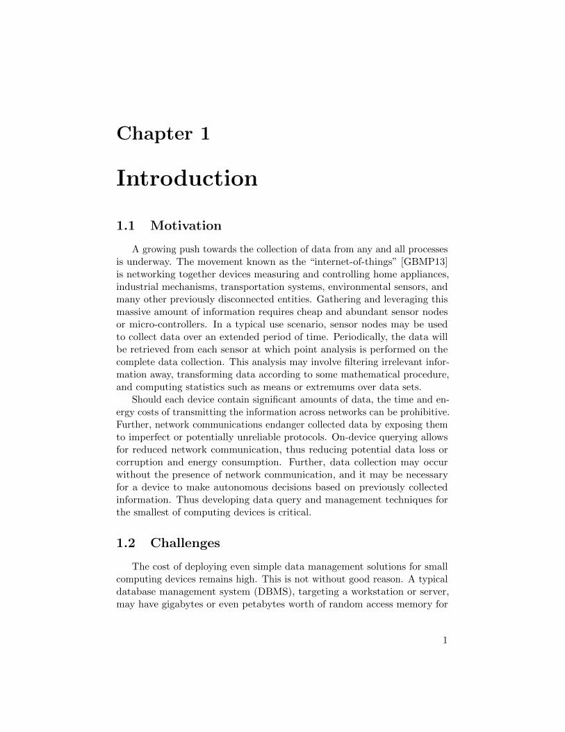
A growing push towards the collection of data from any and all processesis underway. The movement known as the “internet-of-things” [GBMP13]is networking together devices measuring and controlling home appliances,industrial mechanisms, transportation systems, environmental sensors, andmany other previously disconnected entities. Gathering and leveraging thismassive amount of information requires cheap and abundant sensor nodesor micro-controllers. In a typical use scenario, sensor nodes may be usedto collect data over an extended period of time. Periodically, the data willbe retrieved from each sensor at which point analysis is performed on thecomplete data collection. This analysis may involve filtering irrelevant infor-mation away, transforming data according to some mathematical procedure,and computing statistics such as means or extremums over data sets.

Should each device contain significant amounts of data, the time and en-ergy costs of transmitting the information across networks can be prohibitive.Further, network communications endanger collected data by exposing themto imperfect or potentially unreliable protocols. On-device querying allowsfor reduced network communication, thus reducing potential data loss orcorruption and energy consumption. Further, data collection may occurwithout the presence of network communication, and it may be necessaryfor a device to make autonomous decisions based on previously collectedinformation. Thus developing data query and management techniques forthe smallest of computing devices is critical.

1.2 Challenges

The cost of deploying even simple data management solutions for smallcomputing devices remains high. This is not without good reason. A typicaldatabase management system (DBMS), targeting a workstation or server,may have gigabytes or even petabytes worth of random access memory for

1

1.3. Goals and Research Questions

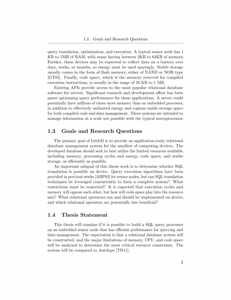
query translation, optimization, and execution. A typical sensor node has 1KB to 1MB of RAM, with many having between 2KB to 64KB of memory.Further, these devices may be expected to collect data on a battery overdays, weeks, or months, so energy must be used sparingly. Stable storageusually comes in the form of flash memory, either of NAND or NOR type[GT05]. Finally, code space, which is the memory reserved for compiledexecution instructions, is usually in the range of 16 KB to 1 MB.

Existing APIs provide access to the most popular relational databasesoftware for servers. Significant research and development effort has beenspent optimizing query performance for these applications. A server couldpotentially have millions of times more memory than an embedded processor,in addition to effectively unlimited energy and copious stable storage spacefor both compiled code and data management. These systems are intended tomanage information at a scale not possible with the typical microprocessor.

1.3 Goals and Research Questions

The primary goal of LittleD is to provide an application-ready relationaldatabase management system for the smallest of computing devices. Thedeveloped database should seek to best utilize the limited resources available,including memory, processing cycles and energy, code space, and stablestorage, as efficiently as possible.

An important subgoal of this thesis work is to determine whether SQLtranslation is possible on device. Query execution algorithms have beenprovided in previous works [ABP03] for sensor nodes, but can SQL translationtechniques be leveraged concurrently to form a complete system? Whatrestrictions must be respected? It is expected that execution cycles andmemory will oppose each other, but how will code space play into the resourcemix? What relational operators can and should be implemented on device,and which relational operators are potentially less beneficial?

1.4 Thesis Statement

This thesis will examine if it is possible to build a SQL query processoron an embedded sensor node that has efficient performance for querying anddata management. The expectation is that a relational database system willbe constructed, and the major limitations of memory, CPU, and code spacewill be analyzed to determine the most critical resource constraints. Thesystem will be compared to Antelope [TD11].

2

Chapter 2

Background

2.1 The Relational Model and its Algebra

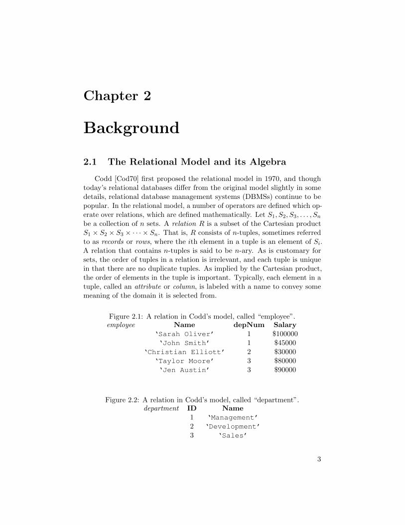
Codd [Cod70] first proposed the relational model in 1970, and thoughtoday’s relational databases differ from the original model slightly in somedetails, relational database management systems (DBMSs) continue to bepopular. In the relational model, a number of operators are defined which op-erate over relations, which are defined mathematically. Let S1, S2, S3, . . . , Snbe a collection of n sets. A relation R is a subset of the Cartesian productS1 × S2 × S3 × · · · × Sn. That is, R consists of n-tuples, sometimes referredto as records or rows, where the ith element in a tuple is an element of Si.A relation that contains n-tuples is said to be n-ary. As is customary forsets, the order of tuples in a relation is irrelevant, and each tuple is uniquein that there are no duplicate tuples. As implied by the Cartesian product,the order of elements in the tuple is important. Typically, each element in atuple, called an attribute or column, is labeled with a name to convey somemeaning of the domain it is selected from.

Figure 2.1: A relation in Codd’s model, called “employee”.employee Name depNum Salary

‘Sarah Oliver’ 1 $100000‘John Smith’ 1 $45000

‘Christian Elliott’ 2 $30000‘Taylor Moore’ 3 $80000‘Jen Austin’ 3 $90000

Figure 2.2: A relation in Codd’s model, called “department”.department ID Name

1 ‘Management’2 ‘Development’3 ‘Sales’

3

2.1. The Relational Model and its Algebra

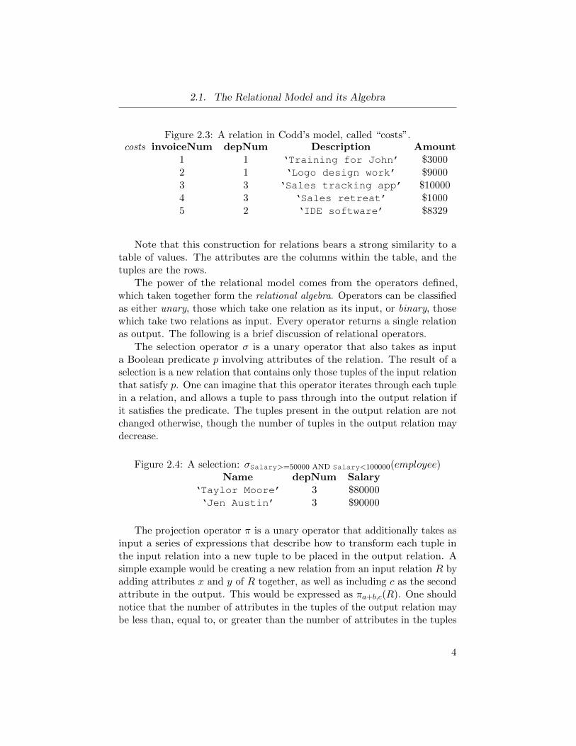
Figure 2.3: A relation in Codd’s model, called “costs”.costs invoiceNum depNum Description Amount

1 1 ‘Training for John’ $30002 1 ‘Logo design work’ $90003 3 ‘Sales tracking app’ $100004 3 ‘Sales retreat’ $10005 2 ‘IDE software’ $8329

Note that this construction for relations bears a strong similarity to atable of values. The attributes are the columns within the table, and thetuples are the rows.

The power of the relational model comes from the operators defined,which taken together form the relational algebra. Operators can be classifiedas either unary, those which take one relation as its input, or binary, thosewhich take two relations as input. Every operator returns a single relationas output. The following is a brief discussion of relational operators.

The selection operator σ is a unary operator that also takes as inputa Boolean predicate p involving attributes of the relation. The result of aselection is a new relation that contains only those tuples of the input relationthat satisfy p. One can imagine that this operator iterates through each tuplein a relation, and allows a tuple to pass through into the output relation ifit satisfies the predicate. The tuples present in the output relation are notchanged otherwise, though the number of tuples in the output relation maydecrease.

Figure 2.4: A selection: σSalary>=50000 AND Salary<100000(employee)Name depNum Salary

‘Taylor Moore’ 3 $80000‘Jen Austin’ 3 $90000

The projection operator π is a unary operator that additionally takes asinput a series of expressions that describe how to transform each tuple inthe input relation into a new tuple to be placed in the output relation. Asimple example would be creating a new relation from an input relation R byadding attributes x and y of R together, as well as including c as the secondattribute in the output. This would be expressed as πa+b,c(R). One shouldnotice that the number of attributes in the tuples of the output relation maybe less than, equal to, or greater than the number of attributes in the tuples

4

2.1. The Relational Model and its Algebra

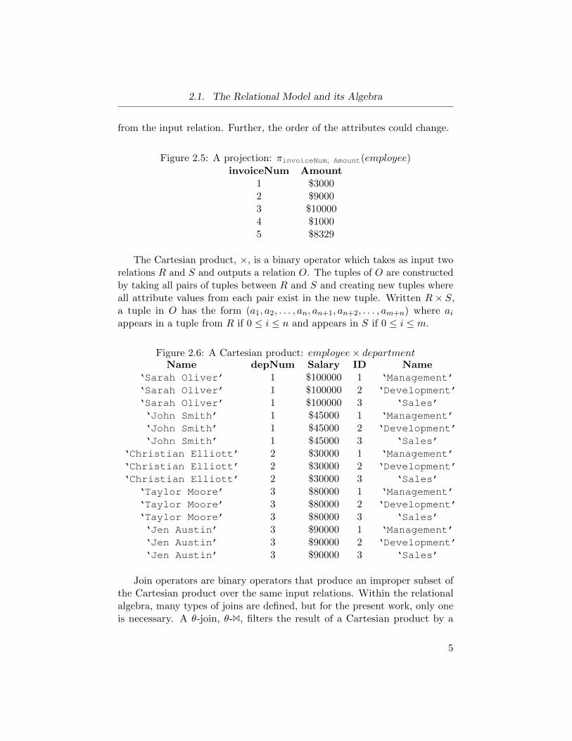
from the input relation. Further, the order of the attributes could change.

Figure 2.5: A projection: πinvoiceNum, Amount(employee)

invoiceNum Amount1 $30002 $90003 $100004 $10005 $8329

The Cartesian product, ×, is a binary operator which takes as input tworelations R and S and outputs a relation O. The tuples of O are constructedby taking all pairs of tuples between R and S and creating new tuples whereall attribute values from each pair exist in the new tuple. Written R× S,a tuple in O has the form (a1, a2, . . . , an, an+1, an+2, . . . , am+n) where aiappears in a tuple from R if 0 ≤ i ≤ n and appears in S if 0 ≤ i ≤ m.

Figure 2.6: A Cartesian product: employee× departmentName depNum Salary ID Name

‘Sarah Oliver’ 1 $100000 1 ‘Management’‘Sarah Oliver’ 1 $100000 2 ‘Development’‘Sarah Oliver’ 1 $100000 3 ‘Sales’‘John Smith’ 1 $45000 1 ‘Management’‘John Smith’ 1 $45000 2 ‘Development’‘John Smith’ 1 $45000 3 ‘Sales’

‘Christian Elliott’ 2 $30000 1 ‘Management’‘Christian Elliott’ 2 $30000 2 ‘Development’‘Christian Elliott’ 2 $30000 3 ‘Sales’

‘Taylor Moore’ 3 $80000 1 ‘Management’‘Taylor Moore’ 3 $80000 2 ‘Development’‘Taylor Moore’ 3 $80000 3 ‘Sales’‘Jen Austin’ 3 $90000 1 ‘Management’‘Jen Austin’ 3 $90000 2 ‘Development’‘Jen Austin’ 3 $90000 3 ‘Sales’

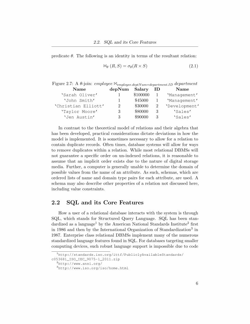
Join operators are binary operators that produce an improper subset ofthe Cartesian product over the same input relations. Within the relationalalgebra, many types of joins are defined, but for the present work, only oneis necessary. A θ-join, θ-1, filters the result of a Cartesian product by a

5

2.2. SQL and its Core Features

predicate θ. The following is an identity in terms of the resultant relation:

1θ (R,S) = σθ(R× S) (2.1)

Figure 2.7: A θ-join: employee 1employee.deptNum=department.ID department

Name depNum Salary ID Name‘Sarah Oliver’ 1 $100000 1 ‘Management’‘John Smith’ 1 $45000 1 ‘Management’

‘Christian Elliott’ 2 $30000 2 ‘Development’‘Taylor Moore’ 3 $80000 3 ‘Sales’‘Jen Austin’ 3 $90000 3 ‘Sales’

In contrast to the theoretical model of relations and their algebra thathas been developed, practical considerations dictate deviations in how themodel is implemented. It is sometimes necessary to allow for a relation tocontain duplicate records. Often times, database systems will allow for waysto remove duplicates within a relation. While most relational DBMSs willnot guarantee a specific order on un-indexed relations, it is reasonable toassume that an implicit order exists due to the nature of digital storagemedia. Further, a computer is generally unable to determine the domain ofpossible values from the name of an attribute. As such, schemas, which areordered lists of name and domain type pairs for each attribute, are used. Aschema may also describe other properties of a relation not discussed here,including value constraints.

2.2 SQL and its Core Features

How a user of a relational database interacts with the system is throughSQL, which stands for Structured Query Language. SQL has been stan-dardized as a language1 by the American National Standards Institute2 firstin 1986 and then by the International Organization of Standardization3 in1987. Enterprise class relational DBMSs implement many of the numerousstandardized language features found in SQL. For databases targeting smallercomputing devices, such robust language support is impossible due to code

1http://standards.iso.org/ittf/PubliclyAvailableStandards/c053681_ISO_IEC_9075-1_2011.zip

2http://www.ansi.org/3http://www.iso.org/iso/home.html

6

2.2. SQL and its Core Features

space restrictions. What immediately follows is a discussion of the core setof SQL features supported by this work.

In SQL, identifiers are used to name relations and attributes, as well asother important objects such as indexes. Reserved words or key words arestrings that cannot be used as identifiers unless identifier quotes are used asdelimiters. Commands such as SELECT and WHERE are examples of reservedwords. SQL is written in statements, which are sets of tokens, includingreserved words and identifiers, that should be interpreted and executed as awhole. Statements are whitespace ignorant except for the whitespace neededto delimit individual tokens. In general, statements are classified by theaction they perform. All statements have a form or syntax they must adhereto in order to be valid.

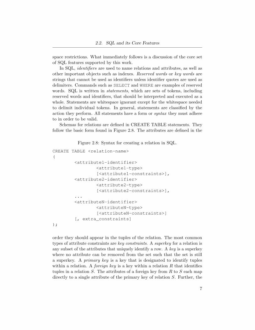
Schemas for relations are defined in CREATE TABLE statements. Theyfollow the basic form found in Figure 2.8. The attributes are defined in the

Figure 2.8: Syntax for creating a relation in SQL.

CREATE TABLE <relation-name>(

<attribute1-identifier><attribute1-type>[<attribute1-constraints>],

<attribute2-identifier><attribute2-type>[<attribute2-constraints>],

...<attributeN-identifier>

<attributeN-type>[<attributeN-constraints>]

[, extra_constraints]);

order they should appear in the tuples of the relation. The most commontypes of attribute constraints are key constraints. A superkey for a relation isany subset of the attributes that uniquely identify a row. A key is a superkeywhere no attribute can be removed from the set such that the set is stilla superkey. A primary key is a key that is designated to identify tupleswithin a relation. A foreign key is a key within a relation R that identifiestuples in a relation S. The attributes of a foreign key from R to S each mapdirectly to a single attribute of the primary key of relation S. Further, the

7

2.2. SQL and its Core Features

domains of the attributes in the foreign key must be an improper subset ofthe domain of the attribute each is mapped to.

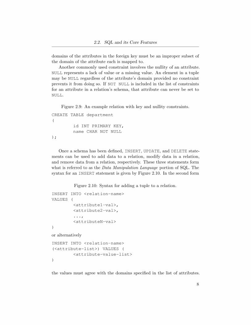
Another commonly used constraint involves the nullity of an attribute.NULL represents a lack of value or a missing value. An element in a tuplemay be NULL regardless of the attribute’s domain provided no constraintprevents it from doing so. If NOT NULL is included in the list of constraintsfor an attribute in a relation’s schema, that attribute can never be set toNULL.

Figure 2.9: An example relation with key and nullity constraints.

CREATE TABLE department(

id INT PRIMARY KEY,name CHAR NOT NULL

);

Once a schema has been defined, INSERT, UPDATE, and DELETE state-ments can be used to add data to a relation, modify data in a relation,and remove data from a relation, respectively. These three statements formwhat is referred to as the Data Manipulation Language portion of SQL. Thesyntax for an INSERT statement is given by Figure 2.10. In the second form

Figure 2.10: Syntax for adding a tuple to a relation.

INSERT INTO <relation-name>VALUES (

<attribute1-val>,<attribute2-val>,...,<attributeN-val>

)

or alternatively

INSERT INTO <relation-name>(<attribute-list>) VALUES (

<attribute-value-list>)

the values must agree with the domains specified in the list of attributes.

8

2.2. SQL and its Core Features

Any unspecified columns in the attribute list are set to NULL. If a nullityconstraint is violated, an error would occur.

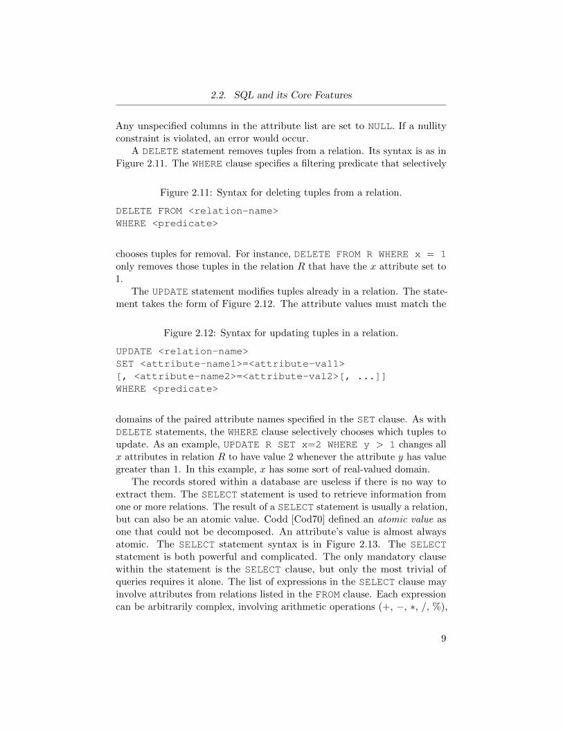
A DELETE statement removes tuples from a relation. Its syntax is as inFigure 2.11. The WHERE clause specifies a filtering predicate that selectively

Figure 2.11: Syntax for deleting tuples from a relation.

DELETE FROM <relation-name>WHERE <predicate>

chooses tuples for removal. For instance, DELETE FROM R WHERE x = 1only removes those tuples in the relation R that have the x attribute set to1.

The UPDATE statement modifies tuples already in a relation. The state-ment takes the form of Figure 2.12. The attribute values must match the

Figure 2.12: Syntax for updating tuples in a relation.

UPDATE <relation-name>SET <attribute-name1>=<attribute-val1>[, <attribute-name2>=<attribute-val2>[, ...]]WHERE <predicate>

domains of the paired attribute names specified in the SET clause. As withDELETE statements, the WHERE clause selectively chooses which tuples toupdate. As an example, UPDATE R SET x=2 WHERE y > 1 changes allx attributes in relation R to have value 2 whenever the attribute y has valuegreater than 1. In this example, x has some sort of real-valued domain.

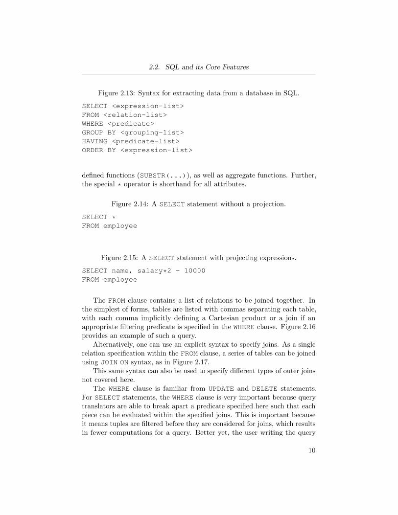
The records stored within a database are useless if there is no way toextract them. The SELECT statement is used to retrieve information fromone or more relations. The result of a SELECT statement is usually a relation,but can also be an atomic value. Codd [Cod70] defined an atomic value asone that could not be decomposed. An attribute’s value is almost alwaysatomic. The SELECT statement syntax is in Figure 2.13. The SELECTstatement is both powerful and complicated. The only mandatory clausewithin the statement is the SELECT clause, but only the most trivial ofqueries requires it alone. The list of expressions in the SELECT clause mayinvolve attributes from relations listed in the FROM clause. Each expressioncan be arbitrarily complex, involving arithmetic operations (+, −, ∗, /, %),

9

2.2. SQL and its Core Features

Figure 2.13: Syntax for extracting data from a database in SQL.

SELECT <expression-list>FROM <relation-list>WHERE <predicate>GROUP BY <grouping-list>HAVING <predicate-list>ORDER BY <expression-list>

defined functions (SUBSTR(...)), as well as aggregate functions. Further,the special * operator is shorthand for all attributes.

Figure 2.14: A SELECT statement without a projection.

SELECT *FROM employee

Figure 2.15: A SELECT statement with projecting expressions.

SELECT name, salary*2 - 10000FROM employee

The FROM clause contains a list of relations to be joined together. Inthe simplest of forms, tables are listed with commas separating each table,with each comma implicitly defining a Cartesian product or a join if anappropriate filtering predicate is specified in the WHERE clause. Figure 2.16provides an example of such a query.

Alternatively, one can use an explicit syntax to specify joins. As a singlerelation specification within the FROM clause, a series of tables can be joinedusing JOIN ON syntax, as in Figure 2.17.

This same syntax can also be used to specify different types of outer joinsnot covered here.

The WHERE clause is familiar from UPDATE and DELETE statements.For SELECT statements, the WHERE clause is very important because querytranslators are able to break apart a predicate specified here such that eachpiece can be evaluated within the specified joins. This is important becauseit means tuples are filtered before they are considered for joins, which resultsin fewer computations for a query. Better yet, the user writing the query

10

2.2. SQL and its Core Features

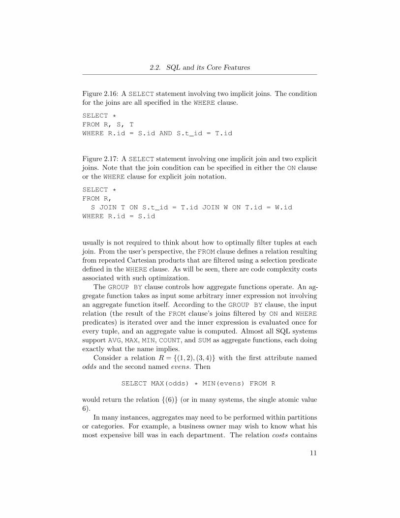
Figure 2.16: A SELECT statement involving two implicit joins. The conditionfor the joins are all specified in the WHERE clause.

SELECT *FROM R, S, TWHERE R.id = S.id AND S.t_id = T.id

Figure 2.17: A SELECT statement involving one implicit join and two explicitjoins. Note that the join condition can be specified in either the ON clauseor the WHERE clause for explicit join notation.

SELECT *FROM R,

S JOIN T ON S.t_id = T.id JOIN W ON T.id = W.idWHERE R.id = S.id

usually is not required to think about how to optimally filter tuples at eachjoin. From the user’s perspective, the FROM clause defines a relation resultingfrom repeated Cartesian products that are filtered using a selection predicatedefined in the WHERE clause. As will be seen, there are code complexity costsassociated with such optimization.

The GROUP BY clause controls how aggregate functions operate. An ag-gregate function takes as input some arbitrary inner expression not involvingan aggregate function itself. According to the GROUP BY clause, the inputrelation (the result of the FROM clause’s joins filtered by ON and WHEREpredicates) is iterated over and the inner expression is evaluated once forevery tuple, and an aggregate value is computed. Almost all SQL systemssupport AVG, MAX, MIN, COUNT, and SUM as aggregate functions, each doingexactly what the name implies.

Consider a relation R = {(1, 2), (3, 4)} with the first attribute namedodds and the second named evens. Then

SELECT MAX(odds) * MIN(evens) FROM R

would return the relation {(6)} (or in many systems, the single atomic value6).

In many instances, aggregates may need to be performed within partitionsor categories. For example, a business owner may wish to know what hismost expensive bill was in each department. The relation costs contains

11

2.2. SQL and its Core Features

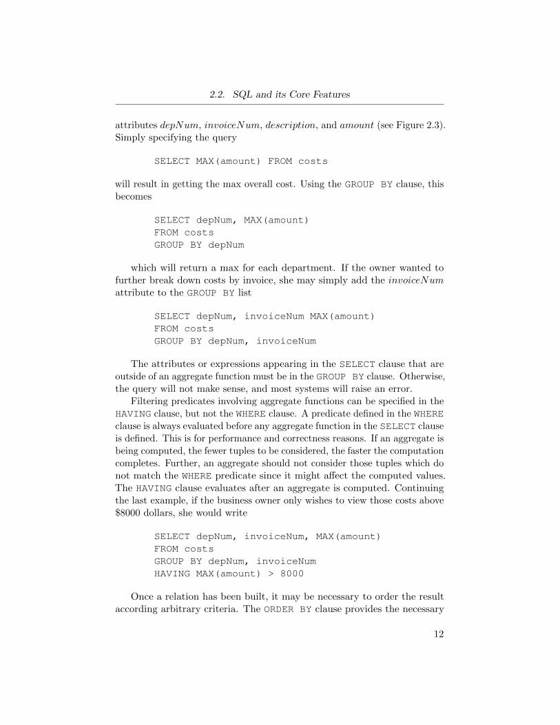
attributes depNum, invoiceNum, description, and amount (see Figure 2.3).Simply specifying the query

SELECT MAX(amount) FROM costs

will result in getting the max overall cost. Using the GROUP BY clause, thisbecomes

SELECT depNum, MAX(amount)FROM costsGROUP BY depNum

which will return a max for each department. If the owner wanted tofurther break down costs by invoice, she may simply add the invoiceNumattribute to the GROUP BY list

SELECT depNum, invoiceNum MAX(amount)FROM costsGROUP BY depNum, invoiceNum

The attributes or expressions appearing in the SELECT clause that areoutside of an aggregate function must be in the GROUP BY clause. Otherwise,the query will not make sense, and most systems will raise an error.

Filtering predicates involving aggregate functions can be specified in theHAVING clause, but not the WHERE clause. A predicate defined in the WHEREclause is always evaluated before any aggregate function in the SELECT clauseis defined. This is for performance and correctness reasons. If an aggregate isbeing computed, the fewer tuples to be considered, the faster the computationcompletes. Further, an aggregate should not consider those tuples which donot match the WHERE predicate since it might affect the computed values.The HAVING clause evaluates after an aggregate is computed. Continuingthe last example, if the business owner only wishes to view those costs above$8000 dollars, she would write

SELECT depNum, invoiceNum, MAX(amount)FROM costsGROUP BY depNum, invoiceNumHAVING MAX(amount) > 8000

Once a relation has been built, it may be necessary to order the resultaccording arbitrary criteria. The ORDER BY clause provides the necessary

12

2.3. Existing Query Processing Techniques

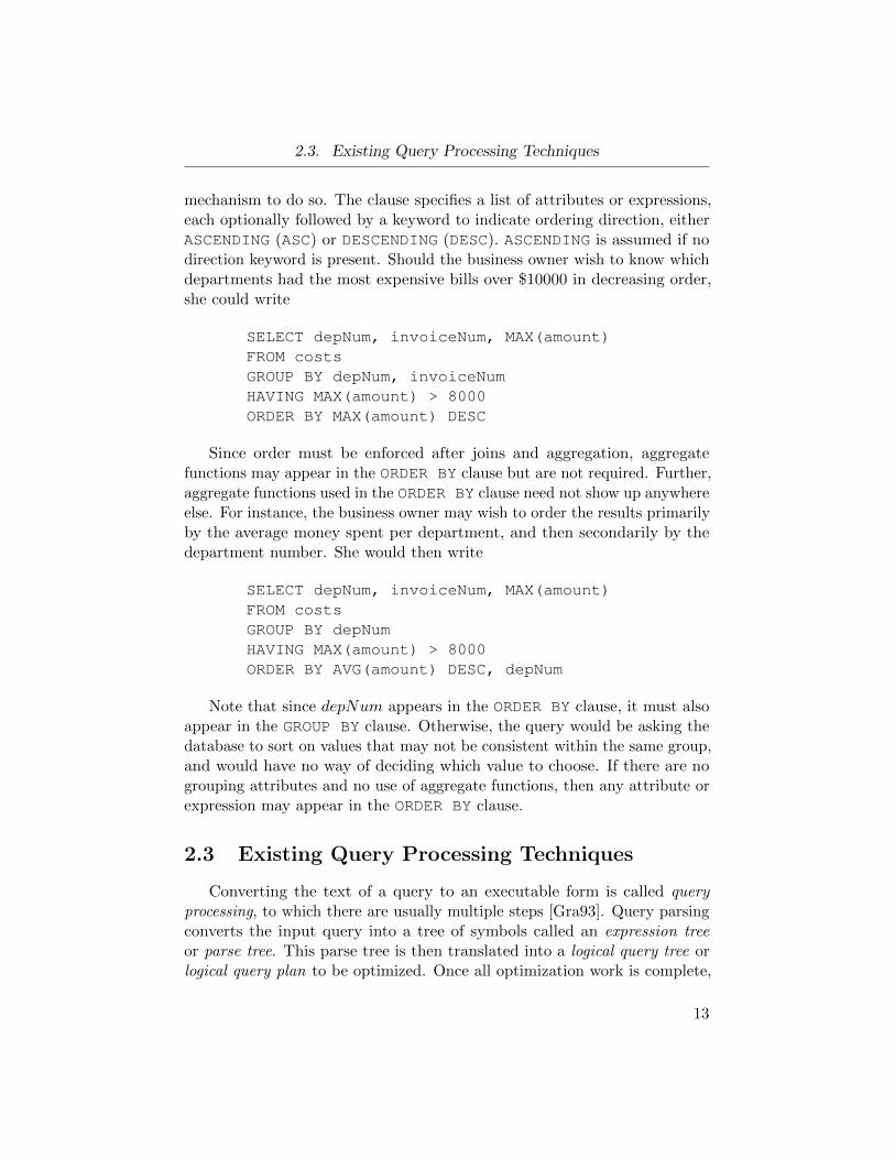
mechanism to do so. The clause specifies a list of attributes or expressions,each optionally followed by a keyword to indicate ordering direction, eitherASCENDING (ASC) or DESCENDING (DESC). ASCENDING is assumed if nodirection keyword is present. Should the business owner wish to know whichdepartments had the most expensive bills over $10000 in decreasing order,she could write

SELECT depNum, invoiceNum, MAX(amount)FROM costsGROUP BY depNum, invoiceNumHAVING MAX(amount) > 8000ORDER BY MAX(amount) DESC

Since order must be enforced after joins and aggregation, aggregatefunctions may appear in the ORDER BY clause but are not required. Further,aggregate functions used in the ORDER BY clause need not show up anywhereelse. For instance, the business owner may wish to order the results primarilyby the average money spent per department, and then secondarily by thedepartment number. She would then write

SELECT depNum, invoiceNum, MAX(amount)FROM costsGROUP BY depNumHAVING MAX(amount) > 8000ORDER BY AVG(amount) DESC, depNum

Note that since depNum appears in the ORDER BY clause, it must alsoappear in the GROUP BY clause. Otherwise, the query would be asking thedatabase to sort on values that may not be consistent within the same group,and would have no way of deciding which value to choose. If there are nogrouping attributes and no use of aggregate functions, then any attribute orexpression may appear in the ORDER BY clause.

2.3 Existing Query Processing Techniques

Converting the text of a query to an executable form is called queryprocessing, to which there are usually multiple steps [Gra93]. Query parsingconverts the input query into a tree of symbols called an expression treeor parse tree. This parse tree is then translated into a logical query tree orlogical query plan to be optimized. Once all optimization work is complete,

13

2.3. Existing Query Processing Techniques

the resulting logical query tree is converted to a physical plan, also called aphysical query tree. The evaluator then executes the physical plan to returnthe query output.

Query optimization is perhaps the most important step for most systems.A logical query plan can be improved to use less computational cycles, lessmemory, or both by using appropriate algorithms for operators as well asby reorganizing entire sections of the query tree. Perhaps the most commoninstance of such reorganization is expression pushing. One form of expressionpushing involves breaking apart predicates and pushing pieces down intooperators at lower portions of the tree such that fewer tuples are processedat operators higher in the tree. This form was discussed in Section 2.2.Another type of expression pushing places new operators, usually projections,at targeted areas in the query plan to reduce the size of each tuple processed.

Algorithm choice for the relational operators is another tool used bydatabase systems to reduce query execution costs. Typical relational databasesystems have the luxury of large amounts of available RAM in addition tovirtually unlimited stable storage. These system qualities allow for business-class RDBMSs to leverage algorithms involving hash buckets [DKO+84],external merge sorts [DKO+84], among other clever tools.

None of these techniques are feasible for databases targeting much smallerdevices. Using valuable code space on complicated optimization proceduresor varying implementations for each operator is impractical. Algorithmsmaking heavy use of memory are not feasible since the database may haveless than 1KB of RAM available to it. Swapping in-memory data to and fromstable storage is also not advisable since flash memories have asymmetricread and write performance characteristics. Thus, new querying techniquesare required.

The simplest technique, as discussed by the PicoDBMS [ABP03] frame-work, is to enforce minimal RAM usage through re-computation. The authorsdefine a framework including algorithms which achieve the lowest RAM foot-print possible for basic relational operators. The authors demonstrate thatthis re-computation becomes exorbitantly costly as the amount of data grows.Giving even small amounts of extra RAM to their algorithms greatly reducesexecution cycles.

A similar class of algorithms for relational operators known as ‘tuple-at-a-time’ algorithms require only a single tuple or two be present in memory at agiven instant. Each operator returns a single tuple on request. When a tupleis requested, it requests the next tuple from each of its child operators andattempts to produce a result. If an operator cannot produce a tuple from thecurrent child tuples, then it will request new child tuples as necessary. When

14

2.3. Existing Query Processing Techniques

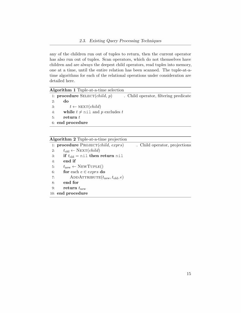
any of the children run out of tuples to return, then the current operatorhas also run out of tuples. Scan operators, which do not themselves havechildren and are always the deepest child operators, read tuples into memory,one at a time, until the entire relation has been scanned. The tuple-at-a-time algorithms for each of the relational operations under consideration aredetailed here.

Algorithm 1 Tuple-at-a-time selection

1: procedure Select(child, p) . Child operator, filtering predicate2: do3: t← next(child)4: while t 6= nil and p excludes t5: return t6: end procedure

Algorithm 2 Tuple-at-a-time projection

1: procedure Project(child, exprs) . Child operator, projections2: told ← Next(child)3: if told = nil then return nil4: end if5: tnew ← NewTuple()6: for each e ∈ exprs do7: AddAttribute(tnew, told, e)8: end for9: return tnew

10: end procedure

15

2.3. Existing Query Processing Techniques

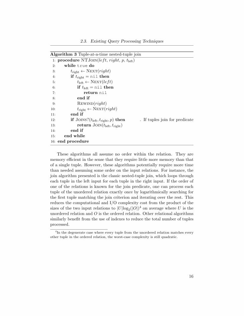
Algorithm 3 Tuple-at-a-time nested-tuple join

1: procedure NTJoin(left, right, p, tleft)2: while true do3: tright ← Next(right)4: if tright = nil then5: tleft ← Next(left)6: if tleft = nil then7: return nil8: end if9: Rewind(right)

10: tright ← Next(right)11: end if12: if Joins?(tleft, tright, p) then . If tuples join for predicate13: return Join(tleft, tright)14: end if15: end while16: end procedure

These algorithms all assume no order within the relation. They arememory efficient in the sense that they require little more memory than thatof a single tuple. However, these algorithms potentially require more timethan needed assuming some order on the input relations. For instance, thejoin algorithm presented is the classic nested-tuple join, which loops througheach tuple in the left input for each tuple in the right input. If the order ofone of the relations is known for the join predicate, one can process eachtuple of the unordered relation exactly once by logarithmically searching forthe first tuple matching the join criterion and iterating over the rest. Thisreduces the computational and I/O complexity cost from the product of thesizes of the two input relations to |U |log2(|O|)4 on average where U is theunordered relation and O is the ordered relation. Other relational algorithmssimilarly benefit from the use of indexes to reduce the total number of tuplesprocessed.

4In the degenerate case where every tuple from the unordered relation matches everyother tuple in the ordered relation, the worst-case complexity is still quadratic.

16

2.4. Previous Work

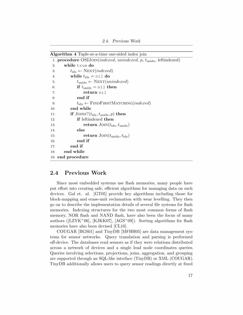
Algorithm 4 Tuple-at-a-time one-sided index join

1: procedure OSIJoin(indexed, unindexed, p, tunidx, leftindexed)2: while true do3: tidx ← Next(indexed)4: while tidx = nil do5: tunidx ← Next(unindexed)6: if tunidx = nil then7: return nil8: end if9: tidx ← FindFirstMatching(indexed)

10: end while11: if Joins?(tidx, tunidx, p) then12: if leftindexed then13: return Join(tidx, tunidx)14: else15: return Join(tunidx, tidx)16: end if17: end if18: end while19: end procedure

2.4 Previous Work

Since most embedded systems use flash memories, many people haveput effort into creating safe, efficient algorithms for managing data on suchdevices. Gal et. al. [GT05] provide key algorithms including those forblock-mapping and erase-unit reclamation with wear levelling. They thengo on to describe the implementation details of several file systems for flashmemories. Indexing structures for the two most common forms of flashmemory, NOR flash and NAND flash, have also been the focus of manyauthors ([LZYK+06], [KJKK07], [AGS+09]). Sorting algorithms for flashmemories have also been devised [CL10].

COUGAR [BGS01] and TinyDB [MFHH05] are data management sys-tems for sensor networks. Query translation and parsing is performedoff-device. The databases read sensors as if they were relations distributedacross a network of devices and a single lead node coordinates queries.Queries involving selections, projections, joins, aggregation, and groupingare supported through an SQL-like interface (TinyDB) or XML (COUGAR).TinyDB additionally allows users to query sensor readings directly at fixed

17

2.4. Previous Work

sampling periods. The sampling periods can be directly specified, or alterna-tively, a lifetime goal in hours, days, or joules used by the system to estimateappropriate sampling rates can be provided. Sensors can be optionally readbased on their voltage requirements. COUGAR also provides mechanismsfor detailing the intended duration of a query.

PicoDBMS [PBVB01] [ABP03] implements a relational DBMSs for smallcomputing devices without on-board query translation. PicoDBMS providesa design framework that recomputes partial query results as much as possi-ble to reduce memory requirements. Further, PicoDBMS implements thisframework to demonstrate the relationship between memory requirementsand execution time. The algorithms described within the work [ABP03]adapt to available memory. Slow execution time results from limited memoryavailable. As the available memory grows, execution time falls drastically.PicoDBMS was specifically designed for smart cards where security is ofgreat importance. A key application is in personal health cards that trackpatient records [PBVB01].

DBMSs for less-constrained embedded devices such as smart phonescurrently exist. The popular SQLite5 is used on iOS and Android phonesand tablets all the way up to web browsers on desktop computers. Otherrelational databases, including H2 Database Engine6, SQL Server Compact7,and MiniSQL8 also target less-constrained embedded systems. Non-relationaldatabases for similar computing devices include UnQLite9 and BerkeleyDB10.None of these systems meet the extreme code space and memory restrictionsof the smallest of devices.

Antelope [TD11] is a relational database for constrained devices thatleverages AQL, a language similar to but not compliant with SQL. AQLhas separate statements for declaring a relation and adding attributes to arelation. Antelope requires indexes for joins and aggregation. It is also ableto use indexes to speed up projections and selections. Further, Anteloperequires a fixed amount of RAM totalling over 3.7KB. For example, theSELECT expression 2*x/3 + 7*y defining a new projected attribute is notsupported in Antelope. Expression evaluation is supported via a shunting-yard style algorithm for parsing to a post-fix byte code to be evaluated.

5http://www.sqlite.org/6http://www.h2database.com/7http://www.microsoft.com/en-us/sqlserver/8http://www.hughes.com.au/products/msql9http://www.unqlite.org/

10http://www.oracle.com/technetwork/database/database-technologies/berkeleydb/overview/index.html

18

Chapter 3

LittleD ImplementationSummary

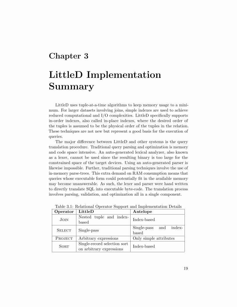
LittleD uses tuple-at-a-time algorithms to keep memory usage to a mini-mum. For larger datasets involving joins, simple indexes are used to achievereduced computational and I/O complexities. LittleD specifically supportsin-order indexes, also called in-place indexes, where the desired order ofthe tuples is assumed to be the physical order of the tuples in the relation.These techniques are not new but represent a good basis for the execution ofqueries.

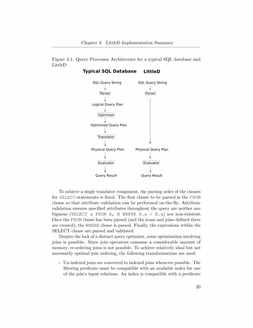
The major difference between LittleD and other systems is the querytranslation procedure. Traditional query parsing and optimization is memoryand code space intensive. An auto-generated lexical analyzer, also knownas a lexer, cannot be used since the resulting binary is too large for theconstrained space of the target devices. Using an auto-generated parser islikewise impossible. Further, traditional parsing techniques involve the use ofin-memory parse-trees. This extra demand on RAM consumption means thatqueries whose executable form could potentially fit in the available memorymay become unanswerable. As such, the lexer and parser were hand writtento directly translate SQL into executable byte-code. The translation processinvolves parsing, validation, and optimization all in a single component.

Table 3.1: Relational Operator Support and Implementation DetailsOperator LittleD Antelope

JoinNested tuple and index-based

Index-based

Select Single-passSingle-pass and index-based

Project Arbitrary expressions Only simple attributes

SortSingle-record selection sorton arbitrary expressions

Index-based

19

Chapter 3. LittleD Implementation Summary

Figure 3.1: Query Processor Architecture for a typical SQL database andLittleD

Parser

SQL Query String

Logical Query Plan

Optimizer

Optimized Query Plan

Translator

Physical Query Plan

Evaluator

Query Result

Typical SQL Database LittleD

Parser

SQL Query String

Physical Query Plan

Evaluator

Query Result

To achieve a single translator component, the parsing order of the clausesfor SELECT-statements is fixed. The first clause to be parsed is the FROMclause so that attribute validation can be performed on-the-fly. Attributevalidation ensures specified attributes throughout the query are neither am-biguous (SELECT a FROM A, B WHERE A.a > B.a) nor non-existent.Once the FROM clause has been parsed (and the scans and joins defined thereare created), the WHERE clause is parsed. Finally, the expressions within theSELECT clause are parsed and validated.

Despite the lack of a distinct query optimizer, some optimization involvingjoins is possible. Since join operators consume a considerable amount ofmemory, re-ordering joins is not possible. To achieve relatively ideal but notnecessarily optimal join ordering, the following transformations are used:

− Un-indexed joins are converted to indexed joins whenever possible. Thefiltering predicate must be compatible with an available index for oneof the join’s input relations. An index is compatible with a predicate

20

Chapter 3. LittleD Implementation Summary

the if index sorts the relation using the attributes from the relation inthe same way they are used in the joining predicate. For instance, arelation’s index which orders on attribute x would not be compatiblewith the join predicate x % 7 = y but would be compatible with thejoin predicate x = y.

− Left-deep join trees are used exclusively. Standard join algorithmsiterate over each tuple in the right relation multiple times for eachtuple in the left relation. If the input relation on the right is itself ajoin, that join must be re-computed multiple times. If it is on the left,it must be computed only a single time. Since indexed joins can haveeither the left or the right relation as the ordered relation, left-deeptrees generally provide good performance characteristics. Left-deeptrees are also easily constructed. During FROM clause parsing, eachrelation can be initialized in the order they appear. Then the joins areinitialized in forward order. That is, after scans for each relation inFROM R1, R2, ..., Rn have been initialized, memory is allocatedfor the n− 1 join operators. Then the first join J1 between R1 and R2

is initialized. The second join between J2 and R3 is initialized, and soforth until all the joins have been constructed.

A key requirement for this type of database is to use a memory allocatorthat is as compact as possible. To accomplish this task, an allocator waswritten using two stacks. An array of fixed sizes is declared statically andthen used as the allocation resource. The beginning and end of the arrayare initially the tops of the front stack and back stack, respectively. Newallocations always occur on the top of one of these stacks, but de-allocationsmay occur in any order. The allocator is able to detect out-of-order de-allocations and mark these regions such that once the top of the stack isfinally freed, any previously marked regions immediately under the top arealso de-allocated. Due to the natural flow of data in relational databases, afixed order of allocations and de-allocations is common.

There are further advantages to using such a memory allocator. Untilthe first de-allocation, no memory can possibly be fragmented. Since inalmost all cases the de-allocation of memory occurs all at the end, there iseffectively no memory fragmentation. The cost of allocating a new segmenton the front of the stack is two pointers and on the back the cost of allocationis one pointer. Detecting out-of-memory errors is accomplished by simplychecking if a new allocation will cause the tops of the stacks to collide. Byknowing ahead of time how much memory is required to execute an executionplan, out-of-memory problems can be detected well before runtime. Valuable

21

Chapter 3. LittleD Implementation Summary

energy is thus conserved and segmentation faults are also avoided, whichcould lead to potential data corruption and other destructive behavior. Manyof the algorithms used to convert SQL into an executable plan require theuse of one or two stacks. In converting mixed-infix expressions into postfixonly byte code, the front stack is used for the resulting expression while theback stack is used to determine operator order based-on operator precedenceand parentheses. Using the front stack for the resulting evaluable expressionmeans not having to reverse the expression once complete.

To reduce overhead even more, special functions were implemented whichallows for the top most memory sections on each stack to be extended insize without modifying the current data. Not only does this reduce memoryoverhead, it also significantly simplifies translation efforts. For example,during the parsing of expressions, the size of byte-code representation of anexpression does not need to be known ahead of time, reducing the amountof work needed for overall execution. Each time a new part of the expressionmust be added, the stack is simply resized.

22

Chapter 4

Experimental Results andDiscussion

4.1 Experimental Setup

In order to compare LittleD’s performance characteristics with Antelope,a common execution platform was needed. A Zolertia Z1 device simulatedby the MSPSim emulator served precisely this purpose. MSPSim is cycle-accurate. Both databases were compiled for the Contiki real-time operatingsystem [Con] and used the Coffee File System [TDHV09] to store relationdata.

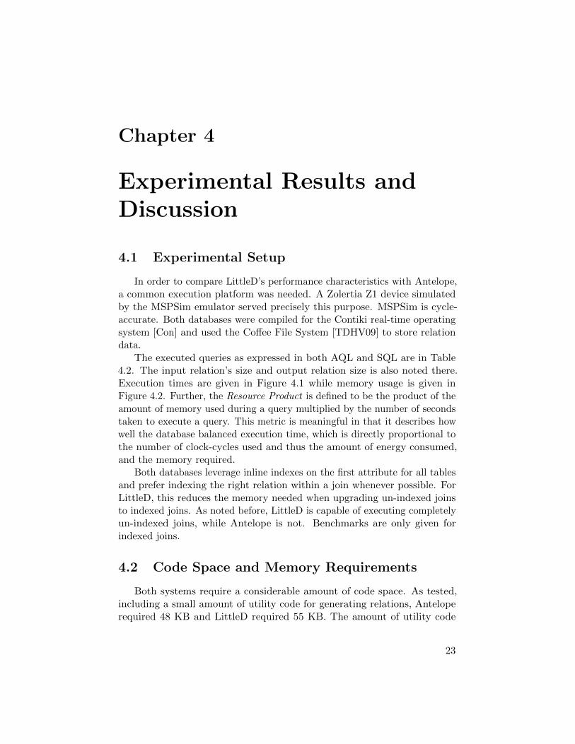
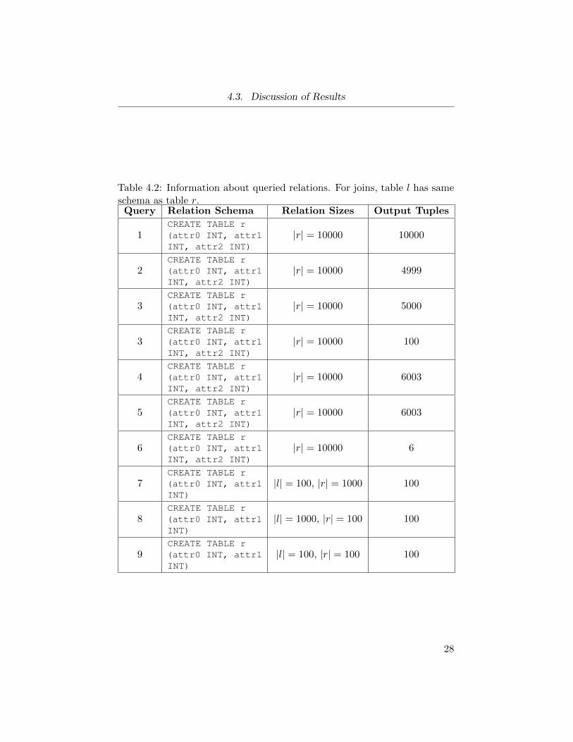
The executed queries as expressed in both AQL and SQL are in Table4.2. The input relation’s size and output relation size is also noted there.Execution times are given in Figure 4.1 while memory usage is given inFigure 4.2. Further, the Resource Product is defined to be the product of theamount of memory used during a query multiplied by the number of secondstaken to execute a query. This metric is meaningful in that it describes howwell the database balanced execution time, which is directly proportional tothe number of clock-cycles used and thus the amount of energy consumed,and the memory required.

Both databases leverage inline indexes on the first attribute for all tablesand prefer indexing the right relation within a join whenever possible. ForLittleD, this reduces the memory needed when upgrading un-indexed joinsto indexed joins. As noted before, LittleD is capable of executing completelyun-indexed joins, while Antelope is not. Benchmarks are only given forindexed joins.

4.2 Code Space and Memory Requirements

Both systems require a considerable amount of code space. As tested,including a small amount of utility code for generating relations, Anteloperequired 48 KB and LittleD required 55 KB. The amount of utility code

23

4.3. Discussion of Results

Figure 4.1: Query Execution Experimental Results

0

2

4

6

8

10

12

14

16

18

20

1 2 3 4 5 6 7 8 9

Tim

e (

seco

nd

s)

Query

Query Execution Times

LittleD Average Execution Time AntelopeDB Average Execution TimeN

ot

exe

cuta

ble

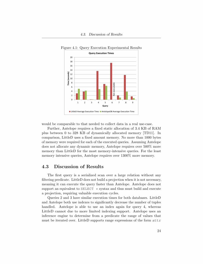
would be comparable to that needed to collect data in a real use-case.Further, Antelope requires a fixed static allocation of 3.4 KB of RAM

plus between 0 to 328 KB of dynamically allocated memory [TD11]. Incomparison, LittleD uses a fixed amount memory. No more than 1000 bytesof memory were required for each of the executed queries. Assuming Antelopedoes not allocate any dynamic memory, Antelope requires over 500% morememory than LittleD for the most memory-intensive queries. For the leastmemory intensive queries, Antelope requires over 1300% more memory.

4.3 Discussion of Results

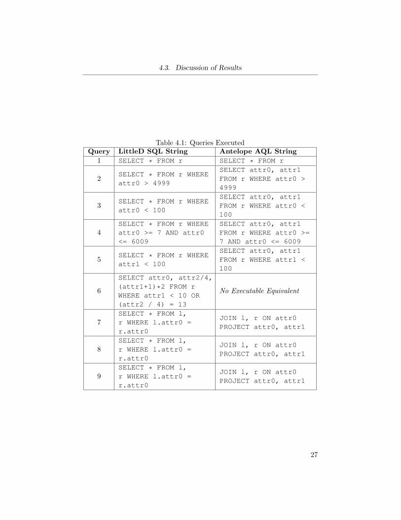
The first query is a serialized scan over a large relation without anyfiltering predicate. LittleD does not build a projection when it is not necessary,meaning it can execute the query faster than Antelope. Antelope does notsupport an equivalent to SELECT * syntax and thus must build and executea projection, requiring valuable execution cycles.

Queries 2 and 3 have similar execution times for both databases. LittleDand Antelope both use indexes to significantly decrease the number of tupleshandled. Antelope is able to use an index again for query 4, whereasLittleD cannot due to more limited indexing support. Antelope uses aninference engine to determine from a predicate the range of values thatmust be iterated over. LittleD supports range expressions of the form attr

24

4.3. Discussion of Results

Figure 4.2: LittleD vs. Antelope Memory Usage

0

500

1000

1500

2000

2500

3000

3500

4000

1 2 3 4 5 6 7 8 9

Mem

ory

Allo

cate

d (

byt

es)

Query

Memory Usage

LittleD Memory Consumption Antelope Memory Consumption

<RELOP> <INTVAL> where <RELOP> is one of =, ! =, >, <, >=, or <=and <INTVAL> is an integer value. Once an index cannot be used, as inquery 5, again the two databases perform nearly equally.

Query 6 clearly demonstrates that the time taken to execute a query islinearly proportional to the number of calculations that must be evaluatedper tuple. Calculating three operations over each tuple significantly increasesthe amount of time needed, despite the small size of the output relation.This query is not executable for Antelope because unlike LittleD, it does nothave support for arbitrary projecting expressions. Antelope only supportsthe projection of individual attributes. In a real application, this wouldmean that each tuple would need to be iterated over to calculate a new value.Not only does this add considerable complexity to an application, it possiblyincreases the amount of memory required for a task.

Queries 7, 8, and 9 all demonstrate Antelope’s superiority in terms ofexecution time for similar joins. However, Antelope makes simplifying as-sumptions, which can likely explain its speed advantage. AQL only allowsfor equijoins, whereas LittleD supports arbitrary inner joins via SQL. Fur-thermore, experimentation revealed that the implementation of the joinalgorithm did not always return correct results. The benchmarks provided allreturned correct output relations, but for a variety of other cases, the outputrelation was incorrect. These limitations make it difficult to compare thejoin performances in a meaningful way, but it should be noted that LittleD

25

4.3. Discussion of Results

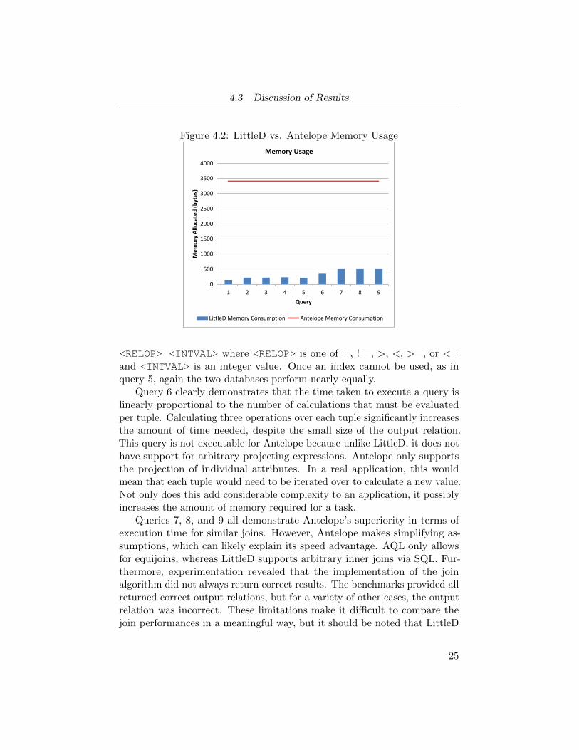
Figure 4.3: Query Resource Efficiency Results

0

5000

10000

15000

20000

25000

1 2 3 4 5 6 7 8 9

Re

sou

rce

Pro

du

ct (

byt

es*

seco

nd

s)

Query

Resource Product

LittleD Antelope

No

t ex

ecu

tab

le

was never more than three times slower than Antelope for the benchmarkedjoins. Query 8 was slower than query 7 for both databases since a greaternumber of binary searches are needed to compute the results.

For all queries, the resource product for LittleD is smaller than forAntelope. In the closest case, Antelope has a resource product that is onlytwice as large as LittleD. In the worst case for Antelope, its resource productis over 40 times larger than that of LittleD.

26

4.3. Discussion of Results

Table 4.1: Queries ExecutedQuery LittleD SQL String Antelope AQL String

1 SELECT * FROM r SELECT * FROM r

2SELECT * FROM r WHEREattr0 > 4999

SELECT attr0, attr1FROM r WHERE attr0 >4999

3SELECT * FROM r WHEREattr0 < 100

SELECT attr0, attr1FROM r WHERE attr0 <100

4SELECT * FROM r WHEREattr0 >= 7 AND attr0<= 6009

SELECT attr0, attr1FROM r WHERE attr0 >=7 AND attr0 <= 6009

5SELECT * FROM r WHEREattr1 < 100

SELECT attr0, attr1FROM r WHERE attr1 <100

6

SELECT attr0, attr2/4,(attr1+1)*2 FROM rWHERE attr1 < 10 OR(attr2 / 4) = 13

No Executable Equivalent

7SELECT * FROM l,r WHERE l.attr0 =r.attr0

JOIN l, r ON attr0PROJECT attr0, attr1

8SELECT * FROM l,r WHERE l.attr0 =r.attr0

JOIN l, r ON attr0PROJECT attr0, attr1

9SELECT * FROM l,r WHERE l.attr0 =r.attr0

JOIN l, r ON attr0PROJECT attr0, attr1

27

4.3. Discussion of Results

Table 4.2: Information about queried relations. For joins, table l has sameschema as table r.Query Relation Schema Relation Sizes Output Tuples

1CREATE TABLE r(attr0 INT, attr1INT, attr2 INT)

|r| = 10000 10000

2CREATE TABLE r(attr0 INT, attr1INT, attr2 INT)

|r| = 10000 4999

3CREATE TABLE r(attr0 INT, attr1INT, attr2 INT)

|r| = 10000 5000

3CREATE TABLE r(attr0 INT, attr1INT, attr2 INT)

|r| = 10000 100

4CREATE TABLE r(attr0 INT, attr1INT, attr2 INT)

|r| = 10000 6003

5CREATE TABLE r(attr0 INT, attr1INT, attr2 INT)

|r| = 10000 6003

6CREATE TABLE r(attr0 INT, attr1INT, attr2 INT)

|r| = 10000 6

7CREATE TABLE r(attr0 INT, attr1INT)

|l| = 100, |r| = 1000 100

8CREATE TABLE r(attr0 INT, attr1INT)

|l| = 1000, |r| = 100 100

9CREATE TABLE r(attr0 INT, attr1INT)

|l| = 100, |r| = 100 100

28

Chapter 5

Conclusion

In this work, LittleD, a relational database for sensor nodes and embeddedcomputing devices, was presented. A tuple-at-a-time approach to queryalgorithms was used. The novel features of LittleD include a single-componentSQL to executable-plan translator and a memory allocator using two stackswithin a single memory region.

Experimentally, LittleD is always more memory efficient than Antelope,the database that most closely matches the goals of LittleD, while having com-parable execution time performance and similar code space requirements. Noquery for LittleD was more than three times slower than a comparable queryfor Antelope, though Antelope always used at least five times more memorythan LittleD. LittleD supports the more familiar SQL standard includingmore general expressions in projections in comparison with Antelope.

This work also provides useful insights to applications of database tech-nology with microprocessors. The use of indexes drastically improves theperformance of many queries and should thus be regarded as a key componentof any database targeting resource constrained platforms. The resourcesavailable, namely memory, stable storage, code space (ROM), and executiontime and energy, are not equally important. While memory is limited, LittleDhas low memory requirements for reasonable SELECT-FROM-WHERE queries.If a database system cannot fit into the code space of a device, it can neverbe used, and thus it should be considered at present the most constrainingresource. Almost half of the ROM required for LittleD to execute is consumedby the query translation system. While SQL translation is possible on device,it is not necessarily beneficial for all applications. Finding ways to reducethe complexity of the parser, possibly by moving query translation off device,would allow for smarter algorithms to be used in query execution, possiblysaving execution cycles and thus energy. Device manufacturer’s would bewise to give these devices more ROM to accommodate for more sophisticatedsolutions. Though not tested here, all resources become significantly moretaxed when sorting and aggregation are also included. Developers usingLittleD or similar systems may well have to choose which features to compilefor an application due to such resource limitations.

29

5.1. Future Work

5.1 Future Work

Future research will focus on further reducing resource costs. A moresophisticated indexing strategy will be investigated for data where an ordercannot be assumed at insertion time. Finding ways to better leverage theindexes throughout the query execution engine will allow for lower RAMand energy usage. Potentially moving query translation off-device could alsosave valuable code space. Improved sorting methods such as MinSort [CL10]will also be implemented.

30

Bibliography

[ABP03] Nicolas Anciaux, Luc Bouganim, and Philippe Pucheral. Mem-ory Requirements for Query Execution in Highly ConstrainedDevices. VLDB ’03, pages 694–705. VLDB Endowment, 2003.→ pages 2, 14, 18

[AGS+09] Devesh Agrawal, Deepak Ganesan, Ramesh Sitaraman, YanleiDiao, and Shashi Singh. Lazy-adaptive tree: An optimized indexstructure for flash devices. Proc. VLDB Endow., 2(1):361–372,August 2009. → pages 17

[BGS01] Philippe Bonnet, Johannes Gehrke, and Praveen Seshadri. To-wards Sensor Database Systems. MDM ’01, pages 3–14, London,UK, 2001. Springer-Verlag. → pages 17

[CL10] Tyler Cossentine and Ramon Lawrence. Fast Sorting on FlashMemory Sensor Nodes. IDEAS ’10, pages 105–113, New York,NY, USA, 2010. ACM. → pages 17, 30

[Cod70] E. F. Codd. A Relational Model of Data for Large Shared DataBanks. Commun. ACM, 13(6):377–387, June 1970. → pages 3,9

[Con] Contiki Operating System. http://www.contiki-os.org/.Accessed: 2013-08-15. → pages 23

[DKO+84] David J DeWitt, Randy H Katz, Frank Olken, Leonard DShapiro, Michael R Stonebraker, and David A. Wood. Im-plementation Techniques for Main Memory Database Systems.SIGMOD Rec., 14(2):1–8, June 1984. → pages 14

[GBMP13] Jayavardhana Gubbi, Rajkumar Buyya, Slaven Marusic, andMarimuthu Palaniswami. Internet of Things (IoT): A Vision,Architectural Elements, and Future Directions. Future Gener.Comput. Syst., 29(7):1645–1660, September 2013. → pages 1

31

Chapter 5. Bibliography

[Gra93] Goetz Graefe. Query Evaluation Techniques for Large Databases.ACM Comput. Surv., 25(2):73–169, June 1993. → pages 13

[GT05] Eran Gal and Sivan Toledo. Algorithms and Data Sructuresfor Flash Memories. ACM Comput. Surv., 37(2):138–163, June2005. → pages 2, 17

[KJKK07] Dongwon Kang, Dawoon Jung, Jeong-Uk Kang, and Jin-SooKim. µ-tree: An Ordered Index Structure for NAND FlashMemory. EMSOFT ’07, pages 144–153, New York, NY, USA,2007. ACM. → pages 17

[LZYK+06] Song Lin, Demetrios Zeinalipour-Yazti, Vana Kalogeraki, Dim-itrios Gunopulos, and Walid A. Najjar. Efficient Indexing DataStructures for Flash-Based Sensor Devices. Trans. Storage,2(4):468–503, November 2006. → pages 17

[MFHH05] Samuel R. Madden, Michael J. Franklin, Joseph M. Hellerstein,and Wei Hong. TinyDB: An Acquisitional Query Processing Sys-tem for Sensor Networks. ACM Trans. Database Syst., 30(1):122–173, March 2005. → pages 17

[PBVB01] Philippe Pucheral, Luc Bouganim, Patrick Valduriez, andChristophe Bobineau. PicoDBMS: Scaling Down Database Tech-niques for the Smartcard. The VLDB Journal, 10(2-3):120–132,September 2001. → pages 18

[TD11] Nicolas Tsiftes and Adam Dunkels. A Database in Every Sensor.SenSys ’11, pages 316–332, New York, NY, USA, 2011. ACM.→ pages 2, 18, 24

[TDHV09] Nicolas Tsiftes, Adam Dunkels, Zhitao He, and Thiemo Voigt.Enabling Large-Scale Storage in Sensor Networks with the CoffeeFile System. IPSN ’09, pages 349–360, Washington, DC, USA,2009. IEEE Computer Society. → pages 23

32