1

1

A Novel Method for Measuring Air Infiltration Rate in Buildings 2

Wei Liua,b, Xingwang Zhaoc, and Qingyan Chenb,c∗ 3

aSchool of Civil Engineering, ZJU-UIUC Institute, Zhejiang University, Haining 314400, 4 China; bCenter for High Performance Buildings, School of Mechanical Engineering, 5

Purdue University, West Lafayette, IN 47907, USA; cTianjin Key Laboratory of Indoor Air 6 Environmental Quality Control, School of Environmental Science and Engineering, Tianjin 7

University, Tianjin 300072, China 8

*Corresponding author: 9 Email: yanchen@purdue.edu 10 Address: School of Mechanical Engineering, Purdue University, 585 Purdue Mall, 11 West Lafayette, IN 47907-2088 12 Phone: (765) 496-7562, FAX: (765) 494-0539 13 14 Abstract 15 16 Measuring the air infiltration rate in buildings is essential for reducing energy 17 use and improving indoor air quality. This rate has traditionally been 18 determined by means of the blower door method, which is disruptive to 19 building occupants, cannot identify the location of infiltration, cannot provide 20 the infiltration rate for a section of the envelope, and requires considerable 21 effort for setup and tear-down. Therefore, this study has developed a novel 22 technique to measure air infiltration in buildings using an infrared camera. A 23 thermographic image of a building envelope produced by an infrared camera 24 and the measured indoor/outdoor air parameters (velocity, temperature, and 25 pressure) were used to identify the effective crack size and air infiltration rate 26 by means of theoretical heat transfer and fluid mechanics analyses. The 27 proposed method was validated by experimental measurements in an 28 environmental chamber and an office. The experiment in the environmental 29 chamber constructed a small-scale room with known crack size. The 30 experimental setup was comparable to actual conditions. The proposed method 31 was able to predict the crack size within a relative error of 20%. For the 32 experiment in the office, this study used the tracer-gas decay method to 33 measure the air infiltration rate, and the relative error of the calculated air 34 infiltration rate was only 3%. 35

36 Keywords: Air infiltration; Infrared camera; Thermography 37

38

39

Liu, W., Zhao, X., and Chen, Q. 2018. “A novel method for measuring air infiltration rate in buildings,” Energy and Buildings, 168: 309-319.

2

1. Introduction 40

In 2015, approximately 40% of total U.S. primary energy or about 39 quadrillion BTU of 41 energy was consumed in residential and commercial buildings [1]. Of the total primary 42 energy used in buildings, 47% of it was for space heating and cooling [2]. The energy loss 43 due to air infiltration through building cracks accounted for a significant portion of the energy 44 consumed in buildings [3]. This portion may be as large as one-third of the energy used for 45 heating and cooling in residential buildings [4] and 40% of the total heat energy demand in 46 industrial buildings [5,6]. Similar results have been obtained in other studies [7-11]. 47 Furthermore, air infiltration has a significant impact on indoor air quality, as it results in the 48 transport of outdoor particles [12-14], gaseous contaminants [15], moisture [16,17], etc., 49 into the indoor environment. Therefore, to reduce energy use and improve air quality inside 50 buildings, it is essential to measure the air infiltration. 51

The traditional method of measuring air infiltration has been the use of a blower door [9,18-52 20]. A blower door is a powerful fan that is mounted on the frame of an exterior door. The 53 fan pulls air out of or pushes air into a building, lowering or increasing the air pressure 54 inside, which leads to airflow through buildings cracks and openings. By measuring the 55 airflow rate through the blower under a given pressure difference between the indoor and 56 outdoor spaces, one can determine the air infiltration rate through the building envelope 57 [21]. Although the blower door method has been widely used, it 58

is disruptive to building occupants, 59

cannot provide the locations of infiltration, 60

cannot be used to measure infiltration through a section of the envelope, and 61

requires considerable effort for setup and tear-down. 62

Recently, new methods were developed to remedy the above-mentioned problems. Infrared 63 thermography was integrated with the blower door method to identify the locations of building 64 cracks [22]. Dufour et al. [23] further used infrared thermography to determine the size of 65 artificial cracks. Since artificial cracks differ significantly from real cracks in buildings, 66 knowing the size of an artificial crack is insufficient for determining the air infiltration rate. 67 Qi [24] developed an inverse modeling method for estimating the air infiltration rate by 68 comparing the monitored boiler gas consumption with the value calculated by use of the 69 EnergyPlus model. However, the predicted air infiltration rate differed greatly from that 70 measured by the blower door test. To fully remedy the above-mentioned problems, further 71 investigation is required. Therefore, this study has developed a novel diagnostic technique 72 for air infiltration in buildings using an infrared camera. To validate the method, we obtained 73 experimental data on the infiltration rate in an environmental chamber and an office. 74

75

2. Method development 76

Air infiltration through cracks in a section of a building envelope is a function of the surface 77 temperature and the pressure and temperature differences between indoor and outdoor 78

3

spaces. The function can be determined by heat transfer and fluid mechanics analyses. This 79 study first assumed a simplified building crack as shown in Figure 1. The dimensions of 80 the crack are D × Lc (length × height) in this two-dimensional figure. 81

82

83

Figure 1. Simplified model for a crack in a section of a building envelope. 84

85

The flow through the crack is assumed to be: 86

Steady-state: / 0 87

Two-dimensional planar flow: w 0, / 0, where z is the third direction 88

Fully developed flow, since D >> Lc: / 0, / 0 89

Constant properties: ρ, µ 90

where u, v, and w are the air velocity in the x, y, and z directions, respectively, t is time, ρ is 91 the air density, and µ is the dynamic viscosity. Then the Navier-Stokes equations that 92 govern the airflow through the crack can be simplified as 93

0 (1) 94

ρv (2) 95

ρv (3) 96

The corresponding boundary conditions are: 97

u y 0, y 0 (4) 98

v y 0, y 0 (5) 99

P x 0 (6) 100

P x D (7) 101

With all the above assumptions and boundary conditions, we have 102

Indoor air

, ,, ,in in inT V P

Outdoor air, ,, ,out out outT V P

Crack

D

cL

,l inT ,l outT

Convection, inh Convection, outh

,w inT ,w outT

x

y

4

u y ∆ ∆ (8) 103

/ ∆ (9) 104

At the same time, the flow through the crack would affect the temperature distribution on 105 the wall. This investigation assumed the heat dissipated by the leaked air to be equal to the 106 summation of the heat convection between the wall and the indoor/outdoor air. We 107 neglected the heat conduction in the vertical direction within the wall and the effect of solar 108 radiation. Thus, we have 109

, , (10) 110

, , (11) 111

, , (12) 112

where Tl,in and Tl,out are the leaked air temperature at the left and right ends of the crack, 113 respectively (refer to Figure. 1), hin and hout are heat convective coefficients, A is the wall 114 area, T∞,in and T∞,out are the ambient indoor and outdoor air temperature, and Tw,in and Tw,out 115 are the inside and outside mean wall temperature. From Eq. 10, we have 116

, ,

(13) 117

By combining Eq. 9 with Eq. 10 to eliminate um, we obtain the crack height Lc: 118

∆ , ,

/

(14) 119

The above equation is for a crack with unit width. If the width of the crack is W, then the 120 crack size is 121

∆ , ,

/

(15) 122

To apply Eqs. 13 and 14, one must measure the following parameters: 123

Wall temperature distribution by infrared camera to obtain Tw,in and Tw,out, 124

Indoor and outdoor ambient air temperature T∞,in and T∞,out, 125

Indoor-outdoor pressure difference ∆P, and 126

Indoor and outdoor air velocity V∞,in and V∞,out in order to calculate hin and hout 127

The specific measurement locations are hard to identify, but we recommend measuring 128 multiple locations that are close to the target building envelop and using the average value. 129 To determine the wall heat convection coefficient, the room height, H, is used as the 130 characteristic length. Then the Reynolds number is 131

, (16) 132

5

, (17) 133

This study assumed the flow over the wall surface to be parallel flow over an isothermal 134 flat plate, and the critical Reynolds number to be Rec = 105~3×106. The following two 135 empirical correlations (Eq. 18 for laminar flow and Eq. 19 for mixed boundary layer 136 conditions) [25] can be applied to determine the average Nusselt number : 137

0.644 / / (18) 138

0.037 / / (19) 139

0.037 / 0.644 / (20) 140

where k is the heat conduction coefficient and Pr is the Prandtl number. Hence, the heat 141 convection coefficient hin and hout can be determined. Please note that the wall can be 142 vertical, horizontal, or angled. 143

144

3. Method validation 145

To validate the infiltration determination method above, this study conducted experimental 146 measurements of the infiltration rate in an environmental chamber and an office. The 147 environmental chamber created ideal, desirable indoor/outdoor environments, while the 148 office was used to demonstrate the applicability of the proposed method to a realistic case. 149

3.1 Experiment in an environmental chamber 150

The environmental chamber was located in the Ray W. Herrick Laboratories at Purdue 151 University. Figure 2 shows the overall layout of the facility, which consisted of two rooms. 152 The larger room was a test chamber with dimensions of 4.8 m × 4.2 m × 2.4 m that was 153 used to simulate the outdoor environment in this experiment. Two air supply diffusers on 154 the floor of the chamber and one exhaust on the ceiling were used to maintain a stable 155 thermo-fluid environment. Inside the test chamber, we constructed a box with dimensions 156 of 0.5 m × 0.5 m × 0.5 m to simulate a small indoor environment. One of the walls of the 157 box had an artificial crack with dimensions of 0.5 m × 18 mm × 1 mm (x × y × z). The 158 box was connected to the climate chamber by a duct, through which air at different 159 temperatures in the climate chamber was supplied to the box; the air then leaked back into 160 the test chamber through the crack. 161

162

6

163

Figure 2. Schematic view of the experimental setup in an environmental chamber. 164

165

Figure 3(a) shows an external view of the small box and duct. The duct was insulated with 166 foam core and aluminum foil. The duct contained a flow meter, a valve, an air compressor, 167 and a heater. Figure 3(b) shows the other side of the box, which was made of plexiglass. 168 The upper part of the plexiglass wall was removable, so that the temperature distribution 169 on the inside wall of the box could be measured. This study installed eight thermocouples 170 to monitor the inside wall temperature of the box and four thermocouples along the duct to 171 monitor the supply air temperature. A manometer was used to measure the inside-outside 172 pressure difference. We conducted repeated measurements for six scenarios with varying 173 air infiltration rate and heater power (Table 1). For all the scenarios, the airflow rate for the 174 test chamber was 7.7 ACH, and the air supply temperature for the test chamber was 175 controlled at 15 oC. 176

177

178

(a) (b) 179

7

Figure 3. Details of the experimental setup: (a) the box and duct and (b) removable wall 180 made of plexiglass. 181

182

Table 1. Summary of the experimental scenarios 183

Scenario 1 2 3 4 5 6

Heater power (W) 25 40 Air infiltration rate (L/min) 25 50 75 25 50 75 ACH (h-1) 1.2 2.4 3.6 1.2 2.4 3.6

184

Using Scenario 1 as an example, Figure 4 shows the box wall temperature and the supply 185 air temperature from the duct. We ran the system for at least five hours before conducting 186 the measurements at 16:30. This study also measured the outside air velocity and 187 temperature with the use of omni-directional hot-sphere anemometers, the inside-outside 188 pressure difference with a manometer (range: +/- 0.2 inch of water and accuracy: +/- 1% of 189 range), and the temperature distribution on the box wall with the crack with an infrared 190 camera. 191

192

193

Figure 4. The box wall temperature and the supply air temperature from the duct. 194

195

We obtained the following data: 196

Wall temperature distribution: Figure 5 shows the outside and inside temperature 197 distributions on the surfaces of the wall with the crack. The outside and inside mean 198 wall temperatures were Tw,out = 24.2 oC and Tw,in = 25.7 oC, respectively. 199

Indoor and outdoor ambient air temperatures: T∞,in = 26.8 oC and T∞,out = 23.1 oC. 200

Indoor-outdoor pressure difference: ∆P = 1.0 P a. The inside air pressure was higher 201 than the outside air pressure, and thus exfiltration occurred. Therefore, this study 202

8

assumed that Tl,in = T∞,in and Tl,out = 25.4 oC, which was determined from the 203 thermographic image in Figure 5(a). 204

Indoor and outdoor air velocities: The measured mean air velocity outside the box 205 was V∞,out = 0.1 m/s. For the indoor velocity, it was impossible to place a hot-sphere 206 anemometer inside the box. We estimated the mean air velocity by dividing the air 207 infiltration rate by the area of the box wall and obtained V∞,in = 0.019 m/s. Using the 208 box height as the characteristic length, H = 0.5 m, yielded Reynolds numbers of Rein 209 = 630 and Reout = 3300. The flow was laminar, and Eq. 18 was applied to determine 210 the average Nusselt number. The calculated convective heat coefficients were hin = 211 0.74W/(m2K) and hout = 1.69W/(m2K). 212 213

214

(a) (b) 215

Figure 5. Temperature distribution on the box wall surfaces with the crack: (a) outside 216 and (b) inside. 217

218

Using the above-mentioned numbers and Eq. 14, we calculated the crack height as Lc,calculated 219 = 1.15 mm for Scenario 1, while the actual size was Lc,actual = 1.0 mm. The relative error was 220 15%. Table 2 summarizes the crack height as calculated by Eq. 14 for the six scenarios. When 221 the air exfiltration rates were 25 L/min and 50 L/min, our proposed method was able predict 222 the crack height with a relative error of less than 20%. When the air exfiltration rate was 223 75 L/min, the method failed to accurately predict the crack height. Possible reasons for this 224 failure will be presented in the discussion section of this paper. 225

226

Table 2. Crack height for the various scenarios as calculated by the proposed method. 227

Scenario 1 2 3 4 5 6

Lc,calculated (mm) 1.15 0.92 0.63 1.05 0.93 0.62 Relative error∗ 15% 8% 37% 5% 7% 38%

9

∗Lc,actual = 1.0 mm

228

3.2 Experiment in an office 229

To investigate the performance of the proposed method under realistic conditions, we used 230 the method to calculate the air infiltration rate in an office as shown in Figure 6. The office 231 was 7.35 m long, 3.5 m wide, and 3.12 m high. It was located on the second floor of a three-232 story building with a south-facing exterior wall and window, on the campus of Tianjin 233 University, Tianjin, China. This study assumed that air infiltration occurred through 234 cracks in and around the window, since the door was interior door and kept closed during 235 the experiment. 236

237

238

Figure 6. Inside view of the office and SF6 sampling locations, with the SF6 source 239 released at the position from which this photo was taken. 240

241

The test was conducted at night to avoid the effect of solar radiation on the window. The 242 air conditioner blew hot air during the test. The outdoor air temperature was around 20 oC 243 in September 2017, and thus the indoor-outdoor air temperature difference was minimal. We 244 used a HOBO data logger and thermocouples to measure the indoor and outdoor air 245 temperatures, omni-directional hot-sphere anemometers to measure the indoor and outdoor 246 air velocities, a manometer (range: +/- 25 Pa and accuracy: +/- 0.4% of range) to measure 247 the indoor-outdoor pressure difference, and an infrared camera to measure the temperature 248 distribution on the external wall. The measurements were conducted after the air-249 conditioner had run for three hours. We collected the following experimental data: 250

Wall temperature distribution: Figure 7 shows the measured temperature 251 distributions on the inside and outside of the external wall and window surfaces. 252

10

The inside and outside mean wall temperatures were Tw,in = 29.9 oC and Tw,out = 253 24.6 oC, respectively. 254

Indoor and outdoor ambient air temperatures: Figure 8 shows the measured indoor 255 and outdoor air temperatures. The measurements were conducted around midnight, 256 when T∞,in = 31.2 oC and T∞,out = 22.9 oC, respectively. 257

Indoor-outdoor pressure difference: The difference was ∆P = 0.3 Pa, where the outside 258 air pressure was higher than the inside air pressure. Infiltration occurred, so that Tl,out 259 = T∞,out and Tl,in = 24.6 oC, where Tl,in was determined from the thermographic image 260 in Figure 7(b). 261

Indoor and outdoor air velocities: The measured mean air velocities for the indoor 262 and outdoor air were V∞,in = 0.41 m/s and V∞,out = 0.56 m/s, respectively. For the 263 indoor air, this study used the height of the office as the characteristic length, H = 264 3.12 m, and the corresponding Reynolds number was Rein = 8.5×104. At this Re, 265 the flow was laminar. Therefore, we used Eq. 18 to determine the average Nusselt 266 number. Furthermore, the calculated heat convection coefficient was hin = 1.41 267 W/(m2K). For the outdoor air, this study again used the height of the office as the 268 characteristic length. However, since the office was on the second floor, Eqs. 18 and 269 19 could not be applied directly. This study first calculated the mean Nusselt 270 number for the first floor with H1 = 3.12 m and Re1,out = 1.2×105. Using Rec = 105 271 and Eq. 19, we obtained Nu1,out = 227 and h1,out = 1.87 W/(m2K). This study then 272 considered the first and second floors together with H2 = 6.24 m. In the same way, 273 the corresponding mean heat convection coefficient was h2,out = 2.06 W/(m2K). 274 Finally, the mean heat convection coefficient for the second floor was hout = (h2,outH2 275 − h1,outH1)/(H2 − H1) = 2.25 W/(m2K). 276

With the above data and Eq. 14, this study determined the air infiltration rate to be 277 Qf,calculated = 24.95 m3/h. 278

279

280

(a) (b) 281

11

Figure 7. Temperature distributions on the external wall: (a) outside surface and (b) 282 inside surface. 283

284

285

Figure 8. Measured indoor and outdoor air temperatures. 286

287

To validate the calculated air infiltration rate in the office, this study applied the tracer-gas 288 decay method using a photoacoustic gas analyzer (model INNOVA 1412) to measure the air 289 infiltration rate. The tracer gas, SF6, was released for about one hour and decayed for two 290 hours. We sampled the SF6 concentration at three locations (indicated in Figure 6) to ensure 291 that the tracer gas was well-mixed in the room. Figure 9(a) shows the measured SF6 292 concentration versus time. The three curves are identical, which means that the SF6 was 293 well-mixed in the office. Next, the curve in the decay period in Location 2 was used for 294 regression in Figure 9(b) to fit the decay equation [26]: 295

C t (21) 296

where CR(ppm) was the initial SF6 concentration in the decay period, and λR(s-1) was the 297 air change rate. We obtained 298

C t 5.26 . (22) 299

The corresponding air infiltration was 0.311 h−1 or Qf,measured = 25.7 m3/h. Compared with 300 the infiltration rate calculated by the proposed method, the relative error was only 3.0%. 301 This effort further validated the proposed method for a realistic scenario. 302

303

12

304

(a) (b) 305

Figure 9. Measured SF6 concentration: (a) at three locations and (b) the regression results 306 for the concentration at Location 2. 307

308

4. Discussions 309

The developed method made several assumptions. For example, this study assumed the flow 310 through the crack to be laminar because the crack would be rather small (D >> Lc). Using 311 the experiment setup in the chamber as an example, we have Lc = 1 mm and Um = 2.5 m/s 312 when the leaked airflow rate was 75 L/min. Then the Reynolds number is Re = 1655 that 313 confirms the assumption of laminar flow. In reality, the crack could be even smaller that 314 leads to smaller Reynolds number. However, some of the assumptions may bring unknown 315 errors or limit the applicability of the developed method. For example, if the path way is not 316 straight, it should not be a major problem as soon as D >> Lc so the method would not generate 317 a notable error. However, if the crack size is not uniform and the size in reality is difficult to find, 318 the corresponding potential errors from this assumption could be a subject for further 319 investigation. 320

This study assumed the flow over the wall surface to be parallel flow over an isothermal flat 321 plate. A wall in reality can hardly be isothermal, which bring in unknown errors. However, 322 such unknown errors would be minimal if the flow near a wall is in the turbulent boundary 323 layer, where the heat convection coefficient varies little. 324

This study neglected the solar radiation that was acceptable if the method was applied at night. 325 During night, the sky radiation may not have a major impact on the accuracy in most conditions. 326 If one need to measure the leakage of the roof, the sky radiation should be included in Eq. 13. 327 This study assumed that all heat transfer through the wall is done by the leaked air flow. This 328 assumption is acceptable only if the indoor and outdoor thermal environments do not 329 change much or there is little heat storage. Therefore, this study recommends using the 330 developed method if the thermal environment is close to steady state and for light 331 construction. 332

13

For the experiment in the environmental chamber, this study established a scaled model (the 333 box) to investigate air infiltration. To determine whether the box was comparable to an actual 334 building, we used the measured data to identify the coefficients in the power law equation [27] for 335 calculating the air infiltration rate: 336

Q ∆ (23) 337

where Cf (m3s−1Pa−n) is the flow coefficient and n is the flow exponent. According to the 338 linear regression shown in Figure 10, the flow exponent was n = 0.7968 and the flow 339 coefficient was 0.000424 m3s−1Pa−n. The flow exponent was within the range (0.5–0.9) 340 found in literature [28]. 341

342

343

Figure 10. Relationship between air infiltration rate and indoor-outdoor pressure 344 difference in the environmental chamber. 345

346

Next, this study calculated the normalized leakage (NL) [28], which is defined as: 347

NL 1000.

. (24) 348

where Af is the floor area, H the building height, and ELA [28] the effective leakage area 349 defined as: 350

ELA ∆ / / (25) 351

With ∆PR = 4 Pa, the calculated NL was 1.24 for the box, while the NL for most buildings 352 in the U.S. is between 0 and 3 [28]. Therefore, the experimental setup in this study was 353 comparable with realistic conditions. 354

The proposed method failed to accurately predict the crack size when the air infiltration rate 355 was 75 L/min for the box in the environmental chamber. To identify the reasons for the 356 failure, we conducted CFD simulations of the airflow and heat transfer within the duct, box, 357

14

and test chamber for Scenario 3. The conjugate heat transfer within the box wall was also 358 simulated. The computational domain included only the environmental chamber. Table 3 359 summarizes the thermal boundary conditions used, where the wall temperatures were 360 measured by an infrared thermometer. 361

362

Table 3. Thermal boundary conditions for the environmental chamber. 363

Boundary T (K) Boundary T (K)

North wall 297.2 Windows 299.2 South wall 297.2 Floor 296.5 West wall 296.8 Ceiling 297.7 East wall 296.6 Duct adiabatic North inlet air 294.6 South inlet air 293.0

364

This study conducted a transient CFD simulation with the re-normalization group (RNG) 365 k-ε model [29] using ANSYS Fluent [30]. The model is widely used for simulating the 366 turbulence in indoor airflow [31]. The Boussinesq approximation [32] was adopted to 367 simulate the buoyancy effect. The wall Prandtl was set at Prt = 0.01 to ensure that the wall 368 function would generate the correct heat transfer according to Zhang et al. [33]. We used 369 a semi-implicit method for pressure-linked equations (SIMPLE) algorithm [34] to couple the 370 velocity and pressure. The PRESTO! scheme was used to discretize the pressure term, and 371 a second-order upwind scheme to discretize the other parameters. The solution was 372 considered to be converged when the sum of the normalized residuals for all the cells became 373 less than 10-6 for energy and 10-4 for all other variables. 374

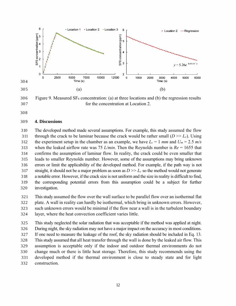
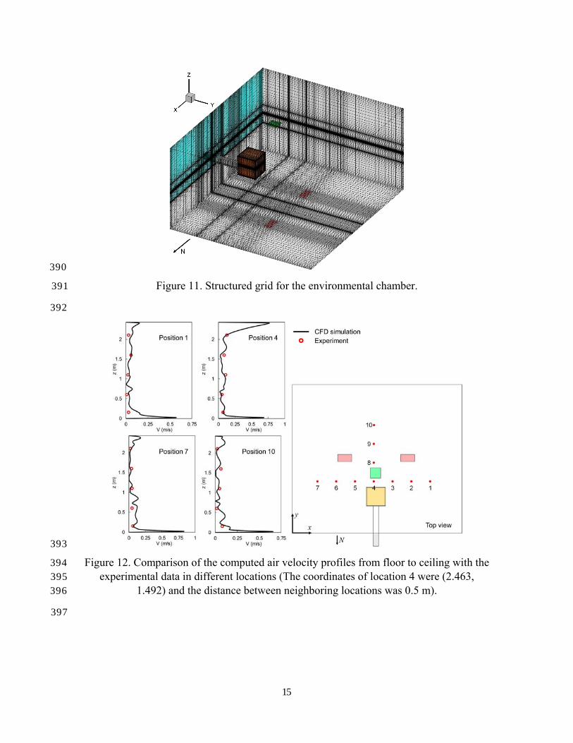
Figure 11 shows a structured grid with 2.5 million cells for the computational domain 375 according to our grid independence test. The grid around the crack and boundaries was 376 refined. This study ran a steady CFD simulation first to initialize the flow variables, such 377 as air pressure, velocity, and temperature. Next, we conducted transient simulation for two 378 time constants (τ = 100 s) to obtain statistically steady data, and for another time constant 379 to obtain a time-averaged solution. The time step size was 0.1 s. To validate the CFD 380 simulation, we compared the predicted air velocity profiles at four typical locations 381 (Locations 1, 4, 7, and 10) with the experimental data, as shown in Figure 12. The CFD 382 simulation agreed well with the experimental data. This study did not compare the 383 computed and measured air temperature because the air temperature variation along the 384 vertical direction was less than 0.5 K. However, Figure 13 shows the computed temperature 385 distributions on the wall with the crack. According to the simulation results, Tw,in = 25.7 oC 386 and Tw,out = 23.9 oC, which are almost the same as the measured data: Tw,in = 26.0 oC and 387 Tw,out = 24.0 oC. 388

389

15

390

Figure 11. Structured grid for the environmental chamber. 391

392

393

Figure 12. Comparison of the computed air velocity profiles from floor to ceiling with the 394 experimental data in different locations (The coordinates of location 4 were (2.463, 395

1.492) and the distance between neighboring locations was 0.5 m). 396

397

16

398

Figure 13. Computed temperature distributions on the wall with the crack: (left) outside 399 surface and (right) inside surface. 400

401

The CFD simulation provided the heat exchange between the ambient air and the box wall 402 surface. According to the CFD results, Qin,exp + Qout,exp = 0.343 W in Eq. 13, while the 403 measured data were Qin,exp + Qout,exp = 0.368 W, which shows that the CFD and measured 404 results were similar for heat flux. However, Tl,in − Tl,out was 1.0 K according to the CFD 405 simulation, whereas the measured temperature difference was 1.8 K. When we used Tl,in 406 −Tl,out = 1.0 K in Eq. 13, the corresponding calculated crack size was Lc,calculated = 0.9 mm, 407 which was very close to the actual crack size. Therefore, the errors in the calculations for 408 Scenarios 3 and 6 in Section 3.1 may have been due to inaccurate estimation of the leaked 409 air temperature. But note that 75 L/min corresponds to 3.6 h-1 that is unlikely to happen in 410 reality, this study believes that there is no difficulty in estimating the leaked air temperature 411 when the developed method is applied in a real condition. That is the reason for using the 412 air infiltration in an office for demonstration. 413

For the experiment in an office, the indoor/outdoor temperature difference was about 9 K 414 and the developed method was still able to accurately identify the air infiltration rate, which 415 means the method is applicable for conditions with low indoor/outdoor temperature 416 difference. However, a larger indoor/outdoor temperature difference would weaken the 417 errors and uncertainties in the developed method and further lead to better accuracy in 418 measuring the air infiltration. If there are multiple surfaces with cracks, one can apply the 419 method to the whole surface to obtain the total air infiltration rate or part of the surface to 420 obtain the regional air infiltration rate. The test in this office also showed that the developed 421 method required only one person and half a day to get the job done. Besides, the equipment 422 used in developed method was light weight and easy for installation comparing with the 423 traditional blower door method. 424

With all the above-mentioned uncertainties and limitations, further validations in different 425 buildings are necessary to improve the developed method. These validations could be used 426 to modify the developed method by using machine learning or data mining technique. 427

428

17

5. Conclusions 429

This study developed a novel method for measuring the air infiltration rate in buildings. 430 The proposed method is able to determine the effective crack size and air infiltration rate 431 by using the air temperature distributions on the interior and exterior surfaces of a wall 432 containing a crack, indoor and outdoor air temperatures, indoor-outdoor pressure 433 difference, and indoor and outdoor air velocities. 434

The proposed method was validated by the measured crack size in a small box installed in an 435 environmental chamber and by the measured infiltration rate in an office with the use of the 436 tracer-gas decay method. The proposed method was able to predict the crack size with a 437 relative error of less than 20% when the air infiltration rate was low. For a higher infiltration 438 rate, the error was larger, possibly because of inaccurate estimation of the leaked air 439 temperature. This inaccuracy was identified by detailed CFD simulation of airflow and 440 temperature distribution in the environmental chamber containing the box. The proposed 441 method estimated the air infiltration rate in the office with a relative error of only 3%. 442

This study confirmed that the small box in the environmental chamber could be used to 443 simulate infiltration in an actual room. This is because the coefficients obtained in the 444 power law equation for calculating the air infiltration rate were in the same range as those 445 in full-scale buildings found in the literature. Furthermore, the normalized leakage 446 determined by using the box data was also within the normal range found in the literature. 447

448

Acknowledgement 449

This research is partially supported by the national key R&D project on Green Buildings 450 and Building Industrialization of the Ministry of Science and Technology, China, through 451 Grant No. 2016YFC0700500; the National Natural Science Foundation of China through 452 Grant No. 51678395; and the key project of the Applied Basic and Frontier Technology 453 Research Program of Tianjin Commission of Science and Technology, China, through 454 Grant No. 15JCZDJC40900. 455

456

Nomenclature 457

Symbol definition 458

A wall area 459 C species concentration 460 Cf flow coefficient 461 Cp specific heat in constant pressure 462 D wall thickness 463 ELA effective leakage area 464 h heat convective coefficient 465 H room height 466

18

Lc crack height 467 n flow exponent 468 Nu Nusselt number 469 NL normalized leakage 470 P air pressure 471 Pr Prandtl number 472 Q heat flux 473 Qf leaked airflow rate 474 Re Reynolds number 475 t time 476 T air temperature 477 u, v, w velocity component in x, y, and z direction, respectively 478 V air velocity 479 x, y, z index of coordinates 480 air density 481 µ dynamic viscosity 482 λ air change rate 483 τ time constant 484

485

Subscripts 486

c critical value 487 in value at indoor side 488 out value at outdoor side 489 l value for leaked air 490 m mean value 491 R reference value 492 w value at the wall 493

∞ value for ambient air 494

495

References 496

[1] US EIA. 2015. “Annual Energy Outlook.” US Energy Information Administration: 497 Washington. 498

[2] DOE. 2015. “Building Energy Data.” 499 [3] Sandberg, P. I., and E. Sikander. 2005. “Airtightness issues in the building process.” 500

Proceedings of the 7th Symposium on Building Physics in the Nordic Countries 420–501 427. 502

[4] Emmerich, S. J., and A. K. Persily. 1998. “Energy impacts of infiltration and ventilation 503 in US office buildings using multizone airflow simulation.” Proc.IAQ Energy 98: 191–504 206. 505

[5] Brinks, P. 2013. “Astron Energy Report and Database Internal Report,” not published. 506 Luxembourg, Diekirch, Lindab SA. 507

19

[6] Brinks, Pascal, Oliver Kornadt, and Rene Oly. 2015. “Air infiltration assessment for 508 industrial buildings.” Energy and Buildings 86: 663–676. 509

[7] Kirkwood, RC. 1977. “Fuel consumption in industrial buildings.” Building Services 510 Engineer 45 (3): 23–31. 511

[8] Nevrala, DJ, and DW Etheridge. 1977. “Natural ventilation in well-insulated houses.” 512 In Proceedings of International Centre for Heat and Mass Transfer, International Seminar, 513 UNESCO, Dubrovnik, Croatia, Vol. 29. 514

[9] Caffey, GE. 1979. “Residential air infiltration.” ASHRAE Trans 85 (part 1). 515 [10] NIST (National Institute of Standards and Technology). 1996. “NIST estimates 516

nationwide energy impact of air leakage in U.S. buildings.” Journal of Research of the 517 NIST 101 (3): 423. 518

[11] Jokisalo, Juha, Targo Kalamees, Jarek Kurnitski, Lari Eskola, Kai Jokiranta, and 519 Juha Vinha. 2008. “A comparison of measured and simulated air pressure conditions 520 of a detached house in a cold climate.” Journal of Building Physics 32 (1): 67–89. 521

[12] Airaksinen, M, P Pasanen, J Kurnitski, and O Seppanen. 2004. “Microbial 522 contamination of indoor air due to leakages from crawl space: A field study.” Indoor Air 523 14 (1): 55–64. 524

[13] Rantala, Jukka, and Virpi Leivo. 2009. “Heat, air, and moisture control in slab-on-525 ground structures.” Journal of Building Physics 32 (4): 335–353. 526

[14] Chen, Chun, and Bin Zhao. 2011. “Review of relationship between indoor and 527 outdoor particles: I/O ratio, infiltration factor and penetration factor.” Atmospheric 528 Environment 45 (2): 275–288. 529

[15] Lstiburek, Joseph, Kim Pressnail, and John Timusk. 2002. “Air pressure and 530 building envelopes.” Journal of Thermal Envelope and Building Science 26 (1): 53–91. 531

[16] Hagentoft, C-E, and E Harderup. 1996. “Moisture conditions in a north facing wall 532 with cellulose loose fill insulation: Constructions with and without vapor retarder and air 533 leakage.” Journal of Thermal Insulation and Building Envelopes 19 (3): 228–243. 534

[17] Younes, Chadi, Caesar Abi Shdid, and Girma Bitsuamlak. 2012. “Air infiltration 535 through building envelopes: A review.” Journal of Building Physics 35 (3): 267–302. 536

[18] Blomsterberg, A. 1977. “Air Leakage in Dwellings.” Dept. Bldg. Constr. Report 537 (15). 538

[19] Harrje, DT, A Blomsterberg, and A Persily. 1979. “Reduction of Air Infiltration 539 Due to Window and Door Retrofits.” CU/CEES Report 85. 540

[20] Sherman, Max. 1995. “The use of blower-door data.” Indoor Air 5 (3): 215–224. 541 [21] ASTM, E. 2011. “Standard test methods for determining airtightness of buildings 542

using an orifice blower door.” ASTM International, West Conshohocken, PA. 543 [22] Kalamees, Targo. 2007. “Air tightness and air leakages of new lightweight single-544

family detached houses in Estonia.” Building and environment 42 (6): 2369–2377. 545 [23] Dufour, Marianne Berube, Dominique Derome, and Radu Zmeureanu. 2009. “Analysis 546

of thermograms for the estimation of dimensions of cracks in building envelope.” Infrared 547 Physics & Technology 52 (2): 70–78. 548

[24] Qi, Te. 2012. “Inverse modeling to predict effective leakage area.” Ph.D. thesis. 549 Georgia Institute of Technology. 550

20

[25] Bergman, Theodore L, and Frank P Incropera. 2011. Fundamentals of heat and mass 551 transfer. John Wiley & Sons. 552

[26] Sherman, Max H. 1990. “Tracer-gas techniques for measuring ventilation in a 553 single zone.” Building and Environment 25 (4): 365–374. 554

[27] Walker, Iain S, David J Wilson, and Max H Sherman. 1998. “A comparison of the 555 power law to quadratic formulations for air infiltration calculations.” Energy and 556 Buildings 27 (3): 293–299. 557

[28] Sherman, Max, and Darryl Dickerhoff. 1994. “Air-tightness of US dwellings.” In 558 Document-air Infiltration Centre AIC PROC, 225–225. OSCAR FABER PLC. 559

[29] Yakhot, Victor, and Steven A Orszag. 1986. “Renormalization-group analysis of 560 turbulence.” Physical Review Letters 57 (14): 1722. 561

[30] Fluent, Ansys. 2009. “12.0 Theory Guide.” Ansys Inc 5. 562 [31] Zhang, Zhao, Wei Zhang, Zhiqiang John Zhai, and Qingyan Yan Chen. 2007. 563

“Evaluation of various turbulence models in predicting airflow and turbulence in 564 enclosed environments by CFD: Part 2 Comparison with experimental data from 565 literature.” HVAC&R Research 13 (6): 871–886. 566

[32] Boussinesq, Joseph. 1903. Theorie analytique de la chaleur: mise en harmonie avec la 567 thermodynamique et avec la th eorie m ecanique de la lumiere. Vol. 2. Gauthier-Villars. 568

[33] Zhang, Tengfei Tim, Hongbiao Zhou, and Shugang Wang. 2013. “An adjustment to 569 the standard temperature wall function for CFD modeling of indoor convective heat 570 transfer.” Building and Environment 68: 159–169. 571

[34] Patankar, Suhas V, and D Brian Spalding. 1972. “A calculation procedure for heat, 572 mass and momentum transfer in three-dimensional parabolic flows.” International 573 Journal of Heat and Mass Transfer 15 (10): 1787–1806. 574

575