Embed Size (px)
Citation preview
AGRICULTURAL PRODUCTS
Livestock Futures and Options: Introduction to Underlying Market Fundamentals
2
Table of Contents
INTRODUCTION . . . . . . . . . . . . . . . . . . . . . . . . . . . . . . . . . . . . . . . . . . . . . . . . . . . . . . . . . . . . . . . . . . . . . . . . . . 4
THE PORK INDUSTRY . . . . . . . . . . . . . . . . . . . . . . . . . . . . . . . . . . . . . . . . . . . . . . . . . . . . . . . . . . . . . . . . . . . . . 5
THE BEEF INDUSTRY . . . . . . . . . . . . . . . . . . . . . . . . . . . . . . . . . . . . . . . . . . . . . . . . . . . . . . . . . . . . . . . . . . . . . . 8
ECONOMIC FACTORS . . . . . . . . . . . . . . . . . . . . . . . . . . . . . . . . . . . . . . . . . . . . . . . . . . . . . . . . . . . . . . . . . . . . 13
THE ECONOMICS OF SUPPLY . . . . . . . . . . . . . . . . . . . . . . . . . . . . . . . . . . . . . . . . . . . . . . . . . . . . . . . . . . . . . 20
THE ECONOMICS OF DEMAND . . . . . . . . . . . . . . . . . . . . . . . . . . . . . . . . . . . . . . . . . . . . . . . . . . . . . . . . . . . . 23
LIVESTOCK CYCLES AND SEASONALITY . . . . . . . . . . . . . . . . . . . . . . . . . . . . . . . . . . . . . . . . . . . . . . . . . . . . 26
CONCLUSION . . . . . . . . . . . . . . . . . . . . . . . . . . . . . . . . . . . . . . . . . . . . . . . . . . . . . . . . . . . . . . . . . . . . . . . . . . . 30
SOURCES OF INFORMATION . . . . . . . . . . . . . . . . . . . . . . . . . . . . . . . . . . . . . . . . . . . . . . . . . . . . . . . . . . . . . . 31
CME GROUP AGRICULTURAL PRODUCTS . . . . . . . . . . . . . . . . . . . . . . . . . . . . . . . . . . . . . . . . . . . . . . . . . . . 32
Livestock Futures and Options: Introduction to Underlying Market Fundamentals
3
In a world of increasing volatility, CME Group is where the world comes to manage risk across all
major asset classes – agricultural commodities, interest rates, equity indexes, foreign exchange,
energy and metals, as well as alternative investments such as weather and real estate. Built on
the heritage of CME, CBOT, and NYMEX, CME Group is the world’s largest and most diverse
derivatives exchange encompassing the widest range of benchmark products available, providing
the tools customers need to meet business objectives and achieve financial goals. CME Group
brings buyers and sellers together on the CME Globex electronic trading platform. CME Group
also operates CME Clearing, one of the world’s leading central counterparty clearing providers,
which offers clearing and settlement services across asset classes for exchange-traded contracts
and over-the-counter derivatives transactions. These products and services ensure that
businesses everywhere can substantially mitigate counterparty credit risk.
Agricultural Products More Agricultural Futures And Options. Greater Opportunity.
CME Group offers the widest range of agricultural derivatives of any exchange, with trading
available on a variety of grains, oilseeds, livestock, dairy, lumber and other products. Representing
the staples of everyday life, these products offer liquidity, transparent pricing and extraordinary
opportunities in a regulated centralized marketplace with equal access for all participants.

4
For many decades CME Group has provided participants
in the livestock industry with valuable tools to manage
risk. Futures and options on Live Cattle, Feeder Cattle and
Lean Hogs serve livestock producers and processors, as
well as traders seeking to capitalize on the extraordinary
opportunities these markets offer.
Market participants should gain an understanding of the
underlying cash markets before entering into the futures
and options markets. CME Group Livestock Futures and
Options: Introduction to Underlying Market Fundamentals
provides basic information regarding the cattle and hog
industries, as well as a fundamental economic framework for
analyzing prices.
The information is divided into two main sections. The first
section provides general information on the cattle and hog
industries, highlighting the life cycle of each species from
birth to slaughter. It also describes the different pricing
mechanisms in each respective industry, and how prices are
realized in the cash markets. The second section provides
information on analytical tools used in price forecasts and
discusses economic factors affecting the livestock industry.
This section also assists the market participant in locating
and understanding the various government livestock reports
used in price forecasts.
This publication provides a starting point for the potential
trader to amass knowledge about the underlying industries.
Each market participant must learn about other types
and sources of pertinent information and how to use the
information available. The emphasis here is on fundamental
analysis; however, the novice trader may also want to explore
technical analysis and discover the benefits it could add to
trading. Some market participants prefer one technique
over the other, while others utilize both types of analysis to
enhance trading skills. The type or combination of techniques
used is solely the preference of the individual.
A useful publication to complement this one is the Self Study
Guide to Hedging with Livestock Futures and Options which
provides a comprehensive overview of using futures and
options for risk management in the livestock markets. Visit
cmegroup.com/livestock for additional resources.
Introduction
Livestock Futures and Options: Introduction to Underlying Market Fundamentals
5
The pork industry can be divided into several basic phases
that correspond to the animals’ life cycle: 1) the production of
young animals (pigs), 2) feeding the pigs to slaughter weight
and 3) slaughter and fabrication.
The Hog Production Facility
Hogs originate from several types of hog farms: farrow-to-
finish, finish-only, farrow-to-feeder, and farrow-to-wean.
Farrow-to-finish operations handle all stages of a pig’s life,
from birth to sale of a market-ready hog, while farrow-to-feeder
operations raise pigs from birth to the feeder pig stage, when
they weigh about 40 to 60 pounds, and are ready to be sold to
finishing farms. Farrow-to-wean farms raise pigs from birth to
only about 10 to 15 pounds, when they are then sold to another
operation and fed to market weight. The swine industry has
seen dramatic change over the last decade due to a move to
contract and vertically coordinated hog production.
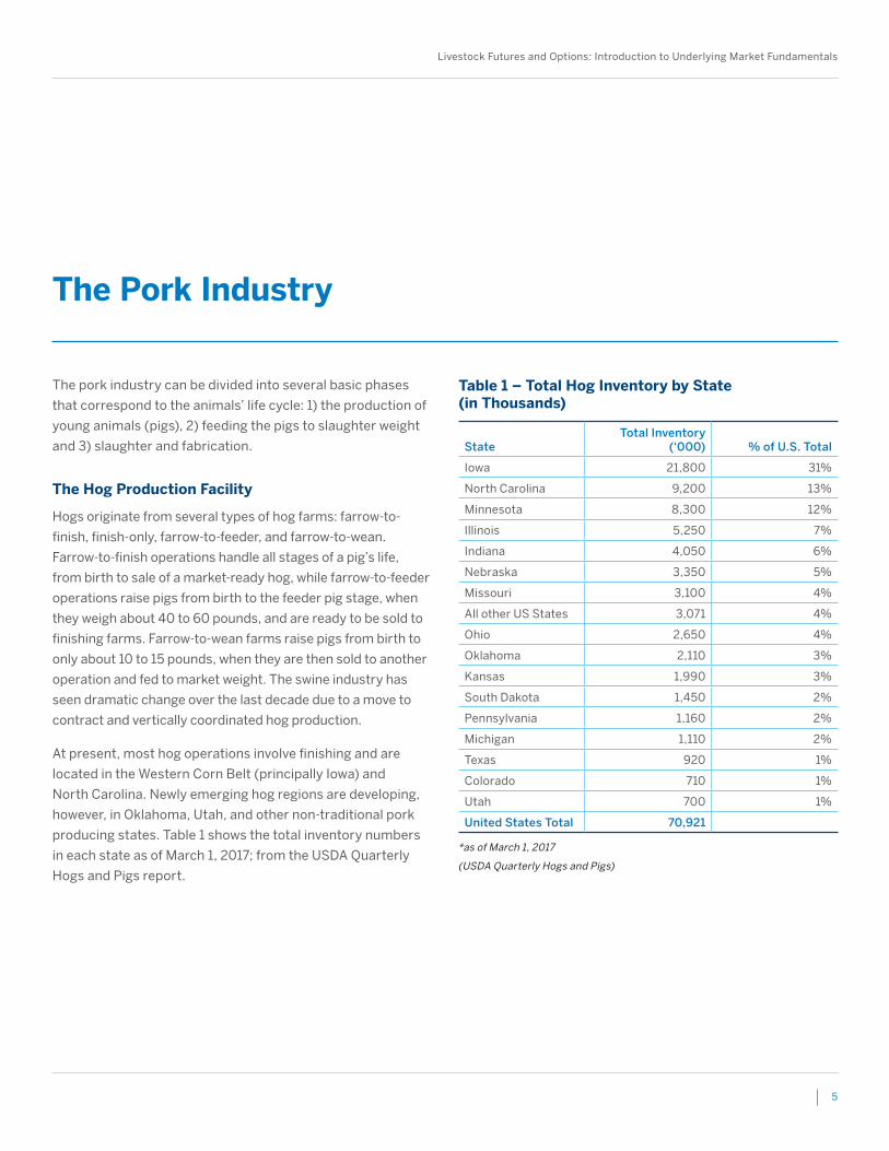
At present, most hog operations involve finishing and are
located in the Western Corn Belt (principally Iowa) and
North Carolina. Newly emerging hog regions are developing,
however, in Oklahoma, Utah, and other non-traditional pork
producing states. Table 1 shows the total inventory numbers
in each state as of March 1, 2017; from the USDA Quarterly
Hogs and Pigs report.
The Pork Industry
*as of March 1, 2017
(USDA Quarterly Hogs and Pigs)
Table 1 – Total Hog Inventory by State (in Thousands)
StateTotal Inventory
(‘000) % of U.S. Total
Iowa 21,800 31%
North Carolina 9,200 13%
Minnesota 8,300 12%
Illinois 5,250 7%
Indiana 4,050 6%
Nebraska 3,350 5%
Missouri 3,100 4%
All other US States 3,071 4%
Ohio 2,650 4%
Oklahoma 2,110 3%
Kansas 1,990 3%
South Dakota 1,450 2%
Pennsylvania 1,160 2%
Michigan 1,110 2%
Texas 920 1%
Colorado 710 1%
Utah 700 1%
United States Total 70,921
6
Hog facilities have grown dramatically larger, evolving from
small hog farms to large corporate and private operations.
According to the last “Overview of the United States Hog
Industry” published on October 29, 2015, 93 percent of the
annual pig crop is produced on operations with at least 5,000
head, up from 88 percent in 2008 and up from 27 percent in
1994. The 2012 Census of Agriculture indicated that only 5
percent of hog and pig operations had 5,000 or more head,
but accounted for 68 percent of the nation’s inventory.
Conversely, 95 percent of operations had fewer than 5,000
head, but accounted for only 32 percent of the inventory.
The driving force behind this shift is the benefits stemming
from economies of scale. Production costs per hog decline
on large farms, in part, because of improved feed efficiency
and labor productivity. As annual marketings increase to
1,000 head, production costs drop sharply, and continue to
decline as the marketings increase above 1,000 head, albeit
at a slower rate. Larger operations also are better able to
negotiate long-term contracts with packers because the
operators can assure them of a constant supply of hogs.
Stages of Hog Production
The life cycle begins with the baby piglet. Each gilt (young
female that has not given birth) and sow (mature female that
has given birth) is generally bred twice a year, on a schedule
to provide a continuous flow of pigs for the operation. To
obtain the breeding stock, operators retain gilts that show
superior growth, leanness, and reproductive potential as
seen in their mothers. Boars (sexually mature males) used for
breeding are generally purchased from breeding farms and
have a working life of approximately two years
There are three main types of hog breeding. The first is pen
mating, in which one or more boars are placed with a group of
sows or gilts. The second and most common method is hand
mating, where one boar is placed with only one sow or gilt at
a time and they are monitored to be sure mating occurs. This
method is more labor intensive than pen mating but there
is more assurance that the female will reproduce. The third
method is artificial insemination. This method allows for new
genetics to be introduced quickly, but it is the most labor
intensive of the three alternatives.
The gestation period for a bred female is approximately
4 months, at which point the female will give birth to an
average of nine to 10 pigs. The number of pigs per litter has
seen steady increases in recent years, due to improved herd
health, genetics, and production efficiencies. This trend has
been an important factor in increasing the US hog inventory.
Accordingly, the pig per litter number is very important in
estimating the supply of market hogs and is closely watched
in the USDA’s Quarterly Hogs and Pigs report.
After these baby pigs are weaned, at around three to four
weeks of age, the sows will either be re-bred or sent to
market. Females are generally kept in the breeding herd
for two to three years until they are sold for slaughter, but
depending on their genetics, health, and weight, they may
be sold earlier.
Between farrowing and weaning, death loss accounts for
approximately five percent of the pigs. Death can occur
from suffocation by the sow laying on the baby pig, disease,
weather conditions, and other external factors. Depending
on the facilities used for farrowing, death loss due to weather
conditions can be higher in severe winters.
As the young pigs grow, they are fed various diets to meet
their specific nutritional needs at different predetermined
weights. These diets must be high in grains because hogs
cannot efficiently convert forages to muscle. Also, many
times barrows (castrated males) and gilts are fed separately
due to their differing nutritional needs. By separating these
two groups, each sex can be fed more efficiently because
their nutritional needs are different. The diet generally
consists of corn, barley, milo, oats, distiller’s grains or
sometimes wheat. The protein comes from oilseed meals and
vitamin and mineral additives.
Most of the feed is mixed on the site of the hog operation
and some farms grow the feed that is used. However,
sometimes complete rations are purchased from feed
manufacturers and can be fed directly without further
processing. On average, a barrow or gilt in the finishing
stage will gain approximately one pound per day with a feed
conversion of 3.5 pounds of feed.
Livestock Futures and Options: Introduction to Underlying Market Fundamentals
7
Typically, it takes six months to raise a pig from birth to
slaughter. Hogs are generally ready for market when they
reach a weight of approximately 270 pounds. According
to the USDA (LM_HG201), the average federally inspected
slaughter weight (or live weight) was 275 pounds with an
average carcass weight of 208 pounds in 2016. The weight at
which hogs are marketed is affected by feed and hog prices.
High feed prices and low hog prices may cause producers
to sell hogs at a lighter weight while low feed prices and high
hog prices might induce producers to feed hogs to a heavier
weight before they are sold.
Generally, market-ready hogs are sold directly to the packer;
however, some are sold through buying stations
and auctions, and a small number are sold through
terminal markets.
In 2015, 93 percent of the annual pig crop is produced on
operations with at least 5,000 head. The 2012 US Ag Census
indicated that only 5 percent of hog and pig operations had
5,000 or more head, but accounted for 68 percent of the
nation’s inventory. Conversely, 95 percent of operations
had fewer than 5,000 head, but accounted for 32 percent
of the inventory.
In 2016, about 67.4 percent of hog production was from
independent producers with the remainder from packer-
owned facilities. Hog producers sell their hogs either as a
negotiated transaction for a particular day or as part of a
formula price. Formula pricing may be used when a large
number of hogs are forward contracted with a packer or
another producer over an extended time period. The formula
price is derived from a “price determining market” such as
the Iowa-Southern Minnesota weighted average price of
51-52 percent lean hogs. There also may be a price differential
subtracted or added based on different factors such as
location or overall quality of the hogs.
It is important to mention that when hogs are priced,
generally, it is with regard to the actual percent lean of
their carcasses, since this percentage determines the
actual amount of meat the carcass will yield. When live
hogs are sold at an auction, however, the price is based
on an expected lean figure, typically 51-52 percent.
Pork Packing and Processing
After hogs are sold, they are shipped to a packer and
slaughtered. The carcasses are cut into wholesale cuts
and sold to retailers. A market hog with a live weight of 270
pounds will typically result in a 200 pound carcass with an
average of 25 percent ham, 25 percent loin, 16 percent belly,
11 percent picnic, 5 percent spareribs and 10 percent butt.
The rest goes into jowl, lean trim, fat (lard) and miscellaneous
cuts and trimmings.
A large portion of pork is further processed and becomes
storable for considerable periods of time. Hams and picnics
(a ham-like cut from the front leg of the hog) can be smoked,
canned, or frozen. Pork bellies (the raw cut of meat used
for bacon) can be frozen and stored for up to a year prior to
processing. The pork belly is the meat from the underside
of the hog. This section is cut to produce two pieces. Belly
pieces vary in size depending on the size of the animal and
are divided into two-pound weight ranges. The bulk of bellies
fall into the 12-14, 14-16 and 16-18 pound weight ranges.
Almost all bellies are treated in a preservative process
(cured) and sliced into bacon.
8
The Cow/Calf Operation
Cattle production begins with a cow-calf producer or rancher
who breeds cows to produce calves using natural service with
a bull or an artificial insemination (A.I.) program. Although the
size of cow-calf operations varies considerably, 91 percent
of beef cow farms have less than 100 head as of 2012.
Operations with 100 or more beef cows comprise 9 percent of
all beef operations and 54 percent of the beef cow inventory.
If using a natural service breeding program, each producer
commonly runs one mature bull per 20-25 cows for breeding
purposes. However, some cow-calf operators choose to breed
their herd with an A.I. program in order to better control
the genetics of any resulting calves. Genetics have grown in
importance with the movement to produce higher quality
beef and heavier weight animals.
A producer, with or without the use of bulls, requires a certain
number of acres of pasture or grazing land to support each
cow-calf unit. The acres of grazing land required per cow-
calf unit is referred to as the stocking rate, and it differs
among regions across the U.S. due to weather conditions and
management practices. In high rainfall areas of the East and
Midwest, for example, the stocking rate can be as low as five
acres per cow-calf unit, while in the West and Southwest it
can be as many as 150 acres.
The ranches themselves vary in size from less than 100 acres
to many thousands of acres. In western states, ranches often
lease summer grazing rights on public lands (particularly the
US Forest Service and Bureau of Land Management). These
grazing leases allow ranchers to graze cattle through the
summer without the costs of land ownership.
Most herds are bred in late summer and after a 9
month gestation period, produce a spring calf crop.
Most producers breed their herd to calve in the spring
to avoid the harsh weather of winter and to assure
abundant forage for the new calves during their first
few months. This spring calving cycle creates strong
seasonal supply effects which ripple across the entire
cattle industry.
Each cow in a herd generally gives birth to one calf; however,
twins are born on rare occasions. Not all cows in a herd will
conceive and the conception rate (the percentage of cows
bred that actually produce a calf) can be adversely affected
by disease, harsh weather, and poor nutrition. A cow that
misses its annual pregnancy is referred to as “open” and is
usually culled from the herd and sent to slaughter, even if
she is still young.
Typically 15 to 25 percent of the cows in a herd are culled
each year. Cows can be culled for several reasons: failure
to become pregnant, old age, bad teeth, drought or market
conditions such as high feed costs. The cows that are
culled must be replaced in order to maintain herd size. To
accomplish this, a certain number of females from the calf
crop must be held back to use as replacement heifers. If the
calf crop does not contain enough suitable heifer calves to
maintain the size of the herd, replacement heifers must be
purchased from another source. During the expansion phase
of the cattle cycle when producers are building their herds,
the retention rate is higher than average and the rate is lower
during the liquidation phase.
The Beef Industry
Livestock Futures and Options: Introduction to Underlying Market Fundamentals
9
Calves, whether being retained for replacement heifers or
being sold for eventual slaughter, remain with the cow for
at least the first six months of their lives. At birth, calves
receive their nourishment exclusively from nursing. Over time,
however, their diet is supplemented with grass and eventually
grain. When calves reach six to eight months of age, they
are weaned from the cow. The average weight of a beef calf
at weaning is between 500 and 600 pounds. Some heavier
weight calves are then put directly into feedlots, but most pass
through an intermediate stage called the “stocker operation.“
The Stocker Operation
Stocker or “backgrounding” operations place weaned calves
on summer grass, winter wheat, or some type of harvest
roughage, depending upon the area and the time of year.
The cow-calf operator may pay a stocker operator for
providing these services or may sell the calves to a stocker
operator. Either way, the stocker phase of the calf’s life may
last from six to ten months, until the animal reaches feedlot
weight of about 600 to 800 pounds. When the cattle are
ready to be placed in feedlots, they are referred to as feeder
cattle. Again, as they pass from the stocker operation to the
feedlot, the animals may or may not change ownership. Many
of the feedlots that stocker calves are sent to are located in
the Great Plains, specifically Colorado, Nebraska, Kansas,
Oklahoma, and Texas.
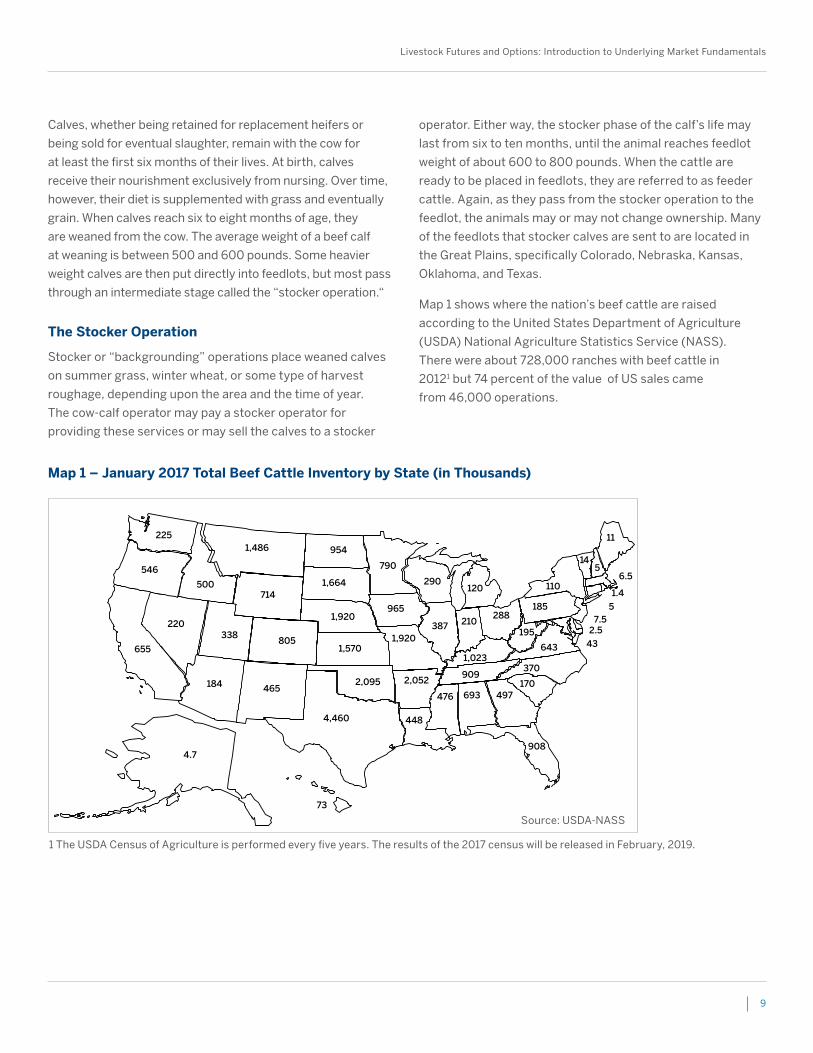
Map 1 shows where the nation’s beef cattle are raised
according to the United States Department of Agriculture
(USDA) National Agriculture Statistics Service (NASS).
There were about 728,000 ranches with beef cattle in
20121 but 74 percent of the value of US sales came
from 46,000 operations.
514
43
2.57.5
5
1.4110
220338
805
387
643
290
73
546
655
4,460
4.7908
497170
370909
185
195
1,023
11
288
693
120
210
476
448
2,052
1,920
965
790
2,095
1,570
1,920
1,664
954
465184
714500
1,486225
6.5
Source: USDA-NASS
1 The USDA Census of Agriculture is performed every five years. The results of the 2017 census will be released in February, 2019.
Map 1 – January 2017 Total Beef Cattle Inventory by State (in Thousands)
10
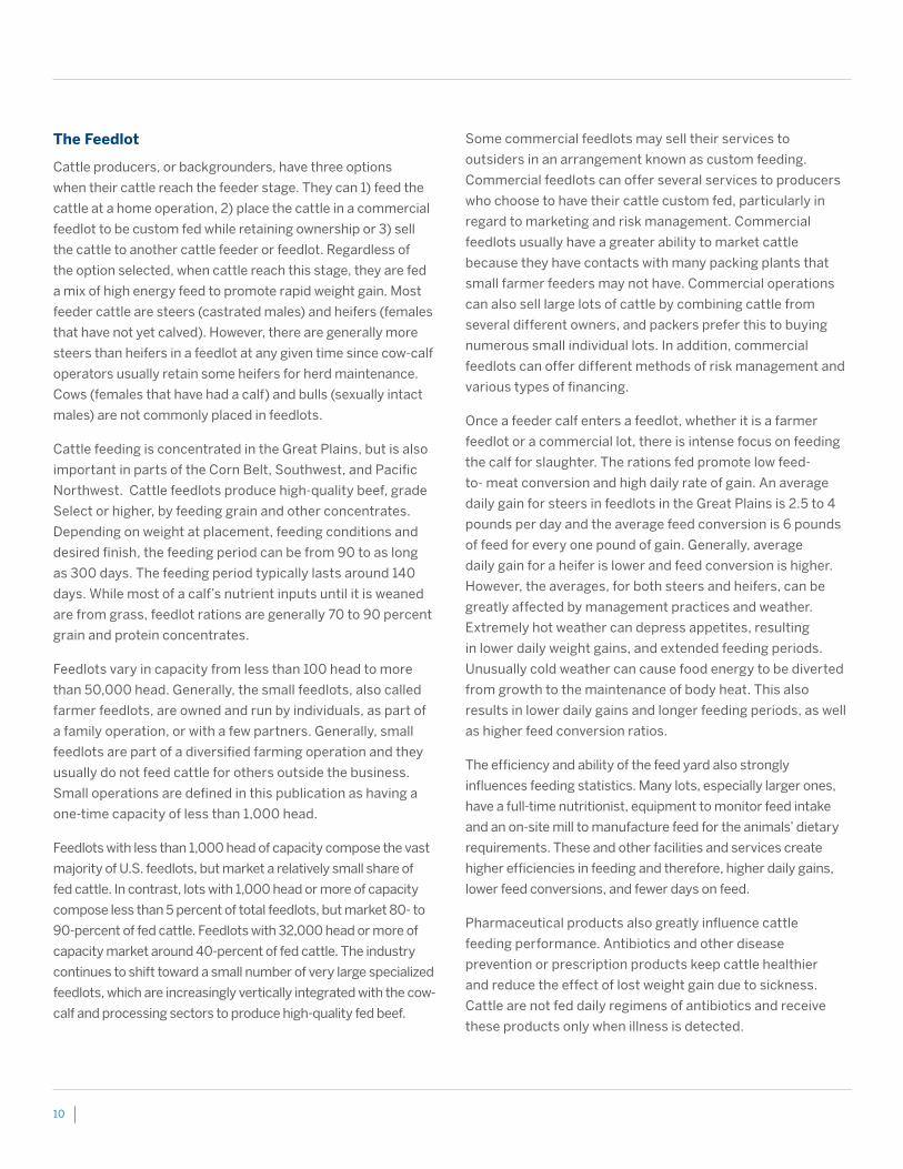
The Feedlot
Cattle producers, or backgrounders, have three options
when their cattle reach the feeder stage. They can 1) feed the
cattle at a home operation, 2) place the cattle in a commercial
feedlot to be custom fed while retaining ownership or 3) sell
the cattle to another cattle feeder or feedlot. Regardless of
the option selected, when cattle reach this stage, they are fed
a mix of high energy feed to promote rapid weight gain. Most
feeder cattle are steers (castrated males) and heifers (females
that have not yet calved). However, there are generally more
steers than heifers in a feedlot at any given time since cow-calf
operators usually retain some heifers for herd maintenance.
Cows (females that have had a calf) and bulls (sexually intact
males) are not commonly placed in feedlots.
Cattle feeding is concentrated in the Great Plains, but is also
important in parts of the Corn Belt, Southwest, and Pacific
Northwest. Cattle feedlots produce high-quality beef, grade
Select or higher, by feeding grain and other concentrates.
Depending on weight at placement, feeding conditions and
desired finish, the feeding period can be from 90 to as long
as 300 days. The feeding period typically lasts around 140
days. While most of a calf’s nutrient inputs until it is weaned
are from grass, feedlot rations are generally 70 to 90 percent
grain and protein concentrates.
Feedlots vary in capacity from less than 100 head to more
than 50,000 head. Generally, the small feedlots, also called
farmer feedlots, are owned and run by individuals, as part of
a family operation, or with a few partners. Generally, small
feedlots are part of a diversified farming operation and they
usually do not feed cattle for others outside the business.
Small operations are defined in this publication as having a
one-time capacity of less than 1,000 head.
Feedlots with less than 1,000 head of capacity compose the vast
majority of U.S. feedlots, but market a relatively small share of
fed cattle. In contrast, lots with 1,000 head or more of capacity
compose less than 5 percent of total feedlots, but market 80- to
90-percent of fed cattle. Feedlots with 32,000 head or more of
capacity market around 40-percent of fed cattle. The industry
continues to shift toward a small number of very large specialized
feedlots, which are increasingly vertically integrated with the cow-
calf and processing sectors to produce high-quality fed beef.
Some commercial feedlots may sell their services to
outsiders in an arrangement known as custom feeding.
Commercial feedlots can offer several services to producers
who choose to have their cattle custom fed, particularly in
regard to marketing and risk management. Commercial
feedlots usually have a greater ability to market cattle
because they have contacts with many packing plants that
small farmer feeders may not have. Commercial operations
can also sell large lots of cattle by combining cattle from
several different owners, and packers prefer this to buying
numerous small individual lots. In addition, commercial
feedlots can offer different methods of risk management and
various types of financing.
Once a feeder calf enters a feedlot, whether it is a farmer
feedlot or a commercial lot, there is intense focus on feeding
the calf for slaughter. The rations fed promote low feed-
to- meat conversion and high daily rate of gain. An average
daily gain for steers in feedlots in the Great Plains is 2.5 to 4
pounds per day and the average feed conversion is 6 pounds
of feed for every one pound of gain. Generally, average
daily gain for a heifer is lower and feed conversion is higher.
However, the averages, for both steers and heifers, can be
greatly affected by management practices and weather.
Extremely hot weather can depress appetites, resulting
in lower daily weight gains, and extended feeding periods.
Unusually cold weather can cause food energy to be diverted
from growth to the maintenance of body heat. This also
results in lower daily gains and longer feeding periods, as well
as higher feed conversion ratios.
The efficiency and ability of the feed yard also strongly
influences feeding statistics. Many lots, especially larger ones,
have a full-time nutritionist, equipment to monitor feed intake
and an on-site mill to manufacture feed for the animals’ dietary
requirements. These and other facilities and services create
higher efficiencies in feeding and therefore, higher daily gains,
lower feed conversions, and fewer days on feed.
Pharmaceutical products also greatly influence cattle
feeding performance. Antibiotics and other disease
prevention or prescription products keep cattle healthier
and reduce the effect of lost weight gain due to sickness.
Cattle are not fed daily regimens of antibiotics and receive
these products only when illness is detected.
Livestock Futures and Options: Introduction to Underlying Market Fundamentals
11
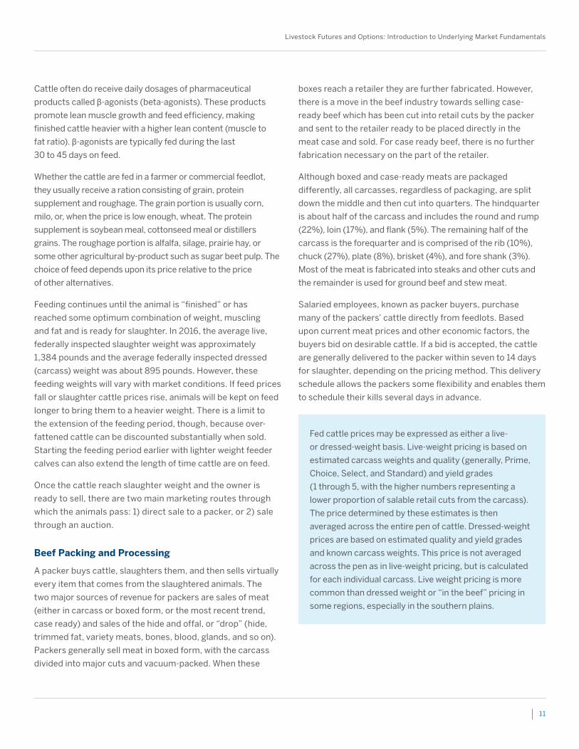
Cattle often do receive daily dosages of pharmaceutical
products called β-agonists (beta-agonists). These products
promote lean muscle growth and feed efficiency, making
finished cattle heavier with a higher lean content (muscle to
fat ratio). β-agonists are typically fed during the last
30 to 45 days on feed.
Whether the cattle are fed in a farmer or commercial feedlot,
they usually receive a ration consisting of grain, protein
supplement and roughage. The grain portion is usually corn,
milo, or, when the price is low enough, wheat. The protein
supplement is soybean meal, cottonseed meal or distillers
grains. The roughage portion is alfalfa, silage, prairie hay, or
some other agricultural by-product such as sugar beet pulp. The
choice of feed depends upon its price relative to the price
of other alternatives.
Feeding continues until the animal is “finished” or has
reached some optimum combination of weight, muscling
and fat and is ready for slaughter. In 2016, the average live,
federally inspected slaughter weight was approximately
1,384 pounds and the average federally inspected dressed
(carcass) weight was about 895 pounds. However, these
feeding weights will vary with market conditions. If feed prices
fall or slaughter cattle prices rise, animals will be kept on feed
longer to bring them to a heavier weight. There is a limit to
the extension of the feeding period, though, because over-
fattened cattle can be discounted substantially when sold.
Starting the feeding period earlier with lighter weight feeder
calves can also extend the length of time cattle are on feed.
Once the cattle reach slaughter weight and the owner is
ready to sell, there are two main marketing routes through
which the animals pass: 1) direct sale to a packer, or 2) sale
through an auction.
Beef Packing and Processing
A packer buys cattle, slaughters them, and then sells virtually
every item that comes from the slaughtered animals. The
two major sources of revenue for packers are sales of meat
(either in carcass or boxed form, or the most recent trend,
case ready) and sales of the hide and offal, or “drop” (hide,
trimmed fat, variety meats, bones, blood, glands, and so on).
Packers generally sell meat in boxed form, with the carcass
divided into major cuts and vacuum-packed. When these
boxes reach a retailer they are further fabricated. However,
there is a move in the beef industry towards selling case-
ready beef which has been cut into retail cuts by the packer
and sent to the retailer ready to be placed directly in the
meat case and sold. For case ready beef, there is no further
fabrication necessary on the part of the retailer.
Although boxed and case-ready meats are packaged
differently, all carcasses, regardless of packaging, are split
down the middle and then cut into quarters. The hindquarter
is about half of the carcass and includes the round and rump
(22%), loin (17%), and flank (5%). The remaining half of the
carcass is the forequarter and is comprised of the rib (10%),
chuck (27%), plate (8%), brisket (4%), and fore shank (3%).
Most of the meat is fabricated into steaks and other cuts and
the remainder is used for ground beef and stew meat.
Salaried employees, known as packer buyers, purchase
many of the packers’ cattle directly from feedlots. Based
upon current meat prices and other economic factors, the
buyers bid on desirable cattle. If a bid is accepted, the cattle
are generally delivered to the packer within seven to 14 days
for slaughter, depending on the pricing method. This delivery
schedule allows the packers some flexibility and enables them
to schedule their kills several days in advance.
Fed cattle prices may be expressed as either a live-
or dressed-weight basis. Live-weight pricing is based on
estimated carcass weights and quality (generally, Prime,
Choice, Select, and Standard) and yield grades
(1 through 5, with the higher numbers representing a
lower proportion of salable retail cuts from the carcass).
The price determined by these estimates is then
averaged across the entire pen of cattle. Dressed-weight
prices are based on estimated quality and yield grades
and known carcass weights. This price is not averaged
across the pen as in live-weight pricing, but is calculated
for each individual carcass. Live weight pricing is more
common than dressed weight or “in the beef” pricing in
some regions, especially in the southern plains.

12
Price determination is either done via a formula or frequent
negotiation. Formula pricing involves using a mathematical
formula that includes some other price as a reference,
such as the average price of the cattle purchased by the
plant for the week prior to the week of slaughter. A portion
of cattle prices are arrived at by negotiating a price on the
cash market. The cattle are sold at the current market price.
Cash market sales include selling at terminal markets (which
are generally located close to slaughter facilities), auction
sales, and direct sales to packers at the cash price (spot bid).
Frequently, pricing grids are used to arrive at a final price.
A price grid establishes a base price (either negotiated or via
a formula) and then specifies premiums and discounts above
and below the base for different carcass attributes, such as
quality and yield grade and whether the carcasses are light
or heavy. The base price is set differently depending on each
packer and can be based on several different prices. Some
of these prices include the futures price, boxed beef cutout
value, or average price of the cattle purchased by the plant
the week prior to the week of slaughter. Grid pricing is also
known as value-based pricing because prices are based on
the known weight of the carcass, and the quality and yield
grade of each individual carcass.
Figure 1 shows the relative popularity of negotiated,
formula, negotiated grid, and forward contract marketing
arrangements for fed cattle. Most significant is the dramatic
decline of negotiated transactions. The decrease in
negotiated transactions has been largely offset by increases
in formula transactions. This phenomenon may be driven
by the added economic “costs” of negotiated transactions
and by the appeal of using an easily observable, transparent
outside market to determine prices.
There is a high amount of industry concentration amongst the
beef packers. The four largest packing firms make up slightly
more than 80% of the Federally Inspected slaughter.
0.0%
5.0%
10.0%
15.0%
20.0%
25.0%
30.0%
35.0%
40.0%
45.0%
50.0%
55.0%
60.0%
Negotiated Formula Forward Contract Negotiated Grid
20052006
20072008
20092010
20112012
20132014
20152016
JAN-JUN 2017
Source: USDA AMS
Figure 1 – Percent of Cattle Sold by Marketing Arrangement
Livestock Futures and Options: Introduction to Underlying Market Fundamentals
13
After gaining an understanding of the production cycles
of hogs and cattle, it is important to recognize how that
knowledge combines with economic factors that affect each
industry. The following sections will examine the relationship
between economic conditions and livestock prices. These
sections will discuss the pipeline approach to the livestock
industry, provide information on supply and demand factors
and explain livestock cycle and seasonality issues.
The Pipeline Approach
The pipeline approach is a forecasting technique that
estimates the quantity of a commodity at a specific point in
the future based on observation at various points during the
production cycle. At birth, livestock enter into a production
pipeline beginning on the farm and terminating at the
supermarket. The assumption is that what goes into the
pipeline must eventually come out, barring minor “leakage”
due to death, loss and exports.
The forecasting technique requires: 1) an estimate of current
supplies at various stages in the pipeline; 2) knowledge of the
average time it takes for the commodity to move from one
stage to the next; and 3) information about any important
leakages, infusions (imports) or feedback loops (diversion
of animals from slaughter back into the breeding herd).
Much of this information is available through United States
Department of Agriculture (USDA) publications.
Hog Pipeline
One of the first pieces of information needed to study the hog
pipeline is the size of the hog inventory. Hog inventory data
can be obtained from the Hogs and Pigs report published
by USDA’s National Agricultural Statistics Service (NASS).
On a quarterly basis, this report provides information for all
fifty U.S. states on the pig crop and total inventory as well as
other relevant information regarding hogs and pigs. It also
publishes a report on the litter size, breeding herd size, and
the number of sows and gilts bred on a monthly basis.
Quarterly data for total United States inventory of market
hogs (those not being kept for breeding purposes), total
commercial hog slaughter and commercial pork production,
are provided in Table 1.
Obtaining Data
Market participants may also need additional information
regarding hog slaughter, depending on the stage in the
pipeline they are studying. This data can be obtained from the
monthly Livestock Slaughter report. Also published by NASS,
it presents statistics on total hog slaughter by head, average
live and dressed weight in commercial plants by state and
in the U.S., information about federally inspected hogs, and
additional slaughter data.
Economic Factors
14
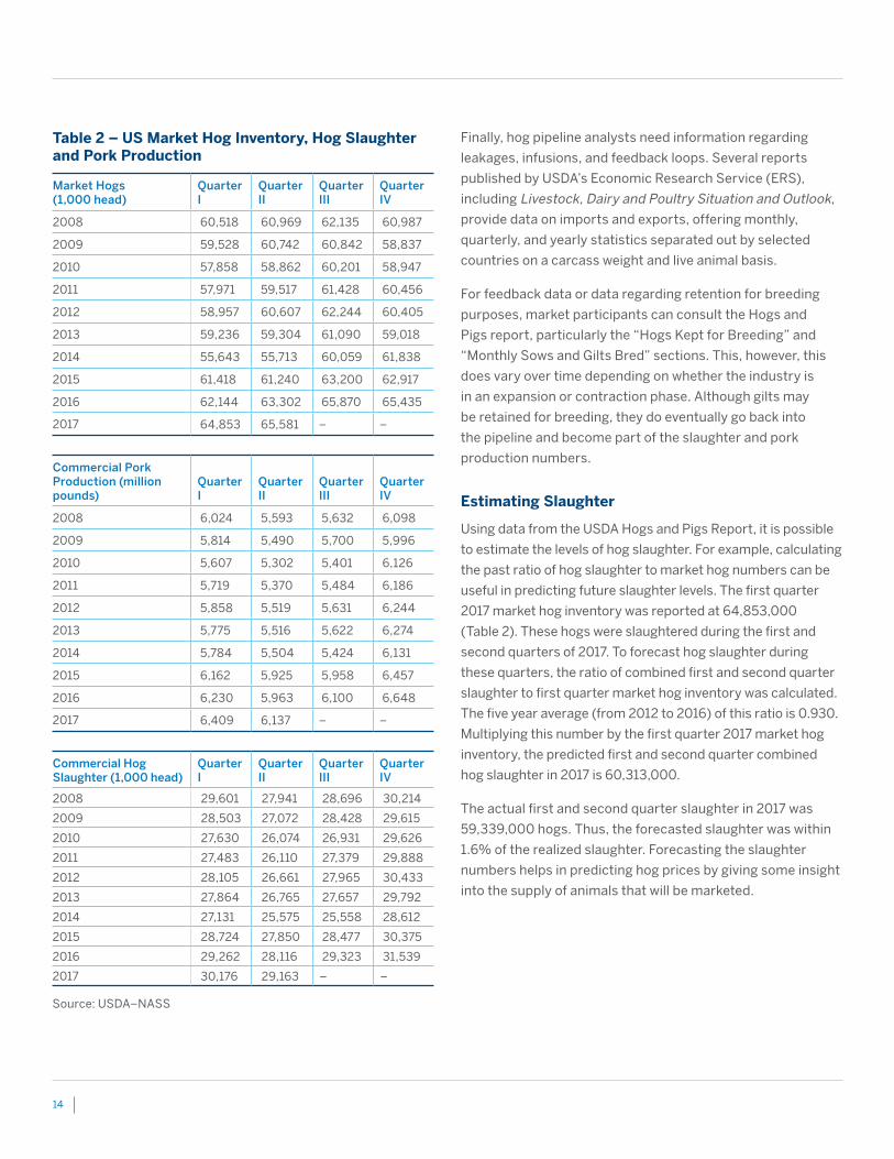
Table 2 – US Market Hog Inventory, Hog Slaughter and Pork Production
Market Hogs (1,000 head)
Quarter I
Quarter II
Quarter III
Quarter IV
2008 60,518 60,969 62,135 60,987
2009 59,528 60,742 60,842 58,837
2010 57,858 58,862 60,201 58,947
2011 57,971 59,517 61,428 60,456
2012 58,957 60,607 62,244 60,405
2013 59,236 59,304 61,090 59,018
2014 55,643 55,713 60,059 61,838
2015 61,418 61,240 63,200 62,917
2016 62,144 63,302 65,870 65,435
2017 64,853 65,581 – –
Commercial Pork Production (million pounds)
Quarter I
Quarter II
Quarter III
Quarter IV
2008 6,024 5,593 5,632 6,098
2009 5,814 5,490 5,700 5,996
2010 5,607 5,302 5,401 6,126
2011 5,719 5,370 5,484 6,186
2012 5,858 5,519 5,631 6,244
2013 5,775 5,516 5,622 6,274
2014 5,784 5,504 5,424 6,131
2015 6,162 5,925 5,958 6,457
2016 6,230 5,963 6,100 6,648
2017 6,409 6,137 – –
Commercial Hog Slaughter (1,000 head)
Quarter I
Quarter II
Quarter III
Quarter IV
2008 29,601 27,941 28,696 30,214
2009 28,503 27,072 28,428 29,615
2010 27,630 26,074 26,931 29,626
2011 27,483 26,110 27,379 29,888
2012 28,105 26,661 27,965 30,433
2013 27,864 26,765 27,657 29,792
2014 27,131 25,575 25,558 28,612
2015 28,724 27,850 28,477 30,375
2016 29,262 28,116 29,323 31,539
2017 30,176 29,163 – –
Source: USDA–NASS
Finally, hog pipeline analysts need information regarding
leakages, infusions, and feedback loops. Several reports
published by USDA’s Economic Research Service (ERS),
including Livestock, Dairy and Poultry Situation and Outlook,
provide data on imports and exports, offering monthly,
quarterly, and yearly statistics separated out by selected
countries on a carcass weight and live animal basis.
For feedback data or data regarding retention for breeding
purposes, market participants can consult the Hogs and
Pigs report, particularly the “Hogs Kept for Breeding” and
“Monthly Sows and Gilts Bred” sections. This, however, this
does vary over time depending on whether the industry is
in an expansion or contraction phase. Although gilts may
be retained for breeding, they do eventually go back into
the pipeline and become part of the slaughter and pork
production numbers.
Estimating Slaughter
Using data from the USDA Hogs and Pigs Report, it is possible
to estimate the levels of hog slaughter. For example, calculating
the past ratio of hog slaughter to market hog numbers can be
useful in predicting future slaughter levels. The first quarter
2017 market hog inventory was reported at 64,853,000
(Table 2). These hogs were slaughtered during the first and
second quarters of 2017. To forecast hog slaughter during
these quarters, the ratio of combined first and second quarter
slaughter to first quarter market hog inventory was calculated.
The five year average (from 2012 to 2016) of this ratio is 0.930.
Multiplying this number by the first quarter 2017 market hog
inventory, the predicted first and second quarter combined
hog slaughter in 2017 is 60,313,000.
The actual first and second quarter slaughter in 2017 was
59,339,000 hogs. Thus, the forecasted slaughter was within
1.6% of the realized slaughter. Forecasting the slaughter
numbers helps in predicting hog prices by giving some insight
into the supply of animals that will be marketed.
Livestock Futures and Options: Introduction to Underlying Market Fundamentals
15
Speed of Commodity Flows
Recall that the pipeline approach requires knowledge of
the speed of the commodity flow. While the average time
between birth and slaughter is roughly six months, the
actual period can vary with economic conditions as well as
with the season and unexpected changes in the weather.
For example, a decline in the cost of feed makes livestock
feeding more profitable, so producers will feed the animals to
heavier weights and therefore, increase the time the animals
are in the pipeline. A rise in the cost of feed can result in
earlier marketing at lighter weights. If livestock prices decline
temporarily, producers may delay marketing in hopes of a
price increase.
Market participants also need to remember that the number
of females withheld from slaughter for breeding purposes
will vary over time. When producers are expanding, they
increase the number of gilts withheld for breeding. During
a contraction phase, however, producers cull females from
the breeding herd and increase the number of sows and
gilts slaughtered. Although no public data provides exact
figures on gilt slaughter in comparison to total hog slaughter,
some inferences can be made from data in the Hogs and
Pigs report. When producers are putting more hogs into the
breeding herd, they are therefore slaughtering fewer females.
These estimates can then be considered when forecasting
hog slaughter using the pipeline approach.
Effects of Imports and Exports
Market participants also need to account for exports and
imports into the hog pipeline to accurately forecast hog
slaughter numbers. They can consult USDA data to determine
the number of exports and imports that enter and exit the
pipeline, apply these numbers to the pipeline forecast, and
then estimate the total slaughter.
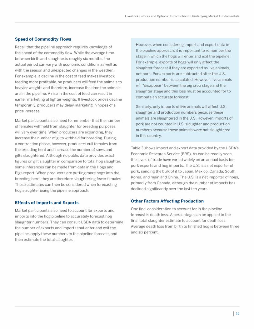
However, when considering import and export data in
the pipeline approach, it is important to remember the
stage in which the hogs will enter and exit the pipeline.
For example, exports of hogs will only affect the
slaughter forecast if they are exported as live animals,
not pork. Pork exports are subtracted after the U.S.
production number is calculated. However, live animals
will “disappear” between the pig crop stage and the
slaughter stage and this loss must be accounted for to
compute an accurate forecast.
Similarly, only imports of live animals will affect U.S.
slaughter and production numbers because these
animals are slaughtered in the U.S. However, imports of
pork are not counted in U.S. slaughter and production
numbers because these animals were not slaughtered
in this country.
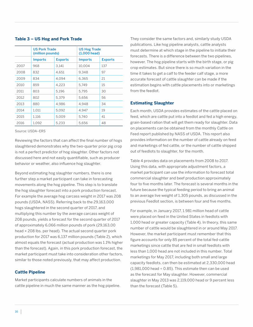
Table 3 shows import and export data provided by the USDA’s
Economic Research Service (ERS). As can be readily seen,
the levels of trade have varied widely on an annual basis for
pork exports and hog imports. The U.S. is a net exporter of
pork, sending the bulk of it to Japan, Mexico, Canada, South
Korea, and mainland China. The U.S. is a net importer of hogs,
primarily from Canada, although the number of imports has
declined significantly over the last ten years.
Other Factors Affecting Production
One final consideration to account for in the pipeline
forecast is death loss. A percentage can be applied to the
final total slaughter estimate to account for death loss.
Average death loss from birth to finished hog is between three
and six percent.
16
Table 3 – US Hog and Pork Trade
US Pork Trade (million pounds)
US Hog Trade (1,000 head)
Imports Exports Imports Exports
2007 968 3,141 10,004 137
2008 832 4,651 9,348 97
2009 834 4,094 6,365 21
2010 859 4,223 5,749 15
2011 803 5,196 5,795 30
2012 802 5,379 5,656 56
2013 880 4,986 4,948 34
2014 1,011 5,092 4,947 19
2015 1,116 5,009 5,740 41
2016 1,092 5,233 5,656 48
Source: USDA–ERS
Reviewing the factors that can affect the final number of hogs
slaughtered demonstrates why the two-quarter prior pig crop
is not a perfect predictor of hog slaughter. Other factors not
discussed here and not easily quantifiable, such as producer
behavior or weather, also influence hog slaughter.
Beyond estimating hog slaughter numbers, there is one
further step a market participant can take in forecasting
movements along the hog pipeline. This step is to translate
the hog slaughter forecast into a pork production forecast.
For example the average hog carcass weight in 2017 was 208
pounds (USDA, NASS). Referring back to the 29,163,000
hogs slaughtered in the second quarter of 2017, and
multiplying this number by the average carcass weight of
208 pounds, yields a forecast for the second quarter of 2017
of approximately 6,066 million pounds of pork (29,163,00
head × 208 lbs. per head). The actual second quarter pork
production for 2017 was 6,137 million pounds (Table 2), which
almost equals the forecast (actual production was 1.1% higher
than the forecast). Again, in this pork production forecast, the
market participant must take into consideration other factors,
similar to those noted previously, that may affect production.
Cattle Pipeline
Market participants calculate numbers of animals in the
cattle pipeline in much the same manner as the hog pipeline.
They consider the same factors and, similarly study USDA
publications. Like hog pipeline analysts, cattle analysts
must determine at which stage in the pipeline to initiate their
forecasts. There is a difference between the two pipelines,
however. The hog pipeline starts with the birth stage, or pig
crop estimates. But since there is so much variation in the
time it takes to get a calf to the feeder calf stage, a more
accurate forecast of cattle slaughter can be made if the
estimation begins with cattle placements into or marketings
from the feedlot.
Estimating Slaughter
Each month, USDA provides estimates of the cattle placed on
feed, which are cattle put into a feedlot and fed a high energy,
grain-based ration that will get them ready for slaughter. Data
on placements can be obtained from the monthly Cattle on
Feed report published by NASS of USDA. This report also
provides information on the number of cattle already on feed
and marketings of fed cattle, or the number of cattle shipped
out of feedlots to slaughter, for the month.
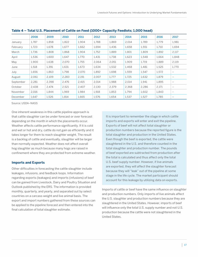
Table 4 provides data on placements from 2008 to 2017.
Using this data, with appropriate adjustment factors, a
market participant can use the information to forecast total
commercial slaughter and beef production approximately
four to five months later. The forecast is several months in the
future because the typical feeding period to bring an animal
to an average live weight of 1,305 pounds, as discussed in the
previous Feedlot section, is between four and five months.
For example, in January 2017, 1.981 million head of cattle
were placed on feed in the United States in feedlots with
1,000 head or greater capacity (Table 4). In theory, this same
number of cattle would be slaughtered in or around May 2017.
However, the market participant must remember that this
figure accounts for only 85 percent of the total fed-cattle
marketings since cattle that are fed in small feedlots with
less than 1,000 head are not included in this number. Total
marketings for May 2017, including both small and large
capacity feedlots, can then be estimated at 2,330,000 head
(1,981,000 head ÷ 0.85). This estimate then can be used
as the forecast for May slaughter. However, commercial
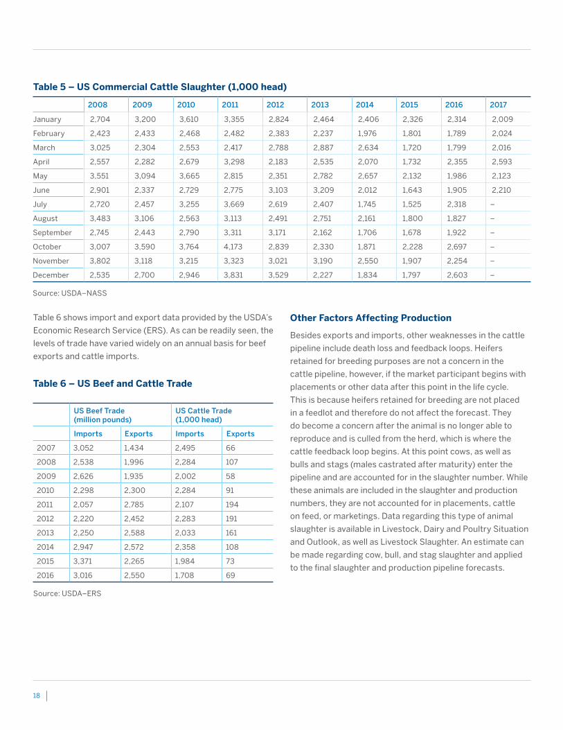
slaughter in May 2013 was 2,119,000 head or 9 percent less
than the forecast (Table 5).
Livestock Futures and Options: Introduction to Underlying Market Fundamentals
17
One inherent weakness in this cattle pipeline approach is
that cattle slaughter can be under forecast or over forecast
depending on the month in which the placements occur.
Weather affects cattle performance significantly. If it is cold
and wet or hot and dry, cattle do not gain as efficiently and it
takes longer for them to reach slaughter weight. The result
is a backlog of cattle and eventually, slaughter will be larger
than normally expected. Weather does not affect overall
hog slaughter as much because many hogs are raised in
confinement where they are protected from extreme weather.
Imports and Exports
Other difficulties in forecasting the cattle slaughter include
leakages, infusions, and feedback loops. Information
regarding exports (leakages) and imports (infusions) of beef
can be gained from Livestock, Dairy and Poultry Situation and
Outlook published by the ERS. The information is provided
monthly, quarterly, and yearly, and separated out by select
countries on a carcass weight and live animal basis. The
export and import numbers gathered from these sources can
be applied to the pipeline forecast and then entered into the
final calculation of total slaughter estimate.
It is important to remember the stage in which cattle
imports and exports will enter and exit the pipeline.
Exports of beef will not affect total slaughter or
production numbers because the reported figure is the
total slaughter and production in the United States.
Even though the beef is exported, the cattle were
slaughtered in the U.S. and therefore counted in the
total slaughter and production number. The pounds
of beef exported are subtracted from production after
the total is calculated and thus affect only the total
U.S. beef supply number. However, if live animals
are exported, they will affect the slaughter forecast
because they will “leak” out of the pipeline at some
stage in the life cycle. The market participant should
account for this leakage by utilizing data on exports.
Imports of cattle or beef have the same influence on slaughter
and production numbers. Only imports of live animals affect
the U.S. slaughter and production numbers because they are
slaughtered in the United States. However, imports of beef
will influence only the total U.S. supply number and not U.S.
production because the cattle were not slaughtered in the
United States.
Table 4 – Total U.S. Placement of Cattle on Feed (1000+ Capacity Feedlots; 1,000 head)
2008 2009 2010 2011 2012 2013 2014 2015 2016 2017
January 1,787 1,858 1,822 1,904 1,788 1,869 2,014 1,789 1,779 1,981
February 1,723 1,678 1,677 1,662 1,694 1,436 1,658 1,551 1,710 1,694
March 1,736 1,808 1,868 1,904 1,752 1,889 1,801 1,809 1,892 2,117
April 1,536 1,600 1,647 1,770 1,431 1,738 1,623 1,548 1,664 1,848
May 1,900 1,638 2,070 1,755 2,064 2,051 1,909 1,719 1,889 2,119
June 1,518 1,391 1,631 1,673 1,634 1,532 1,468 1,481 1,525 1,770
July 1,656 1,863 1,798 2,070 1,892 1,698 1,559 1,547 1,572 –
August 2,061 2,109 2,283 2,191 2,007 1,777 1,725 1,632 1,879 –
September 2,281 2,398 2,476 2,415 2,014 1,988 2,014 1,941 1,895 –
October 2,438 2,474 2,521 2,407 2,130 2,379 2,368 2,286 2,171 –
November 2,016 1,844 1,969 1,984 1,918 1,853 1,794 1,602 1,843 –
December 1,647 1,526 1,814 1,665 1,576 1,654 1,537 1,527 1,785 –
Source: USDA–NASS
18
Table 6 shows import and export data provided by the USDA’s
Economic Research Service (ERS). As can be readily seen, the
levels of trade have varied widely on an annual basis for beef
exports and cattle imports.
Table 6 – US Beef and Cattle Trade
US Beef Trade (million pounds)
US Cattle Trade (1,000 head)
Imports Exports Imports Exports
2007 3,052 1,434 2,495 66
2008 2,538 1,996 2,284 107
2009 2,626 1,935 2,002 58
2010 2,298 2,300 2,284 91
2011 2,057 2,785 2,107 194
2012 2,220 2,452 2,283 191
2013 2,250 2,588 2,033 161
2014 2,947 2,572 2,358 108
2015 3,371 2,265 1,984 73
2016 3,016 2,550 1,708 69
Source: USDA–ERS
Other Factors Affecting Production
Besides exports and imports, other weaknesses in the cattle
pipeline include death loss and feedback loops. Heifers
retained for breeding purposes are not a concern in the
cattle pipeline, however, if the market participant begins with
placements or other data after this point in the life cycle.
This is because heifers retained for breeding are not placed
in a feedlot and therefore do not affect the forecast. They
do become a concern after the animal is no longer able to
reproduce and is culled from the herd, which is where the
cattle feedback loop begins. At this point cows, as well as
bulls and stags (males castrated after maturity) enter the
pipeline and are accounted for in the slaughter number. While
these animals are included in the slaughter and production
numbers, they are not accounted for in placements, cattle
on feed, or marketings. Data regarding this type of animal
slaughter is available in Livestock, Dairy and Poultry Situation
and Outlook, as well as Livestock Slaughter. An estimate can
be made regarding cow, bull, and stag slaughter and applied
to the final slaughter and production pipeline forecasts.
Table 5 – US Commercial Cattle Slaughter (1,000 head)
2008 2009 2010 2011 2012 2013 2014 2015 2016 2017
January 2,704 3,200 3,610 3,355 2,824 2,464 2,406 2,326 2,314 2,009
February 2,423 2,433 2,468 2,482 2,383 2,237 1,976 1,801 1,789 2,024
March 3,025 2,304 2,553 2,417 2,788 2,887 2,634 1,720 1,799 2,016
April 2,557 2,282 2,679 3,298 2,183 2,535 2,070 1,732 2,355 2,593
May 3,551 3,094 3,665 2,815 2,351 2,782 2,657 2,132 1,986 2,123
June 2,901 2,337 2,729 2,775 3,103 3,209 2,012 1,643 1,905 2,210
July 2,720 2,457 3,255 3,669 2,619 2,407 1,745 1,525 2,318 –
August 3,483 3,106 2,563 3,113 2,491 2,751 2,161 1,800 1,827 –
September 2,745 2,443 2,790 3,311 3,171 2,162 1,706 1,678 1,922 –
October 3,007 3,590 3,764 4,173 2,839 2,330 1,871 2,228 2,697 –
November 3,802 3,118 3,215 3,323 3,021 3,190 2,550 1,907 2,254 –
December 2,535 2,700 2,946 3,831 3,529 2,227 1,834 1,797 2,603 –
Source: USDA–NASS
Livestock Futures and Options: Introduction to Underlying Market Fundamentals
19
Market participants must also consider death loss in a cattle
pipeline slaughter forecast. When researching a death loss
percentage, the analyst must consider at which stage the
cattle are in the life cycle. If using placements, the cattle are
in the finishing phase and an average death loss percentage
for this stage for both steers and heifers is about 1 percent.
However, the death loss percentage increases when the cattle
are heifers or if they are placed on feed at a lighter weight.
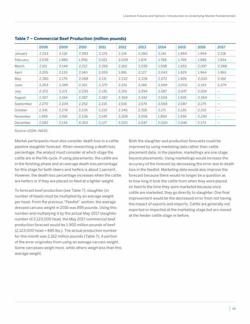
To forecast beef production (see Table 7), slaughter (in
number of head) must be multiplied by an average weight
per head. From the previous “Feedlot” section, the average
dressed carcass weight in 2016 was 895 pounds. Using this
number and multiplying it by the actual May 2017 slaughter
number of 2,123,000 head, the May 2017 commercial beef
production forecast would be 1,900 million pounds of beef
(2,123,000 head × 895 lbs.). The actual production number
for this month was 2,162 million pounds (Table 7). A portion
of the error originates from using an average carcass weight.
Some carcasses weigh more, while others weigh less than this
average weight.
Both the slaughter and production forecasts could be
improved by using marketing data rather than cattle
placement data. In the pipeline, marketings are one stage
beyond placements. Using marketings would increase the
accuracy of the forecast by decreasing the error due to death
loss in the feedlot. Marketing data would also improve the
forecast because there would no longer be a question as
to how long it took the cattle from when they were placed
on feed to the time they were marketed because once
cattle are marketed, they go directly to slaughter. One final
improvement would be the decreased error from not having
the impact of exports and imports. Cattle are generally not
exported or imported at the marketing stage but are moved
at the feeder cattle stage or before.
Table 7 – Commercial Beef Production (million pounds)
2008 2009 2010 2011 2012 2013 2014 2015 2016 2017
January 2,233 2,118 2,083 2,123 2,114 2,260 2,141 1,964 1,954 2,118
February 2,039 1,986 1,956 2,021 2,009 1,874 1,788 1,769 1,885 1,934
March 2,101 2,144 2,212 2,266 2,160 2,039 1,938 1,933 2,097 2,248
April 2,255 2,133 2,140 2,055 1,991 2,127 2,043 1,929 1,964 1,963
May 2,380 2,179 2,088 2,131 2,232 2,228 2,072 1,926 2,030 2,162
June 2,263 2,289 2,321 2,375 2,251 2,166 2,069 2,002 2,193 2,279
July 2,372 2,271 2,230 2,135 2,201 2,294 2,087 2,047 2,024 –
August 2,267 2,184 2,287 2,387 2,369 2,242 2,024 1,935 2,264 –
September 2,270 2,234 2,252 2,215 2,016 2,074 2,068 2,087 2,179 –
October 2,341 2,276 2,235 2,215 2,345 2,318 2,171 2,126 2,210 –
November 1,959 2,016 2,236 2,149 2,208 2,058 1,850 1,936 2,239 –
December 2,082 2,134 4,353 2,127 2,020 2,047 2,000 2,046 2,173 –
Source: USDA–NASS
20
Although the forecasting tools provided in the pipeline
approach offer an estimation of slaughter and production, the
projection will not be accurate if the market participant fails
to monitor the basic economic forces affecting supply.
Many factors can influence supply. However, it is important
to distinguish between the factors changing the quantity
supplied and factors causing a change in supply. These two
circumstances have different influences on the supply curve.
Theoretically, a supply curve is upward sloping because
as price for the output increases (decreases), the quantity
supplied increases (decreases). When the price of the
specific output changes, this creates a change in the quantity
supplied or, more importantly, a movement along the existing
supply curve. A change in the quantity supplied refers only to
changes that result from changes in the price of the product
itself. Also, a change in the quantity supplied is a short-term
or immediate concept.
In contrast, external factors can cause a change in supply,
which is a shift in the entire supply curve. These factors
include: 1) change in the price of inputs, 2) change in the price
of substitute goods, 3) change in the price of joint products,
4) change in technology, and 5) institutional factors. Any of
these factors can shift the supply curve either to the right or
the left, depending on whether the influence on the product
is positive (shift to the right) or negative (shift to the left), all
other factors being held constant.
It is important to note that the effect of these factors on the
supply curve may not be seen immediately. Generally, the
expected effect, either positive or negative, is a long-run
effect and is not realized until the next production cycle.
For example, if there is an incentive for producers to raise
more livestock for slaughter, they will increase their herd size
by either buying females to increase the number of young
born or they will buy younger animals. If livestock feeders
choose the first alternative, more females are held out of
slaughter and put into the breeding herd. When these animals
reproduce, the offspring have to be fed to slaughter weight.
If the feeders choose to buy younger animals, these animals
will have to be fed for a certain time period before they reach
slaughter weight. Once the feeding period for the animals in
both alternatives is complete, the final increase in supply will
be noted.
If the incentive is for producers to cut the size of their herds,
the full response will not be immediate because animals in
the middle of a feeding period will be fed until they reach an
appropriate slaughter weight. The full change is not felt until
after the youngest group of animals has been slaughtered.
Input Price
Inputs are products and factors that produce a final output.
Two significant inputs in the livestock industry are feed and
feeder animals. The costs of these two inputs are highly
influential in shifting the supply curve. If the price of feed or
the price of feeder animals increases and all other variables
are held constant, the supply curve will shift to the left,
resulting in a lower quantity supplied at the same output
price. However, if the prices of the inputs decrease and all else
stays constant, the curve shifts right and a larger quantity is
supplied at the same output price.
The Economics of Supply
Livestock Futures and Options: Introduction to Underlying Market Fundamentals
21
A change in an input price may not immediately affect
supply but may instead have an effect over the long
run that is not evident for a certain amount of time. For
example, if the price of feed declines, there may be a
short-run, or immediate, reduction in the supply of cattle
and hogs, the opposite of what one would expect. The
boost in supply usually does not occur until later. Why?
Because at the time the price of feed declines, animals
almost ready for market have been fed to the point where
the cost of the last pound of gain is almost as much as
the price per pound of animals sold for slaughter.
If feed prices decline, it costs less to feed the hogs or
cattle for each additional pound of gain. This lower cost
makes it more profitable to continue feeding animals
longer and thus creates a short-run reduction in supply.
The expected long-run increase in supply will not appear
for a time equal to the length of the feeding period for
each animal. When feed prices decline, livestock feeders
buy more young animals to increase their feeding herd
size. Not until these animals are fed to slaughter weight
is the increase in supply realized.
Substitute Price
Substitutes, or competing products, are different goods that
can be exchanged for a specific product and produced with
the same resources. For example, beef may be considered a
substitute for pork and conversely, pork may be a substitute
for beef. Substitutes affect supply because if the price of a
competing product (product B) changes relative to the price
of the product in question (product A), the supply curve will
shift. If the price of product B decreases relative to product A,
the supply curve for product A will shift to the right and there
will be a greater supply of product A. The opposite occurs if
the price of product B increases relative to product A. The
price of product B can increase (decrease) relative to product
A because of an increase (decrease) in the price received for
the product or a decrease (increase) in the cost of production
for the product.
Joint Product Price
Joint products are goods derived from a single commodity and
produced in proportion to the quantity of this commodity, such
as pork bellies from a pork carcass or spare ribs from a beef
carcass. If the price of one of these joint products increases, it
can shift the supply curve of the other joint product to the right.
However, if price decreases, the opposite occurs.
Technology
Improvements in technology can make it more economical to
produce a certain product and thereby also shift the supply
curve to the right. This occurs when technology increases the
output of a certain product while the level of inputs remains
constant. In livestock production, examples of technological
improvements would include new breeds, improvements
in reproduction advances in the understanding of genetics,
and a better understanding of what types of feed animals
can most efficiently convert into gain. With improvements in
technology, hog and cattle producers can increase profitability
by increasing the yield of lean meat on a carcass without
increasing their costs of production. This in turn shifts the
supply curve to the right, if all other factors are held constant.
Institutional Factors
Institutional factors generally relate to government programs
or restrictions such as land-use or waste disposal regulations.
These factors can shift the supply curve for the product to the
left or right, depending on the industry. For example, stricter
waste management regulations may result in decreased
livestock production and shift the supply curve to the left, if
the guidelines make it less profitable to produce livestock.
Interest rates are another important institutional factor.
Significant movements in interest rates can affect production
decisions and thus, supply. Capital is an input just like feed
and feeder animals. The magnitude of the effect is greater for
industries with larger up-front costs than for industries whose
costs are spread more evenly throughout the production
period. An increase in interest rates may lead producers to
not expand herds, improve facilities, or adopt new technology
because of the additional cost of financing. However, in times
of decreasing interest rates, the livestock industry may expand
due in part to more economical borrowing costs.
22
Short-Run Supply Impacts
Although the factors discussed so far generally impact the
supply of a commodity over time, there are other factors
that can create an immediate response in an industry. In the
livestock industry, for example, severe weather and disease or
pest outbreaks can immediately shift the supply curve to the
left, assuming all other factors are held constant. In feeding
livestock, extremely hot or cold weather slows the rate of
gain. When this happens, the supply curve immediately shifts
to the left because animals expected to be ready for slaughter
at a certain time are not available.
Disease outbreaks affect the supply curve in much the
same way. If an outbreak occurs in which animals must be
destroyed, the supply curve immediately shifts to the left
because supply is drastically reduced. In an outbreak where
livestock can be treated but the medication used requires
a withdrawal period before slaughter, again the immediate
response is for the supply curve to shift to the left.
Livestock Futures and Options: Introduction to Underlying Market Fundamentals
23
In addition to understanding supply factors, market
participants must also have a solid knowledge of factors
affecting demand and recognize that these factors are often
related to consumer attitudes and decisions. Although many
factors can affect demand, it is again important to distinguish
between factors that change the quantity demanded and
factors that cause a change in demand (demand curve shift).
A change in the quantity demanded is a movement along
the existing demand curve. Opposite of a supply curve, a
demand curve is theoretically downward sloping. As the price
of a product increases, the quantity demanded decreases,
creating a change in the quantity demanded. A change in the
price of the specific product is the only factor adjustment that
can create a change in the quantity demanded.
However, other demand factors can cause the demand curve
to shift either to the right or the left, depending on whether
the factor creating the change is viewed as positive (right
or outward shift) or negative (left or inward shift), all other
factors being held constant. The main factors that may cause
a demand curve to shift include: 1) changes in population size
and its distribution, 2) change in income, 3) change in the
price of substitutes, 4) change in the price of complements,
and 5) change in consumer preferences.
Change in Population Size and Distribution
Population growth can increase demand, and population
reduction can decrease it. A shift in demand can also result
from a change in population distribution, such as a growing
number of elderly versus children, because preferences
and/or needs of the larger population group dominate. For
example, more baby food is sold during a population boom
(increased demand for baby food) while other food products
are sold after those babies have grown (decreased demand
for baby food). However, it is also important to remember that
changes in population occur over many years and therefore,
do not have much of an impact on short-term analysis.
Change in Income
Increasing or decreasing income levels can also shift the
demand curve. When income grows, people tend to spend
a large proportion of the increase on additional goods and
services and put a small proportion into savings. However,
the response of the demand curve to an increase or decrease
in income depends on the specific product. Generally, the
benefits of an increase in income are not usually seen in
food items but in other nonessential items such as cars and
electronics. However, demand for meat has traditionally
responded positively to increased income. This response
is limited, however, by the fact that people can only
consume a certain amount of meat no matter how much
income increases.
Although meat demand generally has a positive relationship
with income growth, not all meats respond in that manner.
For example, if income increases, the demand for more
expensive cuts of meat, such as steaks, may increase and the
demand for less expensive products, such as ground beef,
may decrease. When income decreases, there is usually a
decrease in demand, or a leftward shift of the curve, for more
expensive cuts and an increased demand, or outward shift,
for the less expensive types of meat.
The Economics of Demand
24
Change in the Price of Substitutes
Substitutes are goods that can be used instead of another
good. For example, chicken can be a substitute for either
pork or beef. When the price of a substitute good (product
B) increases, demand typically increases for another good
(product A). When users of product B switch to product
A because they consider the price of product B too high,
demand for product A increases. Similarly, when the price of
a substitute good decreases, users of product A are likely to
switch to the substitute, product B. Thus, demand for product
A decreases and the demand curve shifts to the left.
Change in the Price of Complements
Complements are items that enhance, but are not a necessity
to, a good in question. Barbecue sauce and beef or pork may
be considered by some as complementary products. When
the price of one of the complementary items increases, in this
case, beef or pork, demand for another item, the barbecue
sauce, decreases and shifts left. The opposite is true for a
price decrease: demand would shift to the right, all other
factors being held constant. For example, if the price of pork
or beef decreases, demand for barbecue sauce may increase.
Change in Consumer Preferences
Consumer preferences are constantly changing. There are
many different reasons, such as age, increased awareness,
and advertising. Increased consumer awareness may be
related to increased health consciousness or exposure to
new types of foods or preparation methods. Advertising can
also sway a consumer’s preferences for one item or another.
Sometimes, there is a general shift in preferences for a large
group of the population, such as a move toward a lower fat
diet. It is extremely difficult, however, to measure demand
curve shifts in response to changing preferences because
they are not directly observable. Many times, preference
changes are tied to an additional demand shifter, such as
increased consumer income, which makes additional money
available to buy different items.
Seasonal periods can clearly and predictably result in
changes in tastes and preferences. For example, there
is increased demand for certain cuts of meat during the
summer because many people enjoy grilling outside.
Similarly, at Thanksgiving the demand for turkey increases
while the demand for pork and beef decreases.
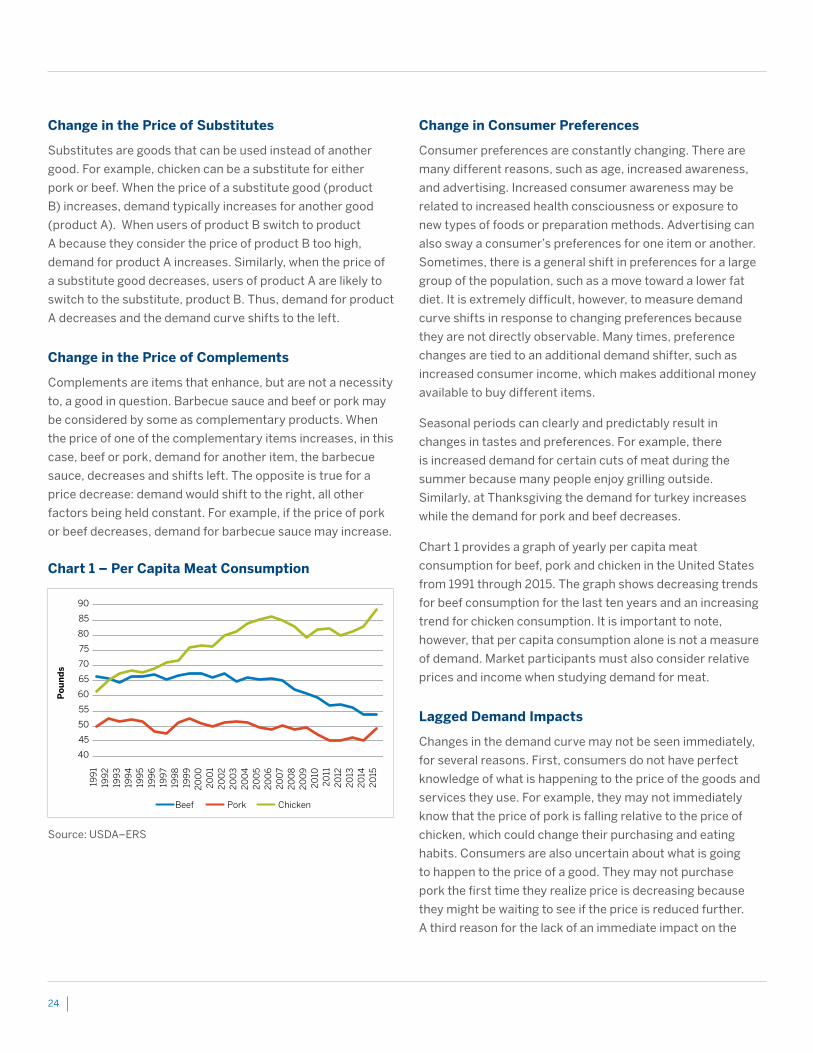
Chart 1 provides a graph of yearly per capita meat
consumption for beef, pork and chicken in the United States
from 1991 through 2015. The graph shows decreasing trends
for beef consumption for the last ten years and an increasing
trend for chicken consumption. It is important to note,
however, that per capita consumption alone is not a measure
of demand. Market participants must also consider relative
prices and income when studying demand for meat.
Lagged Demand Impacts
Changes in the demand curve may not be seen immediately,
for several reasons. First, consumers do not have perfect
knowledge of what is happening to the price of the goods and
services they use. For example, they may not immediately
know that the price of pork is falling relative to the price of
chicken, which could change their purchasing and eating
habits. Consumers are also uncertain about what is going
to happen to the price of a good. They may not purchase
pork the first time they realize price is decreasing because
they might be waiting to see if the price is reduced further.
A third reason for the lack of an immediate impact on the
Po
un
ds
Beef Pork Chicken
40
45
50
55
60
65
70
75
80
85
90
199
1 19
92
19
93
19
94
19
95
19
96
19
97
199
8
199
9
20
00
2
00
1 2
00
2
20
03
2
00
4
20
05
2
00
6
20
07
20
08
2
00
9
20
10
20
11
20
12
20
13
20
14
20
15
Source: USDA–ERS
Chart 1 – Per Capita Meat Consumption
Livestock Futures and Options: Introduction to Underlying Market Fundamentals
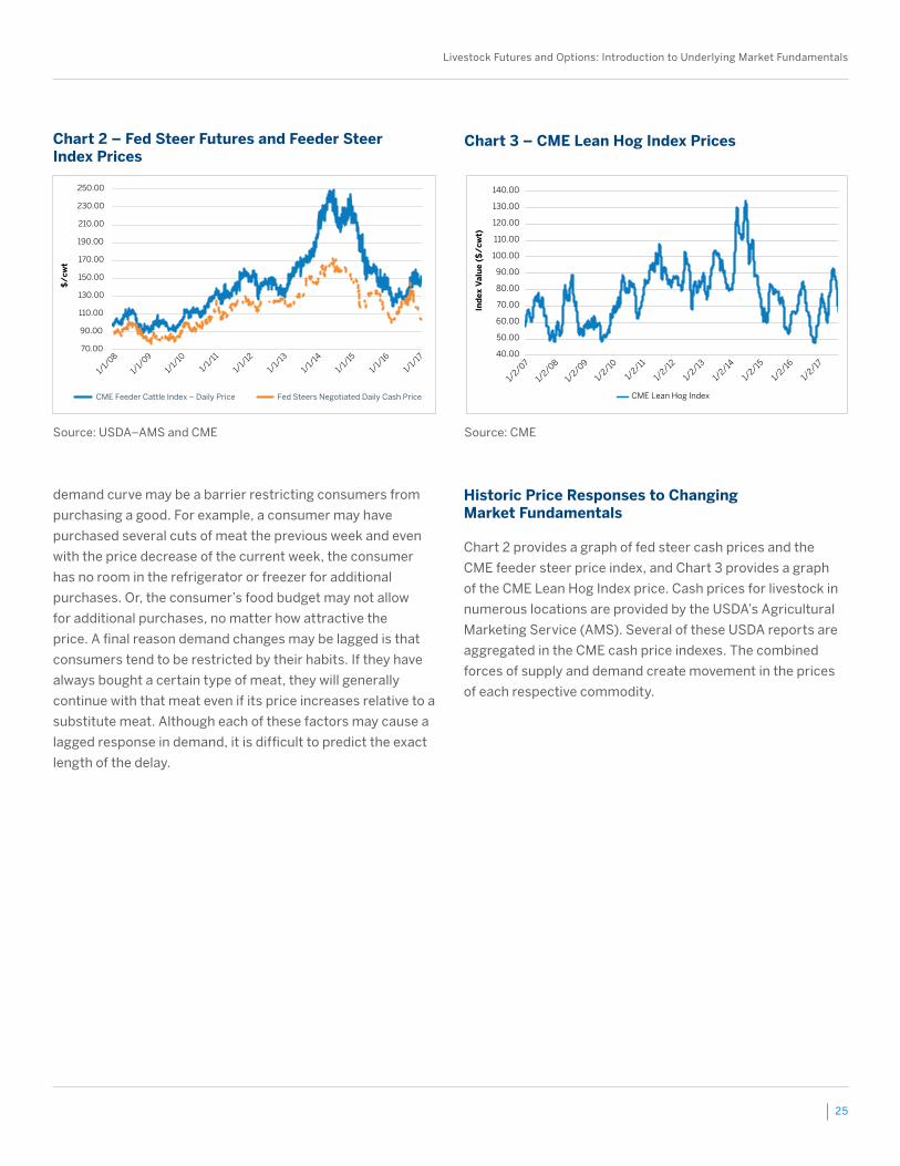
25
demand curve may be a barrier restricting consumers from
purchasing a good. For example, a consumer may have
purchased several cuts of meat the previous week and even
with the price decrease of the current week, the consumer
has no room in the refrigerator or freezer for additional
purchases. Or, the consumer’s food budget may not allow
for additional purchases, no matter how attractive the
price. A final reason demand changes may be lagged is that
consumers tend to be restricted by their habits. If they have
always bought a certain type of meat, they will generally
continue with that meat even if its price increases relative to a
substitute meat. Although each of these factors may cause a
lagged response in demand, it is difficult to predict the exact
length of the delay.
Historic Price Responses to Changing Market Fundamentals
Chart 2 provides a graph of fed steer cash prices and the
CME feeder steer price index, and Chart 3 provides a graph
of the CME Lean Hog Index price. Cash prices for livestock in
numerous locations are provided by the USDA’s Agricultural
Marketing Service (AMS). Several of these USDA reports are
aggregated in the CME cash price indexes. The combined
forces of supply and demand create movement in the prices
of each respective commodity.
CME Feeder Cattle Index – Daily Price Fed Steers Negotiated Daily Cash Price
70.00
90.00
110.00
130.00
150.00
170.00
190.00
210.00
230.00
250.00
$/
cwt
1/1/
08
1/1/
09
1/1/
10
1/1/
11
1/1/
12
1/1/
13
1/1/
14
1/1/
15
1/1/
16
1/1/
17
Source: USDA–AMS and CME
Chart 2 – Fed Steer Futures and Feeder Steer Index Prices
Ind
ex V
alu
e ($
/cw
t)
40.00
50.00
60.00
70.00
80.00
90.00
100.00
110.00
120.00
130.00
140.00
1/2/07
1/2/08
1/2/09
1/2/10
1/2/11
1/2/12
1/2/13
1/2/14
1/2/15
1/2/16
1/2/17
CME Lean Hog Index
Source: CME
Chart 3 – CME Lean Hog Index Prices
26
In addition to knowledge of supply and demand factors, as
well as pipeline production forecasts, market participants
may also want to consider livestock cycles and seasonality
when forecasting prices.
Livestock Cycles
Historically, livestock inventories and production have followed
predictable cycles. These cycles have been useful tools in
both cattle and hog markets for predicting expansion and
contraction phases and thus, the directional movement of
price. In the past, hog cycles have lasted an average of four
years while cattle cycles generally have lasted 10 to 12 years.
An actual cycle consists of the time between a trough (low
point in inventory) and the next trough or the time between a
peak (high point in inventory) and the next peak. The expansion
phase of a cycle is constrained by the time it takes to raise
female animals to breeding age and to produce offspring.
Increasing prices spur producers to retain female
animals to increase the breeding herd. This initially
reduces slaughter numbers and as a result, prices
increase even further. However, once these female
animals begin producing offspring and the offspring in
turn reach slaughter weight, there may be an oversupply
of livestock. Prices begin to decline and it eventually
becomes unprofitable to raise and feed young animals.
Producers begin culling the breeding herd and sending
them to slaughter, adding additional numbers to supply
and causing prices to decrease even further.
This is the contraction or downward phase, which can be
long or short in duration depending on the incentives or
disincentives provided by the price.
Although hogs and cattle have different average cycle
lengths, the dynamics of the cycles are the same. Recently,
there have been arguments about the reliability of the
hog cycle. One claim is that the hog cycle is becoming
more erratic due to changes in hog industry management
strategies and structure, making it a less useful guide to
understanding producer response to prices. The other
side of the argument is that although the variation in hog
production is decreasing over time, the large variations in
price that accompany hog cycles are still present. Therefore,
even though the industry may be going through structural
changes, the hog cycle still exists and can be a useful tool in
providing indications about the directional movement
of price.
Currently, there are no similar arguments regarding the cattle
cycle. This may be because the cattle industry has not seen
the dramatic changes in structure that the hog industry has
experienced. Nonetheless, anyone using either the hog or
cattle cycles must remember that both need to be considered
as long-run factors and are most useful when used in longer
term price analysis.
Seasonality
Seasonality trends refer to ways that both the supply and
demand for a commodity can be affected by factors that
change with reasonable regularity during the year.
Livestock Cycles and Seasonality
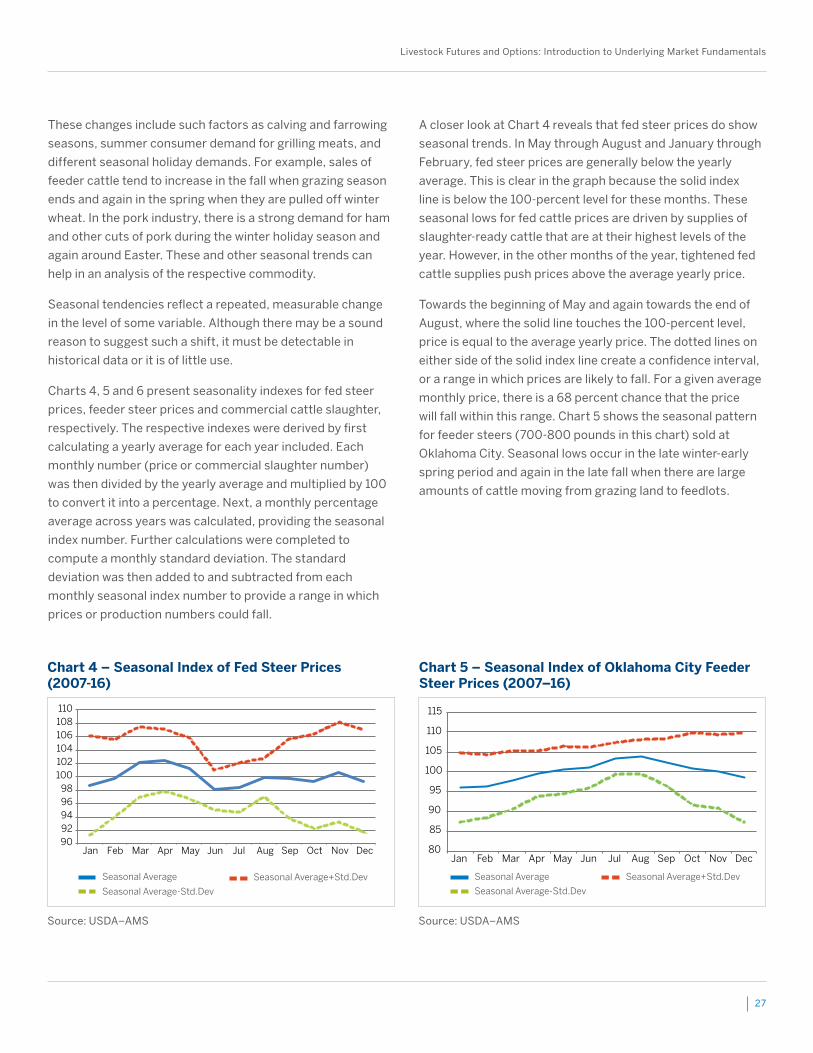
Livestock Futures and Options: Introduction to Underlying Market Fundamentals
27
These changes include such factors as calving and farrowing
seasons, summer consumer demand for grilling meats, and
different seasonal holiday demands. For example, sales of
feeder cattle tend to increase in the fall when grazing season
ends and again in the spring when they are pulled off winter
wheat. In the pork industry, there is a strong demand for ham
and other cuts of pork during the winter holiday season and
again around Easter. These and other seasonal trends can
help in an analysis of the respective commodity.
Seasonal tendencies reflect a repeated, measurable change
in the level of some variable. Although there may be a sound
reason to suggest such a shift, it must be detectable in
historical data or it is of little use.
Charts 4, 5 and 6 present seasonality indexes for fed steer
prices, feeder steer prices and commercial cattle slaughter,
respectively. The respective indexes were derived by first
calculating a yearly average for each year included. Each
monthly number (price or commercial slaughter number)
was then divided by the yearly average and multiplied by 100
to convert it into a percentage. Next, a monthly percentage
average across years was calculated, providing the seasonal
index number. Further calculations were completed to
compute a monthly standard deviation. The standard
deviation was then added to and subtracted from each
monthly seasonal index number to provide a range in which
prices or production numbers could fall.
A closer look at Chart 4 reveals that fed steer prices do show
seasonal trends. In May through August and January through
February, fed steer prices are generally below the yearly
average. This is clear in the graph because the solid index
line is below the 100-percent level for these months. These
seasonal lows for fed cattle prices are driven by supplies of
slaughter-ready cattle that are at their highest levels of the
year. However, in the other months of the year, tightened fed
cattle supplies push prices above the average yearly price.
Towards the beginning of May and again towards the end of
August, where the solid line touches the 100-percent level,
price is equal to the average yearly price. The dotted lines on
either side of the solid index line create a confidence interval,
or a range in which prices are likely to fall. For a given average
monthly price, there is a 68 percent chance that the price
will fall within this range. Chart 5 shows the seasonal pattern
for feeder steers (700-800 pounds in this chart) sold at
Oklahoma City. Seasonal lows occur in the late winter-early
spring period and again in the late fall when there are large
amounts of cattle moving from grazing land to feedlots.
Source: USDA–AMS
Chart 4 – Seasonal Index of Fed Steer Prices (2007-16)
Source: USDA–AMS
Chart 5 – Seasonal Index of Oklahoma City Feeder Steer Prices (2007–16)
9092949698
100102104106108110
Jan Feb Mar Apr May Jun Jul Aug Sep Oct Nov Dec
Seasonal Average
Seasonal Average-Std .Dev
Seasonal Average+Std .Dev
80
85
90
95
100
105
110
115
Jan Feb Mar Apr May Jun Jul Aug Sep Oct Nov Dec
Seasonal Average
Seasonal Average-Std .Dev
Seasonal Average+Std .Dev
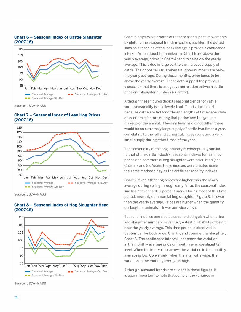
28
Chart 6 helps explain some of these seasonal price movements
by plotting the seasonal trends in cattle slaughter. The dotted
lines on either side of the index line again provide a confidence
interval. When slaughter numbers in Chart 6 are above the
yearly average, prices in Chart 4 tend to be below the yearly
average. This is due in large part to the increased supply of
cattle. The opposite is true when slaughter numbers are below
the yearly average. During these months, price tends to be
above the yearly average. These data support the previous
discussion that there is a negative correlation between cattle
price and slaughter numbers (quantity).
Although these figures depict seasonal trends for cattle,
some seasonality is also leveled out. This is due in part
because cattle are fed for different lengths of time depending
on economic factors during that period and the genetic
makeup of the animal. If feeding lengths did not differ, there
would be an extremely large supply of cattle two times a year,
correlating to the fall and spring calving seasons and a very
small supply during other times of the year.
The seasonality of the hog industry is conceptually similar
to that of the cattle industry. Seasonal indexes for lean hog
prices and commercial hog slaughter were calculated (see
Charts 7 and 8). Again, these indexes were created using
the same methodology as the cattle seasonality indexes.
Chart 7 reveals that hog prices are higher than the yearly
average during spring through early fall as the seasonal index
line lies above the 100-percent mark. During most of this time
period, monthly commercial hog slaughter, Figure 8, is lower
than the yearly average. Prices are higher when the quantity
of slaughter animals is lower and vice versa.
Seasonal indexes can also be used to distinguish when price
and slaughter numbers have the greatest probability of being
near the yearly average. This time period is observed in
September for both price, Chart 7, and commercial slaughter,
Chart 8. The confidence interval lines show the variation
in the monthly average price or monthly average slaughter
level. When the interval is narrow, the variation in the monthly
average is low. Conversely, when the interval is wide, the
variation in the monthly average is high.
Although seasonal trends are evident in these figures, it
is again important to note that some of the variance in
Chart 6 – Seasonal Index of Cattle Slaughter (2007-16)
Source: USDA–NASS
85
90
95
100
105
110
115
Jan Feb Mar Apr May Jun Jul Aug Sep Oct Nov Dec
Seasonal Average
Seasonal Average-Std .Dev
Seasonal Average+Std .Dev
Chart 7 – Seasonal Index of Lean Hog Prices (2007-16)
Source: USDA–NASS
75
80
85
90
95
100
105
110
115
120
125
Jan Feb Mar Apr May Jun Jul Aug Sep Oct Nov Dec
Seasonal Average
Seasonal Average-Std .Dev
Seasonal Average+Std .Dev
Chart 8 – Seasonal Index of Hog Slaughter Head (2007-16)
Source: USDA–NASS
85
90
95
100
105
110
115
Jan Feb Mar Apr May Jun Jul Aug Sep Oct Nov Dec
Seasonal Average
Seasonal Average-Std .Dev
Seasonal Average+Std .Dev
Livestock Futures and Options: Introduction to Underlying Market Fundamentals
29
the movements has been muted due to production and
management practices in the hog industry. For example,
farrowing seasons are not as dictated by the weather as they
once were because many hogs are raised in confinement
with climate control. In the past, many producers would avoid
farrowing during the winter due to the harsh conditions the
baby pigs would have to survive. This is no longer such a strict
practice and there is now a flatter, year-round production
cycle. Although many production and management methods
can help to keep a constant, year-round supply of hogs,
demand factors still play an important role in the hog
industry. For example, there is an increased demand for
pork around the winter holiday season and no matter what
production practices are used, this seasonal demand by
consumers will still exist.
Sound price forecasting should be based on analyzing
all factors that may affect seasonal supply and demand
of beef and pork. Market participants must distinguish
between one-time occurrences and actual trends,
which are movements that occur in the same direction
and roughly during the same time each year for several
years. Once a trend has been identified, the indexes can
then be used to help monitor and analyze the specific
commodity in question.
One final caveat in the use of seasonal indexes is that
although an overall average price or slaughter number
for a particular month may be higher or lower than the
overall yearly average, the specific monthly price or
slaughter number in a specific year may not be higher
or lower than that respective year’s average number.
These figures provide information for prices and
slaughter numbers averaged over a period of years and
data from each individual year cannot be singled out in
the graphs.
Time Horizon
In any fundamental analysis, the time horizon is important to
keep in mind. The factors that will affect prices over the next
few weeks are often different from those that will affect prices
over longer periods.
Take the following situation, for example: suppose the
number of market hogs, as indicated by the USDA Hogs and
Pigs Report, turns out to be much higher than the industry
expectation. At the same time, there is a legislative proposal
to increase the percentage of renewable fuels (such as
ethanol made from corn) in gasoline content. There is also a
forecast that unfavorable weather will reduce the expected
yield of the current domestic corn crop.
What does all of this imply for the price of hogs? One
interpretation would be an immediate price decline followed
a few months later by a price decrease. The reasoning here
is that in the next few weeks large supplies of hogs must be
marketed and packers will only be willing to purchase them
at discounted prices. However, the other news suggests that
corn prices will begin rising immediately, raising the cost of
feeding hogs. This should motivate hog finishers to reduce
feeding periods and market their animals at lighter weights.
After more time passes, the number of hogs on feed will be
decreased resulting in a rise in prices.
Of course, the particular combination of news items here is
unusual. But frequently factors may have both an immediate
and a delayed influence on the available quantity of a
commodity. As a consequence, livestock futures prices
for different delivery months may not move in the same
magnitude and may even move in opposite directions.

30
Becoming a successful livestock trader (whether a hedger
or speculator) or livestock market analyst requires a basic
understanding of the production and life cycles of cattle and
hogs. This publication has attempted to provide an overview
of those cycles to aid in building the skill set needed to
begin trading in these commodities. Although this booklet
introduces analytical techniques and information on the
economics of each industry, it provides only a portion of
what is needed to become successful in trading these
commodities. In addition to understanding the livestock
futures and options products, one must also become familiar
with the actual procedures of trading, such as the different
types of buy and sell orders, performance bond (margin)
requirements, position limits, and the rule language for each
commodity. It may also be helpful for the trader to study
technical factors to assist in proper timing of entry into and
exit out of the market. This additional knowledge, combined
with the information provided in this publication, will help to
create a successful hog and/or cattle commodity trader.
Conclusion
Livestock Futures and Options: Introduction to Underlying Market Fundamentals
31
Daily National Carlot Meat Report (USDA-AMS)
ams.usda.gov/mnreports/lsddb.pdf
Daily Cattle and Beef Summary (USDA-AMS)
ams.usda.gov/mnreports/lsddcbs.pdf
Daily Hog and Pork Summary (USDA-AMS)
ams.usda.gov/mnreports/lsddhps.pdf
Weekly Feeder and Stocker Summary (USDA-AMS)
ams.usda.gov/mnreports/lswnfss.pdf
Weekly National Feeder Pig Report (USDA-AMS)
ams.usda.gov/mnreports/nw_ls255.txt
Monthly Cattle on Feed Report (USDA-NASS)
usda.mannlib.cornell.edu/MannUsda/viewDocumentInfo.
do?documentID=1020
Monthly Livestock Slaughter (USDA-NASS)
usda.mannlib.cornell.edu/MannUsda/viewDocumentInfo.
do?documentID=1096
Monthly Cold Storage Report (USDA-NASS)
usda.mannlib.cornell.edu/MannUsda/viewDocumentInfo.
do?documentID=1034
Monthly Livestock, Dairy and Poultry Outlook (USDA-ERS)
usda.mannlib.cornell.edu/MannUsda/viewDocumentInfo.
do?documentID=1350
Quarterly Hogs and Pigs Report (USDA-NASS)
usda.mannlib.cornell.edu/MannUsda/viewDocumentInfo.
do?documentID=1086
Sources of Information
32
Prices of agricultural products are subject to factors that are
difficult or impossible to control, such as weather, disease
and political decisions. In addition, they represent commodity
supplies that are relatively fixed in the short term while
growth in worldwide demand and global economic expansion
are ongoing. As such, CME Group Agricultural products serve
producers and users seeking risk management and hedging
tools, alongside funds and other traders looking to capitalize
on the extraordinary opportunities these markets offer.
CME Group offers the widest range of agricultural futures,
options and swaps of any U.S. exchange, with trading
available on the following products:
Commodity Indexes
Dairy Products
Grain and Oilseed Products
Livestock Products
Forest Products
CME Group Agricultural Products
Livestock futures and options are listed with and subject to the rules and regulations of CME .
CME Group is a trademark of CME Group Inc . The Globe Logo, CME, Chicago Mercantile Exchange and Globex, are trademarks of Chicago Mercantile Exchange Inc .
The information within this fact card has been compiled by CME Group for general purposes only . Although every attempt has been made to ensure the accuracy of the information within this brochure, CME Group assumes no responsibility for any errors or omissions . Additionally, all examples in this brochure are hypothetical situations, used for explanation purposes only, and should not be considered investment advice or the results of actual market experience .
All matters pertaining to rules and specifications herein are made subject to and are superseded by official CME, rules . Current rules should be consulted in all cases concerning contract specifications .
Futures trading is not suitable for all investors, and involves the risk of loss . Futures are a leveraged investment, and because only a percentage of a contract’s value is required to trade, it is possible to lose more than the amount of money deposited for a futures position . Therefore, traders should only use funds that they can afford to lose without affecting their lifestyles . And only a portion of those funds should be devoted to any one trade because they cannot expect to profit on every trade .
Copyright 2017 CME Group All Rights Reserved . PM954/1217
CME GROUP GLOBAL OFFICESCME GROUP HEADQUARTERS
20 South Wacker DriveChicago, Illinois 60606cmegroup .com
Chicago +1 312 930 1000
Singapore+65 6593 5555
Houston+1 713 658 2347
Tokyo+81 3 3242 6228
New York+1 212 299 2000
Calgary+1 403 444 6876
São Paulo+55 11 2787 6451
Washington D.C.+1 202 638 3838
London+44 20 3379 3700
Hong Kong+852 2582 2200
Seoul+82 2 6336 6722