Embed Size (px)
Citation preview

This thesis has been submitted in fulfilment of the requirements for a postgraduate degree
(e.g. PhD, MPhil, DClinPsychol) at the University of Edinburgh. Please note the following
terms and conditions of use:
This work is protected by copyright and other intellectual property rights, which are
retained by the thesis author, unless otherwise stated.
A copy can be downloaded for personal non-commercial research or study, without
prior permission or charge.
This thesis cannot be reproduced or quoted extensively from without first obtaining
permission in writing from the author.
The content must not be changed in any way or sold commercially in any format or
medium without the formal permission of the author.
When referring to this work, full bibliographic details including the author, title,
awarding institution and date of the thesis must be given.

Load Balancing in Hybrid LiFi and RF
Networks
Yunlu Wang
TH
E
U N I V E R S
I TY
OF
ED I N B U
RG
H
A thesis submitted for the degree of Doctor of Philosophy.
The University of Edinburgh.
January 2018
Abstract
The increasing number of mobile devices challenges the current radio frequency (RF) net-
works. The conventional RF spectrum for wireless communications is saturating, motivating
to develop other unexplored frequency bands. Light Fidelity (LiFi) which uses more than 300
THz of the visible light spectrum for high-speed wireless communications, is considered a
promising complementary technology to its RF counterpart. LiFi enables daily lighting infras-
tructures, i.e. light emitting diode (LED) lamps to realise data transmission, and maintains the
lighting functionality at the same time. Since LiFi mainly relies on line-of-sight (LoS) trans-
mission, users in indoor environments may experience blockages which significantly affects
users’ quality of service (QoS). Therefore, hybrid LiFi and RF networks (HLRNs) where LiFi
supports high data rate transmission and RF offers reliable connectivity, can provide a potential
solution to future indoor wireless communications.
In HLRNs, efficient load balancing (LB) schemes are critical in improving the traffic perfor-
mance and network utilisation. In this thesis, the optimisation-based scheme (OBS) and the
evolutionary game theory (EGT) based scheme (EGTBS) are proposed for load balancing in
HLRNs. Specifically, in OBS, two algorithms, the joint optimisation algorithm (JOA) and the
separate optimisation algorithm (SOA) are proposed. Analysis and simulation results show
that JOA can achieve the optimal performance in terms of user data rate while requiring high
computational complexity. SOA reduces the computational complexity but achieves low user
data rates. EGTBS is able to achieve a better performance/complexity trade-off than OBS and
other conventional load balancing schemes. In addition, the effects of handover, blockages,
orientation of LiFi receivers, and user data rate requirement on the throughput of HLRNs are
investigated. Moreover, the packet latency in HLRNs is also studied in this thesis. The no-
tion of LiFi service ratio is introduced, defined as the proportion of users served by LiFi in
HLRNs. The optimal LiFi service ratio to minimise system delay is mathematically derived
and a low-complexity packet flow assignment scheme based on this optimum ratio is proposed.
Simulation results show that the theoretical optimum of the LiFi service ratio is very close to the
practical solution. Also, the proposed packet flow assignment scheme can reduce at most 90%
of packet delay compared to the conventional load balancing schemes at reduced computational
complexity.
Lay Summary
Due to the exponentially increasing demand for mobile data traffic, the current indoor radio
frequency (RF) systems tend to be overloaded. A potential solution is the hybrid network that
integrates different wireless technologies to improve the network capacity. Light fidelity (LiFi),
which uses existing light emitting diode (LED) lighting infrastructures for high speed wireless
communications, has been considered to form a new tier within the future indoor hybrid net-
works. One major advantage of such a hybrid network is that LiFi and RF signals do not
interfere with each other since they use an entirely different part of the electromagnetic spec-
trum. LiFi can be regarded as nanometre wave (nmWave) wireless communication extending
current millimetre wave (mmWave) wireless technologies. Compared with RF systems, LiFi
can potentially provide a much higher level of signal-to-noise ratio (SNR). Also, LiFi can use a
huge and unregulated bandwidth resource of up to 300 THz, 600,000 times larger than the 500
MHz WiGig (wireless gigabit alliance) channel in the industrial, scientific and medical (ISM)
band.
In indoor environments, a single LiFi cell covers a few square meters due to propagation char-
acteristics of light such as high path loss and low multipath reflections. Hence, multiple light
sources are required to cover a large room, leading to a high spatial spectral efficiency in LiFi
systems. In spite of the dense deployment of access points (APs), LiFi may not provide a uni-
form coverage in terms of data rate performance mainly due to inter-cell interference (ICI) and
blockages. Therefore, a hybrid LiFi/RF network (HLRN) is proposed to mitigate the spatial
fluctuation of data rate offering a system throughput greater than that of stand alone LiFi or RF
networks. In this thesis, the load balancing (LB) in HLRNs is studied, which mainly consists
of AP assignment, resource allocation and handover. At first, the joint optimisation algorithm
(JOA) for LB is proposed, which uses convex optimisation method to jointly optimise all of
the elements in LB. Following that, the evolutionary game theory (EGT) based scheme is pro-
posed, which is able to achieve a better performance/complexity trade-off than JOA and other
benchmark algorithms. At last, the cross-layer load balancing for HLRNs is studied. A delay-
minimisation packet flow assignment scheme is proposed. This scheme is able to reduce 90%
of packet delay comparing to the state-of-the-art schemes.
iii

Declaration of originality
I hereby declare that the research recorded in this thesis and the thesis itself was composed and
originated entirely by myself in the Department of Electronics and Electrical Engineering at
The University of Edinburgh.
Yunlu Wang
Edinburgh, Scotland, UK
Jan. 2018
iv

Acknowledgements
Firstly, I would like to offer my sincerest gratitude to my mother, Xiangxia Fu, without her
continuous support and encouragement I never would have been able to finish my Ph.D courses.
I would give a special thank you to my wife, Jie Zhang. Words cannot describe how lucky I am
to have her in my life. She has selflessly given more to me than I ever could have asked for. I
love you, and look forward to our lifelong journey.
I would like to sincerely appreciate my supervisor Prof. Harald Haas, who has led me into the
world of LiFi. With his guidance and support, I have gained so much knowledge in the cutting-
edge technologies. Thanks very much to his patience and encouragement throughout my Ph.D.
study.
Last but not least, I would like to thank my friends and all guys in Institute of Digital Com-
munications (IDCom) who have helped and encouraged me during my academic experience in
Edinburgh. The time shared with them is the most precious memory in my life.
v
Contents
Lay Summary . . . . . . . . . . . . . . . . . . . . . . . . . . . . . . . . . . . iii
Declaration of originality . . . . . . . . . . . . . . . . . . . . . . . . . . . . . iv
Acknowledgements . . . . . . . . . . . . . . . . . . . . . . . . . . . . . . . . v
Contents . . . . . . . . . . . . . . . . . . . . . . . . . . . . . . . . . . . . . . vi
List of figures . . . . . . . . . . . . . . . . . . . . . . . . . . . . . . . . . . . ix
List of tables . . . . . . . . . . . . . . . . . . . . . . . . . . . . . . . . . . . xii
Acronyms and abbreviations . . . . . . . . . . . . . . . . . . . . . . . . . . . xiii
Nomenclature . . . . . . . . . . . . . . . . . . . . . . . . . . . . . . . . . . . xvi
1 Introduction 1
1.1 Motivation . . . . . . . . . . . . . . . . . . . . . . . . . . . . . . . . . . . . . 1
1.2 Contribution . . . . . . . . . . . . . . . . . . . . . . . . . . . . . . . . . . . . 4
1.3 Thesis Layout . . . . . . . . . . . . . . . . . . . . . . . . . . . . . . . . . . . 6
1.4 Summary . . . . . . . . . . . . . . . . . . . . . . . . . . . . . . . . . . . . . 7
2 Background and System Model 9
2.1 Background . . . . . . . . . . . . . . . . . . . . . . . . . . . . . . . . . . . . 9
2.2 Hybrid LiFi and RF Network Model . . . . . . . . . . . . . . . . . . . . . . . 11
2.2.1 Overall Communication Architecture Description . . . . . . . . . . . . 11
2.2.2 Central Unit and Backhaul Connection . . . . . . . . . . . . . . . . . 12
2.3 LiFi System Model . . . . . . . . . . . . . . . . . . . . . . . . . . . . . . . . 13
2.3.1 LiFi Channel Model . . . . . . . . . . . . . . . . . . . . . . . . . . . 13
2.3.2 O-OFDM Based Transmission . . . . . . . . . . . . . . . . . . . . . . 16
2.3.3 Multiple Access Technology . . . . . . . . . . . . . . . . . . . . . . . 19
2.4 RF System Model . . . . . . . . . . . . . . . . . . . . . . . . . . . . . . . . . 30
2.4.1 RF Channel Model . . . . . . . . . . . . . . . . . . . . . . . . . . . . 31
2.4.2 Multiple Access Technology . . . . . . . . . . . . . . . . . . . . . . . 31
2.5 Summary . . . . . . . . . . . . . . . . . . . . . . . . . . . . . . . . . . . . . 32
3 Dynamic Load Balancing with Handover for HLRNs 33
3.1 Introduction . . . . . . . . . . . . . . . . . . . . . . . . . . . . . . . . . . . . 33
3.2 A Special Case: Optimisation based dynamic LB Scheme with Proportional
Fairness . . . . . . . . . . . . . . . . . . . . . . . . . . . . . . . . . . . . . . 34
3.2.1 Handover scheme . . . . . . . . . . . . . . . . . . . . . . . . . . . . . 36
3.2.2 Load Balancing Algorithm in One State . . . . . . . . . . . . . . . . . 38
3.2.3 Analysis of AP Service Area and System Throughput . . . . . . . . . . 41
3.2.4 Performance Evaluation . . . . . . . . . . . . . . . . . . . . . . . . . 50
3.2.5 Discussion . . . . . . . . . . . . . . . . . . . . . . . . . . . . . . . . 59
3.3 Optimisation based dynamic LB Scheme . . . . . . . . . . . . . . . . . . . . . 59
3.3.1 System model . . . . . . . . . . . . . . . . . . . . . . . . . . . . . . . 60
3.3.2 Joint Optimisation Algorithm (JOA) . . . . . . . . . . . . . . . . . . . 61
3.3.3 Separate Optimisation Algorithm (SOA) . . . . . . . . . . . . . . . . . 69
vi
Contents
3.3.4 QoS Enhancement in JOA and SOA . . . . . . . . . . . . . . . . . . . 71
3.3.5 Performance Evaluation and Discussion . . . . . . . . . . . . . . . . . 73
3.3.6 Discussion . . . . . . . . . . . . . . . . . . . . . . . . . . . . . . . . 80
3.4 Fuzzy Logic based dynamic LB Scheme . . . . . . . . . . . . . . . . . . . . . 81
3.4.1 System setup . . . . . . . . . . . . . . . . . . . . . . . . . . . . . . . 81
3.4.2 Dynamic Load Balancing Scheme with Fuzzy Logic . . . . . . . . . . 82
3.4.3 Simulation Results . . . . . . . . . . . . . . . . . . . . . . . . . . . . 87
3.4.4 Discussion . . . . . . . . . . . . . . . . . . . . . . . . . . . . . . . . 90
3.5 Summary . . . . . . . . . . . . . . . . . . . . . . . . . . . . . . . . . . . . . 91
4 Load Balancing with Shadowing Effects for HLRNs 93
4.1 Introduction . . . . . . . . . . . . . . . . . . . . . . . . . . . . . . . . . . . . 93
4.1.1 Evolutionary game theory . . . . . . . . . . . . . . . . . . . . . . . . 94
4.1.2 Main contributions . . . . . . . . . . . . . . . . . . . . . . . . . . . . 95
4.2 System Model . . . . . . . . . . . . . . . . . . . . . . . . . . . . . . . . . . . 95
4.3 Load Balancing Game . . . . . . . . . . . . . . . . . . . . . . . . . . . . . . 98
4.3.1 Game setup . . . . . . . . . . . . . . . . . . . . . . . . . . . . . . . . 99
4.3.2 Resource allocation . . . . . . . . . . . . . . . . . . . . . . . . . . . . 99
4.3.3 AP assignment . . . . . . . . . . . . . . . . . . . . . . . . . . . . . . 102
4.3.4 Load balancing algorithm . . . . . . . . . . . . . . . . . . . . . . . . 105
4.3.5 Evolutionary Equilibrium and Optimality Analysis . . . . . . . . . . . 107
4.4 Performance Evaluation . . . . . . . . . . . . . . . . . . . . . . . . . . . . . . 109
4.4.1 System setup . . . . . . . . . . . . . . . . . . . . . . . . . . . . . . . 109
4.4.2 Complexity analysis . . . . . . . . . . . . . . . . . . . . . . . . . . . 110
4.4.3 Evaluation of user QoS . . . . . . . . . . . . . . . . . . . . . . . . . . 112
4.4.4 Effect of vertical ROA . . . . . . . . . . . . . . . . . . . . . . . . . . 115
4.4.5 Effect of blockage and shadow . . . . . . . . . . . . . . . . . . . . . . 116
4.5 Summary . . . . . . . . . . . . . . . . . . . . . . . . . . . . . . . . . . . . . 117
5 Optimisation of Packet Flow Assignment for HLRNs 119
5.1 Introduction . . . . . . . . . . . . . . . . . . . . . . . . . . . . . . . . . . . . 119
5.2 System Model . . . . . . . . . . . . . . . . . . . . . . . . . . . . . . . . . . . 120
5.2.1 Hierarchical Buffer Framework . . . . . . . . . . . . . . . . . . . . . 121
5.2.2 Downlink capacity achieved by LiFi and RF APs . . . . . . . . . . . . 123
5.3 Optimisation of Packet Flow Assignment . . . . . . . . . . . . . . . . . . . . 124
5.3.1 Problem Formulation . . . . . . . . . . . . . . . . . . . . . . . . . . . 124
5.3.2 Analysis of feasible region . . . . . . . . . . . . . . . . . . . . . . . . 127
5.3.3 Solution to the optimisation problem . . . . . . . . . . . . . . . . . . . 128
5.3.4 Flow assignment scheme . . . . . . . . . . . . . . . . . . . . . . . . . 130
5.4 Performance Evaluation . . . . . . . . . . . . . . . . . . . . . . . . . . . . . . 131
5.4.1 Simulation Setups . . . . . . . . . . . . . . . . . . . . . . . . . . . . 131
5.4.2 Performance Analysis . . . . . . . . . . . . . . . . . . . . . . . . . . 134
5.5 Summary . . . . . . . . . . . . . . . . . . . . . . . . . . . . . . . . . . . . . 138
6 Conclusions, Limitations and Future Research 139
6.1 Summary and Conclusions . . . . . . . . . . . . . . . . . . . . . . . . . . . . 139
6.2 Limitations and Future Research . . . . . . . . . . . . . . . . . . . . . . . . . 141
vii
Contents
A List of Publications 145
A.1 Journal Papers and Main Contributions . . . . . . . . . . . . . . . . . . . . . . 145
A.2 Conference papers . . . . . . . . . . . . . . . . . . . . . . . . . . . . . . . . 147
References 148
viii
List of figures
2.1 Schematic diagram of the hybrid LiFi/RF network model . . . . . . . . . . . . 11
2.2 Illustration of the angle of incidence to the PDs . . . . . . . . . . . . . . . . . 14
2.3 Illustration of key elements in DCO-OFDM systems . . . . . . . . . . . . . . 17
2.4 Resource allocation in TDMA and OFDMA schemes. . . . . . . . . . . . . . . 20
2.5 Illustration of LiFi networks for the evaluation of the OFDMA-based RA schemes. 21
2.6 Iterative number in optimisation-based RA scheme in OFDMA systems (BL =250 MHz). . . . . . . . . . . . . . . . . . . . . . . . . . . . . . . . . . . . . . 27
2.7 User data rate corresponding to β (BL = 280 MHz for OFDMA-based and
TDMA-based RA schemes) . . . . . . . . . . . . . . . . . . . . . . . . . . . . 29
2.8 Fairness index corresponding to β (BL = 280 MHz for OFDMA-based and
TDMA-based RA schemes) . . . . . . . . . . . . . . . . . . . . . . . . . . . . 30
3.1 Handover Circle Illustration . . . . . . . . . . . . . . . . . . . . . . . . . . . 48
3.2 Simulation Scenario . . . . . . . . . . . . . . . . . . . . . . . . . . . . . . . . 49
3.3 Simulated location of users served by different AP in non-CCI case. (WiFi
sum-throughput 120 Mb/s) . . . . . . . . . . . . . . . . . . . . . . . . . . . . 52
3.4 The analysed and simulated radius of handover circles in non-CCI case. . . . . 52
3.5 Simulated location of users served by different AP in optical CCI case. (WiFi
sum-throughput 120 Mb/s) . . . . . . . . . . . . . . . . . . . . . . . . . . . . 53
3.6 Simulated location of users served by different AP in optical CCI case. (WiFi
sum-throughput 1 Gb/s) . . . . . . . . . . . . . . . . . . . . . . . . . . . . . 53
3.7 Evaluation of LiFi throughput with different setup of WiFi throughputs in non-
CCI and optical CCI cases. (η = 1) . . . . . . . . . . . . . . . . . . . . . . . 55
3.8 CDF of the user data ratio RLiFi/RWiFi in non-CCI and optical CCI case. The
user density is set to be 0.2 person/m2, which is normal in the indoor office
scenario. (η = 1) . . . . . . . . . . . . . . . . . . . . . . . . . . . . . . . . . 56
3.9 CDF of the distance between the LiFi APs and the handover location in non-
CCI case. . . . . . . . . . . . . . . . . . . . . . . . . . . . . . . . . . . . . . 56
3.10 CDF of the distance between the LiFi APs and the handover location in optical
CCI case. . . . . . . . . . . . . . . . . . . . . . . . . . . . . . . . . . . . . . 57
3.11 Spatial throughput in non-CCI case and optical CCI case. ( WiFi throughput 1
Gb/s) . . . . . . . . . . . . . . . . . . . . . . . . . . . . . . . . . . . . . . . 57
3.12 Comparison of optimums between global optimisation and JOA (1000 inde-
pendent and identical simulations are considered.) . . . . . . . . . . . . . . . 68
3.13 Simulation scenario for optimisation-based LB schemes in HLRNs . . . . . . . 72
3.14 The number of iterations with different fairness coefficient β . . . . . . . . . . 74
3.15 QoS Γ0 with outage probability constraints in JOA (η = 1) . . . . . . . . . . . 76
3.16 QoS Γ0 with respect to β and threshold γ in SOA (Φ = 0.1, η = 1). . . . . . . 77
3.17 QoS Γ0 with respect to β and Φ in SOA (γ is optimised, η = 1) . . . . . . . . 77
3.19 The maximum QoS corresponding to Φ with different values of η by using JOA
and SOA . . . . . . . . . . . . . . . . . . . . . . . . . . . . . . . . . . . . . 78
ix
List of figures
3.18 QoS Γ0 with respect to γ and Φ in SOA (β → +∞, η = 1) . . . . . . . . . . . 78
3.20 The maximum QoS with the average handover efficiency for four different al-
gorithms. (Φ = 0.1) . . . . . . . . . . . . . . . . . . . . . . . . . . . . . . . . 80
3.21 Fuzzification . . . . . . . . . . . . . . . . . . . . . . . . . . . . . . . . . . . 84
3.22 Defuzzification . . . . . . . . . . . . . . . . . . . . . . . . . . . . . . . . . . 85
3.23 Simulation Scenario of LiFi/RF Hybrid Network . . . . . . . . . . . . . . . . 87
3.24 CDF of user data rate (Proportional fairness scheduler is considered in JOA). . 89
3.25 CDF of user QoS (Proportional fairness scheduler is considered in JOA). . . . . 90
4.1 Illustration of the blockages for LiFi links . . . . . . . . . . . . . . . . . . . . 97
4.2 Ratios of EGT payoffs to the global optima (1000 independent and identical
simulations are considered.) . . . . . . . . . . . . . . . . . . . . . . . . . . . 107
4.3 Square topology for LiFi and RF network: (a). 1 RF AP; (b). 4 RF APs; (c).
16 LiFi APs. . . . . . . . . . . . . . . . . . . . . . . . . . . . . . . . . . . . 109
4.4 The average user QoS corresponding to the iteration number (1 RF AP, λ =25
Mb/s, NB = 10, θPD = 0, Nµ = 200 and FoV = 90). . . . . . . . . . . . . . . 110
4.5 Evaluation of user QoS with different RF setups. (NB = 10, θPD = 0, Nµ =200 and FoV = 90) . . . . . . . . . . . . . . . . . . . . . . . . . . . . . . . 111
4.6 Evaluation of user QoS achieved by different load balancing algorithms. (1 RF
AP, NB = 10, θPD = 0, Nµ = 200 and FoV = 90) . . . . . . . . . . . . . . . 111
4.7 The user QoS with maximal vertical ROA θPD (1 RF AP, NB = 10, Nµ = 200,
λ = 25 Mb/s); users are fixed and have a random ROA in each simulation. . . 113
4.8 The average data rate with different blockage densities. (1 RF AP, Nµ = 200,
FoV = 90, θPD = 0 and λ = 25 Mb/s) . . . . . . . . . . . . . . . . . . . . . 113
4.9 The CDF of user QoS achieved by EGT algorithms. (1 RF AP, NB = 10,
Nµ = 200, FoV = 45 and λ = 25 Mb/s) . . . . . . . . . . . . . . . . . . . . 114
4.10 CDF of user data rate with different blockage densities. (1 RF AP, Nµ = 200,
FoV = 90, θPD = 0 and λ = 25 Mb/s) . . . . . . . . . . . . . . . . . . . . . 114
4.11 Average user QoS with different blockage densities. (1 RF AP,Nµ = 200, FoV
= 90, θPD = 0 and λ = 25 Mb/s) . . . . . . . . . . . . . . . . . . . . . . . . 116
5.1 Square topology for hybrid LiFi and RF networks . . . . . . . . . . . . . . . . 121
5.2 Fitting of average LiFi and RF data rates in each cell (Simulation parameters
are given in Table .4.1) . . . . . . . . . . . . . . . . . . . . . . . . . . . . . . 124
5.3 CDF of user data rate served by LiFi APs . . . . . . . . . . . . . . . . . . . . 126
5.4 Comparison between PDF f(z) and f0(z). (Rmin = 0, and the other parameters
are shown in Table. 4.1) . . . . . . . . . . . . . . . . . . . . . . . . . . . . . 127
5.5 Analytical and simulation results of average packet delay corresponding to LiFi
service ratio γ. (BL = 50 MHz and BR = 150 MHz) . . . . . . . . . . . . . . 132
5.6 Comparison of optimal LiFi service ratio between simulation results and ana-
lytical results, corresponding to LiFi bandwidth BL. (The 3 dB bandwidth of
LiFi channels is 60 MHz. ) . . . . . . . . . . . . . . . . . . . . . . . . . . . . 133
5.7 Comparison of optimal LiFi service ratio between simulation results and ana-
lytical results, corresponding to RF bandwidth BR. . . . . . . . . . . . . . . . 133
5.8 Comparison of average packet delay between optimal simulation results and
analytical optimal ratio based results, corresponding to LiFi bandwidth BL. . . 135
x

List of figures
5.9 Comparison of average packet delay between optimal simulation results and
analytical optimal ratio based results, corresponding to RF bandwidth BR. . . . 136
5.10 Comparison of packet delay by using different flow assignment schemes. (BL =50 MHz, BR = 150 MHz) . . . . . . . . . . . . . . . . . . . . . . . . . . . . 137
5.11 Comparison of system sum data rate by using different flow assignment schemes.
(BL = 50 MHz, BR = 150 MHz) . . . . . . . . . . . . . . . . . . . . . . . . 137
xi
List of tables
2.1 Modulation and Coding Table . . . . . . . . . . . . . . . . . . . . . . . . . . 22
2.2 Simulation parameters for the evaluation of OFDMA-based RA schemes . . . . 28
3.1 WiFi throughput for hybrid LiFi/WiFi networks . . . . . . . . . . . . . . . . . 36
3.2 Simulation parameters for hybrid LiFi/WiFi networks . . . . . . . . . . . . . . 50
3.3 Simulation parameters for optimisation-based LB schemes in HLRNs . . . . . 73
3.4 Computation Complexity between JOA and SOA (Nap = Nl +Nr) . . . . . . 74
3.5 System average data rate (Φ = 0.1) . . . . . . . . . . . . . . . . . . . . . . . . 80
3.6 Fuzzy Rules (Combining operation: multiplication) . . . . . . . . . . . . . . . 84
3.7 Breakpoints Setup for the FL-based LB scheme . . . . . . . . . . . . . . . . . 87
3.8 Simulation parameters for the FL-based LB scheme . . . . . . . . . . . . . . . 88
4.1 Simulation parameters for the evaluation of the EGT-based LB scheme . . . . 108
4.2 Computation complexity comparison between the EGT based scheme and bench-
marks . . . . . . . . . . . . . . . . . . . . . . . . . . . . . . . . . . . . . . . 110
5.1 Simulation parameters for evaluation of packet flow assignment schemes . . . . 132
5.2 Computation complexity comparison between the proposed scheme and bench-
marks . . . . . . . . . . . . . . . . . . . . . . . . . . . . . . . . . . . . . . . 136
xii
Acronyms and abbreviations
4G 4th generation mobile network
5G 5th generation mobile network
ACO-OFDM Asymmetrically clipped optical orthogonal frequency division multiplexing
AP Access point
APA Access point assignment
AWGN Additive white Gaussian noise
CCI co-channel interference
CDF Cumulative distribution function
CDMA Code division multiple access
CIR Channel impulse response
CSMA Carrier sense multiple access
CSI Channel state information
CU Central unit
DC Direct current
DCO-OFDM Direct current biased optical orthogonal frequency division multiplexing
DD Direct detection
EE Evolutionary equilibrium
EGT Evolutionary game theory
EPF Enhanced proportional fairness
FDD Frequency division duplex
FDMA Frequency-division multiple access
FL Fuzzy logic
FoV Field of view
HD High definition
HetNet Heterogeneous network
HLRN Hybrid LiFi and RF network
ICI Inter-cell interference
IFFT Inverse fast Fourier transform
IM Intensity modulation
xiii
Acronyms and abbreviations
IoT Internet of Things
IR Infra-red
ISM Industrial, scientific and medical
JOA Joint optimisation algorithm
LB Load balancing
LED Light emitting diode
LiFi Light fidelity
LoS Line of sight
LTE Long Term Evolution
MAC Media access control
MCS Modulation and coding scheme
MDP Markov decision process
MF Max-min fairness
MVR Maximal vertical ROA
NE Nash equilibrium
NLoS Non-line-of-sight
OFDMA Orthogonal frequency division multiple access
OOK On-off keying
PAM Pulse amplitude modulation
PD Photo diode
PF Proportional fairness
PLR Packet loss rate
PPM Pulse position modulation
QAM Quadrature amplitude modulation
QoS Quality of service
RA Resource allocation
RAA Random access algorithm
RB Resource block
RF Radio frequency
ROA Receiving orientation angle
RU Resource unit
SE Spectral efficiency
SINR Signal-to-interference-plus-noise ratio
xiv
Acronyms and abbreviations
SNR Signal-to-noise ratio
SOA Separate optimisation algorithm
TAA Threshold-based access algorithm
TDD Time division duplex
TDMA Time division multiple access
TIA Transimpedance amplifier
TTI Transmission time interval
VLC Visible light communication
VoIP Voice over Internet protocol
WDM Wavelength division multiplexing
WiFi Wireless fidelity
xv
Nomenclature
Ap Physical area of the receiver photo-diode
Ar Area of the indoor scenario surface;
BL Baseband bandwidth in LiFi systems
BR Bandwidth in RF systems
CL Set of LiFi APs
CR Set of RF APs
Dµ,α LiFi link data rate with blocking considered
DCU Average delay of packets in the CU buffer
DAP Average delay of packets in the AP buffer
fc Cut-off frequency of the diffuse optical channel
f0 Cut-off frequency of the LiFi front-end filtering effect
g(θ) Concentrator gain in LiFi channel
gµ,α Binary number representing whether user µ is served by AP α
hw Height of the room
h(t) Impulse response of LiFi channel
hme(t) Impulse response of reflective LiFi channel
hfe(t) Impulse response caused by LiFi front-end filtering effect
H(f) Frequency response of LiFi channel
Hme(f) Frequency response of reflective LiFi channel
Hfe(f) Frequency response caused by LiFi front-end filtering effect
Hµ,α Frequency response of LiFi channel between user µ and AP α
lµ Allocatable LiFi AP for user µ in FL-based LB scheme
Lave Average length of a packet
L(d) Large scale fading loss in decibels at the separation distance, d for RF channels
kµ,m Number of RUs allocated to user µ on subcarrier m
kµ,α Proportion of resources allocated to user µ from AP α
Km Number of LiFi OFDM subcarriers
Me Number of effective subcarriers in DCO-OFDM systems
Mα Number of users in set Uα
xvi
Nomenclature
NB Numbers of blockages
Nap Numbers of all APs in HLRNs
Nl Number of LiFi access points
Nr Number of RF access points
Ns Number of states considered in dynamic hybrid LiFi/RF networks
Nα Number of users served by AP α
NL Single-side band noise spectrum in LiFi systems
Pmax Maximum output optical power
Pmin Minimum output optical power
Popt Range of output optical power
PR Transmit power on each subcarrier in RF systems
rµ,m The data rate achieved by user µ on subcarrier m in LiFi systems
rµ,α Link data rate between user µ and AP α with handover considered
Rb The processing data rate of the CU buffer
S Area of the simulation scenario
Sµ,α User satisfaction of user µ served by AP α
Sµ Strategy set for user µ in the EGT-based LB scheme
ta,ap Arrival time of a packet at the AP buffer
ta,cu Arrival time of a packet at the CU buffer
ta,user Arrival time of a packet at the user
tij Handover time from AP i to AP j
Tp Interval of two neighbouring states
Ts(θ) Gain of the optical filter in LiFi channel
Yµ Set of allocatable APs for user µ in the FL-based LB scheme
z Horizontal distance from a LiFi AP to the optical receiver
zµ,α Horizontal distance from LiFi AP α to the optical receiver µ
α Access point
β fairness coefficient
εp Amplification gain in LiFi systems
λ Average user data rate (or packet) requirement
λµ Data rate requirement for user µ
κ Optical to electric conversion efficiency at the LiFi receivers
ζij Mean of handover overhead from AP i to AP j
xvii

Nomenclature
ρ Reflectivity of the walls
θ Angle of incidence to the PDs
θ1/2 Half-intensity radiation angle
θPD Maximal vertical orientation angle of LiFi receivers
φ Angle of irradiation
Φ0 Outage probability of user QoS
ψβ(x) β-proportional fairness utility function
ΘF Half angle of the receiver FoV
µ User in HLRNs
χ Refractive index in LiFi channel
γµ,α Link data rate between user µ and AP α without handover considered
Γµ,α(f) RF channel gain between user µ and RF AP α in the frequency domain
τp,ap Packet processing time by the AP
τp,cu Packet processing time by the CU
τq,ap Packet queueing time in the AP buffer
τq,cu Packet queueing time in the CU buffer
πµ,α Payoff of user µ served by AP α in the EGT-based LB scheme
η Average handover efficiency
ηb Blockage density
ηLoS LoS LiFi channel gain
ηij Handover efficiency from AP i to AP j
σ2 Variance of the additive white Gaussian noise (AWGN)
U Set of users
Uα Set of users that are served by AP α
xviii
Chapter 1
Introduction
1.1 Motivation
It is forecast that the number of Internet-connected mobile terminals all over the world will be
close to 50 billions by 2020 [1–3]. The variety of multimedia and cloud-based services operated
on those terminals, such as watching online high-definition (HD) streams, voice over Internet
phone (VoIP) and cloud storage consume enormous data capacity. It has been reported that by
2020, nearly 44 zettabyes (4.4 × 1022 bytes) of data will be generated and particularly, a vast
amount of them will be generated by machines, i.e. 80 billion Internet-of-Things (IoT) devices
[4]. This rapidly growing data traffic generates huge pressure on the currently established radio
frequency (RF) communication networks, i.e. the 4th generation (4G) mobile network, Wireless
Fidelity (WiFi), Bluetooth etc, and many studies agree that these technologies cannot meet the
tremendous growth of data rate requirement [5, 6]. In order to overcome this issue, academia
and industry have began to develop the new generation of mobile technology termed as the
5th generation (5G) mobile network [7]. This technology aims to improve the data capacity
performance by more than 1000 times compared to the current technologies. An unanimous
idea is that unlike conventional RF systems, the higher ranges of the electromagnetic spectrum
must be considered in 5G to boost wireless system throughputs. Therefore, the 5G concept will
be a combination of various innovative inter-networking schemes rather than based on a single
technology.
An emerging perspective in 4G and 5G is the concept of heterogeneous networks (HetNets)
which combine macro base stations (BSs), small-cell and pico-cell access points (APs) that
operate on different spectra [8–10]. The macro BSs provide ubiquitous coverage while the
small-cell and pico-cell APs are able to offer high area data rates for hot spots. In general,
a higher-frequency carrier means a potentially larger bandwidth in wireless communications.
Light fidelity (LiFi), which works on the 300 THz visible light spectrum - 1000 times larger
than the 300 GHz RF spectrum, has been recently considered as one of the promising solutions
to increase transmission capacity [11, 12]. The LiFi technology exploits light emitting diodes
1
Introduction
(LEDs) that are widely used in homes, offices, buildings and street-lighting systems to provide
high speed wireless communications. Unlike visible light communication (VLC) technology
which is mainly to establish a point-to-point light-based communication link between two de-
vices - essentially a cable replacement, LiFi in contrast provides a completely wireless net-
working system, including bi-directional multi-user communications (i.e. point-to-multipoint
and multipoint-to-point communications), multiple access and handover. The advantages of
LiFi technology include [4, 13]:
i). High spatial data rate: LiFi can potentially use an enormous bandwidth to achieve high data
rates. Despite the bandwidth limit of off-the-shelf LEDs, research shows that LiFi is capable of
achieving speeds of over 7.36 Gbit/s from a single LED [14]. When using wavelength division
multiplexing, LiFi is able to offer data rates of 14 Gbit/s, beyond 6.7 Gbit/s, the throughput of
a WiFi AP in IEEE 802.11 ac Standard [15, 16]. Moreover, since most of the optical power lies
in the line-of-sight (LoS) channel, a LiFi AP covers a spatially confined cell, referred to as an
attocell. The small LiFi attocells ensure that users hardly ever receive severe interference from
ambient LiFi APs. Therefore, LiFi networks can achieve a high spatial spectral efficiency by
radically harnessing bandwidth reuse [17].
ii). High utility and power efficiency: Light resources can be found everywhere in everyday
life from flash-light, to street lamps and lights in hospitals. LiFi enables these light resources
to provide illumination as well as high speed communications. This means that first, we do
not need to generate new transmitters for LiFi systems, leading to an efficient use of facilities;
second, LiFi is able to achieve a significant improvement in energy efficiency [4].
iii). High security: Since light cannot pass through opaque structures, LiFi Internet is
available only to the users within a room and cannot be breached by users in other rooms or
buildings. Also, compared with WiFi, of which signals can be intercepted by any device within
range of the transmitter, LiFi signals are focused and must land directly on the receiver to be
intercepted. This prevents other devices from intercepting and decoding the communications
in LiFi systems. Communication security is greatly improved using LiFi as it enables users to
focus the transfer stream to a very small area.
Despite these advantages, LiFi still has some limitations, such as sensitivity to the LoS blocking
and non-uniform spatial distribution of data rates caused by the co-channel interference (CCI)
[18]. In order to provide users with a high quality of services (QoS), it is better to use LiFi
technology to form an additional layer within the existing RF heterogeneous wireless networks.
An advantage of this hybrid LiFi and RF network (HLRN) is that LiFi and RF do not interfere
2
Introduction
with each other. This means that the hybrid LiFi/RF network can offer a system throughput
greater than that of stand alone LiFi or RF networks. In addition, it has been shown in [18, 19]
that the spatial distribution of data rates achieved by LiFi fluctuates due to the inter-cell CCI
and blockage. A well designed hybrid LiFi and RF network is able to improve both the average
data rate and the outage performance.
In the hybrid LiFi/RF network, users can either be served by a LiFi AP or a RF AP, resulting
in numerous kinds of possible AP assignments (APAs) [20]. This indicates that load balancing
(LB) in hybrid networks can be a very challenging issue. Simply, system LB contains two
aspects: AP assignment and resource allocation (RA) in each cell. In general, the resource can
either be time slots in the time division multiple access (TDMA) scheme, or resource units in the
orthogonal frequency division multiple access (OFDMA) scheme. When a user is transferred
from a LiFi AP to a RF AP, it will increase the load in the respective RF cell. Other users
served by this RF AP may have to be transferred to neighbouring RF APs, or have reduced data
rates. This may also lead to ping-pong effects which have to be avoided. Thus, an efficient LB
technique is necessary in order to improve user data rates and to achieve fairness in the system.
Some research on the system LB for hybrid LiFi/RF networks has been undertaken [21–24].
Rahaim et al. pioneered the early research on VLC/RF hybrid network on the topic of system
throughput optimisation [21]. An experimental study of a practical hybrid VLC/WiFi system
was given in [22]. The authors implemented an asymmetric system comprised of a WiFi uplink
and a VLC downlink, which differs from the network structure of a LiFi/RF downlink combi-
nation. The majority of subsequent research focused on system load balancing so as to improve
the performance of data rate and user fairness [23, 24]. However, most research has not con-
sidered the handover overhead. In contrast to the outdoor heterogeneous networks, the cell size
of indoor LiFi/RF hybrid networks is very small so that the movement of users may frequently
prompt handovers. Mobility scenarios can be classified into horizontal (between different cells
of the same network) and vertical (between different types of networks) [25]. In homogeneous
networks, horizontal handovers are typically required when the serving access router becomes
unavailable due to users’ movement. In heterogeneous networks, the need for vertical han-
dovers can be initiated for convenience rather than connectivity reasons (e.g., according to user
choice for a particular service). In hybrid LiFi/RF networks, the handover between LiFi atto-
cells is the horizontal handover, and the handover between LiFi and WiFi APs is the vertical
handover. During a handover, the signalling information is exchanged between users and the
3
Introduction
central unit (CU). This process takes time ranging from around 30 ms to 3000 ms on average,
depending on the algorithm used [26–28]. Both steps of APA and RA in system load balancing
are under the influence of the handover overhead. In practice, the channel state information
(CSI) of LiFi and RF systems is time-varying because of the user movement, and this dynamic
process can be divided into many quasi-static periods with a short duration which is referred to
as a state. Therefore, the dynamic load balancing can be separated into two sections: static load
balancing in each state and handover. A well designed dynamic LB scheme should ensure high
user throughput, reduce handover overhead, improve fairness and stability in hybrid LiFi/RF
networks. In this work, a comprehensive study of dynamic load balancing aiming at improving
user QoS is undertaken. Specifically, user fairness, data rate requirement, and LoS blockage
and receiver orientation in LiFi systems are considered. The performance of user data rate and
packet latency is analysed.
1.2 Contribution
This thesis focuses on the study of downlink load balancing schemes for hybrid LiFi and RF
networks. Specifically, three research objectives are addressed:
1). Optimisation of load balancing with handover considered in hybrid LiFi/RF networks;
2). Improving the performance of user data rate at low computational complexity for system
LB in practical hybrid LiFi/RF networks;
3). Optimisation of packet flow assignment to reduce packet latency in hybrid LiFi/RF net-
works.
Several contributions have been established in relation to these research objectives. With re-
spect to the first research objective, a novel dynamic LB scheme for hybrid LiFi/RF networks
is proposed, which contains the handover scheme and the static LB scheme. Specifically, two
static LB algorithms that optimise the APA and the RA in each quasi-static state are proposed,
termed as joint optimisation algorithm (JOA) and separate optimisation algorithm (SOA) re-
spectively. In this work, the optimality of JOA and the optimal threshold in SOA are analysed.
A comparison of data rate performance and computational complexity between these two algo-
rithms is made. In addition, the effect of handover overhead on the user data rate is evaluated.
A special case with proportional fairness among user population is discussed. The handover
4
Introduction
boundary and the relationship between LiFi throughput and RF throughput are analysed.
Following the second research objective, a practical hybrid LiFi/RF network including the fol-
lowing issues: i). LiFi LoS blockages; ii). receiving orientation angle (ROA) of LiFi; iii).
user data rate requirement, is considered. Moreover, in order to achieve a better through-
put/complexity trade-off, an evolutionary game theory (EGT) based static LB scheme is pro-
posed. The EGT based LB scheme jointly handle the APA and the RA, and the optimality
of this algorithm is analysed in this study. When considering user data rate requirement, con-
ventional fairness schedulers such as max-min fairness and proportional fairness may lead to
inefficient use of communication resources. In the proposed EGT based algorithm, an en-
hanced proportional fairness scheduler for resource allocation is proposed to avoid inefficient
use of transmission resources. The performance of user satisfaction for both conventional and
proposed fairness schedulers is evaluated by computer simulations. Also, the effects of block-
ages and the ROA, which are unique channel characteristics of LiFi, are analysed in this work.
To the best of the authors knowledge, this is the first time that an investigation on how these
two issues affect the system load balancing in hybrid LiFi/RF networks is conducted.
Finally, regarding the third research objective, we build a bridge between the physical and the
media access control (MAC) layers for cross-layer transmission design to enhance the perfor-
mance of users’ QoS in hybrid LiFi/RF networks. In this study, a two-tier buffer framework
for hybrid LiFi/RF networks is proposed, which contains a CU buffer and one buffer for each
AP. Specifically, the arrival packets will be initially queued in the buffer of a central unit (CU).
The CU coordinates all of the APs and carries out AP assignment for packet flow. According
to the AP assignment results, the packet in the CU buffer will be delivered to the buffers of
serving APs, then transmitted to the target users via wireless channels. In this study, the notion
of a LiFi service ratio is introduced, referring to the proportion of users that are served by LiFi
APs. With the practical distribution of LiFi data rates considered, an analytical solution to the
optimum LiFi service ratio is derived. Based on this optimum LiFi service ratio, a novel AP as-
signment scheme is proposed which is able to minimise the overall system delay. To the best of
the authors knowledge, this is the first time a comprehensive investigation has been conducted
on the performance of packet latency in hybrid LiFi/RF networks.
5
Introduction
1.3 Thesis Layout
The rest of the thesis is organised as follows. In Chapter 2, the communication architecture
of hybrid LiFi/RF networks is firstly introduced. Following that, the characteristics of LiFi
system components and channel model are provided. The basic concepts on modulation and
multiple access schemes in LiFi systems are also introduced in this chapter. Specifically, a low
complexity OFDMA scheme in LiFi systems is proposed, and a data rate comparison between
OFDMA and TDMA is conducted. In addition, the introduction of channel model and multiple
access schemes in the RF system is provided.
In Chapter 3, the optimisation of dynamic load balancing is studied, which needs to address
two issues: static LB and handover. Firstly, a handover scheme to reduce the overhead between
two neighbouring states is proposed. Using this handover scheme, a proportional fairness based
LB scheme is analysed, where the users’ behaviour of handover and the relation of throughput
between LiFi and RF systems are investigated. In order to maximise the system throughput,
the JOA for static LB is proposed with different kinds of fairness considered. Also, the SOA
which separately optimises the APA and the RA is proposed. The complexity and data rate
performance of JOA and SOA are analysed by simulations.
In Chapter 4, an evolutionary game theory based LB scheme is proposed. In this chapter, a
static hybrid LiFi/RF network is considered, and three practical issues, LiFi LoS blockage, ori-
entation angle of LiFi receivers and user data rate requirement are taken into account. Initially,
the blockage model in the LiFi system is introduced. After that, the EGT-based LB scheme
is proposed in which an enhanced proportional fairness RA scheduler is applied in order to
minimise the waste of resources. The performance evaluation on user satisfaction level is pro-
vided and the effect of blockage and orientation angle is evaluated. Based on this analysis,
conclusions are drawn at the end of this chapter.
In Chapter 5, the optimisation of packet flow assignment for hybrid LiFi/RF networks is inves-
tigated. Unlike the LB in the physical layer, the packet latency are taken into account in this
study. At first, a two-tier buffer model for hybrid LiFi/RF network is introduced. Based on the
queueing theory, an analysis to optimise the packet flow assignment is undertaken. The optimal
LiFi service ratio to minimise system delay is mathematically derived and a low-complexity
packet flow assignment scheme based on this optimum ratio is proposed. The performance
evaluation on packet delay is provided via simulations.
6
Introduction
In Chapter 6, the key findings of this thesis are summarised. In addition, the limitations of the
research presented in this thesis and future research directions are also discussed.
1.4 Summary
LiFi is a recently proposed technology that combines illumination and high speed wireless
communication using LEDs. Since a LiFi AP covers a small area, the spatial distribution of
data rates achieved by multi-AP LiFi systems fluctuates due to CCI. Therefore, hybrid LiFi/RF
networks are proposed to provide mobile terminals with better user data rate performance. In
such hybrid networks, efficient load balancing can be a challenge, of which there are three main
issues to address: AP assignment, resource allocation and handover. The research presented in
this thesis provides a comprehensive analysis of dynamic load balancing for hybrid LiFi/RF
networks. The motivation, the main contributions and the layout of the thesis are presented in
this chapter.
7

8
Chapter 2
Background and System Model
2.1 Background
The development of visible light communications (VLCs) can be traced back to the late 19th
century, when Alexander Graham Bell invented the photo-phone by sending speech signals over
modulated sunlight [29]. Inspired by this ground-breaking experiment, the Nakagawa labora-
tory established the implementation of digital signal transmission by using light emitting diodes
(LEDs) in 2001 [30]. Following these pioneering efforts, link-level visible light communication
systems achieving hundreds of Mbit/s using state-of-the-art LEDs and photo diodes (PDs) have
been presented in [31]. Recently, the current achievable data rate in a VLC link can be towards
100 Gb/s by using wavelength division multiplexing (WDM) in conjunction with off-the-shelf
LEDs [15]. In 2011, Haas coined the term light fidelity (LiFi) for VLC at his 2011 TED Global
Talk, showing that unlike VLC, LiFi defines a complete small-cell wireless networking system,
rather than a point-to-point technique. In 2012, pureLiFi, formerly pureVLC, was founded.
This is an original equipment manufacturer (OEM) firm set up to commercialise LiFi products
for integration with existing LED-lighting systems.
The development of visible light communication is essentially based on the sophisticated and
improving techniques of wireless communications as well as the wide use of LEDs. It is envi-
sioned that LEDs will dominate the illumination market due to their energy-efficiency, color-
rendering capability and longevity. When considering wireless communication, LEDs can po-
tentially offer a large modulation bandwidth to achieve high data rates. This modulation band-
width is much greater than the human eyes fusion rate, which will not affect the illumination
function of LEDs. As LiFi is able to realise the dual goal of simultaneous communication and
illumination, it is considered as an eco-friendly technology for the next generation of wireless
communication networks.
Despite the promise of visible light communication applications, they may not be operated in
isolation because of its limited coverage and sensitivity to the line-of-sight (LoS) blocking.
9
Background and System Model
Therefore, hybrid LiFi and RF networks (HLRNs) are proposed to provide users with large
data capacity and pervasive connectivity [32].
The discussion on how optical networks and RF are complementary technologies began in
1998 [33]. The optical network can provide high throughput performance to users within a
confined area while RF networks can offer a much larger coverage at lower data capacity.
This heterogeneous nature of LiFi and RF shows that both systems would benefit from their
combination. Particularly, the indoor environments such as homes, offices and public areas are
the best candidates to implement hybrid LiFi and RF networks. For example, LiFi systems
can be deployed to establish discrete high-speed lighting attocells, each covering a number of
desks, while the WiFi system can be deployed to cover the entire office. The use of hybrid
LiFi/RF networks relies on the growing user demand of seamless connection to the Internet,
while achieving high levels of QoS and avoiding network congestions and delays. There are a
number of research works that have been done on HLRNs. In [21], authors show that hybrid
VLC/RF networks can provide additional aggregate capacity and alleviate contentions on the
RF channels. In [21, 23, 34], load balancing for HLRNs is investigated, where the proportional
fairness utility function which has been widely used in RF heterogeneous networks is taken
into account. In [18], user data rate requirement is considered and the outage performance
of users in HLRNs is analysed. In [35], a new protocol for hybrid VLC and RF networks
is proposed where VLC is used for downlink transmission and orthogonal frequency division
multiple access (OFDMA) based RF network is used for uplink communications. In [36], a
hybrid VLC/RF network is implemented, which allows a fast handover between VLC APs.
Moreover, the combination of power line communication (PLC) and HLRNs has also been
studied. It is shown in [37] that a PLC backhaul system is integrated with HLRNs and user data
rate performance is optimised.
In this thesis, we focus on the investigation of load balancing in downlink HLRNs. The rest
of this chapter is organised as follows. In Section 2.2, the overall introduction of HLRNs
is presented. In Section 2.3, the LiFi system model is introduced, including channel model,
optical-OFDM transmission and multiple access technologies. In Section 2.4, the RF channel
model and multiple access methods are introduced and the summary is given in Section 2.5.
10
Background and System Model
RF AP
Li-Fi
Attocell
Mobile
User
Fixed User
Route
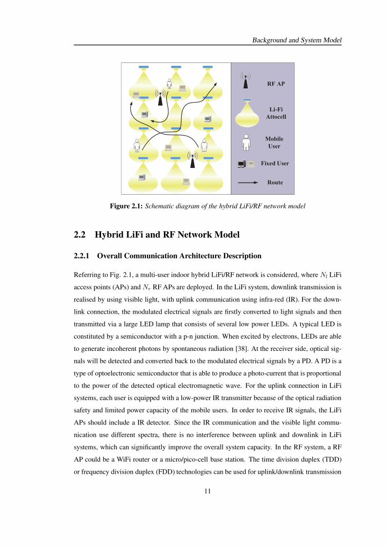
Figure 2.1: Schematic diagram of the hybrid LiFi/RF network model
2.2 Hybrid LiFi and RF Network Model
2.2.1 Overall Communication Architecture Description
Referring to Fig. 2.1, a multi-user indoor hybrid LiFi/RF network is considered, where Nl LiFi
access points (APs) and Nr RF APs are deployed. In the LiFi system, downlink transmission is
realised by using visible light, with uplink communication using infra-red (IR). For the down-
link connection, the modulated electrical signals are firstly converted to light signals and then
transmitted via a large LED lamp that consists of several low power LEDs. A typical LED is
constituted by a semiconductor with a p-n junction. When excited by electrons, LEDs are able
to generate incoherent photons by spontaneous radiation [38]. At the receiver side, optical sig-
nals will be detected and converted back to the modulated electrical signals by a PD. A PD is a
type of optoelectronic semiconductor that is able to produce a photo-current that is proportional
to the power of the detected optical electromagnetic wave. For the uplink connection in LiFi
systems, each user is equipped with a low-power IR transmitter because of the optical radiation
safety and limited power capacity of the mobile users. In order to receive IR signals, the LiFi
APs should include a IR detector. Since the IR communication and the visible light commu-
nication use different spectra, there is no interference between uplink and downlink in LiFi
systems, which can significantly improve the overall system capacity. In the RF system, a RF
AP could be a WiFi router or a micro/pico-cell base station. The time division duplex (TDD)
or frequency division duplex (FDD) technologies can be used for uplink/downlink transmission
11
Background and System Model
[39, 40]. The RF APs are assumed to cover the entire indoor area.
In this study, we mainly focus on the downlink transmission in hybrid LiFi/RF networks. Since
the field of view (FoV) of the LEDs is restricted, each LiFi AP covers a confined area which
is referred to as an optical attocell. In order to improve the spatial spectral efficiency, all LiFi
APs reuse the same modulation bandwidth, and users residing in the cell overlapping areas may
experience optical inter-cell interference (ICI), which is treated as additional noise [34]. The
ICI and blocking effects in the LiFi system may lead to a fluctuating spatial distribution in terms
of LiFi data rates. Therefore, the LiFi network is augmented by a RF network to improve the
users’ quality of service (QoS). To avoid the ICI in the RF system, each RF AP is allocated a
non-overlapping RF spectrum.
2.2.2 Central Unit and Backhaul Connection
In hybrid LiFi/RF networks, all of the LiFi and RF APs are connected to a central unit (CU)
through error free inter-connection links, which can be Ethernet cables, optical fibres or a
power-line backbone. The CU is responsible for the hybrid network management including
AP assignment for users, resource allocation (RA) and handover etc.
Unlike in RF, the LiFi channels do not exhibit significant fading characteristics as the detector
size is much larger than the wavelength [41]. They only exhibit shadowing effects so that
the LiFi channel between fixed APs and users are not time-varying. In the indoor scenario,
moving users are always at a low level of speed and users in the LiFi system do not experience
Doppler shift due to using intensity modulation. This means that LiFi channels vary slowly in
the dynamic indoor environment. In addition, users served by the RF AP in the indoor scenario
can be assumed to experience slow channel fading. Therefore, in the dynamic hybrid LiFi/RF
network, the channel state information (CSI) of both LiFi and RF can be considered constant for
a short period. It is assumed that the coherent time of LiFi and RF channels are denoted by Tl
and Tr, respectively. During the coherent time, the LiFi and RF channels are considered stable.
Accordingly, the hybrid LiFi/RF system can be divided into several quasi-static states over time.
In each state, the CSI of LiFi and RF channels is fixed and the duration of a quasi-static state
is denoted by Tp, which is the minimum between Tl and Tr. The evaluation of the coherent
time in both LiFi and RF systems is out of the scope of this work, but it will be considered
in our future research. The CU monitors the HLRN continuously in every quasi-static state,
where each user is assumed to have a constant data rate requirement. The CU determines the
12
Background and System Model
network load balancing based on the users’ CSI at the beginning of each state, which includes
AP assignment, handover and resource allocation. Handover occurs when the serving AP of a
user changes. During the handover, the overhead will be consumed, leading to a reduction in
the user data rate.
2.3 LiFi System Model
In this section, the LiFi system model is introduced. Specifically, the LiFi channel model,
modulation and multiple access technology will be explained.
2.3.1 LiFi Channel Model
The downlink LiFi channel model consists of three parts: LoS path loss, multi-path effect
in indoor scenarios and the frond-end filtering effect. Due to the limitation of the front-end
devices, the LiFi system uses intensity modulation (IM)/direct detection (DD) and baseband
bandwidth communication for downlink transmission. The LED and the PD function as a low
pass filter [42]. In addition, due to the reflective indoor environment, receivers collect signals
from multiple paths. Therefore, the channel impulse response (CIR) of downlink LiFi system
can be expressed as [17]:
h(t) = (ηLoSδ(t) + hme(t))⊗ hfe(t), (2.1)
where ηLoS is the LoS channel gain; δ(t) is the Dirac delta function; hme(t) is the multi-path
CIR and hfe(t) is the CIR caused by the front-end filtering effect. The corresponding frequency
response of LiFi channels can be calculated by using Fourier transform:
H(f) =
∫ +∞
0(ηLoSδ(t) + hme(t)) ⊗ hfe(t)e
−2πftdt = (ηLoS +Hme(f))Hfe(f). (2.2)
2.3.1.1 LoS Channel Gain
According to [43], the LoS channel gain can be written as:
ηLoS =
(m+1)Ap
2π(z2+h2w)g(θ)Ts(θ) cos
m(φ) cos(θ), θ ≤ ΘF
0, θ > ΘF
, (2.3)
13
Background and System Model
: PD: LED : LoS : Axis
1j
2jq
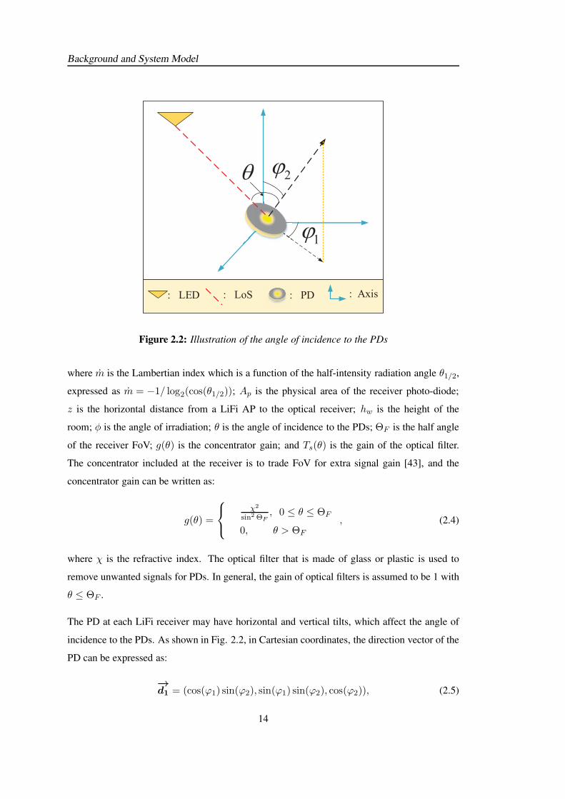
Figure 2.2: Illustration of the angle of incidence to the PDs
where m is the Lambertian index which is a function of the half-intensity radiation angle θ1/2,
expressed as m = −1/ log2(cos(θ1/2)); Ap is the physical area of the receiver photo-diode;
z is the horizontal distance from a LiFi AP to the optical receiver; hw is the height of the
room; φ is the angle of irradiation; θ is the angle of incidence to the PDs; ΘF is the half angle
of the receiver FoV; g(θ) is the concentrator gain; and Ts(θ) is the gain of the optical filter.
The concentrator included at the receiver is to trade FoV for extra signal gain [43], and the
concentrator gain can be written as:
g(θ) =
χ2
sin2 ΘF, 0 ≤ θ ≤ ΘF
0, θ > ΘF
, (2.4)
where χ is the refractive index. The optical filter that is made of glass or plastic is used to
remove unwanted signals for PDs. In general, the gain of optical filters is assumed to be 1 with
θ ≤ ΘF .
The PD at each LiFi receiver may have horizontal and vertical tilts, which affect the angle of
incidence to the PDs. As shown in Fig. 2.2, in Cartesian coordinates, the direction vector of the
PD can be expressed as:
−→
d1 = (cos(ϕ1) sin(ϕ2), sin(ϕ1) sin(ϕ2), cos(ϕ2)), (2.5)
14
Background and System Model
where ϕ1 is the horizontal orientation angle which follows a uniform distribution between 0
and 360; and ϕ2 is the vertical orientation angle which follows a uniform distribution between
0o and θPD, where 0 ≤ θPD ≤ 90 is the maximum vertical orientation angle. A PD of θPD =
0o is perpendicular to the floor. In this case, the angle of incidence to PDs is equal to the angle
of irradiation. The distance vector from a user to a LiFi AP is denoted by:
−→
d2 = (xa − xu, ya − yu, za − zu), (2.6)
where (xa, ya, za) and (xu, yu, zu) are the coordinates of the LiFi AP and the user, respectively.
The angle of incidence to the PDs can be expressed as:
θ = arccos <−→
d1,−→
d2 >, (2.7)
where <,> is the inner product operator.
2.3.1.2 Multi-path Component
Referring to [44–47], the characteristics of non-LoS (NLoS) channels in the indoor environment
in LiFi systems have been widely studied. It has been show that the NLoS channels are mainly
due to diffused reflections caused by human bodies, furniture and other objects, and are difficult
to predict and model. In [45–47], ray-tracing technique based approaches are developed to
calculate the NLoS channel impulse response caused by internal surface reflections. In [44],
according to simulations and measurements, an approximated diffused channel model in the
frequency domain for LiFi systems is proposed:
Hme(f) =ρApe
−j2πf∆T
Ar(1− ρ)(1 + j ffc); (2.8)
where Ar is the area of the indoor scenario surface; ρ is the reflectivity of the walls; ∆T is the
delay between the LoS signal and the onset of the diffuse signals; and fc = 1/2πτ is the cut-off
frequency of the diffuse optical channel with τ denoting the transmission delay of a photon via
reflective channels.
15
Background and System Model
2.3.1.3 Front-end Filtering Effects
The frequency response of a LED shows a low-path characteristic because of the long carrier
lifetime in the device active region and the large capacitance of the LED device [48]. In order
to characterise the LED low pass filtering effect, several expressions are used as approxima-
tions. In [17], it has been shown that the normalised magnitude response in decibel can be
approximated to be inversely proportional to the frequency, which can be expressed as:
HF (f) = exp(− f
vef0), (2.9)
where f0 is the 3 dB cut-off frequency of the front-end filtering effect; and ve = 2.88 is the
fitting coefficient, enabling to achieve |HF (f0)|2 = −3 dB.
2.3.2 O-OFDM Based Transmission
In LiFi networks, typical modulation schemes can fall into one of two categories: single car-
rier modulation and multiple carrier modulation. Due to the increasing data rate requirement,
single carrier modulation schemes such as on-off keying (OOK), pulse position modulation
(PPM) and pulse amplitude modulation (PAM) start to suffer from unwanted effects, such as
non-linear signal distortion at the LED front-end and inter-symbol interference caused by the
frequency selectivity in dispersive optical wireless channels [11]. Moreover, multiple carrier
modulation is more bandwidth-efficient but less energy-efficient than single carrier modulation.
One of the most widely used multiple carrier modulation schemes is orthogonal frequency divi-
sion multiplexing (OFDM) [49]. When using OFDM, parallel data streams are transmitted via
a collection of orthogonal subcarriers. The modulation bandwidth of the modulated signals is
smaller than the coherence bandwidth of the optical channel. Each sub-channel can be consid-
ered as a flat fading channel. This allows for further adaptive bit and power loading techniques
on each subcarrier to enhance system data rate performance.
Due to the complex and bipolar signals generated by the OFDM modulator, the conventional
OFDM scheme cannot fit the IM/DD requirement (positive real-valued signals) in LiFi systems
[50]. Therefore, two methods to modify the conventional OFDM scheme, direct current biased
optical-OFDM (DCO-OFDM) and asymmetrically clipped optical OFDM (ACO-OFDM) are
introduced in this section [51, 52].
16
Background and System Model
Modulation &
Coding
OFDM frame
mapping & S/PIFFT
Add CP and
DC bias
Signal
Clipping
D/A
E/O
O/E
A/D
Remove CP
and DC biasFFTEqualisation
OFDM frame
demapping & P/SDemodulation
and Decoding
Data
Stream
Data
Stream
Optical Channle
Figure 2.3: Illustration of key elements in DCO-OFDM systems
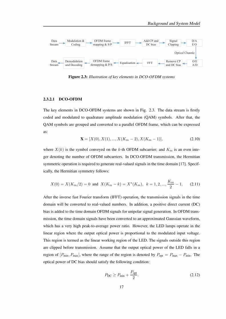
2.3.2.1 DCO-OFDM
The key elements in DCO-OFDM systems are shown in Fig. 2.3. The data stream is firstly
coded and modulated to quadrature amplitude modulation (QAM) symbols. After that, the
QAM symbols are grouped and converted to a parallel OFDM frame, which can be expressed
as:
X = [X(0),X(1), ...,X(Km − 2),X(Km − 1)], (2.10)
where X(k) is the symbol conveyed on the k-th OFDM subcarrier; and Km is an even inte-
ger denoting the number of OFDM subcarriers. In DCO-OFDM transmission, the Hermitian
symmetric operation is required to generate real-valued signals in the time domain [17]. Specif-
ically, the Hermitian symmetry follows:
X(0) = X(Km/2) = 0 and X(Km − k) = X∗(Km), k = 1, 2, ...,Km
2− 1. (2.11)
After the inverse fast Fourier transform (IFFT) operation, the transmission signals in the time
domain will be converted to real-valued numbers. In addition, a positive direct current (DC)
bias is added to the time domain OFDM signals for unipolar signal generation. In OFDM trans-
mission, the time domain signals have been converted to an approximated Gaussian waveform,
which has a very high peak-to-average power ratio. However, the LED lamps operate in the
linear region where the output optical power is proportional to the modulated input voltage.
This region is termed as the linear working region of the LED. The signals outside this region
are clipped before transmission. Assume that the output optical power of the LED falls in a
region of [Pmin, Pmax], where the range of the region is denoted by Popt = Pmax − Pmin. The
optical power of DC bias should satisfy the following condition:
PDC ≥ Pmin +Popt
2. (2.12)
17
Background and System Model
Moreover, the ratio between the range of output optical power and the electric power of modu-
lation signals without bias is denoted by:
ι = Popt/√
Pt. (2.13)
It is shown in [53] that an increase of ι results in a decrease in the probability of LiFi signals
outside the LED linear working region. In general, ι = 6 means that approximately 0.3% of the
signals are clipped. In this case,the clipping noise can be considered negligible.
Since there is no modulation signal transmitted on the 0-th and Km
2 -th subcarriers, a power
amplification can be achieved for the modulation signals on the subcarrier 1, 2, ..Km/2 −1,Km/2 + 1, ..Km. The amplification gain can be denoted as εp =
√
Km/(Km − 2). Partic-
ularly, when Km is a large number, the amplification gain is approximately 1. The signal-to-
noise ratio (SNR) with respect to frequency f in LiFi systems can be written as:
SNRLiFi(f) =(κεpPoptH(f))2
ι2NLBL
, (2.14)
where κ is the optical to electric conversion efficiency at the receivers; H(f) is the LiFi channel
gain in the frequency domain; NL is the single side-band noise spectrum; and BL is the base-
band bandwidth. In LiFi systems, the receive noise mainly consists of shot noise and thermal
noise. Shot noise is due to the particle characteristics of photons [38]. For an incident light with
constant power, the number of incoming photons per unit time follows a Poisson distribution.
This randomness of arriving photon numbers leads to the shot noise. With a large number of
photons, the shot noise can be modelled as an additive white Gaussian noise (AWGN). Thermal
noise mainly results from the temperature variation caused by the resistive units in the receiver
circuit [38]. In most of the optical receivers, a transimpedance amplifier (TIA) is included to
amplify the received signal. The resistance of the TIA is a major source of thermal noise. This
noise can also be modelled as an AWGN.
2.3.2.2 ACO-OFDM
Unlike DCO-OFDM, the Hermitian symmetric operation in ACO-OFDM only uses odd sub-
carriers for data transmission and the even subcarriers are set to zero. In this case, after the
IFFT operation, the signals in the time domain can be positive and real-valued. Therefore, a
large DC-bias is not required in ACO-OFDM, which can achieve better energy efficiency per-
18
Background and System Model
formance than DCO-OFDM [54]. However, as only the odd subcarriers are used, the spectral
efficiency of ACO-OFDM is further halved, compared with DCO-OFDM, resulting in a re-
duction of data rates. In this thesis, the DCO-OFDM is used for LiFi transmission in order to
improve the performance of user data rates.
2.3.3 Multiple Access Technology
In wireless communication networks, a multiple access technology allows several terminals
connected to the same multi-point transmission medium to transmit over it and to share its ca-
pacity. In the RF networks, conventional multiple access technologies include time division
multiple access (TDMA), code division multiple access (CDMA), carrier sense multiple access
(CSMA) and OFDMA, etc [55–57]. In particular, OFDMA is considered as an efficient mul-
tiple access method which has been widely used in 4G and 5G communication networks [58].
One of the main advantages of OFDMA is the flexibility for resource allocation. In the OFDMA
scheme, resources are partitioned in both time and frequency domains. Such time-frequency
blocks are known as resource blocks (RBs), and each RB contains a number of resource units
(RUs), which are the minimum and indivisible time-frequency slots. It is evident that allocat-
ing those RUs to different users is more efficient and flexible than allocating subcarriers or time
slots only. Another benefit of OFDMA is the multi-user diversity gain. OFDMA allows users
to transmit over different sub-channels, and different users may have different high-quality
subchannels. Hence, each user can select their high-quality sub-channels for transmission to
achieve an improvement in overall capacity. In this section, the OFDMA technology and the
relative resource allocation schemes in LiFi systems will be introduced.
2.3.3.1 Introduction: OFDMA in LiFi systems
In the conventional RF networks, the OFDMA method can substantially enhance the overall
system spectral efficiency (SE) by using an adaptive user-to-RU assignment. In recent research
on LiFi systems, OFDMA has been also used for RA [59, 60]. However, most of them assume
an equal channel gain over the OFDM subcarriers. The LiFi OFDMA systems with practical
channel responses have so far not been studied. As shown in Section 2.3.1, the LiFi channel
gain in the frequency domain is mainly affected by the characteristics of front-end devices and
the multi-path effect. It has been shown that in an open space office scenario, LiFi channels
are mainly affected by the front-end filtering effect, functioning as a low-pass filter [17]. This
19
Background and System Model
Frequency
Time
(a). TDMA
Frequency
(b). OFDMA
Time
User 1
User 2
User 3
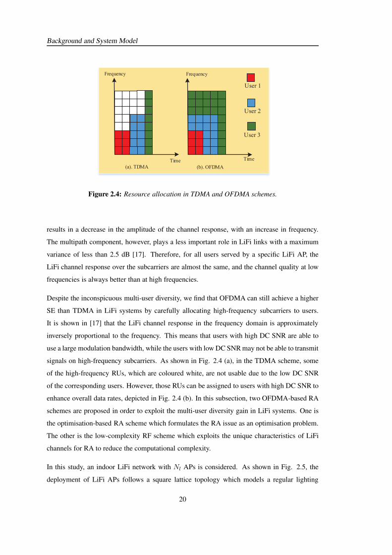
Figure 2.4: Resource allocation in TDMA and OFDMA schemes.
results in a decrease in the amplitude of the channel response, with an increase in frequency.
The multipath component, however, plays a less important role in LiFi links with a maximum
variance of less than 2.5 dB [17]. Therefore, for all users served by a specific LiFi AP, the
LiFi channel response over the subcarriers are almost the same, and the channel quality at low
frequencies is always better than at high frequencies.
Despite the inconspicuous multi-user diversity, we find that OFDMA can still achieve a higher
SE than TDMA in LiFi systems by carefully allocating high-frequency subcarriers to users.
It is shown in [17] that the LiFi channel response in the frequency domain is approximately
inversely proportional to the frequency. This means that users with high DC SNR are able to
use a large modulation bandwidth, while the users with low DC SNR may not be able to transmit
signals on high-frequency subcarriers. As shown in Fig. 2.4 (a), in the TDMA scheme, some
of the high-frequency RUs, which are coloured white, are not usable due to the low DC SNR
of the corresponding users. However, those RUs can be assigned to users with high DC SNR to
enhance overall data rates, depicted in Fig. 2.4 (b). In this subsection, two OFDMA-based RA
schemes are proposed in order to exploit the multi-user diversity gain in LiFi systems. One is
the optimisation-based RA scheme which formulates the RA issue as an optimisation problem.
The other is the low-complexity RF scheme which exploits the unique characteristics of LiFi
channels for RA to reduce the computational complexity.
In this study, an indoor LiFi network with Nl APs is considered. As shown in Fig. 2.5, the
deployment of LiFi APs follows a square lattice topology which models a regular lighting
20
Background and System Model
Serving AP
User
Interfering AP
d m
Desired
signals
Interference
User
d m
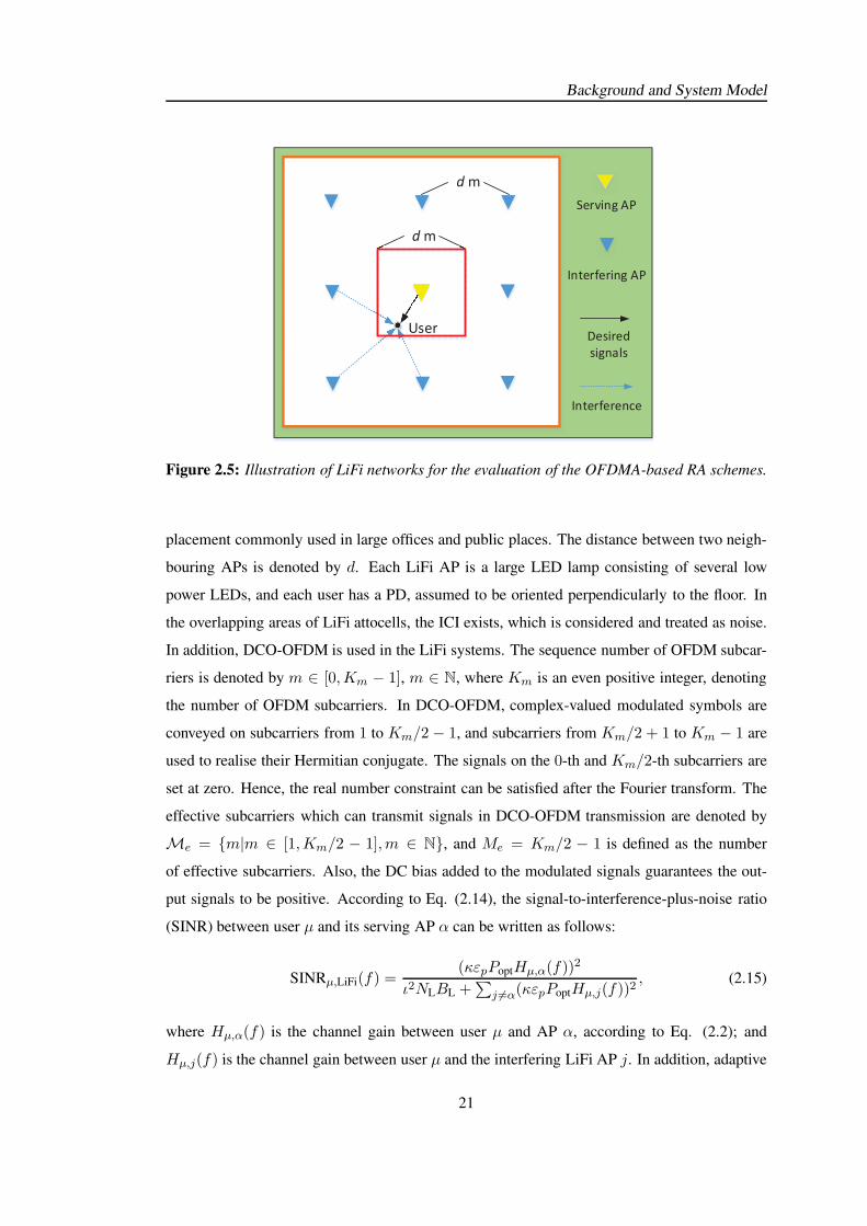
Figure 2.5: Illustration of LiFi networks for the evaluation of the OFDMA-based RA schemes.
placement commonly used in large offices and public places. The distance between two neigh-
bouring APs is denoted by d. Each LiFi AP is a large LED lamp consisting of several low
power LEDs, and each user has a PD, assumed to be oriented perpendicularly to the floor. In
the overlapping areas of LiFi attocells, the ICI exists, which is considered and treated as noise.
In addition, DCO-OFDM is used in the LiFi systems. The sequence number of OFDM subcar-
riers is denoted by m ∈ [0,Km − 1], m ∈ N, where Km is an even positive integer, denoting
the number of OFDM subcarriers. In DCO-OFDM, complex-valued modulated symbols are
conveyed on subcarriers from 1 to Km/2 − 1, and subcarriers from Km/2 + 1 to Km − 1 are
used to realise their Hermitian conjugate. The signals on the 0-th and Km/2-th subcarriers are
set at zero. Hence, the real number constraint can be satisfied after the Fourier transform. The
effective subcarriers which can transmit signals in DCO-OFDM transmission are denoted by
Me = m|m ∈ [1,Km/2 − 1],m ∈ N, and Me = Km/2 − 1 is defined as the number
of effective subcarriers. Also, the DC bias added to the modulated signals guarantees the out-
put signals to be positive. According to Eq. (2.14), the signal-to-interference-plus-noise ratio
(SINR) between user µ and its serving AP α can be written as follows:
SINRµ,LiFi(f) =(κεpPoptHµ,α(f))
2
ι2NLBL +∑
j 6=α(κεpPoptHµ,j(f))2, (2.15)
where Hµ,α(f) is the channel gain between user µ and AP α, according to Eq. (2.2); and
Hµ,j(f) is the channel gain between user µ and the interfering LiFi AP j. In addition, adaptive
21
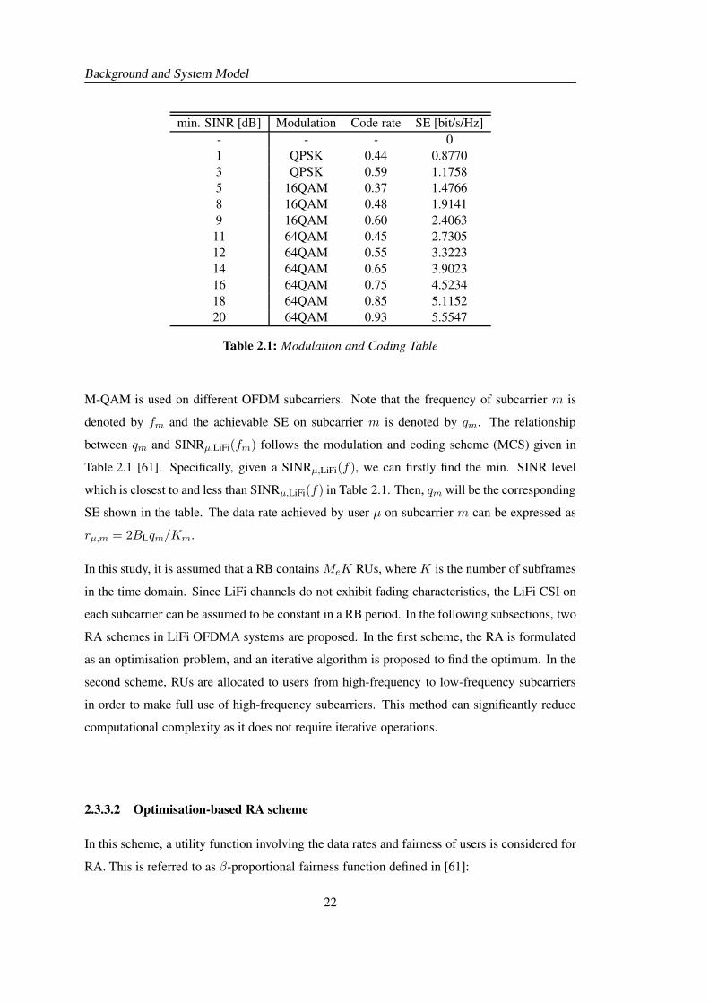
Background and System Model
min. SINR [dB] Modulation Code rate SE [bit/s/Hz]
- - - 0
1 QPSK 0.44 0.8770
3 QPSK 0.59 1.1758
5 16QAM 0.37 1.4766
8 16QAM 0.48 1.9141
9 16QAM 0.60 2.4063
11 64QAM 0.45 2.7305
12 64QAM 0.55 3.3223
14 64QAM 0.65 3.9023
16 64QAM 0.75 4.5234
18 64QAM 0.85 5.1152
20 64QAM 0.93 5.5547
Table 2.1: Modulation and Coding Table
M-QAM is used on different OFDM subcarriers. Note that the frequency of subcarrier m is
denoted by fm and the achievable SE on subcarrier m is denoted by qm. The relationship
between qm and SINRµ,LiFi(fm) follows the modulation and coding scheme (MCS) given in
Table 2.1 [61]. Specifically, given a SINRµ,LiFi(f), we can firstly find the min. SINR level
which is closest to and less than SINRµ,LiFi(f) in Table 2.1. Then, qm will be the corresponding
SE shown in the table. The data rate achieved by user µ on subcarrier m can be expressed as
rµ,m = 2BLqm/Km.
In this study, it is assumed that a RB contains MeK RUs, where K is the number of subframes
in the time domain. Since LiFi channels do not exhibit fading characteristics, the LiFi CSI on
each subcarrier can be assumed to be constant in a RB period. In the following subsections, two
RA schemes in LiFi OFDMA systems are proposed. In the first scheme, the RA is formulated
as an optimisation problem, and an iterative algorithm is proposed to find the optimum. In the
second scheme, RUs are allocated to users from high-frequency to low-frequency subcarriers
in order to make full use of high-frequency subcarriers. This method can significantly reduce
computational complexity as it does not require iterative operations.
2.3.3.2 Optimisation-based RA scheme
In this scheme, a utility function involving the data rates and fairness of users is considered for
RA. This is referred to as β-proportional fairness function defined in [61]:
22
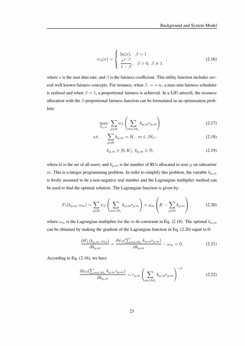
Background and System Model
ψβ(x) =
ln(x), β = 1
x1−β
1− β , β > 0, β 6= 1, (2.16)
where x is the user data rate; and β is the fairness coefficient. This utility function includes sev-
eral well known fairness concepts. For instance, when β → +∞, a max-min fairness scheduler
is realised and when β = 1, a proportional fairness is achieved. In a LiFi attocell, the resource
allocation with the β-proportional fairness function can be formulated as an optimisation prob-
lem:
maxkµ,m
∑
µ∈U
ψβ
(
∑
m∈Me
kµ,mrµ,m
)
(2.17)
s.t.∑
µ∈U
kµ,m = K, m ∈ Me; (2.18)
kµ,m ∈ [0,K], kµ,m ∈ N, (2.19)
where U is the set of all users; and kµ,m is the number of RUs allocated to user µ on subcarrier
m. This is a integer programming problem. In order to simplify this problem, the variable kµ,m
is firstly assumed to be a non-negative real number and the Lagrangian multiplier method can
be used to find the optimal solution. The Lagrangian function is given by:
F1(kµ,m, ωm) =∑
µ∈U
ψβ
(
∑
m∈Me
kµ,mrµ,m
)
+ ωm
K −∑
µ∈U
kµ,m
, (2.20)
where ωm is the Lagrangian multiplier for the m-th constraint in Eq. (2.18). The optimal kµ,m
can be obtained by making the gradient of the Lagrangian function in Eq. (2.20) equal to 0:
∂F1(kµ,m, ωm)
∂kµ,m=∂ψβ(
∑
m∈Mekµ,mrµ,m)
∂kµ,m− ωm = 0, (2.21)
According to Eq. (2.16), we have
∂ψβ(∑
m∈Mekµ,mγµ,m)
∂kµ,m= rµ,m
(
∑
m∈Me
kµ,mrµ,m
)−β
. (2.22)
23
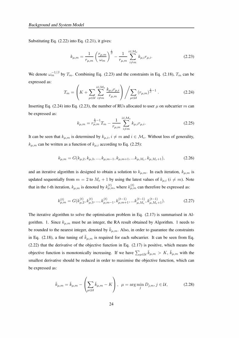
Background and System Model
Substituting Eq. (2.22) into Eq. (2.21), it gives:
kµ,m =1
rµ,m
(
rµ,mωm
) 1β
− 1
rµ,m
i∈Me∑
i 6=m
kµ,irµ,i. (2.23)
We denote ω−1/βm by Tm. Combining Eq. (2.23) and the constraints in Eq. (2.18), Tm can be
expressed as:
Tm =
K +∑
µ∈U
i∈Me∑
i 6=m
kµ,irµ,irµ,m
/
∑
µ∈U
(rµ,m)1β−1
. (2.24)
Inserting Eq. (2.24) into Eq. (2.23), the number of RUs allocated to user µ on subcarrier m can
be expressed as:
kµ,m = r1β−1
µ,m Tm −1
rµ,m
i∈Me∑
i 6=m
kµ,irµ,i. (2.25)
It can be seen that kµ,m is determined by kµ,i, i 6= m and i ∈ Me. Without loss of generality,
kµ,m can be written as a function of kµ,i according to Eq. (2.25):
kµ,m = G(kµ,2, kµ,3, ..., kµ,m−1, kµ,m+1, ...kµ,Me , kµ,Me+1), (2.26)
and an iterative algorithm is designed to obtain a solution to kµ,m. In each iteration, kµ,m is
updated sequentially from m = 2 to Me + 1 by using the latest values of kµ,i (i 6= m). Note
that in the t-th iteration, kµ,m is denoted by k(t)µ,m, where k
(t)µ,m can therefore be expressed as:
k(t)µ,m = G(k(t)µ,2, k
(t)µ,3, ..., k
(t)µ,m−1, k
(t−1)µ,m+1, ...k
(t−1)µ,Me
, k(t−1)µ,Me+1). (2.27)
The iterative algorithm to solve the optimisation problem in Eq. (2.17) is summarised in Al-
gorithm. 1. Since kµ,m must be an integer, the RA result obtained by Algorithm. 1 needs to
be rounded to the nearest integer, denoted by kµ,m. Also, in order to guarantee the constraints
in Eq. (2.18), a fine tuning of kµ,m is required for each subcarrier. It can be seen from Eq.
(2.22) that the derivative of the objective function in Eq. (2.17) is positive, which means the
objective function is monotonically increasing. If we have∑
µ∈U kµ,m > K , kµ,m with the
smallest derivative should be reduced in order to maximise the objective function, which can
be expressed as:
kµ,m = kµ,m −
∑
µ∈U
kµ,m −K
, µ = argminjDj,m, j ∈ U , (2.28)
24
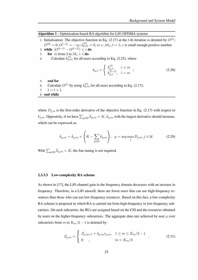
Background and System Model
Algorithm 1 : Optimisation-based RA algorithm for LiFi OFDMA systems
1: Initialisation: The objective function in Eq. (2.17) at the t-th iteration is denoted by O(t);
O(0) = 0; O(−1) = −∞; k(0)µ,m = 0, m ∈ Me; t = 1; ε is small enough positive number.
2: while |O(t−1) −O(t−2)| < ε do
3: for m from 2 to Me + 1 do
4: Calculate k(t)µ,m for all users according to Eq. (2.25), where
kµ,i =
k(t)µ,i, i < m
k(t−1)µ,i , i > m
; (2.30)
5: end for
6: Calculate O(t) by using k(t)µ,m for all users according to Eq. (2.17);
7: t = t+ 1.
8: end while
where Dj,m is the first-order derivative of the objective function in Eq. (2.17) with respect to
kj,m. Oppositely, if we have∑
µ∈U kµ,m < K, kµ,m with the largest derivative should increase,
which can be expressed as:
kµ,m = kµ,m +
K −∑
µ∈U
kµ,m
, µ = argmaxjDj,m, j ∈ U . (2.29)
With∑
µ∈U kµ,m = K , the fine tuning is not required.
2.3.3.3 Low-complexity RA scheme
As shown in [17], the LiFi channel gain in the frequency domain decreases with an increase in
frequency. Therefore, in a LiFi attocell, there are fewer users that can use high-frequency re-
sources than those who can use low-frequency resources. Based on this fact, a low-complexity
RA scheme is proposed in which RA is carried out from high-frequency to low-frequency sub-
carriers. On each subcarrier, the RUs are assigned based on the CSI and the resources obtained
by users on the higher-frequency subcarriers. The aggregate data rate achieved by user µ over
subcarriers from m to Km/2− 1 is denoted by:
Zµ,m =
Zµ,m+1 + kµ,mrµ,m, 1 ≤ m ≤ Km/2− 1
0 , m = Km/2. (2.31)
25
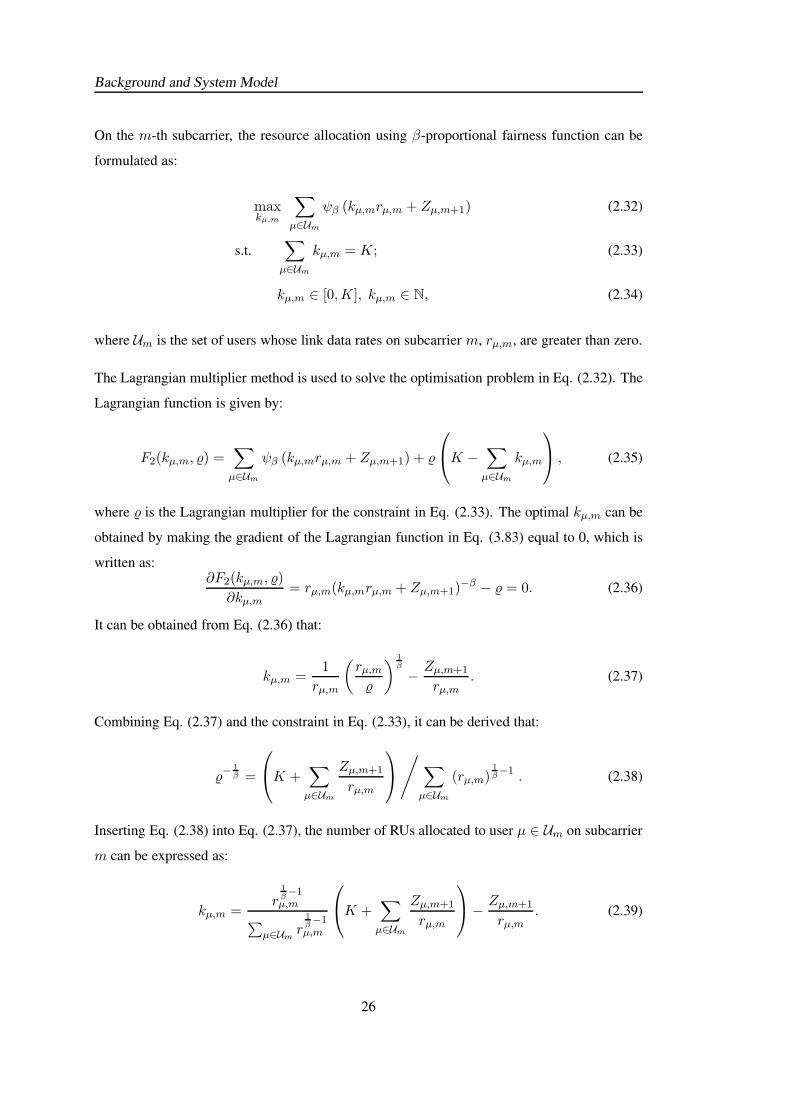
Background and System Model
On the m-th subcarrier, the resource allocation using β-proportional fairness function can be
formulated as:
maxkµ,m
∑
µ∈Um
ψβ (kµ,mrµ,m + Zµ,m+1) (2.32)
s.t.∑
µ∈Um
kµ,m = K; (2.33)
kµ,m ∈ [0,K], kµ,m ∈ N, (2.34)
where Um is the set of users whose link data rates on subcarrier m, rµ,m, are greater than zero.
The Lagrangian multiplier method is used to solve the optimisation problem in Eq. (2.32). The
Lagrangian function is given by:
F2(kµ,m, ) =∑
µ∈Um
ψβ (kµ,mrµ,m + Zµ,m+1) +
K −∑
µ∈Um
kµ,m
, (2.35)
where is the Lagrangian multiplier for the constraint in Eq. (2.33). The optimal kµ,m can be
obtained by making the gradient of the Lagrangian function in Eq. (3.83) equal to 0, which is
written as:∂F2(kµ,m, )
∂kµ,m= rµ,m(kµ,mrµ,m + Zµ,m+1)
−β − = 0. (2.36)
It can be obtained from Eq. (2.36) that:
kµ,m =1
rµ,m
(
rµ,m
)1β
− Zµ,m+1
rµ,m. (2.37)
Combining Eq. (2.37) and the constraint in Eq. (2.33), it can be derived that:
−1β =
K +∑
µ∈Um
Zµ,m+1
rµ,m
/
∑
µ∈Um
(rµ,m)1β−1 . (2.38)
Inserting Eq. (2.38) into Eq. (2.37), the number of RUs allocated to user µ ∈ Um on subcarrier
m can be expressed as:
kµ,m =r
1β−1
µ,m
∑
µ∈Umr
1β−1
µ,m
K +∑
µ∈Um
Zµ,m+1
rµ,m
− Zµ,m+1
rµ,m. (2.39)
26
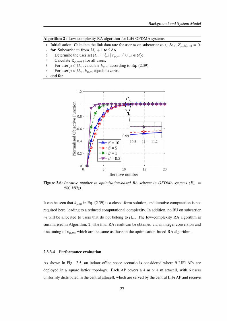
Background and System Model
Algorithm 2 : Low-complexity RA algorithm for LiFi OFDMA systems
1: Initialisation: Calculate the link data rate for user m on subcarrier m ∈ Me; Zµ,Me+2 = 0.
2: for Subcarrier m from Me + 1 to 2 do
3: Determine the user set Um = µ | rµ,m 6= 0, µ ∈ U;4: Calculate Zµ,m+1 for all users;
5: For user µ ∈ Um, calculate kµ,m according to Eq. (2.39);
6: For user µ /∈ Um, kµ,m equals to zeros;
7: end for
Iterative number0 5 10 15 20
Nor
mal
ised
Obj
ectiv
e Fu
nctio
n
0
0.2
0.4
0.6
0.8
1
1.2
β = 10β = 5β = 1β = 0.2
10.8 11 11.2
0.99
1
Figure 2.6: Iterative number in optimisation-based RA scheme in OFDMA systems (BL =250 MHz).
It can be seen that kµ,m in Eq. (2.39) is a closed-form solution, and iterative computation is not
required here, leading to a reduced computational complexity. In addition, no RU on subcarrier
m will be allocated to users that do not belong to Um. The low-complexity RA algorithm is
summarised in Algorithm. 2. The final RA result can be obtained via an integer conversion and
fine tuning of kµ,m, which are the same as those in the optimisation-based RA algorithm.
2.3.3.4 Performance evaluation
As shown in Fig. 2.5, an indoor office space scenario is considered where 9 LiFi APs are
deployed in a square lattice topology. Each AP covers a 4 m × 4 m attocell, with 6 users
uniformly distributed in the central attocell, which are served by the central LiFi AP and receive
27
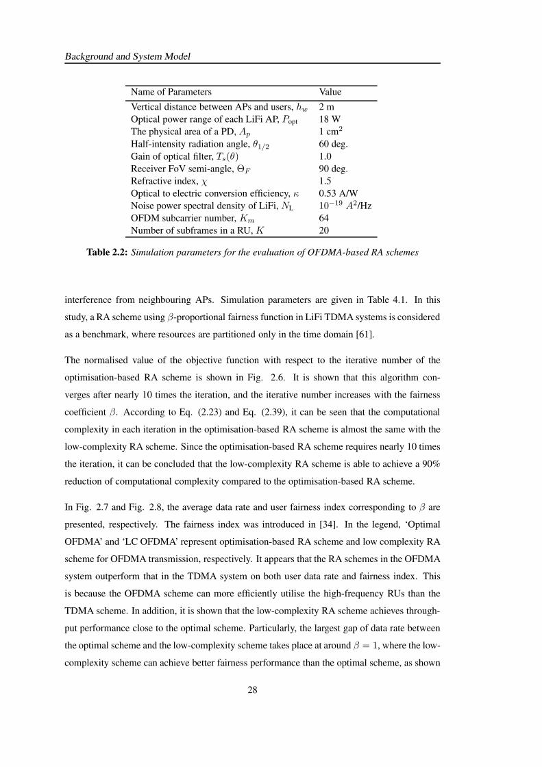
Background and System Model
Name of Parameters Value
Vertical distance between APs and users, hw 2 m
Optical power range of each LiFi AP, Popt 18 W
The physical area of a PD, Ap 1 cm2
Half-intensity radiation angle, θ1/2 60 deg.
Gain of optical filter, Ts(θ) 1.0
Receiver FoV semi-angle, ΘF 90 deg.
Refractive index, χ 1.5
Optical to electric conversion efficiency, κ 0.53 A/W
Noise power spectral density of LiFi, NL 10−19 A2/Hz
OFDM subcarrier number, Km 64
Number of subframes in a RU, K 20
Table 2.2: Simulation parameters for the evaluation of OFDMA-based RA schemes
interference from neighbouring APs. Simulation parameters are given in Table 4.1. In this
study, a RA scheme using β-proportional fairness function in LiFi TDMA systems is considered
as a benchmark, where resources are partitioned only in the time domain [61].
The normalised value of the objective function with respect to the iterative number of the
optimisation-based RA scheme is shown in Fig. 2.6. It is shown that this algorithm con-
verges after nearly 10 times the iteration, and the iterative number increases with the fairness
coefficient β. According to Eq. (2.23) and Eq. (2.39), it can be seen that the computational
complexity in each iteration in the optimisation-based RA scheme is almost the same with the
low-complexity RA scheme. Since the optimisation-based RA scheme requires nearly 10 times
the iteration, it can be concluded that the low-complexity RA scheme is able to achieve a 90%
reduction of computational complexity compared to the optimisation-based RA scheme.
In Fig. 2.7 and Fig. 2.8, the average data rate and user fairness index corresponding to β are
presented, respectively. The fairness index was introduced in [34]. In the legend, ‘Optimal
OFDMA’ and ‘LC OFDMA’ represent optimisation-based RA scheme and low complexity RA
scheme for OFDMA transmission, respectively. It appears that the RA schemes in the OFDMA
system outperform that in the TDMA system on both user data rate and fairness index. This
is because the OFDMA scheme can more efficiently utilise the high-frequency RUs than the
TDMA scheme. In addition, it is shown that the low-complexity RA scheme achieves through-
put performance close to the optimal scheme. Particularly, the largest gap of data rate between
the optimal scheme and the low-complexity scheme takes place at around β = 1, where the low-
complexity scheme can achieve better fairness performance than the optimal scheme, as shown
28
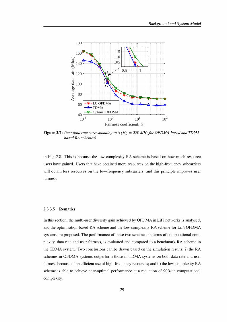
Background and System Model
Fairness coefficient, β10-1 100 101 102
Ave
rage
dat
a ra
te (
Mb/
s)
40
60
80
100
120
140
160
180
LC OFDMATDMAOptimal OFDMA
0.5 1
105110115
Figure 2.7: User data rate corresponding to β (BL = 280 MHz for OFDMA-based and TDMA-
based RA schemes)
in Fig. 2.8. This is because the low-complexity RA scheme is based on how much resource
users have gained. Users that have obtained more resources on the high-frequency subcarriers
will obtain less resources on the low-frequency subcarriers, and this principle improves user
fairness.
2.3.3.5 Remarks
In this section, the multi-user diversity gain achieved by OFDMA in LiFi networks is analysed,
and the optimisation-based RA scheme and the low-complexity RA scheme for LiFi OFDMA
systems are proposed. The performance of these two schemes, in terms of computational com-
plexity, data rate and user fairness, is evaluated and compared to a benchmark RA scheme in
the TDMA system. Two conclusions can be drawn based on the simulation results: i) the RA
schemes in OFDMA systems outperform those in TDMA systems on both data rate and user
fairness because of an efficient use of high-frequency resources; and ii) the low-complexity RA
scheme is able to achieve near-optimal performance at a reduction of 90% in computational
complexity.
29
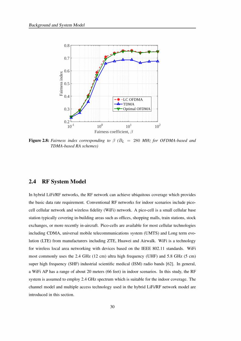
Background and System Model
Fairness coefficient, β 10-1 100 101 102
Fair
ness
inde
x
0.2
0.3
0.4
0.5
0.6
0.7
0.8
LC OFDMATDMAOptimal OFDMA
Figure 2.8: Fairness index corresponding to β (BL = 280 MHz for OFDMA-based and
TDMA-based RA schemes)
2.4 RF System Model
In hybrid LiFi/RF networks, the RF network can achieve ubiquitous coverage which provides
the basic data rate requirement. Conventional RF networks for indoor scenarios include pico-
cell cellular network and wireless fidelity (WiFi) network. A pico-cell is a small cellular base
station typically covering in-building areas such as offices, shopping malls, train stations, stock
exchanges, or more recently in-aircraft. Pico-cells are available for most cellular technologies
including CDMA, universal mobile telecommunications system (UMTS) and Long term evo-
lution (LTE) from manufacturers including ZTE, Huawei and Airwalk. WiFi is a technology
for wireless local area networking with devices based on the IEEE 802.11 standards. WiFi
most commonly uses the 2.4 GHz (12 cm) ultra high frequency (UHF) and 5.8 GHz (5 cm)
super high frequency (SHF) industrial scientific medical (ISM) radio bands [62]. In general,
a WiFi AP has a range of about 20 meters (66 feet) in indoor scenarios. In this study, the RF
system is assumed to employ 2.4 GHz spectrum which is suitable for the indoor coverage. The
channel model and multiple access technology used in the hybrid LiFi/RF network model are
introduced in this section.
30
Background and System Model
2.4.1 RF Channel Model
In the RF system, an omni-directional transmit antenna is employed for the 2.4 GHz RF AP.
The OFDM transmission is used and the RF channel gain between user µ and RF AP α on each
OFDM subcarrier is given by [16]:
Γµ,α(f) =
√
10−L(d)
10 hr, (2.40)
where f is the central frequency of OFDM subcarriers; hr is the small scale fading gain which
has an independent identical Rayleigh distribution with average power 2.46 dB; and L(d) is the
large-scale fading loss in decibels at the separation distance, d, which is given by [16]:
L(d) =
LFS(d) +XSF, d < dBP
LFS(dBP) + 35 log10(d/dBP) +XSF, d ≥ dBP
, (2.41)
where LFS(d) = 20 log10(d)+20 log10(f)−147.5 (dB) is the free space loss up to a breakpoint
distance dBP = 10 m, where f is the carrier frequency; and XSF is the shadowing fading loss
due to large scale blockage, which is 3 dB in typical indoor scenarios. It is assumed that the
RF APs use different spectra to avoid ICI. The SNR on each subcarrier with central frequency
f can be expressed as:
SNRµ,RF(f) =|Γµ,α(f)|2PR
σ2, (2.42)
where PR is the transmit power on each subcarrier; σ2 is the variance of the additive white
Gaussian noise (AWGN); and Γµ,α(f) is the channel gain according to Eq. (2.40).
2.4.2 Multiple Access Technology
In the RF networks, the multiple access technologies include OFDMA, TDMA, CDMA and
CSMA, etc. The OFDMA method is widely used in LTE cellular networks, which has been
introduced in Section 2.3.3. In WiFi networks, CSMA is the main approach for multiple access
in order to avoid ICI [16]. In CSMA transmission, a transmitter attempts to determine whether
another transmission is in progress before initiating a transmission using a carrier-sense mech-
anism. If a carrier is sensed, the transmitter waits for the transmission in progress to end before
initiating its own transmission. Using CSMA, multiple nodes may, in turn, send and receive on
the same medium. In this study, the RF APs work on different sub-channel, therefore the ICI
is avoided and CSMA is not used in this model. Moreover, in order to reduce the complexity,
31
Background and System Model
the OFDM-TDMA method instead of OFDMA is taken into account in RF systems. TDMA
allows the AP to communicate with users through different time slots, which can be realised at
a reduced complexity [58].
2.5 Summary
In this chapter, the downlink system model for hybrid LiFi/RF networks is introduced. The
overall communication architecture is described, and the channel model, OFDM transmission
and multiple access technology for LiFi and RF systems are discussed, respectively. Specifi-
cally, the LiFi channel mainly contains three components: the LoS path loss, front-end low pass
filtering effect. In addition, the DCO-OFDM and ACO-OFDM transmissions are introduced.
Since LiFi uses IM/DD and baseband bandwidth communications, the transmit signals should
be positive and real. In DCO-OFDM, complex modulated signals are conveyed on the first half
of the OFDM subcarriers, and the second half of the subcarriers are used for Hermitian sym-
metry. After IFFT operation, the signals in the time domain are real-valued. Also, a DC bias
is added to signals to guarantee the positivity. In ACO-OFDM, the complex modulated sym-
bols are mapped to the odd subcarriers, and the signals on the other subcarriers are zero. The
time-domain signals after IFFT can be positive and real-valued. In Section 2.3, the multiple ac-
cess technologies for LiFi systems have been introduced, and OFDMA transmission techniques
have been discussed. It has been shown that despite the inconspicuous multi-user diversity in
LiFi networks, OFDMA can still achieve a higher SE than TDMA by carefully allocating high-
frequency subcarriers to users. Two OFDMA-based RA schemes are proposed in order to
exploit the multi-user diversity gain in LiFi systems. One is the optimisation-based RA scheme
which formulates the RA issue as an optimisation problem. The other is the low-complexity RF
scheme which exploits the unique characteristics of LiFi channels for RA to reduce the compu-
tational complexity. Simulation results show that by efficiently using high-frequency bandwidth
resources, the RA schemes in OFDMA systems outperform those in TDMA systems in terms of
both data rate and user fairness. Also, the low-complexity RA scheme is able to achieve near-
optimal performance at a reduction of 90% in computational complexity. Finally, the system
model for RF networks is introduced. In this study, the 2.4 GHz spectrum band is considered
for RF transmission, which is typically appropriate to cover typical in-building areas. In addi-
tion, in order to reduce the complexity, the OFDM-TDMA method instead of OFDMA is taken
into account in RF systems.
32
Chapter 3Dynamic Load Balancing with
Handover for HLRNs
3.1 Introduction
The increasing number of multi-media mobile devices and the extensive use of data-demanding
mobile applications means that current mobile networks are at their maximum capacity due to
the limited availability of the radio frequency (RF) spectrum. The light fidelity (LiFi) technol-
ogy, which uses 300 THz of licence-free and unused optical spectrum for high-speed wireless
communications, has recently been regarded as a solution to this problem [11]. One advantage
of LiFi is that it does not cause interference to existing RF communication systems, because it
uses an entirely different part of the electromagnetic spectrum [23]. This enables the creation
of hybrid networks that combine LiFi with RF systems.
In an indoor situation, a hybrid integration of RF and LiFi is expected to improve both the
system throughput and the user’s quality of service (QoS) [21]. Since LiFi does not affect
the RF coverage and throughput, the total system throughput of a LiFi/RF hybrid network is
always greater than that of separate RF or LiFi networks [23]. On the one hand, according to
the IEEE 802.11 ad standard, the latest wireless fidelity (WiFi) protocol provided by Wireless
Gigabit Alliance (WiGig) enables devices to operate in three centre frequencies (2.4, 5 and 60
GHz), and WiGig can achieve a total data rate up to 6.7 Gb/s [63]. On the other hand, recent
research shows that the achievable data rate of a single light emitting diode (LED) can be more
than 7.3 Gb/s [14]. A large number of LiFi access points (APs) can be deployed in an indoor
scenario and thus a high area spectral efficiency can be achieved with a LiFi network [64], and
the total throughput of a LiFi/RF hybrid system can be considerable. Also, a hybrid network
can improve the user QoS by ensuring a high throughput at all locations. In general, the RF
network can achieve ubiquitous coverage which provides the basic data rate requirement and
LiFi can significantly augment the maximum capacity.
In a hybrid LiFi/RF network, fair and efficient load balancing (LB) can be a challenge due to the
small size of LiFi attocells. Most of the recent research focuses on the resource allocation (RA)
33
Dynamic Load Balancing with Handover for HLRNs
problem in static systems where users are assumed to be fixed [23, 24]. However, in practical
scenarios, some users will be moving. In an indoor scenario, the coverage of a RF AP is beyond
a single room whereas each LiFi cell in a LiFi network covers only a few square meters due
to the rectilinear propagation of light. However, there are many light sources in a room for
illumination purposes and LiFi harnesses significant gains by reusing transmission resources.
As a consequence, when assuming user movement, users may experience many handovers
between LiFi attocells. During a handover, the signalling information exchange between users
and a central unit (CU) is required, resulting from the handover overhead. This overhead must
be considered in the design of LB schemes for such hybrid networks.
In this chapter, dynamic load balancing that contains AP assignment, resource allocation and
handover is studied. Specifically, optimisation-based dynamic LB schemes and the fuzzy logic
(FL) based dynamic LB scheme are proposed. In Section 3.2, a special case for optimisation
based LB schemes with proportional fairness is analysed, and the handover boundary and the
relationship between LiFi throughput and RF throughput are discussed. In Section 3.3, the
optimisation based LB scheme with different user fairness scheduler is proposed. In Section
3.4, the FL based dynamic LB scheme is proposed, where AP assignment, RA and handover
are jointly designed. Section 3.5 gives the summary.
3.2 A Special Case: Optimisation based dynamic LB Scheme with
Proportional Fairness
Referring to Section 2.1-2.2, a LiFi/RF hybrid downlink is considered. This hybrid network
covers an indoor area by Nl LiFi APs and a single RF AP. Each LiFi AP is a large LED
lamp which contains many low power LEDs, and each user has a photo detector (PD). It is
assumed that all of the PDs are oriented perpendicular to the floor. This means that the angle
of irradiation is equal to the angle of incidence. The field of view (FoV) of the LEDs and
PDs can be designed so that the transmission can be contained within a certain space. In
this hybrid network, the network load balancing should be undertaken in regular quasi-static
states. The interval time between two neighbouring states is denoted by Tp. In each state, the
load balancing configuration is assumed to be fixed and users receive constant data rates. The
natural number t denotes the sequence number of the states. The set of LiFi and RF APs is
denoted by CL = α| α ∈ [0, Nl], α ∈ Z, where α = 0 represents the RF AP and α ∈ [1, Nl]
34
Dynamic Load Balancing with Handover for HLRNs
denotes the LiFi APs. The set of users is denoted by U . A full buffer traffic model is considered
so that the maximum achievable data rate can be evaluated for each user at all times.
In this section, the dynamic load balancing algorithm is given and the throughput analysis is
carried out. In order to reduce the complexity of theoretical analysis, we only consider the
LoS path loss in the LiFi channel model, the multi-path effect and the front-end filtering effect
are not taken into account. Therefore, the LiFi channel response in the frequency domain is
considered to be flat. The channel model in the LiFi system can be seen in Section 2.3. When
considering DCO-OFDM transmission, the LiFi signal-to-interference-plus-noise ratio (SINR)
between user µ and AP α can be written as:
SINRµ,α =(κεpPoptHµ,α)
2
ι2NLBL +∑
(κεpPoptHµ,else)2, (3.1)
where κ is the optical to electric conversion efficiency at the receivers; εp ≈ 1 is power am-
plification gain; Hµ,α is the channel gain between user µ and AP α, according to Eq. (2.3);
and Hµ,else is the channel gain between user µ and the interfering LiFi AP; NL is the single
side-band noise spectrum; and BL is the baseband bandwidth. Since approximately half of the
bandwidth can be used for data transmission in DCO-OFDM system, the achievable data rate
is expressed as:
Rµ,α = BL log2(1 + SINRµ,α). (3.2)
The WiFi protocol is considered for RF transmission. During the last ten years, the WiFi phys-
ical layer protocol has been enhanced, including IEEE 802.11 a/g, 802.11 n and 802.11 ac. Ac-
cording to [16], the current IEEE 802.11 protocol can guarantee a constant maximum through-
put for users which are located within 12 m from the transmitter, which is shown in Table. 3.1.
In general, the small scale fading in the RF wireless communication systems results in a fluctu-
ation of the data rates. In order to simplify the analysis complexity, the small scale fading of RF
channels is not considered in this study. This assumption is also used in [23] which considers
the LB problem in hybrid LiFi/WiFi networks. Therefore here, the distance between users and
the RF AP is set to be within 12 m, and the WiFi throughput is assumed to be constant and
equal to the maximum throughput shown in Table. 3.1, which is denoted by R0.
35
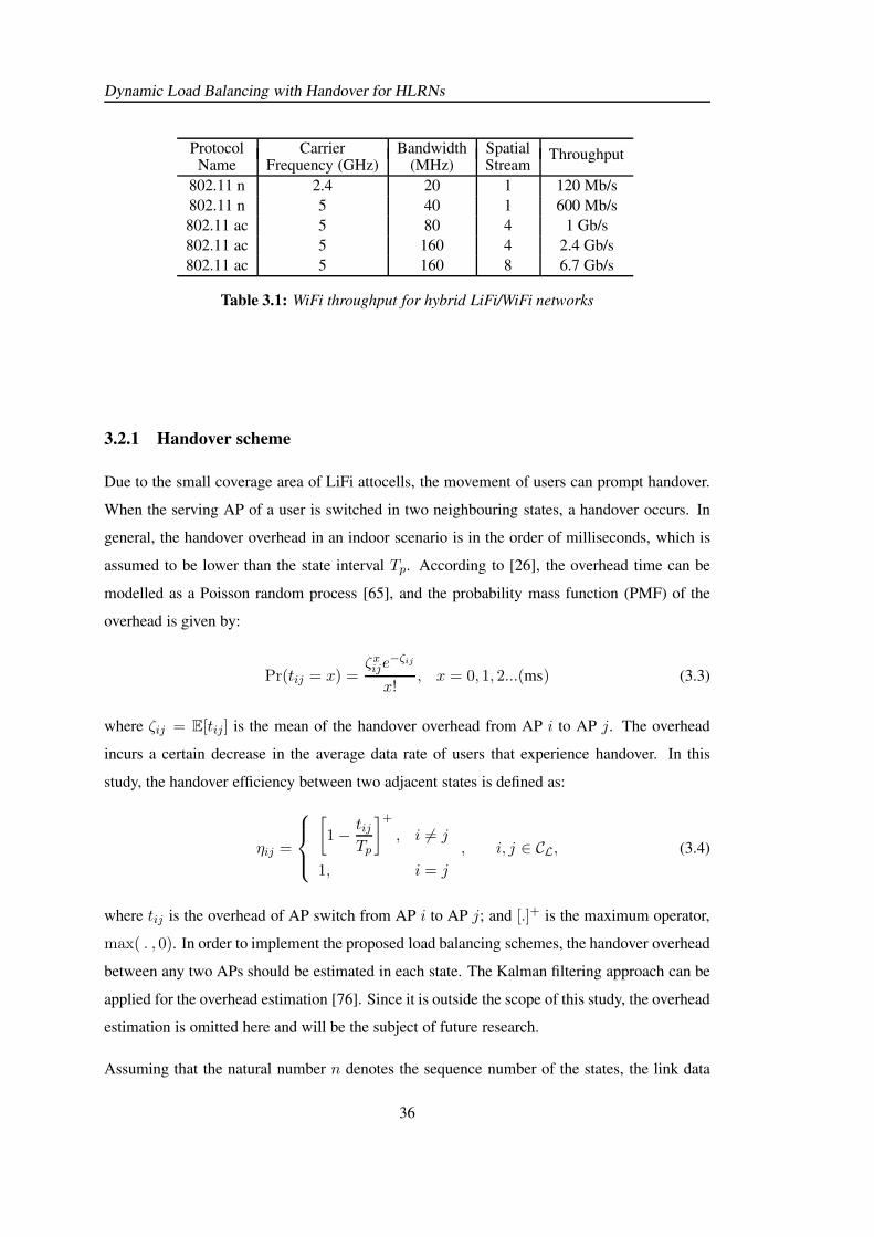
Dynamic Load Balancing with Handover for HLRNs
Protocol Carrier Bandwidth SpatialName Frequency (GHz) (MHz) Stream
Throughput
802.11 n 2.4 20 1 120 Mb/s
802.11 n 5 40 1 600 Mb/s
802.11 ac 5 80 4 1 Gb/s
802.11 ac 5 160 4 2.4 Gb/s
802.11 ac 5 160 8 6.7 Gb/s
Table 3.1: WiFi throughput for hybrid LiFi/WiFi networks
3.2.1 Handover scheme
Due to the small coverage area of LiFi attocells, the movement of users can prompt handover.
When the serving AP of a user is switched in two neighbouring states, a handover occurs. In
general, the handover overhead in an indoor scenario is in the order of milliseconds, which is
assumed to be lower than the state interval Tp. According to [26], the overhead time can be
modelled as a Poisson random process [65], and the probability mass function (PMF) of the
overhead is given by:
Pr(tij = x) =ζxije
−ζij
x!, x = 0, 1, 2...(ms) (3.3)
where ζij = E[tij] is the mean of the handover overhead from AP i to AP j. The overhead
incurs a certain decrease in the average data rate of users that experience handover. In this
study, the handover efficiency between two adjacent states is defined as:
ηij =
[
1− tijTp
]+
, i 6= j
1, i = j
, i, j ∈ CL, (3.4)
where tij is the overhead of AP switch from AP i to AP j; and [.]+ is the maximum operator,
max( . , 0). In order to implement the proposed load balancing schemes, the handover overhead
between any two APs should be estimated in each state. The Kalman filtering approach can be
applied for the overhead estimation [76]. Since it is outside the scope of this study, the overhead
estimation is omitted here and will be the subject of future research.
Assuming that the natural number n denotes the sequence number of the states, the link data
36
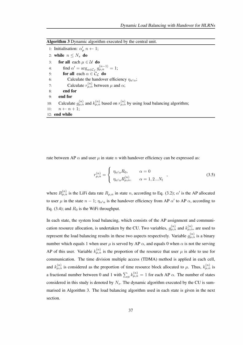
Dynamic Load Balancing with Handover for HLRNs
Algorithm 3 Dynamic algorithm executed by the central unit.
1: Initialisation: α′µ n← 1;
2: while n ≤ Ns do
3: for all each µ ∈ U do
4: find α′ = argα∈CL g(n−1)µ,α = 1;
5: for all each α ∈ CL do
6: Calculate the handover efficiency ηα′α;
7: Calculate r(n)µ,α between µ and α;
8: end for
9: end for
10: Calculate g(n)µ,α and k
(n)µ,α based on r
(n)µ,α by using load balancing algorithm;
11: n← n+ 1;
12: end while
rate between AP α and user µ in state n with handover efficiency can be expressed as:
r(n)µ,α =
ηα′αR0, α = 0
ηα′αR(n)µ,α, α = 1, 2...Nl
, (3.5)
where R(n)µ,α is the LiFi data rate Rµ,α in state n, according to Eq. (3.2); α′ is the AP allocated
to user µ in the state n − 1; ηα′α is the handover efficiency from AP α′ to AP α, according to
Eq. (3.4); and R0 is the WiFi throughput.
In each state, the system load balancing, which consists of the AP assignment and communi-
cation resource allocation, is undertaken by the CU. Two variables, g(n)µ,α and k
(n)µ,α, are used to
represent the load balancing results in these two aspects respectively. Variable g(n)µ,α is a binary
number which equals 1 when user µ is served by AP α, and equals 0 when α is not the serving
AP of this user. Variable k(n)µ,α is the proportion of the resource that user µ is able to use for
communication. The time division multiple access (TDMA) method is applied in each cell,
and k(n)µ,α is considered as the proportion of time resource block allocated to µ. Thus, k
(n)µ,α is
a fractional number between 0 and 1 with∑
µ k(n)µ,α = 1 for each AP α. The number of states
considered in this study is denoted by Ns. The dynamic algorithm executed by the CU is sum-
marised in Algorithm 3. The load balancing algorithm used in each state is given in the next
section.
37
Dynamic Load Balancing with Handover for HLRNs
3.2.2 Load Balancing Algorithm in One State
In this section, the load balancing algorithm used in each state is shown, and the superscript
(n) is omitted for simplicity. According to Eq. (2.16), a logarithmic utility function with β = 1
is used, which achieves proportional fairness [24]. By using the logarithmic utility function,
the load balancing problem can be formulated as a utility maximisation problem, which can be
expressed as:
maxgµ,α,kµ,α
∑
µ∈U
Nl∑
α=0
gµ,α log(kµ,αrµ,α) (3.6)
s.t.
Nl∑
α=0
gµ,α = 1 ∀µ ∈ U ;
∑
µ∈CL
gµ,αkµ,α ≤ 1 ∀α ∈ CL;
gµ,α ∈ 0, 1, kµ,α ∈ [0, 1], ∀µ ∈ U ,∀α ∈ CL;
where rµ,α is the communication link data rate given in Eq. (3.5), which is a positive number.
The optimum kµ,α is shown to be greater than zero in Eq. (3.8) so that log(0) is avoided.
This is a problem of mixed integer and non-linear programming. A decomposition-based ap-
proach can be used to solve the problem by decomposing the original problem into solvable
sub-problems according to [66]. Initially, the variable kµ,α is optimised. With a given gµ,α, the
objective function for AP α in Eq. (3.6) can be expressed as:
F (kµ,α) =∑
µ∈Uα
log(kµ,αrµ,α)
∝ 1
Mα
∑
µ∈Uα
log(kµ,α) = log
∏
µ∈Uα
kµ,α
1Mα
≤ log
(
k1,α + k2,α + ...+ kMα,α
Mα
)
, (3.7)
where Uα is the set of the users allocated to the AP α; and Mα represents its cardinality.
According to the rule of inequality, the maximum in Eq. (3.7) is achieved only when:
kµ,α =1
Mα, ∀µ ∈ Uα. (3.8)
38
Dynamic Load Balancing with Handover for HLRNs
According to Eq. (3.8), all of the users allocated to a specific AP share an equal proportion of
the time resource. By replacing kµ,α with Mα, the problem in Eq. (3.6) can be re-written as:
maxgµ,α,Mα
∑
µ∈U
Nl∑
α=0
gµ,α log
(
rµ,αMα
)
(3.9)
s.t.
Nl∑
α=0
gµ,α = 1 ∀µ ∈ U ; (3.10)
∑
µ∈U
gµ,α =Mα ∀α ∈ CL; (3.11)
gµ,α ∈ 0, 1, ∀µ ∈ U ,∀α ∈ CL;
The Lagrangian multiplier method is used to solve this problem. The two Lagrangian mul-
tipliers µ and ωα correspond to the constraints of Eq. (3.10) and Eq. (3.11), respectively.
Therefore the Lagrangian function can be expressed as:
L =∑
µ∈U
Nl∑
α=0
gµ,α log
(
rµ,αMα
)
+∑
µ∈U
µ
(
1−Nl∑
α=0
gµ,α
)
+
Nl∑
α=0
ωα
Mα −∑
µ∈U
gµ,α
. (3.12)
Due to∑
µ∈U gµ,α =Mα, the Lagrangian function can be re-written as:
L = L1(gµ,α, µ, ωα) + L2(Mα, µ, ωα), (3.13)
where
L1 =∑
µ∈U
Nl∑
α=0
gµ,α(log rµ,α − µ − ωα), (3.14)
L2 =
Nl∑
α=0
Mα(ωα − logMα) +∑
µ∈U
µ. (3.15)
In this case, the problem of Eq. (3.9) can be decomposed into two sub-problems which are to
maximise L1 and L2 using the proper Lagrangian multipliers.
Firstly, µ and ωα are assumed to be fixed; L1 can be maximised when the following expression
39
Dynamic Load Balancing with Handover for HLRNs
is achieved:
g∗µ,α =
1, α = argmaxα∈CL(log rµ,α − µ − ωα)
0, otherwise. (3.16)
Based on Eq. (3.11) and Eq. (3.16), the number of users allocated to AP α can be obtained,
which can be written as:
Mα,1 =∑
µ∈U
g∗µ,α (3.17)
In addition, given the Lagrangian multipliers, the maximum L2 is obtained when the following
expression is achieved:∂L2
∂Mα= 0 =⇒ M∗
α = exp(ωα − 1). (3.18)
Then, a variable δ is introduced to represent the difference between Mα,1 and M∗α, which can
be expressed as:
δ =∑
α∈CL
|Mα,1 −M∗α|. (3.19)
The optimisation problem to maximise the Lagrangian function in Eq. (3.12) is solved itera-
tively by using the gradient projection method [67], where µ and ωα are updated in the oppo-
site direction to the gradient ∇L(µ) and∇L(ωα). The i-th iteration of the gradient projection
algorithm can be expressed as:
µ(i+ 1) = µ(i)− ǫ1(1−∑
α∈CL
g∗µ,α); (3.20)
ωα(i+ 1) = ωα(i)− ǫ2(M∗α −
∑
µ∈U
g∗µ,α), (3.21)
where ǫ1 and ǫ2 are the sufficiently small step sizes required for guaranteeing convergence. Ac-
cording to Eq. (3.16),∑
α∈CLg∗µ,α = 1 is always satisfied in each iteration, and the expression
in Eq. (3.20) is re-written as µ(i+1) = µ(i). Therefore, the Lagrangian multiplier µ can be
set to 0, and only ωα should be updated in the iteration. An appropriate threshold δT is defined
and the variables converge to the optimum when δ ≤ δT is achieved. The threshold δT should
be small enough but it does not necessarily have to be a particular value. A smaller value of δT
will make the convergence slower. The iterative algorithm is shown in Algorithm 4.
40
Dynamic Load Balancing with Handover for HLRNs
Algorithm 4 : Load balancing algorithm in each state.
1: Initialisation: µ(i) = ωα(i) = 0, i← 1 and δ ← +∞;
2: while δ ≥ δT do
3: for all each µ ∈ U do
4: α∗ = argmaxα∈CL(log bµ,α − µ(i) − ωα(i));
5: g∗µ,α =
1, α = α∗
0, otherwise;
6: end for
7: Calculate Mα,1 =∑
µ∈U g∗µ,α, ∀α ∈ CL;
8: for all each α ∈ CL do
9: M∗α = exp(ωα(i)− 1);
10: ωα(i+ 1) = ωα(i) − ǫ2(M∗α −
∑
µ∈U g∗µ,α);
11: end for
12: Calculate δ =∑
α∈CL|Mα,1 −M∗
α|;13: i← i+ 1;
14: end while
15: Calculate gµ,α = g∗µ,α and kµ,α = 1/M∗α;
3.2.3 Analysis of AP Service Area and System Throughput
In order to gain an understanding of the load balancing in a hybrid network, it is important to
study the service area of each AP. In this section, the AP service area is identified with a given
WiFi throughput, and the throughput of each LiFi attocell is analysed. Firstly, a special case
without optical CCI is considered, which is termed as the ‘Non-CCI’ case. Following that, a
generic case with CCI is considered, which is termed as the ‘Optical CCI’ case.
3.2.3.1 Non-CCI case
In the non-CCI case, users served by LiFi APs do not receive any optical signals from other LiFi
APs. It is assumed that each LiFi AP covers the same size of attocell. In order to eliminate the
optical interference, the distance between any two LiFi APs should be greater than the diameter
of LiFi attocells.
It is assumed that receivers in HLRNs point upwards. Therefore the angle of irradiation is equal
to the angle of incidence for each user and the following expression can be achieved:
cos(φ) = cos(θ) =h
√
z2µ,α + h2w
, (3.22)
41
Dynamic Load Balancing with Handover for HLRNs
where zµ,α is the horizontal distance between LiFi AP α and user µ; hw is the height of the
room; φ is the angle of irradiation; and θ is the angle of incidence. The channel model in (2.3)
can be expressed as a function with zµ,α, and the data rate between LiFi AP α and user µ can
be written as:
ρα(zµ,α) = B log2(1 + SNR(zµ,α)) ≥ 0, (3.23)
where
SNR(zµ,α) =[(m+ 1)κPoptApg(θ)Ts(θ)h
m+1w ]2
4π2ι2NLBL
(z2µ,α + h2w)−m−3. (3.24)
It can be seen that ρα(zµ,α) is a monotonic decreasing function with respect to zµ,α.
Lemma 1. It is assumed that users are optimally allocated to APs by using the proposed load
balancing scheme in Algorithm 4. For any LiFi AP α, it can be obtained that:
zi,α ≤ zj,α, ∀i ∈ Uα, j /∈ Uα, (3.25)
where Uα is the set of users allocated to LiFi AP α.
Proof. Firstly, when user j is served by a different LiFi AP from AP α, this user should reside
in the corresponding LiFi attocell. Since the LiFi attocells are not overlapping, the inequality
zi,α ≤ zj,α is satisfied.
When user j is served by the WiFi AP, the method of proof by contradiction is applied to prove
this lemma. It is assumed that the optimal load balancing is achieved by using the proposed
scheme, and the inequality below is achieved:
zi,α > zj,α, ∀i ∈ Uα, j /∈ Uα, (3.26)
where user i is served by LiFi AP α and user j is served by the WiFi AP. The objective function
in Eq. (3.9) can be written as:
F1 = log
(
ρα(zi,α)
Mα
)
+ log
(
R0
M0
)
+∑
µ∈U−i,j
Nl∑
y=0
gµ,y log
(
ρy(zµ,y)
My
)
, (3.27)
where Mα and M0 are the number of users served by LiFi AP α and the WiFi AP, respectively.
Now, the APs allocated to user i and j are exchanged. The values of Mα and M0 stay the same,
42
Dynamic Load Balancing with Handover for HLRNs
and the objective function can be re-written as:
F2 = log
(
R0
M0
)
+ log
(
ρα(zj,α)
Mα
)
+∑
µ∈U−i,j
Nl∑
y=0
gµ,y log
(
ρy(zµ,y)
My
)
. (3.28)
Due to the monotonic decrease of ρα(zµ,α), it can be obtained that:
ρα(zi,α) < ρα(zj,α). (3.29)
As a consequence, F2 > F1 is achieved. This means that the AP allocation for user i and j
is not optimal, leading to a contradiction. The assumption in Eq. (3.26) must be false and the
lemma is proved.
Lemma 1 indicates that users served by LiFi AP α are closer to this AP than the users served
by other APs. The service area of a LiFi AP in the non-CCI case is a circular region, and
handover only occurs when users go through the boundary of the circular regions. In this study,
the boundary is termed as the ‘handover circle’, and the centre of the handover circle is the
location of a LiFi AP. Users that are outside all of the handover circles are served by the WiFi
AP.
The radius of the handover circles is analysed as follows. It is assumed that users are uniformly
distributed in the entire scenario. The area of the scenario is denoted by Y ; the density of users
is denoted by ε; the radius of the attocell covered by LiFi AP α is denoted by Zα; the radius
of the handover circle of LiFi AP α is denoted by να; and the average handover efficiency is
denoted by η, where η = E[ηij] and ηij is given in Eq. (3.4). The number of users served by
each AP can be written as:
Mα(να) =
εY −∑α=Nlα=1 επν2α, α = 0
∑α=Nlα=1 επν2h, α = 1, 2...Nl
, (3.30)
where
Y >
α=Nl∑
α=1
πν2α, 0 < να ≤ Zα, (3.31)
because all of the LiFi attocells are inside the considered scenario. According to the proposed
load balancing scheme, the radius of handover circles can be calculated by solving the optimi-
43
Dynamic Load Balancing with Handover for HLRNs
sation problem in Eq. (3.9), which can be written as:
maxνα
G1(να) +G2(να) (3.32)
s.t. 0 <να ≤ Zα (3.33)
where
G1(να) =
(
εY −α=Nl∑
α=1
επν2α
)
log
(
ηR0
εY −∑α=Nlα=1 επν2α
)
, (3.34)
G2(να) = 2πε
α=Nl∑
α=1
∫ να
0log
(
ηρα(x)
επν2α
)
xdx. (3.35)
Specifically, G1(να) represents the WiFi part (α = 0) in the objective function shown in Eq.
(3.6) and G2(να) represents the LiFi part (α = 1, 2, ..., Nl).
The first order derivatives of G1(να) and G2(να) can be expressed as:
∂G1
∂να= −2πενα
[
log
(
ηR0
εY −∑α=Nlα=1 επν2α
)
− 1
]
, (3.36)
∂G2
∂να= 2πενα
[
log
(
ηρα(να)
επν2α
)
− 1
]
. (3.37)
The derivative of the objective function in Eq. (3.32) can therefore be expressed as:
∂(G1 +G2)
∂να= 2πενα log
(
ρα(να)(Y −∑α=Nl
α=1 πν2α)
πν2αR0
)
. (3.38)
Due to να > 0,∂(G1+G2)
∂ναcan be equal to 0 only when
να = F−1(1) > 0, (3.39)
where F−1 is the inverse function of F (να), which is
F (να) =ρα(να)(Y −
∑α=Nlα=1 πν2α)
πν2αR0, (3.40)
where F (να) > 0 with 0 < να ≤ Zα due to the conditions in Eq. (3.23) and Eq. (3.31). It can
be seen that the function F (να) is monotonically decreasing with respect to να.
44

Dynamic Load Balancing with Handover for HLRNs
When 0 < να ≤ Zα is satisfied, it can be obtained that:
∂2(G1 +G2)
∂ν2α
∣
∣
∣
∣
να=να
= 2πε
[
log(F (να)) +να
F (να)
∂F (να)
∂να
∣
∣
∣
∣
να=να
]
< 0, (3.41)
where∂F (να)∂να
< 0 due to monotonic decrease property. As a consequence, να is the optimum
for the problem in Eq. (3.32). When να > Zα, since F (να) is monotonically decreasing, the
optimum να equals to Zα. The radius of handover circles can be expressed as:
ν∗α =
Zα, να > Zα
να, να ≤ Zα
. (3.42)
The sum throughput achieved by AP α can be written as:
Rsum,α =
R0, α = 0;
2(ν∗α)
2
∫ ν∗α0 ρα(x)xdx, α = 1, 2...Nl
. (3.43)
According to Eq. (3.23) and Eq. (3.40), the LiFi APs with the same transmit power and
modulation bandwidth have the same radius of the handover circles and throughput.
Since all of the users served by an AP share the equal time resource, the resource proportion
can be expressed as:
kµ,α =
1
ε(Y−∑α=Nl
α=1 π(ν∗α)2), α = 0;
1επ(ν∗α)
2 , α = 1, 2...Nl
. (3.44)
According to Eq. (3.40) and Eq. (3.42), it can be obtained that:
F (ν∗α) ≥ 1 (3.45)
⇐⇒ ρα(ν∗α)
επ(ν∗α)2≥ R0
ε(Y −∑α=Nlα=1 π(ν∗α)
2)(3.46)
⇐⇒ ρα(ν∗α)
kµ,α≥ R0
kµ,0, α = 1, 2...Nl (3.47)
where the equality in Eq. (3.47) is achieved when να ≤ Zα. This inequality indicates that the
users served by LiFi APs achieve data rates higher than or equal to those served by the WiFi
45
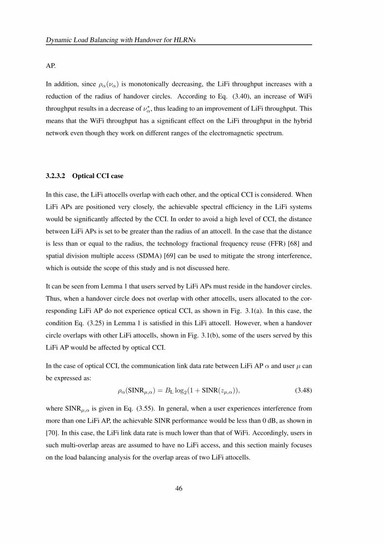
Dynamic Load Balancing with Handover for HLRNs
AP.
In addition, since ρα(να) is monotonically decreasing, the LiFi throughput increases with a
reduction of the radius of handover circles. According to Eq. (3.40), an increase of WiFi
throughput results in a decrease of ν∗α, thus leading to an improvement of LiFi throughput. This
means that the WiFi throughput has a significant effect on the LiFi throughput in the hybrid
network even though they work on different ranges of the electromagnetic spectrum.
3.2.3.2 Optical CCI case
In this case, the LiFi attocells overlap with each other, and the optical CCI is considered. When
LiFi APs are positioned very closely, the achievable spectral efficiency in the LiFi systems
would be significantly affected by the CCI. In order to avoid a high level of CCI, the distance
between LiFi APs is set to be greater than the radius of an attocell. In the case that the distance
is less than or equal to the radius, the technology fractional frequency reuse (FFR) [68] and
spatial division multiple access (SDMA) [69] can be used to mitigate the strong interference,
which is outside the scope of this study and is not discussed here.
It can be seen from Lemma 1 that users served by LiFi APs must reside in the handover circles.
Thus, when a handover circle does not overlap with other attocells, users allocated to the cor-
responding LiFi AP do not experience optical CCI, as shown in Fig. 3.1(a). In this case, the
condition Eq. (3.25) in Lemma 1 is satisfied in this LiFi attocell. However, when a handover
circle overlaps with other LiFi attocells, shown in Fig. 3.1(b), some of the users served by this
LiFi AP would be affected by optical CCI.
In the case of optical CCI, the communication link data rate between LiFi AP α and user µ can
be expressed as:
ρα(SINRµ,α) = BL log2(1 + SINR(zµ,α)), (3.48)
where SINRµ,α is given in Eq. (3.55). In general, when a user experiences interference from
more than one LiFi AP, the achievable SINR performance would be less than 0 dB, as shown in
[70]. In this case, the LiFi link data rate is much lower than that of WiFi. Accordingly, users in
such multi-overlap areas are assumed to have no LiFi access, and this section mainly focuses
on the load balancing analysis for the overlap areas of two LiFi attocells.
46
Dynamic Load Balancing with Handover for HLRNs
Lemma 2. For each LiFi AP α,
SINRi,α ≥ SINRj,α, ∀i ∈ Uα, j /∈ Uα, (3.49)
where Uα is the set of users allocated to LiFi AP α.
Proof. Initially, if j is allocated to the WiFi AP, this lemma is proved by using the method
shown in the proof of Lemma 1.
Then, the case that user j is served by another LiFi AP α′ is considered, and the method of
proof by contradiction is applied to prove this lemma. It is assumed that:
SINRi,α < SINRj,α, ∀i ∈ Uα, j ∈ Uα′ , (3.50)
where Uα′ is the set of the users allocated to LiFi AP α′. According to the assumption in Eq.
(3.50), the expression SINRj,α′ < SINRi,α′ is achieved. Particularly, if user i or j is outside
the overlap area and cannot be served by one of the APs between α and α′, the corresponding
SINR is 0.
The objective function in Eq. (3.9) can be written as:
F3 = log
(
ρα(SINRi,α)
Mα
)
+ log
(
ρα(SINRj,α′)
Mα′
)
+∑
µ∈U−i,j
Nl∑
y=0
gµ,y log
(
ρy(SINRµ,y)
My
)
, (3.51)
where Mα and Mα′ represent the number of users served by LiFi AP α and α′, respectively.
Now, the allocated APs of user i and j are exchanged. The values of Mα and Mα′ stay the
same. In this way, the objective function can be written as:
F4 = log
(
ρα(SINRj,α)
Mα
)
+ log
(
ρα(SINRi,α′)
Mα′
)
+∑
µ∈U−i,j
Nl∑
y=0
gµ,y log
(
ρy(SINRµ,y
My
)
. (3.52)
According to Eq. (3.50), it can be derived that F4 > F3. This means that the allocation of APs
47
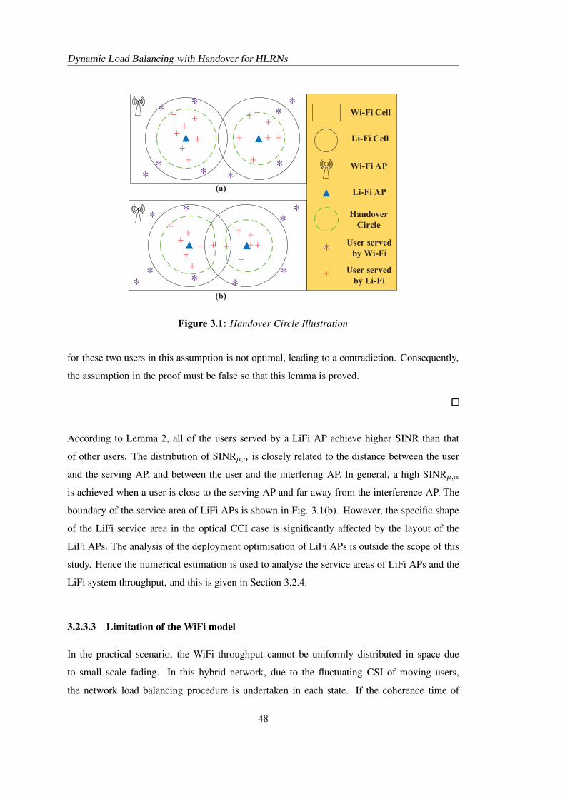
Dynamic Load Balancing with Handover for HLRNs
(a)
(b)
Wi-Fi Cell
Li-Fi Cell
Li-Fi AP
Wi-Fi AP
Handover
Circle
User served
by Wi-Fi
User served
by Li-Fi
Figure 3.1: Handover Circle Illustration
for these two users in this assumption is not optimal, leading to a contradiction. Consequently,
the assumption in the proof must be false so that this lemma is proved.
According to Lemma 2, all of the users served by a LiFi AP achieve higher SINR than that
of other users. The distribution of SINRµ,α is closely related to the distance between the user
and the serving AP, and between the user and the interfering AP. In general, a high SINRµ,α
is achieved when a user is close to the serving AP and far away from the interference AP. The
boundary of the service area of LiFi APs is shown in Fig. 3.1(b). However, the specific shape
of the LiFi service area in the optical CCI case is significantly affected by the layout of the
LiFi APs. The analysis of the deployment optimisation of LiFi APs is outside the scope of this
study. Hence the numerical estimation is used to analyse the service areas of LiFi APs and the
LiFi system throughput, and this is given in Section 3.2.4.
3.2.3.3 Limitation of the WiFi model
In the practical scenario, the WiFi throughput cannot be uniformly distributed in space due
to small scale fading. In this hybrid network, due to the fluctuating CSI of moving users,
the network load balancing procedure is undertaken in each state. If the coherence time of
48
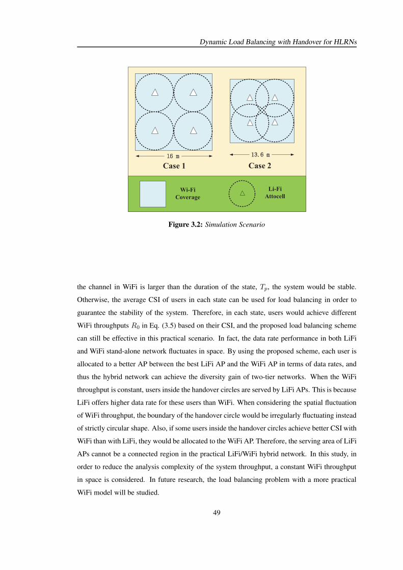
Dynamic Load Balancing with Handover for HLRNs
Case 1 Case 2
Wi-Fi
Coverage
Li-Fi
Attocell
Figure 3.2: Simulation Scenario
the channel in WiFi is larger than the duration of the state, Tp, the system would be stable.
Otherwise, the average CSI of users in each state can be used for load balancing in order to
guarantee the stability of the system. Therefore, in each state, users would achieve different
WiFi throughputs R0 in Eq. (3.5) based on their CSI, and the proposed load balancing scheme
can still be effective in this practical scenario. In fact, the data rate performance in both LiFi
and WiFi stand-alone network fluctuates in space. By using the proposed scheme, each user is
allocated to a better AP between the best LiFi AP and the WiFi AP in terms of data rates, and
thus the hybrid network can achieve the diversity gain of two-tier networks. When the WiFi
throughput is constant, users inside the handover circles are served by LiFi APs. This is because
LiFi offers higher data rate for these users than WiFi. When considering the spatial fluctuation
of WiFi throughput, the boundary of the handover circle would be irregularly fluctuating instead
of strictly circular shape. Also, if some users inside the handover circles achieve better CSI with
WiFi than with LiFi, they would be allocated to the WiFi AP. Therefore, the serving area of LiFi
APs cannot be a connected region in the practical LiFi/WiFi hybrid network. In this study, in
order to reduce the analysis complexity of the system throughput, a constant WiFi throughput
in space is considered. In future research, the load balancing problem with a more practical
WiFi model will be studied.
49
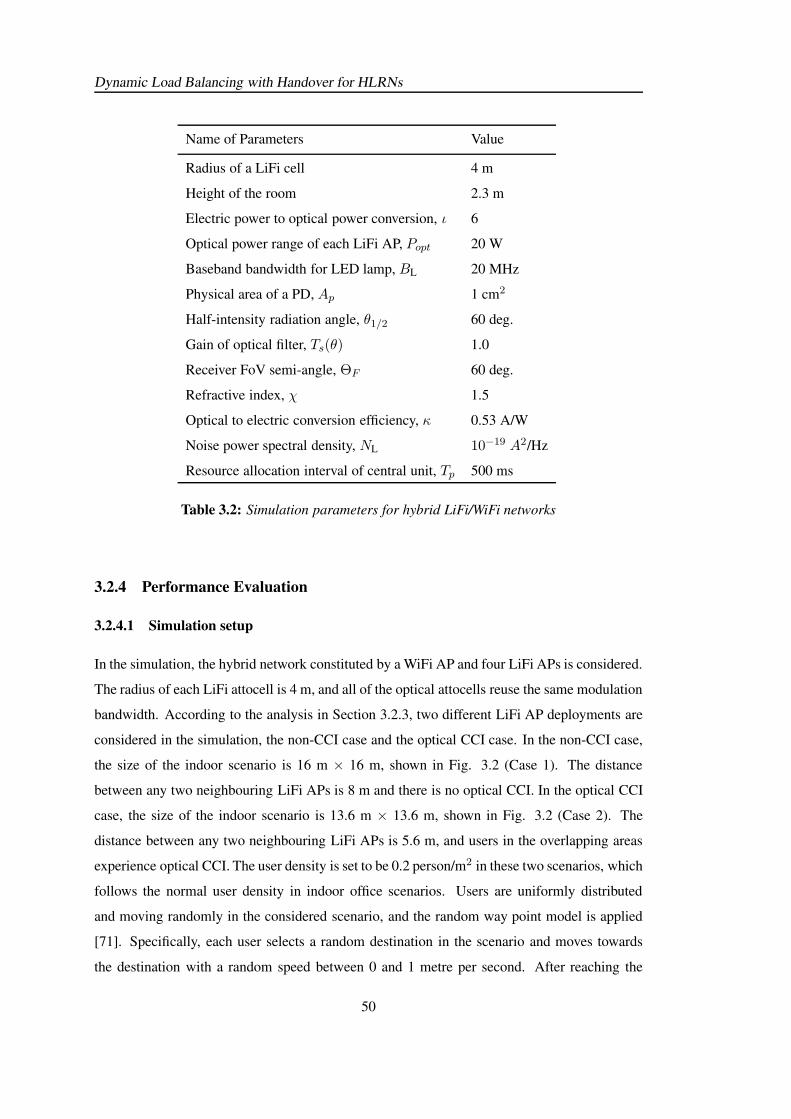
Dynamic Load Balancing with Handover for HLRNs
Name of Parameters Value
Radius of a LiFi cell 4 m
Height of the room 2.3 m
Electric power to optical power conversion, ι 6
Optical power range of each LiFi AP, Popt 20 W
Baseband bandwidth for LED lamp, BL 20 MHz
Physical area of a PD, Ap 1 cm2
Half-intensity radiation angle, θ1/2 60 deg.
Gain of optical filter, Ts(θ) 1.0
Receiver FoV semi-angle, ΘF 60 deg.
Refractive index, χ 1.5
Optical to electric conversion efficiency, κ 0.53 A/W
Noise power spectral density, NL 10−19 A2/Hz
Resource allocation interval of central unit, Tp 500 ms
Table 3.2: Simulation parameters for hybrid LiFi/WiFi networks
3.2.4 Performance Evaluation
3.2.4.1 Simulation setup
In the simulation, the hybrid network constituted by a WiFi AP and four LiFi APs is considered.
The radius of each LiFi attocell is 4 m, and all of the optical attocells reuse the same modulation
bandwidth. According to the analysis in Section 3.2.3, two different LiFi AP deployments are
considered in the simulation, the non-CCI case and the optical CCI case. In the non-CCI case,
the size of the indoor scenario is 16 m × 16 m, shown in Fig. 3.2 (Case 1). The distance
between any two neighbouring LiFi APs is 8 m and there is no optical CCI. In the optical CCI
case, the size of the indoor scenario is 13.6 m × 13.6 m, shown in Fig. 3.2 (Case 2). The
distance between any two neighbouring LiFi APs is 5.6 m, and users in the overlapping areas
experience optical CCI. The user density is set to be 0.2 person/m2 in these two scenarios, which
follows the normal user density in indoor office scenarios. Users are uniformly distributed
and moving randomly in the considered scenario, and the random way point model is applied
[71]. Specifically, each user selects a random destination in the scenario and moves towards
the destination with a random speed between 0 and 1 metre per second. After reaching the
50
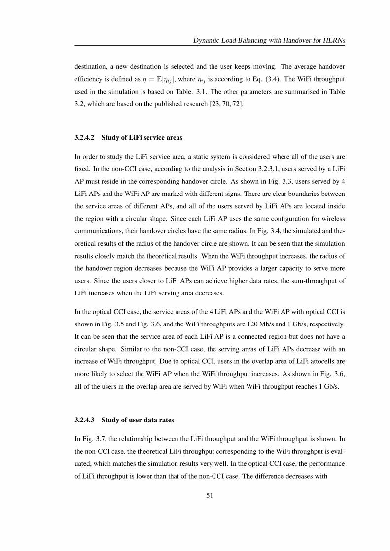
Dynamic Load Balancing with Handover for HLRNs
destination, a new destination is selected and the user keeps moving. The average handover
efficiency is defined as η = E[ηij ], where ηij is according to Eq. (3.4). The WiFi throughput
used in the simulation is based on Table. 3.1. The other parameters are summarised in Table
3.2, which are based on the published research [23, 70, 72].
3.2.4.2 Study of LiFi service areas
In order to study the LiFi service area, a static system is considered where all of the users are
fixed. In the non-CCI case, according to the analysis in Section 3.2.3.1, users served by a LiFi
AP must reside in the corresponding handover circle. As shown in Fig. 3.3, users served by 4
LiFi APs and the WiFi AP are marked with different signs. There are clear boundaries between
the service areas of different APs, and all of the users served by LiFi APs are located inside
the region with a circular shape. Since each LiFi AP uses the same configuration for wireless
communications, their handover circles have the same radius. In Fig. 3.4, the simulated and the-
oretical results of the radius of the handover circle are shown. It can be seen that the simulation
results closely match the theoretical results. When the WiFi throughput increases, the radius of
the handover region decreases because the WiFi AP provides a larger capacity to serve more
users. Since the users closer to LiFi APs can achieve higher data rates, the sum-throughput of
LiFi increases when the LiFi serving area decreases.
In the optical CCI case, the service areas of the 4 LiFi APs and the WiFi AP with optical CCI is
shown in Fig. 3.5 and Fig. 3.6, and the WiFi throughputs are 120 Mb/s and 1 Gb/s, respectively.
It can be seen that the service area of each LiFi AP is a connected region but does not have a
circular shape. Similar to the non-CCI case, the serving areas of LiFi APs decrease with an
increase of WiFi throughput. Due to optical CCI, users in the overlap area of LiFi attocells are
more likely to select the WiFi AP when the WiFi throughput increases. As shown in Fig. 3.6,
all of the users in the overlap area are served by WiFi when WiFi throughput reaches 1 Gb/s.
3.2.4.3 Study of user data rates
In Fig. 3.7, the relationship between the LiFi throughput and the WiFi throughput is shown. In
the non-CCI case, the theoretical LiFi throughput corresponding to the WiFi throughput is eval-
uated, which matches the simulation results very well. In the optical CCI case, the performance
of LiFi throughput is lower than that of the non-CCI case. The difference decreases with
51
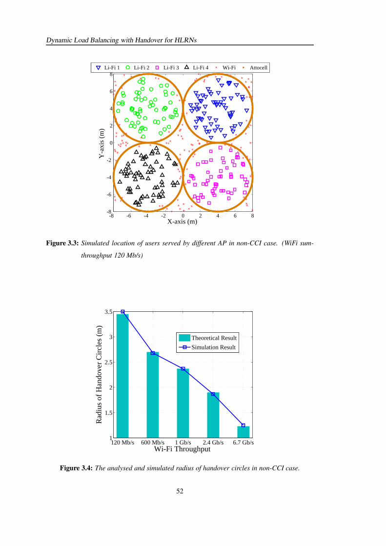
Dynamic Load Balancing with Handover for HLRNs
-8 -6 -4 -2 0 2 4 6 8-8
-6
-4
-2
0
2
4
6
8
X-axis (m)
Y-a
xis
(m)
Li-Fi 1 Li-Fi 2 Li-Fi 3 Li-Fi 4 Wi-Fi Attocell
Figure 3.3: Simulated location of users served by different AP in non-CCI case. (WiFi sum-
throughput 120 Mb/s)
120 Mb/s 600 Mb/s 1 Gb/s 2.4 Gb/s 6.7 Gb/s1
1.5
2
2.5
3
3.5
Wi-Fi Throughput
Rad
ius
of H
ando
ver
Cir
cles
(m
)
Theoretical Result
Simulation Result
Figure 3.4: The analysed and simulated radius of handover circles in non-CCI case.
52
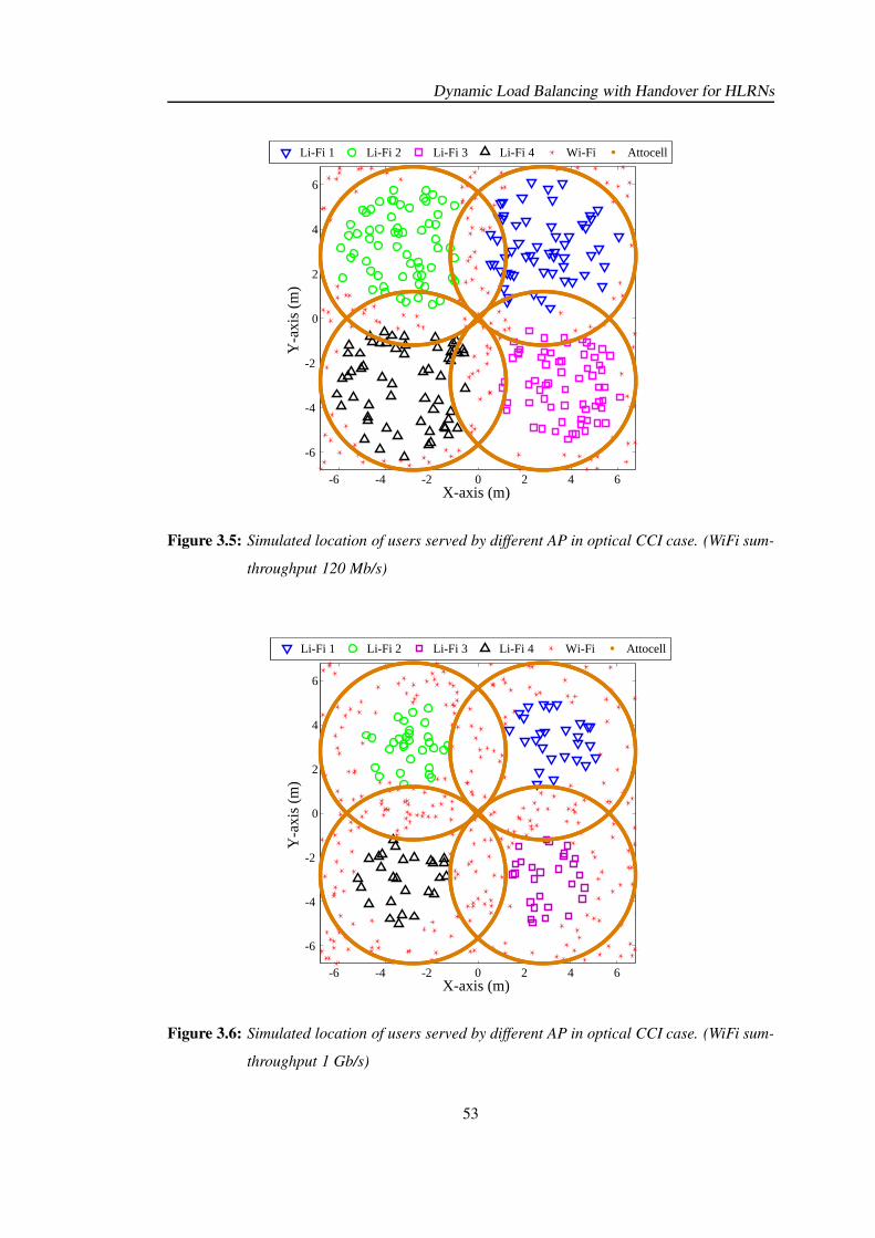
Dynamic Load Balancing with Handover for HLRNs
-6 -4 -2 0 2 4 6
-6
-4
-2
0
2
4
6
X-axis (m)
Y-a
xis
(m)
Li-Fi 1 Li-Fi 2 Li-Fi 3 Li-Fi 4 Wi-Fi Attocell
Figure 3.5: Simulated location of users served by different AP in optical CCI case. (WiFi sum-
throughput 120 Mb/s)
-6 -4 -2 0 2 4 6
-6
-4
-2
0
2
4
6
X-axis (m)
Y-a
xis
(m)
Li-Fi 1 Li-Fi 2 Li-Fi 3 Li-Fi 4 Wi-Fi Attocell
Figure 3.6: Simulated location of users served by different AP in optical CCI case. (WiFi sum-
throughput 1 Gb/s)
53
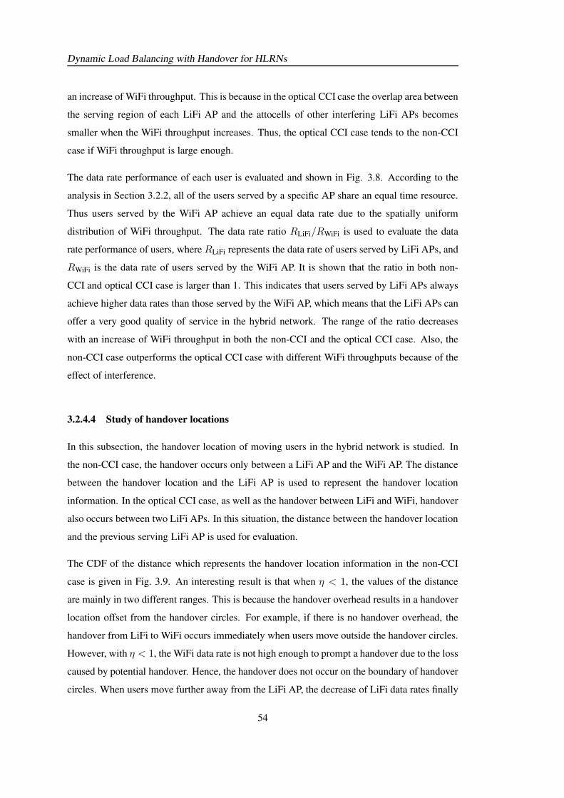
Dynamic Load Balancing with Handover for HLRNs
an increase of WiFi throughput. This is because in the optical CCI case the overlap area between
the serving region of each LiFi AP and the attocells of other interfering LiFi APs becomes
smaller when the WiFi throughput increases. Thus, the optical CCI case tends to the non-CCI
case if WiFi throughput is large enough.
The data rate performance of each user is evaluated and shown in Fig. 3.8. According to the
analysis in Section 3.2.2, all of the users served by a specific AP share an equal time resource.
Thus users served by the WiFi AP achieve an equal data rate due to the spatially uniform
distribution of WiFi throughput. The data rate ratio RLiFi/RWiFi is used to evaluate the data
rate performance of users, where RLiFi represents the data rate of users served by LiFi APs, and
RWiFi is the data rate of users served by the WiFi AP. It is shown that the ratio in both non-
CCI and optical CCI case is larger than 1. This indicates that users served by LiFi APs always
achieve higher data rates than those served by the WiFi AP, which means that the LiFi APs can
offer a very good quality of service in the hybrid network. The range of the ratio decreases
with an increase of WiFi throughput in both the non-CCI and the optical CCI case. Also, the
non-CCI case outperforms the optical CCI case with different WiFi throughputs because of the
effect of interference.
3.2.4.4 Study of handover locations
In this subsection, the handover location of moving users in the hybrid network is studied. In
the non-CCI case, the handover occurs only between a LiFi AP and the WiFi AP. The distance
between the handover location and the LiFi AP is used to represent the handover location
information. In the optical CCI case, as well as the handover between LiFi and WiFi, handover
also occurs between two LiFi APs. In this situation, the distance between the handover location
and the previous serving LiFi AP is used for evaluation.
The CDF of the distance which represents the handover location information in the non-CCI
case is given in Fig. 3.9. An interesting result is that when η < 1, the values of the distance
are mainly in two different ranges. This is because the handover overhead results in a handover
location offset from the handover circles. For example, if there is no handover overhead, the
handover from LiFi to WiFi occurs immediately when users move outside the handover circles.
However, with η < 1, the WiFi data rate is not high enough to prompt a handover due to the loss
caused by potential handover. Hence, the handover does not occur on the boundary of handover
circles. When users move further away from the LiFi AP, the decrease of LiFi data rates finally
54
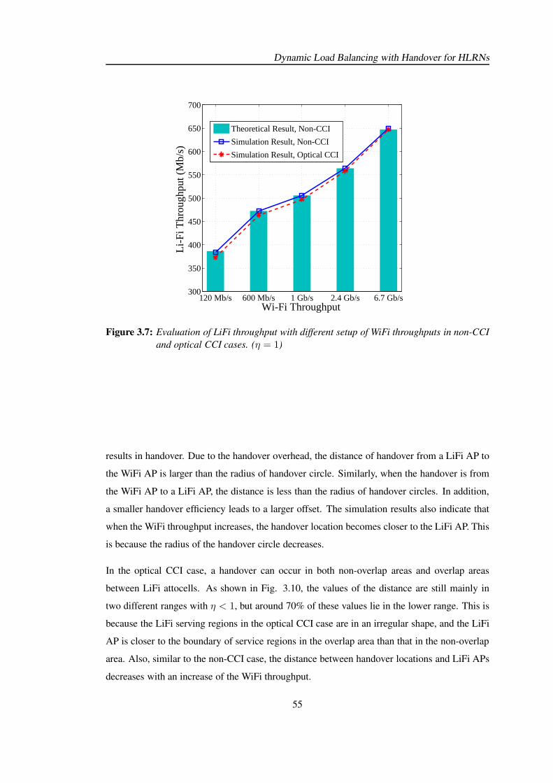
Dynamic Load Balancing with Handover for HLRNs
120 Mb/s 600 Mb/s 1 Gb/s 2.4 Gb/s 6.7 Gb/s300
350
400
450
500
550
600
650
700
Wi-Fi Throughput
Li-
Fi T
hrou
ghpu
t (M
b/s)
Theoretical Result, Non-CCI
Simulation Result, Non-CCI
Simulation Result, Optical CCI
Figure 3.7: Evaluation of LiFi throughput with different setup of WiFi throughputs in non-CCI
and optical CCI cases. (η = 1)
results in handover. Due to the handover overhead, the distance of handover from a LiFi AP to
the WiFi AP is larger than the radius of handover circle. Similarly, when the handover is from
the WiFi AP to a LiFi AP, the distance is less than the radius of handover circles. In addition,
a smaller handover efficiency leads to a larger offset. The simulation results also indicate that
when the WiFi throughput increases, the handover location becomes closer to the LiFi AP. This
is because the radius of the handover circle decreases.
In the optical CCI case, a handover can occur in both non-overlap areas and overlap areas
between LiFi attocells. As shown in Fig. 3.10, the values of the distance are still mainly in
two different ranges with η < 1, but around 70% of these values lie in the lower range. This is
because the LiFi serving regions in the optical CCI case are in an irregular shape, and the LiFi
AP is closer to the boundary of service regions in the overlap area than that in the non-overlap
area. Also, similar to the non-CCI case, the distance between handover locations and LiFi APs
decreases with an increase of the WiFi throughput.
55
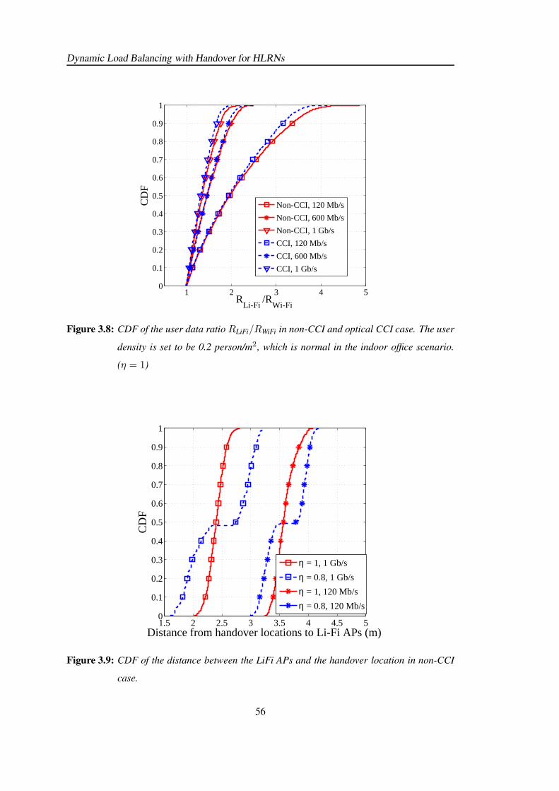
Dynamic Load Balancing with Handover for HLRNs
1 2 3 4 50
0.1
0.2
0.3
0.4
0.5
0.6
0.7
0.8
0.9
1
RLi-Fi
/RWi-Fi
CD
F
Non-CCI, 120 Mb/s
Non-CCI, 600 Mb/s
Non-CCI, 1 Gb/s
CCI, 120 Mb/s
CCI, 600 Mb/s
CCI, 1 Gb/s
Figure 3.8: CDF of the user data ratio RLiFi/RWiFi in non-CCI and optical CCI case. The user
density is set to be 0.2 person/m2, which is normal in the indoor office scenario.
(η = 1)
1.5 2 2.5 3 3.5 4 4.5 50
0.1
0.2
0.3
0.4
0.5
0.6
0.7
0.8
0.9
1
Distance from handover locations to Li-Fi APs (m)
CD
F
η = 1, 1 Gb/s
η = 0.8, 1 Gb/s
η = 1, 120 Mb/s
η = 0.8, 120 Mb/s
Figure 3.9: CDF of the distance between the LiFi APs and the handover location in non-CCI
case.
56
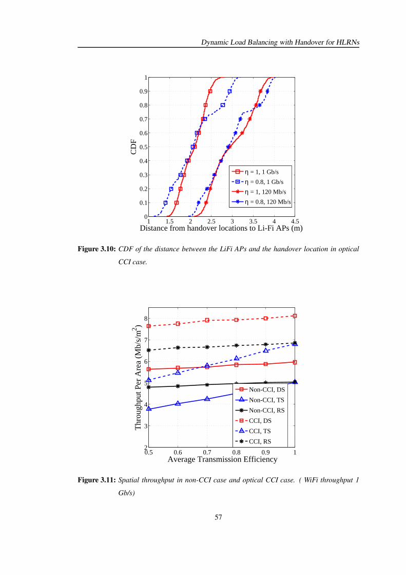
Dynamic Load Balancing with Handover for HLRNs
1 1.5 2 2.5 3 3.5 4 4.50
0.1
0.2
0.3
0.4
0.5
0.6
0.7
0.8
0.9
1
Distance from handover locations to Li-Fi APs (m)
CD
F
η = 1, 1 Gb/s
η = 0.8, 1 Gb/s
η = 1, 120 Mb/s
η = 0.8, 120 Mb/s
Figure 3.10: CDF of the distance between the LiFi APs and the handover location in optical
CCI case.
0.5 0.6 0.7 0.8 0.9 12
3
4
5
6
7
8
Average Transmission Efficiency
Thr
ough
put P
er A
rea
(Mb/
s/m
2 )
Non-CCI, DS
Non-CCI, TS
Non-CCI, RS
CCI, DS
CCI, TS
CCI, RS
Figure 3.11: Spatial throughput in non-CCI case and optical CCI case. ( WiFi throughput 1
Gb/s)
57
Dynamic Load Balancing with Handover for HLRNs
3.2.4.5 Proposed scheme vs. other load balancing schemes
In this subsection, the system throughput of a hybrid LiFi/WiFi network is studied. In order to
fairly compare the non-CCI case and the optical CCI case, the spatial throughput (throughput
per area) is used for evaluation, and is defined as:
Spatial Throughput =System Throughput
Area of Indoor Scenario. (3.53)
The spatial throughput reflects the performance of user data rate with a given user density,
which can be expressed as:
Average user data rate =Spatial Throughput
User density. (3.54)
The spatial throughputs in both the non-CCI and the optical CCI cases are evaluated and shown
in Fig. 3.11. In the legend, the proposed dynamic load balancing scheme is termed as ‘DS’,
and two other load balancing schemes are considered, termed as ‘TS’ and ‘RS’ respectively.
In ‘TS’, a threshold is used to determine whether a user is allocated to the best LiFi AP or the
WiFi AP [72]. In ’RS’, users randomly select the AP between the best LiFi AP and the WiFi
AP. In both schemes, users served by the same AP share an equal proportion of time resource,
and the handover overhead is considered. As shown in Fig. 3.11, the spatial throughput in the
optical CCI case is higher than that of the non-CCI case. This indicates that with the same user
density, each user in the optical CCI case can achieve a higher data rate despite the interference,
resulting from a large reuse of the communication bandwidth. The spatial throughput decreases
with the handover efficiency due to the effect of overhead. The proposed load balancing scheme
always outperforms ‘TS’ and ’RS’ with any value of η. The difference is more than 1 Mb/s/m2.
This is because the AP assignment and time resource allocation in ‘DS’ are jointly designed,
which are formulated as an optimisation problem shown in Eq. (3.6), while they are separately
designed in ‘TS’ and ’RS’, which are undertaken in sequence [72].
In addition to the indoor LiFi/WiFi scenario, the proposed dynamic load balancing scheme can
also be used in hybrid RF small cell networks which combine femto-cells and pico-cells [73].
The pico-cells have a coverage distance of less than 100 meters while the coverage distance of a
femto-cell is less than 30 meters. Therefore, handover may occur frequently in these scenarios,
and the proposed scheme can offer an efficient and stable load balancing for the femto/pico
58
Dynamic Load Balancing with Handover for HLRNs
hybrid networks.
3.2.5 Discussion
In this section, a dynamic load balancing scheme in a LiFi/WiFi hybrid network is proposed,
where the handover overhead is considered. By analysing the service areas of the LiFi APs,
the throughput performance of the hybrid system is theoretically studied. Also, the effects of
the handover overhead on handover locations and user throughput are simulated and discussed.
Three conclusions are made based on the analytical and simulation results: i) the service cover-
age of LiFi APs are connected regions, which are generally smaller than the entire LiFi attocells.
Specifically, these areas are circular in the non-CCI case, but non-circular in the optical CCI
case; ii) the WiFi and LiFi throughput in the hybrid network are related despite the independent
spectrum transmission. The LiFi throughput can be improved by increasing the WiFi through-
put. In addition, the achievable data rates of the users served by LiFi APs are higher than or
equal to that of users allocated to the WiFi AP; iii) a handover occurs only when users move
across the boundaries of the LiFi service areas. The handover overhead can lead to a handover
location offset due to the transmission loss considered in the proposed load balancing scheme.
3.3 Optimisation based dynamic LB Scheme
As known, an efficient load balancing scheme for hybrid networks can improve system through-
put and user QoS. In this section, a comprehensive study of dynamic load balancing aiming at
improving user data rates is undertaken, where a variety of fairness schemes and user QoS re-
quirements are taken into account. Specifically, two specific algorithms that optimise the AP
assignment (APA) and the RA in each quasi-static state are proposed, termed as joint optimisa-
tion algorithm (JOA) and separate optimisation algorithm (SOA) respectively. In this work, the
optimality of JOA and the optimal threshold in SOA are analysed. Also, a comparison of data
rate performance and computational complexity between these two algorithms is made. More-
over, a unified data rate requirement of users is considered as a QoS metric and user outage
probability is introduced. In this study, an optimisation problem that maximises the achievable
user QoS with a certain outage probability is formulated and solved by numerical simulations.
The maximal user QoS in the dynamic hybrid system is evaluated for both JOA and SOA.
59
Dynamic Load Balancing with Handover for HLRNs
3.3.1 System model
In this section, a multi-user indoor hybrid LiFi/RF network is considered, where Nl LiFi APs
and Nr RF APs are deployed. The PDs on each LiFi receivers are assumed to be oriented
perpendicular to the floor. This means that the angle of irradiance is equal to the angle of
incidence in the LoS optical channel. The system setup of hybrid LiFi/RF network follows the
model presented in Section 2.1-2.2. The CU monitors the system continuously in every quasi-
static state, where the load distribution is assumed to be fixed and users receive a constant data
rate. The handover scheme considered in this study is shown in Section 3.2.1. In addition,
TDMA is used in both LiFi and RF systems. The set of users is denoted by U ; the number of
the users is denoted byNu; the set of optical attocells is denoted by CL = l|l ∈ [1, Nl], l ∈ N;and CR = r|r ∈ [1, Nr], r ∈ N is the set of RF cells.
Referring to the LiFi channel model in Section 2.3.1, the signal-to-interference-plus-noise ratio
(SINR) for user µ connected to AP α can be written as follows:
SINRµ,α(f) =(κεpPoptHµ,α(f))
2
ι2NLBL +∑
(κεpPoptHµ,else(f))2, (3.55)
where f is the central frequency of OFDM subcarrier; κ is the optical to electric conversion
efficiency at the receivers; εp ≈ 1 is power amplification gain; NL is the noise power spectral
density in the LiFi link; BL is the baseband modulation bandwidth for each LiFi AP; Hµ,α(f)
is the channel gain in the frequency domain between user µ and LiFi AP; and Hµ,else(f) is the
channel gain between user µ and the interfering LiFi APs, according to Eq. (2.3).
In the RF system, the channel model has been shown in Section 2.4. Since there is no CCI in
the RF system, the SINR is equivalent to SNR on each sub-carrier, which can be expressed as
follows:
SNRµ,α(f) =|Γµ,α(f)|2∆PR
NR∆BR
, (3.56)
where Γµ,α(f) is the RF channel gain, according to Eq. (2.40); ∆BR is the modulation band-
width of each sub-carrier; ∆PR is the transmit power allocated to each sub-carrier; and NR is
the noise power spectral density in RF link. It is assumed that the transmit power is allocated
equally to each sub-carrier. Thus, it is obtained that ∆PR/∆BR = PR/BR, where PR and BR
are the total transmit power and modulation bandwidth for a RF AP.
In order to improve the spectrum efficiency, adaptive bit loading is employed over the OFDM
60
Dynamic Load Balancing with Handover for HLRNs
sub-carriers [53]. Note that the frequency of subcarrier m is denoted by fm and the achievable
SE on subcarrier m is denoted by qm. The relationship between qm and SINRµ,α(fm) (or
SNRµ,α(fm)) follows the MCS given in Table 2.1. Specifically, given a user SINR or SNR, we
can firstly find the min. SINR level which is closest to and less than the user SINR (SNR) in
Table 2.1. Then, qm will be the corresponding SE shown in the table. The link communication
data rate of LiFi and RF between user µ and AP α are denoted as Zµ,α and Υµ,α, respectively.
When considering the handover scheme in Algorithm. 3, the link data rate between AP α and
user µ in state n with handover considered can be expressed as follows:
r(n)µ,α =
ηα′αZ(n)µ,α, α ∈ CL
ηα′αΥ(n)µ,α, α ∈ CR
, (3.57)
where α′ is the AP allocated to user µ in the state n−1; ηα′α is the handover efficiency between
state n− 1 and state n according to Eq. (3.4); and Z(n)µ,α and Υ
(n)µ,α are the data rates of the LiFi
link and the RF link in state n, respectively. The value of r(n)µ,α between user µ and AP α is
calculated by the CU in each state.
Two variables g(n)µ,α and k
(n)µ,α are introduced to model the load balancing in state n. The variable
g(n)µ,α is a binary number which equals 1 when user µ is connected to AP α, otherwise it is 0.
The variable k(n)µ,α is a fractional number between 0 and 1, which represents the proportion of
time resources allocated to user µ by AP α in state n.
3.3.2 Joint Optimisation Algorithm (JOA)
In this section, the JOA that jointly optimises the AP assignment and the time resource allo-
cation in each state is proposed. At first, the joint optimisation problem is formulated and an
iterative algorithm for the problem is given. After that, the convergence and optimality of the
proposed algorithm are analysed. Since the network load balancing of a specific state is studied,
the superscript (n) in parameters g(n)µ,α, k
(n)µ,α and r
(n)µ,α is omitted to enhance clarity.
61
Dynamic Load Balancing with Handover for HLRNs
3.3.2.1 Problem Formulation and Iterative Algorithm
As shown in Section 3.2.2, the β-proportional fairness function that considers both sum-rate
and user fairness is employed. This utility function is repeated and expressed as:
ψβ(x) =
log(x), β = 1
x1−β
1− β , β ≥ 0, β 6= 1, (3.58)
where x is the achievable data rate; and β is the fairness coefficient. The utility function in
Eq. (3.58) includes several well known fairness concepts [74]. Specifically, when β = 1, a
proportional fairness is achieved, where users served by a specific AP share an equal proportion
of time resource; and when β → ∞, a max-min fair scheduler is realised. Particularly, when
β = 0, a linear utility function is obtained which achieves a maximal system throughput. In
this case, each AP only serves the user of the best CSI whereas the other users have zero data
rates, which finally leads to an ineffective load balancing solution. Thus, the situation of β = 0
is beyond the scope of this study.
Using the utility function in Eq. (3.58), the joint optimisation of the APA and the RA can be
formulated as follows:
maxgµ,α,kµ,α
∑
µ∈U
∑
α∈CL∪CR
gµ,αψβ(kµ,αrµ,α) (3.59)
s.t.∑
µ∈U
gµ,αkµ,α ≤ 1 ∀α ∈ CL ∪ CR; (3.60)
∑
α∈CL∪CR
gµ,α = 1 ∀µ ∈ U ;
gµ,α ∈ 0, 1, kµ,α ∈ [0, 1], ∀µ ∈ U ,∀α ∈ CL ∪ CR,
where rµ,α is the communication link data rate given in Eq. (3.57), which is a positive number.
The optimum kµ,α is shown to be greater than zero in Eq. (3.72) so that log(0) is avoided.
This optimisation problem in Eq. (3.59) is a mixed integer non-linear programming (MINLP)
problem which is mathematically intractable because it involves both binary variables and real-
valued positive variables. In order to simplify this problem, the binary variable gµ,α is assumed
to be a fractional number between 0 and 1.
Lemma 3. The original problem in Eq. (3.59) is able to be converted into a concave optimisa-
62
Dynamic Load Balancing with Handover for HLRNs
tion problem using the fractional variable gµ,α.
Proof. It is assumed that gµ,α is a fractional number. The objective function in Eq. 3.13) is
denoted as F (gµ,α, kµ,α), and its Hessian matrix can be written as follows:
H(F ) =
∂2F∂g2µ,α
∂2F∂gµ,α∂kµ,α
∂2F∂kµ,α∂gµ,α
∂2F∂k2µ,α
, (3.61)
where
∂2F
∂g2µ,α= 0; (3.62)
∂2F
∂k2µ,α= − β
r2µ,α(kµ,αrµ,α)β+1
≤ 0. (3.63)
Since all of the principle minors of the Hessian matrix are non-positive, the objective function
is concave with respect to the variables, gµ,α and kµ,α.
The Lagrangian Multiplier method can therefore be used to solve this optimisation problem
[24]. The Lagrangian function is expressed as follows:
L(gµ,α,kµ,α, ωα) =∑
µ∈U
∑
α∈CL∪CR
gµ,α[ψβ(kµ,αrµ,α)
− ωαkµ,α] +∑
α∈CL∪CR
ωα, (3.64)
where gµ,α ∈ [0, 1], kµ,α ∈ [0, 1] and∑
α∈CL∪CRgµ,α = 1. The Lagrangian multiplier ωα
corresponds to the α-th constraints in Eq. (3.11). The optimum of gµ,α and kµ,α can be obtained
by solving the problem:
minωα
maxgµ,α,kµ,α
L(gµ,α, kµ,α, ωα). (3.65)
In this study, the problem in Eq. (3.65) is solved by a distributed algorithm via Lagrangian
decomposition [75]. According to the Lagrangian function in Eq. (3.64), a dual objective
63
Dynamic Load Balancing with Handover for HLRNs
function in terms of user µ is defined as:
Ωµ(gµ,α, kµ,α) =∑
α∈CL∪CR
gµ,α[ψβ(kµ,αrµ,α)− ωαkµ,α]. (3.66)
The problem in Eq. (3.65) is separated into two steps of optimisation. In the first step, the dual
objective function is optimised, and this sub-problem can be formulated as follows:
g∗µ,α, k∗µ,α = arg maxgµ,α,kµ,α∈[0,1]
Ωµ(gµ,α, kµ,α). (3.67)
It can be seen that the function Ωµ(gµ,α, kµ,α) is concave with respect to the variables gµ,α and
kµ,α. The partial derivatives of Ωµ with gµ,α and kµ,α are:
∂Ωµ
∂gµ,α= ψβ(kµ,αrµ,α)− ωαkµ,α, (3.68)
∂Ωµ
∂kµ,α= gµ,α
[
∂ψβ(kµ,αrµ,α)
∂kµ,α− ωα
]
, (3.69)
where ψβ(.) is given in Eq. (3.58) and its derivative with respect to kµ,α is:
∂ψβ(kµ,αrµ,α)
∂kµ,α=
rµ,α(kµ,αrµ,α)β
. (3.70)
In conjunction with Eq. (3.70), it can be shown that Eq. (3.69) monotonically decreases as kµ,α
increases. Also, due to the strict positivity of kµ,α,rµ,α and β it can be derived that:
limkµ,α→0+
rµ,α(kµ,αrµ,α)β
= +∞. (3.71)
Since ωα is finite and gµ,α is non-negative, it can be seen that the condition,∂Ωµ
∂kµ,α|kµ,α=0 ≥ 0
is satisfied. Thus, the optimum kµ,α can be calculated by:
k∗µ,α =
1,∂Ωµ
∂kµ,α|kµ,α=1 ≥ 0
1
rµ,α
(
rµ,αωα
) 1β
,∂Ωµ
∂kµ,α|kµ,α=1 < 0
. (3.72)
With k∗µ,α, the optimum gµ,α is expressed as follows:
g∗µ,α =
1, α = argmaxα′∈CL∪CR
∂Ωµ(k∗µ,α′ )
∂gµ,α′
0, Otherwise. (3.73)
64
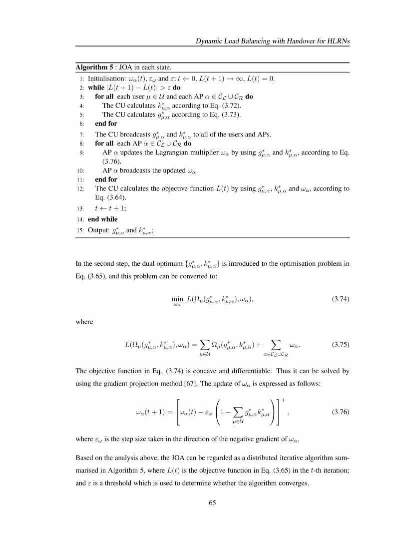
Dynamic Load Balancing with Handover for HLRNs
Algorithm 5 : JOA in each state.
1: Initialisation: ωα(t), εω and ε; t← 0, L(t+ 1)→∞, L(t) = 0.
2: while |L(t+ 1)− L(t)| > ε do
3: for all each user µ ∈ U and each AP α ∈ CL ∪ CR do
4: The CU calculates k∗µ,α according to Eq. (3.72).
5: The CU calculates g∗µ,α according to Eq. (3.73).
6: end for
7: The CU broadcasts g∗µ,α and k∗µ,α to all of the users and APs.
8: for all each AP α ∈ CL ∪ CR do
9: AP α updates the Lagrangian multiplier ωα by using g∗µ,α and k∗µ,α, according to Eq.
(3.76).
10: AP α broadcasts the updated ωα.
11: end for
12: The CU calculates the objective function L(t) by using g∗µ,α, k∗µ,α and ωα, according to
Eq. (3.64).
13: t← t+ 1;
14: end while
15: Output: g∗µ,α and k∗µ,α;
In the second step, the dual optimum g∗µ,α, k∗µ,α is introduced to the optimisation problem in
Eq. (3.65), and this problem can be converted to:
minωα
L(Ωµ(g∗µ,α, k
∗µ,α), ωα), (3.74)
where
L(Ωµ(g∗µ,α, k
∗µ,α), ωα) =
∑
µ∈U
Ωµ(g∗µ,α, k
∗µ,α) +
∑
α∈CL∪CR
ωα. (3.75)
The objective function in Eq. (3.74) is concave and differentiable. Thus it can be solved by
using the gradient projection method [67]. The update of ωα is expressed as follows:
ωα(t+ 1) =
ωα(t)− εω
1−∑
µ∈U
g∗µ,αk∗µ,α
+
, (3.76)
where εω is the step size taken in the direction of the negative gradient of ωα.
Based on the analysis above, the JOA can be regarded as a distributed iterative algorithm sum-
marised in Algorithm 5, where L(t) is the objective function in Eq. (3.65) in the t-th iteration;
and ε is a threshold which is used to determine whether the algorithm converges.
65
Dynamic Load Balancing with Handover for HLRNs
3.3.2.2 Convergence analysis of JOA
According to Algorithm 5, JOA converges after the difference between the objective functions
in two neighbouring iterations is small enough. In particular, we assume ε = |L(t+ 1)|/50 in
the algorithm. According to Eq. (3.76), the step size εω can significantly affect the speed of
convergence. In general, a larger value of εω can result in a faster convergence. However, when
εω is set to be very large, the algorithm becomes unstable so that the objective function tends
to oscillate and the convergence cannot be guaranteed. In order to facilitate both the speed and
the stability of the convergence, an adaptive step size is considered and designed as follows:
εω ← εωdt2 , (0 < d < 1) (3.77)
where t is the number of iterations and d is a bias weight. This step size decreases with t,
which enables more efficient iterations. Moreover, the step size, εω approaches zero when t is
large, and its gradient is affected by d. It is possible that εω tends to zero before the algorithm
converges. Hence, d should be well designed. In this study, it is set to be between 0.8 and
0.9. The simulations confirm that this range is a suitable choice for the simulation scenario
considered in this section.
Since the threshold, ε in JOA cannot be zero, the optimum k∗µ,α gained in JOA may not strictly
satisfy the constraint in Eq. (3.60). In order to avoid the situation∑
µ∈U g∗µ,αk
∗µ,α > 1, the
optimum k∗µ,α achieved by Algorithm 5 should be normalised, which can mathematically be
expressed as follows:
kµ,α =k∗µ,α
∑
µ∈U g∗µ,αk
∗µ,α
, ∀α ∈ CL ∪ CR, (3.78)
where g∗µ,α is the optimum of the variable gµ,α obtained by using JOA. The normalised re-
source proportion kµ,α strictly satisfies the constraint in Eq. (3.60). The load balancing results
achieved by JOA can be denoted as follows:
g(JOA)µ,α = g∗µ,α;
k(JOA)µ,α = kµ,α.
. (3.79)
66
Dynamic Load Balancing with Handover for HLRNs
3.3.2.3 Optimality analysis
Due to the dual decomposition method used in JOA, it is difficult to discover whether the
results attained in Eq. (3.79) after convergence are the global optima or not. Since a closed-
form solution of the original optimisation problem is mathematically intractable, an exhaustive
search is used to find the global optimum.
With the assumption of Nu users and Nl + Nr APs in this network, there are (Nl + Nr)Nu
possibilities of AP allocation. Note that the AP assignments are denoted as g(i), i = 1, 2...(Nl+
Nr)Nu . When a certain g(i) is considered, the joint optimisation problem in Eq. (3.59) can be
transformed as follows:
maxk(i)µ,α
∑
α∈CL∪CR
∑
µ∈Uα
ψβ(k(i)µ,αrµ,α), (3.80)
where Uα is the set of users allocated to AP α. According to Eq. (3.80), the optimisation of
kµ,α can be undertaken independently in each cell, which is expressed as follows:
maxk(i)µ,α
∑
µ∈Uα
ψβ(k(i)µ,αrµ,α), (3.81)
s.t.∑
µ∈Uα
k(i)µ,α ≤ 1, (3.82)
The Lagrangian multiplier method is used to solve this problem. The Lagrangian function is
given by:
F (k(i)µ,α, ω) =∑
µ∈Uα
ψβ(k(i)µ,αrµ,α) + ω
1−∑
µ∈Uα
k(i)µ,α
, (3.83)
where ω is the Lagrangian multiplier for the constraint in Eq. (3.82). The optimum k(i)µ,α can
be found by making the gradient of the Lagrangian function in Eq. (3.83) equal to 0, which is
written as follows:
∂F (k(i)µ,α, ω)
∂k(i)µ,α
=rµ,α
(k(i)µ,αrµ,α)β
− ω = 0, µ ∈ Uα. (3.84)
67
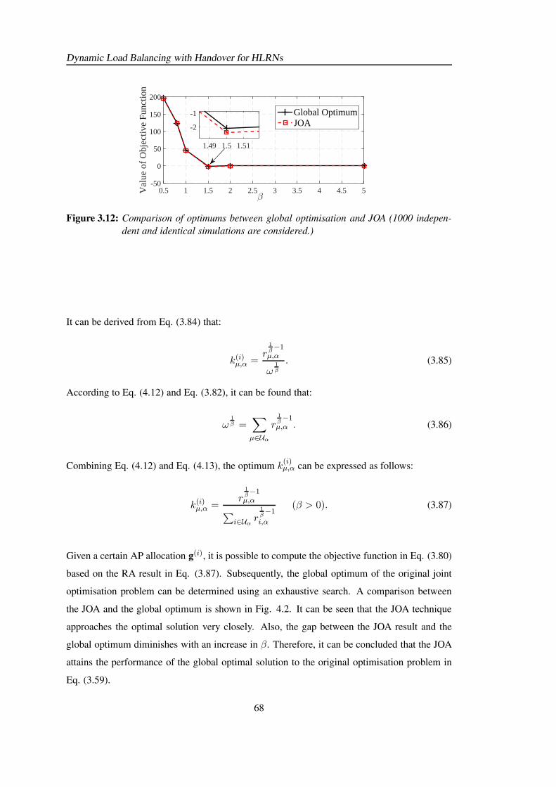
Dynamic Load Balancing with Handover for HLRNs
β0.5 1 1.5 2 2.5 3 3.5 4 4.5 5V
alue
of
Obj
ectiv
e Fu
nctio
n
-50
0
50
100
150
200
Global OptimumJOA
1.49 1.5 1.51
-2
-1
Figure 3.12: Comparison of optimums between global optimisation and JOA (1000 indepen-
dent and identical simulations are considered.)
It can be derived from Eq. (3.84) that:
k(i)µ,α =r
1β−1
µ,α
ω1β
. (3.85)
According to Eq. (4.12) and Eq. (3.82), it can be found that:
ω1β =
∑
µ∈Uα
r1β−1
µ,α . (3.86)
Combining Eq. (4.12) and Eq. (4.13), the optimum k(i)µ,α can be expressed as follows:
k(i)µ,α =r
1β−1
µ,α
∑
i∈Uαr
1β−1
i,α
(β > 0). (3.87)
Given a certain AP allocation g(i), it is possible to compute the objective function in Eq. (3.80)
based on the RA result in Eq. (3.87). Subsequently, the global optimum of the original joint
optimisation problem can be determined using an exhaustive search. A comparison between
the JOA and the global optimum is shown in Fig. 4.2. It can be seen that the JOA technique
approaches the optimal solution very closely. Also, the gap between the JOA result and the
global optimum diminishes with an increase in β. Therefore, it can be concluded that the JOA
attains the performance of the global optimal solution to the original optimisation problem in
Eq. (3.59).
68
Dynamic Load Balancing with Handover for HLRNs
3.3.3 Separate Optimisation Algorithm (SOA)
In this section, the SOA that separately optimises the AP assignment and the time resource
allocation in each state is proposed. As before, the superscript n is omitted in parameters g(n)µ,α,
k(n)µ,α and r
(n)µ,α for clarification.
3.3.3.1 AP assignment in SOA
In order to make use of the high spatial spectrum efficiency of LiFi, the APA step in SOA can be
realised as follows: users achieving LiFi data rates higher than a certain threshold, denoted by
γ, are served by LiFi APs; and the others of data rates falling below the threshold via LiFi links
would be assigned to the RF APs. Moreover, the criterion of maximal effective throughput is
applied for the APA step. In terms of user µ, the LiFi AP offering the maximal link data rate
involving handover is expressed as follows:
τ1,µ = argmaxj∈CL
rµ,j, (3.88)
where rµ,j is the LiFi data rate according to Eq. (3.57). Assuming that the time resource is
equally shared by users in each cell, the potential LiFi data rate of user µ can be written as
follows:
λµ = rµ,τ1,µ/Mτ1,µ , (3.89)
where Mτ1,µ is the number of users served by LiFi AP τ1,µ.
According to the principle of APA step, users following λµ < γ should be allocated to RF APs.
The RF AP assigned to user µ can be written as follows:
τ2,µ = arg maxj∈CR
rµ,j , λµ < γ. (3.90)
Based on Eq. (3.88) (3.90), the APA result of SOA is expressed as follows:
g(SOA)µ,α =
1, α =
τ1,µ, λµ ≥ γτ2,µ, λµ < γ
0, Otherwise
. (3.91)
69
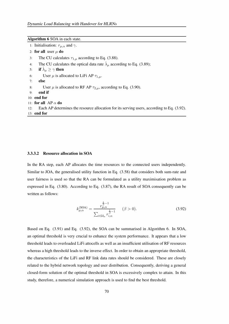
Dynamic Load Balancing with Handover for HLRNs
Algorithm 6 SOA in each state.
1: Initialisation: rµ,α and γ.
2: for all user µ do
3: The CU calculates τ1,µ according to Eq. (3.88).
4: The CU calculates the optical data rate λµ according to Eq. (3.89);
5: if λµ ≥ γ then
6: User µ is allocated to LiFi AP τ1,µ.
7: else
8: User µ is allocated to RF AP τ2,µ, according to Eq. (3.90).
9: end if
10: end for
11: for all AP α do
12: Each AP determines the resource allocation for its serving users, according to Eq. (3.92).
13: end for
3.3.3.2 Resource allocation in SOA
In the RA step, each AP allocates the time resources to the connected users independently.
Similar to JOA, the generalised utility function in Eq. (3.58) that considers both sum-rate and
user fairness is used so that the RA can be formulated as a utility maximisation problem as
expressed in Eq. (3.80). According to Eq. (3.87), the RA result of SOA consequently can be
written as follows:
k(SOA)µ,α =
r1β−1
µ,α
∑
i∈Uαr
1β−1
i,α
(β > 0). (3.92)
Based on Eq. (3.91) and Eq. (3.92), the SOA can be summarised in Algorithm 6. In SOA,
an optimal threshold is very crucial to enhance the system performance. It appears that a low
threshold leads to overloaded LiFi attocells as well as an insufficient utilisation of RF resources
whereas a high threshold leads to the inverse effect. In order to obtain an appropriate threshold,
the characteristics of the LiFi and RF link data rates should be considered. These are closely
related to the hybrid network topology and user distribution. Consequently, deriving a general
closed-form solution of the optimal threshold in SOA is excessively complex to attain. In this
study, therefore, a numerical simulation approach is used to find the best threshold.
70
Dynamic Load Balancing with Handover for HLRNs
3.3.4 QoS Enhancement in JOA and SOA
In the two previous subsections, two load balancing algorithms, JOA and SOA, are proposed.
The user data rate in state n for both JOA and SOA can be written as follows:
R(n)µ =
∑
α∈CL∪CR
g(n)µ,αk(n)µ,αr
(n)µ,α, (3.93)
where g(n)µ,α is given in Eq. (3.79) and Eq. (3.91) for JOA and SOA, respectively; and k
(n)µ,α is
given in Eq. (3.79) and Eq. (3.92) for JOA and SOA, respectively. According to Eq. (3.93), the
data rate of users that are using JOA can be expressed as a function of the fairness coefficient β,
denoted by R(n)µ,JOA(β). Similarly, the data rate of users that are using SOA can be written as a
function of the threshold γ and the fairness coefficient β, denoted by R(n)µ,SOA(γ, β). In JOA and
SOA, the user data rate can be significantly affected by β. An increase in β results in a decrease
in the system sum-rate, but it enables an improvement of the user fairness. Moreover, when
employing SOA, the data rates are also affected by the threshold γ. The optimum threshold
can contribute to an efficient utilisation of the multiple APs for users, which enables the system
load to be well balanced.
In this study, it is assumed that all of the users have the same data rate request. The QoS is
defined as the maximal achievable data rate of users given an outage probability. The QoS is
denoted by Γ0. The outage probability of the user QoS is defined as follows:
Φ0 = Pr( R(n)µ < Γ0 ). (3.94)
This probability can be calculated by Monte Carlo simulations, which is expressed as follows:
Φ0 =
∑
n Number of Users with R(n)µ < Γ0
∑
n Number of Total Users(3.95)
In general, the design specifications of communication systems include a per user rate outage
probability constraint. Let this outage probability constraint be denoted as Φ. The problem
of maximising the QoS in JOA under the outage probability constraint can be formulated as
71
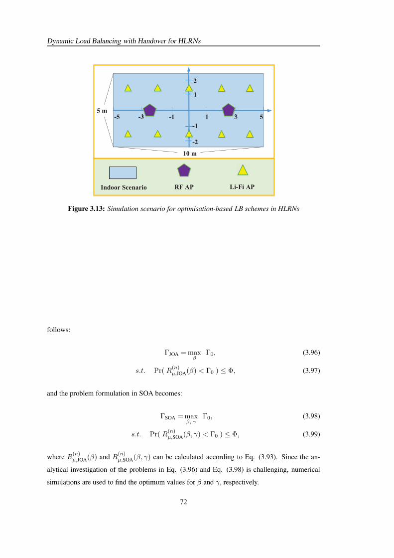
Dynamic Load Balancing with Handover for HLRNs
Indoor Scenario RF AP Li-Fi AP
-1 1-3-5 3 5
1
-1
-2
2
10 m
5 m
Figure 3.13: Simulation scenario for optimisation-based LB schemes in HLRNs
follows:
ΓJOA =maxβ
Γ0, (3.96)
s.t. Pr( R(n)µ,JOA(β) < Γ0 ) ≤ Φ, (3.97)
and the problem formulation in SOA becomes:
ΓSOA =maxβ, γ
Γ0, (3.98)
s.t. Pr( R(n)µ,SOA(β, γ) < Γ0 ) ≤ Φ, (3.99)
where R(n)µ,JOA(β) and R
(n)µ,SOA(β, γ) can be calculated according to Eq. (3.93). Since the an-
alytical investigation of the problems in Eq. (3.96) and Eq. (3.98) is challenging, numerical
simulations are used to find the optimum values for β and γ, respectively.
72
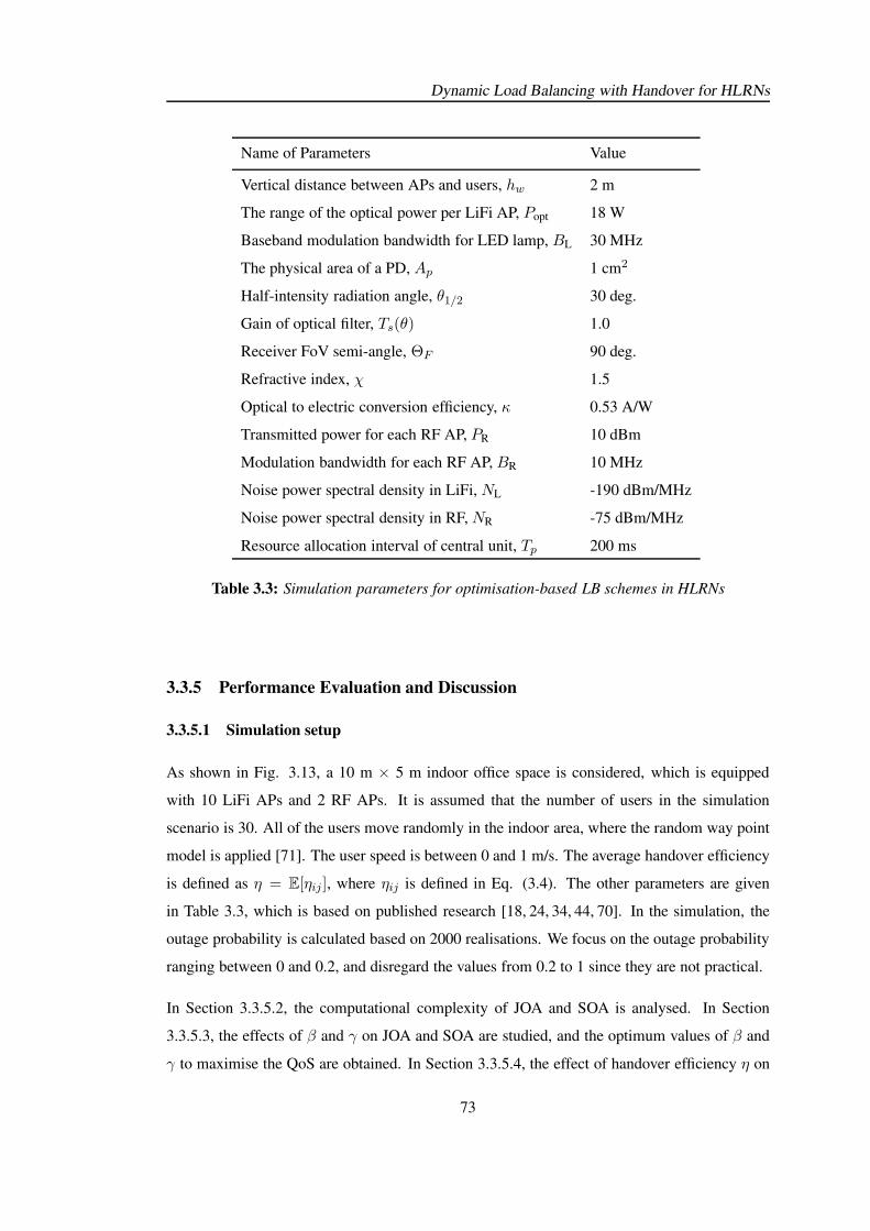
Dynamic Load Balancing with Handover for HLRNs
Name of Parameters Value
Vertical distance between APs and users, hw 2 m
The range of the optical power per LiFi AP, Popt 18 W
Baseband modulation bandwidth for LED lamp, BL 30 MHz
The physical area of a PD, Ap 1 cm2
Half-intensity radiation angle, θ1/2 30 deg.
Gain of optical filter, Ts(θ) 1.0
Receiver FoV semi-angle, ΘF 90 deg.
Refractive index, χ 1.5
Optical to electric conversion efficiency, κ 0.53 A/W
Transmitted power for each RF AP, PR 10 dBm
Modulation bandwidth for each RF AP, BR 10 MHz
Noise power spectral density in LiFi, NL -190 dBm/MHz
Noise power spectral density in RF, NR -75 dBm/MHz
Resource allocation interval of central unit, Tp 200 ms
Table 3.3: Simulation parameters for optimisation-based LB schemes in HLRNs
3.3.5 Performance Evaluation and Discussion
3.3.5.1 Simulation setup
As shown in Fig. 3.13, a 10 m × 5 m indoor office space is considered, which is equipped
with 10 LiFi APs and 2 RF APs. It is assumed that the number of users in the simulation
scenario is 30. All of the users move randomly in the indoor area, where the random way point
model is applied [71]. The user speed is between 0 and 1 m/s. The average handover efficiency
is defined as η = E[ηij ], where ηij is defined in Eq. (3.4). The other parameters are given
in Table 3.3, which is based on published research [18, 24, 34, 44, 70]. In the simulation, the
outage probability is calculated based on 2000 realisations. We focus on the outage probability
ranging between 0 and 0.2, and disregard the values from 0.2 to 1 since they are not practical.
In Section 3.3.5.2, the computational complexity of JOA and SOA is analysed. In Section
3.3.5.3, the effects of β and γ on JOA and SOA are studied, and the optimum values of β and
γ to maximise the QoS are obtained. In Section 3.3.5.4, the effect of handover efficiency η on
73
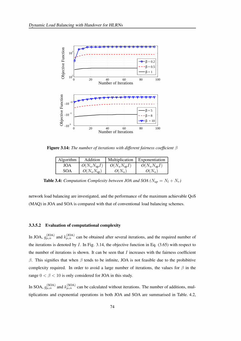
Dynamic Load Balancing with Handover for HLRNs
0 20 40 60 80 10010
2
103
Number of Iterations
Obj
ectiv
e Fu
nctio
n
0 20 40 60 80 100-10
0
-10-5
-10-10
Number of Iterations
Obj
ectiv
e Fu
nctio
n
β = 5
β = 8
β = 10
β = 0.2
β = 0.5
β = 1
Figure 3.14: The number of iterations with different fairness coefficient β
Algorithm Addition Multiplication Exponentiation
JOA O(NuNapI) O(NuNapI) O(NuNapI)SOA O(NuNap) O(Nu) O(Nu)
Table 3.4: Computation Complexity between JOA and SOA (Nap = Nl +Nr)
network load balancing are investigated, and the performance of the maximum achievable QoS
(MAQ) in JOA and SOA is compared with that of conventional load balancing schemes.
3.3.5.2 Evaluation of computational complexity
In JOA, g(JOA)µ,α and k
(JOA)µ,α can be obtained after several iterations, and the required number of
the iterations is denoted by I . In Fig. 3.14, the objective function in Eq. (3.65) with respect to
the number of iterations is shown. It can be seen that I increases with the fairness coefficient
β. This signifies that when β tends to be infinite, JOA is not feasible due to the prohibitive
complexity required. In order to avoid a large number of iterations, the values for β in the
range 0 < β < 10 is only considered for JOA in this study.
In SOA, g(SOA)µ,α and k
(SOA)µ,α can be calculated without iterations. The number of additions, mul-
tiplications and exponential operations in both JOA and SOA are summarised in Table. 4.2,
74
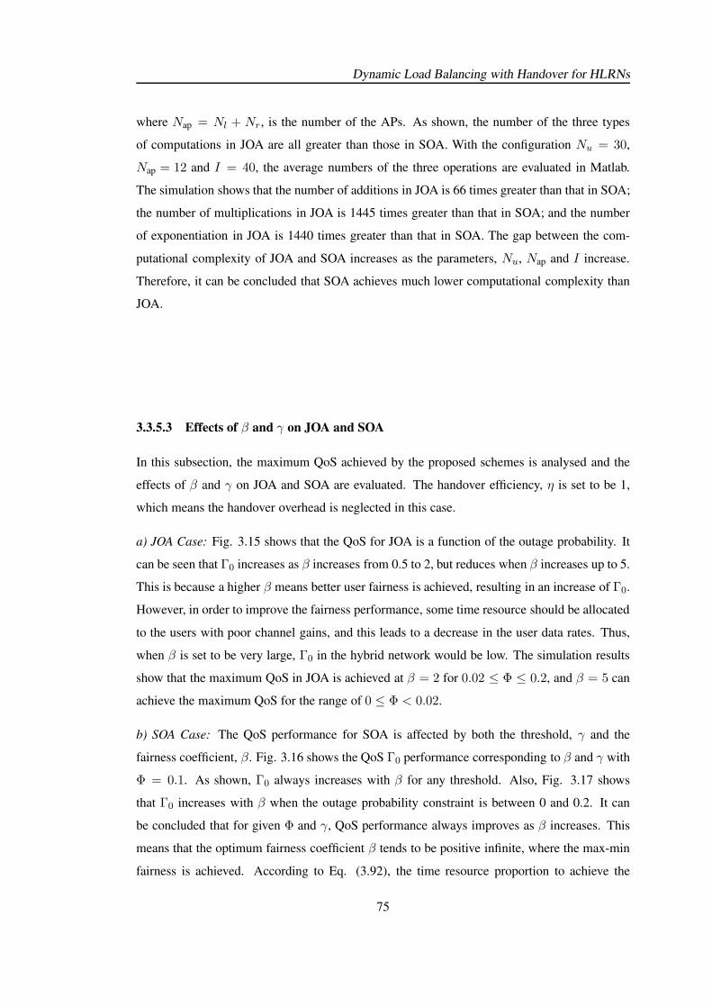
Dynamic Load Balancing with Handover for HLRNs
where Nap = Nl + Nr, is the number of the APs. As shown, the number of the three types
of computations in JOA are all greater than those in SOA. With the configuration Nu = 30,
Nap = 12 and I = 40, the average numbers of the three operations are evaluated in Matlab.
The simulation shows that the number of additions in JOA is 66 times greater than that in SOA;
the number of multiplications in JOA is 1445 times greater than that in SOA; and the number
of exponentiation in JOA is 1440 times greater than that in SOA. The gap between the com-
putational complexity of JOA and SOA increases as the parameters, Nu, Nap and I increase.
Therefore, it can be concluded that SOA achieves much lower computational complexity than
JOA.
3.3.5.3 Effects of β and γ on JOA and SOA
In this subsection, the maximum QoS achieved by the proposed schemes is analysed and the
effects of β and γ on JOA and SOA are evaluated. The handover efficiency, η is set to be 1,
which means the handover overhead is neglected in this case.
a) JOA Case: Fig. 3.15 shows that the QoS for JOA is a function of the outage probability. It
can be seen that Γ0 increases as β increases from 0.5 to 2, but reduces when β increases up to 5.
This is because a higher β means better user fairness is achieved, resulting in an increase of Γ0.
However, in order to improve the fairness performance, some time resource should be allocated
to the users with poor channel gains, and this leads to a decrease in the user data rates. Thus,
when β is set to be very large, Γ0 in the hybrid network would be low. The simulation results
show that the maximum QoS in JOA is achieved at β = 2 for 0.02 ≤ Φ ≤ 0.2, and β = 5 can
achieve the maximum QoS for the range of 0 ≤ Φ < 0.02.
b) SOA Case: The QoS performance for SOA is affected by both the threshold, γ and the
fairness coefficient, β. Fig. 3.16 shows the QoS Γ0 performance corresponding to β and γ with
Φ = 0.1. As shown, Γ0 always increases with β for any threshold. Also, Fig. 3.17 shows
that Γ0 increases with β when the outage probability constraint is between 0 and 0.2. It can
be concluded that for given Φ and γ, QoS performance always improves as β increases. This
means that the optimum fairness coefficient β tends to be positive infinite, where the max-min
fairness is achieved. According to Eq. (3.92), the time resource proportion to achieve the
75
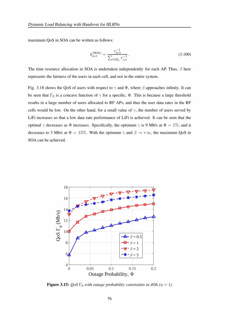
Dynamic Load Balancing with Handover for HLRNs
maximum QoS in SOA can be written as follows:
k(SOA)µ,α =
r−1µ,α
∑
i∈Uαr−1i,α
. (3.100)
The time resource allocation in SOA is undertaken independently for each AP. Thus, β here
represents the fairness of the users in each cell, and not in the entire system.
Fig. 3.18 shows the QoS of users with respect to γ and Φ, where β approaches infinity. It can
be seen that Γ0 is a concave function of γ for a specific, Φ. This is because a large threshold
results in a large number of users allocated to RF APs, and thus the user data rates in the RF
cells would be low. On the other hand, for a small value of γ, the number of users served by
LiFi increases so that a low data rate performance of LiFi is achieved. It can be seen that the
optimal γ decreases as Φ increases. Specifically, the optimum γ is 9 Mb/s at Φ = 1%; and it
decreases to 3 Mb/s at Φ = 15%. With the optimum γ and β → +∞, the maximum QoS in
SOA can be achieved.
Outage Probability, Φ0 0.05 0.1 0.15 0.2
QoS
Γ0 (
Mb/
s)
4
6
8
10
12
14
16
18
β = 0.5
β = 1
β = 2
β = 5
Figure 3.15: QoS Γ0 with outage probability constraints in JOA (η = 1)
76
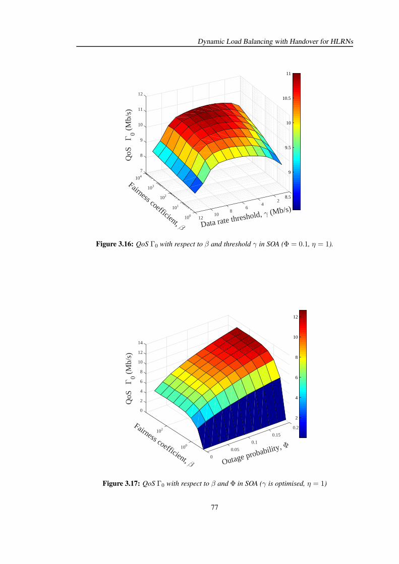
Dynamic Load Balancing with Handover for HLRNs
0
Data rate threshold, γ (Mb/s)2
46
810
12100
Fairness coefficient, β
101
102
103
12
11
10
9
8
7
104
QoS
Γ
0 (M
b/s)
8.5
9
9.5
10
10.5
11
Figure 3.16: QoS Γ0 with respect to β and threshold γ in SOA (Φ = 0.1, η = 1).
0.2
Outage probability, Φ
0.15
0.1
0.05
0
Fairness coefficient, β
100
102
6
4
2
0
8
10
12
14
QoS
Γ
0 (M
b/s)
2
4
6
8
10
12
Figure 3.17: QoS Γ0 with respect to β and Φ in SOA (γ is optimised, η = 1)
77
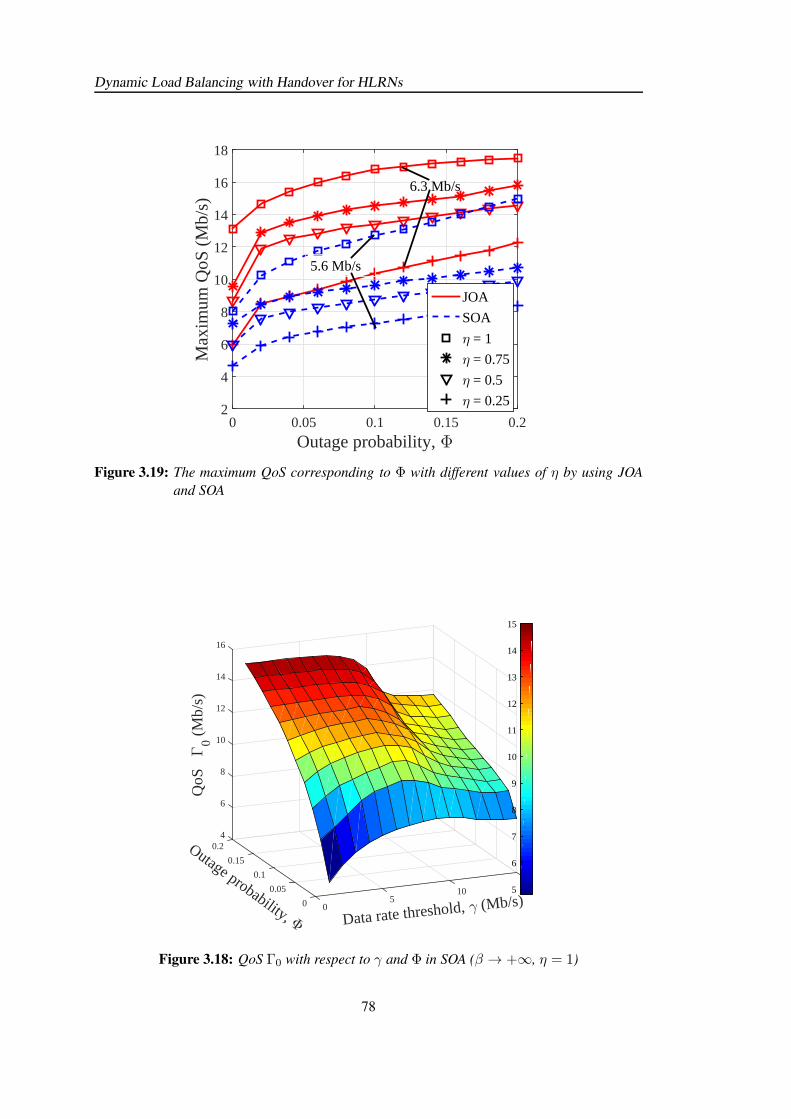
Dynamic Load Balancing with Handover for HLRNs
Outage probability, Φ0 0.05 0.1 0.15 0.2
Max
imum
QoS
(M
b/s)
2
4
6
8
10
12
14
16
18
JOA
SOA
η = 1
η = 0.75
η = 0.5
η = 0.25
5.6 Mb/s
6.3 Mb/s
Figure 3.19: The maximum QoS corresponding to Φ with different values of η by using JOA
and SOA
15
Data rate threshold, γ (Mb/s)10
50
Outage probability, Φ0
0.05
0.1
0.15
16
4
6
8
10
12
14
0.2
QoS
Γ
0 (M
b/s)
5
6
7
8
9
10
11
12
13
14
15
Figure 3.18: QoS Γ0 with respect to γ and Φ in SOA (β → +∞, η = 1)
78
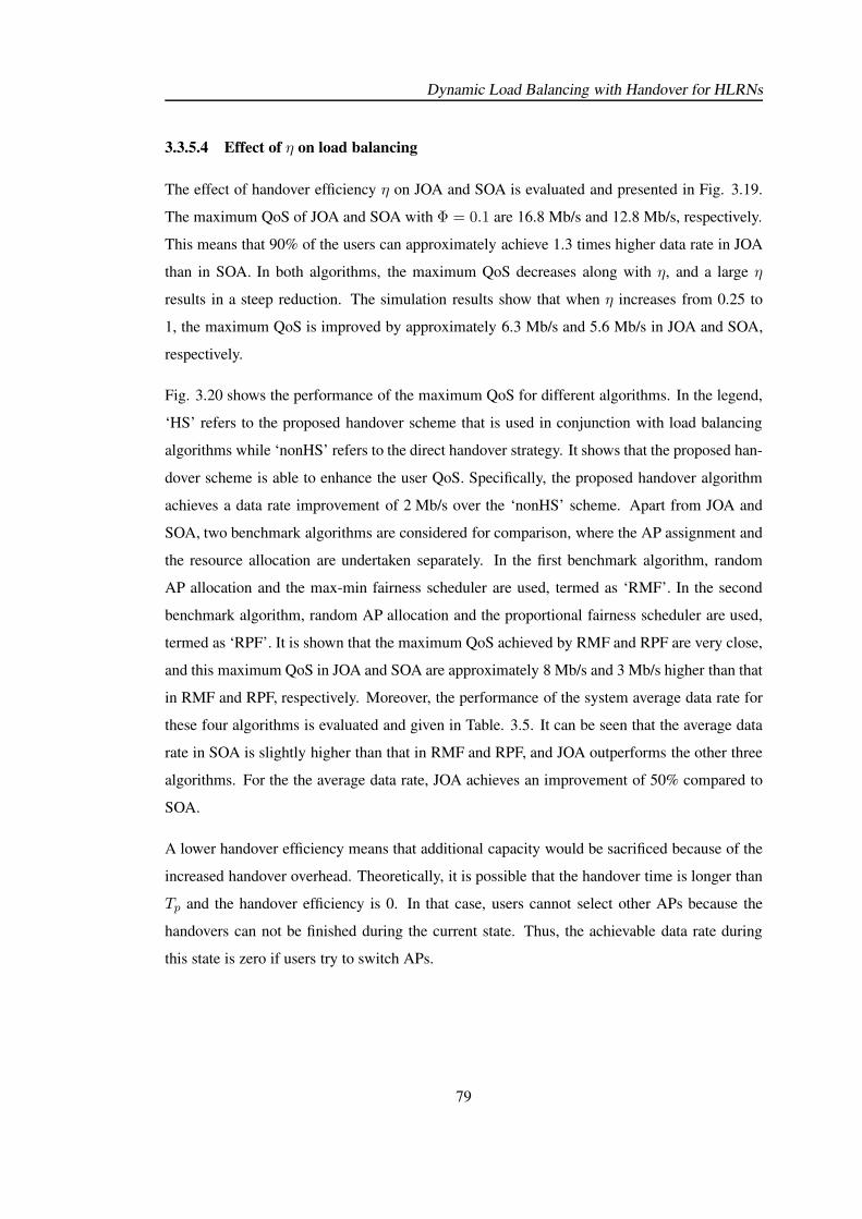
Dynamic Load Balancing with Handover for HLRNs
3.3.5.4 Effect of η on load balancing
The effect of handover efficiency η on JOA and SOA is evaluated and presented in Fig. 3.19.
The maximum QoS of JOA and SOA with Φ = 0.1 are 16.8 Mb/s and 12.8 Mb/s, respectively.
This means that 90% of the users can approximately achieve 1.3 times higher data rate in JOA
than in SOA. In both algorithms, the maximum QoS decreases along with η, and a large η
results in a steep reduction. The simulation results show that when η increases from 0.25 to
1, the maximum QoS is improved by approximately 6.3 Mb/s and 5.6 Mb/s in JOA and SOA,
respectively.
Fig. 3.20 shows the performance of the maximum QoS for different algorithms. In the legend,
‘HS’ refers to the proposed handover scheme that is used in conjunction with load balancing
algorithms while ‘nonHS’ refers to the direct handover strategy. It shows that the proposed han-
dover scheme is able to enhance the user QoS. Specifically, the proposed handover algorithm
achieves a data rate improvement of 2 Mb/s over the ‘nonHS’ scheme. Apart from JOA and
SOA, two benchmark algorithms are considered for comparison, where the AP assignment and
the resource allocation are undertaken separately. In the first benchmark algorithm, random
AP allocation and the max-min fairness scheduler are used, termed as ‘RMF’. In the second
benchmark algorithm, random AP allocation and the proportional fairness scheduler are used,
termed as ‘RPF’. It is shown that the maximum QoS achieved by RMF and RPF are very close,
and this maximum QoS in JOA and SOA are approximately 8 Mb/s and 3 Mb/s higher than that
in RMF and RPF, respectively. Moreover, the performance of the system average data rate for
these four algorithms is evaluated and given in Table. 3.5. It can be seen that the average data
rate in SOA is slightly higher than that in RMF and RPF, and JOA outperforms the other three
algorithms. For the the average data rate, JOA achieves an improvement of 50% compared to
SOA.
A lower handover efficiency means that additional capacity would be sacrificed because of the
increased handover overhead. Theoretically, it is possible that the handover time is longer than
Tp and the handover efficiency is 0. In that case, users cannot select other APs because the
handovers can not be finished during the current state. Thus, the achievable data rate during
this state is zero if users try to switch APs.
79
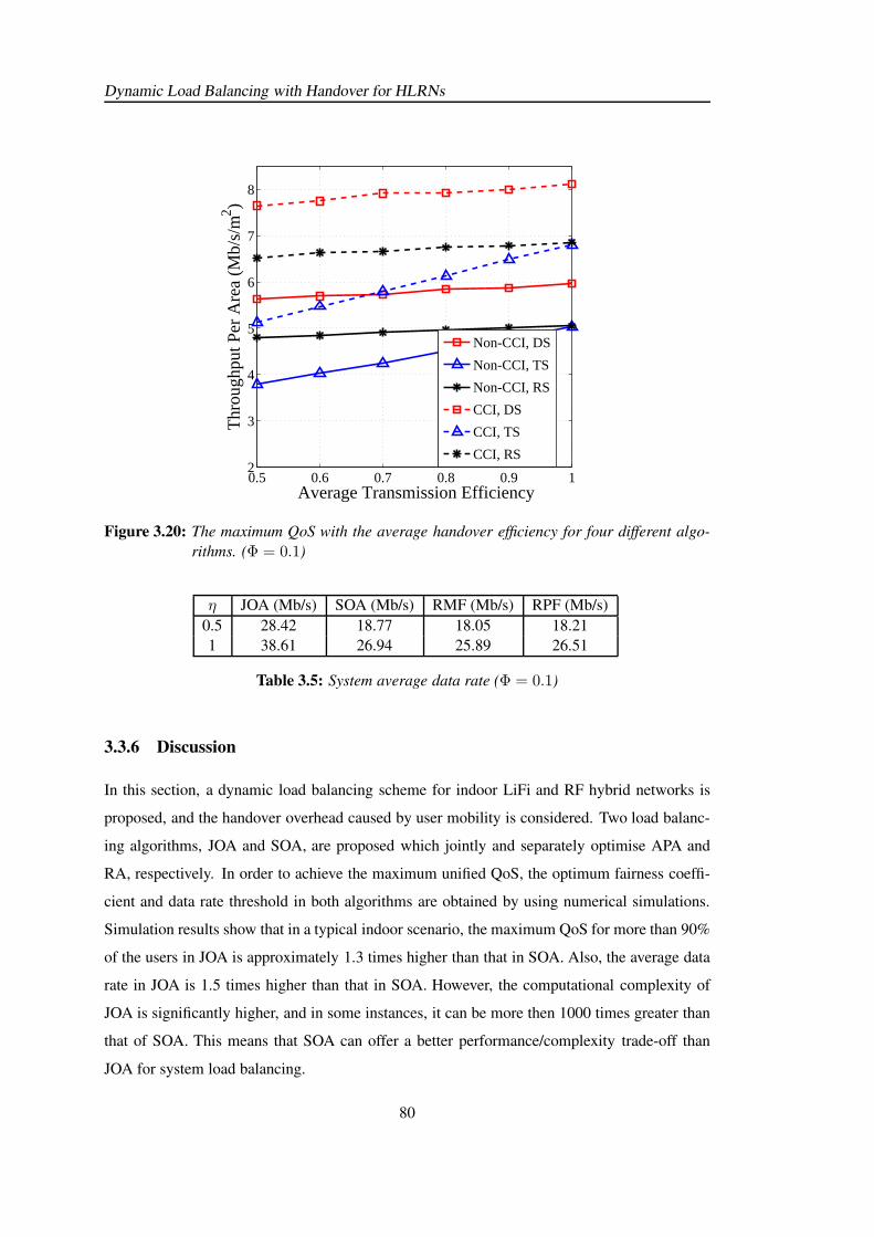
Dynamic Load Balancing with Handover for HLRNs
0.5 0.6 0.7 0.8 0.9 12
3
4
5
6
7
8
Average Transmission Efficiency
Thr
ough
put P
er A
rea
(Mb/
s/m
2 )
Non-CCI, DS
Non-CCI, TS
Non-CCI, RS
CCI, DS
CCI, TS
CCI, RS
Figure 3.20: The maximum QoS with the average handover efficiency for four different algo-
rithms. (Φ = 0.1)
η JOA (Mb/s) SOA (Mb/s) RMF (Mb/s) RPF (Mb/s)
0.5 28.42 18.77 18.05 18.21
1 38.61 26.94 25.89 26.51
Table 3.5: System average data rate (Φ = 0.1)
3.3.6 Discussion
In this section, a dynamic load balancing scheme for indoor LiFi and RF hybrid networks is
proposed, and the handover overhead caused by user mobility is considered. Two load balanc-
ing algorithms, JOA and SOA, are proposed which jointly and separately optimise APA and
RA, respectively. In order to achieve the maximum unified QoS, the optimum fairness coeffi-
cient and data rate threshold in both algorithms are obtained by using numerical simulations.
Simulation results show that in a typical indoor scenario, the maximum QoS for more than 90%
of the users in JOA is approximately 1.3 times higher than that in SOA. Also, the average data
rate in JOA is 1.5 times higher than that in SOA. However, the computational complexity of
JOA is significantly higher, and in some instances, it can be more then 1000 times greater than
that of SOA. This means that SOA can offer a better performance/complexity trade-off than
JOA for system load balancing.
80
Dynamic Load Balancing with Handover for HLRNs
3.4 Fuzzy Logic based dynamic LB Scheme
In Section 3.2 and Section 3.3, dynamic load balancing with handover for hybrid LiFi/RF net-
works is studied. As shown in the handover scheme proposed in Section 3.2.1, the APA and the
RA can only consider the handover effect between the current state and the next state. How-
ever, fast user movement and the occasional strong blockage or angular misalignments of LiFi
signals would prompt ping-pong handovers between LiFi and RF APs, and this effect was not
taken into account in the earlier study. In this section, a novel dynamic handover scheme based
on fuzzy logic (FL) is proposed [77]. The fuzzy logic method can combine a large number
of input information (e.g. instantaneous and average CSI, user speed and required data rate of
users) to determine a suitable load balancing solution with low-complexity, the aim of which is
to improve the system throughput [78–80].
3.4.1 System setup
Referring to Section 2.1-2.2, an indoor hybrid LiFi/RF network is considered. It is assumed
that there are Nl LiFi APs, and the entire scenario is covered by a single RF AP. The set of LiFi
APs is denoted by CL = l| l ∈ [1, Nl], l ∈ N, and the RF AP set is denoted by CR = r.The optical modulation bandwidth is reused in each LiFi attocell, and the optical CCI in the
overlap area is treated as noise in this model. The hybrid network serves multiple users that
are stationary or roaming in the indoor scenario. Note, these users could be internet-of-things
(IoT) devices or mobile handsets. The set of users is denoted by U . In each quasi-static state,
every user has a random required data rate, denoted by λµ, which follows an independent
identical Poisson distribution. The system CU determines the AP assignment and time resource
allocation for each user, and it is connected to all of the APs through error free communication
links. The sequence number of the states is denoted by a natural number n. When a user is
allocated to different APs in two adjacent states, a handover is prompted, and the handover
overhead is also considered in the performance analysis. The SINR (or SNR) for the LiFi and
RF links is based on Eq. (3.55) and Eq. (3.56). Adaptive bit loading is used for both LiFi and
RF systems, and the modulation and coding scheme is given in Table 2.1. The link data rate
between user µ and LiFi AP α is denoted by Dµ,α. The link data rate between user µ and the
RF AP is denoted by Dµ,r .
In the indoor scenario, it is possible that the LoS links of LiFi are blocked by surrounding
81
Dynamic Load Balancing with Handover for HLRNs
objects, people moving or angular misalignments of transmitter and receiver field of views
(FoVs). These events are random and unpredictable. Here it is assumed that the blocking
events follow the Bernoulli distribution, which indicates whether the LiFi reception is blocked
or not [24]. Its probability mass function is expressed as:
I(k) =
1− p, k = 1
p, k = 0, (3.101)
where p denotes the LiFi LoS blocking probability. The LiFi link data rate with blocking
considered is expressed as Dµ,α = kDµ,α, where k is a binary random variable according to
(3.101).
In each state, the CU allocates the most suitable AP to each user. In order to reduce the
complexity, the set of allocatable APs for users only contains the RF AP and the LiFi AP
with the highest SINR, which can be expressed as Yµ = lµ, r, where r is the RF AP; and
lµ = argmaxα∈CL SINRµ,α, where SINRµ,α is according to (3.55).
3.4.2 Dynamic Load Balancing Scheme with Fuzzy Logic
3.4.2.1 Dynamic handover scheme
In the dynamic hybrid LiFi/RF network, the CU determines the AP assignment and resource
allocation for users periodically. When a user is assigned to different APs, a handover is
prompted. In general, the handover overhead in an indoor scenario is in the order of millisec-
onds. The overhead time can be modelled as a Poisson random process, and the probability
mass function (PMF) of the overhead is given in Eq. (3.3). In this study, it is assumed that all
of the handovers follow an independent and identical Poisson distribution, and the Poisson pa-
rameter is denoted by ζ . Due to the overhead, users achieve zero data rates during the handover
period. The number of states considered in the dynamic handover scheme is denoted by Ns.
In order to reduce the data rate loss during user movement, a load balancing scheme is designed
and the following information is considered to be known at the CU in each state: i) the SINR
between users and the APs belonging to Yµ; ii) the average SINR achieved by lµ during the last
M states; iii) the speed of users; and iv) the required data rate. In each state, the CU determines
the AP allocation and resource allocation based on the FL method, which will be given in this
subsection.
82
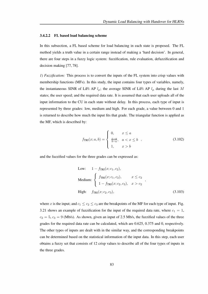
Dynamic Load Balancing with Handover for HLRNs
3.4.2.2 FL based load balancing scheme
In this subsection, a FL based scheme for load balancing in each state is proposed. The FL
method yields a truth value in a certain range instead of making a ‘hard decision’. In general,
there are four steps in a fuzzy logic system: fuzzification, rule evaluation, defuzzification and
decision making [77, 78].
1) Fuzzification: This process is to convert the inputs of the FL system into crisp values with
membership functions (MFs). In this study, the input contains four types of variables, namely,
the instantaneous SINR of LiFi AP lµ; the average SINR of LiFi AP lµ during the last M
states; the user speed; and the required data rate. It is assumed that each user uploads all of the
input information to the CU in each state without delay. In this process, each type of input is
represented by three grades: low, medium and high. For each grade, a value between 0 and 1
is returned to describe how much the input fits that grade. The triangular function is applied as
the MF, which is described by:
fTRI(x; a, b) =
0, x ≤ ax−ab−a , a < x ≤ b1, x > b
, (3.102)
and the fuzzified values for the three grades can be expressed as:
Low: 1− fTRI(x; c1, c2),
Medium:
fTRI(x; c1, c2), x ≤ c21− fTRI(x; c2, c3), x > c2
,
High: fTRI(x; c2, c3), (3.103)
where x is the input; and c1 ≤ c2 ≤ c3 are the breakpoints of the MF for each type of input. Fig.
3.21 shows an example of fuzzification for the input of the required data rate, where c1 = 1,
c2 = 5, c3 = 9 (Mb/s). As shown, given an input of 2.5 Mb/s, the fuzzified values of the three
grades for the required data rate can be calculated, which are 0.625, 0.375 and 0, respectively.
The other types of inputs are dealt with in the similar way, and the corresponding breakpoints
can be determined based on the statistical information of the input data. In this step, each user
obtains a fuzzy set that consists of 12 crisp values to describe all of the four types of inputs in
the three grades.
83
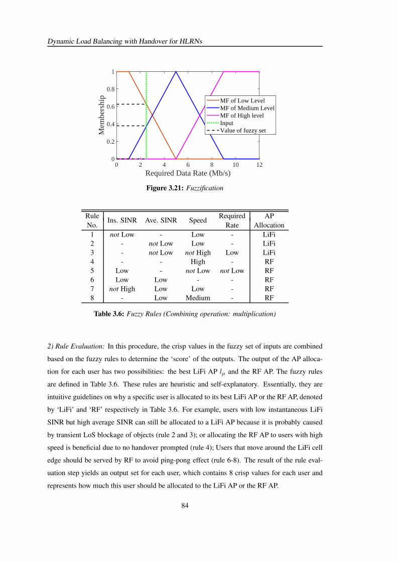
Dynamic Load Balancing with Handover for HLRNs
Required Data Rate (Mb/s)0 2 4 6 8 10 12
Mem
bers
hip
0
0.2
0.4
0.6
0.8
1
MF of Low LevelMF of Medium LevelMF of High levelInputValue of fuzzy set
Figure 3.21: Fuzzification
Rule Required AP
No.Ins. SINR Ave. SINR Speed
Rate Allocation
1 not Low - Low - LiFi
2 - not Low Low - LiFi
3 - not Low not High Low LiFi
4 - - High - RF
5 Low - not Low not Low RF
6 Low Low - - RF
7 not High Low Low - RF
8 - Low Medium - RF
Table 3.6: Fuzzy Rules (Combining operation: multiplication)
2) Rule Evaluation: In this procedure, the crisp values in the fuzzy set of inputs are combined
based on the fuzzy rules to determine the ‘score’ of the outputs. The output of the AP alloca-
tion for each user has two possibilities: the best LiFi AP lµ and the RF AP. The fuzzy rules
are defined in Table 3.6. These rules are heuristic and self-explanatory. Essentially, they are
intuitive guidelines on why a specific user is allocated to its best LiFi AP or the RF AP, denoted
by ‘LiFi’ and ‘RF’ respectively in Table 3.6. For example, users with low instantaneous LiFi
SINR but high average SINR can still be allocated to a LiFi AP because it is probably caused
by transient LoS blockage of objects (rule 2 and 3); or allocating the RF AP to users with high
speed is beneficial due to no handover prompted (rule 4); Users that move around the LiFi cell
edge should be served by RF to avoid ping-pong effect (rule 6-8). The result of the rule eval-
uation step yields an output set for each user, which contains 8 crisp values for each user and
represents how much this user should be allocated to the LiFi AP or the RF AP.
84
Dynamic Load Balancing with Handover for HLRNs
x0 0.2 0.4 0.6 0.8 1
f(x)
0
0.2
0.4
0.6
0.8
1
MF of RFMF of Li-FiFinal score
Figure 3.22: Defuzzification
3) Defuzzification: This process determines the final score of the AP allocation for each user.
According to the rule evaluation step, the maximal score of output state ‘LiFi’ from rule 1
to rule 3, denoted by vl, and the maximal score of output state ‘RF’ from rule 4 to rule 8,
denoted by vr, constitute a fuzzy set of output. Fig. 3.22 shows the defuzzification process of
the proposed FL algorithm. Similar to fuzzification, a MF of each output state (LiFi or RF) is
applied to describe the relationship between that state and the score. The shaded area shown in
Fig. 3.22 represents the weight of each state in the fuzzy set. The centre of gravity of this fuzzy
set is calculated for the final score [77], which is expressed as:
ωµ =
∫ 10 f(x)xdx∫ 10 f(x) dx
, (3.104)
where f(x) is the upper edge of the shaded area based on the rule evaluation process, which is
written as:
f(x) =
min(fMR(x), vr), 0 ≤ x ≤ 0.5
min(fML(x), vl), 0.5 < x ≤ 1,
(3.105)
where fMR(x) = 1−fTRI(x; 0, 0.5) is the MF of the output state RF; and fML(x) = fTRI(x; 0.5, 1)
is the MF of output state LiFi. The final score ωµ for user µ ranges from 0 and 1, and describes
the preference for LiFi AP allocation. For example, the user with a score of 0.8 is more prefer-
able to connect to their best LiFi APs than one with a score of 0.5.
4) Decision Making: In this step, the AP allocation is determined by the CU according to the
final score of each user. The set of users for which the LiFi AP with the highest SINR is α
85
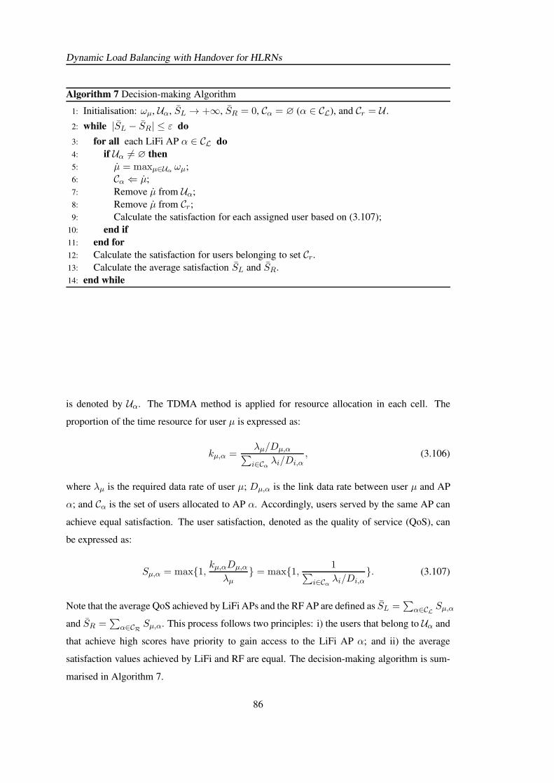
Dynamic Load Balancing with Handover for HLRNs
Algorithm 7 Decision-making Algorithm
1: Initialisation: ωµ, Uα, SL → +∞, SR = 0, Cα = ∅ (α ∈ CL), and Cr = U .
2: while |SL − SR| ≤ ε do
3: for all each LiFi AP α ∈ CL do
4: if Uα 6= ∅ then
5: µ = maxµ∈Uα ωµ;
6: Cα ⇐ µ;
7: Remove µ from Uα;
8: Remove µ from Cr;
9: Calculate the satisfaction for each assigned user based on (3.107);
10: end if
11: end for
12: Calculate the satisfaction for users belonging to set Cr.
13: Calculate the average satisfaction SL and SR.
14: end while
is denoted by Uα. The TDMA method is applied for resource allocation in each cell. The
proportion of the time resource for user µ is expressed as:
kµ,α =λµ/Dµ,α
∑
i∈Cαλi/Di,α
, (3.106)
where λµ is the required data rate of user µ; Dµ,α is the link data rate between user µ and AP
α; and Cα is the set of users allocated to AP α. Accordingly, users served by the same AP can
achieve equal satisfaction. The user satisfaction, denoted as the quality of service (QoS), can
be expressed as:
Sµ,α = max1, kµ,αDµ,α
λµ = max1, 1
∑
i∈Cαλi/Di,α
. (3.107)
Note that the average QoS achieved by LiFi APs and the RF AP are defined as SL =∑
α∈CLSµ,α
and SR =∑
α∈CRSµ,α. This process follows two principles: i) the users that belong to Uα and
that achieve high scores have priority to gain access to the LiFi AP α; and ii) the average
satisfaction values achieved by LiFi and RF are equal. The decision-making algorithm is sum-
marised in Algorithm 7.
86
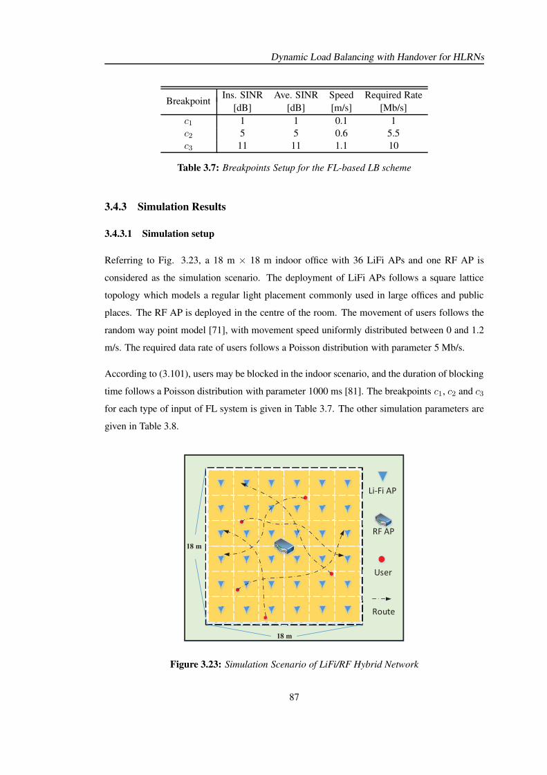
Dynamic Load Balancing with Handover for HLRNs
Ins. SINR Ave. SINR Speed Required RateBreakpoint
[dB] [dB] [m/s] [Mb/s]
c1 1 1 0.1 1
c2 5 5 0.6 5.5
c3 11 11 1.1 10
Table 3.7: Breakpoints Setup for the FL-based LB scheme
3.4.3 Simulation Results
3.4.3.1 Simulation setup
Referring to Fig. 3.23, a 18 m × 18 m indoor office with 36 LiFi APs and one RF AP is
considered as the simulation scenario. The deployment of LiFi APs follows a square lattice
topology which models a regular light placement commonly used in large offices and public
places. The RF AP is deployed in the centre of the room. The movement of users follows the
random way point model [71], with movement speed uniformly distributed between 0 and 1.2
m/s. The required data rate of users follows a Poisson distribution with parameter 5 Mb/s.
According to (3.101), users may be blocked in the indoor scenario, and the duration of blocking
time follows a Poisson distribution with parameter 1000 ms [81]. The breakpoints c1, c2 and c3
for each type of input of FL system is given in Table 3.7. The other simulation parameters are
given in Table 3.8.
Li-Fi AP
RF AP
18 m
18 m
User
Route
Figure 3.23: Simulation Scenario of LiFi/RF Hybrid Network
87
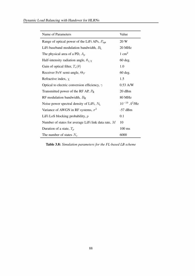
Dynamic Load Balancing with Handover for HLRNs
Name of Parameters Value
Range of optical power of the LiFi APs, Popt 20 W
LiFi baseband modulation bandwidth, BL 20 MHz
The physical area of a PD, Ap 1 cm2
Half-intensity radiation angle, θ1/2 60 deg.
Gain of optical filter, Ts(θ) 1.0
Receiver FoV semi-angle, ΘF 60 deg.
Refractive index, χ 1.5
Optical to electric conversion efficiency, γ 0.53 A/W
Transmitted power of the RF AP, PR 20 dBm
RF modulation bandwidth, BR 80 MHz
Noise power spectral density of LiFi, NL 10−19 A2/Hz
Variance of AWGN in RF systems, σ2 -57 dBm
LiFi LoS blocking probability, p 0.1
Number of states for average LiFi link data rate, M 10
Duration of a state, Tp 100 ms
The number of states Ns 6000
Table 3.8: Simulation parameters for the FL-based LB scheme
88
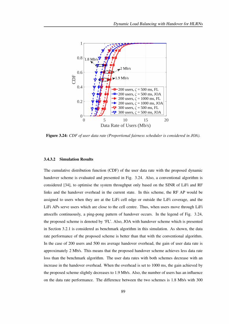
Dynamic Load Balancing with Handover for HLRNs
0 5 10 15 20Data Rate of Users (Mb/s)
0
0.2
0.4
0.6
0.8
1
CD
F
200 users, = 500 ms, FL200 users, = 500 ms, JOA200 users, = 1000 ms, FL200 users, = 1000 ms, JOA300 users, = 500 ms, FL300 users, = 500 ms, JOA
1.9 Mb/s
1.8 Mb/s
2 Mb/s
Figure 3.24: CDF of user data rate (Proportional fairness scheduler is considered in JOA).
3.4.3.2 Simulation Results
The cumulative distribution function (CDF) of the user data rate with the proposed dynamic
handover scheme is evaluated and presented in Fig. 3.24. Also, a conventional algorithm is
considered [34], to optimise the system throughput only based on the SINR of LiFi and RF
links and the handover overhead in the current state. In this scheme, the RF AP would be
assigned to users when they are at the LiFi cell edge or outside the LiFi coverage, and the
LiFi APs serve users which are close to the cell centre. Thus, when users move through LiFi
attocells continuously, a ping-pong pattern of handover occurs. In the legend of Fig. 3.24,
the proposed scheme is denoted by ‘FL’. Also, JOA with handover scheme which is presented
in Section 3.2.1 is considered as benchmark algorithm in this simulation. As shown, the data
rate performance of the proposed scheme is better than that with the conventional algorithm.
In the case of 200 users and 500 ms average handover overhead, the gain of user data rate is
approximately 2 Mb/s. This means that the proposed handover scheme achieves less data rate
loss than the benchmark algorithm. The user data rates with both schemes decrease with an
increase in the handover overhead. When the overhead is set to 1000 ms, the gain achieved by
the proposed scheme slightly decreases to 1.9 Mb/s. Also, the number of users has an influence
on the data rate performance. The difference between the two schemes is 1.8 Mb/s with 300
89
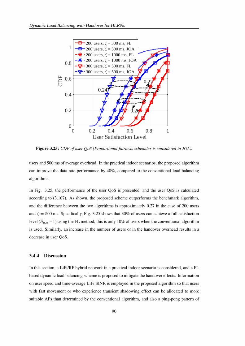
Dynamic Load Balancing with Handover for HLRNs
User Satisfaction Level0 0.2 0.4 0.6 0.8 1
CD
F
0
0.2
0.4
0.6
0.8
1200 users, ζ = 500 ms, FL200 users, ζ = 500 ms, JOA200 users, ζ = 1000 ms, FL200 users, ζ = 1000 ms, JOA300 users, ζ = 500 ms, FL300 users, ζ = 500 ms, JOA
0.26
0.24
0.27
Figure 3.25: CDF of user QoS (Proportional fairness scheduler is considered in JOA).
users and 500 ms of average overhead. In the practical indoor scenarios, the proposed algorithm
can improve the data rate performance by 40%, compared to the conventional load balancing
algorithms.
In Fig. 3.25, the performance of the user QoS is presented, and the user QoS is calculated
according to (3.107). As shown, the proposed scheme outperforms the benchmark algorithm,
and the difference between the two algorithms is approximately 0.27 in the case of 200 users
and ζ = 500 ms. Specifically, Fig. 3.25 shows that 30% of users can achieve a full satisfaction
level (Sµ,α = 1) using the FL method; this is only 10% of users when the conventional algorithm
is used. Similarly, an increase in the number of users or in the handover overhead results in a
decrease in user QoS.
3.4.4 Discussion
In this section, a LiFi/RF hybrid network in a practical indoor scenario is considered, and a FL
based dynamic load balancing scheme is proposed to mitigate the handover effects. Information
on user speed and time-average LiFi SINR is employed in the proposed algorithm so that users
with fast movement or who experience transient shadowing effect can be allocated to more
suitable APs than determined by the conventional algorithm, and also a ping-pong pattern of
90
Dynamic Load Balancing with Handover for HLRNs
handover is avoided. The simulation shows that the FL based dynamic load balancing scheme
has less data rate loss than the conventional load balancing algorithms, and a 40% performance
improvement is achieved in terms of both data rate and user QoS.
3.5 Summary
In this chapter, the dynamic load balancing for hybrid LiFi/RF networks with handover is inves-
tigated. Firstly, an optimisation-based LB scheme with proportional fairness is proposed, and
the throughput performance of the hybrid LiFi/WiFi system is theoretically analysed. Also,
the effects of the handover overhead on handover locations and user throughput are simulated
and discussed. It has been shown that the WiFi and LiFi throughputs in the hybrid network are
related despite the independent spectrum transmission. The LiFi throughput can be improved
by increasing the WiFi throughput due to efficient load balancing. In Section 3.3, the dynamic
load balancing with a variety of fairness schemes is studied, where two specific algorithms JOA
and SOA that optimise the APA and the RA in each quasi-static state are proposed. Moreover,
a unified data rate requirement of users is considered as a QoS metric and user outage probabil-
ity is introduced. Simulation results show that SOA can offer a better performance/complexity
trade-off than JOA for system load balancing. In Section 3.4, a fuzzy logic (FL) based dynamic
LB scheme which jointly handles APA, RA and handover is proposed. Unlike the optimisation-
based schemes, this FL scheme uses not only the CSI, but also the user speed and desired data
rate to determine whether a handover needs to be prompted. Simulation shows that the pro-
posed scheme outperforms the conventional LB algorithms, and the performance improvement
is approximately 40% in terms of both data rate and user satisfaction level.
91

92
Chapter 4
Load Balancing with Shadowing
Effects for HLRNs
4.1 Introduction
As shown in Chapter 1 and 2, the hybrid LiFi/RF network is able to mitigate the spatial fluc-
tuation of data rate, offering a system throughput greater than that of stand alone LiFi or RF
networks [34]. Most published research considers an ideal system model of hybrid networks,
especially the LiFi channel model. In order to attain a more accurate evaluation of the system
performance, three practical factors must be taken into account:
i). Blockage: In general, the signals of line of sight (LoS) paths contribute to most received
signal power in a LiFi system [82]. In an indoor scenario, opaque objects such as people and
furniture can block the LoS optical channel and this would significantly compromise the data
rate performance. Therefore, the shadowing effect in a LiFi system needs to be considered.
ii). Receiving orientation angle (ROA): In most published research, the LiFi receiver is always
assumed to be oriented perpendicularly upwards and for simplicity the incidence angle is set
equal to the angle of irradiation. However, it has been shown in [43] that this incidence angle
varies depending on the users’ behaviour pattern and would significantly affect the receive SNR.
Therefore a random ROA needs to be considered in the LiFi system model.
iii). User data rate requirement: Published research with respect to hybrid networks focuses on
the improvement of system throughput and user fairness [23, 34, 83]. In general, each user has
a required data rate in a short period to support certain wireless services such as browsing a web
page, on-line video stream and voice over Internet protocol (VoIP). On the one hand, achieving
a lower data rate than required would affect the quality of service (QoS) of users. On the other
hand, a higher data rate than the requirement may lead to inefficient use of precious resources
and possibly result in an overload of other cells. Therefore, user data rate requirements should
be considered in the system load balancing (LB) for hybrid networks.
93
Load Balancing with Shadowing Effects for HLRNs
The system throughput and user satisfaction levels in hybrid LiFi/RF networks can be enhanced
by using efficient LB techniques, which address two main issues: AP assignment (APA) and
resource allocation (RA). In [23, 34], the APA and the RA are jointly optimised, and an iterative
algorithm is given to find an optimal solution. In order to reduce the computational complexity,
a LB scheme that separately optimises the APA and the RA is proposed in [18, 83], but the
achievable data rates are significantly compromised. Therefore a novel LB scheme that can
offer a proper performance/complexity trade-off is necessary. Moreover, when considering user
data rate requirement, a piecewise function is normally needed to quantify the satisfaction of
users because a data rate higher than the one required no longer increases the users’ satisfaction
level [84]. The conventional joint optimisation methods are NP-hard problems [23, 34]. Taking
the user data rate requirement into account would further increase the complexity and result
in a mathematically intractable problem. In this study, an evolutionary game theory (EGT)
based LB scheme is proposed, where the problems of APA and RA are jointly handled. This
algorithm accommodates the user data rate requirement for resource allocation and a novel RA
scheme that makes full use of the communication resources is proposed. This EGT algorithm
can greatly improve the system throughput while achieving low computational complexity.
4.1.1 Evolutionary game theory
In recent literature, game theory has been extensively applied to network selection and interfer-
ence management problem in heterogeneous wireless networks [85–87]. The Nash equilibrium
(NE) is the most commonly used solution to the non-cooperative game because it ensures that
no player can improve its payoff without compromising another player. However, when there
are multiple NEs in the game, a refined solution is required to ensure users’ payoff reaches
a stable status. Evolutionary equilibrium (EE), which is based on the EGT, can provide such
a refined solution where a group of players will not change their chosen strategies over time
[88, 89].
In the EGT model, each user selects a strategy by replication and adapts its selection for a better
payoff (i.e. user satisfaction) until no user can increase their payoff by unilaterally changing
strategy. An EGT based method is used in [85] to solve the problem of network selection in
an environment where multiple networks are available. In [86], the EGT based subcarrier and
power allocation for small-cell networks are proposed. In [87], the authors used a stochas-
tic geometry-based approach to analyse the stability of equilibrium of the evolutionary game
94
Load Balancing with Shadowing Effects for HLRNs
in macro/micro heterogeneous wireless networks. In this study, an EGT based system load
balancing scheme for an indoor LiFi/RF network is proposed with user data rate requirement
taken into account. Different from conventional EGT based approaches, the proposed algo-
rithm jointly deals with the APA and the RA rather than only focuses on the network selection.
Specifically, the max-min fairness and the proportional fairness schedulers are used in the RA.
Also, an enhanced proportional fairness scheduler is proposed to improve the efficiency of re-
source utilisation.
4.1.2 Main contributions
• An EGT based load balancing scheme is proposed for hybrid LiFi/RF networks where
the following practical issues are considered: i). channel blockages; ii). LiFi ROA; iii).
user data rate requirement. The proposed algorithm jointly handles the APA and the RA,
and the optimality of this algorithm is analysed in this study.
• When considering user data rate requirement, conventional fairness schedulers such as
max-min fairness and proportional fairness may lead to inefficient use of communica-
tion resources. In the proposed EGT based algorithm, an enhanced proportional fairness
scheduler for resource allocation is proposed to avoid inefficient use of transmission re-
sources. The performance of user satisfaction for both conventional and proposed fair-
ness schedulers is evaluated by computer simulations.
• The effects of blockages and the ROA, which are the channel characteristics of LiFi,
are analysed in this study. To the best of the authors’ knowledge, it is the first time an
investigation on how these two issues affect the system load balancing in hybrid LiFi/RF
networks has been conducted.
The rest of this chapter is organised as follows. The practical hybrid LiFi/RF network model is
introduced in Section 4.2. The EGT based load balancing scheme is given in Section 4.3. The
performance evaluation is presented in Section 4.4 and a summary is drawn in Section 4.5.
4.2 System Model
In this study, an indoor scenario covered by a hybrid LiFi/RF network is considered, where Nl
LiFi APs and Nr RF APs are deployed. The system model of hybrid LiFi and RF networks
95
Load Balancing with Shadowing Effects for HLRNs
can be seen in Section 2.1-2.2. In the LiFi system, the photon detector (PD) at each LiFi
receiver may have horizontal and vertical tilts, as shown in Fig. 2.2. The direction vector of
the PD in Cartesian coordinates is given in Eq. (2.5), and the angle of incidence to the PDs is
shown in Eq. (2.7). Due to the field of view (FoV) of the LED and PDs, each LiFi AP covers
a confined cell, termed as an optical attocell. Since an attocell can significantly reduce the
spread of signals outside a given zone determined by the light cone, LiFi APs are able to reuse
the same bandwidth in a radical manner. Optical inter-cell interference (ICI) is treated as an
additive noise [90]. In this study, a square lattice topology is used for the deployment of LiFi
APs so as to model a regular lighting placement used in large offices and public places. Direct
current biased orthogonal frequency division multiplexing (DCO-OFDM) is applied for LiFi
transmission. In addition, a RF system working at 2.4 GHz covers the whole indoor scenario.
When more than one RF AP is considered, the RF ICI is not negligible. It is assumed that the
RF APs use different channels, and the spectrum used by each RF AP is non-overlapping.
Assume that the channel state information (CSI) in both LiFi and RF systems changes slowly
and is constant in a short period of Tp, which contains numbers of transmission time intervals
(TTIs). During a period of Tp, the load distribution is considered to be fixed in the hybrid
network. In this study, user movement is not taken into account, and the EGT based dynamic
load balancing scheme with handover will be subject to future research.
Time division multiple access (TDMA) is used at each LiFi and RF cell to serve multiple users
[34]. The portion of the time resource allocated to user µ in a signal frame is denoted by
kµ,α, where α is the index of the serving AP and kµ,α ∈ [0, 1]. The data rate requirement of
each user during time Tp is denoted by λµ. The number of users is denoted by Nµ; the set
of LiFi APs is denoted by CL = l| l ∈ [1, Nl], l ∈ N; the set of RF APs is denoted by
CR = r| r ∈ [1, Nr], r ∈ N; and the total number of the APs is denoted as Nap = Nl +Nr.
In this chapter, the blockage caused by opaque objects in LiFi attocells is considered. According
to [91], an object which generates a shadow in an indoor scenario is approximately modelled
by a cylinder, 1.2 m (height) and 0.8 m (diameter). The shape of the shadow caused by this
cylinder is assumed to be a rectangle. As shown in Fig. 4.1, the length of the rectangle is
defined as the distance between the cylinder bottom and the shadow of the cylinder top, and the
width of the rectangle is the diameter of the cylinder. It is assumed that the PDs in the shadows
cannot receive any LoS optical signal from the blocked LiFi APs.
96
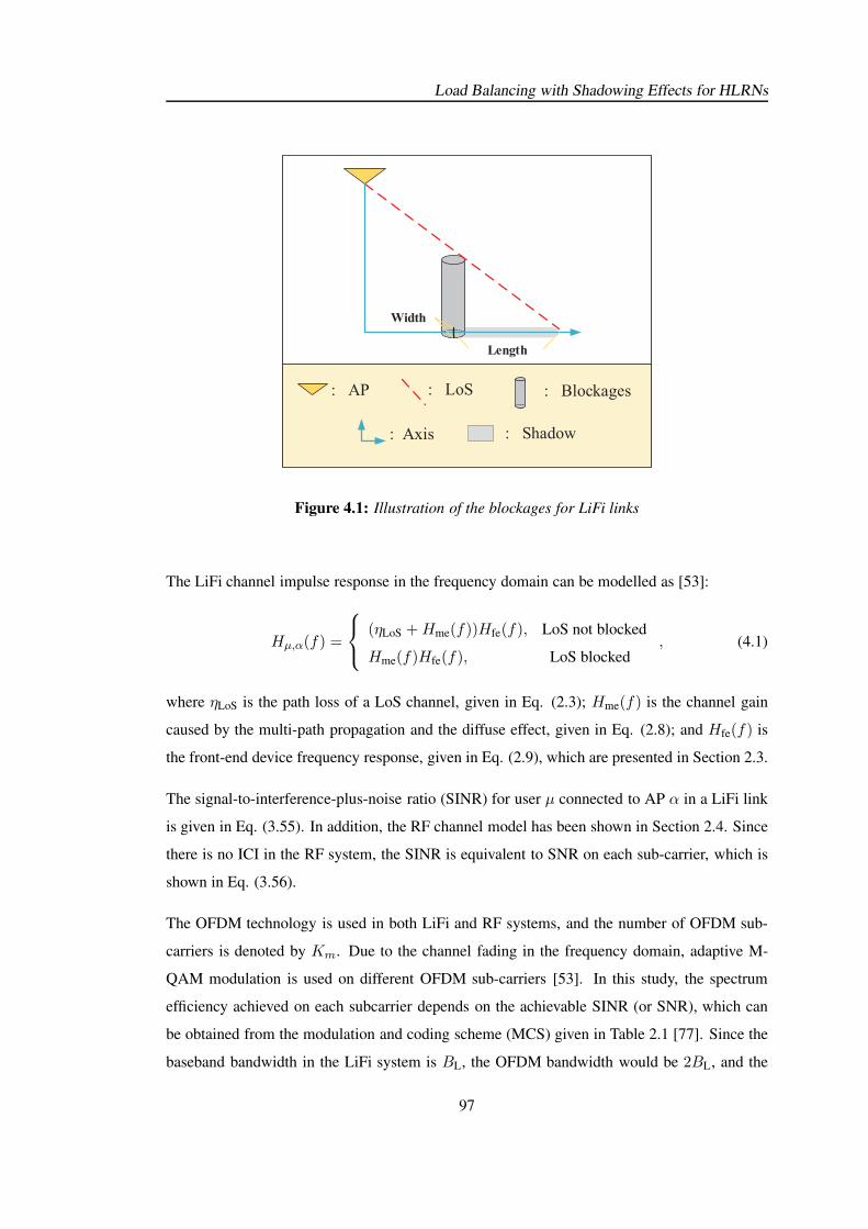
Load Balancing with Shadowing Effects for HLRNs
Length
Width
: AP : LoS
: Axis
: Blockages
: Shadow
Figure 4.1: Illustration of the blockages for LiFi links
The LiFi channel impulse response in the frequency domain can be modelled as [53]:
Hµ,α(f) =
(ηLoS +Hme(f))Hfe(f), LoS not blocked
Hme(f)Hfe(f), LoS blocked, (4.1)
where ηLoS is the path loss of a LoS channel, given in Eq. (2.3); Hme(f) is the channel gain
caused by the multi-path propagation and the diffuse effect, given in Eq. (2.8); and Hfe(f) is
the front-end device frequency response, given in Eq. (2.9), which are presented in Section 2.3.
The signal-to-interference-plus-noise ratio (SINR) for user µ connected to AP α in a LiFi link
is given in Eq. (3.55). In addition, the RF channel model has been shown in Section 2.4. Since
there is no ICI in the RF system, the SINR is equivalent to SNR on each sub-carrier, which is
shown in Eq. (3.56).
The OFDM technology is used in both LiFi and RF systems, and the number of OFDM sub-
carriers is denoted by Km. Due to the channel fading in the frequency domain, adaptive M-
QAM modulation is used on different OFDM sub-carriers [53]. In this study, the spectrum
efficiency achieved on each subcarrier depends on the achievable SINR (or SNR), which can
be obtained from the modulation and coding scheme (MCS) given in Table 2.1 [77]. Since the
baseband bandwidth in the LiFi system is BL, the OFDM bandwidth would be 2BL, and the
97
Load Balancing with Shadowing Effects for HLRNs
LiFi link data rate between user µ and AP α can be written as [13]:
Zµ,α =2BL
Km
Km2
−1∑
i=1
qL(i), (4.2)
where qL(i) is the spectrum efficiency on sub-carrier i in the LiFi system, according to Eq.
(3.55). The link communication data rate of RF can be written as:
Υµ,α =BR
Km
Km−1∑
j=0
qR(j), (4.3)
where qR(j) is the spectrum efficiency on sub-carrier j in the RF system, according to Eq.
(3.56).
In order to reduce the complexity of AP selection, the receivers only select from the candidate
APs with the highest link data rate performance in the stand-alone LiFi or RF system. Without
loss of generality, it is assumed that the link data rates between user µ and the APs follows:
Zµ,l1 ≥ ...Zµ,li ≥ Zµ,li+1... ≥ Zµ,lNl
, li ∈ CLΥµ,r1 ≥ ...Υµ,rj ≥ Υµ,rj+1 ... ≥ Υµ,rNr
, rj ∈ CR.
The AP resource of user µ can be defined as:
Sµ = l1, r1. (4.4)
For simplicity, the link data rate between user µ and its candidate AP α ∈ Sµ is denoted by
γµ,α, which can be expressed as:
γµ,α =
Zµ,α, α ∈ CL ∩ SµΥµ,α, α ∈ CR ∩ Sµ
.
4.3 Load Balancing Game
In this section, a new load balancing scheme is proposed, where the APA and the RA are
formulated as an evolutionary game. Also, the replicator dynamic is used to model the strategy
adaptation process for network load balancing [87]. The evolutionary equilibrium is considered
to be the solution of the formulated load balancing game, and the stability and optimality of this
98
Load Balancing with Shadowing Effects for HLRNs
algorithm are analysed.
4.3.1 Game setup
The load balancing game can be formulated as follows:
1. Players Set (U ): The users in the hybrid network are the players in the game, and the number
of players is denoted by Nµ = |U|.
2. Strategy Set (Sµ): The strategy set for each player is in accordance with Eq. (4.4). Each
player can select one AP from Sµ.
3. Population: In the proposed game, each player should be allocated to an AP. The set of
players connected to AP α (α ∈ CL ∪ CR) is denoted by Uα, where the number of players in
this set is denoted by Nα = |Uα|.
4. Payoff Function: The payoff of a player quantifies the satisfaction level of that player’s action
of AP selection, and this is considered as the user QoS. In general, player µ would be satisfied
when its data rate is higher than the requirement λµ. Otherwise, the satisfaction level would
decrease along with the data rate. Intuitively, the payoff function of user µ that is allocated to
AP α can be written as:
πµ,α = min
kµ,αγµ,αλµ
, 1
, (4.5)
where kµ,α is the time resource portion provided by host AP α; and γµ,α is the link data rate
between player µ and AP α.
4.3.2 Resource allocation
Since TDMA is used in this study, the time slot resource would be allocated to users in each
cell by serving APs. Here the portion of time slot resource allocated by AP α for user µ is
denoted by kµ,α. In this study, the β-proportional fairness function shown in Eq. (2.16) is used,
which is repeated here:
ψβ(x) =
ln(x), β = 1
x1−β
1− β , β ≥ 0, β 6= 1, (4.6)
99
Load Balancing with Shadowing Effects for HLRNs
where x is the user satisfaction level, defined as the user QoS; and β is the fairness coefficient.
Particularly, when β = 0, a linear utility function is obtained, which achieves a maximal system
throughput. In this case, each AP only serves the user with the best channel state information
(CSI) whereas the other users have zero data rates. This scheduler finally leads to an ineffective
network load balancing. Thus, the situation of β = 0 is not under consideration.
In the cell covered by AP α, the resource allocation problem with the β-proportional fairness
function can be formulated as:
maxkµ,α
∑
µ∈Uα
ψβ
(
kµ,αγµ,αλµ
)
(4.7)
s.t.∑
µ∈Uα
kµ,α ≤ 1; (4.8)
where Uα is the set of players allocated to AP α. The Lagrangian multiplier method is used to
solve this problem. The Lagrangian function is given by:
F (kµ,α, ω) =∑
µ∈Uα
ψβ
(
kµ,αγµ,αλµ
)
+ ω
1−∑
µ∈Uα
kµ,α
, (4.9)
where ω is the Lagrangian multiplier for the constraint in Eq. (4.8). The optimal kµ,α can be
obtained by making the gradient of the Lagrangian function in Eq. (4.9) equal to 0, which is
written as:∂F (kµ,α, ω)
∂kµ,α=∂ψβ(kµ,αγµ,α/λµ)
∂kµ,α− ω = 0, (4.10)
where according to Eq. (4.6),
∂ψβ(kµ,αγµ,α/λµ)
∂kµ,α=γµ,αλµ
(
kµ,αγµ,αλµ
)−β
, (β > 0). (4.11)
It can be derived from Eq. (4.10) and Eq. (4.11) that:
kµ,α =
(
γµ,αλµ
) 1β−1
ω− 1β . (4.12)
According to Eq. (4.12) and Eq. (4.8), it can be further calculated that:
ω1β =
∑
µ∈Uα
(
γµ,αλµ
)1β−1
. (4.13)
100
Load Balancing with Shadowing Effects for HLRNs
Combining Eq. (4.12) and Eq. (4.13), the optimum kµ,α can be expressed as:
kµ,α =(γµ,α/λµ)
1β−1
∑
i∈Uα(γi,α/λi)
1β−1
(β > 0). (4.14)
In this study, three fairness schedulers are considered, which are max-min fairness (MF), pro-
portional fairness (PF) and enhanced proportional fairness (EPF).
i). MF: The MF is achieved with β → +∞ [74], and the optimal portion of allocated time
resource can be expressed as:
k(MF)µ,α = lim
β→+∞
(γµ,α/λµ)1β−1
∑
i∈Uα(γi,α/λi)
1β−1
=(γµ,α/λµ)
−1
∑
i∈Uα(γi,α/λi)−1
. (4.15)
Combining Eq. (4.5) and Eq. (4.15), the user payoff with MF scheduler can be written as:
π(MF)µ,α = min
1∑
i∈Uαλi/γi,α
, 1
, (4.16)
where the operation mine1, e2 represents the minimum between e1 and e2. It can be seen
that all players served by AP α achieve equal payoffs.
ii). PF: The PF scheduler is realised by β = 1 [74]. According to Eq. (4.15), the optimal RA
portion can be written as follows:
k(PF)µ,α =
(γµ,α/λµ)1β−1
∑
i∈Uα(γi,α/λi)
1β−1
∣
∣
∣
∣
∣
∣
β=1
=1
Nα, (4.17)
where Nα is the number of users in Uα. The user payoff of proportional scheduler is therefore
expressed as:
π(PF)µ,α = min
γµ,αλµNα
, 1
. (4.18)
In the PF scheduler, receivers in each cell share the same portion of time slot resource. Never-
theless, an inefficient use of resources may occur when users require low data rates. This issue
will be handled by the EPF scheduler.
iii). EPF: Unlike the PF scheduler, the EPF scheduler can avoid inefficient use of resources by
allocating the redundant time slot resources of over-achieving users to those who achieve low
user satisfaction. Specifically, the RA is initially undertaken through the PF scheduler, as shown
101
Load Balancing with Shadowing Effects for HLRNs
Algorithm 8 : Enhanced proportional fairness scheduler in each cell.
1: Initialisation: The set of users served by AP α is denoted by URA = Uα; total time resource
Kr = 1; and the set of users over-achieving is denoted by UWaste 6= ∅.
2: while URA 6= ∅ and UWaste 6= ∅ do
3: Allocate time resource to users in URA using proportional fairness scheduler:
k(EPF)µ,α =
Kr
NRA
, (4.20)
where NRA is the number of users in URA.
4: Update UWaste: UWaste = µ| k(EPF)µ,α γµ,α/λµ > 1, µ ∈ URA. The resource portion
allocated to users in UWaste is changed to k(EPF)µ,α = λµ/γµ,α.
5: Update URA: URA = URA − UWaste.
6: Update total time resource:
Kr = Kr −∑
µ∈UWaste
λµγµ,α
. (4.21)
7: if URA = ∅ then
8: The resource that have not been used can be allocated to all users with proportional
fairness:
k(EPF)µ,α = k(EPF)
µ,α +Kr/Nα. (4.22)
9: end if
10: end while
in Eq. (4.17). After that, the redundant time slot resources of users achieving data rates higher
than the requirements will be re-allocated to the other users via the PF scheduler to improve
their user QoS performance. This re-allocation process is iteratively conducted until no user
receives redundant resources. The EPF scheduler achieves a high level of resource utilisation
as well as a near-proportional fairness. The RA process using the EPF scheduler is summarised
in Algorithm 8. The payoff of each user achieved by the EPF scheduler can be expressed as:
π(EPF)µ,α =
k(EPF)µ,α γµ,αλµ
, (4.19)
where k(EPF)µ,α is the resource portion for user µ which can be obtained from Algorithm 8.
4.3.3 AP assignment
In the context of the evolutionary game for load balancing, the players iteratively adapt their
strategies of AP selection to enhance the payoffs. The duration of each iteration is considered
102

Load Balancing with Shadowing Effects for HLRNs
as a TTI. The strategy adaptation process of AP selection and the corresponding population
evolution can be modelled as follows. In the t-th iteration, the average payoff of players served
by AP α is expressed as:
π(t,j)α =1
Nα
∑
µ∈Uα
π(t,j)µ,α , j ∈ MF,PF,EPF, (4.23)
where π(t,j)µ,α is the payoff for user µ. The global average payoff of all players in this hybrid
network can therefore be obtained:
π(t,j) =1
Nµ
∑
α∈CL∪CR
Nαπ(t,j)α , j ∈ MF,PF,EPF. (4.24)
The AP selection strategy of each player is based on its previous payoff, the average payoff of
each cell and the global average payoff in the last iteration, denoted by π(t−1,j)µ,α , π
(t−1,j)α and
π(t−1,j), respectively. The strategy shift for any player occurs randomly and follows the rule
that the player with a lower value of payoff would be more likely to change its strategy. This
is termed as the ‘mutation and selection mechanism’ in EGT [87]. Based on this principle, the
mutation probability for a strategy shift in the t-th iteration is designed as:
p(t,j)µ =
1− π(t−1,j)µ,α
π(t−1,j), π
(t−1,j)µ,α < π(t−1,j)
0, π(t−1,j)µ,α ≥ π(t−1,j)
. (4.25)
When a player is ‘mutated’, an AP selection for this player is required. The new AP is de-
termined by maximising the estimated payoff in the current iteration, which can be expressed
as:
α(t,j) = argmaxi∈Sµ
π(t,j)µ,α (4.26)
s.t. π(t,j)µ,α =
π(t−1,j)µ,i , i = α(t−1,j)
π(t,j)µ,i , i 6= α(t−1,j)
;
j ∈ MF,PF,EPF, (4.27)
where α(t,j) is the AP selected by player µ at the t-th iteration; π(t,j)µ,i is the estimated payoff if
the player is served by a different AP from α(t−1,j) which here is denoted as υ for simplicity.
The estimated payoff π(t,j)µ,υ is greatly related to the fairness achieving schedulers considered in
103
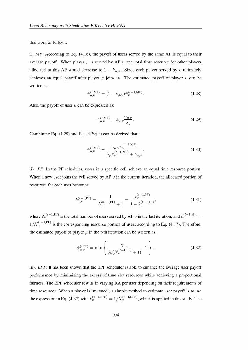
Load Balancing with Shadowing Effects for HLRNs
this work as follows:
i). MF: According to Eq. (4.16), the payoff of users served by the same AP is equal to their
average payoff. When player µ is served by AP υ, the total time resource for other players
allocated to this AP would decrease to 1 − kµ,υ. Since each player served by υ ultimately
achieves an equal payoff after player µ joins in. The estimated payoff of player µ can be
written as:
π(t,MF)µ,υ = (1− kµ,υ)π(t−1,MF)
υ . (4.28)
Also, the payoff of user µ can be expressed as:
π(t,MF)µ,υ = kµ,υ
γµ,υλµ
. (4.29)
Combining Eq. (4.28) and Eq. (4.29), it can be derived that:
π(t,MF)µ,υ =
γµ,υπ(t−1,MF)υ
λµπ(t−1,MF)υ + γµ,υ
. (4.30)
ii). PF: In the PF scheduler, users in a specific cell achieve an equal time resource portion.
When a new user joins the cell served by AP υ in the current iteration, the allocated portion of
resources for each user becomes:
k(t−1,PF)µ,υ =
1
N(t−1,PF)υ + 1
=k(t−1,PF)υ
1 + k(t−1,PF)υ
, (4.31)
whereN(t−1,PF)υ is the total number of users served by AP υ in the last iteration; and k
(t−1,PF)υ =
1/N(t−1,PF)υ is the corresponding resource portion of users according to Eq. (4.17). Therefore,
the estimated payoff of player µ in the t-th iteration can be written as:
π(t,PF)µ,υ = min
γi,υ
λi(N(t−1,PF)υ + 1)
, 1
. (4.32)
iii). EPF: It has been shown that the EPF scheduler is able to enhance the average user payoff
performance by minimising the excess of time slot resources while achieving a proportional
fairness. The EPF scheduler results in varying RA per user depending on their requirements of
time resources. When a player is ‘mutated’, a simple method to estimate user payoff is to use
the expression in Eq. (4.32) with k(t−1,EPF)υ = 1/N
(t−1,EPF)υ , which is applied in this study. The
104
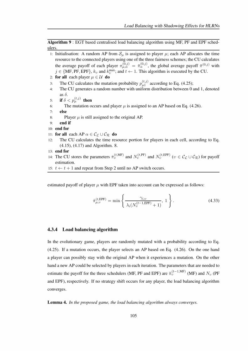
Load Balancing with Shadowing Effects for HLRNs
Algorithm 9 : EGT based centralised load balancing algorithm using MF, PF and EPF sched-
ulers.
1: Initialisation: A random AP from Sµ is assigned to player µ; each AP allocates the time
resource to the connected players using one of the three fairness schemes; the CU calculates
the average payoff of each player π(0,j)µ,α = π
(0,j)α , the global average payoff π(0,j) with
j ∈ MF,PF,EPF, kυ and kmaxυ ; and t← 1. This algorithm is executed by the CU.
2: for all each player µ ∈ U do
3: The CU calculates the mutation probability p(t,j)µ1 according to Eq. (4.25);
4: The CU generates a random number with uniform distribution between 0 and 1, denoted
as δ.5: if δ < p
(t,j)µ then
6: The mutation occurs and player µ is assigned to an AP based on Eq. (4.26).
7: else
8: Player µ is still assigned to the original AP.
9: end if
10: end for
11: for all each AP α ∈ CL ∪ CR do
12: The CU calculates the time resource portion for players in each cell, according to Eq.
(4.15), (4.17) and Algorithm. 8.
13: end for
14: The CU stores the parameters π(t,MF)υ and N
(t,PF)υ and N
(t,EPF)υ (υ ∈ CL ∪ CR) for payoff
estimation.
15: t← t+ 1 and repeat from Step 2 until no AP switch occurs.
estimated payoff of player µ with EPF taken into account can be expressed as follows:
π(t,EPF)µ,υ = min
γi,υ
λi(N(t−1,EPF)υ + 1)
, 1
. (4.33)
4.3.4 Load balancing algorithm
In the evolutionary game, players are randomly mutated with a probability according to Eq.
(4.25). If a mutation occurs, the player selects an AP based on Eq. (4.26). On the one hand
a player can possibly stay with the original AP when it experiences a mutation. On the other
hand a new AP could be selected by players in each iteration. The parameters that are needed to
estimate the payoff for the three schedulers (MF, PF and EPF) are π(t−1,MF)υ (MF) and Nυ (PF
and EPF), respectively. If no strategy shift occurs for any player, the load balancing algorithm
converges.
Lemma 4. In the proposed game, the load balancing algorithm always converges.
105
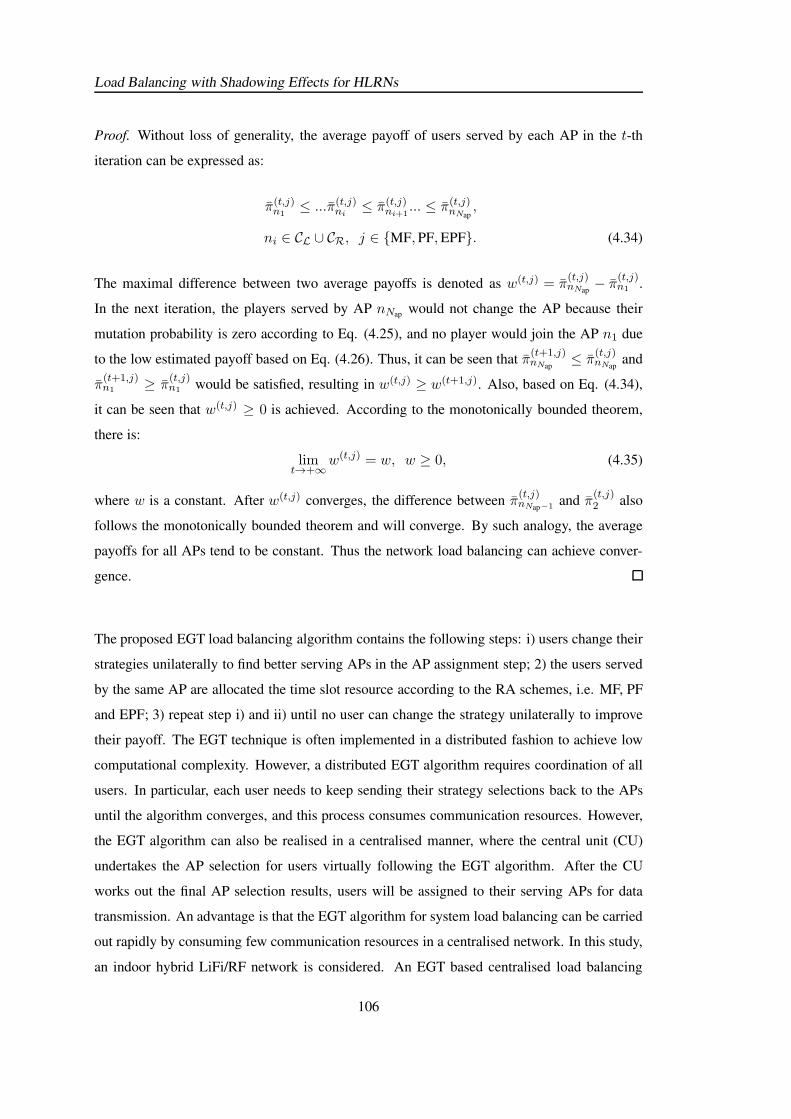
Load Balancing with Shadowing Effects for HLRNs
Proof. Without loss of generality, the average payoff of users served by each AP in the t-th
iteration can be expressed as:
π(t,j)n1≤ ...π(t,j)ni
≤ π(t,j)ni+1... ≤ π(t,j)nNap
,
ni ∈ CL ∪ CR, j ∈ MF,PF,EPF. (4.34)
The maximal difference between two average payoffs is denoted as w(t,j) = π(t,j)nNap− π(t,j)n1 .
In the next iteration, the players served by AP nNap would not change the AP because their
mutation probability is zero according to Eq. (4.25), and no player would join the AP n1 due
to the low estimated payoff based on Eq. (4.26). Thus, it can be seen that π(t+1,j)nNap
≤ π(t,j)nNapand
π(t+1,j)n1 ≥ π
(t,j)n1 would be satisfied, resulting in w(t,j) ≥ w(t+1,j). Also, based on Eq. (4.34),
it can be seen that w(t,j) ≥ 0 is achieved. According to the monotonically bounded theorem,
there is:
limt→+∞
w(t,j) = w, w ≥ 0, (4.35)
where w is a constant. After w(t,j) converges, the difference between π(t,j)nNap−1 and π
(t,j)2 also
follows the monotonically bounded theorem and will converge. By such analogy, the average
payoffs for all APs tend to be constant. Thus the network load balancing can achieve conver-
gence.
The proposed EGT load balancing algorithm contains the following steps: i) users change their
strategies unilaterally to find better serving APs in the AP assignment step; 2) the users served
by the same AP are allocated the time slot resource according to the RA schemes, i.e. MF, PF
and EPF; 3) repeat step i) and ii) until no user can change the strategy unilaterally to improve
their payoff. The EGT technique is often implemented in a distributed fashion to achieve low
computational complexity. However, a distributed EGT algorithm requires coordination of all
users. In particular, each user needs to keep sending their strategy selections back to the APs
until the algorithm converges, and this process consumes communication resources. However,
the EGT algorithm can also be realised in a centralised manner, where the central unit (CU)
undertakes the AP selection for users virtually following the EGT algorithm. After the CU
works out the final AP selection results, users will be assigned to their serving APs for data
transmission. An advantage is that the EGT algorithm for system load balancing can be carried
out rapidly by consuming few communication resources in a centralised network. In this study,
an indoor hybrid LiFi/RF network is considered. An EGT based centralised load balancing
106
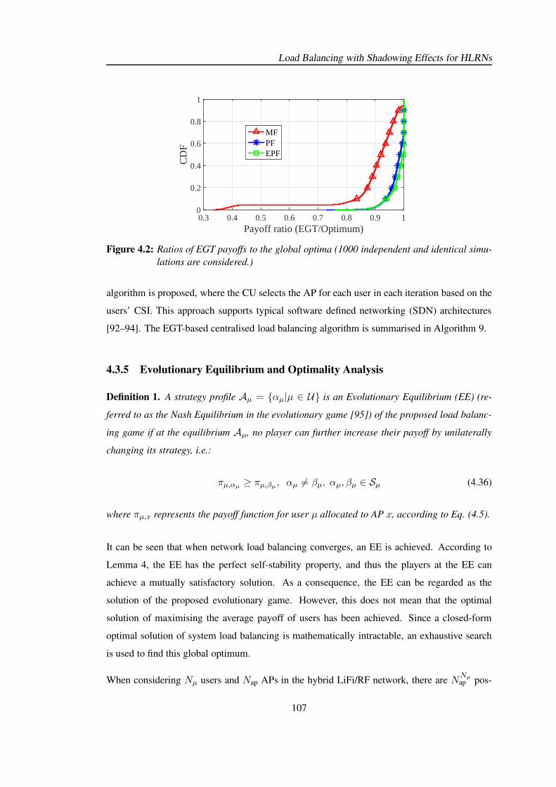
Load Balancing with Shadowing Effects for HLRNs
Payoff ratio (EGT/Optimum)0.3 0.4 0.5 0.6 0.7 0.8 0.9 1
CD
F
0
0.2
0.4
0.6
0.8
1
MFPFEPF
Figure 4.2: Ratios of EGT payoffs to the global optima (1000 independent and identical simu-
lations are considered.)
algorithm is proposed, where the CU selects the AP for each user in each iteration based on the
users’ CSI. This approach supports typical software defined networking (SDN) architectures
[92–94]. The EGT-based centralised load balancing algorithm is summarised in Algorithm 9.
4.3.5 Evolutionary Equilibrium and Optimality Analysis
Definition 1. A strategy profile Aµ = αµ|µ ∈ U is an Evolutionary Equilibrium (EE) (re-
ferred to as the Nash Equilibrium in the evolutionary game [95]) of the proposed load balanc-
ing game if at the equilibrium Aµ, no player can further increase their payoff by unilaterally
changing its strategy, i.e.:
πµ,αµ ≥ πµ,βµ, αµ 6= βµ, αµ, βµ ∈ Sµ (4.36)
where πµ,x represents the payoff function for user µ allocated to AP x, according to Eq. (4.5).
It can be seen that when network load balancing converges, an EE is achieved. According to
Lemma 4, the EE has the perfect self-stability property, and thus the players at the EE can
achieve a mutually satisfactory solution. As a consequence, the EE can be regarded as the
solution of the proposed evolutionary game. However, this does not mean that the optimal
solution of maximising the average payoff of users has been achieved. Since a closed-form
optimal solution of system load balancing is mathematically intractable, an exhaustive search
is used to find this global optimum.
When considering Nµ users and Nap APs in the hybrid LiFi/RF network, there are NNµap pos-
107
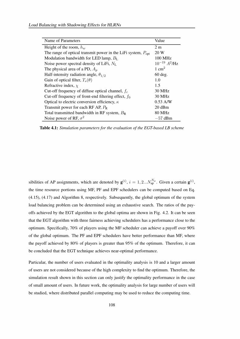
Load Balancing with Shadowing Effects for HLRNs
Name of Parameters Value
Height of the room, hw 2 m
The range of optical transmit power in the LiFi system, Popt 20 W
Modulation bandwidth for LED lamp, BL 100 MHz
Noise power spectral density of LiFi, NL 10−19 A2/Hz
The physical area of a PD, Ap 1 cm2
Half-intensity radiation angle, θ1/2 60 deg.
Gain of optical filter, Ts(θ) 1.0
Refractive index, χ 1.5
Cut-off frequency of diffuse optical channel, fc 30 MHz
Cut-off frequency of front-end filtering effect, f0 30 MHz
Optical to electric conversion efficiency, κ 0.53 A/W
Transmit power for each RF AP, PR 20 dBm
Total transmitted bandwidth in RF system, BR 80 MHz
Noise power of RF, σ2 −57 dBm
Table 4.1: Simulation parameters for the evaluation of the EGT-based LB scheme
sibilities of AP assignments, which are denoted by g(i), i = 1, 2...NNµap . Given a certain g(i),
the time resource portions using MF, PF and EPF schedulers can be computed based on Eq.
(4.15), (4.17) and Algorithm 8, respectively. Subsequently, the global optimum of the system
load balancing problem can be determined using an exhaustive search. The ratios of the pay-
offs achieved by the EGT algorithm to the global optima are shown in Fig. 4.2. It can be seen
that the EGT algorithm with three fairness achieving schedulers has a performance close to the
optimum. Specifically, 70% of players using the MF scheduler can achieve a payoff over 90%
of the global optimum. The PF and EPF schedulers have better performance than MF, where
the payoff achieved by 80% of players is greater than 95% of the optimum. Therefore, it can
be concluded that the EGT technique achieves near-optimal performance.
Particular, the number of users evaluated in the optimality analysis is 10 and a larger amount
of users are not considered because of the high complexity to find the optimum. Therefore, the
simulation result shown in this section can only justify the optimality performance in the case
of small amount of users. In future work, the optimality analysis for large number of users will
be studied, where distributed parallel computing may be used to reduce the computing time.
108
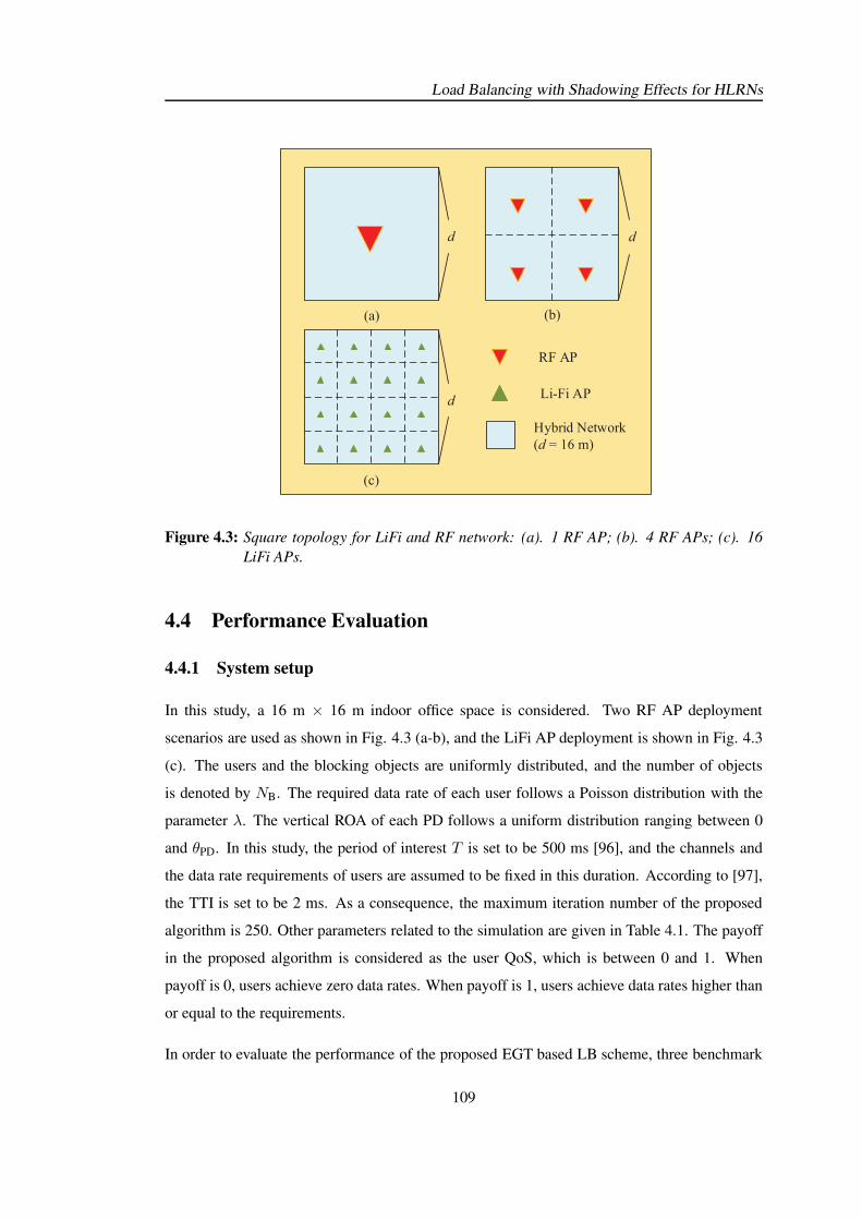
Load Balancing with Shadowing Effects for HLRNs
(b)(a)
(c)
d d
d
RF AP
Li-Fi AP
Hybrid Network
(d = 16 m)
Figure 4.3: Square topology for LiFi and RF network: (a). 1 RF AP; (b). 4 RF APs; (c). 16
LiFi APs.
4.4 Performance Evaluation
4.4.1 System setup
In this study, a 16 m × 16 m indoor office space is considered. Two RF AP deployment
scenarios are used as shown in Fig. 4.3 (a-b), and the LiFi AP deployment is shown in Fig. 4.3
(c). The users and the blocking objects are uniformly distributed, and the number of objects
is denoted by NB. The required data rate of each user follows a Poisson distribution with the
parameter λ. The vertical ROA of each PD follows a uniform distribution ranging between 0
and θPD. In this study, the period of interest T is set to be 500 ms [96], and the channels and
the data rate requirements of users are assumed to be fixed in this duration. According to [97],
the TTI is set to be 2 ms. As a consequence, the maximum iteration number of the proposed
algorithm is 250. Other parameters related to the simulation are given in Table 4.1. The payoff
in the proposed algorithm is considered as the user QoS, which is between 0 and 1. When
payoff is 0, users achieve zero data rates. When payoff is 1, users achieve data rates higher than
or equal to the requirements.
In order to evaluate the performance of the proposed EGT based LB scheme, three benchmark
109
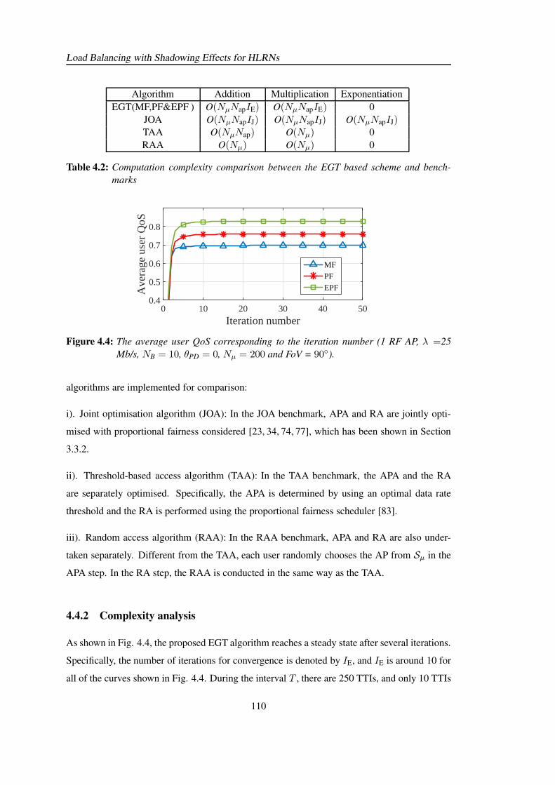
Load Balancing with Shadowing Effects for HLRNs
Algorithm Addition Multiplication Exponentiation
EGT(MF,PF&EPF ) O(NµNapIE) O(NµNapIE) 0
JOA O(NµNapIJ) O(NµNapIJ) O(NµNapIJ)TAA O(NµNap) O(Nµ) 0
RAA O(Nµ) O(Nµ) 0
Table 4.2: Computation complexity comparison between the EGT based scheme and bench-
marks
Iteration number0 10 20 30 40 50
Ave
rage
use
r Q
oS
0.4
0.5
0.6
0.7
0.8
MF
PF
EPF
Figure 4.4: The average user QoS corresponding to the iteration number (1 RF AP, λ =25
Mb/s, NB = 10, θPD = 0, Nµ = 200 and FoV = 90).
algorithms are implemented for comparison:
i). Joint optimisation algorithm (JOA): In the JOA benchmark, APA and RA are jointly opti-
mised with proportional fairness considered [23, 34, 74, 77], which has been shown in Section
3.3.2.
ii). Threshold-based access algorithm (TAA): In the TAA benchmark, the APA and the RA
are separately optimised. Specifically, the APA is determined by using an optimal data rate
threshold and the RA is performed using the proportional fairness scheduler [83].
iii). Random access algorithm (RAA): In the RAA benchmark, APA and RA are also under-
taken separately. Different from the TAA, each user randomly chooses the AP from Sµ in the
APA step. In the RA step, the RAA is conducted in the same way as the TAA.
4.4.2 Complexity analysis
As shown in Fig. 4.4, the proposed EGT algorithm reaches a steady state after several iterations.
Specifically, the number of iterations for convergence is denoted by IE, and IE is around 10 for
all of the curves shown in Fig. 4.4. During the interval T , there are 250 TTIs, and only 10 TTIs
110
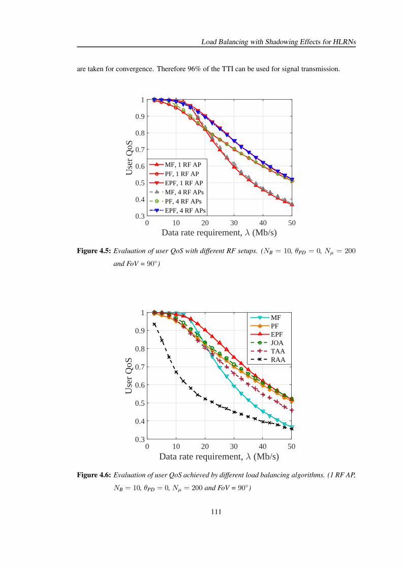
Load Balancing with Shadowing Effects for HLRNs
are taken for convergence. Therefore 96% of the TTI can be used for signal transmission.
Data rate requirement, λ (Mb/s)0 10 20 30 40 50
Use
r Q
oS
0.3
0.4
0.5
0.6
0.7
0.8
0.9
1
MF, 1 RF APPF, 1 RF APEPF, 1 RF APMF, 4 RF APsPF, 4 RF APsEPF, 4 RF APs
Figure 4.5: Evaluation of user QoS with different RF setups. (NB = 10, θPD = 0, Nµ = 200
and FoV = 90)
Data rate requirement, λ (Mb/s)0 10 20 30 40 50
Use
r Q
oS
0.3
0.4
0.5
0.6
0.7
0.8
0.9
1MFPFEPFJOATAARAA
Figure 4.6: Evaluation of user QoS achieved by different load balancing algorithms. (1 RF AP,
NB = 10, θPD = 0, Nµ = 200 and FoV = 90)
111
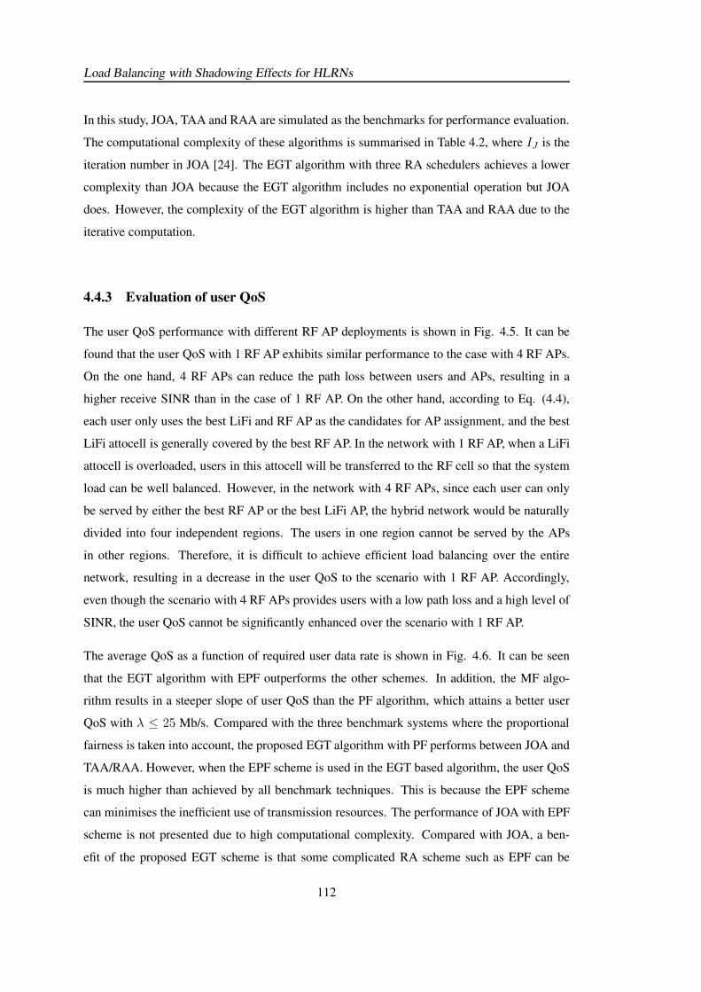
Load Balancing with Shadowing Effects for HLRNs
In this study, JOA, TAA and RAA are simulated as the benchmarks for performance evaluation.
The computational complexity of these algorithms is summarised in Table 4.2, where IJ is the
iteration number in JOA [24]. The EGT algorithm with three RA schedulers achieves a lower
complexity than JOA because the EGT algorithm includes no exponential operation but JOA
does. However, the complexity of the EGT algorithm is higher than TAA and RAA due to the
iterative computation.
4.4.3 Evaluation of user QoS
The user QoS performance with different RF AP deployments is shown in Fig. 4.5. It can be
found that the user QoS with 1 RF AP exhibits similar performance to the case with 4 RF APs.
On the one hand, 4 RF APs can reduce the path loss between users and APs, resulting in a
higher receive SINR than in the case of 1 RF AP. On the other hand, according to Eq. (4.4),
each user only uses the best LiFi and RF AP as the candidates for AP assignment, and the best
LiFi attocell is generally covered by the best RF AP. In the network with 1 RF AP, when a LiFi
attocell is overloaded, users in this attocell will be transferred to the RF cell so that the system
load can be well balanced. However, in the network with 4 RF APs, since each user can only
be served by either the best RF AP or the best LiFi AP, the hybrid network would be naturally
divided into four independent regions. The users in one region cannot be served by the APs
in other regions. Therefore, it is difficult to achieve efficient load balancing over the entire
network, resulting in a decrease in the user QoS to the scenario with 1 RF AP. Accordingly,
even though the scenario with 4 RF APs provides users with a low path loss and a high level of
SINR, the user QoS cannot be significantly enhanced over the scenario with 1 RF AP.
The average QoS as a function of required user data rate is shown in Fig. 4.6. It can be seen
that the EGT algorithm with EPF outperforms the other schemes. In addition, the MF algo-
rithm results in a steeper slope of user QoS than the PF algorithm, which attains a better user
QoS with λ ≤ 25 Mb/s. Compared with the three benchmark systems where the proportional
fairness is taken into account, the proposed EGT algorithm with PF performs between JOA and
TAA/RAA. However, when the EPF scheme is used in the EGT based algorithm, the user QoS
is much higher than achieved by all benchmark techniques. This is because the EPF scheme
can minimises the inefficient use of transmission resources. The performance of JOA with EPF
scheme is not presented due to high computational complexity. Compared with JOA, a ben-
efit of the proposed EGT scheme is that some complicated RA scheme such as EPF can be
112
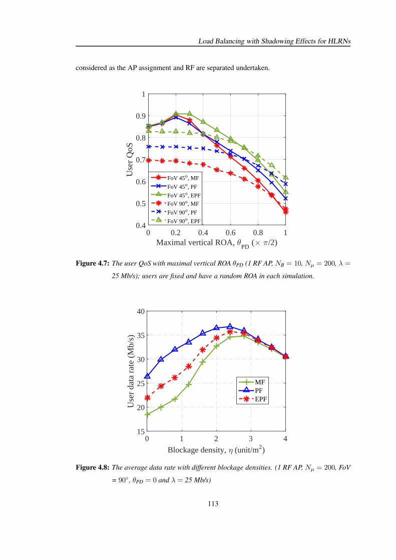
Load Balancing with Shadowing Effects for HLRNs
considered as the AP assignment and RF are separated undertaken.
Maximal vertical ROA, θPD
(× π/2)0 0.2 0.4 0.6 0.8 1
Use
r Q
oS
0.4
0.5
0.6
0.7
0.8
0.9
1
FoV 45o, MF
FoV 45o, PF
FoV 45o, EPF
FoV 90o, MF
FoV 90o, PF
FoV 90o, EPF
Figure 4.7: The user QoS with maximal vertical ROA θPD (1 RF AP,NB = 10, Nµ = 200, λ =
25 Mb/s); users are fixed and have a random ROA in each simulation.
Blockage density, η (unit/m2)
0 1 2 3 4
Use
r da
ta r
ate
(Mb/
s)
15
20
25
30
35
40
MFPFEPF
Figure 4.8: The average data rate with different blockage densities. (1 RF AP, Nµ = 200, FoV
= 90, θPD = 0 and λ = 25 Mb/s)
113
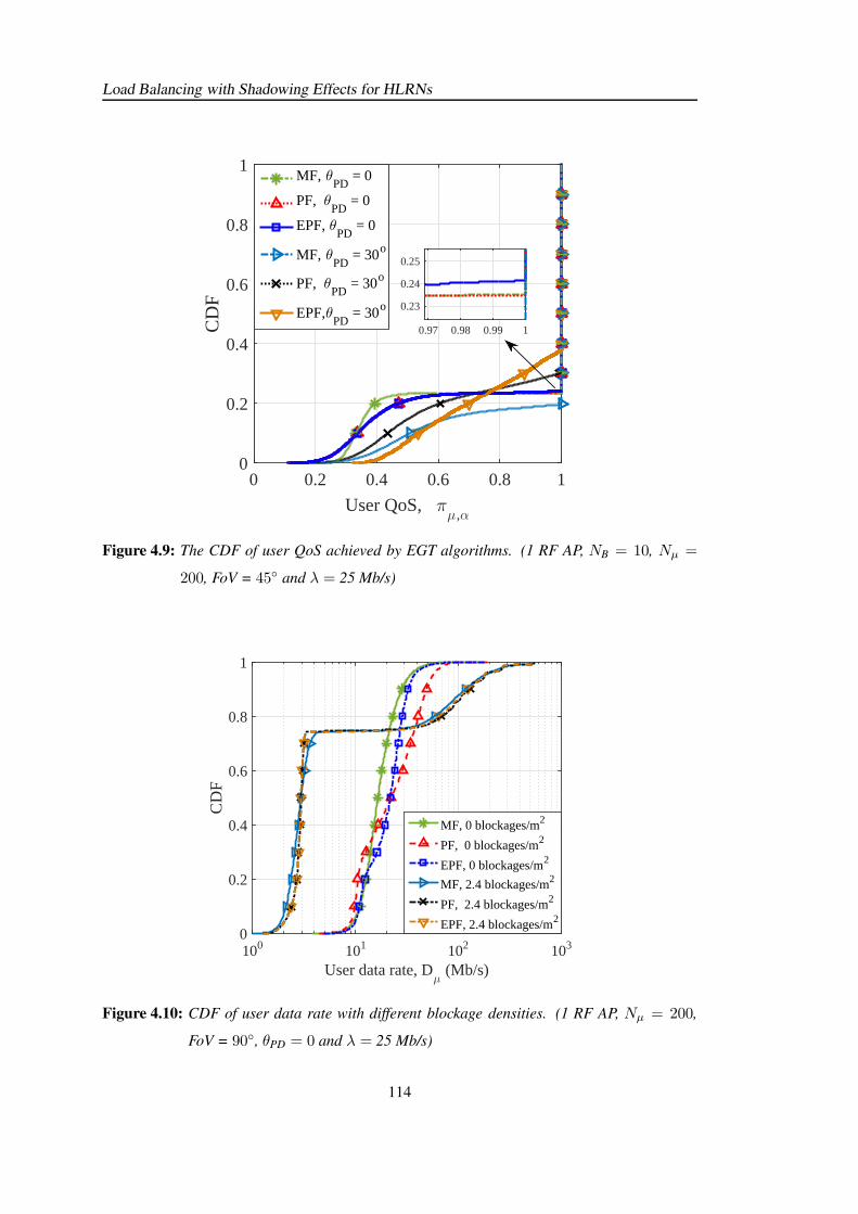
Load Balancing with Shadowing Effects for HLRNs
User QoS, πµ,α
0 0.2 0.4 0.6 0.8 1
CD
F
0
0.2
0.4
0.6
0.8
1MF, θ
PD = 0
PF, θPD
= 0
EPF, θPD
= 0
MF, θPD
= 30o
PF, θPD
= 30o
EPF,θPD
= 30o
0.97 0.98 0.99 1
0.23
0.24
0.25
Figure 4.9: The CDF of user QoS achieved by EGT algorithms. (1 RF AP, NB = 10, Nµ =
200, FoV = 45 and λ = 25 Mb/s)
User data rate, Dµ
(Mb/s)100 101 102 103
CD
F
0
0.2
0.4
0.6
0.8
1
MF, 0 blockages/m2
PF, 0 blockages/m2
EPF, 0 blockages/m2
MF, 2.4 blockages/m2
PF, 2.4 blockages/m2
EPF, 2.4 blockages/m2
Figure 4.10: CDF of user data rate with different blockage densities. (1 RF AP, Nµ = 200,
FoV = 90, θPD = 0 and λ = 25 Mb/s)
114
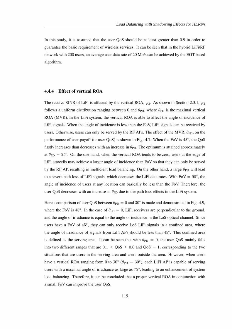
Load Balancing with Shadowing Effects for HLRNs
In this study, it is assumed that the user QoS should be at least greater than 0.9 in order to
guarantee the basic requirement of wireless services. It can be seen that in the hybrid LiFi/RF
network with 200 users, an average user data rate of 20 Mb/s can be achieved by the EGT based
algorithm.
4.4.4 Effect of vertical ROA
The receive SINR of LiFi is affected by the vertical ROA, ϕ2. As shown in Section 2.3.1, ϕ2
follows a uniform distribution ranging between 0 and θPD, where θPD is the maximal vertical
ROA (MVR). In the LiFi system, the vertical ROA is able to affect the angle of incidence of
LiFi signals. When the angle of incidence is less than the FoV, LiFi signals can be received by
users. Otherwise, users can only be served by the RF APs. The effect of the MVR, θPD, on the
performance of user payoff (or user QoS) is shown in Fig. 4.7. When the FoV is 45, the QoS
firstly increases than decreases with an increase in θPD. The optimum is attained approximately
at θPD = 25. On the one hand, when the vertical ROA tends to be zero, users at the edge of
LiFi attocells may achieve a larger angle of incidence than FoV so that they can only be served
by the RF AP, resulting in inefficient load balancing. On the other hand, a large θPD will lead
to a severe path loss of LiFi signals, which decreases the LiFi data rates. With FoV = 90, the
angle of incidence of users at any location can basically be less than the FoV. Therefore, the
user QoS decreases with an increase in θPD due to the path loss effects in the LiFi system.
Here a comparison of user QoS between θPD = 0 and 30 is made and demonstrated in Fig. 4.9,
where the FoV is 45. In the case of θPD = 0, LiFi receivers are perpendicular to the ground,
and the angle of irradiance is equal to the angle of incidence in the LoS optical channel. Since
users have a FoV of 45, they can only receive LoS LiFi signals in a confined area, where
the angle of irradiance of signals from LiFi APs should be less than 45. This confined area
is defined as the serving area. It can be seen that with θPD = 0, the user QoS mainly falls
into two different ranges that are 0.1 ≤ QoS ≤ 0.6 and QoS = 1, corresponding to the two
situations that are users in the serving area and users outside the area. However, when users
have a vertical ROA ranging from 0 to 30 (θPD = 30), each LiFi AP is capable of serving
users with a maximal angle of irradiance as large as 75, leading to an enhancement of system
load balancing. Therefore, it can be concluded that a proper vertical ROA in conjunction with
a small FoV can improve the user QoS.
115
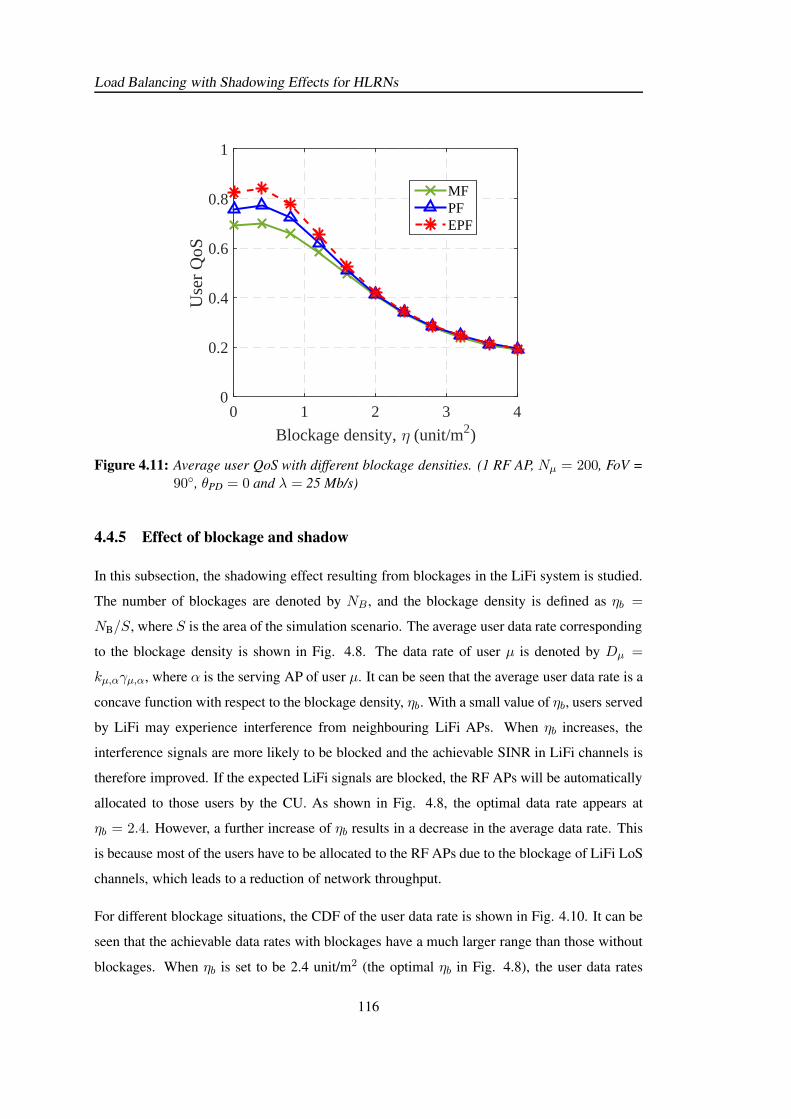
Load Balancing with Shadowing Effects for HLRNs
Blockage density, η (unit/m2)
0 1 2 3 4
Use
r Q
oS
0
0.2
0.4
0.6
0.8
1
MFPFEPF
Figure 4.11: Average user QoS with different blockage densities. (1 RF AP, Nµ = 200, FoV =
90, θPD = 0 and λ = 25 Mb/s)
4.4.5 Effect of blockage and shadow
In this subsection, the shadowing effect resulting from blockages in the LiFi system is studied.
The number of blockages are denoted by NB , and the blockage density is defined as ηb =
NB/S, where S is the area of the simulation scenario. The average user data rate corresponding
to the blockage density is shown in Fig. 4.8. The data rate of user µ is denoted by Dµ =
kµ,αγµ,α, where α is the serving AP of user µ. It can be seen that the average user data rate is a
concave function with respect to the blockage density, ηb. With a small value of ηb, users served
by LiFi may experience interference from neighbouring LiFi APs. When ηb increases, the
interference signals are more likely to be blocked and the achievable SINR in LiFi channels is
therefore improved. If the expected LiFi signals are blocked, the RF APs will be automatically
allocated to those users by the CU. As shown in Fig. 4.8, the optimal data rate appears at
ηb = 2.4. However, a further increase of ηb results in a decrease in the average data rate. This
is because most of the users have to be allocated to the RF APs due to the blockage of LiFi LoS
channels, which leads to a reduction of network throughput.
For different blockage situations, the CDF of the user data rate is shown in Fig. 4.10. It can be
seen that the achievable data rates with blockages have a much larger range than those without
blockages. When ηb is set to be 2.4 unit/m2 (the optimal ηb in Fig. 4.8), the user data rates
116
Load Balancing with Shadowing Effects for HLRNs
would basically be classified into two groups: [0, 4] Mb/s and [30, 600] Mb/s. Compared
with the non-blockage case, 72% of the users in the blockage scenario experience a data rate
degradation, while the remaining users achieve a significant data rate improvement. This means
that although a blockage density of 2.4 unit/m2 results in the largest average user data rate,
more than half of the users in this case have to be served by RF APs and achieve a low data
rate. Moreover, 28% of the users can obtain plenty of LiFi communication resources but their
achievable data rates are much higher than required. Fig. 4.11 shows that when considering the
required data rate of users, the QoS increases at the low blockage densities but decreases with
a further increase in ηb. This indicates that an increase in blockage density cannot provide a
better user experience despite achieving an improvement of the sum data rate.
4.5 Summary
In this chapter, in order to model a practical hybrid LiFi/RF network scenario, three factors are
taken into account: blockages, LiFi ROA and user data rate requirement. An EGT based load
balancing algorithm is proposed to improve the user QoS. Also, an enhanced proportional fair-
ness scheduler is proposed to maximise the usage of communication resources in the RA step.
The effects of the maximal vertical ROA and blockages on the hybrid network are evaluated
and discussed. Three conclusions are drawn based on the simulation results: (i) The proposed
EGT load balancing algorithm achieves a better performance/complexity trade-off than the con-
ventional algorithms. In addition, when the EPF scheme is used, a high level of user QoS can
be attained due to a more efficient exploitation of transmission resources; (ii) When the FoV
of LiFi receivers is 90, the average user QoS decreases with an increase in the maximal ver-
tical ROA θPD. However, when considering a small FoV, there is an optimum of the maximal
vertical ROA that can optimise the QoS performance, leading to improved system load balanc-
ing ; (iii) Given the simulation scenario, an optimal blockage density of ηb = 2.4 unit/m2 can
maximise the system sum data rate. However, when considering user data rate requirement, the
user QoS decreases with an increase in ηb as the blockages cause an inefficient allocation of
communication resources.
117

118
Chapter 5Optimisation of Packet Flow
Assignment for HLRNs
5.1 Introduction
In hybrid LiFi and RF networks (HLRNs), an efficient AP assignment can significantly affect
the overall quality of service (QoS). Many current research efforts have been paid towards im-
proving the performance of hybrid networks. In [23, 24], a centralised load balancing (LB)
scheme is proposed, aiming to maximise the system sum data rate with certain fairness sched-
ulers. In [81, 98, 99], dynamic load balancing is studied, where handovers between different
APs are considered. In [99], a fuzzy logic based scheme is proposed, which readily integrates
static load balancing with direct handover schemes. In [81], a Markov decision process (MDP)
based vertical handover scheme was proposed for hybrid networks consisting of one LiFi AP
and one RF AP. This work aims to find a trade-off solution to reduce the handover cost with-
out significantly sacrificing the system throughput. The aforementioned works primarily focus
on the improvement of data rate performance. In Chapter 3 and 4, the optimisation-based LB
schemes and the evolutionary game theory based LB scheme for HLRNs are proposed, which
also concentrate on load balancing in the physical layer. However, the system delay, which is
essential to the user’s QoS, also needs to be studied for hybrid networks. In [21], the delay
modelling of hybrid visible light communication (VLC) and wireless fidelity (WiFi) networks
has been investigated. In this work, the M/D/1 queuing model is considered and the capaci-
ties with respect to the asymmetric VLC/WiFi and hybrid VLC/WiFi networks are compared.
In [1], the analysis of system delay in hybrid LiFi/RF networks is undertaken, where M/M/1
model is applied. However, all of these works assume that the LiFi users achieve an equal data
rate. In practice, the LiFi data rate significantly depends on the distance between the LiFi APs
and the users [17]. Therefore, the distribution of user data rates must be taken into account
when the system delay is evaluated.
In this chapter, a two-tier buffer framework for hybrid LiFi/RF networks is considered. Specif-
ically, the arrival packets will be initially queued in the buffer of a central unit (CU). The CU
119
Optimisation of Packet Flow Assignment for HLRNs
coordinates all of the APs and carries out AP assignment for packet flow. According to the
AP assignment results, the packets in the CU buffer will be delivered to the buffers of serving
APs, and then transmitted to the target users via wireless channels. In this study, the notion of a
‘LiFi service ratio’ is introduced, which signifies the proportion of users that are served by LiFi
APs. With the practical distribution of LiFi data rates considered, an analytical solution to the
optimum LiFi service ratio is derived. Based on this optimum LiFi service ratio, a novel AP
assignment scheme is proposed which is able to minimise the overall system delay. The main
contributions of this paper are summarised below:
• An analytical solution to the optimum LiFi service ratio for hybrid LiFi/RF networks
is provided. A comparison between the analytical results and simulation results is con-
ducted.
• Based on the analytical optimum LiFi service ratio, a low-complexity cross-layer load
balancing scheme for hybrid LiFi/RF network is proposed to minimise the average packet
delay.
• For various AP assignment schemes, the effects of different network setups on the packet
delay are numerically studied.
The rest of the chapter is organised as follows. The system model of the hybrid LiFi/RF network
is introduced in Section 5.2. The system delay is analysed and an AP assignment scheme to
minimise packet delay is proposed in Section 5.3. The performance evaluation is given in
Section 5.4 and the summary is presented in Section 5.5.
5.2 System Model
Referring to Fig. 5.1, a downlink hybrid LiFi/RF network for an indoor environment is consid-
ered. This hybrid network is covered by several LiFi attocells and a RF cell. The system model
of hybrid LiFi and RF networks refers to Section 2.1-2.2. The deployment of LiFi APs follows
a square lattice topology which models a regular light placement commonly used in large of-
fices and public places. The set of LiFi APs is denoted by CL = l|l ∈ [1, Nl], l ∈ N, where
Nl is the number of LiFi APs. It is assumed that the photo diode (PD) at each user is oriented
perpendicularly to the ceiling. This means that the angle of irradiance is equal to the angle of
incidence in the LoS optical channel. The RF AP is considered to offer a ubiquitous coverage
120
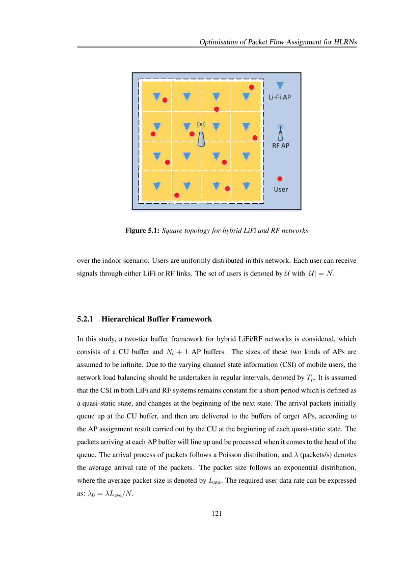
Optimisation of Packet Flow Assignment for HLRNs
Li-Fi AP
RF AP
User
RF A
Figure 5.1: Square topology for hybrid LiFi and RF networks
over the indoor scenario. Users are uniformly distributed in this network. Each user can receive
signals through either LiFi or RF links. The set of users is denoted by U with |U| = N .
5.2.1 Hierarchical Buffer Framework
In this study, a two-tier buffer framework for hybrid LiFi/RF networks is considered, which
consists of a CU buffer and Nl + 1 AP buffers. The sizes of these two kinds of APs are
assumed to be infinite. Due to the varying channel state information (CSI) of mobile users, the
network load balancing should be undertaken in regular intervals, denoted by Tp. It is assumed
that the CSI in both LiFi and RF systems remains constant for a short period which is defined as
a quasi-static state, and changes at the beginning of the next state. The arrival packets initially
queue up at the CU buffer, and then are delivered to the buffers of target APs, according to
the AP assignment result carried out by the CU at the beginning of each quasi-static state. The
packets arriving at each AP buffer will line up and be processed when it comes to the head of the
queue. The arrival process of packets follows a Poisson distribution, and λ (packets/s) denotes
the average arrival rate of the packets. The packet size follows an exponential distribution,
where the average packet size is denoted by Lave. The required user data rate can be expressed
as: λ0 = λLave/N .
121
Optimisation of Packet Flow Assignment for HLRNs
5.2.1.1 Delay in the CU Buffer
The data packets from remote content providers initially queue at the CU buffer. Following the
first-in-first-out rule, each packet is delivered to the target AP via Ethernet cables with a data
rate of Rb. Let t<m>a,cu denote the arrival time of the m-th packet at the CU buffer. The queuing
time of this packet in the CU buffer can be expressed as:
τ<m>q,cu = [τ<m−1>
q,cu + τ<m−1>p,cu − (t<m>
a,cu − t<m−1>a,cu )]+, (5.1)
where τ<m−1>p,cu is the packet transmission time from the CU buffer to the host AP; and [.]+ is
the maximum operator, max( . , 0). For the first packet, the queuing time is zero, i.e. τ<1>q,cu = 0.
According to Eq. (5.1), the arrival time of the m-th packet at the buffer of serving AP can be
expressed as:
t<m>a,ap = t<m>
a,cu + τ<m>q,cu + τ<m>
p,cu . (5.2)
Therefore, the delay of the m-th packet in the CU buffer can be expressed as:
∆T<m>CU = τ<m>
q,cu + τ<m>p,cu . (5.3)
5.2.1.2 Delay in AP Buffers
Based on the AP assignment determined by the CU, all of the packets will be allocated to the
target APs. The arrival packets queue in line in each AP buffer and would be processed by the
corresponding APs independently, following the first-in-first-out rule. Similar to Eq. (5.1), the
arrival time of the q-th packet at the target user can be expressed as:
t<q>a,user = t<q>
a,ap + τ<q>q,ap + τ<q>
p,ap , (5.4)
where τ<q>p,ap is the packet transmission time from the AP to the user; and τ<q>
q,ap is the queuing
time at the AP buffer. The delay for the q-th packet in the AP buffer can be expressed as:
∆T<q>AP = τ<q>
q,ap + τ<q>p,ap . (5.5)
Therefore, the total delay for the p-th packet in the hybrid LiFi/RF network is written as:
∆T<p> = ∆T<p>CU +∆T<p>
AP . (5.6)
122
Optimisation of Packet Flow Assignment for HLRNs
5.2.2 Downlink capacity achieved by LiFi and RF APs
In this study, the LiFi channel model shown in Section 2.3.1 is considered, where field-of-view
(FoV) path loss, front-end filtering effect and multi-path effect are taken into account. The link
data rate between user µ and LiFi AP α is denoted as Rµ,α. The RF channel model is given
in Section 2.4.1, and the link data rate between user µ and the RF AP is denoted by Rµ,RF. In
order to reduce the complexity of AP assignment, the receivers are only served by the LiFi AP
with the highest link data rate performance or the RF AP. It is assumed that αµ denotes the LiFi
AP which offers highest link data rate to user µ.
In hybrid LiFi/RF networks, LiFi AP offers very high spatial spectral efficiency. Thus, users
achieving a high quality of optical channels will be assigned to a LiFi AP, and those with a low
quality of optical channels are assigned to the RF AP. Without loss of generality, the achievable
LiFi data rates of each user follows:
Rµ1,αµ1≥ ...Rµ2,αµ2
≥ RµN−1,αµN−1... ≥ RµN ,αµN
;
µi ∈ U , i = 1, 2, ...N.
It is assumed that the first n users with the highest LiFi data rate are assigned to LiFi APs and
users from µn+1 to µN are served by the RF AP. The parameter γ = n/N is defined as the
“LiFi service ratio”. The average data rate achieved by LiFi can be written as a function with
respect to γ, expressed as:
CL(γ) =1
⌊γN⌋
⌊γN⌋∑
i=1
Rµi,αµi, (5.7)
where ⌊.⌋ is the floor operator. In addition, the average data rate achieved by RF corresponding
to γ can be written as:
CR(γ) =1
N − ⌊γN⌋
N∑
i=⌊γN⌋+1
Rµi,RF. (5.8)
In this study, the polynomial fitting method is applied to find the closed-form solutions toCL(γ)
and CR(γ) [17]. As shown in Fig. 5.1, a square topology of LiFi APs is considered and the RF
AP is settled in the centre of the network. It is assumed that users are uniformly distributed in
this hybrid LiFi/RF network, and Monte Carlo simulations are undertaken to estimate CL(γ)
and CR(γ). Fig. 5.2 shows that CL(γ) is a monotonic function of γ, and this function can
be fitted by a first-order polynomial very well. Therefore, a first-order polynomial is used to
123
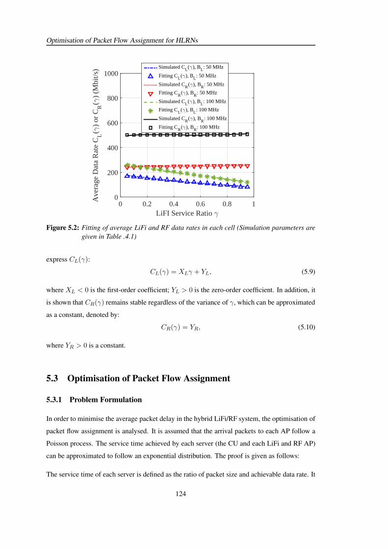
Optimisation of Packet Flow Assignment for HLRNs
LiFI Service Ratio γ0 0.2 0.4 0.6 0.8 1
Ave
rage
Dat
a R
ate
CL
(γ)
or C
R(γ
) (M
bit/s
)
0
200
400
600
800
1000Simulated CL(γ), BL: 50 MHz
Fitting CL(γ), BL: 50 MHz
Simulated CR(γ), BR: 50 MHz
Fitting CR(γ), BR: 50 MHz
Simulated CL(γ), BL: 100 MHz
Fitting CL(γ), BL: 100 MHz
Simulated CR(γ), BR: 100 MHz
Fitting CR(γ), BR: 100 MHz
Figure 5.2: Fitting of average LiFi and RF data rates in each cell (Simulation parameters are
given in Table .4.1)
express CL(γ):
CL(γ) = XLγ + YL, (5.9)
where XL < 0 is the first-order coefficient; YL > 0 is the zero-order coefficient. In addition, it
is shown that CR(γ) remains stable regardless of the variance of γ, which can be approximated
as a constant, denoted by:
CR(γ) = YR, (5.10)
where YR > 0 is a constant.
5.3 Optimisation of Packet Flow Assignment
5.3.1 Problem Formulation
In order to minimise the average packet delay in the hybrid LiFi/RF system, the optimisation of
packet flow assignment is analysed. It is assumed that the arrival packets to each AP follow a
Poisson process. The service time achieved by each server (the CU and each LiFi and RF AP)
can be approximated to follow an exponential distribution. The proof is given as follows:
The service time of each server is defined as the ratio of packet size and achievable data rate. It
124
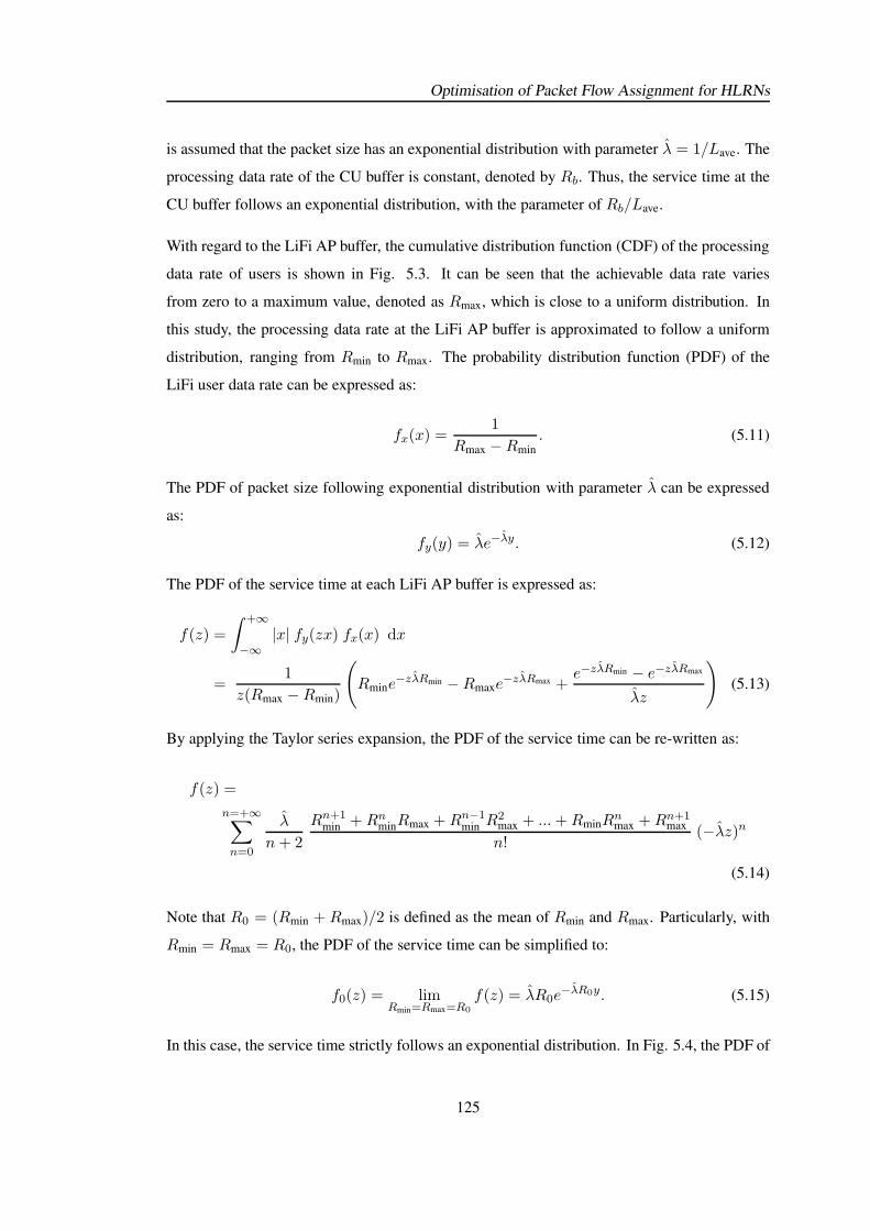
Optimisation of Packet Flow Assignment for HLRNs
is assumed that the packet size has an exponential distribution with parameter λ = 1/Lave. The
processing data rate of the CU buffer is constant, denoted by Rb. Thus, the service time at the
CU buffer follows an exponential distribution, with the parameter of Rb/Lave.
With regard to the LiFi AP buffer, the cumulative distribution function (CDF) of the processing
data rate of users is shown in Fig. 5.3. It can be seen that the achievable data rate varies
from zero to a maximum value, denoted as Rmax, which is close to a uniform distribution. In
this study, the processing data rate at the LiFi AP buffer is approximated to follow a uniform
distribution, ranging from Rmin to Rmax. The probability distribution function (PDF) of the
LiFi user data rate can be expressed as:
fx(x) =1
Rmax −Rmin
. (5.11)
The PDF of packet size following exponential distribution with parameter λ can be expressed
as:
fy(y) = λe−λy. (5.12)
The PDF of the service time at each LiFi AP buffer is expressed as:
f(z) =
∫ +∞
−∞|x| fy(zx) fx(x) dx
=1
z(Rmax −Rmin)
(
Rmine−zλRmin −Rmaxe
−zλRmax +e−zλRmin − e−zλRmax
λz
)
(5.13)
By applying the Taylor series expansion, the PDF of the service time can be re-written as:
f(z) =
n=+∞∑
n=0
λ
n+ 2
Rn+1min +Rn
minRmax +Rn−1min R
2max + ...+RminR
nmax +Rn+1
max
n!(−λz)n
(5.14)
Note that R0 = (Rmin + Rmax)/2 is defined as the mean of Rmin and Rmax. Particularly, with
Rmin = Rmax = R0, the PDF of the service time can be simplified to:
f0(z) = limRmin=Rmax=R0
f(z) = λR0e−λR0y. (5.15)
In this case, the service time strictly follows an exponential distribution. In Fig. 5.4, the PDF of
125
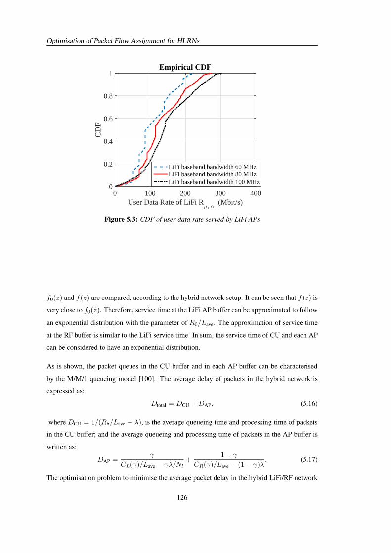
Optimisation of Packet Flow Assignment for HLRNs
User Data Rate of LiFi Rµ, α
(Mbit/s)0 100 200 300 400
CD
F
0
0.2
0.4
0.6
0.8
1Empirical CDF
LiFi baseband bandwidth 60 MHzLiFi baseband bandwidth 80 MHzLiFi baseband bandwidth 100 MHz
Figure 5.3: CDF of user data rate served by LiFi APs
f0(z) and f(z) are compared, according to the hybrid network setup. It can be seen that f(z) is
very close to f0(z). Therefore, service time at the LiFi AP buffer can be approximated to follow
an exponential distribution with the parameter of R0/Lave. The approximation of service time
at the RF buffer is similar to the LiFi service time. In sum, the service time of CU and each AP
can be considered to have an exponential distribution.
As is shown, the packet queues in the CU buffer and in each AP buffer can be characterised
by the M/M/1 queueing model [100]. The average delay of packets in the hybrid network is
expressed as:
Dtotal = DCU +DAP, (5.16)
where DCU = 1/(Rb/Lave − λ), is the average queueing time and processing time of packets
in the CU buffer; and the average queueing and processing time of packets in the AP buffer is
written as:
DAP =γ
CL(γ)/Lave − γλ/Nl+
1− γCR(γ)/Lave − (1− γ)λ. (5.17)
The optimisation problem to minimise the average packet delay in the hybrid LiFi/RF network
126
Optimisation of Packet Flow Assignment for HLRNs
z0 10 20 30 40 50
0
0.05
0.1
0.15
0.2
0.25
f(z), Rmax
: 300 Mbit/s
f0(z), R
max: 300 Mbit/s
f(z), Rmax
: 200 Mbit/s
f0(z), R
max: 200 Mbit/s
Figure 5.4: Comparison between PDF f(z) and f0(z). (Rmin = 0, and the other parameters
are shown in Table. 4.1)
can be formulated as:
minγ
DCU +DAP (5.18)
s.t. 0 ≤ γ ≤ 1; (5.19)
CL(γ)/Lave − γλ/Nl > 0; (5.20)
CR(γ)/Lave − (1− γ)λ > 0; (5.21)
5.3.2 Analysis of feasible region
In order to avoid traffic blockages in the AP buffers, the variable γ should meet the constraints
in Eq. (5.20) and (5.21). According to the constraint in Eq. (5.20), it can be obtained that:
γ <YLNl
Lave(λ−XLNl), (5.22)
where YLNl
Lave(λ−XLNl)> 0 is always satisfied due to XL < 0 and YL, Nl, Lave, λ > 0. Also,
according to the constraint in Eq. (5.21), it can be obtained that:
γ > 1− YRλLave
, (5.23)
127

Optimisation of Packet Flow Assignment for HLRNs
where 1− YR/λLave < 1 is always satisfied.
Based on Eq. (5.22) and Eq. (5.23), it can be derived that
1− YRλLave
< γ <YLNl
Lave(λ−XLNl). (5.24)
Combining the condition in Eq.(5.19), the feasible region can be expressed as
γmin ≤ γ ≤ γmax (5.25)
where γmin = max1 − YR
λLave, 0 is the lower bound of the feasible region and γmax =
min YLNl
Lave(λ−XLNl), 1 is the upper bound of the feasible region. The condition that γmin is
included in the feasible region is 1 − YR
λLave< 0 and the condition that γmax is included is
YLNl
Lave(λ−XLNl)> 1.
In order to guarantee that the feasible region is effective, the condition below should be satisfied:
1− YRλLave
<YLNl
Lave(λ−XLNl). (5.26)
Otherwise, the feasible region will be a null set.
5.3.3 Solution to the optimisation problem
In this section, the solution to the optimisation problem in Eq. (5.18) is provided. The objective
function of this optimisation problem is expressed as:
G(γ) =1
Rb/Lave − λ+
γLave
(XL − λLave/Nl)γ + YL+
(1− γ)Lave
λLaveγ + YR − λLave
(5.27)
Its first order derivative corresponding to γ can be expressed as:
dG(γ)
dγ=
dg0(γ)dγ g1(γ)− dg1(γ)
dγ g0(γ)
g21(γ), (g1(γ) > 0) (5.28)
where we have
g0(γ) = x0γ2 + y0γ + z0
g1(γ) = x1γ2 + y1γ + z1
; (5.29)
128

Optimisation of Packet Flow Assignment for HLRNs
and the coefficients in Eq. (5.29) are listed as follows:
x0 = λL2ave(1 + 1/Nl)− LaveXL,
x1 = λLave(XL − λLave/Nl),
y0 = YRLave +XLLave − YL − λL2ave(1 + 1/Nl),
y1 = λLaveYL + (YR − λLave)(XL − λLave/Nl),
z0 = YLLave, z1 = YL(YR − λLave). (5.30)
The optimum γ can be obtained by making the gradient of the objective function in Eq. (5.28)
equal to 0, which can be written as:
dg0(γ)
dγg1(γ)−
dg1(γ)
dγg0(γ) = 0. (5.31)
By using the coefficients in Eq. (5.30), the function in Eq. (5.31) can be transferred to:
(x0y1 − x1y0)γ2 + 2(x0z1 − x1z0)γ + y0z1 − y1z0 = 0. (5.32)
It can be seen from Eq. (5.32) that there are at most two extreme points for the objective
function. The discriminant of the function in Eq. (5.32) is denoted by:
∆ = 4(x0z1 − x1z0)2 − 4(x0y1 − x1y0)(y0z1 − y1z0). (5.33)
When ∆ > 0 is satisfied, the set of extreme points for the objective function can be expressed
as:
R = 2(x1z0 − x0z1) +√∆
2(x0y1 − x1y0),2(x1z0 − x0z1)−
√∆
2(x0y1 − x1y0). (5.34)
When ∆ = 0 is achieved, the set of extreme points can be written as:
R = x1z0 − x0z1x0y1 − x1y0
. (5.35)
When ∆ < 0 is satisfied, the set of extreme points isR = ∅.
According to the feasible region of the optimisation problem shown in Eq. (5.25), the opti-
mum γ can be obtained by finding the minimum G(γ) among γ ∈ R, where there is R =
129
Optimisation of Packet Flow Assignment for HLRNs
γmin, γmax∪R. The cardinality of R varies from 2 to 4, depending on the discriminant in Eq.
(5.33). Therefore, it can be seen that finding the optimum γ∗ requires very low computational
complexity. The optimum γ∗ can be expressed as:
γ∗ =argminγ∈R
G(γ) (5.36)
s.t. γmin ≤ γ ≤ γmax. (5.37)
Particularly, if γmin and γmax are not included in the feasible region, it can be attained from Eq.
(5.18) that G(γmin) = G(γmax) = +∞. Since G(γ) is a continuous function in the feasible
region, an optimum γ∗ must exist in this case which can minimise G(γ), and this optimum γ∗
should belong toR.
5.3.4 Flow assignment scheme
In this subsection, the packet flow scheme based on the optimum LiFi service ratio is proposed,
which is summarised in Algorithm. 10. Initially, the users achieving zero LiFi data rate due to
severe ICI are assigned to the RF AP. The set of users that can be served by either a LiFi AP or
the RF AP is denoted by Ub. The set of users who can receive the highest LiFi data rate from
the LiFi AP α is denoted by Uα. If |Ub|/|U| ≤ γ∗ is satisfied, the RF cell is overloaded. In this
case, each user belonging to Ub should be assigned to the LiFi AP which can offer them the
highest link data rate. Otherwise, the users in set Ub which have poor-quality of LiFi channel
in set Ub need to assigned to the RF AP.
In the M/M/1 model based packet delay analysis, the numbers of users served by all LiFi APs
are assumed to be equal. In the practical scenario, users are generally uniformly distributed in
the network, and Step. 1 in the proposed scheme is able to guarantee that the number of users
served by each LiFi AP tend to be the same. In addition, it can be seen that in this proposed flow
assignment scheme, the optimum LiFi service ratio γ∗ is essential. However, the optimum γ∗
derived from the M/M/1 model may have a bias to the practical optimum γ∗. This is because
four approximations are used in the M/M/1 model based analysis: i). the distribution of the
average data rate achieved by APs expressed in Eq. (5.9) and (5.10); (ii) the distribution of the
user data rate in each cell, shown in Appendix. A; (iii). the distribution of service time of each
AP, shown in Appendix. A; and (iv). the same number of users served by each LiFi AP. In
Section IV, the accuracy of the analytical optimum γ∗ will be evaluated via simulations.
130
Optimisation of Packet Flow Assignment for HLRNs
Algorithm 10 Packet flow assignment scheme for hybrid LiFi/RF networks.
1: Initialisation: the set of users that can achieve LiFi data rate greater than zero is denoted
by Ub; and the set of users who can receive the highest LiFi data rate from the LiFi AP α is
denoted by Uα.
2: if |Ub|/|U| ≤ γ∗ then
3: Users belonging to Ub are assigned to the LiFi APs which can offer users the highest
LiFi data rates.
4: else
5: while |Ub|/|U| > γ∗ do
6: Find the LiFi AP with maximal number of users in set Uα, denoted by:
α∗ = arg maxα∈CL
|Uα|. (5.38)
7: The LiFi AP α∗ will drop the user that belongs to Uα∗ and achieves lowest link data
rate, which can be expressed as:
µ∗ = arg minµ∈Uα∗
Rµ,α∗ . (5.39)
8: The user µ∗ will be assigned to the RF AP. Update the set Ub and Uα∗ using the
following expressions:
Ub = Ub − µ∗; (5.40)
Uα∗ = Uα∗ − µ∗; (5.41)
9: end while
10: end if
5.4 Performance Evaluation
5.4.1 Simulation Setups
As shown in Fig. 5.1, a 16 m × 16 m indoor office simulation scenario is considered, where
16 LiFi APs are deployed following a square topology. A RF AP is located at the centre
offering ubiquitous wireless coverage. All of the users are uniformly distributed in the sim-
ulation scenario. Three benchmark AP assignment schemes, max-fairness, max-sum-rate and
threshold-based, are used for comparison. In the ‘max-fairness’ scheme, the overall user fair-
ness in the hybrid network is maximised [61, 74]. The ‘max-sum-rate’ scheme enables the
system to achieve a maximal sum data rate with proportional fairness considered [24, 98]. In
the ‘threshold-based’ scheme, a threshold of the LiFi link data rate is used for AP assignment.
131
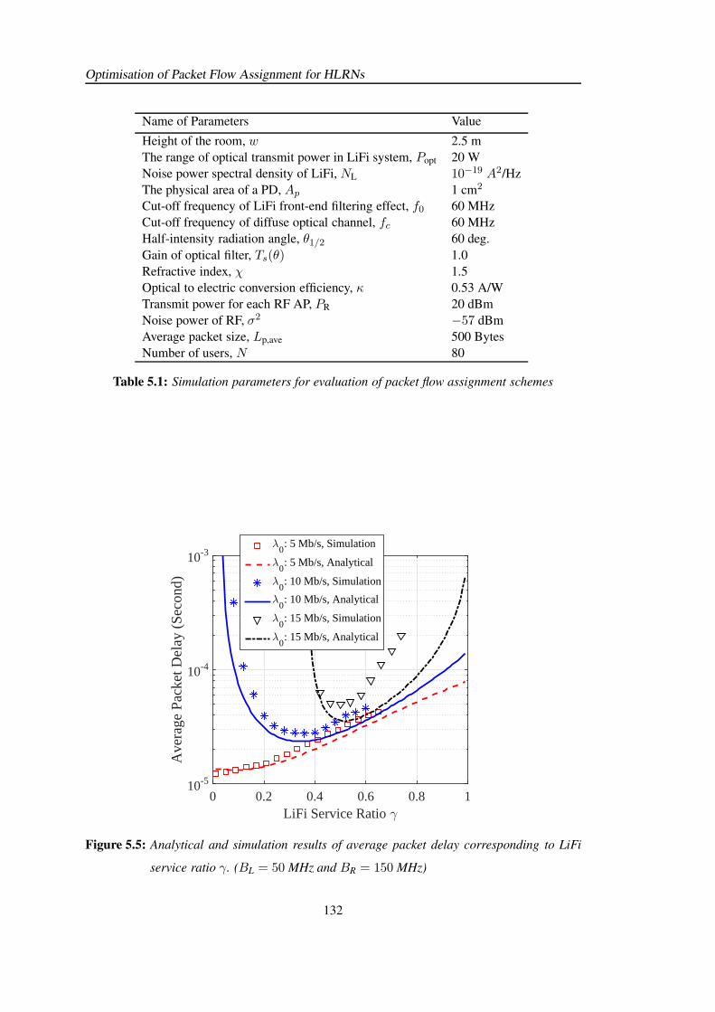
Optimisation of Packet Flow Assignment for HLRNs
Name of Parameters Value
Height of the room, w 2.5 m
The range of optical transmit power in LiFi system, Popt 20 W
Noise power spectral density of LiFi, NL 10−19 A2/Hz
The physical area of a PD, Ap 1 cm2
Cut-off frequency of LiFi front-end filtering effect, f0 60 MHz
Cut-off frequency of diffuse optical channel, fc 60 MHz
Half-intensity radiation angle, θ1/2 60 deg.
Gain of optical filter, Ts(θ) 1.0
Refractive index, χ 1.5
Optical to electric conversion efficiency, κ 0.53 A/W
Transmit power for each RF AP, PR 20 dBm
Noise power of RF, σ2 −57 dBm
Average packet size, Lp,ave 500 Bytes
Number of users, N 80
Table 5.1: Simulation parameters for evaluation of packet flow assignment schemes
LiFi Service Ratio γ0 0.2 0.4 0.6 0.8 1
Ave
rage
Pac
ket D
elay
(Se
cond
)
10-5
10-4
10-3λ
0: 5 Mb/s, Simulation
λ0: 5 Mb/s, Analytical
λ0: 10 Mb/s, Simulation
λ0: 10 Mb/s, Analytical
λ0: 15 Mb/s, Simulation
λ0: 15 Mb/s, Analytical
Figure 5.5: Analytical and simulation results of average packet delay corresponding to LiFi
service ratio γ. (BL = 50 MHz and BR = 150 MHz)
132
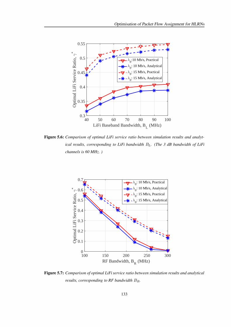
Optimisation of Packet Flow Assignment for HLRNs
LiFi Baseband Bandwidth, BL
(MHz)40 50 60 70 80 90 100
Opt
imal
LiF
i Ser
vice
Rat
io, γ
*
0.3
0.35
0.4
0.45
0.5
0.55
λ0:10 Mb/s, Practical
λ0: 10 Mb/s, Analytical
λ0: 15 Mb/s, Practical
λ0: 15 Mb/s, Analytical
Figure 5.6: Comparison of optimal LiFi service ratio between simulation results and analyt-
ical results, corresponding to LiFi bandwidth BL. (The 3 dB bandwidth of LiFi
channels is 60 MHz. )
RF Bandwidth, BR
(MHz)100 150 200 250 300
Opt
imal
LiF
i Ser
vice
Rat
io, γ
*
0
0.1
0.2
0.3
0.4
0.5
0.6
0.7λ
0: 10 Mb/s, Practical
λ0: 10 Mb/s, Analytical
λ0: 15 Mb/s, Practical
λ0: 15 Mb/s, Analytical
Figure 5.7: Comparison of optimal LiFi service ratio between simulation results and analytical
results, corresponding to RF bandwidth BR.
133
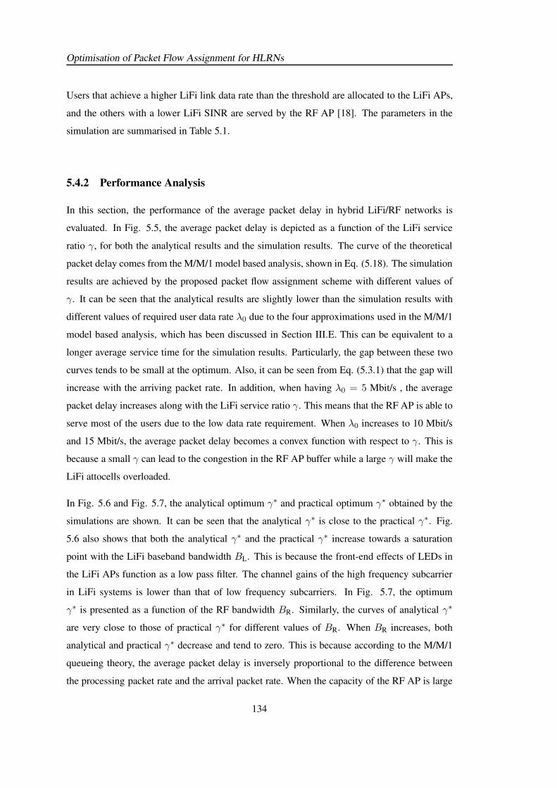
Optimisation of Packet Flow Assignment for HLRNs
Users that achieve a higher LiFi link data rate than the threshold are allocated to the LiFi APs,
and the others with a lower LiFi SINR are served by the RF AP [18]. The parameters in the
simulation are summarised in Table 5.1.
5.4.2 Performance Analysis
In this section, the performance of the average packet delay in hybrid LiFi/RF networks is
evaluated. In Fig. 5.5, the average packet delay is depicted as a function of the LiFi service
ratio γ, for both the analytical results and the simulation results. The curve of the theoretical
packet delay comes from the M/M/1 model based analysis, shown in Eq. (5.18). The simulation
results are achieved by the proposed packet flow assignment scheme with different values of
γ. It can be seen that the analytical results are slightly lower than the simulation results with
different values of required user data rate λ0 due to the four approximations used in the M/M/1
model based analysis, which has been discussed in Section III.E. This can be equivalent to a
longer average service time for the simulation results. Particularly, the gap between these two
curves tends to be small at the optimum. Also, it can be seen from Eq. (5.3.1) that the gap will
increase with the arriving packet rate. In addition, when having λ0 = 5 Mbit/s , the average
packet delay increases along with the LiFi service ratio γ. This means that the RF AP is able to
serve most of the users due to the low data rate requirement. When λ0 increases to 10 Mbit/s
and 15 Mbit/s, the average packet delay becomes a convex function with respect to γ. This is
because a small γ can lead to the congestion in the RF AP buffer while a large γ will make the
LiFi attocells overloaded.
In Fig. 5.6 and Fig. 5.7, the analytical optimum γ∗ and practical optimum γ∗ obtained by the
simulations are shown. It can be seen that the analytical γ∗ is close to the practical γ∗. Fig.
5.6 also shows that both the analytical γ∗ and the practical γ∗ increase towards a saturation
point with the LiFi baseband bandwidth BL. This is because the front-end effects of LEDs in
the LiFi APs function as a low pass filter. The channel gains of the high frequency subcarrier
in LiFi systems is lower than that of low frequency subcarriers. In Fig. 5.7, the optimum
γ∗ is presented as a function of the RF bandwidth BR. Similarly, the curves of analytical γ∗
are very close to those of practical γ∗ for different values of BR. When BR increases, both
analytical and practical γ∗ decrease and tend to zero. This is because according to the M/M/1
queueing theory, the average packet delay is inversely proportional to the difference between
the processing packet rate and the arrival packet rate. When the capacity of the RF AP is large
134
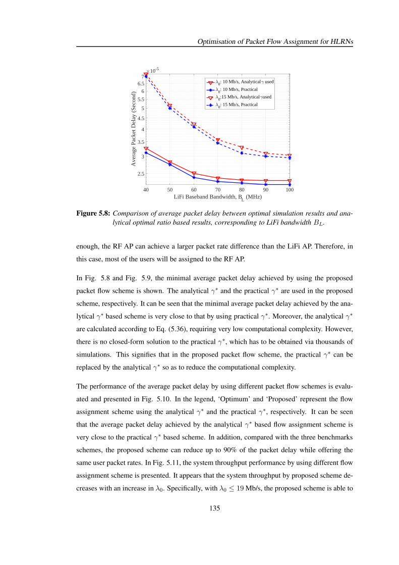
Optimisation of Packet Flow Assignment for HLRNs
40 50 60 70 80 90 100LiFi Baseband Bandwidth, B
L (MHz)
2.5
3
3.5
4
4.5
5
5.5
6
6.57
Ave
rage
Pac
ket D
elay
(Se
cond
)
10-5
0: 10 Mb/s, Analytical used
0: 10 Mb/s, Practical
0:15 Mb/s, Analytical used
0: 15 Mb/s, Practical
Figure 5.8: Comparison of average packet delay between optimal simulation results and ana-
lytical optimal ratio based results, corresponding to LiFi bandwidth BL.
enough, the RF AP can achieve a larger packet rate difference than the LiFi AP. Therefore, in
this case, most of the users will be assigned to the RF AP.
In Fig. 5.8 and Fig. 5.9, the minimal average packet delay achieved by using the proposed
packet flow scheme is shown. The analytical γ∗ and the practical γ∗ are used in the proposed
scheme, respectively. It can be seen that the minimal average packet delay achieved by the ana-
lytical γ∗ based scheme is very close to that by using practical γ∗. Moreover, the analytical γ∗
are calculated according to Eq. (5.36), requiring very low computational complexity. However,
there is no closed-form solution to the practical γ∗, which has to be obtained via thousands of
simulations. This signifies that in the proposed packet flow scheme, the practical γ∗ can be
replaced by the analytical γ∗ so as to reduce the computational complexity.
The performance of the average packet delay by using different packet flow schemes is evalu-
ated and presented in Fig. 5.10. In the legend, ‘Optimum’ and ‘Proposed’ represent the flow
assignment scheme using the analytical γ∗ and the practical γ∗, respectively. It can be seen
that the average packet delay achieved by the analytical γ∗ based flow assignment scheme is
very close to the practical γ∗ based scheme. In addition, compared with the three benchmarks
schemes, the proposed scheme can reduce up to 90% of the packet delay while offering the
same user packet rates. In Fig. 5.11, the system throughput performance by using different flow
assignment scheme is presented. It appears that the system throughput by proposed scheme de-
creases with an increase in λ0. Specifically, with λ0 ≤ 19 Mb/s, the proposed scheme is able to
135
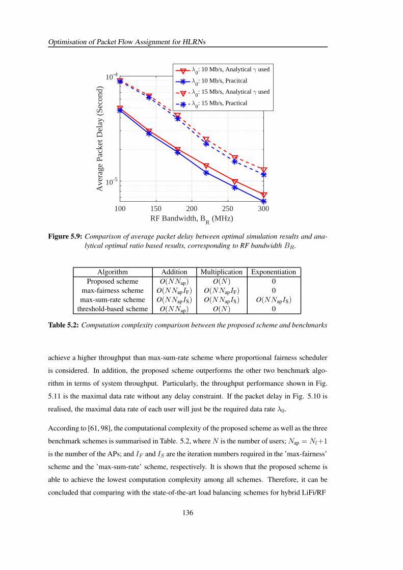
Optimisation of Packet Flow Assignment for HLRNs
RF Bandwidth, BR
(MHz)100 150 200 250 300
Ave
rage
Pac
ket D
elay
(Se
cond
)
10-5
10-4λ
0: 10 Mb/s, Analytical γ used
λ0: 10 Mb/s, Pracitcal
λ0: 15 Mb/s, Analytical γ used
λ0: 15 Mb/s, Practical
Figure 5.9: Comparison of average packet delay between optimal simulation results and ana-
lytical optimal ratio based results, corresponding to RF bandwidth BR.
Algorithm Addition Multiplication Exponentiation
Proposed scheme O(NNap) O(N) 0
max-fairness scheme O(NNapIF) O(NNapIF) 0
max-sum-rate scheme O(NNapIS) O(NNapIS) O(NNapIS)threshold-based scheme O(NNap) O(N) 0
Table 5.2: Computation complexity comparison between the proposed scheme and benchmarks
achieve a higher throughput than max-sum-rate scheme where proportional fairness scheduler
is considered. In addition, the proposed scheme outperforms the other two benchmark algo-
rithm in terms of system throughput. Particularly, the throughput performance shown in Fig.
5.11 is the maximal data rate without any delay constraint. If the packet delay in Fig. 5.10 is
realised, the maximal data rate of each user will just be the required data rate λ0.
According to [61, 98], the computational complexity of the proposed scheme as well as the three
benchmark schemes is summarised in Table. 5.2, whereN is the number of users; Nap = Nl+1
is the number of the APs; and IF and IS are the iteration numbers required in the ’max-fairness’
scheme and the ’max-sum-rate’ scheme, respectively. It is shown that the proposed scheme is
able to achieve the lowest computation complexity among all schemes. Therefore, it can be
concluded that comparing with the state-of-the-art load balancing schemes for hybrid LiFi/RF
136
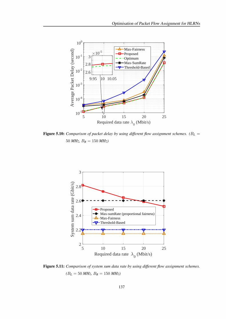
Optimisation of Packet Flow Assignment for HLRNs
Required data rate λ0 (Mbit/s)
5 10 15 20 25
Ave
rage
Pac
ket D
elay
(se
cond
)
10-5
10-4
10-3
10-2
10-1
100
9.95 10 10.05
×10-5
2.6
2.8
3
Max-FairnessProposed OptimumMax-SumRateThreshold-Based
Figure 5.10: Comparison of packet delay by using different flow assignment schemes. (BL =
50 MHz, BR = 150 MHz)
5 10 15 20 25Required data rate
0 (Mbit/s)
2
2.2
2.4
2.6
2.8
3
Syst
em s
um d
ata
rate
(G
bit/s
)
ProposedMax-sumRate (proportional fairness)Max-FairnessThreshold-Based
Figure 5.11: Comparison of system sum data rate by using different flow assignment schemes.
(BL = 50 MHz, BR = 150 MHz)
137
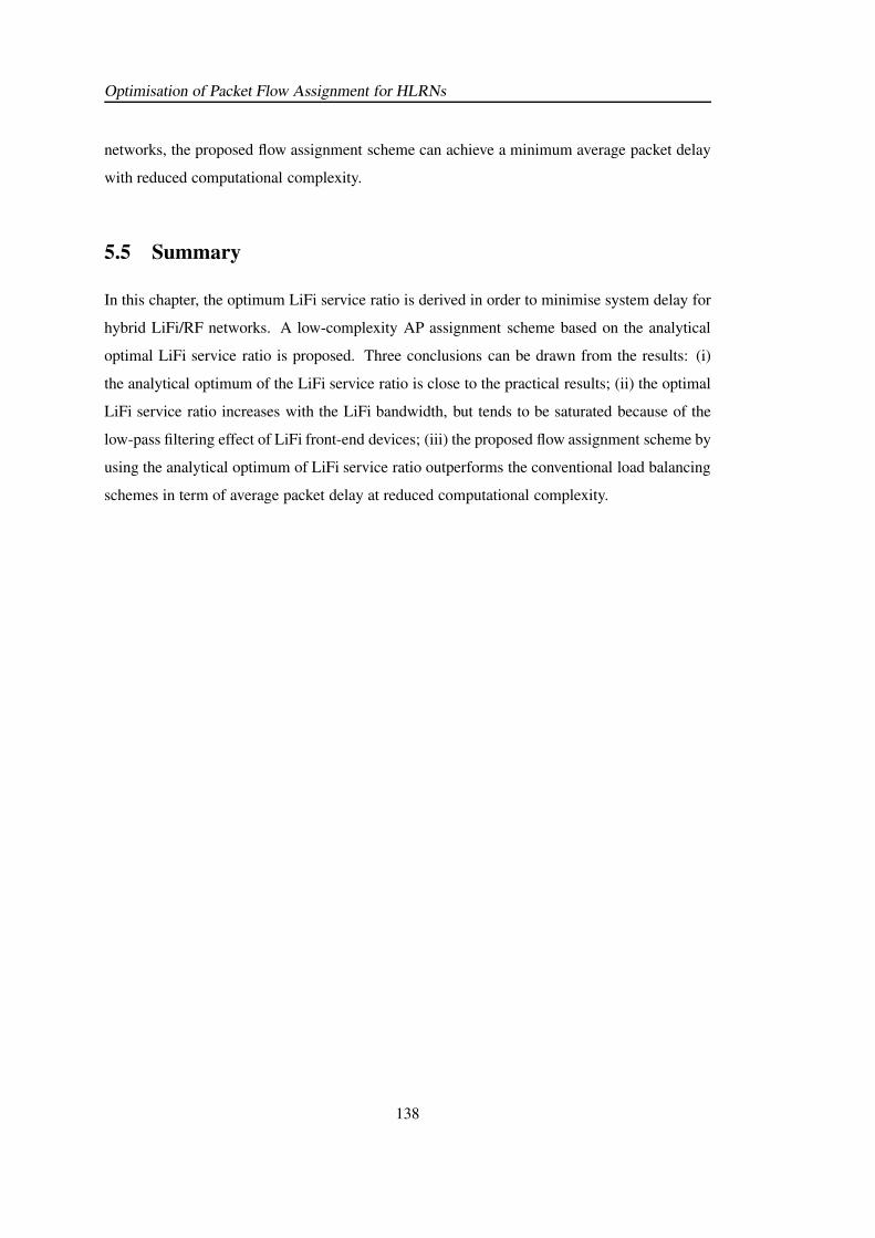
Optimisation of Packet Flow Assignment for HLRNs
networks, the proposed flow assignment scheme can achieve a minimum average packet delay
with reduced computational complexity.
5.5 Summary
In this chapter, the optimum LiFi service ratio is derived in order to minimise system delay for
hybrid LiFi/RF networks. A low-complexity AP assignment scheme based on the analytical
optimal LiFi service ratio is proposed. Three conclusions can be drawn from the results: (i)
the analytical optimum of the LiFi service ratio is close to the practical results; (ii) the optimal
LiFi service ratio increases with the LiFi bandwidth, but tends to be saturated because of the
low-pass filtering effect of LiFi front-end devices; (iii) the proposed flow assignment scheme by
using the analytical optimum of LiFi service ratio outperforms the conventional load balancing
schemes in term of average packet delay at reduced computational complexity.
138
Chapter 6
Conclusions, Limitations and Future
Research
6.1 Summary and Conclusions
In this thesis, hybrid LiFi and RF networks (HLRN) with mobile users are considered and
downlink network load balancing for HLRN is investigated. In the indoor scenario, the channel
state information (CSI) for LiFi and RF link varies slowly. Therefore, in each short period, the
CSI can be considered to be fixed for HLRN, and such a short period is referred to as a quasi-
static state. Downlink load balancing consists of static load balancing in each state and han-
dover. Specifically, static load balancing contains access point assignment (APA) and resource
allocation (RA). In this thesis, several novel load balancing schemes have been developed to
optimise the overall throughput and to improve users’ quality of service (QoS), including users’
satisfaction level and packet delay. In addition, the effects of handover, blockages in LiFi links,
random orientation of photo diodes on the system data rate performance have been evaluated.
In Chapter 2, the relevant background of LiFi technology and hybrid LiFi and RF networks
has been presented. Initially, the brief history of optical wireless communications is introduced
and the overall communication architecture of HLRN is provided. After that, the LiFi channel
model including field-of-view (FoV) path loss, front-end low pass filtering effects and multipath
effect caused by reflections. Then, the optical orthogonal frequency division multiplexing (O-
OFDM) transmission is depicted. Specifically, we focus on the direct current (DC) optical
OFDM (DCO-OFDM) technology because of its high spectral efficiency. In DCO-OFDM, a
DC bias added to the modulated signal ensures that the output signals are positive. Also, at
least half of the OFDM sub-carriers are used to realise the Hermitian conjugate of the complex-
valued symbols so that the strict positive and real number constraint is satisfied after the Fourier
transform. Moreover, the multiple access technology in LiFi systems is investigated. It has
been found that the orthogonal frequency division multiple access (OFDMA) outperforms the
time division multiple access (TDMA) technique in terms of both data rate and user fairness
due to the efficient use of high frequency subcarriers. In addition, a novel low complexity
139
Conclusions, Limitations and Future Research
OFDMA based resource allocation scheme is proposed. This RA scheme exploits the unique
characteristics of LiFi channels functioning as a low pass filter to reduce the computational
complexity. Simulations show that the OFDMA outperforms the time division multiple access
(TDMA) technique in terms of both data rate and user fairness due to the efficient use of high
frequency subcarriers. Finally, the system model for RF networks is introduced. The 2.4 GHz
spectrum band is considered for RF transmission and OFDM-TDMA is considered for multiple
access in order to reduce the complexity.
In Chapter 3, the dynamic load balancing with handover considered for HLRN is studied. First,
the handover scheme between two neighbouring quasi-static states is proposed. Then, the opti-
misation of static load balancing is investigated. The AP assignment and the RA are formulated
as an optimisation problem which is used to maximise the system sum data rate under certain
user fairness conditions. In Section 3.2, an optimisation-based load balancing scheme with pro-
portional fairness is proposed, and the throughput performance of the hybrid LiFi/WiFi network
is theoretically analysed. It has been shown that the WiFi (or RF) and LiFi throughputs in the
hybrid network are related despite the independent spectrum transmission. The LiFi throughput
can be enhanced by increasing the WiFi throughput due to efficient load balancing. Following
that, a comprehensive study of dynamic load balancing with a variety of fairness schemes is
provided. Two specific load balancing algorithms, joint optimisation algorithm (JOA) and sep-
arate optimisation algorithm (SOA) are proposed. A unified data rate requirement of users
is considered as a QoS metric and user outage probability is introduced. Simulation results
show that JOA can achieve an optimal performance of system throughput while requiring high
computational complexity. SOA achieves a lower data rate than JOA at a reduced complexity.
Finally, a fuzzy logic (FL) based dynamic load balancing scheme that jointly handles AP as-
signment, RA and handover is proposed. This FL based scheme uses CSI, user speed and users’
data rate requirement to determine whether a handover is prompted. It is shown that compared
with conventional load balancing scheme, the FL based scheme improve 40% in terms of both
data rate and user satisfaction level due to the reduction of handover frequency.
In Chapter 4, an evolutionary game theory (EGT) based load balancing scheme is proposed
in order to reduce the computational complexity of conventional load balancing approaches.
In the EGT based load balancing scheme, APA and RA are handled separately, resulting in
a low complexity. In addition, the EGT based scheme optimises APA and RA iteratively by
using the relation between them so that a near optimal performance of system throughput can
140
Conclusions, Limitations and Future Research
be achieved. In this chapter, three factors are taken into account in order to model a practical
HLRN: blockages in LiFi channels, random orientation angle and user data rate requirement.
Also, in the RA step in the EGT scheme, an enhanced proportional fairness (EPF) scheduler
is proposed to maximise the usage of communication resources. Three conclusions are drawn
based on the simulation results: i). The EGT load balancing scheme can achieve a better
trade-off between data rate performance and computational complexity; ii). The proposed EPF
scheduler can achieve a higher user QoS than conventional schedulers in the RA step due to
a more efficient exploitation of transmission resources; iii). When the FoV of LiFi receivers
is 90, the average user QoS decreases with an increase in the maximum vertical ROA θPD.
However, when considering a small FoV, there is an optimum of the maximal vertical ROA
that can optimise the QoS performance, leading to improved system load balancing; However,
when considering user data rate requirement, the user QoS decreases with an increase in the
blockage density as blockages cause an inefficient allocation of communication resources.
In Chapter 5, the optimisation of packet flow assignment for HLRN is investigated. Unlike the
load balancing on the physical layer, we focus on the performance improvement on packet delay
instead of system sum data rate. Initially, a two-layer buffer framework including central unit
(CU) buffer and AP buffers for HLRN is introduced. The arrival packets will be firstly queued
in the CU buffer. According to the AP assignment results, the packets in the CU buffer will be
delivered to the AP buffers. In this chapter, a notion of ‘LiFi service ratio’ is introduced, which
signifies the proportion of users that are served by LiFi APs. Moreover, an optimisation analysis
of LiFi service ratio for HLRN is provided. Based on the analytical optimal LiFi service ratio,
a low-complexity flow assignment scheme is proposed in order to minimise the packet delay.
Three conclusions can be drawn from the results: (i) the analytical optimum of the LiFi service
ratio is close to the practical results; (ii) the optimal LiFi service ratio increases with the LiFi
bandwidth, but tends to be saturated because of the low-pass filtering effect of LiFi front-end
devices; (iii) the proposed flow assignment scheme by using the analytical optimum of LiFi
service ratio outperforms the conventional load balancing schemes in term of average packet
delay at reduced computational complexity.
6.2 Limitations and Future Research
In the analysis presented in this thesis, a multitude of factors related to load balancing for HLRN
have been considered. However, in order to reduce the analytical complexity, some assumptions
141
Conclusions, Limitations and Future Research
are introduced to simplify the system models. In Chapter 2, the spatial multiplexing in both
LiFi and RF systems is not taken into account [101]. Multiple light emitting diodes (LEDs)
are essentially used to lighten an indoor environment. Therefore, multiple input and multiple
output (MIMO) system can be naturally employed in an indoor VLC scheme [102]. There is
an amount of research on the VLC MIMO technique. A MIMO approach to model an indoor
VLC system has been introduced in [103] and the capacity of an optical MIMO system is
studied in [104], with a low-speed optical system demonstrated. In [105], research on space-
time coding for diffuse optical communications is investigated. In [106], several preliminary
experiments with a simple MIMO interconnect are reported. Also, multiple LEDs can be used
for space division multiple access (SDMA) systems. It has been shown in [107] that an angle
diversity LiFi transmitter that consists of several LED lamps and generates multiple narrow
beams in different directions simultaneously can realise SDMA. This can significantly improve
the system throughput by increasing bandwidth reuse. In addition, multiple antennas in the RF
system have not been considered. By using MIMO techniques, the uplink and downlink system
throughput can be improved [108], because the techniques such as space time block coding
and beamforming employed in the MIMO system helps in achieving extension of cell coverage
and interference cancellation. Moreover, the data rate increase in both LiFi and RF stand-alone
networks can affect the system load balancing and handover strategies in HLRNs. This topic
that load balancing with advanced antennas technology in HLRNs will be studied in our future
research.
In the LiFi channel model, the non-line-of-sight (NLoS) transmission is modelled by consid-
ering the effects of internal room surfaces only. In order to simulate a more precise reflective
channel, random objects such as human bodies and furniture need to be taken into account.
Though a number of related research has investigated several different communication environ-
ments, the generic characteristics of the effects of objects on NLoS LiFi channels still remain
unknown [109]. This is because there are too many uncertain factors about the random objects
such as the type and the surface reflectivity. Also, the geometry of the random objects are not
as simple as a flat plane. Therefore, it is more difficult to characterise the effects of random
objects on NLoS channel than merely considering indoor surfaces. In order to evaluate the data
rate performance in HLRNs more accurately, more research on modelling LiFi NLoS channel
should be undertaken.
The OFDMA-based RA scheme for LiFi systems has been investigated in Section 2.3.3, and a
142
Conclusions, Limitations and Future Research
novel low-complexity OFDMA scheme has been proposed. Despite the inconspicuous multi-
user diversity, the OFDMA RA scheme outperforms the TDMA in LiFi systems due to an
efficient use of high-frequency resources. However, TDMA instead of OFDMA is employed
when studying load balancing in this thesis. This is because TDMA has a much simpler solution
for RA than OFDMA, and using OFDMA may lead to an intractable problem for load balancing
optimisation. In our future work, the OFDMA-based load balancing algorithms for HLRNs
will be studied. Particularly, by using the low-complexity OFDMA-based RA scheme and
well-designed AP allocation schemes, the computational complexity of LB in OFDMA-based
HLRNs could be reduced.
In Chapter 3, the handover scheme in HLRNs is studied. However, the difference between the
horizontal handover and the vertical handover is not considered. In fact, vertical handovers are
implemented across heterogeneous cells of access systems, which differ in several aspects such
as bandwidth, data rate, frequency of operation, etc. The different characteristics of the net-
works involved make the implementation of vertical handovers more challenging as compared
to horizontal handovers. In future work, some experimental analysis of horizontal and vertical
handovers in HLRNs is expected, and more efficient handover schemes will be developed.
When studying dynamic hybrid LiFi/RF networks, user movement should be considered and
modelled properly. Specifically, user movement contains moving routes/speed and random
orientations of LiFi receivers. For user moving routes/speed, the random way point model is
usually applied in the published research. However, this model is far from being implemented
in practical situations. Users in the shopping mall definitely have different moving performance
from those in the office scenarios. In addition, the random orientations of LiFi receivers will
affect the user data rate, which should be carefully modelled. It has been shown in [110, 111]
that physical and geometrical parameters have a significant effect on VLC communications
and must be considered in VLC channel models. In Chapter 4, a uniform distribution of ver-
tical orientations of LiFi receivers is assumed. This may not be accurate in practical scenarios
according to users’ behaviour. Therefore, in order to make a more effective performance eval-
uation of dynamic LB schemes, an accurate user movement model should be applied. A LB
scheme which relies on an accurate movement model may significantly improve the user data
rate and mitigate the influence caused by handover overhead. The modelling of user movement
in LiFi networks will be investigated in our future work.
In Chapter 5, the media access control (MAC) layer load balancing in HLRNs is investigated.
143
Conclusions, Limitations and Future Research
Similar to conventional RF channels, an efficient and fair MAC protocol is required where
nodes can contend for the channel and eventually transmit without collisions. There are sev-
eral achievements through the research of VLC-based channel access mechanism for indoor
communication [112–114]. In [115], authors test the VLC transceiver prototype design using a
modified version of the 802.11 MAC protocol. The results show that performance of the pro-
tocol is in the acceptable range of 80-90% for only simple simulation scenarios. A significant
difference between LiFi and conventional RF such as LTE, WiFi is that each LiFi AP covers
a much smaller area than RF, leading to more frequent handover. Therefore, more research
should be undertaken on LiFi MAC layer in order to develop an efficient LiFi MAC protocol.
This will be included in our future work.
Finally, bi-directional load balancing is also planned for our future work. Besides dynamic
LB for downlink network, coupling the LiFi and RF links for the uplink network allows it to
offer high degrees of freedom and may require sophisticated network resource optimisation
[116–118]. This work is very important because mobile units are becoming more and more
powerful in terms of computing power and storage and the uplink may experience heavy traffic
caused by mobile multimedia transmissions [119]. Properly distributing heavy traffic in both
the uplink and downlink requires efficient traffic reshaping, which is an unknown problem in
existing mobile networks.
144
Appendix A
List of Publications
This Chapter contains a list of published papers.
A.1 Journal Papers and Main Contributions
Y. Wang, X. Wu and H. Haas, ”Load Balancing Game With Shadowing Effect for Indoor Hybrid
LiFi/RF Networks,” in IEEE Transactions on Wireless Communications, vol. 16, no. 4, pp.
2366-2378, April 2017.
Main contributions: In this paper, an evolutionary game theory (EGT) based load balancing
scheme is proposed for hybrid LiFi/RF networks (HLRNs) where three practical issues are con-
sidered: i). LiFi channel blockages; ii). random orientation angle (ROA) of LiFi receivers; iii)
user data rate requirement. The proposed algorithm jointly handles the access point (AP) as-
signment and resource allocation (RA). The optimality of the proposed algorithm is analysed.
Moreover, when considering user data rate requirement, conventional fairness schedulers such
as max-min fairness and proportional fairness may lead to inefficient use of communication re-
sources. In the proposed EGT based algorithm, an enhanced proportional fairness scheduler for
resource allocation is proposed to avoid inefficient use of transmission resources. The perfor-
mance of user satisfaction for both conventional and proposed fairness schedulers is evaluated
by computer simulations.
Y. Wang, D. A. Basnayaka, X. Wu and H. Haas, ”Optimization of Load Balancing in Hybrid
LiFi/RF Networks,” in IEEE Transactions on Communications, vol. 65, no. 4, pp. 1708-1720,
April 2017.
Main contributions: A novel dynamic load balancing scheme is proposed and the β-proportional
fairness function is applied, where β is the fairness coefficient. The effect of β on user data rate
performance in the hybrid network is evaluated. Two specific algorithms that optimise the AP
assignment and the RA in each quasi-static state are proposed, termed as joint optimisation
145
List of Publications
algorithm (JOA) and separate optimisation algorithm (SOA) respectively. In this work, the op-
timality of JOA and the optimal threshold in SOA are analysed. A comparison of data rate
performance and computational complexity between these two algorithms is made.
Y. Wang and H. Haas, ”Dynamic Load Balancing With Handover in Hybrid LiFi and WiFi
Networks,” in Journal of Lightwave Technology, vol. 33, no. 22, pp. 4671-4682, Nov.15, 15
2015.
Main contributions: In this paper, a dynamic load balancing scheme with handover for hybrid
LiFi and WiFi networks is proposed, where proportional fairness is taken into consideration. In
this work, the service area is defined as the region within which users will be allocated to LiFi
APs. By analysing the service areas of the LiFi APs, the throughput performance of the hybrid
system is theoretically studied. Also, the relation between LiFi throughput and WiFi throughput
is investigated. Moreover, the effects of the handover overhead on handover locations and user
throughput are simulated and discussed.
Y. Wang, X. Wu and H. Haas, ”Cross-layer Load Balancing Design for Hybrid LiFi/RF Net-
works,” submitted to Journal of Lightwave Technology.
Main contributions: A two-tier buffer framework for HLRNs is proposed, which contains a
central unit (CU) buffer and one buffer for each AP. Two multiple access technologies, carrier
sense multiple access (CSMA) and time division multiple access (TDMA), are used in this hi-
erarchical buffer model, and the quality of service (QoS) performance of these two techniques,
including packet loss rate and packet latency is investigated and compared. Also, a dynamic
load balancing scheme that handles the AP assignment, resource allocation and handover for
hybrid networks is proposed. In order to decrease the packet delay, a packet dropping mecha-
nism (PDM) that deletes the expired packets is included in the proposed load balancing scheme.
In addition, an optimisation-based LB scheme is introduced as a benchmark and a comparison
of QoS performance and computational complexity is carried out between the proposed scheme
and the benchmark.
Y. Wang, X. Wu and H. Haas, ”Optimisation of Flow Assignment for Hybrid LiFi/RF Net-
works,” submitted to IEEE Transactions on Wireless Communications.
Main contributions: In this study, a downlink HLRN is considered and the notion of a LiFi
service ratio is introduced, which signifies the proportion of users that are served by LiFi APs.
146
List of Publications
An analytical solution to the optimum LiFi service ratio for HLRNs is provided. A comparison
between the analytical results and simulation results is conducted. Based on the analytical op-
timum LiFi service ratio, a low-complexity AP assignment scheme for hybrid LiFi/RF network
is proposed to minimise the average packet delay. For various AP assignment schemes, the
effects of different network setups on the packet delay are numerically studied.
A.2 Conference papers
Y. Wang, X. Wu and H. Haas, ”OFDMA-Based Resource allocation in LiFi Networks,” ac-
cepted by 2017 IEEE Global Communications Conference (GLOBECOM), Singapore.
Y. Wang, and H. Haas, ”A Comparison of Load Balancing Techniques for Hybrid LiFi/RF
Networks” accepted by 4th ACM Workshop on Visible Light Communication Systems (VLCS
2017), Snowbird.
Y. Wang, X. Wu and H. Haas, ”Fuzzy logic based dynamic handover scheme for indoor Li-
Fi and RF hybrid network,” 2016 IEEE International Conference on Communications (ICC),
Kuala Lumpur, 2016, pp. 1-6.
Y. Wang, X. Wu and H. Haas, ”Analysis of area data rate with shadowing effects in Li-Fi and
RF hybrid network,” 2016 IEEE International Conference on Communications (ICC), Kuala
Lumpur, 2016, pp. 1-5.
Y. Wang, X. Wu and H. Haas, ”Distributed load balancing for Internet of Things by using Li-
Fi and RF hybrid network,” 2015 IEEE 26th Annual International Symposium on Personal,
Indoor, and Mobile Radio Communications (PIMRC), Hong Kong, 2015, pp. 1289-1294.
Y. Wang, D. A. Basnayaka and H. Haas, ”Dynamic load balancing for hybrid Li-Fi and RF
indoor networks,” 2015 IEEE International Conference on Communication Workshop (ICCW),
London, 2015, pp. 1422-1427.
Y. Wang, S. Videv and H. Haas, ”Dynamic load balancing with handover in hybrid Li-Fi and
Wi-Fi networks,” 2014 IEEE 25th Annual International Symposium on Personal, Indoor, and
Mobile Radio Communication (PIMRC), Washington DC, 2014, pp. 575-579.
147

148
References
[1] S. Shao and A. Khreishah, “Delay Analysis of Unsaturated Heterogeneous
Omnidirectional-Directional Small Cell Wireless Networks: The Case of RF-VLC Co-
existence,” IEEE Transactions on Wireless Communications, vol. PP, no. 99, pp. 1–1,
2016.
[2] Cisco, “Cisco Visual Networking Index: Forecast and Methodology, 2014-2019,” 2015.
[3] Ericsson, “Mobility Report on the Pulse of the Networked Society,” 2015.
[4] H. Haas, “LiFi: Conceptions, Misconceptions and Opportunities,” in IEEE Photonics
Conference (IPC), pp. 680–681, 2016.
[5] H. Zhang, S. Chen, X. Li, H. Ji, and X. Du, “Interference Management for Hetero-
geneous Networks with Spectral Efficiency Improvement,” IEEE Wireless Communica-
tions, vol. 22, pp. 101–107, April 2015.
[6] D. Lopez-Perez, I. Guvenc, G. de la Roche, M. Kountouris, T. Q. S. Quek, and J. Zhang,
“Enhanced Intercell Interference Coordination Challenges in Heterogeneous Networks,”
IEEE Wireless Communications, vol. 18, pp. 22–30, June 2011.
[7] A. Tzanakaki, M. Anastasopoulos, I. Berberana, D. Syrivelis, P. Flegkas, T. Korakis,
D. C. Mur, I. Demirkol, J. Gutierrez, E. Grass, Q. Wei, E. Pateromichelakis, N. Vucic,
A. Fehske, M. Grieger, M. Eiselt, J. Bartelt, G. Fettweis, G. Lyberopoulos, E. Theodor-
opoulou, and D. Simeonidou, “Wireless-Optical Network Convergence: Enabling the
5G Architecture to Support Operational and End-User Services,” IEEE Communications
Magazine, vol. 55, pp. 184–192, October 2017.
[8] W. Abdallah and N. Boudriga, “Enabling 5G Wireless Access Using LiFi Technology:
An OFDM Based Approach,” in 18th International Conference on Transparent Optical
Networks (ICTON), pp. 1–6, July 2016.
[9] T. Maksymyuk, M. Brych, Y. Klymash, M. Kyryk, and M. Klymash, “Game Theoreti-
cal Framework for Multi-Operator Spectrum Sharing in 5G Heterogeneous Networks,”
in 4th International Scientific-Practical Conference Problems of Infocommunications,
Science and Technology (PIC S T), pp. 515–518, Oct 2017.
[10] B. Soleyman, A. Zaman, S. H. Rastegar, and V. Shah-Mansour, “RAT Selection Based
on Association Probability in 5G Heterogeneous Networks,” in IEEE Symposium on
Communications and Vehicular Technology (SCVT), pp. 1–6, Nov 2017.
[11] H. Haas, L. Yin, Y. Wang, and C. Chen, “What is LiFi,” Journal of Lightwave Technol-
ogy, vol. 34, pp. 1533–1544, March 2016.
[12] N. V. R. Kumar, A. Srikanth, A. Singha, and B. B. Sam, “Comparison of LIFI and WIFI
and Study of Smart Meter-survey,” in 2017 International Conference on Information
Communication and Embedded Systems (ICICES), pp. 1–8, Feb 2017.
149
References
[13] D. Tsonev, H. Chun, S. Rajbhandari, J. McKendry, S. Videv, E. Gu, M. Haji, S. Watson,
A. Kelly, G. Faulkner, M. Dawson, H. Haas, and D. O’Brien, “A 3-Gb/s Single-LED
OFDM-Based Wireless VLC Link Using a Gallium Nitride uLED ,” IEEE Photonics
Technology Letters, vol. 26, pp. 637–640, Apr. 2014.
[14] M. Islim, R. X. Ferreira, X. He, E. Xie, S. Videv, S. Viola, S. Watson, N. Bamiedakis,
R. V. Penty, I. H. White, A. E. Kelly, E. Gu, H. Haas, and M. D. Dawson, “Towards 10
Gb/s Orthogonal Frequency Division Multiplexing-based Visible Light Communication
Using a GaN Violet Micro-LED,” Photon. Res., pp. A35–A43, 2017.
[15] D. Tsonev, S. Videv, and H. Haas, “Towards a 100 Gb/s Visible Light Wireless Access
Network,” Optics Express, vol. 23, pp. 1627–1637, 2015.
[16] E. Perahia and R. Stacey, “Next Generation Wireless LAN: 802.11n and 802.11ac ,”
Cambridge University Press, 2013.
[17] C. Chen, D. Basnayaka, and H. Haas, “Downlink Performance of Optical Attocell Net-
works,” Journal of Lightwave Technology, vol. 34, pp. 137–156, Apr. 2016.
[18] D. A. Basnayaka and H. Haas, “Hybrid RF and VLC Systems: Improving User Data
Rate Performance of VLC System,” in IEEE Vehicular Technology Conference (VTC
Spring), May 2015.
[19] Y. Wang, X. Wu, and H. Haas, “Analysis of Area Data Rate with Shadowing Effects in
LiFi and RF Hybrid Network,” in 2016 IEEE International Conference on Communica-
tions (ICC), pp. 1–5, May 2016.
[20] X. Wu and H. Haas, “Access Point Assignment in Hybrid LiFi and WiFi Networks in
Consideration of LiFi Channel Blockage,” in IEEE 18th International Workshop on Sig-
nal Processing Advances in Wireless Communications (SPAWC), pp. 1–5, July 2017.
[21] M. B. Rahaim, A. M. Vegni, and T. D. C. Little, “A Hybrid Radio Frequency and Broad-
cast Visible Light Communication System,” in IEEE Global Communications Confer-
ence Workshop (GLOBECOMW), pp. 792–796, Dec. 2011.
[22] S. Shao, A. Khreishah, M. B. Rahaim, H. Elgala, M. Ayyash, T. D. C. Little, and J. Wu,
“An Indoor Hybrid WiFi-VLC Internet Access System,” in IEEE International Confer-
ence on Mobile Ad Hoc and Sensor Systems (MASS), pp. 569–574, Oct. 2014.
[23] X. Li, R. Zhang, and L. Hanzo, “Cooperative Load Balancing in Hybrid Visible Light
Communications and WiFi,” IEEE Transactions on Communications, vol. 63, pp. 1319–
1329, Apr. 2015.
[24] F. Jin, R. Zhang, and L. Hanzo, “Resource Allocation Under Delay-Guarantee Con-
straints for Heterogeneous Visible-Light and RF Femtocell,” IEEE Transactions on Wire-
less Communications, vol. 14, pp. 1020–1034, Feb. 2015.
[25] M. Kassar, B. Kervella, and G. Pujolle, “An Overview of Vertical Handover Decision
Strategies in Heterogeneous Wireless Networks,” Computer Communications, vol. 31,
pp. 2607–2620, Jun. 2008.
150
References
[26] M. Kassab, J. Bonnin, and A. Belghith, “Fast and Secure Handover in WLANs: An Eval-
uation of the Signaling Overhead,” in IEEE Consumer Communications and Networking
Conference (CCNC), pp. 770–775, Jan. 2008.
[27] A. Xhafa and O. Tonguz, “Reducing Handover Time in Heterogeneous Wireless Net-
works,” in IEEE Vehicular Technology Conference (VTC Fall), vol. 4, pp. 2222–2226
Vol.4, Oct. 2003.
[28] H.-H. Choi, “An Optimal Handover Decision for Throughput Enhancement,” IEEE
Communications Letters, vol. 14, pp. 851–853, Sep. 2010.
[29] R. Zhang, J. Wang, Z. Wang, Z. Xu, C. Zhao, and L. Hanzo, “Visible Light Commu-
nications in Heterogeneous Networks: Paving the Way for User Centric Design,” IEEE
Wireless Communications, vol. 22, pp. 8–16, April 2015.
[30] T. Komine and M. Nakagawa, “Fundamental Analysis for Visible Light Communica-
tion System Using LED Lights,” IEEE Transactions on Consumer Electronics, vol. 50,
pp. 100–107, Feb 2004.
[31] J. Grubor, S. Randel, K. D. Langer, and J. W. Walewski, “Broadband Information Broad-
casting Using LED-Based Interior Lighting,” Journal of Lightwave Technology, vol. 26,
pp. 3883–3892, Dec 2008.
[32] X. Wu, M. Safari, and H. Haas, “Joint Optimisation of Load Balancing and Handover
for Hybrid LiFi and WiFi Networks,” in 2017 IEEE Wireless Communications and Net-
working Conference (WCNC), pp. 1–5, March 2017.
[33] D. J. T. Heatley, D. R. Wisely, I. Neild, and P. Cochrane, “Optical Wireless The Story So
Far,” IEEE Communications Magazine, vol. 36, pp. 72–82, Dec 1998.
[34] Y. Wang and H. Haas, “Dynamic Load Balancing with Handover in Hybrid LiFi and
WiFi Networks,” Journal of Lightwave Technology, vol. 33, pp. 4671–4682, Nov. 2015.
[35] A. H. and K. James, “A Novel Protocol Design in Hybrid Networks of Visible Light
Communication and OFDMA System,” in 2015 IEEE International Conference on Elec-
trical, Computer and Communication Technologies (ICECCT), pp. 1–5, March 2015.
[36] M. S. Saud and M. Katz, “Implementation of a Hybrid Optical RF Wireless Network with
Fast Network Handover,” in European Wireless 2017; 23th European Wireless Confer-
ence, pp. 1–6, May 2017.
[37] M. Kashef, M. Abdallah, N. Al-Dhahir, and K. Qaraqe, “On the Impact of PLC Back-
hauling in Multi-User Hybrid VLC and RF Communication Systems,” in 2016 IEEE
Global Communications Conference (GLOBECOM), pp. 1–6, Dec 2016.
[38] Z. Ghassemlooy, W. Popoola, and S. Rajbhandari, “Optical Wireless Communications:
System and Channel Modelling with MATLAB,” in Taylor & Francis, 2012.
[39] P. Jayasinghe, A. Tlli, J. Kaleva, and M. Latva-Aho, “Direct Beamformer Estimation for
Dynamic TDD Networks with Forward-Backward Training,” in IEEE 18th International
Workshop on Signal Processing Advances in Wireless Communications (SPAWC), pp. 1–
6, July 2017.
151
References
[40] Y. Sun, S. Lv, S. Liu, and Y. Zhang, “Density Based User Grouping for Massive MIMO
Downlink in FDD System,” in IEEE 9th International Conference on Communication
Software and Networks (ICCSN), pp. 448–453, May 2017.
[41] Z. Dong, T. Shang, Y. Gao, and Q. Li, “Study on VLC Channel Modeling Under Random
Shadowing,” IEEE Photonics Journal, vol. 9, pp. 1–16, Dec 2017.
[42] J. J. D. McKendry, D. Massoubre, S. Zhang, B. R. Rae, R. P. Green, E. Gu, R. K.
Henderson, A. E. Kelly, and M. D. Dawson, “Visible Light Communications Using a
CMOS-Controlled Micro-Light-Emitting-Diode Array,” Journal of Lightwave Technol-
ogy, vol. 30, pp. 61–67, Jan 2012.
[43] J. Kahn and J. Barry, “Wireless Infrared Communications,” Proceedings of the IEEE,
vol. 85, pp. 265–298, Feb. 1997.
[44] V. Jungnickel, V. Pohl, S. Nonnig, and C. von Helmolt, “A Physical Model of the Wire-
less Infrared Communication Channel,” IEEE Journal on Selected Areas in Communi-
cations, vol. 20, pp. 631–640, Apr. 2002.
[45] J. R. Barry, J. M. Kahn, W. J. Krause, E. A. Lee, and D. G. Messerschmitt, “Simulation
of Multipath Impulse Response for Indoor Wireless Optical Channels,” IEEE Journal on
Selected Areas in Communications, vol. 11, pp. 367–379, Apr 1993.
[46] F. Miramirkhani and M. Uysal, “Channel Modeling and Characterization for Visible
Light Communications,” IEEE Photonics Journal, vol. 7, pp. 1–16, Dec 2015.
[47] F. J. Lopez-Hermandez and M. J. Betancor, “DUSTIN: Algorithm for Calculation of Im-
pulse Response on IR Wireless Indoor Channels,” Electronics Letters, vol. 33, pp. 1804–
1806, Oct 1997.
[48] E. F. Schubert, “Light-Emitting Diodes,” Cambridge University Press, Sept. 2012.
[49] T. Komine, S. Haruyama, and M. Nakagawa, “Performance Evaluation of Narrowband
OFDM on Integrated System of Power Line Communication and Visible Light Wireless
Communication,” in 2006 1st International Symposium on Wireless Pervasive Comput-
ing, Jan 2006.
[50] S. Dimitrov and H. Haas, “Optimum Signal Shaping in OFDM-Based Optical Wireless
Communication Systems,” in IEEE Vehicular Technology Conference (VTC Fall), pp. 1–
5, Sep. 2012.
[51] W. Chu, J. Dang, Z. Zhang, and L. Wu, “Effect of Clipping on the Achievable Rate of
Non-orthogonal Multiple Access with DCO-OFDM,” in 9th International Conference
on Wireless Communications and Signal Processing (WCSP), pp. 1–6, Oct 2017.
[52] Q. Wang, B. Song, D. Boland, B. Corcoran, and A. Lowery, “Efficient IFFT Imple-
mentation in an ACO-OFDM Transmitter,” in Opto-Electronics and Communications
Conference (OECC) and Photonics Global Conference (PGC), pp. 1–3, July 2017.
[53] L. Wu, Z. Zhang, J. Dang, and H. Liu, “Adaptive Modulation Schemes for Visible Light
Communications,” Journal of Lightwave Technology, vol. 33, pp. 117–125, Jan. 2015.
152
References
[54] S. D. Dissanayake, K. Panta, and J. Armstrong, “A Novel Technique to Simultaneously
Transmit ACO-OFDM and DCO-OFDM in IM/DD Systems,” in 2011 IEEE GLOBE-
COM Workshops (GC Wkshps), pp. 782–786, Dec 2011.
[55] H. Jang, S. Y. Yun, J. Shin, and Y. Yi, “Game Theoretic Perspective of Optimal CSMA,”
IEEE Transactions on Wireless Communications, vol. 17, pp. 194–209, Jan 2018.
[56] L. Zhang and Y. Sun, “The Optimal Assignment of Orthogonal Polyphase Sequences in
CDMA Systems,” IEEE Communications Letters, vol. 22, pp. 109–112, Jan 2018.
[57] M. Baghani, A. Mohammadi, and M. Majidi, “Downlink Resource Allocation in
OFDMA Wireless Networks Under Power Amplifier Non-linearity,” IET Communica-
tions, vol. 11, no. 18, pp. 2751–2757, 2017.
[58] S. Sesia, I. Toufik, and M. Baker, “LTE-The UMTS Long Term Evolution: From Theory
to Practice,” A John Wiley and Sons, Ltd, Publication, 2009.
[59] F. Seguel, I. Soto, D. Iturralde, P. Adasme, and B. Nuez, “Enhancement of the QoS
in an OFDMA VLC System,” in International Symposium on Communication Systems,
Networks and Digital Signal Processing (CSNDSP), pp. 1–5, July 2016.
[60] J. Fakidis, D. Tsonev, and H. Haas, “A Comparison between DCO-OFDMA and Syn-
chronous One Dimensional OCDMA for Optical Wireless Communications,” in IEEE
International Symposium on Personal, Indoor, and Mobile Radio Communications
(PIMRC), pp. 3605–3609, Sept 2013.
[61] Y. Wang, X. Wu, and H. Haas, “Load Balancing Game with Shadowing Effect for Indoor
Hybrid LiFi/RF Networks,” IEEE Transactions on Wireless Communications, vol. 16,
pp. 2366–2378, April 2017.
[62] R. Ibrahim, D. Voyer, M. E. Zoghbi, J. Huillery, A. Brard, C. Vollaire, B. Allard, and
Y. Zaatar, “Novel Design for a Rectenna to Collect Pulse Waves at 2.4 GHz,” IEEE
Transactions on Microwave Theory and Techniques, vol. 66, pp. 357–365, Jan 2018.
[63] C. Hansen, “WiGig: Multi-gigabit wireless communications in the 60 ghz band,” Wire-
less Communications, IEEE, vol. 18, pp. 6–7, December 2011.
[64] I. Stefan, H. Burchardt, and H. Haas, “Area Spectral Efficiency Performance Compari-
son between VLC and RF Femtocell Networks,” in Communications (ICC), 2013 IEEE
International Conference on, pp. 3825–3829, June 2013.
[65] Y. Zhou, A. Pahwa, and S.-S. Yang, “Modeling Weather-Related Failures of Overhead
Distribution Lines,” Power Systems, IEEE Transactions on, vol. 21, pp. 1683–1690, Nov
2006.
[66] S. Boyd and L. Vandenberghe, “Convex Optimization,” Cambridge University Press,
2004.
[67] D. Bertsekas and J. Tsitsiklis, “Parallel and Distributed Computation:Numerical Meth-
ods,” Prentice-Hall, Inc,, 1989.
153
References
[68] C. CHEN, S. Videv, D. Tsonev, and H. Haas, “Fractional Frequency Reuse in DCO-
OFDM-based Optical Attocell Networks,” Lightwave Technology, Journal of, vol. 33,
pp. 3986–4000, Oct 2015.
[69] Z. Rong and S. Gray, “Beamforming Loss due to Tracking Error in Downlink SDMA,”
in IEEE International Conference on Universal Personal Communications,, vol. 1,
pp. 441–444, Oct 1998.
[70] M. Chen, C. Ijaz, D. Tsonev, and H. Haas, “Analysis of Downlink Transmission in DCO-
OFDM-Based Optical Attocell Networks,” in IEEE Global Communications Conference
Exhibition and Industry Forum, Dec. 2014.
[71] C. Tsao, Y.-T. Wu, W. Liao, and J.-C. Kuo, “Link Duration of the Random Way Point
Model in Mobile Ad Hoc Networks,” in IEEE WCNC, vol. 1, pp. 367–371, April 2006.
[72] D. A. Basnayaka and H. Haas, “Hybrid RF and VLC systems: Improving user data rate
performance of VLC system,” IEEE Vehicular Technology Conference (VTC Spring),
May 2014.
[73] A. Kamal and V. Mathai, “A Novel Cell Selection Method for LTE HetNet,” in Inter-
national Conference on Communications and Signal Processing (ICCSP), pp. 738–742,
April 2014.
[74] Q. Ye, B. Rong, Y. Chen, M. Al-Shalash, C. Caramanis, and J. Andrews, “User Associ-
ation for Load Balancing in Heterogeneous Cellular Networks,” IEEE Transactions on
Wireless Communications, vol. 12, pp. 2706–2716, Jun. 2013.
[75] S. Low and D. Lapsley, “Optimization Flow Control. I. Basic Algorithm and Conver-
gence,” IEEE/ACM Transactions on Networking, vol. 7, pp. 861–874, Dec. 1999.
[76] J. Choi, D. Love, and P. Bidigare, “Downlink Training Techniques for FDD Massive
MIMO Systems: Open-Loop and Closed-Loop Training With Memory,” IEEE Journal
of Selected Topics in Signal Processing, vol. 8, pp. 802–814, Oct. 2014.
[77] H. Burchardt, S. Sinanovic, Z. Bharucha, and H. Haas, “Distributed and Autonomous
Resource and Power Allocation for Wireless Networks,” IEEE Transactions on Commu-
nications, vol. 61, pp. 2758–2771, July 2013.
[78] X. Wu, M. Safari, and H. Harald, “3-State Fuzzy Logic Game on Resource ALlocation
for Small Cell Networks,” IEEE PIMRC, 2015.
[79] I. S. Feraud, M. M. Lara, and J. E. Naranjo, “A fuzzy logic model to estimate safe driving
behavior based on traffic violation,” in 2017 IEEE Second Ecuador Technical Chapters
Meeting (ETCM), pp. 1–6, Oct 2017.
[80] Z. Shengzhe, W. Kai, and X. Wen, “Fuzzy Logic-based Control Strategy for a Bat-
tery/Supercapacitor Hybrid Energy Storage System in Electric Vehicles,” in Chinese
Automation Congress (CAC), pp. 5598–5601, Oct 2017.
[81] F. Wang, Z. Wang, C. Qian, L. Dai, and Z. Yang, “Efficient Vertical Handover Scheme
for Heterogeneous VLC-RF Systems,” IEEE/OSA Journal of Optical Communications
and Networking, vol. 7, pp. 1172–1180, Dec 2015.
154
References
[82] Q. Wang, D. Giustiniano, and M. Zuniga, “In Light and In Darkness, In Motion and In
Stillness: A Reliable and Adaptive Receiver for the Internet of Lights,” IEEE Journal on
Selected Areas in Communications, vol. 36, pp. 149–161, Jan 2018.
[83] Y. Wang, D. Basnayaka, and H. Haas, “Dynamic Load Balancing for Hybrid LiFi and
RF Indoor Networks,” in IEEE International Conference on Communication Workshop
(ICCW), London, UK, pp. 1422–1427, Jun. 2015.
[84] Y. Wang, X. Wu, and H. Haas, “Distributed Load Balancing for Internet of Things by
Using Li-Fi and RF Hybrid Network,” in IEEE 26th Annual International Symposium
on Personal, Indoor, and Mobile Radio Communications (PIMRC), HongKong, China,
pp. 1289–1294, Aug 2015.
[85] D. Niyato and E. Hossain, “Dynamics of Network Selection in Heterogeneous Wireless
Networks: An Evolutionary Game Approach,” IEEE Transactions on Vehicular Technol-
ogy, vol. 58, pp. 2008–2017, May 2009.
[86] M. Bennis, S. Guruacharya, and D. Niyato, “Distributed Learning Strategies for Inter-
ference Mitigation in Femtocell Networks,” in IEEE Global Telecommunications Con-
ference (GLOBECOM), Houston, USA, pp. 1–5, Dec. 2011.
[87] P. Semasinghe, E. Hossain, and K. Zhu, “An Evolutionary Game for Distributed Re-
source Allocation in Self-Organizing Small Cells,” IEEE Transactions on Mobile Com-
puting, vol. 14, pp. 274–287, Feb. 2015.
[88] C. Leboucher, H. S. Shin, R. Chelouah, S. L. Menec, P. Siarry, M. Formoso, A. Tsourdos,
and A. Kotenkoff, “An Enhanced Particle Swarm Optimisation Method Integrated With
Evolutionary Game Theory,” IEEE Transactions on Games, vol. PP, no. 99, pp. 1–1,
2018.
[89] L. Feng, Q. Yang, and K. S. Kwak, “Incentive-compatible packet forwarding in mobile
social networks via evolutionary game theory,” IEEE Access, vol. 5, pp. 13557–13569,
2017.
[90] S. Dimitrov and H. Haas, “Principles of LED Light Communications - Towards Net-
worked LiFi,” Cambridge University Press, Mar. 2015.
[91] S. Jivkova and M. Kavehrad, “Shadowing and Blockage in Indoor Optical Wireless Com-
munications,” in IEEE Global Communications Conference (GLOBECOM), San Fran-
cisco, USA, vol. 6, pp. 3269–3273, Dec. 2003.
[92] A. Blenk, A. Basta, and W. Kellerer, “HyperFlex: An SDN Virtualization Architecture
with Flexible hypervisor Function Allocation,” in IFIP/IEEE International Symposium
on Integrated Network Management (IM), pp. 397–405, May 2015.
[93] S. Khan, A. Gani, A. W. A. Wahab, A. Abdelaziz, K. Ko, M. K. Khan, and M. Guizani,
“Software-Defined Network Forensics: Motivation, Potential Locations, Requirements,
and Challenges,” IEEE Network, vol. 30, pp. 6–13, Nov. 2016.
155
References
[94] R. Vilalta, R. Munoz, R. Casellas, R. Martinez, S. Peng, R. Nejabati, D. Simeonidou,
N. Yoshikane, T. Tsuritani, I. Morita, V. Lopez, T. Szyrkowiec, and A. Autenrieth, “Mul-
tidomain Network Hypervisor for Abstraction and Control of Openflow- Enabled Mul-
titenant Multitechnology Transport Networks [Invited],” IEEE/OSA Journal of Optical
Communications and Networking, vol. 7, pp. B55–B61, Nov. 2015.
[95] M. S. F. Kader, M. M. Hossain, S. Ghose, and K. R. Zafreen, “Selection of Better Strat-
egy for Self Organized Data Aggregation Techniques using Evolutionary Game Theory,”
in 2016 International Conference on Innovations in Science, Engineering and Technol-
ogy (ICISET), pp. 1–4, Oct 2016.
[96] E. Biglieri, G. Caire, and G. Taricco, “Coding for the fading channel: a survey,” IOS
Press, 1999.
[97] 3GPP, “LTE – an end-to-end description of network architecture and elements,” 3GPP
LTE Encyclopedia, 2009.
[98] Y. Wang, D. A. Basnayaka, X. Wu, and H. Haas, “Optimization of Load Balancing in
Hybrid LiFi/RF Networks,” IEEE Transactions on Communications, vol. 65, pp. 1708–
1720, April 2017.
[99] Y. Wang, X. Wu, and H. Haas, “Fuzzy Logic Based Dynamic Handover Scheme for
Indoor LiFi and RF Hybrid Network,” in 2016 IEEE International Conference on Com-
munications (ICC), pp. 1–6, May 2016.
[100] X. Zhiqiang, L. Jun, L. Zi, and Z. Yanping, “Queue-Theory-Based Service-Section
Communication Bandwidth Calculation for Power Distribution and Utilization of Smart
Grid,” in 2015 8th International Conference on Intelligent Networks and Intelligent Sys-
tems (ICINIS), pp. 137–140, Nov 2015.
[101] J. Lian and M. Brandt-Pearce, “Multiuser MIMO Indoor Visible Light Communica-
tion System Using Spatial Multiplexing,” Journal of Lightwave Technology, vol. 35,
pp. 5024–5033, Dec 2017.
[102] L. Zeng, D. C. O’Brien, H. L. Minh, G. E. Faulkner, K. Lee, D. Jung, Y. Oh, and E. T.
Won, “High Data Rate Multiple Input Multiple Output (MIMO) Optical Wireless Com-
munications Using White LED Lighting,” IEEE Journal on Selected Areas in Communi-
cations, vol. 27, pp. 1654–1662, December 2009.
[103] S. Jivkova, B. A. Hristov, and M. Kavehrad, “Power-Efficient Multispot-Diffuse
Multiple-Input-Multiple-Output Approach to Broad-Band Optical Wireless Communi-
cations,” IEEE Transactions on Vehicular Technology, vol. 53, pp. 882–889, May 2004.
[104] S. Hranilovic and F. R. Kschischang, “A Pixelated MIMO Wireless Optical Commu-
nication System,” IEEE Journal of Selected Topics in Quantum Electronics, vol. 12,
pp. 859–874, July 2006.
[105] M. Garfield, C. Liang, T. P. Kurzweg, and K. R. Dandekar, “MIMO Space-Time Cod-
ing for Diffuse Optical Communication,” Microwave and Optical Technology Letters,
vol. 48, no. 6, pp. 1108–1110, 2006.
156
References
[106] D. C. OBrien, “Indoor Optical Wireless Communications: Recent Developments and
Future Challenges,” Free-Space Laser Communications IX, pp. 6–12, 2009.
[107] Z. Chen and H. Haas, “Space Division Multiple Access in Visible Light Communica-
tions,” in IEEE International Conference on Communications (ICC), pp. 5115–5119,
June 2015.
[108] K. Lee, I. D. Choi, and J. Y. Lee, “16-QAM Impedance Loading Board Design Sup-
porting Single RF Beamspace MIMO System,” in IEEE International Symposium on
Antennas and Propagation (APSURSI), pp. 327–328, June 2016.
[109] T. Komine and M. Nakagawa, “A Study of Shadowing on Indoor Visible Light Wireless
Communication Utilizing Plural White LED Lightings,” in 1st International Symposium
onWireless Communication Systems, 2004., pp. 36–40, Sept 2004.
[110] Behlouli, P. Combeau, S. Sahugude, A. Julien-Vergonjanne, C. L. Bas, and L. Ave-
neau, “Impact of Physical and Geometrical Parameters on Visible Light Communication
Links,” in 2017 Advances in Wireless and Optical Communications (RTUWO), pp. 73–
76, Nov 2017.
[111] Z. Dong, T. Shang, Y. Gao, and Q. Li, “Study on VLC Channel Modeling Under Random
Shadowing,” IEEE Photonics Journal, vol. 9, pp. 1–16, Dec 2017.
[112] T. Nishio, R. Nishioka, M. Morikura, and K. Yamamoto, “VRMAC: A Novel WLAN
Medium Access Control Mechanism Using LEDs and A Camera,” in 2013 IEEE Globe-
com Workshops (GC Wkshps), pp. 1121–1126, Dec 2013.
[113] Y. A. Chen, Y. T. Chang, Y. C. Tseng, and W. T. Chen, “A Framework for Simultane-
ous Message Broadcasting Using CDMA-Based Visible Light Communications,” IEEE
Sensors Journal, vol. 15, pp. 6819–6827, Dec 2015.
[114] Z. Wang, Y. Liu, Y. Lin, and S. Huang, “Full-Duplex MAC Protocol Based on Adaptive
Contention Window for Visible Light Communication,” IEEE/OSA Journal of Optical
Communications and Networking, vol. 7, pp. 164–171, March 2015.
[115] B. Toma, H. M. Tsai, and M. Boban, “Simulating Vehicular Visible Light Communica-
tion: Physical Radio and MAC Modeling,” in 2014 IEEE Vehicular Networking Confer-
ence (VNC), pp. 222–225, Dec 2014.
[116] B. Lin, X. Tang, Z. Ghassemlooy, Y. Li, S. Zhang, Y. Wu, and H. Li, “Interleaved Fre-
quency Division Multiple Access for Uplink VLC,” in 15th International Conference on
Optical Communications and Networks (ICOCN), pp. 1–3, Sept 2016.
[117] M. Ismail, M. Z. Shakir, K. A. Qaraqe, and E. Serpedin, Radio Frequency and Visible
Light Communication Internetworking, pp. 272–277. 2016.
[118] M. T. Alresheedi, A. T. Hussein, and J. M. H. Elmirghani, “Uplink Design in VLC
Systems with IR Sources and Beam Steering,” IET Communications, vol. 11, no. 3,
pp. 311–317, 2017.
157

References
[119] R. Zhang, J. Wang, Z. Wang, Z. Xu, C. Zhao, and L. Hanzo, “Visible Light Commu-
nications in Heterogeneous Networks: Paving the Way for User-Centric Design,” IEEE
Wireless Communications, vol. 22, pp. 8–16, April 2015.
158