University of Pennsylvania University of Pennsylvania

ScholarlyCommons ScholarlyCommons

Accounting Papers Wharton Faculty Research

6-2016

Lobbying and Uniform Disclosure Regulation Lobbying and Uniform Disclosure Regulation

Henry L. Friedman

Mirko S. Heinle University of Pennsylvania

Follow this and additional works at: https://repository.upenn.edu/accounting_papers

Part of the Accounting Commons

Recommended Citation Recommended Citation Friedman, H. L., & Heinle, M. S. (2016). Lobbying and Uniform Disclosure Regulation. Journal of Accounting Research, 54 (3), 863-893. http://dx.doi.org/10.1111/1475-679X.12118

This paper is posted at ScholarlyCommons. https://repository.upenn.edu/accounting_papers/1 For more information, please contact repository@pobox.upenn.edu.

Lobbying and Uniform Disclosure Regulation Lobbying and Uniform Disclosure Regulation

Abstract Abstract This study examines the costs and benefits of uniform accounting regulation in the presence of heterogeneous firms that can lobby the regulator. A commitment to uniform regulation reduces economic distortions caused by lobbying by creating a free-rider problem between lobbying firms at the cost of forcing the same treatment on heterogeneous firms. Resolving this tradeoff, an institutional commitment to uniformity is socially desirable when firms are sufficiently homogeneous or the costs of lobbying to society are large. We show that the regulatory intensity for a given firm can be increasing or decreasing in the degree of uniformity, even though uniformity always reduces lobbying. Our analysis sheds light on the determinants of standard-setting institutions and their effects on corporate governance and lobbying efforts.

Keywords Keywords disclosure, regulation, lobbying

Disciplines Disciplines Accounting

This journal article is available at ScholarlyCommons: https://repository.upenn.edu/accounting_papers/1

Lobbying and uniform disclosure regulation

Henry L. Friedman and Mirko S. Heinle∗

March 7, 2016

Abstract

This study examines the costs and benefits of uniform accounting regulation in the

presence of heterogeneous firms who can lobby the regulator. A commitment to uni-

form regulation reduces economic distortions caused by lobbying by creating a free-rider

problem between lobbying firms at the cost of forcing the same treatment on hetero-

geneous firms. Resolving this trade-off, an institutional commitment to uniformity is

socially desirable when firms are suffi ciently homogeneous or the costs of lobbying to

society are large. We show that regulatory intensity for a given firm can be increas-

ing or decreasing in the degree of uniformity, even though uniformity always reduces

lobbying. Our analysis sheds light on the determinants of standard-setting institutions

and their effects on corporate governance and lobbying efforts.

Keywords: Disclosure, Regulation, Lobbying

JEL Codes: D72, G38, L51, M40, M41

∗Accepted by Haresh Sapra. The authors thank an anonymous referee, Franklin Allen, Stan Baiman,Tony Bernardo, Jeremy Bertomeu, Bruce Carlin, Judson Caskey, Itay Goldstein, Jack Hughes, Wayne Guay,Bob Holthausen, Rick Lambert, Jack Stecher, and workshop participants at the 2012 Junior AccountingTheory Conference, 2013 FARS Midyear Meeting, Carnegie Mellon University, University of Alberta, andthe University of Waterloo for helpful comments. Mirko Heinle thanks the Wolpow family for financialsupport. This paper was previously circulated as “Lobbying and one-size-fits-all disclosure regulation.”Mistakes are the sole responsibility of the authors. Henry Friedman is at UCLA and can be reached athenry.friedman@anderson.ucla.edu. Mirko Heinle (corresponding author) is at the University of Pennsylvaniaand can be reached at 1300 Steinberg Hall - Dietrich Hall, 3620 Locust Walk, Philadelphia PA 19104, 215-898-1267 (phone), miheinle@wharton.upenn.edu.

1 Introduction

The question of whether to standardize disclosure regulation is a fundamental and unan-

swered problem in accounting research (Dye and Sunder [2001]; Bertomeu and Cheynel

[2013]). Individualized regulation (IR) allows for tailoring accounting policies to the char-

acteristics of each regulated firm. Yet, for the most part, accounting rules take a uniform

regulation (UR) approach in which, for example, the principles of US GAAP or IFRS are

applied across different firms and industries.1 Common arguments in favor of UR are that

investors may not understand excessive diversity in standards and that uniformity promotes

comparability (e.g., Ray [2012]). We offer an alternative, lesser known benefit of uniformity.

Because firms must lobby over the same set of rules, uniform regulations imply that each

lobbyist’s personally costly lobbying effort benefits other lobbyists. Uniformity thus creates

a free-rider problem between lobbyists, and greater uniformity exacerbates this free-riding

problem. Hence, uniform rules are less vulnerable to political influence and serve to reduce

equilibrium lobbying efforts and their social costs.2

In the spirit of Peltzman [1976] and Stigler [1971], and recently Bertomeu and Magee

[2011], we model a regulator that is in charge of disclosure regulation for multiple firms. Each

firm faces an agency problem in that an insider (e.g., a blockholder) can take an action that

benefits her while imposing a cost on outsiders (e.g., dispersed investors). As a motivating

example, we focus on asset diversion (e.g., Shleifer and Vishny [1997]), which is ineffi cient

because the cost to outsiders exceeds the insider’s benefit. Regulation can improve social

welfare by reducing insiders’ability to divert firm resources for their own gain.

To capture trade-offs between UR and IR systems, we include a cost to the regulator of

1The current FASB chairman, Russel Golden, espoused the benefits of standards in recent remarks Golden[2013], stating that “standardized financial reporting in the late 19th and early 20th Centuries helped developthe nation’s steel manufacturing capacity.”

2In this vein, Representative John Dingell (D-MI) said in reference to the FASB: “Their job is to pro-mulgate accounting standards of high quality that do not favor any particular industry or interest groupand that maintain the credibility of our financial reporting system. The unparalleled success of the U.S.capital markets is due in no small part to the high quality of the financial reporting and accounting standardspromulgated by FASB.”(as quoted in Beresford [2001])

1

setting different regulation for different firms. A higher cost of setting different regulation

represents a more uniform regulatory environment. In our model, this cost operationalizes

an institutional commitment to common standards, for example in the form of conceptual

statements or the established preferences of standard-setters. Absent lobbying, the regulator

chooses the intensity of regulation to minimize diversion, subject to the costs of regulation.

While expected diversion decreases in regulatory intensity, the direct costs of regulation also

increase in regulatory intensity and, potentially, in regulatory heterogeneity.

In our model, insiders can lobby to weaken disclosure regulation, which enables them to

misreport and divert cash.3 We show how a commitment to uniform regulation can increase

regulatory intensity and social welfare. Specifically, more uniform regulation reduces insiders’

incentives to lobby the regulator. As a stark example, consider a perfectly uniform regulatory

system. Here, the regulator sets identical regulatory intensities for all firms based only on

aggregate rather than firm-specific lobbying. Therefore, relative to individualized regulation,

each insider’s lobbying has a stronger effect on the regulation faced by all other firms but

a weaker impact on the regulation she faces. Because lobbying is individually costly to

insiders, they free-ride on each other’s efforts. This free-rider problem, driven by regulatory

uniformity, hurts insiders but benefits society because it reduces insiders’incentives to lobby.4

When firms are heterogeneous, which we capture with differences in the magnitude of the

diversion problem across firms, changes in regulatory uniformity have two effects. We term

the first the convergence effect. It causes the regulatory intensities for the firms to converge

because of the increased cost of heterogeneous regulation to the regulator. A firm with a

3Lobbying has played a central role in securities regulation —in particular in the context of accountingrules where new standards are (tacitly) approved by political bodies. For example, discussions in Coates[2007] and Gipper, Lombardi, and Skinner [2013] highlight the influence of political forces on regulationrelated to securities law and accounting, including political campaign contributions, the “revolving door”(see, e.g., GAO [2011]; POGO [2011]), public persuasion strategies (Condon [2012]), and quid pro quoarrangements. Similarly, Hochberg, Sapienza, and Vissing-Jørgensen [2009] suggests that managers lobbiedagainst SOX to maintain insider benefits.

4In a similar vein, Rodrik [1986], suggests that industry-wide tariffs are socially preferable to firm-specificsubsidies because they promote free-riding on firms’ tariff-seeking. Although the intuition is similar, ourstudy focuses on agency conflicts between investors and managers rather than problems of under- or over-production caused by product market distortions.

2

higher (lower) regulatory intensity experiences a decrease (increase) in regulatory intensity.

The convergence effect is welfare-reducing because it reflects an increasing constraint on the

regulator to target regulations at the average firm rather than at each individual firm’s opti-

mum. In our setting, the firm with the larger agency problem faces more intense regulation,

and the convergence effect causes its regulatory intensity to decrease.

In addition to the convergence effect, an increase in uniformity increases each insider’s

free-riding on the other’s lobbying, as described above. We term this the free-riding effect. In

contrast to the convergence effect, the free-riding effect reduces the insiders’influence on the

regulator and is, therefore, welfare increasing. For the firm with the smaller agency problem,

convergence and free-riding each imply a higher regulatory intensity. For the firm with the

larger agency problem, convergence reduces regulatory intensity and free-riding increases

it. Which of these two effects dominates depends on how problematic lobbying is in the

economy. The convergence effect dominates if lobbying is prohibitively costly to insiders.

In contrast, the free-riding effect dominates if insiders bear relatively low personal costs for

lobbying.

In an extension to our model, we consider the optimal degree of uniformity from the

perspective of an ex-ante planner (e.g., a legislature) concerned with minimizing the welfare

losses from diversion and the implementation costs borne by the regulator. We show that the

optimal degree of regulatory uniformity from the planner’s perspective decreases with firm

heterogeneity and increases with the magnitude of the agency problems related to lobbying

and diversion. Additionally, allowing the degree of regulatory uniformity to be endogenously

chosen by the planner changes how agency problems related to lobbying affect equilibrium

regulatory quality.

Within the context of our model, we find that regulatory uniformity reduces lobbying

activities. This suggests that jurisdictions where lobbying is relatively easy should feature in-

stitutions with high uniformity (and vice-versa). Similarly, jurisdictions with more diversity

in economic activity should feature institutions with low uniformity. These predictions can

3

be tested with inter-jurisdictional comparisons and in settings where there is a change in the

degree of uniformity of standards (e.g., exchange mergers). Furthermore, public comment

letters and lobbying expenditures offer a setting in which lobbying actions may be partly

observed.

Our results speak to the benefits of uniform regulation in a number of settings. These

include settings where regulation can be industry-specific or uniform across industries, where

an economy either has one financial exchange or multiple exchanges that are regulated

separately, where accounting standards are either domestic (local GAAP) or multinational

(IFRS), and where the auditing environment is characterized by one auditor with a consistent

set of policies or numerous auditors each with their own policies. In each of these settings,

there are benefits to allowing entity-specific treatments that address firm heterogeneity and

uniform treatment that promotes free riding and thereby mitigates agency problems.

The foundation for our study is the early literature on regulatory choice in economics

(e.g., Arrow [1950]) and accounting (e.g., Demski [1973, 1974]). Both streams of literature

help explain observed regulatory choices by highlighting how lobbying and regulatory cap-

ture cause regulators to choose non-welfare-maximizing regulations (e.g., Stigler [1971] and

Watts and Zimmerman [1978]). Recent research in this stream of literature has examined

how various institutional features (e.g., voting rules) affect the interaction between special

interest groups and regulators. For example, Bebchuk and Neeman [2010] investigate a model

where different groups lobby the regulator over the level of investor protection in a perfectly

uniform regulatory regime. Similar to our analysis, Bebchuk and Neeman [2010] assume that

regulation helps to reduce rent seeking activities by insiders. The model in Chung [1999]

features managerial lobbying over accounting regulation, allowing for free riding but focusing

on issues related to whether outsiders can observe managers’ lobbying. In Bertomeu and

Magee [2014], regulatory outcomes are chosen by a combination of a majoritarian vote by

firms and the standard setter’s bliss point. There, political pressure need not result in the

investors’preferred regulation but, instead, can lead to cycles of increased regulation and

4

sudden deregulation. Finally, Perotti and Volpin [2008] predict that political accountability

of the regulator and investor protections are positively associated. To our knowledge, our

study is the first to formally capture the effects of uniformity in a model centered on agency

conflicts and lobbying.

On the topic of uniform versus individualized standard-setting, Sunder [1988] broadly

discusses the economics and mechanisms of standardization, and Gao, Wu, and Zimmerman

[2009] highlight the compliance costs imposed on heterogeneous firms by the one-size-fits-all

Sarbanes-Oxley Act. One way to impose individualized regulation is to allow firms to choose

from a set of multiple standards devised by competing standard-setters. Mahoney [1997]

and Kahan [1997] discuss arguments for and against federal securities regulation as opposed

to exchanges that compete for listings and volume by using different regulatory policies.

Similarly, Dye and Sunder [2001] examine arguments for and against allowing US firms to

choose whether to report following US GAAP or IFRS, and Bertomeu and Cheynel [2013]

show that firms’market values can be higher when they can choose between competing

reporting standards. Ray [2012] models a setting in which individualized regulation is costly

because it forces outsiders and regulators to adjust to different types of regulation, leading

to an otherwise avoidable multiplication of costly efforts. Our model shows instead that

uniform standards can reduce harmful lobbying by inducing a free-rider problem between

lobbyists.

In our model, disclosure is used as a regulatory solution to the problem of managerial

diversion. Several studies have examined disclosure’s effect on diversion in settings that ab-

stract from regulatory choices and focus on firm-level governance. In Gao [2013] and Caskey

and Laux [2015], for example, better disclosures reduce a manager’s ability to divert through

privately beneficial overinvestment. In Beyer, Guttman, and Marinovic [2014], a manager

can manipulate the disclosure on which his compensation is based, providing a contractual

connection between disclosure quality and the ability to divert. Armstrong, Guay, and We-

ber [2010] provide an empirically-oriented review of the interaction between disclosure and

5

corporate governance. Our study contributes to this literature by showing that the commit-

ment to uniform disclosure regulation can help to alleviate the diversion problem. Another

strand of literature examines optimal standard setting in which the objective is to maximize

social welfare. This literature abstracts away from frictions in the regulatory process such as

lobbying. Friedman, Hughes, and Saouma [2016], for example, examine costs and benefits of

mandated reporting biases (e.g., conservatism) in an oligopolist product market and suggest

that biased reporting is warranted because it has positive welfare implications. Chen, Hem-

mer, and Zhang [2007] show that certain disclosure properties can improve risk sharing. Gao,

Sapra, and Xue [2016] show that, to reduce the extent of manipulative behavior, optimal

regulation entails a mixture of principals- and rules-based standards. Our study focuses on

a political friction, lobbying, that influences regulatory choice.

2 The model

2.1 Model setup

We develop a model of political influence and investor protection in a capital market, similar

in spirit to Bebchuk and Neeman [2010]. We begin with a baseline model that features a

conflict between firm insiders and outsiders that potentially differs across firms, a regulator

who can help mitigate the conflicts, and the ability for insiders to influence the regulator.

There are two firms, denoted by i ∈ {1, 2}, and a regulatory agency. The two firms

could also be interpreted as two lobbies, each representing a set of different firms.5 Firms

are composed of risk-neutral insiders and outsiders and there exists an agency problem

between these two parties. This conflict is representative of conflicts between managers

and shareholders, shareholders and debtholders, or blockholders and dispersed owners, for

example. While outsiders have a claim on the assets or cash flows of the firm, insiders

have an opportunity to pursue private benefits, for example, through diversion of funds or

5We take the two firms (or lobbies) as given, consistent with Grossman and Helpman [1994].

6

consumption of perks and slack.6 To fix language, we will refer to the personally beneficial

action that the insider takes as diversion.

Specifically, when the insider diverts funds, she gains Di > 0, but this imposes a cost on

outsiders of Ai = (1 + λ)Di, where λ > 0.7 Insider diversion of funds is therefore socially

ineffi cient and imposes a net welfare loss of Diλ > 0. Our assumption of Di > 0 implies that

the insider always prefers to take the personally beneficial action.8 Furthermore, we assume

that (i) firm i’s cash flows, x̃i ∈ R, are randomly distributed with a mean of µi; (ii) the

insider can divert even if realized cash flows, xi, are negative; and (iii) cash flows are not

contractible. Assumptions (i) and (ii) imply that outsiders cannot perfectly infer whether

the insider has diverted funds, and thus cannot write a forcing contract. Assumption (iii) is

made to simplify the exposition, but is not essential for the main intuition.9

We introduce q ∈ [0, 1) to parameterize firm heterogeneity. Specifically, D1 = D (1− q)

and D2 = D (1 + q), such that D is the average potential diversion in the economy. If q = 0,

the firms are homogeneous. For q > 0, firm 2 faces a larger potential diversion problem than

firm 1, since D2 > D1. For ease of exposition, we refer below to firm 2 as the bad firm and

firm one as the good firm because firm 2 has a (weakly) more severe diversion problem.

Regulation limits the insider’s opportunity to divert by requiring the disclosure of asset

values or cash flow realizations. Empirically, for example, Perotti and Volpin [2008] use

accounting standards as a measure of investor protection, consistent with standards helping

protect investors from expropriation. Formally, if the insider is forced to truthfully disclose

6Albuquerue and Wang [2008] assumes that insiders “steal” cash flows at a personal cost. Shleifer andVishny [1997] and [2000] discuss managerial diversion and expropriation of value from investors, noting theirclose relation to agency problems and perquisite consumption as outlined in Jensen and Meckling [1976].Schipper [1981] provides an early explicit reference to asset diversion by highlighting how insiders “maximizetheir own wealth by diverting firm assets to their private use”(p. 87).

7Firms in our model are heterogeneous in the size of the potential diversion, although they are homoge-neous in the proportional costs of diversion, 1 + λ.

8We assume the cost, Ai is borne only by the outsiders.9We require only that cash flows are suffi ciently random to preclude a contract that forces the insider not

to divert. Technically, our assumptions imply that cash flows to outsiders have non-moving support. In anearlier version of this paper, we relaxed assumption (iii) and showed that contracting on cash flows allowsthe outsiders to mitigate (and for some parameterizations, eliminate) the problems related to diversion andlobbying.

7

cash flows x̃i, then she will not have the opportunity to divert Ai, consume Di, and misreport

net cash flows of x̃i − Ai to outsiders. Specifically, we model the intensity of regulation

governing each firm i as the probability πi that an insider is unable to divert.10 The insider

can misreport and expropriate value from outsiders with probability (1− πi).11

Finally, before the regulator specifies the regulatory intensities, each insider can exert

effort Bi to lobby the regulator to relax the regulatory intensity for his firm. In the model,

neither outsiders nor insiders can form lobbying groups of any kind. This is consistent with,

for instance, small, disorganized, competitive investors and disparate firms. Insiders and

outsiders also cannot contract on the type of lobbying activity we model, nor can insiders

commit ex ante not to lobby ex post. The inability to contract or commit on this dimension

of influence seems plausible, as, for example, it would be diffi cult for arms-length investors to

determine what exact policies managers were promoting in private meetings with regulators,

i.e., whether managers were pursuing beneficial trade protections or harmful regulatory slack.

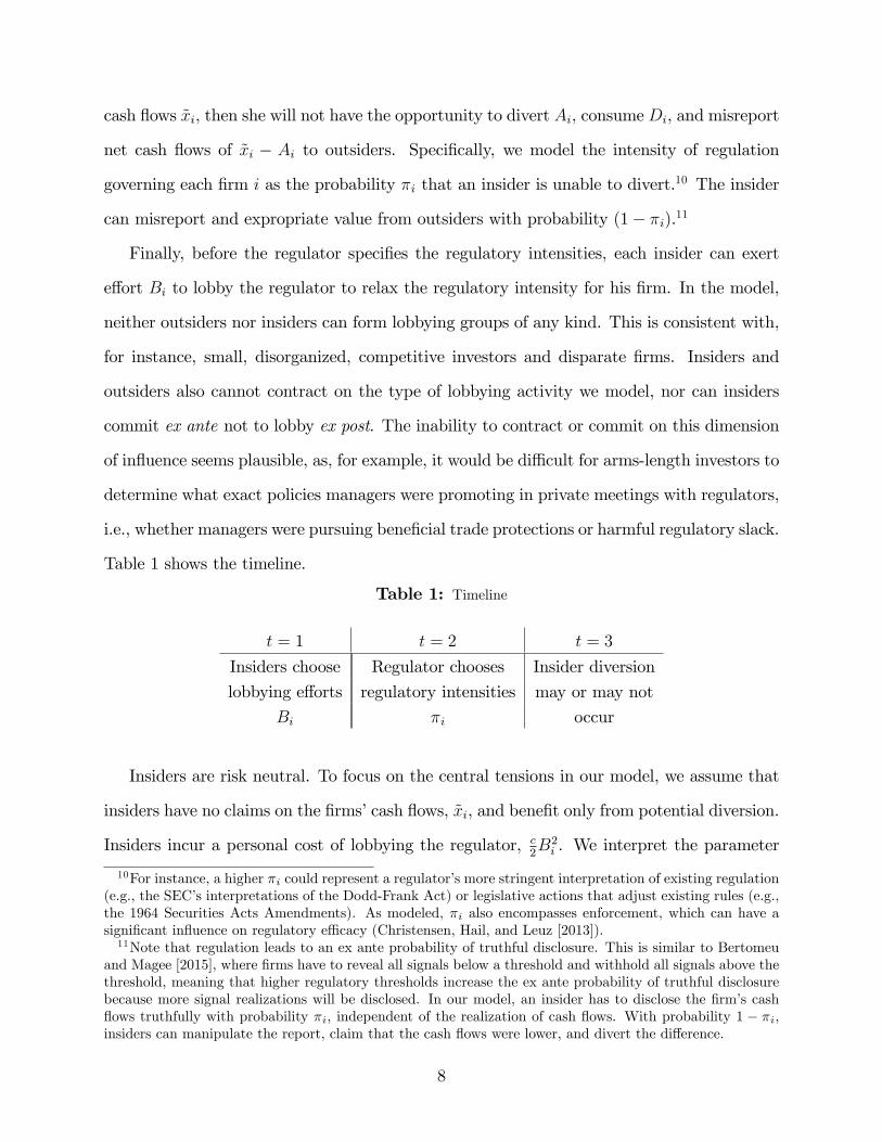
Table 1 shows the timeline.

Table 1: Timeline

t = 1 t = 2 t = 3

Insiders choose Regulator chooses Insider diversion

lobbying efforts regulatory intensities may or may not

Bi πi occur

Insiders are risk neutral. To focus on the central tensions in our model, we assume that

insiders have no claims on the firms’cash flows, x̃i, and benefit only from potential diversion.

Insiders incur a personal cost of lobbying the regulator, c2B2i . We interpret the parameter

10For instance, a higher πi could represent a regulator’s more stringent interpretation of existing regulation(e.g., the SEC’s interpretations of the Dodd-Frank Act) or legislative actions that adjust existing rules (e.g.,the 1964 Securities Acts Amendments). As modeled, πi also encompasses enforcement, which can have asignificant influence on regulatory effi cacy (Christensen, Hail, and Leuz [2013]).11Note that regulation leads to an ex ante probability of truthful disclosure. This is similar to Bertomeu

and Magee [2015], where firms have to reveal all signals below a threshold and withhold all signals above thethreshold, meaning that higher regulatory thresholds increase the ex ante probability of truthful disclosurebecause more signal realizations will be disclosed. In our model, an insider has to disclose the firm’s cashflows truthfully with probability πi, independent of the realization of cash flows. With probability 1 − πi,insiders can manipulate the report, claim that the cash flows were lower, and divert the difference.

8

c > 0 as reflecting the ability of outsiders to effectively monitor and deter insiders’lobbying.

A higher value of c reflects a less severe insider-outsider agency problem on lobbying that

facilitates the subsequent diversion problem. Each insider’s expected utility is given by

Ui = (1− πi)Di −c

2B2i . (1)

With probability (1− πi), the insider is able to take the personally beneficial action and

consumeDi. Insiders always bear the cost of lobbying because they lobby the regulator before

potential diversion occurs. Outsiders receive (unmodeled) payments net of the (modeled)

costs of insider diversion. The collective expected utility of outsiders in firm i, which is also

equal to the value of the outsiders’claim, is given by Vi = µi − (1− πi)Ai.

The timeline above implies that when the regulator decides on the regulatory intensity

at t = 2, the costs of lobbying, c2B2i , are sunk. The regulator influences aggregate utility by

using regulation to reduce the expected losses from diversion:

L (π1, π2;D1, D2, λ) = −λD1 (1− π1)− λD2 (1− π2) (2)

The welfare-interested regulator is only concerned about diversion because of the welfare

loss, λDi, that it imposes on society.12 This welfare loss occurs with probability (1− πi),

for each firm i. The regulator wants to minimize this welfare loss subject to the costs of

regulation.13

12Note that this implies that the regulator would optimally allow insiders to divert when λ = 0. In a moregeneral model, allowing insiders to divert could reduce outsiders’ex ante investment incentives, leading to awelfare-destroying under-investment problem.13Note that c, λ, and πi all capture facets of the regulatory and enforcement environment. We believe

the most direct interpretations of these variables are as follows. First, c captures regulatory corruption andoutsiders’ability to limit insiders’wasteful activities (as c parameterizes the personal cost to the insider oflobbying in the model). Second, λ relates to the protection of property rights (as λ parameterizes the loss ofresources conditional on diversion). Finally, πi relates closely to disclosure quality and protections againstself-dealing (as πi parameterizes the probability that a insider will be able to divert resources, potentiallyby misreporting financial results; see also Djankov et al. [2008]). In our model, πi is endogenous, while cand λ are exogenous because we view corruption and property rights protections to be deeper institutionalparameters than rules and enforcement actions related to disclosure quality and self-dealing.

9

We model three costs associated with regulation. First, we assume a convex cost of

regulation in and of itself, 12π21 + 1

2π22, which avoids bang-bang solutions to the regulatory

choice problem. Second, each insider can influence the regulator through lobbying activ-

ity Bi, which increases the cost of regulatory intensity by Biπi. We refer to the costs

12π21 + 1

2π22 + B1π1 + B2π2 as “implementation costs” that capture both compliance costs

imposed on firms and social costs of implementing regulation. Third, we impose costs of reg-

ulatory heterogeneity, k2

(π1 − π2)2, as heterogeneous regulation plausibly requires greater

care in drafting regulation and increased expenditures in enforcement (e.g., staff costs).

When k = 0, the regulator is free to choose individualized regulation without incurring any

penalty (IR). As k →∞, the regulator will set the same regulatory intensity for both firms,

thereby choosing a one-size-fits-all regime (UR). Note that k can be interpreted as a tech-

nical constraint on the regulator or an institutional commitment (for example, a mission

statement) to regulate different firms in a similar fashion. To capture these alternatives, we

first model the cost parameter k as exogenous and in Section 3 consider an ex-ante planner

(e.g., a legislative body) that chooses k to minimize the welfare losses and implementation

costs.

Thus, the total cost of regulation is given by

C (π1, π2;B1, B2, k) =1

2π21 +

1

2π22 +B1π1 +B2π2 +

k

2(π1 − π2)2 , (3)

and the regulator’s expected utility is

UR = L (π1, π2;D1, D2, λ)− C (π1, π2;B1, B2, k) . (4)

That is, the regulator chooses the regulatory intensity for both firms to minimize the expected

losses from diversion net of the cost of regulation.

10

2.2 The equilibrium

We examine the subgame-perfect Nash equilibrium defined as follows. In period 2, the

regulator chooses optimal regulatory intensities, {π∗1, π∗2} to maximize its objective function

in (4), given {B∗1 , B∗2}. In period 1, each insider i chooses B∗i to maximize her expected

utility in (1) given rational conjectures about the regulator’s strategy in period 2 and the

other insider’s conjectured optimal choice of B∗j .

We solve the equilibrium by backward induction. We begin in period 2, when the reg-

ulator chooses the regulatory intensities. We impose the following two conditions to ensure

interior solutions.

Condition 1 Firms’lobbying costs are suffi ciently high, c > 1λ1+k1+2k

.

Condition 2 Welfare losses from diversion are not too high, D < 1+2k1+2k+q

(λ− 1

c1+k1+2k

)−1.

If c < 1λ1+k1+2k

, then lobbying pushes the optimal regulatory strengths to zero. If D >

1+2k1+2k+q

(λ− 1

c1+k1+2k

)−1, then the regulator’s interest in inhibiting diversion outweighs the im-

plementation costs and the regulator sets π∗i = 1 for at least one firm. For the remainder of

the paper we assume Conditions 1 and 2 are satisfied.

The regulator’s expected utility is concave and has the following first-order conditions:

λDi −Bi − k(π∗i − π∗j

)− π∗i = 0, (5)

for i, j ∈ {1, 2} and i 6= j. The equations in (5) imply

π∗i =(1 + k) (λDi −Bi) + k (λDj −Bj)

1 + 2k. (6)

Note that both ∂π∗i /∂Bi and ∂π∗i /∂Bj are negative, so that more lobbying from either insider

reduces the regulatory intensity for both firms for any k > 0. Higher values of k, i.e., greater

uniformity, imply that an insider’s lobbying has a lower effect on the regulatory intensity his

11

firm faces, since ∂2π∗i /(∂k∂Bi) = (1 + 2k)−2 > 0. This mitigates the negative effect of Bi on

π∗i . In contrast, the influence of insider i’s lobbying on the regulatory intensity of firm j is

increasing in k, since ∂2π∗i /(∂k∂Bj) = − (1 + 2k)−2 < 0. In our model, k captures the cost

to the regulator of setting different regulatory strengths for the two firms. Intuitively, higher

values of k imply that the regulator chooses more similar regulatory intensities for the two

firms, so that one firm’s lobbying has a greater spillover effect on the regulatory intensity of

the other firm, making the negative effect of Bj on π∗i stronger.

Given the anticipated choice of the regulator, insiders choose their influence activities to

maximize Ui in (1). Substituting π∗i into Ui and taking the derivative yields the first-order

conditions. Solving the first-order conditions14 implies that the optimal Bi are given by

B∗i =1

c

1 + k

1 + 2kDi. (7)

This shows that higher personal benefits of misbehavior, Di, are associated with higher

lobbying efforts from insiders, B∗i . Furthermore, note that an increase in k decreases both

insiders’ lobbying efforts, ∂B∗i /∂k = −1cDi (1 + 2k)−2, which is due to the effect that an

increase in k has on the regulator’s response to lobbying efforts.

The equilibrium in terms of exogenous parameters is shown in the following proposition,

which follows straightforwardly from substituting B∗i from (7) into (6) and solving these two

equations for π∗1 and π∗2. All proofs can be found in the appendix.

Proposition 1 There is a unique interior equilibrium with π∗i ∈ (0, 1) for i ∈ {1, 2} defined14The first order conditions are 1+k

1+2kDi − cBi = 0. The second order conditions are satisfied asddBi

(1+k2k+1Di − cBi

)= −c < 0.

12

by

π∗1 = D

(λ− 1

c

1 + k

1 + 2k

)1 + 2k − q

1 + 2k,

π∗2 = D

(λ− 1

c

1 + k

1 + 2k

)1 + 2k + q

1 + 2k,

B∗1 =1

c

1 + k

1 + 2kD (1− q) , and

B∗2 =1

c

1 + k

1 + 2kD (1 + q) .

To understand the characteristics of the equilibrium, it is helpful to investigate the equi-

librium regulatory intensities. Note that equation (6) implies that two factors influence

a firm’s regulatory intensity: potential losses from diversion and insiders’lobbying efforts.

More specifically, denoting ω = 11+2k

, firm i’s regulatory intensity is a weighted average of

firm i’s potential loss from diversion and lobbying effort and the average potential loss from

diversion and lobbying effort:

π∗i = ω (λDi −B∗i ) + (1− ω)(λD − B̄∗

). (8)

B∗i is defined in equation (7) and B̄∗ = (B∗1 +B∗2) /2 = 1

c1+k1+2k

D. Under pure IR, the average

diversion and lobbying have no impact (as limk→0 (1− ω) = 0), while under pure UR, it is

only the average diversion and lobbying that matter (as limk→∞ ω = 0). Note that q ∈ [0, 1)

implies that D2 ≥ D1 and that π∗2 ≥ π∗1.

The expression for π∗i in equation (8) illustrates three important forces in our model.

First, as lobbying becomes prohibitively costly to insiders, i.e., c → ∞, insiders cease lob-

bying. Absent lobbying, the regulator sets the optimal regulatory strength for firm i as a

weighted average of only the expected loss from diversion for the target firm (with deadweight

loss λDi) and the expected loss from diversion for the “average firm”(with deadweight loss

λD).

Second, the degree of uniformity, k, influences the weights on firm-specific and average

13

factors in (8), as ω = 11+2k

. Increases in regulatory uniformity increase the regulator’s weight

on D and B̄∗ in equation (8) relative to the weight on Di and B∗i . Uniformity thus pushes

regulatory qualities toward each other. We call this the convergence effect of regulatory

uniformity. Naturally, the convergence effect pushes the higher (lower) regulatory intensity

down (up). If firms are homogeneous, i.e., q = 0, then D1 = D2 = D, and the convergence

effect is trivial. Absent lobbying (i.e., as c → ∞), π∗2 decreases and π∗1 increases with an

increase in k for any q > 0. When firms are homogeneous and cannot lobby, regulatory

uniformity, k, plays no role in our model.

Third, as discussed above, there is an additional effect of regulatory uniformity on each

firm’s regulatory intensity, via ∂B∗i /∂k < 0 and ∂B̄∗/∂k < 0. This is the free-rider effect

in our model. It reduces both insiders’ lobbying efforts and thereby increases both firms’

regulatory intensities, since B∗i and B̄∗ both enter negatively in (8).

2.3 Equilibrium characteristics

Corollaries 1-3 present our comparative statics results for the baseline model. Corollary 1

summarizes the effects of changes in the cost of lobbying and the effi ciency of diversion.

Corollary 1 Lobbying and the deadweight loss from diversion

(a) As the cost of lobbying, c, increases, (i) the lobbying efforts of both insiders decreaseand (ii) the regulatory intensities for both firms increase.

(b) As the proportional deadweight loss from diversion, λ, increases, (i) the lobbying effortsof both insiders are unchanged and (ii) the regulatory intensities for both firms increase.

Corollary 1 shows that insiders lobby less when their costs of lobbying increase, but their

lobbying efforts do not respond directly to the costs their diversion imposes on outsiders.

When insiders lobby less, regulatory intensities increase, and, as a result, the expected value

of the future payouts to investors increases. Note that a change in c only has a direct effect

on the insiders; regulatory intensities are only affected indirectly. Changes in λ, however,

only have a direct effect on regulatory intensities, an effect which operates through the

14

regulator’s preferences for lower ineffi ciency regardless of lobbying efforts. When λ increases,

the regulator is more interested in high regulatory intensity because the deadweight loss from

diversion decreases.

Corollary 2 analyzes the effects of increases in firm heterogeneity and the average potential

diversion from the firms, both of which are operationalized by the amounts that insiders can

divert, D1 and D2. Specifically, recall that D1 = D (1− q) and D2 = D (1 + q) such that

average diversion is given by D = D1+D22

and heterogeneity is given by q = D2−D12D

.

Corollary 2 Firm heterogeneity and average potential diversion

(a) As firms become more heterogeneous (i.e., q increases), (i) the lobbying effort of thethe bad firm’s insider and the regulatory intensity for the bad firm increase; (ii) thelobbying effort of the good firm’s insider and the regulatory intensity for the good firmdecrease; and (iii) total lobbying is unchanged.

(b) As average potential diversion, D, increases, (i) both insiders lobby the regulator more,and (ii) the regulatory intensities for both firms increase.

Corollary 2 (a) analyzes the effect of increased heterogeneity between firms. First note that

an increase in heterogeneity implies that for firm 2 (1) there is more (less) cash for the

insider to divert and a higher (lower) potential deadweight loss that the regulator would

like to prevent. While the resulting increase in lobbying effort from firm 2’s insider acts to

decrease firm 2’s regulatory intensity, the increased deadweight loss acts to increase π∗2. The

latter effect dominates the former such that firm 2’s regulatory intensity increases despite

the increased lobbying effort from firm 2’s insider. The opposite occurs for firm 1, which

becomes less important to the regulator and whose smaller amount of diversion provides

a weaker motivation to the insider to lobby. The effects of heterogeneity on each firm’s

lobbying are equal and opposite, implying no net effect of heterogeneity on total lobbying.

Part (b) shows that with an increase in average potential diversion in the economy, both

insiders have more resources available to divert, and thus increase their lobbying efforts.

However, since the potential deadweight loss also increases, the regulator is interested in

higher regulatory intensities and, despite the increased lobbying, increases π∗1 and π∗2. If the

15

potential for diversion D increases in the firms’realized or expected cash flows, our model

suggests greater lobbying in macroeconomic expansions than contractions, in contrast to the

prediction in Bertomeu and Magee [2011].

Finally, we analyze the effect of a change in k, which represents the degree of UR relative

to IR. Denote c̄ = 12λ

(2 + 1+q

q

)and c = 1

2λq+1q.15

Corollary 3 Degree of uniformity: As the cost to the regulator of individualized reg-ulation, k, increases, (i) the lobbying efforts of both insiders decrease; (ii) the regulatoryintensity for the good firm increases; (iii) the regulatory intensity for the bad firm decreasesfor c > c̄, first increases then decreases for c̄ > c > c, and always increases for c < c; and(iv) the average regulatory intensity increases.

As discussed in the introduction, constraining the regulator to set similar regulatory intensi-

ties for different firms introduces two effects, the convergence effect and the free-rider effect.

The convergence effect arises because an increase in k makes the regulator more inclined to

apply the same regulatory intensity to both firms. Therefore, π∗1 and π∗2 are set closer to

each other in equilibrium. This effect pushes the higher π∗2 down and the lower π∗1 up. The

free-rider effect occurs because, when the regulator chooses more similar values for π∗1 and

π∗2, the lobbying efforts of firm i’s insider have a stronger effect on the regulatory intensity

of firm j. This leads to a more intense free-rider problem on insiders’lobbying in that each

insider relies more on the other insider’s lobbying efforts to economize on his own efforts.

Insiders therefore reduce their overall lobbying efforts, which increases π∗i for both firms.

The net effects of an increase in k on insiders’lobbying are unambiguous. So, too, are the

net effects of an increase in k on regulatory intensity for the good firm, as the convergence and

free-rider effects both act to increase π∗1. However, the net effects of the convergence and free-

rider effects on regulatory strengths for the bad firm are ambiguous. For π∗2, the convergence

and free-rider effects oppose each other, and either may dominate, yielding implications

for π∗2 that depend on parameter values. When the agency problem is suffi ciently severe

(c < c), such that both firms heavily lobby the regulator, the free-rider effect dominates,

15When q = 0, we set c|q=0 = limq→0 c =∞ and c|q=0 = limq→0 c =∞.

16

causing π∗2 to be increasing in k. When the agency problem is suffi ciently mild (c > c̄), the

convergence effect dominates, causing π∗2 to be decreasing in k. Finally, when the agency

problem has intermediate strength (c̄ > c > c), the free-riding effect dominates for low values

of k, such that dπ∗2/dk > 0, but the convergence effect dominates for high values of k, such

that dπ∗2/dk < 0.16 Ultimately, when k approaches infinity, the regulator sets π∗1 = π∗2,

irrespective of c. Overall, the free-rider effect and the convergence effect complement each

other for the firm with the lower regulatory intensity and conflict with each other for the

firm with the higher regulatory intensity. Given that lobbying for both firms decreases, the

average regulatory intensity increases.

The parameter k reflects the extent to which the regulator is bound to apply the same

regulatory intensity to both firms. As capital market equilibria and the regulatory system

likely evolve together, we next analyze the effect of allowing k to be chosen by an ex-ante

planner concerned with minimizing the welfare losses from diversion and the implementation

costs of regulation.

3 The optimal regulatory system

In this section we examine the optimal choice of balance between uniform and individualized

regulation, i.e., the choice of k, from the perspective of an ex-ante planner concerned with

the welfare loss from diversion and the implementation costs of regulation. We interpret k

as a deep institutional parameter that is set for the long run (or ex ante) and is not subject

to lobbying influence.

We assume that the planner is interested in minimizing the loss from diversion subject to

the costs of implementation.17 While considering implementation costs, we assume that the

16Specifically, if c > c, then dπ∗2/dk < 0 if and only if k >12

(1

λ(c−c) − 1).

17This is similar to maximizing outsiders’expected utility net of the regulator’s implementation costs. Ina competitive stock market where the outsiders represent marginal investors, the outsider’s expected utility,µi − (1− πi) (1 + λ)Di, would be closely related to the stock price. This suggests an interpretation of theplanner as an exchange choosing its degree of uniformity to maximize market capitalization net of regulatoryimplementation costs.

17

planner does not consider the direct costs she imposes on the regulator through her choice

of k, which are (k/2) (π1 − π2)2, or the costs that managers personally bear for socially

undesirable lobbying, which are (c/2)B21 + (c/2)B2

2 .18

The planner’s objective function is given by

US = − (1− π1)λD (1− q)− (1− π2)λD (1 + q)− 1

2

(π21 + π22

)−B1π1 −B2π2. (9)

Recall from Proposition 1 that π∗1 > 0 and π∗2 > 0 requires Condition 1 to hold, i.e., λ >

1c1+k1+2k

. We therefore restrict our attention to λ > 1csuch that the regulator will choose

positive π∗1 and π∗2 for any k ∈ [0,∞), chosen by the planner. The solution is given in the

following proposition.

Proposition 2 When q2 (2cλ− 1)− 1 ≤ 0, the planner chooses a perfectly uniform regula-tory system, k† →∞. When q2 (2cλ− 1)− 1 > 0, the planner chooses

k† =1 + q2 (2− cλ) + q

√2 (1 + q2) + q2 (1− cλ)2

2 (q2 (2cλ− 1)− 1). (10)

The threshold in Proposition 2 is related to the importance of regulatory uniformity in

improving regulatory intensities and to the cost imposed by uniform regulation. Because the

economic forces that drive the decision to choose a perfectly uniform system (k† → ∞) are

the same forces that lead to an increase in k†, we focus our discussion on the comparative

statics presented in the following corollary.

Corollary 4 The optimal degree of uniformity from the planner’s perspective, k†, (i) weaklydecreases in insiders’personal costs of lobbying, c; (ii) weakly decreases in the deadweightloss from insiders’diversion, λ; (iii) is independent of mean firm size, D; and (iv) weaklydecreases in the degree of firm heterogeneity, q.

18Including the costs of heterogeneity imposed on the regulator in the planner’s objective (mechanically)decreases the optimal k. We view these not as true economic costs but rather as a modeling device torepresent a commitment to more or less uniform regulation. Including the managers’costs of lobbying inthe planner’s objective implies that the legislature prefers to make managerial opportunism cheaper, whichseems unreasonable.

18

Corollary 4 shows that it is more valuable to constrain the extent to which the regulator can

individualize regulation when lobbying-related agency problems are severe (low c), firms are

similar (low q), or managerial diversion is effi cient (low λ). Furthermore, these comparative

statics are monotone over the whole parameter range. For example, starting at a high c,

decreases in c first continuously increase k†. As c decreases further and q2 (2cλ− 1)− 1→ 0

from above, the optimal regulatory system approaches perfect uniformity, i.e., k† →∞. The

first two results in the corollary directly point to our two main economic forces: while free-

riding on lobbying reduces the impact of the agency problem and makes UR more preferable,

firm heterogeneity makes regulatory heterogeneity and IR more preferable. The third result

is similar in that low values of λ push the potential welfare losses from diversion in either

firm towards zero and thus towards each other, implying similar results to low heterogeneity

driven by low q. Mean firm size, D, does not affect the optimal k†, as it is a scaling factor

in the planner and regulator’s utilities given equilibrium lobbying efforts.

The following corollary explores how the equilibrium regulatory strengths, π†i , and lobby-

ing efforts, B†i , change with changes in the underlying parameters when k† is endogenously

set by the planner.

Corollary 5 When the planner optimally chooses an interior degree of uniformity (i.e.,q2 (2cλ− 1)− 1 > 0),

(i) the lobbying efforts of (a) both insiders decrease in lobbying costs, c; (b) insider 1, B†1,is non-monotonic in firm heterogeneity, q; (c) insider 2, B†2, increases in firm hetero-geneity, q; and (d) both insiders increase in potential diversion, D, and the welfare lossfrom diversion, λ;

(ii) total lobbying, B†1 + B†2, is decreasing in lobbying costs, c, and increasing in firm het-erogeneity, q, potential diversion, D, and the welfare loss from diversion, λ.

(iii) the regulatory intensity for (a) firm 1, π†1, decreases in lobbying costs, c, and firmheterogeneity, q; (b) firm 2, π†2, increases in lobbying costs, c, and firm heterogeneity,q; and (c) for both firms increase in potential diversion, D, and the welfare loss fromdiversion, λ.

When k† is endogenously chosen by the planner, any change in an exogenous parameter

affects regulatory strength and lobbying efforts through two channels. First, they have

19

direct effects as indicated in the corollaries in Section 2.3. Second, they have indirect effects

on regulatory strength and lobbying efforts through their effects on k†. Taking lobbying

costs as a representative example, an increase in c directly decreases both insiders’lobbying

efforts and increases both firms’regulatory intensities. However, the optimal k† decreases

when c increases, as lobbying becomes less problematic. The less uniform regulatory system

allows the regulator to respond more strongly to the individual characteristics of each firm.

Even though both lobbying efforts decrease, the effect of a reduced k† dominates such that

π†1 decreases and π†2 increases.

Similarly, the extent of regulatory uniformity decreases when firm heterogeneity, q, in-

creases. The decrease in k† works to increase lobbying efforts and to generally decrease

regulatory intensities. (Note that the bad firm’s regulatory intensity may increase due to

the reduced convergence effect.) Furthermore, the increase in q directly reduces the lobbying

effort of the good firm’s insider, which causes B†1 to be non-monotonic in q. Firm 1’s regula-

tory intensity, however, always decreases as the diversion amount gets smaller. In contrast,

for the bad firm, the direct and the indirect effects of q on lobbying reinforce each other such

that B†2 increases. However, the regulator’s interest in reducing the loss from diversion in

firm 2 increases in q such that π†2 increases despite the increased lobbying. As shown in part

(ii) of Corollary 5, total lobbying always increases with firm heterogeneity, q, and the welfare

loss from diversion, λ. In contrast, when uniformity is exogenous, q and λ have no net effects

on total lobbying. Specifically, when k is exogenous, λ has no direct effect on either firm’s

lobbying, and the effects of changes in heterogeneity on B1 and B2 exactly cancel each other

out. When, instead, k is endogenous, increases in q and λ decrease k†, which causes total

lobbying to increase.

Finally, Corollary 4 shows that changes in D have no effect of k†, this implies that the

results from the setting with an exogenous k are unchanged. However, while lobbying efforts

were constant in λ with a constant degree of uniformity, an increase in λ lowers k† such that

both insiders’lobbying efforts increase in λ when k is chosen endogenously by the planner

20

as k†. Table 2 lists the comparative statics for the baseline model and the extension with an

endogenous k†.

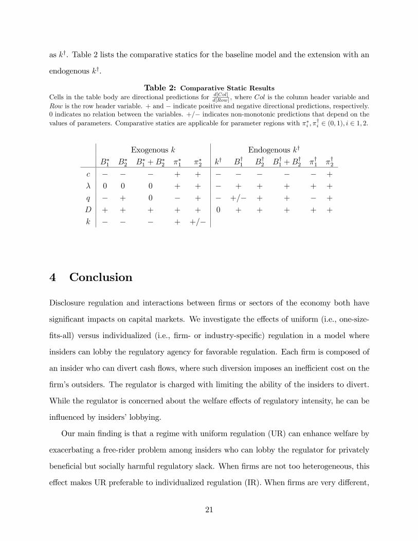
Table 2: Comparative Static ResultsCells in the table body are directional predictions for d[Col]

d[Row] , where Col is the column header variable andRow is the row header variable. + and − indicate positive and negative directional predictions, respectively.0 indicates no relation between the variables. +/− indicates non-monotonic predictions that depend on thevalues of parameters. Comparative statics are applicable for parameter regions with π∗i , π

†i ∈ (0, 1), i ∈ 1, 2.

Exogenous k Endogenous k†

B∗1 B∗2 B∗1 +B∗2 π∗1 π∗2 k† B†1 B†2 B†1 +B†2 π†1 π†2c − − − + + − − − − − +

λ 0 0 0 + + − + + + + +

q − + 0 − + − +/− + + − +

D + + + + + 0 + + + + +

k − − − + +/−

4 Conclusion

Disclosure regulation and interactions between firms or sectors of the economy both have

significant impacts on capital markets. We investigate the effects of uniform (i.e., one-size-

fits-all) versus individualized (i.e., firm- or industry-specific) regulation in a model where

insiders can lobby the regulatory agency for favorable regulation. Each firm is composed of

an insider who can divert cash flows, where such diversion imposes an ineffi cient cost on the

firm’s outsiders. The regulator is charged with limiting the ability of the insiders to divert.

While the regulator is concerned about the welfare effects of regulatory intensity, he can be

influenced by insiders’lobbying.

Our main finding is that a regime with uniform regulation (UR) can enhance welfare by

exacerbating a free-rider problem among insiders who can lobby the regulator for privately

beneficial but socially harmful regulatory slack. When firms are not too heterogeneous, this

effect makes UR preferable to individualized regulation (IR). When firms are very different,

21

however, the benefit of UR in reducing lobbying is outweighed by the costs of setting similar

regulatory intensities for heterogeneous firms.

Through analysis of the model, we provide several empirical implications, which we hope

will be helpful in understanding the effects of the regulatory regime on lobbying and the

quality of disclosure regulation. For example, we predict that regulatory regimes will tend

towards uniformity when agency problems between investors and managers are more severe

or when it is less costly for insiders to lobby the regulator.

Our model suggests that lobbying could be more diffi cult when regulatory standards are

principles-based and apply broadly (even across jurisdictions) as under IFRS, than when

regulatory standards are rules-based and can be tailored firms’and industries’particular

circumstances, as under US GAAP (Herz [2003]). In line with this interpretation, the IASB

might be in effect more immune to political pressure, as suggested by Canham [2009]. Zeff

[2002] observes that Swiss CFOs displayed a preference for US GAAP over IFRS in part due

to preparers’ability to influence regulatory standards in the U.S. Our comparison of rules-

based GAAP and principles-based IFRS suggests that jurisdictions characterized by weaker

agency problems between insiders and outsiders might be more likely to delay or avoid

transitions from GAAP to IFRS, while jurisdictions with significant agency problems would

seek out commitments to regulatory uniformity. This may have been one of several reasons

for the delays in US convergence to IFRS, and might also contribute to other countries’

delays in adopting IFRS.

Similarly, some of the divergence between code and common law legal systems (see, e.g.,

La Porta et al. [2000]) could relate to uniformity in de facto regulations. In common-law

jurisdictions, judicial rulings establish precedents that apply relatively uniformly, while in

code law systems precedents are not established by judicial rulings. This implies that there

is greater de facto uniformity in common-law jurisdictions, which is consistent with the

stronger legal protections of outside investors and enforcement of these rules in common law

countries relative to code law countries (e.g., La Porta et al. [1998]).

22

We generate results in a setting with a single regulator who is potentially constrained

to set uniform regulation. The intuition easily extends to related institutional design prob-

lems, including whether to have a single or multiple accounting standard-setters and the

effects of auditor and financial exchange mergers.19 In the US, for example, there have been

arguments and movements both in favor of UR, through merging the FASB and IASB or

standards convergence, and in favor of IR, through allowing firms to choose to report under

US GAAP or IFRS. Our results imply that changes in regulatory uniformity have impli-

cations for lobbying and regulatory intensity. Different auditors or financial exchanges can

have different policies regarding disclosure, suggesting that mergers of auditing firms can

also be seen as movements towards uniformity. Mergers of auditors and exchanges can help

reduce managerial influence over their disclosure policies, which we show can be beneficial

overall.19When comparing settings with a single or multiple regulators (or standard-setters), it is important to

also consider economic forces related to decentralization that we have not included in our model, such asinformation asymmetry, goal congruence, and coordination across regulators (e.g., Harris, Kriebel, and Raviv[1982]).

23

References

Albuquerue, R., and N. Wang. “Agency conflicts, investment, and asset pricing.”TheJournal of Finance 63 (2008): 1—40.

Armstrong, C. S., W. R. Guay, and J. P. Weber. “The role of information andfinancial reporting in corporate governance and debt contracting.”Journal of Accountingand Economics 50 (2010): 179—234.

Arrow, K. J. “A diffi culty in the concept of social welfare.”Journal of Political Economy(1950): 328—346.

Bebchuk, L., and Z. Neeman. “Investor protection and interest group politics.”Reviewof Financial Studies 23 (2010): 1089—1119.

Beresford, D. R. “Congress looks at accounting for business combinations.”AccountingHorizons 15 (2001): 73—86.

Bertomeu, J., and E. Cheynel. “Toward a positive theory of disclosure regulation: Insearch of institutional foundations.”The Accounting Review 88 (2013): 789—824.

Bertomeu, J., and R. Magee. “From low-quality reporting to financial crises: Politicsof disclosure regulation along the economic cycle.”Journal of Accounting and Economics52 (2011): 209—227.

Bertomeu, J., and R. P. Magee. “Political pressures and the evolution of disclosureregulation.”Review of Accounting Studies 20 (2014): 775—802.

“Mandatory disclosure and asymmetry in financial reporting.”Journal of Account-ing and Economics 59 (2015): 284—299.

Beyer, A., I. Guttman, and I. Marinovic. “Optimal contracts with performancemanipulation.”Journal of Accounting Research 52 (2014): 817—847.

Canham, C. “IASB resists IFRS political pressure,” Accessed athttp://www.theaccountant-online.com/news/iasb-resists-ifrs-political-pressure on June12, 2015, 2009.

Caskey, J., and V. Laux. “Corporate Governance, Accounting Conservatism, and Ma-nipulation.”Management Science, Forthcoming (2015).

Chen, Q., T. Hemmer, and Y. Zhang. “On the relation between conservatism in account-ing standards and incentives for earnings management.”Journal of Accounting Research45 (2007): 541—565.

Christensen, H. B., L. Hail, and C. Leuz. “Mandatory IFRS reporting and changesin enforcement.”Journal of Accounting and Economics 56 (2013): 147—177.

Chung, D. “The informational effect of corporate lobbying against proposed accountingstandards.”Review of Quantitative Finance and Accounting 12 (1999): 243—270.

24

Coates, J. “The goals and promise of the Sarbanes-Oxley Act.”The Journal of EconomicPerspectives 21 (2007): 91—116.

Condon, C. “Money funds seen failing in crisis as SEC bows to lobby.”Bloomberg On-line (2012), Accessed at http://www.bloomberg.com/news/2012-08-01/money-funds-seen-failing-in-crisis-as-sec-bows-to-lobby.html on November 8, 2012.

Demski, J. S. “The general impossibility of normative accounting standards.”The Account-ing Review 48 (1973): 718—723.

“Choice among financial reporting alternatives.”The Accounting Review 49 (1974):221—232.

Djankov, S., R. La Porta, F. Lopez-de Silanes, and A. Shleifer. “The law andeconomics of self-dealing.”Journal of Financial Economics 88 (2008): 430—465.

Dye, R. A., and S. Sunder. “Why not allow FASB and IASB standards to compete inthe US?.”Accounting Horizons 15 (2001): 257—271.

Friedman, H. L., J. S. Hughes, and R. Saouma. “Implications of biased reporting:conservative and liberal accounting policies in oligopolies.”Review of Accounting Studies21 (2016): 251—279.

GAO “Securities And Exchange Commission: Existing post-employment controls couldbe further strengthened.” US Government Accountability Offi ce (2011), accessed athttp://gao.gov/assets/330/320942.html on November 8, 2012.

Gao, F., J. Wu, and J. Zimmerman. “Unintended consequences of granting small firmsexemptions from securities regulation: Evidence from the Sarbanes-Oxley Act.”Journalof Accounting Research 47 (2009): 459—506.

Gao, P. “A measurement approach to conservatism and earnings management.”Journal ofAccounting and Economics 55 (2013): 251—268.

Gao, P., H. Sapra, and H. Xue. “A Model of Principles-Based vs. Rules-Based Stan-dards.,”Working Paper, NYU Stern and Chicago Booth, 2016.

Gipper, B., B. Lombardi, and D. J. Skinner. “The politics of accounting standard-setting: A review of empirical research,”Working paper, 2013.

Golden, R. G. “Remarks of FASB Chairman Russell G. Golden at NASBA Conference inMaui, Hawaii,”Accessed at http://www.fasb.org/cs/ on June 12, 2015, 2013.

Grossman, G., and E. Helpman. “Protection for sale.”American Economic Review 84(1994): 833—850.

Harris, M., C. H. Kriebel, and A. Raviv. “Asymmetric information, incentives andintrafirm resource allocation.”Management Science 28 (1982): 604—620.

25

Herz, R. H. “A year of challenge and change for the FASB.”Accounting Horizons 17 (2003):247—255.

Hochberg, Y., P. Sapienza, and A. Vissing-Jørgensen. “A lobbying approach toevaluating the Sarbanes-Oxley Act of 2002.”Journal of Accounting Research 47 (2009):519—583.

Jensen, M. C., andW. H. Meckling. “Theory of the firm: Managerial behavior, agencycosts and ownership structure.”Journal of Financial Economics 3 (1976): 305—360.

Kahan, M. “Some problems with stock exchange-based securities regulation.”Virginia LawReview 83 (1997): 1509—1519.

La Porta, R., F. Lopez-de Silanes, A. Shleifer, and R. Vishny. “Investor protec-tion and corporate governance.”Journal of Financial Economics 58 (2000): 3—27.

La Porta, R., F. Lopez-de Silanes, A. Shleifer, and R. W. Vishny. “Law andfinance.”Journal of Political Economy 106 (1998): 1113—1155.

Mahoney, P. “The exchange as regulator.”Virginia Law Review 83 (1997): 1453—1500.

Peltzman, S. “Toward a more general theory of regulation.”Journal of Law and Economics19 (1976): 211—240.

Perotti, E., and P. Volpin. “Politics, investor protection and competition,”Workingpaper, 2008.

POGO “Revolving regulators: SEC faces ethics challenges with revolving door.”Project on Government Oversight (2011), accessed at http://www.pogo.org/pogo-files/reports/financial-oversight/revolving-regulators/fo-fra-20110513.html on November8, 2012.

Ray, K. “One size fits all? Costs and benefits of uniform accounting standards,”Workingpaper, 2012.

Rodrik, D. “Tariffs, subsidies, and welfare with endogenous policy.” Journal of Interna-tional Economics 21 (1986): 285—299.

Schipper, K. “Discussion of voluntary corporate disclosure: The case of interim reporting.”Journal of Accounting Research 19 (1981): 85—88.

Shleifer, A., and R. W. Vishny. “A survey of corporate governance.”The Journal ofFinance 52 (1997): 737—783.

Stigler, G. “The theory of economic regulation.”The Bell Journal of Economics 2 (1971):3—21.

Sunder, S. “Political economy of accounting standards.”Journal of Accounting Literature7 (1988): 39—41.

26

Watts, R. L., and J. L. Zimmerman. “Towards a positive theory of the determinationof accounting standards.”The Accounting Review 53 (1978): 112—134.

Zeff, S. “‘Political’lobbying on proposed standards: A challenge to the IASB.”AccountingHorizons 16 (2002): 43—55.

27

Appendix

Proposition 1: The solution to our game is given by the values of four unknowns, Bi and

πi for i ∈ {1, 2}, that solve a constrained system of four linear equations: either the four

FOC’s, (7) and (6); or corner solutions replacing any of the FOCs, such as Bi = 0, πi = 0,

or πi = 1, for i ∈ {1, 2}. For the interior solution, Di > 0 implies B∗i > 0. Substituting B∗i

from (7) into (6) yields

π∗i =

(λ− 1

c

1 + k

1 + 2k

)(1 + k)Di + kDj

1 + 2k. (11)

Since π∗1 < π∗2 implies that π∗2 < 1⇒ π∗1 < 1, we have an interior equilibrium, i.e., π∗i ∈ (0, 1),

if and only if

c >1

λ

1 + k

1 + 2k, which ensures π∗i > 0 for i ∈ {1, 2} , and

D

(λ− 1

c

1 + k

1 + 2k

)(1 +

q

1 + 2k

)< 1, which ensures π∗2 < 1.

The first inequality, c > 1λ1+k1+2k

, is Condition 1. The second inequality,D(λ− 1

c1+k1+2k

) (1 + q

1+2k

)<

1, implies Condition 2. The expressions in Proposition 1 follow directly.

Corollaries 1, 2, and 3: These proofs follow by straightforward differentiation of the

expressions for π∗1, π∗2, B

∗1 , and B

∗2 given in Proposition 1. Derivatives are provided in the

28

table below, where each cell gives d[Column header]d[Row header] :

B∗1 B∗2 π∗1 π∗2

c − 1c2

1+k1+2k

D (1− q) − 1c2

1+k1+2k

D (1 + q) D(1 + k†

)2k+1−qc2(2k+1)2

D (1 + k) 2k+1+q

c2(2k+1)2

λ 0 0 D 2k+1−q2k+1

D 2k+1+q2k+1

q −1c1+k1+2k

D 1c1+k1+2k

D − D1+2k

(λ− 1

c1+k1+2k

)D

1+2k

(λ− 1

c1+k1+2k

)D 1

c1+k1+2k

D (1− q) 1c1+k1+2k

D (1 + q)(λ− 1

c1+k1+2k

)1+2k−q1+2k

(λ− 1

c1+k1+2k

)1+2k+q1+2k

k −D 1−qc(2k+1)2

−D 1+q

c(2k+1)2D (1+q(2cλ−1))(1+2k)−2q

c(1+2k)3D (1+q−2qcλ)(1+2k)+2q

c(1+2k)3

For Corollary 3, part (iv), the average regulatory intensity is given by π∗1+π∗2

2= D cλ(1+2k)−(1+k)

c(1+2k),

and the derivative is given by ddk

(π∗1+π

∗2

2

)= D 1

c(2k+1)2> 0. The signs of the derivatives in

the table are immediate, except for dπ∗idk.20 To show Corollary 3, part (ii), we have

dπ∗1dk

=D

c (1 + 2k)3((1− q) (1 + 2k)− 2q + 2cλq (1 + 2k))

>D

c (1 + 2k)3((1− q) (1 + 2k)− 2q + 2 (1 + k) q)

=D (2k + 1− q)c (1 + 2k)3

> 0,

where the first inequality follows from Condition 1. For Corollary 3, part (iii), the derivative

of π∗2 with respect to k can be written as

dπ∗2dk

=2qD

(2k + 1)2

(1

2c

(2 +

1 + q

q

)− λ− 2

k

c (2k + 1)

)

The derivative is always negative when 12c

(2 + 1+q

q

)−λ < 0, i.e., when c > c̄ = 1

2λ

(2 + 1+q

q

).

20Recall that Condition 1 ensures that λ− 1c1+k1+2k > 0.

29

That is, ∂π∗2

∂k< 0 when c is suffi ciently large. The above derivative is positive when

1

2c

(2 +

1 + q

q

)− λ− 2

k

c (2k + 1)> 0

⇔ 1

2λ

(2 +

1 + q

q− 2

2k

2k + 1

)> c

The term in parentheses ranges from 1+qqto 2 + 1+q

qbecause 2 2k

(2k+1)ranges from 0 to 2. This

implies that ∂π∗2∂k

> 0 whenever c < c = 1λ1+q2q, i.e. when c is suffi ciently small. Finally, for

intermediate values of c, when c̄ > c > c, the derivative is positive for k = 0 and is negative

when k2k+1

>(12c

(2 + 1+q

q

)− λ)c2, i.e., when k > 1

2

(1

λ(c−c) − 1).

Proposition 2: To prove the Proposition, we (I) establish the first-order condition, which

(II) has three solutions. We then rule out two of the three by showing that (III) one of the

solutions is a local minimum, and (IV) another is negative for feasible parameter values. We

(V) establish a condition for the third solution to be a global maximum. Finally, we (VI)

show that if the condition is violated, the optimum is a corner solution with k† →∞.

I. Substituting expressions for π∗i and B∗i from (6) and (7) into US in (9) yields,

U∗S = US (π∗1, π∗2, B

∗1 , B

∗2)

= D

(2D (1 + q2 + 4k (1 + k + q2)) (1 + k − c (1 + 2k)λ)2 − 4c2 (1 + 2k)4 λ

)2c2 (1 + 2k)4

(12)

and maximizing U∗S with respect to k gives the following FOC:

2D21 + q2 + 4k (1 + k + q2 (2 + k))− 4ck (1 + 2k) q2λ

c2 (1 + 2k)5(cλ− 1 + k (2cλ− 1)) = 0. (13)

30

II. The FOC is satisfied for k0 = 1−cλ2cλ−1 ,

k+ =1 + q2 (2− cλ) +

√q2(2 + q2

(3− 2cλ+ c2λ2

))−2 + q2 (−2 + 4cλ)

, and

k− =1 + q2 (2− cλ)−

√q2(2 + q2

(3− 2cλ+ c2λ2

))−2 + q2 (−2 + 4cλ)

.

III. It is straightforward to show that k− < 0 for the relevant values of c, q, and λ (i.e.,

c > 0, λ > 0, and 0 ≤ q ≤ 1).

IV. k0 > 0 if and only if 1 < 2cλ ≤ 2, but in this range, the SOC,

d2U∗Sdk2|k=k0 = −2D2

c2(1− 2cλ)4

(q2 (2cλ− 3) (2cλ− 1)− 1

)< 0,

is violated, implying that k0, if it is a feasible critical point, gives a local minimum. Further-

more, k0 < 0∀λ > 1c.

V. k+ ≥ 0 if and only if q−2 + 1 < 2cλ. The SOC is d2U∗Sdk2|k=k+ < 0, and is satisfied for

parameters that satisfy q−2+1 < 2cλ. Therefore, we require the restriction that q−2+1 < 2cλ,

which cannot be satisfied as q → 0. Given this restriction, k† = k+.

VI. When q−2 + 1 > 2cλ, we do not have an interior solution. We compare limk→0 U∗S

and limk→∞ U∗S to determine whether the planner will in this case set a perfectly uniform or

individualized system. We have

limk→0

U∗S =D(−8c2λ+ 4D (1 + q2) (1− cλ)2

)4c2

, and

limk→∞

U∗S =D(−8c2λ+D (1− 2cλ)2

)4c2

,

31

Comparing these, we have

limk→0

U∗S > limk→∞

U∗S

⇔D(−8c2λ+ 4D (1 + q2) (1− cλ)2

)4c2

>D(−8c2λ+D (1− 2cλ)2

)4c2

⇔ q2 >4cλ− 3

4 (cλ− 1)2(14)

It is algebraically straightforward but tedious to verify that US∗S|k=k+ is greater than limk→0 U∗S

and limk→∞ U∗S when 2cλ > q−2 + 1. So, we next combine the condition in (14) with

the condition for not having an interior maximum, q−2 + 1 > 2cλ, which is equivalent to

(2cλ− 1)−1 > q2 when λ > 1c. We seek to determine if there are values of q satisfying both

conditions, i.e., if there exist values of q in [0, 1) such that (2cλ− 1)−1 > q2 and q2 > 4cλ−34(cλ−1)2 .

For existence of such a q, we require

1

(2cλ− 1)>

4cλ− 3

4 (cλ− 1)2

⇔ 4 (cλ− 1)2 − (4cλ− 3) (2cλ− 1) > 0

⇔ −c(λ− 1

c

)(3cλ+ 1) > c2λ2, (15)

but (15) contradicts λ > 1c. So, there is no feasible q that satisfies both conditions, which

implies that limk→0 U∗S < limk→∞ U

∗S for all relevant parameter values and the planner chooses

k† →∞ whenever q−2 + 1 > 2cλ.

32

Corollary 4: The derivatives are given by

dk†

dc= −1

2λq2

q (cλ (1− q2) + 5q2 + 3) + (3q2 + 1)√

2 (1 + q2) + q2 (1− cλ)2

(1− 2cλq2 + q2)2√

2 (1 + q2) + q2 (1− cλ)2< 0,

dk†

dλ= −1

2cq2

q (cλ (1− q2) + 5q2 + 3) + (3q2 + 1)√

2 (1 + q2) + q2 (1− cλ)2

(1− 2cλq2 + q2)2√

2 (1 + q2) + q2 (1− cλ)2< 0,

dk†

dD= 0, and

dk†

dq= −

2q2 + c2q2λ2 + 1 + q√

2 (1 + q2) + q2 (1− cλ)2 (cλ+ 1)

(1− 2cλq2 + q2)2√

2 (1 + q2) + q2 (1− cλ)2< 0.

Corollary 5: The comparative statics follow from applying the chain rule using the results

from Corollaries 1-4. When applying the chain rule below, we use the following identities:

∂X†

∂Y= dX∗

dYfor X ∈ {Bi, πi}i=1,2 and Y ∈ {c, λ, q,D} ; and ∂X†

∂k† = dX∗

dkfor X ∈ {Bi, πi}i=1,2.

To facilitate the following computations, we begin by deriving expressions for 1+k†

1+2k† and(1 + k†

) (1 + 2k†

)and then express two derivatives from Corollary 4 as functions of k†.

First, substituting k† and rearranging terms yields:

1 + k†

1 + 2k†=

3cq2λ− 1 + q√

2q2 + q2 (1− cλ)2 + 2

2q2 + 2cq2λ+ 2q√

2q2 + q2 (1− cλ)2 + 2, (16)

1 + k†

1 + 2k†=

1

4

3 + cλ−

√2 (1 + q2) + q2 (1− cλ)2

q

, and (17)

(1 + k†

) (1 + 2k†

)= q

q + cqλ+√

2 (1 + q2) + q2 (1− cλ)2

2 (1− 2cq2λ+ q2)2

×(

3cq2λ− 1 + q

√2 (1 + q2) + q2 (1− cλ)2

). (18)

33

Second, using k† from equation (10) in dk†

dcand dk†

dqyields

dk†

dc= −qλ

1 + q2 (3− 2cλ) + 2q√

2 (1 + q2) + q2 (1− cλ)2

(−1 + q2 (3 + 4cλ))√

2 (1 + q2) + q2 (1− cλ)2

(1 + k†

) (1 + 2k†

)and(19)

dk†

dq= −

q (3 + cλ) +√

2 (1 + q2) + q2 (1− cλ)2

q (q2 (3 + 4cλ)− 1)√

2 (1 + q2) + q2 (1− cλ)2

(1 + k†

) (1 + 2k†

)(20)

In what follows we first derive the comparative statics for B1 and B2 (numbered items 1—6),

for B1 +B2 (item 7), and then for π1 and π2 (items 8—14).

1. dB†1dc: Using the chain rule and (19) yields

dB†1dc

=∂B†1∂c

+∂B†1∂k

dk†

dc

=D (1− q)

(1 + k†

)c2 (1 + 2k†)

× A1 < 0, (21)

where

A1 =

qcλ (1 + q2 (3− 2cλ)) +

((1− 2cq2λ− 3q2)

√2 (1 + q2) + q2 (1− cλ)2

)(q2 (3 + 4cλ)− 1)

√2 (1 + q2) + q2 (1− cλ)2

.

The inequality, dB†1

dc< 0, holds because, first, for k∗ = k† (i.e., when the optimal k is

finite), it has to be the case that q−2+1 < 2cλ, which implies that (q2 (2cλ− 1)− 1) >

0. Second, for the denominator of A1:

(q2 (3 + 4cλ)− 1

)≥

(q2 (2cλ− 1)− 1

)(q2 (3 + 4cλ)− 1

)−(q2 (2cλ− 1)− 1

)≥ 0

2q2 (cλ+ 2) ≥ 0.

34

Third, the numerator of A1 is given by

qcλ(1 + q2 (3− 2cλ)

)+

((1− q2 (2cλ+ 3)

)√2 (1 + q2) + q2 (1− cλ)2

)= −qcλ

(q2 (2cλ− 1)− 1− 2q2

)−((q2 (2cλ− 1)− 1 + 4q2

)√2 (1 + q2) + q2 (1− cλ)2

)= −

(q2 (2cλ− 1)− 1

)(qcλ+

√2 (1 + q2) + q2 (1− cλ)2

)+2q2

(qcλ− 2

√2 (1 + q2) + q2 (1− cλ)2

)

The first term, − (q2 (2cλ− 1)− 1)

(qcλ+

√2 (1 + q2) + q2 (1− cλ)2

), is negative by

our assumption that q−2+1 > 2cλ. The second term, 2q2(qcλ− 2

√2 (1 + q2) + q2 (1− cλ)2

),

is also negative, as

qcλ−(

2

√2 (1 + q2) + q2 (1− cλ)2

)< 0

⇔ (qcλ)2 < 4(2(1 + q2

)+ q2 (1− cλ)2

)⇔ 0 < 8

(1 + q2

)+ 3q2 (1− cλ)2 + q2 (1− cλ)2 − (qcλ)2

⇔ 0 < 2q2 (cλ− 2)2 + 4q2 + 8 + q2c2λ2.

So, the numerator of A1 is negative and the denominator is positive. As the leading

fraction in (21),D(1−q)(1+k†)c2(1+2k†)

, is positive, dB†1

dc< 0.

2. dB†2dc: Using the chain rule and (19) yields

dB†2dc

=D (1 + q)

(1 + k†

)c2 (1 + 2k†)

A1 < 0. (22)

The expression in (22) is negative, because dB†2dc

=dB†1dc∗ 1+q1−q , and

1+q1−q > 0.

35

3. dB†1dq: Using the chain rule and (20) yields

dB†1dq

=D(1 + k†

)c (1 + 2k†)

× A2 ≷ 0, (23)

where

A2 =(1− q) q (3 + cλ) + (1− 4cq3λ− 3q3)

√2 (1 + q2) + q2 (1− cλ)2

q (q2 (3 + 4cλ)− 1)√

2 (1 + q2) + q2 (1− cλ)2.

The leading fraction,D(1+k†)c(1+2k†)

, is positive, and A2 is positive (negative) for q = 1/4,

c = 1, and λ = 19 (λ = 32).

4. dB†2dq: The chain rule yields

dB†2dq

=∂B†2∂q

+∂B†2∂k†

dk†

dq> 0.

The inequality holds because ∂B†2∂q

=dB∗2dq

> 0, ∂B†2

∂k† =dB∗2dk

< 0, and dk†

dq< 0.

5. dB†1dD

and dB†2dD: The chain rule yields

dB†1dD

=∂B†1∂D

+∂B†1∂k†

dk†

dD> 0 and

dB†2dD

=∂B†2∂D

+∂B†2∂k†

dk†

dD> 0,

where ∂B†1∂D

=dB∗1dD

> 0, ∂B†2

∂D=

dB∗2dD

> 0, and dk†

dD= 0.

6. dB†1dλand dB†2

dλ: The chain rule yields

dB†1dλ

=∂B†1∂λ

+∂B†1∂k†

dk†

dλ> 0 and

dB†2dλ

=∂B†2∂λ

+∂B†2∂k†

dk†

dλ> 0,

36

where ∂B†1∂λ

=∂B†2∂λ

=dB∗1dλ

=dB∗2dλ

= 0, ∂B†1

∂k† =dB∗1dk

< 0, ∂B†2

∂k† =dB∗2dk

< 0, and dk†

dλ< 0.

7. From Corollary 5, it is clear thatd[B†1+B

†2]

dc< 0,

d[B†1+B†2]

dλ> 0, and

d[B†1+B†2]

dD> 0. For

d[B†1+B†2]

dq, from the chain rule, B†1 + B†2 = 2D

c1+k†

1+2k† and∂

[1+k†1+2k†

]∂k† = − 1

(1+2k†)2 , we have

d[B†1+B†2]

dq= −2D

c1

(1+2k†)2dk†

dq≥ 0, where the inequalities follow from dk†

dq≤ 0 and dk†

dλ≤ 0

as shown in Corollary 4.

8. dπ†1dc: The chain rule yields

dπ†1dc

= D(1 + k†

) (2k† + 1)− q

c2 (2k† + 1)2

+

(D

(1 + q (2cλ− 1))(1 + 2k†

)− 2q

c (1 + 2k†)3

)− qλk†(1 + 2k†

)√2 (1 + q2) + q2 (1− cλ)2

.We substitute k† and rearrange terms to get

dπ†1dc

= − D

4qc2√

2 (1 + q2) + q2 (1− cλ)2τ ,

where

τ = 2− 4q + 3q2 − 6q3 +(2q3 − q2

)cλ+ q3 (cλ)2 (1− cλ)

+(1− 3q + 3q2 + q2 (cλ)2

)√2 (1 + q2) + q2 (1− cλ)2.

Next, we reduce the dimensionality and simplify the range of parameters by substitut-

ing cλ = y + 1, where cλ > 1⇒ y > 0. We denote the result ty:

ty = 2− 4q + 3q2 − 6q3 +(2q3 − q2

)(y + 1)− q3 (y + 1)2 y

+(1− 3q + 3q2 + q2 (y + 1)2

)√2 (1 + q2) + q2y2

= tyA + tyB + tyC + tyD,

37

where

tyA = −q3y3 + q2y2√

2 + q2 (2 + y2),

tyB = −2y2q3 + 2yq2√

2 + q2 (2 + y2),

tyC = −yq2 (1− q) + q (1− q)√

2 + q2 (2 + y2), and

tyD = 2 (1− 2q)(q2 + 1

)+((1− 2q)2 + q2

)√2 + q2 (2 + y2).

(i) Note that tyA is positive, as

tyA > 0

⇔(y2q2

√2 + q2 (2 + y2)

)2>(q3y3

)2⇔ 2y4q4

(q2 + 1

)> 0.

(ii) tyB is positive, as

tyB > 0

⇔(

2q2y√

2 + q2 (2 + y2))2>(2y2q3

)2⇔ 8y2q4

(q2 + 1

)> 0.

(iii) tyC is positive, as

tyC > 0

⇔(q (1− q)

√2 + q2 (2 + y2)

)2>(yq2 (1− q)

)2⇔ 2q2

(q2 + 1

)(1− q)2 > 0.

(iv) Finally, each term in tyD is weakly positive for q ≤ 1/2, such that tyD ≥ 0 holds

for q ≤ 1/2. This implies that ty > 0 for q ∈ (0, 1/2], because each of the components,

38

tyA through tyA, is strictly positive and tyD is weakly positive in this range of q. Next,

to show that ty is positive for q ∈ (1/2, 1), rewrite ty as

ty = tyA + tyBCD,

where

tyA = −q3y3 + q2y2√

2 + q2 (2 + y2) and

tyBCD =(2yq2 + q (1− q)

) (√2 + q2 (2 + y2)− qy

)+2 (1− 2q)

(q2 + 1

)+((2q − 1)2 + q2

)√2 + q2 (2 + y2).

We first show that the derivative of each part with respect to y is positive when q > 1/2,

which implies that the derivative of ty with respect to y is positive when q > 1/2. This

further implies that ty is minimized when y approaches its lower bound. We then show

that the minimum of ty is positive, which implies that ty is positive everywhere. That

is, first,

dtyBCDdty

= q2y (2q − 1)2 + 4q2 + 4 + qy + 4q2y2 − (1− q + 4qy)

√2 + q2 (2 + y2)√

2 + q2 (2 + y2)

and this term is positive for q > 1/2, as

dtyBCDdty

> 0

⇔(y (2q − 1)2 + 4q2 + 4 + qy + 4q2y2

)2>((1− q + 4qy)2 (2 + q2 (2 + y2))

)⇔ 2 (2q + 7q2 + 7 + 4y (2q − 1) (3q − 1)) (q2 + 1)

+((2q − 1)2 + q2

)(1− 2q + 8q2y + 3q2) y2 > 0.

39

Next, we show that dtyAdy

> 0, which follows as

dtyAdy

=(

4q2 + 3q2y2 − 3qy√

2q2 + q2y2 + 2 + 4) q2y√

2q2 + q2y2 + 2> 0

⇔ 4q2 + 3q2y2 + 4− 3qy√

2q2 + q2y2 + 2 > 0

⇔(4q2 + 3q2y2 + 4

)2 − (3qy√

2q2 + q2y2 + 2)2> 0

⇔ 2(q2 + 1

) (8q2 + 3q2y2 + 8

)> 0.

Finally, we show that miny ty > 0. Because dtydy

> 0, miny ty is achieved at the lower

bound for y, where y > 1−q22q2

follows from q2 (2cλ− 1)−1 > 0 and y = cλ−1. Therefore,

minyty = lim

y→ 1−q22q2

ty = q−1(q + 2q2 + 1

)(1− q) > 0.

That is, ty > 0 holds everywhere. Therefore, dπ†1

dc< 0, as dπ†1

dc∝ −dty

dy.

9. dπ†2dc: The chain rule yields

dπ†2dc

=∂π†2∂c

+∂π†2∂k†

dk†

dc.

As shown in the proof of Corollary (3), the derivative ∂π†2∂k† =

dπ∗2dkis always negative

when

1

2c

(2 +

1 + q

q

)− λ < 0, which is equivalent to

q (2cλ− 1)− 1 > 0. (24)

The condition in (24) is implied by the condition for interior k†, q2 (2cλ− 1)− 1, and

0 < q < 1, as

q (2cλ− 1)− 1 > q2 (2cλ− 1)− 1.

Therefore, q2 (2cλ− 1) − 1 ⇒ q (2cλ− 1) − 1 ⇒ ∂π†2∂k† < 0 for the feasible range. Fur-

thermore, ∂π†2

∂c=

dπ∗2dc

> 0 and dk†

dc< 0, so dπ†2

dc=

∂π†2∂c

+∂π†2∂k†

dk†

dcis the sum of two positive

40

terms in the relevant range, implying dπ†2dc

> 0.

10. dπ†1dq: The chain rule yields

dπ†1dq

=∂π†1∂q

+∂π†1∂k†

dk†

dq< 0.

The inequality holds because ∂π†1∂q

=dπ∗1dq

< 0, ∂π†1

∂k† =dπ∗1dk

> 0, and dk†

dq< 0.

11. dπ†2dq: The chain rule yields

dπ†2dq

=∂π†2∂q

+∂π†2∂k†

dk†

dq> 0.

The inequality holds because ∂π†2∂q

=dπ∗2dq

> 0, ∂π†2∂k† =

dπ∗2dk

< 0, and dk†

dq< 0, where we

show that ∂π†2∂k† < 0 for the relevant range of parameters in the proof of dπ

†2

dc> 0.

12. dπ†1dDand dπ†2

dD: The chain rule yields

dπ†1dD

=∂π†1∂D

+∂π†1∂k†

dk†

dD> 0 and

dπ†2dD

=∂π†2∂D

+∂π†2∂k†

dk†

dD> 0.

The inequalities hold because ∂π†1∂D

=dπ∗1dD

> 0, ∂π†2

∂D=

dπ∗2dD

> 0, and dk†

dD= 0.

13. dπ†1dλ: We can write

dπ†1dλ

=D

4√

2 (1 + q2) + q2 (1− cλ)2σ,

where

σ = 2 + q2 (5 + cλ (2cλ− 5))− q + qcλ+ (3− q − 2qcλ)

√2 (1 + q2) + q2 (1− cλ)2.

41

Next, define cλ = y + 1, and σy as σ after substituting y for cλ− 1:

σy =(yq −

√2 + q2 (2 + y2)

)2+ yq (1− q) + 3 (1− q)

√2 + q2 (2 + y2).

which is the sum of three positive terms, given y > 0 and 0 < q < 1. Finally,

σy > 0⇒ σ > 0⇒ dπ†1dλ

> 0.

14. dπ†2dλ: The chain rule yields

dπ†2dλ

=∂π†2∂λ

+∂π†2∂k†

dk†

dλ> 0.

The inequality holds because ∂π†2∂λ

=dπ∗2dλ

> 0, ∂π†2

∂k† =dπ∗2dk

< 0, and dk†

dλ< 0. We show

that ∂π†2∂k† < 0 for the relevant range of parameters in the proof of dπ

†2

dc> 0.

42