Embed Size (px)
Citation preview

Linkoping Studies in Science and Technology. DissertationsNo. 802
Local and Piecewise AffineApproaches to System
Identification
Jacob Roll
Department of Electrical EngineeringLinkoping University, SE–581 83 Linkoping, Sweden
Linkoping 2003

Local and Piecewise Affine Approaches to System Identification
c© 2003 Jacob Roll
http://www.control.isy.liu.se
Division of Automatic ControlDepartment of Electrical Engineering
Linkoping UniversitySE–581 83 Linkoping
Sweden
ISBN 91-7373-608-2 ISSN 0345-7524
Printed by Bokakademin, Linkoping, Sweden 2003
Abstract
Identification of nonlinear systems is a multifaceted research area, with many di-verse approaches and methods. This thesis considers two different approaches:(nonparametric) local modelling, and identification of piecewise affine systems.
Local models and methods predict the system behavior by constructing func-tion estimates from observations in a local neighborhood of the point of interest.For many local methods, it turns out that the function estimates are in practiceweighted sums of the observations, so a central question is how to choose theweights. Many of the existing methods are designed using asymptotic (in the num-ber of observations) arguments, which may lead to problems when only few dataare available. To avoid this, an approach named direct weight optimization is pro-posed, where an upper bound on the worst-case mean squared error is minimizeddirectly with respect to the weights of a linear or affine estimator. It is shownthat the estimator will have a finite bandwidth, and that it keeps several of theproperties of an asymptotically optimal estimator.
The case when bounds on the estimated function and its derivatives are knowna priori is also studied, and it is shown that one can sometimes, but not always,benefit from this extra information. The problem of estimating the function deriva-tives is also considered.
Another way of approaching the nonlinear system identification problem is touse a parameterized model class. Piecewise affine systems are an interesting classfor this purpose. They have universal approximation properties, and are also closelyrelated to hybrid systems. Here, an overview of different approaches appearingin the literature is presented, and a new identification method based on mixed-integer programming is proposed. One notable property of the latter method isthat the global optimum is guaranteed to be found within a finite number of steps.The complexity of the mixed-integer programming approach is discussed, and itsrelations to existing approaches are pointed out. The special case of identification ofWiener models is considered in detail, since this model structure makes it possibleto reduce the computational complexity. Some suboptimal modifications of themixed-integer programming approach are also investigated.
As for hybrid systems in general, there has been a growing interest for piecewiseaffine systems in recent years, and they occur in many application areas. In manycases, safety is an important issue, and there is a need for tools that prove thatcertain states are never reached, or that some states are reached in finite time. Theprocess of proving these kinds of statements is called verification. Many verificationtools for hybrid systems have emerged in the last ten years. They all depend ona model of the system, which will in practice be an approximation of the realsystem. Therefore, it would be desirable to learn how large the model errors canbe, before the verification is not valid anymore. In this thesis, a verification methodfor piecewise affine systems is presented, where bounds on the allowed model errorsare given along with the verification.
i


Acknowledgments
Acknowledgments usually follow a rather standardized pattern. The main reasonfor this is probably that it is difficult to always find new ways of expressing one’sgratitude. This acknowledgment is no exception. Nevertheless, even if the phrasesare used many times before, I do mean all of them.
With this in mind, first of all I would like to thank my supervisor ProfessorLennart Ljung, for excellent guidance and support during my time here at theDivision of Automatic Control. I would also like to thank Professor AlexanderNazin, for a fruitful collaboration with many nice and interesting discussions, andfor many valuable remarks on preliminary versions of the thesis. Also Dr. AlbertoBemporad deserves many thanks, for a nice and rewarding collaboration and forletting me visit the control group in the wonderful city of Siena.
The thesis has been proofread by Martin Enqvist, Markus Gerdin, David Lind-gren, and Fredrik Tjarnstrom, for which I am extremely grateful. Earlier versionsof the text have also been read by Ola Harkegard, Frida Gunnarsson, and JohanLofberg. Your comments and remarks have been of great value and without doubtimproved the quality of the thesis considerably.
I would also like to thank Mans Ostring, Gustaf Hendeby, Rickard Karlsson,and Mikael Norrlof for help with LATEX problems and similar issues. Ulla Salaneckhas always been helpful when it comes to administrative and practical problems,and deserves much gratitude. Ola Harkegard and Fredrik Tjarnstrom also deservespecial thanks for putting up with all kinds of questions with a never-ending en-thusiasm. In addition, many other people have been helpful during various phasesof my work, and I thank all of you for your assistance.
This work has been supported by the ECSEL graduate school in Linkoping,which is gratefully acknowledged.
The spirit and atmosphere in the Control and Communication group is a greatsource of inspiration, not to be forgotten, and I would like to thank everyone inthe group for being a part of this.
Finally, I would like to thank Karin, for all the happiness we share and foralways being there when I need you. You are the most valuable part of my life.
Linkoping, March 2003
Jacob Roll
iii

iv
Contents
Notation xi
1 Introduction 1
1.1 Nonlinear Systems and Models . . . . . . . . . . . . . . . . . . . . . 21.1.1 Linear Models . . . . . . . . . . . . . . . . . . . . . . . . . . 31.1.2 Some Specific Nonlinear Model Classes . . . . . . . . . . . . . 41.1.3 Noise . . . . . . . . . . . . . . . . . . . . . . . . . . . . . . . 6
1.2 System Identification . . . . . . . . . . . . . . . . . . . . . . . . . . . 61.2.1 Prediction Error Methods . . . . . . . . . . . . . . . . . . . . 71.2.2 Identification of Piecewise Affine Systems . . . . . . . . . . . 81.2.3 Nonparametric Methods and Local Modelling . . . . . . . . . 9
1.3 Verification . . . . . . . . . . . . . . . . . . . . . . . . . . . . . . . . 131.3.1 Robust Verification . . . . . . . . . . . . . . . . . . . . . . . . 14
1.4 Thesis Outline . . . . . . . . . . . . . . . . . . . . . . . . . . . . . . 161.5 Contributions . . . . . . . . . . . . . . . . . . . . . . . . . . . . . . . 16
I Local Modelling Using Direct Weight Optimization 19
2 Nonparametric Methods and Local Modelling 21
v
vi Contents
2.1 Introduction and Problem Formulation . . . . . . . . . . . . . . . . . 222.2 Kernel Estimators . . . . . . . . . . . . . . . . . . . . . . . . . . . . 252.3 Local Polynomial Modelling . . . . . . . . . . . . . . . . . . . . . . . 272.4 Different Performance Criteria . . . . . . . . . . . . . . . . . . . . . 30
2.4.1 The MSE and MISE Criteria . . . . . . . . . . . . . . . . . . 302.4.2 The Mean Squared Prediction Error and Risk Function . . . 322.4.3 Classical Methods . . . . . . . . . . . . . . . . . . . . . . . . 332.4.4 Direct Plug-In Methods . . . . . . . . . . . . . . . . . . . . . 352.4.5 The Worst-Case MSE Criterion . . . . . . . . . . . . . . . . . 36
2.5 Kernel Functions . . . . . . . . . . . . . . . . . . . . . . . . . . . . . 362.5.1 Optimal Kernels . . . . . . . . . . . . . . . . . . . . . . . . . 37
2.6 Gaussian Processes . . . . . . . . . . . . . . . . . . . . . . . . . . . . 382.7 A Direct Weight Optimization Approach . . . . . . . . . . . . . . . . 40
3 Local DWO Modelling of Univariate Functions 43
3.1 The DWO Approach . . . . . . . . . . . . . . . . . . . . . . . . . . . 443.1.1 Minimizing an Upper Bound on the Worst-Case MSE . . . . 45
3.2 Some Properties of the Approach . . . . . . . . . . . . . . . . . . . . 483.2.1 Automatic Finite Bandwidth and Boundary Adaptation . . . 483.2.2 Explicit Expressions for the Optimal Weights . . . . . . . . . 563.2.3 Expressions for Nonnegative Weights . . . . . . . . . . . . . . 573.2.4 Relation to Local Polynomial Modelling . . . . . . . . . . . . 593.2.5 Asymptotic Behavior . . . . . . . . . . . . . . . . . . . . . . . 603.2.6 The Estimated Function . . . . . . . . . . . . . . . . . . . . . 623.2.7 Global Models . . . . . . . . . . . . . . . . . . . . . . . . . . 63
3.3 Examples . . . . . . . . . . . . . . . . . . . . . . . . . . . . . . . . . 653.4 Proof of the Asymptotic Expressions in Theorem 3.4 . . . . . . . . . 67
4 Local DWO Modelling of Multivariate Functions 71
4.1 Problem Formulation . . . . . . . . . . . . . . . . . . . . . . . . . . . 714.2 Properties . . . . . . . . . . . . . . . . . . . . . . . . . . . . . . . . . 744.3 Examples . . . . . . . . . . . . . . . . . . . . . . . . . . . . . . . . . 76
5 Using Prior Knowledge 79
5.1 The Univariate Case . . . . . . . . . . . . . . . . . . . . . . . . . . . 805.1.1 Class F = F2(L, δ,∆) . . . . . . . . . . . . . . . . . . . . . . 815.1.2 Class F = F2(L,∆) . . . . . . . . . . . . . . . . . . . . . . . 835.1.3 Class F = F2(L, 0) . . . . . . . . . . . . . . . . . . . . . . . . 855.1.4 Class F = F2(L) . . . . . . . . . . . . . . . . . . . . . . . . . 865.1.5 QP Formulations . . . . . . . . . . . . . . . . . . . . . . . . . 865.1.6 Proofs of Theorems 5.2 and 5.4 . . . . . . . . . . . . . . . . . 895.1.7 Adjusting the Estimate . . . . . . . . . . . . . . . . . . . . . 94
5.2 Estimating Multivariate Functions . . . . . . . . . . . . . . . . . . . 955.3 An Example . . . . . . . . . . . . . . . . . . . . . . . . . . . . . . . . 97
Contents vii
6 Other Extensions 99
6.1 Estimating the Derivative . . . . . . . . . . . . . . . . . . . . . . . . 996.1.1 Class F = F2(L, δ,∆) . . . . . . . . . . . . . . . . . . . . . . 1006.1.2 Class F = F2(L,∆) . . . . . . . . . . . . . . . . . . . . . . . 1026.1.3 Class F = F2(L) . . . . . . . . . . . . . . . . . . . . . . . . . 1046.1.4 QP Formulations . . . . . . . . . . . . . . . . . . . . . . . . . 1046.1.5 Can We Use the Derivative Estimate to Improve the Function
Estimate? . . . . . . . . . . . . . . . . . . . . . . . . . . . . . 1056.2 Minimizing the Exact Worst-Case MSE . . . . . . . . . . . . . . . . 106
6.2.1 Maximizing the MSE for Given Weights . . . . . . . . . . . . 1086.2.2 Properties of the Exact Worst-Case MSE Solution . . . . . . 109
6.3 Other Extensions . . . . . . . . . . . . . . . . . . . . . . . . . . . . . 110
7 Conclusions 113
7.1 Using the DWO Approach for Dynamic Systems . . . . . . . . . . . 1157.2 Adaptive Bandwidth Selection . . . . . . . . . . . . . . . . . . . . . 1167.3 Structure of the Regression Vector . . . . . . . . . . . . . . . . . . . 1187.4 Algorithmic and Implementation Issues . . . . . . . . . . . . . . . . 118
II Identification of Piecewise Affine Systems 121
8 Prediction Error Methods for System Identification 123
8.1 Prediction Error Methods . . . . . . . . . . . . . . . . . . . . . . . . 1238.2 Numerical Minimization . . . . . . . . . . . . . . . . . . . . . . . . . 1248.3 Regularization . . . . . . . . . . . . . . . . . . . . . . . . . . . . . . 126
9 Piecewise Affine Systems 127
9.1 Continuous Time Models . . . . . . . . . . . . . . . . . . . . . . . . 1279.1.1 Switched Systems . . . . . . . . . . . . . . . . . . . . . . . . 128
9.2 Discrete Time Models . . . . . . . . . . . . . . . . . . . . . . . . . . 1299.2.1 Models in Regression Form . . . . . . . . . . . . . . . . . . . 1299.2.2 Chua’s Canonical Representation and Hinging Hyperplane
Models . . . . . . . . . . . . . . . . . . . . . . . . . . . . . . 1309.2.3 Representations with Fixed Regions . . . . . . . . . . . . . . 133
9.3 State Jumps . . . . . . . . . . . . . . . . . . . . . . . . . . . . . . . . 1349.4 Control and Analysis of Piecewise Affine Systems . . . . . . . . . . . 134
10 Identification of Piecewise Affine Systems 135
10.1 Existing Approaches . . . . . . . . . . . . . . . . . . . . . . . . . . . 13710.1.1 Identifying All Parameters Simultaneously . . . . . . . . . . . 13810.1.2 Adding One Partition at a Time . . . . . . . . . . . . . . . . 13810.1.3 Finding Regions and Models in Several Steps . . . . . . . . . 14210.1.4 Using Predetermined Regions . . . . . . . . . . . . . . . . . . 145
10.2 Discussion . . . . . . . . . . . . . . . . . . . . . . . . . . . . . . . . . 146
viii Contents
11 PWA Identification Using MILP/MIQP 149
11.1 Formulating the Identification Problem as an MILP/MIQP Problem 15111.1.1 Reformulating the Criterion Function . . . . . . . . . . . . . 15211.1.2 Reformulating the Constraints . . . . . . . . . . . . . . . . . 15311.1.3 Restricting the Search Space . . . . . . . . . . . . . . . . . . 15611.1.4 Some Examples . . . . . . . . . . . . . . . . . . . . . . . . . . 157
11.2 Extensions . . . . . . . . . . . . . . . . . . . . . . . . . . . . . . . . . 16011.2.1 Unknown Number of Positive Max Functions . . . . . . . . . 16111.2.2 Discontinuous Hinging Hyperplane Models . . . . . . . . . . 16411.2.3 Robust Hinging Hyperplane Models . . . . . . . . . . . . . . 16611.2.4 General PWARX Systems . . . . . . . . . . . . . . . . . . . . 167
11.3 Computational Complexity and Theoretical Aspects . . . . . . . . . 16911.3.1 Number of Feasible δ Combinations . . . . . . . . . . . . . . 169
11.4 Piecewise Affine Wiener Models . . . . . . . . . . . . . . . . . . . . . 17211.4.1 Reformulating the Identification Problem . . . . . . . . . . . 17311.4.2 Complexity Analysis . . . . . . . . . . . . . . . . . . . . . . . 178
11.5 Using Suboptimal MILP/MIQP Solutions . . . . . . . . . . . . . . . 17911.6 Using Change Detection to Reduce Complexity . . . . . . . . . . . . 184
11.6.1 Complexity . . . . . . . . . . . . . . . . . . . . . . . . . . . . 18711.6.2 Approximating General Nonlinear Systems . . . . . . . . . . 188
11.7 Related Approaches . . . . . . . . . . . . . . . . . . . . . . . . . . . 18811.8 Conclusions . . . . . . . . . . . . . . . . . . . . . . . . . . . . . . . . 191
III Robust Verification 193
12 Robust Verification 195
12.1 Some Notation and Assumptions . . . . . . . . . . . . . . . . . . . . 19612.2 Problem Formulation for Known Systems . . . . . . . . . . . . . . . 19712.3 The Problem of Robust Verification . . . . . . . . . . . . . . . . . . 19912.4 Solutions to the Robust Verification Problems . . . . . . . . . . . . . 201
12.4.1 ∆(v) = 0, γ = 0, δ(v) is Varied . . . . . . . . . . . . . . . . . 20212.4.2 γ = 0, ∆(v) and δ(v) are Varied . . . . . . . . . . . . . . . . 20212.4.3 Multiple Requirements . . . . . . . . . . . . . . . . . . . . . . 20412.4.4 ∆ = 0, δ and γ are Varied . . . . . . . . . . . . . . . . . . . . 20412.4.5 ∆, δ and γ are Varied . . . . . . . . . . . . . . . . . . . . . . 206
12.5 Interpretations . . . . . . . . . . . . . . . . . . . . . . . . . . . . . . 20712.6 Computational Complexity . . . . . . . . . . . . . . . . . . . . . . . 20712.7 Extensions . . . . . . . . . . . . . . . . . . . . . . . . . . . . . . . . . 208
12.7.1 Inner Approximations . . . . . . . . . . . . . . . . . . . . . . 20812.7.2 Switched Systems . . . . . . . . . . . . . . . . . . . . . . . . 210
12.8 An Example: A Chemical Reactor . . . . . . . . . . . . . . . . . . . 21012.8.1 System Model . . . . . . . . . . . . . . . . . . . . . . . . . . . 21112.8.2 What to Verify . . . . . . . . . . . . . . . . . . . . . . . . . . 21212.8.3 Deriving Bounds for Parameter Uncertainties . . . . . . . . . 213
Contents ix
12.8.4 Adjusting Control Rules . . . . . . . . . . . . . . . . . . . . . 21412.9 Conclusions . . . . . . . . . . . . . . . . . . . . . . . . . . . . . . . . 216
IV Appendices 219
A Mathematical Preliminaries 221
A.1 Explicit Solution of a System of Linear Equations . . . . . . . . . . . 221A.2 Lipschitz Conditions . . . . . . . . . . . . . . . . . . . . . . . . . . . 224A.3 Convex Sets and Polyhedra . . . . . . . . . . . . . . . . . . . . . . . 227A.4 MILP/MIQP . . . . . . . . . . . . . . . . . . . . . . . . . . . . . . . 230
A.4.1 A Branch-and-Bound Algorithm . . . . . . . . . . . . . . . . 231A.5 Separating Points with Hyperplanes . . . . . . . . . . . . . . . . . . 235A.6 Inverting a Univariate Piecewise Affine Function . . . . . . . . . . . 238
Bibliography 241


Notation
The following lists of symbols, acronyms, etc. are mainly intended to list notationthat is used frequently in this thesis. Note that the same symbol may sometimesbe used for different purposes. The numbers in the right column refer to sectionswhere the notation is used or explained.
Symbols, Operators and Functions
R the set of real numbersvi (if v is a vector) the ith element of vMi (if M is a matrix) the ith row of MMij (if M is a matrix) the element in the ith row and jth
column of MI identity matrixdiag(v) the diagonal matrix with the elements from the vector v
as diagonal elementsE[·], E[·|·] expectation, conditional expectationP (·), P (·|·) probability, conditional probability‖ · ‖ Euclidean norm, equal by definition∈ belongs to
xi

xii Notation
S ⊆ P S is a subset of Pu(t) input at time t 1.1y(t) output at time t 1.1e(t) noise at time t 1.1x(t) state vector at time t 1.1f(·) system function 1.1ϕ(t) regression vector at time t 1.1x time derivative of x 1.1yt2t1 {y(t1), y(t1 + 1), . . . , y(t2)} 1.1Zt2t1 {ut2t1 , y
t2t1} 1.1
θ parameter vector 1.1n dimension, e.g., of the state vector 1.1N number of data (observations) 1.2na number of output lags in ϕ(t) 1.2.1nb number of input lags in ϕ(t) 1.2.1∇f gradient of f 1.2.3ϕ0 point of estimation 1.2.3ϕ(k) ϕ(k)− ϕ0 2.1wk weights of a linear or affine estimator 2.1σ standard deviation of e(t) 2.1L Lipschitz constant 2.1f(ϕ0) estimate of f(ϕ0) 2.1Fp+1(L) function class with Lipschitz continuous pth derivatives 2.1Σ(β, L) Holder class 2.1Gp+1(L) function class of Taylor expansion type 2.1Fp+1(L, δ,∆) like Fp+1(L), but with bounds on f(ϕ0) and ∇f(ϕ0) 2.1a a priori estimate of f(ϕ0) 2.1δ bound on |f(ϕ0)− a| 2.1b a priori estimate of ∇f(ϕ0) 2.1∆ bound on ‖∇f(ϕ0)− b‖ 2.1K(·) kernel function 2.2Kh(·) K(·/h)/h 2.2h bandwidth of a kernel function Kh 2.2Ψk(K)
∫ukK(u)du 2.2
r(K)∫K2(u)du 2.2
pϕ(ϕ(k)) probability density function of ϕ(k) 2.2Φ matrix constructed of powers of ϕ(k) 2.3Kh diag(Kh(ϕ(1)), . . . ,Kh(ϕ(N))) 2.3Y
(y(1) . . . y(N)
)T 2.3ei ith standard basis vector 2.3f (j)(ϕ0) estimate of f (j)(ϕ0) 2.3O(h) a(h) = O(h) as h → 0 if a(h)/h is bounded in a neigh-
borhood of h = 02.4.1
o(h) a(h) = o(h) as h→ 0 if a(h)/h→ 0 as h→ 0 2.4.1
Notation xiii
hAMSE asymptotically optimal (local) bandwidth 2.4.1hAMISE asymptotically optimal (global) bandwidth 2.4.1P (f) mean squared prediction error 2.4.2P (f) resubstitution estimate of P (f) 2.4.3H hat matrix 2.4.3tr(M) trace of M 2.4.3infl(ϕ0) influence function 2.4.3sgn(t) sign function 2.5.1µ(ϕ) mean function of Gaussian process 2.6C(ϕ(i), ϕ(j)) covariance function of Gaussian process 2.6s slack variables 3.1.1w∗ optimal value of w 3.1.1g nonnegative highest-degree coefficient of the weight func-
tion3.2.1
µ Lagrangian multipliers corresponding to equality con-straints
3.2.1
λ± Lagrangian multipliers corresponding to inequality con-straints
3.2.1
rk sgn(w∗k) 3.2.2n number of nonzero weights wk (for univariate function
estimates)3.2.2
1n n-dimensional vector with all elements equal to 1 3.2.2ϕ1:n
(ϕ(1) . . . ϕ(n)
)T 3.2.2ζ denominator of the explicit expressions for w∗ 3.2.2Φn
(1n ϕ1:n
)3.2.4
� aN � bN ⇔ aN/bN → 1, N →∞ 3.2.5f
(p)i1...ip
partial pth derivative of f 4.1µ
(j)i1...ij
Lagrangian multipliers corresponding to equality con-straints
4.2
UF (w0, w),UF (w)
upper bounds on the worst-case MSE for the functionclass F
5.1.1
sgnp(t) sign function with sgnp(0) = p 5.1.6U1F (w0, w),
U1F (w)
upper bounds on the worst-case MSE for a derivativeestimator and the function class F
6.1.1
y(t|θ) prediction of y(t) 8.1ε(t, θ) residual, ε(t, θ) = y(t)− y(t|θ) 8.1V (θ, ZN1 ) criterion function 8.1`2(ε) `2(ε) = ε2 8.1θ parameter estimate 8.1θ(i) value at iteration i in, e.g., a Newton algorithm 8.2∇2f Hessian of f 8.2A(v), B(v),b(v), C(v),D(v), d(v)
system matrices in a piecewise affine system 9.1
xiv Notation
v key vector 9.1C, d matrices defining the set of switching hyperplanes 9.1.1X(v) regions of the different affine subsystems 9.1.1{−1, 0, 1}M the set of vectors in RM , where each element has one of
the values −1, 0, and 19.1.1
M number of switching hyperplanes or hinges 9.1.1θ(v) parameter vector of the subsystem v 9.2.1M+ number of positive hinges 9.2.2θi parameter vector of the ith hinge function 9.2.2`1(ε) `1(ε) = |ε| 10Li(t), Ui(t) lower and upper bounds on ϕT (t)θi 11.1≺,4 componentwise inequalities (for vectors) 11.1V1 1-norm criterion function 11.1.1V2 2-norm criterion function 11.1.1zi(t) auxiliary real variables in MILP/MIQP reformulations 11.1.1δi(t) auxiliary binary variables in MILP/MIQP reformulations 11.1.2µ arbitrarily small positive number, in practice chosen, e.g.,
to the machine precision11.1.2
σi auxiliary binary variables in MILP/MIQP reformulations 11.2.1ζi(t) auxiliary real variables in MILP/MIQP reformulations 11.2.1(Nk
)binomial term,
(Nk
)= N !
k!(N−k)! 11.3.1q delay operator, q−1x(t) = x(t− 1) 11.4ah, bk coefficients in the linear part of the Wiener model 11.4αi, βi coefficients in the nonlinearity of the Wiener model 11.4L length of the sliding window 11.6Φ(t, δ(t))
(ϕT (t) ±δ1(t)ϕT (t) . . . ±δM (t)ϕT (t)
)T 11.7∆(v) uncertainty in A(v) 12.3δ(v) uncertainty in b(v) 12.3γ uncertainty in d defining the position of the switching
hyperplanes12.3
X closure of the set X 12.4.1λ coefficients of convex combinations 12.4.2P[vj ] matrix picking out the rows corresponding to the zero
entries of vj12.4.4
Q[vj ] matrix picking out and scaling the rows corresponding tothe nonzero entries of vj
12.4.4
f(n,N) number of regions into which Rn can be divided by Nhyperplanes through the origin
A.5

Notation xv
Acronyms
AMISE Asymptotic mean integrated squared error 2.4.1AMSE Asymptotic mean squared error 2.4.1ARX Autoregressive exogenous 1.1.1DWO Direct weight optimization 3.1HL CPWL High level canonical piecewise linear 9.2.3HS Hinging sigmoid 10.1.2KKT Karush-Kuhn-Tucker 3.2.1LCV Localized cross-validation 2.4.3LP Linear program(ming) A.4MILP Mixed-integer linear program(ming) A.4MIQP Mixed-integer quadratic program(ming) A.4MISE Mean integrated squared error 2.4.1MLD Mixed logical dynamical 9.2MSE Mean squared error 2.4.1NARX Nonlinear autoregressive exogenous 1.1.1NFIR Nonlinear finite impulse response 1.1.2PWA Piecewise affine 1.1.2PWARX Piecewise autoregressive exogenous 9.2.1QP Quadratic program(ming) 3.1.1SOCP Second-order cone program(ming) 5.2WMSE Worst-case mean squared error 2.4.5

xvi Notation

1
Introduction
Modelling, identification, and prediction are ubiquitous phenomena. Through oursenses, we gather information about the world; we interpret, predict, and thenreact according to our perceptions. In natural science, long series of experimentsand observations have led us to formulate laws of nature, which describe differentaspects of the world and let us predict (again from observations) all sorts of things,like planet movements or tomorrow’s weather. Also in technology, modelling andidentification have much to offer. Everywhere around us, there is a need for au-tomatic control mechanisms (to a higher or lower degree): in aeroplanes, cars,chemical process plants, mobile phones, heating of houses etc. However, to be ableto control a system (like the heating of a house or a process plant), one needs toknow at least something about how it behaves and reacts to different actions takenon it (control inputs). Hence, we need a model of the system.
A system can informally be defined as an entity which interacts with the restof the world (other systems) through more or less well-defined input and outputchannels. A model is then a (more or less approximate) description of the system.For example, a car may be described as being affected by the maneuvers the drivermakes with the steering wheel and pedals. These could hence be seen as inputsignals. The position and velocity of the car can be seen as output signals. Bydescribing the relationship between the driver’s maneuvers and the position andvelocity of the car, we get a model of it. The relationships may be more or lessaccurately described, depending on what approximations are made. Of course, the
1

2 Introduction
model can also be made more detailed, e.g., by considering the aerodynamics ofthe car, friction, amount of petrol left in the tank, etc.
An ideal model should be both simple, accurate, and general. By simplicity, wecould mean that it is simple to understand and interpret, easy to use, and that itleads to simple computations when making predictions. By accuracy is meant thatthe model describes the system well and makes accurate predictions. Generalitymeans that the model should be able to handle many kinds of different situations.Unfortunately, there is an inherent conflict between these three ideal properties,which forces us to trade off between them. In the car model example, a simplemodel that does not consider aerodynamics and friction may work well when goingstraight forward with a low velocity. However, for high velocities and sharp turns,the effects of friction and aerodynamics can no longer be neglected, and we need amore complex model.
Instead of having one global model, which is general and covers many situations,and thus probably becomes complex, an alternative is to use different local modelsfor each situation, or even to use a new model for each prediction. In this way thelocal models can be made simpler while still being able to make accurate predictionswithin their domains.
In this thesis, different approaches to the nonlinear system identification prob-lem are considered, namely using local modelling and using piecewise affine systems.This chapter gives a brief introduction and an outline to the rest of the thesis. Apartfrom system identification, a verification method for piecewise affine systems is alsoconsidered. An introduction to verification can be found in Section 1.3.
1.1 Nonlinear Systems and Models
As mentioned, a general system has output signals y(t), which can be observed/measured, and input signals u(t), with which the system can be affected. Thesystem may also be disturbed by noise e(t). Often (but not always) the systemis assumed to be causal, which means that the outputs are determined only fromwhat has happened in the past, not what happens in the future. A common way ofdescribing systems is to use state-space models. In this kind of models, the historyof the system is reflected in the state vector x(t). The output y(t) of the systemthus depends on x(t) (representing what has happened in the past), the input signalu(t), and the noise e(t). A fairly general, continuous time state-space model takesthe form
x(t) = f(x(t), u(t), e(t))y(t) = g(x(t), u(t), e(t))
(1.1)
where x(t) ∈ Rn, and x(t) as usual denotes the time derivative of x(t). A specialcase of this form is considered in Part III.
In the model (1.1), the signals are time continuous, i.e., they are defined forall time points. This is of course a very natural way of describing physical signals.However, when observing the system, the signals can only be measured at a finite
1.1 Nonlinear Systems and Models 3
number of time points. Often the signals are sampled at regular time points, andso it makes sense to consider discrete time models. A discrete time state-spacemodel can be written as∗
x(t+ 1) = f(x(t), u(t), e(t))y(t) = g(x(t), u(t), e(t))
(1.2)
An alternative form is
y(t) = f(y(t− 1), y(t− 2), . . . , u(t− 1), u(t− 2), . . . , e(t), e(t− 1), . . . ) (1.3)
i.e., y(t) is a function of all previous input and output signals, and of the noise.For notational convenience, we will use the notation
yt2t1 , {y(t1), y(t1 + 1), . . . , y(t2)}Zt2t1 , {u
t2t1 , y
t2t1}
(1.4)
In this way, we can write (1.3) as
y(t) = f(Zt−1−∞, e
t−∞) (1.5)
A common assumption about the noise, covering most of the systems consideredin this thesis, is given in the class of systems described by
y(t) = f(Zt−1−∞) + e(t) (1.6)
where E[e(t)] = 0 and e(t) is independent of Zt−1−∞ (see Section 1.1.3 for some more
discussion about noise). Although being general, the form (1.6) is not very conve-nient in practice, though, since Zt−1
−∞ contains infinitely many elements. Instead,one can, e.g., use a model where the output y(t) is a function of a fixed-lengthregression vector ϕ(t)†:
y(t) = f(ϕ(t)) + e(t) (1.7)
The regression vector ϕ(t) can be composed of, e.g., old inputs and outputs. Thiskind of models in regression form is going to be used in Parts I and II.
If a model class can be represented by a model which is completely determinedby a number of parameters, we speak about a parameterized model class. Theparameters are often collected in a parameter vector θ. Examples of this are givenin the following sections.
1.1.1 Linear Models
Linear models (in the data) form a subclass of the general models (1.1), (1.2), and(1.5). For these models f is a linear function of the data, so that, e.g., a linearregression model (1.7) can be written as
y(t) = ϕT (t)θ + e(t) (1.8)∗It should be emphasized that f and g in this section represent general functions, and are not
(necessarily) the same functions in (1.1) and (1.2).†Another alternative is to use the notion of an initial state x(0), and let the system class be
described by y(t) = f(Zt−11 , x(0)) + e(t)
4 Introduction
where ϕ(t) consists of past data which enters linearly, and θ is the parametervector. Depending on what elements are included in the regression vector ϕ(t),one distinguishes between different model classes (see [142, 146]):
• FIR (Finite Impulse Response) models have a regression vector which consistsonly of old inputs u(t− τ), i.e.,
ϕ(t) =(u(t− 1) u(t− 2) . . . u(t− nb)
)Tfor a given positive integer nb.
• AR (AutoRegressive) models include only old outputs y(t−τ), τ > 0, in ϕ(t).
• ARX (AutoRegressive eXogenous) models include both old inputs and out-puts in ϕ(t).
Apart from these options, the regression vector may also depend on the parameters,i.e.,
y(t) = ϕT (t, θ)θ + e(t)
This is not a true linear regression form, but is often called pseudo-linear regres-sion. Examples of such models are ARMAX (AutoRegressive Moving AverageeXogenous) models, OE (Output Error) models, and BJ (Box-Jenkins) models.For more details, see, e.g., [94].
Often, one refers to a model like (1.8) as being linear in the parameters, sincey(t) depends linearly on θ. A model may of course be linear in the parameters butnonlinear in the data, e.g., if ϕ(t) in (1.8) is a nonlinear function of past data.
1.1.2 Some Specific Nonlinear Model Classes
Let us now briefly mention some specific nonlinear model classes. First, let usreturn to the nonlinear regression models (1.7). Like in the linear case, we candistinguish between different model classes depending on the construction of theregression vector [142]: If ϕ(t) consists only of old inputs u(t − τ), the model iscalled an NFIR (Nonlinear Finite Impulse Response) model; if ϕ(t) consists of bothold inputs and outputs it is an NARX model, etc. Models of these types will beused throughout the thesis.
A special class of nonlinear systems is obtained if the functions f and g in (1.1)or (1.2) are piecewise affine. In the last years, there has been a growing interestin these piecewise affine (PWA) systems, partly because of their close relation-ship to hybrid systems. Hybrid systems are systems that have both continuousand discrete dynamics. A simple example could be a physical system with con-tinuous dynamics, controlled by a discrete controller. The continuous dynamics ofhybrid systems is typically associated with physical systems (possibly controlled bycontinuous controllers), while the discrete dynamics for instance may come fromdiscrete controllers, inherent nonlinearities in the physical system, on/off switches,or external discrete events influencing the system.
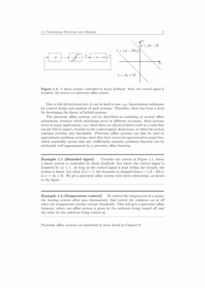
1.1 Nonlinear Systems and Models 5
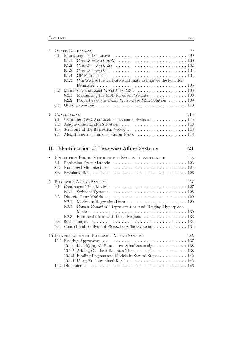
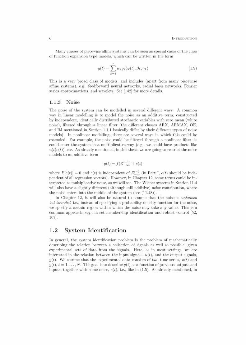
- --
6
-
@@@@@@@@@
@@@@@@@@@
u x
x = (A−BL)x
x = Ax+B
x = Ax+ Bu−L
x = Ax−Bx2
x1
Figure 1.1: A linear system, controlled by linear feedback. Since the control signal isbounded, the system is a piecewise affine system.
Due to this hybrid structure, it can be hard to use, e.g., linearization techniquesfor control design and analysis of such systems. Therefore, there has been a needfor developing the theory of hybrid systems.
The piecewise affine systems can be described as consisting of several affinesubsystems, between which switchings occur at different occasions. Such systemsoccur in many applications, e.g., when there are physical limits (such as a tank thatcan get full or empty), bounds on the control signal, dead-zones, or when the systemcontains switches and thresholds. Piecewise affine systems can also be used toapproximate nonlinear systems, since they have universal approximation properties,which essentially means that any (sufficiently smooth) nonlinear function can bearbitrarily well approximated by a piecewise affine function.
Example 1.1 (Bounded signal) Consider the system in Figure 1.1, wherea linear system is controlled by linear feedback, but where the control signal isbounded by |u| ≤ 1. As long as the control signal is kept within the bounds, thesystem is linear, but when |Lx| > 1, the dynamics is changed from x = (A−BL)xto x = Ax±B. We get a piecewise affine system with three subsystems, as shownin the figure.
Example 1.2 (Temperature control) To control the temperature in a house,the heating system often uses thermostats, that switch the radiators on or offwhen the temperature reaches certain thresholds. This will give a piecewise affinebehavior, where one affine system is given by the radiators being turned off, andthe other by the radiators being turned on.
Piecewise affine systems are described in more detail in Chapter 9.
6 Introduction
Many classes of piecewise affine systems can be seen as special cases of the classof function expansion type models, which can be written in the form
y(t) =r∑
k=1
αkgk(ϕ(t), βk, γk) (1.9)
This is a very broad class of models, and includes (apart from many piecewiseaffine systems), e.g., feedforward neural networks, radial basis networks, Fourierseries approximations, and wavelets. See [142] for more details.
1.1.3 Noise
The noise of the system can be modelled in several different ways. A commonway in linear modelling is to model the noise as an additive term, constructedby independent, identically distributed stochastic variables with zero mean (whitenoise), filtered through a linear filter (the different classes ARX, ARMAX, OE,and BJ mentioned in Section 1.1.1 basically differ by their different types of noisemodels). In nonlinear modelling, there are several ways in which this could beextended. For example, the noise could be filtered through a nonlinear filter, itcould enter the system in a multiplicative way (e.g., we could have products likeu(t)e(t)), etc. As already mentioned, in this thesis we are going to restrict the noisemodels to an additive term
y(t) = f(Zt−1−∞) + e(t)
where E[e(t)] = 0 and e(t) is independent of Zt−1−∞ (in Part I, e(t) should be inde-
pendent of all regression vectors). However, in Chapter 12, some terms could be in-terpreted as multiplicative noise, as we will see. The Wiener systems in Section 11.4will also have a slightly different (although still additive) noise contribution, wherethe noise enters into the middle of the system (see (11.48)).
In Chapter 12, it will also be natural to assume that the noise is unknownbut bounded, i.e., instead of specifying a probability density function for the noise,we specify a certain region within which the noise may take any value. This is acommon approach, e.g., in set membership identification and robust control [52,107].
1.2 System Identification
In general, the system identification problem is the problem of mathematicallydescribing the relation between a collection of signals as well as possible, givenexperimental sets of data from the signals. Here, as in most settings, we areinterested in the relation between the input signals, u(t), and the output signals,y(t). We assume that the experimental data consists of two time-series, u(t) andy(t), t = 1, . . . , N . The goal is to describe y(t) as a function of previous outputs andinputs, together with some noise, e(t), i.e., like in (1.5). As already mentioned, in
1.2 System Identification 7
this thesis we will mostly consider the form (1.6). For a more thorough introductionto system identification, see, e.g., [94].
1.2.1 Prediction Error Methods
To be able to identify a system, we must know, or at least assume, somethingabout its structure. If nothing whatsoever is known about the system function, theidentification problem is meaningless – the only things we can say are statementslike: “At time t and for the input u(1), . . . , u(t), the output was y(t) (at least thistime!)”. In other words, the best description of the system we can get is the set ofexperimental data itself.
If, however, we can assume that the system can be described (reasonably well)by a model belonging to a certain model class, more can be said. The modelclass can be specified in different ways. For instance, the classes described inSection 1.1.1 and by (1.9) are examples of parameterized model classes, i.e., theclass can be represented by a parameterized model. When using such a model class,the system identification problem amounts to finding values of the parameters, suchthat the resulting model describes the system as well as possible. Such methodsare called parametric methods. One family of identification methods, containingmany well-known and commonly used approaches, are the prediction error methods(PEM), which are described in Chapter 8. The methods in Part II are also of thiskind. Basically, the prediction error methods form parameterized predictions y(t|θ),where θ is the parameter vector. From these the residuals
ε(t, θ) = y(t)− y(t|θ)
i.e., the differences between the true output and the predicted output are formed.The parameter vector is then chosen to minimize the residuals according to somecriterion. A very common criterion is the least-squares criterion
V (θ, ZN1 ) =1N
N∑t=1
ε2(t, θ) =1N
N∑t=1
(y(t)− y(t|θ))2
Let us conclude this section by considering a simple example.
Example 1.3 (ARX model) As mentioned in Section 1.1.1, an ARX modelis a model with the following structure:
y(t) = −a1y(t− 1)− · · · − anay(t− na)+ b1u(t− 1) + · · ·+ bnbu(t− nb) + e(t)
= ϕT (t)θ + e(t)
where
ϕ(t) =(−y(t− 1) . . . −y(t− na) u(t− 1) . . . u(t− nb)
)Tθ =
(a1 . . . ana b1 . . . bnb
)T
8 Introduction
The natural predicted output is
y(t|θ) = ϕT (t)θ
so the least squares criterion is given by
V (θ, ZN1 ) =1N
N∑t=1
ε2(t, θ) =1N
N∑t=1
(y(t)− ϕT (t)θ)2
which is minimized by
θ =
(N∑t=1
ϕ(t)ϕT (t)
)−1 N∑t=1
ϕ(t)y(t)
Hence
y(t|θ) = ϕT (t)
(N∑l=1
ϕ(l)ϕT (l)
)−1 N∑k=1
ϕ(k)y(k)
=N∑k=1
wk(ϕ(t))y(k)
where
wk(ϕ(t)) = ϕT (t)
(N∑l=1
ϕ(l)ϕT (l)
)−1
ϕ(k) (1.10)
In other words, we can see the prediction y(t|θ) as a weighted sum of the observedoutputs. This perspective will be relevant in Part I.
1.2.2 Identification of Piecewise Affine Systems
Many tools and methods for verification, as well as for control, stability analysis,etc., of hybrid systems have emerged in recent years. To be able to use these tools,however, a model of the system is needed.
Identification of hybrid systems (e.g., piecewise affine systems) is an area thatis related to many other research fields within nonlinear system identification. Inparticular, one can find several different methods and approaches which are appli-cable, or at least related to the piecewise affine system identification problem. Someexamples of approaches that result in piecewise affine systems are neural networkswith piecewise affine perceptrons [8, 51, 86], Chua’s canonical representation andhinging hyperplanes [22, 27, 28, 77, 79, 80, 124], self-exciting threshold autoregres-sive (SETAR) models for time-series analysis [104, 105], special-purpose methodsfor physical applications [81], and some function approximation approaches [76, 78].In [142], which is a good overview of different nonlinear identification techniques,the relations between several different approaches are explored.
1.2 System Identification 9
The piecewise affine system identification problem will be considered in Part II,where an overview of different approaches occurring in the literature in Chapter 10will be given. An approach based on mixed-integer programming will also bepresented in Chapter 11. This approach guarantees that an optimal model (withrespect to the particular criterion used and the experimental data available) isfound, but this guarantee comes at a price of greater computational complexity.
In Chapters 10 and 11, we will mostly consider models in regression form likein (1.7). It turns out that once the partitioning of the state-space is known, thepiecewise affine system identification problem reduces to a problem, comparable toa linear system identification problem in terms of complexity. However, finding thebest partition may be a very complex problem. Hence, there are two fundamentalapproaches: Either an a priori partition can be used, or the partitioning can beestimated along with the different subsystems. The latter can be done simultane-ously or iteratively. The first approach gives a simple estimation process, but thenumber of regions needed to give enough flexibility in the model structure may bevery large. In the second approach, the number of subsystems can be kept low, butthe estimation will be more complex. This dilemma will be treated more in detailin Chapters 10 and 11.
Approximating Nonlinear Systems by Piecewise Affine Systems
As previously mentioned, many classes of piecewise affine systems have universalapproximation properties, which make them suitable for approximating arbitrarynonlinear functions. Therefore, an efficient identification method for piecewiseaffine systems would also be of interest for identification of nonlinear functions. Inthis case, the exact shape of the regions is of less direct importance, since the truesystem does not consist of affine subsystems. Instead, being able to approximatethe nonlinear function well, using few parameters and a representation that is easyto handle, becomes the main question.
1.2.3 Nonparametric Methods and Local Modelling
In Section 1.2.1, we saw that one way of specifying a model class is to representit by a parameterized model. An alternative way could be to specify differentproperties that the model should satisfy. For instance, we could assume that themodels can be described by (1.7), where f is continuously differentiable, and thederivative satisfies a Lipschitz condition
‖∇f(ϕ(1))−∇f(ϕ(2))‖ ≤ L‖ϕ(1)− ϕ(2)‖ ∀ϕ(1), ϕ(2) ∈ Rn (1.11)
Here, and throughout this thesis, ‖ · ‖ stands for the Euclidean norm (if nothingelse is stated). We can also assume that the noise variance is finite (and given). Inthis case, it is hard to parameterize the model class, so either we have to approxi-mate the model class by a parameterized class, or we have to use a nonparametricidentification method.
10 Introduction
−1 −0.5 0 0.5 11
1.5
2
2.5
φ
y
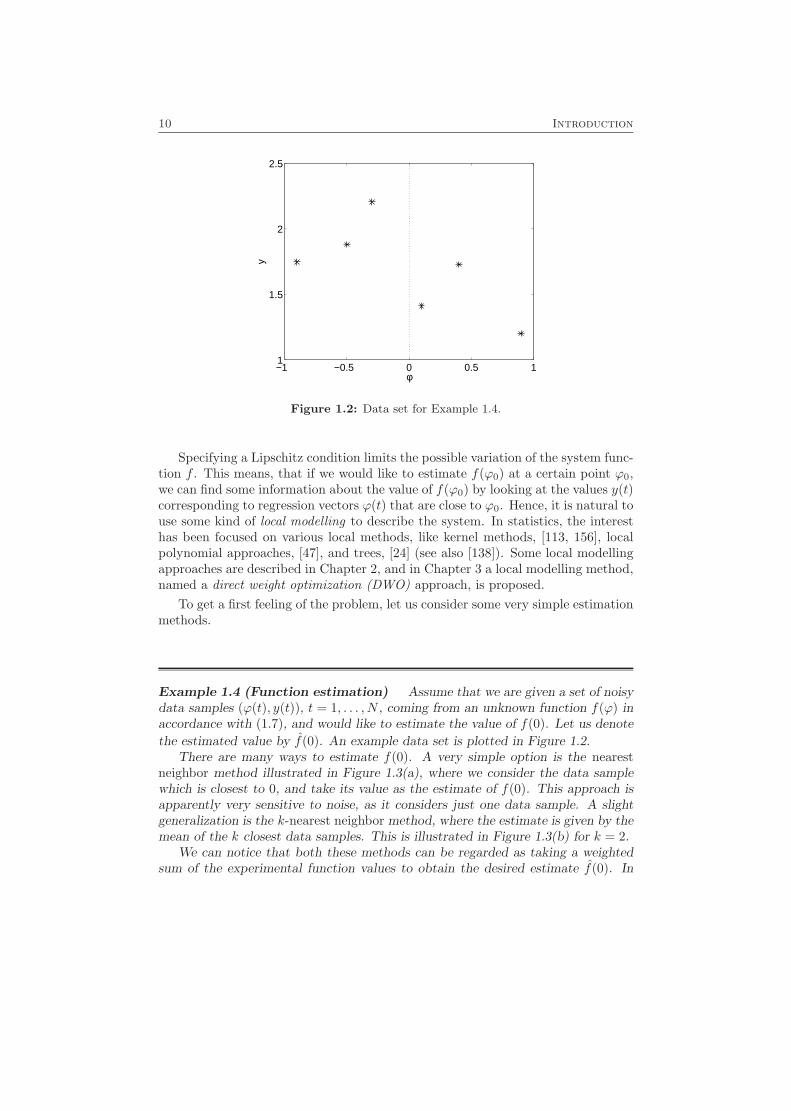
Figure 1.2: Data set for Example 1.4.
Specifying a Lipschitz condition limits the possible variation of the system func-tion f . This means, that if we would like to estimate f(ϕ0) at a certain point ϕ0,we can find some information about the value of f(ϕ0) by looking at the values y(t)corresponding to regression vectors ϕ(t) that are close to ϕ0. Hence, it is natural touse some kind of local modelling to describe the system. In statistics, the interesthas been focused on various local methods, like kernel methods, [113, 156], localpolynomial approaches, [47], and trees, [24] (see also [138]). Some local modellingapproaches are described in Chapter 2, and in Chapter 3 a local modelling method,named a direct weight optimization (DWO) approach, is proposed.
To get a first feeling of the problem, let us consider some very simple estimationmethods.
Example 1.4 (Function estimation) Assume that we are given a set of noisydata samples (ϕ(t), y(t)), t = 1, . . . , N , coming from an unknown function f(ϕ) inaccordance with (1.7), and would like to estimate the value of f(0). Let us denote
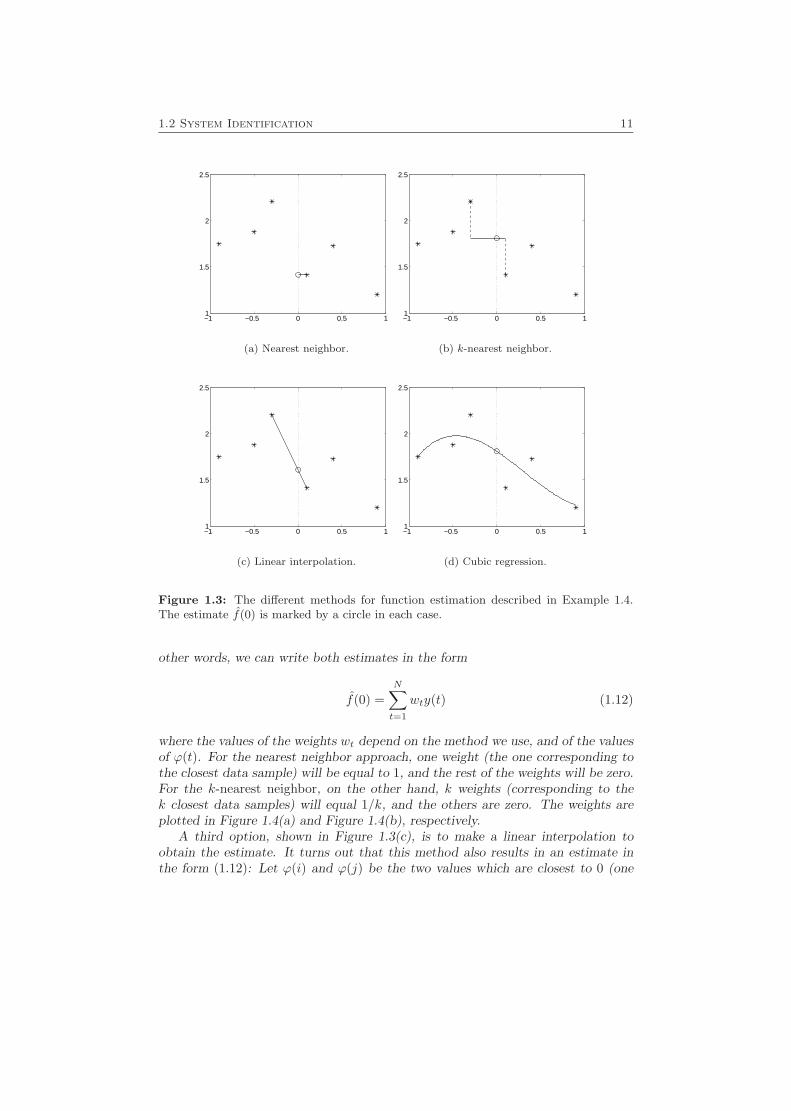
the estimated value by f(0). An example data set is plotted in Figure 1.2.There are many ways to estimate f(0). A very simple option is the nearest
neighbor method illustrated in Figure 1.3(a), where we consider the data samplewhich is closest to 0, and take its value as the estimate of f(0). This approach isapparently very sensitive to noise, as it considers just one data sample. A slightgeneralization is the k-nearest neighbor method, where the estimate is given by themean of the k closest data samples. This is illustrated in Figure 1.3(b) for k = 2.
We can notice that both these methods can be regarded as taking a weightedsum of the experimental function values to obtain the desired estimate f(0). In
1.2 System Identification 11
−1 −0.5 0 0.5 11
1.5
2
2.5
(a) Nearest neighbor.
−1 −0.5 0 0.5 11
1.5
2
2.5
(b) k-nearest neighbor.
−1 −0.5 0 0.5 11
1.5
2
2.5
(c) Linear interpolation.
−1 −0.5 0 0.5 11
1.5
2
2.5
(d) Cubic regression.
Figure 1.3: The different methods for function estimation described in Example 1.4.The estimate f(0) is marked by a circle in each case.
other words, we can write both estimates in the form
f(0) =N∑t=1
wty(t) (1.12)
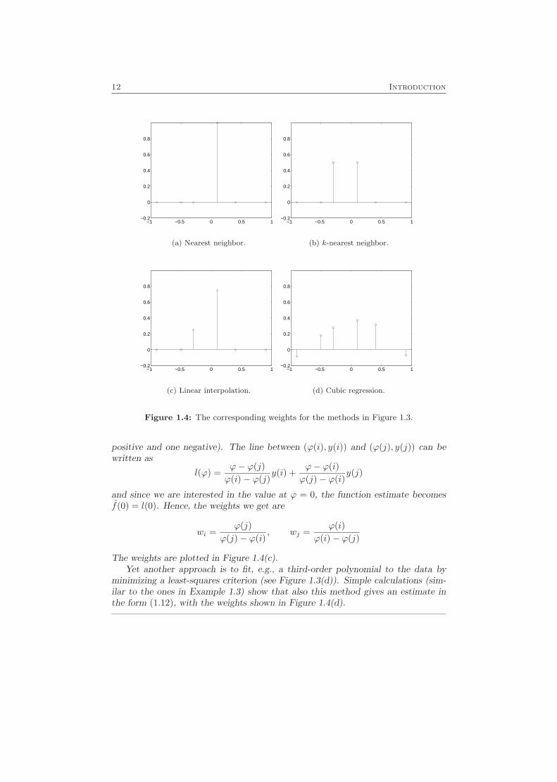
where the values of the weights wt depend on the method we use, and of the valuesof ϕ(t). For the nearest neighbor approach, one weight (the one corresponding tothe closest data sample) will be equal to 1, and the rest of the weights will be zero.For the k-nearest neighbor, on the other hand, k weights (corresponding to thek closest data samples) will equal 1/k, and the others are zero. The weights areplotted in Figure 1.4(a) and Figure 1.4(b), respectively.
A third option, shown in Figure 1.3(c), is to make a linear interpolation toobtain the estimate. It turns out that this method also results in an estimate inthe form (1.12): Let ϕ(i) and ϕ(j) be the two values which are closest to 0 (one
12 Introduction
−1 −0.5 0 0.5 1−0.2
0
0.2
0.4
0.6
0.8
(a) Nearest neighbor.
−1 −0.5 0 0.5 1−0.2
0
0.2
0.4
0.6
0.8
(b) k-nearest neighbor.
−1 −0.5 0 0.5 1−0.2
0
0.2
0.4
0.6
0.8
(c) Linear interpolation.
−1 −0.5 0 0.5 1−0.2
0
0.2
0.4
0.6
0.8
(d) Cubic regression.
Figure 1.4: The corresponding weights for the methods in Figure 1.3.
positive and one negative). The line between (ϕ(i), y(i)) and (ϕ(j), y(j)) can bewritten as
l(ϕ) =ϕ− ϕ(j)ϕ(i)− ϕ(j)
y(i) +ϕ− ϕ(i)ϕ(j)− ϕ(i)
y(j)
and since we are interested in the value at ϕ = 0, the function estimate becomesf(0) = l(0). Hence, the weights we get are
wi =ϕ(j)
ϕ(j)− ϕ(i), wj =
ϕ(i)ϕ(i)− ϕ(j)
The weights are plotted in Figure 1.4(c).Yet another approach is to fit, e.g., a third-order polynomial to the data by
minimizing a least-squares criterion (see Figure 1.3(d)). Simple calculations (sim-ilar to the ones in Example 1.3) show that also this method gives an estimate inthe form (1.12), with the weights shown in Figure 1.4(d).
1.3 Verification 13
Note that the first three methods of Example 1.4 are local methods, while thelast method is global. However, also the last method can be made local, by onlyconsidering the data samples which are closest to the point of interest (ϕ0 = 0in Example 1.4) when fitting the polynomial. The method then becomes a localpolynomial modelling method. This kind of methods is described in greater detailin Chapter 2.
Since many methods lead to a linear estimator of the kind given in (1.12) (seealso the predictor in Example 1.3), we can view the estimation problem as a problemof finding appropriate weights for (1.12). No matter what type of local modellingapproach is taken, the central problem is which of the data samples should betaken into consideration when forming the estimate (i.e., which weights should benonzero). Intuitively, it is clear that the answer must depend on three items:
1. How many data are available (and how are they spread)?
2. How smooth is the function surface (supposed to be)?
3. How much noise is there in the observations?
This problem has been studied extensively in the statistical literature, and thereare several solutions based on asymptotic (in the number of observations) analysis.
In Part I, another solution, which is not based on the asymptotic behaviorof the estimates, is proposed. Based on the smoothness measure given by theLipschitz condition (1.11) and the noise variance, we compute a uniform upperbound of the mean squared error (MSE) of a linear estimate, as a function of theestimator parameters. This upper bound is then minimized directly with respectto the weights in (1.12). It turns out that this problem can be reformulated as aquadratic programming (QP) problem, which can be solved efficiently. It also turnsout that this solution has many of the key features of the asymptotically optimalestimators, but for finite number of observations it produces better guaranteederror bounds.
1.3 Verification
In many application areas, such as in chemical industry and aeronautics, safetyis a very important issue. For example, given certain assumptions on the system,one would like to be able to ensure that the system never reaches certain specifiedbad (or dangerous) states. Typical requirements for control design might there-fore include that the system should never reach some specific (possibly dangerous)states, that the system should reach a certain region in the state-space, and/orthat there should be invariant regions (once you get there, you will never leavethe region). After the design process, one would often like to make sure that thespecified requirements are satisfied. This process is known as verification.
Even if a system model is given, it is mostly just an approximation – goodor bad – of the real system. Therefore, in Part III, the verification problem is
14 Introduction
considered for piecewise affine systems with model uncertainties. A robust verifi-cation method is presented, where upper bounds on the uncertainties that can betolerated are computed along with the verification process. This section providesa short description of the concept of verification.
Solving a verification problem exactly is in general possible only for some re-stricted classes of hybrid systems [2, 4]. Many verification methods for the problemof avoiding bad states found in the literature are based on computing a conserva-tive approximation of the system [2, 3, 14, 29–31, 43, 84, 150]. This means thateither the model of the system is replaced by a (computationally) simpler model,which is an outer approximation of the original system, or that the trajectoriesfrom a given initial set of states are replaced by an outer approximation. An outerapproximation is an approximation that guarantees that if a trajectory is allowedby the original system, it is also allowed in the simplified model. In this way itcan be guaranteed that if a certain bad state is never reached in the simple model,it is never reached in the original system either. A good overview over numerousdifferent approaches is given in [44].
For the problem of assuring that a certain region is reached, an inner approxi-mation can be used analogously to what is described above (see [43]). If a transitionis guaranteed to occur in an inner approximation, it is also guaranteed to occur inthe original system. However, other techniques might be needed to compute theinner approximation.
1.3.1 Robust Verification
The verification method presented in Chapter 12 is partly built upon a methodpresented in [43]. For this method, we will consider continuous time piecewiseaffine systems in state-space form, where the dynamics depend on in which regionof the state-space the current state x(t) is (see (9.2)). The regions (denoted X(v))are assumed to be polyhedral. To verify the desired properties, the behavior ofthe vector field x(t) at the borders of the regions X(v) is analyzed. Specifically,questions such as “At a given face of the polyhedron X(v), is there a point, x0, suchthat x0 is pointing out of X(v), or are all trajectories at this face going into X(v)?”are answered (this kind of computations has also been used by others, e.g., by [72]).The information obtained is used to determine which transitions between differentregions are possible, which transitions are guaranteed to occur nondeterministically(i.e., one transition out of a set of transitions from a given polyhedron is guaranteedto occur) and which are not. Then finite automata are constructed, showing theguaranteed or possible transitions. The finite automata give an approximation ofthe system, and can be used for different kinds of verification. For example, we canguarantee that certain states in the original system are not reachable from someother initial states, by proving that there is no sequence of possible transitions inthe finite automata, taking the system state from the region of the initial states tothe region of the final states.
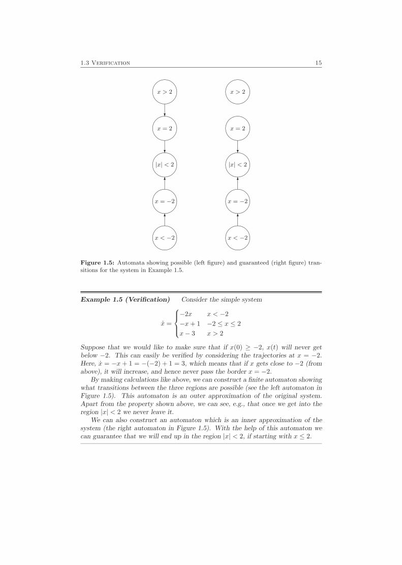
1.3 Verification 15
"!# x > 2
"!# x = 2
"!# |x| < 2
"!# x = −2
"!# x < −2
?
?
6
6
"!# x > 2
"!# x = 2
"!# |x| < 2
"!# x = −2
"!# x < −2
?
6
6
Figure 1.5: Automata showing possible (left figure) and guaranteed (right figure) tran-sitions for the system in Example 1.5.
Example 1.5 (Verification) Consider the simple system
x =
−2x x < −2−x+ 1 −2 ≤ x ≤ 2x− 3 x > 2
Suppose that we would like to make sure that if x(0) ≥ −2, x(t) will never getbelow −2. This can easily be verified by considering the trajectories at x = −2.Here, x = −x+ 1 = −(−2) + 1 = 3, which means that if x gets close to −2 (fromabove), it will increase, and hence never pass the border x = −2.
By making calculations like above, we can construct a finite automaton showingwhat transitions between the three regions are possible (see the left automaton inFigure 1.5). This automaton is an outer approximation of the original system.Apart from the property shown above, we can see, e.g., that once we get into theregion |x| < 2 we never leave it.
We can also construct an automaton which is an inner approximation of thesystem (the right automaton in Figure 1.5). With the help of this automaton wecan guarantee that we will end up in the region |x| < 2, if starting with x ≤ 2.

16 Introduction
Like all other methods mentioned above, the method in [43] assumes that amodel of the system is given. It would be desirable to be able to perform theverification, and simultaneously compute how sensitive the verification proof (e.g.,the approximating automata) is to changes in the underlying systems, both in thedynamics and in the switching surfaces. This is what is called robust verificationin this thesis. Such information could be used to get a measure of how robust theverification process is to model errors, or as an aid in a control design process, ifwe would like to adjust the system dynamics without losing the verified property.Sometimes we would only be interested in that some crucial transitions should notchange, whereas in other cases we might want the entire approximating automatato remain invariant.
Since the approximating method in [43] considers the behavior of x(t) at theborders of the regions X(v), we must determine how this behavior changes withvarying dynamics of the submodel corresponding to X(v), and with translations ofthe surfaces that bound X(v). How this can be done is the topic of Chapter 12.
1.4 Thesis Outline
The thesis consists of three main parts:
• Local modelling and the direct weight optimization (DWO) approach can befound in Part I. Chapter 2 gives an overview of the problem and of existingmethods. In Chapter 3 the DWO approach is introduced for a special class ofonce differentiable, univariate functions. This is then extended in Chapter 4to multivariate functions, with higher degrees of differentiability. Chapter 5considers the case when bounds on the function value and derivatives areknown. Some other extensions are given in Chapter 6 and conclusions inChapter 7.
• In Part II, the problem of identification of piecewise affine systems is studied.Chapter 8 gives a brief introduction to prediction error methods. In Chap-ter 9, different classes of piecewise affine systems are presented. Chapter 10gives a survey of existing identification approaches, while Chapter 11 consid-ers the identification of piecewise affine systems using mixed-integer linear orquadratic programming.
• Part III, which consists of Chapter 12, concerns robust verification for piece-wise affine systems.
Apart from this, some mathematical preliminaries are given in Appendix A.
1.5 Contributions
The main contributions of this thesis are:
1.5 Contributions 17
• A method for finding the function estimate that minimizes an upper boundon the worst-case mean squared error (MSE) through quadratic programming(QP), as outlined in the DWO approach in Chapters 3 (for once differentiable,univariate functions) and 4 (for p times differentiable, multivariate functions).
• Extension of the DWO approach to the case when bounds on the functionand its derivatives are known a priori, presented in Chapter 5.
• Extension of the DWO approach to the estimation of derivatives using QP,given in Section 6.1.
• The algorithm in Section 6.2 for finding the function estimate minimizingthe exact worst-case MSE for once differentiable, univariate functions, withderivatives satisfying a Lipschitz condition.
• The techniques in Chapter 11 of using mixed-integer linear/quadratic pro-gramming (MILP/MIQP) to identify piecewise affine systems. A techniqueof reformulating products of continuous affine functions and discrete variablesas linear inequalities, described in Section 11.1.2.
• Extension of an identification algorithm proposed by Hush and Horne [69],and showing its relationship to the MILP/MIQP formulations. This is foundin Section 11.7.
• The robust verification methods in Chapter 12.
Some of the material in this thesis has been presented previously. The DWOapproach in Part I has been presented for once differentiable, univariate functionsin
J. Roll, A. Nazin, and L. Ljung. A non-asymptotic approach to localmodelling. In The 41st IEEE Conference on Decision and Control,pages 638–643, Dec. 2002
The extension to multivariate functions was considered in
J. Roll, A. Nazin, and L. Ljung. Local modelling of nonlinear dynamicsystems using direct weight optimization. Accepted for the 13th IFACSymposium on System Identification, Rotterdam, Aug. 2003
and
J. Roll, A. Nazin, and L. Ljung. Direct weight optimization for nonpara-metric estimation of a regression function at a given point. Submittedto Scandinavian Journal of Statistics, 2003
The case when bounds on the function value and the derivative are given is pre-sented in

18 Introduction
J. Roll, A. Nazin, and L. Ljung. Local modelling with a priori knownbounds using direct weight optimization. Submitted to the EuropeanControl Conference, Cambridge, Sept. 2003
Much of the material in Sections 11.1, 11.2, 11.4, and 11.6 in Part II is joint workwith Dr. Alberto Bemporad. This material is also published in
A. Bemporad, J. Roll, and L. Ljung. Identification of hybrid systems viamixed-integer programming. In The 40th IEEE Conference on Decisionand Control, pages 786–792, Dec. 2001.
and
J. Roll, A. Bemporad, and L. Ljung. Identification of piecewise affinesystems via mixed-integer programming. Provisionally accepted for Au-tomatica, 2003
Some of the material in Chapter 12 has previously been published in
J. Roll. Invariance of approximating automata for piecewise linear sys-tems with uncertainties. In Hybrid Systems: Computation and Control,volume 1790 of Lecture Notes in Computer Science, pages 396–406.Springer-Verlag, 2000.
Other parts of Chapter 12 also appear in
J. Roll. Robust verification of piecewise affine systems. In 15th IFACWorld Congress on Automatic Control, Session T-We-A21, July 2002.

Part I
Local Modelling UsingDirect Weight Optimization
19

2
Nonparametric Methods and
Local Modelling
As mentioned in Section 1.2, the system identification problem is a problem ofdescribing the relationship between input and output signals. This problem can ofcourse be regarded as a kind of function approximation or a regression problem:Given a set of regression vectors ϕ(k) and output signals y(k), we can assume thatthe outputs are generated as noisy measurements of an unknown function
y(k) = f(ϕ(k)) + e(k)
and our goal is to recover the function f(ϕ).A very common approach in nonlinear system identification is to use some kind
of local models (see e.g., [112]) and/or methods. A local model or method buildsthe function estimate or prediction from observations in a local neighborhood ofthe point of interest. Also most function expansion methods are of this character:A radial basis neural network is built up from basis functions with local support,and the standard sigmoidal (one hidden layer feed-forward) network is local aroundcertain hyperplanes in the regressor space (see [94]).
If the model classes used are parameterized, this means that the identificationproblem is reduced to finding the parameters that makes the model match theobserved data as well as possible. This is referred to as parametric methods. Incontrast, nonparametric methods do not use a parameterized model class, but makepointwise estimates of e.g., the frequency response, the step response, or, as in this
21
22 Nonparametric Methods and Local Modelling
part of the thesis, the system function f . However, the boundary between thedifferent categories is not always sharp.
In this part, a nonparametric local modelling approach to the regression problemis considered. Following the definition in [47], the local modelling approach can bedescribed as follows: For any given point ϕ0, for which we would like to estimatef(ϕ0), we should model f around ϕ0 using only the data that are close to ϕ0.There are two main points in this:
• The local modelling approach is a local method, and uses only data from theneighborhood of ϕ0.
• For each new point in which f should be estimated, a “new model” is formed,in contrast to, e.g., the piecewise affine models in Part II, where each sub-model has a certain validity region.
The local modelling approach and similar ideas have occurred in many contexts[18, 47, 61, 122, 141, 155] under names such as Model on Demand [146], lazylearning and least commitment learning [5, 6, 17]. A central question is how manypoints should be used when forming the estimate (also referred to as the bandwidthquestion). The answer to this mainly depends on three factors:
1. The number of data available (and the actual spreading of the regressionvectors).
2. The smoothness of the function f .
3. The variance of the noise e(k).
This problem has been studied extensively in the statistical literature, and thereare several solutions based on asymptotic (in the number of observations) analysis.
This chapter gives an overview of the problem and some existing methods,mainly based on the presentations in [47, 146]. Other good overviews can be foundin [5, 155]. The following chapters then present a direct weight optimization (DWO)approach, which is not based on asymptotic analysis.
2.1 Introduction and Problem Formulation
Throughout this part of the thesis, we will assume that we are given a set ofinput-output pairs {(ϕ(k), y(k))}Nk=1, coming from the relation
y(k) = f(ϕ(k)) + e(k) (2.1)
The function f : Rn → R (we will often consider the univariate case n = 1) isassumed to be unknown. The noise terms e(k) are independent random variableswith E[e(k)] = 0 and E[e2(k)] = σ2, and should be independent of the regressionvariables ϕ(k).
One usually distinguishes between two ways of viewing the regression variables.If they are viewed as independent, identically distributed random variables with
2.1 Introduction and Problem Formulation 23
a certain probability density function pϕ, this is referred to as random design. If,on the other hand, ϕ(k) are deterministic, we call this fixed design. A special caseof the latter is the equally spaced fixed design, where the distance between twoneighboring samples is constant (e.g., ϕ(k) = k/N in the univariate case).
The problem we consider is the problem of estimating the value f(ϕ0) at a givenpoint ϕ0. In the sequel, it will be convenient to also use the notation
ϕ(k) = ϕ(k)− ϕ0 (2.2)
As we saw in Section 1.2, many methods for estimating f(ϕ0) lead to a linearestimator in the form
f(ϕ0) =N∑k=1
wky(k) (2.3)
where f(ϕ0) is our estimate of f(ϕ0). In words, the estimate f(ϕ0) is a weightedsum of the observations y(k). As it will turn out in Chapter 5, in some cases it willalso be useful to consider an affine estimator given by
f(ϕ0) = w0 +N∑k=1
wky(k) (2.4)
In both these cases, the weights w0 ∈ R and w = (w1 . . . wN )T ∈ RN can befunctions of ϕ0 and the regression vectors ϕ(k), k = 1, . . . , N . In many methods,they also depend of the noise variance σ2 and of some measure of the smoothnessof f . However, it is worth noting that the weights in most methods do not dependon y(k).
Assuming one of the forms (2.3) or (2.4), the problem then reduces to findinggood weights wk, which give reasonably small bias and variance of the estimate.In Section 2.4, different criteria are given for assessing the estimators. A popularcriterion is the mean squared error (MSE)
MSE (f(ϕ0)) , E[(f(ϕ0)− f(ϕ0))2|ϕN1 ] (2.5)
where ϕN1 = {ϕ(1), . . . , ϕ(N)}. Sometimes when considering random design, theMSE is defined as the corresponding unconditional expectation, but in this thesis,only the definition (2.5) will be used. In the case of fixed design, the conditioningwill of course have no effect. The worst-case MSE over a class F of functions
WMSE (f(ϕ0),F) , supf∈F
MSE (f(ϕ0)) (2.6)
is another commonly used criterion. In this way, one can get a guaranteed upperbound on the MSE (assuming that all assumptions hold). In statistics, the worst-case MSE is also called maximum MSE. Using this criterion is often referred to as aminimax approach (see, e.g., [85, 88, 137, 138]). The worst-case MSE (or rather anupper bound on the worst-case MSE) will be used in the DWO approach presentedin this thesis.
Depending on the method, different assumptions are made about f . In thefollowing, some common function classes will be presented.
24 Nonparametric Methods and Local Modelling
Class Fp+1(L)
A common assumption is that f is p times differentiable. Another frequently usedassumption is that the pth derivative is Lipschitz continuous. For p = 1, this meansthat there is a constant L (called the Lipschitz constant) such that
‖∇f(ϕ(1))−∇f(ϕ(2))‖ ≤ L‖ϕ(1)− ϕ(2)‖ ∀ϕ(1), ϕ(2) ∈ Rn (2.7)
where ‖·‖ denotes the Euclidean norm. For more general cases, see Chapter 4. Theclass of p times differentiable functions with Lipschitz continuous pth derivatives,having a Lipschitz constant L, will be denoted by Fp+1(L). (With some abuse ofnotation, we will use this notation regardless of the value of n, i.e., n is supposedto be fixed and known.)
Holder Class Σ(β, L)
A generalization of this class for univariate functions is the Holder class [88]. Theunivariate function f is said to belong to the Holder smoothness class Σ(β, L) if fis p times differentiable, β = p+ α with 0 < α ≤ 1, and
|f (p)(ϕ(1))− f (p)(ϕ(2))| ≤ L|ϕ(1)− ϕ(2)|α ∀ϕ(1), ϕ(2) ∈ R (2.8)
We can notice that for univariate functions and integers β, we have Σ(β, L) =Fβ(L).
Class Gp+1(L)
A related assumption is given in [85], where the univariate function f is supposedto take the following form:
f(ϕ) = a0 + a1ϕ+ · · ·+ apϕp + c(ϕ)ϕp+1 (2.9)
where ai ∈ R and supϕ |c(ϕ)| ≤ M . Note that under this assumption, f does notneed to be continuous (except at ϕ0). Thus, for univariate functions, the functionclass Fp+1((p+1)!M) is a proper subclass of this class. However, the function classis connected to the point ϕ0 of the function estimate, and thus is not so useful inpractice, if one would like to estimate f in several points. We will denote thefunction class by Gp+1((p+ 1)!M).
Class Fp+1(L, δ,∆)
In some situations, one might have some prior knowledge of what would be areasonable value for the function and/or its derivatives. This can be incorporatedin the DWO approach by assuming that there are known constants a, δ, and ∆,and a vector b, such that
|f(ϕ0)− a| ≤ δ (2.10a)‖∇f(ϕ0)− b‖ ≤ ∆ (2.10b)
2.2 Kernel Estimators 25
The function classes satisfying (2.7) and (2.10) will be denoted by Fp+1(L, δ,∆),and will be studied (for the case p = 1) in Chapter 5.
When the data come from a dynamic system, such that the regression vectorsdepend on old values of y, this means that ϕ(i) and e(j) will not be independentfor all values of i, j anymore. However, we will neglect this fact for the time being,and discuss the implications further in Chapter 7. Note also that for NFIR models(see Section 1.1.2), such problems will not occur.
2.2 Kernel Estimators
A classic family of methods to decide the weights of (2.3) are the kernel estima-tors. Here, a kernel function K, which usually is a symmetric probability densityfunction, is used to determine the weights. For simplicity, we will only treat theunivariate case in this section. Some common choices of kernel functions are theGaussian kernel
K(u) =1√2πe−
u22 (2.11)
and the Epanechnikov kernel [45]
K(u) =34
max{1− u2, 0} (2.12)
For more details about the kernel functions, see Section 2.5.The width of the kernel is determined by introducing a bandwidth parameter
h, and letting
Kh(·) =1hK(·/h) (2.13)
As an example of a kernel estimator, the Nadaraya-Watson estimator [113, 156](see also [123] for a related estimator) is given by
fNW (ϕ0) =∑Nk=1Kh(ϕ(k))y(k)∑N
i=1Kh(ϕ(i))(2.14)
Comparing this expression with (2.3), we can see that the weights are given by
wk =Kh(ϕ(k))∑Ni=1Kh(ϕ(i))
(2.15)
Apparently, the denominator makes the estimate a weighted average of y(k) bynormalizing so that
N∑k=1
wk = 1
Another kernel estimator is the Gasser-Muller estimator [53]. Assuming thatthe data ϕ(k) are ordered in ascending order, the Gasser-Muller estimator is defined
26 Nonparametric Methods and Local Modelling
by
fGM (ϕ0) =N∑k=1
∫ uk
uk−1
Kh(u− ϕ0)du y(k)
u0 = −∞, uN =∞, uk =ϕ(k) + ϕ(k + 1)
2for k = 1, . . . , N − 1
(2.16)
One advantage with this estimator compared to the Nadaraya-Watson estimatoris, as pointed out in [47], that no normalizing denominator is needed, since
N∑k=1
∫ uk
uk−1
Kh(u− ϕ0)du =∫ ∞−∞
Kh(u− ϕ0)du = 1
if Kh is a probability density function.For both these methods, the choice of bandwidth is a bias/variance trade-off
problem, which will be discussed more in detail in Section 2.4. The asymptotic(for N →∞) bias and variance for the methods are given in Table 2.1, taken from[47]. Here a random design is assumed, where the samples ϕ(k) are taken froma distribution with a differentiable probability density function pϕ. Furthermore,it is assumed that the true function f is two times differentiable. For notationalsimplicity, the definitions
Ψk(K) =∫ukK(u)du (2.17)
r(K) =∫K2(u)du (2.18)
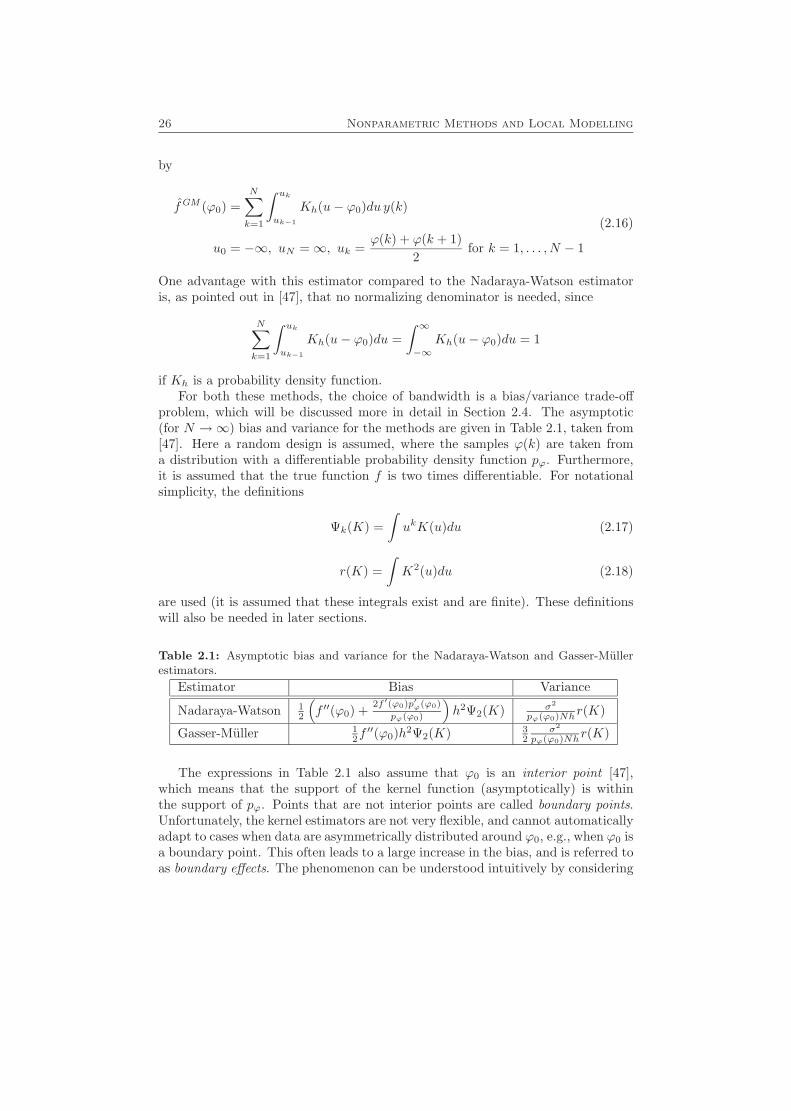
are used (it is assumed that these integrals exist and are finite). These definitionswill also be needed in later sections.
Table 2.1: Asymptotic bias and variance for the Nadaraya-Watson and Gasser-Mullerestimators.
Estimator Bias Variance
Nadaraya-Watson 12
(f ′′(ϕ0) + 2f ′(ϕ0)p′ϕ(ϕ0)
pϕ(ϕ0)
)h2Ψ2(K) σ2
pϕ(ϕ0)Nhr(K)
Gasser-Muller 12f′′(ϕ0)h2Ψ2(K) 3
2σ2
pϕ(ϕ0)Nhr(K)
The expressions in Table 2.1 also assume that ϕ0 is an interior point [47],which means that the support of the kernel function (asymptotically) is withinthe support of pϕ. Points that are not interior points are called boundary points.Unfortunately, the kernel estimators are not very flexible, and cannot automaticallyadapt to cases when data are asymmetrically distributed around ϕ0, e.g., when ϕ0 isa boundary point. This often leads to a large increase in the bias, and is referred toas boundary effects. The phenomenon can be understood intuitively by considering
2.3 Local Polynomial Modelling 27
the problem of estimating an increasing function in a point ϕ0 such that ϕ0 > ϕ(k)for all k = 1, . . . , N . Using the Nadaraya-Watson or Gasser-Muller estimator witha nonnegative kernel function, the estimate f(ϕ0) will be a weighted average of theobservations y(k) = f(ϕ(k))+e(k), and never gets larger than maxk y(k), althoughit probably should.
To get around this problem, many methods have been proposed. For instance,[53, 54] consider special boundary kernels to reduce the bias.
2.3 Local Polynomial Modelling
A slightly more sophisticated alternative to the kernel estimators is the local poly-nomial modelling approach (see, e.g., [32, 47, 61, 147, 155]). In this approach, theestimator is determined by locally fitting a polynomial to the given data via min-imization of a weighted least-squares problem, which in the univariate case takesthe form
β = arg minβ
N∑k=1
Kh(ϕ(k))
y(k)−p∑j=0
βjϕj(k)
2
(2.19)
where Kh is given by (2.13). The resulting estimator is obtained as fLP (ϕ0) = β0.When p = 0, it turns out that fLP (ϕ0) will be the Nadaraya-Watson estimator.
The Gasser-Muller estimator is instead obtained if Kh(ϕ(k)) in (2.19) is replacedby∫ uiui−1
Kh(u − ϕ0)du. Since we can obtain these estimators by locally fitting aconstant term to the observed data (i.e., by using (2.19) with p = 0), we can referto them as local constant approximators [47].
If we introduce
Φ =
1 ϕ(1) · · · ϕp(1)...
......
1 ϕ(N) · · · ϕp(N)
(2.20)
Kh =
Kh(ϕ(1)) 0 · · · 0
0 Kh(ϕ(2)) · · · 0...
.... . .
...0 0 · · · Kh(ϕ(N))
(2.21)
and
Y =
y(1)...
y(N)
, β =
β0
...βp
(2.22)
we can rewrite the problem (2.19) as
minβ
(Y − Φβ)T Kh(Y − Φβ) (2.23)
with the solutionβ = (ΦT KhΦ)−1ΦT KhY (2.24)

28 Nonparametric Methods and Local Modelling
The function estimate fLP (ϕ0) is given by
fLP (ϕ0) = β0 = eT1 (ΦT KhΦ)−1ΦT KhY (2.25)
Comparing once again to (2.3), this will correspond to
w = KhΦ(ΦT KhΦ)−1e1 (2.26)
These weights are often referred to as equivalent weights (see, e.g., [47]), to separatethem from the weights Kh(ϕ(k)) of the weighted least-squares problem (2.19). Notealso that, for j ≤ p, we have
N∑k=1
wkϕj(k) = eTj ΦTw = eTj ΦT KhΦ(ΦT KhΦ)−1e1 = eTj e1 (2.27)
This is a desirable property, and will be shared by the DWO estimator in Chapters 3and 4. For instance, as we will see in Chapter 3, they imply that the worst-caseMSE over Fp+1(L) is finite.
The case p = 1 may be worth a closer look. In this case, the estimator is calleda local linear estimator, and can be expressed explicitly as
fLP (ϕ0) =∑Nk=1 αky(k)∑Nk=1 αk
, (2.28)
αk = Kh(ϕ(k))
(N∑i=1
Kh(ϕ(i))ϕ2(i)− ϕ(k)N∑i=1
Kh(ϕ(i))ϕ(i)
)
For the local linear estimator, (2.27) implies that
N∑k=1
wk = 1,N∑k=1
wkϕ(k) = 0 (2.29)
Another interesting thing to note is that if Kh is an even function, and the datasamples are lying symmetrically, i.e., if the nonzero ϕ(k) can be paired so that foreach pair (ϕ(i), ϕ(j)) we have ϕ(i) = −ϕ(j), then the local linear estimator (2.28)and the Nadaraya-Watson estimator will coincide.
The local polynomial models (for p ≥ 1) are better than the kernel estimatorsat adapting automatically to data lying asymmetrically, e.g., at boundaries [47].However, since the number of data samples taken into account is determined onlyby the choice of bandwidth, there might (as pointed out by [34]) still be problemsif the latter choice is only asymptotically based and does not take the actual valuesof ϕ(k) into account. Furthermore, the asymptotically optimal kernel functions aredifferent depending on if ϕ0 is an interior point or a boundary point.
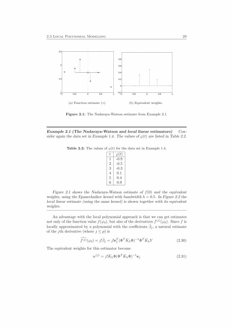
2.3 Local Polynomial Modelling 29
−1 −0.5 0 0.5 11
1.5
2
2.5
(a) Function estimate (◦).
−1 −0.5 0 0.5 1−0.2
0
0.2
0.4
0.6
0.8
(b) Equivalent weights.
Figure 2.1: The Nadaraya-Watson estimate from Example 2.1.
Example 2.1 (The Nadaraya-Watson and local linear estimators) Con-sider again the data set in Example 1.4. The values of ϕ(t) are listed in Table 2.2.
Table 2.2: The values of ϕ(t) for the data set in Example 1.4.
t ϕ(t)1 -0.92 -0.53 -0.34 0.15 0.46 0.9
Figure 2.1 shows the Nadaraya-Watson estimate of f(0) and the equivalentweights, using the Epanechnikov kernel with bandwidth h = 0.5. In Figure 2.2 thelocal linear estimate (using the same kernel) is shown together with its equivalentweights.
An advantage with the local polynomial approach is that we can get estimatesnot only of the function value f(ϕ0), but also of the derivatives f (j)(ϕ0). Since f islocally approximated by a polynomial with the coefficients βj , a natural estimateof the jth derivative (where j ≤ p) is
f (j)(ϕ0) = j!βj = j!eTj (ΦT KhΦ)−1ΦT KhY (2.30)
The equivalent weights for this estimator become
w(j) = j!KhΦ(ΦT KhΦ)−1ej (2.31)
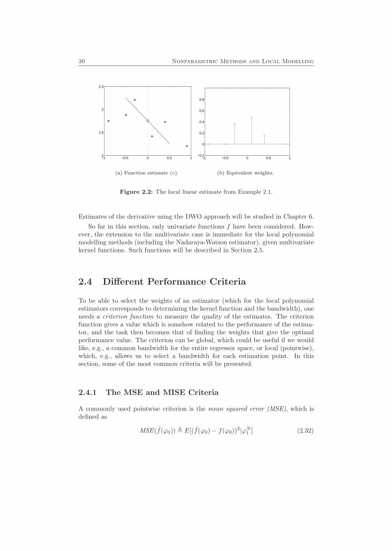
30 Nonparametric Methods and Local Modelling
−1 −0.5 0 0.5 11
1.5
2
2.5
(a) Function estimate (◦).
−1 −0.5 0 0.5 1−0.2
0
0.2
0.4
0.6
0.8
(b) Equivalent weights.
Figure 2.2: The local linear estimate from Example 2.1.
Estimates of the derivative using the DWO approach will be studied in Chapter 6.So far in this section, only univariate functions f have been considered. How-
ever, the extension to the multivariate case is immediate for the local polynomialmodelling methods (including the Nadaraya-Watson estimator), given multivariatekernel functions. Such functions will be described in Section 2.5.
2.4 Different Performance Criteria
To be able to select the weights of an estimator (which for the local polynomialestimators corresponds to determining the kernel function and the bandwidth), oneneeds a criterion function to measure the quality of the estimates. The criterionfunction gives a value which is somehow related to the performance of the estima-tor, and the task then becomes that of finding the weights that give the optimalperformance value. The criterion can be global, which could be useful if we wouldlike, e.g., a common bandwidth for the entire regressor space, or local (pointwise),which, e.g., allows us to select a bandwidth for each estimation point. In thissection, some of the most common criteria will be presented.
2.4.1 The MSE and MISE Criteria
A commonly used pointwise criterion is the mean squared error (MSE), which isdefined as
MSE (f(ϕ0)) , E[(f(ϕ0)− f(ϕ0))2|ϕN1 ] (2.32)
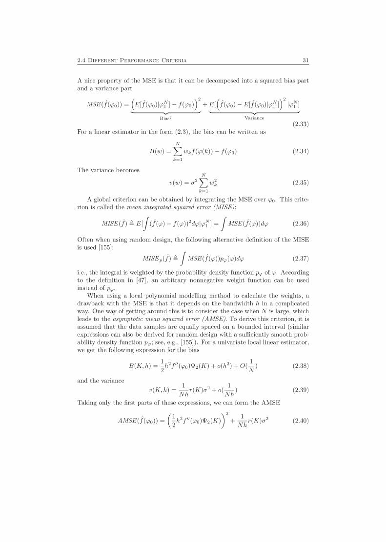
2.4 Different Performance Criteria 31
A nice property of the MSE is that it can be decomposed into a squared bias partand a variance part
MSE (f(ϕ0)) =(E[f(ϕ0)|ϕN1 ]− f(ϕ0)
)2
︸ ︷︷ ︸Bias2
+ E[(f(ϕ0)− E[f(ϕ0)|ϕN1 ]
)2
|ϕN1 ]︸ ︷︷ ︸Variance
(2.33)For a linear estimator in the form (2.3), the bias can be written as
B(w) =N∑k=1
wkf(ϕ(k))− f(ϕ0) (2.34)
The variance becomes
v(w) = σ2N∑k=1
w2k (2.35)
A global criterion can be obtained by integrating the MSE over ϕ0. This crite-rion is called the mean integrated squared error (MISE):
MISE (f) , E[∫
(f(ϕ)− f(ϕ))2dϕ|ϕN1 ] =∫
MSE (f(ϕ))dϕ (2.36)
Often when using random design, the following alternative definition of the MISEis used [155]:
MISEp(f) ,∫
MSE (f(ϕ))pϕ(ϕ)dϕ (2.37)
i.e., the integral is weighted by the probability density function pϕ of ϕ. Accordingto the definition in [47], an arbitrary nonnegative weight function can be usedinstead of pϕ.
When using a local polynomial modelling method to calculate the weights, adrawback with the MSE is that it depends on the bandwidth h in a complicatedway. One way of getting around this is to consider the case when N is large, whichleads to the asymptotic mean squared error (AMSE). To derive this criterion, it isassumed that the data samples are equally spaced on a bounded interval (similarexpressions can also be derived for random design with a sufficiently smooth prob-ability density function pϕ; see, e.g., [155]). For a univariate local linear estimator,we get the following expression for the bias
B(K,h) =12h2f ′′(ϕ0)Ψ2(K) + o(h2) +O(
1N
) (2.38)
and the variancev(K,h) =
1Nh
r(K)σ2 + o(1Nh
) (2.39)
Taking only the first parts of these expressions, we can form the AMSE
AMSE (f(ϕ0)) =(
12h2f ′′(ϕ0)Ψ2(K)
)2
+1Nh
r(K)σ2 (2.40)
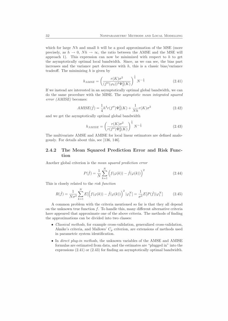
32 Nonparametric Methods and Local Modelling
which for large Nh and small h will be a good approximation of the MSE (moreprecisely, as h → 0, Nh → ∞, the ratio between the AMSE and the MSE willapproach 1). This expression can now be minimized with respect to h to getthe asymptotically optimal local bandwidth. Since, as we can see, the bias partincreases and the variance part decreases with h, this is a classic bias/variancetradeoff. The minimizing h is given by
hAMSE =(
r(K)σ2
(f ′′(ϕ0))2Ψ22(K)
) 15
N−15 (2.41)
If we instead are interested in an asymptotically optimal global bandwidth, we cando the same procedure with the MISE. The asymptotic mean integrated squarederror (AMISE) becomes:
AMISE (f) =14h4r(f ′′)Ψ2
2(K) +1Nh
r(K)σ2 (2.42)
and we get the asymptotically optimal global bandwidth
hAMISE =(
r(K)σ2
r(f ′′)Ψ22(K)
) 15
N−15 (2.43)
The multivariate AMSE and AMISE for local linear estimators are defined analo-gously. For details about this, see [136, 146].
2.4.2 The Mean Squared Prediction Error and Risk Func-tion
Another global criterion is the mean squared prediction error
P (f) =1N
N∑k=1
(f(ϕ(k))− f(ϕ(k))
)2
(2.44)
This is closely related to the risk function
R(f) =1
Nσ2
N∑k=1
E[(f(ϕ(k))− f(ϕ(k))
)2
|ϕN1 ] =1σ2E[P (f)|ϕN1 ] (2.45)
A common problem with the criteria mentioned so far is that they all dependon the unknown true function f . To handle this, many different alternative criteriahave appeared that approximate one of the above criteria. The methods of findingthe approximations can be divided into two classes:
• Classical methods, for example cross-validation, generalized cross-validation,Akaike’s criteria, and Mallows’ Cp criterion, are extensions of methods usedin parametric system identification.
• In direct plug-in methods, the unknown variables of the AMSE and AMISEformulas are estimated from data, and the estimates are “plugged in” into theexpressions (2.41) or (2.43) for finding an asymptotically optimal bandwidth.
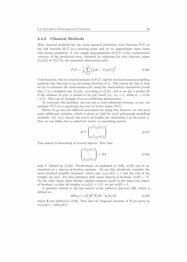
2.4 Different Performance Criteria 33
2.4.3 Classical Methods
Most classical methods use the mean squared prediction error function P (f) orthe risk function R(f) as a starting point and try to approximate these usingonly known quantities. A very simple approximation of P (f) is the resubstitutionestimate of the prediction error, obtained by replacing the true function valuesf(ϕ(k)) in P (f) by the measured observations y(k):
P (f) =1N
N∑k=1
(y(k)− f(ϕ(k))
)2
(2.46)
Unfortunately, this is a biased estimate of P (f), and for local polynomial modellingmethods this function is an increasing function of h. The reason for this is thatwe try to estimate the observations y(k) using the observations themselves (recallthat f is a weighted sum of y(k), according to (2.3)), and so we get a perfect fitif the estimate of y(k) is chosen to be y(k) itself (i.e., wk = 1, while wi = 0 fori 6= k). This can be thought of as an overfitting phenomenon.
To overcome this problem, one can use a cross-validation strategy, or one canmultiply P (f) by a penalizing function to better mimic P (f).
Before we go into the different procedures for doing this, however, we will needsome additional notation, which is given in [146] for local polynomial modellingmethods. Let w(ϕ) denote the vector of weights for estimating f in the point ϕ.Now we can define the so-called hat matrix or smoothing matrix
H ,
wT (ϕ(1))...
wT (ϕ(N))
(2.47)
This matrix is interesting in several aspects. Note that f(ϕ(1))...
f(ϕ(N))
= HY (2.48)
with Y defined by (2.22). Furthermore, as explained in [146], tr(H) can be in-terpreted as a degrees-of-freedom measure. To see this intuitively, consider themost localized possible estimator, where only wk(ϕ(k)) = 1 and the rest of theweights are zero. For this estimator with many degrees of freedom, tr(H) = N .On the other hand, when fitting a global constant model to the data (one degreeof freedom), so that all weights wi(ϕ(k)) = 1/N , we get tr(H) = 1.
A quantity related to the hat matrix is the influence function [96], which isdefined as
infl(ϕ0) = eT1 (ΦT KhΦ)−1e1Kh(0) (2.49)
where Φ was defined in (2.20). Note that the diagonal elements of H are given bywk(ϕ(k)) = infl(ϕ(k)).
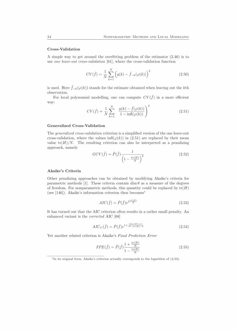
34 Nonparametric Methods and Local Modelling
Cross-Validation
A simple way to get around the overfitting problem of the estimator (2.46) is touse one leave-out cross-validation [61], where the cross-validation function
CV (f) =1N
N∑k=1
(y(k)− f−k(ϕ(k))
)2
(2.50)
is used. Here f−k(ϕ(k)) stands for the estimate obtained when leaving out the kthobservation.
For local polynomial modelling, one can compute CV (f) in a more efficientway:
CV (f) =1N
N∑k=1
(y(k)− f(ϕ(k))1− infl(ϕ(k))
)2
(2.51)
Generalized Cross-Validation
The generalized cross-validation criterion is a simplified version of the one leave-outcross-validation, where the values infl(ϕ(k)) in (2.51) are replaced by their meanvalue tr(H)/N . The resulting criterion can also be interpreted as a penalizingapproach, namely
GCV (f) = P (f)1(
1− tr(H)N
)2 (2.52)
Akaike’s Criteria
Other penalizing approaches can be obtained by modifying Akaike’s criteria forparametric methods [1]. These criteria contain dim θ as a measure of the degreesof freedom. For nonparametric methods, this quantity could be replaced by tr(H)(see [146]). Akaike’s information criterion then becomes∗
AIC (f) = P (f)e2tr(H)N (2.53)
It has turned out that the AIC criterion often results in a rather small penalty. Anenhanced variant is the corrected AIC [68]
AICC(f) = P (f)e1+2(tr(H)+1)N−tr(H)−2 (2.54)
Yet another related criterion is Akaike’s Final Prediction Error
FPE (f) = P (f)1 + tr(H)
N
1− tr(H)N
(2.55)
∗In its original form, Akaike’s criterion actually corresponds to the logarithm of (2.53).
2.4 Different Performance Criteria 35
Mallows’ Cp Criterion
Mallows’ Cp criterion [102] for parametric methods is an unbiased criterion ofthe risk function (2.45), which was extended to local regression by Cleveland andDevlin [33]. The latter version can be written
CP(f) =1σ2P (f) + 2
tr(H)N
− 1 (2.56)
Localized Versions
All criteria mentioned in this subsection are global. However, they can be localized(or made adaptive) by weighting the sums, so that the influence from data lyingclose to ϕ0 becomes more important. For local polynomial methods, the weightsused for this are those given by the kernel, i.e., the same weights as in the weightedleast-squares problem (2.19). Instead of using f(ϕ(k)), e.g., as in (2.50), the localpolynomial model estimated in ϕ0 is used (i.e., the polynomial with the coefficientβ from (2.19)). Denoting this polynomial by fϕ0(ϕ), we can for instance write thelocalized cross-validation as
LCV (f(ϕ0)) ,∑Nk=1Kh(ϕ(k))
(y(k)− fϕ0
−k(ϕ(k)))2∑N
k=1Kh(ϕ(k))(2.57)
Analogously to the global case, fϕ0−k means the estimate we get when leaving out
the kth observation. For details about localization of the other criteria, see [146].
2.4.4 Direct Plug-In Methods
The main alternative to the classical methods occurring in the literature is theclass of direct plug-in methods [47, 155]. These methods use the formulas (2.41)and (2.43) for the asymptotically optimal bandwidths, and “plug in” estimates ofthe unknown quantities, e.g., r(f ′′) and σ2 for hAMISE . To get the estimates, apreliminary model (e.g., a global, higher-order model) is used to obtain so-calledpilot estimates, for instance of f(ϕ(k)) and f ′′(ϕ(k)). Then r(f ′′) can be estimatedby
r(f ′′) =1N
N∑k=1
(ˆf ′′(ϕ(k))
)2
(2.58)
and σ2 by
σ2 =1
N − 2 tr(H) + tr(HTH)
N∑k=1
(y(k)− ˆ
f(ϕ(k)))2
(2.59)
where ˆf ′′(ϕ(k)) and ˆ
f(ϕ(k)) are pilot estimates.Plug-in methods have been popular during the last decade, and they have by
some been regarded as superior to classical methods. However, Loader [95, 97]challenges this, and points out that they very much depend on the choice of pilot
36 Nonparametric Methods and Local Modelling
bandwidth. If this is not appropriately chosen, something which may be hard todo ad hoc, the final selected bandwidth may also be bad.
2.4.5 The Worst-Case MSE Criterion
An alternative to approximating a noncomputable criterion is to find a computableupper bound. This approach has the advantage of having a certain degree of built-in robustness, in the sense that we can give a guarantee that the fit will not beworse than a certain limit (if all assumptions about the function, noise etc., arecorrect). This limit value is then what is optimized.
As mentioned previously, a common pointwise criterion is the worst-case MSEwhich is the supremum of the MSE over a given function class F , i.e.,
WMSE (f(ϕ0),F) = supf∈F
E[(f(ϕ0)− f(ϕ0))2|ϕN1 ] (2.60)
This criterion will often be used in this thesis. Kernel estimators that minimizethe worst-case MSE over a function class are sometimes called minimax estimators[85, 88, 137, 138].
An interesting quantity in this context is the linear minimax risk (see [47]),defined by
R(F) = inff(ϕ0)
supf∈F
E[(f(ϕ0)− f(ϕ0))2|ϕN1 ] (2.61)
where the infimum is taken over all linear estimators. This can be interpreted asthe best possible performance (in terms of worst-case MSE) one can get using alinear estimator.
2.5 Kernel Functions
The performance of the kernel estimators and local polynomial estimators naturallydepends on what kernel function is used. As mentioned in Section 2.2, the kernelfunction is normally chosen as a symmetric probability density function, whichmeans that it satisfies the conditions∫
K(u)du = 1,∫uK(u)du = 0 (2.62)
It also means that K(u) ≥ 0 for all u. However, sometimes it is useful to considerkernel functions that also take negative values. The kernel functions known ashigh-order kernels are examples of such kernels.
A popular family of kernels is the “symmetric Beta family” [47], defined by
1Beta( 1
2 , γ + 1)max{1− u2, 0}γ , γ ∈ N (2.63)
Here, the Beta function just acts as a normalizing factor, making the kernel satisfy(2.62). When γ = 0, we get the uniform kernel. The choice γ = 1 leads to
2.5 Kernel Functions 37
the Epanechnikov kernel (2.12). The kernels obtained for γ = 2 and γ = 3 arecalled biweight and triweight kernels, respectively [47]. A common property for the“symmetric Beta family” is that the kernels have finite support, which is desirablefrom a computational point of view [34].
In some applications where kernels that smoothly descend to zero are desirable(e.g., in signal processing and spectral analysis), a common kernel is the tricubekernel
K(u) =7081
max{1− |u|3, 0}3 (2.64)
This kernel is the default choice in the robust Lowess and Loess estimators [32,33], and Locfit [96] estimators. Also other kernels have been proposed; see, e.g.,[74].
When estimating multivariate functions, one also needs multivariate kernelfunctions. A common method is to construct a multivariate kernel function K(u)from a univariate function K1(u), either via a product construction
K(u) =n∏i=1
K1(ui) (2.65)
or using a radial construction
K(u) = CKK1(‖u‖) (2.66)
where CK is a normalizing constant. Common choices of multivariate kernels arethe Gaussian kernel, which can be regarded as being constructed by either of theproduct or radial constructions, and the spherical Epanechnikov kernel [47]
K(u) = CK max{1− ‖u‖2, 0} (2.67)
which is a radial construction.To specify the width of the kernel a bandwidth matrix H is introduced, and the
kernelKH(u) = det(H)−1K(H−1u) (2.68)
is used when calculating the weights. To avoid having too many design parameters,one often does not let H be fully parameterized, but uses a diagonal matrix or,even simpler, H = hI, where I is the identity matrix.
2.5.1 Optimal Kernels
In the statistical literature, there exist many optimality results about kernels. Anumber of them consider the asymptotic mean squared error.
For kernel estimators, Legostaeva and Shiryaev [85] consider the class of func-tions Gp+1(L) described by (2.9). The kernel estimator they consider is a continuousversion of (2.3), namely
f(ϕ0) =∫ ∞−∞
Kh(ϕ)y(ϕ)dϕ
38 Nonparametric Methods and Local Modelling
where y(ϕ) = f(ϕ) + η(ϕ), and η(ϕ) is a “white noise” process with E[η(ϕ)] = 0,E[η(φ)η(ϕ)] = σ2δ(φ− ϕ). With some additional assumptions, one may interpretthis as an asymptotic approximation to the fixed, equally spaced design. For thissetup, a necessary and a sufficient condition for a weight function to minimize theworst-case MSE (2.6) is given. It turns out that the asymptotically optimal kernelfunctions have the form
K(u) = sgnPp(u) max{|Pp(u)| − ψ0|t|p+1, 0} (2.69)
where Pp(u) is a pth order polynomial, whose coefficients together with ψ0 > 0should be determined from∫ ∞
−∞K(u)du = 1,
∫ ∞−∞
K2(u)du = q,
∫ ∞−∞
ukK(u)du = 0 (2.70)
where q is a positive constant and k = 1, . . . , p. In particular, for p = 1, the optimalkernel is the Epanechnikov kernel. The minimax problem for Gp+1(L) has also beenconsidered, e.g., in [137].
Kernel estimators that minimize the asymptotic worst-case MSE for the Holderclass Σ(β, L) defined by (2.8) are given in [88], where a similar kernel estimator asin [85] is considered. For the special case β = 2 (i.e., for F2(L)), which was alsoconsidered in [162], the kernel function is a symmetric quadratic spline, havingan infinite number of knots (breakpoints) in a finite interval. Furthermore, itslocal extrema have alternating signs and form a geometric series. Originally, thisfunction was given as a solution of a related problem in [50].
In [54], asymptotic minimum variance kernels and asymptotically optimal ker-nels in the AMISE sense are given for estimation of a p times differentiable functionand its derivatives. Also here, the Epanechnikov kernel turns out to be optimal ina special case.
For local polynomial modelling with random design, the Epanechnikov kernelhas been shown to be optimal among the nonnegative kernels in the AMSE andAMISE sense [47]. In [47], it is also shown that the local linear estimator asymp-totically achieves the linear minimax risk for a class of functions satisfying (2.9), ifthe Epanechnikov kernel is used with a bandwidth given by
h =(
15σ2
pϕ(ϕ0)L2N
)1/5
(2.71)
where pϕ is the probability density of the observations ϕ(k) (cf. (2.41)).
2.6 Gaussian Processes
A slightly different approach to local modelling is the modelling by Gaussian pro-cesses (see, e.g., [56, 125]). An excellent introduction to the subject can be foundin [101]. A Gaussian process can informally be described as a Gaussian probabilitydistribution on a space F of functions f(ϕ). More formally, a Gaussian process is
2.6 Gaussian Processes 39
a collection of random variables {f(ϕ)}ϕ∈Φ, indexed by a set Φ, such that for anyfinite subset {ϕ(1), . . . , ϕ(N)} ⊆ Φ, the corresponding set {f(ϕ(1)), . . . , f(ϕ(N))}has a joint multivariate Gaussian distribution.
A Gaussian process is fully specified by its mean function
µ(ϕ) = E[f(ϕ)]
and covariance function
C(ϕ(i), ϕ(j)) = E[(f(ϕ(i))− µ(ϕ(i)))(f(ϕ(j))− µ(ϕ(j)))]
Often µ(ϕ) is assumed to be identically equal to zero.The system model used is the general model (2.1), where the noise terms e(t)
are assumed to be independent, identically distributed Gaussian variables withvariance σ2. This implies that {y(t)}N+1
t=1 are jointly Gaussian, with zero mean (ifµ(ϕ) ≡ 0) and a covariance matrix
CN+1 = Q+ σ2I
where
Q =
C(ϕ(1), ϕ(1)) C(ϕ(1), ϕ(2)) · · · C(ϕ(1), ϕ(N + 1))C(ϕ(2), ϕ(1)) C(ϕ(2), ϕ(2)) · · · C(ϕ(2), ϕ(N + 1))
......
. . ....
C(ϕ(N + 1), ϕ(1)) C(ϕ(N + 1), ϕ(2)) · · · C(ϕ(N + 1), ϕ(N + 1))
For calculation of the one-step-ahead prediction, we will need to partition thecovariance matrix CN+1 as follows
CN+1 =(CN kNkTN κ
)where CN ∈ RN×N , kN ∈ RN , and κ ∈ R. Also introduce
Y =
y(1)...
y(N)
Given a Gaussian process with µ(ϕ) ≡ 0 and C(ϕ(i), ϕ(j)) given, the prediction
of y(N + 1) can now be performed using
P (y(N + 1)|yN1 ) =P (yN+1
1 )P (yN1 )
This conditional probability distribution is Gaussian, with mean and variance givenby
y(N + 1) , E[y(N + 1)|yN1 ] = kTNC−1N Y
E[(y(N + 1)− y(N + 1))2|yN1 ] = κ− kTNC−1N kN
40 Nonparametric Methods and Local Modelling
Notice that the prediction y(N+1) is a linear function of the previous outputs, i.e.,it can be written in the form (2.3). In general, however, the conditions (2.29) arenot satisfied, which (as we will see in Chapter 3) means that the worst-case MSEover F2(L) is infinite. Another thing to note is that neither CN nor Y depend onϕ(N + 1), so y(N + 1) can be written in the form
y(N + 1) =N∑t=1
vtC(ϕ(t), ϕ(N + 1))
where
v =
v1
...vN
= C−1N Y
In words, the prediction y(N+1) as a function of ϕ(N+1) is a weighted sum of thecovariance function between ϕ(N + 1) and all the previous regression vectors ϕ(t).Hence, the basic shape of the predicted function is completely determined by theshape of the covariance function C(ϕ(i), ϕ(j)). Therefore, an important problemshould be to find the “true” Gaussian process, i.e., the “true” covariance function.
Finding the form of the covariance is a problem related to finding the propermodel structure in parametric system identification. Assuming a certain structure,a common approach is to use a parameterized covariance function, and estimatethe parameters θ by maximizing P (θ|ZN1 ) (Evidence maximization, see [100]). Thisis in general a nonconvex optimization problem. Another approach is to compute
P (y(N + 1)|ϕ(N + 1), ZN1 ) =∫P (y(N + 1)|ϕ(N + 1), ZN1 , θ)P (θ|ZN1 )dθ
numerically using Monte Carlo methods [116, 158].There are several approaches which could be interpreted as Gaussian processes
[100]. One such example is [67], which uses a parameterized piecewise affine modelwith Gaussian a priori distributions for the parameters. Inference is done viaMonte Carlo methods.
2.7 A Direct Weight Optimization Approach
Most of the different methods given in this chapter for choosing the weights wk inthe linear estimator (2.3) were all justified using asymptotic arguments, as N →∞.However, in reality only a finite number of data is given. Furthermore, these datamay be sparsely and nonuniformly spread. This might deteriorate the performanceof the estimation methods, as pointed out in [34]. In that paper, the suggestedsolution is to use either a nearest neighbor bandwidth selection approach, perhapscombined with an adaptive bandwidth selection using a localized Cp criterion.
In the following chapters, we will instead present a nonasymptotic approachfor determining the weights, based on a uniform (over Fp+1(L)) upper bound on

2.7 A Direct Weight Optimization Approach 41
the MSE (and hence on the worst-case MSE and linear minimax risk). Unlike,e.g., the local polynomial modelling methods, the approach directly optimizes thecriterion with respect to the weights wk, without using any kernel function or localpolynomial model. Hence, it will be called a direct weight optimization (DWO)approach. Similar ideas were also given in [138].
Chapter 3 considers the case when f is univariate (f : R → R) and belongs toF2(L). The extension to multivariate functions and a Lipschitz condition on thepth derivative (i.e., f ∈ Fp+1(L)) is then treated in Chapter 4.
If there are a priori known bounds on f(ϕ0) and/or ∇f(ϕ0), this can easilybe incorporated into the DWO approach. This is described in Chapter 5. Chap-ter 6 presents other possible extensions, such as estimating the derivative, whileconclusions are given in Chapter 7.

42 Nonparametric Methods and Local Modelling
3
Local DWO Modelling of
Univariate Functions
As could be seen in Chapter 2 and Example 1.4, many methods for local modellingend up in a linear estimator in the form (2.3). The direct weight optimization(DWO) approach presented in this and following chapters is based on the ideaof optimizing the linear estimator directly with respect to the weights, withouttaking the detour of fitting a local model to the data or deciding the weights froman asymptotically optimal kernel function. The criterion which is optimized is anupper bound on the (worst-case) MSE.
An early contribution following these lines is [138], where the authors considerthe minimax estimation problem for an extension of the class Gp+1(L). The ideaof obtaining the weights via optimization was also proposed in [146], where anestimate of the MSE is minimized. In the latter approach a bandwidth and anestimate of the Hessian have to be provided. This is solved via iterative searchover different bandwidths, and by using a localized version of the criteria given inSection 2.4.3 to choose an appropriate bandwidth. The estimate of the Hessian isgiven by first estimating a local cubic model. In contrast, the method given in thisthesis just needs the ratio L/σ in advance, where L is the Lipschitz constant in(2.7) and σ2 is the noise variance. In the following chapters, we will assume thatthis ratio is given. However, if it is not known, a procedure similar to that in [146]could be used. This is further discussed in Chapter 7.
The present chapter focuses on the estimation of univariate functions with aLipschitz condition on the first derivative, and presents the basic ideas behind the
43
44 Local DWO Modelling of Univariate Functions
DWO approach. Section 3.2 also shows some of the properties of the approach andits solutions.
3.1 The DWO Approach
Let us, just as in Chapter 2, consider the problem of estimating the value f(ϕ0)of an unknown univariate function f : R → R at a given point ϕ0, given a set ofinput-output pairs {(ϕ(k), y(k))}Nk=1, coming from the relation
y(k) = f(ϕ(k)) + e(k) (3.1)
Here, we will assume that the function f is continuously differentiable, and thatthere is a Lipschitz constant L such that
|f ′(ϕ(1))− f ′(ϕ(2))| ≤ L|ϕ(1)− ϕ(2)| ∀ϕ(1), ϕ(2) ∈ R (3.2)
We use the notation F2(L), introduced in Section 2.1, for this class of functions.As before, the noise terms e(k) are independent random variables withE[e(k)] =
0 and E[e2(k)] = σ2, and are assumed to be independent of ϕ(i) for all i. BothL and σ are assumed to be positive constants, given a priori. We also use thepreviously introduced notation
ϕ(k) = ϕ(k)− ϕ0 (3.3)
To estimate f(ϕ0), we will use a linear estimator in the form (2.3), i.e.,
f(ϕ0) =N∑k=1
wky(k) (3.4)
The criterion we consider is the worst-case MSE, defined by (2.60). For the esti-mator (3.4) and the function class F2(L), the worst-case MSE becomes
WMSE (f(ϕ0),F2(L)) = supf∈F2(L)
E[
(N∑k=1
wky(k)− f(ϕ0)
)2
|ϕN1 ]
= supf∈F2(L)
E[
(N∑k=1
wk(f(ϕ(k)) + e(k))− f(ϕ0)
)2
|ϕN1 ]
= supf∈F2(L)
(N∑k=1
wkf(ϕ(k))− f(ϕ0)
)2
+ σ2N∑k=1
w2k (3.5)
= supf∈F2(L)
(f(ϕ0)
(N∑k=1
wk − 1
)+ f ′(ϕ0)
N∑k=1
wkϕ(k)
+N∑k=1
wk (f(ϕ(k))− f(ϕ0)− f ′(ϕ0)ϕ(k))
)2
+ σ2N∑k=1
w2k
3.1 The DWO Approach 45
By Lemma A.3 in the Appendix, the last sum of the bias is bounded according to
|f(ϕ(k))− f(ϕ0)− f ′(ϕ0)ϕ(k)| ≤ L
2ϕ2(k) (3.6)
However, f(ϕ) and f ′(ϕ) may be arbitrarily large. Hence, for the worst-case bias(and hence the worst-case MSE) in (3.5) to be finite, some requirements on theweights wk are needed, namely
N∑k=1
wk = 1 (3.7a)
N∑k=1
wkϕ(k) = 0 (3.7b)
These are exactly the same relations as (2.29), which were satisfied by the locallinear estimator. If (3.7) does not hold, the bias is unbounded over F2(L). More-over, under these restrictions, any linear function is estimated with zero bias, sincealso the last term of the bias (the left hand side in (3.6)) is zero in this case.
Unfortunately, even though it turns out that the worst-case MSE (3.5) is aconvex function of the weights wk (this will be discussed further in Section 6.2), it isrelatively difficult to minimize directly with respect to w. Instead, an upper boundon (3.5) will be derived and minimized in the following section. Section 6.2 analyzesthe problem of minimizing the exact worst-case MSE. However, if considering thefunction class G2(L) given by (2.9), we will see that the upper bound will be tight,and therefore it will be the exact worst-case MSE which is minimized.
3.1.1 Minimizing an Upper Bound on the Worst-Case MSE
Under the restrictions (3.7), the worst-case MSE becomes
WMSE (f(ϕ0),F2(L)) (3.8)
= supf∈F2(L)
(N∑k=1
wk (f(ϕ(k))− f(ϕ0)− f ′(ϕ0)ϕ(k))
)2
+ σ2N∑k=1
w2k
Using (3.6), we can get an upper bound on this expression
WMSE (f(ϕ0),F2(L)) ≤ L2
4
(N∑k=1
ϕ2(k)|wk|)2
+ σ2N∑k=1
w2k (3.9)
Note that this bound is tight and attained by a parabola with f ′′(ϕ) = L if theweights wk are nonnegative. Also, if the function class G2(L) is considered insteadof F2(L), we have
supf∈G2(L)
(N∑k=1
wk (f(ϕ(k))− f(ϕ0)− f ′(ϕ0)ϕ(k))
)2
=L2
4
(N∑k=1
ϕ2(k)|wk|)2
46 Local DWO Modelling of Univariate Functions
where the supremum is attained, e.g., if
f(ϕ0) = f ′(ϕ0) = 0, f(ϕ(k)) =L
2sgn(wk)ϕ2(k), k = 1, . . . , N
This means that the worst-case MSE in this case is given by the right-hand side of(3.9), and that we nonasymptotically reach the linear minimax risk.
It is now natural to minimize the upper bound in (3.9). Hence, we would like tochoose the values of wk that minimize the following convex optimization problem:
minw
L2
4
(N∑k=1
ϕ2(k)|wk|)2
+ σ2N∑k=1
w2k
subj. toN∑k=1
wk = 1
N∑k=1
wkϕ(k) = 0
(3.10)
It turns out that this problem can be rewritten as a convex quadratic program (QP)[19], as the following theorem shows.
Theorem 3.1Consider the optimization problem (3.10). The weight vector w∗ = (w∗1 . . . w∗N )T
is a minimizer of (3.10) if and only if there is a vector s∗, such that (w∗, s∗) is aminimizer of the following QP:
minw,s
L2
4
(N∑k=1
ϕ2(k)sk
)2
+ σ2N∑k=1
s2k
subj. to sk ≥ wksk ≥ −wkN∑k=1
wk = 1
N∑k=1
wkϕ(k) = 0
(3.11)
Furthermore, s∗k = |w∗k|, k = 1, . . . , N .
Proof Given a feasible solution w to (3.10), we can get a feasible solution to (3.11)with the same value of the objective function by using the same w and sk = |wk|.Hence (3.11) is a relaxation of (3.10), and it suffices to show that when the optimalvalue of (3.11) is reached, then sk = |wk| for all k = 1, . . . , N . Suppose, e.g., thats1 > |w1|. Then, without changing any other variables, the value of the objective
3.1 The DWO Approach 47
function can be reduced by decreasing s1. This can be seen by observing thatthe coefficient before s1 in the first sum of the objective function is nonnegative,and the coefficient before s2
1 in the second sum is positive, so decreasing s1 willdecrease the objective function. Therefore, when the objective function will reachits minimum, then sk = |wk|, and the equivalence is shown. �
Looking at the QP (3.11), if we divide the objective function by σ2, we can notethat only the ratio L/σ is important for determining the weights w∗k, and not theactual values of L and σ. Intuitively, the larger ratio L/σ, the smaller number ofdata should be taken into account, since the bias term becomes more dominatingwith a larger ratio. Example 3.1 will illustrate this.
It should be pointed out, that the fact that the upper bound in (3.9) is tight fornonnegative weights wk (considering the function class F2(L)) does not necessarilymean that minimizing (3.11) yields the weights that minimize the worst-case MSE,even if the resulting weights are positive. The reason for this is that a subset ofthe weights that really minimize the worst-case MSE may be negative, and so theupper bound is not tight for these weights. This is discussed in greater detail inSection 6.2.
Solving the QP (3.11) can be done very efficiently using standard solvers, e.g.,Cplex [70].
Example 3.1 Consider once again the data set from Examples 1.4 and 2.1. For agiven ratio L/σ, we can compute the weights wk of the DWO approach by solving(3.11). The QP we need to solve can be written
minw,s
L2
4((−0.9)2s1 + (−0.5)2s2 + (−0.3)2s3 + 0.12s4 + 0.42s5 + 0.92s6
)2+ σ2
6∑k=1
s2k
subj. to sk ≥ wksk ≥ −wk
6∑k=1
wk = 1
− 0.9w1 − 0.5w2 − 0.3w3 + 0.1w4 + 0.4w5 + 0.9w6 = 0(3.12)
Figure 3.1 shows the weights for some different values of L. Note that for highvalues of L, most of the weights are zero. We will see in Section 3.2 that this isa general property. For very large L values, the weights equal those of the linearinterpolation in Example 1.4. The smaller the value of L, the more nonzero weightswe get. If L = 0, we obtain the same weights as for a global linear regression, aswe will see later in Theorem 3.5.
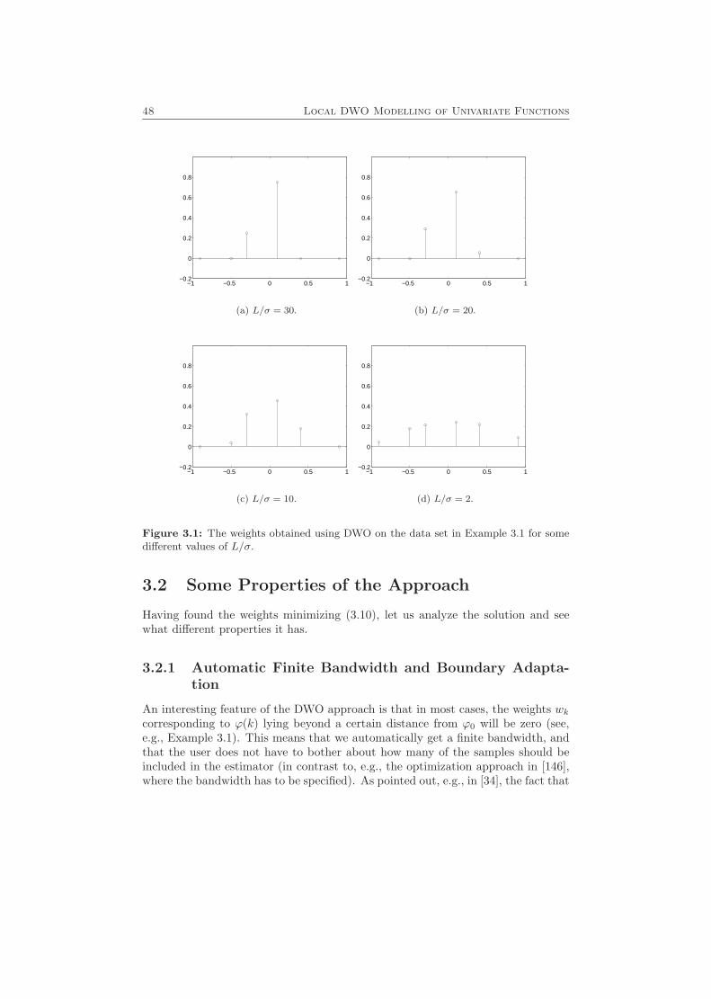
48 Local DWO Modelling of Univariate Functions
−1 −0.5 0 0.5 1−0.2
0
0.2
0.4
0.6
0.8
(a) L/σ = 30.
−1 −0.5 0 0.5 1−0.2
0
0.2
0.4
0.6
0.8
(b) L/σ = 20.
−1 −0.5 0 0.5 1−0.2
0
0.2
0.4
0.6
0.8
(c) L/σ = 10.
−1 −0.5 0 0.5 1−0.2
0
0.2
0.4
0.6
0.8
(d) L/σ = 2.
Figure 3.1: The weights obtained using DWO on the data set in Example 3.1 for somedifferent values of L/σ.
3.2 Some Properties of the Approach
Having found the weights minimizing (3.10), let us analyze the solution and seewhat different properties it has.
3.2.1 Automatic Finite Bandwidth and Boundary Adapta-tion
An interesting feature of the DWO approach is that in most cases, the weights wkcorresponding to ϕ(k) lying beyond a certain distance from ϕ0 will be zero (see,e.g., Example 3.1). This means that we automatically get a finite bandwidth, andthat the user does not have to bother about how many of the samples should beincluded in the estimator (in contrast to, e.g., the optimization approach in [146],where the bandwidth has to be specified). As pointed out, e.g., in [34], the fact that
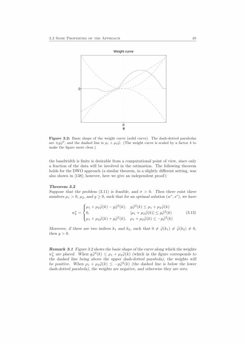
3.2 Some Properties of the Approach 49
0
0
Weight curve
φ
Figure 3.2: Basic shape of the weight curve (solid curve). The dash-dotted parabolasare ±gϕ2, and the dashed line is µ1 + µ2ϕ. (The weight curve is scaled by a factor 4 tomake the figure more clear.)
the bandwidth is finite is desirable from a computational point of view, since onlya fraction of the data will be involved in the estimation. The following theoremholds for the DWO approach (a similar theorem, in a slightly different setting, wasalso shown in [138]; however, here we give an independent proof):
Theorem 3.2Suppose that the problem (3.11) is feasible, and σ > 0. Then there exist threenumbers µ1 > 0, µ2, and g ≥ 0, such that for an optimal solution (w∗, s∗), we have
w∗k =
µ1 + µ2ϕ(k)− gϕ2(k), gϕ2(k) ≤ µ1 + µ2ϕ(k)0, |µ1 + µ2ϕ(k)| ≤ gϕ2(k)µ1 + µ2ϕ(k) + gϕ2(k), µ1 + µ2ϕ(k) ≤ −gϕ2(k)
(3.13)
Moreover, if there are two indices k1 and k2, such that 0 6= ϕ(k1) 6= ϕ(k2) 6= 0,then g > 0.
Remark 3.1 Figure 3.2 shows the basic shape of the curve along which the weightsw∗k are placed. When gϕ2(k) ≤ µ1 + µ2ϕ(k) (which in the figure corresponds tothe dashed line being above the upper dash-dotted parabola), the weights willbe positive. When µ1 + µ2ϕ(k) ≤ −gϕ2(k) (the dashed line is below the lowerdash-dotted parabola), the weights are negative, and otherwise they are zero.
50 Local DWO Modelling of Univariate Functions
In Figure 3.3, the weights are shown for some different cases. We can see clearlythat the bandwidth increases with a decreasing ratio L/σ, and that negative weightsoccur if the data samples are asymmetrically placed around the point of interest.
More explicit expressions for the weights are given in Section 3.2.2.
Proof The proof uses the Karush-Kuhn-Tucker (KKT) conditions (see, e.g.,[117]). Since the QP (3.11) is a convex optimization problem with linear con-straints, the KKT conditions are necessary and sufficient conditions for optimalityof a solution (see, e.g., [19] for details).
The Lagrangian function of (3.11) can be written
L(w, s;µ, λ) =L2
4
(N∑k=1
ϕ2(k)sk
)2
+ σ2N∑k=1
s2k − 2σ2µ1
(N∑k=1
wk − 1
)
− 2σ2µ2
N∑k=1
wkϕ(k)− 2σ2N∑k=1
(λ+k (sk − wk) + λ−k (sk + wk))
(3.14)
where λ±k ≥ 0, k = 1, . . . , N , and µ are the Lagrangian multipliers, scaled by afactor 1/2σ2. Since s∗k = |w∗k| for an optimal solution (w∗, s∗), the KKT conditionsare equivalent to the following relations:
µ1 + µ2ϕ(k) = λ+k − λ
−k (3.15a)
L2
4σ2
(N∑t=1
ϕ2(t)|w∗t |)ϕ2(k) + |w∗k| = λ+
k + λ−k (3.15b)
N∑k=1
w∗k = 1 (3.15c)
N∑k=1
w∗kϕ(k) = 0 (3.15d)
s∗k = |w∗k| (3.15e)
λ+k (|w∗k| − w∗k) = 0 (3.15f)
λ−k (|w∗k|+ w∗k) = 0 (3.15g)
λ±k ≥ 0, k = 1, . . . , N (3.15h)
Let
g =L2
4σ2
(N∑t=1
ϕ2(t)|w∗t |)
(3.16)
From (3.15f) and (3.15g), we can see that w∗k > 0 implies λ−k = 0, and that w∗k < 0implies λ+
k = 0. Hence, we can eliminate λ±k from the KKT conditions in thesecases, getting
w∗k = µ1 + µ2ϕ(k)− sgn(w∗k)gϕ2(k), w∗k 6= 0 (3.17)
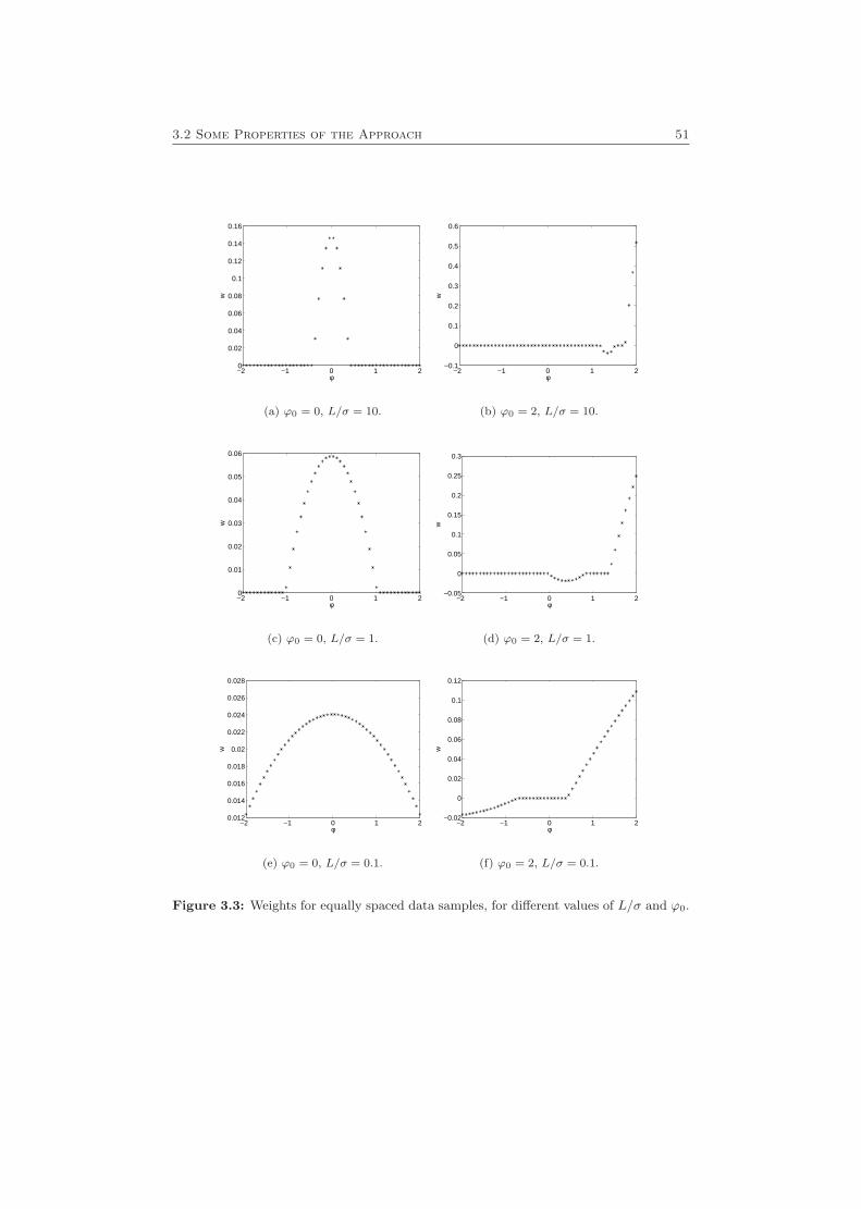
3.2 Some Properties of the Approach 51
−2 −1 0 1 20
0.02
0.04
0.06
0.08
0.1
0.12
0.14
0.16
φ
w
(a) ϕ0 = 0, L/σ = 10.
−2 −1 0 1 2−0.1
0
0.1
0.2
0.3
0.4
0.5
0.6
φ
w
(b) ϕ0 = 2, L/σ = 10.
−2 −1 0 1 20
0.01
0.02
0.03
0.04
0.05
0.06
φ
w
(c) ϕ0 = 0, L/σ = 1.
−2 −1 0 1 2−0.05
0
0.05
0.1
0.15
0.2
0.25
0.3
φ
w
(d) ϕ0 = 2, L/σ = 1.
−2 −1 0 1 20.012
0.014
0.016
0.018
0.02
0.022
0.024
0.026
0.028
φ
w
(e) ϕ0 = 0, L/σ = 0.1.
−2 −1 0 1 2−0.02
0
0.02
0.04
0.06
0.08
0.1
0.12
φ
w
(f) ϕ0 = 2, L/σ = 0.1.
Figure 3.3: Weights for equally spaced data samples, for different values of L/σ and ϕ0.
52 Local DWO Modelling of Univariate Functions
We can see that
w∗k > 0 ⇒ µ1 + µ2ϕ(k) > gϕ2(k)
w∗k < 0 ⇒ µ1 + µ2ϕ(k) < −gϕ2(k)
Finally, if w∗k = 0, we get from (3.15a), (3.15b), and (3.15h) that
2λ+k = µ1 + µ2ϕ(k) + gϕ2(k) ≥ 0
2λ−k = −µ1 − µ2ϕ(k) + gϕ2(k) ≥ 0
which implies−gϕ2(k) ≤ µ1 + µ2ϕ(k) ≤ gϕ2(k)
From these expressions, (3.13) is readily obtained.
Obviously, we have g ≥ 0 from (3.16). Now suppose that there are two indicesk1 and k2, such that 0 6= ϕ(k1) 6= ϕ(k2) 6= 0, and suppose that g = 0. Then (3.13)implies that w∗k = µ1 + µ2ϕ(k) for all k = 1, . . . , N . Furthermore, (3.16) impliesthat w∗k1
= w∗k2= 0. But this means that µ1 = µ2 = 0, which makes w∗k = 0 for all
k = 1, . . . , N . But this contradicts (3.15c), so g > 0.
To show that µ1 > 0, assume the opposite, i.e., µ1 ≤ 0. We also assume µ2 ≥ 0(if µ2 is negative, we can instead consider the problem we get by replacing ϕ(k)by −ϕ(k)). Let S+ be the set of indices k such that w∗k > 0. Obviously, S+ isnonempty; otherwise, (3.15c) will not be satisfied. Similarly, let S− be the set ofindices k such that w∗k < 0.
First assume that g > 0. For all k ∈ S+, it holds that
µ1 + µ2ϕ(k) > gϕ2(k) ⇒ µ2 −√µ2
2 + 4µ1g
2g< ϕ(k) <
µ2 +√µ2
2 + 4µ1g
2g
Similarly, for all k ∈ S−, it holds that
µ1 + µ2ϕ(k) < −gϕ2(k) ⇒ −µ2 −√µ2
2 − 4µ1g
2g< ϕ(k) <
−µ2 +√µ2
2 − 4µ1g
2g
Since straightforward calculations show that
0 ≤ −µ2 +√µ2
2 − 4µ1g
2g≤ µ2 −
õ2
2 + 4µ1g
2g
we have thatmaxk∈S−
ϕ(k) < mink∈S+
ϕ(k), 0 < mink∈S+
ϕ(k) (3.18)
If instead g = 0, it holds for all k ∈ S+ that
µ1 + µ2ϕ(k) > 0 ⇒ µ2 > 0, ϕ(k) > 0
3.2 Some Properties of the Approach 53
(this follows from the assumptions µ1 ≤ 0 and µ2 ≥ 0), and since for all k ∈ S−
µ1 + µ2ϕ(k) < 0
we can conclude that (3.18) holds also in this case.
Now, from (3.15c), (3.15d), and (3.18) we get
0 =∑k∈S+
w∗kϕ(k) +∑k∈S−
w∗kϕ(k)
≥ mink∈S+
ϕ(k)∑k∈S+
w∗k + maxk∈S−
ϕ(k)∑k∈S−
w∗k
≥ mink∈S+
ϕ(k)
(∑k∈S+
w∗k +∑k∈S−
w∗k
)= mink∈S+
ϕ(k) > 0
and we have a contradiction. It follows that µ1 > 0, and the theorem is proved.�
By examining the proof of Theorem 3.2, we can make an additional observa-tion. Suppose that we have an optimal solution w∗ to (3.11), with correspondingLagrangian multipliers λ± and µ, and constant g given by (3.16). Now, let usextend the data set ϕ(k), k = 1, . . . , N by adding a point ϕ(N + 1) that satisfies
−gϕ2(N + 1) ≤ µ1 + µ2ϕ(N + 1) ≤ gϕ2(N + 1) (3.19)
and consider the optimization problem (3.11) for the new data set. It turns outthat the KKT conditions (3.15) will be satisfied by the same weights w∗ as before,together with w∗N+1 = s∗N+1 = 0 and the Lagrangian multipliers µ, λ±, and λ±N+1,where λ±N+1 are given by (3.15a) and (3.15b). In other words, the solution doesnot change, except that w∗N+1 = 0 and λ±N+1 are appended. We summarize this ina corollary:
Corollary 3.1Suppose that ϕ(k), k = 1, . . . , N , L, and σ are given, and let (w∗, s∗) be an optimalsolution to (3.11). Let λ± and µ be the corresponding Lagrangian multipliers, andg the constant defined by (3.16). If the data set is extended by ϕ(N + 1) satisfying(3.19), then an optimal solution to (3.11) using the extended data set is given by(
s∗
0
),
(w∗
0
)with the corresponding Lagrangian multipliers(
λ+
λ+N+1
),
(λ−
λ−N+1
), µ
54 Local DWO Modelling of Univariate Functions
where
λ+N+1 =
12
(L2
4σ2
(N∑t=1
ϕ2(t)|w∗t |)ϕ2(N + 1) + µ1 + µ2ϕ(N + 1)
)
λ−N+1 =12
(L2
4σ2
(N∑t=1
ϕ2(t)|w∗t |)ϕ2(N + 1)− µ1 − µ2ϕ(N + 1)
)
The result opens up for a possible reduction of the computational complexity:Since many of the weights wk will be zero, we can already beforehand excludedata that will most likely correspond to zero weights, thus making the QP (3.11)considerably smaller. Having solved (3.11), one can easily check whether or notthe excluded weights really should be zero, by checking if the excluded data pointssatisfy |µ1 + µ2ϕ(k)| ≤ gϕ2(k) (the middle case of (3.13)). In Section 7.4, this isdiscussed in some more detail.
For the case when the data samples ϕ(k) are lying symmetrically, the followingtheorem shows that the weights are nonnegative, and lie along the positive part ofa parabola symmetrically around ϕ0 (compare this with the local linear estimator(2.28)).
Theorem 3.3Assume that the data samples ϕ(k) in (3.11) are lying symmetrically, i.e., that thenonzero ϕ(k) can be paired so that for each pair (ϕ(i), ϕ(j)) we have ϕ(i) = −ϕ(j).Also assume that ϕ(k) 6= 0 for at least one (hence two) indices k. Then µ2 = 0,i.e., the weights satisfy
w∗k = max{µ1 − gϕ2(k), 0} (3.20)
with µ1 > 0, g > 0.
Proof The positiveness of µ1 and g follows directly from Theorem 3.2 and thefact that we have two distinctive, nonzero ϕ(k). For the proof we now need toconsider the explicit expressions of the weights and Lagrangian multipliers thatwill be given in Section 3.2.2. Provided that the weights w∗k are all nonnegative, weget from (3.32) that µ2 = 0. Since the KKT conditions are sufficient for optimality,it then suffices to show that there exists a solution with nonnegative weights w∗k to(3.15). This will be done by induction. We assume that the data samples ϕ(k) areordered by ascending magnitude. Let us also use the notation w
[N0]k and µ[N0] for
the solution to (3.15), using the set of data samples ϕ(1), . . . , ϕ(N0), and g[N0] forthe corresponding g, given by (3.16).
For the case of just two nonzero data samples, the theorem is easily checked –(3.32)-(3.33) is obviously a solution to (3.15).
Now suppose that the theorem holds for all cases of at most N0 − 1 samples,and consider the case of N0 samples. The optimal weights w[N0−2]
k using N0 − 2
3.2 Some Properties of the Approach 55
samples are given by (3.33), and the corresponding µ[N0−2] is given by (3.32). Forϕ(N0) (and ϕ(N0 − 1) = −ϕ(N0)), there are now two possibilities: Either
µ[N0−2]1 ≤ g[N0−2]ϕ2(N0) (3.21)
org[N0−2]ϕ2(N0) < µ
[N0−2]1 (3.22)
In the first case we can apply Corollary 3.1, and we get a solution by lettingw
[N0]k = w
[N0−2]k for k = 1, . . . , N0 − 2, and w
[N0]N0−1 = w
[N0]N0
= 0. If on the otherhand (3.22) holds, we need to show that there is a nonnegative solution to (3.15).For this, it is sufficient to show that the weights we get using (3.33) are all positive,because then the KKT conditions will be satisfied using the corresponding µ[N0]
from (3.32). But from (3.33), (3.20), and (3.22) we get that
w[N0]i =
2
8N0σ2
L2 +∑N0j=1
∑N0k=1(ϕ2(j)− ϕ2(k))2
·(
4σ2
L2+
N0∑k=1
ϕ4(k)−(N0∑k=1
ϕ2(k)
)ϕ2(i)
)
=2
8N0σ2
L2 +∑N0j=1
∑N0k=1(ϕ2(j)− ϕ2(k))2
·(
4σ2
L2+N0−2∑k=1
ϕ4(k)−(N0−2∑k=1
ϕ2(k)
)ϕ2(i) + 2ϕ2(N0)(ϕ2(N0)− ϕ2(i))
)
=2
8N0σ2
L2 +∑N0j=1
∑N0k=1(ϕ2(j)− ϕ2(k))2
·((
4(N0 − 2)σ2
L2+
12
N0−2∑j=1
N0−2∑k=1
(ϕ2(j)− ϕ2(k))2
)(µ
[N0−2]1 − g[N0−2]ϕ2(i)
)
+ 2ϕ2(N0)(ϕ2(N0)− ϕ2(i))
)> 0, i = 1, . . . , N0
where in the last inequality we have used the fact that
g[N0−2]ϕ2(i) ≤ g[N0−2]ϕ2(N) ≤ µ[N0−2]1 , i = 1, . . . , N0
by (3.22). Hence, all weights (for all i = 1, . . . , N0) given by (3.33) are positive,and the theorem is proven. �
Since the DWO method automatically decides which data samples should betaken into account by minimizing (3.10), it also automatically adapts to the casewhen the data samples are lying asymmetrically, e.g., when ϕ0 is a boundary point,
56 Local DWO Modelling of Univariate Functions
or when only few data are available. The estimate will always be optimal in theworst-case MSE sense if considering G2(L), and in the sense of (3.10) for F2(L).This is a great advantage, especially compared to the kernel estimators, but alsoto the local polynomial modelling approach.
3.2.2 Explicit Expressions for the Optimal Weights
Let us take a closer look at (3.11), and derive explicit expressions for the weights.Assume that L and σ are both strictly positive. Let S be the set of indices k suchthat w∗k 6= 0. Let also
rk =
1 w∗k > 00 w∗k = 0−1 w∗k < 0
(3.23)
For the nonzero weights (i.e., for k ∈ S), (3.16) and (3.17) give
w∗k = µ1 + µ2ϕ(k)− rkL2
4σ2
(∑t∈S
rtϕ2(t)w∗t
)ϕ2(k) (3.24)
Reorder the data samples so that w∗1 , . . . , w∗n are the nonzero weights. Using the
notation
1n =
1...1
∈ Rn, ϕ1:n =
ϕ(1)...
ϕ(n)
, z =
r1ϕ2(1)...
rnϕ2(n)
, w∗ =
w∗1...w∗n
we can write the expression (3.24), together with the constraints (3.7), in matrixform as follows: − L2
4σ2 zzT − I 1n ϕ1:n
1Tn 0 0ϕT1:n 0 0
w∗µ1
µ2
=
010
(3.25)
This system is closely related to the in optimization well-known KKT system (see[117]). According to Lemma A.1, the system is nonsingular if L/σ > 0∗ and thereare at least two distinct values of ϕ(k), k = 1, . . . , n. Furthermore, we get the
∗In fact, the system is nonsingular even if L = 0, as long as the other requirement holds(see, e.g., [117]). However, for simplicity we only consider L > 0 here. The case L = 0 will beconsidered in Section 3.2.7.
3.2 Some Properties of the Approach 57
solution
w∗i =1ζ
(γ n∑k=1
ϕ2(k)−(
n∑k=1
rkϕ3(k)
)2
+
(n∑k=1
rkϕ2(k)
n∑k=1
rkϕ3(k)− γ
n∑k=1
ϕ(k)
)ϕ(i) (3.26)
+
(n∑k=1
ϕ(k)n∑k=1
rkϕ3(k)−
n∑k=1
ϕ2(k)n∑k=1
rkϕ2(k)
)riϕ
2(i)
)
µ =1ζ
γ
n∑k=1
ϕ2(k)−(
n∑k=1
rkϕ3(k)
)2
−γn∑k=1
ϕ(k) +n∑k=1
rkϕ2(k)
n∑k=1
rkϕ3(k)
(3.27)
where
γ = 4σ2
L2+ zT z
ζ =16
n∑i=1
n∑j=1
n∑k=1
(ϕ(i)(rkϕ2(k)− rjϕ2(j)) + ϕ(j)(riϕ2(i)− rkϕ2(k))
+ ϕ(k)(rjϕ2(j)− riϕ2(i)))2
+ 2σ2
L2
n∑i=1
n∑k=1
(ϕ(i)− ϕ(k))2
As mentioned in the remark after Lemma A.1, we can note that γ and ζ are bothstrictly positive.
3.2.3 Expressions for Nonnegative Weights
Suppose now that all nonzero weights are positive, i.e., that rk = 1, k = 1, . . . , n.In this case, the expressions can be somewhat simplified.
Note that ζ can also be written as
ζ =16
n∑i=1
n∑j=1
n∑k=1
(ϕ(i)− ϕ(j))2(ϕ(j)− ϕ(k))2(ϕ(k)− ϕ(i))2
+ 2σ2
L2
n∑i=1
n∑k=1
(ϕ(i)− ϕ(k))2
=16
n∑i=1
n∑j=1
n∑k=1
(ϕ(i)− ϕ(j))2(ϕ(j)− ϕ(k))2(ϕ(k)− ϕ(i))2 (3.28)
+ 2σ2
L2
n∑i=1
n∑k=1
(ϕ(i)− ϕ(k))2
58 Local DWO Modelling of Univariate Functions
sincen∑i=1
n∑j=1
n∑k=1
(ϕ(i)− ϕ(j))2(ϕ(j)− ϕ(k))2(ϕ(k)− ϕ(i))2
=n∑i=1
n∑j=1
n∑k=1
(ϕ(i)ϕ(j)ϕ(k)− ϕ2(i)ϕ(j)− ϕ(i)ϕ2(k) + ϕ2(i)ϕ(k)
− ϕ2(j)ϕ(k) + ϕ(i)ϕ2(j) + ϕ(j)ϕ2(k)− ϕ(i)ϕ(j)ϕ(k))2
=n∑i=1
n∑j=1
n∑k=1
(ϕ(i)(ϕ2(j)− ϕ2(k)) + ϕ(j)(ϕ2(k)− ϕ2(i))
+ ϕ(k)(ϕ2(i)− ϕ2(j)))2
This means that ζ is independent of ϕ0 as long as the same weights are positive.After simple but tedious calculations, we get the following expressions for µ andw∗:
µ =1ζ
γ
n∑k=1
ϕ2(k)−(
n∑k=1
ϕ3(k)
)2
n∑k=1
ϕ2(k)n∑k=1
ϕ3(k)− γn∑k=1
ϕ(k)
(3.29)
=1ζ
12
n∑j=1
n∑k=1
ϕ2(j)ϕ2(k)(ϕ(j)− ϕ(k))2 + 4σ2
L2
n∑k=1
ϕ2(k)
−12
n∑j=1
n∑k=1
ϕ(j)ϕ(k)(ϕ(j) + ϕ(k))(ϕ(j)− ϕ(k))2 − 4σ2
L2
n∑k=1
ϕ(k)
and
w∗i =1ζ
(γ n∑k=1
ϕ2(k)−(
n∑k=1
ϕ3(k)
)2
+
(n∑k=1
ϕ2(k)n∑k=1
ϕ3(k)− γn∑k=1
ϕ(k)
)ϕ(i)
+
n∑k=1
ϕ(k)n∑k=1
ϕ3(k)−(
n∑k=1
ϕ2(k)
)2 ϕ2(i)
)
=12ζ
n∑j=1
n∑k=1
ϕ2(j)ϕ2(k)(ϕ(j)− ϕ(k))2 + 8σ2
L2
n∑k=1
ϕ2(k)
(3.30)
−
n∑j=1
n∑k=1
ϕ(j)ϕ(k)(ϕ(j) + ϕ(k))(ϕ(j)− ϕ(k))2 + 8σ2
L2
n∑k=1
ϕ(k)
ϕ(i)
3.2 Some Properties of the Approach 59
+
n∑j=1
n∑k=1
ϕ(j)ϕ(k)(ϕ(j)− ϕ(k))2
ϕ2(i)
=
12ζ
(n∑j=1
n∑k=1
(ϕ(i)− ϕ(j))(ϕ(i)− ϕ(k))(ϕ(j)− ϕ(k))2(ϕ(j)− ϕ0)(ϕ(k)− ϕ0)
+ 8σ2
L2
n∑k=1
(ϕ(k)− ϕ(i))(ϕ(k)− ϕ0)
), i = 1, . . . , n (3.31)
In particular, when ϕ(k) are lying symmetrically around 0, all odd terms willdisappear from the expressions above, and we get (after some calculations)
ζ =12
n∑k=1
ϕ2(k)
n∑j=1
n∑k=1
(ϕ2(j)− ϕ2(k))2 + 8nσ2
L2
which gives
µ1 =2γ∑n
j=1
∑nk=1(ϕ2(j)− ϕ2(k))2 + 8n σ2
L2
, µ2 = 0 (3.32)
and
w∗i =2∑n
j=1
∑nk=1(ϕ2(j)− ϕ2(k))2 + 8n σ2
L2
(γ −
(n∑k=1
ϕ2(k)
)ϕ2(i)
)(3.33)
3.2.4 Relation to Local Polynomial Modelling
We can compare the DWO approach with the local linear estimator in the followingway. Use the notation of Section 3.2.2. Let
Φn =(1n ϕ1:n
)(3.34)
G =L2
4σ2zzT + I (3.35)
where z is defined as in Section 3.2.2. Comparing (3.25) to the proof of Lemma A.1in the Appendix shows that the weights of the DWO approach can be written as
w∗ = G−1Φn(ΦTnG−1Φn)−1e1 (3.36)
This can now be compared with the equivalent weights (2.26) of local polynomialmodelling. A word of caution is needed, though: In (3.35) and (3.36), only the datasamples corresponding to nonzero weights are included. On the other hand, in thepresentation of the local polynomial modelling, Φ includes all data samples, alsothose for which we get zero weights. Analogously, Kh generally contains many zeroentries in the diagonal. However, the solution of the local polynomial modelling
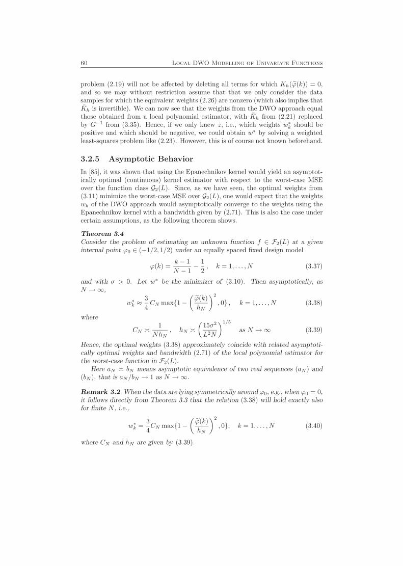
60 Local DWO Modelling of Univariate Functions
problem (2.19) will not be affected by deleting all terms for which Kh(ϕ(k)) = 0,and so we may without restriction assume that that we only consider the datasamples for which the equivalent weights (2.26) are nonzero (which also implies thatKh is invertible). We can now see that the weights from the DWO approach equalthose obtained from a local polynomial estimator, with Kh from (2.21) replacedby G−1 from (3.35). Hence, if we only knew z, i.e., which weights w∗k should bepositive and which should be negative, we could obtain w∗ by solving a weightedleast-squares problem like (2.23). However, this is of course not known beforehand.
3.2.5 Asymptotic Behavior
In [85], it was shown that using the Epanechnikov kernel would yield an asymptot-ically optimal (continuous) kernel estimator with respect to the worst-case MSEover the function class G2(L). Since, as we have seen, the optimal weights from(3.11) minimize the worst-case MSE over G2(L), one would expect that the weightswk of the DWO approach would asymptotically converge to the weights using theEpanechnikov kernel with a bandwidth given by (2.71). This is also the case undercertain assumptions, as the following theorem shows.
Theorem 3.4Consider the problem of estimating an unknown function f ∈ F2(L) at a giveninternal point ϕ0 ∈ (−1/2, 1/2) under an equally spaced fixed design model
ϕ(k) =k − 1N − 1
− 12, k = 1, . . . , N (3.37)
and with σ > 0. Let w∗ be the minimizer of (3.10). Then asymptotically, asN →∞,
w∗k ≈34CN max{1−
(ϕ(k)hN
)2
, 0} , k = 1, . . . , N (3.38)
where
CN �1
NhN, hN �
(15σ2
L2N
)1/5
as N →∞ (3.39)
Hence, the optimal weights (3.38) approximately coincide with related asymptoti-cally optimal weights and bandwidth (2.71) of the local polynomial estimator forthe worst-case function in F2(L).
Here aN � bN means asymptotic equivalence of two real sequences (aN ) and(bN ), that is aN/bN → 1 as N →∞.
Remark 3.2 When the data are lying symmetrically around ϕ0, e.g., when ϕ0 = 0,it follows directly from Theorem 3.3 that the relation (3.38) will hold exactly alsofor finite N , i.e.,
w∗k =34CN max{1−
(ϕ(k)hN
)2
, 0}, k = 1, . . . , N (3.40)
where CN and hN are given by (3.39).
3.2 Some Properties of the Approach 61
Proof Let us apply Theorem 3.2, from which it follows that there are threenumbers µ1 > 0, µ2, and g > 0, such that
w∗k = max{µ1 + µ2ϕ(k)− gϕ2(k), 0}, k = 1, . . . , N (3.41)
if and only if µ1 + µ2ϕ(k) + gϕ2(k) ≥ 0 for all k = 1, . . . , N , which is the case if
µ22 ≤ 4gµ1 (3.42)
Also recall that the KKT conditions (3.15) applied in the proof of Theorem 3.2represent necessary and sufficient conditions for optimality of the solution to theconsidered QP problem. Thus, in order to prove the first part of the theorem, itsuffices to demonstrate that
limN→∞
µ22
gµ1= 0 (3.43)
for the three parameters µ1, µ2, and g satisfying (3.15c), (3.15d), and (3.16),with the weights w∗k given by (3.41). Denote the support of the function w(ϕ) =max{µ1 + µ2ϕ− gϕ2, 0} by [a, b], that is
µ1 + µ2a− ga2 = 0, µ1 + µ2b− gb2 = 0, a < b (3.44)
and suppose that [a, b] ∈ [−0.5− ϕ0, 0.5− ϕ0]. If we find a solution to the systemof the three equations (3.15c), (3.15d), and (3.16) with respect to µ1 > 0, µ2, andg > 0, and (3.42) is satisfied, then we have proved (3.41). The following asymptoticrelation for nonnegative weights (3.41) holds true as N →∞:
1N
N∑k=1
wkϕm(k) =
b∫a
(µ1 + µ2ϕ− gϕ2
)ϕmdϕ+O(h/N) (µ1 + |µ2|+ g) (3.45)
for any m = 0, 1, 2, where
h =b− a
2
Thus, the equations (3.15c), (3.15d), and (3.16) may be written as follows:
1N
=
b∫a
(µ1 + µ2ϕ− gϕ2
)dϕ+O(h/N) (µ1 + |µ2|+ g) (3.46)
0 =
b∫a
(µ1 + µ2ϕ− gϕ2
)ϕdϕ+O(h/N) (µ1 + |µ2|+ g) (3.47)
4σ2
L2
g
N=
b∫a
(µ1 + µ2ϕ− gϕ2
)ϕ2dϕ+O(h/N) (µ1 + |µ2|+ g) (3.48)
62 Local DWO Modelling of Univariate Functions
with
a =µ2 −
õ2
2 + 4gµ1
2g, b =
µ2 +√µ2
2 + 4gµ1
2g, h =
õ2
2 + 4gµ1
2g(3.49)
Note that the terms O(h/N) in (3.46)–(3.48) do not depend on (µ1, µ2, g). Conse-quently, O(h/N)|µ2| is uniformly bounded over µ2 as N →∞.
Now, one might verify by direct substitution (see Section 3.4 for a detailedproof) that the solution to (3.46)–(3.48) has the following asymptotics:
µ1 �3
4NhN, µ2 = O(N−1), g � µ1
h2N
(3.50)
with
h =
õ2
2 + 4gµ1
2g� hN �
(15σ2
L2N
)1/5
(3.51)
Thus, we obtain
limN→∞
µ22
gµ1= limN→∞
µ1
g
(µ2
µ1
)2
= 0 (3.52)
and relation (3.43) is proved.
Since µ2 = o(µ1), the relation (3.38) follows directly from (3.50). This provesthe theorem. �
3.2.6 The Estimated Function
Another interesting aspect to consider is how the estimate f(ϕ0) behaves as afunction of ϕ0. For this purpose we use the explicit expressions from Section 3.2.2.To begin with, let us consider the case when wk are nonnegative for all k. In thiscase, we know from (3.28) that ζ does not depend on ϕ0, and from (3.30), we cansee that ϕ0 enters quadratically in the numerator of the expression for the weights.Furthermore, since f(ϕ0) is a linear combination of the weights, the quadraticcharacteristics are inherited by f(ϕ0) from wk. Altogether, this means that f(ϕ0)is a piecewise quadratic function in the intervals of ϕ0 for which the weights wk areall nonnegative.
When there are negative weights, ζ is no longer independent of ϕ0. It can beshown that ζ is a fourth order polynomial in ϕ0. Since ϕ enters also the numeratorpolynomially, the result is that f(ϕ0) is a piecewise rational function in the intervalsof ϕ0 where some weights wk are negative.
One should note, however, that f(ϕ0) does not necessarily satisfy the Lipschitzcondition (3.2), since the noise in the observations may be arbitrarily large, andhence may scale terms in f(ϕ0) to an arbitrary degree. This phenomenon is alsopointed out in [137].
3.2 Some Properties of the Approach 63
Example 3.2 Let us consider a simple example, where N = 11 data samplesϕ(1), . . . , ϕ(11) are equally spaced on the interval [−2, 2]. Let L/σ = 1. Supposethat the function f(ϕ) is to be estimated in several different points ϕ0. In Fig-ure 3.4, the values of the weights w1, . . . , w6 are plotted as functions of ϕ0. (Theplots for the remaining weights w7, . . . , w11 will be a mirrored version of w1, . . . , w5
due to the symmetry.) Also the (numerically computed) derivatives of the weightswith respect to ϕ0 are plotted. As we can see, when ϕ0 ∈ [−2,−1.5] or ϕ0 ∈ [1.5, 2](approximately), some weights are negative. For the remaining interval, i.e., forϕ0 ∈ [−1.5, 1.5], the weights are clearly piecewise quadratic functions of ϕ0.
When the weights are piecewise quadratic, so is also f(ϕ0), since it is a linear
combination of the weights. In Figure 3.5, f(ϕ0) is shown for a particular set ofobservations.
3.2.7 Global Models
What happens when L = 0, i.e., when the underlying function is linear? What onewould expect is that the resulting estimator would coincide with the usual globallinear regression, i.e., that it uses all data samples to estimate a linear functionwhich minimizes an unweighted least-squares criterion. The following theoremshows that this is exactly what happens.
Theorem 3.5Suppose that there are at least two indices k1 and k2, such that ϕ(k1) 6= ϕ(k1).Then, when L = 0, the DWO approach gives the same result as a local linear modelwith Kh(ϕ) ≡ 1.
Proof When L = 0, (3.10) becomes
minw
σ2N∑k=1
w2k
subj. toN∑k=1
wk = 1
N∑k=1
wkϕ(k) = 0
(3.53)
Letting
ΦT =(
1 . . . 1ϕ(1) . . . ϕ(N)
)the problem (3.53) is equivalent to
minw
‖w‖2
subj. to ΦTw = e1
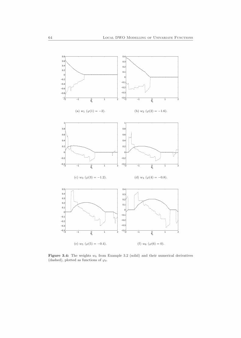
64 Local DWO Modelling of Univariate Functions
−2 −1 0 1 2−1
−0.8
−0.6
−0.4
−0.2
0
0.2
0.4
0.6
0.8
φ0
(a) w1 (ϕ(1) = −2).
−2 −1 0 1 2−0.4
−0.3
−0.2
−0.1
0
0.1
0.2
0.3
0.4
φ0
(b) w2 (ϕ(2) = −1.6).
−2 −1 0 1 2−0.4
−0.2
0
0.2
0.4
0.6
0.8
1
φ0
(c) w3 (ϕ(3) = −1.2).
−2 −1 0 1 2−0.4
−0.2
0
0.2
0.4
0.6
0.8
1
φ0
(d) w4 (ϕ(4) = −0.8).
−2 −1 0 1 2−0.4
−0.3
−0.2
−0.1
0
0.1
0.2
0.3
0.4
0.5
φ0
(e) w5 (ϕ(5) = −0.4).
−2 −1 0 1 2−0.4
−0.3
−0.2
−0.1
0
0.1
0.2
0.3
0.4
φ0
(f) w6 (ϕ(6) = 0).
Figure 3.4: The weights wk from Example 3.2 (solid) and their numerical derivatives(dashed), plotted as functions of ϕ0.
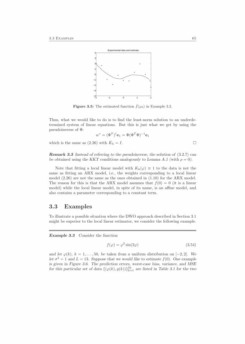
3.3 Examples 65
−2 −1 0 1 2−4
−3
−2
−1
0
1
2
3
4Experimental data and estimate:
Figure 3.5: The estimated function f(ϕ0) in Example 3.2.
Thus, what we would like to do is to find the least-norm solution to an underde-termined system of linear equations. But this is just what we get by using thepseudoinverse of Φ:
w∗ = (ΦT )†e1 = Φ(ΦTΦ)−1e1
which is the same as (2.26) with Kh = I. �
Remark 3.3 Instead of referring to the pseudoinverse, the solution of (3.2.7) canbe obtained using the KKT conditions analogously to Lemma A.1 (with ρ = 0).
Note that fitting a local linear model with Kh(ϕ) ≡ 1 to the data is not thesame as fitting an ARX model, i.e., the weights corresponding to a local linearmodel (2.26) are not the same as the ones obtained in (1.10) for the ARX model.The reason for this is that the ARX model assumes that f(0) = 0 (it is a linearmodel) while the local linear model, in spite of its name, is an affine model, andalso contains a parameter corresponding to a constant term.
3.3 Examples
To illustrate a possible situation where the DWO approach described in Section 3.1might be superior to the local linear estimator, we consider the following example.
Example 3.3 Consider the function
f(ϕ) = ϕ2 sin(2ϕ) (3.54)
and let ϕ(k), k = 1, . . . , 50, be taken from a uniform distribution on [−2, 2]. Welet σ2 = 1 and L = 13. Suppose that we would like to estimate f(0). One exampleis given in Figure 3.6. The prediction errors, worst-case bias, variance, and MSEfor this particular set of data {(ϕ(k), y(k))}50
k=1 are listed in Table 3.1 for the two
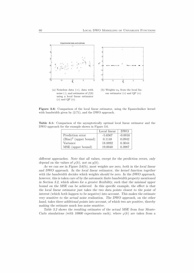
66 Local DWO Modelling of Univariate Functions
−2 −1 0 1 2−4
−2
0
2
4
6Experimental data and estimate
φk
(a) Noiseless data (×), data with
noise (·), and estimates of f(0)using a local linear estimator(◦) and QP (�).
−2 −1 0 1 2−3
−2
−1
0
1
2
3
4
φk
wk
(b) Weights wk from the local lin-
ear estimator (◦) and QP (∗).
Figure 3.6: Comparison of the local linear estimator, using the Epanechnikov kernelwith bandwidth given by (2.71), and the DWO approach.
Table 3.1: Comparison of the asymptotically optimal local linear estimator and theDWO approach for the example shown in Figure 3.6.
Local linear DWOPrediction error -5.6567 -0.0016(Bias)2 (upper bound) 0.1148 0.0942Variance 18.8892 0.3044MSE (upper bound) 19.0040 0.3987
different approaches. Note that all values, except for the prediction errors, onlydepend on the values of ϕ(k), not on y(k).
As we can see in Figure 3.6(b), most weights are zero, both in the local linearand DWO approach. In the local linear estimator, the kernel function togetherwith the bandwidth decides which weights should be zero. In the DWO approach,however, this is taken care of by the automatic finite bandwidth property mentionedin Section 3.2, which allows for a greater flexibility, such that the minimal upperbound on the MSE can be achieved. In this specific example, the effect is thatthe local linear estimator just takes the two data points closest to the point ofinterest (which both happen to be negative) into account. This makes the estimatevery sensitive to the actual noise realization. The DWO approach, on the otherhand, takes three additional points into account, of which two are positive, therebymaking the estimate much less noise sensitive.
Table 3.2 shows the resulting estimates of the actual MSE from four Monte-Carlo simulations (with 10000 experiments each), where ϕ(k) are taken from a
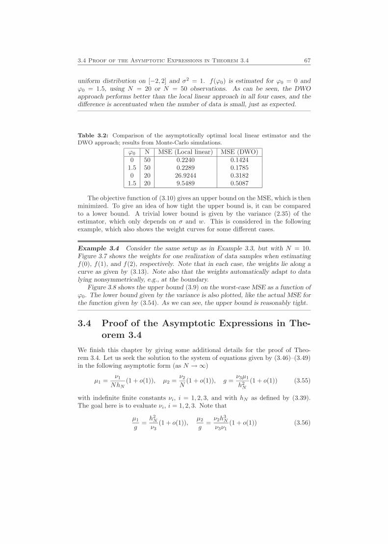
3.4 Proof of the Asymptotic Expressions in Theorem 3.4 67
uniform distribution on [−2, 2] and σ2 = 1. f(ϕ0) is estimated for ϕ0 = 0 andϕ0 = 1.5, using N = 20 or N = 50 observations. As can be seen, the DWOapproach performs better than the local linear approach in all four cases, and thedifference is accentuated when the number of data is small, just as expected.
Table 3.2: Comparison of the asymptotically optimal local linear estimator and theDWO approach; results from Monte-Carlo simulations.
ϕ0 N MSE (Local linear) MSE (DWO)0 50 0.2240 0.1424
1.5 50 0.2289 0.17850 20 26.9244 0.3182
1.5 20 9.5489 0.5087
The objective function of (3.10) gives an upper bound on the MSE, which is thenminimized. To give an idea of how tight the upper bound is, it can be comparedto a lower bound. A trivial lower bound is given by the variance (2.35) of theestimator, which only depends on σ and w. This is considered in the followingexample, which also shows the weight curves for some different cases.
Example 3.4 Consider the same setup as in Example 3.3, but with N = 10.Figure 3.7 shows the weights for one realization of data samples when estimatingf(0), f(1), and f(2), respectively. Note that in each case, the weights lie along acurve as given by (3.13). Note also that the weights automatically adapt to datalying nonsymmetrically, e.g., at the boundary.
Figure 3.8 shows the upper bound (3.9) on the worst-case MSE as a function ofϕ0. The lower bound given by the variance is also plotted, like the actual MSE forthe function given by (3.54). As we can see, the upper bound is reasonably tight.
3.4 Proof of the Asymptotic Expressions in The-orem 3.4
We finish this chapter by giving some additional details for the proof of Theo-rem 3.4. Let us seek the solution to the system of equations given by (3.46)–(3.49)in the following asymptotic form (as N →∞)
µ1 =ν1
NhN(1 + o(1)), µ2 =
ν2
N(1 + o(1)), g =
ν3µ1
h2N
(1 + o(1)) (3.55)
with indefinite finite constants νi, i = 1, 2, 3, and with hN as defined by (3.39).The goal here is to evaluate νi, i = 1, 2, 3. Note that
µ1
g=h2N
ν3(1 + o(1)),
µ2
g=ν2h
3N
ν3ν1(1 + o(1)) (3.56)
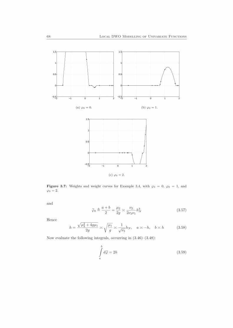
68 Local DWO Modelling of Univariate Functions
−2 −1 0 1 2−0.5
0
0.5
1
1.5
(a) ϕ0 = 0.
−2 −1 0 1 2−0.5
0
0.5
1
1.5
(b) ϕ0 = 1.
−2 −1 0 1 2−0.5
0
0.5
1
1.5
(c) ϕ0 = 2.
Figure 3.7: Weights and weight curves for Example 3.4, with ϕ0 = 0, ϕ0 = 1, andϕ0 = 2.
and
ϕ0 ,a+ b
2=µ2
2g� ν2
2ν3ν1h3N (3.57)
Hence
h =
õ2
2 + 4gµ1
2g�√µ1
g� 1√
ν3hN , a � −h, b � h (3.58)
Now evaluate the following integrals, occurring in (3.46)–(3.48):
b∫a
dϕ = 2h (3.59)
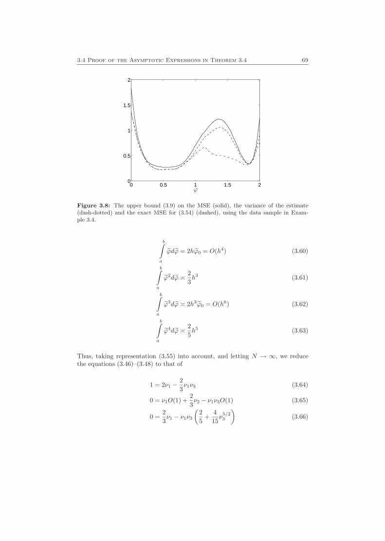
3.4 Proof of the Asymptotic Expressions in Theorem 3.4 69
0 0.5 1 1.5 20
0.5
1
1.5
2
ϕ
Figure 3.8: The upper bound (3.9) on the MSE (solid), the variance of the estimate(dash-dotted) and the exact MSE for (3.54) (dashed), using the data sample in Exam-ple 3.4.
b∫a
ϕdϕ = 2hϕ0 = O(h4) (3.60)
b∫a
ϕ2dϕ � 23h3 (3.61)
b∫a
ϕ3dϕ � 2h3ϕ0 = O(h6) (3.62)
b∫a
ϕ4dϕ � 25h5 (3.63)
Thus, taking representation (3.55) into account, and letting N → ∞, we reducethe equations (3.46)–(3.48) to that of
1 = 2ν1 −23ν1ν3 (3.64)
0 = ν1O(1) +23ν2 − ν1ν3O(1) (3.65)
0 =23ν1 − ν1ν3
(25
+415ν
5/23
)(3.66)

70 Local DWO Modelling of Univariate Functions
from what the unique nontrivial solution
ν1 =34, ν2 = O(1), ν3 = 1 (3.67)
follows directly. This proves the asymptotic relations (3.50).
4
Local DWO Modelling of
Multivariate Functions
In Chapter 3, the DWO approach was presented for the case of univariate func-tions. In this chapter, the approach is extended to multivariate functions, whichis useful in many applications, particularly when considering dynamic systems.Furthermore, the functions in Chapter 3 were assumed to be once continuouslydifferentiable, and the first derivatives should satisfy a Lipschitz condition. Thiscan be extended to any degree of assumed differentiability. As we will see, manyof the properties shown in Chapter 3 will also carry over to the multivariate case.
4.1 Problem Formulation
The problem we consider is the same as in Chapter 3, except that the function fis multivariate, f : Rn → R, and that the assumptions are somewhat different. Weassume that f ∈ Fp+1(L), which means that f is p times continuously differentiable(p ≥ 1), and that the pth derivative satisfies a Lipschitz condition. By the latterwill be meant that there is a constant L, such that
max‖ξ‖=1
∣∣∣∣∣∣n∑
i1=1
. . .
n∑ip=1
(f
(p)i1...ip
(ϕ+ h)− f (p)i1...ip
(ϕ))ξi1 . . . ξip
∣∣∣∣∣∣ ≤ L‖h‖ (4.1)
71
72 Local DWO Modelling of Multivariate Functions
for all ϕ, h ∈ Rn. Here f (p)i1...ip
means
f(p)i1...ip
=∂pf
∂ϕi1 . . . ∂ϕip(4.2)
One can show that, for p = 1, (4.1) is equivalent to (2.7), i.e., to
‖∇f(ϕ+ h)−∇f(ϕ)‖ ≤ L‖h‖
for all ϕ, h ∈ Rn.The noise assumptions are the same as in Chapter 3. As before, f will be
estimated using a linear estimator (3.4), where the weights are chosen to minimizean upper bound on the worst-case MSE (2.60). Remember, however, that in orderfor the worst-case MSE to be finite in the univariate case, the weights of (3.4) hadto satisfy the additional requirements (3.7). The corresponding requirements forthe multivariate case are given in the following theorem.
Theorem 4.1Consider f : Rn → R, f ∈ Fp+1(L). Then, for a linear estimator (3.4), theworst-case MSE is finite if and only if
N∑k=1
wk = 1
N∑k=1
wkϕi1(k) = 0 i1 = 1, . . . , n (4.3)
...
N∑k=1
wkϕi1(k) · . . . · ϕip(k) = 0 ij = 1, . . . , n, j = 1, . . . , p
On this subspace, the following upper bound can be given for the worst-case MSE:
WMSE (f(ϕ0),Fp+1(L)) ≤(
L
(p+ 1)!
N∑k=1
|wk|‖ϕ(k)‖p+1
)2
+ σ2N∑k=1
w2k (4.4)
Proof Analogously to (3.5), the worst-case MSE can be written as
WMSE (f(ϕ0),Fp+1(L)) = supf∈Fp+1(L)
(N∑k=1
wkf(ϕ(k))− f(ϕ0)
)2
+ σ2N∑k=1
w2k
= supf∈Fp+1(L)
(f(ϕ0)
(N∑k=1
wk − 1
)+
n∑i1=1
f ′i1(ϕ0)N∑k=1
wkϕi1(k) + . . . (4.5)
+1p!
n∑i1=1
. . .
n∑ip=1
f(p)i1...ip
(ϕ0)N∑k=1
wkϕi1(k) . . . ϕip(k)
4.1 Problem Formulation 73
+N∑k=1
wk
(f(ϕ(k))− f(ϕ0)−
n∑i1=1
f ′i1(ϕ0)ϕi1(k)− . . .
− 1p!
n∑i1=1
. . .
n∑ip=1
f(p)i1...ip
(ϕ0)ϕi1(k) . . . ϕip(k)))2
+ σ2N∑k=1
w2k
In this expression, all the terms of the bias, except for the last sum, are unbounded,and so, to guarantee a finite worst-case MSE, the requirements (4.3) need to beimposed. The last sum, on the other hand, is bounded according to Lemma A.3.Using this lemma and imposing (4.3), we can see that (4.4) is an upper bound on(4.5). �
We can note that instead of considering Fp+1(L), we could have considered amultivariate extension of the function class Gp+1(L) given by
f(ϕ) = f(ϕ0) +n∑
i1=1
f ′i1(ϕ0)ϕi1 + . . .+1p!
n∑i1=1
. . .n∑
ip=1
f(p)i1...ip
(ϕ0)ϕi1 . . . ϕip (4.6)
+ c(ϕ)‖ϕ‖p+1
where|c(ϕ)| ≤ L
(p+ 1)!In this case, the bound on the worst-case MSE in (4.4) is tight and is attained if
c(ϕ(k)) =L
(p+ 1)!sgn(wk)
Now, (4.4) can be minimized with respect to the weights wk. This can be doneusing a QP, as the following theorem shows.
Theorem 4.2Consider the following optimization problem:
minw
(L
(p+ 1)!
N∑k=1
|wk|‖ϕ(k)‖p+1
)2
+ σ2N∑k=1
w2k
subj. toN∑k=1
wk = 1
N∑k=1
wkϕi1(k) = 0 i1 = 1, . . . , n
...
N∑k=1
wkϕi1(k) · . . . · ϕip(k) = 0 ij = 1, . . . , n, j = 1, . . . , p
(4.7)
74 Local DWO Modelling of Multivariate Functions
The weight vector w∗ = (w∗1 . . . w∗N )T is a minimizer of (4.7) if and only if thereis a vector s∗, such that (w∗, s∗) is a minimizer of the following QP:
minw,s
(L
(p+ 1)!
N∑k=1
sk‖ϕ(k)‖p+1
)2
+ σ2N∑k=1
s2k
subj. to sk ≥ ±wkN∑k=1
wk = 1
N∑k=1
wkϕi1(k) = 0 i1 = 1, . . . , n
...
N∑k=1
wkϕi1(k) · . . . · ϕip(k) = 0 ij = 1, . . . , n, j = 1, . . . , p
(4.8)
Furthermore, s∗k = |w∗k|, k = 1, . . . , N .
Proof Completely analogous to Theorem 3.1. �
4.2 Properties
Several of the properties of the univariate case hold also for multivariate functions.For instance, when L = 0, the resulting weights equal those obtained by globallyfitting a pth polynomial to the data. The proof is simple and a straightforwardextension of Theorem 3.5.
Also the finite bandwidth property and boundary adaptation occur in the mul-tivariate case. We can prove the following theorem, which corresponds to Theo-rem 3.2, and is also related to the asymptotic results of [85].
Theorem 4.3Suppose that the problem (4.8) is feasible. Then there exist numbers µ(0), µ
(1)i1
, . . . ,
µ(p)i1...ip
, ij = 1, . . . , n, j = 1, . . . , p, and g ≥ 0, such that for an optimal solution
(w∗, s∗), we have
w∗k =
P (ϕ(k))− g‖ϕ(k)‖p+1, g‖ϕ(k)‖p+1 ≤ P (ϕ(k))0, −g‖ϕ(k)‖p+1 ≤ P (ϕ(k)) ≤ g‖ϕ(k)‖p+1
P (ϕ(k)) + g‖ϕ(k)‖p+1, P (ϕ(k)) ≤ −g‖ϕ(k)‖p+1
(4.9)
where
P (ϕ(k)) = µ(0) +n∑
i1=1
µ(1)i1ϕi1(k)+ . . .+
n∑i1=1
. . .
n∑i1=1
µ(p)i1...ip
ϕi1(k) · . . . · ϕip(k) (4.10)
4.2 Properties 75
Remark 4.1 Note that the notation µ(j)i1...ij
is used only to associate these numbers
with the corresponding derivatives of f . The numbers µ(j)i1...ij
are just constants,no derivatives or functions.
Proof The proof uses the KKT conditions, which, since the QP (4.8) is a convexoptimization problem with linear constraints, are necessary and sufficient condi-tions for optimality of a solution.
The Lagrangian function of (4.8) can be written
L(w, s;µ, λ) =
(L
(p+ 1)!
N∑k=1
sk‖ϕ(k)‖p+1
)2
+ σ2N∑k=1
s2k
− 2σ2µ(0)
(N∑k=1
wk − 1
)− 2σ2
n∑i1=1
µ(1)i1
N∑k=1
wkϕi1(k)− . . . (4.11)
− 2σ2n∑
i1=1
. . .
n∑ip=1
µ(p)i1...ip
N∑k=1
wkϕi1(k) . . . ϕip(k)
− 2σ2N∑k=1
(λ+k (sk − wk) + λ−k (sk + wk))
where λ±k ≥ 0, k = 1, . . . , N , and µ(0), µ(j)i1...ij
, i = 1, . . . , n, j = 1, . . . , p are theLagrangian multipliers, scaled by a factor 1/2σ2. Since s∗k = |w∗k| for an optimalsolution (w∗, s∗), the KKT conditions are equivalent to the following relations:
P (ϕ(k)) = λ+k − λ
−k (4.12a)
L2
((p+ 1)!)2σ2
(N∑t=1
|w∗t |‖ϕ(t)‖p+1
)‖ϕ(k)‖p+1 + |w∗k| = λ+
k + λ−k (4.12b)
N∑k=1
w∗k = 1
N∑k=1
wkϕi1(k) = 0 i1 = 1, . . . , n
...N∑k=1
wkϕi1(k) · . . . · ϕip(k) = 0 ij = 1, . . . , n, j = 1, . . . , p
(4.12c)
s∗k = |w∗k| (4.12d)
λ+k (|w∗k| − w∗k) = 0 (4.12e)
76 Local DWO Modelling of Multivariate Functions
λ−k (|w∗k|+ w∗k) = 0 (4.12f)
λ±k ≥ 0, k = 1, . . . , N (4.12g)
Let
g =L2
((p+ 1)!)2σ2
(N∑t=1
|w∗t |‖ϕ(t)‖p+1
)(4.13)
From (4.12e) and (4.12f), we can see that w∗k > 0 implies λ−k = 0, and that w∗k < 0implies λ+
k = 0. Hence, we can eliminate λ±k from the KKT conditions in thesecases, getting
w∗k = P (ϕ(k))− sgn(w∗k)g‖ϕ(k)‖p+1, w∗k 6= 0 (4.14)
We can see that
w∗k > 0 ⇒ P (ϕ(k)) > g‖ϕ(k)‖p+1
w∗k < 0 ⇒ P (ϕ(k)) < −g‖ϕ(k)‖p+1
Finally, if w∗k = 0, we get from (4.12a), (4.12b), and (4.12g) that
2λ+k = P (ϕ(k)) + g‖ϕ(k)‖p+1 ≥ 0
2λ−k = −P (ϕ(k)) + g‖ϕ(k)‖p+1 ≥ 0
which implies−g‖ϕ(k)‖p+1 ≤ P (ϕ(k)) ≤ g‖ϕ(k)‖p+1
From these expressions, (4.9) is readily obtained.
�
4.3 Examples
The extension of the DWO approach to the multivariate case makes it applicableto many applications, e.g., to the prediction problem for dynamic systems. In thissection, we will see two examples of this. As pointed out in Section 2.1, having aregression vector that depends on old values of y means that ϕ(i) and e(j) will notbe independent for all values of i and j. For the time being, we will simply neglectthis and assume that the effects will be small. The issue is discussed further inSection 7.1.
Example 4.1 Consider the following extended version of the linear system knownas the Astrom system [94]:
y(t) = (4.15)1.5y(t− 1)− 0.7y(t− 2) + u(t− 1) + 0.5u(t− 2)
+ α+ L0(cos y(t− 1) + 0.5u2(t− 1)) + e(t)
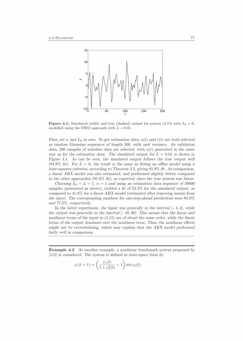
4.3 Examples 77
0 50 100 150 200−10
−5
0
5
10
15
t
y
Figure 4.1: Simulated (solid) and true (dashed) output for system (4.15) with L0 = 0,modelled using the DWO approach with L = 0.01.
First, set α and L0 to zero. To get estimation data, u(t) and e(t) are both selectedas random Gaussian sequences of length 500, with unit variance. As validationdata, 200 samples of noiseless data are selected, with u(t) generated in the sameway as for the estimation data. The simulated output for L = 0.01 is shown inFigure 4.1. As can be seen, the simulated output follows the true output well(84.9% fit). For L = 0, the result is the same as fitting an affine model using aleast-squares criterion, according to Theorem 3.5, giving 85.9% fit. As comparison,a linear ARX model was also estimated, and performed slightly better comparedto the other approaches (91.8% fit), as expected, since the true system was linear.
Choosing L0 = L = 1, α = 1 and using an estimation data sequence of 50000samples (generated as above), yielded a fit of 52.4% for the simulated output, ascompared to 41.8% for a linear ARX model (estimated after removing means fromthe data). The corresponding numbers for one-step-ahead predictions were 94.8%and 77.5%, respectively.
In the latter experiment, the input was generally in the interval [−4, 4], whilethe output was generally in the interval [−10, 30]. This means that the linear andnonlinear terms of the input in (4.15) are of about the same order, while the linearterms of the output dominate over the nonlinear term. Thus, the nonlinear effectsmight not be overwhelming, which may explain that the ARX model performedfairly well in comparison.
Example 4.2 As another example, a nonlinear benchmark system proposed by[115] is considered. The system is defined in state-space form by
x1(t+ 1) =(
x1(t)1 + x2
1(t)+ 1)
sinx2(t)
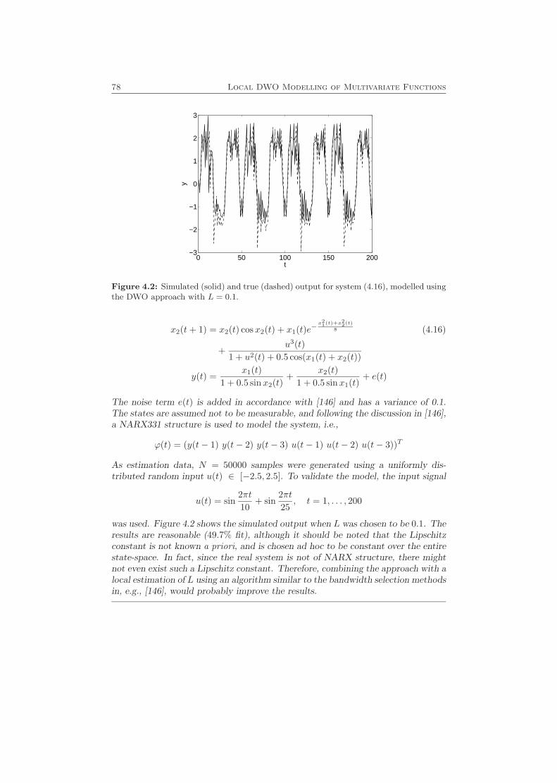
78 Local DWO Modelling of Multivariate Functions
0 50 100 150 200−3
−2
−1
0
1
2
3
t
y
Figure 4.2: Simulated (solid) and true (dashed) output for system (4.16), modelled usingthe DWO approach with L = 0.1.
x2(t+ 1) = x2(t) cosx2(t) + x1(t)e−x21(t)+x2
2(t)8 (4.16)
+u3(t)
1 + u2(t) + 0.5 cos(x1(t) + x2(t))
y(t) =x1(t)
1 + 0.5 sinx2(t)+
x2(t)1 + 0.5 sinx1(t)
+ e(t)
The noise term e(t) is added in accordance with [146] and has a variance of 0.1.The states are assumed not to be measurable, and following the discussion in [146],a NARX331 structure is used to model the system, i.e.,
ϕ(t) = (y(t− 1) y(t− 2) y(t− 3) u(t− 1) u(t− 2) u(t− 3))T
As estimation data, N = 50000 samples were generated using a uniformly dis-tributed random input u(t) ∈ [−2.5, 2.5]. To validate the model, the input signal
u(t) = sin2πt10
+ sin2πt25
, t = 1, . . . , 200
was used. Figure 4.2 shows the simulated output when L was chosen to be 0.1. Theresults are reasonable (49.7% fit), although it should be noted that the Lipschitzconstant is not known a priori, and is chosen ad hoc to be constant over the entirestate-space. In fact, since the real system is not of NARX structure, there mightnot even exist such a Lipschitz constant. Therefore, combining the approach with alocal estimation of L using an algorithm similar to the bandwidth selection methodsin, e.g., [146], would probably improve the results.
5
Using Prior Knowledge
One can easily imagine situations when something is known in advance about thefunction to estimate. For instance, we might have a rough idea of what would bereasonable values of the function from earlier experience, or physical limits mighttell us, e.g., that the function only can take positive values. Furthermore, we mightknow that the rate of change is limited by some known constant.
If such bounds are known, it would be tempting to try to use them to improvethe estimate. One could then remove the constraints (3.7) (which were imposedto get rid of the influence of the values f(ϕ0) and f ′(ϕ0) on the estimate), andinstead consider a restricted family of functions with some prior knowledge of thefunction value and its derivative:
|f(ϕ0)− a| ≤ δ, |f ′(ϕ0)− b| ≤ ∆ (5.1)
It is easy to see that, provided that the assumptions (5.1) are correct, this will notmake the worst-case MSE worse (we could always use weights satisfying (3.7), evenif it is not required). On the other hand, if the bounds are very wide, they willprobably not be of much help, either. Such issues will be discussed in this chapter.
Section 5.1 starts with the univariate case. For simplicity, we only consider theclass F2(L). In Section 5.2, the extension to multivariate functions is considered.
79
80 Using Prior Knowledge
5.1 The Univariate Case
The basic problem is still the same: estimate the value f(ϕ0) of an unknownfunction f : R → R at a given point ϕ0, given a set of input-output pairs{(ϕ(k), y(k))}Nk=1, coming from
y(k) = f(ϕ(k)) + e(k) (5.2)
We assume that f is continuously differentiable, and that there are known positiveconstants L, δ, ∆, and known constants a, b such that
|f ′(ϕ(1))− f ′(ϕ(2))| ≤ L|ϕ(1)− ϕ(2)| ∀ϕ(1), ϕ(2) ∈ R (5.3)|f(ϕ0)− a| ≤ δ (5.4)|f ′(ϕ0)− b| ≤ ∆ (5.5)
Following the notation of Chapter 2, this class of functions is denoted byF2(L, δ,∆).The noise terms are as previously independent, identically distributed random vari-ables with zero mean and known variance σ2.
There are some particular cases that deserve special attention:
• If δ →∞ then the limit class
F2(L,∆) , F2(L,∆,∞) =∞⋃t=1
F2(L, δ,∆)|δ=t (5.6)
describes the situation where we have no direct a priori information on thefunction value f(ϕ0).
• If in addition ∆ → 0+, then the limit class F2(L, 0) represents a set offunctions meeting condition (5.3) and having a given derivative f ′(ϕ0) = b.
• If both δ →∞ and ∆→∞, we are back to the function class F2(L) studiedin Chapter 3.
In the previous chapters, we have used a linear estimator (2.3). For the currentfunction classes, it turns out to be useful to consider the slightly more general classof affine estimators:
f(ϕ0) = w0 +N∑k=1
wky(k) (5.7)
As for the linear estimators in previous chapters, the weights of the affine estimatorwill depend on ϕ0, ϕ(k), L, and σ, but not on y(k). Furthermore, they may alsodepend on a, b, δ, and ∆.
The performance of an estimator f(ϕ0) will, as before, be evaluated by anupper bound on the worst-case MSE. In the following, such bounds are given forthe different function classes defined above. As it turns out, these upper boundscan then be minimized using quadratic programming, yielding optimal (in thissense) estimators.
5.1 The Univariate Case 81
5.1.1 Class F = F2(L, δ,∆)
As suggested, let us consider the affine estimator (5.7) and the function classF2(L, δ,∆) for finite δ, ∆. For this estimator and class, the worst-case MSE hasthe following upper bound:
WMSE (f(ϕ0),F2(L, δ,∆)) ≤ UF2(L,δ,∆)(w0, w)
=
(∣∣∣∣∣w0 + a
(N∑k=1
wk − 1
)+ b
N∑k=1
wkϕ(k)
∣∣∣∣∣+ δ
∣∣∣∣∣N∑k=1
wk − 1
∣∣∣∣∣+ ∆
∣∣∣∣∣N∑k=1
wkϕ(k)
∣∣∣∣∣+L
2
N∑k=1
|wk|ϕ2(k)
)2
+ σ2N∑k=1
w2k
(5.8)
This is true, since for any function f ∈ F2(L, δ,∆) the estimation error may berepresented as follows
f(ϕ0)− f(ϕ0) = w0 +N∑k=1
wky(k)− f(ϕ0)
= w0 +N∑k=1
wk(f(ϕ(k)) + e(k))− f(ϕ0)
= w0 + a
(N∑k=1
wk − 1
)+ b
N∑k=1
wkϕ(k) (5.9)
+ (f(ϕ0)− a)
(N∑k=1
wk − 1
)+ (f ′(ϕ0)− b)
N∑k=1
wkϕ(k)
+N∑k=1
wk(f(ϕ(k))− f(ϕ0)− f ′(ϕ0)ϕ(k)) +N∑k=1
wke(k)
Due to Lemma A.3, the inequality
|f(ϕ(k))− f(ϕ0)− f ′(ϕ0)ϕ(k)| ≤ L
2ϕ2(k) (5.10)
follows from (5.3). Now, the MSE satisfies
MSE (f(ϕ0)) =
(w0 + a
(N∑k=1
wk − 1
)+ b
N∑k=1
wkϕ(k) (5.11)
+ (f(ϕ0)− a)
(N∑k=1
wk − 1
)+ (f ′(ϕ0)− b)
N∑k=1
wkϕ(k)
+N∑k=1
wk(f(ϕ(k))− f(ϕ0)− f ′(ϕ0)ϕ(k))
)2
+ σ2N∑k=1
w2k
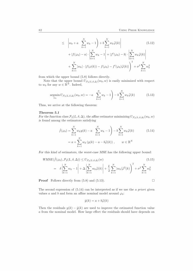
82 Using Prior Knowledge
≤(∣∣∣∣∣w0 + a
(N∑k=1
wk − 1
)+ b
N∑k=1
wkϕ(k)
∣∣∣∣∣ (5.12)
+ |f(ϕ0)− a| ·∣∣∣∣∣N∑k=1
wk − 1
∣∣∣∣∣+ |f ′(ϕ0)− b| ·∣∣∣∣∣N∑k=1
wkϕ(k)
∣∣∣∣∣+
N∑k=1
|wk| · |f(ϕ(k))− f(ϕ0)− f ′(ϕ0)ϕ(k)|)2
+ σ2N∑k=1
w2k
from which the upper bound (5.8) follows directly.Note that the upper bound UF2(L,δ,∆)(w0, w) is easily minimized with respect
to w0 for any w ∈ RN . Indeed,
argminw0
UF2(L,δ,∆)(w0, w) = −a(
N∑k=1
wk − 1
)− b
N∑k=1
wkϕ(k) (5.13)
Thus, we arrive at the following theorem:
Theorem 5.1For the function class F2(L, δ,∆), the affine estimator minimizing UF2(L,δ,∆)(w0, w)is found among the estimators satisfying
f(ϕ0) =N∑k=1
wky(k)− a(
N∑k=1
wk − 1
)− b
N∑k=1
wkϕ(k) (5.14)
= a+N∑k=1
wk (y(k)− a− bϕ(k)) , w ∈ RN
For this kind of estimators, the worst-case MSE has the following upper bound:
WMSE (f(ϕ0),F2(L, δ,∆)) ≤ UF2(L,δ,∆)(w) (5.15)
=
(δ
∣∣∣∣∣N∑k=1
wk − 1
∣∣∣∣∣+ ∆
∣∣∣∣∣N∑k=1
wkϕ(k)
∣∣∣∣∣+L
2
N∑k=1
|wk|ϕ2(k)
)2
+ σ2N∑k=1
w2k
Proof Follows directly from (5.8) and (5.13). �
The second expression of (5.14) can be interpreted as if we use the a priori givenvalues a and b and form an affine nominal model around ϕ0:
y(k) = a+ bϕ(k)
Then the residuals y(k) − y(k) are used to improve the estimated function valuea from the nominal model. How large effect the residuals should have depends on
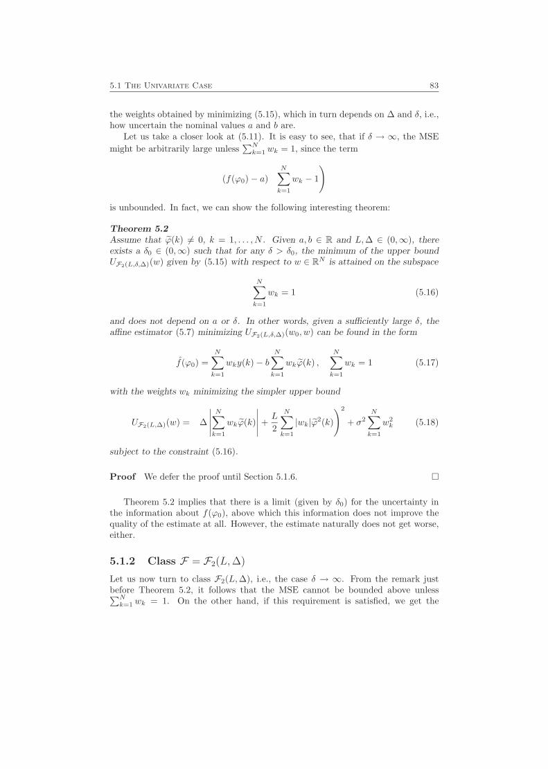
5.1 The Univariate Case 83
the weights obtained by minimizing (5.15), which in turn depends on ∆ and δ, i.e.,how uncertain the nominal values a and b are.
Let us take a closer look at (5.11). It is easy to see, that if δ → ∞, the MSEmight be arbitrarily large unless
∑Nk=1 wk = 1, since the term
(f(ϕ0)− a)
(N∑k=1
wk − 1
)
is unbounded. In fact, we can show the following interesting theorem:
Theorem 5.2Assume that ϕ(k) 6= 0, k = 1, . . . , N . Given a, b ∈ R and L,∆ ∈ (0,∞), thereexists a δ0 ∈ (0,∞) such that for any δ > δ0, the minimum of the upper boundUF2(L,δ,∆)(w) given by (5.15) with respect to w ∈ RN is attained on the subspace
N∑k=1
wk = 1 (5.16)
and does not depend on a or δ. In other words, given a sufficiently large δ, theaffine estimator (5.7) minimizing UF2(L,δ,∆)(w0, w) can be found in the form
f(ϕ0) =N∑k=1
wky(k)− bN∑k=1
wkϕ(k) ,N∑k=1
wk = 1 (5.17)
with the weights wk minimizing the simpler upper bound
UF2(L,∆)(w) =
(∆
∣∣∣∣∣N∑k=1
wkϕ(k)
∣∣∣∣∣+L
2
N∑k=1
|wk|ϕ2(k)
)2
+ σ2N∑k=1
w2k (5.18)
subject to the constraint (5.16).
Proof We defer the proof until Section 5.1.6. �
Theorem 5.2 implies that there is a limit (given by δ0) for the uncertainty inthe information about f(ϕ0), above which this information does not improve thequality of the estimate at all. However, the estimate naturally does not get worse,either.
5.1.2 Class F = F2(L,∆)
Let us now turn to class F2(L,∆), i.e., the case δ → ∞. From the remark justbefore Theorem 5.2, it follows that the MSE cannot be bounded above unless∑Nk=1 wk = 1. On the other hand, if this requirement is satisfied, we get the
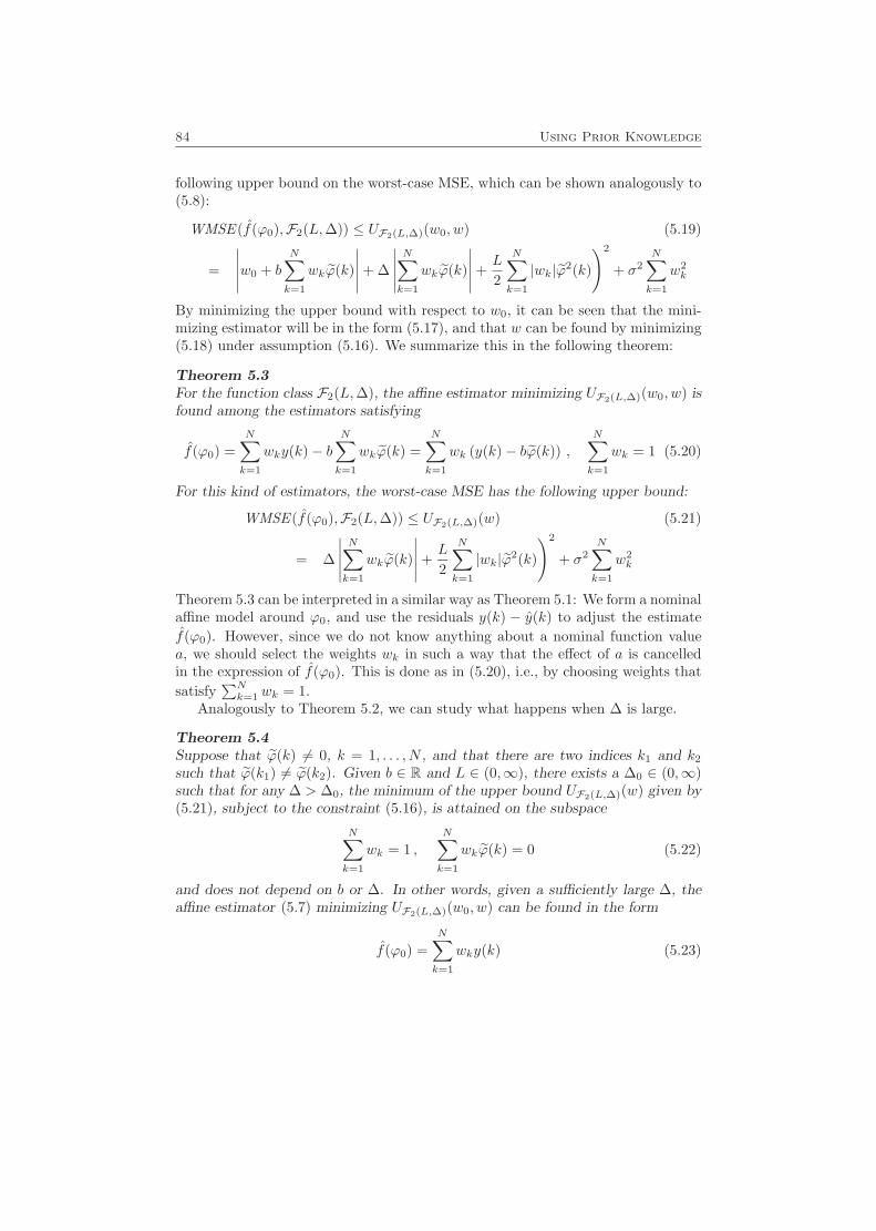
84 Using Prior Knowledge
following upper bound on the worst-case MSE, which can be shown analogously to(5.8):
WMSE (f(ϕ0),F2(L,∆)) ≤ UF2(L,∆)(w0, w) (5.19)
=
(∣∣∣∣∣w0 + b
N∑k=1
wkϕ(k)
∣∣∣∣∣+ ∆
∣∣∣∣∣N∑k=1
wkϕ(k)
∣∣∣∣∣+L
2
N∑k=1
|wk|ϕ2(k)
)2
+ σ2N∑k=1
w2k
By minimizing the upper bound with respect to w0, it can be seen that the mini-mizing estimator will be in the form (5.17), and that w can be found by minimizing(5.18) under assumption (5.16). We summarize this in the following theorem:
Theorem 5.3For the function class F2(L,∆), the affine estimator minimizing UF2(L,∆)(w0, w) isfound among the estimators satisfying
f(ϕ0) =N∑k=1
wky(k)− bN∑k=1
wkϕ(k) =N∑k=1
wk (y(k)− bϕ(k)) ,N∑k=1
wk = 1 (5.20)
For this kind of estimators, the worst-case MSE has the following upper bound:
WMSE (f(ϕ0),F2(L,∆)) ≤ UF2(L,∆)(w) (5.21)
=
(∆
∣∣∣∣∣N∑k=1
wkϕ(k)
∣∣∣∣∣+L
2
N∑k=1
|wk|ϕ2(k)
)2
+ σ2N∑k=1
w2k
Theorem 5.3 can be interpreted in a similar way as Theorem 5.1: We form a nominalaffine model around ϕ0, and use the residuals y(k) − y(k) to adjust the estimatef(ϕ0). However, since we do not know anything about a nominal function valuea, we should select the weights wk in such a way that the effect of a is cancelledin the expression of f(ϕ0). This is done as in (5.20), i.e., by choosing weights thatsatisfy
∑Nk=1 wk = 1.
Analogously to Theorem 5.2, we can study what happens when ∆ is large.
Theorem 5.4Suppose that ϕ(k) 6= 0, k = 1, . . . , N , and that there are two indices k1 and k2
such that ϕ(k1) 6= ϕ(k2). Given b ∈ R and L ∈ (0,∞), there exists a ∆0 ∈ (0,∞)such that for any ∆ > ∆0, the minimum of the upper bound UF2(L,∆)(w) given by(5.21), subject to the constraint (5.16), is attained on the subspace
N∑k=1
wk = 1 ,N∑k=1
wkϕ(k) = 0 (5.22)
and does not depend on b or ∆. In other words, given a sufficiently large ∆, theaffine estimator (5.7) minimizing UF2(L,∆)(w0, w) can be found in the form
f(ϕ0) =N∑k=1
wky(k) (5.23)
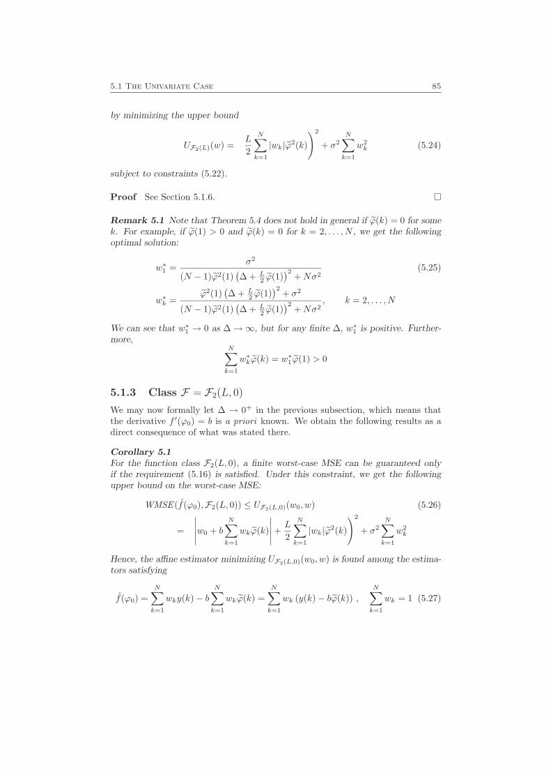
5.1 The Univariate Case 85
by minimizing the upper bound
UF2(L)(w) =
(L
2
N∑k=1
|wk|ϕ2(k)
)2
+ σ2N∑k=1
w2k (5.24)
subject to constraints (5.22).
Proof See Section 5.1.6. �
Remark 5.1 Note that Theorem 5.4 does not hold in general if ϕ(k) = 0 for somek. For example, if ϕ(1) > 0 and ϕ(k) = 0 for k = 2, . . . , N , we get the followingoptimal solution:
w∗1 =σ2
(N − 1)ϕ2(1)(∆ + L
2 ϕ(1))2
+Nσ2(5.25)
w∗k =ϕ2(1)
(∆ + L
2 ϕ(1))2
+ σ2
(N − 1)ϕ2(1)(∆ + L
2 ϕ(1))2
+Nσ2, k = 2, . . . , N
We can see that w∗1 → 0 as ∆→∞, but for any finite ∆, w∗1 is positive. Further-more,
N∑k=1
w∗kϕ(k) = w∗1ϕ(1) > 0
5.1.3 Class F = F2(L, 0)
We may now formally let ∆ → 0+ in the previous subsection, which means thatthe derivative f ′(ϕ0) = b is a priori known. We obtain the following results as adirect consequence of what was stated there.
Corollary 5.1For the function class F2(L, 0), a finite worst-case MSE can be guaranteed onlyif the requirement (5.16) is satisfied. Under this constraint, we get the followingupper bound on the worst-case MSE:
WMSE (f(ϕ0),F2(L, 0)) ≤ UF2(L,0)(w0, w) (5.26)
=
(∣∣∣∣∣w0 + b
N∑k=1
wkϕ(k)
∣∣∣∣∣+L
2
N∑k=1
|wk|ϕ2(k)
)2
+ σ2N∑k=1
w2k
Hence, the affine estimator minimizing UF2(L,0)(w0, w) is found among the estima-tors satisfying
f(ϕ0) =N∑k=1
wky(k)− bN∑k=1
wkϕ(k) =N∑k=1
wk (y(k)− bϕ(k)) ,N∑k=1
wk = 1 (5.27)
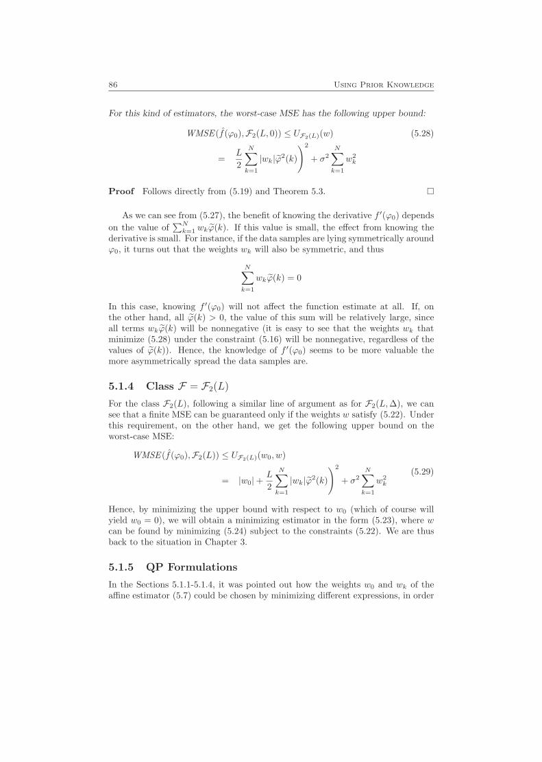
86 Using Prior Knowledge
For this kind of estimators, the worst-case MSE has the following upper bound:
WMSE (f(ϕ0),F2(L, 0)) ≤ UF2(L)(w) (5.28)
=
(L
2
N∑k=1
|wk|ϕ2(k)
)2
+ σ2N∑k=1
w2k
Proof Follows directly from (5.19) and Theorem 5.3. �
As we can see from (5.27), the benefit of knowing the derivative f ′(ϕ0) dependson the value of
∑Nk=1 wkϕ(k). If this value is small, the effect from knowing the
derivative is small. For instance, if the data samples are lying symmetrically aroundϕ0, it turns out that the weights wk will also be symmetric, and thus
N∑k=1
wkϕ(k) = 0
In this case, knowing f ′(ϕ0) will not affect the function estimate at all. If, onthe other hand, all ϕ(k) > 0, the value of this sum will be relatively large, sinceall terms wkϕ(k) will be nonnegative (it is easy to see that the weights wk thatminimize (5.28) under the constraint (5.16) will be nonnegative, regardless of thevalues of ϕ(k)). Hence, the knowledge of f ′(ϕ0) seems to be more valuable themore asymmetrically spread the data samples are.
5.1.4 Class F = F2(L)
For the class F2(L), following a similar line of argument as for F2(L,∆), we cansee that a finite MSE can be guaranteed only if the weights w satisfy (5.22). Underthis requirement, on the other hand, we get the following upper bound on theworst-case MSE:
WMSE (f(ϕ0),F2(L)) ≤ UF2(L)(w0, w)
=
(|w0|+
L
2
N∑k=1
|wk|ϕ2(k)
)2
+ σ2N∑k=1
w2k
(5.29)
Hence, by minimizing the upper bound with respect to w0 (which of course willyield w0 = 0), we will obtain a minimizing estimator in the form (5.23), where wcan be found by minimizing (5.24) subject to the constraints (5.22). We are thusback to the situation in Chapter 3.
5.1.5 QP Formulations
In the Sections 5.1.1-5.1.4, it was pointed out how the weights w0 and wk of theaffine estimator (5.7) could be chosen by minimizing different expressions, in order
5.1 The Univariate Case 87
to get estimators with guaranteed upper bounds on the worst-case MSE. In thissection we will show that these minimization problems can be formulated as convexquadratic programs.
To begin with, let us consider the function class F2(L, δ,∆) and the problem offinding the affine estimator minimizing (5.15).
Theorem 5.5Given the positive numbers δ,∆, L, consider the following minimization problem:
minw,s
(δsa + ∆sb +
L
2
N∑k=1
ϕ2(k)sk
)2
+ σ2N∑k=1
s2k
subj. to sa ≥ ±(
N∑k=1
wk − 1
)
sb ≥ ±N∑k=1
wkϕ(k)
sk ≥ ±wk, k = 1, . . . , N
(5.30)
where s = (sa, sb, s1, . . . , sN ). Then w∗ is a minimizer of UF2(L,δ,∆)(w) as definedin (5.15) if and only if there is a vector s∗ such that (w∗, s∗) is a minimizer of(5.30). Furthermore, the following relations hold:
s∗a =
∣∣∣∣∣N∑k=1
w∗k − 1
∣∣∣∣∣s∗b =
∣∣∣∣∣N∑k=1
w∗kϕ(k)
∣∣∣∣∣ (5.31)
s∗k = |w∗k|, k = 1, . . . , N
Proof Given a feasible solution w to (5.15), we can get a feasible solution to(5.30) with the same value of the objective function by using the same w and
sa =
∣∣∣∣∣N∑k=1
wk − 1
∣∣∣∣∣sb =
∣∣∣∣∣N∑k=1
wkϕ(k)
∣∣∣∣∣ (5.32)
sk = |wk|, k = 1, . . . , N
Hence (5.30) is a relaxation of (5.15), and it suffices to show that for a minimizer(w∗, s∗) of (5.30), (5.32) will hold. Suppose, e.g., that s∗1 > |w∗1 |. Then, withoutchanging any other variables, the value of the objective function can be reduced
88 Using Prior Knowledge
by decreasing s∗1. This can be seen by observing that the coefficient before s∗1 isnonnegative in the first sum of the objective function, and positive in the secondsum of the objective function, so decreasing s∗1 will decrease at least one of thesesums, and hence the objective function. Hence, s∗1 = |w∗1 |. By similar arguments,one can show that the other equalities of (5.32) will also hold at the optimum,which proves the theorem. �
Note that (5.30) is a convex QP and can therefore be solved efficiently.Starting from Theorem 5.5, we can now formulate QP:s for all the other cases
mentioned in Section 5.1. Since the constraints (5.16) and (5.22) are all linear in w,they can just be added to the QP. For the function class F2(L), the correspondingQP was given in Theorem 3.1. For F2(L,∆), the resulting theorem is listed below.
Theorem 5.6Given the positive numbers ∆, L, consider the following minimization problems:
minw
(∆
∣∣∣∣∣N∑k=1
wkϕ(k)
∣∣∣∣∣+L
2
N∑k=1
|wk|ϕ2(k)
)2
+ σ2N∑k=1
w2k
subj. toN∑k=1
wk = 1
(5.33)
and
minw,s
(∆sb +
L
2
N∑k=1
ϕ2(k)sk
)2
+ σ2N∑k=1
s2k
subj. to sb ≥ ±N∑k=1
wkϕ(k)
sk ≥ ±wk, k = 1, . . . , NN∑k=1
wk = 1
(5.34)
where w = (w1, . . . , wN ) and s = (sb, s1, . . . , sN ). Then w∗ is a minimizer of(5.33) if and only if there is a vector s∗ such that (w∗, s∗) is a minimizer of (5.34).Furthermore, the following relations hold:
s∗b =
∣∣∣∣∣N∑k=1
w∗kϕ(k)
∣∣∣∣∣s∗k = |w∗k|, k = 1, . . . , N
(5.35)
5.1 The Univariate Case 89
5.1.6 Proofs of Theorems 5.2 and 5.4
Now, when the minimization problems have been reformulated as QP:s, we areready to prove Theorems 5.2 and 5.4.
Proof (Proof of Theorem 5.4) From Theorem 5.6 we know that minimizing(5.21) subject to the constraint (5.16) is equivalent to solving (5.34). We also notethat the optimization problem we get by adding
N∑k=1
wkϕ(k) = 0
as a constraint to (5.34) is nothing else than (3.11), and will yield a (finite) optimalvalue if we have at least two distinctive points ϕ(k). Call this value d.
The Lagrangian function of (5.34) can be written
L(w, s;µ, λ) =
(∆sb +
L
2
N∑k=1
ϕ2(k)sk
)2
+ σ2N∑k=1
s2k − µ
(N∑k=1
wk − 1
)
− λ+b
(sb −
N∑k=1
wkϕ(k)
)− λ−b
(sb +
N∑k=1
wkϕ(k)
)
−N∑k=1
(λ+k (sk − wk) + λ−k (sk + wk))
(5.36)
where λ±k ≥ 0, k = 1, . . . , N , λ±b ≥ 0, and µ are the Lagrangian multipliers. Let usalso introduce
g(w,∆) = 2
(∆
∣∣∣∣∣N∑k=1
wkϕ(k)
∣∣∣∣∣+L
2
N∑k=1
ϕ2(k)|wk|)
(5.37)
Note thatg(w,∆) ≥ Lmin
kϕ2(k) > 0 (5.38)
Let (w∗, s∗b , s∗) be an optimal solution of (5.34). Using the relations
s∗b =
∣∣∣∣∣N∑k=1
w∗kϕ(k)
∣∣∣∣∣ , s∗k = |w∗k|
together with the necessary KKT conditions, we get
g(w∗,∆)∆ = λ+b + λ−b
µ+ (λ−b − λ+b )ϕ(k) = λ+
k − λ−k
g(w∗,∆)L
2ϕ2(k) + 2σ2|w∗k| = λ+
k + λ−k
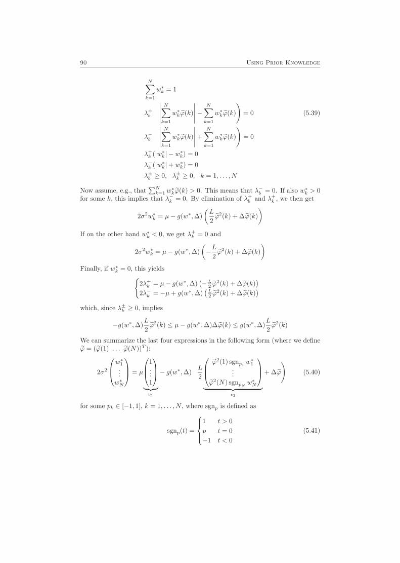
90 Using Prior Knowledge
N∑k=1
w∗k = 1
λ+b
(∣∣∣∣∣N∑k=1
w∗kϕ(k)
∣∣∣∣∣−N∑k=1
w∗kϕ(k)
)= 0 (5.39)
λ−b
(∣∣∣∣∣N∑k=1
w∗kϕ(k)
∣∣∣∣∣+N∑k=1
w∗kϕ(k)
)= 0
λ+k (|w∗k| − w∗k) = 0
λ−k (|w∗k|+ w∗k) = 0
λ±b ≥ 0, λ±k ≥ 0, k = 1, . . . , N
Now assume, e.g., that∑Nk=1 w
∗kϕ(k) > 0. This means that λ−b = 0. If also w∗k > 0
for some k, this implies that λ−k = 0. By elimination of λ+b and λ+
k , we then get
2σ2w∗k = µ− g(w∗,∆)(L
2ϕ2(k) + ∆ϕ(k)
)If on the other hand w∗k < 0, we get λ+
k = 0 and
2σ2w∗k = µ− g(w∗,∆)(−L
2ϕ2(k) + ∆ϕ(k)
)Finally, if w∗k = 0, this yields{
2λ+k = µ− g(w∗,∆)
(−L2 ϕ2(k) + ∆ϕ(k)
)2λ−k = −µ+ g(w∗,∆)
(L2 ϕ
2(k) + ∆ϕ(k))
which, since λ±k ≥ 0, implies
−g(w∗,∆)L
2ϕ2(k) ≤ µ− g(w∗,∆)∆ϕ(k) ≤ g(w∗,∆)
L
2ϕ2(k)
We can summarize the last four expressions in the following form (where we defineϕ = (ϕ(1) . . . ϕ(N))T ):
2σ2
w∗1...w∗N
= µ
1...1
︸ ︷︷ ︸v1
− g(w∗,∆)
(L
2
ϕ2(1) sgnp1w∗1
...ϕ2(N) sgnpN w
∗N
︸ ︷︷ ︸
v2
+ ∆ϕ
)(5.40)
for some pk ∈ [−1, 1], k = 1, . . . , N , where sgnp is defined as
sgnp(t) =
1 t > 0p t = 0−1 t < 0
(5.41)
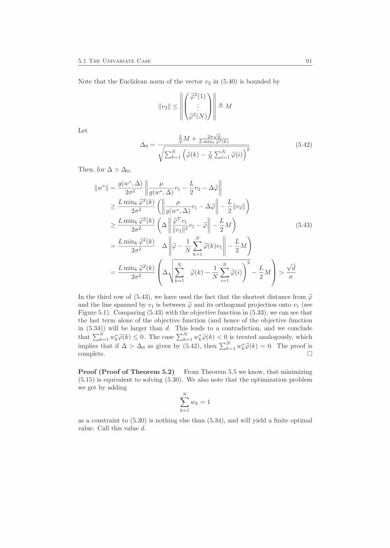
5.1 The Univariate Case 91
Note that the Euclidean norm of the vector v2 in (5.40) is bounded by
‖v2‖ ≤
∥∥∥∥∥∥∥ ϕ2(1)
...ϕ2(N)
∥∥∥∥∥∥∥ ,M
Let
∆0 =L2M + 2σ
√d
Lmink ϕ2(k)√∑Nk=1
(ϕ(k)− 1
N
∑Ni=1 ϕ(i)
)2(5.42)
Then, for ∆ > ∆0,
‖w∗‖ =g(w∗,∆)
2σ2
∥∥∥∥ µ
g(w∗,∆)v1 −
L
2v2 −∆ϕ
∥∥∥∥≥ Lmink ϕ2(k)
2σ2
(∥∥∥∥ µ
g(w∗,∆)v1 −∆ϕ
∥∥∥∥− L
2‖v2‖
)≥ Lmink ϕ2(k)
2σ2
(∆∥∥∥∥ ϕT v1
‖v1‖2v1 − ϕ
∥∥∥∥− L
2M
)(5.43)
=Lmink ϕ2(k)
2σ2
(∆
∥∥∥∥∥ϕ− 1N
N∑k=1
ϕ(k)v1
∥∥∥∥∥− L
2M
)
=Lmink ϕ2(k)
2σ2
∆
√√√√ N∑k=1
(ϕ(k)− 1
N
N∑i=1
ϕ(i)
)2
− L
2M
>
√d
σ
In the third row of (5.43), we have used the fact that the shortest distance from ϕand the line spanned by v1 is between ϕ and its orthogonal projection onto v1 (seeFigure 5.1). Comparing (5.43) with the objective function in (5.33), we can see thatthe last term alone of the objective function (and hence of the objective functionin (5.34)) will be larger than d. This leads to a contradiction, and we concludethat
∑Nk=1 w
∗kϕ(k) ≤ 0. The case
∑Nk=1 w
∗kϕ(k) < 0 is treated analogously, which
implies that if ∆ > ∆0 as given by (5.42), then∑Nk=1 w
∗kϕ(k) = 0. The proof is
complete. �
Proof (Proof of Theorem 5.2) From Theorem 5.5 we know, that minimizing(5.15) is equivalent to solving (5.30). We also note that the optimization problemwe get by adding
N∑k=1
wk = 1
as a constraint to (5.30) is nothing else than (5.34), and will yield a finite optimalvalue. Call this value d.
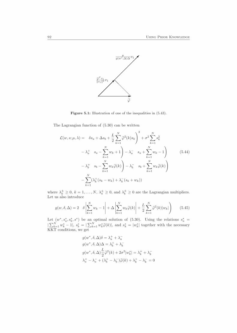
92 Using Prior Knowledge
-������
������������
@@
@@@
ϕT v1‖v1‖2 v1
ϕ
µg(w∗,∆)∆v1
Figure 5.1: Illustration of one of the inequalities in (5.43).
The Lagrangian function of (5.30) can be written
L(w, s;µ, λ) =
(δsa + ∆sb +
L
2
N∑k=1
ϕ2(k)sk
)2
+ σ2N∑k=1
s2k
− λ+a
(sa −
N∑k=1
wk + 1
)− λ−a
(sa +
N∑k=1
wk − 1
)(5.44)
− λ+b
(sb −
N∑k=1
wkϕ(k)
)− λ−b
(sb +
N∑k=1
wkϕ(k)
)
−N∑k=1
(λ+k (sk − wk) + λ−k (sk + wk))
where λ±k ≥ 0, k = 1, . . . , N , λ±a ≥ 0, and λ±b ≥ 0 are the Lagrangian multipliers.Let us also introduce
g(w, δ,∆) = 2
(δ
∣∣∣∣∣N∑k=1
wk − 1
∣∣∣∣∣+ ∆
∣∣∣∣∣N∑k=1
wkϕ(k)
∣∣∣∣∣+L
2
N∑k=1
ϕ2(k)|wk|)
(5.45)
Let (w∗, s∗a, s∗b , s∗) be an optimal solution of (5.30). Using the relations s∗a =
|∑Nk=1 w
∗k − 1|, s∗b = |
∑Nk=1 w
∗kϕ(k)|, and s∗k = |w∗k| together with the necessary
KKT conditions, we get
g(w∗, δ,∆)δ = λ+a + λ−a
g(w∗, δ,∆)∆ = λ+b + λ−b
g(w∗, δ,∆)L
2ϕ2(k) + 2σ2|w∗k| = λ+
k + λ−k
λ+a − λ−a + (λ+
b − λ−b )ϕ(k) + λ+
k − λ−k = 0
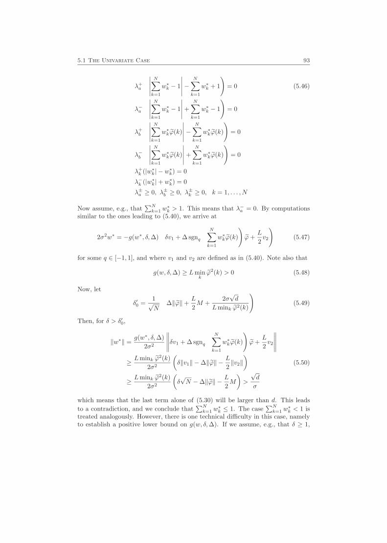
5.1 The Univariate Case 93
λ+a
(∣∣∣∣∣N∑k=1
w∗k − 1
∣∣∣∣∣−N∑k=1
w∗k + 1
)= 0 (5.46)
λ−a
(∣∣∣∣∣N∑k=1
w∗k − 1
∣∣∣∣∣+N∑k=1
w∗k − 1
)= 0
λ+b
(∣∣∣∣∣N∑k=1
w∗kϕ(k)
∣∣∣∣∣−N∑k=1
w∗kϕ(k)
)= 0
λ−b
(∣∣∣∣∣N∑k=1
w∗kϕ(k)
∣∣∣∣∣+N∑k=1
w∗kϕ(k)
)= 0
λ+k (|w∗k| − w∗k) = 0
λ−k (|w∗k|+ w∗k) = 0
λ±a ≥ 0, λ±b ≥ 0, λ±k ≥ 0, k = 1, . . . , N
Now assume, e.g., that∑Nk=1 w
∗k > 1. This means that λ−a = 0. By computations
similar to the ones leading to (5.40), we arrive at
2σ2w∗ = −g(w∗, δ,∆)
(δv1 + ∆ sgnq
(N∑k=1
w∗kϕ(k)
)ϕ+
L
2v2
)(5.47)
for some q ∈ [−1, 1], and where v1 and v2 are defined as in (5.40). Note also that
g(w, δ,∆) ≥ Lminkϕ2(k) > 0 (5.48)
Now, let
δ′0 =1√N
(∆‖ϕ‖+
L
2M +
2σ√d
Lmink ϕ2(k)
)(5.49)
Then, for δ > δ′0,
‖w∗‖ =g(w∗, δ,∆)
2σ2
∥∥∥∥∥δv1 + ∆ sgnq
(N∑k=1
w∗kϕ(k)
)ϕ+
L
2v2
∥∥∥∥∥≥ Lmink ϕ2(k)
2σ2
(δ‖v1‖ −∆‖ϕ‖ − L
2‖v2‖
)(5.50)
≥ Lmink ϕ2(k)2σ2
(δ√N −∆‖ϕ‖ − L
2M
)>
√d
σ
which means that the last term alone of (5.30) will be larger than d. This leadsto a contradiction, and we conclude that
∑Nk=1 w
∗k ≤ 1. The case
∑Nk=1 w
∗k < 1 is
treated analogously. However, there is one technical difficulty in this case, namelyto establish a positive lower bound on g(w, δ,∆). If we assume, e.g., that δ ≥ 1,
94 Using Prior Knowledge
we get
g(w, δ,∆) ≥ 2
∣∣∣∣∣N∑k=1
wk − 1
∣∣∣∣∣+ L
N∑k=1
ϕ2(k)|wk|
It is easy to see that the minimum of this expression with respect to the weightswk is obtained for weights satisfying wk ≥ 0,
∑Nk=1 wk ≤ 1. Hence, we get
g(w, δ,∆) ≥ minwk ≥ 0∑Nk=1 wk ≤ 1
2− 2N∑k=1
wk + LN∑k=1
ϕ2(k)wk
= minwk ≥ 0∑Nk=1 wk ≤ 1
2 +N∑k=1
wk(Lϕ2(k)− 2
)= min{Lmin
kϕ2(k), 2} > 0
With
δ0 = max{1, 1√N
(∆‖ϕ‖+
L
2M +
2σ√d
min{Lmink ϕ2(k), 2}
)} (5.51)
we can now perform similar calculations as for the case∑Nk=1 wk > 1, which implies
that if δ > δ0 as given by (5.51), then∑Nk=1 w
∗k = 1. The proof is complete. �
5.1.7 Adjusting the Estimate
For the function class F2(L, δ,∆), we assume that we know a bound on f(ϕ0).However, even if this was taken into account when deriving the QP (5.30), using theoptimal weights from (5.30) when computing the estimate f(ϕ0) does not guaranteethat the latter falls within the bounds, i.e., that
|f(ϕ0)− a| ≤ δ (5.52)
The reason for this is that the weights wk do not depend on y(k), and the actualnoise realization might therefore in unlucky cases deteriorate f(ϕ0) to such a degreethat it falls outside the bounds.
Fortunately, this is easily handled by adjusting the estimate afterwards accord-ing to
fADJ(ϕ0) = min{max{f(ϕ0), a− δ}, a+ δ} (5.53)
Using this adjustment, fADJ(ϕ0) is guaranteed to satisfy (5.52). Note that theworst-case MSE will not increase by making this alteration, if the true functionf ∈ F2(L, δ,∆). A similar adjustment was done in [137] for a problem of estimatingthe expected value of a random variable, when some of the observations are biased.
5.2 Estimating Multivariate Functions 95
5.2 Estimating Multivariate Functions
So far in this chapter, we have assumed that the function to be estimated hasa scalar argument. However, as mentioned previously, the regressors will have ahigher dimension in many applications, in particular to dynamic systems. Theextension to this case is immediate. In this section, we will describe some of theaspects of this kind of extension.
We now consider the problem of estimating the value f(ϕ0) of an unknownmultivariate, continuously differentiable function f : Rn → R at a given point ϕ0,given a set of input-output pairs {(ϕ(k), y(k))}Nk=1, coming from the relation
y(k) = f(ϕ(k)) + e(k) (5.54)
Instead of the assumptions (5.3)-(5.5), we make the following assumptions:
‖∇f(ϕ(1))−∇f(ϕ(2))‖ ≤ L‖ϕ(1)− ϕ(2)‖ ∀ϕ(1), ϕ(2) ∈ Rn (5.55)|f(ϕ0)− a| ≤ δ (5.56)
‖∇f(ϕ0)− b‖ ≤ ∆ (5.57)
With some abuse of notation, we let F2(L, δ,∆), F2(L,∆), and F2(L) denotealso their multivariate counterparts. For F2(L, δ,∆) and an affine estimator (5.7),the worst-case MSE has the following upper bound, which is similar to the univari-ate case:
WMSE (f(ϕ0),F2(L, δ,∆)) ≤ UF2(L,δ,∆)(w0, w)
=
(∣∣∣∣∣w0 + a
(N∑k=1
wk − 1
)+ bT
N∑k=1
wkϕ(k)
∣∣∣∣∣+ δ
∣∣∣∣∣N∑k=1
wk − 1
∣∣∣∣∣+ ∆
∥∥∥∥∥N∑k=1
wkϕ(k)
∥∥∥∥∥+L
2
N∑k=1
|wk|‖ϕ(k)‖2)2
+ σ2N∑k=1
w2k
(5.58)
As in the univariate case, we can immediately eliminate w0 by minimizing (5.58)for an arbitrary w, giving the following theorem:
Theorem 5.7For multivariate functions of the function class F2(L, δ,∆), the affine estimatorminimizing UF2(L,δ,∆)(w0, w) is found among the estimators satisfying
f(ϕ0) =N∑k=1
wky(k)− a(
N∑k=1
wk − 1
)− bT
N∑k=1
wkϕ(k) (5.59)
= a+N∑k=1
wk(y(k)− a− bT ϕ(k)
), w ∈ RN
96 Using Prior Knowledge
For this kind of estimators, the worst-case MSE has the following upper bound:
WMSE (f(ϕ0),F2(L, δ,∆)) ≤ UF2(L,δ,∆)(w) (5.60)
=
(δ
∣∣∣∣∣N∑k=1
wk − 1
∣∣∣∣∣+ ∆
∥∥∥∥∥N∑k=1
wkϕ(k)
∥∥∥∥∥+L
2
N∑k=1
|wk|‖ϕ(k)‖2)2
+ σ2N∑k=1
w2k
Proof Analogous to the univariate case. �
So far, the differences to the univariate case have been small and obvious. How-ever, when trying to transform the problem of minimizing (5.60) into a standardconvex optimization problem, it turns out that it is impossible to formulate it as aQP problem. What prohibits this is the term
∆
∥∥∥∥∥N∑k=1
wkϕ(k)
∥∥∥∥∥ (5.61)
which is the norm of a linear combination of vectors. Instead, we can formulatethe problem as a second-order cone program (SOCP), which is another standardclass of convex optimization problems (see [19]). To do this, we introduce someslack variables s = (s1 . . . sN )T and t = (ta tb tc)T , and get
minw,s,t
tc
subj. to
(δta + ∆tb +
L
2
N∑k=1
‖ϕ(k)‖2sk
)2
+ σ2N∑k=1
s2k ≤ tc∣∣∣∣∣
N∑k=1
wk − 1
∣∣∣∣∣ ≤ ta∥∥∥∥∥N∑k=1
wkϕ(k)
∥∥∥∥∥ ≤ tb|wk| ≤ sk, k = 1, . . . , N
(5.62)
This problem is in standard SOCP form, except for the first, quadratic constraint.However, straightforward calculations show that this constraint is equivalent to∥∥∥∥∥∥∥
2(δta + ∆tb + L
2
∑Nk=1 ‖ϕ(k)‖2sk
)2σs
1− tc
∥∥∥∥∥∥∥ ≤ 1 + tc (5.63)
thus completing the problem reformulation.For the other function classes, F2(L,∆) and F2(L), the extension to the multi-
variate case is done completely similarly. The minimization problem for F2(L,∆)will also yield a SOCP, while the minimization problem for F2(L) will still be pos-sible to express as a QP (as we saw in Chapter 4), since the term (5.61) vanishes.

5.3 An Example 97
5.3 An Example
The following simple example illustrates the fact that the information about boundson the function value and derivatives can be useful, but only if the bounds are tightenough.
Example 5.1 Let us consider the simple nonlinear system (with f : R2 → R)
y(t) = f(ϕ(t)) + e(t)f(ϕ) = 5(ϕ2
1 + ϕ22) + 5ϕ1 + 10ϕ2 + 15
(5.64)
where e(t) ∈ N(0, 1). Suppose that we would like to estimate y for ϕ0 =(0 0
)T,
given only N = 20 data samples taken from the distribution ϕ(t) ∈ N(0, I). Weassume that we know that (5.55) is satisfied for L = 10 (this is, of course, the bestpossible L), and that we also know some approximate values a and b of the functionf(ϕ0) and ∇f(ϕ0), respectively, and the bounds δ and ∆ according to (5.56) and(5.57). For simplicity, let a and b be the true values, a = f(ϕ0) and b = ∇f(ϕ0).
Now we can use the estimator in (5.59), for which the appropriate weights areobtained by solving the SOCP given by (5.62) and (5.63). Solving the SOCP canbe done using Yalmip [98] and SeDuMi [149]. Naturally, different δ and ∆ values
should give different estimates. Figure 5.2(a) shows f(ϕ0) for some different valuesof δ and ∆. In Figure 5.2(b) the part of the estimate coming from the a prioriknowledge of the function value (i.e., the second term of (5.59)) is plotted. As wecan see, for small values of δ, the estimate is based entirely on this information,while for large values, the a priori knowledge is not used at all, in agreement withTheorem 5.2. In Figure 5.2(c), the part of the f(ϕ0) coming from the knowledgeof ∇f(ϕ0) (the third term of (5.59)) is used. For this example, we can see thatthis information is not used very much, but that it gives a certain contribution forsmall values of ∆ (as long as δ is large enough, so that we do not only use theinformation about f(ϕ0)).
Finally, Figure 5.3 shows the optimal value of the criterion function, whichdecreases both with δ and ∆, just as should be expected.
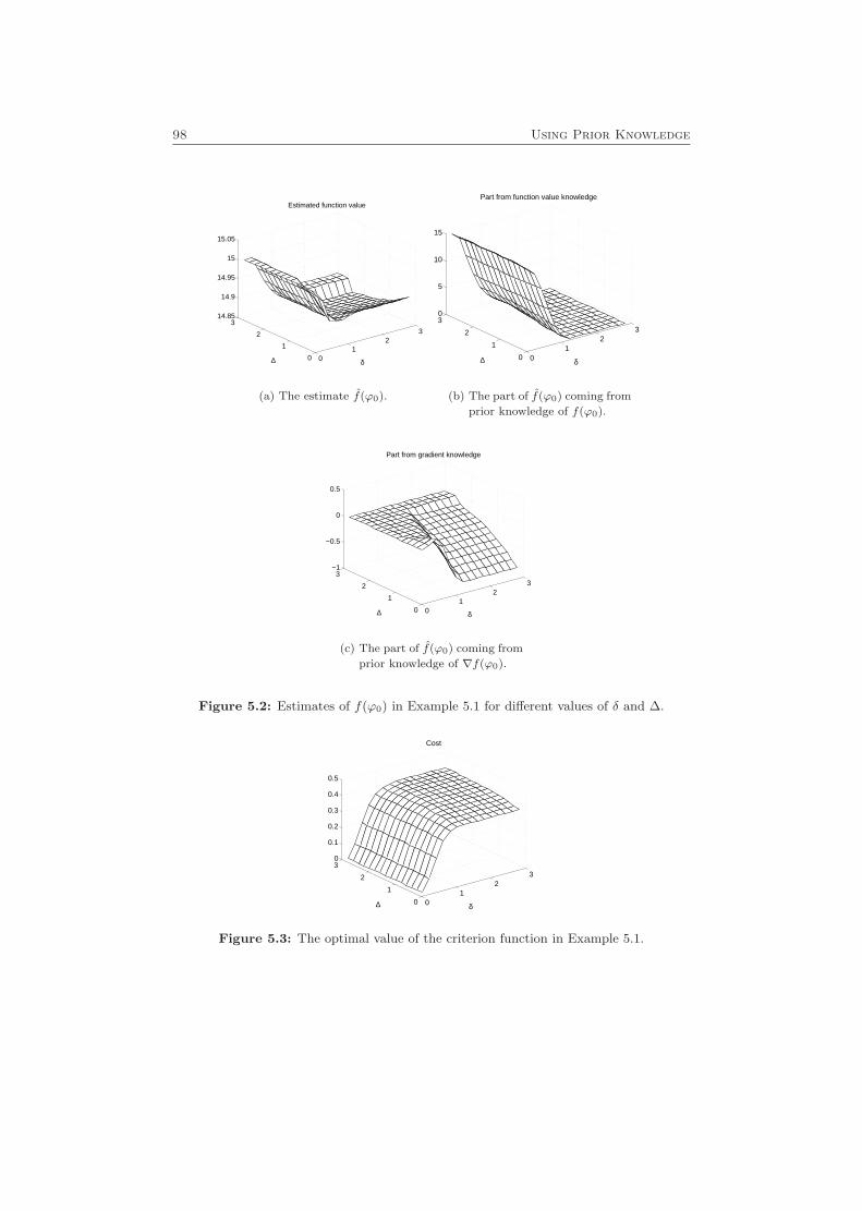
98 Using Prior Knowledge
01
23
0
1
2
314.85
14.9
14.95
15
15.05
δ
Estimated function value
∆
(a) The estimate f(ϕ0).
01
23
0
1
2
30
5
10
15
δ
Part from function value knowledge
∆
(b) The part of f(ϕ0) coming from
prior knowledge of f(ϕ0).
01
23
0
1
2
3−1
−0.5
0
0.5
δ
Part from gradient knowledge
∆
(c) The part of f(ϕ0) coming from
prior knowledge of ∇f(ϕ0).
Figure 5.2: Estimates of f(ϕ0) in Example 5.1 for different values of δ and ∆.
01
23
0
1
2
30
0.1
0.2
0.3
0.4
0.5
δ
Cost
∆
Figure 5.3: The optimal value of the criterion function in Example 5.1.
6
Other Extensions
This chapter presents some extensions that can be made to the proposed DWOapproach. These extensions include estimation of the derivative, which may beuseful in many applications. Section 6.2 considers the minimization of the exactworst-case MSE over F2(L). Other extensions are the case of nonconstant variance,and the usage of more general function classes. These issues are described inSection 6.3.
6.1 Estimating the Derivative
In Chapter 5, we saw that prior information about the function value f(ϕ0) andits derivatives (f ′(ϕ0) in the univariate case) can be of use if they are not toouncertain. The question is, given no prior information about f(ϕ0) and f ′(ϕ0), ifwe can improve our estimate of f(ϕ0) by first estimating the derivative, and thenuse this estimate when estimating f(ϕ0). As we will see, the answer to this questionis no for any reasonable linear estimate of f ′(ϕ0), using the same given data setas for estimating f(ϕ0). However, since estimating the derivative is interestingin itself, we will first consider this topic in some more detail. We will treat theproblem for the univariate case, for the three classes of functions that have beenpreviously discussed, and use affine estimators according to (5.7).
Let us denote a general affine derivative estimator by f ′(ϕ0). The MSE for
99
100 Other Extensions
f ′(ϕ0) is
MSE (f ′(ϕ0)) = E[(f ′(ϕ0)− f ′(ϕ0)
)2
|ϕN1 ] (6.1)
and the worst-case MSE becomes
WMSE (f ′(ϕ0),F) = supf∈F
MSE (f ′(ϕ0)) (6.2)
Recall that for an affine estimator (5.7), its worst-case MSE (6.2) is a function ofthe estimator parameters w0 and w. It also depends on the given class of functionsF . As for the function estimators, w0 and w will be computed by minimizing anupper bound on the worst-case MSE.
6.1.1 Class F = F2(L, δ,∆)
Let us begin with the function class F2(L, δ,∆). Using an affine estimator (5.7),we get the following upper bound on the worst-case MSE:
WMSE (f ′(ϕ0),F2(L, δ,∆)) ≤ U1F2(L,δ,∆)(w0, w)
=
(∣∣∣∣∣w0 + aN∑k=1
wk + b
(N∑k=1
wkϕ(k)− 1
)∣∣∣∣∣+ δ
∣∣∣∣∣N∑k=1
wk
∣∣∣∣∣+ ∆
∣∣∣∣∣N∑k=1
wkϕ(k)− 1
∣∣∣∣∣+L
2
N∑k=1
|wk|ϕ2(k)
)2
+ σ2N∑k=1
w2k
(6.3)
This can be seen by first considering the estimation error, which for any functionf ∈ F2(L, δ,∆) may be represented as follows
f ′(ϕ0)− f ′(ϕ0) = w0 +N∑k=1
wk(f(ϕ(k)) + e(k))− f ′(ϕ0)
= w0 + a
N∑k=1
wk + b
(N∑k=1
wkϕ(k)− 1
)(6.4)
+ (f(ϕ0)− a)N∑k=1
wk + (f ′(ϕ0)− b)(
N∑k=1
wkϕ(k)− 1
)
+N∑k=1
wk(f(ϕ(k))− f(ϕ0)− f ′(ϕ0)ϕ(k)) +N∑k=1
wke(k)
Using Lemma A.3, the MSE (6.1) becomes
MSE (f ′(ϕ0)) =
(w0 + a
N∑k=1
wk + b
(N∑k=1
wkϕ(k)− 1
)
6.1 Estimating the Derivative 101
+ (f(ϕ0)− a)N∑k=1
wk + (f ′(ϕ0)− b)(
N∑k=1
wkϕ(k)− 1
)(6.5)
+N∑k=1
wk(f(ϕ(k))− f(ϕ0)− f ′(ϕ0)ϕ(k))
)2
+ σ2N∑k=1
w2k
≤(∣∣∣∣∣w0 + a
N∑k=1
wk + b
(N∑k=1
wkϕ(k)− 1
)∣∣∣∣∣+ |f(ϕ0)− a| ·∣∣∣∣∣N∑k=1
wk
∣∣∣∣∣ (6.6)
+|f ′(ϕ0)− b| ·∣∣∣∣∣N∑k=1
wkϕ(k)− 1
∣∣∣∣∣+L
2
N∑k=1
|wk|ϕ2(k)
)2
+ σ2N∑k=1
w2k
from which the upper bound (6.3) follows directly.Similarly to the function estimation case, the upper bound U1
F2(L,δ,∆)(w0, w) iseasily minimized with respect to w0 for any w ∈ RN , resulting in
argminw0
U1F2(L,δ,∆)(w0, w) = −a
N∑k=1
wk − b(
N∑k=1
wkϕ(k)− 1
)(6.7)
Thus, we arrive at the following theorem:
Theorem 6.1For the function class F2(L, δ,∆), the affine estimator minimizing U1
F2(L,δ,∆)(w0, w)is found among the estimators satisfying
f ′(ϕ0) =N∑k=1
wky(k)− aN∑k=1
wk − b(
N∑k=1
wkϕ(k)− 1
)(6.8)
= b+N∑k=1
wk (y(k)− a− bϕ(k))
For this kind of estimators, the worst-case MSE (6.2) over the class F2(L, δ,∆) hasthe following upper bound:
WMSE (f ′(ϕ0),F2(L, δ,∆)) ≤ U1F2(L,δ,∆)(w) (6.9)
=
(δ
∣∣∣∣∣N∑k=1
wk
∣∣∣∣∣+ ∆
∣∣∣∣∣N∑k=1
wkϕ(k)− 1
∣∣∣∣∣+L
2
N∑k=1
|wk|ϕ2(k)
)2
+ σ2N∑k=1
w2k
The interpretation of Theorem 6.1 is similar to the one of Theorem 5.1. From thea priori given values a and b we form an affine nominal model
y(k) = a+ bϕ(k)
The residuals of this model y(k)− y(k) are then used to adjust the given nominalvalue b of f ′(ϕ0), and the effect of the adjustment depends on the weights, whichare determined from (6.9).
102 Other Extensions
When δ is large, it turns out that there is a theorem corresponding to Theo-rem 5.2 also for derivative estimators:
Theorem 6.2Assume that ϕ(k) 6= 0, k = 1, . . . , N . Given a, b ∈ R and L,∆ ∈ (0,∞), thereexists a δ0 ∈ (0,∞), such that for any δ > δ0, the minimum of the upper boundU1F2(L,δ,∆)(w) given by (6.9) with respect to w ∈ RN is attained on the subspace
N∑k=1
wk = 0 (6.10)
and does not depend on a or δ. In other words, given a sufficiently large δ, theaffine derivative estimator (5.7) minimizing U1
F2(L,δ,∆)(w0, w) can be found in theform
f ′(ϕ0) =N∑k=1
wky(k)− b(
N∑k=1
wkϕ(k)− 1
),
N∑k=1
wk = 0 (6.11)
with the weights wk minimizing the simpler upper bound
U1F2(L,∆)(w) =
(∆
∣∣∣∣∣N∑k=1
wkϕ(k)− 1
∣∣∣∣∣+L
2
N∑k=1
|wk|ϕ2(k)
)2
+ σ2N∑k=1
w2k (6.12)
subject to the constraint (6.10).
Proof Analogous to the proof of Theorem 5.2. �
In words this means that if the value a is too uncertain, it will not have any effectat all on the estimate f ′(ϕ0).
6.1.2 Class F = F2(L,∆)
For the class F2(L,∆), when δ → ∞, it is easy to see that the MSE cannot havea finite upper bound unless (6.10) holds. With this constraint satisfied, the upperbound on the worst-case MSE can be written
WMSE (f ′(ϕ0),F2(L,∆)) ≤ U1F2(L,∆)(w0, w)
=
(∣∣∣∣∣w0 + b
(N∑k=1
wkϕ(k)− 1
)∣∣∣∣∣+ ∆
∣∣∣∣∣N∑k=1
wkϕ(k)− 1
∣∣∣∣∣+L
2
N∑k=1
|wk|ϕ2(k)
)2
+ σ2N∑k=1
w2k
(6.13)
We can minimize this bound with respect to w0, and the resulting minimizingestimator will be in the form (6.11). It also follows that w can be computed byminimizing (6.12) subject to the constraint (6.10). This is summarized in thefollowing theorem:
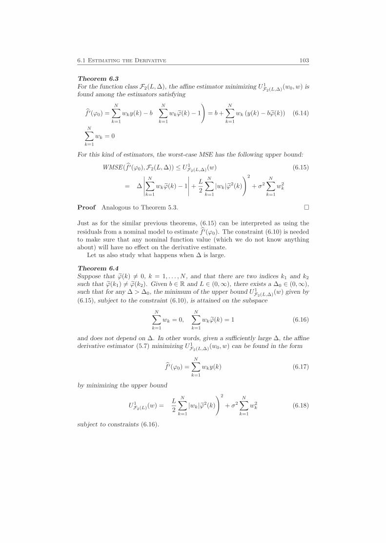
6.1 Estimating the Derivative 103
Theorem 6.3For the function class F2(L,∆), the affine estimator minimizing U1
F2(L,∆)(w0, w) isfound among the estimators satisfying
f ′(ϕ0) =N∑k=1
wky(k)− b(
N∑k=1
wkϕ(k)− 1
)= b+
N∑k=1
wk (y(k)− bϕ(k)) (6.14)
N∑k=1
wk = 0
For this kind of estimators, the worst-case MSE has the following upper bound:
WMSE (f ′(ϕ0),F2(L,∆)) ≤ U1F2(L,∆)(w) (6.15)
=
(∆
∣∣∣∣∣N∑k=1
wkϕ(k)− 1
∣∣∣∣∣+L
2
N∑k=1
|wk|ϕ2(k)
)2
+ σ2N∑k=1
w2k
Proof Analogous to Theorem 5.3. �
Just as for the similar previous theorems, (6.15) can be interpreted as using theresiduals from a nominal model to estimate f ′(ϕ0). The constraint (6.10) is neededto make sure that any nominal function value (which we do not know anythingabout) will have no effect on the derivative estimate.
Let us also study what happens when ∆ is large.
Theorem 6.4Suppose that ϕ(k) 6= 0, k = 1, . . . , N , and that there are two indices k1 and k2
such that ϕ(k1) 6= ϕ(k2). Given b ∈ R and L ∈ (0,∞), there exists a ∆0 ∈ (0,∞),such that for any ∆ > ∆0, the minimum of the upper bound U1
F2(L,∆)(w) given by
(6.15), subject to the constraint (6.10), is attained on the subspace
N∑k=1
wk = 0,N∑k=1
wkϕ(k) = 1 (6.16)
and does not depend on ∆. In other words, given a sufficiently large ∆, the affinederivative estimator (5.7) minimizing U1
F2(L,∆)(w0, w) can be found in the form
f ′(ϕ0) =N∑k=1
wky(k) (6.17)
by minimizing the upper bound
U1F2(L)(w) =
(L
2
N∑k=1
|wk|ϕ2(k)
)2
+ σ2N∑k=1
w2k (6.18)
subject to constraints (6.16).
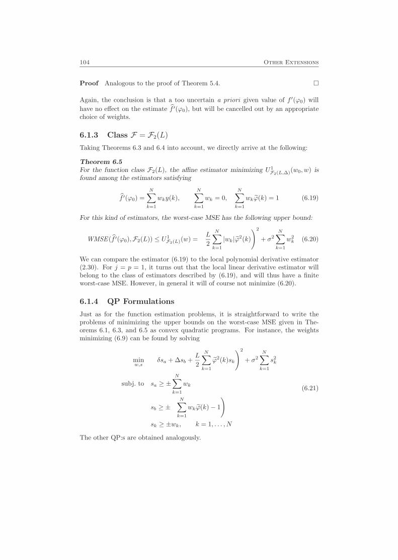
104 Other Extensions
Proof Analogous to the proof of Theorem 5.4. �
Again, the conclusion is that a too uncertain a priori given value of f ′(ϕ0) willhave no effect on the estimate f ′(ϕ0), but will be cancelled out by an appropriatechoice of weights.
6.1.3 Class F = F2(L)
Taking Theorems 6.3 and 6.4 into account, we directly arrive at the following:
Theorem 6.5For the function class F2(L), the affine estimator minimizing U1
F2(L,∆)(w0, w) isfound among the estimators satisfying
f ′(ϕ0) =N∑k=1
wky(k),N∑k=1
wk = 0,N∑k=1
wkϕ(k) = 1 (6.19)
For this kind of estimators, the worst-case MSE has the following upper bound:
WMSE (f ′(ϕ0),F2(L)) ≤ U1F2(L)(w) =
(L
2
N∑k=1
|wk|ϕ2(k)
)2
+ σ2N∑k=1
w2k (6.20)
We can compare the estimator (6.19) to the local polynomial derivative estimator(2.30). For j = p = 1, it turns out that the local linear derivative estimator willbelong to the class of estimators described by (6.19), and will thus have a finiteworst-case MSE. However, in general it will of course not minimize (6.20).
6.1.4 QP Formulations
Just as for the function estimation problems, it is straightforward to write theproblems of minimizing the upper bounds on the worst-case MSE given in The-orems 6.1, 6.3, and 6.5 as convex quadratic programs. For instance, the weightsminimizing (6.9) can be found by solving
minw,s
(δsa + ∆sb +
L
2
N∑k=1
ϕ2(k)sk
)2
+ σ2N∑k=1
s2k
subj. to sa ≥ ±N∑k=1
wk
sb ≥ ±(
N∑k=1
wkϕ(k)− 1
)sk ≥ ±wk, k = 1, . . . , N
(6.21)
The other QP:s are obtained analogously.
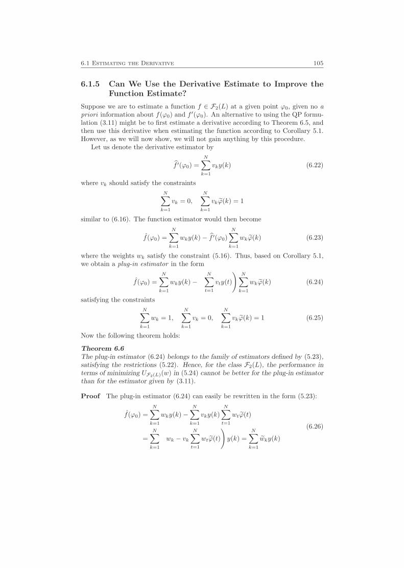
6.1 Estimating the Derivative 105
6.1.5 Can We Use the Derivative Estimate to Improve theFunction Estimate?
Suppose we are to estimate a function f ∈ F2(L) at a given point ϕ0, given no apriori information about f(ϕ0) and f ′(ϕ0). An alternative to using the QP formu-lation (3.11) might be to first estimate a derivative according to Theorem 6.5, andthen use this derivative when estimating the function according to Corollary 5.1.However, as we will now show, we will not gain anything by this procedure.
Let us denote the derivative estimator by
f ′(ϕ0) =N∑k=1
vky(k) (6.22)
where vk should satisfy the constraintsN∑k=1
vk = 0,N∑k=1
vkϕ(k) = 1
similar to (6.16). The function estimator would then become
f(ϕ0) =N∑k=1
wky(k)− f ′(ϕ0)N∑k=1
wkϕ(k) (6.23)
where the weights wk satisfy the constraint (5.16). Thus, based on Corollary 5.1,we obtain a plug-in estimator in the form
f(ϕ0) =N∑k=1
wky(k)−(
N∑t=1
vty(t)
)N∑k=1
wkϕ(k) (6.24)
satisfying the constraintsN∑k=1
wk = 1,N∑k=1
vk = 0,N∑k=1
vkϕ(k) = 1 (6.25)
Now the following theorem holds:
Theorem 6.6The plug-in estimator (6.24) belongs to the family of estimators defined by (5.23),satisfying the restrictions (5.22). Hence, for the class F2(L), the performance interms of minimizing UF2(L)(w) in (5.24) cannot be better for the plug-in estimatorthan for the estimator given by (3.11).
Proof The plug-in estimator (6.24) can easily be rewritten in the form (5.23):
f(ϕ0) =N∑k=1
wky(k)−N∑k=1
vky(k)N∑t=1
wtϕ(t)
=N∑k=1
(wk − vk
N∑t=1
wtϕ(t)
)y(k) =
N∑k=1
wky(k)
(6.26)
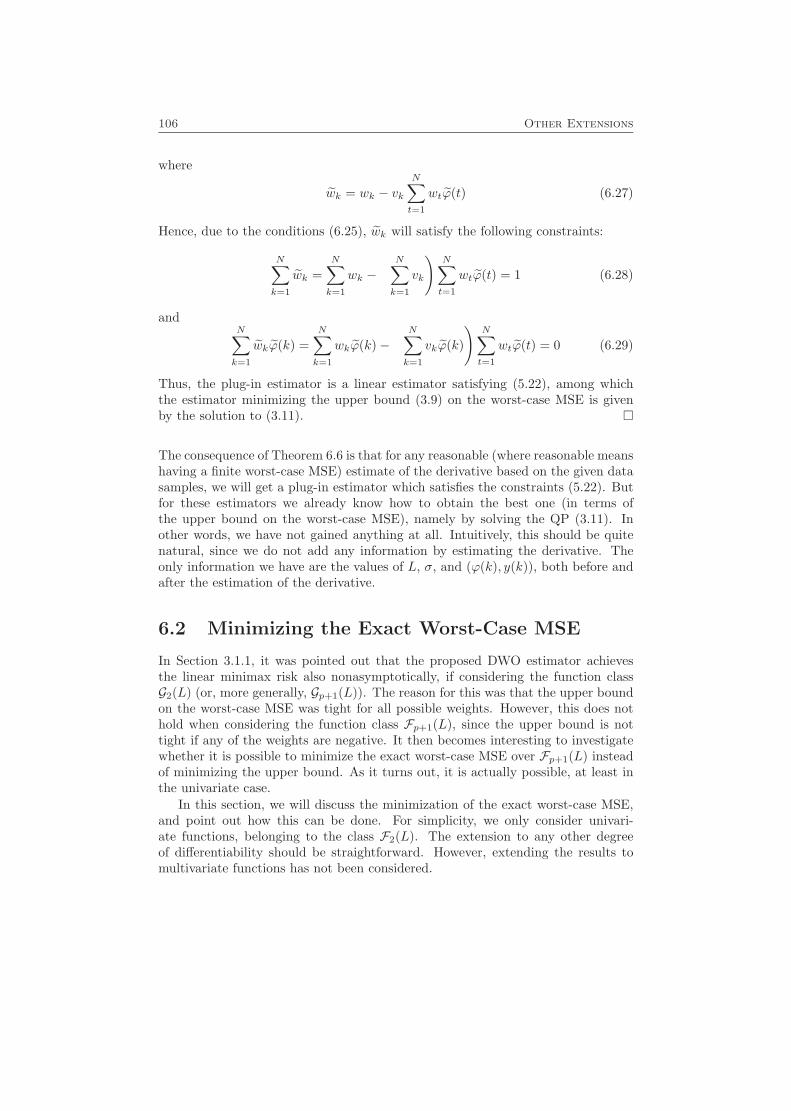
106 Other Extensions
where
wk = wk − vkN∑t=1
wtϕ(t) (6.27)
Hence, due to the conditions (6.25), wk will satisfy the following constraints:
N∑k=1
wk =N∑k=1
wk −(
N∑k=1
vk
)N∑t=1
wtϕ(t) = 1 (6.28)
andN∑k=1
wkϕ(k) =N∑k=1
wkϕ(k)−(
N∑k=1
vkϕ(k)
)N∑t=1
wtϕ(t) = 0 (6.29)
Thus, the plug-in estimator is a linear estimator satisfying (5.22), among whichthe estimator minimizing the upper bound (3.9) on the worst-case MSE is givenby the solution to (3.11). �
The consequence of Theorem 6.6 is that for any reasonable (where reasonable meanshaving a finite worst-case MSE) estimate of the derivative based on the given datasamples, we will get a plug-in estimator which satisfies the constraints (5.22). Butfor these estimators we already know how to obtain the best one (in terms ofthe upper bound on the worst-case MSE), namely by solving the QP (3.11). Inother words, we have not gained anything at all. Intuitively, this should be quitenatural, since we do not add any information by estimating the derivative. Theonly information we have are the values of L, σ, and (ϕ(k), y(k)), both before andafter the estimation of the derivative.
6.2 Minimizing the Exact Worst-Case MSE
In Section 3.1.1, it was pointed out that the proposed DWO estimator achievesthe linear minimax risk also nonasymptotically, if considering the function classG2(L) (or, more generally, Gp+1(L)). The reason for this was that the upper boundon the worst-case MSE was tight for all possible weights. However, this does nothold when considering the function class Fp+1(L), since the upper bound is nottight if any of the weights are negative. It then becomes interesting to investigatewhether it is possible to minimize the exact worst-case MSE over Fp+1(L) insteadof minimizing the upper bound. As it turns out, it is actually possible, at least inthe univariate case.
In this section, we will discuss the minimization of the exact worst-case MSE,and point out how this can be done. For simplicity, we only consider univari-ate functions, belonging to the class F2(L). The extension to any other degreeof differentiability should be straightforward. However, extending the results tomultivariate functions has not been considered.
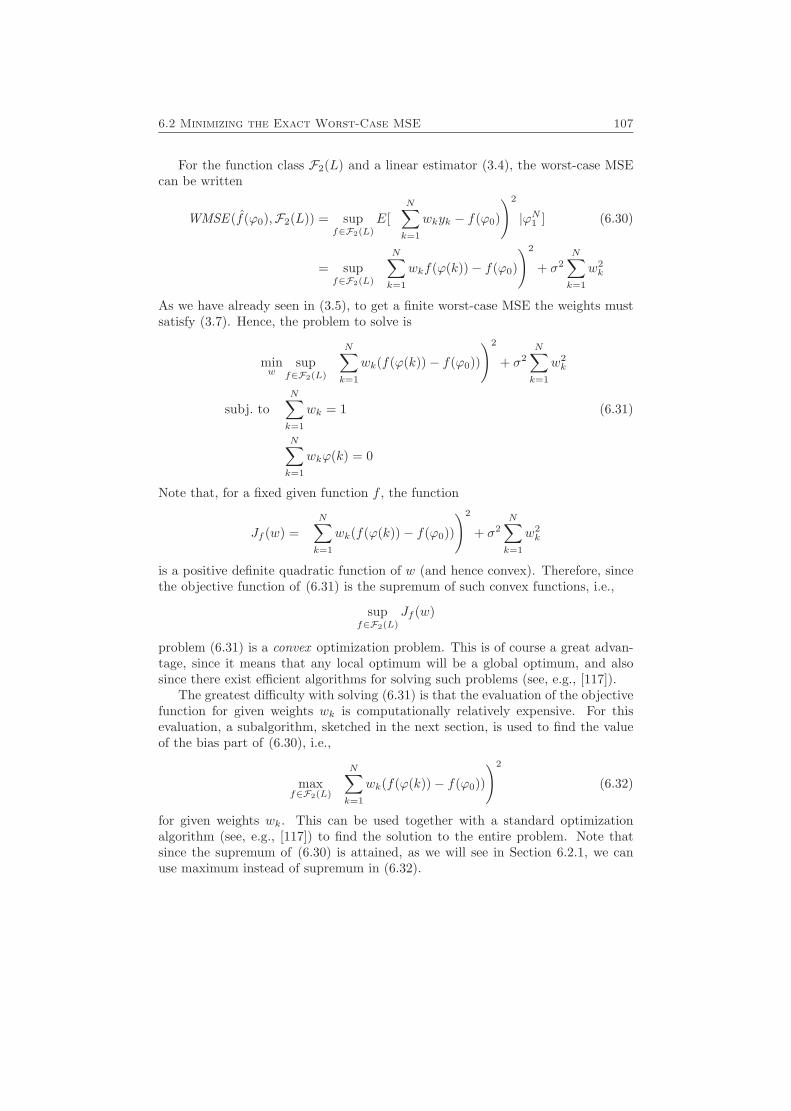
6.2 Minimizing the Exact Worst-Case MSE 107
For the function class F2(L) and a linear estimator (3.4), the worst-case MSEcan be written
WMSE (f(ϕ0),F2(L)) = supf∈F2(L)
E[
(N∑k=1
wkyk − f(ϕ0)
)2
|ϕN1 ] (6.30)
= supf∈F2(L)
(N∑k=1
wkf(ϕ(k))− f(ϕ0)
)2
+ σ2N∑k=1
w2k
As we have already seen in (3.5), to get a finite worst-case MSE the weights mustsatisfy (3.7). Hence, the problem to solve is
minw
supf∈F2(L)
(N∑k=1
wk(f(ϕ(k))− f(ϕ0))
)2
+ σ2N∑k=1
w2k
subj. toN∑k=1
wk = 1 (6.31)
N∑k=1
wkϕ(k) = 0
Note that, for a fixed given function f , the function
Jf (w) =
(N∑k=1
wk(f(ϕ(k))− f(ϕ0))
)2
+ σ2N∑k=1
w2k
is a positive definite quadratic function of w (and hence convex). Therefore, sincethe objective function of (6.31) is the supremum of such convex functions, i.e.,
supf∈F2(L)
Jf (w)
problem (6.31) is a convex optimization problem. This is of course a great advan-tage, since it means that any local optimum will be a global optimum, and alsosince there exist efficient algorithms for solving such problems (see, e.g., [117]).
The greatest difficulty with solving (6.31) is that the evaluation of the objectivefunction for given weights wk is computationally relatively expensive. For thisevaluation, a subalgorithm, sketched in the next section, is used to find the valueof the bias part of (6.30), i.e.,
maxf∈F2(L)
(N∑k=1
wk(f(ϕ(k))− f(ϕ0))
)2
(6.32)
for given weights wk. This can be used together with a standard optimizationalgorithm (see, e.g., [117]) to find the solution to the entire problem. Note thatsince the supremum of (6.30) is attained, as we will see in Section 6.2.1, we canuse maximum instead of supremum in (6.32).
108 Other Extensions
6.2.1 Maximizing the MSE for Given Weights
Instead of solving (6.32), we can try to find a function that maximizes the bias,i.e.,
fmax ∈ argmaxf∈F2(L)
N∑k=1
wk(f(ϕ(k))− f(ϕ0)) (6.33)
This function will then also maximize the MSE. Note that fmax by no means isunique (as we will see below, we can for instance find functions with any functionvalue and derivative at ϕ0, which will maximize the bias). In some texts, thenotation Argmax is used instead of argmax to show that the result is a set ofarguments, instead of a single argument. Note also that we equally well could haveused argmin instead of argmax in (6.33), since −fmax would minimize the bias,and what we are really interested in is the squared bias (6.32).
To find the value of (6.33), we first note that every function in F2(L) can bewritten as
f(ϕ) = f(ϕ0) + f ′(ϕ0)ϕ+ f0(ϕ)
where f0 ∈ F2(L), f0(ϕ0) = f ′0(ϕ0) = 0. This gives us
N∑k=1
wk(f(ϕ(k))− f(ϕ0)) = f ′(ϕ0)N∑k=1
wkϕ(k) +N∑k=1
wkf0(ϕ) =N∑k=1
wkf0(ϕ)
which means that we, without restrictions, can assume that f(ϕ0) = f ′(ϕ0) = 0.Secondly, we can assume that the maximal value of (6.33) is obtained for a piece-
wise quadratic function with a finite number of breakpoints, and with |f ′′(ϕ)| = L(where the second derivative exists). The reason for this is that the only interestingvalues of the function are f(ϕ(k)) and f ′(ϕ(k)) for each data point, and it is quiteeasy to show that for a given set of admissible values for f(ϕ(k)) and f ′(ϕ(k)),there is a piecewise quadratic function with |f ′′(ϕ)| = L (and a finite number ofbreakpoints) such that these values are obtained.
Hence we can parameterize f as follows:
f(ϕ) = ±L
ϕ2
2+
p+∑j=1
(−1)j max{ϕ− b+j , 0}2 +p−∑j=1
(−1)j max{b−j − ϕ, 0}2
where b−p− < · · · < b−1 < 0 ≤ b+1 < · · · < b+p+ are the breakpoints. Now we candifferentiate the bias with respect to the breakpoints:
∂
∂b+j
N∑k=1
wkf(ϕ(k)) = ±2L(−1)j+1N∑k=1
wk max{ϕ(k)− b+j , 0}
∂
∂b−j
N∑k=1
wkf(ϕ(k)) = ±2L(−1)jN∑k=1
wk max{b−j − ϕ(k), 0}
6.2 Minimizing the Exact Worst-Case MSE 109
−2 −1 0 1 2−0.02
0
0.02
0.04
0.06
0.08
0.1
0.12
0.14
φ
(a) Interior point, ϕ0 = 0.
−2 −1 0 1 2−0.2
0
0.2
0.4
0.6
0.8
φ
(b) Boundary point, ϕ0 = −2.
Figure 6.1: Optimal weights with respect to the exact worst-case MSE (∗) and weightscomputed with the DWO approach (·), for two different values of ϕ0.
Note that each derivative is a (piecewise affine) function of only one variable,namely the variable with respect to which the bias was differentiated. This meansthat we only have to consider the function
g+(b) =N∑k=1
wk max{ϕ(k)− b, 0}
and its zeros and sign changes to find the locations of the positive breakpoints,and a corresponding function g−(b) to find the negative breakpoints. The detailsof this are theoretically quite simple, although a bit tricky to implement, partlysince it is difficult to know how many breakpoints are needed. It is easy to see,though, that at most N breakpoints are needed, since the derivative is piecewiseaffine and can have at most one zero in each interval between two consecutive datapoints ϕ(k). Further investigations show that the number of breakpoints neededare at most the number of sign changes of wk.
6.2.2 Properties of the Exact Worst-Case MSE Solution
We illustrate the properties of the resulting weights by an example.
Example 6.1 Let us consider the case with N = 50 data samples, where ϕ(k) aretaken from a uniform distribution on the interval [−2, 2]. Let L/σ = 5. Figure 6.1shows both the weights minimizing the worst-case MSE and the weights from theDWO approach (3.11) for two different values of ϕ0, namely ϕ0 = 0 (which isan interior point) and ϕ0 = −2 (a boundary point). The weights minimizing theworst-case MSE were computed using the Matlab function fmincon.
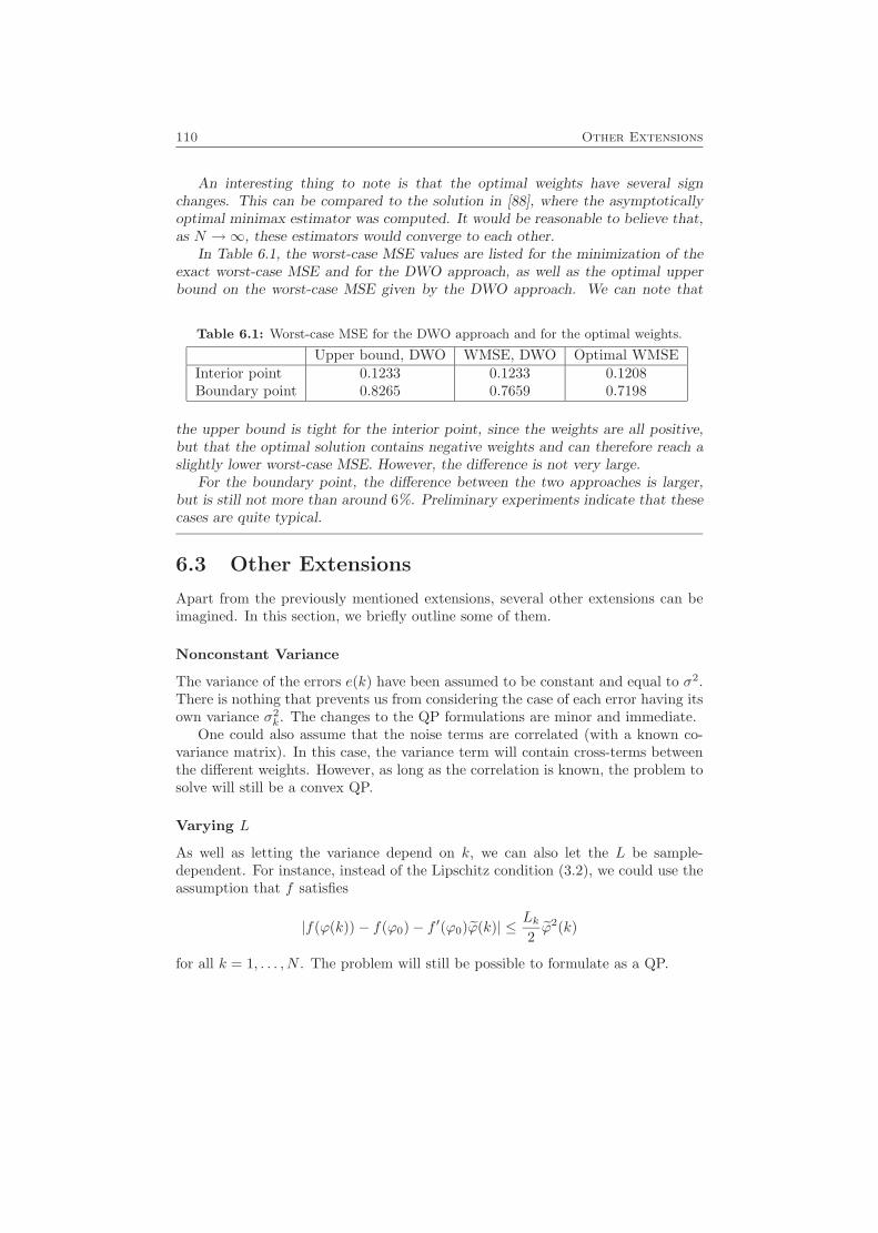
110 Other Extensions
An interesting thing to note is that the optimal weights have several signchanges. This can be compared to the solution in [88], where the asymptoticallyoptimal minimax estimator was computed. It would be reasonable to believe that,as N →∞, these estimators would converge to each other.
In Table 6.1, the worst-case MSE values are listed for the minimization of theexact worst-case MSE and for the DWO approach, as well as the optimal upperbound on the worst-case MSE given by the DWO approach. We can note that
Table 6.1: Worst-case MSE for the DWO approach and for the optimal weights.
Upper bound, DWO WMSE, DWO Optimal WMSEInterior point 0.1233 0.1233 0.1208Boundary point 0.8265 0.7659 0.7198
the upper bound is tight for the interior point, since the weights are all positive,but that the optimal solution contains negative weights and can therefore reach aslightly lower worst-case MSE. However, the difference is not very large.
For the boundary point, the difference between the two approaches is larger,but is still not more than around 6%. Preliminary experiments indicate that thesecases are quite typical.
6.3 Other Extensions
Apart from the previously mentioned extensions, several other extensions can beimagined. In this section, we briefly outline some of them.
Nonconstant Variance
The variance of the errors e(k) have been assumed to be constant and equal to σ2.There is nothing that prevents us from considering the case of each error having itsown variance σ2
k. The changes to the QP formulations are minor and immediate.One could also assume that the noise terms are correlated (with a known co-
variance matrix). In this case, the variance term will contain cross-terms betweenthe different weights. However, as long as the correlation is known, the problem tosolve will still be a convex QP.
Varying L
As well as letting the variance depend on k, we can also let the L be sample-dependent. For instance, instead of the Lipschitz condition (3.2), we could use theassumption that f satisfies
|f(ϕ(k))− f(ϕ0)− f ′(ϕ0)ϕ(k)| ≤ Lk2ϕ2(k)
for all k = 1, . . . , N . The problem will still be possible to formulate as a QP.

6.3 Other Extensions 111
A special case of varying L is to consider a modified version of class Gp+1(L),which is obtained if the Lipschitz condition (4.1) is replaced by∣∣∣∣∣∣f(ϕ)− f(ϕ0)−
n∑i1=1
f ′i1(ϕ)ϕi1 − . . .−1p!
n∑i1=1
. . .
n∑ip=1
f(p)i1...ip
(ϕ)ϕi1 . . . ϕip
∣∣∣∣∣∣≤ 1
(p+ 1)!‖Qϕ‖p+1
where Q ∈ Rn×n is a quadratic matrix. This means that the upper bound dependson in what direction we are looking.
More General Function Classes
Following the presentation in [138], we can consider an extension of the functionclass Gp+1(L), specified by∣∣∣∣∣f(ϕ0)−
p∑k=0
akfk(ϕ)
∣∣∣∣∣ ≤M(ϕ)
where fk and M are given functions. Letting fk(ϕ) = ϕk and M(x) = M |ϕ|p+1
brings us back to the definition (2.9) of Gp+1(L). The changes to the problemformulations will be straightforward.

112 Other Extensions
7
Conclusions
In this part of the thesis, a direct weight optimization approach to the functionestimation problem has been proposed and studied. As have been pointed out, theapproach has a number of interesting features, including the following:
• The problem is phrased without any reference to bandwidth. The formulationoffers the possibility to use all observations. The weights resulting from theDWO approach however show that there is a bandwidth feature even for afinite number of measurements: Observations outside a certain band carryweights that are exactly zero.
• Although the DWO approach does not give strictly better estimates (in theMSE sense) than, say, the local polynomial approach in all cases, the impor-tant point is that the delivered guaranteed MSE bound is better than whatother approaches can offer. In practice, it is of course only this guaranteedbound that can be used for confidence intervals etc., since the actual MSEdepends on the unknown function.
• The improvement over asymptotically optimal estimates is more pronounced(naturally enough) for fewer data, and more nonuniformly spread observationpoints ϕ(k). For applications to higher regressor dimensions and dynamicalsystems, this is a very valuable property.
113

114 Conclusions
• The approach is easily extended to the case when a priori bounds on thefunction and its derivative are known, and improvements can be made bymaking use of this information. Theorems 5.2 and 5.4 however showed thatwhen the bounds are very wide, the extra information may not be enough toimprove the solution.
• For the class of affine functions (L = 0), the solution equals the one obtainedby globally fitting an affine model to the data using the least-squares criterion,as should be expected.
• Asymptotically, for univariate functions and equally spaced design, and whenminimizing the worst-case MSE over G2(L) (or, equivalently, the upper bound(3.9) on the worst-case MSE over F2(L)), we obtain the weights of the locallinear estimator using an asymptotically optimal Epanechnikov kernel. It isconjectured that these results could be extended also to more general designsand other degrees of differentiability. Furthermore, it is conjectured that min-imizing the exact worst-case MSE over Fp+1(L), as was done in Section 6.2,asymptotically leads to the optimal kernels given by [88] under appropriatedesign assumptions.
Local modelling has found a wide range of applications, like for instance robotcontrol, computer graphics, fermentation processes, econometrics, etc. A goodsurvey is given in [5]. In all these domains, the DWO might naturally be analternative.
In Section 4.3, some examples were given on how local modelling in general,and the DWO approach in particular, can be used in connection with system iden-tification and prediction of dynamic systems. The idea of storing old data froma dynamic system in a database, and only retrieve the data needed each time aprediction is to be formed, has been called a Model On Demand (MOD) approach,and is considered in [146]. As described there, the predictions can be used, e.g.,for model predictive control (MPC). An early contribution employing similar ideasis [7], where a simple MOD-like method is used to control robots. “Experiences”are stored in a database, and when predictions are to be made, the database issearched for similar situations. Related ideas can also be found, e.g., in [17].
In addition, frequency domain applications are given in [146], such as automaticsmoothing of periodograms and empirical transfer function estimates (ETFE) [94].
This part of the thesis has been focused on the main ideas of the DWO approach,and a number of properties have been pointed out and shown. Still, however, thereare a number of questions that need to be discussed. One such question is whathappens when there is a correlation between the noise and regression variables,when using the approach for dynamic systems. Another issue is how to find ap-propriate values of the design parameters, such as the structure of ϕ and the ratioL/σ. These problems will now be considered.
7.1 Using the DWO Approach for Dynamic Systems 115
7.1 Using the DWO Approach for Dynamic Sys-tems
As pointed out in Chapter 2, many of the local modelling approaches, including theDWO approach, assume that the regression vectors ϕ(i) and noise contributionse(i) are independent. However, when the data come from a dynamic system, suchthat ϕ(i) will contain old values y(j), j < i, this independence will not hold. Thequestion is whether or not the DWO approach can be used for dynamic systemsanyway. A simple answer is yes: instead of considering the minimization of (3.11)as minimizing the upper bound on the worst-case MSE, it can be viewed as areasonable heuristic criterion to minimize. As could be seen in Examples 4.1 and4.2, it can also work well in practice.
Let us have a closer look at the problem. For simplicity we consider the functionclass Fp+1(L). Suppose that the regression vector ϕ(k) contains y(k − 1). Thiswould mean that if ϕ(k), k = 1, . . . , N are given, then also the correspondingy(k − 1) are given. Hence, the MSE becomes
MSE (f(ϕ0)) = E[(f(ϕ0)− f(ϕ0))2|ϕN1 ]
= E[
(N∑k=1
wky(k)− f(ϕ0)
)2
|ϕN1 ]
= E[
(N−1∑k=1
wky(k) + wNf(ϕ(N))− f(ϕ0) + wNeN
)2
|ϕN1 ] (7.1)
=
(N−1∑k=1
wky(k) + wNf(ϕ(N))− f(ϕ0)
)2
+ σ2w2N
=
(N∑k=1
wkf(ϕ(k))− f(ϕ0) +N−1∑k=1
wk(y(k)− f(ϕ(k))
))2
+ σ2w2N
=
(N∑k=1
wkf(ϕ(k))− f(ϕ0)
)2
+ 2
(N∑k=1
wkf(ϕ(k))− f(ϕ0)
)(N−1∑k=1
wk(y(k)− f(ϕ(k))
))
+ 2N−2∑k=1
N−1∑j=k+1
wkwj(y(k)− f(ϕ(k))
)(y(j)− f(ϕ(j))
)+N−1∑k=1
w2k
(y(k)− f(ϕ(k))
)2 + σ2w2N
Since f is unknown, there is generally no way to evaluate this expression, and wecannot get an upper bound either. However, for large N , the second and third
116 Conclusions
terms of the last expression should generally be much smaller than the squaredterms, since y(k) − f(ϕ(k)) = e(k) is the noise contribution, which is averaged inthese sums. Furthermore, the fourth and fifth terms should be well approximatedby the variance term (2.35). Hence, it seems reasonable to approximate the secondand third terms in this expression by 0, and the fourth term by
σ2N−1∑k=1
w2k
and we are back to the MSE expression (2.33) together with (2.34) and (2.35). Theonly difference is that this is not the true MSE anymore, but an approximation.
One should also note that, as N →∞, the weights from the DWO approach willbe nonzero only in a very small neighborhood of ϕ0. For most reasonable dynamicsystems, unless ϕ is an equilibrium point, this means that the regression vectorscorresponding to the nonzero weights will have very different indices k, and so theywill in general only be weakly correlated. This means that the approximation ofthe worst-case MSE used by the DWO approach will be asymptotically correct.
7.2 Adaptive Bandwidth Selection
Throughout the presentation of the DWO approach, the ratio L/σ has been as-sumed to be known. However, in practice this is often not the case∗. Instead,the ratio would have to be estimated. One option is to use the methods known asclassical methods (e.g., cross-validation techniques), described in Section 2.4.3. If aglobal estimate is desired, the adaptation of these methods to the DWO approachis immediate. However, in many applications a local estimate of the ratio would beto prefer. In this case, an appealing alternative is to take the view of Section 3.2.4,i.e., to regard the DWO weights as coming from a local polynomial model, wherethe least-squares problem (2.23) is weighted by the matrix G−1 from (3.35) insteadof Kh. Using this view, it is now straightforward to extend the localized adaptivebandwidth selection procedures as described in Section 2.4.3 (and in more detail in[146]) to the DWO approach, where, e.g., the sum
∑Nk=1 wk is replaced by tr(G−1).
For instance, the localized cross-validation criterion (2.57) would take the form
LCV (f(ϕ0)) , (Y1:n − F1:n)TG−1(Y1:n − F1:n)tr(G−1)
(7.2)
∗Note however, that as long as the true function belongs to the function class Fp+1(L0) forany L0, and the noise variance is σ0, we could get an upper bound on the worst-case MSE bysolving (3.10) with any L > L0 and σ > σ0. Hence, any ratio L/σ will correspond to an upperbound on the worst-case MSE. However, it will certainly not be the best bound in general.
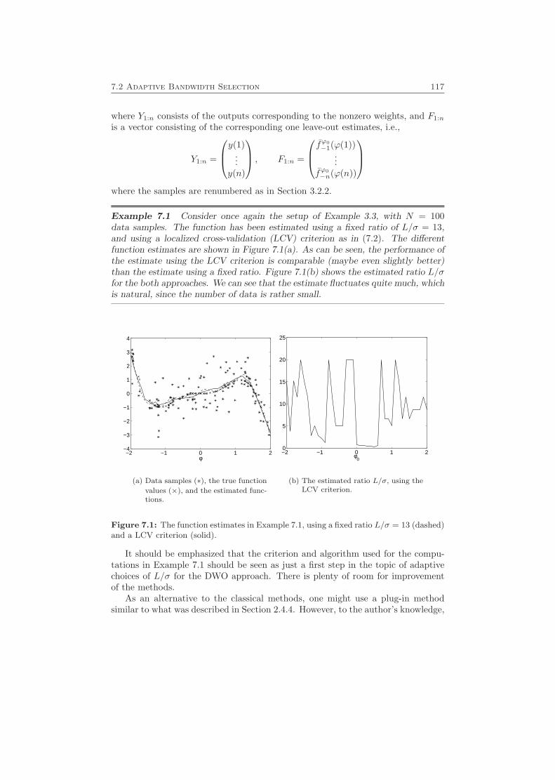
7.2 Adaptive Bandwidth Selection 117
where Y1:n consists of the outputs corresponding to the nonzero weights, and F1:n
is a vector consisting of the corresponding one leave-out estimates, i.e.,
Y1:n =
y(1)...
y(n)
, F1:n =
fϕ0−1(ϕ(1))
...fϕ0−n(ϕ(n))
where the samples are renumbered as in Section 3.2.2.
Example 7.1 Consider once again the setup of Example 3.3, with N = 100data samples. The function has been estimated using a fixed ratio of L/σ = 13,and using a localized cross-validation (LCV) criterion as in (7.2). The differentfunction estimates are shown in Figure 7.1(a). As can be seen, the performance ofthe estimate using the LCV criterion is comparable (maybe even slightly better)than the estimate using a fixed ratio. Figure 7.1(b) shows the estimated ratio L/σfor the both approaches. We can see that the estimate fluctuates quite much, whichis natural, since the number of data is rather small.
−2 −1 0 1 2−4
−3
−2
−1
0
1
2
3
4
φ
(a) Data samples (∗), the true function
values (×), and the estimated func-tions.
−2 −1 0 1 20
5
10
15
20
25
φ0
(b) The estimated ratio L/σ, using theLCV criterion.
Figure 7.1: The function estimates in Example 7.1, using a fixed ratio L/σ = 13 (dashed)and a LCV criterion (solid).
It should be emphasized that the criterion and algorithm used for the compu-tations in Example 7.1 should be seen as just a first step in the topic of adaptivechoices of L/σ for the DWO approach. There is plenty of room for improvementof the methods.
As an alternative to the classical methods, one might use a plug-in methodsimilar to what was described in Section 2.4.4. However, to the author’s knowledge,
118 Conclusions
not much has been done to estimate a Lipschitz constant as the one used in theDWO approach. The main focus of the plug-in approaches has been to approximatethe MSE, rather than the worst-case MSE. Thus, much can still be done in orderto find a reliable estimate of L/σ, which is also easy to compute.
7.3 Structure of the Regression Vector
We have assumed that the correct choice of elements for the regression vectors isknown. This choice is a structure problem which is common to most approaches insystem identification, and there has been a great deal of research within this area.One example is [126], where a method using false nearest neighbors was proposedfor dynamic systems. This technique builds on the philosophy that has been atheme of this part, namely that outputs corresponding to regression vectors closeto each other should be similar (i.e., that the true underlying regression functionis smooth). However, if the regression vector is chosen to be too small, two similarregression vectors may correspond to very different output data, since the regressionvariables that are not included in the chosen regression vector may have a significanteffect on the output. These regression vectors are then false neighbors, i.e., theyare neighbors in the chosen (too small) regressor space, but are far from each otherin the true regressor space. In this way, if several false neighbors are found, onecan deduce that the chosen regressor space is too small.
A recent contribution in the area of regressor selection is [92], where ANOVA(ANalysis Of VAriance) is used to determine a good regression vector.
7.4 Algorithmic and Implementation Issues
There are many aspects on how to find the solution, e.g., of (3.10). In the earlypaper [138], a Newton-like algorithm (very similar to the hinge-finding algorithmin [22], described in Section 10.1.2) is proposed. However, nothing is shown aboutconvergence.
The field of convex optimization has developed rapidly during the last decade,and there exist efficient algorithms that can solve a large variety of problems,including large-scale convex QP and SOCP problems. For a good introduction,see [19]. However, for the specific problems presented in this part of the thesis,we can use the knowledge of the automatic finite bandwidth property (describedin Section 3.2.1) to make the computations even faster, according to what wassuggested in the discussion after Corollary 3.1. If we would be able to guess whichof the weights that should be nonzero, only these data points need to be taken intoaccount, which leads to a much smaller QP to be solved. The solution can thenbe easily checked, by investigating if all the excluded data samples lie in the areaswhere the weight function is zero. This is the case if all excluded data samplessatisfy the middle case of (3.13), i.e., if
−gϕ2(k) ≤ µ1 + µ2ϕ(k) ≤ gϕ2(k)
7.4 Algorithmic and Implementation Issues 119
If this requirement is satisfied for all excluded data, the solution is globally optimal.Otherwise, we can include the data that do not satisfy the requirement and solvethe new QP we get.
The main question that arises is how to find an initial guess of which weightsshould be nonzero. One immediate option would be to use the asymptoticallyoptimal bandwidths (2.41) or (2.43) (or their multivariate counterparts). It turnsout that a slight overestimation of these bandwidths is a better choice, since takingsome too many data samples into consideration is to prefer before considering toofew, and instead having to solve two QP:s.
A problem with this approach is that the design density has to be known.Furthermore, with sparsely and unevenly spread data samples (which is often thecase particularly for higher dimensions) there is a risk that too few data samplesfalls within the guessed bandwidth. An alternative is therefore to use a k-nearestneighbor approach to find an initial guess of the set of nonzero weights. k shouldbe chosen to be at least larger than the dimension, i.e., k > n, in order not to getan underdetermined problem.
If the guess of the set of nonzero weights was wrong, one way of choosing a newset would be to consider all data samples falling into the area where the computedweight function is nonzero. Another alternative is to simply increase the guessedbandwidth by a factor α > 1.
Preliminary experiments, using a 2n-nearest neighbor approach to get an initialguess of which weights should be nonzero, have shown that the computationalspeed can be considerably improved compared to solving one large QP. However,much can probably be done to further improve the algorithms, and to use thestructure of the problem in a more refined way. This is of particular importanceif using adaptive bandwidth selection, which makes the computational complexitysignificantly larger.
The problem of finding and retrieving relevant data samples from a databaseof samples is another relevant issue. For an overview of this, see, e.g., [5, 146].

120 Conclusions

Part II
Identification of PiecewiseAffine Systems
121

8
Prediction Error Methods for
System Identification
When linear models are not sufficient for accurately describing the dynamics ofa system, there are several different possible approaches to choose between. InPart I, a nonlinear model was built “on the fly”, by locally estimating the systemdynamics for each time point. In this part a parametric identification approachis considered, namely using piecewise affine (PWA) models. This might be anattractive alternative, both when the real system actually is piecewise affine, butalso sometimes for a general nonlinear system.
This chapter briefly describes a few general issues concerning prediction er-ror methods, which is a commonly used family of parametric system identificationmethods. Chapter 9 then introduces different classes of piecewise affine systems,while Chapters 10 and 11 are devoted to the identification of piecewise affine sys-tems.
8.1 Prediction Error Methods
Let us first once again formulate the system identification problem. We assumethat we are given a set of inputs, u(t), and outputs, y(t), t = 1, . . . , N , comingfrom a real (physical) system of some structure. The structure considered here isthe form given in (1.6), i.e.,
y(t) = f(Zt−1−∞) + e(t) (8.1)
123
124 Prediction Error Methods for System Identification
where E[e(t)] = 0 and e(t) is independent of Zt−1−∞. Using the given set of data,
we would like to find a model that describes the true system as well as possible insome sense.
As already mentioned, the prediction error methods are parametric methods,which means that we search for the best model within a family of models, parame-terized by a set of parameters collected in a parameter vector θ. In our context, thismeans that we only consider a parameterized family of functions f(Zt−1
1 , θ) witha certain structure. The system identification problem then reduces to finding theparameter values θ∗ that fit the model to the experimental data as well as possible.In the prediction error methods, this is done by considering the predicted output
y(t|θ) = f(Zt−11 , θ)
and the residualε(t, θ) = y(t)− y(t|θ)
Here, y(t|θ) is our guess of the value of y(t), given the information Zt−11 . Since e(t)
is independent of Zt−11 , the best guess we can obtain is what we get by replacing
e(t) in (8.1) by its expected value, which is 0. The residual ε(t, θ) can be seen as ameasure of how close the guess was.
Then the model is fitted to the data by minimizing a criterion function
V (θ, ZN1 ) =1N
N∑t=1
`(ε(t, θ)) (8.2)
that is,θ = argmin
θV (θ, ZN1 )
There are many possible choices for the function `(ε). A very common choice is
`2(ε) = ε2
which gives the least squares criterion. We have already seen an example of usingthe least squares criterion in Example 1.3.
It can be noted, that given that the true system belongs to the parameterizedmodel class, and given that e(t) are independent with the probability distribu-tion function fe(x), the θ(vj) that minimizes (8.2) will be the maximum likelihoodestimate if
`(ε) = − log fe(ε)
(see [94]). From this it follows, e.g., that `2 corresponds to the maximum likelihoodestimator for a system where e(t) has a Gaussian distribution with known variance.
8.2 Numerical Minimization
In Example 1.3, it was possible to minimize V (θ, ZN1 ) analytically. In general, how-ever, V (θ, ZN1 ) can be a (possibly nonconvex) function which has to be minimized
8.2 Numerical Minimization 125
using numerical algorithms. Some of the most important numerical algorithms arethe Newton and quasi-Newton algorithms [117]. These are iterative algorithms,that update the estimate of argminθ V (θ) according to
θ(i+1) = θ(i) − α(i)(R(θ(i))
)−1
∇V (θ(i)) (8.3)
where ∇V (θ(i)) is the gradient of V (θ) evaluated in θ(i). The role played by R(θ(i))will soon be explained. α(i) is a scalar that determines the step size of the update,i.e., how much the estimate θ(i) should change in each iteration.
If V (θ) is a positive definite quadratic function of θ,
V (θ) =12
(θ − θmin)TP (θ − θmin)
we could get right to the minimum in one step using α(0) = 1 and R(θ) = ∇2V (θ)(the Hessian of V ), since
θ(1) = θ(0) −(∇2V (θ(0))
)−1
∇V (θ(0)) = θ(0) − P−1P (θ(0) − θmin) = θmin
If V (θ) is not quadratic, we can use the Taylor expansion to approximate it with aquadratic function. However, since the approximation may be good only in a smallregion around θ(i), we might need to adjust the value of α(i) to ensure that V (θ(i))will actually decrease for increasing i. Methods where α(i) 6= 1 are sometimes calleddamped.
The Newton algorithms use R(θ) = ∇2V (θ), as described above. However, itmight be time-consuming to compute the Hessian∇2V (θ(i)) in each step, comparedto computing only the gradient. Moreover, the Hessian is not necessarily positivedefinite when being far away from local minima. An alternative is therefore to usequasi-Newton algorithms, such as Gauss-Newton, that instead form an estimate of∇2V (θ), and use that in (8.3). The estimates can be constructed in such a way thatthey are always positive semidefinite, which can be used to guarantee convergenceto a stationary point. For more details about numerical minimization algorithms,see, e.g., [94, 117].
Using numerical minimization algorithms like the ones described above meansthat there is a risk of getting stuck in local minima. One way of getting around thisproblem is to try different initial values for the algorithm. In this way we might atleast find several local minima, from which we can choose the one with the lowestvalue of V (θ, ZN1 ). In the presence of noise and model errors, it also might not beabsolutely necessary to find the global minimum, since we do not know if it givesthe correct description of the system anyway. Nevertheless, we would like to finda good model, that gives a low value for V (θ, ZN1 ), so the question arises: How dowe find a good solution (or an initial value that leads to a good local minimum)?This question will be treated for piecewise affine systems in Chapters 10 and 11.

126 Prediction Error Methods for System Identification
8.3 Regularization
In the Newton and quasi-Newton algorithms, the update equation (8.3) containsthe inverse (R(θ(i)))−1. Sometimes R(θ) may be ill-conditioned or even singular.To make it better conditioned, a term λI can be added to R(θ). This is knownas regularization. One can also add a term λ‖θ − θ#‖2 to the criterion functionV (θ, ZN1 ) in (8.2), which will also have the effect of adding 2λI to ∇2V (θ, ZN1 ).This can be interpreted as providing a guess θ# of the value of θ, and trying tokeep θ close to the guess. The coefficient λ can be used to weigh the importanceof staying close to θ# against minimizing the prediction error.
9
Piecewise Affine Systems
Piecewise affine systems are an important class of nonlinear systems, which inrecent years have been subject to considerable research, due to their close relationto hybrid systems. In this chapter, some different classes and different descriptionsof piecewise affine systems will be presented. For notational simplicity, we considernoiseless models. The noise will later be included as an additive term, as in (1.6).
9.1 Continuous Time Models
A general continuous time piecewise affine system could be described by
x = A(v)x+B(v)u+ b(v)y = C(v)x+D(v)u+ d(v)
(9.1)
where x is our state vector, u is the input to the system, and y is the systemoutput. The vector v is a key vector, describing in what mode (i.e., in what affinesubsystem) the system is for the time being. v can be a function of x, t, u, or someother external input. We assume that v can only take a finite number of differentvalues.
The systems described by (9.1) include systems which are not always calledpiecewise affine systems. A common restriction (see for example [72]) is that v only
127
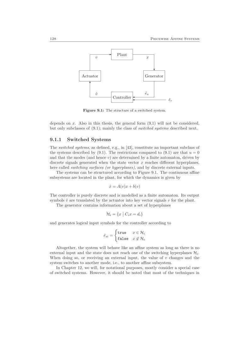
128 Piecewise Affine Systems
?
�
6
-
�
Generator
Plant
Controller
Actuator
v x
esv
er
Figure 9.1: The structure of a switched system.
depends on x. Also in this thesis, the general form (9.1) will not be considered,but only subclasses of (9.1); mainly the class of switched systems described next.
9.1.1 Switched Systems
The switched systems, as defined, e.g., in [43], constitute an important subclass ofthe systems described by (9.1). The restrictions compared to (9.1) are that u = 0and that the modes (and hence v) are determined by a finite automaton, driven bydiscrete signals generated when the state vector x reaches different hyperplanes,here called switching surfaces (or hyperplanes), and by discrete external inputs.
The systems can be structured according to Figure 9.1. The continuous affinesubsystems are located in the plant, for which the dynamics is given by
x = A(v)x+ b(v)
The controller is purely discrete and is modelled as a finite automaton. Its outputsymbols v are translated by the actuator into key vector signals v for the plant.
The generator contains information about a set of hyperplanes
Hi = {x∣∣ Cix = di}
and generates logical input symbols for the controller according to
esi =
{true x ∈ Hifalse x 6∈ Hi
Altogether, the system will behave like an affine system as long as there is noexternal input and the state does not reach one of the switching hyperplanes Hi.When doing so, or receiving an external input, the value of v changes and thesystem switches to another mode, i.e., to another affine subsystem.
In Chapter 12, we will, for notational purposes, mostly consider a special caseof switched systems. However, it should be noted that most of the techniques in
9.2 Discrete Time Models 129
Chapter 12 can be applied to the more general kind of switched systems describedabove. The systems considered will be in the form
x = A(v)x+ b(v) , x ∈ X(v) , v ∈ {−1, 0, 1}M (9.2)
where the state-space is partitioned into different regions X(v) by M hyperplanes.The key vector v is a function of x, and has one element for each separatinghyperplane. The elements of v are 1 or −1, depending on on which side of thehyperplanes x is situated, or 0 if x lies in a hyperplane. In this way, v has a one-to-one relationship to X(v). This also implies that the dynamics of a trajectory x(t)just depends on x, not on t or on any external input. The different regions X(v)will be polyhedra (see Section A.3).
9.2 Discrete Time Models
The descriptions in Section 9.1 are continuous time models. It is also common touse discrete time models for the piecewise affine systems. A general form could be
x(t+ 1) = A(v)x(t) +B(v)u(t) + b(v)y(t) = C(v)x(t) +D(v)u(t) + d(v)
(9.3)
Other notable model structures for discrete time piecewise affine systems includeMLD (Mixed Logical Dynamical) models [12], MMPS (Max-Min-Plus-Scaling) mod-els, LC (Linear Complementary) models, and ELC (Extended Linear Complemen-tary) models [62]. Essentially, these classes are the same as (9.3), where v is apiecewise constant function of x and u, and is constant over polyhedra in the com-bined state-space and input space (this is shown in [9] (for MLD), [62] (all classes)).
9.2.1 Models in Regression Form
In Chapters 10 and 11, we will use models in regression form, i.e.,
y(t) = ϕT (t)θ(v) (9.4)
where the key vector v only can take a finite number of values, and θ(v) is a functionof v. The vector ϕ is our regression vector, which could for instance consist of oldinputs and outputs, e.g.,
ϕ(t) =(1 −y(t− 1) . . . −y(t− na) u(t− 1) . . . u(t− nb)
)T (9.5)
Here we have included a constant 1 in the regression vector, to be able to expresspiecewise affine systems in the form (9.4). If we would not include the constant,(9.4) would be a piecewise linear system. Throughout this thesis, whenever weare dealing with piecewise affine systems in regression form, we will assume thatthe first element of ϕ(t) equals 1. We will also assume that the key vector v is
130 Piecewise Affine Systems
uniquely determined by the regression vector ϕ(t), and that the regions of the dif-ferent affine subsystems are polyhedral. When including additive white noise in themodel (see Section 1.1.3), this kind of systems has been called PWARX (PieceWiseAutoRegressive eXogenous) systems [13, 48]. These systems are a subclass of thesystems described by (9.3), and can easily be transformed into that form by usingthe elements of ϕ(t) (except the constant) as state variables.
However, there are also many other possible choices of ϕ. In general, ϕ(t) couldbe any function of u and y, i.e.,
ϕ(t) =(f1(Zt−1
1 ) . . . fn(Zt−11 )
)TIn this case, a system in the form (9.4) could be called a PWNARX (PieceWiseNonlinear AutoRegressive eXogenous) system. This is of course not a piecewiseaffine system in general, but as we will see, most of the theory in Chapter 11 alsoapplies to systems with this choice of ϕ(t).
Just as in Part I, we assume that the form of the regression vectors is given, i.e.,that we know which kind of data is relevant to predict y(t). We refer to [92, 126]for ideas about how to determine this.
9.2.2 Chua’s Canonical Representation and Hinging Hyper-plane Models
A special class of piecewise affine functions are the functions that can be representedby the canonical representation introduced by Chua and Kang [28, 80]:
y(t) = αT0 ϕ(t) +M∑i=1
ci|αTi ϕ(t)| (9.6)
where ϕ(t) is given from (9.5). As can be seen, the functions described by Chua’scanonical representation are continuous in ϕ(t). It turns out (see [28]) that ev-ery scalar, continuous, piecewise affine function of one variable can be uniquelyexpressed in this form with αi2 = 1 (where αi2 is the second element of αi), i.e., as
y(t) = α01 + α02x(t) +M∑i=1
ci|αi1 + x(t)|
(here we let ϕ(t) =(1 x(t)
)T ). However, not every multivariate, continuous,piecewise affine function can be expressed on the canonical representation (seeExample 9.2). A necessary condition for this is that the regions of the differentaffine subsystems must be separated by hyperplanes. In [27], a necessary andsufficient condition for a function to be expressible in the canonical form is given.There are also other canonical representations covering larger classes of systems.One of them is Guzelis’ model class [59], where two nested absolute values areallowed:
y(t) = αT0 ϕ(t) +M∑i=1
bi|αTi ϕ(t)|+K∑j=1
cj
∣∣∣∣∣γTj ϕ(t) +M∑i=1
dij |αTi ϕ(t)|∣∣∣∣∣ (9.7)
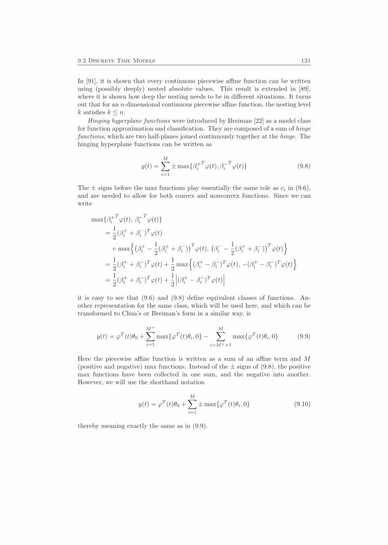
9.2 Discrete Time Models 131
In [91], it is shown that every continuous piecewise affine function can be writtenusing (possibly deeply) nested absolute values. This result is extended in [89],where it is shown how deep the nesting needs to be in different situations. It turnsout that for an n-dimensional continuous piecewise affine function, the nesting levelk satisfies k ≤ n.
Hinging hyperplane functions were introduced by Breiman [22] as a model classfor function approximation and classification. They are composed of a sum of hingefunctions, which are two half-planes joined continuously together at the hinge. Thehinging hyperplane functions can be written as
y(t) =M∑i=1
±max{β+i
Tϕ(t), β−i
Tϕ(t)} (9.8)
The ± signs before the max functions play essentially the same role as ci in (9.6),and are needed to allow for both convex and nonconvex functions. Since we canwrite
max{β+i
Tϕ(t), β−i
Tϕ(t)}
=12
(β+i + β−i )Tϕ(t)
+ max{(β+i −
12
(β+i + β−i )
)Tϕ(t),
(β−i −
12
(β+i + β−i )
)Tϕ(t)
}=
12
(β+i + β−i )Tϕ(t) +
12
max{
(β+i − β−i )Tϕ(t), −(β+
i − β−i )Tϕ(t)}
=12
(β+i + β−i )Tϕ(t) +
12
∣∣∣(β+i − β−i )Tϕ(t)
∣∣∣it is easy to see that (9.6) and (9.8) define equivalent classes of functions. An-other representation for the same class, which will be used here, and which can betransformed to Chua’s or Breiman’s form in a similar way, is
y(t) = ϕT (t)θ0 +M+∑i=1
max{ϕT (t)θi, 0} −M∑
i=M++1
max{ϕT (t)θi, 0} (9.9)
Here the piecewise affine function is written as a sum of an affine term and M(positive and negative) max functions. Instead of the ± signs of (9.8), the positivemax functions have been collected in one sum, and the negative into another.However, we will use the shorthand notation
y(t) = ϕT (t)θ0 +M∑i=1
±max{ϕT (t)θi, 0} (9.10)
thereby meaning exactly the same as in (9.9).
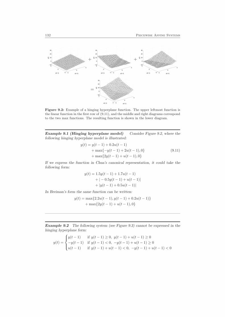
132 Piecewise Affine Systems
−5
0
5
−5
0
5−10
0
10
20
30
y(t−1)u(t−1)
y(t)
+
−5
0
5
−5
0
5−10
0
10
20
30
y(t−1)u(t−1)
y(t)
+
−5
0
5
−5
0
5−10
0
10
20
30
y(t−1)u(t−1)
y(t)
=
−5
0
5
−5
0
5−10
0
10
20
30
y(t−1)u(t−1)
y(t)
Figure 9.2: Example of a hinging hyperplane function. The upper leftmost function isthe linear function in the first row of (9.11), and the middle and right diagrams correspondto the two max functions. The resulting function is shown in the lower diagram.
Example 9.1 (Hinging hyperplane model) Consider Figure 9.2, where thefollowing hinging hyperplane model is illustrated:
y(t) = y(t− 1) + 0.2u(t− 1)+ max{−y(t− 1) + 2u(t− 1), 0} (9.11)+ max{2y(t− 1) + u(t− 1), 0}
If we express the function in Chua’s canonical representation, it could take thefollowing form:
y(t) = 1.5y(t− 1) + 1.7u(t− 1)+ | − 0.5y(t− 1) + u(t− 1)|+ |y(t− 1) + 0.5u(t− 1)|
In Breiman’s form the same function can be written:
y(t) = max{2.2u(t− 1), y(t− 1) + 0.2u(t− 1)}+ max{2y(t− 1) + u(t− 1), 0}
Example 9.2 The following system (see Figure 9.3) cannot be expressed in thehinging hyperplane form:
y(t) =
y(t− 1) if y(t− 1) ≥ 0, y(t− 1) + u(t− 1) ≥ 0−y(t− 1) if y(t− 1) < 0, −y(t− 1) + u(t− 1) ≥ 0u(t− 1) if y(t− 1) + u(t− 1) < 0, −y(t− 1) + u(t− 1) < 0
9.2 Discrete Time Models 133
−5
0
5 −5
0
5
0
5
u(t−1)y(t−1)
y(t)
Figure 9.3: A piecewise affine system not expressible in the hinging hyperplane form.
This is due to the fact that the regions of the different subsystems are not separatedby hyperplanes (but half-hyperplanes), so there is no way to place the hinges inthe hinging hyperplane representation to get this partition of the state-space.
A property of the class described by (9.6), (9.8), and (9.9), which makes itsuitable for function approximation, is that it has universal approximation prop-erties [90]. Roughly speaking, this means that we can approximate any functionarbitrarily well by using sufficiently many hinge functions (i.e., by letting M →∞).
We can note that the parameters of (9.9) are not uniquely determined, sincefor example
ϕT θ0 + max{ϕT θ1, 0} = ϕT (θ0 + θ1) + max{−ϕT θ1, 0}
This means that we can replace max{ϕT θ1, 0} by max{−ϕT θ1, 0}, include thedifference in the linear term, and still have the same system. Another reason forthe ambiguity of (9.9) is that we can reorder the max functions. One way to atleast partially avoid this ambiguity is to require that 0 ≤ wT θ1 ≤ · · · ≤ wT θM+
and 0 ≤ wT θM++1 ≤ · · · ≤ wT θM for some constant (nonzero) vector w.
9.2.3 Representations with Fixed Regions
In function approximation applications, it is quite common to use piecewise affinemodels where the state-space is partitioned into a regular pattern of regions, withan affine function for each region. For example, in [76, 78], a representation calledHL CPWL (High Level Canonical PieceWise Linear) representation is used, whichis based on a partition of the state space into simplices (polytopes with n + 1corners, where n is the dimension).
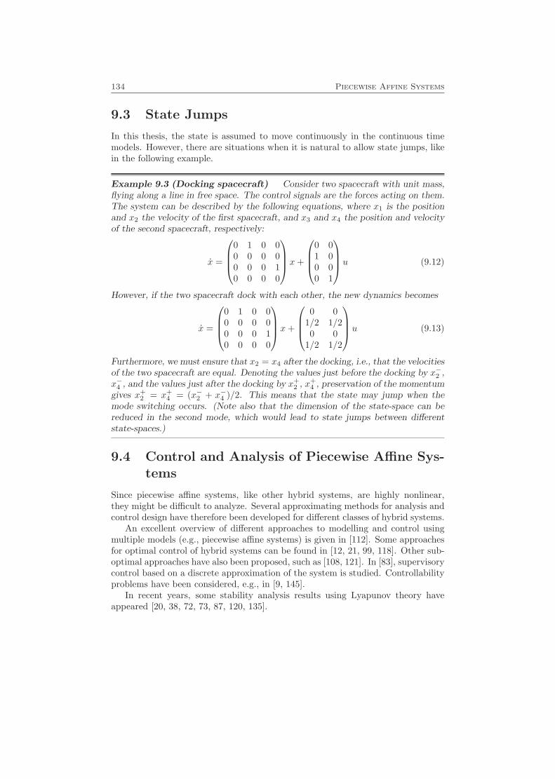
134 Piecewise Affine Systems
9.3 State Jumps
In this thesis, the state is assumed to move continuously in the continuous timemodels. However, there are situations when it is natural to allow state jumps, likein the following example.
Example 9.3 (Docking spacecraft) Consider two spacecraft with unit mass,flying along a line in free space. The control signals are the forces acting on them.The system can be described by the following equations, where x1 is the positionand x2 the velocity of the first spacecraft, and x3 and x4 the position and velocityof the second spacecraft, respectively:
x =
0 1 0 00 0 0 00 0 0 10 0 0 0
x+
0 01 00 00 1
u (9.12)
However, if the two spacecraft dock with each other, the new dynamics becomes
x =
0 1 0 00 0 0 00 0 0 10 0 0 0
x+
0 0
1/2 1/20 0
1/2 1/2
u (9.13)
Furthermore, we must ensure that x2 = x4 after the docking, i.e., that the velocitiesof the two spacecraft are equal. Denoting the values just before the docking by x−2 ,x−4 , and the values just after the docking by x+
2 , x+4 , preservation of the momentum
gives x+2 = x+
4 = (x−2 + x−4 )/2. This means that the state may jump when themode switching occurs. (Note also that the dimension of the state-space can bereduced in the second mode, which would lead to state jumps between differentstate-spaces.)
9.4 Control and Analysis of Piecewise Affine Sys-tems
Since piecewise affine systems, like other hybrid systems, are highly nonlinear,they might be difficult to analyze. Several approximating methods for analysis andcontrol design have therefore been developed for different classes of hybrid systems.
An excellent overview of different approaches to modelling and control usingmultiple models (e.g., piecewise affine systems) is given in [112]. Some approachesfor optimal control of hybrid systems can be found in [12, 21, 99, 118]. Other sub-optimal approaches have also been proposed, such as [108, 121]. In [83], supervisorycontrol based on a discrete approximation of the system is studied. Controllabilityproblems have been considered, e.g., in [9, 145].
In recent years, some stability analysis results using Lyapunov theory haveappeared [20, 38, 72, 73, 87, 120, 135].
10
Identification of Piecewise
Affine Systems
To be able to control and analyze a system, one will (in one way or another)need a model of the system that shows the relation between input and outputsignals, and the sensitivity to disturbances. Depending on what one would like toachieve, the model might be more or less accurate. In many cases, a linear modelaround the working point will be sufficient. However, when the nonlinearities arenot negligible within the operating region, a piecewise affine model might be anattractive alternative. This can be the case both when the real system actually ispiecewise affine, and for a general nonlinear system. Obtaining such a model fromexperimental data can be done in several different ways.
In this chapter, some existing approaches are investigated and compared. Someof the approaches are quite general nonlinear identification methods, for whichspecial cases lead to piecewise affine models, while other approaches are more spe-cialized on piecewise affine systems.
The system models considered in this and the next chapter will mostly be inregression form as described in Section 9.2.1, i.e.,
y(t) = ϕT (t)θ(v) + e(t) (10.1)
where θ(v) is a function of the key vector v, which in turn is a piecewise constantfunction v = v(ϕ) of the regression vector ϕ, taking only a finite number of values.As described in Section 1.1.3, the noise e(t) should satisfy E[e(t)] = 0, and should
135
136 Identification of Piecewise Affine Systems
be independent of Zt−1−∞. The regression vector could consist of old inputs and
outputs, e.g.,
ϕ(t) =(1 −y(t− 1) . . . −y(t− na) u(t− 1) . . . u(t− nb)
)TThe modes are consequently determined by v. If we let nv be the number of
different modes of the system, and let θ =(θ(v1) . . . θ(vnv )
)T , the criterionfunction to be minimized (cf. Section 8.1) for this kind of models can be written as
V (θ, ZN1 ) =1N
N∑t=1
nv∑j=1
`(y(t)− ϕT (t)θ(vj)
)χvj (ϕ(t)) (10.2)
where
χvj (ϕ) =
{1 v(ϕ) = vj
0 otherwise
The two most common choices for the function ` in (10.2), and the ones that willbe considered here, are the squared Euclidean norm (2-norm)
`2(ε) = ε2
and the 1-norm`1(ε) = |ε|
Obviously, for a given ϕ, exactly one of the functions χvj (ϕ) equals 1. Thismeans that all the terms in the inner sum in (10.2) except for one are zero. Hence, ifthe partitioning χvj of the state-space is known, i.e., if we know what experimentaldata belongs to which affine subsystem, then using 2-norm will reduce the problemof identifying piecewise affine systems of this kind to a least-squares problem likein Example 1.3, which can easily be solved using standard techniques. However,when the partitioning is unknown, and consequently both χvj (or, equivalently,v(ϕ)) and θ should be estimated, the problem becomes much more difficult. Thereare two fundamental approaches to take. The first possibility is to define an apriori grid (like in Section 9.2.3), and estimate one affine subsystem per cell inthe grid (see, e.g., [78]). This approach leads to a simple estimation process, butwill in a sense suffer from the curse of dimensionality, since the number of cells(and hence the number of parameters) will grow exponentially with the number ofdimensions, which also leads to a need for very large datasets. The other possibleapproach is to estimate both the partitioning and the subsystems simultaneouslyor iteratively (like in, e.g., [22, 48, 77]). This means that we will in general needa smaller number of subsystems, but that the estimation process will be morecomplex, with potentially many local minima, that will complicate the use of localsearch minimization algorithms.
Using piecewise affine systems for modelling and identification can be seen asa special case of multiple model approaches. In [112], an excellent introduction tononlinear modelling using multiple models is given together with a survey of thefield.
Some of the main issues in piecewise affine system identification are
10.1 Existing Approaches 137
• the ability to find a good model of the real system, preferably requiring asfew parameters as possible,
• the ability to avoid getting stuck in local minima during the search for a goodmodel, and
• the computational complexity of the identification process.
In the next chapter, an identification method based on mixed-integer linear orquadratic programming (MILP/MIQP; see Section A.4) will be presented in de-tail. As we will see, the mixed-integer programming approach guarantees that theglobal optimum is reached, at the cost of increased complexity. However, using a“truncated mixed-integer optimization algorithm” or a change detection algorithmmight in some cases be a feasible alternative, as will be discussed in Section 11.5.
10.1 Existing Approaches
Different approaches to piecewise affine system identification can be found in manyfields in the literature, as mentioned in Section 1.2.2. However, many of themare related. One of the crucial points that separate different groups of approachesfrom each other is how the partition into different regions is done. As we haveseen from (10.2), as soon as we know the different regions, it is easy to identifythe different affine subsystems one by one, using standard linear system identifica-tion techniques. From this viewpoint, the different approaches to identification ofpiecewise affine systems can be categorized as follows:
• All parameters, both the parameters determining the partition and the pa-rameters of the submodels, are identified simultaneously. Such approachescan be found, e.g., in [8, 51, 77, 124].
• All parameters are identified simultaneously for a model class with a very sim-ple partition, and new submodels/regions are added when needed. Examplesof this kind of approach are found in [22, 46, 64, 69, 77, 124].
• The regions and submodels are identified iteratively or in several steps, eachstep considering either the regions or the models. The methods in [48, 65,119, 143, 144] belong to this category. This is also the main approach in[112].
• The regions are predetermined or determined using only information aboutthe distribution of the regression vectors, and the local submodels are identi-fied after that. The approaches described in [26, 76, 78, 82, 103, 148, 152, 154]fall into this category.
The following sections describe the different categories more extensively, andsome advantages and drawbacks are pointed out. It should also be mentioned thatthere are of course alternative ways of categorizing the different approaches. Forexample, one can distinguish between online and offline algorithms.
138 Identification of Piecewise Affine Systems
10.1.1 Identifying All Parameters Simultaneously
Perhaps the most straightforward way of attacking the piecewise affine systemidentification problem is to formulate the criterion function (10.2), parameterizedaccording to a certain model structure, and then minimize it directly, using a nu-merical method, e.g., a Gauss-Newton search (see Section 8.2). In that way boththe partitioning and the submodels are estimated simultaneously. The greatestadvantage with such an approach might be its simplicity, and a reasonable compu-tational complexity (depending on what numerical method is used).
The greatest drawback with this approach is that the optimization algorithmmight get trapped in a local minimum. This drawback is shared with many otherof the categories.
The result also depends on how the model is parameterized. In general, itis desirable to have as few free parameters as possible, both for numerical andcomplexity reasons.
One example of this approach is given by Pucar and Sjoberg [124] where ahinging hyperplane model, as defined in Section 9.2.2, is used. Another example isfound in Julian et al. [77], where Chua’s canonical representation (9.6) is usedto approximate nonlinear functions. In both cases, the number of hinge functionsis assumed to be known. Pucar and Sjoberg present a damped Newton methodfor estimating all parameters of the model simultaneously, while Julian et al. usea Gauss-Newton algorithm. Local convergence of the parameters is proven. Asimilar approach, but for one-dimensional functions, is described in [57].
In an earlier article by Batruni [8], a multilayer neural network with piecewiseaffine functions in Chua’s canonical representation (as described in Section 9.2.2) ineach layer is proposed. The parameters would be estimated using backpropagation,which basically is a kind of gradient search.
An approach using a 1-norm criterion function can be found in Gad et al.[51]. Since the criterion function itself becomes a piecewise affine function of theparameters, they can use a simplex-like optimization algorithm to efficiently find alocal minimum. However, as for the other approaches in this category, convergenceto a global minimum cannot be guaranteed.
There are several general numerical optimization algorithms that try to reducethe risk of getting stuck in a local minimum. These include simulated annealing,genetic algorithms, etc. (see, e.g., [37] for both simulated annealing and geneticalgorithms). The basic idea of both simulated annealing and genetic algorithms isto modify a standard numerical optimization algorithm, such as the ones describedin Section 8.2, by repeatedly using random updates of the parameter estimates.These kinds of algorithms can be used for the piecewise affine system identificationproblem, at the cost of increased computational complexity.
10.1.2 Adding One Partition at a Time
Instead of solving the entire optimization problem at once, it can be divided intoseveral different steps, to get a number of easier optimization problems that can
10.1 Existing Approaches 139
be solved one at a time. One way of achieving this is to start with a simple model,for instance a hinging hyperplane model with only one hinge function, and fit it tothe data. Let us call this hinge function k1(ϕ, θ1). The criterion to be minimizedis
V 1(θ1, ZN1 ) =
1N
N∑t=1
` (y(t)− k1(ϕ(t), θ1))
If the resulting model k1(ϕ, θ1) is not satisfactory, one can add a new hinge functionby fitting it to the residual ε1(t) = y(t)− k1(ϕ(t), θ1); that is, we minimize
V 2(θ2, ZN1 ) =
1N
N∑t=1
` (ε1(t)− k2(ϕ(t), θ2))
The sum of the two models, k1(ϕ(t), θ1)+k2(ϕ(t), θ2), will then be a better approx-imation of the system. This procedure is repeated until the value of the criterionfunction (10.2) does not decrease significantly anymore, or until the resulting modelis satisfactory. One also has to take into consideration the risk of overfitting, whichmeans that the model might start to adjust to the particular noise realization, ifgiven too many degrees of freedom (e.g., too many hinge functions).
In addition to this algorithm, one can include a refitting procedure: Whenhaving added the hth hinge function, the previously added hinge functions are re-fitted one by one, so that the ith function ki(ϕ, θi), i ≤ h, is fitted to the residualy(t) −
∑j 6=i kj(ϕ(t), θj). This procedure can also be iterated until no further im-
provement can be observed. Note that the criterion function will not increase bythe refitting, so there is no risk of getting stuck in limit cycles.
The advantage of this approach of adding one, e.g., hinge function at a time,compared to the previous one of identifying all parameters simultaneously, is thateach optimization problem is easier to solve. On the other hand, one has tosolve several optimization problems instead of just one. When the number of re-gions/hinge functions of the real system is unknown, this approach may also havean advantage compared to the previous one. Just as for the first category, there isa risk of getting stuck in a local minimum.
Breiman [22] introduced the hinging hyperplane models and the algorithmsdescribed above for use in function approximation. The algorithm for estimatingone single hinge function is called the hinge-finding algorithm. It starts by assumingthat the dataset is partitioned into two subsets, and then estimates local affinemodels to each of the two sets. These affine models constitute the two submodelsof a hinge function. From the fact that the hinge function should be continuous,the hinge of the hinge function can be determined. However, this new hinge mayvery well partition the data into two subsets which are different from the originalsubsets. Therefore, the procedure can be repeated using the new partition, andin this way we iterate until the same partitions are obtained in two consecutiveiterations. Then a local minimum of V 1(θ1, Z
N1 ) is found.
The problem with this algorithm is that there is no guarantee for convergence.One can get stuck into limit cycles, or one can get least-squares problems that
140 Identification of Piecewise Affine Systems
do not have a unique solution, which corresponds to a partition where one of theregions does not contain enough data points.
The identification algorithms in [22] were analyzed further in Pucar and Sjo-berg [124], and it was shown that the hinge-finding algorithm is a special case of a(nondamped) Newton algorithm, as presented in Section 8.2. It was also modifiedto guarantee convergence, yielding a damped Newton algorithm. Pucar and Sjobergalso give a greedy algorithm, where – just as in the previously described algorithms– one hinge function at a time is added. The model is written as a weighted sumof the hinge functions, and when a new function is added, its parameters areestimated together with the weights of the other hinge functions, while all otherparameters are kept fixed. Pucar and Sjoberg compare the performance of thisgreedy function with the performance of the algorithm mentioned in the previoussection for a noiseless example, and it turns out that the simultaneous estimationof the parameters performs better when the true model is within the model class(for this specific example).
Julian et al. [77] use a similar algorithm, but for Chua’s canonical represen-tation. They also mention the possibility of adding several hinge functions at atime.
Hush and Horne [69] use what they call hinging sigmoid (HS) functions forfunction approximation. A HS function is defined by
σ(ϕ) =
θ+ ϕT θ ≥ θ+
ϕT θ θ− ≤ ϕT θ ≤ θ+
θ− ϕT θ ≤ θ−
Like in [22], one HS function is added at a time, and is fitted to the residual fromthe previous estimations. A refitting procedure similar to the one in [22] is alsosuggested. For the fitting of a single HS function three algorithms are proposed, ofwhich the first is due to Breiman and Friedman [23]. All the algorithms make useof the fact that once the partition is known, finding the parameters θ, θ+ and θ− isa least-squares problem with linear constraints (corresponding to the requirementthat the partition should not change). A similar approach is also presented inSection 11.7.
The Breiman/Friedman algorithm is analogous to the hinge-finding algorithmin [22] mentioned above, only for a different model class. It is a Newton algorithm,where in each iteration the updated parameter estimate is directly placed at theminimum of the local quadratic function. As for the hinge-finding algorithm, thereis no guarantee for convergence for this algorithm. To avoid convergence problems,one should be able to modify the step size of the parameter update in a way similarto what is being done with the hinge-finding algorithm in [124].
The second algorithm in [69] also starts by assuming a partition. Given thepartition, it solves the obtained QP problem including the linear constraints, andthen detects if there are any data points at the borders of the partition. In that case,these data points are assigned to the other region (as long as this does not destroythe positive definiteness of the quadratic objective function), and the new QP
10.1 Existing Approaches 141
problem is solved. This is repeated until the objective function does not decreaseanymore.
This algorithm is also related to the Newton algorithms. Here the minimum isfound within the region where the criterion function is quadratic (which correspondsto preserving the current partition of data points), and then, if this minimum issituated at a border of the region, a new step is taken into one of the adjacentregions. This means that each iteration explores exactly one new partition, andthat the parameter estimates only move between adjacent regions of the piecewisequadratic criterion function.
The third algorithm described in [69] is an extension of the second, and canbasically be seen as a way to give good initial values to the second algorithm. Itfirst fits an affine function ϕT θ to the data. This affine function is used as theinitial middle (nonconstant) part of the HS function. The data points are orderedalong the direction of the gradient of the affine function, and the hinges are initiallyplaced at the two extreme points on each side. From this initial partition, algorithm2 is used to find a local minimum. Then one data point at a time is taken fromthe middle region and assigned to the upper region (where ϕT θ ≥ θ+) to see ifimprovements can be made. After this the other hinge location is optimized, andfinally algorithm 2 is performed again.
In the article [46] by Ernst, hinging hyperplanes are used together with a treestructure, where a hinge function is added to the subregion with the worst fit. Thisapproach is related both to the tree structures in [55] and to the model trees in[148], and is explained in more detail in Section 10.1.4.
A similar approach is taken by Johansen and Foss [71]. The models that areused resemble the hinging hyperplane trees, in the sense that the different subre-gions are partitioned hierarchically: The state-space is split by a hyperplane, andeach of the two new regions are independently partitioned etc. To determine theposition of the first hyperplane, their algorithm starts by performing an exhaustivesearch over models with 2 + k regions. The best of these models determines wherethe first hyperplane should be placed. Having fixed that, the algorithm determinesthe second partitioning hyperplane by an exhaustive search over models with 3 +kregions etc. Since the authors use interpolation between the different submodels,the resulting model is not a piecewise affine system, but the method could be usedalso for piecewise affine systems.
Heredia and Arce [64] use continuous piecewise affine systems with rectan-gular subregions with the borders parallel to the coordinate axes, and a somewhatdifferent representation called Continuous Threshold Decomposition. Each borderis defined by a threshold, and the authors use the same set of thresholds for allvariables. They propose a method where one threshold at a time is added using anumerical method. An Akaike criterion [94] is used to decide how many thresholdsshould be added.
142 Identification of Piecewise Affine Systems
10.1.3 Finding Regions and Models in Several Steps
The last two categories are related in the sense that identifying the different regionsand the different subsystems are done separately, in different steps. Many of themethods found in the literature are constructed in a similar way:
• Local affine models are used to find the partition of the data.
• After the partition is done, the parameters of the affine subsystems can easilybe identified.
The local affine models in the first step can either be used to cluster the data pointsinto different clusters, in which all data points have similar model parameters, orthey can be used together with a change detection algorithm, in order to find themode switchings.
One example of such an approach is found in [48] by Ferrari-Trecate et al.They consider PWARX systems, as defined in Section 9.2.1. Their identificationalgorithm consists of five steps. The first step is to estimate local affine modelsaround each data point. This is done using the c data points that are closest tothe point for which the local model is estimated, where c is a constant specifiedby the user. Then a measure of the “confidence level” for each local estimation iscomputed, based on how scattered the points used for the estimation are, and on theempirical covariance matrix for the estimation. After this, a K-means algorithmis used to cluster the data points (see [16], or [41] for an overview of differentclustering techniques), based both on their position and on the parameters of thelocal model. The two last steps are to estimate an affine submodel for each cluster,and to try to find hyperplanes that separate the clusters from each other.
Another approach is proposed by Bemporad et al. [10]. The authors con-sider general PWARX systems, but with unknown but bounded (UBB) noise (seeSection 1.1.3). The number of submodels is not fixed. The approach consistsof three main steps. To get the initial assignment of data samples to differentsubmodels and an initial estimate of θ(vj) (and the number of submodels), an al-gorithm is used to approximately find the largest subset of inequalities of the form|ϕ(t)T θ(v1)−y(t)| ≤ δ that has a feasible solution. Having got an estimate of θ(v1),the process is repeated on the remaining data samples to get θ(v2), etc.
In the second phase the points are reassigned to different submodels accordingto the following scheme:
• Points that satisfy |ϕ(t)T θ(vi) − y(t)| ≤ δ for only one i are assigned to thecorresponding class.
• Points that satisfy |ϕ(t)T θ(vi) − y(t)| ≤ δ for several values of i are calledundecidable, and are not assigned to any class.
• Points that do not satisfy |ϕ(t)T θ(vi)− y(t)| ≤ δ for any value of i are calledinfeasible, and are not assigned to any class.
10.1 Existing Approaches 143
Given the new classification, θ(v1), . . . , θ(vnv ) are reestimated. This is iterateduntil convergence. During this procedure, submodels that are too similar to eachother are merged. Also, submodels containing too few points are removed. In thisway, the number of submodels can be kept low.
In the last step, an algorithm similar to the first step is used to find the sep-arating hyperplanes, giving the least possible number of misclassified points. Op-tionally, support vector machines (SVM) can then be used to optimize the locationof the separating hyperplanes.
Hoffmann and Engell [65, 66] consider a hybrid system model with severalmodes, where the dynamics of each mode is affine. When the state reaches oneof several switching regions, the system switches to another mode according to atable. State jumps (see Section 9.3) are also allowed, and are modelled by affinefunctions, one for each switching region.
The identification process is divided into several steps: First the mode switchesare detected with a standard change detection algorithm, where a model
x(k + 1) = Ax(k) +Bu(k) + d(k)H(k −K)
is fitted to a window of the time series. When ‖d(k)‖ exceeds a given threshold,this indicates that a mode switching has occurred.
In the second step, the switching points are clustered and classified as belongingto different switching regions, and the regions are approximated by hyperspheres.Then a possible mode sequence is found. From this a discrete model for the differentmode switchings is built.
In the last steps, the affine functions for the state jumps and the continuous dy-namics of each mode are estimated using standard linear identification techniques.
One problem with the approach by Hoffmann and Engell is that the systemmodel is only valid along the trajectories of the experimental data. This is dueto the very flexible hybrid model, which does not allow any conclusions aboutunexplored parts of the state-space to be drawn, since there might for instance bean undiscovered switching region anywhere in these parts.
In Munz and Krebs [109], the authors propose to, as a first step, use separat-ing hyperplanes which are parallel to the coordinate axes. The position of these areoptimized one by one in an iterative fashion. Having done this, each rectangularsubregion is divided into simplices for which affine subsystems are identified.
In Skeppstedt et al. [143, 144], an online approach is considered. Themodels taken into consideration are of PWARX type. A multiple-model recursiveparameter estimation algorithm called XAFFM is used to estimate the currentparameter value. XAFFM does not only give estimates of the parameters, but alsoof the covariance matrix and posterior probability of the parameter estimate.
By applying Bayes’ rule, using information about the operating point and theoutput of the sample, it is determined to which of the affine submodels that thecurrent sample most likely belongs. If the posterior probability of the currentestimated parameter value is high enough, the parameter value of the submodel isupdated. However, if the estimate of the current parameter value and the previously

144 Identification of Piecewise Affine Systems
estimated submodel parameter value differ too much, no updating is done. Instead,if this happens repeatedly, a new submodel is added to the total model.
After the update of the dynamics, the separating hyperplanes are updated bya standard procedure for linear discrimination.
The Switching Dynamical Systems considered in Petridis and Kehagias [119]do not really belong to the model classes considered so far in this chapter. Theyconsist of a number of subsystems, between which switchings occur with a certainprobability for each time step. The dependence between the current state andmode, which is inherent in the models considered previously, is not considered in[119].
For these systems, an iterative identification algorithm related to the algorithmby Skeppstedt et al. is presented. Initially, the number of submodels K is set toone, t = 1 and a threshold ε is chosen. Then the following steps are executediteratively:
1. For k = 1, . . . ,K, compute predictions yk(t) of y(t) using the current models.
2. For k = 1, . . . ,K, if |y(t)− yk(t)| < ε, let y(t) be assigned to model k and godirectly to step 3. If no model satisfies the requirement, let K = K + 1, addone model and assign y(t) to this model.
3. Estimate all submodels using the data assigned to them. Let t = t + 1 andgo to 1.
Some convergence results are given, in the sense that the ratio between the falselyand the correctly classified data points will asymptotically approach 0 with prob-ability 1.
In Gelfand and Ravishankar [55], a tree structure is used to partition thestate-space. Each node represents a subregion, and to each node the best affinemodel of the particular subregion is associated. The structure will be consideredin some more detail in Section 10.1.4. To update the parameters and to prune thetree, an online, gradient-based, two-step updating procedure is used.
Medeiros et al. [104, 105] use an algorithm called GRASP (Greedy Ran-domized Adaptive Search Procedure) to iteratively and heuristically find good par-titions of the state-space. When a partition is given, the remaining parameters areestimated using least squares, and the mean squared error is taken as a measure ofhow good the partition was.
Related to this category are the Local Learning methods of [110, 111] byMurray-Smith and Gollee, also considered in [112]. They use local linear mod-els, which are interpolated to get the total system model. The interpolation impliesthat the resulting systems are not piecewise affine systems. The identification pro-cess follows an iterative algorithm, where the model structure is first determinedusing a priori knowledge. Then the model parameters are identified locally for eachsubmodel. After this, the algorithm determines where the model structure needsimprovement, and the structure is adjusted. The last two steps are then iterateduntil the result is satisfactory.

10.1 Existing Approaches 145
There are also some relationships to the local modelling methods in Part I, andsimilar methods [122, 141]. In fact, if estimating a local linear model from a givenset of estimation data, using a weighted least squares criterion and a piecewise con-stant weight function, the resulting global model will be a piecewise affine system(even if it consists of a very large number of submodels). The shapes of the differentregions and the submodels are determined by the choice of weight function, which(as described earlier) becomes a trade-off between incorporating as much data aspossible to decrease the variance of the estimate, and building a model which is aslocal as possible to avoid a biased model.
10.1.4 Using Predetermined Regions
One possible approach is to partition the state-space in a regular grid, with oneaffine subsystem for each region in the grid. Since both the partitioning of the state-space and the identification of the subsystems become very easy (given enough ex-perimental data in each region), this approach might work well for low-dimensionalsystems. However, the number of regions grows exponentially with the dimen-sions, so both the computational complexity and the need for experimental dataare exponential in the number of dimensions, making the approach infeasible forhigher-dimensional systems.
One example of this kind of approach is given by Billings and Voon [15],where the state-space is partitioned into rectangular regions, with sides parallel tothe coordinate axes. Another example is found in [78] by Julian (see also [76]).Here the author considers nonlinear function approximation using the HL CPWLclass (see Section 9.2.3). Also Simani et al. [140] use a given simplicial partitionand identify affine models for each subregion. Some of the noise characteristics isalso identified.
Instead of deciding on the partition completely independently of the experi-mental data, another option might be to take the distribution of the regressionvectors into account. In this way, the state-space can be partitioned in such away that each region gets a proper amount of experimental data to allow for theestimation of an affine subsystem, and the exponential complexity can be avoided.The approach in [26] and the model trees proposed in [148] fall into this category.
In [26] by Choi and Choi, a method is proposed, where the state-space is firstpartitioned into hypertriangles, with experimental data points in each corner. Foreach hypertriangle an affine subsystem is fitted. Since only n+1 points are used tofit each n-dimensional subsystem, this method is quite sensitive to noise. Therefore,the authors also suggest to use an unsupervised learning algorithm with fewer cellsto get the partition. Then the problem of estimating the affine subsystems becomesa standard identification problem.
In the neural network literature, one can find several other examples of methodsthat start by clustering the data, and then build local linear models for each cluster;see, e.g., [82, 103, 152, 154].
The model trees proposed by Stromberg et al. [148] stem from the Classifi-cation and Regression Trees (CART) [24]. Here, a binary tree is built, where each
146 Identification of Piecewise Affine Systems
node represents a region of the state-space, and the regions of the children nodesform a partition of the region of the parent node. Then one linear subsystem isassociated with each leaf of the tree.
The obvious disadvantage with just considering the distribution of the regressionvectors, and not the corresponding y values, is that a set of data which really shouldbelong to the same subsystem might be split arbitrarily. To somewhat make upfor this drawback, one option is to make the partition rather fine (with manyregions), and then afterwards merge adjacent regions with similar subsystems (cf.the pruning strategy in [148]). A minor problem with this approach is that themerged regions may be of varying shapes and sizes, and it might be difficult torepresent them efficiently. For models represented as a tree structure, this is noproblem as long as the adjacent regions are also adjacent leaves in the tree. Then, allthat needs to be done is to erase the leaves and let their parent node become a newleaf representing the merged region. However, if the regions belong to completelydifferent branches of the tree, it may even be hard to determine whether they areadjacent or not.
One idea would be to use Breiman’s Hinge Finding Algorithm (or the modifiedversion in [124]) to find good partitions for the model trees. This would reduce therisk that two adjacent regions with similar dynamics would end up in completelydifferent branches of the tree. This is what is done by Ernst in [46].
In Gelfand and Ravishankar [55], the splitting of a region is decided based onthe best affine model for that region. A threshold is chosen as the mean of theexperimental outputs in that region. If the predicted output from the best affinemodel of the region exceeds this threshold, the data sample is assigned to one ofthe children nodes; otherwise it is assigned to the other. In this way, the nodesare assigned approximately the same number of data samples, but the problem ofadjacent regions with similar dynamics being split into different branches is notnecessarily avoided.
10.2 Discussion
The recurring problems with piecewise affine system identification concern howto find good solutions (a global minimum or a good local minimum) to the iden-tification problem given a model structure, and how to keep the computationalcomplexity and model complexity (number of model parameters) low. The com-putational complexity for a given algorithm is a function both of the number ofregions/subsystems, the number of experimental data, and of the number of di-mensions of the regression vector. Hence, there are many trade-off situations whencomparing different methods and tuning parameters for given algorithms.
One such issue was mentioned already in Section 1.2.2: The choice betweenchoosing an a priori grid or estimating the partitioning together with the subsys-tems. The first option leads to a simple estimation process, but to get a goodresult, the numbers of regions and data needed will increase exponentially withthe number of dimensions. Hence, this approach may be good for low-dimensional
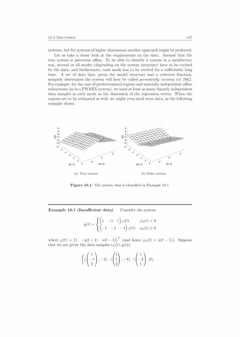
10.2 Discussion 147
systems, but for systems of higher dimensions another approach might be preferred.Let us take a closer look at the requirements on the data. Assume that the
true system is piecewise affine. To be able to identify a system in a satisfactoryway, several or all modes (depending on the system structure) have to be excitedby the data, and furthermore, each mode has to be excited for a sufficiently longtime. A set of data that, given the model structure and a criterion function,uniquely determines the system will here be called persistently exciting (cf. [94]).For example, for the case of predetermined regions and mutually independent affinesubsystems (as in a PWARX system), we need at least as many linearly independentdata samples in each mode as the dimension of the regression vector. When theregions are to be estimated as well, we might even need more data, as the followingexample shows.
−3−2
−10
12
3−2
0
2
−6−4−2
024
u(t−1)y(t−1)
y(t)
(a) True system.
−3−2
−10
12
3−2
0
2
−6−4−2
024
u(t−1)y(t−1)
y(t)
(b) False system.
Figure 10.1: The system that is identified in Example 10.1.
Example 10.1 (Insufficient data) Consider the system
y(t) =
(
1 −1 1)ϕ(t) ϕ3(t) < 0(
−1 −1 −1)ϕ(t) ϕ3(t) ≥ 0
where ϕ(t) =(1 −y(t− 1) u(t− 1)
)T(and hence ϕ3(t) = u(t − 1)). Suppose
that we are given the data samples (ϕ(t), y(t)):
{(
1−12
,−2), (
112
,−4), (
1−21
, 0),
148 Identification of Piecewise Affine Systems
(
1−1−2
, 0), (
12−1
,−2), (
11−2
,−2)}
Given the true partition of the state-space, these points determine the systemuniquely, since there are three linearly independent samples in each region (seeFigure 10.1(a)). However, we could alternatively choose another, incorrect par-tition and get a completely different system. An example of this is shown inFigure 10.1(b), where the system
y(t) =
(−2.5 −1.5 −0.5
)ϕ(t) ϕ2(t) < 0(
−3.5 0.5 −0.5)ϕ(t) ϕ2(t) ≥ 0
is shown to match the experimental data perfectly.
The need for enough data from each subsystem limits the number of subsys-tems that would be feasible to identify. Therefore, for larger examples it becomesadvantageous to allow the regions to be formed according to the data, to allow forfewer regions and parameters.
Another trade-off issue is the one concerning the choice between the three firstcategories of the previous sections. The first category – simultaneous identificationof all parameters – is perhaps the most straightforward and general option, sinceany numerical optimization algorithm can be applied. The other categories aremore heuristic, and the problem is split up into several subproblems, each of whichmight be easier to solve than tackling the entire problem directly. Generally, itis hard to say which strategy should be preferred, regarding the quality of thesolutions and the computational complexity. Some comparisons exist, e.g., the onein [124] mentioned previously, but no extensive study comparing several methodsand their performance has been found by the author.
There is also a trade-off between model complexity and the result quality. Themore degrees of freedom that are built into the model structure, the closer themodel can approximate the experimental data. However, since in practice data aremore or less corrupted by noise, a too large degree of model flexibility might causethe model to adjust to the actual noise realization, thereby causing overfitting.This is a general problem of system identification, occurring not only for piecewiseaffine systems.
Finally, there is a trade-off between the computational complexity of the algo-rithm chosen, and the quality of the resulting model. This is most obvious in thealgorithms where all parameters are identified simultaneously. The risk of endingup in a local minimum varies, depending on what numerical optimization algorithmis chosen. For example, having chosen a Gauss-Newton method, a simple way ofincreasing the chance of finding at least a good suboptimal model is to run theGauss-Newton method several times, starting from different initial values. Thiswill (on average) increase the quality of the solution, but at the same time increasethe computational complexity. In the next chapter we will see another example ofimproving the result at the cost of increased complexity.
11
PWA Identification Using
MILP/MIQP
The algorithms described in Chapter 10 all have one property in common: Theycannot guarantee that the optimal solution, i.e., the global minimum of (10.2), isfound. In this chapter, a type of algorithms that reach the globally optimal solutionin a finite number of steps is presented. The algorithms are based on mixed-integerlinear/quadratic programming (MILP/MIQP), which is described in Section A.4in the Appendix. The basic algorithms are described in Section 11.1, and someextensions are presented in Section 11.2.
Although it was shown, e.g., that the hinge-finding algorithm, proposed in [22]and described in Section 10.1.2, converges to the global minimum for a noiselesssystem consisting of one single hinge, local minima can lead to problems even invery simple cases for noisy systems or systems with multiple hinges. The followingexample illustrates this.
Example 11.1 Consider the problem of fitting a hinge function to the six datasamples given in Figure 11.1(a), using a 2-norm criterion. Figure 11.1(a) alsoshows the corresponding globally optimal function, with the optimal cost 0.98.In Figure 11.1(c) the cost is plotted as a function of the position of the hinge(recall that once the hinge position is known, the identification problem is simple),and we can see that there is a local minimum between 4 and 5 with the cost2.25. The corresponding function is plotted in Figure 11.1(b). Furthermore, simple
149
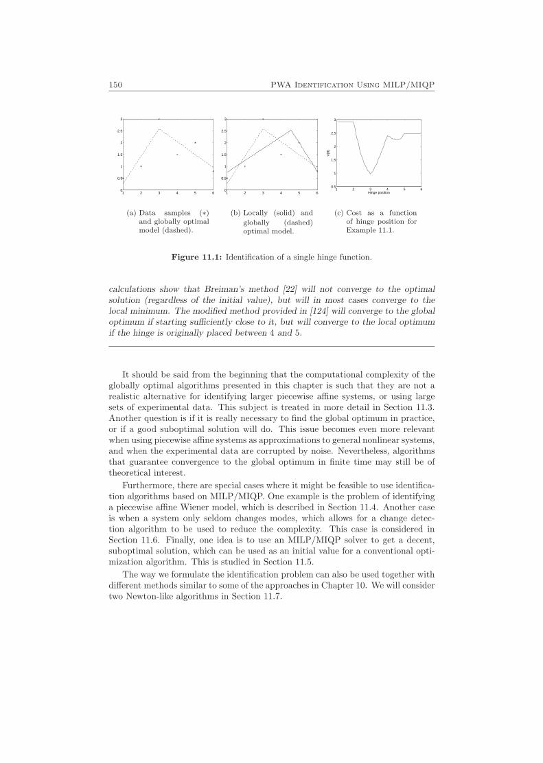
150 PWA Identification Using MILP/MIQP
1 2 3 4 5 60
0.5
1
1.5
2
2.5
3
(a) Data samples (∗)and globally optimalmodel (dashed).
1 2 3 4 5 60
0.5
1
1.5
2
2.5
3
(b) Locally (solid) and
globally (dashed)optimal model.
1 2 3 4 5 60.5
1
1.5
2
2.5
3
Hinge position
V(θ
)
(c) Cost as a functionof hinge position forExample 11.1.
Figure 11.1: Identification of a single hinge function.
calculations show that Breiman’s method [22] will not converge to the optimalsolution (regardless of the initial value), but will in most cases converge to thelocal minimum. The modified method provided in [124] will converge to the globaloptimum if starting sufficiently close to it, but will converge to the local optimumif the hinge is originally placed between 4 and 5.
It should be said from the beginning that the computational complexity of theglobally optimal algorithms presented in this chapter is such that they are not arealistic alternative for identifying larger piecewise affine systems, or using largesets of experimental data. This subject is treated in more detail in Section 11.3.Another question is if it is really necessary to find the global optimum in practice,or if a good suboptimal solution will do. This issue becomes even more relevantwhen using piecewise affine systems as approximations to general nonlinear systems,and when the experimental data are corrupted by noise. Nevertheless, algorithmsthat guarantee convergence to the global optimum in finite time may still be oftheoretical interest.
Furthermore, there are special cases where it might be feasible to use identifica-tion algorithms based on MILP/MIQP. One example is the problem of identifyinga piecewise affine Wiener model, which is described in Section 11.4. Another caseis when a system only seldom changes modes, which allows for a change detec-tion algorithm to be used to reduce the complexity. This case is considered inSection 11.6. Finally, one idea is to use an MILP/MIQP solver to get a decent,suboptimal solution, which can be used as an initial value for a conventional opti-mization algorithm. This is studied in Section 11.5.
The way we formulate the identification problem can also be used together withdifferent methods similar to some of the approaches in Chapter 10. We will considertwo Newton-like algorithms in Section 11.7.
11.1 Formulating the Identification Problem as an MILP/MIQP Problem 151
11.1 Formulating the Identification Problem as anMILP/MIQP Problem
The system class we will consider in this section is the class of hinging hyperplanesystems given by (9.10) and repeated here for convenience:
y(t) = ϕT (t)θ0 +M∑i=1
±max{ϕT (t)θi, 0}+ e(t) (11.1)
Recall that this is shorthand notation for
y(t) = ϕT (t)θ0 +M+∑i=1
max{ϕT (t)θi, 0} −M∑
i=M++1
max{ϕT (t)θi, 0}+ e(t)
where we assume M+ and M to be known. As mentioned in Section 9.2.2, twoproperties of this class are that the piecewise affine function is continuous, and thatthe affine subsystems are separated by the hyperplanes ϕT (t)θi = 0.
Letting θ =(θT0 . . . θTM
)T , the predicted output y(t|θ) becomes
y(t|θ) = ϕT (t)θ0 +M∑i=1
±max{ϕT (t)θi, 0} (11.2)
As in Chapter 8, we are given y(t), ϕ(t), t = 1, . . . , N , and would like to minimizethe prediction error according to some criterion function, i.e.,
minθ
V (θ, ZN1 ) =N∑t=1
`(ε(t, θ)) (11.3)
where
ε(t, θ) = y(t)− y(t|θ) = y(t)−(ϕT (t)θ0 +
M∑i=1
±max{ϕT (t)θi, 0})
In this chapter, we will use`2(ε) = ε2
and`1(ε) = |ε|
The main question of this section is: How can we rewrite these problems to fitinto the mixed-integer programming (MILP/MIQP) framework? If we would beable to formulate the piecewise affine system identification problem as an MILPor MIQP, then the optimal solution could be found in a finite number of steps,e.g., by using the algorithm described in Section A.4. There are two steps toaccomplish that: To rewrite (11.3) as a linear/quadratic function of the unknowns
152 PWA Identification Using MILP/MIQP
by introducing auxiliary variables, and to rewrite the constraints of the auxiliaryvariables as linear inequalities plus the constraint on some of the variables to bediscrete.
To be able to make the reformulation into a MILP or MIQP, we will need boundson the products ϕT (t)θi. Therefore, we will make the assumption that there areknown bounds for the parameters θi. These bounds could be in any norm withoutaffecting the later results, but for simplicity the Euclidean norm is chosen here,i.e.,
‖θi‖ ≤ Uθi , i = 1, . . . ,M
This implies that ϕT (t)θi are bounded:
Li(t) , −‖ϕ(t)‖Uθi ≤ ϕT (t)θi ≤ ‖ϕ(t)‖Uθi , Ui(t)
This is not a serious restriction, since the bounds can be chosen arbitrarily large.However, the tighter the bounds, the more efficiently the optimization can be per-formed. Other types of bounds that could be imagined include componentwisebounds on θi, i.e.,
Lθi 4 θi 4 Uθiwhere 4 denotes componentwise inequalities. If this type of bounds is used, thedefinitions of Li(t) and Ui(t) should be changed accordingly.
11.1.1 Reformulating the Criterion Function
Let us start with the criterion function. The problem here is that y(t|θ) is anonlinear function of θ. To eliminate that problem, introduce the auxiliary variables
zi(t) = max{ϕT (t)θi, 0}, i = 1, . . . ,M, t = 1, . . . , N (11.4)
and regard these as unknown variables in our minimization. The criterion functionfor `2(ε) now takes the form
V2 =N∑t=1
(y(t)−
(ϕT (t)θ0 +
M∑i=1
±zi(t)))2
(11.5)
which is quadratic in the unknowns θ0 and zi(t). The corresponding function for`1(ε) is
V1 =N∑t=1
∣∣∣∣∣y(t)−(ϕT (t)θ0 +
M∑i=1
±zi(t))∣∣∣∣∣ (11.6)
This function is unfortunately neither linear, nor quadratic. However, there isa standard trick for rewriting functions like this as a linear function with linearconstraints. Introduce the slack variables s1, . . . , sN . Then, minimizing V1 is the
11.1 Formulating the Identification Problem as an MILP/MIQP Problem 153
same as solving
minθ,z,s
N∑t=1
st
subj. to st ≥ y(t)− ϕT (t)θ0 −M∑i=1
±zi(t) (11.7)
st ≥ −(y(t)− ϕT (t)θ0 −
M∑i=1
±zi(t))
zi(t) = max{ϕT (t)θi, 0}
Now the criterion function is linear at the price of increasing the number of variablesby N and the number of linear constraints by 2N . However, in the context this isnot a very serious complexity increase, since it is generally the discrete variablesintroduced in the next section that determine the complexity.
11.1.2 Reformulating the Constraints
By introducing the auxiliary variables zi(t), we have also introduced the additionalnonlinear constraints (11.4). The next step in our reformulation process is torewrite these constraints as linear constraints, with the help of additional discretevariables. To that end, define
δi(t) =
{0 ϕT (t)θi < 01 ϕT (t)θi ≥ 0
i = 1, . . . ,M (11.8)
This means that we can write zi(t) as
zi(t) = δi(t)ϕT (t)θi
Notice also that geometrically, δi(t) tells us on what side of the ith hinge ϕ(t) ispositioned. Now we can use the method described in [12] to transform the con-straints (11.4) and (11.8) to linear inequalities. However, there is a more efficientway, which will now be described. This transformation method is related to themethod of transforming boolean expressions into linear inequalities, described in[106], and should be possible to use in many applications, where similar transfor-mations are needed.
Consider zi(t) and δi(t) for given i and t. In Figure 11.2, the feasible regionfor the two constraints (definitions) (11.4) and (11.8) is drawn as two solid lines.What we would like is to be able to express that region as the intersection betweena polyhedron (the linear constraints) and the set δi(t) = {0, 1}. The simplestway of doing this is to construct the convex hull (see Section A.3) of the feasibleregion (marked with dashed lines in Figure 11.2). This will both give the smallestpolyhedron including the original feasible region and the smallest set of linear
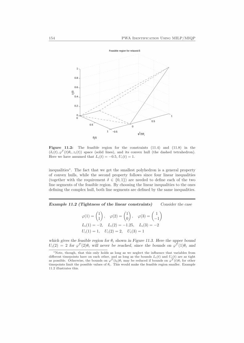
154 PWA Identification Using MILP/MIQP
0
0.5
1 −0.5
0
0.5
10
0.2
0.4
0.6
0.8
1
φT(t)θi
Feasible region for relaxed δ
δi(t)
z i(t)
Figure 11.2: The feasible region for the constraints (11.4) and (11.8) in the(δi(t), ϕ
T (t)θi, zi(t)) space (solid lines), and its convex hull (the dashed tetrahedron).Here we have assumed that Li(t) = −0.5, Ui(t) = 1.
inequalities∗. The fact that we get the smallest polyhedron is a general propertyof convex hulls, while the second property follows since four linear inequalities(together with the requirement δ ∈ {0, 1}) are needed to define each of the twoline segments of the feasible region. By choosing the linear inequalities to the onesdefining the complex hull, both line segments are defined by the same inequalities.
Example 11.2 (Tightness of the linear constraints) Consider the case
ϕ(1) =(
11
), ϕ(2) =
(10
), ϕ(3) =
(1−1
)Li(1) = −2, Li(2) = −1.25, Li(3) = −2Ui(1) = 1, Ui(2) = 2, Ui(3) = 1
which gives the feasible region for θi shown in Figure 11.3. Here the upper boundUi(2) = 2 for ϕT (2)θi will never be reached, since the bounds on ϕT (1)θi and
∗Note, though, that this only holds as long as we neglect the influence that variables fromdifferent timepoints have on each other, and as long as the bounds Li(t) and Ui(t) are as tightas possible. Otherwise, the bounds on ϕT (t0)θi may be reduced if bounds on ϕT (t)θi for othertimepoints limit the possible values of θi. This would make the feasible region smaller. Example11.2 illustrates this.

11.1 Formulating the Identification Problem as an MILP/MIQP Problem 155
-
6
��
��
�����
@@
@@
@@@@@ �
�����
@@@@@R
��
��
��
���@
@@@@
�����@
@@@@@@@@
-
θi2
θi1
ϕ(1)
ϕ(2)
ϕ(3)
Figure 11.3: The feasible region (bounded by the thick outer lines) in Example 11.2.The thin lines show ϕT (1)θi = 0 and ϕT (3)θi = 0.
ϕT (3)θi also give an implicit bound on ϕT (2)θi (corresponding to the rightmostvertex of the feasible region). Furthermore, if ϕT (1)θi ≥ 0 (i.e., δi(1) = 1), thelower bound Li(2) = −1.25 for ϕT (2)θi (corresponding to the leftmost vertical linein Figure 11.3) will not be reached either. Hence, whether or not Li(2) is a tightlower bound on ϕT (2)θi depends on the value of δi(1).
At first sight, the convex hull in Figure 11.2 seems to be defined byzi(t) ≥ 0zi(t) ≤ Ui(t)δi(t)ϕT (t)θi ≤ zi(t)(1− δi(t))Li(t) + zi(t) ≤ ϕT (t)θi
(11.9)
However, there is one problem in using these inequalities. According to (11.8),the point (δi(t), ϕT (t)θi, zi(t)) = (0, 0, 0) should not be part of the feasible region.This means that the convex hull is described by the union of all regions obtainedby different positive µ in the following inequalities
zi(t) ≥ 0zi(t) ≤ Ui(t)δi(t)(1− δi(t))µ+ ϕT (t)θi ≤ zi(t)(1− δi(t))Li(t) + zi(t) ≤ ϕT (t)θi
µ > 0 (11.10)
which is a description that might be awkward to work with, due to the nonfixedparameter µ. Actually, this is more of a theoretical than a practical problem. Thereason for this is best understood geometrically: When ϕT (t)θi = 0, it means that
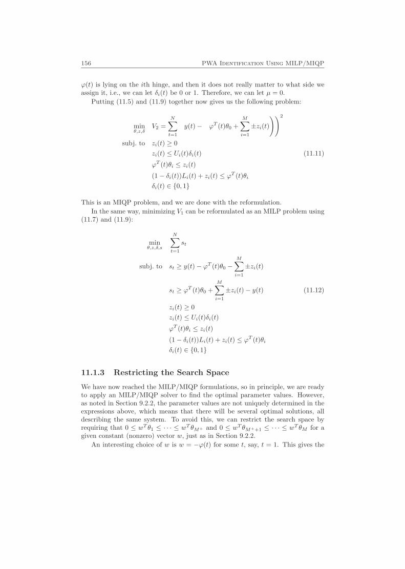
156 PWA Identification Using MILP/MIQP
ϕ(t) is lying on the ith hinge, and then it does not really matter to what side weassign it, i.e., we can let δi(t) be 0 or 1. Therefore, we can let µ = 0.
Putting (11.5) and (11.9) together now gives us the following problem:
minθ,z,δ
V2 =N∑t=1
(y(t)−
(ϕT (t)θ0 +
M∑i=1
±zi(t)))2
subj. to zi(t) ≥ 0zi(t) ≤ Ui(t)δi(t) (11.11)
ϕT (t)θi ≤ zi(t)(1− δi(t))Li(t) + zi(t) ≤ ϕT (t)θiδi(t) ∈ {0, 1}
This is an MIQP problem, and we are done with the reformulation.In the same way, minimizing V1 can be reformulated as an MILP problem using
(11.7) and (11.9):
minθ,z,δ,s
N∑t=1
st
subj. to st ≥ y(t)− ϕT (t)θ0 −M∑i=1
±zi(t)
st ≥ ϕT (t)θ0 +M∑i=1
±zi(t)− y(t) (11.12)
zi(t) ≥ 0zi(t) ≤ Ui(t)δi(t)ϕT (t)θi ≤ zi(t)(1− δi(t))Li(t) + zi(t) ≤ ϕT (t)θiδi(t) ∈ {0, 1}
11.1.3 Restricting the Search Space
We have now reached the MILP/MIQP formulations, so in principle, we are readyto apply an MILP/MIQP solver to find the optimal parameter values. However,as noted in Section 9.2.2, the parameter values are not uniquely determined in theexpressions above, which means that there will be several optimal solutions, alldescribing the same system. To avoid this, we can restrict the search space byrequiring that 0 ≤ wT θ1 ≤ · · · ≤ wT θM+ and 0 ≤ wT θM++1 ≤ · · · ≤ wT θM for agiven constant (nonzero) vector w, just as in Section 9.2.2.
An interesting choice of w is w = −ϕ(t) for some t, say, t = 1. This gives the
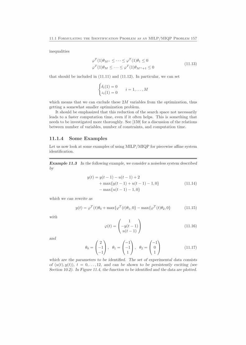
11.1 Formulating the Identification Problem as an MILP/MIQP Problem 157
inequalities
ϕT (1)θM+ ≤ · · · ≤ ϕT (1)θ1 ≤ 0
ϕT (1)θM ≤ · · · ≤ ϕT (1)θM++1 ≤ 0(11.13)
that should be included in (11.11) and (11.12). In particular, we can set{δi(1) = 0zi(1) = 0
i = 1, . . . ,M
which means that we can exclude these 2M variables from the optimization, thusgetting a somewhat smaller optimization problem.
It should be emphasized that this reduction of the search space not necessarilyleads to a faster computation time, even if it often helps. This is something thatneeds to be investigated more thoroughly. See [159] for a discussion of the relationsbetween number of variables, number of constraints, and computation time.
11.1.4 Some Examples
Let us now look at some examples of using MILP/MIQP for piecewise affine systemidentification.
Example 11.3 In the following example, we consider a noiseless system describedby
y(t) = y(t− 1)− u(t− 1) + 2+ max{y(t− 1) + u(t− 1)− 1, 0}−max{u(t− 1)− 1, 0}
(11.14)
which we can rewrite as
y(t) = ϕT (t)θ0 + max{ϕT (t)θ1, 0} −max{ϕT (t)θ2, 0} (11.15)
with
ϕ(t) =
1−y(t− 1)u(t− 1)
(11.16)
and
θ0 =
2−1−1
, θ1 =
−1−11
, θ2 =
−101
(11.17)
which are the parameters to be identified. The set of experimental data consistsof (u(t), y(t)), t = 0, . . . , 12, and can be shown to be persistently exciting (seeSection 10.2). In Figure 11.4, the function to be identified and the data are plotted.
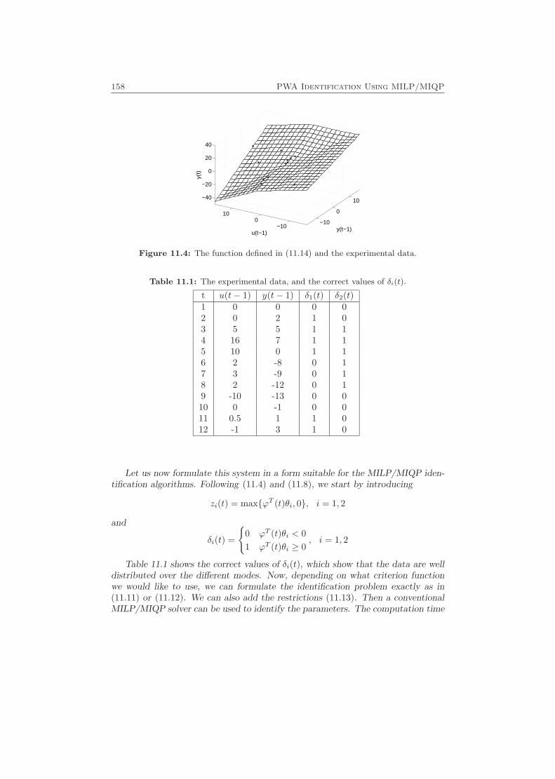
158 PWA Identification Using MILP/MIQP
−10
0
10
−100
10
−40
−20
0
20
40
y(t−1)u(t−1)
y(t)
Figure 11.4: The function defined in (11.14) and the experimental data.
Table 11.1: The experimental data, and the correct values of δi(t).
t u(t− 1) y(t− 1) δ1(t) δ2(t)1 0 0 0 02 0 2 1 03 5 5 1 14 16 7 1 15 10 0 1 16 2 -8 0 17 3 -9 0 18 2 -12 0 19 -10 -13 0 010 0 -1 0 011 0.5 1 1 012 -1 3 1 0
Let us now formulate this system in a form suitable for the MILP/MIQP iden-tification algorithms. Following (11.4) and (11.8), we start by introducing
zi(t) = max{ϕT (t)θi, 0}, i = 1, 2
and
δi(t) =
{0 ϕT (t)θi < 01 ϕT (t)θi ≥ 0
, i = 1, 2
Table 11.1 shows the correct values of δi(t), which show that the data are welldistributed over the different modes. Now, depending on what criterion functionwe would like to use, we can formulate the identification problem exactly as in(11.11) or (11.12). We can also add the restrictions (11.13). Then a conventionalMILP/MIQP solver can be used to identify the parameters. The computation time
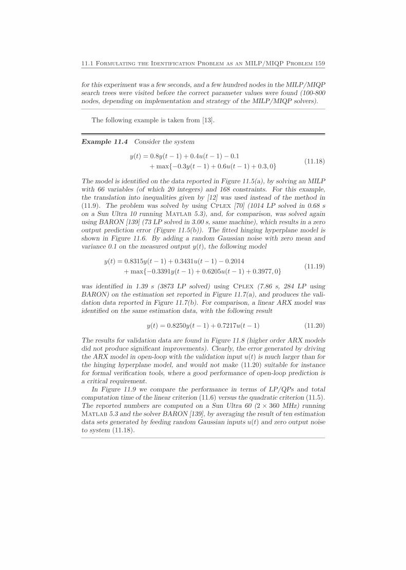
11.1 Formulating the Identification Problem as an MILP/MIQP Problem 159
for this experiment was a few seconds, and a few hundred nodes in the MILP/MIQPsearch trees were visited before the correct parameter values were found (100-800nodes, depending on implementation and strategy of the MILP/MIQP solvers).
The following example is taken from [13].
Example 11.4 Consider the system
y(t) = 0.8y(t− 1) + 0.4u(t− 1)− 0.1+ max{−0.3y(t− 1) + 0.6u(t− 1) + 0.3, 0}
(11.18)
The model is identified on the data reported in Figure 11.5(a), by solving an MILPwith 66 variables (of which 20 integers) and 168 constraints. For this example,the translation into inequalities given by [12] was used instead of the method in(11.9). The problem was solved by using Cplex [70] (1014 LP solved in 0.68 son a Sun Ultra 10 running Matlab 5.3), and, for comparison, was solved againusing BARON [139] (73 LP solved in 3.00 s, same machine), which results in a zerooutput prediction error (Figure 11.5(b)). The fitted hinging hyperplane model isshown in Figure 11.6. By adding a random Gaussian noise with zero mean andvariance 0.1 on the measured output y(t), the following model
y(t) = 0.8315y(t− 1) + 0.3431u(t− 1)− 0.2014+ max{−0.3391y(t− 1) + 0.6205u(t− 1) + 0.3977, 0}
(11.19)
was identified in 1.39 s (3873 LP solved) using Cplex (7.86 s, 284 LP usingBARON) on the estimation set reported in Figure 11.7(a), and produces the vali-dation data reported in Figure 11.7(b). For comparison, a linear ARX model wasidentified on the same estimation data, with the following result
y(t) = 0.8250y(t− 1) + 0.7217u(t− 1) (11.20)
The results for validation data are found in Figure 11.8 (higher order ARX modelsdid not produce significant improvements). Clearly, the error generated by drivingthe ARX model in open-loop with the validation input u(t) is much larger than forthe hinging hyperplane model, and would not make (11.20) suitable for instancefor formal verification tools, where a good performance of open-loop prediction isa critical requirement.
In Figure 11.9 we compare the performance in terms of LP/QPs and totalcomputation time of the linear criterion (11.6) versus the quadratic criterion (11.5).The reported numbers are computed on a Sun Ultra 60 (2 × 360 MHz) runningMatlab 5.3 and the solver BARON [139], by averaging the result of ten estimationdata sets generated by feeding random Gaussian inputs u(t) and zero output noiseto system (11.18).
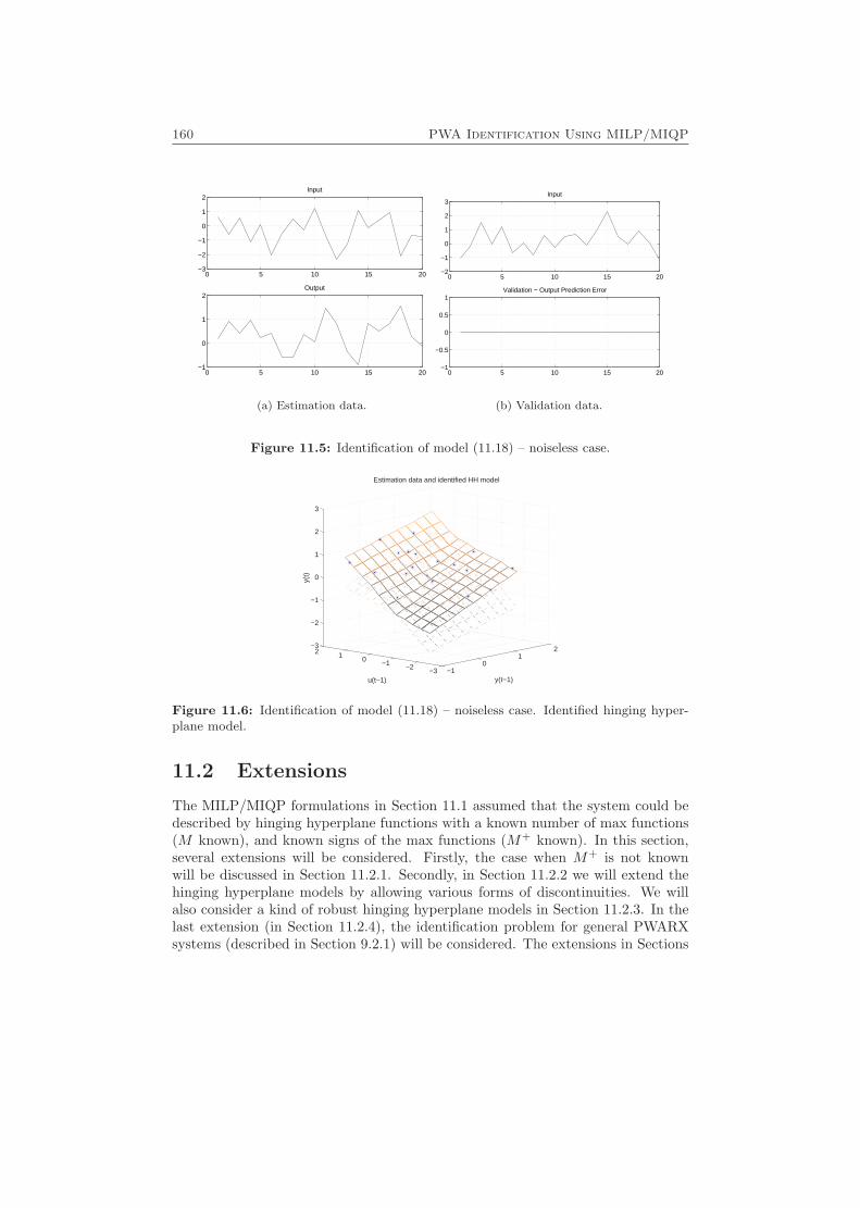
160 PWA Identification Using MILP/MIQP
0 5 10 15 20−3
−2
−1
0
1
2Input
0 5 10 15 20−1
0
1
2Output
(a) Estimation data.
0 5 10 15 20−2
−1
0
1
2
3Input
0 5 10 15 20−1
−0.5
0
0.5
1Validation − Output Prediction Error
(b) Validation data.
Figure 11.5: Identification of model (11.18) – noiseless case.
−10
12
−3−2−1012−3
−2
−1
0
1
2
3
y(t−1)
Estimation data and identified HH model
u(t−1)
y(t)
Figure 11.6: Identification of model (11.18) – noiseless case. Identified hinging hyper-plane model.
11.2 Extensions
The MILP/MIQP formulations in Section 11.1 assumed that the system could bedescribed by hinging hyperplane functions with a known number of max functions(M known), and known signs of the max functions (M+ known). In this section,several extensions will be considered. Firstly, the case when M+ is not knownwill be discussed in Section 11.2.1. Secondly, in Section 11.2.2 we will extend thehinging hyperplane models by allowing various forms of discontinuities. We willalso consider a kind of robust hinging hyperplane models in Section 11.2.3. In thelast extension (in Section 11.2.4), the identification problem for general PWARXsystems (described in Section 9.2.1) will be considered. The extensions in Sections
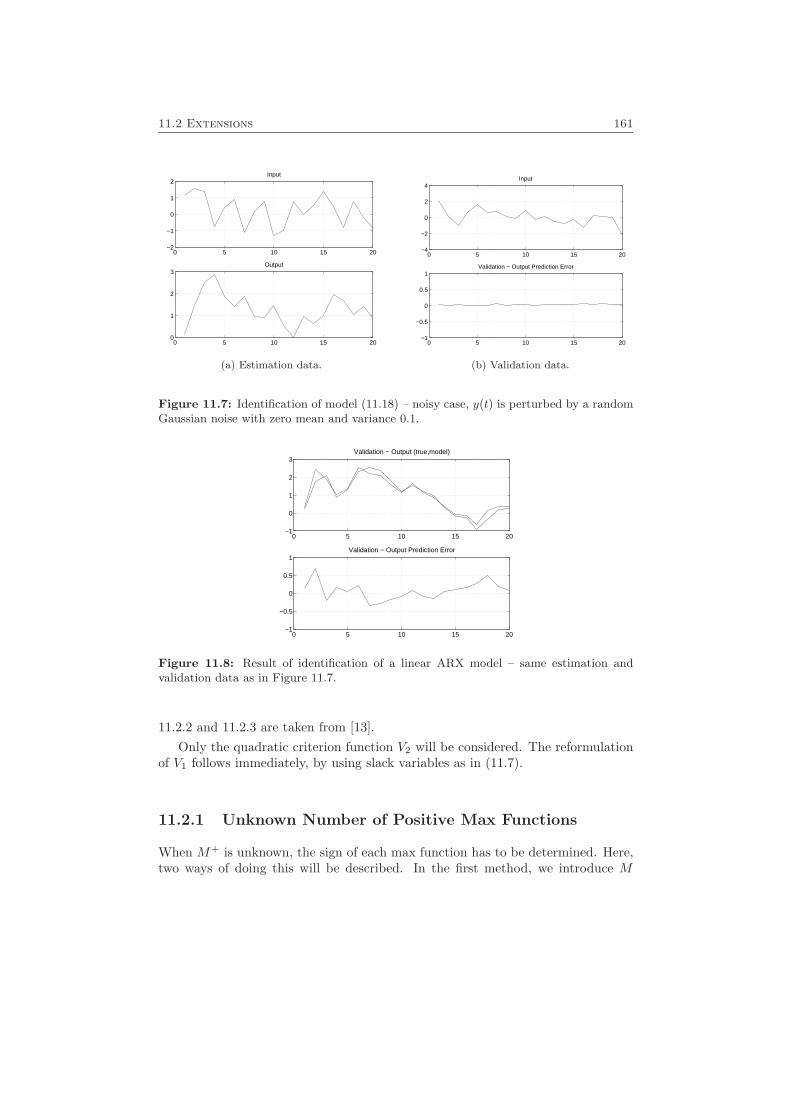
11.2 Extensions 161
0 5 10 15 20−2
−1
0
1
2Input
0 5 10 15 200
1
2
3Output
(a) Estimation data.
0 5 10 15 20−4
−2
0
2
4Input
0 5 10 15 20−1
−0.5
0
0.5
1Validation − Output Prediction Error
(b) Validation data.
Figure 11.7: Identification of model (11.18) – noisy case, y(t) is perturbed by a randomGaussian noise with zero mean and variance 0.1.
0 5 10 15 20−1
0
1
2
3Validation − Output (true,model)
0 5 10 15 20−1
−0.5
0
0.5
1Validation − Output Prediction Error
Figure 11.8: Result of identification of a linear ARX model – same estimation andvalidation data as in Figure 11.7.
11.2.2 and 11.2.3 are taken from [13].Only the quadratic criterion function V2 will be considered. The reformulation
of V1 follows immediately, by using slack variables as in (11.7).
11.2.1 Unknown Number of Positive Max Functions
When M+ is unknown, the sign of each max function has to be determined. Here,two ways of doing this will be described. In the first method, we introduce M
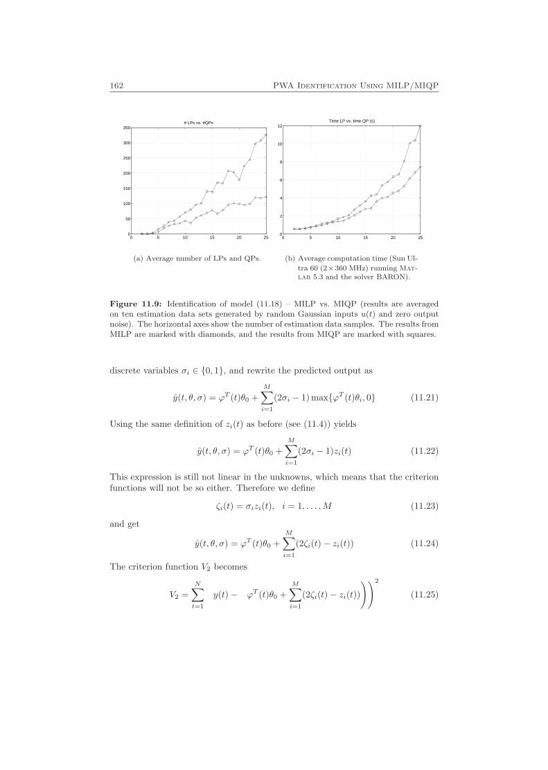
162 PWA Identification Using MILP/MIQP
0 5 10 15 20 250
50
100
150
200
250
300
350# LPs vs. #QPs
(a) Average number of LPs and QPs.
0 5 10 15 20 250
2
4
6
8
10
12Time LP vs. time QP (s)
(b) Average computation time (Sun Ul-
tra 60 (2×360 MHz) running Mat-
lab 5.3 and the solver BARON).
Figure 11.9: Identification of model (11.18) – MILP vs. MIQP (results are averagedon ten estimation data sets generated by random Gaussian inputs u(t) and zero outputnoise). The horizontal axes show the number of estimation data samples. The results fromMILP are marked with diamonds, and the results from MIQP are marked with squares.
discrete variables σi ∈ {0, 1}, and rewrite the predicted output as
y(t, θ, σ) = ϕT (t)θ0 +M∑i=1
(2σi − 1) max{ϕT (t)θi, 0} (11.21)
Using the same definition of zi(t) as before (see (11.4)) yields
y(t, θ, σ) = ϕT (t)θ0 +M∑i=1
(2σi − 1)zi(t) (11.22)
This expression is still not linear in the unknowns, which means that the criterionfunctions will not be so either. Therefore we define
ζi(t) = σizi(t), i = 1, . . . ,M (11.23)
and get
y(t, θ, σ) = ϕT (t)θ0 +M∑i=1
(2ζi(t)− zi(t)) (11.24)
The criterion function V2 becomes
V2 =N∑t=1
(y(t)−
(ϕT (t)θ0 +
M∑i=1
(2ζi(t)− zi(t))))2
(11.25)
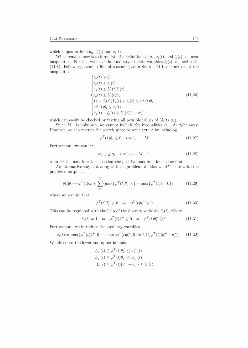
11.2 Extensions 163
which is quadratic in θ0, ζi(t) and zi(t).What remains now is to formulate the definitions of σi, zi(t), and ζi(t) as linear
inequalities. For this we need the auxiliary discrete variables δi(t), defined as in(11.8). Following a similar line of reasoning as in Section 11.1, one arrives at theinequalities
ζi(t) ≥ 0ζi(t) ≤ zi(t)zi(t) ≤ Ui(t)δi(t)ζi(t) ≤ Ui(t)σi(1− δi(t))Li(t) + zi(t) ≤ ϕT (t)θiϕT (t)θi ≤ zi(t)zi(t)− ζi(t) ≤ Ui(t)(1− σi)
(11.26)
which can easily be checked by testing all possible values of (δi(t), σi).Since M+ is unknown, we cannot include the inequalities (11.13) right away.
However, we can restrict the search space to some extent by including
ϕT (1)θi ≤ 0, i = 1, . . . ,M (11.27)
Furthermore, we can let
σi+1 ≤ σi, i = 1, . . . ,M − 1 (11.28)
to order the max functions, so that the positive max functions come first.An alternative way of dealing with the problem of unknown M+ is to write the
predicted output as
y(t|θ) = ϕT (t)θ0 +M∑i=1
(max{ϕT (t)θ+i , 0} −max{ϕT (t)θ−i , 0}) (11.29)
where we require that
ϕT (t)θ+i ≥ 0 ⇔ ϕT (t)θ−i ≥ 0 (11.30)
This can be regulated with the help of the discrete variables δi(t), where
δi(t) = 1 ⇔ ϕT (t)θ+i ≥ 0 ⇔ ϕT (t)θ−i ≥ 0 (11.31)
Furthermore, we introduce the auxiliary variables
zi(t) = max{ϕT (t)θ+i , 0} −max{ϕT (t)θ−i , 0} = δi(t)ϕT (t)(θ+
i − θ−i ) (11.32)
We also need the lower and upper bounds
L+i (t) ≤ ϕT (t)θ+
i ≤ U+i (t)
L−i (t) ≤ ϕT (t)θ−i ≤ U−i (t)
Li(t) ≤ ϕT (t)(θ+i − θ−i ) ≤ Ui(t)
164 PWA Identification Using MILP/MIQP
The problem can now be written as
minθ±,z,δ
V2 =N∑t=1
(y(t)−
(ϕT (t)θ0 +
M∑i=1
zi(t)
))2
subj. to ϕT (t)θ+i ≥ L+
i (t)(1− δi(t))ϕT (t)θ+
i ≤ U+i (t)δi(t)
ϕT (t)θ−i ≥ L−i (t)(1− δi(t))ϕT (t)θ−i ≤ U−i (t)δi(t)zi(t) ≥ Li(t)δi(t)zi(t) ≤ Ui(t)δi(t)ϕT (t)(θ+
i − θ−i ) ≥ zi(t) + Li(t)(1− δi(t))ϕT (t)(θ+
i − θ−i ) ≤ zi(t) + Ui(t)(1− δi(t))δi(t) ∈ {0, 1}
(11.33)
Here the method from [12] is used to transform the definitions of zi(t) and δi(t)into inequalities. The first four inequalities establish the relation between θ+
i , θ−i ,and δi(t), while the last four inequalities define zi(t).
The advantage of this method compared to the first alternative is that we needfewer variables. A drawback is that θ+
i and θ−i cannot be uniquely determined; if(θ+i
∗, θ−i
∗) is a solution, so is, e.g., (θ+
i
∗+ λθ+
i
∗, θ−i
∗+ λθ+
i
∗) for λ ≥ 0, as long as
the upper and lower bounds are not reached. Another drawback is that the twohinging hyperplanes given by θ+
i and θ−i will not always correspond to one singlehinging hyperplane giving the same partition of the estimation dataset.
To restrict the search space, we can include the following inequalities that cor-respond to (11.13):{
ϕT (1)θ+i ≤ 0 i = 1, . . . ,M
ϕT (1)(θ+1 − θ−1 ) ≤ · · · ≤ ϕT (1)(θ+
M − θ−M )
which makes the variables δi(1), zi(1) redundant.
11.2.2 Discontinuous Hinging Hyperplane Models
In hinging hyperplane models, the output y(t) is a continuous function of theregressor ϕ(t). On the other hand, hybrid systems often consist of piecewise affinediscontinuous mappings. In order to tackle discontinuities, we can modify thehinging hyperplane model (11.2) in the form
y(t|θ) = ϕT (t)θ0 +M∑i=1
(ϕT (t)θi + ai)δi(t) (11.34a)
δi(t) =
{0 ϕT (t)θi < 01 ϕT (t)θi ≥ 0
(11.34b)
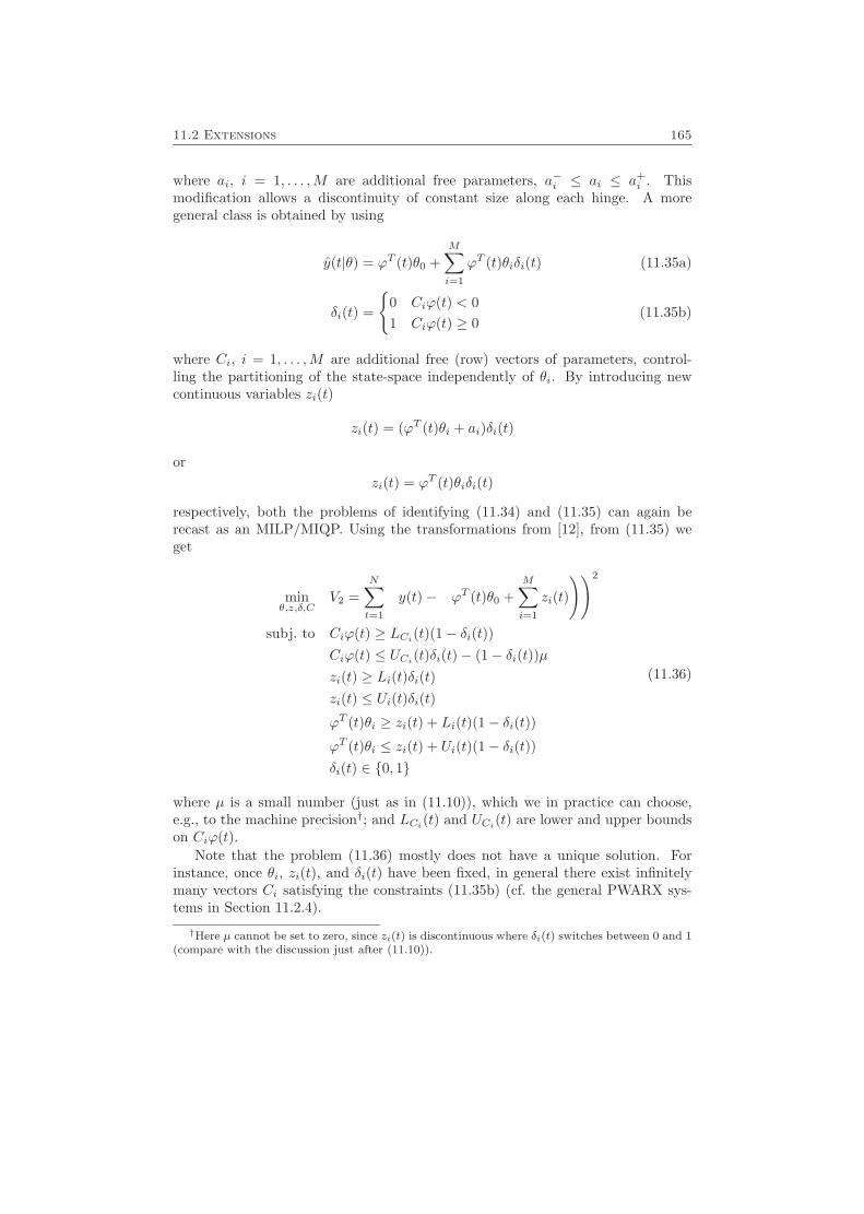
11.2 Extensions 165
where ai, i = 1, . . . ,M are additional free parameters, a−i ≤ ai ≤ a+i . This
modification allows a discontinuity of constant size along each hinge. A moregeneral class is obtained by using
y(t|θ) = ϕT (t)θ0 +M∑i=1
ϕT (t)θiδi(t) (11.35a)
δi(t) =
{0 Ciϕ(t) < 01 Ciϕ(t) ≥ 0
(11.35b)
where Ci, i = 1, . . . ,M are additional free (row) vectors of parameters, control-ling the partitioning of the state-space independently of θi. By introducing newcontinuous variables zi(t)
zi(t) = (ϕT (t)θi + ai)δi(t)
orzi(t) = ϕT (t)θiδi(t)
respectively, both the problems of identifying (11.34) and (11.35) can again berecast as an MILP/MIQP. Using the transformations from [12], from (11.35) weget
minθ,z,δ,C
V2 =N∑t=1
(y(t)−
(ϕT (t)θ0 +
M∑i=1
zi(t)
))2
subj. to Ciϕ(t) ≥ LCi(t)(1− δi(t))Ciϕ(t) ≤ UCi(t)δi(t)− (1− δi(t))µzi(t) ≥ Li(t)δi(t)zi(t) ≤ Ui(t)δi(t)ϕT (t)θi ≥ zi(t) + Li(t)(1− δi(t))ϕT (t)θi ≤ zi(t) + Ui(t)(1− δi(t))δi(t) ∈ {0, 1}
(11.36)
where µ is a small number (just as in (11.10)), which we in practice can choose,e.g., to the machine precision†; and LCi(t) and UCi(t) are lower and upper boundson Ciϕ(t).
Note that the problem (11.36) mostly does not have a unique solution. Forinstance, once θi, zi(t), and δi(t) have been fixed, in general there exist infinitelymany vectors Ci satisfying the constraints (11.35b) (cf. the general PWARX sys-tems in Section 11.2.4).
†Here µ cannot be set to zero, since zi(t) is discontinuous where δi(t) switches between 0 and 1(compare with the discussion just after (11.10)).
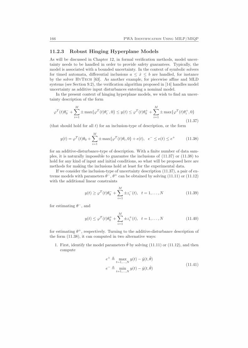
166 PWA Identification Using MILP/MIQP
11.2.3 Robust Hinging Hyperplane Models
As will be discussed in Chapter 12, in formal verification methods, model uncer-tainty needs to be handled in order to provide safety guarantees. Typically, themodel is associated with a bounded uncertainty. In the context of symbolic solversfor timed automata, differential inclusions a ≤ x ≤ b are handled, for instanceby the solver HyTech [63]. As another example, for piecewise affine and MLDsystems (see Section 9.2), the verification algorithm proposed in [14] handles modeluncertainty as additive input disturbances entering a nominal model.
In the present context of hinging hyperplane models, we wish to find an uncer-tainty description of the form
ϕT (t)θ−0 +M∑i=1
±max{ϕT (t)θ−i , 0} ≤ y(t) ≤ ϕT (t)θ+0 +
M∑i=1
±max{ϕT (t)θ+i , 0}
(11.37)(that should hold for all t) for an inclusion-type of description, or the form
y(t) = ϕT (t)θ0 +M∑i=1
±max{ϕT (t)θi, 0}+ e(t), e− ≤ e(t) ≤ e+ (11.38)
for an additive-disturbance-type of description. With a finite number of data sam-ples, it is naturally impossible to guarantee the inclusions of (11.37) or (11.38) tohold for any kind of input and initial conditions, so what will be proposed here aremethods for making the inclusions hold at least for the experimental data.
If we consider the inclusion-type of uncertainty description (11.37), a pair of ex-treme models with parameters θ−, θ+ can be obtained by solving (11.11) or (11.12)with the additional linear constraints
y(t) ≥ ϕT (t)θ−0 +M∑i=1
±z−i (t), t = 1, . . . , N (11.39)
for estimating θ−, and
y(t) ≤ ϕT (t)θ+0 +
M∑i=1
±z+i (t), t = 1, . . . , N (11.40)
for estimating θ+, respectively. Turning to the additive-disturbance description ofthe form (11.38), it can computed in two alternative ways:
1. First, identify the model parameters θ by solving (11.11) or (11.12), and thencompute
e+ , maxt=1,...,N
y(t)− y(t, θ)
e− , mint=1,...,N
y(t)− y(t, θ)(11.41)
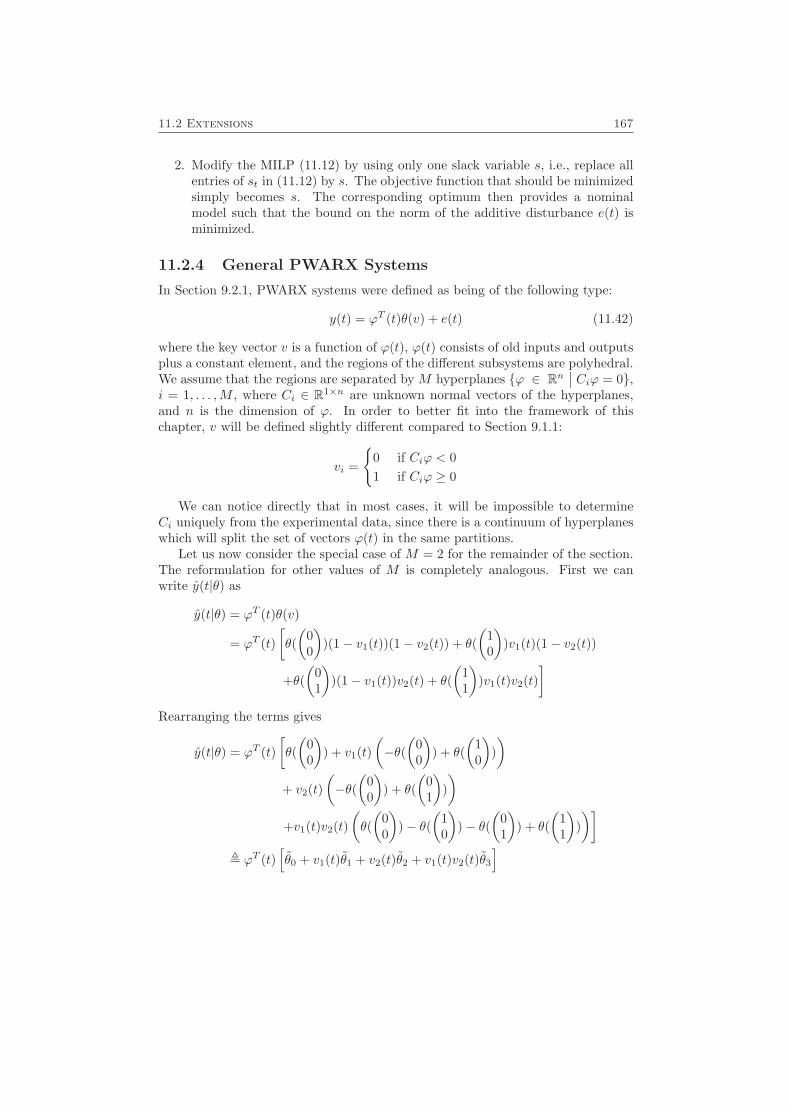
11.2 Extensions 167
2. Modify the MILP (11.12) by using only one slack variable s, i.e., replace allentries of st in (11.12) by s. The objective function that should be minimizedsimply becomes s. The corresponding optimum then provides a nominalmodel such that the bound on the norm of the additive disturbance e(t) isminimized.
11.2.4 General PWARX Systems
In Section 9.2.1, PWARX systems were defined as being of the following type:
y(t) = ϕT (t)θ(v) + e(t) (11.42)
where the key vector v is a function of ϕ(t), ϕ(t) consists of old inputs and outputsplus a constant element, and the regions of the different subsystems are polyhedral.We assume that the regions are separated by M hyperplanes {ϕ ∈ Rn
∣∣ Ciϕ = 0},i = 1, . . . ,M , where Ci ∈ R1×n are unknown normal vectors of the hyperplanes,and n is the dimension of ϕ. In order to better fit into the framework of thischapter, v will be defined slightly different compared to Section 9.1.1:
vi =
{0 if Ciϕ < 01 if Ciϕ ≥ 0
We can notice directly that in most cases, it will be impossible to determineCi uniquely from the experimental data, since there is a continuum of hyperplaneswhich will split the set of vectors ϕ(t) in the same partitions.
Let us now consider the special case of M = 2 for the remainder of the section.The reformulation for other values of M is completely analogous. First we canwrite y(t|θ) as
y(t|θ) = ϕT (t)θ(v)
= ϕT (t)[θ((
00
))(1− v1(t))(1− v2(t)) + θ(
(10
))v1(t)(1− v2(t))
+θ((
01
))(1− v1(t))v2(t) + θ(
(11
))v1(t)v2(t)
]Rearranging the terms gives
y(t|θ) = ϕT (t)[θ((
00
)) + v1(t)
(−θ(
(00
)) + θ(
(10
)))
+ v2(t)(−θ(
(00
)) + θ(
(01
)))
+v1(t)v2(t)(θ((
00
))− θ(
(10
))− θ(
(01
)) + θ(
(11
)))]
, ϕT (t)[θ0 + v1(t)θ1 + v2(t)θ2 + v1(t)v2(t)θ3
]
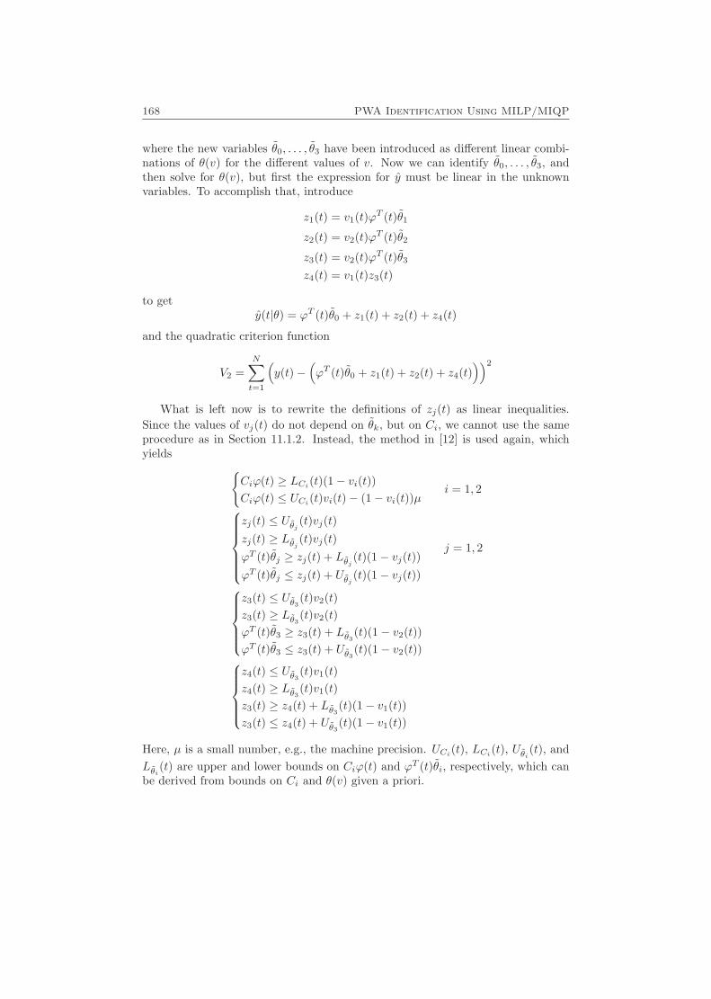
168 PWA Identification Using MILP/MIQP
where the new variables θ0, . . . , θ3 have been introduced as different linear combi-nations of θ(v) for the different values of v. Now we can identify θ0, . . . , θ3, andthen solve for θ(v), but first the expression for y must be linear in the unknownvariables. To accomplish that, introduce
z1(t) = v1(t)ϕT (t)θ1
z2(t) = v2(t)ϕT (t)θ2
z3(t) = v2(t)ϕT (t)θ3
z4(t) = v1(t)z3(t)
to gety(t|θ) = ϕT (t)θ0 + z1(t) + z2(t) + z4(t)
and the quadratic criterion function
V2 =N∑t=1
(y(t)−
(ϕT (t)θ0 + z1(t) + z2(t) + z4(t)
))2
What is left now is to rewrite the definitions of zj(t) as linear inequalities.Since the values of vj(t) do not depend on θk, but on Ci, we cannot use the sameprocedure as in Section 11.1.2. Instead, the method in [12] is used again, whichyields {
Ciϕ(t) ≥ LCi(t)(1− vi(t))Ciϕ(t) ≤ UCi(t)vi(t)− (1− vi(t))µ
i = 1, 2zj(t) ≤ Uθj (t)vj(t)zj(t) ≥ Lθj (t)vj(t)ϕT (t)θj ≥ zj(t) + Lθj (t)(1− vj(t))ϕT (t)θj ≤ zj(t) + Uθj (t)(1− vj(t))
j = 1, 2
z3(t) ≤ Uθ3(t)v2(t)z3(t) ≥ Lθ3(t)v2(t)ϕT (t)θ3 ≥ z3(t) + Lθ3(t)(1− v2(t))ϕT (t)θ3 ≤ z3(t) + Uθ3(t)(1− v2(t))z4(t) ≤ Uθ3(t)v1(t)z4(t) ≥ Lθ3(t)v1(t)z3(t) ≥ z4(t) + Lθ3(t)(1− v1(t))z3(t) ≤ z4(t) + Uθ3(t)(1− v1(t))
Here, µ is a small number, e.g., the machine precision. UCi(t), LCi(t), Uθi(t), andLθi(t) are upper and lower bounds on Ciϕ(t) and ϕT (t)θi, respectively, which canbe derived from bounds on Ci and θ(v) given a priori.
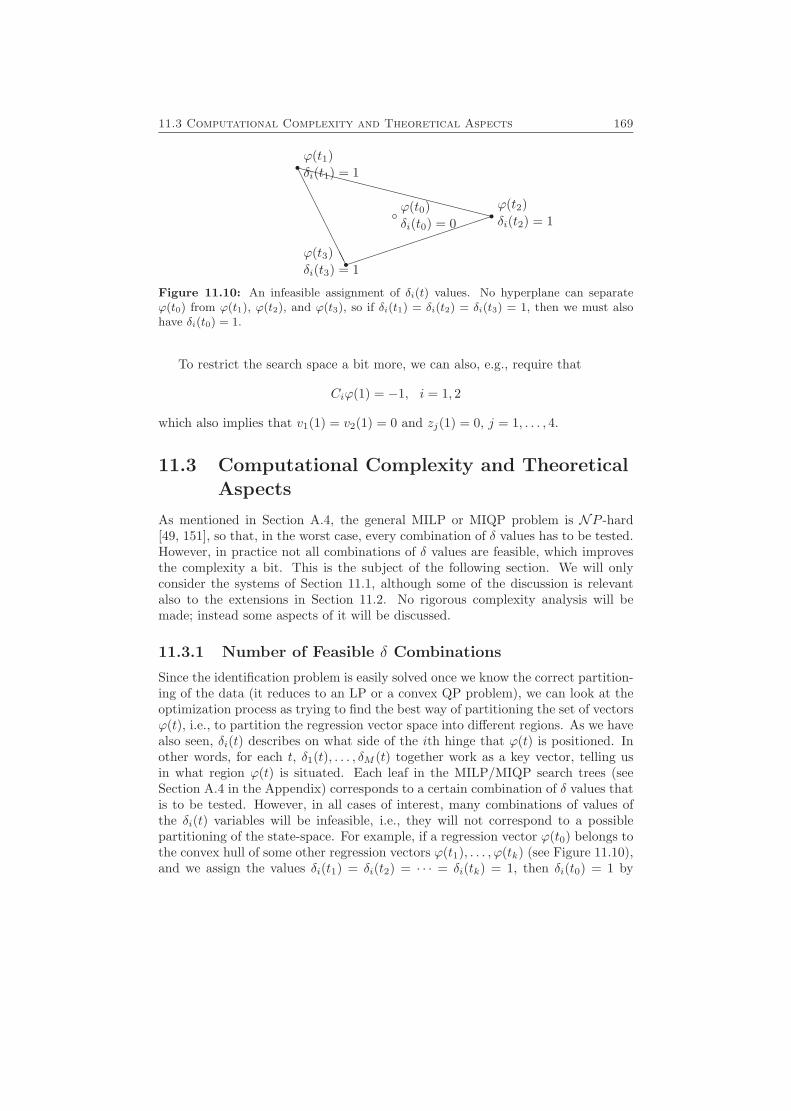
11.3 Computational Complexity and Theoretical Aspects 169
rr
rb
AAAAAAAA��
����
�����XX
XXXXXX
XXXXXX
X
ϕ(t0)δi(t0) = 0
ϕ(t1)δi(t1) = 1
ϕ(t2)δi(t2) = 1
ϕ(t3)δi(t3) = 1
Figure 11.10: An infeasible assignment of δi(t) values. No hyperplane can separateϕ(t0) from ϕ(t1), ϕ(t2), and ϕ(t3), so if δi(t1) = δi(t2) = δi(t3) = 1, then we must alsohave δi(t0) = 1.
To restrict the search space a bit more, we can also, e.g., require that
Ciϕ(1) = −1, i = 1, 2
which also implies that v1(1) = v2(1) = 0 and zj(1) = 0, j = 1, . . . , 4.
11.3 Computational Complexity and TheoreticalAspects
As mentioned in Section A.4, the general MILP or MIQP problem is NP -hard[49, 151], so that, in the worst case, every combination of δ values has to be tested.However, in practice not all combinations of δ values are feasible, which improvesthe complexity a bit. This is the subject of the following section. We will onlyconsider the systems of Section 11.1, although some of the discussion is relevantalso to the extensions in Section 11.2. No rigorous complexity analysis will bemade; instead some aspects of it will be discussed.
11.3.1 Number of Feasible δ Combinations
Since the identification problem is easily solved once we know the correct partition-ing of the data (it reduces to an LP or a convex QP problem), we can look at theoptimization process as trying to find the best way of partitioning the set of vectorsϕ(t), i.e., to partition the regression vector space into different regions. As we havealso seen, δi(t) describes on what side of the ith hinge that ϕ(t) is positioned. Inother words, for each t, δ1(t), . . . , δM (t) together work as a key vector, telling usin what region ϕ(t) is situated. Each leaf in the MILP/MIQP search trees (seeSection A.4 in the Appendix) corresponds to a certain combination of δ values thatis to be tested. However, in all cases of interest, many combinations of values ofthe δi(t) variables will be infeasible, i.e., they will not correspond to a possiblepartitioning of the state-space. For example, if a regression vector ϕ(t0) belongs tothe convex hull of some other regression vectors ϕ(t1), . . . , ϕ(tk) (see Figure 11.10),and we assign the values δi(t1) = δi(t2) = · · · = δi(tk) = 1, then δi(t0) = 1 by
170 PWA Identification Using MILP/MIQP
necessity, since no hyperplane ϕT θi = 0 can separate ϕ(t0) from ϕ(t1), . . . , ϕ(tk).The natural question arises: How many feasible combinations of δi(t) values arethere?
If the dimension of ϕ(t) equals n + 1, the question can also be formulated as:In how many ways can we group N points in Rn (that is, the points composed byelements number 2 to n+ 1 of ϕ(t), t = 1, . . . , N) by separating them with M hy-perplanes? This question is answered in Corollary A.2. Note that ϕ(t) correspondsexactly to the vectors used in the proof of Corollary A.1, since the first element ofϕ(t) always equals 1.
To be able to use Corollary A.2, we need the data to be in general position,but since – according to Section A.5 – for a randomly chosen set of points in Rn,this condition should be satisfied with probability one, the restriction should notbe too serious, especially if we assume white noise in our experimental data.
We assume that M and M+ are known, and that the data set is persistentlyexciting. This implies that trivial partitions like having one hinge going outsidethe data set, or several hinges positioned at the same place, are – albeit feasible –unnecessary to try.
We also have to remember that some of the hinge functions should be positiveand some negative. This will increase the number of δ combinations that have tobe tested, since at each possible position for a hinge, both a positive and a negativehinge function has to be tested.
We summarize the previous discussion in the following corollary:
Corollary 11.1Assume that N samples of data in general position are given, and that a hinginghyperplane model with M+ positive and M− = M −M+ negative hinge functionsshould be fitted to it, using (11.11) or (11.12). Then the number of combinationsof values of δi(t) that have to be tested equals
fδ(n,N,M,M+) =(f(n+ 1, N)/2− 1
M
)·(M
M+
)(11.43)
where
f(n,N) = 2n−1∑k=0
(N − 1k
)
Proof According to Corollary A.2, there are(f(n+1,N)/2−1
M
)nontrivial ways in
which a set of N points in Rn can be partitioned by M hyperplanes. For eachpartition, we should decide which of the M hyperplanes that should be hinges ofthe positive hinge functions. In other words, out of M hinge functions, we shouldchoose M+ to be positive. �
A MILP/MIQP search tree with only the feasible, nontrivial solutions as leaves,and the other cut away, would therefore have fδ(n,N,M,M+) leaves, and conse-quently contain 2fδ(n,N,M,M+)−1 nodes altogether. Table 11.2 lists some values
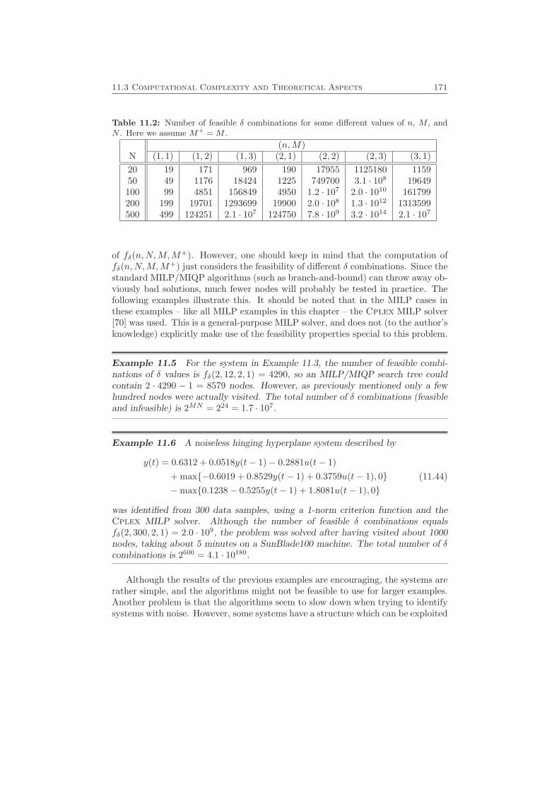
11.3 Computational Complexity and Theoretical Aspects 171
Table 11.2: Number of feasible δ combinations for some different values of n, M , andN . Here we assume M+ = M .
(n,M)N (1, 1) (1, 2) (1, 3) (2, 1) (2, 2) (2, 3) (3, 1)20 19 171 969 190 17955 1125180 115950 49 1176 18424 1225 749700 3.1 · 108 19649100 99 4851 156849 4950 1.2 · 107 2.0 · 1010 161799200 199 19701 1293699 19900 2.0 · 108 1.3 · 1012 1313599500 499 124251 2.1 · 107 124750 7.8 · 109 3.2 · 1014 2.1 · 107
of fδ(n,N,M,M+). However, one should keep in mind that the computation offδ(n,N,M,M+) just considers the feasibility of different δ combinations. Since thestandard MILP/MIQP algorithms (such as branch-and-bound) can throw away ob-viously bad solutions, much fewer nodes will probably be tested in practice. Thefollowing examples illustrate this. It should be noted that in the MILP cases inthese examples – like all MILP examples in this chapter – the Cplex MILP solver[70] was used. This is a general-purpose MILP solver, and does not (to the author’sknowledge) explicitly make use of the feasibility properties special to this problem.
Example 11.5 For the system in Example 11.3, the number of feasible combi-nations of δ values is fδ(2, 12, 2, 1) = 4290, so an MILP/MIQP search tree couldcontain 2 · 4290 − 1 = 8579 nodes. However, as previously mentioned only a fewhundred nodes were actually visited. The total number of δ combinations (feasibleand infeasible) is 2MN = 224 = 1.7 · 107.
Example 11.6 A noiseless hinging hyperplane system described by
y(t) = 0.6312 + 0.0518y(t− 1)− 0.2881u(t− 1)+ max{−0.6019 + 0.8529y(t− 1) + 0.3759u(t− 1), 0}−max{0.1238− 0.5255y(t− 1) + 1.8081u(t− 1), 0}
(11.44)
was identified from 300 data samples, using a 1-norm criterion function and theCplex MILP solver. Although the number of feasible δ combinations equalsfδ(2, 300, 2, 1) = 2.0 · 109, the problem was solved after having visited about 1000nodes, taking about 5 minutes on a SunBlade100 machine. The total number of δcombinations is 2600 = 4.1 · 10180.
Although the results of the previous examples are encouraging, the systems arerather simple, and the algorithms might not be feasible to use for larger examples.Another problem is that the algorithms seem to slow down when trying to identifysystems with noise. However, some systems have a structure which can be exploited
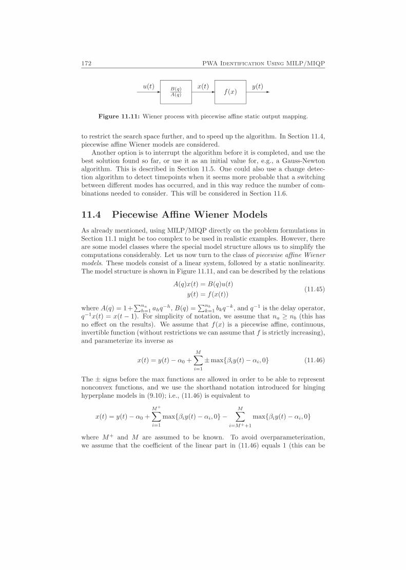
172 PWA Identification Using MILP/MIQP
B(q)A(q) f(x)- --u(t) x(t) y(t)
Figure 11.11: Wiener process with piecewise affine static output mapping.
to restrict the search space further, and to speed up the algorithm. In Section 11.4,piecewise affine Wiener models are considered.
Another option is to interrupt the algorithm before it is completed, and use thebest solution found so far, or use it as an initial value for, e.g., a Gauss-Newtonalgorithm. This is described in Section 11.5. One could also use a change detec-tion algorithm to detect timepoints when it seems more probable that a switchingbetween different modes has occurred, and in this way reduce the number of com-binations needed to consider. This will be considered in Section 11.6.
11.4 Piecewise Affine Wiener Models
As already mentioned, using MILP/MIQP directly on the problem formulations inSection 11.1 might be too complex to be used in realistic examples. However, thereare some model classes where the special model structure allows us to simplify thecomputations considerably. Let us now turn to the class of piecewise affine Wienermodels. These models consist of a linear system, followed by a static nonlinearity.The model structure is shown in Figure 11.11, and can be described by the relations
A(q)x(t) = B(q)u(t)y(t) = f(x(t))
(11.45)
where A(q) = 1+∑nah=1 ahq
−h, B(q) =∑nbk=1 bkq
−k, and q−1 is the delay operator,q−1x(t) = x(t − 1). For simplicity of notation, we assume that na ≥ nb (this hasno effect on the results). We assume that f(x) is a piecewise affine, continuous,invertible function (without restrictions we can assume that f is strictly increasing),and parameterize its inverse as
x(t) = y(t)− α0 +M∑i=1
±max{βiy(t)− αi, 0} (11.46)
The ± signs before the max functions are allowed in order to be able to representnonconvex functions, and we use the shorthand notation introduced for hinginghyperplane models in (9.10); i.e., (11.46) is equivalent to
x(t) = y(t)− α0 +M+∑i=1
max{βiy(t)− αi, 0} −M∑
i=M++1
max{βiy(t)− αi, 0}
where M+ and M are assumed to be known. To avoid overparameterization,we assume that the coefficient of the linear part in (11.46) equals 1 (this can be
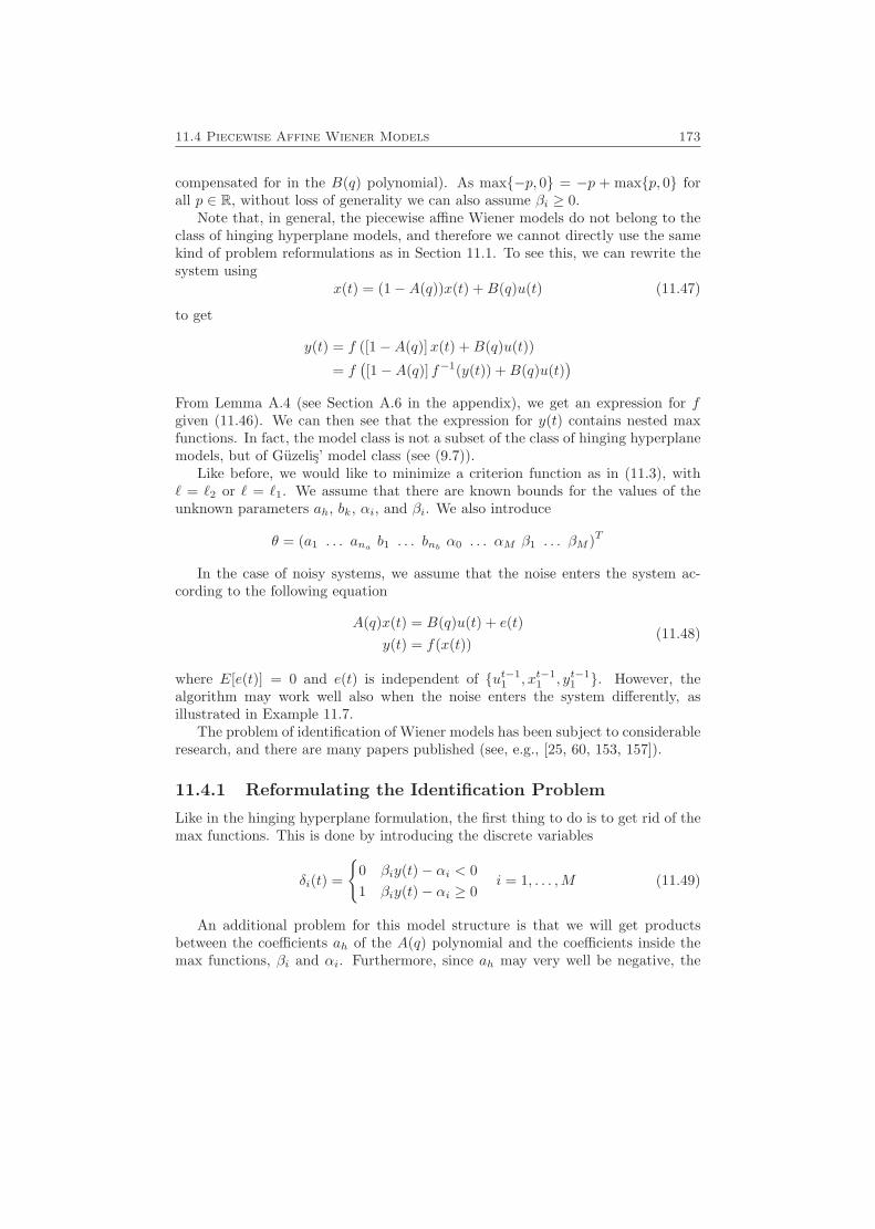
11.4 Piecewise Affine Wiener Models 173
compensated for in the B(q) polynomial). As max{−p, 0} = −p + max{p, 0} forall p ∈ R, without loss of generality we can also assume βi ≥ 0.
Note that, in general, the piecewise affine Wiener models do not belong to theclass of hinging hyperplane models, and therefore we cannot directly use the samekind of problem reformulations as in Section 11.1. To see this, we can rewrite thesystem using
x(t) = (1−A(q))x(t) +B(q)u(t) (11.47)
to get
y(t) = f ([1−A(q)]x(t) +B(q)u(t))
= f([1−A(q)] f−1(y(t)) +B(q)u(t)
)From Lemma A.4 (see Section A.6 in the appendix), we get an expression for fgiven (11.46). We can then see that the expression for y(t) contains nested maxfunctions. In fact, the model class is not a subset of the class of hinging hyperplanemodels, but of Guzelis’ model class (see (9.7)).
Like before, we would like to minimize a criterion function as in (11.3), with` = `2 or ` = `1. We assume that there are known bounds for the values of theunknown parameters ah, bk, αi, and βi. We also introduce
θ = (a1 . . . ana b1 . . . bnb α0 . . . αM β1 . . . βM )T
In the case of noisy systems, we assume that the noise enters the system ac-cording to the following equation
A(q)x(t) = B(q)u(t) + e(t)y(t) = f(x(t))
(11.48)
where E[e(t)] = 0 and e(t) is independent of {ut−11 , xt−1
1 , yt−11 }. However, the
algorithm may work well also when the noise enters the system differently, asillustrated in Example 11.7.
The problem of identification of Wiener models has been subject to considerableresearch, and there are many papers published (see, e.g., [25, 60, 153, 157]).
11.4.1 Reformulating the Identification Problem
Like in the hinging hyperplane formulation, the first thing to do is to get rid of themax functions. This is done by introducing the discrete variables
δi(t) =
{0 βiy(t)− αi < 01 βiy(t)− αi ≥ 0
i = 1, . . . ,M (11.49)
An additional problem for this model structure is that we will get productsbetween the coefficients ah of the A(q) polynomial and the coefficients inside themax functions, βi and αi. Furthermore, since ah may very well be negative, the
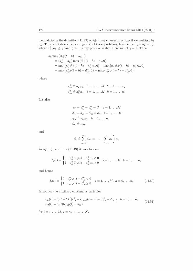
174 PWA Identification Using MILP/MIQP
inequalities in the definition (11.49) of δi(t) may change directions if we multiply byah. This is not desirable, so to get rid of these problems, first define ah = a+
h −a−h ,
where a+h , a
−h ≥ γ, and γ > 0 is any positive scalar. Here we let γ = 1. Then
ah max{βiy(t− h)− αi, 0}= (a+
h − a−h ) max{βiy(t− h)− αi, 0}
= max{a+h βiy(t− h)− a+
h αi, 0} −max{a−h βiy(t− h)− a−h αi, 0}= max{c+ihy(t− h)− d+
ih, 0} −max{c−ihy(t− h)− d−ih, 0}
where
c±ih , a±h βi, i = 1, . . . ,M, h = 1, . . . , na
d±ih , a±h αi, i = 1, . . . ,M, h = 1, . . . , na
Let also
ci0 = c+i0 = c−i0 , βi, i = 1, . . . ,M
di0 = d+i0 = d−i0 , αi, i = 1, . . . ,M
d0h , ahα0, h = 1, . . . , na
d00 , α0,
and
d0 ,na∑h=0
d0h =
(1 +
na∑h=1
ah
)α0
As a+h , a
−h > 0, from (11.49) it now follows
δi(t) =
{0 a±h βiy(t)− a±h αi < 01 a±h βiy(t)− a±h αi ≥ 0
i = 1, . . . ,M, h = 1, . . . , na
and hence
δi(t) =
{0 c±ihy(t)− d±ih < 01 c±ihy(t)− d±ih ≥ 0
i = 1, . . . ,M, h = 0, . . . , na (11.50)
Introduce the auxiliary continuous variables
zih(t) = δi(t− h)((c+ih − c
−ih)y(t− h)− (d+
ih − d−ih)), h = 1, . . . , na
zi0(t) = δi(t)(ci0y(t)− di0)(11.51)
for i = 1, . . . ,M , t = na + 1, . . . , N .
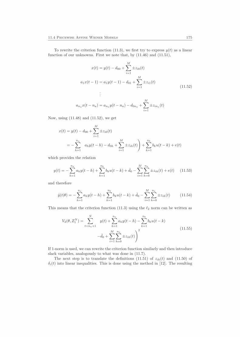
11.4 Piecewise Affine Wiener Models 175
To rewrite the criterion function (11.3), we first try to express y(t) as a linearfunction of our unknowns. First we note that, by (11.46) and (11.51),
x(t) = y(t)− d00 +M∑i=1
±zi0(t)
a1x(t− 1) = a1y(t− 1)− d01 +M∑i=1
±zi1(t)
...
anax(t− na) = anay(t− na)− d0na +M∑i=1
±zina(t)
(11.52)
Now, using (11.48) and (11.52), we get
x(t) = y(t)− d00 +M∑i=1
±zi0(t)
= −na∑h=1
(ahy(t− h)− d0h +
M∑i=1
±zih(t)
)+
nb∑k=1
bku(t− k) + e(t)
which provides the relation
y(t) = −na∑h=1
ahy(t− h) +nb∑k=1
bku(t− k) + d0 −M∑i=1
na∑h=0
±zih(t) + e(t) (11.53)
and therefore
y(t|θ) = −na∑h=1
ahy(t− h) +nb∑k=1
bku(t− k) + d0 −M∑i=1
na∑h=0
±zih(t) (11.54)
This means that the criterion function (11.3) using the `2 norm can be written as
V2(θ, ZN1 ) =N∑
t=na+1
(y(t) +
na∑h=1
ahy(t− h)−nb∑k=1
bku(t− k)
−d0 +M∑i=1
na∑h=0
±zih(t)
)2 (11.55)
If 1-norm is used, we can rewrite the criterion function similarly and then introduceslack variables, analogously to what was done in (11.7).
The next step is to translate the definitions (11.51) of zih(t) and (11.50) ofδi(t) into linear inequalities. This is done using the method in [12]. The resulting
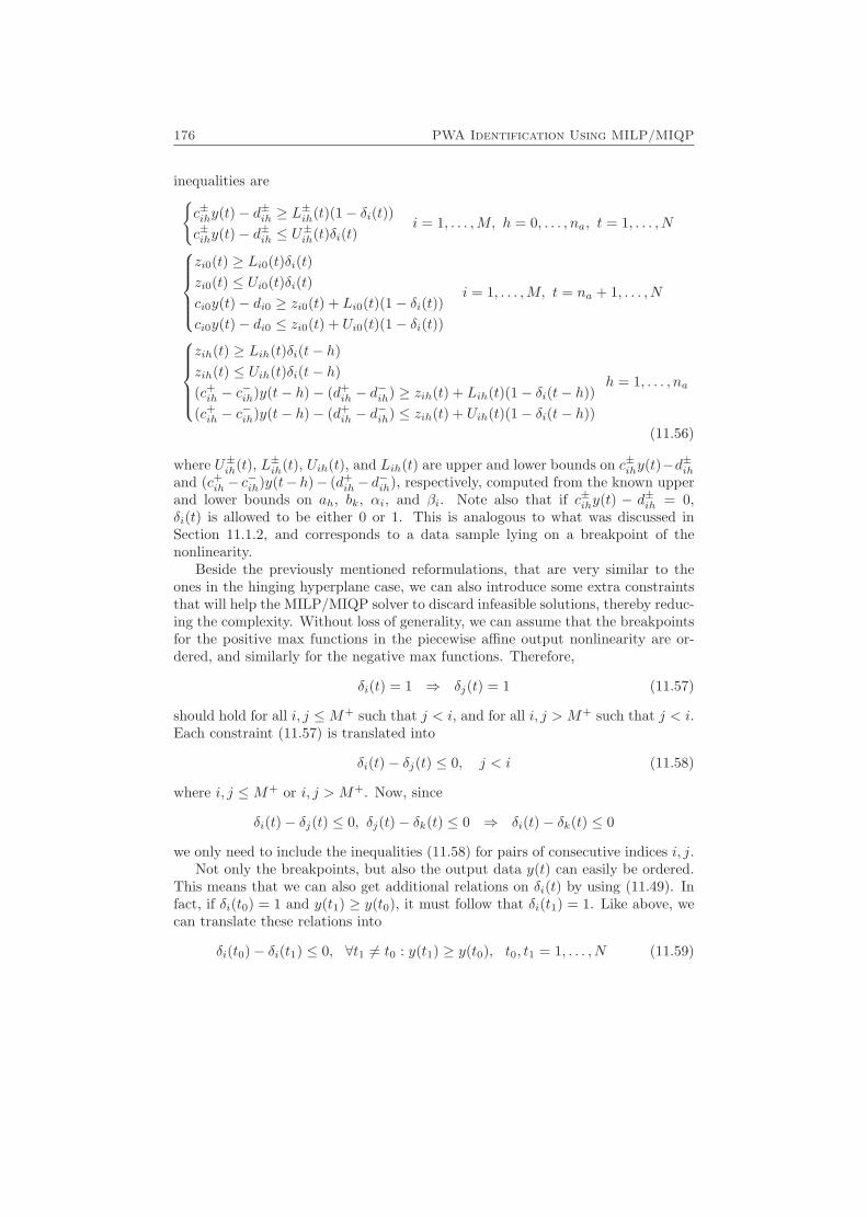
176 PWA Identification Using MILP/MIQP
inequalities are{c±ihy(t)− d±ih ≥ L
±ih(t)(1− δi(t))
c±ihy(t)− d±ih ≤ U±ih(t)δi(t)
i = 1, . . . ,M, h = 0, . . . , na, t = 1, . . . , Nzi0(t) ≥ Li0(t)δi(t)zi0(t) ≤ Ui0(t)δi(t)ci0y(t)− di0 ≥ zi0(t) + Li0(t)(1− δi(t))ci0y(t)− di0 ≤ zi0(t) + Ui0(t)(1− δi(t))
i = 1, . . . ,M, t = na + 1, . . . , N
zih(t) ≥ Lih(t)δi(t− h)zih(t) ≤ Uih(t)δi(t− h)(c+ih − c
−ih)y(t− h)− (d+
ih − d−ih) ≥ zih(t) + Lih(t)(1− δi(t− h))
(c+ih − c−ih)y(t− h)− (d+
ih − d−ih) ≤ zih(t) + Uih(t)(1− δi(t− h))
h = 1, . . . , na
(11.56)
where U±ih(t), L±ih(t), Uih(t), and Lih(t) are upper and lower bounds on c±ihy(t)−d±ihand (c+ih− c
−ih)y(t− h)− (d+
ih− d−ih), respectively, computed from the known upper
and lower bounds on ah, bk, αi, and βi. Note also that if c±ihy(t) − d±ih = 0,δi(t) is allowed to be either 0 or 1. This is analogous to what was discussed inSection 11.1.2, and corresponds to a data sample lying on a breakpoint of thenonlinearity.
Beside the previously mentioned reformulations, that are very similar to theones in the hinging hyperplane case, we can also introduce some extra constraintsthat will help the MILP/MIQP solver to discard infeasible solutions, thereby reduc-ing the complexity. Without loss of generality, we can assume that the breakpointsfor the positive max functions in the piecewise affine output nonlinearity are or-dered, and similarly for the negative max functions. Therefore,
δi(t) = 1 ⇒ δj(t) = 1 (11.57)
should hold for all i, j ≤M+ such that j < i, and for all i, j > M+ such that j < i.Each constraint (11.57) is translated into
δi(t)− δj(t) ≤ 0, j < i (11.58)
where i, j ≤M+ or i, j > M+. Now, since
δi(t)− δj(t) ≤ 0, δj(t)− δk(t) ≤ 0 ⇒ δi(t)− δk(t) ≤ 0
we only need to include the inequalities (11.58) for pairs of consecutive indices i, j.Not only the breakpoints, but also the output data y(t) can easily be ordered.
This means that we can also get additional relations on δi(t) by using (11.49). Infact, if δi(t0) = 1 and y(t1) ≥ y(t0), it must follow that δi(t1) = 1. Like above, wecan translate these relations into
δi(t0)− δi(t1) ≤ 0, ∀t1 6= t0 : y(t1) ≥ y(t0), t0, t1 = 1, . . . , N (11.59)
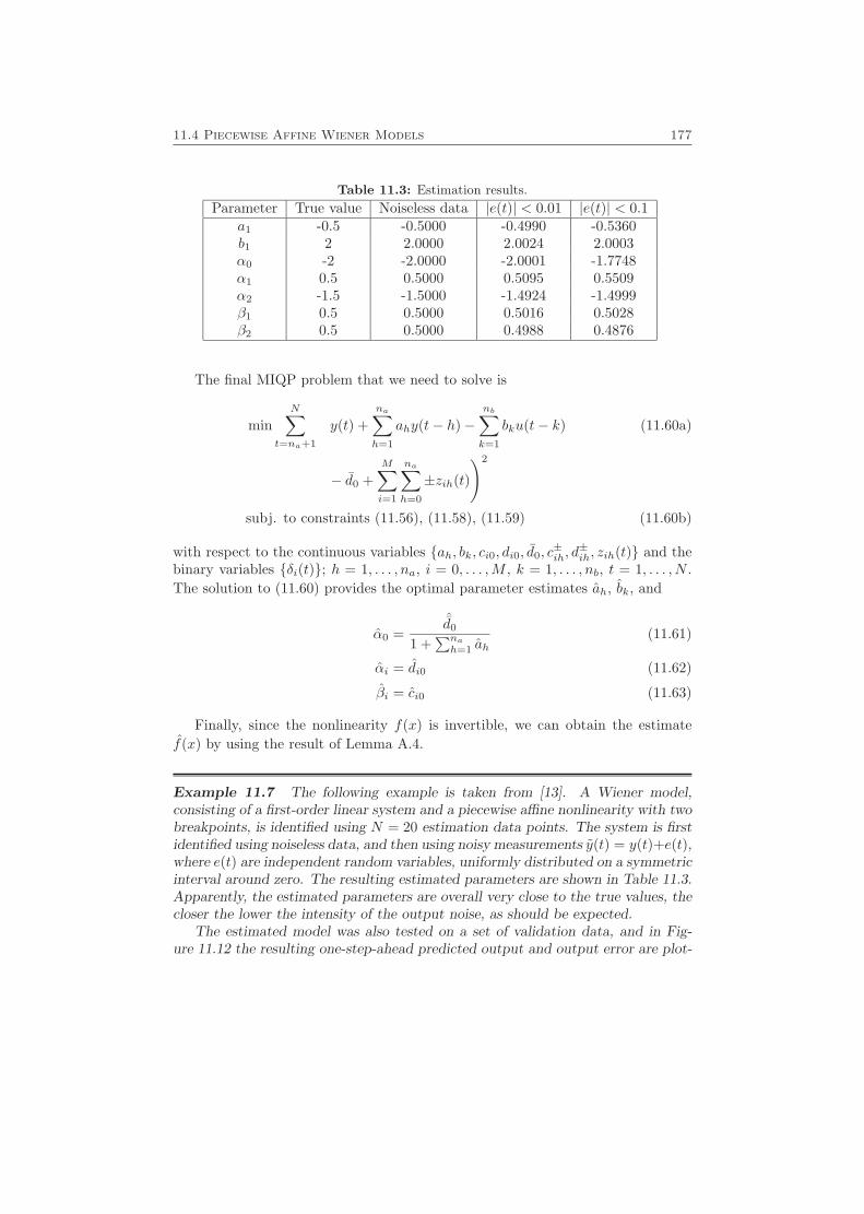
11.4 Piecewise Affine Wiener Models 177
Table 11.3: Estimation results.
Parameter True value Noiseless data |e(t)| < 0.01 |e(t)| < 0.1a1 -0.5 -0.5000 -0.4990 -0.5360b1 2 2.0000 2.0024 2.0003α0 -2 -2.0000 -2.0001 -1.7748α1 0.5 0.5000 0.5095 0.5509α2 -1.5 -1.5000 -1.4924 -1.4999β1 0.5 0.5000 0.5016 0.5028β2 0.5 0.5000 0.4988 0.4876
The final MIQP problem that we need to solve is
minN∑
t=na+1
(y(t) +
na∑h=1
ahy(t− h)−nb∑k=1
bku(t− k) (11.60a)
− d0 +M∑i=1
na∑h=0
±zih(t)
)2
subj. to constraints (11.56), (11.58), (11.59) (11.60b)
with respect to the continuous variables {ah, bk, ci0, di0, d0, c±ih, d
±ih, zih(t)} and the
binary variables {δi(t)}; h = 1, . . . , na, i = 0, . . . ,M , k = 1, . . . , nb, t = 1, . . . , N .The solution to (11.60) provides the optimal parameter estimates ah, bk, and
α0 =ˆd0
1 +∑nah=1 ah
(11.61)
αi = di0 (11.62)
βi = ci0 (11.63)
Finally, since the nonlinearity f(x) is invertible, we can obtain the estimatef(x) by using the result of Lemma A.4.
Example 11.7 The following example is taken from [13]. A Wiener model,consisting of a first-order linear system and a piecewise affine nonlinearity with twobreakpoints, is identified using N = 20 estimation data points. The system is firstidentified using noiseless data, and then using noisy measurements y(t) = y(t)+e(t),where e(t) are independent random variables, uniformly distributed on a symmetricinterval around zero. The resulting estimated parameters are shown in Table 11.3.Apparently, the estimated parameters are overall very close to the true values, thecloser the lower the intensity of the output noise, as should be expected.
The estimated model was also tested on a set of validation data, and in Fig-ure 11.12 the resulting one-step-ahead predicted output and output error are plot-
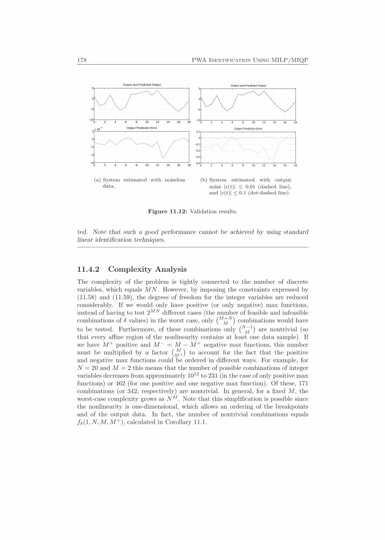
178 PWA Identification Using MILP/MIQP
0 2 4 6 8 10 12 14 16 18−10
−5
0
5Output and Predicted Output
0 2 4 6 8 10 12 14 16 18−6
−4
−2
0
2x 10
−5 Output Prediction Error
(a) System estimated with noiselessdata.
0 2 4 6 8 10 12 14 16 18−10
−5
0
5Output and Predicted Output
0 2 4 6 8 10 12 14 16 18−0.4
−0.3
−0.2
−0.1
0
0.1Output Prediction Error
(b) System estimated with output
noise |e(t)| ≤ 0.01 (dashed line),and |e(t)| ≤ 0.1 (dot-dashed line).
Figure 11.12: Validation results.
ted. Note that such a good performance cannot be achieved by using standardlinear identification techniques.
11.4.2 Complexity Analysis
The complexity of the problem is tightly connected to the number of discretevariables, which equals MN . However, by imposing the constraints expressed by(11.58) and (11.59), the degrees of freedom for the integer variables are reducedconsiderably. If we would only have positive (or only negative) max functions,instead of having to test 2MN different cases (the number of feasible and infeasiblecombinations of δ values) in the worst case, only
(M+NM
)combinations would have
to be tested. Furthermore, of these combinations only(N−1M
)are nontrivial (so
that every affine region of the nonlinearity contains at least one data sample). Ifwe have M+ positive and M− = M −M+ negative max functions, this numbermust be multiplied by a factor
(MM+
)to account for the fact that the positive
and negative max functions could be ordered in different ways. For example, forN = 20 and M = 2 this means that the number of possible combinations of integervariables decreases from approximately 1012 to 231 (in the case of only positive maxfunctions) or 462 (for one positive and one negative max function). Of these, 171combinations (or 342, respectively) are nontrivial. In general, for a fixed M , theworst-case complexity grows as NM . Note that this simplification is possible sincethe nonlinearity is one-dimensional, which allows an ordering of the breakpointsand of the output data. In fact, the number of nontrivial combinations equalsfδ(1, N,M,M+), calculated in Corollary 11.1.

11.5 Using Suboptimal MILP/MIQP Solutions 179
11.5 Using Suboptimal MILP/MIQP Solutions
One advantage with the MILP/MIQP algorithms is that they give intermediateresults, which are suboptimal, but get better and better the longer the algorithmruns. This feature could be used for complex MILP/MIQP problems, where thetime to find the optimal solution (and then prove that it really is optimal) mightbe extremely long. Instead of waiting for the optimal solution, one can abort thecomputations and use the best solution found so far.
In the case of piecewise affine system identification, one possibility is to usethe suboptimal solutions obtained from the MILP/MIQP solver as initial valuesfor a standard local minimization algorithm, e.g., Gauss-Newton (see Section 8.2).Finding good initial values for minimization algorithms is an important issue, andhopefully, using the intermediate solutions from MILP/MIQP as initial values givesbetter results than just using randomly picked initial values. Experiments showthat this is often the case. However, it might sometimes take a little while until theMILP/MIQP solver finds suboptimal solutions that are worth using. The followingexamples illustrate this.
Example 11.8 Consider once again the system in Example 11.3 and the 2-normcriterion function. The intermediate results from a simple, straightforward Mat-
lab implementation of an MIQP solver are shown in Table 11.4. The parametersof these suboptimal solutions were then used as initial values of the Matlab opti-mization functions fminsearch and lsqnonlin, and the resulting criterion functionvalues are also found in Table 11.4.
As comparison, a number of random values were given as initial parametersto fminsearch and lsqnonlin. In Figure 11.13, the values obtained by usingthe intermediate results from MIQP as initial values are compared to the meanresult of using random initial values. We can see that already after about 250visited nodes, the combined MIQP/fminsearch and MIQP/lsqnonlin algorithmsperform better than using only fminsearch and lsqnonlin, respectively.
Example 11.9 Consider the system in Example 11.6, but with white noise addedto y(t) in (11.44). The variance of the noise is 0.1, while the input is white noisewith unit variance. The system was identified using 100 such data samples and the1-norm criterion function. The problem was reformulated according to (11.12) andgiven to the Cplex MILP solver. The intermediate solutions were used as initialvalues to the Matlab function fminsearch. Just as in Example 11.8, a numberof random initial values to fminsearch were also used as comparison. Table 11.5shows the resulting values of the criterion function. In Figure 11.14, the values ofthe criterion function are shown as a function of the approximative computationtime for the MILP (on a SunBlade 100). Here, the combined MILP/fminsearchperforms better than using random initial values from the very first intermediateresult produced by the MILP solver.
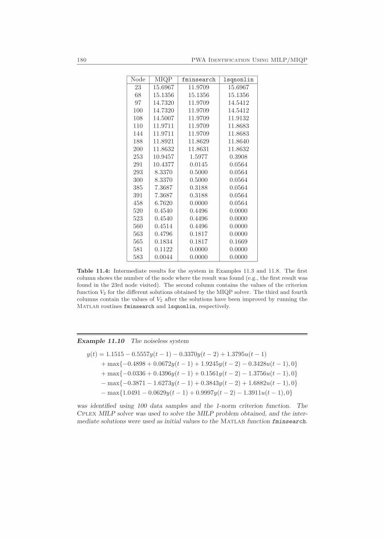
180 PWA Identification Using MILP/MIQP
Node MIQP fminsearch lsqnonlin23 15.6967 11.9709 15.696768 15.1356 15.1356 15.135697 14.7320 11.9709 14.5412100 14.7320 11.9709 14.5412108 14.5007 11.9709 11.9132110 11.9711 11.9709 11.8683144 11.9711 11.9709 11.8683188 11.8921 11.8629 11.8640200 11.8632 11.8631 11.8632253 10.9457 1.5977 0.3908291 10.4377 0.0145 0.0564293 8.3370 0.5000 0.0564300 8.3370 0.5000 0.0564385 7.3687 0.3188 0.0564391 7.3687 0.3188 0.0564458 6.7620 0.0000 0.0564520 0.4540 0.4496 0.0000523 0.4540 0.4496 0.0000560 0.4514 0.4496 0.0000563 0.4796 0.1817 0.0000565 0.1834 0.1817 0.1669581 0.1122 0.0000 0.0000583 0.0044 0.0000 0.0000
Table 11.4: Intermediate results for the system in Examples 11.3 and 11.8. The firstcolumn shows the number of the node where the result was found (e.g., the first result wasfound in the 23rd node visited). The second column contains the values of the criterionfunction V2 for the different solutions obtained by the MIQP solver. The third and fourthcolumns contain the values of V2 after the solutions have been improved by running theMatlab routines fminsearch and lsqnonlin, respectively.
Example 11.10 The noiseless system
y(t) = 1.1515− 0.5557y(t− 1)− 0.3370y(t− 2) + 1.3795u(t− 1)+ max{−0.4898 + 0.0672y(t− 1) + 1.9245y(t− 2)− 0.3428u(t− 1), 0}+ max{−0.0336 + 0.4396y(t− 1) + 0.1561y(t− 2)− 1.3756u(t− 1), 0}−max{−0.3871− 1.6273y(t− 1) + 0.3843y(t− 2) + 1.6882u(t− 1), 0}−max{1.0491− 0.0629y(t− 1) + 0.9997y(t− 2)− 1.3911u(t− 1), 0}
was identified using 100 data samples and the 1-norm criterion function. TheCplex MILP solver was used to solve the MILP problem obtained, and the inter-mediate solutions were used as initial values to the Matlab function fminsearch.
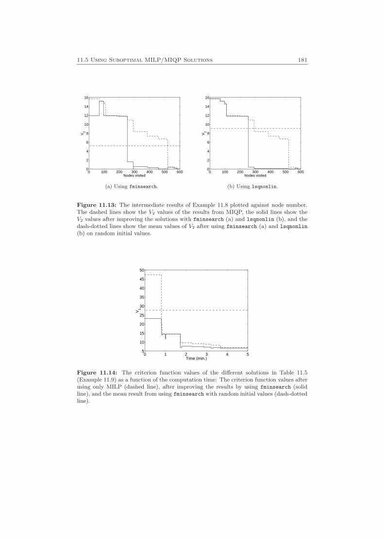
11.5 Using Suboptimal MILP/MIQP Solutions 181
0 100 200 300 400 500 6000
2
4
6
8
10
12
14
16
Nodes visited
V2
(a) Using fminsearch.
0 100 200 300 400 500 6000
2
4
6
8
10
12
14
16
Nodes visited
V2
(b) Using lsqnonlin.
Figure 11.13: The intermediate results of Example 11.8 plotted against node number.The dashed lines show the V2 values of the results from MIQP, the solid lines show theV2 values after improving the solutions with fminsearch (a) and lsqnonlin (b), and thedash-dotted lines show the mean values of V2 after using fminsearch (a) and lsqnonlin
(b) on random initial values.
0 1 2 3 4 55
10
15
20
25
30
35
40
45
50
Time (min.)
V1
Figure 11.14: The criterion function values of the different solutions in Table 11.5(Example 11.9) as a function of the computation time: The criterion function values afterusing only MILP (dashed line), after improving the results by using fminsearch (solidline), and the mean result from using fminsearch with random initial values (dash-dottedline).
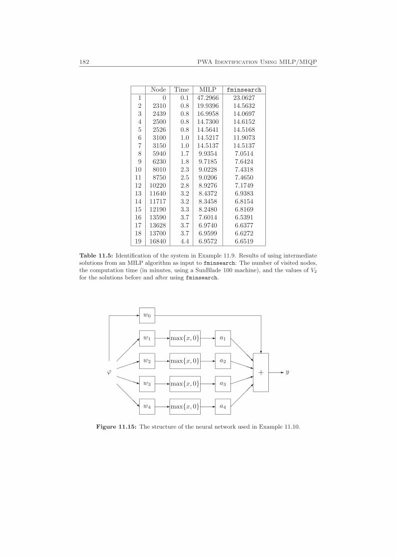
182 PWA Identification Using MILP/MIQP
Node Time MILP fminsearch1 0 0.1 47.2966 23.06272 2310 0.8 19.9396 14.56323 2439 0.8 16.9958 14.06974 2500 0.8 14.7300 14.61525 2526 0.8 14.5641 14.51686 3100 1.0 14.5217 11.90737 3150 1.0 14.5137 14.51378 5940 1.7 9.9354 7.05149 6230 1.8 9.7185 7.6424
10 8010 2.3 9.0228 7.431811 8750 2.5 9.0206 7.465012 10220 2.8 8.9276 7.174913 11640 3.2 8.4372 6.938314 11717 3.2 8.3458 6.815415 12190 3.3 8.2480 6.816916 13590 3.7 7.6014 6.539117 13628 3.7 6.9740 6.637718 13700 3.7 6.9599 6.627219 16840 4.4 6.9572 6.6519
Table 11.5: Identification of the system in Example 11.9. Results of using intermediatesolutions from an MILP algorithm as input to fminsearch: The number of visited nodes,the computation time (in minutes, using a SunBlade 100 machine), and the values of V2
for the solutions before and after using fminsearch.
�����
@@@@R
PPPPq
����1
-
-
-
-@@@@RPPPPq
����1
�����
-
-
?
-
-
-
-
max{x, 0}
max{x, 0}
max{x, 0}
max{x, 0}
w0
w1
w2
w3
w4
a1
a2
a3
a4
ϕ + y
Figure 11.15: The structure of the neural network used in Example 11.10.
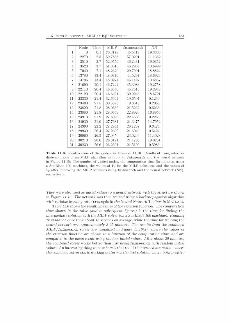
11.5 Using Suboptimal MILP/MIQP Solutions 183
Node Time MILP fminsearch NN1 0 0.1 76.3178 45.5419 19.33662 2270 2.5 59.7858 57.0291 11.13623 3510 3.7 52.9559 46.2431 19.03524 3520 3.7 51.3513 46.2964 10.69995 7040 7.1 48.2320 29.7991 18.88246 13780 13.4 48.0376 44.5297 18.69237 13796 13.4 48.0274 46.1497 10.68678 21690 20.1 46.7244 45.3083 19.27589 22110 20.4 46.6540 45.7513 19.2948
10 22120 20.4 46.6491 39.9945 18.672111 23330 21.4 32.6644 19.6507 0.123912 23490 21.5 30.5823 19.3618 0.206613 23820 21.8 28.0669 21.5232 0.623614 23880 21.8 28.0649 22.8920 16.895415 23910 21.9 27.8096 22.4603 0.226516 24930 21.9 27.7681 24.3475 14.795217 24390 22.2 27.2844 26.1267 0.342418 29930 26.4 27.2509 21.6040 0.542419 30060 26.5 27.0350 23.0246 11.402820 30210 26.6 26.3121 21.1705 19.025121 30230 26.6 26.2591 21.5190 0.5986
Table 11.6: Identification of the system in Example 11.10. Results of using interme-diate solutions of an MILP algorithm as input to fminsearch and the neural networkin Figure 11.15: The number of visited nodes, the computation time (in minutes, usinga SunBlade 100 machine), the values of V2 for the MILP solutions, and the values ofV2 after improving the MILP solutions using fminsearch and the neural network (NN),respectively.
They were also used as initial values to a neural network with the structure shownin Figure 11.15. The network was then trained using a backpropagation algorithmwith variable learning rate (traingdx in the Neural Network Toolbox in Matlab).
Table 11.6 shows the resulting values of the criterion function. The computationtime shown in the table (and in subsequent figures) is the time for finding theintermediate solution with the MILP solver (on a SunBlade 100 machine). Runningfminsearch once took about 15 seconds on average, while the time for training theneural network was approximately 3-25 minutes. The results from the combinedMILP/fminsearch solver are visualized in Figure 11.16(a), where the values ofthe criterion function are shown as a function of the computation time, and arecompared to the mean result using random initial values. After about 20 minutes,the combined solver works better than just using fminsearch with random initialvalues. An interesting thing to note here is that the 11th intermediate result – wherethe combined solver starts working better – is the first solution where both positive
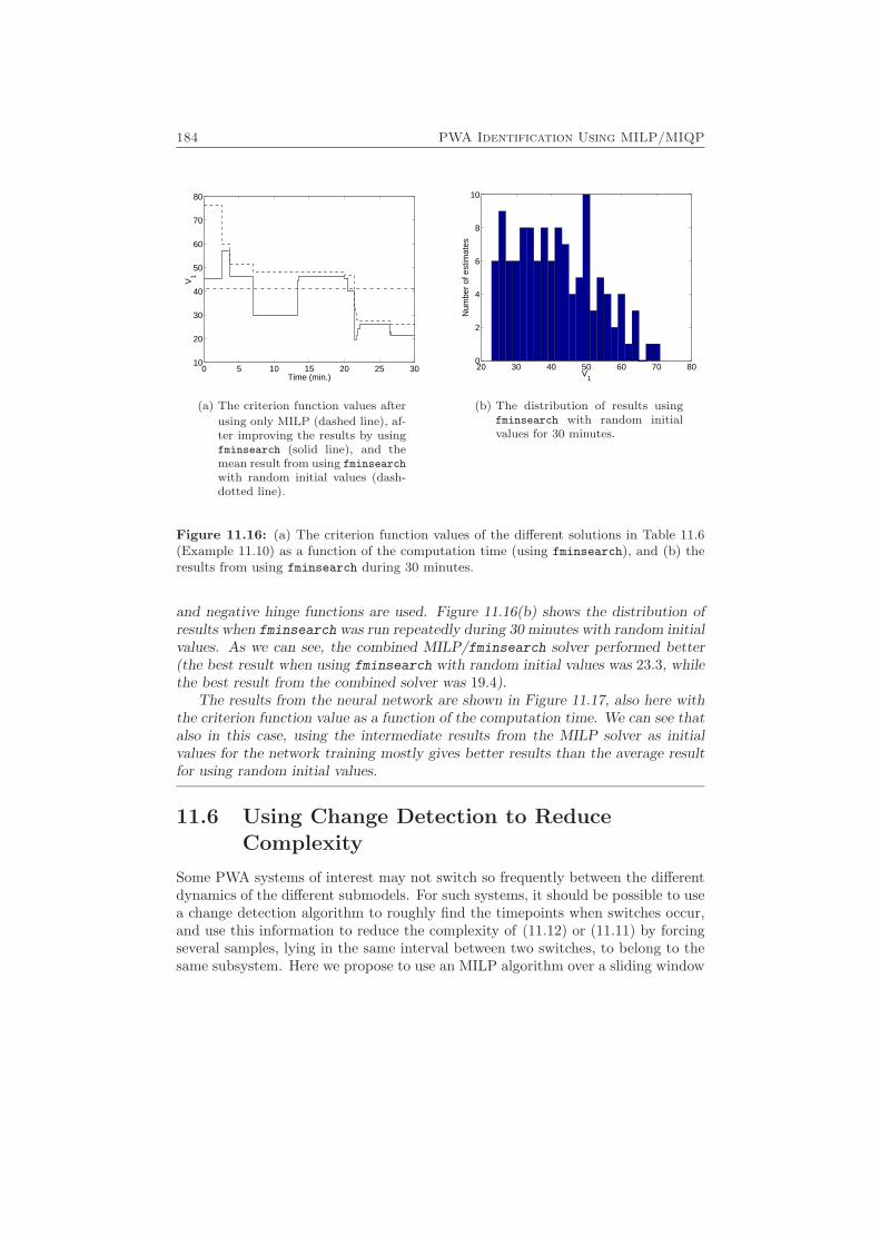
184 PWA Identification Using MILP/MIQP
0 5 10 15 20 25 3010
20
30
40
50
60
70
80
Time (min.)
V1
(a) The criterion function values after
using only MILP (dashed line), af-ter improving the results by usingfminsearch (solid line), and themean result from using fminsearch
with random initial values (dash-dotted line).
20 30 40 50 60 70 800
2
4
6
8
10
V1
Num
ber
of e
stim
ates
(b) The distribution of results usingfminsearch with random initialvalues for 30 minutes.
Figure 11.16: (a) The criterion function values of the different solutions in Table 11.6(Example 11.10) as a function of the computation time (using fminsearch), and (b) theresults from using fminsearch during 30 minutes.
and negative hinge functions are used. Figure 11.16(b) shows the distribution ofresults when fminsearch was run repeatedly during 30 minutes with random initialvalues. As we can see, the combined MILP/fminsearch solver performed better(the best result when using fminsearch with random initial values was 23.3, whilethe best result from the combined solver was 19.4).
The results from the neural network are shown in Figure 11.17, also here withthe criterion function value as a function of the computation time. We can see thatalso in this case, using the intermediate results from the MILP solver as initialvalues for the network training mostly gives better results than the average resultfor using random initial values.
11.6 Using Change Detection to ReduceComplexity
Some PWA systems of interest may not switch so frequently between the differentdynamics of the different submodels. For such systems, it should be possible to usea change detection algorithm to roughly find the timepoints when switches occur,and use this information to reduce the complexity of (11.12) or (11.11) by forcingseveral samples, lying in the same interval between two switches, to belong to thesame subsystem. Here we propose to use an MILP algorithm over a sliding window
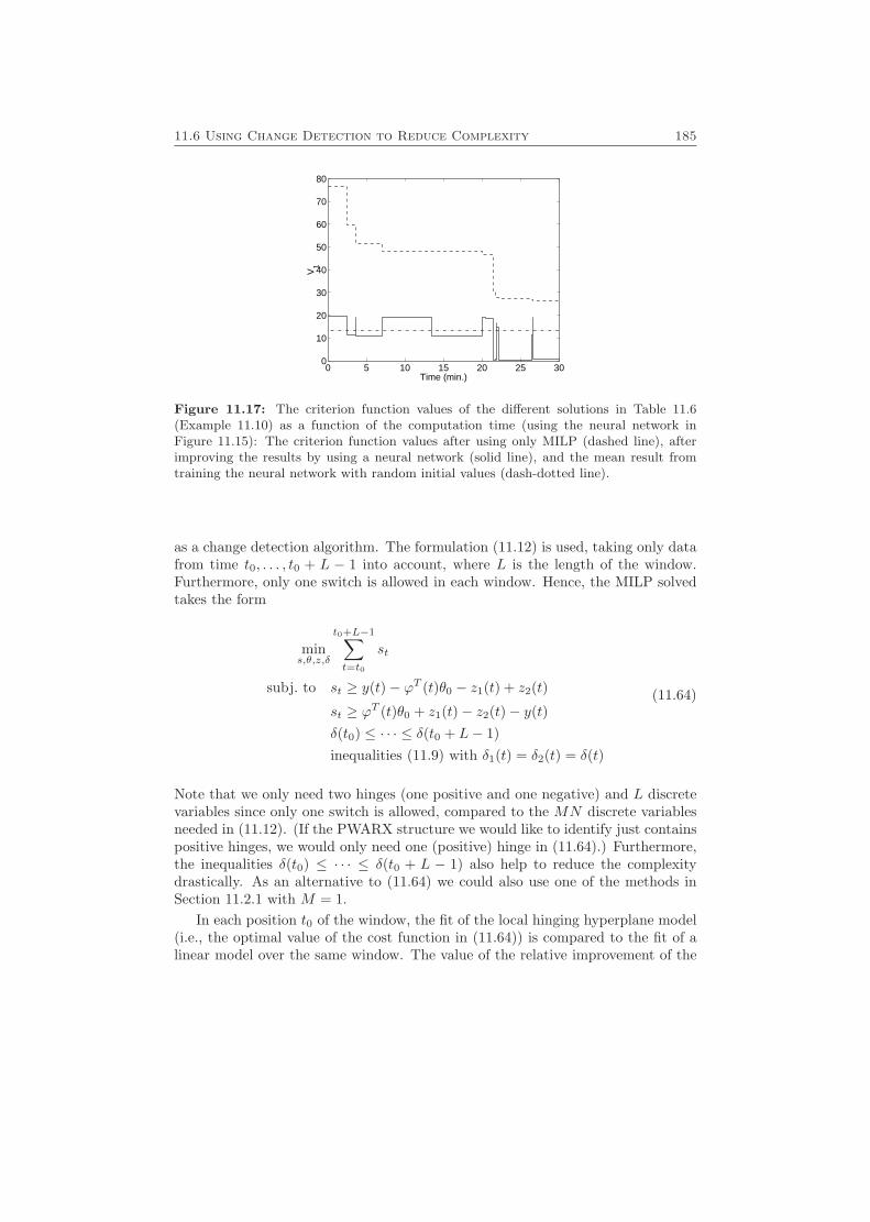
11.6 Using Change Detection to Reduce Complexity 185
0 5 10 15 20 25 300
10
20
30
40
50
60
70
80
Time (min.)
V1
Figure 11.17: The criterion function values of the different solutions in Table 11.6(Example 11.10) as a function of the computation time (using the neural network inFigure 11.15): The criterion function values after using only MILP (dashed line), afterimproving the results by using a neural network (solid line), and the mean result fromtraining the neural network with random initial values (dash-dotted line).
as a change detection algorithm. The formulation (11.12) is used, taking only datafrom time t0, . . . , t0 + L − 1 into account, where L is the length of the window.Furthermore, only one switch is allowed in each window. Hence, the MILP solvedtakes the form
mins,θ,z,δ
t0+L−1∑t=t0
st
subj. to st ≥ y(t)− ϕT (t)θ0 − z1(t) + z2(t)
st ≥ ϕT (t)θ0 + z1(t)− z2(t)− y(t)δ(t0) ≤ · · · ≤ δ(t0 + L− 1)inequalities (11.9) with δ1(t) = δ2(t) = δ(t)
(11.64)
Note that we only need two hinges (one positive and one negative) and L discretevariables since only one switch is allowed, compared to the MN discrete variablesneeded in (11.12). (If the PWARX structure we would like to identify just containspositive hinges, we would only need one (positive) hinge in (11.64).) Furthermore,the inequalities δ(t0) ≤ · · · ≤ δ(t0 + L − 1) also help to reduce the complexitydrastically. As an alternative to (11.64) we could also use one of the methods inSection 11.2.1 with M = 1.
In each position t0 of the window, the fit of the local hinging hyperplane model(i.e., the optimal value of the cost function in (11.64)) is compared to the fit of alinear model over the same window. The value of the relative improvement of the
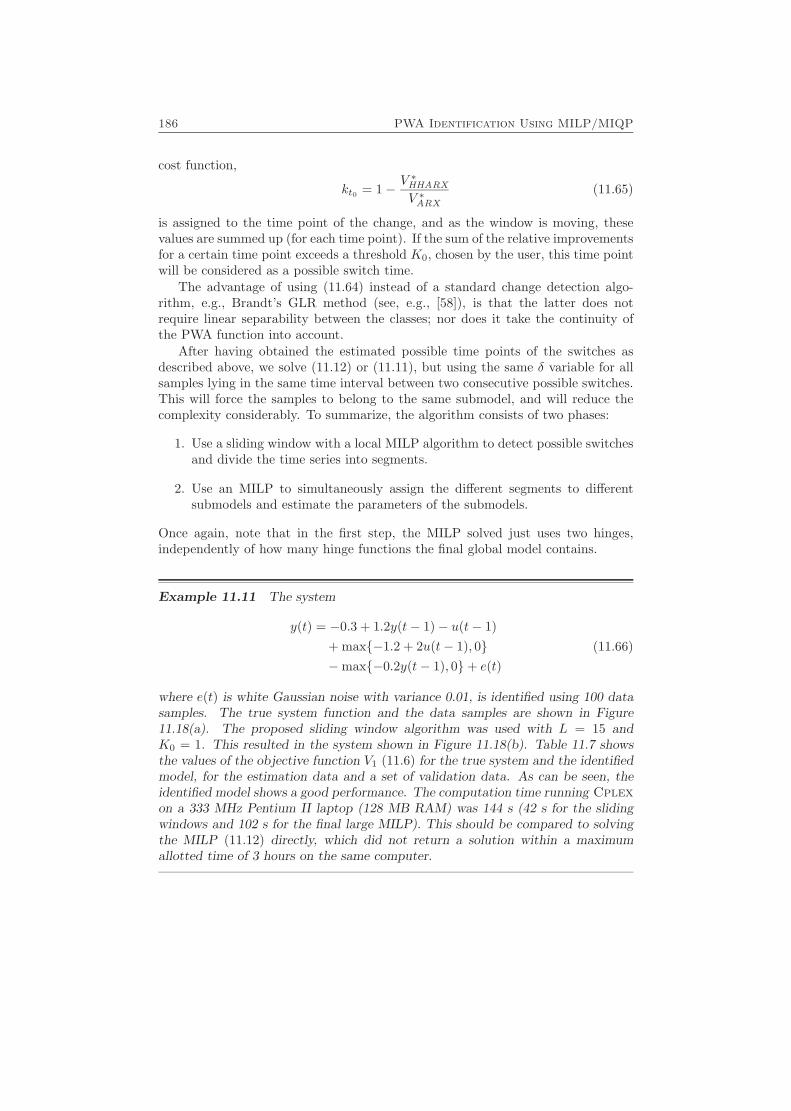
186 PWA Identification Using MILP/MIQP
cost function,
kt0 = 1− V ∗HHARX
V ∗ARX
(11.65)
is assigned to the time point of the change, and as the window is moving, thesevalues are summed up (for each time point). If the sum of the relative improvementsfor a certain time point exceeds a threshold K0, chosen by the user, this time pointwill be considered as a possible switch time.
The advantage of using (11.64) instead of a standard change detection algo-rithm, e.g., Brandt’s GLR method (see, e.g., [58]), is that the latter does notrequire linear separability between the classes; nor does it take the continuity ofthe PWA function into account.
After having obtained the estimated possible time points of the switches asdescribed above, we solve (11.12) or (11.11), but using the same δ variable for allsamples lying in the same time interval between two consecutive possible switches.This will force the samples to belong to the same submodel, and will reduce thecomplexity considerably. To summarize, the algorithm consists of two phases:
1. Use a sliding window with a local MILP algorithm to detect possible switchesand divide the time series into segments.
2. Use an MILP to simultaneously assign the different segments to differentsubmodels and estimate the parameters of the submodels.
Once again, note that in the first step, the MILP solved just uses two hinges,independently of how many hinge functions the final global model contains.
Example 11.11 The system
y(t) = −0.3 + 1.2y(t− 1)− u(t− 1)+ max{−1.2 + 2u(t− 1), 0}−max{−0.2y(t− 1), 0}+ e(t)
(11.66)
where e(t) is white Gaussian noise with variance 0.01, is identified using 100 datasamples. The true system function and the data samples are shown in Figure11.18(a). The proposed sliding window algorithm was used with L = 15 andK0 = 1. This resulted in the system shown in Figure 11.18(b). Table 11.7 showsthe values of the objective function V1 (11.6) for the true system and the identifiedmodel, for the estimation data and a set of validation data. As can be seen, theidentified model shows a good performance. The computation time running Cplex
on a 333 MHz Pentium II laptop (128 MB RAM) was 144 s (42 s for the slidingwindows and 102 s for the final large MILP). This should be compared to solvingthe MILP (11.12) directly, which did not return a solution within a maximumallotted time of 3 hours on the same computer.
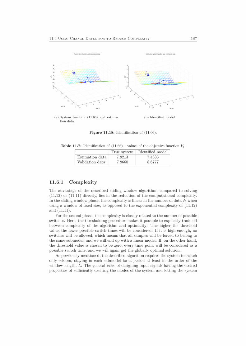
11.6 Using Change Detection to Reduce Complexity 187
−3−2
−10
12
3
−3
−2
−1
0
1
2
3
−3
−2
−1
0
1
2
3
−y(t−1)
True system function and estimation data
u(t−1)
y(t)
(a) System function (11.66) and estima-tion data.
−3−2
−10
12
3
−3
−2
−1
0
1
2
3
−2
−1
0
1
2
3
−y(t−1)
Estimated system function and estimation data
u(t−1)
y(t)
(b) Identified model.
Figure 11.18: Identification of (11.66).
Table 11.7: Identification of (11.66) – values of the objective function V1.
True system Identified modelEstimation data 7.8213 7.4833Validation data 7.8668 8.6777
11.6.1 Complexity
The advantage of the described sliding window algorithm, compared to solving(11.12) or (11.11) directly, lies in the reduction of the computational complexity.In the sliding window phase, the complexity is linear in the number of data N whenusing a window of fixed size, as opposed to the exponential complexity of (11.12)and (11.11).
For the second phase, the complexity is closely related to the number of possibleswitches. Here, the thresholding procedure makes it possible to explicitly trade offbetween complexity of the algorithm and optimality: The higher the thresholdvalue, the fewer possible switch times will be considered. If it is high enough, noswitches will be allowed, which means that all samples will be forced to belong tothe same submodel, and we will end up with a linear model. If, on the other hand,the threshold value is chosen to be zero, every time point will be considered as apossible switch time, and we will again get the globally optimal solution.
As previously mentioned, the described algorithm requires the system to switchonly seldom, staying in each submodel for a period at least in the order of thewindow length, L. The general issue of designing input signals having the desiredproperties of sufficiently exciting the modes of the system and letting the system
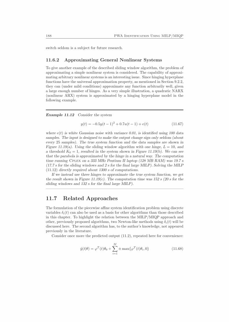
188 PWA Identification Using MILP/MIQP
switch seldom is a subject for future research.
11.6.2 Approximating General Nonlinear Systems
To give another example of the described sliding window algorithm, the problem ofapproximating a simple nonlinear system is considered. The capability of approxi-mating arbitrary nonlinear systems is an interesting issue. Since hinging hyperplanefunctions have the universal approximation property, as mentioned in Section 9.2.2,they can (under mild conditions) approximate any function arbitrarily well, givena large enough number of hinges. As a very simple illustration, a quadratic NARX(nonlinear ARX) system is approximated by a hinging hyperplane model in thefollowing example.
Example 11.12 Consider the system
y(t) = −0.5y(t− 1)2 + 0.7u(t− 1) + e(t) (11.67)
where e(t) is white Gaussian noise with variance 0.01, is identified using 100 datasamples. The input is designed to make the output change sign only seldom (aboutevery 25 samples). The true system function and the data samples are shown inFigure 11.19(a). Using the sliding window algorithm with one hinge, L = 10, anda threshold K0 = 1, resulted in the system shown in Figure 11.19(b). We can seethat the parabola is approximated by the hinge in a natural way. The computationtime running Cplex on a 333 MHz Pentium II laptop (128 MB RAM) was 19.7 s(17.7 s for the sliding windows and 2 s for the final large MILP). Solving the MILP(11.12) directly required about 1300 s of computations.
If we instead use three hinges to approximate the true system function, we getthe result shown in Figure 11.19(c). The computation time was 152 s (20 s for thesliding windows and 132 s for the final large MILP).
11.7 Related Approaches
The formulation of the piecewise affine system identification problem using discretevariables δi(t) can also be used as a basis for other algorithms than those describedin this chapter. To highlight the relation between the MILP/MIQP approach andother, previously proposed algorithms, two Newton-like methods using δi(t) will bediscussed here. The second algorithm has, to the author’s knowledge, not appearedpreviously in the literature.
Consider once more the predicted output (11.2), repeated here for convenience:
y(t|θ) = ϕT (t)θ0 +M∑i=1
±max{ϕT (t)θi, 0} (11.68)
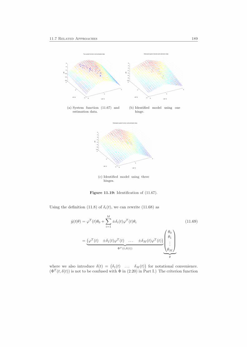
11.7 Related Approaches 189
−5
0
5
−5
0
5
−20
−15
−10
−5
0
5
−y(t−1)
True system function and estimation data
u(t−1)
y(t)
(a) System function (11.67) andestimation data.
−5
0
5
−5
0
5
−10
−8
−6
−4
−2
0
2
4
−y(t−1)
Estimated system function and estimation data
u(t−1)
y(t)
(b) Identified model using onehinge.
−5
0
5
−5
0
5
−10
−8
−6
−4
−2
0
2
4
−y(t−1)
Estimated system function and estimation data
u(t−1)
y(t)
(c) Identified model using threehinges.
Figure 11.19: Identification of (11.67).
Using the definition (11.8) of δi(t), we can rewrite (11.68) as
y(t|θ) = ϕT (t)θ0 +M∑i=1
±δi(t)ϕT (t)θi (11.69)
=(ϕT (t) ±δ1(t)ϕT (t) . . . ±δM (t)ϕT (t)
)︸ ︷︷ ︸ΦT (t,δ(t))
θ0
θ1
...θM
︸ ︷︷ ︸
θ
where we also introduce δ(t) =(δ1(t) . . . δM (t)
)for notational convenience.
(ΦT (t, δ(t)) is not to be confused with Φ in (2.20) in Part I.) The criterion function
190 PWA Identification Using MILP/MIQP
V2 from (11.5) can now be written
V2 =N∑t=1
(y(t)− ΦT (t, δ(t))θ)2 (11.70)
This form can be used as the starting point for several different identificationalgorithms not using MILP/MIQP, often related to the approaches presented inChapter 10. Here, some of the possible approaches will be discussed.
For a given set of δ(t), (11.70) would be minimized by
θ =
(N∑t=1
Φ(t, δ(t))ΦT (t, δ(t))
)−1 N∑t=1
Φ(t, δ(t))y(t)
However, the fact that δ(t) is determined by θ and ϕ(t) has been neglected here.What one could do is to compute the value of δ(t) corresponding to θ. Let us callthis value δ(0)(t). Now we can iterate, letting
θ(k) =
(N∑t=1
Φ(t, δ(k−1)(t))ΦT (t, δ(k−1)(t))
)−1 N∑t=1
Φ(t, δ(k−1)(t))y(t) (11.71a)
and
δ(k)i (t) =
{0 ϕT (t)θ(k)
i < 01 ϕT (t)θ(k)
i ≥ 0(11.71b)
When, for some k, θ(k+1) = θ(k), we have reached a local minimum.This algorithm is a variant of the hinge-finding algorithm due to Breiman,
described in [22]. The difference between them is that this version considers allhinge functions simultaneously, instead of fitting one hinge function at a time. Thelast property makes it belong to the first category of approaches listed in Chapter10. Like the hinge-finding algorithm, there is no guarantee for convergence, butthe algorithm can be modified to guarantee convergence. In this case it becomesthe same algorithm as in [124].
Another option, inspired by one of the algorithms proposed in [69], is to solvethe convex QP
minθ
V2 =N∑t=1
(y(t)− ΦT (t, δ(t))θ)2
subj. to
{ϕT (t)θi ≤ 0 if δi(t) = 0ϕT (t)θi ≥ 0 if δi(t) = 1
(11.72)
for given δi(t). The algorithm is as follows:
11.8 Conclusions 191
Algorithm 11.1
1. Assign initial values to δi(t) and solve the corresponding QP (11.72).
2. There are two possibilities for the resulting θ:
• If θ does not satisfy ϕT (t)θi = 0 for any t = 1, . . . , N , i = 1, . . . ,M ,
this means that θ lies in the interior of the feasible region of (11.72). Inother words, no data sample ϕ(t) lies on a hinge. This means that a localminimum for the original problem (11.70) is found, and we stop.
• Otherwise, we collect all pairs (t, i) such that ϕT (t)θi = 0, and change thevalues of the corresponding δi(t) (or a subset of them). This is the sameas assigning some of the data points ϕ(t) lying on a hinge to the regionon the other side of the hinge. Then go to 3.
3. Solve (11.72) for the new set of δi(t) values. If ϕT (t)θi = 0 for the same pairs(t, i) as before, go to 4. Otherwise, go to 2.
4. If not all possible assignments of values to δi(t) for the pairs (t, i) with
ϕT (t)θi = 0 are tested, choose a new assignment and go to 3. Otherwise,we have found a local minimum, and stop.
Note that the value of V2 will never increase, since the optimal solution of theprevious problem is a feasible solution to the new problem as well. This meansthat the algorithm will converge.
This algorithm is almost a damped Newton algorithm, as explained in Sec-tion 10.1.2 for the corresponding algorithm in [69]. The differences compared tothe algorithm in [69] are that hinging hyperplanes are used instead of hingingsigmoids, and that all parameters are updated simultaneously.
11.8 Conclusions
In this chapter, an approach to piecewise affine system identification using mixed-integer programming has been considered. The theoretical advantage of this ap-proach, compared to, e.g., using standard local minimization tools, is that we areguaranteed to find the global optimum in a finite number of steps. Furthermore, anupper bound on the number of steps can be given. In practice, however, the compu-tational complexity is too large to make the approach applicable to medium-sizedor large identification problems of general piecewise affine systems.
In spite of this, using MILP/MIQP for identification might be a feasible optionin some cases. As described in Section 11.4, some model structures, like the piece-wise affine Wiener models, allow a significant reduction of the complexity, due tothe fact that the nonlinearity is one-dimensional. Another, potentially attractive,way of utilizing the MILP/MIQP formulation was described in Section 11.5, whereintermediate solutions from the MILP/MIQP solver were used as initial values for

192 PWA Identification Using MILP/MIQP
a local minimization algorithm. One problem with the MILP/MIQP formulationsis that the computational complexity increases quite rapidly with the number ofexperimental data. However, if we are only interested in obtaining good initial val-ues for another algorithm, we might very well choose a subset of the experimentaldataset, consisting of, say, a few hundred data samples, that are well distributedover the state-space, and use these for the MILP/MIQP algorithm.
For the case when the estimation data not so frequently switch between differentmodes, a change detection approach was proposed. However, one should keep inmind that the task of designing a seldom-switching input, which at the same time ispersistently exciting, might not be an easy task. Furthermore, much could probablybe done to develop and improve the proposed algorithm.
Finally, the relation between the mixed-integer programming approach andsome Newton-like methods was pointed out, and an extension of an algorithmproposed in [69] was given.
There are still issues that need to be investigated. One interesting topic is whatconditions can be given to ensure that the experimental data is persistently exciting,given different model structures. For continuous-time piecewise affine systems inChua’s canonical form, some work has been done on this [75]. The MILP/MIQPsolving strategies could probably also be specialized to exploit the structure of thiskind of problems. More experiments could be done to compare the performance ofdifferent algorithms. In particular, the algorithms of Section 11.5 should only beseen as a first step in exploring the approach of using intermediate results from anMILP/MIQP solver. These algorithms could probably be developed substantially.

Part III
Robust Verification
193

12
Robust Verification
As mentioned in Section 1.3, the problem of verification is to prove that a set ofbad states is always avoided, or alternatively that a set of target states is actuallyreached. These types of questions often arise in applications in connection withsafety issues. Verification of discrete systems is a well-established research field,with a broad range of applications. With the growing interest of hybrid systemsin the last decade, verification of hybrid systems has also found a number of ap-plications in control. One application area where verification methods for hybridsystems have been applied is the chemical industry, where safety is an importantissue [44]. Another application example is the verification of some properties of thelanding gear system of a certain Swedish aircraft [43, 114]. Verification has alsobeen used for special cases of a collision avoidance system for air-traffic aroundairports [93].
In this chapter, the main question will be the one of proving that some statesare never reached. As most system models contain uncertainties in one way or theother, an important question is how large uncertainties can be tolerated before theverified properties can no longer be guaranteed to hold. The system may also bedisturbed by noise, which must be taken into account in the verification. Thesetwo problems will be addressed.
We will consider systems, where the state-space is partitioned into several poly-hedral regions, with one affine subsystem for each region. The mathematical def-inition of the system class is done in Section 12.1. As in Example 1.5, we will
195
196 Robust Verification
study the behavior of the trajectories at the boundaries of the regions. From thisinformation, a finite automaton which is an outer approximation of the originalsystem can be constructed, analogously to what was done in Example 1.5. Theconcept of inner and outer approximations was explained in Section 1.3. We willnot consider how the discrete verification problem is performed, given the approx-imating automaton. This is described in more detail in, e.g., [43]. Instead we willassume that we are given a set of transitions, for which we should prove if theywill possibly occur or not. In other words, we expect to be given a guarantee ofthe kind: “If these transitions never occur, then the set of bad states will neverbe reached”. In the example in Section 12.8, we will see that it can sometimes bequite easy to find such sets of transitions by direct inspection. The problems solvedin this chapter are formulated in Section 12.2 and Section 12.3.
The methods can also be extended to find an inner approximation of the systembehavior, and hence to show that a set of states will really be reached in finite time.How this can be done is studied in Section 12.7.1. In Section 12.7.2, we will showthat the methods work for switched systems as well.
It would also be nice to be able to combine the verification with other objectives.Section 12.8 shows an example of how this could be done.
12.1 Some Notation and Assumptions
The systems considered in this chapter are in the form (9.2), that is,
x = A(v)x+ b(v), x ∈ X(v) , v ∈ {−1, 0, 1}M (12.1)
where A(v) ∈ Rn×n, b(v) ∈ Rn are given for all v ∈ {−1, 1}M such that X(v)is nonempty (this will be explained in more detail below). The vector v is a keyvector, which is a piecewise constant function of x and can be seen as a label foreach region X(v). The regions X(v) ⊂ Rn are polyhedra, separated from eachother by M hyperplanes. These are defined by
{x ∈ Rn∣∣ Cix = di}, i = 1, . . . ,M (12.2)
where Ci ∈ R1×n and di ∈ R are given. To allow for a compact representation, welet Ci form the rows in an M × n matrix C, and collect di into the vector d.
Now v is defined according to the following rule:
vi =
−1 if Cix < di
0 if Cix = di
1 if Cix > di
(12.3)
In this way there is a one-to-one relationship between v and X(v). Since vi = 0implies that X(v) ⊆ {x ∈ Rn
∣∣ Cix = di}, we notice that a nonempty X(v) willbe contained in an (n− 1)-dimensional affine subspace of Rn if and only if there isat least one zero entry in v. Nonempty polyhedra X(v) corresponding to vectors
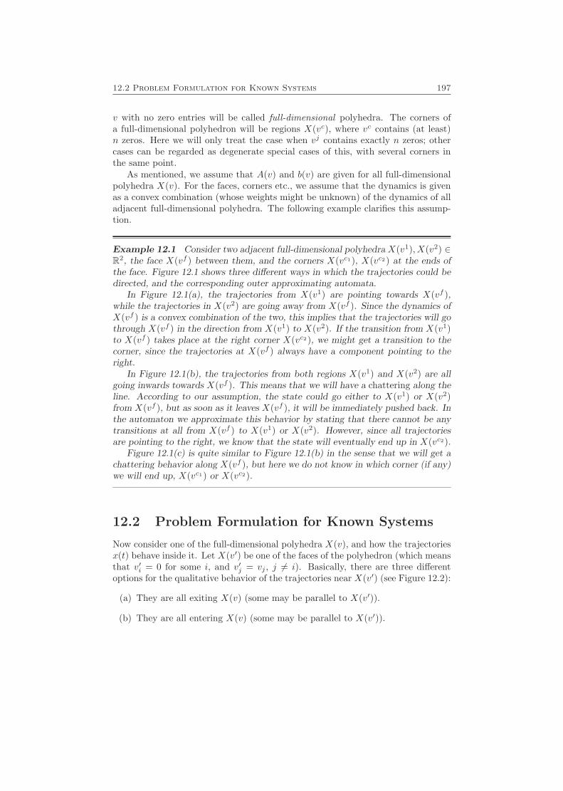
12.2 Problem Formulation for Known Systems 197
v with no zero entries will be called full-dimensional polyhedra. The corners ofa full-dimensional polyhedron will be regions X(vc), where vc contains (at least)n zeros. Here we will only treat the case when vj contains exactly n zeros; othercases can be regarded as degenerate special cases of this, with several corners inthe same point.
As mentioned, we assume that A(v) and b(v) are given for all full-dimensionalpolyhedra X(v). For the faces, corners etc., we assume that the dynamics is givenas a convex combination (whose weights might be unknown) of the dynamics of alladjacent full-dimensional polyhedra. The following example clarifies this assump-tion.
Example 12.1 Consider two adjacent full-dimensional polyhedra X(v1),X(v2) ∈R2, the face X(vf ) between them, and the corners X(vc1), X(vc2) at the ends ofthe face. Figure 12.1 shows three different ways in which the trajectories could bedirected, and the corresponding outer approximating automata.
In Figure 12.1(a), the trajectories from X(v1) are pointing towards X(vf ),while the trajectories in X(v2) are going away from X(vf ). Since the dynamics ofX(vf ) is a convex combination of the two, this implies that the trajectories will gothrough X(vf ) in the direction from X(v1) to X(v2). If the transition from X(v1)to X(vf ) takes place at the right corner X(vc2), we might get a transition to thecorner, since the trajectories at X(vf ) always have a component pointing to theright.
In Figure 12.1(b), the trajectories from both regions X(v1) and X(v2) are allgoing inwards towards X(vf ). This means that we will have a chattering along theline. According to our assumption, the state could go either to X(v1) or X(v2)from X(vf ), but as soon as it leaves X(vf ), it will be immediately pushed back. Inthe automaton we approximate this behavior by stating that there cannot be anytransitions at all from X(vf ) to X(v1) or X(v2). However, since all trajectoriesare pointing to the right, we know that the state will eventually end up in X(vc2).
Figure 12.1(c) is quite similar to Figure 12.1(b) in the sense that we will get achattering behavior along X(vf ), but here we do not know in which corner (if any)we will end up, X(vc1) or X(vc2).
12.2 Problem Formulation for Known Systems
Now consider one of the full-dimensional polyhedra X(v), and how the trajectoriesx(t) behave inside it. Let X(v′) be one of the faces of the polyhedron (which meansthat v′i = 0 for some i, and v′j = vj , j 6= i). Basically, there are three differentoptions for the qualitative behavior of the trajectories near X(v′) (see Figure 12.2):
(a) They are all exiting X(v) (some may be parallel to X(v′)).
(b) They are all entering X(v) (some may be parallel to X(v′)).
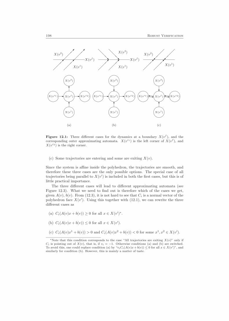
198 Robust Verification
����
����
������
������
����
����
����
����
- -
6
6
X(v1)
X(v2)
X(vf )
X(vf )
X(v2)
X(v1)
X(vc1 ) X(vc2 )
(a)
����
����
������
������
����
����
@@@R
@@@R
- -?
6
X(v1)
X(v2)
X(vf )
X(vf )
X(v2)
X(v1)
X(vc1 ) X(vc2 )
(b)
����
����
������
������
����
����
���
���
�- �-
?
6
X(v1)
X(v2)
X(vf )
X(v2)
X(v1)
X(vc1 ) X(vc2 )
(c)
Figure 12.1: Three different cases for the dynamics at a boundary X(vf ), and thecorresponding outer approximating automata. X(vc1) is the left corner of X(vf ), andX(vc2) is the right corner.
(c) Some trajectories are entering and some are exiting X(v).
Since the system is affine inside the polyhedron, the trajectories are smooth, andtherefore these three cases are the only possible options. The special case of alltrajectories being parallel to X(v′) is included in both the first cases, but this is oflittle practical importance.
The three different cases will lead to different approximating automata (seeFigure 12.3). What we need to find out is therefore which of the cases we get,given A(v), b(v). From (12.3), it is not hard to see that Ci is a normal vector of thepolyhedron face X(v′). Using this together with (12.1), we can rewrite the threedifferent cases as
(a) Ci(A(v)x+ b(v)) ≥ 0 for all x ∈ X(v′)∗.
(b) Ci(A(v)x+ b(v)) ≤ 0 for all x ∈ X(v′).
(c) Ci(A(v)x1 + b(v)) > 0 and Ci(A(v)x2 + b(v)) < 0 for some x1, x2 ∈ X(v′).
∗Note that this condition corresponds to the case “All trajectories are exiting X(v)” only ifCi is pointing out of X(v), that is, if vi = −1. Otherwise conditions (a) and (b) are switched.To avoid this, one could replace condition (a) by “viCi(A(v)x+ b(v)) ≤ 0 for all x ∈ X(v′)”, andsimilarly for condition (b). However, this is mainly a matter of taste.
12.3 The Problem of Robust Verification 199
(a) (b) (c)
Figure 12.2: Three options for the behavior of the trajectories in the vicinity of apolyhedron face.
��������
��������
��������
���7 �
��/ �����
��
X(v)
X(v′)
X(v)
X(v′)
X(v)
X(v′)
Figure 12.3: Parts of the automata corresponding to the three cases in Figure 12.2.
These conditions can all be easily checked for given A(v), b(v), C and d, for exampleby finding the maximum and minimum values on X(v′) of Ci(A(v)x+b(v)), yieldingtwo LP problems.
12.3 The Problem of Robust Verification
In Section 12.2, we assumed that the dynamics of the system was completely known.In practice, however, there will almost always be model errors, and the systemsmight be disturbed by noise. To that end, let us introduce some uncertainty in oursystem model:
x = (A(v)−∆(v))x+ b(v)− δ(v), x ∈ X(v) , v ∈ {−1, 0, 1}M (12.4)
where v is defined by
vi =
−1 if Cix < di + γi
0 if Cix = di + γi
1 if Cix > di + γi
(12.5)
Depending on the applications, the matrices ∆(v) ∈ Rn×n, δ(v) ∈ Rn and γ ∈ RMcan be viewed either as uncertainties in the model, or as matrices of our choice(the latter case can occur, e.g., in the control design process). We can see that
200 Robust Verification
the different matrices affect the system dynamics in different ways: ∆(v) and δ(v)affect the dynamics of the different subsystems, while γ affects the partitioning ofthe state-space.
We will only allow values of γ that do not affect the topology of the state-spacepartition compared to the case γ = 0. In other words, the regions X(v) will alwayshave the same number of faces and the same neighbors as they would have if theseparating hyperplanes were defined by Cx = d. This also means that we willnot allow regions to disappear or new regions to be created when changing γ. Anequivalent way of stating this assumption is to say that for each corner X(vc), vc
should remain constant, and not be changed because a γ value causes the cornerto cross another hyperplane. The following example illustrates this.
Example 12.2 (Preserving topology) Consider the polyhedral partition ofthe state-space in Figure 12.4 (which is the same as in Example A.1). The partitioncan be described using the matrices
C =
1 11 −11 0
, d =
10−1
The open polytope corresponding to P in Example A.1 can now be written as
X(v), where v =(−1 −1 1
)T(P is the closure of this open polytope).
Now assume that we do not know where the real location of the hyperplanecorresponding to the third row of C and d (so far modelled by x1 = −1) is. We caninclude this uncertainty in the model by writing x1 = −1 + γ3. Now, if γ3 > 1.5,we can see that the hyperplane is moved to the right of the corner where the othertwo hyperplanes meet. In this way, the polytope P disappears, and a new polytopeis created. To avoid these kinds of phenomena, we can require that γ3 < 1.5.
Assuming (12.4), the three cases from the previous section now become
(a) Ci[(A(v)−∆(v))x+ b(v)− δ(v)] ≥ 0 for all x ∈ X(v′).
(b) Ci[(A(v)−∆(v))x+ b(v)− δ(v)] ≤ 0 for all x ∈ X(v′).
(c) Ci[(A(v)−∆(v))x1+b(v)−δ(v)] > 0 and Ci[(A(v)−∆(v))x2+b(v)−δ(v)] < 0for some x1, x2 ∈ X(v′).
An interesting question is: How much could ∆(v), δ(v) and γ change, withoutchanging the qualitative behavior at each face of the polyhedron, i.e., without oneface switching from, say, case (a) to case (c)? In other words, for what values of∆(v), δ(v) and γ do the different cases occur? This is the main question of thischapter.
Depending on how many of the parameters are varied simultaneously, this ques-tion may be more or less difficult to answer. If all of them are varied, the problem is
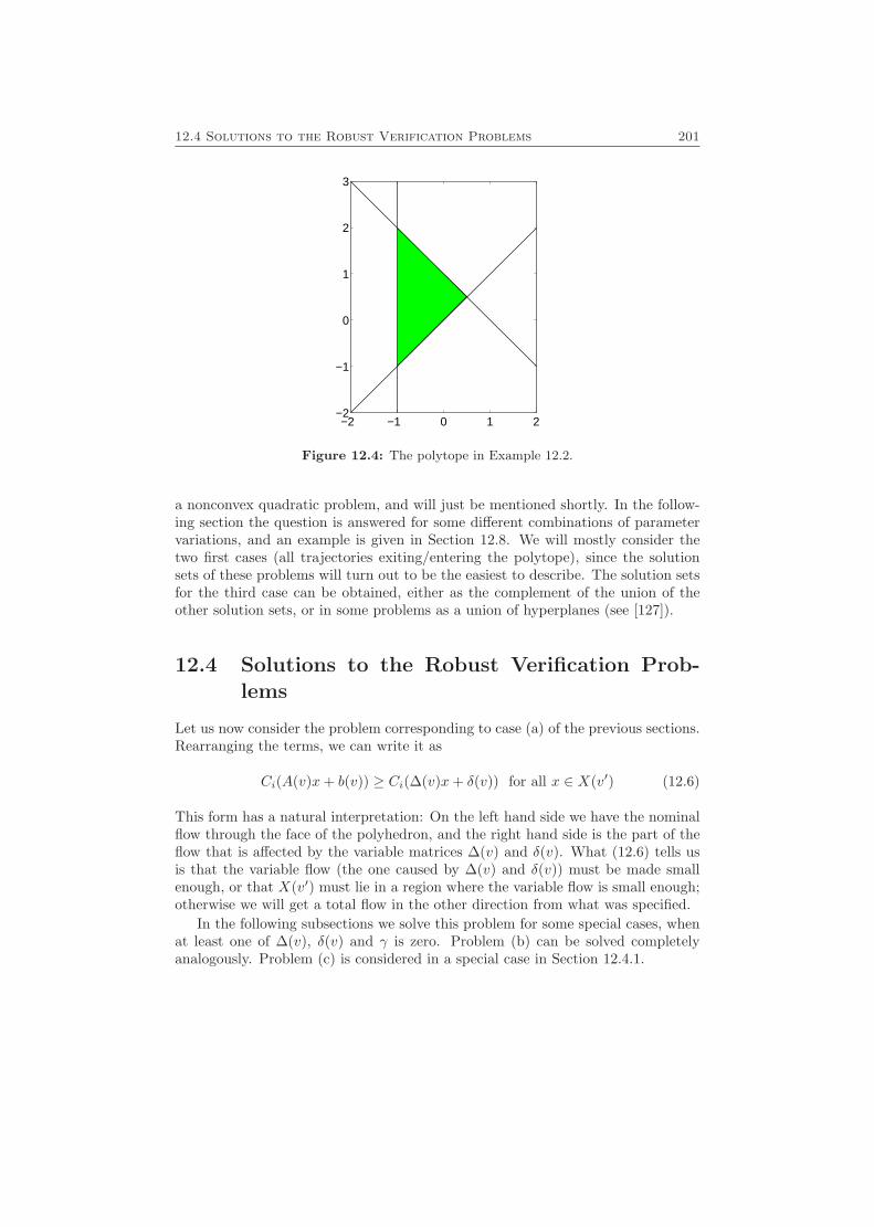
12.4 Solutions to the Robust Verification Problems 201
−2 −1 0 1 2−2
−1
0
1
2
3
Figure 12.4: The polytope in Example 12.2.
a nonconvex quadratic problem, and will just be mentioned shortly. In the follow-ing section the question is answered for some different combinations of parametervariations, and an example is given in Section 12.8. We will mostly consider thetwo first cases (all trajectories exiting/entering the polytope), since the solutionsets of these problems will turn out to be the easiest to describe. The solution setsfor the third case can be obtained, either as the complement of the union of theother solution sets, or in some problems as a union of hyperplanes (see [127]).
12.4 Solutions to the Robust Verification Prob-lems
Let us now consider the problem corresponding to case (a) of the previous sections.Rearranging the terms, we can write it as
Ci(A(v)x+ b(v)) ≥ Ci(∆(v)x+ δ(v)) for all x ∈ X(v′) (12.6)
This form has a natural interpretation: On the left hand side we have the nominalflow through the face of the polyhedron, and the right hand side is the part of theflow that is affected by the variable matrices ∆(v) and δ(v). What (12.6) tells usis that the variable flow (the one caused by ∆(v) and δ(v)) must be made smallenough, or that X(v′) must lie in a region where the variable flow is small enough;otherwise we will get a total flow in the other direction from what was specified.
In the following subsections we solve this problem for some special cases, whenat least one of ∆(v), δ(v) and γ is zero. Problem (b) can be solved completelyanalogously. Problem (c) is considered in a special case in Section 12.4.1.
202 Robust Verification
12.4.1 ∆(v) = 0, γ = 0, δ(v) is Varied
The simplest problem arises when we only allow δ(v) in (12.4) to vary, and let ∆(v)and γ equal 0. Equation (12.6) then takes the form
Ci(A(v)x+ b(v)) ≥ Ciδ(v) for all x ∈ X(v′) (12.7)
This problem can be solved immediately by solving the LP problem
minx
Ci(A(v)x+ b(v))
subj. to x ∈ X(v′)(12.8)
where X(v′) is the closure of X(v′) (see Section A.3). Denoting the solution of theLP problem by x∗, the solution set to (12.7) is
Sδ = {δ ∈ Rn∣∣ Ciδ ≤ Ci(A(v)x∗ + b(v))} (12.9)
Problem (b) is solved by maximizing instead of minimizing Ci(A(v)x+ b(v)) toget the limit x∗, and the solution set consists of all δ satisfying Ciδ ≥ Ci(A(v)x∗+b(v)). The values of δ for which Ciδ lies in between x∗ and x∗ are solutions toproblem (c). Thus, in this case all solution sets will be convex.
12.4.2 γ = 0, ∆(v) and δ(v) are Varied
When letting both ∆(v) and δ(v) vary, we need to find a direct representation(see Section A.3) of X(v′) to get a solution to (12.6). For the case when X(v′) isbounded, the direct representation will be on the following form:
X(v′) = {r∑j=1
λjxj∣∣ λj ∈ R, λj > 0,
r∑j=1
λj = 1} (12.10)
Here xj ∈ Rn, j = 1, . . . r are the corners of X(v′).According to Equation (A.11), when X(v′) is unbounded, we must include in
the direct representation some vectors, xr+1, . . . , xr+h, which are parallel to theunbounded edges of X(v′). A direct representation of X(v′) would then be:
X(v′) = {r+h∑j=1
λjxj∣∣ λj ∈ R, λj > 0,
r∑j=1
λj = 1} (12.11)
Note that, as in (A.11), λr+1, . . . , λr+h are not included in the set of λj that shouldsum up to one; they can be arbitrarily large. In some cases there are no corners,e.g., when X(v′) consists of an entire hyperplane. As mentioned in Section A.3, insuch cases, a “dummy” corner must be introduced somewhere in X(v′).
For notational simplicity, let us drop the argument v of A(v) etc. for a while.Now the following theorem gives the solutions to our problem.
12.4 Solutions to the Robust Verification Problems 203
Theorem 12.1Consider the system given by (12.4) and (12.5). Assume that γ = 0. Then the setof solutions to the problem (12.6) is given by
S∆δ = {(∆, δ)∣∣ Ci(Axj + b) ≥ Ci(∆xj + δ), j = 1, . . . , r;
CiAxr+j ≥ Ci∆xr+j , j = 1, . . . , h} (12.12)
Proof To show that the inequality (12.6) is satisfied for an arbitrary point x ∈X(v′), we use the direct representation (12.11):
Ci(Ax+ b) = Ci(Ar+h∑j=1
λjxj + b)
=r∑j=1
λjCi(Axj + b) +r+h∑j=r+1
λjCiAxj
≥r∑j=1
λjCi(∆xj + δ) +r+h∑j=r+1
λjCi∆xj
= Ci(∆r+h∑j=1
λjxj + δ)
= Ci(∆x+ δ)
To see that the first r conditions of (12.12) are necessary, we just need to noticethat they are precisely (12.6) for the corners of X(v′). If a corner would not satisfy(12.6), then for continuity reasons, there would be points in X(v′) not satisfying(12.6) either. To show the necessity of the last h conditions, fix ∆ and δ, supposethat CiAxr+j < Ci∆xr+j for some j, and study x = x1 + λxr+j ∈ X(v′), whereλ > Ci(Ax
1+b−∆x1−δ)Ci(∆xr+j−Axr+j) > 0. We then have
Ci(Ax+ b) = Ci(Ax1 + b) + λCiAxr+j
= Ci(Ax1 + b) + λCi(Axr+j −∆xr+j) + λCi∆xr+j
< Ci(Ax1 + b)− Ci(Ax1 + b−∆x1 − δ) + λCi∆xr+j
= Ci(∆x1 + δ) + λCi∆xr+j
= Ci(∆x+ δ)
where the direction of the inequality follows since λ is multiplied by a negativenumber. This means that (∆, δ) is outside the solution set, and the necessity isshown. �
When X(v′) is a polytope, Theorem 12.1 can interpreted as follows: The in-equality (12.6) holds for all x ∈ X(v′) if and only if it holds for the corners ofX(v′). This property follows directly from the inequality being linear in x.
Note that the solution set S∆δ is a polyhedron in the space Rn×n × Rn, andtherefore convex.
204 Robust Verification
12.4.3 Multiple Requirements
So far, we have only been looking at one single polyhedron face. In most cases, therequirements may stipulate that several transitions of an approximating automatonshould remain invariant. This case is easily handled by partitioning the probleminto subproblems of the form treated above, and then taking the intersection of thesolution sets as the solution set for the entire problem. How many transitions weneed to consider will depend on the system and what we want to verify. For exam-ple, if all we are interested in is keeping the state on one side of a hyperplane, weonly need to consider transitions through this hyperplane. It should be noted thatconsidering fewer transitions will lead to a larger – and therefore less conservative– solution set, and will also require less computations.
12.4.4 ∆ = 0, δ and γ are Varied
The problem gets more complicated as soon as γ is not fixed anymore. We imme-diately notice from (12.4) and (12.5) that the regions X(v) will no longer be fixed,but vary with γ. We also have to consider several regions X(v) simultaneously,since moving a hyperplane will affect all regions adjacent to it. As mentioned inSection 12.3, we will only allow values of γ that keep the topology of the state-spaceregions invariant. If we do not make this requirement, new regions – for which wedo not know the system dynamics – can be created by moving the hyperplanesdefined by Cx = d+ γ.
With this requirement, and with ∆(v) = 0 for all v, the problem is still convex,as will be shown in the following. What we need to do first is to express thecorners as functions of γ. Having done that, we can use these functions to expressthe topology preservation requirements and the properties to be verified.
First, remember that each corner xj of the full-dimensional polyhedron X(v) isitself a region X(vj), where vj contains n zeros. The zeros of vj correspond to theequations Cixj = di+γi that xj satisfies. To be able to pick out the correspondingrows of Ci, di, and γi, we need to introduce some new matrices.
Let D[vj ] = diag(vj). From D[vj ] we then construct Q[vj ] ∈ R(M−n)×M bydeleting all rows containing only zeros. Similarly, we define P[vj ] ∈ Rn×M bydeleting all rows in I −D2
[vj ] containing only zeros.Now P[vj ] has the following property: When multiplying another matrix from
the left by P[vj ], it picks out the rows corresponding to the zero entries of vj . Q[vj ],on the other hand, picks out the rows not picked out by P[vj ], and furthermoremultiplies the rows corresponding to the −1 entries of vj by −1.
With this notation, we can pick out the equalities in (12.5) by writing
P[vj ]Cxj = P[vj ](d+ γ)
Since xj is uniquely determined by the equalities in (12.5), P[vj ]C will always beinvertible. Hence, we can write
xj = (P[vj ]C)−1P[vj ](d+ γ) (12.13)
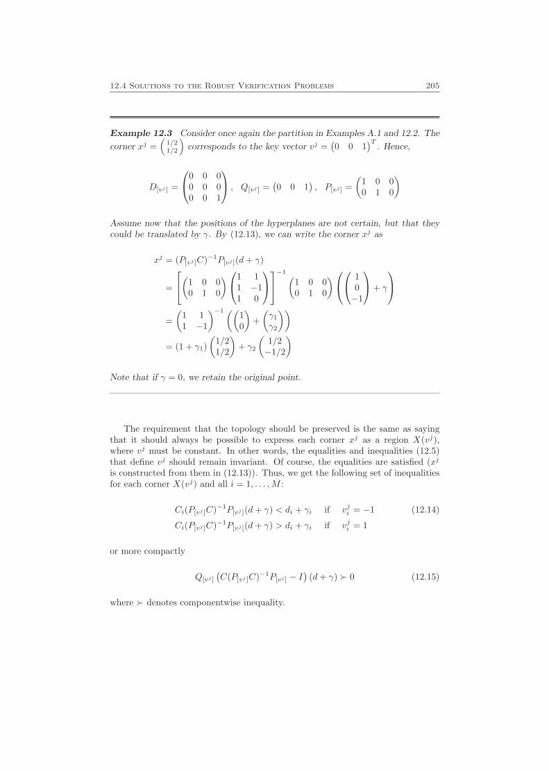
12.4 Solutions to the Robust Verification Problems 205
Example 12.3 Consider once again the partition in Examples A.1 and 12.2. The
corner xj =(
1/21/2
)corresponds to the key vector vj =
(0 0 1
)T. Hence,
D[vj ] =
0 0 00 0 00 0 1
, Q[vj ] =(0 0 1
), P[vj ] =
(1 0 00 1 0
)
Assume now that the positions of the hyperplanes are not certain, but that theycould be translated by γ. By (12.13), we can write the corner xj as
xj = (P[vj ]C)−1P[vj ](d+ γ)
=
(1 0 00 1 0
)1 11 −11 0
−1(1 0 00 1 0
) 10−1
+ γ
=(
1 11 −1
)−1((10
)+(γ1
γ2
))= (1 + γ1)
(1/21/2
)+ γ2
(1/2−1/2
)
Note that if γ = 0, we retain the original point.
The requirement that the topology should be preserved is the same as sayingthat it should always be possible to express each corner xj as a region X(vj),where vj must be constant. In other words, the equalities and inequalities (12.5)that define vj should remain invariant. Of course, the equalities are satisfied (xj
is constructed from them in (12.13)). Thus, we get the following set of inequalitiesfor each corner X(vj) and all i = 1, . . . ,M :
Ci(P[vj ]C)−1P[vj ](d+ γ) < di + γi if vji = −1 (12.14)
Ci(P[vj ]C)−1P[vj ](d+ γ) > di + γi if vji = 1
or more compactly
Q[vj ]
(C(P[vj ]C)−1P[vj ] − I
)(d+ γ) � 0 (12.15)
where � denotes componentwise inequality.
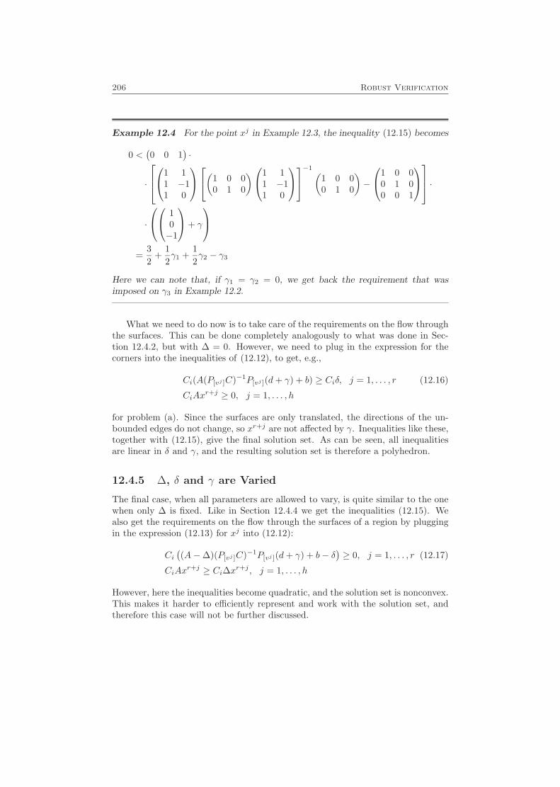
206 Robust Verification
Example 12.4 For the point xj in Example 12.3, the inequality (12.15) becomes
0 <(0 0 1
)·
·
1 1
1 −11 0
(1 0 00 1 0
)1 11 −11 0
−1(1 0 00 1 0
)−
1 0 00 1 00 0 1
·
·
10−1
+ γ
=
32
+12γ1 +
12γ2 − γ3
Here we can note that, if γ1 = γ2 = 0, we get back the requirement that wasimposed on γ3 in Example 12.2.
What we need to do now is to take care of the requirements on the flow throughthe surfaces. This can be done completely analogously to what was done in Sec-tion 12.4.2, but with ∆ = 0. However, we need to plug in the expression for thecorners into the inequalities of (12.12), to get, e.g.,
Ci(A(P[vj ]C)−1P[vj ](d+ γ) + b) ≥ Ciδ, j = 1, . . . , r (12.16)
CiAxr+j ≥ 0, j = 1, . . . , h
for problem (a). Since the surfaces are only translated, the directions of the un-bounded edges do not change, so xr+j are not affected by γ. Inequalities like these,together with (12.15), give the final solution set. As can be seen, all inequalitiesare linear in δ and γ, and the resulting solution set is therefore a polyhedron.
12.4.5 ∆, δ and γ are Varied
The final case, when all parameters are allowed to vary, is quite similar to the onewhen only ∆ is fixed. Like in Section 12.4.4 we get the inequalities (12.15). Wealso get the requirements on the flow through the surfaces of a region by pluggingin the expression (12.13) for xj into (12.12):
Ci((A−∆)(P[vj ]C)−1P[vj ](d+ γ) + b− δ
)≥ 0, j = 1, . . . , r (12.17)
CiAxr+j ≥ Ci∆xr+j , j = 1, . . . , h
However, here the inequalities become quadratic, and the solution set is nonconvex.This makes it harder to efficiently represent and work with the solution set, andtherefore this case will not be further discussed.
12.5 Interpretations 207
12.5 Interpretations
Perhaps the most obvious interpretation is to view ∆(v), δ(v) and γ in (12.4)and (12.5) as uncertainties due to model errors and/or noise. The methods inSection 12.4 then provide bounds for the uncertainties for the requirements of theapproximating automata to hold. For natural reasons, the bounds may be veryasymmetric, indicating that the system is more sensitive to certain types of modelerrors than to others.
The problem formulation is quite general in that no structure of ∆(v), δ(v)or γ is assumed. It should be stressed that these uncertainties by no means needto be constant over time; we have showed that as long as they are kept withinthe computed bounds, the verification will hold, no matter how the uncertaintiesvary. The only structure that is assumed is the topology of the different polyhedralregions X(v). If the uncertainty has some further structure, we can parameterize∆(v) and δ(v) accordingly, thereby reducing the dimensionality and simplifying theproblem. For example, if only the upper left element of A(v) is uncertain, we canwrite ∆(v) as
∆(v) =(
∆1 00 0
)Another example is to set ∆(v) = 0 as in Section 12.4.1, which can be interpretedas a model with additive noise:
x = A(v)x+ b(v)− δ(v), x ∈ X(v) , i = 1, . . . , N (12.18)
A nonzero ∆(v) can also be interpreted as multiplicative noise.Another type of parameterization is used in the example in Section 12.8. In this
parameterization, some of the elements of ∆(v) and δ(v) are common to severalpolyhedra.
An alternative interpretation is to consider ∆(v), δ(v) and/or γ as parametersof our choice, to be used for control design. One natural parameterization wouldthen be γ = 0, δ(v) = 0, ∆(v) = B(v)L(v), where B(v) are fixed vectors thatdepend on the system, while we can choose L(v) freely. In this way we get (piece-wise) linear state feedback control, and the problem becomes that of finding thelinear state feedback vectors L(v) that make our system fulfill the requirementson the approximating automata. Another parameterization would be the one inSection 12.4.4, where we can regard γ as a vector that lets us place the switchingsurfaces of a controller in an optimal manner.
12.6 Computational Complexity
In this section, some aspects on the computational complexity will be discussed.However, no rigorous analysis is made.
The computational complexity depends on what parameters we let vary. As wecould see in Section 12.4.1, when only δ is varied we just need to solve one or twoLP problems for each requirement. This can be done efficiently (see, e.g., [39]).
208 Robust Verification
When only γ is fixed, the complexity gets a bit worse. From Section 12.4.2we see, that once we know a direct representation of X(v′), it is trivial to divideRn×n × Rn into the three solution sets corresponding to problem (a), (b) and (c).Conversely, if we want the solutions to be written as intersections of half-spaces(as in (12.12)), we need to know the direct representation of X(v′). Therefore thecomputational complexity for this problem is essentially identical to that of findingthe direct representation. Unfortunately, the number of vectors needed in such arepresentation grows very quickly with the size of the problem. An upper boundfor the number of corners in a polyhedron can be calculated in the following way:In a corner, n linearly independent faces meet (where n is still the dimension ofthe state-space). Since the polyhedron has m faces, the number of corners cannotbe larger than
(mn
)(i.e., the binomial coefficient).
However, if we restrict ourselves to the case where the polyhedra are formed bythe state-space being divided by hyperplanes (as we have done in this chapter), itis fairly easy (but still quite time-consuming) to calculate the direct representationof all the polyhedra once and for all. The total number of corners is then boundedabove by
(Mn
), where M is the number of separating hyperplanes.
Finally, letting δ and γ vary leads to a similar set of inequalities as in theprevious case. However, we cannot find the corners directly, since they are functionsof γ. Instead we can store the inverses (P[vj ]C)−1 for each corner. Thus, we willneed n times as large storage, and about the same amount of computations as whenδ and ∆ vary.
12.7 Extensions
The considered methods can be extended in different ways. We will consider twokinds of extensions: Using inner instead of outer approximations (that can be usedto prove that a certain region of the state-space really is reached in finite time),and extending the model class to switched systems.
12.7.1 Inner Approximations
So far, we have only dealt with the behavior of the trajectories at the border of eachregion. As we have seen, using the analysis of this behavior we can construct outerapproximating finite automata, with the help of which we may be able to guaranteethat some states are never reached. Another kind of verification, that one mightbe interested in, is to prove that a certain region really is reached. This can beharder, since it is not enough to consider only what happens at the borders of aregion. The reason for this is that the state, being in a region X(v), might neverget to the border of X(v) if the system has a stable equilibrium or a limit cycleinside X(v). Another difficulty with this kind of verification is that even if we knowthat the state trajectory leaves the region X(v), we might not know through whichface it will exit, since this information may be lost when approximating the systemwith a discrete automaton. We only know that one out of a set of transitions will
12.7 Extensions 209
occur. Following the terminology of [43], we say that the transitions are guaranteedto occur nondeterministically.
In this thesis, we will not go into detail with how the analysis of the resultingnondeterministic approximating automata is performed. For more details aboutthis, see [43]. Instead, a sufficient condition for the trajectories to be guaranteedto exit X(v) will be given. This condition also comes from [43]:
Proposition 12.1A sufficient condition for the state trajectory to exit a polyhedron, X(v), is thatthe normal vector, Ci, of one of its faces, X(v′), satisfies
viCix < 0, ∀x ∈ X(v) (12.19)
Proof See [43]. �
Intuitively, the condition in Proposition 12.1 means that the velocity vector isalways pointing towards the hyperplane Cix = di (or Cix = di + γi for a systemwith uncertainties). Now, given the face X(v′), we can include this case in ourframework with the following theorem:
Theorem 12.2Consider the system given by (12.4) and (12.5). Let a direct representation of X(v)be given by
X(v) = {s+k∑j=1
λjxj∣∣ λj ∈ R, λj > 0,
s∑j=1
λj = 1} (12.20)
Assume that γ = 0. Then, for a given X(v′), the set of solutions to (12.19) is givenby
S∆δ = {(∆, δ)∣∣ viCi(Axj + b) < viCi(∆xj + δ), j = 1, . . . , s;
viCiAxs+j < viCi∆xs+j , j = 1, . . . , k} (12.21)
If we assume instead that ∆ = 0, the set of solutions is given by
Sδγ = {(δ, γ)∣∣ Ci(A(P[vj ]C)−1P[vj ](d+ γ) + b) ≥ Ciδ, j = 1, . . . , s;
CiAxs+j ≥ 0, j = 1, . . . , k (12.22)
Q[vc]
(C(P[vc]C)−1P[vc] − I
)(d+ γ) � 0, ∀ corners vc}
Proof Analogous to the proof of Theorem 12.1 and the results in Section 12.4.4.�
Note that since in Theorem 12.2 a face X(v′) must be given, the condition issomewhat more restrictive than in Proposition 12.1, where it is sufficient that anyof the faces satisfies (12.19).
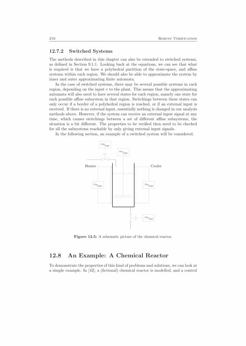
210 Robust Verification
12.7.2 Switched Systems
The methods described in this chapter can also be extended to switched systems,as defined in Section 9.1.1. Looking back at the equations, we can see that whatis required is that we have a polyhedral partition of the state-space, and affinesystems within each region. We should also be able to approximate the system byinner and outer approximating finite automata.
In the case of switched systems, there may be several possible systems in eachregion, depending on the input v to the plant. This means that the approximatingautomata will also need to have several states for each region, namely one state foreach possible affine subsystem in that region. Switchings between these states canonly occur if a border of a polyhedral region is reached, or if an external input isreceived. If there is no external input, essentially nothing is changed in our analysismethods above. However, if the system can receive an external input signal at anytime, which causes switchings between a set of different affine subsystems, thesituation is a bit different. The properties to be verified then need to be checkedfor all the subsystems reachable by only giving external input signals.
In the following section, an example of a switched system will be considered.
On/Off
On/Off
On/Off
On/Off
On/Off
Heater Cooler
Figure 12.5: A schematic picture of the chemical reactor.
12.8 An Example: A Chemical Reactor
To demonstrate the properties of this kind of problems and solutions, we can look ata simple example. In [42], a (fictional) chemical reactor is modelled, and a control
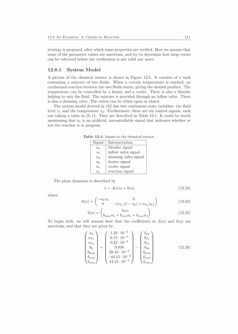
12.8 An Example: A Chemical Reactor 211
strategy is proposed, after which some properties are verified. Here we assume thatsome of the parameter values are uncertain, and try to determine how large errorscan be tolerated before the verification is not valid any more.
12.8.1 System Model
A picture of the chemical reactor is shown in Figure 12.5. It consists of a tankcontaining a mixture of two fluids. When a certain temperature is reached, anexothermal reaction between the two fluids starts, giving the desired product. Thetemperature can be controlled by a heater and a cooler. There is also a blenderhelping to mix the fluid. The mixture is provided through an inflow valve. Thereis also a draining valve. The valves can be either open or closed.
The system model derived in [42] has two continuous state variables: the fluidlevel x1 and the temperature x2. Furthermore, there are six control signals, eachone taking a value in {0, 1}. They are described in Table 12.1. It could be worthmentioning that ur is an artificial, uncontrollable signal that indicates whether ornot the reaction is in progress.
Table 12.1: Inputs to the chemical reactor.
Signal Interpretationub blender signalui inflow valve signalud draining valve signaluh heater signaluc cooler signalur reaction signal
The plant dynamics is described by
x = A(u)x+ b(u) (12.23)
where
A(u) =(−ahud 0
0 −(aT1(1− ub) + aT2ub)
)(12.24)
b(u) =(
bhui
bheatuh + bcooluc + breacur
)(12.25)
To begin with, we will assume here that the coefficients in A(u) and b(u) areuncertain, and that they are given by
ah
aT1
aT2
bhbheat
bcool
breac
=
1.23 · 10−3
0.15 · 10−3
0.22 · 10−3
9.83829.43 · 10−3
−44.15 · 10−3
44.15 · 10−3
−
δah
δT1
δT2
δbh
δheat
δcool
δreac
(12.26)

212 Robust Verification
0 2 4 6 8 10 120
50
100
150
Level, x1
Tem
per
atu
re,x
2
Figure 12.6: The switching hyperplanes and an example trajectory.
where the numerical values are the nominal parameter values used in [42].The controller is designed such that the control signals are switched on or off
when the state reaches certain hyperplanes. The rules are listed below (the lastrule is given by the physical properties of the system):
1. ub = 0 when x1 < 3, ub = 1 otherwise.
2. ui is set to 0 when 25x1 + x2 ≥ 300, and is set to 1 when 25x1 + x2 ≤ 250.
3. ud = 0 when x2 < 50, ud = 1 otherwise.
4. uh = 1 when x2 < 50, uh = 0 otherwise.
5. uc is set to 0 when x2 ≤ 110, and is set to 1 when x2 ≥ 130.
6. ur = 0 when x2 < 50, ur = 1 otherwise.
Note that the system contains hysteresis in ui and uc. This is handled by con-sidering each polyhedron where the hysteresis occurs as two polyhedra with twodifferent subsystems.
In Section 12.8.4, we will consider changing the thresholds for different controlactions.
The switching hyperplanes and an example trajectory are shown in Figure 12.6.For further details concerning the system model, see [42].
12.8.2 What to Verify
There are certain requirements on the controller, which are verified in [42]. Theseare:
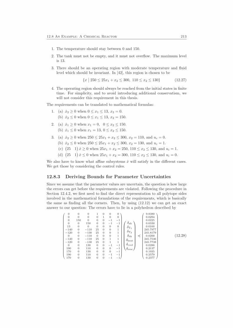
12.8 An Example: A Chemical Reactor 213
1. The temperature should stay between 0 and 150.
2. The tank must not be empty, and it must not overflow. The maximum levelis 13.
3. There should be an operating region with moderate temperature and fluidlevel which should be invariant. In [42], this region is chosen to be
{x∣∣ 250 ≤ 25x1 + x2 ≤ 300, 110 ≤ x2 ≤ 130} (12.27)
4. The operating region should always be reached from the initial states in finitetime. For simplicity, and to avoid introducing additional conservatism, wewill not consider this requirement in this thesis.
The requirements can be translated to mathematical formulas:
1. (a) x2 ≥ 0 when 0 ≤ x1 ≤ 13, x2 = 0.(b) x2 ≤ 0 when 0 ≤ x1 ≤ 13, x2 = 150.
2. (a) x1 ≥ 0 when x1 = 0, 0 ≤ x2 ≤ 150.(b) x1 ≤ 0 when x1 = 13, 0 ≤ x2 ≤ 150.
3. (a) x2 ≥ 0 when 250 ≤ 25x1 + x2 ≤ 300, x2 = 110, and uc = 0.(b) x2 ≤ 0 when 250 ≤ 25x1 + x2 ≤ 300, x2 = 130, and uc = 1.(c)
(25 1
)x ≥ 0 when 25x1 + x2 = 250, 110 ≤ x2 ≤ 130, and ui = 1.
(d)(25 1
)x ≤ 0 when 25x1 + x2 = 300, 110 ≤ x2 ≤ 130, and ui = 0.
We also have to know what affine subsystems x will satisfy in the different cases.We get those by considering the control rules.
12.8.3 Deriving Bounds for Parameter Uncertainties
Since we assume that the parameter values are uncertain, the question is how largethe errors can get before the requirements are violated. Following the procedure inSection 12.4.2, we first need to find the direct representation to all polytope sidesinvolved in the mathematical formulations of the requirements, which is basicallythe same as finding all the corners. Then, by using (12.12) we can get an exactanswer to our question: The errors have to lie in a polyhedron described by
0 0 0 1 0 0 00 0 0 0 1 0 00 150 0 0 0 −1 −10 0 150 0 0 −1 −113 0 0 0 0 0 0−140 0 −110 25 0 0 1−120 0 −130 25 0 0 1
0 0 −110 0 0 0 1−140 0 −110 25 0 1 1−120 0 −130 25 0 1 1
0 0 130 0 0 −1 −1190 0 110 0 0 0 −1170 0 130 0 0 0 −1190 0 110 0 0 −1 −1170 0 130 0 0 −1 −1
δah
δT1
δT2
δbh
δheat
δcool
δreac
4
9.83800.02940.02250.03300.0160
245.7977245.81790.0200
245.7536245.77380.02860.21370.19350.25790.2377
(12.28)
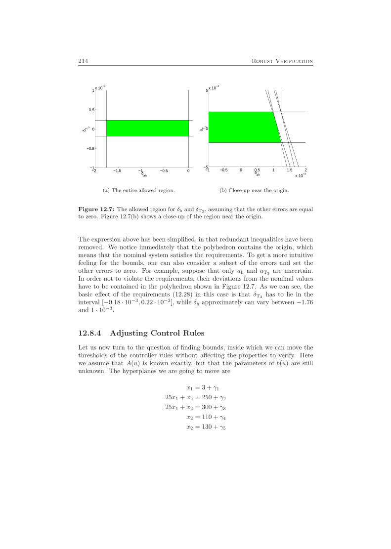
214 Robust Verification
−2 −1.5 −1 −0.5 0−1
−0.5
0
0.5
1x 10
−3
δah
δ T2
(a) The entire allowed region.
−1 −0.5 0 0.5 1 1.5 2
x 10−3
−5
0
5x 10
−4
δah
δ T2
(b) Close-up near the origin.
Figure 12.7: The allowed region for δh and δT2 , assuming that the other errors are equalto zero. Figure 12.7(b) shows a close-up of the region near the origin.
The expression above has been simplified, in that redundant inequalities have beenremoved. We notice immediately that the polyhedron contains the origin, whichmeans that the nominal system satisfies the requirements. To get a more intuitivefeeling for the bounds, one can also consider a subset of the errors and set theother errors to zero. For example, suppose that only ah and aT2 are uncertain.In order not to violate the requirements, their deviations from the nominal valueshave to be contained in the polyhedron shown in Figure 12.7. As we can see, thebasic effect of the requirements (12.28) in this case is that δT2 has to lie in theinterval [−0.18 · 10−3, 0.22 · 10−3], while δh approximately can vary between −1.76and 1 · 10−3.
12.8.4 Adjusting Control Rules
Let us now turn to the question of finding bounds, inside which we can move thethresholds of the controller rules without affecting the properties to verify. Herewe assume that A(u) is known exactly, but that the parameters of b(u) are stillunknown. The hyperplanes we are going to move are
x1 = 3 + γ1
25x1 + x2 = 250 + γ2
25x1 + x2 = 300 + γ3
x2 = 110 + γ4
x2 = 130 + γ5

12.8 An Example: A Chemical Reactor 215
These are the thresholds for the blender, the inflow valve, and the cooler signals.The other hyperplanes are assumed to be fixed (by physical properties of the plant).We would like to know how much we can change the values of γ1, . . . , γ5.
First we should make sure that we preserve the topology. Applying (12.15) toall corners yields the condition (after removing several redundant inequalities)
−1 0 0 0 01 0 0 0 00 −1 0 0 00 1 0 0 00 0 −1 0 00 0 1 0 00 0 0 −1 00 0 0 1 00 0 0 0 −10 0 0 0 125 −1 0 1 025 −1 0 0 125 −1 0 0 025 0 −1 1 025 0 −1 0 125 0 −1 0 00 1 −1 0 00 −1 0 1 00 1 0 −1 00 −1 0 0 10 1 0 0 −10 0 −1 1 00 0 1 −1 00 0 −1 0 10 0 1 0 −10 0 0 1 −1
γ ≺
31010075150256040802065452511595755014018512020519013517015520
(12.29)
The first ten inequalities make sure that the moving hyperplanes do not pass anyof the corners of the fixed hyperplanes (compare with Figure 12.6). The remaininginequalities state the relations between the moving hyperplanes (for example, thelast inequality tells us that the cooler should be turned off at a lower temperaturethan when it is turned on).
In addition to the topological requirement, the system also has to satisfy theproperties to verify. This is achieved if δbh, δheat, δcool, δreac, and γ satisfy thefollowing set of inequalities, obtained from (12.16):
1 0 0 0 0 0 0 0 00 1 0 0 0 0 0 0 00 0 −1 −1 0 0 0 0 025 0 0 1 0 0.0012 0 −0.001 025 0 0 1 0 0.0012 0 0 −0.0010 0 0 1 0 0 0 0.0002 025 0 1 1 0 0.0012 0 −0.001 025 0 1 1 0 0.0012 0 0 −0.0010 0 −1 −1 0 0 0 0 −0.00020 0 0 −1 0 0 −0.0012 0.001 00 0 0 −1 0 0 −0.0012 0 0.0010 0 −1 −1 0 0 −0.0012 0.001 00 0 −1 −1 0 0 −0.0012 0 0.001
δbh
δheat
δcool
δreac
γ1
γ2
γ3
γ4
γ5
4
9.83800.02940.0225
245.7977245.81790.0200
245.7536245.77380.02860.21380.19350.25790.2377
(12.30)
Together with (12.29), (12.30) now describes the region, in which the values ofδbh, δheat, δcool, δreac, and γ are allowed to vary. We can also note that settingδah = δT1 = δT2 = 0 in (12.28) and γ = 0 in (12.30) both give the same restrictionsfor the remaining uncertainties δbh, δheat, δcool, and δreac.
216 Robust Verification
From (12.30), one can go further and, e.g., find the values of γ that allowas large uncertainties as possible in the b parameters. This gives in a sense themaximally robust controller satisfying the verification, and is calculated similarlyto the computation of the Chebychev center of a polyhedron (the center of thelargest sphere inscribed in a polyhedron; see [19]). Here we would like to find thelargest disc, parallel to the γ coordinate axes and with its center somewhere alongthe subspace δ = 0, inscribed in the polyhedron defined by (12.29) and (12.30).Let us represent the disc as
D = {(
0γ
)+(δ0
) ∣∣ ‖δ‖ ≤ R} (12.31)
where the vector(
0γ
)is the center of the disc and R is the radius. We would like to
maximize R subject to the constraint that D satisfies (12.29) and (12.30). Let usstack (12.29) and (12.30) on top of each other, and denote the resulting matricesaccording to
F
(δγ
)4 g (12.32)
For each row i in (12.32), the constraint that D should satisfy Fi(δγ
)≤ gi can be
expressed
Fi
(0γ
)+ sup‖δ‖≤R
Fi
(δ0
)≤ gi
But since
sup‖δ‖≤R
Fi
(δ0
)= sup‖δ‖≤R
Fi
(I0
)δ = R
∥∥∥∥Fi(I0)∥∥∥∥
(where I is an identity matrix with the same number of rows as δ), we get
Fi
(0γ
)+R
∥∥∥∥Fi(I0)∥∥∥∥ ≤ gi
This is a linear inequality in γ and R, and the desired value of γ can be computedfrom the LP
maxγ,R
R
subj. to Fi
(0γ
)+R
∥∥∥∥Fi(I0)∥∥∥∥ ≤ gi, i = 1, . . . ,MF
(12.33)
where MF is the number of rows of F .
12.9 Conclusions
We have suggested an approach to investigate how sensitive approximating au-tomata for piecewise affine systems might be to changes in the underlying subsys-tems, to noise, and to translations of the switching surfaces. Section 12.4 provided

12.9 Conclusions 217
the sets of system matrices that satisfy certain requirements on the behavior ofthe system. As pointed out, these can either be seen as giving a measure of howrobust the approximating automata are to uncertainties in the system, or as givinglimits for how much the system can be changed, e.g., in a control design process,without altering the overall behavior described by the approximating automata.The methods can also be extended to switched systems, which was mentioned inSection 12.7.2.
It would be natural to combine these requirements with other objectives. Oneexample of this was given in Section 12.8.4. To give another example, when usingthe state feedback parameterization described in Section 12.5, one would probablywant to find L(v) that are optimal in a certain respect. Since the solution sets ofthe two first problems in Section 12.4.2 and Section 12.4.4 are convex, we can formall sorts of convex optimization problems, which can be solved very efficiently oncewe know the direct representations of the polyhedra (see for example [19]).

218 Robust Verification

Part IV
Appendices
219

A
Mathematical Preliminaries
In this appendix, some general concepts and results needed in previous chaptersare introduced. These include some material about convex sets and polyhedra,system identification, mixed-integer programming, and some combinatorial aspectsin classification. References for further reading are given in each section.
A.1 Explicit Solution of a System of Linear Equa-tions
In Part I, we need to be able to solve a certain form of systems of linear equations.This is accomplished using the following lemma.
Lemma A.1Let ρ > 0, x, z ∈ Rn where n ≥ 2, and let x have at least two elements that arenot equal. Then −ρzzT − I 1n x
1Tn 0 0xT 0 0
wµ1
µ2
=
010
(A.1)
221
222 Mathematical Preliminaries
(with w ∈ Rn and µ1, µ2 ∈ R) is nonsingular, and has the solution
wi =1ζ
γ n∑k=1
x2k −
(n∑k=1
xkzk
)2+
(n∑k=1
zk
n∑k=1
xkzk − γn∑k=1
xk
)xi (A.2)
+
(n∑k=1
xk
n∑k=1
xkzk −n∑k=1
x2k
n∑k=1
zk
)zi
)
µ =(µ1
µ2
)=
1ζ
γ
n∑k=1
x2k −
(n∑k=1
xkzk
)2
−γn∑k=1
xk +n∑k=1
zk
n∑k=1
xkzk
(A.3)
where
γ =1ρ
+ zT z
ζ =16
n∑i=1
n∑j=1
n∑k=1
(xi(zk − zj) + xj(zi − zk) + xk(zj − zi))2 +12ρ
n∑i=1
n∑k=1
(xi − xk)2
Remark A.1 Note that both γ and ζ are strictly positive.
Proof Let
G = −ρzzT − I, A =(
1TnxT
)First we need to show that (A.1) is nonsingular. It is easy to show (see, e.g., [161,Theorem 2.2]) that
det(G AT
A 0
)= det(G) det(−AG−1AT )
Since A has full rank and G is negative definite, it follows that AG−1AT is negativedefinite, and hence the system (A.1) is nonsingular.
Now,
(wµ
)=(G AT
A 0
)−1 0(
10
) =(G−1AT (AG−1AT )−1
−(AG−1AT )−1
)(10
)(A.4)
according to well-known matrix inversion formulas (see, e.g., [161, Theorem 2.4]).Furthermore,
G−1 = −I +1γzzT
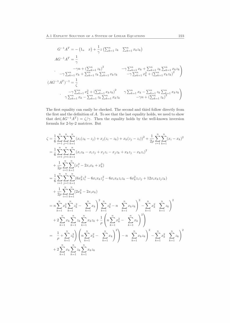
A.1 Explicit Solution of a System of Linear Equations 223
G−1AT = −(1n x
)+
1γz(∑n
k=1 zk∑nk=1 xkzk
)AG−1AT =
1γ
·(
−γn+ (∑nk=1 zk)2 −γ
∑nk=1 xk +
∑nk=1 zk
∑nk=1 xkzk
−γ∑nk=1 xk +
∑nk=1 zk
∑nk=1 xkzk −γ
∑nk=1 x
2k + (
∑nk=1 xkzk)2
)
(AG−1AT )−1 =1ζ
·(−γ∑nk=1 x
2k + (
∑nk=1 xkzk)2
γ∑nk=1 xk −
∑nk=1 zk
∑nk=1 xkzk
γ∑nk=1 xk −
∑nk=1 zk
∑nk=1 xkzk −γn+ (
∑nk=1 zk)2
)
The first equality can easily be checked. The second and third follow directly fromthe first and the definition of A. To see that the last equality holds, we need to showthat det(AG−1AT ) = ζ/γ. Then the equality holds by the well-known inversionformula for 2-by-2 matrices. But
ζ =16
n∑i=1
n∑j=1
n∑k=1
(xi(zk − zj) + xj(zi − zk) + xk(zj − zi))2 +12ρ
n∑i=1
n∑k=1
(xi − xk)2
=16
n∑i=1
n∑j=1
n∑k=1
(xizk − xizj + xjzi − xjzk + xkzj − xkzi)2
+12ρ
n∑i=1
n∑k=1
(x2i − 2xixk + x2
k)
=16
n∑i=1
n∑j=1
n∑k=1
(6x2kz
2i − 6xixkz2
j − 6xixkzizk − 6x2kzizj + 12xixkzjzk)
+12ρ
n∑i=1
n∑k=1
(2x2k − 2xixk)
= n
n∑k=1
x2k
n∑k=1
z2k −
(n∑k=1
xk
)2 n∑k=1
z2k − n
(n∑k=1
xkzk
)2
−n∑k=1
x2k
(n∑k=1
zk
)2
+ 2n∑k=1
xk
n∑k=1
zk
n∑k=1
xkzk +1ρ
n n∑k=1
x2k −
(n∑k=1
xk
)2
=
(1ρ
+n∑k=1
z2k
)n n∑k=1
x2k −
(n∑k=1
xk
)2− n( n∑
k=1
xkzk
)2
−n∑k=1
x2k
(n∑k=1
zk
)2
+ 2n∑k=1
xk
n∑k=1
zk
n∑k=1
xkzk
224 Mathematical Preliminaries
= γ1γ2
γ2n
n∑k=1
x2k − γn
(n∑k=1
xkzk
)2
− γ(
n∑k=1
zk
)2 n∑k=1
x2k
+
(n∑k=1
zk
)2( n∑k=1
xkzk
)2
− γ2
(n∑k=1
xk
)2
+ 2γn∑k=1
xk
n∑k=1
zk
n∑k=1
xkzk
−(
n∑k=1
zk
)2( n∑k=1
xkzk
)2
= γ det(AG−1AT )
where, in the third and fourth steps, the indices of several terms are switched. Thisshows the expression for (AG−1AT )−1.
From (A.4), we can now see that µ is given by the first column of (AG−1AT )−1,multiplied by −1, which gives the desired expression (A.3). For w, (A.4) gives thatmultiplying the expression for G−1AT by the first column of (AG−1AT )−1 yieldsthe desired expression, which is just a vector version of (A.2). �
A.2 Lipschitz Conditions
When studying multivariate functions in Chapter 4, some assumptions are madeabout the pth derivative satisfying a Lipschitz condition defined in (4.1). Underthis assumption, one can show a useful inequality, given by Lemma A.3. However,to be able to carry out the proof, the following lemma is needed. We use thenotation f
(p)i1...ip
for
f(p)i1...ip
=∂pf
∂xi1 . . . ∂xip(A.5)
Lemma A.2Let f : Rn → R be p times differentiable. Then
f(x+ t0h)− f(x)− t0n∑
i1=1
f ′i1(x)hi1 − . . .−tp0p!
n∑i1=1
. . .
n∑ip=1
f(p)i1...ip
(x)hi1 . . . hip
=∫ t0
0
∫ t1
0
. . .
∫ tp−1
0n∑
i1=1
. . .n∑
ip=1
(f
(p)i1...ip
(x+ tph)− f (p)i1...ip
(x))hi1 . . . hipdtp . . . dt2dt1
Proof The proof is carried out using induction. For p = 1, the lemma is trivial.Now suppose that the lemma is shown for p = q − 1, and consider the case p = q.
A.2 Lipschitz Conditions 225
Then
f(x+ t0h)− f(x)− t0n∑
i1=1
f ′i1(x)hi1 − . . .−tq0q!
n∑i1=1
. . .n∑
iq=1
f(q)i1...iq
(x)hi1 . . . hiq
=∫ t0
0
n∑i1=1
f ′i1(x+ t1h)hi1 −n∑
i1=1
f ′i1(x)hi1 − . . .
− tq−11
(q − 1)!
n∑i1=1
. . .n∑
iq=1
f(q)i1...iq
(x)hi1 . . . hiqdt1
=∫ t0
0
n∑i1=1
hi1
(f ′i1(x+ t1h)− f ′i1(x)− . . .
− tq−11
(q − 1)!
n∑i2=1
. . .
n∑iq=1
f(q)i1...iq
(x)hi2 . . . hiq
)dt1
=∫ t0
0
n∑i1=1
hi1
(∫ t1
0
. . .
∫ tq−1
0
n∑i2=1
. . .n∑
iq=1
(f
(q)i1...iq
(x+ tqh)− f (q)i1...iq
(x))hi2 . . . hiqdtq . . . dt2
)dt1
=∫ t0
0
∫ t1
0
. . .
∫ tq−1
0n∑
i1=1
. . .n∑
iq=1
(f
(q)i1...iq
(x+ tqh)− f (q)i1...iq
(x))hi1 . . . hiqdtq . . . dt2dt1
where the induction hypothesis was used in the third step, with f replaced by f ′i1 .The lemma is shown. �
The following lemma is a generalization of [40, Lemmas 4.1.12, 4.1.14].
Lemma A.3Let f : Rn → R be p times differentiable and satisfy the Lipschitz condition
max‖ξ‖=1
∣∣∣∣∣∣n∑
i1=1
. . .
n∑ip=1
(f
(p)i1...ip
(x+ h)− f (p)i1...ip
(x))ξi1 . . . ξip
∣∣∣∣∣∣ ≤ L‖h‖ (A.6)
for all h ∈ Rn. Then∣∣∣∣∣∣f(x+ h)− f(x)−n∑
i1=1
f ′i1(x)hi1 − . . .−1p!
n∑i1=1
. . .n∑
ip=1
f(p)i1...ip
(x)hi1 . . . hip
∣∣∣∣∣∣≤ L
(p+ 1)!‖h‖p+1 (A.7)

226 Mathematical Preliminaries
Remark A.2 Note that for p = 1, the Lipschitz condition (A.6) reduces to
‖∇f(x+ h)−∇f(x)‖ ≤ L‖h‖
and (A.7) becomes ∣∣f(x+ h)− f(x)−∇T f(x)h∣∣ ≤ L
2‖h‖2
For p = 2, (A.6) is equivalent to
‖∇2f(x+ h)−∇2f(x)‖ ≤ L‖h‖
where ∇2f is the Hessian of f , and where we use the usual induced 2-norm formatrices. Also, (A.7) reduces to∣∣∣∣f(x+ h)− f(x)−∇T f(x)h− 1
2hT∇2f(x)h
∣∣∣∣ ≤ L
6‖h‖3
Proof For h = 0, equality holds trivially. Now consider h 6= 0, and let h = h/‖h‖.By using Lemma A.2 we get∣∣∣∣∣∣f(x+ h)− f(x)−
n∑i1=1
f ′i1(x)hi1 − . . .−1p!
n∑i1=1
. . .
n∑ip=1
f(p)i1...ip
(x)hi1 . . . hip
∣∣∣∣∣∣=
∣∣∣∣∣∫ 1
0
∫ t1
0
. . .
∫ tp−1
0
n∑i1=1
. . .
n∑ip=1
(f
(p)i1...ip
(x+ tph)− f (p)i1...ip
(x))hi1 . . . hipdtp . . . dt2dt1
∣∣∣∣∣≤∫ 1
0
∫ t1
0
. . .
∫ tp−1
0∣∣∣∣∣∣n∑
i1=1
. . .
n∑ip=1
(f
(p)i1...ip
(x+ tph)− f (p)i1...ip
(x))hi1 . . . hip
∣∣∣∣∣∣ dtp . . . dt2dt1= ‖h‖p
∫ 1
0
∫ t1
0
. . .
∫ tp−1
0∣∣∣∣∣∣n∑
i1=1
. . .
n∑ip=1
(f
(p)i1...ip
(x+ tph)− f (p)i1...ip
(x))hi1 . . . hip
∣∣∣∣∣∣ dtp . . . dt2dt1≤ ‖h‖p
∫ 1
0
∫ t1
0
. . .
∫ tp−1
0
max‖ξ‖=1
∣∣∣∣∣∣n∑
i1=1
. . .
n∑ip=1
(f
(p)i1...ip
(x+ tph)− f (p)i1...ip
(x))ξi1 . . . ξip
∣∣∣∣∣∣ dtp . . . dt2dt1
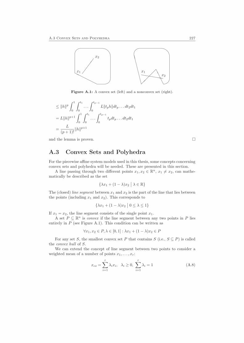
A.3 Convex Sets and Polyhedra 227
�
$�
�
$�
����
hhhhhhHH
HHHH
AAAA�
���CCCCCCCCx2
x1 x1x2
Figure A.1: A convex set (left) and a nonconvex set (right).
≤ ‖h‖p∫ 1
0
∫ t1
0
. . .
∫ tp−1
0
L‖tph‖dtp . . . dt2dt1
= L‖h‖p+1
∫ 1
0
∫ t1
0
. . .
∫ tp−1
0
tpdtp . . . dt2dt1
=L
(p+ 1)!‖h‖p+1
and the lemma is proven. �
A.3 Convex Sets and Polyhedra
For the piecewise affine system models used in this thesis, some concepts concerningconvex sets and polyhedra will be needed. These are presented in this section.
A line passing through two different points x1, x2 ∈ Rn, x1 6= x2, can mathe-matically be described as the set
{λx1 + (1− λ)x2
∣∣ λ ∈ R}The (closed) line segment between x1 and x2 is the part of the line that lies betweenthe points (including x1 and x2). This corresponds to
{λx1 + (1− λ)x2
∣∣ 0 ≤ λ ≤ 1}
If x1 = x2, the line segment consists of the single point x1.A set P ⊆ Rn is convex if the line segment between any two points in P lies
entirely in P (see Figure A.1). This condition can be written as
∀x1, x2 ∈ P, λ ∈ [0, 1] : λx1 + (1− λ)x2 ∈ P
For any set S, the smallest convex set P that contains S (i.e., S ⊆ P ) is calledthe convex hull of S.
We can extend the concept of line segment between two points to consider aweighted mean of a number of points x1, . . . , xr:
xco =r∑i=1
λixi, λi ≥ 0,r∑i=1
λi = 1 (A.8)
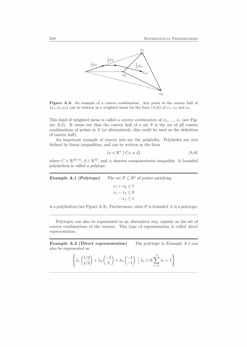
228 Mathematical Preliminaries
x1
x2
x3
13x1
13x2
13x3
xcoHHHHHHHHHHAAAAAAAAAA�
��
�������1
-XXXXXXXz������
������
��1
-XXXXXXXXXXXXXXXXXXXz
Figure A.2: An example of a convex combination. Any point in the convex hull of{x1, x2, x3} can be written as a weighted mean (in the form (A.8)) of x1, x2 and x3.
This kind of weighted mean is called a convex combination of x1, . . . , xr (see Fig-ure A.2). It turns out that the convex hull of a set S is the set of all convexcombinations of points in S (or alternatively, this could be used as the definitionof convex hull).
An important example of convex sets are the polyhedra. Polyhedra are setsdefined by linear inequalities, and can be written in the form
{x ∈ Rn∣∣ Cx 4 d} (A.9)
where C ∈ RM×n, d ∈ RM , and 4 denotes componentwise inequality. A boundedpolyhedron is called a polytope.
Example A.1 (Polytope) The set P ⊆ R2 of points satisfying
x1 + x2 ≤ 1x1 − x2 ≤ 0−x1 ≤ 1
is a polyhedron (see Figure A.3). Furthermore, since P is bounded, it is a polytope.
Polytopes can also be represented in an alternative way, namely as the set ofconvex combinations of the corners. This type of representation is called directrepresentation.
Example A.2 (Direct representation) The polytope in Example A.1 canalso be represented as{
λ1
(1/21/2
)+ λ2
(−12
)+ λ3
(−1−1
) ∣∣∣ λi ≥ 0,3∑i=1
λi = 1
}
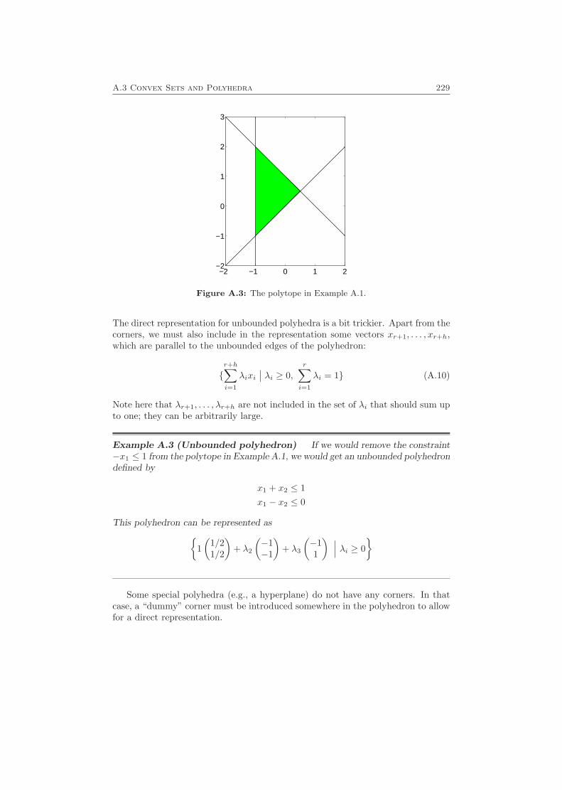
A.3 Convex Sets and Polyhedra 229
−2 −1 0 1 2−2
−1
0
1
2
3
Figure A.3: The polytope in Example A.1.
The direct representation for unbounded polyhedra is a bit trickier. Apart from thecorners, we must also include in the representation some vectors xr+1, . . . , xr+h,which are parallel to the unbounded edges of the polyhedron:
{r+h∑i=1
λixi∣∣ λi ≥ 0,
r∑i=1
λi = 1} (A.10)
Note here that λr+1, . . . , λr+h are not included in the set of λi that should sum upto one; they can be arbitrarily large.
Example A.3 (Unbounded polyhedron) If we would remove the constraint−x1 ≤ 1 from the polytope in Example A.1, we would get an unbounded polyhedrondefined by
x1 + x2 ≤ 1x1 − x2 ≤ 0
This polyhedron can be represented as{1(
1/21/2
)+ λ2
(−1−1
)+ λ3
(−11
) ∣∣∣ λi ≥ 0}
Some special polyhedra (e.g., a hyperplane) do not have any corners. In thatcase, a “dummy” corner must be introduced somewhere in the polyhedron to allowfor a direct representation.
230 Mathematical Preliminaries
Unfortunately, going from direct representation (A.10) to the form (A.9) is ingeneral computationally quite complex.
In Chapter 12, we are going to use open polyhedra. By this will be meant a set,whose direct representation is
{r+h∑i=1
λixi∣∣ λi > 0,
r∑i=1
λi = 1} (A.11)
i.e., where all λi are strictly positive. Note that this does not necessarily meanthat the set is open. However, relative to the smallest affine subspace containingthe open polyhedron, it is an open set.
Example A.4 (Open polyhedron) The (open) line segment{λ1
(12
)+ λ2
(23
) ∣∣∣ λi > 0, λ1 + λ2 = 1}
is an open polyhedron (in fact an open polytope), but not an open subset of R2.However, seen as a subset of the line through the points ( 1
2 ) and ( 23 ), it is open.
An excellent introduction to convex sets can be found in [19].
A.4 MILP/MIQP
In Chapter 11, some different piecewise affine system identification problems areformulated as Mixed-Integer Linear Programs (MILP) and Mixed-Integer QuadraticPrograms (MIQP). These are two types of optimization problems that involve bothdiscrete and continuous variables. In general, an MILP problem has the followingstructure:
minx,δ
pT(xδ
)subj. to C
(xδ
)≤ d (A.12)
x ∈ Rn, δ ∈ {0, 1}m
The MIQP problem is almost identical, except that the objective function is quad-ratic:
minx,δ
(xT δT
)Q
(xδ
)+ pT
(xδ
)subj. to C
(xδ
)≤ d (A.13)
x ∈ Rn, δ ∈ {0, 1}m
A.4 MILP/MIQP 231
We assume that Q is positive definite or semidefinite. If it is only positivesemidefinite, one could use regularization techniques as in Section 8.3 to make itpositive definite.
As we can see, the only difference compared to an ordinary LP or QP (Linearor Quadratic Program) is that the δ variables are discrete. However, although LPand QP problems can be solved efficiently using standard algorithms, it has beenshown that solving a general MILP/MIQP problem is NP-hard [49, 151]. Thismeans that there is no known algorithm solving the MILP/MIQP problems withpolynomial worst-case complexity, and that if such an algorithm is found, severalother hard problems would also be solvable in polynomial time. It is quite easy tofind an algorithm, for which we in the worst case have to test all combinations ofδ values, so the worst-case complexity is at most 2m times the complexity of anLP/QP problem in n variables. However, there are algorithms that work better formany practical cases. Some solvers for the MILP/MIQP problems can be foundin, e.g., [11, 36, 70, 139].
A.4.1 A Branch-and-Bound Algorithm
Let us take a closer look at (A.12) and (A.13). If we would replace the requirementδ ∈ {0, 1}m by 0 ≤ δ ≤ 1, the problems would become ordinary LP or QP problems.Similarly, if we fix some of the elements of δ to either 0 or 1 and relax the otherelements, we would also get LP/QP problems. These combined relaxations andrestrictions can be used to form a branch-and-bound algorithm, which will beillustrated by an example:
Example A.5 (Branch-and-bound, depth first) We would like to solve theproblem
minx,δ
J = x− 2δ1 − δ2
subj. to x+ 5δ1 + 6δ2 ≤ 9 (A.14)0 ≤ x ≤ 1δ1, δ2 ∈ {0, 1}
Figure A.4 shows the feasible region for this problem. Let us start by solving therelaxed problem we get by replacing δ1, δ2 ∈ {0, 1} by 0 ≤ δ1 ≤ 1, 0 ≤ δ2 ≤ 1. Thisis an LP problem with the solution
J∗ = −8/3x = 0δ1 = 1δ2 = 2/3
In Figure A.4, the feasible region for the relaxed problem is the three-dimensionalregion bounded by the cube and the plane x + 5δ1 + 6δ2 = 9. Let us now fix one
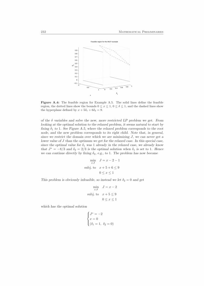
232 Mathematical Preliminaries
00.5
1 0 0.2 0.4 0.6 0.8 1
−0.1
0
0.1
0.2
0.3
0.4
0.5
0.6
0.7
0.8
0.9
δ1
Feasible region for the MILP example
x
δ 2
Figure A.4: The feasible region for Example A.5. The solid lines define the feasibleregion, the dotted lines show the bounds 0 ≤ x ≤ 1, 0 ≤ δ ≤ 1, and the dashed lines showthe hyperplane defined by x+ 5δ1 + 6δ2 = 9.
of the δ variables and solve the new, more restricted LP problem we get. Fromlooking at the optimal solution to the relaxed problem, it seems natural to start byfixing δ1 to 1. See Figure A.5, where the relaxed problem corresponds to the rootnode, and the new problem corresponds to its right child. Note that, in general,since we restrict the domain over which we are minimizing J , we can never get alower value of J than the optimum we get for the relaxed case. In this special case,since the optimal value for δ1 was 1 already in the relaxed case, we already knowthat J∗ = −8/3 and δ2 = 2/3 is the optimal solution when δ1 is set to 1. Hencewe can continue directly by fixing δ2, e.g., to 1. The problem has now become
minx,δ
J = x− 2− 1
subj. to x+ 5 + 6 ≤ 90 ≤ x ≤ 1
This problem is obviously infeasible, so instead we let δ2 = 0 and get
minx,δ
J = x− 2
subj. to x+ 5 ≤ 90 ≤ x ≤ 1
which has the optimal solutionJ∗ = −2x = 0(δ1 = 1, δ2 = 0)
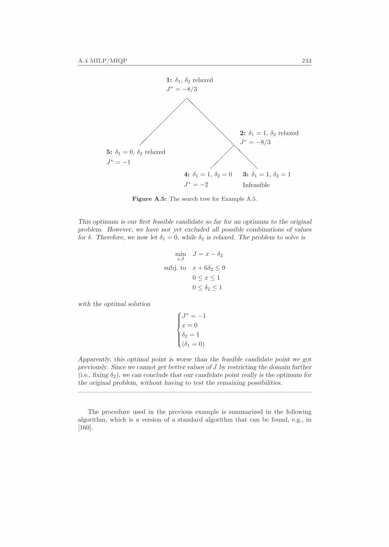
A.4 MILP/MIQP 233
@@
@@�
���
@@
@@
@@
@@��������
1: δ1, δ2 relaxedJ∗ = −8/3
2: δ1 = 1, δ2 relaxedJ∗ = −8/3
3: δ1 = 1, δ2 = 1
Infeasible
4: δ1 = 1, δ2 = 0
J∗ = −2
5: δ1 = 0, δ2 relaxed
J∗ = −1
Figure A.5: The search tree for Example A.5.
This optimum is our first feasible candidate so far for an optimum to the originalproblem. However, we have not yet excluded all possible combinations of valuesfor δ. Therefore, we now let δ1 = 0, while δ2 is relaxed. The problem to solve is
minx,δ
J = x− δ2
subj. to x+ 6δ2 ≤ 90 ≤ x ≤ 10 ≤ δ2 ≤ 1
with the optimal solution J∗ = −1x = 0δ2 = 1(δ1 = 0)
Apparently, this optimal point is worse than the feasible candidate point we gotpreviously. Since we cannot get better values of J by restricting the domain further(i.e., fixing δ2), we can conclude that our candidate point really is the optimum forthe original problem, without having to test the remaining possibilities.
The procedure used in the previous example is summarized in the followingalgorithm, which is a version of a standard algorithm that can be found, e.g., in[160].
234 Mathematical Preliminaries
Algorithm A.1 (Branch-and-bound, depth first)
Given: A problem like (A.12) or (A.13).Initialization: Set LB = −∞ and UB = ∞. Relax the problem by allowingall elements in δ to take any value in the interval [0, 1]. Start building on a treestructure by creating a root node. (Each level in the tree structure will correspondto one more element in δ being fixed; cf. Figure A.5.)
1. Solve the current LP/QP problem. If it is infeasible, go to 4. If it is feasible,denote the optimal point by x∗, δ∗, and the optimal value by J∗. If δ∗ ∈{0, 1}m, go to 3. Otherwise, go to 2.
2. If J∗ > UB, the optimal solution will not be in this branch of the tree, so goto 4. Else, fix one of the relaxed elements in δ to 0 or 1, according to somestrategy. Add one child to the current node in the tree and move to the childnode. If all of the currently fixed elements of δ have already previously beenfixed to their other possible values, and if J∗ > LB, set LB = J∗. Go to 1.
3. If J∗ < UB, set UB = J∗, and let xmin = x∗ and δmin = δ∗. Go to 4.
4. Go up one level in the tree, i.e., relax the δ element that was last fixed. If theother possible value of that element has not yet been tested, fix the elementto that value. (In other words, if the element was fixed to 0 and has not yetbeen fixed to 1, set it to 1.) Otherwise, go up one level at a time in the treeuntil an untested value of a δ element is found. Then go to 1. If the root nodeis reached and no untested value is found, we are done. Then set LB = UB.
When these iterations are done, the optimal value of the objective function equalsLB = UB. If LB = UB = ∞, the problem is infeasible. Otherwise, the optimalpoint is given by xmin and δmin.
There are some remarks to be made. Firstly, the algorithm does not specify howto choose the element to be fixed in step 2. There are several possible strategiesto use for this. In Example A.5, the element of δ that was closest to an integervalue was chosen. The thought behind this is to quickly reach a good feasible pointfor the original problem. With its help, entire subtrees can be ruled out as beingobviously bad (or at least worse than the best value found so far), which may savea large amount of computations, just as in the example.
During the iterations of Algorithm A.1, the variables UB and LB give anupper and a lower bound on the optimal value. This could be useful, e.g., if thecomputation is stopped before the search for the optimal value is completed. Thenthe best suboptimal point so far might be usable, together with the lower bound,that shows how far from the optimum we can be at most.
There are variants of this algorithm. For example, one can also traverse thesearch tree in a best-first manner, where the nodes with the best optimal values J∗
are traversed first, or in a breadth-first manner, or in a combination of the three.There are also several other algorithms besides the branch-and-bound algorithmsfor solving the MILP/MIQP problems. A good reference is [160].
A.5 Separating Points with Hyperplanes 235
A.5 Separating Points with Hyperplanes
When investigating the computational complexity of the algorithms in Chapter11, a question that will arise is: In how many ways can we group N points inRn by separating them with M hyperplanes? To be able to answer this questionunambiguously, we need to restrict ourselves to only consider a certain kind ofpoint sets. The terminology here partly follows [35].
Definition A.1A set of points X ∈ Rn is in general position, if for every subset of pointsx1, . . . , xk ∈ X, where k ≤ n+ 1, the vectors(
1x1
), . . . ,
(1xk
)are linearly independent.
This definition is equivalent to specifying that no subset of k points shouldbe contained in an affine subspace of a lower dimension than min{k − 1, n}. Forexample, if we consider points in R2, no points should coincide, and three pointsshould never be on a line. Note that, nonstrictly speaking, for an arbitrarily chosenset of points in Rn, this condition is satisfied with probability one.
Let us begin by determining in how many ways a set of points can be split byone hyperplane. This result will follow as a corollary to the following theorem,which is also found in, e.g., [35].
Theorem A.1Consider N hyperplanes in Rn going through the origin, such that the normalvectors of any subset consisting of n or fewer hyperplanes are linearly independent.Let f(n,N) be the number of regions into which Rn is divided by the hyperplanes.Then f(n,N) can be written as a sum of binomial terms
f(n,N) = 2n−1∑k=0
(N − 1k
)(A.15)
for n ≥ 1, N ≥ 1 (we let(
00
)= 1 and
(Nk
)= 0 for k > N).
Proof We prove the theorem by induction. Clearly, f(n, 1) = 2 = 2∑n−1k=0
(0k
)for
n ≥ 1, since one hyperplane divides the space into two half-spaces. We also havef(1, N) = 2 = 2
(N−1
0
)for N ≥ 1 (a one-dimensional line can only be divided into
two half-lines, no matter how many points you put in the origin).
Now suppose that the theorem has been shown for all {(n,N)∣∣ n ≤ n0, N ≤
N0 − 1}, and suppose that we have placed N0 − 1 hyperplanes in Rn0 , and areabout to place one more (see Figure A.6(a)). The N0th hyperplane is an (n0 − 1)-dimensional subspace of Rn0 , and will be cut by all the other N0 − 1 hyperplanes.
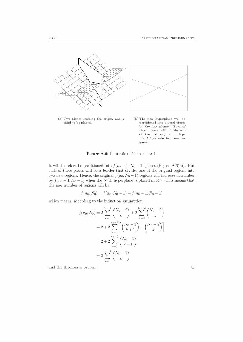
236 Mathematical Preliminaries
(a) Two planes crossing the origin, and athird to be placed.
(b) The new hyperplane will bepartitioned into several piecesby the first planes. Each ofthese pieces will divide oneof the old regions in Fig-ure A.6(a) into two new re-gions.
Figure A.6: Illustration of Theorem A.1.
It will therefore be partitioned into f(n0 − 1, N0 − 1) pieces (Figure A.6(b)). Buteach of these pieces will be a border that divides one of the original regions intotwo new regions. Hence, the original f(n0, N0 − 1) regions will increase in numberby f(n0 − 1, N0 − 1) when the N0th hyperplane is placed in Rn0 . This means thatthe new number of regions will be
f(n0, N0) = f(n0, N0 − 1) + f(n0 − 1, N0 − 1)
which means, according to the induction assumption,
f(n0, N0) = 2n0−1∑k=0
(N0 − 2k
)+ 2
n0−2∑k=0
(N0 − 2k
)
= 2 + 2n0−2∑k=0
[(N0 − 2k + 1
)+(N0 − 2k
)]
= 2 + 2n0−2∑k=0
(N0 − 1k + 1
)
= 2n0−1∑k=0
(N0 − 1k
)and the theorem is proven. �
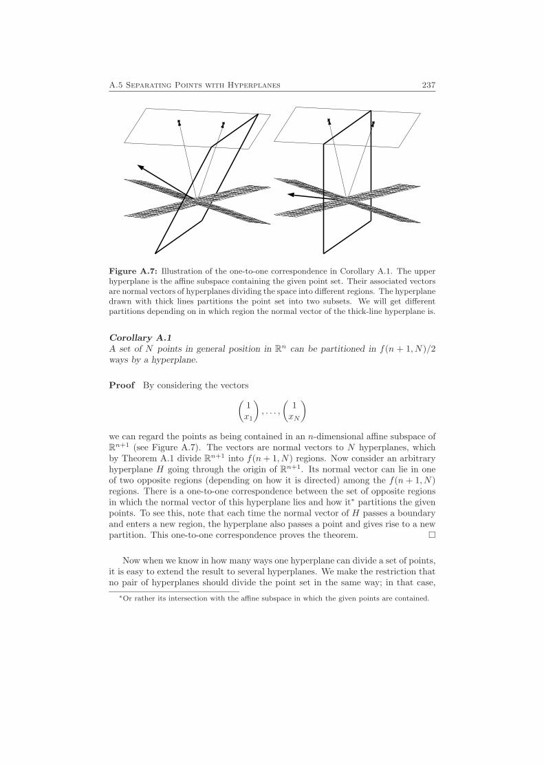
A.5 Separating Points with Hyperplanes 237
Figure A.7: Illustration of the one-to-one correspondence in Corollary A.1. The upperhyperplane is the affine subspace containing the given point set. Their associated vectorsare normal vectors of hyperplanes dividing the space into different regions. The hyperplanedrawn with thick lines partitions the point set into two subsets. We will get differentpartitions depending on in which region the normal vector of the thick-line hyperplane is.
Corollary A.1A set of N points in general position in Rn can be partitioned in f(n + 1, N)/2ways by a hyperplane.
Proof By considering the vectors(1x1
), . . . ,
(1xN
)we can regard the points as being contained in an n-dimensional affine subspace ofRn+1 (see Figure A.7). The vectors are normal vectors to N hyperplanes, whichby Theorem A.1 divide Rn+1 into f(n+ 1, N) regions. Now consider an arbitraryhyperplane H going through the origin of Rn+1. Its normal vector can lie in oneof two opposite regions (depending on how it is directed) among the f(n + 1, N)regions. There is a one-to-one correspondence between the set of opposite regionsin which the normal vector of this hyperplane lies and how it∗ partitions the givenpoints. To see this, note that each time the normal vector of H passes a boundaryand enters a new region, the hyperplane also passes a point and gives rise to a newpartition. This one-to-one correspondence proves the theorem. �
Now when we know in how many ways one hyperplane can divide a set of points,it is easy to extend the result to several hyperplanes. We make the restriction thatno pair of hyperplanes should divide the point set in the same way; in that case,∗Or rather its intersection with the affine subspace in which the given points are contained.
238 Mathematical Preliminaries
they could be replaced by one hyperplane. Since the trivial partitions obtainedby letting all points lie on the same side of a hyperplane will be uninterestingin Chapter 11, we also exclude these cases. The remaining partitions are callednontrivial.
Corollary A.2A set of N points in general position in Rn can be partitioned in
(f(n+1,N)/2−1
M
)nontrivial ways by M hyperplanes.
Proof From f(n + 1, N)/2 − 1 nontrivial options of placing one hyperplane, weshould choose M different ways to place the hyperplanes. �
A.6 Inverting a Univariate Piecewise Affine Func-tion
In Chapter 11, we will also need to invert a univariate, continuous, piecewise affinefunction. The following lemma can be used for this purpose.
Lemma A.4Consider the function
f(x) = x− α0 +M∑i=1
σi max{βix− αi, 0}
βi > 0,α1
β1<α2
β2< · · · < αM
βM
(A.16)
where σi ∈ {−1, 1}, and assume that f is strictly increasing, i.e.†,
0 <k∑
m=0
σmβm <∞ ∀k = 1, . . . ,M (A.17)
Then the inverse of f(x) is
f−1(y) = y + α0 −M∑k=1
σk max{βky − αk, 0}
βk =βk∑k−1
m=0 σmβm∑km=0 σmβm
αk =∑k−1m=0 σm(βmαk − βkαm)∑k−1m=0 σmβm
∑km=0 σmβm
(A.18)
†For the sake of a more compact notation, let σ0 = β0 = 1.
A.6 Inverting a Univariate Piecewise Affine Function 239
Proof We prove the statement by induction over M . For M = 0, we havef(x) = x − α0, so f−1(y) = y + α0. Now suppose that the statement holds for acertain M−1 ≥ 0, and consider a function f with M breakpoints. For x < αM/βM ,f has only M − 1 breakpoints, so in this region f−1 can be written as in (A.18),according to the induction assumption. For x ≥ αM/βM , we get
f(x) =
(M∑m=0
σmβm
)x−
M∑m=0
σmαm (A.19)
so
f−1(y) =y +
∑Mm=0 σmαm∑M
m=0 σmβm(A.20)
Since x = f−1(y), we can rewrite the condition x ≥ αM/βM as
y +∑Mm=0 σmαm∑M
m=0 σmβm≥ αMβM
⇔ 1∑Mm=0 σmβm
(y − 1
βM
M−1∑m=0
σm(βmαM − βMαm)
)≥ 0
⇔ y ≥ αM
βM
Now, for y ≥ αM/βM , by using simple but tedious calculations we can rewrite(A.20) as
f−1(y) =y +
∑M−1m=0 σmαm∑M−1
m=0 σmβm
+−σMβM∑M−1
m=0 σmβm∑Mm=0 σmβm
(y − 1
βM
M−1∑m=0
σm(βmαM − βMαm)
)= f−1
M−1(y)− σM (βMy − αM )
where f−1M−1(y) is the inverse of the given function without the Mth max func-
tion. Since this function equals f(x) for x < αM/βM , we get f−1M−1(y) = f−1(y)
for y < αM/βM . Furthermore, by using a max function and by the inductionassumption we now can write
f−1(y) = f−1M−1(y)− σM max{βMy − αM , 0}
= y + α0 −M−1∑k=1
σk max{βky − αk, 0} − σM max{βMy − αM , 0}
= y + α0 −M∑k=1
σk max{βky − αk, 0}
which is just what we wanted to prove. �

240 Mathematical Preliminaries

Bibliography
[1] H. Akaike. Information theory and an extension of the maximum likelihoodprinciple. In Second International Symposium on Information Theory, pages267–281, 1973.
[2] R. Alur, C. Courcoubetis, N. Halbwachs, T. A. Henzinger, P.-H. Ho,X. Nicollin, A. Olivero, J. Sifakis, and S. Yovine. The algorithmic analy-sis of hybrid systems. Theoretical Computer Science, 138:3–34, 1995.
[3] R. Alur, T. A. Henzinger, and P.-H. Ho. Automatic symbolic verification ofembedded systems. IEEE Transactions on Software Engineering, 22:181–201,1996.
[4] R. Alur, T. A. Henzinger, G. Lafferriere, and G. J. Pappas. Discrete ab-stractions of hybrid systems. Proceedings of the IEEE, 88(7):971–984, July2000.
[5] C. G. Atkeson, A. W. Moore, and S. Schaal. Locally weighted learning.Artificial Intelligence Review, 11(1-5):11–73, Feb. 1997.
[6] C. G. Atkeson, A. W. Moore, and S. Schaal. Locally weighted learning forcontrol. Artificial Intelligence Review, 11(1-5):75–113, Feb. 1997.
241
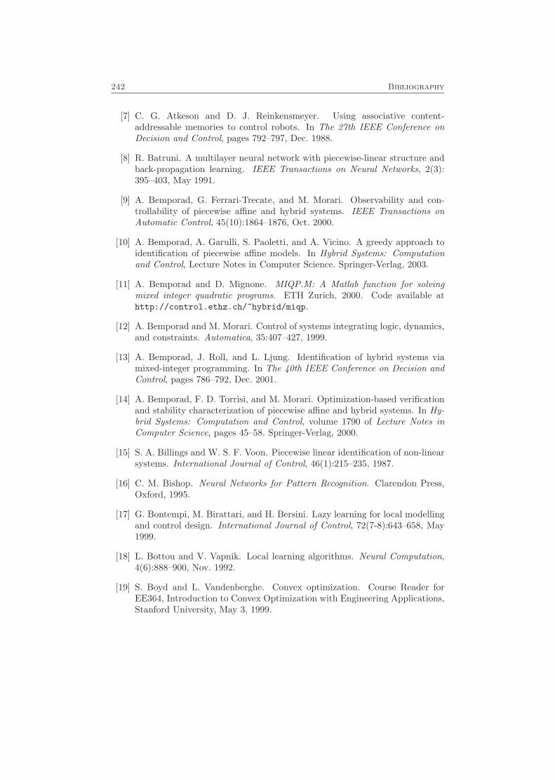
242 Bibliography
[7] C. G. Atkeson and D. J. Reinkensmeyer. Using associative content-addressable memories to control robots. In The 27th IEEE Conference onDecision and Control, pages 792–797, Dec. 1988.
[8] R. Batruni. A multilayer neural network with piecewise-linear structure andback-propagation learning. IEEE Transactions on Neural Networks, 2(3):395–403, May 1991.
[9] A. Bemporad, G. Ferrari-Trecate, and M. Morari. Observability and con-trollability of piecewise affine and hybrid systems. IEEE Transactions onAutomatic Control, 45(10):1864–1876, Oct. 2000.
[10] A. Bemporad, A. Garulli, S. Paoletti, and A. Vicino. A greedy approach toidentification of piecewise affine models. In Hybrid Systems: Computationand Control, Lecture Notes in Computer Science. Springer-Verlag, 2003.
[11] A. Bemporad and D. Mignone. MIQP.M: A Matlab function for solvingmixed integer quadratic programs. ETH Zurich, 2000. Code available athttp://control.ethz.ch/~hybrid/miqp.
[12] A. Bemporad and M. Morari. Control of systems integrating logic, dynamics,and constraints. Automatica, 35:407–427, 1999.
[13] A. Bemporad, J. Roll, and L. Ljung. Identification of hybrid systems viamixed-integer programming. In The 40th IEEE Conference on Decision andControl, pages 786–792, Dec. 2001.
[14] A. Bemporad, F. D. Torrisi, and M. Morari. Optimization-based verificationand stability characterization of piecewise affine and hybrid systems. In Hy-brid Systems: Computation and Control, volume 1790 of Lecture Notes inComputer Science, pages 45–58. Springer-Verlag, 2000.
[15] S. A. Billings and W. S. F. Voon. Piecewise linear identification of non-linearsystems. International Journal of Control, 46(1):215–235, 1987.
[16] C. M. Bishop. Neural Networks for Pattern Recognition. Clarendon Press,Oxford, 1995.
[17] G. Bontempi, M. Birattari, and H. Bersini. Lazy learning for local modellingand control design. International Journal of Control, 72(7-8):643–658, May1999.
[18] L. Bottou and V. Vapnik. Local learning algorithms. Neural Computation,4(6):888–900, Nov. 1992.
[19] S. Boyd and L. Vandenberghe. Convex optimization. Course Reader forEE364, Introduction to Convex Optimization with Engineering Applications,Stanford University, May 3, 1999.
Bibliography 243
[20] M. S. Branicky. Multiple Lyapunov functions and other analysis tools forswitched and hybrid systems. IEEE Transactions on Automatic Control, 43(4):475–482, Apr. 1998.
[21] M. S. Branicky, V. S. Borkar, and S. K. Mitter. A unified framework forhybrid control: Model and optimal control theory. IEEE Transactions onAutomatic Control, 43(1):31–45, 1998.
[22] L. Breiman. Hinging hyperplanes for regression, classification, and functionapproximation. IEEE Transactions on Information Theory, 39(3):999–1013,May 1993.
[23] L. Breiman and J. H. Friedman. Function approximation using ramps. InSnowbird Workshop. Machines that Learn, 1994.
[24] L. Breiman, J. H. Friedman, R. A. Olshen, and C. J. Stone. Classification AndRegression Trees. Wadsworth & Brooks/Cole Advanced Books & Software,1984.
[25] J. Bruls, C. T. Chou, B. R. J. Haverkamp, and M. Verhaegen. Linear and non-linear system identification using separable least-squares. European Journalof Control, 5(1):116–128, 1999.
[26] C.-H. Choi and J. Y. Choi. Constructive neural networks with piecewiseinterpolation capabilities for function approximations. IEEE Transactionson Neural Networks, 5(6):936–944, Nov. 1994.
[27] L. O. Chua and A.-C. Deng. Canonical piecewise-linear representation. IEEETransactions on Circuits and Systems, 35(1):101–111, Jan. 1988.
[28] L. O. Chua and S. M. Kang. Section-wise piecewise-linear functions: Canon-ical representation, properties and applications. Proceedings of the IEEE, 65:915–929, 1977.
[29] A. Chutinan. Hybrid System Verification Using Discrete Model Approxi-mations. PhD thesis, Department of Electrical and Computer Engineering,Carnegie Mellon University, May 1999.
[30] A. Chutinan and B. H. Krogh. Computing approximating automata for aclass of linear hybrid systems. In Hybrid Systems V, Lecture Notes in Com-puter Science. Springer-Verlag, 1998.
[31] A. Chutinan and B. H. Krogh. Computing polyhedral approximations toflow pipes for dynamic systems. In The 37th IEEE Conference on Decisionand Control: Session on Synthesis and Verification of Hybrid Control Laws(TM-01), 1998.
[32] W. S. Cleveland. Robust locally weighted regression and smoothing scatter-plots. Journal of the American Statistical Association, 74(368):829–836, Dec.1979.
244 Bibliography
[33] W. S. Cleveland and S. J. Devlin. Locally weighted regression: An approachto regression analysis by local fitting. Journal of the American StatisticalAssociation, 83(403):596–610, Sept. 1988.
[34] W. S. Cleveland and C. L. Loader. Smoothing by local regression: Principlesand methods. In W. Haerdle and M. G. Schimek, editors, Statistical Theoryand Computational Aspects of Smoothing, pages 10–49. Springer, New York,1996.
[35] T. M. Cover. Geometrical and statistical properties of systems of linearinequalities with applications in pattern recognition. IEEE Transactions onElectronic Computers, 14(3):326–334, June 1965.
[36] Dash Associates. XPRESS-MP User Guide, 1999.
[37] L. Davis. Genetic Algorithms and Simulated Annealing. London: Pitman;Los Altos, Calif.: Kaufmann, 1987.
[38] R. A. DeCarlo, M. S. Branicky, S. Pettersson, and B. Lennartsson. Per-spectives and results on the stability and stabilizability of hybrid systems.Proceedings of the IEEE, 88(7):1069–1082, July 2000.
[39] D. den Hertog. Interior Point Approach to Linear, Quadratic and ConvexProgramming: Algorithms and Complexity. Kluwer Academic, 1994.
[40] J. E. Dennis, Jr. and R. B. Schnabel. Numerical Methods for UnconstrainedOptimization and Nonlinear Equations. Prentice-Hall, 1983.
[41] R. O. Duda and P. E. Hart. Pattern Classification and Scene Analysis. JohnWiley & Sons, 1973.
[42] V. Einarsson. On verification of switched systems using abstractions. Li-centiate Thesis, Department of Electrical Engineering, Linkoping University,SE-581 83 Linkoping, Sweden. Thesis No. 705, 1998.
[43] V. Einarsson. Model Checking Methods for Mode Switching Systems. PhDthesis, Department of Electrical Engineering, Linkoping University, SE-581 83 Linkoping, Sweden, 2000.
[44] S. Engell, S. Kowalewski, C. Schulz, and O. Stursberg. Continuous-discreteinteractions in chemical processing plants. Proceedings of the IEEE, 88(7):1050–1068, July 2000.
[45] V. A. Epanechnikov. Non-parametric estimation of a multivariate probabilitydensity. Theory of Probability and its Applications, 14:153–158, 1969.
[46] S. Ernst. Hinging hyperplane trees for approximation and identification. InThe 37th IEEE Conference on Decision and Control, volume 2, pages 1266–1271, 1998.
Bibliography 245
[47] J. Fan and I. Gijbels. Local Polynomial Modelling and Its Applications. Chap-man & Hall, 1996.
[48] G. Ferrari-Trecate, M. Muselli, D. Liberati, and M. Morari. A clusteringtechnique for the identification of piecewise affine systems. Automatica, 39(2):205–217, Feb. 2003.
[49] C. A. Floudas. Nonlinear and Mixed-Integer Optimization: Fundamentalsand Applications. Oxford University Press, 1995.
[50] A. T. Fuller. Relay control systems optimized for various performance crite-ria. In 1st World Congress IFAC, pages 584–607, 1960.
[51] E. F. Gad, A. F. Atiya, S. Shaheen, and A. El-Dessouki. A new algorithmfor learning in piecewise-linear neural networks. Neural Networks, 13(4-5):485–505, 2000.
[52] A. Garulli, A. Tesi, and A. Vicino, editors. Robustness in Identification andControl. Lecture Notes in Control and Information Sciences. Springer-Verlag,1999.
[53] T. Gasser and H.-G. Muller. Kernel estimation of regression functions. InT. Gasser and M. Rosenblatt, editors, Smoothing Techniques for Curve Esti-mation, Lecture Notes in Mathematics, pages 23–68. Springer-Verlag, 1979.
[54] T. Gasser, H.-G. Muller, and V. Mammitzsch. Kernels for nonparametriccurve estimation. Journal of the Royal Statistical Society. Series B, StatisticalMethodology, 47(2):238–252, 1985.
[55] S. B. Gelfand and C. S. Ravishankar. A tree-structured piecewise linearadaptive filter. IEEE Transactions on Information Theory, 39(6):1907–1922,Nov. 1993.
[56] M. N. Gibbs. Bayesian Gaussian Processes for Regression and Classification.PhD thesis, University of Cambridge, 1997.
[57] R. E. Groff, D. E. Koditschek, and P. P. Khargonekar. Piecewise linear home-omorphisms: The scalar case. In Proceedings of the IEEE-INNS-ENNS In-ternational Joint Conference on Neural Networks (IJCNN), volume 3, pages259–264, 2000.
[58] F. Gustafsson. Adaptive Filtering and Change Detection. John Wiley & Sons,2000.
[59] C. Guzelis and I. C. Goknar. A canonical representation for piecewise-affinemaps and its applications to circuit analysis. IEEE Transactions on Circuitsand Systems, 38(11):1342–1354, Nov. 1991.

246 Bibliography
[60] A. Hagenblad. Aspects of the identification of Wiener models. Licentiate The-sis, Department of Electrical Engineering, Linkoping University, SE-581 83Linkoping, Sweden. Thesis No. 793, 1999.
[61] W. Hardle. Applied Nonparametric Regression. Number 19 in EconometricSociety Monographs. Cambridge University Press, 1990.
[62] W. P. M. H. Heemels, B. D. Schutter, and A. Bemporad. Equivalence ofhybrid dynamical models. Automatica, 37(7):1085–1091, July 2001.
[63] T. A. Henzinger, P.-H. Ho, and H. Wong-Toi. HyTech: A model checker forhybrid systems. Software Tools for Technology Transfer, 1:110–122, 1997.
[64] E. A. Heredia and G. R. Arce. Piecewise linear system modeling based on acontinuous threshold decomposition. IEEE Transactions on Signal Process-ing, 44(6):1440–1453, June 1996.
[65] I. Hoffmann. Identifikation hybrider dynamischer Systeme. PhD thesis, Uni-versitat Dortmund, 1999.
[66] I. Hoffmann and S. Engell. Identification of hybrid systems. In AmericanControl Conference, pages 711–712, 1998.
[67] C. C. Holmes and B. K. Mallick. Bayesian regression with multivariate linearsplines. Journal of the Royal Statistical Society. Series B, Statistical Method-ology, 63(1):3–17, 2001.
[68] C. M. Hurvich, J. S. Simonoff, and C.-L. Tsai. Smoothing parameter selectionin nonparametric regression using an improved Akaike information criterion.Journal of the Royal Statistical Society. Series B, Statistical Methodology, 60(2):271–293, 1998.
[69] D. R. Hush and B. Horne. Efficient algorithms for function approximationwith piecewise linear sigmoidal networks. IEEE Transactions on Neural Net-works, 9(6):1129–1141, Nov. 1998.
[70] ILOG, Inc. CPLEX 7.0 User’s Manual. Gentilly, France, 2000.
[71] T. A. Johansen and B. A. Foss. Identification of non-linear system structureand parameters using regime decomposition. Automatica, 31(2):321–326, Feb.1995.
[72] M. Johansson. Piecewise Linear Control Systems. PhD thesis, Departmentof Automatic Control, Lund Institute of Technology, Lund University, Box118, SE-221 00 Lund, Sweden, 1999.
[73] M. Johansson and A. Rantzer. Computation of piece-wise quadratic Lya-punov functions for hybrid systems. IEEE Transactions on Automatic Con-trol, 43(4):555–559, 1998.
Bibliography 247
[74] M. C. Jones and M. P. Wand. Asymptotic effectiveness of some higher orderkernels. Journal of Statistical Planning and Inference, 31(1):15–21, Apr. 1992.
[75] M. A. Jordan and O. A. A. Orqueda. Persistency of excitation and richnessin continuous-time piecewise linear systems. In 1st International Conferenceon Control of Oscillations and Chaos, volume 2, pages 234–237, Aug. 1997.
[76] P. Julian, A. Desages, and O. Agamennoni. High level canonical piecewiselinear representation using a simplicial partition. IEEE Transactions on Cir-cuits and Systems – I: Fundamental Theory and Applications, 46(4):463–480,1999.
[77] P. Julian, M. Jordan, and A. Desages. Canonical piecewise-linear approxi-mation of smooth functions. IEEE Transactions on Circuits and Systems, 45(5):567–571, May 1998.
[78] P. M. Julian. A High Level Canonical Piecewise Linear Representation: The-ory and Applications. PhD thesis, Departamento de Ingenierıa Electrica,Universidad Nacional del Sur, 1999.
[79] C. Kahlert and L. O. Chua. The complete canonical piecewise-linear repre-sentation — part i: The geometry of the domain space. IEEE Transactionson Circuits and Systems, 39:222–236, 1992.
[80] A. M. Kang and L. O. Chua. A global representation of multidimensionalpiecewise-linear functions. IEEE Transactions on Circuits and Systems, CAS-25:938–940, Nov. 1978.
[81] G. Kerschen, J.-C. Golinval, and K. Worden. Theoretical and experimentalidentification of a non-linear beam. Journal of Sound and Vibration, 244(4):597–613, July 2001.
[82] T. Koskela, M. Varsta, J. Heikkonen, and K. Kaski. Recurrent SOM withlocal linear models in time series prediction. In 6th European Symposium onArtificial Neural Networks, pages 167–172, Apr. 1998.
[83] X. D. Koutsoukos, P. J. Antsaklis, J. A. Stiver, and M. D. Lemmon. Super-visory control of hybrid systems. Proceedings of the IEEE, 88(7):1026–1049,July 2000.
[84] S. Kowalewski, O. Stursberg, M. Fritz, H. Graf, I. Hoffmann, J. Preußig,M. Remelhe, S. Simon, and H. Treseler. A case study in tool-aided analysisof discretely controlled continuous systems: the two tanks problem. In HybridSystems V, volume 1567 of Lecture Notes in Computer Science, pages 163–185. Springer-Verlag, 1999.
[85] I. L. Legostaeva and A. N. Shiryaev. Minimax weights in a trend detectionproblem of a random process. Theory of Probability and its Applications, 16(2):344–349, 1971.
248 Bibliography
[86] C.-A. Lehalle and R. Azencott. Piecewise affine neural networks and non-linear control. In International Conference on Artificial Neural Networks,volume 2, pages 633–638, Sept. 1998.
[87] C.-A. Lehalle and R. Azencott. Piecewise affine neural networks and non-linear control: Stability results. In International Conference on ArtificialNeural Networks, pages 608–612, Sept. 1999.
[88] S. L. Leonov. Remarks on extremal problems in nonparametric curve esti-mation. Statistics & Probability Letters, 43(2):169–178, 1999.
[89] X. Li, S. Wang, and W. Yin. A canonical representation of high-dimensionalcontinuous piecewise-linear functions. IEEE Transactions on Circuits andSystems – I: Fundamental Theory and Applications, 48(11):1347–1351, Nov.2001.
[90] J.-N. Lin and R. Unbehauen. Canonical piecewise-linear approximations.IEEE Transactions on Circuits and Systems – I: Fundamental Theory andApplications, 39(8):697–699, Aug. 1992.
[91] J.-N. Lin, H.-Q. Xu, and R. Unbehauen. A generalization of canonicalpiecewise-linear functions. IEEE Transactions on Circuits and Systems –I: Fundamental Theory and Applications, 41(4):345–347, Apr. 1994.
[92] I. Lind. Regressor selection in system identification using ANOVA. Licen-tiate Thesis, Department of Electrical Engineering, Linkoping University,SE-581 83 Linkoping, Sweden. Thesis No. 921, 2001.
[93] C. Livadas, J. Lygeros, and N. A. Lynch. High-level modeling and analysisof the traffic alert and collision avoidance system (TCAS). Proceedings of theIEEE, 88(7):926–948, July 2000.
[94] L. Ljung. System Identification: Theory for the User. Prentice-Hall, 2ndedition, 1999.
[95] C. R. Loader. Old Faithful erupts: Bandwidth selection reviewed. Technicalreport, AT&T Bell Laboratories, 1995.
[96] C. R. Loader. Locfit: An introduction. Technical report, AT&T Bell Labo-ratories, 1997.
[97] C. R. Loader. Bandwidth selection: Classical or plug-in? The Annals ofStatistics, 27(2):415–438, Apr. 1999.
[98] J. Lofberg. YALMIP 2.2 – Yet Another LMI Parser. Linkoping University,SE-581 83 Linkoping, Sweden, 2002. http://www.control.isy.liu.se/~johanl/yalmip.html.
[99] J. Lygeros, C. Tomlin, and S. Sastry. Controllers for reachability specifica-tions for hybrid systems. Automatica, 35(3):349–370, 1999.

Bibliography 249
[100] D. J. C. MacKay. Bayesian interpolation. Neural Computation, 4(3):415–447,1992.
[101] D. J. C. MacKay. Gaussian processes: A replacement for supervised neuralnetworks? Lecture notes for a tutorial at NIPS 1997, 1997.
[102] C. L. Mallows. Some comments on Cp. Technometrics, 15:661–676, 1973.
[103] T. M. Martinetz, S. G. Berkovich, and K. J. Schulten. “Neural-gas” networkfor vector quantization and its application to time-series prediction. IEEETransactions on Neural Networks, 4(4):558–569, July 1993.
[104] M. C. Medeiros, M. G. C. Resende, and A. Veiga. Piecewise linear time seriesestimation with GRASP. Technical report, AT&T Labs Research, FlorhamPark, NJ 07932 USA, 1999.
[105] M. C. Medeiros, A. Veiga, and M. G. C. Resende. A combinatorial approachto piecewise linear time series analysis. Technical report, AT&T Labs Re-search, Florham Park, NJ 07932 USA, 1999.
[106] D. Mignone, A. Bemporad, and M. Morari. A framework for control, faultdetection, state estimation, and verification of hybrid systems. In AmericanControl Conference, pages 134–138, June 1999.
[107] M. Milanese and A. Vicino. Optimal estimation theory for dynamic systemswith set membership uncertainty: An overview. Automatica, 27(6):997–1009,Nov. 1991.
[108] T. Moor and J. Raisch. Discrete control of switched linear systems. InEuropean Control Conference, Aug.–Sept. 1999.
[109] E. Munz and V. Krebs. Identification of hybrid systems using a priori knowl-edge. In 15th IFAC World Congress on Automatic Control, July 2002.
[110] R. Murray-Smith. Local model networks and local learning. In Fuzzy Duis-burg, pages 404–409, Feb. 1994.
[111] R. Murray-Smith and H. Gollee. A constructive learning algorithm for lo-cal model networks. In IEEE Workshop on Computer-intensive methods incontrol and signal processing, pages 21–29, 1994.
[112] R. Murray-Smith and T. A. Johansen, editors. Multiple Model Approachesto Modelling and Control. Taylor & Francis, 1997.
[113] E. A. Nadaraya. On estimating regression. Theory of Probability and itsApplications, 10:186–190, 1964.
[114] S. Nadjm-Tehrani and J.-E. Stromberg. Formal verification of dynamic prop-erties in an aerospace application. Formal Methods in System Design, 14(2):135–169, Mar. 1999.
250 Bibliography
[115] K. S. Narendra and S.-M. Li. Neural networks in control systems. InP. Smolensky, M. C. Mozer, and D. E. Rumelhart, editors, MathematicalPerspectives on Neural Networks, chapter 11, pages 347–394. Lawrence Erl-baum Associates, 1996.
[116] R. M. Neal. Monte Carlo implementation of Gaussian process models forBayesian regression and classification. Technical Report 9702, Departmentof Statistics, University of Toronto, Jan. 1997.
[117] J. Nocedal and S. J. Wright. Numerical Optimization. Springer Series inOperations Research. Springer-Verlag, 1999.
[118] D. L. Pepyne and C. G. Cassandras. Optimal control of hybrid systems inmanufacturing. Proceedings of the IEEE, 88(7):1108–1123, July 2000.
[119] V. Petridis and A. Kehagias. Identification of switching dynamical systemsusing multiple models. In The 37th IEEE Conference on Decision and Con-trol: Session on System Identification I (WA-07), 1998.
[120] S. Pettersson. Analysis and Design of Hybrid Systems. PhD thesis, Con-trol Engineering Laboratory, Department of Signals and Systems, ChalmersUniversity of Technology, SE-412 96 Goteborg, Sweden, 1999.
[121] P. Philips, M. Weiss, and H. A. Preisig. Control based on discrete-eventmodels of continuous systems. In European Control Conference, Aug.–Sept.1999.
[122] C. Pizzi and P. Pellizzari. Adaptive local linear models for financial timeseries. Journal of Computational Intelligence in Finance, Jan. 1998.
[123] M. B. Priestley and M. T. Chao. Non-parametric function fitting. Journal ofthe Royal Statistical Society. Series B, Statistical Methodology, 34, 385-3921972.
[124] P. Pucar and J. Sjoberg. On the hinge-finding algorithm for hinging hyper-planes. IEEE Transactions on Information Theory, 44(3):1310–1319, May1998.
[125] C. E. Rasmussen. Evaluation of Gaussian Processes and Other Methods forNon-Linear Regression. PhD thesis, University of Toronto, 1996.
[126] C. Rhodes and M. Morari. The false nearest neighbors algorithm: Anoverview. Computers & Chemical Engineering, 21(Suppl. 1):S1149–S1154,May 1997.
[127] J. Roll. Invariance of approximating automata for piecewise linear systems.Technical Report LiTH-ISY-R-2178, Department of Electrical Engineering,Linkoping University, SE-581 83 Linkoping, Sweden, 1999.
Bibliography 251
[128] J. Roll. Invariance of approximating automata for piecewise linear systemswith uncertainties. In Hybrid Systems: Computation and Control, volume1790 of Lecture Notes in Computer Science, pages 396–406. Springer-Verlag,2000.
[129] J. Roll. Robust verification of piecewise affine systems. In 15th IFAC WorldCongress on Automatic Control, Session T-We-A21, July 2002.
[130] J. Roll, A. Bemporad, and L. Ljung. Identification of piecewise affine sys-tems via mixed-integer programming. Provisionally accepted for Automatica,2003.
[131] J. Roll, A. Nazin, and L. Ljung. A non-asymptotic approach to local mod-elling. In The 41st IEEE Conference on Decision and Control, pages 638–643,Dec. 2002.
[132] J. Roll, A. Nazin, and L. Ljung. Direct weight optimization for nonpara-metric estimation of a regression function at a given point. Submitted toScandinavian Journal of Statistics, 2003.
[133] J. Roll, A. Nazin, and L. Ljung. Local modelling of nonlinear dynamic sys-tems using direct weight optimization. Accepted for the 13th IFAC Sympo-sium on System Identification, Rotterdam, Aug. 2003.
[134] J. Roll, A. Nazin, and L. Ljung. Local modelling with a priori known boundsusing direct weight optimization. Submitted to the European Control Con-ference, Cambridge, Sept. 2003.
[135] M. Rubensson. Discrete-time stability analysis of hybrid systems. LicentiateThesis, Department of Signals and Systems, Chalmers University of Technol-ogy, Sweden, 2000.
[136] D. Ruppert and M. P. Wand. Multivariate locally weighted least squaresregression. The Annals of Statistics, 22(3):1346–1370, Sept. 1994.
[137] J. Sacks and W. Strawderman. Improvements on linear minimax estimates.In Statistical decision theory and related topics III, volume 2, pages 287–304.Academic Press, 1982.
[138] J. Sacks and D. Ylvisaker. Linear estimation for approximately linear models.The Annals of Statistics, 6(5):1122–1137, 1978.
[139] N. V. Sahinidis. BARON – Branch And Reduce Optimization Navigator.Technical report, University of Illinois at Urbana-Champaign, Dept. of Chem-ical Engineering, Urbana, IL, USA, 2000.
[140] S. Simani, C. Fantuzzi, R. Rovatti, and S. Beghelli. Parameter identificationfor piecewise-affine fuzzy models in noisy environment. International Journalof Approximate Reasoning, 22(1-2):149–167, Sept.–Oct. 1999.
252 Bibliography
[141] A. C. Singer, G. W. Wornell, and A. V. Oppenheim. Codebook prediction:A nonlinear signal modeling paradigm. In IEEE International Conference onAcoustics, Speech, and Signal Processing, volume 5, pages 325–328, 1992.
[142] J. Sjoberg, Q. Zhang, L. Ljung, A. Benveniste, B. Delyon, P. Y. Glorennec,H. Hjalmarsson, and A. Juditsky. Nonlinear black-box modeling in systemidentification: a unified overview. Automatica, 31(12):1691–1724, 1995.
[143] A. Skeppstedt. Construction of composite models from large data-sets. Li-centiate Thesis, Department of Electrical Engineering, Linkoping University,SE-581 83 Linkoping, Sweden. Thesis No. 149, 1988.
[144] A. Skeppstedt, L. Ljung, and M. Millnert. Construction of composite modelsfrom observed data. International Journal of Control, 55(1):141–152, 1992.
[145] E. D. Sontag. Interconnected automata and linear systems: A theoreticalframework in discrete-time. In R. Alur, T. A. Henzinger, and E. D. Son-tag, editors, Hybrid Systems III - Verification and Control, number 1066 inLecture Notes in Computer Science, pages 436–448. Springer-Verlag, 1996.
[146] A. Stenman. Model on Demand: Algorithms, Analysis and Applications.PhD thesis, Department of Electrical Engineering, Linkoping University, SE-581 83 Linkoping, Sweden, 1999.
[147] C. J. Stone. Consistent nonparametric regression. The Annals of Statistics,5(4):595–645, 1977.
[148] J.-E. Stromberg, F. Gustafsson, and L. Ljung. Trees as black-box modelstructures for dynamical systems. In European Control Conference, pages1175–1180, Grenoble, France, July 1991.
[149] J. F. Sturm. SeDuMi 1.05, 2002. http://fewcal.kub.nl/sturm/software/sedumi.html.
[150] O. Stursberg and S. Kowalewski. Approximating switched continuous systemsby rectangular automata. In European Control Conference, Aug.–Sept. 1999.
[151] S. A. Vavasis. Nonlinear Optimization: Complexity Issues. Oxford UniversityPress, 1991.
[152] J. Vesanto. Using the SOM and local models in time-series prediction. InWorkshop on Self-Organizing Maps, pages 209–214, Espoo, Finland, June1997.
[153] J. Voros. Parameter identification of Wiener systems with discontinuousnonlinearities. Systems & Control Letters, 44(5):363–372, Dec. 2001.
[154] J. Walter, H. Ritter, and K. Schulten. Non-linear prediction with self-organizing maps. In International Joint Conference on Neural Networks,volume 2, pages 747–752, 1990.

Bibliography 253
[155] M. P. Wand and M. C. Jones. Kernel Smoothing. Chapman & Hall, 1995.
[156] G. S. Watson. Smooth regression analysis. Sankhya, Series A, 26:359–372,1964.
[157] T. Wigren. Recursive prediction error identification using the nonlinearWiener model. Automatica, 29(4):1011–1025, 1993.
[158] C. K. I. Williams and C. E. Rasmussen. Gaussian processes for regression.In D. S. Touretzky, M. C. Mozer, and M. E. Hasselmo, editors, Advances inNeural Information Processing Systems 8. MIT Press, 1996.
[159] H. P. Williams. Model Building in Mathematical Programming. John Wiley& Sons, 4th edition, 1999.
[160] L. A. Wolsey. Integer Programming. Wiley, 1998.
[161] F. Zhang. Matrix Theory: Basic Results and Techniques. Springer-Verlag,1999.
[162] L. H. Zhao. Minimax linear estimation in a white noise problem. The Annalsof Statistics, 25(2):745–755, 1997.

254 Bibliography

PhD Dissertations,Division of Automatic Control, Linkoping University
M. Millnert: Identification and control of systems subject to abrupt changes.Thesis no. 82, 1982. ISBN 91-7372-542-0.A.J.M. van Overbeek: On-line structure selection for the identification of mul-tivariable systems. Thesis no. 86, 1982. ISBN 91-7372-586-2.B. Bengtsson: On some control problems for queues. Thesis no. 87, 1982. ISBN91-7372-593-5.S. Ljung: Fast algorithms for integral equations and least squares identificationproblems. Thesis no. 93, 1983. ISBN 91-7372-641-9.H. Jonson: A Newton method for solving non-linear optimal control problemswith general constraints. Thesis no. 104, 1983. ISBN 91-7372-718-0.E. Trulsson: Adaptive control based on explicit criterion minimization. Thesisno. 106, 1983. ISBN 91-7372-728-8.K. Nordstrom: Uncertainty, robustness and sensitivity reduction in the designof single input control systems. Thesis no. 162, 1987. ISBN 91-7870-170-8.B. Wahlberg: On the identification and approximation of linear systems. Thesisno. 163, 1987. ISBN 91-7870-175-9.S. Gunnarsson: Frequency domain aspects of modeling and control in adaptivesystems. Thesis no. 194, 1988. ISBN 91-7870-380-8.A. Isaksson: On system identification in one and two dimensions with signalprocessing applications. Thesis no. 196, 1988. ISBN 91-7870-383-2.M. Viberg: Subspace fitting concepts in sensor array processing. Thesis no. 217,1989. ISBN 91-7870-529-0.K. Forsman: Constructive commutative algebra in nonlinear control theory. The-sis no. 261, 1991. ISBN 91-7870-827-3.F. Gustafsson: Estimation of discrete parameters in linear systems. Thesis no.271, 1992. ISBN 91-7870-876-1.P. Nagy: Tools for knowledge-based signal processing with applications to systemidentification. Thesis no. 280, 1992. ISBN 91-7870-962-8.T. Svensson: Mathematical tools and software for analysis and design of nonlinearcontrol systems. Thesis no. 285, 1992. ISBN 91-7870-989-X.S. Andersson: On dimension reduction in sensor array signal processing. Thesisno. 290, 1992. ISBN 91-7871-015-4.H. Hjalmarsson: Aspects on incomplete modeling in system identification. The-sis no. 298, 1993. ISBN 91-7871-070-7.I. Klein: Automatic synthesis of sequential control schemes. Thesis no. 305, 1993.ISBN 91-7871-090-1.J.-E. Stromberg: A mode switching modelling philosophy. Thesis no. 353, 1994.ISBN 91-7871-430-3.

K. Wang Chen: Transformation and symbolic calculations in filtering and con-trol. Thesis no. 361, 1994. ISBN 91-7871-467-2.T. McKelvey: Identification of state-space models from time and frequency data.Thesis no. 380, 1995. ISBN 91-7871-531-8.J. Sjoberg: Non-linear system identification with neural networks. Thesis no.381, 1995. ISBN 91-7871-534-2.R. Germundsson: Symbolic systems – theory, computation and applications.Thesis no. 389, 1995. ISBN 91-7871-578-4.P. Pucar: Modeling and segmentation using multiple models. Thesis no. 405,1995. ISBN 91-7871-627-6.H. Fortell: Algebraic approaches to normal forms and zero dynamics. Thesis no.407, 1995. ISBN 91-7871-629-2.A. Helmersson: Methods for robust gain scheduling. Thesis no. 406, 1995. ISBN91-7871-628-4.P. Lindskog: Methods, algorithms and tools for system identification based onprior knowledge. Thesis no. 436, 1996. ISBN 91-7871-424-8.J. Gunnarsson: Symbolic methods and tools for discrete event dynamic systems.Thesis no. 477, 1997. ISBN 91-7871-917-8.M. Jirstrand: Constructive methods for inequality constraints in control. Thesisno. 527, 1998. ISBN 91-7219-187-2.U. Forssell: Closed-loop identification: Methods, theory, and applications. Thesisno. 566, 1999. ISBN 91-7219-432-4.A. Stenman: Model on demand: Algorithms, analysis and applications. Thesisno. 571, 1999. ISBN 91-7219-450-2.N. Bergman: Recursive Bayesian estimation: Navigation and tracking applica-tions. Thesis no. 579, 1999. ISBN 91-7219-473-1.K. Edstrom: Switched bond graphs: Simulation and analysis. Thesis no. 586,1999. ISBN 91-7219-493-6.M. Larsson: Behavioral and structural model based approaches to discrete diag-nosis. Thesis no. 608, 1999. ISBN 91-7219-615-5.F. Gunnarsson: Power control in cellular radio systems: Analysis, design andestimation. Thesis no. 623, 2000. ISBN 91-7219-689-0.V. Einarsson: Model checking methods for mode switching systems. Thesis no.652, 2000. ISBN 91-7219-836-2.M. Norrlof: Iterative learning control: Analysis, design, and experiments. Thesisno. 653, 2000. ISBN 91-7219-837-0.F. Tjarnstrom: Variance expressions and model reduction in system identifica-tion. Thesis no. 730, 2002. ISBN 91-7373-253-2.J. Lofberg: Minimax approaches to robust model predictive control. Thesis no.812, 2003. ISBN 91-7373-622-8.