Embed Size (px)
Citation preview

LOCAL CONTRAST ENHANCEMENT UTILIZING
BIDIRECTIONAL SWITCHING EQUALIZATION OF SEPARATED
AND CLIPPED SUB-HISTOGRAMS
HOO SENG CHUN
UNIVERSITI SAINS MALAYSIA
2014

LOCAL CONTRAST ENHANCEMENT UTILIZING
BIDIRECTIONAL SWITCHING EQUALIZATION OF SEPARATED
AND CLIPPED SUB-HISTOGRAMS
by
HOO SENG CHUN
Thesis submitted in fulfilment of the requirements
for the degree of
Master of Science
SEPTEMBER 2014
ii
ACKNOWLEDGEMENTS
Many people have played important roles during my postgraduate study. It is time to
express my gratitude to those whose support and encouragement were essential
components for the successful completion of this thesis.
First and foremost, I would like to thank my supervisor Dr. Haidi Ibrahim for
his guidance, support and encouragement throughout my research at Universiti Sains
Malaysia (USM). I consider myself very fortunate to have work under Dr Haidi’s
supervision. During the duration of this postgraduate study, it was his great ideas,
vision, motivation and invaluable inputs that have brought me to this phase. Not only
that, Dr Haidi is always ready and willing to sacrifice his invaluable time especially
during weekends to teach and guide me in image processing and C++ programming.
Besides, I am extremely grateful to Dr Haidi for undertaking the behemoth tasks of
proof-reading this thesis and several of my previous manuscripts.
I would also like to thank my parents Hoo Pak Chin and Saw Lay Hwa for
their immense support given to me to pursue my goals. Without their unparalleled
love and encouragement, this thesis could not have materialized. Further, I am
greatly indebted to my loving wife, Khoo Wei Mei, for providing me with infinite
courage, care and support.
Further, I would like to thank the viva voce committees for their time in
evaluating and giving constructive comments in this research. They are Dr. John
Chiverton (the external examiner from University of Portsmouth, UK), Dr. Dzati
Athiar Ramli (the internal examiner), Associate Professor Dr. Shahrel Azmin Sundi
@ Suandi (the Dean’s representative during the viva voce), Professor Dr. Mohd Zaid
Abdullah (the Dean) and Associate Professor Dr. Mashitah Mat Don (the chairman
during the viva voce, from the school of Chemical Engineering).
Next, I would like to extend my thanks to USM. This research was supported
in part by the USM’s Research University: Individual (RUI) with account number
1001/PELECT/814169.
Finally, my acknowledgement would not be completed without expressing
my personal belief in and gratitude towards GOD. I feel very blessed to have the
opportunity to do my postgraduate study in USM.

iii
TABLE OF CONTENTS
Acknowledgements ii
Table of Contents iii
List of Tables viii
List of Figures ix
List of Abbreviations xii
Abstrak xiv
Abstract xv
CHAPTER 1 – INTRODUCTION
1.1 Research Background 1
1.2 Problem Statement 3
1.3 Objectives of Study 4
1.4 Scope of Study 4
1.5 Structure of the Thesis 5
CHAPTER 2 – LITERATURE REVIEW
2.1 Digital Image 6
2.1.1 Binary Image 7
2.1.2 Grayscale Image 7
2.1.3 Color Image 8

iv
2.2 Physics of Color 9
2.2.1 RGB Color Model 10
2.2.2 CMY Color Model 11
2.2.3 HSI Color Model 12
2.2.3.1 RGB to HSI Color Conversion 13
2.2.3.2 HSI to RGB Color Conversion 14
2.3 Image Processing 15
2.4 Types of Image Enhancement 16
2.5 Histograms 18
2.6 Extensions of Histogram Equalization (HE) 20
2.6.1 Global Histogram Equalization 20
2.6.2 Mean Brightness Preserving Histogram Equalization
(MBPHE) 22
2.6.2.1 Brightness Preserving Bi-Histogram
Equalization (BBHE) 24
2.6.2.2 Dualistic Sub-Image Histogram Equalization
(DSIHE) 26
2.6.2.3 Minimum Mean Brightness Error
Bi-Histogram Equalization (MMBEBHE) 27
2.6.2.4 Recursive Mean-Separate Histogram
Equalization (RMSHE) 28
2.6.2.5 Recursive Sub-Image Histogram Equalization
(RSIHE) 30

v
2.6.3 Bin Modified Histogram Equalization (BMHE) 30
2.6.3.1 Bi-Histogram Equalization with a Plateau
Limit (BHEPL) 31
2.6.3.2 Histogram Equalization with Bin Underflow
and Bin Overflow (BUBOHE) 34
2.6.4 Local Histogram Equalization (LHE) 37
2.6.4.1 Non-Overlapped Block Histogram Equalization
(NOBHE) 39
2.6.4.2 Block Overlapped Histogram Equalization
(BOHE) 41
2.6.4.3 Interpolated Adaptive Histogram Equalization
(IAHE) 43
2.6.4.4 Contrast Limited Adaptive Histogram
Equalization (CLAHE) 45
2.6.4.5 Multiple Layers Block Overlapped Histogram
Equalization (MLBOHE) 47
2.7 Image Quality Measures 48
2.7.1 Entropy 48
2.7.2 Maximum Difference 49
2.7.3 Speckle Index 49
2.7.4 Mean Structure Similarity Index Map 49
2.7.5 Song-Der Chen’s IQM 50
2.8 Remarks 51

vi
CHAPTER 3 – METHODOLOGY
3.1 Flow Diagram of LCE-BSESCS 55
3.2 Define the Contextual Region 56
3.3 Create Local Histogram 58
3.4 Separate Histogram into Two Sub-histograms 59
3.5 Clip the Corresponding Sub-Histogram 59
3.6 Create the Bidirectional Intensity Switching Mapping Function 61
3.7 Map the Center Pixel 62
3.8 LCE-BSESCS with Short Computational Time 65
3.9 Remarks 68
CHAPTER 4 – RESULTS AND DISSCUSSIONS
4.1 LCE-BSESCS Filter Size 70
4.2 LCE-BSESCS Qualitative Analysis 73
4.3 LCE-BSESCS Quantitative Analysis 79
4.4 Survey 81
4.5 Review 84
CHAPTER 5 – CONCLUSION AND FUTURE WORK
5.1 Overview 85
5.2 Suggestion for Future Work 86

vii
References 88
APPENDICES 94
APPENDIX A – BOHE Filter Size 95
APPENDIX B – Image and its Histogram 105
List of Publications 115

viii
LISTS OF TABLES
Page
Table 2.1 Comparison of various extensions of HE methods 51
Table 2.1 Continued 52
Table 3.1 The execution time for the processed image of Hill 67
Table 3.2 Brief summary of LCE-BSESCS implementation 69
Table 4.1 MBE values obtained from 9 input images 80
Table 4.2 SNS values obtained from 9 input images 81
Table 4.3 The mean value for each of the 4 questions for every image 83
Table 4.3 Continued 84
Table 4.4 The average value rating for each enhancement method 84
Table A.1 Name assignment of input image 99

ix
LISTS OF FIGURES
Page
Figure 2.1 Primary and secondary colors of light and pigments 10
Figure 2.2 Schematic representation of the color cube 11
Figure 2.3 RGB 24-bit color cube 11
Figure 2.4 Double cone HSI color model 13
Figure 2.5 Example of images and their corresponding histograms 19
Figure 2.6 Block diagram of HE’s extension 20
Figure 2.7 Example of images produced by GHE and their
corresponding histograms 23
Figure 2.8 An input histogram of BBHE is divided based on its mean 24
Figure 2.9 An input histogram of RMSHE is divided based on its mean
recursively 28
Figure 2.10 An example of BMHE 31
Figure 2.11 An example of BHEPL 34
Figure 2.12 The basic concept of LHE operation 38
Figure 2.13 The relationship of an input image of size NM and the
non-overlapped block of nm 40
Figure 2.14 An example of NOBHE 40
Figure 2.15 The relationship of the NM input image and the ji, -th
block 42
Figure 2.16 An example of BOHE 43
Figure 2.17 An example of CLAHE 46

x
Figure 3.1 Flow diagram of LCE-BSESCS 55
Figure 3.1 Continued 56
Figure 3.2 Local processing with 3 × 3 CR 58
Figure 3.3 An example of process in LCE-BSESCS 63
Figure 3.3 Continued 64
Figure 3.4 An example of LCE-BSESCS with short computational
time by using filter of size 3 × 3 66
Figure 3.5 The direction of sliding filter 67
Figure 3.6 The enhanced image of Hill by using two different versions
of LCE-BSESCS with filter of size 129 × 129 pixels 68
Figure 4.1 Nine input color images used in LCE-BSESCS
experiment 71
Figure 4.2 Enhanced Hill images by using LCE-BSESCS of different
filter size 72
Figure 4.3 Statistics of the number of non-empty histogram bins versus
the size of filter used 73
Figure 4.4 Fire and its enhanced version 76
Figure 4.5 Statue and its enhanced version 77
Figure 4.6 Hill and its enhanced version 78
Figure 4.7 Configuration of the volunteer seating distance from the
monitor screen 81
Figure 4.8 Rating scale of survey form 82
Figure A.1 Ten input images used in BOHE experiment 96
Figure A.2 The BOHE-ed image of Fire 98
Figure A.3 The BOHE-ed image of Frogs 100

xi
Figure A.4 The BOHE-ed image of Sea 101
Figure A.5 The statistical graph of IQM versus the different filter size 102
Figure A.5 Continued 103
Figure A.5 Continued 104
Figure B.1 Monkey and its enhanced versions with corresponding
histogram 106
Figure B.2 Fruits and its enhanced versions with corresponding
histogram 107
Figure B.3 Fire and its enhanced versions with corresponding
histogram 108
Figure B.4 Statue and its enhanced versions with corresponding
histogram 109
Figure B.5 Alley and its enhanced versions with corresponding
histogram 110
Figure B.6 Cafe and its enhanced versions with corresponding
histogram 111
Figure B.7 Hill and its enhanced versions with corresponding
histogram 112
Figure B.8 Sunset and its enhanced versions with corresponding
histogram 113
Figure B.9 Sea and its enhanced versions with corresponding
histogram 114

xii
LISTS OF ABBREVIATIONS
AHE Adaptive Histogram Equalization
AMBE Absolute Mean Brightness Error
BBHE Brightness Preserving Bi-Histogram Equalization
BHEPL Bi-Histogram Equalization with a Plateau Limit
BLS Black Level Stretch
BMHE Bin Modified Histogram Equalization
BO Bin Overflow
BOHE Block Overlapped Histogram Equalization
BU Bin Underflow
BUBOHE Histogram Equalization with Bin Underflow and Bin
Overflow
CDF Cumulative Density Function
CLAHE Contrast Limited Adaptive Histogram Equalization
CR Contextual Region
CT Computed Tomography
DLP Digital Light Processing
DSIHE Dual Sub-Image Histogram Equalization
E Entropy
GHE Global Histogram Equalization
HE Histogram Equalization
HVP Human Visual Perception

xiii
IAHE Interpolated Adaptive Histogram Equalization
IQM Image Quality Measure
LCD Liquid Crystal Display
LCE-BSESCS Local Contrast Enhancement Utilizing Bidirectional Switching
Equalization of Separated and Clipped Sub-Histograms
LED Light Emitting Diode
LHE Local Histogram Equalization
MBE Mean Brightness Error
MBPHE Mean Brightness Preserving Histogram Equalization
MLBOHE Multiple Layers Block Overlapped Histogram Equalization
MMBEBHE Minimum Mean Brightness Error Bi-Histogram Equalization
MRI Magnetic Resonance Imaging
MSSIM Mean Structure Similarity Index Map
NOBOHE Non-Overlapped Block Histogram Equalization
PDF Probability Density Function
PSNR Peak Signal-to-Noise Ratio
RMSHE Recursive Mean-Separate Histogram Equalization
RSIHE Recursive Sub-Image Histogram Equalization
SDCIQM Song-Der Chen’s Image Quality Measure
SI Speckle Index
SNS Speckle Noise Strength
SSIM Structure Similarity Index Map
WLS White Level Stretch
xiv
PENYERLAHAN BEZA JELAS SETEMPAT MENGGUNAKAN
PENYERAGAMAN PENSUISAN DWIARAH
SUB-HISTOGRAM TERPISAH DAN TERPOTONG
ABSTRAK
Kaedah penyerlahan beza jelas imej digit berdasarkan teknik penyeragaman
histogram adalah berguna dalam penggunaan produk elektronik pengguna
disebabkan pelaksanaan yang mudah. Walau bagaimanapun, kebanyakan kaedah
penyerlahan yang dicadangkan adalah menggunakan teknik proses sejagat dan tidak
menekan kepada kandungan setempat. Oleh itu, satu kaedah penyerlahan beza jelas
imej yang baru, iaitu Penyerlahan Beza Jelas Setempat Menggunakan Penyeragaman
Pensuisan Dwiarah Sub-Histogram Terpisah dan Terpotong (Local Contrast
Enhancement Utilizing Bidirectional Switching Equalization of Separated and
Clipped Sub-Histograms (LCE-BSESCS)) telah dicadangkan. Kaedah yang
dicadangkan ini adalah hasil lanjutan daripada Penyeragaman Dwi-Histogram
Pemeliharaan Kecerahan (Brightness Preserving Bi-Histogram Equalization
(BBHE)) dan Penyeragaman Dwi-Histogram dengan Had Paras (Bi-Histogram
Equalization with a Plateau Limit (BHEPL)). LCE-BSESCS mempunyai persamaan
dengan BBHE dari segi penggunaan metodologi min-pemisahan yang sama. Tidak
seperti BBHE yang menggunakan purata nilai keamatan sejagat sebagai titik
pemisahan, titik pemisahan setempat untuk LCE-BSESCS adalah berdasarkan purata
keamatan daripada sampel di rantau kontekstual. Di samping itu, serupa dengan
BHEPL, LCE-BSESCS memotong histogram dengan nilai ambang yang diperolehi
daripada nilai purata sub-histogram. Tetapi, tidak seperti BHEPL, pendekatan secara
pensuisan telah digunakan. Pendekatan secara pensuisan ini dapat mengurangkan
masa pemprosesan kerana rangkap pindah hanya dikira daripada satu sub-histogram
sahaja berbanding dengan dua sub-histogram. Pelaksanaan LCE-BSESCS bermula
dengan mendefinisikan rantau kontekstual, dan kemudian diikuti dengan
mewujudkan histogram setempat, memisahkan histogram kepada dua sub-histogram,
memotong sub-histogram yang berkaitan, mewujudkan rangkap pemetaan keamatan
dwiarah dan akhir sekali pemetaan piksel pusat. Daripada analisis di kalangan semua
kaedah yang dinilai, LCE-BSESCS mempunyai nilai yang terendah bagi Ralat Min
Kecerahan (iaitu 3.4570) dan Kekuatan Bunyi Bintik (iaitu 6.4639).

xv
LOCAL CONTRAST ENHANCEMENT UTILIZING
BIDIRECTIONAL SWITCHING EQUALIZATION OF
SEPARATED AND CLIPPED SUB-HISTOGRAMS
ABSTRACT
Digital image contrast enhancement methods that are based on histogram
equalization (HE) technique are useful for the use in consumer electronic products
due to their simple implementation. However, almost all the suggested enhancement
methods are using global processing technique, which does not emphasize local
contents. Therefore, a novel local histogram equalization method, which is Local
Contrast Enhancement Utilizing Bidirectional Switching Equalization of Separated
and Clipped Sub-Histograms (LCE-BSESCS) has been proposed. This proposed
method is an extension to Brightness Preserving Bi-Histogram Equalization (BBHE)
and Bi-Histogram Equalization with a Plateau Limit (BHEPL). LCE-BSESCS is
similar to BBHE in terms of using the same mean-separation methodology. Unlike
BBHE that uses global average intensity value as the splitting point, the local
splitting point in LCE-BSESCS is the average intensity value from the samples
within the contextual region. In addition, similar to BHEPL, LCE-BSESCS clip the
histogram with a threshold value obtained using the average value from sub-
histogram. However, unlike BHEPL, a switching approach has been used. This
switching approach reduces the processing time as the transfer function is calculated
from one sub-histogram only instead of two sub-histograms. The implementation of
LCE-BSESCS method starts by first defining the contextual region, and then
followed by creating local histogram, separating the histogram into two sub-
histograms, clipping the corresponding sub-histogram, creating the bidirectional
intensity switching mapping function and finally mapping the center pixel. From the
analysis for all the methods evaluated, LCE-BSESCS has the lowest value for Mean
Brightness Error (i.e. 3.4570) and Speckle Noise Strength (i.e. 6.4639).

1
CHAPTER 1
INTRODUCTION
1.1 Research Background
Image processing is a technique to improve the quality of pictorial information in
raw images taken from cameras or sensors. Image processing systems are widely
used in various applications due to easy access to powerful computers, large size
memory devices and graphical software. Typically, there are two types of image
processing methods which are analog and digital image processing (Reddy et al.,
2012). Analog image processing is defined as image alteration by varying the
electrical signal magnitude continuously. On the other hand, digital image processing
relates to processing image with a digital computer.
Image processing is an interesting field of study because there are many
applications that make use of image processing or analysis techniques. Generally,
almost every discipline uses cameras or sensors to collect image data from the
surrounding around us. Examples of disciplines using image processing are
astronomy, autonomous navigation, microscopy, oceanography, radar, radiology,
robot guidance, surveillance and many other fields (Bovik, 2009). Usually, the image
data is multidimensional and thus need to be converted into a suitable format for
human viewing.
Images can be digitalized for human viewing. There are several types of
digital images which include binary image, grayscale image and color image. A
binary image has only two level of brightness, for example a black and white image.
A grayscale image contains brightness information whereby the brightness
graduation can be observed. For color image, the brightness for each pixel is
characterized with three values. Several common color models are RGB (red, green,
blue), CMY (cyan, magenta, yellow) and CMYK (cyan, magenta, yellow, black).
There are two common approaches for digital image representation which are
spatial domain approach and frequency domain approach. The term spatial domain
indicates that the pixels in an image are manipulated directly. On the other hand,
frequency domain approach is based on modifying the frequency components of an

2
image. The frequency components of the image can be obtained via some
transformation, such as Fourier transform. Yet enhancement techniques based on
various combinations of methods from these two categories are common (Gonzalez
and Woods, 2002). In this thesis, only the spatial domain approach is considered.
The field of image processing is very wide. Image processing can be
expanded further to image restoration, image segmentation and image enhancement
techniques. Image enhancement is one of the most interesting and important research
areas in digital image processing field. The principal objective of this area is to
improve the quality of visual information in an image for human observer as well as
the transformation of an image into a more suitable format for computer-aided
process (Koschan and Abidi, 2008). Image enhancement is rather subjective because
it depends strongly on the specific information the user is hoping to get from the
image (Solomon and Breckon, 2011).
Due to the wide scope of image processing, this thesis is focused on image
enhancement with contrast manipulation only. Hence, the terms of image
enhancement and contrast enhancement will be used interchangeably in this thesis.
Contrast enhancement plays an active role in digital image processing applications,
such as in digital photography, medical image analysis, remote sensing, liquid crystal
display processing, and scientific visualization (Arici et al., 2009). Some of the
reasons of an image or video showing poor contrast are poor illumination conditions,
low quality imaging sensors, user operation errors and media deterioration (Wu,
2011). These effects cause under utilization of the offered dynamic range. Hence,
such images and videos may have a washed out and unnatural look and may not
reveal all the details in the captured scene (Arici et al., 2009). For improved human
interpretation of image semantics and higher perceptual quality, contrast
enhancement is often performed to eliminate the aforementioned problems. It has
been an active research topic since early days of digital image processing, consumer
electronics and computer vision (Wu, 2011).
3
1.2 Problem Statement
Histogram Equalization (HE) is one of the popular digital image contrast
enhancement methods (Cheng and Xu, 2000). This method is simple and easy to be
implemented. HE enhances the given input image by using a monotonic transform
function, where this transform function is derived from the intensity histogram of the
input image. Alternatively, this transform function can be derived from the
probability density function, which is basically the normalized version of the
histogram (Yang et al., 2003). In order to produce an overall contrast enhancement,
HE stretches the dynamic range of the image’s histogram.
Global Histogram Equalization (GHE) is a HE method used to stretch and
expand the dynamic range of an image by using only one transfer function calculated
from the whole pixels in the image (Gonzalez and Woods, 2002). As a result, GHE
expands gray levels with large pixel populations to occupy a larger range of gray
levels while compress gray levels with fewer pixels to smaller ranges. Despite of
GHE simple and powerful implementation, it cannot effectively enhance the contrast
of local regions of an image (Solomon and Breckon, 2011). Hence, some parts of the
image suffer from contrast stretching ratio limitation, and resulting in significant
contrast loses in the background and other small regions (Kim et al., 2001).
Local Histogram Equalization (LHE) based enhancement methods have been
developed to overcome the limitations mentioned above. LHE is a process of
applying histogram modification to each pixel sequentially based on the histogram of
pixels within a moving filter neighborhood (Pratt, 2007). The gray level mapping for
enhancement is applied only to the center pixel of the filter which effectively
increasing local contrast. However, there are some problems associated with LHE
that need to be solved. First, computing the transform at every pixel is
computationally intensive and time consuming. For example, for a 2,448 × 3,264
pixels image, the histogram equalization must be performed maximally 7,990,272
times. Consequently, there is a need to reduce the processing time. Second, LHE
methods are not able to preserve the mean intensity brightness of an input image,
hence leading to saturation effect (Russ, 2011). Therefore, saturation effect reduction
process should be included in the implementation of LHE contrast enhancement
methods. Third, LHE sometimes produce unnatural enhancement and thus leading to

4
overly enhance speckle noise in homogenous area or background (Kong and Ibrahim,
2011). As a result, it is essential to reduce noise amplification in an enhanced image.
Besides, owning to the fundamentally different nature of one image from the next, it
is difficult and there is no general guide to choose the suitable filter size for LHE
contrast enhancement (Solomon and Breckon, 2011). Therefore, in this research, a
novel method, which is called as the Local Contrast Enhancement Utilizing
Bidirectional Switching Equalization of Separated and Clipped Sub-Histograms
(LCE-BSESCS) has been proposed to address the aforementioned problems.
1.3 Objectives of Study
Given the drawbacks of LHE methods as mentioned above, the objectives of this
research are:
i) To reduce the processing time. Switching approach has been used so that
instead of calculating transfer functions from both sub-histograms, LCE-
BSESCS calculates one transfer function from one sub-histogram only.
Moreover, two modifications based on local histogram creation and sliding
direction of the LCE-BSESCS filter further reduce the processing time.
ii) To reduce saturation effect. LCE-BSESCS uses bidirectional equalization,
where the intensity mappings move towards the local mean.
iii) To reduce noise amplification. LCE-BSESCS utilizes clipped sub-histograms
in order to avoid abrupt intensity changes.
1.4 Scope of Study
The scopes of this research are as below:
1. The research only deals with images taken from optical camera. Other types
of images such as medical or satellite images will not be considered as part of
this research.
2. This research is limited to HE based method only although there are still
many more approaches for contrast enhancement.
5
3. This research is limited to 8-bit-per-pixel grayscale images and 24-bit-per-
pixel color images.
1.5 Structure of the Thesis
The structure of this thesis is as follow. Chapter 1 presents an introduction to contrast
enhancement and histogram. Chapter 2 gives a brief review of the types of image,
physics of color, image processing, types of image enhancement and image quality
measures. Moreover, Chapter 2 also highlight about histograms and the previous
works on the extensions to HE method which are GHE, mean brightness preserving
HE, bin modified HE, and local HE. Chapter 3 introduces the new proposed method,
which is LCE-BSESCS. Chapter 4 shows the experimental results and discussions of
the proposed method. Besides, the evaluation of different filter sizes towards the
performance of LCE-BSESCS is discussed. Chapter 5 concludes with a summary
about the entire work and possible future research directions.

6
CHAPTER 2
LITERATURE REVIEW
This chapter gives a review on types of images, physics of color, image processing,
types of image enhancement, histograms, various types of Histogram Equalization
(HE) methods and image quality measures. This chapter is divided as follows.
Section 2.1 gives a brief introduction about digital image as this research is carried
out and tested based on this type of input. Section 2.2 reviews about the physic of
color. This section also explains several types of color model that are normally used
in digital image processing. Section 2.3 describes about image processing. Section
2.4 explains about the types of image enhancement. Section 2.5 narrates about
histograms. Section 2.6 describes the extensions of HE which are Global HE, Mean
Brightness Preserving HE, Bin Modified HE and Local HE. Section 2.7 conveys
about the image quality measures used in Block Overlapped HE experiment (as in
APPENDIX A) to benchmark the method with other types of HE extensions. Finally,
section 2.8 remarks about the various types of HE extensions in a table.
2.1 Digital Image
A digital image is an image ),( jiX , where i , j and the amplitude values of X are
all finite, discrete quantities. A digital image that has M rows and N columns can
be denoted as an NM array of elements. Each element of the array is called
picture element, image element, pel or pixel. There are no requirements on M and
N , as long as they are positive integers (Gonzalez and Woods, 2002). An example
of NM digital image is shown in the following matrix format:
)1,1()1,1()0,1(
)1,1()1,1()0,1(
)1,0()1,0()0,0(
),(
NMMM
N
N
XXX
XXX
XXX
jiX
(2.1)
with 1),(0 LjiX , where usually L is expressed as:
kL 2 (2.2)

7
Here, k is a positive integer. Thus the discrete levels are equally spaced and they are
integers in the interval 1,0 L . For example, in an 8-bit-per-pixel digital image, the
pixels’ values are in the range of 255,0 because L is equal to 256 (i.e., 82 ).
The processing of an image by means of a computer is generally referred as
digital image processing. The use of computers to process images provides more
flexibility and adaptability in terms of no hardware modifications are required to
reprogram digital computers to solve different tasks. Besides, the digital image can
be effectively stored using image compression algorithms. Moreover, the
transmission of digital data from one computer to another computer in other place is
easier (Jayaraman et al., 2009).
2.1.1 Binary Image
A binary image takes only two levels of brightness. A threshold value, T , that
corresponds to a brightness level is selected. Then, at any point ),( ji for which
TjiX ),( is set to white and represented in the image memory as ‘1’. Otherwise,
the remaining points ),( ji for which TjiX ),( are set to black and represented as
‘0’. Thus, brightness graduation cannot be differentiated in a binary image. The
process time for a binary image is quick because it only requires a very small amount
of memory to store an image (Akeel and Watanabe, 1999). Binary image can be used
to extract easily the geometric properties of an object, like the orientation of the
object or the location of the centroid of the object (Jayaraman et al., 2009).
2.1.2 Grayscale Image
A grayscale image consists of a single channel to carry brightness or intensity
information. Each pixel in the image memory corresponds to an amount or quantity
of light. The brightness graduation can be differentiated in a grayscale image
(Jayaraman et al., 2009). A grayscale image that uses 8 bit-per-pixel has intensity
value from the range of [0,…,255], where ‘0’ represents the minimum brightness
(i.e., black) and ‘255’ represents the maximum brightness (i.e., white). However, 8

8
bit-per-pixel is not sufficient for many print applications and professional
photography, as well as in astronomy and medicine. Usually for these types of
domain, image depths of 12, 14 and even 16 bits are used (Burger and Burge, 2009).
Although the processing time for grayscale image is slower than binary image, it has
significant advantage in reliability and is fast enough for many applications (Akeel
and Watanabe, 1999).
2.1.3 Color Image
The perception of color is very important to human beings. Color information
enables human to distinguished objects, materials, food, places, and even the time of
the day (Shapiro and Stockman, 2001). Each pixel in a color image has three values
to measure the intensity and chrominance of light (Shi and Sun, 2000). Intensity is an
attribute of visible light, while chrominance can be described as the combination of
both hue and saturation (Gonzalez and Woods, 2002). The hue of a color is
characterized by the dominant wavelength in a mixture of light waves. Saturation is
the measure of white light mixed with a hue or in other words, purity of a color. Each
pixel in an image is a vector of color components. Color image can be modeled as
three-band monochrome image data, where each band of data corresponds to a
different color (Jayaraman et al., 2009). For a color image with an 8-bit depth, each
component of color requires 8 bits. Hence, each pixel requires (3 channels) × (8 bits /
channel) = 24 bits to encode all three components, and the range of each individual
color component is [0,…,255]. For professional applications, color images with 30,
36, and 42 bits per pixel are used (Burger and Burge, 2009). Different color models
are used in a variety of applications. For color video cameras and monitors, RGB
(red, green, blue) model is used. In color printing, CMY (cyan, magenta, yellow) and
CMYK (cyan, magenta, yellow, black) models are used. Similarly with the way
human interpret and describe color, the HSI (hue, saturation, intensity) model is
introduced (Gonzalez and Woods, 2002).

9
2.2 Physics of Color
In the 17th
century, Sir Isaac Newton reported that white light from the sun consists
of a continuous spectrum of colors ranging from violet at one end to red at the other.
Basically, the light reflected from an object determines the colors perceive by
humans and some other animals. Only a narrow section of the electromagnetic
spectrum is visible to human, with wavelength from approximately 380nm to
740nm (Sonka et al., 2008). Colors can be represented as combinations of the so
called primary colors red (R), green (G), and blue (B). In the year of 1931, for the
purpose of standardization, the CIE (Commission Internationale de l’Eclairage-the
International Commission on Illumination) had designated the following specific
wavelength values to the three primary colors: blue = 435.8nm, green = 541.6nm,
and red = 700nm (Gonzalez and Woods, 2002). However, this standardization does
not mean that all colors can be synthesized as combinations of these three primary
colors.
Secondary colors of light – magneta (red plus blue), cyan (green plus blue),
and yellow (red plus green) are produced by adding the primary colors. A proper
combination of the three primaries, or a secondary with its opposite primary color in
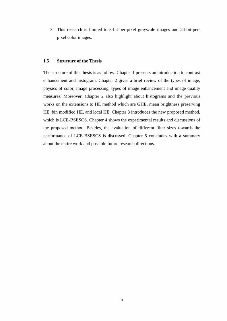
the right intensities, will give rise to white light. This is illustrated in Figure 2.1(a),
which shows the three primary colors and their combinations to produce the
secondary colors (Gonzalez and Woods, 2002).
The primary colors of light and the primary colors of pigments or colorants
are different in meaning. In the latter, a primary color is defined as one that absorbs
or subtracts a primary color of light and reflects or transmits the other two. Hence,
magenta, cyan and yellow are the primary colors of pigments, and red, green and
blue are the secondary colors. Mixing the three pigment primaries in equal amount,
or a secondary with its opposite primary, produces black (Gonzalez and Woods,
2002). These colors are shown in Figure 2.1(b).
Color models provide a standard way to specify a particular color by defining
a coordinate system and a subspace within that system where each color is
represented by a single point. Any color can be specified using a model. Each color
model is orientated either towards hardware (such as for color monitors and printers)
10
or towards specific software application (such as the creation of color graphics for
animation) (Gonzalez and Woods, 2002).
(a) Mixtures of light (b) Mixtures of pigments
(additive primaries) (subtractive primaries)
Figure 2.1: Primary and secondary colors of light and pigments
2.2.1 RGB Color Model
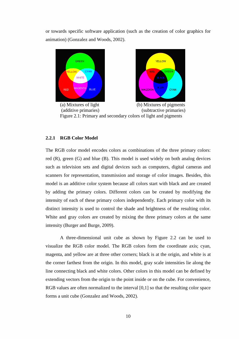
The RGB color model encodes colors as combinations of the three primary colors:
red (R), green (G) and blue (B). This model is used widely on both analog devices
such as television sets and digital devices such as computers, digital cameras and
scanners for representation, transmission and storage of color images. Besides, this
model is an additive color system because all colors start with black and are created
by adding the primary colors. Different colors can be created by modifying the
intensity of each of these primary colors independently. Each primary color with its
distinct intensity is used to control the shade and brightness of the resulting color.
White and gray colors are created by mixing the three primary colors at the same
intensity (Burger and Burge, 2009).
A three-dimensional unit cube as shown by Figure 2.2 can be used to
visualize the RGB color model. The RGB colors form the coordinate axis; cyan,
magenta, and yellow are at three other corners; black is at the origin, and white is at
the corner farthest from the origin. In this model, gray scale intensities lie along the
line connecting black and white colors. Other colors in this model can be defined by
extending vectors from the origin to the point inside or on the cube. For convenience,
RGB values are often normalized to the interval [0,1] so that the resulting color space
forms a unit cube (Gonzalez and Woods, 2002).

11
Figure 2.2: Schematic representation of the color cube. Reproduced from:
http://zone.ni.com/reference/en-XX/help/372916P-01/nivisionconcepts/color_spaces
The trichromatic RGB encoding in graphics systems usually uses three bytes
or 24-bit to produce roughly 16 million colors (i.e. (28)3
= 16,777,216). Each 3-byte
or 24-bit RGB pixel includes one byte for each of red, green, and blue. This 24-bit
RGB image is denoted as full color image shown in Figure 2.3 (Gonzalez and
Woods, 2002).
Figure 2.3: RGB 24-bit color cube. Reproduced from:
http://www.cs.ru.nl/~ths/rt2/col/h2/colorcube.jpg
2.2.2 CMY Color Model
CMY is an abbreviation of cyan (C), magenta (M) and yellow (Y) which are the
secondary colors of light or, alternatively, the primary colors of pigments. This color
model uses subtractive color mixing that is found in most devices like printers and
copiers (Jayaraman et al., 2009). It describes the appropriate reflections when a
printed image is illuminated with white light. For example, yellow absorbs blue light
from reflected white light, which itself consists of the same amount of red, green and
blue light. Normally, the RGB to CMY conversion in printing devices is performed
by using the following simple operation:

12
B
G
R
Y
M
C
1
1
1
(2.3)
where all color values are assume to be normalized in the range [0,1]. Equation
above shows that red is absorbed when a pure cyan surface is illuminated with white
light (that is, RC 1 in the equation). Similarly, pure magenta absorbs green, and
pure yellow absorbs blue (Shapiro and Stockman, 2001).
When equal amount of cyan, magenta, and yellow are combined, it will
produce a muddy looking black. In order to produce a true black, which is used
abundantly in printed documents, a fourth color, black, is added. Thus, this gives rise
to the CMYK color model also known as “four-color printing”. For clarity, CMYK
refers to the three colors in CMY color model plus black (Gonzalez and Woods,
2002).
2.2.3 HSI Color Model
In order to describe colors that are suitable for human interpretation, HSI color
model is introduced. HSI stands for hue, saturation and intensity. Hue can be
described as the dominant color perceived by an observer. It is an attribute associated
with the dominant wavelength. Saturation measures the degree in which a pure color
is diluted by white light. Intensity reflects the brightness of the color. HSI decouples
the intensity component from the color, while hue and saturation correspond to
human perception, hence it is very useful to develop image processing algorithm
with this representation. HSI is a popular color model because it is based on human
color perception (Jayaraman et al., 2009).
The double cone model of HSI is shown in Figure 2.4. The Hue (H)
corresponds to the angle 0, varying from 0° to 360°. Saturation (S) represented to the
radius, varying from 0 to 1. Intensity varies along the z axis in the range of 0 being
black to 1 being white (Singh et al., 2003).

13
Figure 2.4: Double cone HSI color model. Reproduced from Singh et al. (2003)
2.2.3.1 RGB to HSI Color Conversion
In a RGB color image format, the H component of each RGB pixel is obtained by
using (Gonzalez and Woods, 2002):
GB
GBH
if360
if
(2.4)
where
21
2
1 2
1
cosBGBRGR
BRGR
(2.5)
The saturation component is given by:
BGR
BGRS ,,min
31
(2.6)
Finally, the intensity component is given by:
BGRI 3
1 (2.7)
The RGB values are assumed to be normalized in the range [0,1] and that
is measured with respect to the red axis of the HSI space. By dividing all values from
equation (2.4) with 360°, hue values that are normalized in the range of [0,1] are
14
obtained. The other two HSI components are in this range if the given RGB values
are in the interval [0,1] (Gonzalez and Woods, 2002).
2.2.3.2 HSI to RGB Color Conversion
For HSI values in the interval [0,1], the corresponding RGB values in the same range
can be found. The equations used in this conversion depend on the values of H .
Referring to Figure 2.4, there are three sectors of interests corresponding to the 120°
intervals in the separation of primaries. Initially, the H component is multiplied by
360° so that the hue is returned to its original range of [0°,360°] (Gonzalez and
Woods, 2002).
RG sector (0°≤ H ≤120°): If the given value of H is in this range, the RGB
components are:
SIB 1 (2.8)
H
HSIR
60cos
cos1 (2.9)
BRIG 3
(2.10)
GB sector (120°≤ H ≤240°): When H is in this sector, first subtract 120° from it:
120HH (2.11)
Then, the RGB components are:
SIR 1 (2.12)
H
HSIG
60cos
cos1 (2.13)
and
GRIB 3 (2.14)

15
BR sector (240°≤ H ≤360°): Finally if H is in this sector, subtract 240° from it:
240HH (2.15)
Then, the RGB components are:
SIG 1 (2.16)
H
HSIB
60cos
cos1 (2.17)
and
BGIR 3 (2.18)
2.3 Image Processing
The scope of digital image processing is wide. Therefore, in this section, only four
digital image processing branches will be discussed. They are image restoration,
image segmentation, image compression and image enhancement.
Image restoration is used to reverse the distortions undergone by an image to
recover the original image. The distortions are due to motion blur, noise and camera
misfocus (Jayaraman et al., 2009). The techniques of image restoration are very
mathematical in nature, which can be formulated either in spatial or frequency
domain (Gonzalez and Woods, 2002).
Image segmentation can be used to extract certain characteristics of an image
in order to obtain the region of interest for further analysis and interpretation (Petrou
and Petrou, 2010). Segmentation deals with dividing an image by splitting it up into
connected areas. There are three different approaches for image segmentation which
are edge approach, boundary approach and region approach (Jayaraman et al., 2009).
Nowadays, digital images comprise of an enormous amount of data due to the
advances in technology. As a result, image compression is needed to reduce the
amount of data required to store a digital image (Gonzalez and Woods, 2002). In
other words, image compression is related to the mapping from higher dimensional
space to a lower dimensional space. Image compression can be classified into
lossless compression and lossy compression (Jayaraman et al., 2009).

16
The goal of image enhancement is to improve the perception and
interpretability of the information present in images for human viewers. The scope of
image enhancement includes contrast enhancement, pseudo coloring, interpolation,
sharpening and smoothing (Jain, 1989). Contrast enhancement is used to process an
input image such that the visual content of the output image is more pleasing or more
useful for machine vision applications by changing the intensity values of the input
image (Celik, 2012). Therefore, the dynamic range of the image is expanded, besides
enlarging the intensity difference among objects and background. Pseudo color
image processing involves assigning colors to gray level values based on a specified
criterion (Jain, 1989). This is because human eye perceive color more easily compare
to variations in intensity. Image interpolation is essentially a process of magnifying
image to ensure that the resultant image has better visual effect for special need
(Zhou et al., 2012). Sharpening refers to any enhancement techniques that highlight
edges and fine details in an image (Bovik, 2009). Usually highpass filters are
associated with sharpening that significantly amplify high frequencies without
attenuating lower frequencies. Smoothing process is related to noise reduction and
blurring of an image (Jain, 1989). Lowpass filters are used to reduce high frequency
components, and hence smoothing an image.
2.4 Types of Image Enhancement
There are several types of image enhancement methods. Nonetheless, only several
types of image enhancement methods are discussed such as image negative, log
transformation, power law transformation, linear spatial filter, non-linear spatial filter
and histogram processing.
The negative transformation inverses the intensity of an image in the range
1,0 L . The negative transformation function is given by (Jayaraman et al., 2009):
),(1),( jiXLjiY (2.19)
where ),( jiX is the input image and ),( jiY is the output image. A photographic
negative image is obtained by reversing the intensity levels of an image. Negative
images are useful in producing negative prints of medical images.

17
The log transformation is used to spread out a narrow range of low intensity
levels in the input image into a wider range of output levels. The log transformation
is defined as (Gonzalez and Woods, 2002):
)),(1log(),( jiXcjiY (2.20)
where c is a constant. For example, this transformation function spreads the values
of dark pixels while compressing the higher values. The opposite is true for the
inverse log transformation whereby the transformation function maps the narrow
range of high intensity levels in the input image into a wider range of output levels.
The intensity of light generated by cathode ray tube monitors has an
intensity-to-voltage response that is not linear. Hence, this non-linearity must be
compensated by a power law function to achieve correct reproduction of intensity.
The power law transformation is obtained by (Gonzalez and Woods, 2002):
)),((),( jiXcjiY (2.21)
where c and is a constant. The power law transformation function is the same as
the log transformation albeit it is much more versatile and a family of possible
transformation can be obtained by varying the value. For 1 , the low intensity
levels in the input image are spread out and the opposite is true for 1 .
Spatial filtering involves neighbourhood operation. This process is
implemented by simply sliding the filter from one pixel to another pixel of an image.
The response of the filter at each point ),( ji is calculated using a predefined
relationship. For linear spatial filter, each pixel value in the output image is the
average of the pixels in the neighbourhood of the corresponding pixel in the input
image (Gonzalez and Woods, 2002). This filter sometimes is called the mean filter.
On the other hand, non-linear spatial filter replaces each pixel with the ranking result
based on the pixels enclose by the filter (Jayaraman et al., 2009). An example of this
kind of filter is the median filter which reduces impulse noise in an image.
Besides the image enhancement methods mentioned above, the visual quality
of an image can be improved by manipulating the histogram of an input image. The
following sections give the idea about histogram and the histogram equalization
techniques used to enhance the quality of an image.

18
2.5 Histograms
Histograms play an important role in contrast enhancement as well as other image
processing applications (Gonzalez and Woods, 2002). The histogram is used to
represent image statistics in an easily interpreted visual format (Burger and Burge,
2009). In order to define a histogram, first, assume that ),( jiXX is a digital
image with L discrete gray levels in the intensity range of 110 LXXX ...,,, .
),( jiX represents the intensity of the image at spatial location ),( ji with the
condition that 110 ...,,,),( LXXXjiX . The histogram of a digital image is a
discrete function as all the intensities are in discrete values. Thus, the histogram h is
defined as:
1...,,1,0 for,)( LknXh kk (2.22)
where kX is the k -th gray level and kn shows the number of pixels in the image
having gray level kX . In general, histogram depicts the frequency of the intensity
values that occur in an image (Burger and Burge, 2009). The histogram provides
more insight about image contrast and brightness, but it is unable to convey any
information regarding spatial relationships between pixels (Jayaraman et al., 2009).
Usually, the histogram of an image X is presented as a graph plots of )( kXh versus
kX . Shown in Figure 2.5 are some examples of images and their respective
histograms.
These images show four basic gray level characteristics which are dark,
bright, low contrast and high contrast. Figure 2.5(a) corresponds to a dark image
dominated by low intensity pixels. Thus, the components of histogram are biased
toward the left side of the gray scale as shown in Figure 2.5(b). On the other hand,
the snow image as shown in Figure 2.5(c) is a bright image dominated by high
intensity pixels. Hence, as shown in Figure 2.5(d), the components of histogram tend
to be concentrated on the right side of the gray scale. A dull and washed-out image is
shown in Figure 2.5(e). This is a low contrast image which has a histogram of narrow
gray scale range as depicted in Figure 2.5(f). Finally, a high contrast image is show
in Figure 2.5(g). The components of histogram cover almost all the entire range of

19
possible gray levels. Besides, the distribution for most of the pixels is not too far
from uniform. Therefore, a high contrast has a large variety of gray tones.
(a) Image of Hong Kong night view (b) Histogram of (a)
(c) Image of snow (d) Histogram of (c)
(e) Image of turtle (f) Histogram of (e)
(g) Image of fruit stall (h) Histogram of (g)
Figure 2.5: Example of images and their corresponding histograms
20
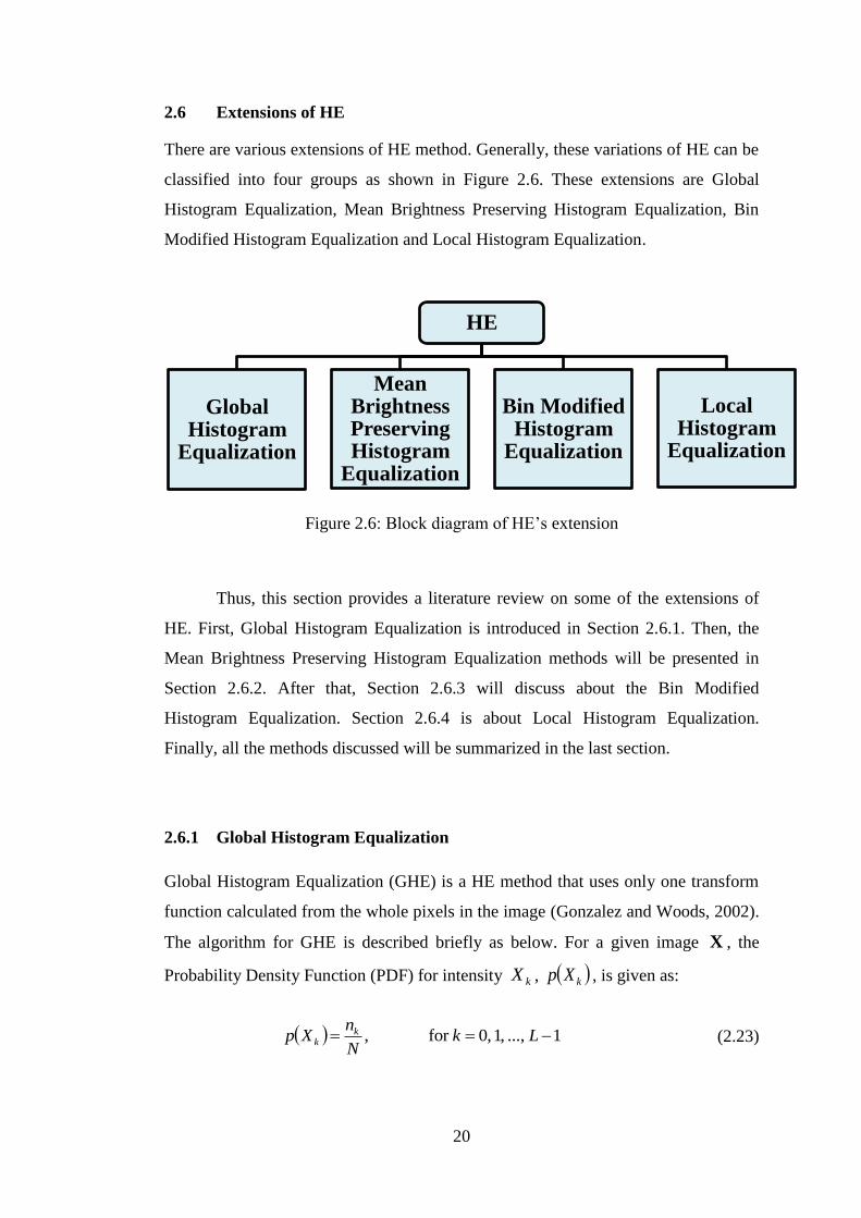
2.6 Extensions of HE
There are various extensions of HE method. Generally, these variations of HE can be
classified into four groups as shown in Figure 2.6. These extensions are Global
Histogram Equalization, Mean Brightness Preserving Histogram Equalization, Bin
Modified Histogram Equalization and Local Histogram Equalization.
Figure 2.6: Block diagram of HE’s extension
Thus, this section provides a literature review on some of the extensions of
HE. First, Global Histogram Equalization is introduced in Section 2.6.1. Then, the
Mean Brightness Preserving Histogram Equalization methods will be presented in
Section 2.6.2. After that, Section 2.6.3 will discuss about the Bin Modified
Histogram Equalization. Section 2.6.4 is about Local Histogram Equalization.
Finally, all the methods discussed will be summarized in the last section.
2.6.1 Global Histogram Equalization
Global Histogram Equalization (GHE) is a HE method that uses only one transform
function calculated from the whole pixels in the image (Gonzalez and Woods, 2002).
The algorithm for GHE is described briefly as below. For a given image X , the
Probability Density Function (PDF) for intensity kX , kXp , is given as:
1...,,1,0for , LkN
nXp k
k (2.23)
HE
Global Histogram
Equalization
Mean Brightness Preserving Histogram
Equalization
Bin Modified Histogram
Equalization
Local Histogram
Equalization

21
where N is the total number of samples in the image. The PDF is actually a
normalized version of the histogram.
The sum of all components of the normalized histogram or PDF results a
Cumulative Density Function (CDF) of an image. Based on the PDF in equation
(2.23), the CDF for intensity kX , kXc , is given as:
1...,,1,0for ,0
LkXpXc
k
j jk (2.24)
By definition, 11 LXc . Similar to PDF, CDF of an image also can be represented
as a plot of kXc versus kX . In GHE, CDF is used as the intensity transform
function for intensity value mapping.
GHE is a scheme that maps the input image into the entire dynamic range,
10 , LXX , by using CDF as its transformation function. Now, let kXx . The
transform function, xf , is defined based on CDF as (Kim, 1997):
xcXXXxf L 010 (2.25)
From here, the output image produced by GHE, jiY ,Y , can be expressed as:
XY jiXjiXfxf ,, (2.26)
GHE usually causes brightness saturation effect and washed out appearance.
This happens because GHE extremely pushes the intensities towards the right (i.e.,
bright) or the left (i.e., dark) side of the histogram. GHE is applied to images in
Figures 2.5(a), (c), (e) and (g). Notice that for a dark image, it is clearly visible that
the output of GHE image shown in Figure 2.7(a) suffers from brightness saturation.
Hence, the histogram is pushed to the right side as depicted in Figure 2.7(b). On the
other hand, GHE causes dark saturation effect on bright image shown in Figure
2.7(c). The corresponding histogram is shifted towards the left side as in Figure
2.7(d). This saturation effect, not only degrades the appearance of the image, but also
leads to information loss (Wadud et al., 2007). The result of applying GHE to low
contrast image is shown in Figure 2.7(e). Referring to its histogram in Figure 2.7(f),
GHE expands the contrast of high histogram region and compress the contrast of low
histogram region. Finally, Figure 2.7(g) shows a high contrast image processed by

22
GHE. By comparing its histogram in Figure 2.7(h) with the original histogram in
Figure 2.5(h), it is concluded that GHE fail completely when the original image is
already occupying the full dynamic range. Generally, important objects have a higher
and wider histogram region, so the contrast of these objects is stretched. On the other
hand, the contrast of lower and narrower histogram regions, such as background is
lost (Kim et al., 2001).
The enhancement process is done globally in GHE method without
considering the local contents of the image. Therefore, GHE is effective in enhancing
the low contrast image when the input image contains only one big single object, or
when there is no appearance contrast change between the object and the background
in the image (Cheng and Shi, 2004). In addition, GHE causes over enhancement in
the part of a histogram which has high probabilities of intensity levels, while loss of
contrast for low probabilities of levels (Kim et al., 1998; Cheng and Shi, 2004; Wang
and Ward, 2007; Wadud et al., 2007; Kim and Chung, 2008). Thus, GHE might
enhances parts of the image which are unimportant for the viewer such as the
background area of the image (Zimmerman et al., 1988; Csapodi and Roska, 1996).
As a result, GHE method is not applicable to many image modalities, such as
infrared image, because this method usually enhances the image’s background
instead of the object that occupies only a small portion of the image (Wang et al.,
2006). With the limitations of GHE as discussed above, many researches actively
develop various extensions to HE method. These extensions include Mean
Brightness Preserving HE, Bin Modified HE and Local HE.
2.6.2 Mean Brightness Preserving Histogram Equalization (MBPHE)
Mean Brightness Preserving Histogram Equalization (MBPHE) is an extension to
HE. Generally, these methods separate the histogram of the input image into several
sub histograms, and the equalization is carried out independently in each of the sub-
histograms (Kong and Ibrahim, 2008). The basic idea of MBPHE is to separate the
histogram into several segment boundaries based on certain type of threshold value.
Examples of MBPHE are Brightness Preserving Bi-Histogram Equalization, Dual
Sub-Image Histogram Equalization, Minimum Mean Brightness Error Bi-Histogram
Equalization, Recursive Mean-Separate Histogram Equalization, and Recursive Sub-

23
Image Histogram Equalization. The following subsections describe each of the
MBPHE methods in details.
(a) Enhanced image of Hong Kong night view (b) Histogram of (a)
(c) Enhanced image of snow (d) Histogram of (c)
(e) Enhanced image of turtle (f) Histogram of (e)
(g) Enhanced image of fruit stall (h) Histogram of (g)
Figure 2.7: Example of images produced by GHE and their corresponding
histograms