Local Model Predictive Control Experiences with

1-4244-2577-8/08/$20.00 ©2008 IEEE

Local Model Predictive Control Experiences with Differential Driven Wheeled Mobile Robots

Lluís Pacheco, Ningsu Luo, Jordi Ferrer Institute of Informatics and Applications University of Girona. Technical School

Av. Lluís Santaló sn 17071 Girona, Spain {lluispa, ningsu, [email protected]}

Abstract - This work extends a previously developed research concerning about the use of local model predictive control in differential driven mobile robots. Hence, experimental results are presented as a way to improve the methodology by considering aspects as trajectory accuracy and time performance. In this sense, the cost function and the prediction horizon are important aspects to be considered. The aim of the present work is to test the control method by measuring trajectory tracking accuracy and time performance. Moreover, strategies for the integration with perception system and path planning are briefly introduced. In this sense, monocular image data can be used to plan safety trajectories by using goal attraction potential fields. Index Terms – autonomous mobile robot, system identification, model based control, local predictive control, trajectory planning, robot vision.

I. INTRODUCTION

The path tracking error minimization is considered as an important mobile robot objective that is accomplished by reducing the error between the robot and the desired path. Other aspects as vehicle speed or even acceleration profile can also be analysed as important issues to be considered in the path tracking strategies [1]. Hence, the dynamics of the robot becomes an important issue in planning accurate and safe trajectories, in which on-robot sensors provide enough environmental knowledge to avoid colliding with obstacles and to reach the final desired coordinates. The scientific community has carried out several studies in this field. The use of a dynamic window approach, with available robot speeds, the reactive and safety stopping distances, derived from robot motion dynamics, allow WMRs (wheeled mobile robots) reactively avoiding obstacles [2]. Rimon presented methodologies for exact motion planning and control, based on artificial potential fields where complete information about the free space and goal are encoded [3]. The main drawback of the potential fields is the local minimal failures. However, the flexibility is reported as an advantage when small or moving obstacles are met. Probabilistic Roadmap Method (PRM) [4] is a methodology not suffered from local minimal failures, but with drawbacks as unattractive path generation and lack of flexibility. Path optimization can be improved using local motions controlled by local potential fields [5]. Some approaches to mobile robots propose using potential fields, which satisfy the stability in a Lyapunov sense on a short prediction horizon [6].

In the present work, model predictive control (MPC) is presented as an accurate nonlinear methodology that allows an exact trajectory tracking by minimizing the cost function. In this sense, simulated and experimental results are presented as an extension of previously developed work [7].

Hence, several studies concerning about the trajectory tracking accuracy are reported. Moreover, a trajectory planning framework consisted of a narrow and dense field of view and a goal attracting potential field point are used to test the MPC performance. From a monocular perception system, the selected free cell should avoid the obstacle collisions and approach the robot to the final desired configuration through the attraction objective field. Once the local desired cell is obtained a straight line between the cell and the robot is generated. These kinds of trajectories are used also to test the performance of robot trajectory tracking. The control action consists in steering and straight line following, such actions are common to a wide range of nonholonomic vehicles [8]. Hence, at each perception step, a tracking straight line is commanded as a new trajectory to be followed by the robot. The visual data are the meaningful source of information in order to accomplish with the tasks of obstacle detection. However, other data provided by the encoder-based odometer system are also considered.

This paper is organized as follows. Section I briefly presents the aim of the present work. Section II introduces the MPC methodology and algorithms. The WMR PRIM, consisting of a differential driven robot with a free rotating wheel, is used as an available platform in order to orient the results [9]. Once the robot models are known several simulations are depicted. In the Section III, the experimental results attaining the trajectory tracking performance are presented. Hence, horizon of prediction, cost function, and time performance are studied. Moreover, the experimental results are developed within a context of path planning strategy with local monocular visual perception data in which trajectories with safe obstacle avoidance can approach the robot to the goal. Consequently, it can be used to test the control performance. Finally, in Section IV, some conclusions are drawn and future research is outlined.

II. LOCAL MODEL PREDICTIVE CONTROL In this section it is presented a useful methodology, which explains how to deal with the simplified dynamic system models and the odometer system. The LMPC trajectory tracking can be considered as a meaningful contribution of this paper, thus the cost function minimization is considered as a convex optimization problem and thus can be easily solved by using optimal interval search and taking into account some physical constraints. The LMPC algorithm design studies are also reported.

A. System Identification

Authorized licensed use limited to: UNIVERSITAT DE GIRONA. Downloaded on May 8, 2009 at 07:16 from IEEE Xplore. Restrictions apply.

In this work, it is used parametric identification process based on black box models [10]. Thus, the transfer functions are related to a set of polynomials that allow the use of analytic methods in order to deal with the problem of controller design. The nonholonomic system dealt with in this work is considered initially as a MIMO (multiple input multiple output) system, due to the dynamic influence between two dc motors. The approach of multiple transfer functions consists in making the experiments with three different (slow, medium and fast) speeds. The parameter estimation is done by using a PRBS (Pseudo Random Binary Signal) as excitation input signal. The ARX (auto-regressive with external input) structure has been used to identify the parameters of the system. The problem consists in finding a model that minimizes the error between the real and estimated data. By expressing the ARX equation as a lineal regression, the estimated output can be written as:

θϕ=y (1) With y being the estimated output vector, θ the vector of estimated parameters and φ the vector of measured input and output variables. The system is identified by using the identification toolbox “ident” of Matlab. As e.g., after frequency filtering the following medium speed continuous transfer function matrix is obtained:

( )2 ⎟⎟⎠

⎞⎜⎜⎝

⎛

⎟⎟⎟⎟⎟

⎠

⎞

⎜⎜⎜⎜⎜

⎝

⎛

++

++

++

++++

++

++

++

=⎟⎟⎠

⎞⎜⎜⎝

⎛

L

R

2

2

2

22

2

2

2

L

RUU

89.4s84.5s12.5s72.1s11.0

89.4s84.5s28.0s41.3s26.0

89.4s84.5s32.0s27.0s02.0

89.4s84.5s46.4s82.4s35.0

YY

Where YR, and YL represent the speeds of right and left

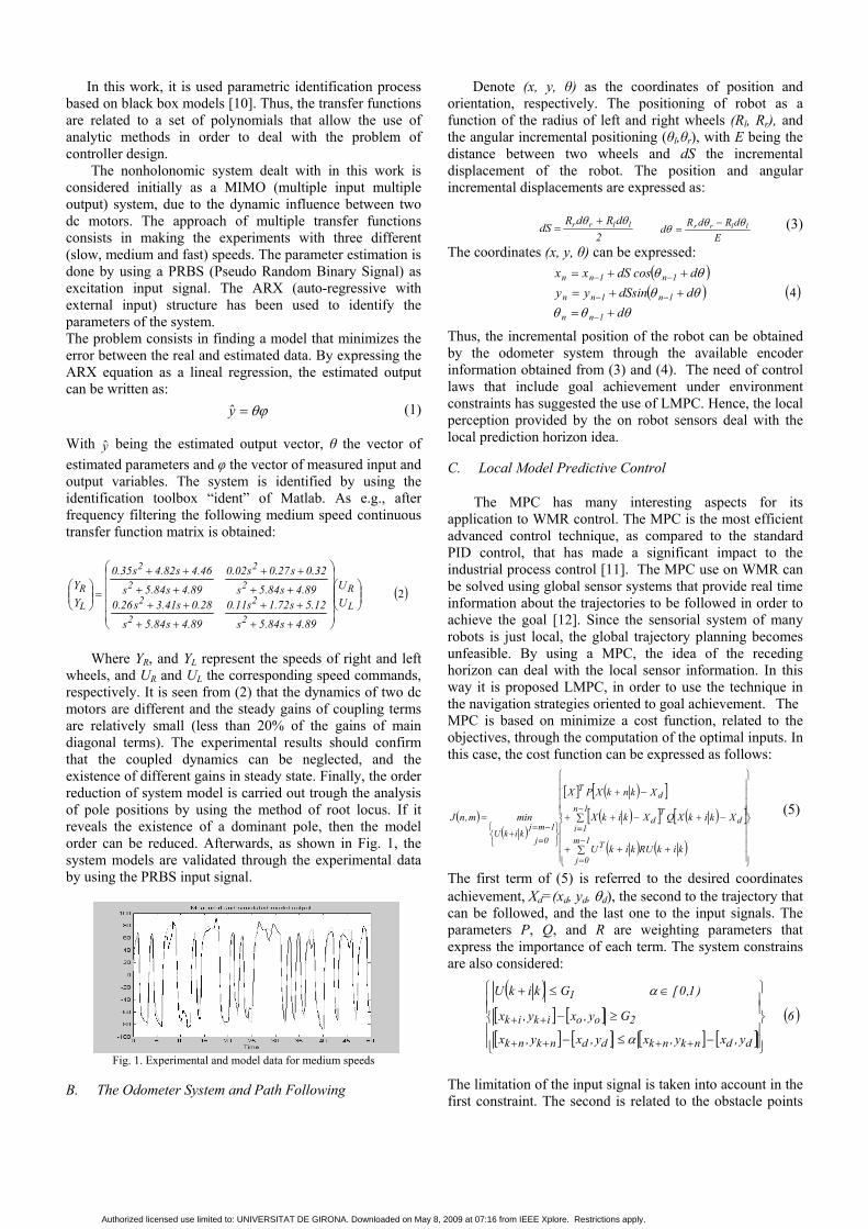
wheels, and UR and UL the corresponding speed commands, respectively. It is seen from (2) that the dynamics of two dc motors are different and the steady gains of coupling terms are relatively small (less than 20% of the gains of main diagonal terms). The experimental results should confirm that the coupled dynamics can be neglected, and the existence of different gains in steady state. Finally, the order reduction of system model is carried out trough the analysis of pole positions by using the method of root locus. If it reveals the existence of a dominant pole, then the model order can be reduced. Afterwards, as shown in Fig. 1, the system models are validated through the experimental data by using the PRBS input signal.

Fig. 1. Experimental and model data for medium speeds

B. The Odometer System and Path Following

Denote (x, y, θ) as the coordinates of position and orientation, respectively. The positioning of robot as a function of the radius of left and right wheels (Rl, Rr), and the angular incremental positioning (θl,θr), with E being the distance between two wheels and dS the incremental displacement of the robot. The position and angular incremental displacements are expressed as:

2dRdR

dS llrr θθ +=

EdRdRd llrr θθθ −

= (3)

The coordinates (x, y, θ) can be expressed:

( )( ) ( )

θθθθθθθ

dddSsinyydcosdSxx

1nn

1n1nn

1n1nn

+=++=++=

−

−−

−−

4

Thus, the incremental position of the robot can be obtained by the odometer system through the available encoder information obtained from (3) and (4). The need of control laws that include goal achievement under environment constraints has suggested the use of LMPC. Hence, the local perception provided by the on robot sensors deal with the local prediction horizon idea. C. Local Model Predictive Control The MPC has many interesting aspects for its application to WMR control. The MPC is the most efficient advanced control technique, as compared to the standard PID control, that has made a significant impact to the industrial process control [11]. The MPC use on WMR can be solved using global sensor systems that provide real time information about the trajectories to be followed in order to achieve the goal [12]. Since the sensorial system of many robots is just local, the global trajectory planning becomes unfeasible. By using a MPC, the idea of the receding horizon can deal with the local sensor information. In this way it is proposed LMPC, in order to use the technique in the navigation strategies oriented to goal achievement. The MPC is based on minimize a cost function, related to the objectives, through the computation of the optimal inputs. In this case, the cost function can be expressed as follows:

( )( )

[ ] ( )[ ]( )[ ] ( )[ ]

( ) ( )⎪⎪⎪⎪

⎭

⎪⎪⎪⎪

⎬

⎫

⎪⎪⎪⎪

⎩

⎪⎪⎪⎪

⎨

⎧

++∑+

∑ −+−++

−+

=

−

=

−

=

⎭⎬⎫

⎩⎨⎧

=−=

+

kikRUkikU

XkikXQXkikX

XknkXPX

minm,nJ

1m

0j

T

1n

1id

Td

dT

0j1mj

kikU

(5)

The first term of (5) is referred to the desired coordinates achievement, Xd=(xd, yd, θd), the second to the trajectory that can be followed, and the last one to the input signals. The parameters P, Q, and R are weighting parameters that express the importance of each term. The system constrains are also considered:

( )[ ] [ ][ ] [ ] [ ] [ ]

( )6

y,xy,xy,xy,x

Gy,xy,x

)1,0[GkikU

ddnknkddnknk

2ooikik

1

⎪⎪⎭

⎪⎪⎬

⎫

⎪⎪⎩

⎪⎪⎨

⎧

−≤−

≥−

∈≤+

++++

++

α

α

The limitation of the input signal is taken into account in the first constraint. The second is related to the obstacle points


where the robot should avoid the collision. The last one is just a convergence criterion. The LMPC algorithm is run in following steps:

1) To read the actual position 2) To minimize the cost function, and to obtain a

series of optimal input signals. 3) To choose the first obtained input signal as

command signal 4) Go back to the step one in the next sampling

period.

The minimization of the cost function is a nonlinear problem in which the following equation should be verified: ( ) ( ) ( ) ( )7yfxfyxf βαβα +≤+ It is a convex optimization problem caused by the trigonometric functions used in (4). The use of interior point methods can solve the above problem [13]. Among many algorithms that can solve the optimization, the descent methods are used, such as the gradient descent method, steepest descent method, or the Newton’s method, among others. The gradient descent algorithm has been implemented in this work. In order to obtain the optimal solution, some constraints over the inputs are taken into account [11]. There is a fixed signal increment during part of prediction horizon, hence, on expression (5) input signals are commanded until j=m-1. The input signals are constant during the remaining interval of time, in (5) n-m-1, where n represents the prediction horizon. Normally, just forward movements are commanded, accordingly with the field of view perception. The input constraints present advantages such like the reduction in the computation time and the smooth behavior of the robot during the prediction horizon. Thus, the set of available inputs are reduced to just one value. In order to reduce the optimal signal value search, the possible input sets are as a bidimensional array, as shown in Fig. 2. Then, the array is decomposed into four zones, and the search is just located to analyze the center points of each zone. It is considered just the region that offers better optimization, where the algorithm is repeated for each sub-zone, until no sub-interval can be found. The results were obtained by testing all possible inputs and the subinterval search algorithm, which were compared by simulating a 2m straight line tracking, as shown in Fig. 3.

Fig. 2: Optimal interval search.

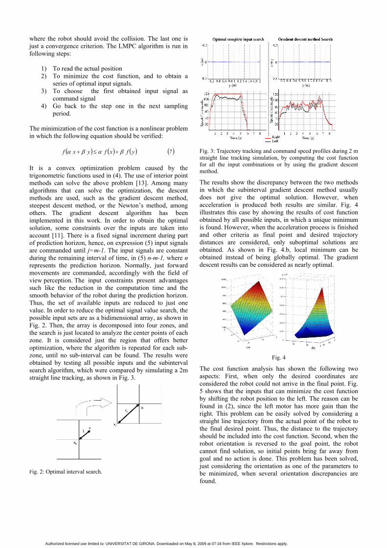
Fig. 3: Trajectory tracking and command speed profiles during 2 m straight line tracking simulation, by computing the cost function for all the input combinations or by using the gradient descent method.

The results show the discrepancy between the two methods in which the subinterval gradient descent method usually does not give the optimal solution. However, when acceleration is produced both results are similar. Fig. 4 illustrates this case by showing the results of cost function obtained by all possible inputs, in which a unique minimum is found. However, when the acceleration process is finished and other criteria as final point and desired trajectory distances are considered, only suboptimal solutions are obtained. As shown in Fig. 4.b, local minimum can be obtained instead of being globally optimal. The gradient descent results can be considered as nearly optimal.

Fig. 4

The cost function analysis has shown the following two aspects: First, when only the desired coordinates are considered the robot could not arrive in the final point. Fig. 5 shows that the inputs that can minimize the cost function by shifting the robot position to the left. The reason can be found in (2), since the left motor has more gain than the right. This problem can be easily solved by considering a straight line trajectory from the actual point of the robot to the final desired point. Thus, the distance to the trajectory should be included into the cost function. Second, when the robot orientation is reversed to the goal point, the robot cannot find solution, so initial points bring far away from goal and no action is done. This problem has been solved, just considering the orientation as one of the parameters to be minimized, when several orientation discrepancies are found.


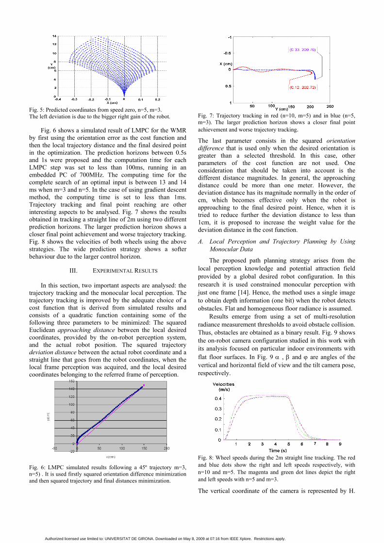
Fig. 5: Predicted coordinates from speed zero, n=5, m=3. The left deviation is due to the bigger right gain of the robot. Fig. 6 shows a simulated result of LMPC for the WMR by first using the orientation error as the cost function and then the local trajectory distance and the final desired point in the optimization. The prediction horizons between 0.5s and 1s were proposed and the computation time for each LMPC step was set to less than 100ms, running in an embedded PC of 700MHz. The computing time for the complete search of an optimal input is between 13 and 14 ms when m=3 and n=5. In the case of using gradient descent method, the computing time is set to less than 1ms. Trajectory tracking and final point reaching are other interesting aspects to be analysed. Fig. 7 shows the results obtained in tracking a straight line of 2m using two different prediction horizons. The larger prediction horizon shows a closer final point achievement and worse trajectory tracking. Fig. 8 shows the velocities of both wheels using the above strategies. The wide prediction strategy shows a softer behaviour due to the larger control horizon.

III. EXPERIMENTAL RESULTS

In this section, two important aspects are analysed: the trajectory tracking and the monocular local perception. The trajectory tracking is improved by the adequate choice of a cost function that is derived from simulated results and consists of a quadratic function containing some of the following three parameters to be minimized: The squared Euclidean approaching distance between the local desired coordinates, provided by the on-robot perception system, and the actual robot position. The squared trajectory deviation distance between the actual robot coordinate and a straight line that goes from the robot coordinates, when the local frame perception was acquired, and the local desired coordinates belonging to the referred frame of perception.

Fig. 6: LMPC simulated results following a 45º trajectory m=3, n=5) . It is used firstly squared orientation difference minimization and then squared trajectory and final distances minimization.

Fig. 7: Trajectory tracking in red (n=10, m=5) and in blue (n=5, m=3). The larger prediction horizon shows a closer final point achievement and worse trajectory tracking.

The last parameter consists in the squared orientation difference that is used only when the desired orientation is greater than a selected threshold. In this case, other parameters of the cost function are not used. One consideration that should be taken into account is the different distance magnitudes. In general, the approaching distance could be more than one meter. However, the deviation distance has its magnitude normally in the order of cm, which becomes effective only when the robot is approaching to the final desired point. Hence, when it is tried to reduce further the deviation distance to less than 1cm, it is proposed to increase the weight value for the deviation distance in the cost function.

A. Local Perception and Trajectory Planning by Using Monocular Data

The proposed path planning strategy arises from the local perception knowledge and potential attraction field provided by a global desired robot configuration. In this research it is used constrained monocular perception with just one frame [14]. Hence, the method uses a single image to obtain depth information (one bit) when the robot detects obstacles. Flat and homogeneous floor radiance is assumed.

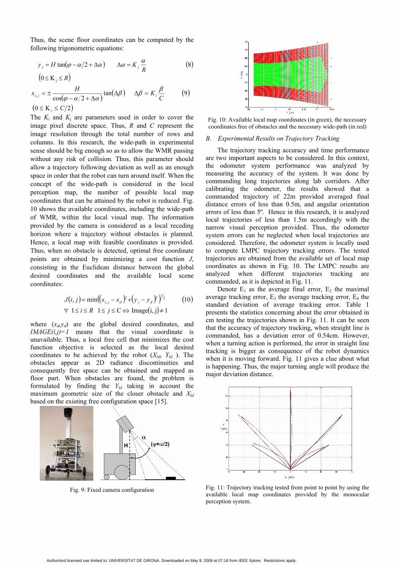
Results emerge from using a set of multi-resolution radiance measurement thresholds to avoid obstacle collision. Thus, obstacles are obtained as a binary result. Fig. 9 shows the on-robot camera configuration studied in this work with its analysis focused on particular indoor environments with flat floor surfaces. In Fig. 9 α , β and ϕ are angles of the vertical and horizontal field of view and the tilt camera pose, respectively.

Fig. 8: Wheel speeds during the 2m straight line tracking. The red and blue dots show the right and left speeds respectively, with n=10 and m=5. The magenta and green dot lines depict the right and left speeds with n=5 and m=3.

The vertical coordinate of the camera is represented by H.


Thus, the scene floor coordinates can be computed by the following trigonometric equations:

( ) ( )

( ) K0

8 2tan

j RR

KHy jj

≤≤

=ΔΔ+−=ααααϕ

( ) ( ) ( )

( ) 2K0

9 tan2cos

i

,

CC

KHx iji

≤≤

=ΔΔΔ+−

±=βββ

ααϕ

The Ki and Kj are parameters used in order to cover the image pixel discrete space. Thus, R and C represent the image resolution through the total number of rows and columns. In this research, the wide-path in experimental sense should be big enough so as to allow the WMR passing without any risk of collision. Thus, this parameter should allow a trajectory following deviation as well as an enough space in order that the robot can turn around itself. When the concept of the wide-path is considered in the local perception map, the number of possible local map coordinates that can be attained by the robot is reduced. Fig. 10 shows the available coordinates, including the wide-path of WMR, within the local visual map. The information provided by the camera is considered as a local receding horizon where a trajectory without obstacles is planned. Hence, a local map with feasible coordinates is provided. Thus, when no obstacle is detected, optimal free coordinate points are obtained by minimizing a cost function J, consisting in the Euclidean distance between the global desired coordinates and the available local scene coordinates:

( ) ( ) ( )( ) ( )( ) 1ji,ImageC1 1

10 min, 2122

,

≠⇔≤≤≤≤∀

−+−=

jRi

yyxxjiJ djdji

where (xd,yd) are the global desired coordinates, and IMAGE(i,j)=1 means that the visual coordinate is unavailable. Thus, a local free cell that minimizes the cost function objective is selected as the local desired coordinates to be achieved by the robot (Xld, Yld ). The obstacles appear as 2D radiance discontinuities and consequently free space can be obtained and mapped as floor part. When obstacles are found, the problem is formulated by finding the Yld taking in account the maximum geometric size of the closer obstacle and Xld based on the existing free configuration space [15].

Fig. 9: Fixed camera configuration

Fig. 10: Available local map coordinates (in green), the necessary coordinates free of obstacles and the necessary wide-path (in red)

B. Experimental Results on Trajectory Tracking

The trajectory tracking accuracy and time performance are two important aspects to be considered. In this context, the odometer system performance was analyzed by measuring the accuracy of the system. It was done by commanding long trajectories along lab corridors. After calibrating the odometer, the results showed that a commanded trajectory of 22m provided averaged final distance errors of less than 0.5m, and angular orientation errors of less than 5º. Hence in this research, it is analyzed local trajectories of less than 1.5m accordingly with the narrow visual perception provided. Thus, the odometer system errors can be neglected when local trajectories are considered. Therefore, the odometer system is locally used to compute LMPC trajectory tracking errors. The tested trajectories are obtained from the available set of local map coordinates as shown in Fig. 10. The LMPC results are analyzed when different trajectories tracking are commanded, as it is depicted in Fig. 11.

Denote E1 as the average final error, E2 the maximal average tracking error, E3 the average tracking error, E4 the standard deviation of average tracking error. Table 1 presents the statistics concerning about the error obtained in cm testing the trajectories shown in Fig. 11. It can be seen that the accuracy of trajectory tracking, when straight line is commanded, has a deviation error of 0.54cm. However, when a turning action is performed, the error in straight line tracking is bigger as consequence of the robot dynamics when it is moving forward. Fig. 11 gives a clue about what is happening. Thus, the major turning angle will produce the major deviation distance.

Fig. 11: Trajectory tracking tested from point to point by using the available local map coordinates provided by the monocular perception system.


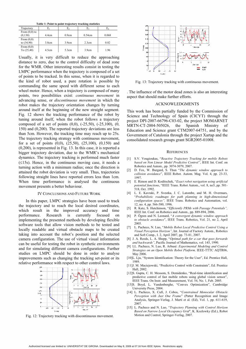
Table 1: Point to point trajectory tracking statistics Trajectory E1 E2 E3 E4 From (0,0) to (0,130)

4.4cm

0.9cm

0.54cm

0.068

From (0,0) to (34,90)

3.8cm

3.9cm

2.3cm

0.82

From (0,0) To (25,40)

4.5cm

5.3cm

3.9cm

1.96

Usually, it is very difficult to reduce the approaching distance to zero, due to the control difficulty of dead zone for the WMR. Other interesting results consist in testing the LMPC performance when the trajectory is composed of a set of points to be tracked. In this sense, when it is regarded to the kind of robot used, a pure rotation is possible by commanding the same speed with different sense to each wheel motor. Hence, when a trajectory is composed of many points, two possibilities exist: continuous movement in advancing sense, or discontinuous movement in which the robot makes the trajectory orientation changes by turning around itself at the beginning of the new straight segment. Fig. 12 shows the tracking performance of the robot by tuning around itself, when the robot follows a trajectory composed of a set of points (0,0), (-25,50), (-25,100), (0, 150) and (0,200). The reported trajectory deviations are less than 5cm. However, the tracking time may reach up to 25s. The trajectory tracking strategy with continuous movement, for a set of points (0,0), (25,50), (25,100), (0,150) and (0,200), is represented in Fig. 13. In this case, it is reported a bigger trajectory deviation, due to the WMR’s mechanical dynamics. The trajectory tracking is performed much faster (≤15s). Hence, in the continuous moving case, it needs a turning action with a minimum radius; once the direction is attained the robot deviation is very small. Thus, trajectories following straight lines have reported errors less than 1cm. When time performance is analysed the continuous movement presents a better behaviour.

IV CONCLUSIONS AND FUTURE WORK

In this paper, LMPC strategies have been used to track the trajectory and to reach the local desired coordinates, which result in the improved accuracy and time performance. Research is currently focused on implementing the presented methods by developing flexible software tools that allow vision methods to be tested and locally readable and virtual obstacle maps to be created taking into account the robot’s position and the selected camera configuration. The use of virtual visual information can be useful for testing the robot in synthetic environments and for simulating different camera configurations. Further studies on LMPC should be done in order to analyse improvements such as changing the tracking set-point or its relative performance with respect to other control laws.

Fig. 12: Trajectory tracking with discontinuous movement.

Fig. 13: Trajectory tracking with continuous movement.

. The influence of the motor dead zones is also an interesting aspect that should make further efforts.

ACKNOWLEDGMENTS

This work has been partially funded by the Commission of Science and Technology of Spain (CICYT) through the project DPI-2007-66796-C03-02, the project MOMARNET MRTN-CT-2004-505026, the Spanish Ministry of Education and Science grant CTM2007-64751, and by the Government of Catalonia through the project Xartap and the consolidated research groups grant SGR2005-01008.

REFERENCES [1] S.V. Vougioukas, “Reactive Trajectory Tracking for mobile Robots

based on Non Linear Model Predictive Control”, IEEE Int. Conf. on Robotics and Autom., pp. 3074-3079, 2007.

[2] D. Fox, W. Burgard, S. Thun “The dynamic window approach to collision avoidance”, IEEE Robot. Autom. Mag. Vol. 4, pp. 23-33, 1997.

[3] E. Rimon and D. Koditschek, “Exact robot navigation using artificial potential functions, “IEEE Trans. Robot Autom., vol. 8, no5, pp. 501-518, Oct. 1992.

[4] L. E. Kavraki, P. Svestka, J. C. Latombe, and M. H. Overmars, “Probabilistic roadmaps for path planning in high-dimensional configuration spaces”, IEEE Trans. Robotics and Automation, vol. 12, no. 4, pp. 566-580, 1996.

[5] R. Katz, S. Hutchinson, “Efficiently PRMs with Passage Potentials”, IEEE Int. Conf. on Robotics and Autom., pp. 889-894, 2006.

[6] P. Ögren and N. Leonard, “A convergent dynamic window approach to obstacle avoidance”, IEEE Trans. Robotics, Vol. 21, no 2, April 2005.

[7] L. Pacheco, N. Luo, “Mobile Robot Local Predictive Control Using a Visual Perception Horizon”, Int. Journal of Factory Autom., Robotics and Soft Comp., I. 2, April 2007, pp. 73-81, 2007.

[8] J. A. Reeds, L. A. Shepp, “Optimal path for a car that goes forwards and backwards”, Pacific Journal of Mathematics, vol. 145, 1990.

[9] LL. Pacheco, N. Luo, R. Arbusé: Experimental Modeling and Control Strategies on an Open Mobile Robot Platform, IEEE-TTTC AQTR06, May 2006.

[10] L. Lju, “System Identification: Theory for the User”, Ed. Prentice Hall, 1989.

[11] J. M. Maciejowski, “Predictive Control with Constraints”, Ed. Prentice Hall, 2002.

[12] S. Gupta, C. H. Messom, S. Demidenko, “Real-time identification and predictive control of fast mobile robots using global vision sensor”, IEEE Trans. On Instr. and Measurement, Vol. 54, No. 1, Feb. 2005.

[13] S. Boyd, L. Vandenberghe, “Convex Optimization”, Cambridge University Press, 2004.

[14] L. Pacheco, X. Cufí, J. Cobos, “Constrained Monocular Obstacle Perception with Just One Frame” (Patter Recognition and Image Analysis, Springer-Verlag, J. Martí et al. (Ed), Vol. 1, pp. 611-619, 2007.

[15] L. Pacheco and N. Luo, “Trajectory Planning with Control Horizon Based on Narrow Local Occupancy Grid”, K. Kozlowky (Ed.), Robot Motion and Control, Springer-Verlag, 2007.


Documents

Local Model Predictive Control Experiences with