Local Polynomial Order in Regression Discontinuity Designs

Working Paper Series

Local Polynomial Order in Regression Discontinuity Designs David Card, UC Berkeley, NBER, and IZA

Zhuan Pei, Brandeis University

David S. Lee, Princeton University and NBER

Andrea Weber, University of Mannheim and IZA

2014 | 81

Local Polynomial Order in Regression Discontinuity Designs1

David Card

UC Berkeley, NBER and IZA

David S. Lee

Princeton University and NBER

Zhuan Pei

Brandeis University

Andrea Weber

University of Mannheim and IZA

October 21, 2014

Abstract

The local linear estimator has become the standard in the regression discontinuity design literature,but we argue that it should not always dominate other local polynomial estimators in empirical studies.We show that the local linear estimator in the data generating processes (DGP’s) based on two well-known empirical examples does not always have the lowest (asymptotic) mean squared error (MSE).Therefore, we advocate for a more flexible view towards the choice of the polynomial order, p, andsuggest two complementary approaches for picking p: comparing the MSE of alternative estimatorsfrom Monte Carlo simulations based on an approximating DGP, and comparing the estimated asymptoticMSE using actual data.

Keywords: Regression Discontinuity Design; Regression Kink Design; Local Polynomial Estima-tion; Polynomial Order

1We thank Pat Kline, Pauline Leung and seminar participants at Brandeis and George Washington University for helpful com-ments, and we thank Samsun Knight and Carl Lieberman for excellent research assistance.

1 Introduction

The seminal work of Hahn et al. (2001) has established local linear nonparametric regression as a standard

approach for estimating the treatment effect in a regression discontinuity (RD) design. Recent influential

studies on nonparametric estimation in RD designs have built upon the local linear framework. Imbens and

Kalyanaraman (2012) propose bandwidth selectors optimal for the local linear RD estimator (henceforth the

“IK bandwidth”), and Calonico et al. (2014b) introduce a procedure to correct the bias in the local linear

estimator and to construct robust confidence intervals.

The prevailing preference for the local linear estimator is based on the order of its asymptotic bias, but

this alone cannot justify the universal dominance of the linear specification over other polynomial orders.

Hahn et al. (2001) choose the local linear estimator over the local constant1 for its smaller order of asymp-

totic bias – specifically, the bias of the local linear estimator is of order O(h2) and the local constant O(h)

(h here refers to the bandwidth that shrinks as the sample size n becomes large). However, the argument

based on asymptotic order comparisons per se does not imply that local linear should always be preferred

to alternative local polynomial estimators. Under standard regularity conditions, the asymptotic bias is of

order O(h3) for the local quadratic RD estimator, O(h4) for local cubic, and O(hp+1) for the p-th order local

polynomial sharp RD estimator, τp (Lemma A1 Calonico et al. (2014b)). Therefore, if the goal is to maxi-

mize the shrinkage rate of the asymptotic bias, researchers should choose a p as large as possible. The fact

that Hahn et al. (2001) do not recommend a very large p for RD designs implies that finite sample properties

of the estimator must be taken into consideration. But if finite sample properties are important, the desired

polynomial choice may depend on the sample size: the local constant estimator τ0 may be preferred to τ1

when the sample size is small, and higher-order local polynomial estimators may be preferred when the

sample size is large.

In a given finite sample, the derivatives of the conditional expectation function of the outcome variable

are also important for the local polynomial order choice, even though they are omitted under the O(·)

notation of asymptotic rates. If the conditional expectation of the outcome variable Y is close to being a

constant function of the assignment variable X , then the local constant specification will provide adequate

approximation, and consequently τ0 will perform well. On the other hand, if the said conditional expectation

function has a large curvature, researchers may consider choosing a higher-order local polynomial estimator

1The local constant estimator is equivalent to a kernel regression estimator, which is the terminology used by Hahn et al. (2001).

1

instead.

Because the performance of a local polynomial estimator depends on the sample size and the properties

of the data generating process (DGP), a single choice like p = 1, though convenient, may not be the best for

all empirical RD applications. In this paper, we explore the best local polynomial order choice in the spirit of

Fan and Gijbels (1996) by comparing the mean squared error (MSE) of τp and its asymptotic approximation

(AMSE) across p. Using the (A)MSE of the local estimator as a measuring stick is consistent with the

optimal bandwidth literature and answers to the critique of Gelman and Imbens (2014) that the goodness of

fit measure used in choosing a global polynomial order “is not closely related to the research objective of

causal inference”.

Similar to Imbens and Kalyanaraman (2012) and Calonico et al. (2014b), we use the data generating

processes (DGP’s) based on Lee (2008) and Ludwig and Miller (2007) to illustrate the points above. We

document that local regressions with orders other than p = 1 may perform better than with the local linear

estimator τ1. We provide details in the following section.

2 Mean Squared Error and the Local Polynomial Order

In this section, we rank the τp’s based on their (A)MSE for the approximating DGP’s of Lee (2008) and

Ludwig and Miller (2007). In subsection 2.1, we calculate the theoretical asymptotic mean squared error

evaluated at the optimal bandwidth for the Lee and Ludwig-Miller DGP. Based on the calculation, we show

that whether or not the local linear estimator τ1 theoretically dominates an alternative τp depends on the

sample size as well as the DGP. In subsection 2.2, we examine the actual mean squared error of the local

polynomial estimators via Monte Carlo simulation and confirm that τ1 is not always the best-performing RD

estimator. In subsection 2.3, we show that the estimated AMSE serves as a sensible basis for choosing the

polynomial order. In subsection 2.4, we discuss the properties of the local polynomial estimators in light

of the recent study, Gelman and Imbens (2014). Gelman and Imbens (2014) point out that an undesirable

property of a high-order global polynomial estimator is that it may assign very large weights (henceforth

“GI weights”) to observations far away from the discontinuity threshold. We show in subsection 2.4 that this

does not appear to be the case for high-order local polynomial estimators for the Lee and Ludwig-Miller data

when using the corresponding optimal bandwidth selector. In subsection 2.5, we argue that the MSE-based

methods for choosing the polynomial order can be easily applied to the fuzzy design and the regression kink

2

design (RKD).

2.1 Theoretical AMSE

We specify the Lee and Ludwig-Miller DGP following Imbens and Kalyanaraman (2012) and Calonico et

al. (2014b). Let Y denote the outcome of interest, let X denote the normalized running variable, and let D =

1[X>0] denote the treatment. For both DGP’s, the running variable X follows the distribution 2B(2,4)−1,

where B(α,β ) denotes a beta distribution with shape parameters α and β . The outcome variable is given

by Y = E[Y |X = x]+ε , where ε ∼ N(0,σ2ε ) with σε = 0.1295 and the conditional expectation functions are

specified as

Lee: E[Y |X = x] =

0.48+1.27x+7.18x2 +20.21x3 +21.54x4 +7.33x5 if x < 0

0.52+0.84x−3.00x2 +7.99x3−9.01x4 +3.56x5 if x > 0

Ludwig-Miller: E[Y |X = x] =

3.71+2.30x+3.28x2 +1.45x3 +0.23x4 +0.03x5 if x < 0

0.26+18.49x−54.81x2 +74.30x3−45.02x4 +9.83x5 if x > 0.

To obtain the conditional expectation functions, Imbens and Kalyanaraman (2012) and Calonico et al.

(2014b) first discard the outliers (i.e. observations for which the absolute value of the running variable

is very large) and then fit a separate quintic function on each side of the threshold to the remaining observa-

tions.

Because the DGP is analytically specified, we can apply Lemma 1 of Calonico et al. (2014b) to compute

the theoretical AMSE-optimal bandwidth for the various local polynomial estimators and the corresponding

AMSE’s. Since the k-th order derivative of the conditional expectation functions is zero on both sides of the

cutoff for k > 5, the highest-order estimator we allow is the local quartic in order to ensure the finiteness

of the optimal bandwidth. Tables 1 and 2 summarize the results for two kernels and two sample sizes. The

kernel choices are uniform and triangular, the most popular in the RD literature. The two sample sizes are

n = 500 and n = nactual . Imbens and Kalyanaraman (2012) and Calonico et al. (2014b) use n = 500 in

their simulations, while nactual = 6558 is the actual sample size of the Lee data and nactual = 3138 for the

Ludwig-Miller data.

As summarized in Tables 1 and 2, p = 4 is the preferred choice based on theoretical AMSE. For the Lee

3

DGP, τ1 dominates τ2 when n = 500, but the AMSE of τp, denoted by AMSEτp monotonically decreases

with p when n = 6558. For the Ludwig-Miller DGP, AMSEτp decreases with p for both n = 500 and

n = 6558. In general, the AMSEτp is smaller under the triangular kernel than under the uniform kernel,

confirming the boundary optimality of the triangular kernel per Cheng et al. (1997).

It can be easily shown that AMSEτp is proportional to n−2p+22p+3 , suggesting that a high-order estimator

should have an asymptotically smaller AMSE. Therefore, when q > p, τq either always has a lower AMSE

than τp or it does when the sample size exceeds a threshold. We compute the sample sizes for which

AMSEτp < AMSEτ1 for p = 0,2,3,4, and the results are summarized in Table 3 and 4. Under the Lee

DGP, AMSEτ0 < AMSEτ1 when the sample size falls below 296 under the uniform kernel and 344 under

the triangular kernel; similarly, a higher-order estimator (p = 2,3,4) has a smaller AMSE than τ1 only when

the sample size is large enough. In contrast, τp has a smaller AMSE regardless of the sample size under the

Ludwig-Miller DGP as a result of the large curvature therein.

We also compute the AMSE for the bias-corrected estimator from Calonico et al. (2014b), τbcp,p+1, hence-

forth “the CCT estimator”. Calonico et al. (2014b) propose to estimate the bias of the local RD estimator

τp by using a local regression of order p+1 and account for the variance in the bias estimation. The CCT

estimator τbcp,p+1 is equal to the sum of the conventional estimator τp and the bias-correction term. We use

results from Theorem A1 of Calonico et al. (2014b) to compute the AMSE’s of τbcp,p+1 evaluated at optimal

where p = 0,1,2,3. We omit the p = 4 case to ensure that the optimal bandwidth used in bias estimation is

finite.

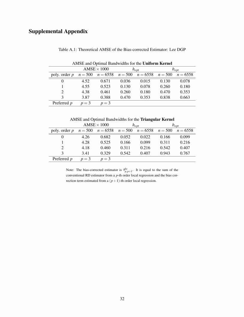
The theoretical AMSE results for the CCT estimators are summarized in Table A.1 and A.2 in the

Supplemental Appendix. Similar to the AMSE for the conventional estimators, higher-order estimators

have a lower AMSE than local linear, and τbc3,4 has the smallest AMSE for both the Lee and Ludwig-Miller

DGP’s. In fact, the relative ranking of AMSEτbc

p,p+1in Table A.1 and A.2 for each sample size and kernel

choice is the same as that of AMSEτp+1 in Table 1 and 2.2 It is also worth noting that τbc1,2, the local linear

CCT estimator, has the largest AMSE among the four estimators when n = 500.

We summarize sample sizes for which AMSEτbc

p,p+1< AMSE

τbc1,2

for p = 0,2,3 in Table 3 and A.2. The

results are similar to those in Table 3 and 4 for the conventional estimator. For the Lee DGP, p = 0 is

preferred to p = 1 when n is small, and p = 2,3 is preferred when n is large. For the Ludwig-Miller DGP,

2This is not surprising in light of Remark 7 in Calonico et al. (2014b): when b, the pilot bandwidth for bias estimation, is equalto h, the main bandwidth for the conventional estimator, the estimator τbc

p,p+1 is the same as τp+1 and therefore has the same AMSE.

4

τbc1,2 is preferred to τbc

0,1 regardless of sample size, whereas τbc2,3 and τbc

3,4 always have a smaller AMSE than

τbc1,2 .

As its name suggests, the AMSE is an asymptotic approximation of the actual mean squared error, and

the approximation may or may not be good for a given DGP and sample size. Therefore, the ranking of

estimators by theoretical AMSE may not be the same as the ranking by MSE. We present the latter for the

two DGP’s in the following subsection.

2.2 MSE from Simulations

In this subsection, we present results from Monte Carlo simulations, which show that higher-order local

estimators have lower MSE than their local linear counterpart for the actual sample sizes in the Lee and

Ludwig-Miller application. Tables 5 and 6 report the MSE for τp under the theoretical AMSE-optimal

bandwidth for the Lee and Ludwig-Miller DGP respectively, where the MSE is computed over 10,000

repeated samples. For the Lee DGP, we report results for p between 0 and 4; for the Ludwidg-Miller DGP,

we omit τ0 because too few observations lie within its theoretical optimal bandwidth.

For the smaller sample size of n = 500, τ1 appears to have the lowest MSE for the Lee DGP, which is

in contrast with the AMSE ranking in Table 1. However, τ4 does have the lowest MSE when n = 6558,

suggesting that AMSE provides a better approximation under this larger sample size for the Lee DGP. As in

Table 2, τ4 has the lowest MSE for both n = 500 and n = 3138 for the Ludwig-Miller DGP as seen in Table

6. Again, the AMSE approximation is generally better for the larger sample size.

We also report the coverage rate of the 95% confidence interval constructed using τp, which is the focus

of Calonico et al. (2014b). The coverage rate is above 91% when p > 1 for both DGP’s, and that of τ0 for the

Lee DGP is just under 90%. Therefore, all the estimators in Tables 5 and 6 appear to be sensible candidates

in terms of coverage rates.

The theoretical AMSE optimal bandwidth is never known in any empirical application, and it has to

be estimated. Consequently, we also evaluate the performance of alternative estimators with the estimated

optimal bandwidth in Monte Carlo simulations. We adopt two alternative bandwidth choices, the CCT

bandwidth with and without regularization,3 and the corresponding results are reported in Tables 7-10.

For both the Lee and Ludwig Miller DGP, the MSE-preferred polynomial order is lower under the default

3The regularization Calonico et al. (2014b) implement in their default bandwidth selector follows the spirit of Imbens andKalyanaraman (2012). It decreases with the variance of the bias estimator and prevents the bandwidth from becoming large. We donot adopt the IK bandwidth here because it is only proposed for τ1.

5

CCT bandwidth (i.e., with regularization), denoted by hCCT , than under the theoretical optimal bandwidth,

hopt . One explanation is that the average hCCT is much smaller than hopt for higher order p, and the cor-

responding variance of τp is larger under hCCT than under hopt . In comparison, the average value of the

CCT bandwidth without regularization, hCCT,noreg, is much closer to hopt for p = 3,4. As a consequence,

the MSE-preferred polynomial orders under hCCT,noreg are closer to those under hopt . For the Lee DGP, the

MSE-preferred polynomial orders are the same as those for hopt : p = 1 for n = 500 and p = 4 for n = 6558.

For the Ludwig-Miller DGP, τ3 is the MSE-preferred estimator when n = 500, and τ3 and τ4 have very sim-

ilar MSE’s when n = 3138. In this latter case, MSEτ3 > MSEτ4 under the uniform kernel, MSEτ4 > MSEτ3

under the triangular kernel. In summary, a higher order τp has a lower MSE than τ1 for the actual sample

sizes in the two empirical applications.

We also examine the MSE of the CCT bias-corrected estimators, τbcp,p+1, from Monte Carlo simulations,

and the results are presented in Tables A.5-A.10. We find that the bias-corrected linear estimator, the default

estimator in Calonico et al. (2014b), never delivers the smallest MSE. In fact, τbc0,1 or τbc

2,3 have the lowest

MSE, depending on the sample size and kernel choice for the Lee DGP, whereas τbc2,3 consistently have the

lowest MSE for the Ludwig-Miller DGP. In the next subsection, we explore the use of the estimated AMSE

for picking the polynomial order.

2.3 Estimated AMSE

When computing the optimal bandwidth for a local polynomial RD estimator, the asymptotic bias and

variance are both estimated. It follows that the AMSE of the estimator, which is the sum of the squared

bias and variance, can be easily estimated as well. As suggested by Fan and Gijbels (1996), comparing the

estimated AMSE for alternative local polynomial estimators, AMSEτp , can serve as a basis for choosing

p. We adapt the suggestion by Fan and Gijbels (1996) to the RD design and investigate the choice of

polynomial order p based on the estimated AMSE of τp and τbcp,p+1.

Tables 11-14 summarize the statistics of AMSEτp from Monte Carlo simulations. We report the average

AMSEτp over 10,000 repeated samples, the fraction of times each τp has the smallest AMSE and the average

computed optimal bandwidth. Comparing these four tables to the MSE Tables 7-10 reveals that the most

likely choice of p based on AMSE does not always have the smallest MSE, but it is nevertheless sensible in

most cases. For the Lee DGP under hCCT , τ0 and τ1 are the most likely choice based on AMSE for n = 500

and n = 6558, respectively, and they have the second lowest MSE. For the Lee DGP under hCCT,noreg, τ1

6

is the most likely choice based on AMSE for both n = 500 and n = 6558; although it performs less well

compared to the higher-order estimators for n = 6558, it does have the lowest MSE for n = 500. For the

Ludwig-Miller DGP, AMSE-based order choice does well: in seven out of the eight cases, it has the smallest

MSE; for the remaining case (n = 3138, uniform kernel and hCCT,noreg), its MSE comes as a close second.

We also estimate the AMSE of τbcp,p+1 based on Theorem A1 of Calonico et al. (2014b) and summarize

the simulation results in Tables A.11-A.14. Again, we examine whether the AMSE-based choice of τbcp,p+1

has the lowest MSE by way of comparison to Tables A.7-A.10. As with the conventional estimator τp, the

most likely choice of p for the bias-corrected estimator based on AMSE does not always have the lowest

MSE – it does so in ten out of the 16 cases. In the remaining six cases, whenever the most likely p is not

1, the associated MSE is lower than that of τbc1,2. Therefore, for the Lee and Ludwig DGP, using AMSE

improves upon the fixed choice of the bias-corrected linear estimator τbc1,2.

In summary, using AMSE leads to a sensible polynomial order choice in many instances. In the vast

majority of cases in our simulation, the most likely choice of p based on AMSE does have the lowest or the

second lowest MSE among alternative estimators. With only two exceptions out of 32 cases, the most likely

choice of p has an MSE that is lower than or equal to that of the default p = 1. Therefore, estimating AMSE

can complement Monte Carlo simulations based on approximating DGP’s for choosing the local polynomial

order.

2.4 GI Weights for Local Regressions

As mentioned at the beginning of section 2, Gelman and Imbens (2014) recently raise concerns of using a

global or local high-order polynomial (e.g. cubic or quartic) to estimate the RD treatment effect. One issue

in particular is that estimators based on high-order global regressions sometimes assign too much weight

to observations far away from the RD cutoff. Since we have demonstrated above that high-order local

estimators may be desirable in certain cases for the Lee and Ludwig-Miller DGP’s, we examine whether

noisy weights raise concerns for local regressions in the two applications.

Using the actual Lee and Ludwig-Miller data, Figures 1-8 plot the GI weights for the left and right

intercept estimators that make up τp for p = 0,1, ...,5 . As with the previous subsections, we examine the

weights for two kernel choices (uniform and triangular) and two bandwidth choices (hCCT and hCCT,noreg).

For high-order local estimators, observations far away from the threshold receive little weight as compared

7

to those close to the threshold as desired. In fact, even the GI weights in the global estimators for the Lee

and Ludwig-Miller data are reasonably well-behaved: as seen from Figures A.1 and A.2, observations far

away from the RD cutoff never receive significantly larger weights than those close to the threshold.

The other two concerns regarding high-order global estimators voiced by Gelman and Imbens (2014)

are 1) they are not chosen based on a criterion relevant for the causal parameter of interest and 2) the

corresponding 95% confidence interval has incorrect coverage rates. As argued in section 1, the (A)MSE

of the RD estimator is an important benchmark of the literature and therefore dispels the first concern. As

demonstrated in the simulations, when a higher order p is preferred, the coverage rate of the corresponding

95% confidence interval is quite close to 95%, which helps to alleviate the second concern. Together with

well-behaved GI weights, we believe that high-order local polynomial RD estimators in certain cases are

good alternatives to local linear.

2.5 Extensions: Fuzzy RD and Regression Kink Design

In this subsection, we briefly discuss how (A)MSE-based local polynomial order choice applies to two

popular extensions of the sharp RD design. The first extension is the fuzzy RD design, where the treatment

assignment rule is not strictly followed. In the existing RD literature, p = 1 is still the default choice in

the fuzzy RD. But by the same argument as above, local linear is not necessarily the best estimator in all

applications. In the same way that we can calculate the AMSE and simulate the MSE of sharp RD estimators,

we can rely on Lemma A2 and Theorem A2 of Calonico et al. (2014b) and do it for the fuzzy RD estimators.

Similarly, the same principle can be applied to the regression kink design (RKD) proposed and explored by

Nielsen et al. (2010) and Card et al. (2012). For RKD, Calonico et al. (2014b) recommends using p = 2 as

the default polynomial order following its RD analog, but again the best polynomial choice should depend

on the particular data set. The ideas presented in this paper readily apply to the RKD case and may help

researchers choose the best polynomial order for their study.

3 Conclusion

The local linear estimator has become the standard in the regression discontinuity literature. In this paper, we

argue that p = 1 should not be the universally preferred polynomial order across all empirical applications.

The mean squared error of the p-th order local estimator depends on the sample size and the intrinsic

8

properties of the data generating process. In two well-known empirical examples, p = 1 is not necessarily

the polynomial order that delivers the lowest (A)MSE.

We do not oppose the use of local linear estimator in RD studies; it is a convenient choice and performs

quite well in many applications. However, we do oppose the notion that a single polynomial order can be

optimal for all RD analyses. We advocate for a more flexible view that an empiricist should be able to

adopt a different local polynomial estimator if it is better suited for the application. If the empiricist would

like to explore the polynomial order choice, we suggest two complementary options to her: 1) estimate an

approximating DGP to the data at hand and conduct Monte Carlo simulations to gauge the performance of

alternative estimators; 2) estimate the AMSE and compare it across alternative estimators.

Each option has its own advantages and disadvantages. Option 1 reveals the exact MSE’s (and gives the

coverage rates of the 95% confidence interval) with an approximating DGP4, whereas option 2 estimates an

approximate MSE using the actual data. It is ideal if the two options point to the same p; when they do not,

it is perhaps prudent to present the value of both estimators, as is typically done in empirical research.

4In light of Gelman and Imbens (2014), if the approximating DGP is estimated using a high-order global polynomial, it may beadvisable to trim the outliers as Imbens and Kalyanaraman (2012) and Calonico et al. (2014b) have done.

9

References

Calonico, Sebastian, Matias D. Cattaneo, and Rocio Titiunik, “Robust Data-Driven Inference in theRegression-Discontinuity Design,” Stata Journal, 2014, 14 (4), 909–946.

, , and , “Robust Nonparametric Confidence Intervals for Regression-Discontinuity Designs,” Econo-metrica, November 2014, 82 (6), 2295–2326.

Card, David, David S. Lee, Zhuan Pei, and Andrea Weber, “Nonlinear Policy Rules and the Identificationand Estimation of Causal Effects in a Generalized Regression Kink Design,” NBER Working Paper 18564November 2012.

Cheng, Ming-Yen, Jianqing Fan, and J. S. Marron, “On automatic boundary corrections,” The Annals ofStatistics, 08 1997, 25 (4), 1691–1708.

Fan, Jianqing and Irene Gijbels, Local Polynomial Modelling and Its Applications, Chapman and Hall,1996.

Gelman, Andrew and Guido Imbens, “Why High-order Polynomials Should Not Be Used in RegressionDiscontinuity Designs,” NBER Working Paper 20405 August 2014.

Hahn, Jinyong, Petra Todd, and Wilbert Van der Klaauw, “Identification and Estimation of TreatmentEffects with a Regression-Discontinuity Design,” Econometrica, 2001, 69 (1), 201–209.

Imbens, Guido W. and Karthik Kalyanaraman, “Optimal Bandwidth Choice for the Regression Discon-tinuity Estimator.,” Review of Economic Studies, 2012, 79 (3), 933 – 959.

Lee, David S., “Randomized Experiments from Non-random Selection in U.S. House Elections,” Journalof Econometrics, February 2008, 142 (2), 675–697.

Ludwig, J. and D. Miller, “Does Head Start Improve Children’s Life Chances? Evidence from a RegressionDiscontinuity Design,” Quarterly Journal of Economics, 2007, 122(1), 159–208.

Nielsen, Helena Skyt, Torben Sørensen, and Christopher R. Taber, “Estimating the Effect of StudentAid on College Enrollment: Evidence from a Government Grant Policy Reform,” American EconomicJournal: Economic Policy, 2010, 2 (2), 185–215.

10

Table 1: Theoretical AMSE of the Conventional Estimator: Lee DGP

AMSE and Optimal Bandwidth for the Uniform KernelAMSE×1000 hopt

poly. order p n = 500 n = 6558 n = 500 n = 65580 4.42 0.795 0.036 0.0151 4.12 0.526 0.130 0.0782 4.33 0.477 0.260 0.1803 4.11 0.417 0.470 0.3534 3.52 0.339 0.838 0.663

Preferred p p = 4 p = 4

AMSE and Optimal Bandwidth for the Triangular KernelAMSE×1000 hopt

poly. order p n = 500 n = 6558 n = 500 n = 65580 4.09 0.735 0.052 0.0221 3.89 0.496 0.166 0.0992 4.14 0.456 0.311 0.2163 3.96 0.402 0.542 0.4074 3.41 0.329 0.943 0.767


Note: The function form of the Lee DGP is

E[Y |X = x] =

{0.48+1.27x+7.18x2 +20.21x3 +21.54x4 +7.33x5 if x < 00.52+0.84x−3.00x2 +7.99x3−9.01x4 +3.56x5 if x > 0

11

Table 2: Theoretical AMSE of the Conventional Estimator: Ludwig-Miller DGP

AMSE and Optimal Bandwidth for the Uniform KernelAMSE×1000 hopt

poly. order p n = 500 n = 3138 n = 500 n = 31380 20.3 5.98 0.008 0.0041 8.28 1.90 0.065 0.0452 5.74 1.19 0.196 0.1513 4.48 0.88 0.431 0.3514 3.46 0.65 0.854 0.722


AMSE and Optimal Bandwidth for the Triangular KernelAMSE×1000 hopt

poly. order p n = 500 n = 3138 n = 500 n = 31380 18.8 5.52 0.011 0.0061 7.81 1.80 0.082 0.0572 5.49 1.14 0.235 0.1813 4.32 0.84 0.497 0.4054 3.35 0.63 0.961 0.813


Note: The function form of the Ludwig-Miller DGP is

E[Y |X = x] =

{3.71+2.30x+3.28x2 +1.45x3 +0.23x4 +0.03x5 if x < 00.26+18.49x−54.81x2 +74.30x3−45.02x4 +9.83x5 if x > 0

12

Table 3: Comparison of Polynomial Orders by Theoretical AMSE for the Conventional Estimator: Lee DGP

Polynomial order pis preferred to p = 1 for the

conventional RD estimator when ...Uniform Kernel Triangular Kernel

0 n < 296 n < 3442 n > 1167 n > 14663 n > 476 n > 6074 n > 177 n > 150

Note: The comparison is based on the theoretical AMSE evaluated at the opti-

mal bandwidth.

Table 4: Comparison of Polynomial Orders by Theoretical AMSE for the Conventional Estimator: Ludwig-Miller DGP


conventional RD estimator when ...Uniform Kernel Triangular Kernel

0 Never Never2 Always Always3 Always Always4 Always Always


mal bandwidth(s).

13

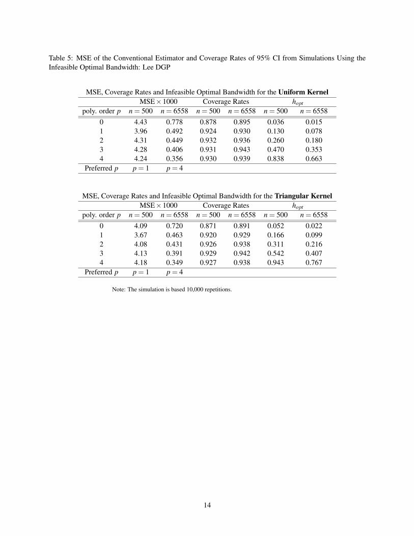
Table 5: MSE of the Conventional Estimator and Coverage Rates of 95% CI from Simulations Using theInfeasible Optimal Bandwidth: Lee DGP

MSE, Coverage Rates and Infeasible Optimal Bandwidth for the Uniform KernelMSE×1000 Coverage Rates hopt

poly. order p n = 500 n = 6558 n = 500 n = 6558 n = 500 n = 65580 4.43 0.778 0.878 0.895 0.036 0.0151 3.96 0.492 0.924 0.930 0.130 0.0782 4.31 0.449 0.932 0.936 0.260 0.1803 4.28 0.406 0.931 0.943 0.470 0.3534 4.24 0.356 0.930 0.939 0.838 0.663


MSE, Coverage Rates and Infeasible Optimal Bandwidth for the Triangular KernelMSE×1000 Coverage Rates hopt



Note: The simulation is based 10,000 repetitions.

14

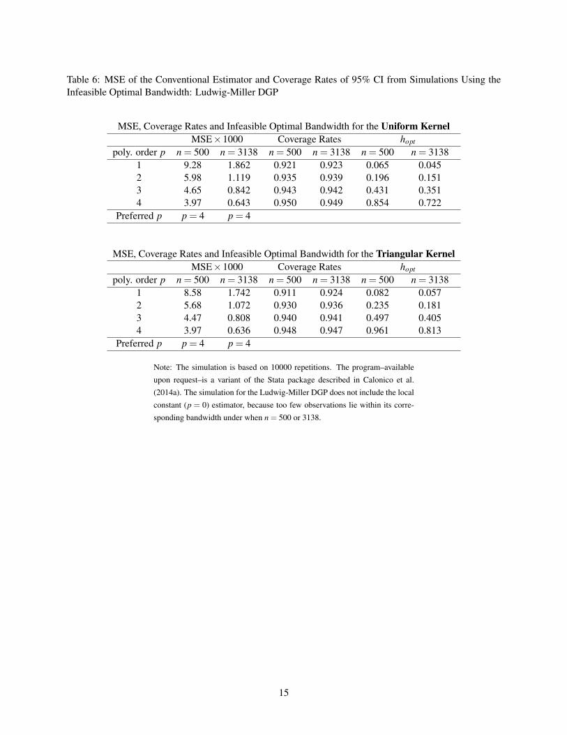
Table 6: MSE of the Conventional Estimator and Coverage Rates of 95% CI from Simulations Using theInfeasible Optimal Bandwidth: Ludwig-Miller DGP

MSE, Coverage Rates and Infeasible Optimal Bandwidth for the Uniform KernelMSE×1000 Coverage Rates hopt

poly. order p n = 500 n = 3138 n = 500 n = 3138 n = 500 n = 31381 9.28 1.862 0.921 0.923 0.065 0.0452 5.98 1.119 0.935 0.939 0.196 0.1513 4.65 0.842 0.943 0.942 0.431 0.3514 3.97 0.643 0.950 0.949 0.854 0.722


MSE, Coverage Rates and Infeasible Optimal Bandwidth for the Triangular KernelMSE×1000 Coverage Rates hopt



Note: The simulation is based on 10000 repetitions. The program–available

upon request–is a variant of the Stata package described in Calonico et al.

(2014a). The simulation for the Ludwig-Miller DGP does not include the local

constant (p = 0) estimator, because too few observations lie within its corre-

sponding bandwidth under when n = 500 or 3138.

15

Table 7: MSE of the Conventional Estimator and Coverage Rates of 95% CI from Simulations Using theCCT Bandwidth: Lee DGP

MSE, Coverage Rates and CCT Bandwidth for the Uniform KernelMSE×1000 Coverage Rates hCCT



MSE, Coverage Rates and CCT Bandwidth for the Triangular KernelMSE×1000 Coverage Rates hCCT



Note: The simulation is based on 10000 repetitions. The program–availableupon request–is a variant of the Stata package described in Calonico et al.(2014a).The reported CCT bandwidth, hCCT , is the average over repeated simulationsamples.

16

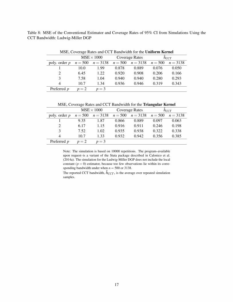
Table 8: MSE of the Conventional Estimator and Coverage Rates of 95% CI from Simulations Using theCCT Bandwidth: Ludwig-Miller DGP

MSE, Coverage Rates and CCT Bandwidth for the Uniform KernelMSE×1000 Coverage Rates hCCT



MSE, Coverage Rates and CCT Bandwidth for the Triangular KernelMSE×1000 Coverage Rates hCCT



Note: The simulation is based on 10000 repetitions. The program–availableupon request–is a variant of the Stata package described in Calonico et al.(2014a). The simulation for the Ludwig-Miller DGP does not include the localconstant (p = 0) estimator, because too few observations lie within its corre-sponding bandwidth under when n = 500 or 3138.The reported CCT bandwidth, hCCT , is the average over repeated simulationsamples.

17

Table 9: MSE of the Conventional Estimator and Coverage Rates of 95% CI from Simulations Using theCCT Bandwidth without Regularization: Lee DGP

MSE, Coverage Rates and CCT Bandwidth for the Uniform KernelMSE×1000 Coverage Rates hCCT,noreg



MSE, Coverage Rates and CCT Bandwidth for the Triangular KernelMSE×1000 Coverage Rates hCCT,noreg



Note: The simulation is based on 10000 repetitions. The program–availableupon request–is a variant of the Stata package described in Calonico et al.(2014a).The reported CCT bandwidth, hCCT,noreg, is the average over repeated simu-lation samples.

18

Table 10: MSE of the Conventional Estimator and Coverage Rates of 95% CI from Simulations Using theCCT Bandwidth without Regularization: Ludwig-Miller DGP

MSE, Coverage Rates and CCT Bandwidth for the Uniform KernelMSE×1000 Coverage Rates hCCT,noreg



MSE, Coverage Rates and CCT Bandwidth for the Triangular KernelMSE×1000 Coverage Rates hCCT,noreg



Note: The simulation is based on 10000 repetitions. The program–availableupon request–is a variant of the Stata package described in Calonico et al.(2014a). The simulation for the Ludwig-Miller DGP does not include the localconstant (p = 0) estimator, because too few observations lie within its corre-sponding bandwidth under when n = 500 or 3138.The reported CCT bandwidth, hCCT,noreg, is the average over repeated simu-lation samples.

19

Table 11: Estimated AMSE from Simulations Using the CCT Bandwidths: Lee DGP

Estimated AMSE, Preferred p and CCT Bandwidths for the Uniform KernelAMSE×1000 Fraction of Times Preferred hCCT


Most Likely Choice of p p = 0 p = 1

Estimated AMSE, preferred p and CCT Bandwidths for the Triangular KernelAMSE×1000 Fraction of Times Preferred hCCT



Note: The simulation is based 10,000 repetitions. The program–available uponrequest–is a variant of the Stata package described in Calonico et al. (2014a).The reported AMSE measure and CCT bandwidth, AMSE× 1000 and hCCTare the averages over repeated simulation samples.

20

Table 12: Estimated AMSE from Simulations Using the CCT Bandwidths: Ludwig-Miller DGP

Estimated AMSE, Preferred p and CCT Bandwidths for the Uniform KernelAMSE×1000 Fraction of Times Preferred hCCT



Estimated AMSE, Preferred p and CCT Bandwidths for the Triangular KernelAMSE×1000 Fraction of Times Preferred hCCT



Note: The simulation is based on 10000 repetitions. The program–availableupon request–is a variant of the Stata package described in Calonico et al.(2014a). Unlike in Tables 6, 8 and 10, results are reported for the local constantestimator. This is because only the optimal bandwidth for the local estimatoris calculated and not the value of local estimator itself.The reported AMSE measure and CCT bandwidths, AMSE×1000 and hCCT ,are the averages over repeated simulation samples.

21

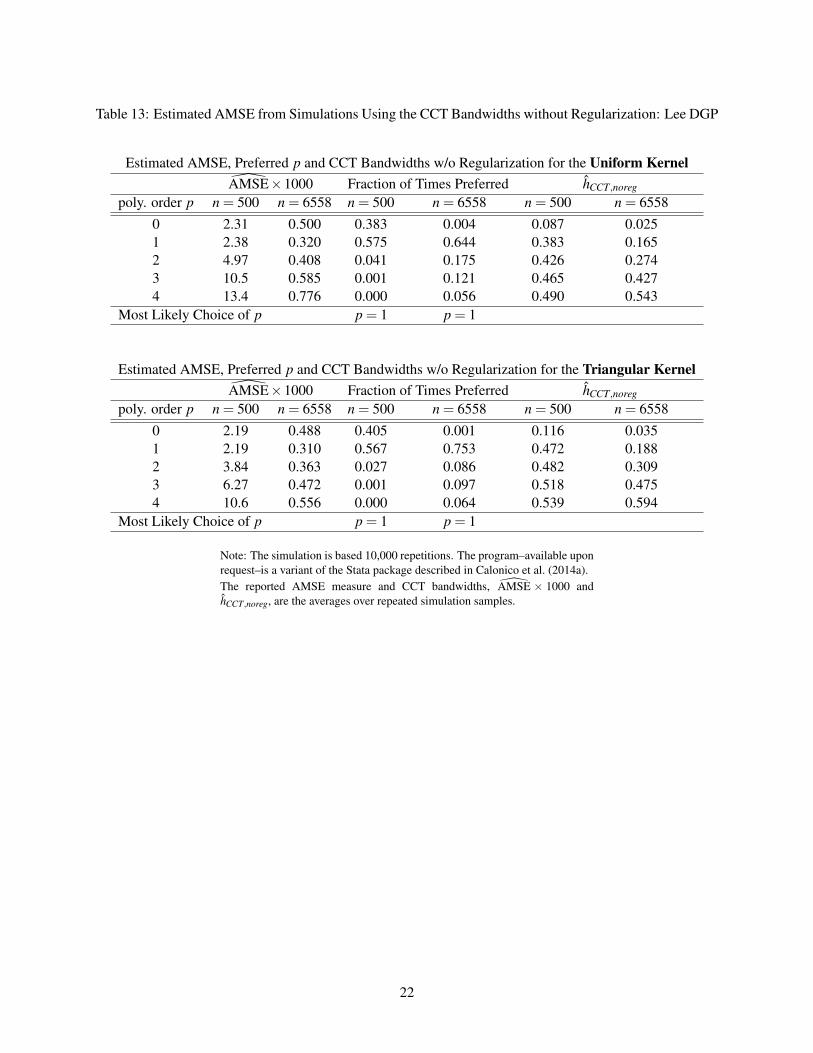
Table 13: Estimated AMSE from Simulations Using the CCT Bandwidths without Regularization: Lee DGP

Estimated AMSE, Preferred p and CCT Bandwidths w/o Regularization for the Uniform KernelAMSE×1000 Fraction of Times Preferred hCCT,noreg



Estimated AMSE, Preferred p and CCT Bandwidths w/o Regularization for the Triangular KernelAMSE×1000 Fraction of Times Preferred hCCT,noreg



Note: The simulation is based 10,000 repetitions. The program–available uponrequest–is a variant of the Stata package described in Calonico et al. (2014a).The reported AMSE measure and CCT bandwidths, AMSE × 1000 andhCCT,noreg, are the averages over repeated simulation samples.

22

Table 14: Estimated AMSE from Simulations Using the CCT Bandwidths: Ludwig-Miller DGP

Estimated AMSE, Preferred p and CCT Bandwidths w/o Regularization for the Uniform KernelAMSE×1000 Fraction of Times Preferred hCCT,noreg



Estimated AMSE, Preferred p and CCT Bandwidths w/o Regularization for the Triangular KernelAMSE×1000 Fraction of Times Preferred hCCT,noreg



Note: The simulation is based on 10000 repetitions. The program–availableupon request–is a variant of the Stata package described in Calonico et al.(2014a). Unlike in Tables 6, 8 and 10, results are reported for the local constantestimator. This is because only the optimal bandwidth for the local estimatoris calculated and not the value of local estimator itself.The reported AMSE measure and CCT bandwidths, AMSE × 1000 andbCCT,noreg, are the averages over repeated simulation samples.

23

Figure 1: Weights for Local Polynomial Estimators: Lee Data, above the RD Cutoff, CCT Bandwidth

-50

050

100

Wei

ght

0 .1 .2 .3 .4x

Local poly. order p=0

-50

050

100

Wei

ght

0 .1 .2 .3 .4x


-50

050

100

Wei

ght

0 .1 .2 .3 .4x


-50

050

100

Wei

ght

0 .1 .2 .3 .4x


-50

050

100

Wei

ght

0 .1 .2 .3 .4x


-50

050

100

Wei

ght

0 .1 .2 .3 .4x


Weights for Local Polynomial Estimators: Lee DataAbove RD cutoff, Uniform Kernel, CCT BW

050

100

Wei

ght

0 .1 .2 .3 .4 .5x


050

100

Wei

ght

0 .1 .2 .3 .4 .5x


050

100

Wei

ght

0 .1 .2 .3 .4 .5x


050

100

Wei

ght

0 .1 .2 .3 .4 .5x


050

100

Wei

ght

0 .1 .2 .3 .4 .5x


050

100

Wei

ght

0 .1 .2 .3 .4 .5x


Weights for Local Polynomial Estimators: Lee DataAbove RD cutoff, Triangular Kernel, CCT BW

Note: The graphs plot the GI weights for the local estimator τp with the default

CCT bandwidth, for p = 0,1, ...,5.

24

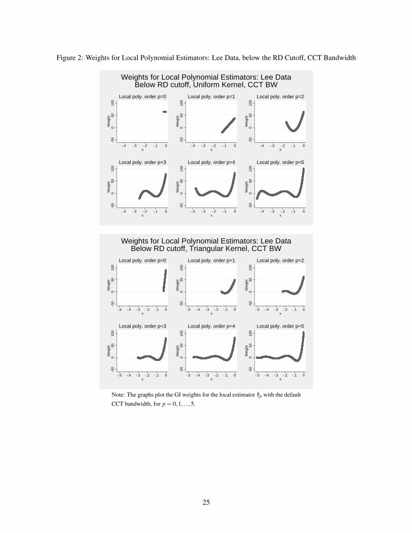
Figure 2: Weights for Local Polynomial Estimators: Lee Data, below the RD Cutoff, CCT Bandwidth

-50

050

100

Wei

ght

-.4 -.3 -.2 -.1 0x


-50

050

100

Wei

ght

-.4 -.3 -.2 -.1 0x


-50

050

100

Wei

ght

-.4 -.3 -.2 -.1 0x


-50

050

100

Wei

ght

-.4 -.3 -.2 -.1 0x


-50

050

100

Wei

ght

-.4 -.3 -.2 -.1 0x


-50

050

100

Wei

ght

-.4 -.3 -.2 -.1 0x


Weights for Local Polynomial Estimators: Lee DataBelow RD cutoff, Uniform Kernel, CCT BW

-50

050

100

Wei

ght

-.5 -.4 -.3 -.2 -.1 0x


-50

050

100

Wei

ght

-.5 -.4 -.3 -.2 -.1 0x


-50

050

100

Wei

ght

-.5 -.4 -.3 -.2 -.1 0x


-50

050

100

Wei

ght

-.5 -.4 -.3 -.2 -.1 0x


-50

050

100

Wei

ght

-.5 -.4 -.3 -.2 -.1 0x


-50

050

100

Wei

ght

-.5 -.4 -.3 -.2 -.1 0x


Weights for Local Polynomial Estimators: Lee DataBelow RD cutoff, Triangular Kernel, CCT BW



25

Figure 3: Weights for Local Polynomial Estimators: Ludwig-Miller Data, above the RD Cutoff, CCT Band-width

-100

010

020

030

040

0W

eigh

t

0 2 4 6 8 10x


-100

010

020

030

040

0W

eigh

t

0 2 4 6 8 10x


-100

010

020

030

040

0W

eigh

t

0 2 4 6 8 10x


-100

010

020

030

040

0W

eigh

t

0 2 4 6 8 10x


-100

010

020

030

040

0W

eigh

t

0 2 4 6 8 10x


-100

010

020

030

040

0W

eigh

t

0 2 4 6 8 10x


Weights for Local Polynomial Estimators: LM DataAbove RD cutoff, Uniform Kernel, CCT BW

-100

010

020

030

040

0W

eigh

t

0 2 4 6 8 10x


-100

010

020

030

040

0W

eigh

t

0 2 4 6 8 10x


-100

010

020

030

040

0W

eigh

t

0 2 4 6 8 10x


-100

010

020

030

040

0W

eigh

t

0 2 4 6 8 10x


-100

010

020

030

040

0W

eigh

t

0 2 4 6 8 10x


-100

010

020

030

040

0W

eigh

t

0 2 4 6 8 10x


Weights for Local Polynomial Estimators: LM DataAbove RD cutoff, Triangular Kernel, CCT BW

Note:The graphs plot the GI weights for the local estimator τp with the default


26

Figure 4: Weights for Local Polynomial Estimators: Ludwig-Miller Data, below the RD Cutoff, CCT Band-width

-100

010

020

030

040

0W

eigh

t

-10 -8 -6 -4 -2 0x


-100

010

020

030

040

0W

eigh

t

-10 -8 -6 -4 -2 0x


-100

010

020

030

040

0W

eigh

t

-10 -8 -6 -4 -2 0x


-100

010

020

030

040

0W

eigh

t

-10 -8 -6 -4 -2 0x


-100

010

020

030

040

0W

eigh

t

-10 -8 -6 -4 -2 0x


-100

010

020

030

040

0W

eigh

t

-10 -8 -6 -4 -2 0x


Weights for Local Polynomial Estimators: LM DataBelow RD cutoff, Uniform Kernel, CCT BW

-100

010

020

030

040

0W

eigh

t

-10 -8 -6 -4 -2 0x


-100

010

020

030

040

0W

eigh

t

-10 -8 -6 -4 -2 0x


-100

010

020

030

040

0W

eigh

t

-10 -8 -6 -4 -2 0x


-100

010

020

030

040

0W

eigh

t

-10 -8 -6 -4 -2 0x


-100

010

020

030

040

0W

eigh

t

-10 -8 -6 -4 -2 0x


-100

010

020

030

040

0W

eigh

t

-10 -8 -6 -4 -2 0x


Weights for Local Polynomial Estimators: LM DataBelow RD cutoff, Triangular Kernel, CCT BW



27

Figure 5: Weights for Local Polynomial Estimators: Lee Data, above the RD Cutoff, CCT Bandwidthwithout Regularization

-20

020

4060

80W

eigh

t

0 .1 .2 .3 .4 .5x


-20

020

4060

80W

eigh

t

0 .1 .2 .3 .4 .5x


-20

020

4060

80W

eigh

t

0 .1 .2 .3 .4 .5x

Local poly. order p=2-2

00

2040

6080

Wei

ght

0 .1 .2 .3 .4 .5x


-20

020

4060

80W

eigh

t

0 .1 .2 .3 .4 .5x


-20

020

4060

80W

eigh

t

0 .1 .2 .3 .4 .5x


Weights for Local Polynomial Estimators: Lee DataAbove RD cutoff, Uniform Kernel, CCT BW w/o Regul.

-20

020

4060

80W

eigh

t

0 .2 .4 .6 .8x


-20

020

4060

80W

eigh

t

0 .2 .4 .6 .8x


-20

020

4060

80W

eigh

t

0 .2 .4 .6 .8x


-20

020

4060

80W

eigh

t

0 .2 .4 .6 .8x


-20

020

4060

80W

eigh

t

0 .2 .4 .6 .8x


-20

020

4060

80W

eigh

t

0 .2 .4 .6 .8x


Weights for Local Polynomial Estimators: Lee DataAbove RD cutoff, Triangular Kernel, CCT BW w/o Regul.

Note: The graphs plot the GI weights for the local estimator τp with the no-

regularization CCT bandwidth, for p = 0,1, ...,5.

28

Figure 6: Weights for Local Polynomial Estimators: Lee Data, below the RD Cutoff, CCT Bandwidthwithout Regularization

-20

020

4060

80W

eigh

t

-.5 -.4 -.3 -.2 -.1 0x


-20

020

4060

80W

eigh

t

-.5 -.4 -.3 -.2 -.1 0x


-20

020

4060

80W

eigh

t

-.5 -.4 -.3 -.2 -.1 0x


00

2040

6080

Wei

ght

-.5 -.4 -.3 -.2 -.1 0x


-20

020

4060

80W

eigh

t

-.5 -.4 -.3 -.2 -.1 0x


-20

020

4060

80W

eigh

t

-.5 -.4 -.3 -.2 -.1 0x


Weights for Local Polynomial Estimators: Lee DataBelow RD cutoff, Uniform Kernel, CCT BW w/o Regul.

-20

020

4060

80W

eigh

t

-.8 -.6 -.4 -.2 0x


-20

020

4060

80W

eigh

t

-.8 -.6 -.4 -.2 0x


-20

020

4060

80W

eigh

t

-.8 -.6 -.4 -.2 0x


-20

020

4060

80W

eigh

t

-.8 -.6 -.4 -.2 0x


-20

020

4060

80W

eigh

t

-.8 -.6 -.4 -.2 0x


-20

020

4060

80W

eigh

t

-.8 -.6 -.4 -.2 0x


Weights for Local Polynomial Estimators: Lee DataBelow RD cutoff, Triangular Kernel, CCT BW w/o Regul.



29

Figure 7: Weights for Local Polynomial Estimators: Ludwig-Miller Data, above the RD Cutoff, CCT Band-width without Regularization

-100

010

020

030

0W

eigh

t

0 5 10 15x


-100

010

020

030

0W

eigh

t

0 5 10 15x


-100

010

020

030

0W

eigh

t

0 5 10 15x


000

100

200

300

Wei

ght

0 5 10 15x


-100

010

020

030

0W

eigh

t

0 5 10 15x


-100

010

020

030

0W

eigh

t

0 5 10 15x


Weights for Local Polynomial Estimators: LM DataAbove RD cutoff, Uniform Kernel, CCT BW w/o Regul.

-100

010

020

030

040

0W

eigh

t

0 5 10 15 20x


-100

010

020

030

040

0W

eigh

t

0 5 10 15 20x


-100

010

020

030

040

0W

eigh

t

0 5 10 15 20x


-100

010

020

030

040

0W

eigh

t

0 5 10 15 20x


-100

010

020

030

040

0W

eigh

t

0 5 10 15 20x


-100

010

020

030

040

0W

eigh

t

0 5 10 15 20x


Weights for Local Polynomial Estimators: LM DataAbove RD cutoff, Triangular Kernel, CCT BW w/o Regul.

Note:The graphs plot the GI weights for the local estimator τp with the no-


30

Figure 8: Weights for Local Polynomial Estimators: Ludwig-Miller Data, below the RD Cutoff, CCT Band-width without Regularization

-100

010

020

030

0W

eigh

t

-15 -10 -5 0x


-100

010

020

030

0W

eigh

t

-15 -10 -5 0x


-100

010

020

030

0W

eigh

t

-15 -10 -5 0x


000

100

200

300

Wei

ght

-15 -10 -5 0x


-100

010

020

030

0W

eigh

t

-15 -10 -5 0x


-100

010

020

030

0W

eigh

t

-15 -10 -5 0x


Weights for Local Polynomial Estimators: LM DataBelow RD cutoff, Uniform Kernel, CCT BW w/o Regul.

-100

010

020

030

0W

eigh

t

-20 -15 -10 -5 0x


-100

010

020

030

0W

eigh

t

-20 -15 -10 -5 0x


-100

010

020

030

0W

eigh

t

-20 -15 -10 -5 0x


-100

010

020

030

0W

eigh

t

-20 -15 -10 -5 0x


-100

010

020

030

0W

eigh

t

-20 -15 -10 -5 0x


-100

010

020

030

0W

eigh

t

-20 -15 -10 -5 0x


Weights for Local Polynomial Estimators: LM DataBelow RD cutoff, Triangular Kernel, CCT BW w/o Regul.



31

Supplemental Appendix

Table A.1: Theoretical AMSE of the Bias-corrected Estimator: Lee DGP

AMSE and Optimal Bandwidths for the Uniform KernelAMSE×1000 hopt bopt



AMSE and Optimal Bandwidths for the Triangular KernelAMSE×1000 hopt bopt



Note: The bias-corrected estimator is τbcp,p+1. It is equal to the sum of the

conventional RD estimator from a p-th order local regression and the bias cor-

rection term estimated from a (p+1)-th order local regression.

32

Table A.2: Theoretical AMSE of the Bias-corrected Estimator: Ludwig-Miller DGP

AMSE and Optimal Bandwidths for the Uniform KernelAMSE×1000 hopt bopt



AMSE and Optimal Bandwidths for the Triangular KernelAMSE×1000 hopt bopt




conventional RD estimator from a p-th order local regression and the bias cor-

rection term estimated from a (p+1)-th order local regression.

33

Table A.3: Comparison of Polynomial Orders by Theoretical AMSE for the Bias-Corrected Estimator: LeeDGP


bias-corrected RD estimator when ...Uniform Kernel Triangular Kernel

0 n < 531 n < 5302 n > 137 n > 2533 n > 10 n > 30


mal bandwidths.

Table A.4: Comparison of Polynomial Orders by Theoretical AMSE for the Bias-Corrected Estimator:Ludwig-Miller DGP


bias-corrected RD estimator when ...Uniform Kernel Triangular Kernel

0 Never Never2 Always Always3 Always Always


mal bandwidths.

34

Table A.5: MSE of the Bias-Corrected Estimator and Coverage Rates of 95% Robust CI from SimulationsUsing the Infeasible Optimal Bandwidths: Lee DGP

MSE, Coverage Rates and Infeasible Optimal Bandwidths for the Uniform KernelMSE×1000 Coverage Rates hopt bopt

poly. order p n = 500 n = 6558 n = 500 n = 6558 n = 500 n = 6558 n = 500 n = 65580 4.73 0.668 0.925 0.943 0.036 0.015 0.130 0.0781 4.80 0.523 0.933 0.943 0.130 0.078 0.260 0.1802 4.77 0.465 0.934 0.946 0.260 0.180 0.470 0.3533 4.59 0.405 0.937 0.950 0.470 0.353 0.838 0.663


MSE, Coverage Rates and Infeasible Optimal Bandwidths for the Triangular KernelMSE×1000 Coverage Rates hopt bopt




conventional RD estimator from a p-th order local regression and the bias cor-rection term estimated from a (p+1)-th order local regression.The simulation is based 10,000 repetitions. The program–available upon re-quest–is a variant of the Stata package described in Calonico et al. (2014a).

35

Table A.6: MSE of the Bias-Corrected Estimator and Coverage Rates of 95% Robust CI from SimulationsUsing the CCT Bandwidth: Ludwig-Miller DGP

MSE, Coverage Rates and Infeasible Optimal Bandwidths for the Uniform KernelMSE×1000 Coverage Rates hopt bopt

poly. order p n = 500 n = 3138 n = 500 n = 3138 n = 500 n = 3138 n = 500 n = 31381 8.57 1.65 0.942 0.947 0.065 0.045 0.196 0.1512 5.90 1.07 0.946 0.950 0.196 0.151 0.431 0.3513 4.77 0.828 0.948 0.950 0.431 0.351 0.854 0.722


MSE, Coverage Rates and Infeasible Optimal Bandwidths for the Triangular KernelMSE×1000 Coverage Rates hopt bopt




conventional RD estimator from a p-th order local regression and the bias cor-rection term estimated from a (p+1)-th order local regression.The simulation is based on 10000 repetitions. The program–available uponrequest–is a variant of the Stata package described in Calonico et al. (2014a).The simulation for the Ludwig-Miller DGP does not include the local constant(p = 0) estimator, because too few observations lie within its correspondingbandwidth under when n = 500 or 3138.

36

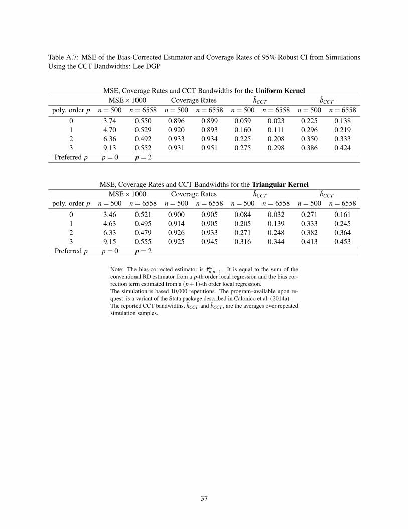
Table A.7: MSE of the Bias-Corrected Estimator and Coverage Rates of 95% Robust CI from SimulationsUsing the CCT Bandwidths: Lee DGP

MSE, Coverage Rates and CCT Bandwidths for the Uniform KernelMSE×1000 Coverage Rates hCCT bCCT



MSE, Coverage Rates and CCT Bandwidths for the Triangular KernelMSE×1000 Coverage Rates hCCT bCCT




conventional RD estimator from a p-th order local regression and the bias cor-rection term estimated from a (p+1)-th order local regression.The simulation is based 10,000 repetitions. The program–available upon re-quest–is a variant of the Stata package described in Calonico et al. (2014a).The reported CCT bandwidths, hCCT and bCCT , are the averages over repeatedsimulation samples.

37

Table A.8: MSE of the Bias-Corrected Estimator and Coverage Rates of 95% Robust CI from SimulationsUsing the CCT Bandwidth: Ludwig-Miller DGP

MSE, Coverage Rates and CCT Bandwidths for the Uniform KernelMSE×1000 Coverage Rates hCCT bCCT



MSE, Coverage Rates and CCT Bandwidths for the Triangular KernelMSE×1000 Coverage Rates hCCT bCCT




conventional RD estimator from a p-th order local regression and the bias cor-rection term estimated from a (p+1)-th order local regression.The simulation is based on 10000 repetitions. The program–available uponrequest–is a variant of the Stata package described in Calonico et al. (2014a).The simulation for the Ludwig-Miller DGP does not include the local constant(p = 0) estimator, because too few observations lie within its correspondingbandwidth under when n = 500 or 3138.The reported CCT bandwidths, hCCT and bCCT , are the averages over repeatedsimulation samples.

38

Table A.9: MSE of the Bias-Corrected Estimator and Coverage Rates of 95% Robust CI from SimulationsUsing the CCT Bandwidths without Regularization: Lee DGP

MSE, Coverage Rates and CCT Bandwidths w/o Regularization for the Uniform KernelMSE×1000 Coverage Rates hCCT,noreg bCCT,noreg



MSE, Coverage Rates and CCT Bandwidths for the Triangular KernelMSE×1000 Coverage Rates hCCT,noreg bCCT,noreg




conventional RD estimator from a p-th order local regression and the bias cor-rection term estimated from a (p+1)-th order local regression.The simulation is based 10,000 repetitions. The program–available upon re-quest–is a variant of the Stata package described in Calonico et al. (2014a).The reported CCT bandwidths, hCCT,noreg and bCCT,noreg, are the averages overrepeated simulation samples.

39

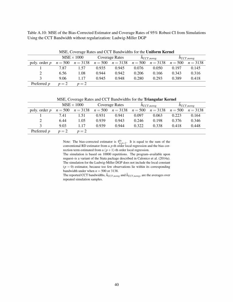
Table A.10: MSE of the Bias-Corrected Estimator and Coverage Rates of 95% Robust CI from SimulationsUsing the CCT Bandwidth without regularization: Ludwig-Miller DGP

MSE, Coverage Rates and CCT Bandwidths for the Uniform KernelMSE×1000 Coverage Rates hCCT,noreg bCCT,noreg



MSE, Coverage Rates and CCT Bandwidths for the Triangular KernelMSE×1000 Coverage Rates hCCT,noreg bCCT,noreg




conventional RD estimator from a p-th order local regression and the bias cor-rection term estimated from a (p+1)-th order local regression.The simulation is based on 10000 repetitions. The program–available uponrequest–is a variant of the Stata package described in Calonico et al. (2014a).The simulation for the Ludwig-Miller DGP does not include the local constant(p = 0) estimator, because too few observations lie within its correspondingbandwidth under when n = 500 or 3138.The reported CCT bandwidths, hCCT,noreg and bCCT,noreg, are the averages overrepeated simulation samples.

40

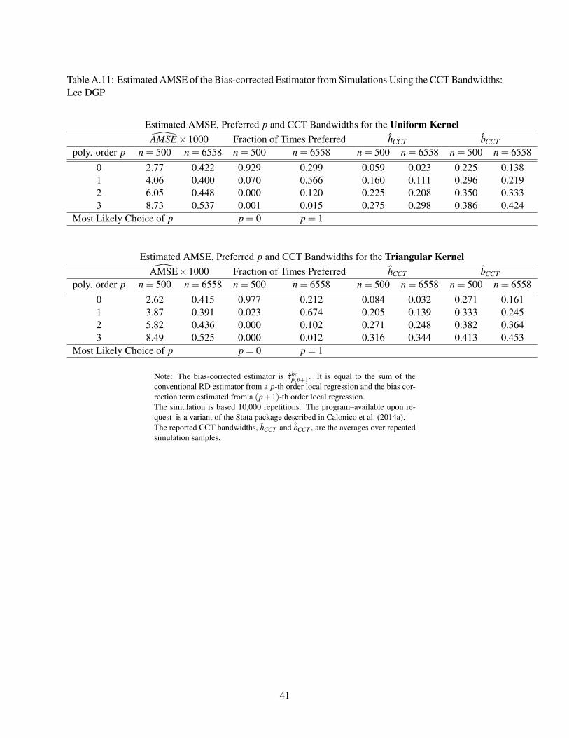
Table A.11: Estimated AMSE of the Bias-corrected Estimator from Simulations Using the CCT Bandwidths:Lee DGP

Estimated AMSE, Preferred p and CCT Bandwidths for the Uniform KernelAMSE×1000 Fraction of Times Preferred hCCT bCCT



Estimated AMSE, Preferred p and CCT Bandwidths for the Triangular KernelAMSE×1000 Fraction of Times Preferred hCCT bCCT




conventional RD estimator from a p-th order local regression and the bias cor-rection term estimated from a (p+1)-th order local regression.The simulation is based 10,000 repetitions. The program–available upon re-quest–is a variant of the Stata package described in Calonico et al. (2014a).The reported CCT bandwidths, hCCT and bCCT , are the averages over repeatedsimulation samples.

41

Table A.12: Estimated AMSE of the Bias-corrected Estimator from Simulations Using the CCT Bandwidths:Ludwig-Miller DGP

Estimated AMSE, Preferred p and CCT Bandwidths for the Uniform KernelAMSE×1000 Fraction of Times Preferred hCCT bCCT



Estimated AMSE, Preferred p and CCT Bandwidths for the Triangular KernelAMSE×1000 Fraction of Times Preferred hCCT bCCT




conventional RD estimator from a p-th order local regression and the bias cor-rection term estimated from a (p+1)-th order local regression.The simulation is based on 10000 repetitions. The program–available uponrequest–is a variant of the Stata package described in Calonico et al. (2014a).The simulation for the Ludwig-Miller DGP does not include the local constant(p = 0) estimator, because too few observations lie within its correspondingbandwidth under when n = 500 or 3138.The reported CCT bandwidths, hCCT and bCCT , are the averages over repeatedsimulation samples.

42

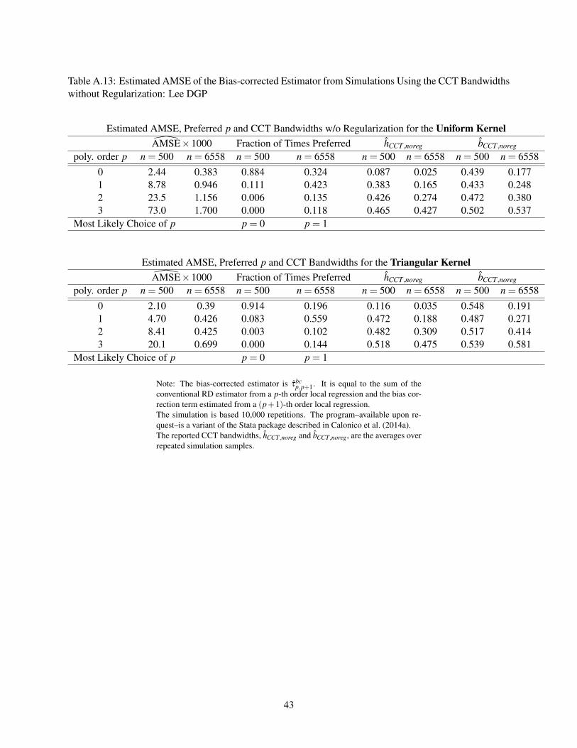
Table A.13: Estimated AMSE of the Bias-corrected Estimator from Simulations Using the CCT Bandwidthswithout Regularization: Lee DGP

Estimated AMSE, Preferred p and CCT Bandwidths w/o Regularization for the Uniform KernelAMSE×1000 Fraction of Times Preferred hCCT,noreg bCCT,noreg



Estimated AMSE, Preferred p and CCT Bandwidths for the Triangular KernelAMSE×1000 Fraction of Times Preferred hCCT,noreg bCCT,noreg




conventional RD estimator from a p-th order local regression and the bias cor-rection term estimated from a (p+1)-th order local regression.The simulation is based 10,000 repetitions. The program–available upon re-quest–is a variant of the Stata package described in Calonico et al. (2014a).The reported CCT bandwidths, hCCT,noreg and bCCT,noreg, are the averages overrepeated simulation samples.

43

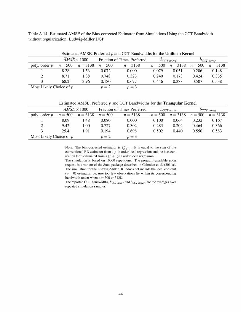
Table A.14: Estimated AMSE of the Bias-corrected Estimator from Simulations Using the CCT Bandwidthwithout regularization: Ludwig-Miller DGP

Estimated AMSE, Preferred p and CCT Bandwidths for the Uniform KernelAMSE×1000 Fraction of Times Preferred hCCT,noreg bCCT,noreg



Estimated AMSE, Preferred p and CCT Bandwidths for the Triangular KernelAMSE×1000 Fraction of Times Preferred hCCT,noreg bCCT,noreg




conventional RD estimator from a p-th order local regression and the bias cor-rection term estimated from a (p+1)-th order local regression.The simulation is based on 10000 repetitions. The program–available uponrequest–is a variant of the Stata package described in Calonico et al. (2014a).The simulation for the Ludwig-Miller DGP does not include the local constant(p = 0) estimator, because too few observations lie within its correspondingbandwidth under when n = 500 or 3138.The reported CCT bandwidths, hCCT,noreg and bCCT,noreg, are the averages overrepeated simulation samples.

44

Figure A.1: Weights for Global Polynomial Estimators: Lee Data

-10

010

2030

40W

eigh

t

0 .2 .4 .6 .8 1x

Global poly. order p=0

-10

010

2030

40W

eigh

t

0 .2 .4 .6 .8 1x


-10

010

2030

40W

eigh

t

0 .2 .4 .6 .8 1x


-10

010

2030

40W

eigh

t

0 .2 .4 .6 .8 1x


-10

010

2030

40W

eigh

t

0 .2 .4 .6 .8 1x


-10

010

2030

40W

eigh

t

0 .2 .4 .6 .8 1x


Weights for Global Polynomial Estimators: Lee DataAbove RD cutoff

-20

020

4060

Wei

ght

-1 -.8 -.6 -.4 -.2 0x


-20

020

4060

Wei

ght

-1 -.8 -.6 -.4 -.2 0x


-20

020

4060

Wei

ght

-1 -.8 -.6 -.4 -.2 0x


-20

020

4060

Wei

ght

-1 -.8 -.6 -.4 -.2 0x


-20

020

4060

Wei

ght

-1 -.8 -.6 -.4 -.2 0x


-20

020

4060

Wei

ght

-1 -.8 -.6 -.4 -.2 0x


Weights for Global Polynomial Estimators: Lee DataBelow RD cutoff

45

Figure A.2: Weights for Global Polynomial Estimators: Ludwig-Miller Data

-50

050

100

150

200

Wei

ght

0 5 10 15 20 25x


-50

050

100

150

200

Wei

ght

0 5 10 15 20 25x


-50

050

100

150

200

Wei

ght

0 5 10 15 20 25x


-50

050

100

150

200

Wei

ght

0 5 10 15 20 25x


-50

050

100

150

200

Wei

ght

0 5 10 15 20 25x


-50

050

100

150

200

Wei

ght

0 5 10 15 20 25x


Weights for Global Polynomial Estimators: LM DataAbove RD cutoff

-50

050

Wei

ght

-60 -40 -20 0x


-50

050

Wei

ght

-60 -40 -20 0x


-50

050

Wei

ght

-60 -40 -20 0x


-50

050

Wei

ght

-60 -40 -20 0x


-50

050

Wei

ght

-60 -40 -20 0x


-50

050

Wei

ght

-60 -40 -20 0x


Weights for Global Polynomial Estimators: LM DataBelow RD cutoff

46

Documents

Local Polynomial Order in Regression Discontinuity Designs