Local Variance Gamma and ExplicitCalibration to Option Prices

Peter Carr Sergey NadtochiyCourant Institute of Mathematical Sciences Department of Mathematics at University of MichiganNew York University University of MichiganNew York, NY 10012 Ann Arbor, MI 48109pcarr@nyc.rr.com sergeyn@umich.edu

This version: February 3, 20141

File reference: lvg8.tex

First draft: April 11, 2012

Abstract

In some options markets (e.g. commodities), options are listed with only a single maturity for each

underlying. In others, (e.g. equities, currencies), options are listed with multiple maturities. In this

paper, we analyze a special class of pure jump Markov martingale models and provide an algorithm for

calibrating such model to match the market prices of European options of multiple strikes and maturities.

This algorithm matches option prices exactly and only requires solving several one-dimensional root-search

problems and applying elementary functions. We show how to construct a time-homogeneous process which

meets a single smile, and a piecewise time-homogeneous process which can meet multiple smiles.

1We are very grateful for comments from Laurent Cousot, Bruno Dupire, David Eliezer, Travis Fisher, Bjorn Flesaker,Alexey Polishchuk, Serge Tchikanda, Arun Verma, Jan Ob loj, and Liuren Wu. We also thank the anonymous referee forvaluable remarks and suggestions which helped us improve the paper significantly. We are responsible for any remainingerrors.

arX

iv:1

308.

2326

v2 [

q-fi

n.PR

] 3

1 Ja

n 20

14

I Introduction

Why is there always so much month left at the end of the money? – Sarah Lloyd

The very earliest literature on option pricing imposed a process on the underlying asset price and

derived unique option prices as a consequence of the dynamical assumptions and no arbitrage. We may

characterize this literature as going “From Process to Prices”. However, once the notion of implied volatility

was introduced, the inverse problem of going “From Prices to Process” was established. The term that

practitioners favor for this inverse problem is calibration - the practice of determining the required inputs

to a model so that they are consistent with a specified set of market prices. Implied volatility is just the

simplest example of this calibration procedure, wherein a single option price is given and the volatility

input to the Black Scholes model is determined so as to gain exact consistency with this one market price.

When the number of calibration instruments is expanded to several options of different maturities,

the Black Scholes model can be readily adapted to be consistent with this information set. One simply

assumes that the instantaneous variance is a piecewise constant function of time, which jumps at each

option maturity. The staircase levels are chosen so that the time-averaged cumulative variance matches the

implied variance at each maturity. So long as the given option prices are arbitrage-free, this deterministic

volatility version of the Black Scholes model is capable of achieving exact consistency with any given term

structure of market option prices. As a bonus, the ability to have closed form solutions for European

option prices is retained.

Unfortunately, when the number of calibration instruments is instead expanded to several co-terminal

options of different strikes, there is no unique simple extension of the Black Scholes model which is capable

of meeting this information set. Whenever the implied volatility at a single term is a non-constant function

of the strike price, there are, instead, many ways to gain exact consistency with the associated option prices.

The earliest work on this problem seems to be Rubinstein[18] in his presidential address. Working in a

discrete time setting, he assumed that the price of the underlying asset is a Markov chain evolving on a

binomial lattice. Assuming that the terminal nodes of the lattice fell on option strikes, he was able to find

1

the nodes and the transition probabilities that determine this lattice. A continuous time and state version

of the Rubinstein result can be found in Carr and Madan[5]. Other methods of calibrating to a single

smile are presented in Cox, Hobson and Ob loj[7], [9], [17], and to multiple smiles, in Madan and Yor[16].

However, all these works assume the availability of continuous smiles, i.e. option prices for a continuum

of strikes.

In this paper, we present a new way to go from a given set of option prices to a Markovian martingale

in a continuous time setting. This calibration method can be successfully applied to continuous smiles,

as well as a finite family of option prices with multiple strikes and maturities. In order to implement our

algorithm, one only needs to solve several one-dimensional root-search problems and apply the elementary

functions. To the authors’ knowledge, this is the first example of explicit exact calibration to a finite set of

option prices with multiple strikes and maturities, such that the calibrated (continuous time) process has

continuous distribution at all times. In addition, if the given market options are co-terminal, the calibrated

process becomes time-homogeneous.

Suppose that the risk-neutral process for the (forward) price of an asset, underlying a set of European

options, is a driftless time-homogeneous diffusion running on an independent and unbiased Gamma process.

We christen this model “Local Variance Gamma” (LVG), since it combines ideas from both the Local

Variance model of Dupire[8] and the Variance Gamma model of Madan and Seneta[15]. Since the diffusion

is time-homogeneous and the subordinating Gamma process is Levy, their independence implies that the

spot price process is also Markov and time-homogeneous. Since the subordinator is a pure jump process,

the LVG process governing the underlying spot price is also pure jump. In addition, the forward and

backward equations governing options prices in the LVG model turn into much simpler partial differential

difference equations (PDDE’s). The existence of these PDDE’s permits both explicit calibration of the

LVG model and fast numerical valuation of contingent claims. As a result of the forward PDDE holding,

the diffusion coefficient can be explicitly represented (calibrated) in terms of a single (continuous) smile.

The backward PDDE, then, allows for efficient valuation of other contingent claims, by successively solving

a finite sequence of second order linear ordinary differential equations (ODE’s) in the spatial variable.

2

While the single smile results are relevant for commodity option markets, they are not as relevant for

market makers in equity and currency options markets where multiple option maturities trade simulta-

neously. In order to be consistent with multiple smiles, we also present an extension of the LVG model

that results in a piecewise time-homogeneous process for the underlying asset price. The calibration pro-

cedure remains explicit in the case of multiple smiles: in particular, it does not require application of any

optimization methods.

The above results allow us to calibrate LVG model, or its extension, to continuous arbitrage-free

smiles, implying, in particular, that option prices for a continuum of strikes must be observed in the

market. To get rid of this unrealistic assumption, we show how to use the PDDE’s associated with

the LVG model to construct continuous arbitrage-free smiles from a finite family of option prices, for

multiple strikes and maturities. To the authors’ knowledge, this is the first construction of a continuously

differentiable arbitrage-free interpolation of implied volatility across strikes, that only requires solutions to

one-dimensional root-search problems and application of elementary functions.

This paper is structured as follows. In the next section, we present the basic assumptions and construct

the LVG process, i.e. a driftless time-homogeneous diffusion subordinated to an unbiased gamma process.

In the following section, we derive the forward and backward PDDE’s that govern option prices. In the

penultimate section, we discuss calibration strategies. To meet multiple smiles, we construct a piecewise

time-homogeneous extension of the LVG process and develop the corresponding forward and backward

PDDE’s. The algorithm for constructing continuous smiles from a finite set of option prices, along with

the corresponding theorem and numerical results, is presented in Subsection IV − C. The final section

summarizes the paper and makes some suggestions for future research.

3

II Local Variance Gamma Process

II-A Model Assumptions

In this subsection, we lay out the general financial and mathematical assumptions used throughout the

paper. For simplicity, we assume zero carrying costs for all assets. As a result, we have zero interest

rates, dividend yields, etc. It is straightforward to extend our results to the case when these quantities

are deterministic functions of time (the associated numerical issues are discussed in Remark 19). We also

assume frictionless markets and no arbitrage. Motivated by the fundamental theorem of asset pricing, we

assume that there exists a probability measure Q such that market prices of all assets are Q-martingales.

Following standard terminology, we will refer to Q as a risk-neutral probability measure.

We assume that the market includes a family of European call options written on a common underlying

asset whose prices process we denote by S. We assume that the initial spot price S0 is known. Throughout

this paper, we denote by (L,U), with −∞ ≤ L < U ≤ ∞, the spatial interval on which the S process

lives. The boundary points L and U may or may not be attainable. If a boundary point is attainable,

we assume that the process is absorbed at that point. If a boundary point is infinite, we assume it is not

attainable. Since we interpret S as the price process, for simplicity, one can think of L and U as 0 and ∞,

respectively.

In the following subsections, we consider several specific classes of the underlying processes and use

them as building blocks to construct the Local Variance Gamma process. Namely, the desired pure-jump

process arises by subordinating a driftless diffusion to an unbiased gamma process.

II-B Driftless Diffusion

To elaborate on this additional structure, let W be a standard Brownian motion. We define D as a driftless

time-homogeneous diffusion with the generator 12a2(D)∂2

DD,

dDs = a(Ds)dWs, s ∈ [0, ζ], (1)

4

and with the initial value x ∈ (L,U). The stopping time ζ denotes the first time the diffusion exits

the interval (L,U). The process is stopped (absorbed) at ζ. We assume that the diffusion coefficient

a : (L,U) → (0,∞) is a piecewise continuous function, with a finite number of discontinuities of the first

order (i.e. the left and right limits exist at each point), bounded uniformly from above and away from

zero, and having finite limits at those boundary points that are finite. Under these assumptions, for any

initial condition x ∈ (L,U), the SDE (1) has a weak solution which is unique in the sense of probability

law (cf. Theorem 5.7, on p. 335, in [11]). It is easy to see that, under these assumptions, a boundary

point, L or U , is accessible if and only if it is finite. Note also that one can extend the set of initial

conditions to the entire real line by assuming that the solution to (1) remains at x, for any x ∈ R \ (L,U).

The collection of distributions of the weak solutions to (1), for all x ∈ R, forms a Markov family, in the

sense of Definition 2.5.11, on p. 74, in [11]. More precisely, on the canonical space of continuous paths

ΩD = C ([0,∞)), equipped with the Borel sigma algebra B (C ([0,∞))), we consider a family of probability

measuresQD,x

, for x ∈ R, such that every QD,x is the distribution of a weak solution to (1), with initial

condition x. As follows, for example, from Theorem 5.4.20 and Remark 5.4.21, on p. 322, in [11],QD,x

and the canonical process D : ω 7→ (ω(t), t ≥ 0) form a Markov family. Due to the growth restrictions on

a, D is a true martingale, with respect to its natural filtration, under any measure QD,x.

It is worth mentioning that there is a reason why we construct D in this particular way, introducing

the familyQD,x

. Namely, in order to carry out the constructions in Subsections II-D and, in turn, IV-B,

we need to consider the diffusion process D as a function of its initial condition x. In particular, we use

certain properties of its distribution QD,x, such as the measurability of the mapping x 7→ QD,x, which

follows from the definition of a Markov family (cf. Definition 2.5.11, on p. 74, in [11]).

We can compute prices of European options in a model where the risk-neutral dynamics of the un-

derlying are given by the above driftless diffusion. Namely, given a Borel measurable and exponentially

bounded payoff function φ, we recall the time t price of the associated European type claim, with the time

of maturity T :

V D,φt (T ) = Ex

(φ(DT )| FDt

)= Ey (φ(DT−t))|y=Dt

,

5

which holds for all x ∈ R and t ∈ [0, T ]. In the above, we denote by Ex the expectation with respect to

QD,x and by FD the filtration generated by D. The last equality is due to Markov property. Thus, in a

driftless diffusion model, the price of a European type option, at any time, can be computed via the price

function:

V D,φ(τ, x) = Ex (φ(Dτ )) . (2)

Throughout the paper, τ is used as an auxiliary variables, which, often, has a meaning of the time to

maturity : τ = T − t. In addition, we differentiate prices, as random variables, from the price functions by

adding a subscript (typically, “t”). The option price function in a driftless diffusion model is expected to

satisfy the Black-Scholes equation in (τ, x):

∂τVD,φ(τ, x) =

1

2a2(x)∂2

xxVD,φ(τ, x), V D,φ(0, x) = φ(x). (3)

Notice, however, that the coefficient in the above equation can be discontinuous, therefore, we can only

expect the value function to satisfy this equation in a weak sense.

Theorem 1. Assume that φ : (L,U)→ R is exponentially bounded and continuously differentiable, and that

φ′ is absolutely continuous, with a square integrable derivative. Then, V D,φ (defined in (2)) is the unique

weak solution to (3), in the sense that: V D,φ is continuous, its weak derivatives ∂τVD,φ and ∂2

xxVD,φ are

square integrable in (0, T )× (L,U), for any fixed T > 0, and V D,φ satisfies (3).

The proof of Theorem 1 is given in Appendix A. For a special class of contingent claims, we can derive

an additional parabolic PDE, satisfied by the option prices. Recall that, in a driftless diffusion model, the

price of a call option with strike K and maturity T is given by:

CDt (T,K) = Ex

((DT −K)+

∣∣FDt ) = CD(T − t,K,Dt),

for all x ∈ R and t ∈ [0, T ]. In the above, we denote by CD the call price function, which is defined as

CD(τ,K, x) = Ex((Dτ −K)+

). (4)

The call price function satisfies another parabolic PDE, in (τ,K), known as the Dupire’s equation:

∂τCD(τ,K, x) =

1

2a2(K)∂2

KKCD(τ,K, x). (5)

6

Due to the possible discontinuity of a, we can only establish this equation in a weak sense.

Theorem 2. For any x ∈ (L,U), the call price function CD(τ,K, x) (defined in (4)) is absolutely con-

tinuous as a function of K ∈ [L,U ]. Its partial derivative ∂KCD(τ, . , x) has a unique nondecreasing and

right continuous modification, which defines a probability measure on [L,U ] (choosing ∂KCD(τ, U, x) = 0).

Moreover, for any bounded Borel function φ, with a compact support in (L,U), we have∫ U

L

CD(τ,K, x)φ(K)dK =

∫ U

L

(x−K)+φ(K)dK +1

2

∫ τ

0

∫ U

L

a2(K)φ(K) d(∂KC

D(u,K, S))du, (6)

for all τ > 0 and all x ∈ (L,U).

The proof of Theorem 2 is given in Appendix A.

II-C Gamma Process

Let Γt(t∗, α), t > 0 be an independent gamma process with parameters t∗ > 0 and α > 0. As is well

known, a gamma process is an increasing Levy process whose Levy density is given by:

kΓ(t) =e−αt

t∗t, t > 0, (7)

with parameters t∗ > 0 and α > 0. Intuitively, jumps whose size lies in the interval [t, t + dt] occur as

a Poisson process with intensity kΓ(t)dt. The fraction 1/t∗ controls the rate of jump arrivals, while 1/α

controls the mean jump size, given that a jump has occurred. One can also get direct intuition on t∗ and

α, rather than their reciprocals. Since a gamma process has infinite activity, the number of jumps over

any finite time interval is infinite for small jumps and finite for large jumps. If we ignore the small jumps,

then the larger is t∗, the longer one must wait on average for a fixed number of large jumps to occur.

Furthermore, the larger is α, the longer it takes the running sum of these large jumps to reach a fixed

positive level. For an introduction to gamma processes, and Levy processes more generally, see Bertoin[2],

Sato[19], or Applebaum[1]. For their application in a financial context, see Schoutens[20] or Cont and

Tankov[6].

7

The marginal distribution of a gamma process at time t ≥ 0 is a gamma distribution:

QΓt ∈ ds =αt/t

∗

Γ(t/t∗)st/t

∗−1e−αsds, s > 0, t > 0, (8)

for parameters α > 0 and t∗ > 0. For t < t∗, this PDF has a singularity at s = 0, while for t > t∗, the

PDF vanishes at s = 0. At t = t∗, the PDF is exponential with mean 1α

. As a result, we henceforth refer

to the parameter t∗ > 0 as the characteristic time of the Gamma process. The characteristic time t∗ of a

Gamma process Γ is the unique deterministic waiting time t until the distribution of Γt is exponential.

Recall that the mean of Γt is given by:

EQΓt =t

αt∗, (9)

for all t ≥ 0. If we set the parameter α = 1/t∗, then the gamma process becomes unbiased, i.e. EQΓt = t

for all t ≥ 0. In general, the variance of Γt is:

t

α2t∗, t > 0. (10)

As a result, the standard deviation of an unbiased gamma process Γt is just the geometric mean of t and

t∗. Setting α = 1/t∗ in (10), we obtain the unbiased Gamma process. The distribution of the unbiased

gamma process Γ at time t ≥ 0 is:

QΓt ∈ ds =st/t

∗−1e−s/t∗

(t∗)t/t∗Γ(t/t∗)ds, s > 0, (11)

When t = t∗, this PDF is exponential, and the fact that the gamma process is unbiased implies that the

mean and the standard deviation of Γt∗ are both t∗.

Remark 3. The choice of α = 1/t∗ in the above construction is motivated merely by the desire to have a

Gamma process which is unbiased: its expectation at time t is equal to t. We consider this as a natural

property, since, in what follows, we use Gamma process as a time change. However, it is not at all

necessary for the Gamma process to be unbiased. In fact, the results of the subsequent sections will hold

for any α > 0. In particular, if the unbiased Gamma process produces unrealistic paths (e.g. having a lot

8

of very small jumps and very few extremely large ones), one may change the parameter α to obtain more

realistic dynamics.2

II-D Construction of the Local Variance Gamma Process

We assume that the risk-neutral process of the underlying spot price S is obtained by subordinating

the driftless diffusion D to an independent unbiased gamma process Γ. Recall that D is constructed as

the canonical process on the space of continuous paths ΩD = C ([0,∞)), equipped with the Borel sigma

algebra B (C ([0,∞))), and with the probability measures QD,x, for x ∈ R. On a different probability space(ΩΓ,FΓ

), with a probability measure QΓ, we construct an unbiased gamma process Γ, with parameter t∗.

Finally, on the product space(ΩD × ΩΓ,B (C ([0,∞)))⊗FΓ

)we define the risk-neutral dynamics of the

underlying, for every (ω1, ω2) ∈ ΩD × ΩΓ, as follows:

St(ω1, ω2) = DΓt(ω2)(ω1), t ≥ 0. (12)

It can be shown easily, by conditioning, that S inherits the martingale property of D, with respect to its

natural filtration, under any measure

Qx = QD,x ×QΓ (13)

Remark 4. Considered as a function of the forward spatial variable, the PDF of St (when it exists) may

possess some unusual properties for t small but not infinitesimal. For example, when a is constant, it is

easy to see that the PDF is infinite at x, for times t < t∗/2. As a result, for short term options, the graph

of value against strike will be C1, but not C2. Similarly, gamma will not exist for short term ATM options.

For a piecewise continuous a, we conjecture that the PDF of St has a jump at every point of discontinuity

of a. Then, at every such point, the call price is C1, but not C2, viewed as a function of strike.

As a diffusion time changed with an independent Levy clock, the process S, along with Qx (defined

in (13)), for x ∈ R, form a Markov family. The following proposition makes this statement rigorous and,

2We thank Jan Ob loj for pointing out that the simulated paths of the unbiased Gamma process may look unrealistic, forcertain values of t∗

9

in addition, shows how to reduce the computation of option prices in LVG model to the case of driftless

diffusion. Recall that, in a model where the risk-neutral dynamics of underlying are given by S, with initial

value S0 = x, the time t price of a European type option with payoff function φ and maturity T is given

by

V φt (T ) = Ex

(φ(ST )| FSt

), (14)

where FS is the filtration generated by S, and, with a slight abuse of notation, we denote by Ex the

expectation with respect to Qx. The following proposition, in particular, shows that option prices in a

LVG model are determined by the price function, defined as

V φ(τ, x) = Exφ(Sτ ), (15)

Proposition 5. The process S and the family of measures Qxx∈R form a Markov family (cf. Definition

2.5.11 in [11]). In particular, for any Borel measurable and exponentially bounded function φ, the following

holds, for all T ≥ 0 and x ∈ R:

V φt (T ) = V φ(T − t, St), V φ(τ, x) =

∫ ∞0

uτ/t∗−1e−u/t

∗

(t∗)τ/t∗Γ(τ/t∗)V D,φ(u, x)du, (16)

where V φt , V φ, and V D,φ are given by (14), (15), and (2), respectively.

Proof. According to Definition 2.5.11 and Proposition 2.5.13 in [11], in order to prove that S and Qxx∈R

form a Markov family, we need to show two properties. First, for any F ∈ B (C ([0,∞)))⊗FΓ, the mapping

x 7→ Qx(F ) =(QD,x ×QΓ

)(F ) is universally measurable. This property can be deduced easily from the

universal measurability of the mapping x 7→ QD,x(F ), for any F ∈ B (C ([0,∞))), via the monotone class

theorem. Secondly, we need to verify that, for any B ∈ B(R) and any u, t ≥ 0,

Qx(Su+t ∈ B| FSu

)= Qy (St ∈ B)|y=Su

The latter is done easily by conditioning on Γ and using the Markov property of D. Similarly, one obtains

the second equation in (16). The first equation in (16) follows from the Markov property.

10

Suppose that time to maturity τ is equal to the characteristic time t∗ of the gamma process. Then (16)

yields

V φ(t∗, x) =

∫ ∞0

e−u/t∗

t∗V D,φ(u, x)du. (17)

In particular, for the call options, we obtain:

Ct(T,K) = Ex(

(ST −K)+∣∣FSt ) = C(T − t,K, St),

where C(τ,K, x) is the call price function in LVG model, satisfying

C(τ,K, x) =

∫ ∞0

uτ/t∗−1e−u/t

∗

(t∗)τ/t∗Γ(τ/t∗)CD(u,K, x)du, (18)

with CD given by (4). When τ = t∗, we have

C(t∗, K, x) =

∫ ∞0

e−u/t∗

t∗CD(u,K, x)du. (19)

The next section shows how the above representations can be used to generate new equations that govern

option prices.

III PDDE’s for Option Prices

In this section, we show that the additional structure imposed on S in Subsection II-D causes the equa-

tions presented in the previous section to reduce to much simpler partial differential difference equations

(PDDE’s). The new equations can be used for a faster computation of option prices, as well as for exact

calibration of the model to market prices of call options. In this section and the next, we will assume that

the local variance rate function a2(D) of the diffusion and the characteristic time t∗ of the gamma process

are somehow known. In the following section, we will discuss various ways in which this positive function

and this positive constant can be identified from market data.

III-A Black-Scholes PDDE for option prices

Consider a European type contingent claim, which pays out φ(ST ) at the time of maturity T . Recall the

price function of this claim in a LVG model, V φ, defined in (15). Equation (17) implies that this price

11

function is just a Laplace-Carson 3 transform of the price function in diffusion model, where the transform

argument is evaluated at 1/t∗. Integrating both sides of the Black-Scholes equation (3), and observing that

limτ↓0

V φ(τ, x) = φ(x),

we, heuristically, derive the Black-Scholes PDDE (20) for the price function in LVG model. Recall that the

Black-Scholes PDE (3) is understood in a weak sense, due to the possible discontinuities of the coefficient

a2. The following theorem addresses this, as well as some other, difficulties, and makes the derivations

rigorous.

Theorem 6. Assume that φ(x) is once continuously differentiable in x ∈ (L,U) and that it has zero limits

at L+ and U−. Assume, in addition, that φ′ is absolutely continuous and has a square integrable derivative.

Then, the following holds.

1. For any τ ≥ t∗, the function V φ(τ, ·) (defined in (15)) possesses the same properties as φ: it has

zero limits at the boundary, it is once continuously differentiable, with absolutely continuous first

derivative, and its second derivative is square integrable.

2. In addition, for all x ∈ (L,U), except the points of discontinuity of a, V φ(t∗, x) is twice continuously

differentiable in x and satisfies

1

2a2(x)∂2

xxVφ(t∗, x)− 1

t∗(V φ(t∗, x)− φ(x)

)= 0 (20)

The properties 1-2 determine function V φ(t∗, ·) uniquely.

The proof of Theorem 6 is given in Appendix A. Note that the value of a contingent claim with maturity

T > t∗, at an arbitrary future time t ∈ (0, T − t∗], V φt , can be viewed as a payoff of another claim, with

maturity t and the payoff function V φ(T − t, ·). Indeed, Theorem 6 states that function V φ(T − t, ·)3The Laplace-Carson transform of a suitable function f(t) is defined as

∫ t0λe−λtf(t)dt, where λ, in general, is a complex

number whose real part is positive.

12

possesses the same properties as φ. Therefore, if the current time to maturity is t∗ + τ , with τ ≥ t∗, the

price function has to satisfy equation (20), with V φ(τ, ·) in lieu of φ:

1

2a2(x)∂2

xxVφ(t∗ + τ, x)− 1

t∗(V φ(t∗ + τ, x)− V φ(τ, x)

)= 0 (21)

The PDDE (21) can be used to compute numerically the price function at all τ = nt∗, for n = 1, 2, . . ., by

solving a sequence of one-dimensional ODE’s, as opposed to a parabolic PDE (compare to (3)). Namely,

the price function can be propagated forward in τ , starting from the initial condition:

V φ(0, x) = φ(x),

and solving (21) recursively, to obtain the values at each next τ . In fact, we will show that, if a is chosen

to be piecewise constant, the above ODE can be solved in a closed form.

Furthermore, one can approximate the option value at an arbitrary time to maturity τ > 0. For τ = t∗,

one can compute option prices via the ODE (20). For τ ∈ (0, t∗) ∪ (t∗, 2t∗), the price function V φ(τ, x)

can be approximated by Monte Carlo methods, or analytically, by computing a numerical solution to (3)

and integrating it with the density of Γτ . Having done this, one can use (21) to propagate the price values

forward in τ , as described above.

III-B Dupire’s PDDE for Call Prices

In this subsection we focus on call options. We will derive equations that, although looking similar to

the Black-Scholes equations, are of a very different nature, and are specific to the call (or put) payoff

function. As before, we, first, use equation (19) to conclude that the price function of a European call in a

LVG model is a Laplace-Carson transform of its price function in a diffusion model. Then, similar to the

heuristic derivation of (20), we integrate both sides of the Dupire’s equation (5) and, heuristically, derive

the Dupire’s PDDE for call prices in the LVG model:

1

2a2(K)∂2

KKC(t∗, K, x)− 1

t∗(C(t∗, K, x)− (x−K)+

)= 0 (22)

13

One of the main obstacles in making the above derivation rigorous is that, as stated in Theorem 2, the

Dupire’s equation (5) can only be understood in a very weak sense. Let us show how to overcome this

obstacle and prove that the call prices in LVG model do, indeed, satisfy equation (22).

Lemma 7. For any x ∈ (L,U), the call price function C(t∗, K, x) (given by (19)) is continuously differ-

entiable, as a function of K ∈ (L,U), and its derivative is absolutely continuous. Moreover, the second

order derivative ∂2KKC(t∗, . , x) is the density of St∗ on (L,U).

The proof of Lemma 7 is given in Appendix A. Using this result, it is not hard to derive the desired

equation.

Theorem 8. For any x ∈ (L,U), the call price function C(t∗, K, x) (given by (19)) satisfies the boundary

conditions:

limK↓L

(C(t∗, K, x)− (x−K)+

)= lim

K↑UC(t∗, K, x) = 0 (23)

In addition, the partial derivative of the call price function, ∂KC(t∗, K, x), is absolutely continuous, and

its second derivative, ∂2KKC(t∗, K, x), is square integrable in K ∈ (L,U). Moreover, everywhere except

the points of discontinuity of a, ∂2KKC(t∗, ·, x) is continuous and satisfies (22). The call price function

C(t∗, ·, x) is determined uniquely by these properties.

It is shown in the next section how the PDDE (22) can be used for exact calibration of the LVG model

to market prices of call options with a single maturity. In order to handle the case of multiple maturities,

we need a mild generalization of (22). Note that (22) can be interpreted as a no arbitrage constraint

holding at t = 0 between the value of a discrete calendar spread,

C(t+ t∗, K, x)− C(t,K, x)

t∗,

and the value of a limiting butterfly spread,

∂2

∂K2C(t+ t∗, K, x) = lim

4K↓0

C(t+ t∗, K +4K, x)− 2C(t+ t∗, K, x) + C(t+ t∗, K −4K, x)

(4K)2

14

This no arbitrage constraint would hold at all prior times τ ≤ 0 and starting at any spot price level x.

Furthermore, due to the time homogeneity of the Sx process, we may write:

a2(K)

2

∂2

∂K2C(τ + t∗, K, x)− 1

t∗(C(τ + t∗, K, x)− C(τ,K, x)) = 0. (24)

Theorem 9. For any τ ≥ 0 and x ∈ (L,U), the call price function C(τ + t∗, ·, x) (given by (18)) is the

unique function that satisfies the boundary conditions (23), has an absolutely continuous first derivative

and a square integrable second derivative, and such that, everywhere except the points of discontinuity of

a, its second derivative is continuous and satisfies (24).

A rigorous proof of Theorem 9 is given in Appendix A.

Remark 10. We note that European put prices also satisfy the PDDE (24). This follows easily from the

put-call parity.

One can differentiate (24), to obtain, formally, a PDDE for deltas, gammas, and higher order spatial

derivatives of option prices. We, however, do not provide a rigorous derivation of such equations in this

paper. As in the case of Black-Scholes PDDE (21), equation (24) can be used to compute numerically

the price function at all τ = nt∗, for n = 1, 2, . . ., by solving a sequence of one-dimensional ODE’s (24).

Having an approximation of C(τ,K, x), for τ ∈ (0, t∗), one can, similarly, compute the price values for all

τ ≥ 0.

In the next section, we show that, if a is chosen to be piecewise constant, the PDDE (24) can be solved

in a closed form. We also show how this equation can be used to calibrate the model to market prices of

call options of multiple strikes and maturities.

IV Calibration

In the previous sections, we assumed that the local variance function a2(x) and the characteristic time

t∗ are somehow known. In this section, we first discuss how one can deduce a and t∗ from a family of

15

observed call prices, for a single maturity and continuum of strikes. We, then, show how a mild extension

of the LVG model can be calibrated to a finite number of price curves (or, implied smiles), for different

maturities, and, still, continuum of strikes. Finally, we consider a more realistic setting and show how

these continuous price curves (or, implied volatility curves) can be reconstructed from a finite number

of option prices, by means of a LVG model with piecewise constant diffusion coefficient. The resulting

calibration algorithm only requires solution to a single linear feasibility problem and a finite number of

one-dimensional root-search problems. It allows for exact calibration to an arbitrary (finite) number of

strikes and maturities!

IV-A Calibrating LVG model to a Continuous Smile

Suppose that we are given current prices of a family of call options,C(K)

, for a single time to maturity

τ ∗ and all strikes K changing in the interval (L,U). We can also observe the current level of underlying

x ∈ (L,U). Of course, we can, equivalently, assume the availability of implied smile and the current level

of underlying. We assume that:

1. limK↓L(C(K)− (x−K)+

)= limK↑U C(K) = 0;

2. C ′′ is strictly positive and continuous everywhere in [L,U ], except a finite number of discontinuities

of the first order;

3.(C(K)− (x−K)+

)/C ′′(K) is bounded from above and away from zero, uniformly over K ∈ (L,U).

Then, we can set t∗ = τ ∗ and

a2(K) =2

τ ∗C(K)− (x−K)+

C ′′(K)

It is easy to see, that, under the above assumptions, C ′′ is square integrable. Then, Theorem 9 implies

that the LVG model with the above parameters reproduces the market call pricesC(K)

.

The method presented here is an example of an explicit exact calibration of a time-homogeneous

martingale model to a continuous smile of an arbitrary (single) maturity. A more general construction,

16

which, however, may lead to time-inhomogeneous dynamics, is described in [7].

To motivate the above conditions 1-3, recall that our standing assumptions include zero carrying costs

and the existence of a martingale measure Q which produces prices of all contingent claims as the ex-

pectations of respective payoffs (cf. Subsection II-A). It is, then, natural to require that the observed

market prices are consistent with this assumption: i.e. they are given by expectations of respective payoffs

in some martingale model. In this case, the market call prices have to satisfy condition 1 above, along

with C ′′(K) ≥ 0 and C(K)− (x−K)+ ≥ 0. Thus, the above conditions 1-3 can be viewed as a stronger

version of the no-arbitrage assumption. A more realistic setting, with only a finite number of traded op-

tions, is considered in Subsection IV-C, where slightly less restrictive assumptions on the market data are

introduced.

Now suppose that we plan to recalibrate the model on a daily basis. In the single smile setting, we

may distinguish two types of options markets. The first type is a fixed term market, where the time to

maturity of the single observable smile remains constant as calibration time moves forward. An example

of a fixed term options market is the OTC FX options market for an EM currency, where only one term is

liquid. The other type of options market that we may distinguish is a fixed expiry market, where the time

to maturity of the single observable smile declines linearly toward zero as calibration time moves forward.

An example of a fixed expiry options market is the market for options on commodity futures4.

In a fixed term options market, the t∗ parameter would remain constant as calibration time moves

forward. In particular, if the result of the first calibration is (a, t∗), then, it is possible (albeit it unlikely)

that the output of all subsequent calibrations will be the same: for example, if the true dynamics of the

underlying are, indeed, given by an LVG model with these parameters. Now consider a fixed expiry options

market. If we calibrate to one day options on a daily basis, there is no issue. However, if we calibrate

to longer dated options on a daily basis, then the t∗ parameter would drop through calibration time as

we near maturity. Hence in this case, calibrating an LVG model, we know a priori that the result of the

next calibration will always be different from the current one. In particular, even if the underlying truly

4These options are American-style but are rarely exercised early.

17

follows an LVG model with the parameters captured by the initial calibration, (a, t∗), each subsequent

recalibration of the model will lead to different parameter values. In this case, the LVG model can be used

as a tool for arbitrage-free interpolation of option prices, but one cannot have much faith in the model

itself.

IV-B Calibrating to Multiple Continuous Smiles

For many types of underlying, options of multiple maturities and strikes trade liquidly. For OTC currency

options, the maturity dates at which there is price transparency move through calendar time, so that the

time to maturity for each liquid option remains constant as calendar time evolves. In contrast, for listed

stock options, the maturity dates at which there is price transparency are fixed calendar times. Hence, the

time to maturity of each listed stock option shortens as calendar time evolves. In this section, we address

the issue of calibrating to multiple smiles. In order to do this, we, first, develop a non-homogeneous

extension of LVG model.

Recall that, if one wishes to match market-given quotes at a single strike and multiple discrete ma-

turities, then one can extend the constant volatility Black-Scholes model by assuming that the square of

volatility is a piecewise constant function of time. Analogously, in order to match market-given smiles

at several discrete maturities, we extend the LVG model so that the local variance function a2 and the

parameter t∗ are piecewise constant functions of time. Consider a finite collection of LVG families,

Sm, Qm,xx∈R

Mm=1

,

with the parameters am, t∗m, Lm, UmMm=1, respectively. Recall that we extend the definition of each LVG

process to all initial conditions x ∈ R by assuming that Qm,x (Smt = x, for all t ≥ 0) = 1, for any x ∈ R \

(Lm, Um). For m = 1, . . . ,M , we denote by Qm,xt the marginal distribution of Smt under Qx. We assume that

QM+1,xt = QM,x

t . We also introduce a sequence of times TmM+1m=0 via Tm =

∑mi=1 t

∗i , T0 = 0, and TM+1 =∞.

Finally, we define the non-homogeneous LVG process S, with parameters am, t∗m, Lm, UmMm=1, as

a non-homogeneous Markov process, whose transition kernel is defined, for all t ∈ [Ti, Ti+1) and T ∈

18

[Ti+j, Ti+j+1), with t ≤ T , 0 ≤ i ≤M , and 0 ≤ j ≤M − i, as follows:

p(t, x;T,B) =

∫R

∫R· · ·∫RQi+j+1,xi+jT−Ti+j (B)Qi+j,xi+j−1

Ti+j−Ti+j−1(dxi+j) · · ·Qi+2,xi+1

Ti+2−Ti+1(dxi+2)Qi+1,x

Ti+1−t(dxi+1),

where B ⊂ R is an arbitrary Borel set. Notice that the above integral is well defined, since every mapping

x 7→ Qm,xt is universally measurable (cf. Definition 2.5.11, on p. 74, in [11]). Using the above transition

kernel, for any fixed initial condition x ∈ R, it is a standard exercise to construct a candidate family of

finite-dimensional distributions of S, so that it is consistent. Then, due to the Kolmogorov’s existence

theorem, there exists a unique probability measure Qx, on the space of paths, that reproduces these

finite-dimensional distributions. For every initial condition x ∈ R, the LVG process S is constructed as a

canonical process on the space of paths, under the measure Qx.

Intuitively, the process S evolves as Sm+1, between the times Tm and Tm+1, with the initial condition

being the left limit of the process S at the end of the previous interval, [Tm−1, Tm] . However, making

such definition rigorous is not straightforward, since it requires certain properties of the processes Sm

as functions of the initial condition x ∈ R (e.g. the measurability in x). Recall that, due to potential

discontinuity of a, we had to construct each LVG process Sm using the weak, rather than strong, solutions

to equation (1). This, in particular, makes it rather hard to analyze the dependence of Sm on the initial

condition x in the almost sure sense. This is why we introduced the family of measuresQD,x

, and,

in turn, Qx, and established the measurability of these families as functions of x. However, once the

distribution of S is constructed, we no longer need to keep track of its dependence on the initial condition.

In particular, it is not necessary to construct the process S on a canonical space (which supports all

measures Qx): one can construct S for every different value of the initial condition x separately, possibly,

on a different probability space. We chose to construct the process S as shown above, only in order to be

consistent with the constructions made in preceding sections.

Let us compute the call prices in a model where the risk-neutral dynamics of the underlying are given

by S and the market filtration, F S, is generated by the process. Recall that S is a non-homogeneous

Markov process. In particular, for Tm ≤ t ≤ T ≤ Tm+1, we can compute the time t price of a European

19

call option with strike K and maturity T as follows:

Ct(T,K) = Ex(

(ST −K)+ | F St)

=

∫Rp(t, St;T, y)(y −K)+dy =

∫R(y −K)+Qm+1,St

T−t (dy)

= Cm+1(T − t,K, St), (25)

where Ex denotes the expectation with respect to Qx and Cm+1 is the call price function associated with

the LVG model Sm+1 (given by (18)). Notice that the time zero call price in a non-homogeneous LVG

model, with initial condition x, is given by

C0(T,K) = C(T,K, x)

where the call price function C is defined as

C(T,K, x) = Ex(ST −K

)+

.

Then

C(Tm+1, K, x)− C(Tm, K, x) = Ex(CTm(Tm+1, K)− CTm(Tm, K)

)= Ex

(Cm+1(Tm+1 − Tm, K, STm)− (STm −K)+

)= Ex

(Cm+1(t∗m+1, K, STm)− (STm −K)+

)=t∗m+1

2a2m+1(K)Ex

(∂2KKC

m+1(t∗m+1, K, STm))

=t∗m+1

2a2m+1(K)∂2

KKExCm+1(t∗m+1, K, STm)

=t∗m+1

2a2m+1(K)∂2

KKExCTm(Tm + t∗m+1, K) =t∗m+1

2a2m+1(K)∂2

KKC(Tm+1, K, x)

where we made use of (22). In the above, we interchanged the differentiation and expectation, using

the Fubini’s theorem. To justify this, we recall that the function ∂2KKC

m+1(t∗m+1, K, ·) is measurable,

as a limit of continuous functions (since this derivative exists in a classical sense, everywhere except a

finite number of points K). In addition, it is absolutely bounded, due to equation (24) and the fact that

Cm+1(t∗m+1, K, x)− (x−K)+ vanishes at x ↑ U and x ↓ L (which, in turn, can be shown by a dominated

convergence theorem) Thus, we conclude that, for any m = 1, . . . ,M , the call price function C(Tm, ·, x)

satisfies

1

2a2m(K)∂2

KKC(Tm, K, x)− 1

t∗m

(C(Tm, K, x)− C(Tm−1, K, x)

)= 0 (26)

20

Theorem 11. For any x ∈ (Lm, Um), consider the time zero call price in a non-homogeneous LVG model,

C(Tm, K, x) (given by (25)). Then, C(Tm, K, x) is the unique function of K ∈ (Lm, Um) that satisfies

the boundary conditions (23), has an absolutely continuous first derivative and a square integrable second

derivative, and such that its second derivative is continuous and satisfies (26) everywhere except the points

of discontinuity of am.

Proof. We have already shown that C(Tm, ·, x) satisfies (26) and possesses all the properties stated in the

above theorem. Notice that the homogeneous version of (26) (with zero in place of C(Tm−1, K, x)) is the

same as the homogeneous version of (24). The uniqueness of solution to the latter equation follows from

Theorem 9. This completes the proof of Theorem 11.

Now, the calibration strategy for multiple maturities becomes obvious. Suppose that the market pro-

vides us with continuous price curves for call options at multiple maturities 0 < T1 < T2 < · · · < TM <∞:

Cm(K) : K ∈ (Lm, Um)

, for m = 1, . . . ,M,

as well as the current underlying level x ∈ R. Equivalently, we can assume the knowledge of implied smiles

for a continuum of strikes and multiple maturities. Using the notational convention T0 = 0, we define

C0(K) = (x−K)+, for all K ∈ R. In addition, we extend each market price curve Cm(K) to all K ∈ R,

recursively, starting with m = 1, and defining Cm(K) = Cm−1(K), for K /∈ (Lm, Um).

Assumption 1. For all m = 1, . . . ,M , we assume that:

1. limK↓Lm(Cm(K)− Cm−1(K)

)= limK↑Um

(Cm(K)− Cm−1(K)

)= 0;

2. ∂2KKC

m is positive and continuous everywhere in [Lm, Um], except a finite number of discontinuities

of the first order;

3.(Cm(K)− Cm−1(K)

)/∂2

KKCm(K) is bounded from above and away from zero, uniformly over K ∈

(Lm, Um).

21

Then, we can set t∗m = Tm − Tm−1 and

a2m(K) =

2

t∗m

Cm(K)− Cm−1(K)

∂2KKC

m(K), (27)

for m = 1, . . . ,M It is easy to see, that, under the above assumptions, each ∂2KKC

m is square integrable,

for m = 1, . . . ,M . Then, Theorem 11 implies that the non-homogeneous LVG model with the parameters

am, t∗m, Lm, UmMm=1 reproduces the market price curves

Cm

.

When the maturity spacing is not uniform, then the above calibration strategy may lead to grossly

time-inhomogeneous dynamics for the resulting gamma process. In particular, even if the true risk-neutral

dynamics of the underlying are given by a time-homogeneous Markov process, the calibrated process may

have very inhomogeneous paths. This occurs when the times between available maturities vary significantly:

then, t∗i = Ti−Ti−1 varies with i, and the associated unbiased Gamma process has either many small jumps,

or few large ones, depending on the time interval. This phenomenon is discussed in Remark 3, where it is

also suggested that, in order to fix, or mitigate, the problem, one may use a biased, rather than unbiased,

Gamma process (i.e. with α 6= 1/t∗), which provides more flexibility for controlling the path properties

of the process. If one is nonetheless worried about the lack of homogeneity in the maturities, one can

sometimes add data to induce a more uniform maturity spacing. Of course, in this case, the additional

data will affect the dynamics of calibrated process, and one may need to choose this data accordingly, to

reproduce the desired characteristics of the paths.

Remark 12. Notice that the above model for S can be modified to obtain other methods of interpolating

option prices across maturities. Namely, instead of using a Gamma process to construct each Sm,x, we

can time change a driftless diffusion by any independent increasing process whose distribution at time t∗m

is exponential. It is easy to see that, in this case, option prices will satisfy equation (26). This was already

observed in [7], in the case of a single maturity. However, when only one maturity is available, the use of

Gamma process is justified by the fact that it is the only Levy process that has an exponential marginal.

Therefore, it is the only possible time change that produces time-homogeneous Markov dynamics for the

underlying. On the other hand, once we calibrate to multiple maturities, the time homogeneity is, typically,

lost, and there is no particular reason to use Gamma process anymore.

22

IV-C Constructing Arbitrage-free Smiles from a Finite Family of Call Prices

In this subsection, we show how to construct continuous call price curves, satisfying Assumption 1 in

Subsection IV-B, from a finite number of observed option prices. This can be viewed as an interpolation

problem. Nevertheless, due to the non-standard constraints given by Assumption 1, this problem cannot

be solved by a simple application of existing methods, such as polynomial splines. In particular, the

second part of Assumption 1 implies that we have to restrict the interpolating curves to the space of

convex functions, while the other parts of Assumption 1 introduce several additional levels of difficulty.

Perhaps, the most popular existing method for cross-strike interpolation of option prices is known as the

SVI (or SSVI) parameterization (see, for example, [10] and references therein). In order to fit a function

from the SVI family to the observed implied volatilities, one solves numerically a multivariate optimization

problem, to find the right values of the parameters. Then, provided these values satisfy certain no-arbitrage

conditions, one can easily obtain the interpolating call price curves, for each maturity, such that they satisfy

conditions 1 − 2 of Assumption 1. The SVI family has many advantages: in particular, it allows one to

produce smooth implied volatility (and call price) curves using only few parameters. In addition, each

of the parameters has a certain financial interpretation, which makes SVI useful for developing intuition

about the observed set of option prices. As it is shown, for example, in [10], the empirical quality of SVI

fit, applied to the options on S&P 500, is quite good. However, the SVI family was not designed to fit an

arbitrary combination of arbitrage-free option prices, which also reveals itself in the numerical results of [10],

where the interpolated implied volatility, occasionally, crosses the bid and ask values. In this subsection,

we provide an interpolation method that is guaranteed to succeed for any given (strictly admissible) set

of option prices. We also present an explicit algorithm for constructing such an interpolation, which does

not use any multivariate optimization. In addition, the interpolation method proposed here produces

price curves that satisfy the, rather non-standard, condition 3 of Assumption 1 (which is needed for cross-

maturity calibration). Finally, the proposed method is particularly appealing in the setting of the present

paper, as the interpolating price curves are constructed via the LVG models.

We start by considering a specific class of LVG processes that have a piecewise constant variance

23

function a2. Assume that L and U are both finite, and

a(x) =R+1∑j=1

σj1[νj−1,νj)(x),

for a partition L = ν0 < ν1 < . . . < νR < νR+1 = U and a set of strictly positive numbers σjR+1j=1 . The

choice of t∗, in this case, is not important. To simplify the notation, we denote z =√

2/t∗. In addition,

for fixed x and z, we denote

χ(K) = C

(1

z2, K, x

)The PDDE (22), in this model, becomes

a2(K)χ′′(K)− z2χ(K) = −z2(x−K)+ (28)

Notice that, for K ∈ (L, x), V (K) = χ(K) − (x − K) satisfies the homogeneous version of the above

equation:

a2(K)V ′′(K)− z2V (K) = 0 (29)

For K ∈ (x, U), V (K) = χ(K) satisfies the above equation as well. Notice that we have introduced the

time-value function

V (K) = χ(K)− (x−K)+

Function V is not a global solution to equation (29), as its weak second derivative contains delta function

at K = x. However, on each interval, (L, x) and (x, U), it is a once continuously differentiable solution

to (29), satisfying zero boundary conditions at L or U , respectively. In addition, V (K) is continuous at

K = x and V ′(K) has jump of size −1 at K = x. It turns out that these conditions determine function V

uniquely, as follows.

• For K ∈ (L, x), V (K) = V 1(K), where V 1 ∈ C1(L, x) satisfies (29), with zero initial condition at

K = L, and, hence, has to be of the form:

V 1(K) =R+1∑j=1

(c1,1j e−Kz/σj + c2,1

j eKz/σj)1[νj−1,νj)(K) (30)

24

with the coefficients c1,1j and c2,1

j determined recursively:

c1,1j+1e

−zνj/σj+1 =1

2

((1 +

σj+1

σj

)c1,1j e−zνj/σj +

(1− σj+1

σj

)c2,1j ezνj/σj

),

c2,1j+1e

zνj/σj+1 =1

2

((1− σj+1

σj

)c1,1j e−zνj/σj +

(1 +

σj+1

σj

)c2,1j ezνj/σj

), (31)

for j ≥ 1, starting with c1,11 = −λ1e

zL/σ1 and c2,11 = λ1e

−zL/σ1 , with some λ1 > 0.

• For K ∈ (x, U), V (K) = V 2(K), where V 2 ∈ C1(x, U) satisfies (29), with zero initial condition at

K = U , and, hence, has to be of the form:

V 2(K) =R+1∑j=1

(c1,2j e−Kz/σj + c2,2

j eKz/σj)1[νj−1,νj)(K) (32)

with the coefficients c1,2j and c2,2

j determined recursively:

c1,2j e−zνj/σj =

1

2

((1 +

σjσj+1

)c1,2j+1e

−zνj/σj+1 +

(1− σj

σj+1

)c2,2j+1e

zνj/σj+1

),

c2,2j ezνj/σj =

1

2

((1− σj

σj+1

)c1,2j+1e

−zνj/σj+1 +

(1 +

σjσj+1

)c2,2j+1e

zνj/σj+1

), (33)

for j ≤ R, starting with c1,2R+1 = λ2e

zU/σR+1 and c2,2R+1 = −λ2e

−zU/σR+1 , with some λ2 > 0.

• The constants λ1 > 0 and λ2 > 0 should be chosen to fulfill the C1 property of χ(K) at K = x.

Namely, we denote the above functions V 1(K) and V 2(K), by V 1(λ1, K) and V 2(λ2, K), respectively.

We need to show that there exists a unique pair (λ1, λ2), such that: V 1(λ1, x) = V 2(λ2, x) and

∂KV1(λ1, x) = ∂KV

2(λ2, x) + 1. It is clear that

V 1(λ1, K) = λ1V1(1, K), V 2(λ2, K) = λ2V

2(1, K)

Thus, we need to find λ1 > 0 and λ2 > 0, satisfying

λ1V1(1, x) = λ2V

2(1, x), λ1∂KV1(1, x) = λ2∂KV

2(1, x) + 1

Lemma 13. Function V 1(1, K) is strictly increasing in K ∈ (L,U), and V 2(1, K) is strictly decreas-

ing in K ∈ (L,U).

25

The proof of Lemma 13 is straightforward. The C1 property and equation (29) imply convexity of

V 1. In addition, the choice of the coefficients c1,11 and c2,1

1 ensures that V 1(L+) = 0 and V 1′(L+) > 0.

Hence, V 1 stays strictly increasing in (L,U). Similarly, we can show that V 2 is strictly decreasing.

Lemma 13 ensures that there is a unique solution (λ∗1 > 0, λ∗2 > 0) to the above system of equations.

• Thus, the time value function is uniquely determined by

V (K) = V 1(λ∗1, K)1K≤x + V 2(λ∗2, K)1K>x

We denote by V ν,σ,z,x the time value function produced by an LVG model with piecewise constant

diffusion coefficient a, given by ν = νjR+1j=0 and σ = σjR+1

j=1 , with t∗ = 2/z2, and with the initial level of

underlying x. Similarly, we denote the call prices produced by such model, for maturity t∗ = 2/z2 and all

strikes K ∈ (L,U), via

Cν,σ,z,x(K) = V ν,σ,z,x(K) + (x−K)+ (34)

Now, we can go back to the problem of calibration.

Assumption 2. We make the following assumptions on the structure of available market data.

1. We are given a finite family of maturities 0 < T1 < T2 < · · · < TM <∞, and, for each maturity Ti,

there is a set of available strikes −∞ < Ki1 < · · · < Ki

Ni<∞. In addition, the following is satisfied,

for each i = 1, . . . ,M − 1: (Ki+1j

Ni+1

j=1\Kij

Nij=1

)∩(Ki

1, KiNi

)= ∅

In other words, we assume that each strike available for the later maturity is either available for the

earlier one as well, or has to lie outside of the range of strikes available for the earlier maturity.

2. We observe market prices of the corresponding call options:

C(Ti, K

ij) : j = 1, . . . , Ni, i = 1, . . . ,M

,

as well as the current underlying level x ∈ R.

26

3. In addition, for each i = 1, . . . ,M , we are given an interval (Li, Ui), such that:

(Ki1, K

iNi

) ⊂ (Li, Ui) ⊂ (Li+1, Ui+1),

x ∈ (Li, Ui) ⊂(

maxm>i, j≥1

Kmj : Km

j < Ki1

, minm>i, j≥1

Kmj : Km

j > KiNi

)where we use the standard convention: max ∅ = −∞ and min ∅ =∞. The interval [Li, Ui] represents

the set of possible values of the underlying on the time interval (Ti−1, Ti]. Of course, there exist

infinitely many families Li, Ui that satisfy the above properties. However, the economic meaning of

the underlying may restrict, or even determine uniquely, the choice of Li, Ui (e.g. if the underlying

is an asset price, then, it is natural to choose Li = 0). The intervals (Li, Ui) can remain the same,

for all i ≥ 1, only if all strikes available for the later maturities are also available for the earlier ones.

The next property of the market data is closely related to the absence of arbitrage, and, therefore, we

present it separately.

Definition 14. The market dataTi, K

ij, C(Ti, K

ij), Li, Ui, x

, satisfying Assumption 2, is called strictly

admissible if the following holds, for each i = 1, . . . ,M :

• the linear interpolation of the graph

(x− Li, Li) ,

(C(Ti, K

i1), Ki

1

), . . . ,

(C(Ti, K

iNi

), KiNi

), (0, Ui)

,

is strictly decreasing and convex, and no three distinct points in the above sequence lie on the same

line;

• for all j = 1, . . . , Ni, we have C(Ti, Kij) > (x−Ki

j)+, and, in addition, if i > 1 and Ki

j ∈ (Li−1, Ui−1),

then C(Ti, Kij) > C(Ti−1, K

i−1j ).

In what follows, we assume that the market data is strictly admissible. In practice, due to the presence

of transaction costs, this additional assumption is no loss of generality.

27

Remark 15. The simplest possible setting in which the above assumption on the structure of available

strikes (Assumption 2) is satisfied, is when the same strikes are available for all maturities. Then, we can

define Li and Ui to be independent of i ≥ 1. Even though Assumption 2 allows for a slightly more general

structure of available strikes, in practice, this assumption is often violated. In particular, this is typically

the case when one considers discounted prices (recall that strikes shift after discounting). However, if

option prices for some strikes are not available for earlier maturities, one can fill in the missing prices

so that they satisfy the above strict admissibility conditions. This amounts to a multivariate optimization

problem, which, nevertheless, is particularly simple, as the constraints are linear. Such problems are known

as the linear feasibility problems, and they can be solved rather efficiently, for example, by means of the

interior point method (cf. [3]).

The problem, now, is to interpolate the observed call prices across strikes. Namely, we need to find a

family of functions

K 7→ Ci(K), K ∈ R,

for i = 1, . . . ,M , such that: they match the observed market prices, Ci(Kj) = C(Ti, Kj), for all i and j,

and the family of price curvesCi

satisfies Assumption 1, stated in Subsection IV − B. We provide an

explicit algorithm for constructing such functions, making use of the LVG models with piecewise constant

diffusion coefficients.

Theorem 16. For any z > 0, and any positive integers M and NiMi=1, there exists a function that maps

any strictly admissible market data,Ti, K

ij, C(Ti, K

ij), Li, Ui, x

i=1,...,M, j=1,...,Ni

to the vector of parameters:

νi =

Li = νi0 < νi1 < · · · < νi3M(N+2) < νi3M(N+2)+1 = Ui

, σi =

σi1 > 0, . . . , σi3M(N+2)+1 > 0

Mi=1

,

such that the associated call price curvesCi = Cνi,σi,z,x

Mi=1

, defined in (34), match the given valuesC(Ti, K

ij)

and satisfy Assumption 1.

Moreover, this mapping can be expressed as a finite superposition of elementary functions (exp, +, ×,

/, max), real constants, and functions f : Rn → R, such that each value f(x) is determined as the solution

28

to

g(x, y) = 0, y ∈ [a(x), b(x)],

where a, b : Rn → R ∪ −∞ ∪ +∞ and g : Rn+1 → R are finite superpositions of elementary functions

and real constants, satisfying: a(x) < b(x) and g(x, ·) is continuous, with exactly one zero, on (a(x), b(x)).

Remark 17. The vectors νi and σi do not always need to have a length of exactly 3M(N + 2) + 2 and

3M(N + 2) + 1. In fact, if the length of these vectors is smaller than the aforementioned number, we can

always add dummy entries to νi, making the corresponding entries of σi be equal to each other and to one

of the adjacent entries. Thus, 3M(N + 2) + 2 should be understood as the maximal possible length of νi.

Remark 18. The above theorem provides a method for explicit exact interpolation of call prices across

strikes. To interpolate these price curves across maturities, we apply the method described in Subsection

IV −B. Note that the pice-wise constant diffusion coefficients, which produce the interpolated price curves,

do not have to coincide with the diffusion coefficients of the non-homogeneous LVG model, calibrated to

these price curves as shown in Subsection IV −B. More precisely, the diffusion coefficients only coincide

for the smallest maturity (i = 1). The LVG models with piecewise constant coefficients, introduced in this

subsection, are only used to obtain the cross-strike interpolation of options prices. The final calibrated non-

homogeneous LVG model will have piecewise continuous, but not necessarily piecewise constant, diffusion

coefficients.

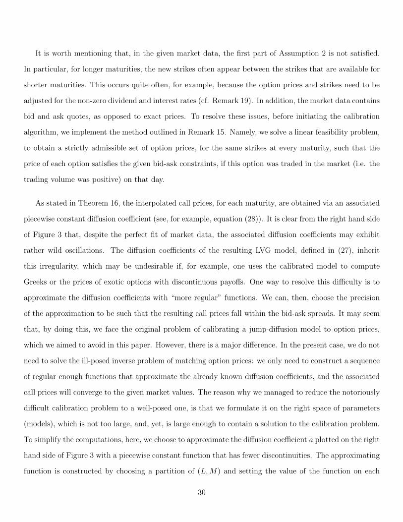
Figures 1–3 show the results of cross-maturity interpolation of the market prices of European options

written on the S&P 500 index, on January 12, 20115. Figure 1 contains the resulting price curves of

call options, as functions of strike. Each curve corresponds to a different maturity: 2, 7, 27, 47, and 67

working days, respectively. In particular, Figure 1 demonstrates that the monotonicity of option prices

across maturities is preserved by the interpolation. The quality of the fit is shown on Figures 2–3, via the

implied volatility curves. It is easy to see that the fit is perfect, in the sense that the implied volatility of

interpolated prices always falls within the implied volatilities of the bid and ask quotes.

5The option prices, as well as the dividend and interest rates, are provided by Bloomberg.

29

It is worth mentioning that, in the given market data, the first part of Assumption 2 is not satisfied.

In particular, for longer maturities, the new strikes often appear between the strikes that are available for

shorter maturities. This occurs quite often, for example, because the option prices and strikes need to be

adjusted for the non-zero dividend and interest rates (cf. Remark 19). In addition, the market data contains

bid and ask quotes, as opposed to exact prices. To resolve these issues, before initiating the calibration

algorithm, we implement the method outlined in Remark 15. Namely, we solve a linear feasibility problem,

to obtain a strictly admissible set of option prices, for the same strikes at every maturity, such that the

price of each option satisfies the given bid-ask constraints, if this option was traded in the market (i.e. the

trading volume was positive) on that day.

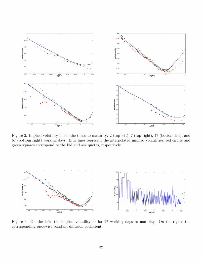
As stated in Theorem 16, the interpolated call prices, for each maturity, are obtained via an associated

piecewise constant diffusion coefficient (see, for example, equation (28)). It is clear from the right hand side

of Figure 3 that, despite the perfect fit of market data, the associated diffusion coefficients may exhibit

rather wild oscillations. The diffusion coefficients of the resulting LVG model, defined in (27), inherit

this irregularity, which may be undesirable if, for example, one uses the calibrated model to compute

Greeks or the prices of exotic options with discontinuous payoffs. One way to resolve this difficulty is to

approximate the diffusion coefficients with “more regular” functions. We can, then, choose the precision

of the approximation to be such that the resulting call prices fall within the bid-ask spreads. It may seem

that, by doing this, we face the original problem of calibrating a jump-diffusion model to option prices,

which we aimed to avoid in this paper. However, there is a major difference. In the present case, we do not

need to solve the ill-posed inverse problem of matching option prices: we only need to construct a sequence

of regular enough functions that approximate the already known diffusion coefficients, and the associated

call prices will converge to the given market values. The reason why we managed to reduce the notoriously

difficult calibration problem to a well-posed one, is that we formulate it on the right space of parameters

(models), which is not too large, and, yet, is large enough to contain a solution to the calibration problem.

To simplify the computations, here, we choose to approximate the diffusion coefficient a plotted on the right

hand side of Figure 3 with a piecewise constant function that has fewer discontinuities. The approximating

function is constructed by choosing a partition of (L,M) and setting the value of the function on each

30

subinterval to be such that the average of 1/a2 is matched. The motivation for such metric comes from the

observation that, for short maturities, the asymptotic behavior of interpolated option prices is determined

by the geodesic distance∫dx/a2(x). The right hand side of Figure 4 shows the two diffusion coefficients,

and its left hand side demonstrates the implied volatility produced by the new coefficient. It is easy to see

that the new diffusion coefficient is much smoother, while the resulting implied volatility still fits within

the bid-ask spread.

1100 1150 1200 1250 1300 1350 14000

20

40

60

80

100

120

140

160

180

200

K

ca

ll p

ric

e

Figure 1: Interpolated call prices as functions of strike. Different colors correspond to different maturities.The spot is at 1286.

Remark 19. Notice that we only use the first 5 maturities in our numerical analysis, although there are

market quotes for options with 5 longer matures available on that day. This restriction is explained by

the fact that the available bid and ask quotes may not allow for a strictly admissible set of option prices

(in the sense of cf. Definition 14). This, however, does not necessarily generate arbitrage, due to the

following two observations. First, the option quotes for different strikes and maturities, provided in the

database, are not always recorded simultaneously. Second, the interest rate is not identically zero, and the

stocks included in the S&P 500 index do pay dividends. In order to address the second issue, we had to

assume that the dividend and interest rates are deterministic. Then, we discounted the option prices and

strikes accordingly, to obtain expectations of the payoff functions applied to a martingale. The assumption

31

−0.07 −0.06 −0.05 −0.04 −0.03 −0.02 −0.01 0 0.010.05

0.1

0.15

0.2

0.25

0.3

log(K/S)

imp

lie

d v

ola

tili

ty

−0.2 −0.1 0 0.10.1

0.15

0.2

0.25

0.3

0.35

0.4

0.45

0.5

log(K/S)

imp

lie

d v

ola

tili

ty

−0.4 −0.3 −0.2 −0.1 0 0.1

0.2

0.25

0.3

0.35

0.4

log(K/S)

imp

lie

d v

ola

tili

ty

−0.25 −0.2 −0.15 −0.1 −0.05 0 0.050.16

0.18

0.2

0.22

0.24

0.26

0.28

0.3

0.32

log(K/S)

imp

lie

d v

ola

tili

ty

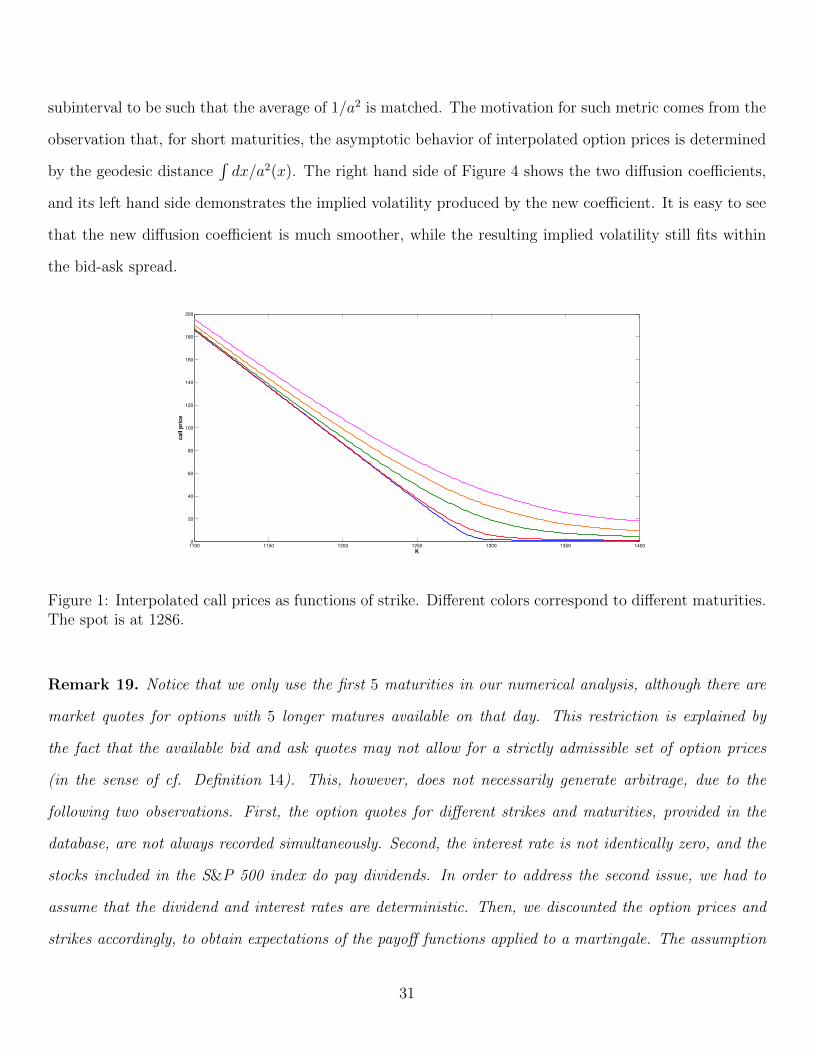
Figure 2: Implied volatility fit for the times to maturity: 2 (top left), 7 (top right), 47 (bottom left), and67 (bottom right) working days. Blue lines represent the interpolated implied volatilities, red circles andgreen squares correspond to the bid and ask quotes, respectively.

−0.35 −0.3 −0.25 −0.2 −0.15 −0.1 −0.05 0 0.05 0.1

0.15

0.2

0.25

0.3

0.35

0.4

log(K/S)

imp

lie

d v

ola

tili

ty

−0.25 −0.2 −0.15 −0.1 −0.05 0 0.050

50

100

150

200

250

log(K/S)

loc

al

vo

lati

lity

Figure 3: On the left: the implied volatility fit for 27 working days to maturity. On the right: thecorresponding piecewise constant diffusion coefficient.

32

−0.35 −0.3 −0.25 −0.2 −0.15 −0.1 −0.05 0 0.05

0.15

0.2

0.25

0.3

0.35

0.4

log(K/S)

imp

lied

vo

lati

lity

−0.25 −0.2 −0.15 −0.1 −0.05 0 0.050

50

100

150

200

250

log(K/S)

loc

al

vo

lati

lity

Figure 4: On the right: the diffusion coefficient corresponding to 27 working days to maturity (in blue) andits approximation (in red). On the left: the implied volatility associated with the approximate diffusioncoefficient (in blue), as well as the implied volatilities of bid and ask quotes (in red and green).

of deterministic rates, of course, may not always be consistent with the pricing rule chosen by the market.

However, this problem (as well as the first issue outlined above) goes beyond the scope of the present paper.

It is important to mention that the method of cross-strike interpolation, presented in this subsection,

is valuable on its own, not only in the context of LVG models. Indeed, having constructed the price

curves, which have the C1 and piecewise C2 properties, one can interpolate them across maturities via a

non-homogeneous LVG model. However, as discussed in Remark 12, by considering driftless diffusions run

on different stochastic clocks, one can easily find other models that allow for a cross-maturity interpolation

in a very similar way. Another way to interpolate option prices across maturities is to define

C(T,K) =eTi − eT

eTi − eTi−1Ci−1(K) +

eT − eTi−1

eTi − eTi−1Ci(K),

for T ∈ [Ti−1, Ti). Then, at least formally, one can define a non-homogeneous local volatility model that

reproduces the above option price surface. The corresponding diffusion coefficient a is given by the Dupire’s

formula:

a2(T,K) =2∂TC(T,K)

∂2KKC(T,K)

, K ∈ (Li, Ui),

for all T ∈ [Ti−1, Ti), with i = 1, . . . ,M . Note that the parabolic PDE’s associated with the above local

volatility (i.e. the Dupire’s and Black-Scholes equations) are well posed, as follows, for example, from the

results of [13]. However, defining the associated diffusion process may still be a challenging problem, due

33

to the discontinuities of a. Of course, using the results of this section, one can also find a non-homogeneous

LVG model, which has “more regular” diffusion coefficients and which approximates option prices up to the

bid-ask spreads. This is done by approximating the pice-wise constant diffusion coefficient, which results

from the calibration algorithm, as stated in Theorem 16, with functions that possess the desired regularity.

Such an approximation is discussed in the paragraph preceding Remark 19.

The rest of this subsection is devoted to the proof of Theorem 16. In fact, this proof provides a detailed

algorithm for computing the parametersνij, σ

ij

that reproduce market call prices.

Structure of the proof. The proof is presented in the form of an algorithm, which facilitates the

implementation. However, it is rather technical and uses a lot of new notation. Therefore, here, we outline

the structure and the main ideas of the proof. It is easy to see that any set of call price curves (as

functions of strikes) produced by a family of homogeneous LVG models (different model for each curve),

with piecewise constant diffusion coefficients, satisfies conditions 1− 2 of Assumption 1. However, we still

need to ensure that the LVG models are chosen so that the resulting price curves also satisfy part 3 of

Assumption 1, which is a stronger version of the absence of calendar spread arbitrage. Thus, for each

maturity Ti, we need to construct a pice-wise constant diffusion coefficient ai and the associated time value

function V i (which is uniquely defined by (29) and the subsequent paragraph), such that: each time value

curve V i matches the time values observed in the market, and the absence of calendar spread arbitrage

is preserved (V i > V i−1, for all i). In order to match the observed market values, each V i is constructed

recursively, passing from Kj to Kj+1. This allows us to construct ai and V i locally, so that V i solves (29)

on (Li, Kj+1), with ai in lieu of a. However, in order to obtain a bona fide time value function, we have to

ensure that V i satisfies the zero boundary conditions at Li and Ui, and has a jump of size −1 at x. These

conditions force us to control the value of the left derivative of V i at each strike Kj, in addition to the

value of V i(Kj) itself (which must coincide with the market value). In order to satisfy the constraints on

derivatives, along with the positivity of time value, we introduce two additional partition points between

every Kj and Kj+1. The choice of the additional partition points, as well as the proof that they are

sufficient to fulfill the aforementioned conditions, takes most of the proof of Theorem 16 (Steps 1.1-1.3).

34

The proof, itself, has an inductive nature: with the induction performed over maturities, and, for every

fixed maturity, over strikes. We show that the results of each iteration possess the necessary properties to

serve as the initial condition for the next iteration.

Step 0. Let us denote the market time values by V :

V (Ti, Kij) = C(Ti, K

ij)− (x−Ki

j)+,

for i = 1, . . . ,M , j = 1, . . . , Ni. It is clear that matching the market call prices is equivalent to matching

their time values. To simplify the notation, we add the strikesKi0 = Li andKi

Ni+1 = Ui, for all i = 1, . . . ,M ,

to the set of available market strikes, with the corresponding market time values being zero (since, in the

calibrated model, the underlying cannot leave the interval [Li, Ui] by the time Ti). We will construct the

interpolated price curves that match the original market prices, along with these additional ones.

Our construction will be recursive in i, starting from i = 1. Assume that we have constructed the

interpolated time values for each maturity Tm,

V m(K) = V νm,σm,z,x(K), K ∈ R,

with m = 0, . . . , i − 1. For m = 0, we set V 0 ≡ 0. In addition to matching the market time values, we

assume that these functions satisfy:

V m(K) > V m−1(K), K ∈ (Lm, Um),

for m = 1, . . . , i− 1, and V i−1 is strictly smaller than the market time values for maturities Ti and larger.

Our goal now is to construct V i = V νi,σi,z,x, such that the extended family V mim=1 still satisfies the

above monotonicity properties.

Without loss of generality, we can assume that the underlying level x coincides with one of the strikes.

If x is not among the available strikes, we can always add a new market call price, for strike x and

maturities T1, . . . , Ti, as follows: if x ∈ (Kij, K

ij+1), then, we choose an arbitrary δ1 ∈ (0, 1) and introduce

the additional market time values

V (Tm, x) = V m(x), m = 1, . . . , i− 1,

35

V (Ti, x) = δ1

(C(Ti, K

ij

) Kij+1 − x

Kij+1 −Ki

j

+ C(Ti, K

ij+1

) x−Kij

Kij+1 −Ki

j

)+ (1− δ1) max

(V i−1(x), C

(Ti, K

ij+1

))It is easy to see that the new family of market call prices, for m = i, . . . ,M , is strictly admissible, and the

constructed time value functions, V 1, . . . , V i−1, satisfy the properties discussed in the previous paragraph,

with respect to the new data.

The construction of V i(K) is done recursively in K, splitting the real line into several segments. We

set V i(K) = 0, for all K ∈ (−∞, Li]. We, then, extend V i to each [Li, Kij], increasing j by one, as long as

Kij+1 < x.

Step 1. Assume that Kij+1 < x and that, for all K ∈ [Li, K

ij], we have constructed the time value function

V i(K) in the form (30), with someLi = ν0 < · · · < νl(j) = Ki

j

and

σ1 > 0, . . . , σl(j) > 0

. In addition,

we assume that V i(K) > V i−1(K), for all K ∈ [Li, Kij], and the left derivative of V i(K) at K = Ki

j,

denoted B, satisfies:

B <V (Ti, K

ij+1)− V (Ti, K

ij)

Kij+1 −Ki

j

(35)

We need to extend V i to [Li, Kij+1] in such a way that: it remains in the form (30), on this interval, it

matches the market time value at Kij+1, and its left derivative at Ki

j+1 satisfies the above inequality.

Note that the case j = 0 is not included in the above discussion. In this case, the left derivative of V i

at Ki0 = Li is zero. However, the derivative of V i does not have to be continuous at this point, hence, we

can change its value to a positive number. We choose this number as follows: fix an arbitrary δ2 ∈ (0, 1)

and define

B = δ2V (Ti, K

i1)

Ki1 − Li

+ (1− δ2)V i−1+ (Li) , (36)

where V i−1+ is the right derivative of V i−1. Due to the strict admissibility of market data, as well as the

convexity of V i−1(K) for K ∈ [Li, x], and the fact that V i−1(Ki1) < V (Ti, K

i1), we easily deduce that B

given by (36) satisfies (35), with j = 0, and, in addition, B > V i−1+ (Li).

Step 1.1. Choose an arbitrary δ3 ∈ (0, 1), and define

B1 = δ3

V (Ti, Kij+2)− V (Ti, K

ij+1)

Kij+2 −Ki

j+1

+ (1− δ3)V (Ti, K

ij+1)− V (Ti, K

ij)

Kij+1 −Ki

j

36

0 0.1 0.2 0.3 0.4 0.5 0.6 0.7 0.8 0.9 10

0.1

0.2

0.3

0.4

0.5

0.6

0.7

0.8

0.9

1

strike

pri

ce

wKj

Kj+1

A1 + B

1K

A + BK

0 0.1 0.2 0.3 0.4 0.5 0.6 0.7 0.8 0.9 10

0.1

0.2

0.3

0.4

0.5

0.6

0.7

0.8

0.9

1

strike

pri

ce

yK

j

Kj+1

Vi−1

A + BK

Figure 5: Visualization of the points w (on the left) and y (on the right). Red circles represent markettime values for the current maturity. Red lines represent the already constructed time value interpolations.

This will be the target derivative of extended time value function V i(K) at K = Kij+1. To match this

value, we need to introduce an additional jump point for the associated diffusion coefficients.

Step 1.2. Introduce

w =V (Ti, K

ij+1) +BKi

j − A−B1Kij+1

B −B1

where A > 0 is the left limit of V i(K) at K = Kij. Due to the definition of B1 and the inequality (35),

we have w ∈ (Kij, K

ij+1). In other words, w is the abscissa of the intersection point of two lines: one that

goes through (Kij, A), with slope B, and the other one, that goes through (Ki

j+1, V (Ti, Kij+1)), with slope

B1 (cf. Figure 5).

Step 1.3. Another potential problem is that the extended function V i needs to be strictly larger than

V i−1 on [Li, Kij+1]. The two functions can intersect only if A+ (Ki

j+1 −Kij)B < V i−1(Ki

j+1). If the latter

inequality is satisfied, we introduce y ∈ (Kij, K

ij+1) as the abscissa of the point at which the linear function

intersects V i−1:

A+ (y −Kij)B = V i−1(y)

Since V i−1 is strictly convex and, either A > V i−1(Kij), or A > V i−1(Ki

j) and B > V i−1+ (Ki

j), the solution

to the above equation exists and is unique in the interval (Kij, K

ij+1). It can be computed, for example,

via the bisection method. If A+ (Kij+1 −Ki

j)B ≥ V i−1(Kij+1), we set y = Ki

j+1.

37

Next, we need to consider two cases.

Step 1.3.a. If w ≤ y, we search for the desired time value function V i(K), for K ∈ [Kij, w], in the form

V i(K) = f 1l(j)+1e

−zK/σ + f 2l(j)+1e

zK/σ, (37)

where σ is an unknown variable. In order to guarantee that the interpolated time value function remains

in the form (30), the coefficients f 1l(j)+1 and f 2

l(j)+1 must satisfy:

f 2l(j)+1e

zKij/σ =

1

2

(A+

σ

zB), f 1

l(j)+1e−zKi

j/σ =1

2

(A− σ

zB),

Since the extended time value function, V i, given above, is a convex function with derivative B at K = Kj,

and because of the assumption w ≤ y, it is easy to see that, for any choice of σ > 0, V i(K) dominates the

time value of earlier maturity, V i−1(K), from above, on the interval K ∈ [Li, w] (cf. Figure 6).

Next, we show that there exists a unique value of σ, such that the time value function (37) allows for

a further extension to [Li, Kij+1], such that it matches the market time value at Ki

j+1 and remains in the

form (30). Notice that the value of V i(w) is given by A, and its left derivative is B, where:

A = A(σ) =1

2

(A− σ

zB)e−z(w−K

ij)/σ +

1

2

(A+

σ

zB)ez(w−K

ij)/σ, (38)

B = B(σ) = − z

2σ

(A− σ

zB)e−z(w−K

ij)/σ +

z

2σ

(A+

σ

zB)ez(w−K

ij)/σ (39)

Lemma 20. Functions A(σ) and B(σ), defined in (38)-(39), are strictly decreasing in σ > 0. Moreover,

the range of values of A is given by (A+B(w −Ki

j),∞),

and the range of values of B is (B,∞).

The proof of Lemma 20 is given in Appendix B. Recall that, for any σ > 0, the time value V i can

be extended to [Li, w] via (37). Thus, we need to find σ, such that this time value function V i can be

extended further, to [Li, Kij+1], so that it matches the given market time value, and the target derivative,

B1, at Kij+1. Since V i(K) remains in the form (30), on the interval K ∈ [w,Ki

j+1], it has to be given by

1

2

(A(σ) +

σ

zB(σ)

)ez(K−w)/σ +

1

2

(A(σ)− σ

zB(σ)

)e−z(K−w)/σ,

38

where σ has to be such that the market time value at K = Kij+1 is matched. From Lemma 20, we know

that, for any fixed σ > 0, the function

σ 7→ 1

2

(A(σ) +

σ

zB(σ)

)ez(K

ij+1−w)/σ +

1

2

(A(σ)− σ

zB(σ)

)e−z(K

ij+1−w)/σ,

defined for all σ > 0, is strictly decreasing, and its range of values is(A(σ) + B(σ)(Ki

j+1 − w),∞)

Due to (35), we have

A+B(w −Kij) +B(Ki

j+1 − w) < V (Ti, Kij+1)

Using the above and Lemma 20, we conclude that there exists a unique σ satisfying

A(σ) + B(σ)(Kij+1 − w) = V (Ti, K

ij+1)

The above observation, along with the aforementioned monotonicity, implies that, for each σ > σ, there

exists a unique σ = σ(σ) > 0 satisfying

1

2

(A(σ) +

σ

zB(σ)

)ez(K

ij+1−w)/σ +

1

2

(A(σ)− σ

zB(σ)

)e−z(K

ij+1−w)/σ = V (Ti, K

ij+1),

which can be obtained via the bisection method. Notice that σ(σ) is strictly decreasing in σ ∈ (σ,∞).

Thus, for each choice of σ > σ, we can extend the time value function V i from [Li, Kij] to [Li, K

ij+1],

so that it matches the market time value at Kij+1 and remains in the form (30). It only remains to find

σ such that the left derivative of V i(K) at K = Kij+1 coincides with the target value, B1. This condition

can be expressed as follows:

z

2σ(σ)

(A(σ) +

σ(σ)

zB(σ)

)ez(K

ij+1−w)/σ(σ) − z

2σ(σ)

(A(σ)− σ(σ)

zB(σ)

)e−z(K

ij+1−w)/σ(σ) = B1 (40)

Lemma 21. The left hand side of (40) is a strictly increasing function of σ ∈ (σ,∞), and its range of

values includes B1.

The proof of Lemma 21 is given in Appendix B. Lemma 21 implies that there exists a unique solution

σ = σ to the equation (40), and it can be computed via the bisection method. Finally, we set: νl(j)+1 = w,

σl(j)+1 = σ, νl(j)+2 = Kij+1 and σl(j)+2 = σ(σ), and l(j + 1) = l(j) + 2.

39

0 0.1 0.2 0.3 0.4 0.5 0.6 0.7 0.8 0.9 10

0.1

0.2

0.3

0.4

0.5

0.6

0.7

0.8

0.9

1

strike

pri

ce

wKj

Kj+1

Vi−1

A + BK

A1 + B

1K

0 0.1 0.2 0.3 0.4 0.5 0.6 0.7 0.8 0.9 10

0.1

0.2

0.3

0.4

0.5

0.6

0.7

0.8

0.9

1

strike

pri

ce

Kj

A + BK

A1 + B

1K

yVi−1 K

j+1w

Figure 6: On the left: the case described in Step 1.3.a, where the yellow line represents the functionA(σ) + B(σ)K, for K ≥ w, and the vertical interval in green represents the range of values of A(σ), forσ ≥ σ. On the right: the case described in Step 1.3.b, where the yellow line represents the functionA(σ) + B(σ)K, for K ≥ y, and the vertical interval in green represents the range of values of A(σ), forσ ≥ σ.

Step 1.3.b. If w > y, we search for the time value function V i(K), on the interval K ∈ [Kij, y], in the

following form

V i(K) =1

2

(A− σ

zB)e−z(K−K

ij)/σ +

1

2

(A+

σ

zB)ez(K−K

ij)/σ

The above expression guarantees that, for K ∈ [Kij, y],

V i(K) > A+B(K −Kij) ≥ V i−1(K),

due to convexity of V i−1 and the definition of y (cf. Figure 6). In addition, for any σ > 0, the extended

time value function remains in the form (30), on the interval K ∈ [Li, y]. The values of V i(K) and its

derivative, at K = y, are given, respectively, by:

A(σ) =1

2

(A− σ

zB)e−z(y−K

ij)/σ +

1

2

(A+

σ

zB)ez(y−K

ij)/σ,

B(σ) = − z

2σ

(A− σ

zB)e−z(y−K

ij)/σ +

z

2σ

(A+

σ

zB)ez(y−K

ij)/σ

The functions A and B, introduced above, are the same as those introduced in Step 1.3.a, with y in place

of w. Lemma 20 can still holds for these functions (one can simply repeat its proof given in Appendix B).

In particular, A(σ) and B(σ) are strictly decreasing in σ ∈ (0,∞), and the range of values of A(σ) is given

by

(A+B(y −Kij),∞),

40

while the range of values of B is (B,∞). These observations yield the following lemma.

Lemma 22. The function

σ 7→ A(σ) + B(σ)(Kij+1 − y),

defined for all σ > 0, is strictly decreasing, and its range of values is (A+B(Kij+1 −Ki

j),∞).

Due to the convexity of V i−1, and the fact that V i−1(Kij) < V i(Ki

j) and V i−1(y) = V i(y), we obtain:

V i−1(Kij+1) > A+B(Ki

j+1 −Kij)

Thus, there exists a unique σ satisfying

A(σ) + B(σ)(Kij+1 − y) = V i−1(Ki

j+1),

which can be computed via the bisection algorithm (cf. Figure 6).

Lemma 23. The following inequalities hold:

B(σ) <V (Ti, K

ij+1)− A(σ)

Kij+1 − y

< B1, A(σ) + B(σ)(K − y) > V i−1(K),

for all K ∈ [y,Kij+1).

The proof of Lemma 23 is given in Appendix B. We add the next element of the partition, νl(j)+1 = y,

and the next value of the diffusion coefficient, σl(j)+1 = σ. Finally, we repeat Step 1, with y in lieu of Kij,

and with A(σ) and with B(σ) in lieu of A and B respectively. The already constructed time value function

V i, dominates V i−1, on the interval [Li, y]. Due to Lemma 23, the values of A(σ) and B(σ), satisfy all

the properties assumed for A and B at the beginning of Step 1. In addition, due to the last inequality

in Lemma 23, the graphs of A(σ) + B(σ)(K − y) and V i−1 do not intersect on [y,Kij+1] (cf. Figure 6).

Hence, the algorithm in Step 1.3 ends up in case a. As a result, we obtain the values of νl(j)+2, σl(j)+2,

νl(j)+3 = Kj+1, σl(j)+3, and set l(j + 1) = l(j) + 3.

We repeat Step 1, increasing j by one each time, as long as Kij+1 < x. Thus, we obtain an interpolation

of the time value function on the interval K ∈ [Li, Kij], where j is such that x = Ki

j+1.

41

Step 2. Perform Step 1, moving from K = Ui backwards. Namely, we consider the change of variables:

from K ∈ [Li, Ui] to K ′ = Li + Ui −K ∈ [Li, Ui]. We apply this change of variables to the market time

values, as well as to the interpolated time value functions for earlier maturities. In particular, we obtain

the new underlying level x′ = Li+Ui−x, as well as the new market time values V (Ti, Li+Ui−K ′j), for all

strikes K ′j = Li +Ui −KiNi+1−j, with j = 0, . . . , Ni + 1. Then, we repeat Step 1, using this new, modified,

data as an input. This gives us an interpolated time value function on the interval K ′ ∈ [Li, K′j], where

j is such that x′ = K ′j+1. In the original variables, we obtain an interpolation of the time value function

on the interval K ∈ [KiNi+1−j, Ui], where, in turn, x = Ki

Ni−j. It is easy to see that the interpolated time

value, on the interval [KiNi+1−j, Ui], is in the form (32).

Step 3. Finally, we extend the interpolated time value function to the entire interval [Li, Ui]. Recall that

x coincides with one of the strikes, say Kij. In Steps 1 and 2, we constructed the interpolated time value

function for K ∈ [Li, Kij−1] ∪ [Ki

j+1, Ui]. Notice that, repeating the algorithm outlined in Steps 1 and 2,

we can extend V i to the entire interval [Li, Ui], so that it matches all market time values, dominates V i−1

from above, and, in addition, it is in the form (30) on [Li, x], in the form (32) on [x, Ui], and it has the

prescribed left and right derivatives at x, B1 and B2 respectively. In order for the interpolation function

V i to be a bona fide time value, it needs to have a jump of size −1 at x. In other words, we need to choose

B1 and B2 so that B1 − 1 = B2. The only constraints on the choices of B1 and B2 come from the market

data and the previous constructed interpolation function on K ∈ [Li, Kij−1]∪ [Ki

j+1, Ui]. These constraints

are given by:

B1 >V (Ti, K

ij)− V (Ti, K

ij−1)

Kij −Ki

j−1

, B2 <V (Ti, K

ij+1)− V (Ti, K

ij)

Kij+1 −Ki

j

=C(Ti, K

ij+1)− C(Ti, K

ij)

Kij+1 −Ki

j

(41)

Thus, we choose an arbitrary δ4 ∈ (0, 1) and define

B1 = δ4 + δ4

V (Ti, Kij+1)− V (Ti, K

ij)

Kij+1 −Ki

j

+ (1− δ4)V (Ti, K

ij)− V (Ti, K

ij−1)

Kij −Ki

j−1

= δ4

C(Ti, Kij+1)− C(Ti, K

ij)

Kij+1 −Ki

j

− δ4

C(Ti, Kij)− C(Ti, K

ij−1)

Kij −Ki

j−1

+V (Ti, K

ij)− V (Ti, K

ij−1)

Kij −Ki

j−1

Similarly, we define

B2 = B1 − 1 = δ4 − 1 + δ4

V (Ti, Kij+1)− V (Ti, K

ij)

Kij+1 −Ki

j

+ (1− δ4)V (Ti, K

ij)− V (Ti, K

ij−1)

Kij −Ki

j−1

42

= δ4

C(Ti, Kij+1)− C(Ti, K

ij)

Kij+1 −Ki

j

+ (1− δ4)C(Ti, K

ij)− C(Ti, K

ij−1)

Kij −Ki

j−1

Since the market call prices are strictly admissible (in particular, strictly convex across strikes), we conclude

that B1 and B2 satisfy (41).

The following lemma, whose proof is given in Appendix B, completes the proof of the theorem.

Lemma 24. For any z > 0 and any strictly admissible market data,Ti, K

ij, C(Ti, K

ij), Li, Ui, x

, the

vectors νi and σi, for i = 1, . . . ,M , produced by the above algorithm (Steps 0 − 3) are such that the

associated price curvesCi = Cνi,σi,z,x

Mi=1

satisfy Assumption 1.

Remark 25. Notice that the constants δi, for i = 1, 2, 3, 4, appearing in the proof, can be chosen arbitrarily

(within the interval (0, 1)). The choice of the boundary points Li, Ui introduces additional flexibility

in the algorithm. It is worth mentioning that the properties of interpolated implied volatilities and the

associated diffusion coefficients may depend on the choices of these constants. Therefore, one may try to

optimize over different values of δi and Li, Ui, for example, to improve the smoothness of resulting

diffusion coefficients. Continuing along these lines, one may also want to iterate over all possible choices

of arbitrage-free option prices, consistent with the market. Recall that the market data contains only bid

and ask quotes, and we propose to choose the exact values of option prices by solving a linear feasibility

problem (cf. Remark 15). Optimizing over all possible choices of option prices, in theory, may improve

the smoothness properties of the output. However, this would come at a very high computational cost, and

would lead to a multivariate nonlinear optimization problem, which we tried to avoid in the present paper.

V Summary and Extensions

In this paper, we considered the risk-neutral process for the (forward) price of an asset, underlying a set

of European options, in the form of a driftless time-homogeneous diffusion subordinated to an unbiased

gamma process. We named this model LVG and showed that it yields forward and backward PDDE’s

for option prices. These PDDE’s can be used to speed up the computations, but, more importantly,

they allow for explicit exact calibration of a LVG model to European options prices. In particular, the

43

diffusion coefficient of the underlying can be represented explicitly through a single (continuous) implied

volatility smile. A mild extension of LVG allows for analogous calibration to multiple continuous smiles.

Finally, we showed how the aforementioned PDDE’s can be used to construct continuously differentiable

(with piecewise continuous second derivative) arbitrage-free implied volatility smiles from a finite set of

option prices, with multiple strikes and maturities. The resulting calibration algorithm does not involve

any multivariate optimization, and it only requires solutions to one-dimensional root-search problems and

elementary functions. We illustrated the theory with numerical results based on a real market data.

There are many possible avenues for future research. One of the potential criticism of the proposed

calibration method is the fact that the resulting diffusion coefficient has (a finite number of) discontinuities.

This feature may create difficulties when computing the greeks, or prices of path-dependent and American-

style options in the calibrated model. An idea on how to resolve this problem is outlined briefly in the few

paragraphs preceding the proof of Theorem 16. However, a more detailed analysis would be very useful.

Another limitation of the results presented herein is that the risk-neutral price process of the underlying

is assumed to be a martingale. Indeed, in many cases, the dividend and interest rates are not negligible. If

they are assumed to be deterministic, then, the calibration problem can be easily reduced to the driftless

case by discounting. However, as discussed in Remark 19, the assumption of deterministic rates may not be

consistent with the market. Therefore, an extension of the proposed model that allows for a non-zero drift

of the underlying is very desirable. In particular, it seems possible to extend the results of this paper to a

risk-neutral price process obtained as a time change of a diffusion with drift. However, certain challenges

may arise and they need to be addressed: in particular, the associated PDDE’s may no longer have closed

form solutions even if the diffusion and drift coefficients are piecewise constant.

A more thorough numerical analysis, in particular, investigating the prices of exotic products produced

by the calibrated models, is also very desirable. We did not conduct such a study in the present paper,

due to its already quite extensive length.

Finally, one can examine the problem of calibrating a LVG model to other financial instruments, such

44

as the barrier or American options.

Appendix A

Proof of Theorem 1. Theorems 2.2 and 2.7 in [13], as well as Theorem 1.II in [4] (a respective theorem

is applicable depending on whether each of the boundary points is finite) provide existence and uniqueness

results for a class of parabolic PDEs with initial and boundary conditions. This class includes the following

equation:

∂τu(τ, x) =1

2a2(x)∂2

xu(τ, x) +1

2a2(x)φ′′(x), u(0, x) = u(τ, L+) = u(τ, U−) = 0,

implying that it has a unique weak solution. In addition u is absolutely bounded by a constant (which

follows from the estimates in Theorems 2.2 and 2.7, in [13], and in Theorem 1.II, in [4]), and it is vanishing at

L and U . Then, v = u+φ solves (3) and satisfies v(0, x) = φ(x). In addition, it satisfies: v(τ, L+) = φ(L+)

and/or v(τ, U−) = φ(U−), whenever L and/or U are finite. To show that this solution coincides with V D,φ,

we apply the generalized Ito’s formula (cf. Theorem 2.10.1 in [14]), to obtain

Exv(T − ζr,R ∧ T,Dζr,R∧T ) = v(T, x),

where ζr,R is the first exit time of D from the interval (r, R), with arbitrary L < r < R < U . Notice that

v(τ, x) is bounded by an exponential of x, uniformly over τ ∈ (0, T ). Thus, we can apply the dominated

convergence theorem, to conclude that, as r ↓ L and R ↑ U ,

v(T, x) = Exv(T − ζr,R ∧ T,Dζr,R∧T )→ Exv(T − ζ ∧ T,Dζ∧T ) = Exv(T − ζ,Dζ)1ζ≤T + Exφ(DT )1ζ>T,

where ζ is the time of the first exit of D from (L,U). Recall that the diffusion can only exit the interval

(L,U) through a finite boundary point. Thus,

v (T − ζ,Dζ) 1ζ≤T = v (T − ζ, L+) 1ζ≤T,Dζ=L+ + v (T − ζ, U−) 1ζ≤T,Dζ=U−

= φ(L+)1ζ≤T,Dζ=L+ + φ(U−)1ζ≤T,Dζ=U− = φ(Dζ)1ζ≤T

45

Since the diffusion is absorbed at the boundary points, we have:

v(T, x) = Ex(φ(DT )1ζ>T

)+ Ex

(φ(Dζ)1ζ≤T

)= Ex

(φ(DT )1ζ>T

)+ Ex

(φ(DT )1ζ≤T

)= Exφ(DT ),

which completes the proof of the theorem.

Proof of Theorem 2. Let us apply the Ito-Tanaka rule (cf. Theorem 7.1, on page 218, in [11]) to the

call payoff:

(Dt −K)+ = (D0 −K)+ +

∫ t

0

a(Ds)1Ds≥KdWs + Λt(K),

where Λ is the local time of D. Taking expectations, we obtain

CD(t,K, x) = Ex(Dt −K)+ = (x−K)+ + EΛt(K).

Multiplying by φ and integrating, we use the properties of local time (cf. Theorem 7.1, on page 218, in

[11]), to obtain∫ U

L

CD(t,K, x)φ(K)dK =

∫ U

L

(x−K)+φ(K)dK +1

2

∫ t

0

Ex(a2(Du)φ(Du)

)du.

Using Fubini’s theorem, we obtain the following identity:

QD,x(Du ≤ K) = Ex1Du≤K = ∂KCD(u,K, x),

which holds for almost allK ∈ (L,U). Therefore, the measure generated by ∂KCD(u, ·, x) is the distribution

of Du under measure QD,x. Thus, we conclude:∫ U

L

CD(t,K, x)φ(K)dK =

∫ U

L

(x−K)+φ(K)dK +1

2

∫ t

0

∫ U

L

a2(K)φ(K)d(∂KC

D(u,K, x))du.

Proof of Theorem 6. Let us multiply the left hand side of equation (3) by the density of Γt and an

arbitrary test function ϕ ∈ C∞0 ((L,U)), then, divide it by a2/2 and integrate with respect to τ and x:∫ U

L

∫ T

0

τ t/t∗−1e−τ/t

∗

(t∗)t/t∗Γ(t/t∗)∂τV

D,φ(τ, x)2ϕ(x)

a2(x)dτdx =

∫ U

L

∫ T

0

τ t/t∗−1e−τ/t

∗

(t∗)t/t∗Γ(t/t∗)∂τ(V D,φ(τ, x)− φ(x)

)dτ

2ϕ(x)

a2(x)dx

=T t/t

∗−1e−T/t∗

(t∗)t/t∗Γ(t/t∗)

∫ U

L

(V D,φ(T, x)− φ(x)

) 2ϕ(x)

a2(x)dx (42)

46

−∫ T

0

((t/t∗ − 1)τ t/t

∗−2 − τ t/t∗−1/t∗)e−τ/t

∗

(t∗)t/t∗Γ(t/t∗)

∫ U

L

(V D,φ(τ, x)− φ(x)

) 2ϕ(x)

a2(x)dxdτ

→∫ U

L

∫ ∞0

(τ t/t

∗−1/t∗ − (t/t∗ − 1)τ t/t∗−2)e−τ/t

∗

(t∗)t/t∗Γ(t/t∗)

(V D,φ(τ, x)− φ(x)

)dτ

2ϕ(x)

a2(x)dx,

as T →∞. In the above, we applied Fubini’s theorem and used the fact that φ is absolutely bounded and,

hence, so is V D,φ. Recall also that τ ≥ t∗. Applying Fubini’s theorem once more, we interchange the order

of integration in the left hand side of (42), and, using equation (3), integrate by parts with respect to x.

This, together with the convergence in (42), implies:∫ ∞0

τ t/t∗−1e−τ/t

∗

(t∗)t/t∗Γ(t/t∗)

∫ U

L

V D,φ(τ, x)ϕ′′(x)dxdτ (43)

=

∫ U

L

∫ ∞0

(τ t/t

∗−1/t∗ − (t/t∗ − 1)τ t/t∗−2)e−τ/t

∗

(t∗)t/t∗Γ(t/t∗)

(V D,φ(τ, x)− φ(x)

)dτ

2

a2(x)ϕ(x)dx,

where both integrals are absolutely convergent. Using Fubini’s theorem and the definition of V φ, we

conclude that ∫ ∞0

τ t/t∗−1e−τ/t

∗

(t∗)t/t∗Γ(t/t∗)

∫ U

L

V D,φ(τ, x)ϕ′′(x)dxdτ =

∫ U

L

V φ(t, x)ϕ′′(x)dx (44)

Next, we notice that, since t ≥ t∗, the expression inside the outer integral in the right hand side of (43) is

a locally integrable function of x ∈ (L,U). Then, the fact that equations (42) and (43) hold for all test

functions ϕ yields:

∂2xxV

φ(t, x) =2

a2(x)

∫ ∞0

(τ t/t

∗−1/t∗ − (t/t∗ − 1)τ t/t∗−2)e−τ/t

∗

(t∗)t/t∗Γ(t/t∗)

(V D,φ(τ, x)− φ(x)

)dτ, (45)

which holds for every t ≥ t∗ and almost all x ∈ (L,U). Since the second derivative of V φ(τ, ·) is locally

integrable, its first derivative is absolutely continuous. To show that V φ(τ, L+) = V φ(τ, U−) = 0, we

recall the definition of V φ as an expectation and apply the dominated convergence theorem. When t = t∗,

equation (45) becomes

∂2xxV

φ(t∗, x) =2

a2(x)t∗

∫ ∞0

e−τ/t∗

t∗(V D,φ(τ, x)− φ(x)

)dτ =

2

a2(x)t∗(V φ(t, x)− φ(x)

),

which holds for almost all x ∈ (L,U). Since V φ(τ, ·) and φ are continuous, the above equation holds for all

points x at which a is continuous. Therefore, V φ(t∗, ·) possesses all the properties stated in the theorem.

47

Next, we show uniqueness. Consider any function u ∈ C1(L,U), which has an absolutely continuous

derivative and satisfies (20), along with zero boundary conditions. Applying the generalized Ito’s formula

(cf. Theorem 2.10.1 in [14]), we obtain:

u(Dt∧ζr,R)− u(D0) =

∫ t∧ζr,R

0

1

2a2(Ds)u

′′(Ds)ds+

∫ t∧ζr,R

0

u′(Ds)dDs,

where, as before, ζr,R is the first exit time of D from the interval (r, R), with arbitrary L < r < R < U .

Notice that, since u is continuous and satisfies zero boundary conditions, it is absolutely bounded. Due to

equation (20), u′′ is absolutely bounded as well. Thus, taking expectations and applying the dominated

convergence theorem, as r ↓ L and R ↑ U , we obtain

Exu(Dt)− u(x) = E∫ t

0

1

2a2(Ds)u

′′(Ds)1s≤ζds

Since Γ is independent of D, we can plug Γt∗ , in place of t, into the above expression, to obtain:

Exu (DΓt∗ )− u(x) = Ex∫ Γt∗

0

1

2a2(Ds)u

′′(Ds)1s≤ζds,

∫ ∞0

e−t/t∗

t∗Exu(Dt)dt− u(x) =

∫ ∞0

e−t/t∗

t∗Ex∫ t

0

1

2a2(Ds)u

′′(Ds)1s≤ζdsdt,∫ ∞0

e−t/t∗

t∗Exu(Dt)dt− u(x) =

∫ ∞0

e−t/t∗

t∗Ex∫ t

0

1

t∗(u(Ds)− φ(Ds)) 1s≤ζdsdt,∫ ∞

0

e−t/t∗

t∗Exu(Dt)dt− u(x) =

1

t∗

∫ ∞0

e−t/t∗

t∗

∫ t

0

Ex (u(Ds)− φ(Ds)) dsdt, (46)

where we made use of the fact that u(L+) = u(U−) = φ(L+) = φ(U−) = 0, to obtain (46). Thus, we

continue: ∫ ∞0

e−t/t∗

t∗Exu(Dt)dt− u(x) =

1

t∗

∫ ∞0

e−t/t∗Ex (u(Dt)− φ(Dt)) dt, (47)

where we integrated by parts in the right hand side of (46), to obtain (47). This yields:

u(x) =1

t∗

∫ ∞0

e−t/t∗Exφ(Dt)dt = V φ(t∗, x)

Proof of Lemma 7. Let us show that St∗ has a density in (L,U) under any Qx. Consider arbitrary

K ∈ (L,U) and ε ∈ (0, 1), s.t. [K − ε,K + 2ε] ⊂ (L,U). Choose a smooth function ρε, which dominates

48

the indicator function of [K,K + ε] from above, whose support is contained in [K − ε,K + 2ε], and which

satisfies ∫ U

L

ρ2ε(x)dx ≤ 2ε.

Introduce

u(x) = Ex (ρε(St∗)) ,

for all x ∈ (L,U). Theorem 6 implies that u ∈ C1(L,U), u(L+) = u(U−) = 0, u′′ ∈ L2(L,U), and it

satisfies:

1

2a2(x)u′′(x)− 1

t∗(u(x)− ρε(x)) = 0, (48)

for all x ∈ (L,U), except the points of discontinuity of a. Next, we need to recall the standard estimates

for the weak solutions of elliptic PDEs via the norm of the right hand side (see, for example, [12] and

references therein). The only issue that needs to be resolved, before we can apply the standard results, is

that, although u belongs to the Sobolev space W 22 ((L,U)), it may not belong to W 2

2 (R). This is due to

the fact that u′ may have a discontinuity at L or U , if the boundary point is attainable. To resolve this

problem, we consider a sequence of functions un ∈ C∞0 (R) ⊂ W 22 (R) which approximates u in the sense of

the Sobolev norm ‖ · ‖W 22 (L,U). Applying Remark 3.3, in [12], to un and passing to the limit, as n → ∞,

we estimate the Sobolev norm of u:∫ U

L

u2(x) + (u′(x))2 + (u′′(x))2dx ≤ c1

∫ U

L

ρ2ε(x)dx, (49)

where the constant c1 is independent of ε. Next, the Morrey’s inequality yields

supx∈(L,U)

|u(x)| ≤ c2

(∫ U

L

u2(x) + (u′(x))2dx

)1/2

≤ c3

(∫ U

L

ρ2ε(x)dx

)1/2

≤ c3

√2ε

Finally, we obtain

Qx(St∗ ∈ [K,K + ε]) ≤ u(x) ≤ c3

√2ε,

Therefore, the distribution of St∗ is absolutely continuous with respect to the Lebesgue measure on (L,U)

and, in particular, it has a density. It was shown in the proof of Theorem 2 that

Qx(St∗ ≤ K) = ∂KC(t∗, K, x)

49

Therefore, ∂KC(t∗, K, x) is absolutely continuous in K ∈ (L,U), and its derivative, ∂2KKC(t∗, ·, x), is the

density of St∗ under Qx.

Proof of Theorem 8. Differentiating both sides of (6) with respect to τ , then, multiplying them by

an exponential and a test function ϕ ∈ C∞0 ((L,U)), we integrate, to obtain∫ T

0

e−τ/t∗

t∗d

dτ

∫ U

L

CD(τ,K, x)2

a2(K)ϕ(K)dKdτ =

∫ T

0

e−τ/t∗

t∗

∫ U

L

ϕ(K)d(∂KC

D(τ,K, x))dτ (50)

Let us perform integration by parts in the left hand side of (50):∫ T

0

e−τ/t∗

t∗d

dτ

∫ U

L

CD(τ,K, x)2

a2(K)ϕ(K)dKdτ =

e−T/t∗

t∗

∫ U

L

CD(T,K, x)2

a2(K)ϕ(K)dK

− 1

t∗

∫ U

L

(x−K)+ 2

a2(K)ϕ(K)dK +

1

t∗

∫ T

0

e−τ/t∗

t∗

∫ U

L

CD(τ,K, x)2

a2(K)ϕ(K)dKdτ, (51)

where we made use of the fact that

limτ↓0

CD(τ,K, x) = (x−K)+,

which, in turn, follows from square integrability of the martingale D and the dominated convergence

theorem. Using (51), as well as the dominated convergence and Fubini’s theorems, we obtain:

limT→∞

∫ T

0

e−τ/t∗

t∗d

dτ

∫ U

L

CD(τ,K, x)2

a2(K)ϕ(K)dKdτ =

∫ U

L

2

a2(K)t∗(C(t∗, K, x)− (x−K)+

)ϕ(K)dK

On the other hand, integrating by parts and applying the Fubini and dominated convergence theorems

once more, we derive:

limT→∞

∫ T

0

e−τ/t∗

t∗

∫ U

L

ϕ(K)d(∂KC

D(τ,K, x))dτ = lim

T→∞

∫ U

L

ϕ′′(K)

∫ T

0

e−τ/t∗

t∗CD(τ,K, x)dτdK

=

∫ U

L

C(t∗, K, x)ϕ′′(K)dK =

∫ U

L

∂2KKC(t∗, K, x)ϕ(K)dK

Collecting the above, we rewrite equation (50) as∫ U

L

(1

t∗(C(t∗, K, x)− (x−K)+

)− 1

2a2(K)∂2

KKC(t∗, K, x)

)ϕ(K)dK = 0,

which holds for any ϕ ∈ C∞0 ((L,U)). This implies that equation (22) holds for almost every K ∈ (L,U).

Since C(t∗, ·, x) and (x− ·)+ are continuous functions, we conclude that (22) holds everywhere except the

points of discontinuity of a.

50

The boundary conditions for call price function follow from the dominated convergence theorem. The

square integrability of ∂2KKC(t∗, ·, x) follows from the fact that it is absolutely integrable and vanishes at the

boundary (the latter, in turn, follows from the boundary conditions and equation (22)). To show unique-

ness, we assume that there exists another function, with the same properties, and denote the difference

between the two by u. Function u is a weak solution of the homogeneous version of (22):

1

2a2(x)u′′(x)− 1

t∗u(x) = 0,

vanishing at the boundary. Finally, as in the proof of Lemma 7, we apply Remark 3.3 in [12] to obtain an

estimate for the Sobolev norm of u, analogous to (49), with zero in lieu of ρε. This implies that u ≡ 0.

Proof of Theorem 9. Notice that, for a fixed K ∈ (L,U), the function C(t∗, K, . ) is measurable.

This follows from the measurability of CD(T,K, . ), which, in turn, follows from the measurability of the

mapping x 7→ QD,x, as a property of Markov family. At any point K ∈ (L,U) that does not coincide with

a discontinuity point of a, the call price function is twice continuously differentiable in K, and, hence, its

second derivative, ∂2KKC(t∗, K, x), is also measurable as a function of x. Thus, we can use (22) to obtain

1

t∗(ExC(t∗, K, Sτ )− Ex(Sτ −K)+

)=a2(K)

2Ex(∂2KKC(t∗, K, Sτ )

), (52)

which holds for all τ ≥ 0 and all K ∈ (L,U) except the points of discontinuity of a. Since ∂2KKC(t∗, ·, Sτ )

is nonnegative and integrates to one, the application of Fubini’s theorem yields

Ex(∂2KKC(t∗, K, Sτ )

)= ∂2

KKExC(t∗, K, Sτ ) = ∂2KKC(τ + t∗, K, x), (53)

where the derivatives in the right hand side are understood in a weak sense, and we used Proposition 5 to

obtain the last equality. Due to (52), ∂2KKC(τ+t∗, ·, x) is, in fact, locally integrable on (L,U), and equation

(24) holds for almost every K ∈ (L,U). Using the monotone convergence theorem, it is easy to show that

C(τ, ·, x) is continuous, for any τ ≥ 0, and, hence, (24) holds everywhere except the points of discontinuity

of a. The boundary conditions follow from the dominated convergence theorem. In addition, (53) and

an application of Fubini’s theorem imply that ∂2KKC(τ + t∗, ·, x) is absolutely integrable on (L,U). This,

along with the boundary conditions and equation (24), imply that ∂2KKC(τ + t∗, ·, x) is square integrable.

To show uniqueness, we apply the same argument as at the end of the proof of Theorem 8.

51

Appendix B

Proof of Lemma 20. Notice that, for all y > 0, we have:

((1 + y)e−2y + y − 1

)′= 1− e−2y(1 + 2y) > 0,

which follows from the inequality e2y > 1 + 2y. Since (1 + 0)e−2·0 + 0− 1 = 0, we obtain

(1 + y)e−2y + y − 1 > 0, y > 0.

Therefore, for any positive A and B,

A′(σ) =1

2

((A− σ

zB) z(w −Ki

j)

σ2− B

z

)e−z(w−K

ij)/σ − 1

2

((A+

σ

zB) z(w −Ki

j)

σ2− B

z

)ez(w−K

ij)/σ

=1

2

(Az(w −Ki

j)

σ2− B

z

(z(w −Ki

j)

σ+ 1

))e−z(w−K

ij)/σ

−1

2

(Az(w −Ki

j)

σ2+B

z

(z(w −Ki

j)

σ− 1

))ez(w−K

ij)/σ =

1

2Az(w −Ki

j)

σ2

(e−z(w−K

ij)/σ − ez(w−Ki

j)/σ)

−1

2

B

zez(w−K

ij)/σ

((z(w −Ki

j)

σ+ 1

)e−2z(w−Ki

j)/σ +

(z(w −Ki

j)

σ− 1

))≤ 0

Similarly, we have:

B′(σ) = −1

2

(( zσA−B

) z(w −Kij)

σ2− z

σ2A

)e−z(w−K

ij)/σ

+1

2

(−( zσA+B

) z(w −Kij)

σ2− z

σ2A

)ez(w−K

ij)/σ

= − z

2σ2

(z(w −Ki

j)

σA−B(w −Ki

j)− A)e−z(w−K

ij)/σ

− z

2σ2

(z(w −Ki

j)

σA+B(w −Ki

j) + A

)ez(w−K

ij)/σ

≤ z

2σ2

(B(w −Ki

j) + A)e−z(w−K

ij)/σ − z

2σ2

(B(w −Ki

j) + A)ez(w−K

ij)/σ ≤ 0

Taking limits as σ converges to 0 and ∞, we complete the proof of the lemma.

Proof of Lemma 21. For any a < V (Ti, Kij+1) and any

b ∈

(0,V (Ti, K

ij+1)− a

Kij+1 − w

),

52

we introduce Σ = Σ(a, b) as the unique solution to

1

2

(a+

Σ

zb

)ez(K

ij+1−w)/Σ +

1

2

(a− Σ

zb

)e−z(K

ij+1−w)/Σ = V (Ti, K

ij+1), (54)

It is shown in the proof of Theorem 16 that such Σ exists and is unique. It was also shown that the left

hand side of (54) is strictly increasing in a and b, and it is strictly decreasing in Σ. This yields that Σ(a, b)

is strictly increasing in a and b.

Consider the associated function

F (a, b;K) =1

2

(a+

Σ(a, b)

zb

)ez(K−w)/Σ(a,b) +

1

2

(a− Σ(a, b)

zb

)e−z(K−w)/Σ(a,b),

defined for K ∈ [w,Kij+1]. Note that F (a, b; ·) is convex, increasing, and it solves the ODE (29). In

addition, F (a, b;w) = a, ∂KF (a, b;w) = b, F (a, b;Kij+1) = V (Ti, K

ij+1), and

∂KF (a, b;Kij+1) =

z

2Σ(a, b)

(a+

Σ(a, b)

zb

)ez(K

ij+1−w)/Σ(a,b) − z

2Σ(a, b)

(a− Σ(a, b)

zb

)e−z(K

ij+1−w)/Σ(a,b)

Let us show that, for a fixed b, ∂KF (a, b;Kij+1) is strictly decreasing as a function of

a ∈(V(Ti, K

ij+1

)− b(Kij+1 − w

), V(Ti, K

ij+1

))Choose any two points a1 < a2, from the above interval. Notice that the function u(K) = F (a1, b;K) −

F (a2, b;K) satisfies:

u′′(K)− z2

Σ2(a2, b)u(K) =

(z2

Σ2(a1, b)− z2

Σ2(a2, b)

)F (a1, b;K), (55)

on the interval K ∈ (w,Kij+1) The right hand side of (55) is nonnegative. Notice that u(w) = a1 −

a2 < 0. Assume that there is K ∈ (w,Kij+1), such that u(K) > 0, then, there must exist a point

w1 ∈ (w,Kij+1), such that u(w1) > 0 and u′(w1) > 0. From (55), we conclude that u(K) is strictly

convex in the interval K ∈ [w1, Kij+1]. In particular, it means that u(Ki

j+1) > 0, which is a contradic-

tion. Therefore, the above assumption is wrong and u(K) ≤ 0, for all K ∈ [w,Kij+1]. This means that

F (a1, b;K) ≤ F (a2, b;K), for all K ∈ [w,Kij+1], and, due to the fact that F (a1, b;K

ij+1) = F (a2, b;K

ij+1),

we obtain ∂KF (a1, b;Kij+1) ≥ ∂KF (a2, b;K

ij+1). To show that the inequality is strict, we notice that, if

53

∂KF (a1, b;Kij+1) = ∂KF (a2, b;K

ij+1), then, u′(Ki

j+1) = 0 and (55) implies that u′′(Kij+1) > 0, which, in

turn, implies that u is strictly positive in a left neighborhood of Kij+1, which is impossible. Repeating

the above arguments, one can show that ∂KF (a, b;Kij+1) is strictly decreasing in b ∈ (0, (V (Ti, K

ij+1) −

a)/(Kij+1 − w)).

Finally, using both the current notation and that introduced in the proof of Theorem 16 (Step 1.3.a),

we notice that:

σ(σ) = Σ(A(σ), B(σ)),

and recall that A(σ) and B(σ) are strictly decreasing in σ ∈ (σ,∞). It is easy to see that the range

of values of (A(σ), B(σ)) belongs to the set of admissible values of (a, b), defined earlier in this proof.

Collecting the above, we conclude that

z

2σ(σ)

(A(σ) +

σ(σ)

zB(σ)

)ez(K

ij+1−w)/σ(σ) − z

2σ(σ)

(A(σ)− σ(σ)

zB(σ)

)e−z(K

ij+1−w)/σ(σ)

= ∂KF(A(σ), B(σ);Ki

j+1

), (56)

is a strictly increasing function of σ ∈ (σ, 0). Notice that, as σ ↓ σ, we have: σ(σ) → ∞, and the left

hand side of (56) converges to B(σ) < B1. When σ → ∞, we obtain: A(σ) → A + B(w − Kij) and

B(σ) → B, and, in turn, ∂KF(A(σ), B(σ);Ki

j+1

)→ ∂KF

(A+B(w −Kj), B;Ki

j+1

). Since F (a, b; ·) is

strictly convex, we have

∂KF(A+B(w −Ki

j), B;Kij+1

)>F(A+B(w −Ki

j), B;Kij+1

)− F

(A+B(w −Ki

j), B;w)

Kij+1 − w

=V (Ti, K

ij+1)− A−B(w −Ki

j)

Kij+1 − w

= B1,

where the last equality is due to the definition of w. This completes the proof of the lemma.

Proof of Lemma 23. To show the first inequality in the statement of the lemma, we notice that

A(σ) + B(σ)(Kij+1 − y) = V i−1(Ki

j+1) = V (Ti−1, Kij+1) < V (Ti, K

ij+1)

In addition, since y < w and B < B1, we have:

A(σ) +B1(Kij+1 − y) > A+B(y −Ki

j) +B1(Kij+1 − y)

54

> A+B(w −Kij) +B1(Ki

j+1 − w) = V (Ti, Kij+1)

The last inequality in the statement of the lemma follows from the strict convexity of V i−1 and the following

two observations:

A(σ) + B(σ)(Kij+1 − y) = V i−1(Ki

j+1), A(σ) > A+B(y −Kij) = V i−1(y)

Proof of Lemma 24. Parts 1 and 2 of Assumption 1 are satisfied by construction. Let us show

that the price curves Ci = Cνi,σi,z,x satisfy the following: for all i ≥ 1,(Ci(K)− Ci−1(K)

)/∂2

KKCi(K) is

bounded from above and away from zero, uniformly over K ∈ (Li, Ui). Observe that

Ci(K)− Ci−1(K)

∂2KKC

i(K)=

z2

a2i (K)

V νi,σi,z,x(K)− V νi−1,σi−1,z,x(K)

V νi,σi,z,x(K),

where

ai(K) =n∑j=1

σij1[νij−1,νij)

(K)

Since each value function V νi,σi,z,x is bounded from above and away from zero, on any compact in (Li, Ui),

we only need to analyze the limiting behavior of the above ratio, as K ↓ Li and K ↑ Ui. Due to Assumption

2, Li ≤ Li−1, for all i. If Li < Li−1, then, as K ↓ Li,

V νi,σi,z,x(K)− V νi−1,σi−1,z,x(K)

V νi,σi,z,x(K)→ 1

If Li = Li−1, we have:

limK↓Li

V νi,σi,z,x(K)− V νi−1,σi−1,z,x(K)

V νi,σi,z,x(K)

= limK↓Li

λiez(K−Li)/σi1 − λie−z(K−Li)/σi1 − λi−1ez(K−Li)/σ

i−11 + λi−1e−z(K−Li)/σ

i−11

λiez(K−Li)/σi1 − λie−z(K−Li)/σi1

, (57)

=λi/σi1 − λi−1/σi−1

1

λi/σi1,

with some positive constants λi and λi−1. Notice that V i+(Li) = 2λi/σi1, where V i

+ is the right derivative of

V i = V νi,σi,z,x. Similarly, V i−1+ (Li) = 2λi−1/σi−1

1 . Recall (36), which guarantees that V i+(Li) > V i−1

+ (Li).

Hence, the right hand side of (57) is strictly positive. Analogous arguments hold in the case of K ↑ Ui,

which completes the proof of the lemma.

55

References

[1] D. Applebaum. Levy Processes and Stochastic Calculus. Cambridge University Press, 2004.

[2] J. Bertoin. Levy processes. Cambridge University Press, 1996.

[3] S. Boyd and L. Vandenberghe. Convex Optimization. Cambridge University Press, 2004.

[4] S. Campanato. Sul problema di cauchy-dirichlet per equazioni paraboliche del secondo ordine, non vari-

azionali, a coefficienti discontinui. Rendiconti del Seminario Matematico della Universita di Padova,

41:153–163, 1968.

[5] P. Carr and D. Madan. Determining volatility surfaces and option values from an implied volatility

smile. In M. Avellaneda, editor, Quantitative Analysis of Financial Markets, Vol II, pages 163–191.

1998.

[6] R. Cont and P. Tankov. Financial Modelling with Jump Processes. Chapman & Hall, 2004.

[7] A. Cox, D. Hobson, and J. Ob loj. Time-homogeneous diffusions with a given marginal at a random

time. ESAIM: Probability and Statistics, 15:11–24, 2011.

[8] B. Dupire. Pricing with a smile. Risk, 7(1):18–20, 1994.

[9] E. Ekstrom, D. Hobson, S. Janson, and J. Tysk. Can time-homogeneous diffusions produce any

distribution? Probability Theory and Related Fields, 155:493–520, 2013.

[10] J. Gatheral and A. Jacquier. Arbitrage-free SVI volatility surfaces. Quantitative Finance, 14(1):59–71,

2014.

[11] I. Karatzas and S. Shreve. Brownian motion and stochastic calculus. Springer Science+Business

Media, Inc., 1998.

[12] D. Kim and N. Krylov. Elliptic differential equations with coefficients measurable with respect to one

variable and vmo with respect to the others. SIAM J. Math. Anal., 39(2):489–506, 2007.

56

[13] D. Kim and N. Krylov. Parabolic equations with measurable coefficients. Potential Analysis, 26:345–

361, 2007.

[14] N. Krylov. Controlled Diffusion Processes. Springer-Verlag New York Inc., 1980.

[15] D. Madan and E. Seneta. The variance gamma (v.g.) model for share market returns. Journal of

Busines, 63:511–524, 1990.

[16] D. Madan and M. Yor. Making markov martingales meet marginals: with explicit constructions.

Bernoulli, 8:509–536, 2002.

[17] J. Noble. Time homogeneous diffusions with a given marginal at a deterministic time. Stochastic

Processes and Applications, 123(3):675–718, 2013.

[18] I. Rubinstein and L. Rubinstein. Implied binomial trees. Journal of Finance, 49(3):771 – 818, 1994.

[19] K. Sato. Levy processes and Infinitely Divisible Distributions. Cambridge University Press, 1999.

[20] W. Schoutens. Levy Processes in Finance : Pricing Financial Derivatives. John Wiley & Sons Ltd.,

2003.

57