Local Volatility Models: Approximation andRegularization

Stefan Gerhold

Vienna UT

Joint work with P. Friz and M. Yor

June 2013

Overview

I Local vol model: recreates marginals of a given diffusion (viacall price surface)

I Inconsistent with jumps in the underlyingI Local Lévy modelsI We propose a simple truncation to improve the classical

diffusion local vol modelI Quantifying the blowup of local vol for small time

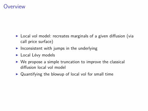
Local volatility (r = 0 for simplicity)

I If an underlying satisfies

dSt/St = σ(t, St)dWt ,

then call prices C(K ,T ) satisfy the forward PDE

∂T C(K ,T ) = 12K 2σ(K ,T )2∂KK C(K ,T ).

I Conversely: The local volatility model

dSt/St = σloc(St , t)dWt

reproduces a given smooth call price surface C , where:I Dupire’s formula (1994)

σ2loc(K ,T ) =

2∂T CK 2∂KK C

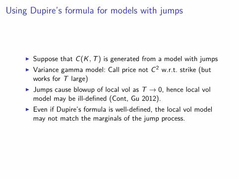
Using Dupire’s formula for models with jumps

I Suppose that C(K ,T ) is generated from a model with jumpsI Variance gamma model: Call price not C2 w.r.t. strike (but

works for T large)I Jumps cause blowup of local vol as T → 0, hence local vol

model may be ill-defined (Cont, Gu 2012).I Even if Dupire’s formula is well-defined, the local vol model

may not match the marginals of the jump process.

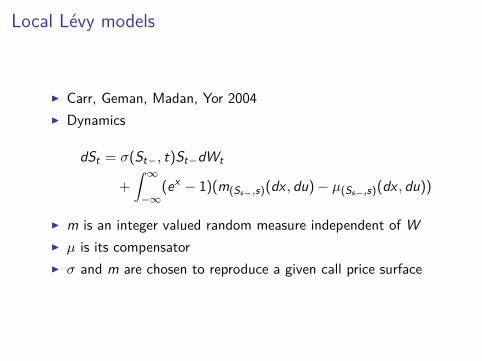
Local Lévy models

I Carr, Geman, Madan, Yor 2004I Dynamics

dSt = σ(St−, t)St−dWt

+

∫ ∞−∞

(ex − 1)(m(Ss−,s)(dx , du)− µ(Ss−,s)(dx , du))

I m is an integer valued random measure independent of WI µ is its compensatorI σ and m are chosen to reproduce a given call price surface

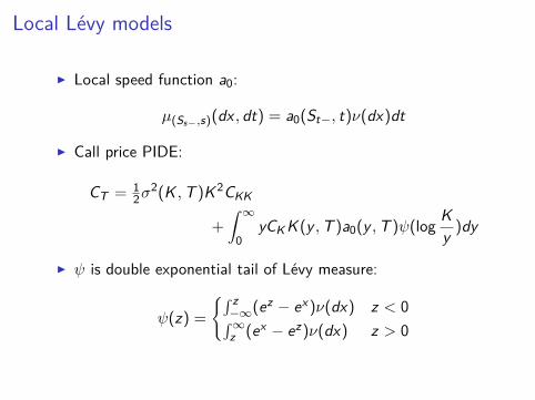
Local Lévy models

I Local speed function a0:

µ(Ss−,s)(dx , dt) = a0(St−, t)ν(dx)dt

I Call price PIDE:

CT = 12σ

2(K ,T )K 2CKK

+

∫ ∞0

yCK K (y ,T )a0(y ,T )ψ(log Ky )dy

I ψ is double exponential tail of Lévy measure:

ψ(z) =

{∫ z−∞(ez − ex )ν(dx) z < 0∫∞z (ex − ez)ν(dx) z > 0

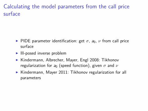
Calculating the model parameters from the call pricesurface

I PIDE parameter identification: get σ, a0, ν from call pricesurface

I Ill-posed inverse problemI Kindermann, Albrecher, Mayer, Engl 2008: Tikhonov

regularization for a0 (speed function), given σ and νI Kindermann, Mayer 2011: Tikhonov regularization for all

parameters

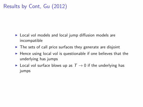
Results by Cont, Gu (2012)

I Local vol models and local jump diffusion models areincompatible

I The sets of call price surfaces they generate are disjointI Hence using local vol is questionable if one believes that the

underlying has jumpsI Local vol surface blows up as T → 0 if the underlying has

jumps

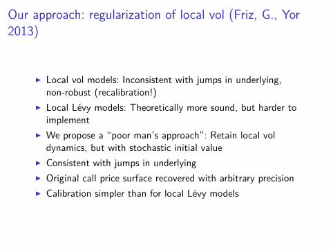
Our approach: regularization of local vol (Friz, G., Yor2013)

I Local vol models: Inconsistent with jumps in underlying,non-robust (recalibration!)

I Local Lévy models: Theoretically more sound, but harder toimplement

I We propose a “poor man’s approach”: Retain local voldynamics, but with stochastic initial value

I Consistent with jumps in underlyingI Original call price surface recovered with arbitrary precisionI Calibration simpler than for local Lévy models

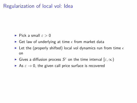
Regularization of local vol: Idea

I Pick a small ε > 0I Get law of underlying at time ε from market dataI Let the (properly shifted) local vol dynamics run from time ε

onI Gives a diffusion process Sε on the time interval [ε,∞)

I As ε→ 0, the given call price surface is recovered

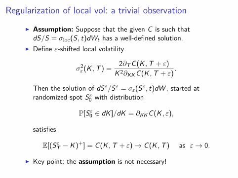
Regularization of local vol: a trivial observation

I Assumption: Suppose that the given C is such thatdS/S = σloc(S, t)dWt has a well-defined solution.

I Define ε-shifted local volatility

σ2ε (K ,T ) =

2∂T C(K ,T + ε)

K 2∂KK C(K ,T + ε).

Then the solution of dSε/Sε = σε(Sε, t)dW , started atrandomized spot Sε

0 with distribution

P[Sε0 ∈ dK ]/dK = ∂KK C(K , ε),

satisfies

E[(SεT − K )+] = C(K ,T + ε)→ C(K ,T ) as ε→ 0.

I Key point: the assumption is not necessary!

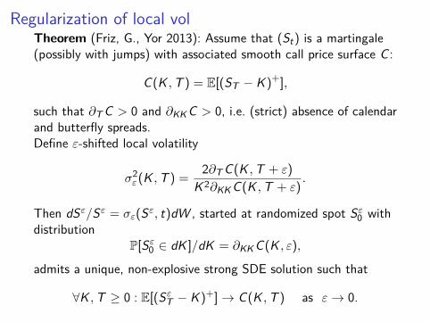
Regularization of local volTheorem (Friz, G., Yor 2013): Assume that (St) is a martingale(possibly with jumps) with associated smooth call price surface C :

C(K ,T ) = E[(ST − K )+],

such that ∂T C > 0 and ∂KK C > 0, i.e. (strict) absence of calendarand butterfly spreads.Define ε-shifted local volatility

σ2ε (K ,T ) =

2∂T C(K ,T + ε)

K 2∂KK C(K ,T + ε).

Then dSε/Sε = σε(Sε, t)dW , started at randomized spot Sε0 with

distributionP[Sε

0 ∈ dK ]/dK = ∂KK C(K , ε),

admits a unique, non-explosive strong SDE solution such that

∀K ,T ≥ 0 : E[(SεT − K )+]→ C(K ,T ) as ε→ 0.

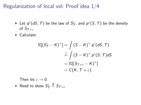
Regularization of local vol: Proof idea 1/4

I Let qε(dS,T ) be the law of SεT , and pε(S,T ) be the density

of ST+ε

I Calculate

E[(SεT − K )+] =

∫(S − K )+ qε(dS,T )

!=

∫(S − K )+ pε(S,T )dS

= E[(ST+ε − K )+]

= C(K ,T + ε).

Then let ε→ 0.I Need to show Sε

Td= ST+ε

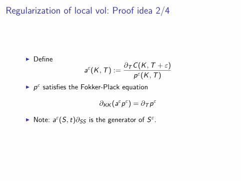
Regularization of local vol: Proof idea 2/4

I Defineaε(K ,T ) :=

∂T C(K ,T + ε)

pε(K ,T )

I pε satisfies the Fokker-Plack equation

∂KK (aεpε) = ∂T pε

I Note: aε(S, t)∂SS is the generator of Sε.

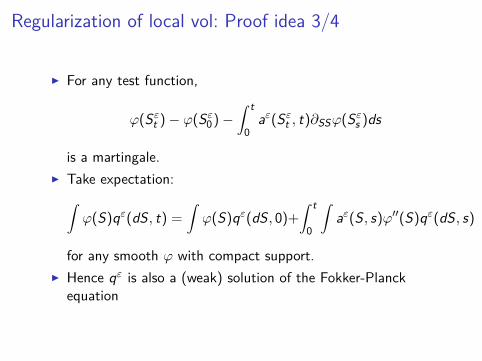
Regularization of local vol: Proof idea 3/4

I For any test function,

ϕ(Sεt )− ϕ(Sε

0)−∫ t

0aε(Sε

t , t)∂SSϕ(Sεs )ds

is a martingale.I Take expectation:∫

ϕ(S)qε(dS, t) =

∫ϕ(S)qε(dS, 0)+

∫ t

0

∫aε(S, s)ϕ′′(S)qε(dS, s)

for any smooth ϕ with compact support.I Hence qε is also a (weak) solution of the Fokker-Planck

equation

Regularization of local vol: Proof idea 4/4

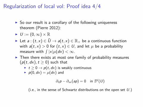
I So our result is a corollary of the following uniquenesstheorem (Pierre 2012):

I U := (0,∞)× RI Let a : (t, x) ∈ U → a(t, x) ∈ R+ be a continuous function

with a(t, x) > 0 for (t, x) ∈ U, and let µ be a probabilitymeasure with

∫|x |µ(dx) <∞.

I Then there exists at most one family of probability measures(p(t, dx), t ≥ 0) such that

I t ≥ 0→ p(t, dx) is weakly continuousI p(0, dx) = µ(dx) and

∂tp − ∂xx (ap) = 0 in D′(U)

(i.e., in the sense of Schwartz distributions on the open set U.)

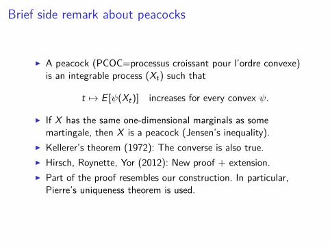
Brief side remark about peacocks

I A peacock (PCOC=processus croissant pour l’ordre convexe)is an integrable process (Xt) such that

t 7→ E [ψ(Xt)] increases for every convex ψ.

I If X has the same one-dimensional marginals as somemartingale, then X is a peacock (Jensen’s inequality).

I Kellerer’s theorem (1972): The converse is also true.I Hirsch, Roynette, Yor (2012): New proof + extension.I Part of the proof resembles our construction. In particular,

Pierre’s uniqueness theorem is used.

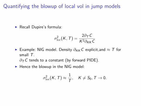
Quantifying the blowup of local vol in jump models

I Recall Dupire’s formula:

σ2loc(K ,T ) =

2∂T CK 2∂KK C

I Example: NIG model. Density ∂KK C explicit,and ≈ T forsmall T .∂T C tends to a constant (by forward PIDE).

I Hence the blowup in the NIG model:

σ2loc(K ,T ) ≈ 1

T , K 6= S0,T → 0.

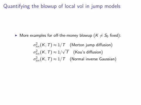
Quantifying the blowup of local vol in jump models

I More examples for off-the-money blowup (K 6= S0 fixed):

σ2loc(K ,T ) ≈ 1/T (Merton jump diffusion)σ2

loc(K ,T ) ≈ 1/√

T (Kou’s diffusion)σ2

loc(K ,T ) ≈ 1/T (Normal inverse Gaussian)

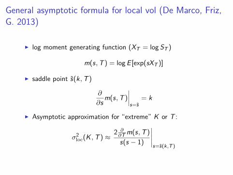
General asymptotic formula for local vol (De Marco, Friz,G. 2013)

I log moment generating function (XT = log ST )

m(s,T ) = log E [exp(sXT )]

I saddle point s(k,T )

∂

∂s m(s,T )

∣∣∣∣s=s

= k

I Asymptotic approximation for “extreme” K or T :

σ2loc(K ,T ) ≈

2 ∂∂T m(s,T )

s(s − 1)

∣∣∣∣∣s=s(k,T )

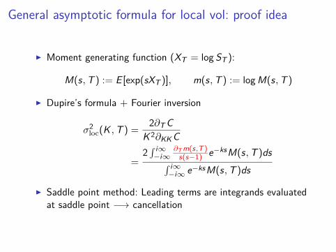
General asymptotic formula for local vol: proof idea

I Moment generating function (XT = log ST ):

M(s,T ) := E [exp(sXT )], m(s,T ) := logM(s,T )

I Dupire’s formula + Fourier inversion

σ2loc(K ,T ) =

2∂T CK 2∂KK C

=2∫ i∞−i∞

∂T m(s,T )s(s−1) e−ksM(s,T )ds∫ i∞

−i∞ e−ksM(s,T )ds

I Saddle point method: Leading terms are integrands evaluatedat saddle point −→ cancellation

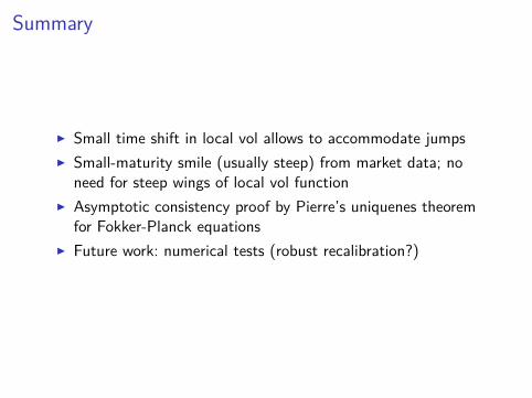
Summary

I Small time shift in local vol allows to accommodate jumpsI Small-maturity smile (usually steep) from market data; no

need for steep wings of local vol functionI Asymptotic consistency proof by Pierre’s uniquenes theorem

for Fokker-Planck equationsI Future work: numerical tests (robust recalibration?)

References

I P. Carr, H. Geman, D. Madan, M. Yor, From localvolatility to local Lévy models, 2004.

I R. Cont Y. Gu, Local vs. non-local forward equations foroption pricing, 2012.

I S. De Marco, P. Friz, S. Gerhold, Rational shapes oflocal volatility, 2013.

I P. Friz, S. Gerhold, M. Yor, How to make Dupire’slocal volatility work with jumps, 2013.

I F. Hirsch, B. Roynette, M. Yor, Kellerer’s theoremrevisited, 2012.