Embed Size (px)
Citation preview
i
Localization in Wireless Sensor Networks
Shubham Shekhar
111CS0157
National Institute of Technology Rourkela
Rourkela, 769 008, Odisha, India
ii
Localization in Wireless Sensor Networks
A Thesis
Submitted in partial fulfillment
Of the requirements for the degree of
Bachelor of Technology
by
Shubham Shekhar
(Roll 111CS0157)
Under the supervision of
Professor Sanjay Kumar Jena
Department of Computer Science & Engineering
National Institute of Technology Rourkela
Rourkela – 769 008; India
May 2015

iii
Declaration by Student
I certify that
The work enclosed in this thesis has been done by me under the supervision of my project
guide.
The work has not been submitted to any other institute for any degree or diploma.
I have confirmed to the norms and guidelines given in the Ethical Code of Conduct of
National Institute of Technology, Rourkela.
Whenever I have adopted materials (data, theoretical analysis, figure and text) from other
authors, I have given them due credits through citations and by giving their details in the
references.
NAME: Shubham Shekhar
DATE: May 11,2015
SIGNATURE:
iv
Dr. Sanjay Kumar Jena
Professor
May 11, 2015
Certificate
This is to certify that the work in the project entitled Localization in Wireless Sensor
Networks by Shubham Shekhar is a record of an original work carried out by her under my
intendance and supervision in partial attainment of the requirements for the degree of
Bachelor of Technology in Computer Science and Engineering. Neither this project nor
any part of it has been submitted for any degree or academic award elsewhere.
Sanjay Kumar Jena

v
Acknowledgement
I take this privilege to express my gratitude to all those people who supported me directly or
indirectly throughout the course of the project. It would never have been possible without their
benign support and assistance. Their endeavoring guidance, invaluable positive criticism and
constructive advice helped a lot in the project.
I thank whole heartedly, Prof. S. K. Jena for his support, guidance, and constant encouragement.
As my supervisor, he constantly has encouraged me to remain focused on achieving my goal. His
valuable comments and observations helped me to give my research a proper direction and to
proceed forward with an in depth investigation.
I am highly indebted to my project external guide Mr. Asish Dalai, for his constant supervision
and guidance. He provided all the necessary information regarding the project and also his constant
support helped a lot in completing the project.
I would also like to thank my colleagues for their help in finding bugs in the project and their
constant feedback that helped improve the project a lot.
NAME: Shubham Shekhar
SIGNATURE:
vi
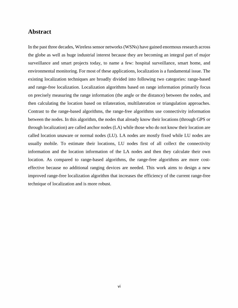
Abstract
In the past three decades, Wireless sensor networks (WSNs) have gained enormous research across
the globe as well as huge industrial interest because they are becoming an integral part of major
surveillance and smart projects today, to name a few: hospital surveillance, smart home, and
environmental monitoring. For most of these applications, localization is a fundamental issue. The
existing localization techniques are broadly divided into following two categories: range-based
and range-free localization. Localization algorithms based on range information primarily focus
on precisely measuring the range information (the angle or the distance) between the nodes, and
then calculating the location based on trilateration, multilateration or triangulation approaches.
Contrast to the range-based algorithms, the range-free algorithms use connectivity information
between the nodes. In this algorithm, the nodes that already know their locations (through GPS or
through localization) are called anchor nodes (LA) while those who do not know their location are
called location unaware or normal nodes (LU). LA nodes are mostly fixed while LU nodes are
usually mobile. To estimate their locations, LU nodes first of all collect the connectivity
information and the location information of the LA nodes and then they calculate their own
location. As compared to range-based algorithms, the range-free algorithms are more cost-
effective because no additional ranging devices are needed. This work aims to design a new
improved range-free localization algorithm that increases the efficiency of the current range-free
technique of localization and is more robust.
vii
Contents
1. Introduction 1
1.1 Motivation……………………………………………………………………………1
1.2 Localization System Components………………………………………………........2
1.3 Localization Algorithm Categories…………………………………………………..2
1.4 Thesis Outline………………………………………………………………………..3
2. Localization Problem 4
2.1 Optimal Linear Arrangement Problem……………………………………………....4
2.2 1D Localization Problem…………………………………………………………….5
2.3 Proof by Reduction………………………………………………………………….5
2.4 Classification………………………………………………………………………..6
3. Range-Based Localization 8
3.1 Received Signal Strength Indicator…………………………………………………8
3.2 Time of Arrival……………………………………………………………………...8
3.3 Angle of Arrival……………………………………………………………………..9
3.4 Position Computation………………………………………………………………..9
3.4.1 Trilateration………………………………………………………………….9
3.4.2 Multilateration………………………………………………………………10
4. Range-Free Localization 11
4.1 DV-Hop Based Algorithm…………………………………………………………...12
4.2 Implementation………………………………………………………………………13
4.3 Improved DV-Hop Based Algorithm………………………………………………...15
4.4 Simulations………………………………………………………………………….. 16
4.5 Conclusion…………………………………………………………………………... 20
1
Chapter 1
Introduction
The discussion of distributed sensor networks has been continuing for over 30 years, but wireless
sensor networks (WSNs) came into existence only because of the recent technologies and advances
in electronics and wireless communications. They help to develop multi-function sensors that are
very efficient in cost and power and also are small in size. They are able to communicate over
short distances. In recent years, inexpensive and intelligent sensors which are networked with the
help of wireless links and distributed in large numbers, provide novel methods to monitor and
control cities, homes, and even the environment. Additionally, networked sensors also have a wide
range of applications in the defense area which in turn helps to generate new capabilities for
intelligence and surveillance, as well as many other tactical military applications. Location
estimation capability is vital in almost all wireless sensor network applications. Applications that
monitor the environment like the ones that monitoring animal habitat or water quality or
surveillance of bush fire and agriculture, the measured data will have no significance if there is no
information about the location from where the data has been obtained. The information about the
location of any data enables innumerable applications such as managing inventory, detection of
intruders, monitoring health, monitoring road traffic, intelligence and surveillance.
Motivation
In recent years, the terminology of a localization system has become a very fundamental yet crucial
subject of an enormous number of WSN applications. The location information is hard to
determine in advance because the sensor networks are deployed mostly in the areas which cannot
be easily accessed by humans like disaster relief operations or inaccessible topography. Thus, there
is a need for a localization system which will facilitate computing location coordinates for the
sensor nodes. The prominence of localization information has several factors responsible, mostly
related primarily to WSNs. These factors include the recognition and correlational coefficient of
collected data, addressing of nodes, evaluation of nodes’ coverage and density, management and
inquiry of nodes localized in a known region, geographic routing, object tracking, generation of
2
energy map, and other geographic algorithms. All of the above mentioned factors make
localization systems a very important technology for the operation and development of WSNs.
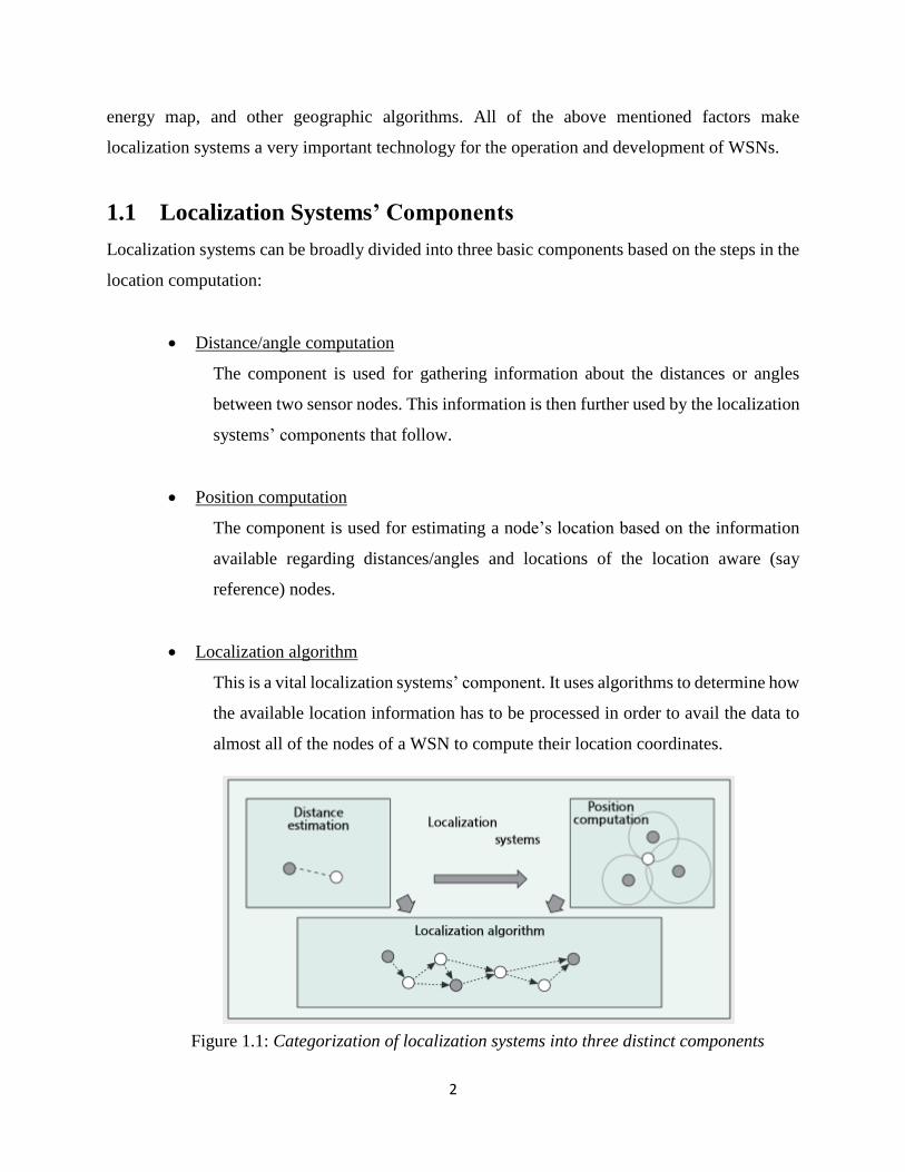
1.1 Localization Systems’ Components
Localization systems can be broadly divided into three basic components based on the steps in the
location computation:
Distance/angle computation
The component is used for gathering information about the distances or angles
between two sensor nodes. This information is then further used by the localization
systems’ components that follow.
Position computation
The component is used for estimating a node’s location based on the information
available regarding distances/angles and locations of the location aware (say
reference) nodes.
Localization algorithm
This is a vital localization systems’ component. It uses algorithms to determine how
the available location information has to be processed in order to avail the data to
almost all of the nodes of a WSN to compute their location coordinates.
Figure 1.1: Categorization of localization systems into three distinct components
3
1.2 Localization Algorithm Categories
Localization algorithms are divided into two categories:
Range-Free
The input to the range-free localization algorithms is the connectivity information data
of the nodes. These algorithms do not require any extra hardware components which
in turn makes them very cost efficient.
Range-Based
Range-based localization assumes that the absolute distance between a sender node
and a receiver node can be approximately calculated by the time-of-flight or by the
received signal strength of the communication signal from the sender node to the
receiver node.
The accuracy of such an estimation is affected a lot by the surrounding environment
and the transmission medium and usually involves a complex hardware.
Here we will study and simulate the range-free localization as well as the range-based localization
and develop an improved localization system combining techniques from existing range-free
localization algorithms with a motive to reduce the location error, the cost and other overheads.
1.3 Thesis Outline
A brief introduction to wireless sensor networks and the importance of location estimation is
presented in chapter 1. The rest of the thesis includes three chapters.
Chapter 2- This chapter discusses the problem statement and classifies the localization problem.
Chapter 3- This chapter discusses the range-based localization algorithm and its type. The chapter
also gives a brief overview of ns-2 for understanding the simulations.
Chapter 4- This chapter discusses the range-free localization algorithm and its type.
4
Chapter 2
Localization Problem
The localization problem has been proven to be NP-complete by polynomial transformation of the
graph linear arrangement problem into the localization problem. The main causes of computational
intractability in 3D space were identified to be mirroring and flipping [2].
Flip Ambiguity- Caused by inappropriate geometric relations among anchor nodes
(nodes with known location information) used for calculation.
Mirroring- When anchor nodes’ positions are almost collinear, they form a mirror
through which a node’s position can be reflected.
Here a proof has been provided for the computational intractability of the localization problem. To
clearly explain the reasons of complexity in a localization system and to learn about the importance
of noise in measurements, the following proof is provided which also states the conditions under
which a localization problem is proved to be NP-complete [2]. Even in the absence of mirroring
and flipping occurs, it can be concluded that the localization problem is NP-complete, errors in
measurements being the prime causes. Also it has been seen that the distance measurement step
that is involved in the localization algorithm is prone to error and so taking into account that error
using an error model, there is a need to design a powerful and robust optimization mechanism for
location estimation. The 1D Location Discovery problem is proved to be NP-complete by
transforming a known instance of the NP-complete problem––optimal linear arrangement problem
into the given problem in polynomial time [2].
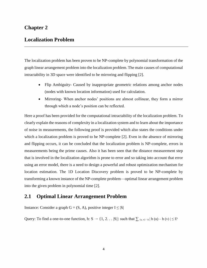
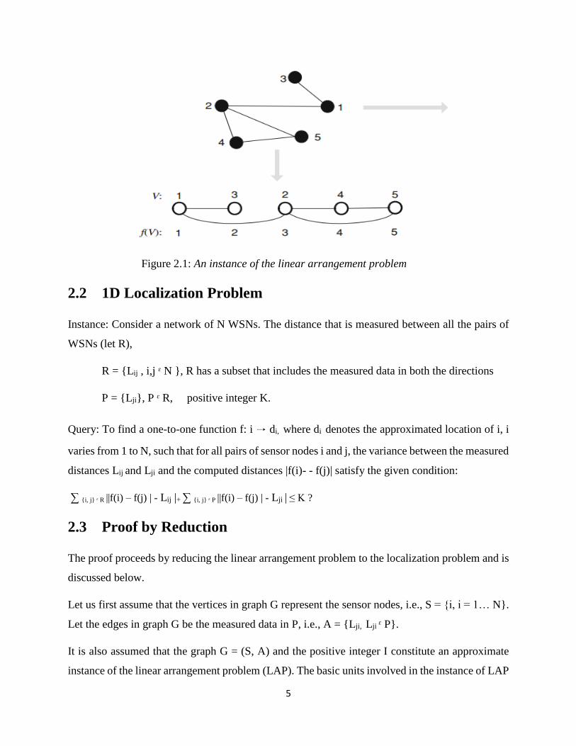
2.1 Optimal Linear Arrangement Problem
Instance: Consider a graph G = (S, A), positive integer I ≤ |S|
Query: To find a one-to-one function, h: S ⇢ {1, 2. . . |S|} such that ∑ {u, v} ᵋ A | h (u) – h (v) | ≤ I?
5
Figure 2.1: An instance of the linear arrangement problem
2.2 1D Localization Problem
Instance: Consider a network of N WSNs. The distance that is measured between all the pairs of
WSNs (let R),
R = {Lij , i,j ᵋ N }, R has a subset that includes the measured data in both the directions
P = {Lji}, P ᵋ R, positive integer K.
Query: To find a one-to-one function f: i ⇢ di, where di denotes the approximated location of i, i
varies from 1 to N, such that for all pairs of sensor nodes i and j, the variance between the measured
distances Lij and Lji and the computed distances |f(i)- - f(j)| satisfy the given condition:
∑ {i, j} ᵋ R ||f(i) – f(j) | - Lij |+ ∑ {i, j} ᵋ P ||f(i) – f(j) | - Lji | ≤ K ?
2.3 Proof by Reduction
The proof proceeds by reducing the linear arrangement problem to the localization problem and is
discussed below.
Let us first assume that the vertices in graph G represent the sensor nodes, i.e., S = {i, i = 1… N}.
Let the edges in graph G be the measured data in P, i.e., A = {Lji, Lji ᵋ P}.
It is also assumed that the graph G = (S, A) and the positive integer I constitute an approximate
instance of the linear arrangement problem (LAP). The basic units involved in the instance of LAP
6
are the edges and the vertices of the graph G. Given below is a complete specification of the
instance of the localization problem:
i = {s: s ᵋ S}
Lji = { {j,i} : {j,i} ᵋ A }
K = I + O, where O=1/4(I2+I+2) (I-1)
It is apparent that this particular instance can be derived in linear time. The measured distances Lij
act as an “agent”, which guide the way the sensor nodes must be placed by putting additional
restrictions. Distinctively, all the Lij have value I + b, where b specifies the minimum computed
distance between any arbitrary pair of nodes. The agent has its importance also because it very
well helps in preventing identical location assignment to multiple nodes, which is required as the
condition in linear arrangement problem requires that each node must have a unique location and
the distance between any two of them is at least 1 unit. Therefore, there is a mapping from each
node to a unique integer location between 0 and I.
Function h exists iff there exists a function f that satisfies the following condition
∑ {i, j} ᵋ R |f(i) – f(j) - Lij| + ∑ {i, j} ᵋ P |f(i) – f(j) - Lji | ≤ K
Suppose f such that
∑ {i, j} ᵋ R ||f(i) – f(j) |- Lij| + ∑ {i, j} ᵋ P ||f(i) – f(j)| - Lji | ≤ K
Consequently, there exists an h such that
∑ {i, j} ᵋ R |h(i) – h(j) | ≤ I
Therefore, function h satisfies the condition
∑ {u, v} ᵋ A |h(u) – h(v) | ≤ I since R = { Lji : {j,i} ᵋ A}
2.4 Classification
There are many ways in which a Location Discovery algorithm can be classified, such as
7
How the algorithms is executed—centralized versus Localized.
What is the target environment of the algorithm —Indoor versus Outdoor?
Network topology—static versus dynamic networks.
Available resources—GPS-based versus GPS-less.
Centralized algorithms have the property that all the computations are done at a single place
with the condition that the complete information about all the measurements is provided.
Localized algorithms, on the other hand, are carried out by multiple nodes concurrently and/or
successively where the nodes do not have all the complete information, they just have the data
provided by their neighbor nodes. Some networks consist of anchors/beacons (the nodes that
have GPS devices installed on them and therefore, they know their absolute locations while
some networks do not). In GPS-based Location Discovery, it is possible to calculate the
absolute locations of the location unaware nodes, whereas the locations derived are relative
locations in GPS-less networks [2]. However, it is possible to derive the absolute locations
from the relative locations given the coordinates are of at least three nodes. In addition, there
are also several algorithms which are specifically designed for mobile networks. In the chapters
that follow, the Location Discovery algorithms, which take as inputs of the algorithm, the
available resources used to derive the locations, are being discussed: range-based and range-
free Location Discovery.
8
Chapter 3
Range-Based Localization
The methodology of range-based localization depends on accurate ranging results among sensor
nodes. These ranging results include point-to-point distance, angle, or velocity relative
measurements. After obtaining ranging results, the positions of sensor nodes can be estimated
through geographical calculations such as trilateration, multilateration or triangulation.
3.1 Received Signal Strength Indicator
In this method, the absolute distance between any two sensor nodes is estimated by the signal’s
strength received by another sensor node. The signal strength gradually decreases with the increase
in distance to the receiver node. Hypothetically, it is known that the strength of a signal is inversely
proportional to the distance squared and using a known model of radio propagation, the signal
strength can be converted into distance [1]. However, in actual scenarios and environments, this
particular strength indicator is highly affected by obstacles, noises, and the antenna type, which
makes the mathematical model’s design hard. Like the others, this method also has both
advantages and disadvantages. The prime advantage is its cheap cost because it is easy for most of
the receivers to estimate the received signal strength [1]. The main disadvantage is that it is easily
affected by noise and interferences from the environment, which in turn results in more
inaccuracies in estimation of distance [1].
3.2 Time of Arrival
Time of Arrival is used to calculate the distance between two sensor nodes based on the time of
arrival of the signal from the source node (generally LA) to the destination node (generally LU).
It is known that the distance between two points is directly proportional to the time a signal takes
to travel from one of them to the other, similar is the case with two nodes. This way, if a signal
was sent from the sender node at time ti and it was acknowledged by the receiver node at time tj,
then the distance between the sender node and the receiver node is (let d); d = s*(tj – ti), where s
denotes the travel speed of the radio signal in that medium (speed of light), and ii and tj denotes
9
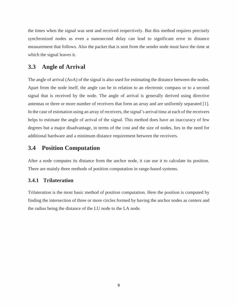
the times when the signal was sent and received respectively. But this method requires precisely
synchronized nodes as even a nanosecond delay can lead to significant error in distance
measurement that follows. Also the packet that is sent from the sender node must have the time at
which the signal leaves it.
3.3 Angle of Arrival
The angle of arrival (AoA) of the signal is also used for estimating the distance between the nodes.
Apart from the node itself, the angle can be in relation to an electronic compass or to a second
signal that is received by the node. The angle of arrival is generally derived using directive
antennas or three or more number of receivers that form an array and are uniformly separated [1].
In the case of estimation using an array of receivers, the signal’s arrival time at each of the receivers
helps to estimate the angle of arrival of the signal. This method does have an inaccuracy of few
degrees but a major disadvantage, in terms of the cost and the size of nodes, lies in the need for
additional hardware and a minimum distance requirement between the receivers.
3.4 Position Computation
After a node computes its distance from the anchor node, it can use it to calculate its position.
There are mainly three methods of position computation in range-based systems.
3.4.1 Trilateration
Trilateration is the most basic method of position computation. Here the position is computed by
finding the intersection of three or more circles formed by having the anchor nodes as centers and
the radius being the distance of the LU node to the LA node.
10
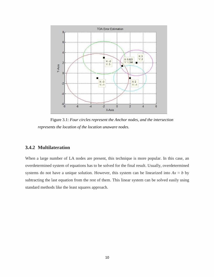
Figure 3.1: Four circles represent the Anchor nodes, and the intersection
represents the location of the location unaware nodes.
3.4.2 Multilateration
When a large number of LA nodes are present, this technique is more popular. In this case, an
overdetermined system of equations has to be solved for the final result. Usually, overdetermined
systems do not have a unique solution. However, this system can be linearized into Ax ≈ b by
subtracting the last equation from the rest of them. This linear system can be solved easily using
standard methods like the least squares approach.
11
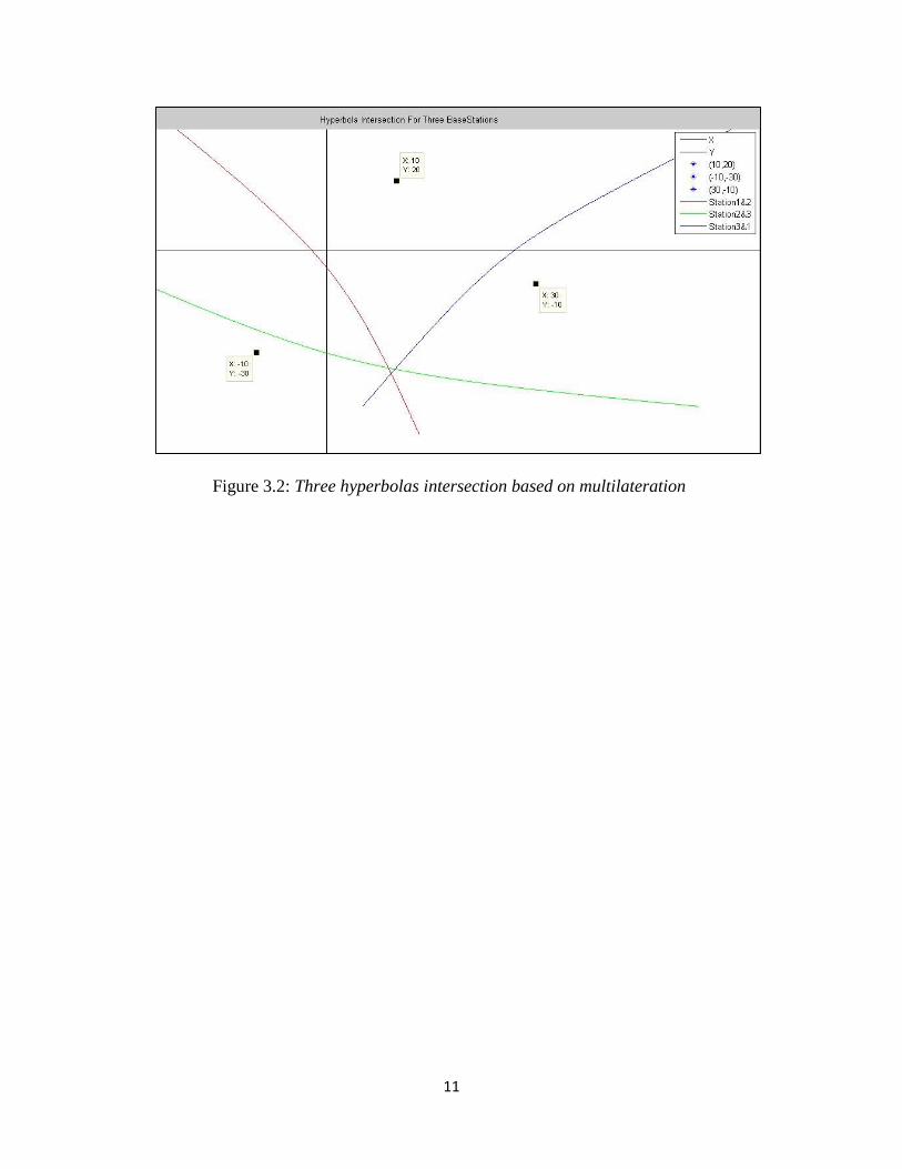
Figure 3.2: Three hyperbolas intersection based on multilateration
12
Chapter 4
Range-Free Localization
While the range-based localization techniques precisely measure the distance or angle between
nodes, the range-free schemes use connectivity information. The connectivity information can be
the hop count between two sensor nodes, indicating how close the two nodes are. For example, if
one node is within the communications range of the other node, the distance between two nodes
can be estimated as one hop, and these two nodes can be called as neighbors.
In range-free localization schemes, the nodes that are aware of their positions are called anchor
nodes (LA) while those who do not know their location are called normal nodes (LU). Normal
nodes first collect the connectivity information as well as the location information of the anchors,
and then compute their own coordinates. Since ranging information is not needed, the range-free
schemes can easily be implemented on low-cost WSNs. Another major advantage of the range-
free schemes is their robustness; the connectivity information between nodes is very rarely affected
by the environment. As a result, the main aim is to design an improved range-free localization
algorithm which further reduces the error in location computation.
4.1 DV-Hop Based Algorithm
In this algorithm, first the anchor nodes floods packets containing their location and a variable
‘hop-count’ initialized to zero. As the intermediate nodes receive these packets, they store the
location, hop-count and increase the hop-count by 1 and flood again. One major activity that is
done by the LU nodes is comparing the hop count value that it receives for a particular LA node
from all the sources. As soon as it receives a packet that has a hop count value lower than its
present hop count value to a particular LA node, it updates its hop count value and transmits the
packet whereas if the value is greater than the current one, the packet is discarded. When flooding
completes, each node has the data with the coordinates of all the LA nodes included and also the
least hops to them.
13
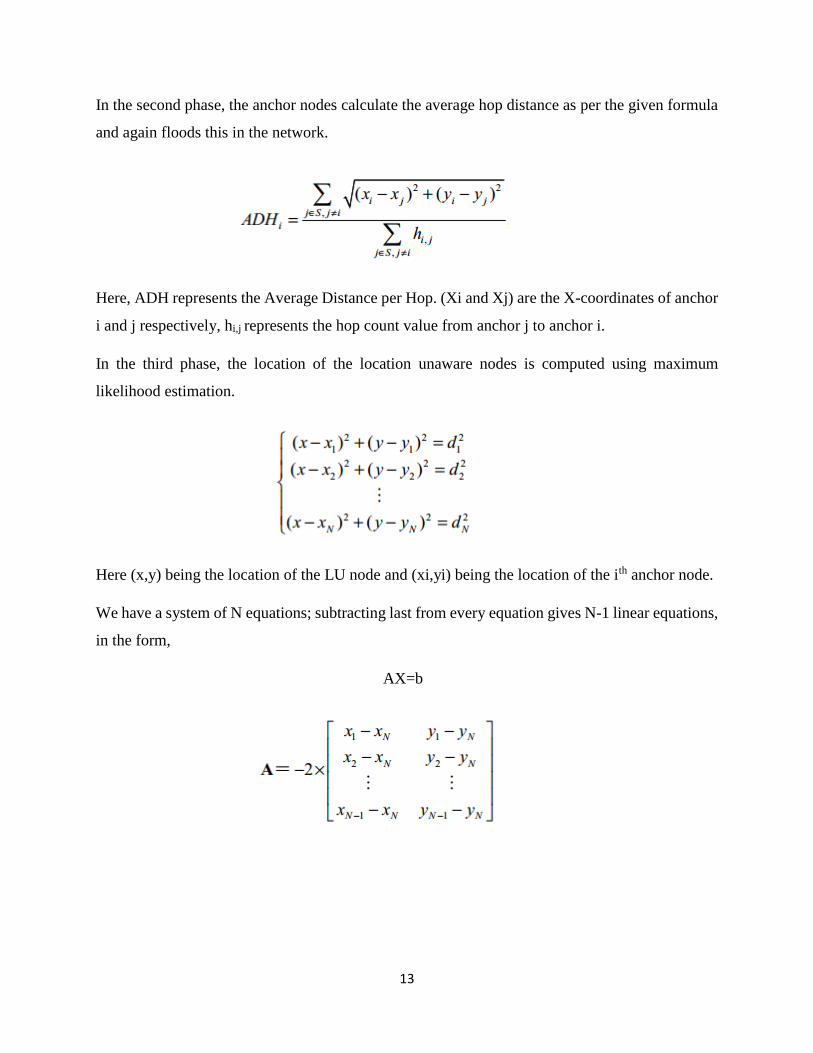
In the second phase, the anchor nodes calculate the average hop distance as per the given formula
and again floods this in the network.
Here, ADH represents the Average Distance per Hop. (Xi and Xj) are the X-coordinates of anchor
i and j respectively, hi,j represents the hop count value from anchor j to anchor i.
In the third phase, the location of the location unaware nodes is computed using maximum
likelihood estimation.
Here (x,y) being the location of the LU node and (xi,yi) being the location of the ith anchor node.
We have a system of N equations; subtracting last from every equation gives N-1 linear equations,
in the form,
AX=b
14
The solution is obtained as
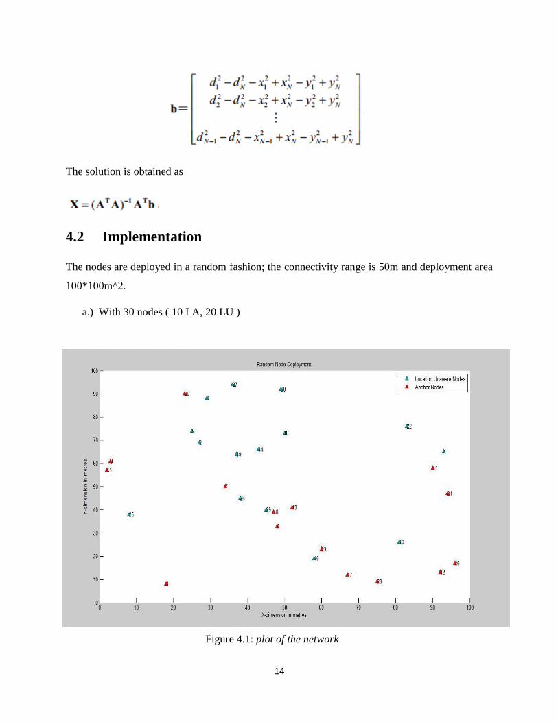
4.2 Implementation
The nodes are deployed in a random fashion; the connectivity range is 50m and deployment area
100*100m^2.
a.) With 30 nodes ( 10 LA, 20 LU )
Figure 4.1: plot of the network
15
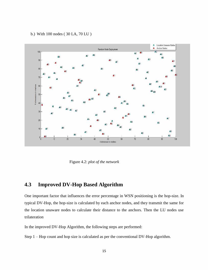
b.) With 100 nodes ( 30 LA, 70 LU )
Figure 4.2: plot of the network
4.3 Improved DV-Hop Based Algorithm
One important factor that influences the error percentage in WSN positioning is the hop-size. In
typical DV-Hop, the hop-size is calculated by each anchor nodes, and they transmit the same for
the location unaware nodes to calculate their distance to the anchors. Then the LU nodes use
trilateration
In the improved DV-Hop Algorithm, the following steps are performed:
Step 1 – Hop count and hop size is calculated as per the conventional DV-Hop algorithm.
16
Step 2 – The LA nodes recalculate their position using the approach of the conventional DV-Hop
algorithm.
Step 3 – Step 2 is iterated to modify the hop size for finding the minimum average anchor position
error. The iteration stops when the optimum hop size is obtained. The correction factor is
calculated and is broadcasted.
Step 4 – After finding the hop correction value, the nodes calculate their position using weighted
averaging method where with each LA nodes is associated a weight based on the LU node’s hop
count with the LA node. More the hops between LU and LA node, a smaller value is assigned to
the weighing factor.
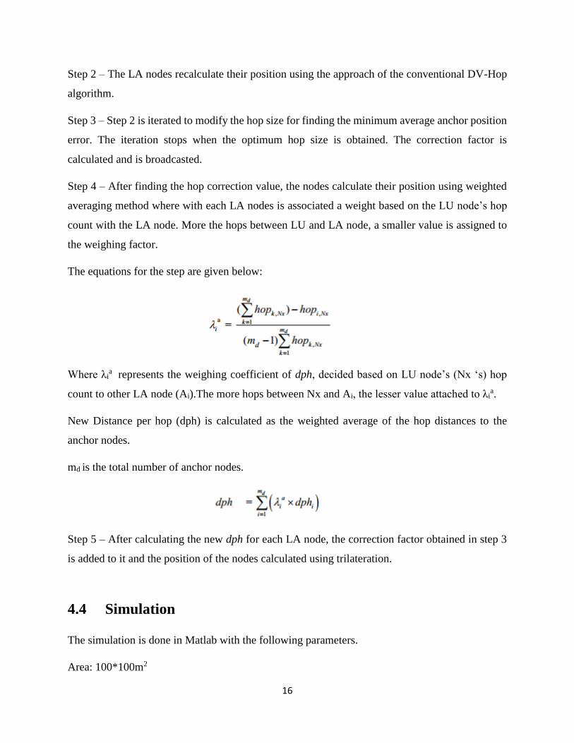
The equations for the step are given below:
Where λia represents the weighing coefficient of dph, decided based on LU node’s (Nx ‘s) hop
count to other LA node (Ai).The more hops between Nx and Ai, the lesser value attached to λia.
New Distance per hop (dph) is calculated as the weighted average of the hop distances to the
anchor nodes.
md is the total number of anchor nodes.
Step 5 – After calculating the new dph for each LA node, the correction factor obtained in step 3
is added to it and the position of the nodes calculated using trilateration.
4.4 Simulation
The simulation is done in Matlab with the following parameters.
Area: 100*100m2
17
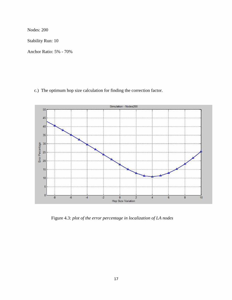
Nodes: 200
Stability Run: 10
Anchor Ratio: 5% - 70%
c.) The optimum hop size calculation for finding the correction factor.
Figure 4.3: plot of the error percentage in localization of LA nodes
18
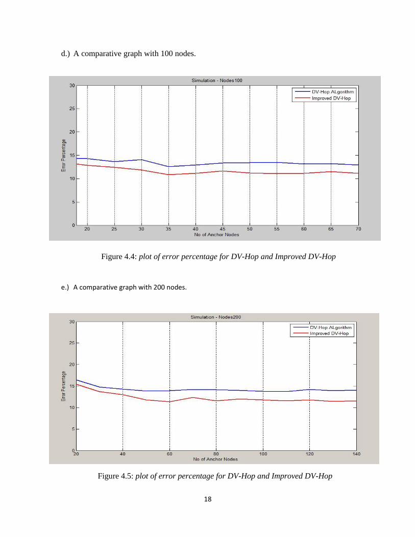
d.) A comparative graph with 100 nodes.
Figure 4.4: plot of error percentage for DV-Hop and Improved DV-Hop
e.) A comparative graph with 200 nodes.
Figure 4.5: plot of error percentage for DV-Hop and Improved DV-Hop
19
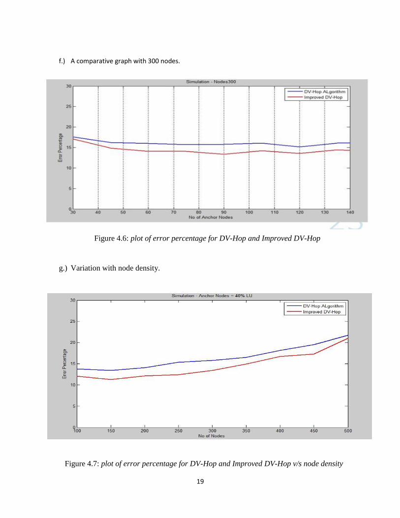
f.) A comparative graph with 300 nodes.
Figure 4.6: plot of error percentage for DV-Hop and Improved DV-Hop
g.) Variation with node density.
Figure 4.7: plot of error percentage for DV-Hop and Improved DV-Hop v/s node density
20
4.5 Conclusion
The new improved DV-Hop algorithm improves the error percentage of the classic DV-Hop by
around 5% when the nodes are deployed in a random fashion. Also, the complexity of
computation is comparable to the existing DV-Hop algorithm. If the anchor nodes (LA) are
deployed in a particular fashion, the error rate can be further improved.
21
Bibliography
[1] Azzedine Boukerche, Horacio A. B. F. Oliveira, Antonio A. F. Loureiro, Localization Systems
For Wireless Sensor Networks, ISBN 1536-1284, DOI 10.1109/MWC.2007.4407221,IEEE
Wireless Communications 2007,Pages 6-12.
[2] Jessica Feng Sanford, Miodrag Potkonjak, Sasha Slijepcevic, Localization in Wireless
Networks, Foundation and Applications, ISBN 978-1-4614-1838-2, DOI 10.1007/978-1-4614-
1839-9,Springer New York Heidelberg Dordrecht London
[3] Gayan S, Dias D, Dept. of Electronics & Telecommunication Eng., Univ. of Moratuwa, Sri
Lanka, Improved DV-Hop algorithm through anchor position re-estimation, ISBN 978-1-4799-
3710-3, DOI 10.1109/APWiMob.2014.6920272,IEEE Conference, Bali, pages 126-131.
[4] Guoqiang Mao (University of Sydney, Australia) and Baris Fidan (National ICT Australia and
Australian National University, Australia), Localization Algorithms and Strategies for Wireless
Sensor Networks, ISBN-13 978-1605663968, publisher- Information Science Reference (15 June
2009).