Localized Sliced Inverse Regression

Qiang Wu, Feng Liang, and Sayan Mukherjee∗

We develop an extension of sliced inverse regression (SIR) that we call localized

sliced inverse regression (LSIR). This method allows for supervised dimension reduc-

tion by projection onto a linear subspace that captures the nonlinear subspace relevant

to predicting the response. The method is also extended to the semi-supervised setting

where one is given labeled and unlabeled data. We introduce asimple algorithm that

implements this method and illustrate its utility on real and simulated data.

Key Words: dimension reduction, sliced inverse regression, localization, semi-

supervised learning

∗Qiang Wu is a Visiting Assistant Professor in the Departmentof Mathematics, Michigan State Uni-

versity, East Lansing, MI 48824, U.S.A. (Email: wuqiang@math.duke.edu). Feng Liang is an Assistant

Professor in the Department of Statistics, University of Illinois at Urbana-Champaign, IL 61820, U.S.A.

(Email: liangf@uiuc.edu). Sayan Mukherjee is an AssistantProfessor in the Departments of Statistical Sci-

ence and Computer Science and the Institute for Genome Sciences & Policy, Duke University, Durham, NC

27708-0251, U.S.A. (Email:sayan@stat.duke.edu).

1

1 Introduction

The importance of dimension reduction for predictive modeling and visualization has

a long and central role in statistical graphics and computation (Adcock, 1878; Edeg-

worth, 1884; Fisher, 1922; Hotelling, 1933; Young, 1941). Principal components anal-

ysis (Hotelling, 1933) is the most used and one of the earliest dimension reduction

methods, however it does not take the response variable intoaccount. The idea of su-

pervised dimension reduction (SDR) which has become central in the modern context

of high-dimensional data analysis is to posit that the functional dependence between

a response variableY and a large set of explanatory variablesX ∈ Rp is driven by a

low dimensional subspace of thep variables. A variety of methods for SDR have been

proposed to characterize this subspace (Li, 1991; Cook and Weisberg, 1991; Li, 1992;

Hastie and Tibshirani, 1996; Vlassis et al., 2001; Xia et al., 2002; Fukumizu et al.,

2003; Li et al., 2004; Goldberger et al., 2005; Fukumizu et al., 2005; Globerson and

Roweis, 2006; Martin-Merino and Roman, 2006; Mukherjee and Zhou, 2006; Mukher-

jee and Wu, 2006; Nilsson et al., 2007; Sugiyama, 2007; Cook,2007; Li et al., 2007;

Mukherjee et al., 2009; Wu et al., 2007; Tokdar et al., 2008).

A strongly related branch of research that has been of great interest in the machine

learning community of late is nonlinear dimension reduction which can be traced back

to multi-dimensional scaling (Young, 1941). This researchhas motivated a variety of

manifold learning algorithms (Tenenbaum et al., 2000; Roweis and Saul, 2000; Donoho

and Grimes, 2003; Belkin and Niyogi, 2003). Though the aforementioned manifolds

learning methods are unsupervised in that the algorithms take into account only the

explanatory variables, this issue can be addressed by extending the unsupervised algo-

2

rithms to use the label or response data (Globerson and Roweis, 2006). The central

idea in the manifold learning framework is to use local metrics to generate a similarity

graph from the data and then use spectral methods for dimension reduction. This rests

on the observation that properties of the ambient space are true locally on smooth man-

ifolds. The main problem with these methods is that they do not operate on the space

of the predictor or explanatory variables which can cause problems if the projective

dimensions need to be interpreted.

In this paper we extend the classic SDR method of sliced inverse regression model

(SIR) by taking into account local structure of the explanatory variables conditioned on

the response variable. This integrates the idea of local estimates from manifold learning

with the sliced inverse framework for SDR. The resulting algorithm allows us to infer

a linear projective subspace that can capture nonlinear predictive structure, see Figure

1 for an illustration. The method applies to both classification and regression problems

and allows for the inclusion of ancillary unlabeled data in semi-supervised learning.

In the context of classification two other methods have been proposed to exploit local

information for SDR (Hastie and Tibshirani, 1996; Sugiyama, 2007). Comparing with

these two methods, our approach incorporates the local information at a more direct

way, see Section 2.3 for a comparison.

The paper is arranged as follows. Localized sliced inverse regression is introduced

in Section 2 for continuous and categorical response variables. We also compare the

method to previous localization procedures in this section. In Section 3 we illustrate

how LSIR can be extended to incorporate unlabeled data naturally. The utility of the

method with respect to predictive accuracy as well as exploratory data analysis via

3

visualization is demonstrated on a variety of simulated andreal data in Section 4. We

close with discussions in Section 5.

2 Local SIR

We begin with a brief review of sliced inverse regression. Wethen develop LSIR

which incorporates localization ideas from manifold learning into the SIR framework.

We close by comparing LSIR with related methods for dimension reduction (Hastie

and Tibshirani, 1996; Sugiyama, 2007).

2.1 Sliced inverse regression

Assume the functional dependence between a response variable Y and an explanatory

variableX ∈ Rp is given by

Y = f(β′1X, . . . , β′

LX, ε), (1)

where{β1, ..., βL} are unknown orthogonal vectors inRp andε is noise independent of

X . Let B denote theL-dimensional subspace spanned by{β1, ..., βL} andPB denote

the corresponding projection operator onto spaceB. ThenPBX provides a sufficient

summary of the information inX relevant toY in the sense thatY ⊥⊥ X |PBX . Es-

timatingB becomes the central problem in supervised dimension reduction. Though

we defineB here via a model assumption (1), a general definition based onconditional

independence betweenY andX givenPBX can be found in Cook and Yin (2001).

Following Cook and Yin (2001), we refer toB as the dimension reduction (d.r.) sub-

space and{β1, ..., βL} as the d.r. directions.

4

The sliced inverse regression model was introduced in Duan and Li (1991) and Li

(1991) to estimate the d.r. directions. Consider a simple case whereX has an identity

covariance matrix. The conditional expectationE(X |Y = y) is a curve inRp on which

y varies. It is called the inverse regression curve since the position of X andY are

switched as compared to the classical regression setting, where of interest isE(Y |X =

x). It is shown in Li (1991) that the inverse regression curve iscontained in the d.r.

spaceB under some mild assumptions. According to this result the d.r. directions

{β1, ..., βL} correspond to eigenvectors with nonzero eigenvalues of thecovariance

matrix Γ = Cov[E(X |Y )]. In general when the covariance matrix ofX is Σ, the d.r.

directions can be obtained by solving a generalized eigen-decomposition problem

Γβ = λΣβ. (2)

The following simple algorithm implements SIR. Given a set of observations{(xi, yi)}ni=1

:

1. Compute an empirical estimate ofΣ,

Σ =1

n

n∑

i=1

(xi − µ)(xi − µ)T

whereµ = 1

n

∑ni=1

xi is the sample mean.

2. Divide the samples intoH groups (or slices)G1, . . . , GH according to the value

of y. Compute an empirical estimate ofΓ,

Γ =

H∑

h=1

nh

n(µh − µ)(µh − µ)T .

where

µh =1

nh

∑

j∈Gh

xj

is the sample mean for groupGh with nh being the group size.

5

3. Estimate the d.r. directionsβ by solving the generalized eigen-decomposition

problem

Γβ = λΣβ. (3)

Wheny takes categorical values as in classification problems, it is natural to divide

the data into different groups by their group labels. In the case of two groups SIR is

equivalent to Fisher’s linear discriminant analysis (FDA)– with the caveat that SIR

measures distances with respect to the inverse of the overall covariance matrix of the

predictor variables, while FDA uses the inverse of the within group covariance matrix.

SIR has been successfully used for dimension reduction in many applications.

However, it has some known shortcomings. For example, it is easy to construct a

functionf such thatE(X |Y = y) = 0 and in this case SIR will fail to retrieve any

useful directions (Cook and Weisberg, 1991). The degeneracy of SIR also restricts its

use in binary classification problems since only one direction can be obtained. The

failure of SIR in these scenario is partly due to the fact thatthe algorithm uses only the

mean in each slice,E(X |Y = y), to summarize information in the slice. For nonlinear

structures this is clearly not enough information. Generalizations of SIR such as SAVE

(Cook and Weisberg, 1991), SIR-II (Li, 2000), and covariance inverse regression esti-

mation (Cook and Ni, 2006) address this issue by adding second moment information

on the conditional distribution ofX givenY . It may not be enough however to use mo-

ments or global summary statistics to characterize the information in each slice. For

example, analogous to the multimodal situation consideredby Sugiyama (2007), the

data in a slice may form several clusters for which global statistics such as moments

would not provide a good description of the data. The clustercenters would be good

6

summary statistics in this case. We now propose a generalization of SIR that uses local

statistics based on the local structure of the explanatory variables in each slice.

2.2 Localized SIR

A key principle in manifold learning is that Euclidean structure around a data point in

Rp is only meaningful locally. Under this principle computinga global averageµh for

a slice is not meaningful since some of the observations in a slice may be far apart in

the ambient space. Instead we should consider local averages. Localized SIR (LSIR)

implements this idea.

We first provide an intuition of the method. Without loss of generality we assume

the data has been standardized to identity empirical covariance. In the original SIR

method we would shift the all the transformed data points by the corresponding group

average and then perform a spectral decomposition on the covariance matrix of the

shifted data to identify the SIR directions. The rationale behind this approach is that if

a direction does not differentiate different groups well, the group means projected onto

that direction would be very close and therefore the variance of the shifted data will be

small in that direction. A natural way to incorporate localization into this approach is

to shift each transformed data point to the average of a localneighborhood instead of

the average of its global neighborhood (i.e., the whole group). In manifold learning,

local neighborhoods are often defined by thek nearest neighbors (kNN) of a point.

Note that the neighborhood selection in LSIR takes into account locality of points in

the ambient space as well as information about the response variable due to slicing.

Recall that in SIR the group averageµh is used in estimatingΓ = Cov[E(X |Y )]

7

and the estimateΓ is equivalent to the sample covariance of a data set{µi}ni=1 with

µi = µh, the average of the groupGh to whichxi belongs. In LSIR, we setµi equal

to a local average of observations in groupGh nearxi. We then use the corresponding

sample covariance matrix to replaceΓ in equation (3).

The following algorithm implements LSIR:

1. ComputeΣ as in SIR.

2. Slice the samples intoH groups as in SIR. For each sample(xi, yi) compute

µi,loc =1

k

∑

j∈si

xj ,

where

si = {j : xj belongs to thek nearest neighbors ofxi in Gh} ,

andh indexes the groupGh to which i belongs. Then we compute a localized

version ofΓ

Γloc =1

n

n∑

i=1

(µi,loc − µ)(µi,loc − µ)T .

3. Solve the generalized eigen-decomposition problem

Γlocβ = λΣβ. (4)

The neighborhood sizek in LSIR is a tuning parameter specified by users. When

k is large enough, for example larger than the size of any group, thenΓloc = Γ and

LSIR recovers the SIR directions. On the other hand, whenk is small, for example

k = 1, then Γloc = Σ and LSIR keeps allp dimensions. A regularized version of

LSIR, which we introduce in the next section, withk = 1 is empirically equivalent to

8

principal components analysis (PCA), see Appendix A. In this light by varyingk LSIR

bridges between PCA and SIR and can be expected to retrieve directions lost by SIR

due to degeneracy. Relations between SIR and PCA are also explored in Cook (2007);

Li et al. (2007).

For classification problems LSIR becomes a localized version of FDA with the

caveat of the covariance metric. Suppose the number of classes isC, then the estimate

Γ from the original FDA is of rank at mostC −1, which means FDA can only estimate

at mostC − 1 directions. This is why FDA is seldom used for binary classification

problems whereC = 2. In LSIR we use more than the centers of the two classes to

describe the data. Mathematically this is reflected by the increase of the rank ofΓloc

which is no longer bounded byC and hence produces more directions. Moreover, if the

data from some classes are composed of several sub-clusters, LSIR can automatically

identify this subtle structure. We will show in one of our examples that this property of

LSIR is very useful in data analysis such as cancer subtype discovery in genomic data.

The additional computational complexity in LSIR is the computation of thekNN

for each point. Assuming we use an Euclidean metric for distance this results in an

additional complexity of O(p2n2), since we are required to performn nearest neigh-

bor searches. The dominating complexity in SIR for the setting wherep ≫ n is the

eigen-decomposition which is O(p3) and dominates the complexity added by thekNN

searches. In summary for thep ≫ n setting the computational complexity is

SIR : O(p3)

LSIR : O(p3 + p2n2).

9

2.3 Connection to existing work

The idea of localization has been introduced in dimension reduction for classifica-

tion problems (Hastie and Tibshirani, 1996; Globerson and Roweis, 2006; Sugiyama,

2007). We will focus our comparison to two similar localization methods: local dis-

criminant information (LDI) (Hastie and Tibshirani, 1996)and Local Fisher discrimi-

nant analysis (LFDA) (Sugiyama, 2007). In LDI, a between-group covariance matrix

Γi is computed locally over the nearest neighbors at every point xi and then averaged,

Γ = 1

n

∑ni=1

Γi. The eigenvectors ofΓ corresponding to the top eigenvalues provide

estimates of the d.r. directions. LFDA extends LDI by incorporating local information

to the within-group covariance matrix. In this case the matrix B = Σ − Γ replacesΣ

in the eigen-decomposition in equation (2).

Compared to these two approaches, LSIR utilizes the local information directly for

each data point rather than in the computation of the between-group and within-group

covariances matrices. There are some advantages to the direct approach. The first

advantage is with respect to the number of parameters neededto be estimated. LSIR

computes onlyn local mean points and one covariance matrix while LDI requires the

estimate of(n × C) local mean points as well as the local between-class covariance

matrix. LSIR is also preferred when there is not be enough data or information to

accurately estimate the local covariance matrix. This matrix can also be degenerate,

for example if data points in the neighborhood aroundi have the same label thenΓi

will be zero. The local mean provides a more reliable summaryof the local information

than the second moment (i.e., the local covariance matrix).

Furthermore, this simple localization used in LSIR allows for incorporation of un-

10

labeled data in the semi-supervised setting. Such an extension is less straightforward

for methods that operate on covariance matrices rather thandirectly on the data points.

2.4 Regularization

In many high-dimensional problems the matrixΣ will be singular or poorly conditioned

and as a result the generalized eigen-decomposition problem (4) will be unstable. A

common solution to poorly conditioned covariance estimates is the introduction of a

regularization or shrinkage parameter (Schafer and Strimmer, 2005; Li and Yin, 2008)

which in this case results in the following generalized eigen-decomposition problem

Γlocβ = λ(Σ + sI)β (5)

wheres > 0 is a regularization parameter and I is the identity matrix. Asimilar

adjustment has also been proposed in Hastie and Tibshirani (1996). In practice, we

recommend trying different values ofs coupled with a sensitivity analysis ofs. A

more data driven way to selects is to introduce a criterion measuring the goodness

of dimension reduction such as the ratio of between- group variance and within-group

variance and then use cross-validation to chooses (Zhong et al., 2005).

2.5 Localization methods

In Section 2.2 we have suggested usingk-nearest neighbors to localize data points.

An alternative is to use a kernel-weighted average. Given a positive monotonically

decreasing function onR+ the local mean for each point is computed as

µi,loc =

∑j∈Gh

xjW (‖xj − xi‖)∑j∈Gh

W (‖xj − xi‖)

11

whereGh is the group containing the sample(xi, yi). Examples of the functionW

include the Gaussian kernel and a zeroth order spline

W (t) = e−t2/σ2

W (t) = 1t≤r,

where1 is the indicator function. A common localization approach in manifold learn-

ing is to truncate a smooth kernel by multiplying it by the constant function. The band-

width parameter (σ or r) plays the same role as the parameterk in kNN. Sensitivity

analysis or cross-validation is recommended for the selection of these parameters.

3 Semi-supervised learning

The idea of semi-supervised learning is to use ancillary unlabeled data with labeled

data to build more accurate predictive regression or classification models. There are

two obvious suboptimal approaches for dimension reductionin this setting: i) ignore

the response variable and apply PCA to the entire data; ii) ignore the unlabeled data

and apply supervised dimension reduction methods such as SIR to this subset. Neither

approach utilizes all of the data.

LSIR can be easily modified to incorporate information from the unlabeled data

into a supervised analysis of the labeled data. We define the set of labeled covariates as

XL and the set of unlabeled covariates asXU . The covariance matrixΣ is computed

using all the labeled and unlabeled data. For each sample a local mean is computed by

first computing a local neighborhood for each pointxi. For the unlabeled points we do

not know the response variable so they can be placed in any slice resulting in the neigh-

12

borhood setui = {j : xj ∈ XU are thekNN of xi}. For the labeled points we use the

same criteria as beforeli = {j : xj ∈ XL are thekNN of xi in the same sliceGh}.

The neighborhood set is the union of the two setssi = ui

⋃li. The local means are

computed from these sets

µi,loc =1

k

∑

j∈si

xj .

To reduce the influence of the unlabeled data one can weight labeled and unlabeled

points differently in calculatingµi,loc.

4 Results on simulated and real data

We compare LSIR with a variety of SDR methods on simulated andreal data. The sim-

ulated data will be used to illustrate nonlinear dimension reduction, semi-supervised

learning, and the effect of the localization parameterk. The real data highlights the ef-

ficacy of the method in the high-dimensional setting with fewdata points. The ability

to capture substructure in the data is also illustrated.

4.1 Simulated data

In this section we compare the performance of LSIR to severaldimension reduction

methods such as SIR, SAVE (sliced average variance estimation), pHd (principal Hes-

sian directions), and LFDA (local Fisher discriminant analysis). Without loss of gen-

erality we normalize each of thep covariate dimensions to have unit variance.

13

4.1.1 Comparison metric

We introduce a metric to measure the accuracy in estimating the d.r. spaceB. Without

loss of generality assume the vectors in the d.r. spaceB to be of unit length. Let

B = (β1, . . . , βL) denote an estimate ofB, the columnsβi of B are the (normalize)

estimated d.r. directions. Define

Accuracy(B, B) =1

L

L∑

i=1

‖PBβi‖2 =

1

L

L∑

i=1

‖(BBT )βi‖2,

which is the percentage of the d.r. spaceB that has been accurately estimated by

B. For example, supposeB = (e1, e2) whereei is the i-th coordinator unit vector

andB = (e2,1√2e1 + 1√

2e3). Then Accuracy(B, B) = 75% which means that the

estimateB recovered 75% of the d.r. spaceB.

4.1.2 Nonlinear dimension reduction

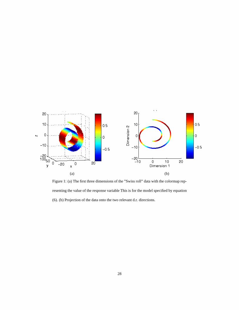
Example 1. Swiss roll

The first example illustrates how we can capture a nonlinear predictive manifold

using a linear projection. This data set called the “Swiss roll” data (Roweis and Saul,

2000) is commonly used in manifold learning. The following model is used to gen-

erate the10 dimensional covariates and response variable. The first three covariate

dimensions are given by

X1 = t cos t, X2 = 21h, X3 = t sin t,

wheret = 3π2

(1 + 2θ), θ ∼ Uniform[0, 1] andh ∼ Uniform[0, 1]. The remaining7

dimensions ofX are draws from independent standard Gaussian noise.

14

To illustrate how a linear projection can caption a nonlinear manifold, let us con-

sider a response variable taking the following form

Y = sin(5πθ) + ǫ, (6)

where we set the noise asǫ ∼ N(0, 0.12). The d.r. space is the two dimensional

subspace spanned byX1 andX3. Note that the predictive nonlinear manifold is one

dimensional but two coordinates are required to capture this one dimension. As shown

in Figure 1, the covariates can be projected into the two d.r.directions and still capture

information on the regression function,

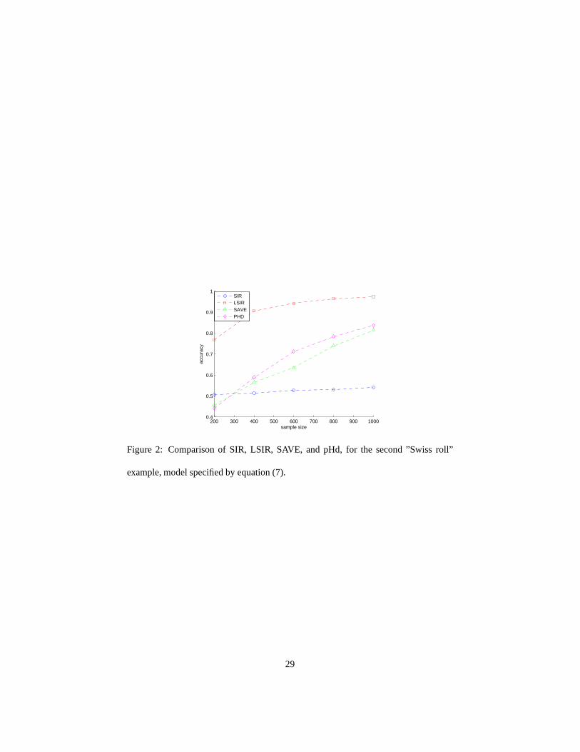
To compare the performance of LSIR with SIR, SAVE, and pHd we used a more

complicated regression model

Y = sin(5πθ) + h2 + ǫ. (7)

We randomly drewn = {200, 400, 600, 800, 1000} samples from the above model.

We computed the d.r. directions for each method and computedthe accuracy using

the comparison metric above. As can be seen in Figure 2, LSIR outperforms the other

methods. SAVE and pHd outperform SIR which is not designed for nonlinear man-

ifolds. For LSIR and SIR we set the number of slicesH and the number of nearest

neighborsk as(5, 5) for n = 200, (10, 10) for n = 400, and(10, 15) for other cases,

all parameter settings were obtained using cross validation.

Example 2. (Tai Chi)

The Tai Chi figure is well known in East Asian culture where theconcepts of Yin-

Yang provide the intellectual framework for much of ancientChinese scientific de-

velopment Ebrey (1993). A 6-dimensional data set for this example is generated as

15

follows: X1 andX2 are from the Tai Chi structure as shown in Figure 3(a) where the

Yin and Yang regions are assigned class labelsY = −1 andY = 1, respectively. The

remaining dimensionsX3, . . . , X6 are independent Gaussian random noise.

The Tai Chi data set was used as a dimension reduction examplein (Li, 2000,

Chapter 14) before. The correct d.r. subspaceB here is span(e1, e2). SIR, SAVE and

pHd are known to fail for this example. By taking the local structure into account, LSIR

can easily retrieve the relevant directions. Following Li (2000), we generaten = 1000

samples as the training data, then run LSIR withk = 10 and repeat this100 times. The

average accuracy is98.6% and the result from one run is shown in Figure 3.

As a fairer comparison we also applied LFDA to this example. The average esti-

mation accuracy is82% which is much better than SIR, SAVE and pHd, but still worse

than LSIR.

As pointed out by Li (2000), the major difference between Yinand Yang is roughly

along the directione1 +e2. The difference along the second directione1−e2 is subtle.

Li (2000) suggested using SIR to identify the first directionand then using SIR-II to

identify the second direction by slicing the data based on the value of bothy and the

projection onto the first direction. LSIR recovers the two directions directly.

4.1.3 Semi-supervised learning

We illustrate the efficacy of the semi-supervised setting with a classification problem

with ten dimensions where the d.r. directions are the first two dimensions and the

remaining eight dimensions are Gaussian noise. The data in the first two relevant di-

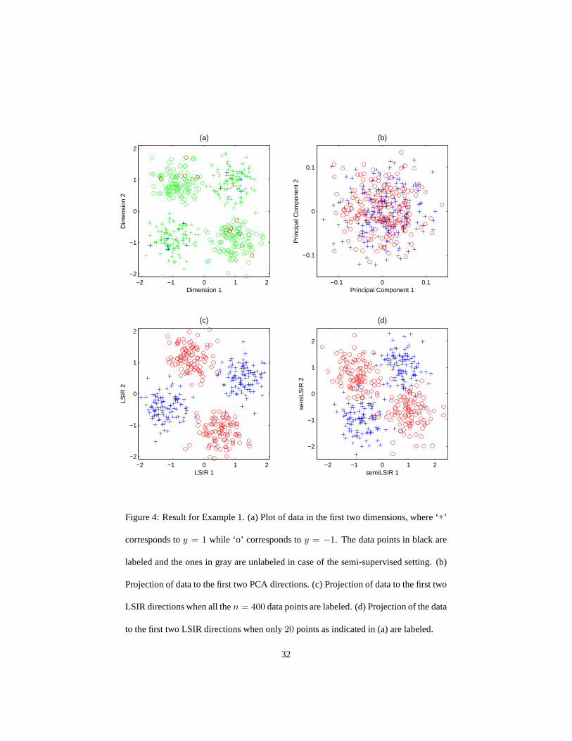
mensions have the structure of an exclusive-or, see Figure 4(a). In this example SIR

16

cannot identify the two d.r. directions because the group averages of the two groups

are roughly the same for the first two dimensions, due to symmetry. Using local aver-

ages instead of group average, LSIR can find both directions,see Figure 4(c). In this

case SAVE and pHd can also capture the two groups since the higher-order moments

capture differences between the groups.

We generated a semi-supervised data set by drawing400 samples, see Figure 4(a),

and labeling20 of the400 samples,10 from each group. The projection of the data us-

ing the top two principal components computed using al the data does not separate the

classes, see Figure 4(b). Including label information should provide this information.

To illustrate the advantage of a semi-supervised approach we evaluate the accuracy

of the semi-supervised version of LSIR with two supervised methods SAVE and pHd

which use only the labeled data. In Table 1 we report the average accuracy and standard

error of twenty independent draws of the data using the procedure stated above. For

one draw of the data we plot the labeled points in Figure 4(a) and the projection onto

the top two LSIR directions in Figure 4(c). These results clearly indicate that LSIR

out-performs the other two supervised dimension reductionmethods.

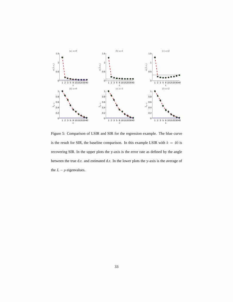
4.1.4 Regression: the effect of k

The following regression model is used to illustrate the effect ofk and to compare SIR

and LSIR. Consider a regression model

Y = X31 − aeX2

1/2 + ε, X1, . . . , X10

iid∼ N(0, 1), ε ∼ N(0, 0.1).

The d.r. direction is the first coordinatee1. SIR can easily identify this direction when

a is very small. However asa increases, the second term which is a symmetric function

17

becomes dominant and the performance of SIR deteriorates.

We first study the effect of the choice ofk whena varies. We drawn = 400 samples

that are split intoh = 10 slices with each slice containing40 samples. We measure the

error by the angle between the true d.r. direction and the estimateβ, which is denoted

by α(β, e1), smaller angles correspond to lower error. The averaged errors from1000

runs are shown in Figure 5 (a-c) wherek ranges from1 to 40 anda = {0, 1, 2}. When

k > 1, the estimatesβ from LSIR are very close to the true d.r. direction. When

a = 0 which is the case favoring SIR, we can see the errors from LSIRdecrease ask

increases since LSIR withk = 40 is identical to SIR. Whena = 1, the results from

SIR and LSIR agree for a wide range ofk. But whena = 2, LSIR outperforms SIR.

Next we study how the choice ofk influences the estimate of the number of d.r.

directions. In Figure 5 (d-f) we plot the change of the mean ofthe smallest (p − L)

eigenvalues (theoretically this should be0)

λp−L =1

p − L

p∑

i=L+1

λi

with respect to the choice ofk asa varies. Recall that in SIRλp−L is asymptoticallyχ2

and can be used to test the number of d.r. directions (Li, 1991). In LSIR the smallest

eigenvalues may not be0 and λp−L no longer follows a scaledχ2 distribution due

localization. We do not consider this as a serious drawback.Since cross-validation or

permutation procedures can be used to infer the number of d.r. directions. Also, most

learning algorithms are sensitive to the accuracy of the d.r. directions but very stable to

the addition of1 or 2 noisy directions.

18

4.2 Real data

4.2.1 Digit recognition

The MNIST data set (Y. LeCun,http://yann.lecun.com/exdb/mnist/), contains60, 000

images of handwritten digits{0, 1, 2, ..., 9} as training data and10, 000 images as test

data. Each image consists ofp = 28× 28 = 784 gray-scale pixel intensities. This data

set is commonly believed to have strong nonlinear structures.

In our analysis, we randomly sampled1000 images (100 samples for each digit)

as training data. We applied LSIR and computedd = 20 e.d.r. directions. We then

projected the training data and10000 sample test data onto these directions. Using a

k-nearest neighbor classifier withk = 5 to classify the test data, we report the classi-

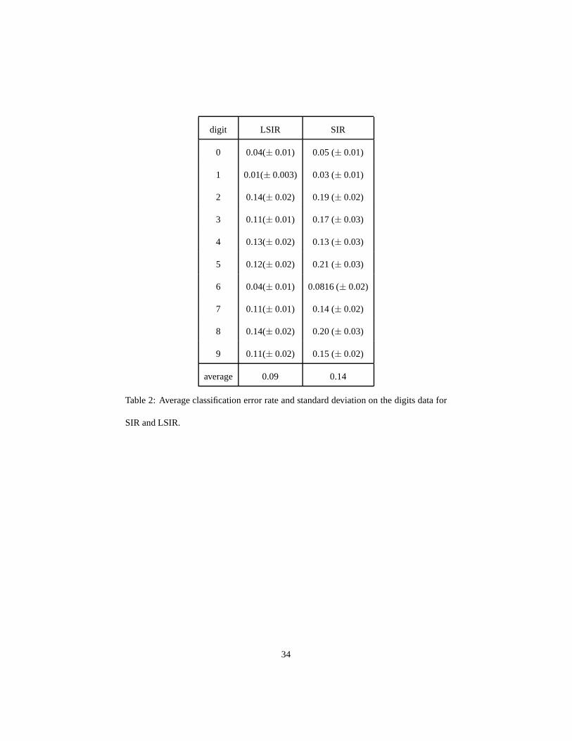
fication error over100 iterations in Table 2. For comparison we also report the classi-

fication error rate using SIR. Increasing the number of d.r. directions improves classi-

fication accuracy for almost all digits. The improvement fordigits2, 3, 5, 8 is rather

significant. The overall average accuracy for LSIR is comparable with many nonlinear

methods.

4.2.2 Gene expression data

We use a common gene expression classification data set to apply the method in the

largep smalln setting and illustrate that the method can capture structure correspond-

ing to subclasses. The leukemia data in Golub et al. (1999) consists of gene expres-

sion assays from7, 129 genes or expressed sequence tags (ests) over72 patients with

leukemia. This data has been used extensively to evaluate a variety of machine learning

and statistical methods and was explored in the context of dimension reduction in Bura

19

and Pfeiffer (2005); Chiaromonte and Martinelli (2002). This data was split into a test

set of34 samples and a training set of38 samples. In this problemp = 7129 and for the

training setn = 34. Each patient had one of two types of leukemia acute lymphoblastic

leukemia (ALL) or acute myeloid leukemia (AML). Lymphoblastic leukemia is char-

acterized by excess of lymphoblasts and myeloid leukemia iscancer of the myeloid

blood cell lines. The ALL category can be further subdividedinto two subsets: the

B-cell ALL and T-cell ALL samples. We used only the ALL-AML categorization in

our analysis. The relevance of this data was to illustrate that the two types of caner

can be accurately predicted using machine learning approaches, a problem of practical

clinical relevance. Error rates on the test set using commonmachine learning methods

such as support vector machines (SVMs) range from zero to two.

LSIR and SIR were run on the training data with no preprocessing. The shrinkage

approach described in Section 2.4 was used for both SIR and LSIR due to rank defi-

ciency. A wide range of values for the regularization parameterλ resulted in a test error

of zero or one on the test data using a variety of classifiers, such askNN, and one or

two d.r. directions. The projected subspace for LSIR was insensitive to the regulariza-

tion parameter as was the projective subspace for SIR over a wide range of parameter

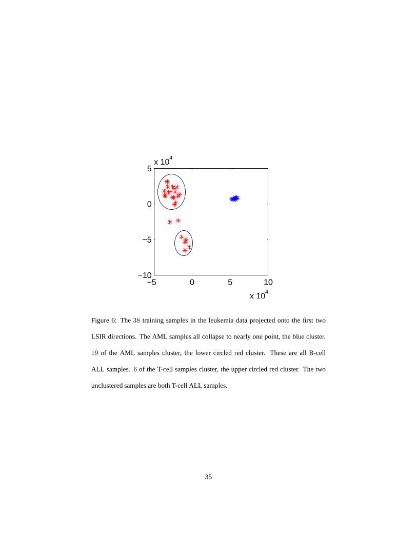
settings. LSIR is able to capture subclass structure while SIR is not. In Figure 6 we

show the projection of the training data onto the first two LSIR directions. The AML

samples all collapse to nearly one point. Of the27 ALL samples19 form one cluster,6

form another cluster, and two samples do not not fall into either. The19 sample cluster

are all B-cell AML cases, the6 sample cluster are all T-cell AML cases, and the two

unclustered samples are T-cell ALL.

20

This is a small data set and the reason the accuracy of LSIR andSIR are similar

is that there are not enough samples such that the nonlinear information captured by

LSIR offers a predictive advantage. However, it is interesting that even is such an

underpowered data set LSIR is able to suggest subclass structure. This suggests the use

of LSIR as a discovery tool.

5 Discussion

LSIR incorporates local information to extend the classic SIR procedure alleviating

many of the degeneracy problems in SIR and increasing accuracy, especially when the

data has underlying nonlinear structure. LSIR can also identify sub-cluster structure.

LSIR extends naturally to the semi-supervised setting. A regularization parameter is

added for computational stability.

LSIR allows us to bridge PCA and SIR by varying the degree of localization, con-

trolled by the number ofk nearest neighbors. The influence of the choice ofk is subtle.

In cases where SIR works well,k should be chosen to be large so that LSIR performs

similar to SIR. Conversely, in case where SIR does not work well, small values ofk

result in better results. A better theoretical understanding of the method is of interest

including a rigorous analysis of the effect ofk.

Recently there has been an increasing interest in extendinglinear dimension reduc-

tion methods to kernel models (Wu, 2008; Fukumizu et al., 2008) to realize nonlinear

dimension reduction. Since the computation of LSIR involves only inner products be-

tween data points, it is straightforward to extend LSIR to operate on a reproducing

21

kernel Hilbert space with the inner product replaced by a kernel functionK(xi, xj).

This may also be of computational advantage even in the case of the linear kernel since

the eigen-decomposition will be on matrices that aren×n rather thanp×p. However,

from the perspective of inference we are skeptical of an additional advantage a kernel

offers since the LSIR directions already extract local information on a nonlinear man-

ifold. In addition, using a nonlinear kernel results in lossof interpretation of the d.r.

directions in terms of the explanatory variables.

Appendix. LSIR and PCA

Here we show that the regularized version of LSIR realizes PCA with k = 1. Recall

that Γloc = Σ whenk = 1. The generalized eigen-decomposition problem for LSIR

becomes

Σβ = λ(Σ + sI)β. (8)

Denote the singular decomposition ofΣ by UDUT whereD = diag(di)pi=1

. Then (8)

becomes

UDUT β = λU(D + sI)UT β,

which is equivalent to solve

Dγ = λ(D + sI)γ

with γ = UT β. Sinced/(d + s) is increasing with respect tod for anys > 0, it is

easy to see that thei-th eigenvectorβi is given by theith column ofU which is theith

principal component.

22

References

Adcock, R. (1878). A problem in least squares.The Analyst 5, 53–54.

Belkin, M. and P. Niyogi (2003). Laplacian eigenmaps for dimensionality reduction

and data representation.Neural Computation 15(6), 1373–1396.

Bura, E. and R. M. Pfeiffer (2005). Graphical methods for class prediction using

dimension reduction techniques on DNA microarray data.Bioinformatics 19(10),

1252–1258.

Chiaromonte, F. and J. Martinelli (2002). Dimension reduction strategies for analyzing

global gene expression data with a response.Math’l Biosciences 176(1), 123–144.

Cook, R. (2007). Fisher lecture: Dimension reduction in regression. Statistical Sci-

ence 22(1), 1–26.

Cook, R. and L. Ni (2006). Using intra-slice covariances forimproved estimation of

the central subspace in regression.Biometrika 93(1), 65–74.

Cook, R. and S. Weisberg (1991). Disussion of li (1991).J. Amer. Statist. Assoc. 86,

328–332.

Cook, R. and X. Yin (2001). Dimension reduction and visualization in discriminant

analysis (with discussion).Aust. N. Z. J. Stat. 43(2), 147–199.

Donoho, D. and C. Grimes (2003). Hessian eigenmaps: new locally linear embedding

techniques for highdimensional data.PNAS 100, 5591–5596.

23

Duan, N. and K. Li (1991). Slicing regression: a link-free regression method.Ann.

Stat. 19(2), 505–530.

Ebrey, P. (1993).Chinese Civilization: A sourceboook. New York: Free Press.

Edegworth, F. (1884). On the reduction of observations.Philosophical Magazine,

135–141.

Fisher, R. (1922). On the mathematical foundations of theoretical statistics.Philosoph-

ical Transactions of the Royal Statistical Society A 222, 309–368.

Fukumizu, K., F. Bach, and M. Jordan (2003). Kernel dimensionality reduction for

supervised learning. InAdvances in Neural Information Processing Systems 16.

Fukumizu, K., F. Bach, and M. Jordan (2005). Dimensionalityreduction in super-

vised learning with reproducing kernel Hilbert spaces.Journal of Machine Learning

Research 5, 73–99.

Fukumizu, K., F. R. Bach, and M. I. Jordan (2008). Kernel dimension reduction in

regression.Ann. Statist.. to appear.

Globerson, A. and S. Roweis (2006). Metric learning by collapsing classes. In Y. Weiss,

B. Scholkopf, and J. Platt (Eds.),Advances in Neural Information Processing Sys-

tems 18, pp. 451–458. Cambridge, MA: MIT Press.

Goldberger, J., S. Roweis, G. Hinton, and R. Salakhutdinov (2005). Neighbourhood

component analysis. InAdvances in Neural Information Processing Systems 17, pp.

513–520.

24

Golub, T., D. Slonim, P. Tamayo, C. Huard, M. Gaasenbeek, J. Mesirov, H. Coller,

M. Loh, J. Downing, M. Caligiuri, C. Bloomfield, and E. Lander(1999). Molecular

classification of cancer: class discovery and class prediction by gene expression

monitoring.Science 286, 531–537.

Hastie, T. and R. Tibshirani (1996). Discrminant adaptive nearest neighbor classifi-

cation. IEEE Transacations on Pattern Analysis and Machine Intelligence 18(6),

607–616.

Hotelling, H. (1933). Analysis of a complex of statistical variables in principal com-

ponents.Journal of Educational Psychology 24, 417–441.

Li, B., H. Zha, and F. Chiaromonte (2004). Linear contour learning: A method for

supervised dimension reduction. pp. 346–356. UAI.

Li, K. (1991). Sliced inverse regression for dimension reduction (with discussion).J.

Amer. Statist. Assoc. 86, 316–342.

Li, K. C. (1992). On principal hessian directions for data visulization and dimension

reduction: another application of stein’s lemma.J. Amer. Statist. Assoc. 87, 1025–

1039.

Li, K. C. (2000). High dimensional data analysis via the sir/phd approach.

Li, L., R. Cook, and C.-L. Tsai (2007). Partial inverse regression. Biometrika 94,

615–625.

Li, L. and X. Yin (2008). Sliced inverse regression with regularizations.Biometrics 64,

124–131.

25

Martin-Merino, M. and J. Roman (2006). A new semi-supervised dimension reduction

technique for textual data analysis. InIntelligent Data Engineering and Automated

Learning.

Mukherjee, S. and Q. Wu (2006). Estimation of gradients and coordinate covariation

in classification.J. Mach. Learn. Res. 7, 2481–2514.

Mukherjee, S., Q. Wu, and D.-X. Zhou (2009). Learning gradients and feature selection

on manifolds.

Mukherjee, S. and D. Zhou (2006). Learning coordinate covariances via gradients.J.

Mach. Learn. Res. 7, 519–549.

Nilsson, J., F. Sha, and M. Jordan (2007). Regression on manifolds using kernel di-

mension reduction. InProceedings of the 24th International Conference on Machine

Learning.

Roweis, S. and L. Saul (2000). Nonlinear dimensionality reduction by locally linear

embedding.Science 290, 2323–2326.

Schafer, J. and K. Strimmer (2005). An empirical Bayes approach to inferring large-

scale gene association networks.Bioinformatics 21(6), 754–764.

Sugiyama, M. (2007). Dimension reduction of multimodal labeled data by local fisher

discriminatn analysis.Journal of Machine Learning Research 8, 1027–1061.

Tenenbaum, J., V. de Silva, and J. Langford (2000). A global geometric framework for

nonlinear dimensionality reduction.Science 290, 2319–2323.

26

Tokdar, S., Y. Zhu, and J. Ghosh (2008). A bayesian implementation of sufficient

dimension reduction in regression. Technical report, Purdue Univ.

Vlassis, N., Y. Motomura, and B. Krose (2001). Supervised dimension reduction of

intrinsically low-dimensional data.Neural Computation, 191–215.

Wu, H.-M. (2008). Kernel sliced inverse regression with applications on classification.

Journal of Computational and Graphical Statistics 7(3), 590–610.

Wu, Q., J. Guinney, M. Maggioni, and S. Mukherjee (2007). Learning gradients: Pre-

dictive models that infer geometry and dependence. Technical Report 07, Duke

University.

Wu, Q., F. Liang, and S. Mukherjee (2007). Regularized sliced inverse regression for

kernel models. Technical report, ISDS Discussion Paper, Duke University.

Xia, Y., H. Tong, W. Li, and L.-X. Zhu (2002). An adaptive estimation of dimension

reduction space.Journal of the Royal Statistical Society Series B 64(3), 363–410.

Young, G. (1941). Maximum likelihood estimation and factoranalysis. Psychome-

trika 6, 49–53.

Zhong, W., P. Zeng, P. Ma, J. S. Liu, and Y. Zhu (2005). RSIR: regularized sliced

inverse regression for motif discovery.Bioinformatics 21(22), 4169–4175.

27

(a) (b)

Figure 1: (a) The first three dimensions of the ”Swiss roll” data with the colormap rep-

resenting the value of the response variable This is for the model specified by equation

(6). (b) Projection of the data onto the two relevant d.r. directions.

28

200 300 400 500 600 700 800 900 10000.4

0.5

0.6

0.7

0.8

0.9

1

sample size

accu

racy

SIRLSIRSAVEPHD

Figure 2: Comparison of SIR, LSIR, SAVE, and pHd, for the second ”Swiss roll”

example, model specified by equation (7).

29

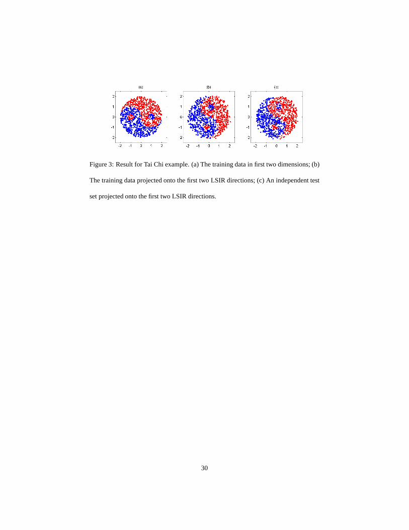
Figure 3: Result for Tai Chi example. (a) The training data infirst two dimensions; (b)

The training data projected onto the first two LSIR directions; (c) An independent test

set projected onto the first two LSIR directions.

30

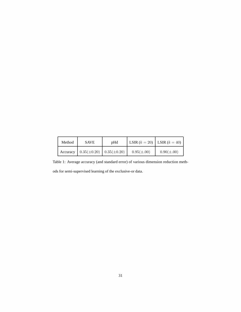
Method SAVE pHd LSIR (k = 20) LSIR (k = 40)

Accuracy 0.35(±0.20) 0.35(±0.20) 0.95(±.00) 0.90(±.00)

Table 1: Average accuracy (and standard error) of various dimension reduction meth-

ods for semi-supervised learning of the exclusive-or data.

31

−2 −1 0 1 2−2

−1

0

1

2

Dimension 1

Dim

ensi

on 2

(a)

−0.1 0 0.1

−0.1

0

0.1

Principal Component 1P

rinci

pal C

ompo

nent

2

(b)

−2 −1 0 1 2−2

−1

0

1

2

LSIR 1

LSIR

2

(c)

−2 −1 0 1 2

−2

−1

0

1

2

semiLSIR 1

sem

iLS

IR 2

(d)

Figure 4: Result for Example 1. (a) Plot of data in the first twodimensions, where ‘+’

corresponds toy = 1 while ‘o’ corresponds toy = −1. The data points in black are

labeled and the ones in gray are unlabeled in case of the semi-supervised setting. (b)

Projection of data to the first two PCA directions. (c) Projection of data to the first two

LSIR directions when all then = 400 data points are labeled. (d) Projection of the data

to the first two LSIR directions when only20 points as indicated in (a) are labeled.

32

1 2 3 5 8 10152030400

0.5

1

1.5(a) a=0

k

α(β

,e 1

)

1 2 3 5 8 10152030400

0.2

0.4

0.6

0.8

1(d) a=0

k

λp−

L

1 2 3 5 8 10152030400

0.5

1

1.5(b) a=1

k

α(β

,e 1

)

1 2 3 5 8 10152030400

0.2

0.4

0.6

0.8

1(e) a=1

k

λp−

L

1 2 3 5 8 10152030400

0.5

1

1.5(c) a=2

k

α(β

,e 1

)

1 2 3 5 8 10152030400

0.2

0.4

0.6

0.8

1(f) a=2

k

λp−

L

Figure 5: Comparison of LSIR and SIR for the regression example. The blue curve

is the result for SIR, the baseline comparison. In this example LSIR with k = 40 is

recovering SIR. In the upper plots the y-axis is the error rate as defined by the angle

between the true d.r. and estimated d.r. In the lower plots the y-axis is the average of

theL − p eigenvalues.

33

digit LSIR SIR

0 0.04(± 0.01) 0.05 (± 0.01)

1 0.01(± 0.003) 0.03 (± 0.01)

2 0.14(± 0.02) 0.19 (± 0.02)

3 0.11(± 0.01) 0.17 (± 0.03)

4 0.13(± 0.02) 0.13 (± 0.03)

5 0.12(± 0.02) 0.21 (± 0.03)

6 0.04(± 0.01) 0.0816 (± 0.02)

7 0.11(± 0.01) 0.14 (± 0.02)

8 0.14(± 0.02) 0.20 (± 0.03)

9 0.11(± 0.02) 0.15 (± 0.02)

average 0.09 0.14

Table 2: Average classification error rate and standard deviation on the digits data for

SIR and LSIR.

34

−5 0 5 10

x 104

−10

−5

0

5x 10

4

Figure 6: The38 training samples in the leukemia data projected onto the first two

LSIR directions. The AML samples all collapse to nearly one point, the blue cluster.

19 of the AML samples cluster, the lower circled red cluster. These are all B-cell

ALL samples.6 of the T-cell samples cluster, the upper circled red cluster. The two

unclustered samples are both T-cell ALL samples.

35