Wright State University Wright State University

CORE Scholar CORE Scholar

Browse all Theses and Dissertations Theses and Dissertations

2016

Locally Optimized Covariance Kriging for Non-stationary System Locally Optimized Covariance Kriging for Non-stationary System

Responses Responses

Daniel Lee Clark Jr. Wright State University

Follow this and additional works at: https://corescholar.libraries.wright.edu/etd_all

Part of the Mechanical Engineering Commons

Repository Citation Repository Citation Clark, Daniel Lee Jr., "Locally Optimized Covariance Kriging for Non-stationary System Responses" (2016). Browse all Theses and Dissertations. 1502. https://corescholar.libraries.wright.edu/etd_all/1502

This Thesis is brought to you for free and open access by the Theses and Dissertations at CORE Scholar. It has been accepted for inclusion in Browse all Theses and Dissertations by an authorized administrator of CORE Scholar. For more information, please contact library-corescholar@wright.edu.

Locally Optimized Covariance Kriging forNon-Stationary System Responses

A thesis submitted in partial fulfillmentof the requirements for the degree of

Master of Science in Engineering

by

Daniel L. Clark, Jr.B.S.M.E., Wright State University, 2014

2016Wright State University

Wright State UniversitySCHOOL OF GRADUATE STUDIES

May 24, 2016

I HEREBY RECOMMEND THAT THE THESIS PREPARED UNDER MY SUPER-VISION BY Daniel L. Clark, Jr. ENTITLED Locally Optimized Covariance Kriging forNon-Stationary System Responses BE ACCEPTED IN PARTIAL FULFILLMENT OFTHE REQUIREMENTS FOR THE DEGREE OF Master of Science in Engineering.

Ha-Rok Bae, Ph.D.Thesis Director

George P. Huang, Ph.D.Chair, Department of Mechanical and

Materials Engineering

Committee onFinal Examination

Ha-Rok Bae, Ph.D.

Ramana V. Grandhi, Ph.D.

Joseph C. Slater, Ph.D., P.E.

Robert E.W. Fyffe, Ph.D.Dean, School of Graduate Studies

ABSTRACT

Clark, Jr., Daniel. M.S.Egr., Department of Mechanical and Materials Engineering, Wright StateUniversity, 2016. Locally Optimized Covariance Kriging for Non-Stationary System Responses.

In this thesis, the Locally-Optimized Covariance (LOC) Kriging method is developed.

This method represents a flexible surrogate modeling approach for approximating a non-

stationary Kriging covariance structures for deterministic responses. The non-stationary

covariance structure is approximated by aggregating multiple stationary localities. The

aforementioned localities are determined to be statistically significant utilizing the Non-

Stationary Identification Test. This methodology is applied to various demonstration prob-

lems including simple one and two-dimensional analytical cases, a deterministic fatigue

and creep life model, and a five-dimensional fluid-structural interaction problem. The

practical significance of LOC-Kriging is discussed in detail and is directly compared to

stationary Kriging considering computational cost and accuracy.

iii

Contents

1 Introduction 1

2 Background Theory 32.1 Design Optimization . . . . . . . . . . . . . . . . . . . . . . . . . . . . . 32.2 Surrogate Models . . . . . . . . . . . . . . . . . . . . . . . . . . . . . . . 7

2.2.1 Design of Experiments . . . . . . . . . . . . . . . . . . . . . . . . 82.2.2 Regression Analysis . . . . . . . . . . . . . . . . . . . . . . . . . 112.2.3 Gaussian Process Modeling . . . . . . . . . . . . . . . . . . . . . 142.2.4 Regression Kriging . . . . . . . . . . . . . . . . . . . . . . . . . . 19

2.3 Research Contribution . . . . . . . . . . . . . . . . . . . . . . . . . . . . 21

3 Non-Stationary Surrogate Modeling 223.1 Literature Review . . . . . . . . . . . . . . . . . . . . . . . . . . . . . . . 25

3.1.1 Geostatistics Development . . . . . . . . . . . . . . . . . . . . . . 253.1.2 Engineering Development . . . . . . . . . . . . . . . . . . . . . . 27

3.2 Summary . . . . . . . . . . . . . . . . . . . . . . . . . . . . . . . . . . . 28

4 Locally-Optimized Covariance Kriging 294.1 Formulation . . . . . . . . . . . . . . . . . . . . . . . . . . . . . . . . . . 29

4.1.1 Kriging Model with Locally-Optimized Covariance . . . . . . . . . 294.1.2 Local Window Size Optimization . . . . . . . . . . . . . . . . . . 314.1.3 Construction and Aggregation of Multiple Local Kriging Models . 334.1.4 Imposing Physics on LOC-Kriging . . . . . . . . . . . . . . . . . 34

4.2 Non-stationary Identification Test . . . . . . . . . . . . . . . . . . . . . . 354.3 Demonstation . . . . . . . . . . . . . . . . . . . . . . . . . . . . . . . . . 40

4.3.1 One-Dimensional Example . . . . . . . . . . . . . . . . . . . . . . 414.3.2 Two-Dimensional Example . . . . . . . . . . . . . . . . . . . . . . 454.3.3 Ti-6242S Fatigue and Creep Coupled Numerical Experiment . . . . 504.3.4 Five-Dimensional Fluid Structural Interaction Example . . . . . . . 57

4.4 Summary . . . . . . . . . . . . . . . . . . . . . . . . . . . . . . . . . . . 63

5 Summary and Future Work 65

iv

Bibliography 68

v

List of Figures

2.1 Design Optimization Process . . . . . . . . . . . . . . . . . . . . . . . . . 42.2 Local Optimal Solutions . . . . . . . . . . . . . . . . . . . . . . . . . . . 72.3 Factorial Design Schemes . . . . . . . . . . . . . . . . . . . . . . . . . . . 92.4 Latin Hypercube Sampling . . . . . . . . . . . . . . . . . . . . . . . . . . 102.5 Regression Models . . . . . . . . . . . . . . . . . . . . . . . . . . . . . . 142.6 Gaussian Correlation Function . . . . . . . . . . . . . . . . . . . . . . . . 162.7 Kriging Response Decomposition . . . . . . . . . . . . . . . . . . . . . . 182.8 Regression Kriging Response Decomposition . . . . . . . . . . . . . . . . 202.9 Example Regression Kriging Response . . . . . . . . . . . . . . . . . . . 20

3.1 Adaptive One-Dimensional Stationary Kriging Response . . . . . . . . . . 243.2 Even One-Dimensional Stationary Kriging Response . . . . . . . . . . . . 243.3 Moving Window Kriging . . . . . . . . . . . . . . . . . . . . . . . . . . . 263.4 Nonlinear Mapping Approach . . . . . . . . . . . . . . . . . . . . . . . . 28

4.1 LOC Window Membership function . . . . . . . . . . . . . . . . . . . . . 304.2 LOC Window Aggregation Membership Function . . . . . . . . . . . . . . 344.3 Non-stationary Identification Test Outline . . . . . . . . . . . . . . . . . . 364.4 Voronoi Test Points With Contour . . . . . . . . . . . . . . . . . . . . . . 374.5 Linear Regression Model . . . . . . . . . . . . . . . . . . . . . . . . . . . 384.6 Initial Localities . . . . . . . . . . . . . . . . . . . . . . . . . . . . . . . . 394.7 Four Identified Localities . . . . . . . . . . . . . . . . . . . . . . . . . . . 404.8 1-D LOC-Kriging Predictions . . . . . . . . . . . . . . . . . . . . . . . . 424.9 1-D Comparison of Methods . . . . . . . . . . . . . . . . . . . . . . . . . 424.10 1-D Convergence Histories . . . . . . . . . . . . . . . . . . . . . . . . . . 454.11 2-D Adaptively Collected Data . . . . . . . . . . . . . . . . . . . . . . . . 464.12 2-D Over-plot and Contour, Stationary Kriging . . . . . . . . . . . . . . . 474.13 Upper and Lower Estimated Error Bounds, Stationary . . . . . . . . . . . . 474.14 2-D LOC-Kriging Models . . . . . . . . . . . . . . . . . . . . . . . . . . 484.15 2-D Over-plot and Contour, LOC-Kriging . . . . . . . . . . . . . . . . . . 494.16 Upper and Lower Estimated Error Bounds, LOC-Kriging . . . . . . . . . . 504.17 HTV-3X Aircraft Frame . . . . . . . . . . . . . . . . . . . . . . . . . . . 524.18 Loading Scenario . . . . . . . . . . . . . . . . . . . . . . . . . . . . . . . 52

vi

4.19 Analytical Life Model . . . . . . . . . . . . . . . . . . . . . . . . . . . . . 544.20 Over-plot and Contour, Stationary Kriging . . . . . . . . . . . . . . . . . . 554.21 Over-plot and Contour, LOC-Kriging. . . . . . . . . . . . . . . . . . . . . 574.22 Computational Domain and Coarse C-Grid . . . . . . . . . . . . . . . . . 594.23 CFD Convergence Histories . . . . . . . . . . . . . . . . . . . . . . . . . 604.24 Sting Mounted Airfoil . . . . . . . . . . . . . . . . . . . . . . . . . . . . . 604.25 FSI Two-Dimensional True Response Surfaces . . . . . . . . . . . . . . . 614.26 FSI One-Dimensional Slice . . . . . . . . . . . . . . . . . . . . . . . . . . 63

5.1 Modified Regression Kriging Response . . . . . . . . . . . . . . . . . . . 66

vii

List of Tables

4.1 1-D Performance Comparison . . . . . . . . . . . . . . . . . . . . . . . . 444.2 1-D Computational Times . . . . . . . . . . . . . . . . . . . . . . . . . . 444.3 2-D Performance Comparison . . . . . . . . . . . . . . . . . . . . . . . . 494.4 2-D Computational Times . . . . . . . . . . . . . . . . . . . . . . . . . . 494.5 Life Model Performance Comparison . . . . . . . . . . . . . . . . . . . . 564.6 Life Model Computational Times . . . . . . . . . . . . . . . . . . . . . . . 564.7 Design Parameters and Ranges . . . . . . . . . . . . . . . . . . . . . . . . 614.8 FSI Performance Comparison . . . . . . . . . . . . . . . . . . . . . . . . . 624.9 FSI Computational Times . . . . . . . . . . . . . . . . . . . . . . . . . . . 63

viii

AcknowledgmentsI would like to take this opportunity to extend my thanks to Dr. Ha-Rok Bae for his men-

toring and guidance throughout my graduate studies. The opportunities and experience I

obtained as his graduate student has allowed me to grow as a person, researcher, and an

academic. Dr. Ha-Rok Bae installed in me the confidence to pursue my Ph.D. at Wright

State University.

None of the research presented herein would have been possible if it were not for the

support and funding from Drs. Ravi Penmetsa and Edwin Forrester from the Air Force

Research Laboratory (AFRL).

Additionally, I would like to extend my gratitude to two more individuals, Dr. Ramana

Grandhi and Dr. Joseph Slater, who took the time to evaluate this thesis. I am grateful for

their willingness to help and be a part of my final examination committee.

Finally, I would like to thank the members of Dr. Ramana Grandhi’s research group, CE-

PRO, Ohio Center of Excellence for Product Reliability and Optimization. Their support

was invaluable in both my research and course work. I specifically would like to thank

Koorosh Gobal for his expertise in developing the fluid-structural interaction problem used

in this thesis.

ix

Dedicated to My Parents.

x

Introduction

The increasing scale and complexity of computer simulations have significantly prolifer-

ated the computational cost of performing design exploration in both academic and indus-

trial applications. Typical explorations include design optimization, database construction,

and reliability-based design optimization. To alleviate the computational burden, various

surrogate models, also known as response surface models or metamodels, are considered

for approximating large scale and complex engineering simulations. Generally, surrogate

models are constructed with a limited number of training points [1][2][3][4][5][6]. Among

the many different surrogate models, Kriging has gained its popularity due to high accuracy

and flexibility representing non-linear system responses [7][8]. Kriging has many different

formulations including: Regression Kriging[9], Gradient-Enhanced Kriging[10], Dynamic

Kriging[11], and Stochastic Kriging[12].

Essentially, Kriging produces an optimal interpolation by combining both the trend re-

gression and the realization of a local random process modeled by an optimized covariance

structure. One of the benefits of Kriging is the expected Mean Square Error (MSE) calcu-

lated along with a response prediction at any location of interest. This unique benefit of the

MSE is not present in Response Surface Method (RSM) or Radial Basis Functions (RBF)

and this is why RSM and RBF are not investigated along side Kriging. The MSE is typically

viewed as model uncertainty due to lack of training data points. Therefore, it is utilized in

numerous global surrogate optimization strategies. In the Efficient Global Optimization

(EGO) method [8], the expected improvement is defined as a function of MSE and a cur-

1

rent minimum response. MSE plays a key role to deploy adaptive data points sequentially

in EGO. The Efficient Global Reliability Analysis (EGRA)[13] also uses EGO to construct

an adaptive Kriging model of a limit state boundary function for efficient reliability assess-

ment. The Multiple Surrogate Efficient Global Optimization (MSEGO) method[14] uses

MSE from Kriging as a universal uncertainty estimate for other types of surrogate models.

Thus, an accurate representation of both the estimated response and the MSE are critical in

many methodologies.

To more accurately predict the response of deterministic systems the proposed Locally-

Optimized Covariance (LOC) Kriging methodology approximates a non-stationary covari-

ance matrix. The approximation is accomplished through the use of local surrogate models.

The surrogate locations can either be predefined or found through a statistical significance

test. Once the initial sizes and locations are established, the sizes are optimized and aggre-

gated. The use of localities allows for a more accurate representation of local fluctuations

in response. Therefore, the MSE is also represented more accurately in both situations:

more data is needed or sufficient data was collected.

The remainder of this thesis is organized as follows. In Chapter 2, background theory

is presented for design optimization, surrogate modeling and the primary contribution of

this thesis is discussed. A brief literature review is then discussed in Chapter 3 concerning

past contributions in the fields of geostatistics and engineering addressing non-stationary

surrogate modeling. The Locally-Optimized Covariance Kriging methodology is then de-

scribed in detail with numerical examples in Chapter 4. The thesis is concluded with a brief

discussion of future work and applications.

2

Background Theory

Based on the Introduction in Chapter 1, the importance of surrogate models for large scale

problems is established to decrease computational cost. However, where, when and how

to implement these approximation techniques has yet to be addressed in the thesis. In

this chapter, a clear indication of where and when surrogate models are utilized in design

optimization is defined. From there, gradient based design optimization methodologies

are discussed. This discussion is essential to establish the importance of continuity and

local behaviors of a surrogate model. Then, three common stationary surrogate modeling

techniques are presented including Regression Modeling, Gaussian Process Modeling, and

Regression Kriging. First, the standard Design Optimization process is discussed in the

context of a structural optimization problem.

2.1 Design Optimization

The design optimization framework that is introduced in this chapter is based on the typical

process for structural optimization. An illustration of this process is given in Fig. 2.1. The

process begins by selecting an initial design or configuration of the system. The system’s

performance is then evaluated by an objective function and a set of constraints that the

design must satisfy while minimizing the objective. The objective function and constraints

are typically evaluated utilizing commercial finite element analysis (FEA) software such

as Ansys, Abaqus, or Nastran. Sensitivity or gradient information can be extracted using

3

finite difference methods or determined analytically. However, for each gradient extracted

an additional run is required, increasing computational cost at each iteration. The gradient

information is then used as an input for the selected optimization algorithm to find the next

design. This process is repeated until the objective function converges.

Figure 2.1: Design Optimization Process. Standard structural design optimization pro-cess. Figure 4.1 from reference [15]

An important consideration in the design optimization process is construction the ob-

jective and constraints. Traditionally, the mass of the structure is minimized while con-

straints are placed on displacements, natural frequencies, stresses, or a combination of the

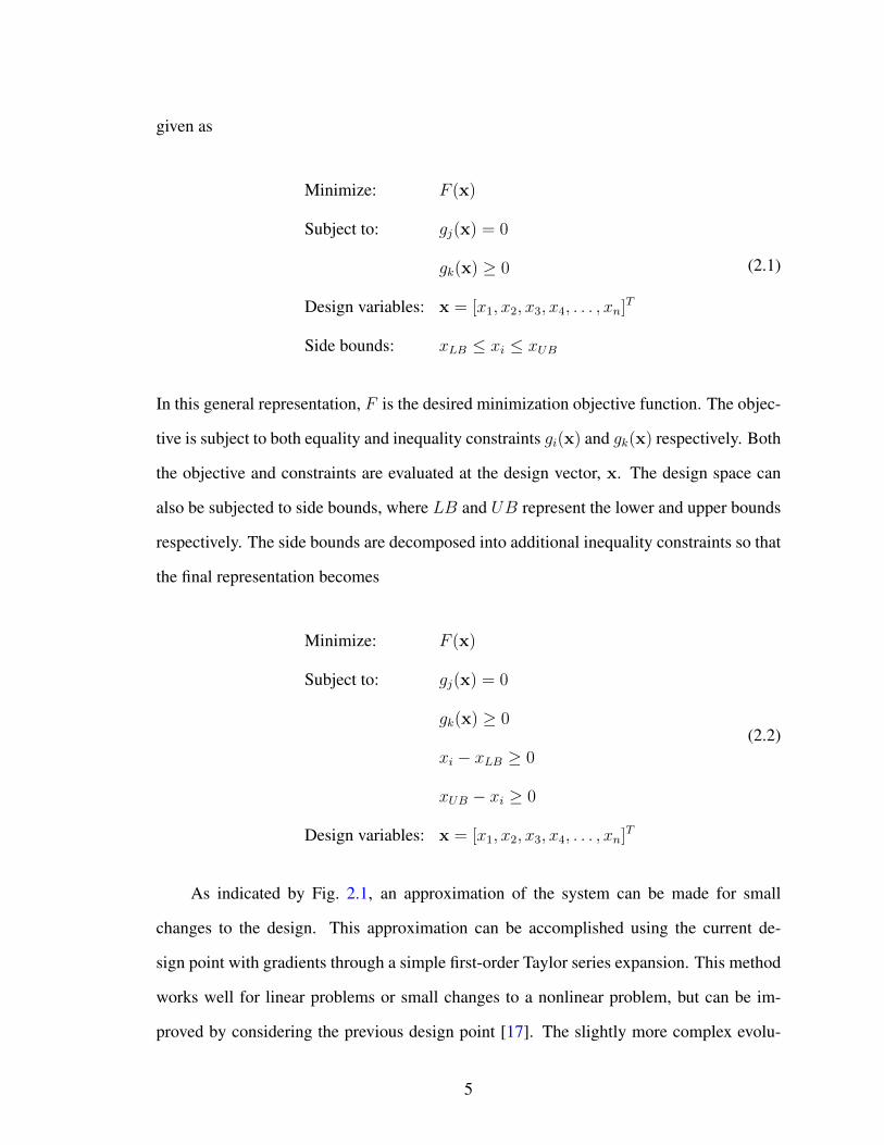
three. The standard mathematical optimization formulation for a structural problem [16] is

4

given as

Minimize: F (x)

Subject to: gj(x) = 0

gk(x) ≥ 0

Design variables: x = [x1, x2, x3, x4, . . . , xn]T

Side bounds: xLB ≤ xi ≤ xUB

(2.1)

In this general representation, F is the desired minimization objective function. The objec-

tive is subject to both equality and inequality constraints gi(x) and gk(x) respectively. Both

the objective and constraints are evaluated at the design vector, x. The design space can

also be subjected to side bounds, where LB and UB represent the lower and upper bounds

respectively. The side bounds are decomposed into additional inequality constraints so that

the final representation becomes

Minimize: F (x)

Subject to: gj(x) = 0

gk(x) ≥ 0

xi − xLB ≥ 0

xUB − xi ≥ 0

Design variables: x = [x1, x2, x3, x4, . . . , xn]T

(2.2)

As indicated by Fig. 2.1, an approximation of the system can be made for small

changes to the design. This approximation can be accomplished using the current de-

sign point with gradients through a simple first-order Taylor series expansion. This method

works well for linear problems or small changes to a nonlinear problem, but can be im-

proved by considering the previous design point [17]. The slightly more complex evolu-

5

tion, the two-point function approximations, are advantageous during gradient based design

optimization because more information is being leveraged in the iterative process where

gradients are already required for the algorithm. However, the two-point approximations

rely on optimally finding the nonlinearity index. This optimization may fail, causing a miss

representation of the response.

Another option is to approximate the entire system or small subsections of the de-

sign space. By selecting a strategic design of experiments (DOE), the objective function,

and constraints can be approximated at every untried location in the domain of interest.

Depending on the desired approximation method, gradients can also be evaluated at the

sample points but are not always necessary. Once the FEA model is evaluated at all of the

DOE points and the approximation model built, the entire loop of Fig. 2.1 can be evaluated

with approximate analytical equations. It is considered good practice to evaluate the true

FEA model at the approximated optimal design variables to ensure the approximation is

accurate and none of the constraints are violated. If a violation occurs, the approximation

is rebuilt with the additional design point causing the optimization algorithm to avoid the

previous optimal location. This process is then repeated until an optimal is found that does

not violate the constraints.

Approximating the entire system and creating an approximate problem both have their

merits. However, for general design exploration, approximating the entire system utilizing

a surrogate model is further developed. In this case, both global and gradient optimization

algorithms can be utilized. In this thesis, gradient algorithms are illustrated in further detail

due to their speed and reduced computational cost in optimization.

In Fig. 2.2, a theoretical objective function, f(x), is evaluated from xε[−2.5, 3]. If

this objective function is initially evaluated to the left or right of x = 0 the optimal solution

will be different due to the gradient information acquired at the point. For illustration

purposes, four initial points and gradients are shown in gray and red respectively. Points 1

and 2 will lead a gradient algorithm to a local optimum whereas points 3 and 4 will yield a

6

global optimum for the domain. Because potential situations like these exist it is important

to consider multiple initial points when optimizing. This process of selecting multiple

starting locations is indicative of a global method, section of initial points is not covered in

this thesis. However, the effect of local fluctuations of the response on the optimal solution

should be considered when selecting a surrogate model.

x-3 -2 -1 0 1 2 3 4

f(x)

-50

0

50

100

150

200

1

23

4

Objective FunctionInitial PointGradient

Figure 2.2: Local Optimal Solutions. Gradient information is collected at four initialpoints leading to two different optimal solutions.

Many advanced surrogate modeling techniques can introduce nonphysical changes in

the response where there is a lack of information. This can cause the optimizer to select

sub-optimal solutions. However, with the process of design optimization well defined, the

general formulation established, and possibility of local optimal solutions acknowledged,

techniques for surrogate modeling are now presented.

2.2 Surrogate Models

Approximating computer and experimental data is always advantageous when large quan-

tities of data are necessary to perform the analysis. This can be because of cost or time

constraints. Nevertheless, surrogate models fulfill this need. Surrogate models are char-

7

acterized by the method in which they attempt to fit the data they are applied to. The

data is assumed to have a functional relationship between measured variables (indepen-

dent variables) and predicted variables (dependent variables). Typically two categories are

considered, interpolation and extrapolation methods. Interpolation methods are utilized

to construct new data points within the range of collected data and should never be ap-

plied outside of the range of the original data due to inaccuracies. Extrapolation methods

estimate new data points based on the perceived trend of the collected data. However,

utilization of either method requires a sample data set before construction.

Before introducing Regression Analysis (extrapolation method), Gaussian Process

Modeling (interpolation method) and Regression Kriging (hybrid method), the concept of

Design of Experiments is presented. This method allows for the intelligent selection of

sampling points for the construction of a desired surrogate model with an optimal number

of samples.

2.2.1 Design of Experiments

Data collection should always be performed as efficiently as possible to avoid additional

time and cost. For this reason, various Design of Experiment (DOE) methods have been

established. Typically, these methods are dependent on the type of model that is fitted

to the data. The advantage of DOE methods is their direct utilization of the system to

obtain approximate mathematical solutions of the problem even in cases where the system

equations cannot be solved easily. The following descriptions clarify the basic limitations

of two basic sampling methods: Latin Hypercube Sampling (LHS) and Factorial Design.

The simplest of the two DOE methods is the Factorial Design.

Factorial Designs come in many forms including fractional and full factorial designs.

The most basic design is the 2k Full factorial design. Where 2 indicates the number of

levels and k, the number of design variables. 2k designs are typically used early on in the

design process to detect simple relationships between the inputs and the system response.

8

The primary limitation being the design’s fitting capabilities. With two levels, typically

denoted as [−1, 1], per design variable, only a simple linear model can be applied to the

system.

When higher order models are desired more points are required. The simplest method

is to add a center point to the design space in the form of a point [0, 0] for a two-dimensional

case. This can be used to check for curvature of the system, however, to approximate more

coefficients a more complex design is required. For this case, a 3k design can be used to

approximate the additional coefficients by mixing the center point with the previous two

levels. Figure 2.3 demonstrates the evolution of the experiment from a 2k design, to a

2k design with a center point, to a 3k design. This process works for an N dimensional

system. However, as the number of design variables increases, the computational cost rises

exponentially due the strict structure of the samples.

x1 Levels

-1 0 1

x2 L

evels

-1

0

1

2k Design

2k with Center point

3k Design

Figure 2.3: Factorial Design Schemes. Starting with a 2k design, additional points can beadded in a sequential sequence to approximate

To combat the computational cost of multiple level Factual Designs and high dimen-

sionally, Latin Hypercube Sampling (LHS) is utilized. LHS design is a stratified sampling

technique, i.e. both space-filling and guarantees non-overlapping designs. For LHS designs

without perturbations from the grid center locations, the total number of possible outcomes

9

can be defined as

(M−1∏n=0

(M − n)

)N−1

= (M !)N−1 (2.3)

where M is the number of sample points and N is the dimensionality of the problem.

LHS can be carried out with numerous criterion including maximization of the minimum

distance between points (MaxMin) and minimization of the potential correlation between

points. Both methods are illustrated in Fig. 2.4. The correlation reduction criterion for

LHS designs can be shown to be the minimization of the sum of between-column squared

correlations after performing ranked Gram-Schmidt step to orthogonalize the sample loca-

tions. In this case, the perturbations from the grid center locations are zero. This lack of

perturbation is evident in Fig. 2.4.

x1 Levels

0 0.1 0.3 0.5 0.7 0.9 1

x2 L

eve

ls

0

0.1

0.3

0.5

0.7

0.9

1

(a) Reduce Correlation

x1 Levels

0 0.1 0.3 0.5 0.7 0.9 1

x2 L

eve

ls

0

0.1

0.3

0.5

0.7

0.9

1

(b) Maximize the Minimum Distance

Figure 2.4: Latin Hypercube Sampling. LHS of the same domain with different criterion.

In order to perform the MaxMin case the distances between points must be defined.

This is accomplished as

ρp (si, sj) =

[Nd∑k=1

|si,k − sj,k|p] 1

p

(2.4)

10

where ρp is the distance measure of the pth order between points si and sj , (j 6= i), and Nd

is the dimensionality of s. When the distance is Euclidean, p = 2. And p = 1 represents

rectangular distance. The optimization formulation for determining a sampling plan is

defined as

Find: Dsf

maximize: minxεD [ρp (xi − xj)](2.5)

With two popular sampling methods defined, regression analysis can be introduced in

the following section. It is important to consider the deterministic nature of the simulations

investigated in this thesis. In this context, regressions are structured so that the data is

actually interpolated. This requires either high order terms or structuring the regression to

match the DOE.

2.2.2 Regression Analysis

In many engineering systems, two or more design variables are inherently related. The

investigation of the functional relationship between the design variables is the fundamental

idea behind regression analysis. Regression analysis can be characterized by two types:

linear and nonlinear. If the relationship between the dependent variable and the indepen-

dent variables can be characterized by a linear combination of some parameters, the model

is referred to as linear; otherwise, it is called nonlinear. The typical form of regression anal-

ysis is known as the least squares method. This technique minimizes the sum of squares of

the residuals to find the best fit.

First consider the equation of a linear regression model

y(x) = β0 + β1f1(x) + ...+ βkfk(x) + ε (2.6)

11

where βi, i = 0, 1, 2, ..., k, are the regression coefficients and ε is the model error, assumed

to be normally distributed with a zero mean and variance σ2e . Equation 2.6 is often written

in matrix notation for n sample values of x and y as

Y = Fβ + ε (2.7)

In expanded form Eq. 2.7 becomes

y1

y2...

yn

=

1 f1(x1) f2(x1) · · · fk(x1)

1 f1(x2) f2(x2) · · · fk(x2)

......

... . . . ...

1 f1(xn) f2(xn) · · · fk(xn)

β1

β2...

βn

+

ε1

ε2...

εn

(2.8)

The method of least squares is used to obtain the regression coefficients as

β =(F TF

)−1F TY (2.9)

The fitted model is typically represented as

Y = Fβ (2.10)

with residuals

e = Y − Y (2.11)

The residuals can be used to assess the quality of the regression’s fit. The nonlinear repre-

sentation is not significantly different from Eq. 2.6. The linear regression of a polynomial

12

model of a one-dimensional case can be written as

y(x) = β0p0(x) + β1p1(x) + · · ·+ βmpm(x) + ε (2.12)

where the degree of pi(x) is i = 0, · · · ,m and the polynomial approximation is of order m

for this case. The simplest polynomial model consists of monomials xm. This regression

model can also be solved using Eq. 2.9. This time the F matrix is written as

F =

p0(x1) p1(x1) p2(x1) · · · pm(x1)

p0(x2) p1(x2) p2(x2) · · · pm(x2)

......

... . . . ...

p0(xn) p1(xn) p2(xn) · · · pm(xn)

(2.13)

where p0(x) = 1, p1(x) = x, · · · , pm(x) = xm. An important issue is to determine the

order of polynomials. High-order polynomials can be utilized to closely fit sets of data, but

the high-order model are generally less accurate between DOE points. This also means,

when utilized in a gradient optimization technique, there is the potential to become stuck at

a local optimum.The significance of a regression model can be accessed through the uses of

ANalysis of VAriance (ANOVA). ANOVA utilizes the residuals as well as other statistical

means to assess the lack of fit and confidence of the predicted response. When assessed

iteratively, the model can be reduced based on the significance of the coefficients.

13

x0 1 2 3 4 5

f(x)

2

4

6

8

10

12

14

16

18

True SystemSamplesLinear Regression

(a) Linear Regression

x0 1 2 3 4 5

f(x)

-4

-3

-2

-1

0

1

2

3

4

True SystemSamplesQuadratic Regression

(b) Nonlinear Regression

Figure 2.5: Regression Models. The models are applied to appropriate data sets with noiseto illustrate their fitting behaviors.

Due to the deterministic nature of most computer simulations, regression models allow

for quick and simple approximates or in some cases exact replications of the system if the

underlying physics is well understood. With the combination of DOE, regression models

can also act as an interpolation scheme with an optimal number of samples based on the

order of the model. However, many systems have highly nonlinear responses. Given a large

DOE, regression models can fit the previously mention pneumonia, but it quickly becomes

computationally expensive. Therefore, more advanced methods are explored.

2.2.3 Gaussian Process Modeling

Unlike the regression models, Gaussian Process Models are always an interpolation model.

Kriging is a special case of the Gaussian Process Model. In the standard Kriging model,

the response at locations x are estimated by the combination of the global trend (linear or

non-linear regression) and realization of a stochastic process (fit of the regression error),

Eq. 2.14.

y(x) = m(x) + z(x) (2.14)

14

Here, the global trend function, is the same as Eq. 2.7. For completeness, the global trend

is rewritten as

m(x) = Fβ (2.15)

where F is a user-selected basis function vector, and an unknown regression coefficient

vector, β, obtained from the generalized least-squares method. The stochastic process,

z(x), describes localized deviations with zero mean and a covariance structure as

COV [z(si), z(sj)] = σ2R(θk, si, sj, pk) (2.16)

where σ2 is the process variation and R is the correlation function between the two sample

data points, si and sj , with the correlation parameter vectors, θ and p. θk can be thought of

as the activeness of the function whereas pk is the function smoothness for the kth design

space dimension [8]. The correlation function can be selected from a collection of various

function forms. The Gaussian function is often used in engineering applications and defines

each element of the correlation matrix as

R(θ,p, si, sj) = corr(si, sj) =

Nd∏k=1

exp (−θkdpkk ) (2.17)

whereNd is the parameter dimension and dk = si,k−sj,k is the distance between the sample

points, si and sj in the kth dimensional direction, and pk is defined as 2. To demonstrate

the effect of the activeness parameter on the correlation function, θ, Fig. 2.6 is presented.

From the plot, there is an inverse relationship between θ and correlation length, i.e. as θ

becomes smaller the correlation length becomes larger.

15

Figure 2.6: Gaussian Correlation Function. The correlation function is shown with vari-ous activeness parameters.

With the individual elements of the correlation matrix defined and θ characterized, the

correlation matrix between samples becomes

R =

∏Nd

k=1 exp (−θk|s1,k − s1,k|2) · · ·∏Nd

k=1 exp (−θk|s1,k − sn,k|2)... . . . ...∏Nd

k=1 exp (−θk|sn,k − s1,k|2) · · ·∏Nd

k=1 exp (−θk|sn,k − sn,k|2)

(2.18)

The values for θ are determined by maximizing the likelihood of the samples described by

Eq. 2.19 over θ > 0.

L(β, σ2

)=

1

(2π)n2 (2σ2)

n2 |R| 12

exp

[−(y − 1β)TR−1(y − 1β)

2σ2

](2.19)

Based on the generalized least square regression, the regression coefficient vector is found

by Eq. 2.20 while minimizing the mean squared error defined by Eq. 2.21.

β =(FTR−1F

)−1FTR−1y (2.20)

16

φ(s) = E[(y(s)− y(s))2

](2.21)

Here, y and y are the samples and predicted response vectors respectively. The estimate of

the variance from the global trend is obtained by

σ2 =1

n

(y − Fβ

)TR−1

(y − Fβ

)(2.22)

where, n is the number of sample points. When Eq.’s 2.20 and 2.22 are substituted into Eq.

2.19 the result is the so-called ’concentrated likelihood function’. This simplifies to Eq.

2.23. In this study, the optimization of the correlation parameter is performed by a Design

of Experiments-based optimization. To obtain the optimum solution in a robust way, an ad-

vanced tailored optimization method such as generalized pattern search algorithm [18], can

be used. Typically, it is assumed that the underlying function behavior is stationary within

the exploration space of interest. Thus, the same correlation function is applied over the

entire exploration space to predict the function behavior. However, if this assumption is vi-

olated unnecessary fluctuations and over-amplifications of both the response and expected

mean squared error predictions are introduced. This violation is explored and addressed in

detail in the following chapter.

Minimize Φ(θ) = −1

2ln(|R|)− n

2ln(σ2) (2.23)

Now that θ is found the Kriging prediction can be obtained at x with Eq. 2.24. Where

r is the correlation between estimation points x and sample points s.

y = Fβ + rTR−1(y − Fβ

)(2.24)

Equation 2.24 is in the same form as Eq. 2.14. The first term, Fβ, represents the regression

17

model, and the second term, rTR−1(y − Fβ

), is the fit of the regression error. To illus-

trate this, Fig. 2.7 decomposes the two processes into separate response before combining

them. The line touching the second data point in 2.7a represents the error, or distance from

the regression at point two. Figure 2.7b shows that the error or the distance to the points

are fitted with a continuous function, resulting in 2.7c.

(a) Regression Component (b) Stochastic Component

(c) Total Response

Figure 2.7: Kriging Response Decomposition.

As demonstrated, Kriging produces an interpolation of the supplied sample points.

However, some computer simulations may have a significant amount of noise due to con-

vergence or various run time errors. Therefore, regression models may better approximate

the true surface. A compromise between the traditional regression modeling techniques

and Kriging is Regression Kriging.

18

2.2.4 Regression Kriging

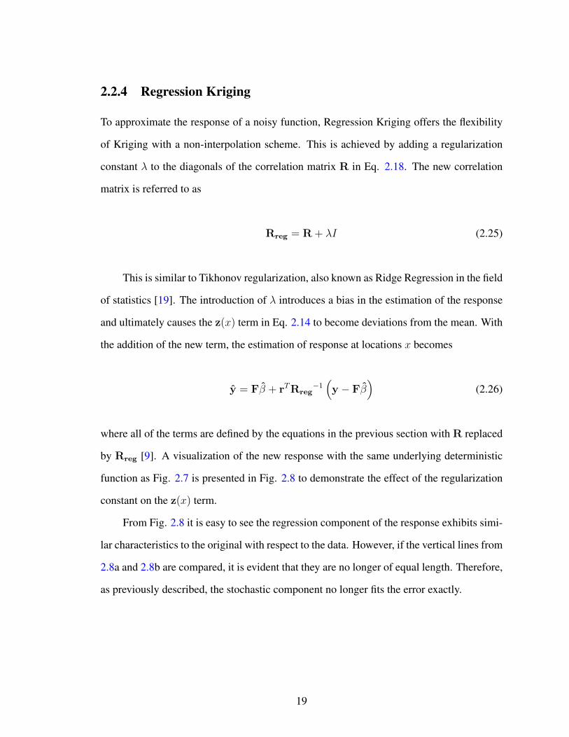
To approximate the response of a noisy function, Regression Kriging offers the flexibility

of Kriging with a non-interpolation scheme. This is achieved by adding a regularization

constant λ to the diagonals of the correlation matrix R in Eq. 2.18. The new correlation

matrix is referred to as

Rreg = R + λI (2.25)

This is similar to Tikhonov regularization, also known as Ridge Regression in the field

of statistics [19]. The introduction of λ introduces a bias in the estimation of the response

and ultimately causes the z(x) term in Eq. 2.14 to become deviations from the mean. With

the addition of the new term, the estimation of response at locations x becomes

y = Fβ + rTRreg−1(y − Fβ

)(2.26)

where all of the terms are defined by the equations in the previous section with R replaced

by Rreg [9]. A visualization of the new response with the same underlying deterministic

function as Fig. 2.7 is presented in Fig. 2.8 to demonstrate the effect of the regularization

constant on the z(x) term.

From Fig. 2.8 it is easy to see the regression component of the response exhibits simi-

lar characteristics to the original with respect to the data. However, if the vertical lines from

2.8a and 2.8b are compared, it is evident that they are no longer of equal length. Therefore,

as previously described, the stochastic component no longer fits the error exactly.

19

(a) Regression Component (b) Stochastic Component

(c) Total Response

Figure 2.8: Regression Kriging Response Decomposition.

(a) 20 Sample Points (b) 200 Sample Points

Figure 2.9: Example Regression Kriging Response.

Regression Kriging adds simple flexibility to the traditional Kriging formulation. How-

ever, Regression Kriging’s expected mean-squared error does not perform as one might

20

expect. Figure 2.9 illustrates the collapse of the MSE (gray bounds) around the predicted

mean response (red line). In turn, the MSE becomes highly nonconservative of the true

three standard deviation bounds (green bounds) of the true response (black line) constructed

from the dotted samples. Regression Kriging also trends to the global regression outside

of the data fitted by the stochastic process. Therefore, Regression Kriging’s ability to ex-

trapolate is similar to Kriging. The implications of the Regression Kriging formation will

be discussed further with a potential application in the proposed methodology in the Future

Work section.

An additional shortcoming of both the typical Kriging formulation and the Regression

Kriging formulation is their inabilities to predict non-stationary mean responses and data

with non-stationary variation in the case of Regression Kriging. This can become detri-

mental in many engineering applications. In Chapter 3 non-stationary surrogate models

from both the engineering and geostatistical communities are discussed in detail.

2.3 Research Contribution

To remove the stationary response assumption from the Kriging framework, a new flexi-

ble and efficient framework was developed in this research. The new framework is called

Locally Optimized Covariance Kriging (LOC-Kriging). The LOC-Kriging methodology

approximates a non-stationary covariance structure by using multiple stationary covariance

structures optimized for local function behaviors. Eliminating the need for the stationary

response assumption. This work also resulted in an original Non-Stationary Identifica-

tion Test capable of identifying localities of a NS covariance structure for deterministic re-

sponses. The possibility and realization of a physics based Kriging is also explored through

the uses of a weighting function and the LOC-Kriging framework. This work also resulted

in two American Institute of Aeronautic and Astronautic (AIAA) conferences papers [20]

[21] and one AIAA journal article [22].

21

Non-Stationary Surrogate Modeling

In this chapter, the various methods to address modeling of non-stationary responses with

surrogate models are discussed and demonstrated. However, first it is necessary to define a

stationary response. In the context of this document, a stationary response for a determinis-

tic computer simulation is defined as a response where the frequency of fluctuations do not

change drastically or suddenly over the spatial domain. For a non-deterministic response,

stationarity is defined as a stochastic process whose joint probability distribution does not

change with time. Kriging specifically utilizes a stationary assumption when constructing

its covariance structure. Violation of this assumption is discussed in detail in the following

paragraphs.

Typically, the mean-squared-error (MSE) calculation performed in Kriging is esti-

mated with a stationary covariance structure that is a distance correlation among samples.

It is expected that the function being predicted has consistent or stationary fluctuations

within the domain of interest. Therefore, a trend function and a stochastic random pro-

cess with a single correlation function are applied to predict the underlying function. In

most engineering applications, the correlation is typically modeled with a Gaussian func-

tion. To characterize the correlation among the sample data, the hyperparameters of the

correlation function are optimized using the maximum likelihood approach along each di-

mension. Recently, to address the challenges of the maximum likelihood approach in find-

ing model parameters the Generalized Pattern Search algorithm [18] (GPS) and Penalized

Log-Likelihood function [23] (PLL) have been developed. However, hyperparameter op-

22

timization will likely fail to find a true optimum for a non-stationary function; in fact, the

hyperparameter, if found, will be inadequate to capture non-stationary behaviors, resulting

in inaccurate predictions and amplified mean square error estimations.

When there are a large number of samples, stationary Kriging can address non-stationary

behaviors with increased computational costs. However, with an insufficient number of

samples, Kriging may fail to find a globally well-fitted stationary covariance structure for

a non-stationary function. This malfunction can be significantly amplified when data is

scattered unevenly as a result of an adaptive sampling technique that is often used in engi-

neering design exploration. In Figs. 3.1 and 3.2, a moderately non-stationary true function

[18] is approximated with 17 adaptive samples and 17 uniform samples utilizing stationary

Kriging. The stationary Kriging model utilizes the same Gaussian correlation function and

a second-order polynomial global trend function as Xiongs demonstration of this function

[18]. The MSE with ±3σ is calculated with an optimized stationary covariance structure

and over-plotted to represent an unbiased uncertainty. It is noted the Kriging expected

Mean Square Error (MSE) calculated with evenly collected samples produces a type-II

statistical error, shown in Fig. 3.2. The Kriging prediction would miss the true function be-

havior within the low input range (input < 0.3) where the true function shows a relatively

high-frequency behavior.

23

Input0 0.2 0.4 0.6 0.8 1

Re

sp

on

se

-1.2

-0.8

-0.4

0

0.4

0.8

1.2

± 3σY

true

YKriging

Data

Figure 3.1: Adaptive One-Dimensional Stationary Kriging Response.

Input0 0.2 0.4 0.6 0.8 1

Re

sp

on

se

-1.2

-0.8

-0.4

0

0.4

0.8

1.2

± 3σY

true

YKriging

Data

Figure 3.2: Even One-Dimensional Stationary Kriging Response.

Typically, more samples are needed to capture the rapidly changing system response

of some functions. Figure 3.1 demonstrates an adaptive sampling process where more

24

samples are deployed within the low input range. For this function, the hyperparameter of

the stationary covariance structure is heavily influenced by the data tightly clustered in the

low input range. As a result, the Kriging model produces high fluctuations of the predicted

response and severe amplification of the MSE within the high input range (input > 0.4)

shown in Fig. 3.1.

From this example, it is clear the stationary covariance assumption could be inade-

quate to capture transitional non-stationary system behavior due to its introduction of un-

necessary fluctuations and over-amplifications of both the response and MSE predictions.

This can be generalized for all instances where the response is non-stationary. To address

this, many Non-Stationary (NS) methods were proposed by researchers, especially in the

fields of geostatistics and environmental processes. Both their work and research developed

in the field of engineering are presented in the following section.

3.1 Literature Review

Both the geostatistics and environmental processes, and engineering communities have

contributed significantly to the development of Non-Stationary (NS) methods. However,

due to the dimensionality of their respective problems, they face significantly different

challenges. Therefore, the solutions posed by each community are presented separately.

The methods developed by the geostatistics community are presented first because they

were generally developed first.

3.1.1 Geostatistics Development

For simple NS structures, the geostatistics community offers a verity of methods. Isaaks

and Srivastaya suggested a direct implementation method accomplished by using locally

varying sills [24]. This method fails to capture the non-stationary behavior of complex and

25

varying structures. Sampson and Guttorp [25] proposed a nonlinear transformation method

to obtain an approximate stationary covariance structure. This transformation method can

be sensitive to variance values and provide poor or unstable predictions especially with a

complex and multimodal non-stationary system.

Haas developed Moving Window Kriging (MWK) [26]. MWK is a method in which

a covariance structure is constructed within a circular neighborhood centering at an esti-

mation point where a previous global DOE was constructed. Figure 3.3 is an illustration

of MWK. As the prediction region moves though the design space an optimal local vari-

ogram or semivariogram structure is constructed and are formed under the local stationary

assumption. The optimal size of the moving window is determined by model bias statistics

such as root-mean-squared error (RMSE) and confidence bounds.

Figure 3.3: Moving Window Kriging. Figure 1 from the Environmental Systems ResearchInstitute, Inc. website [27] .

Harris [28] proposed a geographically weighted variogram (GWV) MWK to smooth

the individual variograms by using a kernel function with an optimal inverse distance-

weighting scheme. Since an optimal window size and a new covariance are calculated as the

prediction location moves through the space, the computational cost of the method could

be prohibitive for high dimensional problems. Most of the proposed methods mentioned

from the geostatistics community were aimed at situations where a significant number of

26

samples are available within a low-dimensional design space. Therefore, they are not well

suited for large-scale, high-dimensional engineering design exploration.

3.1.2 Engineering Development

For engineering design applications, Lin, et al.[29] proposed the Sequential Exploratory

Experimental Design (SEED) in which the entries of the covariance matrix are adjusted

by using the previous correlation parameter information over the course of sequential data

sampling. The main focus of their work was to optimize adaptive sampling in the SEED

process, but not to implement a NS-Kriging model. However, the method is notable in its

ability to construct NS covariance matrices.

Ba and Joseph [30] developed the Composite Gaussian Process (CGP) model, in

which two stationary Gaussian processes for global trend and local variation are used to

address non-stationary system behavior. This is accomplished by defining the input re-

gions based on the space-filling properties of data. However, the CGP model needs to

optimize a vector of hyperparameters and three unknown parameters to fit both global and

local processes. This optimization is accomplished in one sequence but requires relatively

large amounts of data. To address the difficulties with high-dimensional engineering prob-

lems, Xiong, et al.[18] adopted the nonlinear map approach to convert a NS covariance

structure into an approximated stationary structure.

Xiang’s approximation was accomplished using parameterized density function with

predefined knots or local density functions. A conceptual illustration of the nonlinear map

approach is shown in Fig. 3.4. In practice the continuous density function illustrated below

the original space, is approximated as a piecewise density function. This method can be

computationally intensive depending on the number of knots [31]. Also, the approximated

univariate density functions may become a major source of error when a density function

becomes complex with multimodal non-stationarity.

27

Figure 3.4: Nonlinear Mapping Approach. a) the original space and b) the new space.Figure 2 in reference [18].

The one-dimensional example problem developed by Xiong, et al. [18] is used as a

validation case for the method presented later in this thesis. With 8 knots, they were able to

achieve a 0.0109 RMSE error. Later it is demonstrated that Locally Optimized Covariance

Kriging produces a 0.0175 RMSE value with only 3 local models.

3.2 Summary

In summery, there are numerous ways to address responses where the frequency of fluc-

tuations changes drastically or suddenly over a domain of interest also known as non-

stationary responses. The methods range from coordinate transformations to modifications

of surrogate covariance structures. Every method has its merits in addressing NS behavior,

however, most suffer from the “curse of dimensionality”. To address this challenge, a new

flexible and efficient framework of Locally Optimized Covariance Kriging (LOC-Kriging)

is proposed. The proposed LOC-Kriging approximates a NS covariance structure by using

multiple stationary covariance structures optimized for local function behaviors. A statis-

tical test process using a set of model training points is proposed to identify localities of a

NS covariance structure. The prediction of a NS function behavior is estimated by blend-

ing multiple LOC-Krigings based on their local membership functions. In this study, it is

also discussed how the physical understanding, such as global sensitivities of the specific

system behaviors, can be implemented within the proposed framework of LOC-Kriging to

enhance engineering design exploration.

28

Locally-Optimized Covariance Kriging

4.1 Formulation

To alleviate the computational difficulties using the NS covariance structure for practi-

cal engineering application, Locally Optimized Covariance Kriging (LOC-Kriging) is pro-

posed. In this method, multiple local stationary structures are identified and used to approx-

imate the global non-stationary covariance structure. Unlike the aforementioned MWK

method, which moves a local window along with a prediction point, LOC-Kriging con-

structs a finite number of local stationary structures according to the localities of function

behaviors. The local window sizes are simultaneously optimized using an aggregated max-

imum likelihood function. The center locations of the localities can be user-defined based

on prior knowledge or identified by the proposed local statistical testing method described

in Section 4.2. The prediction of the LOC-Kriging is obtained by combining multiple local

stationary models based on an aggregation membership function.

4.1.1 Kriging Model with Locally-Optimized Covariance

In the construction of the local Kriging model, the bell-shaped membership function shown

in Fig. 4.1 is used to apply the degree of membership to samples within the identified

locality windows. This function maintains the continuity of the predicted response across

the finite local window boundaries. The samples within the range of full membership

29

have unit weightings. Over the full membership boundary, there is the transitional range

defined by αxω, where α is the scale factor of the transition range. When implemented,

membership, both full and transitional, is determined by the Euclidean distance between

the center of the window and the sample of interest. This is true for any dimensionality

because the local window is represented as a hypersphere. In this study, the Gaussian

function is used to vary the membership between unity and zero within the transition range.

In practice, any transition function can be used, such as a linear, spline, or an exponential

function depending on the desired smoothness.

Figure 4.1: LOC Window Membership Function. The range from -1 one to +1 is withinthe window, and the transitional range extends a distance proportional to the radius

With the membership weightings applied to the samples in a local window, the locally

weighted Kriging model is constructed by the generalized least square regression as

φ = E[W (s) (y(s)− y(s))2

](4.1)

where W is the diagonal matrix of the membership weights. The weighted regression

30

coefficient vector, βw is calculated using Eq.4.2.

βw =(F TR−1W F

)−1F TR−1w y (4.2)

Here Rw−1 =

(√W)T

R−1(√

W)

. The LOC-Kriging prediction, y1, at an untried

location x, is obtained as

y1 = fβw + rTwR−1w

(y − Fβw

)(4.3)

where rw =(√

W)−1

r. Utilizing the weighting membership function as described allows

the local model to maintain their interpolation behavior within the full membership. The

membership function also results in an informed extrapolation range within the scaled tails

for aggregation between local models. This decreasing weight region can also be thought of

as a fading interpolation. The following section explains how to optimize the local window

size of multiple models.

4.1.2 Local Window Size Optimization

To avoid an over-parameterization in the global regression and to minimize the finite num-

ber of the local models, the local window sizes are optimized as

Find: [ω1, ω2, . . . , ωl]T

Minimize: Φ =l∑

i=1

φi(θ)

Subject to: gi = ωi − ωmin ≥ 0

gl+1 = λ− λmin ≥ 0

gl+2 = −λ+ λmax ≥ 0

(4.4)

31

where ω is the local window size measured by the ratio between the current window and

the entire design space; ωmin is the required minimum size; Φ is the aggregated likelihood

function; λ is the global coverage parameter with user-provided upper and lower bounds,

λmin and λmax. Nominally these quantities are selected to be 01 and 0.5 respectively. With

a small quantity of data, less than five points per dimension, it is suggested to increase

λmax accordingly. The local window size ω can be viewed as a hypersphere radius in a

multidimensional problem.

In the optimization formulation, an aggregated likelihood function Φ is considered as

the objective function to capture the global fitness of the combined local covariance struc-

tures. In this study, the uniform aggregation of the local likelihood measurements is used.

However, any aggregation strategy can be implemented to reflect one’s understanding of

the underlying function behavior with a different importance scheme. The global coverage

parameter, λ, represents the amount of overlap that occurs between windows or simply

put, it is a measure of double counted/claimed sample points by multiple windows. This is

accomplished by

λ =

∑li=1Wi

lN(4.5)

where the numerator is the sum of the diagonal matrix of the membership weights Wi for

the ith model, l is the number of models, and N is the number of sample points. Like

stationary Kriging, this formulation cannot ensure the entire domain is covered with full

membership; this is only true if the sample points are representative of the domain. How-

ever, as long as the localities are statistically significant, the global coverage parameter

guarantees overlap between localities and the transitional scale factor from the previous

section ensures a smooth transition.

Any prior information or knowledge regarding the system’s local behavior can be

implemented into the minimum window size requirements. The minimum window size

32

should also be determined by considering the order of the basis function. This ensures

the total number of available samples does not result in over fitting. The upper and lower

bounds of the global coverage parameter should be selected to yield continuous transitions

across the local windows.

In this study, the interior point optimization algorithm is used to find the solution of

the optimization problem formulated in Eq. 4.4 in a reliable and efficient manner. Note

that the optimization in which local Krigings are constructed and tested can benefit from

parallel computing to maximize the computational efficiency.

4.1.3 Construction and Aggregation of Multiple Local Kriging Mod-

els

With the expectation of mutually overlapped LOC-Krigings over the entire design domain,

it is important to maintain a smooth and continuous transition across local windows. The

aggregation method used to combine the prediction of the models is essentially a weighted

average as

ya(x) =

∑li=1 yi(x)γi(x)∑l

i=1 γi(x)(4.6)

where l is the number of local models; yi is the prediction array from the ith local model,

and γi is the weight array of the local model at each prediction site. The weight of the

aggregation response is a modified version of the membership function shown in Fig. 4.1.

The full membership region is reduced by the tail factor α, decreasing the weight of the less

accurate tail region of the curve as shown in Fig. 4.2. fdsafdsasd This ensures the tails have

significantly less weight when aggregating multiple windows while maintaining a smooth

transition. When two or more full members are combined, Eq. 4.6 provides an average of

the windows. This same aggregation technique is applied to the estimated variance.

33

Figure 4.2: LOC Window Aggregation Membership Function.

4.1.4 Imposing Physics on LOC-Kriging

In the typical Kriging framework covered in Chapter 2, Kriging is composed of a trend

function and stochastic process, Eq. 2.14. If the general trend of the physical process is

known, an appropriate regression can be selected. Many physical processes have a sug-

gested trend line. For example, fatigue data, the base ten logarithm of cyclic life as a

function of stress amplitude, is typically fitted by a linear function. However, when fitted

with Kriging, the stochastic process may cause unnecessary fluctuations thus, violating the

fundamental physical behavior. Other more complex interactions such as fatigue-coupled

creep are understood to have a monotonically decreasing response while not having a closed

form regression function. Both of these cases can be addressed by relaxing the contribution

from the stochastic process causing the trend behavior to become more prominent between

training points as

yl = fβw + rTwR−1w

(y − Fβw

)δ(s,x, ζ) (4.7)

34

here, δ is the stochastic process relaxation function. This relaxation process is not possible

with traditional Kriging due to a single global trend function covering the entire domain.

However, the proposed framework of LOC-Kriging provides the necessary computational

flexibility. When the relaxation function is applied, the stochastic deviations from the local

trend for individual LOC windows are reduced. The relaxation function, δ, is formulated

in Eq. 4.8.

δ(s,x, ζ) = 1− min{||x− x||}12max{min{||si − sj||}}

(1− ζ) (4.8)

Here, the numerator of the fraction is a vector of the minimum distance between each

prediction site and all of the sample points. The denominator is a scalar of the maximum

of the minimum distances between sample points divided by two, where i 6= j, and ζ

is the optimal global relaxation parameter. The optimal global relaxation parameter is

determined to satisfy the fundamental behavior of the underlying function of interest, such

as a monotonic behavior in a fatigue model. This additional relaxation function allows

for the implementation of known physics into the Kriging framework while maintaining

Kriging’s interpolation characteristic at sample points.

4.2 Non-stationary Identification Test

Due to the increased computational cost of approximating the non-stationary covariance

structure, it is important to establish a framework to validate the additional cost. The frame-

work is divided into five sequential steps:

1. Deploy virtual test points

2. Perform user prescribed regression

3. Calculate the root-mean-squared error (RMSE) at each local regression

35

4. Perform cluster analysis on the RMSE response

5. Determine the spatial statistical significance of the clusters

The fundamental idea is that the regression will produce similar model bias statistics within

different local regions of similar nonlinearities. A basic outline of the framework used in

the two-dimensional space is defined in Fig. 4.3. This framework is critical when con-

sidering the utilization of LOC-Kriging in a high dimensional space due to its ability to

define localities. This is important because the number of localities is not dimensionally

dependent, but it is dependent on both the nature of the problem and the collected samples.

For example, a 1-D problem can have five localities whereas a 7-D problem can have four

localities.

Figure 4.3: Non-stationary Identification Test Outline. Illustrative preprocessor outlinefor the two-dimensional example with specific virtual points and regression model labeled.

The first step of the process is to deploy virtual test points between the sample points.

In this study, linearly spaced points are selected for one-dimensional space. In higher

36

dimensional space, Voronoi vertices [32] can be selected by creating a Voronoi diagram

around the sample points. The vertices can also be supplemented with another space filling

method if desired. In Fig. 4.4 the Voronoi vertices are represented by the large lightly

colored circles while the function evaluation points are small black circles. Within local

windows centering individual virtual test points, the user prescribes the local regression

models to quantify the local RMSEs.

Figure 4.4: Voronoi Test Points With Contour. Voronoi vertices used as test sites for theillustrative example with response contour and sample points.

The window of the local regression is the same for each vertex. The window size is

either user-provided or adjusted to include a minimum number of sample points for the

estimations of non-zero local RMSEs. If little is known about the system, it is suggested

that the same order regression model is utilized as the global trend function in Kriging. As

an illustrative two-dimensional example, shown in Fig. 4.5, a linear regression with the

minimum four sample points is used. One of the regression models is shown as a solid red

plane with respect to the meshed surface of the true response in Fig. 4.5a. A contour of

the local regression with its regression data points captured by the window is shown in Fig.

4.5b.

37

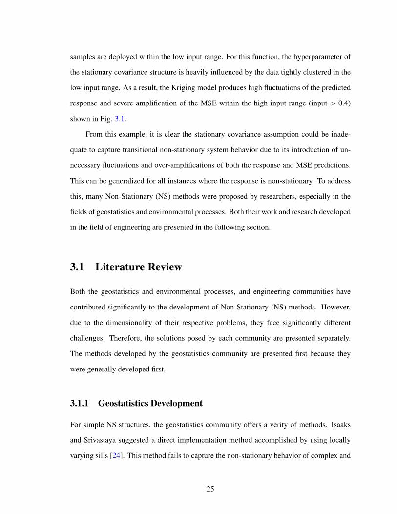
Figure 4.5: Linear Regression Model. (a) Meshed view of the red regression plane and(b) Contour of the regression with window indicated by a circle.

With the local regression model selected, the RMSE is calculated and considered as

the local stationary measurement at each Voronoi vertex or center. With the RMSE mea-

surements, the K-means [33] clustering algorithm is used to determine the locality of the

system response. The K-means clustering algorithm is a long-standing, robust, unsuper-

vised learning algorithm, capable of identifying a user defined number of clusters based on

sample distances. The vertices that make up the individual clusters are then averaged to

create center points of potential localities. The initial number of center points was assumed

to be two, indicated by stars in Fig. 4.6. The triangles and diamonds illustrate to which

cluster each point belongs.

38

Figure 4.6: Initial Localities. Two black stars identify the initial localities; diamonds andtriangles indicate points that belonging to each clusters.

The spatial coordinates of the initial center points are compared to the distribution of

the obtained cluster center points by using hypothesized mean student t-test [34] with a 95%

confidence interval. This comparison is done on a dimension-by-dimension basis, which

means the xi-coordinate of each cluster is compared to the xi-coordinates of the samples

that make up every cluster. This is then repeated for every dimension. For an example, the

matrix for the x dimension is constructed with an arbitrary number of clusters n, as

Dxi =

ttest(µ1, C1) . . . ttest(µn, C1)

... . . . ...

ttest(µ1, Cn) . . . ttest(µn, Cn)

(4.9)

where µi is the center coordinate of the ith cluster in dimension x; andCi is the x-coordinates

of samples from the ith cluster. The null hypothesis is: the mean of one window matches

the population of another. If one fails to reject the null, the test returns a 0. If the null

is rejected, i.e. the mean does not match the population of another the test returns a 1.

Non-stationary is determined to be significant if 50% or more of the total test are rejected,

this is true for each dimension. If significant, the cluster center points should be considered

to reflect the localities of the function behavior. Otherwise, a stationary Kriging model is

39

sufficient and LOC-Kriging will be constructed with a single window. If only one dimen-

sion is significant, the K-means algorithm is rerun on the spatial coordinates of the clusters.

This helps to ensure a space filling distribution of center points. However, it is possible that

the given samples do not present any non-stationary behavior. This means the results of the

proposed LOC-Kriging does depend on the given samples.

In the illustrated example in Fig. 4.6, the X1 coordinates are found to be significantly

different while the X2 coordinates were not. Therefore, the K-means algorithm is used

on the spatial coordinates of each cluster separately to ensure a space filling distribution

of center points. Figure 4.7 illustrates the four local windows indicated by large circles

centering the black stars. These four windows will be used as initial local windows in the

proposed LOC-Kriging method.

Figure 4.7: Four Identified Localities. Four black stars identify the final localities; blackand lighter diamonds, and triangles indicate points that belonging to clusters.

4.3 Demonstation

In this section, the performance of the proposed LOC-Kriging method is compared to tra-

ditional stationary Kriging through the use of representative examples of engineering ap-

plications. The basic concepts and details of LOC-Kriging are explained through the use

of a simple one-dimensional mathematical problem. Then, a two-dimensional case is pre-

40

sented to demonstrate the potential of LOC-Kriging. A fatigue and creep-testing scenario

with zero variation is presented utilizing empirical damage model equations to illustrate the

flexibility of LOC-Kriging. Lastly, a five-dimensional fluid-structure interaction problem

is presented to demonstrate the accuracy and applicability to a high-dimensional problem.

4.3.1 One-Dimensional Example

The simple one-dimensional mathematical example is given by Eq. 4.10 is considered first.

In Fig. ??a, the true response (black dot-dash line) shows a non-stationary behavior within

the x range of interest. The stationary Kriging response and estimated error bounds are

depicted with a solid red line and filled gray region respectively along with the adaptively

collected samples. By using conventional Kriging, the error bounds are unnecessarily am-

plified in the second half input range as shown in Fig. ??a. This amplification is due to

the assumption that the underlying function behavior is stationary. The regression of the

Kriging prediction is assumed to be a second order polynomial, the same as Xiong [18].

y(x) = sin(30(x− 0.9)4) cos(2(x− 0.9)) +x− 0.9

2(4.10)

Based on the process described in the previous section: a linear regression is selected

to capture the changing behavior, three K-means clusters are prescribed, and a 95% con-

fidence is selected to compare the similarities of the spatial components of the clusters.

This resulted in the identification of three local covariance structures. Their optimal range

of coverage is found by solving the optimization problem formulated in Eq. 4.4 with the

Interior-Point Algorithm. The LOC models were built in parallel during each optimization

iteration to decrease computational time. The resulting sizes of the three LOCs are shown

in Fig. 4.8. The triangles indicate the center locations of local windows, and the full mem-

bership range is identified using arrows. The three models are built using a second-order

polynomial regression and Gaussian correlation function. The models are labeled as LOC-

41

1, LOC-2, and LOC-3 in the figure. The legend is the same as Fig. ??. The three LOC

models are weighted according to their individual aggregation membership functions.

Figure 4.8: 1-D LOC Predictions. LOC-Krigings for LOC-1, 2 and 3 with correspondingranges signified via black arrows.

By aggregating the three LOC-Krigings, the approximated non-stationary Kriging pre-

diction is obtained and compared to the stationary Kriging response side by side in Fig. 4.9.

Figure 4.9 visibly demonstrates LOC-Kriging’s ability to produce more reasonable and

consistent predictions than stationary Kriging. The plot also showcases LOC-Kriging’s er-

ror bounds that match our physical understanding within both the low and high input ranges

unlike stationary Kriging. Cross-validation can be employed to access the validity of the

obtained error bounds.

Figure 4.9: 1-D Comparison of Methods. (a) Stationary Kriging and (b) AggregatedLOC-Kriging.

In this study, performance is measured using three metrics: The root-mean-square

42

error (RMSE), the maximum standard deviation of the prediction, and the integral of the

expected mean-squared error. The RMSE between the true and predicted Kriging response

is calculated as

RMSE =

√√√√ 1

N

N∑i=1

(ytrue,i − yi)2 (4.11)

where N is the total number of test data points; ytrue is the true response, and y is the

Kriging prediction. Equation 4.12 defines the improvement between the two methods as

Improvement(%) =Stationary − LOC

Stationaryx100 (4.12)

The quantitative results of the current example are summarized in Table 4.1. The

RMSE was evaluated using 4000 evenly spaced testing points. The aggregated LOC-

Kriging shows 74.10% RMSE improvement in the response prediction against the station-

ary Kriging. There is a maximum reduction of the standard deviation of 82.40% and most

notably, the integral of the MSE is reduced by almost 100%. This was achieved by relax-

ing the strong assumption of stationary covariance within the design domain and reflecting

localities of function behaviors properly. Computational wall times are presented in Table

4.2 in seconds. All simulations were performed utilizing the MATLAB on desktop PC with

an Intel Core i7-5820K Haswell-E 3.3GHz LGA 2011-v3 Processor and 16 GB of DDR4

2666MHz RAM.

43

Table 4.1: 1-D Performance Comparison. Root- mean-square error, maximum standarddeviation, and integral of the MSE performance measures between Stationary Kriging andLOC-Kriging.

Metrics Stationary Kriging LOC-Kriging Improvement

RMSE 6.753E-02 1.749E-02 74.10%

Max σ 3.594E-01 6.325E-02 82.40%

Integral MSE 3.382E-02 5.579E-04 98.35%

Table 4.2: 1-D Computational Times. Reported wall times in seconds between StationaryKriging and LOC-Kriging.

Metrics Stationary Kriging LOC-Kriging

Single Model Build Time (s) 0.0426 0.0585

Optimal Model Build Time (s) – 2.3820

Prediction Time (s) 0.0203 0.0727

The convergence plots for LOC-Kriging’s window optimizations objective history and

window size history is presented in Fig. 4.10. The convergence histories show there were

a required 45 parallel model builds to reach a converged solution. This translates to LOC-

Kriging taking 2.38 seconds to arrive at an optimal model. However, this cost is dependent

on the convergence criteria of the optimization loop, initial window sizes and the number of

localities. In this example, the time required for LOC-Kriging to build three parallel mod-

els is 0.0585 seconds, this is almost identical to the single stationary Kriging build time.

Depending on the problem it is possible to use the initial windows to generate a prediction

making computational times very similar. Now, if large-scale problems are considered,

the matrix inversion times for a single Stationary model can become computationally ex-

pensive. Large-scale stationary Kriging models often suffer from numerical instabilities as

44

well. Whereas the local models in LOC-Kriging are constructed in parallel and are signif-

icantly smaller. Therefore, as problems become more complex LOC-Kriging will become

more advantageous compared to stationary Kriging. LOC-Kriging can also be further op-

timized. For example, in Fig. 4.10b, LOC-3s window size does not change after model

build 20, but in the current formulation the model is rebuilt at each iteration. Nevertheless,

considering the high computational costs of generating samples by running engineering

simulations such as Finite Element Analysis (FEA) or Fluid Structural Interaction (FSI),

the costs of building LOC-Kriging models could be marginal.

Figure 4.10: 1-D Convergence Histories. (a) Objective function histories and (b) Windowsize as a diameter for all three windows.

4.3.2 Two-Dimensional Example

To demonstrate the performance of the proposed LOC-Kriging, a two-dimensional mathe-

matical example is presented. The mathematical function has polynomial and trigonometric

terms, and interactions between x1 and x2 as shown in Eq. 4.13.

y(x1, x2) = sin(21(x1 − 0.9)4) cos(2(x1 − 0.9)) +x− 0.7

2+ 2x22 sin(x1x2) (4.13)

45

10.5

X1

00X

2

0.5

1

-1

-0.5

0

0.5

2

1.5

1

y(X

1,X

2)

(a) True meshed surface

X1

0 0.2 0.4 0.6 0.8 1

X2

0

0.1

0.2

0.3

0.4

0.5

0.6

0.7

0.8

0.9

1

(b) True contour

Figure 4.11: 2-D Adaptively Collected Data.

The true function shows distinctive non-stationary behavior with respect to the in-

put variable x1 as shown in Fig. 4.11. A similar behavior can be observed when plotting

aerodynamic drag of an airfoil as a function of angle of attack and Mach number when con-

sidering the transitional Mach regime. For this example, twenty-four samples are collected

adaptively focusing on the region of fluctuating response. It is suspected Ordinary Kriging,

or Kriging with a Gaussian correlation function and zero order regression, will have diffi-

culties finding a single optimum covariance structure that covers the entire domain. With

the optimum set of stationary correlation parameters, Fig. 4.12 shows an over-plot of the

meshed surface of the stationary Kriging prediction against the solid red surface of the true

response.

46

1

0.5

X1

00X

2

0.5

2

1.5

1

0.5

0

-0.5

-11

y(X

1,X

2)

(a) Over-plot

X1

0 0.2 0.4 0.6 0.8 1

X2

0

0.1

0.2

0.3

0.4

0.5

0.6

0.7

0.8

0.9

1

(b) Contour plot

Figure 4.12: 2-D Adaptively Collected Data. (a) Kriging prediction (meshed) against thetrue surface (red) and (b) contour of the stationary Kriging prediction.

Figure 4.13 shows the estimated ±3σ variation bounds that are unnecessarily ampli-

fied due to the stationary requirement on the covariance structure. The variation bounds

are much larger with respect to the response; they are likely to be misleading if utilized in

an iterative design exploration process. With the unnecessarily amplified bounds, one may

seek a minimum in the high x1 and low x2 range of the domain since the lower MSE bound

in the range is the minimum in the entire domain.

Figure 4.13: Upper and Lower Estimated Error Bounds, Stationary. Upper and lowerestimated error bounds (±3σ, meshed surfaces) by stationary Kriging.

With the given set of samples collected unevenly, the non-stationary identification test

47

was utilized with two initial windows. As illustrated in Section-4.2 in detail, four LOC-

Krigings are obtained centering the points marked by black stars as shown in Fig. 4.14.

The optimum coverages and correlation parameters of the LOC-Krigings are obtained by

solving the optimization problem as described in Eq. 4.4.

Figure 4.14: 2-D LOC-Kriging models. Four LOC-Kriging models and their optimumfull membership coverage over top of the true contour.

The LOC-Kriging predictions are aggregated based on the weighting function is given

by Eq. 4.6. The following figure shows the over-plot of the aggregated LOC-Kriging pre-

dictions represented with the meshed surface against the true responses indicated with the

solid red surface. The performance metrics for the two-dimensional function are evaluated

on a 120 × 120 point grid to ensure the rapidly changing region is captured. The perfor-

mance metric comparisons between LOC-Kriging and Ordinary Kriging are shown in Table

4.3. The computational wall times are presented in Table 4.4 and are similar to the times of

example 1. The four LOC-Kriging models are constructed in about 0.046 seconds in each

iteration, this is almost the same time it takes to create a single stationary Kriging model,

and the LOC-Kriging takes slightly longer than stationary Kriging to make a prediction.

The model build time for LOC-Kriging represents 39 model builds to arrive at a converged

solution in 2.8 seconds.

48

Figure 4.15: 2-D Over-plot and Contour, LOC-Kriging. (a) Over-plot of the LOC-Kriging prediction (meshed) against the true surface (red) and (b) Contour plot of theLOC-Kriging prediction.

Table 4.3: 2-DPerformance Comparison. Root-mean-square error, maximum standarddeviation, and integral of the MSE performance measures between Stationary Kriging andLOC-Kriging.

Metrics Stationary Kriging LOC-Kriging Improvement

RMSE 0.2896 0.0842 70.93%

Max σ 0.5693 0.2781 51.15%

Integral MSE 0.0629 0.0149 76.31%

Table 4.4: 2-D Computational Times. Reported wall times in seconds between StationaryKriging and LOC-Kriging.

Metrics Stationary Kriging LOC-Kriging

Single Model Build Time (s) 0.0417 0.0460

Optimal Model Build Time (s) – 2.7983

Prediction Time (s) 0.0208 0.0619

As a result, the study shows LOC-Kriging produces a 70.93% more accurate result

49

than stationary Kriging. More importantly, the estimated±3σ variation bounds from LOC-

Kriging provide a more accurate representation of the uncertainty based on the collected

samples. This will be meaningful especially in a design exploration with an adaptive sam-

pling scheme. This is accomplished by eliminating the stationary covariance assumption

and is shown in Fig. 16. The estimated maximum error from LOC-Kriging is reduced

by 51.15% and the integral of the MSE is reduced by 76.31% compared to that from the

stationary Kriging.

Figure 4.16: Upper and Lower Estimated Error Bounds, LOC-Kriging. Upper andlower estimated error bounds (±3σ, meshed surfaces) by LOC-Kriging.

4.3.3 Ti-6242S Fatigue and Creep Coupled Numerical Experiment

Hypersonic aircraft provide the strategic potential to perform an aerospace mission any-

where in the world within one hour. The United States Air Force has invested considerable

efforts to develop and demonstrate the effectiveness of hypersonic technologies. Lockheed

Martin Aerospace recently entered a 3-phase project with the objective of evaluating cur-

rent predictive capabilities for hypersonic structural response and life prediction. Phase I

and II have been approved for public release [35], [36]. Lockheed Martin investigated the

usage of the DARPA Falcon program developed HTV-3X loft Fig. 4.17, for its translation

into an operational vehicle with the hypothetical cruise profile of 30 minutes at Mach 5.2.

50

From a structural science and technology perspective, fatigue and creep predictions

under the repetitive thermo-mechanical acoustic loadings from the extreme harsh flight

conditions are essential to assess flight critical damage states with high confidence. There-

fore, collecting high-quality material data from physical experiments is of the utmost im-

portance to achieve high confidence. If LOC-Kriging can reduce the amount of physical

experiments by even a small fraction, the savings would be sizable. Panel 3, for example,

is constructed from sheets of Ti-6Al-2Sn-4Zr-2Mo-0.1Si and a Ti-BETA21S core in Fig.

4.17. Both materials are relatively expensive to produce but more importantly, the amount

of material information necessary for only a single composite component can become enor-

mous when considering a large variety of loading conditions at varying temperature condi-

tions.

The proposed LOC-Kriging will be used to construct the fatigue-creep model and to

assess the model fitness for an optimal data collection plan. The experimental procedure

is an idealized uniaxial fatigue and creep coupled testing scenario. The material being

tested is Ti-6Al-2Sn-4Zr-2Mo-0.1Si. The test is conducted utilizing empirical equations,

a damage model, and limited sample points at various temperatures. The loading scenario

involves one fully reversible fatigue cycle followed by an equally long creep period at the

maximum stress amplitude of the cycle. The ranges investigated are 72 to 900 ◦F and 15

to 160 ksi. An illustrative load example is shown in Fig. 4.18 with unit stress amplitude.

51

Figure 4.17: HTV-3X Aircraft Frame The panels are labeled one through four, panel threeis the panel of interest. Figure 3.0.1 from Reference [36].

Figure 4.18: Loading Scenario. Fatigue cycle followed by creep

The Manson and Halford [37] empirical model represents fatigue life under various

strains in Eq. 4.14. Here, ∆ε is the total strain (in/in); ε′f is a fatigue ductility coefficient

(in/in); σ′f is a fatigue strength coefficient (ksi); σm is mean stress (ksi); E is the elastic

modulus (ksi), and b and c are material constants.

∆ε

2=σ′f − σm

E

(2N

(fat)i

)b+ ε′f

(σ′f − σmσ′f

) cb (

2N(fat)i

)c(4.14)

The Robinson rule for cumulative creep and a creep rupture rule are utilized as the empirical

52

model for creep life as

1

N(cr)i

= tcycexp

(C − 1000

T + 273.15LMP

)(4.15)

where the Larson-Miller Parameter (LMP) is exploited to represent viable creep rupture

rules across the applicable temperature range; T is in units F ; tcyc is the cycle time in

hours; and C is a material constant. The various material parameters for both Eq. 4.14 and

4.15 are presented in detail by Gordon [38]. To combine the two curves, Palgren-Miner

rule for cumulative damage is implemented in Eq. 4.16.

Dtotal =1

N(cr)i

+1

N(fat)i

(4.16)

The combined analytical life model is represented in Fig. 4.19, where X1 is temper-

ature and X2 is stress amplitude. The life model will be assumed as the true model for

comparison. Now, consider a situation where a life model is constructed with the 19 avail-

able samples depicted by the black dots in Fig. 4.19. The samples from the true model are

assumed as statistical percentile life measurements after accounting sampling randomness

in data. Since the true surface is highly nonlinear, a Kriging model is used to capture the

combined life response.

53

Figure 4.19: Analytical Life Model. Log10 life prediction at various combinations oftemperature and stress amplitude.

Figure 4.20 represents the conventional stationary Kriging response with a first order

trend function and a Gaussian correlation function. Conventional Kriging can be detrimen-

tal when utilized in engineering design exploration causing the trend to miss represent the

fundamental physics. Again, the surface of the Kriging prediction is the meshed surface

and the true surface is indicated by solid red in the normalized design space. From the

contour, highlighted by a bold red line in Fig 4.20, it is observed that the predicted fatigue

and creep life from the stationary Kriging decreases, increases, and decreases again as

stress amplitude increases. Based on fundamental physics, fatigue and creep should show

monotonically decreasing behavior as temperature or stress amplitude increase.

54

Figure 4.20: Over-plot and Contour, Stationary Kriging. (a) Over-plot of the stationaryKriging prediction (meshed) against the true surface (red) in the normalized design spaceand (b) Contour.

To capture the fatigue life behavior based on our understanding of fundamental physics,

four LOC windows are identified and optimized by the proposed process as shown in Fig

4.21. From the new contour it is immediately evident the LOC methodology produces

a more accurate prediction utilizing the same local linear regressions and Gaussian cor-

relation functions. However, the contour still shows the discrepancy from the expected

monotonic behavior. To address this issue, the weighting function, δ is used to relax

the stochastic process as illustrated in Section 4.1.4. The relaxation is used to generate

a Physics-Informed (PI) LOC-Kriging model shown in the bottom of Fig. 4.21.

The performance comparison of Physics-Informed LOC-Kriging and stationary Krig-

ing is shown in Table 4.5. The relaxed LOC-Kriging method not only improves all three-

performance measures, but it also produces a more physically meaningful prediction than

stationary Kriging. The computational time comparisons are shown in Table 4.6. Again,

LOC-Kriging’s model build time is represented by 35 model builds in 2.7 seconds to obtain

a converged solution and stationary Kriging’s time of 0.038 seconds is a single build. For

this particular example, LOC-Kriging constructs the four parallel windows in 0.045 sec-

onds, only 0.0073 seconds slower than stationary Kriging. In this example the underlying

physics of the fatigue-creep interaction is imposed on the surrogate utilizing an additional

55

weighting function. The proposed function is kept general so that it can be implemented

in many different aerospace applications where the physical trend is well understood and a

regression model is inadequate.

Table 4.5: Life Model Performance Comparison. Root-mean-square error, maximumstandard deviation, and integral of the MSE performance measures between StationaryKriging and PI-LOC-Kriging.

Metrics Stationary Kriging PI-LOC-Kriging Improvement

RMSE 1.1468 0.5818 49.27%

Max σ 0.6357 0.4667 26.58%

Integral MSE 0.1939 0.1286 33.68%

Table 4.6: Life Model Computational Times. Reported wall times in seconds betweenStationary Kriging and PI-LOC-Kriging.

Metrics Stationary Kriging PI-LOC-Kriging

Single Model Build Time (s) 0.0377 0.0450

Optimal Model Build Time (s) – 2.6940

Prediction Time (s) 0.0927 0.2266

56

Figure 4.21: Over-plot and Contour, LOC-Kriging. (a) Over-plot of the LOC-Krigingprediction (meshed) against the true surface (red) and (b) the prediction contour. (c) Over-plot of the Physics-Informed LOC prediction and (d) is the associated contour.

4.3.4 Five-Dimensional Fluid Structural Interaction Example

Understanding the interaction of immersed elastic structure with surrounding fluid has ap-

plications in many fields of engineering such as: the stability and response of aircraft wings

and the vibration of turbine blades. To understand these phenomena it is necessary to model

both the structure and the fluid.

Aeroelasticity is a specific class of fluid-structure interaction problems. It studies the

effect of aerodynamic forces on elastic bodies. The aeroelasticity coupling mechanism

can be explained as follows. The aerodynamic forces acting on an aircraft depend on the

orientation of its lifting surfaces with respect to the flow. The orientation of the aircraft

57

depends on its elastic deformations. Hence, the magnitude of the aerodynamic forces can-

not be known until the elastic deformations they induce are first determined. It follows

that the external loads cannot be evaluated until the coupled aeroelastic problem is solved

[39]. The ability to accurately predict the coupled aeroelastic response of aircraft is essen-

tial for developing high performance, safe designs. There are a number of computational

methods for achieving this objective. Many computational methods such as doublet-lattice

method and piston theory are based on the linear aeroelastic assumptions [40]. However,

in designing such systems, the large shape change of the lifting surfaces and deformation

of structure can produce noticeable changes in the aeroelastic behavior. This behavior can

be accounted for only by using a rigorous nonlinear analysis [41].

One of the most powerful computational tools available for aerodynamic analysis is

the computational fluid dynamic (CFD) model for solving the Navier-Stokes equations.

Such model is often desirable for advanced aerospace applications since it makes the fewest

assumptions about the characteristics of the flow field and is capable of accurately pre-

dicting its complex response. However, the computational resources required to treat the

Navier-Stokes equations are significant. In this section, the proposed LOC-Kriging is used

to explore the design space of different wing configuration based on limited data points.

The response being investigated is lift over drag.

The shape of the lifting surface is parameterized using the Joukowski transform. This

is defined in the complex plane and maps the image of a circle passing through z1 = 1 and

containing the point z2 = −1 to an airfoil using the following equation.

J(z) = z +1

z, z = x+ iy (4.17)

The shape of the airfoil is defined using the coordinates of circle’s center coordinate.

The x-coordinate of the center defines the thickness and y-coordinate defines the chamber

of the airfoil. The computational domain, Fig. 4.22a, extends 20 chord lengths downstream

58

and 15 chord lengths to the sides and upstream. The size ensures the boundary effects are

not felt near the surface of the airfoil. A two-dimensional structured C-Grid domain is used

to discretize the domain. A coarse grid of 29000 points is shown in Fig. 4.22b to illustrate

the mesh structure around an airfoil with a thickness parameter of -0.1, and chamber of

0.1. As shown in the figure, the mesh is refined near the airfoil to capture the effect of the

viscous boundary layer.

Figure 4.22: Computational Domain and Coarse C-Grid. (a) Illustration of the compu-tational domain around the airfoil. (b) Structured C-Grid of 29000 points with a highlightedregion used to check convergence.

OpenFOAM CFD solver is used to model the steady viscous flow around the airfoil.

The flow is modeled as an incompressible fluid with turbulence modeled using the Spalart-

Allmaras model. The mesh convergence study is accomplished using three levels of grid

cells, coarse (29000), medium (145000), and fine (232000). The flow results between

these different grids are compared by plotting the pressure and velocity magnitude on the

red line shown in Fig. 23b. As shown in Fig. 4.23, the difference between the results for

the medium and fine grid are negligible. Therefore, the fine grid is selected for the rest of

the simulations

The wing’s structure is modeled as a cantilever beam of 1 meter with square cross

section (0.04 m × 0.04 m). The modulus of elasticity of the beam is selected as 200GPa.

A simple visual representation of the model is shown in Fig. 4.24. The model is similar to

59

the Jointed Wing mounted airfoil presented by Liu and Canfield [42]. The only difference

is the lack of the strut, causing this model to be interpreted as a traditional wing.

(a) Y-direction velocity (b) X-direction velocity

(c) Pressure

Figure 4.23: CFD Convergence Histories.

Figure 4.24: Sting Mounted Airfoil. Joukowski airfoil mounted to an Euler-BernoulliBeam.

Both a stationary and LOC-Kriging model are fitted to the five-dimensional design

60

space using 161 points, Gaussian correlation functions, and linear global/local regressions.

The design parameters and their corresponding ranges are listed in Table 4.7.

Table 4.7: Design Parameters and Ranges. Parameters and ranges were selected to rep-resent a low speed aircraft.

Design Parameters RangeThickness X0 -0.3 -0.01Chamber Y0 0 0.2667Velocity U∞ 40m/s 70m/s

Angle of Attack AoA 1◦ 7◦

Mounting Point Xm -0.25m 0m

The thickness and chamber airfoil shape parameters were determined to have the most

significant effect with respect to the lift over drag response. Therefore, 23 points are eval-

uated adaptively between thickness and chamber. This process is repeated by varying the

other three design parameters within the high and low ranges. This approximation will act

as an early stage model exploration. In Fig. 4.25, the true Lift/Drag response is shown

as a function of two variables, thickness (X0) and chamber (Y0), while holding: U∞ = 50

meters per second, AoA = 1 degree, and Xm = -0.125 meters. Figure 4.25b demonstrates

how much the response varies by changing the angle of attack to 7 degrees and the red

highlighted cross section is shown in detail in Fig. 4.26.

Figure 4.25: FSI Two-Dimensional True Response Surfaces. (a) and (b) true meshedsurface of the FSI evaluation points.

61

The performance results of the two methods are found in Tables 4.8 and 4.9. Due

to the high computational cost of the FSI problem the RMSE was evaluated using 540

additional model evaluations and the prediction time is also based on 540 sites. Again,

the LOC-Kriging methodology is more computationally expensive, taking 0.37 seconds to

build six parallel models when stationary Kriging takes 0.30 seconds to build one model.

LOC-Kriging’s model build time includes 35 model builds to find a converged solution in

10.02 seconds. With this additional cost, the LOC-Kriging method outperforms the station-

ary method with respect to all three metrics. The LOC-Kriging method also produces fewer

fluctuations due to its non-stationary covariance structure, shown in Fig. 4.26. Figure 4.26

is a one-dimensional slice of the design domain where: thickness is -0.1711, velocity is

50 meters per second, angle of attack is 7 degrees, mounting point is negative 0.25 meters,

and chamber is varied from 0 to 0.2667 in the normalized space. The dots are the dis-

crete RMSE evaluation sites where the diamonds are two samples of the 161 samples used

to construct the approximations. The reduction in fluctuations from the stationary Kriging

model to the LOC-Kriging’s predicted response is important when considering an optimiza-

tion algorithm. Gradient-based methods have a difficult time coping with large fluctuations

and will likely select one of the valleys as a local optimum. This means LOC-Kriging

will not only provided the user a more accurate surface, but a surface more favorable for

optimization.

Table 4.8: FSI Performance Comparison. Root-mean-square error, maximum standarddeviation, and integral of the MSE performance measures between Stationary Kriging andLOC-Kriging.

Metrics Stationary Kriging LOC-Kriging Improvement

RMSE 0.7938 0.6678 15.88%

Max σ 5.5750 4.9815 10.64%

Integral MSE 18.3185 10.1291 44.70%

62

Table 4.9: FSI Computational Times. Reported wall times in seconds between StationaryKriging and LOC-Kriging.

Metrics Stationary Kriging LOC-Kriging

Single Model Build Time (s) 0.3041 0.3700

Optimal Model Build Time (s) – 10.0156

Prediction Time (s) 0.0139 0.3356

Figure 4.26: FSI One-Dimensional Slice.Thickness, velocity, angle of attack, and mount-ing point are all held constant as chamber is varied between its max and min in the normal-ized space.

4.4 Summary

In summary, the proposed locally optimized covariance Kriging method was shown to be

more accurate than stationary Kriging thorough the use of four examples: a simple one-

dimensional analytical expression, page 45; a complex two-dimensional analytical expres-

sion, page 45; a analytical material life model, page 50 and an explicit fluid structural

interaction problem, page 57. In all of the examples LOC-Kriging also demonstrated its

ability to proved an efficient and flexible computational framework capable of capturing

transitional system behaviors. In the analytical material life model example LOC-Kriging

63

demonstrated additional flexibility by imposing physical understanding in the surrogate

construction process.

64

Summary and Future Work

To address the non-stationary covariance structure with unevenly distributed adaptive sam-

ples, the locally optimized covariance Kriging (LOC-Kriging) method is proposed. The

proposed method begins with the non-stationary identification process to capture potential

localities of an underlying function behavior. With the localities identified, an optimization

problem is formulated to determine the optimal sizes of individual local windows by con-

sidering the balance between local stationarity and global trend behavior representations.

Multiple Krigings with locally optimized covariance structures are aggregated by using

membership-weighting function to capture non-stationary behaviors over the entire design

domain.

The proposed LOC method demonstrates several potential benefits. First, segmen-

tation of the design space through the uses of membership sets is equivalent to a divide-

and-conquer strategy, which can take advantage of parallel computing; therefore, reducing

the computational cost significantly. Second, using multiple covariance structures, LOC-

Kriging effectively removes the unnecessary amplified modeling errors and provides more

meaningful MSE bounds that can be useful in a follow-up process, such as the estimation

of expected improvement for an adaptive sampling or a design exploration. Third, physi-

cal understanding of the system can be implemented by selecting a locally representative

regression and relaxing the stochastic process with a weighting function to preserve inter-

polation qualities.

In this study, it was assumed an initial DOE was constructed, in future work, the ob-

65

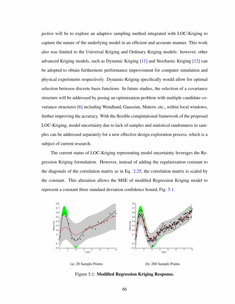
jective will be to explore an adaptive sampling method integrated with LOC-Kriging to

capture the nature of the underlying model in an efficient and accurate manner. This work

also was limited to the Universal Kriging and Ordinary Kriging models: however, other

advanced Kriging models, such as Dynamic Kriging [11] and Stochastic Kriging [12] can

be adopted to obtain furthermore performance improvement for computer simulation and

physical experiments respectively. Dynamic-Kriging specifically would allow for optimal

selection between discrete basis functions. In future studies, the selection of a covariance

structure will be addressed by posing an optimization problem with multiple candidate co-

variance structures [6] including Wendland, Gaussian, Matern, etc., within local windows,

further improving the accuracy. With the flexible computational framework of the proposed

LOC-Kriging, model uncertainty due to lack of samples and statistical randomness in sam-

ples can be addressed separately for a new effective design exploration process, which is a

subject of current research.

The current status of LOC-Kriging representing model uncertainty leverages the Re-

gression Kriging formulation. However, instead of adding the regularization constant to

the diagonals of the correlation matrix as in Eq. 2.25, the correlation matrix is scaled by

the constant. This alteration allows the MSE of modified Regression Kriging model to

represent a constant three standard deviation confidence bound, Fig. 5.1.

(a) 20 Sample Points (b) 200 Sample Points

Figure 5.1: Modified Regression Kriging Response.

66

The plots above are constructed using a nonlinear mean response and a constant nor-

mal standard deviation of 0.05. The green fill represents the true ±3σ error bounds and

the gray fill represents the variation predicted by Kriging. With this is mind, it is evident

that as more sample points are added the approximation of both the mean and standard

deviation are improved. In the future, this methodology will be coupled with LOC-Kriging

to create a framework capable of predicting both a non-stationary mean and variation. This

will enable swift identification of key Validation and Verification factors. Once coupled

with an adaptive sampling technique, this methodology will be capable of maximizing the

confidence of improvement for additional samples.

67

Bibliography

[1] Sacks, J., Welch, W. J., Mitchell, T. J., and Wynn, H. P., “Design and Analysis of

Computer Experiments,” Statistical science, 1989, pp. 409–423.

[2] Meckesheimer, M., Booker, A. J., Barton, R. R., and Simpson, T. W., “Computation-

ally inexpensive Metamodel Assessment Strategies,” AIAA Journal, Vol. 40, No. 10,

2002, pp. 2053–2060.

[3] Simpson, T. W., Poplinski, J., Koch, P. N., and Allen, J. K., “Metamodels for

Computer-Based Engineering Design: Survey and Recommendations,” Engineering

with computers, Vol. 17, No. 2, 2001, pp. 129–150.

[4] Jin, R., Chen, W., and Simpson, T. W., “Comparative studies of metamodelling tech-

niques under multiple modelling criteria,” Structural and Multidisciplinary Optimiza-

tion, Vol. 23, No. 1, 2001, pp. 1–13.

[5] Forrester, A. I. and Keane, A. J., “Recent advances in surrogate-based optimization,”

Progress in Aerospace Sciences, Vol. 45, No. 1, 2009, pp. 50–79.

[6] Lophaven, S. N., Nielsen, H. B., and Søndergaard, J., “DACE-A Matlab Kriging

Toolbox, version 2.0,” Tech. rep., IMM-TR-2002-12, Informatics and Mathematical

Modeling, Technical University of Denmark, 2002.

68

[7] Wang, G. G. and Shan, S., “Review of metamodeling techniques in support of engi-

neering design optimization,” Journal of Mechanical Design, Vol. 129, No. 4, 2007,

pp. 370–380.

[8] Jones, D. R., Schonlau, M., and Welch, W. J., “Efficient global optimization of ex-

pensive black-box functions,” Journal of Global optimization, Vol. 13, No. 4, 1998,

pp. 455–492.

[9] J. Forrester, A. I., Keane, A. J., and Bressloff, N. W., “Design and analysis of” Noisy”

computer experiments,” AIAA Journal, Vol. 44, No. 10, 2006, pp. 2331–2339.

[10] Han, Z.-H., Gortz, S., and Zimmermann, R., “Improving variable-fidelity surrogate

modeling via gradient-enhanced kriging and a generalized hybrid bridge function,”

Aerospace Science and Technology, Vol. 25, No. 1, 2013, pp. 177–189.

[11] Zhao, L., Choi, K., and Lee, I., “Metamodeling method using dynamic Kriging for

design optimization,” AIAA Journal, Vol. 49, No. 9, 2011, pp. 2034–2046.

[12] Ankenman, B., Nelson, B. L., and Staum, J., “Stochastic kriging for simulation meta-

modeling,” Operations research, Vol. 58, No. 2, 2010, pp. 371–382.

[13] Bichon, B. J., Eldred, M. S., Swiler, L. P., Mahadevan, S., and McFarland, J. M.,

“Efficient global reliability analysis for nonlinear implicit performance functions,”

AIAA Journal, Vol. 46, No. 10, 2008, pp. 2459–2468.

[14] Viana, F. A., Haftka, R. T., and Watson, L. T., “Efficient global optimization algorithm

assisted by multiple surrogate techniques,” Journal of Global Optimization, Vol. 56,

No. 2, 2013, pp. 669–689.

[15] Deaton, J. D., Design of Thermal Structures using Topology Optimization, Ph.D. Dis-

sertation, Wright State University, 2014.

69

[16] Haftka, R. T. and Gurdal, Z., Elements of structural optimization, Vol. 11, Springer

Science & Business Media, 2012.

[17] Wang, L. and Grandhi, R. V., “Improved two-point function approximations for de-

sign optimization,” AIAA Journal, Vol. 33, No. 9, 1995, pp. 1720–1727.

[18] Xiong, Y., Chen, W., Apley, D., and Ding, X., “A non-stationary covariance-based

Kriging method for metamodelling in engineering design,” International Journal for

Numerical Methods in Engineering, Vol. 71, No. 6, 2007, pp. 733–756.

[19] Tikhonov, A. N. and Arsenin, V. k., Solutions of ill-posed problems, Vh Winston,

1977.

[20] Clark, D. L., Bae, H.-R., and Penmetsa, R. C., “Engineering Design Exploration

Utilizing Locally Optimized Covariance Kriging,” 18th AIAA Non-Deterministic Ap-

proaches Conference. San Diego, California, (AIAA 2016-0428), 2016, p. 0428.

[21] Clark, D. L., Bae, H.-R., and Penmetsa, R. C., “Locally-Optimized Covariance Krig-

ing for Engineering Design Exploration,” 17th AIAA Non-Deterministic Approaches

Conference. Florida, Kissimmee, (AIAA 2015-1372), 2015, p. 1372.

[22] Clark, D. L., Bae, H.-R., G. K., and Penmetsa, R. C., “Engineering Design Explo-

ration Utilizing Locally Optimized Covariance Kriging,” AIAA journal, (Accepted).

[23] Song, H., Choi, K., and Lamb, D., “A study on improving the accuracy of krig-

ing models by using correlation model/mean structure selection and penalized log-

likelihood function,” 10th World Congress on Structural and Multidisciplinary Opti-

mization. Florida, Orlando, 2013.

[24] Isaaks, E. and Srivastava, R., An Introduction to Applied Geostatistics, Oxford Uni-

versity Press, New York.

70

[25] Sampson, P. D. and Guttorp, P., “Nonparametric estimation of nonstationary spatial

covariance structure,” Journal of the American Statistical Association, Vol. 87, No.

417, 1992, pp. 108–119.

[26] Haas, T. C., “Lognormal and moving window methods of estimating acid deposition,”

Journal of the American Statistical Association, Vol. 85, No. 412, 1990, pp. 950–963.

[27] Environmental Systems Research Institute, I., “How moving window kriging works,”

2016.

[28] Harris, P., Charlton, M., and Fotheringham, A. S., “Moving window kriging with

geographically weighted variograms,” Stochastic Environmental Research and Risk

Assessment, Vol. 24, No. 8, 2010, pp. 1193–1209.

[29] Lin, Y., Mistree, F., Allen, J. K., Tsui, K.-L., and Chen, V., “Sequential metamodel-

ing in engineering design,” AIAA/ISSMO Multidisciplinary Analysis and Optimization

Conference. Albany, New York, (AIAA 2004-4304), 2004.

[30] Ba, S., Joseph, V. R., et al., “Composite Gaussian process models for emulating ex-

pensive functions,” The Annals of Applied Statistics, Vol. 6, No. 4, 2012, pp. 1838–

1860.

[31] Toal, D. J. J. and Keane, A. J., “Non-stationary kriging for design optimization,”

Engineering Optimization, Vol. 44, No. 6, 2012, pp. 741–765.

[32] Aurenhammer, F., “Voronoi diagramsa survey of a fundamental geometric data struc-

ture,” ACM Computing Surveys (CSUR), Vol. 23, No. 3, 1991, pp. 345–405.

[33] Bishop, C. M., Pattern recognition and machine learning, springer, 2006.

[34] Montgomery, D. C. and Runger, G. C., Applied statistics and probability for engi-

neers, John Wiley & Sons, 2010.

71

[35] Zuchowski, B., “Predictive Capability for Hypersonic Structural Response and Life

Prediction, Phase 1–Identification of Knowledge Gaps,” Tech. rep., AFRL-RB-WP-

TR-2010-3069, Air Force Research Laboratory, 2010.

[36] Zuchowski, B., “Predictive Capability for Hypersonic Structural Response and Life

Prediction, Phase 2-Detailed Design of Hypersonic Cruise Vehicle Hot-Structure,”

Tech. rep., AFRL-RB-WP-TR-2012-0208, Air Force Research Laboratory, 2012.

[37] Manson, S. and Halford, G. R., A Method of Estimating High Temperature Low Cycle

Fatigue Behavior of Materials, NASA, 1967.

[38] Gordon, A. P., Judd, E., Bouchenot, T., and Penmetsa, R., “A Microstructurally-

Informed, Continuum-Level Life Prediction Model for Thermo-Acousto-

Mechanically Fatigued Ti-6242S and IN617,” 56th AIAA/ASCE/AHS/ASC Structures,

Structural Dynamics, and Materials Conference, AIAA SciTech. Kissimmee, Florida,

(AIAA 2015-1580), 2015.

[39] Farhat, C., “CFD-based nonlinear computational aeroelasticity,” Encyclopedia of

computational mechanics, Vol. 3, 2004, pp. 459–480.

[40] Hou, G., Wang, J., and Layton, A., “Numerical methods for fluid-structure interaction

a review,” Commun. Comput. Phys, Vol. 12, No. 2, 2012, pp. 337–377.

[41] Mardanpour, P., Hodges, D. H., and Rezvani, R., “Nonlinear aeroelasticity of high-

aspect-ratio wings excited by time-dependent thrust,” Nonlinear Dynamics, Vol. 75,

No. 3, 2014, pp. 475–500.

[42] Liu, S. and Canfield, R. A., “Boundary velocity method for continuum shape sensi-

tivity of nonlinear fluid–structure interaction problems,” Journal of Fluids and Struc-

tures, Vol. 40, 06, 2013, pp. 284–301.

72