Embed Size (px)
Citation preview

Location and design of a competitive facility for profit
maximisation
Frank Plastria∗
BEIF - Department of Management Informatics
Vrije Universiteit Brussel
Pleinlaan 2, B 1050 Brussels, Belgium
e-mail: [email protected]
Emilio Carrizosa†
Facultad de Matematicas
Universidad de Sevilla
Tarfia s/n, 41012 Sevilla, Spain
e-mail: [email protected]
Sevilla, September 24, 2001
Abstract
A single facility has to be located in competition with fixed existing facilities of similar type.Demand is supposed to be concentrated at a finite number of points, and consumers patronisethe facility to which they are attracted most. Attraction is expressed by some function of thequality of the facility and its distance to demand. For existing facilities quality is fixed, whilequality of the new facility may be freely chosen at known costs. The total demand capturedby the new facility generates income. The question is to find that location and quality for thenew facility which maximises the resulting profits.
It is shown that this problem is well posed as soon as consumers are novelty oriented, i.e.attraction ties are resolved in favor of the new facility. Solution of the problem then maybe reduced to a bicriterion maxcovering-minquantile problem for which solution methods areknown. In the planar case with Euclidean distances and a variety of attraction functions thisleads to a finite algorithm polynomial in the number of consumers, whereas, for more generalinstances, the search of a maximal profit solution is reduced to solving a series of small-scalenonlinear optimisation problems. Alternative tie-resolution rules are finally shown to result inill-posed problems.Keywords: Competitive location, Consumer behaviour, Facility design, Maxcovering, Min-quantile, Biobjective.
1 Introduction
This paper addresses the location of a new facility in a competitive environment. Competitionconsists of a number of existing facilities having a known fixed location within the market. Typicallythe expected income the new facility will generate directly depends upon the market share itcaptures. This market share will be determined by several factors, among which we single outits location and its quality as compared to the competing facilities. These two factors are bothcontrollable for a new facility and are considered as decision variables.
With respect to spatial consumer distribution, we assume that demand is concentrated at afinite number of known fixed points in some metric space. Thinking of individual customers this isthe most correct description of reality, although one might have to be more precise by consideringcustomers not only as persons, but rather as “persons at a particular time period”— a same personat home does not necessarily behave the same way as at work, and usually has different locationsin these two situations. The number of individuals to be considered is, however, usually too
∗Corresponding author†Partially supported by Grant PB96-1416-C02-02 of the D.G.E.S., Spain
1

F.Plastria & E.Carrizosa / Profit maximal competitive facility location 2
large for such a precise description of reality to be feasible, both in terms of amount of necessarydata as in terms of complexity for practical solution. Therefore one often resorts to either astatistical description, in many cases pragmatically oversimplified into some uniform distributions,as in Vaughan (1987), or to aggregation of demand into a few ‘conglomerate’ consumers, seee.g. Goodchild (1979) and Francis-Lowe (1992). It is this latter approach that is followed here.However, we allow for possible presence of several customer-groups at a same site, each with theirown particular behaviour towards facility choice. This enables the modeller to split the populationat a given site into several groups, e.g. by time period and/or, as is often done, by income, activityand/or age. In what follows we will call each such customer-groups simply a customer, having itsown individual behaviour and location.
Spatial consumer behaviour has been studied in several disciplines such as geography, economicsand marketing, see Eiselt-Laporte-Thisse (1993). Generalising many of these models we start byconsidering some measure of the attraction a consumer feels for a facility, often also called the utilityof the facility for this consumer. This attraction is some function of the distance between facilityand customer on the one hand, and on the other hand of internal characteristics of the facility,which we express as one global positive measure we will call the quality. The particular functiondescribing attraction may differ from one customer to the other, but is always nonincreasing withdistance and nondecreasing with quality. Two typical examples of such attraction functions areadditive ones, i.e. a weighted difference of quality and distance (compare with T. Drezner (1994)),with weights possibly differing between customers, or multiplicative ones, leading to gravity typeattraction, given by quality divided by some strictly positive power of distance (see Plastria (1997)).
We restrict our attention here to deterministic behavioural models. In these models eachcustomer is supposed to patronise that facility to which it is attracted most, in contrast to inprobabilistic behaviour models where attraction is interpreted as (proportional to) a probability,and the expected value of the demand attracted to each facility is considered (see e.g. T. Drezner(1995)).
When setting up the new facility the main decisions relate to its site and to its design. Inour models they consist of two choices: the location and the quality, and these decisions directlyinfluence both the level of sales at the facility and the operational costs. Sales or income aregenerated in an increasing way by the total demand attracted to the facility. This will dependupon the actual site to be chosen, but also on the quality of the facility. The costs involvedin starting up and running the facility are evidently related to its quality in an increasing way.Indeed, quality is determined by a mixture of several facility attributes, e.g. floor area, number ofcheck-counters, point of sales-system (bar coding, bank-card readers, . . . ), product mix, price-level,marketing in a retail context, and raising the level of any of these attributes always involves highercosts.
Our aim in this paper is to maximise profit. We allow profit to be any indicator of profitabilitywith the minimal properties one may expect of such: it should increase with income and decreasewith cost. The standard examples are sales minus cost or sales divided by cost. We will show thatprofit-maximisation with respect to both the location and the quality of the new facility may beobtained under some mild conditions by inspecting only a finite number of solutions, obtained aftersolving some biobjective maxcovering-minquantile location problem, as studied in Carrizosa andPlastria (1995). More specific assumptions on the nature of the distance and attraction functionused will allow to obtain quite efficient algorithms for this task.
The first competitive location model involving both the choice of location and facility’s charac-teristic simultaneously seems to have been Plastria (1997), of which the present study is a broadgeneralisation. All other papers we are aware of either consider a fixed site and attempt to max-imize profit by an adequate choice of quality (also called attractiveness), or consider the qualityfixed and construct an optimal site. Models of the first type are studied by Eiselt and Laporte(1988a,b) with demand uniformly distributed on a linear market, while T. Drezner (1994) discussesa model of the second type in a planar situation with discrete demand and Euclidean distance.As such our model may be considered as a simultaneous generalization of both these studies. Fora general overview of competitive location models we refer to the survey of Eiselt, Laporte and
F.Plastria & E.Carrizosa / Profit maximal competitive facility location 3
Thisse (1993) and to the more restricted but more recent survey by Plastria (2001).The paper is organised as follows. Section 2 gives the formal description of the model and
introduces the notations to be used. In Section 3 we show how to reduce the solution of the modelto the biobjective location problem. Section 4 is devoted to the planar case, emphasising gravity-type attraction models with Euclidean distances, illustrated with a small-size example showing thepower of our methodology to obtain optimal solutions and perform sensitivity analysis. Extensionsto different types of attraction functions or distances are also discussed, ending with a discussionabout alternative tie-breaking rules in Section 5.
2 The general profit-maximising competitive location model
A finite set of consumer(group)s is denoted by A. Each consumer a ∈ A has a known locationxa and a strictly positive weight ωa, supposed to be an indicator of its buying power, e.g. thepopulation or total wealth represented by consumer(group) a.
A finite set of competing facilities with which our new facility is to compete is denoted by CF .Competing facility f ∈ CF is located at site xf and has a quality αf considered to be known andfixed.
Any consumer a ∈ A feels an attraction attr(a, f) towards facility f at xf , which depends onfactors such as the distance from xa to xf , the facility (and its firm’s) attractiveness, tradition,etc.
Consider a new facility with unknown site x and unknown quality α, of at least some minimalquality α0 > 0. Its attraction on consumer a ∈ A is given by Aa(α,dista(x)), a function of itsquality α and the distance dista(x) from the consumer to the facility. The possibly +∞-valuedfunction Aa : [α0,+∞[×[0,+∞[−→ [0,+∞] satisfies
1. For each fixed d ≥ 0, the function Aa(·, d) is nondecreasing and upper-semicontinuous
2. For each fixed α ≥ α0, the function Aa(α, ·) is nonincreasing and upper-semicontinuous.
Note that these functions are allowed to differ from one customer to the other, enabling differ-entiation in their spatial behaviour.
Examples 1
Example 1.1
A typical example is attraction of (generalised) gravity type, given by
Agrava (α, d) =
αka
dp∀d ≥ 0, α ≥ α0 > 0, (1)
where p is any strictly positive exponent, and ka > 0 represents some proportionality constantdepending on a.
The exponent p allows the analyst to finetune the sensitivity of attraction to distance. In puregravity type models p = 2, by similarity with the gravitational law in Physics, see the iso-attractioncurves in Figure 1. The models considered by Eiselt and Laporte (1988a,b) use p = 1, whereas thecase of general p > 0 was considered in Plastria (1997).
One small technical point should be raised here, which is apparently ignored, but probablyimplicitly assumed in all literature on these types of consumer behaviour models : gravity-typeattraction is infinite as soon as dista(x) = 0, e.g. when the facility location coincides with thelocation xa of consumer a. This might also happen with other types of attraction functions. Ingeneral we will evidently consider that in such a case the attraction is infinite (+∞). In otherwords, it is impossible for a to be attracted more by some other facility located elsewhere than atzero distance of xa.

F.Plastria & E.Carrizosa / Profit maximal competitive facility location 4
α0
α
6
0d
-
High attraction
Low attraction
k
Figure 1: Iso-attraction curves for Agrav (p = 2)
α0
α
6
0d
-
High attraction
Low attraction
k
Figure 2: Iso-attraction curves for Aadd

F.Plastria & E.Carrizosa / Profit maximal competitive facility location 5
Example 1.2
Note, however, that for attraction functions with a finite value for d = 0, it might be possible for aconsumer to be attracted less to a facility located at its own site than to some facility elsewhere, assoon as the quality of the latter is sufficiently high. Such a situation might arise with an additiveattraction function,
Aadda (α, d) = max{0, αka − ca(d)} (2)
where ka > 0 and ca any nondecreasing lower-semicontinuous function. One example of an additiveattraction function is obtained when considering the real prices carried by a customer in a mill-pricing system (see e.g. Hansen et al., 1995). In this interpretation ka represents the normalprice to pay for the quantity of some good consumer a needs to obtain per trip, ca(d) denotesthe transport cost carried by the consumer a when travelling over distance d, and α is the price-reduction factor (per unit) offered. The attraction Aadd
a (α, d) then expresses the reduction on thetotal cost the consumer obtains at a facility with price reduction factor α at distance d. Obviouslyit might be better to go to a cheaper shop further (but not too far) away than to buy at high priceright here. See in Figure 2 iso-attraction curves for c(d) =
√d.
Example 1.3
Quality and distances might also be combined through an attraction of the minimum disutilityform
Amina (α, d) = min {αka, ca(d)} (3)
for some upper-semicontinuous nonincreasing ca, in which consumers measure facility attractionthrough its least favourable feature: either the utility due to its quality (kaα) or the utility due to
travel cost (ca(d)). See in Figure 3 iso-attraction curves for c(d) = d− 1
2 .
α0
α
6
0d
-
High attraction
Low attraction
k
Figure 3: Iso-attraction curves for Amin
Example 1.4
In fact one might also consider max-type functions as
Amaxa (α, d) = max {αka, ca(d)} (4)
with shape something like in next figure.

F.Plastria & E.Carrizosa / Profit maximal competitive facility location 6
α0
α
6
0d
-
High attraction
Low attraction
k
Figure 4: Iso-attraction curves for Amax
Example 1.5
Observe also that, since functions Aa are not assumed to be continuous, one can also considerwithin this framework non-compensatory models, such as
Astepa (α, d) =
{
βa, if α ≥ αa and d ≤ da
0, else(5)
for which the attraction felt is null unless the quality is sufficiently high (α ≥ αa) and the facilityis not too distant (d ≤ da), see e.g. Roberts and Lilien (1993). See figure 5 for its shape.
α0
α
6
0d
-
attraction = 0
attraction = β
α
d
Figure 5: Iso-attraction curves for Astep

F.Plastria & E.Carrizosa / Profit maximal competitive facility location 7
Example 1.6
Partially non-compensatory models can also be considered; indeed, define Aparta as
Aparta (α, d) =
{
Aa(α, d), if d ≤ da
0, else(6)
where Aa is, e.g., of types (1)-(4) and da is a given non-negative threshold value. This yieldsan attraction function which behaves exactly as Aa when distances are not too high (up to thethreshold distance da), but drops to zero (thus no compensation is possible) as soon as distancesexceed this threshold. In Figure 6 the reader can see the effect produced when altering (1), asdepicted in Figure 1, by introducing a threshold distance d.
α0
α
6
0d
-
High attraction
Low attraction
attraction = 0
k
d
Figure 6: Iso-attraction curves for Apart
We denote the attraction felt by consumer a ∈ A towards an existing facility f ∈ CFby attr(a, f), whereas the attraction towards the new facility at x with quality α is given byAa(α,dista(x)), where dista(x) denotes the distance between xa and x. Hence, with the determin-istic consumer choice rule, it will capture those consumers attracted more to the new facility thanto any competing facility in CF . The set of captured consumers is thus given by
Capt(α, x) = {a ∈ A | ∀f ∈ CF : Aa(α,dista(x)) ≥ attr(a, f)}.
Note the use of ≥ in this definition, which means that for consumers equally attracted by thenew facility and any existing facility they patronised before, we assume they will start patronisingthe new facility as soon as it arrives on the market. In other words we consider consumers to benovelty oriented. It will turn out in Section 3 that this assumption leads to clear results in ourmodel, while, as shown in Section 5, any other assumption on the resolution of attraction ties leadsto technical difficulties, more precisely non-existence of optimal solutions (strictu sensu) when αmay vary continuously.
The total weight captured by the new facility is now given by
CW (α, x) =∑
a∈Capt(α,x)
ωa (7)

F.Plastria & E.Carrizosa / Profit maximal competitive facility location 8
The sales income at the new facility is given as some strictly increasing function σ of the capturedweight. The operating costs of the new facility are given by a strictly increasing function γ of itsquality α. Profit is expressed by some profit-indicator function π which is strictly increasing insales and strictly decreasing in costs, yielding a profit indicator
Π(α, x) = π( σ(CW (α, x)) , γ(α) ) (8)
Typical examples of such indicator functions are the standard notion of profit, i.e. the differenceof sales minus costs, π(s, c) = s − c, yielding
Π(α, x) = σ(CW (α, x)) − γ(α), (9)
or a profitability ratio like sales divided by costs, π(s, c) = sc , giving rise to
Π(α, x) =σ(CW (α, x))
γ(α)
It is the profit-indicator Π in (8) we want to optimise by an adequate choice of both the qualityα ≥ α0 and the site x within some set of feasible sites S :
max{Π(α, x) | x ∈ S, α ≥ α0}. (10)
Given a fixed quality α, profit maximisation is achieved by maximisation of the total capturedweight, in other words we obtain a maximal covering problem as studied in the planar contextby Z. Drezner (1981) and Mehrez and Stulman (1982). This is in fact what T. Drezner (1994)proposes. Since to us α is a variable, we would have to solve such a maximal covering problemfor each possible value of α. At first glance this seems possible only when no more than a finitenumber of feasible quality values are available.
This is however not the approach we want to use here: we want to optimise over the full rangeof positive α-values no less than α0. Instead, we show in Section 3 how to solve Problem (10) byreducing it to a bicriterion problem, which was addressed by the authors in Carrizosa and Plastria(1995). In particular, this will enable to solve (10) in a number of cases by inspecting a finitenumber of points, polynomial in the cardinality of A.
3 Bicriterion minquantile/maxcovering view
We now take a closer look at the capturing process. Consumer a is captured by the new facilitygiven by (α, x) iff for any facility f ∈ CF we have Aa(α,dista(x)) ≥ attr(a, f). Let us defineµa ∈ [0,+∞], the decisive attraction of a, as the highest attraction consumer a felt before theadvent of the new facility, i.e.,
µa = max{attr(a, f) | f ∈ CF}, (11)
We may now write the capturing of a by the new facility at x as
a ∈ Capt(α, x) ⇐⇒ Aa(α,dista(x)) ≥ µa
⇐⇒ α ∈ {α ≥ α0 : Aa(α,dista(x)) ≥ µa}Since, by assumption, for each a ∈ A and d ≥ 0, the function Aa(·, d) is nondecreasing and
upper semicontinuous, the set {α ≥ α0 : Aa(α, d) ≥ µa} is a closed (possibly empty) subintervalof [α0,+∞]. It then has either the form [Ba(d),+∞], or it is empty, in which case we define Ba(d)as +∞.
¿From this definition one immediately obtains that
Ba(d) ≤ α ⇐⇒ Aa(α, d) ≥ µa, (12)
This means that Ba(d) indicates, as a function of d, the quality threshold above which customer aat distance d is captured. We call this partial inverse function of Aa the decisive quality function.
We have the following property
F.Plastria & E.Carrizosa / Profit maximal competitive facility location 9
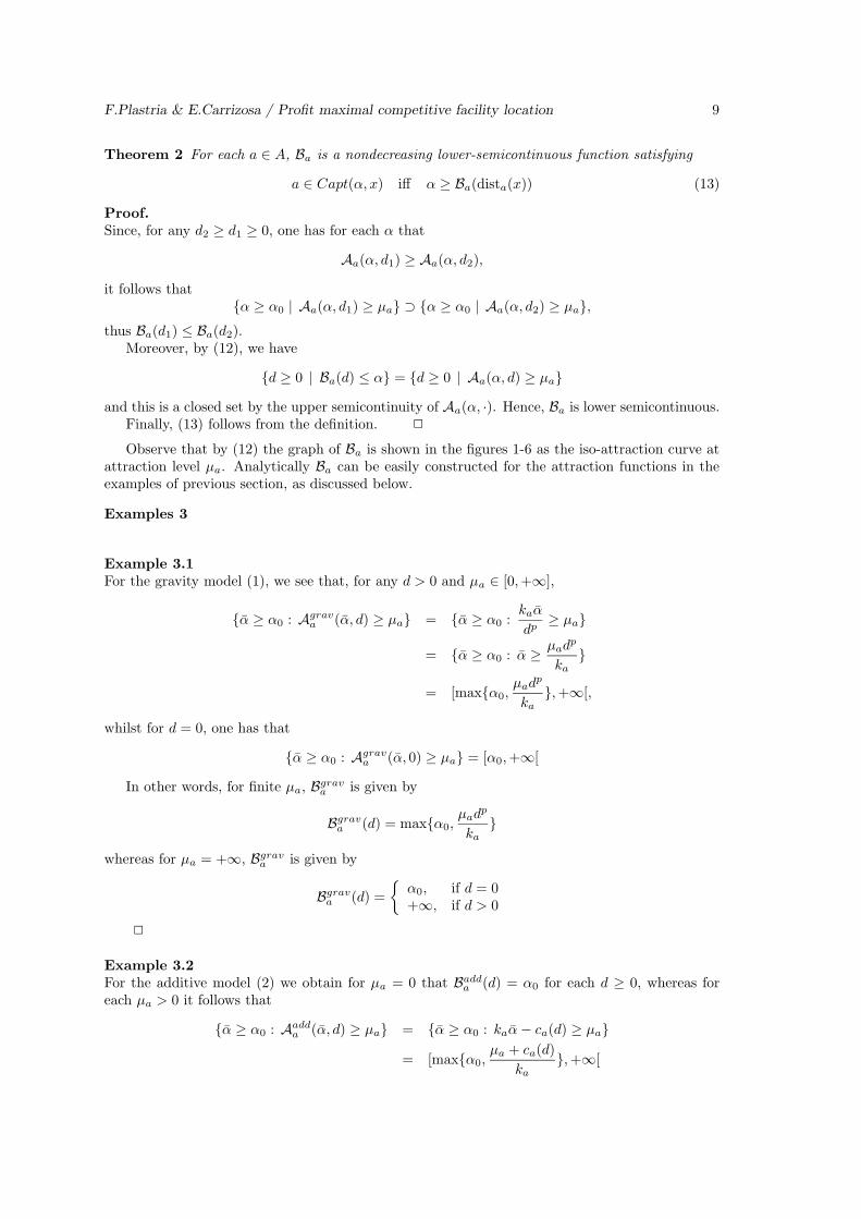
Theorem 2 For each a ∈ A, Ba is a nondecreasing lower-semicontinuous function satisfying
a ∈ Capt(α, x) iff α ≥ Ba(dista(x)) (13)
Proof.
Since, for any d2 ≥ d1 ≥ 0, one has for each α that
Aa(α, d1) ≥ Aa(α, d2),
it follows that{α ≥ α0 | Aa(α, d1) ≥ µa} ⊃ {α ≥ α0 | Aa(α, d2) ≥ µa},
thus Ba(d1) ≤ Ba(d2).Moreover, by (12), we have
{d ≥ 0 | Ba(d) ≤ α} = {d ≥ 0 | Aa(α, d) ≥ µa}
and this is a closed set by the upper semicontinuity of Aa(α, ·). Hence, Ba is lower semicontinuous.Finally, (13) follows from the definition. 2
Observe that by (12) the graph of Ba is shown in the figures 1-6 as the iso-attraction curve atattraction level µa. Analytically Ba can be easily constructed for the attraction functions in theexamples of previous section, as discussed below.
Examples 3
Example 3.1
For the gravity model (1), we see that, for any d > 0 and µa ∈ [0,+∞],
{α ≥ α0 : Agrava (α, d) ≥ µa} = {α ≥ α0 :
kaα
dp≥ µa}
= {α ≥ α0 : α ≥ µadp
ka}
= [max{α0,µadp
ka},+∞[,
whilst for d = 0, one has that
{α ≥ α0 : Agrava (α, 0) ≥ µa} = [α0,+∞[
In other words, for finite µa, Bgrava is given by
Bgrava (d) = max{α0,
µadp
ka}
whereas for µa = +∞, Bgrava is given by
Bgrava (d) =
{
α0, if d = 0+∞, if d > 0
2
Example 3.2
For the additive model (2) we obtain for µa = 0 that Badda (d) = α0 for each d ≥ 0, whereas for
each µa > 0 it follows that
{α ≥ α0 : Aadda (α, d) ≥ µa} = {α ≥ α0 : kaα − ca(d) ≥ µa}
= [max{α0,µa + ca(d)
ka},+∞[
F.Plastria & E.Carrizosa / Profit maximal competitive facility location 10
Hence, if µa = 0 then Badda (d) = α0 for all d whereas, for µa > 0, Badd
a has the form
Badda (d) = max{α0,
µa + ca(d)
ka}
2
Example 3.3
For the minimum disutility model (3), Bmina takes the form
Bmina (d) =
{
max{α0,µa
ka
}, if ca(d) ≥ µa
+∞, else
Since ca is assumed to be non-increasing, it follows that, for µa > ca(0), Bmina = +∞. For µa ≤
ca(0), since ca is upper-semicontinuous, we can define da as
da := max {d ≥ 0 : ca(d) ≥ µa} ∈ [0,+∞], (14)
yielding the following equivalent expression of Bmina
Bmina (d) =
{
max{α0,µa
ka
}, if d ≤ da
+∞, else,(15)
Example 3.4
Similarly for the max-type model (4),
Bmaxa (d) =
{
max{α0,µa
ka
}, if ca(d) < µa
α0, else
yielding
Bmaxa (d) =
{
max{α0,µa
ka
}, if d > da
α0, else(16)
with da defined by (14).
Example 3.5
For the step model (5), one has that, for µa ≤ βa,
Bstepa (d) =
{
αa, if d ≤ da
+∞, else,(17)
whereas, for µa > βa, one obtains that Bstepa is constantly +∞. Observe that this expression has
the same form as (15), obtained for a different attraction model.
Example 3.6
For Aparta given in (6) for some given Aa with corresponding partial inverse Ba, the construction
of Bparta is straightforward; indeed, since, for µa = 0,
{α ≥ α0 : Aparta (α, d) ≥ 0} = [α0,+∞[,
we get for µa = 0 that Bparta (d) = α0 for all d ≥ 0. On the other hand, for µa > 0,
{α ≥ α0 : Aparta (α, d) ≥ µa} =
{
{α ≥ α0 : Aa(α, d) ≥ µa} if d ≤ da
∅, else
Hence, for µa > 0 we obtain
Bparta (d) =
{
Ba(d), if d ≤ da
+∞, else
2

F.Plastria & E.Carrizosa / Profit maximal competitive facility location 11
Our optimisation problem may now be stated as follows. For each a ∈ A we have a functiondista(·), a weight ωa and a threshold value µa as defined in (11). For any quality α ≥ α0 ≥ 0, thecaptured weight CW (α, x) is defined in (7) as
CW (α, x) =∑
{ωa | a ∈ Capt(α, x)}
=∑
a
{ωa | Aa(α,dista(x)) ≥ µa}
=∑
a
{ωa | Ba(dista(x)) ≤ α}
and the maximisation of the profit-indicator function Π defined in (8) yields
max
α ≥ α0, x ∈ S
Π(α, x) := π(σ(CW (α, x)), γ(α))(18)
Following Plastria (1997), we propose to find a maximal profit solution (i.e., to solve (18))through the determination of the efficient (or nondominated, or Pareto-optimal) solutions of thebi-objective problem
min αmax CW (α, x)
α ≥ α0 ; x ∈ S(19)
We first recall that a feasible solution (α, x) is said to be efficient for (19) iff there exists nofeasible pair (α∗, x∗) satisfying
α∗ ≤ α
CW (α∗, x∗) ≥ CW (α, x),
with at least one of the two inequalities above as strict (see e.g. Steuer, 1986).As a direct consequence of this definition of efficient solutions, and the fact that, by assumption,
σ, γ, π are strictly monotonic in their arguments, one obtains the following
Theorem 4 Any maximal profit solution is an efficient solution for (19).
Problems of type (19), called biobjective minquantile-maxcovering problems were defined andstudied in Carrizosa and Plastria (1995) in a general theoretical setting. In the next section weshow that, under mild conditions, the general theory developed there leads, in the planar context,to a finite number of candidates for being maximal profit solutions, obtained through a geometricalprocedure in the most common model (gravity-type attraction, Euclidean distances) or after solvinga finite number of small-scale nonlinear optimisation problems.
Theorem 4 asserts that, if maximal profit solutions exist, then they all are efficient for thebiobjective problem (19). Sufficient conditions for the existence of such maximal profit solutionsare given in the next result.
Theorem 5 Suppose that, for each a ∈ A, dista is a continuous function of the location x, and,for any β ≥ 0, the set {x ∈ S : dista(x) ≤ β} is compact. Then, under novelty orientation, thereexists a maximal profit solution.
Proof.
For a given α ≥ α0, let Q(α) denote the highest market capture which can be obtained for a qualityα, if the facility is properly located,
Q(α) = supx∈S
CW (α, x) = maxx∈S
CW (α, x)

F.Plastria & E.Carrizosa / Profit maximal competitive facility location 12
where the last equality is a consequence of the fact that CW can take only finitely many values.Then,
Q(α) = maxA∗⊆A
{∑
a∈A∗
wa : for some x ∈ S we have (∀a ∈ A∗ : Ba(dista(x)) ≤ α ) }
= maxA∗⊆A
{∑
a∈A∗
wa : for some x ∈ S we have maxa∈A∗
Ba(dista(x)) ≤ α }
Since each function dista is assumed to be continuous, and, by Theorem 2, Ba is lower-semicontinuous,then, for any A∗ ⊆ A, the function x 7−→ maxa∈A∗ Ba(dista(x)) is also lower-semicontinuous.
By Theorem 2, each Ba is non-decreasing, and, by assumption, the sets {x ∈ S : dista(x) ≤ β}are compact, thus, given x0 ∈ S, for each A∗ ⊆ A,
inf {maxa∈A∗
Ba(dista(x)) : x ∈ S} =
= inf {maxa∈A∗
Ba(dista(x)) : x ∈ S,dista(x) ≤ dista(x0) for some a ∈ A∗},
and the latter infimum is attained, since it is the infimum of a lower-semicontinuous function overthe compact set
⋂
a∈A∗
{x ∈ S : dista(x) ≤ dista(x0)}
Hence, for each non-empty A∗ ⊆ A, there exists some x(A∗) such that
inf {maxa∈A∗
Ba(dista(x)) : x ∈ S} = maxa∈A∗
Ba(dista(x(A∗)))
Therefore,
Q(α) = maxA∗⊆A
{∑
a∈A∗
wa : maxa∈A∗
Ba(dista(x(A∗))) ≤ α} (20)
=∑
a∈A∗
α
wa
for some A∗α ⊆ A satisfying
maxa∈A∗
α
Ba(dista(x(A∗α))) ≤ α
Hence, for any α ≥ α0,
Q(α) ≥ β iff α ≥ max
{
minx∈S
maxa∈A∗
Ba(dista(x)) : A∗ ⊆ A,∑
a∈A∗
wa ≥ β
}
(21)
Now observe that, by the finiteness of A, the set of values taken by CW (α, x) when α ranges[α0,+∞[ and x ranges S is finite: c1, . . . , cN . Then,
maxα≥α0, x∈S
π(σ(CW (α, x), γ(α))) = max1≤i≤N
maxα≥α0,Q(α)≥ci
π(σ(ci), γ(α)),
thus, since by assumption, γ is strictly increasing, and π is strictly decreasing in its second argu-ment, it follows from (21) that
maxα≥α0, x∈S
π(σ(CW (α, x), γ(α))) = max1≤i≤N
π(σ(ci), γ(min{α ≥ α0 : Q(α) ≥ ci})),
and this value is attained at a certain quality level α∗, from which an optimal location x∗ isobtained by (20). 2
Hence, under mild assumptions (which are automatically satisfied, e.g., under the assumptionsof the model in Section 4, namely, S is a closed set in the plane and each dista is induced by anorm), novelty orientation leads to optimization problems which are well behaved, in the sensethat an optimal solution (α, x) exists.

F.Plastria & E.Carrizosa / Profit maximal competitive facility location 13
4 Location in the plane
4.1 General attraction and distance measure
When the facility is to be located in a closed convex subset S of the plane R2, distances are usually
assumed to be measured by some norm (or gauge, when non-symmetric), possibly differing withdemand point, see e.g. Plastria (1995). It follows that the distance function dista(x) to a fixedpoint a is convex in x, see e.g. Michelot (1993) for this and further results on distances. This keyproperty induces (quasi)convexity properties on the objective function of (19). We refer the readerto Avriel et al. (1988) for concepts and properties on quasiconvex functions.
Lemma 6 Let Da : R2 −→ [0,+∞] be defined as
Da : x 7−→ Ba(dista(x))
One then has:
1. Da is quasiconvex and lower-semicontinuous.
2. If Aa is quasiconcave, then Ba and Da are convex.
Proof.
Since distances dista are assumed to be induced by gauges, they are convex functions and thereforecontinuous. By Theorem 2, Ba is non-decreasing and lower-semicontinuous, thus, by composition,Da is quasiconvex and lower-semicontinuous, showing part 1.
To show part 2, we first show that Ba is convex. Indeed, let d1, d2 ≥ 0 and 0 < λ < 1. Bydefinition, for i = 1, 2, Ba(di) is the optimal solution to the problem
inf αs.t. α ≥ α0
Aa(α, di) ≥ µa
(22)
Obviously, if any of these problems is infeasible, then the inequality
Ba((1 − λ)d1 + λd2) ≤ (1 − λ)Ba(d1) + λBa(d2) (23)
immediately follows since the right hand side equals +∞.If both problems are feasible, the upper semicontinuity of Aa(·, di) implies that their feasible
regions are closed intervals, thus their optimal values, Ba(d1),Ba(d2), are attained. In other words,
Aa(Ba(di), di) ≥ µa for i = 1, 2
The quasiconcavity of Aa implies
µa ≤ min{Aa(Ba(d1), d1),Aa(Ba(d2), d2)}≤ Aa((1 − λ)(Ba(d1), d1) + λ(Ba(d2), d2))
= Aa((1 − λ)Ba(d1) + λBa(d2), (1 − λ)d1 + λd2),
thus (1 − λ)Ba(d1) + λBa(d2) is feasible for the optimization problem
min{α ≥ α0 : Aa(α, (1 − λ)d1 + λd2) ≥ µa},
the optimal solution of which is, by definition, Ba((1 − λ)d1 + λd2). Therefore (23) follows, thusBa is convex.
Finally, Da is the composition of the convex nondecreasing function Ba with the convex functiondista, thus Da is convex, which concludes part 2. 2

F.Plastria & E.Carrizosa / Profit maximal competitive facility location 14
Remark 7 Quasiconcavity of Aa (thus convexity of Da) is easily checked for the gravity-typemodel (1), the additive attraction model (2) for convex ca, models (3)–(5), and for model (6)induced by an attraction function Aa which is quasiconcave.
One can then use the application of Helly-Drezner theorem presented in Carrizosa and Plastria(1995) to conclude that efficient solutions for (19) are optimal solutions to simple single-objectiveproblems:
Theorem 8 Let (α∗, x∗) be an efficient solution for (19). Then, one has:
1. When Capt(α∗, x∗) 6= ∅ there exists a nonempty subset T ⊂ A, with cardinality at most 3such that
(a) x∗ solves the generalized single-facility minmax location problem
minx∈S
maxa∈T
Da(x) (PT )
(b) α∗ is the optimal value of (PT ), which is finite.
2. In case Capt(α∗, x∗) = ∅ (i.e. µa ≥ A(α0, 0) for all a ) one must have α∗ = α0, and anyother pair (α0, x) is then also efficient for (19).
By Theorem 4, any profit-maximising solution (α∗, x∗) is also efficient for (19). Hence, Theorem8 implies that, after finding the optimal value αT of each of the O(n3) problems of the form (PT ),and finding the set ST of optimal solutions for (PT ) we end up with a list L of pairs (αT , xT )known to contain the set of efficient solutions for (19). Therefore we obtain the following
General Algorithm in the Plane
Step 1 Initialise the list of candidate solutions L with the singleton {(α0, x0)}, with x0 ∈ Sarbitrarily chosen.
Step 2 For all T ⊂ A, with cardinality 1, 2 or 3, do
1. Compute αT , the optimal value of (PT )
2. If αT < +∞ then find the set ST of optimal solutions for (PT ) and add {(αT , xT ) :xT ∈ ST } to L.
Step 3 For each (α, x) ∈ L evaluate Π(α, x) and select the one yielding the maximal value.
Observe that in step 2.2 all optimal solutions xT ∈ ST will have the same corresponding qualityvalue αT . In step 3 only the ones with maximal captured weight will be retained. Therefore wemay replace step 2.2 by
2. If αT < +∞ then find the set ST of optimal solutions for (PT )
3. find the set S∗T of optimal solutions to the subproblem
max{CW (αT , x) | x ∈ ST } (24)
and add {(αT , xT ) : xT ∈ S∗T } to L.
In general the problems (PT ), or its subproblem (24), may have an infinite number of optimalsolutions, thus the algorithm as such does not always yield a finite procedure. When ST , or S∗
T , isinfinite we may retain just one solution in S∗
T which will still guarantee finding at least one optimalsolution.
Observe that the subproblem (24) to be solved is just a maximal covering location problem,but with a peculiar locational constraint x ∈ ST . If the corresponding solution (αT , x∗
T ) turns out

F.Plastria & E.Carrizosa / Profit maximal competitive facility location 15
to be the optimal profit-mix, then all optimal solutions to this subproblem will be optimal profitlocations, all combined with the same quality αT .
As we will see in the next section, in several important cases the problems (PT ) have a finite,often unique solution. Although (quasi)convex (see Lemma 6 and Theorem 8)), solving (PT ) isusually not straightforward, and will involve a convergent iterative search, see e.g. Plastria (1988)and Section 4.4. Step 2 involves solving O(n3) problems (PT ), so this will take quite some time.
For a given solution (α, x) the captured weight can be computed in O(n) time in a straightfor-ward manner. Therefore, when ST (or S′
T ) is finite for all T , Step 3 can be performed in O(n|L|),where |L| denotes the cardinality of the list L generated in Step 2.
In the following we show how in some very relevant cases, the structure of the function Aa andthe geometry of the distances dista can be used to obtain finite and low-complexity procedures.
4.2 Gravity-type attraction and Euclidean distances
Let us now focus on the case of gravity-type attraction functions and Euclidean distances in theEuclidean plane. This means that for any a ∈ A we have, as introduced in (1),
Aa(α, x) =kaα
‖x − xa‖p, (25)
(‖x− xa‖ standing here for the Euclidean distance from xa to x), which leads to (see Example3.1)
Da(x) = max
{
α0,
(
µa
ka
)
‖x − xa‖p
}
Under these assumptions, the problems (PT ) introduced in Section 4.1 have a rich structurewhich will allow us to easily identify their optima. First we have that (PT ) can be re-written as
minx∈S
max
(
α0,maxa∈T
Da(x)
)
Defining Problem (QT ) as
minx∈S
maxa∈T
µa
ka‖x − xa‖p (QT )
we see that both problems are equivalent (same optimal solutions, same objective value), exceptfor the degenerate case in which (QT ) has an optimal value not greater than α0. This enables usto rephrase Theorem 8 as
Theorem 9 Let (α∗, x∗) be an efficient solution for (19). Then, one has:
1. If Capt(α∗, x∗) 6= ∅ then there exists a nonempty subset T ⊂ A, with cardinality at most 3such that
(a) x∗ solves the single-facility minmax location problem (QT )
(b) α∗ is the maximum between α0 and the optimal value of (QT ), which is finite.
2. If Capt(α∗, x∗) = ∅ (i.e. µa ≥ A(α0, 0) for all a ) then α∗ = α0, and any pair (α0, x) is alsoefficient for (19).
For Problem (QT ) we first have:
Lemma 10 For each T ⊂ A, Problem (QT ) has exactly one optimal solution xT .
F.Plastria & E.Carrizosa / Profit maximal competitive facility location 16
Proof.
With the current assumptions Ba is strictly increasing and ‖·‖ is a round norm, thus the uniquenessof solution follows from the general results on minmax problems with round norms described inPelegrın-Michelot-Plastria (1985). 2
Since, at the optimal solution xT of (QT ), at least one function Da is active, i.e. Da(xT ) =maxb∈T Db(xT ), in order to find xT we can search for it sequentially in the locus of points whereexactly one, then where exactly two, and finally where exactly three of the functions are active.
It follows that we will need to consider sets of points of following form. Define the mediatrix oftwo consumers a, b located at different sites (xa 6= xb) — it would be empty otherwise — as thefollowing set of points of the plane
med(a, b) = {x ∈ R2 :
µa
ka‖x − xa‖p =
µb
kb‖x − xb‖p}
Denoting λa ≡ (µa/ka)1/p and by da(x) ≡ λa‖x − xa‖ the Euclidean distance between con-sumer’s a’s site and x, inflated by the factor λa, we may also write
med(a, b) = {x ∈ R2 : da(x) = db(x)}
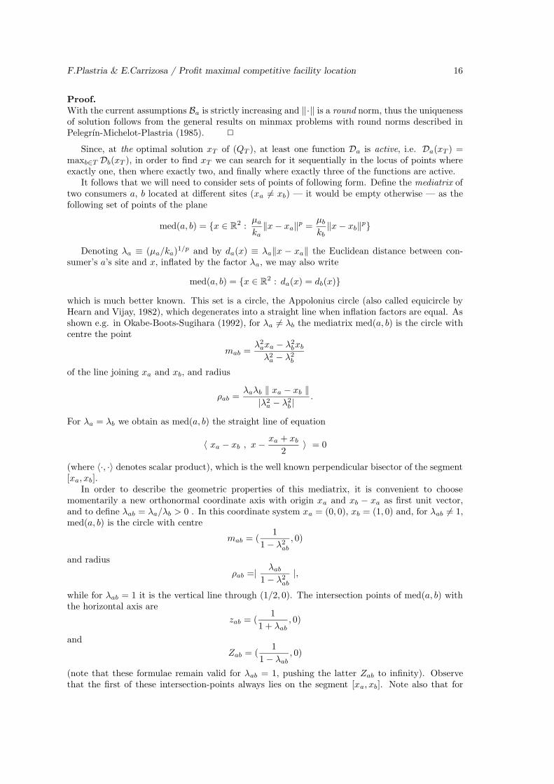
which is much better known. This set is a circle, the Appolonius circle (also called equicircle byHearn and Vijay, 1982), which degenerates into a straight line when inflation factors are equal. Asshown e.g. in Okabe-Boots-Sugihara (1992), for λa 6= λb the mediatrix med(a, b) is the circle withcentre the point
mab =λ2
axa − λ2bxb
λ2a − λ2
b
of the line joining xa and xb, and radius
ρab =λaλb ‖ xa − xb ‖
|λ2a − λ2
b |.
For λa = λb we obtain as med(a, b) the straight line of equation
〈 xa − xb , x − xa + xb
2〉 = 0
(where 〈·, ·〉 denotes scalar product), which is the well known perpendicular bisector of the segment[xa, xb].
In order to describe the geometric properties of this mediatrix, it is convenient to choosemomentarily a new orthonormal coordinate axis with origin xa and xb − xa as first unit vector,and to define λab = λa/λb > 0 . In this coordinate system xa = (0, 0), xb = (1, 0) and, for λab 6= 1,med(a, b) is the circle with centre
mab = (1
1 − λ2ab
, 0)
and radius
ρab =| λab
1 − λ2ab
|,
while for λab = 1 it is the vertical line through (1/2, 0). The intersection points of med(a, b) withthe horizontal axis are
zab = (1
1 + λab, 0)
and
Zab = (1
1 − λab, 0)
(note that these formulae remain valid for λab = 1, pushing the latter Zab to infinity). Observethat the first of these intersection-points always lies on the segment [xa, xb]. Note also that for

F.Plastria & E.Carrizosa / Profit maximal competitive facility location 17
λab = 0.2
λab = 0.5
λab = 1
λab = 1.25
λab = 2
λab = 5
λab = 0.8
a b
Figure 7: med(a, b) for different values of λab = λa/λb
λab 6= 1 the centre mab lies on the line xaxb, but always outside the segment [xa, xb], closest to thatpoint among xa, xb with highest corresponding λ, and that it is this latter point that lies insidethe circle. Figure 7 illustrates these properties.
Assuming λab < 1, the points of med(a, b) may be described parametrically as x = (t, h) with
1
1 + λab≤ t ≤ 1
1 − λab
and
h2 = (t − 1
1 + λab)(
1
1 − λab− t)
while the inflated distances to xa and xb are given by
da(x) = db(x) =
√
2t − 1
1 − λ2ab
which is an increasing function of t. For λab > 1 the first inequalities above should simply beinverted, and the inflated distance then decreases with t.
In any case inflated distance is always minimised on med(a, b) at the point zab for t = 11+λab
and
grows continuously along both upper and lower half-circles in symmetric way towards its (common)maximum at Zab reached when t = 1
1−λab
.
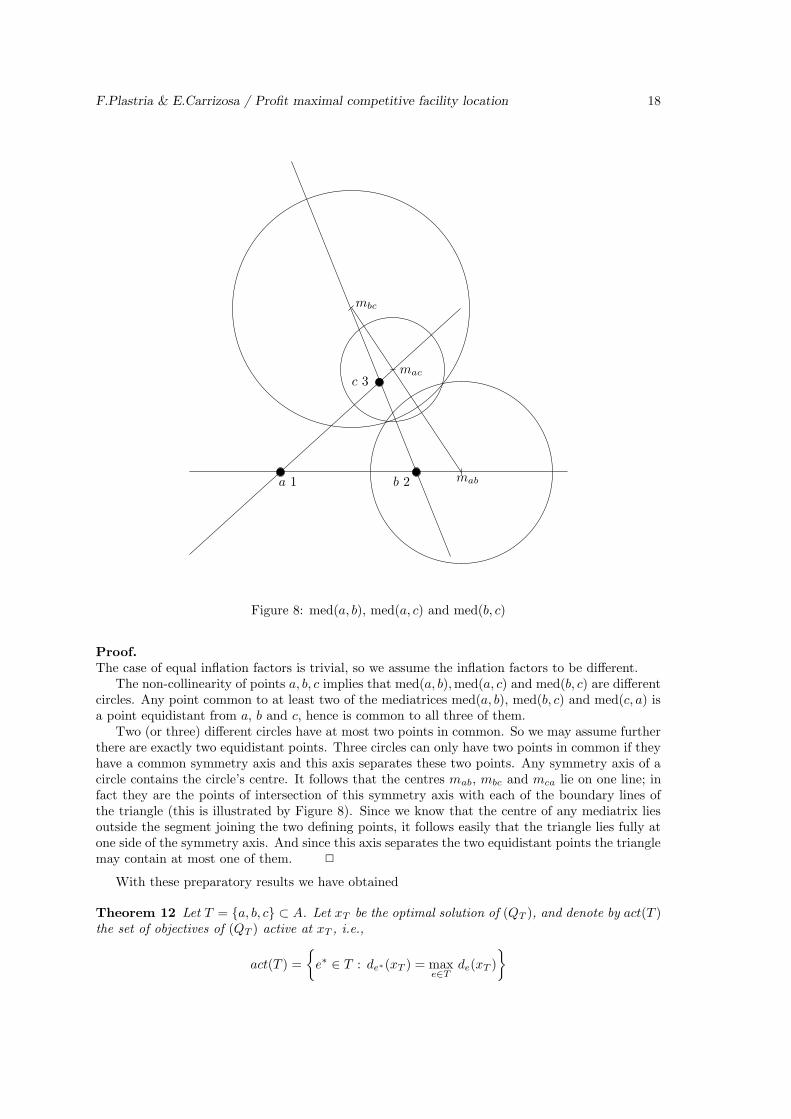
Lemma 11 Let a, b and c be three non-collinear points in the plane with strictly positive inflationfactors λa, λb and λc. Then at most one point equidistant from a, b and c exists lying within thetriangle formed by them.
F.Plastria & E.Carrizosa / Profit maximal competitive facility location 18
mbc
mac
maba 1 b 2
c 3
Figure 8: med(a, b), med(a, c) and med(b, c)
Proof.
The case of equal inflation factors is trivial, so we assume the inflation factors to be different.The non-collinearity of points a, b, c implies that med(a, b),med(a, c) and med(b, c) are different
circles. Any point common to at least two of the mediatrices med(a, b), med(b, c) and med(c, a) isa point equidistant from a, b and c, hence is common to all three of them.
Two (or three) different circles have at most two points in common. So we may assume furtherthere are exactly two equidistant points. Three circles can only have two points in common if theyhave a common symmetry axis and this axis separates these two points. Any symmetry axis of acircle contains the circle’s centre. It follows that the centres mab, mbc and mca lie on one line; infact they are the points of intersection of this symmetry axis with each of the boundary lines ofthe triangle (this is illustrated by Figure 8). Since we know that the centre of any mediatrix liesoutside the segment joining the two defining points, it follows easily that the triangle lies fully atone side of the symmetry axis. And since this axis separates the two equidistant points the trianglemay contain at most one of them. 2
With these preparatory results we have obtained
Theorem 12 Let T = {a, b, c} ⊂ A. Let xT be the optimal solution of (QT ), and denote by act(T )the set of objectives of (QT ) active at xT , i.e.,
act(T ) =
{
e∗ ∈ T : de∗(xT ) = maxe∈T
de(xT )
}

F.Plastria & E.Carrizosa / Profit maximal competitive facility location 19
1. If act(T ) = {a}, then xT is the point of S closest (with respect to the Euclidean distance) toxa
2. If act(T ) = {a, b}, then xT is the point of S on med(a, b) minimising da(x), if any, and isfound
• either on the line segment joining xa and xb, if this (unique) point zab of med(a, b) liesin S
• or by intersecting med(a, b) with S’s boundary and selecting among the intersectionpoints (if any) the one(s) (at most two of such) closest to xa (or equivalently to xb)
3. If act(T ) = {a, b, c}, then xT is the intersection of the three mediatrices corresponding toeach choice of two points among them and the triangle with vertices the points in T and liesin S.
It follows that the list of candidate efficient solutions is of length at most n + 2n(n − 1)/2 +n(n − 1)(n − 2)/6 = n(n + 1)(n + 2)/6, where n is the cardinality of A. It is therefore an easytask to construct this full list of length O(n3), and to evaluate each candidate, taking O(n) timefor evaluating the captured weight each time, which leads to an overall O(n4) method.
In fact this same task may be done more efficiently by mixing the evaluation of each candidatesolution with the generation process, leading to a much better algorithm of complexity O(n3 log n).For the technical details of this method the interested reader is referred to Plastria (1996).
Now we illustrate the method just described by means of a small-size example.
Example 13
Consider a set A = {a1, . . . , a10} of consumers, located at the points plotted as empty circles inFigure 9, with coordinates xa and weights ωa given in Table 2.
a1
a7
a8
a5
a6
a4
a10
a9 a3
a2
f1f2
S
Figure 9: Consumers and existing facilities
A set of two facilities, CF = {f1, f2}, plotted as solid circles in Figure 9, already compete inthe region. Their coordinates xf and qualities αf are given in Table 1.

F.Plastria & E.Carrizosa / Profit maximal competitive facility location 20
f xf αf
f1 (20, 73) 1250f2 (50, 70) 1000
Table 1: Existing facilities
We assume that for each consumer a the attraction to any facility has the form (25) with eachka = 1, α0 ≈ 0, α0 = 0.000001, say, and p = 2 for each a, i.e.
Aa(α, x) =α
‖x − xa‖2
Before the advent of the new facility, consumer a is captured by the existing facility yielding highestattraction. This is determined by calculating the decisive attractions µa following (11):
µa = max
{
αf
‖xa − xf‖2| f ∈ CF
}
which are listed together with the currently attracting facility f(a) in the last two columns of Table2. See also Figure 9 for the current patronisings.
a xa ωa µa f(a)a1 (64, 34) 600 0.6702 f2
a2 (60, 19) 100 0.3702 f2
a3 (50, 38) 100 0.9766 f2
a4 (45, 55) 100 4.0000 f2
a5 (20, 52) 400 2.8345 f1
a6 (27.8, 7) 300 0.2830 f1
a7 (24, 40) 100 1.1312 f1
a8 (20, 31) 100 0.7086 f1
a9 (9, 36) 100 0.8389 f1
a10 (3.8, 7) 600 0.2707 f1
Table 2: Attraction parameters
A new facility must be located within the region S, — represented in Figure 9 by the convexpolygon with endpoints (0, 0), (50, 0), (50, 20), (25, 45), (0, 45) — to maximize a profit indicatorfunction Π of type (8), whose parameters σ and γ will be specified later.
With this information, we already know, by Theorems 4 and 12, that an optimal solution(α∗, x∗) can be found within a finite set of candidate points, the locations and qualities of whichare obtained by intersecting discs in the plane. This set of candidate locations is plotted in Figure10 as small solid circles. One can see that 10 candidate points with a single active objective arepresent (the closest-point projections of each customer-site on S — coinciding with the site whenin S), the other candidate points along S’s boundary where two objectives are active, and severalcandidate points within S \ A where three objectives are active.
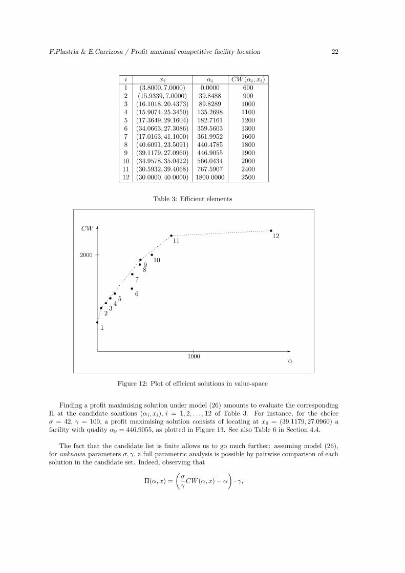
However, most of the elements in this set are not real candidates, since they are not efficientfor problem (19). After eliminating dominated elements, (see Carrizosa -Plastria 1995, 1998b fordetails), one obtains the reduced list of 12 candidates (αi, xi), given in Table 3 and shown in Figure11 as small solid circles. Figure 12 shows a plot of attractiveness αi versus market share CW (xi)for these efficient solutions.
Assume now that further assumptions on Π are made. For instance, suppose Π correspondsa sales-minus-cost model (9) in which sales income are assumed to be proportional to the weight

F.Plastria & E.Carrizosa / Profit maximal competitive facility location 21
f1f2
S
Figure 10: Location of candidates
f1f2
S
Figure 11: Location of efficient solutions
captured, with proportionality constant σ, and operating costs are proportional to the quality ofthe facility, with proportionality constant γ. In this case, the profit indicator Π takes the simplerform
Π(α, x) = σ · CW (α, x) − γ · α, (26)
for given constants σ, γ > 0.
F.Plastria & E.Carrizosa / Profit maximal competitive facility location 22
i xi αi CW (αi, xi)1 (3.8000, 7.0000) 0.0000 6002 (15.9339, 7.0000) 39.8488 9003 (16.1018, 20.4373) 89.8289 10004 (15.9074, 25.3450) 135.2698 11005 (17.3649, 29.1604) 182.7161 12006 (34.0663, 27.3086) 359.5603 13007 (17.0163, 41.1000) 361.9952 16008 (40.6091, 23.5091) 440.4785 18009 (39.1179, 27.0960) 446.9055 190010 (34.9578, 35.0422) 566.0434 200011 (30.5932, 39.4068) 767.5907 240012 (30.0000, 40.0000) 1800.0000 2500
Table 3: Efficient elements
-
α1000
6CW
2000
1
234
56
7
89
10
1112
Figure 12: Plot of efficient solutions in value-space
Finding a profit maximising solution under model (26) amounts to evaluate the correspondingΠ at the candidate solutions (αi, xi), i = 1, 2, . . . , 12 of Table 3. For instance, for the choiceσ = 42, γ = 100, a profit maximising solution consists of locating at x9 = (39.1179, 27.0960) afacility with quality α9 = 446.9055, as plotted in Figure 13. See also Table 6 in Section 4.4.
The fact that the candidate list is finite allows us to go much further: assuming model (26),for unknown parameters σ, γ, a full parametric analysis is possible by pairwise comparison of eachsolution in the candidate set. Indeed, observing that
Π(α, x) =
(
σ
γCW (α, x) − α
)
· γ,

F.Plastria & E.Carrizosa / Profit maximal competitive facility location 23
f1f2
S
x9
Figure 13: Optimal location for (26) with σ = 42, γ = 100
we see that maximising Π(α, x) is equivalent to maximising
Πτ (α, x) = τCW (α, x) − α.
Comparing the solutions in Table 3 we obtain, for each (αi, xi), the interval [τi, τi] such that (αi, xi)is a profit-maximising solution under model (26) if and only if τ belongs to [τi, τi]. The results aresummarized in Table 4, where it is readily seen that not all the efficient solutions of Table 3 can beoptimal under model (26): only the extreme efficient solutions, vertices of the upper left boundaryof the convex hull of the efficient value pairs, shown by a dotted line in Figure 12, appear. This isdue to the fact that profit is linear in α and CW .
i xi αi CW (αi, xi) τi τi
1 (3.8000, 7.0000) 0.0000 600 0.0000 0.13282 (15.9339, 7.0000) 39.8488 900 0.1328 0.40719 (39.1179, 27.0960) 446.9055 1900 0.4071 0.641411 (30.5932, 39.4068) 767.5907 2400 0.6414 10.324112 (30.0000, 40.0000) 1800.0000 2500 10.3241 ∞
Table 4: Full parametric analysis under model (26)
As mentioned before, the applicability of our methodology is not at all restricted to the sales-minus-costs model (26), and a similar analysis can be carried out for other choices of the profitindicator function Π. For instance, assume now that Π is of the type sales divided by operatingcosts, where operating costs consist of a fixed cost γ0 and a cost proportional to quality, i.e.,
Π(α, x) = CW (α, x)/ (γ0 + γ · α, ) (27)
Again by inspecting the efficient solutions (αi, xi), we can find, for each (αi, xi) the interval[τi, τi] such that (αi, xi) is a profit-maximising solution under model (27) if and only if γ0
γ belongs

F.Plastria & E.Carrizosa / Profit maximal competitive facility location 24
to [τi, τi]. See the results in Table 5, where we again only find the extreme efficient solutions, nowdue to the fact that profit is a linear fractional function of quality and covered weight.
i xi αi CW (αi, xi) τi τi
1 (3.8000, 7.0000) 0.0000 600 0.0000 79.69762 (15.9339, 7.0000) 39.8488 900 79.6976 326.50239 (39.1179, 27.0960) 446.9056 1900 326.5023 771.698511 (30.5932, 39.4068) 767.5908 2400 771.6985 24010.241712 (30.0000, 40.0000) 1800.0005 2500 24010.2417 ∞
Table 5: Full parametric analysis under model (27)
Remark 14 The geometric approach described above has as cornerstone the fact that mediatricesare circles. This property extends to slightly different attraction functions such as
A1a(α, d) =
kaα
ha + d2
or the particular case of (2) given by
A2a(α, d) = max{0, αka − had2}.
Indeed, one easily obtains
B1a(d) = max{α0,
µa
ka(ha + d2)}
and
B2a(d) = max{α0,
µa + d2
ka}
for µa > 0 or B2a(d) = α0 for µa = 0, see Example 3.2.
In both cases mediatrices are of circular shape (see Carrizosa and Plastria, 1998a), and may behandled in a way similar to the method explained in this section.
4.3 Step attractions and Euclidean distances
Both the minimum disutility attraction (3) and the step attraction (5) lead to a binary Ba of theform (17),
Ba(d) =
{
αa, if d ≤ da
+∞, else,
Hence, the function Da will have under Euclidean distances the form
Da(x) =
{
αa, if ‖x − xa‖ ≤ da
+∞, else,
for some threshold value da.This shows how different shapes for the attraction functions Aa can lead to the same function
Da, thus also to the same subproblems (PT ) to be solved and the same set of candidate points asoutput of our general algorithm.
Let us now have a closer look at the optimisation problems (PT ) obtained in this particularcase. Since Ba is no longer strictly increasing (it is in fact constant when finite!) no analog toLemma 10 holds, and the list L obtained by directly using the general algorithm described in

F.Plastria & E.Carrizosa / Profit maximal competitive facility location 25
Section 4.1 would be infinite (and useless!). Nevertheless, the structure of this problem can beused to develop simple procedures to skip this technical handicap.
Indeed, if we denote by DT the (possibly empty) intersection of the disks centered at xa, xb, xc
with radii da, db, dc, it follows that the set of optimal solutions for (PT ) is DT , whereas the optimalvalue is αT := max{αa, αb, αc}.
This implies the following
Theorem 15 Let (α∗, x∗) be an efficient solution for (19) with CW (α∗, x∗) > 0. Then there existssome a ∈ A such that
1. α∗ = αa
2. ‖x∗ − xa‖ ≤ da
Moreover, the set C(x∗) of points{
x ∈ S : ‖x − xb‖ ≤ db for all b ∈ A such that ‖x∗ − xb‖ ≤ db
}
is such that any pair (α∗, x), with x ∈ C(x∗), is also efficient for (19), with same quality andcoverage than (α∗, x∗).
Consider for each a ∈ A a maxcovering problem as discussed by T. Drezner (1994) with cus-tomerset reduced to A(αa) = {b ∈ A : αb ≤ αa}, keeping the original radii and weights. Then,finding one optimal solution for each of these maxcovering problems leads to a list L∗ such that,for any efficient solution (α, x), there is some (α∗, x∗) in L∗ which is equivalent (same coverage,same quality) to (α, x).
One may then find the optimal profit quality α∗ by inspecting all pairs in L∗ and then applyTheorem 15 using this α∗ in order to obtain all optimal profit locations.
4.4 Other planar distance measures
The question whether non-Euclidean distances in the plane might be handled is a quite subtle one.The basic theory carries through since (inflated) distance functions remain convex, yielding
the same basic properties of the candidate efficient solutions, see Carrizosa and Plastria (1995).However, it is less evident whether the corresponding candidate points may easily be calculated.
First it will not be easy to detect that all candidates have indeed been generated because (someof) the problems (PT ) may have several (usually isolated) solutions. Assuming each Ba is strictlyincreasing and round norms, e.g. `p distances (1 < p < ∞), Lemma 10 remains valid, so theprocess reduces to finding the O(n3) optimal solutions of the (quasi)convex small-scale problems(PT ).
However, the geometrical procedure described in Section 4.2 does not seem to extend to thismore general context. Indeed, although determining closest points to a polygon in a non-Euclideanmetric is not too hard, the notion of Appolonius circle does not work anymore; these shouldbe replaced by equidistance sets, which often do not have analytical equations, meaning thatintersecting them with S’s boundary will not be easy, nor finding points of equal distance to atriplet of consumers.
In general one will have to rely on iterative techniques for determination of each type of point.Since O(n3) such iterative algorithms should be carried out, it seems evident that the computationalburden will substantially increase with the number n of consumers.
This was attempted for different `r norms using the Optimization toolbox of Matlab to solveeach of the subproblems (QT ). Table 6 shows the results obtained for the additive model (26),with σ = 42, γ = 100, for different values of r.
For simple distance measures like the rectangular `1, or any other block norm, these difficultiesare relatively easy to overcome and geometric procedures can again be used. A new difficultyarises, however, when considering such norms because they are not round, hence the subproblems(PT ) might have an infinite number of solutions and in each such case another subproblem of LPtype has to be solved to obtain S∗
T . See Carrizosa and Plastria (1998b) for further details.

F.Plastria & E.Carrizosa / Profit maximal competitive facility location 26
r x(r) α(r) CW (α(r), x(r)) Π1.60 (16.0556, 7.0000) 38.0152 900 33998.47941.65 (16.0359, 7.0000) 38.3388 900 33966.12191.70 (16.0177, 7.0000) 38.6292 900 33937.07581.75 (38.4713, 27.2559) 457.7094 1900 34029.06401.80 (38.6153, 27.2240) 455.4035 1900 34259.64711.85 (38.7515, 27.1921) 453.1701 1900 34482.98701.90 (38.8805, 27.1601) 451.0095 1900 34699.05191.95 (39.0024, 27.1281) 448.9215 1900 34907.85432.00 (39.1179, 27.0960) 446.9055 1900 35109.4438
Table 6: Optimal solutions under (27) for varying distance measure `r
5 Alternate tie resolution rules
Throughout this paper we have assumed novelty orientation as tie breaking rule. The other extremetie resolution rule, as compared to novelty orientation, states that in case of an attraction tie withthe new facility the existing facility will be favored. This rule may be called conservative behaviourby the customers.
T. Drezner’s (1995) rule takes the middle path in between novelty orientation and conservatism:in case of attraction tie the demand is split equally between new and existing facility. When demandpoints are considered as population centres and attraction is viewed as behaviour of individualcustomers, this assumption means that customers are novelty oriented with probability of 0.5 andotherwise conservative. It is clear that we may generalise this to a θ-mixed behaviour, θ being avector of the form (θa)a∈A, 0 ≤ θa ≤ 1∀a ∈ A, stating that in case of a tie for consumer a, a fractionθa of his/her demand will patronise the new facility, the remaining fraction 1− θa patronising theexisting facilities.
Note that 0-mixed behaviour is the same as conservatism, while novelty orientation correspondswith θ-mixed behaviour, θ being then a vector with all its coordinates equal to 1.
The following result states that in fact, novelty orientation is the unique θ−mixed behaviourwhich is guaranteed to always yield well behaved problems.
For any (α, x) let us define the set of active demand points
act(α, x) ≡ {a ∈ A | Ba(dista(x)) = α}.
The total attracted weight in case of θ-mixed behaviour may then be written as
CWθ(α, x) ≡ CW (α, x) −∑
a∈act(α,x)
(1 − θa)wa
The profit for θ-mixed behaviour is now given as
Πθ(α, x) = π( σ(CWθ(α, x)) , γ(α) ).
Theorem 16 Let the profit-indicator function π(t, ·) be continuous for any fixed t and the costfunction γ also be continuous. Under θ-mixed behaviour, if a profit-maximising pair (α∗, x∗) existswith α∗ > α0, then at least one consumer a ∈ Capt(α, x) (i.e., Ba(dista(x∗)) ≤ α∗) is novelty-oriented, i.e. θa = 1.
In particular if all θa are equal to some fixed θ0 and a profit-maximising pair (α∗, x∗) existswith α∗ > α0, then θ0 = 1, i.e. we have full novelty orientation.
Proof.
Let (α∗, x∗) be a profit-maximising solution with α∗ > α0. We first show that act(α∗, x∗) is

F.Plastria & E.Carrizosa / Profit maximal competitive facility location 27
non-empty. Indeed, if act(α∗, x∗) = ∅, then any consumer a ∈ A is either strictly covered(Ba(dista(x∗)) < α∗) or strictly uncovered, (Ba(dista(x∗) > α∗).
Defining α as the lowest possible quality yielding the same market share,
α = max{α0,max {Ba(dista(x∗)) : Ba(dista(x∗)) < α∗}} < α∗,
we then have that
CW (α, x∗) = CW (α∗, x∗)
γ(α) < γ(α∗),
thus, by the strictly decreasing character of π(t, ·),
Π(α, x∗) > Π(α∗, x∗),
contradicting the optimality of (α∗, x∗). Hence,
act(α∗, x∗) 6= ∅, (28)
as asserted.We are now in position to show that there exists some (partially) captured a ∈ A such that
θa = 1. By contradiction, assume that
θa < 1 ∀a ∈ A such that Ba(dista(x∗)) ≤ α. (29)
Define α1 as
α1 = max{α0,min{Ba(dista(x∗)) : Ba(dista(x∗)) > α∗, a ∈ A}},
or α1 = +∞ if the latter set is empty.In particular, α1 > α∗. Hence, for any α ∈]α∗, α1[
CWθ(α, x∗) = CW (α, x∗)
= CW (α∗, x∗)
> CWθ(α∗, x∗)
In particular,π(CWθ(α, x∗), γ(α)) = π(CWθ(α
∗, x∗), γ(α)),
thus, by the continuity of γ and π(t, ·),
limα↓α∗
π(CWθ(α, x∗), γ(α)) = limα↓α∗
π(CW (α∗, x∗), γ(α))
= π(CW (α∗, x∗), γ(α∗))
> π(CWθ(α∗, x∗), γ(α∗))
Hence, for α (slightly) greater than α∗, one would obtain, at the same location, a strictly greaterprofit, contradicting the optimality of (α∗, x∗).
The second claim is then straightforward. 2
In spite of this negative result for θ 6= 1 it turns out that the efficient solutions derived inSection 3 for θ = 1 nevertheless yield interesting sites and information. Locating at such a pointindeed guarantees that any other location sufficiently nearby may be beaten by choosing a qualityslightly above the one of the corresponding θ = 1 efficient solution.

F.Plastria & E.Carrizosa / Profit maximal competitive facility location 28
References
[1] Avriel, M., Diewert, W.E., Schaible, S., and Zhang, I., (1988), Generalized concavity, Plenum,New York.
[2] Carrizosa, E., and Plastria, F. (1995), On minquantile and maxcovering optimisation, Math-ematical Programming 71, 101-112.
[3] Carrizosa, E., and Plastria, F. (1998a), Locating an undesirable facility by generalized cuttingplanes, Mathematics of Operations Research 23, 3, 680-694.
[4] Carrizosa, E., and Plastria, F. (1998b), Polynomial algorithms for parametric minquantile andmaxcovering planar location problems with locational constraints, TOP 6, 179-194.
[5] Drezner, T. (1994), Locating a single new facility among existing unequally attractive facilities,Journal of Regional Science 34, 2, 237-252.
[6] Drezner, T. (1995), Competitive facility location in the plane, in Facility Location. A surveyof applications and methods, Z. Drezner (Ed.), Springer, Berlin, 285-300.
[7] Drezner, Z. (1981), On a modified one-center problem, Management Science 27, 848-851.
[8] Eiselt, H.A., and Laporte, G., (1988a), Location of a new facility on a linear market in thepresence of weights, Asia-Pacific Journal of Operational Research 5, 160-165.
[9] Eiselt, H.A., and Laporte, G., (1988b), Trading areas of facilities with different sizes, RAIRORecherche Operationnelle/Operations Research 22,1, 33-44.
[10] Eiselt, H.A., Laporte, G., and Thisse,J.–F. (1993), Competitive location models: a frameworkand bibliography, Transportation Science, 27, 44-54.
[11] Francis,R.L., Lowe,T.J., (1992), On worst case aggregation analysis for network location prob-lems, Annals of Operations Research, 40, 229-246.
[12] Goodchild,M.F., (1979), The aggregation problem in location-allocation, Geographical Analy-sis, 11, 240-255.
[13] Hansen, P., Peeters, D. and Thisse, J.-F., (1995), The profit-maximizing Weber Problem,Location Science 3, 2, 67-85.
[14] Hearn,D.W., and Vijay, J., (1982), Efficient algorithms for the (weighted) minimum circleproblem, Operations Research 30, 777-795.
[15] Mehrez, A., and Stulman, A. (1982), The maximal covering location problem with facilityplacement on the entire plane, Journal of Regional Science 22, 361-365.
[16] Michelot, C., (1993), The mathematics of continuous location, Studies in Locational Analysis,5, 59–83.
[17] Okabe, A., Boots, B., and Sugihara, K., (1992), Spatial tesselations, Concepts and applicationsof Voronoi diagrams, John Wiley & Sons, Chichester.
[18] Pelegrın, B., Michelot, C. and Plastria, F., (1985), On the uniqueness of optimal solutions incontinuous location theory, European Journal of Operational Research, 20, 327-331.
[19] Plastria, F., (1988), The minimisation of lower subdifferentiable functions under nonlinearconstraints, an all feasible cutting plane method, Journal of Optimisation Theory and Appli-cations, 57, 463-484.
F.Plastria & E.Carrizosa / Profit maximal competitive facility location 29
[20] Plastria, F. (1995a). Continuous Location Problems, in Z. Drezner (Ed.), Facility Location:A Survey of Applications and Methods, Springer-Verlag, 1995, 225–262.
[21] Plastria, F. (1996), Profit maximising location in the plane of a single competitive facility withdeterministic gravity-type consumer behaviour, Report BEIF/93, Vrije Universiteit Brussel,Brussels, Belgium.
[22] Plastria, F. (1997), Profit maximising single competitive facility location in the plane, Studiesin Locational Analysis, 11, 115-126.
[23] Plastria, F. (2001), Static competitive facility location: an overview of optimisation ap-proaches, European Journal of Operational Research, 129, 461-470.
[24] Roberts, J.H., and Lilien, G.L., (1993), Explanatory and Predictive Models of ConsumerBehavior, in Marketing, Handbooks in Operations Research and Management Science (Vol.5), (J. Eliashberg and G.L. Lilien, Eds.), North-Holland, Amsterdam.
[25] Steuer, R. (1986), Multiple criteria optimization, Wiley, New York.
[26] Vaughan, R., (1987), Urban Spatial Traffic Patterns, Pion Limited, London.