Embed Size (px)
Citation preview

Location-Based Activity Recognition
Lin Liao
A dissertation submitted in partial fulfillment ofthe requirements for the degree of
Doctor of Philosophy
University of Washington
2006
Program Authorized to Offer Degree: Computer Science and Engineering


University of WashingtonGraduate School
This is to certify that I have examined this copy of a doctoral dissertation by
Lin Liao
and have found that it is complete and satisfactory in all respects,and that any and all revisions required by the final
examining committee have been made.
Co-Chairs of the Supervisory Committee:
Dieter Fox
Henry Kautz
Reading Committee:
Dieter Fox
Henry Kautz
Martha E. Pollack
Date:


In presenting this dissertation in partial fulfillment of the requirements for the doctoraldegree at the University of Washington, I agree that the Library shall make its copiesfreely available for inspection. I further agree that extensive copying of this dissertation isallowable only for scholarly purposes, consistent with “fair use” as prescribed in the U.S.Copyright Law. Requests for copying or reproduction of this dissertation may be referredto Proquest Information and Learning, 300 North Zeeb Road, Ann Arbor, MI 48106-1346,1-800-521-0600, to whom the author has granted “the right to reproduce and sell (a) copiesof the manuscript in microform and/or (b) printed copies of the manuscript made frommicroform.”
Signature
Date


University of Washington
Abstract
Location-Based Activity Recognition
Lin Liao
Co-Chairs of the Supervisory Committee:Associate Professor Dieter Fox
Computer Science and Engineering
Professor Henry KautzComputer Science and Engineering
Automatic recognition of human activities can support many applications, from context
aware computing to just-in-time information systems to assistive technology for the disabled.
Knowledge of a person’s location provides important context information for inferring a
person’s high-level activities. This dissertation describes the application of machine learning
and probabilistic reasoning techniques to recognizing daily activities from location data
collected by GPS sensors.
In the first part of the dissertation, we present a new framework of activity recognition
that builds upon and extends existing research on conditional random fields and relational
Markov networks. This framework is able to take into account complex relations between
locations, activities, and significant places, as well as high level knowledges such as number
of homes and workplaces. By extracting and labeling activities and significant places simul-
taneously, our approach achieves high accuracy on both extraction and labeling. We present
efficient inference algorithms for aggregate features using Fast Fourier Transform or local
Markov Chain Monte Carlo within the belief propagation framework, and a novel approach
for feature selection and parameter estimation using boosting with virtual evidences.
In the second part, we build a hierarchical dynamic Bayesian network model for trans-
portation routines. It can predict a user’s destination in real time, infer the user’s mode of


transportation, and determine when a user has deviated from his ordinary routines. The
model encodes general knowledge such as street maps, bus routes, and bus stops, in order
to discriminate different transportation modes. Moreover, our system could automatically
learn navigation patterns at all levels from raw GPS data, without any manual labeling! We
develop an online inference algorithm for the hierarchical transportation model based on the
framework of Rao-Blackwellised particle filters, which performs analytical inference both at
the low level and at the higher levels of the hierarchy while sampling other variables.


TABLE OF CONTENTS
List of Figures . . . . . . . . . . . . . . . . . . . . . . . . . . . . . . . . . . . . . . . . iii
List of Tables . . . . . . . . . . . . . . . . . . . . . . . . . . . . . . . . . . . . . . . . . vii
Chapter 1: Introduction . . . . . . . . . . . . . . . . . . . . . . . . . . . . . . . . . 1
1.1 Challenges of Activity Recognition . . . . . . . . . . . . . . . . . . . . . . . . 3
1.2 Overview . . . . . . . . . . . . . . . . . . . . . . . . . . . . . . . . . . . . . . 4
1.3 Related Work . . . . . . . . . . . . . . . . . . . . . . . . . . . . . . . . . . . . 7
1.4 Outline . . . . . . . . . . . . . . . . . . . . . . . . . . . . . . . . . . . . . . . 15
Chapter 2: Relational Markov Networks and Extensions . . . . . . . . . . . . . . . 16
2.1 Background . . . . . . . . . . . . . . . . . . . . . . . . . . . . . . . . . . . . . 17
2.2 Extensions of Relational Markov Networks . . . . . . . . . . . . . . . . . . . . 22
2.3 Summary . . . . . . . . . . . . . . . . . . . . . . . . . . . . . . . . . . . . . . 26
Chapter 3: Inference in Relational Markov Networks . . . . . . . . . . . . . . . . . 27
3.1 Markov Chain Monte Carlo (MCMC) . . . . . . . . . . . . . . . . . . . . . . 28
3.2 Belief Propagation (BP) . . . . . . . . . . . . . . . . . . . . . . . . . . . . . . 30
3.3 Efficient Inference with Aggregate Features . . . . . . . . . . . . . . . . . . . 33
3.4 Summary . . . . . . . . . . . . . . . . . . . . . . . . . . . . . . . . . . . . . . 40
Chapter 4: Training Relational Markov Networks . . . . . . . . . . . . . . . . . . 41
4.1 Maximum Likelihood (ML) Estimation . . . . . . . . . . . . . . . . . . . . . . 41
4.2 Maximum Pseudo-Likelihood (MPL) Estimation . . . . . . . . . . . . . . . . 46
4.3 Virtual Evidence Boosting . . . . . . . . . . . . . . . . . . . . . . . . . . . . . 48
4.4 Comparison of Learning Algorithms . . . . . . . . . . . . . . . . . . . . . . . 55
4.5 Summary . . . . . . . . . . . . . . . . . . . . . . . . . . . . . . . . . . . . . . 59
Chapter 5: Extracting Places and Activities from GPS Traces . . . . . . . . . . . 60
5.1 Relational Activity Model . . . . . . . . . . . . . . . . . . . . . . . . . . . . . 62
5.2 Inference . . . . . . . . . . . . . . . . . . . . . . . . . . . . . . . . . . . . . . . 70
i

5.3 Experimental Results . . . . . . . . . . . . . . . . . . . . . . . . . . . . . . . . 725.4 Indoor Activity Recognition . . . . . . . . . . . . . . . . . . . . . . . . . . . . 775.5 Summary . . . . . . . . . . . . . . . . . . . . . . . . . . . . . . . . . . . . . . 78
Chapter 6: Learning and Inferring Transportation Routines . . . . . . . . . . . . . 796.1 Hierarchical Activity Model . . . . . . . . . . . . . . . . . . . . . . . . . . . . 806.2 Inference . . . . . . . . . . . . . . . . . . . . . . . . . . . . . . . . . . . . . . . 846.3 Learning . . . . . . . . . . . . . . . . . . . . . . . . . . . . . . . . . . . . . . . 996.4 Experimental Results . . . . . . . . . . . . . . . . . . . . . . . . . . . . . . . . 1016.5 Application: Opportunity Knocks . . . . . . . . . . . . . . . . . . . . . . . . . 1066.6 Summary . . . . . . . . . . . . . . . . . . . . . . . . . . . . . . . . . . . . . . 107
Chapter 7: Indoor Voronoi Tracking . . . . . . . . . . . . . . . . . . . . . . . . . . 1107.1 Voronoi Tracking . . . . . . . . . . . . . . . . . . . . . . . . . . . . . . . . . . 1117.2 Inference and Learning . . . . . . . . . . . . . . . . . . . . . . . . . . . . . . . 1137.3 Experimental Results . . . . . . . . . . . . . . . . . . . . . . . . . . . . . . . . 1147.4 Summary . . . . . . . . . . . . . . . . . . . . . . . . . . . . . . . . . . . . . . 117
Chapter 8: Conclusion and Future Work . . . . . . . . . . . . . . . . . . . . . . . 1188.1 Conclusion . . . . . . . . . . . . . . . . . . . . . . . . . . . . . . . . . . . . . 1188.2 Future Work . . . . . . . . . . . . . . . . . . . . . . . . . . . . . . . . . . . . 119
Bibliography . . . . . . . . . . . . . . . . . . . . . . . . . . . . . . . . . . . . . . . . . 123
Appendix A: Derivations . . . . . . . . . . . . . . . . . . . . . . . . . . . . . . . . . 133A.1 Derivation of Likelihood Approximation using MCMC . . . . . . . . . . . . . 133A.2 Derivation of the LogitBoost Extension to Handle Virtual Evidence . . . . . . 134
ii

LIST OF FIGURES
Figure Number Page
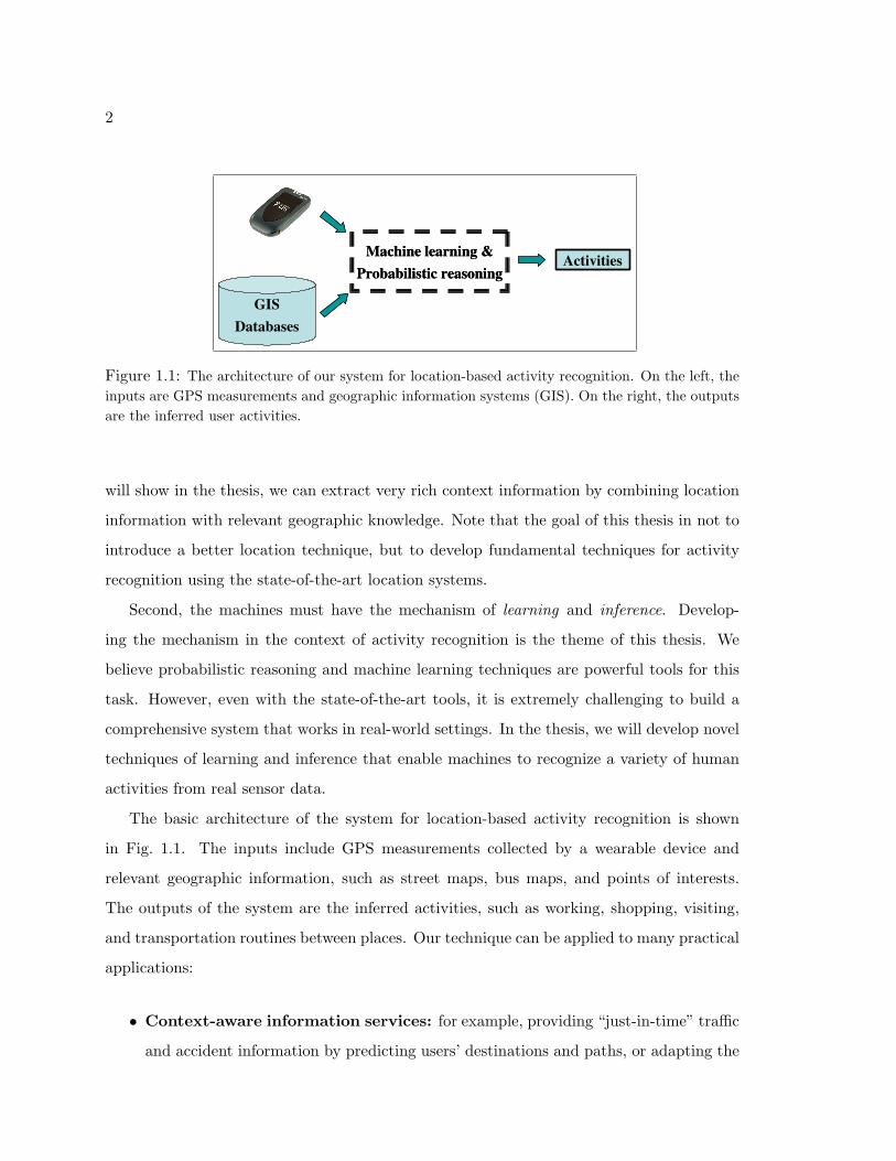
1.1 The architecture of our system for location-based activity recognition. On the left,the inputs are GPS measurements and geographic information systems (GIS). Onthe right, the outputs are the inferred user activities. . . . . . . . . . . . . . . . . 2
1.2 An associative network of liquor shopping (courtesy to [15]). The meaningsof the edges are: each shopping activity includes a “go” step, liquor-shoppingis an instance of shopping, and the store of liquor-shopping is a liquor store. . 9
1.3 Bayesian networks constructed for the activity of liquor shopping (courtesy to[15]). The nodes with grey background are observations and those withoutgrey background are hidden variables for explanation. On the left is thenetwork after observing a “go” action (named go1); on the right is the networkafter observing another evidence: the destination of the “go” action is a liquorstore (named ls2). Given the observations, the explanation is lss3, which isan instance of liquor-shopping. . . . . . . . . . . . . . . . . . . . . . . . . . . 9
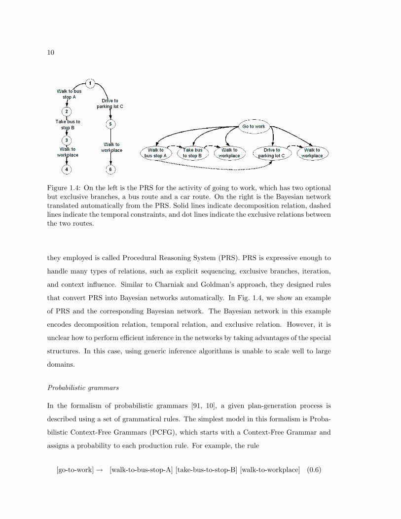
1.4 On the left is the PRS for the activity of going to work, which has two optionalbut exclusive branches, a bus route and a car route. On the right is theBayesian network translated automatically from the PRS. Solid lines indicatedecomposition relation, dashed lines indicate the temporal constraints, anddot lines indicate the exclusive relations between the two routes. . . . . . . . 10
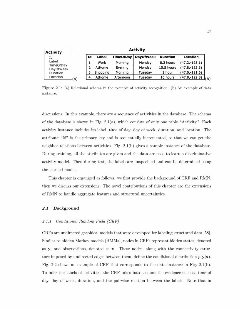
2.1 (a) Relational schema in the example of activity recognition. (b) An example ofdata instance. . . . . . . . . . . . . . . . . . . . . . . . . . . . . . . . . . . . . 17
2.2 An example of CRF for activity recognition, where each Label represents a hiddenstate and TimeOfDay, DayOfWeek, and Duration are observations. . . . . . . . . . 18
2.3 The relationship between RMN and CRF. . . . . . . . . . . . . . . . . . . . . . . 20
2.4 The instantiated CRF after using only the template of time of day. . . . . . . . . . 21
2.5 The instantiated CRF after using the aggregate features. . . . . . . . . . . . . . . 24
3.1 (a) Pairwise CRF that represents ysum =∑8
i=1 yi; (b) Summation tree that rep-resents ysum =
∑8i=1 yi; (c) Computation time for summation cliques versus the
number of nodes in the summation. The Si’s in (a) and (b) are auxiliary nodes toensure the summation relation . . . . . . . . . . . . . . . . . . . . . . . . . . . . 34
iii

3.2 (a) A CRF piece in which yagg is the aggregate of y1, . . . ,y8 and the aggregationis encoded in the potential of auxiliary variable Sagg; (b) Convergence comparisonof local MCMC with global MCMC (G-R statistics approaching 1 indicates goodconvergence); (c) Comparison of the inference with and without caching the randomnumbers. . . . . . . . . . . . . . . . . . . . . . . . . . . . . . . . . . . . . . . . 39
4.1 (a) Original CRF for learning; (b) Converted CRF for MPL learning by copying thetrue labels of neighbors as local evidence. . . . . . . . . . . . . . . . . . . . . . . 46
4.2 Classification accuracies in experiments using synthetic data, where the error barsindicate 95% confidence intervals. (a) VEB vs. BRF when the transition probabili-ties (pairwise dependencies) turn from weak to strong. (b) Comparison of differentlearning algorithms for feature selection. . . . . . . . . . . . . . . . . . . . . . . 57
4.3 The CRF model for simultaneously inferring motion states and spatial contexts(observations are omitted for simplicity). . . . . . . . . . . . . . . . . . . . . . . 58
5.1 The concept hierarchy for location-based activity recognition. For each day of datacollection, the lowest level typically consists of several thousand GPS measurements,the next level contains around one thousand discrete activity cells, and the place levelcontains around five places. . . . . . . . . . . . . . . . . . . . . . . . . . . . . . 62
5.2 The relational schema of location-based activity recognition. Dash lines indicate thereferences between classes. . . . . . . . . . . . . . . . . . . . . . . . . . . . . . . 63
5.3 CRF for associating GPS measurements to street patches. The shaded areas indi-cate different types of cliques: from the left, they are smoothness clique, temporalconsistency clique, and GPS noise clique. . . . . . . . . . . . . . . . . . . . . . . 64
5.4 CRF for labeling activities and places. Each activity node ai is connected to E
observed local evidence nodes eij . Local evidence comprises information such as timeof day, duration, and geographic knowledges. Place nodes p1 to pK are generatedbased on the activities inferred at the activity level. Each place is connected to allactivity nodes that are within a certain distance. . . . . . . . . . . . . . . . . . . 68
5.5 Illustration of inference on part of a GPS trace, the area of size 2km x 1km is visitedseveral times. (a) The raw GPS data has substantial variability due to sensor noise.(b) GPS trace snapped to 10m street patches, multiple visits to the same patch areplotted on top of each other. (c) Activities estimated for each patch. (d) Placesgenerated by clustering significant activities, followed by a determination of placetypes. . . . . . . . . . . . . . . . . . . . . . . . . . . . . . . . . . . . . . . . . . 73
5.6 (a) GPS trace (gray circles) and the associated street patches (black circles) on thestreet map (lines). (b) Comparison of accuracies on extracting significant places. . . 75
iv

6.1 Hierarchical activity model representing a person’s outdoor movements during ev-eryday activities. The upper level is used for novelty detection, and the middle layerestimates the user’s goal and the trip segments he or she is taking to get there. Thelowest layer represents the user’s mode of transportation, speed, and location. Twotime slices, k and k − 1, are shown. . . . . . . . . . . . . . . . . . . . . . . . . . 81
6.2 Kalman filter prediction (upper panel) and correction (lower panel) on a street graph.The previous belief is located on edge e4. When the predicted mean transits over thevertex, then the next location can be either on e3 or e5, depending on the samplededge transition τk. In the correction step (lower panel), the continuous coordinatesof the GPS measurement, zk, are between edges e2 and e5. Depending on the valueof the edge association, θk, the correction step moves the estimate up-wards ordown-wards. . . . . . . . . . . . . . . . . . . . . . . . . . . . . . . . . . . . . . 91
6.3 (a) Street map along with goals (dots) learned from 30 days of data. Learned tripswitching locations are indicated by cross marks. (b) Most likely trajectories betweengoals obtained from the learned transition matrices. Text labels were manually added.101
6.4 Close up of the area around the workplace. (a) Shown are edges that are connectedby likely transitions (probability above 0.75), given that the goal is the workplace(dashed lines indicate car mode, solid lines bus, and dashed-dotted lines foot). (b)Learned transitions in the same area conditioned on home being the goal. . . . . . . 102
6.5 Comparison of flat model and hierarchical model. (a) Probability of the true goal(workplace) during an episode from home to work, estimated using the flat and thehierarchical model. (b) Location and transportation mode prediction capabilities ofthe learned model. . . . . . . . . . . . . . . . . . . . . . . . . . . . . . . . . . . 103
6.6 The probabilities of typical behavior vs. user errors in two experiments (when nogoals are clamped, the prior ratio of typical behavior, user error and deliberatenovel behavior is 3:1:2; when a goal is clamped, the probability of deliberately novelbehavior is zero): (a) Bus experiment with a clamped goal; (b) Bus experiment withan unclamped goal; (c) Foot experiment with a clamped goal; (d) Foot experimentwith an unclamped goal. . . . . . . . . . . . . . . . . . . . . . . . . . . . . . . . 105
6.7 The client-server architecture of Opportunity Knocks . . . . . . . . . . . . . . . . 106
6.8 An experiment using Opportunity Knocks (Part I) . . . . . . . . . . . . . . . 108
6.9 An experiment using Opportunity Knocks (Part II) . . . . . . . . . . . . . . 109
7.1 DBN model of the Voronoi tracking . . . . . . . . . . . . . . . . . . . . . . . . . 111
v

7.2 Voronoi graphs for location estimation: (a) Indoor environment along with manuallypruned Voronoi graph. Shown are also the positions of ultrasound Crickets (circles)and infrared sensors (squares). (b) Patches used to compute likelihoods of sensormeasurements. Each patch represents locations over which the likelihoods of sensormeasurements are averaged. (c) Likelihood of an ultra-sound cricket reading (upper)and an infrared badge system measurement (lower). While the ultra-sound sensorprovides rough distance information, the IR sensor only reports the presence of aperson in a circular area. (d) Corresponding likelihood projected onto the Voronoigraph. . . . . . . . . . . . . . . . . . . . . . . . . . . . . . . . . . . . . . . . . 112
7.3 (a) Sensor model of ultrasound crickets and infrared badge system. The x-axisrepresents the distance from the detecting infrared sensor and ultrasound sensor(4m ultrasound sensor reading), respectively. The y-axis gives the likelihood for thedifferent distances from the sensor. (b) Localization error for different numbers ofsamples. . . . . . . . . . . . . . . . . . . . . . . . . . . . . . . . . . . . . . . . 115
7.4 (a) Trajectory of the robot during a 25 minute period of training data collection.True path (in light color) and most likely path as estimated using (b) Voronoi track-ing and (c) original particle filters. (d) Motion model learned using EM. The arrowsindicate those transitions for which the probability is above 0.65. Places with highstopping probabilities are represented by disks. Thicker arcs and bigger disks indi-cate higher probabilities. . . . . . . . . . . . . . . . . . . . . . . . . . . . . . . . 116
vi

LIST OF TABLES
Table Number Page
4.1 Accuracy for inferring states and contexts . . . . . . . . . . . . . . . . . . . . . . 59
5.1 Summary of a typical day based on the inference results. . . . . . . . . . . . . . . 745.2 Activity confusion matrix of cross-validation data with (left values) and without
(right values) considering places for activity inference. . . . . . . . . . . . . . . . . 765.3 Confusion matrix of place detection and labeling. . . . . . . . . . . . . . . . . . . 765.4 Average accuracy for indoor activities . . . . . . . . . . . . . . . . . . . . . . . . 77
6.1 Comparison of goal predictions using 2MM and hierarchical model . . . . . . . . . 104
7.1 Evolution of test error during EM learning. . . . . . . . . . . . . . . . . . . . . . 117
vii

ACKNOWLEDGMENTS
During my Ph.D. study, I am extremely fortunate to have two great advisors, Dieter Fox
and Henry Kautz. I am deeply indebted to Dieter for teaching me how to do research, write
papers, and give presentations. His tireless pursuit of excellence and extreme sharpness on
discovering new problems strongly influence me. I would like to thank Henry for guiding
me to the world of artificial intelligence and to the fruitful project of Assisted Cognition.
His insights and broad knowledge always help me stay on the right track.
I would like to thank other members in my thesis committee, Gaetano Borriello, Martha
E. Pollack, and R. Jeffrey Wilkes, for their inspiring questions and suggestions. Their
supports are important for me to complete the dissertation smoothly. I am also grateful to
Jeff Bilmes, Pedro Domingos, Carl Ebeling, Alon Halevy, Steve Seitz, and Dan Weld, for
their valuable comments and warm encouragements during my study.
I am very lucky to have the chance to collaborate with many great researchers at the
University of Washington and the Intel Research Lab at Seattle. I have learned a lot from
Don J. Patterson during the countless hours we spent together to discuss the algorithms and
to make them work with real data. I thank Tanzeem Choudhury for her help when I was an
intern at the Intel Research Lab; the project I worked on there and the thorough discussions
with her were truly enlightening. I would like to express my appreciation and gratitude to
other collaborators, Gaetano Borriello, Krzysztof Gajos, Jeff Hightower, Jonathan Lester,
Benson Limketkai and Dirk Schulz for teaching me so many things. Enormous thanks to
many other friends in my department for helping me in various ways and bringing so much
fun to my life.
I would give my special thank to my wife, Xiaolin. It is such a wonderful thing that we
can meet in Seattle and get married. Finally I thank my parents and sister. Although they
live in China and I cannot see them often, their care and support is invaluable.
viii

1
Chapter 1
INTRODUCTION
In our daily lives, we always try to understand the activities of people around us and
adjust our behavior accordingly. At home, we are curious about whether other family
members are cooking, reading or watching TV; during work, we may need to know if a
coworker is in a meeting or on the phone; when driving, we must be aware of the behavior
of surrounded cars. This ability of activity recognition seems so natural and simple for
ordinary people, but it actually requires complicated functions of sensing, learning, and
inference. Think, for example, how we recognize a cooking activity. Maybe we happen
to see some person is in the kitchen at the dinner time, or we smell something is cooked,
or we just find the stove is on. From such evidences, we could infer the activity based
on our past experiences. All these functions of sensing the environments, learning from
past experience, and applying knowledge for inference are still great challenges for modern
computers. The goal of our research is to enable computers to have similar capabilities
as humans for recognizing people’s activities. If eventually we develop computers that can
reliably recognize people’s various activities, we can dramatically improve the way people
interact with computers, we will have huge impact on behavior, social and cognitive sciences,
and we are much closer to our dreams of developing robots that can offer help in our daily
lives. To achieve this goal, we must provide computers with the two types of functions that
ordinary people possess.
The first is the function of sensing. That is, we need to equip the computers with eyes,
ears, noses, or other sensors. Different sensors have their own strengths and weaknesses. For
example, cameras are very useful for low-level activities, but they are often limited to small
environments and hard to be used at large scales. Our work focuses on location sensors,
which can record people’s physical locations at a large scale over long periods of time. As we
2
GISDatabases
Machine learning &Probabilistic reasoning
Machine learning &Probabilistic reasoning
Activities
Figure 1.1: The architecture of our system for location-based activity recognition. On the left, theinputs are GPS measurements and geographic information systems (GIS). On the right, the outputsare the inferred user activities.
will show in the thesis, we can extract very rich context information by combining location
information with relevant geographic knowledge. Note that the goal of this thesis in not to
introduce a better location technique, but to develop fundamental techniques for activity
recognition using the state-of-the-art location systems.
Second, the machines must have the mechanism of learning and inference. Develop-
ing the mechanism in the context of activity recognition is the theme of this thesis. We
believe probabilistic reasoning and machine learning techniques are powerful tools for this
task. However, even with the state-of-the-art tools, it is extremely challenging to build a
comprehensive system that works in real-world settings. In the thesis, we will develop novel
techniques of learning and inference that enable machines to recognize a variety of human
activities from real sensor data.
The basic architecture of the system for location-based activity recognition is shown
in Fig. 1.1. The inputs include GPS measurements collected by a wearable device and
relevant geographic information, such as street maps, bus maps, and points of interests.
The outputs of the system are the inferred activities, such as working, shopping, visiting,
and transportation routines between places. Our technique can be applied to many practical
applications:
• Context-aware information services: for example, providing “just-in-time” traffic
and accident information by predicting users’ destinations and paths, or adapting the

3
interface of mobile devices based on current activities.
• Technologies for long term healthcare: for example, in Chapter 6 we will discuss
a system called Opportunity Knocks that is able to help cognitively-impaired people
use public transit independently and safely.
• “Life log”: automatically recording people’s daily activities, which will be very use-
ful for the healthcare for senior or mentally retarded people and for the research of
behavior science and social science.
In this chapter, we first explain the main challenges for automatic activity recognition.
Then we provide an overview of the techniques. Finally we discuss related work, followed
by the outline of the thesis.
1.1 Challenges of Activity Recognition
The significant potentials of automatic activity recognition have been realized for decades
in computer science communities. Since 1980’s, researchers have been pushing the envelope
of activity recognition techniques. However, most early systems only work in toy examples
and not until recent years had researchers begun to build systems using real data. Even
today, activity recognition systems still have very limited capabilities. For instance, they
focus on only a small set of activities and work only in specific environments. It is extremely
challenging to build practical systems that are able to recognize a variety of daily activities
at a large scale. One type of challenge is related to the function of sensing: it is difficult
to develop a sensing platform that can collect information over long periods of time and is
unintrusive to users. This thesis addresses the second type of challenge, which is related to
the capabilities of learning and inference.
• First, there exists a big gap between low level sensor measurements and high level
activities. To bridge the gap, inference has to go through a number of intermediate
layers. For example, when predicting a person’s destinations from raw GPS measure-
ments, the system may have to infer street, mode of transportation, and travel route
in order to make reliable predictions of destinations.

4
• Second, many factors affect human behaviors and some of them are hard to determine
precisely. For instance, preferences and capabilities of people strongly affect their
activity patterns but are difficult to characterize. Therefore for learning and inference,
the system has to take into account many sources of vague evidence.
• Third, activities are strongly correlated. As a consequence, the system should consider
their relationships during inference rather than recognizing each activity separately.
• Finally, the system requires a large amount of domain knowledge. For example, what
are the features that distinguish the variety of activities (working, shopping, visiting,
driving, etc.)? And how to combine them for making inference? Manually feeding
the knowledge is apparently infeasible in practice and we must develop appropriate
learning mechanisms.
1.2 Overview
Because of the uncertainty and variability of human activities, it is impractical to model
activities in a deterministic manner. Probabilistic reasoning thus becomes the dominant
approach for activity recognition. Our system is built upon the recent advances on proba-
bilistic reasoning for large and complex systems.
1.2.1 Discriminative Approach vs. Generative Approach
Although a lot of models have been proposed for probabilistic reasoning, no single model
has been found to outperform others in all the situations. In general, there are two main
types of models: discriminative models and generative models [111, 79]. Discriminative
models, such as logistic regression and conditional random fields, directly represent the
conditional distributions of the hidden labels given all the observations. During training,
the parameters could be adjusted to maximize the conditional likelihood of the data. In
contrast, generative models, such as naive Bayesian models, hidden Markov models, and
dynamic Bayesian networks, represent the joint distributions and use the Bayes rule to
obtain the conditional distribution. Generative models are usually trained by maximizing

5
the joint likelihood. Because of the differences on representation and training methods, the
two approaches often behave differently:
• Generative models often assume the independence of observations given the hidden
labels. When this assumption does not hold, generative models could have significant
bias and thereby perform worse than their discriminative counterparts [58, 104].
• On the other hand, generative models can converge relatively faster during training
and have less variance. Therefore, when the independence assumption holds, or when
only small amount of training data are available, generative approach could outperform
discriminative approach [79].
• Training generative models is usually easier than training discriminative models, es-
pecially when there are missing labels.
In this thesis, we apply both discriminative and generative approaches. Specifically, we
apply discriminative models (conditional random fields and relational Markov networks) to
activity classification, and apply generative models (dynamic Bayesian networks) to infer-
ring transportation routines. This is due to the different characteristics of the two tasks:
The goal of classifying activities is to learn the discriminative features of various activities,
while the goal of inferring transportation routines is to estimate the transition patterns so
as to predict distant destinations and paths. Furthermore, in order to classify various ac-
tivities, we must take many sources of evidence into account. Discriminative models are
well-suited for such tasks that involve complex and overlapped evidences. And for learn-
ing transportation routines generative approach may be more suitable because we can use
standard algorithms for unsupervised learning.
1.2.2 Contributions of the Thesis
The goal of this thesis is to develop probabilistic reasoning techniques for activity recogni-
tion. From the perspective of activity recognition, the main contributions are:

6
1. We present a new framework of activity recognition that builds upon and extends
existing research on conditional random fields and relational Markov networks. We
demonstrate using the framework for location-based activity recognition as well as
preliminary results on classifying finer-grained activities from other sensors. This
framework is able to take into account complex relations between locations, activities,
and significant places, as well as high level knowledges such as number of homes and
workplaces. By extracting and labeling activities and significant places simultaneously,
our approach achieves high accuracy on both extraction and labeling. Using GPS
data collected by different people, we have demonstrated the feasibility of transferring
knowledge from people who have labeled data to those who have no or very little
labeled data.
2. We present an effective approach for learning motion models based on the graphical
structure of environments, such as outdoor street maps and indoor Voronoi graphs
(i.e., skeletons of free space). The graphs provide a compact and natural way of
delineating human movements, so that motion patterns can be readily learned in an
unsupervised manner using the Expectation Maximization (EM) algorithm.
3. We build a hierarchical dynamic Bayesian model for transportation routines. The
model can predict a user’s destination in real time, even hundreds of city blocks away;
it can infer the user’s mode of transportation, such as foot, bus or car; and it can
determine when a user has deviated from his ordinary routines. The model encodes
general knowledge such as street maps, bus routes, and bus stops, in order to discrim-
inate different transportation modes. Moreover, our system could automatically learn
navigation patterns at all levels from raw GPS data, without any manual labeling!
Based on this work we have developed a personal guidance system called Opportunity
Knocks, to help people with cognitive disabilities use public transit. The system warns
the user if it infers a high likelihood of user error (e.g., taking the wrong bus), and
provides real-time instructions on how to recover from the error.

7
From the machine learning and probabilistic reasoning perspective, the main contribu-
tions of the thesis are:
1. We extend the relational Markov networks to handle aggregate features. Especially,
we develop efficient inference algorithms by combining belief propagation and Fast
Fourier Transform (FFT) or Markov Chain Monte Carlo. This technique can be
valuable in other probabilistic inference scenarios involving aggregate features.
2. We introduce a novel training method for CRFs, called virtual evidence boosting,
which simultaneously performs feature selection and parameter estimation. To achieve
this, we extend standard boosting algorithm to handle virtual evidence, i.e., an obser-
vation is specified as a distribution rather than a single number. This extension allows
us to develop a unified framework for learning both local and compatibility features
in CRFs. In experiments on synthetic data as well as real classification problems, the
new training algorithm significantly outperforms other training approaches.
3. We develop an online inference algorithm for the hierarchical transportation model
based on the framework of Rao-Blackwellised particle filters. We perform analytical
inference both at the low level and at the higher levels of the hierarchy while sampling
other variables. This technique allows us to infer goals, transportation modes, and
user errors simultaneously in an efficient way.
1.3 Related Work
In this section we discuss two types of work related to this thesis: activity recognition and
location techniques.
1.3.1 Probabilistic Models for Activity Recognition
Activity recognition, also known as plan recognition, goal recognition, or behavior recogni-
tion 1, has been a long-term endeavor in the communities of artificial intelligence, ubiquitous
1Although different terms may emphasize different aspects of human activities, their essential goals are thesame. Thus we do not distinguish the minor differences and use the term activity recognition throughoutthe thesis.

8
computing, and human computer interaction. Early efforts tackled the problem using deter-
ministic models (e.g., [49]), but they could hardly be used for practical applications because
of the uncertainty inherent in human activities. In this section, we give a brief survey
of a variety of probabilistic models used for activity recognition. Specifically, we will dis-
cuss four representative models: Bayesian networks, probabilistic grammars, probabilistic
logic models and dynamic Bayesian models. We focus on two aspects of these models: the
expressiveness and the efficiency.
Bayesian networks
A Bayesian network [86] is a directed, acyclic graph whose nodes represent random variables
and whose edges indicate direct influence between variables. Bayesian networks provide a
compact way to represent the joint distributions of the variables by capturing the conditional
independence among variables. Since Bayesian networks have been successfully applied in
many areas for inference under uncertainty, it is natural to choose Bayesian networks for
human behavior modeling. Bayesian networks have many strengths: they are expressive,
flexible, and many off-the-shelf learning and inference algorithms have been developed.
The model proposed by Charniak and Goldman is one of the earliest [15]. Their approach
manually translates activity knowledge into an associative network (Fig. 1.2). Then it uses
a number of rules to automatically convert an associative network to the corresponding
Bayesian network. Charniak and Goldman’s approach is bottom-up: it only considers the
activity hypothesis compatible with the observations and tries to keep the network as small
as possible. As shown in Fig. 1.3, their approach constructs Bayesian networks in a dynamic
way to incorporate the latest evidence. This model has a number of weaknesses. It relies
on general Bayesian network inference engines to solve the problem and thereby it cannot
utilize the special relations among the variables. This approach seems only suitable for
abstraction and decomposition relations (i.e., part-subpart relations); for example, it is
unclear how to express the temporal constraints in this model.
Huber et al. presented a top-down approach [47]. That is, the Bayesian networks are
constructed from the plan library before receiving any observations. The plan language

9
Figure 1.2: An associative network of liquor shopping (courtesy to [15]). The meanings ofthe edges are: each shopping activity includes a “go” step, liquor-shopping is an instanceof shopping, and the store of liquor-shopping is a liquor store.
Figure 1.3: Bayesian networks constructed for the activity of liquor shopping (courtesy to[15]). The nodes with grey background are observations and those without grey backgroundare hidden variables for explanation. On the left is the network after observing a “go” action(named go1); on the right is the network after observing another evidence: the destinationof the “go” action is a liquor store (named ls2). Given the observations, the explanation islss3, which is an instance of liquor-shopping.
10
Figure 1.4: On the left is the PRS for the activity of going to work, which has two optionalbut exclusive branches, a bus route and a car route. On the right is the Bayesian networktranslated automatically from the PRS. Solid lines indicate decomposition relation, dashedlines indicate the temporal constraints, and dot lines indicate the exclusive relations betweenthe two routes.
they employed is called Procedural Reasoning System (PRS). PRS is expressive enough to
handle many types of relations, such as explicit sequencing, exclusive branches, iteration,
and context influence. Similar to Charniak and Goldman’s approach, they designed rules
that convert PRS into Bayesian networks automatically. In Fig. 1.4, we show an example
of PRS and the corresponding Bayesian network. The Bayesian network in this example
encodes decomposition relation, temporal relation, and exclusive relation. However, it is
unclear how to perform efficient inference in the networks by taking advantages of the special
structures. In this case, using generic inference algorithms is unable to scale well to large
domains.
Probabilistic grammars
In the formalism of probabilistic grammars [91, 10], a given plan-generation process is
described using a set of grammatical rules. The simplest model in this formalism is Proba-
bilistic Context-Free Grammars (PCFG), which starts with a Context-Free Grammar and
assigns a probability to each production rule. For example, the rule
[go-to-work]→ [walk-to-bus-stop-A] [take-bus-to-stop-B] [walk-to-workplace] (0.6)

11
means that an agent has a 0.6 probability to take the bus route when he goes to work.
Standard parsing algorithms can be used to infer the most probable plan that explains
the observed sequence. However, parsing algorithms are hard to use in practice, because
they require complete sequence for inference and cannot handle partial strings, but a plan
recognizer rarely has complete observations. In [91], the problem is solved by converting
a PCFG to a Bayesian network and then performing inference in the Bayesian network.
Another problem for PCFG is that it is overly restrictive, since it does not keep track of the
current state of the agent. One way to overcome this difficulty is to use Context-Sensitive
Grammars, but that quickly leads to intractable complexity. Another alternative is the
so-call Probabilistic State-Dependent Grammars (PSDG) [92]. PSDG introduces explicit
variables to represent the states of the world and the agent, while still imposing enough
structures to simplify inference. In PSDG, the probability assigned to each production rule
is a function of the states. For example, the rule of going to work becomes
[go-to-work]→ [walk-to-bus-stop-A] [take-bus-to-stop-B] [walk-to-workplace]
(0.5 if rain and 0.8 if no rain)
where “rain” is a state variable. When doing inference, the approach translates PSDG
into dynamic Bayesian networks (DBN) [77] and uses a specialized inference algorithm
that exploits the independence properties and the restricted set of queries. However, this
inference algorithm has been found inadequate for complex domains [14].
Logic models
Activity models based on logic formalism have a long history. Kautz’s event hierarchy is
one of the earliest models for activity recognition [49]. His model uses first-order logic to
represent the abstraction and decomposition relations. However, the model does not take
uncertainty into account.
Goldman et al. [40] formalized activity recognition as a problem of Probabilistic Horn
Abduction (PHA) [90]. PHA uses Prolog-like Horn rules to distinguish various hypotheses.
In the scenario of activity recognition, the hypotheses are the possible activities that explain

12
the observations. Goldman et al. [40] showed that such a formalism is able to handle a
number of situations that will cause troubles in other formalisms, such as partial ordering,
plan interleaving, context influence, and the interactions between the recognizer and the
agent. For inference, an abductive theorem prover [89] is used. Although such a model
is quite expressive, the efficiency of inference was ignored in the paper. Using a general-
purpose theorem prover seems hard to scale to large domains.
Dynamic Bayesian models
It is natural to think activity recognition as a state estimation problem in a dynamic sys-
tem, in which the hidden states represent the sequence of activities. However, standard
dynamic models, such as hidden Markov models, are inadequate to handle the variety of re-
lations and features for activities, such as decomposition, abstraction, duration, long-range
dependencies, and so on. Thus many extensions have been proposed, including layered
hidden Markov models [80], quantitative temporal Bayesian networks [18], propagation net-
works [100], aggregate dynamic Bayesian models [83].
The most relevant example of these extensions is the abstract hidden Markov model
(AHMM) presented by Bui et al., which is closely related to our dynamic Bayesian network
of transportation routines (Chapter 6). AHMM bridges the gap between activities and low
level states using a hierarchical structure, which can be converted to DBN for efficient infer-
ence. A key to AHMM is that a strong conditional independence exists: given the current
level k activity as well as its starting time and starting state, the activities above level k
and below level k are independent. By exploiting such a conditional independence, Bui et
al. developed an approximate inference scheme using Rao-Blackwellised particle filters [25].
It has been shown that this algorithm scales well as the number of levels in the hierarchy
increases. However, AHMM is limited in its expressiveness; in particular, it can only rep-
resent memoryless policies. The abstract hidden Markov memory model (AHMEM) [12]
extends the AHMM by adding a memory node at each level. The expressiveness of AHMEM
encompasses that of PSDG [91]. More importantly, the Rao-Blackwellised particle filters
for AHMM can be easily extended to AHMEM, which ensures AHMEM be computationally

13
attractive.
1.3.2 Location Techniques
A vast variety of techniques have been developed to obtain people’s locations. In this section
we briefly discuss location techniques based on satellites, WiFi beacons, and mobile phone
networks, all of which have been widely used for location estimation at a large scale. See
[46] for an excellent survey and comparison of various location systems.
Satellite-based location systems
The most widely used location system is the global positioning system (GPS), which relies on
the 24 satellites operated by the United States. The other two satellite-based systems are the
GLONASS by Russia and the Galileo system by the Europe Union. In order to determine
the locations of an object, satellite-based systems require the object be equipped with a
specially-designed receiver that can receive satellite signals using pre-defined channels. A
receiver measures the travel time from satellites and computes the distances. If an receiver
could receive signals from at least three satellites, it can determine its 3D position using
triangulation. In practice, because the internal clock in a receiver is usually imperfect, a
fourth satellite is needed to resolve the clock error.
The satellite-based systems can provide location information at almost any place on the
earth. For state-of-the-art GPS receivers, the location errors could be as small as a few
meters, given enough visible satellites. However, when a receivers are indoor or close to
tall buildings, the location errors could be much bigger, or even worse, receivers may fail to
localize. This is the severe limitation of satellite-based systems.
WiFi-based location systems
In contrast with satellite-based systems, WiFi-based systems can potentially work both
outdoors and indoors. For example, RADAR is an indoor location system based on WiFi
signals [4]. It uses two methods to calculate locations from signal information. The first
is to use a signal propagation model, which quantifies how wireless signal attenuates with

14
distance. Then it estimates the distances from multiple access points from signal strengths.
Triangulation can then be used to determine the location. However, signal strength is
influenced by a number of factors other than distance, including obstacles, reflection, and
refraction, so in practice it is virtually impossible to obtain an accurate propagation model.
As a consequence, this method can only provide coarse location information. The second
method is based on fingerprinting. This method works by building a database that maps
each location cell to the signal statistics measured at that cell. After the database is built,
location can be determined by mapping the signal information back. Fingerprinting can
give good location accuracy, however, it requires intense manual work to build the mapping
database. Therefore, it can hardly be applied at a large scale.
One large scale location system based on WiFi signals is the place lab, which works both
indoors and outdoors [59, 61]. The place lab emphasizes the coverage of the system rather
than the accuracy. The critical part of the place lab system is to build beacon databases
that record the locations of the WiFi access points. These location data may come from
the WiFi deployment specifications, or from the war-drivers who drive around recording
both WiFi signals and GPS measurements. The place lab system can cover indoor places
and many “urban canyons” where GPS does not work. It does not require any specific
location hardware and thus have a cost advantage. However, the location information is
less accurate and less reliable, and maintaining the up-to-date beacon databases is a very
challenging task.
Mobile-phone-based location systems
Similar to WiFi-based systems, location systems based on mobile phone networks can also
work both indoors and outdoors. There are two different architectures for mobile phone
location systems: station-based and client-based. For station-based system, cell-phone com-
panies track a phone user by measuring the wireless signal strength or time-of-flight at a
number of base stations. The location information is used for emergency reasons or sold to
the user for a fee. For client-based systems [112], a handset measures the signal strengths
from a number of base stations and determines its locations, in a similar way as WiFi-based

15
systems. Although the mobile phone systems have high coverage, they suffer from the prob-
lem of low accuracy — the average error at this time is about 100 meters. Station-based
systems are relatively more accurate, but end users may have the concerns of privacy and
cost. Client-based systems are cheaper and give end users more controls, but the handsets
have to maintain the location databases and support complex programming interface.
1.4 Outline
The technical contents of the thesis are divided into two parts.
The first part is from Chapter 2 to Chapter 5. In this part, we develop a probabilistic
framework for extracting and classifying activities from sequences of sensor readings. Our
framework is based on discriminative models such as conditional random fields and relational
Markov networks. In Chapter 2, we provide the background of these models and explain our
extensions. We discuss the inference and learning techniques in Chapter 3 and Chapter 4,
respectively. Then in Chapter 5, we demonstrate how this general framework can be applied
to activity recognition. We focus on location-based recognition systems, but also present
initial results of activity recognition using other sensors.
The second part consists of Chapter 6 and Chapter 7. The goal of this part is to
develop generative models for learning and inferring people’s transportation routines as
well as indoor movement patterns. In Chapter 6, we build a hierarchical dynamic Bayesian
network for estimating travel destinations, modes of transportation, and user errors from
raw GPS measurements. We explain how to perform efficient inference and unsupervised
learning in such a complicated model. Then in Chapter 7, we show how to apply similar
techniques indoors with sparse and noise location sensors.
We conclude and discuss future work in Chapter 8. In Appendix A, we provide derivation
details of some equations in the thesis.

16
Chapter 2
RELATIONAL MARKOV NETWORKS AND EXTENSIONS
In the first part of this thesis (Chapter 2 to Chapter 5), our goal is to develop a proba-
bilistic framework that can extract and label high-level activities from sequences of sensor
readings. This task can be described as a supervised learning problem: different activity
patterns are learned automatically from the manually labeled data, and are then applied
to data without labels. Because of the strong correlation between activities, traditional
techniques that assume the independence between labels become inadequate. We build the
framework upon the more recent development of the conditional random field (CRF) [58]
and its relational counterpart, the relational Markov network (RMN) [104]. Compared with
traditional classification models that label each sample independently (e.g., logistic regres-
sion), CRF and RMN allow us to specify the relations between labels and to label all the
data in a collective manner. However, existing CRF and RMN models do not meet all our
needs. We make two extensions to RMN. First, we allow the specification of aggregate
features, such as summations. Second, we extend the language to handle the case where
the model structure depends on hidden labels. This chapter is focused on the syntax and
semantics of the model, and the discussions of inference and learning are left to the next
two chapters.
Note that CRF and RMN are examples of statistical models for relational data. In re-
cent years, a number of other models have been proposed, including knowledge-based model
construction [53, 50], stochastic logic programming [75], probabilistic relational models [35],
Markov logic [95], probabilistic entity-relationship models [45], dynamic probabilistic rela-
tional models [96], and so on (see [36] for more discussions in this area). In this thesis, we
only focus on CRF and RMN, although many techniques can be easily adapted to other
models.
Throughout this chapter, we use a simple example of activity recognition to ground our
17
ActivityIdL a b e lT i m e O f D a yD a y O f W e e kD u r a t i o nL o c a t i o n (a) (47.8,-122.3)
(47.0 ,-121.6)(47.8,-122.3)(47.2,-123.1)
Location
10 h o u r sT u e s d a yA f t e r n o o nA t H o m e4M o r n i n gE v e n i n gM o r n i n g
T im e O f D ay
T u e s d a yM o n d a yM o n d a y
D ay O f W e e k
1 h o u rS h o p p i n g315 .5 h o u r sA t H o m e28.2 h o u r sW o r k1D u r ationLab e lI d
(47.8,-122.3)(47.0 ,-121.6)(47.8,-122.3)(47.2,-123.1)
Location
10 h o u r sT u e s d a yA f t e r n o o nA t H o m e4M o r n i n gE v e n i n gM o r n i n g
T im e O f D ay
T u e s d a yM o n d a yM o n d a y
D ay O f W e e k
1 h o u rS h o p p i n g315 .5 h o u r sA t H o m e28.2 h o u r sW o r k1D u r ationLab e lI d
Activity
(b)
Figure 2.1: (a) Relational schema in the example of activity recognition. (b) An example of datainstance.
discussions. In this example, there are a sequence of activities in the database. The schema
of the database is shown in Fig. 2.1(a), which consists of only one table “Activity.” Each
activity instance includes its label, time of day, day of week, duration, and location. The
attribute “Id” is the primary key and is sequentially incremented, so that we can get the
neighbor relations between activities. Fig. 2.1(b) gives a sample instance of the database.
During training, all the attributes are given and the data are used to learn a discriminative
activity model. Then during test, the labels are unspecified and can be determined using
the learned model.
This chapter is organized as follows. we first provide the background of CRF and RMN,
then we discuss our extensions. The novel contributions of this chapter are the extensions
of RMN to handle aggregate features and structural uncertainties.
2.1 Background
2.1.1 Conditional Random Field (CRF)
CRFs are undirected graphical models that were developed for labeling structured data [58].
Similar to hidden Markov models (HMMs), nodes in CRFs represent hidden states, denoted
as y, and observations, denoted as x. These nodes, along with the connectivity struc-
ture imposed by undirected edges between them, define the conditional distribution p(y|x).
Fig. 2.2 shows an example of CRF that corresponds to the data instance in Fig. 2.1(b).
To infer the labels of activities, the CRF takes into account the evidence such as time of
day, day of week, duration, and the pairwise relation between the labels. Note that in

18
������������1
������������ ������������ ������������
����
Label TimeOfDay DayOfWeek Duration
2 3 4
Figure 2.2: An example of CRF for activity recognition, where each Label represents a hidden stateand TimeOfDay, DayOfWeek, and Duration are observations.
general CRFs can have arbitrary graph structures even though this example has a chain
structure. Instead of relying on the Bayes rule, CRFs directly represent the conditional
distribution over hidden states given the observations. Unlike HMMs, which assume that
observations are independent given the hidden states, CRFs make no assumptions on the
dependency structure between observations. CRFs are thus especially suitable for classifi-
cation tasks with complex and overlapped features. CRFs have been successfully applied
in areas such as natural language processing [58, 99], information extraction [87, 54], web
page classification [104], and computer vision [56, 93].
The fully connected sub-graphs of a CRF are called cliques. For example, in Fig. 2.2,
label 1 and its time of day is a clique, and label 1 and label 2 is another clique. Cliques play a
key role in the definition of the conditional distribution represented by a CRF. Let C be the
set of all cliques in a given CRF. Then, a CRF factorizes the conditional distribution into a
product of clique potentials φc(xc,yc), where every c ∈ C is a clique of the graph and xc and
yc are the observed and hidden nodes in such a clique. Clique potentials are functions that
map variable configurations to non-negative numbers. Intuitively, a potential captures the
“compatibility” among the variables in the clique: the larger the potential value, the more
likely the configuration. For example, in the clique potential φc(label 1, label 2), the pair
(AtHome,Work) should have a relatively high value, because it is common to go to work
from home. Using clique potentials, the conditional distribution over the hidden states is

19
written as
p(y | x) =1
Z(x)
∏c∈C
φc(xc,yc), (2.1)
where Z(x) =∑
y′∏
c∈C φc(xc,y′c) is the normalizing partition function. The computation
of this partition function is exponential in the size of hidden states since it requires summa-
tion over all possible configurations. Hence, exact inference is possible for a limited class of
CRF models only.
Without loss of generality, potentials φc(xc,yc) are described by log-linear combinations
of feature functions fc(), i.e.,
φc(xc,yc) = exp{wT
c · fc(xc,yc)}
, (2.2)
where wTc is the transpose of a weight vector wc, and fc(xc,yc) is the feature vector. Each
feature is a binary or real valued function and is typically designed by the user. As we
will show in Chapter 4, the weights are learned from labeled training data. Intuitively, the
weights represent the importance of different features for correctly identifying the hidden
states. The log-linear feature representation (2.2) is very compact and guarantees the non-
negativeness of potential values. We can now rewrite the conditional distribution (2.1)
as
p(y | x) =1
Z(x)
∏c∈C
exp{wT
c · fc(xc,yc)}
=1
Z(x)exp
{∑c∈C
wTc · fc(xc,yc)
}. (2.3)
where (2.3) follows by moving the products into the exponent.
2.1.2 Relational Markov Networks (RMN)
In the CRF shown in Fig. 2.2, there are three pairwise cliques: (label 1, label 2), (label 2,
label 3), and (label 3, label 4). Intuitively, because these cliques represent the same type of

20
Data instances
Instantiated models(CRF)
Class 1
Class 2 Class 3
Domain schema
RMN
Figure 2.3: The relationship between RMN and CRF.
relation (i.e., compatibility between adjacent activities), their features and weights should
be tied. This idea is called parameter sharing. Relational Markov networks (RMNs) [104,
106] extend CRFs by providing a relational language for describing clique structures and
enforcing parameter sharing at the template level. Fig. 2.3 explains the relationship between
RMN and CRF. The schema (see Fig. 2.1(a) for an example) specifies the set of classes (i.e.,
entity types) and attributes in each class. An attribute could be an observation, a hidden
label, or a reference that specifies a relation between classes. A data instance I of a schema
specifies the set of entities for each class and their attribute values (see Fig. 2.1(b)). RMN is
defined over the domain schema. In a nutshell, an RMN consists of a set of relational clique
templates C, and each template C ∈ C is associated with a potential function ΦC (represented
as a log-linear combination of features). Given a data instance, the clique templates are
used to instantiate the structure of CRF and the potential function of a template is shared
by all the cliques from the template. Below we explain how the templates are defined and
how the instantiation works.
A relational clique template C ∈ C is defined as a relational database query (e.g., SQL),
which selects tuples from the data instance I. Formally, a basic template consists of three
parts:
• FROM clause: indicating the classes that are involved in the template.
• WHERE clause: a boolean formula that defines the filtering criterion: only the data
satisfying the criterion are relevant to the template.

21
Label TimeOfDay
2 3 41
Figure 2.4: The instantiated CRF after using only the template of time of day.
• SELECT clause: the particular variables that are directly connected by the template.
By applying the query to a data instance I, we get the query result I(C). Each tuple
vC ∈ I(C) generates a clique in the instantiated CRF. For example, the following template
captures the relation between an activity label and its time of day:
SELECT Label, TimeOfDay
FROM Activity .
Given the data instance in Fig. 2.1(b), this query selects four tuples and each tuple consists of
an activity label and corresponding time of day, which are then connected in the instantiated
CRF, as shown in Fig. 2.4. As another example, the template capturing this relation between
adjacent activities is defined as
SELECT a1.Label, a2.Label
FROM Activity a1, Activity a2
WHERE a1.Id + 1 = a2.Id ,
where the adjacency is encoded in the values of the primary key “Id.” If we apply this
pairwise template as well as all the local templates including time of day, day of week, and
duration, we get the CRF in Fig. 2.2.
After the structure of an instantiated CRF is generated, the clique potential of a template
is shared by all the cliques built by that template. Thus we get a complete specification of
the CRF.
In summary, given a specific data instance I, an RMN defines a conditional distribution
p(y|x) by instantiating the CRF. The cliques of the unrolled network are built by applying
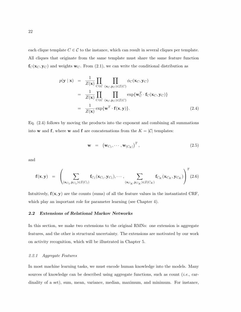
22
each clique template C ∈ C to the instance, which can result in several cliques per template.
All cliques that originate from the same template must share the same feature function
fC(xC ,yC) and weights wC . From (2.1), we can write the conditional distribution as
p(y | x) =1
Z(x)
∏C∈C
∏(xC ,yC)∈I(C)
φC(xC ,yC)
=1
Z(x)
∏C∈C
∏(xC ,yC)∈I(C)
exp{wTC · fC(xC ,yC)}
=1
Z(x)exp{wT · f(x,y)}. (2.4)
Eq. (2.4) follows by moving the products into the exponent and combining all summations
into w and f , where w and f are concatenations from the K = |C| templates:
w =(wC1 , · · · ,w|CK |
)T, (2.5)
and
f(x,y) =
∑(xC1
,yC1)∈I(C1)
fC1(xC1 ,yC1), · · · ,∑
(xCK,yCK
)∈I(CK)
fCK(xCK
,yCK)
T
.(2.6)
Intuitively, f(x,y) are the counts (sums) of all the feature values in the instantiated CRF,
which play an important role for parameter learning (see Chapter 4).
2.2 Extensions of Relational Markov Networks
In this section, we make two extensions to the original RMNs: one extension is aggregate
features, and the other is structural uncertainty. The extensions are motivated by our work
on activity recognition, which will be illustrated in Chapter 5.
2.2.1 Aggregate Features
In most machine learning tasks, we must encode human knowledge into the models. Many
sources of knowledge can be described using aggregate functions, such as count (i.e., car-
dinality of a set), sum, mean, variance, median, maximum, and minimum. For instance,

23
in an image the color variance of the same type of objects is usually small; in a sentence
the numbers of noun phrases and verb phrases could be related; and in human activity
recognition, we know that most people only have one lunch and one dinner everyday. How
can this type of knowledge help the labeling of an individual object, phrase, or activity? In
this section, we extend RMN to encode such aggregate features that can be used for the
inference of individual labels. To achieve this, we extend the syntax of relational clique
templates as follows:
• First, we allow aggregates of tuples, such as COUNT(), SUM(), MEAN(), and ME-
DIAN() in the SELECT clause. Therefore, we can group tuples using GROUP BY
clause and define potentials over aggregates of the groups.
• Second, the WHERE clause can include label attributes. Because labels are hidden
during inference, such templates can generate cliques that potentially involve all the
tuples.
We use a concrete example to illustrate how such aggregate templates can be used
to instantiate CRFs. For instance, to have a soft constraint that limits the number of
“DiningOut” activity per day of week, we can define the following clique template:
SELECT COUNT(*)
FROM Activity
WHERE Label = DiningOut
GROUP BY DayOfWeek ,
where the GROUP BY clause groups tuples with the same DayOfWeek. The potential
function of this template indicates the likelihood of each possible count. For example, we
can define the potential function as a geometric distribution (a discrete counterpart of the
exponential distribution) to penalize big counts.
To illustrate how to unroll the aggregate template, we apply the above SQL query to
the data in Fig. 2.1(b). The instantiated CRF is shown in Fig. 2.5. This query results in
two groups and an aggregate (count) node is created for each group (node “count 1” and
“count 2” ). We define local potentials for aggregate nodes using the template potential.

24
������������1
������������ ������������ ������������
����TimeOfDay DayOfWeek Duration
2 3 4Label
Number of "DiningOut"Count 1 Count 2
Figure 2.5: The instantiated CRF after using the aggregate features.
For instance, the local potential of count 1 could be a geometric distribution, which implies
dining out multiple times a day is less likely. Then we build a clique that consists of
each aggregate node and all the variables used for computing the aggregate, and the clique
potential encodes the aggregation. For example, we build a clique over count 1 (c1), label
1 (l1), and label 2 (l2), and the potential function encodes the counting relation as:
φc(l1, l2, c1) =
1 if c1 = δ(l1 = DiningOut) + δ(l2 = DiningOut);
0 otherwise,(2.7)
To summarize, to instantiate an aggregate template, we create an aggregate node for
each aggregate in the query result, and then we generates two types of cliques. The first
type of clique is the standard: it connects the variables in the SELECT clause. This type
of clique includes aggregate nodes and perhaps other regular nodes as well, and shares the
clique potential defined in the template. The second type of clique connects each aggregate
node with all the variables used for computing the aggregate. The potentials of such cliques
encode the relation of aggregation, such as count or sum, so that they are often deterministic
functions. Note that in practical applications, the second type of clique could be very large
and make the inference very challenging. We will discuss efficient inference over aggregations
in Section 3.3.

25
2.2.2 Structural Uncertainty
So far we have assumed we know the exact structures of the instantiated CRFs and thus
the only uncertainties in our models are the hidden labels. However, in many domains there
may be structural uncertainty [81, 34]. One example is the reference uncertainty [34], i.e.,
the reference relations between the entities could be unknown. In this section we discuss
another type of structural uncertainty, called instance uncertainty. Such uncertainties could
appear when the existence of objects depends on hidden variables. For instance, suppose
in the running example we have a new class “Restaurant” that stores the list of restaurants
the person has been to. If all the activity labels are given, we can simply generate the list
of restaurants based on the locations of “DiningOut” activities. However, since the activity
labels are unknown, the instances in “Restaurant” and thereby the structure of the unrolled
model are not fixed. In general, enumerating all the possible structures is intractable, so we
only consider a small set of structures based on certain heuristics. For example, we could
use the most likely configuration of the labels or the top n configurations to generate the
model structures. To encode such heuristics in our model , we add a new keyword BEST(n)
in the RMN syntax to specify the best n configurations in a query; thus BEST(1) is the
most likely configuration.
As an example, the following template generates the instances in “Restaurant” from the
most likely configuration of activity labels:
INSERT INTO Restaurants (Location)
SELECT Location
FROM BEST(1) Activity
WHERE Label = DiningOut.
When this template is used, the most likely sequence of labels is first inferred. Based on
the most likely sequence, we can find the “DiningOut” activities and insert those locations
to the set of “Restaurant.” Then we can instantiate the complete CRF involving both
activities and restaurants. We may repeat this procedure until the structure converges, as
will be discussed in Chapter 5. We can also use BEST(n) (n > 1) to generate n sets of
“Restaurant” and thereby n different model structures. In that case, we could perform

26
inference in the n models separately and select the “best” model based on certain criterion.
However, the discussion of model selection in RMNs is beyond the scope of this thesis.
The extension of instance uncertainty greatly enhances the applicability of RMN. As
another example, we can express the segmentation of temporal sequences using clique tem-
plates. Suppose we have a sequence of temporal objects stored in table “TemporalSequence.”
Each temporal object consists of a hidden label, a timestamp, etc. The goal of segmenta-
tion is to chop the sequence into a list of segments so that the temporal objects within each
segment are consecutive and have identical label. This procedure can be represented using
the following template:
INSERT INTO Segment (Label, StartTime, EndTime)
SELECT Label, MIN(Timestamp), MAX(Timestamp)
FROM BEST(1) TemporalSequence
GROUP CONSECUTIVELY BY Label.
The input to this template is the tuples in TemporalSequence, and the output is the tuples
in table Segment. Each segment consists of a start time, an end time, and a label of that
segment. Because the hidden variable “Label” appear in the “GROUP BY” clause, we again
have the problem of instance uncertainty. To deal with it, we indicate BEST(1) so that the
segmentation is based on the most likely labels. Note in the “GROUP BY” clause we add
a new keyword “CONSECUTIVELY.” This extension makes sure the temporal objects in
a group are alway consecutive.
2.3 Summary
In this chapter, we began with the discussion of the conditional random field (CRF) model,
a probabilistic model developed for structured data. Then we explained the relational
Markov network (RMN) model that defines CRF at the template level. However, we found
the original RMN is inadequate to define all the features in activity recognition. So we have
made two extensions in this chapter: aggregate features and instance uncertainty.

27
Chapter 3
INFERENCE IN RELATIONAL MARKOV NETWORKS
In last chapter, we have demonstrated that the relational Markov network (RMN) is a
very flexible and concise framework for defining features that can be used in the activity
recognition context. After we have specified an RMN, there are still two essential tasks to
do: inference and learning. In this chapter we discuss the inference, and the learning is
left to the next chapter. The novel contributions in this chapter are the efficient inference
algorithms for aggregate features, such as the application of Fast Fourier Transform (FFT)
for summation features and the local MCMC algorithm that can be applied to generic
aggregates.
The task of inference in the context of RMN is to infer the hidden values (e.g., activity
labels) from the observations (e.g., time of day, duration, etc.). Because the correlations
between the hidden labels, we would like to perform collective classification to infer their
values simultaneously. Given a model of RMN including the set of features and their weights
(we will discuss how to estimate the weights in next chapter), we first instantiate the CRF
from the data instance, as discussed in Chapter 2, then we do inference over the instantiated
CRF. Exact inference in a general Markov network (including CRF) is NP-hard [19], so it
often becomes intractable in practice. In this chapter, we first discuss two widely used
approximated algorithms – Markov Chain Monte Carlo (MCMC) and belief propagation
(BP), and then we present optimized inference algorithms for aggregate features.
Note that the inference in a CRF could have two meanings: to estimate the posterior
distribution of each hidden variable, and to estimate the most likely configuration of the
hidden variables (i.e., the maximum aposteriori, or MAP, estimation). Here we focus on
posterior distribution estimation; we briefly discuss the MAP inference in the section of
belief propagation.

28
3.1 Markov Chain Monte Carlo (MCMC)
When the exact form of the posterior distribution p(y | x) is difficult to estimate, we
could approximate it by drawing enough samples from p(y | x) and simply counting the
frequencies. This is the basic idea of Monte Carlo approaches. However, because the
state space of p(y | x) is exponential to the number of hidden variables, it often becomes
prohibitive to draw samples independently. One strategy is to generate samples using a
Markov chain mechanism, which is called Markov Chain Monte Carlo (MCMC). The basic
idea of MCMC is to start with some point in the state space, sample the next point based
on the current point and a given transition matrix (or transition kernel for continuous state
space), and repeat sampling until it has enough samples. The transition matrix must be
carefully designed so that the process can efficiently obtain enough samples from the target
distribution p(y | x). There exist a large variety of MCMC algorithms, which have been
widely used in statistics, economics, physics and computer science [38, 1, 82]. In this section
we give a brief introduction to applying MCMC for CRF inference. Specifically, we discuss
how to initialize MCMC samples, how to generate new samples, when to stop the process,
and how to approximate posterior distributions from samples.
• Initialization: The exact initial point is usually not important. A simple way to get
started is to randomly sample each hidden label.
• State transition: Given the current configuration y(i), we sample the next configu-
ration y(i+1) using a specific transition matrix. The design of the transition matrix is
key to the correctness and efficiency of the algorithm. The following three strategies
are often used:
Gibbs sampling: The Gibbs sampler [33] flips one label at a time, by conditioning on
all other labels. That is, the labels of y(i+1) are identical to those of y(i) except for
one component j. Specifically, we obtain y(i+1) as
y(i+1)j′ = y
(i)j′ if j′ 6= j;
y(i+1)j ∼ p(yj | y(i)
−j ,x) = p(yj | MB(i)(yj)
),
(3.1)

29
where y−j stand for all the labels except label yj and MB(yj) is the Markov blanket
of label yj , which contains the immediate neighbors of yj in the CRF graph. The
conditional distribution p(yj | MB(i)(yj)
)is usually easy to compute and to sample
from. Sometimes it is more efficient to flip a block of variables at a time, and thus we
get block Gibbs sampler.
Metropolis-Hastings sampling: A Metropolis-Hastings (MH) sampler [43, 72] uses a
proposal distribution q(y′ | y(i),x) to sample a candidate configuration y′. To guaran-
tee the desired target distribution, the next configuration y(i+1) is set to the candidate
y′ with an acceptance probability, defined as:
a(y′,y(i)) = min
{1,
p(y′ | x)q(y(i) | y′,x)p(y(i) | x)q(y′ | y(i),x)
}(3.2)
= min{
1,exp{wT · f(x,y′)}exp{wT · f(x,y(i))}
}, (3.3)
and otherwise y(i+1) = y(i). To get (3.3) from (3.2), we assume the proposal distri-
bution is symmetric, i.e., q(y(i) | y′,x) = q(y′ | y(i),x), and we apply (2.4) in which
the partition functions for p(y′ | x) and p(y(i) | x) are canceled out. The performance
of MH sampling strongly depends on the choice of the proposal distribution, which
could be some generic heuristics (e.g., switching two labels) or could encode domain
knowledge.
Mixtures of transition matrices: It is also possible to mix several transition matrices
into an MCMC sampler. For example, at each time step, we can choose a Gibbs
sampler with probability γ(0 < γ < 1), and choose an MH sampler with probability
1− γ. If each individual sampler converges to the desired target distribution, so does
the mixed one [109]. In some cases using mixtures of transition matrices could be
much more efficient than using any individual sampler.
• Stop criterion: It is difficult to estimate how many samples are needed for a given
problem, and there has no satisfactory theoretical answer yet. In practice people often
make decisions by observing the MCMC outputs and performing some statistical tests,
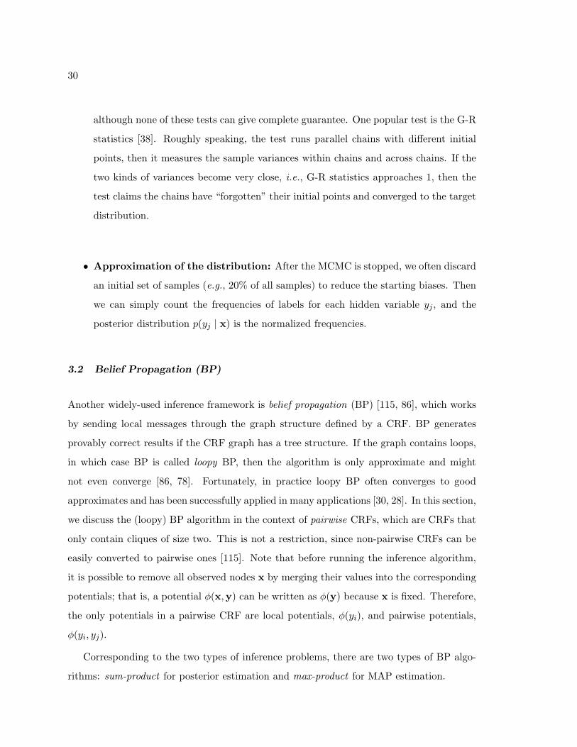
30
although none of these tests can give complete guarantee. One popular test is the G-R
statistics [38]. Roughly speaking, the test runs parallel chains with different initial
points, then it measures the sample variances within chains and across chains. If the
two kinds of variances become very close, i.e., G-R statistics approaches 1, then the
test claims the chains have “forgotten” their initial points and converged to the target
distribution.
• Approximation of the distribution: After the MCMC is stopped, we often discard
an initial set of samples (e.g., 20% of all samples) to reduce the starting biases. Then
we can simply count the frequencies of labels for each hidden variable yj , and the
posterior distribution p(yj | x) is the normalized frequencies.
3.2 Belief Propagation (BP)
Another widely-used inference framework is belief propagation (BP) [115, 86], which works
by sending local messages through the graph structure defined by a CRF. BP generates
provably correct results if the CRF graph has a tree structure. If the graph contains loops,
in which case BP is called loopy BP, then the algorithm is only approximate and might
not even converge [86, 78]. Fortunately, in practice loopy BP often converges to good
approximates and has been successfully applied in many applications [30, 28]. In this section,
we discuss the (loopy) BP algorithm in the context of pairwise CRFs, which are CRFs that
only contain cliques of size two. This is not a restriction, since non-pairwise CRFs can be
easily converted to pairwise ones [115]. Note that before running the inference algorithm,
it is possible to remove all observed nodes x by merging their values into the corresponding
potentials; that is, a potential φ(x,y) can be written as φ(y) because x is fixed. Therefore,
the only potentials in a pairwise CRF are local potentials, φ(yi), and pairwise potentials,
φ(yi, yj).
Corresponding to the two types of inference problems, there are two types of BP algo-
rithms: sum-product for posterior estimation and max-product for MAP estimation.

31
3.2.1 Sum-product for Posterior Estimation
In the BP algorithm, we introduce a “message” mij(yj) for each pair of neighbors yi and
yj , which is a distribution (not necessarily normalized) sent from node i to its neighbor
j about which state variable yj should be in. The messages propagate through the CRF
graph until they (possibly) converge, and the marginal distributions can be estimated from
the stable messages. A complete BP algorithm defines how to initialize messages, how to
update messages, how to schedule the order of updating messages, and when to stop passing
messages.
• Message initialization: Usually all messages mij(yj) are initialized as uniform dis-
tributions over yj .
• Message update rule: The message mij(yj) sent from node i to its neighbor j is
updated based on local potentials φ(yi), the pairwise potential φ(yi, yj), and all the
messages to i received from i’s neighbors other than j (denoted as n(i) \ j). More
specifically, for sum-product, we have
mij(yj) =∑yi
φ(yi)φ(yi, yj)∏
k∈n(i)\j
mki(yi) (3.4)
• Message update order: The algorithm iterates the message update rule until it
(possibly) converges. Usually at each iteration, it updates each message once, and the
specific order is not important (although it might affect the convergence speed).
• Convergence conditions: To test whether the algorithm converges at an iteration,
for each message, BP measures the difference between the old message and the updated
one, and the convergence condition is met when all the differences are below a given
threshold ε. More formally, the condition is
||mij(yj)(k) −mij(yj)(k−1)|| < ε, ∀i, and ∀j ∈ n(i) (3.5)
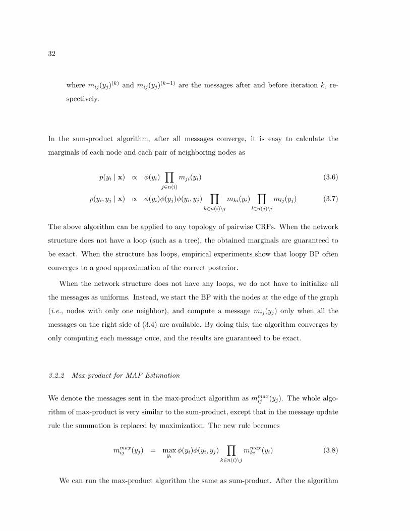
32
where mij(yj)(k) and mij(yj)(k−1) are the messages after and before iteration k, re-
spectively.
In the sum-product algorithm, after all messages converge, it is easy to calculate the
marginals of each node and each pair of neighboring nodes as
p(yi | x) ∝ φ(yi)∏
j∈n(i)
mji(yi) (3.6)
p(yi, yj | x) ∝ φ(yi)φ(yj)φ(yi, yj)∏
k∈n(i)\j
mki(yi)∏
l∈n(j)\i
mlj(yj) (3.7)
The above algorithm can be applied to any topology of pairwise CRFs. When the network
structure does not have a loop (such as a tree), the obtained marginals are guaranteed to
be exact. When the structure has loops, empirical experiments show that loopy BP often
converges to a good approximation of the correct posterior.
When the network structure does not have any loops, we do not have to initialize all
the messages as uniforms. Instead, we start the BP with the nodes at the edge of the graph
(i.e., nodes with only one neighbor), and compute a message mij(yj) only when all the
messages on the right side of (3.4) are available. By doing this, the algorithm converges by
only computing each message once, and the results are guaranteed to be exact.
3.2.2 Max-product for MAP Estimation
We denote the messages sent in the max-product algorithm as mmaxij (yj). The whole algo-
rithm of max-product is very similar to the sum-product, except that in the message update
rule the summation is replaced by maximization. The new rule becomes
mmaxij (yj) = max
yi
φ(yi)φ(yi, yj)∏
k∈n(i)\j
mmaxki (yi) (3.8)
We can run the max-product algorithm the same as sum-product. After the algorithm

33
converges, we calculate the MAP belief at each node yi as
b(yi) ∝ φ(yi)∏
j∈n(i)
mmaxji (yi) (3.9)
Suppose there is a unique MAP configuration y∗. Then each component of y∗ is simply the
most likely value in MAP belief:
y∗i = argmaxyi
b(yi) (3.10)
3.3 Efficient Inference with Aggregate Features
In Section 2.2, we extend the original RMN to model aggregate features, such as summation.
Although the syntax is fairly simple, those aggregate features could generate cliques that
contain all nodes over which the aggregation is performed. Because the size of the potential
is exponential to the number of variables in the aggregation, those large cliques can easily
make standard (loopy) BP intractable. In these cases, we could use MCMC for inference.
However, standard MCMC algorithms, such as Gibbs sampling, often converge very slow in
complex models, and developing customized and efficient transition matrices is extremely
challenging. For example, we initially applied an MCMC algorithm for location-based ac-
tivity recognition that uses a mixture of Gibbs sampler and MH sampler [66]. However, we
found such Monte Carlo algorithms usually scale up to only a few hundred variables in an
aggregation. Here we present two more efficient inference algorithms for aggregate features.
The first is specifically developed for summation features, by combining BP and the Fast
Fourier Transform (FFT). Summation features are very common and some other aggregate
features, such as count and average, can also be represented as summations. The new al-
gorithm can easily handle thousands of variables [65]. In the second algorithm, we apply
MCMC within the framework of BP. That is, we use MCMC locally to compute the “hard”
messages, while we still compute other messages in analytical forms. This new technique,
we call it local MCMC, is very general and can be applied to a variety of aggregate features.

34
y1 y2 y8y7y6y5y4y3
Ssum
ysum
(a) y1 y2 y8y7y6y5y4y3
S 12 S 34 S 56 S 78
y12 y34 y56 y78
S 1234 S 5678
y1234 y5678
S sum
ysum
(b) 10 100 10000
1000
2000
3000
Number of nodes
Runn
ing
Tim
e [s
]
Naive BPMCMCOptimized BP
(c)
Figure 3.1: (a) Pairwise CRF that represents ysum =∑8
i=1 yi; (b) Summation tree that representsysum =
∑8i=1 yi; (c) Computation time for summation cliques versus the number of nodes in the
summation. The Si’s in (a) and (b) are auxiliary nodes to ensure the summation relation
3.3.1 Optimized summation templates using FFT
The aggregate features defined using RMN generate cliques that contain all nodes over
which the aggregation is performed. To apply BP algorithm, we first convert the unrolled
model into a pairwise CRF by introducing auxiliary variables [115], as shown in Fig. 3.1(a).
The potential functions of the auxiliary variables encode the aggregation. Because of the
high dimensionality of those aggregate potentials, standard message updates (Eq. (3.4))
often become intractable.
To handle summation cliques with potentially large numbers of addends, our inference
dynamically builds a summation tree, which is a pairwise Markov network as shown in
Fig. 3.1(b). In a summation tree, the leaves are the original addends and each internal
node yjk represents the sum of its two children yj and yk; this sum relation is encoded
by an auxiliary node Sjk. The state space of Sjk consists of the joint (cross-product) state
of its neighbors: yj , yk, and yjk. It is easy to see that the summation tree guarantees
that the root ysum equals∑n
i=1 yi, where y1 to yn are the leaves of the tree. To define
the BP protocol for summation trees, we need to specify two types of messages: an upward
message from an auxiliary node to its parent (e.g., mS12y12), and a downward message from
an auxiliary node to one of its two children (e.g., mS12y1).
Upward message update: Starting with Eq. (3.4), we can update an upward message

35
mSijyij as follows.
mSijyij (yij) =∑yi,yj
φS(yi,yj ,yij) myiSij (yi) myjSij (yj)
=∑yi
myiSij (yi) myjSij (yij − yi) (3.11)
= F−1(F(myiSij (yi)) · F(myjSij (yj))
)(3.12)
where φS(yi,yj ,yij) is the potential of Sij encoding the equality yij = yi + yj , i.e.,
φS(yi,yj ,yij) equals 1 if yij = yi +yj and 0 otherwise. (3.11) follows because all terms not
satisfying the equality disappear. Therefore, message mSijyij is the convolution of myiSij
and myjSij . (3.12) follows from the convolution theorem, which states that the Fourier
transform of a convolution is the point-wise product of Fourier transforms [11], where F
and F−1 represent the Fourier transform and its inverse, respectively. When the messages
are discrete functions, the Fourier transform and its inverse can be computed efficiently using
the Fast Fourier Transform (FFT) [11, 70]. The computational complexity of a summation
using FFT is O(k log k), where k is the maximum number of states in yi and yj .
Downward message update: We also allow messages to pass from sum variables
downward to its children. This is necessary if we want to use the belief on sum variables (e.g.,
knowledge on the count of “DiningOut” activities) to change the distribution of individual
variables (e.g., activity labels). From Eq. (3.4) we get the downward message mSijyi as
mSijyi(yi) =∑
yj ,yij
φS(yi,yj ,yij)myjSij (yj)myijSij (yij)
=∑yj
myjSij (yj)myijSij (yi + yj) (3.13)
= F−1(F(myjSij (yj)) · F(myijSij (yij))
)(3.14)
where (3.13) again follows from the sum relation. Note that the downward message mSijyi
turns out to be the correlation of messages myjSij and myijSij . (3.14) follows from the
correlation theorem [11], which is similar to the convolution theorem except, for correlation,
we must compute the complex conjugate of the first Fourier transform, denoted as F . Again,
for discrete messages, (3.14) can be evaluated efficiently using FFT.

36
At each level of a summation tree, the number of messages (nodes) is reduced by half
and the size of each message is doubled. Suppose the tree has n upward messages at the
bottom and the maximum size of a message is k . For large summation trees where n� k,
the total complexity of updating the upward messages at all the log n levels follows now as
log n∑i=1
n
2i·O(2i−1k log 2i−1k
)= O
(n
2
log n∑i=1
log 2i−1
)= O(n log2 n) (3.15)
Similar reasoning shows that the complexity of the downward pass is O(n log2 n) as well.
Therefore, updating all messages in a summation clique takes O(n log2 n) instead of time
exponential in n, as would be the case for a non-specialized implementation of aggregation.
We empirically compare our FFT-based BP algorithm for summation cliques with in-
ference based on MCMC and regular BP, using the model and data from [66]. In our
experiments, the test accuracies resulting from using the different algorithms are almost
identical. Therefore, we only focus on comparing the efficiency and scalability of summa-
tion aggregations. We show in Fig. 3.1(c) the running times for the different algorithms as
the number of nodes in a summation clique increases. As can be seen, a naive implementa-
tion of BP becomes extremely slow for only 20 nodes, MCMC only works for up to a few
hundreds nodes, while our algorithm can perform summation for 2, 000 variables within a
few minutes.
3.3.2 Combining BP and Local MCMC for Aggregate Features
For summation features, we have developed efficient algorithm using FFT. However, for
other aggregate features, this algorithm may not apply. In this section, we present an
inference algorithm for complex models with generic aggregate features, by combining BP
and MCMC. The rationale is the following: In such complex models, usually most BP
messages can be computed efficiently in analytical forms except those involving aggregate
features; thus we only need to compute those “hard” messages using MCMC and still
compute others messages analytically. The essential part of this new framework is to develop
local MCMC algorithms for any given aggregate feature. The new algorithm can be much

37
more efficient than BP because it avoids the exponential complexity of computing aggregate
messages; it can also be more efficient than traditional MCMC because the local MCMC only
needs to deal with a single feature. For example, Gibbs sampling often does not work well for
complicated models, but can be efficient enough for single aggregate relations. Furthermore,
the modules of local MCMC algorithms can be reused in many different models. Since the
number of frequently used aggregate functions is limited, it is possible to develop highly-
optimized algorithms for each function.
In the following we explain how to efficiently compute messages using local MCMC. We
use Gibbs sampling as an example, but the algorithm can be extended to other MCMC
techniques. In Fig. 3.2(a), we show a pairwise CRF piece encoding a certain aggregate
feature. During BP, we need to compute the messages from Sagg to yagg and each yi.
Denote Y = {y1, . . . ,yn,yagg}, and for any y ∈ Y , we can compute the message as:
mSaggy(y) ∝∑
y′∈Y,y′ 6=y
φ(y1, . . . ,yn,yagg)∏
y′∈Y,y′ 6=y
my′Sagg(y′) (3.16)
where φ(y1, . . . ,yn,yagg) is the potential encoding the aggregate equality, i.e., φ(y1, . . . ,yn,yagg)
equals 1 if yagg = agg(y1, . . . ,yn) and 0 otherwise. Standard nonparametric BP [102] re-
quires a sampling procedure for each message, i.e., we need to run MCMC n + 1 times to
get all the messages in this piece of CRF. Fortunately, we can use a trick that requires only
one Markov chain for all the messages. The trick works by multiplying mySagg(y) on both
sides of (3.16), and we get
mSaggy(y)mySagg(y) ∝∑
y′∈Y,y′ 6=y
φ(y1, . . . ,yn,yagg)∏y′∈Y
my′Sagg(y′) (3.17)
Note that, on the right side of (3.17), the terms inside the summation sign are exactly the
same for all y ∈ Y . Therefore, instead of sample each message mSaggy(y) directly, we can
run a single MCMC chain to estimate mSaggy(y)mySagg(y) for any y ∈ Y and then we can
compute each message easily.
The algorithm of local Gibbs sampler is describe in Alg. 3.1, which can be easily extended
to other MCMC algorithms. Note that because of the deterministic aggregate relation, we

38
inputs : Messages myaggSagg(yagg) and myiSagg(yi), 1 ≤ i ≤ noutput: Messages mSaggyagg(yagg) and mSaggyi(yi), 1 ≤ i ≤ n
Initialization: sample yi ∼ myiSagg(yi), 1 ≤ i ≤ n and set yagg = agg(y1, . . . ,yn) ;1.
for k = 1, . . . ,K iterations do2.
for i = 1, . . . , n do3.
Compute conditional distribution4.
p(y′i | y−i) ∝ myaggSagg(agg(y−i,y′i))myiSagg(y′i) ;Sample yi ∼ p(y′i | y−i) ;5.
end6.
Set yagg = agg(y1, . . . ,yn) ;7.
end8.
Estimate mSaggy(y)mySagg(y),y ∈ {y1, . . . ,yn,yagg} by frequency counting ;9.
Compute mSaggy(y) =mSaggy(y)mySagg (y)
mySagg (y) ,y ∈ {y1, . . . ,yn,yagg} ;10.
Algorithm 3.1: Computing aggregate messages using local Gibbs sampling
do not need to sample yagg, but can compute it from other components. At Step 4, the
conditional distribution for component yi is computed based on other components and the
aggregate, which follows from (3.17). Then at Step 5, yi is sampled from the conditional
distribution. When all yi are updated, we compute the value of yagg at Step 7. After the
sampling process, each mSaggy(y)mySagg(y) is estimate based on the samples, and at the
last step we compute each message mSaggy(y).
To evaluate our algorithm, we apply the algorithm to the model of mobile robot map
building [69]. The goal of that project is to enhance metric maps with semantic information
about types of objects in an environment, such as door, wall, and others. To do that, line
segments are first extracted from laser-range scans and then fed into a classifier. The model
takes into account the following evidence:
• Local features, such as the length of a line segment;
• Indentation between neighboring line segments (for example, wall-wall should have
small indentations but wall-door should have larger indentations);
• Variance of the door widths in the same hallway, which can be modeled as a zero-mean
Gaussian with learned standard deviation;

39
y1 y2 y8y7y6y5y4y3
Sagg
yagg
(a) 0 2000 4000 6000 8000 100001
1.05
1.1
1.15
1.2
1.25
1.3
MCMC Iteration
G−R
Sta
tistic
Global MCMCLocal MCMC
(b) 0 10 20 30 40 50 600
0.2
0.4
0.6
0.8
1
BP iteration
L2−N
orm
of M
ax M
essa
ge C
hang
e
Caching random numbersNo caching
(c)
Figure 3.2: (a) A CRF piece in which yagg is the aggregate of y1, . . . ,y8 and the aggregation isencoded in the potential of auxiliary variable Sagg; (b) Convergence comparison of local MCMCwith global MCMC (G-R statistics approaching 1 indicates good convergence); (c) Comparison ofthe inference with and without caching the random numbers.
• Variance of the angles of the wall segments which can also be modeled using a zero-
mean Gaussian;
Here the last two features involves aggregate function “variance” and can be implemented
using the local MCMC algorithm.
In a preliminary experiment, we compare the convergence rate of the local and global
Gibbs sampling. As shown in Fig. 3.2(b), for local Gibbs sampling, G-R statistics becomes
less than 1.05 after a few hundred iterations while for global sampling it takes more than
6, 000 iterations. This is not a surprise because the local Gibbs sampling only involves a
single feature, but the global Gibbs sampling takes into account all the features.
One issue of using local MCMC is that the sampling variance could potentially make
BP instable. To reduce the sampling variance, we found it very useful to cache the random
numbers locally and reuse them in later BP iterations. We compare the convergence of BP
with and without random number caching. The convergence is measured by the maximal
change between the messages before and after each iteration. A typical evolution of maximal
changes is shown in Fig. 3.2(c). It is clear that by reusing the random numbers, BP converges
much faster to a stable level.

40
3.4 Summary
The goal of this chapter is to discuss efficient inference algorithms for CRFs and RMNs.
Exact inference often becomes intractable for practical models, so we have focused on ap-
proximated algorithms. We started with brief introductions to two widely used algorithms:
Markov Chain Monte Carlo and (loopy) belief propagation. However, neither of them is
efficient enough for models involving aggregate features. In this chapter we presented two
optimized algorithms to accelerate the inference with aggregate features. Both algorithms
are developed in the framework of belief propagation. For the widely used summation fea-
tures, we can construct summation trees and apply FFT for message computation at each
internal node of the tree. The complexity of the new algorithm is only O(n log2 n) instead
of exponential in n, where n is the number of variables in a summation. For other generic
aggregate features, we proposed to use local MCMC to compute the messages through ag-
gregations. By running sampling only on some portions of a model, the overall performance
can be greatly improved.

41
Chapter 4
TRAINING RELATIONAL MARKOV NETWORKS
In last chapter, we have discussed a variety of inference techniques for conditional ran-
dom fields (CRF) and relational Markov networks (RMN). In this chapter, we discuss the
other task: learning the model parameters. In RMN, the goal of parameter learning is to
determine the optimal weights of relational clique templates given the labeled training data.
Similar to inference, the learning of RMN starts with instantiating CRFs from the training
data, and then searches for the weights so as to optimize a certain criterion. In this chapter,
we discuss three different criteria: maximum likelihood (ML), maximum pseudo-likelihood
(MPL), and maximum per-label likelihood (as in boosting). The contributions of this chap-
ter include a novel learning algorithm called virtual evidence boosting, an algorithm that
simultaneously estimates the likelihood of train data and its gradient using MCMC, and
empirical comparisons between different learning algorithms.
This chapter starts with the discussion of the ML estimation, which requires running the
inference using MCMC or BP. In the second section we explain the MPL estimation. Then
we present a new learning algorithm called virtual evidence boosting, which is a general
approach for feature selection and parameter estimation for CRF and RMN. Finally we
show experimental results on comparing different learning algorithms.
4.1 Maximum Likelihood (ML) Estimation
Given labeled training data (x,y), the conditional likelihood p(y | x) only depends on the
feature weights w, as can be seen in (2.4). From now on we will write the conditional
likelihood as p(y | x,w) to highlight its dependency on w.
A common parameter estimation method is to search for the w that maximizes this
conditional likelihood, or equivalently, that minimizes the negative log-likelihood, − log p(y |
x,w) [58, 104, 66]. To avoid overfitting, one typically imposes a so-called shrinkage prior

42
on the weights that keeps weights from getting too large. More specifically, we define the
objective function to minimize as the following:
L(w) , − log p(y | x,w) +wTw2σ2
(4.1)
= −wT · f(x,y) + log Z(x,w) +wTw2σ2
(4.2)
The rightmost term in (4.1) serves as a zero-mean, Gaussian prior with variance σ2 on each
component of the weight vector. (4.2) follows directly from (4.1) and (2.4). While there is
no closed-form solution for minimizing (4.2), it can be shown that (4.2) is convex relative to
w. Thus, L has a global optimum which can be found using numerical gradient algorithms.
The gradient of the objective function L(w) is given by
∇L(w) = −f(x,y) +∇Z(x,w)Z(x,w)
+wσ2
(4.3)
= −f(x,y) +
∑y′ exp{wT · f(x,y′)}f(x,y′)
Z(x,w)+
wσ2
(4.4)
= −f(x,y) +∑y′
p(y′ | x,w)f(x,y′) +wσ2
(4.5)
= −f(x,y) + Ep(y′|x,w)[f(x,y′)] +wσ2
(4.6)
where (4.4) follows from the definition of partition function, Z(x,w) =∑
y′ exp{wT ·
f(x,y′)}, (4.5) follows from the definition of the conditional likelihood, and in (4.6), the
second term is expressed as an expectation over the distribution p(y′ | x,w). Therefore, the
gradient is just the difference between the empirical feature values f(x,y) and the expected
feature values Ep(y′|x,w)[f(x,y′)], plus a prior term. To compute the expected feature values
it is necessary to run inference in the CRF using the current weights w. Previous work has
shown that straightforward gradient descent often converges slowly, but that modern numer-
ical optimization algorithms, such as conjugate gradient or quasi-Newton techniques, can
be much faster [99]. However, these techniques additionally require evaluating the objective
values L(w). To compute the objective values in (4.2) is not easy, because the partition
function Z(x,w) requires us to enumerate all the configurations of hidden variables. In this

43
section we describe how to get around this difficulty by using Monte-Carlo approximation
or Bethe approximation.
4.1.1 MCMC-based ML Estimation
When MCMC is used for inference, the posterior distribution p(y | x,w) is approxi-
mated using a set of M samples, y(i), 1 ≤ i ≤ M . Then the expected feature values
Ep(y′|x,w)[f(x,y′)] ≈ 1M
∑Mi=1 f(x,y(i)). From (4.6), the gradient can be computed as
∇L(w) ≈ −f(x,y) +1M
M∑i=1
f(x,y(i)) +wσ2
=1M
M∑i=1
∆f (i) +wσ2
(4.7)
where ∆f (i) = f(x,y(i)) − f(x,y) is the difference between sampled feature values and the
empirical feature values.
As we just said, it is more difficult to evaluate the objective value L(w), which is
necessary for advanced optimization techniques. The key idea is that, instead of evaluating
the absolute values of L(w), we only need to estimate their relative values for the purpose
of ML estimation. And we can approximate the relative values quite efficiently using Monte
Carlo approach [37]. More specifically, L(w) can be approximated relative to L(w), where
w is the reference weight vector. We have (see Appendix A.1 for the derivation):
L(w) = L(w) + log
(1M
M∑i=1
exp{
(w − w)T ·∆f (i)})
+wT ·w − wT · w
2(4.8)
where ∆f (i) = f(x, y(i))− f(x,y) is the difference between sampled feature values using w
and the empirical feature values. It can be shown that the best approximation in (4.8) is
obtained when w is near the optimal w [37]. We should take this into account and use
better w whenever possible.
If we compare Eq. (4.7) and (4.8), we see both require the difference between the
sampled feature values and the empirical feature values. But the samples in (4.8) are from

44
inputs : the given weights woutput: the objective function value L(w) and its gradient ∇L(w)
//Evaluate the gradient ∇L(w)Run MCMC with w and get M samples from p(y | x,w) ;1.
Get feature value difference ∆f (i) = f(x,y(i))− f(x,y) for 1 ≤ i ≤M ;2.
Compute the gradient ∇L(w) using Eq. (4.7) ;3.
//Evaluate the objective value L(w)if First time calling this function then4.
L(w) = L(w) = 0; w = w ;5.
∆f (i) = ∆f (i) for 1 ≤ i ≤M ;6.
else7.
Compute L(w) using Eq. (4.8) ;8.
if L(w) < L(w) then9.
L(w) = L(w); w = w ;10.
∆f (i) = ∆f (i) for 1 ≤ i ≤M ;11.
end12.
end13.
Algorithm 4.1: MCMC-based algorithm for evaluating objective function and its gradient
the distribution p(y | x, w) while the samples in (4.7) are from the distribution p(y | x,w).
As we will show, by picking the reference weight vector w in a specific way and caching the
results, we can reuse the samples and simultaneously estimate both the objective value and
its gradient .
The algorithm of evaluating objective function and its gradient using MCMC is shown
in Alg. 4.1. The algorithm works as a function used by efficient optimization algorithms
such as quasi-Newton or conjugate gradient. The input of the algorithm is the weight vector
provided by the optimizer and the algorithm returns the estimated objective function and
its gradient. To estimate the gradient, we use MCMC sampler to get M samples from the
posterior distribution p(y | x,w) (Step 1) and then calculate the difference between the
sampled feature values and the empirical feature values (Step 2). In order to estimate the
objective value, we keeps the up-to-now best estimator w, along with L(w) and ∆f (i)(1 ≤
i ≤ M). When the optimizer first calls this function, w is initialized as w, and both L(w)
and L(w) are set as 0 (Step 5). Therefore, all the objective values are relative to the
objective value of initial weights. In later iterations, when we find a better w that makes

45
L(w) less than L(w), we update w with the new w (Step 10 and Step 11). Thus function
value estimation becomes very efficient—it re-use the sampled feature values from gradient
estimation. Moreover, we can get more accurate estimates as w approaches closer to the
optimal weights, which is important for the optimizer to converge.
4.1.2 BP-based ML Estimation
We can also perform ML estimation using BP inference. Without loss of generality, we only
consider the case where the instantiated CRFs are pairwise. At each step of optimization,
BP inference gives the posterior distribution for each clique c, p(y′c | x) (in Eq. (3.6) and
Eq. (3.7)). Thus we get the expected feature values as
Ep(y′|x,w)
[f(x,y′)
]=
∑c∈C
fc(x,y′c)p(y′c|x) (4.9)
where C denotes all the cliques in a CRF and fc is the feature values counted on clique c.
We can then compute the gradient using (4.6).
To approximate the objective value L(w), we can use Bethe method [117]. Specifically,
we approximate the partition function Z as
− log Z ≈ UBethe −HBethe, (4.10)
where UBethe is called Bethe average energy and HBethe is called Bethe entropy, and they
are computed as
UBethe = −∑c∈C
∑y′c
p(y′c | x)(wT · fc(x,y′c)
),
and
HBethe = −∑c∈C
∑y′c
p(y′c | x) log p(y′c | x) +N∑
i=1
(di − 1)∑y′i
p(y′i | x) log p(y′i | x),
where i ranges over all the variables and di is the degree for variable i.

46
������������1
������������ ������������ ������������
����
Label TimeOfDay DayOfWeek Duration
2 3 4
(a)
������������TimeOfDay DayOfWeek Duration������������Label Neighbor label
���������������
��������� �
��� ���
��������� �
� ������ ���
��������� ���
��������� ���
��������� ���
��������� ���
���������1 2 43
(b)
Figure 4.1: (a) Original CRF for learning; (b) Converted CRF for MPL learning by copying thetrue labels of neighbors as local evidence.
After we have an estimate of the partition function Z, we can approximate the objective
values using (4.2). When the instantiated CRFs have no loops, the Bethe method gives the
exact value of the objective values and thereby in theory the ML learning converges to the
global optimum. When the CRFs do have loops, the Bethe method only gives approximated
result; therefore, the learning may not converge to the optimum, or may not converge (even
when the BP inference converges).
4.2 Maximum Pseudo-Likelihood (MPL) Estimation
A key assumption in traditional machine learning algorithms is the independence between
hidden labels. RMN and CRF break this assumption by considering the mutual influ-
ence between labels. This breakthrough greatly enhances the expressiveness and flexibility,
however, at a cost of more expensive learning. As discussed in last section, ML learning
requires running an inference procedure at each iteration of the optimization, which can be
very expensive even for approximated algorithms. To circumvent this cost, another learning
algorithm was developed that instead maximizes the pseudo-likelihood of the training data
(MPL) [9].
To give some intuitions on how MPL works, let’s start with the CRF example discussed

47
in Chapter 2. We show the model structure again in Fig. 4.1(a). MPL converts the original
CRF to a CRF as shown in Fig. 4.1(b), where the true labels of neighbors (known during
learning) are copied as local attributes. By doing this, the structure of the CRF is signif-
icantly simplified — it becomes a set of separated chunks where each chunk has only one
hidden variable. MPL estimation is essentially the ML estimation on this simplified model.
Specifically, MPL maximizes the following pseudo-likelihood :
pl(y | x,w) ,n∏
i=1
p(yi | MB(yi),w) (4.11)
Here, MB(yi) is the Markov blanket of variable yi, which contains the immediate neighbors
of yi in the CRF graph (note that the value of each node is known during learning). Thus,
the pseudo-likelihood is the product of all the local likelihoods, p(yi | MB(yi),w). By
representing the local likelihoods as log-linear combinations of features, we can rewrite the
pseudo-likelihood as
pl(y | x,w) =n∏
i=1
1Z(MB(yi),w)
exp{wT · f(yi,MB(yi))
}, (4.12)
where f(yi,MB(yi)) is the local feature values involving variable yi, and Z(MB(yi),w) =∑y′i
exp{wT · f(y′i,MB(y′i))
}is the local normalizing function. Therefore, computing pseudo-
likelihood is much more efficient than computing likelihood p(y|x,w), because pseudo-
likelihood only requires computing local normalizing functions and avoids computing the
global partition function Z(x,w).
Similar to ML, in practice we minimize the negative log-pseudo-likelihood plus a shrink-
age prior, and the objective function becomes
PL(w) , − log pl(y | x,w) +wTw2σ2
(4.13)
= −n∑
i=1
log p(yi | MB(yi),w) +wTw2σ2
(4.14)
=n∑
i=1
(−wT · f(yi,MB(yi)) + log Z(MB(yi),w)
)+
wTw2σ2
(4.15)

48
PL(w) is a convex function (think PL(w) as the ML objective function in the simplified
model) and we can apply gradient-based algorithms to find w that minimizes PL(w). The
gradient of PL(w) can be computed as
∇PL(w) =n∑
i=1
(−f(yi,MB(yi)) + Ep(y′i|MB(yi),w)
[f(y′i,MB(yi))
])+
wσ2
. (4.16)
As we can see, (4.16) can be expressed as the difference between empirical feature values
and expected feature values, similar to (4.6). However, the key difference is that (4.16) can
be evaluated very efficiently without running a complete inference procedure.
MPL has been shown to perform well in several domains [56, 95]. However, it is possible
that the results of MPL differ significantly from the results of ML [37] and no general
guidance has been given on when MPL can be safely used.
Finally, readers may notice that the simplified model as in Fig. 4.1(b) cannot be used
for inference, since it assumes that the hidden states y are known.
4.3 Virtual Evidence Boosting
Boosting is a general approach for supervised learning and has been successfully applied
in a lot of domains [29, 31]. Given the training data (x1,y1), . . ., (xN ,yN ), where xi is
an observation vector and yi is the label, boosting works by sequentially learning a set of
weak classifiers and combining them for final decisions. Can we apply boosting to CRFs?
At the first look, the answer seems to be no, since the boosting algorithms assume the
independence between training examples but in CRFs the labels are dependent. However,
we can overcome this difficulty by borrowing the idea of MPL; that is, we cut an instantiated
CRF into individual patches (see Fig. 4.1(b)), and use these patches as training instances
for boosting. Based on this idea, we introduce a novel learning algorithm, called virtual
evidence boosting (VEB) [63], which combines boosting and CRF. The key difference to
MPL, however, is that in the new algorithm the neighbor labels are not treated as observed,
but as virtual evidence. This avoids over-estimating the neighborhood dependencies, as
often happens to MPL.
VEB is a general approach for feature selection and parameter estimation in CRFs and

49
RMNs. This approach is able to
• simultaneously perform feature selection and parameter estimation;
• select compatible features between labels and thus learn dependency structures in the
relational data;
• handle both discrete and continuous observations;
• and select various features in a unified and efficient manner, by simply running one
iteration of BP and performing feature counting at each boosting iteration.
To develop the algorithm, we extend the standard boosting algorithms so that the input
observations are either virtual evidences in the form of likelihood values or deterministic
quantities.
4.3.1 Extending Boosting to Handle Virtual Evidence
While traditional boosting algorithms assume observation values be deterministic, in this
section we extend them with virtual evidence [86], i.e., an observation could have a dis-
tribution over its domain rather than a single, observed value. Specifically, we generalize
the LogitBoost algorithm [31], which directly handles probabilities and is closely related to
random field models. For simplicity, we will only explain LogitBoost and our extension for
the binary classification case, i.e., yi ∈ {0, 1}, but both can be easily extended to multi-class
problems [31].
LogitBoost algorithm
LogitBoost works by minimizing the negative per-label-log-likelihood:
L(F ) = −N∑
i=1
log p(yi) (4.17)
where F refers to the ensemble of weak learners, i.e., F (x) =∑M
m=1 fm(x), and p(yi) is a
short notation that represents the posterior probability of a true label conditioned on its

50
evidences. We have
p(yi) =
e−F (xi)
eF (xi)+e−F (xi)if yi = 0;
eF (xi)
eF (xi)+e−F (xi)if yi = 1.
(4.18)
where we assume without loss of generality that ensembles are reverse for yi = 1 and 0.
It is easy to identify the consistency between (4.18) and the logistic regression models, in
which eF (xi) and e−F (xi) represent the potentials for yi = 1 and 0, respectively.
LogitBoost minimizes the objective function (4.17) respect to F using Newton steps.
Given the current ensemble F , the next weak learner in a Newton step is obtained by
solving the weighted least-square-error (WLSE) problem [31]:
fm(x) = argminf
N∑i=1
αi (f(xi)− zi)2 (4.19)
where αi = p(yi)(1−p(yi)) and zi = yi−0.5p(yi)
are the weight and working response for sample
i, respectively.
Extension with virtual evidence
To extend the LogitBoost with virtual evidence, we denote the training data as (ve(x1),y1),
. . ., (ve(xN ),yN ), where each virtual evidence ve(xi) is a given distribution over the obser-
vation domain {1, . . . , X} 1. We again aim to minimize the negative per-label-log-likelihood,
defined in (4.17). However, the computation of the posterior probability p(yi) has to take
the virtual evidence into account:
p(yi) =
PX
xi=1 ve(xi)e−F (xi)PX
xi=1 ve(xi)eF (xi)+PX
xi=1 ve(xi)e−F (xi)if yi = 0;PX
xi=1 ve(xi)eF (xi)PX
xi=1 ve(xi)eF (xi)+PX
xi=1 ve(xi)e−F (xi)if yi = 1.
(4.20)
where∑X
xi=1 ve(xi)e±F (xi) computes the expected potentials given the virtual evidence.
To determine the next weak learner fm(x), we modify the LogitBoost error criterion
1Here virtual evidence is always a discrete distribution, which is enough for our purpose of training CRFswith discrete hidden states.

51
inputs : training data (ve(xi),yi), xi ∈ {1, . . . , X} and yi ∈ {0, 1}, 1 ≤ i ≤ N , andF = 0
output: F that approximately minimizes Eq. (4.17)
for m = 1, 2, · · · ,M do1.
for i = 1, 2, · · · , N do2.
Compute the likelihood p(yi) using Eq. (4.20);3.
Compute the weight αi = p(yi)(1− p(yi));4.
Compute the working response zi = yi−0.5p(yi)
;5.
end6.
Obtain “best” fm(x) by solving Eq. (4.21);7.
Update F (x) = F (x) + fm(x) ;8.
end9.
Algorithm 4.2: Extending LogitBoost with virtual evidence
(4.19) by taking the expectation w.r.t. the virtual evidence:
fm(x) = argminf
N∑i=1
αiE (f(xi)− zi)2
= argminf
N∑i=1
X∑xi=1
αive(xi) (f(xi)− zi)2 , (4.21)
where αi and zi can be computed as in LogitBoost, using p(yi) obtained from (4.20). It
can be shown that by taking the expectation we are essentially performing Newton steps
for optimization (see Appendix A.2 for the derivation).
The algorithm is described in Alg. 4.2, which constructs F in M iterations. Within
each iteration, the algorithm first formulates the WLSE problem (line 2 to 6), and then
solves it to obtain the next weak learner (line 7). When ve(x) is a deterministic value,
Eq. (4.20) becomes (4.18) and Eq. (4.21) becomes (4.19); thus we get exactly the original
LogitBoost algorithm. So our extension with virtual evidence is a generalization of the
original LogitBoost and is able to handle deterministic evidence as well.
4.3.2 Virtual Evidence Boosting
Our extension to boosting allows us to consistently learn both local features (with deter-
ministic evidence) and compatible features (with virtual evidence). Note that as we select

52
more features, we must also update the virtual evidence accordingly; this can be efficiently
done using the BP procedure. VEB is a very general technique: It can handle both contin-
uous and discrete observations, and can be used in CRFs with arbitrary structures. We will
explain VEB in the context of binary classification; the algorithm can be readily extended
to the cases of multi-class labels, and we have done that for our experiments.
The algorithm
Intuitively, virtual evidence is closely related to the messages in BP inference: both influence
the posterior distributions of hidden labels. To build the quantitative relationship between
them, consider the simple case where a label yi only receives a message from its only
neighbor, yk. Thus
p(yi) ∝∑yk
∏j∈n(k)\i
mjk(yk)e±F (yk), (4.22)
where n(k) \ i denotes k’s neighbors other than i, mjk(yk) is the message from yj to yk
during BP, and e±F (yk) is the pairwise potential between yi and yk (the sign depends on
yi = 1 or 0). To make (4.22) consistent with (4.20) on computing the probability, we define
the virtual evidence from yk to yi as:
vei(yk) , β∏
j∈n(k)\i
mjk(yk), (4.23)
where β is used for normalization.
Now we are ready to apply extended LogitBoost into CRFs. The VEB algorithm is
described in Alg. 4.3, which is similar to Alg. 4.2. However, while in Alg. 4.2 the virtual
evidences remain unchanged, they are updated via BP at each iteration of VEB (line 2). For
efficiency, the algorithm does not have to run BP to its convergence. In our experiments,
we run it only for one iteration and it works well.

53
inputs : CRFs with labels y1, . . . ,yN , yi ∈ {0, 1}, and its observations x1, . . . ,xN ,and F = 0
output: Learned F
for m = 1, 2, · · · ,M do1.
Run BP with the current F to obtain marginal probability p(yi) and virtual2.
evidence vei(yk) ;for i = 1, 2, · · · , N do3.
Compute the weight αi = p(yi)(1− p(yi));4.
Compute the working response zi = yi−0.5p(yi)
;5.
end6.
Obtain a weak learner fm by solving the WLSE problem (see Section 4.3.2 for7.
details) ;Update F = F + fm ;8.
end9.
Algorithm 4.3: Training CRFs using VEB
Feature selection in VEB
In step 7 of Alg. 4.3, the “best” weak learner fm is found by solving the WLSE problem with
respect to α and z. In this section, we discuss how to formulate weak learners for CRFs and
solve the WLSE problem efficiently. Note that since a weak learner in CRFs is a certain kind
of combination of features, the algorithm is essentially performing feature selection. In this
paper we only consider weak learners that are linear combinations of features and involve
one single type of local attribute or neighbor 2. Specifically, we consider three different cases:
when the weak learner involves a continuous attribute, a discrete attribute, or a neighbor
relationship. While the first two cases can be treated just like in regular LogitBoost, we
apply extended boosting for the neighbor relationships to handle virtual evidences, with the
evidences provided by BP.
• For a continuous attribute x(k), the weak learner is a linear combination of decision
stump features:
f(x(k)) = w1δ(x(k) ≥ h) + w2δ(x(k) < h),
2Complex weak learners, such as decision trees involving different attributes, can also be learned in similarways.

54
where h is the threshold, and w1 and w2 are the feature weights. We get their
(approximately) optimal values by solving the WLSE problem in (4.19). Specifically,
h is determined using some heuristic, e.g., to maximize the information gain. Then we
compute the optimal w1 and w2 analytically by setting the first-order partial derivative
of the square error equal to zero. Thus we get
w1 =∑N
i=1 αiziδ(x(k)i ≥ h)∑N
i=1 αiδ(x(k)i ≥ h)
w2 =∑N
i=1 αiziδ(x(k)i < h)∑N
i=1 αiδ(x(k)i < h)
(4.24)
• Given a discrete attribute x(k) ∈ {1, · · · , D}, the weak learner is expressed as
f(x(k)) =D∑
d=1
wdδ(x(k) = d),
where wd is the weight for feature δ(x(k) = d), an indicator function. The optimal
weights can be calculated similarly as:
wd =∑N
i=1 αiziδ(x(k)i = d)∑N
i=1 αiδ(x(k)i = d)
(4.25)
• Given a certain type of neighbor and corresponding virtual evidence vei(yk), we
write the weak learner as the weighted sum of two indicator functions (compatible
features):
f(yk) =1∑
d=0
wdδ(yk = d).
Solving the WLSE problem with virtual evidence, as in (4.21), we get the optimal
weights:
wd =∑N
i=1 αizivei(yk = d)∑Ni=1 αivei(yk = d)
(4.26)

55
We can unify the expressions (4.24), (4.25), and (4.26) for computing optimal feature
weights as follows:
wd =∑N
i=1 αizicdi∑Ni=1 αicdi
(4.27)
where cdi is the count of feature d counted in data instance i (assume we have cut CRFs
into individual patches). cdi can be 0 and 1 for local features, or a real number between
0 and 1 for virtual evidence. It can also be greater than 1 if we allow parameter sharing
within an instance, for example, when a node is connected with more than one neighbor of
the same type. Thus in our approach parameter estimation is solved by simply performing
feature counting, which makes the whole algorithm very efficient.
So far, we have explained how the algorithm determines the optimal parameters in a
weak learner, but it must also determine the “best” weak learner. To accomplish that,
the algorithm enumerates all possible weak learners, computes the optimal parameters and
corresponding square error for each of them, and then picks the one which has the least
square error overall. It is important to notice that the algorithm typically first picks re-
liable local attributes since virtual evidences are close to uniform at the beginning, then
after some iterations it starts picking compatible features as virtual evidences provide more
information.
4.4 Comparison of Learning Algorithms
In the section, we compare the performance of different algorithms. We perform experiments
using both synthetic data and a dataset collected for real applications.
4.4.1 Synthetic Data
Virtual evidence boosting vs. boosted random fields
VEB is similar to boosted random fields (BRF) presented by Torralba et al. [110]: both
run boosting and BP alternately, and both can be used for feature selection. However,
BRF assumes the graphs are densely connected and thereby each individual message is

56
not very informative. Based on this assumption, they approximate the compatibility weak
learner as a linear function of beliefs. In contrast, VEB does not require any assumption
about the connectivity structure and formulates the compatibility weak learner differently.
This difference is significant because although their assumption is often true for the vision
applications discussed in [110], it may be invalid for many other applications. In this
experiment, we examine the performance of VEB and BRF as the dependencies between
nodes get stronger.
The synthetic data is generated using a first-order Markov chain with binary labels.
To emphasize the difference on learning compatible features, we intentionally use weak
observation models: each label is connected to 50 binary observations and the conditional
probabilities in the observation models are uniformly sampled from the range [0.45, 0.55].
We set the transition probabilities (from label 0 to 0 and from label 1 to 1) from 0.5 to 0.99.
For each given transition and observation model, we generate 10 chains and each has 2,000
labels. We then perform leave-one-out cross-validation using a linear-chain CRF: train the
model using 9 chains, test on the remaining one, and repeat for different combinations. We
additionally run the experiments several times by randomly generating different observation
models.
We run VEB as well as BRF for 50 iterations, and in each iteration we run one iteration
of BP. The running durations of both algorithms are very similar, so we only compare the ac-
curacies. The accuracies are calculated based on the MAP inference sequence. The average
accuracies using VEB and BRF and their confidence intervals are shown in Fig. 4.2(a). It is
clear that when the compatible dependencies are not strong (transition probabilities range
from 0.5 to 0.8), both methods give very similar accuracies. However, as the dependencies
get stronger (from 0.9 to 0.99), VEB dramatically outperforms BRF, mainly because the
weak interaction assumption underlying BRF does not hold any more.
Feature selection in complex models
Standard training techniques, such as ML and MPL, can be inefficient and prone to over-
fitting because of the lack of feature selection. In this section we compare ML and MPL

57
0.5 0.6 0.7 0.8 0.90.5
0.6
0.7
0.8
0.9
1
Transition Prob
Accu
racy
VEBBRF
(a)0.5
0.55
0.6
0.65
0.7
Accu
racy
VEB BRF MPL ML (b)
Figure 4.2: Classification accuracies in experiments using synthetic data, where the error barsindicate 95% confidence intervals. (a) VEB vs. BRF when the transition probabilities (pairwisedependencies) turn from weak to strong. (b) Comparison of different learning algorithms for featureselection.
with VEB which performs feature selection explicitly. In ML and MPL learning, we use a
shrinkage prior with zero mean and unit variance to avoid overfitting.
Many real sequential data have long-range dependencies, which can be modeled using
high-order Markov models. However in practice it is often impossible to know the exact
order, so people may have to use Markov models that have longer dependencies than actual
data. In this experiment, we simulate this scenario by generating synthetic data using a
high-order Markov model, whose transition probability p(yn | y1:n−1) = p(yn | yn−k), where
k is a constant (the observation model is similar as the one in the previous experiment).
That is, a label yn only depends on one past label yn−k, but the value of k is unknown to
the CRF model. Specifically, we pick k from 1 to 5, and we set the transition probability
p(yn | yn−k) as 0.9 if yn = yn−k and 0.1 otherwise. For a given k, we generate ten 2,000-long
chains and perform leave-one-out cross-validation. We repeat the experiment for different
k and compute the average.
Since the exact value of k is unknown to the CRF model, we generate a densely-connected
CRF that has connections between each pair of nodes whose distance is less than or equal to
5; then the CRF is trained using different algorithms. In our experiments, VEB can reliably
identify the correct values of k, i.e., picking only pairwise features whose distance is k or
multiples of k. Although BRF also performs feature selection and structure learning, it does
not perform as well as VEB. The average classification accuracies are shown in Fig. 4.2(b).

58
c 2 c 3c 1 c Tc T−1c T−2
s 2 s 3s 1 s Ts T−1s T−2
...
... State sequence
Context sequence
Figure 4.3: The CRF model for simultaneously inferring motion states and spatial contexts (obser-vations are omitted for simplicity).
Because VEB can robustly extract the sparse structures, it significantly outperforms other
approaches. As to the running time, VEB, BRF, and MPL are all quite efficient; each
training takes only tens of seconds. In contrast, the training using ML takes about 20
minutes.
4.4.2 Real Data for Recognizing Motions and Spatial Contexts
Subramanya et al. [101] proposed a model for simultaneously recognizing motion states (e.g.,
stationary, walking, running, driving, and going up/down stairs) and spatial contexts (e.g.,
indoors, outdoors, vehicle) from wearable sensors. They train local features using AdaBoost
and incorporate the boosted classifiers as observation into a HMM that infers jointly the
states and contexts. Their data set consists of 12 episodes and about 100,000 labels. In our
experiment, we perform the same task with the same data set, but using a CRF instead
of HMM. As shown in Fig. 4.3, the CRF captures the pairwise relations between states
and contexts. One difficulty in this experiment is that learning algorithms must be able to
handle continuous sensor data. Although VEB can handle continuous observations directly,
doing that in ML and MPL is not straightforward. The performance of ML and MPL is
terrible if we simply use the continuous measurements as feature values. We try two tricks
to circumvent this difficulty. One is to learn decision stumps for all observations, using the
heuristics as in VEB. The other is to use boosting (e.g., LogitBoost in our experiment) to
select a set of decision stump features and these decision stumps are then fed into ML and
MPL for weight estimation.
We perform leave-one-out cross-validation using different learning approaches. In such

59
Table 4.1: Accuracy for inferring states and contexts
Training algorithm Average overall accuracy and confidence intervalVEB 88.8± 4.4%
MPL + all observations 72.1± 3.9%MPL + boosting 70.9± 6.5%
HMM + AdaBoost 85.8± 2.7%
huge and loopy CRFs, ML becomes completely intractable and does not finish in two days.
MPL and VEB take about 2 hours for training. The overall average accuracies are shown in
Table 4.4.2. Our VEB clearly outperforms MPL, as well as the result in the original paper.
4.5 Summary
In this chapter we discussed three algorithms for training CRFs and RMNs: maximum
likelihood (ML), maximum pseudo-likelihood (MPL), and virtual evidence boosting (VEB).
ML has been most widely used for training CRFs. However, ML requires running the
inference at each iteration of the optimization and can be very expensive even for approxi-
mated inference algorithms, such as MCMC and BP. Moreover, when using approximated
inference, the learning procedure could converge to suboptimal results or even diverge. In
contrast, MPL is usually very efficient. However, no general guidance has been given on
when MPL can be safely used. Indeed MPL has been observed to over-estimate the de-
pendency parameters in some experiments. In addition, neither ML nor MPL performs
feature selection and neither of them is able to adequately handle continuous observations.
Compared with ML and MPL, VEB performs feature selection explicitly and can handle
continuous observations directly. In our experiments using both synthetic and real data, it
significantly outperforms other alternatives.
Another promising approach is max-margin Markov network [105], which extends sup-
port vector machines (SVM) to CRFs. The comparison between VEB and max-margin
Markov network is a very interesting piece of future work.

60
Chapter 5
EXTRACTING PLACES AND ACTIVITIES FROM GPS TRACES
From Chapter 2 to Chapter 4, we described a powerful probabilistic framework that is
flexible to encode complicated relations and at the same time supports efficient inference
and learning. In this chapter, we discuss the application of the framework onto location-
based activity recognition [65, 66, 67]. Given a sequence of GPS data collected by a person,
our goal is to recognize the high-level activities in which a person is engaged over a period
of many weeks, and to further determine the relationship between activities and locations
that are important to the user. For example, we want to segment a user’s day into everyday
activities such as “working,” “visiting,” “travel,” and to recognize and label significant
places that are associated with one or more activity, such as “workplace,” “friend’s house,”
“user’s bus stop.” The information of activities and significant places is very useful for
context-aware services. Such activity logs can also be used as an automated personal diary,
or collected from a group of users for large-scale studies of human behavior across time and
space for disciplines such as urban studies and sociology [17].
Previous approaches to automated activity and place labeling suffer from design decisions
that limit their accuracy and flexibility:
Restricted activity models: Previous approaches to location-based activity recognition
have rather limited models of a person’s activities. Ashbrook and colleagues [3] only
reason about moving between places, without considering different types of places or
different routes between places. In the context of indoor mobile robotics, Bennewitz
et al. [7] showed how to learn different motion paths between places. However, their
approach does not model different types of places and does not estimate the user’s
activities when moving between places.
Inaccurate place detection: Virtually all previous approaches address the problem

61
of determining a person’s significant places by assuming that a geographic location
is significant if and only if the user spends at least θ minutes there, for some fixed
threshold θ [3, 64, 39, 7]. In practice, unfortunately, there is no threshold that leads
to a satisfying detection of all significant locations. For instance, locations such as the
place where the user drops off his children at school may be visited only briefly, and
so would be excluded when using a high threshold θ. A low threshold, on the other
hand, would include too many insignificant locations, for example, a place where the
user waited at a traffic light. Such detection errors can only be resolved by taking
additional context information into account, such as the user’s current activity.
In this chapter we present a novel, unified approach to automated activity and place
labeling which overcomes these limitations. Our approach is based on the framework of
RMN and the key features of our system are:
• It achieves high accuracy in detecting significant places by taking a user’s context into
account when determining which places are significant. This is done by simultaneously
estimating a person’s activities over time, identifying places that correspond to sig-
nificant activities, and labeling these places by their types. As a result, our approach
does not rely on arbitrary thresholds regarding the time spent at a location or on a
pre-specified number of significant places.
• It creates a rich interpretation of a user’s data, including modes of transportation as
well as activities performed at particular places. It allows different kinds of activities
to be performed at the same location, and vice-versa.
• This complex estimation task requires efficient, approximate inference and learning
algorithms. Our system performs inference using belief propagation (BP), and param-
eter learning is done using maximum pseudo-likelihood (MPL). In order to efficiently
reason about aggregations, we apply the optimized algorithm described in Section 3.3.
Although the main content of this chapter is activity recognition using GPS data, the
framework is general enough to model indoor activities. In this chapter we also present

62
g 1 g Tg T−1g r+1g r g rg 2 g 3 g 4 g 5 g 6 g 7
a 1 a 2 a 3 a I−1 a I
p 1 p 2
......
walk, drive, visit, sleep, pickup, get on bus
home, work, bus stop, parking lot, friendSignificant places
Activity sequence
GPS measurementsassociation to street map
...
Figure 5.1: The concept hierarchy for location-based activity recognition. For each day of datacollection, the lowest level typically consists of several thousand GPS measurements, the next levelcontains around one thousand discrete activity cells, and the place level contains around five places.
preliminary results of indoor activity recognition from audio, acceleration, and light sensor
data.
This chapter is organized as follows. We begin with modeling the problem of location-
based activity recognition using the framework of RMN. In the next section, we explain the
inference, especially how we handle instance uncertainty. Then, we present experimental re-
sults on real-world data that demonstrate significant improvement in coverage and accuracy
over previous work. Finally we show the results of indoor activity recognition.
5.1 Relational Activity Model
The basic concept underlying our activity model is shown in Fig. 5.1. Each circle in the
model indicates an object such as a GPS measurement, an activity, or a significant place.
The edges illustrate probabilistic dependencies between these objects. The relational schema
is shown in Fig. 5.2.
GPS measurements are the input to our model — a typical trace consists of approx-
imately one GPS reading per second, each reading includes a timestamp and the
corresponding coordinates in the 2D space. We segment a GPS trace in order to gen-
erate a discrete sequence of activity nodes at the next level of the model (see Fig. 5.1).
If a street map is available, then we perform the segmentation by associating the GPS
readings to a discretized version of the streets in the map (in our experiments we used
10m for discretization). See Fig. 5.6(a) for an example of street association.

63
IdActivity ActivityLabel StreetPatch TimeOfDay DayOfWeek Duration NearRestaurant NearStore NearBusStop OnBusRoute Place
Measurement Timestamp Coordinates StreetPatch
Place Id
Location PlaceLabel
Figure 5.2: The relational schema of location-based activity recognition. Dash lines indicate thereferences between classes.
Activities are estimated based on spatially segmented GPS trace, as illustrated in Fig. 5.1.
Put differently, our model labels a person’s activity whenever she passes through
or stays at a 10m patch of the environment. We distinguish two main groups of
activities, significant activities and navigation activities. Significant activities are
typically performed while the user is at some significant locations, such as work,
leisure, sleep, visit, drop off / pickup, getting on/off the bus, or getting into/out of
the car. Activities related to navigation are walking, driving car, and riding bus.
To determine activities, our model relies on temporal features associated with each
activity node such as duration and time of day, and on geographic information such
as whether a location is near restaurant or store.
Significant places are those locations that play a significant role in the activities of a
person. Such places include a person’s home and work place, the bus stops and parking
lots the person typically uses, the homes of friends, stores the person frequently shops
in, and so on. Note that our model allows different types of activities to occur at the
same significant place. For example, at a friend’s home, the activity could be visiting
or picking up friend. Furthermore, due to signal loss and noise in the GPS readings,
the same significant place can comprise multiple, different locations.

64
g 2 g 3 g Tg T−1g 1 g T−2
s 2 s 3 s Ts T−1s 1 s T−2
Street patches
GPS trace
....
....
Figure 5.3: CRF for associating GPS measurements to street patches. The shaded areas indicatedifferent types of cliques: from the left, they are smoothness clique, temporal consistency clique, andGPS noise clique.
5.1.1 GPS to Street Map Association
As mentioned above, we segment GPS traces by grouping consecutive GPS readings based
on their spatial relationship. Without a street map, this segmentation can be performed
by simply combining all consecutive readings that are within a certain distance from each
other (10m in our implementation). However, it might be desirable to associate GPS traces
to a street map, for example, in order to relate locations to addresses in the map. Street
maps are represented by graph structures, where one edge typically represents a city block
section of a street, and a vertex is an intersection between streets [64].
To jointly estimate the GPS to street association and the trace segmentation, we asso-
ciate each GPS measurement to a 10m patch on a street edge. The associated street patch
indicates the street, the patch location, and the moving direction. As shown in Fig. 5.6(a)
in Section 5.3, GPS traces can deviate significantly from the street map, which is mostly
because of measurement errors and inaccuracies in street maps. One straightforward way to
performing this association is to snap each GPS reading to the nearest street patch. How-
ever, such an approach would clearly give wrong results in situations such as the one shown
in Fig. 5.6(a). To generate a consistent association, we construct a RMN that takes into ac-
count the spatial relationship between GPS measurements and street patches. Specifically,
based on the schema in Fig. 5.2, the RMN defines the following relational clique templates.
• GPS noise and map uncertainty are considered by cliques whose features measure the
squared distance between a GPS measurement and the center of the street patch it is

65
associated with. The SQL query of the template is
SELECT StreetPatch st, Coordinates gt
FROM Measurement .
The corresponding feature function is defined as
fm(gt, st) =||gt − st.location||2
σ2
where gt is the location of the t-th GPS reading, st is the index of one of the street
patches in the vicinity of gt, st.location (not shown in the schema) denotes the central
location of street patch st, and σ is used to control the scale of the distance (note that
this feature function corresponds to a Gaussian noise model for GPS measurements).
The feature fm is shared for the potential functions of all cliques connecting GPS
readings and their street patches (one such clique is shown as the dark shaded area in
Fig. 5.3).
• Temporal consistency is ensured by four node cliques that compare the spatial rela-
tionship between consecutive GPS readings and the spatial relationship between their
associated street patches (light shaded area in Fig. 5.3). The more similar these rela-
tionships, the more consistent the association. This comparison is done via a template
defined as
SELECT m1.StreetPatch st, m2.StreetPatch st+1,
m1.Coordinates gt, m2.Coordinates gt+1
FROM Measurement m1, Measurement m2
WHERE m1.Timestamp + 1 = m2.Timestamp
and a feature function that compares the vectors between GPS readings and associated
patches:
ft(gt, gt+1, st, st+1) =||(gt+1 − gt)− (st+1.location− st.location)||2
σ2
Here, st and st+1 are the indices of street patches associated at two consecutive times-
tamps.

66
• Smoothness cliques prefer traces that do not switch frequently between different
streets. To model this preference, we use binary features that test whether con-
secutive patches are on the same street and in the same direction. Note that in our
model each street patch has a direction, either up or down the street, so we can define
the template as:
SELECT m1.StreetPatch st, m2.StreetPatch st+1
FROM Measurement m1, Measurement m2
WHERE m1.Timestamp + 1 = m2.Timestamp ,
and
fs(st, st+1) = δ(st.street, st+1.street) · δ(st.direction, st+1.direction)
where δ(u, v) is the indicator function which equals 1 if u = v and 0 otherwise.
The structure of the instantiated CRF is shown in Fig. 5.3. The values of each st range
over the street patches in the map that are within a certain distance of the GPS reading gt.
Using the feature functions defined above, this conditional distribution can be written as
p(s1:T |g1:T ) =1
Z(x)exp
{T∑
t=1
wm · fm(gt, st) +T−1∑t=1
wt · ft(gt, gt+1, st, st+1) +T−1∑t=1
ws · fs(st, st+1)
},
where wm,wt and ws are the corresponding weights of the features. During inference, the
CRF uses the above features to estimate distributions over st.
5.1.2 Extracting and Inferring Activities
Our system estimates a person’s activities based on the segmented GPS traces, which cor-
responds to generating and labeling the second level of the hierarchy (see Fig. 5.1). Here
we have the problem of instance uncertainty since the set of activity nodes is unknown be-
forehand. As discussed in Section 2.2.2, we can handle this uncertainty using the extended
RMN model. To specify the generation of activity nodes, we define the following RMN
template:
INSERT INTO Activity (StreetPatch, TimeOfDay, DayOfWeek, Duration)

67
SELECT StreetPatch, TimestampToTimeOfDay(MIN(Timestamp)),
TimestampToDayOfWeek(MIN(Timestamp)), MAX(Timestamp)-MIN(Timestamp)
FROM BEST(1) Measurement
GROUP CONSECUTIVELY BY StreetPatch .
This template instantiates the activities using the MAP sequence of the street patches.
Fig. 5.6(a) illustrates the MAP association of a GPS trace to a map. Such an association
also provides a unique segmentation of the GPS trace. This is done by simply combining
consecutive GPS readings that are associated to the same street patch. Each segment of
consecutive measurements generates an instance of activity. The temporal information of
each activity can be extracted from the group of measurements. For example, the Time-
OfDay of an activity is obtained from the starting timestamp, MIN(Timestamp), and its
duration is just the temporal length of the segment, MAX(Timestamp)-MIN(Timestamp).
Each activity entity also includes geographical information (not shown in the SQL), such
as NearRestaurant, NearStore, NearBusStop, and OnBusRoute, which is extracted from
geographic databases using the coordinates of the street patch.
After extracting the activity instances, we define relational clique templates that connect
the labels of activities with all sources of evidence. These sources of evidence include:
• Temporal information such as time of day, day of week, and duration of the stay.
These measures are discretized in order to allow more flexible feature functions. For
example, time of day can be Morning, Noon, Afternoon, Evening, or Night. The
instantiated cliques connect each activity node to one of the solid nodes in the CRF
shown in Fig. 5.4. And the features are binary indicator functions, one for each
possible combination of temporal feature and activity. For instance, the following
function returns 1 if the activity is work and the time of day is morning, and 0
otherwise: f(ai, di) = δ(ai,Work) · δ(di,Morning).
• Average speed through a segment, which is important for discriminating different
transportation modes. The speed value is also discretized and indicator features are

68
aN−2 aN−12a
p1 p2 pK
a1
....
Activity
Place
Local evidencee
11 e1N eNE
e1E
aN
....
....
....
Figure 5.4: CRF for labeling activities and places. Each activity node ai is connected to E observedlocal evidence nodes eij . Local evidence comprises information such as time of day, duration, andgeographic knowledges. Place nodes p1 to pK are generated based on the activities inferred at theactivity level. Each place is connected to all activity nodes that are within a certain distance.
used, similar to temporal information. This discretization has the advantage over a
linear feature function that multi-modal velocity distributions can be modeled.
• Information extracted from geographic databases, such as whether a patch is on a bus
route, whether it is close to a bus stop, and whether it is near a restaurant or grocery
store. Again, we use indicator features to incorporate this information.
• Additionally, each activity node is connected to its neighbors using the following tem-
plate:
SELECT a1.ActivityLabel ai, a2.ActivityLabel ai+1
FROM Activity a1, Activity a2
WHERE a1.Id + 1 = a2.Id .
The corresponding features measure compatibility between types of activities at neigh-
boring nodes in the trace. For instance, it is extremely unlikely to get on the bus at
one location and drive a car at the neighboring location right afterwards. The feature
function is f(ai, ai+1) = δ(ai, OnBus) · δ(ai+1, Car), where ai and ai+1 are specific
activities at two consecutive activity nodes. The weight of this feature should be a
negative value after supervised learning, thereby giving a labeling that contains this
combination a low probability.
The instantiated CRF encoding all these features is shown as the lower levels of Fig. 5.4

69
without the nodes of places.
5.1.3 Extracting and Labeling Significant Places
Our model also aims at determining those places that play a significant role in the activities
of a person, such as home, workplace, friends’ home, grocery stores, restaurants, and bus
stops. Such significant places comprise the upper level of the CRF shown in Fig. 5.4.
However, since these places are unknown a priori, we must additionally detect a person’s
significant places. Again we encounter the problem of instance uncertainty. To handle this
problem, we define the following template:
INSERT INTO Place (Location)
SELECT Cluster(StreetPatch)
FROM BEST(1) Activity
WHERE IsSignificant(ActivityLabel).
From the MAP sequence of the activity labels, this template looks for all the significant
activities using a filter function IsSignificant(). Then all the street patches of significant
activities are clustered and the set of clusters is added into the set of significant places.
After we get the set of significant places, we define the following templates in order to
infer place types:
• The activities that occur at a place strongly indicate the type of the place. For
example, at grocery stores people mainly do shopping, and at a friends’ home people
either visit or pick up / drop off friend. Our template captures the dependencies
between the place labels and the activity labels:
SELECT a.ActivityLabel ai, p.PlaceLabel pj
FROM Activity a, Place p
WHERE a.Place = p.Id,
which generates a clique between each place label and each activity label in its vicinity,
as shown in Fig. 5.4. For each combination of type of place and type of activity, we

70
then have an indicator feature, such as
f(pj , ai) = δ(pj , Store) · δ(ai, Shopping)
• A person usually has only a limited number of different homes or work places. To use
this knowledge to improve labeling places, we add two additional templates that count
the number of different homes and work places. These counts provide soft constraints
that bias the system to generate interpretations that result in reasonable numbers of
different homes and work places. For example, the template for count of homes is
SELECT COUNT(*)
FROM Place
WHERE PlaceLabel = Home,
and the feature is simply the count, which could make the likelihood of labels decrease
exponentially as the count increases. Note that these templates can generate very large
cliques in the unrolled CRF. This is because we must build a clique for all the place
nodes in order to count the number of homes or workplaces.
5.2 Inference
Given the structure of instantiated CRF, the inference is rather straightforward: we run
BP to get MAP configuration of all the labels. To make the inference efficient with large
aggregate cliques, we apply the optimized BP algorithm described in Section 3.3. However,
we have the problem of structure uncertainty because activity nodes and place nodes are
not given a priori. To handle such uncertainty, we construct the CRF in three steps. In
the first step, the GPS trace is segmented as discussed in Section 5.1.1: segmentation
of a trace is performed by either clustering consecutive GPS readings that are nearby or
associating the GPS trace to a discretized street map using the CRF shown in Fig. 5.3.
In the second step, the activity nodes are generated based on the MAP segmentation,
as discussed in Section 5.1.2. However, since significant places are not yet known at this
stage, the instantiated CRF contains no place nodes. MAP inference is then performed
in this restricted CRF so as to determine the MAP activity sequence. Then in the third

71
inputs : GPS trace 〈g1, g2, . . . , gT 〉output: MAP activity sequence a∗ and significant places p∗
//Generate activity segments and local evidence by grouping consecutive GPS readings(〈a1, . . . , aN 〉, 〈e11 , e12 , . . . , e1E , e21 , . . . , eNE
〉) = segmentation(〈g1, g2, . . . , gT 〉) ;1.
//Generate CRF without places (lower two levels in Fig. 5.4)CRF0 = instantiate crf(〈 〉, 〈a1, . . . , aN 〉, 〈e11 , e12 , . . . , e1E , e21 , . . . , eNE
〉) ;2.
a∗0 = MAP inference(CRF0) ; // Determine MAP sequence of activities3.
i = 0 ;4.
repeat5.
i = i + 1 ;6.
//Generate places by clustering significant activities〈p1, . . . , pK〉i = generate places(a∗i−1)7.
//Generate complete CRF with instantiated placesCRFi = instantiate crf(〈p1, . . . , pK〉i, 〈a1, . . . , aN 〉, 〈e11 , e12 , . . . , e1E , e21 , . . . , eNE
〉)8.
//Perform MAP inference in complete CRF〈a∗i,p∗
i〉 = MAP inference( CRFi)9.
until a∗i = a∗i−1 ;10.
a∗ = a∗i ;11.
p∗ = p∗i ;12.
Algorithm 5.1: Detecting and labeling activities and places
step, the MAP activity sequence is used to extract a set of significant places. As discussed
in Section 5.1.3, this is done by classifying individual activities in the sequence into whether
or not they belong to a significant place. For instance, while walking, driving car, or riding
bus is not associated to significant places, working or getting on or off the bus indicates a
significant place. Each instance at which a significant activity occurs generates a place node.
Because a place can be visited multiple times within a sequence, we perform clustering and
merge duplicate places into the same place node. Thus we have instantiated the complete
CRF model as shown in Fig. 5.4, and we are able to do inference to obtain the labels for
both activities and significant places. However, because the complete CRF has a different
structure than the restricted CRF, it might generate a different MAP activity sequence. If
this is the case, the third step is repeated until the activity sequence does not change. In
our experiments we observed that this algorithm converges very quickly, typically after only
two iterations. The complete iterative algorithm is shown in Alg. 5.1.

72
5.3 Experimental Results
In our experiments we evaluate how well our system can extract and label a person’s activities
and significant places. Furthermore, we demonstrate that it is feasible to learn models from
data collected by a set of people and then apply this model to another person. That is, our
system can recognize a person’s activities without requiring any manual labeling of that
person’s data.
We collected GPS data traces from four different persons, approximately six days of
data per person. Each trace consisted of roughly 40,000 GPS measurements, resulting
in about 9,000 segments. We then manually labeled all activities and significant places
in these traces 1. We used leave-one-out cross-validation for evaluation, that is, learning
was performed based on the data collected by three persons and the learned model was
evaluated on the fourth person. We used maximum pseudo-likelihood (MPL) for learning,
which took, on a regular PC less than one minute to converge on the training data collected
by three persons. For each evaluation, we used the algorithm described in Alg. 5.1, which
typically extracted the MAP activities and places from a one week trace within one minute
of computation. When a street map was used, the association between GPS trace and street
map at Step 1 in Alg. 5.1 took additional four minutes.
5.3.1 Example Analysis
The different steps involved in the analysis of a GPS trace are illustrated in Fig. 5.5. The
second panel (b) shows the GPS trace snapped to 10m patches on the street map. This
association is performed by Step 1 of the algorithm given in Alg. 5.1, using the CRF discussed
in Section 5.1.1. The visited patches along with local information such as time of day or
duration are used to generate the activity CRF. This is done by Step 2 in Alg. 5.1, generating
the activity level of Fig. 5.4. MAP inference in this CRF determines one activity for each
patch visit, as shown in panel (c) of Fig. 5.5 (Step 3 of the algorithm). Note that this
example analysis misses the get off bus activity at the left end of the bus trip. The significant
1Even though we performed the manual labeling as thoroughly as possible, we might have “missed” somesignificant places and activities. This might result in a slightly lower false negative rate than reportedhere.

73
(a)
(b)
(c)
(d)
Figure 5.5: Illustration of inference on part of a GPS trace, the area of size 2km x 1km is visitedseveral times. (a) The raw GPS data has substantial variability due to sensor noise. (b) GPS tracesnapped to 10m street patches, multiple visits to the same patch are plotted on top of each other. (c)Activities estimated for each patch. (d) Places generated by clustering significant activities, followedby a determination of place types.

74
Table 5.1: Summary of a typical day based on the inference results.
Time Activity and transportation8:15am - 8:34am Drive from home1 to parking lot2, walk to workplace1;8:34am - 5:44pm Work at workplace1;5:44pm - 6:54pm Walk from workplace1 to parking lot2, drive to friend3’s place;6:54pm - 6:56pm Pick up/drop off at friend3’s place;6:56pm - 7:15pm Drive from friend3’s place to other place2;9:01pm - 9:20pm Drive from other place2 to friend1’s place;9:20pm - 9:21pm Pick up/drop off at friend1’s place;9:21pm - 9:50pm Drive from friend1’s place to home1;9:50pm - 8:22am Sleep at home1.
activities in the MAP sequence are clustered and additional place nodes are generated in
a new CRF (Step 7 and Step 8 in Alg. 5.1). MAP inference in this CRF provides labels
for the detected places, as shown in Fig. 5.5(d). The algorithm repeats generation of the
CRFs until the MAP activity sequence does not change any more. In all experiments, this
happens within the first four iterations of the algorithm.
Fig. 5.6(a) provides another example of the quality achieved by our approach to snapping
GPS traces to street maps. Note how the complete trace is snapped consistently to the street
map. Table 5.1 shows a typical summary of a person’s day provided by the MAP sequence
of activities and visited places. Note that the system determines where significant places
are, how the person moves between them, and what role the different places play for this
person.
5.3.2 Extracting Significant Places
In this experiment we compare our system’s ability to detect significant places to the results
achieved with a widely-used approach that applies a time threshold to determine whether
or not a location is significant [3, 42, 64, 66, 39]. Our model was trained on data collected
by three persons and tested on the fourth person. For the threshold method, we generated
results for different thresholds from 1 minute to 10 minutes. The data contained 21 sig-
nificant places. Fig. 5.6(b) shows the false positive and false negative rates achieved with
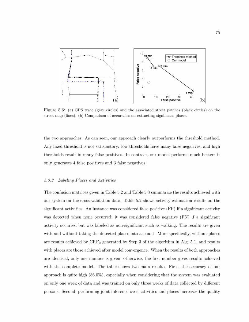
75
(a)0 10 20 30 400
2
4
6
8
10
Fals
e ne
gativ
e
False positive
1 min
3 min5 min
10 min Threshold methodOur model
(b)
Figure 5.6: (a) GPS trace (gray circles) and the associated street patches (black circles) on thestreet map (lines). (b) Comparison of accuracies on extracting significant places.
the two approaches. As can seen, our approach clearly outperforms the threshold method.
Any fixed threshold is not satisfactory: low thresholds have many false negatives, and high
thresholds result in many false positives. In contrast, our model performs much better: it
only generates 4 false positives and 3 false negatives.
5.3.3 Labeling Places and Activities
The confusion matrices given in Table 5.2 and Table 5.3 summarize the results achieved with
our system on the cross-validation data. Table 5.2 shows activity estimation results on the
significant activities. An instance was considered false positive (FP) if a significant activity
was detected when none occurred; it was considered false negative (FN) if a significant
activity occurred but was labeled as non-significant such as walking. The results are given
with and without taking the detected places into account. More specifically, without places
are results achieved by CRF0 generated by Step 3 of the algorithm in Alg. 5.1, and results
with places are those achieved after model convergence. When the results of both approaches
are identical, only one number is given; otherwise, the first number gives results achieved
with the complete model. The table shows two main results. First, the accuracy of our
approach is quite high (86.0%), especially when considering that the system was evaluated
on only one week of data and was trained on only three weeks of data collected by different
persons. Second, performing joint inference over activities and places increases the quality

76
Table 5.2: Activity confusion matrix of cross-validation data with (left values) and without (rightvalues) considering places for activity inference.
Inferred labelsTruth Work Sleep Leisure Visit Pickup On/off car Other FNWork 12 / 11 0 0 / 1 0 0 0 1 0Sleep 0 21 1 2 0 0 0 0
Leisure 2 0 20 / 17 1 / 4 0 0 3 0Visiting 0 0 0 / 2 7 / 5 0 0 2 0Pickup 0 0 0 0 1 0 0 2
On/Off car 0 0 0 0 1 13 / 12 0 2 / 3Other 0 0 0 0 0 0 37 1FP 0 0 0 0 2 2 3 -
Table 5.3: Confusion matrix of place detection and labeling.
Inferred labelsTruth Work Home Friend Parking Other FNWork 5 0 0 0 0 0Home 0 4 0 0 0 0Friend 0 0 3 0 2 0Parking 0 0 0 8 0 2Other 0 0 0 0 28 1FP 0 0 1 1 2 -
of inference. The reason for this is that a place node connects all the activities occurring in
its spatial area so that these activities can be labeled in a more consistent way.
Finally, the confusion matrix shown in Table 5.3 summarizes the results achieved on
detecting and labeling significant places. As can be seen, the approach commits zero errors
in labeling the home and work locations of the persons used for testing. The overall accuracy
in place detection and labeling is 90.6%.
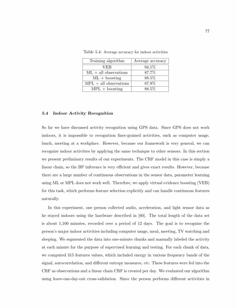
77
Table 5.4: Average accuracy for indoor activities
Training algorithm Average accuracyVEB 94.1%
ML + all observations 87.7%ML + boosting 88.5%
MPL + all observations 87.9%MPL + boosting 88.5%
5.4 Indoor Activity Recognition
So far we have discussed activity recognition using GPS data. Since GPS does not work
indoors, it is impossible to recognition finer-grained activities, such as computer usage,
lunch, meeting at a workplace. However, because our framework is very general, we can
recognize indoor activities by applying the same technique to other sensors. In this section
we present preliminary results of our experiments. The CRF model in this case is simply a
linear chain, so the BP inference is very efficient and gives exact results. However, because
there are a large number of continuous observations in the sensor data, parameter learning
using ML or MPL does not work well. Therefore, we apply virtual evidence boosting (VEB)
for this task, which performs feature selection explicitly and can handle continuous features
naturally.
In this experiment, one person collected audio, acceleration, and light sensor data as
he stayed indoors using the hardware described in [60]. The total length of the data set
is about 1,100 minutes, recorded over a period of 12 days. The goal is to recognize the
person’s major indoor activities including computer usage, meal, meeting, TV watching and
sleeping. We segmented the data into one-minute chunks and manually labeled the activity
at each minute for the purpose of supervised learning and testing. For each chunk of data,
we computed 315 features values, which included energy in various frequency bands of the
signal, autocorrelation, and different entropy measures, etc. These features were fed into the
CRF as observations and a linear chain CRF is created per day. We evaluated our algorithm
using leave-one-day-out cross-validation. Since the person performs different activities in

78
different days, the accuracies can vary significantly from day to day. So we only compare
the overall average accuracy of VEB with ML and MPL. Because ML and MPL cannot
handle continuous features directly, we used the two tricks mentioned in Section 4.4.2. The
results are shown in Table 5.4, in which VEB is about 5% to 6% better than ML and MPL,
no matter how they incorporated the continuous observations.
5.5 Summary
In this chapter we have developed a novel approach to performing location-based activity
recognition. In contrast to existing techniques, our approach uses one consistent framework
for both the extraction and the labeling of a person’s activities and significant places, as
well as the low-level segmentation. Our model is able to take many sources of evidence
into account in order to detect and label the significant places of a person. Furthermore,
once these places are determined, they help to better recognize activities occurring in their
vicinity. Therefore, by capturing complex relations between the activities and the high level
context, our approach can create a rich and consistent interpretation of a user’s data with
high accuracy. Our experiments based on traces of GPS data showed that our system signif-
icantly outperforms existing approaches, both in expressiveness and in accuracy. Moreover,
both inference and learning can be done very efficiently.
Our technique is very general and can be readily applied to other tasks of activity recog-
nition. In our preliminary experiments, we presented promising results of indoor activity
recognition from multi-modal sensors. In particular we showed that using virtual evidence
boosting for feature selection and parameter estimation can significantly outperform our
learning algorithms such as maximum likelihood and maximum pseudo-likelihood.

79
Chapter 6
LEARNING AND INFERRING TRANSPORTATION ROUTINES
In previous chapters, our task was to recognize different types of activities and significant
places from GPS data, which is essentially a supervised classification problem. However,
as we discussed in Chapter 1, the techniques of classification may not be suitable for all
location-based services. In this chapter, we describe a dynamic Bayesian network that
captures a user’s daily movement patterns between places. Instead of to learn the discrimi-
native features, we aim to understand the transition patterns at all levels of transportation
routines and to make accurate prediction at real time [64, 68]. Specifically, our system is
able to
• Robustly track and predict a user’s location even with loss of GPS signals or in the
presence of other sources of noise;
• Infer at real time a user’s mode of transportation (i.e., traveling by foot, car, or bus)
and predict when and where she will change modes;
• Predict her future movements, both in the short term (Will the user turn left at the
next street corner?) and in terms of distant goals (Is she going to work?);
• Infer when a user has deviated from her ordinary routine, and in some cases explicitly
infer that a user has made an error, such as boarding the wrong bus to get to the
doctor.
We are motivated in this work by the development of personal guidance systems to help
cognitively-impaired individuals move safely and independently through their community.
This technology also supports many other applications, such as customized “just in time”
information services for presenting relevant bus schedules and traffic information based on
routes.

80
Our approach is based on a hierarchical Markov model trained to model a user with data
collected by a small portable GPS unit. The model is compactly represented by a dynamic
Bayesian network, and inference is efficiently performed using Rao-Blackwellized particle
filtering both for the low level sensor integration and for the higher levels of the hierarchical
model.
The main research contribution in this chapter is a demonstration of efficient inference
and the development of unsupervised learning algorithms for the hierarchical predictive
models of transportation routines. Previous work has described inference in hierarchical
models [14] and learning non-hierarchical transportation models [84], but our work is the
first to combine these techniques. A second research contribution is in unifying this model
with detecting novel and erroneous behavior [85].
This chapter is organized as follows. In the next section, we provide an overview of the
hierarchical activity model, followed by a description of inference and learning algorithms.
Then we present experimental results and an end-to-end implementation of these techniques
called “Opportunity Knocks.”
6.1 Hierarchical Activity Model
We estimate a person’s activities using the three level dynamic Bayesian network model
shown in Fig. 6.1. The individual nodes in such a temporal graphical model represent
different components of the state space and the arcs indicate dependencies between the
nodes [21, 77]. Temporal dependencies are represented by arcs connecting the two time
slices k − 1 and k. The highest level of the model, the novelty mode, indicates whether
the user is currently behaving normally, doing something novel, or making a transportation
error. The second level of the model represents two concepts: the person’s next goal (e.g.,
her workplace) and the user’s current trip segment. A trip segment is a route with a single
transportation mode, which can be concatenated with other trip segments to form a plan for
transiting between goals. The person’s instantaneous transportation mode, location, and
velocity are estimated from the GPS sensor measurements at the lowest level of the model.

81
s e mTrip segment t = <t ,t ,t >k−1t
mk−1 mk
kt
f k−1t
f k−1g
f kt
k−1x
z kz k−1
kx
k−1θ kθ
kτ
fg
ft
fm
k−1τ
k−1n kn
k−1g kg
f kg
f k−1m f k
m
Transportation mode m
Goal g
GPS reading z
Location and velocity, andcar location: x = <l,v,c>
Trip switching
Goal switching
Mode switching counter
Edge transition τ
Data (edge) associationθ
Novelty n
Figure 6.1: Hierarchical activity model representing a person’s outdoor movements during everydayactivities. The upper level is used for novelty detection, and the middle layer estimates the user’sgoal and the trip segments he or she is taking to get there. The lowest layer represents the user’smode of transportation, speed, and location. Two time slices, k and k − 1, are shown.
6.1.1 Locations and transportation modes
We denote by xk = 〈lk, vk, ck〉 the location (lk) and velocity (vk) of the person, and the
location of the person’s car (ck) (subscripts k indicate discrete time). A key point of our
representation is that we constrain all locations to be on a street map. Thus, locations (both
lk and ck) can be represented using a directed graph G = (V,E) whose edges correspond to
streets or footpaths and whose vertices correspond to intersections. A location is determined
by an edge and distance pair. The edge corresponds to a street, with a given direction either
up or down the street, and the distance is the distance from the start vertex of the edge.

82
The direction of velocity vk is identical to the direction of the edge. The location of the
person at time k depends on his previous location, lk−1, the velocity, vk, and the transition,
τk. Vertex transitions τk model the decision a person makes when moving over a vertex in
the graph, corresponding to an intersection on the street map. The domain of τk is the set
of outgoing neighbors of the current edge; for example, the user could turn right, left, or
not at all when transiting a street intersection. (For simplicity we assume here the person
never performs U-turns to reverse moving direction on a street. In our implementation we
allow U-turns with a fixed small probability and the detail is omitted here.)
GPS sensor measurements, zk, are generated by the person carrying a GPS sensor. Since
measurements are simply points in continuous xy-coordinates, they have to be “snapped”
onto an edge in the graph structure. The edge to which a specific measurement is “snapped”
to is estimated by the association variable θk. Note that θk is picked from the edges close
to zk (e.g., within 50 meters from zk) independently from the edge of location lk.
Both the motion model, p(lk | lk−1, vk, τk), and the sensor model, p(zk | lk, θk) are
represented as (conditional) Gaussian models, as we will describe in Section 6.2.
The transportation mode mk can take on four different values BUS, FOOT , CAR, and
BUILDING. Similar to [84], these modes influence the velocity, vk, which is picked from
a Gaussian mixture model. For example, the FOOT mode draws velocities only from the
Gaussian representing walking speeds, while BUS and CAR modes draw velocities from
Gaussian distributions representing both high and low velocities. BUILDING is a special
mode that occurs only when the GPS signal is lost for significantly long time, corresponding
to the assumption that the person is indoors and not moving.
Finally, the location of the car only changes when the person is in the car and thus in
CAR mode, in which case the car location is set to the person’s location. If the person is not
in CAR mode, the car’s location affects whether a person can switch into the CAR mode.
(For these experiments we assume that the user only rides in her own car. The approach
could be generalized to distinguish “car travel as driver” and “car travel as passenger.”)

83
6.1.2 Trip segments
A trip segment is defined by its start location, tk.start, end location, tk.end, and the
mode of transportation, tk.mode, the person uses during the segment. For example, a trip
segment models information such as “the user boards the bus at location tk.start, rides
the bus to location tk.end, and then debarks”. In addition to transportation mode, a trip
segment predicts the route on which the person gets from tk.start to tk.end. This route
is not specified through a deterministic sequence of edges on the graph, but rather through
transition probabilities on the graph. These probabilities provide a prediction of the person’s
change in direction when reaching an intersection, or equivalently, when crossing a vertex
in the graph. This dependency is indicated by the arc from tk to τk.
The transfer between modes and trip segments is handled by the switching nodes fmk
and f tk, respectively. The Boolean trip switching node f t
k is set to true whenever the person
reaches the end location tk.end of the current trip segment. In this case, the trip segment is
allowed to switch with the constraint that the start location of the next segment is identical
to the end location of the current segment. The next trip segment is chosen according to
the segment transition conditioned on the current goal gk as well as the car location ck−1
(indicated using the link from xk−1 to tk). Once the next trip segment is active, the person
still has to change mode of transportation. This does not happen instantaneously, since, for
example, a person has to wait for the bus even though he already reached the bus stop (and
thus entered the bus trip segment). This semi-Markov property of delayed mode switching
is modeled by the node fmk , which is a counter that measures the time steps until the next
transportation mode is entered. The counter is initialized by the next trip segment, then
decremented until it reaches a value of zero, which triggers the mode switch. 1
6.1.3 Goals
A goal represents the current target location of the person. Goals include locations such as
the person’s home, workplace, the grocery store, and locations of friend’s homes. The goal
1This semi-Markov mode switch may be handled more efficiently by using fixed lag smoothing andobserving when significant velocity changes are made.

84
of the person can only change when the person reaches the end of a trip segment. This is
facilitated by a goal switching node fgk which is true only when the trip switching node f t
k
is true and the end of the current trip segment tk is identical to the goal gk. If the goal
switches, the next goal is chosen according to a learned goal-to-goal transition model.
6.1.4 Novelty
At the highest level is a boolean variable nk, indicating whether a user’s behavior is consis-
tent with historical patterns. Different values of nk instantiate different parameters for the
lower part of the model.
When a user is behaving normally, nk = false, the hierarchical model functions as
described up to this point and the parameters are trained using historical data. When a
user’s behavior is novel, nk = true, the goal and the trip segment are set to a distinguished
value “UNKNOWN” and as a consequence the parameters of the lowest layer of the model
(i.e., transportation mode transitions and edge transitions) are switched to their untrained
values: An “UNKNOWN” goal and trip segment does not provide any information about
the direction that a user will go when she gets to an intersection, or ways in which she will
change modes of transportation. The model that is instantiated in this way is referred to
as a flat model because there is no influence of high level model elements on the inference
at the street level. A flat model respects basic intuitions about changing transportation
modes and moving on a street map, but is not influenced by long-term goals such as where
and how the user is getting home from work. Instead the flat model utilizes straightforward
Markov transition probabilities in the lowest level of Fig. 6.1 analogous to [84].
6.2 Inference
After we have defined the structure of the model and assumed values for the transition
parameters (parameter estimation will be discussed in the next section), we must develop
efficient algorithms to infer the distribution of hidden variables at real time given a sequence
of GPS readings. In this section, we first focus on the estimation of locations and modes of
transportation. For simplicity, we present a version of this algorithm that does not apply
switching nodes and waiting time counters. These concepts will be discussed in the context

85
of the hierarchical model, which additionally estimates a person’s high level goals, trip
segments, and novelty.
6.2.1 Flat Model
First we will explain the estimation of locations and transportation modes using a flat
model. This is the model shown in Fig. 6.1 with the top two levels removed. Note that
removing the top levels may introduce additional direct dependencies in the lowest level.
For instance, we must add arcs from xk−1 to mk, τk, and fmk . Remember our system tracks
people’s locations on a street map. Because street maps have a complex structure and
the estimation problem contains a variety of continuous (locations, velocities) and discrete
states (edge transition, transportation mode, etc.), exact inference is intractable. Instead,
we rely on Rao-Blackwellized particle filters for inference in the flat model [25]. In our case,
the Rao-Blackwellized particle filter combines particle filters with Kalman filters. Particle
filters [24, 107] and Kalman filters [107, 6] are two widely-used techniques for state tracking
in dynamic systems. The goal of state tracking is to estimate the posterior distribution,
p(sk | z1:k), at each time step k, where sk represents the set of state variables at k and z1:k
is the sequence of observations up to time k. In this section, we will first briefly describe
the particle filters and Kalman filters in general, and then discuss the application of these
techniques in our flat model.
Particle filters
Particle filters represent posterior distributions over the state space with temporal sets, Sk,
of n weighted samples:
Sk = {s(i)k , w
(i)k | 1 ≤ i ≤ N}
Here s(i)k is a sample (or state), and w
(i)k is a non-negative numerical factor called an im-
portance weight. The basic particle filter updates the posterior according to the following
sampling procedure, often referred to as sequential importance sampling with re-sampling
(SISR, see also [24, 107]).

86
• Sampling: Draw n samples, s(i)k−1, from the previous set and generate n new samples,
s(i)k , using the proposal distribution, q(sk | s
(i)k−1, zk)
• Importance sampling: Assign each sample an importance weight w(i)k as
w(i)k ∝ w
(i)k−1
p(zk | s(i)k )p(s(i)
k | s(i)k−1)
q(s(i)k | s
(i)k−1, zk)
(6.1)
• Re-sampling: Multiply / discard samples by drawing samples with replacement
according to the distribution defined through the importance weights w(i)k .
It is often convenient to choose the proposal distribution to be the prediction as
q(sk | s(i)k−1, zk) = p(sk | s
(i)k−1) (6.2)
By substituting (6.2) into (6.1), we get
w(i)k ∝ w
(i)k−1 p(zk | s
(i)k ) (6.3)
Kalman filters
Kalman filtering [107, 6] represents beliefs by a unimodal Gaussian distribution,N (sk;µk,Σk),
where µk and Σk are the mean and the variance, respectively. At each time step, Kalman
filters update these Gaussian beliefs by two steps: a prediction step followed by a correction
step.
In the prediction step, Kalman filters predict the state distribution based on the previous
belief N (sk−1;µk−1,Σk−1) and the system dynamics p(sk | sk−1). Under the assumption
that the state at time k is a linear function of the previous state with additive Gaussian noise,
the system dynamics can be represented by another Gaussian N (sk;Atsk−1, Rt), where At
is the dynamics matrix and Rt is the covariance of the Gaussian noise. The prediction is
a convolution of these two Gaussians and thus the result is also a Gaussian over the state

87
space:
N (sk; µk, Σk) =∫N (sk;Atsk−1, Rt) N (sk−1;µk−1,Σk−1) dsk−1 (6.4)
Here, 〈µk, Σk〉 denote the parameters defining the predictive belief at time k, that is, the
belief before the observation zk is considered. The parameters can be computed in closed
form as
µk = Atµk−1
Σk = AtΣk−1ATt + Rt. (6.5)
In the correction step, the most recent measurement zk is used to adjust the prediction
N (sk; µk, Σk). If we assume that sensor measurements zk are linear functions of the state sk,
with added Gaussian noise, then the sensor model p(zk | sk) is the GaussianN (zk;Cksk, Qk).
Here the matrix Ck maps states to observations and Qt is the covariance of the observation
noise. The posterior belief is again a Gaussian
N (sk;µk,Σk) ∝ N (zk;Ctsk, Qk) N (sk; µk, Σk) (6.6)
with
µk = µk + Kk (zk − Ct µk)
Σk = (1−KkCk) Σk (6.7)
where Kk = ΣkCTk /(CkΣkC
Tk + Qk) is the so-called Kalman gain.
Rao-Blackwellized particle filters for estimation in the flat model
The main advantage of Kalman filters is their computational efficiency. This efficiency, how-
ever, comes at the cost of restricted representation power because Kalman filters only apply
to (approximately) linear systems that can be described by unimodal distributions. While
particle filters can be applied to arbitrary, non-linear systems, they are less efficient than

88
Kalman filters. The key idea of Rao-Blackwellized particle filters (RBPF) is to combine
both representations, thereby leveraging the efficiency of Kalman filters and the representa-
tional power of particle filters. RBPFs have been applied with great success to various state
estimation problems, including robot mapping [76, 73], tracking [24, 57, 98], and system
monitoring [20, 74].
In our approach, we estimate the posterior over the location of the person and the car,
and the complete histories of the other parts of the state space, conditioned on z1:k, the
sequence of GPS measurements observed so far. As we will see, the estimation of these
histories is necessary for the derivation of the filter, but implementations of the RBPF
typically keep track of the current state only. The following factorization of the posterior
forms the basis for our Rao-Blackwellized particle filter:
p(ck, lk,m1:k, v1:k, τ1:k, θ1:k | z1:k)
= p(ck | lk,m1:k, v1:k, τ1:k, θ1:k, z1:k)
p(lk | m1:k, v1:k, τ1:k, θ1:k, z1:k) p(m1:k, v1:k, τ1:k, θ1:k | z1:k) (6.8)
This factorization separates the state space of our estimation problem into three parts. From
right to left, the first part contains histories over the transportation mode m1:k, velocity
v1:k, edge transition τ1:k, and edge association θ1:k, which are represented by the samples
in a particle filter. The second part is the location of the person lk on the graph, which is
estimated using Kalman filters conditioned on the samples. The third part represents the
car location which, as we will show, is a function of the person’s location.
Each particle of the flat RBPF has the following form:
s(i)k =
⟨〈ξ(i)
k ,Ξ(i)k 〉, 〈µ
(i)k ,Σ(i)
k 〉, m(i)1:k, v
(i)1:k, τ
(i)1:k, θ
(i)1:k
⟩, (6.9)
where 〈ξ(i)k ,Ξ(i)
k 〉 and 〈µ(i)k ,Σ(i)
k 〉 represent the mean and variance of the car location and
person location estimates, respectively. Here we present a memory efficient version of the
RBPF algorithm that only stores the most recent states. Whenever a new GPS measurement
arrives, the RBPF draws a particle s(i)k−1 from the previous sample set. The updated particles

89
are then generated in three steps, evaluating (6.8) from right to left: First, the state histories
are expanded by sampling the most recent states. Second, the person’s location estimate
is updated using a Kalman filter update conditioned on the measurement and the sampled
values. Finally, the car location is updated conditioned on these estimates.
Sampling step
The updated histories m(i)1:k, v
(i)1:k, τ
(i)1:k, and θ
(i)1:k are generated by expanding s
(i)k−1’s histories
via sampling the states at time k and attaching them to the existing histories. First, the
transportation mode m(i)k is sampled from p(m(i)
k | m(i)k−1, µ
(i)k−1, ξ
(i)k−1) and then attached to
the particle’s mode history m(i)1:k−1 to generate m
(i)1:k. Mode transitions take information
about bus routes and the person’s car into account. For instance, whenever the person’s
location µ(i)k−1 was near a bus stop and the previous mode was FOOT, then m
(i)k switches to
BUS with a small probability. Similarly, the person can only switch into the CAR mode if he
was near the car location ξ(i)k−1.
Once the transportation mode is sampled, the motion velocity v(i)k is sampled from a
mixture of Gaussians which is conditioned on the mode. The value of the next edge tran-
sition variable τ(i)k is sampled based on the previous position of the person and a learned
transition model. This is used in case the mean of the location estimate reaches an in-
tersection. The edge association variable θ(i)k “snaps” the GPS reading to a street in the
map. To sample θ(i)k , we first determine the distance between the measurement, zk, and
the different streets in the vicinity. The probability of “snapping” zk to one of these streets
is then computed from this distance. These assignments are crucial for the Kalman filter
update described next.
Kalman filter step
After the RBPF generated all the sampled histories of a particle, that is,
s(i)k =
⟨〈 , 〉, 〈 , 〉,m(i)
1:k, v(i)1:k, τ
(i)1:k, θ
(i)1:k
⟩,

90
it then generates the missing location estimate 〈µ(i)k ,Σ(i)
k 〉 by updating the Kalman filter
conditioned on the already sampled values. To elaborate, let us rewrite the second term on
the right hand side of (6.8):
p(lk | m(i)1:k, v
(i)1:k, τ
(i)1:k, θ
(i)1:k, z1:k)
= p(lk | 〈µ(i)k−1,Σ
(i)k−1〉,m
(i)k , v
(i)k , τ
(i)k , θ
(i)k , zk) (6.10)
∝ p(zk | lk, θ(i)k )∫
p(lk | v(i)k , τ
(i)k , l
(i)k−1) N (l(i)k−1;µ
(i)k−1,Σ
(i)k−1) dl
(i)k−1 (6.11)
(6.10) follows from the fact that the Gaussian estimate 〈µ(i)k−1,Σ
(i)k−1〉 of the person’s location
is a sufficient statistic for all observations up to time k−1, when conditioned on the particle’s
histories over the other parts of the state space. The justification of this step is the key reason
for estimating histories rather than only the most recent states. Equation (6.11) now follows
by applying Bayes rule and the independences in our estimation problem (cf. Fig. 6.1). It
represents a standard recursive Bayes filter update rule; see [107, 6] for details. The prior
probability is given by the Gaussian of the previous Kalman filter estimate. Conditioned
on the already sampled values θ(i)k , v
(i)k , and τ
(i)k , (6.11) reduces to a standard Kalman filter
update.
In the prediction step, the traveled distance is predicted using the sampled Gaussian ve-
locity component. The prediction, 〈µ(i)k , Σ(i)
k 〉, results then from shifting and convolving the
previous estimate by the predicted motion, thereby implementing the integration in (6.11)
via the Kalman update (6.5). This prediction step is straightforward if the person stays
on the same edge of the graph. If she transits over a vertex of the graph, then the next
edge is given by the previously sampled edge transition τk(i) (see upper panel in Fig. 6.2).
To simplify computation, only the predicted mean µ(i)k is used to determine whether the
person switches edges. In our experience this approximation is accurate enough for location
tracking.
In the correction step, the predicted estimate 〈µ(i)k , Σ(i)
k 〉 is corrected based on the most
recent GPS measurement zk, using (6.7). Intuitively, this correction compares the predicted
mean µ(i)k with the location of zk and shifts the mean toward the measurement (under

91
µ
1 e2
k−1kµ
e3
e4 e5
τif =ek 3
τif =ek 5
e
if =e
k
3k
z
θ =e5k
θ =e2k
e4 e5
e1 e2kµ
θif =ek 3
θ
Figure 6.2: Kalman filter prediction (upper panel) and correction (lower panel) on a street graph.The previous belief is located on edge e4. When the predicted mean transits over the vertex, thenthe next location can be either on e3 or e5, depending on the sampled edge transition τk. In thecorrection step (lower panel), the continuous coordinates of the GPS measurement, zk, are betweenedges e2 and e5. Depending on the value of the edge association, θk, the correction step moves theestimate up-wards or down-wards.
consideration of the uncertainties). The correction step for one Gaussian is illustrated in
the lower panel of Fig. 6.2. Because we restrict the location estimates to the graph, we
“snap” the GPS measurements onto the graph. The already sampled value of the edge
association variable θ(i)k uniquely determines to which edge the reading is snapped. After a
GPS measurement is snapped onto one of the edges, we find the shortest path on the graph
between the µ(i)k and the snapped measurement using the standard A* search algorithm.
Then we can apply a one-dimensional Kalman filtering correction step and get the posterior
location estimate 〈µk(i),Σk
(i)〉.
Finally, the car location is updated. We rewrite the first term of the factorization in

92
(6.8) as
p(ck | lk, v1:k,m1:k, θ1:k, τ1:k, z1:k)
=
δ(lk − ck) if mk = CAR
δ(ck−1 − ck) p(ck−1 | lk−1, v1:k−1,m1:k−1, θ1:k−1, τ1:k−1, z1:k−1) otherwise
(6.12)
where δ(x) is the Dirac delta function that returns infinity if x = 0 and zero otherwise.
(6.12) is based on the assumption that the person is always using the same vehicle and that
nobody else moves the vehicle. As a result, if the person is in the car, then the car location
is set to the person’s location. Otherwise, the car location is the same as in the previous
time step.
Importance weights
After all components of each particle are generated, the importance weights of the particles
need to be updated using Equation (6.1). In our case, the sampling steps do not consider
the most recent observation zk and the proposal distribution is identical to (6.2), resulting
in importance weights proportional to the observation likelihood:
w(i)k ∝ w
(i)k−1 p(zk | s
(i)k ) (6.13)
= w(i)k−1 p(zk | 〈ξ
(i)k−1,Ξ
(i)k−1〉, 〈µ
(i)k−1,Σ
(i)k−1〉,m
(i)1:k, v
(i)1:k, τ
(i)1:k, θ
(i)1:k) (6.14)
= w(i)k−1 N (zk; µ
(i)k , Σ(i)
k + Qk) (6.15)
This observation likelihood is computed based on each particle’s sampled values, as given
in (6.13). The likelihood can be computed in closed form from the Kalman filter correction
step [107]. In the case of GPS readings, the likelihood of a measurement is given by a
Gaussian with mean at the predicted location µ(i)k and variance given by the predicted
location uncertainty Σ(i)k plus measurement noise Qk, as given in (6.15).

93
inputs : Sample set Sk−1 = {〈s(i)k−1, w
(i)k−1〉 | 1 ≤ i ≤ N} and observation zk
output: Current sample set: Sk = {〈s(i)k , w
(i)k 〉 | 1 ≤ i ≤ N}
Sk = ∅ ; // Initialize1.
for i = 1, . . . , N do2.
Sample m(i)k ∼ p(m(i)
k | m(i)k−1, µ
(i)k−1, ξ
(i)k−1) ; // Sample transportation mode3.
Sample v(i)k ∼ p(v(i)
k | m(i)k ); // Sample velocity4.
Sample τ(i)k ∼ p(τ (i)
k | µ(i)k−1,m
(i)k ) ; // Sample decision at next vertex5.
Sample θ(i)k ∼ p(θ(i)
k | zk) ; // Sample GPS to edge association6.
Compute 〈µ(i)k ,Σ(i)
k 〉 conditioned on 〈µ(i)k−1,Σ
(i)k−1〉, v
(i)k ,τ (i)
k , θ(i)k , and zk ;7.
if m(i)k = CAR then 〈ξ(i)
k ,Ξ(i)k 〉 := 〈µ(i)
k ,Σ(i)k 〉 ; // Car moves with person8.
else 〈ξ(i)k ,Ξ(i)
k 〉 := 〈ξ(i)k−1,Ξ
(i)k−1〉 ; // Car does not move9.
w(i)k = w
(i)k−1 N (zk; µ
(i)k , Σ(i)
k + Qk) ; // Kalman filter likelihood10.
Sk = Sk ∪ {〈s(i)k , w
(i)k 〉} ; // Insert into sample set11.
end12.
Multiply / discard samples in Sk based on normalized weights ;13.
Algorithm 6.1: RBPF for flat model
RBPF algorithm for the flat model
The algorithm RBPF Flat is summarized in Alg. 6.1. The algorithm accepts as inputs
a sample set representing the previous belief and the most recent GPS measurement. For
each particle, the algorithm first samples the transportation mode in Step 3. The sampling
distribution models that a person can only get on or off a bus when she is near a bus stop,
and she can only get into the car when she is near the location where the car is parked.
Then, the algorithm samples the velocity conditioned on the mode, the motion decision at
the next vertex, and the association of the GPS reading to an edge in the street map (
Step 4 to Step 6).
Then, in Step 7, the Gaussian estimate of the person’s location is updated using Kalman
filtering. Step 8 and Step 9 set the car location accordingly. The weight of each particle is
determined in Step 10, based on the Kalman filter estimate of the person’s location. After
inserting each particle into the sample set, the algorithm performs resampling based on
the importance weights. Resampling with minimal variance can be implemented efficiently
(constant time per sample) using a procedure known as deterministic selection [51, 2] or

94
stochastic universal sampling [5].
6.2.2 Hierarchical Model
Up to this point, we have described state estimation in a “flat” model, that is, a model that
does not reason about a person’s goals, trip segments, and novelty. We will now describe
how to extend the RBPF for the flat model so as to estimate the posterior over the complete
hierarchical model shown in Fig. 6.1. To additionally model goals, trip segments, novelty,
and improved mode switching, we add the corresponding components to each particle of
the RBPF 2:
s(i)k =
⟨n
(i)k , 〈g(i)
k , t(i)k 〉, f
g(i)k , 〈ξ(i)
k ,Ξ(i)k 〉, 〈µ
(i)k ,Σ(i)
k 〉, v(i)k ,m
(i)k , f
m(i)k , f
t(i)k , θ
(i)k , τ
(i)k
⟩(6.16)
Here each 〈g(i)k , t
(i)k 〉 is a discrete distribution over goals and trip segments. These distri-
butions are estimated using exact inference conditioned on the sampled values, just like
exact Kalman filtering is performed for the location estimates 〈µ(i)k ,Σ(i)
k 〉 in the flat model.
Boolean variable n(i)k represents whether or not the person is currently following an ex-
pected route, where the expectation is based on historical data. The values fg(i)k , f
t(i)k ,
and fm(i)k represent sampled information about switching between goals, trip segments, and
transportation modes, respectively.
RBPF algorithm for the hierarchical model
Alg. 6.2 summarizes one update step of the algorithm RBPF Hierarchical, which imple-
ments Rao-Blackwellized particle filtering for the complete model except novel behavior. We
omit a full derivation of this algorithm; it is similar to the derivation of RBPF Flat and
to Rao-Blackwellized inference for abstract hidden Markov models, with which our model
shares the high-level structure [12].
The algorithm accepts as inputs the sample set representing the previous belief and the
most recent measurement. In order to be able to sample the switching nodes conditioned on
2For simplicity we omit the histories of sampled values. Similar to the case of flat model, those historiesare necessary for deriving the algorithm, but do not have to be stored during implementation.

95
inputs : Sample set Sk−1 = {〈s(i)k−1, w
(i)k−1〉 | 1 ≤ i ≤ N} and observation zk
output: Current sample set: Sk = {〈s(i)k , w
(i)k 〉 | 1 ≤ i ≤ N}
Sk = ∅ ; // Initialize1.
for i = 1, . . . , N do2.
Sample (g(i)k−1, t
(i)k−1) ∼ p(g(i)
k−1, t(i)k−1) ; // Draw goal and trip segment3.
if µ(i)k−1 = t
(i)k−1.end then f t
k(i) := true ; // Just reached end of trip segment?4.
else f tk(i) := false ;5.
if f tk(i) = true and g
(i)k−1 = t
(i)k−1.end then f
g(i)k := true ; // Goal reached?6.
else fg(i)k := false ;7.
if f tk(i) = true then8.
fmk
(i) ∼ Uniform[0,max-waiting-time] ; // Sample when to switch mode9.
else fmk
(i) := fm(i)k−1 − 1 ;10.
Compute p(g(i)k , t
(i)k | f
gk
(i), f t
k(i)
, g(i)k−1, t
(i)k−1, ξ
(i)k−1) ;11.
Sample (g(i)k , t
(i)k ) ∼ p(g(i)
k , t(i)k ) ; // Draw goal and trip segment12.
if fmk
(i) = 0 then m(i)k = t
(i)k .mode ; // Change transportation mode?13.
else m(i)k = m
(i)k−1 ;14.
Sample v(i)k ∼ p(v(i)
k | m(i)k ) ; // Sample velocity15.
Sample τ(i)k ∼ p(τ (i)
k | µ(i)k−1, t
(i)k ) ; // Sample decision at next vertex16.
Sample θ(i)k ∼ p(θ(i)
k | zk) ; // Sample GPS to edge association17.
Compute 〈µ(i)k ,Σ(i)
k 〉 conditioned on 〈µ(i)k−1,Σ
(i)k−1〉, v
(i)k ,τ (i)
k , θ(i)k , and zk ;18.
if m(i)k = CAR then 〈ξ(i)
k ,Ξ(i)k 〉 := 〈µ(i)
k ,Σ(i)k 〉 ; // Car moves with person19.
else 〈ξ(i)k ,Ξ(i)
k 〉 := 〈ξ(i)k−1,Ξ
(i)k−1〉 ; // Car does not move20.
Compute p(g(i)k , t
(i)k | m
(i)k , τ
(i)k , g
(i)k , t
(i)k )21.
w(i)k = w
(i)k−1 N (zk; µ
(i)k , Σ(i)
k + Qk) ; // Update particle weight22.
Sk = Sk ∪ {〈s(i)k , w
(i)k 〉}; // Insert into sample set23.
end24.
Multiply / discard samples in Sk based on normalized weights25.
Algorithm 6.2: RBPF for hierarchical model

96
the high-level nodes, the algorithm first samples a goal / trip segment combination from the
previous distribution (Step 3). Then, Step 4 tests whether the previous location reached the
end of the trip segment. In our implementation, this test returns true if µ(i)k−1 just entered
the edge of t(i)k−1.end. The goal switching node f
g(i)k is set to true if the end of the trip
segment is reached and the trip segment ends in the goal location (Step 6). The time period
until the transportation mode on the new trip segment is switched, is sampled in Step 9,
and decremented in Step 10. This semi-Markov mode switching enables the RBPF to model
non-exponential waiting times between, for example, reaching a bus stop and getting on the
bus. We found that this technique is far more robust than a straightforward approach that
samples a mode switch at every iteration.
Then, in Step 11, the distribution over goals and trip segments is projected forward
conditioned on the sampled switching nodes as well as the car location ξ(i)k−1. Similar to
Step 3, a goal / trip segment combination is sampled from the predicted distribution in
Step 12. If the transportation mode switching counter reaches zero, then m(i)k is set to the
mode of the sampled trip segment (Step 13). Step 15 through Step 20 correspond exactly
to Step 4 through Step 9 in the flat model, with a key difference in Step 16: While the flat
model samples the transition τ(i)k at the next intersection solely based on the location µ
(i)k−1
and m(i)k , the hierarchical model takes the current trip segment t
(i)k into account. Thus, the
hierarchical model can have different transition probabilities at an intersection depending
on the trip segment the person is following. As we will show in the experimental results,
this additional dependency leads to greatly improved predictive capabilities.
The distribution over goals and trip segments is updated in Step 21. The sampled
transition τ(i)k plays an important role in this update, since it indicates in which direction
the person is moving. Similarly, the sampled transportation mode m(i)k indicates transitions
between trip segments. After each particle is weighted and inserted into the sample set, the
algorithm finishes with the resampling step.
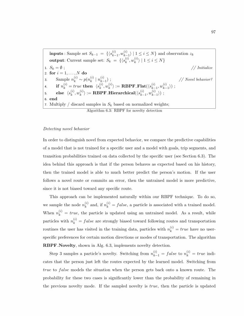
97
inputs : Sample set Sk−1 = {〈s(i)k−1, w
(i)k−1〉 | 1 ≤ i ≤ N} and observation zk
output: Current sample set: Sk = {〈s(i)k , w
(i)k 〉 | 1 ≤ i ≤ N}
Sk = ∅ ; // Initialize1.
for i = 1, . . . , N do2.
Sample n(i)k ∼ p(n(i)
k | n(i)k−1) ; // Novel behavior?3.
if n(i)k = true then 〈s(i)
k , w(i)k 〉 := RBPF Flat(〈s(i)
k−1, w(i)k−1〉) ;4.
else 〈s(i)k , w
(i)k 〉 := RBPF Hierarchical(〈s(i)
k−1, w(i)k−1〉) ;5.
end6.
Multiply / discard samples in Sk based on normalized weights;7.
Algorithm 6.3: RBPF for novelty detection
Detecting novel behavior
In order to distinguish novel from expected behavior, we compare the predictive capabilities
of a model that is not trained for a specific user and a model with goals, trip segments, and
transition probabilities trained on data collected by the specific user (see Section 6.3). The
idea behind this approach is that if the person behaves as expected based on his history,
then the trained model is able to much better predict the person’s motion. If the user
follows a novel route or commits an error, then the untrained model is more predictive,
since it is not biased toward any specific route.
This approach can be implemented naturally within our RBPF technique. To do so,
we sample the node n(i)k and, if n
(i)k = false, a particle is associated with a trained model.
When n(i)k = true, the particle is updated using an untrained model. As a result, while
particles with n(i)k = false are strongly biased toward following routes and transportation
routines the user has visited in the training data, particles with n(i)k = true have no user-
specific preferences for certain motion directions or modes of transportation. The algorithm
RBPF Novelty, shown in Alg. 6.3, implements novelty detection.
Step 3 samples a particle’s novelty. Switching from n(i)k−1 = false to n
(i)k = true indi-
cates that the person just left the routes expected by the learned model. Switching from
true to false models the situation when the person gets back onto a known route. The
probability for these two cases is significantly lower than the probability of remaining in
the previous novelty mode. If the sampled novelty is true, then the particle is updated

98
using the untrained, flat RBPF algorithm in Step 4. Here, we choose the flat model since
it supports unbiased motion more naturally and efficiently than a hierarchical model with
uniform transitions. If the novelty is false, then the particle is updated using a hierarchical
model that is trained on historical data collected by the user (Step 5). Finally, if the novelty
mode switches from n(i)k−1 = true to n
(i)k = false, we re-initialize the distribution over goals
and trip segments to uniform.
The resulting technique is able to detect when a user deviates from a known route and
when she returns to a previously used route. The interpretation of the novelty, however,
depends on the context: it could mean user errors (e.g., taking a wrong bus) or deliberate
novel behavior (e.g., driving to a new place). In some cases, we may want to explicitly
estimate the probability of an error. This can be done by combining two factors: the
probability of novelty and the probability of an error given a novel behavior, as the following:
P (Error) = P (nk = true)P (Error | nk = true) (6.17)
When the true goal is unknown (as we have assumed so far), P (nk = true) is estimated
by sampling as we have discussed, and P (Error | nk = true) is a user-dependent parameter
that we set manually: for people who seldom make mistakes, we could choose its value as
0, while for people with cognitive disabilities, the value should be set much higher.
When the user’s true intention is known, we can integrate the knowledge into our infer-
ence and predict errors more accurately. It is possible for the system to know where the user
is going, for example, if the user asks for directions to a destination, if a care-giver or job
coach indicates the “correct” destination, or if the system has access to a location enabled
date-book (see Section 6.5 for an example). In these cases, P (nk) = true in (6.17) can be
estimated similarly to the previous case; the difference is that we now clamp the supplied
value of the goal and/or trip segment in the learned model. If the user has specified the
goal, then P (Error | nk = true) should be set close to 1, i.e., if a user follows a novel route
while heading toward a familiar goal, there is a strong probability that he is making an
error.

99
6.3 Learning
Learning the hierarchical model of a given user includes two procedures. The first is to
identify the possible sets of goals and trip segments, which comprise the range of the vari-
ables gk and tk in the hierarchical model shown in Fig. 6.1. This corresponds to finding
the set of significant places including frequently-used bus stops and parking areas. We can
identify those significant places robustly using the techniques discussed in Chapter 5. In
this section, we discuss the second task — estimating the transition matrices at all levels
of the hierarchical model, including the transition matrix between the goals, the transition
matrix between the trip segments given a goal, and the street transition matrix within a
trip segment. The street transition matrices in a flat model can be estimated similarly (see
[84] for details).
Given the GPS data collected by a person moving through the community, one way
of learning the transition parameters is to require the person to keep a diary for several
weeks of their transportation routines in order to create a supervised training set. Then
we can estimate the transition matrices by simply counting the corresponding transitions
and normalizing the counts. However, it is extremely hard in practice to obtain the labeled
training data, and thus we want to estimate those parameters in an unsupervised manner
without any manual labels. A general approach for solving such learning problems is the
well-known Expectation-Maximization (EM) algorithm [22, 94]. EM solves such problems
by iterating between an Expectation step (E-step) and a Maximization step (M-step). In a
nutshell, each E-step estimates expectations (distributions) over the transition counts using
the GPS observations along with the current estimate of the model parameters. Then in the
M-step the model parameters are updated using the expectations obtained in the E-step.
The updated model is then used in the next E-step to obtain more accurate estimates of
the hidden transition counts. EM theory tells us that in each iteration the estimation of
the parameters will be improved and it will eventually converge to a local optimum.
A brief description of the learning algorithm is shown in Alg. 6.4. In Step 1, all the
transition parameters are initialized: p(gi′ | gi) is initialized as uniform, p(tj′ | tj , gi) is also
a uniform distribution given tj′ .start = tj .end, and similarly p(ek′ | ek, tj) is initialized as

100
inputs : GPS trace zk, set of goals g1, . . . , gI , set of trip segments t1, . . . , tJ , and setof streets e1, . . . , eK
output: Estimated transition matrices between goals p(gi′ | gi), trip segmentsp(tj′ | tj , gi), and streets p(ek′ | ek, tj), 1 ≤ i, i′ ≤ I, 1 ≤ j, j′ ≤ J ,1 ≤ k, k′ ≤ K
Initialize all the transition parameters;1.
repeat2.
//E-step:Perform forward filtering pass using current estimate of transition parameters;3.
Perform backward filtering pass using current estimate of transition parameters;4.
Obtain smoothed transition counts by combining forward and backward passes;5.
//M-step:Updated transition parameters based on smoothed transition counts in the E-step;6.
until transition parameters converge7.
Algorithm 6.4: Transition parameter estimation in hierarchical model using EM
uniform for all the outgoing streets of ek.
Then in the E-step (Step 3 through Step 5), both the forward filtering pass and a
backward (in time) filtering path are performed using the current estimate of the parame-
ters [84, 108]. The forward filtering pass uses the Rao-Blackwellised particle filter shown in
Alg. 6.2 (transition parameters are used in Step 11, Step 16, and Step 21). The backward
filtering pass is very similar to the forward pass except the GPS readings are played in
a reverse order. The transition parameters for the backward pass can be computed from
the normal (forward) transition parameters using Bayes rules. The expected transition
counts are smoothed by combining the results from forward and backward passes, and these
smoothed counts are used in the M-step (Step 6) to update the transition parameters [84, 94].
Our approach is in fact a direct extension of the Monte Carlo EM algorithm [114]. The
only difference is that we allow particles to evolve with time. It has been shown that when
the number of particles n is large enough, Monte Carlo EM estimation converges to the
theoretical EM estimation [62].
In addition to the user specific transition parameters our model requires the specification
of other parameters, such as motion velocity model and the GPS sensor model. The motion
velocity is modeled as a mixture of Gaussians from which velocities are drawn at random.

101
Friend
Friend
Friend
Grocery
Home
Work (a)Work
Grocery
Home
Friend
Friend
Friend
(b)
Figure 6.3: (a) Street map along with goals (dots) learned from 30 days of data. Learned tripswitching locations are indicated by cross marks. (b) Most likely trajectories between goals obtainedfrom the learned transition matrices. Text labels were manually added.
The probabilities of the mixture components depend on the current motion mode and can
be learned beforehand using data labeled with the correct mode of motion [84]. The GPS
sensor noise is modeled as a Gaussian with a fixed variance. Our system does not currently
learn the parameters associated with novelty detection. This would entail learning the
likelihood of a user making an error versus doing something novel, and is beyond the scope
of this work.
6.4 Experimental Results
To validate our model, we collected 60 days of GPS data from one person wearing a small
GPS unit. We used the first 30 days for learning and the second 30 days for testing.

102
Parking lot
Parking lot
Bus stop
Work
(a)
Parking lot
Parking lot
Bus stop
Work
(b)
Figure 6.4: Close up of the area around the workplace. (a) Shown are edges that are connected bylikely transitions (probability above 0.75), given that the goal is the workplace (dashed lines indicatecar mode, solid lines bus, and dashed-dotted lines foot). (b) Learned transitions in the same areaconditioned on home being the goal.
6.4.1 Activity Model Learning
The learning was done without manual labeling. The system precisely identifies the subject’s
six most common transportation goals and all frequently used bus stops and parking lots,
as shown in Fig. 6.3 (a). In this experiment, goals are those locations where the person
spent more than an hour in total, and bus stops and parking lots are determined using 0.85
as the transition threshold . After recognizing the goals and transfer locations, parameter
learning estimates the transition matrices at all levels of the model. Using those transition
matrices, we can extract the most likely trajectories on the street map between pairs of the
goals, as shown in Fig. 6.3 (b).
Fig. 6.4 shows a close up display of the area near the workplace. The learned results
clearly show the common routes using different modes of transportation, as well as the usual
bus stops and parking lots.
6.4.2 Empirical Comparison to Other Models
The hierarchical model is very expressive and able to answer many useful queries. For
example, many applications need to query the probability of a given goal. In this section we
present results comparing the goal prediction performance of our hierarchical model with a
flat model [84] and a second-order Markov model (2MM) trained on sequences of goals [3].

103
0 100 200 300 400 500 6000
0.1
0.2
0.3
0.4
0.5
0.6
0.7
0.8
0.9
1
Time [sec]
Prob
abilit
y
Flat modelHierarchical model
(a)0 50 100 150 200
0
0.2
0.4
0.6
0.8
1
City blocks
Pro
babi
lity
of c
orre
ctly
pre
dict
ing
x or
m
ore
bloc
ks a
nd tr
ansp
orta
tion
mod
es Flat modelHierarchical model
(b)
Figure 6.5: Comparison of flat model and hierarchical model. (a) Probability of the true goal(workplace) during an episode from home to work, estimated using the flat and the hierarchicalmodel. (b) Location and transportation mode prediction capabilities of the learned model.
The flat model is basically a first-order Markov model over the street blocks. Thus, in
order to calculate the probability of a goal, one must calculate the sum over all possible
paths to the goal, which is intractable if the goal is far away. A reasonable approximation
is to compute the probability of the most likely path to the goal. Fig. 6.5(a) compares the
result of such a query on the probability of the goal being the workplace during an episode
of traveling from home to work. As one can see, the hierarchical model quickly assigns a
high probability to the true goal, while the estimate from the flat model is meaningless until
the user is near the goal. In [84], the flat model is also used to predict the street blocks and
transportation modes in the future. As shown in Fig. 6.5(b), the prediction capability of
the hierarchical model is much better than that of the flat model. For instance, in 50% of
the cases, the flat model is able to correctly predict the motion and transportation mode of
the person for 5 city blocks, while the hierarchical model can predict correctly for 43 blocks.
The 2MM model introduced in [3] is a second-order Markov model that only reasons
about transitions between goal locations. Since this model ignores GPS measurements
collected during transit between goals, it cannot refine the goal prediction as a person
moves to a goal. To show the difference in performance, we labeled the 30 days of test
data with the true goals and computed the prediction accuracy using the 2MM and our
hierarchical model, which was learned using the same training data. The average prediction

104
Table 6.1: Comparison of goal predictions using 2MM and hierarchical model
Avg. accuracy at given timeModel beginning 25% 50% 75%2MM 0.69 0.69 0.69 0.69
Hierarchical model 0.66 0.75 0.82 0.98
accuracies at the beginning of each trip and after 25%, 50%, and 75% of each trip was
completed are listed in Table 6.1. At the beginning, our model predicts the next goal using
first-order transition matrices; it performs only slightly worse than the 2MM. However,
by integrating real time measurements, our predictions become much more accurate while
2MM’s estimates remain the same.
6.4.3 Error Detection
Another important feature of our model is the capability to differentiate normal, erroneous,
and deliberately novel activities.
Whenever a true destination is known, the system can clamp it as the user’s goal, gk,
in the hierarchical model, estimate the novelty probability and then compute the error
probability using Equation (6.17). To evaluate the effect of clamping on our model’s ability
to detect errors we conducted two experiments. In each experiment, we calculated the
probabilities of normal behavior and user errors over time and compared the results (see
Fig. 6.6).
In the first experiment, the user had notified the system that the true destination was
going home; however, the user took an incorrect bus toward one of his friend’s houses. Both
the correct bus route and the incorrect bus route had been learned during training. For
the first 700 seconds, the wrong bus route coincided with the correct one and both the
clamped and unclamped inference engines believed that the user was in normal mode, i.e.,
nk = false (see Fig. 6.6(a and b)). But when the incorrect bus took a turn at time 700
that the user had never taken to get home, the probability of errors in the model with the
goal clamped to home dramatically jumped (see Fig. 6.6(a)). In contrast, the unclamped

105
0 200 400 600 8000
0.2
0.4
0.6
0.8
1
Time [sec]
Prob
abili
ty Typical behaviorUser error
(a)0 200 400 600 8000
0.2
0.4
0.6
0.8
1
Time [sec]
Prob
abili
ty
Typical behaviorUser error
(b)
0 100 200 300 4000
0.2
0.4
0.6
0.8
1
Time [sec]
Prob
abili
ty
Typical behaviorUser error
(c)0 100 200 300 4000
0.2
0.4
0.6
0.8
1
Time [sec]Pr
obab
ility
Typical behaviorUser error
(d)
Figure 6.6: The probabilities of typical behavior vs. user errors in two experiments (when no goalsare clamped, the prior ratio of typical behavior, user error and deliberate novel behavior is 3:1:2;when a goal is clamped, the probability of deliberately novel behavior is zero): (a) Bus experimentwith a clamped goal; (b) Bus experiment with an unclamped goal; (c) Foot experiment with aclamped goal; (d) Foot experiment with an unclamped goal.
model could not conclude that the user was making an error because the user, while on the
wrong bus route to get home, was on a bus route consistent with going to other familiar
goals (see Fig. 6.6(b)).
In the second experiment, the user left his office and then proceeded to walk in a direction
away from his normal parking spot. When the destination was not specified (see Fig. 6.6(d)),
the tracker had a fairly steady level of confidence in the user’s path (there were many
previously observed paths from his office consistent with the observed data). However,
when the destination was specified (see Fig. 6.6(c)), the system initially inferred that the
behavior was consistent with walking toward the parking lot, and then, as the user began
to turn away at time 125, the tracker started doubting the success of the user’s intentions.
The tracker’s confidence in the user’s success correspondingly dropped.
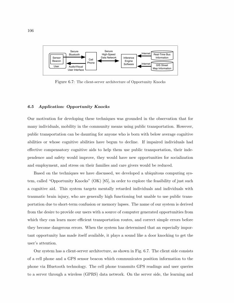
106
Internet
Internet
InferenceEngine
Software
Real-Time BusInformation
GIS StreetMap Information
User
Sensor Beacon
SecureBluetooth
Audio/VisualUser Interface
SecureHigh-Speed
Data NetworkCell
Phone
Figure 6.7: The client-server architecture of Opportunity Knocks
6.5 Application: Opportunity Knocks
Our motivation for developing these techniques was grounded in the observation that for
many individuals, mobility in the community means using public transportation. However,
public transportation can be daunting for anyone who is born with below average cognitive
abilities or whose cognitive abilities have begun to decline. If impaired individuals had
effective compensatory cognitive aids to help them use public transportation, their inde-
pendence and safety would improve, they would have new opportunities for socialization
and employment, and stress on their families and care givers would be reduced.
Based on the techniques we have discussed, we developed a ubiquitous computing sys-
tem, called “Opportunity Knocks” (OK) [85], in order to explore the feasibility of just such
a cognitive aid. This system targets mentally retarded individuals and individuals with
traumatic brain injury, who are generally high functioning but unable to use public trans-
portation due to short-term confusion or memory lapses. The name of our system is derived
from the desire to provide our users with a source of computer generated opportunities from
which they can learn more efficient transportation routes, and correct simple errors before
they become dangerous errors. When the system has determined that an especially impor-
tant opportunity has made itself available, it plays a sound like a door knocking to get the
user’s attention.
Our system has a client-server architecture, as shown in Fig. 6.7. The client side consists
of a cell phone and a GPS sensor beacon which communicates position information to the
phone via Bluetooth technology. The cell phone transmits GPS readings and user queries
to a server through a wireless (GPRS) data network. On the server side, the learning and

107
inference engine integrates the user information with map and bus information, and sends
inference results or suggestions back to the client side.
In the experiment, explained in Fig. 6.8 and Fig. 6.9, a user with our device boarded
a bus to get home after carrying the system with them for 1 month (a similar scenario
to Fig. 6.6(a, b), but with different data). Unfortunately, the user boarded the wrong bus,
which shared the first part of the bus route in common with the correct bus. OK detected
the mistake and guided the user back on track. The top of each panel in the figures display
a representation of the reasoning process that the inference engine is undertaking. The
center portion of each panel displays what the user interface displayed at each stage of the
experiment, and the bottom portion holds a text description of the frame.
6.6 Summary
We have described the foundations and experimental validation of a hierarchical model that
can learn and infer a user’s daily movements and use of different modes of transportation.
The model can be learned using unlabeled data, and online inference can be efficiently
performed. Our results showed that the approach can provide predictions of movements
to distant goals, and support a simple and effective strategy for detecting novel events
that may indicate user errors. Based on this technique, we implemented a system called
“Opportunity Knocks” that is able to help cognitively impaired people use public transit
independently and safely.

108
Home
Grocery
Friend
Friend
Work Work
Home
Bus stop
Parking lotBus stop
Work
Home
Bus stop
Bus stop
This frame shows the user atwork when the system iden-tified the most likely desti-nations. Circle areas corre-spond to relative likelihood.The phone displayed imagesof the most likely destina-tions left to right, top to bot-tom: home, friend 1, friend 2,grocery store.
After the user indicated thathe’d like to go home, the sys-tem identified two routes thathe usually takes, a bus routeshown in solid lines and a carroute shown in dashed lines.The system asked the userwhich way he would like toproceed.
The user selected the busroute and OK presenteda text description of thelearned route. The user pro-ceeded to the bus stop, andboarded a bus. The bus thatthe user boarded however wasgoing to his friend’s house, afamiliar, but incorrect routeconsidering the expressed in-tention to go home.
1 2 3
Figure 6.8: An experiment using Opportunity Knocks (Part I)

109
Work
Home
Bus stop
0 100 200 300 400 500 600 700 8000
0.1
0.2
0.3
0.4
0.5
0.6
0.7
0.8
0.9
1
Time [sec]
Err
or P
roba
bilit
y
This graph shows how the system reasonsabout errors. When the error probabilityrises above 50% confidence, the system be-lieves an abnormal condition exists. OKwaits until a clamped curve breaks 80% con-fidence before alerting.
Work
Bus stop
Bus stop
Home
The system was unable toidentify that the user wason the wrong bus becausethe routes coincided for thefirst portion of the bus ride.Before getting to the cor-rect bus stop for going home,the system observed that theuser had departed from theexpected trip segment andturned west.
When the bus diverted fromthe correct route, the systemidentified the behavior condi-tion as an error. This waspossible even though the userwas on a frequently takenroute. In response it proac-tively made its door knockingalert noise and showed a cor-responding message
Once off the incorrect bus,the user reselects home as thedestination. This time OKqueries a real-time bus plan-ning system for a route home.The user is directed to walkback to the arterial road andcatch a different bus that isgoing the correct way.
4 5 6
Figure 6.9: An experiment using Opportunity Knocks (Part II)

110
Chapter 7
INDOOR VORONOI TRACKING
In last chapter, we described a person’s transportation routines using a DBN model,
whose parameters are customized based on GPS data collected by the person. We applied
Rao-Blackwellised particle filters for inference and EM algorithm for unsupervised learning.
In this chapter, we apply similar approach to learning people’s movement patterns in indoor
environments.
The first difficulty for indoor environments is the ineffectiveness of GPS; thus we have
to resort to other tracking techniques. The indoor location estimation has gained a lot
of attention in the robotics community [27, 97, 55]. Most existing approaches to people
tracking rely on laser range-finders [27, 8, 97] or cameras [55]. A key advantage of these
sensors is their location accuracy. Unfortunately, they usually do not provide information
about the identity of people. Over the last years, especially in the ubiquitous computing
community, people have started to equip indoor environments with networks of sensors that
are capable of providing information about a person’s location and identity [113, 4]. Such
sensors, however, have the disadvantage that they provide only relatively coarse location
information in practice. In addition to being corrupted by noise, such sensors provide
measurements at low frame rates only. In this chapter, we discuss a robust approach for
location estimation using such sparse and noisy sensor data.
Another difficulty is that we do not have street maps available indoors, which play a
important role in our outdoor models. To overcome this difficulty, we track the locations of
people on (generalized) Voronoi graphs [16] of indoor environments (see Fig. 7.2(a) for an
example). Thus we can naturally represent typical human motion along the main axes of
the free space. The estimated trajectories on the Voronoi graph help us to bridge the gap
between continuous sensor data and discrete, abstract models of human motion behavior.
Surprisingly, such an approximation can also improve the tracking accuracy in the case of

111
mk−1 mk
k−1x kx
z k−1 z k
k−1v kv
Mode m
Sensor readings z
Location x = <e,d>
Velocity v
Figure 7.1: DBN model of the Voronoi tracking
sparse and noisy sensor data, as we will show in the experiments.
This chapter is organized as follows. we first present a DBN model for indoor location
tracking. Although the motion model is similar to outdoor case, the sensor model is very
different. Then we briefly explain the inference and learning algorithms. Finally, we will
show experimental results of Voronoi tracking.
7.1 Voronoi Tracking
We define a Voronoi graph G = (V,E) by a set V of vertices vi and a set E of directed
edges ej . Roughly speaking, Voronoi graph of an environment is the skeleton of the free
space. Fig. 7.2(a) shows the Voronoi graph representing the Intel Research Lab Seattle,
our indoor testing environment. Note that this graph results from manual pruning of the
original Voronoi graph [16] and that for clarity only the undirected version of the graph is
shown.
Similar to outdoor GPS tracking and the inference of modes of transportation, we con-
struct a DBN model, as shown in Fig. 7.1. From the top of the model, mk ∈ {stopped,moving}
indicates the current motion mode of the object, which depends on the previous mode mk−1
and previous edge ek−1. Intuitively, places such as offices should have higher stopping prob-
abilities and hallways should have lower stopping probabilities. Therefore, by learning the
mode transition probabilities at each edge, we can have some idea of the different types of
places. The next level is velocity. If mk = stopped, then vk = 0; otherwise vk is governed
by a Gaussian distribution whose mean and variance are manually set based on ordinary

112
(a) (b)
(c) (d)
Figure 7.2: Voronoi graphs for location estimation: (a) Indoor environment along with manuallypruned Voronoi graph. Shown are also the positions of ultrasound Crickets (circles) and infraredsensors (squares). (b) Patches used to compute likelihoods of sensor measurements. Each patchrepresents locations over which the likelihoods of sensor measurements are averaged. (c) Likelihoodof an ultra-sound cricket reading (upper) and an infrared badge system measurement (lower). Whilethe ultra-sound sensor provides rough distance information, the IR sensor only reports the presenceof a person in a circular area. (d) Corresponding likelihood projected onto the Voronoi graph.
human movements. The current location of an object is represented by xk = 〈ek, dk〉, where
ek denotes the current edge on the graph, dk indicates the distance of the object from the
start vertex of edge ek. Given xk−1 and vk, xk is determined by the edge transition matrix
p(ej |ei), which describes the probability that the object transits to node ej given that the
previous node was ei and an edge transition took place.
In general, the motion model of the indoor Voronoi tracking is similar to that of the flat
model for GPS tracking. However, its sensor model p(zk | xk) is quite different from that
of GPS. At each time a single object can get measurements from more than one sensors.
Denote the sequence of observations at time k as zk1, · · · , zk
I . By assuming the observations

113
are generated independently, we have
p(zk | xk) =I∏
i=1
p(zki | xk) (7.1)
A straightforward implementation of p(zki | xk) for Voronoi graphs would be to sim-
ply compute the likelihood of observations for positions on the graph, as done in the GPS
tracking. However, in reality people can move anywhere in the free space, and thus com-
puting the likelihoods only on the graph is not a valid and robust approach. Note that each
discretized position on the graph actually represents a patch of the free space, as shown in
Fig. 7.2(b). The patch S(x) consists of the set of all the 2d positions whose “projection”
on the graph is x, or more strictly, S(x) is defined as
S(x) = {ν ∈ free space | x = argminx′ on graph
|x′ − ν|} (7.2)
Then, to compute the likelihood of an observation zki given a position xk on the graph,
we have to integrate over all 2d positions in the patch S(xk):
p(zki|xk) =
1|S(xk)|
∑ν∈S(xk)
p(zki | ν) (7.3)
In our implementation of the sensor model, we discretize positions on the graph and pre-
compute the patch for each position. Fig. 7.2(c) shows the original sensor models in the 2d
space for infrared badge system and ultra-sound cricket system, and Fig. 7.2(d) shows the
corresponding sensor model on the Voronoi graph by averaging the measurement likelihood
within each patch.
7.2 Inference and Learning
In last chapter, we combined Kalman filters and particle filters for location estimation on a
graph. A key assumption was the Gaussian distribution of the GPS sensor model. However,
for many indoor location sensors, such as infrared sensors (see Section 7.3), the Gaussian
assumption does not hold. Therefore, we only apply the particle filters for the inference

114
without using the Kalman update. Because the limited space of indoor environment, the
inference is still very efficient.
The application of particle filters to location estimation on a Voronoi graph is rather
straightforward. We first sample the motion state mk with probability proportional to
p(mk | mk−1, ek−1). If mk = moving, then we randomly draw the velocity vk from the
Gaussian distribution and compute the traveled distance vk∆t. Then we have to determine
whether the motion along the edge results in a transition to another edge. If not, then
dk = dk−1 + vk∆t and ek = ek−1. Otherwise, dk = dk−1 + vk∆t− |ek−1| and the next edge
ek is drawn with probability p(ek | ek−1). If the motion state mk = stopped, the position
xk is set to be xk−1. The importance sampling step of the particle filter is implemented by
weighting each sample proportional to the projected observation likelihood as given in (7.1),
and the reweight step is identical to standard particle filters.
The task of learning in our model is to estimate the edge transition matrix p(ej |ei)
and the mode transition matrix p(mk|mk−1, ek−1). Similar to the parameter estimation for
transportation routines, we again apply the Expectation-Maximization (EM) algorithm. In
a nutshell, each iteration of the EM begins with an expectation step, which estimates the
trajectory of the person using particle filtering forward and backward through the data set.
The trajectories are used to count the edge transitions of particles on the Voronoi graph and
the switching between motion modes. These values are then converted into probabilities
during the M-step, which generates a new model estimate. The updated model is then
used in the next iteration to re-estimate the trajectory of the person. For the first E-step,
we initialize the mode transition parameters with some reasonable values using background
knowledge of typical human motion and a uniform distribution for the outgoing edges at
each vertex of the Voronoi graph.
7.3 Experimental Results
We evaluate the performance of the Voronoi tracking (VT) approach based on data recorded
at the Intel Research Lab Seattle. As shown in Fig. 7.2(a), the office environment is equipped
with two different kinds of ID sensors, including 73 Versus infrared receivers which provide
information about the presence of a person in the vicinity of a sensor and three Cricket

115
0 2 4 6 8 10 12
Distance (m)
p(z
| d
ista
nce
)
Versus infrared sensorCricket ultrasound sensor
(a) 0 200 400 600 800 10000
2
4
6
8
10
Number of particles
Ave
rag
e er
ror
(m)
Particle filteringVoronoi tracking
(b)
Figure 7.3: (a) Sensor model of ultrasound crickets and infrared badge system. The x-axis repre-sents the distance from the detecting infrared sensor and ultrasound sensor (4m ultrasound sensorreading), respectively. The y-axis gives the likelihood for the different distances from the sensor. (b)Localization error for different numbers of samples.
ultrasound receivers which provide identity and distance estimates (see [46] for more details
on the sensors). Fig. 7.3(a) shows a model of the uncertainty of the two sensor types, used
to compute p(zki | ν) in (7.3). The sensor parameters are manually set based on experience.
Note that especially the infrared badge sensor model is highly non-Gaussian. Additionally,
both sensors suffer from a high probability of false-negative readings, i.e., they frequently
fail to detect a person.
To generate data for which ground truth is available, we equipped a mobile robot with
two Versus badges, a Cricket beacon, and additionally with a Sick laser range-finder. Our
experiment is based on a 35-minute-long log of sensor measurements received while driving
the robot through the environment. The robot moved at an average velocity of 30 cm/s and
was stopped at designated resting places. The laser range-finder allowed us to accurately
estimate the path of the robot using the map shown in Fig. 7.2(a).
As an initial test, we determined the average localization error when using un-trained VT
vs. a particle filter (PF) representing locations in the complete free space of the environment.
The resulting error on the complete log was 2.34m for VT and 3.78m for PF. This result
is extremely encouraging since it indicates that the projection onto the Voronoi graph does
not only result in a good approximation of the PF, but yields better performance than the
PF. Fig. 7.4 (b) and (c) show typical maximum likelihood trajectories using VT and PF,

116
(a) (b)
(c) (d)
Figure 7.4: (a) Trajectory of the robot during a 25 minute period of training data collection. Truepath (in light color) and most likely path as estimated using (b) Voronoi tracking and (c) originalparticle filters. (d) Motion model learned using EM. The arrows indicate those transitions for whichthe probability is above 0.65. Places with high stopping probabilities are represented by disks.Thicker arcs and bigger disks indicate higher probabilities.
respectively. These paths were generated from the trajectory (history) of the most likely
particle at the end of the run. The graphs clearly demonstrate the superior performance of
the VT technique.
We also compared the tracking performance for different sample set sizes. The results
are given in Fig. 7.3(b). It becomes clear that VT makes very efficient use of particles and
it is able to track well using only 200 particles.
Next, we evaluated the learning performance of VT. We split the complete data log into
a training set of 25 minutes and a test set of 10 minutes. We trained the VT model using
the EM algorithm on the training set and determined the tracking error on the test data
using the motion model learned at each iteration. The results are summarized in Table 7.1.
As can be seen, the algorithm converges after only 3 iterations of EM, and using the

117
Table 7.1: Evolution of test error during EM learning.
EM Iteration Avg. Tracking Error ReductionErrors (m) after Learning
before learning 2.63 -1 2.27 13.7%2 2.05 22.1%3 1.84 30.0%4 1.79 31.9%5 1.76 33.1%
learned model increases the tracking accuracy significantly. This shows that the Voronoi
graph is able to extract the correct motion patterns from the training data. This fact is
supported by Fig. 7.4(d), which visualizes the motion model learned after 5 iterations. The
model correctly reflects the path and resting locations of the robot.
7.4 Summary
We have presented an approach to tracking the location of people and learning their motion
patterns in indoor environments. The technique is able to robustly estimate a person’s
location even when using only sparse, noisy information provided by id-sensors. The key
idea of our approach is to use a particle filter that is projected onto a Voronoi graph of
the environment. The resulting model is similar to the hierarchical DBN for modeling
transportation routines. Using data collected by a mobile robot, we demonstrate that our
approach has two key advantages. First, it is by far more efficient and robust than particle
filters which estimate the location of people in the complete free space of an environment.
Second, the Voronoi graph provides a natural discretization of human motion, which allows
us to learn typical motion patterns using expectation maximization. More recent work has
extended our approach by applying advanced sensor models and using mixed representation
of Voronoi graph and free space [61, 26].

118
Chapter 8
CONCLUSION AND FUTURE WORK
8.1 Conclusion
The goal of our research is to develop fundamental techniques that enable machines to un-
derstand human activities. In this thesis, we have developed two techniques for recognizing
people’s activities and transportation routines from GPS data.
First, we have presented a framework of activity recognition that builds upon and extends
existing research on statistical relational learning, such as conditional random fields and
relational Markov networks. This framework is able to take into account complex relations
between locations, activities, and significant places, as well as high level knowledges such
as number of homes and workplaces. By extracting and labeling activities and significant
places simultaneously, our approach achieves high accuracy on both extraction and labeling.
The framework is very expressive. Using SQL-like templates, it can capture complicated
relations and instance uncertainty. The framework also supports efficient inference and
learning. We have presented efficient inference algorithms for aggregate features using FFT
or local MCMC, and a novel approach for feature selection and parameter estimation using
boosting with virtual evidences. Using GPS data collected by different people, we have
demonstrated the feasibility of transferring knowledge from people who have labeled data
to those who have no or very little labeled data.
Second, we have built a hierarchical dynamic Bayesian network model for transportation
routines. It can predict a user’s destination in real time, infer the user’s mode of trans-
portation, and determine when a user has deviated from his ordinary routines. The model
encodes general knowledge such as street maps, bus routes, and bus stops, in order to dis-
criminate different transportation modes. Moreover, our system could automatically learn
navigation patterns at all levels from raw GPS data, without any manual labeling! Based
on this work we have developed a personal guidance system called Opportunity Knocks, to

119
help people with cognitive disabilities use public transit.
Although the two techniques are very different, they share a number of common charac-
teristics. For example, both have hierarchical structures so as to bridge the gap between low
level sensor data and high level activities; both encode a large amount of domain knowledges
and complex relations; and both recognize activities in a collective manner so as to create
a comprehensive and consistent interpretation of a user’s data.
The focus of the thesis is location-based activity recognition from GPS data. In addi-
tion, we have shown preliminary results for indoor activity recognition and motion pattern
learning. We believe many techniques we have developed, such as the efficient inference
algorithms for aggregate features, the virtual evidence boosting algorithm, and the Rao-
Blackwellized particle filtering in hierarchical models, can be applied into other probabilistic
reasoning tasks as well.
8.2 Future Work
We have just begun to scratch the surface of what can be done with this general approach
to modeling activity patterns of people. Many theoretical challenges remain unsolved, such
as learning models with partially labeled data and clustering people based on different
behavioral patterns. At the same time our technique can be applied in many domains, such
as mobile user modeling and assistive technologies; building these practical systems is also
interesting future work.
8.2.1 Semi-supervised Learning
One of the biggest problems in training discriminative activity models is that it requires a
large amount of fully labeled data. In practice, it is very expensive and time-consuming to
manually label all the training data. The idea of semi-supervised learning in our case is to
train discriminative activity models using only partially labeled data. For example, we may
only have labels for some time but not all the time, or in hierarchical activity models we may
only have labels for high level activities but not low level activities. The goal is to learn CRF-
like models that utilize all the data, including both labeled and unlabeled. There have been
some progresses on applying CRFs in semi-supervised learning (see [93, 103, 48]). However,

120
the learning algorithms in previous work mainly use ML criterion and are hard to scale to
large data sets; at the same time it is unclear how pseudo-likelihood and virtual evidence
boosting can be extended for semi-supervised cases. Therefore, it is still an open challenge
to develop more efficient training algorithms for CRFs in a semi-supervised manner, and
this work could have great impact for many practical applications.
8.2.2 Pattern Clustering
In this thesis, we have demonstrated the feasibility of transferring activity knowledge be-
tween different people: we train a model from some people and apply the learned model
to others. This method works well in our experiments. However, we only used data from
subjects whose activities are more or less similar, for example, they all have families and
day-time jobs. In order to apply our approach to thousands of people, we must be able to
handle very different behavior patterns. A promising approach is to cluster people based
on their activity patterns and learn a generic model for each cluster. For a new person, we
determine which cluster the person belongs to and then apply the model of that cluster to
infer his activities. There are two main challenges. First, in this setting of clustering, each
input includes all the data from a single person. What metrics shall we use to determine
the similarities between the inputs? Shall we use all the RMN features directly, or shall we
apply feature selection or dimension reduction? Second, how shall we determine the cluster
that the person belongs to, since the labels of the new person are unknown? We may think
this as a online model selection problem, and we could pick the model that maximize some
criterion, such as the conditional likelihood of the MAP sequence.
8.2.3 Adaptive Mobile Devices
User modeling is important to adaptive user interfaces, personalized Web search, and proac-
tive user assistance. For modeling desktop users, inputs from the keyboard and mouse are
primary sources of information. In a mobile environment, however, it is essential to take
people’s physical activities into account. By integrating ubiquitous sensor data (e.g., loca-
tions), mobiles devices can potentially better understand users’ interaction patterns, and

121
more accurately predict their needs. However, mobile devices have less memory and com-
putational power, so the learning and inference must be very efficient even with limited
resources. Future research on mobile user modeling will benefit from previous work on
adaptive desktop systems and ubiquitous activity recognition, and will address the trade-off
between reasoning performance and resource usage.
8.2.4 Long-term Health Care
The ability to automate activity tracking and anomaly detection will enable important
applications in health care. However, we must connect our research more closely with
findings from neuropsychology and other sources of domain knowledge. For example, if
we have knowledge of how a specific neurological deficit (e.g., mild Alzheimer’s disease)
impairs a variety of human activities, then we can develop patient-specific behavior models
and provide targeted intervention. The challenge, however, is how to obtain such knowledge,
since neither hand-coding nor completely supervised learning will be scalable. A feasible
way could be to start with the general domain knowledge, and refine our knowledge in an
unsupervised manner as real patients use the system. It may be also necessary to group
patients based on their similarities and allow knowledge transfer between people. This
research will not only help computers recognize user errors, but also help us understand the
causes of these behavioral deficits in functional and computational terms.
8.2.5 From Sensors to Human Sense
People have invented a large variety of sensors that are capable of providing various in-
formation about the world, for example, RFID can tell which object has been touched,
body sensors can continuously measure the body temperature and blood pressure, sensor
networks can be used to detect anomalies in wild environments, etc. However, what people
often need is high level information of contexts, such as activities, intentions, needs, healthy
conditions, and so on. There exists a big gap between the low level sensor measurements
and high level human sense. In this thesis, we focus on bridging the gap between location
data and relevant activities using machine learning and probabilistic reasoning techniques.

122
We believe the framework can be applied in many other applications with similar goals.
In order to provide efficient and well-founded solutions to practical applications, we must
leverage synergies between artificial intelligence and ubiquitous computing, so that we can
benefit from the advances in both domains.

123
BIBLIOGRAPHY
[1] C. Andrieu, N. de Freitas, A. Doucet, and M. I. Jordan. An introduction to MCMCfor machine learning. Machine Learning, 2003.
[2] S. Arulampalam, S. Maskell, N. Gordon, and T. Clapp. A tutorial on particle filtersfor on-line non-linear / non-Gaussian Bayesian tracking. IEEE Transactions on SignalProcessing, 2001.
[3] D. Ashbrook and T. Starner. Using GPS to learn significant locations and predictmovement across multiple users. Personal and Ubiquitous Computing, 7(5), 2003.
[4] P. Bahl and V. Padmanabhan. RADAR: An in-building RF-based user location andtracking system. In Proceedings of IEEE INFOCOM, 2000.
[5] J. E. Baker. Reducing bias and inefficiency in the selection algorithm. In Proc. of theSecond International Conference on Genetic Algorithms, 1987.
[6] Y. Bar-Shalom, X. R. Li, and T. Kirubarajan. Estimation with Applications to Track-ing and Navigation. John Wiley, 2001.
[7] M. Bennewitz, W. Burgard, G. Cielniak, and S. Thrun. Learning motion patternsof people for compliant robot motion. International Journal of Robotics Research(IJRR), 24(1), 2005.
[8] M. Bennewitz, W. Burgard, and S. Thrun. Using EM to learn motion behaviors ofpersons with mobile robots. In Proc. of the IEEE/RSJ International Conference onIntelligent Robots and Systems (IROS), 2002.
[9] J. Besag. Statistical analysis of non-lattice data. The Statistician, 24, 1975.
[10] A. F. Bobick and Y. A. Ivanov. Action recognition using probabilistic parsing. Tech-nical report, MIT Media Lab, 1998.
[11] E. O. Brigham. Fast Fourier Transform and Its Applications. Prentice Hall, 1988.
[12] H. H. Bui. A general model for online probabilistic plan recognition. In Proc. of theInternational Joint Conference on Artificial Intelligence (IJCAI), 2003.
[13] H. H. Bui, S. Venkatesh, and G. West. On the recognition of abstract Markov policies.In Proc. of the National Conference on Artificial Intelligence (AAAI), 2000.

124
[14] H. H. Bui, S. Venkatesh, and G. West. Policy recognition in the abstract hiddenMarkov model. Journal of Artificial Intelligence Research, 2002.
[15] E. Charniak and R. P. Goldman. A Bayesian model of plan recognition. In Proc. ofthe National Conference on Artificial Intelligence (AAAI), 1993.
[16] H. Choset. Sensor Based Motion Planning: The Hierarchical Generalized VoronoiGraph. PhD thesis, Caltech, 1996.
[17] T. Choudhury, B. Clarkson, S. Basu, and A Pentland. Learning communities: Con-nectivity and dynamics of interacting agents. In Proc. of the International JointConference on Neural Networks, 2003.
[18] D. Colbry, B. Peintner, and M. E. Pollack. Execution monitoring with quantitativetemporal Bayesian networks. In 6th International Conference on AI Planning andScheduling, 2002.
[19] R. Cowell, A. Dawid, S. Lauritzen, and D. Spiegelhalter. Probabilistic Networks andExpert Systems. Springer, 1999.
[20] N. de Freitas. Rao-Blackwellised particle filtering for fault diagnosis. IEEE Aerospace,2002.
[21] T. Dean and K. Kanazawa. Probabilistic temporal reasoning. In Proc. of the NationalConference on Artificial Intelligence (AAAI), 1988.
[22] A. P. Dempster, N. M. Laird, and D. B. Rubin. Maximum-likelihood from incompletedata via the EM algorithm. Journal of the Royal Statistical Society, 1977.
[23] T. Dietterich, A. Ashenfelter, and Y. Bulatov. Training conditional random fields viagradient tree boosting. In Proc. of the International Conference on Machine Learning(ICML), 2004.
[24] A. Doucet, N. de Freitas, and N. Gordon, editors. Sequential Monte Carlo in Practice.Springer-Verlag, New York, 2001.
[25] A. Doucet, N. de Freitas, K. Murphy, and S. Russell. Rao-Blackwellised particlefiltering for dynamic Bayesian networks. In Proc. of the National Conference onArtificial Intelligence (AAAI), 2000.
[26] B. Ferris, D. Hahnel, and D. Fox. Gaussian processes for signal strength-based locationestimation. In Proc. of Robotics: Science and Systems, 2006.

125
[27] A. Fod, A. Howard, and M. J. Mataric. Laser-based people tracking. In Proc. of theIEEE International Conference on Robotics & Automation (ICRA), 2002.
[28] W. Freeman, E. Pasztor, and O. Carmichael. Learning low-level vision. InternationalJournal of Computer Vision, 2000.
[29] Y. Freund and R. E. Schapire. A decision-theoretic generalization of on-line learningand an application to boosting. Journal of Computer and System Sciences, 55(1):119–139, 1997.
[30] B. J. Frey and D. MacKay. A revolution: Belief propagation in graphs with cycles.In Advances in Neural Information Processing Systems (NIPS), 1997.
[31] J. Friedman, T. Hastie, and R. Tibshirani. Additive logistic regression: a statisticalview of boosting. The Annals of Statistics, 38(2):337–374, 2000.
[32] N. Friedman, L. Getoor, D. Koller, and A. Pfeffer. Learning probabilistic relationalmodels. In Proc. of the International Joint Conference on Artificial Intelligence (IJ-CAI), 1999.
[33] S. Geman and D. Geman. Stochastic relaxation, Gibbs distributions and the Bayesianrestoration of images. Transactions on Pattern Analysis and Machine Intelligence(PAMI), 1984.
[34] L. Getoor, N. Friedman, D. Koller, and A. Pfeffer. Relational Data Mining, chapterLearning Probabilistic Relational Models. Springer-Verlag, 2001.
[35] L. Getoor, N. Friedman, D. Koller, and B. Taskar. Learning probabilistic models ofrelational structure. In Proc. of the International Conference on Machine Learning(ICML), 2001.
[36] L. Getoor and B. Taskar, editors. Statistical Relational Learning. forthcoming book,2006.
[37] C. J. Geyer and E. A. Thompson. Constrained Monte Carlo Maximum Likelihood fordependent data. Journal of Royal Statistical Society, 1992.
[38] W. R. Gilks, S. Richardson, and D. J. Spiegelhalter. Markov Chain Monte Carlo inPractice. Chapman and Hall/CRC, 1995.
[39] V. Gogate, R. Dechter, C. Rindt, and J. Marca. Modeling transportation routinesusing hybrid dynamic mixed networks. In Proc. of the Conference on Uncertainty inArtificial Intelligence (UAI), 2005.

126
[40] R. P. Goldman, C. W. Geib, and C. A. Miller. A new model of plan recognition. InProc. of the Conference on Uncertainty in Artificial Intelligence (UAI), 1999.
[41] K. Gopalratnam, H. Kautz, and D. Weld. Extending continuous time Bayesian net-works. In Proc. of the National Conference on Artificial Intelligence (AAAI), 2005.
[42] R. Hariharan and K. Toyama. Project Lachesis: parsing and modeling location his-tories. In Geographic Information Science, 2004.
[43] W. K. Hastings. Monte Carlo sampling methods using Markov chains and their ap-plications. Biometrika, 1970.
[44] D. Heckerman. A tutorial on learning with Bayesian networks. Technical report,Microsoft Research, 1995.
[45] D. Heckerman, D. Meek, and D. Koller. Probabilistic models for relational data. Tech-nical Report MSR-TR-2004-30, Microsoft Research and Stanford University, 2004.
[46] J. Hightower. The Location Stacks. PhD thesis, University of Washington, 2004.
[47] M. J. Huber, H. D Edmund, and M. P. Wellman. The automated mapping of plansfor plan recognition. In Proc. of the National Conference on Artificial Intelligence(AAAI), 1994.
[48] A. Kapoor. Learning Discriminative Models with Incomplete Data. PhD thesis, MIT,2006.
[49] H. Kautz. A Formal Theory of Plan Recognition. PhD thesis, University of Rochester,1987.
[50] K. Kersting and L. de Raedt. Towards combining inductive logic programming withBayesian networks. In Proceedings of the International Conference on Inductive LogicProgramming, 2001.
[51] G. Kitagawa. Monte Carlo filter and smoother for non-Gaussian nonlinear state spacemodels. Journal of Computational and Graphical Statistics, 5(1), 1996.
[52] D. Koller and A. Pfeffer. Probabilistic frame-based systems. In Proc. of the NationalConference on Artificial Intelligence (AAAI), 1998.
[53] D. Koller and A. Prfeffer. Learning probabilities for noisy first-order rules. In Proc. ofthe International Joint Conference on Artificial Intelligence (IJCAI), 1997.

127
[54] T. Kristjannson, A. Culotta, P. Viola, and A. McCallum. Interactive informationextraction with constrained conditional random fields. In Proc. of the National Con-ference on Artificial Intelligence (AAAI), 2004.
[55] E. Kruse and F. Wahl. Camera-based monitoring system for mobile robot guidance.In Proc. of the IEEE/RSJ International Conference on Intelligent Robots and Systems(IROS), 1998.
[56] S. Kumar and M. Hebert. Discriminative random fields: A discriminative frameworkfor contextual interaction in classification. In Proc. of the International Conferenceon Computer Vision (ICCV), 2003.
[57] C. Kwok and D. Fox. Map-based multiple model tracking of a moving object. InRoboCup 2004: Robot Soccer World Cup VIII, 2004.
[58] J. Lafferty, A. McCallum, and F. Pereira. Conditional random fields: Probabilisticmodels for segmenting and labeling sequence data. In Proc. of the InternationalConference on Machine Learning (ICML), 2001.
[59] A. LaMarca, Y. Chawathe, S. Consolvo, J. Hightower, I. Smith, J. Scott, T. Sohn,J. Howard, J. Hughes, F. Potter, J. Tabert, P. Powledge, G. Borriello, and B. Schilit.Place Lab: Device positioning using radio beacons in the wild. In proceedings ofPervasive, 2005.
[60] J. Lester, T. Choudhury, N. Kern, G. Borriello, and B. Hannaford. A hybriddiscriminative-generative approach for modeling human activities. In Proc. of theInternational Joint Conference on Artificial Intelligence (IJCAI), 2005.
[61] J. Letchner, D. Fox, and A LaMarca. Large-scale localization from wireless signalstrength. In Proc. of the National Conference on Artificial Intelligence (AAAI), 2005.
[62] R. Levine and G. Casella. Implementations of the Monte Carlo EM algorithm. Journalof Computational and Graphical Statistics, 10, 2001.
[63] L. Liao, T. Choudhury, D. Fox, H. Kautz, and B. Limketkai. Training conditionalrandom fields using virtual evidence boosting. In Proc. of the International JointConference on Artificial Intelligence (IJCAI), 2007.
[64] L. Liao, D. Fox, and H. Kautz. Learning and inferring transportation routines. InProc. of the National Conference on Artificial Intelligence (AAAI), 2004.
[65] L. Liao, D. Fox, and H. Kautz. Location-based activity recognition. In Advances inNeural Information Processing Systems (NIPS), 2005.

128
[66] L. Liao, D. Fox, and H. Kautz. Location-based activity recognition using relationalMarkov networks. In Proc. of the International Joint Conference on Artificial Intel-ligence (IJCAI), 2005.
[67] L. Liao, D. Fox, and H. Kautz. Extracting places and activities from GPS traces.International Journal of Robotics Research (IJRR), 2006. accepted.
[68] L. Liao, D.J. Patterson, D. Fox, and H. Kautz. Learning and inferring transportationroutines. Artifitial Intelligence, 2006. accepted.
[69] B. Limketkai, L. Liao, and D. Fox. Relational object maps for mobile robots. InProc. of the International Joint Conference on Artificial Intelligence (IJCAI), 2005.
[70] Y. Mao, F. R. Kschischang, and B. J. Frey. Convolutional factor graphs as probabilisticmodels. In Proc. of the Conference on Uncertainty in Artificial Intelligence (UAI),2004.
[71] A. McCallum. Efficiently inducing features or conditional random fields. In Proc. ofthe Conference on Uncertainty in Artificial Intelligence (UAI), 2003.
[72] N. Metropolis, A. W. Rosenbluth, M. N. Rosenbluth, A. H. Teller, and E. Teller.Equations of state calculations by fast computing machines. Journal of ChemicalPhysics, 1953.
[73] M. Montemerlo, S. Thrun, D. Koller, and B. Wegbreit. FastSLAM: A factored solutionto the simultaneous localization and mapping problem. In Proc. of the NationalConference on Artificial Intelligence (AAAI), 2002.
[74] R. Morales-Menendez, N. de Freitas, and D. Poole. Real-time monitoring of complexindustrial processes with particle filters. In Advances in Neural Information ProcessingSystems (NIPS), 2002.
[75] S. Muggleton. Stochastic logic programming. In Advances in inductive logic program-ming, 1996.
[76] K. Murphy. Bayesian map learning in dynamic environments. In Advances in NeuralInformation Processing Systems (NIPS), 1999.
[77] K. Murphy. Dynamic Bayesian Networks: Representation, Inference and Learning.PhD thesis, UC Berkeley, 2002.
[78] K. Murphy, Y. Weiss, and M. Jordan. Loopy belief propagation for approximateinference: An empirical study. In Proc. of the Conference on Uncertainty in ArtificialIntelligence (UAI), 1999.

129
[79] A. Ng and M. Jordan. On discriminative vs. generative classifiers: A comparison oflogistic regression and Naive Bayes. In Advances in Neural Information ProcessingSystems (NIPS), 2002.
[80] N. Oliver, E. Horvitz, and A. Garg. Layered representations for learning and infer-ring office activity from multiple sensory channels. In Proceedings of Int. Conf. onMultimodal Interfaces, 2002.
[81] H. Pasula, B. Marthi, B. Milch, S. Russell, and I. Shpitser. Identity uncertainty andcitation matching. In Advances in Neural Information Processing Systems (NIPS),2002.
[82] H. Pasula and S. Russell. Approximate inference for first-order probabilistic languages.In Proc. of the International Joint Conference on Artificial Intelligence (IJCAI), 2001.
[83] D. J. Patterson, D. Fox, H. Kautz, and M. Philipose. Fine-grained activity recogni-tion by aggregating abstract object usage. In Proceedings of the IEEE InternationalSymposium on Wearable Computers, 2005.
[84] D. J. Patterson, L. Liao, D. Fox, and H. Kautz. Inferring high-level behavior fromlow-level sensors. In International Conference on Ubiquitous Computing (UbiComp),2003.
[85] D. J. Patterson, L. Liao, K. Gajos, M. Collier, N. Livic, K. Olson, S. Wang, D. Fox,and H. Kautz. Opportunity Knocks: a system to provide cognitive assistance withtransportation services. In International Conference on Ubiquitous Computing (Ubi-Comp), 2004. submitted.
[86] J. Pearl. Probabilistic Reasoning in Intelligent Systems: Networks of Plausible Infer-ence. Morgan Kaufmann, 1988.
[87] F. Peng and A. McCallum. Accurate information extraction from research papersusing conditional random fields. In HLT-NAACL, 2004.
[88] A. Pfeffer and T. Tai. Asynchronous dynamic Bayesian networks. In Proc. of theConference on Uncertainty in Artificial Intelligence (UAI), 2005.
[89] D. Poole. Logic programming, abduction and probability: a top-down anytime algo-rithm for estimating prior and posterior probabilities. New Generation Computing,1993.
[90] D. Poole. Probabilistic Horn abduction and Bayesian networks. Artificial Intelligence,1993.

130
[91] D. V. Pynadath. Probabilistic Grammars for Plan Recognition. PhD thesis, Universityof Michigan, 1999.
[92] D. V. Pynadath and M. P. Wellman. Probabilistic state-dependent grammars forplan recognition. In Proc. of the Conference on Uncertainty in Artificial Intelligence(UAI), 2000.
[93] A. Quattoni, M. Collins, and T. Darrell. Conditional random fields for object recog-nition. In Advances in Neural Information Processing Systems (NIPS), 2004.
[94] L. R. Rabiner. A tutorial on hidden Markov models and selected applications in speechrecognition. In Proceedings of the IEEE. IEEE, 1989. IEEE Log Number 8825949.
[95] M. Richardson and P. Domingos. Markov logic networks. Machine Learning, 2006.
[96] S. Sanghai, P. Domingos, and D. Weld. Dynamic probabilistic relational models. InProc. of the International Joint Conference on Artificial Intelligence (IJCAI), 2003.
[97] D. Schulz, W. Burgard, and D. Fox. People tracking with a mobile robot usingjoint probabilistic data association filters. International Journal of Robotics Research(IJRR), 2003.
[98] D. Schulz, D. Fox, and J. Hightower. People tracking with anonymous and ID-sensorsusing Rao-Blackwellised particle filters. In Proc. of the International Joint Conferenceon Artificial Intelligence (IJCAI), 2003.
[99] F. Sha and F. Pereira. Shallow parsing with conditional random fields. In Proceedingsof Human Language Technology-NAACL, 2003.
[100] Y. Shi, Y. Huang, D. Minnen, A. Bobick, and I. Essa. Propagation networks forrecognition of partially ordered sequential action. In Proc. of the IEEE ComputerSociety Conference on Computer Vision and Pattern Recognition (CVPR), 2004.
[101] A. Subramanya, A. Raj, J. Bilmes, and D. Fox. Recognizing activities and spatialcontext using wearable sensors. In Proc. of the Conference on Uncertainty in ArtificialIntelligence (UAI), 2006.
[102] E. Sudderth, A. Ihler, W. Freeman, and A. Willsky. Nonparametric belief propagation.In Proc. of the IEEE Computer Society Conference on Computer Vision and PatternRecognition (CVPR), 2003.
[103] M. Szummer. Learning diagram parts with hidden random fields. In InternationalConference on Document Analysis and Recognition, 2005.

131
[104] B. Taskar, P. Abbeel, and D. Koller. Discriminative probabilistic models for relationaldata. In Proc. of the Conference on Uncertainty in Artificial Intelligence (UAI), 2002.
[105] B. Taskar, C. Guestrin, V. Chatalbashev, and D. Koller. Max-Margin Markov net-works. In Advances in Neural Information Processing Systems (NIPS), 2004.
[106] B. Taskar, M. Wong, P. Abbeel, and D. Koller. Link prediction in relational data. InAdvances in Neural Information Processing Systems (NIPS), 2003.
[107] S. Thrun, W. Burgard, and D. Fox. Probabilistic Robotics. MIT Press, 2005.
[108] S. Thrun, J. Langford, and D. Fox. Monte Carlo hidden Markov models: Learningnon-parametric models of partially observable stochastic processes. In Proc. of theInternational Conference on Machine Learning (ICML), 1999.
[109] L. Tierney. Markov chains for exploring posterior distributions. The Annals of Statis-tics, 1994.
[110] A. Torralba, K. P. Murphy, and W. T. Freeman. Contextual models for object de-tection using boosted random fields. In Advances in Neural Information ProcessingSystems (NIPS), 2004.
[111] V. N. Vapnik. Statistical Learning Theory. John Wiley & Sons, 1998.
[112] A. Varshavsky, M. Chen, E. D. Lara, J. Froehlich, D. Haehnel, J. Hightower,A. LaMarca, F. Potter, T. Sohn, K. Tang, and I. Smith. Are GSM phones THEsolution for localization? In 7th IEEE Workshop on Mobile Computing Systems andApplications (HotMobile), 2006.
[113] R. Want, A. Hopper, V. Falcao, and J. Gibbons. The active badge location system.ACM Transactions on Information Systems, 10(1), 2001.
[114] G. Wei and M.A. Tanner. A Monte Carlo implementation of the EM algorithm andthe poor mans data augmentation algorithms. Journal of the American StatisticalAssociation, 85, 2001.
[115] J. S. Yedidia, W. T. Freeman, and Y. Weiss. Exploring Artificial Intelligence in theNew Millennium, chapter Understanding Belief Propagation and Its Generalizations.Morgan Kaufmann Pub, 2001.
[116] J. S. Yedidia, W. T. Freeman, and Y. Weiss. Constructing free-energy approximationsand generalized belief propagation algorithms. IEEE Transactions on InformationTheory, 51(7):2282–2312, 2005.

132
[117] J. S. Yedidia, W. T. Freeman, and Weiss Y. Constructing free energy approximationsand generalized belief propagation algorithms. Technical report, MERL, 2002.
133
Appendix A
DERIVATIONS
A.1 Derivation of Likelihood Approximation using MCMC
Derivation of Eq. (4.8)
Suppose we already know the value L(w) for a weight vector w. Then we have (ignore
the shrinkage prior for simplicity)
L(w)− L(w) = − log P (y | x,w) + log P (y | x, w)
= logP (y | x, w)P (y | x,w)
= logexp{wT · f(x,y)}/Z(x, w)exp{wT · f(x,y)}/Z(x,w)
= logZ(x,w)/Z(x, w)
exp{(w − w)T · f(x,y)}
= logZ(x,w)Z(x, w)
− (w − w)T · f(x,y), (A.1)
where Z(x,w)/Z(x, w) can be estimated using Monte-Carlo methods:
Z(x,w)Z(x, w)
=
∑y exp{wT · f(x,y)}
Z(x, w)
=∑y
exp{(w − w)T · f(x,y)}exp{wT · f(x,y)}Z(x, w)
=∑y
exp{(w − w)T · f(x,y)}P (y | x, w)
≈ 1M
M∑i=1
exp{(w − w)T · f(x, y(i))}. (A.2)
At the last step of (A.2), we use MCMC to get M random samples, y(i)(1 ≤ i ≤ M) from
the distribution P (y | x, w).

134
Substitute (A.2) into (A.1), we get
L(w) ≈ L(w) + log
(1M
M∑i=1
exp{
(w − w)T · (f(x, y(i))− f(x,y))})
= L(w) + log
(1M
M∑i=1
exp{
(w − w)T ·∆f (i)})
, (A.3)
where ∆f (i) = f(x, y(i))− f(x,y) is the difference between sampled feature counts using w
and the empirical feature counts.
Eq. (4.8) is just Eq. (A.3) plus a prior term.
A.2 Derivation of the LogitBoost Extension to Handle Virtual Evidence
Derivation of Eq. (4.21)
The goal of our optimization is to minimize the negative per-label-log-likelihood, defined
as
L(F ) = −N∑
i=1
log p(yi) (A.4)
where p(yi) is is a short notation that represents the posterior probability of a true label
conditioned on its evidences. In the cases with virtual evidence, p(yi) can be computed
using (4.20), or equivalently as the following:
p(yi) =1
1 +PX
xi=1 ve(xi)e(1−2yi)F (xi)PXxi=1 ve(xi)e(2yi−1)F (xi)
=1
1 + Gi(F )(A.5)
where Gi(F ) ,PX
xi=1 ve(xi)e(1−2yi)F (xi)PX
xi=1 ve(xi)e(2yi−1)F (xi).
In (A.4), substitute the likelihood with (A.5), the objective function can be expressed

135
as
LF =N∑
i=1
log(1 + Gi(F )) (A.6)
Similar to original LogitBoost, our extension performs Newton step to minimize (A.6),
which can be reduced to a weighted least square error (WLSE) problem defined in Eq. (4.21).
The derivation is shown below.
Suppose at one iteration the estimate is F . Then to take the Newton step, we first
compute the derivative of LF+f relative to f when f → 0. We have
s ,∂LF+f
∂f
∣∣∣f=0
=N∑
i=1
∂Gi(F+f)∂f
1 + Gi(F + f)
∣∣∣f=0
=N∑
i=1
2(1− 2yi)Gi(F )1 + Gi(F )
(A.7)
=N∑
i=1
2(1− 2yi)(1− p(yi)) (A.8)
where (A.7) follows from the following relation that can be easily verified
∂Gi(F + f)∂f
∣∣∣f=0
= 2(1− 2yi)Gi(F ) (A.9)
Second, we compute the Hessian as
H ,∂2LF+f
∂f2
∣∣∣f=0
= −N∑
i=1
2(1− 2yi)∂p(yi)
∂f
∣∣∣f=0
(A.10)
= −N∑
i=1
2(1− 2yi)∂ 1
1+Gi(F+f)
∂f
∣∣∣f=0
(A.11)
=N∑
i=1
4p(yi)(1− p(yi)) (A.12)

136
where (A.10) follows by substituting the derivative with (A.8), Eq. (A.11) follows from
(A.5), and we can get (A.12) by applying standard calculus and using (A.9).
The Newton update is then
F (x) ← F (x)− s
H
= F (x) +∑N
i=1(yi − 0.5)(1− p(yi))∑Ni=1 p(yi)(1− p(yi))
= F (x) +
∑Ni=1 αi
yi−0.5p(yi)∑N
i=1 αi
(A.13)
where αi = p(yi)(1 − p(yi)). Therefore, we can get the “best” f by solving the following
weighted least-square approximation
f∗(x) = argminf
N∑i=1
αiE
(f(x)− yi − 0.5
p(yi)
)2
= argminf
N∑i=1
X∑x=1
αive(xi)(
f(x)− yi − 0.5p(yi)
)2
(A.14)
which is just Eq. (4.21).

137
VITA
Lin Liao received his B.S. and M.S. in Automation from Tsinghua University, China,
in 1998 and 2001. In 2001, he came to the U.S. and became a graduate student in the
Department of Computer Science and Engineering at the University of Washington, where he
received a second M.S. in 2003 and a Ph.D. in 2006. His research focuses on the combination
of techniques from artificial intelligence, machine learning, and ubiquitous computing and
their application to practical domains, such as human activity recognition and robotics.
Lin has published a dozen of referred papers, and the paper on ”Learning and Inferring
Transportation Routines” won the Outstanding Paper Award at AAAI 2004. Lin received
the Outstanding Graduate Award from Tsinghua University in 2001 and the CSE Educator’s
Fellowship from the University of Washington in 2005.
Lin has worked at Microsoft Research and Intel Research as interns and joined Google
in 2006.


![Clustering-Based Ensemble Learning for Activity Recognition in … · with the aforementioned techniques in activity recognition [15]. Three base classifiers were considered, namely](https://img.pdfslide.net/doc/110x75/5f7d1ae304f85124d5198690/clustering-based-ensemble-learning-for-activity-recognition-in-with-the-aforementioned.jpg)