Embed Size (px)
Citation preview

Location information andHandover optimization in
WLAN/WPAN
Group : 998
Supervisors :Hans Peter SchwefelIstvan Kovacs
Group member :Sukesh ReddyKim LamYann MalidorChristophe MartineauGuillaume MonghalKrishna Mohan
9th Semester of Mobile CommunicationAalborg University, autumn 2004

AALBORG UNIVERSITY - Institute of Electronic SystemsFredrik Bajer Vej 7 - 9220 AalborgMobile communication: 9th semester
Location information andHandover optimization in
WLAN/WPAN
Project Period : 2nd September - 4th January 2005
Group : 998
Supervisors :Hans Peter SchwefelIstvan Kovacs
Group member :Kim LamYann MalidorChristophe MartineauKrishna MohanGuillaume MonghalSukesh Reddy
Number of report : 7
Number of pages : 96
AbstractThis project aims to give concepts and provide a simulation of an enhanced han-dover solution for Bluetooth networks. Handover between Access Points enablesthe user to maintain a continuous connection while moving from the coverage areaof one Access Point to another. Additionally, in this project, location data col-lection and movement prediction techniques are adequately used to enhance thehandover process.

Contents
1 Introduction 9
2 Background 112.1 Bluetooth . . . . . . . . . . . . . . . . . . . . . . . . . . . . . . 11
2.1.1 A recent booming technology . . . . . . . . . . . . . . . 112.1.2 Bluetooth technology . . . . . . . . . . . . . . . . . . . . 112.1.3 Connection scheme . . . . . . . . . . . . . . . . . . . . . 122.1.4 Data Communication . . . . . . . . . . . . . . . . . . . . 122.1.5 States of Bluetooth Devices . . . . . . . . . . . . . . . . 142.1.6 Bluetooth packet . . . . . . . . . . . . . . . . . . . . . . 17
2.2 Location techniques . . . . . . . . . . . . . . . . . . . . . . . . . 192.2.1 Cell Identification . . . . . . . . . . . . . . . . . . . . . 192.2.2 Angle of Arrival . . . . . . . . . . . . . . . . . . . . . . 192.2.3 Triangulation methods . . . . . . . . . . . . . . . . . . . 202.2.4 Database Support . . . . . . . . . . . . . . . . . . . . . . 212.2.5 Discussion on the different location techniques . . . . . . 22
2.3 Movement Prediction . . . . . . . . . . . . . . . . . . . . . . . . 282.3.1 Utility of movement prediction . . . . . . . . . . . . . . . 282.3.2 The predictive techniques . . . . . . . . . . . . . . . . . 282.3.3 Different methods for location prediction . . . . . . . . . 29
2.4 Conclusions . . . . . . . . . . . . . . . . . . . . . . . . . . . . . 32
3 Theoretical analysis 333.1 Probability Issues in Location . . . . . . . . . . . . . . . . . . . 33
3.1.1 Definitions . . . . . . . . . . . . . . . . . . . . . . . . . 333.1.2 Algorithm of the Localization . . . . . . . . . . . . . . . 353.1.3 Summary of the Localization algorithm . . . . . . . . . . 38
3.2 Propagation aspects . . . . . . . . . . . . . . . . . . . . . . . . . 413.2.1 Theoretical Propagation . . . . . . . . . . . . . . . . . . 413.2.2 Propagation . . . . . . . . . . . . . . . . . . . . . . . . . 41
3.3 Movement Prediction . . . . . . . . . . . . . . . . . . . . . . . . 443.3.1 Human movement model . . . . . . . . . . . . . . . . . . 443.3.2 Parameter Estimation . . . . . . . . . . . . . . . . . . . . 493.3.3 Position Prediction . . . . . . . . . . . . . . . . . . . . . 493.3.4 Estimation of the Distance from the Access Point . . . . . 50
3

CONTENTS
3.4 Handover . . . . . . . . . . . . . . . . . . . . . . . . . . . . . . 523.4.1 Establishing connection in Bluetooth network . . . . . . . 523.4.2 Inquiry Procedure . . . . . . . . . . . . . . . . . . . . . . 523.4.3 Paging Procedure . . . . . . . . . . . . . . . . . . . . . . 533.4.4 The Paging timers . . . . . . . . . . . . . . . . . . . . . 54
3.5 Conclusions . . . . . . . . . . . . . . . . . . . . . . . . . . . . . 55
4 Simulations 564.1 Scenario . . . . . . . . . . . . . . . . . . . . . . . . . . . . . . . 564.2 Simulator Principle . . . . . . . . . . . . . . . . . . . . . . . . . 564.3 Functionalities Breakdown . . . . . . . . . . . . . . . . . . . . . 57
4.3.1 Generation of RSSI measurements . . . . . . . . . . . . . 574.3.2 Location of a fixed Device . . . . . . . . . . . . . . . . . 604.3.3 Location of a moving Device . . . . . . . . . . . . . . . . 784.3.4 Movement Prediction . . . . . . . . . . . . . . . . . . . . 814.3.5 Handover . . . . . . . . . . . . . . . . . . . . . . . . . . 82
4.4 Conclusions . . . . . . . . . . . . . . . . . . . . . . . . . . . . . 93
5 Conclusions 95
Appendix 97
A Detailed calculation of the Distance estimation 98A.1 Space overview: . . . . . . . . . . . . . . . . . . . . . . . . . . . 98A.2 Calculation of pfΘ,s,dt(dt+∆t): . . . . . . . . . . . . . . . . . . . 99
B Paging procedure details 104
C Abbreviation 106
Bibliography 107
4

List of Figures
2.1 Connection scheme of Bluetooth Devices . . . . . . . . . . . . . 132.2 Packet exchange between Master-Slave . . . . . . . . . . . . . . 142.3 Different states of a Bluetooth Device . . . . . . . . . . . . . . . 152.4 Intervals in Hold mode . . . . . . . . . . . . . . . . . . . . . . . 172.5 Communication slot . . . . . . . . . . . . . . . . . . . . . . . . . 172.6 Packet description . . . . . . . . . . . . . . . . . . . . . . . . . . 182.7 Cell Identification location method . . . . . . . . . . . . . . . . . 192.8 Angle of Arrival location method . . . . . . . . . . . . . . . . . . 192.9 Signal strengh (triangulation method) . . . . . . . . . . . . . . . 202.10 Uplink Time (Difference) of Arrival Location Method . . . . . . . 212.11 Downlink Observe Difference Location Method . . . . . . . . . . 212.12 Database Correlation . . . . . . . . . . . . . . . . . . . . . . . . 222.13 Location Pattern Matching . . . . . . . . . . . . . . . . . . . . . 222.14 Principle of movement prediction . . . . . . . . . . . . . . . . . . 282.15 Predictive techniques . . . . . . . . . . . . . . . . . . . . . . . . 292.16 Accuracy of the prediction . . . . . . . . . . . . . . . . . . . . . 302.17 Possible links between APs within a Full Meshed Networks . . . . 302.18 Possible links between APs within an Arbitrary Network . . . . . 312.19 Example of probabilities . . . . . . . . . . . . . . . . . . . . . . 312.20 Location Criterion . . . . . . . . . . . . . . . . . . . . . . . . . . 322.21 Direction Criterion . . . . . . . . . . . . . . . . . . . . . . . . . 32
3.1 Circles of probabilities . . . . . . . . . . . . . . . . . . . . . . . 373.2 Localization algorithm . . . . . . . . . . . . . . . . . . . . . . . 393.3 Free space propagation (distances unit is dm) . . . . . . . . . . . 433.4 Curve using our propagation model (distances unit is dm) . . . . . 433.5 Construction of the mean curve . . . . . . . . . . . . . . . . . . . 443.6 Description of the stochastic process of the speed . . . . . . . . . 453.7 PDF of the speed of all the moving bodies . . . . . . . . . . . . . 463.8 Example of PDF of the speed of one precise moving body . . . . 473.9 PDF of the direction of all the moving bodies . . . . . . . . . . . 483.10 PDF of the direction for one precise moving body . . . . . . . . . 483.11 Packet Exchange in the Paging Process . . . . . . . . . . . . . . . 54
4.1 Possible configuration of the Room . . . . . . . . . . . . . . . . . 574.2 Simulation . . . . . . . . . . . . . . . . . . . . . . . . . . . . . . 57
5

LIST OF FIGURES
4.3 Summary of all the simulations performed . . . . . . . . . . . . . 584.4 RSSI generation simulator element . . . . . . . . . . . . . . . . . 594.5 Delay generation element . . . . . . . . . . . . . . . . . . . . . . 604.6 Trajectory element . . . . . . . . . . . . . . . . . . . . . . . . . 604.7 Block of the RSSI measurement generation along a trajectory . . . 614.8 Representation of the RSSI measurement on a time axis per AP . . 614.9 Room for the first case . . . . . . . . . . . . . . . . . . . . . . . 624.10 Room for the second case . . . . . . . . . . . . . . . . . . . . . . 634.11 Room for the third case . . . . . . . . . . . . . . . . . . . . . . . 634.12 Room for the forth case . . . . . . . . . . . . . . . . . . . . . . . 644.13 Simulator for the localization of a fixed Device . . . . . . . . . . 644.14 PDF of the position estimation in the first case . . . . . . . . . . . 664.15 PDF of the position estimation in the second case . . . . . . . . . 674.16 PDF of the position estimation in the third case . . . . . . . . . . 684.17 Precision of the maximum likelihood estimation . . . . . . . . . . 694.18 Comparison for case 1 . . . . . . . . . . . . . . . . . . . . . . . 754.19 Comparison for case 2 . . . . . . . . . . . . . . . . . . . . . . . 764.20 Comparison for case 3 . . . . . . . . . . . . . . . . . . . . . . . 774.21 Comparison for case 4 . . . . . . . . . . . . . . . . . . . . . . . 774.22 Room, trajectory and APs . . . . . . . . . . . . . . . . . . . . . . 784.23 Method for choosing the measurements to localize . . . . . . . . 794.24 Updating time scheme . . . . . . . . . . . . . . . . . . . . . . . 804.25 One of the possible configurations of the room (view from the top) 834.26 Possible area transitions performed by the Device in the case of
Handover without location . . . . . . . . . . . . . . . . . . . . . 844.27 Time for Paging in Handover without Location . . . . . . . . . . 854.28 Time for Paging without Location (1) . . . . . . . . . . . . . . . 864.29 Time for Paging without Location (2) . . . . . . . . . . . . . . . 864.30 Loss of quality of the signal for Handover without Location . . . . 884.31 Loss of the signal for Handover without Location . . . . . . . . . 894.32 Example of coverage areas of the Three Access Points . . . . . . 904.33 Sectorization of the room . . . . . . . . . . . . . . . . . . . . . . 904.34 Principle of Handover with Movement Prediction . . . . . . . . . 92
A.1 Space Overview . . . . . . . . . . . . . . . . . . . . . . . . . . . 98A.2 Meaning of δp . . . . . . . . . . . . . . . . . . . . . . . . . . . . 99A.3 Calculation of the different angles . . . . . . . . . . . . . . . . . 100A.4 Angular area . . . . . . . . . . . . . . . . . . . . . . . . . . . . . 101A.5 Example of a distance estimation . . . . . . . . . . . . . . . . . . 103
6

List of Tables
2.1 Possible use of the locations techniques in an Outdoor with LOS case 232.2 Possible use of the locations techniques in an Outdoor without LOS
case . . . . . . . . . . . . . . . . . . . . . . . . . . . . . . . . . 242.3 Possible use of the locations techniques in an Indoor with LOS case 242.4 Possible use of the locations techniques in an Indoor without LOS 252.5 Advantages and drawbacks of location techniques . . . . . . . . . 26
3.1 Summary of the different steps of our Location process . . . . . . 40
4.1 Summing-up of the different cases . . . . . . . . . . . . . . . . . 624.2 Summing up of the results obtained . . . . . . . . . . . . . . . . 664.3 Table of results . . . . . . . . . . . . . . . . . . . . . . . . . . . 694.4 Localization with former informations about the location of the
Device . . . . . . . . . . . . . . . . . . . . . . . . . . . . . . . . 704.5 Results for the case 1 . . . . . . . . . . . . . . . . . . . . . . . . 714.6 Results for the case 2 . . . . . . . . . . . . . . . . . . . . . . . . 724.7 Results for the case 3 . . . . . . . . . . . . . . . . . . . . . . . . 734.8 Results for the case 4 . . . . . . . . . . . . . . . . . . . . . . . . 744.9 Results of the simulation . . . . . . . . . . . . . . . . . . . . . . 794.10 Results for a moving Device . . . . . . . . . . . . . . . . . . . . 814.11 Total time for Paging procedure with and without Self Configurability 874.12 Comparison between Handover With and Without location infor-
mation . . . . . . . . . . . . . . . . . . . . . . . . . . . . . . . . 93
7

Acknowledgment
Our very special thanks are dedicated to our supervisors Hans Peter Schwefel andIstvan Kovacs who provided us useful guidance in formulating the problem, choos-ing and applying the theories and constructing the structure of the project. We alsothank Joao Figueiras for his help at the end of the project.
The group members would like to thank each other for good teamwork, devotionand efforts in carrying out this project. We are thankful for this experience, com-pletely contented with our results and we are proud to have managed this projectso well.
8

Chapter 1
Introduction
Nowadays, Bluetooth is subject to considerable developments due to the flexibilityof its interface. Moreover, its applications in the currently booming Personal AreaNetworks (PAN), which enable the equipments of a sole user to be linked, leadsBluetooth to a series of advances.
Nonetheless, one of the drawbacks of this technology is the limitation of the mobil-ity of the Bluetooth equipments due to the absence of the handover concept in theBluetooth Specification. In fact, since Bluetooth has small power requirements, theequipments can be physically small and by this way easily movable. Meanwhile,Bluetooth is a short-range technology: the coverage of the cell is reduced. Thesetwo factors lead to the need of a handover system.
The main aim of this project is to develop and evaluate a mechanism to obtainhandover in a Bluetooth based network. Moreover, it seems that the accurate loca-tion of a moving body generally enables to improve resource-saving such as trans-mitted power, bandwidth and Quality of Services. Consequently, this project willhandle the study of a handover based on location information as precise as possible.
Finally, if knowing the coordinates of a mobile equipment, tracking it and ana-lyzing its past movements is relevant to improve handover, then why not enhancemore location information by predicting the future movements of the body?
The 2nd chapter of this report states the project backgrounds including Bluetoothspecifications, location techniques and movement prediction techniques. A theo-retical analysis is presented in the 3rd chapter. Location, movement prediction,propagation model and handover are defined according to a precise scenario. Fi-nally, the 4th chapter focuses on the simulator implementation and comments onthe obtained results.
9

CHAPTER 1. INTRODUCTION
Motivations
As we saw, Handover could be a relevant progress in the Bluetooth technology.In addition, our team is interested in dealing with Bluetooth because it has a sig-nificant role in the booming short-range data transfer market, interconnecting alldevices of the personal sphere, such as Mobile Phone, PDA, PC, etc. Besides,we are deeply concerned in this project since it allows us to discover an originalnetworking architecture.
10

Chapter 2
Background
This chapter will give a general description of the specificities and capabilities ofthe Bluetooth technology regarding interconnections of Devices, communicationtypes and states of Devices. Then, an enumeration and comparison of the availablelocations techniques will be done in the purpose of using one of them in our project.The last part of this chapter will explore the movement prediction possibilities withthe aim of understanding the solution which is chosen in this project.
2.1 Bluetooth
Bluetooth is a short range wireless technology and a worldwide open standardwhich permits Personal Area Networks to be set up instantly among different De-vices. It is a low cost, low power technology, originally developed as a cablereplacement to connect Devices with each other such as mobile phones, headsets,PDA’s, etc. for both voice and data communication with security functionalities.
2.1.1 A recent booming technology
Created in 1994 by the Swedish company Ericsson, this technology was namedas Bluetooth in 1998 after the foundation of the Special Interest Group (SIG). Atthe beginning this industrial organization was composed of Ericsson, IBM, Intel,Nokia and Toshiba. The SIG purpose is to define both Bluetooth specificationsand certifications (to verify the compatibility and inter-operability of the productsbetween them).In 2001 appeared the first consumer products for mass market and at the same timespecification 1.1 was released.In 2004 the SIG has more than 2500 members. Moreover, the group has launchedBluetooth specification 2.0 +Enhance Data Rate in november 2004
2.1.2 Bluetooth technology
Bluetooth corresponds to a radio interface between two mobile equipments or be-tween equipments and a transmitter/receiver. The purpose of this interface is to
11

CHAPTER 2. BACKGROUND
make a network allowing the interconnection of different types of Devices. Blue-tooth operates in the unlicensed Industrial-Scientific-Medical (ISM) band at 2.4GHz ( to 2.4835) which is also used by other technologies such as WLAN.
Bluetooth devices can operate within two different networking frameworks:- The infrastructure mode, in which devices communicate with each other by firstgoing through an Access Point.- The ad-hoc mode, in which devices or stations communicate directly with eachother, without using an Access Point.An Access Point (AP) is a hardware device or a computer’s software that acts asa communication hub for users of a wireless device to connect to a wired LAN(WLAN).
2.1.3 Connection scheme
Bluetooth system can manage a number of low-cost point-to-point (only two Blue-tooth units involved) or point-to-multipoint links up to a distance of 100 m (thedistance depends on the transmitted power of the Device, which is between 1mWand 100mW).[8]
Several connection schemes have been defined in the Bluetooth specification. Oneof them is called piconet, which can contain up to eight active Devices: one mas-ter and its seven active slaves. Any Device can be master or slave. The masteris the one that initiates the communication link and the other units are slaves. Amaster and its slaves belong to the same piconet. Once a piconet has been es-tablished, master-slave roles can be exchanged. There is no direct transmissionbetween slaves in a Bluetooth piconet. The Device can only transmit and receivedata in one piconet at a time.
Furthermore, two or more piconets can be interconnected, forming what is calleda scatternet. A Bluetooth unit can simultaneously be a slave member of multiplepiconets, but only master in one.
2.1.4 Data Communication
Communication in a piconet is organized so that the master polls each slave ac-cording to a polling scheme. A slave is only allowed to transmit after having beenpolled by the master. The slave will start its transmission in the slave-to-mastertimeslot after it has received a packet from the master. The master may or may notinclude data in the packet used to poll a slave.
2.1.4.1 Packets on the Physical Links
Between master and slave(s), two link types have been defined:
• Synchronous Connection-Oriented (SCO)
12

CHAPTER 2. BACKGROUND
Bluetooth unit, master
Bluetooth unit, slave
Bluetooth unit - master in onepiconet, slave in another
Bluetooth unit - slave in twopiconets
Bluetooth unit - master in onepiconet, slave in two
Bluetooth unit - slave in threepiconets
Piconet 1
Piconet 7
Piconet 6
Piconet 5
Piconet 4
Piconet 3
Piconet 2 Piconet 8
Piconet 9
Piconet 10
Piconet 11
Piconet 12
Figure 2.1: Connection scheme of Bluetooth Devices [8]
• Asynchronous Connection-Less (ACL)
The SCO link is used for voice transmission. This application is used in real-timetwo-way communication. A point-to-point link is established between a master andonly one slave, and specific time slots at regular intervals are used. The latency timeis reduced as much as possible. In this mode, packets are never re-transmitted. Themaximum throughput is 64 Kb/s full-duplex.
The ACL link is used for non real-time transmission where data integrity is impor-tant. The packets are retransmitted until there are no more errors at the receptionor if an upper time limit is reached. That is why automatic repeat request is usedin this mode. Asynchronous connection can support symmetrical or asymmetrical,packet-switching, point-to-multipoint connections. In asymmetric connection, themaximum bit rate is 723.2Kb/s in one way and 57.6Kb/s in the other way. In sym-metrical connection, it is 433.9Kb/s in both ways.
2.1.4.2 Time Division Duplexing
More precisely, the Bluetooth system provides duplex transmission based on slot-ted Time-Division Duplex (TDD), where the duration of each slot is 625 µs. Thedivision by slot enables each member of the piconet to participate because TDD
13

CHAPTER 2. BACKGROUND
uses the same channel and continuously alternates between sending and receiving.
ACL ACLSCO SCO SCO
Master
Slave1
Slave2
Figure 2.2: Packet exchange between Master-Slave
2.1.4.3 Frequency Hop Spread Spectrum
Bluetooth uses Frequency Hop Spread Spectrum (FHSS) as an interference avoid-ance technique. The binary data in the baseband level of Bluetooth is modulated byusing Gaussian Frequency Shift Keying (GSFK). Then, they are transmitted usinga carrier determined by a frequency synthesizer.
Instead of producing only a single carrier frequency, the synthesizer is controlledby a hop code generator that causes it to change carrier frequency at a nominal rateof 1,600 hops per second. One Bluetooth data packet is sent per hop. A Deviceuses one frequency in one timeslot. Then, by a frequency hop, it will change offrequency in the next timeslot and so on. Thus, for two Devices to communicateusing FHSS, they must be properly synchronized in order to hop together fromchannel to channel. This means that the Devices must:
• Use the same channel set
• Use the same hopping sequence within that channel set
• Be time-synchronized within the hopping sequence
• Ensure that one transmits while the other receives, and vice versa (TDDprinciple)
All of these synchronization parameters are determined by the piconet master. Themaster passes the FHSS synchronization parameters to a slave during the Pageprocess. When an external Device wants to enter the piconet, it has to acknowledgethis continuation of frequency hoping to be able to follow it.
2.1.5 States of Bluetooth Devices
Figure 2.3 shows all possible states of a Bluetooth Device. There are two mainstates in the Bluetooth link controller: standby and connected.
14

CHAPTER 2. BACKGROUND
- The standby state is the default state in the Bluetooth unit. In this state, theBluetooth unit is in a low-power mode where the energy consumption of theDevice is highly reduced.
- The connected state means that the Device participates in a piconet.
Active Hold Sniff Park
Connect
Stanby
Page scan Page Inquiry Inquiry scan
Slave Response
Master Response
Inquiry response
Figure 2.3: Different states of a Bluetooth Device
The others sub-states are:
- Inquiry: The master will search which units are in range, and what their De-vice addresses and clocks are to initialize the communication. This requestwill be repeated as long as a unit has not been found.
- Inquiry scan: used by a slave to listen to an Inquiry.
- Inquiry response: the state of the Device switches from the Inquiry scansubstate to the Inquiry response substate when it answers to the master In-quiry by sending its address and its clock state.
After receiving the Inquiry response, a connection is established for the Pagingprocedure. A more detailed part about Inquiry and Paging is done in Section 3.4.
- Paging: used by a master to establish a piconet with a particular slave whoseBluetooth Device address is known.
- Page scan: used by a slave to listen to its page.
- Slave response: state of the Device after receiving the message from themaster for a connection. Then the slave will send its Access Code to themaster (explained in detail in 2.1.6.3).
15

CHAPTER 2. BACKGROUND
- Master response: after the reception of the slave response, the master willsend a packet called Frequency Hopping Synchronization (FHS) which willpermit the slave to be synchronized with the master clock.
- Connected: the connection has been established and packets can be sentback and forth. The channel (master) Access Code and the master Bluetoothclock are used to determine the sequence of Frequency Hopping used in thispiconet.
- Active: the Bluetooth unit actively participates on the channel. The masterschedules the transmission based on traffic demands to and from the differentslaves. Regular transmissions are made by the master to keep the slavessynchronized to the channel.
Once connected, the unit is able to transmit and receive data. To save battery power,three low power modes are available: Sniff, Hold, and Park (in decreasing orderof power efficiency). These modes are useful for:
- enabling more than seven slaves to be in a piconet
- giving the master time to bring other slaves into its piconets
- conserving energy
The main goal of these modes is to reduce the time for a Device receiver to remainon. It allows the Devices to adjust the power depending on the range of commu-nication. The lower power level covers a distance of about 10 meters, while thehigher power level can cover about 100 meters. [8]
In this part, only Hold mode will be treated as it is the one that interests us inthe Handover part.
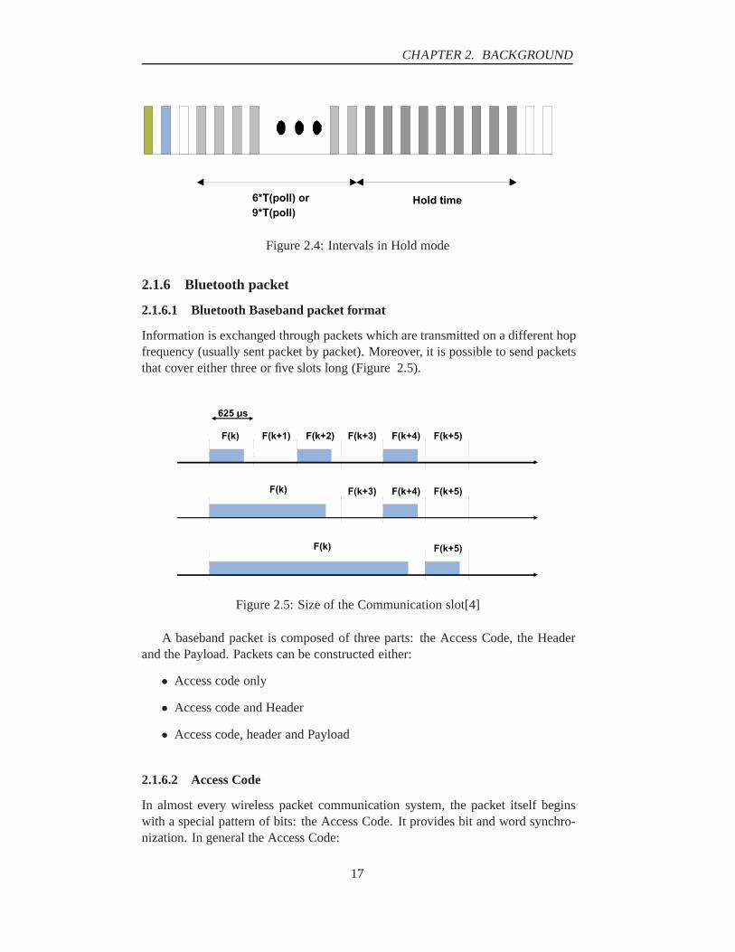
The Hold mode is a one-time exit from the obligation of a piconet and it canbe used when no data needs to be transmitted for long time intervals (up to 41swithout re-synchronization)[4]. An internal timer determines when the unit will bereactivated. In this mode, a slave does not receive any asynchronous packets (ACLpackets are suspended) and only listens to determine if it should become activeagain. It does not affect SCO traffic. In the Hold mode (“hold timeout”) the slavecan do other things like scanning, paging, inquiring, or attending another piconet.During this mode the Device is still considered an active member of the piconet.Thus, it remains synchronized with the master (Figure 2.4). Hold mode cannotbegin until 6 ∗ Tpoll intervals after the hold request packet has been sent (9 ∗ Tpoll
if the parameters must be negotiated). Tpoll is a poll interval that is negotiated be-tween the master and the slave. Tpoll = 40 slots [30].
16
CHAPTER 2. BACKGROUND
Hold time6*T(poll) or 9*T(poll)
Figure 2.4: Intervals in Hold mode
2.1.6 Bluetooth packet
2.1.6.1 Bluetooth Baseband packet format
Information is exchanged through packets which are transmitted on a different hopfrequency (usually sent packet by packet). Moreover, it is possible to send packetsthat cover either three or five slots long (Figure 2.5).
625 us
F(k) F(k+1) F(k+2) F(k+3) F(k+4) F(k+5)
F(k) F(k+3) F(k+4) F(k+5)
F(k) F(k+5)
Figure 2.5: Size of the Communication slot[4]
A baseband packet is composed of three parts: the Access Code, the Headerand the Payload. Packets can be constructed either:
• Access code only
• Access code and Header
• Access code, header and Payload
2.1.6.2 Access Code
In almost every wireless packet communication system, the packet itself beginswith a special pattern of bits: the Access Code. It provides bit and word synchro-nization. In general the Access Code:
17

CHAPTER 2. BACKGROUND
68 (72)access code packet header payload
preambule sync. (trailer) AM adress type flow ARON SECN HEC
54 0-2745 bits
bits bits4 (4) 3 4 1 1 1 1
Figure 2.6: Packet description
• Can be used by a slave to resynchronize its clock to the clock of the piconet
• Provides bit and word synchronization
• Includes basic piconet identification information
The Access Code is derived from the 24 first least significant bits of the BD_ADDR.Thus, different Access Code are required depending on the context:
• Channel Access Code (CAC)
• Device Access Code (DAC)
• General Inquiry Access Code (GIAC)
• Dedicated Inquiry Access Code (DIAC)
Particularly the DAC is used by the master for Paging a specific Bluetooth Devicefor entry into its piconet. The master knows the paged Device’s BD_ADRR via anInquiry process and can assemble the correct DAC from this address.
2.1.6.3 Using the Access Code in Short Hopping Sequences
During the Inquiry and Paging processes, a prospective master tries to find (inquire)or connect (page) with a prospective slave. The time for a successful Inquiry orPage can be reduced significantly if the usual 79-channel frequencies are reducedto 32-channel frequencies. This is possible because the Access Code used forInquiry and Paging transmissions meets the Federal Communications Commission(FCC) rules for a hybrid Spread Spectrum system. This 32-channel frequenciescan be further divided into two parts.[8]
18

CHAPTER 2. BACKGROUND
2.2 Location techniques
This section sums up different location techniques used in wireless technologies.They can be divided into different groups according to the used technology and theaccuracy: Cell-Identification, Angle of Arrival, Triangulation, Time Difference ofArrival and Database Correlation. Discussion of their advantages and drawbacksin different environments and uses will be made at the end of this section.
2.2.1 Cell Identification
This technique just returns that the Device is in the coverage area of the AP whichit is bound to, as presented in Figure 2.7. The accuracy depends directly from thecoverage area of the AP. Thus, this is not an accurate mean of location. However,no calculation is needed. So it is easily implementable.
x,yDevice
Base Station
Figure 2.7: Cell Identification location method
2.2.2 Angle of Arrival
Two APs measure the arrival angle of the signal which is transmitted by a Device.The intersection area of the two lines determines the position of the Device.This isshown in Figure 2.8.The main drawback of this technique is that a line of sight is required. Furthermore,directional antennas are needed.
α2
Beacon 2
α1
Possible location of the device
Beacon 1
Figure 2.8: Angle of Arrival location method
19

CHAPTER 2. BACKGROUND
2.2.3 Triangulation methods
The following methods use triangulation methods (need at least 3 APs).
2.2.3.1 Signal strength
The Device measures the strength of the AP signal and sends it back to the AP:indeed, in Bluetooth frame there is a possibility to get the Ratio Signal StrengthIndicator (RSSI) calculated by the Device. Thus, because the power received isproportional to the distance between two Devices, when three APs get this in-formation, three circles can be obtained and the intersection of them defines theprobable location of the Device.This is presented in Figure 2.9.The main drawbacks are the need of at least three APs and preferably an envi-ronment with LoS, otherwise a variation of 30-40 dB can appear in the measures.
d1
d2
d3
Confidence Ellipse
Figure 2.9: Signal strengh (triangulation method)
2.2.3.2 Uplink Time of Arrival
ToA (Time of Arrival):APs measure the time for the signal to arrive from the Device. Because this mea-surement is directly related to the distance between the two stations, triangulationmethod can be used. Hyperbolas are obtained and their intersections give the loca-tion of the Device, as illustrated in Figure 2.10.
TDoA (Timing Differences technique):If stations are not synchronised, TDoA is used to determine the (relative) time ofarrival between the 2 stations. The main drawback is that this method needs 3 APs.
2.2.3.3 Downlink Observed Difference
Downlink Observed Difference is a Timing Differences technique. Measurementsare made by the Device, which measures the time difference of the signals from
20

CHAPTER 2. BACKGROUND
Difference 2-3
Difference 1-3
Difference 2-3
Clock Time 1
Clock Time 3
Clock Time 2
BTS1
BTS1
BTS3
Figure 2.10: Uplink Time (Difference) of Arrival Location Method
several APs. Synchronization is needed between the Device and the APs. Theaccuracy also depends on LoS, multipath, etc. (Figure 2.11).
Difference 2-3
Difference 1-3
Difference 2-3
Clock Time 1
Clock Time 3
Clock Time 2
BTS1
BTS1
BTS3
Figure 2.11: Downlink Observe Difference Location Method
2.2.4 Database Support
The two following techniques use information on location stored in a database.
2.2.4.1 Database Correlation
Information samples, called fingerprints, are taken from the areas covered by theAPs: it can be signal strength or time delay. When the Device measures one ofthese parameters, it sends the measurements to a database server which comparesthis data with the data stored in a database (Figure 2.12).
21

CHAPTER 2. BACKGROUND
GSM/GPRS/UMTS
Network + Internet
Mobile terminal
Location server- system information
- Calibration data
- Digital maps
Location estimation by using signal fingerprint and database
BTS
Location estimate
Application servers
Location estimate
Received signal fingerprint
Figure 2.12: Database Correlation
2.2.4.2 Location Pattern Matching
This technique compares the results obtained by measurements taken from a De-vice with some pre-trained sequences, simulated with some algorithms, on a server.These two techniques cannot be used in dynamic networks.(Figure 2.13)
handset or vehicle
Carriers antennas receive signal and forward it to the carriers switch
1
2
Sophisticated gear analyses the acoustic characteristics of the signal, compares it to previously acquired patterns, and determines the callers location
3
4
2
2Switch forwards voice calland location data to a server
Figure 2.13: Location Pattern Matching
2.2.5 Discussion on the different location techniques
For each case, different number of Devices and Access Point have been chosen.Indeed some techniques cannot be used if the number of Devices increases or ifthe number of AP is not sufficient.
22

CHAPTER 2. BACKGROUND
1. Outdoor with LOSThe table 2.1 shows the cases where the different techniques can be useddepending on the number of Access Points, Devices and on two factors ofusage: outdoor and with line of sight (LoS).
1 Access Point 2 Access Points 3 Access Points
1 Device - Cell-ID - Cell-ID - Cell-ID- Database Correlation - Database Correlation - Database Correlation- Location Pattern Matching - Location Pattern Matching - Location Pattern Matching
- AoA - AoA- ToA- RSSI
2 Devices - Cell-ID - Cell-ID - Cell-ID- Database Correlation - Database Correlation - Database Correlation- Location Pattern Matching - Location Pattern Matching - Location Pattern Matching
- AoA - AoA- ToA- RSSI
7 Devices - Cell-ID - Cell-ID - Cell-ID- Database Correlation - Database Correlation - Database Correlation- Location Pattern Matching - Location Pattern Matching - Location Pattern Matching
- AoA - AoA- ToA UL (but problems)- ToA DL- RSSI
Table 2.1: Possible use of the locations techniques in an Outdoor with LOS case
2. Outdoor without LOSThe table 2.2 shows the cases where the different techniques can be useddepending on the number of Access Points, Devices and on two factors ofusage: outdoor and without line of sight (NoLoS).
3. Indoor with LOSThe table 2.3 shows the cases where the different techniques can be useddepending on the number of Access Points, Devices and on two factors ofusage: indoor and with line of sight (LoS).
4. Indoor without LOSThe table 2.4 shows the cases where the different techniques can be useddepending on the number of Access Points, Devices and on two factors ofusage: indoor and without line of sight (NoLoS):
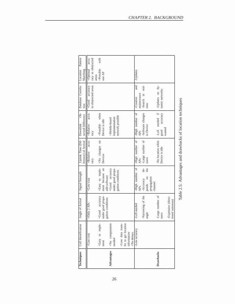
5. Advantages and drawbacks of location techniques (Table 2.5)
23

CHAPTER 2. BACKGROUND
1 Access Point 2 Access Points 3 Access Points
1 Device - Cell-ID - Cell-ID - Cell-ID- Database Correlation - Database Correlation - Database Correlation- Location Pattern Matching - Location Pattern Matching - Location Pattern Matching
- ToA- RSSI (but with less accuracy)
2 Devices - Cell-ID - Cell-ID - Cell-ID- Database Correlation - Database Correlation - Database Correlation- Location Pattern Matching - Location Pattern Matching - Location Pattern Matching
- ToA (but with less accuracy)- RSSI
7 Devices - Cell-ID - Cell-ID - Cell-ID- Database Correlation - Database Correlation - Database Correlation- Location Pattern Matching - Location Pattern Matching - Location Pattern Matching
- ToA UL (but problems)- ToA DL- RSSI (but with less accuracy)
Table 2.2: Possible use of the locations techniques in an Outdoor without LOS case
1 Access Point 2 Access Points 3 Access Points
1 Device - Cell-ID - Cell-ID - Cell-ID- Database Correlation - Database Correlation - Database Correlation- Location Pattern Matching - Location Pattern Matching - Location Pattern Matching
- AoA - AoA- ToA- RSSI
2 Devices - Cell-ID - Cell-ID - Cell-ID- Database Correlation - Database Correlation - Database Correlation- Location Pattern Matching - Location Pattern Matching - Location Pattern Matching
- AoA - AoA- ToA- RSSI
7 Devices - Cell-ID - Cell-ID - Cell-ID- Database Correlation - Database Correlation - Database Correlation- Location Pattern Matching - Location Pattern Matching - Location Pattern Matching
- GPS- AoA - AoA
- ToA UL (but problems)- ToA DL- RSSI
Table 2.3: Possible use of the locations techniques in an Indoor with LOS case
24

CHAPTER 2. BACKGROUND
1 Access Point 2 Access Points 3 Access Points
1 Device - Cell-ID - Cell-ID - Cell-ID- Database Correlation - Database Correlation - Database Correlation- Location Pattern Matching - Location Pattern Matching - Location Pattern Matching
- ToA UL (but problems)- ToA DL- RSSI (but with less accuracy)
2 Devices - Cell-ID - Cell-ID - Cell-ID- Database Correlation - Database Correlation - Database Correlation- Location Pattern Matching - Location Pattern Matching - Location Pattern Matching
- ToA UL (but problems)- ToA DL- RSSI (but with less accuracy)
7 Devices - Cell-ID - Cell-ID - Cell-ID- Database Correlation - Database Correlation - Database Correlation- Location Pattern Matching - Location Pattern Matching - Location Pattern Matching
- ToA UL (but problems)- ToA DL- RSSI (but with less accuracy)
Table 2.4: Possible use of the locations techniques in an Indoor without LOS
25
CHAPTER 2. BACKGROUND
Tec
hniq
ues
Cel
lIde
ntifi
catio
nA
ngle
ofA
rriv
alSi
gnal
Stre
ngth
Upl
ink
Tim
e(D
if-
fere
nce)
ofA
rriv
alD
ownl
ink
Ob-
serv
edD
iffe
renc
eD
atab
ase
Cor
rela
-tio
nL
ocat
ion
Patte
rnM
atch
ing
+L
ow-c
ost
+O
nly
2A
Ps+
Low
-cos
t+
Rel
ativ
eac
cu-
racy
+R
elat
ive
accu
-ra
cy+
Goo
dac
cura
cyin
obst
ruct
edar
eas
+O
ptim
alac
cu-
racy
inob
stru
cted
area
s+
Eas
yto
impl
e-m
ent
+G
ood
accu
racy
unde
rgo
odpr
opa-
gatio
nco
nditi
ons
+E
asy
toim
ple-
men
tbe
caus
eno
add-
soft
war
e
+N
och
ange
son
Dev
ices
+Po
ssib
lew
hen
Dev
ice
isid
le+
Poss
ible
with
one
AP
Adv
anta
ges
+N
oco
mpu
tatio
nne
eded
+G
ood
accu
racy
unde
rgo
odpr
opa-
gatio
nco
nditi
ons
+M
obile
-bas
edim
plem
enta
tion
netw
ork
poss
ible
+L
owda
tatr
ans-
fer
toge
tlo
catio
nin
form
atio
n+
No
dela
ys-L
owac
cura
cy-L
oSne
eded
-Hig
hnu
mbe
rof
APs
-Hig
hnu
mbe
rof
APs
-Hig
hnu
mbe
rof
APs
-Cre
atio
nan
dm
aint
enan
ce-U
pdat
es
-Nar
row
ing
ofth
ean
gle
-Acc
urac
yde
-pe
nds
onth
epr
opag
atio
nch
anne
l
-Lar
genu
mbe
rof
user
s-S
oftw
are
chan
ges
inD
evic
e-S
earc
hin
real
-tim
e
Dra
wba
cks
-Lar
genu
mbe
rof
user
s-N
olo
catio
nw
hile
Dev
ice
isid
le-L
oSne
eded
ifgo
odac
cura
cyw
ante
d
-Upd
ates
ondy
-na
mic
netw
orks
-Exp
ensi
ve(d
irec
-tio
nal
ante
nnas
) Tabl
e2.
5:A
dvan
tage
san
ddr
awba
cks
oflo
catio
nte
chni
ques
26

CHAPTER 2. BACKGROUND
Summary
Pros and cons of each technique have been studied. They are summarized below:
• Cell Identification: this technique is not enough accurate to enable a goodimplementation of handover
• Angle of Arrival: the main drawback of this technique is the need of Line ofSight which is not possible in real conditions
• Database support: this technique needs too much maintenance and updatesto be used with Bluetooth technology
• Triangulation methods: this technique seems to be the more appropriableone. Among the three location methods, the Signal Strength technique ap-pears to be more easy-implementable, adaptable and accurate in most casesthan the two others (Uplink time of Arrival and Downlink Observed Differ-ence). Moreover, RSSI measurements can be directly obtained from Blue-tooth packets
Thus, Signal Strength seems to be a good choice for location in Bluetooth. Be-sides, it is a well-documented technique [5] which has been already implementedto offer new ways of communicating by enabling end-users to obtain corporateinformation wherever they are.
27

CHAPTER 2. BACKGROUND
2.3 Movement Prediction
2.3.1 Utility of movement prediction
Movement prediction allows to predict the future location of the users with a certainaccuracy. Then it will be easier to anticipate handover situation and consequentlysave time and/or power resources. By tracking the Device, it is surely possible to
++
+
+
+
T-4T-3
T-2
T-1
T
T+1?
Periodical positions of the device
Access Point 1
Access Point 3
Access Point 2
Predicted point
Figure 2.14: Principle of movement prediction
predict in which cell it is going to move and warn only the concerned Access Point.Moreover, according to its velocity, it is possible to predict when it will enter thecell (Figure 2.14). Thus, the handover procedure which is quite long could be time-reduced.
It is assumed that:
• Users move with a certain degree of regular (random) movements.
• Users carry with themselves movement history from both past and present.
• It is possible to gather and use this movement history (recent and past) topredict future movement.
2.3.2 The predictive techniques
To determine the movement of a user, the techniques of location prediction aremainly based on a mobility model (Figure 2.15).
28

CHAPTER 2. BACKGROUND
Arbitrary movements without constraints
Predefined movement path or real mobility trace
Movement bounded by environmental constraints
random model deterministic model
mobility model
hybrid model
Figure 2.15: Predictive techniques
Most simulations are based on random mobility models, but these ones are insuf-ficient to reflect the environmental constraints. Moreover deterministic models aretoo complex and real user traces are hard to obtain. Thus, hybrid mobility modelscombine both of the two and make tradeoffs between simplicity and reality. In ourcase, we will use the hybrid model [35].
There are three main techniques for movement prediction:
• storage of the historical movement pattern in a database and comparisonbetween the recent states and the movement tracks
• comparison with a table of possible locations and the probability that theuser is located in there in a determined period of time
2.3.3 Different methods for location prediction
Different methods for location prediction are based on historical data. A method totrack the Device in a cell is to periodically locate it in the cell (Figure 2.14). Then,with at least one precedent position it is possible to predict where the next pointcould be. Obviously, the more previous positions taken into account, the better theprediction. Therefore this information has to be collected over a sufficiently longperiod of time to reflect user behavior (Figure 2.16).
2.3.3.1 Movement prediction using Location criterion and Direction crite-rion
With a Full Meshed NetworksIn a full meshed network, each Access Point is directly linked with all the neigh-bors, even if the handover between two of them is not possible (because of walls,machines,etc.) (Figure 2.17). In this case the link is useless.
With an Arbitrary NetworkIn this example (Figure 2.18), the Device cannot move from AP1 to AP3 or to
29

CHAPTER 2. BACKGROUND
+
+ +
+
+
+
T-3
T-2 T-1
T
T+1
T+1
By taking into account at least twoprevious positions it is possible toknow that the device is turning.By taking into account only thepositions T and T-1 you cannot.
Figure 2.16: Accuracy of the prediction
AP
AP
AP
AP
AP
AP
AP
AP
AP
AP
AP
AP
N = 2 N = 12 N = 30
AP
N: Number of possible handovers
Possible moves
Figure 2.17: Possible links between APs within a Full Meshed Networks
30

CHAPTER 2. BACKGROUND
AP4 because of the wall. These links are consequently useless.
AP 2
AP 3
AP 1
AP 4
Figure 2.18: Possible links between APs within an Arbitrary Network
Moreover, the probability that the Device goes from AP2 to AP4 (and conversely)is less important than the probability it moves from AP2 to AP3 or from AP3 toAP4 (and conversely).
These factors could be taken into account to optimize the handover process.
Example with the previous case:It is now possible to develop criterions (Figure 2.20 and Figure 2.21).
AP 1 AP 2
AP 3AP 4
p=0
p=0
p=0
p=0.3
p=0.7
p=0.2
p=0 p=0.6
p=0.5
p=1 p=0.3
p=0.4
Figure 2.19: Example of probabilities that a Handover could occur using an Arbi-trary Network
In the location criterion, probabilities are calculated without using the precedentlocation, whereas in the direction criterion the previous location is used to establishthe probabilities of the most probable future locations.
31

CHAPTER 2. BACKGROUND
Present Location
AP1
AP3
AP4
30%
50%
20%
AP2
Figure 2.20: Location Criterion[15]
AP1
AP3
AP4
15%
80%
5%
AP2AP4
Direction oftravel
Figure 2.21: Direction Criterion[15]
2.4 Conclusions
For the purpose of our project, a Bluetooth Device must be located and forecastin its motion in the most accurate way. Within this context, we have been throughthe possible techniques and have chosen the most appropriate one according tosome assumed operational constraints. Thus, we have chosen the triangulationmethod as the location technique, and particularly Signal Strength based on RSSImeasurements. As motion prediction, the hybrid one has been chosen. Our methodfor location and movement prediction will be inspired on historical data.The following chapters will now deal with the analysis and the implementation ofthose methods into details.
32

Chapter 3
Theoretical analysis
This chapter gives a detailed explanation right from the location process of theDevice to the Handover procedure encountered by the mobile Device. Using theconcepts of RSSI values and probabilities, location of the mobile Device is esti-mated. Future movement of the Device is predicted using this location informationproperly. Finally this will help the handover procedure to be implemented.
3.1 Probability Issues in Location
3.1.1 Definitions
3.1.1.1 Triangulation and Probabilities
Our choice of location technique is the triangulation using Ratio Signal StrengthIndicator (RSSI) measurements. As seen, it is the most adapted to Bluetooth. Theprinciple of the triangulation with power measurements looks very simple. A mov-ing Device is receiving a signal from three APs. Power of the signal is evaluatedand sent back to the APs. From this power W , each AP deduces the distance dof the device based on a propagation model. By drawing circles of radius d, it ispossible to find the position M(x, y) of a device at the intersection point of thecircles.
W1,2,3 ⇒ d1, d2, d3 ⇒ M(x, y) (3.1)
Practically it is not simple. Indeed, each power measurement will not correspondto only one distance but to a probability density function (PDF) of the distance:fD(d|RSSI = W ).In fact by measurements at a fixed distance, it is noticed that the power measure-ment is not constant [7]: it moves around a center value. Then, with three AP, thePDF of the location fX,Y (x, y|RSSI = W ) is deduced with (X,Y) as the coordi-nates of the Device.
W ⇒ fD(d|RSSI = W ) ⇒ fX,Y (x, y|RSSI = W )) (3.2)
The following sections focuses on the parameters and the functions that have to bedefined to solve the problem properly and rigorously.
33
CHAPTER 3. THEORETICAL ANALYSIS
3.1.1.2 Definition of The Parameters
D: this is the random variable of the distance between the considered AP and themoving Device. Its unit is the meter.
Ω(D): this is the set of all the possible distances that can be observed. If the APsare in a 20-meter large and 20-meter long square room, the distance is limited bythe walls. In the project, the used distances are equal to the length of the projectionon the floor. So in this case: Ω(D) = [0, dMax] and dMax = 20
√2
RSSI: this is the random variable of RSSI measurements.
Ω(RSSI): this is the set of all the possible RSSI measurements that can be ob-served. The Device has a lower limit under which it is not possible to collect anyvalue. It also has an upper limit. Here Ω(RSSI) = [−85, 0[ in dB.
t: this variable represents the elapsed time during the movement of the Device.It is a relevant factor because the aim is to track a moving Device. It means thatdifferent probabilities have to be considered at different times. ’t’ can be put as anindex on each random variable.
3.1.1.3 Probability Density Functions
In this part, all the PDF that will be used in the further steps of this work are de-fined: Location, Movement Prediction and Handover. Also, their relationship withthe problem and the meaning of each variable will be given. The order in whichthese PDFs are presented is the order that has to be used to solve the problem.
At a fixed distance dfRSSI(W |D = d) (3.3)
This is the PDF of the RSSI measurement given that the distance is equal to d. Itis the only PDF that can be built by measurements. Indeed, by making thousandsof measurements at the distance d, a distribution of RSSI measurements at this dis-tance is got. Then this distribution is put into a PDF. This has been done in [7].Yet the parameter t is not taken into account in the measurement. Indeed by mea-surement, a function that is correct at any time is built. So:
fRSSIt(Wt|Dt = dt) = fRSSI(W |D = d) (3.4)
At fixed RSSI measurement
fD(d|RSSI = W ) (3.5)
This is the PDF of the distance knowing the RSSI measurement. This PDF willdirectly be used to locate the Device. In fact, each time an AP get a RSSI measure-ment, this function expresses the probability of the distance between the AP and
34

CHAPTER 3. THEORETICAL ANALYSIS
the Device. However, it is not possible to build it because it is impossible to fix theparameter RSSI and observe the distance. So this function has to be calculatedthrough other parameters using especially fRSSI(W |D = d).
PDF of both RSSI measurement and distance
fD,RSSI(d,W ) (3.6)
This PDF has two variables. In practice one of the two parameters has to be fixedto observe the other one.
PDF of the distancefD(d) (3.7)
This is the PDF of the distance considering all the possible RSSI measurements.According to the theory of probabilities [33], its definition is:
fD(d) =∫
Ω(RSSI)fD,RSSI(d,W ) d W (3.8)
PDF of the RSSI measurement
fRSSI(W ) (3.9)
This is the PDF of the RSSI measurement that can be obtained considering all thepossible distances. From the point of view of one AP, it corresponds to the proba-bility distribution of the RSSI measurements that can be obtained. The definitionis :
fRSSI(W ) =∫
Ω(D)fD,RSSI(d,W ) d d (3.10)
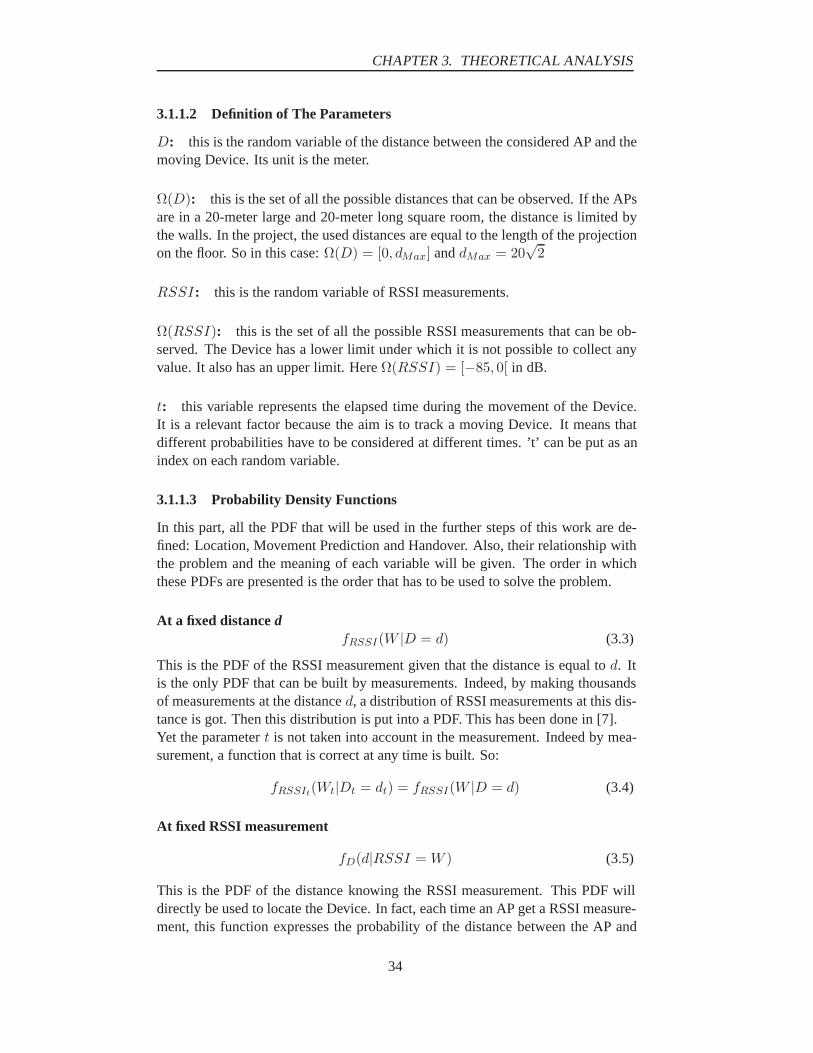
3.1.2 Algorithm of the Localization
The localization is performed in two steps. First, it consists in deducing the PDF ofthe distance between the Device and the AP for each AP. Then Triangulation mustbe performed with these PDF of the distance. The result is a PDF of the location.
3.1.2.1 PDF of the distance between the Device and the AP
As presented previously, only fD(d|RSSI = W ) is interesting for the location.Indeed, what is got from the AP is the RSSI measurement which is used to know theprobability of the distance. Then with three Access Points it is possible to performtriangulation. Now the question is: how can fD(d|RSSI = W ) be computed?The theory of the probabilities states that for a problem with two random variables,the formula is:
fD,RSSI(d,W ) = fD(d|RSSI = W ) × fRSSI(W ) (3.11)
35

CHAPTER 3. THEORETICAL ANALYSIS
Thereafter:fD,RSSI(d,W ) = fRSSI(W,D = d) × fD(d) (3.12)
So it is deduced:
fD(d|RSSI = W ) =fRSSI(W,D = d) × fD(d)
fRSSI(W )(3.13)
In this equation, fRSSI(W |D = d) is already known because it was determinedwith the initial measurements. The question now is: what about fRSSI and fD? Isit necessarily to know everything about them?First, it is noticed that fD(d|RSSI = W ) is a PDF of the distance d. So becauseit is a PDF it is stated that:∫
Ω(D)fD(d|RSSI = W ) d d = 1 (3.14)
As fRSSI is not a function of d :∫Ω(D) (fRSSI(W,D = d) × fD(d)) d d
fRSSI(W )= 1 (3.15)
So, eq (3.13) + eq (3.15) give:
fD(d|RSSI = W ) = fRSSI(W,D=d)×fD(d)Ω(D)
(fRSSI(W,D=d)×fD(d)) d d (3.16)
This means that there is no need to find fRSSI to calculate fD(d|RSSI = W ).Nevertheless, fD has to be known. Two possibilities could be considered :
• There is a priori no knowledge about the distance. That is why it is possibleto consider either that all the distances have the same probability or that allthe coordinates of the Device have the same probability (and it is not thesame at all). In this case:
fD(d) =1
DMax(3.17)
• There is a priori knowledge about the distance. In this case, there is nouniform probability distribution: there are only areas where the Device hasmore chances to be. It corresponds to a case in which time is taken intoaccount, and where fD can be built from fDT−∆t
.It means that the functionF∆t is such as
fDt = F∆t(fDt−∆t(dt−∆t|Wt−∆t)) (3.18)
This function F could be built after having mentioned the Human Movementmodel.
36

CHAPTER 3. THEORETICAL ANALYSIS
3.1.2.2 Triangulation: build a PDF of the location
As the Triangulation method is used in a location process, three RSSI measure-ments have to be obtained. According to the mechanism described above, threePDF of the distance fD1,D2,D3(.|W ) are deduced from these measurements. Withthese three PDFs, the PDF of the location could be built. The definition is:
• M(X,Y ) is a location. (X,Y ) are the coordinates in the Cartesian coordi-nates system (0, x, y)
• Ω(M) is the set of all the possible locations
• fM (X,Y |RSSI = W1,W2,W3) is the PDF of the location at a time tknowing the three RSSI measurements of the three APs: W1, W2 and W3
• build fM(X,Y |RSSI = W1,W2,W3). The explanation of how this func-tion will be built are described right after.
Simple example considering only two APs : AP1 and AP2.
> P1(d) is the probability that the distance between the AP1 and the Device isd
> P2(d) is the probability that the distance between the AP2 and the Device isd
The distance between AP1 and AP2 is supposed to be 10 meters and the probabilitydistribution is:
> P1(1) = 0.8 and P1(8) = 0.2
> P2(3) = 0.4 and P2(5) = 0.6
The “circles of probabilities” are drawn in Figure 3.1.
A
B
C
D
P1=0,2
d=8m
P1=0,6
P1=0,4
P1=0,8
d=1m
d=5m
d=3m
AP2 AP2
Figure 3.1: Circles of probabilities
37

CHAPTER 3. THEORETICAL ANALYSIS
There are four intersection points. To find the probability of each intersection point,the probabilities of two crossing circles have to be multiplied and then normalizedwith PA + PB + PC + PD = 1. Consequently:
> PA = PD = 0.2×0.60.4 = 0.3
> PB = PC = 0.2×0.40.4 = 0.2
The division by 0.4 is used for the normalization.
The PDF of the location is built in the same way. The first calculated functionis:
∀M(X,Y ) ∈ Ω(M)
gM (X,Y |RSSI = W1,W2,W3) =3∏
i=1
fD(di|RSSI = Wi) (3.19)
di =√
(Xi − X)2 + (Yi − Y )2 (3.20)
where di is the distance between the APi and the Device. After normalization itgives:
fM (X,Y |RSSI = W1,W2,W3) = gM (X,Y |RSSI=W1,W2,W3)Ω(M)
gM (X,Y |RSSI=W1,W2,W3) dX dY
(3.21)
3.1.3 Summary of the Localization algorithm
3.1.3.1 Static Localization
The bloc “Power to distance” uses the formula 3.16 with either the assumptions ofthe formula 3.17 or of the formula 3.18.
3.1.3.2 Dynamic Localization
If a notion of time is introduced in the localization process, this one becomes morecomplex. The table 3.1 summarizes its different steps. In each column (at eachmeasurement time), is measured or calculated the function or the parameter of eachcell. The different steps that are calculated at the time t are stated in this order:
1. The RSSI is measured
2. The PDF of the distance knowing the RSSI measurement is calculated. Thisfunction is the most relevant concerning the distance
3. With the three PDFs of the distance knowing the RSSI measurement, thePDF of the location knowing the RSSI measurements is found
38
CHAPTER 3. THEORETICAL ANALYSIS
fD1(.|RSSI1) fD2(.|RSSI2) fD3(.|RSSI3)
Power todistance
Power todistance
Power todistance
Triangulation
W1 W2 W3
fM (.|RSSI1, RSSI2, RSSI3)
AP1(X1, Y1)
AP3(X3, Y3)
AP2(X2, Y2)
fD1
fD2
fD3
Figure 3.2: Localization algorithm
39

CHAPTER 3. THEORETICAL ANALYSIS
It is noticeable that for fDt0(d|RSSI = Wi), there is no previous fD(d|RSSI =
Wi) where T < t0. Thus it is not possible to compute any fDt0. A function that
does not depend on time fD as to be used. It can be chosen at the point where allthe distances have the same probabilities because there is a priori no knowledgeabout the position.
Time APi PDF of d PDF of d knowing Wi PDF of M knowing Wi
t0 Wt0 fD fDt0(dt0 |RSSIt0 =
Wt0,i
fMt0(dt0 |RSSIt0 =
W1,2,3,t0 )
t1 = t0 + ∆t1 Wt1,ifDt1
= F∆t1 (fDt0(dt0 |RSSIt0 = Wt0,i
)) fDt1(dt1 |RSSIt1 =
Wi)
fMt1(d|RSSIt0 =
W1,2,3,t1 )
t2 = t1 + ∆t2 Wt2,ifDt2
= F∆t2 (fDt0(dt1 |RSSIt1 = Wt1,i
)) fDt2(dt2 |RSSIt2 =
Wi)
fMt2(d|RSSIt0 =
W1,2,3,t2 )
Table 3.1: Summary of the different steps of our Location process
40

CHAPTER 3. THEORETICAL ANALYSIS
3.2 Propagation aspects
3.2.1 Theoretical Propagation
The following assumptions are made in order to simplify the problem
1. APs are placed on the ceiling
2. The Device is moving in a specific trajectory in the xy-plane at the table-height (approx. 1m)
3. Reflections from walls and ground are considered. They are neglected fromthe ceiling.
4. Only single perfect reflections are considered
5. Antennas are Omni directional
3.2.2 Propagation
3.2.2.1 Free Space Propagation
In free space propagation, the electric field in the xy-plane is considered only fordirect rays. For the three APs in the room, the general expression of the electricfield in free space propagation is
Ed(r, t) = Em(r)ei(kx+ωt) (3.22)
where
k = wave number = 2πλ
λ = wavelength : cf
ω = 2πf : angular frequency
r: distance between AP and Device
t: time
f = 2400MHz: Bluetooth frequency
In equation (3.22), Em(r) represents the free space path loss and the exponentialterm stands for the sinusoidal dependency with distance and time. Em(r) is givenby:
Em(r) =1r
√Z0PT GT
2π(3.23)
where GT is the gain of the transmitter, Z0 is the impedance in the air and PT isthe power transmitted by the antenna. The relation between the electric field andthe power in function of the distance is given by
P (x) =|E(r, t)|2
2Z0Aeff (3.24)
41

CHAPTER 3. THEORETICAL ANALYSIS
whereAeff= effective aperture of Device antenna
Aeff =λ2
4πGR (3.25)
where GR is the gain of the receiving antenna.Thus, in free space propagation, the final expression for the received power re-ceived in dB is given by
PdB(r) = 10 log(PT GT GR) + 20 log(λ
4πx) (3.26)
This equation does not include any expression for reflections. In fact it is only fordirect ray.
3.2.2.2 Propagation with AP1, AP2, AP3
The three APs (AP1,AP2,AP3) are placed against the ceiling of a room. Fromtheir locations, reflections from floor (rF ) and from the opposite walls (rW ) areconsidered. This assumption leads to the following expression of the electric field:
E(x, t) = Ed(r, t) + [EF (rF ) + EW (rW )] (3.27)
whereEd(r, t) = electric field for direct rayEF = electric field after reflections from floorEW = electric field after reflection from walls
Reflection coefficients: The reflections are considered as perfect. It means thatthe reflections coefficients ΓF and ΓW are equal to e−jπ.
E(x, t) = Em1rej(kr−wt) −
∑α=F,W
Em1rα
ej(krα−ωt) (3.28)
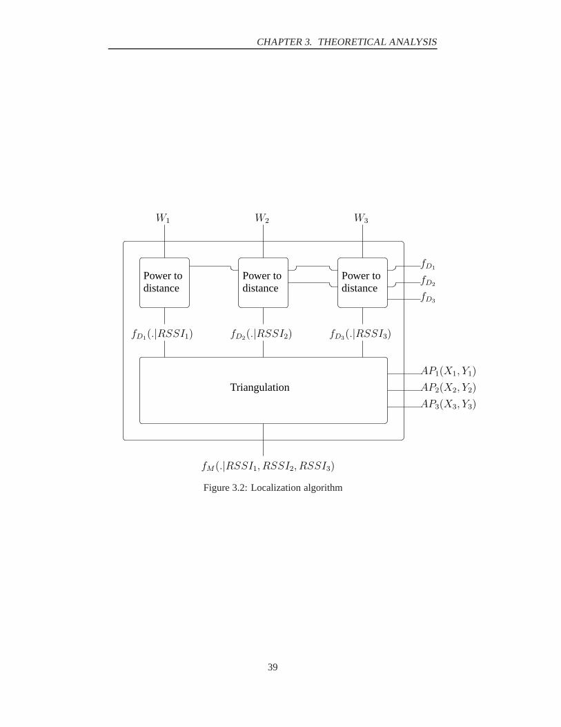
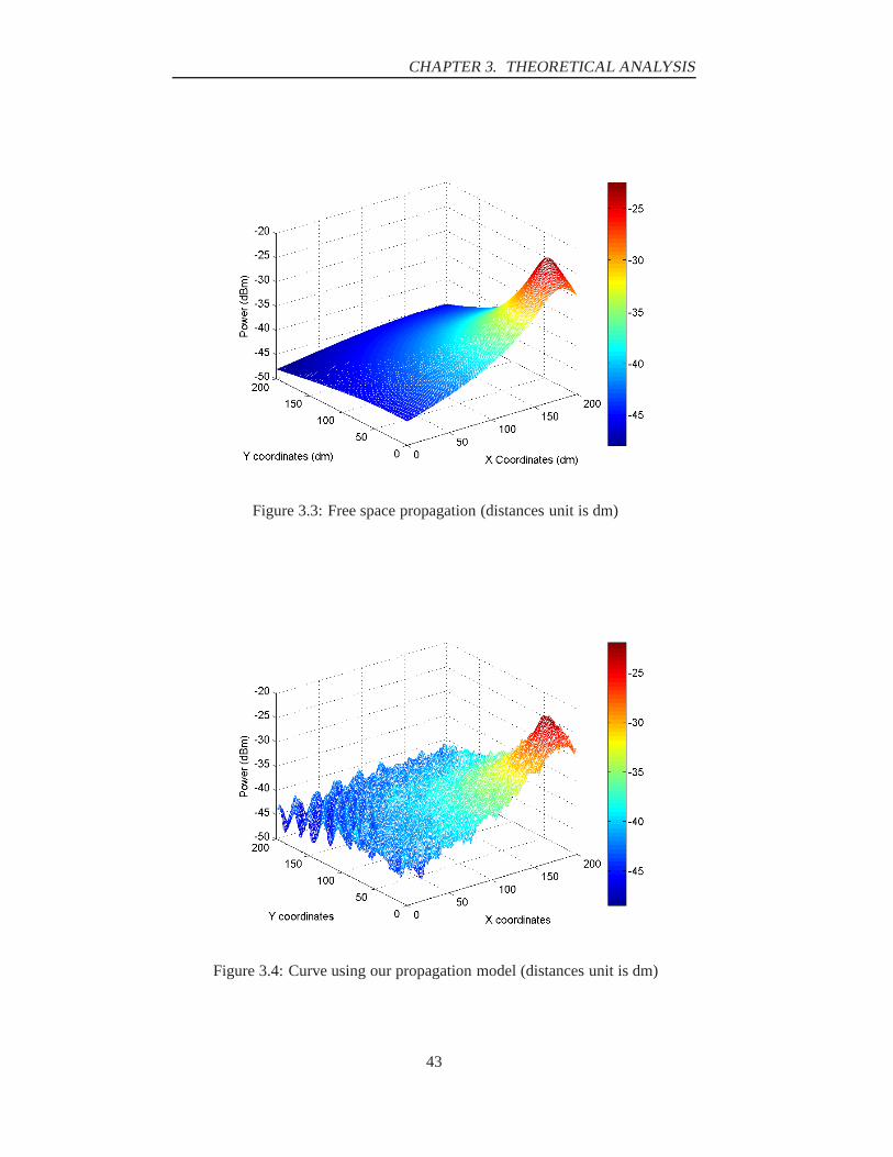
3.2.2.3 Simulation of the propagation model
There is a comparison between a low passed curve of the propagation model thattakes into account all the reflections against the walls (Figure 3.4) in a room of 20mby 20m and the free space model (Figure 3.3). The coordinates of the AP for thisexample are ( X=18.0 , Y=2.0 ).
Explanation of the low passed curve: As there is a lot of fast fading (Figure 3.3)we take a mean curve that is more readable as in the Figure 3.4. This mean curveis built by taking for each point the mean of the neighboring values as presentedin the Figure 3.5. The mean value is constructed by taking a square which is 1.1meters length. The wavelength in Bluetooth is equal to about 0.125 meter. Thus,the square is about 10 times longer than the wavelength. This fulfills the conditionsexposed in [34].
42
CHAPTER 3. THEORETICAL ANALYSIS
Figure 3.3: Free space propagation (distances unit is dm)
Figure 3.4: Curve using our propagation model (distances unit is dm)
43

CHAPTER 3. THEORETICAL ANALYSIS
0,5
met
er
0,5 meterThe value of this point is equal to the sum of all the values of the neighbouring points that are distant from the considered point from less than half a meter, divided by the number of these points.
Figure 3.5: Construction of the mean curve
3.3 Movement Prediction
The previous parts only focus on static aspects. From this point, movement is in-troduced. Because the project mainly deals with handover, location is performedon a moving Device. Movement is a capital factor. By estimating how a Devicehas moved, it could be possible to improve the performed location. By predictingthe future movement, it could also be possible to make the Handover easier.
First, a simple intuitive Human movement model is built. This model is basedon fundamental parameters that describe the movement. In this part is explainedhow to get these fundamental parameters from the previous movement. Then, ourmethod to estimate or to predict the position and the distance from an AP withthese parameters is explained.
3.3.1 Human movement model
3.3.1.1 Parameters to model the movement
The movement can be modeled with only two parameters. These two parametersare chosen as:
• the instant speed s = |s|• the instant direction Θ = arg(s)
The aim now is to model these two parameters. The first assumption is that thereis no correlation between them. An independent model can be built for these twoparameters.
3.3.1.2 Speed Parameter
Assumption When an individual is mobile, he is mainly moving with a charac-teristic speed. Our intuition is that when somebody is walking in a place without
44

CHAPTER 3. THEORETICAL ANALYSIS
any obstacle, he moves with a certain speed: his characteristic speed.
Description of the model
Our model of speed is a stochastic process that is stationary, but not ergodic. Itmeans that the statistic of the values collected across the ensemble of speed at anyinstant is different from the statistic of the values collected on one sample. To beclear, this assumption needs further explanations.
At a fixed time, is considered an infinity of people moving according to themodel. gS is the function of the statistic representing all the speeds s. gS(s) isthe frequency of apparition of the speed s.
For a moving body i, we consider all the speeds it can have during an infinitelylong period of time. fSi is the function of the statistic representing all the speeds sit has during this period. fSi(s) is the frequency of apparition of the speed s.
The stochastic process speed is not ergodic because fSi and gS are not necessar-ily equals. We dwell on this fact since it is important to consider that each personmoves according to personal movement settings. In addition, the whole stochasticprocess will be mathematically described by these two functions fSi and gS . Theprinciple is illustrated in figure 3.6.
samples(i)
time(t)
s3(t)
s2(t)
s1(t)
statistic across the samples
acrosst on onesample
statistic
Figure 3.6: Description of the stochastic process of the speed
Mathematical description of the model:
45

CHAPTER 3. THEORETICAL ANALYSIS
⇒ The statistic gS of the values collected across the ensemble of speed at anyinstant gives the distribution assumed on the figure 3.7: a gaussian centeredon the speed 1m/s with a variance equal to 0,5m/s :
for s < 0:gS(s) = 0
for s > 0:
gS(s) =e(− (1−s)2
2×0.52)
∫∞0 e
(− (1−s)2
2×0.52)
(3.29)
0 0.5 1 1.5 2 2.5 30
0.002
0.004
0.006
0.008
0.01
0.012
0.014
0.016
0.018
speed (m/s)
prob
abili
ty
Figure 3.7: PDF of the speed of all the moving bodies
⇒ The statistic fSi of a given sample function Si is equal to a gaussian centeredin the characteristic speed schar
i of the moving body with a standard deviationof 0.1m/s:
fSi(s) =1
2π × 0.5e(− (schar
i −s)2
2×0.52)
(3.30)
An example is proposed with the Figure 3.8 where schar = 1.2m/s:
3.3.1.3 Direction Parameter
Assumption It is considered in our model that humans go straight to their goal.If it is assumed that there is no obstacle, it means that the instant direction will not
46

CHAPTER 3. THEORETICAL ANALYSIS
0 0.4 0.8 Schar=1.2 1.6 2 2.40
0.05
0.1
0.15
0.2
0.25
0.3
0.35
0.4
0.45
0.5
speed (m/s)
prob
abili
ty
Figure 3.8: Example of PDF of the speed of one precise moving body
change a lot and will move around a centered value which is called the character-istic direction.
Description of the model
Our model of the direction is similar to the model of speed. It is also a stochasticprocess that is stationary but not ergodic.
Mathematical description of the stochastic process:
⇒ Statistics gΘ of the values collected across the ensemble of directions at anyinstant gives a PDF with a uniform distribution for all the directions as pre-sented in figure 3.9.for θ < −180 and θ > 180:
gΘ(θ) = 0
for −180 < θ < 180gΘ(θ) =
1360
(3.31)
⇒ The statistic of a given sample function fθiis equal to a gaussian centered in
the general direction of the moving body θchari and with a standard deviation
of 30:
fΘi(θ) =1
2π × 30e(− (θchar
i −θ)2
2×302)
(3.32)
An example is proposed with the Figure 3.10 where θchar = 45.
47

CHAPTER 3. THEORETICAL ANALYSIS
−180° −90° 0° 90° 180°
1/720
1/360
direction (degrees)
prob
abili
ty
Figure 3.9: PDF of the direction of all the moving bodies
−180° −135° −90° −45° 0° 45° 90° 135° 180°0
0.05
0.1
0.15
0.2
0.25
0.3
0.35
direction (degrees)
prob
abili
ty
Figure 3.10: PDF of the direction for one precise moving body
48

CHAPTER 3. THEORETICAL ANALYSIS
3.3.2 Parameter Estimation
Our location system enables to get PDFs of the location at the present location timet and also at the last measurement time t−∆tp. The aim is to predict a PDF of thelocation at time t + ∆t from the two last performed locations and using our modelof human movement. The ∆t parameter can be chosen. It means that it is possibleto choose when a prediction must be perform.
Information from the past: The two last locations are considered. The Deviceis at the point Mt−∆tp at time t−∆tp and at the point Mt at time t. Since there aredifferent locations at different times, the speed is not known continuously. Velocityvectors representing the mean of the speed between the two last locations are theonly available factors. The speed and the direction of the mobile can be deducedfrom these vectors.
Statistic estimators: The prediction uses statistic estimators. It is consideredthat the speed of the mobile between t − ∆tp and t is close to the mean of theinstant speed i.e. the characteristic speed. So the estimation of the characteristicspeed is:
schar =−−−−−−−→Mt−∆tpMt
∆tp(3.33)
It is the same process for the estimation of the direction:
θchar = arg(−−−−−−−→Mt−∆tpMt) (3.34)
3.3.3 Position Prediction
A Device i is considered and now the aim is to determine a PDF of its location attime t + ∆t. The PDF of the speed fS and the PDF of the direction fΘ are usefulfor this work. There are two cases:
• less than two localization have been previously performed. The parametersΘchar and Schar cannot have been computed. So we take:
fΘ = gΘ (3.35)
fS = gS (3.36)
• more than two localizations have been previously performed. Consequently,the parameters Θchar and Schar can be deduced from the two last localiza-tions:
fΘ = fΘi (3.37)
fS = fSi (3.38)
49

CHAPTER 3. THEORETICAL ANALYSIS
The prediction of the PDF of the location at t+∆t is performed using the followingprocess:
∀Mt+∆t(Xt+∆t, Yt+∆t) ∈ Ω(M)
fMt+∆t(Xt+∆t, Yt+∆t) =
∏Mt∈Ω(M) fMt(Xt, Yt)
fΘ(σ)×fS (υ)Ω(M)
fΘ(σ)×fS (υ) dX dY
(3.39)
where σ = arg(−−−−−−→MtMt+∆t) and υ = MtMt+∆t
∆t
3.3.4 Estimation of the Distance from the Access Point
Since the location has already been predicted, it is useless to estimate the distance.However, it has been shown in the section 3.1 that fDt+∆t(dt+∆t) is estimatedfrom fDt(dt|RSSI). This prediction is useful at this point of the location algo-rithm. Our procedure is explained in this section.
The estimated PDF of the speed of the Device fS , the estimated PDF of the di-rection of the Device fΘ at time t and fDt(.|RSSI) are used to build this function.
The general formula is:
P(d∆t+t) =∑
s,dt∈Ω(D) pfΘ,s,dt(dt+∆t)fS(s)fDt(dt|RSSIt)δs.δdt
(3.40)where:
• P(d∆t+t) is a discrete probability distribution function of the estimated dis-tance between the Device and the considered AP at time t + ∆t. It is adiscrete Probability because a finite distance method is used for computingit. Indeed, there is no way to compute it with analytic methods.
• pfΘ,s,dt(dt+∆t) is the probability considering a fixed speed s and a fixed dis-tance from the AP at time t: dt. The index fΘ means that the calculation ofthis parameter includes the use of the knowledge about the direction. Any-way, since the computation of this parameter, considering the angle, needstoo much computation power, we computed it without taking into accountthe knowledge about the direction.
• fS(s) is the PDF of the speed that is used for this estimation. It can be eitheran estimation from a characteristic speed or the general distribution of thespeed. It depends on the history of the movement. We will further explainwhich one we chose.
• δs is the space between two considered speed values.
• fDt(dt|RSSI) is the PDF of the distance at the time t knowing the RSSImeasurement.
50

CHAPTER 3. THEORETICAL ANALYSIS
• δdt is the space between two considered distance values.
In the formula 3.40, the product δdt.δs corresponds to a little integration surface ofthe integration of the functions fS(s) and fDt(dt|RSSIt) weighted by the factorpfΘ,s,dt .
The details of the calculation of the factor pfΘ,s,dt are given in Appendix A.
51

CHAPTER 3. THEORETICAL ANALYSIS
3.4 Handover
Handover is a process of seamless connectivity in which a Device moves from oneAccess Point coverage area to another.
At first, the Inquiry and Paging process are detailed in order to have a better under-standing of our handover.
3.4.1 Establishing connection in Bluetooth network
During the establishment of a connection in Bluetooth network, the Access Pointand the Device can take different states [1].
Inquiry Used by an AP to discover the Bluetooth Device Address(BD_ADDR), the clock (CLK) and other information of the De-vice in range
Inquiry scan Used by a Device to listen for an InquiryPage Used by AP to establish a connection with a particular Device
whose BD_ADDR is knownPage scan Used by a Device to listen for its page
The connection between an AP and a Device can be established either by Inquiryand Paging when the Device details are unknown, or only by Paging when theBluetooth Device Address is already known by the AP.
3.4.2 Inquiry Procedure
This process occurs when the piconet has not been established. The AP is definedas the prospective Master and the Device as the prospective Slave.
The following steps sum up the Inquiry procedure [1]:
1. To discover a new Device in its range, the AP launches an Inquiry procedure.It transmits two Inquiry Access Code (IACs) on two consecutive hop fre-quencies from the 32-hop Inquiry sequence during an even-numbered timeslot. The AP listens on the two corresponding Inquiry response hop frequen-cies in sequence during the next odd-numbered slot.
2. Meanwhile, the Device listens for the IAC on one of the Inquiry hop fre-quencies for about 11 ms each time it enters INQUIRY SCAN state.
3. Upon hearing the IAC, the Device delays a random time. Then it listens forthe IAC on the same frequency again. After having received the second IACpacket, the Device transmits its FHS packet 625 µs later on the correspond-ing Inquiry response hop frequency.
4. The AP does not respond to the FHS packet, but stores it for future use ifneeded.
52

CHAPTER 3. THEORETICAL ANALYSIS
Thus, after the Inquiry, the AP knows the following information about the Devicethanks to the FHS packet:
• the Device address (BD_ADDR) which is unique for each Bluetooth Device.
• the Scan Repetition which is the time interval between two successive PageScan windows
• the Scan Period which is the time period in which the mandatory Page Scanmode will be used by the Device after it responds to an Inquiry.
• the clock of the Device (CLKN).
As noticed, the FHS packet contains the sender’s entire BD_ADRR and enoughbits of CLKN that can help the receiver to program a hop generator to follow thesender’s hopping from channel to channel.Thus, this information is sent to a “Handover Agent” (HA) which will transmitit to all the APs in our scenario: this process could speed up the page process asexplained in the next section.
3.4.3 Paging Procedure
After the Inquiry process, the next step to the connection of the Device to a piconetis the Paging process.The Paging procedure is used by the AP to establish a connection with the Device.For Paging, the AP has to know the BD_ADDR of the Device (it has been done inthe Inquiry process). In this process, the Device must be in PAGE state and the APin PAGE SCAN state.
The Paging procedure follows different steps as explained below [1].
1. The AP transmits two Devices DACs on two consecutive hop frequencies,f(k) and f(k+1) from the 32-hop page sequence during an even-numberedtime slot.
2. The AP listens on the two corresponding hop frequencies in sequence duringthe next odd-numbered time slot.
3. Meanwhile, the Device listens for its DAC on one of the page hop frequen-cies for about 11 ms each time it enters the PAGE SCAN state.
4. Upon hearing its DAC, the Device then transmits the same DAC 625µs lateron the corresponding page response hop frequency.
5. If the AP hears the DAC returned on the corresponding page response fre-quency then it sends its FHS packet to the Device.
6. Now the AP and the Device are connected as Master and Slave.
53

CHAPTER 3. THEORETICAL ANALYSIS
In our scenario, the Device information is known by all the APs. Thus, the Pageand Page response hop sequences are both derived from the Device’s BD_ADDR.However the hop phase has not yet been coordinated precisely, except for the AP’sestimate of the clock of the Device. It will be done with the FHS packet responseof the AP (step 5). Two cases may happen in the Paging process: either the Device
f(k) f(k+1) f’(k) f’(k+1)f(k+1)
t
t
t
t
DAC Page
DAC
FHS
DAC
625us
Device
Tx
Rx
Tx
Rx
POLL
NULL
Page and Page response hoping sequence Channel Hoping sequence
g(m) g(m+1)
AP
Figure 3.11: Packet Exchange in the Paging Process
receives the DAC packet in the first half of the even-numbered time slot or in thesecond half. The p-salve cannot know that. So, it considers the worst case (thesecond half of the time slot). Thus, after 312.5 µs, the Device is ready to listen tothe frequency f(k+1).
Overall, the Paging process, until a complete connection, lasts 4 timeslots (2.5ms) in the best case. If all the 32 frequencies have to be scanned by the AP, thepage can lasts 36 timeslots (22.5 ms).
3.4.4 The Paging timers
Several timers are defined to avoid infinite loops when a response is expected bythe AP or by the Device from the other one [1].
Page timeout (pageTO): it is the number of time slots that the PAGE state canlast before exiting if there is no response to the page. By default pageTO is set to5,12s. However it can be set to another value by the user.
Page response (pagerespTO):
• for the Device it is the time between the acknowledgment of the Page from
54

CHAPTER 3. THEORETICAL ANALYSIS
the Device and the FHS packet from the AP. It is set to 8 slots.
• for the AP it is the number of time slots it will wait for the Device to respondto the FHS packet. This Paging timer is also set to 8 slots.
New connection timeout (newconnectionTO): it is number of timeslots the APhas to wait for the Device to respond to the POLL packet. After expiration ofnewconnectionTO, the AP and the Device return respectively to PAGE and PAGESCAN states.
3.5 Conclusions
To estimate the future location of the Device and its movement, previous location,speed and direction are taken into account. Probabilities calculation are computedwith these parameters to determine the most probable location of the Device. Be-sides, a boundary will be defined for each AP. They limit the area covered by eachAP. When a boundary is crossed by the Device, the handover procedure is per-formed.
55

Chapter 4
Simulations
This chapter will cover the implementation details of the methods previously dis-cussed in the Theoretical Analysis. In order to achieve a realistic simulation, weneed to set up some “near real-life” conditions through a given scenario. Giventhese assumptions, the simulation will perform the actual sequential steps of ourmodel. In other words, how to get data from the Device, forecast its movementsand use both real and forecast information to achieve handover. At last but notleast, the different results obtained with the simulation and a comparative studywill be given.
4.1 Scenario
The proposed scenario consists in 3 APs in a single room and in a mobile devicemoving along a specified trajectory in the xy plan. For the sake of the scenario,some parameters have been defined. The room is 20 meters large and 20 meterslong. The height of the room is 2.3 meters. The Access Points are placed on theceiling of this room. They are linked by wire to a Handover Agent whose rolewill be defined in the Handover section (4.3.5). The Device is moving in a planeparallel to the ground at a height of 1m. The figure 4.1 represents the room in 3-D.However all calculations and movements will be considered in 2-D (in the plane ofthe Device). The place of the APs (in the figure they are placed in the corners) arearbitrary : this is just an example of a possible configuration of the room. They canbe put in other places on the ceiling.
4.2 Simulator Principle
Our simulations are split into five parts. The goal is to simulate the whole scenarioby taking into account fundamental parameters. Here are the different followedsteps:
+ Generation of RSSI measurements
+ Location of the Device
56

CHAPTER 4. SIMULATIONS
zy
x 0
AP3
AP2 AP1
Device
1m
20m
20m
2.3m
Figure 4.1: Possible configuration of the Room
+ Location of a moving Device
+ Movement Prediction
+ Handover
The principle of all these parts is explained in the section 4.3. They have been com-puted in the same order because each part needs the previous ones to be achieved.The Figures 4.2 and 4.3 summarizes all the performed simulations.
Different possible settings
Simulations
Figure 4.2: Simulation
4.3 Functionalities Breakdown
4.3.1 Generation of RSSI measurements
Location is based on RSSI measurements get from the three APs. These mea-surements have to be simulated properly in order to measure the performances ofthe Location, the Movement Prediction and the Handover processes. Two mainparameters have to be generated. First, the RSSI measurement of a Device at agiven position. Then, the delay between two RSSI measurements that correspondsexactly to the Inquiry process delay.
4.3.1.1 Generation of one RSSI measurement
It is the first step. The considerations in this part are limited to one AP and theDevice. The parameters taken into account to generate measurements are the re-
57

CHAPTER 4. SIMULATIONS
Generation of measurements
R S S I D e l a yb e t w e e n t w om e a s u r e m e n t so f R S S I
measurement
Device L o c a t i o no f a
fixed point
Location of a moving device
M o v e m e n t P r e d i c t i o n
H a n d o v e r
Free space measurements (distance dependant)
measurements taking into account the propagation model with reflections (position dependent)
Delay corresponding to the inquiry time (no dependance)
Fixed in one c o o r d i n a t e (X,Y)
Moving along a defined t r a j e c t o r y [X(t),Y(t)]
Location Performances in free space
Location performances in the propagation model with reflections
Performances with basic location
Performances taking into account the movement model
Reliability of the prediction
Location with adding
information about position
General Setings
Room of 20*20m
Localization in the horizontal plan
3 AP
Figure 4.3: Summary of all the simulations performed
58

CHAPTER 4. SIMULATIONS
spective positions of the AP and the Device. There are two different ways togenerate measurements:
⇒ With a free space propagation model. In this case, the received powerdepends only on the distance between the AP and the Device.
⇒ With a propagation model considering reflections (see Section 3.2). Inthis case, the received power depends on both places of the Device and theAP.
These two models give us the mean of the power the AP should receive fromthe Device at different places. According to the Master Thesis of Joao Figueiras[7], the power received by the AP when the Device is at a given place follows aGaussian centered in the mean power with a standard deviation of σ = 2.026. Any-way, we can represent the RSSI measure generation with the box in the Figure 4.4.
RSSIGeneration
device (x,y)AP(X,Y)
ω
Figure 4.4: RSSI generation simulator element
4.3.1.2 Generation of a Delay between two RSSI measurements
The RSSI measurements are not instantaneous. As the considered RSSI measure-ments are the measurements given after an Inquiry, there is a delay correspondingto this Inquiry time defined in Bluetooth Specifications [4]. This delay is generatedon the basis of Joao Figueira’s master thesis [7]. It means the delay is generatedrandomly, weighted by the PDF of the Inquiry time calculated for 1 AP consideredin [7]. The box in the Figure 4.5 represents the Delay generation.
4.3.1.3 Generation of measurements for a trajectory
The scenario is a Device following a precise trajectory in a room with three APs. Someasurements have to be generated for the three APs during the whole trajectory.As there are three APs inquiring at the same time, we are making the followingassumption: there is no influence between each AP for the Inquiry time. Be-cause only one packet is sent at the end of the Inquiry, it is reasonable to make this
59

CHAPTER 4. SIMULATIONS
Delay ∆t
Figure 4.5: Delay generation element
assumption. Thus, each AP can be considered the same way and a set of measure-ments can be done independently for each AP.
In order to explain the complete procedure of the generation of measurements,it is better to explain what a trajectory in our programs is.
A trajectory is considered as a set of points. Each point corresponds to a pre-cise point in time. The Figure 4.6 represents a trajectory.
Trajectoryt x(t),y(t)
Figure 4.6: Trajectory element
The Figure 4.7 explains how the measurements are generated for the whole trajec-tory.
The RSSI measurements can be represented on the three APs with the Figure 4.8.
Finally, it is noticeable that all APs can get measurements at really different times.One of the difficulties will be to locate a moving Device with RSSI measurementswhich do not correspond to the same location of the Device. Anyway, before goingfurther into these problems, we have to be able to localize a fixed Device.
4.3.2 Location of a fixed Device
The first step, after generating measurements, is to locate the Device at a fixedpoint. The first test appraises the validity of the location system built in this project(section 3.1). It also gives a visual impression of the mean behavior of the locationby averaging the obtained PDF of a great number of localizations. The other testsanalyse the performances for this location system by changing different parame-ters. The labels of the figures of the rooms are in meter.
60

CHAPTER 4. SIMULATIONS
Delay
Trajectory
t
RSSIGeneration
AP(X,Y)
(x(t),y(t))
Stop the loop
t>tmax
t<tmax
wt
New delay generated once the RSSI is generated
Enter the
loopAt t=0
Figure 4.7: Block of the RSSI measurement generation along a trajectory
AP1
AP2
AP3
t
t
t
= RSSI measurement
Figure 4.8: Representation of the RSSI measurement on a time axis per AP
61

CHAPTER 4. SIMULATIONS
4.3.2.1 Different Location of the Access Points
The table 4.1 gives the characteristic of proximity in our cases.
Device far from the AP Case 1 Case 2: worst caseDevice closer to the AP Case 3: best case Case 4
Table 4.1: Summing-up of the different cases
Case 1 The AP and the Device are at the following coordinates as in Figure 4.9:AP1 (2.0,18.0)AP2 (2.0,2.0)AP3 (18.0,18.0)Device (10.0,10.0)
−5 0 5 10 15 20 25−5
0
5
10
15
20
25
AP1
AP2
AP3
Device
X−axis
Y−
axis
Room
Figure 4.9: Room for the first case
Case 2 The AP and the Device are at the following coordinates as in Figure 4.10:AP1 (2.0,18.0)AP2 (2.0,2.0)AP3 (18.0,18.0)Device (18.0,2.0)
Case 3 The AP and the Device are at the following coordinates as in Figure 4.11:AP1 (7.5,12.5)AP2 (7.5,7.5)AP3 (12.5,7.5)Device (10.0,10.0)
62

CHAPTER 4. SIMULATIONS
−5 0 5 10 15 20 25−5
0
5
10
15
20
25
AP1
AP2
AP3
Device
X−axis
Y−
axis
Room
Figure 4.10: Room for the second case
−5 0 5 10 15 20 25−5
0
5
10
15
20
25
AP1
AP2 AP3
Device
X−axis
Y−
axis
Room
Figure 4.11: Room for the third case
63

CHAPTER 4. SIMULATIONS
Case 4 The AP and the Device are at the following coordinates as in Figure 4.12:AP1 (12.5,7.5)AP2 (12.5,2.5)AP3 (17.5,2.5)Device (18.0,7.5)
−5 0 5 10 15 20 25−5
0
5
10
15
20
25
AP1
AP2 AP3
Device
X−axis
Y−
axis
Room
Figure 4.12: Room for the forth case
4.3.2.2 General behavior of the program
The Figure 4.13 shows how the different parts of the simulator are put together toperform the localization of a fixed Device.
RSSIGeneration
RSSIGeneration
RSSIGeneration
AP1 AP2 AP3
W1
W2
W3
Localizationf
D1
fD2
fD3
fM
(. | RSSI1,2,3
)
Device (x,y)
AP1AP2AP3
Figure 4.13: Simulator for the localization of a fixed Device
It consists in computing the mean of the n PDFs of the location calculated for
64

CHAPTER 4. SIMULATIONS
n iterations. It uses the formula (3.16) to compute the PDF of the distance for eachAP and then, equation (3.21) to compute the PDF of the location. As it is a staticprocess, we do not have any former information about the location of the Device.Thus, the assumption of the equation (3.17) is made: the Device can be anywherein the room.
As the aim is to see the reliability of the program, the first set of tests are madeby generating measurements with the free space model. As indicators, we com-pute the following parameters on the obtained curves:
+ The coordinates of the maximum likelihood estimator in the final PDF ofthe location.
+ The distance between the maximum likelihood estimator and the real loca-tion: this parameter gives us obviously the reliability of the estimation ofthe location by the highest point of the density. The greater the distance theworse this estimation.
+ The MeanRadius: it is the radius of an area we assimilate to a circle. On thecurves of density, we calculate the area A where there are values greater thanthe half or the fifth of the maximum value. If we assimilate A to a circle, the
radius is√
Aπ . It is called the MeanRadius because it expresses the mean of
the distance between the point with the greatest value and the borders of theconsidered area. Then, this parameter helps us to have an idea on how farfrom the good location the result obtained could be.
+ The Half-beam area: it is the area where the values of the density are greaterthan the half of the maximum value.
+ The Probability Ratio of the highest point: it is the ratio of the value ofthe real position density to the maximum of the density. We have differentcases to interpret this value:
- If it is very close to 1, the estimation of the location by the highest pointis a good option.
- If it is more than 0.5, it means the half-beam area is a correct estimationof the location.
Results: Table 4.2
Case 1 The coordinates of the point calculated tend to be at a close distancefrom the original ones: in a radius of 0.84 meter. However the mean radius (halfbeam) computed is very large, around 4.3 meters: that means that the shape of thefinal PDF is very spread (Figure 4.14). It implies that the location program cannotlocalize very precisely with such a configuration.
65

CHAPTER 4. SIMULATIONS
case Number of measures Coordinate Max distance(m) Meanradius(m) probability ratioX Y
1 100 9.4 10.6 0.84835 4.32443 0.97632000 9.4 10.6 0.84835 4.15207 0.97875000 9.4 10.6 0.84835 4.11007 0.9781
2 100 15.6 3.8 3.0 4.70211 0.85952000 16.8 3.1 1.62788 4.54549 0.94245000 16.8 3.0 1.56205 4.50858 0.8595
3 100 9.9 9.5 0.50990 1.44833 0.95792000 9.8 9.8 0.28284 1.47014 0.97645000 9.8 9.8 0.28284 1.44943 0.9759
4 100 17.3 9.8 0.72801 3.40296 0.93372000 17.7 9.4 0.67082 2.79601 0.9373
Table 4.2: Summing up of the results obtained
Figure 4.14: PDF of the position estimation in the first case
66

CHAPTER 4. SIMULATIONS
Case 2 In this case, we can observe that the coordinates of the point calculatedtend to be quite far from the original ones: in a radius of 1.7 meters. This resultmeans that this case for location is a very bad one. This observation is confirmedby the fact that the mean radius (half power) computed is very large, around 4.5meters: the shape of the final PDF, like in the first case, is very spread. Thus, thiscase is the worst case for location: indeed, the Access Points are very far from theDevice and this latter is near from the borders. Besides, the shape is as spread as inthe first case: this means the borders have just a little effect on the calculated PDFs(Figure 4.15).
Figure 4.15: PDF of the position estimation in the second case
Case 3 This case shows best results: indeed, the Access Points are near fromthe Device which is far from the borders. The distance from the calculated pointand the original one is small, only 2.8 meters. The location is fairly good here.Moreover, the Mean Radius (half power) is the lowest of all the four tests: 1.44meters (Figure 4.16).
Case 4 Same conclusions can be made in this case. Indeed, the configurationis the same as in the case 3. As we used a “free space” model to generate themeasurements, there is no effect from the proximity to the walls
Conclusion For the accuracy of our location, we can say that a good percentageof location is obtained when a Mean Radius is taken for a fifth of the power. Indeed,the percentage is improved significantly compared to the case when a mean radiusis taken for the half power. However, in the two first cases, the Mean Radius (fifthpower) is large: it means that the location is not very accurate. On the contrary,
67

CHAPTER 4. SIMULATIONS
Figure 4.16: PDF of the position estimation in the third case
when the APs and the Device are close to each other, the accuracy of location isincreased.
4.3.2.3 Efficiency of the localization
These tests consist in computing the following parameters for 300 localizations:the distance between the maximum point and the real location, the half beam, thefifth beam area and their MeanRadius. We also compute the percentage of thetimes when the real location is in the half beam and the fifth beam area. By thisway we can determine the accuracy and the efficiency of the location. The resultsare displayed in the table 4.3.
Results:
Conclusion Probability and distance are relevant of the nature of the localization.In the two first cases, the APs are further than 10 meters from the Device. It is alarge distance for Bluetooth. The Device is located only nearly 20% of the cases atless than 2m from the maximum likelihood estimation. In the cases 3 and 4, wherethe device is closer to the AP (nearly 5 meters), the device is located in more than80% of the cases at less than 2m from the maximum likelihood estimation. Thesimple conclusion that can be made there is that the localization is more precisewhen the APs are close to the device as seen on the Figure 4.17.
68

CHAPTER 4. SIMULATIONS
Case 1 Case 2 Case 3 Case 4
Mean of the Distance(m) 3,43 3,62 1,33 1,04Standard Deviation (m) 2,05 2,49 0,94 0,57Confidence Interval (m) (95% of probability) + or-
0,23 0,28 0,11 0,06
Percentage below 1m 6 4 38,3 54Percentage below 2m 26,3 16,3 85,3 94,3Percentage below 3m 46 54 93 100Percentage below 4m 68,3 69,3 97 100
Mean of the MeanRadius in the area greater than50% of the maximum likelihood (m)
3,01 2,72 1,08 1,04
Standard Deviation of the MeanRadius (m) 0,36 0,81 0,15 0,28Confidence Interval (95% of probability) + or - 0,04 0,09 0,02 0,03Percentage of presence of the Device in this area 49,6 59,6 46,3 55,3Confidence Interval of the percentage (95% ofprobability) + or -
0 0 0 0
Mean of the MeanRadius in the area greater than20% of the maximum likelihood (m)
4,65 3,91 1,74 1,56
Standart Deviation of the MeanRadius (m) 0,5 0,97 0,2 0,39Confidence Interval (95% of probability) + or - 0,06 0,11 0,03 0,05Percentage of presence of the Device in this area 7 9,3 86,3 77,6 89Confidence Interval of the percentage (95% ofprobability) + or -
0 0 0 0
Table 4.3: Table of results
0 1 2 3 4 5 6 70
10
20
30
40
50
60
70
80
90
100
Distance between the maximum likelihood estimate and the real location (m)
perc
enta
ge o
f cas
es w
here
the
dist
ance
is in
ferio
r
Case 2
Case 1
Case 3
Case 4
Figure 4.17: Precision of the maximum likelihood estimation
69

CHAPTER 4. SIMULATIONS
Another tested parameter is the area with more than a certain threshold of prob-ability. In previous analysis we have tested the areas with a probability superior to20% and 50% of the probability of the maximum likelihood estimation. It is therenoticeable that for the same threshold, the probabilities of presence of the device inthe area are comparable. Indeed it is nearly 50% for a threshold of 50% and 80%for a threshold of 20%. Nevertheless, the size of the area changes a lot accordingto the different cases. In the cases 1 and 2, the area with a threshold of 20% has aMeanRadius of nearly 4m. In the cases 3 and 4, the MeanRadius is nearly equalto 1.7m. There is also a relevant difference between the precisions in both cases,when the APs are “far” and when they are “close ” to the Device.
Choice These conclusions lead us to an orientation to determine the best positionfor the APs. They clearly have to be as close as possible to the Device. It meansthey do not have to be close to the walls. A configuration similar to the case 3seems to be one of the best. Indeed, anywhere in the room, the device would neverbe further than 15m from any AP.
4.3.2.4 Location with former information about the location of the Device
This test consists in adding information about the location of the Device. Indeed,the goal of the project is to find the location of a moving Device. The locationsbefore t give information about the locations at t. The goal in this test is to see howinformation about the location can improve the localization.
We are not making the assumption (3.17) anymore now. In this part, only thecase 3 is treated because one case is sufficient to have and idea of the improve-ment. Instead of (3.17):
∀ d ∈ [3.5, 8.5] fD(d) =15
else fD(d) = 0
Results:
Former informa-tion
MeanDistance(m) MeanRadiusHalf-Power(m)
Percentage ofgood location inthe halfbeam
MeanRadiusFifth-Power(m)
Percentage ofgood location inthe fifthbeam
No 1.477 1.094 48 1.770 73.5Yes 1.117 0.439 78.5 0.670 89.5
Table 4.4: Localization with former informations about the location of the Device
Conclusion The results are quite impressive compared to the original results.The main significance is that all information that can be obtained on previous lo-cations are really relevant for the accuracy of the computed location of the Device.
70

CHAPTER 4. SIMULATIONS
4.3.2.5 Localization by generating measures with the room propagation model
The goal of these tests is to see the influence of the reflections on the walls on theprecision of the localization. For each case, the test of efficiency has been redone.The following tables contain results without reflection and with reflections (Tables4.5, 4.6, 4.7 and 4.8):
Case 1No reflection With reflection
Mean of the Distance(m) 3.43 3.55Standard Deviation (m) 2.05 1.66Confidence Interval (m) (95% of probability) + or - 0.23 0.18
Percentage below 1m 6 4.3Percentage below 2m 26.3 18.6Percentage below 3m 46 41Percentage below 4m 68.3 62.3
Mean of the MeanRadius in the area greater than 50% of themaximum likelihood (m)
3.01 2.66
Standard Deviation of the MeanRadius (m) 0.36 0.19Confidence Interval (95% of probability) + or - 0.04 0.02Percentage of presence of the Device in this area 49.6 38Confidence Interval of the percentage (95% of probability) +or -
0 0
Mean of the MeanRadius in the area greater than 20% of themaximum likelihood (m)
4.65 4.13
Standard Deviation of the MeanRadius (m) 0.5 0.28Confidence Interval (95% of probability) + or - 0.06 0.03Percentage of presence of the Device in this area 79.3 64Confidence Interval of the percentage (95% of probability) +or -
0 0
Table 4.5: Results for the case 1
71

CHAPTER 4. SIMULATIONS
Case 2No reflection With reflection
Mean of the Distance(m) 3.62 4.03Standard Deviation (m) 2.49 2.74Confidence Interval (m) (95% of probability) + or - 0.28 0.31
Percentage below 1m 4 3.3Percentage below 2m 16.3 18.6Percentage below 3m 54 46.6Percentage below 4m 69.3 59.3
Mean of the MeanRadius in the area greater than 50% of themaximum likelihood (m)
2.72 2.87
Standard Deviation of the MeanRadius (m) 0.81 0.76Confidence Interval (95% of probability) + or - 0.09 0.08Percentage of presence of the Device in this area 59.6 51.68Confidence Interval of the percentage (95% of probability) +or -
0 0
Mean of the MeanRadius in the area greater than 20% of themaximum likelihood (m)
3.91 4.16
Standard Deviation of the MeanRadius (m) 0.97 0.95Confidence Interval (95% of probability) + or - 0.11 0.11Percentage of presence of the Device in this area 86.3 81.3Confidence Interval of the percentage (95% of probability) +or -
0 0
Table 4.6: Results for the case 2
72

CHAPTER 4. SIMULATIONS
Case 3No reflection With reflection
Mean of the Distance(m) 1.33 2.06Standart Deviation (m) 0.94 1.59Confidence Interval (m) (95% of probability) + or - 0.11 0.18
Percentage below 1m 38.3 30Percentage below 2m 85.3 65.6Percentage below 3m 93 76.6Percentage below 4m 97 82.3
Mean of the MeanRadius in the area greater than 50% of themaximum likelihood (m)
1.08 1.23
Standard Deviation of the MeanRadius (m) 0.15 0.23Confidence Interval (95% of probability) + or - 0.02 0.03Percentage of presence of the Device in this area 46.3 38Confidence Interval of the percentage (95% of probability) +or -
0 0
Mean of the MeanRadius in the area greater than 20% of themaximum likelihood (m)
1.74 2.05
Standard Deviation of the MeanRadius (m) 0.2 0.44Confidence Interval (95% of probability) + or - 0.03 0.05Percentage of presence of the Device in this area 77.6 65.6Confidence Interval of the percentage (95% of probability) +or -
0 0
Table 4.7: Results for the case 3
73

CHAPTER 4. SIMULATIONS
Case 4No reflection With reflection
Mean of the Distance(m) 1.04 3.15Standart Deviation (m) 0.57 2.35Confidence Interval (m) (95% of probability) + or - 0.06 0.26
Percentage below 1m 54 10.6Percentage below 2m 94.3 35Percentage below 3m 100 65.6Percentage below 4m 100 79
Mean of the MeanRadius in the area greater than 50% of themaximum likelihood (m)
1.04 1.31
Standard Deviation of the MeanRadius (m) 0.28 0.24Confidence Interval (95% of probability) + or - 0.03 0.03Percentage of presence of the Device in this area 55.3 23.3Confidence Interval of the percentage (95% of probability) +or -
0 0.05
Mean of the MeanRadius in the area greater than 20% of themaximum likelihood (m)
1.56 2.07
Standard Deviation of the MeanRadius (m) 0.39 0.30Confidence Interval (95% of probability) + or - 0.05 0.03Percentage of presence of the Device in this area 89 50Confidence Interval of the percentage (95% of probability) +or -
0 0
Table 4.8: Results for the case 4
74

CHAPTER 4. SIMULATIONS
Conclusion: The results are globally worse when the reflections are taken intoaccount while generating the measurements than without reflection. Indeed, asseen in the part 3.3, reflections bring variations to the smooth curve of the free spacepropagation model. These variations bring less correlation between the distanceand the signal power. Thus, there is less precision in the localization.
Cases 1 and 2 give worse localization results than without considering reflec-tions. However the difference is not so great, especially when considering thedistance between the maximum likelihood estimation (red curve) and the real lo-cation (green curve)(see Figures 4.18 and 4.19). Indeed, at distances over 10m,the power does not vary too much. It remains between -40 and -45dB. It can beinferred that the variations brought by the consideration of the reflections hardlyaffect the precision of the localization. Indeed the power is always in the samenarrow area. Given the powers found, it is normal that large areas are deduced. Wecan see on the results that the most reliable percentage of presence in an area is thepercentage of presence in the area greater than 20% of the maximum likelihoodestimation. Finally, only bad localizations can be expected when the Device is farfrom the APs.
0 1 2 3 4 5 6 70
10
20
30
40
50
60
70
80
90
100
Distance between the maximum likelihood estimate and the real location (m)
perc
enta
ge o
f cas
es w
here
the
dist
ance
is in
ferio
r
Figure 4.18: Comparison for case 1
Cases 3 and 4 show greater differences. There the APs are close to the device.The variations brought by the reflections have more influence on the results. In-deed, when the Device is close to the APs (below 10m), the power varies a lot withrespect to the distance: it varies between -25dB and -40dB. This phenomenon canalso been observed through the mean of the distance between the good locationand the maximum likelihood estimated point. In case 3, this distance increases by0.7m and in case 4 by 2.1m. The 2-meter area around the maximum likelihood es-timation is not a reliable area anymore for the localization. Indeed, in case 3 only
75

CHAPTER 4. SIMULATIONS
0 1 2 3 4 5 6 70
10
20
30
40
50
60
70
80
90
100
Distance between the maximum likelihood estimate and the real location (m)
perc
enta
ge o
f cas
es w
here
the
dist
ance
is in
ferio
r
Figure 4.19: Comparison for case 2
65,6% of cases are good compared to 85.3% and in case 4 only 35% compared to94.3%.
We can also state that the results for the case 4 become really worse than thosefor the case 3 after considering the reflections. We can clearly see it through thedistance between the maximum likelihood estimation and the real location (seeFigures 4.20 and 4.21). The percentage of good localization in the area of proba-bility greater than 20% of the maximum likelihood estimation goes from 77.6% to65.6% in case 3. It sags from 89% to 50% in the case 4. The latter deteriorationis due to the proximity of the APs from the wall. When an AP is close to a wall,the reflected signal from the closest wall has almost the same power than the directsignal. It means that the phase difference affects more the resulting signal.
Anyway, it does not mean that the localization is better in cases 1 and 2 than incases 3 and 4. The areas found in the two first cases are too large. To improvethe localization percentage in cases 3 and 4, it is sufficient to increase the size ofthe considered areas. The different results of the percentage in the cases where thedistance between real location and maximum likelihood estimation is below 1, 2,3 and 4m shows that in all cases a good localization is achieved below 4m.
Definitive Choice: All in all, configuration of case 3 seems to be the best one.The APs are as close as possible to the probable Device and the APs are not closeto the walls. This kind of configuration will be used in our future experiments witha moving Device.
76

CHAPTER 4. SIMULATIONS
0 1 2 3 4 5 6 70
10
20
30
40
50
60
70
80
90
100
Distance between the maximum likelihood estimate and the real location (m)
perc
enta
ge o
f cas
es w
here
the
dist
ance
is in
ferio
r
Figure 4.20: Comparison for case 3
0 1 2 3 4 5 6 70
10
20
30
40
50
60
70
80
90
100
Distance between the maximum likelihood estimate and the real location (m)
perc
enta
ge o
f cas
es w
here
the
dist
ance
is in
ferio
r
Figure 4.21: Comparison for case 4
77

CHAPTER 4. SIMULATIONS
4.3.3 Location of a moving Device
In this section, time and motion are two more parameters taken into account. Thecoming problem is due to the fact that RSSI measurements of each AP will not betaken at the same time. It also means that the device will not be at the same placeat each measurement.
4.3.3.1 Scenario settings
Position of the Access Points: the positions are chosen according to the previoustests. They are centered in the room.AP1 (10.0,15.0)AP2 (5.0,5.0)AP3 (15.0 ,5.0)
Trajectory: The Device is moving from the right of the room to the left of theroom at the speed of 2m/s. It means that the carrier of the Device is a fast walkerif we refer to the considered movement model. More precisely it starts from thepoint of coordinate (20,10) and it reaches the point (0,10) in 10 seconds.
0 5 10 15 200
2
4
6
8
10
12
14
16
18
20
AP1
AP2 AP3
Device
X−axis
Y−
axis
Room
Figure 4.22: Room, trajectory and APs
4.3.3.2 Basic location of a moving body
The basic idea to locate a moving device is to perform localization as soon aswe have one RSSI measurement for each AP and then wait for three other RSSImeasurements to localize again. The obvious problem is that the time intervalbetween the three considered RSSI measurements used for each location is notoptimized. It can be very long. It seems to be difficult to optimize it and to findsets of three RSSI measurements that have the smallest time interval. Indeed, it
78

CHAPTER 4. SIMULATIONS
is not sure that there is always a set with a small time interval. Furthermore itadds some problems with the frequency of localization. There is also the option oflocalizing by triangulation after using each received RSSI measurement from oneAP with the last RSSI measurements of the two other APs. This method which isour option is explained on the Figure 4.23.
AP1
AP2
AP3
1st Set 4th Set
2nd Set 3rd Set
RSSI Measurements
t
t
t
Figure 4.23: Method for choosing the measurements to localize
Simulation The localization PDF is computed each time an RSSI measurementis received as explained above. The PDF is computed with the formulas (3.16) and(3.21). Moreover the assumption (3.17) is made. This is made exactly like in thelocation of a fixed Device. Finally, the main error factor that appears, compared toa fixed location, is the delay between the different measurements. The trajectoryis run 20 times and we calculate the mean of the evaluation parameters on all thelocations performed. The results are displayed in the table 4.9.
Number OfLocations
MeanDistance(m)
MeanRadiusHalfbeam(m)
Percentage ofgood location inthe halfbeam
MeanRadiusFifthbeam(m)
Percentage ofgood location inthe fifthbeam
203 4.536 1.357 22.66 2.143 36.94
Table 4.9: Results of the simulation
Conclusion The results are really bad there. It is impossible to rely on theselocalizations. Another system has to be found.
79

CHAPTER 4. SIMULATIONS
4.3.3.3 Localization with human movement model
The solution found is to take into account the human movement model. Local-ization is also performed there each time an RSSI measurement is received. Thedifference with the basic location of a moving body is that the localization is notperformed directly on the three last RSSI measurements. The following calcula-tions are made at time t where one of the APs receives an RSSI measurement:
⇒ For the AP that receives the measurement, the corresponding PDF of thedistance is calculated directly with (3.16). There are two solutions for fD:
. If an RSSI measurement has been performed before on this AP, fDis the updated PDF of the distance with the last RSSI measurementwith Eq: 3.40. This PDF represents information about the location.The human movement model says that the Device can be at certainpositions with more probability than other positions. Combined withthe present RSSI measurement, it is possible to compute a more precisePDF of the distance.
. If there has not been any previous RSSI measurement, the assumption(3.17) is made.
⇒ For the two other APs, the PDF of the distance is updated with Eq: 3.40 bytaking for ∆t the distance between the time t and the last RSSI measurementof the considered AP. This way, there is less chance that the PDF used forthe triangulation might be false.
With the three resulting PDFs of the distance, triangulation is performed with theformula Eq: 3.21.
The Figure 4.24 summarizes what is done with the RSSI measurements.
t
t
t
AP1
AP2
AP3
Updating
Updating
Updating
Localization
Figure 4.24: Updating time scheme
Simulation: To simulate this process, we should deduce a characteristic speedand a characteristic direction schar and θchar after two localizations with Eq: 3.33and
80
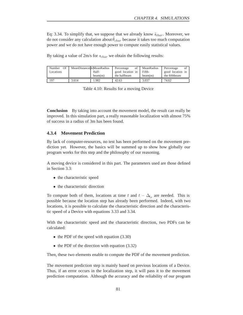
CHAPTER 4. SIMULATIONS
Eq: 3.34. To simplify that, we suppose that we already know schar. Moreover, wedo not consider any calculation about θchar because it takes too much computationpower and we do not have enough power to compute easily statistical values.
By taking a value of 2m/s for schar we obtain the following results:
Number OfLocations
MeanDistance(m)MeanRadiusHalf-beam(m)
Percentage ofgood location inthe halfbeam
MeanRadiusFifth-beam(m)
Percentage ofgood location inthe fifthbeam
197 3.614 1.982 42.63 3.037 74.62
Table 4.10: Results for a moving Device
Conclusion By taking into account the movement model, the result can really beimproved. In this simulation part, a really reasonable localization with almost 75%of success in a radius of 3m has been found.
4.3.4 Movement Prediction
By lack of computer-resources, no test has been performed on the movement pre-diction yet. However, the basics will be summed up to show how globally ourprogram works for this step and the philosophy of our reasoning.
A moving device is considered in this part. The parameters used are those definedin Section 3.3:
• the characteristic speed
• the characteristic direction
To compute both of them, locations at time t and t − ∆tp are needed. This ispossible because the location step has already been performed. Indeed, with twolocations, it is possible to calculate the characteristic direction and the characteris-tic speed of a Device with equations 3.33 and 3.34.
With the characteristic speed and the characteristic direction, two PDFs can becalculated:
• the PDF of the speed with equation (3.30)
• the PDF of the direction with equation (3.32)
Then, these two elements enable to compute the PDF of the movement prediction.
The movement prediction step is mainly based on previous locations of a Device.Thus, if an error occurs in the localization step, it will pass it to the movementprediction computation. Although the accuracy and the reliability of our program
81

CHAPTER 4. SIMULATIONS
have not been tested yet, this part cannot be eluded. Indeed, as we will notice later,movement prediction is really relevant for the implementation of the handover pro-cedure.
4.3.5 Handover
4.3.5.1 General Scenario
In this chapter we will first focus on Handover without Location information andthen on Handover with Location information and Movement Prediction. This willenable us to compare both cases.
As seen in the section 4.1 of this chapter, we already have defined a scenario.Three Access Points (APs) are placed on the ceiling of a room. We have just seenthat it was preferable to put them in the center of the room. However, for morecommodities, they have been put in the corners in this chapter (Figure 4.25): thishas no impact on the handover study.
Each AP is connected by wire to a Handover Agent (HA), a server whose prin-cipal functions are:
• Without location
– To transmit the clock and the BD_ADRR of the Device to all the APs
– To concentrate the RSSI measurements of the APs
• With location and movement prediction
– To transmit the clock and the BD_ADRR of the Device to all APs
– To receive the RSSI measurements of the APs and analyse it to predictnext location
– To maintain the database of the room (location of the APs, boundaryregions, location of the Device,etc.)
4.3.5.2 Timers defined during Paging procedure
To evaluate the time for the Paging procedure in both cases (with and withoutlocation), several timers have been defined in the section 3.4.4. A value has beenassigned for each one:
Page timeout (pageTO) = 1.28s, which is the average time of Paging process [8]and equal to the Time Between Page Scans (see Appendix B).
Page response (pagerespTO) = 8 slots for the Device and for the APs.
New connection timeout (newconnectionTO) = 32 timeslots.
Tpoll = 40 slots
82

CHAPTER 4. SIMULATIONS
AP2 AP1
AP3
Handover Agent
Device
Wired network
Figure 4.25: One of the possible configurations of the room (view from the top)
4.3.5.3 Handover without location information
In this case the accurate location of the Device is not known. In fact we only haveCell ID location (see Section 2.2.1). Handover is carried on the basis of ReceivedSignal Strength Indicator (RSSI).
Assumptions
• The Device has already been connected to the AP1 with Inquiry and Pagingprocedures. The first Inquiry for connecting the Device has given to each APthe FHS packet of the Device through the HA.
• A Threshold is defined to set the area boundary of each AP (Figure 4.26).
• Information transmission between the APs and the HA are immediate
• The Device cannot be in STANDBY state. It will only be either in CON-NECT state or PAGE SCAN state.
• The HA initiates the AP for the Paging procedure in an increasing order (firstAP2 and then AP3).
• The origin of the time for Paging is taken as soon as the Device is in Holdmode (150ms after the Hold Request).
• The Paging timers are taken into account.
• The Paging procedure always succeeds before the Page timeout if the Deviceis in the range of the considered AP.
83

CHAPTER 4. SIMULATIONS
Handover Agent
Wired network
AP1AP2
AP3
Device
Transit 1-2 Transit 2-1
Transit 1-3Transit 3-1
Transit 3-2
Transit 2-3
Figure 4.26: Possible area transitions performed by the Device in the case of Han-dover without location
Handover procedure The principle of this handover method is that, when theDevice needs to change of AP, the APs try to page the Device in an increasing or-der because the Device cannot receive two page packets (DAC packet) in the sametime slot.
1. First the Device is bound to the AP1. This AP1 is known as the ActiveAccess Point and is called A(AP).Two cases have to be considered:
(a) Movement from AP1 to AP2
i. The Device is moving from AP1 region to the AP2 region. Whenthe RSSI value is equal or below to the defined threshold, the AP1forces the Device into PAGE SCAN state. At the same time, theAP1 notifies the HA for a handover procedure.
ii. HA notifies the AP2 for a Paging procedure: the AP2 enters thePAGE state.
iii. As the Device is in the coverage area of the AP2, the Pagingprocess can happen. When the Device is connected to the AP2,it deletes the link with the AP1.
(b) Movement from AP1 to AP3
i. The Device is moving from AP1 region to the AP3 region. Whenthe RSSI value is equal or below to the defined threshold, the AP1forces the Device into PAGE SCAN state. At the same time, theAP1 notifies the HA for a handover procedure.
84
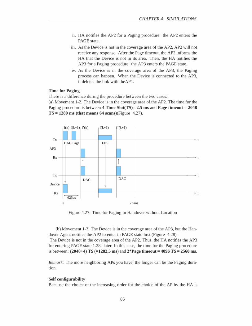
CHAPTER 4. SIMULATIONS
ii. HA notifies the AP2 for a Paging procedure: the AP2 enters thePAGE state.
iii. As the Device is not in the coverage area of the AP2, AP2 will notreceive any response. After the Page timeout, the AP2 informs theHA that the Device is not in its area. Then, the HA notifies theAP3 for a Paging procedure: the AP3 enters the PAGE state.
iv. As the Device is in the coverage area of the AP3, the Pagingprocess can happen. When the Device is connected to the AP3,it deletes the link with theAP1.
Time for PagingThere is a difference during the procedure between the two cases:(a) Movement 1-2. The Device is in the coverage area of the AP2. The time for thePaging procedure is between 4 Time Slot(TS)= 2.5 ms and Page timeout = 2048TS = 1280 ms (that means 64 scans)(Figure 4.27).
f(k) f(k+1) f’(k) f’(k+1)f(k+1)
t
t
t
t
DAC Page
DAC
FHS
0 2.5ms
DAC
625us
Device
Tx
Rx
Tx
Rx
AP3
Figure 4.27: Time for Paging in Handover without Location
(b) Movement 1-3. The Device is in the coverage area of the AP3, but the Han-dover Agent notifies the AP2 to enter in PAGE state first.(Figure 4.28)The Device is not in the coverage area of the AP2. Thus, the HA notifies the AP3
for entering PAGE state 1.28s later. In this case, the time for the Paging procedureis between: (2048+4) TS (=1282,5 ms) and 2*Page timeout = 4096 TS = 2560 ms.
Remark: The more neighboring APs you have, the longer can be the Paging dura-tion.
Self configurabilityBecause the choice of the increasing order for the choice of the AP by the HA is
85

CHAPTER 4. SIMULATIONS
f(k) f(k+1) f’(k) f(k+1)
t
t
t
t
DAC Page
0
625us
Device
AP2
Tx
Rx
Tx
Rx
f(k+3) f(k+31)f(k+32)
1280ms
DAC Page DAC Page
Figure 4.28: Time for Paging without Location (1)
f(k) f(k+1) f’(k) f’(k+1)f(k+1)
t
t
t
t
DAC Page
DAC
FHS
DAC
625us
Device
Tx
Rx
Tx
Rx
AP3
1282.5ms1280ms
Figure 4.29: Time for Paging without Location (2)
86

CHAPTER 4. SIMULATIONS
not very pertinent, self-configurability has been developed. It will try to enhancethe Paging duration.
This method consists in defining an order of priority which allows to launch theInquiry procedure from the most probable AP where the Device has more proba-bility to be located (see section probability tree 2.3.3.1).
To do that, transitions are defined. Each time that the Device crosses a transitboundary, this one is loaded into memory which name is ’order table’.
• Movement 1-2The ’order table’ gives the following results:
– Transit 1-2 happens more than transit 1-3: time for Paging= [2.5; 1280].
– Transit 1-3 happens more than transit 1-2: time for Paging= [1282.5;2560].
• Movement 1-3The ’order table’ gives the following results:
– Transit 1-2 happens more than transit 1-3: time for Paging= [1282.5;2560].
– Transit 1-3 happens more than transit 1-2: time for Paging= [2.5;1280].
Summary of the total time for Paging procedure:
Movement 1-2 Movement 1-3Paging Min Time Max Time Min Time Max Time
Without self configurability 2.5ms 1280 ms 1282.5 ms 2560 msTransit 1-2 > Transit 1-3 2.5ms 1280 ms 1282.5 ms 2560 msTransit 1-3 > Transit 1-2 1282.5 ms 2560 ms 2.5ms 1280 ms
Table 4.11: Total time for Paging procedure with and without Self Configurability
When the probability of the movement from the AP1 to the AP where the Devicehas moved is bigger than the other one, time taken by Paging procedure is eitherequal or diminished. For the less probable case, the time is equal or increased.Thus, the self configurability has been set to diminish the time for Paging if themovement studied has the highest probability.
Drawback of the Handover without LocationPRSSI measurements are done each time the Device receives an inquiry from oneof the APs. This procedure takes generally between 1 and 4 seconds. That couldbe a disadvantage in some case as demonstrated in Figure 4.30 and Figure 4.31.
Following parameters are defined:
87

CHAPTER 4. SIMULATIONS
AP a AP btD+tP
tL
T0
Figure 4.30: Loss of quality of the signal for Handover without Location
• T0 is the moment of the first inquiry of APa.
• tD is the time between the first and the second Inquiry of the APa.
• tP is the duration between the moment the APa warns the Handover Agentand the moment the APb finds the Device in range.
• tL is the total time during which the quality of the connection decreased.
Explanation:At time T0, APa launches an Inquiry to know the RSSI that the Device calculates.Thus, it knows that the Device is still in its range.
After the delay tD, APa launches a new Inquiry, trying to know the RSSI of theDevice and more precisely if this RSSI is under the defined Threshold. In fact theDevice has moved out of its coverage area. Thus, APa warns the Handover Agentand asks the other APs to alternatively search for the Device (according to the or-der defined in the “order table”). Right from the moment that the APb launches thePaging, it will find the Device. But during the time tL the connection state betweenthe Device and the APa has not been as good as it could have been if the APb hadrecovered the Device. In the worse case, this time tL can reach 4 seconds (con-sidering as maximum time of the Inquiry procedure + Paging procedure of severalAccess Points).
In the case of the Figure 4.30 this phenomena is not very relevant because theconnection is kept by APa during tL. But the case of the Figure 4.31 is more prob-lematic since during the time tL, the connection with APa is totally lost.
Conclusion for Handover without LocationWe notice that the duration of the Paging procedure depends on the digit (order)
88

CHAPTER 4. SIMULATIONS
T0
tL
tD+tP
AP aAP b
Figure 4.31: Loss of the signal for Handover without Location
affected to the AP. A system of self-configurability has been implemented temptingto optimize this digit allocation. However there always will be cases where thePaging duration will be higher than 1280 ms (if the Device moves in one directionwhich is not the most probable one).In our scenario, the problems of connection, where there is a loss of the connection,are not relevant. But, as we have seen, they could be in the case of a room change.Thus, Handover without Location has some shortcomings.
4.3.5.4 Handover with location and movement prediction
In this case the accurate location of the Device is known and the next location isestimated by the HA. As the next location is estimated, there is no need to considertwo different moves: they are symmetrical considering Paging duration. Handoveris carried on the basis of Received Signal Strength Indicator (RSSI). We consideronly the movement from the AP1 to the AP2. Handover is carried on the basis ofReceived Signal Strength Indicator (RSSI).
Assumptions
• The Device is already connected to the AP1 with Inquiry and Paging proce-dures. The first Inquiry for connecting the Device has given to the APs theFHS packet of the Device through the HA.
• Each point of the boundaries (Figure 4.32) is defined as being at equal dis-tance from the 2 closest Access Points. So the quality of the connection oneach side of the boundary is the best we can have.
• Information transmission between the APs and the HA are immediate.
• The Device cannot be in STANBY state. It will only be either in CONNECTstate or PAGE SCAN state.
• The HA initiates the AP for the Paging procedure in an increasing order (firstAP2 and then AP3).
89

CHAPTER 4. SIMULATIONS
Figure 4.32: Example of coverage areas of the Three Access Points
AP2 AP1
AP3
Handover Agent
Device
Wired network
Area 3
Area 1
Area 2
Figure 4.33: Sectorization of the room
90

CHAPTER 4. SIMULATIONS
• The origin of the time for Paging is taken as soon as the Device is in Holdmode (150ms after the Hold Request).
• The Paging timers are taken into account.
• The Paging procedure succeeds before the Page timeout.
Handover procedureThe principle of this handover method is that, when the Device is going to changeof cell (this is known thanks to movement prediction), the HA warns the concernedAP to start the Paging procedure right from the moment the Device enters the rangeof the AP.
1. First, the Device is bound to the AP1. This AP1 is known as the ActiveAccess Point and is called A(AP).
2. The Device is moving from AP1 region to the AP2 (or AP3) region. Whenthe HA predicts a location out of the boundary of the AP1 (in the coveragearea of AP2 (or AP3)), the AP1 forces the Device into PAGE SCAN state.At the same time, the AP1 notifies the HA for a handover procedure.
3. HA notifies the AP2 (or AP3) for a Paging procedure: the AP2(or AP3)enters the PAGE state.
4. As the Device is in the coverage area of the AP2 (or AP3), the Paging processcan happen. When the Device is connected to the AP2 (or AP3), it deletesthe link with the AP1.
Time for pagingThere is no difference considering the two possible movements (1-2 and 1-3). Forthe two cases the time for the Paging procedure is between 4TS (= 2.5 ms) andPage timeout = 2048 TS = 1280 ms.
Advantage of the Handover using Location and Movement Prediction(Figure 4.34):To perform the handover using Location and Movement Prediction we are sup-
posed to have the PDF of the Location and of the Prediction. Because the Locationand Prediction are not very accurate we will not take the maximum point of eachPDF but a set of locations that have a probability greater than a specified threshold.According to the previous studies, this set will include all the locations that have aprobability more than the fifth of the maximum probability.Then we can determine the maximum possible distance that the Device can travel(in the case where the real position of the Device is 1a and the real prediction willbe 1b) and the minimum one (the real position of the Device is 2a and the realprediction will be 2b). This enables us to find the longest and the smallest distancebefore that the Device crosses the boundary.
The PDF of the speed of the Device is known. The two probabilities that are farfrom the variance to the most probable speed will give us what we will considerthe slowest and the fastest speed that the Device can have.
91

CHAPTER 4. SIMULATIONS
Set of the locations that have a probability more than the specified ThresholdSet of the predictions that have a probability more than the specified Threshold.
1a2a
1b
2b
Max Possible Distance
Min Possible Distance
Longest distanceto the bourdary
Shortest distanceto the bourdary
Boundary
Possible position of the device
Figure 4.34: Principle of Handover with Movement Prediction
By dividing the smallest distance to the boundary by the fastest speed we obtainthe minimum time the Device can take to reach the boundary.In the same way, by dividing the longest distance to the boundary by the slowestspeed we obtain the maximum time the Device can take to reach the boundary.
Using this method, we can start the Handover right from the moment the De-vice goes through the boundary (because we know the boundary location). In themethod without Location, we had to wait for an RSSI value under a certain Thresh-old, meaning that the Device could already be in the new area.
Conclusion with Location and Movement PredictionIn the present case, the time for the Paging procedure is always the same. Indeed,the estimation of the next location allows to know the AP where the Device isgoing to. Moreover, as just seen, the Paging procedure can be started right fromthe moment the Device enters the neighboring boundary. This means that the casewhere the connection is lost could be avoided.
4.3.5.5 Comparison between Handover with and without Location informa-tion
The shortcomings of Handover without Location information are that the Pagingprocedure can be quite long (this depends of the number of neighboring APs too)and that in some cases the connection can be lost.According to this study, Handover using Location information and Movement Pre-diction allows to compensate for the drawbacks of the Handover that does not usethese techniques.
92

CHAPTER 4. SIMULATIONS
Duration of Paging Quality LossesHandover Without Location The Paging can be
more than 1280 mslong.
Possibility of connec-tion loss.
Handover With Location The Paging is alwaysless than 1280 ms
No connection loss
Table 4.12: Comparison between Handover With and Without location information
4.4 Conclusions
After a specific scenario has been defined, this chapter contained the steps that havebeen followed to develop the simulator and calculation:
- RSSI generation
- Location
- Location of a moving Device
- Movement Prediction
- Handover
Some tests have been made to validate the well-working and the accuracy of thesimulator.In the first part of this chapter, generation of RSSI measurements have been im-plemented. Two cases have been made: measures of RSSI for a fixed point, andmeasures of RSSI after a certain delay, according to the PDF of Inquiry time, for amoving Device with a defined trajectory.
In a second part this first implementation enabled to implement calculation of thelocation of the Device in the two precedent cases. For that, different cases havebeen made and test-parameters implemented to test the accuracy and well-runningof the programs. It was showed that with previous knowledge about the locationand using the propagation model of the room, the location could be considerablyimproved.
In a third part, Movement Prediction process had been implemented, but no testsconcerning its accuracy had been performed because of the lack of computer-resources.In the last part of this chapter, comparison between two handovers has been made.It has proved that the handover used in our scenario is more in adequacy with theprinciple of mobility of the project: the duration it takes has been significantlyreduced due to the use of some parameters:
- Location
- Movement prediction
93

CHAPTER 4. SIMULATIONS
- Paging for connecting directly two Bluetooth Devices
Indeed, the use of these three parameters allows to save up to 2.5s during the Pagingprocedure and avoid loosing the connection in some cases. Overall the handoverused is enhance in time and in space.
94

Chapter 5
Conclusions
As far as mobility is concerned, Bluetooth networks offer limited capabilities ashandover concept is not specified in Bluetooth specifications. Adding a handoverprocess in a short-range technology leads to need fast cell changes and to targetarea of expected movements.
Yet because connections in Bluetooth can only be established with Inquiry andPaging, which are two long processes, it is relevant to start the handover processas soon as possible in the right area. That is why it has been thought to bypass theInquiry process by using a Handover Agent. Its goal is to provide neighbouringAccess Points the parameters that enable to bypass the Inquiry.
Then, as concerns targeting the right future area, we thought of a system of lo-calization complemented by a movement prediction process. Sets of tests haveproved that the location we have implemented gives quite good results at the mo-ment but is time-consuming to compute. In addition, it has been demonstrated thatusing location and movement prediction to perform the handover can enable us toavoid some extreme cases where the connection could be lost.
95

CHAPTER 5. CONCLUSIONS
Future workMeasurementsDue to lack of time and to some malfunction of the hardware, we were not able tomake any measurements with a Bluetooth AP. Our simulations are based on genera-tion of measurements. One of the future works will be to validate our measurementgeneration by:
• Performing basic RSSI measurements, with three fixed APs.
• Performing RSSI measurements of a moving Device and three APs.
With these measurements it is then possible to determine maybe more parameterson which depend the measured values, and then to achieve more realistic simula-tions.
Implementation of the localizationThe localization is made with large matrices. The more accurate the localization,the higher the space resolution, and the larger the matrices. Our simulations arebased on matrices of size 200*200 and it seems impossible to make “real time”localization with our implementation. An important further work will be:
• To optimize the algorithms. For example a lot of computations can be avoidedby avoiding all the calculations where there are zeros in the PDFs of the dis-tance.
• To develop the algorithms in C language. An implementation in C languagewould be faster and would allow more control on the computations A realtime implementation of our handover would be then possible.
Influence between the localization process and the linkAs we have to probe the Device to get RSSI measurements, it takes time and low-ers the bandwidth of the link. More information will be needed to evaluate thereliability of the localization in the Handover optimization process.
Improvement of the localizationConsideration of the link quality could improve a lot the localization process be-cause this measurement is done during the link and not after the Inquiry procedure.Duration of the Inquiry procedure is unknown, so the information brought by theRSSI measurement is not frequent. Unlike the Inquiry procedure, the link qualitybrings continuous and useful information, even if it this information is issued onlyby one AP.
More scenarios of localizationDue to lack of time, we have not analyzed different cases. We look forward toexperimenting different scenarios such as:
• More than 1 Device.
96

CHAPTER 5. CONCLUSIONS
• More than 1 AP in a same place.
• More than 1 room where loss of signal is encountered.
• Practical implementations.
97

Appendix A
Detailed calculation of theDistance estimation
This Appendix presents the details of the calculations of the Distance estimationi.e. the details of the calculations of the parameter pfΘ,s,dt in the formula 3.40:
P(d∆t+t) =∑
s,dt∈Ω(D)
pfΘ,s,dt(dt+∆t)fS(s)fDt(dt|RSSIt)δsδdt
A.1 Space overview:
As on the figure A.1, we can see that the device can be on a circle of radius s∆taround its last position. Here we are only dealing with the case where dt > s∆t.In the other case, the calculations are a bit different but follow the same principle.
a
dt
dt+∆t
b s∆t
Figure A.1: Space Overview
We have to calculate for a little variation δd of dt+∆t the corresponding varia-tion of the covered distance on the circle δp. See the figure A.1.
98
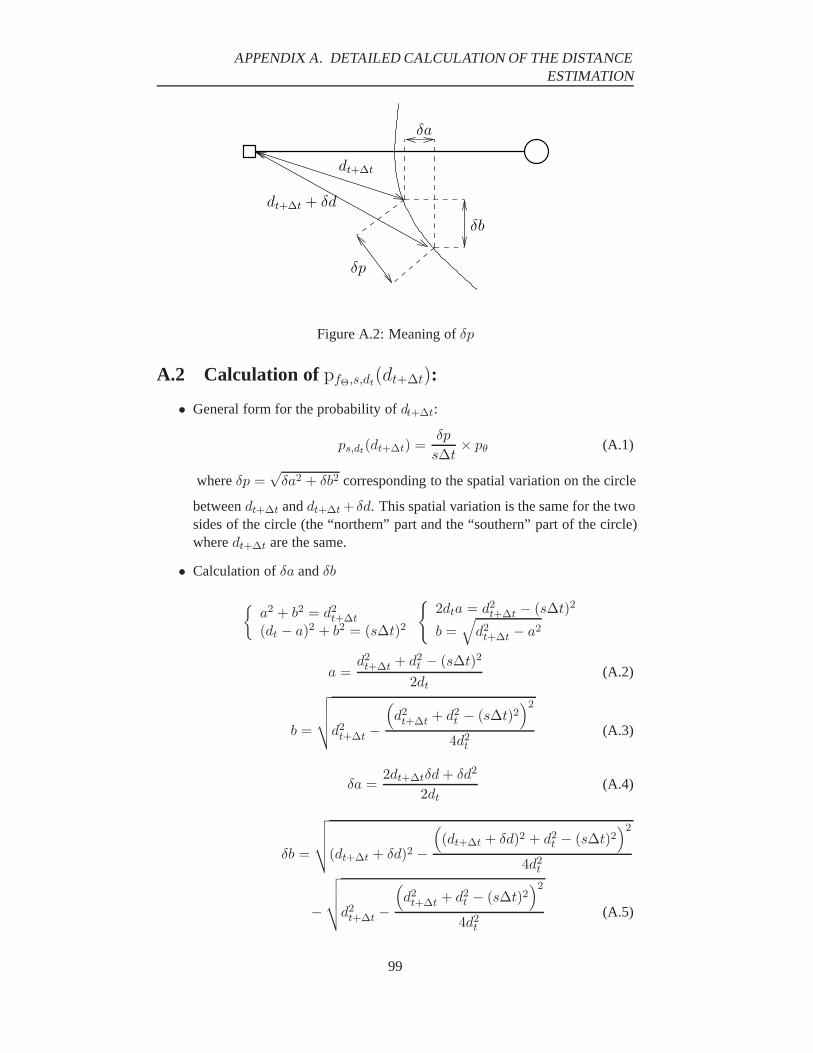
APPENDIX A. DETAILED CALCULATION OF THE DISTANCEESTIMATION
δb
δp
δa
dt+∆t
dt+∆t + δd
Figure A.2: Meaning of δp
A.2 Calculation of pfΘ,s,dt(dt+∆t):
• General form for the probability of dt+∆t:
ps,dt(dt+∆t) =δp
s∆t× pθ (A.1)
where δp =√
δa2 + δb2 corresponding to the spatial variation on the circle
between dt+∆t and dt+∆t + δd. This spatial variation is the same for the twosides of the circle (the “northern” part and the “southern” part of the circle)where dt+∆t are the same.
• Calculation of δa and δb
a2 + b2 = d2
t+∆t
(dt − a)2 + b2 = (s∆t)2
2dta = d2
t+∆t − (s∆t)2
b =√
d2t+∆t − a2
a =d2
t+∆t + d2t − (s∆t)2
2dt(A.2)
b =
√√√√d2
t+∆t −(d2
t+∆t + d2t − (s∆t)2
)2
4d2t
(A.3)
δa =2dt+∆tδd + δd2
2dt(A.4)
δb =
√√√√(dt+∆t + δd)2 −
((dt+∆t + δd)2 + d2
t − (s∆t)2)2
4d2t
−
√√√√d2
t+∆t −(d2
t+∆t + d2t − (s∆t)2
)2
4d2t
(A.5)
99

APPENDIX A. DETAILED CALCULATION OF THE DISTANCEESTIMATION
• Weight of the considered direction pθ: We have to take into account thepredicted direction. This factor takes into account both the northern part ofthe circle and the southern part.If we cannot predict the direction, we take the uniform distribution assumedabove and then:
pθ =1π
(A.6)
If we can predict it, we have to go into more complicated calculations detailsbelow. We have the PDF fΘ of the direction. The calculations are made withrespect to the figure A.3.The axis (Ox′) and (Oy′) are parallel to the axis (Ox) and (Oy), the main
(Ox′)
(Oy′)(Ob)
(Oa)
dt
φ
θ
θ′
dt+∆t
s∆t
Figure A.3: Calculation of the different angles
axis of our scenario.We first have to calculate the angle φ:Xi and Yi are the coordinates of the AP i. xt and yt are the coordinates ofthe moving device at the time t.If we define the angle Φ as being :
Φ = arctan
(|Yi − yt||Xi − xt|
)(A.7)
thenyt > Yi and xt > Xi ⇒ φ = Φ
yt > Yi and xt < Xi ⇒ φ = π − Φ
100

APPENDIX A. DETAILED CALCULATION OF THE DISTANCEESTIMATION
yt < Yi and xt > Xi ⇒ φ = −Φ
yt < Yi and xt < Xi ⇒ φ = Φ − π (A.8)
The next step is to calculate the PDF of the direction in the new coordinatesystem. We make this change of coordinate: θ′ = θ − φ. In each case,we define first a function gΘ(θ′) = fΘ(θ − φ) then we determinate f′
Θ, thePDF of the direction in the new coordinate system (Oa), (Ob). Here are thedifferent shifting cases:if phi > 0 then
∀θ′ ∈ [−π, π − φ[ f ′Θ(θ′) = gΘ(θ′)
∀θ′ ∈ [π − φ, π[ f ′Θ(θ′) = gΘ(θ′ − 2π)
if phi < 0 then
∀θ′ ∈ [−π − φ, π[ f ′Θ(θ′) = gΘ(θ′)
∀θ′ ∈ [−π,−π − φ[ f ′Θ(θ′) = gΘ(θ′ + 2π) (A.9)
Then we can calculate the weight of the angle as represented on the figureA.4.
(Ob)
(Oa)b1b2
θ2
θ1
δp
Figure A.4: Angular area
We have to calculate, with the formula A.3, the two distances b: b1 and b2
which bound δp. With b1 and b2 we calculate the corresponding angles θ1and θ2.There are two cases:
101

APPENDIX A. DETAILED CALCULATION OF THE DISTANCEESTIMATION
if d2t+∆t < d2
t + (s∆t)2
then
θ1 = π − arcsin
(b1
s∆t
)
θ2 = π − arcsin
(b2
s∆t
)
if d2t+∆t > d2
t + (s∆t)2
then
θ1 = arcsin
(b1
s∆t
)
θ2 = arcsin
(b2
s∆t
)
finally we calculate the weight of the direction this way :
pθ =∫ θ1
θ2
f ′Θ(θ′)dθ′ +
∫ π−θ2
π−θ1
f ′Θ(θ′)dθ′ (A.10)
Finally by putting the equation A.6 or A.10 in A.1 we can finally find 3.40.
example: We take an example with:
• fS = fSCharwith SChar = 1m/s
• fDt(dt|RSSIt) = δ(10 − dt)
• ∆t = 2s
• fΘ(θ) = gΘ. See the definition of the formula 3.31
102

APPENDIX A. DETAILED CALCULATION OF THE DISTANCEESTIMATION
0 5 10 15 20 25 30 35 400
0.005
0.01
0.015
0.02
0.025
0.03
Distance (m)
Pro
babi
lity
Figure A.5: Example of a distance estimation
103

Appendix B
Paging procedure details
Prospective slave: Page scan and page response statesA slave can enter in the page scan state from the STANDBY state or from theCONNECT state. For the paging process, two parameters have to be taken intoaccount:
• Page Scan Window: Tw_page_scan
• Time Between Page Scan: Tpage_scan: time between the successive pagescans.
The Page Scan Window is the time duration that the device spends in the PAGESCAN state. In Bluetooth specifications[4], it is set to 11,25ms: the time for theAP (the master) to page 16 frequencies.
The Time Between Page Scan is set by the device:
• for a continuous page scan Tw_page_scan = T page_scan
• if the device is already occupied in another piconet or is in a low power mode(for example hold mode), it can bet set to 1,28 s or 2,56 s.
For the shortest response time, both parameters should be equal, i.e. the deviceshould always scan for the page. It is feasible but it consumes a lot of power. Thus,it is discussed how long the device should be in page scan state for a successfulcommunication.
Furthermore, when a device enters the PAGING state, it should put its ACL linksinto park or hold mode: indeed, ACL connection are ’stopped’ during the PAG-ING. In our scenario, SCO links are not considered: if it had been, we should havetaken into account the fact that SCO links have a higher priority and thus couldinterrupt the paging process.
Prospective master: Page and page response statesIt is already discussed that the master will enter the PAGE state and repeatedly
104

APPENDIX B. PAGING PROCEDURE DETAILS
transmits the slave’s DAC on the page hop channels, two per even-numbered timeslot, and listens for the response in the corresponding odd numbered time slot. Asthe master does not know when the slave will enter page scan sate, it must continueto send the DAC’s until receiving a response or timeout. For the best scenario themaster should transmit DAC when the slave is in PAGE CAN state.
We also knows that the slave will be in PAGE SCAN state long enough for themaster to page on 16 frequencies (11,25 ms). Thus, the purpose for the master isto select a set of 16 frequencies including the one on which the slave is listening:this can be done because, knowing the clock of the device (CLKN) received in theFHS packet, the master analyzes some bits of it and can guess the hop sequenceused by the device when entering the next PAGE SCAN state
105
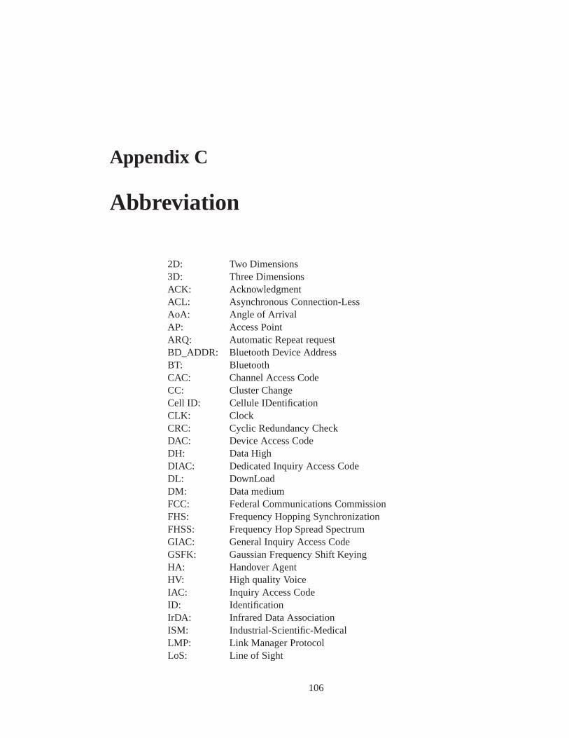
Appendix C
Abbreviation
2D: Two Dimensions3D: Three DimensionsACK: AcknowledgmentACL: Asynchronous Connection-LessAoA: Angle of ArrivalAP: Access PointARQ: Automatic Repeat requestBD_ADDR: Bluetooth Device AddressBT: BluetoothCAC: Channel Access CodeCC: Cluster ChangeCell ID: Cellule IDentificationCLK: ClockCRC: Cyclic Redundancy CheckDAC: Device Access CodeDH: Data HighDIAC: Dedicated Inquiry Access CodeDL: DownLoadDM: Data mediumFCC: Federal Communications CommissionFHS: Frequency Hopping SynchronizationFHSS: Frequency Hop Spread SpectrumGIAC: General Inquiry Access CodeGSFK: Gaussian Frequency Shift KeyingHA: Handover AgentHV: High quality VoiceIAC: Inquiry Access CodeID: IdentificationIrDA: Infrared Data AssociationISM: Industrial-Scientific-MedicalLMP: Link Manager ProtocolLoS: Line of Sight
106

APPENDIX C. ABBREVIATION
NAK: Negative acknowledgmentNoLoS: Without Line of SightPAN: Personal Area NetworkPC: Personal ComputerPDA: Personal Digital AssistantPDF: Probability Density FunctionQoS: Quality of ServiceRSSI: Ratio Signal Strenght IndicatorSBC: Systematic Bloc CodesSCO: Synchronous Connection-OrientedSIG: Special Interest GroupTCS: Telephony Control SpecificationTDD: Time-Division DuplexTDoA: Timing Differences of ArrivalToA: Time of ArrivalTS: Time SlotUL: UpLoadWLAN: Wireless Local Area Network
107

Bibliography
[1] Robert Morrow, Bluetooth Operation and use, McGraw-Hill,2002.
[2] M. Frodigh, P. Johansson, P. Larsson, Wireless ad hoc networking. The art ofnetworking without a network Ericsson Review, No. 4, 2000
[3] Khaldoun Al Agha, Guy Pujolle, Guillaume Vivier, Réseaux de mobiles etréseaux sans fil, Eyrolles, 2001
[4] Bluetooth specification, Website. http://www.bluetooth.org.
[5] BLIP Systems, Webpage http://www.blipsystems.com.
[6] Personal Contact with BLIP Systems Lars Christensen.
[7] Joao Figueiras, Development and evaluation of mechanisms to obtain lo-cation information in Bluetooth networks,Master thesis, Aalborg University2004.
[8] Tatiana K. Madsen, lecture notes, 2004.
[9] Heikki Laitinen, Cellular Location Techniques, MLW 2001,6.6.2001.
[10] Mario Proietti, Comparison of Location Technologies for Phase II WirelessE-911, Fall 2001.
[11] Chrysanthos Dellarocas, Lecture Notes for 15.564, Information technology I
[12] Fredrik Gustafsson, Particle Filters for Positioning with focus on WirelessNetworks, 2002-12-09.
[13] Graham Wilde, Performance Implications of Wireless Location Technologies- The Effect on Location-based Service Revenue Growth, 2003.
[14] R.Chellapa-Doss, A.Jennings, N.Shenoy, User Mobil-ity Prediction in Hybrid and Ad Hoc Wireless Networks,http://atnac2003.atcrc.com/ORALS/CHELLAPPA.pdf
[15] Paul Flynn, Management of Wireless Networks: Resource Al-location Predictive Algorithm For Micro-Mobility Networks,www.itsligo.ie/research/docs/Paul%20Flynn%20Pres.pdf
108

BIBLIOGRAPHY
[16] J.Biesterfeld, E.Ennigrou, K.Jobmann, Neural Networks for Location Predic-tion in Mobile Networks.
[17] Naresh Verma, Autonomous prediction Algorithns for Wireless Cellular AndHoc Networks, 2003.
[18] Matlab User Manual.
[19] Antoine Mercier, Bluetooth, lectures note,2004.
[20] Seppo Sahi, Services in UMTS Environment, 4th March 2003.
[21] Birgit Muehlenhaus, The Diffusion of Retail Locatin-based Ser-vices:Geography and Privacy Issue, May 2004
[22] L.Aalto, N.Göthlin, J.Korhonen, T.Ojala, Bluetoothand WAP Push BasedLocation-Aware Mobile Advertising System, 2004
[23] Sairam Mannar, Location aware services using Bluetooth, 2004.
[24] Rolf Kraemer, Bluetooth Based Wireless Internet Applications for Indoor HotSpots : experience of a Successful Experiment During CeBIT 2001, 2001.
[25] Zeev Weissman, Indoor Location, White Paper, 2004.
[26] Hyun-Sang Jang, BlueWIN-Bluetooth Wireless Network Indoor Networkovercomes many shortcomings of Bluetooth, 2002.
[27] Frederic Collomb, Location Service Study Report,D2.3.1,MOVIES-RE-2300-002-FDC, 2002.
[28] Nicolas Boulay, Julien Gros, Bluetooth white paper, http://www.com1-support.com/wpapers/doc/bluetooth.doc, 2003.
[29] John A. Borrie, Stochastic systems for engineers, Prentice Hall, 1992.
[30] Jennifer Bray, Masters and Slaves: Roles in a Bluetooth Pi-conet,http://www.phptr.com/articles/article.asp?p=21324&seqNum=4
[31] SIG Forum, Time Taken to complete Inquiry/Paging Procedures,http://www.palowireless.com/infotooth/knowbase/baseband/99.asp, 2000.
[32] Norman S. Matloff, Probability modeling and computer simulation, PWS-KENT, 1988.
[33] Gérard Frugier, Louis Gacôgne, Probabilité et statistiques, Eyrolles.
[34] David Parsons, The Mobile Radio Propagation Channel, Pentech Press, 1994.
[35] Paul Flynn, Management of Wireless Networks: Analysis ofPredictive Methods for Handover in a Cellular IP Network,http://www.ittconference.com/anonftp/pdf/2003-presentations/PaulFlynn-mgmt-wireless.pdf, IT&T, 2003
109