Locking depths estimated from geodesy and seismology along ...shearer/mahi/PDF/2011/SmithKonter_JGR...Locking depths estimated from geodesy and seismology along the San Andreas Fault

Locking depths estimated from geodesy and seismology alongthe San Andreas Fault System: Implications for seismicmoment release

Bridget R. Smith‐Konter,1 David T. Sandwell,2 and Peter Shearer2

Received 23 November 2010; revised 18 February 2011; accepted 24 February 2011; published 3 June 2011.

[1] The depth of the seismogenic zone is a critical parameter for earthquake hazard models.Independent observations from seismology and geodesy can provide insight into the depthsof faulting, but these depths do not always agree. Here we inspect variations in fault depthsof 12 segments of the southern San Andreas Fault System derived from over 1000 GPSvelocities and 66,000 relocated earthquake hypocenters. Geodetically determined lockingdepths range from 6 to 22 km, while seismogenic thicknesses are largely limited to depths of11–20 km. These seismogenic depths best match the geodetic locking depths when estimatedat the 95% cutoff depth in seismicity, and most fault segment depths agree to within2 km. However, the Imperial, Coyote Creek, and Borrego segments have significantdiscrepancies. In these cases the geodetically inferred locking depths are much shallowerthan the seismogenic depths. We also examine variations in seismic moment accumulationrate per unit fault length as suggested by seismicity and geodesy and find that bothapproaches yield high rates (1.5–1.8 × 1013 Nm/yr/km) along the Mojave and Carrizosegments and low rates (∼0.2 × 1013 Nm/yr/km) along several San Jacinto segments. Thelargest difference in seismic moment between models is calculated for the Imperial segment,where the moment rate from seismic depths is a factor of ∼2.5 larger than that from geodeticdepths. Such variability has important implications for the accuracy to which futuremajor earthquake magnitudes can be estimated.

Citation: Smith‐Konter, B. R., D. T. Sandwell, and P. Shearer (2011), Locking depths estimated from geodesy and seismology alongthe San Andreas Fault System: Implications for seismic moment release, J. Geophys. Res., 116, B06401, doi:10.1029/2010JB008117.

1. Introduction

[2] Fault depth within the seismogenic zone is a criticalparameter for seismic hazard models. Earthquake moment isproportional to the rupture area of a brittle fault, defined as theproduct of a fault’s length and width (i.e., depth for a verticalfault). Major earthquakes (Mo > 8) have been shown to rup-ture the entire brittle fault zone [Das and Scholz, 1983; Hillet al., 1990] and recent studies of seismicity using relocatedhypocenters in Southern California [Nazareth and Hauksson,2004] show that the depth above which 99% of the momentrelease of background seismicity occurs provides a realisticestimate of the maximum rupture depth in moderate to largeearthquakes. Thus accurate estimates of maximum fault depthare fundamental in accurately forecasting the magnitude offuture earthquakes.[3] Geophysical observations from both seismology and

geodesy can provide estimates of the fault depth. Earthquakehypocenters (Figure 1a) define a depth range of active seis-

micity within the crust, representing a transition from seis-mic faulting (velocity weakening) to aseismic slip (velocitystrengthening) [Brace and Byerlee, 1970;Marone and Scholz,1988]. While the average thickness of the seismogenic zonefor the San Andreas Fault System (SAFS) is fairly shallow at∼12 km, large variations from less than 10 km in the SaltonTrough area to greater than 25 km at the southwestern edge ofthe San Joaquin Valley have been identified [Nazareth andHauksson, 2004]. Similarly, the seismogenic thickness ofthe SAFS can vary significantly along strike [e.g., Petersonet al., 1996; Magistrale, 2002; Wdowinski, 2009]. Theseestimates of seismogenic thickness and fault segment length(i.e., slip area), combined with estimates of long‐term faultslip rate, have been used to estimate the earthquake potentialof faults along the SAFS [Stein, 2008].[4] Geodetic surface deformation measurements (i.e., GPS

(Figure 1b) or InSAR), combined with amathematical model,can be used to estimate the effective thickness of the zoneof interseismic strain accumulation, commonly referred to asthe fault locking depth. The simple elastic dislocation model[Savage and Burford, 1973] describes the accumulation ofelastic strain along a vertical strike‐slip fault. The 2‐D modelvelocity profile across the locked fault zone is given by

v xð Þ ¼ V

�tan�1 x

D; ð1Þ

1Department of Geological Sciences, University of Texas at El Paso,El Paso, Texas, USA.

2Institute for Geophysics and Planetary Physics, Scripps Institution ofOceanography, University of California, San Diego, La Jolla, California,USA.

Copyright 2011 by the American Geophysical Union.0148‐0227/11/2010JB008117

JOURNAL OF GEOPHYSICAL RESEARCH, VOL. 116, B06401, doi:10.1029/2010JB008117, 2011

B06401 1 of 12

http://dx.doi.org/10.1029/2010JB008117

where V is the far‐field velocity, x is the horizontal fault‐perpendicular distance, and D is the locking depth (Figure 2with d = 0). The actual variation of slip with depth is prob-ably a gradual transition rather than an abrupt step andphysical models can be easily modified to simulate a gradualtransition. However, it has been demonstrated that the exactshape of this transition with depth cannot be resolved usingsurface geodetic data [Savage, 2006]. Moreover, for earth-quake moment assessment, it is the effective thickness of thelocked zone that is of interest, so the shape of the depthtransition is irrelevant for this application and most inves-tigators simply solve for the locking depth.[5] The derivative of the velocity profile across the fault is

the shear strain rate _". The peak strain rate occurs directlyabove the fault and has an amplitude given by

_" ¼ V

�D: ð2Þ

[6] Another related parameter is the seismic moment accu-mulation rate per unit fault length given by

_M

L¼ �VD; ð3Þ

where m is the crustal shear modulus. Both strain rateand moment accumulation rate are important for assessing

earthquake hazard. Strain rate multiplied by the shearmodulus and the time since the last major rupture provides afirst‐order estimate of the stress that has accumulated sincethe last earthquake. While several studies have shown thatearthquakes do not follow a characteristic rupture cycle[Weldon et al., 2004], the accumulated stress is still a quan-titative measure of whether a particular fault is early or latein its earthquake cycle. The seismic moment accumulationrate, however, is a more important measure of earthquakepotential since this rate multiplied by the time since the lastmajor rupture and the length of a potential rupture is a provenmeasure of earthquake size [Stein, 2008]. Since both strainrate and moment accumulation rate depend on slip rate andlocking depth, or the thickness of the locked zone if the faulthas shallow fault creep, understanding how these param-eters are estimated and how they are applied in models isan important exercise.[7] In this study we compare the effective thickness of

the locked zone derived from seismicity with the thicknessderived from geodesy to quantitatively measure the similar-ities and differences in the two approaches along the SAFS.Seismogenic thickness is derived from 66,775 earthquakeepicenters [Lin et al., 2007] and fault locking depths areestimated from 1099 GPS velocities for 12 fault segments.We examine variations in seismic moment accumulationrate along the fault system as suggested by seismicity andgeodesy. Finally, we explore plausible explanations for faultdepth discrepancies and examine the associated strengthsand weaknesses of each method.

2. Locking Depth Estimated From Geodesy

[8] GPS velocity measurements can be used to estimateboth the strain and moment accumulation rate. As describedabove, the key model parameters are the far‐field velocity Vand the locking depthD. An accurate estimate of the far‐fieldvelocity requires GPS velocity data more than several lock-ing depths away from the fault (>50 km), while an accu-rate estimate of the locking depth requires a high density ofGPS velocity data within one‐half locking depth of the fault

Figure 1. (a) Relocated seismicity for Southern Californiafrom 1981 to 2005 [from Lin et al., 2007]. (b) Southern Ca-lifornia EarthScope Plate Boundary Observatory GPS stationlocations. An additional high‐density GPS array [Lyons et al.,2002] straddling the Imperial fault was also combined withthe EarthScope data set to provide additional coverage.

Figure 2. Diagram of a strike‐slip fault of length L that islocked to depthD. The far‐field slip rate is V. Some faults alsohave shallow fault creep to depth d, which reduces the effec-tive thickness of the locked zone to D – d. The locked zoneis sometimes equated to the seismogenic zone where thefault behavior is velocity weakening [Marone and Scholz,1988]. Darker shading represents a hypothetical distributionof seismicity versus depth.

SMITH‐KONTER ET AL.: FAULT DEPTHS FROM GEODESY AND SEISMOLOGY B06401B06401

2 of 12

(<6 km spacing). However, the typical spacing of GPSvelocity measurements along the SAFS (Figure 1b) is only10–20 km [Wei et al., 2010]. Because of sparse geodetic datain some locations, depth uncertainties can be on the order of3–6 km. Some faults also exhibit evidence of shallow faultcreep [Bürgmann et al., 2000; Lyons et al., 2002] whichreduces the effective width of the locked zone and can furthercomplicate estimations of locking depth. In addition, realfault geometry is not simply two‐dimensional and so the 3‐Dinversion for both slip rate and locking depth is usually illconditioned [McCaffrey, 2005].[9] A simple 2‐D inversion example illustrates both issues

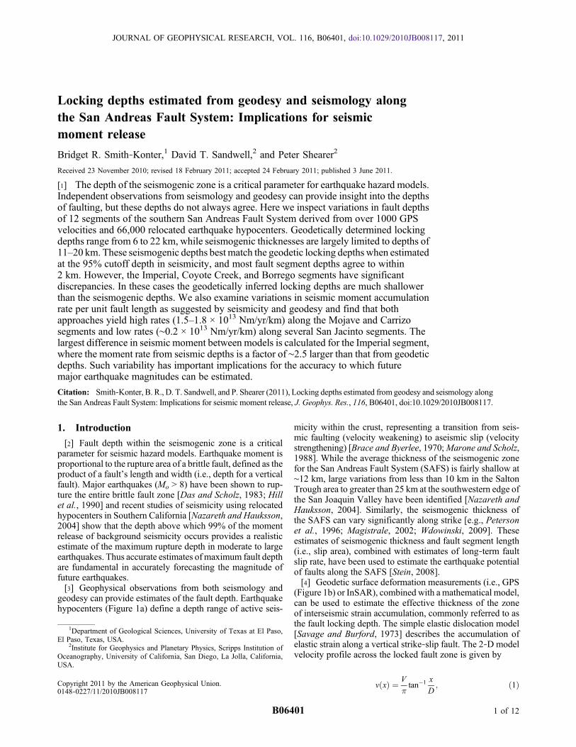
of shallow creep and the ill conditioning of the slip rate andlocking depth parameter estimation problem.We consider thecase of the Imperial fault where there is a single fault strandwith better than average spatial sampling owing to a denseGPS array above the fault zone (Figure 3). The first issue isthat this fault has known shallow creep [Goultry et al., 1978;Genrich et al., 1997; Lyons et al., 2002]. A least squaressensitivity analysis by Lyons et al. [2002] showed that thenear‐fault creep is explained by a shallow locking depth d of3 km and a creep rate of 9 mm/yr. Moreover, they showedthat the important lumped parameter is the effective thicknessof the locked zone or D – d. Given these shallow fault creep

parameters, we calculate the chi‐square misfit of the simplearctangent model versus locking depth and slip rate (Figure 3).The contours of misfit are elongated, showing a high correla-tion between slip rate and locking depth. The best fit model hasa slip rate of 36.5 mm/yr and a locking depth of 5.6 km,although models with locking depths between 4 and 8.7 kmand slip rates between 32 and 43 mm/yr are acceptable. Amodel with a shallow locking depth of 4 km requires a low sliprate of 32 mm/yr, while a model with a deep locking depth of10 km requires a slip rate of 44 mm/yr. This correlationbetween locking depth and slip rate has been demonstrated inseveral previous publications. For example, Segall [2002]showed a similar result for the Carrizo segment of the SAFand suggested that geological bounds on slip rate could be usedto place bounds on the locking depth.[10] In general, there are two practical approaches to esti-

mating slip rate and locking depth from sparse geodetic data.Both start with a segmented representation of the fault systemand use an elastic half‐space or layered viscoelastic modelto estimate crustal velocities at GPS sites. The standardapproach is to fix the locking depth and invert for the slip rateor degree of coupling [Becker et al., 2004;Meade and Hager,2005a; McCaffrey, 2005]. The assumed locking depth (typi-cally a constant 12, 15, or 20 km) is based on previous geo-

Figure 3. Bounds on best fitting two‐dimensional dislocation models for dense GPS velocity measure-ments across the Imperial fault [Lyons et al., 2002]. All models include 9 mm/yr of creep for depths lessthan 3 km. (a) Chi‐square misfit versus deep locking depthD and far‐field slip rate V shows the high degreeof correlation between these two parameters. The crosses mark the bounds of the acceptable models plottedin Figure 3b. (b) Fault‐perpendicular model profiles showing the best fitting model (locking depth of 5.6 kmand slip rate of 36.5 mm/yr) and a sample of acceptable models (locking depths between 4 (32 mm/yr) and8.7 km (44 mm/yr)).


3 of 12

detic studies or the average thickness of the seismogeniczone approximated from relocated earthquakes. An alternateapproach is to fix the slip rate to the long‐term rates assem-bled from numerous geological studies and invert for thelocking depth along each segment [Smith and Sandwell,2003]. Neither approach is completely satisfactory. In par-ticular, if there are significant variations of 5–10 km inlocking depth, then an approach using a fixed locking depthwill result in estimates of slip rate that are significantly dif-ferent (lower) than the true rate. For example, Meade andHager [2005a] used a locking depth of 15 km for the SanBernardino segment of the SAF and found the best fit slip ratewas only 5.1 ± 1.5 mm/yr, which is significantly less than thegeologic estimate of 23–25 mm/yr [Weldon and Sieh, 1985].Smith‐Konter and Sandwell [2009] found an acceptable fit tothe geodetic data using a slip rate of 16 mm/yr and a lockingdepth of 21 km. A third approach, not yet considered in anygeodetic study, is to use variable depths frommicroseismicityas a proxy for the base of the locked zone.[11] In this study we establish spatial variations in locking

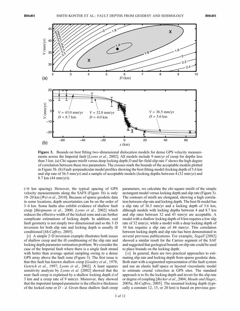
depth along 12main segments of the southern SAFS (Figure 4)using a geodetically constrained semianalytic dislocationmodel [Smith and Sandwell, 2003, 2006; Smith‐Konterand Sandwell, 2009]. Fault segments include Imperial (1),Coachella (2), Palm Springs (3), San Bernardino (4),Mojave (5), Carrizo (6), Superstition Mountains (7), Borrego(8), Coyote Creek (9), Anza (10), San Jacinto Valley (11),San Jacinto Mountains (12) (Table 1). In addition to thesemain segments, the total model (spanning 1000 × 1700 km inthe east‐west and north‐south directions) consists of 42 ver-tical fault segments imbedded in an elastic plate overlying aviscoelastic half‐space. Parameters and additional details forthis model are provided in the work of Smith‐Konter andSandwell [2009]. Deep slip is prescribed along each of themajor fault segments, which drives the secular interseismiccrustal block motions. Slip rates are largely derived fromgeological studies [Working Group on California EarthquakeProbabilities (WGCEP), 1995, 2003, 2007], which are incor-

porated into the model such that the cumulative slip rate acrossparalleling faults is constant. Fault segments are locked fromthe surface down to a variable locking depth,D, which is tunedto match the present‐day GPS measurements.[12] The relationship between surface velocity and lock-

ing depth is nonlinear, thus we estimate the depths using aniterative, least squares approach based on the Gauss‐Newtonmethod [cf. Smith and Sandwell, 2003]. The locking depth isvaried along each fault segment to minimize the weighted‐residual misfit to 1099 EarthScope Plate Boundary Observa-tory (PBO) GPS‐derived horizontal velocities. This methodsearches the parameter space for optimal combinations oflocking depths for all fault segments defined in the model.Uncertainties in estimated locking depths (1s standarddeviation) are determined from the covariance matrix of thefinal inversion iteration. Locking depth results are providedin Table 1. In a few special cases where recent single‐faultsegment investigations of locking depth are available and thefault is nearly two‐dimensional [i.e., Lyons et al., 2002], weadopt these estimates and adjust the uncertainty to reflect therange of results.[13] Geodetically determined locking depths for the south-

ern SAFS range from 5.9 to 21.5 km, with a mean of 13.9 kmand a standard deviation of 5.7 km. Uncertainties in lockingdepth are typically 1 to 3 km, depending on the density andquality of nearby geodetic observations. Lower uncertain-ties are estimated along the Coachella and Mojave segments(0.5 and 0.4 km, respectively) where the EarthScope GPSarray is quite dense (Figure 1b) and the velocity measure-ments have small errors. Larger uncertainties in locking depthoccur along the Palm Springs and San Jacinto Valley seg-ments (8 and 6.3 km, respectively). These fault segmentsare fairly complex and our simplified segmented model maynot capture their complex deformation. Note also, we assigngeologic slip rates of 23 and 12 mm/yr for the Palm Springsand San Jacinto Valley segments, respectively; however, sliprates for both of these segments are also highly contested[Sharp, 1981;Weldon and Sieh, 1985; Bird and Kong, 1994;

Figure 4. Fault location map of the southern San Andreas Fault System. Segment names and numbers cor-respond to those in Table 1.


4 of 12

Becker et al., 2004; Meade and Hager, 2005a]. A trade‐offin slip rate between the parallel strands of the San Andreasand San Jacinto faults has been suggested [Bennett et al.,2004] and our model likely requires an adjusted slip rate inthis region to provide tighter constraints on the locking depthover variable timescales.[14] The dense GPS array at the Imperial fault (Figure 5a)

illustrates the issues with shallow creep, showing that geod-esy only estimates the thickness of locked zone. Publishedvalues of locking depth for the Imperial fault range from 6 to13 km [Archuleta, 1984; Genrich et al., 1997; Lyons et al.,2002; Smith and Sandwell, 2003], typically accompanying35–40 mm/yr of slip. However, the Imperial fault is known toexhibit fairly complex slip behavior with associated creep andperhaps cannot be accurately modeled as a single fault seg-ment that is simply locked at depth. Our 3‐D locking depthinversion is 5.5 km, which includes 3 km of shallow creep.Because the Imperial fault is nearly straight, this 3‐D inver-sion corresponds to the 2‐D estimate shown in Figure 3.[15] As this approach of using geologically derived slip

rates to estimate locking depth is unique to our work, analysesby other groups are needed to relate our formal uncertaintiesin locking depth to the range of locking depths derived usingother methods. Recently, the Southern California EarthquakeCenter (SCEC) hosted a workshop to evaluate the role ofgeodetic data for updating the Unified California EarthquakeRupture Forecast Version 3 (UCERF3; see http://www.scec.org/workshops‐/2010/gpsucerf3‐Report_on_2010_SCEC_GPS_UCERF3‐_Workshop_v2.pdf and Smith‐Konter et al.[2010]). One of the exercises (E. Hearn, personal communi-cation, 2010) was to fit the geodetic data across the Carrizosegment of the SAF using whatever method investigators feltwas most appropriate. Six investigators participated in thisexercise using nine different modeling approaches rangingfrom simple elastic half‐space back slip models to full num-erical analyses using nonlinear time‐dependent rheology.Remarkably, all of the analyses provided roughly the samelocking depth solution (16.7 ± 2.2 km), suggesting thatthe derived value is largely independent of the method or

investigator. These 9 values disagree with older publishedmodels with a 25 km locking depth [Eberhart‐Phillips et al.,1990], suggesting that newer campaign data provided by theUSGS and EarthScope have helped refine the locking depthfor this segment. Slip rates along this region are reasonablywell constrained (i.e., 36 mm/yr; see Schmalzle et al. [2006]).Our estimate of locking depth for the Carrizo segment of18.7 +/− 2.0 km (Figure 5b) is on the higher end of the 6analyses but still within one standard deviation of the rangeof estimates. On the basis of this comparison of results,we believe that our geodetic estimates are accurate and theuncertainties depend on both the near‐fault data distributionand 3‐D geometry.

3. Seismogenic Thickness Estimated FromSeismicity

[16] A number of studies have examined the maximumdepth of seismicity in different regions in California andrelated the results to differences in heat flow, rock type, andmain shock rupture models [Doser and Kanamori, 1986;Miller and Furlong, 1988; Sanders, 1990; Williams, 1996;Magistrale and Zhou, 1996; Richards‐Dinger and Shearer,2000; Bonner et al., 2003; Nazareth and Hauksson, 2004].In general, these results depend upon the quality of theearthquake locations and the choice of a cutoff criteria usedto define the maximum depth. To achieve robust depth esti-mates that are insensitive to occasional stray earthquakelocations at large depth, most studies have assigned a cut-off percentile depth, which has ranged from 90% [Miller andFurlong, 1988; Richards‐Dinger and Shearer, 2000], to 95%[Williams, 1996], to 99% [Bonner et al., 2003]. A somewhatdifferent approachwas used byNazareth andHauksson [2004],who computed the 99.9% limit in total seismic moment(estimated from the local earthquake magnitudes for smallearthquakes). This study (NH04, hereafter) used earthquakesrelocated using a 3‐D velocity model and found that the 99.9%moment limit in background seismicity reliably predicted themaximum rupture depth of moderate to large earthquakesin Southern California.

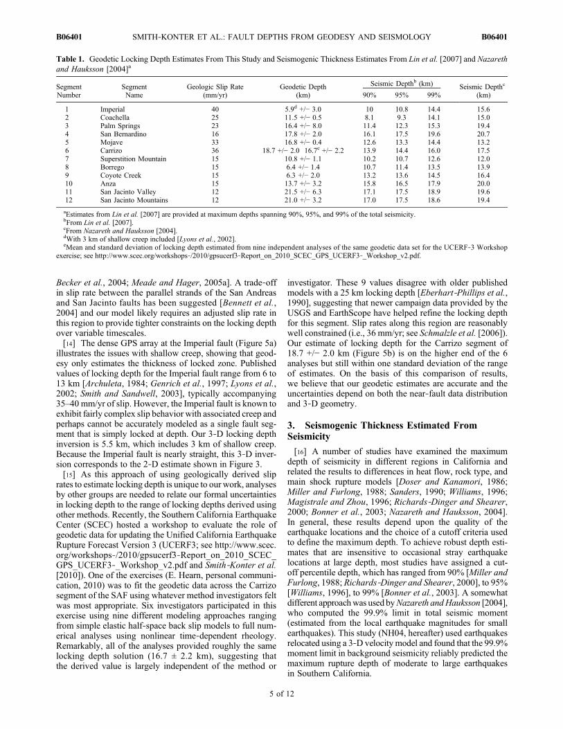
Table 1. Geodetic Locking Depth Estimates From This Study and Seismogenic Thickness Estimates From Lin et al. [2007] and Nazarethand Hauksson [2004]a

SegmentNumber

SegmentName

Geologic Slip Rate(mm/yr)

Geodetic Depth(km)

Seismic Depthb (km) Seismic Depthc

(km)90% 95% 99%

1 Imperial 40 5.9d +/− 3.0 10 10.8 14.4 15.62 Coachella 25 11.5 +/− 0.5 8.1 9.3 14.1 15.03 Palm Springs 23 16.4 +/− 8.0 11.4 12.3 15.3 19.44 San Bernardino 16 17.8 +/− 2.0 16.1 17.5 19.6 20.75 Mojave 33 16.8 +/− 0.4 12.6 13.3 14.4 13.26 Carrizo 36 18.7 +/− 2.0 16.7e +/− 2.2 13.9 14.4 16.0 17.57 Superstition Mountain 15 10.8 +/− 1.1 10.2 10.7 12.6 12.08 Borrego 15 6.4 +/− 1.4 10.7 11.4 13.5 13.99 Coyote Creek 15 6.3 +/− 2.0 13.2 13.6 14.5 16.410 Anza 15 13.7 +/− 3.2 15.8 16.5 17.9 20.011 San Jacinto Valley 12 21.5 +/− 6.3 17.1 17.5 18.9 19.612 San Jacinto Mountains 12 21.0 +/− 3.2 17.0 17.5 18.6 19.4

aEstimates from Lin et al. [2007] are provided at maximum depths spanning 90%, 95%, and 99% of the total seismicity.bFrom Lin et al. [2007].cFrom Nazareth and Hauksson [2004].dWith 3 km of shallow creep included [Lyons et al., 2002].eMean and standard deviation of locking depth estimated from nine independent analyses of the same geodetic data set for the UCERF‐3 Workshop

exercise; see http://www.scec.org/workshops‐/2010/gpsucerf3‐Report_on_2010_SCEC_GPS_UCERF3‐_Workshop_v2.pdf.


5 of 12

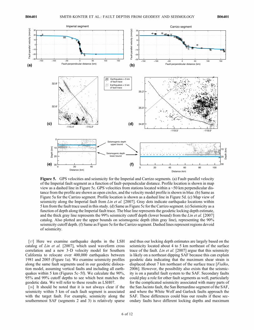
[17] Here we examine earthquake depths in the LSHcatalog of Lin et al. [2007], which used waveform crosscorrelation and a new 3‐D velocity model for SouthernCalifornia to relocate over 400,000 earthquakes between1981 and 2005 (Figure 1a). We examine seismicity profilesalong the same fault segments used in our geodetic disloca-tion model, assuming vertical faults and including all earth-quakes within 5 km (Figures 5c–5f). We calculate the 90%,95% and 99% cutoff depths to see which best matches thegeodetic data. We will refer to these results as LSH07.[18] It should be noted that it is not always clear if the

seismicity within 5 km of each fault segment is associatedwith the target fault. For example, seismicity along thesouthernmost SAF (segments 2 and 3) is relatively sparse

and thus our locking depth estimates are largely based on theseismicity located about 4 to 5 km northeast of the surfacetrace of the fault. Lin et al. [2007] argue that this seismicityis likely on a northeast dipping SAF because this can explaingeodetic data indicating that the maximum shear strain isdisplaced about 7 km northeast of the surface trace [Fialko,2006]. However, the possibility also exists that the seismic-ity is on a parallel fault system to the SAF. Secondary faultscould play a role for other fault segments as well, particularlyfor the complicated seismicity associated with many parts ofthe San Jacinto fault, the San Bernardino segment of the SAF,and where the White Wolf and Garlock faults approach theSAF. These differences could bias our results if these sec-ondary faults have different locking depths and maximum

Figure 5. GPS velocities and seismicity for the Imperial and Carrizo segments. (a) Fault‐parallel velocityof the Imperial fault segment as a function of fault‐perpendicular distance. Profile location is shown in mapview as a dashed line in Figure 5c. GPS velocities from stations located within a ∼50 km perpendicular dis-tance from the profile are shown as open circles, and the velocity model profile is shown in blue. (b) Same asFigure 5a for the Carrizo segment. Profile location is shown as a dashed line in Figure 5d. (c) Map view ofseismicity along the Imperial fault from Lin et al. [2007]. Gray dots indicate earthquake locations within5 km from the fault trace used in this study. (d) Same as Figure 5c for the Carrizo segment. (e) Seismicity as afunction of depth along the Imperial fault trace. The blue line represents the geodetic locking depth estimate,and the thick gray line represents the 99% seismicity cutoff depth (lower bound) from the Lin et al. [2007]catalog. Also plotted are the upper bounds on seismogenic depth (thin gray line), representing the 90%seismicity cutoff depth. (f) Same as Figure 5e for the Carrizo segment. Dashed lines represent regions devoidof seismicity.


6 of 12

seismicity depths than the main fault. However, as we willshow later, we generally observe a correlation between ourmeasured maximum seismicity depth and geodetic lockingdepth for these segments, suggesting that any biases owingto off‐fault seismicity are small.[19] For the fault segments used in this study, seismicity

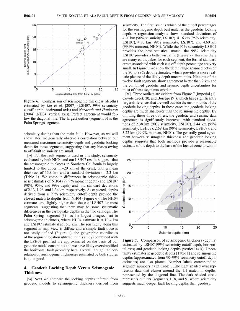
evaluated by both NH04 and our LSH07 results suggests thatthe seismogenic thickness in Southern California is largelylimited to the upper 11–20 km of the crust, with a meanthickness of 15.8 km and a standard deviation of 2.3 km(Table 1). We compute differences in seismogenic thick-ness estimates of NH04 (99.9% moment depth) and LSH07(90%, 95%, and 99% depth) and find standard deviationsof 2.13, 1.96, and 1.34 km, respectively. As expected, depthsderived from a 99% seismicity cutoff depth provide theclosest match to depths from NH04 (Figure 6). The NH04estimates are slightly higher than those of LSH07 for mostsegments, suggesting that there may be some systematicdifferences in the earthquake depths in the two catalogs. ThePalm Springs segment (3) has the largest disagreement inseismogenic thickness, where NH04 estimate it at 19.4 kmand LSH07 estimate it at 15.3 km. The seismicity along thissegment in map view is diffuse and a simple fault trace isnot easily defined (Figure 1); the geographic coordinatesof the segment location utilized in this study (combined withthe LSH07 profiles) are approximated on the basis of ourgeodetic model constraints and we have likely oversimplifiedthe horizontal fault geometry here. Overall though, the cor-relation of seismogenic thicknesses estimated by both studiesis quite good.

4. Geodetic Locking Depth Versus SeismogenicThickness

[20] Next we compare the locking depths inferred fromgeodetic models to seismogenic thickness derived from

seismicity. The first issue is which of the cutoff percentagesfor the seismogenic depth best matches the geodetic lockingdepth. A regression analysis shows standard deviations of4.20 km (90% seismicity, LSH07), 4.16 km (95% seismicity,LSH07), 4.30 km (99% seismicity, LSH07), and 4.60 km(99.9% moment, NH04). While the 95% seismicity LSH07provides the best statistical match, the 99% seismicityLSH07 provides a better visual fit (Figure 7). Because thereare many earthquakes for each segment, the formal standarderrors associated with each cut‐off depth percentage are verysmall. In Figure 7 we show the depth range spanned betweenthe 90 to 99% depth estimates, which provides a more real-istic picture of the likely depth uncertainties. Nine out of thetwelve fault segments show agreement better than 2 km andthe combined geodetic and seismic depth uncertainties formost of these segments overlap.[21] Three outliers are evident from Figure 7 (Imperial (1),

Coyote Creek (8), and Borrego (9)), which have significantlylarger differences that are well outside the error bounds of thegeodetic locking depths. In these cases the geodetic lockingdepths are much shallower than the seismogenic depths. Byomitting these three outliers, the geodetic and seismic dataagreement is significantly improved, with standard devia-tions of 2.38 km (90% seismicity, LSH07), 2.44 km (95%seismicity, LSH07), 2.68 km (99% seismicity, LSH07), and3.22 km (99.9% moment, NH04). The generally good agree-ment between seismogenic thickness and geodetic lockingdepths suggests that both methods provide a reasonableestimate of the depth to the base of the locked zone to within

Figure 6. Comparison of seismogenic thickness (depths)estimated by Lin et al. [2007] (LSH07, 99% seismicitycutoff depth, horizontal axis) and Nazareth and Hauksson[2004] (NH04, vertical axis). Perfect agreement would fol-low the diagonal line. The largest outlier (segment 3) is thePalm Springs segment.

Figure 7. Comparison of seismogenic thickness (depths)estimated by LSH07 (99% seismicity cutoff depth, horizon-tal axis) and geodetic locking depths (vertical axis). Uncer-tainty estimates in geodetic depths (Table 1) and seismogenicdepths (approximated from 90–99% seismicity cutoff depthestimates) are also plotted. Number labels correspond tosegment numbers as in Table 1.The light shaded oval rep-resents data that cluster around the 1:1 match in depths,represented by the diagonal line. The dark shaded circlerepresents outliers (segments 1, 8, and 9) where seismicitysuggests much deeper fault locking depths than geodesy.


7 of 12

a mean accuracy of 2.5 km when the three significant out-liers are excluded.

5. Seismic Moment Rate

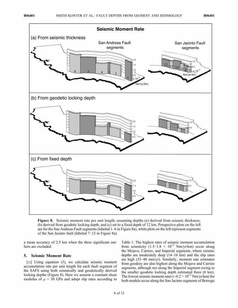
[22] Using equation (3), we calculate seismic momentaccumulation rate per unit length for each fault segment ofthe SAFS using both seismically and geodetically derivedlocking depths (Figure 8). Here we assume a constant shearmodulus of m = 30 GPa and adopt slip rates according to

Table 1. The highest rates of seismic moment accumulationfrom seismicity (1.5–1.8 × 1013 Nm/yr/km) occur alongthe Mojave, Carrizo, and Imperial segments, where seismicdepths are moderately deep (14–16 km) and the slip ratesare high (33–40 mm/yr). Similarly, moment rate estimatesfrom geodesy are also highest along the Mojave and Carrizosegments, although not along the Imperial segment owing tothe smaller geodetic locking depth estimated there (6 km).The lowest seismic moment rates (∼0.2 × 1013 Nm/yr/km) forboth models occur along the San Jacinto segments of Borrego

Figure 8. Seismic moment rate per unit length, assuming depths (a) derived from seismic thickness,(b) derived from geodetic locking depth, and (c) set to a fixed depth of 12 km. Perspective plots on the leftare for the San Andreas Fault segments (labeled 1–6 in Figure 8a), while plots on the left represent segmentsof the San Jacinto fault (labeled 7–12 in Figure 8a).


8 of 12

and Coyote Creek where the locking depth is shallower(∼6 km) and the slip rates are 12–15 mm/yr.

6. Discussion

[23] As previous studies have demonstrated, microseis-micity along the SAFS shows significant variations in seis-mogenic depth, ranging between 10 and 25 km [Nazarethand Hauksson, 2004]. Our geodetic analysis yields a slightlylarger depth range of 6 to 22 km. This relative agreementsuggests that these variations in fault depth are real. Dis-tributions of fault depths can be attributed to both geologicaland geophysical factors, such as crustal temperature andlithology [e.g., Miller and Furlong, 1988; Magistrale andZhou, 1996; Magistrale, 2002; Bonner et al., 2003]. Thesestudies suggest an inverse correlation between maximumdepth of seismicity and heat flow along the southern SAF,and our estimates of depth, both seismic and geodetic,are consistent with these results. High heat flow values(∼100 mW/m2; see Blackwell and Steele [1992]) and shallowdepths (6–10 km) are found in the Imperial Valley, whichis characterized by thick sediments and young mafic igneousrocks [Fuis et al., 1982; Lachenbruch et al., 1985;Magistrale,2002]. Alternatively, some of the lowest heat flow values inthis region (∼60 mW/m2) and deeper locking depths (18–21 km) are found in granitic rocks along the San GorgonioPass, straddling the San Bernardino and San Jacinto Valley/Mountains segments [Magistrale, 2002].

6.1. Seismic and Geodetic Depth Discrepancies

[24] The three significant outliers (1, Imperial; 8, CoyoteCreek; and 9, Borrego) all have geodetic locking depths thatare much less than the seismogenic depths. Of course thecreeping segment of the SanAndreas Fault is themost notableexample of this behavior, since the microseismicity extendsto a depth of ∼7–9 km [Bedrosian et al., 2004] while thethickness of the geodetic locked zone is essentially zero[Savage and Burford, 1973; Thatcher, 1979]. A recent studyof the San Jacinto fault zone (including both the Coyote Creekand Borrego segments) arrives at the same conclusion thatthe seismogenic depth is much greater than the thickness ofthe geodetically derived locked zone [Wdowinski, 2009].Creep rates of ∼5 mm/yr have been observed along thesouthern San Jacinto fault [Louie et al., 1985]; however, radarinterferometry [Vincent, 1998; Lyons and Sandwell, 2003]shows no evidence for shallow creep except along thesouthernmost Superstition Mountain segment where theslip occurs in episodes with a mean rate of 3 mm/yr [Weiet al., 2010]. The largest outlier is the Imperial fault wherethe geodetic locking depth is only 6 km and the seismogenicdepth is 14 km. This is a case where geodetically determineddepths track middle‐depth clusters of seismicity (∼5–10 km;see Figure 5e). As previously discussed, the Imperial segmentis known to exhibit both locked fault and creeping deformationbehaviors with depth [Lyons et al., 2002; Shearer, 2002],which appear to complicate both geodetic and seismic esti-mates of the thickness of the locked zone.[25] It is possible that discrepancies in seismic and geodetic

depths are revealing time‐varying stress adjustments at depththroughout the earthquake cycle. If a recent earthquake hasoccurred on a fault segment, microseismicity can reflect a

redistribution of stress within the fault zone. Outlier segments1 and 9 have had relatively recent earthquakes (Imperial,1940 and 1979; Borrego, 1968). In particular, aftershocksin the first 2 months following theM6.6 1979 Imperial Valleyearthquake were 2–3 km deeper than premain shock seis-micity [Doser and Kanamori, 1986]. Similar behavior wasobserved for the 1992 M7.3 Landers earthquake [Rolandoneet al., 2004] where aftershock depths deepened from pre‐earthquake levels by as much as 3 km over 4 years. Thus it ispossible that deeper distributions of seismicity along histor-ically active faults of the SAFS can be attributed to post-seismic stress adjustments. Earthquake cycle effects are alsoknown to complicate geodetic estimations of true lockingdepth [Savage, 1990; Meade and Hager, 2004], where faultlocking depths tend to deepen nearing the end of an earth-quake cycle.[26] We must also consider the possibility that some of the

differences in depth may be explained by along‐strike var-iations in slip mechanisms, such as patches of verticalcreeping between locked regions. The Parkfield segmentnorth of our study area is known to exhibit such localized slipvariations [Harris and Segall, 1987; Werner et al., 1997;Murray et al., 2001]. Combined with the long‐wavelengthalong‐strike variations in depth along the entire SAFS, it iscertainly possible that individual fault segments may havesmall vertical creeping patches that are unaccounted for here.The impact of along‐strike creeping patches on geodeticdepths depends on the assigned fault segment length, and if asegment were to exhibit a significant span of creep along‐strike, then geodetic measurements straddling such a regionshould yield a shallower depth than a fault segment that wasstrictly locked along strike.[27] Recent evidence of nonvolcanic tremor has also been

linked to vertical transition zones from fault locking toaseismic slip [Obara et al., 2004; Rogers and Dragert, 2003].While nonvolcanic tremor has been identified in six regionsin California to date [Nadeau and Dolenc, 2005; Gomberget al., 2008], the only known tremor location relevant tothis study is along the San Jacinto Valley segment nearHemet, CA.Here tremor depths, although poorly constrained,are estimated at 12 km depth [Gomberg et al., 2008]. Thisdepth is much shallower than the geodetic depth (21 km) andthe 99% seismicity cutoff depth (19 km) determined for thissegment. There is no evidence of shallow fault creep alongthis fault segment, but perhaps deeper aseismic slip is takingplace here, as has been suggested for fault segments to thesouth of this segment along the San Jacinto fault [Wdowinski,2009].

6.2. Fault Geometry

[28] This analysis assumes that the fault depth is constantwith each predefined fault segment strike. How realistic is thisassumption? Both geodetic and seismic estimates presentedhere are basically an along‐strike average of the data sampled.Since geodetic estimates are model dependent and requirea complicated segmentation scheme to provide sufficientalong‐strike resolution to address realistic variations, someguidance is provided by the seismicity. Significant along‐strike variations in fault depth are evident in the seismicrecord, where for example, the San Bernardino segment hasa maximum depth of seismicity that is much deeper in the


9 of 12

south (∼20 km) than in the north (10–15 km) [Magistrale andZhou, 1996; Richards‐Dinger and Shearer, 2000, Plate 6;Nazareth and Hauksson, 2004]. Such variations may be dueto reverse faulting in the structurally complex area along theSan Gorgonio Pass [Yule and Sieh, 2003]. In this study wesegment sections of the SAF consistent with our geodeticanalysis, which follows previous segmentation schemes byWGCEP [1995, 2007] and Plesch et al. [2007]. In particular,we treat most of the San Bernardino segment as one estimate.NH04 considered this issue and evaluated seismic depths on a5 km scale, in addition to an along‐strike average. For the SanBernardino segment, for example, the 5 km segmentation andthe along‐strike average have depth differences of about3 km. Geodetic determination of locking depth requires adense array of stations within <6 km of a fault (across‐strike),and while this is available along some fault segments (e.g.,Imperial), it is not feasible for the entire system so the seg-mentation must be rather coarse. This coarse segmenta-tion does not always capture the transition from lockedto unlocked faults. Nevertheless, locking depth estimatesfrom geodesy do provide realistic locking depths in regionswhere microseismicity is relatively scarce (i.e., Death Valley,Eastern California Shear Zone).[29] Dipping fault geometry may also play an important

role in understanding discrepancies between geodetic andseismic fault depths. While the orientations of most segmentsof the SAFS are assumed to be vertical (Community FaultModel; see http://structure.harvard.edu/cfm, Plesch andShaw [2003], and Plesch et al. [2007]), some recent studieshave suggested a variable degree of dip. Most notably, alongthe Carrizo and Coachella segments, fault dips are estimatedbetween 55 and 75 degrees to the southwest and between 37and 60 degrees to the northeast, respectively [Lin et al., 2007;Fuis, 2007; Fuis et al., A new perspective on the geometry ofthe San Andreas Fault in Southern California and its rela-tionship to lithospheric structure, submitted to Bulletin of theSeismological Society of America]. Fault dip has also beenestimated for the Imperial fault at roughly 80 degrees tothe east [Reilinger and Larsen, 1986]. Our geodetic modelassumes a vertical dipping geometry for all fault segments ofthe SAFS, and this assumption may introduce an additionalsource of error when estimating fault depth. The fact thatwe observe seismic depths that are mostly a few kilometersdeeper than geodetic depths follows the idea that a dippingfault would lengthen the geodetic locking depth. The largestdiscrepancy of fault depth, however, is largely derived fromsegments of the San Jacinto fault. Fault dip for segments ofthe San Jacinto fault are not well documented in the literatureand the faults are typically assumed to be vertical. Inspectionof the seismicity along the San Jacinto fault in map view alsosupports a vertical fault geometry, as the earthquake locationsprimarily align with the known mapped fault trace. Thesouthernmost 15 km of the Coyote Creek fault segment,however, does show a clustering of seismicity to the southeastof the mapped fault trace, suggesting a dipping geometry maybe relevant here.

6.3. Role of Fault Depth in Seismic Hazard Analyses

[30] These results have major implications for the seismicmoment accumulation rate of segments of the SAFS.Momentaccumulation rate is often calculated from observed rates of

surface strain accumulation [WGCEP, 1995, 1999; Ward,1994; Savage and Simpson, 1997] and typically evaluatedfor a constant locking depth of 10–15 km [WGCEP, 1995,WGNCEP, 1996; Meade and Hager, 2005b]. However, asour results clearly illustrate, seismic moment accumulationrates are very different when a constant locking depth of, forexample, 12 km is adopted (Figure 8c). In this case, the largestmoment accumulation rate occurs along the Imperial andCarrizo segments where the slip rate is largest (∼37 mm/yr).The factor of 2 increase on the Imperial segment in com-parison with geodetic depths (Figure 8b) reflects the factorof 2 increase in locking depth, while the 1/3 decrease inmomentrate along the Carrizo segment is related to the 1/3 decrease inlocking depth. The mean value of each group of seismicmoment accumulation rates is also reflective of depth behavior:0.99 × 1013 Nm/yr/km (seismic depths), 0.87 × 1013 Nm/yr/km(geodetic depths), and 0.77 × 1013 Nm/yr/km (constant D =12 km). Moreover, we find that the main San Andreas Faultstrand (including segments 1–6) accumulates roughly 67–70%of the seismic moment budget for all three models.[31] The Uniform California Earthquake Rupture Fore-

cast Version 2 (UCERF2) report [WGCEP, 2007] similarlyrecognizes the southern San Andreas as a region of elevatedseismic potential. Overall, this study emphasizes the southernSan Andreas (segments 2–6 here) as the region of most sig-nificant earthquake hazard in all of California, having a 59%probability of aM ≥ 6.7 event over the next 30 years.WGCEP[2007] also determines a 31% probability for the San Jacintosegment (segments 7–12 here) and a 27% probability forthe Imperial segment. For the faults included in our study,the UCERF2 report presents the highest “participationprobability” of rupture occurrence for theMojave and Carrizosegments of the San Andreas, consistent with the rela-tively higher seismic moment rates of these segments fromboth seismic and geodetic estimates (Figure 8). Conversely,UCERF2 segment rupture probabilities are highest along theCoachella segment, while this segment’s calculated seismicmoment rate is not unusually large; only when one accountsfor the time elapsed since the last major earthquake event(300+ years) does the Coachella segment’s accumulatedseismic moment become significant. It is also importantto note that depths utilized by the WGCEP [2007] for theUCERF2 report (which are largely based onmaximum depthsof background seismicity; seeNazareth andHauksson [2004]and Plesch et al. [2007]) span a relatively small range, ∼10–17 km, in comparison with the 6–22 km geodetic depth rangepresented here. While UCERF2 fault depths are sometimeslarger than our geodetic depths (e.g., 15.9 km for CoyoteCreek), relative shallower depths are also reported (e.g.,12.8 km for San Bernardino).

7. Conclusions

[32] In summary, this study of seismic and geodeticdepths of the southern San Andreas Fault System has shownthat maximum depths of seismicity largely agree with faultlocking depths derived from geodetic models. Of the 12 faultsegments analyzed here, we identify 3 outliers (Imperial,Coyote Creek, and Borrego segments) with significant(>8 km) seismic verses geodetic depth disagreements. Forthese segments, maximum seismicity depths are much larger


10 of 12

than geodetic locking depth estimates, suggesting that shal-low creep or temporal variations in strain release throughoutthe earthquake cycle may contribute to these discrepancies.[33] These results also highlight several important points

that warrant further consideration. First, significant depthvariations exist throughout the southern SAFS, bracketed bya range as large as 6 to 22 km. This result, combined witha statistical correlation between locking depth and slip rate,suggests that geodetically derived slip rates using modelshaving fixed locking depths (i.e., 12 or 15 km) may beinaccurate. At least 7 of the 12 segments studied here havegeodetic locking depths outside of the standard 12–15 kmrange. Furthermore, while geodetic depths indicate that12 km is closer to the mean depth for segments of the southernSAFS, seismicity shows that 12 km might be a minimumfaulting depth. This analysis also suggests that part of thedisagreement between geodetically derived slip rates andgeologically derived slip rates [e.g., Weldon and Sieh, 1985;Meade and Hager, 2005a] may be due in part to an incorrectassumption of a constant locking depth for fault segments.Moreover, when evaluating slip rates on faults, geodeticmodels should consider adopting variable depths from micro-seismicity to approximate the base of the locked zone.[34] Finally, we urge future earthquake probability work-

ing groups and other independent seismic hazard analysesto consider depth variations reflected in geodetic models.Dense geodetic data sets (GPS and InSAR) are now availableto further scrutinize fault locking depths of the SAFS. Asdemonstrated here, geodetic depths are largely consistentwith maximum seismicity depths but provide a larger rangeof depth variations throughout the fault system. Thesedepths can yield drastically different seismic moment ratesfor a single segment (in some cases, over a factor of 2), whichshould ultimately be reflected in earthquake probabilityforecasts.

[35] Acknowledgments. We thank Ross Stein and an anonymousreviewer for their helpful comments for improving this manuscript. We alsothank Teira Solis for her assistance with figure graphics. This research wassupported by the National Science Foundation (NSF; EAR0838252,EAR0811772, and EAR0847499), NASA (NNX09AD12G), and the South-ern California Earthquake Center (SCEC). SCEC is funded by NSF Cooper-ative Agreement EAR‐0106924 and USGS Cooperative Agreement02HQAG0008. The SCEC contribution number for this paper is 1471.

ReferencesArchuleta, R. J. (1984), A faulting model for the 1979 Imperial Valleyear thquake, J. Geophys. Res. , 89 , 4559–4585, doi:10.1029/JB089iB06p04559.

Becker, T. W., J. Hardebeck, and G. Anderson (2004), Constraints on faultslip rates of the Southern California plate boundary from GPS velocityand stress inversions, Geophys. J. Int., 160, 634–650, doi:10.1111/j.1365-246.

Bedrosian, P. A., M. J. Unsworth, G. D. Egert, and C. H. Thurber (2004),Geophysical images of the creeping segment of the San Andreas Fault:Implications for the role of crustal fluids in the earthquake process,Tectonophysics, 385, 137–158, doi:10.1016/j.tecto.2004.02.010.

Bennett, R. A., A. M. Friedrich, and K. P. Furlong (2004), Co‐dependenthistories of the San Andreas and San Jacinto fault zones from inversionof geologic displacement rate data, Geology, 32, 961–964, doi:10.1130/G20806.1.

Bird, P., and X. Kong (1994), Computer simulations of California tectonicsconfirm very slow strength of major faults, Geol. Soc. Am. Bull., 106,159–174, doi:10.1130/0016-7606(1994)106<0159:CSOCTC>2.3.CO;2.

Blackwell, D. D., and J. L. Steele (1992), The decade of North Americangeology, geothermal map of North America, scale 1:5,000,000, Geol.Soc. of Am., Denver.

Bonner, J. L., D. D. Blackwell, and E. T. Herrin (2003), Thermal con-straints on earthquake depths in California, Bull. Seismol. Soc. Am., 93,2333–2354, doi:10.1785/0120030041.

Brace, W. F., and J. D. Byerlee (1970), California earthquakes: Why onlyshallow focus?, Science, 168, 1573–1575, doi:10.1126/science.168.3939.1573.

Bürgmann, R., D. Schmidt, R. M. Nadeau, M. d’Alessio, E. Fielding,D. Manaker, T. V. McEvilly, and M. H. Murray (2000), Earthquakepotential along the northern Hayward fault, California, Science, 289,1178–1182, doi:10.1126/science.289.5482.1178.

Das, S., and C. H. Scholz (1983), Why large earthquakes do not nucleate atshallow depths, Nature, 305, 621–623, doi:10.1038/305621a0.

Doser, D. I., and H. Kanamori (1986), Depth of seismicity in the ImperialValley region (1997–1983) and its relationship to heat flow, crustalstructure, and the October 15, 1979, earthquake, J. Geophys. Res., 91,675–688, doi:10.1029/JB091iB01p00675.

Eberhart‐Phillips, D., M. Lisowski, and M. D. Zoback (1990), Crustalstrain near the Big Bend of the San Andreas Fault: Analysis of the LosPadres‐Tehachapi trilateration networks, California, J. Geophys. Res.,95, 1139–1153, doi:10.1029/JB095iB02p01139.

Fialko, Y. (2006), Interseismic strain accumulation and the earth-quake potential on the southern San Andreas Fault System, Nature,441, 968–971, doi:10.1038/nature04797.

Fuis, G. (2007), The San Andreas Fault in Southern California is almostnowhere vertical–Implications for tectonics, paper presented at theAnnual Meeting of the Geological Society of America, Denver.

Fuis, G., W. Mooney, J. Healey, G. McMechan, and W. Lutter (1982),Crustal structure of the Imperial Valley region, U.S. Geol. Surv. Prof.Pap., 1254, 25–50.

Genrich, J. F., Y. Bock, and R. G. Mason (1997), Crustal deformationacross the Imperial fault: Results from kinematic GPS surveys and trila-teration of a densely spaced, small‐aperture network, J. Geophys. Res.,102, 4985–5004, doi:10.1029/96JB02854.

Gomberg, J., J. Rubinstein, Z. Peng, K. Creager, J. Vidale, and P. Boudin(2008), Widespread triggering of nonvolcanic tremor in California,Science, 319, 173, doi:10.1126/science.1149164.

Goultry, N. R., R. O. Burford, C. R. Allen, R. Gilman, C. E. Johnson, andR. P. Keller (1978), Large creep events on the Imperial fault, California,Bull. Seismol. Soc. Am., 68, 517–521.

Harris, R. A., and P. Segall (1987), Detection of a locked zone at depth onthe Parkfield, California, segment on the San Andreas Fault, J. Geophys.Res., 92, 7945–7962, doi:10.1029/JB092iB08p07945.

Hill, D. P., J. P. Eaton, and L. M. Jones (1990), Seismicity, U.S. Geol. Surv.Prof. Pap., 1515, 115–151.

Lachenbruch, A., J. Sass, and S. Galanis Jr. (1985), Heat flow in southern-most California and the origin of the Salton trough, J. Geophys. Res., 90,6709–6736, doi:10.1029/JB090iB08p06709.

Lin, G., P. M. Shearer, and E. Hauksson (2007), Applying a three‐dimensional velocity model, waveform cross correlation, and clusteranalysis to locate Southern California seismicity from 1981 to 2005,J. Geophys. Res., 112, B12309, doi:10.1029/2007JB004986.

Louie, J. N., C. R. Allen, D. C. Johnson, P. C. Haase, and S. N. Cohn(1985), Fault slip in Southern California, Bull. Seismol. Soc. Am., 75,811–833.

Lyons, S., and D. Sandwell (2003), Fault creep along the southern SanAndreas from interferometric synthetic aperture radar, permanent scat-terers, and stacking, J. Geophys. Res., 108(B1), 2047, doi:10.1029/2002JB001831.

Lyons, S., Y. Bock, and D. T. Sandwell (2002), Creep along the Imperialfault, Southern California, from GPS measurements, J. Geophys. Res.,107(B10), 2249, doi:10.1029/2001JB000763.

Magistrale, H. (2002), Relative contributions of crustal temperature andcomposition to controlling the depth of earthquakes in Southern Califor-nia, Geophys. Res. Lett., 29(10), 1447, doi:10.1029/2001GL014375.

Magistrale, H., and H. Zhou (1996), Lithologic control of the depthof earthquakes in Southern California, Science, 273, 639–642,doi:10.1126/science.273.5275.639.

Marone, C., and C. H. Scholz (1988), The depth of seismic faulting and theupper transition from stable to unstable slip regimes, Geophys. Res. Lett.,15, 621–624, doi:10.1029/GL015i006p00621.

McCaffrey, R. (2005), Block kinematics of the Pacific–North Americaplate boundary in the southwestern United States from inversion ofGPS, seismological, and geologic data, J. Geophys. Res., 110, B07401,doi:10.1029/2004JB003307.


11 of 12

Meade, B. J., and B. H. Hager (2004), Viscoelastic deformation for a clus-tered earthquake cycle, Geophys. Res. Lett., 31, L10610, doi:10.1029/2004GL019643.

Meade, B. J., and B. H. Hager (2005a), Block models of crustal motion inSouthern California constrained by GPS measurements, J. Geophys. Res.,110, B03403, doi:10.1029/2004JB003209.

Meade, B. J., and B. H. Hager (2005b), Spatial localization of moment def-icits in Southern California, J. Geophys. Res., 110, B04402, doi:10.1029/2004JB003331.

Miller, C. K., and K. P. Furlong (1988), Thermal‐mechanical controls onseismicity depth distributions in the San Andreas Fault Zone, Geophys.Res. Lett., 15, 1429–1432, doi:10.1029/GL015i012p01429.

Murray, J. R., P. Segall, P. Cervelli, W. Prescott, and J. Svarc (2001),Inversion of GPS data for spatially variable slip‐rate on the San AndreasFault near Parkfield, CA, Geophys. Res. Lett., 28, 359–362, doi:10.1029/2000GL011933.

Nadeau, R. M., and D. Dolenc (2005), Nonvolcanic tremors beneath theSan Andreas Fault, Science, 307, 389, doi:10.1126/science.1107142.

Nazareth, J. J., and E. Hauksson (2004), The seismogenic thickness of theSouthern California crust, Bull. Seismol. Soc. Am., 94, 940–960,doi:10.1785/0120020129.

Obara, K., H. Hirose, F. Yamamizu, and K. Kasahara (2004), Episodicslow slip events accompanied by nonvolcanic tremors in southwest Japansubduction zone, Geophys. Res. Lett., 31, L23602, doi:10.1029/2004GL020848.

Peterson, M. D., W. A. Bryant, C. H. Cramer, T. Cao, M. S. Reichle, A. D.Frankel, J. J. Lienkaemper, P. A. McCrory, and D. P. Schwartz (1996),Probabilistic seismic hazard assessment for the state of California, U.S.Geol. Surv. Open File Rep. 96‐76, 1–64.

Plesch, A., and J. H. Shaw (2003), SCEC CFM: A WWW accessible com-munity fault model for Southern California, Eos Trans. AGU, 84(46),Fall Meet. Suppl., Abstract S12B‐0395.

Plesch, A., et al. (2007), Community Fault Model (CFM) for SouthernCalifornia, Bull. Seismol. Soc. Am., 97, 1793–1802, doi:10.1785/0120050211.

Reilinger, R., and S. Larsen (1986), Vertical crustal deformation associatedwith the 1979 M = 6.6 Imperial Valley, California, earthquake: Impli-cations for fault behavior, J. Geophys. Res., 91, 14,044–14,056,doi:10.1029/JB091iB14p14044.

Richards‐Dinger, K. B., and P. M. Shearer (2000), Earthquake locationsin Southern California obtained using source‐specific station terms,J. Geophys. Res., 105, 10,939–10,960, doi:10.1029/2000JB900014.

Rogers, G., and H. Dragert (2003), Episodic tremor and slip on theCascadia Subduction Zone: The chatter of silent slip, Science, 300,1942–1943, doi:10.1126/science.1084783.

Rolandone, F., R. Bürgmann, and R. M. Nadeau (2004), The evolution ofthe seismic‐aseismic transition during the earthquake cycle: Constraintsfrom the time‐dependent depth distribution of aftershocks, Geophys.Res. Lett., 31, L23610, doi:10.1029/2004GL021379.

Sanders, C. O. (1990), Earthquake depths and the relation to strain accu-mulation and stress near strike‐slip faults in Southern California,J. Geophys. Res., 95, 4751–4762, doi:10.1029/JB095iB04p04751.

Savage, J. C. (1990), Equivalent strike‐slip earthquake cycles in half‐spaceand lithosphere‐asthenosphere earth models, J. Geophys. Res., 95, 4873–4879, doi:10.1029/JB095iB04p04873.

Savage, J. C. (2006), Dislocation pileup as a representation of strainaccumulation on a strike‐slip fault, J. Geophys. Res., 111, B04405,doi:10.1029/2005JB004021.

Savage, J. C., and R. O. Burford (1973), Geodetic determination of relativeplate motion in central California, J. Geophys. Res., 78, 832–845,doi:10.1029/JB078i005p00832.

Savage, J. C., and R. W. Simpson (1997), Surface strain accumulation andthe seismic moment tensor, Bull. Seismol. Soc. Am., 87, 1345–1353.

Schmalzle, G., T. Dixon, R. Malservisi, and R. Govers (2006), Strain accu-mulation across the Carrizo segment of the San Andreas Fault, Califor-nia: Impact of laterally varying crustal properties, J. Geophys. Res.,111, B05403, doi:10.1029/2005JB003843.

Segall, P. (2002), Integrating geologic and geodetic estimates of slip rate onthe San Andreas Fault system, Int. Geol. Rev., 44, 62–82, doi:10.2747/0020-6814.44.1.62.

Sharp, R. V. (1981), Variable rates of late Quaternary strike slip on theSan Jacinto fault zone, Southern California, J. Geophys. Res., 86,1754–1762, doi:10.1029/JB086iB03p01754.

Shearer, P. M. (2002), Parallel fault strands at 9‐km depth resolved on theImperial fault, Southern California, Geophys. Res. Lett., 29(14), 1674,doi:10.1029/2002GL015302.

Smith, B., and D. Sandwell (2003), Coulomb stress accumulation alongthe San Andreas Fault System, J. Geophys. Res., 108(B6), 2296,doi:10.1029/2002JB002136.

Smith, B. R., and D. T. Sandwell (2006), A model of the earthquake cyclealong the San Andreas Fault System for the past 1000 years, J. Geophys.Res., 111, B01405, doi:10.1029/2005JB003703.

Smith‐Konter, B., and D. Sandwell (2009), Stress evolution of theSan Andreas Fault System: Recurrence interval versus locking depth,Geophys. Res. Lett., 36, L13304, doi:10.1029/2009GL037235.

Smith‐Konter, B., D. T. Sandwell, and M. Wei (2010), Integrating GPS andInSAR to resolve stressing rates of the SAF system, EarthScope inSightsNewsl., Summer 2010, 1–3.

Stein, R. S. (2008), Appendix D: Earthquake Rate Model 2 of the 2007Working Group for California Earthquake Probabilities, Magnitude‐AreaRelationships, U.S. Geol. Surv. Open File Rep., 2007‐1437D, 1–16.

Thatcher, W. (1979), Systematic inversion of geodetic data in centralCal ifornia , J. Geophys. Res. , 84 , 2283–2295, doi :10.1029/JB084iB05p02283.

Vincent, P. (1998), Application of SAR interferometry to low‐rate crustaldeformation fields, Ph.D. dissertation, Univ. of Colo. at Boulder,Boulder, Colo.

Ward, S. N. (1994), A multidisciplinary approach to seismic hazard inSouthern California, Bull. Seismol. Soc. Am., 84, 1293–1309.

Wdowinski, S. (2009), Deep creep as a cause for the excess seismicityalong the San Jacinto fault, Nat. Geosci., 2, 882–885, doi:10.1038/ngeo684.

Wei, M., D. T. Sandwell, and B. Smith‐Konter (2010), Optimal combina-tion of InSAR and GPS for measuring interseismic crustal deformation,Adv. Space Res., 46, 236–249, doi:10.1016/j.asr.2010.03.013.

Weldon, R., and K. E. Sieh (1985), Holocene rate of slip and tentativerecurrence interval for large earthquakes on the San Andreas Fault, CajonPass, Southern California, Geol. Soc. Am. Bull., 96, 793–812,doi:10.1130/0016-7606(1985)96<793:HROSAT>2.0.CO;2.

Weldon, R., T. Fumal, and G. Biasi (2004), Wrightwood and theearthquake cycle: What a long recurrence record tells us about howfaults work, GSA Today, 14, 4–10, doi:10.1130/1052-5173(2004)014<4:WATECW>2.0.CO;2.

Werner, C. L., P. Rosen, S. Hensley, E. Fielding, and S. Buckley (1997),Detection of aseismic creep along the San Andreas Fault near Parkfield,California, with ERS‐1 radar interferometry, paper presented at the 3rdERS Symposium, Eur. Space Agency, Florence, Italy.

Williams, C. F. (1996), Temperature and the seismic/aseismic transition:Observations from the 1992 Landers earthquake, Geophys. Res. Lett.,23, 2029–2032, doi:10.1029/96GL02066.

Working Group on California Earthquake Probabilities (WGCEP) (1995),Seismic hazards in Southern California: Probable earthquakes, 1994 to2024, Bull. Seismol. Soc. Am., 85, 379–439.

Working Group on California Earthquake Probabilities (WGCEP) (1999),Earthquake probabilities in the San Francisco Bay Region: 2000 to2030—A summary of findings, U.S. Geol. Surv. Open File Rep., 99‐517, 1–60. (Available at http://geopubs.wr.usgs.gov/open‐file/of99‐517/.)

Working Group on California Earthquake Probabilities (WGCEP) (2003),Earthquake probabilities in the San Francisco Bay region: 2002–2031,U.S. Geol. Surv. Open File Rep., 03‐214, 1–235. (Available at http://pubs.usgs.gov/of/2003/of03‐214/.)

Working Group on California Earthquake Probabilities (WGCEP) (2007),The Uniform California Earthquake Rupture Forecast, Version 2(UCERF 2), U.S. Geol. Surv. Open File Rep., 2007‐1473, 1–104.

Working Group on Northern California Earthquake Potential (WGNCEP)(1996), Database of potential sources for earthquakes larger than magni-tude 6 in Northern California, U.S. Geol. Surv. Open File Rep., 96‐705.

Yule, D., and K. Sieh (2003), Complexities of the San Andreas Fault nearSan Gorgonio Pass: Implications for large earthquakes, J. Geophys. Res.,108(B11), 2548, doi:10.1029/2001JB000451.

D. Sandwell and P. Shearer, Institute for Geophysics and PlanetaryPhysics, Scripps Institution of Oceanography, University of California,San Diego, 500 W. University Dr., La Jolla, CA 92093‐0225, USA.B. Smith‐Konter, Department of Geological Sciences, University of

Texas at El Paso, El Paso, TX 79968‐0555, USA. ([email protected])


12 of 12

Documents

Locking depths estimated from geodesy and seismology along ...shearer/mahi/PDF/2011/SmithKonter_JGR...Locking depths estimated from geodesy and seismology along the San Andreas Fault