Embed Size (px)
Citation preview
Łódź, 2008
Intelligent Text Processinglecture 2
Multiple and approximate string matching.Full-text indexing: suffix tree, suffix array
Szymon [email protected]
http://szgrabowski.kis.p.lodz.pl/IPT08/
2
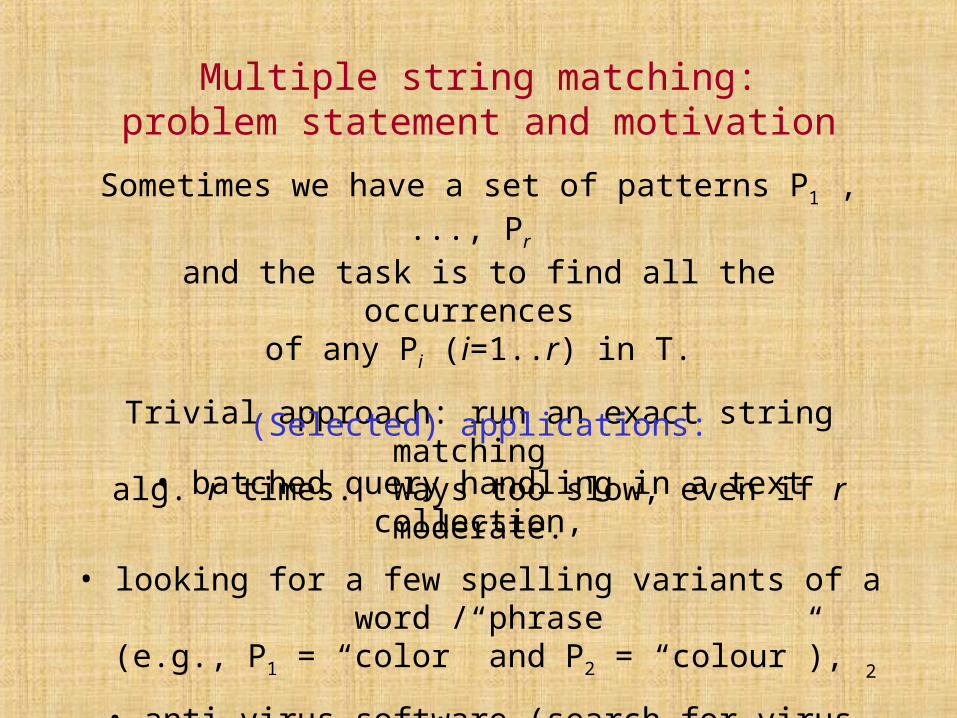
Multiple string matching:problem statement and motivation
Sometimes we have a set of patterns P1 , ..., Pr and the task is to find all the occurrences
of any Pi (i=1..r) in T.
Trivial approach: run an exact string matching alg. r times. Ways too slow, even if r moderate.
(Selected) applications:
• batched query handling in a text collection,
• looking for a few spelling variants of a word / phrase(e.g., P1 = “color” and P2 = “colour”),
• anti-virus software (search for virus signatures).
3
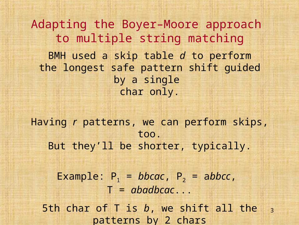
Adapting the Boyer–Moore approach to multiple string matching
BMH used a skip table d to performthe longest safe pattern shift guided by a single
char only.
Having r patterns, we can perform skips, too.But they’ll be shorter, typically.
Example: P1 = bbcac, P2 = abbcc, T = abadbcac...
5th char of T is b, we shift all the patterns by 2 chars(2 = min(2,3)).
4
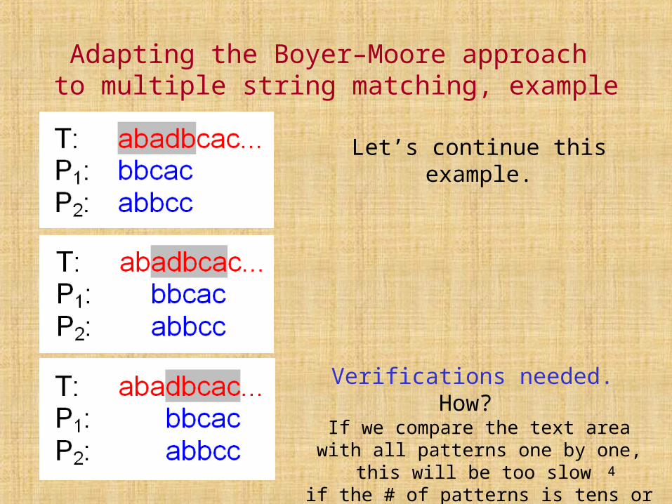
Adapting the Boyer–Moore approach to multiple string matching, example
Let’s continue this example.
Verifications needed. How? If we compare the text area with all
patterns one by one, this will be too slow if the # of patterns is tens or more.
We can do it better...
E.g. with a trie.
5
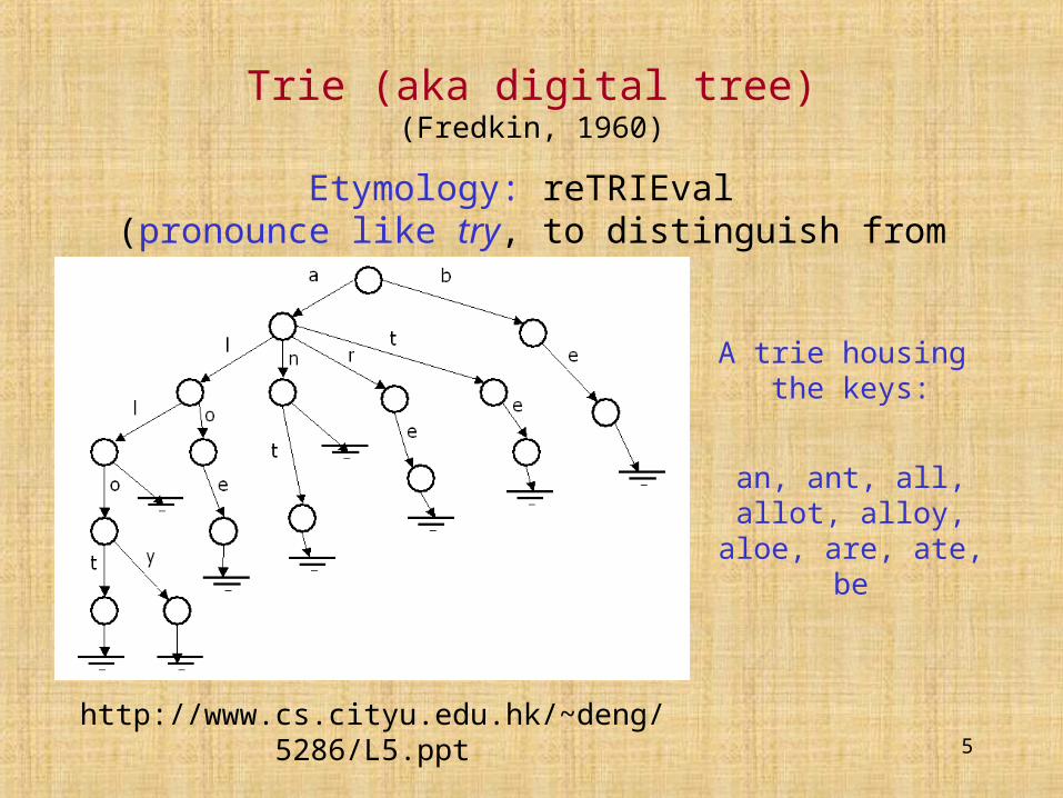
Trie (aka digital tree)(Fredkin, 1960)
Etymology: reTRIEval (pronounce like try, to distinguish from tree)
http://www.cs.cityu.edu.hk/~deng/5286/L5.ppt
A trie housing the keys:
an, ant, all, allot, alloy, aloe, are, ate,
be
6
Trie design dilemma
Natural tradeoff between search timeand space occupancy.
If only pointers from the “existing” chars in a node are kept, it’s more space-efficient but time spent in a node
is O(log ) (binary search in a node).Note: binary search is good in theory
(for the worst case), but usually bad in practice(apart from top trie levels / large alphabets?).
The time per node can be improved to O(1) (a single lookup) if each node takes O() space.
In total, pattern search takes either O(m log ) or O(m) worst case time.
7
Let’s trie to do it better...
In most cases tries require a lot of space.
A widely-used improvement: path compression, i.e., combining every non-branching
node with its child = Patricia trie (Morrison, 1968).
Other ideas: using smartly only one bit per pointer, or one pointer for all the children of a node.
PATRICIA stands for Practical Algorithm To Retrieve InformationCoded in Alphanumeric
8
Rabin–Karp algorithmcombined with binary search
(Kytöjoki et al., 2003)
From the cited paper:
Preprocessing: hash values for all patterns are calculated and stored in an ordered table.
Matching can then be done by calculating the hash value for each m-char string of the text and searching the
ordered table for this hash value using binary search. If a matching hash value is found, the corresponding
pattern is compared with the text.

9
Rabin–Karp alg combined with binary search, cont’d(Kytöjoki et al., 2003)
Kytöjoki et al. implemented this method for m = 8, 16, and 32.
The hash values for patterns of m = 8:A 32bit int is formed of the first 4 bytes of the pattern and
another from the last 4 bytes. These are then XOR’ed together resulting in the following hash function:
Hash(x1 ... x8) = x1x2x3x4 ^ x5x6x7x8
The hash values for m = 16:
Hash16(x1 ... x16) = x1x2x3x4 ^ x5x6x7x8 ^ x9x10x11x12 ^ x13x14x15x16
Hash32 analogously.
10
Approximate string matching
Exact string matching problems are quite simpleand almost closed in theory
(new algorithms appear but most of them are useful heuristics rather than setting new achievements for the theory).
Approximate matching, on the other hand, is still a very active research area.
Many practical notions of “approximateness” proposed, e.g., for tolerating typos in text,
false notes in music scores, variations (mutations)of DNA sequences, music melodies transposed to
another key, etc. etc.
11
Edit distance(aka Levenshtein distance)
One of the most frequently used measures in string matching.
edit(A, B) is the min number of elementary operationsneeded to convert A into B (or vice versa).
Those allowed basic operations are:
• insert a single char,
• delete a single char,
• substitute a char.
Example: edit(pile, spine) = 2 (insert s; replace l with n).
12
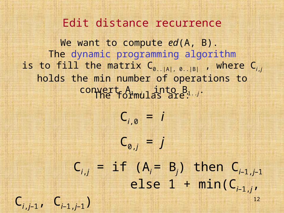
Edit distance recurrence
We want to compute ed(A, B). The dynamic programming algorithm
is to fill the matrix C0..|A|, 0..|B| , where Ci,j holds the min number of operations to convert A1..i into B1..j.
The formulas are:
Ci,0 = i
C0,j = j
Ci,j = if (Ai = Bj) then Ci–1,j–1
else 1 + min(Ci–1,j, Ci,j–1, Ci–1,j–1)
13
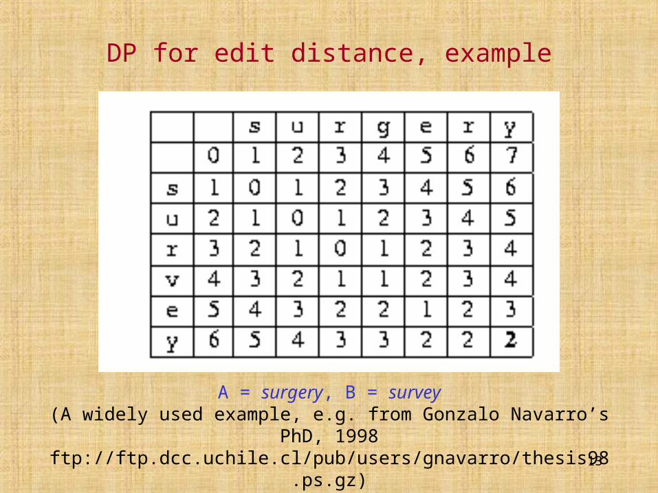
A = surgery, B = survey(A widely used example, e.g. from Gonzalo Navarro’s PhD, 1998
ftp://ftp.dcc.uchile.cl/pub/users/gnavarro/thesis98.ps.gz)
DP for edit distance, example
14
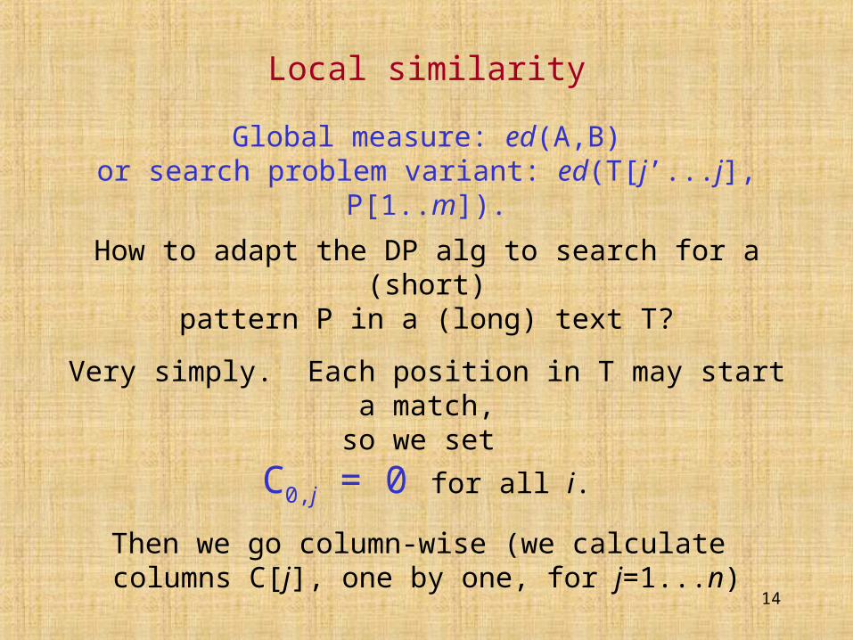
Local similarity
Global measure: ed(A,B)or search problem variant: ed(T[j’...j], P[1..m]).
How to adapt the DP alg to search for a (short)pattern P in a (long) text T?
Very simply. Each position in T may start a match,so we set
C0,j = 0 for all i.
Then we go column-wise (we calculate columns C[j], one by one, for j=1...n)
15
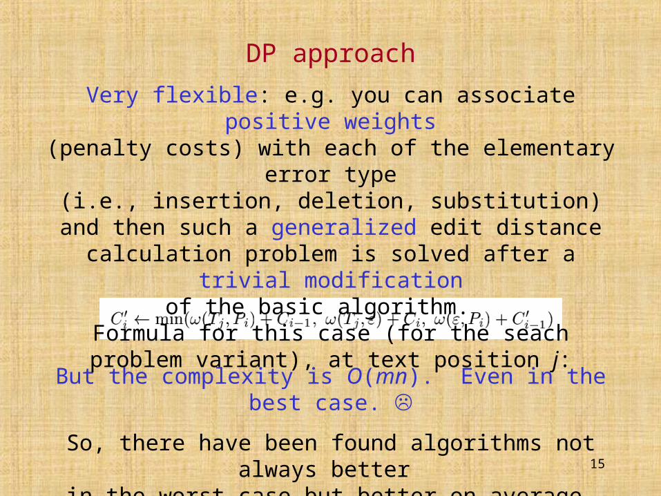
But the complexity is O(mn). Even in the best case.
So, there have been found algorithms not always better in the worst case but better on average.
Very flexible: e.g. you can associate positive weights(penalty costs) with each of the elementary error type
(i.e., insertion, deletion, substitution)and then such a generalized edit distance calculation
problem is solved after a trivial modificationof the basic algorithm.
Formula for this case (for the seach problem variant), at text position j:
DP approach

16
Partitioning lemma for the edit distance
We look for approximate occurrences of a pattern, with max allowed error k.
Lemma (Rivest, 1976; Wu & Manber, 1992): If the pattern is split into k+1 (disjoint) pieces,
then at least one piece must appear unaltered in anapproximate occurrence of the pattern.
More generally we can say that if splitting P into k+l partsthen at least l pieces must appear unaltered.
17
Partitioning lemmais a special case of the Dirichlet principle
Dirichlet principle (aka pigeonhole principle)is a very obvious (but useful in math) general observation.
Roughly, it says that if a pigeon is not going to occupy apigeonhole which already contains a pigeon,
there is no way to fit n pigeons in less than n pigeonholes.
Others prefer an example with rabbits.If you have 10 rabbits and 9 cages, (at least) one cage
must have (at least) two rabbits.Or (more appropriate for our partitioning lemma):
9 rabbits and 10 cages one cage must be empty.

18
Dirichlet principle(if you want to be serious)
For any natural number n, there does not exist a bijection between
a set S such that |S|=n and a proper subset of S.
19
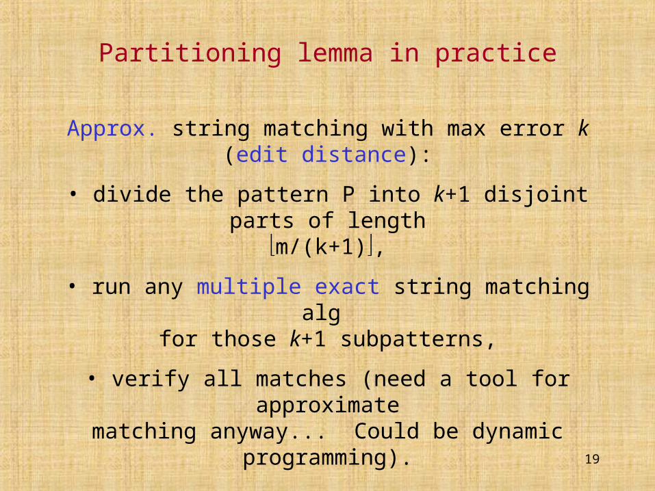
Partitioning lemma in practice
Approx. string matching with max error k (edit distance):
• divide the pattern P into k+1 disjoint parts of lengthm/(k+1),
• run any multiple exact string matching alg for those k+1 subpatterns,
• verify all matches (need a tool for approximatematching anyway... Could be dynamic programming).
20
Indel distance
Very similar to edit distance, but only INsertionsand DELetions are allowed.
Trivially, indel(A, B) edit(A, B).
Both edit() and indel() distance functionsare metrics.
That is, they satisfy the four conditions:non-negativity,
indentity of indescernibles,symmetry
and the triangle inequality ( d(A, B) d(A, C) + d(C, B) ).
21
Hamming distance
Very simple (but with limited applications).
By analogy to the binary alphabet,dH(S1, S2) is the number of positions at which
S1 and S2 differ.
If | S1 | | S2 |, then dH(S1, S2) = .
Example
S1 = Donald DuckS2 = Donald Tusk
dH(S1, S2) = 2.
22
Longest Common Subsequence (LCS)
Given strings A, B, |A| = n, |B| = m, find the longest subsequence shared by both strings.
More precisely, find 1 i1 i2 ... ik–1 ik n, and 1 j1 j2 ... jk–1 jk m, such thatA[i1] = B[j1], A[i2] = B[j2], ..., A[ik] = B[jk]
and k is maximized.
k is the length of the LCS(A, B), also denoted as LLCS(A, B).
Sometimes we are interested in a simpler problem:finding only the LLCS, not the matching sequence.
23
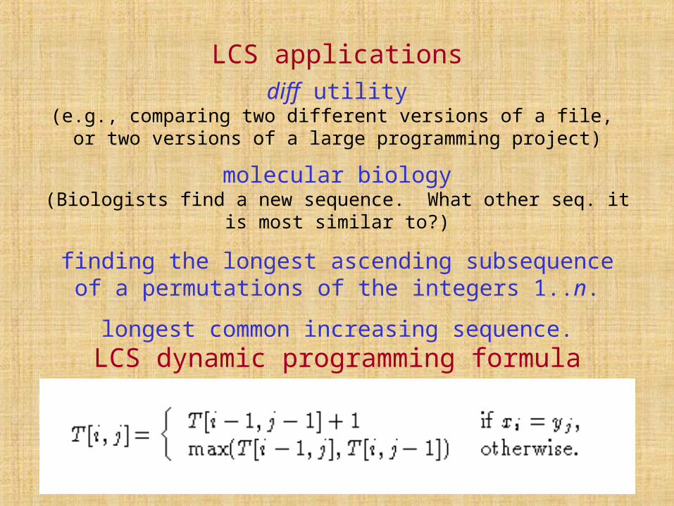
LCS applicationsdiff utility
(e.g., comparing two different versions of a file, or two versions of a large programming project)
molecular biology(Biologists find a new sequence. What other seq. it is most similar to?)
finding the longest ascending subsequenceof a permutations of the integers 1..n.
longest common increasing sequence.
LCS dynamic programming formula
24
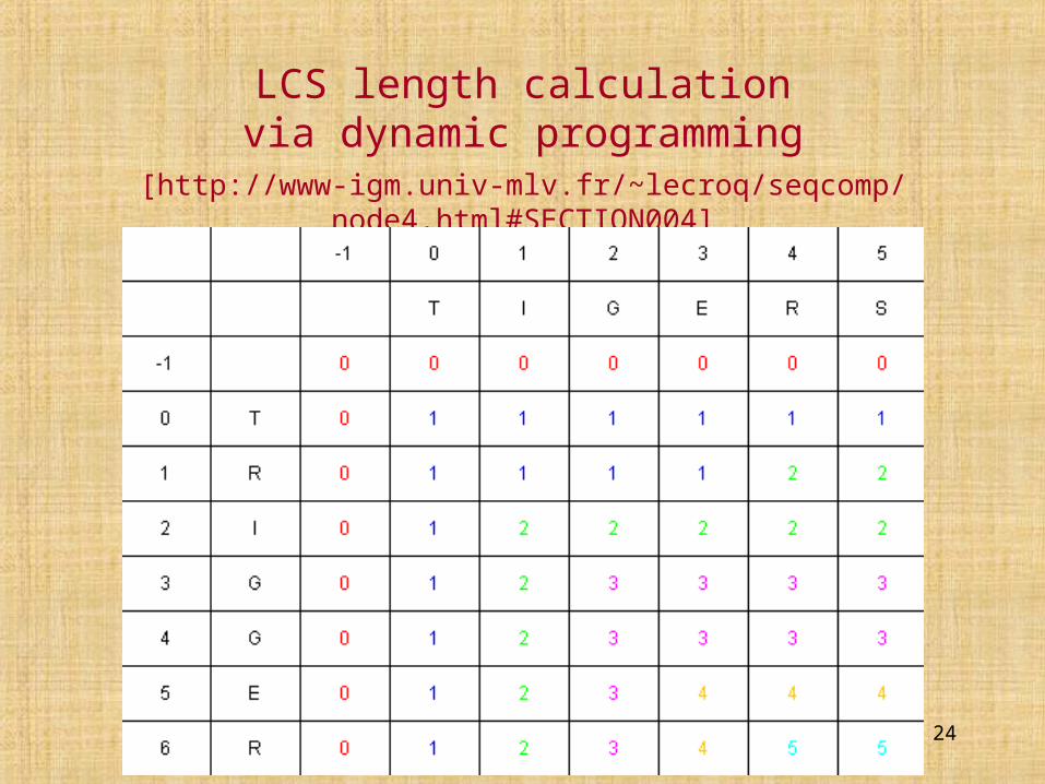
LCS length calculationvia dynamic programming
[http://www-igm.univ-mlv.fr/~lecroq/seqcomp/node4.html#SECTION004]
25
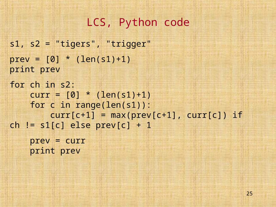
LCS, Python code
s1, s2 = "tigers", "trigger"
prev = [0] * (len(s1)+1)print prev
for ch in s2: curr = [0] * (len(s1)+1) for c in range(len(s1)): curr[c+1] = max(prev[c+1], curr[c]) if ch != s1[c] else prev[c] + 1
prev = curr print prev
26
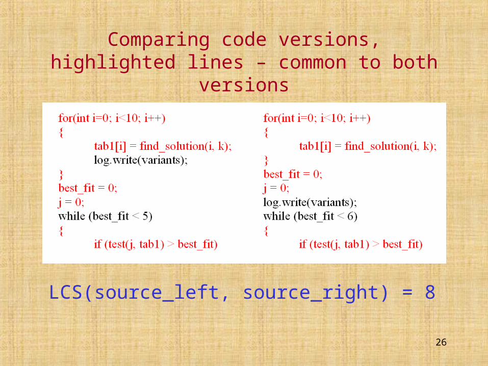
Comparing code versions,highlighted lines – common to both versions
LCS(source_left, source_right) = 8
27
LCS, anything better than plain DP?
The basic dyn. programming is clearly O(mn) in the worst case.
Surprisingly, we can’t beat this result significantlyin the worst case.
The best practical idea for the worst case is a bit-parallelalgorithm (there are a few variants)
with O(n m/w) time (and a few times faster than the plain DP in practice).
Still, we also have algorithms with output-dependentcomplexities, e.g., the Hunt–Szymanski (1977) one
with O(r log m) worst case time,where r is the number of matching cells in the DP matrix
(that is, r is mn in the worst case).
28
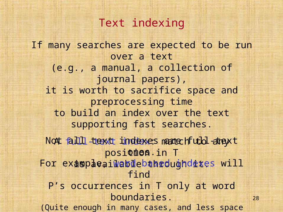
Text indexing
If many searches are expected to be run over a text(e.g., a manual, a collection of journal papers),
it is worth to sacrifice space and preprocessing timeto build an index over the text
supporting fast searches.
A full-text index: match to any position in Tis available through it.
Not all text indexes are full-text ones.For example, word based indexes will find
P’s occurrences in T only at word boundaries.(Quite enough in many cases, and less spaceconsuming, often more flexible in some ways.)
29
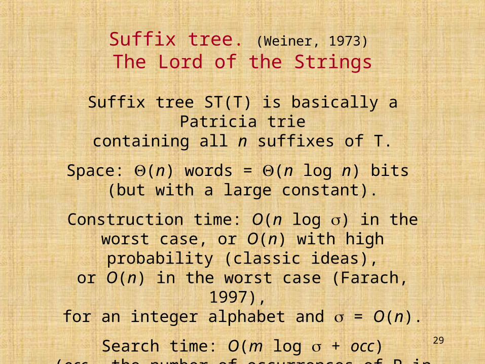
Suffix tree. (Weiner, 1973)
The Lord of the Strings
Suffix tree ST(T) is basically a Patricia triecontaining all n suffixes of T.
Space: (n) words = (n log n) bits (but with a large constant).
Construction time: O(n log ) in the worst case, or O(n) with high probability (classic ideas),or O(n) in the worst case (Farach, 1997),
for an integer alphabet and = O(n).
Search time: O(m log + occ)(occ – the number of occurrences of P in T)
30
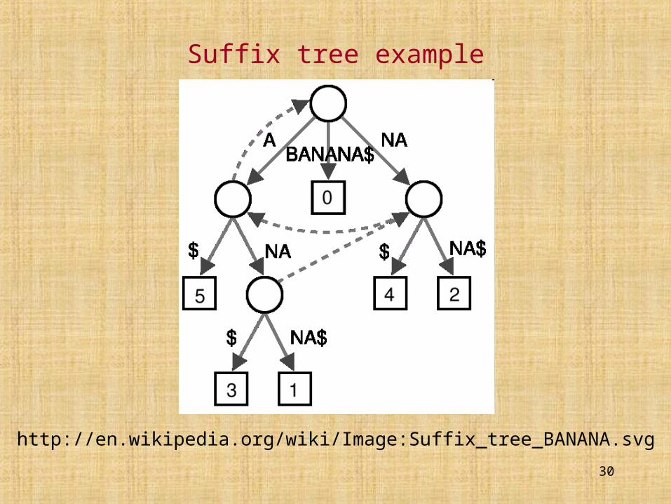
Suffix tree example
http://en.wikipedia.org/wiki/Image:Suffix_tree_BANANA.svg
31
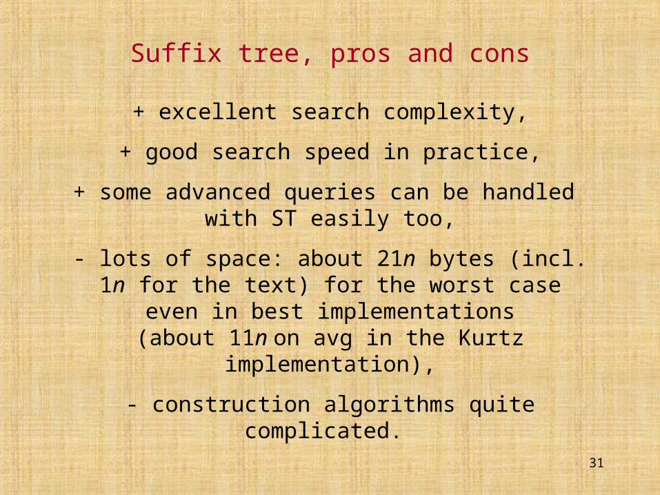
Suffix tree, pros and cons
+ excellent search complexity,
+ good search speed in practice,
+ some advanced queries can be handled with ST easily too,
- lots of space: about 21n bytes (incl. 1n for the text) for the worst case even in best implementations(about 11n on avg in the Kurtz implementation),
- construction algorithms quite complicated.
32
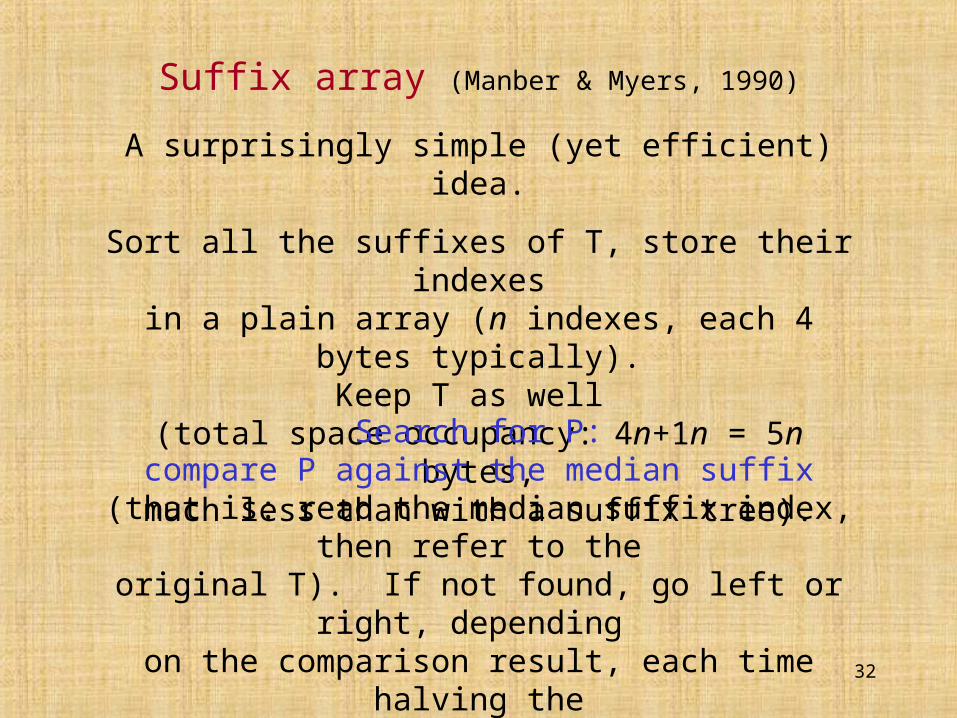
Suffix array (Manber & Myers, 1990)
A surprisingly simple (yet efficient) idea.
Sort all the suffixes of T, store their indexesin a plain array (n indexes, each 4 bytes typically).
Keep T as well (total space occupancy: 4n+1n = 5n bytes,
much less than with a suffix tree).
Search for P:compare P against the median suffix
(that is: read the median suffix index, then refer to theoriginal T). If not found, go left or right, depending
on the comparison result, each time halving therange of suffixes. So, this is binary search based.
33
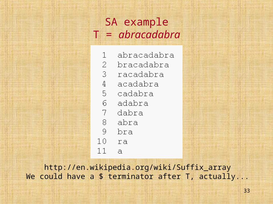
SA exampleT = abracadabra
http://en.wikipedia.org/wiki/Suffix_arrayWe could have a $ terminator after T, actually...
34
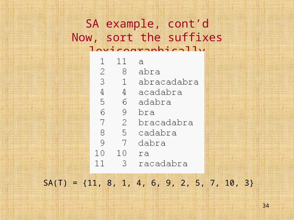
SA example, cont’dNow, sort the suffixes lexicographically
SA(T) = {11, 8, 1, 4, 6, 9, 2, 5, 7, 10, 3}
35
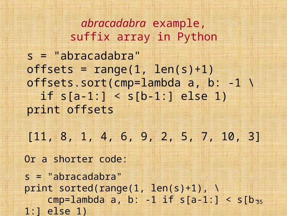
s = "abracadabra"offsets = range(1, len(s)+1) offsets.sort(cmp=lambda a, b: -1 \ if s[a-1:] < s[b-1:] else 1)print offsets
[11, 8, 1, 4, 6, 9, 2, 5, 7, 10, 3]
abracadabra example,suffix array in Python
Or a shorter code:
s = "abracadabra"print sorted(range(1, len(s)+1), \ cmp=lambda a, b: -1 if s[a-1:] < s[b-1:] else 1)
36
SA search properties
The search basic mechanism is thateach pattern occurring in text T
must be some prefix of a suffix of T.
Worst case search time: O(m log n + occ).
But in practice it is closer to O(m + log n + occ).
SA: very simple, very practical,very inspiring.
37
How to create the suffix array (=sort suffixes)efficiently
The classic integer sorting algorithms (e.g., quick sort, merge sort)
are no good for sorting suffixes.
They are quite slow in typical cases and extremely slow (need e.g. O(n2 log n) time) in pathological cases;a pathological case may be e.g. an extremely long
repetition of the same short pattern (abcabcabc...abc – a few million times), or a concatenation of two copies of the
same book.
38
Better solutions
There are O(n) worst-case time algorithms forbuilding the suffix TREE. It is then easily possible to obtain
the suffix array from the suffix tree in O(n) time.But this approach is not practical.
Some other choices:
Manber–Myers (1990), O(n log n) (but slow in practice)
Larsson–Sadakane (1999), O(n log n) (quite practical, used as one of sort components in bzip2 compressor)
Kärkkäinen–Sanders (2003), O(n) directly (not via ST building)
Puglisi–Maniscalco (2006), fast in practice.
![Suffix Trees and Suffix Arrays. Some problems Given a pattern P = P[1..m], find all occurrences of P in a text S = S[1..n] Another problem: –Given two](https://img.pdfslide.net/doc/110x75/56649d135503460f949e6de9/suffix-trees-and-suffix-arrays-some-problems-given-a-pattern-p-p1m.jpg)