Embed Size (px)
Citation preview

NGU Report 2011.026
Mannen unstable rock slope (Møre & Romsdal): Logging of borehole and drill core KH-01-10,
geomorphologic digital elevation model interpretation & displacement analysis by
terrestrial laser scanning
Geological Survey of Norway Postboks 6315 Sluppen NO-7491 Trondhelm, Norway Tel.: 47 73 904000 REPORT Telefax 477392 1620
Report no.: 2011.026 ISSN 0800-3416 Grading: Open Title:
Mannen unstable rock slope (M0re & Romsdal): Logging of borehole and drill core KH-Ol-10, geomorphologic digital elevation model interpretation & displacement analysis by terrestrial laser scannmg
Authors: Client: Aline Saintot, Harald Elvebakk, Thierry Aknes/Tafjord Beredskapssenter IKS Oppikofer, Guri V. Ganef0d & Tor 0. Farsund
County: Commune: M0re & Romsdal Rauma
Map-sheet name (M=l :250.000) Map-sheet no. and -name (M= I :50.000) Alesund 1319 II Romsdalen
Deposit name and grid-reference: Number of pages: 130 Price (NOK): 530 Mannen Map enclosures: 0
Fieldwork carried out: Date of report: Project no.: P~~n resv~e: 2010 1 September 2011 336700 //1
//l/4JA./ -:;::p Summary: if I Mannen is an unstable rock slope located in Romsdalen in M0re og Romsdal eoulty. The most active part is located in the uppermost part of the slope and has an estimated volume of 2.5-3 Mm3 and moves with a velocity of approximately 4-5 cm/year. Since 2009, the unstable rock slope at Mannen is under continuous monitoring by the Aknes/Tafjord Beredskapssenter IKS.
A 138 m deep, vertical cored borehole has been drilled in 2010 in the uppermost part of the Mannen rock slope. The aim of this coring was to characterize weakness zones that may explain the active deformation. This report presents the geological logging of the drill core and the geophysical logging of the borehole by an optical televiewer, which gives orientation of fractures and structures, as well as fracture frequency. Both the geological core logging and geophysical borehole logging resulted in the observation of many highly deformed and even crushed levels at several depths. Among them, the core interval between 57 and 81 m depth shows the highest density of severely crushed zones associated with fine-grained products, such as breccias or even clay-rich gouges. This interval is interpreted to be the subsurface expression of the main basal sliding surface.
The geomorphologic analysis of a high-resolution digital elevation model in combination with photographs allowed delimiting different scenarios for the Mannen rock slope instability. Based on the orientations of the structures forming the basal failure surface, a wedge failure mechanism is proposed for the most active block (scenario A). The orientation of the wedge intersection line formed by the two basal surfaces is consistent with the displacement vector obtained by dGPS measurements and repetitive terrestrial laser scans, which are also presented in this report. Moreover, the analysis of the terrestrial laser scanning datasets reveals toppling movements of the uppermost part of the instability. These might be related to toppling of shallow, free-standing blocks. At the location of the borehole, the basal failure surface inferred from the digital elevation model is at approximately 70 m depth. This coincides well with the heavily crushed zone logged in the drill core and borehole.
Keywords: Drill core logging Borehole logging
Fractures Damage zones Televiewer
Digital elevation model TelTestriallaser scanning Unstable rock slope
CONTENTS 1. INTRODUCTION ............................................................................................................ 10 2. GEOLOGICAL AND STRUCTURAL CORE LOGGING ............................................ 13
2.1 THE BEDROCK AND ITS MECHANICAL PROPERTIES .................................. 13 2.2 DUCTILE FOLDS .................................................................................................... 14 2.3 FRACTURING, CRUSHED ZONES AND FAULT ROCKS ................................. 39
2.3.1 Large intervals of poor rock mass quality .......................................................... 39 2.3.2 Discrete intervals of poor rock mass quality ...................................................... 39 2.3.3 Clay-rich intervals .............................................................................................. 41
2.4 SUMMARY OF OBSERVATIONS AND INTERPRETATION ............................ 41 3. TELEVIEWER LOGGING OF THE BOREHOLE ........................................................ 43
3.1 INSTRUMENTATION, DATA ACQUISITION AND PROCESSING .................. 43 3.2 STRUCTURAL DATA ALONG THE BOREHOLE ............................................... 44
3.2.1 Overview of the attitude of the structural data along the entire borehole .......... 44 3.2.2 Structural data in the c. 3.1–31.7 m depth interval ............................................ 46 3.2.3 Structural data in the 32–58 m depth interval .................................................... 60 3.2.4 Structural data in depth interval: 57–77 m ......................................................... 74 3.2.5 Structural data in depth interval: 89–133 m ....................................................... 84
3.3 SUMMARY OF THE ATTITUDE OF THE METAMORPHIC FOLIATION AND FRACTURES ALONG THE ENTIRE BOREHOLE OF MANNEN ............................... 102
4. GEOMORPHOLOGIC ANALYSIS OF DIGITAL ELEVATION MODEL AND COMBINAISON WITH DRILL CORE AND BOREHOLE DATA .................................... 106 5. MAP OF DISPLACEMENT BY TERRESTRIAL LASER SCAN ANALYSIS ......... 108
5.1 METHODOLOGY .................................................................................................. 108 5.1.1 TLS data acquisition ......................................................................................... 108 5.1.2 Error assessment ............................................................................................... 109
5.2 TLS DISPLACEMENT ANALYSIS ...................................................................... 111 5.2.1 Shortest distance comparison ........................................................................... 111 5.2.2 Roto-translation matrix analysis ....................................................................... 113
6. CONCLUSION AND PERSPECTIVES ....................................................................... 115 7. REFERENCES ............................................................................................................... 116 8. APPENDIX .................................................................................................................... 117
FIGURES Figure 1. Mannen unstable rock slope on the southern side of Romsdalen (Western Norway).
.................................................................................................................................................. 11Figure 2. Location of drilling site at the top of Mannen unstable rock slope (UTM32 coordinates: 436618.5E; 6925616N). Possible limits of the different unstable volumes, i.e. scenarios labelled A, B and C on figure, and as explained in Chapter 4. ................................ 12Figure 3. Photograph of the drilling site on the top of the moving block. The main back-crack (black wall) is on the right side. ............................................................................................... 12Figure 4. Structural and geological core logging from 0 to 7 m depth. Pictures of the 1 m long bits of the dry (left) and wet (right) core. ................................................................................. 16Figure 5. Structural and geological core logging from 7 to 13 m depth (see Figure 4). .......... 17Figure 6. Structural and geological core logging from 13 to 19 m depth (see Figure 4). ........ 18Figure 7. Structural and geological core logging from 19 to 25 m depth (see Figure 4). ........ 19Figure 8. Structural and geological core logging from 25 to 31 m depth (see Figure 4). ........ 20Figure 9. Structural and geological core logging from 31 to 37 m depth (see Figure 4). ........ 21Figure 10. Structural and geological core logging from 37 to 43 m depth (see Figure 4). ...... 22Figure 11. Structural and geological core logging from 43 to 49 m depth (see Figure 4). ...... 23Figure 12. Structural and geological core logging from 49 to 55 m depth (see Figure 4). ...... 24Figure 13. Structural and geological core logging from 55 to 61 m depth (see Figure 4). ...... 25Figure 14. Structural and geological core logging from 61 to 67 m depth (see Figure 4). ...... 26Figure 15. Structural and geological core logging from 67 to 73 m depth (see Figure 4). ...... 27Figure 16. Structural and geological core logging from 73 to 79 m depth (see Figure 4). ...... 28Figure 17. Structural and geological core logging from 79 to 85 m depth (see Figure 4). ...... 29Figure 18. Structural and geological core logging from 85 to 91 m depth (see Figure 4). ...... 30Figure 19. Structural and geological core logging from 91 to 97 m depth (see Figure 4). ...... 31Figure 20. Structural and geological core logging from 97 to 103 m depth (see Figure 4). .... 32Figure 21. Structural and geological core logging from 103 to 109 m depth (see Figure 4). .. 33Figure 22. Structural and geological core logging from 109 to 115 m depth (see Figure 4). .. 34Figure 23. Structural and geological core logging from 115 to 121 m depth (see Figure 4). .. 35Figure 24. Structural and geological core logging from 121 to 127 m depth (see Figure 4). .. 36Figure 25. Structural and geological core logging from 127 to 133 m depth (see Figure 4). .. 37Figure 26. Structural and geological core logging from 133 to 138 m depth (see Figure 4). .. 38Figure 27. Mannen borehole deviation: north and east components (left) on the vertical section and direction viewed from the top (right). ................................................................... 43Figure 28. Stereoplots (lower hemisphere, Schmidt’s projection) of the foliation planes measured along the borehole by televiewer imaging. .............................................................. 45Figure 29. Stereoplots (lower hemisphere, Schmidt’s projection) of the fractures measured along the borehole by optical televiewer imaging. .................................................................. 45Figure 30. Unwrapped optical images of the wall of Mannen borehole with digitised foliation planes in the 4–16 m depth interval (left). Dip angle and dip direction of each plane are displayed on the arrow plot (N up; centre). Attitude of foliation plane is seen from two different angles (to N315 and N045 or to N290 and N020) with strike (right hand rule) and dip angle of the plane (right). ................................................................................................... 47Figure 31. Unwrapped optical images of the wall of Mannen borehole with digitised foliation planes in the 16–28 m depth interval (caption as in Figure 30). .............................................. 48Figure 32. Unwrapped optical images of the wall of Mannen borehole with digitised foliation planes in the 28–31.7 m depth interval (caption as in Figure 30) and stereoplots of the metamorphic foliation (planes and poles) in the 4–11 and 11–31.7 m depth intervals (data listed in Appendix 1). ............................................................................................................... 49

Figure 33. Contour plots with poles of fractures providing four main fracture sets (marked by different colours) in the c. 3–32 m depth interval. The prominent fracture set is the blue coloured set with dip direction/dip angle 019°/36°. ................................................................. 50Figure 34. Rose diagram of the fractures in the 3–32 m depth interval. .................................. 50Figure 35. Arrow plots (N up) of the 128 fractures in the c. 3–32 m depth interval, frequency histograms of the four fractures sets as defined by the statistical analysis (see Figure 33; with identical colours representing the fracture sets). The deviation of the borehole (arrow plot; N up) is shown in the right. .......................................................................................................... 51Figure 36. Optical televiewer synthetic images with digitised planar fractures in the 3.1–7.6 m depth interval (left); arrow plots of the fracture orientation (N up; centre); attitude of the fracture from two different view angles (to N290 and N020 herein) and strike/dip angle of the fracture with main characteristics (right). ................................................................................ 53Figure 37. Optical televiewer synthetic images with digitised planar fractures in the 8–12 m depth interval (caption as on Figure 36). .................................................................................. 54Figure 38. Optical televiewer synthetic images with digitised planar fractures in the 12–16 m depth interval (caption as on Figure 36). .................................................................................. 55Figure 39. Optical televiewer synthetic images with digitised planar fractures in the 16–20 m depth interval (caption as on Figure 36). .................................................................................. 56Figure 40. Optical televiewer synthetic images with digitised planar fractures in the 20–24 m depth interval (caption as on Figure 36). .................................................................................. 57Figure 41. Optical televiewer synthetic images with digitised planar fractures in the 24–28.2 m depth interval (caption as on Figure 36). ............................................................................. 58Figure 42. Optical televiewer synthetic images with digitised planar fractures in the 28.2–31.7 m depth interval (caption as on Figure 36). ............................................................................. 59Figure 43. Optical televiewer images showing crushed zones in the two 23–24.5 m (left) and 27–29 m (right) depth intervals. The two layers of clay-rich gouges are well observed in the 27–29 m depth interval. ............................................................................................................ 60Figure 44. Unwrapped optical images of the wall of Mannen borehole with digitised foliation planes in the 32–44 m depth interval (caption as in Figure 30). .............................................. 61Figure 45. Unwrapped optical images of the wall of Mannen borehole with digitised foliation planes in the 44–56 m depth interval (caption as in Figure 30). .............................................. 62Figure 46. Unwrapped optical images of the wall of Mannen borehole with digitised foliation planes in the 56–58 m depth interval (caption as in Figure 30) and stereoplot of the metamorphic foliation (planes and poles) in the 33.5–38, 38–42, 42–47, 47–55, 55–57 and 57–58 m depth intervals (data listed in Appendix 1). .............................................................. 63Figure 47. Contour plots, with poles of fractures, providing four main fracture sets in the c. 32–58 m depth interval. ............................................................................................................ 64Figure 48. Rose diagram of the fractures in the 32–58 m depth interval. ................................ 64Figure 49. Arrow plots (N up) of the 71 fractures in the c. 32–58 m depth interval, frequency histograms of the five fractures sets as defined by the statistical analysis (see Figure 47). The deviation of the borehole (arrow plot; N up) is shown in the right. ......................................... 65Figure 50. Optical televiewer synthetic images with digitised planar fractures in the 32–36 m depth interval (caption as on Figure 36). .................................................................................. 67Figure 51. Optical televiewer synthetic images with digitised planar fractures in the 36–40 m depth interval (caption as on Figure 36). .................................................................................. 68Figure 52. Optical televiewer synthetic images with digitised planar fractures in the 40–44 m depth interval (caption as on Figure 36). .................................................................................. 69Figure 53. Optical televiewer synthetic images with digitised planar fractures in the 44–48 m depth interval (caption as on Figure 36). .................................................................................. 70Figure 54. Optical televiewer synthetic images with digitised planar fractures in the 48–52 m depth interval (caption as on Figure 36). .................................................................................. 71
Figure 55. Optical televiewer synthetic images with digitised planar fractures in the 52–56 m depth interval (caption as on Figure 36). .................................................................................. 72Figure 56. Optical televiewer synthetic images with digitised planar fractures in the 56–58 m depth interval (caption as on Figure 36). .................................................................................. 73Figure 57. Optical televiewer images showing crushed zones at 46.7 m (left) and 56.3 m (right) depths. ........................................................................................................................... 74Figure 58. Unwrapped optical images of the wall of Mannen borehole with digitised foliation planes in the 57.4–69 m depth interval (caption as in Figure 30). ........................................... 75Figure 59. Unwrapped optical images of the wall of Mannen borehole with digitised foliation planes in the 69–77.6 m depth interval (caption as in Figure 30) and stereoplot of the metamorphic foliation (planes and poles) in the 58–59.5, 61–64.5, 64.5–71 and 71–77 m depth interval (data listed in Appendix 1). ............................................................................... 76Figure 60. Contour plots, with poles of fractures, providing one main fracture set in the c. 57–77 m depth interval. Note that the strong dispersion of the 18 fractures provides a statistic analysis of low significance. .................................................................................................... 77Figure 61. Rose diagram of the fractures in the 57–77 m depth interval. ................................ 77Figure 62. Arrow plots (N up) of the 18 fractures in the c. 57–77 m depth interval, frequency histograms of the single fracture set as defined by the statistical analysis (see Figure 60). The deviation of the borehole (arrow plot; N up) is shown in the right. ......................................... 78Figure 63. Optical televiewer synthetic images with digitised planar fractures in the 57.4–61.5 m depth interval (caption as on Figure 36). ............................................................................. 79Figure 64. Optical televiewer synthetic images with digitised planar fractures in the 61.5–65.5 m depth interval (caption as on Figure 36). ............................................................................. 80Figure 65. Optical televiewer synthetic images with digitised planar fractures in the 65.5–69.5 m depth interval (caption as on Figure 36). ............................................................................. 81Figure 66. Optical televiewer synthetic images with digitised planar fractures in the 69.5–73.5 m depth interval (caption as on Figure 36). ............................................................................. 82Figure 67. Optical televiewer synthetic images with digitised planar fractures in the 73.0–77.6 m depth interval (caption as on Figure 36). ............................................................................. 83Figure 68. Optical televiewer images showing crushed zones at 59.4 m (left) and 73.2 m (right) depths. The filling of the fractures is partly cement, which was injected to stabilise the borehole. The cement is especially visible in the picture to the right as a grey mass. ............. 84Figure 69. Unwrapped optical images of the wall of Mannen borehole with digitised foliation planes in the 89–101 m depth interval (caption as in Figure 30). ............................................ 85Figure 70. Unwrapped optical images of the wall of Mannen borehole with digitised foliation planes in the 101–113 m depth interval (caption as in Figure 30). .......................................... 86Figure 71. Unwrapped optical images of the wall of Mannen borehole with digitised foliation planes in the 113–126 m depth interval (caption as in Figure 30). .......................................... 87Figure 72. Unwrapped optical images of the wall of Mannen borehole with digitised foliation planes in the 126–132 m depth interval (caption as in Figure 30) and stereoplot of the metamorphic foliation (planes and poles) in the 90–110.2, 110.9–112, 113.5–116.2, 116.4–122.3, 124–126.6 and 127–133 m depth interval (data listed in Appendix 1). ........................ 88Figure 73. Contour plots, with poles of fractures, providing four main fracture sets in the c. 89–133 m depth interval. .......................................................................................................... 89Figure 74. Rose diagram of the fractures in the 90–131 m depth interval. .............................. 89Figure 75. Arrow plots (N up) of the 90 fractures in the c. 89–133 m depth interval, frequency histograms of the four fractures sets as defined by the statistical analysis (see Figure 73). The deviation of the borehole (arrow plot; N up) is shown in the right. ......................................... 91Figure 76. Optical televiewer synthetic images with digitised planar fractures in the 89–93 m depth interval (caption as on Figure 36). .................................................................................. 92
Figure 77. Optical televiewer synthetic images with digitised planar fractures in the 93–97 m depth interval (caption as on Figure 36). .................................................................................. 93Figure 78. Optical televiewer synthetic images with digitised planar fractures in the 97–101 m depth interval (caption as on Figure 36). .................................................................................. 94Figure 79. Optical televiewer synthetic images with digitised planar fractures in the 105–109 m depth interval (caption as on Figure 36). ............................................................................. 95Figure 80. Optical televiewer synthetic images with digitised planar fractures in the 110–114 m depth interval (caption as on Figure 36). ............................................................................. 96Figure 81. Optical televiewer synthetic images with digitised planar fractures in the 114–118 m depth interval (caption as on Figure 36). ............................................................................. 97Figure 82. Optical televiewer synthetic images with digitised planar fractures in the 118–122 m depth interval (caption as on Figure 36). ............................................................................. 98Figure 83. Optical televiewer synthetic images with digitised planar fractures in the 122–126 m depth interval (caption as on Figure 36). ............................................................................. 99Figure 84. Optical televiewer synthetic images with digitised planar fractures in the 126–130 m depth interval (caption as on Figure 36). ........................................................................... 100Figure 85. Optical televiewer synthetic images with digitised planar fractures in the 130–133 m depth interval (caption as on Figure 36). ........................................................................... 101Figure 86. Optical televiewer images showing a crushed zone in the 112–114 m depth interval. ................................................................................................................................... 102Figure 87. Dip direction of fractures and foliation in function to depth. ............................... 103Figure 88. Arrow plots of the foliation and fractures planes in the 4–58 m depth interval. .. 104Figure 89. Arrow plots of the foliation and fractures planes in the 58–133 m depth interval.
................................................................................................................................................ 105Figure 90. (a), Aerial photograph draped on a meter-scale resolution DEM of the Mannen rock slope with the inferred limits of scenarios A, B and C (yellow lines); red pins mark the location of the dGPS antennas. (b), Photograph from helicopter of the unstable rock slope of Mannen (scenario A) with an important set of N–S trending opened fractures, a bulge at the front and a sliding surface underlined by rockfall events. The red cone is the location of the drilling site on the top of the unstable slope. (c), determination of a wedge failure on two outcropping surfaces at the limits of scenario A. Note the good fit between the wedge intersection line and the displacement vector obtained from dGPS measurements (the red arrow on the map indicates the direction of the vector displacement). .................................. 106Figure 91: Pictures of the scan extents in a) August 2008 from viewpoint A; b) June 2010 from viewpoint A; c) and d) June 2010 from viewpoint B. ................................................... 109Figure 92: Hillshade maps of 25 cm cell size DEMs created on the TLS point clouds from 2008 (in green) and 2010 (in red). The scan positions and directions are shown. The inset shows a map of the blocks used for the roto-translation matrix technique. ........................... 110Figure 93: Shortest distance comparison between the 2008 and 2010 TLS point clouds (view to the W). Positive differences up to +25 cm are shown in yellow to red colours and negative differences up to −25 cm in blue to violet colours. The 6 compartments on the instability and 4 blocks along the back-crack used for the detailed displacement analysis using the roto-translation matrix technique are outlined. A major rockfall occurred at the foot of the investigated area. Snow covered areas in 2010 and areas not covered by the 2008 dataset were excluded from the shortest distance comparison (grey areas). ............................................... 111Figure 94: Shortest distance comparison of the Mannen instability (view to the WNW): a) eastern part with blocks 1 and 2 sliding towards the SSE by 10−12 cm and block 3 and loose blocks in the graben essentially showing subsidence by 5−12 cm; b) western part with blocks 4 and 5 that also move downward by 5−10 cm. The computed translation vectors of each block are indicated by the displacement length and the trend and plunge of the vector orientation. .............................................................................................................................. 112

Figure 95: Shortest distance comparison for the 4 blocks along the back-crack (view to the W). The three columns are detached from the stable rock mass behind. The middle column can be divided into two parts BC2a and BC2b with high displacement rates (25 cm) for the latter. ....................................................................................................................................... 112
TABLES Table 1. Results of rock mechanical laboratory analysis. ........................................................ 15Table 2. Fracture frequency along the core. The length of the bars for the fracture frequency is proportional to the maximum number of 13 fractures found in the interval 67–68 m. The length of the bars for the thickness of crush zones is proportional to 100 cm length of the core interval, i.e. a percentage like for the RQD (Rock Quality Designation) values. The symbol * indicates core loss along the interval. ....................................................................................... 40Table 3. Samples for XRD analysis and grain size distribution ............................................... 41Table 4. Observation in the 3.4–31.7 m depth interval of crushed and fractured zones, open fractures, orientation and stereoplot. Mean dip angles and dip angles at the bottom of the fractured zone are shown. ......................................................................................................... 52Table 5. Observation in the 39.8–56.3 m depth interval of crushed and fractured zones, open fractures, orientation and stereoplot. Mean dip angles and dip angles at the bottom of the fractured zone are shown. ......................................................................................................... 66Table 6. Observation in the 57.4–77.6 m depth interval of crushed and fractured zones, open fractures, orientation and stereoplot. Mean dip angles and dip angles at the bottom of the fractured zone are shown. (* = uncertain dip direction). ......................................................... 78Table 7. Observation in the 89–133 m depth interval of crushed and fractured zones, open fractures, orientation and stereoplot. Mean dip angles and dip angles at the bottom of the fractured zone are shown. ......................................................................................................... 90Table 8: Accuracy assessment of the roto-translation matrix technique for 5 stable reference blocks at Mannen. .................................................................................................................. 110Table 9: Displacement analysis of the Mannen instability using the roto-translation matrix technique for 4 unstable blocks along the back-crack and 6 compartments in the uppermost part of the unstable area. Grey-shaded values are not significant given the mean errors measured on the stable reference compartments (Table 8). Errors on the translation orientation and the toppling azimuth depend on the translation length and toppling angle, respectively.
................................................................................................................................................ 113 APPENDIX Appendix 1 ............................................................................................................................. 117Appendix 2 ............................................................................................................................. 121Appendix 3 ............................................................................................................................. 129
10
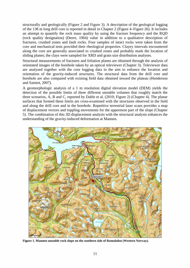
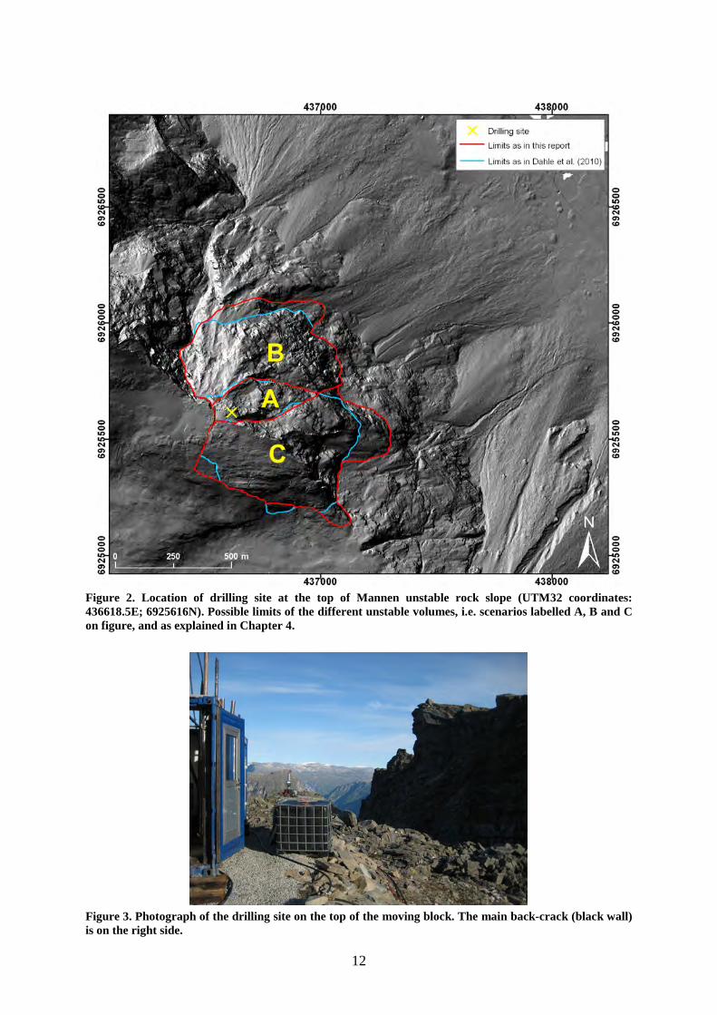
1. INTRODUCTION The locality of Mannen is a large rock slope instability, which developed in Proterozoic gneisses at the edge of the elevated plateau south of Romsdalen Valley (Møre og Romsdal County, Western Norway; Figure 1). Detailed surveys of Mannen began in 2006 with geological surface mapping (Henderson and Saintot, 2007) and risk analysis (Dahle et al., 2008, 2010). Large open cracks are conspicuous far inward the plateau but the largest gravity-induced deformation occurred at the edge of the plateau, where a several Mm3 large block already moved down-slope by approximately 20 m (Figure 2). Displacement rates measured by yearly differential Global Positioning System (dGPS) reach 4–5 cm/year for the upper part of the unstable rock slope. Based on these displacement measurements, the past slope displacement and the high potential consequences of a rock avalanche from Mannen (see Dahle et al., 2008, 2010), the instability has been classified as a high-risk object in 2009. From that time, instrumentation for permanent monitoring is set out under the authority of the Åknes-Tafjord Early-Warning Centre (Stranda, Møre og Romsdal). In parallel, further geological investigations were performed in order to better constrain the gravitational deformation. They comprise the geological logging of a 138 m long core vertically drilled in the unstable rock slope, the borehole logging by an optical televiewer, the analysis of a 1 m resolution digital elevation model acquired by NGU in 2009 (cf. Farsund, 2010, 2011) and a displacement analysis by terrestrial laser scanning. These investigations made in 2010 and 2011 are presented in this report.
Following structural and geological analysis of the surrounding areas, Henderson and Saintot (2007) deducted a translational sliding as mechanism of deformation. A several meter wide opened, steep crack is obvious at the back of the collapsing block and leads to detach the unstable block from the edge of the plateau. However, a basal sliding surface that would accommodate its downward motion is not identified so far. Based on a structural and morphological interpretation, Dahle et al. (2008) proposed the occurrence of two parallel north-dipping sliding surfaces that both developed from the main back-crack but at different depths. The model is refined in Dahle et al. (2010) with the implementation of steps along both sliding surfaces. These steps are inferred from steep tensile structures observed on the topographic surface. The main issue of such a model is that the instability is not considered any longer as a single volume, but as an assemblage of smaller blocks that may fail independently each other.
The bedrock consists of Proterozoic sillimanite-bearing gneiss units. In a first attempt, they may be assumed strong in terms of rheology and therefore difficult to deform under gravity. However, the numerous structures inherited from a protracted tectonic history that encompassed both the ductile and brittle domains of deformation lead to an important weakening (‘tectonic weakening’) of the rock mass (cf. Saintot et al. 2011). Specifically, the metamorphic foliation surfaces are prone to be reactivated where favourably orientated in regards to the gravitational forces. Many rockslides in the gneisses of Western Norway have basal sliding surfaces that developed along the metamorphic foliation ideally dipping toward the fjords or valleys (see in Henderson et al. 2006). At Mannen, the lack of access due to the steepness of the slope does not permit to measure the foliation elsewhere than on the plateau and the top of the unstable rock slope. On the plateau the foliation strikes approximately E–W and steeply dips towards either the south or the north. A recumbent fold is identified along the southern wall of the main back-crack, and even, shapes the wall. In addition, Henderson and Saintot (2007) identified that a large N–S epidote-rich cataclastic vertical fault zone forms the western border of the instability. Anyhow, pre-existing planar structures on which north-dipping sliding surfaces may develop are not (yet) observed at Mannen.
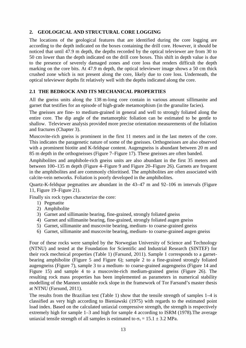
The vertical drilling of the unstable rock slope from its top surface in 2010 was principally carried out in order to establish the existence of sliding surface(s) and to characterise them
11
structurally and geologically (Figure 2 and Figure 3). A description of the geological logging of the 138 m long drill core is reported in detail in Chapter 2 (Figure 4–Figure 26). It includes an attempt to quantify the rock mass quality by using the fracture frequency and the RQD (rock quality designation) (Deere, 1964) value in addition to a qualitative description of fractures, crushed zones and fault rocks. Four samples of intact rocks were taken from the core and mechanical tests provided their rheological properties. Clayey intervals encountered along the core are generally associated to crushed zones and probably mark the location of sliding planes; the clays were sampled for XRD and grain size distribution analyses.
Structural measurements of fractures and foliation planes are obtained through the analysis of orientated images of the borehole taken by an optical televiewer (Chapter 3). Televiewer data are analysed together with the core logging data in the aim to enhance the location and orientation of the gravity-induced structures. The structural data from the drill core and borehole are also compared with existing field data obtained inward the plateau (Henderson and Saintot, 2007).
A geomorphologic analysis of a 1 m resolution digital elevation model (DEM) yields the detection of the possible limits of three different unstable volumes that roughly match the three scenarios, A, B and C, reported by Dahle et al. (2010; Figure 2) (Chapter 4). The planar surfaces that formed these limits are cross-examined with the structures observed in the field and along the drill core and in the borehole. Repetitive terrestrial laser scans provides a map of displacement vectors and toppling movements for the uppermost part of the slope (Chapter 5). The combination of this 3D displacement analysis with the structural analysis enhances the understanding of the gravity-induced deformation at Mannen.
Figure 1. Mannen unstable rock slope on the southern side of Romsdalen (Western Norway).
12
Figure 2. Location of drilling site at the top of Mannen unstable rock slope (UTM32 coordinates: 436618.5E; 6925616N). Possible limits of the different unstable volumes, i.e. scenarios labelled A, B and C on figure, and as explained in Chapter 4.
Figure 3. Photograph of the drilling site on the top of the moving block. The main back-crack (black wall) is on the right side.
13
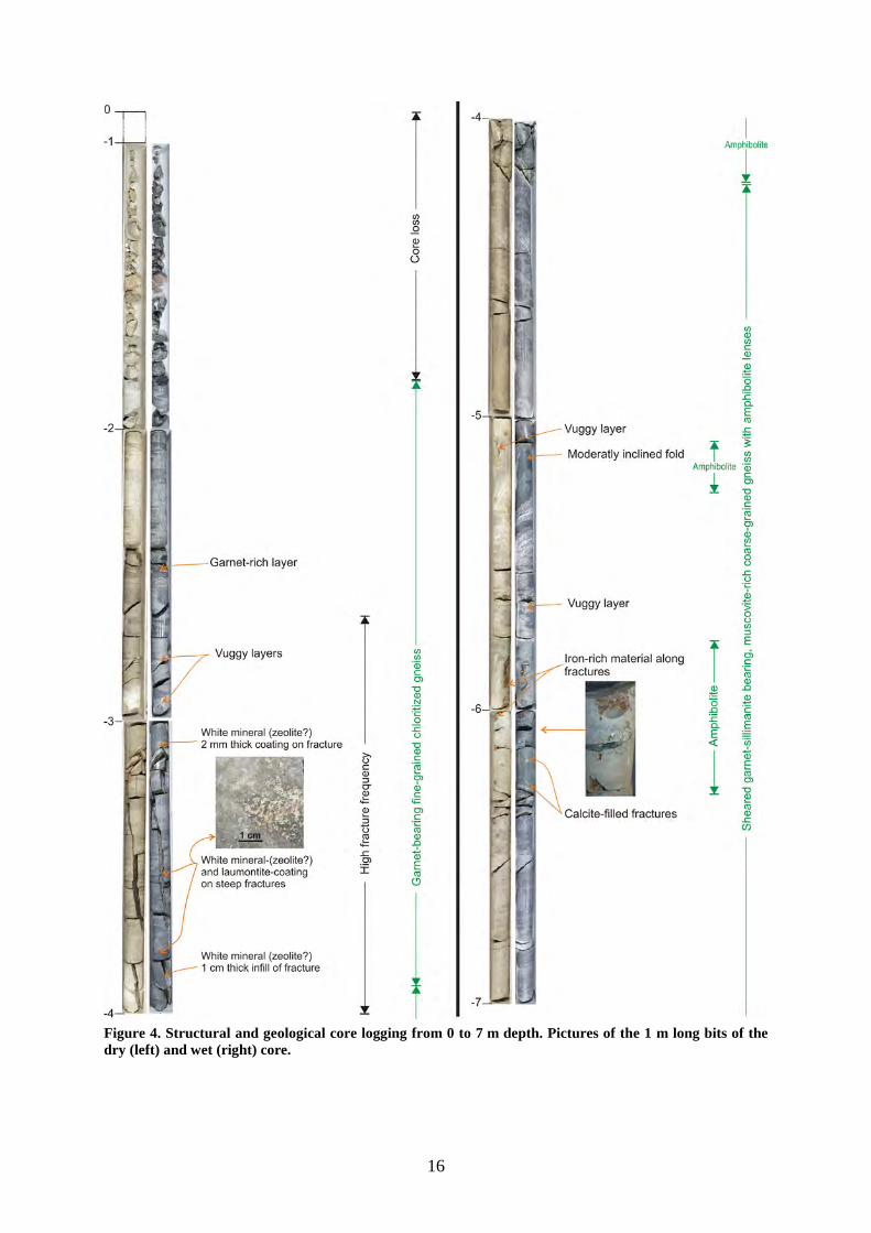
2. GEOLOGICAL AND STRUCTURAL CORE LOGGING The locations of the geological features that are identified during the core logging are according to the depth indicated on the boxes containing the drill core. However, it should be noticed that until 47.9 m depth, the depths recorded by the optical televiewer are from 30 to 50 cm lower than the depth indicated on the drill core boxes. This shift in depth value is due to the presence of severely damaged zones and core loss that renders difficult the depth marking on the core bits. At 47.9 m depth, the optical televiewer image shows a 50 cm thick crushed zone which is not present along the core, likely due to core loss. Underneath, the optical televiewer depths fit relatively well with the depths indicated along the core. 2.1 THE BEDROCK AND ITS MECHANICAL PROPERTIES All the gneiss units along the 138 m-long core contain in various amount sillimanite and garnet that testifies for an episode of high-grade metamorphism (in the granulite facies).
The gneisses are fine- to medium-grained in general and well to strongly foliated along the entire core. The dip angle of the metamorphic foliation can be estimated to be gentle to shallow. Televiewer analysis provided more precise orientation measurements of the foliation and fractures (Chapter 3).
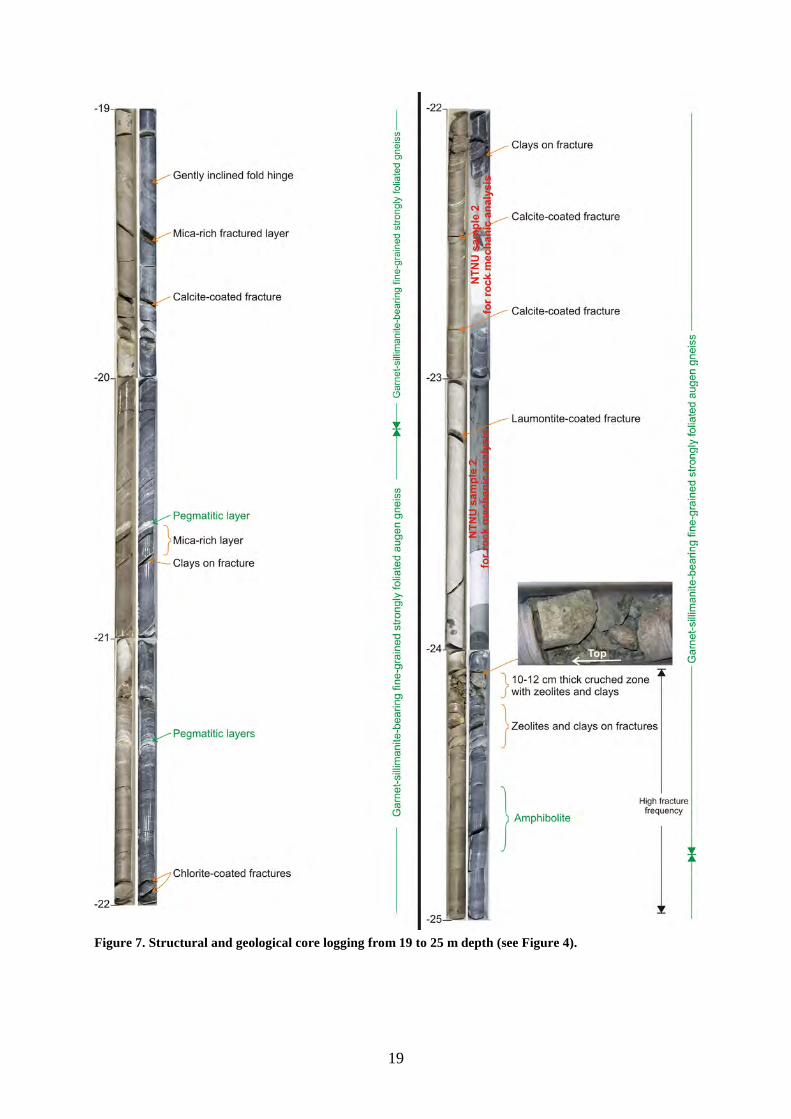
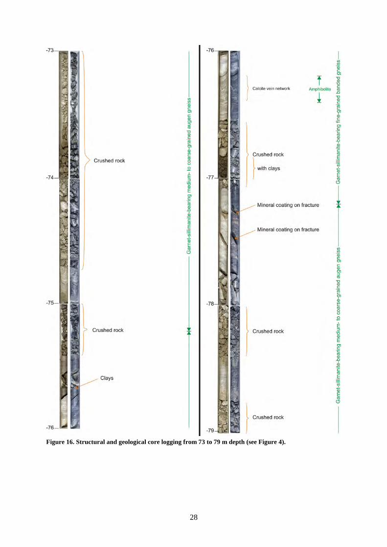
Muscovite-rich gneiss is prominent in the first 11 meters and in the last meters of the core. This indicates the paragenetic nature of some of the gneisses. Orthogneisses are also observed with a prominent biotite and K-feldspar content. Augengneiss is abundant between 20 m and 85 m depth in the orthogneisses (Figure 7–Figure 17). These gneisses are often banded.
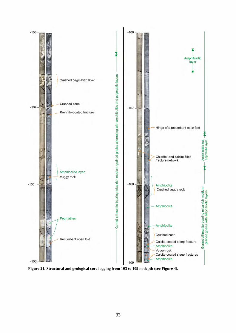
Amphibolites and amphibole-rich gneiss units are also abundant in the first 35 meters and between 100–135 m depth (Figure 4–Figure 9 and Figure 20–Figure 26). Garnets are frequent in the amphibolites and are commonly chloritised. The amphibolites are often associated with calcite-vein networks. Foliation is poorly developed in the amphibolites.
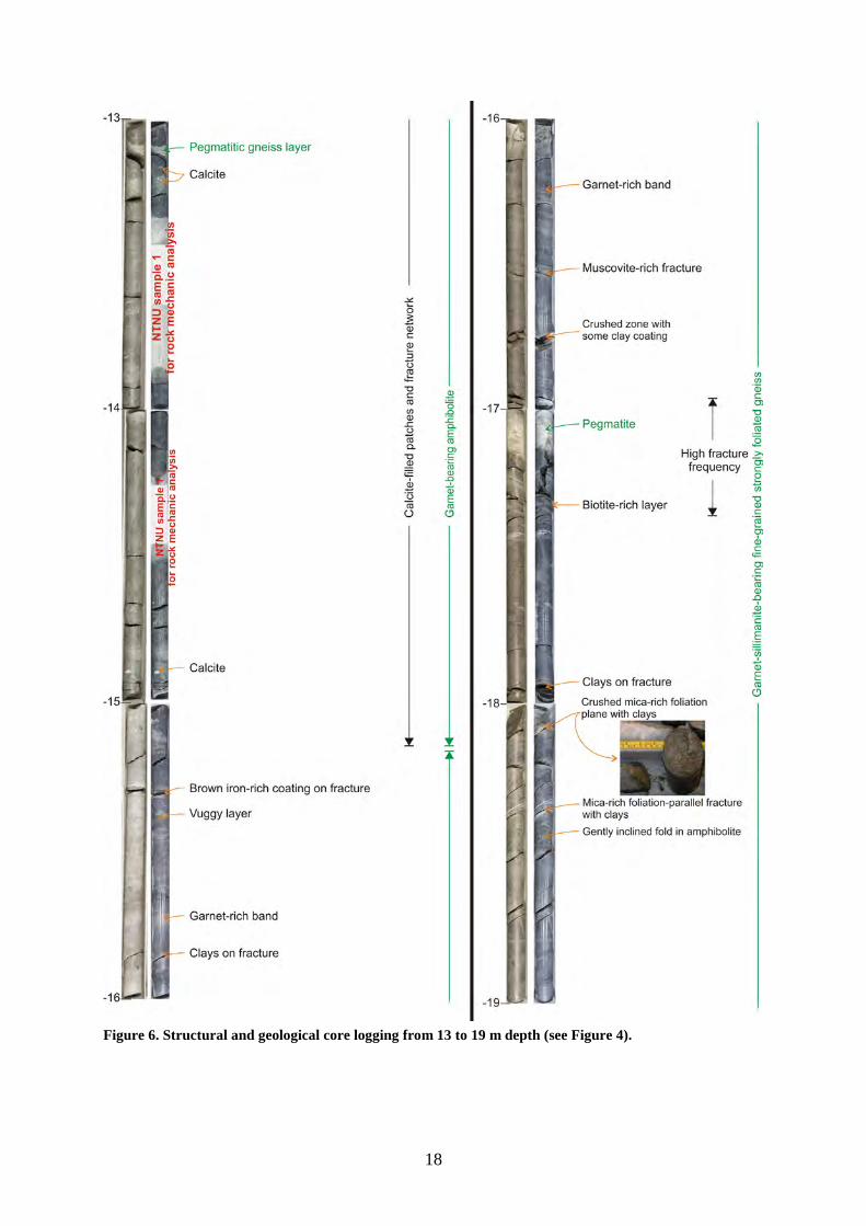
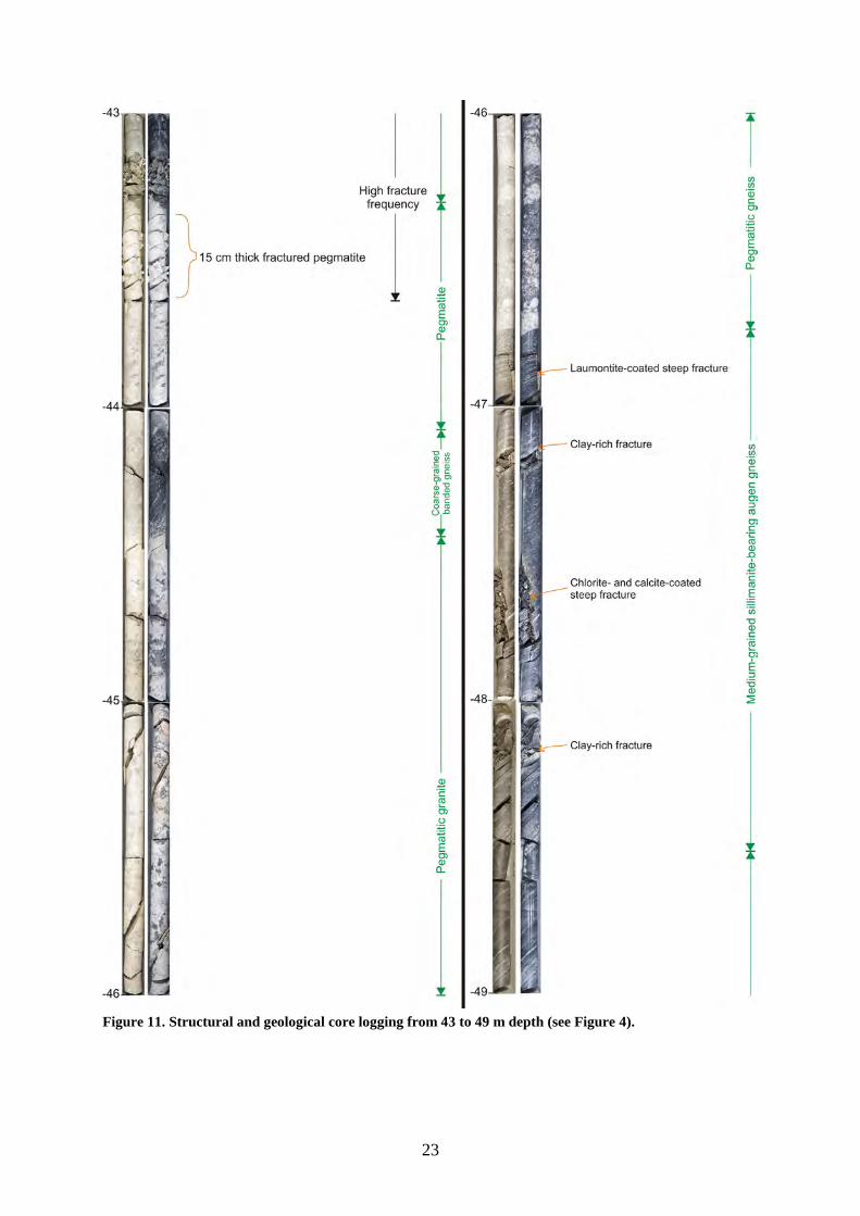
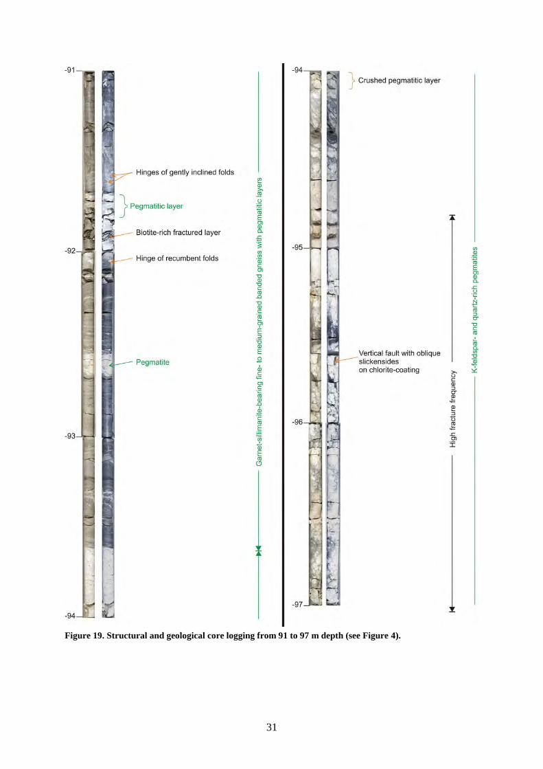
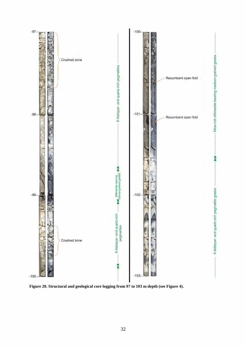
Quartz-K-feldspar pegmatites are abundant in the 43–47 m and 92–106 m intervals (Figure 11, Figure 19–Figure 21).
Finally six rock types characterize the core: 1) Pegmatite 2) Amphibolite 3) Garnet and sillimanite bearing, fine-grained, strongly foliated gneiss 4) Garnet and sillimanite bearing, fine-grained, strongly foliated augen gneiss 5) Garnet, sillimanite and muscovite bearing, medium- to coarse-grained gneiss 6) Garnet, sillimanite and muscovite bearing, medium- to coarse-grained augen gneiss
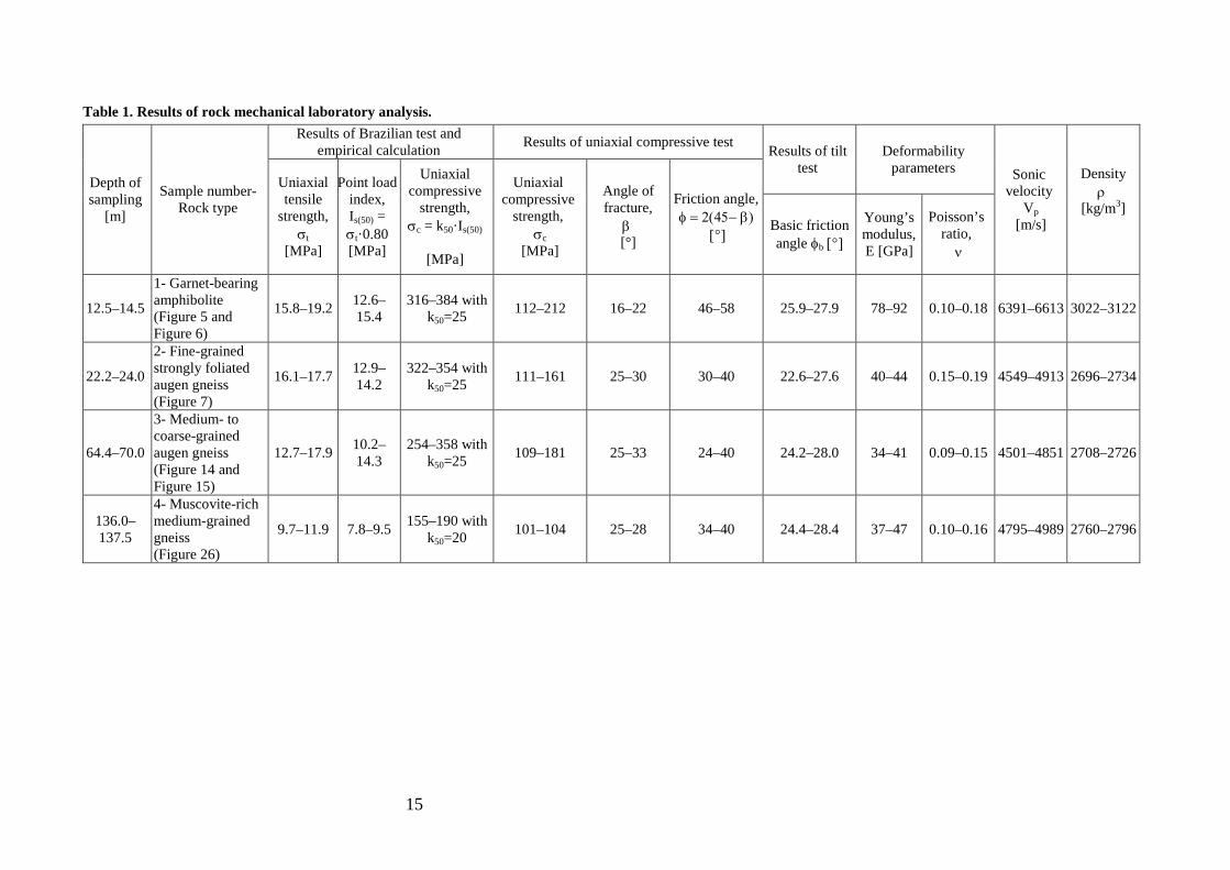
Four of these rocks were sampled by the Norwegian University of Science and Technology (NTNU) and tested at the Foundation for Scientific and Industrial Research (SINTEF) for their rock mechnical properties (Table 1) (Farsund, 2011). Sample 1 corresponds to a garnet-bearing amphibolite (Figure 5 and Figure 6); sample 2 to a fine-grained strongly foliated augengneiss (Figure 7), sample 3 to a medium- to coarse-grained augengneiss (Figure 14 and Figure 15) and sample 4 to a muscovite-rich medium-grained gneiss (Figure 26). The resulting rock mass properties has been implemented as parameters in numerical stability modelling of the Mannen unstable rock slope in the framework of Tor Farsund’s master thesis at NTNU (Farsund, 2011).
The results from the Brazilian test (Table 1) show that the tensile strength of samples 1–4 is classified as very high according to Bieniawski (1975) with regards to the estimated point load index. Based on the calculated uniaxial compressive strength, the strength is respectively extremely high for sample 1–3 and high for sample 4 according to ISRM (1978).The average uniaxial tensile strength of all samples is estimated to σt = 15.1 ± 3.2 MPa.
14
The results of uniaxial compressive tests show that the strength of sample 1, 3 and 4 is very high and that the one of sample 2 is medium to very high (ISRM 1978). The average uniaxial compressive strength of all samples is estimated to be σc = 136 ± 37 MPa; this strength is classified as very high according to ISRM (1978). The average angle of fracture in the uniaxial compressive tests is β = 26° ± 5° and the resulting average friction angle is φ = 39° ± 11°.
The results of tilt tests on all samples provides an average basic friction angle of φb = 25.9 ± 2.0°.
The two deformability parameters, the Young’s modulus and Poisson’s ratio of all samples have average values of E = 51 ± 20 GPa and ν = 0.14 ± 0.03, respectively. The amphibolite (sample 1) is characterised by remarkably high Young’s modulus values ranging from 78 to 92 GPa.
The sonic velocity and density of each sample is presented in Table 1. The average sonic velocity is estimated to Vp = 5155 ± 765 m/s. The average density is 2812 ± 149 kg/m3 with however, a value of density for the amphibolite (ρ > 3000 kg/m3; Table 1) well above the other rocks (2696 < ρ < 2796 kg/m3; Table 1).
With regards of all the values obtained by mechanical tests (Table 1), the amphibolite is certainly the strongest rock among the four types of rocks which, however, can be all assumed to be very strong.
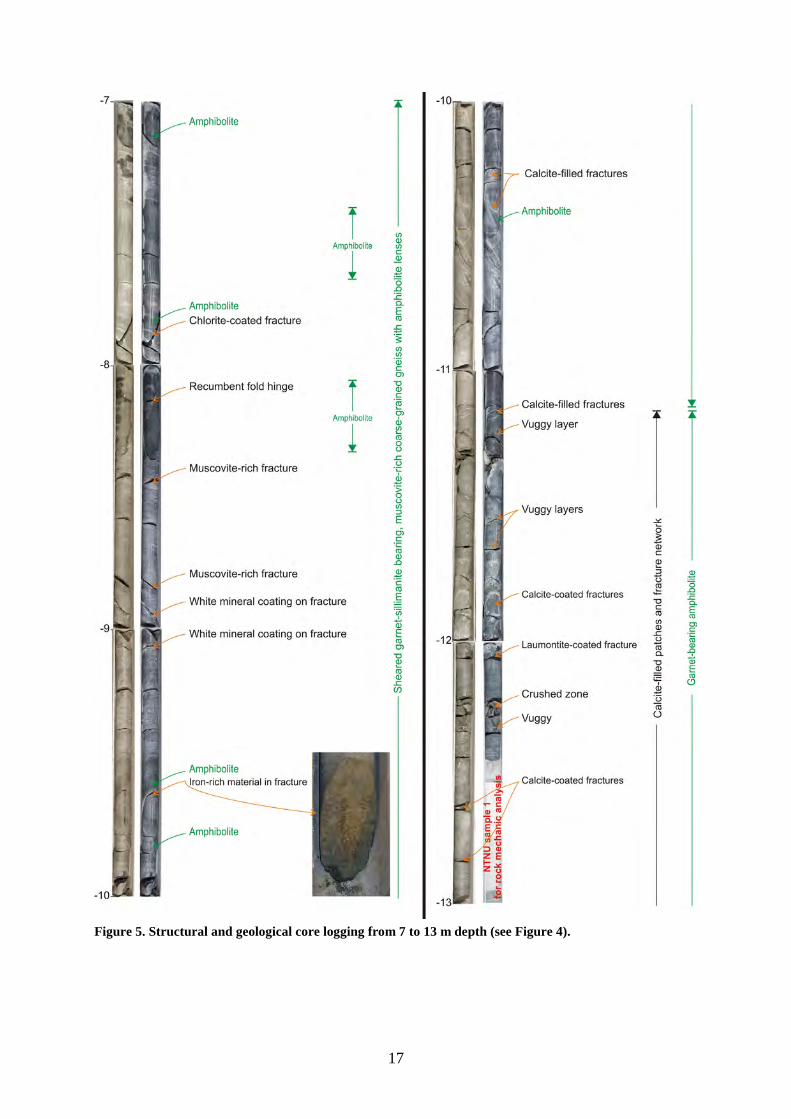
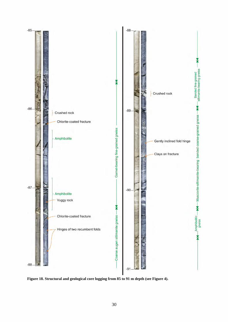
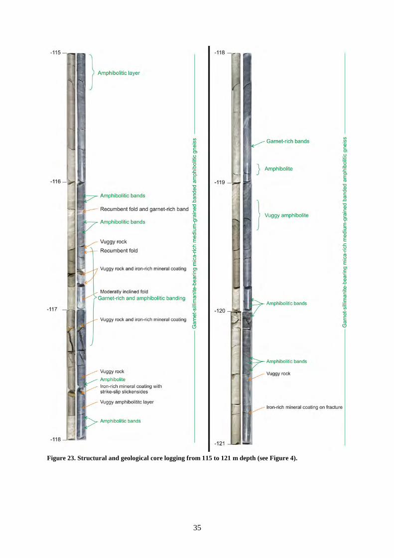
2.2 DUCTILE FOLDS Folds hinges were observed at several intervals and mainly in amphibolite layers. Most of them correspond to recumbent folds and are conspicuous at c. 8 m (Figure 5), 87–88 m (Figure 18), 92 m (Figure 19), 100.5–101 m (Figure 20), 105m (Figure 21), 116–116.5 m (Figure 23), 131.8 m (Figure 25) and 133.6 m (Figure 26) depth. Gently to moderately inclined folds with horizontal to gently plunging hinges are also observed at c. 5 m (Figure 4), 18.5 m (Figure 6), 19.5 m (Figure 7), 89.4 m (Figure 18), 91.5 m (Figure 19), 117 m (Figure 23), 121.4 m (Figure 24) and 130.5–132.5 m (Figure 25) depth.
15
Table 1. Results of rock mechanical laboratory analysis.
Depth of sampling
[m]
Sample number- Rock type
Results of Brazilian test and empirical calculation
Results of uniaxial compressive test Results of tilt
test Deformability
parameters Sonic velocity
Vp [m/s]
Density ρ
[kg/m3]
Uniaxial tensile
strength, σt
[MPa]
Point load index, Is(50) = σt·0.80 [MPa]
Uniaxial compressive
strength, σc = k50·Is(50)
[MPa]
Uniaxial compressive
strength, σc
[MPa]
Angle of fracture,
β [°]
Friction angle, φ = 2(45− β)
[°] Basic friction angle φb [°]
Young’s modulus, E [GPa]
Poisson’s ratio,
ν
12.5–14.5
1- Garnet-bearing amphibolite (Figure 5 and Figure 6)
15.8–19.2 12.6–15.4
316–384 with k50=25
112–212 16–22 46–58 25.9–27.9 78–92 0.10–0.18 6391–6613 3022–3122
22.2–24.0
2- Fine-grained strongly foliated augen gneiss (Figure 7)
16.1–17.7 12.9–14.2
322–354 with k50=25
111–161 25–30 30–40 22.6–27.6 40–44 0.15–0.19 4549–4913 2696–2734
64.4–70.0
3- Medium- to coarse-grained augen gneiss (Figure 14 and Figure 15)
12.7–17.9 10.2–14.3
254–358 with k50=25
109–181 25–33 24–40 24.2–28.0 34–41 0.09–0.15 4501–4851 2708–2726
136.0–137.5
4- Muscovite-rich medium-grained gneiss (Figure 26)
9.7–11.9 7.8–9.5 155–190 with
k50=20 101–104 25–28 34–40 24.4–28.4 37–47 0.10–0.16 4795–4989 2760–2796
16
Figure 4. Structural and geological core logging from 0 to 7 m depth. Pictures of the 1 m long bits of the dry (left) and wet (right) core.
17
Figure 5. Structural and geological core logging from 7 to 13 m depth (see Figure 4).
18
Figure 6. Structural and geological core logging from 13 to 19 m depth (see Figure 4).
19
Figure 7. Structural and geological core logging from 19 to 25 m depth (see Figure 4).
20
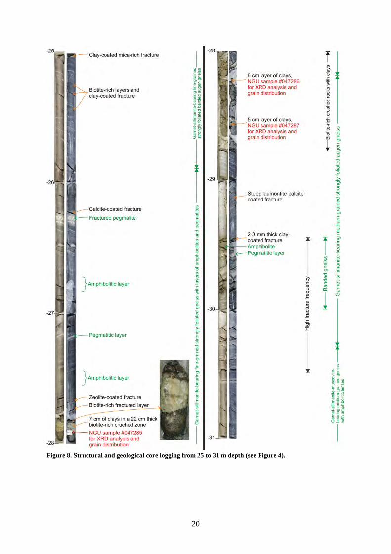
Figure 8. Structural and geological core logging from 25 to 31 m depth (see Figure 4).
21
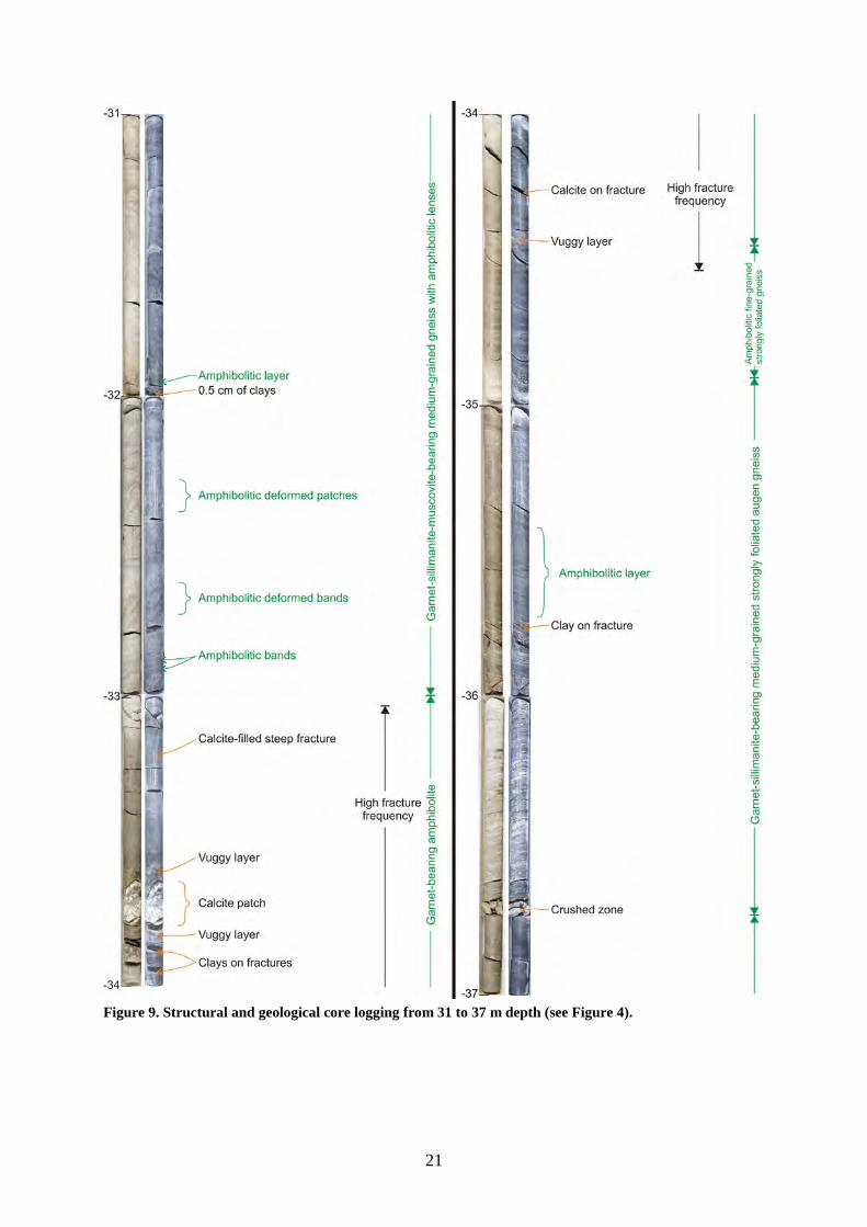
Figure 9. Structural and geological core logging from 31 to 37 m depth (see Figure 4).
22
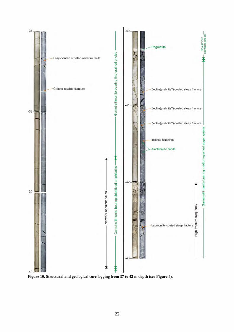
Figure 10. Structural and geological core logging from 37 to 43 m depth (see Figure 4).
23
Figure 11. Structural and geological core logging from 43 to 49 m depth (see Figure 4).
24
Figure 12. Structural and geological core logging from 49 to 55 m depth (see Figure 4).
25
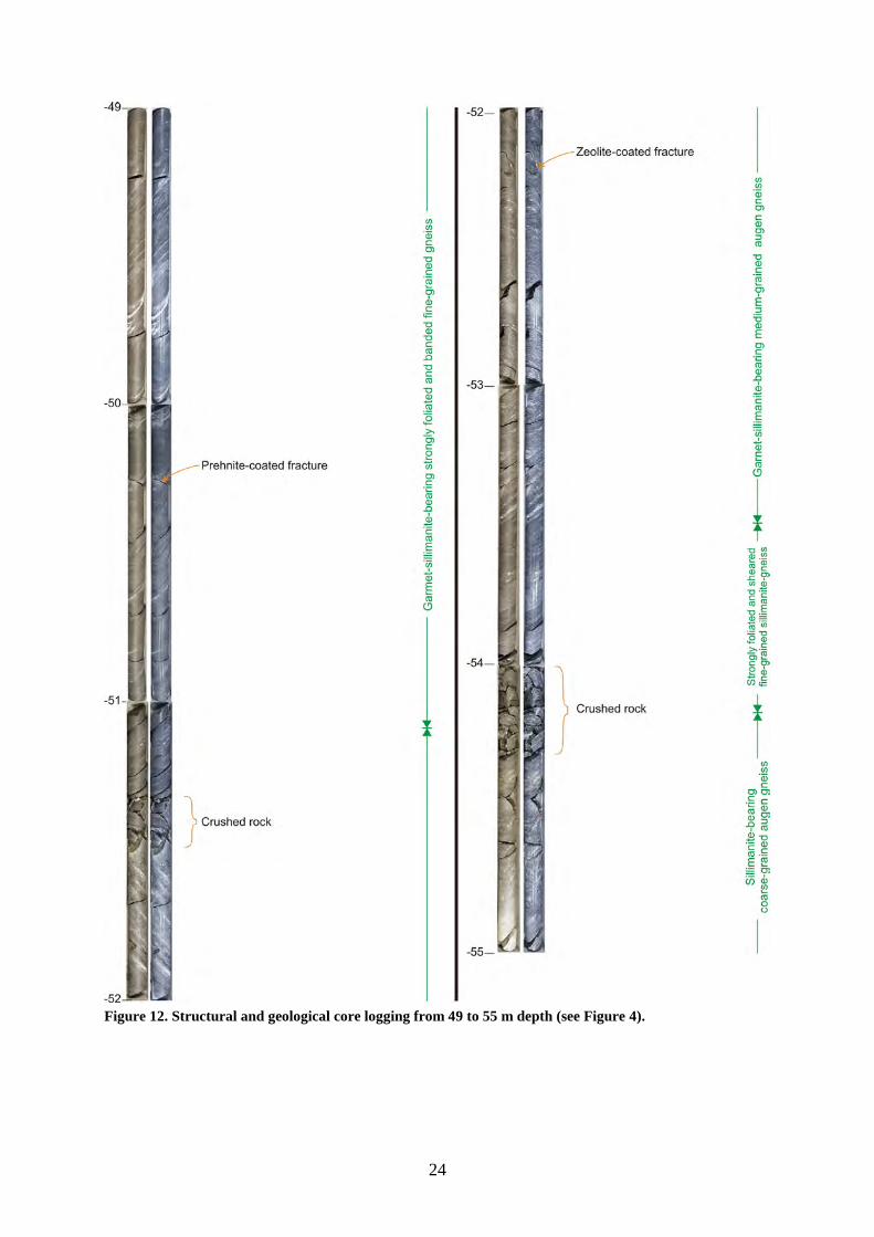
Figure 13. Structural and geological core logging from 55 to 61 m depth (see Figure 4).
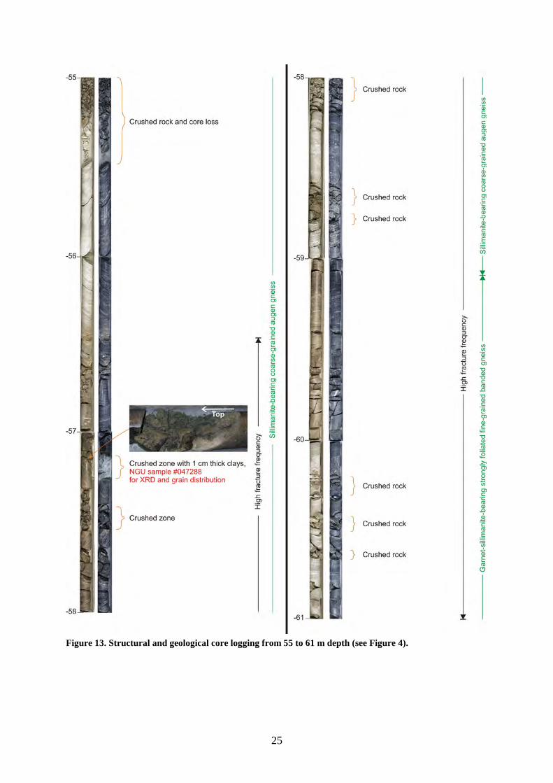
26
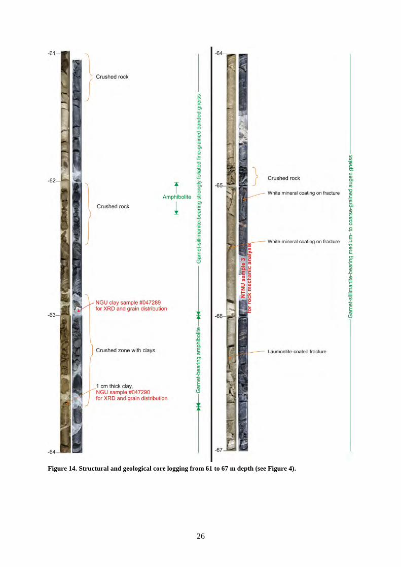
Figure 14. Structural and geological core logging from 61 to 67 m depth (see Figure 4).
27
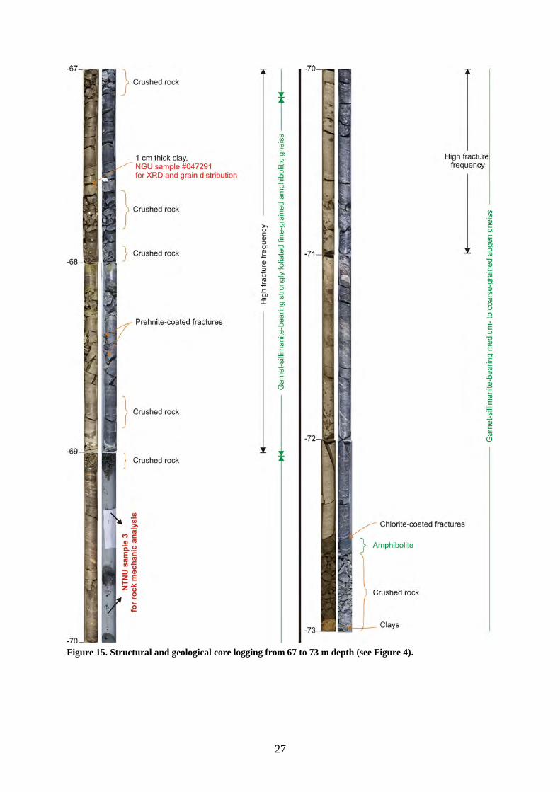
Figure 15. Structural and geological core logging from 67 to 73 m depth (see Figure 4).
28
Figure 16. Structural and geological core logging from 73 to 79 m depth (see Figure 4).
29
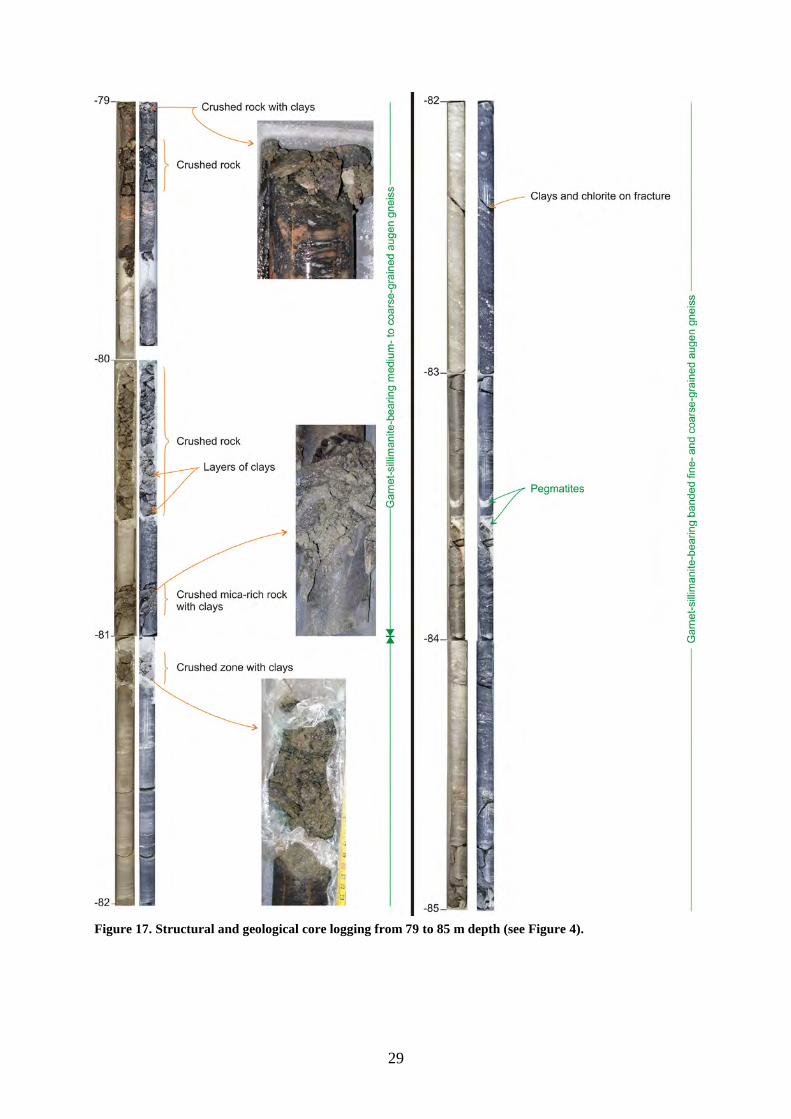
Figure 17. Structural and geological core logging from 79 to 85 m depth (see Figure 4).
30
Figure 18. Structural and geological core logging from 85 to 91 m depth (see Figure 4).
31
Figure 19. Structural and geological core logging from 91 to 97 m depth (see Figure 4).
32
Figure 20. Structural and geological core logging from 97 to 103 m depth (see Figure 4).
33
Figure 21. Structural and geological core logging from 103 to 109 m depth (see Figure 4).
34
Figure 22. Structural and geological core logging from 109 to 115 m depth (see Figure 4).
35
Figure 23. Structural and geological core logging from 115 to 121 m depth (see Figure 4).
36
Figure 24. Structural and geological core logging from 121 to 127 m depth (see Figure 4).
37
Figure 25. Structural and geological core logging from 127 to 133 m depth (see Figure 4).
38
Figure 26. Structural and geological core logging from 133 to 138 m depth (see Figure 4).
39
2.3 FRACTURING, CRUSHED ZONES AND FAULT ROCKS Fractures are generally mineral-coated (mainly with zeolites) and especially the steep fractures. It should be noted that the latter are underrepresented due to the verticality of the borehole. Fractures occur along the metamorphic foliation and at the contact between amphibolites and gneiss units. In intervals with high fracture frequency, the fractures are generally not found along the foliation. Therefore, the fracturing along the metamorphic foliation does not represent in general the main process of failure, except in the 24–25 m core interval where fractures follow the metamorphic foliation (see Table 2).
2.3.1 The 28–31 m depth interval (
Large intervals of poor rock mass quality
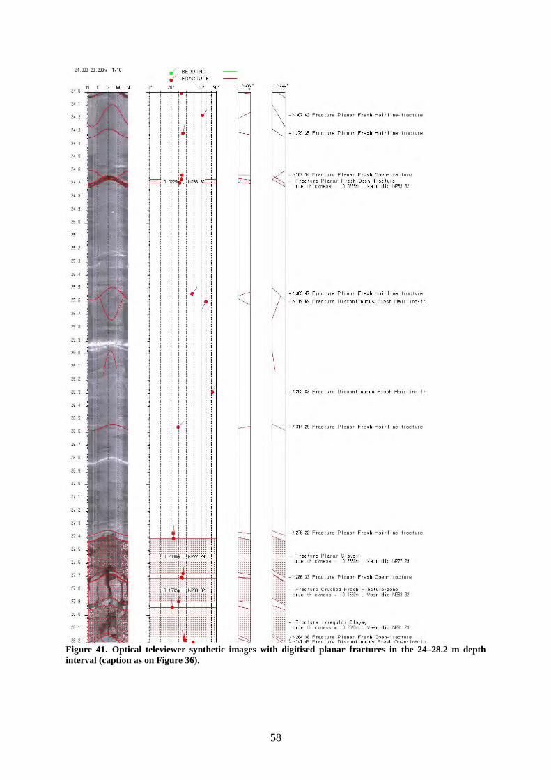
Figure 8) is characterised by a low RQD value. It corresponds to 80 cm of crushed rocks in the 28–29 m interval and to a high fracture frequency in the 29–31 m interval (Table 2). Clay-rich zones varying in thickness from mm to c. 8 cm are encountered and sampled at 27.90–27.92 m, 28.21–28.25 m and 28.55–28.61 m (Table 3).
The 57–64 m depth interval (Figure 13 and Figure 14) comprises rock with poor quality. In the intervals 57–59 and 61–64 m, the low RQD values are due to important thicknesses of crushed rocks with up to 60–70% of crushed rocks at 62–64 m depth. A 1 cm thick clayey interval was sampled at 57.20 m depth (Table 3). In the 59–61 m depth interval, the RQD value is slightly higher due to the absence of crushed zones, but the fracture frequency remains very high (Table 2). The 61–64 m depth interval is also characterised by thin (mm-scale) clayey zones. Two of them were sampled at 63.00 m and 63.66 m (Table 3).
The 72–81 m depth interval (is distinguished by zones of crushed rocks (Table 2, Figure 15 and Figure 16). These zones can be more than 1 m thick, and clays are present within some of the zones.
2.3.2 The 67–68 m depth interval (
Discrete intervals of poor rock mass quality
Figure 15) includes several zones of crushed rock (Table 2) and a c. 1 cm thick clayey zone at 67.60 m that was sampled (Table 3). The maximum value of fracture frequency is found in this depth interval and reaches a value of 13 fractures/m (Table 2).
The 97–98 m depth interval consists almost entirely of crushed rock (Table 2 and Figure 20).
The 108–109 m depth interval comprises several small (dm-scale) zones with crushed rocks (Table 2 and Figure 21).
The 99–100 m depth interval contains a c. 40 cm thick crushed zone (Table 2 and Figure 20).
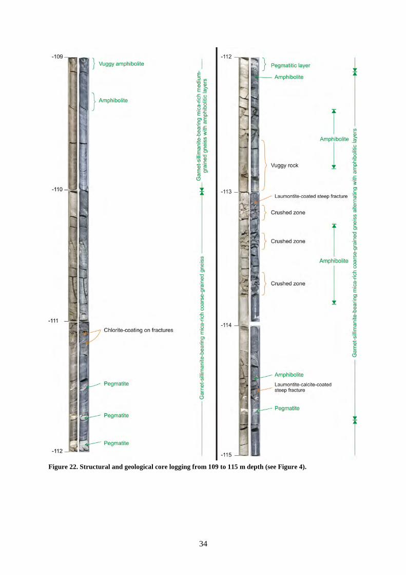
The 113–114 m depth interval has three distinct zones of crushed rocks; two of them are located within an amphibolite layer (Table 2 and Figure 22).
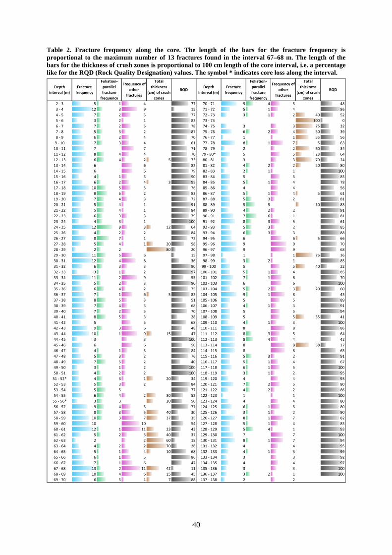
40
Table 2. Fracture frequency along the core. The length of the bars for the fracture frequency is proportional to the maximum number of 13 fractures found in the interval 67–68 m. The length of the bars for the thickness of crush zones is proportional to 100 cm length of the core interval, i.e. a percentage like for the RQD (Rock Quality Designation) values. The symbol * indicates core loss along the interval.
Depth interval (m)
Fracture frequency
Foliation-parallel fracture
frequency
Frequency of other
fractures
Total thickness
(cm) of crush zones
RQDDepth
interval (m)Fracture
frequency
Foliation-parallel fracture
frequency
Frequency of other
fractures
Total thickness
(cm) of crush zones
RQD
2 - 3 5 1 4 77 70 - 71 9 4 5 483 - 4 12 3 9 15 71 - 72 5 1 4 864 - 5 7 2 5 77 72 - 73 3 1 2 40 525 - 6 3 2 1 83 73 - 74 100 06 - 7 7 2 5 78 74 - 75 3 3 75 327 - 8 5 3 2 87 75 - 76 6 2 4 50 398 - 9 6 2 4 70 76 - 77 1 1 55 56
9 - 10 7 3 4 61 77 - 78 8 1 7 5 6310 - 11 7 7 71 78 - 79 2 2 60 3411 - 12 8 4 4 70 79 - 80* 5 5 23 6412 - 13 6 4 2 5 73 80 - 81 3 3 70 2413 - 14 6 6 82 81 - 82 4 2 2 20 8014 - 15 6 6 79 82 - 83 2 1 1 10015 - 16 4 1 3 90 83 - 84 5 5 8516 - 17 6 2 4 3 95 84 - 85 5 1 4 7817 - 18 10 5 5 76 85 - 86 4 4 5618 - 19 8 6 2 82 86 - 87 5 1 4 5 6119 - 20 7 4 3 72 87 - 88 5 3 2 8120 - 21 5 4 1 91 88 - 89 5 5 10 8321 - 22 5 4 1 84 89 - 90 4 2 2 9122 - 23 6 3 3 79 90 - 91 7 6 1 8123 - 24 4 3 1 100 91 - 92 8 3 5 6124 - 25 12 9 3 12 64 92 - 93 5 3 2 8525 - 26 4 2 2 84 93 - 94 6 3 3 8826 - 27 8 7 1 72 94 - 95 6 6 5 6627 - 28 5 4 1 20 58 95 - 96 9 9 7028 - 29 2 2 80 20 96 - 97 9 9 6829 - 30 11 5 6 15 97 - 98 1 1 75 3630 - 31 12 4 8 36 98 - 99 3 2 1 8531 - 32 6 3 3 90 99 - 100 5 5 40 2232 - 33 3 1 2 97 100 - 101 5 1 4 8533 - 34 11 2 9 55 101 - 102 7 1 6 7034 - 35 5 2 3 90 102 - 103 6 6 10035 - 36 6 4 2 75 103 - 104 5 2 3 20 6036 - 37 7 1 6 5 82 104 - 105 9 1 8 4537 - 38 8 5 3 51 105 - 106 5 5 8938 - 39 7 4 3 68 106 - 107 4 1 3 9139 - 40 7 2 5 70 107 - 108 5 5 9440 - 41 8 5 3 28 108 - 109 5 5 35 4141 - 42 5 5 68 109 - 110 4 1 3 10042 - 43 9 3 6 48 110 - 111 8 8 8643 - 44 10 1 9 15 47 111 - 112 8 3 5 6444 - 45 3 3 100 112 - 113 8 4 4 4245 - 46 6 6 50 113 - 114 8 8 58 1746 - 47 4 1 3 84 114 - 115 8 8 6547 - 48 5 3 2 76 115 - 116 5 3 2 9148 - 49 7 5 2 40 116 - 117 5 1 4 6749 - 50 3 1 2 100 117 - 118 6 1 5 10050 - 51 4 2 2 100 118 - 119 3 1 2 95
51 - 52* 4 3 1 20 34 119 - 120 4 4 9352 - 53 5 3 2 84 120 - 121 7 2 5 8053 - 54 5 5 77 121 - 122 4 2 2 8654 - 55 6 4 2 30 52 122 - 123 1 1 100
55 - 56* 3 3 20 50 123 - 124 4 4 8056 - 57 9 4 5 77 124 - 125 6 1 5 8057 - 58 8 3 5 40 30 125 - 126 3 1 2 9058 - 59 10 3 7 37 35 126 - 127 8 1 7 8259 - 60 10 10 54 127 - 128 5 1 4 8560 - 61 12 1 11 23 43 128 - 129 5 4 1 9361 - 62 5 2 3 40 37 129 - 130 7 7 10062 - 63 2 2 60 18 130 - 131 8 1 7 9463 - 64 4 2 2 70 26 131 - 132 4 4 9564 - 65 5 1 4 10 68 132 - 133 4 1 3 9965 - 66 6 1 5 86 133 - 134 3 3 9266 - 67 7 1 6 47 134 - 135 4 4 9767 - 68 13 2 11 42 11 135 - 136 3 3 10068 - 69 10 4 6 15 45 136 - 137 3 2 1 10069 - 70 6 5 1 7 88 137 - 138 2 2
41
2.3.3 Clay-rich zones were sampled during the core logging for XRD analysis and grain size distribution (see above for the description of sampled zones,
Clay-rich intervals
Table 3). The results of laboratory analysis were not yet available at the time of the finalization of this present report. They will be fully described and interpreted in a separate report.
Table 3. Samples for XRD analysis and grain size distribution Sample number Depth of sampling - material
47285 27.90–27.92 m - gouge / clays (see Figure 8)
47286 28.21–28.25 m - gouge / clays (see Figure 8)
47287 28.55–28.61 m - gouge / clays (see Figure 8)
47288 57.20 m - gouge / clays (see Figure 13)
47289 63.00 m - gouge / clays (see Figure 14)
47290 63.66 m - gouge / clays (see Figure 14)
47291 67.60 m - gouge / clays (see Figure 15)
The clays are typically the products of the chemical weathering of gneissic minerals. Because (1) angular fragments of the host rock are preserved in the clayey matrix and (2) severely fractured and crushed zones commonly surround the clay-rich intervals, it is inferred that they also derive from the weathering of frictional products and characterise the gouge infill of fault cores. This assertion is supported by the fact that the clayey zones are generally surrounded by crushed zones, which correspond to the typical damaged zone of shear zones.
The three several cm thick clay-rich shear zones at 27 or 28 m depth cannot be explained by only gravity-induced forces. Indeed, we assume that at this shallow depth it will require more than the 10 000 years to form such thickness of weathered products only by gravity-induced forces and slow creep. It is thus likely that the gouge-filled zones are of tectonic origin and that, after the ice sheet melting, these intrinsically weak zones localized the gravitational deformation leading to the development of sliding surfaces.
Whatever their origin and formation the clayey zones locally contribute to lower the stability of the rock mass. For stability assessments it is important to better characterise the content of swelling clays.
2.4 SUMMARY OF OBSERVATIONS AND INTERPRETATION The bedrock types near the surface reappear further down in the drill core. This is likely due to the occurrence of recumbent folding, which is observed both on surface outcrops (i.e. along the back-crack) and in the drill core.
0–24 m: In this interval, the rock is fractured, but the rock mass quality is generally good.
24–40 m: From 24 m depth and downwards, crushed zones occur and specifically in the 28–31 m depth interval. At c. 27.8–28.0 m, a major shear plane is observed. It consists of a 8–10 cm thick fault core filled by a clay-rich gouge, bordered by two zones of c. 10 cm crushed biotite-rich gneiss. This main shear zone is succeeded by a crushed zone containing two narrow zones with 3–4 cm thick gouge infill. Below these zones, the rock is heavily fractured.
40–54 m: Crushed zones occur regularly from 40 m and downwards, with occasional core loss.
54–56 m: Two 20–30 cm thick zones of severely fractured rocks with interlayered clays, but without a distinct clay/gouge fault core, are present in this interval.
42
56–82 m: Rocks are either crushed or strongly fractured and several zones are so distinguished between 57–59m, 59–61 m, 61–64 m and 67–68 m. Gouges in fault cores surrounded by damaged rocks are abundant in these zones. The interval between 72.5 and 81.2 m depth consists of zones of crushed rock and narrow zones with a clay-rich gouge.
This high frequency of weak zones in the 56–82 m depth interval (see Table 2) may indicate the location of the potential sliding surfaces of the Mannen rock slope instability.
82–92 m: There are fewer occurrences of zones with crushed rock below 81.2 m, and the frequency of such zones as well as fracturing decrease with depth.
92-138 m: The fracturing decreases and rock mass quality improves with depth, except in a few zones of crushed rocks. A 6–7 m wide zone of heavily fractured pegmatite occurs at c. 93.6–99.9 m, which is crushed in the interval 97–98 m. Other remarkable crushed zones are in the 99–100 m, 108–109 m and 113–114 m depth intervals. At c. 115 m and below the rock in the core is more intact.
Below 92 m, fewer foliation parallel fractures appear compared to above 92 m. This might be due to the frequent changes in the attitude of the foliation due to the folding of the bedrock. In this lower part, the fractures are concentrated in zones where amphibolites occur.
43
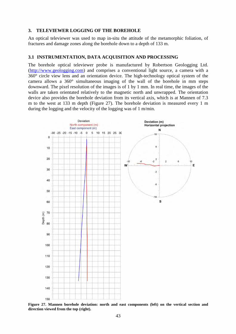
3. TELEVIEWER LOGGING OF THE BOREHOLE An optical televiewer was used to map in-situ the attitude of the metamorphic foliation, of fractures and damage zones along the borehole down to a depth of 133 m.
3.1 INSTRUMENTATION, DATA ACQUISITION AND PROCESSING The borehole optical televiewer probe is manufactured by Robertson Geologging Ltd. (http://www.geologging.com) and comprises a conventional light source, a camera with a 360° circle view lens and an orientation device. The high-technology optical system of the camera allows a 360° simultaneous imaging of the wall of the borehole in mm steps downward. The pixel resolution of the images is of 1 by 1 mm. In real time, the images of the walls are taken orientated relatively to the magnetic north and unwrapped. The orientation device also provides the borehole deviation from its vertical axis, which is at Mannen of 7.3 m to the west at 133 m depth (Figure 27). The borehole deviation is measured every 1 m during the logging and the velocity of the logging was of 1 m/min.
Figure 27. Mannen borehole deviation: north and east components (left) on the vertical section and direction viewed from the top (right).
44
The digitalisation of specific geological features, as fractures, crushed zones that are observed along the images allows to gather their characteristics (thickness, opening, infill...) and orientation (dip direction and angle) relatively to the magnetic north and corrected from the borehole deviation. The magnetic deviation at Mannen is 0.6° eastward and can thus be neglected. The orientations of planar structures given by the instrumentation are so considered relative to the geographic north. Hence, these measurements are afterwards processed like classical structural data.
The interpretation software RG-DIP from Robertson Geologging Ltd. allows to display the core images and the planar data orientations (with conventional arrow plots, stereoplots, rose diagrams) (see in Appendix 1).
The drilling was interrupted two times due to collapse of the hole. This was where crushed rocks were encountered at c. 32 m and 59 m depth. Drilling went on after stabilization and casing of the borehole. The logging by the optical televiewer was made before the casing of the borehole and thus followed the steps of drilling. The televiewer logging had also to be interrupted between 77 and 89 m because of the high risk of jamming the probe in an unstable severely damaged rock. The logging continued to the bottom of the hole after the installation of a drill string.
The method of logging by a borehole optical televiewer is described in detail in http://www.ngu.no/no/hm/Norges-geologi/Geofysikk/Borehullsgeofysikk/ (in Norwegian).
3.2 STRUCTURAL DATA ALONG THE BOREHOLE The data from the optical televiewer are presented according to this four logged depth intervals which are, from the top to the bottom, 3.1–31.7 m (in Chapter 3.2.2), 32–58 m (in Chapter 3.2.3), 57–77 m (in Chapter 3.2.4) and 89–133 m (in Chapter 3.2.5). The hole was dry down to 123.9 m depth.
In each interval, the digitised metamorphic foliation planes are visible and measured (see tables in Appendix 1). All the measurement of fractures and fractured zones are listed in Appendix 2 with characterisation of the thickness and/or aperture of fractures. The fracture frequency is also analysed (parameters for the fracture frequency calculation is given in Appendix 3).
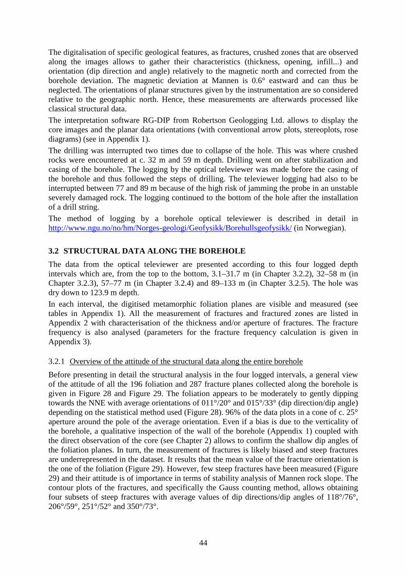
3.2.1 Before presenting in detail the structural analysis in the four logged intervals, a general view of the attitude of all the 196 foliation and 287 fracture planes collected along the borehole is given in
Overview of the attitude of the structural data along the entire borehole
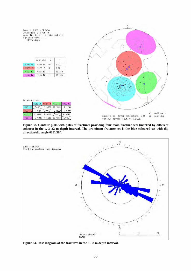
Figure 28 and Figure 29. The foliation appears to be moderately to gently dipping towards the NNE with average orientations of 011°/20° and 015°/33° (dip direction/dip angle) depending on the statistical method used (Figure 28). 96% of the data plots in a cone of c. 25° aperture around the pole of the average orientation. Even if a bias is due to the verticality of the borehole, a qualitative inspection of the wall of the borehole (Appendix 1) coupled with the direct observation of the core (see Chapter 2) allows to confirm the shallow dip angles of the foliation planes. In turn, the measurement of fractures is likely biased and steep fractures are underrepresented in the dataset. It results that the mean value of the fracture orientation is the one of the foliation (Figure 29). However, few steep fractures have been measured (Figure 29) and their attitude is of importance in terms of stability analysis of Mannen rock slope. The contour plots of the fractures, and specifically the Gauss counting method, allows obtaining four subsets of steep fractures with average values of dip directions/dip angles of 118°/76°, 206°/59°, 251°/52° and 350°/73°.
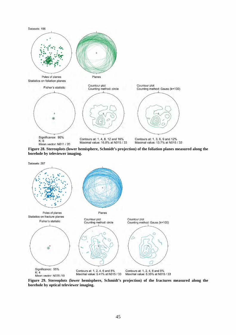
45
Figure 28. Stereoplots (lower hemisphere, Schmidt’s projection) of the foliation planes measured along the borehole by televiewer imaging.
Figure 29. Stereoplots (lower hemisphere, Schmidt’s projection) of the fractures measured along the borehole by optical televiewer imaging.
46
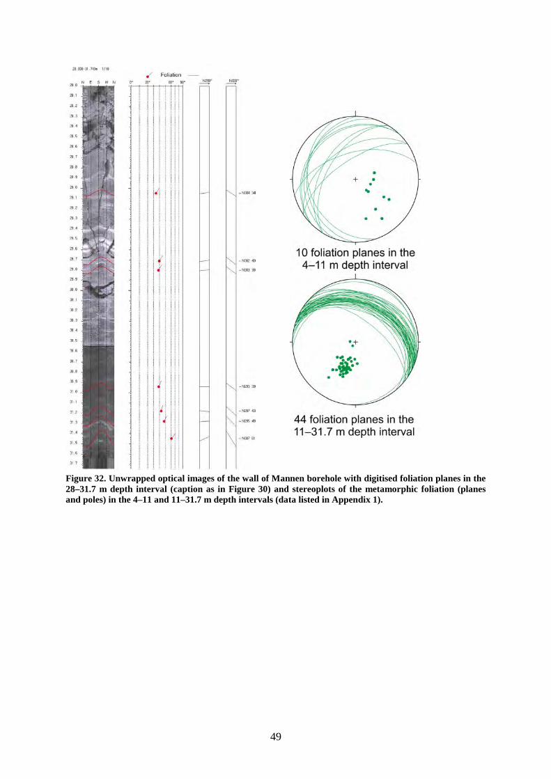
3.2.2 3.2.2.1 Metamorphic foliation in the 4–31.7 m depth interval
Structural data in the c. 3.1–31.7 m depth interval
The foliation was measured at 54 different depths along the 4–31.7 m interval (Figure 30–Figure 32 and Appendix 1). In the first 11 m depth of the hole, the foliation dips to the NW (dip direction: 304°) and the dip angle varies from 20° to 64° (Figure 30, Figure 32). From 15 m depth to the bottom of the studied interval at 31.7 m, the foliation dips towards the NNE (dip direction: 025°), i.e. towards the valley, with an average angle of 25° (Figure 30–Figure 32).
3.2.2.2 Fractures in the c. 3–32 m depth interval
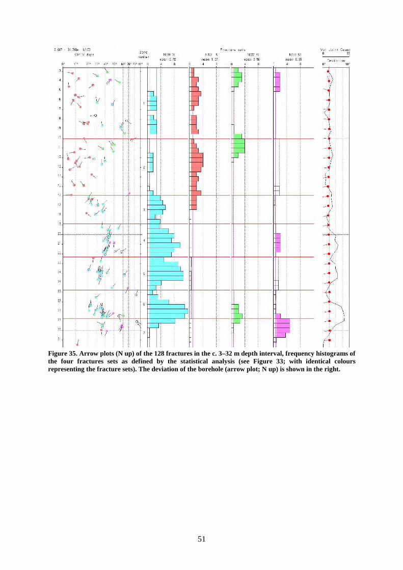
Figure 33 shows the four main fractures sets out of the 128 fractures encountered in the 3–32 m depth interval. The majority of mapped fractures is parallel to the foliation and the main set corresponds to fractures dipping toward the NNE, directly to the valley with a dip angle of 36°. This main set is also well displayed on the rose diagram of all fractures (Figure 34).
The frequency histogram of the four fracture sets detected in the c. 3–32 m depth interval shows clearly the spatial distribution of the fractures (Figure 35). Very shallow fractures are prominent in the first 15 m of the depth interval (in red on Figure 35). The major fracture set of the interval (dip direction and angle: N019/36; in blue on Figure 35) is nearly present in the entire interval and largely prevails in the c. 15–29.5 m depth with frequency reaching 10–12 fractures/m. From 29 to 32 m depth, interestingly, a set of steep fractures (dip direction and angle: N210/53; in pink on Figure 35) becomes predominant.
The c. 3–32 m depth interval was divided in 7 zones with regards to the fracture frequency (Figure 35) during the numerical calculation and according to the results listed in Appendix 3.
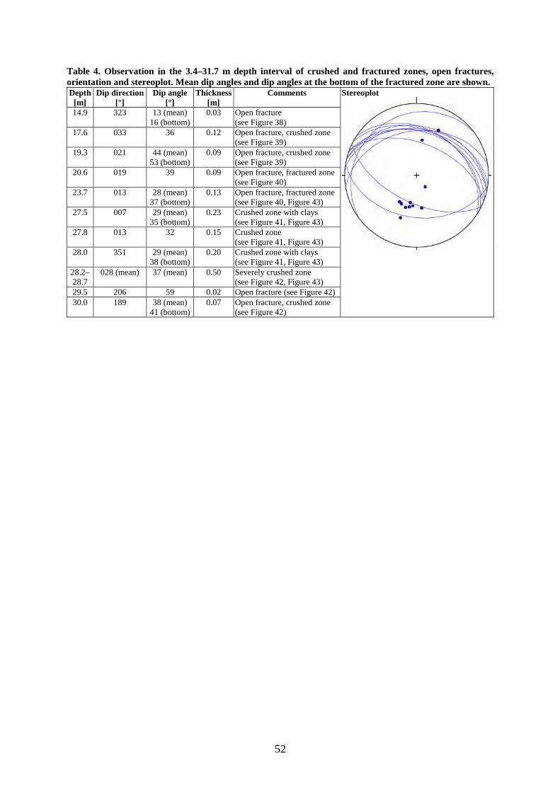
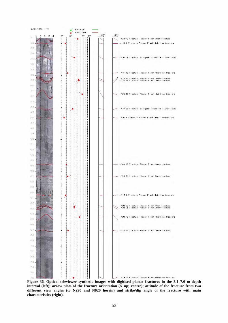
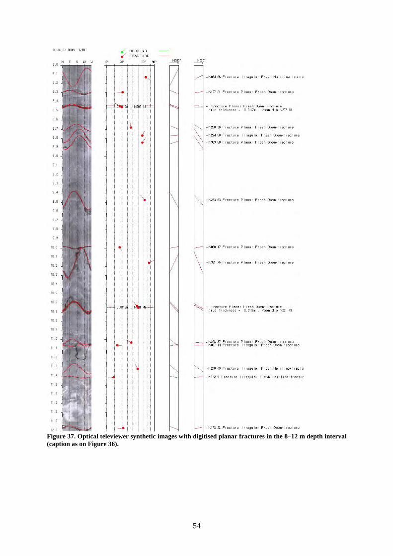
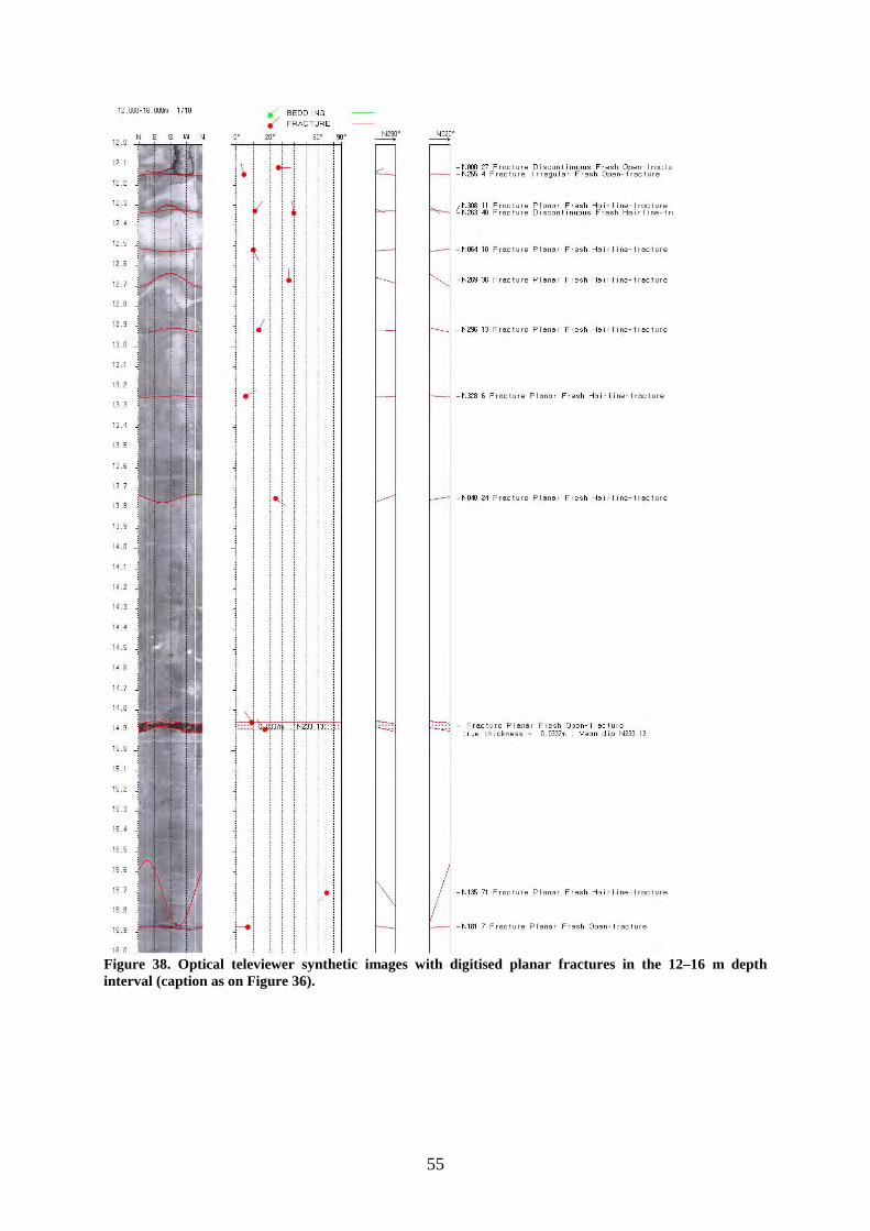
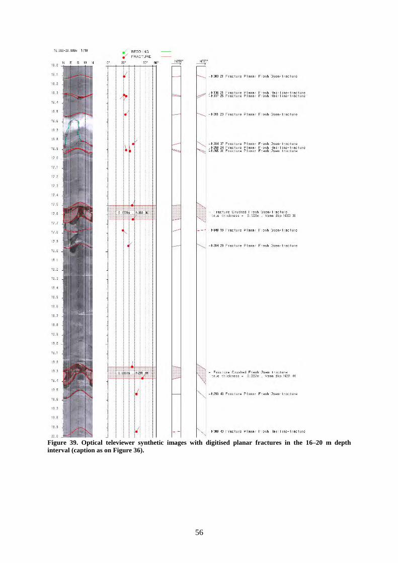
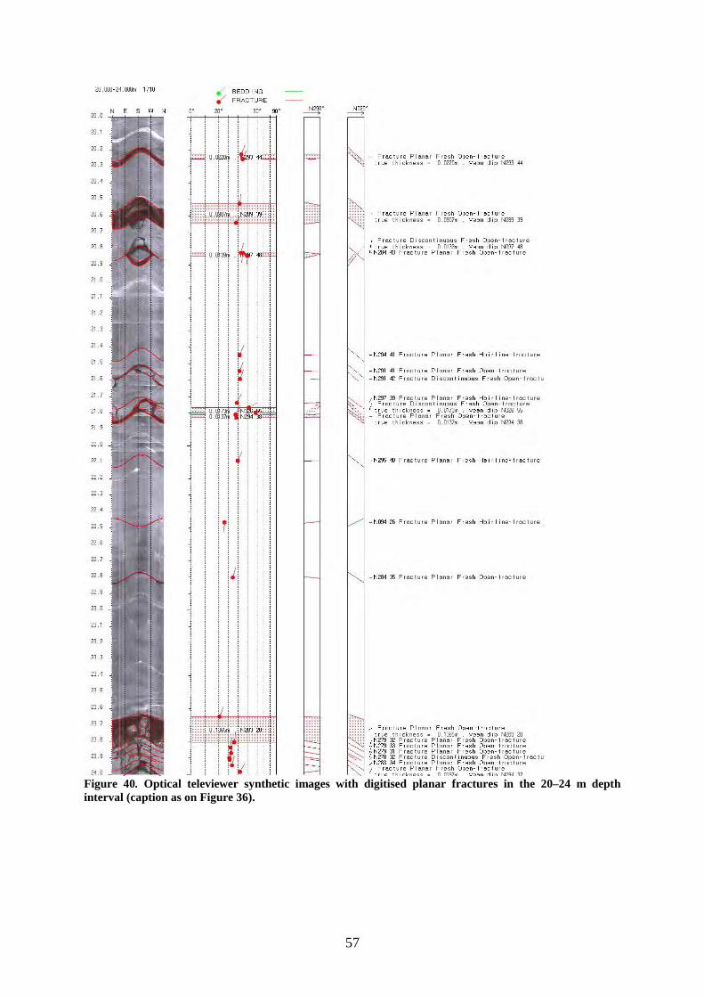
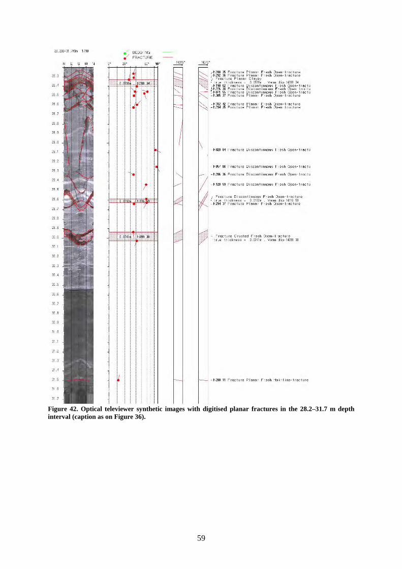
Figure 36–Figure 42 give the detailed pictures of the fractures in the 3.1–31.7 m depth interval. Foliation-parallel fractures are conspicuous from 20 m downward 31.7 m depth as well as the occurrence of 10–50 cm thick crushed zones (Table 4). The thickest crushed zone occurs between 28.2 and 28.7 m and corresponds to a zone reported from the core logging (Chapter 2). The clay-rich gouges sampled during the core logging (see Chapter 2.3.3) are well observed on the optical televiewer images (Figure 43). In general, it is in the 21–29 m depth interval that the crushed zones, accompanied or not by clays, and opened fractures are abundant. It also fits with the increase of the fracture frequency (see Figure 35). The digitalisation of the borders of these crushed zones allows to determine their orientations (Table 4), which clearly correspond to the main set of fractures dipping moderately towards the valley (dip direction/dip angle: 019°/36°; in blue on Figure 35). It may be assumed that the gravity-induced destabilisation of the overriding blocks may have produced the crushed zones by sliding along these favourably orientated surfaces. The thick clay-rich fault rocks are more difficult to explain at such shallow depth as only the results of gravity forces and may be probably the witness of the tectonic origin of the main set of NNE-dipping fractures (see also discussion in Chapter 2.3.3).

47
Figure 30. Unwrapped optical images of the wall of Mannen borehole with digitised foliation planes in the 4–16 m depth interval (left). Dip angle and dip direction of each plane are displayed on the arrow plot (N up; centre). Attitude of foliation plane is seen from two different angles (to N315 and N045 or to N290 and N020) with strike (right hand rule) and dip angle of the plane (right).
48
Figure 31. Unwrapped optical images of the wall of Mannen borehole with digitised foliation planes in the 16–28 m depth interval (caption as in Figure 30).
49
Figure 32. Unwrapped optical images of the wall of Mannen borehole with digitised foliation planes in the 28–31.7 m depth interval (caption as in Figure 30) and stereoplots of the metamorphic foliation (planes and poles) in the 4–11 and 11–31.7 m depth intervals (data listed in Appendix 1).
50
Figure 33. Contour plots with poles of fractures providing four main fracture sets (marked by different colours) in the c. 3–32 m depth interval. The prominent fracture set is the blue coloured set with dip direction/dip angle 019°/36°.
Figure 34. Rose diagram of the fractures in the 3–32 m depth interval.
51
Figure 35. Arrow plots (N up) of the 128 fractures in the c. 3–32 m depth interval, frequency histograms of the four fractures sets as defined by the statistical analysis (see Figure 33; with identical colours representing the fracture sets). The deviation of the borehole (arrow plot; N up) is shown in the right.
52
Table 4. Observation in the 3.4–31.7 m depth interval of crushed and fractured zones, open fractures, orientation and stereoplot. Mean dip angles and dip angles at the bottom of the fractured zone are shown. Depth
[m] Dip direction
[°] Dip angle
[°] Thickness
[m] Comments Stereoplot
14.9 323 13 (mean) 16 (bottom)
0.03 Open fracture (see Figure 38)
17.6 033 36 0.12 Open fracture, crushed zone (see Figure 39)
19.3 021 44 (mean) 53 (bottom)
0.09 Open fracture, crushed zone (see Figure 39)
20.6 019 39 0.09 Open fracture, fractured zone (see Figure 40)
23.7 013 28 (mean) 37 (bottom)
0.13 Open fracture, fractured zone (see Figure 40, Figure 43)
27.5 007 29 (mean) 35 (bottom)
0.23 Crushed zone with clays (see Figure 41, Figure 43)
27.8 013 32 0.15 Crushed zone (see Figure 41, Figure 43)
28.0 351 29 (mean) 38 (bottom)
0.20 Crushed zone with clays (see Figure 41, Figure 43)
28.2–28.7
028 (mean) 37 (mean) 0.50 Severely crushed zone (see Figure 42, Figure 43)
29.5 206 59 0.02 Open fracture (see Figure 42) 30.0 189 38 (mean)
41 (bottom) 0.07 Open fracture, crushed zone
(see Figure 42)
53
Figure 36. Optical televiewer synthetic images with digitised planar fractures in the 3.1–7.6 m depth interval (left); arrow plots of the fracture orientation (N up; centre); attitude of the fracture from two different view angles (to N290 and N020 herein) and strike/dip angle of the fracture with main characteristics (right).
54
Figure 37. Optical televiewer synthetic images with digitised planar fractures in the 8–12 m depth interval (caption as on Figure 36).
55
Figure 38. Optical televiewer synthetic images with digitised planar fractures in the 12–16 m depth interval (caption as on Figure 36).
56
Figure 39. Optical televiewer synthetic images with digitised planar fractures in the 16–20 m depth interval (caption as on Figure 36).
57
Figure 40. Optical televiewer synthetic images with digitised planar fractures in the 20–24 m depth interval (caption as on Figure 36).
58
Figure 41. Optical televiewer synthetic images with digitised planar fractures in the 24–28.2 m depth interval (caption as on Figure 36).
59
Figure 42. Optical televiewer synthetic images with digitised planar fractures in the 28.2–31.7 m depth interval (caption as on Figure 36).
60
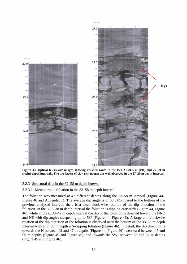
Figure 43. Optical televiewer images showing crushed zones in the two 23–24.5 m (left) and 27–29 m (right) depth intervals. The two layers of clay-rich gouges are well observed in the 27–29 m depth interval.
3.2.3 3.2.3.1 Metamorphic foliation in the 33–58 m depth interval
Structural data in the 32–58 m depth interval
The foliation was measured at 47 different depths along the 33–58 m interval (Figure 44–Figure 46 and Appendix 1). The average dip angle is of 33°. Compared to the bottom of the previous analysed interval, there is a clear clock-wise rotation of the dip direction of the foliation. In the 33.5–38 m depth interval the foliation is dipping eastwards (Figure 44, Figure 46), while in the c. 38–42 m depth interval the dip of the foliation is directed toward the NNE and NE with dip angles steepening up to 58° (Figure 44, Figure 46). A large anti-clockwise rotation of the dip direction of the foliation is observed until the bottom of the 33–58 m depth interval with at c. 58 m depth a S-dipping foliation (Figure 46). In detail, the dip direction is towards the N between 42 and 47 m depths (Figure 44–Figure 46), westward between 47 and 55 m depths (Figure 45 and Figure 46), and towards the SW, between 55 and 57 m depths (Figure 45 and Figure 46).
Clays
61
Figure 44. Unwrapped optical images of the wall of Mannen borehole with digitised foliation planes in the 32–44 m depth interval (caption as in Figure 30).
62
Figure 45. Unwrapped optical images of the wall of Mannen borehole with digitised foliation planes in the 44–56 m depth interval (caption as in Figure 30).
63
Figure 46. Unwrapped optical images of the wall of Mannen borehole with digitised foliation planes in the 56–58 m depth interval (caption as in Figure 30) and stereoplot of the metamorphic foliation (planes and poles) in the 33.5–38, 38–42, 42–47, 47–55, 55–57 and 57–58 m depth intervals (data listed in Appendix 1).
3.2.3.2 Fractures in the 32–58 m depth interval
The analysis of the 71 fracture orientations in the 32–58 m depth interval reveals five different well-defined fracture sets (Figure 47). The rose diagram of Figure 48 well displays the dispersion of fractures in this interval. The main set is however largely represented by 35 very shallow NE-dipping fractures.
64
Figure 47. Contour plots, with poles of fractures, providing four main fracture sets in the c. 32–58 m depth interval.
Figure 48. Rose diagram of the fractures in the 32–58 m depth interval.
65
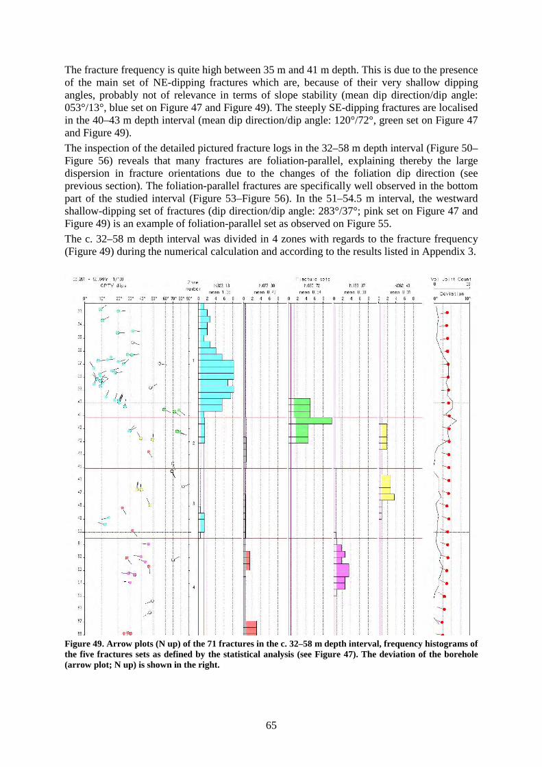
The fracture frequency is quite high between 35 m and 41 m depth. This is due to the presence of the main set of NE-dipping fractures which are, because of their very shallow dipping angles, probably not of relevance in terms of slope stability (mean dip direction/dip angle: 053°/13°, blue set on Figure 47 and Figure 49). The steeply SE-dipping fractures are localised in the 40–43 m depth interval (mean dip direction/dip angle: 120°/72°, green set on Figure 47 and Figure 49).
The inspection of the detailed pictured fracture logs in the 32–58 m depth interval (Figure 50–Figure 56) reveals that many fractures are foliation-parallel, explaining thereby the large dispersion in fracture orientations due to the changes of the foliation dip direction (see previous section). The foliation-parallel fractures are specifically well observed in the bottom part of the studied interval (Figure 53–Figure 56). In the 51–54.5 m interval, the westward shallow-dipping set of fractures (dip direction/dip angle: 283°/37°; pink set on Figure 47 and Figure 49) is an example of foliation-parallel set as observed on Figure 55.
The c. 32–58 m depth interval was divided in 4 zones with regards to the fracture frequency (Figure 49) during the numerical calculation and according to the results listed in Appendix 3.
Figure 49. Arrow plots (N up) of the 71 fractures in the c. 32–58 m depth interval, frequency histograms of the five fractures sets as defined by the statistical analysis (see Figure 47). The deviation of the borehole (arrow plot; N up) is shown in the right.
66
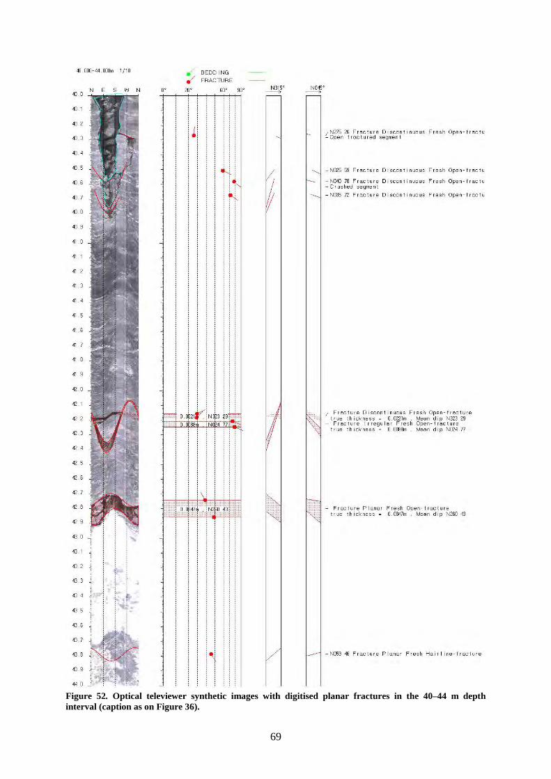
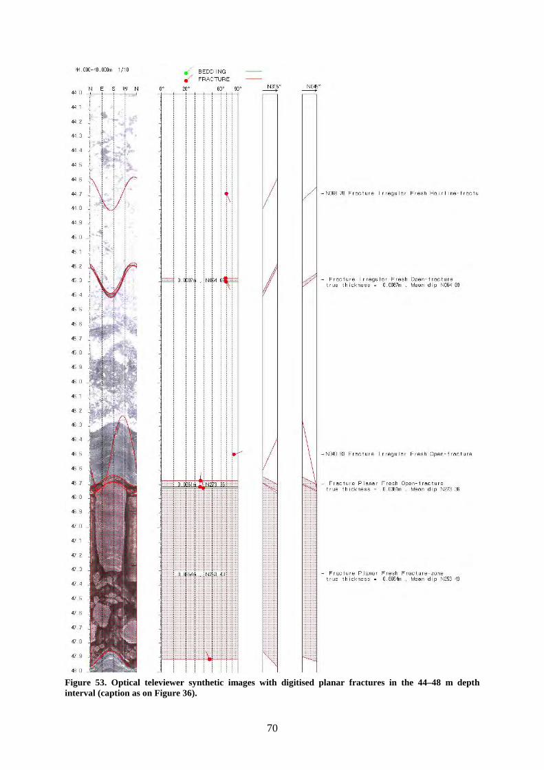
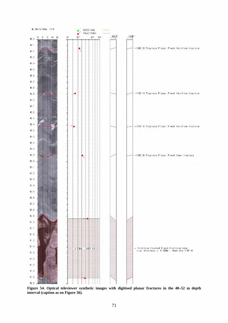
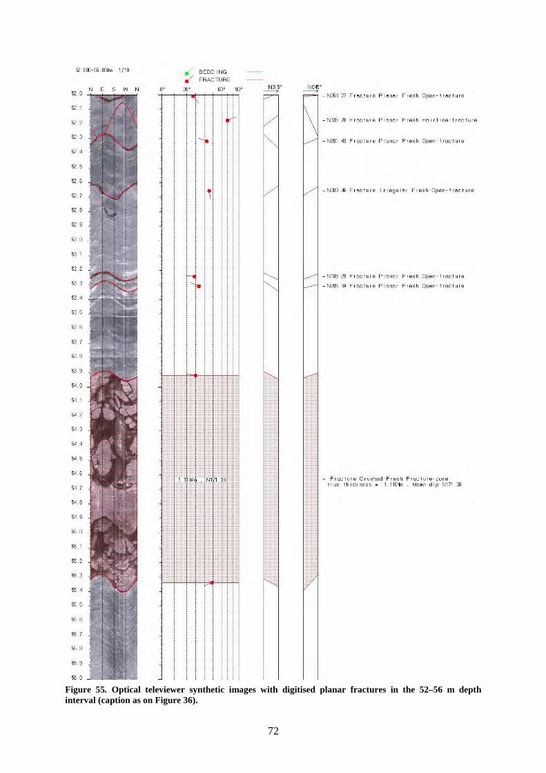
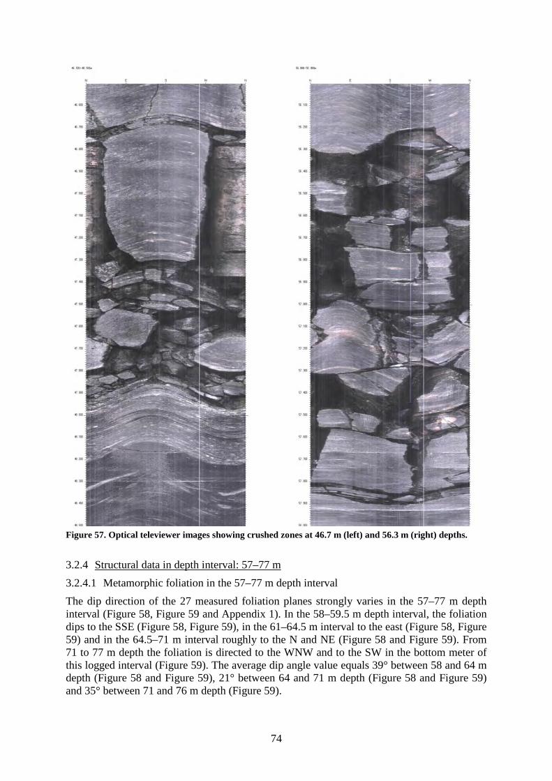
In the 32–58 m depth interval, five crushed zones and opened fractures are extracted from the detailed analysis of the logs as displayed in Figure 50–Figure 56 and listed in Table 5. They are located between 39.8 m and 56.3 m depth. The thickness of crushed zones varies from 0.1–1.2 m. Figure 57 illustrates two of these zones at 46.7 m and 56.3 m depth. All the zones developed along the metamorphic foliation.
Table 5. Observation in the 39.8–56.3 m depth interval of crushed and fractured zones, open fractures, orientation and stereoplot. Mean dip angles and dip angles at the bottom of the fractured zone are shown. Depth
[m] Dip direction
[°] Dip angle
[°] Thickness
[m] Comments Stereoplot
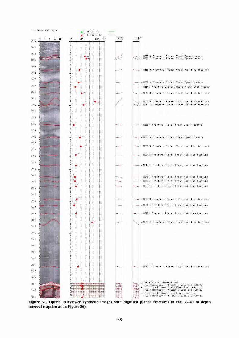
39.8 030 20 0.12 Crushed zone, vertical fracture (see Figure 51)
46.7 343 43 (mean) 46 (bottom)
0.86 Crushed zone, vertical fracture (see Figure 53, Figure 57)
50.9 277 43 0.72 Vertical open zone (see Figure 54)
53.9 261 38 (mean) 49 (bottom)
1.11 Crushed zone (see Figure 55)
56.3 224 36(mean) 28 (bottom)
1.28 Crushed zone (see Figure 56, Figure 57)
67
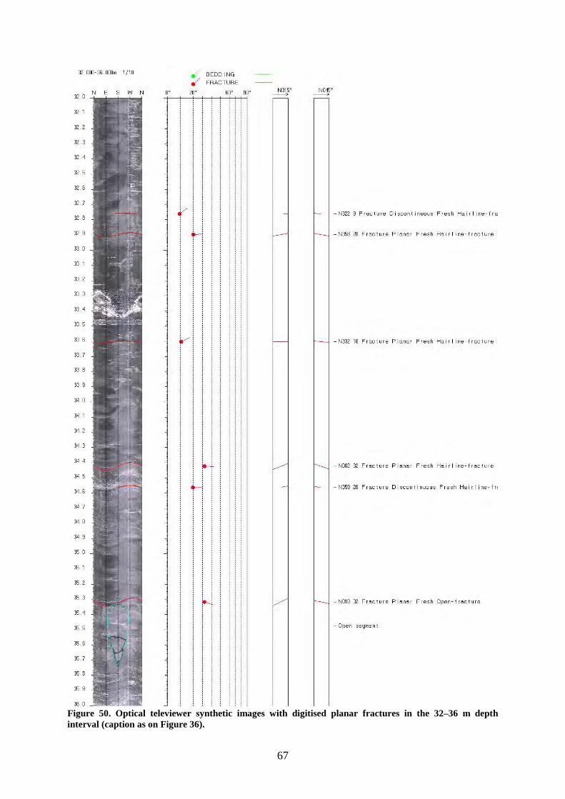
Figure 50. Optical televiewer synthetic images with digitised planar fractures in the 32–36 m depth interval (caption as on Figure 36).
68
Figure 51. Optical televiewer synthetic images with digitised planar fractures in the 36–40 m depth interval (caption as on Figure 36).
69
Figure 52. Optical televiewer synthetic images with digitised planar fractures in the 40–44 m depth interval (caption as on Figure 36).
70
Figure 53. Optical televiewer synthetic images with digitised planar fractures in the 44–48 m depth interval (caption as on Figure 36).
71
Figure 54. Optical televiewer synthetic images with digitised planar fractures in the 48–52 m depth interval (caption as on Figure 36).
72
Figure 55. Optical televiewer synthetic images with digitised planar fractures in the 52–56 m depth interval (caption as on Figure 36).
73
Figure 56. Optical televiewer synthetic images with digitised planar fractures in the 56–58 m depth interval (caption as on Figure 36).
74
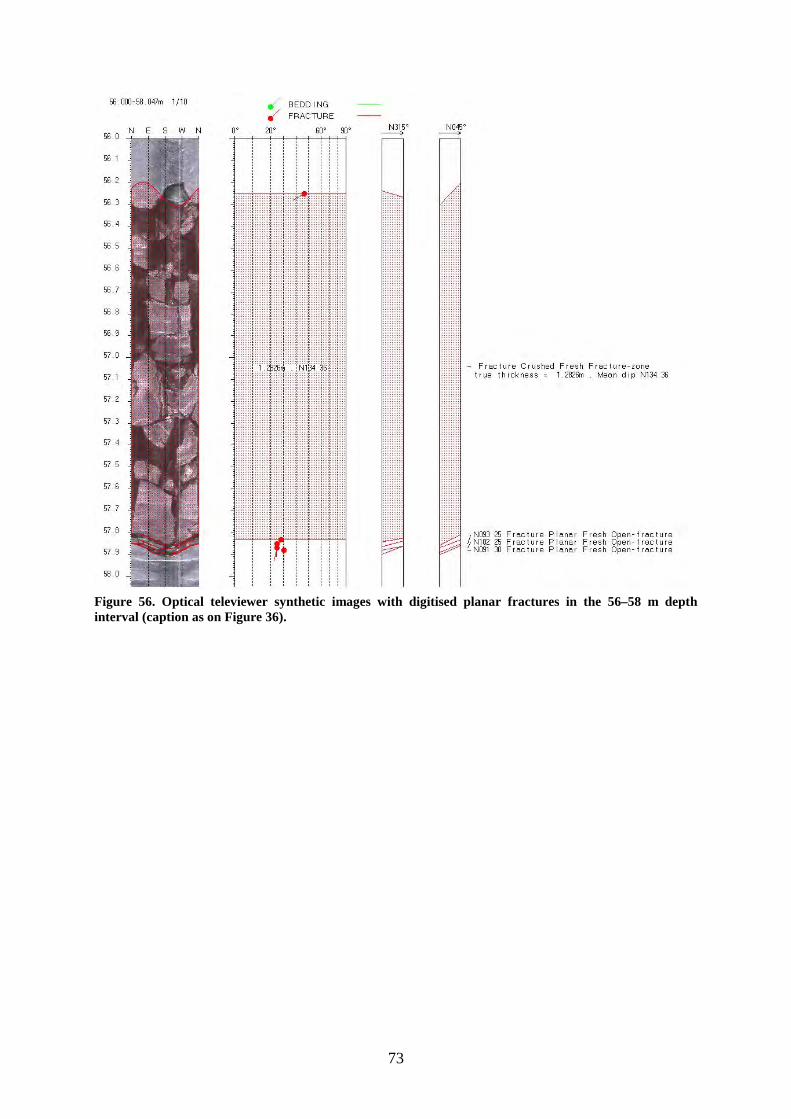
Figure 57. Optical televiewer images showing crushed zones at 46.7 m (left) and 56.3 m (right) depths.
3.2.4 3.2.4.1 Metamorphic foliation in the 57–77 m depth interval
Structural data in depth interval: 57–77 m
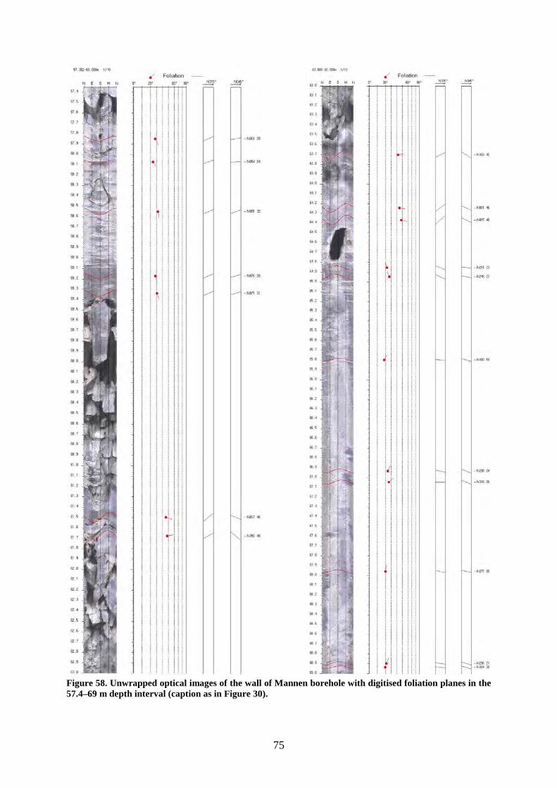
The dip direction of the 27 measured foliation planes strongly varies in the 57–77 m depth interval (Figure 58, Figure 59 and Appendix 1). In the 58–59.5 m depth interval, the foliation dips to the SSE (Figure 58, Figure 59), in the 61–64.5 m interval to the east (Figure 58, Figure 59) and in the 64.5–71 m interval roughly to the N and NE (Figure 58 and Figure 59). From 71 to 77 m depth the foliation is directed to the WNW and to the SW in the bottom meter of this logged interval (Figure 59). The average dip angle value equals 39° between 58 and 64 m depth (Figure 58 and Figure 59), 21° between 64 and 71 m depth (Figure 58 and Figure 59) and 35° between 71 and 76 m depth (Figure 59).
75
Figure 58. Unwrapped optical images of the wall of Mannen borehole with digitised foliation planes in the 57.4–69 m depth interval (caption as in Figure 30).

76
Figure 59. Unwrapped optical images of the wall of Mannen borehole with digitised foliation planes in the 69–77.6 m depth interval (caption as in Figure 30) and stereoplot of the metamorphic foliation (planes and poles) in the 58–59.5, 61–64.5, 64.5–71 and 71–77 m depth interval (data listed in Appendix 1).
77
3.2.4.2 Fractures in the 57–77 m depth interval
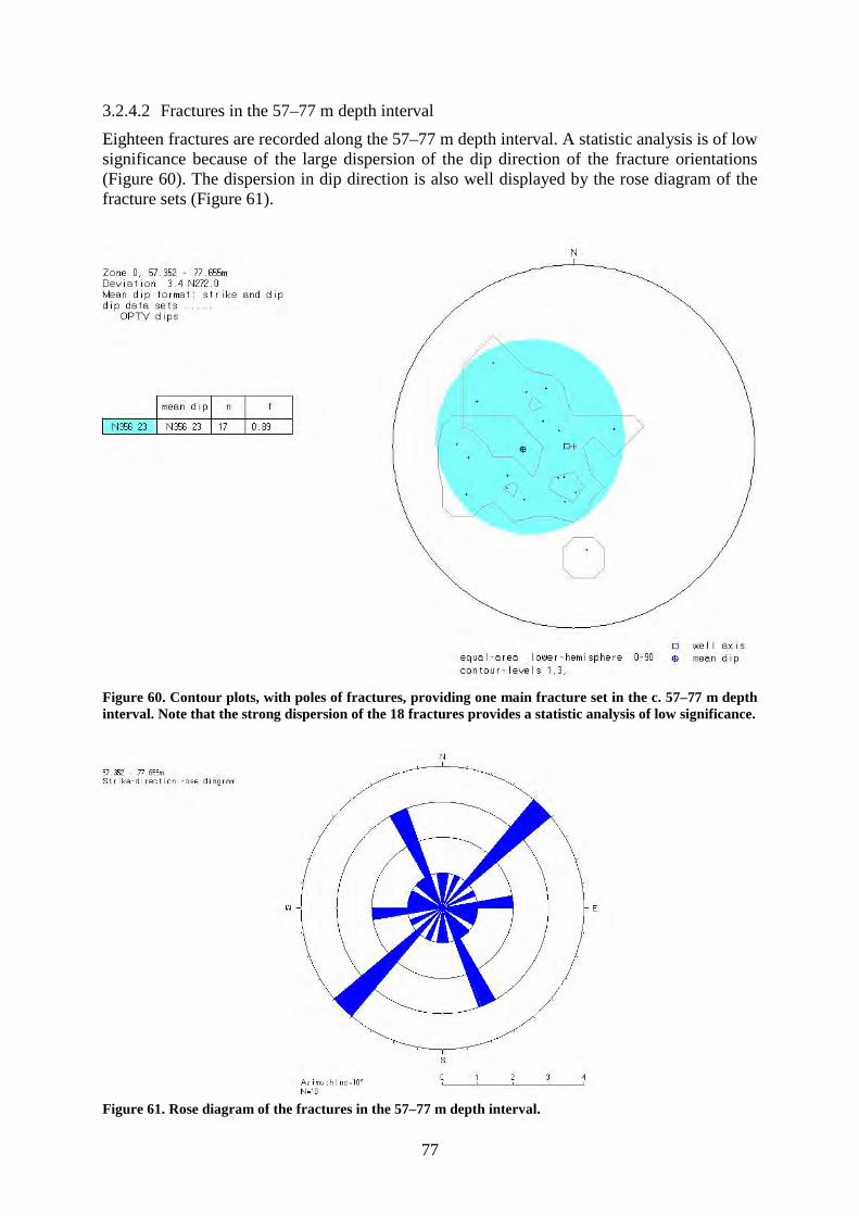
Eighteen fractures are recorded along the 57–77 m depth interval. A statistic analysis is of low significance because of the large dispersion of the dip direction of the fracture orientations (Figure 60). The dispersion in dip direction is also well displayed by the rose diagram of the fracture sets (Figure 61).
Figure 60. Contour plots, with poles of fractures, providing one main fracture set in the c. 57–77 m depth interval. Note that the strong dispersion of the 18 fractures provides a statistic analysis of low significance.
Figure 61. Rose diagram of the fractures in the 57–77 m depth interval.
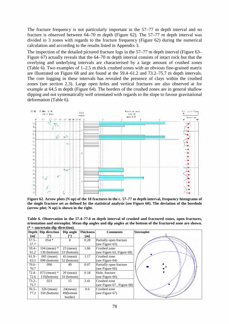
78
The fracture frequency is not particularly important in the 57–77 m depth interval and no fracture is observed between 64–70 m depth (Figure 62). The 57–77 m depth interval was divided in 3 zones with regards to the fracture frequency (Figure 62) during the numerical calculation and according to the results listed in Appendix 3. The inspection of the detailed pictured fracture logs in the 57–77 m depth interval (Figure 63–Figure 67) actually reveals that the 64–70 m depth interval consists of intact rock but that the overlying and underlying intervals are characterised by a large amount of crushed zones (Table 6). Two examples of 1–2.5 m thick crushed zones with an obvious fine-grained matrix are illustrated on Figure 68 and are found at the 59.4–61.2 and 73.2–75.7 m depth intervals. The core logging in these intervals has revealed the presence of clays within the crushed zones (see section 2.3). Large open holes and vertical fractures are also observed at for example at 64.5 m depth (Figure 64). The borders of the crushed zones are in general shallow dipping and not systematically well orientated with regards to the slope to favour gravitational deformation (Table 6).
Figure 62. Arrow plots (N up) of the 18 fractures in the c. 57–77 m depth interval, frequency histograms of the single fracture set as defined by the statistical analysis (see Figure 60). The deviation of the borehole (arrow plot; N up) is shown in the right. Table 6. Observation in the 57.4–77.6 m depth interval of crushed and fractured zones, open fractures, orientation and stereoplot. Mean dip angles and dip angles at the bottom of the fractured zone are shown. (* = uncertain dip direction). Depth
[m] Dip direction
[°] Dip angle
[°] Thickness
[m] Comments Stereoplot
57.5–57.7
054 * 8 0.28 Partially open fracture (see Figure 63)
59.4–61.2
104 (mean) * 130 (bottom)
23 (mean) 53 (bottom)
1.66 Crushed zone (see Figure 63, Figure 68)
61.9–63.5
081 (mean) 090 (bottom)
43 (mean) 52 (bottom)
1.17 Crushed zone (see Figure 64)
70.6–70.7
090 49 0.07 Partially open fracture (see Figure 66)
72.4–72.6
073 (mean) * 135(bottom)
20 (mean) 10 (bottom)
0.18 Hole, fracture (see Figure 66)
73.2–75.7
023 15 2.41 Crushed zone (see Figure 67 , Figure 68)
76.5–77.2
326 (mean) 350 (bottom)
24(mean) 49(bottom
border)
0.6 Crushed zone (see Figure 67)
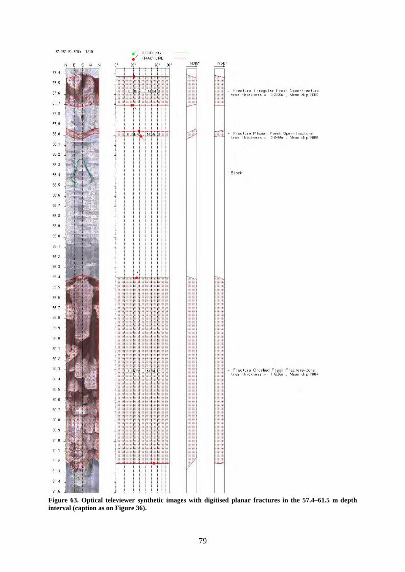
79
Figure 63. Optical televiewer synthetic images with digitised planar fractures in the 57.4–61.5 m depth interval (caption as on Figure 36).
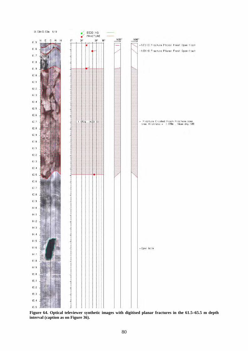
80
Figure 64. Optical televiewer synthetic images with digitised planar fractures in the 61.5–65.5 m depth interval (caption as on Figure 36).
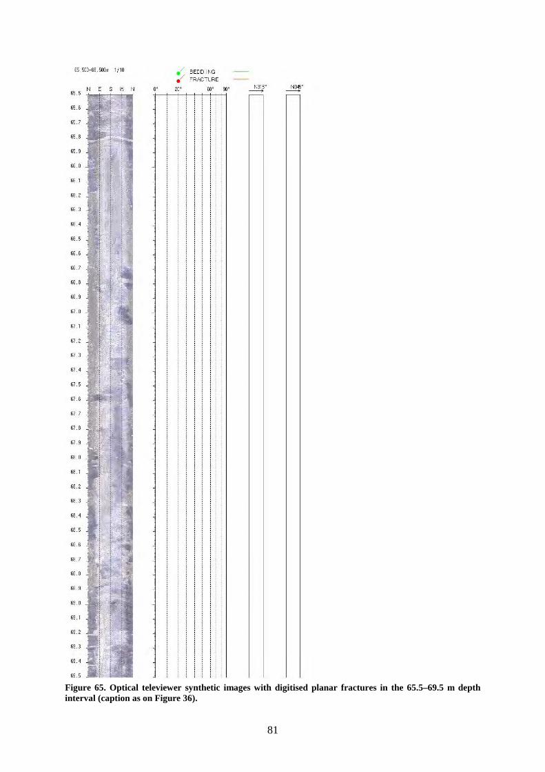
81
Figure 65. Optical televiewer synthetic images with digitised planar fractures in the 65.5–69.5 m depth interval (caption as on Figure 36).
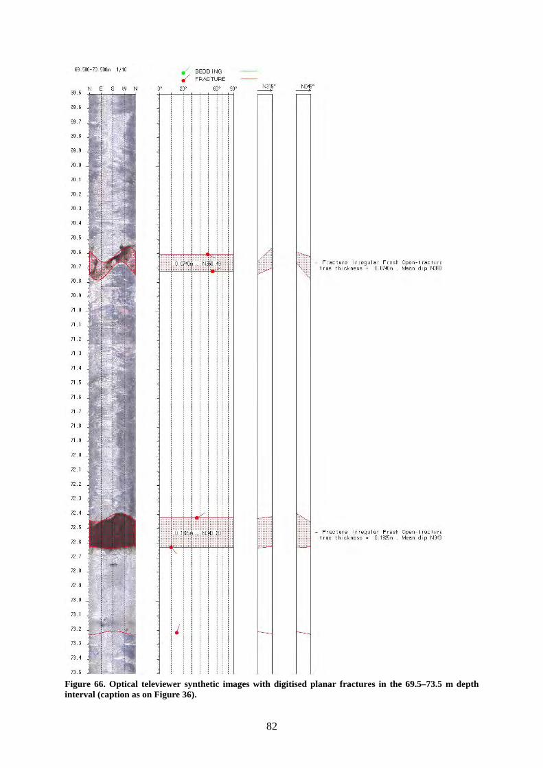
82
Figure 66. Optical televiewer synthetic images with digitised planar fractures in the 69.5–73.5 m depth interval (caption as on Figure 36).
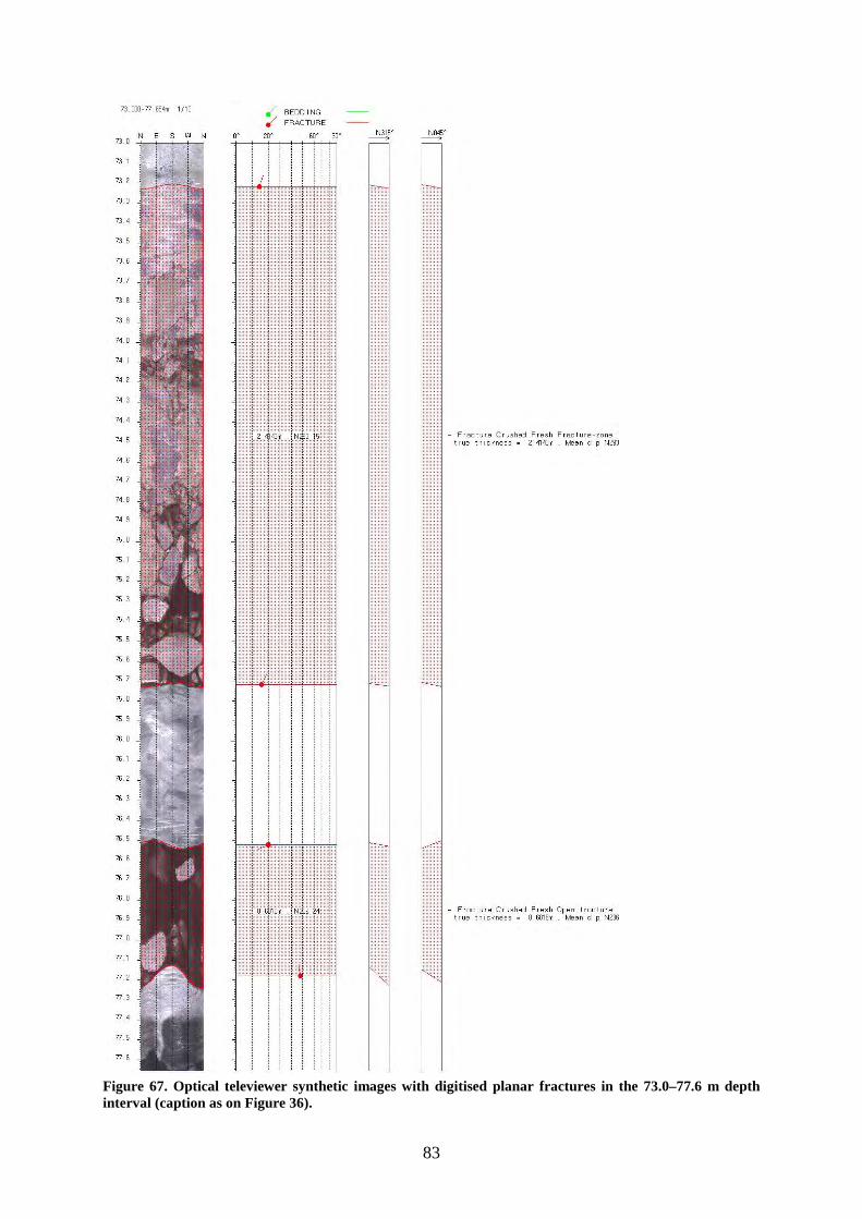
83
Figure 67. Optical televiewer synthetic images with digitised planar fractures in the 73.0–77.6 m depth interval (caption as on Figure 36).
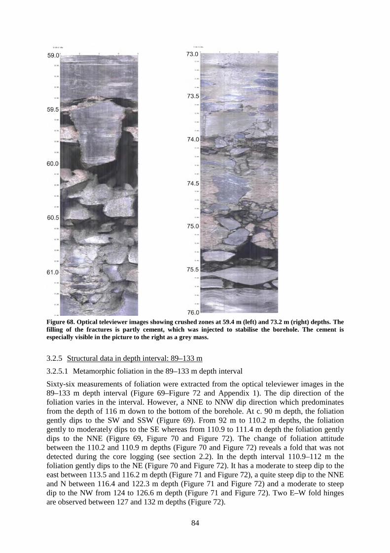
84
Figure 68. Optical televiewer images showing crushed zones at 59.4 m (left) and 73.2 m (right) depths. The filling of the fractures is partly cement, which was injected to stabilise the borehole. The cement is especially visible in the picture to the right as a grey mass.
3.2.5 3.2.5.1 Metamorphic foliation in the 89–133 m depth interval
Structural data in depth interval: 89–133 m
Sixty-six measurements of foliation were extracted from the optical televiewer images in the 89–133 m depth interval (Figure 69–Figure 72 and Appendix 1). The dip direction of the foliation varies in the interval. However, a NNE to NNW dip direction which predominates from the depth of 116 m down to the bottom of the borehole. At c. 90 m depth, the foliation gently dips to the SW and SSW (Figure 69). From 92 m to 110.2 m depths, the foliation gently to moderately dips to the SE whereas from 110.9 to 111.4 m depth the foliation gently dips to the NNE (Figure 69, Figure 70 and Figure 72). The change of foliation attitude between the 110.2 and 110.9 m depths (Figure 70 and Figure 72) reveals a fold that was not detected during the core logging (see section 2.2). In the depth interval 110.9–112 m the foliation gently dips to the NE (Figure 70 and Figure 72). It has a moderate to steep dip to the east between 113.5 and 116.2 m depth (Figure 71 and Figure 72), a quite steep dip to the NNE and N between 116.4 and 122.3 m depth (Figure 71 and Figure 72) and a moderate to steep dip to the NW from 124 to 126.6 m depth (Figure 71 and Figure 72). Two E–W fold hinges are observed between 127 and 132 m depths (Figure 72).
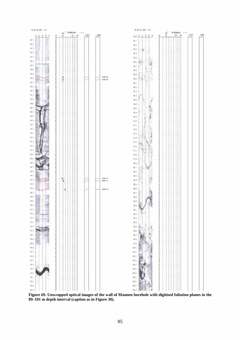
85
Figure 69. Unwrapped optical images of the wall of Mannen borehole with digitised foliation planes in the 89–101 m depth interval (caption as in Figure 30).
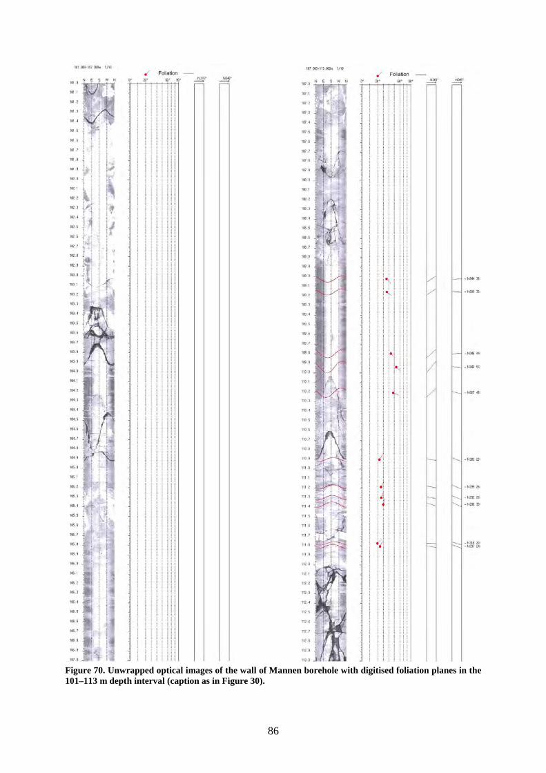
86
Figure 70. Unwrapped optical images of the wall of Mannen borehole with digitised foliation planes in the 101–113 m depth interval (caption as in Figure 30).
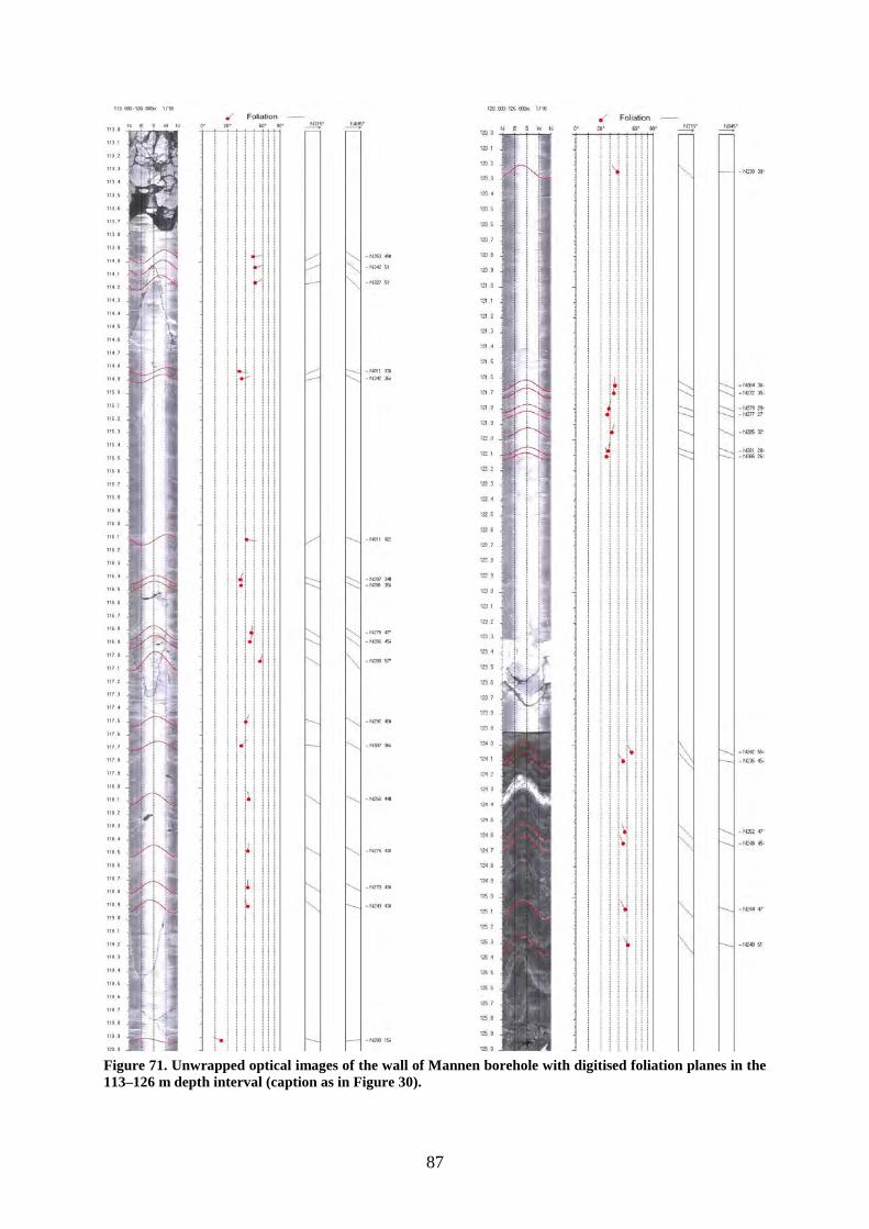
87
Figure 71. Unwrapped optical images of the wall of Mannen borehole with digitised foliation planes in the 113–126 m depth interval (caption as in Figure 30).
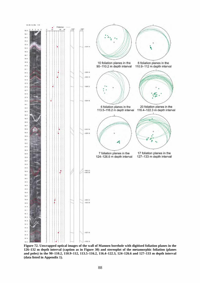
88
Figure 72. Unwrapped optical images of the wall of Mannen borehole with digitised foliation planes in the 126–132 m depth interval (caption as in Figure 30) and stereoplot of the metamorphic foliation (planes and poles) in the 90–110.2, 110.9–112, 113.5–116.2, 116.4–122.3, 124–126.6 and 127–133 m depth interval (data listed in Appendix 1).
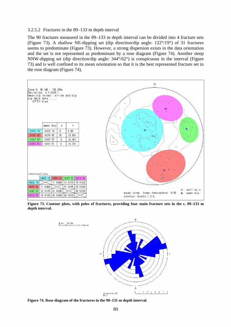
89
3.2.5.2 Fractures in the 89–133 m depth interval
The 90 fractures measured in the 89–133 m depth interval can be divided into 4 fracture sets (Figure 73). A shallow NE-dipping set (dip direction/dip angle: 122°/19°) of 31 fractures seems to predominate (Figure 73). However, a strong dispersion exists in the data orientation and the set is not represented as predominant by a rose diagram (Figure 74). Another steep NNW-dipping set (dip direction/dip angle: 344°/62°) is conspicuous in the interval (Figure 73) and is well confined to its mean orientation so that it is the best represented fracture set in the rose diagram (Figure 74).
Figure 73. Contour plots, with poles of fractures, providing four main fracture sets in the c. 89–133 m depth interval.
Figure 74. Rose diagram of the fractures in the 90–131 m depth interval.
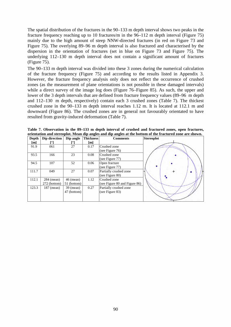
90
The spatial distribution of the fractures in the 90–133 m depth interval shows two peaks in the fracture frequency reaching up to 10 fractures/m in the 96–112 m depth interval (Figure 75) mainly due to the high amount of steep NNW-directed fractures (in red on Figure 73 and Figure 75). The overlying 89–96 m depth interval is also fractured and characterised by the dispersion in the orientation of fractures (set in blue on Figure 73 and Figure 75). The underlying 112–130 m depth interval does not contain a significant amount of fractures (Figure 75).
The 90–133 m depth interval was divided into these 3 zones during the numerical calculation of the fracture frequency (Figure 75) and according to the results listed in Appendix 3. However, the fracture frequency analysis only does not reflect the occurrence of crushed zones (as the measurement of plane orientations is not possible in these damaged intervals) while a direct survey of the image log does (Figure 76–Figure 85). As such, the upper and lower of the 3 depth intervals that are defined from fracture frequency values (89–96 m depth and 112–130 m depth, respectively) contain each 3 crushed zones (Table 7). The thickest crushed zone in the 90–133 m depth interval reaches 1.12 m. It is located at 112.1 m and downward (Figure 86). The crushed zones are in general not favourably orientated to have resulted from gravity-induced deformation (Table 7).
Table 7. Observation in the 89–133 m depth interval of crushed and fractured zones, open fractures, orientation and stereoplot. Mean dip angles and dip angles at the bottom of the fractured zone are shown.
Depth [m]
Dip direction [°]
Dip angle [°]
Thickness [m]
Comments Stereoplot
91.9 061 27 0.17 Crushed zone (see Figure 76)
93.5 166 23 0.08 Crushed zone (see Figure 77)
94.5 107 52 0.06 Open fracture (see Figure 77)
111.7 049 27 0.07 Partially crushed zone (see Figure 80)
112.1 284 (mean) 272 (bottom)
46 (mean) 51 (bottom)
1.12 Crushed zone (see Figure 80 and Figure 86)
123.3 187 (mean) 39 (mean) 47 (bottom)
0.27 Partially crushed zone (see Figure 83)
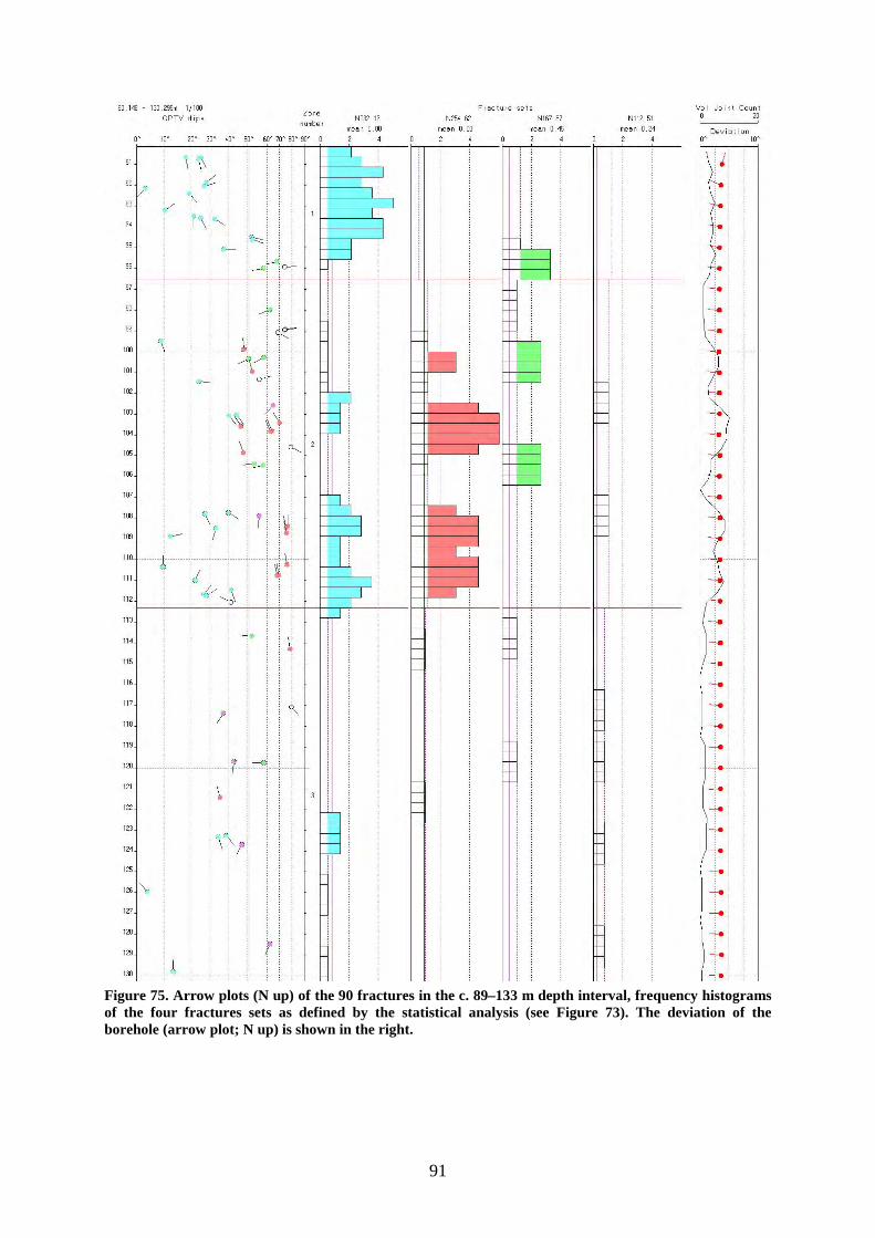
91
Figure 75. Arrow plots (N up) of the 90 fractures in the c. 89–133 m depth interval, frequency histograms of the four fractures sets as defined by the statistical analysis (see Figure 73). The deviation of the borehole (arrow plot; N up) is shown in the right.
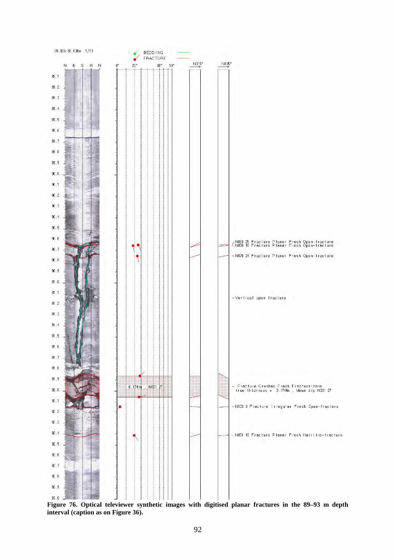
92
Figure 76. Optical televiewer synthetic images with digitised planar fractures in the 89–93 m depth interval (caption as on Figure 36).
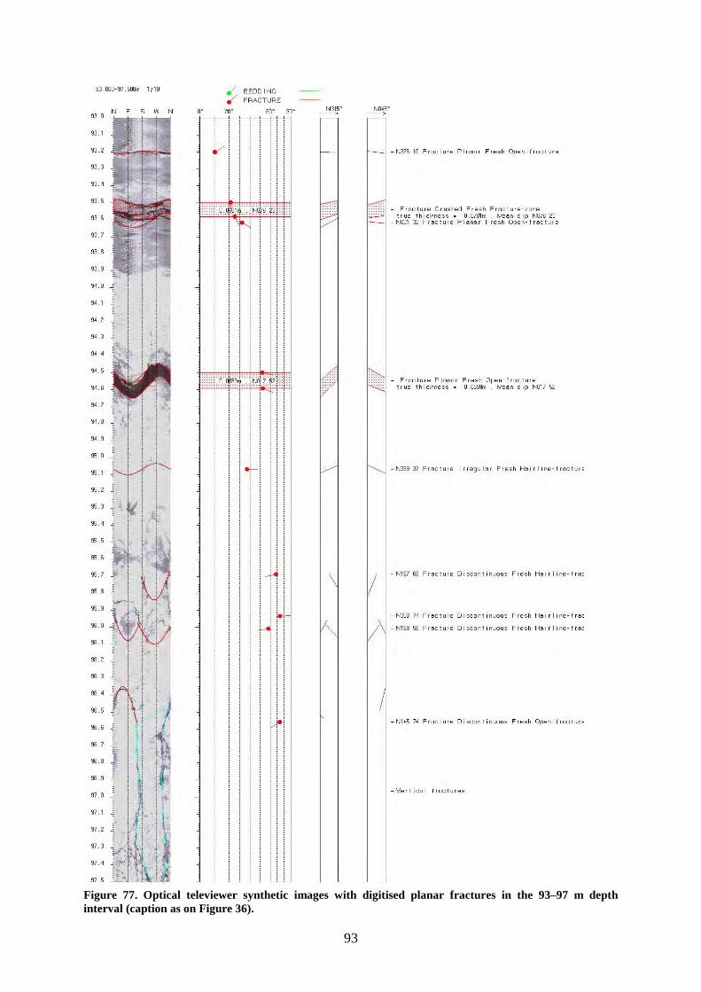
93
Figure 77. Optical televiewer synthetic images with digitised planar fractures in the 93–97 m depth interval (caption as on Figure 36).
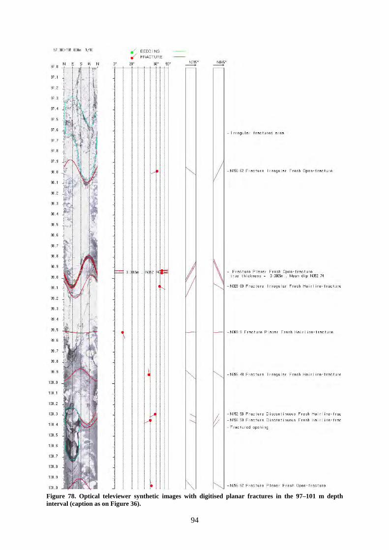
94
Figure 78. Optical televiewer synthetic images with digitised planar fractures in the 97–101 m depth interval (caption as on Figure 36).
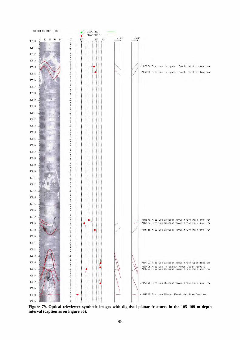
95
Figure 79. Optical televiewer synthetic images with digitised planar fractures in the 105–109 m depth interval (caption as on Figure 36).
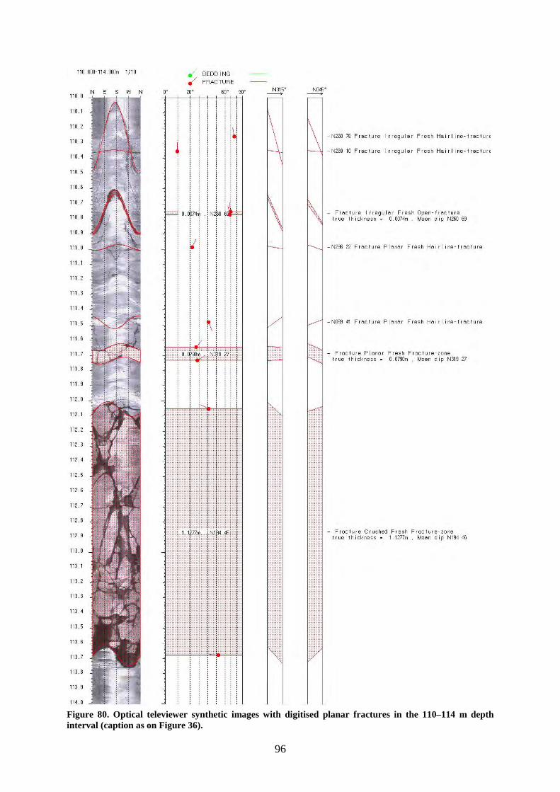
96
Figure 80. Optical televiewer synthetic images with digitised planar fractures in the 110–114 m depth interval (caption as on Figure 36).
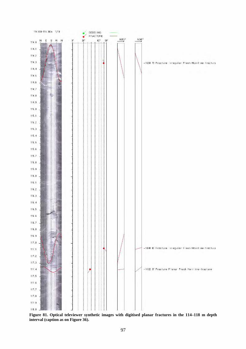
97
Figure 81. Optical televiewer synthetic images with digitised planar fractures in the 114–118 m depth interval (caption as on Figure 36).
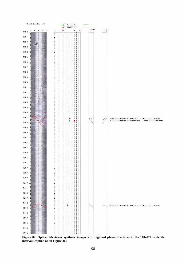
98
Figure 82. Optical televiewer synthetic images with digitised planar fractures in the 118–122 m depth interval (caption as on Figure 36).
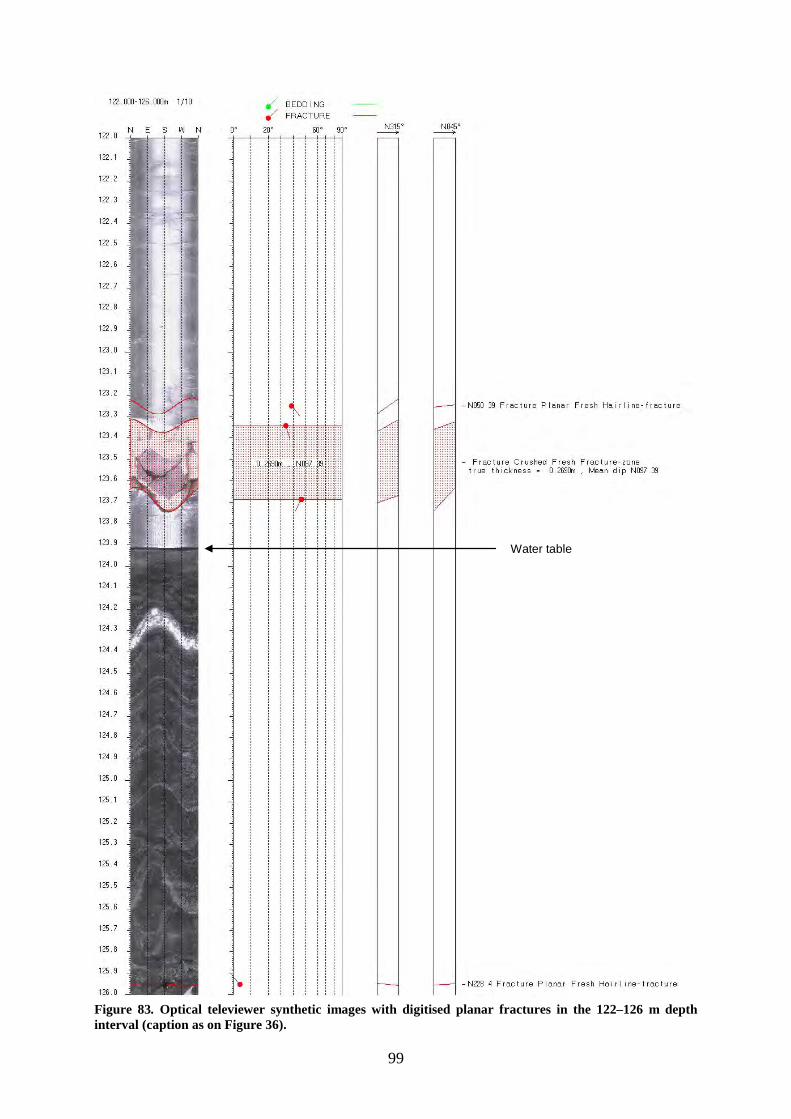
99
Figure 83. Optical televiewer synthetic images with digitised planar fractures in the 122–126 m depth interval (caption as on Figure 36).
Water table
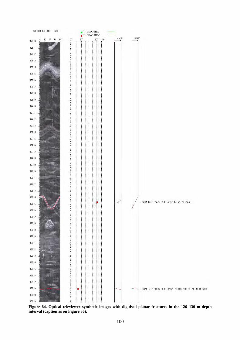
100
Figure 84. Optical televiewer synthetic images with digitised planar fractures in the 126–130 m depth interval (caption as on Figure 36).
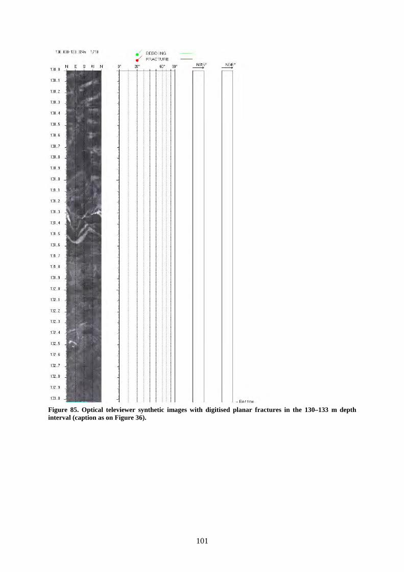
101
Figure 85. Optical televiewer synthetic images with digitised planar fractures in the 130–133 m depth interval (caption as on Figure 36).
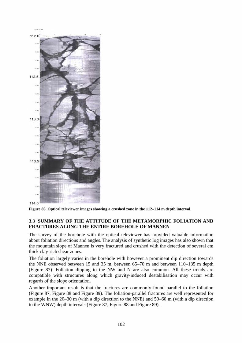
102
Figure 86. Optical televiewer images showing a crushed zone in the 112–114 m depth interval. 3.3 SUMMARY OF THE ATTITUDE OF THE METAMORPHIC FOLIATION AND FRACTURES ALONG THE ENTIRE BOREHOLE OF MANNEN The survey of the borehole with the optical televiewer has provided valuable information about foliation directions and angles. The analysis of synthetic log images has also shown that the mountain slope of Mannen is very fractured and crushed with the detection of several cm thick clay-rich shear zones.
The foliation largely varies in the borehole with however a prominent dip direction towards the NNE observed between 15 and 35 m, between 65–70 m and between 110–135 m depth (Figure 87). Foliation dipping to the NW and N are also common. All these trends are compatible with structures along which gravity-induced destabilisation may occur with regards of the slope orientation.
Another important result is that the fractures are commonly found parallel to the foliation (Figure 87, Figure 88 and Figure 89). The foliation-parallel fractures are well represented for example in the 20–30 m (with a dip direction to the NNE) and 50–60 m (with a dip direction to the WNW) depth intervals (Figure 87, Figure 88 and Figure 89).
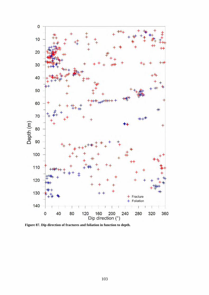
103
Figure 87. Dip direction of fractures and foliation in function to depth.
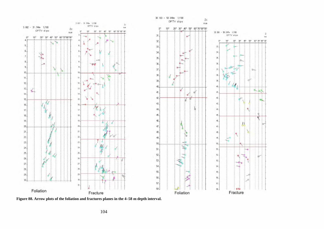
104
Figure 88. Arrow plots of the foliation and fractures planes in the 4–58 m depth interval.
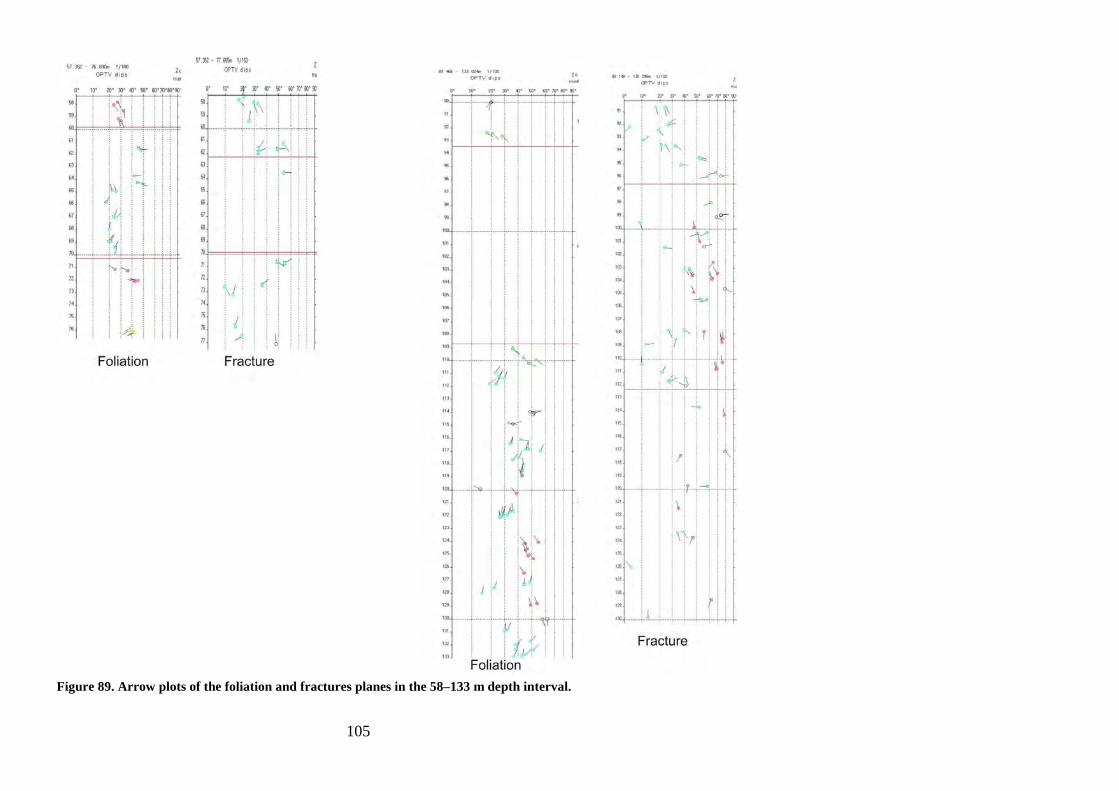
105
Figure 89. Arrow plots of the foliation and fractures planes in the 58–133 m depth interval.
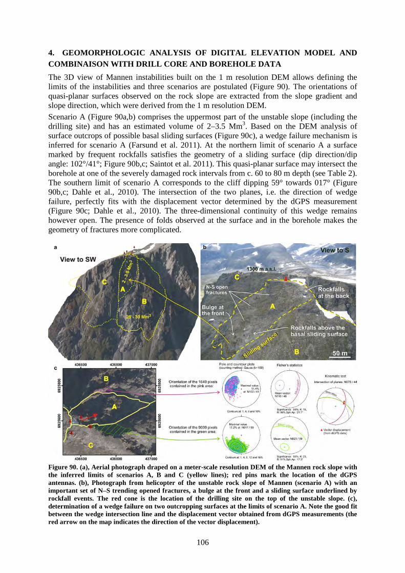
106
4. GEOMORPHOLOGIC ANALYSIS OF DIGITAL ELEVATION MODEL AND COMBINAISON WITH DRILL CORE AND BOREHOLE DATA The 3D view of Mannen instabilities built on the 1 m resolution DEM allows defining the limits of the instabilities and three scenarios are postulated (Figure 90). The orientations of quasi-planar surfaces observed on the rock slope are extracted from the slope gradient and slope direction, which were derived from the 1 m resolution DEM.
Scenario A (Figure 90a,b) comprises the uppermost part of the unstable slope (including the drilling site) and has an estimated volume of 2–3.5 Mm3. Based on the DEM analysis of surface outcrops of possible basal sliding surfaces (Figure 90c), a wedge failure mechanism is inferred for scenario A (Farsund et al. 2011). At the northern limit of scenario A a surface marked by frequent rockfalls satisfies the geometry of a sliding surface (dip direction/dip angle: 102°/41°; Figure 90b,c; Saintot et al. 2011). This quasi-planar surface may intersect the borehole at one of the severely damaged rock intervals from c. 60 to 80 m depth (see Table 2). The southern limit of scenario A corresponds to the cliff dipping 59° towards 017° (Figure 90b,c; Dahle et al., 2010). The intersection of the two planes, i.e. the direction of wedge failure, perfectly fits with the displacement vector determined by the dGPS measurement (Figure 90c; Dahle et al., 2010). The three-dimensional continuity of this wedge remains however open. The presence of folds observed at the surface and in the borehole makes the geometry of fractures more complicated.
Figure 90. (a), Aerial photograph draped on a meter-scale resolution DEM of the Mannen rock slope with the inferred limits of scenarios A, B and C (yellow lines); red pins mark the location of the dGPS antennas. (b), Photograph from helicopter of the unstable rock slope of Mannen (scenario A) with an important set of N–S trending opened fractures, a bulge at the front and a sliding surface underlined by rockfall events. The red cone is the location of the drilling site on the top of the unstable slope. (c), determination of a wedge failure on two outcropping surfaces at the limits of scenario A. Note the good fit between the wedge intersection line and the displacement vector obtained from dGPS measurements (the red arrow on the map indicates the direction of the vector displacement).

107
Scenario B includes scenario A and represents a deformed maximum volume of 25–30 Mm3 and is considered to be less active (Figure 90; Dahle et al., 2010). Its upper limits coincide with the ones of the 2–3.5 Mm3 block, but its basal limits are not obvious and its kinematics are not fully understood.
The total volume (scenario C, including scenarios A and B) affected by gravity-induced deformation far inward the plateau may reach 80–100 Mm3 (Figure 90). The basal limits are not clearly visible at the surface and this scenario C is expected to be inactive (Dahle et al., 2010).
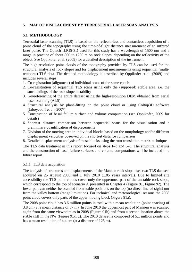
108
5. MAP OF DISPLACEMENT BY TERRESTRIAL LASER SCAN ANALYSIS
5.1 METHODOLOGY Terrestrial laser scanning (TLS) is based on the reflectorless and contactless acquisition of a point cloud of the topography using the time-of-flight distance measurement of an infrared laser pulse. The Optech ILRIS-3D used for this study has a wavelength of 1500 nm and a range in practice of about 800 to 1200 m on rock slopes, depending on the reflectivity of the object. See Oppikofer et al. (2009) for a detailed description of the instrument.
The high-resolution point clouds of the topography provided by TLS can be used for the structural analysis of rock slopes and for displacement measurements using sequential (multi-temporal) TLS data. The detailed methodology is described by Oppikofer et al. (2009) and includes several steps: 1. Co-registration (alignment) of individual scans of the same epoch 2. Co-registration of sequential TLS scans using only the (supposed) stable area, i.e. the
surroundings of the rock slope instability 3. Georeferencing of the entire dataset using the high-resolution DEM obtained from aerial
laser scanning (ALS) 4. Structural analysis by plane-fitting on the point cloud or using Coltop3D software
(Jaboyedoff et al., 2007) 5. Construction of basal failure surface and volume computation (see Oppikofer, 2009 for
details) 6. Shortest distance comparison between sequential scans for the visualisation and a
preliminary quantification of displacements 7. Division of the moving area in individual blocks based on the morphology and/or different
displacement velocities observed on the shortest distance comparison 8. Detailed displacement analysis of these blocks using the roto-translation matrix technique
The TLS data treatment in this report focused on steps 1–3 and 6–8. The structural analysis and the construction of basal failure surfaces and volume computations will be included in a future report.
5.1.1 The analysis of structures and displacements of the Mannen rock slope uses two TLS datasets acquired on 25 August 2008 and 1 July 2010 (1.85 years interval). Due to limited site accessibility the TLS point clouds cover only the uppermost part of the unstable rock slope, which correspond to the top of scenario A presented in Chapter 4 (
TLS data acquisition
Figure 91, Figure 92). The lower part can neither be scanned from stable positions on the top (no direct line-of-sight) nor from the valley bottom (range limitation). For technical and meteorological reasons the 2008 point cloud covers only parts of the upper moving block (Figure 91a).
The 2008 point cloud has 3.6 million points in total with a mean resolution (point spacing) of 3.8 cm (at a mean distance of 87 m). In June 2010 the uppermost part of Mannen was scanned again from the same viewpoint as in 2008 (Figure 91b) and from a second location above the stable cliff in the NW (Figure 91c, d). The 2010 dataset is composed of 5.1 million points and has a mean resolution of 4.4 cm (at a distance of 125 m).
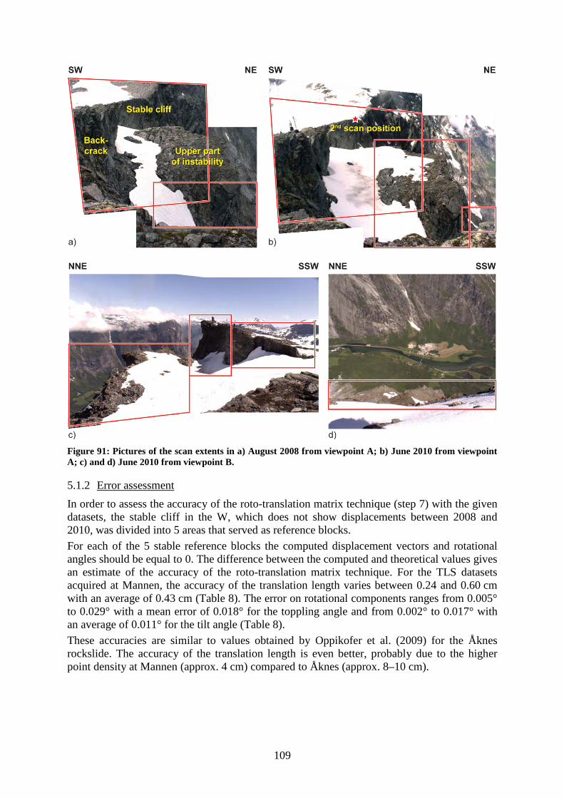
109
Figure 91: Pictures of the scan extents in a) August 2008 from viewpoint A; b) June 2010 from viewpoint A; c) and d) June 2010 from viewpoint B.
5.1.2 In order to assess the accuracy of the roto-translation matrix technique (step 7) with the given datasets, the stable cliff in the W, which does not show displacements between 2008 and 2010, was divided into 5 areas that served as reference blocks.
Error assessment
For each of the 5 stable reference blocks the computed displacement vectors and rotational angles should be equal to 0. The difference between the computed and theoretical values gives an estimate of the accuracy of the roto-translation matrix technique. For the TLS datasets acquired at Mannen, the accuracy of the translation length varies between 0.24 and 0.60 cm with an average of 0.43 cm (Table 8). The error on rotational components ranges from 0.005° to 0.029° with a mean error of 0.018° for the toppling angle and from 0.002° to 0.017° with an average of 0.011° for the tilt angle (Table 8).
These accuracies are similar to values obtained by Oppikofer et al. (2009) for the Åknes rockslide. The accuracy of the translation length is even better, probably due to the higher point density at Mannen (approx. 4 cm) compared to Åknes (approx. 8–10 cm).
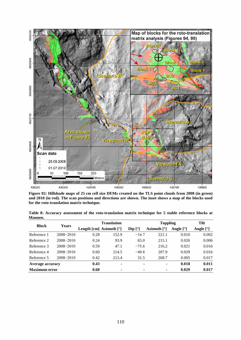
110
Figure 92: Hillshade maps of 25 cm cell size DEMs created on the TLS point clouds from 2008 (in green) and 2010 (in red). The scan positions and directions are shown. The inset shows a map of the blocks used for the roto-translation matrix technique. Table 8: Accuracy assessment of the roto-translation matrix technique for 5 stable reference blocks at Mannen.
Block Years Translation Toppling Tilt
Length [cm] Azimuth [°] Dip [°] Azimuth [°] Angle [°] Angle [°] Reference 1 2008−2010 0.28 152.9 −16.7 221.1 0.010 0.002
Reference 2 2008−2010 0.24 93.9 65.0 215.1 0.026 0.006
Reference 3 2008−2010 0.59 47.1 −75.6 216.2 0.021 0.016
Reference 4 2008−2010 0.60 214.5 −40.8 207.9 0.029 0.016
Reference 5 2008−2010 0.42 213.4 31.5 268.7 0.005 0.017
Average accuracy 0.43 - - - 0.018 0.011 Maximum error 0.60 - - - 0.029 0.017

111
5.2 TLS DISPLACEMENT ANALYSIS
5.2.1 The shortest distance comparison image between the 2008 and 2010 dataset reveals significant displacements of the uppermost part of the unstable rock slope and of several blocks along the back-crack (up to 25 cm in two years), as well as significant rockfalls (
Shortest distance comparison
Figure 93). The vertical cliffs in the west of the instability were used as reference for the alignment of the sequential scans and for the shortest distance comparison. Figure 93 reveals that these cliffs are indeed stable, since there are no differential movements over the entire cliff.
The detailed comparison image shows sliding and subsidence by up to 12 cm between 2008 and 2010 (Figure 94). Blocks 1 and 2 slide towards the SSE (Figure 94a), while blocks 3–5 appear essentially to subside. Subsidence of block 3 and other loose blocks in the opened graben is likely to fill voids opened by the downslope sliding of the rock slope (Figure 94a). The apparent subsidence movement of blocks 4 and 5 is probably also related to sliding along a steeply inclined sliding surface (Figure 94b).
The shortest distance comparison of the blocks along the back-crack (Figure 95) shows high displacement rates for two columns that are detached from the stable rock mass behind and that are free to move. These columns are moving by up to 15 cm towards the ENE. The top of the middle column (BC2b) is even moving by up to 25 cm. Block BC1 with the webcam and one of the laser distance meters shows little to no significant displacements on the shortest distance comparison.
Figure 93: Shortest distance comparison between the 2008 and 2010 TLS point clouds (view to the W). Positive differences up to +25 cm are shown in yellow to red colours and negative differences up to −25 cm in blue to violet colours. The 6 compartments on the instability and 4 blocks along the back-crack used for the detailed displacement analysis using the roto-translation matrix technique are outlined. A major rockfall occurred at the foot of the investigated area. Snow covered areas in 2010 and areas not covered by the 2008 dataset were excluded from the shortest distance comparison (grey areas).
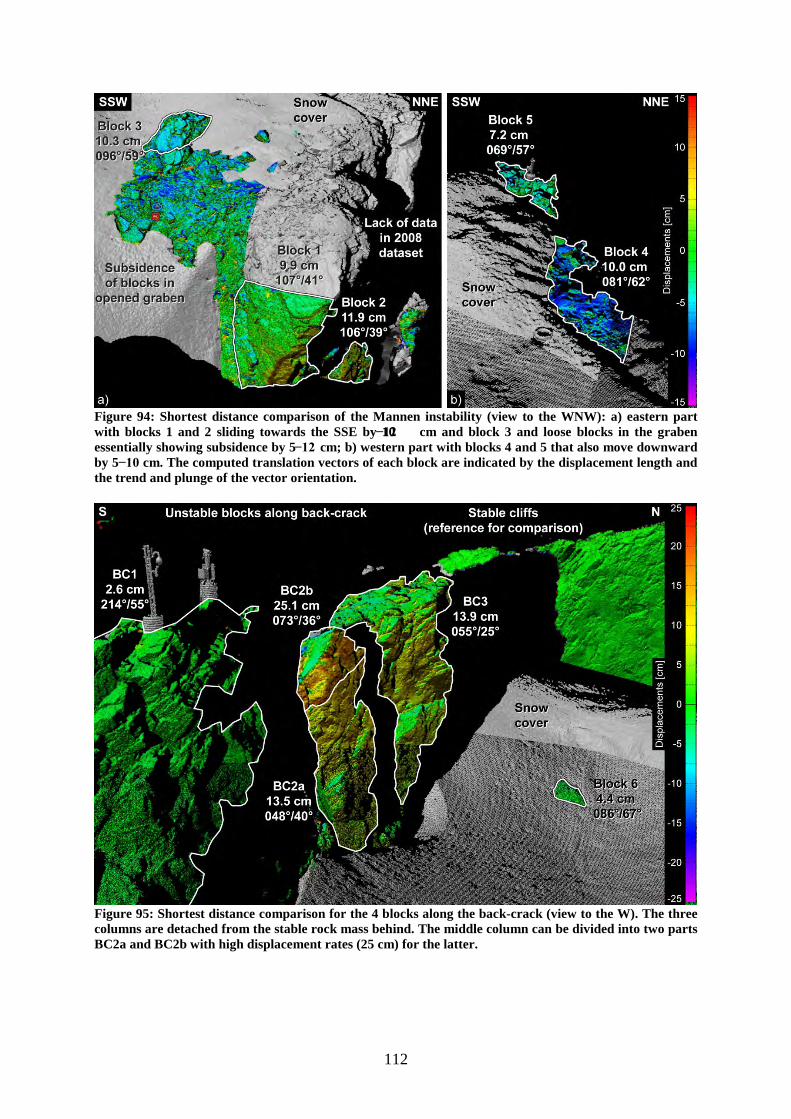
112
Figure 94: Shortest distance comparison of the Mannen instability (view to the WNW): a) eastern part with blocks 1 and 2 sliding towards the SSE by 10−12 cm and block 3 and loose blocks in the graben essentially showing subsidence by 5−12 cm; b) western part with blocks 4 and 5 that also move downward by 5−10 cm. The computed translation vectors of each block are indicated by the displacement length and the trend and plunge of the vector orientation.
Figure 95: Shortest distance comparison for the 4 blocks along the back-crack (view to the W). The three columns are detached from the stable rock mass behind. The middle column can be divided into two parts BC2a and BC2b with high displacement rates (25 cm) for the latter.
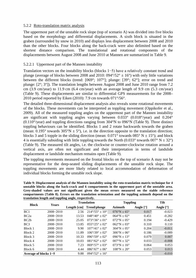
113
5.2.2 The uppermost part of the unstable rock slope (top of scenario A) was divided into five blocks based on the morphology and differential displacements. A sixth block is situated in the graben (surrounded by snow in 2010) and displays less displacement between 2008 and 2010 than the other blocks. Four blocks along the back-crack were also delimited based on the shortest distance comparison. The translational and rotational components of the displacements between August 2008 and June 2010 at Mannen are summarized in
Roto-translation matrix analysis
Table 9.
5.2.2.1 Uppermost part of the Mannen instability
Translation vectors on the instability blocks (blocks 1−5) have a relatively constant trend and plunge (average of blocks between 2008 and 2010: 094°/52° ± 16°) with only little variations between the different blocks (trend: [069°; 107°]; plunge: [39°; 62°]; error on trend and plunge: [2°; 3°]). The translation lengths between August 2008 and June 2010 range from 7.2 cm (3.9 cm/year) to 11.9 cm (6.4 cm/year) with an average length of 9.9 cm (5.3 cm/year) (Table 9). These displacements are similar to differential GPS measurements for the 2008–2010 period reported by Eiken (2010): 7.9 cm towards 071°/56°.
The detailed three-dimensional displacement analysis also reveals some rotational movements of the blocks. These movements can be interpreted as toppling movement (Oppikofer et al., 2009). All of the measured toppling angles on the uppermost part of the Mannen instability are significant with toppling angles varying between 0.033° (0.018°/year) and 0.204° (0.110°/year) and toppling directions ranging from 304°N to 096°N (Table 9). Three distinct toppling behaviours can be identified. Blocks 1 and 2 rotate backwards towards the graben (mean: 0.195° towards 305°N ± 5°), i.e. in the direction opposite to the translation direction; blocks 3 and 5 topple in the sliding direction (mean: 0.071° towards 085° N ± 15°); and block 4 is essentially subsiding with little toppling towards the North (0.033° towards 007° N ± 32°) (Table 9). The measured tilt angles, i.e. the clockwise or counter-clockwise rotation around a vertical axis, are often not significant and their interpretation in terms of landslide displacement or landslide mechanism remains open (Table 9).
The toppling movements measured on the frontal blocks on the top of scenario A may not be representative for the deep-seated sliding displacements of the unstable rock slope. The toppling movements are more likely related to local accommodation of deformation of individual blocks forming the unstable rock slope.
Table 9: Displacement analysis of the Mannen instability using the roto-translation matrix technique for 4 unstable blocks along the back-crack and 6 compartments in the uppermost part of the unstable area. Grey-shaded values are not significant given the mean errors measured on the stable reference compartments (Table 8). Errors on the translation orientation and the toppling azimuth depend on the translation length and toppling angle, respectively.
Block Years Translation Toppling Tilt
Length [cm] Trend/plunge Azimuth Angle [°] Angle [°] BC1 2008−2010 2.56 214°/55° ± 10° 076°N ± 65° 0.017 -0.023 BC2a 2008−2010 13.53 048°/40° ± 02° 064°N ± 02° 0.451 -0.282 BC2b 2008−2010 25.05 073°/36° ± 01° 072°N ± 05° 0.194 -0.429 BC3 2008−2010 13.85 055°/25° ± 02° 062°N ± 03° 0.310 0.110 Block 1 2008−2010 9.90 107°/41° ± 02° 304°N ± 05° 0.204 -0.011 Block 2 2008−2010 11.89 106°/39° ± 02° 306°N ± 06° 0.186 -0.089 Block 3 2008−2010 10.33 096°/59° ± 02° 096°N ± 13° 0.079 0.007 Block 4 2008−2010 10.03 081°/62° ± 02° 007°N ± 32° 0.033 -0.008 Block 5 2008−2010 7.23 069°/57° ± 03° 073°N ± 16° 0.064 0.053 Block 6 2008−2010 4.44 086°/67° ± 06° 108°N ± 20° 0.053 0.013 Average of blocks 1−5 9.88 094°/52° ± 16° -0.010

114
5.2.2.2 Unstable blocks along the back-crack
As already observed on the shortest distance comparison, the unstable blocks along the back-crack move independently with different velocities and directions (Table 9). The block BC1 with the webcam and laser distancemeter shows small displacements (2.6 cm; 1.4 cm/year) towards the SSW. This movement opposite to the general slope direction lets suppose that it is due to small alignment errors between the sequential scans and that this block is indeed stable. The very low toppling angles also support this hypothesis.
In contrast, the other blocks along the back-crack are clearly moving with high displacement rates (13.5 to 25.1 cm; 7.3 to 13.5 cm/year) in NE to ENE direction. The top part of the middle column (BC2b) has significantly higher displacement rates than the lower part (BC2a). The toppling angles and directions for blocks BC2a, BC2b and BC3 are fairly constant. These freestanding columns slide and topple in downslope direction.
The volume of the blocks along the back-crack being limited to few hundreds cubicmeters, their eventual collapse will neither significantly affect the stability of the unstable rock slope nor pose a threat to the settlements in the valley.
115
6. CONCLUSION AND PERSPECTIVES The geological logging of a vertically drilled core at the top of the Mannen rock slope instability has allowed identifying several zones of damaged rocks. Some of these zones contain highly deformed rocks or crushed rocks, such as fine-grained breccias and/or clay-rich gouges. However, the relationship with the gravitational slope deformation is not clearly determined for all of the zones. The highly deformed zones logged in the drill core were confirmed by optical televiewer from the borehole, including fracture frequency, opening of fractures and occurrence of clay-rich zones.
The geomorphological analysis of the DEM of the slope confirmed the different scenarios of slope deformation at Mannen. Scenario A has a volume of 2.5–3 Mm3 and shows highest displacements rates of several cm/year. Scenario B has an estimated volume of 25–30 Mm3 and includes scenario A. The unstable rock slope in scenario B shows presently no signs of activity related to its motion. The entire gravitationally deformed rock slope corresponding to scenario C has a volume of 80–100 Mm3, but displays no signs of activity and its basal limits are not clearly developed.
A wedge failure mechanism is inferred for scenario A based on the orientation of quasi-planar structures delimiting scenario A. One of these basal surfaces would correspond to one of the four intervals of highly deformed rock encountered between 57 and 81 m along the core and characterised by severely crushed rocks. These intervals are expected to be very weak and will not support the load of the moving volume for long due to the inherent fatigue of the material, but until now the rate of deformation measured by the dGPS datasets is in agreement with a steady-state deformation (i.e. no acceleration of sliding is detected).
The orientation of the wedge intersection line formed by the two basal surfaces is parallel to the displacement vector determined by periodic dGPS measurement. This orientation is also consistent with the direction of movement obtained by processed successive acquisitions of terrestrial laser scans of the uppermost part of scenario A. Small toppling movements measured by sequential terrestrial laser scanning are interpreted to be the local accommodation of deformation and are likely not representative for the entire unstable rock slope.
A more detailed analysis of the processed 1 m resolution DEM will be described in a separate report. Future work will focus to integrate borehole data, geophysical data, surface observations, DEM interpretation and displacements measurements to create a complete geological model of the instabilities. The results of the numerical slope stability modelling for scenarios A and B will also be presented in this future report.
116
7. REFERENCES Bieniawski, Z. (1975). The point-load test in geotechnical practice, Engineering Geology 9(1), 1–11.
Deere, D.U. (1964). Technical description of rock cores for engineering purposes, Rock Mechanics Engineering Geology, 1, 16–22.
Eiken, T. (2010). GNSS-måling fjellskred Møre og Romsdal 2010. Technical report, University of Oslo, unpublished.
Farsund, T.Ø. (2010). Geology, DEM analysis and geohazard assessment of the Romsdalen valley. Project thesis, Norwegian University of Science and Technology, Trondheim, unpublished, 56 pp.
Farsund, T.Ø. (2011). Geological and numerical stability modelling of Mannen, Romsdalen. MSc thesis, Norwegian University of Science and Technology, Trondheim, unpublished, 119 pp.
IGRF (2011). http://www.ngdc.noaa.gov/IAGA/vmod/igrf.html
ISRM (1978). International Society for Rock Mechanics Commission on standardization of laboratory and field tests: Suggested methods for the quantitative description of discontinuities in rock masses. International Journal of Rock Mechanics and Mining Sciences & Geomechanics, Abstracts, 15(6), 319–368.
Jaboyedoff, M., Metzger, R., Oppikofer, T., Couture, R., Derron, M., Locat, J. & Turmel, D. (2007). New insight techniques to analyze rock slope relief using DEM and 3D-imaging cloud points: COLTOP-3D software. In: Rock mechanics: Meeting Society's challenges and demands. Proceedings of the 1st Canada - U.S. Rock Mechanics Symposium, Vancouver, Canada, 27–31 May 2007, eds. E. Eberhardt, D. Stead & T. Morrison, Taylor & Francis, London, pp. 61–68.
Oppikofer, T. (2009). Detection, analysis and monitoring of slope movements by high-resolution digital elevation models. PhD thesis, Institute of Geomatics and Analysis of Risk, University of Lausanne, Switzerland.
Oppikofer, T., Jaboyedoff, M., Blikra, L.H. & Derron, M. (2009). Characterization and monitoring of the Åknes rockslide using terrestrial laser scanning. Natural Hazards and Earth System Sciences, 9(3), 1003–1019.
Saintot, A., Henderson, I. & Derron, M.-H. (2011). Inheritance of ductile and brittle structures in the development of large rock slope instabilities: examples from Western Norway. Geological Society, London, Special Publication, 351, 27–78.
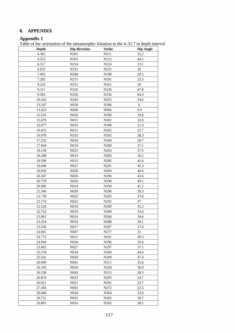
117
8. APPENDIX Appendix 1 Table of the orientation of the metamorphic foliation in the 4–31.7 m depth interval Depth Dip direction Strike Dip Angle 4.302 N301 N211 52.2
4.523 N302 N212 44.2
6.517 N314 N224 23.1
6.631 N315 N225 20
7.092 N288 N198 20.5
7.282 N271 N181 23.5
8.232 N251 N161 26
9.311 N326 N236 47.8
9.583 N326 N236 64.4
10.416 N345 N255 54.6
13.247 N036 N306 6
13.423 N096 N006 6.9
15.516 N026 N296 29.8
15.679 N031 N301 32.8
16.077 N018 N288 21.4
16.453 N012 N282 25.7
16.976 N355 N265 28.3
17.232 N034 N304 28.7
17.844 N010 N280 37.1
18.139 N023 N293 37.5
18.288 N013 N283 36.2
18.599 N015 N285 41.6
19.698 N021 N291 45.3
19.939 N030 N300 40.6
20.347 N026 N296 43.6
20.778 N020 N290 49.1
20.996 N024 N294 41.2
21.366 N020 N290 39.3
21.739 N025 N295 37.8
22.174 N022 N292 37
22.528 N019 N289 35.2
22.752 N019 N289 33.6
22.961 N014 N284 34.6
23.354 N018 N288 39.1
23.536 N017 N287 37.6
24.061 N007 N277 31
24.772 N021 N291 30.3
24.944 N026 N296 35.6
25.062 N027 N297 37.1
25.378 N034 N304 44.4
25.541 N039 N309 47.4
26.009 N041 N311 25.6
26.195 N050 N320 30.9
26.558 N043 N313 28.3
26.874 N023 N293 24.7
26.921 N021 N291 23.7
27.365 N002 N272 22.5
29.046 N034 N304 33.9
29.711 N032 N302 39.7
29.801 N033 N303 38.5
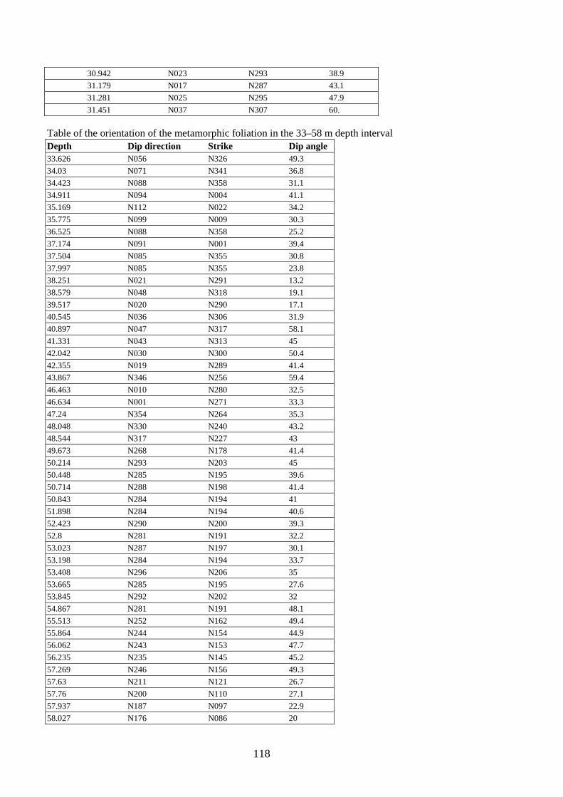
118
30.942 N023 N293 38.9
31.179 N017 N287 43.1
31.281 N025 N295 47.9
31.451 N037 N307 60.
Table of the orientation of the metamorphic foliation in the 33–58 m depth interval Depth Dip direction Strike Dip angle 33.626 N056 N326 49.3
34.03 N071 N341 36.8
34.423 N088 N358 31.1
34.911 N094 N004 41.1
35.169 N112 N022 34.2
35.775 N099 N009 30.3
36.525 N088 N358 25.2
37.174 N091 N001 39.4
37.504 N085 N355 30.8
37.997 N085 N355 23.8
38.251 N021 N291 13.2
38.579 N048 N318 19.1
39.517 N020 N290 17.1
40.545 N036 N306 31.9
40.897 N047 N317 58.1
41.331 N043 N313 45
42.042 N030 N300 50.4
42.355 N019 N289 41.4
43.867 N346 N256 59.4
46.463 N010 N280 32.5
46.634 N001 N271 33.3
47.24 N354 N264 35.3
48.048 N330 N240 43.2
48.544 N317 N227 43
49.673 N268 N178 41.4
50.214 N293 N203 45
50.448 N285 N195 39.6
50.714 N288 N198 41.4
50.843 N284 N194 41
51.898 N284 N194 40.6
52.423 N290 N200 39.3
52.8 N281 N191 32.2
53.023 N287 N197 30.1
53.198 N284 N194 33.7
53.408 N296 N206 35
53.665 N285 N195 27.6
53.845 N292 N202 32
54.867 N281 N191 48.1
55.513 N252 N162 49.4
55.864 N244 N154 44.9
56.062 N243 N153 47.7
56.235 N235 N145 45.2
57.269 N246 N156 49.3
57.63 N211 N121 26.7
57.76 N200 N110 27.1
57.937 N187 N097 22.9
58.027 N176 N086 20
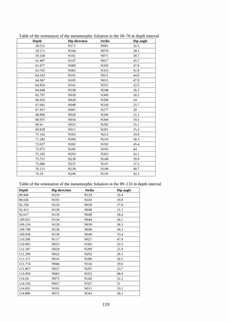
119
Table of the orientation of the metamorphic foliation in the 58–76 m depth interval
Depth Dip direction Strike Dip angle 58.551 N171 N081 32.5
59.171 N166 N076 28.1
59.338 N161 N071 30.7
61.497 N107 N017 45.7
61.677 N080 N350 47.9
63.702 N083 N353 41.8
64.243 N101 N011 44.6
64.367 N105 N015 47.9
64.854 N341 N251 22.5
64.948 N338 N248 26.5
65.797 N030 N300 18.2
66.932 N028 N298 24
67.045 N048 N318 25.7
67.957 N007 N277 20
68.896 N026 N296 21.2
68.937 N034 N304 19.5
69.41 N025 N295 25.1
69.828 N011 N281 25.3
71.142 N302 N212 24.8
71.283 N300 N210 36.3
72.027 N282 N192 45.4
72.073 N285 N195 44
72.165 N293 N203 42.1
75.757 N238 N148 39.9
75.989 N237 N147 37.5
76.111 N239 N149 40.7
76.19 N246 N156 42.3
Table of the orientation of the metamorphic foliation in the 89–133 m depth interval
Depth Dip direction Strike Dip angle 89.966 N219 N129 20.4
90.026 N193 N103 19.9
92.358 N129 N039 17.9
92.412 N138 N048 21.1
92.617 N139 N049 28.4
109.022 N134 N044 36.1
109.156 N129 N039 36.3
109.798 N136 N046 44.1
109.938 N130 N040 53.4
110.206 N117 N027 47.9
110.902 N033 N303 23.3
111.187 N029 N299 25.9
111.299 N022 N292 26.1
111.371 N016 N286 30.1
111.774 N046 N316 19.6
111.807 N027 N297 23.7
113.958 N083 N353 48.8
114.04 N072 N342 51.2
114.156 N057 N327 51
114.831 N101 N011 33.1
114.886 N072 N342 36.1
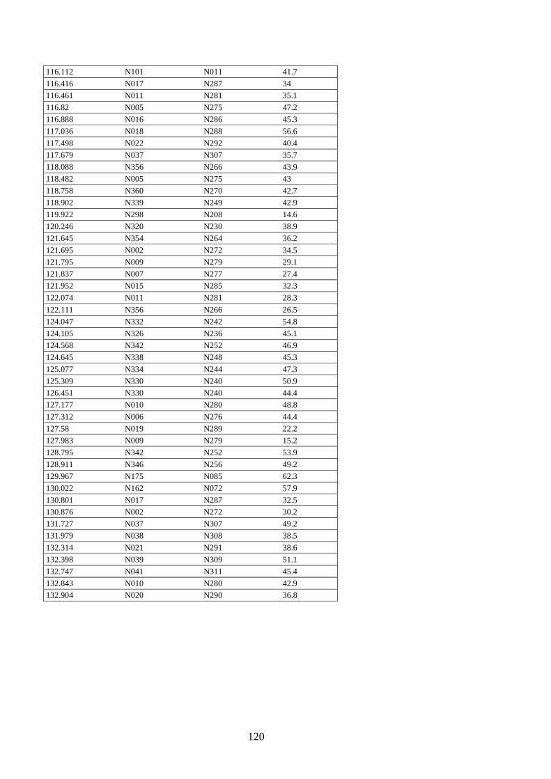
120
116.112 N101 N011 41.7
116.416 N017 N287 34
116.461 N011 N281 35.1
116.82 N005 N275 47.2
116.888 N016 N286 45.3
117.036 N018 N288 56.6
117.498 N022 N292 40.4
117.679 N037 N307 35.7
118.088 N356 N266 43.9
118.482 N005 N275 43
118.758 N360 N270 42.7
118.902 N339 N249 42.9
119.922 N298 N208 14.6
120.246 N320 N230 38.9
121.645 N354 N264 36.2
121.695 N002 N272 34.5
121.795 N009 N279 29.1
121.837 N007 N277 27.4
121.952 N015 N285 32.3
122.074 N011 N281 28.3
122.111 N356 N266 26.5
124.047 N332 N242 54.8
124.105 N326 N236 45.1
124.568 N342 N252 46.9
124.645 N338 N248 45.3
125.077 N334 N244 47.3
125.309 N330 N240 50.9
126.451 N330 N240 44.4
127.177 N010 N280 48.8
127.312 N006 N276 44.4
127.58 N019 N289 22.2
127.983 N009 N279 15.2
128.795 N342 N252 53.9
128.911 N346 N256 49.2
129.967 N175 N085 62.3
130.022 N162 N072 57.9
130.801 N017 N287 32.5
130.876 N002 N272 30.2
131.727 N037 N307 49.2
131.979 N038 N308 38.5
132.314 N021 N291 38.6
132.398 N039 N309 51.1
132.747 N041 N311 45.4
132.843 N010 N280 42.9
132.904 N020 N290 36.8
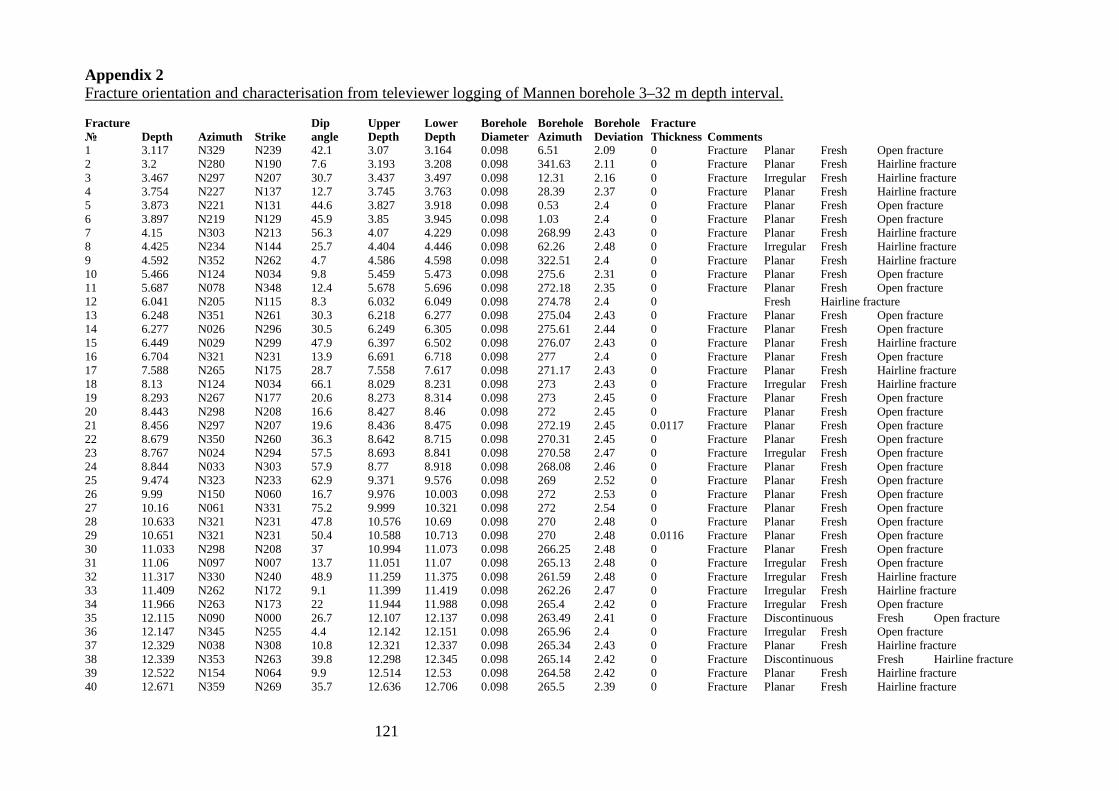
121
Appendix 2
Fracture orientation and characterisation from televiewer logging of Mannen borehole 3–32 m depth interval.
Fracture Dip Upper Lower Borehole Borehole Borehole Fracture № Depth Azimuth Strike angle Depth Depth Diameter Azimuth Deviation Thickness Comments 1 3.117 N329 N239 42.1 3.07 3.164 0.098 6.51 2.09 0 Fracture Planar Fresh Open fracture 2 3.2 N280 N190 7.6 3.193 3.208 0.098 341.63 2.11 0 Fracture Planar Fresh Hairline fracture 3 3.467 N297 N207 30.7 3.437 3.497 0.098 12.31 2.16 0 Fracture Irregular Fresh Hairline fracture 4 3.754 N227 N137 12.7 3.745 3.763 0.098 28.39 2.37 0 Fracture Planar Fresh Hairline fracture 5 3.873 N221 N131 44.6 3.827 3.918 0.098 0.53 2.4 0 Fracture Planar Fresh Open fracture 6 3.897 N219 N129 45.9 3.85 3.945 0.098 1.03 2.4 0 Fracture Planar Fresh Open fracture 7 4.15 N303 N213 56.3 4.07 4.229 0.098 268.99 2.43 0 Fracture Planar Fresh Hairline fracture 8 4.425 N234 N144 25.7 4.404 4.446 0.098 62.26 2.48 0 Fracture Irregular Fresh Hairline fracture 9 4.592 N352 N262 4.7 4.586 4.598 0.098 322.51 2.4 0 Fracture Planar Fresh Hairline fracture 10 5.466 N124 N034 9.8 5.459 5.473 0.098 275.6 2.31 0 Fracture Planar Fresh Open fracture 11 5.687 N078 N348 12.4 5.678 5.696 0.098 272.18 2.35 0 Fracture Planar Fresh Open fracture 12 6.041 N205 N115 8.3 6.032 6.049 0.098 274.78 2.4 0 Fresh Hairline fracture 13 6.248 N351 N261 30.3 6.218 6.277 0.098 275.04 2.43 0 Fracture Planar Fresh Open fracture 14 6.277 N026 N296 30.5 6.249 6.305 0.098 275.61 2.44 0 Fracture Planar Fresh Open fracture 15 6.449 N029 N299 47.9 6.397 6.502 0.098 276.07 2.43 0 Fracture Planar Fresh Hairline fracture 16 6.704 N321 N231 13.9 6.691 6.718 0.098 277 2.4 0 Fracture Planar Fresh Open fracture 17 7.588 N265 N175 28.7 7.558 7.617 0.098 271.17 2.43 0 Fracture Planar Fresh Hairline fracture 18 8.13 N124 N034 66.1 8.029 8.231 0.098 273 2.43 0 Fracture Irregular Fresh Hairline fracture 19 8.293 N267 N177 20.6 8.273 8.314 0.098 273 2.45 0 Fracture Planar Fresh Open fracture 20 8.443 N298 N208 16.6 8.427 8.46 0.098 272 2.45 0 Fracture Planar Fresh Open fracture 21 8.456 N297 N207 19.6 8.436 8.475 0.098 272.19 2.45 0.0117 Fracture Planar Fresh Open fracture 22 8.679 N350 N260 36.3 8.642 8.715 0.098 270.31 2.45 0 Fracture Planar Fresh Open fracture 23 8.767 N024 N294 57.5 8.693 8.841 0.098 270.58 2.47 0 Fracture Irregular Fresh Open fracture 24 8.844 N033 N303 57.9 8.77 8.918 0.098 268.08 2.46 0 Fracture Planar Fresh Open fracture 25 9.474 N323 N233 62.9 9.371 9.576 0.098 269 2.52 0 Fracture Planar Fresh Open fracture 26 9.99 N150 N060 16.7 9.976 10.003 0.098 272 2.53 0 Fracture Planar Fresh Open fracture 27 10.16 N061 N331 75.2 9.999 10.321 0.098 272 2.54 0 Fracture Planar Fresh Open fracture 28 10.633 N321 N231 47.8 10.576 10.69 0.098 270 2.48 0 Fracture Planar Fresh Open fracture 29 10.651 N321 N231 50.4 10.588 10.713 0.098 270 2.48 0.0116 Fracture Planar Fresh Open fracture 30 11.033 N298 N208 37 10.994 11.073 0.098 266.25 2.48 0 Fracture Planar Fresh Open fracture 31 11.06 N097 N007 13.7 11.051 11.07 0.098 265.13 2.48 0 Fracture Irregular Fresh Open fracture 32 11.317 N330 N240 48.9 11.259 11.375 0.098 261.59 2.48 0 Fracture Irregular Fresh Hairline fracture 33 11.409 N262 N172 9.1 11.399 11.419 0.098 262.26 2.47 0 Fracture Irregular Fresh Hairline fracture 34 11.966 N263 N173 22 11.944 11.988 0.098 265.4 2.42 0 Fracture Irregular Fresh Open fracture 35 12.115 N090 N000 26.7 12.107 12.137 0.098 263.49 2.41 0 Fracture Discontinuous Fresh Open fracture 36 12.147 N345 N255 4.4 12.142 12.151 0.098 265.96 2.4 0 Fracture Irregular Fresh Open fracture 37 12.329 N038 N308 10.8 12.321 12.337 0.098 265.34 2.43 0 Fracture Planar Fresh Hairline fracture 38 12.339 N353 N263 39.8 12.298 12.345 0.098 265.14 2.42 0 Fracture Discontinuous Fresh Hairline fracture 39 12.522 N154 N064 9.9 12.514 12.53 0.098 264.58 2.42 0 Fracture Planar Fresh Hairline fracture 40 12.671 N359 N269 35.7 12.636 12.706 0.098 265.5 2.39 0 Fracture Planar Fresh Hairline fracture
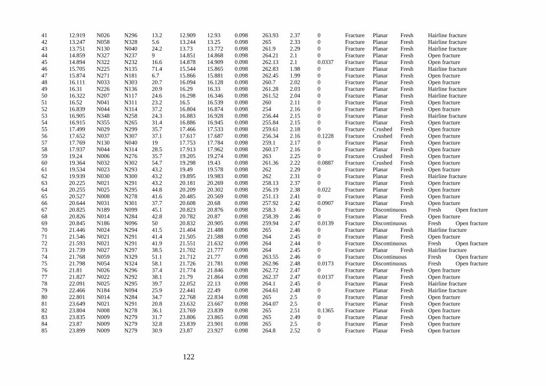
122
41 12.919 N026 N296 13.2 12.909 12.93 0.098 263.93 2.37 0 Fracture Planar Fresh Hairline fracture 42 13.247 N058 N328 5.6 13.244 13.25 0.098 265 2.33 0 Fracture Planar Fresh Hairline fracture 43 13.751 N130 N040 24.2 13.73 13.772 0.098 261.9 2.29 0 Fracture Planar Fresh Hairline fracture 44 14.859 N327 N237 9 14.851 14.868 0.098 264.21 2.1 0 Fracture Planar Fresh Open fracture 45 14.894 N322 N232 16.6 14.878 14.909 0.098 262.13 2.1 0.0337 Fracture Planar Fresh Open fracture 46 15.705 N225 N135 71.4 15.544 15.865 0.098 262.83 1.98 0 Fracture Planar Fresh Hairline fracture 47 15.874 N271 N181 6.7 15.866 15.881 0.098 262.45 1.99 0 Fracture Planar Fresh Open fracture 48 16.111 N033 N303 20.7 16.094 16.128 0.098 260.7 2.02 0 Fracture Planar Fresh Open fracture 49 16.31 N226 N136 20.9 16.29 16.33 0.098 261.28 2.03 0 Fracture Planar Fresh Hairline fracture 50 16.322 N207 N117 24.6 16.298 16.346 0.098 261.52 2.04 0 Fracture Planar Fresh Hairline fracture 51 16.52 N041 N311 23.2 16.5 16.539 0.098 260 2.11 0 Fracture Planar Fresh Open fracture 52 16.839 N044 N314 37.2 16.804 16.874 0.098 254 2.16 0 Fracture Planar Fresh Open fracture 53 16.905 N348 N258 24.3 16.883 16.928 0.098 256.44 2.15 0 Fracture Planar Fresh Hairline fracture 54 16.915 N355 N265 31.4 16.886 16.945 0.098 255.84 2.15 0 Fracture Planar Fresh Open fracture 55 17.499 N029 N299 35.7 17.466 17.533 0.098 259.61 2.18 0 Fracture Crushed Fresh Open fracture 56 17.652 N037 N307 37.1 17.617 17.687 0.098 256.34 2.16 0.1228 Fracture Crushed Fresh Open fracture 57 17.769 N130 N040 19 17.753 17.784 0.098 259.1 2.17 0 Fracture Planar Fresh Open fracture 58 17.937 N044 N314 28.5 17.913 17.962 0.098 260.17 2.16 0 Fracture Planar Fresh Open fracture 59 19.24 N006 N276 35.7 19.205 19.274 0.098 263 2.25 0 Fracture Crushed Fresh Open fracture 60 19.364 N032 N302 54.7 19.298 19.43 0.098 261.36 2.22 0.0887 Fracture Crushed Fresh Open fracture 61 19.534 N023 N293 43.2 19.49 19.578 0.098 262 2.29 0 Fracture Planar Fresh Open fracture 62 19.939 N030 N300 43.2 19.895 19.983 0.098 262 2.31 0 Fracture Planar Fresh Hairline fracture 63 20.225 N021 N291 43.2 20.181 20.269 0.098 258.13 2.37 0 Fracture Planar Fresh Open fracture 64 20.255 N025 N295 44.8 20.209 20.302 0.098 256.19 2.38 0.022 Fracture Planar Fresh Open fracture 65 20.527 N008 N278 41.6 20.485 20.569 0.098 251.13 2.41 0 Fracture Planar Fresh Open fracture 66 20.644 N031 N301 37.7 20.608 20.68 0.098 257.92 2.42 0.0907 Fracture Planar Fresh Open fracture 67 20.825 N189 N099 45.1 20.823 20.876 0.098 258.3 2.46 0 Fracture Discontinuous Fresh Open fracture 68 20.826 N014 N284 42.8 20.782 20.87 0.098 258.39 2.46 0 Fracture Planar Fresh Open fracture 69 20.845 N186 N096 50 20.832 20.905 0.098 259.94 2.47 0.0139 Fracture Discontinuous Fresh Open fracture 70 21.446 N024 N294 41.5 21.404 21.488 0.098 265 2.46 0 Fracture Planar Fresh Hairline fracture 71 21.546 N021 N291 41.4 21.505 21.588 0.098 264 2.45 0 Fracture Planar Fresh Open fracture 72 21.593 N021 N291 41.9 21.551 21.632 0.098 264 2.44 0 Fracture Discontinuous Fresh Open fracture 73 21.739 N027 N297 38.5 21.702 21.777 0.098 264 2.45 0 Fracture Planar Fresh Hairline fracture 74 21.768 N059 N329 51.1 21.712 21.77 0.098 263.55 2.46 0 Fracture Discontinuous Fresh Open fracture 75 21.798 N054 N324 58.1 21.726 21.781 0.098 262.96 2.48 0.0173 Fracture Discontinuous Fresh Open fracture 76 21.81 N026 N296 37.4 21.774 21.846 0.098 262.72 2.47 0 Fracture Planar Fresh Open fracture 77 21.827 N022 N292 38.1 21.79 21.864 0.098 262.37 2.47 0.0137 Fracture Planar Fresh Open fracture 78 22.091 N025 N295 39.7 22.052 22.13 0.098 264.1 2.45 0 Fracture Planar Fresh Hairline fracture 79 22.466 N184 N094 25.9 22.441 22.49 0.098 264.61 2.48 0 Fracture Planar Fresh Hairline fracture 80 22.801 N014 N284 34.7 22.768 22.834 0.098 265 2.5 0 Fracture Planar Fresh Open fracture 81 23.649 N021 N291 20.8 23.632 23.667 0.098 264.07 2.5 0 Fracture Planar Fresh Open fracture 82 23.804 N008 N278 36.1 23.769 23.839 0.098 265 2.51 0.1365 Fracture Planar Fresh Open fracture 83 23.835 N009 N279 31.7 23.806 23.865 0.098 265 2.49 0 Fracture Planar Fresh Open fracture 84 23.87 N009 N279 32.8 23.839 23.901 0.098 265 2.5 0 Fracture Planar Fresh Open fracture 85 23.899 N009 N279 30.9 23.87 23.927 0.098 264.8 2.52 0 Fracture Planar Fresh Open fracture
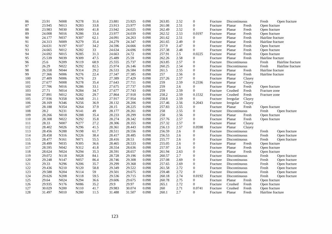
123
86 23.91 N008 N278 31.6 23.881 23.925 0.098 263.85 2.52 0 Fracture Discontinuous Fresh Open fracture 87 23.945 N013 N283 33.8 23.913 23.977 0.098 261.08 2.51 0 Fracture Planar Fresh Open fracture 88 23.983 N030 N300 41.8 23.942 24.025 0.098 262.49 2.52 0 Fracture Planar Fresh Open fracture 89 24.008 N016 N286 33.4 23.977 24.039 0.098 262.52 2.53 0.0197 Fracture Planar Fresh Open fracture 90 24.177 N037 N307 62.1 24.091 24.263 0.098 261.62 2.51 0 Fracture Planar Fresh Hairline fracture 91 24.313 N009 N279 35.4 24.279 24.347 0.098 261.65 2.49 0 Fracture Planar Fresh Hairline fracture 92 24.631 N197 N107 34.2 24.596 24.666 0.098 257.9 2.47 0 Fracture Planar Fresh Open fracture 93 24.665 N012 N282 33 24.634 24.696 0.098 257.38 2.48 0 Fracture Planar Fresh Open fracture 94 24.692 N015 N285 31.3 24.663 24.72 0.098 257.91 2.5 0.0225 Fracture Planar Fresh Open fracture 95 25.539 N039 N309 47.5 25.489 25.59 0.098 262.26 2.58 0 Fracture Planar Fresh Hairline fracture 96 25.6 N209 N119 68.9 25.555 25.737 0.098 263.85 2.57 0 Fracture Discontinuous Fresh Hairline fracture 97 26.29 N022 N292 82.5 25.974 26.146 0.098 260.25 2.54 0 Fracture Discontinuous Fresh Hairline fracture 98 26.558 N044 N314 29.2 26.533 26.584 0.098 261.5 2.55 0 Fracture Planar Fresh Hairline fracture 99 27.366 N006 N276 22.4 27.347 27.385 0.098 257 2.56 0 Fracture Planar Fresh Hairline fracture 100 27.409 N006 N276 23 27.389 27.429 0.098 257.26 2.57 0 Fracture Planar Clayey 101 27.677 N008 N278 35.4 27.643 27.711 0.098 259 2.59 0.2336 Fracture Planar Clayey 102 27.706 N016 N286 33.1 27.675 27.737 0.098 259 2.6 0 Fracture Planar Fresh Open fracture 103 27.71 N014 N284 34.7 27.677 27.743 0.098 259 2.59 0 Fracture Crushed Fresh Fracture zone 104 27.891 N012 N282 29.7 27.864 27.918 0.098 258.2 2.59 0.1532 Fracture Crushed Fresh Fracture zone 105 27.936 N358 N268 21.1 27.917 27.954 0.098 258.8 2.59 0 Fracture Irregular Clayey 106 28.169 N346 N256 36.9 28.132 28.206 0.098 257.46 2.56 0.2043 Fracture Irregular Clayey 107 28.188 N354 N264 37.9 28.15 28.225 0.098 257.83 2.55 0 Fracture Planar Fresh Open fracture 108 28.2 N231 N141 49 28.177 28.261 0.098 258 2.55 0 Fracture Discontinuous Fresh Open fracture 109 28.266 N018 N288 35.4 28.233 28.299 0.098 258 2.56 0 Fracture Planar Fresh Open fracture 110 28.308 N022 N292 35.8 28.274 28.342 0.098 257.76 2.57 0 Fracture Planar Fresh Open fracture 111 28.33 N007 N277 27.2 28.306 28.355 0.098 257.32 2.57 0 Fracture Planar Clayey 112 28.402 N026 N296 41.5 28.361 28.443 0.098 256.13 2.57 0.0598 Fracture Planar Clayey 113 28.456 N288 N198 61.7 28.511 28.556 0.098 256.59 2.6 0 Fracture Discontinuous Fresh Open fracture 114 28.458 N316 N226 38.4 28.417 28.485 0.098 256.53 2.6 0 Fracture Discontinuous Fresh Open fracture 115 28.477 N161 N071 55.5 28.416 28.53 0.098 255.77 2.6 0 Fracture Discontinuous Fresh Open fracture 116 28.499 N035 N305 36.6 28.465 28.533 0.098 255.05 2.6 0 Fracture Planar Fresh Open fracture 117 28.595 N042 N312 41.8 28.554 28.636 0.098 257.97 2.6 0 Fracture Planar Fresh Open fracture 118 28.624 N024 N294 35.3 28.591 28.657 0.098 261.94 2.63 0 Fracture Planar Fresh Open fracture 119 29.072 N118 N028 84.1 28.728 29.196 0.098 260.57 2.7 0 Fracture Discontinuous Fresh Open fracture 120 29.248 N147 N057 86.4 28.746 29.308 0.098 257.08 2.69 0 Fracture Discontinuous Fresh Open fracture 121 29.33 N296 N206 35.7 29.299 29.368 0.098 257.65 2.69 0 Fracture Discontinuous Fresh Open fracture 122 29.436 N210 N120 58.8 29.349 29.522 0.098 261.58 2.72 0 Fracture Discontinuous Fresh Open fracture 123 29.588 N204 N114 59 29.501 29.675 0.098 259.48 2.72 0 Fracture Discontinuous Fresh Open fracture 124 29.626 N208 N118 59.5 29.536 29.715 0.098 260.18 2.74 0.0192 Fracture Discontinuous Fresh Open fracture 125 29.64 N024 N294 36.6 29.606 29.675 0.098 260.78 2.75 0 Fracture Planar Fresh Open fracture 126 29.935 N176 N086 35.2 29.9 29.97 0.098 265.1 2.72 0 Fracture Crushed Fresh Open fracture 127 30.029 N200 N110 41.7 29.983 30.074 0.098 260 2.71 0.0741 Fracture Crushed Fresh Open fracture 128 31.497 N010 N280 11.5 31.488 31.507 0.098 260.1 2.7 0 Fracture Planar Fresh Hairline fracture
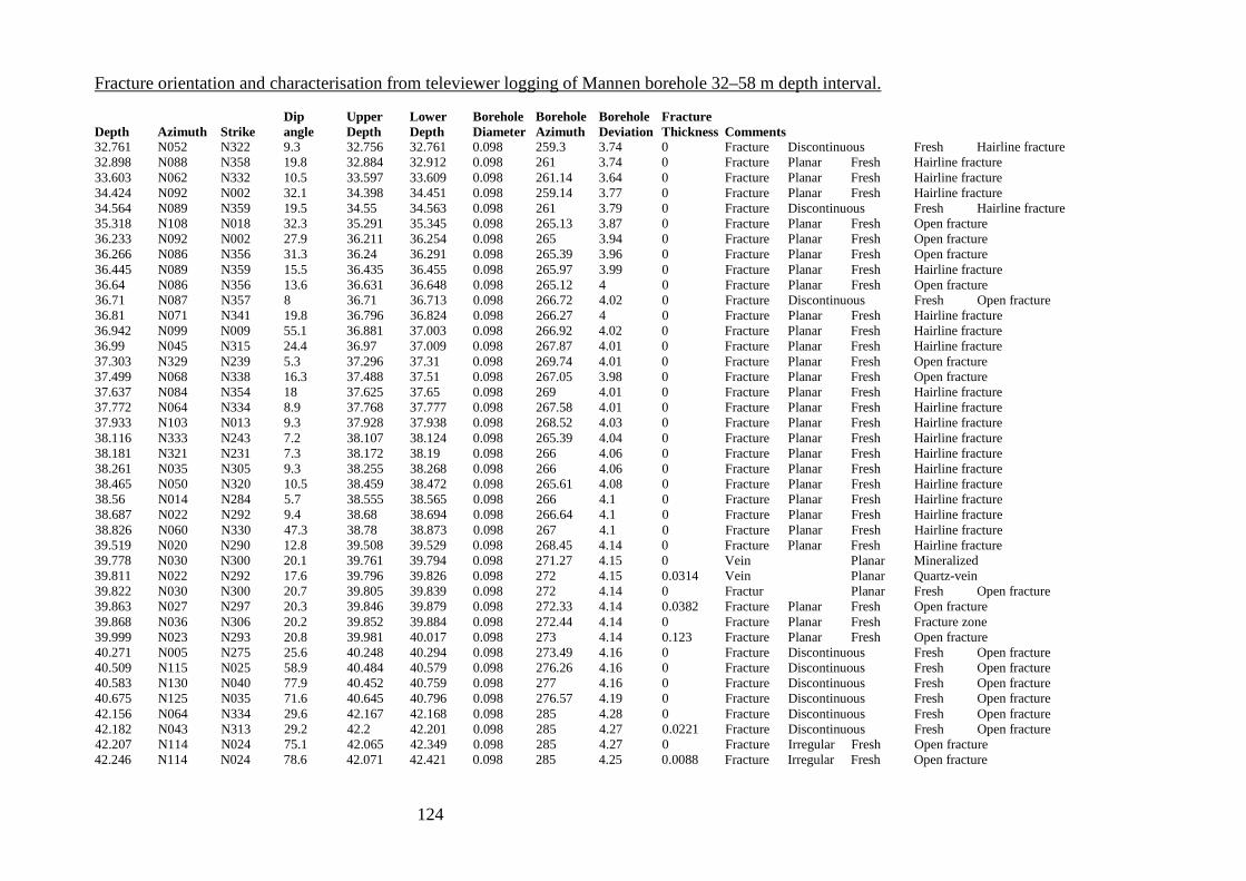
124
Fracture orientation and characterisation from televiewer logging of Mannen borehole 32–58 m depth interval.
Dip Upper Lower Borehole Borehole Borehole Fracture Depth Azimuth Strike angle Depth Depth Diameter Azimuth Deviation Thickness Comments 32.761 N052 N322 9.3 32.756 32.761 0.098 259.3 3.74 0 Fracture Discontinuous Fresh Hairline fracture 32.898 N088 N358 19.8 32.884 32.912 0.098 261 3.74 0 Fracture Planar Fresh Hairline fracture 33.603 N062 N332 10.5 33.597 33.609 0.098 261.14 3.64 0 Fracture Planar Fresh Hairline fracture 34.424 N092 N002 32.1 34.398 34.451 0.098 259.14 3.77 0 Fracture Planar Fresh Hairline fracture 34.564 N089 N359 19.5 34.55 34.563 0.098 261 3.79 0 Fracture Discontinuous Fresh Hairline fracture 35.318 N108 N018 32.3 35.291 35.345 0.098 265.13 3.87 0 Fracture Planar Fresh Open fracture 36.233 N092 N002 27.9 36.211 36.254 0.098 265 3.94 0 Fracture Planar Fresh Open fracture 36.266 N086 N356 31.3 36.24 36.291 0.098 265.39 3.96 0 Fracture Planar Fresh Open fracture 36.445 N089 N359 15.5 36.435 36.455 0.098 265.97 3.99 0 Fracture Planar Fresh Hairline fracture 36.64 N086 N356 13.6 36.631 36.648 0.098 265.12 4 0 Fracture Planar Fresh Open fracture 36.71 N087 N357 8 36.71 36.713 0.098 266.72 4.02 0 Fracture Discontinuous Fresh Open fracture 36.81 N071 N341 19.8 36.796 36.824 0.098 266.27 4 0 Fracture Planar Fresh Hairline fracture 36.942 N099 N009 55.1 36.881 37.003 0.098 266.92 4.02 0 Fracture Planar Fresh Hairline fracture 36.99 N045 N315 24.4 36.97 37.009 0.098 267.87 4.01 0 Fracture Planar Fresh Hairline fracture 37.303 N329 N239 5.3 37.296 37.31 0.098 269.74 4.01 0 Fracture Planar Fresh Open fracture 37.499 N068 N338 16.3 37.488 37.51 0.098 267.05 3.98 0 Fracture Planar Fresh Open fracture 37.637 N084 N354 18 37.625 37.65 0.098 269 4.01 0 Fracture Planar Fresh Hairline fracture 37.772 N064 N334 8.9 37.768 37.777 0.098 267.58 4.01 0 Fracture Planar Fresh Hairline fracture 37.933 N103 N013 9.3 37.928 37.938 0.098 268.52 4.03 0 Fracture Planar Fresh Hairline fracture 38.116 N333 N243 7.2 38.107 38.124 0.098 265.39 4.04 0 Fracture Planar Fresh Hairline fracture 38.181 N321 N231 7.3 38.172 38.19 0.098 266 4.06 0 Fracture Planar Fresh Hairline fracture 38.261 N035 N305 9.3 38.255 38.268 0.098 266 4.06 0 Fracture Planar Fresh Hairline fracture 38.465 N050 N320 10.5 38.459 38.472 0.098 265.61 4.08 0 Fracture Planar Fresh Hairline fracture 38.56 N014 N284 5.7 38.555 38.565 0.098 266 4.1 0 Fracture Planar Fresh Hairline fracture 38.687 N022 N292 9.4 38.68 38.694 0.098 266.64 4.1 0 Fracture Planar Fresh Hairline fracture 38.826 N060 N330 47.3 38.78 38.873 0.098 267 4.1 0 Fracture Planar Fresh Hairline fracture 39.519 N020 N290 12.8 39.508 39.529 0.098 268.45 4.14 0 Fracture Planar Fresh Hairline fracture 39.778 N030 N300 20.1 39.761 39.794 0.098 271.27 4.15 0 Vein Planar Mineralized 39.811 N022 N292 17.6 39.796 39.826 0.098 272 4.15 0.0314 Vein Planar Quartz-vein 39.822 N030 N300 20.7 39.805 39.839 0.098 272 4.14 0 Fractur Planar Fresh Open fracture 39.863 N027 N297 20.3 39.846 39.879 0.098 272.33 4.14 0.0382 Fracture Planar Fresh Open fracture 39.868 N036 N306 20.2 39.852 39.884 0.098 272.44 4.14 0 Fracture Planar Fresh Fracture zone 39.999 N023 N293 20.8 39.981 40.017 0.098 273 4.14 0.123 Fracture Planar Fresh Open fracture 40.271 N005 N275 25.6 40.248 40.294 0.098 273.49 4.16 0 Fracture Discontinuous Fresh Open fracture 40.509 N115 N025 58.9 40.484 40.579 0.098 276.26 4.16 0 Fracture Discontinuous Fresh Open fracture 40.583 N130 N040 77.9 40.452 40.759 0.098 277 4.16 0 Fracture Discontinuous Fresh Open fracture 40.675 N125 N035 71.6 40.645 40.796 0.098 276.57 4.19 0 Fracture Discontinuous Fresh Open fracture 42.156 N064 N334 29.6 42.167 42.168 0.098 285 4.28 0 Fracture Discontinuous Fresh Open fracture 42.182 N043 N313 29.2 42.2 42.201 0.098 285 4.27 0.0221 Fracture Discontinuous Fresh Open fracture 42.207 N114 N024 75.1 42.065 42.349 0.098 285 4.27 0 Fracture Irregular Fresh Open fracture 42.246 N114 N024 78.6 42.071 42.421 0.098 285 4.25 0.0088 Fracture Irregular Fresh Open fracture
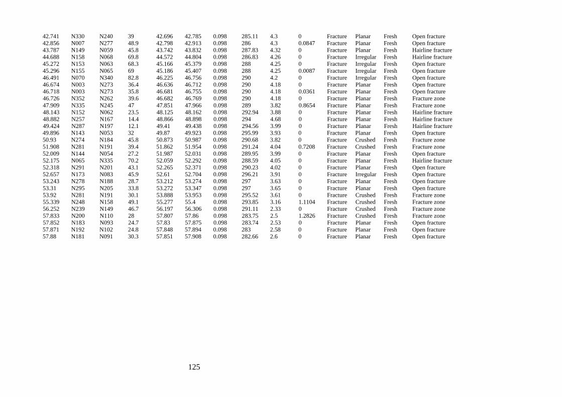
125
42.741 N330 N240 39 42.696 42.785 0.098 285.11 4.3 0 Fracture Planar Fresh Open fracture 42.856 N007 N277 48.9 42.798 42.913 0.098 286 4.3 0.0847 Fracture Planar Fresh Open fracture 43.787 N149 N059 45.8 43.742 43.832 0.098 287.83 4.32 0 Fracture Planar Fresh Hairline fracture 44.688 N158 N068 69.8 44.572 44.804 0.098 286.83 4.26 0 Fracture Irregular Fresh Hairline fracture 45.272 N153 N063 68.3 45.166 45.379 0.098 288 4.25 0 Fracture Irregular Fresh Open fracture 45.296 N155 N065 69 45.186 45.407 0.098 288 4.25 0.0087 Fracture Irregular Fresh Open fracture 46.491 N070 N340 82.8 46.225 46.756 0.098 290 4.2 0 Fracture Irregular Fresh Open fracture 46.674 N003 N273 36.4 46.636 46.712 0.098 290 4.18 0 Fracture Planar Fresh Open fracture 46.718 N003 N273 35.8 46.681 46.755 0.098 290 4.18 0.0361 Fracture Planar Fresh Open fracture 46.726 N352 N262 39.6 46.682 46.769 0.098 290 4.18 0 Fracture Planar Fresh Fracture zone 47.909 N335 N245 47 47.851 47.966 0.098 289 3.82 0.8654 Fracture Planar Fresh Fracture zone 48.143 N152 N062 23.5 48.125 48.162 0.098 292.94 3.88 0 Fracture Planar Fresh Hairline fracture 48.882 N257 N167 14.4 48.866 48.898 0.098 294 4.68 0 Fracture Planar Fresh Hairline fracture 49.424 N287 N197 12.1 49.41 49.438 0.098 294.56 3.99 0 Fracture Planar Fresh Hairline fracture 49.896 N143 N053 32 49.87 49.923 0.098 295.99 3.93 0 Fracture Planar Fresh Open fracture 50.93 N274 N184 45.8 50.873 50.987 0.098 290.68 3.82 0 Fracture Crushed Fresh Fracture zone 51.908 N281 N191 39.4 51.862 51.954 0.098 291.24 4.04 0.7208 Fracture Crushed Fresh Fracture zone 52.009 N144 N054 27.2 51.987 52.031 0.098 289.95 3.99 0 Fracture Planar Fresh Open fracture 52.175 N065 N335 70.2 52.059 52.292 0.098 288.59 4.05 0 Fracture Planar Fresh Hairline fracture 52.318 N291 N201 43.1 52.265 52.371 0.098 290.23 4.02 0 Fracture Planar Fresh Open fracture 52.657 N173 N083 45.9 52.61 52.704 0.098 296.21 3.91 0 Fracture Irregular Fresh Open fracture 53.243 N278 N188 28.7 53.212 53.274 0.098 297 3.63 0 Fracture Planar Fresh Open fracture 53.31 N295 N205 33.8 53.272 53.347 0.098 297 3.65 0 Fracture Planar Fresh Open fracture 53.92 N281 N191 30.1 53.888 53.953 0.098 295.52 3.61 0 Fracture Crushed Fresh Fracture zone 55.339 N248 N158 49.1 55.277 55.4 0.098 293.85 3.16 1.1104 Fracture Crushed Fresh Fracture zone 56.252 N239 N149 46.7 56.197 56.306 0.098 291.11 2.33 0 Fracture Crushed Fresh Fracture zone 57.833 N200 N110 28 57.807 57.86 0.098 283.75 2.5 1.2826 Fracture Crushed Fresh Fracture zone 57.852 N183 N093 24.7 57.83 57.875 0.098 283.74 2.53 0 Fracture Planar Fresh Open fracture 57.871 N192 N102 24.8 57.848 57.894 0.098 283 2.58 0 Fracture Planar Fresh Open fracture 57.88 N181 N091 30.3 57.851 57.908 0.098 282.66 2.6 0 Fracture Planar Fresh Open fracture
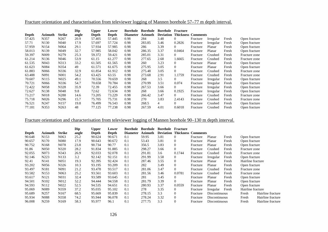
126
Fracture orientation and characterisation from televiewer logging of Mannen borehole 57–77 m depth interval.
Dip Upper Lower Borehole Borehole Borehole Fracture Depth Azimuth Strike angle Depth Depth Diameter Azimuth Deviation Thickness Comments 57.425 N357 N267 20.9 57.405 57.445 0.98 284 3.48 0 Fracture Irregular Fresh Open fracture 57.71 N130 N040 17.9 57.697 57.724 0.98 283.85 3.46 0.2826 Fracture Irregular Fresh Open fracture 57.959 N154 N064 29.1 57.934 57.985 0.98 286 3.39 0 Fracture Planar Fresh Open fracture 58.013 N139 N049 32.7 57.985 58.042 0.98 286.35 3.37 0.0464 Fracture Planar Fresh Open fracture 59.397 N009 N279 25.3 59.372 59.421 0.98 285.01 3.31 0 Fracture Crushed Fresh Fracture zone 61.214 N136 N046 53.9 61.15 61.277 0.98 277.65 2.68 1.6665 Fracture Crushed Fresh Fracture zone 61.535 N043 N313 33.2 61.505 61.565 0.98 260 3.23 0 Fracture Planar Fresh Open fracture 61.623 N084 N354 49 61.571 61.675 0.98 275.95 3.05 0 Fracture Planar Fresh Open fracture 61.883 N066 N336 32.9 61.854 61.912 0.98 275.48 3.05 0 Fracture Crushed Fresh Fracture zone 63.488 N091 N001 54.2 63.425 63.55 0.98 273.68 2.91 1.1759 Fracture Crushed Fresh Fracture zone 70.607 N115 N025 49.1 70.556 70.659 0.98 268 3.5 0 Fracture Irregular Fresh Open fracture 70.721 N066 N336 54.7 70.658 70.784 0.98 270.99 3.51 0.074 Fracture Irregular Fresh Open fracture 72.422 N058 N328 35.9 72.39 72.455 0.98 267.53 3.66 0 Fracture Irregular Fresh Open fracture 72.627 N138 N048 9.8 72.62 72.634 0.98 268 3.66 0.1925 Fracture Irregular Fresh Open fracture 73.217 N018 N288 14.6 73.205 73.229 0.98 266.42 3.47 0 Fracture Crushed Fresh Fracture zone 75.718 N026 N296 15.7 75.705 75.731 0.98 270 3.83 2.4143 Fracture Crushed Fresh Fracture zone 76.521 N247 N157 19.8 76.499 76.543 0.98 268.5 4 0 Fracture Crushed Fresh Open fracture 77.181 N353 N263 48 77.125 77.238 0.98 267.59 4.01 0.6018 Fracture Crushed Fresh Open fracture
Fracture orientation and characterisation from televiewer logging of Mannen borehole 90–130 m depth interval.
Dip Upper Lower Borehole Borehole Borehole Fracture Depth Azimuth Strike angle Depth Depth Diameter Azimuth Deviation Thickness Comments 90.648 N153 N063 25.2 90.624 90.671 0.1 59.95 3.81 0 Fracture Planar Fresh Open fracture 90.657 N170 N080 17.9 90.643 90.672 0.1 53.43 3.81 0 Fracture Planar Fresh Open fracture 90.752 N168 N078 23.8 90.734 90.77 0.1 356.5 3.83 0 Fracture Planar Fresh Open fracture 91.86 N050 N320 28.2 91.834 91.885 0.1 298.27 3.66 0 Fracture Crushed Fresh Fracture zone 92.055 N073 N343 26.9 92.033 92.078 0.1 291.81 3.6 0.1744 Fracture Crushed Fresh Fracture zone 92.146 N223 N133 3.2 92.142 92.151 0.1 291.99 3.58 0 Fracture Irregular Fresh Open fracture 92.41 N141 N051 19.3 92.395 92.424 0.1 287.46 3.55 0 Fracture Planar Fresh Hairline fracture 93.202 N056 N326 10.3 93.195 93.209 0.1 282 3.49 0 Fracture Planar Fresh Open fracture 93.497 N181 N091 21.2 93.478 93.517 0.1 281.06 3.47 0 Fracture Crushed Fresh Fracture zone 93.582 N153 N063 25.2 93.561 93.603 0.1 281.56 3.46 0.0781 Fracture Crushed Fresh Fracture zone 93.617 N121 N031 32.4 93.589 93.645 0.1 281 3.45 0 Fracture Planar Fresh Open fracture 94.501 N102 N012 52.2 94.444 94.558 0.1 281.79 3.39 0 Fracture Planar Fresh Open fracture 94.593 N112 N022 52.5 94.535 94.651 0.1 280.93 3.37 0.0559 Fracture Planar Fresh Open fracture 95.069 N089 N359 37.2 95.035 95.102 0.1 278 3.35 0 Fracture Irregular Fresh Hairline fracture 95.689 N257 N167 68.5 95.669 95.839 0.1 278.15 3.3 0 Fracture Discontinuous Fresh Hairline fracture 95.934 N088 N358 74.2 95.944 96.078 0.1 278.24 3.32 0 Fracture Discontinuous Fresh Hairline fracture 96.008 N259 N169 58.3 95.977 96.1 0.1 277.75 3.3 0 Fracture Discontinuous Fresh Hairline fracture
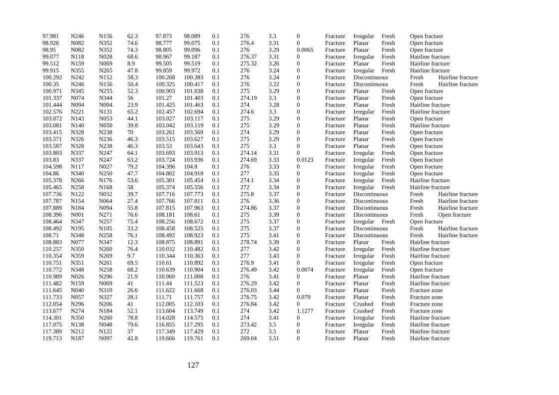
127
97.981 N246 N156 62.3 97.873 98.089 0.1 276 3.3 0 Fracture Irregular Fresh Open fracture 98.926 N082 N352 74.6 98.777 99.075 0.1 276.4 3.31 0 Fracture Planar Fresh Open fracture 98.95 N082 N352 74.3 98.805 99.096 0.1 276 3.29 0.0065 Fracture Planar Fresh Open fracture 99.077 N118 N028 68.6 98.967 99.187 0.1 276.37 3.31 0 Fracture Irregular Fresh Hairline fracture 99.512 N159 N069 8.9 99.505 99.519 0.1 275.32 3.26 0 Fracture Planar Fresh Hairline fracture 99.915 N355 N265 47.8 99.859 99.972 0.1 276 3.24 0 Fracture Irregular Fresh Hairline fracture 100.292 N242 N152 58.3 100.268 100.383 0.1 276 3.24 0 Fracture Discontinuous Fresh Hairline fracture 100.35 N246 N156 50.4 100.325 100.417 0.1 276 3.22 0 Fracture Discontinuous Fresh Hairline fracture 100.971 N345 N255 52.3 100.903 101.038 0.1 275 3.29 0 Fracture Planar Fresh Open fracture 101.337 N074 N344 56 101.27 101.403 0.1 274.19 3.3 0 Fracture Planar Fresh Open fracture 101.444 N094 N004 23.9 101.425 101.463 0.1 274 3.28 0 Fracture Planar Fresh Hairline fracture 102.576 N221 N131 65.2 102.457 102.694 0.1 274.6 3.3 0 Fracture Irregular Fresh Hairline fracture 103.072 N143 N053 44.1 103.027 103.117 0.1 275 3.29 0 Fracture Planar Fresh Open fracture 103.081 N140 N050 39.8 103.042 103.119 0.1 275 3.29 0 Fracture Planar Fresh Hairline fracture 103.415 N328 N238 70 103.261 103.569 0.1 274 3.29 0 Fracture Planar Fresh Open fracture 103.571 N326 N236 46.3 103.515 103.627 0.1 275 3.29 0 Fracture Planar Fresh Open fracture 103.587 N328 N238 46.3 103.53 103.643 0.1 275 3.3 0 Fracture Planar Fresh Open fracture 103.803 N337 N247 64.1 103.693 103.913 0.1 274.14 3.31 0 Fracture Irregular Fresh Open fracture 103.83 N337 N247 63.2 103.724 103.936 0.1 274.69 3.33 0.0123 Fracture Irregular Fresh Open fracture 104.598 N117 N027 79.2 104.396 104.8 0.1 276 3.33 0 Fracture Irregular Fresh Open fracture 104.86 N340 N250 47.7 104.802 104.918 0.1 277 3.35 0 Fracture Irregular Fresh Open fracture 105.378 N266 N176 53.6 105.301 105.454 0.1 274.1 3.34 0 Fracture Irregular Fresh Hairline fracture 105.465 N258 N168 58 105.374 105.556 0.1 272 3.34 0 Fracture Irregular Fresh Hairline fracture 107.736 N122 N032 39.7 107.716 107.773 0.1 275.8 3.37 0 Fracture Discontinuous Fresh Hairline fracture 107.787 N154 N064 27.4 107.766 107.811 0.1 276 3.36 0 Fracture Discontinuous Fresh Hairline fracture 107.889 N184 N094 55.8 107.815 107.963 0.1 274.86 3.37 0 Fracture Discontinuous Fresh Hairline fracture 108.396 N001 N271 76.6 108.181 108.61 0.1 275 3.39 0 Fracture Discontinuous Fresh Open fracture 108.464 N347 N257 75.4 108.256 108.672 0.1 275 3.37 0 Fracture Irregular Fresh Open fracture 108.492 N195 N105 33.2 108.458 108.525 0.1 275 3.37 0 Fracture Discontinuous Fresh Hairline fracture 108.71 N348 N258 76.1 108.492 108.923 0.1 275 3.41 0 Fracture Discontinuous Fresh Hairline fracture 108.883 N077 N347 12.3 108.875 108.891 0.1 278.74 3.39 0 Fracture Planar Fresh Hairline fracture 110.257 N350 N260 76.4 110.032 110.482 0.1 277 3.42 0 Fracture Irregular Fresh Hairline fracture 110.354 N359 N269 9.7 110.344 110.363 0.1 277 3.43 0 Fracture Irregular Fresh Hairline fracture 110.751 N351 N261 69.5 110.61 110.892 0.1 276.9 3.41 0 Fracture Irregular Fresh Open fracture 110.772 N348 N258 68.2 110.639 110.904 0.1 276.49 3.42 0.0074 Fracture Irregular Fresh Open fracture 110.989 N026 N296 21.9 110.969 111.008 0.1 276 3.41 0 Fracture Planar Fresh Hairline fracture 111.482 N159 N069 41 111.44 111.523 0.1 276.29 3.42 0 Fracture Planar Fresh Hairline fracture 111.645 N040 N310 26.6 111.622 111.668 0.1 276.03 3.44 0 Fracture Planar Fresh Fracture zone 111.733 N057 N327 28.1 111.71 111.757 0.1 276.75 3.42 0.079 Fracture Planar Fresh Fracture zone 112.054 N296 N206 41 112.005 112.103 0.1 276.84 3.42 0 Fracture Crushed Fresh Fracture zone 113.677 N274 N184 52.1 113.604 113.749 0.1 274 3.42 1.1277 Fracture Crushed Fresh Fracture zone 114.301 N350 N260 78.8 114.028 114.575 0.1 274 3.41 0 Fracture Irregular Fresh Hairline fracture 117.075 N138 N048 79.6 116.855 117.295 0.1 273.42 3.5 0 Fracture Irregular Fresh Hairline fracture 117.389 N212 N122 37 117.349 117.429 0.1 272 3.5 0 Fracture Planar Fresh Hairline fracture 119.713 N187 N097 42.8 119.666 119.761 0.1 269.04 3.51 0 Fracture Planar Fresh Hairline fracture
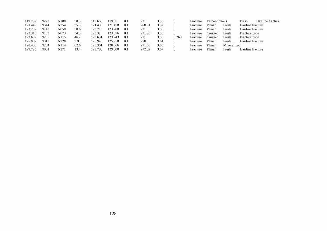
128
119.757 N270 N180 58.3 119.663 119.85 0.1 271 3.53 0 Fracture Discontinuous Fresh Hairline fracture 121.442 N344 N254 35.3 121.405 121.478 0.1 268.91 3.52 0 Fracture Planar Fresh Hairline fracture 123.252 N140 N050 38.6 123.215 123.288 0.1 271 3.58 0 Fracture Planar Fresh Hairline fracture 123.343 N163 N073 34.3 123.31 123.376 0.1 271.95 3.55 0 Fracture Crushed Fresh Fracture zone 123.687 N205 N115 46.7 123.631 123.743 0.1 271 3.55 0.269 Fracture Crushed Fresh Fracture zone 125.952 N318 N228 3.9 125.946 125.958 0.1 270 3.64 0 Fracture Planar Fresh Hairline fracture 128.463 N204 N114 62.6 128.361 128.566 0.1 271.65 3.65 0 Fracture Planar Mineralized 129.795 N001 N271 13.4 129.783 129.808 0.1 272.02 3.67 0 Fracture Planar Fresh Hairline fracture
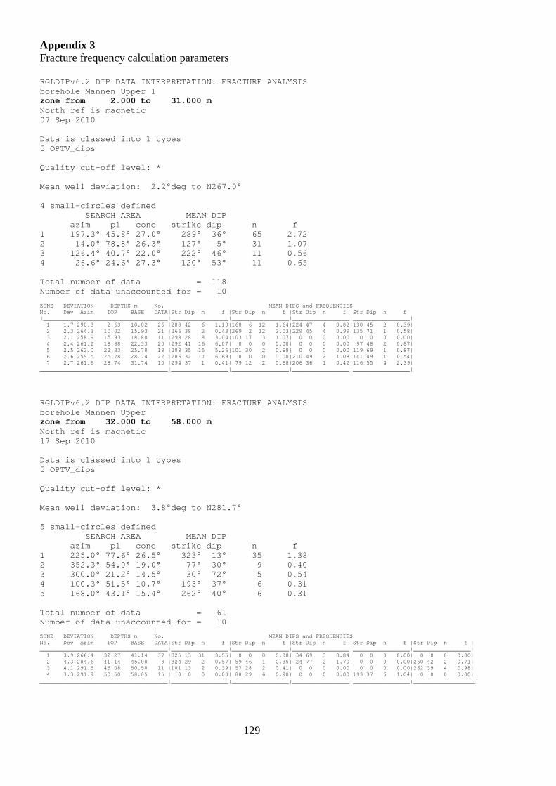
129
Appendix 3
Fracture frequency calculation parameters
RGLDIPv6.2 DIP DATA INTERPRETATION: FRACTURE ANALYSIS borehole Mannen Upper 1 zone from 2.000 to 31.000 m North ref is magnetic 07 Sep 2010 Data is classed into 1 types 5 OPTV_dips Quality cut-off level: * Mean well deviation: 2.2°deg to N267.0° 4 small-circles defined SEARCH AREA MEAN DIP azim pl cone strike dip n f 1 197.3° 45.8° 27.0° 289° 36° 65 2.72 2 14.0° 78.8° 26.3° 127° 5° 31 1.07 3 126.4° 40.7° 22.0° 222° 46° 11 0.56 4 26.6° 24.6° 27.3° 120° 53° 11 0.65 Total number of data = 118 Number of data unaccounted for = 10 ZONE DEVIATION DEPTHS m No. MEAN DIPS and FREQUENCIES No. Dev Azim TOP BASE DATA|Str Dip n f |Str Dip n f |Str Dip n f |Str Dip n f |_____________________________________|_________________|_________________|_________________|_________________| 1 1.7 290.3 2.63 10.02 26 |288 42 6 1.10|168 6 12 1.64|224 47 4 0.82|130 45 2 0.39| 2 2.3 264.3 10.02 15.93 21 |266 38 2 0.43|269 2 12 2.03|229 45 4 0.99|135 71 1 0.58| 3 2.1 258.9 15.93 18.88 11 |298 28 8 3.04|103 17 3 1.07| 0 0 0 0.00| 0 0 0 0.00| 4 2.4 261.2 18.88 22.33 20 |292 41 16 6.07| 0 0 0 0.00| 0 0 0 0.00| 97 48 2 0.87| 5 2.5 262.0 22.33 25.78 18 |288 35 15 5.26|101 30 2 0.68| 0 0 0 0.00|119 69 1 0.87| 6 2.6 259.5 25.78 28.74 22 |286 32 17 6.69| 0 0 0 0.00|210 49 2 1.08|141 49 1 0.54| 7 2.7 261.6 28.74 31.74 10 |294 37 1 0.41| 79 12 2 0.68|206 36 1 0.42|116 55 4 2.39| ______________________________________|_________________|_________________|_________________|_________________|
RGLDIPv6.2 DIP DATA INTERPRETATION: FRACTURE ANALYSIS borehole Mannen Upper zone from 32.000 to 58.000 m North ref is magnetic 17 Sep 2010 Data is classed into 1 types 5 OPTV_dips Quality cut-off level: * Mean well deviation: 3.8°deg to N281.7° 5 small-circles defined SEARCH AREA MEAN DIP azim pl cone strike dip n f 1 225.0° 77.6° 26.5° 323° 13° 35 1.38 2 352.3° 54.0° 19.0° 77° 30° 9 0.40 3 300.0° 21.2° 14.5° 30° 72° 5 0.54 4 100.3° 51.5° 10.7° 193° 37° 6 0.31 5 168.0° 43.1° 15.4° 262° 40° 6 0.31 Total number of data = 61 Number of data unaccounted for = 10 ZONE DEVIATION DEPTHS m No. MEAN DIPS and FREQUENCIES No. Dev Azim TOP BASE DATA|Str Dip n f |Str Dip n f |Str Dip n f |Str Dip n f |Str Dip n f | ______________________________________|_________________|_________________|_________________|_________________|_________________| 1 3.9 266.4 32.27 41.14 37 |325 13 31 3.55| 0 0 0 0.00| 34 69 3 0.84| 0 0 0 0.00| 0 0 0 0.00| 2 4.3 284.6 41.14 45.08 8 |324 29 2 0.57| 59 46 1 0.35| 24 77 2 1.70| 0 0 0 0.00|260 42 2 0.71| 3 4.1 291.5 45.08 50.50 11 |181 13 2 0.39| 57 28 2 0.41| 0 0 0 0.00| 0 0 0 0.00|262 39 4 0.98| 4 3.3 291.9 50.50 58.05 15 | 0 0 0 0.00| 88 29 6 0.90| 0 0 0 0.00|193 37 6 1.04| 0 0 0 0.00| ______________________________________|_________________|_________________|_________________|_________________|_________________|
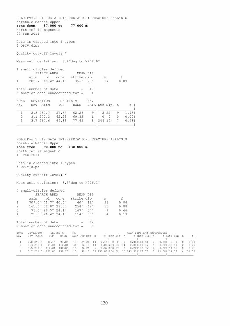
130
RGLDIPv6.2 DIP DATA INTERPRETATION: FRACTURE ANALYSIS borehole Mannen Upper zone from 57.000 to 77.000 m North ref is magnetic 02 Feb 2011 Data is classed into 1 types 5 OPTV_dips Quality cut-off level: * Mean well deviation: 3.4°deg to N272.0° 1 small-circles defined SEARCH AREA MEAN DIP azim pl cone strike dip n f 1 282.7° 68.4° 44.1° 356° 23° 17 0.89 Total number of data = 17 Number of data unaccounted for = 1 ZONE DEVIATION DEPTHS m No. No. Dev Azim TOP BASE DATA|Str Dip n f | ______________________________________|_________________| 1 3.3 282.7 57.35 62.28 9 | 3 22 9 1.93| 2 3.1 270.3 62.28 69.83 1 | 0 0 0 0.00| 3 3.7 267.6 69.83 77.65 8 |344 19 7 0.93| ______________________________________|_________________|
RGLDIPv6.2 DIP DATA INTERPRETATION: FRACTURE ANALYSIS borehole Mannen Upper zone from 90.000 to 130.000 m North ref is magnetic 18 Feb 2011 Data is classed into 1 types 5 OPTV_dips Quality cut-off level: * Mean well deviation: 3.3°deg to N276.1° 4 small-circles defined SEARCH AREA MEAN DIP azim pl cone strike dip n f 1 309.0° 71.7° 40.0° 40° 19° 33 0.86 2 161.6° 32.0° 28.5° 254° 62° 16 0.88 3 75.3° 28.5° 24.1° 167° 57° 9 0.46 4 21.5° 21.4° 24.1° 114° 57° 4 0.19 Total number of data = 62 Number of data unaccounted for = 8 ZONE DEVIATION DEPTHS m No. MEAN DIPS and FREQUENCIES No. Dev Azim TOP BASE DATA|Str Dip n f |Str Dip n f |Str Dip n f |Str Dip n f | ______________________________________|_________________|_________________|_________________|_________________| 1 2.8 293.9 90.15 97.04 17 | 29 21 14 2.14| 0 0 0 0.00|168 63 2 0.70| 0 0 0 0.00| 2 3.3 275.4 97.04 112.81 40 | 32 18 13 0.86|253 63 14 2.01|161 56 5 0.62|113 59 2 0.26| 3 3.5 271.3 112.81 130.05 13 | 86 21 6 0.37|258 57 2 0.22|182 55 2 0.22|114 55 2 0.21| 4 3.7 271.0 130.05 130.29 13 | 40 19 33 139.88|254 62 16 143.39|167 57 9 75.30|114 57 4 31.06| ______________________________________|_________________|_________________|_________________|________________