Embed Size (px)
Citation preview

LOGIC FOR GRAY-CODE COMPUTATION
ULRICH BERGER AND KENJI MIYAMOTO AND HELMUT SCHWICHTENBERGAND HIDEKI TSUIKI
Abstract. Gray-code is a well-known binary number system whereneighboring values differ in one digit only. Tsuiki (2002) has introducedGray code to the field of real number computation. He assigns to eachnumber a unique 1⊥-sequence, i.e., an infinite sequence of {−1, 1,⊥}containing at most one copy of ⊥ (meaning undefinedness). In this pa-per we take a logical and constructive approach to study real numbercomputation based on Gray-code. Instead of Tsuiki’s indeterministicmultihead Type-2 machine, we use pre-Gray code, which is a represen-tation of Gray-code as a sequence of constructors, to avoid the difficultydue to ⊥ which prevents sequential access to a stream. We extractreal number algorithms from proofs in an appropriate formal theory in-volving inductive and coinductive definitions. Examples are algorithmstransforming pre-Gray code into signed digit code of real numbers, andconversely, the average for pre-Gray code and a translation of finitesegments of pre-Gray code into its normal form. These examples areformalized in the proof assistant Minlog.
Keywords: Gray-code, real number computation, inductive and coin-ductive definitions, program extraction.
2010 Mathematics Subject Classification: 03D78, 03F60, 03B70, 03B35
1. Introduction
Gray-code (also called reflected binary code) is widely known in digitalcommunication, due to its property that the Hamming distance betweenadjacent Gray-codes is always 1. Based on Gray-code, Di Gianantonio andTsuiki studied independently an expansion of real numbers as infinite se-quences of {0, 1,⊥} each of which contains at most one ⊥ standing forundefinedness [5, 12]. Tsuiki called it modified Gray expansion. He alsostudied computability of real numbers, and presented several algorithms to
This work was supported by the International Research Staff Exchange Scheme (IRSES)Nr. 612638 CORCON and Nr. 294962 COMPUTAL of the European Commission, theJSPS Core-to-Core Program, A. Advanced research Networks and JSPS KAKENHI GrantNumber 15K00015.
1

2 U. BERGER, K. MIYAMOTO, H. SCHWICHTENBERG AND H. TSUIKI
do real number computation via Gray-code. The motivation of this paperis to shed light on the logical aspect of Gray-code computation from theconstructive standpoint. We formalize Gray-code in the Theory of Com-putable Functionals, TCF in short, and also in the proof assistant Minlog1,which is an implementation of TCF, by means of inductive and coinductivedefinitions [10]. In order to make use of Tsuiki’s idea in TCF, we intro-duce pre-Gray code which is Gray-code represented as ordinary streams.Through the realizability interpretation we extract from proofs programs asterms in an extension T+ of Godel’s T involving higher type recursion andcorecursion operators. As case studies we extract real number algorithms inour setting of pre-Gray code. The correctness of the extracted programs isautomatically ensured by the soundness theorem.
The rest of this paper is organized as follows. In Section 2 we investigateGray-code and introduce pre-Gray code representation of real numbers. InSection 3 we describe realizability in our framework TCF, w.r.t. inductiveand coinductive definitions. This provides a suitable setting to study logicalaspects of signed digit streams and pre-Gray code. Section 4 presents proofsabout coinductive representations that correspond to algorithms; the latterare described informally. 4.1 studies the average of two real numbers insigned digit code, and 4.4 directly for pre-Gray code. In 4.2 and 4.3 wegive translators from pre-Gray into signed digit code, and vice versa. 4.5studies a translation of finite segments of pre-Gray code into its normalform. Section 5 deals with the conversion of Gray-code to modified Grayexpansion. In Section 6 we present and discuss the terms extracted fromformalizations (in the proof assistant Minlog) of the proofs in Sections 4 and5.
Related work. There are programming languages which can process mo-dified Gray expansion directly. Tsuiki and Sugihara studied an extensionof Haskell with the non-deterministic choice operator gamb which works asMcCarthy’s amb operator [14]. Tsuiki studied a logic programming languagewith guarded clauses and committed choice [13]. Terayama and Tsuiki stud-ied an extension of PCF with parallelism [11]. In this paper we avoid usingthe above features by adopting pre-Gray code. Concerning stream basedreal arithmetic. Wiedmer [15, 16] used signed digit streams for real num-ber computation. Its corecursive treatment was studied by Ciaffaglione andDi Gianantonio in Coq [4]. Berger and Seisenberger studied program ex-traction to obtain programs dealing with signed digit streams [2]. Some of
1See http://www.minlog-system.de/
LOGIC FOR GRAY-CODE COMPUTATION 3
their results are formalized by Miyamoto and Schwichtenberg in TCF andMinlog [7, 8]. Chuang studied the average and the multiplication of realnumbers using coinduction in Agda via the Curry-Howard isomorphism [3].
2. Gray-code and its variations
2.1. Expansions of real numbers. We define binary expansion of theunit interval as the expansion of the unit2 interval I = [−1, 1] as infinitesequences of PSD = {−1, 1} (proper signed digits) so that v = a1a2 . . .represents
∞∑i=1
ai2i.(1)
With binary expansion, a finite sequence a1, a2, . . . , an denotes the intervalfa1(fa2 . . . (fan(I) . . . ) for fa the function
fa(x) =x+ a
2,
and a1a2 . . . denotes the real number that belongs to the intersection ofthe intervals denoted by its finite truncations. Though binary expansionis simple and has little redundancy, it cannot be used for stream-basedcomputation of the reals because, for example, the first digit of the number0 cannot be determined by any arbitrary approximation information of thenumber. To remedy this, signed digit code is commonly used in real numbercomputation. Signed digit code is a representation of the same interval withthe same formula (1), but with three digits SD = {−1, 0, 1}. In this paper,we view finite sequences of SD as a free algebra I with a nullary constructornilI and three unary constructors C−1,C0,C1 of type I→ I. That is,
I = nilI + C−1 I + C0 I + C1 I.
Signed digit code has a lot of redundancy, as 11 and 01 represent the sameinterval [−1/2, 0] and 11 and 01 represent the same interval [0, 1/2]. Here,1 is the notation of −1 in a sequence.
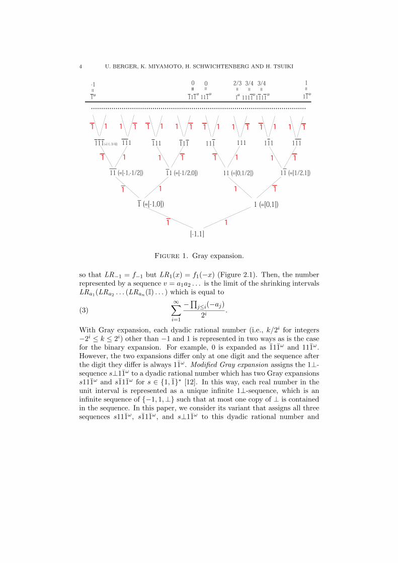
Modified Gray expansion is a unique representation of I that can be usedfor real number computation. It is based on Gray expansion which is anotherway of expanding I with PSD. In Gray expansion, the sequence is flippedafter an appearance of 1. That is, let LRa for a ∈ PSD be functions definedas
(2) LRa(x) = −ax− 1
2
2For simplicity we base our study on [−1, 1] rather than [0, 1].
4 U. BERGER, K. MIYAMOTO, H. SCHWICHTENBERG AND H. TSUIKI
1 (=[-1,0]) 1 (=[0,1])
11 (=[0,1/2])11 (=[-1,-1/2]) 11 (=[-1/2,0]) 11 (=[1/2,1])
.........................................................................................................
[-1,1]
111(=[-1,-3/4])
11ωω 1ω1 ω ω111 111 ω ω1111 1111
111 111 111 111111111111
=-1
=
0
=
0
= =
2/3
=
3/4
=
3/4
=
1
Figure 1. Gray expansion.
so that LR−1 = f−1 but LR1(x) = f1(−x) (Figure 2.1). Then, the numberrepresented by a sequence v = a1a2 . . . is the limit of the shrinking intervalsLRa1(LRa2 . . . (LRan(I) . . . ) which is equal to
(3)
∞∑i=1
−∏j≤i(−aj)2i
.
With Gray expansion, each dyadic rational number (i.e., k/2i for integers−2i ≤ k ≤ 2i) other than −1 and 1 is represented in two ways as is the casefor the binary expansion. For example, 0 is expanded as 111ω and 111ω.However, the two expansions differ only at one digit and the sequence afterthe digit they differ is always 11ω. Modified Gray expansion assigns the 1⊥-sequence s⊥11ω to a dyadic rational number which has two Gray expansionss111ω and s111ω for s ∈ {1, 1}∗ [12]. In this way, each real number in theunit interval is represented as a unique infinite 1⊥-sequence, which is aninfinite sequence of {−1, 1,⊥} such that at most one copy of ⊥ is containedin the sequence. In this paper, we consider its variant that assigns all threesequences s111ω, s111ω, and s⊥11ω to this dyadic rational number and
LOGIC FOR GRAY-CODE COMPUTATION 5
simply call it the (infinite) Gray-code. Gray-codes of real numbers in [−1, 1]range over the subset {1, 1}ω ∪{1, 1}∗⊥11ω of {−1, 1,⊥}ω. We will also calleach 1⊥-sequence in this set an (infinite) Gray-code. The following tableshows the difference of the three representations according to the charactera allowed when a dyadic rational number is represented as sa11ω.
Gray expansion a ∈ {−1, 1},Modified Gray expansion a = ⊥,Gray-code a ∈ {−1, 1,⊥}.
As we will study in Section 5, Gray-code and modified Gray expansion areequivalent in that a Gray-code can be coinductively converted to modifiedGray expansion.
In order to define the meaning of Gray-codes more precisely, we introducefinite Gray-codes. A finite 1⊥-sequence of length n is an infinite sequencet = t0t1 . . . of {−1, 1,⊥} such that tn−1 6= ⊥, tk = ⊥ for k ≥ n, and tk = ⊥for at most one k < n. We sometime omit the suffix ⊥ω of a finite 1⊥-sequence and write it as a sequence of {−1, 1,⊥} of length n. We call afinite 1⊥-sequence in {1, 1}∗ ∪ {1, 1}∗⊥11∗ a finite Gray-code. We definethe order generated by ⊥ v −1 and ⊥ v 1 on {−1, 1,⊥}, and its productorder on {−1, 1,⊥}ω. The set of finite/infinite 1⊥-sequences form a Scott-Ershov domain BD with compact elements finite 1⊥-sequences. Similarly,finite/infinite Gray-codes form a Scott-Ershov domain RD with compactelements finite Gray-codes. We say that a finite 1⊥-sequence t approximatesa 1⊥-sequence s if t v s.
We can define the meaning of Gray-code based on this domain structure.The meaning [[s]] of a finite Gray-code s is the same interval as the meaningof s with Gray expansion if s ∈ {1, 1}∗, and is the union of [[s′111n]] and[[s′111n]] if s has the form s′⊥11n for s′ ∈ {1, 1}∗. The meaning [[t]] of aninfinite Gray-code t is the unique real number that belongs to the intersectionof [[s]] for s finite Gray-codes that approximate t. The following propositionis immediate from the definition.
Proposition 2.1.
(a) For t ∈ {−1, 1}ω, [[t]] is the same as the value obtained by (3).(b) For s⊥10ω with s ∈ {−1, 1}∗, [[s⊥10ω]] = [[s010ω]] = [[s110ω]].
2.2. An algebra of ⊥-sequences. Note that ⊥ is not an ordinary cha-racter and a machine cannot read or write a ⊥ on a tape. In [12] anIM2-machine (indeterministic multihead Type-2 machine) was introducedto input and output 1⊥-sequences. An IM2-machine has two heads on eachinput/output tape so that it can skip a ⊥ and access the rest the sequence.
6 U. BERGER, K. MIYAMOTO, H. SCHWICHTENBERG AND H. TSUIKI
In this paper, instead of such a direct manipulation of 1⊥-sequences, wedefine pre-Gray code, which is a “representation” of Gray-code as sequencesof constructors representing how an 1⊥-sequence is obtained, and considercomputation through usual stream programs instead of IM2-machines.
Before introducing pre-Gray code, we introduce an algebra OB = (|OB|,C ∪ {nil}) of finite 1⊥-sequences. The carrier set |OB| is the set of fi-nite 1⊥-sequences. It is generated by four unary constructors in C :={cons1, cons−1, ins1, ins−1} as well as a nullary constructor nil. Recall thatan ordinary binary sequence is a term of a free algebra with two unary con-structors consa for a ∈ {−1, 1} which prepend a to a sequence as well asnil. On the other hand, a 1⊥-sequence is generated by two additional con-structors insa for a ∈ {−1, 1} which insert a as the second character to asequence.
Example 2.2. The term ins1(ins−1(cons−1(ins1 nil))) denotes 111⊥1:
nil denotes ⊥ω,(ins1 nil) denotes ⊥1⊥ω,
(cons−1(ins1 nil)) denotes 1⊥1⊥ω,(ins−1(cons−1(ins1 nil))) denotes 11⊥1⊥ω,
(ins1(ins−1(cons−1(ins1 nil)))) denotes 111⊥1⊥ω.
When writing a term of OB, we omit nil and write it as a sequence ofC. Thus, we write [ins1, ins−1, cons−1, ins1] for this term. One can calculatethat [cons−1, cons1, cons−1, ins1] also denotes the same 1⊥-sequence.
We write ϕ(p) for the 1⊥-sequence denoted by p ∈ C∗. More precisely,ϕ([c1, . . . , cn]) = (c1 ◦ · · · ◦ cn)(⊥ω).
For coalgebraic computation, one needs to read sequences of constructorsfrom left to right. If a sequence of C is read from left to right, then it can beconsidered as a procedure to construct a 1⊥-sequence as follows. We startwith an infinite tape with the state ⊥ω. We view consa as the operation tofill the leftmost ⊥ with a and insa as the operation to fill the second ⊥ fromthe left with a.
We write ψ(p) for the 1⊥-sequence obtained by this procedure. Moreprecisely, if we define c′ : {−1, 1,⊥}ω → {−1, 1,⊥}ω (c ∈ C) by
cons′a(s) = filling in s the first bottom from the left by a
ins′a(s) = filling in s the second bottom from the left by a
then ψ([c1, . . . , cn]) = (c′n ◦ · · · ◦ c′1)(⊥ω).

LOGIC FOR GRAY-CODE COMPUTATION 7
Example 2.3. We construct 111⊥1 according to [cons−1, cons1, cons−1, ins1]as ⊥ω → 1⊥ω → 11⊥ω → 111⊥ω → 111⊥1⊥ω and according to [ins1, ins−1,cons−1, ins1] as ⊥ω → ⊥1⊥ω → ⊥11⊥ω → 111⊥ω → 111⊥1⊥ω.
Proposition 2.4. ϕ(p) = ψ(p) for p ∈ C∗.
Proof. We show that
(4) (c1 ◦ · · · ◦ cn)(⊥ω) = (c′n ◦ · · · ◦ c′1)(⊥ω).
Note that c′ satisfies the equations
c′(b : s) = b : c′(s) (b 6= ⊥),
cons′a(⊥ : s) = a : s,
ins′a(⊥ : s) = ⊥ : cons′a(s).
Using the equations for c and c′ one easily verifies that
c(⊥ω) = c′(⊥ω),(5)
c ◦ d′ = d′ ◦ c.(6)
From (6) one obtains
(7) (c1 ◦ · · · ◦ cn) ◦ c′ = c′ ◦ (c1 ◦ · · · ◦ cn)
by induction on n. Now (7) and (5) yield (4), again by induction on n. �
Note that c′ is increasing. That is, s v c′(s) for c ∈ C. Therefore, wecan consider an infinite sequence q ∈ Cω of the four constructors cons1,cons1, ins1, ins1 as representing an infinite 1⊥-sequence which is obtainedas the least upper bound of {ϕ(p)(= ψ(p)) | p is a finite prefix of q }. Forexample, [ins1, ins−1, ins−1, ins−1, . . . ] represents ⊥11ω. We write ϕ(q) forthe 1⊥-sequence represented by q ∈ Cω.
As we have noted, the algebra OB is not a free algebra and we haveequations
insa ◦ consb = consb ◦ consa(8)
for a, b ∈ PSD. Actually, OB is the universal algebra in that the set offinite 1⊥-sequences is equal to the quotient of C∗ by these equations.
2.3. An algebra of Gray-code and an auxiliary algebra. Recall thatfinite Gray-codes form a subset {1, 1}∗ ∪ {1, 1}∗⊥11∗ of the set of finite 1⊥-sequences. In order to represent only this set of finite Gray-codes, we definea subalgebra G of OB simultaneously with another subalgebra H. The
8 U. BERGER, K. MIYAMOTO, H. SCHWICHTENBERG AND H. TSUIKI
carrier set of G is the set of finite Gray-codes. A naive attempt is to definethem as follows.
G = ({1, 1}∗ ∪ {1, 1}∗⊥11∗,
{ consa : G→ G | a ∈ PSD } ∪ {ins1 : H→ G, nilG : G})H = (⊥1∗, {ins−1 : H→ H, nilH : H})
However, this definition does not allow filling a bottom with a digit by theconsa constructor in the coinductive treatment of an 1⊥-sequence. For thispurpose, we need to add the constructors consa : G → H for a ∈ PSD tothe above definition. In order to distinguish the two constructors consa oftypes G → G and G → H, we give them different names LRa and Fina.We also rename ins1 and ins−1 to U and D, respectively, and define thetwo algebras G and H with carrier sets |G| = {1, 1}∗ ∪ {1, 1}∗⊥11∗ and|H| = {1, 1}+ ∪ {1, 1}+⊥11∗ ∪ ⊥1∗ mutually recursively as follows.
G = (|G|, {LRa : G→ G | a ∈ PSD } ∪ {U: H→ G, nilG : G})H = (|H|, {Fina : G→ H | a ∈ PSD } ∪ {D: H→ H, nilH : H})
Note that the carrier sets of both algebras are generated (but not freely) bytheir constructors. We call a term of type G a finite pre-Gray code.
In the coinductive treatment of an 1⊥-sequence, U: H → G means toleave the current cell U ndefined and fill the next cell with 1, D: H → Hmeans to Delay the determination of the value of the unfilled cell and add1 to the end of the sequence, and Fina means to Finally fill the unfilled cellwith a. Thus, both U(D(Fin−1(U(nilH)))) and LR−1(LR1(LR−1(U(nilH))))are terms of type G representing the sequence 111⊥1.
We call an infinite sequence of these constructors all of whose finite trun-cations are term of type G an infinite term of type G, and similary, definean infinite term of H. An infinite term p of type G is representing an infi-nite Gray-code ϕ(p) and thus representing a real number [[p]] ∈ I defined as[[ϕ(p)]]. For example, for p = [U,D,D, . . . ], ϕ(p) = ⊥11ω and [[p]] = 0. Wecall an infinite term of type G an (infinite) pre-Gray code.
Since consa, and insa satisfy (8), the constructors of G and H satisfy thefollowing equations for a ∈ PSD.
U ◦ Fina = LRa ◦ LR1,(9)
D ◦ Fina = Fina ◦ LR−1.(10)
We show that the set of finite Gray-codes is the quotient of the term algebraof G with these equations.

LOGIC FOR GRAY-CODE COMPUTATION 9
Proposition 2.5. Let p be a term of type G and ai ∈ PSD (1 ≤ i ≤ m).
(a) If ϕ(p) = a1 . . . am⊥11l, the equation p = [LRa1 , . . . ,LRam ,U,Dl]
can be derived from (9) and (10).(b) If ϕ(p) = a1 . . . am, the equation p = [LRa1 , . . . ,LRam ] can be derived
from (9) and (10).
Proof. Let p = [c1, . . . , cn]. We have n = l + m because each constructoradds one digit to a sequence. Suppose that the argument type of ci is H fori ≥ k and the return type of ck is G. Then, from the definition of G and H,we have k = m + 1 and ck, . . . , cn are uniquely determined as ck = U andci = D for i > k. Therefore, (a) is immediately derived from (b). We prove(b) by induction on m. If m = 0, then p = nilG and this statement holds.Suppose that cm = LRb. Since ϕ(p) = ψ(p) by Proposition 2.4, am = band ϕ([c1, . . . , cm−1]) = a1 . . . am−1. Therefore, it holds by the inductionhypothesis. Suppose that cm = Finb. Since the argument type of cm−1 isH, p has the form [c1, . . . , cm−k−2,U,D
k,Finb]. By induction hypothesis,[c1, . . . , cm−k−2] = [LRa1 , . . . ,LRam−k−2
] is derived. On the other hand,
[U,Dk,Finb] = [LRb,LR1,LRk−1] is derived by applying (10) k times and
then applying (9). Thus, (b) is proved. �
2.4. Pre-Gray code. As we defined, Gray-codes are representations of Ias {−1, 1,⊥}-sequences and pre-Gray codes are terms of the algebra G ofGray-codes. For our study of real number computation based on pre-Graycode, we redefine G and H as free algebras and assign affine functions fc tounary constructors c of G and H so that one can directly define meaningsof pre-Gray codes.
First, since nilG and nilH express the empty 1⊥-sequence, they denote theunit interval I. It is natural to define fLRa and fU as
fLRa = −ax− 1
2(= LRa in (2)),(11)
fU(x) =x
2.(12)
Since (9) and (10) hold, fFina and fD should satisfy
fU ◦ fFina = fLRa ◦ fLR1 ,(13)
fD ◦ fFina = fFina ◦ fLR−1 .(14)
From (13), we have
(15) fFina(x) = ax+ 1
2= fLRa(−x),
10 U. BERGER, K. MIYAMOTO, H. SCHWICHTENBERG AND H. TSUIKI
1⊥1
1 1⊥1
1⊥11111 11 ⊥11 11
11⊥1 11⊥1111111 111 1⊥11 111 11⊥1 11⊥1111111 111 1⊥11 111⊥111
11ωω 1ω1 ω
ω ω
⊥11
111 111
ω
ω ω
1⊥11
1111 1111
........................................................................................................
11
1 1
1
1
1111111
1
U
U U
U U U U
F1 F1D
F1 F1D
F1 F1D
F1F1D
DF1 1
U1F1
DF1
U1F1 1 F1
DF1 1
U1
DF1 F1
U1 11
U1
DF1
U1F1 1 F1
DF1 1
U1
DF1 F1
U1 1
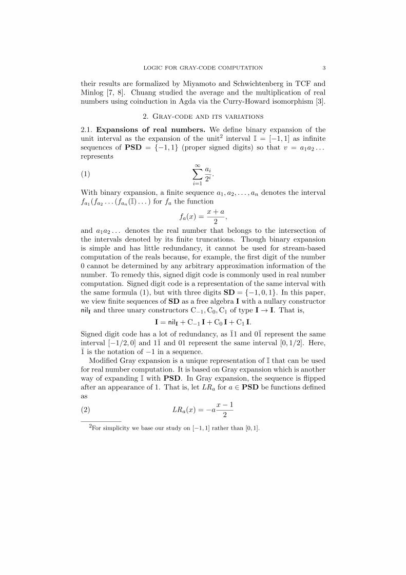
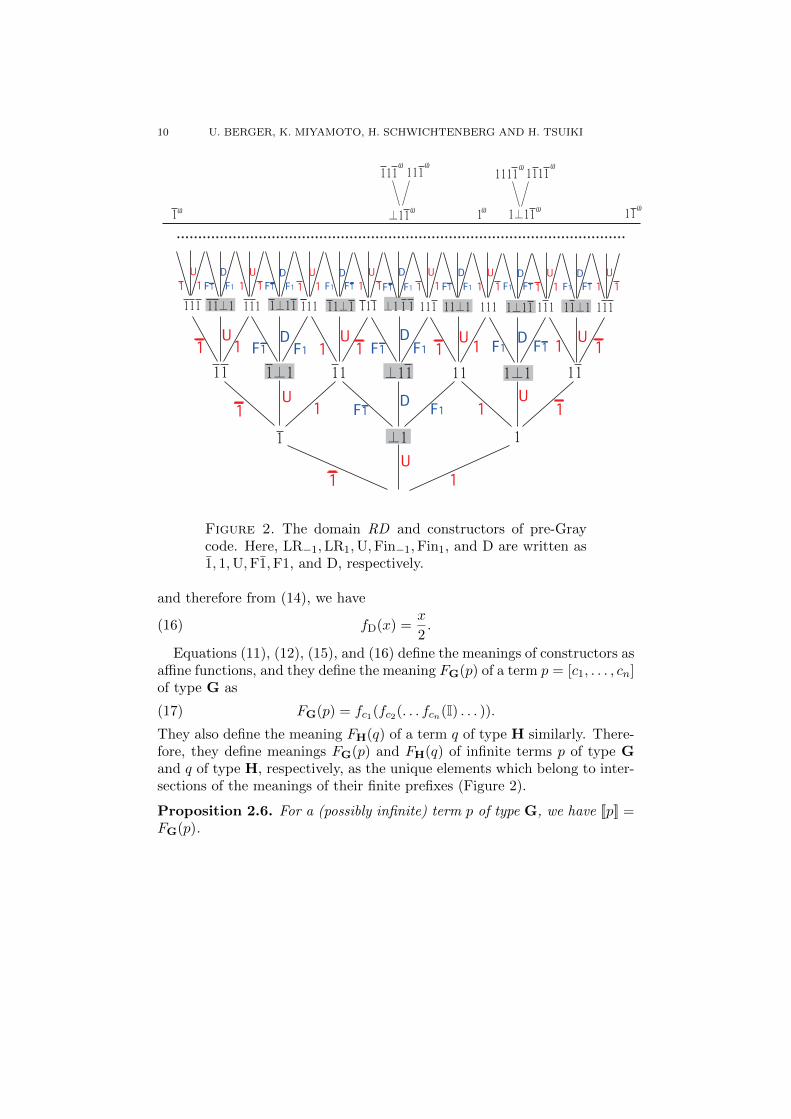
Figure 2. The domain RD and constructors of pre-Graycode. Here, LR−1,LR1,U,Fin−1,Fin1, and D are written as1, 1,U,F1,F1, and D, respectively.
and therefore from (14), we have
(16) fD(x) =x
2.
Equations (11), (12), (15), and (16) define the meanings of constructors asaffine functions, and they define the meaning FG(p) of a term p = [c1, . . . , cn]of type G as
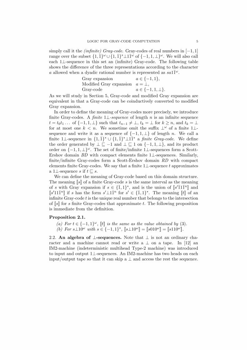
(17) FG(p) = fc1(fc2(. . . fcn(I) . . . )).They also define the meaning FH(q) of a term q of type H similarly. There-fore, they define meanings FG(p) and FH(q) of infinite terms p of type Gand q of type H, respectively, as the unique elements which belong to inter-sections of the meanings of their finite prefixes (Figure 2).
Proposition 2.6. For a (possibly infinite) term p of type G, we have [[p]] =FG(p).
LOGIC FOR GRAY-CODE COMPUTATION 11
Proof. We first prove the statement for the case that p is finite. Sinceequations (13) and (14) hold, we only need to consider the cases p =[LRa1 , . . . ,LRam ,U,D
n] and p = [LRa1 , . . . ,LRam ] by Proposition 2.5. Thelatter case is immediate from the definition. In the former case, we haveϕ(p) = a1 . . . am⊥11n. Let g = fLRa1
◦ · · · ◦ fLRam. We have
[[p]] = [[a1 . . . am111n]] ∪ [[a1 . . . am111n]]
= g(fLR−1 ◦ fLR1 ◦ fnLR−1(I)) ∪ g(fLR1 ◦ fLR1 ◦ fnLR−1
(I))
= g([−1/2n+1, 0]) ∪ g([0, 1/2n+1])
= g([−1/2n+1, 1/2n+1])
= (g ◦ fU ◦ fnD)(I)= FG([LRa1 , . . . ,LRam ,U,D
n]).
The case p is infinite is immediately derived from the finite case. �
Note that the meaning FH(p) of a term p of type H is also defined. If pis a term of type H, then ϕ(p) may not be a finite Gray-code and even if itis, FH(p) is different from [[ϕ(p)]] in general. For example, ϕ([D]) = ⊥1 and[[11]] ∪ [[11]] = [−1,−1/2] ∪ [1/2, 1] is not an interval, and [[ϕ([Fin1,LR1])]] =[[11]] = [0, 1/2] whereas FH([Fin1,LR1]) = [1/2, 1].
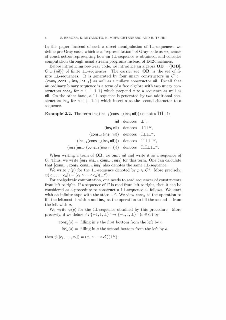
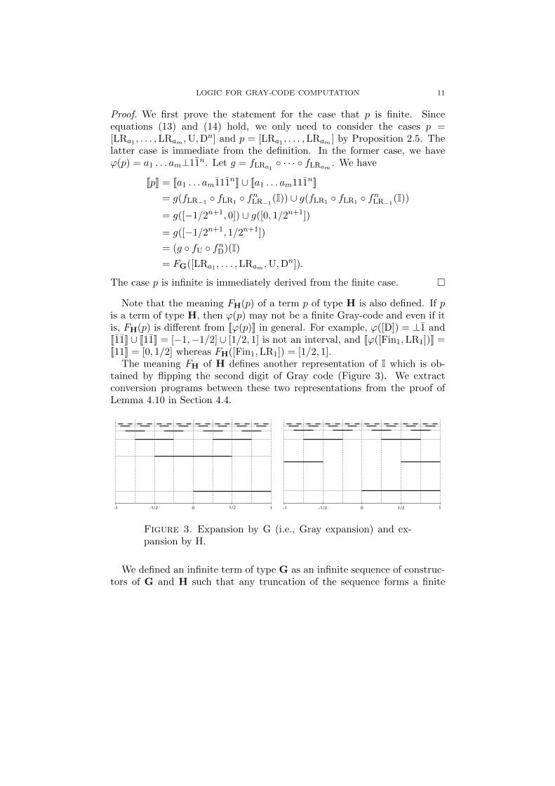
The meaning FH of H defines another representation of I which is ob-tained by flipping the second digit of Gray code (Figure 3). We extractconversion programs between these two representations from the proof ofLemma 4.10 in Section 4.4.
0 1-1 -1/2 1/2 0 1-1 -1/2 1/2
Figure 3. Expansion by G (i.e., Gray expansion) and ex-pansion by H.
We defined an infinite term of type G as an infinite sequence of construc-tors of G and H such that any truncation of the sequence forms a finite
12 U. BERGER, K. MIYAMOTO, H. SCHWICHTENBERG AND H. TSUIKI
term of type G. In TCF, infinite structures like this can be treated as coto-tal ideals. Each algebra definition of TCF generates a basic domain of theScott-Ershov model of partial continuous functionals. Among the ideals ofsuch a domain we single out the total and cototal ones, which are our well-founded and non-well-founded objects, respectively. For the details, pleaseconsult [10]. For our algebras I, G, and H, every total ideal is a finite termand every cototal ideal is an infinite term of the algebra.
The notion of a cototal ideal also makes sense when the underlying algebradoes not have nullary constructors. Since we will only be concerned withcototal ideals we take advantage of this fact and from now on omit thenullary constructor from our algebras. This will simplify the argumentsbelow considerably (for instance in comparison with [8]). We also redefineour free algebras I, G and H so that I has a binary constructor C of typeSD→ I→ I and so on; the intention is LRa(p) = LR(a, p). To sum up, ouralgebras have the following definitions.
I = C SD I,
G = LR PSD G + U H,
H = Fin PSD G + D H.
3. Coinductive representation of Gray-code via realizability
A constructive proof of a formula A can be viewed as a solution to theproblem posed by A [6]. Such a solution is a (computable) function of a cer-tain type τ(A) determined by the formulaA. For example, ∀n∃m(Prime(m)∧m > n) has type N→ N. Sometimes the solution is only a verification, likefor ∀n1,n2,n3>0,m>2(nm1 + nm2 6= nm3 ). In such cases a solution has no com-putational content and the formula A is called non-computational (n.c., orHarrop); the other ones are called computationally relevant (c.r.). The onlyway c.r. formulas can arise is via inductively defined predicates, like I orcoI below (we consider ∃xA and A ∨B as inductively defined). The clausesof the inductive definition determine the data type (free algebra) of a solu-tion or “realizer”. It is essential that we allow non-computational universalquantifiers ∀nc [1] to obtain the desired data type. For instance, in the clause∀ncx ∀d(I(x)→ I(x+d
2 )) (d ∈ {−1, 0, 1}) for I one is not interested in the realnumber x as input, but only in how the digit d gives rise to a new element ofI. Here we work in such a constructive arithmetical theory with realizability(called TCF in [10]).
We want to extract algorithms for real number computation from proofsin an appropriate formal theory involving coinductive definitions. The idea

LOGIC FOR GRAY-CODE COMPUTATION 13
is to leave infinite streams implicit, as realizers of atomic propositions onreals. For example, consider the problem to compute the average of two realnumbers coded by infinite streams. We will coinductively define a unarypredicate coI and prove
(18) ∀ncx,x′(
coI(x)→ coI(x′)→ coI(x+ x′
2))
(recall that ∀nc indicates that the reals x, x′ have no computational signifi-cance, only the assumptions coI(x), coI(x′) have). Associated with coI is its“realizability extension” (coI)r, a relation between streams v of signed digitsand real numbers x. We can understand (coI)r(v, x) as saying that v is astream representation of x witnessing coI(x). The soundness theorem gives
(coI)r(v, x)→ (coI)r(v′, x′)→ (coI)r(f(v, v′),x+ x′
2)
for some function f extracted from the proof. The function is the streamtransformer for the average, and it is obtained (together with a proof of itscorrectness) from the proof of (18), which never mentions streams.
Now what is the predicate coI? Consider the operator
Φ(X) := {x | ∃rx′∈X∃d(x =
x′ + d
2) },
where d ranges over SD := {−1, 0, 1}. The r in ∃r (not to be confused withthe r in (coI)r) indicates that the quantified variable x′ has no computationalsignificance, only the kernel of the existential formula has. Since Φ(X) isstricly positive in X, our underlying theory provides us with unary predi-cates (or sets; they are not distinguished) I and coI for the least and greatestfixed point of Φ:
I := µXΦ(X) least fixed pointcoI := νXΦ(X) greatest fixed point
satisfying the (strengthened) axioms
Φ(I ∩X) ⊆ X → I ⊆ X induction
X ⊆ Φ(coI ∪X)→ X ⊆ coI coinduction
(they are called “strengthened” because their hypotheses are weaker thanthe fixed point property Φ(X) = X).
14 U. BERGER, K. MIYAMOTO, H. SCHWICHTENBERG AND H. TSUIKI
The realizability extensions Ir and (coI)r are binary predicates on streamsv of signed digits (coming from ∃d in the definition of Φ(X)) and real num-bers x. Consider the operator
Φr(Y ) := { (v, x) | ∃u(v′,x′)∈Y ∃d(x =
x′ + d
2∧ v = Cd(v
′))) }
(the u in ∃u indicates that neither the quantified variable nor the kernel hascomputational significance). Since Φr(Y ) is strictly positive in Y , again ourunderlying theory provides us with binary predicates (or relations) Ir and(coI)r for the least and greatest fixed point of Φr:
Ir := µY Φr(Y ) least fixed point
(coI)r := νY Φr(Y ) greatest fixed point
satisfying the (strengthened) axioms
Φr(Ir ∩ Y ) ⊆ Y → Ir ⊆ Y induction
Y ⊆ Φr((coI)r ∪ Y )→ Y ⊆ (coI)r coinduction.
The following proposition states that the definition of coI is correct in thesense that the realizers of coI(x) are exactly the signed digit representationsof x.
Proposition 3.1. For v = a1a2 . . . ∈ SDω and x ∈ I
(coI)r(v, x)↔ x ∈∞⋂n=1
fa1(fa2(. . . fan(I) . . . ))
Proof. For the direction from left to right we show
∀v,x((coI)r(v, x)→ v = a1a2 . . . ∧ x ∈ fa1(fa2(. . . fan(I) . . . )))
by induction on n. For n = 0 this holds since x ∈ I. For n+ 1 suppose that(coI)r(v, x) holds. Then, since (coI)r is a fixed point of Φr,
∃v′,x′,a1((coI)r(v′, x′) ∧ x = fa1(x′) ∧ v = Ca1(v′)).
Let v′ = a2a3 . . .. By induction hypothesis, x′ ∈ fa2(fa3(. . . fan+1(I) . . . )).We have v = Ca1(v′) = a1a2 . . . and x ∈ fa1(fa2 . . . (fan+1(I)) . . . ).
The direction from right to left is shown by coinduction. Setting
{ (v, x) | v = a1a2 . . . , x ∈ fa1(fa2(. . . fan(I) . . . )) for every n }it suffices to show P ⊆ Φr(P ). Assume (v, x) ∈ P . Set x′ := 2x − a1 and
v′ := a2a3 . . .. Then clearly P (v′, x′), x = x′+a12 and v = a1v
′ = Ca1(v′).Hence (v, x) ∈ Φr(P ). �

LOGIC FOR GRAY-CODE COMPUTATION 15
For Gray-code we proceed similarly; for brevity only for the infinite case.We now need two predicates coG and coH instead of coI. The correspondingoperators Γ, ∆ are defined by
Γ(X,Y ) := { y | ∃rx∈X∃a(y = −ax− 1
2) ∨ ∃r
x∈Y (y =x
2) },
∆(X,Y ) := { y | ∃rx∈X∃a(y = a
x+ 1
2) ∨ ∃r
x∈Y (y =x
2) }
and we define (coG, coH) := ν(X,Y )(Γ(X,Y ),∆(X,Y )). This is understoodas the greatest fixed point of (Γ,∆), expressed by the (strengthened) simul-taneous coinduction axiom
(X,Y ) ⊆ (Γ(coG∪X, coH ∪ Y ),∆(coG∪X, coH ∪ Y ))→ (X,Y ) ⊆ (coG, coH),
where inclusion ⊆ is meant component-wise.For later use we note immediate consequences of the fact that (coG, coH)
is a (simultaneous) fixed point of (Γ,∆), CoGClause and CoGClauseInv:
∀ncx (coG(x)→ ∃r
x′∈coG∃a(x = −ax′ − 1
2) ∨ ∃r
x′∈coH(x =x′
2)),(19)
∀ncx (∃r
x′∈coG∃a(x = −ax′ − 1
2) ∨ ∃r
x′∈coH(x =x′
2)→ coG(x)).(20)
The realizability extensions (coG)r and (coH)r are binary predicates oncototal ideals p in G or q in H (respectively) and real numbers x. Considerthe operators
Γr(Z,W ) := { (p, x) | ∃(p′,x′)∈Z∃a(x = −ax′ − 1
2∧ p = LRa(p
′)) ∨u
∃(q′,x′)∈W (x =x′
2∧ p = U(q′)) },
∆r(Z,W ) := { (q, x) | ∃(p′,x′)∈Z∃a(x = ax′ + 1
2∧ q = Fina(p
′)) ∨u
∃(q′,x′)∈W (x =x′
2∧ q = D(q′)) }
(the u in ∨u indicates that the disjunction has no computational signifi-cance). Since both Γr(Z,W ) and ∆r(Z,W ) are strictly positive in Z,W ,our underlying theory provides us with a pair of binary predicates (coG)r,(coH)r for the greatest fixed point of (Γr,∆r):
((coG)r, (coH)r) := ν(Z,W )(Γr(Z,W ),∆r(Z,W ))

16 U. BERGER, K. MIYAMOTO, H. SCHWICHTENBERG AND H. TSUIKI
satisfying the (strengthened) simultaneous coinduction axiom
(Z,W ) ⊆ (Γr((coG)r ∪ Z, (coH)r ∪W ),∆r((coG)r ∪ Z, (coH)r ∪W ))→(Z,W ) ⊆ ((coG)r, (coH)r)
where again inclusion ⊆ is meant component-wise.Similar to Proposition 3.1, we show that coG is correct in the sense that
the realizers of coG(x) are exactly the pre-Gray codes of x.
Proposition 3.2. For x ∈ I and cototal ideals p in G and q in H
(coG)r(p, x)↔ x = FG(p),
(coH)r(q, x)↔ x = FH(q).
Proof. Recall that if p = [c1, c2, . . .] is a cototal ideal in G, then
FG(p) =
∞⋂n=1
fc1(fc2(. . . fcn(I) . . . ))
and similary for FH(q). The proof is similar to the case of signed digits, butslightly more involved because of the simultaneous definition of (coG)r and(coH)r. �
Remark 3.3 (Nested definition). As an alternative to the above simulta-neous definition of coG and coH, we can take the nested definition coG′ =νXΓ(X, coH ′(X)) where coH ′X = νY ∆(X,Y ). The witnessing algebras wouldalso be changed. In this paper we adopt the simultaneous one, since theextracted programs are simpler.
4. Proofs about coinductive representations that correspondto algorithms
In each of the examples below, after the proof we state the rules (equa-tions) expressing the algorithm implicit in this proof. Such an “informalprogram extraction” can be difficult and error-prone. In Section 6 this willbe done precisely, using Minlog to extract a program (i.e., a term in anextension of Godel’s T ) from a formalization of this proof.
4.1. Average for signed digit code. As a warm-up we prove the averageproperty (18), following [2]. Consider two sets of averages, the second onewith a “carry” i ∈ SD2 := {−2,−1, 0, 1, 2}:
P := { x+ y
2| x, y ∈ coI }, Q := { x+ y + i
4| x, y ∈ coI, i ∈ SD2 },

LOGIC FOR GRAY-CODE COMPUTATION 17
where SD2 are the “extended signed digits” {−2,−1, 0, 1, 2}; let i, j rangeover SD2. Recall that coI is a fixed point of Φ. Hence coI ⊆ Φ(coI), i.e.
(21) ∀ncx∈coI∃r
x′∈coI∃d(x =x′ + d
2) coI-clause.
It suffices to show that Q satisfies (21), for then by the greatest-fixed-pointaxiom for coI we have Q ⊆ coI. Since we also have P ⊆ Q we then obtainP ⊆ coI, which is our claim.
Lemma 4.1 (CoIAvToAvc).
∀ncx,y∈coI∃r
x′,y′∈coI∃i(x+ y
2=x′ + y′ + i
4).
Proof. Immediate from (21). �
Lemma 4.2 (CoIAvcSatCoICl).
∀i∀ncx,y∈coI∃r
x′,y′∈coI∃j,d(x+ y + i
4=
x′+y′+j4 + d
2).
Proof. We need functions J : SD → SD → SD2 → SD2 and K : SD →SD → SD2 → SD such that d + e + 2i = J(d, e, i) + 4K(d, e, i). Theycan be defined easily by cases on d, e and i. Using these we can relate thefunctions x+d
2 and x+y+i4 by
(22)x+d
2 + y+e2 + i
4=
x+y+J(d,e,i)4 +K(d, e, i)
2.
Now (21) gives the claim. �
By coinduction from Lemma 4.2 we obtain
Lemma 4.3 (CoIAvcToCoI).
∀ncz (∃r
x,y∈coI∃i(z =x+ y + i
4)→ coI(z)).
Proposition 4.4 (CoIAverage).
∀ncx,y(
coI(x)→ coI(y)→ coI(x+ y
2)).
Proof. Immediate from Lemmata 4.1 and 4.3. �
Implicit algorithm. Lemma 4.1 computes the first “carry” i ∈ SD2 and thetails of the inputs. Then f : SD2 × I× I→ I defined corecursively by
f(i,Cd(v),Ce(w)) = CK(d,e,i)(f(J(d, e, i), v, w))
is called repeatedly in order to compute the average step by step.

18 U. BERGER, K. MIYAMOTO, H. SCHWICHTENBERG AND H. TSUIKI
4.2. From pre-Gray to signed digit code. We prove coG ⊆ coI. However,to be able to do this by coinduction we need to generalize our goal to
Lemma 4.5 (CoGToCoIAux). ∀ncx (∃a(coG(ax) ∨ coH(ax))→ coIx).
Proof. For P := {x | ∃a(coG(ax) ∨ coH(ax)) } we must show P ⊆ coI. Bycoinduction it suffices to prove P ⊆ Φ(coI ∪ P ). Let x1 ∈ P . We showx1 ∈ Φ(coI ∪ P ):
(23) ∃rx∈coI∪P∃d(x1 =
x+ d
2).
Since x1 ∈ P we have a such that coG(ax1) ∨ coH(ax1).Case coG(ax1). The coG-clause coG ⊆ Γ(coG, coH) applied to ax1 ∈ coG
gives us
∃rx∈coG∃b(ax1 = −bx− 1
2) ∨ ∃r
x∈coH(ax1 =x
2).
If the left hand side holds, we have x2 ∈ coG and b such that ax1 = −bx2−12 .
Then (23) holds for x := −abx2 and d := ab, since −abx2 ∈ P (by x2 ∈ coGand the definition of P ), and
x1 = a2x1 = −abx2 − 1
2=−abx2 + ab
2=x+ d
2.
If the right hand side holds, we have x2 ∈ coH such that ax1 = x22 . Then
(23) holds for x := ax2 and d := 0, since ax2 ∈ P (by x2 ∈ coH and thedefinition of P ), and
x1 = a2x1 = ax2
2=ax2 + 0
2=x+ d
2.
Case coH(ax1). The coH-clause coH ⊆ ∆(coG, coH) applied to ax1 ∈ coHgives
∃rx∈coG∃b(ax1 = b
x+ 1
2) ∨ ∃r
x∈coH(ax1 =x
2).
If the left hand side holds, we have x2 ∈ coG and b such that ax1 = bx2+12 .
Then (23) holds for x := abx2 and d := ab, since abx2 ∈ P (by x2 ∈ coG andthe definition of P ), and
x1 = a2x1 = abx2 + 1
2=abx2 + ab
2=x+ d
2.
If the right hand side holds, we have x2 ∈ coH such that ax1 = x22 . Then
(23) holds for x := ax2 and d := 0, since ax2 ∈ P (by x2 ∈ coH and thedefinition of P ), and
x1 = a2x1 = ax2
2=ax2 + 0
2=x+ d
2. �

LOGIC FOR GRAY-CODE COMPUTATION 19
Implicit algorithm. [f, g] : PSD×G + PSD×H→ I defined by
f(a,LRb(p)) = Cab(f(−ab, p)), g(a,Finb(p)) = Cab(f(ab, p)),
f(a,U(q)) = C0(g(a, q)), g(a,D(q)) = C0(g(a, q)).
An immediate consequence is
Proposition 4.6 (CoGToCoI). ∀ncx (coG(x)→ coI(x)).
4.3. From signed digit to pre-Gray code. Conversely we also have coI ⊆coG. Again, to be able to prove this by coinduction we need to generalizeour goal to
Lemma 4.7 (CoIToCoGAux).
∀ncx (∃acoI(ax)→ coGx),
∀ncx (∃acoI(ax)→ coHx).
Proof. For P := {x | ∃a(ax ∈ coI) } we show P ⊆ coG simultaneously withP ⊆ coH. By coinduction it suffices to prove (i) P ⊆ Γ(coG ∪ P, coH ∪ P )and (ii) P ⊆ ∆(coG ∪ P, coH ∪ P ). For (i), let x1 ∈ P . We show x1 ∈Γ(coG ∪ P, coH ∪ P ):
(24) ∃rx∈coG∪P∃a(x1 = −ax− 1
2) ∨ ∃r
x∈coH∪P (x1 =x
2).
Since x1 ∈ P we have a1 such that coI(a1x1). The coI-clause coI ⊆ Φ(coI)applied to a1x1 ∈ coI gives us
∃rx∈coI∃d(a1x1 =
x+ d
2).
Hence we have x2 ∈ coI and d such that a1x1 = x2+d2 .
Case d = −1. Then the left hand of (24) holds for x := x2 and a := −a1,since x2 ∈ P (by x2 ∈ coI and the definition of P ), and
x1 = a1a1x1 = a1x2 + d
2= a1
x2 − 1
2.
Case d = 1. Then the left hand of (24) holds for x := −x2 and a := a1,since −x2 ∈ P (by x2 ∈ coI and the definition of P ), and
x1 = a1a1x1 = a1x2 + d
2= a1
x2 + 1
2= −a1
−x2 − 1
2.
Case d = 0. Then the right hand of (24) holds for x := a1x2, sincea1x2 ∈ P (by x2 ∈ coI and the definition of P ), and
x1 = a1a1x1 = a1x2 + d
2=a1x2
2.

20 U. BERGER, K. MIYAMOTO, H. SCHWICHTENBERG AND H. TSUIKI
This finishes the proof of (i). The proof of (ii) is similar, and we omit it. �
Implicit algorithm. g : τ → G and h : τ → H with τ := PSD× I, defined by
g(b,C−1(v)) = LR−b(g(1, v)), h(b,C−1(v)) = Fin−b(g(−1, v)),
g(b,C1(v)) = LRb(g(−1, v)), h(b,C1(v)) = Finb(g(1, v)),
g(b,C0(v)) = U(h(b, v)), h(b,C0(v)) = D(h(b, v)).
An immediate consequence is
Proposition 4.8 (CoIToCoG). ∀ncx (coI(x)→ coG(x)).
4.4. Average for pre-Gray code. We consider the problem to computethe average of two real numbers given in pre-Gray code directly, withoutgoing via signed digit code.
As a preparation we treat the unary minus function. Here we make useof the fact that our coinduction axioms are in strengthened form (that isX ⊆ Φ(coI ∪X)→ X ⊆ coI instead of X ⊆ Φ(X)→ X ⊆ coI, for example).
Lemma 4.9 (CoGMinus).
∀ncx (coG(−x)→ coGx),
∀ncx (coH(−x)→ coHx).
Proof. For P := {x | −x ∈ coG) } and Q := {x | −x ∈ coH) } we showP ⊆ coG simultaneously with Q ⊆ coH. By coinduction it suffices to prove(i) P ⊆ Γ(coG ∪ P, coH ∪ Q) and (ii) Q ⊆ ∆(coG ∪ P, coH ∪ Q). For (i), letx1 ∈ P . We show x1 ∈ Γ(coG ∪ P, coH ∪Q):
(25) ∃rx∈coG∪P∃a(x1 = −ax− 1
2) ∨ ∃r
x∈coH∪Q(x1 =x
2).
The coG-clause applied to −x1 ∈ coG gives us
∃rx∈coG∃a(−x1 = −ax− 1
2) ∨ ∃r
x∈coH(−x1 =x
2).
In the first case we have x2 ∈ coG and a with −x1 = −ax2−12 . Then the left
hand side of (25) holds for x2 and −a (here we use that our coinductionaxiom is in strengthened form). In the second case we have x2 ∈ coH with−x1 = x2
2 . Then the right hand side of (25) holds for −x2. This finishes theproof of (i). The proof of (ii) is similar, and we omit it. �
Implicit algorithm. f : G→ G and f ′ : H→ H defined by
f(LRa(p)) = LR−a(p), f ′(Fina(p)) = Fin−a(p),
f(U(q)) = U(f ′(q)), f ′(D(q)) = D(f ′(q)).

LOGIC FOR GRAY-CODE COMPUTATION 21
Using Lemma 4.9 we prove that coG and coH are in fact equivalent.
Lemma 4.10 (CoHToCoG).
∀ncx (coHx→ coGx),
∀ncx (coGx→ coHx).
Proof. We show coH ⊆ coG simultaneously with coG ⊆ coH. By coinductionit suffices to prove (i) coH ⊆ Γ(coG ∪ coH, coH ∪ coG) and (ii) coG ⊆ ∆(coG ∪coH, coH ∪ coG). For (i), let x1 ∈ coH. We show x1 ∈ Γ(coG ∪ coH, coH ∪ coG):
(26) ∃rx∈coG∪coH∃a(x1 = −ax− 1
2) ∨ ∃r
x∈coH∪coG(x1 =x
2).
The coH-clause applied to x1 ∈ coH gives us
∃rx∈coG∃a(x1 = a
x+ 1
2) ∨ ∃r
x∈coH(x1 =x
2).
In the first case we have x2 ∈ coG and a with x1 = ax2+12 . Then the left
hand side of (26) holds for −x2 and a, using Lemma 4.9 and (again) thatour coinduction axiom is in strengthened form. In the second case we havex2 ∈ coH with x1 = x2
2 . Then the right hand side of (25) holds for x2. Thisfinishes the proof of (i). The proof of (ii) is similar, and we omit it. �
Implicit algorithm. g : H→ G and h : G→ H:
g(Fina(p)) = LRa(f−(p)), h(LRa(p)) = Fina(f
−(p)),
g(D(q)) = U(q), h(U(q)) = D(q)
where f− := cCoGMinus (cL denotes the function extracted from the proofof a lemma L). Notice that no corecursive call is involved.
The direct proof of the existence of the average w.r.t. Gray-coded realsis similar to the proof in Section 4.1 of the existence of the average w.r.t.signed digit stream coded reals. It proceeds as follows. To prove
∀ncx,y(
coG(x)→ coG(y)→ coG(x+ y
2))
consider again two sets of averages, the second one with a “carry”:
P := { x+ y
2| x, y ∈ coG }, Q := { x+ y + i
4| x, y ∈ coG, i ∈ SD2 }.
It suffices to show that Q satisfies the clause coinductively defining coG, forthen by the greatest-fixed-point axiom for coG we have Q ⊆ coG. Since wealso have P ⊆ Q we then obtain P ⊆ coG, which is our claim.
22 U. BERGER, K. MIYAMOTO, H. SCHWICHTENBERG AND H. TSUIKI
Lemma 4.11 (CoGAvToAvc).
∀ncx,y∈coG∃r
x′,y′∈coG∃i(x+ y
2=x′ + y′ + i
4).
Proof. Immediate from CoGClause (19). �
Implicit algorithm. We use f∗ for cCoGPsdTimes and s for cCoHToCoG.
f(LRa(p),LRa′(p′)) = (a+ a′, f∗(−a, p), f∗(−a′, p′)),
f(LRa(p),U(q)) = (a, f∗(−a, p), s(q)),f(U(q),LRa(p)) = (a, s(q), f∗(−a, p)),f(U(q),U(q′)) = (0, s(q), s(q′)).
Lemma 4.12 (CoGAvcSatCoICl).
∀i∀ncx,y∈coG∃r
x′,y′∈coG∃j,d(x+ y + i
4=
x′+y′+j4 + d
2).
Proof. As in Lemma 4.2 we need the functions J,K with their property (22).Then (19) gives the claim. �
Implicit algorithm.
f(i,LRa(p),LRa′(p′)) = (J(a, a′, i),K(a, a′, i), f∗(−a, p), f∗(−a′, p′)),
f(i,LRa(p),U(q)) = (J(a, 0, i),K(a, 0, i), f∗(−a, p), s(q)),f(i,U(q),LRa(p)) = (J(0, a, i),K(0, a, i), s(q), f∗(−a, p)),f(i,U(q),U(q′)) = (J(0, 0, i),K(0, 0, i), s(q), s(q′)).
Lemma 4.13 (CoGAvcToCoG).
∀ncz (∃r
x,y∈coG∃i(z =x+ y + i
4)→ coG(z)),
∀ncz (∃r
x,y∈coG∃i(z =x+ y + i
4)→ coH(z)).
Proof. We show Q ⊆ coG simultaneously with Q ⊆ coH. By coinduction itsuffices to prove (i) Q ⊆ Γ(coG∪Q, coH∪Q) and (ii) Q ⊆ ∆(coG∪Q, coH∪Q).For (i), let z1 ∈ Q. We show z1 ∈ Γ(coG ∪Q, coH ∪Q):
(27) ∃rz∈coG∪Q∃a(z1 = −az − 1
2) ∨ ∃r
z∈coH∪Q(z1 =z
2).
Lemma 4.12 applied to z1 ∈ Q gives us x1, y1 ∈ coG and i1, d1 such that
z1 =x1+y1+i1
4 + d1
2.
LOGIC FOR GRAY-CODE COMPUTATION 23
Case d1 = 0. Go for the right hand side of (27) with z := (x1 + y1 + i1)/4 ∈Q. Case d1 = ±1. Go for the left hand side of (27) with a := d1 andz := (−ax1 − ay1 − ai1)/4 ∈ Q. Then
−az − 1
2= −a4z − 4
8=x1 + y1 + i1 + 4a
8= z1.
This finishes the proof of (i). The proof of (ii) is similar, and we omit it. �
Implicit algorithm. In the proof we used SdDisj: ∀d(d = 0 ∨ ∃a(d = a)).
g(i, p, p′) = let (i1, d, p1, p′1) = cCoGAvcSatCoICl(i, p, p′) in
case cSdDisj(d) of
0→ U(h(i, p1, p′1))
a→ LRa(g(−ai, f∗(−a, p1), f∗(−a, p′1))),
h(i, p, p′) = let (i1, d, p1, p′1) = cCoGAvcSatCoICl(i, p, p′) in
case cSdDisj(d) of
0→ D(h(i, p1, p′1))
a→ Fina(g(−ai, f∗(−a, p1), f∗(−a, p′1))).
Proposition 4.14 (CoGAverage).
∀ncx,y(
coG(x)→ coG(y)→ coG(x+ y
2)).
Proof. Compose Lemmata 4.11 and 4.13. �
4.5. A bounded translation from pre-Gray code to its normal form.For pre-Gray code there are many ways of expressing the same real numberas we noted in Section 2. In particular, the two terms U(Dk(Fina p))) andLRa(LR1(LRk
−1 p)))) denote the same number as Proposition 2.5 says (Dk
and LRk−1 denote k-times repetition of the same constructor). Here we
extract a program which transfers the former pattern in the first n elementsof a pre-Gray code into the latter pattern.
Similar to G we inductively define a binary relation zG between real andnatural numbers (used as bounds), this time with an initial clause. Thedefinition is no longer simultaneous with H, but the latter can be definedindependently in advance:
z∆(Z) := { (y,m) | m = 0 ∨ ∃rx∈Z(y =
x
2∧m = n+ 1) }.
24 U. BERGER, K. MIYAMOTO, H. SCHWICHTENBERG AND H. TSUIKI
With zH = µZz∆(Z) we can now define
zΓ(X) := { (y,m) | m = 0 ∨ ∃r(x,n)∈X∃a(y = −ax− 1
2∧m = n+ 1) ∨
∃r(x,n)∈zH(y =
x
2∧m = n+ 1) }
and zG = µXzΓ(X). From a proof of { (x, n) | coG(x) } ⊆ zG, we extract the
desired program to compute a prefix of a pre-Gray code of x of length nwhich does not contain a subsequence of the form UDkFina from a pre-Graycode of x. The associated algebra for zH it is just the natural numbers N,and for zG it is zG with constructors
Nz: zG, LRz: PSD→ zG→ zG, Uz: N→ zG.
Lemma 4.15 (GenCoGLR). ∀ncx ∀a(coG(x)→ coG(−ax−1
2 )).
Proof. Easy by coinduction. �
Lemma 4.16 (CoGToBGAux).
∀n∀ncx (coG(x)→ zG(x, n)),
∀n∀ncx (coH(x)→ zH(x, n) ∨ ∃r
y∈coG∃a(zG(y, n− 1) ∧ x = ay + 1
2)).
Proof. We prove both statements simultaneously by induction on n. Thecase n = 0 is trivial. For the step case, we first assume coG(x1) and prove(x1, n+ 1) ∈ zG. We have
∃rx2∈coG∃a(x1 = −ax2 − 1
2) ∨ ∃r
x2∈coH(x1 =x2
2).
(Case A) Suppose that the left hand side holds. Then, by inductionhypothesis applied to x2, we have zG(x2, n). Therefore (x1, n+1) ∈ zΓ(zG) =zG because
∃r(x2,n)∈zG∃a(x1 = −ax2 − 1
2).
(Case B) Suppose that the right hand side holds. Then, x1 = x22 for
x2 ∈ coH. Therefore, by induction hypothesis,
zH(x2, n) ∨ ∃rx3∈coG∃a(
zG(x3, n− 1) ∧ x2 = ax3 + 1
2).
(Case B1) Suppose that the left hand side holds. Then, since zH(x2, n)and x1 = x2
2 , zG(x1, n+ 1) holds.(Case B2) Suppose that the right hand side holds. Then,
x1 =x2
2= a3
x3 + 1
4= −a3
−x3−12 − 1
2= −a3
x4 − 1
2
LOGIC FOR GRAY-CODE COMPUTATION 25
for some a3, x3 ∈ coG and x4 := −x3−12 . Since x1 = −a3
x4−12 , for our goal
zG(x1, n + 1) it suffices to prove zG(x4, n). In case n = 0 this follows fromthe initial clause for zG, and in case n = m+ 1 it follows from zG(x3, n− 1)by the first generating clause for zG, since x4 = −x3−1
2 .Next, we suppose that coH(x1) and prove
zH(x1, n+ 1) ∨ ∃ry∈coG∃a(zG(y, n) ∧ x1 = a
y + 1
2).
The argument is almost the same as above. Since coH(x1), we have
∃rx2∈coG∃a(x1 = a
x2 + 1
2) ∨ ∃r
x2∈coH(x1 =x2
2).
(Case A) Suppose that the left hand side holds. We have x1 = a2x2+1
2 fora2 and x2 ∈ coG. By induction hypothesis, zG(x2, n). Therefore
∃ry∈coG∃a(zG(y, n) ∧ x1 = a
y + 1
2).
(Case B) Suppose that the right hand side holds. We have x1 = x22 for
x2 ∈ coH. By induction hypothesis,
zH(x2, n) ∨ ∃rx3∈coG∃a(
zG(x3, n− 1) ∧ x2 = ax3 + 1
2).
(Case B1) Suppose that the left hand side holds. Then, since zH(x2, n)and x1 = x2
2 , we have zH(x1, n+ 1).(Case B2) Suppose that the right hand side holds. Then,
x1 =x2
2= a
x3 + 1
4= a
x3−12 + 1
2= a
x4 + 1
2
for x4 := x3−12 . We prove the right hand side of our goal for x4 and a. Since
x1 = ax4+12 it suffices to prove x4 ∈ coG and zG(x4, n). From x3 ∈ coG we
obtain x4 ∈ coG by Lemma 4.15. To prove zG(x4, n) we argue by cases onn. In case n = 0 this follows from the initial clause for zG, and in casen = m+ 1 it follows from zG(x3, n− 1) by the first generating clause for zG,since x4 = x3−1
2 . �
Implicit algorithm. f : N→ G→ zG and g : N→ H→ N+PSD×G× zGare defined by simultaneous recursion
f(0, p) = 0 g(0, q) = 0
f(n+ 1,LRa(p)) = LRza(f(n, p))
f(n+ 1,U(q)) = case g(n, q) of
m→ m

26 U. BERGER, K. MIYAMOTO, H. SCHWICHTENBERG AND H. TSUIKI
(a, p, r)→ LRza(case n of
0→ 0
m+ 1→ LRz1(r))
g(n+ 1,Fina(p)) = (a, p, f(n, p)))
g(n+ 1,D(q)) = case g(n, q) of
m→ m+ 1
(a, p, r)→ (a,LR−1(p), f(n,LR−1(p)))
An immediate consequence is
Proposition 4.17 (CoGToBG). ∀n∀ncx (coG(x)→ zG(x, n)).
5. Conversion from Gray-code to modified Gray expansion
As we studied in Section 2.1, each dyadic rational number has three re-presentations of the forms s111ω, s111ω and s⊥11ω in Gray-code, and onlythe last one in modified Gray expansion. We show that Gray-code can beconverted to modified Gray expansion. We denote by K(RD) and L(RD)the sets of compact and non-compact elements of RD , which coincide withthe sets of finite Gray-codes and infinite Gray-codes, respectively. We alsodenote by M(L(RD)) the set of minimal elements of L(RD), which coincideswith the set of modified Gray expansions.
We say that s is a predecessor of t if s v t and no u ∈ K(RD) satisfiess v u v t. ⊥ω have no predecessor, s′⊥11k, 1k and 11k have one predecessor,and the other elements of K(RD) have two predecessors (see Figure 2). Wedefine a function ρ on K(RD) so that ρ(s) is the meet of the predecessorsof s for s 6= ⊥. In the following definition, a ∈ {1, 1}, k ≥ 0, s′ ∈ {1, 1}∗,and a1k−1 means ⊥ω if k = 0.
ρ(s) =
⊥ω (s = ⊥ω)
s′⊥11k−1 (s = s′⊥11k)
a1k−1 (s = a1k)
s′⊥11k−1 (s = s′a11k)
Since ρ(s) v s, we have [[ρ(s)]] ⊇ [[s]]. Moreover, [[ρ(s)]] is the smalleststandard interval whose interior contains [[s]].
One can verify that ρ is monotonic. Therefore, ρ can be extended to acontinuous function from RD to RD because RD is a Scott-Ershov domain.It is obvious that ρ(L(RD)) ⊆ L(RD). The following proposition says thatρ is a conversion function from Gray-code to modified Gray expansion.

LOGIC FOR GRAY-CODE COMPUTATION 27
Proposition 5.1. ρ is a retract function from L(RD) to M(L(RD)). Thatis, ρ(t) ∈ M(L(RD)) and ρ(t) v t for t ∈ L(RD). In particular, ρ(t) = tfor t ∈M(L(RD)).
Proof. Since ρ(s) v s for s ∈ K(RD), ρ(t) v t for t ∈ L(RD), and thereforeρ(t) = t for t ∈ M(L(RD)). We show ρ(L(RD)) ⊆ M(L(RD)). Supposethat t ∈ L(RD) \M(L(RD)) and let t = sa11ω for some s ∈ {1, 1}∗ anda ∈ {1, 1}. Since ρ(sa11k) = s⊥11k−1 for every k ≥ 0, ρ(t) = s⊥11ω ∈M(L(RD)). �
We develop an algorithm to compute the function ρ at the level of pre-Gray code, i.e. we transform a pre-Gray code p to a pre-Gray code p′ suchthat ϕ(p′) = ρ(ϕ(p)), in particular p′ will be the modified Gray-expansionof the real number denoted by p.
In the following, we sometimes write a for LRa for simplicity. Sinceρ(a11) = ⊥1 for a ∈ PSD, if the sequence begins with [LRa,LR1,LR−1],then we apply Equation (9) from right to left and replace it with [U,Fina,LR−1]and fix U. We write this rule simply as
a 1 1 7→ U | Fina 1.
On the other hand, since ρ(a11)=a, if the sequence begins with [U,Fina,LR1],we apply Equation (9) from left to right and replace it with [LRa,LR1,LR1]and fix LRa. Therefore, we have
U Fina 1 7→ a 1 1.
Similarly, we have the following rules
Fina 1 1 7→ D | Fina 1,
D Fina 1 7→ Fina | 1 1.
If the sequence does not match to these four patterns, then we fix the firstcharacter. We repeat this procedure to the rest of the sequence. One canverify that the implicit algorithm extracted from the proof of Proposition 5.5behaves in this way.
We extract a program that converts Gray-code to modified Gray expan-sion. To this end we define variants coM of coG and coN of coH. Recall thatthe predicate (coG)r(p, y) expresses that p is a pre-Gray code of y by Proposi-tion 3.2, and it is defined (as greatest fixed point) to mean that p = LRa(p
′),y = −ax−1
2 and (coG)r(p′, x) or else p = U(q), y = x2 and (coH)r(q, x). In
this definition, p = LR−1(p′) happens only if y ≤ 0, p = LR1(p′) happensonly if y ≥ 0 and p = U(q) happens only if −1
2 ≤ y ≤ 12 . Modified Gray
expansion is obtained by restricting these three cases to y < 0, y > 0, and

28 U. BERGER, K. MIYAMOTO, H. SCHWICHTENBERG AND H. TSUIKI
−12 < y < 1
2 . Therefore, coM is defined so that the left clause of coG is
restricted to y 6= 0 and the right clause of coG is restricted to y 6= ±12 . A
similar restriction must be imposed on coH. Accordingly we define variantsΓ′, ∆′ of the operators Γ, ∆ by
Γ′(X,Y ) := { y | ∃rx∈X∃a(y = −ax− 1
2∧ y 6= 0) ∨ ∃r
x∈Y (y =x
2∧ y 6= ±1
2) },
∆′(X,Y ) := { y | ∃rx∈X∃a(y = a
x+ 1
2∧ y 6= 0) ∨ ∃r
x∈Y (y =x
2∧ y 6= ±1
2) }
and we define (coM, coN) := ν(X,Y )(Γ′(X,Y ),∆′(X,Y )).
The corresponding realizability predicates are defined by the operators
(Γ′)r(Z,W ) := { (p, x) | ∃(p′,x′)∈Z∃a(x = −ax′ − 1
2∧ p = LRa(p
′) ∧ x 6= 0) ∨u
∃(q′,x′)∈W (x =x′
2∧ p = U(q′)) ∧ x 6= ±1
2},
(∆′)r(Z,W ) := { (q, x) | ∃(p′,x′)∈Z∃a(x = ax′ + 1
2∧ q = Fina(p
′) ∧ x 6= 0) ∨u
∃(q′,x′)∈W (x =x′
2∧ q = D(q′)) ∧ x 6= ±1
2}
as ((coM)r, (coN)r) := ν(Z,W )((Γ′)r(Z,W ), (∆′)r(Z,W )).
The following proposition shows that coM is correct in the sense that therealizers of coM(x) are exactly the pre-Gray codes of x that are mapped byϕ to a modified Gray-expansion of x.
Proposition 5.2. For cototal ideals p in G and x ∈ I(coM)r(p, x)↔ ϕ(p) is a modified Gray-expansion of x.
Proof. This is a direct consequence of the following lemma, because themodified Gray expansion of −1 and 1 are 1ω and 11ω, respectively, andthey are the only cases modified Gray expansion has the form s1ω for s ∈{1, 1}∗. �
Lemma 5.3. For x ∈ I and cototal ideals p in G and q in H
(coM)r(p, x)↔ x = FG(p) ∧ (x ∈ {−1, 1} ∨ ϕ(p) 6= s1ω for s ∈ {1, 1}∗),(coN)r(q, x)↔ x = FH(q) ∧ (x ∈ {−1, 1} ∨ ϕ(q) 6= s1ω for s ∈ {1, 1}∗).
Proof. (From left to right). First, obviously, (coM)r(p, x) → (coG)r(p, x)and (coN)r(q, x) → (coH)r(q, x). Therefore, (coM)r(p, x) → x = FG(p) and(coN)r(q, x)→ x = FH(q) holds by Proposition 3.2. We show
∀s,p,x((coM)r(p, x)→ x ∈ {−1, 1} ∨ ϕ(p) 6= s1ω)(28)
LOGIC FOR GRAY-CODE COMPUTATION 29
∀s,q,x((coN)r(q, x)→ x ∈ {−1, 1} ∨ ϕ(q) 6= s1ω)(29)
by induction on the length |s| of s ∈ {1, 1}∗. As the base case, (28) holdsfor |s| = 0 because ϕ(p) = 1ω ∧ x = FG(p) implies x = −1. We study(29) for |s| = 0. We show that there is no pair (q, x) such that ϕ(q) = 1ω
and (coN)r(q, x). Suppose that such a pair exists. We have x = FH(q) andFH(q) = 0 (cf. Figure 3 on page 11). Since (coN)r is a fixed point of (∆′)r,
∃p′,x′,a((coM)r(p′, x′) ∧ x = ax′ + 1
2∧ p = Fina(p
′) ∧ x 6= 0)
or
∃q′,x′((coN)r(q′, x′) ∧ x =x′
2∧ p = D(q′) ∧ x 6= ±1
2).
Since x = 0, we have the latter case and p = D(q′) and (coN)r(q′, 0). Againfor q′, we have q′ = D(q′′) and (coN)r(q′′, 0). In this way, we have q = Dω
and ϕ(q) = ⊥1ω, and we have contradiction. Thus, (29) holds for |s| = 0.Suppose that (28) and (29) hold for |s| = n and prove (28) for |s| = n+1.
Suppose that (coM)r(p, x). Since (coM)r is a fixed point of (Γ′)r,
∃p′,x′,a((coM)r(p′, x′) ∧ x = −ax′ − 1
2∧ p = LRa(p
′) ∧ x 6= 0)
or
∃q′,x′((coN)r(q′, x′) ∧ x =x′
2∧ p = U(q′) ∧ x 6= ±1
2.
In the former case, by induction hypothesis, x′ ∈ {−1, 1} or else ϕ(p′) 6= s1ω
for any s ∈ {1, 1}n. The case x′ = 1 does not happen because x 6= 0.If x′ = −1, then x ∈ {−1, 1}. If ϕ(p′) 6= s1ω for any s ∈ {1, 1}n, thenϕ(p) = ϕ(LRa(p
′)) = a : ϕ(p′) 6= s′1ω for any s′ ∈ {1, 1}n+1.In the latter case, by induction hypothesis, x′ ∈ {−1, 1} or else ϕ(q′) 6=
s1ω for any s ∈ {1, 1}n. The case x′ ∈ {−1, 1} does not happen becausex 6= ±1
2 . Suppose that ϕ(q′) 6= s1ω for any s ∈ {1, 1}n. We have, fora : t = ϕ(q′), ϕ(p) = ϕ(U(q′)) = a : 1 : t and a : 1 : t 6= s′1ω for anys′ ∈ {1, 1}n+1.
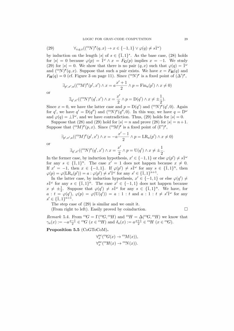
The step case of (29) is similar and we omit it.(From right to left). Easily proved by coinduction. �
Remark 5.4. From coG = Γ(coG, coH) and coH = ∆(coG, coH) we know thatγa(x) := −ax−1
2 ∈coG (x ∈ coH) and δa(x) := ax+1
2 ∈coH (x ∈ coG).
Proposition 5.5 (CoGToCoM).
∀ncx (coG(x)→ coM(x)),
∀ncx (coH(x)→ coN(x)).

30 U. BERGER, K. MIYAMOTO, H. SCHWICHTENBERG AND H. TSUIKI
Proof. For P := coG and Q := coH we show P ⊆ coM simultaneously withQ ⊆ coN . By coinduction it suffices to prove (i) P ⊆ Γ′(coM ∪ P, coN ∪ Q)and (ii) Q ⊆ ∆′(coM ∪ P, coN ∪ Q). For (i), let x0 ∈ P . We show x0 ∈Γ′(coM ∪ P, coN ∪Q):
(30) ∃rx∈coM∪P∃a(x0 = −ax− 1
2∧ x0 6= 0) ∨ ∃r
x∈coN∪Q(x0 =x
2∧ x0 6= ±
1
2).
The coG-clause applied to x0 ∈ coG gives us
(31) ∃rx∈coG∃a(x0 = −ax− 1
2) ∨ ∃r
x∈coH(x0 =x
2).
Case ga. The lhs of (31) holds. We have x1 ∈ coG and a1 with x0 = −a1x1−1
2 .The coG-clause applied to x1 ∈ coG gives us
(32) ∃rx∈coG∃a(x1 = −ax− 1
2) ∨ ∃r
x∈coH(x1 =x
2).
Case gaa. The lhs of (32) holds. We have x2∈coG and a2 with x1 = −a2x2−1
2 .Case ga1. Assume a2 = −1. Go for the lhs of (30) with x1 ∈ P and a1.
The goal x0 = −a1x1−1
2 holds by the choice of x1, a1. Since x2 ∈ [−1, 1],
x1 = x2−12 6= 1. Thus, x0 = −a1
x1−12 6= 0.
Case ga1. Assume a2 = 1. The coG-clause applied to x2 ∈ coG gives us
(33) ∃rx∈coG∃a(x2 = −ax− 1
2) ∨ ∃r
x∈coH(x2 =x
2).
Case ga1a. The lhs of (33) holds. We have x3∈coG and a3 with x2=−a3x3−1
2 .Case ga11. Assume a3 = −1. Go for the rhs of (30) with x = δa1(x2) :=
a1x2+1
2 ∈ Q (since x2 ∈ coG implies δa(x2) ∈ coH). The goal x0 = x2 holds
since
x0 = −a1x1 − 1
2= −a1
−a2x2−1
2 − 1
2= a1
x2 − 1 + 2
4=x
2.
On the other hand, since x3 ∈ [−1, 1], x2 = x3−12 ∈ [−1, 0] and therefore,
x0 = a1x2+1
4 ∈ [−14 ,
14 ]. Thus, x0 6= ±1
2 .Case ga11. Assume a3 = 1. Go for the lhs of (30) with x1 ∈ P and a1.
The goal x0 = −a1x1−1
2 holds by the choice of x1, a1. Since x3 ∈ [−1, 1],
x2 = −x3−12 ∈ [0, 1] and hence x1 = −x2−1
2 6= 1. Thus, x0 = −a1x1−1
2 6= 0.Case ga1U. The rhs of (33) holds. We have x3 ∈ coH with x2 = x3
2 .
Go for the lhs of (30) with x = x1 ∈ Q and a1. The goal x0 = −a1x1−1
2
holds by the choice of x1, a1. Since x3 ∈ [−1, 1], x2 ∈ [−12 ,
12 ] and therefore
x1 = −x2−12 6= 1. Thus, x0 = −a1
x1−12 6= 0.
LOGIC FOR GRAY-CODE COMPUTATION 31
Case gaU. The rhs of (32) holds. We have x2 ∈ coH with x1 = x22 . Go for
the lhs of (30) with x = x1 ∈ Q and a1. The goal x0 = −a1x1−1
2 holds by the
choice of x1, a1. Since x2 ∈ [−1, 1], x1 = x22 6= 1. Thus, x0 = −a1
x1−12 6= 0.
Case gU. The rhs of (31) holds. We have x1 ∈ coH with x0 = x12 . We
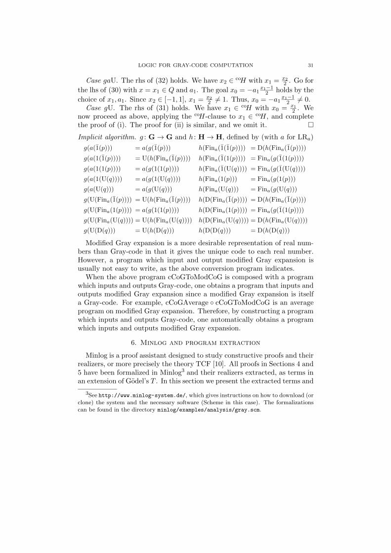
now proceed as above, applying the coH-clause to x1 ∈ coH, and completethe proof of (i). The proof for (ii) is similar, and we omit it. �
Implicit algorithm. g : G→ G and h : H→ H, defined by (with a for LRa)
g(a(1(p))) = a(g(1(p))) h(Fina(1(1(p)))) = D(h(Fina(1(p))))
g(a(1(1(p)))) = U(h(Fina(1(p)))) h(Fina(1(1(p)))) = Fina(g(1(1(p))))
g(a(1(1(p)))) = a(g(1(1(p)))) h(Fina(1(U(q)))) = Fina(g(1(U(q))))
g(a(1(U(q)))) = a(g(1(U(q)))) h(Fina(1(p))) = Fina(g(1(p)))
g(a(U(q))) = a(g(U(q))) h(Fina(U(q))) = Fina(g(U(q)))
g(U(Fina(1(p)))) = U(h(Fina(1(p)))) h(D(Fina(1(p)))) = D(h(Fina(1(p))))
g(U(Fina(1(p)))) = a(g(1(1(p)))) h(D(Fina(1(p)))) = Fina(g(1(1(p))))
g(U(Fina(U(q)))) = U(h(Fina(U(q)))) h(D(Fina(U(q)))) = D(h(Fina(U(q))))
g(U(D(q))) = U(h(D(q))) h(D(D(q))) = D(h(D(q)))
Modified Gray expansion is a more desirable representation of real num-bers than Gray-code in that it gives the unique code to each real number.However, a program which input and output modified Gray expansion isusually not easy to write, as the above conversion program indicates.
When the above program cCoGToModCoG is composed with a programwhich inputs and outputs Gray-code, one obtains a program that inputs andoutputs modified Gray expansion since a modified Gray expansion is itselfa Gray-code. For example, cCoGAverage ◦ cCoGToModCoG is an averageprogram on modified Gray expansion. Therefore, by constructing a programwhich inputs and outputs Gray-code, one automatically obtains a programwhich inputs and outputs modified Gray expansion.
6. Minlog and program extraction
Minlog is a proof assistant designed to study constructive proofs and theirrealizers, or more precisely the theory TCF [10]. All proofs in Sections 4 and5 have been formalized in Minlog3 and their realizers extracted, as terms inan extension of Godel’s T . In this section we present the extracted terms and
3See http://www.minlog-system.de/, which gives instructions on how to download (orclone) the system and the necessary software (Scheme in this case). The formalizationscan be found in the directory minlog/examples/analysis/gray.scm.

32 U. BERGER, K. MIYAMOTO, H. SCHWICHTENBERG AND H. TSUIKI
discuss how they operate. They involve recursion and corecursion operatorswhere the original proofs used induction or coinduction axioms, and theconversion rules for these operators determine how the extracted terms canbe used as programs. The results of such an analysis have been shown inSections 4 and 5 under the label “implicit algorithm”.
6.1. Corecursion. Recall the type of the corecursion operator for I:
(34) coRτI : τ → (τ → SD× (I + τ))→ I.
The type SD× (I + τ) appears since I has the single constructor C of typeSD→ I→ I. The meaning of coRτINM is defined by the conversion rule
coRτINM 7→ Cπ1(MN)([idI→I, λy(
coRτIyM)]π2(MN)).
We have used π1, π2 for the two projections of type ρ× σ, and the notation[f, g] : ρ+ σ → τ (for f : ρ→ τ and g : σ → τ) defined by
[f, g](z) :=
{f(x) if z = inl(x),
g(y) if z = inr(y).
We will also need the simultaneous corecursion operators coR(G,H),(σ,τ)G
and coR(G,H),(σ,τ)H for G, H, of type
coR(G,H),(σ,τ)G : σ → δG → δH → G
coR(G,H),(σ,τ)H : τ → δG → δH → H
(35)
with step types
δG := σ → PSD× (G + σ) + (H + τ),
δH := τ → PSD× (G + σ) + (H + τ).
The type PSD×(G+σ)+(H+τ) appears since G has the two constructorsLR: PSD → G → G and U: H → G, and H has the two constructorsFin: PSD → G → H and D: H → H. Omitting the upper indices of coR,the terms coRGNMM ′ and coRHN
′MM ′ are defined by the conversionrules
coRGNMM ′ 7→
{LRπ1(u)([id, λy(
coRGyMM ′)]π2(u)) if MN = inl(u)
U([id, λz(coRHzMM ′)]v) if MN = inr(v)
coRHN′MM ′ 7→
{Finπ1(u)([id, λy(
coRGyMM ′)]π2(u)) if M ′N ′ = inl(u)
D([id, λz(coRHzMM ′)]v) if M ′N ′ = inr(v)

LOGIC FOR GRAY-CODE COMPUTATION 33
6.2. Notational conventions of Minlog. Types:
iv, ag, ah, bg base types for the algebra I, G, H, zG
rho=>sigma function type
rho@@sigma product type
rho ysum sigma sum type
Variables (with fixed types)
v, p, q of type I, G and H
d, a, i of type SD, PSD, SD2
ivw of type SD2 × I× I
jdvw of type SD2 × SD× I× I
ap of type PSD×G
apq of type PSD× (G + H)
bv of type PSD× I
ipp of type SD2 ×G×G
idpp of type SD2 × SD×G×G
psf of type (G→ zG× zG)× (H→ (N + PSD×G× zG)2)
apbg of type PSD×G× zG
Constants
Rec, CoRec recursion, corecursion
Des destructor
PsdToSd embedding of PSD into SD
plus, times, inv arithmetic in SD
cL realizer for lemma L
Terms
[x]r lambda abstraction λxr
r@s product term
left r, right r components (prefix, binding strongest)
InL, InR injections into a sum type
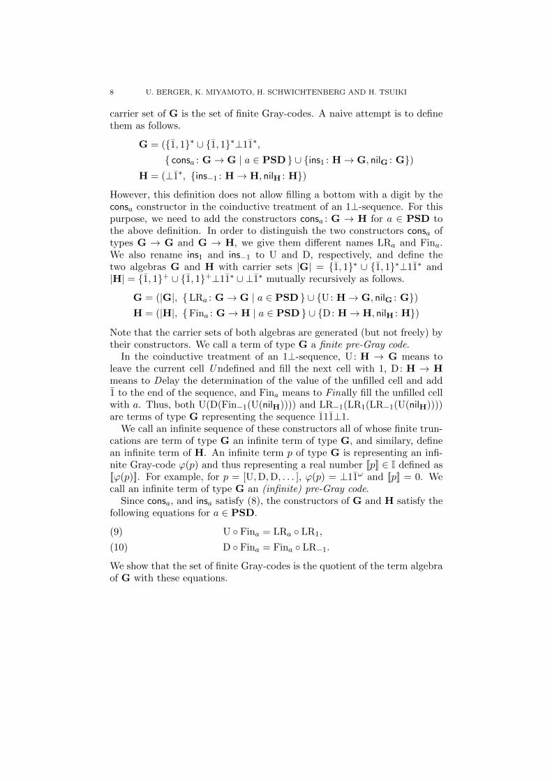
6.3. CoIAverage. We analyze the term in Figure 4 extracted from CoI-Average. The first argument N of the corecursion operator destructs v, v0
34 U. BERGER, K. MIYAMOTO, H. SCHWICHTENBERG AND H. TSUIKI
[v,v0](CoRec sdtwo@@iv@@iv=>iv)
(left Des v plus left Des v0@right Des v@right Des v0)
([ivw][let jdvw
(J left Des left right ivw
left Des right right ivw
left ivw@
K left Des left right ivw
left Des right right ivw
left ivw@
right Des left right ivw@
right Des right right ivw)
(left right jdvw@InR(left jdvw@right right jdvw))])
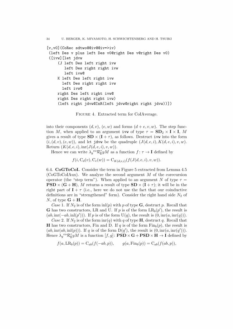
Figure 4. Extracted term for CoIAverage.
into their components (d, v), (e, w) and forms (d + e, v, w). The step func-tion M , when applied to an argument ivw of type τ = SD2 × I × I, Mgives a result of type SD × (I + τ), as follows. Destruct ivw into the form(i, (d, v), (e, w)), and let jdvw be the quadruple (J(d, e, i),K(d, e, i), v, w).Return (K(d, e, i), inr(J(d, e, i), v, w)).
Hence we can write λycoRτIyM as a function f : τ → I defined by
f(i,Cd(v),Ce(w)) = CK(d,e,i)(f(J(d, e, i), v, w)).
6.4. CoGToCoI. Consider the term in Figure 5 extracted from Lemma 4.5(CoGToCoIAux). We analyze the second argument M of the corecursionoperator (the “step term”). When applied to an argument N of type τ =PSD× (G + H), M returns a result of type SD× (I + τ); it will be in theright part of I + τ (i.e., here we do not use the fact that our coinductivedefinitions are in “strengthened” form). Consider the right hand side N2 ofN , of type G + H.
Case 1. If N2 is of the form inl(p) with p of type G, destruct p. Recall thatG has two constructors, LR and U. If p is of the form LRb(p
′), the result is(ab, inr(−ab, inl(p′))). If p is of the form U(q), the result is (0, inr(a, inr(q))).
Case 2. If N2 is of the form inr(q) with q of type H, destruct q. Recall thatH has two constructors, Fin and D. If q is of the form Finb(p), the result is(ab, inr(ab, inl(p))). If q is of the form D(q′), the result is (0, inr(a, inr(q′))).Hence λy
coRτIyM is a function [f, g] : PSD×G+PSD×H→ I defined by
f(a,LRb(p)) = Cab(f(−ab, p)), g(a,Finb(p)) = Cab(f(ab, p)),

LOGIC FOR GRAY-CODE COMPUTATION 35
[apq](CoRec psd@@(ag ysum ah)=>iv)apq
([apq0][case (right apq0)
(InL p -> [case (Des p)
(InL ap ->
PsdToSd(left apq0 times left ap)@
InR(inv(left apq0 times left ap)@InL right ap))
(InR q -> Mid@InR(left apq0@InR q))])
(InR q -> [case (Des q)
(InL ap ->
PsdToSd(left apq0 times left ap)@
InR(left apq0 times left ap@InL right ap))
(InR q0 -> Mid@InR(left apq0@InR q0))])])
Figure 5. Extracted term for CoGToCoIAux.
f(a,U(q)) = C0(g(a, q)), g(a,D(q)) = C0(g(a, q)).
6.5. CoIToCoG. For Lemma 4.7 (CoIToCoGAux) we obtain the extractedterm in Figure 6.
[bv](CoRec psd@@iv=>ag psd@@iv=>ah)bv
([bv0][case (left Des right bv0)
(Lft -> InL(inv left bv0@InR(PRht@right Des right bv0)))
(Rht -> InL(left bv0@InR(PLft@right Des right bv0)))
(Mid -> InR(InR(left bv0@right Des right bv0)))])
([bv0][case (left Des right bv0)
(Lft -> InL(inv left bv0@InR(PLft@right Des right bv0)))
(Rht -> InL(left bv0@InR(PRht@right Des right bv0)))
(Mid -> InR(InR(left bv0@right Des right bv0)))])
Figure 6. Extracted term for CoIToCoGAux.
To understand this term recall the type (35) of the simultaneous corecur-
sion operators coR(G,H),(τ,τ)G and coR(G,H),(τ,τ)
H , or shortly coRG and coRH,with τ := PSD× I and step types δ := τ → PSD× (G+ τ) + (H+ τ). Weagain analyze the particular step functions M,M ′ extracted from our proof.When applied to an argument N of type τ = PSD× I, M returns a resultof type PSD× (G+ τ) + (H+ τ), in the right part of G+ τ or H+ τ . LetN = (b, v) with v of type I, of the form Cd(v
′). The result is
inl(−b, inr(1, v′)) if d = −1,

36 U. BERGER, K. MIYAMOTO, H. SCHWICHTENBERG AND H. TSUIKI
inl(b, inr(−1, v′)) if d = 1,
inr(inr(b, v′)) if d = 0.
Similarly, when applied to an argument N of type τ = PSD× I, M ′ returnsa result of type PSD× (G + τ) + (H + τ). Let N = (b, v) with v of type I,of the form Cd(v
′). The result is
inl(−b, inr(−1, v′)) if d = −1,
inl(b, inr(1, v′)) if d = 1,
inr(inr(b, v′)) if d = 0.
Hence we can write the two functions λycoRGyMM ′ and λy
coRHyMM ′
as g : τ → G and h : τ → H defined by
g(b,C−1(v)) = LR−b(g(1, v)), h(b,C−1(v)) = Fin−b(g(−1, v)),
g(b,C1(v)) = LRb(g(−1, v)), h(b,C1(v)) = Finb(g(1, v)),
g(b,C0(v)) = U(h(b, v)), h(b,C0(v)) = D(h(b, v)).
6.6. CoGAverage. For Lemma 4.9 (CoGMinus) the extracted term is shownin Figure 7.
[p](CoRec ag=>ag ah=>ah)p
([p0][case (Des p0)
(InL ap -> InL(inv left ap@InL right ap))
(InR q -> InR(InR q))])
([q][case (Des q)
(InL ap -> InL(inv left ap@InL right ap))
(InR q0 -> InR(InR q0))])
Figure 7. Extracted term for CoGMinus.
We need simultaneous corecursion operators coR(G,H),(σ,τ)G , coR(G,H),(σ,τ)
Hof type (35). By analyzing the particular step functions M,M ′ extractedfrom our proof we see that we can write λy
coRGyMM ′ and λzcoRHzMM ′
as functions f : σ → G and f ′ : τ → H defined by
f(LRa(p)) = LR−a(p), f ′(Fina(p)) = Fin−a(p),
f(U(q)) = U(f ′(q)), f ′(D(q)) = D(f ′(q)).
Lemma 4.9 (CoGMinus) gave us Lemma 4.10 (CoHToCoG).The extracted term in Figure 8 clearly represents the functions shown as
implicit algorithm in Section 4.4.
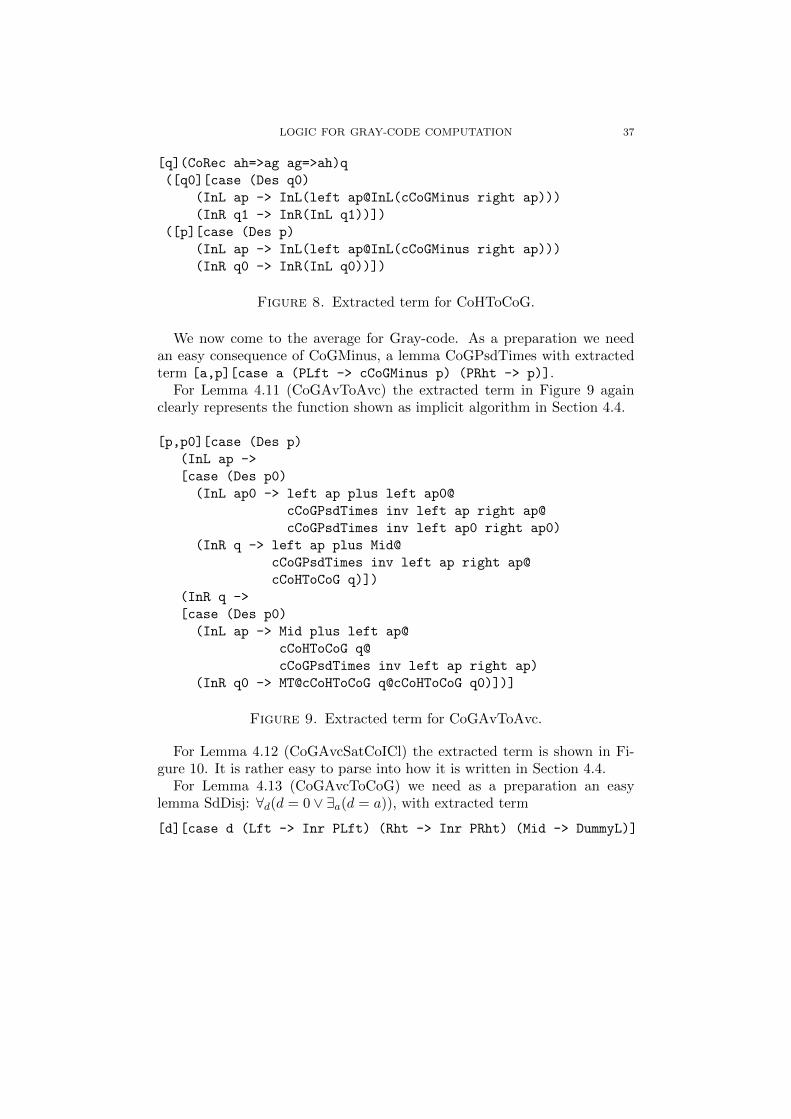
LOGIC FOR GRAY-CODE COMPUTATION 37
[q](CoRec ah=>ag ag=>ah)q
([q0][case (Des q0)
(InL ap -> InL(left ap@InL(cCoGMinus right ap)))
(InR q1 -> InR(InL q1))])
([p][case (Des p)
(InL ap -> InL(left ap@InL(cCoGMinus right ap)))
(InR q0 -> InR(InL q0))])
Figure 8. Extracted term for CoHToCoG.
We now come to the average for Gray-code. As a preparation we needan easy consequence of CoGMinus, a lemma CoGPsdTimes with extractedterm [a,p][case a (PLft -> cCoGMinus p) (PRht -> p)].
For Lemma 4.11 (CoGAvToAvc) the extracted term in Figure 9 againclearly represents the function shown as implicit algorithm in Section 4.4.
[p,p0][case (Des p)
(InL ap ->
[case (Des p0)
(InL ap0 -> left ap plus left ap0@
cCoGPsdTimes inv left ap right ap@
cCoGPsdTimes inv left ap0 right ap0)
(InR q -> left ap plus Mid@
cCoGPsdTimes inv left ap right ap@
cCoHToCoG q)])
(InR q ->
[case (Des p0)
(InL ap -> Mid plus left ap@
cCoHToCoG q@
cCoGPsdTimes inv left ap right ap)
(InR q0 -> MT@cCoHToCoG q@cCoHToCoG q0)])]
Figure 9. Extracted term for CoGAvToAvc.
For Lemma 4.12 (CoGAvcSatCoICl) the extracted term is shown in Fi-gure 10. It is rather easy to parse into how it is written in Section 4.4.
For Lemma 4.13 (CoGAvcToCoG) we need as a preparation an easylemma SdDisj: ∀d(d = 0 ∨ ∃a(d = a)), with extracted term
[d][case d (Lft -> Inr PLft) (Rht -> Inr PRht) (Mid -> DummyL)]

38 U. BERGER, K. MIYAMOTO, H. SCHWICHTENBERG AND H. TSUIKI
[i,p,p0][case (Des p)
(InL ap ->
[case (Des p0)
(InL ap0 -> J(PsdToSd left ap)(PsdToSd left ap0)i@
K(PsdToSd left ap)(PsdToSd left ap0)i@
cCoGPsdTimes inv left ap right ap@
cCoGPsdTimes inv left ap0 right ap0)
(InR q -> J(PsdToSd left ap)Mid i@
K(PsdToSd left ap)Mid i@
cCoGPsdTimes inv left ap right ap@
cCoHToCoG q)])
(InR q ->
[case (Des p0)
(InL ap -> J Mid(PsdToSd left ap)i@
K Mid(PsdToSd left ap)i@
cCoHToCoG q@
cCoGPsdTimes inv left ap right ap)
(InR q0 -> J Mid Mid i@K Mid Mid i@
cCoHToCoG q@cCoHToCoG q0)])]
Figure 10. Extracted term for CoGAvcSatCoICl.
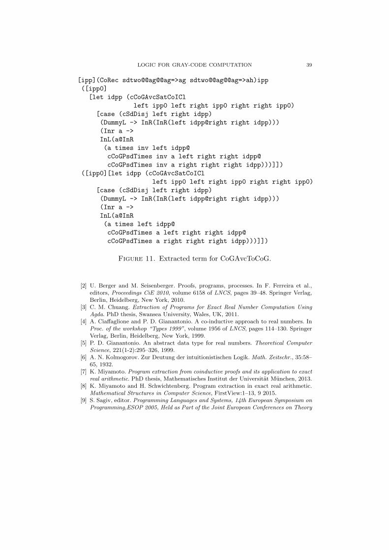
It is easy to see that the extracted term for Lemma 4.13 (in Figure 11) givesthe algorithm in Section 4.4.
Now for Proposition 4.14 (CoGAverage) the extracted term is obtainedjust by composition of those for Lemmata 4.11 and 4.13:
[p,p0]cCoGAvcToCoG(cCoGAvToAvc p p0)
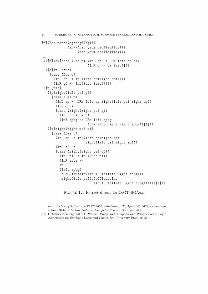
6.7. CoGToBG. For Lemma 4.16 again the extracted term (see Figure 12)represents the algorithms given in Section 4.5
6.8. CoGToCoM. Finally Figure 13 gives the term extracted from ourproof of Proposition 5.5.
References
[1] U. Berger. Program extraction from normalization proofs. In M. Bezem and J. Groote,editors, Typed Lambda Calculi and Applications, volume 664 of LNCS, pages 91–106.Springer Verlag, Berlin, Heidelberg, New York, 1993.
LOGIC FOR GRAY-CODE COMPUTATION 39
[ipp](CoRec sdtwo@@ag@@ag=>ag sdtwo@@ag@@ag=>ah)ipp
([ipp0]
[let idpp (cCoGAvcSatCoICl
left ipp0 left right ipp0 right right ipp0)
[case (cSdDisj left right idpp)
(DummyL -> InR(InR(left idpp@right right idpp)))
(Inr a ->
InL(a@InR
(a times inv left idpp@
cCoGPsdTimes inv a left right right idpp@
cCoGPsdTimes inv a right right right idpp)))]])
([ipp0][let idpp (cCoGAvcSatCoICl
left ipp0 left right ipp0 right right ipp0)
[case (cSdDisj left right idpp)
(DummyL -> InR(InR(left idpp@right right idpp)))
(Inr a ->
InL(a@InR
(a times left idpp@
cCoGPsdTimes a left right right idpp@
cCoGPsdTimes a right right right idpp)))]])
Figure 11. Extracted term for CoGAvcToCoG.
[2] U. Berger and M. Seisenberger. Proofs, programs, processes. In F. Ferreira et al.,editors, Proceedings CiE 2010, volume 6158 of LNCS, pages 39–48. Springer Verlag,Berlin, Heidelberg, New York, 2010.
[3] C. M. Chuang. Extraction of Programs for Exact Real Number Computation UsingAgda. PhD thesis, Swansea University, Wales, UK, 2011.
[4] A. Ciaffaglione and P. D. Gianantonio. A co-inductive approach to real numbers. InProc. of the workshop “Types 1999”, volume 1956 of LNCS, pages 114–130. SpringerVerlag, Berlin, Heidelberg, New York, 1999.
[5] P. D. Gianantonio. An abstract data type for real numbers. Theoretical ComputerScience, 221(1-2):295–326, 1999.
[6] A. N. Kolmogorov. Zur Deutung der intuitionistischen Logik. Math. Zeitschr., 35:58–65, 1932.
[7] K. Miyamoto. Program extraction from coinductive proofs and its application to exactreal arithmetic. PhD thesis, Mathematisches Institut der Universitat Munchen, 2013.
[8] K. Miyamoto and H. Schwichtenberg. Program extraction in exact real arithmetic.Mathematical Structures in Computer Science, FirstView:1–13, 9 2015.
[9] S. Sagiv, editor. Programming Languages and Systems, 14th European Symposium onProgramming,ESOP 2005, Held as Part of the Joint European Conferences on Theory
40 U. BERGER, K. MIYAMOTO, H. SCHWICHTENBERG AND H. TSUIKI
[n](Rec nat=>(ag=>bg@@bg)@@
(ah=>(nat ysum psd@@ag@@bg)@@
(nat ysum psd@@ag@@bg)))
n
(([p]Nz@[case (Des p) (InL ap -> LRz left ap Nz)
(InR q -> Uz Zero)])@
([q]InL Zero@
[case (Des q)
(InL ap -> InR(left ap@right ap@Nz))
(InR q0 -> InL(Succ Zero))]))
([n0,psf]
([p]right(left psf p)@
[case (Des p)
(InL ap -> LRz left ap right(left psf right ap))
(InR q ->
[case (right(right psf q))
(InL n -> Uz n)
(InR apbg -> LRz left apbg
(LRz PRht right right apbg))])])@
([q]right(right psf q)@
[case (Des q)
(InL ap -> InR(left ap@right ap@
right(left psf right ap)))
(InR q0 ->
[case (right(right psf q0))
(InL n1 -> InL(Succ n1))
(InR apbg ->
InR
(left apbg@
cCoGClauseInv(InL(PLft@left right apbg))@
right(left psf(cCoGClauseInv
(InL(PLft@left right apbg))))))])]))
Figure 12. Extracted term for CoGToBGAux.
and Practice of Software, ETAPS 2005, Edinburgh, UK, April 4-8, 2005, Proceedings,volume 3444 of Lecture Notes in Computer Science. Springer, 2005.
[10] H. Schwichtenberg and S. S. Wainer. Proofs and Computations. Perspectives in Logic.Association for Symbolic Logic and Cambridge University Press, 2012.

LOGIC FOR GRAY-CODE COMPUTATION 41
[11] K. Terayama and H. Tsuiki. A stream calculus of bottomed sequences for real numbercomputation. Electr. Notes Theor. Comput. Sci., 298:383–402, 2013.
[12] H. Tsuiki. Real number computation through Gray code embedding. TheoreticalComputer Science, 284:467–485, 2002.
[13] H. Tsuiki. Real number computation with committed choice logic programming lan-guages. J. Log. Algebr. Program., 64(1):61–84, 2005.
[14] H. Tsuiki and K. Sugihara. Streams with a bottom in functional languages. In Sagiv[9], pages 201–216.
[15] E. Wiedmer. Exaktes Rechnen mit reellen Zahlen und anderen unendlichen Objekten.PhD thesis, ETH Zurich, 1977.
[16] E. Wiedmer. Computing with infinite objects. Theoretical Comput. Sci., 10:133–155,1980.

42 U. BERGER, K. MIYAMOTO, H. SCHWICHTENBERG AND H. TSUIKI
[p](CoRec ag=>ag ah=>ah)p
([p0][case (Des p0)
(InL ap -> [case (Des right ap)
(InL ap0 -> [case (left ap0)
(PLft -> InL(left ap@InR right ap))
(PRht -> [case (Des right ap0)
(InL ap1 -> [case (left ap1)
(PLft -> InR(InR(cCoHClauseInv
(InL(left ap@right ap0)))))
(PRht -> InL(left ap@InR right ap))])
(InR q -> InL(left ap@InR right ap))])])
(InR q -> InL(left ap@InR right ap))])
(InR q -> [case (Des q)
(InL ap -> [case (Des right ap)
(InL ap0 -> [case (left ap0)
(PLft -> InR(InR(cCoHClauseInv(InL ap))))
(PRht -> InL(left ap@InR(cCoGClauseInv
(InR(cCoHClauseInv(InL(PRht@right ap0)))))))])
(InR q0 -> InR(InR(cCoHClauseInv(InL ap))))])
(InR q0 -> InR(InR q))])])
([q][case (Des q)
(InL ap -> [case (Des right ap)
(InL ap0 -> [case (left ap0)
(PLft -> [case (Des right ap0)
(InL ap1 -> [case (left ap1)
(PLft -> InR(InR(cCoHClauseInv
(InL(left ap@right ap0)))))
(PRht -> InL(left ap@InR right ap))])
(InR q0 -> InL(left ap@InR right ap))])
(PRht -> InL(left ap@InR right ap))])
(InR q0 -> InL(left ap@InR right ap))])
(InR q0 -> [case (Des q0)
(InL ap -> [case (Des right ap)
(InL ap0 -> [case (left ap0)
(PLft -> InR(InR(cCoHClauseInv(InL ap))))
(PRht -> InL(left ap@InR(cCoGClauseInv
(InR(cCoHClauseInv(InL(PLft@right ap0)))))))])
(InR q1 -> InR(InR(cCoHClauseInv(InL ap))))])
(InR q1 -> InR(InR q0))])])
Figure 13. Extracted term for CoGToCoM.