Embed Size (px)
Citation preview
Logic, Graphs, and Algorithms
Martin GroheHumboldt-Universitat zu Berlin
September 10, 2007
Abstract
Algorithmic meta theoremsare algorithmic results that apply to whole families of combinatorialproblems, instead of just specific problems. These familiesare usually defined in terms of logic andgraph theory. An archetypal algorithmic meta theorem is Courcelle’s Theorem [9], which states thatall graph properties definable in monadic second-order logic can be decided in linear time on graphs ofbounded tree width.
This article is an introduction into the theory underlying such meta theorems and a survey of the mostimportant results in this area.
1 Introduction
In 1990, Courcelle [9] proved a fundamental theorem statingthat graph properties definable in monadicsecond-order logic can be decided in linear time on graphs ofbounded tree width. This is the first in aseries ofalgorithmic meta theorems. More recent examples of such meta theorems state that all first-orderdefinable properties of planar graphs can be decided in linear time [43] and that all first-order definableoptimisation problems on classes of graphs with excluded minors can be approximated in polynomial timeto any given approximation ratio [19]. The term “meta theorem” refers to the fact that these results do notdescribe algorithms for specific problems, but for whole families of problems, whose definition typicallyhas a logical and a structural (usually graph theoretical) component. For example, Courcelle’s Theorem isaboutmonadic second-order logicongraphs of bounded tree width.
This article is an introductory survey on algorithmic meta theorems. Why should we care about suchtheorems? First of all, they often provide a quick way to prove that a problem is solvable efficiently. Forexample, to show that the 3-colourability problem can be solved in linear time on graphs of bounded treewidth, we observe that 3-colourability is a property of graphs definable in monadic second-order logic andapply Courcelle’s theorem. Secondly, and more substantially, algorithmic meta theorems yield a betterunderstanding of the scope of general algorithmic techniques and, in some sense, the limits of tractability.In particular, they clarify the interactions between logicand combinatorial structure, which is fundamentalfor computational complexity.
The general form of algorithmic meta theorems is:
All problemsdefinable in a certainlogic on a certain class ofstructurescan be solvedeffi-ciently.
Problemsmay be of different types, for example, they may be optimisation or counting problems, but inthis article we mainly consider decision problems. We briefly discuss other types of problems in Sec-tion 7.2.Efficient solvabilitymay mean, for example, polynomial time solvability, linearor quadratic timesolvability, or fixed-parameter tractability. We will discuss this in detail in Section 2.3. Let us now focuson the two main ingredients of the meta theorems, logic and structure.
Author’s address: Martin Grohe, Institut fur Informatik, Humboldt-Universitat, Unter den Linden 6, 10099 Berlin, Germany.Email:[email protected]
1
Electronic Colloquium on Computational Complexity, Report No. 91 (2007)
ISSN 1433-8092
The twologics that, so far, have been considered almost exclusively for meta theorems are first-orderlogic and monadic second-order logic. Techniques from logic underlying the theorems are Feferman-Vaught style composition lemmas, automata theoretic techniques, and locality results such as Hanf’s The-orem and Gaifman’s Theorem.
Thestructuresin algorithmic meta theorems are usually defined by graph theoretic properties. Actually,to ease the presentation, the only structures we will consider in this survey are graphs. Many of the metatheorems are tightly linked withgraph minor theory. This deep theory, mainly developed by Robertson andSeymour in a long series of papers, describes the structure of graphs with excluded minors. It culminatesin the graph minor theorem [73], which states that every class of graphs closed under taking minors can becharacterised by a finite set of excluded minors. The theory also has significant algorithmic consequences.Robertson and Seymour [71] proved that every class of graphsthat is closed under taking minors canbe recognised in cubic time. More recently, results from graph minor theory have been combined withalgorithmic techniques that had originally been developedfor planar graphs to obtain polynomial timeapproximation schemes and fixed parameter tractable algorithms for many standard optimisation problemson families of graphs with excluded minors. The methods developed in this context are also underlying themore advanced algorithmic meta theorems.
There are some obvious similarities between algorithmic meta theorems and results fromdescriptivecomplexity theory, in particular such results from descriptive complexity theory that also involve restrictedclasses of graphs. As an example, consider the theorem stating that fixed-point logic with counting capturespolynomial time on graphs of bounded tree width [49], that is, a property of graphs of bounded tree widthis definable in fixed-point logic with counting if and only if it is decidable in polynomial time. Comparethis to Courcelle’s Theorem. Despite the similarity, thereare two crucial differences: On the one hand,Courcelle’s Theorem is weaker as it makes no completeness claim, that is, it does not state thatall propertiesof graphs of bounded tree width that are decidable in linear time are definable in monadic second-orderlogic. On the other hand, Courcelle’s Theorem is stronger inits algorithmic content. Whereas it is veryeasy to show that all properties of graphs (not only graphs ofbounded tree width) definable in fixed-pointlogic with counting are decidable in polynomial time, the proof of Courcelle’s theorem relies on substantialalgorithmic ideas like the translation of monadic second-order logic over trees into tree automata [78] and alinear time algorithm for computing tree decompositions [5]. In general, algorithmic meta theorems involvenontrivial algorithms, but do not state completeness, whereas in typical results from descriptive complexity,the algorithmic content is limited, and the nontrivial partis completeness. But there is no clear dividingline. Consider, for example, Papadimitriou and Yannakakis’s [64] well known result that all optimisationproblems in the logically defined class MAXSNP have a constant factor approximation algorithm. Thistheorem does not state completeness, but technically it is much closer to Fagin’s Theorem [37], a centralresult of descriptive complexity theory, than to the algorithmic meta theorems considered here. In any case,both algorithmic meta theorems and descriptive complexitytheory are branches of finite model theory, andthere is no need to draw a line between them.
When I wrote this survey, it was my goal to cover the developments up to the most recent and strongestresults, which are concerned with monadic second-order logic on graphs of bounded rank width and withfirst-order logic on graphs with excluded minors. The proofsof most theorems are at least sketched, so thathopefully the reader will not only get an impression of the results, but also of the techniques involved intheir proofs.
2 The basics
R, Q, Z, andN denote the sets of real numbers, rational numbers, integers, and natural numbers (that is,positive integers), respectively. For a setS⊆R, byS≥0 we denote the set of nonnegative numbers inS. Forintegersm,n, by [m,n] we denote the intervalm,m+1, . . . ,n, which is empty ifn < m. Furthermore, welet [n] = [1,n]. The power set of a setS is denoted by 2S, and the set of allk-element subsets ofSby
(Sk
).
2.1 Graphs
A graph G is a pair(V(G),E(G)), whereV(G) is a finite set whose elements are calledverticesandE(G) ⊆
(V(G)2
)is a set of unordered pairs of vertices, which are callededges. Hence graphs in this paper
2
are alwaysfinite, undirected, andsimple, where simple means that there are no loops or parallel edges.If e= u,v is an edge, we say that the verticesu andv areadjacent, and that bothu andv are incidentwith e. A graphH is a subgraphof a graphG (we write H ⊆ G) if V(H) ⊆ V(G) andE(H) ⊆ E(G).If E(H) = E(G)∩
(V(H)2
), thenH is an inducedsubgraph ofG. For a setW ⊆ V(G), we write G[W]
to denote the induced subgraph(W,E(G)∩
(W2
))andG\W to denoteG[V(G) \W]. For a setF ⊆ E,
we let GJFK be the subgraph(⋃
F,F). Here
⋃F denote the union of all edges inF , that is, the set
of all vertices incident with at least one edge inF . We call GJFK the subgraph ofG generatedby F ;note that it is not necessarily an induced subgraph ofG. Theunionof two graphsG andH is the graphG∪H = (V(G)∪V(H),E(G)∪E(H)), and theintersection G∩H is defined similarly. Thecomplementof a graphG = (V,E) is the graphG =
(V,(V
2
)\E). There is a uniqueempty graph( /0, /0). For n≥ 1, we
let Kn be the complete graph withn vertices. To be precise, let us sayKn =([n],([n]
2
)). We letKn,m be the
complete bipartite graph with parts of sizem,n, respectively.Occasionally, we consider (vertex) labelled graphs. Alabelled graphis a tuple
G =(V(G),E(G),P1(G), . . . , P (G)
),
wherePi(G) ⊆ V(G) for all i ∈ [`]. The symbolsPi are calledlabels, and if v ∈ Pi(G) we say thatv islabelledby Pi . Subgraphs, union, and intersection extend to labelled graphs in a straightforward manner.Theunderlying graphof a labelled graphG is (V(G),E(G)). Whenever we apply graph theoretic notionssuch as connectivity to labelled graphs, we refer to the underlying graph.
Theorder |G| of a graphG is the number of vertices ofG. We usually use the lettern to denote theorder of a graph. Thesizeof G is the number||G|| = |G|+ |E(G)|. Up to a constant factor, this is the sizeof the adjacency list representation ofG under a uniform cost model.
G denotes the class of all graphs. For every classC of graphs, we letClb be the class of all labelledgraphs whose underlying graph is inC . A graph invariantis a mapping defined on the classG of all graphsthat is invariant under isomorphisms. All graph invariantsconsidered in this paper are integer valued. Fora graph invariantf : G → Z and a classC of graphs, we say thatC has bounded fif there is ak∈ Z suchthat f (G) ≤ k for all G∈ C .
Let G = (V,E) be a graph. ThedegreedegG(v) of a vertexv∈V is the number of edges incident withv. We omit the superscriptG if G is clear from the context. The(maximum) degreeof G is the number
∆(G) = maxdeg(v) | v∈V.
Theminimum degreeδ (G) is defined analogously, and theaverage degree d(G) is 2|E(G)|/|V(G)|. Ob-serve that||G|| = O(d(G) · |G|). Hence if a classC of graphs has bounded average degree, then the size ofthe graphs inC is linearly bounded in the order. In the following, “degree”of a graph, without qualifica-tions, always means “maximum degree”.
A path in G = (V,E) of length n≥ 0 from a vertexv0 to a vertexvn is a sequencev0, . . . ,vn of distinctvertices such thatvi−1,vi ∈ E for all i ∈ [n]. Note that the length of a path is the number of edges onthe path. Two paths aredisjoint if they have no vertex in common.G is connectedif it is nonempty andfor all v,w∈V there is a path fromv to w. A connected componentof G is a maximal (with respect to⊆)connected subgraph.G is k-connected, for somek ≥ 1, if |V| > k and for everyW ⊆ V with |W| < k thegraphG\W is connected.
A cycle in a graphG = (V,E) of length n≥ 3 is a sequencev1 . . .vn of distinct vertices such thatvn,v1 ∈ E andvi−1,vi ∈ E for all i ∈ [2,n]. A graphG is acyclic, or aforest, if it has no cycle.G is atree if it is acyclic and connected. It will be a useful conventionto call the vertices of treesnodes. A nodeof degree at most 1 is called aleaf. The set of all leaves of a treeT is denoted byL(T). Nodes that are notleaves are calledinner nodes. A rooted treeis a tripleT = (V(T),E(T), r(T)), where(V(T),E(T)) is atree andr(T) ∈ V(T) is a distinguished node called theroot. A nodet of a rooted treeT is theparentofa nodeu, andu is achild of t, if t is the predecessor ofu on the unique path from the rootr(T) to u. Twonodes that are children of the same parent are calledsiblings. A binary treeis a rooted treeT in whichevery node has either no children at all or exactly two children.
3
2.2 Logic
I assume that the reader has some background in logic and, in particular, is familiar with first-order pred-icate logic. To simplify matters, we only consider logics over (labelled) graphs, even though most resultsmentioned in this survey extend to more general structures.Let us briefly review the syntax and semanticsof first-order logicFO andmonadic second-order logicMSO. We assume that we have an infinite supplyof individual variables, usually denoted by the lowercase lettersx,y,z, and an infinite supply ofset vari-ables, usually denoted by uppercase lettersX,Y,Z. First-order formulasin the language of graphs are builtup from atomic formulasE(x,y) andx = y by using the usual Boolean connectives¬ (negation),∧ (con-junction),∨ (disjunction),→ (implication), and↔ (bi-implication) and existential quantification∃x anduniversal quantification∀x over individual variables. Individual variables range over vertices of a graph.The atomic formulaE(x,y) expresses adjacency, and the formulax = y expresses equality. From this, thesemantics of first-order logic is defined in the obvious way. First-order formulas over labelled graphs maycontain additional atomic formulasPi(x), meaning thatx is labelled byPi . If a labelPi does not appear in alabelled graphG, then we always interpretPi(G) as the empty set. Inmonadic second-order formulas, wehave additional atomic formulasX(x) for set variablesX and individual variablesx, and we admit existen-tial and universal quantification over set variables. Set variables are interpreted by sets of vertices, and theatomic formulaX(x) means that the vertexx is contained in the setX.
The free individual and set variables of a formula are defined in the usual way. Asentenceis a for-mula without free variables. We writeϕ(x1, . . . ,xk,X1, . . . ,X`) to indicate thatϕ is a formula with freevariables amongx1, . . . ,xk, X1, . . . ,X`. We use this notation to conveniently denote substitutionsand as-signments to the variables. IfG = (V,E) is a graph,v1, . . . ,vk ∈ V, andW1, . . . ,W ⊆ V, then we writeG |= ϕ(v1, . . . ,vk,W1, . . . ,W ) to denote thatϕ(x1, . . . ,xk,X1, . . . ,X`) holds inG if the variablesxi are inter-preted by the verticesvi and the variablesXi are interpreted by the vertex setsWi .
Occasionally, we consider monadic second-order formulas that contain no second-order quantifiers,but have free set variables. We view such formulas as first-order formulas, because free set variables areessentially the same as labels (unary relation symbols). Anexample of such a formula is the formuladom(X) in Example 2.1 below. We say that a formulaϕ(X) is positive in Xif X only occurs in the scopeof an even number of negation symbols. It isnegative in Xif X only occurs in the scope of an odd numberof relation symbols.
We freely use abbreviations such as∧k
i=1 ϕi instead of(ϕ1∧ . . .∧ϕk) andx 6= y instead of¬x = y.
Example 2.1.A dominating setin a graphG = (V,E) is a setS⊆V such that for everyv∈V, eitherv is inSor v is adjacent to a vertex inS.
The following first-order sentencedomk says that a graph has a dominating set of sizek:
domk = ∃x1 . . .∃xk( ∧
1≤i< j≤k
xi 6= x j ∧∀yk∨
i=1
(y = xi ∨E(y,xi)
)).
The following formuladom(X) says thatX is a dominating set:
dom(X) = ∀y(
X(y)∨∃z(X(z)∧E(z,y)
)).
More precisely, for every graphG and every subsetS⊆V(G) it holds thatG |= dom(S) if and only if S is adominating set ofG. y
Example 2.2.The following monadic second-order sentencesconnandacycsay that a graph is connectedand acyclic, respectively:
conn= ∃xx= x∧∀X((
∃xX(x)∧∀x∀y((X(x)∧E(x,y)) → X(y)
))→∀xX(x)
),
acyc= ¬∃X(∃xX(x)∧∀x
(X(x) →∃y1∃y2
(y1 6= y2∧E(x,y1)∧E(x,y2)∧X(y1)∧X(y2)
))).
The sentenceacyc is based on the simple fact that a graph has a cycle if and only if it has a nonemptyinduced subgraph in which every vertex has degree at least 2.Then the sentencetree= conn∧acycsaysthat a graph is a tree. y
4

G H
v u w
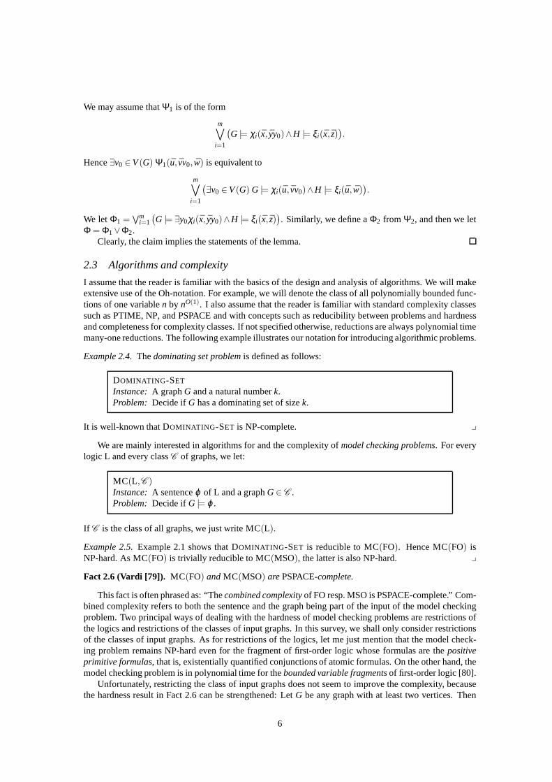
Figure 2.1. An illustration of Lemma 2.3
Thequantifier rankof a first-order or monadic second-order formulaϕ is the nesting depth of quan-tifiers in ϕ . For example, the quantifier rank of the formulaacyc in Example 2.2 is 4. LetG be a graphand v = (v1, . . . ,vk) ∈ V(G)k, for some nonnegative integerk. For everyq ≥ 0, thefirst-order q-type ofv in G is the set tpFO
q (G, v) of all first-order formulasϕ(x1, . . . ,xk) of quantifier rank at mostq such thatG |= ϕ(v1, . . . ,vk). Themonadic second-order q-type ofv in G, tpMSO
q (G, v) is defined analogously. Assuch, types are infinite sets, but we can syntacticallynormaliseformulas in such a way that there are onlyfinitely many normalised formulas of fixed quantifier rank andwith a fixed set of free variables, and thatevery formula can effectively be transformed into an equivalent normalised formula of the same quantifierrank. We represent a type by the set of normalised formulas itcontains. There is a fine line separating de-cidable and undecidable properties of types and formulas. For example, it is decidable whether a formula iscontained in a type: We just normalise the formula and test ifit is equal to one of the normalised formulasin the type. It is undecidable whether a set of normalised formulas actually is (more precisely: represents)a type. To see this, remember that types are satisfiable by definition and that the satisfiability of first-orderformulas is undecidable.
For a tuple ¯v = (v1, . . . ,vk), we sloppily writev to denote the setv1, . . . ,vk. It will always be clearfrom the context whetherv refers to the setv1, . . . ,vk or the 1-element set(v1, . . . ,vk). For tuplesv= (v1, . . . ,vk) andw= (w1, . . . ,w`), we writevw to denote their concatenation(v1, . . . ,vk,w1, . . . ,w`). Weshall heavily use the following “Feferman-Vaught style” composition lemma.
Lemma 2.3. Let tp be one oftpFO, tpMSO. Let G,H be labelled graphs andu ∈ V(G)k, v ∈ V(G)`, w ∈V(H)m such that V(G)∩V(H) = u (cf. Figure 2.1). Then for all q≥ 0, tpq(G∪H, uvw) is determinedby tpq(G, uv) and tpq(H, uw). Furthermore, there is an algorithm that computestpq(G∪H, uvw) fromtpq(G, uv) andtpq(H, uw).
Let me sketch a proof of this lemma for first-order types. The version for monadic second-order typescan be proved similarly, but is more complicated (see, for example, [57]).
Proof sketch.Let G,H be labelled graphs and ¯u∈V(G)k such thatV(G)∩V(H) = u. By induction onϕ , we prove the following claim:
Claim: Let ϕ(x, y, z) be a first-order formula of quantifier rankq, where ¯x is a k-tuple and ¯y, z aretuples of arbitrary length. Then there is a Boolean combination Φ(x, y, z) of expressionsG |= ψ(x, y) andH |= χ(x, z) for formulasψ ,χ of quantifier rank at mostq, such that for all tuples ¯v of vertices ofG andwof vertices ofH of the appropriate lengths it holds that
G∪H |= ϕ(u, v,w) ⇐⇒ Φ(u, v,w).
HereΦ(u, v,w) denotes the statement obtained fromΦ(x, y, z) by substituting ¯u for x, v for y, andw for z.Furthermore, the construction ofΦ from ϕ is effective.
The claim holds for atomic formulas, because there are no edges fromV(G)\V(H) to V(H)\V(G) inG∪H. It obviously extends to Boolean combinations of formulas.So suppose thatϕ(x, y, z)= ∃x0ψ(x,x0, y, z).Let v,w be tuples inG, H of the appropriate lengths. By the induction hypothesis, there areΨ1(x, yy0, z)andΨ2(x, y, zz0) such that
G∪H |= ϕ(u, v,w)
⇐⇒∃v0 ∈V(G) Ψ1(u, vv0,w) or ∃w0 ∈V(H) Ψ2(u, v,ww0).
5
We may assume thatΨ1 is of the form
m∨
i=1
(G |= χi(x, yy0)∧H |= ξi(x, z)
).
Hence∃v0 ∈V(G) Ψ1(u, vv0,w) is equivalent to
m∨
i=1
(∃v0 ∈V(G) G |= χi(u, vv0)∧H |= ξi(u,w)
).
We letΦ1 =∨m
i=1
(G |= ∃y0χi(x, yy0)∧H |= ξi(x, z)
). Similarly, we define aΦ2 from Ψ2, and then we let
Φ = Φ1∨Φ2.Clearly, the claim implies the statements of the lemma.
2.3 Algorithms and complexity
I assume that the reader is familiar with the basics of the design and analysis of algorithms. We will makeextensive use of the Oh-notation. For example, we will denote the class of all polynomially bounded func-tions of one variablen by nO(1). I also assume that the reader is familiar with standard complexity classessuch as PTIME, NP, and PSPACE and with concepts such as reducibility between problems and hardnessand completeness for complexity classes. If not specified otherwise, reductions are always polynomial timemany-one reductions. The following example illustrates our notation for introducing algorithmic problems.
Example 2.4.Thedominating set problemis defined as follows:
DOMINATING -SET
Instance: A graphG and a natural numberk.Problem: Decide ifG has a dominating set of sizek.
It is well-known that DOMINATING -SET is NP-complete. y
We are mainly interested in algorithms for and the complexity of model checking problems. For everylogic L and every classC of graphs, we let:
MC(L,C )Instance: A sentenceϕ of L and a graphG∈ C .Problem: Decide ifG |= ϕ .
If C is the class of all graphs, we just write MC(L).
Example 2.5.Example 2.1 shows that DOMINATING -SET is reducible to MC(FO). Hence MC(FO) isNP-hard. As MC(FO) is trivially reducible to MC(MSO), the latter is also NP-hard. y
Fact 2.6 (Vardi [79]). MC(FO) andMC(MSO) arePSPACE-complete.
This fact is often phrased as: “Thecombined complexityof FO resp. MSO is PSPACE-complete.” Com-bined complexity refers to both the sentence and the graph being part of the input of the model checkingproblem. Two principal ways of dealing with the hardness of model checking problems are restrictions ofthe logics and restrictions of the classes of input graphs. In this survey, we shall only consider restrictionsof the classes of input graphs. As for restrictions of the logics, let me just mention that the model check-ing problem remains NP-hard even for the fragment of first-order logic whose formulas are thepositiveprimitive formulas, that is, existentially quantified conjunctions of atomic formulas. On the other hand, themodel checking problem is in polynomial time for thebounded variable fragmentsof first-order logic [80].
Unfortunately, restricting the class of input graphs does not seem to improve the complexity, becausethe hardness result in Fact 2.6 can be strengthened: LetG be any graph with at least two vertices. Then
6

it is PSPACE-hard to decide whether a given FO-sentenceϕ holds in the fixed graphG. Of course thisimplies the corresponding hardness result for MSO. Hence not only the combined complexity, but also theexpression complexityof FO and MSO is PSPACE-complete. Expression complexity refers to the problemof deciding whether a given sentence holds in a fixed graph. The reason for the hardness result is that ingraphs with at least two vertices we can take atoms of the formx= y to represent Boolean variables and usethis to reduce the PSPACE-complete satisfiability problem for quantified Boolean formulasto the modelchecking problem. Let us explicitly state the following consequence of this hardness result, where we calla class of graphsnontrivial if it contains at least one graph with at least two vertices.
Fact 2.7. For every nontrivial classC of graphs, the problemsMC(FO,C ) andMC(MSO,C ) arePSPACE-hard.
So what can we possibly gain by restricting the class of inputgraphs of our model checking problems?As there are no polynomial time algorithms (unless PTIME= PSPACE) even for very simple classesC ofinput graphs, we have to relax our notion of “tractability”.A drastic way of doing this is to considerdatacomplexityinstead of combined complexity, that is, consider the complexity of evaluating a fixed sentenceof the logic in a given graph. The following fact implies thatthe data complexity of FO is in PTIME:
Fact 2.8. There is an algorithm that solvesMC(FO) in time O(k2 ·nk), where n denotes the order of theinput graph G and k the length of the input sentenceϕ .
Even though FO and MSO have the same combined complexity and the same expression complexity,the following example shows that the two logics differ in their data complexity:
Example 2.9.It is easy to see that there is an MSO-formula3-col saying that a graph is 3-colourable. Asthe 3-colourability problem is NP-complete, this shows that the data complexity of MSO is NP-hard. y
There are, however, nontrivial classesC of graphs such that the data complexity of MSO restricted toC is in PTIME. As we shall see later, an example of such a class isthe class of all trees. Thus things arestarting to get interesting.
Still, while we have seen that polynomial combined complexity is too restrictive, polynomial data com-plexity may be too liberal as a notion of tractability. Recall from the introduction that this survey is aboutalgorithmic meta theorems, that is, uniform tractability results for classes of algorithmic problems definedin terms of logic. Fact 2.8 implies such a meta theorem:Every graph property definable in first-order logiccan be decided in polynomial time.A serious draw back of this result is that it does not bound thedegreesof the polynomial running times of algorithms deciding first-order properties. An important justificationfor PTIME being a reasonable mathematical model of the classof “tractable” (that is, efficiently solvable)problems is that most problems solvable in polynomial time are actually solvable by algorithms whoserunning time is bounded by polynomials of low degree, usually not more than three. However, this is notthe case for parameterized families of polynomial time definable problems such as the family of first-orderdefinable graph properties, for which the degree of the polynomials is unbounded. Or more plainly, evenfor a property that is defined by a fairly short first-order sentence, say, of lengthk = 10, an algorithm de-ciding this property in timeO(n10) hardly qualifies as efficient. A much more useful meta theoremwouldstate that first-order definable graph properties can be decided “uniformly” in polynomial time, that is, intime bounded by polynomials of a fixed degree. Unfortunately, such a theorem does not seem to hold, atleast not for first-order definable properties of the class ofall graphs.
The appropriate framework for studying such questions is that of parameterized complexity theory[28, 40, 61]. Aparameterized problemis a pair(P,κ), whereP is a decision problem in the usual sense andκ is a polynomial time computable mapping that associates a natural number, called theparameter, witheach instance ofP.1
Here we are mainly interested in model checking problems parameterized by the length of the inputformula. For a logic L and a classC of graphs, we let:
1At some places in this paper (the first time in Remark 3.19) we are dealing with “parameterized problems” where the parameter-ization is not polynomial time computable. Whenever this appears here, the parameterization is computable by an fpt algorithm (seebelow), and this is good enough for our purposes. The same issue is also discussed in Section 11.4 of [40].
7

p-MC(L,C )Instance: A sentenceϕ of L and a graphG∈ C .
Parameter: |ϕ |.Problem: Decide ifG |= ϕ .
A parameterized problem(P,κ) is fixed-parameter tractableif there is an algorithm deciding whetheran instancex is in P in time
f (κ(x)) · |x|c, (2.1)
for some computable functionf and some constantc. We call an algorithm that achieves such a runningtime anfpt algorithm. Slightly imprecisely, we callf theparameter dependenceof the algorithm andc theexponent. An fpt algorithm with exponent 1 is called alinear fpt algorithm. Similarly, fpt algorithms withexponents 2 and 3 are calledquadraticandcubic. FPT denotes the class of all parameterized problems thatare fixed-parameter tractable.
Hence a parameterized model checking problem is fixed-parameter tractable if and only if it is “uni-formly” in polynomial time, in the sense discussed above. (By requiring the functionf bounding therunning time to be computable, we impose a slightly strongeruniformity condition than above. This isinessential, but technically convenient.)
Parameterized complexity theory is mainly concerned with the distinction between running times likeO(2k ·n) (fpt) andO(nk) (not fpt). Running times of the latter type yield the parameterized complexity classXP. Intuitively, a problem is in XP if it can be solved by an algorithm whose running time is polynomialfor fixed parameter values. Formally, XP is the class of all parameterized problems that can be decided intime
O(|x| f (κ(x))),
for some computable functionf . Hence essentially, the parameterized model checking problem for a logicis in XP if and only if the data complexity of the logic is polynomial time. The class XP strictly containsFPT; this is an easy consequence of the time hierarchy theorem.
There is an appropriate notion offpt reductionand a wide range of parameterized complexity classesbetween FPT and XP.
Example 2.10.A clique in a graph is the vertex set of a complete subgraph. Theparameterized cliqueproblemis defined as follows:
p-CLIQUE
Instance: A graphG and a natural numberk.Parameter: k.
Problem: Decide ifG has a clique of sizek.
It is easy to see thatp-CLIQUE ∈ XP. It can be proved thatp-CLIQUE is complete for the parameterizedcomplexity class W[1] under fpt reductions [27]. y
Example 2.11.Theparameterized dominating set problemis defined as follows:
p-DOMINATING -SET
Instance: A graphG and a natural numberk.Parameter: k.
Problem: Decide ifG has a dominating set of sizek.
It is easy to see thatp-DOMINATING -SET ∈ XP. It can be proved thatp-DOMINATING -SET is completefor the parameterized complexity class W[2] under fpt reductions [26]. y
The parameterized complexity classes W[1] and W[2] form thefirst two levels of the so-calledW-hierarchyof classes between FPT and XP. Yet another parameterized complexity class, located betweenthe W-hierarchy and XP, is called AW[∗]. Thus we have
FPT⊆ W[1] ⊆ W[2] ⊆ W[3] ⊆ ·· · ⊆ AW[∗] ⊆ XP.
8

It is conjectured that all containments between the classesare strict.
Fact 2.12 (Downey, Fellows, and Taylor [29]). p-MC(FO) is AW[∗]-complete under fpt reductions.
Observe that by Example 2.9,p-MC(MSO) is not even in XP unless PTIME= NP.This concludes our brief introduction to parameterized complexity theory. For proofs of all results
mentioned in this section, I refer the reader to [40].
3 Monadic second-order logic on tree-like classes of graphs
The model checking problem for monadic second-order logic turns out to be tractable on trees and graphclasses that are sufficiently similar to trees. A well-knownmeasure for the similarity of a graph with a treeis tree width. In this article, however, we will work withbranch widthinstead. The tree width and branchwidth of a graph are the same up to a factor of 3/2, so the results are essentially the same. Some of theresults, including Courcelle’s theorem, may sound unfamiliar this way, but the reader can substitute “tree”for “branch” almost everywhere, and the results will remaintrue (up to constant factors, which we usuallydisregard anyway). Using branch width instead of tree widthmay make this article a bit more interestingfor those who do not want to read the definition of tree width for the 100th time. However, the main reasonfor working with branch width is that it combines nicely withthe other graph invariant that we shall studyin this section,rank width. Indeed, both branch width and rank width of a graph are instances of the sameabstract notion of branch width of a set function.
3.1 Trees
Let T denote the class of all trees. Recall that thenTlb denotes the class of labelled trees.
Theorem 3.1 (Folklore). p-MC(MSO,Tlb) is solvable by a linear fpt algorithm.
We sketch two proofs of this theorem. Even though one may viewthem as “essentially the same”, thefirst is more natural from an algorithmic point of view, whilethe second will be easier to generalise later.
First proof sketch.Using a standard encoding of arbitrary trees in binary treesvia the “first-child/next-sibling” representation, we can reduce the model checking problem for monadic second-order logic onarbitrary labelled trees to the model checking problem for monadic second-order logic on labelled binarytrees. By a well-known theorem due to Thatcher and Wright [78], we can effectively associate a (determin-istic) bottom-up tree automatonAϕ with every MSO-sentenceϕ over binary trees such that a binary treeTsatisfiesϕ if and only if the automatonAϕ acceptsT. By simulating the run ofAϕ onT, it can be checkedin linear time whetherAϕ accepts a treeT.
Second proof sketch.Again, we first reduce the model checking problem to binary trees. LetT be a la-belled binary tree, and letϕ be a monadic second-order sentence, say, of quantifier rankq. For everyt ∈V(T), letTt be the subtree ofT rooted int. Starting from the leaves, our algorithm computes tpMSO
q (Tt ,t)for everyt ∈ T, using Lemma 2.3. Then it decides ifϕ ∈ tpMSO
q (T, r) for the rootr of T.
The fpt algorithms described in the two proofs of Theorem 3.1are linear in the size of the input trees.Clearly, this is optimal in terms ofn (up to a constant factor). But what about the parameter depen-dence, that is, the functionf in an fpt running timef (k) · n? Recall that a functionf : Nn → N is ele-mentaryif it can be formed from the successor function, addition, subtraction, and multiplication usingcomposition, projections, bounded addition of the form∑`≤mg(n1, . . . ,nk, `), and bounded multiplicationof the form∏`≤mg(n1, . . . ,nk, `). Let exp(h) denote theh-fold exponentiation defined by exp(0)(n) = n and
exp(h)(n) = 2exp(h−1)(n) for all n,h∈ N. It is easy to see that exp(h) is elementary for allh≥ 0 and that if afunction f : N → N is elementary then there is anh≥ 0 such thatf (n) ≤ exp(h)(n) for all n∈ N. It is wellknown that there is no elementary functionf such that the number of states of the smallest automatonAϕequivalent to an MSO-formulaϕ of lengthk is at mostf (k). It follows that the parameter dependence of ourautomata based fpt algorithm forp-MC(MSO,T ) is non-elementary. Similarly, the number of monadicsecond-orderq-types is nonelementary in terms ofq, and hence the type based fpt algorithm also has a
9

nonelementary parameter dependence. But this does not ruleout the existence of other fpt algorithms witha better parameter dependence. The following theorem showsthat, under reasonable complexity theoreticassumptions, no such algorithms exist, not even for first-order model checking:
Theorem 3.2 (Frick and Grohe [44]).
(1) UnlessPTIME = NP, there is no fpt algorithm for p-MC(MSO,T ) with an elementary parameterdependence.
(2) UnlessFPT= W[1], there is no fpt algorithm for p-MC(FO,T ) with an elementary parameterdependence.
As almost all classesC of graphs we shall consider in the following contain the class T of trees, wehave corresponding lower bounds for the model checking problems on these classesC . The only exceptionare classes of graphs of bounded degree, but even for such classes, we have a triply exponential lowerbound [44] (cf. Remark 4.12).
3.2 Branch decompositions
We first introduce branch decompositions in an abstract setting and then specialise them to graphs in twodifferent ways.
3.2.1 Abstract branch decompositions
Let A be a nonempty finite set andκ : 2A → R. In this context, the functionκ is often called aconnectivityfunction. A branch decompositionof (A,κ) is a pair(T,β ) consisting of a binary treeT and a bijectionβ : L(T) → A. (Recall thatL(T) denotes the set of leaves of a treeT.) We inductively define a mappingβ : V(T) → 2A by letting
β (t) =
β (t) if t is a leaf,
β (t1)∪ β (t2) if t is an inner node with childrent1,t2.
Thewidthof the branch decomposition(T,κ) is defined to be the number
width(T,κ) = max
κ(β(t))∣∣ t ∈V(T)
,
and thebranch widthof (A,κ), denoted by bw(A,κ), is defined to be the minimum of the widths of allbranch decompositions of(A,κ). We extend the definition of branch width to empty ground setsA byletting bw( /0,κ) = κ( /0) for all κ : /0 → R. Note that( /0,κ) does not have a branch decomposition,because the empty graph, not being connected, is not a tree.
Usually, the connectivity functionsκ considered for branch decompositions are integer-valued,sym-metric, and submodular. A functionκ : 2A → R is symmetricif κ(B) = κ(A\B) for all B ⊆ A, and it issubmodularif
κ(B)+ κ(C)≥ κ(B∪C)+ κ(B∩C) (3.1)
for all B,C⊆ A.
Example 3.3.Let A⊆ Rn be finite. For everyB⊆ A, let r(B) be the dimension of the linear subspace ofRn generated byB, or equivalently, the rank of the matrix with column vectorsB (defined to be 0 ifB= /0).Defineκlin : 2A → Z by
κlin(B) = r(B)+ r(A\B)− r(A).
κlin measures the dimension of the intersection of the subspace generated byB and the subspace generatedby A\B. It is easy to see thatκlin is symmetric and submodular.
For example, let
A =
1000
,
0100
,
0010
,
0001
,
1100
,
1111
⊆ R4.
10

1000
0100
1100
1111
0010
0001
1000
0010
1100
1111
0100
0001
Figure 3.1. Two branch decompositions of(A,κlin) from Example 3.3
Figure 3.1 shows two branch decompositions of(A,κlin). I leave it as an exercise for the reader to verifythat the first decomposition has width 1 and the second has width 2. Observe that bw(A,κlin) = 1, becauseevery branch decomposition(T,β ) of (A,κlin) has a leaft ∈ L(T) with β (t) = (1,1,1,1)T , and we haveκlin((1,1,1,1)T) = 1. y
Example 3.4.Again, letA⊆ Rn. Now, for B⊆ A let d(B) be the dimension of the affine subspace ofRn
spanned byB (defined to be−1 if B = /0), and let
κaff(B) = d(B)+d(A\B)−d(A).
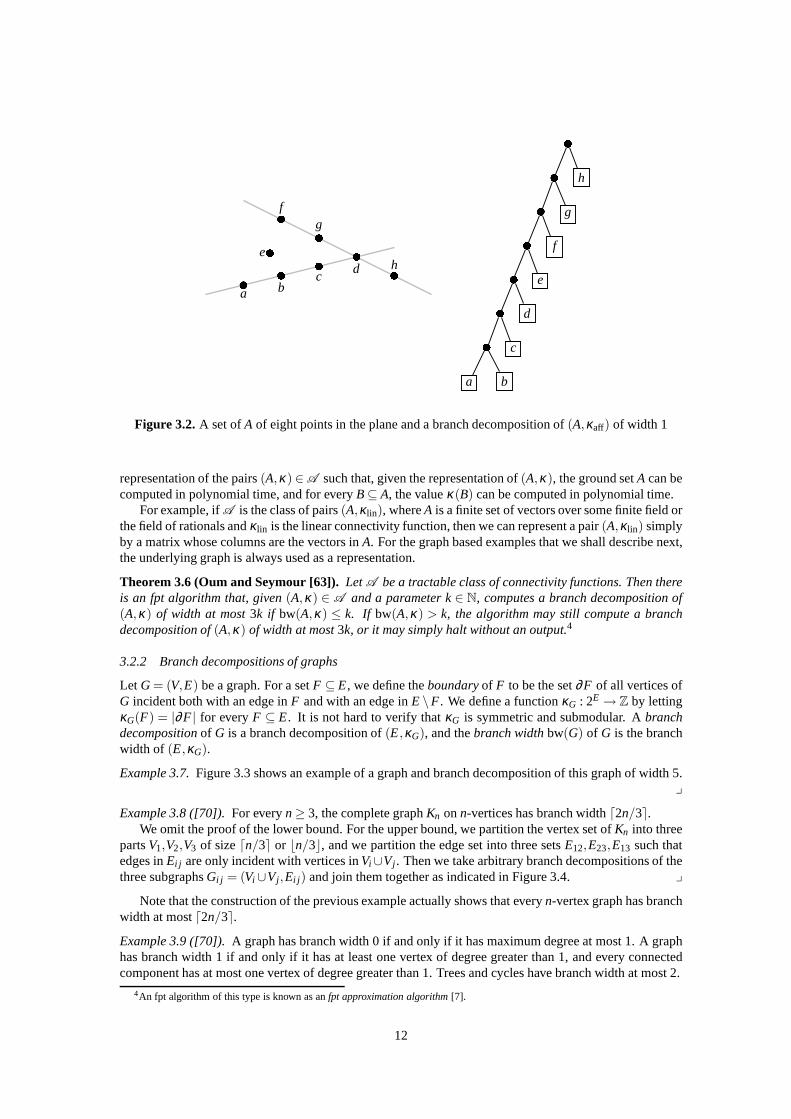
It is not hard to prove thatκaff is also symmetric and submodular.Figure 3.2 shows an example of a setA = a,b,c,d,e, f ,g,h ⊆ R2 and a branch decomposition of
(A,κaff) of width 1. y
Example 3.5.The previous two examples have a common generalisation, which is known as the branchwidth of matroids.2 Let M be a matroid with base setA and rank functionrM. Then the functionκ : 2A →Z
defined byκM(B) = rM(B)+ rM(A\B)− rM(A)
is known as theconnectivity functionof the matroid.3 Obviously,κM is symmetric, and as the rank functionrM is submodular,κM is also submodular. y
Before we return to graphs, let us state a very general algorithmic result, which shows that approxi-mately optimal branch decompositions can be computed by an fpt algorithm. The proof of this theorem isbeyond the scope of this survey. It is based on a deep algorithm for minimizing submodular functions dueto Iwata, Fleischer, and Fujishige [52].
When talking about algorithms for branch decompositions, we have to think about how the input ofthese algorithms is specified. LetA be a class of pairs(A,κ), whereκ : 2A →Z is symmetric and submod-ular and takes only nonnegative values. We callA a tractable class of connectivity functions, if we have a
2Readers who do not know anything about matroids should not worry. This example is the only place in this survey where theyappear.
3Often, the connectivity function is defined byκM(B) = rM(B)+ rM(A\B)− rM(A)+1, but this difference is inessential here.
11
a bc
de
fg
h
a b
c
d
e
f
g
h
Figure 3.2. A set ofA of eight points in the plane and a branch decomposition of(A,κaff) of width 1
representation of the pairs(A,κ) ∈ A such that, given the representation of(A,κ), the ground setA can becomputed in polynomial time, and for everyB⊆ A, the valueκ(B) can be computed in polynomial time.
For example, ifA is the class of pairs(A,κlin), whereA is a finite set of vectors over some finite field orthe field of rationals andκlin is the linear connectivity function, then we can represent apair(A,κlin) simplyby a matrix whose columns are the vectors inA. For the graph based examples that we shall describe next,the underlying graph is always used as a representation.
Theorem 3.6 (Oum and Seymour [63]). LetA be a tractable class of connectivity functions. Then thereis an fpt algorithm that, given(A,κ) ∈ A and a parameter k∈ N, computes a branch decomposition of(A,κ) of width at most3k if bw(A,κ) ≤ k. If bw(A,κ) > k, the algorithm may still compute a branchdecomposition of(A,κ) of width at most3k, or it may simply halt without an output.4
3.2.2 Branch decompositions of graphs
Let G = (V,E) be a graph. For a setF ⊆ E, we define theboundaryof F to be the set∂F of all vertices ofG incident both with an edge inF and with an edge inE \F. We define a functionκG : 2E → Z by lettingκG(F) = |∂F | for everyF ⊆ E. It is not hard to verify thatκG is symmetric and submodular. Abranchdecompositionof G is a branch decomposition of(E,κG), and thebranch widthbw(G) of G is the branchwidth of (E,κG).
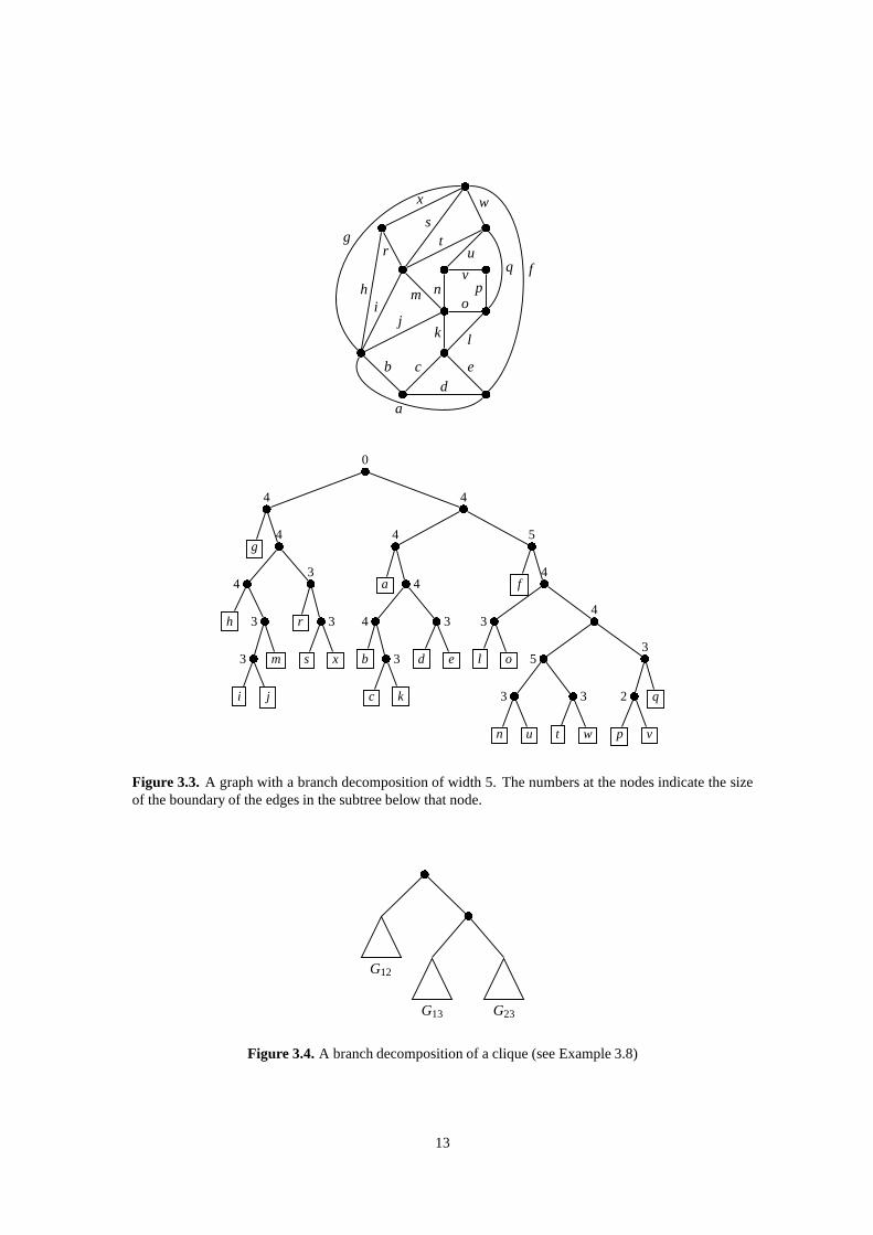
Example 3.7.Figure 3.3 shows an example of a graph and branch decomposition of this graph of width 5.y
Example 3.8 ([70]).For everyn≥ 3, the complete graphKn onn-vertices has branch widthd2n/3e.We omit the proof of the lower bound. For the upper bound, we partition the vertex set ofKn into three
partsV1,V2,V3 of sizedn/3e or bn/3c, and we partition the edge set into three setsE12,E23,E13 such thatedges inEi j are only incident with vertices inVi ∪Vj . Then we take arbitrary branch decompositions of thethree subgraphsGi j = (Vi ∪Vj ,Ei j ) and join them together as indicated in Figure 3.4. y
Note that the construction of the previous example actuallyshows that everyn-vertex graph has branchwidth at mostd2n/3e.
Example 3.9 ([70]).A graph has branch width 0 if and only if it has maximum degree at most 1. A graphhas branch width 1 if and only if it has at least one vertex of degree greater than 1, and every connectedcomponent has at most one vertex of degree greater than 1. Trees and cycles have branch width at most 2.
4An fpt algorithm of this type is known as anfpt approximation algorithm[7].
12
db c
f
e
h
ji
k l
m no
p
qr
st
v
u
wx
a
g
0
4
g4
4
h 3
3
i j
m
3
r3
s x
4
4
a4
4
b3
c k
3
d e
5
f4
3
l o
4
5
3
n u
3
t w
!3
2"
p v
q
Figure 3.3. A graph with a branch decomposition of width 5. The numbers atthe nodes indicate the sizeof the boundary of the edges in the subtree below that node.
#
G12
$
G13 G23
Figure 3.4. A branch decomposition of a clique (see Example 3.8)
13
G2×2
G3×3
G4×4
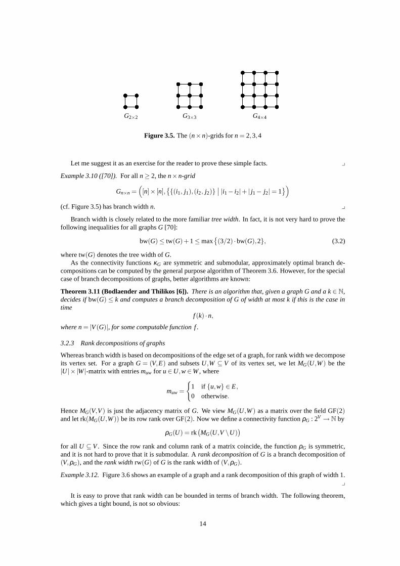
Figure 3.5. The(n×n)-grids forn = 2,3,4
Let me suggest it as an exercise for the reader to prove these simple facts. y
Example 3.10 ([70]).For all n≥ 2, then×n-grid
Gn×n =([n]× [n],
(i1, j1),(i2, j2)
∣∣ |i1− i2|+ | j1− j2| = 1)
(cf. Figure 3.5) has branch widthn. y
Branch width is closely related to the more familiartree width. In fact, it is not very hard to prove thefollowing inequalities for all graphsG [70]:
bw(G) ≤ tw(G)+1≤ max(3/2) ·bw(G),2, (3.2)
where tw(G) denotes the tree width ofG.As the connectivity functionsκG are symmetric and submodular, approximately optimal branch de-
compositions can be computed by the general purpose algorithm of Theorem 3.6. However, for the specialcase of branch decompositions of graphs, better algorithmsare known:
Theorem 3.11 (Bodlaender and Thilikos [6]). There is an algorithm that, given a graph G and a k∈ N,decides ifbw(G) ≤ k and computes a branch decomposition of G of width at most k ifthis is the case intime
f (k) ·n,
where n= |V(G)|, for some computable function f .
3.2.3 Rank decompositions of graphs
Whereas branch width is based on decompositions of the edge set of a graph, for rank width we decomposeits vertex set. For a graphG = (V,E) and subsetsU,W ⊆ V of its vertex set, we letMG(U,W) be the|U |× |W|-matrix with entriesmuw for u∈U,w∈W, where
muw =
1 if u,w ∈ E,
0 otherwise.
HenceMG(V,V) is just the adjacency matrix ofG. We viewMG(U,W) as a matrix over the field GF(2)and let rk(MG(U,W)) be its row rank over GF(2). Now we define a connectivity functionρG : 2V → N by
ρG(U) = rk(MG(U,V \U)
)
for all U ⊆ V. Since the row rank and column rank of a matrix coincide, the functionρG is symmetric,and it is not hard to prove that it is submodular. Arank decompositionof G is a branch decomposition of(V,ρG), and therank widthrw(G) of G is the rank width of(V,ρG).
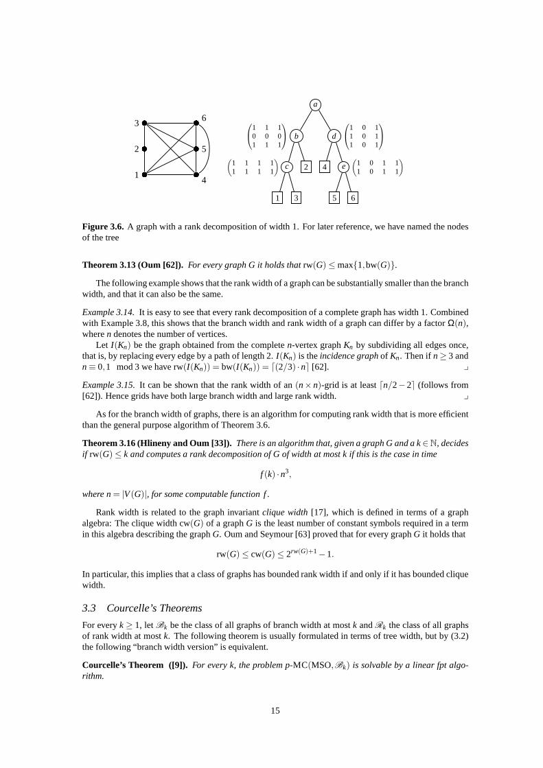
Example 3.12.Figure 3.6 shows an example of a graph and a rank decomposition of this graph of width 1.y
It is easy to prove that rank width can be bounded in terms of branch width. The following theorem,which gives a tight bound, is not so obvious:
14
1
2
3
4
5
6
a
1 1 10 0 01 1 1
b
(1 1 1 11 1 1 1
)c
1 3
2
d
1 0 11 0 11 0 1
4 e(
1 0 1 11 0 1 1
)
5 6
Figure 3.6. A graph with a rank decomposition of width 1. For later reference, we have named the nodesof the tree
Theorem 3.13 (Oum [62]). For every graph G it holds thatrw(G) ≤ max1,bw(G).
The following example shows that the rank width of a graph canbe substantially smaller than the branchwidth, and that it can also be the same.
Example 3.14.It is easy to see that every rank decomposition of a complete graph has width 1. Combinedwith Example 3.8, this shows that the branch width and rank width of a graph can differ by a factorΩ(n),wheren denotes the number of vertices.
Let I(Kn) be the graph obtained from the completen-vertex graphKn by subdividing all edges once,that is, by replacing every edge by a path of length 2.I(Kn) is theincidence graphof Kn. Then ifn≥ 3 andn≡ 0,1 mod 3 we have rw(I(Kn)) = bw(I(Kn)) = d(2/3) ·ne [62]. y
Example 3.15.It can be shown that the rank width of an(n×n)-grid is at leastdn/2−2e (follows from[62]). Hence grids have both large branch width and large rank width. y
As for the branch width of graphs, there is an algorithm for computing rank width that is more efficientthan the general purpose algorithm of Theorem 3.6.
Theorem 3.16 (Hlineny and Oum [33]). There is an algorithm that, given a graph G and a k∈N, decidesif rw(G) ≤ k and computes a rank decomposition of G of width at most k if this is the case in time
f (k) ·n3,
where n= |V(G)|, for some computable function f .
Rank width is related to the graph invariantclique width[17], which is defined in terms of a graphalgebra: The clique width cw(G) of a graphG is the least number of constant symbols required in a termin this algebra describing the graphG. Oum and Seymour [63] proved that for every graphG it holds that
rw(G) ≤ cw(G) ≤ 2rw(G)+1−1.
In particular, this implies that a class of graphs has bounded rank width if and only if it has bounded cliquewidth.
3.3 Courcelle’s Theorems
For everyk ≥ 1, letBk be the class of all graphs of branch width at mostk andRk the class of all graphsof rank width at mostk. The following theorem is usually formulated in terms of tree width, but by (3.2)the following “branch width version” is equivalent.
Courcelle’s Theorem ([9]). For every k, the problem p-MC(MSO,Bk) is solvable by a linear fpt algo-rithm.
15

As for Theorem 3.1, we sketch two proofs. The first is a reduction to Theorem 3.1, whereas the secondis a generalisation of the second proof of Theorem 3.1.
First proof sketch.Let us fix k ≥ 1. We reduce the model checking problem on the classBk to that onlabelled trees and then apply Theorem 3.1. We associate witheach graphG ∈ Bk a labelled treeT+ andwith each MSO-sentenceϕ over graphs a sentenceϕ+ over labelled trees such thatG |= ϕ ⇐⇒ T+ |= ϕ+.We will do this in such a way thatT+ is computable fromG in linear time and thatϕ+ is computable fromϕ . Then our model checking algorithm proceeds as follows: GivenG∈Bk andϕ ∈ MSO, it computesT+
andϕ+ and then tests ifT+ satisfiesϕ+ using the algorithm of Theorem 3.1.The mappingG 7→ T+ will not be canonical, i.e., isomorphic graphsG will not necessarily yield iso-
morphic treesT+. The treeT+ will depend on the specific representation of the input graphG and on thealgorithm we use to compute a branch decomposition of this input graph. Note that this does not affect thecorrectness of our algorithm.
We constructT+ from G as follows: Without loss of generality we assume thatG has no isolatedvertices. We first compute a branch decomposition(T,β ) of G of width at mostk, which can be done inlinear time by Theorem 3.11. Then we define a labelling ofT that allows us to reconstructG from thelabelled treeT+ within MSO. Formally, we define the labelling in such a way thatG is MSO-interpretablein T+. Then we can constructϕ+ from ϕ using the method of syntactic interpretations (see [32, 12]).
We assume thatT is an ordered binary tree, that is, each inner node has a left and a right child. Recallthat, for a nodet of T, β (t) is the set of all edgese of G such thate = β (u) for some leafu of T thatappears in the subtree rooted att. Let Bt = ∂ β (t) be the boundary ofβ (t), that is, the set of all verticesincident with an edge inβ (t) and with an edge inE(G) \ β(t). Since the width of(T,β ) is at mostk wehave|Bt | ≤ k for all nodest. The labelling of the treeT+ encodes for every inner nodet with left child t1and right childt2 how Bt intersects the setsBt1 andBt2. We assume some linear order of the vertices ofG.Then there will be labelsP1i j , for i, j ∈ [k], indicating that theith vertex inBt1 is equal to thejth vertex inBt , and similarly labelsP2i j for t2. Note thatBt ⊆ Bt1 ∪Bt2, so these labels “determine”Bt . We do not labelthe leaves.
For each leaft, the setBt consists of the two endpoints of the edgeβ (t) (unless one or both endpointshave degree 1). It is easy to write down four MSO-sentenceseqi j (x,y), for i, j ∈ 0,1, such that for allleavesu,t of T we haveT+ |= eqi j (u,v) if and only if theith vertex inBu is equal to thejth vertex inBt .Recalling our assumption thatG has no isolated vertices, it is now easy to reconstructG from T+ withinMSO.
Second proof sketch.Let G be a graph of branch widthk, and letϕ be an MSO-sentence, say, of quantifierrank q. We compute a branch decomposition(T,β ) of G of width k. We fix some linear order on thevertices ofG. For everyt ∈V(T) we let bt be the ordered tuple of the elements of∂ β (t). Recall that for asubsetB⊆ E(G), by GJBK we denote the subgraph(
⋃B,B) generated byB.
Starting from the leaves we inductively compute tpq(GJβ (t)K, bt) for all t ∈V(T), applying Lemma 2.3at every node. For this to work, it is important that for all nodest with childrent1 andt2 it holds that
V(GJβ (t1)K∩GJβ (t2)K
)⊆ ∂ β (t1)∪∂ β(t2)
and∂ β (t) ⊆ ∂ β (t1)∪∂ β(t2).
Finally, we check ifϕ ∈ tpq(GJβ (r)K, br) for the rootr. (Note thatbr is actually the empty tuple, but thisdoes not matter.)
The following theorem was first proved by Courcelle [8, 11] ina version phrased in terms of certaingraph grammars. Later, a version for clique width was provedby Courcelle, Makowsky, and Rotics [14],and finally the relation between clique width and rank width was established by Oum and Seymour [63].
Theorem 3.17 ([8, 11, 14, 63]). For every k, p-MC(MSO,Rk) is solvable by a cubic fpt algorithm.
Proof sketch.The proof follows the same strategy as the first proof of Courcelle’s Theorem: We fixk. Forevery graphG∈Rk we construct a labelled treeT∗ such thatG can be reconstructed fromT∗ within MSO.Then using the method of syntactic interpretations, for every MSO-sentenceϕ over graphs we obtain anMSO-sentenceϕ∗ over labelled trees such thatG |= ϕ ⇐⇒ T∗ |= ϕ∗.
16
T∗ is obtained by suitably labelling the treeT of a rank decomposition(T,β ) of G of width k. Thedifficulty here is to encodeG in a labelling ofT that uses only finitely many labels. Lett be an inner nodeof T with childrent1 andt2. For i = 1,2, letUi = β (ti). Furthermore, letU =U1∪U2 andW =V \U . Thenβ (t) = U , and the matrices at the nodest1,t2,t can be written as
M(U1,V \U1) =(M(U1,U2) M(U1,W)
),
M(U2,V \U2) =(M(U2,U1) M(U2,W)
),
M(U,V \U) =
(M(U1,W)M(U2,W)
).
Note thatM(U2,U1) is the transpose ofM(U1,U2). (We omit the subscriptG for the matricesMG(·, ·).)For every nodet ∈V(T) we compute a setBt of at mostk vertices ofG such that the rows corresponding
to the vertices inBt form a basis of the row space of the matrixM(U,V \U), whereU = β (t). We define alabelling of the (inner) nodes ofT as follows: Lett be an inner node with childrent1 andt2 andU1 = β (t1),U2 = β (t2), U = U1∪U2 = β (t). Then att the labelling encodes
• the matrixM(Bt1,Bt2),
• for i = 1,2 and eachv∈ Bti a representation of the row ofM(U,V \U) corresponding tov as a linearcombination of vectors of the basis corresponding toBt over the field GF(2).
Note that this amounts to at most 3k2 bits of information: The matrix requires at mostk2 bits, and a linearcombination ofk vectors over GF(2) requiresk bits.
We now describe how the graphG can be reconstructed from the labelled treeT∗. The vertices ofG correspond to the leaves ofT∗. To find out whether there is an edge between a vertexv1, say, withv1 = β (u1) and a vertexv2, say withv2 = β (u2), we proceed as follows: Lett be the first common ancestorof u1 and u2, and lett1 and t2 be the children oft such thatui is a descendant ofti , for i = 1,2. LetUi = β (ti) andU = U1∪U2 = β (t). Thenvi ∈Ui . Note thatBui = vi, because the matrices at the leavesonly have one row. Hence, using the labelling, we can recursively find a representation of the row of thematrixM(Ui ,V \Ui) corresponding tovi as a linear combination of the rows corresponding toBti . Then wecan use the matrixM(Bt1,Bt2), which is also part of the labelling, to compute the entrymv1v2 of the matrixM(U1,U2), and this entry tells us whether there is an edge betweenv1 andv2. The following exampleillustrates this construction.
Example 3.18.Consider the graphG and branch decomposition displayed in Figure 3.6. We define the“bases” as follows:
t 1 2 3 4 5 6 a b c d eBt 1 2 3 4 5 6 /0 1 1 4 5
Then for example, at nodeb the following information is stored: The matrix
M(1,2) = (1),
and a representation of the rowsr1 = (1 1 1) andr2 = (0 0 0) of the matrixM(1,2,3,4,5,6) in termsof the rowr1:
r1 = 1 · r1, r2 = 0 · r1.
To determine whether there is an edge, say, between betweenv1 = 3 andv2 = 5 we take the least commonancestor of the two leaves,a with its two childrenb andd. The representation of rowr3 = (1 1 1) ofM(1,2,3,4,5,6) with respect toBb = 1 is r3 = 1 · r1, and the representation of rowr5 = (1 0 1) ofM(4,5,6,1,2,3) with respect toBd = 4 is r5 = 1· r4. Hencem35 = 1·1·m14 = 1, that is, there is anedge between 3 and 5. y
It follows from Theorem 3.2 that the parameter dependence ofthe fpt algorithms in the previous twotheorems has to be nonelementary.
We close this section with two remarks about strengtheningsof the two theorems:
17
Remark 3.19.Our proofs yield stronger theorems than stated: Not only is the MSO model checking prob-lem fixed-parameter tractable on every class of graphs whosebranch width is bounded, but actually thefollowing doubly parameterized model checking problem is fixed-parameter tractable:
Instance: A sentenceϕ ∈ MSO and a graphG.Parameter: |ϕ |+bw(G).
Problem: Decide ifG |= ϕ .
The same is true for rank width. y
Remark 3.20.It is easy to see that both theorems can be extended to labelled graphs.Courcelle’s Theorem even holds for a stronger monadic second order logic, denoted by MSO2, that
admits quantification not only over sets of vertices of a graph, but also over sets of edges. This strongerresult can easily be derived from the (labelled) version of Courcelle’s Theorem. Define theincidence graphI(G) of a graphG to be the graph(VI ,EI ), whereVI =V(G)∪E(G) andEI =
v,e
∣∣ v∈ e
. It is not hardto see that for every graphG of branch width at least 2 it holds that bw(G) = bw(I(G)). Furthermore, everyMSO2-formula overG can be translated to an MSO-formula over the labelled incidence graph(I(G),P),whereP = E(G) (The labelling is not really needed, but convenient.) Henceit follows from Courcelle’sTheorem thatp-MC(MSO2,Bk) has a linear fpt algorithm for everyk≥ 1.
This does not work for rank width, because the rank width of the incidence graph can be much largerthan that of the original graph. Surprisingly, the rank width of the incidence graph of a graph is closelyrelated to the branch width of the original graph. Oum [62] proved that
bw(G)−1≤ rw(I(G)) ≤ bw(G)
for every graphG with at least one vertex of degree 2. y
4 First-order logic on locally tree-like classes of graphs
There is not much hope for extending the tractability of monadic second-order model checking to furthernatural classes of graphs such as planar graphs or graphs of bounded degree. Indeed, the MSO-definable3-colourability problem is NP-complete even when restricted to planar graphs of degree 4. For first-orderlogic, however, the model checking problem is tractable on much larger classes of graphs. Seese [75]showed that first-order model checking admits a linear fpt algorithm on all classes of bounded degree.Later Frick and Grohe [43] proved the same for planar graphs,essentially by the general approach that weshall describe in this section. The crucial property of first-order logic that we exploit is itslocality.
4.1 The Locality of First-Order Logic
Let G = (V,E) be a graph. ThedistancedistG(v,w) between two verticesv,w ∈ V is the length of theshortest path fromv to w. For everyv∈V andr ∈ N, ther-neighbourhoodof v in G is the set
NGr (v) = w∈V | distG(v,w) ≤ r
of all vertices of distance at mostr from v. For a setW ⊆V, we letNGr (W) =
⋃w∈W NG
r (w). We omit thesuperscriptG if G is clear from the context. Theradiusof a connected graphG is the leastr for which thereis a vertexv∈V(G) such thatV(G) ⊆ Nr(v). The radius of a disconnected graph is∞.
Observe that distance is definable in first-order logic, thatis, for everyr ≥ 0 there is a first-order formuladist≤r(x,y) such that for all graphsG andv,w∈V(G),
G |= dist≤r(v,w) ⇐⇒ dist(v,w) ≤ r.
In the following, we will writedist(x,y)≤ r instead ofdist≤r(x,y) anddist(x,y) > r instead of¬dist≤r(x,y).A first-order formulaϕ(x1, . . . ,xk) is r-local if for every graphG and allv1, . . . ,vk ∈V(G) it holds that
G |= ϕ(v1, . . . ,vk) ⇐⇒ G[Nr(v1, . . . ,vk)
]|= ϕ(v1, . . . ,vk).
18

This means that it only depends on ther-neighbourhood of a vertex tuple whether anr-local formula holdsat this tuple. A formula islocal if it is r-local for somer.
A basic local sentenceis a first-order sentence of the form
∃x1 . . .∃xk
(∧
1≤i< j≤k
dist(xi ,x j) > 2r ∧k∧
i=1
ϕ(xi)
),
whereϕ(x) is r-local. In particular, for every local formulaϕ(x) the sentence∃x ϕ(x) is a basic localsentence.
Gaifman’s Locality Theorem ([45]). Every first-order sentence is equivalent to a Boolean combinationof basic local sentences.
Furthermore, there is an algorithm that computes a Boolean combination of basic local sentencesequivalent to a given first-order sentence.
We shall illustrate the following proof sketch in Example 4.1 below. To appreciate the cleverness of theproof, the reader may try to find a Boolean combination of basic local sentences equivalent to the simplesentenceϕ = ∃x∃y
(¬E(x,y)∧P(x)∧Q(y)
)considered in the example before reading the proof.
Proof sketch.The proof is by structural induction on first-order formulas. To enable this induction, weneed to prove a stronger statement that also includes formulas with free variables. We say that a first-orderformula is inGaifman normal form (GNF)if it is a Boolean combination of basic local sentences and localformulas.
Claim: Every first-order formula is equivalent to a formula in GNF.
The claim is trivial for atomic formulas, because all atomicformulas are 0-local. It obviously extendsto Boolean combinations of formulas. Universal quantification can be reduced to existential quantficationand negation. The only remaining case is that of existentially quantified formulas
ϕ(x) = ∃y ψ(x,y),
whereψ(x,y) is in GNF. We may assume thatψ(x,y) is of the form
m∨
i=1
(χi ∧ξi(x,y)
),
where eachχi is a Boolean combination of basic local sentences and eachξi(x,y) is local. Here we use thesimple observation that a Boolean combination of local formulas is local. Thenϕ(x) is equivalent to theformula
m∨
i=1
(χi ∧∃y ξi(x,y)
).
It remains to prove that each formulaϕ ′(x) = ∃y ξ (x,y),
whereξ (x,y) is local, is equivalent to a formula in GNF. Letr ≥ 0 such thatξ (x,y) is r-local. We observethatϕ ′(x) is equivalent to the formula
∃y(dist(x,y) ≤ 2r +1∧ξ (x,y)
)∨∃y
(dist(x,y) > 2r +1∧ξ (x,y)
), (4.1)
wheredist(x,y) ≤ 2r + 1 abbreviates∨
i dist(xi ,y) ≤ 2r + 1. The first formula in the disjunction (4.1)is (3r + 1)-local. Hence we only need to consider the second,∃y
(dist(x,y) > 2r + 1∧ ξ (x,y)
). Using
Lemma 2.3 and ther-locality of ξ (x,y), it is not hard to see that this formula is equivalent to a Booleancombination of formulas of the form
ζ (x)∧∃y(dist(x,y) > 2r +1∧η(y)
),
19

whereζ (x) andη(y) arer-local. Letr ′ = 2r +1. It remains to prove that
ϕ ′′(x) = ∃y(dist(x,y) > r ′∧η(y)
)
is equivalent to a formula in GNF. This is the core of the wholeproof. Suppose that ¯x = (x1, . . . ,xk).Let G be a graph and ¯v = (v1, . . . ,vk) ∈ V(G)k. When doesG |= ϕ ′′(v) hold? Clearly, it holds if thereare w1, . . . ,wk+1 of pairwise distance greater than 2r ′ such thatG |= η(wj) for all j, because eachr ′-neighbourhoodNr ′(vi) contains at most onewj and hence there is at least onewj of distance greater thanr ′ from all thevi . For` ≥ 1, let
θ` = ∃y1 . . .∃y`
( ∧
1≤i< j≤`
dist(yi ,y j) > 2r ′∧η(yi)).
Note thatθ` is a basic local sentence. We have just seen thatθk+1 implies ϕ ′′(x). But of courseϕ ′′(x)may also hold ifθk+1 does not. Let us return to our graphG and the tuple ¯v ∈ V(G)k. Let ` ≥ 1 bemaximum such thatG |= θ` and suppose that` ≤ k. In the following case distinction, we shall determinewhenG |= ϕ ′′(v).
Case 1: There are now1, . . . ,w` ∈ Nr ′(v) of pairwise distance greater than 2r ′ such thatG |= η(wj )for all j.
As G |= θ`, this implies that there is at least onew 6∈ Nr ′(v) such thatG |= η(w). HenceG |= ϕ ′′(v).
Case 2: There is aw∈ N3r ′(v) such thatw 6∈ Nr ′(v) andG |= η(w).Then, trivially,G |= ϕ ′′(v).
Case 3:Neither Case 1 nor Case 2, that is, there arew1, . . . ,w` ∈ Nr ′(v) of pairwise distance greaterthan 2r ′ such thatG |= η(wj ) for all j, and there is now∈ N3r ′(v)\Nr ′(v) such thatG |= η(w).
ThenG 6|= ϕ ′′(v). To see this, suppose for contradiction that there is aw∈V(G) such thatw 6∈ Nr ′(v)andG |= η(w). Thenw 6∈ N3r ′(v) and therefore dist(wj ,w) > 2r ′ for all j ∈ [`]. ThusG |= θ`+1, whichcontradicts the maximality of.
HenceG |= ϕ ′′(v) if any only if we are in Case 1 or 2. Note that the conditions describing these casescan be defined by local formulas, say,γ`,1(x) andγ`,2(x). Thus if G |= θ` ∧¬θ`+1, thenG |= ϕ ′′(v) if andonly if G |= γ`,1(v)∨ γ`,2(v).
Overall,ϕ ′′(x) is equivalent to the formula
θk+1∨k∨
`=1
(θ` ∧¬θ`+1∧
(γ`,1(x)∨ γ`,2(x)
)),
which is in GNF. It is not hard to show that our construction yields an algorithm that computes a formulain GNF equivalent to a given first-order formula.
Example 4.1.Let us follow the proof of Gaifman’s theorem and construct a Boolean combination of basiclocal sentences equivalent to the sentence
ϕ = ∃x∃y(¬E(x,y)∧P(x)∧Q(y)
),
which is a sentence over labelled graphs with labelsP andQ.The quantifier free formulaϕ0(x,y) =
(¬E(x,y)∧P(x)∧Q(y)
)is 0-local. Hence we start the construc-
tion with the formulaϕ1(x) = ∃y
(¬E(x,y)∧P(x)∧Q(y)
).
ϕ1(x) is equivalent to the formula
ϕ ′1 = P(x)∧∃y
(¬E(x,y)∧Q(y)
).
Splitting ∃y(¬E(x,y)∧Q(y)
)with respect to the distance betweenx andy as in (4.1) (withr = 0) and
simplifying the resulting formula, we obtain
P(x)∧(
Q(x)∨∃y(dist(x,y) > 1∧Q(y)
)).
20
It remains to consider the formulaϕ ′′1 (x) = ∃y
(dist(x,y) > 1∧Q(y)
). Following the proof of Gaifman’s
theorem (withϕ ′′ = ϕ ′′1 , η(y) = Q(y), r = 0, andk = 1), we obtain the following equivalent formula in
GNF:
ϕ ′′′1 (x) = θ2∨
(θ1∧¬θ2∧
(¬∃y(dist(x,y) ≤ 1∧Q(y))
∨∃y(dist(x,y) ≤ 3∧dist(x,y) > 1∧Q(y))))
whereθ1 = ∃y1Q(y1) andθ2 = ∃y1∃y2(dist(y1,y2) > 2∧Q(y1)∧Q(y2)
). Henceϕ1(x) is equivalent to
the formulaP(x)∧(Q(x)∨ϕ ′′′
1 (x)). The step fromϕ1(x) to ϕ = ∃xϕ1(x) is simple, because there are no
free variables left. By transforming the formulaP(x)∧(Q(x)∨ϕ ′′′
1 (x))
into disjunctive normal form andpushing the existential quantfier inside, we obtain the formula:
∃x(P(x)∧Q(x)
)
∨(∃x P(x)∧θ2
)
∨(∃x(P(x)∧¬∃y(dist(x,y) ≤ 1∧Q(y))
)∧θ1∧¬θ2
)
∨(∃x(P(x)∧∃y(dist(x,y) ≤ 3∧dist(x,y) > 1∧Q(y))
)∧θ1∧¬θ2
).
Observe that this is indeed a Boolean combination of basic local sentences equivalent toϕ . A slightlysimpler Boolean combination of basic local sentences equivalent toϕ is constructed in Example 3 of [51]by a different technique. y
It has recently been proved in [20] that the translation of a first-order sentence into a Boolean combi-nation of basic local sentences may involve a nonelementaryblow-up in the size of the sentence.
4.2 Localisations of graph invariants
Recall thatG denotes the class of all graphs. For every graph invariantf : G → N we can define itslocalisation` f : G ×N → N by
` f (G, r) = max
f(G[Nr(v)]
) ∣∣∣ v∈V(G)
.
Hence to computef (G, r), we apply f to everyr-neighbourhood inG and then take the maximum. Wesay that a classC of graphs haslocally bounded fif there is a computable5 functiong : N → N such that` f (G, r) ≤ g(r) for all G∈ C and allr ∈ N.
Example 4.2.One of the simplest graph invariants is the order of a graph. Observe that a class of graphshas locally bounded order if and only if it has bounded degree.
Moreover, if a classC has bounded degree then it has locally boundedf for every computable graphinvariant f . y
In this section, we are mainly interested in the localisation of branch width. Maybe surprisingly, thereare several natural classes of graphs of locally bounded branch width. We start with two trivial examplesand then move on to more interesting ones:
Example 4.3.Every class of graphs of bounded branch width has locally bounded branch width. y
Example 4.4.Every class of graphs of bounded degree has locally bounded branch width. This followsimmediately from Example 4.2. y
Example 4.5 ([68, 76]).The class of planar graphs has locally bounded branch width.More precisely, aplanar graph of radiusr has branch width at most 2r +1.
Let me sketch the proof. LetG be a planar graph of radiusr, and letv0 be a vertex such thatV(G) ⊆Nr(v0). We show how to recursively partition the edge set ofG in such a way that at each stage, the
21

v0
v
w
C
P
Q
A
B
A B
(a) The graph is cut alongPQ
v0
v
w
x
P
Q
R
B1
B2
A
B1 B2
(b) PartB is cut again alongR
v0
w
x
Q
R
e
A
B1
e
B2\ e(c) Edgee= w,x is split off partB2
Figure 4.1. Schematic branch decomposition of a planar graph
22

boundary of each part has cardinality at most 2r +1. This will give us a branch decomposition of width atmost 2r +1.
Without loss of generality we may assume thatG is 2-connected; if it is not, we first decompose it intoits 2-connected blocks. Figure 4.1 illustrates the following steps. We fix a planar embedding ofG, and letC be the exterior cycle. We pick two verticesv,w onC and shortest pathsP,Q from v0 to v,w, respectively.Then we cut alongP andQ. This gives us a partition ofE(G) into two parts whose boundary is containedin V(P∪Q). We can add the edges inE(P∪Q) arbitrarily to either of the two parts. Now we consider eachof the parts separately. The boundary cycle consists ofP, Q, and a piece of the cycleC. If this piece ofCis just one edge, we can split it off and then further decompose the rest. Otherwise, we pick a vertexx onthe piece ofC and a shortest pathR from v0 to x. We obtain two new parts with boundariesV(P∪R) andV(Q∪R). We partition these new parts recursively until they only consist of their boundaries, and then wepartition the rest arbitrarily. Of course this proof sketchomits many details and special cases. For example,the vertexv0 could be on the exterior cycle to begin with. I leave it to the reader to work out these details.
The branch decomposition in Figure 3.3 was obtained by this method. Note that the graph has radius2, with centrev0 being the vertex incident with the edgesm and j. The initial pathsP andQ have edgesetsE(P) = s,m andE(Q) = j. The right part consists of the edgesa,b,c,k,d,e, f , l ,o,n,u,t,w, p,v,q.The edges ofP∪Q were added to the left part. In the next step, the right part was split along the pathR with E(R) = k,e. The right part of this split consists of the edgesf , l ,o,n,u,t,w, p,v,q. The edgefimmediately can be split off, and the new boundary cycle isw,q, l ,k,m,s. The new splitting path consistsof the edgeo, et cetera. y
Example 4.6 ([35]).Thegenusof a graph is the minimum genus of an orientable or nonorientable surfacethe graph can be embedded into. For everyk, the class of all graphs of genus at mostk has locally boundedbranch width. Moreover, for everyk the class of all graphs ofcrossing numberat mostk has locallybounded branch width. y
In the next example, we shall construct an artificial class ofgraphs of locally bounded branch width.It serves as an illustration that the global structure of graphs of locally bounded branch width can be quitecomplicated. In particular, this example shows that there are classes of graphs of locally bounded branchwidth and of unbounded average degree. Recall that if a classC of graphs has unbounded average degreethen the size of the graphs inC is superlinear in their order. The graph classes in all previous exampleshave bounded average degree and thus size linear in the order. For planar graphs and graphs of boundedgenus, this follows from Euler’s formula.
Example 4.7 ([43]).Recall that thegirth of a graph is the length of its shortest cycle, and thechromaticnumberis the least number of colours needed to colour the graph in such a way that no two adjacent verticesreceive the same colour. We shall use the well-known fact, due to Erdos [36], that for allg,k≥ 1 there existgraphs of girth greater thang and chromatic number greater thank. The proof of this fact (see [2]) showsthat we can effectively construct such a graphGg,k for giveng andk.
Then for everyk≥ 1, every graphGk,k must have a subgraphHk of minimum degree at leastk; otherwisewe could properly colourGwith k colours by a straightforward greedy algorithm (see [25], Corollary 5.2.3).Let Hk ⊆ Gk,k be such a subgraph. As a subgraph ofGk,k the graphHk still has girth greater thank.
Let C = Hk | k≥ 1. ThenC has unbounded minimum degree and hence unbounded average degree.Nevertheless,C has locally bounded branch width. To see this, simply observe that ther-neighbourhoodof every vertex in a graph of girth greater than 2r +1 is a tree. As the branch width of a tree is at most 2,for every graphH ∈ C and everyr ≥ 1 we have
`bw(H, r) ≤ max(
bw(Hk)∣∣ k≤ 2r +1
∪2
). y
4.3 Model checking algorithms
Theorem 4.8. Let f be a graph invariant such that the following parameterization of the model checkingproblem for first-order logic is fixed-parameter tractable:
5It would be more precise to call this notion “effectively locally boundedf ”, but this would make the terminology even moreawkward.
23
p-MC(FO, f )Instance: A sentenceϕ ∈ FO and a labelled graphG.
Parameter: |ϕ |+ f (G).Problem: Decide ifG |= ϕ .
Then for every classC of graphs of locally bounded f , the problem p-MC(FO,C ) is fixed-parametertractable.
The proof of the theorem relies on Gaifman’s Locality Theorem and the following lemma:
Lemma 4.9 ([43]). Let f andC be as in Theorem 4.8. Then the following problem is fixed-parametertractable:
Instance: A labelled graphG = (V,E,P) ∈ Clb andk, r ∈ N.Parameter: k+ r.
Problem: Decide if there are verticesv1, . . . ,vk ∈ P such that dist(vi ,v j) > 2r for 1≤ i <j ≤ k.
For simplicity, we only prove the lemma for graph invariantsf that areinduced-subgraph-monotone,that is, for all graphsG and induced subgraphsH ⊆ G we havef (H) ≤ f (G). Note that both branch widthand rank width are induced-subgraph-monotone.
Proof sketch of Lemma 4.9.GivenG = (V,E,P) andk, r ∈ N, we first compute a maximal (with respect toinclusion) setS⊆ P of vertices of pairwise distance greater than 2r. If |S| ≥ k, then we are done.
Otherwise, we know thatP ⊆ N2r(S). Let H be the induced subgraph ofG with vertex setN3r(S).As |S| < k, the radius of each connected component ofH is at most(3r + 1) · k. Hence, becausef isinduced-subgraph-monotone,
f (H) ≤ ` f (G,(3r +1) ·k) ≤ g((3r +1) ·k),
whereg is a function witnessing thatC has locally boundedf .SinceP⊆ N2r(S) andV(H) = N3r(S), for all verticesv,w∈ P it holds that distG(v,w) > 2r if and only
if distH(v,w) > 2r. Hence it remains to check whetherH containsk vertices labelledP of pairwise distancegreater than 2r. This is equivalent to saying thatH satisfies the first-order sentence
∃x1 . . .∃xk
(∧
1≤i< j≤k
dist(xi ,x j) > 2r ∧k∧
i=1
P(xi)
).
We can use an fpt algorithm forp-MC(FO, f ) to check this.
Proof sketch of Theorem 4.8.Let G = (V,E) ∈ C andϕ ∈ FO. We first transformϕ into an equivalentBoolean combination of basic local sentences. Then we checkseparately for each basic local sentence inthis Boolean combination whether it is satisfied byG and use the results to determine whetherϕ holds.
So let us consider a basic local sentence
ψ = ∃x1 . . .∃xk
(∧
1≤i< j≤k
dist(xi ,x j) > 2r ∧k∧
i=1
χ(xi)
),
whereχ(x) is r-local. For each vertexv of G we check whetherG[Nr(v)] satisfiesχ(v) using an fptalgorithm forp-MC(FO, f ). We can do this within the desired time bounds becausef (G[Nr(v)])≤ ` f (G, r).If G[Nr(v)] satisfiesχ(v), we labelv by P. To determine whetherG satisfiesψ , we have to check whetherthe labelled graph(V,E,P) hask vertices inP of pairwise distance greater than 2r. By Lemma 4.9, this canbe done by an fpt algorithm.
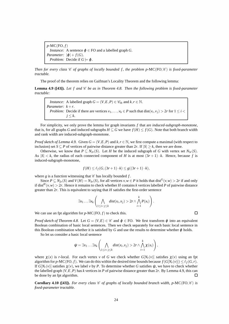
Corollary 4.10 ([43]). For every classC of graphs of locally bounded branch width, p-MC(FO,C ) isfixed-parameter tractable.
24
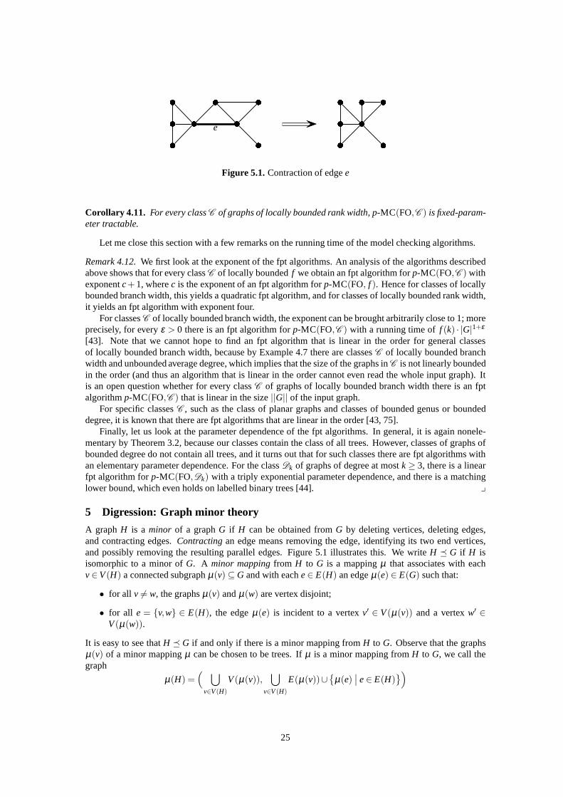
e
Figure 5.1. Contraction of edgee
Corollary 4.11. For every classC of graphs of locally bounded rank width, p-MC(FO,C ) is fixed-param-eter tractable.
Let me close this section with a few remarks on the running time of the model checking algorithms.
Remark 4.12.We first look at the exponent of the fpt algorithms. An analysis of the algorithms describedabove shows that for every classC of locally boundedf we obtain an fpt algorithm forp-MC(FO,C ) withexponentc+1, wherec is the exponent of an fpt algorithm forp-MC(FO, f ). Hence for classes of locallybounded branch width, this yields a quadratic fpt algorithm, and for classes of locally bounded rank width,it yields an fpt algorithm with exponent four.
For classesC of locally bounded branch width, the exponent can be broughtarbitrarily close to 1; moreprecisely, for everyε > 0 there is an fpt algorithm forp-MC(FO,C ) with a running time off (k) · |G|1+ε
[43]. Note that we cannot hope to find an fpt algorithm that is linear in the order for general classesof locally bounded branch width, because by Example 4.7 there are classesC of locally bounded branchwidth and unbounded average degree, which implies that the size of the graphs inC is not linearly boundedin the order (and thus an algorithm that is linear in the ordercannot even read the whole input graph). Itis an open question whether for every classC of graphs of locally bounded branch width there is an fptalgorithmp-MC(FO,C ) that is linear in the size||G|| of the input graph.
For specific classesC , such as the class of planar graphs and classes of bounded genus or boundeddegree, it is known that there are fpt algorithms that are linear in the order [43, 75].
Finally, let us look at the parameter dependence of the fpt algorithms. In general, it is again nonele-mentary by Theorem 3.2, because our classes contain the class of all trees. However, classes of graphs ofbounded degree do not contain all trees, and it turns out thatfor such classes there are fpt algorithms withan elementary parameter dependence. For the classDk of graphs of degree at mostk ≥ 3, there is a linearfpt algorithm forp-MC(FO,Dk) with a triply exponential parameter dependence, and there is a matchinglower bound, which even holds on labelled binary trees [44]. y
5 Digression: Graph minor theory
A graphH is a minor of a graphG if H can be obtained fromG by deleting vertices, deleting edges,and contracting edges.Contractingan edge means removing the edge, identifying its two end vertices,and possibly removing the resulting parallel edges. Figure5.1 illustrates this. We writeH G if H isisomorphic to a minor ofG. A minor mappingfrom H to G is a mappingµ that associates with eachv∈V(H) a connected subgraphµ(v) ⊆ G and with eache∈ E(H) an edgeµ(e) ∈ E(G) such that:
• for all v 6= w, the graphsµ(v) andµ(w) are vertex disjoint;
• for all e = v,w ∈ E(H), the edgeµ(e) is incident to a vertexv′ ∈ V(µ(v)) and a vertexw′ ∈V(µ(w)).
It is easy to see thatH G if and only if there is a minor mapping fromH to G. Observe that the graphsµ(v) of a minor mappingµ can be chosen to be trees. Ifµ is a minor mapping fromH to G, we call thegraph
µ(H) =( ⋃
v∈V(H)
V(µ(v)),⋃
v∈V(H)
E(µ(v))∪
µ(e)∣∣ e∈ E(H)
)
25
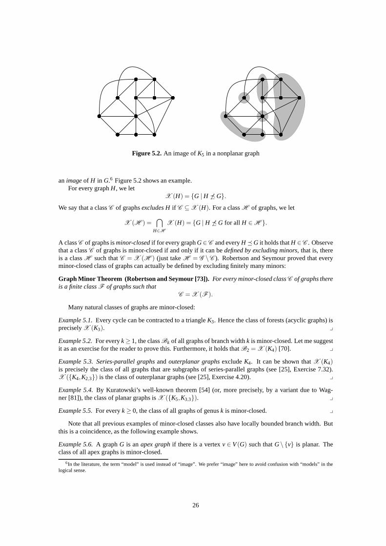
Figure 5.2. An image ofK5 in a nonplanar graph
an imageof H in G.6 Figure 5.2 shows an example.For every graphH, we let
X (H) = G | H 6 G.
We say that a classC of graphsexcludes Hif C ⊆ X (H). For a classH of graphs, we let
X (H ) =⋂
H∈H
X (H) = G | H 6 G for all H ∈ H .
A classC of graphs isminor-closedif for every graphG∈C and everyH G it holds thatH ∈C . Observethat a classC of graphs is minor-closed if and only if it can bedefined by excluding minors, that is, thereis a classH such thatC = X (H ) (just takeH = G \C ). Robertson and Seymour proved that everyminor-closed class of graphs can actually be defined by excluding finitely many minors:
Graph Minor Theorem (Robertson and Seymour [73]). For every minor-closed classC of graphs thereis a finite classF of graphs such that
C = X (F ).
Many natural classes of graphs are minor-closed:
Example 5.1.Every cycle can be contracted to a triangleK3. Hence the class of forests (acyclic graphs) ispreciselyX (K3). y
Example 5.2.For everyk≥ 1, the classBk of all graphs of branch widthk is minor-closed. Let me suggestit as an exercise for the reader to prove this. Furthermore, it holds thatB2 = X (K4) [70]. y
Example 5.3. Series-parallel graphsandouterplanar graphsexcludeK4. It can be shown thatX (K4)is precisely the class of all graphs that are subgraphs of series-parallel graphs (see [25], Exercise 7.32).X (K4,K2,3) is the class of outerplanar graphs (see [25], Exercise 4.20). y
Example 5.4.By Kuratowski’s well-known theorem [54] (or, more precisely, by a variant due to Wag-ner [81]), the class of planar graphs isX (K5,K3,3). y
Example 5.5.For everyk≥ 0, the class of all graphs of genusk is minor-closed. y
Note that all previous examples of minor-closed classes also have locally bounded branch width. Butthis is a coincidence, as the following example shows.
Example 5.6.A graphG is anapex graphif there is a vertexv ∈ V(G) such thatG\ v is planar. Theclass of all apex graphs is minor-closed.
6In the literature, the term “model” is used instead of “image”. We prefer “image” here to avoid confusion with “models” inthelogical sense.
26
The class of apex graphs does not have locally bounded branchwidth. To see this, consider the “pyra-mid graphs”Pn obtained from the(n×n)-grid Gn×n by adding a new vertex and connecting it to all verticesof the grid. Obviously, the pyramid graphs are apex graphs, and for everyn≥ 1 we have
`bw(Pn,1) ≥ bw(Gn×n) ≥ n,
where the second inequality holds by Example 3.10. y
Example 5.7.A graph isknot freeif it can be embedded intoR3 in such a way that no cycle of the graph isknotted in a nontrivial way. It is easy to see that the class ofall knot free graphs is minor-closed.
Similarly, the class of all graphs that can be embedded intoR3 in such a way that no pair of cycles islinked is minor-closed. y
Let me also mention a “non-example”: The class of all graphs of crossing numberk ≥ 1 is not minor-closed.
5.1 Structure theory
The proof of the graph minor theorem relies on a deep structure theory for classes of graphs with excludedminors. While it is far beyond the scope of this survey to describe this theory in adequate detail, or evengive a precise statement of the main structural result, I would like to give the reader a glimpse of the theory,because the model checking algorithms for graphs with excluded minors heavily rely on it. Let me startwith a disclaimer: The following intuitive remarks may makea nice story, but they do not always reflectthe actual proofs and thus should be taken with some care.
Suppose we have a classC with excluded minors. ThenC ⊆ X (Kk) for somek, because every graphis a minor of some complete graph. We fixC andk for the rest of this section. We want to describe thestructure of the graphs inC by “decomposing” them into “simple” building blocks. We shall define laterwhat exactly we mean by “decomposing” a graph. For now, let usjust remark that if a graph has boundedbranch width, then we can decompose it into pieces of boundedsize. Thus we are mainly interested inclassesC of unbounded branch width. The following theorem, which is one of the fundamental results ofthe whole theory, gives us a handle on the structure of graphsof unbounded branch width:
Excluded Grid Theorem (Robertson and Seymour [69]). There is a computable function f such thatfor every k≥ 1 and every graph G, ifbw(G) ≥ f (k) then Gk×k G.
A proof of this theorem can be found in [25].The Excluded Grid Theorem tells us that if our classC has unbounded branch width, then the graphs
in C contain large grids as minors. Now we can try to use these large grids as “coordinate systems” anddescribe the structure of the graphs relative to the grids. So suppose we have a graphG∈ C with a largegrid minor, and letH ⊆ G be the image of a large grid. Let us further assume thatG is highly connected;if it is not we first decompose it into highly connected parts and then consider each of them separately. Wecome back to this decomposition process later. We think of the grid as embedded into the plane and therest ofG being glued ontoH. It can be proved now thatG\H must be glued ontoH in a fairly “orderly”way: If there are many pairwise far apart “crossings” in the interior ofG then we can find aKk-minor inG,which is impossible becauseG∈ C ⊆ X (Kk). Here a crossing consists of two pairwise disjoint paths withendpointsv1,v3 andv2,v4 respectively, such thatv1,v2,v3,v4 occur in this clockwise order on some cycleof the grid. Figure 5.3 shows a grid with two crossings. This leaves us with the following structure: Thereis a bounded number of vertices, calledapices, that are connected to the grid in an arbitrary fashion. Afterremoving the apices, there still may be many crossings, but they must be grouped together into a boundednumber of small regions, calledvortices. Apart from the apices and the vortices, the rest ofG must fitnicely into the planar structure of the grid, that is, the components ofG\H are planar pieces, each ofwhich can be embedded into a “square” of the grid. However, sofar we have only talked about the interiorof the grid. There may be connections between different parts of the exterior cycle of the grid, but theycannot be too wild either, because otherwise we could find a large clique minor again. We can subdividethe exterior cycle into a bounded number of segments and stick some of these together. This gives us agraph that can be embedded into a surface of bounded genus (recall that every surface can be obtained by
27

Figure 5.3. A grid with two crossings
c
b
a
f
e
d
i
h
g
=c
b
a
f
e
d
⊕f
e
d
i
h
g
Figure 5.4. A clique sum
gluing together edges of a convex polygon in the plane). Thusafter removing a bounded number of apicesand vortices,G can be embedded into a surface of bounded genus. We say thatG hasalmost boundedgenus. We assumed thatG is highly connected; if it is not then we can decompose it intopieces with thisproperty. This is Robertson and Seymour’s main structure theorem [72]:For every classC of graphs withan excluded minor, the graphs inC can be decomposed into graphs that have almost bounded genus.
Let us now make it precise what we mean by “decomposing” a graph. Intuitively, we want to recursivelysplit the graph along small separators until there no longerare small separators and the graph is highlyconnected. But if we do this, we lose too much structure in thedecomposition process, because twovertices that are far apart on one side of the partition may beclose together on the other side and hence inthe original graph. Thus “locality”, and similarly “connectivity”, may be destroyed in the decompositionprocess, and this is something we would like to avoid. We takea very drastic approach: Whenever weseparate a graph, on both sides we add edges between all vertices in the separator.
We call a graphG a clique sumof graphsG1 andG2 (and writeG = G1⊕G2) if G1∩G2 is a completegraph,V(G) = V(G1)∪V(G2), E(G) ⊆ E(G1)∪E(G2), andE(G1) \E(G) ⊆ E(G2), E(G2) \E(G) ⊆E(G1). ThusG is a subgraph ofG1 ∪G2 obtained by possibly deleting some of the edges inG1 ∩G2.Figure 5.4 illustrates this. Note that we are slightly abusing notation here because there may be severalnon-isomorphic graphsG such thatG = G1⊕G2.
A clique sum decompositionof a graphG is a pair(T,γ) consisting of a binary treeT and a mappingγ that associates a graphγ(t) with every nodet ∈V(T) such thatγ(r) = G for the rootr of T andγ(t) =γ(t1)⊕γ(t2) for all nodest with childrent1,t2. Figure 5.5 shows an example of a clique sum decompositionof a graph. The decomposition in Figure 5.5 iscompletein the sense that the graphs at the leaves cannot bedecomposed any further. In general, the clique sum decompositions we are interested in are not necessarilycomplete.
We call the graphsγ(t) in a clique sum decomposition(T,γ) the parts of the decomposition and thepartsγ(t) for the leavest theatomic parts, or justatoms. (T,γ) is a clique sum decompositionovera classA of graphs if all atoms of(T,γ) belong toA . We call a graphdecomposable overA if it has a cliquesum decomposition overA and denote the class of all graphs that are decomposable overA by D(A ).
28

Figure 5.5. A clique sum decomposition
Example 5.8.Letk≥1, and letOk be the class of all graphs of order at mostk. If a graphG is decomposableoverOk, then bw(G) ≤ maxk,2. Let me suggest it as an exercise for the reader to verify thissimple fact.
Conversely, it is not too hard to prove that if a graph has branch width at mostk, then it is decomposableoverOd(3/2)·ke.
Let me remark that a graph has tree widthk if and only if it is decomposable overOk+1. This followsfrom the fact that a graph has tree width at mostk if and only if it is a subgraph of a chordal graph of cliquenumberk+1 (see Corollary 12.3.12 of [25]). The result for branch width then follows by (3.2). y
I leave it as an exercise to prove the following simple lemma:
Lemma 5.9. If a classA of graphs is minor-closed, then the classD(A ) is also minor-closed.
Robertson and Seymour’s structure theorem for classes of graphs with excluded minors can now bestated slightly more precisely as follows:For every classC of graphs with an excluded minor there is aclassA of graphs that have almost bounded genus such thatC ⊆ D(A ). Of course this still leaves itopen what exactly is meant by “almost bounded genus”. We refer the curious reader to the last chapter ofDiestel’s book [25] for a more comprehensive introduction to the theory, or to Robertson and Seymour’soriginal article [72].
We close this section by stating a simplified version of a Robertson and Seymour’s structure theoremthat will be sufficient for our purposes. Recall that`bw denotes the localization of branch width. Minor-closed classes of locally bounded branch width are particularly well behaved. Eppstein [34, 35] provedthat a minor closed classC has locally bounded branch width if and only if it does not contain all apexgraphs (recall the definition of apex graphs from Example 5.6). Demaine and Hajiaghayi [22] proved thatif a class of graphs has locally bounded branch width, then there actually is a linear bound on the localbranch width, that is, there is aλ ≥ 1 such that for allG∈ C and for allr ≥ 1 it holds that bw(G, r)≤ λ · r.This motivates the definition of the following classes of graphs, for everyλ ≥ 1:
Lλ =
G∣∣ `bw(H, r) ≤ λ · r for all H G
.
For everyµ ≥ 0, we define a class of graphs that are “µ-close” toLλ :
Lλ ,µ =
G∣∣ ∃X ⊆V(G) : |X| ≤ µ andG\X ∈ Lλ
.
29

Theorem 5.10 (Grohe [48]). For every classC with excluded minors, there exist nonnegative integersλ ,µ such that
C ⊆ D(Lλ ,µ).
To obtain this result from Robertson and Seymour’s structure theorem, one only has to prove that graphsof almost bounded genus are inLλ ,µ for suitableλ ,µ . This is not very difficult.
5.2 Algorithms
Before we get back to model checking problems, let me briefly describe some other algorithmic applica-tions of graph minor theory. Consider the following two parameterized problems:
p-DISJOINT-PATHS
Instance: A graphG and verticess1,t1, . . . ,sk,tk ∈V(G).Parameter: k.
Problem: Decide if there are pairwise disjoint pathsPi, for i ∈ [k], from si to ti in G.
p-M INOR
Instance: GraphG,H.Parameter: |H|.
Problem: Decide ifH G.
For neither of the two problems, it is even obvious that they belong to the class XP, that is, can besolved in polynomial time for fixedk, |H|, respectively. For DISJOINT-PATHS, this was a long standingopen problem posed by Garey and Johnson [46]. Robertson and Seymour proved that both problems arefixed-parameter tractable:
Theorem 5.11 (Robertson and Seymour [71]).p-DISJOINT-PATHS and p-M INOR have cubic fpt algorithms.
The reader may wonder why we combine both problems in one theorem. The reason is that they areboth special cases of the more generalrooted minor problem. A rooted graphis a tuple(G,v1, . . . ,vk),whereG is a graph andv1, . . . ,vk ∈V(G), and a rooted graph(H,w1, . . . ,wk) is arooted minorof a rootedgraph(G,v1, . . . ,vk) if there is a minor mapµ from H into G such thatvi ∈ V(µ(wi)) for all i ∈ [k].The parameterized problemp-ROOTED-M INOR is defined asp-M INOR, but for rooted graphs. I leave itto the reader to reducep-DISJOINT-PATHS to p-ROOTED-M INOR. Robertson and Seymour proved thatp-ROOTED-M INOR has a cubic fpt algorithm.
To get an idea of the proof it is easiest to look at the disjointpaths problem. Suppose we are givena graphG ands1,t1, . . . ,sk,tk ∈ V(G). Let us further assume, to simplify the presentation, thatG is 2k-connected. IfK3k G, then we know that there are disjoint paths from thesis to thetis: As the graphis 2k-connected, by Menger’s theorem we can find disjoint paths from s1,t1, . . . ,sk,tk to an image ofK3k.Then in the image ofK3k, we can connect the pieces in the right way because all connections are there.This is not entirely trivial, because we only have an image ofK3k and not a subgraph, but it can be done.So now we can assume thatK3k 6 G, and we can apply the structure theory for graphs with excludedK3k. If the branch width ofG is bounded, we can solve the disjoint paths problem easily, for example, byapplying Courcelle’s theorem. If the branch width is large,then by the Excluded Grid Theorem, we canfind a large grid inG. By the arguments described above, we can now find a small set of vertices such thatafter removing these vertices, the whole graphG fits nicely into the planar structure of the grid. Passingto a smaller grid if necessary, we may assume that all thesi andti are outside the grid. Now it can beproved that if there are disjoint paths fromsi to ti for all i ∈ [k], then there are such paths that avoid themiddle vertex of the grid (say, the grid has odd order). Intuitively, it is plausible that if we have a very largegrid andk disjoint paths traversing the grid, then we can always re-route them to avoid the middle vertex.Proving this formally turns out to be the most difficult part of the whole proof [66, 67]. It builds on the fullstructure theory described in the previous section. However, once this is done, we know that we can delete
30
the middle vertex of the grid and obtain a smaller graphG′ such that there are disjoint paths fromsi to tifor all i ∈ [k] in G if and only if there are such paths inG′. We repeatedly delete “irrelevant” vertices thisway until we obtain a graph of bounded branch width, and then we solve the problem on this graph. Thiscompletes our outline of the proof of Theorem 5.11.
Combined with the Graph Minor Theorem, Theorem 5.11 has the following stunning consequence.
Corollary 5.12. Every minor-closed classC of graphs is decidable in cubic time.
Note that a priori there is no reason why every minor-closed classC of graphs should be decidable atall.
Remarkably, Corollary 5.12 just claims the existence of algorithms, without actually giving us thealgorithms. For example, by Example 5.7 it implies the existence of a cubic time algorithm for decidingwhether a graph is knot free. But we still do not know such an algorithm! The reason is that we do not knowa finite family of excluded minors defining the class of knot free graphs. Corollary 5.12 is constructive inthe sense that if we are given a finite family of excluded minors that defines the classC , then we canconstruct a cubic time algorithm decidingC . However, for many minor-closed classes we do not knowsuch a finite family.
In recent years, there has been a substantial body of work on algorithms for graph problems restrictedto graph classes with excluded minors or even generalisations of such classes [1, 21, 23, 24, 48, 53]. Thealgorithmic meta theorems presented in the following section should be seen in this context as an attemptto get a more global view on the potentials of algorithmic graph minor theory.
We close this section with a lemma that we will need in the nextsection.
Lemma 5.13. For every minor-closed classA of graphs there is an algorithm that, given a graph G∈D(A ), computes a clique sum decomposition of G overA in time O(n5).
Note that, in particular, the lemma implies an algorithmic version of Theorem 5.10: For every classC
with excluded minors there is a polynomial time algorithm that, given a graph inC , computes a clique sumdecomposition ofG overLλ ,µ .
Proof sketch of Lemma 5.13.Recall that if we writeG = G1⊕G2, this implies thatV(G1∩G2) induces aclique in bothG1 andG2, but not necessarily inG. If it also induces a clique inG, and henceG= G1∪G2,we call the clique sumsimplicial. We call a clique sum decomposition(T,γ) asimplicial decompositionifthe clique sums at all nodes ofT are simplicial. We call a simplicial decompositioncompleteif its atomscan not be decomposed any further. Simplicial decompositions are much easier to handle than clique sumdecompositions. Tarjan [77] showed that a separating clique of a graph can be found in quadratic time.This implies that a complete simplicial decomposition of a graph can be found in cubic time.
Observe that if a graphG has a clique sum decomposition overA , then some supergraphG′ ⊇ G withthe same vertex set has a simplicial decomposition overA . As A is closed under taking subgraphs, wemay actually assume that this simplicial decomposition is complete.
To compute a clique sum decomposition of a graphG over A , we proceed as follows: We add amaximal set of edges toG so that the resulting graphG′ is still in the classD(A ). We can do this intime O(n5), testing membership in the minor-closed classD(A ) in cubic time for every potential edge.Then we compute a complete simplicial decomposition of the graphG′. This also gives us a clique sumdecomposition ofG.
6 First-order logic on graph classes with excluded minors
Let C be a class of graphs with excluded minors. Our goal is to design an fpt algorithm for the first-ordermodel checking problem onC . Recall that by Theorem 5.10, the graphs inC are decomposable into graphsthat “almost” have locally bounded branch width, where almost means after removing a bounded numberof vertices. We know how to deal with graphs of locally bounded branch width, and it is not hard to extendthis to graphs of almost locally bounded branch width. Moreover, we know how to deal with tree structuredgraphs. By combining these things, so it seems, it should notbe too hard to obtain the desired result. Thisis true, but there are technical difficulties to overcome.
31
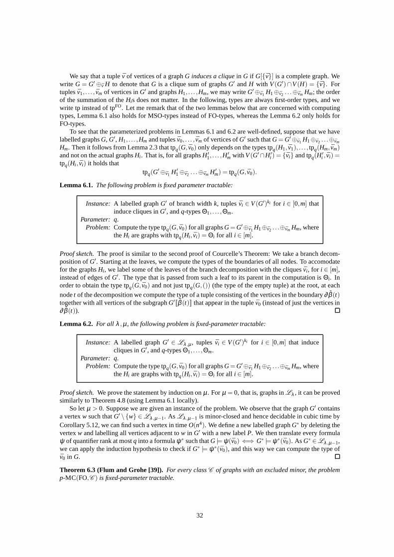
We say that a tuple ¯v of vertices of a graphG induces a cliquein G if G[v] is a complete graph. Wewrite G = G′ ⊕v H to denote thatG is a clique sum of graphsG′ andH with V(G′)∩V(H) = v. Fortuplesv1, . . . , vm of vertices inG′ and graphsH1, . . . ,Hm, we may writeG′⊕v1 H1⊕v2 . . .⊕vm Hm; the orderof the summation of theHis does not matter. In the following, types are always first-order types, and wewrite tp instead of tpFO. Let me remark that of the two lemmas below that are concernedwith computingtypes, Lemma 6.1 also holds for MSO-types instead of FO-types, whereas the Lemma 6.2 only holds forFO-types.
To see that the parameterized problems in Lemmas 6.1 and 6.2 are well-defined, suppose that we havelabelled graphsG, G′, H1, . . . ,Hm and tuples ¯v0, . . . , vm of vertices ofG′ such thatG= G′⊕v1 H1⊕v2 . . .⊕vm
Hm. Then it follows from Lemma 2.3 that tpq(G, v0) only depends on the types tpq(H1, v1), . . . , tpq(Hm, vm)and not on the actual graphsHi . That is, for all graphsH ′
1, . . . ,H′m with V(G′∩H ′
i ) = vi and tpq(H′i , vi) =
tpq(Hi , vi) it holds thattpq(G
′⊕v1 H ′1⊕v2 . . .⊕vm H ′
m) = tpq(G, v0).
Lemma 6.1. The following problem is fixed parameter tractable:
Instance: A labelled graphG′ of branch widthk, tuples ¯vi ∈ V(G′)ki for i ∈ [0,m] thatinduce cliques inG′, andq-typesΘ1, . . . ,Θm.
Parameter: q.Problem: Compute the type tpq(G, v0) for all graphsG= G′⊕v1 H1⊕v2 . . .⊕vm Hm, where
theHi are graphs with tpq(Hi , vi) = Θi for all i ∈ [m].
Proof sketch.The proof is similar to the second proof of Courcelle’s Theorem: We take a branch decom-position ofG′. Starting at the leaves, we compute the types of the boundaries of all nodes. To accomodatefor the graphsHi , we label some of the leaves of the branch decomposition withthe cliques ¯vi , for i ∈ [m],instead of edges ofG′. The type that is passed from such a leaf to its parent in the computation isΘi. Inorder to obtain the type tpq(G, v0) and not just tpq(G,()) (the type of the empty tuple) at the root, at each
nodet of the decomposition we compute the type of a tuple consisting of the vertices in the boundary∂ β (t)together with all vertices of the subgraphG′Jβ (t)K that appear in the tuple ¯v0 (instead of just the vertices in∂ β (t)).
Lemma 6.2. For all λ ,µ , the following problem is fixed-parameter tractable:
Instance: A labelled graphG′ ∈ Lλ ,µ , tuples ¯vi ∈ V(G′)ki for i ∈ [0,m] that inducecliques inG′, andq-typesΘ1, . . . ,Θm.
Parameter: q.Problem: Compute the type tpq(G, v0) for all graphsG= G′⊕v1 H1⊕v2 . . .⊕vm Hm, where
theHi are graphs with tpq(Hi , vi) = Θi for all i ∈ [m].
Proof sketch.We prove the statement by induction onµ . Forµ = 0, that is, graphs inLλ , it can be provedsimilarly to Theorem 4.8 (using Lemma 6.1 locally).
So letµ > 0. Suppose we are given an instance of the problem. We observethat the graphG′ containsa vertexw such thatG′ \ w ∈ Lλ ,µ−1. As Lλ ,µ−1 is minor-closed and hence decidable in cubic time byCorollary 5.12, we can find such a vertex in timeO(n4). We define a new labelled graphG∗ by deleting thevertexw and labelling all vertices adjacent tow in G′ with a new labelP. We then translate every formulaψ of quantifier rank at mostq into a formulaψ∗ such thatG |= ψ(v0) ⇐⇒ G∗ |= ψ∗(v0). AsG∗ ∈Lλ ,µ−1,we can apply the induction hypothesis to check ifG∗ |= ψ∗(v0), and this way we can compute the type ofv0 in G.
Theorem 6.3 (Flum and Grohe [39]). For every classC of graphs with an excluded minor, the problemp-MC(FO,C ) is fixed-parameter tractable.
32

G′
H4 H3
H2
I
H1
G′⊕H1⊕ . . .⊕H4⊕ I
G′⊕H1⊕ . . .⊕H3⊕ I
G′⊕H1⊕H2⊕ I
G′⊕H1⊕H2
G′⊕H1
G′ H1
H2
I
H3
H4
Figure 6.1. The left hand side shows a graph and the right hand side a clique sum decomposition of thisgraph where the atomG′ intersects four other atoms and the atomH2 intersects two other atoms
Proof sketch.Let G∈ C andϕ ∈ FO, say, of quantifier rankq.Let λ ,µ ≥ 0 such thatC ⊆ D(Lλ ,µ). Using Lemma 5.13, we compute a clique sum decomposition
(T,γ) of G overLλ ,µ .Now the obvious idea is to compute theq-types of the “boundary tuples” for the partsγ(t) in the de-
composition in a bottom-up fashion, similarly to the secondproof of Courcelle’s Theorem. Unfortunately,this simple idea does not work, because a clique sum decomposition is not as well-behaved as a branchdecomposition, and the boundaries of the parts may have unbounded size. It may even happen that an atomof the decomposition (corresponding to a leaf of the tree) intersects all other atoms. Figure 6.1 illustratesthis.
Observe that a graph inLλ ,µ cannot contain a clique with more thank = d(3/2) ·λ + µe vertices.Hence for all nodest of T with childrent1,t2, we must haveV(γ(t1)∩ γ(t2)) ≤ k, becauseV(γ(t1)∩ γ(t2))is a clique in theγ(ti), and this clique will appear in some atom of the decomposition. Let us fix some orderof the vertices ofG. For every inner nodet with childrent1, t2, we letct be the ordered tuple that containsthe elements ofV(γ(t1)∩ γ(t2)).
Our algorithm proceeds recursively, that is, “top-down”, instead of “bottom up” as the algorithm in theproof of Courcelle’s Theorem, to compute the types of the tuples ct . Let us start at the rootr of T. Ourgoal is to compute theq-type of the empty tuple inG. Suppose that the clique sum atr is G= G1⊕G2. Wenow want to compute theq-type of the tuple ¯cr in bothG1 andG2; from that we easily get theq-type of theempty tuple inG using Lemma 2.3. So let us continue by computing theq-type of cr in G1. Suppose thechildren oft1 aret11 andt12. Let c1 = ct1. Now we have a problem: To determine theq-type of cr in G1,it does not suffice to compute theq-types ofc1 in G11 andG12, because ¯cr andc1 may be disjoint tuples.It seems that we have to compute theq-type of the longer tuple ¯c1cr in both graphs. But clearly we cannotafford the tuples to get longer at every recursion level. Nowrecall thatcr is a clique inG1. Hence it iseither contained inc1 = V(G11)∩V(G12), in which case we have no problem anyway, or it is containedin precisely one of the two graphsG11, G12. Suppose ¯cr is contained inG12. Then we first compute theq-typeΘ of the tuple ¯c1 in G11. Now we have to compute the type of ¯cr in the graphG1 = G11⊕G12. Thatis, we are in the situation where we have to compute the type ofa tuplev of vertices of a graphG′ in agraphG′⊕v′ H for some (and hence all) graph(s)H with tpq(H, v′) = Θ. Furthermore, we know that ¯v, v′
induce cliques inG′. The general problem we have to solve recursively at all nodes of the decompositiontree is the following:
Compute theq-type of a tuple ¯v0 of vertices of a graphG′ in a graphG′⊕v1 H1⊕v2 . . .⊕vm Hm
for some (and hence all) graph(s)Hi with tpq(Hi , ci) = Θi . Here all the tuples ¯vi have length atmostk, and they induce cliques inG′.
At the leaves we can use Lemma 6.2 to do this. At the inner nodes, we proceed as described for the nodet1above.
The proof of the theorem actually shows that for all classesC with excluded minors,p-MC(FO,C )has an fpt algorithm with exponent at most 5. Hence, the exponent is independent of the classC . Thus we
33
have “almost” proved that there is an fpt algorithm for the model checking problem parameterized both byformula size and the size of the excluded minor. With considerable additional effort, we can get rid of the“almost” in this statement. Let me explain where the difficulties are and, in very general terms, how theyare resolved.
Let us first make the statement precise. We define a new graph invariantexcluded minor order (emo)by letting
emo(G) = min|H| | H 6 G
for every graphG. Note that emo(G) = minn | Kn 6 G and that a classC excludes a minor if and onlyif it has bounded excluded minor order. Our goal is to prove that the following problem is fixed-parametertractable:
p-MC(FO,emo)Instance: A graphG and a sentenceϕ ∈ FO.
Parameter: |ϕ |+emo(G).Problem: Decide ifG |= ϕ .
We have already proved that for everyk there is an fpt algorithmAk with exponent 5 for the first-ordermodel checking problem on the class of all graphs of excludedminor order at mostk. The problem isthat the familyAk of algorithms isnonuniform, that is, we have a different algorithm for everyk. Toprove thatp-MC(FO,emo) is fixed-parameter tractable, we need a uniform familyAk, or equivalently,a single algorithmA that takesk as an additional input. The family of algorithms we construct in theproof is nonuniform because we use Corollary 5.12 to get decision algorithms for the minor-closed classesLλ ,µ (in the proof of Lemma 6.2) andD(Lλ ,µ) (in the proof of Lemma 5.13) for parametersλ ,µ thatdepend on the excluded minor order of the input graph. If we could compute finite families of excludedminors characterising the classesLλ ,µ andD(Lλ ,µ) from the parametersλ ,µ , then we would be fine,but we currently do not know how to do this. Fortunately, there is an alternative approach that avoidsCorollary 5.12 entirely. The application of Corollary 5.12in the proof of Lemma 5.13 yielded an algorithmfor computing a clique sum decomposition of a graph overD(Lλ ,µ). While we do not know how tocompute such a decomposition uniformly inλ andµ , in [18] we found a way to compute, uniformly inλ ,µ , a decomposition that is a sufficiently good approximation of the desired clique sum decomposition.The algorithm recursively splits the input graph along small separators that are sufficiently “balanced”.The application of Corollary 5.12 in the proof of Lemma 6.2 was needed to find a set of at mostµ verticesin a graph inLλ ,µ whose removal left a graph inLλ . In [18], we found an fpt algorithm that, given agraphG∈Lλ ,µ , computes a setW ⊆V(G) of at mostµ vertices such thatG\W ∈ Lλ ′ for someλ ′ that iseffectively bounded in terms ofλ . This is good enough for our purposes. Putting everything together, weobtain the following result:
Theorem 6.4 (Dawar, Grohe, and Kreutzer [18]). p-MC(FO,emo) is fixed-parameter tractable.
We say that a classlocally excludes a minorif it has locally bounded excluded minor order. Thencombining Theorems 6.4 and 4.8, we get:
Corollary 6.5 ([18]). For every classC locally excluding a minor, the problem p-MC(FO,C ) is fixed-parameter tractable.
7 Other logics and other problems
In this section, we briefly discuss some extensions of the main results mentioned in this survey to morepowerful logics, and also to variants of the basic model checking problem.
7.1 Other logics
It is really not much that is known about algorithmic meta theorems for logics other than first-order andmonadic second-order logic. Courcelle’s Theorem and its variant for graphs of bounded rank width can be
34

extended to the extension of monadic second order logic by modulo counting quantifiers [10, 12] (also see[57]), and clearly not to full binary second order logic.
As for the results for first-order logic, let us consider potential extensions of the model-checking re-sults tomonadic transitive closure logicandmonadic least fixed-point logic. Both transitive closure logicand least fixed-point logic have been extensively studied infinite model theory [31, 55]. Their monadicfragments are strictly contained in monadic second-order logic, and they strictly contain first-order logic.(When we say that a logiccontainsanother logic, we mean semantic containment, that is, L1 containsL2
if every formula of L2 is logically equivalent to a formula of L1. We say that L1 strictly containsL2 it L1
contains L2, but L2 does not contain L1.) Monadic transitive closure logic and monadic least fixed-pointlogic seem to mark the boundary of the range of logics to whichthe tractability results for first-order modelchecking can be extended.
Monadic transitive closure logicTC1 is the extension of first-order logic by formulas of the form[TCx,yϕ ](x,y), whereϕ is a formula with free variables amongx,y. The free variables of the formula[TCx,yϕ ](x,y) arex andy. It is allowed to nest TC-operators arbitrarily and interleave them with first-orderquantifiers and connectives. However, we do not allow any other free variables thanx andy in the formulaϕ in [TCx,yϕ ](x,y). The semantics is defined as follows: IfG is a (labelled) graph andv,w∈V(G), thenG |= [TCx,yϕ ](v,w) if and only if there is anm≥ 1 and verticesv1, . . . ,vm ∈V(G) such thatv= v1,w = vm,andG |= ϕ(vi ,vi+1) for all i ∈ [m−1].
Example 7.1.The following TC1-sentence states that a graph is connected:
∀x∀y[TCx,yE(x,y)](x,y).
It is known that there is no sentence of first-order logic defining connectivity (see, e.g., [31, 32, 55]). y
Example 7.2.The following TC1-sentence states that a graph has no cyclic walk of odd lengthand henceis bipartite
¬∃x∃y([
TCx,y∃z(E(x,z)∧E(z,y)
)](x,y)∧E(y,x)
).
Again, it is known that there is no sentence of first-order logic defining bipartiteness. y
The logic TC1 trivially contains FO, and it is strictly contained in MSO. As opposed to MSO, its datacomplexity is still in polynomial time (actually, in nondeterministic logarithmic space).
Theorem 7.3. Let C be a class of graphs that contains all planar graphs of degreeat most3. Thenp-MC(TC1,C ) is hard for the parameterized complexity classAW[∗].
Proof sketch.We reduce the model checking problem for first-order logic onarbitrary graphs, which isknown to be AW[∗]-complete (by Theorem 2.12), top-MC(TC1,C ). Let G be a graph andϕ a first-ordersentence.
We start with constructing a drawing ofG in the plane, which of course may involve edge crossings.We can find a drawing with at most polynomially many (in the number of vertices ofG) crossings such thatin each point of the plane at most 2 edges cross. We introduce five new labelsP1,P2,Q1,Q2,R. We definea new labelled graphG1 by labelling each vertex of the original graphG with P1 and replacing each edgecrossing in the drawing ofG by a little gadget, as shown in Figure 7.1. Observe that the edge relation ofthe graphG can be defined inG1 by a TC1-formula (but not by an FO-formula, because an edge may crossmany other edges).G1 is planar, but may have degree greater than 3. We define a graphG2 by replacingevery vertexv of G1 of degreed by a binary tree with exactlyd leaves. With each leaf we associate onevertexw adjacent tov in G1. We connect the leaf of thev-tree associated withw with the leaf of thew-treeassociated withv. Then we identifyv with the root of its tree, label itP1, and label all other vertices of thetreeP2. Then the edge relation ofG is also definable inG2 by a TC1-formula. We can use this formula totranslate the formulaϕ into a TC1-formulaϕ2 such that
G |= ϕ ⇐⇒ G2 |= ϕ2.
G2 is a planar graph of degree at most 3, and it clearly can be computed fromG in polynomial time. Thisgives us the desired reduction.
35
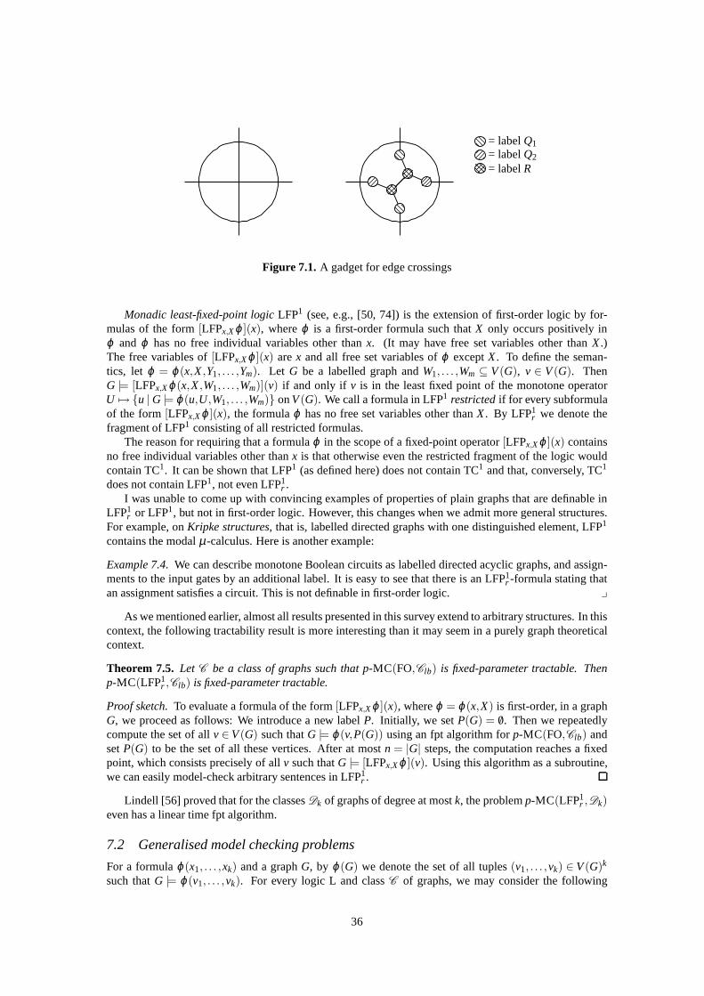
= labelQ1= labelQ2
= labelR
Figure 7.1. A gadget for edge crossings
Monadic least-fixed-point logicLFP1 (see, e.g., [50, 74]) is the extension of first-order logic byfor-mulas of the form[LFPx,Xϕ ](x), whereϕ is a first-order formula such thatX only occurs positively inϕ and ϕ has no free individual variables other thanx. (It may have free set variables other thanX.)The free variables of[LFPx,Xϕ ](x) arex and all free set variables ofϕ exceptX. To define the seman-tics, let ϕ = ϕ(x,X,Y1, . . . ,Ym). Let G be a labelled graph andW1, . . . ,Wm ⊆ V(G), v ∈ V(G). ThenG |= [LFPx,Xϕ(x,X,W1, . . . ,Wm)](v) if and only if v is in the least fixed point of the monotone operatorU 7→ u | G |= ϕ(u,U,W1, . . . ,Wm) onV(G). We call a formula in LFP1 restrictedif for every subformulaof the form[LFPx,Xϕ ](x), the formulaϕ has no free set variables other thanX. By LFP1
r we denote thefragment of LFP1 consisting of all restricted formulas.
The reason for requiring that a formulaϕ in the scope of a fixed-point operator[LFPx,Xϕ ](x) containsno free individual variables other thanx is that otherwise even the restricted fragment of the logic wouldcontain TC1. It can be shown that LFP1 (as defined here) does not contain TC1 and that, conversely, TC1
does not contain LFP1, not even LFP1r .I was unable to come up with convincing examples of properties of plain graphs that are definable in
LFP1r or LFP1, but not in first-order logic. However, this changes when we admit more general structures.
For example, onKripke structures, that is, labelled directed graphs with one distinguished element, LFP1
contains the modalµ-calculus. Here is another example:
Example 7.4.We can describe monotone Boolean circuits as labelled directed acyclic graphs, and assign-ments to the input gates by an additional label. It is easy to see that there is an LFP1
r -formula stating thatan assignment satisfies a circuit. This is not definable in first-order logic. y
As we mentioned earlier, almost all results presented in this survey extend to arbitrary structures. In thiscontext, the following tractability result is more interesting than it may seem in a purely graph theoreticalcontext.
Theorem 7.5. Let C be a class of graphs such that p-MC(FO,Clb) is fixed-parameter tractable. Thenp-MC(LFP1
r ,Clb) is fixed-parameter tractable.
Proof sketch.To evaluate a formula of the form[LFPx,Xϕ ](x), whereϕ = ϕ(x,X) is first-order, in a graphG, we proceed as follows: We introduce a new labelP. Initially, we setP(G) = /0. Then we repeatedlycompute the set of allv∈V(G) such thatG |= ϕ(v,P(G)) using an fpt algorithm forp-MC(FO,Clb) andsetP(G) to be the set of all these vertices. After at mostn = |G| steps, the computation reaches a fixedpoint, which consists precisely of allv such thatG |= [LFPx,Xϕ ](v). Using this algorithm as a subroutine,we can easily model-check arbitrary sentences in LFP1
r .
Lindell [56] proved that for the classesDk of graphs of degree at mostk, the problemp-MC(LFP1r ,Dk)
even has a linear time fpt algorithm.
7.2 Generalised model checking problems
For a formulaϕ(x1, . . . ,xk) and a graphG, by ϕ(G) we denote the set of all tuples(v1, . . . ,vk) ∈ V(G)k
such thatG |= ϕ(v1, . . . ,vk). For every logic L and classC of graphs, we may consider the following
36

variants of the model checking problemp-MC(L,C ): The input always consists of a graphG ∈ C anda formulaϕ ∈ L, possibly with free variables. The parameter is|ϕ |. Thedecision problemsimply asksif ϕ(G) is nonempty. For logics closed under existential quantification, this problem is equivalent to themodel checking problemp-MC(L,C ). Therefore, we will not consider it here anymore. Theconstructionproblemasks for a solution ¯v∈ ϕ(G) if there exists one. Theevaluation (or listing) problemasks for allsolutions, that is, for the whole setϕ(G). Finally, thecounting (or enumeration) problemasks for thenumber|ϕ(G)| of solutions. All these problems have natural applications.
The results on monadic second-order model checking on graphs of bounded branch width and boundedrank width (Theorems 3.3 and 3.17) can be extended to the corresponding construction and counting prob-lems [3, 15, 38, 41]. For the evaluation problem, the situation is a bit more complicated because the sizeof the answerϕ(G) may be much larger than the size of the input (nk for a graph of ordern and a formulawith k free variables), hence we cannot expect an algorithm that isfixed-parameter tractable. However, ithas been proved that there is a linear time fpt algorithm for this problem if the running time is measured interms of the input size plus the output size [16, 38]. Recently, it has been shown that there even is such analgorithm that does a linear (in terms of the input size) pre-computation and then produces solutions withdelay bounded in terms of the parameter [4, 13].
Frick [41, 42] proved that the construction problem and counting problem for many classes of graphsof locally bounded branch width, including planar graphs and graphs of bounded degree, has a linear fptalgorithm. This is a nontrivial extension of the model checking results. Even for a simple first-orderdefinable counting problem like the parameterized independent set counting problem (“Count the numberof independent sets of sizek in a graph.”), say, on a class of graphs of bounded degree, it is not obvioushow to solve it by an fpt algorithm. For the evaluation problem, again there are linear time fpt algorithmsif the running time is measured in terms of the input size plusthe output size [41]. For classes of graphsof bounded degree, Durand and Grandjean [30] proved that there is an fpt algorithm for the first-orderevaluation problem that does a linear pre-computation and then produces solutions with delay bounded interms of the parameter.
Finally, let us take a brief look at optimisation problems, which play a central role in complexity the-ory, but have not been studied very systematically in the context of meta theorems. Consider a first-orderformulaϕ(X) that is positive in a free set variableX. Such a formula naturally describes a minimisationproblem: Given a graphG, find a setS⊆ V(G) of minimum size such thatG |= ϕ(S). Many naturalminimisation problems on graphs can be described this way. An example is the minimum dominating setproblem, which can be described by the formuladom(X) of Example 2.1. Similarly, formulasϕ(X) thatare negative inX naturally describe maximisation problems. An example is the maximum independent setproblem, which is described by the formulaind(X) = ∀x∀y(¬X(x)∨¬X(y)∨¬E(x,y)). We call such op-timisation problemsfirst-order definable. It was proved in [19] that the restriction of a first-order definableoptimisation problem to a class of graphs with an excluded minor has a polynomial time approximationscheme, that is, can be approximated in polynomial time to any factor(1+ ε), whereε > 0.
8 Concluding remarks and open questions
Figure 8.1 gives an overview of the classes of graphs we have studied in this survey. Let me conclude bymentioning a few directions for further research that I find particularly promising:
8.1 Further tractable classes
Many of the classes of graphs considered in this survey, including all classes excluding a minor, havebounded average degree. It may be tempting to conjecture that first-order model checking is tractable onall classes of graphs of bounded average degree, but it is easy to see that this is not the case. As StephanKreutzer observed, it is not even the case for classes of bounded maximum average degree, where themaximum average degreeof a graphG is the maximum of the average degrees of all subgraphs ofG. Tosee this, just observe that model-checking on a graphG can be reduced to model-checking on its incidencegraph (i.e., the graph obtained fromG by subdividing each edge once), and that every incidence graph hasmaximum average degree at most 4.
Nesetril and Ossona de Mendez [59] introduced a property of graph classes that may be viewed as a
37

Trees
Bounded Branch Width
Bounded Rank Width
Planar
Bounded Genus
Bounded Local Branch Widthwith Excluded Minor
Bounded Degree
Bounded LocalBranch Width
Exluded Minor
Locally Excluding a MinorBounded Local Rank Width
MSO
FO
Figure 8.1. Classes of graphs with a tractable first-order model checking problems. Double-lined ellipsescontain families of classes. Classes below the dashed line have a tractable monadic second-order modelchecking problem
refinement of maximum average degree and that avoids such problems. LetG be a graph. Theradiusof aminor mappingµ from a graphH to G is the minimum of the radii of the subgraphsG[µ(v)], for v∈V(H).We writeH r G if there is a minor mapping of radius at mostr from H to G. Note thatH 0 G if andonly if H is a subgraph ofG. Thegreatest reduced average density (grad) of rank r of Gis the number
∇r(G) = max
|E(H)|
|V(H)|
∣∣∣∣H r G
.
Note that∇0(G) is half the maximum average degree ofG. Now a classC of graphs hasbounded expansionif there is some functionf such that∇r(G)≤ f (r) for all G∈C andr ≥ 0. Nesetril and Ossona de Mendezobserved that every class of graphs excluding a minor has bounded expansion. It can be shown that thereare classes of bounded expansion that do not exclude a minor,not even locally. Conversely, there areclasses of bounded local tree width and hence classes locally excluding a minor that do not have boundedexpansion. This follows from Example 4.7 and the fact that classes of bounded expansion have boundedaverage degree. I refer the reader to [58, 59, 60] for an introduction to classes of bounded expansion andan overview of their nice algorithmic properties.
Open Problem 8.1. Is p-MC(FO,C ) fixed-parameter tractable for every classC of graphs of boundedexpansion?
There is no need to restrict the study of structural properties that facilitate efficient model checkingto graph theoretic properties such as those predominant in this survey. For example, it would also bevery interesting to study the complexity of model-checkingproblems on finite algebraic structures such asgroups, rings, fields, lattices, et cetera.
Open Problem 8.2. Are p-MC(FO,C ) and p-MC(MSO,C ) fixed-parameter tractable for the classesC
of finite groups, finite abelian groups, finite rings, finite fields?
8.2 Necessary conditions for tractability
The main results presented in this survey may be viewed as giving sufficient conditions for classes ofgraphs to have tractable first-order or monadic second-order model checking problems.What are necessary
38
conditions for tractability, and which classes have hard model checking problems?Note that it is not easyto come up with structural conditions for hardness, becausewe can “cheat” and, for example, pad graphsthat have a structure presumably making model checking difficult with a large number of isolated vertices.This makes the model checking problem “easier” just becauseit gives us more time to solve it. Thus weprobably want to impose closure conditions on the classes ofgraphs we consider, such as being closedunder taking subgraphs.
It follows from the Excluded Grid Theorem that for minor-closed classesC of graphs,p-MC(MSO,C )is fixed-parameter tractable if and only ifC has bounded branch width. Actually, this can be slightlystrengthened to classes closed under taking topological minors. I do not know of any results beyond that.To stimulate research in this direction, let me state a conjecture:
Conjecture 8.3. LetC be a class of graphs that is closed under taking subgraphs. Suppose that the branchwidth ofC is not poly-logarithmically bounded, that is, there is no constant c such thatbw(G) ≤ logc |G|for every G∈ C .
Then p-MC(MSO,C ) is not fixed parameter tractable.
Of course, with current techniques we can only hope to prove this conjecture under some complexitytheoretic assumption.
For first-order logic, I have much less intuition. Clearly, the present results are very far from optimal.Just as an illustration, observe that if a classC of graphs has a tractable first-order model checking problem,then so has the closure ofC under complementation. (Recall that thecomplementof a graphG = (V,E)
is the graphG =(V,(V
2
)\E)
.) However, most of the classes we considered here are not closed under
complementation.
8.3 Average Case Analysis
Instead of the worst case running time, it is also interesting to consider the average case. Here even themost basic questions are wide open. Forn ≥ 1, let Wn be a probability space of graphs with vertex set[n]. We say that a model checking algorithm isfpt on average over
(Wn)
n≥1 if its expected running time
on inputG∈ Wn andϕ is bounded byf (|ϕ |) ·nO(1), for some computable functionf . For every functionp : N→ [0,1] (here[0,1] denotes an interval of real numbers), letG (n, p) denote the probability space of allgraphs over[n] with edge probabilityp(n) (see, e.g., [2]). For a constantc∈ [0,1], we letG (n,c) = G (n, p)for the constant functionp(n) = c. In [47], I observed that forp(n) = min1,c/n, wherec ∈ R≥0 is aconstant, there is a model checking algorithm for first-order logic that is fpt on average over
(G (n, p)
)n≥1.
Open Problem 8.4. Is there a model checking algorithm for first-order logic that is fpt on average over(G (n,1/2)
)n≥1?
Let me suggest it as an exercise for the reader to design a model checking algorithm for existentialfirst-order logic that is fpt on average over
(G (n,1/2)
)n≥1.
8.4 Structures of bounded rank width
Most of the results of this survey can easily be extended fromclassesC of graphs to the classesCstr ofarbitrary relational structures whose underlying graphs (Gaifman graphs) are inC . However, this is nottrue for the results that involve rank width. It is not at all obvious what an appropriate notion of rank widthfor arbitrary structures could look like, and I think it is a challenging open problem to find such a notion.
8.5 Model checking for monadic least fixed-point logic
Conjecture 8.5. Let C be a class of graphs such that p-MC(FO,Clb) is fixed-parameter tractable. Thenp-MC(LFP1,Clb) is fixed-parameter tractable.
It will be difficult to prove this conjecture, because it is related to the notoriously open problem ofwhether the model checking problem for the modalµ-calculus is in polynomial time. But maybe theconjecture is wrong; refuting it might be more feasible.
39

Acknowledgements
I would like to thank Bruno Courcelle, Arnaud Durand, Sang-Il Oum, Stephan Thomasse for patientlyanswering various questions I had while writing this survey. Thanks to Isolde Adler, Albert Atserias, YijiaChen, Anuj Dawar, Reinhard Diestel, Jorg Flum, Magdalena Gruber, Stephan Kreutzer, Nicole Schweikardtfor valuable comments on earlier drafts of the survey.
References
[1] I. Abraham, C. Gavoille, and D. Malkhi. Compact routing for graphs excluding a fixed minor. InP. Fraigniaud, editor,Proceedings of the 19th International Conference on Distributed Computing,volume 3724 ofLecture Notes in Computer Science, pages 442–456. Springer-Verlag, 2005.
[2] N. Alon and J. Spencer.The Probabilistic Method. Wiley, 2nd edition, 2000.
[3] S. Arnborg, J. Lagergren, and D. Seese. Easy problems fortree-decomposable graphs.Journal ofAlgorithms, 12:308–340, 1991.
[4] G. Bagan. MSO queries on tree decomposable structures are computable with linear delay. In Z.Esik,editor,Proceedings of the 20th International Workshop on ComputerScience Logic, volume 4207 ofLecture Notes in Computer Science, pages 167–181. Springer-Verlag, 2006.
[5] H.L. Bodlaender. A linear-time algorithm for finding tree-decompositions of small treewidth.SIAMJournal on Computing, 25:1305–1317, 1996.
[6] H.L. Bodlaender and D.M. Thilikos. Constructive lineartime algorithms for branchwidth. InP. Degano, R. Gorrieri, and A. Marchetti-Spaccamela, editors,Proceedings of the 24th InternationalColloquium on Automata, Languages and Programming, volume 1256 ofLecture Notes in ComputerScience, pages 627–637. Springer-Verlag, 1997.
[7] Y. Chen, M. Grohe, and M. Gruber. On parameterized approximability. In Proceedings of the 2ndInternational Workshop on Parameterized and Exact Computation, volume 4169 ofLecture Notes inComputer Science, pages 109–120. Springer-Verlag, 2006.
[8] B. Courcelle. An axiomatic definition of context-free graph grammars and applications to nlc gram-mars.Theoretical Computer Science, 55:141–181, 1987.
[9] B. Courcelle. Graph rewriting: An algebraic and logic approach. In J. van Leeuwen, editor,Handbookof Theoretical Computer Science, volume B, pages 194–242. Elsevier Science Publishers, 1990.
[10] B. Courcelle. The monadic second-order logic of graphs. I. Recognizable sets of finite graphs.Infor-mation and Computation, 85(1):12–75, 1990.
[11] B. Courcelle. The monadic second-order logic of graphsVII: Graphs as relational structures.Theo-retical Computer Science, 101:3–33, 1992.
[12] B. Courcelle. The expression of graph properties and graph transformations in monadic second-orderlogic. In G. Rozenberg, editor,Handbook of graph grammars and computing by graph transfor-mations, Vol. 1 : Foundations, chapter 5, pages 313–400. World Scientific (New-Jersey, London),1997.
[13] B. Courcelle. Linear delay enumeration and monadic second-order logic, 2006. Available athttp://www.labri.fr/perso/courcell/ActSci.html.
[14] B. Courcelle, J.A. Makowsky, and U. Rotics. Linear timesolvable optimization problems on graphsof bounded clique width.Theory of Computing Systems, 33(2):125–150, 2000.
[15] B. Courcelle, J.A. Makowsky, and U. Rotics. On the fixed-parameter complexity of graph enumera-tion problems definable in monadic second-order logic.Discrete Applied Mathematics, 108(1–2):23–52, 2001.
40
[16] B. Courcelle and M. Mosbah. Monadic second-order evaluations on tree-decomposable graphs.The-oretical Computer Science, 109:49–82, 1993.
[17] B. Courcelle and S. Olariu. Upper bounds to the clique-width of graphs.Discrete Applied Mathemat-ics, 101:77–114, 2000.
[18] A. Dawar, M. Grohe, and S. Kreutzer. Locally excluding aminor. InProceedings of the 22nd IEEESymposium on Logic in Computer Science, 2007. To appear.
[19] A. Dawar, M. Grohe, S. Kreutzer, and N. Schweikardt. Approximation schemes for first-order de-finable optimisation problems. InProceedings of the 21st IEEE Symposium on Logic in ComputerScience, pages 411–420, 2006.
[20] A. Dawar, M. Grohe, S. Kreutzer, and N. Schweikardt. Model theory makes formulas large. InProceedings of the 34th International Colloquium on Automata, Languages and Programming, 2007.To appear.
[21] E.D. Demaine, F.V. Fomin, M.T. Hajiaghayi, and D.M. Thilikos. Subexponential parameterized al-gorithms on graphs of bounded-genus andH-minor-free graphs. InProceedings of the 15th AnnualACM-SIAM Symposium on Discrete Algorithms, pages 830–839, 2004.
[22] E.D. Demaine and M.T. Hajiaghayi. Equivalence of localtreewidth and linear local treewidth and itsalgorithmic applications. InProceedings of the Fifteenth Annual ACM-SIAM Symposium on DiscreteAlgorithms, pages 840–849, 2004.
[23] E.D. Demaine, M.T. Hajiaghayi, and K. Kawarabayashi. Algorithmic graph minor theory: Decom-position, approximation, and coloring. InProceedings of the 45th Annual IEEE Symposium on Foun-dations of Computer Science, pages 637–646, 2005.
[24] E.D. Demaine, M.T. Hajiaghayi, and K.-I. Kawarabayashi. Algorithmic graph minor theory: Im-proved grid minor bounds and wagner’s contraction. In S.K. Madria, K.T. Claypool, R. Kannan,P. Uppuluri, and M.M. Gore, editors,Proceedings of the Third International Conference on Dis-tributed Computing and Internet Technology, volume 4317 ofLecture Notes in Computer Science,pages 3–15. Springer-Verlag, 2006.
[25] R. Diestel.Graph Theory. Springer-Verlag, 3rd edition, 2005.
[26] R.G. Downey and M.R. Fellows. Fixed-parameter tractability and completeness I: Basic results.SIAMJournal on Computing, 24:873–921, 1995.
[27] R.G. Downey and M.R. Fellows. Fixed-parameter tractability and completeness II: On completenessfor W[1]. Theoretical Computer Science, 141:109–131, 1995.
[28] R.G. Downey and M.R. Fellows.Parameterized Complexity. Springer-Verlag, 1999.
[29] R.G. Downey, M.R. Fellows, and U. Taylor. The parameterized complexity of relational databasequeries and an improved characterization of W[1]. In D.S. Bridges, C. Calude, P. Gibbons, S. Reeves,and I.H. Witten, editors,Combinatorics, Complexity, and Logic, volume 39 ofProceedings ofDMTCS, pages 194–213. Springer-Verlag, 1996.
[30] A. Durand and E.Grandjean. First-order queries on structures of bounded degree are computable withconstant delay.ACM Transactions on Computational Logic. To appear.
[31] H.-D. Ebbinghaus and J. Flum.Finite Model Theory. Springer-Verlag, 2nd edition, 1999.
[32] H.-D. Ebbinghaus, J. Flum, and W. Thomas.Mathematical Logic. Springer-Verlag, 2nd edition,1994.
[33] P. Hlineny and S.-I. Oum. Finding branch-decompositions and rank-decompositions. Available athttp://www.math.uwaterloo.ca/˜sangil/.
41

[34] D. Eppstein. Subgraph isomorphism in planar graphs andrelated problems.Journal of Graph Algo-rithms and Applications, 3:1–27, 1999.
[35] D. Eppstein. Diameter and treewidth in minor-closed graph families. Algorithmica, 27:275–291,2000.
[36] P. Erdos. Graph theory and probability.Canadian Journal of Mathematics, 11:34–38, 1959.
[37] R. Fagin. Generalized first–order spectra and polynomial–time recognizable sets. In R. M. Karp,editor,Complexity of Computation, SIAM-AMS Proceedings, Vol. 7, pages 43–73, 1974.
[38] J. Flum, M. Frick, and M. Grohe. Query evaluation via tree-decompositions.Journal of the ACM,49(6):716–752, 2002.
[39] J. Flum and M. Grohe. Fixed-parameter tractability, definability, and model checking.SIAM Journalon Computing, 31(1):113–145, 2001.
[40] J. Flum and M. Grohe.Parameterized Complexity Theory. Springer-Verlag, 2006.
[41] M. Frick. Easy Instances for Model Checking. PhD thesis, Albert-Ludwigs-Universitat Freiburg,2001.
[42] M. Frick. Generalized model-checking over locally tree-decomposable classes. In H. Alt and A. Fer-reira, editors,Proceedings of the 19th Annual Symposium on Theoretical Aspects of Computer Sci-ence, volume 2285 ofLecture Notes in Computer Science, pages 632–644. Springer-Verlag, 2002.
[43] M. Frick and M. Grohe. Deciding first-order properties of locally tree-decomposable structures.Journal of the ACM, 48:1184–1206, 2001.
[44] M. Frick and M. Grohe. The complexity of first-order and monadic second-order logic revisited.Annals of Pure and Applied Logic, 130:3–31, 2004. LICS 2002 Special Issue.
[45] H. Gaifman. On local and non-local properties. In J. Stern, editor,Proceedings of the HerbrandSymposium, Logic Colloquium ‘81, pages 105–135. North Holland, 1982.
[46] M.R. Garey and D.S. Johnson.Computers and Intractability: A Guide to the Theory of NP-Completeness. Freeman, 1979.
[47] M. Grohe. Generalized model-checking problems for first-order logic. In H. Reichel and A. Ferreira,editors,Proceedings of the 18th Annual Symposium on Theoretical Aspects of Computer Science,volume 2010 ofLecture Notes in Computer Science, pages 12–26. Springer-Verlag, 2001.
[48] M. Grohe. Local tree-width, excluded minors, and approximation algorithms. Combinatorica,23(4):613–632, 2003.
[49] M. Grohe and J. Marino. Definability and descriptive complexity on databases of bounded tree-width.In C. Beeri and P. Buneman, editors,Proceedings of the 7th International Conference on DatabaseTheory, volume 1540 ofLecture Notes in Computer Science, pages 70–82. Springer-Verlag, 1999.
[50] M. Grohe, N. Schweikardt, and S. Kreutzer. The expressive power of two-variable least fixed-pointlogics. In J. Jedrzejowicz and A. Szepietowski, editors,Proceedings of the 30th International Sympo-sium on Mathematical Foundations of Computer Science, volume 3618 ofLecture Notes in ComputerScience, pages 422–434. Springer-Verlag, 2005.
[51] M. Grohe and S. Wohrle. An existential locality theorem. Annals of Pure and Applied Logic,129:131–148, 2004.
[52] S. Iwata, L. Fleischer, and S. Fujishige. A combinatorial strongly polynomial algorithm for minimiz-ing submodular functions.Journal of the ACM, 48(4):761–777, 2001.
42
[53] K.-I. Kawarabayashi and B. Mohar. Approximating the list-chromatic number and the chromaticnumber in minor-closed and odd-minor-closed classes of graphs. InProceedings of the 38th ACMSymposium on Theory of Computing, pages 401–416, 2006.
[54] K. Kuratowski. Sur le probleme des courbes gauches en topologie. Fundamenta Mathematicae,15:271–283, 1930.
[55] L. Libkin. Elements of Finite Model Theory. Springer-Verlag, 2004.
[56] S. Lindell. Computing monadic fixed-points in linear-time on doubly-linked data structures, 2005.Available at http://www.haverford.edu/cmsc/slindell/.
[57] J.A. Makowsky. Algorithmic uses of the Feferman-Vaught theorem. Annals of Pure and AppliedLogic, 126:159–213, 2004.
[58] J. Nesetril and P. Ossona de Mendez. Linear time low tree-width partitions and algorithmic con-sequences. InProceedings of the 38th ACM Symposium on Theory of Computing, pages 391–400,2006.
[59] J. Nesetril and P. Ossona de Mendez. Grad and classes with bounded expansion I: Decompositions.European Journal of Combinatorics, 2007. To appear.
[60] J. Nesetril and P. Ossona de Mendez. Grad and classes with bounded expansion II: Algorithmicaspects.European Journal of Combinatorics, 2007. To appear.
[61] R. Niedermeier.Invitation to Fixed-Parameter Algorithms. Oxford University Press, 2006.
[62] S.-I. Oum. Rank-width is less than or equal to branch-width, 2006. Available athttp://www.math.uwaterloo.ca/˜sangil/.
[63] S.-I. Oum and P.D. Seymour. Approximating clique-width and branch-width.Journal of Combinato-rial Theory, Series B, 96:514–528, 2006.
[64] C.H. Papadimitriou and M. Yannakakis. Optimization, approximation, and complexity classes.Jour-nal of Computer and System Sciences, 43:425–440, 1991.
[65] N. Robertson and P.D. Seymour. Graph minors I–XXIII. Appearing inJournal of CombinatorialTheory, Series Bsince 1982.
[66] N. Robertson and P.D. Seymour. Graph minors XXI. Graphswith unique linkages. To appear.
[67] N. Robertson and P.D. Seymour. Graph minors XXII. Irrelevant vertices in linkage problems. Toappear.
[68] N. Robertson and P.D. Seymour. Graph minors III. Planartree-width. Journal of CombinatorialTheory, Series B, 36:49–64, 1984.
[69] N. Robertson and P.D. Seymour. Graph minors V. Excluding a planar graph.Journal of Combinato-rial Theory, Series B, 41:92–114, 1986.
[70] N. Robertson and P.D. Seymour. Graph minors X. Obstructions to tree-decomposition.Journal ofCombinatorial Theory, Series B, 52:153–190, 1991.
[71] N. Robertson and P.D. Seymour. Graph minors XIII. The disjoint paths problem.Journal of Combi-natorial Theory, Series B, 63:65–110, 1995.
[72] N. Robertson and P.D. Seymour. Graph minors XVI. Excluding a non-planar graph.Journal ofCombinatorial Theory, Series B, 77:1–27, 1999.
[73] N. Robertson and P.D. Seymour. Graph minors XX. Wagner’s conjecture.Journal of CombinatorialTheory, Series B, 92:325–357, 2004.
43
[74] N. Schweikardt. On the expressive power of monadic least fixed point logic. Theoretical ComputerScience, 350:325–344, 2006.
[75] D. Seese. Linear time computable problems and first-order descriptions.Mathematical Structures inComputer Science, 6:505–526, 1996.
[76] H. Tamaki. A linear time heuristic for the branch-decomposition of planar graphs. In G. Di Battistaand U. Zwick, editors,Proceedings of the 11th Annual European Symposium on Algorithms, volume2832 ofLecture Notes in Computer Science, pages 765–775. Springer-Verlag, 2003.
[77] R.E. Tarjan. Decomposition by clique separators.Discrete Mathematics, 55:221–232, 1985.
[78] J.W. Thatcher and J.B. Wright. Generalised finite automata theory with an application to a decisionproblem of second-order logic.Mathematical Systems Theory, 2:57–81, 1968.
[79] M.Y. Vardi. The complexity of relational query languages. InProceedings of the 14th ACM Sympo-sium on Theory of Computing, pages 137–146, 1982.
[80] M.Y. Vardi. On the complexity of bounded-variable queries. InProceedings of the 14th ACM Sym-posium on Principles of Database Systems, pages 266–276, 1995.
[81] K. Wagner. Uber eine Eigenschaft der ebenen Komplexe.Mathematische Annalen, 114:570–590,1937.
44
http://eccc.hpi-web.de/ ECCC ISSN 1433-8092