Logic Synthesis Meets Machine Learning:Trading Exactness for Generalization

Shubham Raif,6,†, Walter Lau Neton,10,†, Yukio Miyasakao,1, Xinpei Zhanga,1, Mingfei Yua,1, Qingyang Yia,1,Masahiro Fujitaa,1, Guilherme B. Manskeb,2, Matheus F. Pontesb,2, Leomar S. da Rosa Juniorb,2,

Marilton S. de Aguiarb,2, Paulo F. Butzene,2, Po-Chun Chienc,3, Yu-Shan Huangc,3, Hoa-Ren Wangc,3,Jie-Hong R. Jiangc,3, Jiaqi Gud,4, Zheng Zhaod,4, Zixuan Jiangd,4, David Z. Pand,4, Brunno A. de Abreue,5,9,

Isac de Souza Camposm,5,9, Augusto Berndtm,5,9, Cristina Meinhardtm,5,9, Jonata T. Carvalhom,5,9,Mateus Grellertm,5,9, Sergio Bampie,5, Aditya Lohanaf,6, Akash Kumarf,6, Wei Zengj,7, Azadeh Davoodij,7,

Rasit O. Topalogluk,7, Yuan Zhoul,8, Jordan Dotzell,8, Yichi Zhangl,8, Hanyu Wangl,8, Zhiru Zhangl,8,Valerio Tenacen,10, Pierre-Emmanuel Gaillardonn,10, Alan Mishchenkoo,†, and Satrajit Chatterjeep,†

aUniversity of Tokyo, Japan, bUniversidade Federal de Pelotas, Brazil, cNational Taiwan University,Taiwan, dUniversity of Texas at Austin, USA, eUniversidade Federal do Rio Grande do Sul, Brazil,fTechnische Universitaet Dresden, Germany, jUniversity of Wisconsin–Madison, USA, kIBM, USA,

lCornell University, USA, mUniversidade Federal de Santa Catarina, Brazil, nUniversity of Utah, USA,oUC Berkeley, USA, pGoogle AI, USA

The alphabets in the superscript represent the affiliation while the numbers represent the team number†Equal contribution. Email: shubham.rai@tu-dresden.de, walter.launeto@utah.edu, alanmi@berkeley.edu, schatter@google.com

Abstract—Logic synthesis is a fundamental step in hard-ware design whose goal is to find structural representationsof Boolean functions while minimizing delay and area.If the function is completely-specified, the implementa-tion accurately represents the function. If the function isincompletely-specified, the implementation has to be trueonly on the care set. While most of the algorithms in logicsynthesis rely on SAT and Boolean methods to exactlyimplement the care set, we investigate learning in logicsynthesis, attempting to trade exactness for generalization.This work is directly related to machine learning wherethe care set is the training set and the implementationis expected to generalize on a validation set. We presentlearning incompletely-specified functions based on the re-sults of a competition conducted at IWLS 2020. The goalof the competition was to implement 100 functions givenby a set of care minterms for training, while testing theimplementation using a set of validation minterms sampledfrom the same function. We make this benchmark suiteavailable and offer a detailed comparative analysis of thedifferent approaches to learning.

I. INTRODUCTION

Logic synthesis is a key ingredient in modern electronicdesign automation flows. A central problem in logicsynthesis is the following: Given a Boolean functionf : Bn → B (where B denotes the set {0, 1}), constructa logic circuit that implements f with the minimumnumber of logic gates. The function f may be completelyspecified, i.e., we are given f(x) for all x ∈ Bn, or it maybe incompletely specified, i.e., we are only given f(x)for a subset of Bn called the careset. An incompletelyspecified function provides more flexibility for optimizingthe circuit since the values produced by the circuit outsidethe careset are not of interest.

Recently, machine learning has emerged as a keyenabling technology for a variety of breakthroughs inartificial intelligence. A central problem in machinelearning is that of supervised learning: Given a classH of functions from a domain X to a co-domain Y , find

a member h ∈ H that best fits a given set of trainingexamples of the form (x, y) ∈ X×Y . The quality of thefit is judged by how well h generalizes, i.e., how well hfits examples that were not seen during training.

Thus logic synthesis and machine learning are closelyrelated. Supervised machine learning can be seen aslogic synthesis of an incompletely specified functionwith an added constraint (or objective): the circuit mustalso generalize well to the test set. Conversely, logicsynthesis may be seen as a machine learning problemwhere in addition to generalization, we care about findingan element of H that has small size, and the sets X andY are not smooth but discrete.

To explore this connection between the two fields, thetwo last authors of this paper organized a programmingcontest at the 2020 International Workshop in LogicSynthesis. The goal of this contest was to come upwith an algorithm to synthesize a small circuit for aBoolean function f : Bn → B learnt from a training setof examples. Each example (x, y) in the training set is aninput-output pair, i.e., x ∈ Bn and y ∈ B. The training setwas chosen at random from the 2n possible inputs of thefunction (and in most cases was much smaller than 2n).The quality of the solution was evaluated by measuringaccuracy on a test set not provided to the participants.

The synthesized circuit for f had to be in the formof an And-Inverter Graph (AIG) [1, 2] with no morethan 5000 nodes. An AIG is a standard data structureused in logic synthesis to represent Boolean functionswhere a node corresponds to a 2-input And gate andedges represent direct or inverted connections. Since anAIG can represent any Boolean function, in this problemH is the full set of Boolean functions on n variables.

To evaluate the algorithms proposed by the participants,we created a set of 100 benchmarks drawn from amix of standard problems in logic synthesis such as

arX

iv:2

012.

0253

0v1

[cs

.LG

] 4

Dec

202

0

synthesis of arithmetic circuits and random logic fromstandard logic synthesis benchmarks. We also includedsome tasks from standard machine learning benchmarks.For each benchmark the participants were provided withthe training set (which was sub-divided into a training setproper of 6400 examples and a validation set of another6400 examples though the participants were free to usethese subsets as they saw fit), and the circuits returnedby their algorithms were evaluated on the correspondingtest set (again with 6400 examples) that was kept privateuntil the competition was over. The training, validationand test sets were created in the PLA format [3]. Thescore assigned to each participant was the average testaccuracy over all the benchmarks with possible ties beingbroken by the circuit size.

Ten teams spanning 6 countries took part in the contest.They explored many different techniques to solve thisproblem. In this paper we present short overviews of thetechniques used by the different teams (the superscriptfor an author indicates their team number), as well acomparative analysis of these techniques. The followingare our main findings from the analysis:• No one technique dominated across all the bench-

marks, and most teams including the winning teamused an ensemble of techniques.

• Random forests (and decision trees) were verypopular and form a strong baseline, and may bea useful technique for approximate logic synthesis.

• Sacrificing a little accuracy allows for a significantreduction in the size of the circuit.

These findings suggest an interesting direction for futurework: Can machine learning algorithms be used forapproximate logic synthesis to greatly reduce power andarea when exactness is not needed?

Finally, we believe that the set of benchmarks usedin this contest along with the solutions provided by theparticipants (based on the methods described in this paper)provide an interesting framework to evaluate furtheradvances in this area. To that end we are making theseavailable at https://github.com/iwls2020-lsml-contest/.

II. BACKGROUND AND PRELIMINARIES

We review briefly the more popular techniques used.Sum-of-Products (SOP), or disjunctive normal form,

is a two-level logic representation commonly used inlogic synthesis. Minimizing the SOP representation of anincompletely specified Boolean function is a well-studiedproblem with a number of exact approaches [4, 5, 6] aswell as heuristics [7, 8, 9, 10] with ESPRESSO [7] beingthe most popular.

Decision Trees (DT) and Random Forests (RF) arevery popular techniques in machine learning and theywere used by many of the teams. In the contest scope,the decision trees were applied as a classification tree,where the internal nodes were associated to the functioninput variables, and terminal nodes classify the functionas 1 or 0, given the association of internal nodes. Thus,each internal node has two outgoing-edges: a true edgeif the variable value exceeds a threshold value, and afalse value otherwise. The threshold value is definedduring training. Hence, each internal node can be seenas a multiplexer, with the selector given by the thresholdvalue. Random forests are composed by multiple decisiontrees, where each tree is trained over a distinct feature,

Table I: An overview of different types of functions inthe benchmark set. They are selected from three domains:Arithmetic, Random Logic, and Machine Learning.

00-09 2 MSBs of k-bit adders for k ∈ {16, 32, 64, 128, 256}10-19 MSB of k-bit dividers and remainder circuits for k ∈ {16, 32, 64, 128, 256}20-29 MSB and middle bit of k-bit multipliers for k ∈ {8, 16, 32, 64, 128}30-39 k-bit comparators for k ∈ {10, 20, . . . , 100}40-49 LSB and middle bit of k-bit square-rooters with k ∈ {16, 32, 64, 128, 256}50-59 10 outputs of PicoJava design with 16-200 inputs and roughly balanced onset & offset60-69 10 outputs of MCNC i10 design with 16-200 inputs and roughly balanced onset & offset70-79 5 other outputs from MCNC benchmarks + 5 symmetric functions of 16 inputs80-89 10 binary classification problems from MNIST group comparisons90-99 10 binary classification problems from CIFAR-10 group comparisons

so that trees are not very similar. The output is given bythe combination of individual predictions.

Look-up Table (LUT) Network is a network ofrandomly connected k-input LUTs, where each k-inputLUT can implement any function with up to k variables.LUT networks were first employed in a theoreticalstudy to understand if pure memorization (i.e., fittingwithout any explicit search or optimization) could leadto generalization [11].

III. BENCHMARKS

The set of 100 benchmarks used in the contest canbe broadly divided into 10 categories, each with 10 test-cases. The summary of categories is shown in Table I. Forexample, the first 10 test-cases are created by consideringthe two most-significant bits (MSBs) of k-input addersfor k ∈ {16, 32, 64, 128, 256}.

Test-cases ex60 through ex69 were derived fromMCNC benchmark [12] i10 by extracting outputs 91,128, 150, 159, 161, 163, 179, 182, 187, and 209 (zero-based indexing). For example, ex60 was derived usingthe ABC command line: &read i10.aig; &cone -O 91.

Five test-cases ex70 through ex74 were similarlyderived from MCNC benchmarks cordic (both outputs),too large (zero-based output 2), t481, and parity.

Five 16-input symmetric functions used in ex75through ex79 have the following signatures:

00000000111111111, 11111100000111111,00011110001111000, 00001110101110000, and00000011111000000.

They were generated by ABC using command sym-fun 〈signature〉.

Table II shows the rules used to generate the last 20benchmarks. Each of the 10 rows of the table containstwo groups of labels, which were compared to generateone test-case. Group A results in value 0 at the output,while Group B results in value 1. The same groupswere used for MNIST [13] and CIFAR-10 [14]. Forexample, benchmark ex81 compares odd and even labelsin MNIST, while benchmark ex91 compares the samelabels in CIFAR-10.

In generating the benchmarks, the goal was to fulfill thefollowing requirements: (1) Create problems, which arenon-trivial to solve. (2) Consider practical functions, suchas arithmetic logic and symmetric functions, extract logiccones from the available benchmarks, and derive binaryclassification problems from the MNIST and CIFAR-10machine learning challenges. (3) Limit the number of AIGnodes in the solution to 5000 to prevent the participantsfrom generating large AIGs and rather concentrate onalgorithmic improvements aiming at high solution qualityusing fewer nodes.

Table II: Group comparisons for MNIST and CIFAR10

ex Group A Group B

0 0-4 5-91 odd even2 0-2 3-53 01 234 45 675 67 896 17 387 09 388 13 789 03 89

There was also an effort to discourage the participantsfrom developing strategies for reverse-engineering thetest-cases based on their functionality, for example, detect-ing that some test-cases are outputs of arithmetic circuits,such as adders or multipliers. Instead, the participantswere encouraged to look for algorithmic solutions tohandle arbitrary functions and produce consistently goodsolutions for every one independently of its origin.

IV. OVERVIEW OF THE VARIOUS APPROACHES

Team 1’s solution is to take the best one amongESPRESSO, LUT network, RF, and pre-defined standardfunction matching (with some arithmetic functions). Ifthe AIG size exceeds the limit, a simple approximationmethod is applied to the AIG.

ESPRESSO is used with an option to finish optimiza-tion after the first irredundant operation. LUT networkhas some parameters: the number of levels, the numberof LUTs in each level, and the size of each LUT. Theseparameters are incremented like a beam search as longas the accuracy is improved. The number of estimatorsin random forest is explored from 4 to 16.

A simple approximation method is used if the numberof AIG nodes is more than 5000. The AIG is simulatedwith thousands of random input patterns, and the nodewhich most frequently outputs 0 is replaced by constant-0 while taking the negation (replacing with constant-1)into account. This is repeated until the AIG size meetsthe condition. The nodes near the outputs are excludedfrom the candidates by setting a threshold on levels.The threshold is explored through try and error. It wasobserved that the accuracy drops 5% when reducing3000-5000 nodes.

Team 2’s solution uses J48 and PART AI classifiersto learn the unknown Boolean function from a singletraining set that combines the training and validationsets. The algorithm first transforms the PLA file in anARFF (Attribute-Relation File Format) description tohandle the WEKA tool [15]. We used the WEKA tool torun five different configurations to the J48 classifier andfive configurations to the PART classifier, varying theconfidence factor. The J48 classifier creates a decisiontree that the developed software converts in a PLA file. Inthe sequence, the ABC tool transforms the PLA file intoan AIG file. The PART classifier creates a set of rules thatthe developed software converts in an AAG file. After,the AIGER transforms the AAG file into an AIG fileto decide the best configuration for each classifier. Also,we use the minimum number of objects to determine thebest classifier. Finally, the ABC tool checks the size ofthe generated AIGs to match the contest requirements.

Team 3’s solution consists of decision tree basedand neural network (NN) based methods. For each

benchmark, multiple models are trained and 3 are selectedfor ensemble. For the DT-based method, the fringe featureextraction process proposed in [16, 17] is adopted. TheDT is trained and modified for multiple iterations. Ineach iteration, the patterns near the fringes (leave nodes)of the DT are identified as the composite features of2 decision variables. These newly detected features arethen added to the list of decision variables for the DTtraining in the next iteration. The procedure terminateswhen there are no new features found or the number ofthe extracted features exceeds the preset limit.

For the NN-based method, a 3-layer network isemployed, where each layer is fully-connected and usessigmoid as the activation function. As the synthesizedcircuit size of a typical NN could be quite large, theconnection pruning technique proposed in [18] is adoptedto meet the stringent size restriction. The NN is pruneduntil the number of fanins of each neuron is at most12. Each neuron is then synthesized into a LUT byrounding its activation [11]. The overall dataset, trainingand validation set combined, for each benchmark is re-divided into 3 partitions before training. Two partitionsare selected as the new training set, and the remaining oneas the new validation set, resulting in 3 different groupingconfigurations. Under each configuration, multiple modelsare trained with different methods and hyper-parameters,and the one with the highest validation accuracy is chosenfor ensemble.

Team 4’s solution is based on multi-level ensemble-based feature selection, recommendation-network-basedmodel training, subspace-expansion-based prediction, andaccuracy-node joint exploration during synthesis.

Given the high sparsity in the high-dimensional booleanspace, a multi-level feature importance ranking is adoptedto reduce the learning space. Level 1: a 100-ExtraTreebased AdaBoost [19] ensemble classifier is used with10-repeat permutation importance [20] ranking to selectthe top-k important features, where k ∈ [10, 16]. Level 2:a 100-ExtraTree based AdaBoost classifier and anXGB classifier with 200 trees are used with stratified 10-fold cross-validation to select top-k important features,where k ranges from 10 to 16, given the 5,000 nodeconstraints.

Based on the above 14 groups of selected features, 14state-of-the-art recommendation models, Adaptive Factor-ization Network (AFN) [21], are independently learnedas DNN-based boolean function approximators. A 128-dimensional logarithmic neural network is used to learnsparse boolean feature interaction, and a 4-layer MLP isused to combine the formed cross features with overfittingbeing handled by fine-tuned dropout. After training, ak-feature trained model will predict the output for 2k

input combinations to expand the full k-dimensionalhypercube, where other pruned features are set to DON’TCARE type in the predicted .pla file to allow enoughsmoothness in the Boolean hypercube. Such a subspaceexpansion technique can fully-leverage the predictioncapability of our model to maximize the accuracy on thevalidation/test dataset while constraining the maximumnumber of product terms for node minimization duringsynthesis.

Team 5’s solution explores the use of DTs and RFs,along with NNs, to learn the required Boolean functions.DTs/RFs are easy to convert into SOP expressions. Toevaluate this proposal, the implementation obtains the

models using the Scikit-learn Python library [22]. Thesolution is chosen from simulations using Decision-TreeClassifier for the DTs, and an ensemble of Decision-TreeClassifier for the RFs – the RandomForestClassifierstructure would be inconvenient, considering the 5000-gate limit, given that it employs a weighted average ofeach tree.

The simulations are performed using different treedepths and feature selection methods (SelectKBest andSelectPercentile). NNs are also employed to enhanceour exploration capabilities, using the MLPClassifierstructure. Given that SOPs cannot be directly obtainedfrom the output of the NN employed, the NN is used as afeature selection method to obtain the importance of eachinput based on their weight values. With a small sub-set of weights obtained from this method, the proposedsolution performs a small exhaustive search by applyingcombinations of functions on the four features with thehighest importance, considering OR, XOR, AND, andNOT functions. The SOP with the highest accuracy(respecting the 5001-gate limit) out of the DTs/RFsand NNs tested was chosen to be converted to an AIGfile. The data sets were split into an 80%-20% ratio,preserving the original data set’s target distribution. Thesimulations were run using half of the newly obtainedtraining set (40%) and the whole training set to increaseour exploration.

Team 6’s solution learns the unknown Boolean func-tion using the method as mentioned in [11]. In order toconstruct the LUT network, we use the minterms as inputfeatures to construct layers of LUTs with connectionsstarting from the input layer. We then carry out twoschemes of connections between the layers: ‘randomset of input’ and ‘unique but random set of inputs’. By‘random set of inputs’, we imply that we just randomlyselect the outputs of preceding layer and feed it to the nextlayer. This is the default flow. By ‘unique but random setof inputs’, we mean that we ensure that all outputs from apreceding layer is used before duplication of connection.

We carry out experiments with four hyper parameters toachieve accuracy– number of inputs per LUT, number ofLUTS per layers, selection of connecting edges from thepreceding layer to the next layer and the depth (numberof LUT layers) of the model. We experiment with varyingnumber of inputs for each LUT in order to get themaximum accuracy. We notice from our experiments that4-input LUTs returns the best average numbers acrossthe benchmark suite.

Once the network is created, we convert the networkinto an SOP form using sympy package in python. Thisis done from reverse topological order starting from theoutputs back to the inputs. Using the SOP form, wegenerate the verilog file which is then used with ABC tocalculate the accuracy.

Team 7’s solution is a mix of conventional ML andpre-defined standard function matching. If a training setmatches a pre-defined standard function, a custom AIGof the identified function is written out. Otherwise, anML model is trained and translated to an AIG.

Team 7 adopts tree-based ML models for the straight-forward conversion from tree nodes to SOP terms. Themodel is either a decision tree with unlimited depth, oran extreme gradient boosting (XGBoost) of 125 treeswith a maximum depth of five, depending on the resultsof a 10-fold cross validation on training data.

With the learned model, all underlying tree leavesare converted to SOP terms, which are minimized andcompiled to AIGs with ESPRESSO and ABC, respectively.If the model is a decision tree, the converted AIG is final.If the model is XGBoost, the value of each tree leaf isfirst quantized to one bit, and then aggregated with a3-layer network of 5-input majority gates for efficientimplementation of AIGs.

Tree-based models may not perform well in symmetricfunctions or complex arithmetic functions. However,patterns in the importance of input bits can be observedfor some pre-defined standard functions such as adders,comparators, outputs of XOR or MUX. Before ML, Team7 checks if the training data come from a symmetricfunction, and compares training data with each identifiedspecial function. In case of a match, an AIG of theidentified function is constructed directly without ML.

Team 8’s solution is an ensemble drawing frommultiple classes of models. It includes a multi-layerperceptron (MLP), binary decision tree (BDT) augmentedwith functional decomposition, and a RF. These modelsare selected to capture various types of circuits. For allbenchmarks, all models are trained independently, and themodel with the best validation accuracy that results in acircuit with under 5000 gates is selected. The MLP uses aperiodic activation instead of the traditional ReLU to learnadditional periodic features in the input. It has three layers,with the number of neurons divided in half betweeneach layer. The BDT is a customized implementationof the C4.5 tree that has been modified with functionaldecomposition in the cases where the information gainis below a threshold. The RF is a collection of 17 treeslimited to a maximum depth of 8. RF helps especiallyin the cases where BDT overfits.

After training, the AIGs of the trained models aregenerated to ensure they are under 5000 gates. In all cases,the generated AIGs are simplified using the BerkeleyABC tool to produce the final AIG graph.

Team 9’s proposes a Bootstrapped flow that exploresthe search algorithm Cartesian Genetic Programming(CGP). CGP is an evolutionary approach proposed asa generalization of Genetic Programming used in thedigital circuit’s domain. It is called Cartesian because thecandidate solutions are composed of a two-dimensionalnetwork of nodes. CGP is a population-based approachoften using the evolution strategies (1+λ)-ES algorithmfor searching the parameter space. Each individual is acircuit, represented by a two-dimensional integer matrixdescribing the functions and the connections amongnodes.

The proposed flow decides between two initialization:1) starts the CGP search from random (unbiased) indi-viduals seeking for optimal circuits; or, 2) exploring abootstrapped initialization with individuals generated bypreviously optimized SOPs created by decision trees orESPRESSO when they provide AIGs with more than55% of accuracy. This flow restricts the node functionsto XORs, ANDs, and Inverters; in other words, we mayuse AIG or XAIG to learn the circuits. Variation isadded to the individuals through mutations seeking tofind a circuit that optimizes a given fitness function. Themutation rate is adaptive, according to the 1/5th rule[23]. When the population is bootstrapped with DTs orSOP, the circuit is fine-tuned with the whole trainingset. When the random initialization is used, it was tested

Table III: Performance of the different teams

team ↓ test accuracy And gates levels overfit

1 88.69 2517.66 39.96 1.867 87.50 1167.50 32.02 0.058 87.32 1293.92 21.49 0.143 87.25 1550.33 21.08 5.762 85.95 731.92 80.63 8.709 84.65 991.89 103.42 1.754 84.64 1795.31 21.00 0.485 84.08 1142.83 145.87 4.17

10 80.25 140.25 10.90 3.866 62.40 356.26 8.73 0.88

✔ ✔ ✔✔✔✔

✔

✔✔

✔✔

✔

✔

✔

✔

✔

✔

✔

Fig. 1: Representation used by various teams

with multiple configurations of sizes and mini-batchesof the training set that change based on the number ofgenerations processed.

Team 10’s solution learns Boolean function representa-tions, using DTs. We developed a Python program usingthe Scikit-learn library where the parameter max depthserves as an upper-bound to the growth of the trees,and is set to be 8. The training set PLA, treated as anumpy matrix, is used to train the DT. On the other hand,the validation set PLA is then used to test whether theobtained DT meets the minimum validation accuracy,which we empirically set to be 70%. If such a conditionis not met, the validation set is merged with the trainingset. According to empirical evaluations, most of thebenchmarks with accuracy < 70% showed a validationaccuracy fluctuating around 50%, regardless of the sizeand shapes of the DTs. This suggests that the trainingsets were not able to provide enough representative casesto effectively exploit the adopted technique, thus leadingto DTs with very high training accuracy, but completelynegligible performances. For DTs having a validationaccuracy ≥ 70%, the tree structure is annotated as aVerilog netlist, where each DT node is replaced with amultiplexer. The obtained Verilog netlist is then processedwith the ABC Synthesis Tool in order to generate acompact and optimized AIG structure. This approach hasshown an average accuracy over the validation set of 84%,with an average size of AIG of 140 nodes (and no AIGwith more than 300 nodes). More detailed informationabout the adopted technique can be found in [24].

V. RESULTS

A. AccuracyTable III shows the average accuracy of the solutions

found by all the 10 teams, along with the average circuitsize, the average number of levels in the circuit, andthe overfit measured as the average difference between

500 1000 1500 2000 2500number of And gates

50

60

70

80

90

100

test

acc

urac

y

(1140.76, 91.0)(537, 89.88)

Pareto curve for virtual bestAverage accuracy by teamTop accuracy achieved by Team 1

Fig. 2: Acc-size trade-off across teams and for virtual best

0 20 40 60 80 100benchmarks

50

60

70

80

90

100

test

acc

urac

y

Fig. 3: Maximum accuracy achieved for each example

the accuracy on the validation set and the test set. Thefollowing interesting observations can be made: (i) mostof the teams achieved more than 80% accuracy. (ii) theteams were able to find circuits with much fewer gatesthan the specification.

When it comes to comparing network size vs accuracy,there is no clear trend. For instance, teams 1 and 7 havesimilar accuracy, with very divergent number of nodes,as seen in Table III. For teams that have relied on justone approach, such as Team 10 and 2 who used onlydecision trees, it seems that more AND nodes might leadto better accuracy. Most of the teams, however, use aportfolio approach, and for each benchmark choose anappropriate technique. Here it is worth pointing out thatthere is no approach, which is consistently better acrossall the considered benchmarks. Thus, applying severalapproaches and deciding which one to use, dependingon the target Boolean functions, seems to be the beststrategy. Fig. 1 presents the approaches used by eachteam.

While the size of the network was not one of theoptimization criteria in the contest, it is an importantparameter considering the hardware implementation, asit impacts area, delay, and power. The average areareported by individual teams are shown in Fig. 2 as ‘×’.Certain interesting observations can be made from Fig. 2.Apart from showing the average size reached by variousteams, it also shows the Pareto-curve between the averageaccuracy across all benchmarks and their size in terms ofnumber of AND gates. It can be observed that while 91%accuracy constraint requires about 1141 gates, a reductionin accuracy constraint of merely 2%, requires a circuitof only half that size. This is an insightful observationwhich strongly suggests that with a slight compromise

1 2 3 4 5 6 7 8 9 10team

0

10

20

30

40

50

60

70

num

ber o

f exa

mpl

es w

ith h

ighe

st a

ccur

acy

BestWithin top-1%

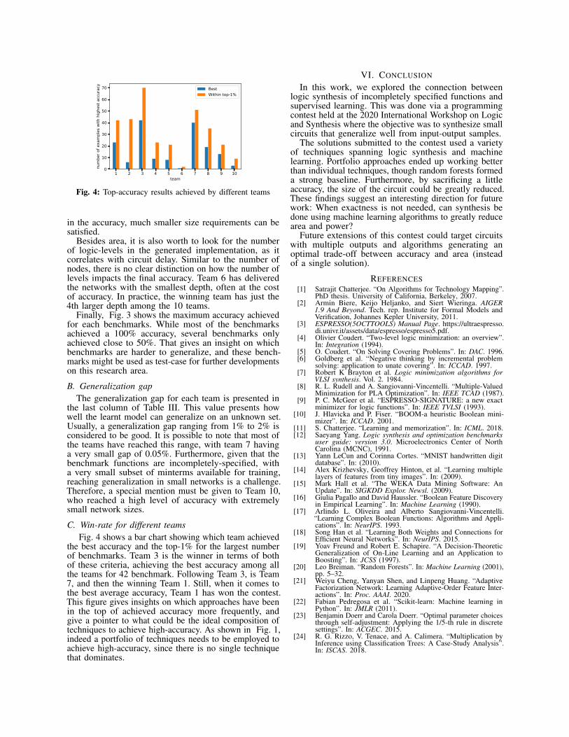
Fig. 4: Top-accuracy results achieved by different teams

in the accuracy, much smaller size requirements can besatisfied.

Besides area, it is also worth to look for the numberof logic-levels in the generated implementation, as itcorrelates with circuit delay. Similar to the number ofnodes, there is no clear distinction on how the number oflevels impacts the final accuracy. Team 6 has deliveredthe networks with the smallest depth, often at the costof accuracy. In practice, the winning team has just the4th larger depth among the 10 teams.

Finally, Fig. 3 shows the maximum accuracy achievedfor each benchmarks. While most of the benchmarksachieved a 100% accuracy, several benchmarks onlyachieved close to 50%. That gives an insight on whichbenchmarks are harder to generalize, and these bench-marks might be used as test-case for further developmentson this research area.

B. Generalization gapThe generalization gap for each team is presented in

the last column of Table III. This value presents howwell the learnt model can generalize on an unknown set.Usually, a generalization gap ranging from 1% to 2% isconsidered to be good. It is possible to note that most ofthe teams have reached this range, with team 7 havinga very small gap of 0.05%. Furthermore, given that thebenchmark functions are incompletely-specified, witha very small subset of minterms available for training,reaching generalization in small networks is a challenge.Therefore, a special mention must be given to Team 10,who reached a high level of accuracy with extremelysmall network sizes.

C. Win-rate for different teamsFig. 4 shows a bar chart showing which team achieved

the best accuracy and the top-1% for the largest numberof benchmarks. Team 3 is the winner in terms of bothof these criteria, achieving the best accuracy among allthe teams for 42 benchmark. Following Team 3, is Team7, and then the winning Team 1. Still, when it comes tothe best average accuracy, Team 1 has won the contest.This figure gives insights on which approaches have beenin the top of achieved accuracy more frequently, andgive a pointer to what could be the ideal composition oftechniques to achieve high-accuracy. As shown in Fig. 1,indeed a portfolio of techniques needs to be employed toachieve high-accuracy, since there is no single techniquethat dominates.

VI. CONCLUSION

In this work, we explored the connection betweenlogic synthesis of incompletely specified functions andsupervised learning. This was done via a programmingcontest held at the 2020 International Workshop on Logicand Synthesis where the objective was to synthesize smallcircuits that generalize well from input-output samples.

The solutions submitted to the contest used a varietyof techniques spanning logic synthesis and machinelearning. Portfolio approaches ended up working betterthan individual techniques, though random forests formeda strong baseline. Furthermore, by sacrificing a littleaccuracy, the size of the circuit could be greatly reduced.These findings suggest an interesting direction for futurework: When exactness is not needed, can synthesis bedone using machine learning algorithms to greatly reducearea and power?

Future extensions of this contest could target circuitswith multiple outputs and algorithms generating anoptimal trade-off between accuracy and area (insteadof a single solution).

REFERENCES[1] Satrajit Chatterjee. “On Algorithms for Technology Mapping”.

PhD thesis. University of California, Berkeley, 2007.[2] Armin Biere, Keijo Heljanko, and Siert Wieringa. AIGER

1.9 And Beyond. Tech. rep. Institute for Formal Models andVerification, Johannes Kepler University, 2011.

[3] ESPRESSO(5OCTTOOLS) Manual Page. https://ultraespresso.di.univr.it/assets/data/espresso/espresso5.pdf.

[4] Olivier Coudert. “Two-level logic minimization: an overview”.In: Integration (1994).

[5] O. Coudert. “On Solving Covering Problems”. In: DAC. 1996.[6] Goldberg et al. “Negative thinking by incremental problem

solving: application to unate covering”. In: ICCAD. 1997.[7] Robert K Brayton et al. Logic minimization algorithms for

VLSI synthesis. Vol. 2. 1984.[8] R. L. Rudell and A. Sangiovanni-Vincentelli. “Multiple-Valued

Minimization for PLA Optimization”. In: IEEE TCAD (1987).[9] P. C. McGeer et al. “ESPRESSO-SIGNATURE: a new exact

minimizer for logic functions”. In: IEEE TVLSI (1993).[10] J. Hlavicka and P. Fiser. “BOOM-a heuristic Boolean mini-

mizer”. In: ICCAD. 2001.[11] S. Chatterjee. “Learning and memorization”. In: ICML. 2018.[12] Saeyang Yang. Logic synthesis and optimization benchmarks

user guide: version 3.0. Microelectronics Center of NorthCarolina (MCNC), 1991.

[13] Yann LeCun and Corinna Cortes. “MNIST handwritten digitdatabase”. In: (2010).

[14] Alex Krizhevsky, Geoffrey Hinton, et al. “Learning multiplelayers of features from tiny images”. In: (2009).

[15] Mark Hall et al. “The WEKA Data Mining Software: AnUpdate”. In: SIGKDD Explor. Newsl. (2009).

[16] Giulia Pagallo and David Haussler. “Boolean Feature Discoveryin Empirical Learning”. In: Machine Learning (1990).

[17] Arlindo L. Oliveira and Alberto Sangiovanni-Vincentelli.“Learning Complex Boolean Functions: Algorithms and Appli-cations”. In: NeurIPS. 1993.

[18] Song Han et al. “Learning Both Weights and Connections forEfficient Neural Networks”. In: NeurIPS. 2015.

[19] Yoav Freund and Robert E. Schapire. “A Decision-TheoreticGeneralization of On-Line Learning and an Application toBoosting”. In: JCSS (1997).

[20] Leo Breiman. “Random Forests”. In: Machine Learning (2001),pp. 5–32.

[21] Weiyu Cheng, Yanyan Shen, and Linpeng Huang. “AdaptiveFactorization Network: Learning Adaptive-Order Feature Inter-actions”. In: Proc. AAAI. 2020.

[22] Fabian Pedregosa et al. “Scikit-learn: Machine learning inPython”. In: JMLR (2011).

[23] Benjamin Doerr and Carola Doerr. “Optimal parameter choicesthrough self-adjustment: Applying the 1/5-th rule in discretesettings”. In: ACGEC. 2015.

[24] R. G. Rizzo, V. Tenace, and A. Calimera. “Multiplication byInference using Classification Trees: A Case-Study Analysis”.In: ISCAS. 2018.

APPENDIXThe detailed version of approaches adopted by indi-

vidual teams are described below.

I. TEAM 1Authors: Yukio Miyasaka, Xinpei Zhang, Mingfei Yu,

Qingyang Yi, Masahiro Fujita, The University of Tokyo,Japan and University of California, Berkeley, USA

A. Learning MethodsWe tried ESPRESSO, LUT network, and Random

forests. ESPRESSO will work well if the underlyingfunction is small as a 2-level logic. On the other hand,LUT network has a multi-level structure and seems goodfor the function which is small as a multi-level logic.Random forests also support multi-level logic based ona tree structure.

ESPRESSO is used with an option to finish optimiza-tion after the first irredundant operation. LUT networkhas some parameters: the number of levels, the numberof LUTs in each level, and the size of each LUT. Theseparameters are incremented like a beam search as longas the accuracy is improved. The number of estimatorsin Random forests is explored from 4 to 16.

If the number of AIG nodes exceeds the limit (5000),a simple approximation method is applied to the AIG.The AIG is simulated with thousands of random inputpatterns, and the node which most frequently outputs0 is replaced by constant-0 while taking the negation(replacing with constant-1) into account. This is repeateduntil the AIG size meets the condition. To avoid the resultbeing constant 0 or 1, the nodes near the outputs areexcluded from the candidates by setting a threshold onlevel. The threshold is explored through try and error.

B. Preliminary ExperimentWe conducted a simple experiment. The parameters of

LUT was fixed as follows: the number of levels was 8,the number of LUTs in a level was 1028, and the size ofeach LUT was 4. The number of estimators in Randomforests was 8. The test accuracy and the AIG size of themethods is shown at Fig. 5 and Fig. 6. Generally Randomforests works best, but LUT network works better in afew cases among case 90-99. All methods failed to learncase 0, 2, 4, 6, 8, 20, 22, 24, 26, 28, and 40-49. Theapproximation was applied to AIGs generated by LUTnetwork and Random forests for these difficult cases andcase 80-99. ESPRESSO always generates a small AIGwith less than 5000 nodes as it conforms to less than tenthousands of min-terms.

The effect of approximation of the AIGs generated byLUT network is shown at Fig. 7. For difficult cases, theaccuracy was originally around 50%. For case 80-99, theaccuracy drops at most 5% while reducing 3000-5000nodes. Similar thing was observed in the AIGs generatedby Random forests.

C. Pre-defined standard function matchingThe most important method in the contest was actually

matching with a pre-defined standard functions. Thereare difficult cases where all of the methods above fail toget meaningful accuracy. We analyzed these test casesby sorting input patterns and was able to find adders,multipliers, and square rooters fortunately because the

inputs of test cases are ordered regularly from LSBto MSB for each word. Nevertheless, it seems almostimpossible to realize significantly accurate multiplier andsquare rooters with more than 100 inputs within 5000AIG nodes.

D. Exploration After The Contest1) Binary Decision Tree: We examined BDT (Binary

Decision Tree), inspired by the methods of other teams.Our target is the second MSB of adder because only BDTwas able to learn the second MSB of adder with morethan 90% accuracy according to the presentation of the3rd place team. In normal BDT, case-splitting by adding anew node is performed based on the entropy gain. On theother hand, in their method, when the best entropy gainis less than a threshold, the number of patterns where thenegation of the input causes the output to be negated toois counted for each input, and case-splitting is performedat the input which has such patterns the most.

First of all, the 3rd team’s tree construction highlydepends on the order of inputs. Even in the smallestadder (16-bit adder, case 0), there is no pattern such thatthe pattern with an input negated is also included in thegiven set of patterns. Their program just chooses the lastinput in such case and fortunately works in the contestbenchmark, where the last input is the MSB of one inputword. However, if the MSB is not selected at first, theaccuracy dramatically drops. When we sort the inputs atrandom, the accuracy was 59% on average of 10 times.

Next, we tried SHAP analysis [1] on top of XGBoost,based on the method of the 2nd place team, to find out theMSBs of input-words. The SHAP analysis successfullyidentifies the MSBs for a 16-bit adder, but not that for alarger adder (32-bit adder, case 2).

0.4

0.5

0.6

0.7

0.8

0.9

1

0 10 20 30 40 50 60 70 80 90 100

accu

racy

benchmarkESPRESSO

LUTNetworkRandomForest

Fig. 5: The test accuracy of the methods

In conclusion, it is almost impossible for BDT to learn32-bit or larger adders with random input order. If theproblem provides a black box simulator as in ICCADcontest 2019 problem A [2], we may be able to knowthe MSBs by simulating one-bit flipped patterns, such asone-hot patterns following an all-zero pattern. Anothermention is that BDT cannot learn a large XOR (16-XOR,case 74). This is because the patterns are divided into twoparts after each case-splitting and the entropy becomeszero at a shallow level. So, BDT cannot learn a deepadder tree (adder with more than 2 input-words), muchless multipliers.

0

1000

2000

3000

4000

5000

0 10 20 30 40 50 60 70 80 90 100

AIG

no

des

benchmark

ESPRESSO

LUTNetwork

RandomForest

Fig. 6: The resulting AIG size of the methods

0.4

0.5

0.6

0.7

0.8

0.9

1

0 10 20 30 40 50 60 70 80 90 100 0

2000

4000

6000

8000

10000

12000

accu

racy

AIG

nodes

benchmarkLUTNetwork

LUTNetwork-OriginalSizeOfLUTNetwork

SizeOfLUTNetwork-Original

Fig. 7: The test accuracy and AIG size of LUT network beforeand after approximation

2) Binary Decision Diagram: We also tried BDD(Binary Decision Diagram) to learn adder. BDD mini-mization using don’t cares [3] is applied to the BDDof the given on-set. Given an on-set and a care-set, wetraverse the BDD of on-set while replacing a node by itschild if the other child is don’t care (one-sided matching),by an intersection of two children if possible (two-sidedmatching), or by an intersection between a complementedchild and the other child if possible (complementedtwo-sided matching). Unlike BDT, BDD can learn alarge XOR up to 24-XOR (using 6400 patterns) becausepatterns are shared where nodes are shared.

BDD was able to learn the second MSB of adder treeonly if the inputs are sorted from MSB to LSB mixing allinput-words (the MSB of the first word, the MSB of thesecond word, the MSB of the third word, ..., the MSB ofthe last word, the second MSB of the first word, ...). Fornormal adder (2 words), one-sided matching achieved98% accuracy. The accuracy was almost the same amongany bit-width because the top dozens of bits control theoutput. For 4-word adder tree, one-sided matching gotaround 80% accuracy, while two-sided matching using athreshold on the gain of substitution achieved around 90%accuracy. Note that naive two-sided matching fails (gets50% accuracy). Furthermore, a level-based minimization,where nodes in the same level are merged if the gain

does not exceed the threshold, achieved more than 95%accuracy. These accuracy on 4-word adder tree is highcompared to BDT, whose accuracy was only 60% evenwith the best ordering.

For 6-word adder tree, the accuracy of the level-basedmethod was around 80%. We came up with anotherheuristic that if both straight two-sided matching andcomplemented two-sided matching are available, the onewith the smaller gain is used, under a bias of 100 nodeson the complemented matching This heuristic increasedthe accuracy of the level-based method to be 85-90%.However, none of the methods above obtained meaningful(more than 50%) accuracy for 8-word adder tree.

We conclude that BDD can learn a function if theBDD of its underlying function is small under someinput order and we know that order. The main reason forminimization failure is that merging inappropriate nodesis mistakenly performed due to a lack of contradictorypatterns. Our heuristics prevent it to some degree. Ifwe have a black box simulator, simulating patternsto distinguish straight and complemented two-sidedmatching would be helpful. Reordering using don’t caresis another topic to explore.

II. TEAM 2Authors: Guilherme Barbosa Manske, Matheus

Ferreira Pontes, Leomar Soares da Rosa Junior,Marilton Sanchotene de Aguiar, Paulo Francisco Butzen,Universidade Federal de Pelotas, Universidade Federaldo Rio Grande do Sul, Brazil

A. Proposed solutionOur solution is a mix of two machine learning

techniques, J48 [4] and PART [5]. We will first present ageneral overview of our solution. Then we will focus onindividual machine learning classifier techniques. Finally,we present the largest difference that we have foundbetween both strategies, showing the importance ofexploring more than only one solution.

The flowchart in Fig. 8 illustrates our overall solution.The first step was to convert the PLA structure into onethat Weka [6] could interpret. We decided to use theARFF structure due to how the structure of attributes andclasses is arranged.

Fig. 8: Solution’s flowchart.

After converting to ARFF, as shown in the flowchart’ssecond block, the J48 and PART algorithms are executed.In this stage of the process, the confidence factor is variedin five values (0.001, 0.01, 0.1, 0.25, and 0.5) for eachalgorithm. In total, this step will generate ten results.The statistics extracted from cross-validation were usedto determine the best classifier and the best confidencefactor.

This dynamic selection between the two classifiersand confidence factors was necessary since a common

configuration was not found for all the examples providedin the IWLS Contest. After selecting the best classifierand the best confidence factor, six new configurations areperformed. At this point, the parameter to be varied isthe minimum number of instances per sheet, that is, theWeka parameter ”-M”. The minimum number of instancesper sheet was defined (0, 1, 3, 4, 5, and 10). Again, theselection criterion was the result of the cross-validationstatistic.

1) J48: Algorithms for constructing decision trees areamong the most well known and widely used machinelearning methods. With decision trees, we can classifyinstances by sorting them based on feature values. Weclassify the samples starting at the root node and sortedbased on their feature values so that in each node, werepresent a feature in an example to be classified, and eachbranch represents a value that the node can assume. In themachine learning community, J. Ross Quinlan’s ID3 andits successor, C4.5 [4], are the most used decision treealgorithms. J48 is an open-source Java implementationof the C4.5 decision tree algorithm in Weka.

The J48 classifier output is a decision tree, which wetransform into a new PLA file. First, we go through thetree until we reach a leaf node, saving all internal nodes’values in a vector. When we get to the leaf node, we usethe vector data to write a line of the PLA file. After, weread the next node, and the amount of data that we keepin the vector depends on the height of this new node.

Our software keeps going through the tree until theend of the J48 file, and then it finishes the PLA filewriting the metadata. Finally, we use the ABC tool tocreate the AIG file, using the PLA file that our softwarehas created.

In Fig. 9, we show an example of how our softwareworks. Fig. 9 (a) shows a decision tree (J48 output) with7 nodes, 4 of which are leaves. Fig. 9 (b) shows the PLAfile generated by our software. The PLA file has 1 linefor every leaf in the tree. Fig. 9 (c) shows the pseudocodej48topla, where n control the data in the vector and x isthe node read in the line.

Fig. 9: (a) Decision tree (J48 output), (b) PLA file generatedby our software and (c) pseudocode j48topla.

2) PART: In the PART algorithm [5], we can inferrules generating partial decision trees. Thus two majorparadigms for rule generation are combined: creatingrules from decision trees and the separate-and-conquerrule learning technique. Once we build a partial tree,we extract a single rule from it, and for this reason, thePART algorithm avoids post-processing.

The PART classifier’s output is a set of rules, whichchecks from the first to the last rule to define the output

for a given input. We transform this set of rules in anAAG file, and to follow the order of the rules, we havecreated a circuit that guarantees this order. Each rule isan AND logic gate with a varied number of inputs.

First, we go through the PART file and create all therules (ANDs), inverting the inputs that are 0. We needto save the values and positions of all rules in a datastructure. After, we read this data structure, connectingall the outputs. If a rule makes the output goes to 1,we add an OR logic gate to connect with the rest ofthe rules. If a rule makes the output goes to 0, we addan AND logic gate, with an inverter in the first input.These guarantees that the first correct rule will define theoutput. Finally, we use the AIGER [7] library to convertthe created AAG to AIG.

In Fig. 10, we can see how this circuit is cre-ated. Fig. 10(a) shows a set of rules (PART file) with fourrules, where a blank line separates each rule. Fig. 10 (b)shows the circuit created with this set of rules.

Fig. 10: (a) Set of rules (PART file) and (b) circuit createdwith this set of rules.

B. ResultsFig. 11 shows the accuracy of the ten functions that

varied the most between the J48 and PART classifiers.We compared the best result of J48 and the best resultof PART with the Weka parameter ”-M” fixed in 2. Thebiggest difference happened in circuit 29, with J48 getting69.74% of accuracy and PART 99.27%, resulting in adifference of 29.52%.

Most of the functions got similar accuracy for bothclassifiers. The average accuracy of the J48 classifierwas 83.50%, while the average accuracy of the PARTclassifier was 84.53%, a difference of a little over 1%.After optimizing all the parameters in the Weka tool, wegot an average accuracy of 85.73%. All accuracy valueswere obtained with cross-validation.

In Fig. 12, we compare the number of ANDs in theAIG in the same ten functions. The interesting pointobserved in this plot refers to circuits 43, 51, and 52.The better accuracy for these circuits is obtained throughthe J48 classifier, while the resulting AIG is smaller thanthe ones created from PART solution. The complementarybehavior is observed in circuits 4, and 75. This behaviorreinforces the needed for diversification in machinelearning classifiers.

Fig. 13: Fringe DT learning flow.

Fig. 14: 12 fringe patterns.

Fig. 11: Accuracy of the ten functions that had the biggestdifference in accuracy between J48 and PART classifiers.The10 functions are 0, 2, 4, 6, 27, 29, 43, 51, 52 and 75

Fig. 12: Number of ANDs in ten functions used in Fig. 11.

III. TEAM 3Authors: Po-Chun Chien, Yu-Shan Huang, Hoa-Ren

Wang, and Jie-Hong R. Jiang, Graduate Institute ofElectronics Engineering, Department of ElectricalEngineering, National Taiwan University, Taipei, Taiwan

Team 3’s solution consists of decision tree (DT) basedand neural network (NN) based methods. For eachbenchmark, multiple models are generated and 3 areselected for ensemble.

A. DT-based methodFor the DT-based method, the fringe feature extraction

process proposed in [8, 9] is adopted. The overall learningprocedure is depicted in Fig. 13. The DT is trained andmodified for multiple iterations. In each iteration, thepatterns near the fringes (leave nodes) of the DT areidentified as the composite features of 2 decision variables.As illustrated in Fig. 14, 12 different fringe patternscan be recognized, each of which is the combination of2 decision variables under various Boolean operations.These newly detected features are then added to the listof decision variables for the DT training in the nextiteration. The procedure terminates when there are nonew features found or the number of the extracted featuresexceeds the preset limit. After training, the DT modelcan be synthesized into a MUX-tree in a straightforwardmanner, which will not be covered in detail in the paper.

B. NN-based methodFor the NN-based method, a 3-layer network is

employed, where each layer is fully-connected and usessigmoid(σ) as the activation function. As the synthesizedcircuit size of a typical NN could be quite large, theconnection pruning technique proposed in [10] is adoptedin order to meet the stringent size restriction. Networkpruning is an iterative process. In each iteration, a portionof unimportant connections (the ones with weights closeto 0) are discarded and the network is then retrained torecover its accuracy. The NN is pruned until the numberof fanins of each neuron is at most 12. To synthesize thenetwork into a logic circuit, an alternative can be doneby utilizing the arithmetic modules, such as adders andmultipliers, for the intended computation. Nevertheless,the synthesized circuit size can easily exceed the limitdue to the high complexity of the arithmetic units. Instead,each neuron in the NN is converted into a LUT byrounding and quantizing its activation. Fig. 15 shows anexample transformation of a neuron into a LUT, whereall possible input assignments are enumerated, and theneuron output is quantized to 0 or 1 as the LUT outputunder each assignment. The synthesis of the network canbe done quite fast, despite the exponential growth of theenumeration step, since the number of fanins of eachneuron has been restricted to a reasonable size during theprevious pruning step. The resulting NN after pruningand synthesis has a structure similar to the LUT-networkin [11], where, however, the connections were assignedrandomly instead of learned iteratively.

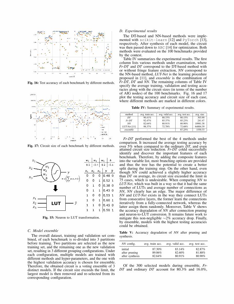
Fig. 16: Test accuracy of each benchmark by different methods.

Fig. 17: Circuit size of each benchmark by different methods.

Fig. 15: Neuron to LUT transformation.

C. Model ensembleThe overall dataset, training and validation set com-

bined, of each benchmark is re-divided into 3 partitionsbefore training. Two partitions are selected as the newtraining set, and the remaining one as the new validationset, resulting in 3 different grouping configurations. Undereach configuration, multiple models are trained withdifferent methods and hyper-parameters, and the one withthe highest validation accuracy is chosen for ensemble.Therefore, the obtained circuit is a voting ensemble of 3distinct models. If the circuit size exceeds the limit, thelargest model is then removed and re-selected from itscorresponding configuration.

D. Experimental resultsThe DT-based and NN-based methods were imple-

mented with scikit-learn [12] and PyTorch [13],respectively. After synthesis of each model, the circuitwas then passed down to ABC [14] for optimization. Bothmethods were evaluated on the 100 benchmarks providedby the contest.

Table IV summarizes the experimental results. The firstcolumn lists various methods under examination, whereFr-DT and DT correspond to the DT-based method withor without fringe feature extraction, NN correspond tothe NN-based method, LUT-Net is the learning procedureproposed in [11], and ensemble is the combination ofFr-DT, DT and NN. The remaining columns of Table IVspecify the average training, validation and testing accu-racies along with the circuit sizes (in terms of the numberof AIG nodes) of the 100 benchmarks. Fig. 16 and 17plot the testing accuracy and circuit size of each case,where different methods are marked in different colors.

Table IV: Summary of experimental results.

method avg. train acc. avg. valid acc. avg. test acc. avg. sizeDT 90.41% 80.33% 80.15% 303.90

Fr-DT 92.47% 85.37% 85.23% 241.47NN 82.64% 80.91% 80.90% 10981.38

LUT-Net [11] 98.37% 72.78% 72.68% 64004.39ensemble - - 87.25% 1550.33

Fr-DT performed the best of the 4 methods undercomparison. It increased the average testing accuracy byover 5% when compared to the ordinary DT, and evenattained circuit size reduction. Fr-DT could successfullyidentify and discover the important features of eachbenchmark. Therefore, by adding the composite featuresinto the variable list, more branching options are providedand thus the tree has the potential to create a bettersplit during the training step. On the other hand, eventhough NN could achieved a slightly higher accuracythan DT on average, its circuit size exceeded the limit in75 cases, which is undesirable. When comparing NN toLUT-Net, which was built in a way so that it had the samenumber of LUTs and average number of connections asNN, NN clearly has an edge. The major difference ofNN and LUT-Net exists in the way they connect LUTsfrom consecutive layers, the former learn the connectionsiteratively from a fully-connected network, whereas thelatter assign them randomly. Moreover, Table V showsthe accuracy degradation of NN after connection pruningand neuron-to-LUT conversion. It remains future work tomitigate this non-negligible ∼2% accuracy drop. Finally,by ensemble, models with the highest testing accuraciescould be obtained.

Table V: Accuracy degradation of NN after pruning andsynthesis.

NN config. avg. train acc. avg. valid acc. avg. test acc.

initial 87.30% 83.14% 82.87%after pruning 89.06% 82.60% 81.88%after synthesis 82.64% 80.91% 80.90%

Of the 300 selected models during ensemble, Fr-DT and ordinary DT account for 80.3% and 16.0%,

N-dimensional Training dataset

(1) Multi-Level Feature Selection

(2) Sparse Feature Learning via AFN

Lower imp.

(3) Inference with Sub-space Expansion

000000010010

1111...

AFN

... 1

000000010010

1111...

AFN

... 1

--0000 1--0001 0--0010 0--0011 1...--1111 1

.pla

CrossValidation

(4) Node Constrained AIG Search

Synth.

--0000 1--0001 0--0010 0--0011 1...--1111 1

.pla(i) mltest

.aig(i).aig(i)

>5000

<=5000 and high acc.

Next best pla <= 5000

and low acc.

Resplit datago to (1)

done

Fig. 18: Deep-learning-based Boolean function approximationframework.

1 0

1

0

0

SparselySampled Space

DON’T CARE

Fig. 19: Smoothness assumption in the sparse high-dimensionalBoolean space.

respectively, with NN taking up the remaining 3.7%.As expected, the best-performing Fr-DT models are inthe majority. It seems that the DT-based method is better-suited for this learning task. However, there were severalcases, such as case 75 where NN achieved 89.97% testingaccuracy over Fr-DT’s 87.38%, with an acceptable circuitsize (2320 AIG nodes).

E. Take-AwayTeam 3 adopted DT-based and NN-based methods

to tackle the problem of learning an unknown Booleanfunction. The team ranked 4 in terms of testing accuracyamong all the contestants of the IWLS 2020 programmingcontest. From the experimental evaluation, the approachthat utilized decision tree with fringe feature extractioncould achieve the highest accuracy with the lowest circuitsize in average. This approach is well-suited for thisproblem and can generate a good solution for almostevery benchmark, regardless of its origin.

IV. TEAM4Authors: Jiaqi Gu, Zheng Zhao, Zixuan Jiang,

David Z. Pan, Department of Electrical and ComputerEngineering, University of Texas at Austin, USA

A. Deep-Learning-Based Boolean Function Approxima-tion

Given the universal approximation theorem, neuralnetworks can be used to fit arbitrarily complex functions.For example, multi-layer perceptrons (MLPs) with enoughwidth and depth are capable to learn the most non-smoothbinary function in the high-dimensional hypercube, i.e.,XNOR or XOR [15]. For this contest, we adopt adeep-learning-based method to learn an unknown high-dimensional Boolean function with 5k node constraintsand extremely-limited training data, formulated as fol-lows,

min L(W ;Dtrn), (1)s.t. N (AIG(W )) ≤ 5, 000,

where L(W,Dtrn) is the binary classification loss func-tion on the training set, N (AIG(W )) is the num-ber of node of the synthesized AIG representationbased on the learned model. To solve this constrainedstochastic optimization, we adopt the following tech-niques, 1) multi-level ensemble-based feature selection,2) recommendation-network-based model training, 3)subspace-expansion-based prediction, and 4) accuracy-node joint exploration during synthesis. The frameworkis shown in Fig. 18. We demonstrate the test result andgive an analysis to show our performance on the 100public benchmarks.

B. Feature Selection with Multi-Level Model EnsembleThe first critical step for this learning task is to perform

data pre-processing and feature engineering. The public100 benchmarks have very unbalanced input dimensions,ranging from 10 to over 700, but the training datasetmerely has 6,400 examples per benchmark, which givesan inadequate sampling of the true distribution. Wealso observe that a naive AIG representation directlysynthesized from the given product terms has orders-of-magnitude more AND gates than the 5,000 nodeconstraint. The number of AND gate after node optimiza-tion of the synthesizer highly depends on the selectionof don’t-care set. Therefore, we make a smoothnessassumption in the sparse high-dimensional hypercubethat any binary input combinations that are not explicitlydescribed in the PLA file are set to don’t-care state, suchthat the synthesizer has enough optimization space to cutdown the circuit scale, shown in Fig. 19.

Based on this smoothness assumption, we performinput dimension reduction to prune the Boolean spaceby multi-level feature selection. Since we have 6,400randomly sampled examples for each benchmark, weassume the training set is enough to recover the truefunctionality of circuits with less than blog2 6, 400c = 12inputs and do not perform dimension reduction on thosebenchmarks. For benchmarks with more than 13 inputs,we empirically pre-define a feature dimension d rangingfrom 10 to 16, which is appropriate to cover enoughoptimization space under accuracy and node constraints.For each dimension d, we first perform the first levelof feature selection by pre-training a machine learningmodel ensemble.

Given the good interpretability and generalization,traditional machine learning models are widely used in

#N

od

e (k)

0

1000

2000

3000

4000

5000

50

60

70

80

90

100

ex00

ex04

ex08

ex1

2

ex16

ex20

ex24

ex28

ex32

ex36

ex40

ex44

ex4

8

ex52

ex56

ex60

ex64

ex68

ex72

ex76

ex80

ex8

4

ex88

ex92

ex96

#N

ode

Accura

cy (

%)

Validation Acc. (%) #Node

0

1000

2000

3000

4000

5000

50

60

70

80

90

100

ex00

ex04

ex08

ex1

2

ex16

ex20

ex24

ex28

ex32

ex36

ex40

ex44

ex4

8

ex52

ex56

ex60

ex64

ex68

ex72

ex76

ex80

ex8

4

ex88

ex92

ex96

#N

ode

Accura

cy (

%)

Validation Acc. (%) #Node

0

1000

2000

3000

4000

5000

6000

50

60

70

80

90

100

ex00

ex04

ex08

ex12

ex16

ex2

0

ex24

ex28

ex32

ex36

ex4

0

ex44

ex48

ex52

ex56

ex60

ex64

ex68

ex72

ex76

ex80

ex84

ex8

8

ex92

ex96

#N

ode

Accu

racy (

%)

Validation Acc. (%) #Node

Fig. 21: Evaluation results on IWLS 2020 benchmarks.

d to 10 embedding

LNN 128

Exponential & Concatenation

FC-80 + Dropout-0.5

FC-64 + Dropout-0.5

FC-64 + Dropout-0.4

Logarithmic Transform

Input Sparse Boolean Feature...

Sparse Feature Embedding

Logarithmic NN

MLP Classifier

Binary Output

Fig. 20: AFN [18] and configurations used for Boolean functionapproximation.

feature engineering to evaluate the feature importance.We pre-train an AdaBoost [16] ensemble classifierwith 100 ExtraTree sub-classifier on the trainingset to generate the importance score for all features.Then we perform permutation importance ranking [17]for 10 times to select the top-d important features asthe care set variables F 1(d). Given that the ultimateaccuracy is sensitive to the feature selection, we generateanother feature group at the second level to expand thesearch space. At the second level, we train two classifierensembles, one is an XGB classifier with 200 sub-treesand another is a 100-ExtraTree based AdaBoostclassifier. Besides, a stratified 10-fold cross-validation isused to select top-d important features F 2(d) based onthe average scores from the above two models. The entire14 candidates of input feature groups for each benchmarkare F = {F 1(d), F 2(d)}16d=10.

1) Deep Learning in the Sparse High-DimensionalBoolean Space: This learning problem is different fromcontinuous-space learning tasks, e.g., time-sequence-prediction, computer vision-related tasks, since its inputsare binarized with poor smoothness, which means high-frequency patterns in the input features are important tothe model prediction, e.g., XNOR and XOR. Besides, theextremely-limited training set gives an under-samplingof the real distribution, such that a simple multi-layerperceptron is barely capable of fitting the dataset whilestill having good generalization. Therefore, motivated by

a similar problem, the recommendation system designwhich targets at predicting the click rate based ondense and sparse features, we adopt a state-of-the-artrecommendation model, adaptive factorization network(AFN) [18], to fit the sparse Boolean dataset. Fig. 20demonstrates the AFN structure and network configurationwe use to fit the Boolean dataset. The embedding layermaps the high-dimensional Boolean feature to a 10-dspace and transform the sparse feature with a logarithmictransformation layer. In the logarithmic neural network,multiple vector-wise logarithmic neurons are constructedto represent any cross features to obtain different higher-order input combinations [18],

yj = exp( m∑

i=1

wij ln(Embed(F (d)))). (2)

Three small-scale fully-connected layers are used tocombine and transform the crossed features after log-arithmic transformation layers. Dropout layers after eachhidden layers are used to during training to improve thegeneralization on the unknown don’t-care set.

2) Inference with Sub-Space Expansion: After trainingthe AFN-based function approximator, we need to gener-ate the dot-product terms in the PLA file and synthesizethe AIG representation. Since we ignore all pruned inputdimension, we only assume our model can generalize inthe reduced d-dimensional hypercube. Hence, we predictall 2d input combinations with our trained approximator,and set all other pruned inputs to don’t-care state. On 14different feature groups F , we trained 14 different models{AFN0, · · · ,AFNd, · · · }, sorted in a descending order interms of validation accuracy. With the above 14 models,we predict 14 corresponding PLA files {P0, · · · ,Pd. · · · }with sub-space expansion to maximize the accuracy inour target space while minimizing the node count bypruning all other product terms, shown in Fig. 18. In theABC [19] tool, we use the node optimization commandsequence as resyn2, resyn2a, resyn3, resyn2rs,and compress2rs.

3) Accuracy-Node Joint Search with ABC: For eachbenchmark, we obtain multiple predicted PLA files tobe selected based on the node constraints. We searchthe PLA with the best accuracy that meets the nodeconstraints,

P∗ = argmaxP∼{··· ,Pd,··· }

Acc(AIG(P),Dval), (3)

s.t. N (AIG(P)) ≤ 5, 000.

If the accuracy is still very low, e.g., 60%, we resplit thedataset Dtrn and Dval and go to step (1) again in Fig. 18.

4) Results and Analysis: Fig. 21 shows our validationaccuracy and number of node after node optimization.Our model achieves high accuracy on most benchmarks.While on certain cases regardless of the input count, ourmodel fails to achieve a desired accuracy. An intuitiveexplanation is that the feature-pruning-based dimensionreduction is sensitive on the feature selection. A repeatingprocedure by re-splitting the dataset may help find a goodfeature combination to improve accuracy.

C. Conclusion and Future WorkWe introduce the detailed framework we use to learn

the high-dimensional unknown Boolean function for

Train. set

Valid. setMerge sets

Obtainproportions

Generate newtrain. andvalid. sets

Train DTs/RFs

Train NN Get importantfeatures

GenerateEQN/AIG

Reduce Nodeand Logic

LevelAIG

Evaluation

AIG withhighest

accuracy within5000-AND limit

GenerateSOP

Fig. 22: Design flow employed in this proposal.

IWLS’20 contest. Our recommendation system basedmodel achieves a top 3 smallest generalization gap onthe test set (0.48%), which is a suitable selection for thistask. A future direction is to combine more networks andexplore the unique characteristic of various benchmarks.

V. TEAM 5Authors: Brunno Alves de Abreu, Isac de Souza

Campos, Augusto Berndt, Cristina Meinhardt,Jonata Tyska Carvalho, Mateus Grellert and SergioBampi, Universidade Federal do Rio Grande do Sul,Universidade Federal de Santa Catarina, Brazil

Fig. 22 presents the process employed in this proposal.In the first stage, the training and valid sets provided in theproblem description are merged. The ratios of 0’s and 1’sin the output of the newly merged set are calculated, andwe split the set into two new training and validation sets,considering an 80%-20% ratio, respectively, preservingthe output variable distribution. Additionally, a secondtraining set is generated, equivalent to half of thepreviously generated training set. These two trainingsets are used separately in our training process, and theiraccuracy results are calculated using the same validationset to enhance our search for the best models. This wasdone because the model with the training set containing80% of the entire set could potentially lead to modelswith overfitting issues, so using another set with 40% ofthe entire provided set could serve as an alternative.

After the data sets are prepared, we train the DTsand RFs models. Every decision model in this proposaluses the structures and methods from the Scikit-learnPython library. The DTs and RFs from this library usethe Classification and Regression Trees (CART) algorithmto assemble the tree-based decision tools [20]. To trainthe DT, we use the DecisionTreeClassifier structure,limiting its max depth hyper-parameter to values of 10and 20 due to the 5000-gate limitation of the contest. TheRF model was trained similarly, but with an ensembleof DecisionTreeClassifier: we opted not to employthe RandomForestClassifier structure given that itapplied a weighted average of the preliminary decisionsof each DT within it. Considering that this would requirethe use of multipliers, and this would not be suitable toobtain a Sum-Of-Products (SOP) equivalent expression,using several instances of the DecisionTreeClassifierwith a simple majority voter in the output was the choicewe adopted. In this case, each DT was trained with arandom subset of the total number of features. Based

on preliminary testing, we found that RFs could notscale due to the contest’s 5000-gate limitation. This wasmainly due to the use of the majority voting, consideringthat the preliminaries expressions for that are too largeto be combined between each other. Therefore, for thisproposal, we opted to limit the number of trees used inthe RFs to a value of three.

Other parameters in the DecisionTreeClassifiercould be varied as well, such as the split metric, bychanging the Gini metric to Entropy. However, prelimi-nary analyses showed that both metrics led to very similarresults. Since Gini was slightly better in most scenariosand is also less computationally expensive, it was chosen.

Even though timing was not a limitation describedby the contest, we still had to provide a solution thatwe could verify that was yielding the same AIGs asthe ones submitted. Therefore, for every configurationtested, we had to test every example given in the problem.Hence, even though higher depths could be used withoutsurpassing the 5000-gate limitation, we opted for 10 and20 only, so that we could evaluate every example in afeasible time.

Besides training the DTs and RFs with varying depths,we also considered using feature selection methodsfrom the Scikit-learn library. We opted for the useof the SelectKBest and SelectPercentile methods.These methods perform a pre-processing in the features,eliminating some of them prior to the training stage.The SelectKBest method selects features according tothe k highest scores, based on a score function, namelyf classif , mutual info classif or chi2, according tothe Scikit-learn library [12]. The SelectPercentile issimilar but selects features within a percentile range givenas parameter, based on the same score functions [12].We used the values of 0.25, 0.5, and 0.75 for k, and thepercentiles considered were 25%, 50%, and 75%.

The solution employing neural networks (NNs) wasconsidered after obtaining the accuracy results for theDTs/RFs configurations. In this case, we train the modelusing the MLPClassifier structure, to which we usedthe default values for every parameter. Considering thatNNs present an activation function in the output, whichis non-linear, the translation to a SOP would not bepossible using conventional NNs. Therefore, this solutiononly uses the NNs to obtain a subset of features basedon their importance, i.e., select the set of features withthe corresponding highest weights. With this subset offeatures obtained, we evaluate combinations of functions,using ”OR,” ”AND,” ”XOR,” and ”NOT” operationsamong them. Due to the fact that the combinations offunctions would not scale well, in terms of time, with thenumber of features, we limit the sub-set to contain onlyfour features. The number of expressions evaluated foreach NN model trained was 792. This part of the proposalwas mainly considered given the difficulty of DTs/RFsin finding trivial solutions for XOR problems. Despitesolving the problems from specific examples whosesolution was a XOR2 between two of the inputs, witha 100% accuracy, we were able to slightly increase themaximum accuracy of other examples through this scan offunctions. The parameters used by the MLPClassifierwere the default ones: 100 hidden layers and ReLuactivation function [12].

The translation from the DT/RF to SOP was imple-mented as follows: the program recursively passes through

every tree path, concatenating every comparison. Whenit moves to the left child, this is equivalent to a ”true”result in the comparison. In the right child, we need a”NOT” operator in the expression as well. In a singlepath to a leaf node, the comparisons are joined throughan ”AND” operation, given that the leaf node result willonly be true when all the comparisons conditions are true.However, given that this is a binary problem, we onlyconsider the ”AND” expression of a path when the leafleads to a value of 1. After that, we perform an ”OR”operation between the ”AND” expressions obtained foreach path, which yields the final expression of that DT.

The RF scenario works the same way, but it considersthe expression required for the majority gate as well,whose inputs are the ”OR” expressions of each DT.

From the SOP, we obtain the AIG file. The generatedAIG file is then optimized using commands of the ABCtool [14] attempting to reduce the number of AIG nodesand the number of logic levels by performing iterativecollapsing and refactoring of logic cones in the AIG, andrewrite operations. Even if these commands could beiteratively executed, we decided to run them only oncegiven that the 5000-gate limitation was not a significantissue for our best solutions, and a single sequence of themwas enough for our solutions to adhere to the restriction.

Finally, we run the AIG file using the AIG evaluationcommands provided by ABC to collect the desired resultsof accuracy, number of nodes, and number of logic levelsfor both validation sets generated at the beginning of ourflow.

All experiments were performed three times withdifferent seed values using the Numpy randomseed method. This was necessary given that theDecisionTreeClassifier structure has a degree ofrandomness. Considering it was used for both DTs andRFs, this would yield different results at each execution.The MLPClassifier also inserts randomnesses in theinitialization of weights and biases. Therefore, to ensurethat the contest organizers could perfectly replicate thecode with the same generated AIGs, we fixed the seedsto values of 0, 1, and 2. Therefore, we evaluated twoclassifiers (DTs/RFs), with two maximum depths, twodifferent proportions, and three different seeds, whichleads to 24 configurations. For each of the SelectKBestand SelectPercentile methods, considering that we ana-lyzed three values of K and percentage each, respectively,along with three scoring functions, we have a total of 18feature selection methods. Given that we also tested themodels without any feature selection method, we have19 possible combinations. By multiplying the numberof configurations (24) with the number of combinationswith and without feature selection methods (adding upto 19), we obtain a total of 456 different DT/RF modelsbeing evaluated. Additionally, each NN, as mentioned,evaluated 792 expressions. These were also tested withtwo different training set proportions and three differentseeds, leading to a total of 4752 expressions for each ofthe 100 examples of the contest.

Table VI presents some additional information on theconfigurations that presented the best accuracy for theexamples from the contest. As it can be seen, when wesplit the 100 examples by the decision tool employed,most of them obtained the best accuracy results whenusing DTs, followed by RFs and NNs, respectively. Theuse of RFs was not as significant due to the 5000-gate

limitation, as it restrained us from using a higher numberof trees. The NNs were mainly useful to solve XOR2problems and in problems whose best accuracy resultsfrom DTs/RFs were close to 50%. It can also be observedthat the use of the feature selection methods along withDTs/RFs was helpful; therefore, cropping a sub-set offeatures based on these methods can definitely improvethe model obtained by the classifiers. The number of bestexamples based on the different scoring functions used inthe feature selection methods shows that the chi2 functionwas the most useful. This is understandable given thatthis is the default function employed by the Scikit-learnlibrary. Lastly, even though the proportions from 80%-20% represented the majority of the best results, it canbe seen that running every model with a 40%-20% wasalso a useful approach.

Table VI: Number of best examples based on the characteristicsof the configurations.

Characteristic Parameter # of examplesDT 55RF 28Decision ToolNN 17

Select K Best 48Select Percentile 11Feature Selection

None 41chi2 34

f classif 6mutual info classif 19Scoring Function

None 4140%-20% 23

Proportion 80%-20% 77

VI. TEAM 6Authors: Aditya Lohana, Shubham Rai and Akash Ku-

mar, Chair for Processor Design, Technische UniversitaetDresden, GermanyTo start of with, we read the training pla files usingABC and get the result of &mltest directly on the traindata. This gives the upper limit of the number of ANDgates which are used. Then, in order to learn the unknownBoolean function, we have used the method as mentionedin [11]. We used LUT network as a means to learn fromthe known set to synthesize on an unknown set. Weuse the concept of memorization and construct a logicnetwork.

In order to construct the LUT network, we use theminterms as input features to construct layers of LUTswith connections starting from the input layer. We thentry out two schemes of connections between the layers:‘random set of input’ and ‘unique but random set ofinputs’. By ‘random set of inputs’, we imply that wejust randomly select the outputs of preceding layer andfeed it to the next layer. This is the default flow. By‘unique but random set of inputs’, we mean that weensure that all outputs from a preceding layer is usedbefore duplication of connection. This obviously makessense when the number of connections is more than thenumber of outputs of the preceding layer.

We have four hyper parameters to experiment with inorder to achieve good accuracy– number of inputs perLUT, number of LUTS per layers, selection of connectingedges from the preceding layer to the next layer and the

x1?

x3? 1

1 0

1

1

0

0

(a)

.i 3

.o 1

.p 3

1-- 1

.ilb x1 x2 x30-0 10-1 0

.e

(b)

Fig. 23: (a) A decision tree and (b) its corresponding PLA.

x1?

x3? +0.3

+0.8 -0.2

1

1

0

0x2?

x1?

+0.3 -0.5

1

1

0

0

-0.7

x3?

+0.6

10+ +…

(a)x1?

x3? 1

1 0

1

1

0

0x2?

x1?

1 0

1

1

0

0

0

x3?

1

10+ +…

(b)

Fig. 24: XGBoost of decision trees, (a) before and (b) afterquantization of leaf values. Plus signs mean to add up resultingleaf values, one from each tree.

depth (number of LUT layers) of the model. We carryout experiments with varying number of inputs for eachLUT in order to get the maximum accuracy. We noticefrom our experiments that 4-input LUTs returns the bestaverage numbers across the benchmark suite. We alsofound that increasing the number of LUTs per layer ornumber of layers does not directly increases the accuracy.This is due to the fact, because increasing the numberof LUTs allows repeatability of connections from thepreceding layer. This leads to passing of just zeros/onesto the succeeding layers. Hence, the overall network tendstowards a constant zero or constant one.

After coming up with an appropriate set of connections,we create the whole network. Once we create the network,we convert the network into an SOP form using sympypackage in python. This is done from reverse topologicalorder starting from the outputs back to the inputs. Wethen pass the SOP form of the final output and create averilog file out of that. Using the verilog file, we convertit into AIG format and then use the ABC command to listout the output of the &mltest. We also report accuracyof our network using sklearn.

We have also incorporated use of data from validationtestcase. For our training model, we have used ‘0.4’ partof the minterms in our training.

VII. TEAM7: LEARNING WITH TREE-BASEDMODELS AND EXPLANATORY ANALYSISAuthors: Wei Zeng, Azadeh Davoodi, and Rasit Onur

Topaloglu, University of Wisconsin–Madison, IBM, USA

Team 7’s solution is a mix of conventional machinelearning (ML) and pre-defined standard function match-ing. If the training set matches a pre-defined standardfunction, a custom AIG of the identified function iswritten out. Otherwise, an ML model is trained andtranslated to an AIG.

Team 7 adopts tree-based ML models, considering thestraightforward correspondence between tree nodes andSOP terms. The model is either a single decision treewith unlimited depth, or an extreme gradient boosting(XGBoost) [21] of 125 trees with a maximum depth of5, depending on the results of a 10-fold cross validationon training data.

It is straightforward to convert a decision tree to SOPterms used in PLA. Fig. 23 shows a simple example ofdecision tree and its corresponding SOP terms. Numbersin leaves (rectangular boxes) indicate the predicted outputvalues. XGBoost is a more complex model in two aspects.First, it is a boosting ensemble of many shallow decisiontrees, where the final output is the sum of all leaf valuesthat a testing data point falls into, expressed in log oddslog[P (y = 1)/P (y = 0)]. Second, since the output isa real number instead of a binary result, a threshold ofclassification is needed to get the binary prediction (thedefault value is 0). Fig. 24(a) shows a simple exampleof a trained XGBoost of trees.

With the trained model, each underlying tree isconverted to a PLA, where each leaf node in the treecorresponds to a SOP term in the PLA. Each PLA areminimized and compiled to an AIG with the integratedespresso and ABC, respectively. If the function islearned by a single decision tree, the converted AIG isfinal. If the function is learned by XGBoost of trees, theexact final output of a prediction would be the sum of the125 leaves (one for each underlying tree) where the testingdata point falls into. In order to implement the AIGsefficiently, the model is approximated in the followingtwo steps. First, the value of each underlying tree leafis quantized to one bit, as shown in Fig. 24(b). Eachtest data point will fall into 125 specific leaves, yielding125 output bits. To mimic the summation of leaf valuesand the default threshold of 0 for classification, a 125-input majority gate could be used to get the final output.However, again for efficient implementation, the 125-input majority gate is further approximated by a 3-layernetwork of 5-input majority gates as shown in Fig. 25.

In the above discussion, it is assumed that the gatecount does not exceed the limit of 5000. If it is not thecase, the maximum depth of the decision tree and thetrees in XGBoost, and/or the number of trees in XGBoost,can be reduced at the cost of potential loss of accuracy.

Tree-based models may not perform well in somepre-defined standard functions, especially symmetricfunctions and complex arithmetic functions. However,symmetric functions are easy to be identified by com-paring the number of ones and the output bit. And itcan be implemented by adding a side circuit that countsN1, i.e., the number of ones in the input bits, and adecision tree that learns the relationship between N1 andthe original output. For arithmetic functions, patterns in

0 20 40 60 80 100 120Input bit

−4

−2

0

2

4Mea

n SH

AP

Fig. 27: Mean SHAP values of input bits in ex35, comparatorof two 60-bit signed integers, showing a pattern of “weights”that correspond to two signed integers with opposite polarities.

MAJ5MAJ5 …

MAJ5 …MAJ5

…

(125 outputs from underlying trees)

(Final prediction)

Fig. 25: Network of 5-input majority gates as an approximationof a 125-input majority gate.

0 10 20 30 40 50 60Input bit

−0.02

−0.01

0.00

0.01

0.02

0.03

Corr. coe

f.

(a)

0 10 20 30 40 50 60Input bit

0.0

0.5

1.0

1.5

2.0

2.5

3.0

Mea

n |SHA

P|

Fig. 26: Comparison of two importance metrics: (a) correlationcoefficient and (b) mean absolute SHAP value in ex25, theMSB of a 32x32 multiplier.

the importance of input bits can be observed in some pre-defined standard functions, such as adders, comparators,outputs of XOR or MUX. This is done by training aninitial XGBoost of trees and use SHAP tree explainer[1] to evaluate the importance of each input bit. Fig. 26shows that SHAP importance shows a pattern in trainingsets that suggests important input bits, while correlationcoefficient fails to show a meaningful pattern. Fig. 27shows an pattern of mean SHAP values of input bits,which suggests the possible existence of two signed binarycoded integers with opposite polarities in the function.Based on these observations, Team 7 checks before MLif the training data come from a symmetric function, andcompares training data with each identified pre-definedstandard function. In case of a match, an AIG of thestandard function is constructed directly without ML.With function matching, all six symmetric functions and25 out of 40 arithmetic functions can be identified withclose to 100% accuracy.

VIII. TEAM 8: LEARNING BOOLEANCIRCUITS WITH ML MODEL ENSEMBLEAuthors: Yuan Zhou, Jordan Dotzel, Yichi Zhang,

Hanyu Wang, Zhiru Zhang, School of Electrical andComputer Engineering, Cornell University, Ithaca, NY,USA

A. Machine Learning Model EnsembleModel ensemble is a common technique in the machine

learning community to improve the performance on aclassification or regression task. For this contest, we usea specific type of ensemble called “bucket of models”,where we train multiple machine learning models for eachbenchmark, generate the AIGs, and select the model thatachieves the best accuracy on the validation set fromall models whose AIGs are within the area constraintof 5k AND gates. The models we have explored inthis contest include decision trees, random forests, andmulti-layer perceptrons. The decision tree and multi-layerperceptron models are modified to provide better resultson the benchmarks, and our enhancements to these modelsare introduced in Section VIII-B and Section VIII-D,respectively. We perform a grid search to find the bestcombination of hyper-parameters for each benchmark.

B. Decision Tree for Logic LearningUsing decision trees to learn Boolean functions can be

dated back to the 1990s [22]. As a type of light-weightmachine learning models, decision trees are very effectivewhen the task’s solution space has a “nearest-neighbor”property and can be divided into regions with similarlabels by cuts that are parallel to the feature axes. ManyBoolean functions have these two properties, making themideal targets for decision trees. In the rest of this sectionwe introduce our binary decision tree implementation, andprovide some insights on the connection between decisiontree and Espresso [23], a successful logic minimizationalgorithm.

ABC f000 0

001 0

010 1

011 1

100 1

101 1

110 0

111 0

𝑓 = 𝐴 𝑥𝑜𝑟 𝐵 A=1

Entries 0,1,2,3

Entries4,5,6,7

No Yes

C=1

Entries0,2,4,6

Entries1,3,5,7

No Yes

Mutual information = 0

Mutual information = 0

Fig. 28: Example of learning a two-input XOR with anirrelevant input. The whole truth table is provided for illustrationpurposes. The impurity function based on mutual informationcannot distinguish the useful inputs (A and B) from theirrelevant input C. This is because mutual information onlyconsiders the probability distributions at the current node (root)and its children.

1) Binary Decision Tree: We use our own implemen-tation of the C4.5 decision tree [24] for the IWLS’20programming contest. The decision trees directly take theBoolean variables as inputs. We use mutual informationas the impurity function: when evaluating the splittingcriterion at each non-leaf node, the feature split thatprovides the maximum mutual information is selected.During training, our decision tree continues splitting ateach node unless one of the following three conditionsis satisfied:

1) All samples at a node have the same label.2) All samples at a node have exactly the same features.3) The number of samples at a node is smaller than a

hyper-parameter N set by the user.The hyper-parameter N helps avoid overfitting by allow-ing the decision tree to tolerate errors in the trainingset. With larger N , the decision tree learns a simplerclassification function, which may not achieve the bestaccuracy on the training set but generalizes better tounseen data.

2) Functional Decomposition for Split Criterion Selec-tion: The splitting criterion selection method describedin Section VIII-B1 is completely based on the probabilitydistribution of data samples. One drawback of suchprobability-based metrics in logic learning is that they arevery sensitive to the sampling noise, especially when thesampled data is only a very small portion of the completetruth table. Fig. 28 shows an example where we try tolearn a three-input function whose output is the XOR oftwo inputs A and B. An optimal decision tree for learningthis function should split by either variable A or B atthe root node. However, splitting by the correct variableA or B does not provide higher gain than splitting bythe irrelevant variable C. Depending on the tie-breakingmechanism, the decision tree might choose to split byeither of the three variables at the root node. For thecontest benchmarks, only a small portion of the truthtable is available. As a result, it is possible that thesampling noise will cause a slight imbalance between

the samples with zero and one labels. In such cases, it islikely that the decision tree will pick an irrelevant featureat the root node.

If the decision tree selects an irrelevant or incorrectfeature at the beginning, it is very difficult for it to”recover” during the rest of the training process due tothe lack of a backtracking procedure. Finding the bestdecision tree for any arbitrary dataset requires exponentialtime. While recent works [25] propose to use smartbranch-and-bound methods to find optimal sparse decisiontrees, it is still impractical to use such approaches forlogic learning when the number of inputs is large. Asa result, we propose to apply single-variable functionaldecomposition when the maximum mutual information islower than a set threshold τ during splitting. The valueof τ is a hyper-parameter and is included in the gridsearch for tuning. At each none-leaf node, we test allnon-used features to find a feature that satisfies either ofthe following two requirements:

1) At least one branch is constant after splitting by thisfeature.

2) One branch is the complement of the other aftersplitting by this feature.

In many cases we don’t have enough data samples tofully test the second requirement. As a result, we takean aggressive approach where we consider the secondrequirement as being satisfied unless we find a counterexample. While such an aggressive approach may notfind the best feature to split, it provides an opportunity toavoid the effect of sampling noise. In our implementation,functional decomposition is triggered more often at thebeginning of the training and less often when close tothe leaf nodes. This is because the number of samples ateach non-leaf node decreases exponentially with respectto the depth of the node, and the sampling noise becomesmore salient with few data samples. When the numberof samples is small enough, the mutual information isunlikely to fall below τ , so functional decomposition willno longer be triggered.

We observed significant accuracy improvement afterincorporating functional decomposition into the trainingprocess. However, we also realized that the improve-ment in some benchmarks might be because of animplementation detail: if multiple features satisfy thetwo requirements listed above, we select the last one.This implementation decision happens to help for somebenchmarks, mostly because our check for the secondrequirement is too aggressive. This finding was alsoconfirmed by team 1 after our discussion with them.

3) Connection with Espresso: We found an interestingconnection between decision tree and the Espresso logicoptimization method. For the contest benchmarks, only6.4k entries of the truth table are given and all otherentries are don’t cares. Espresso exploits don’t cares byexpanding the min-terms in the SOP, which also leveragesthe “nearest neighbor” property in the Boolean inputspace. Decision trees also leverage this property, butthey exploit don’t cares by making cuts in the inputspace. As a result, neither Espresso nor decision tree isable to learn a logic function from an incomplete truthtable if the nearest neighbor property does not hold. Forexample, according to our experiments, neither techniquecan correctly learn a parity function even if 90% of thetruth table has been given.

4) Converting into AIG: One advantage of usingdecision trees for logic learning is that converting adecision tree into a logic circuit is trivial. Each non-leaf node in the tree can be implemented as a two-inputmultiplexer, and the multiplexers can be easily connectedby following the structure of the tree. The values at theleaf nodes are simply implemented as constant inputs tothe multiplexers. We follow this procedure to convert eachdecision tree into an AIG, and use ABC [14] to furtheroptimize the AIG to reduce area. After optimization, noneof the AIGs generated from decision trees exceeds thearea budget of 5k AND gates.

C. Random ForestRandom forest can be considered as an ensemble of

bagged decision trees. Each random forest model containsmultiple decision trees, where each tree is trained with adifferent subset of data samples or features so that thetrees won’t be very similar to each other. The final outputof the model is the majority of all the decision trees’predictions.

We used the random forest implementation from sci-kit learn [12] and performed grid search to find the bestcombination of hyper-parameters. For all benchmarkswe use a collection of seventeen trees with a maximumdepth of eight. To generate the AIG, we first converteach tree into a separate AIG, and then connect allthe AIGs together with a seventeen-input majority gate.The generated AIG is further optimized using ABC.None of the AIGs exceeds the 5K gate constraint afteroptimization.

D. Multi-Layer PerceptronOur experiments find that multi-layer perceptrons

(MLP) with a variety of activation functions performwell on certain benchmark classes. These models comewith a few core challenges. First, it is difficult totranslate a trained floating-point model to an AIG withoutsignificantly decreasing the accuracy. Thus, we limitthe size of the MLP, synthesize it precisely throughenumeration of all input-output pairs, and carefully reduceresultant truth table. Second, MLP architectures havedifficulties with latent periodic features. To address this,we utilize the sine activation function which can selectfor periodic features in the input, validating previouswork in its limited applicability to learning some classesof functions.

E. Sine ActivationWe constructed a sine-based MLP that performed as

well or better than the equivalent ReLU-based MLPon certain benchmark classes. This work is concurrentwith a recent work that applies periodic activationsto implicit neural representation [26], and draws fromintermittent work over the last few decades on periodicactivation functions [27][28]. In our case, we find the sineactivation function performs well in certain problems thathave significant latent frequency components, e.g. paritycircuit. It also performs well in other cases since forsufficiently small activations sine is monotonic, whichpasses gradients in a similar manner to the standardactivation functions, e.g ReLU. We learn the period ofthe activation function implicitly through the weightsinputted into the neuron. However, we find that one

disadvantage is the exponential increase in local minima[29], which makes training more unstable.

F. Logic SynthesisAfter training the (sine-based) MLP models, we convert

them into AIGs. Some common methods for this conver-sion are binary neural networks [30], quantized neuralnetworks [31], or directly learned logic [32]. Instead, wetook advantage of the small input size and generated thefull truth tables of the neural network by enumeratingall inputs and recording their outputs. Then, we passedthis truth table to ABC for minimization. This methodis a simpler variant to one described in LogicNets [33].It easily produces models within the 5k gate limit forsmaller models, which with our constraints correspondsto benchmarks with fewer than 20 inputs.

G. Summary and Future WorkWe have described the ML models we used for

the IWLS’20 contest. Based on our evaluation on thevalidation set, different models achieve strong resultson different benchmarks. Decision trees achieve thebest accuracy for simple arithmetic benchmarks (0-39),random forest gives better performance on the binaryclassification problems (80-99), while our special MLPdominates on the symmetric functions (70-79). It remainsa challenge to learn complex arithmetic functions (40-49)from a small amount of data. Another direction for futurework is to convert MLP with a large number of inputsinto logic.

IX. TEAM 9:BOOTSTRAPPED CGP LEARNINGFLOW

Authors: Augusto Berndt, Brunno Alves de Abreu,Isac de Souza Campos, Cristina Meinhardt, MateusGrellert, Jonata Tyska Carvalho, Universidade Federalde Santa Catarina, Universidade Federal do Rio Grandedo Sul, Brazil

A. IntroductionTeam 9 uses a population-based optimization method

called Cartesian Genetic Programming (CGP) for synthe-sizing circuits for solving the IWLS’20 contest problems.The flow used includes bootstrapping the initial pop-ulation with solutions found by other well-performingmethods as decision trees and espresso technique, andfurther improving them. The results of this flow aretwo-fold: (i) it allows to improve further the solutionsfound by the other techniques used for bootstrappingthe evolutionary process, and (ii) alternatively, whenno good solutions are provided by the bootstrappingmethods, CGP starts the search from random (unbiased)individuals seeking optimal circuits. This text starts witha brief introduction to the CGP technique, followed bypresenting the proposed flow in detail.

CGP is a stochastic search algorithm that uses anevolutionary approach for exploring the solution’s param-eter space, usually starting from a random population ofcandidate solutions. Through simple genetic operatorssuch as selection, mutation and recombination, the searchprocess often leads to incrementally improved solutions,despite there is no guarantee of optimality.

The evolutionary methods seek to maximize a fitnessfunction, which usually is user-defined and problem-related, that measures each candidate solution’s per-formance, also called individual. The parameter spacesearch is conducted by adding variation to the individualsby mutation or recombination and retaining the bestperforming individuals through the selection operatorafter evaluation. Mutation means that specific individ-ual’s parameters are randomly modified with a certainprobability. Recombination means that individuals canbe combined to generate new individuals, also witha given probability. This latter process is referred toas crossover. However, the CGP variation does notemploy the crossover process since it does not improveCGP efficiency [34]. The genetic operators are appliediteratively, and each iteration is usually called generation.

Fig. 29 presents an example of a CGP implementationwith one individual, its set of primitive logic functions,and the individual’s genetic code. The CGP structure isrepresented as a logic circuit, and the CGP Cartesianvalues are also shown. Notice that there is only oneline present in the two-dimensional graph, in reference[35] it is shown that such configuration provides fasterconvergence when executing the CGP search. Recentworks also commonly make use of such configuration[36]. The CGP implemented in work presented hereinused such configuration of only one line and multiplecolumns. Please note that one may represent any logiccircuit in a single line as one would in a complete two-dimensional graph.

Fig. 29 also presents the individuals’ representation,sometimes called genotype or genetic coding. This codeis given by a vector of integers, where a 3-tuple describeseach node, the first integer corresponds to the node’s logicfunction, and the other two integers correspond to thefan-ins’ Cartesian values. The number of primary inputs,primary outputs, and internal CGP nodes is fixed, i.e.,are not under optimization. For the contest specifically,the PIs and POs sizes will always correspond to theinput PLA file’s values. At the same time, the numberof internal CGP nodes are parametrized and set as oneof the program’s input information.

Notice that the circuit presented in Fig. 29 is composedof a functional and a non-functional portion, meaningthat a specific section of the circuit does not influence itsprimary output. The non-functional portion of the circuitis drawn in gray, while the functional portion is black.The functional portion of a CGP individual is said tobe its Phenotype, in other words, the observable portionwith relation to the circuit’s primary outputs. At the same

Fig. 29: Single Line CGP Example.

time, its complete genetic code representation is knownas its Genotype.

As demonstrated by [35], the CGP search has abetter convergence if phenotypically larger solutionsare considered preferred candidates when analyzing theindividual’s fitness scores. In other words, if, during theevolution, there are two individuals with equal accuracybut different functional sizes, the larger one will bepreferred. The proposed flow makes use of such atechnique by always choosing AIGs with larger availablesizes as fathers when a tie in fitness values happens.

The proposed CGP flow is presented in Fig. 30. Itfirst tries to start from a well-performing AIG previouslyfound using some other method as, for instance, DecisionTrees(DT) or SOP via the Espresso technique. We call thisinitialization process bootstrap. It is noteworthy that theproposed flow can use any AIG as initialization, makingit possible to explore previous AIGs from differentsyntheses and apply the flow as a fine-tuning process.

If the bootstrapped AIG has an accuracy inferior to55%, the CGP starts the search from a random (unbiased)population seeking optimal circuits; otherwise, it runs abootstrapped initialization with the individual generatedby previously optimized Sum of Products created byDecision Trees or Espresso. Summarizing, the flow’s firststep is to evaluate the input AIG provided by anothermethod and check whether it will be used to run theCGP search, or the search will be conducted using a newrandom AIG.

Fig. 30: Proposed CGP Flow.

Due to the CGP training approach, the learning setmust be split among the CGP and the other method forusing the Bootstrap option. When this is the case, thetraining set is split in a 40%-40%/20% format, meaninghalf the training set is used by the initialization methodand the other half by the CGP, while leaving 20% ofthe dataset for testing with both methods involved in theAIG learning.

An empiric exploration of input hyper-parameters con-figurations was realized, attempting to look for superiorsolutions. The evolutionary approach used is the (1+4)-ES rule. In this approach, one individual generates fournew mutated copies of itself, and the one with thebest performance is selected for generating the mutated

InitializationType

AIGSize

Train/TestFormat

(%)

BatchSize

ChangeEach

Bootstrap Twice theOriginal AIG 40-40/20 Half

Train SetNot

Applicable

Random 500,5000 80/20

1024,CompleteTrain Set

1000,2000

Table VII: Hyper-Parameters Dependent on Initialization

copies of the next generation. Variation is added to theindividuals through mutations. The mutation rate is underoptimization according to the 1/5th rule [37], in whichmutation rate value varies jointly with the proportion ofindividuals being better or worst than their ancestor.

The CGP was run with three main hyper-parameter:(1) the number of generations with values of 10, 20, 25,50 and 100 thousand; (2) two logic structures available:AIG and XAIG; and (3) the program had the option tocheck for all nodes as being a PO during every traininggeneration. The latter is a computationally intensivestrategy, but some exemplars demonstrated good resultswith it. The CGP flow runs exhaustively, combining thesethree main hyper-parameter options.

Together with the previously mentioned hyper-parameters, there is a set of four other hyper-parametersdependent on the initialization option, presented in Ta-ble VII. For a bootstrap option of a previous AIG, thereis a single configuration where the CGP size is twicethe Original AIG, meaning that for each node in theOriginal AIG, a non-functional node is incremented to thelearning model, increasing the search space. The trainingconfiguration takes half the training set since the otherhalf was already used by the initialization method. Thisbootstrap option does not execute with mini-batches sincethey add stochasticity for the search and the intention isto fine-tune the AIG solution.

For a random initialization, multiple hyper-parametersalternatives are explored in parallel. The AIG size isconfigured to 500 and 5000 nodes. The training set doesnot have to be shared, meaning that the whole training setis employed for the search. Training mini-batches of size1024 are used, meaning that the individuals are evaluatedusing the same examples during a certain number ofconsecutive generations. The number of generations amini-batch is kept is determined by the change eachhyper-parameter, meaning that the examples used forevaluating individuals change each time that number ofgenerations is reached. A previous study showed thatthis technique could lead to the synthesis of more robustsolutions, i. e., solutions that generalize well to unseeninstances [38]. The random initialization could also usethe complete train set as if the batch size was the sameas the training set available.

Finally, the last step evaluates the AIGs generated,collecting results of accuracy, number of nodes, and logiclevels for the validation sets. All the AIGs generated bythe CGP respect the size limit of 5000 AND nodes.The AIG with the highest accuracy is chosen as thefinal solution for the benchmark. The CGP flow showsthe potential to optimize previous solutions, where theoptimization metric is easily configurable.

Experiments were executed on the Emulab Utah [39]research cluster, the computers available operate under a

Ubuntu 18.04LTS image. The CGP was implemented inC++ with object-oriented paradigm, codes were compiledon GCC 7.5.

X. TEAM 10Authors: Valerio Tenace, Walter Lau Neto, and

Pierre-Emmanuel Gaillardon, University of Utah, USA

In order to learn incompletely specified Booleanfunctions for the contest, we decided to resort to decisiontrees (DTs). Fig. 31 presents an overview of the adopteddesign flow.

TrainingPLA

ValidationPLA

DT Training

AccuracyCheck

VerilogGeneration

TrainingAugmentation

Synthesis andOptimization

Validation <= 70%Validation > 70%

Custom Python

ABC

Fig. 31: Overview of adopted flow.

We developed a Python program using the Scikit-learnlibrary where the parameter max depth serves as an upper-bound to the growth of the trees. Through many rounds ofevaluation, we opted to set the max depth to 8, as it givessmall AIG networks without sacrificing the accuracy toomuch. The training set PLAs, provided by the contest, areread into a numpy matrix, which is used to train the DT.On the other hand, the validation set PLA is used to testwhether the obtained DT meets the minimum validationaccuracy, which is empirically set to be 70%. If such acondition is not met, the training set is augmented bymerging it with the validation set. According to empiricalevaluations, most of these benchmarks with performance< 70% showed a validation accuracy fluctuating around50%, regardless of the size and shapes of the DTs. Thissuggests that the training sets were not able to provideenough representative cases to effectively exploit theadopted technique, thus leading to DTs with very hightraining accuracy, but completely negligible performances.For DTs having a validation accuracy ≥ 70%, the treestructure is annotated as a Verilog netlist, where each DTnode is replaced with a multiplexer. In cases where theaccuracy does not achieve the lower bound of 70%, we re-train the DT with the augmented set, and then annotate itin Verilog. The obtained netlist is then processed with theABC Synthesis Tool in order to generate a compact andoptimized AIG structure. More detailed information aboutthe adopted technique can be found in [40]. Overall, ourapproach was capable of achieving very good accuracyfor most of the cases, without exceeding 300 AIG nodesin any benchmark, thus yielding the smallest averagenetwork sizes among all the participants. In many cases,we achieved an accuracy greater than 90% with lessthan 50 nodes, and a mean accuracy of 84% with only

140 AND gates on average. Fig. 32 presents the accuracyachieved for all the adopted benchmarks, whereas Fig. 33shows the AIG size for the same set of circuits. Theseresults clearly show that DTs are a viable technique tolearn Boolean functions efficiently.

Benchmarks

Acc

urac

y (%

)

0255075

100

ex00ex07

ex14ex21

ex28ex35

ex42ex49

ex56ex63

ex70ex77

ex84ex91

ex98

Fig. 32: Accuracy for different benchmarks.

Benchmarks

AN

D G

ates

0

100

200

300

ex00ex07

ex14ex21

ex28ex35

ex42ex49

ex56ex63

ex70ex77

ex84ex91

ex98

Fig. 33: Number of AIG nodes for different benchmarks.

REFERENCES

[1] Scott M. Lundberg et al. “From local explanations to globalunderstanding with explainable AI for trees”. In: NatureMachine Intelligence 2.1 (2020), pp. 56–67.

[2] Pei-wei Chen et al. “Circuit Learning for Logic Regression onHigh Dimensional Boolean Space”. In: Proceedings of DesignAutomation Conference (DAC). 2020.

[3] Thomas R. Shiple et al. “Heuristic minimization of BDDs usingdon’t cares”. In: Proceedings of Design Automation Conference(DAC). New York, New York, USA: ACM Press, 1994, pp. 225–231.

[4] J. Ross Quinlan. C4.5: Programs for Machine Learning. SanFrancisco, CA, USA: Morgan Kaufmann Publishers Inc., 1993.

[5] Eibe Frank and Ian H. Witten. “Generating Accurate Rule SetsWithout Global Optimization”. In: Proceedings of the FifteenthInternational Conference on Machine Learning. ICML ’98. SanFrancisco, CA, USA: Morgan Kaufmann Publishers Inc., 1998,pp. 144–151.

[6] Mark Hall et al. “The WEKA Data Mining Software: AnUpdate”. In: SIGKDD Explor. Newsl. (2009).

[7] Armin Biere, Keijo Heljanko, and Siert Wieringa. AIGER1.9 And Beyond. Tech. rep. Institute for Formal Models andVerification, Johannes Kepler University, 2011.

[8] Giulia Pagallo and David Haussler. “Boolean Feature Discoveryin Empirical Learning”. In: Machine Learning (1990).

[9] Arlindo L. Oliveira and Alberto Sangiovanni-Vincentelli.“Learning Complex Boolean Functions: Algorithms and Appli-cations”. In: NeurIPS. 1993.

[10] Song Han et al. “Learning Both Weights and Connections forEfficient Neural Networks”. In: NeurIPS. 2015.

[11] S. Chatterjee. “Learning and memorization”. In: ICML. 2018.[12] Fabian Pedregosa et al. “Scikit-learn: Machine learning in

Python”. In: JMLR (2011).[13] Adam Paszke et al. “PyTorch: An Imperative Style, High-

Performance Deep Learning Library”. In: Advances in NeuralInformation Processing Systems (NeurIPS) 32. Ed. by H.Wallach et al. Curran Associates, Inc., 2019, pp. 8024–8035.

[14] Robert Brayton and Alan Mishchenko. “ABC: An AcademicIndustrial-Strength Verification Tool”. In: Proc. CAV. 2010,pp. 24–40.

[15] K. Hornik, M. Stinchcombe, and H. White. “Multilayer Feed-forward Networks Are Universal Approximators”. In: NeuralNetw. 2.5 (1989), pp. 359–366.

[16] Yoav Freund and Robert E. Schapire. “A Decision-TheoreticGeneralization of On-Line Learning and an Application toBoosting”. In: JCSS (1997).

[17] Leo Breiman. “Random Forests”. In: Machine Learning (2001),pp. 5–32.

[18] Weiyu Cheng, Yanyan Shen, and Linpeng Huang. “AdaptiveFactorization Network: Learning Adaptive-Order Feature Inter-actions”. In: Proc. AAAI. 2020.

[19] Robert Brayton and Alan Mishchenko. “ABC: An AcademicIndustrial-Strength Verification Tool”. In: Proc. CAV. 2010,pp. 24–40.

[20] Dan Steinberg and Phillip Colla. “CART: classification andregression trees”. In: The top ten algorithms in data mining 9(2009), p. 179.

[21] Tianqi Chen and Carlos Guestrin. “XGBoost: A Scalable TreeBoosting System”. In: Proceedings of the 22nd ACM SIGKDDInternational Conference on Knowledge Discovery and DataMining. San Francisco, California, USA: ACM, 2016, pp. 785–794.

[22] Arlindo L Oliveira and Alberto Sangiovanni-Vincentelli. “Learn-ing complex boolean functions: Algorithms and applications”.In: Advances in Neural Information Processing Systems. 1994,pp. 911–918.

[23] R. L. Rudell and A. Sangiovanni-Vincentelli. “Multiple-ValuedMinimization for PLA Optimization”. In: IEEE TCAD (1987).

[24] John Quinlan. C4. 5: programs for machine learning. Elsevier,2014.

[25] Xiyang Hu, Cynthia Rudin, and Margo Seltzer. “Optimal sparsedecision trees”. In: Advances in Neural Information ProcessingSystems. 2019, pp. 7267–7275.

[26] Vincent Sitzmann et al. “Implicit Neural Representations withPeriodic Activation Functions”. In: CVPR. 2020.

[27] Alan Lapedes and Robert Farber. “How Neural Nets Work”.In: Advances in Neural Information Processing Systems. MITPress, 1987, pp. 442–456.

[28] J.M. Sopena, Enrique Romero, and Rene Alquezar. “NeuralNetworks with Periodic and Monotonic Activation Functions:A Comparative Study in Classification Problems”. In: Inter-national Conference on Artificial Neural Networks (ICANN).1999, 323–328 vol.1.

[29] Giambattista Parascandolo, H. Huttunen, and T. Virtanen.Taming the waves: sine as activation function in deep neuralnetworks. 2017.

[30] Zechun Liu et al. ReActNet: Towards Precise Binary NeuralNetwork with Generalized Activation Functions. 2020.

[31] Ritchie Zhao et al. “Improving Neural Network Quantizationwithout Retraining using Outlier Channel Splitting”. In: In-ternational Conference on Machine Learning (ICML) (2019),pp. 7543–7552.

[32] E Wang et al. “LUTNet: Learning FPGA Configurationsfor Highly Efficient Neural Network Inference”. In: IEEETransactions on Computers (2020).

[33] Yaman Umuroglu et al. LogicNets: Co-Designed NeuralNetworks and Circuits for Extreme-Throughput Applications.2020.

[34] Julian Francis Miller. “Cartesian genetic programming: itsstatus and future”. In: Genetic Programming and EvolvableMachines (2019), pp. 1–40.

[35] Nicola Milano and Stefano Nolfi. “Scaling Up CartesianGenetic Programming through Preferential Selection of LargerSolutions”. In: arXiv preprint arXiv:1810.09485 (2018).

[36] Abdul Manazir and Khalid Raza. “Recent developments inCartesian genetic programming and its variants”. In: ACMComputing Surveys (CSUR) 51.6 (2019), pp. 1–29.

[37] Benjamin Doerr and Carola Doerr. “Optimal parameter choicesthrough self-adjustment: Applying the 1/5-th rule in discretesettings”. In: ACGEC. 2015.

[38] Jonata Tyska Carvalho, Nicola Milano, and Stefano Nolfi.“Evolving Robust Solutions for Stochastically Varying Prob-lems”. In: 2018 IEEE Congress on Evolutionary Computation(CEC). IEEE. 2018, pp. 1–8.

[39] Brian White et al. “An Integrated Experimental Environmentfor Distributed Systems and Networks”. In: OSDI02. USENIX-ASSOC. Boston, MA, Dec. 2002, pp. 255–270.

[40] R. G. Rizzo, V. Tenace, and A. Calimera. “Multiplication byInference using Classification Trees: A Case-Study Analysis”.In: ISCAS. 2018.