Logistic Regression Analysis - SAGE Publications · analysis allows us to predict values on a dependent variable ... represents another variable ... Choose the following menus to

98

88

Logistic Regression Analysis

Much like ordinary least squares (OLS) linear regression analysis (seeChapter 7: Correlation and Regression Analysis), logistic regression

analysis allows us to predict values on a dependent variable from informationthat we have about other (independent) variables. Logistic regression analysisis also known as logit regression analysis, and it is performed on a dichoto-mous dependent variable and dichotomous independent variables. Throughthe use of dummy variables, it is possible to incorporate independent vari-ables that have more than two categories. The dependent variable usuallymeasures the presence of something or the likelihood that a future event willhappen; examples include predictions of whether students will graduate ontime or whether a student will graduate at all.

Preparing Variables for Use in Logistic Regression Analysis

In order to be able to compute a logistic regression model with SPSS/PASWStatistics, all of the variables to be used should be dichotomous. Furthermore,they should be coded as “1” representing existence of an attribute, and “0” todenote none of that attribute. This may involve considerable recoding, evenfrom dichotomies between “1” and “2” to dichotomies between “0” and “1.”

For our example logistic regression, suppose we were interested inwork status as predicted by gender and race/ethnicity. In Chapter 7:Correlation and Regression Analysis, “male,” a dummy variable for sex, wascreated; the “1–2” dichotomy was transformed into a “0–1” dichotomy,where 0 = female and 1 = male.

Chapter 8 Logistic Regression Analysis—99

The GSS variable “wrkstat” has eight categories, so we will need todecide what one category we want to examine. In recoding this variable, wecreate a variable that shows whether the respondent is (a) working full-time, or (b) not working full-time. To carry out this transformation, followthe instructions below:

TRANSFORM � RECODE INTO DIFFERENT VARIABLES . . .

In the dialog box that appears, find the original variable, “wrkstat,” anddrag it into the “Numeric Variable � Output Variable” area. Now, choosea new name (the example here is “wrkstatD”) and label (Employed Full-time(D)). Click the “Change” button, and verify that the new variable namechange has been marked next to the original variable name. Now click the“Old and New Values . . .” button.

100—USING IBM® SPSS® STATISTICS FOR SOCIAL STATISTICS AND RESEARCH METHODS

In the “Old and New Values” dialog box, have the old value of 1(employed full-time) coded as 1 in the new variable. All other values, orthose from 2 to 8, should be coded as 0, since they represent individuals whoare not employed full-time. Be sure to include an instruction to SPSS/PASWStatistics for missing cases, like the one in the screen image above.

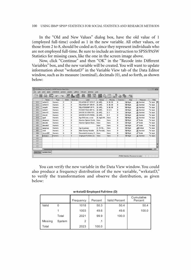
Now, click “Continue” and then “OK” in the “Recode into DifferentVariables” box, and the new variable will be created. You will want to updateinformation about “wrkstatD” in the Variable View tab of the Data Editorwindow, such as its measure (nominal), decimals (0), and so forth, as shownbelow:

You can verify the new variable in the Data View window. You couldalso produce a frequency distribution of the new variable, “wrkstatD,”to verify the transformation and observe the distribution, as givenbelow:


Notice the approximately even distribution of “wrkstatD” (full-timeemployment dichotomy). If there were only a small percentage in eithercategory, the variable would not be suitable for use in this analysis andwould need to be recoded in some other way to capture more variation.

Creating a Set of Dummy Variables to Represent a Multicategory Nominal Variable

Our other independent variables will represent race/ethnicity. We will usethe four-category race variable that was recoded using the original racevariable and the variable “Hispanic.” The categories are: White, Black,Other, and Hispanic. Since there are four categories, we will need to createthree dummy variables. The number of dummy variables in a set that rep-resents a nominal variable is equal to K–1, where K is the number of cate-gories. To do this, first produce a frequency distribution, as follows:

ANALYZE � DESCRIPTIVE STATISTICS � FREQUENCIES . . .

After requesting the frequency for race (as recoded with additional infor-mation from the variable “Hispanic,” in Chapter 2: Transforming Variables),we get the following chart:

Since the “Other” category is relatively small at just 4.2% of valid cases,you might wish to define those in that category as missing and proceedwith a three-category variable (White, Black, and Hispanic), producing twodummy variables: K–1 = 2.


We will proceed with all four categories. Let’s make four dummy vari-ables, and then we’ll choose which three to use for the analysis, based onwhich groups we wish to compare. First select the following menus:

TRANSFORM � COMPUTE VARIABLE . . .

Name the target variable; in this case it will be “White.” Now, set allcases in the new variable equal to zero, as above. Then, click “OK.” You canverify in the Data Editor window that a new variable has been appended tothe data file that has all zeros as data.

Next, we will want to correct those cases for which the respondent waswhite. To do that, again select these menus:



Now, change the value in the Numeric Expression area to 1. Then, click“If . . .” in the lower left corner of the “Compute Variable” box. The follow-ing dialog box will appear:

Now, let’s use the same procedure to create the variable “Black.” Clickthe following menus:



Select the radio button next to “Include if case satisfies condition:”.Then type “race=1” in the box beneath. Now click “Continue” and then“OK.” You’ll be given the following warning. Be sure to click “OK” to verifythat you do wish to alter some of the data in this variable.

First, click the “Reset” button to eliminate information from the priortransformation. Then set all of the cases in the new variable, “Black,” equalto zero. Then click “OK.” Once you verify the creation of the new variablein your Data Editor window, again click these menus:



Here, in the Numeric Expression area, you will enter 1. Now, click the“If . . .” button, and in the dialog box that appears, choose the “Include ifcase satisfies condition:” radio button and enter the equation “race=2” inthe box beneath. Now, click “Continue” and then “OK.”


Next, follow the same procedure for “Other/Others” and“Hispanic/Latino,” as described below:

1. For “Others,” select TRANSFORM � COMPUTE VARIABLE . . . , andthen set Others = 0. Next, using the Compute command, set Others = 1, IF:race = 3. (We are using the name “Others” instead of “Other,” since “Other”represents another variable in the GSS original data file. You are free to labelthis new variable as “Other,” though that would delete the original variable thatcontains data about other Protestant denominations.)

2. For “Latino,” select TRANSFORM � COMPUTE VARIABLE . . . , thenset Latino = 0. Next, using the Compute command, set Latino = 1, IF: race = 4.(We are using the name “Latino,” since “Hispanic” represents another variablein the GSS original data file. In fact, the original variable, “Hispanic,” containsinformation that we used to recode the very race variable we are using here byadding a fourth category in Chapter 2: Transforming Variables. You couldrename “Hispanic” to something else and use that name here if you wish.)

Now, for all four new variables, go to the Variable View window and editthe settings to reflect each new variable’s decimals (0), measure (nominal), andso on.

The method we have used above creates dummy variables in two steps:(1) Name the new variable and set all cases equal to zero, and (2) changethe settings for the appropriate cases corresponding to the race/ethnicityequal to one. Note that we are able to set the variables equal to zero first,without worrying about missing cases only because there happen to be nomissing cases for the race variable. If there were missing cases, we wouldneed to handle those cases with the Compute command, as well.

Logistic Regression Analysis

Choose the following menus to begin the logistic regression analysis:

ANALYZE � REGRESSION � BINARY LOGISTIC . . .


Select “wrkstatD” as the dependent variable by dragging it from thecolumn on the left into the box under “Dependent.” Independent variableswill go in the box labeled “Covariates.” For gender, use “male.” For race/eth-nicity, think about which category you want to use as a reference. Whateverresults you get will reveal whether other groups are more or less likely tohave full-time employment than the reference (left out) category.

In this case, if we omit “White,” then the comparison can be made fromother groups to whites. Let’s use that in our example. Enter the three otherdummy variables as they appear in the screen image above. Then click“OK.” A selection from the output produced is as follows. See “InterpretingOdds Ratios” at the end of this chapter for an explanation of how to inter-pret the central parts of the logistic regression output.


Logistic Regression Using a Categorical Covariate Without Dummy Variables

The logistic regression command has a built-in way to analyze a nomi-nal/categorical variable like our recoded race variable. The results pro-duced will be identical to those described earlier in this chapter, and thereis no need to create dummy variables. There are, however, some situationsin SPSS/PASW Statistics where you must create and use dummy variables,and that method directly exposes the user to how the data are being treatedand analyzed. The following method should be used only by those whofully understand the nature of categorical analysis within a logistic regres-sion model, and it should be noted that there are limitations: The referencecategory can be only the first or last category of the variable to be used as acovariate. In the case of the race variable, “White” is the first category and“Latino” is the last category. Had we wished to use “Black” or “Others” as areference category, we would need either to have created dummy variablesas above or to have recoded “race” to suit our needs. Another limitation willbe addressed toward the end of this chapter; it concerns complicationswhen using certain methods of inclusion for variables.

In any case, follow the instructions below to produce the logisticregression equation using the categorical variable method:

ANALYZE � REGRESSION � BINARY LOGISTIC . . .


As before, select “wrkstatD” as the dependent variable. Also, add“male” as one of the covariates. Now, simply add “race” as one of thecovariates. You cannot stop here and run the analysis; the results would bewithout useful interpretation. So it is necessary to tell SPSS/PASW Statisticsthat “race” is a categorical/nominal variable and to tell it which categoryshould be the designated reference category (and therefore “left out” of theanalysis in the same way it was in our utilization of dummy variables). Todo this, click the “Categorical” button . . .


Now, in the dialog box with which you are presented, select “race” fromthe list of covariates on the left, and drag it into the box under “CategoricalCovariates.” Then select “First” as the reference category, and click the“Change” button. You should notice the word “first” appear as in the screenimage above. Now click “Continue” and then “OK.” The output from thiscommand is displayed and interpreted in the following section.

Interpreting Odds Ratios

Logistic regression uses natural logarithms to produce a logistic curve as apredictor, whereas you may remember that OLS linear regression uses theleast squares method to produce a straight line as a predictor. The coeffi-cients in a logistic regression model can be exponentiated as log oddsratios. Selected output from the logistic regression command, above, hasbeen printed below:

Notice that in the Model Summary box, two different r-squares (r2) arepresented: Cox and Snell as well as Nagelkerke. While computed differently,these numbers can be interpreted in much the same way as r2 itself, thecoefficient of determination. (See Chapter 7: Correlation and RegressionAnalysis, for more details on PRE [proportional reduction in error] statis-tics and the coefficient of determination.)


In the “Variables in the Equation” box, the coefficients themselves arefound in column “B,” but they have been exponentiated in the column“Exp(B).” This value tells how much more or less likely a subject in the des-ignated category is to be in the affirmative category on the dependent vari-able (employed full-time) than a subject in the omitted reference category.For the coefficient, male, the odds ratio is 2.308, and it is statistically sig-nificant (p = 0.000 in the “Sig.” column); therefore, men are 2.308 timesmore likely than women to be employed full-time and not fall into someother category of employment.

The first race row in the “Variables in the Equation” box is the omittedreference category, White. Notice that there is no coefficient or exponentiatedcoefficient in that row. In the rows below, “race(1)” represents the next cate-gory, Black; “race(2)” represents the third category, Other/Others; and“race(3)” represents the last category, Hispanic/Latino. The only category (ordummy variable) that is statistically significant for race is Hispanic/Latino (p = 0.022). The exponentiated coefficient reveals that Hispanics were 1.391times more likely than those in the reference category (Whites) to have full-time employment and not fall in some other category of the original variable:employed part-time, retired, keeping house, and so forth. Comparisons candirectly be made only with the reference category.

To have SPSS/PASW Statistics help produce the equation with the bestset of statistically significant variables, so that you will not need to try eachcombination manually, you can select a different option from the pull downmenu in the “Method” pane in the “Logistic Regression” dialog box, such as“Backward: Conditional,” as demonstrated below. While this method workseffectively when using the dummy variable approach to logistic regressionanalysis, it is not effective with the categorical variable method.


From the output produced, the following selection reveals the finalcoefficients. Notice that each step removes variables that are not statisticallysignificant and that contribute the least to the model. In the third step, thefinal model is provided. The number of steps that are required bySPSS/PASW Statistics to produce the final equation depends on numerousfactors.

Notice that in our simple example, the final equation is very similar tothe model we produced above, though the nonsignificant dummy variableshave been removed from the model. Notice, too, that the value of r2 (bothCox & Snell, and Nagelkerke) is not reduced as a result of the removal ofvariables (i.e., in conjunction with the other variables in the equation, thevariation in the deleted variables did not account for any variation in thedependent variable). Granted, the Nagelkerke calculation did declineslightly from 0.059 to 0.058.

Documents

Logistic Regression Analysis - SAGE Publications · analysis allows us to predict values on a dependent variable ... represents another variable ... Choose the following menus to