Lok Lamsal, Nickolay Krotkov, Randall Martin, Kenneth Pickering, Chris Loughner, James Crawford, Chris McLinden

TEMPO Science Team MeetingHuntsville, Alabama

27-28 May 2015

Development of TEMPO NO2 Algorithm to Infer Vertical Columns from Total Slant

Columns

1) Stratosphere-troposphere separation2) Sensitivity to NO2 profiles

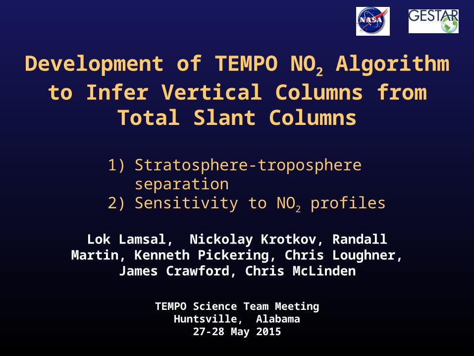
Attention Needed for Removal of Stratospheric NO2

-150 -100 -5020

30

40

50

60

70

0

0.1

0.2

0.3

0.4

0.5

Fraction of total NO2 column in the troposphere can be smallUrban/Industrial areas: 30-80%

Rural/background areas: 10-30%

Need unbiased method to remove stratospheric NO2

Figure from Chris McLinden

Fraction

OMI (2009) annual mean

GMI model (July average)

6 AM 12 PM 6 PM

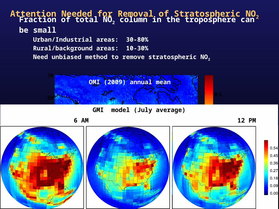
Candidate Stratosphere-troposphere Separation Algorithms

1) Reference sector method (zonal invariance and data from Pacific)

2) Image processing /wave analysis

3) Goddard method for OMI (OMNO2)

Observation based, spatial filtering, filling, and interpolation

4) KNMI method for OMI (DOMINO)

Data assimilation

x

Stratospheric NO2

July 21, 2006

NASA GMI model

Adaptation of OMI algorithms to TEMPO may require improvements when there is a large gradient in NO2 field

3) Observation based

4) Assimilation

Candidate Stratosphere-troposphere Separation Algorithms

OMI heritage algorithm for TEMPO

Rapid decline around sunrise, slow increase during day, rapid increase around sunset

Two CMAQ simulations: Model set up

Horizontal resolution 4 km x 4 km

Vertical levels 45 (surface-100 hPa)

Chemical mechanism CB05

Aerosols AE5

Dry deposition M3DRY

Vertical diffusion ACM2

Boundary condition RAQMS; 12 km x 12 km

Biogenic emissions Calculated within CMAQ with BEIS

Biomass burning emissions FINNv1

Lightning emissions Calculated within CMAQ

Anthropogenic emissions NEI-2005 projected to 2012

Simulation 1 Simulation 2

PBL scheme ACM2 (Assymetric Convective Model v2)

YSU (Yonsei Univ.)

High Resolution CMAQ Simulations to Study Retrieval Sensitivity to Diurnal Changes in NO2 Profiles

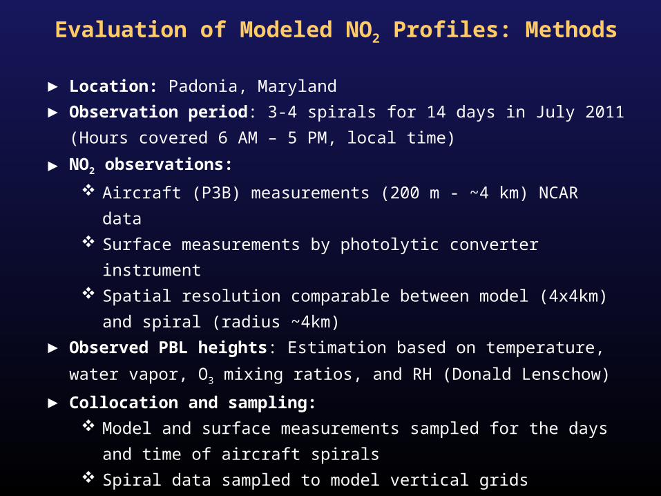
Evaluation of Modeled NO2 Profiles: Methods

► Location: Padonia, Maryland

► Observation period: 3-4 spirals for 14 days in July 2011 (Hours covered 6

AM – 5 PM, local time)

► NO2 observations:

Aircraft (P3B) measurements (200 m - ~4 km) NCAR data

Surface measurements by photolytic converter instrument

Spatial resolution comparable between model (4x4km) and spiral

(radius ~4km)

► Observed PBL heights: Estimation based on temperature, water vapor, O3

mixing ratios, and RH (Donald Lenschow)

► Collocation and sampling:

Model and surface measurements sampled for the days and time of

aircraft spirals

Spiral data sampled to model vertical grids

Diurnal Changes in NO2 Vertical Distribution

Models capture overall diurnal variation, but some differences related to emissions, PBL height, vertical mixing are evident.

Padonia, MD (July)

3 PM

Surface reflectivities: 0.1 to 0.15 at

0.01 steps

Solar zenith angles: 10° to 85° at 5°

steps

Aerosol optical depths: 0.1 to 0.9 at

0.1 steps

6 AMImproved Model Simulation Reduces Retrieval Errors

Model Need to Well Represent PBL Mixing to Minimize Errors from NO2 Profiles

► PBL scheme alone can

cause different AMF

errors

► Greater performance for

certain hours for both

ACM2 and YSU

► Diurnal pattern in AMF

errors for ACM2

► We need model that

represents PBL mixing

and emissions to

minimize errors in

retrievals