LOMA LINDA UNIVERSITY The School of Science and Technology Faculty

LOMA LINDA UNIVERSITY

The School of Science and Technology in conjunction with the

Faculty of Graduate Studies

__________________________

Responses to Salinity of Color Polymorphs in Two Populations of the Sea Star, Pisaster

ochraceus

by

Viren Johann Perumal

___________________________

A Thesis submitted in partial satisfaction of the requirements for the degree of

Master of Science in Biology

_____________________________

December 2006

© 2006

Viren Johann Perumal All Rights Reserved

iii

Each person whose signature appears below certifies that this dissertation in their opinion is adequate, in scope and quality, as a thesis for the degree of Master of Science. , Chairperson Stephen G. Dunbar, Assistant Professor of Biology ________________________________________________________________________ David L. Cowles, Professor of Biology, Walla Walla College, College Place, WA ________________________________________________________________________ William K. Hayes, Professor of Biology ________________________________________________________________________ Lawrence R. McCloskey, Professor of Biology, La Sierra University, Riverside, CA

iv

ACKNOWLEDGEMENTS

I would like to thank the many individuals who have contributed in so many

ways, supporting me both directly and indirectly, throughout the course of this project.

First, I would like to express my appreciation to my guidance committee members: Dr.

David Cowles, Dr. William Hayes, Dr. Larry McCloskey, and especially my major

professor, Dr. Stephen Dunbar. Their support, guidance, encouragement, and knowledge

were invaluable to me during the entirety of this project, and the ideas brought forward

from the many reviews were invaluable. I feel that the support and friendship I have

gained through working with these individuals and the insights that I have learned from

them will help me in my future endeavors.

I wish to thank Dr. Stephen Dunbar for use of equipment and for support through

funding. Dr. Dunbar additionally took much of his time revising several drafts of this

thesis; his critical feedback allowed me to better develop my writing skills. Dr. David

Cowles generously provided lab space at the Walla Walla College Marine Station at

Rosario Beach (WWCMS-RB). He took time out of his busy summer schedule to indulge

many conversations about my project, assist with equipment problems, teach me the art

of collecting respirometry data, and drive boats for field collections. Without his help, the

data collection for this project would not have been completed. Dr. James Nestler and

David Habenicht of the WWCMS-RB were both generous with their time, equipment,

and space at the marine station. My metabolic chambers may never have been

constructed without Dave’s well equipped shop at the research station. The Department

of Earth and Biological Sciences at Loma Linda University (LLU) supported this

research by funding two Summer Undergraduate Research Program (SURP) students to

v

assist with this project, and a Marine Research Group (LLU) grant assisted with funding

for this project.

I would like to thank my SURP assistants for their help with the data collection

for this project. Tyler Shelton and N. Stephen Neilson took their time to help me, and

brought valuable energy and ideas to the project.

I also want to especially thank my wife Julie Maguire, who not only assisted in

data collection but also provided encouragement, support, and much-needed patience

throughout my journey during this program. She was always there as an inspiration to

keep on plugging away at the research and writing in order to finish my thesis.

I am in debt to all the friends, family members, and colleagues who have shared

energy, ideas, and encouragement with me along the way. For the friends who have

distracted me from being productive by dragging me out to go cycling, rock climbing, or

kayaking when I should have been writing, I owe thanks to you for my sanity.

Most importantly, I wish to thank God for all the blessings I have found while

learning about the mysteries in Biology, for the amazing natural world to play in, and for

His constant and unwavering love.

vi

TABLE OF CONTENTS

Approval Page.................................................................................................................................iii Acknowledgements......................................................................................................................... iv Table of Contents............................................................................................................................ vi List of Tables .................................................................................................................................vii List of Figures................................................................................................................................vii Abstract........................................................................................................................................... ix Chapter 1. Introduction............................................................................................................................... 1

Natural History of P. ochraceus ......................................................................................... 1 Anatomy of Sea Stars ......................................................................................................... 2 Ecological Importance of P. ochraceus .............................................................................. 4 Color Polymorphism........................................................................................................... 4 Environmental Variations between the Open Coast and Inland Straits of Washington State .................................................................................................................................... 7 Salinity Tolerance in P. ochraceus ................................................................................... 10 Oxygen Consumption and Measuring Aerobic Metabolism in P. ochraceus .................. 12 Project Goals, Objectives and Significance ...................................................................... 13

2. Materials and Methods............................................................................................................... 14 Collection Methods........................................................................................................... 14 Specimen Maintenance ..................................................................................................... 15 Aerobic Respiration Experiment....................................................................................... 18 Ammonia Excretion Experiment ...................................................................................... 31 Self-Righting Experiment ................................................................................................. 33 Statistical Methods............................................................................................................ 36

3. Results........................................................................................................................................ 37 Aerobic Respiration .......................................................................................................... 37 Ammonia Excretion.......................................................................................................... 42 Self-Righting..................................................................................................................... 47

4. Discussion.................................................................................................................................. 51

Aerobic Respiration .......................................................................................................... 51 Ammonia Excretion ......................................................................................................... 53 Self-Righting..................................................................................................................... 56 Ecological Applications .................................................................................................... 58 Conclusions....................................................................................................................... 59 Suggestions for Further Study .......................................................................................... 60

Literature Cited .............................................................................................................................. 61

vii

TABLES

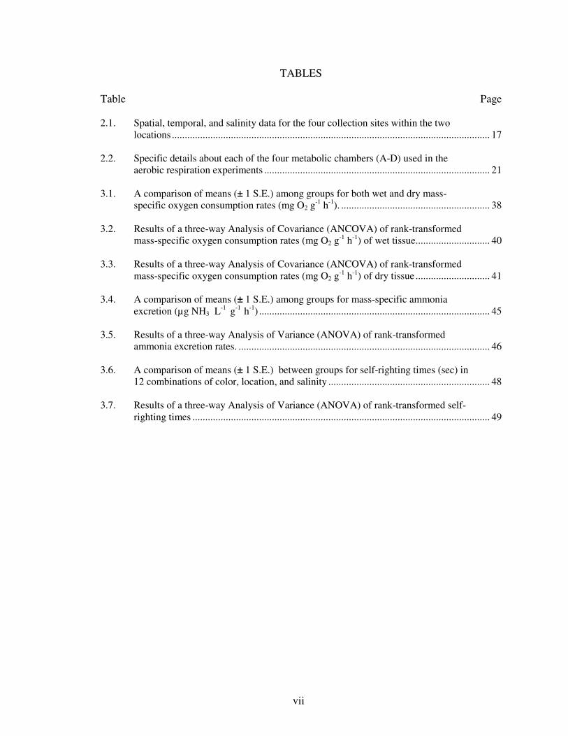
Table Page 2.1. Spatial, temporal, and salinity data for the four collection sites within the two

locations ............................................................................................................................ 17 2.2. Specific details about each of the four metabolic chambers (A-D) used in the

aerobic respiration experiments ........................................................................................ 21 3.1. A comparison of means (± 1 S.E.) among groups for both wet and dry mass-

specific oxygen consumption rates (mg O2 g-1 h-1). .......................................................... 38

3.2. Results of a three-way Analysis of Covariance (ANCOVA) of rank-transformed

mass-specific oxygen consumption rates (mg O2 g-1 h-1) of wet tissue............................. 40

3.3. Results of a three-way Analysis of Covariance (ANCOVA) of rank-transformed

mass-specific oxygen consumption rates (mg O2 g-1 h-1) of dry tissue ............................. 41

3.4. A comparison of means (± 1 S.E.) among groups for mass-specific ammonia

excretion (µg NH3 L-1 g-1 h-1) .......................................................................................... 45

3.5. Results of a three-way Analysis of Variance (ANOVA) of rank-transformed

ammonia excretion rates. .................................................................................................. 46 3.6. A comparison of means (± 1 S.E.) between groups for self-righting times (sec) in

12 combinations of color, location, and salinity ............................................................... 48 3.7. Results of a three-way Analysis of Variance (ANOVA) of rank-transformed self-

righting times .................................................................................................................... 49

viii

FIGURES

Figure Page 2.1. Northwestern Washington state showing the two different locations where

Pisaster ochraceus were collected.................................................................................... 16 2.2. Flow-chart displaying the experimental design of the aerobic respiration study.............. 20 2.3. Chambers A and B with experiment in progress .............................................................. 22 2.4. Chambers A and B empty and with lids off...................................................................... 22 2.5. Chambers C (right) and D (left)........................................................................................ 23 2.6. The probe housing for chamber D on top of a magnetic stir plate.................................... 23 2.7. Chamber D being aerated with a 60cc syringe. ................................................................ 26 2.8. A purple specimen being weighed on a balance scale before being placed in a

chamber............................................................................................................................. 26 2.9. The displacement apparatus with a graduated cylinder being filled with water

displaced by a sea star....................................................................................................... 27 2.10. Sample of cleaned and smoothed data-chart plotting a final slope with standardized

residuals removed. ............................................................................................................ 30 2.11. Sea stars run simultaneously in a self-righting chamber................................................... 34 2.12. Tests of open coast individuals set up on the shore of the WWC-MS.............................. 34 2.13. Tests of Inland Straits individuals set up in an outdoor sea tank at the

WWC-MS. ........................................................................................................................ 35

3.1. A comparison of means (± 1 S.E.) among groups for dry mass-specific oxygen consumption rates (mg O2 g

-1 h-1) ..................................................................................... 39 3.2. Standard curve of concentrations of ammonia that were analyzed by spectrophotometry at 690 nm....................................................................................... 43 3.3. Standard curve of concentrations of ammonia that were analyzed by spectrophotometry at 690 nm....................................................................................... 44 3.4. A comparison of the mean turnover response times (seconds) of different colors,

locations and salinities. ..................................................................................................... 50

ix

ABSTRACT

Responses to Salinity of Color Polymorphs in Two Populations of the Sea Star, Pisaster

ochraceus

by

Viren Johann Perumal

Master of Science, Graduate Program in Biology

Loma Linda University, December 2006 Dr. Stephen G. Dunbar, Chairperson

Pisaster ochraceus was analyzed to determine if varying salinities, animal color, or

location affect the physiology of these sea stars. The three responses analyzed were aerobic

respiration, ammonia excretion, and self-righting. The tested variables included two different

color morphs (orange and purple) of P. ochraceus, two different locations (open coast and inland

straits) in Washington State, and three salinities (22, 30, and 40 psu).

Wet mass-specific oxygen consumption rates were not significantly affected by color,

location, or salinity, and Dry mass-specific oxygen consumption rates showed no significant

differences for main effects, but a three-way interaction was identified. Similarly, ammonia

excretion rates were unrelated to color, location, or salinity. Self-righting times were

significantly different with color, location, and salinity.

Although measurements from the three experiments carried out in this study do not all

point to differences in responses of the two color morphs, they nonetheless provide some

evidence that color and location both have a significant effect on self-righting times at the three

salinities tested. The results of my study suggest that, within a certain range (± 8 psu), P.

ochraceus appears to be able to maintain normal aerobic respiration and ammonia excretion.

However, when stressed to greater extremes outside of the range they are able to cope with, such

as salinities of ± 10 psu or greater, their basic functions of mobility, such as self-righting

responses, may be impaired.

1

CHAPTER ONE

INTRODUCTION

Natural History of P. ochraceus

The ochre sea star, Pisaster ochraceus (Brandt, 1835), is a benthic echinoderm in

the class Asteriodea and is common and well distributed from Prince William Sound,

Alaska, to Cedros Island, Baja California (Ricketts et al., 1985). This species inhabits the

lower limits of the intertidal zone as well the subtidal zones down to 97 meters, but is

most abundant in the middle to lower intertidal zones that are exposed to waves or

currents (Morris et al., 1980; Lambert, 2000). P. ochraceus can usually be found on

rocky substrates of the open coast. This predatory species is one of the most conspicuous

and colorful of the intertidal fauna (Ricketts et al., 1985). The species name, ochraceus,

is derived from the Greek word ochros, in reference to the pale yellow or ochre color of

some specimens (Lambert, 2000).

Pisaster ochraceus is commonly called the ochre or purple sea star, or the

common starfish (Feder, 1957), and is not to be confused with the “common starfish”

Asterias rubens, found on the Atlantic coast (Hendler et al., 1995). Specimens of P.

ochraceus generally range from 15 to 36 cm diameter (Ricketts et al., 1985), and

although smaller individuals are difficult to find, juveniles can be found in crevices and

under rocks (L. McCloskey, pers. comm.). These organisms begin their lives as pale

orange to salmon pink eggs 150 to 175 µm in diameter (Lambert, 2000). Around six

days after the egg has been released, a planktotrophic (feed on other plankton) bipinnaria

larva forms which lasts for up to two months. Following this stage, a bilaterally

symmetrical brachiolaria larva develops, which attaches to the substrate and

2

metamorphoses into a radially symmetrical juvenile sea star (Lambert, 2000). Juveniles

reach maturity in around five years and can live longer than 20 years as adults. A large

adult individual can release approximately 40 million eggs in one spawning season

(Millott, 1967; Brusca and Brusca, 2003).

Anatomy of Sea Stars

The general body plan of P. ochraceus, as in all other asteroids, is stellate (star

shaped) and members of this species possess a pentamerous radial symmetry with body

parts organized around an oral-aboral axis. Asteroids have a central disk and

symmetrically projecting arms, which are called rays (Hendler et al., 1995). Sea stars

differ from other members of the phylum Echinodermata in that they have five or more

open furrows, called ambulacral grooves, that are found on the underside, or oral surface,

of their rays. These ambulacral grooves bear rows of tube feet, digestive glands, and

gonads radiating into each ray. Members of Pisaster ochraceus usually have five stiff

arms, a highly arched disc and a sunken mouth. The aboral surface contains a formation

of white spines that form a net-like pattern. Papulae, also called gills or dermal branchea,

lie between the spines. These papulae are thin-walled extensions of the coelom that

protrude between skeletal plates and allow the exchange of respiratory gasses between

the surrounding sea water and the organisms’ internal fluid. They are thought to assist in

the coloration differences of individuals, since this is where pigmentation occurs.

Between the papulae are several types of pedicellariae, or pincher-like appendages, that

may play a role in preventing microorganisms from settling on the skin of the sea star.

These pedicellariae structures respond to external stimuli independently of the sea stars’

3

main nervous system and possess their own neuromuscular reflex components. The types

of pedicellariae found in P. ochraceus are furcated, crossed, lanceolate and straight

toothed, with the furcated form being most characteristic of this species (Millott, 1967;

Lambert, 2000; Brusca and Brusca, 2003).

Sea stars are known for both their appetite as well as their diverse feeding

strategies (Hendler et al., 1995) and P. ochraceus are known to be voracious predators of

low intertidal zone invertebrates (Ricketts et al., 1985). They feed primarily in the

summer and prefer mussels, barnacles, limpets and snails. However, at least 30 prey

items have been documented and their diet depends on the availability of prey (Feder,

1959). One of the most common prey items of this organism is the California mussel,

Mytilus californianus, which is abundant on wave-exposed, rocky substrates. Pisaster

ochraceus eats mussels by inserting its stomach between the shells, secreting digestive

enzymes and simultaneously pulling the bivalves shells apart with its tube feet (Morris et

al., 1980; Lambert, 2000).

The specialized tube feet of P. ochraceus are fleshy projections that contain

external hollow suckers, called podia, that are used for locomotion, gas exchange,

feeding, attachment and sensory reception. They are operated hydraulically by a unique

coelomic water vascular system which contains a complex of fluid-filled canals with a

single opening on the aboral surface known as the madreporite, or sieve plate. The water

vascular system also aids in the internal transport of the coelomic fluid (Brusca and

Brusca, 2003).

4

Ecological Importance of Pisaster ochraceus

Being a principal predator in intertidal areas of the Pacific coast (Johnson, 1976),

P. ochraceus plays an important ecological role in intertidal community dynamics. Paine

(1966) has shown in classical ecological studies that P. ochraceus is a keystone predator

that has an amplified effect on the structure and diversity of the intertidal areas it inhabits.

Paine (1966; 1969) and others (Menge and Sutherland, 1987; Garza, 2005) showed, that

without sea star predation on Mytilus californianus, the rocky intertidal community

shifted from a diverse mix of algae and invertebrates to a dominance of M. californianus.

Sweere (unpublished) also studied the direct and indirect effects of P. ochraceus on tide

pool communities and found that in the presence of P. ochraceus, there was a decline in

the richness and diversity of other mobile tide pool species in experimental pools.

Although we understand much about the ecological role of this important species,

much less research has been done on the causes of their most obvious character – their

vivid color polymorphism. Understanding the significance and cause of this variation is

almost completely lacking in the literature.

Color Polymorphism

Adult Pisaster ochraceus occur in a wide range of color morphs. Specimens are

most commonly seen as purple, orange, brown, and less often in yellow, red, and pink

(Ricketts et al., 1985; Raimondi et al., in press).

Vevers (1966) reviewed pigmentation in echinoderms and confirmed that they are

among the most brightly colored of all marine animals and that nearly all their coloration

is due to pigments. In Asteroids, the most widespread chemical pigments are the

5

carotenoids. Carotenoids are yellow to red pigments of aliphatic or alicyclic structure,

composed of isoprene units (Karrer and Jucker, 1950). These integumentary carotenoids

are often linked to proteins to form water-soluble carotenoproteins. In asteroids, the

principal carotenoids found are β-carotene, cryptoxanthin, echinenone, astaxanthin, and

one or more keto-carotenoids, as well as traces of xanthophylls. Because carotenoids are

essentially plant pigments which animals are thought to be incapable of synthesizing de

novo (Karrer and Jucker, 1950; Fox and Hopkins, 1966; Vevers, 1966), it seems likely

that the coloration of P. ochraceus is at least partially controlled by diet.

Studies by Fox and Scheer (1941) shed light on the fact that Pisaster ochraceus

stores considerable amounts of mytiloxanthin, a carotenoid found specifically in its main

prey item, Mytilus californianus (which gains these pigments through its diet). They

hypothesized that a carnivorous organism such as P. ochraceus would obtain more

oxygenated carotenoids through its diet than would an herbivorous organism. To my

knowledge, no published studies have tested the genetic basis for incorporating plant

pigments, such as carotenoids, into the integuments of animals. How environmental

factors play a role in the survivability of different color morphs is not known

Humphreys (2003) observed that in protected waters like those in the Pacific

Northwest, there are more purple individuals, whereas on exposed coasts, the seastars

tend to be more orange or brown. It is unknown whether these polymorphs are really

genetically fixed morphs, or rather are color phases that may change during the course of

the organism’s growth and development. Rearing studies have not been carried out which

could shed light on how environmental factors such as salinity, diet, temperature, pH, and

6

UV exposure play a role in the ontonogenic determination of color (C. Harley, Pers.

Comm).

Raimondi et al. (2004; in press) reviewed common explanations for color

polymorphism in animals and applied them to P. ochraceus. They determined that non-

random mating, apostatic selection (which is a negative frequency-dependant selection

pressure based on predation pressures), and disruption through crypsis, would not support

the basis for polymorphism in P. ochraceus. They did, however, identify a consistency in

frequencies of orange to purple color morphs. They sampled 26 sites along the open coast

from Southern California to Northern Oregon, and found consistently that the range in

percent orange morphs for all sites was 12.6 % - 27 % (mean = 20.0 % ± 4.4 % s.d). This

consistent frequency of percent orange, however, is not exhibited throughout the

protected waters in the Inland Straits1 in Washington State. Individuals found in the

Inland Straits tend to be larger than the coast populations and contain a higher frequency

of purple, lower frequency of orange, and no brown individuals (Raimondi et al, in press,

D. Cowles, pers. com.).

Harley et al. are presently comparing the genetic structure of Inland Straight and

open coast populations in British Columbia, Canada (C. Harley pers. com.). To date, they

have found no major genetic differences between these populations. This seems

unsupportive of the more obvious possibilities of a founder effect or incipient speciation

between the populations that may be assumed under these circumstances (Bilton et al.,

2002).

1 Refers to protected bodies of marine waters found inland in North-Western Washington State including the Strait of Juan de Fuca, the Puget Sound, and the waters adjacent to the San Juan Islands.

7

These data suggest that another possibility is for certain color morphs to have

different physiological tolerances to environmental factors. If, for example, orange

individuals were more sensitive than purple individuals to certain ecological factors

present in the inland straits, a prediction about the distribution of colors between the two

locations could be tested.

Environmental Variations Between the Open Coast and Inland Straits of

Washington State

A look at the spatial distribution of color morphs of these organisms may provide

evidence that the cause of color polymorphism in P. ochraceus is directly related to its

environment. Sea stars, such as P. ochraceus that inhabit the intertidal zone are exposed

to great fluctuations in water temperature and, to a greater extent, air temperature in their

natural environment. While the coastal waters of Washington State usually do not drop

below 10˚C or rise above 16˚C, Feder (1957) has shown that P. ochraceus will tolerate

air temperatures of up to 21˚C in the laboratory for at least three hours. This may be

partially due to the fact that these organisms are able to keep their own temperatures

down to some extent by evaporative cooling.

Studies of other asteroids have shown that temperature has an effect on rates of

locomotion as well as self-righting behavior, which is a measure of a turnover response

time after placing the animal on its aboral surface (Feder and Christensen, 1966).

Kinne (1963) points out that organisms tend to adapt to their total environment

rather than to isolated factors. One of the most important physical factors that can exert

pressure on the survival of marine organisms, along with temperature, is salinity. An

8

example of how this interaction has an effect on sea stars was demonstrated on Solaster

endeca by Ursin (reviewed in Feder and Christensen, 1966). This seastar avoids areas

with a mean temperature >14˚C in the warmest month, but also requires a salinity of at

least 30 practical salinity units (psu). Schlieper (1956, in Feder and Christensen, 1966)

and Kowalski (1955, in Feder and Christensen, 1966) studied the asteroid, Asterias

rubens, from two distinct environmental salinities (30 psu and 15 psu). Data from these

experiments showed that lower salinity populations took longer to right themselves when

exposed to higher temperatures. They suggested that this decreased response is related to

the higher content of water in the tissues of the organisms found in the more hypo-saline

environment. Brattstrom (1941, in Feder and Christensen, 1966) and Ursin (1960, in

Feder and Christensen, 1966), have documented the distribution of sea stars as a function

of salinity.

Lowered tolerance for hypo-saline conditions is well documented in some

asteroids. Smith (1940; in Feder and Christensen, 1966) found that Asterias vulgaris

could survive in the laboratory for at least three days at a salinity of 14 psu at 20˚C. Field

sampling showed, however, that that no individuals were found in environments

containing salinities below 23 psu.

The environments between the open coast and the Inland Straits of Washington

State are very distinct, with the open coast having a higher salinitiy (with an average of

35 psu), warmer water temperatures, more cloudy and foggy days, and consistent wave

exposure (D. Cowles pers. comm.). In contrast, inland waters have lower salinities with

an average annual salinity of 29 psu (NEER, 2006), consistently cooler water

temperatures and limited wave exposure. The hypo-saline conditions in the protected

9

waters of the Pacific Northwest are due to the size of the Inland Straits’ watershed and

surface runoff from over 10,000 rivers and streams (Finlayson, 2004).

The bodies of water associated with the Inland Straits are considered estuarian.

An estuary can be defined as an inlet where sea water is diluted by the inflow of

freshwater, or simply as a river with variable salinity due to the mixing of seawater

(Green, 1968). The Rosario Strait in which the Inland Straits populations were collected

for the current study was adjacent to the Strait of Juan de Fuca.

The Strait of Juan de Fuca, Georgia Straits, and Rosario Strait, are tidally

dominated, but have estuarine components (Holbrook and Halpern, 1982). Southerly

winds push water against Vancouver Island, which forms the northern portion of the

mouth of the Strait of Juan de Fuca. These winds reverse the sea-surface slope in the

Strait, resulting in a landward intrusion of fresh, warm surface water and seaward retreat

of deep, more saline water (Cannon, 2003).

In contrast to the dynamic mixing of the inland waters, the Olympic coastal areas

of Washington State maintain temperatures and salinities which are kept more constant

throughout the year. Factors that contribute to this consistency include shallow

continental shelves that prevent coastal upwellings and consistent fog-induced

temperature regimes (Sanford, 1999; 2001). The open coast is said to be remarkably

stable in its physico-chemical conditions (Morris et al., 1980) in comparison to the inland

straits.

10

Salinity Tolerance in P. ochraceus

My research examined the effects of salinity on three color morphs of P.

ochraceus from two environmentally distinct populations of the open coast and the inland

straits of Washington State. Salinity tolerance was chosen due to the fact that

echinoderms are reported to have poor abilities to osmo- and iono-regulate, and lack

evidence of excretory systems (Stickle and Diehl, 1987; Brusca and Brusca, 2003). The

choice to test acute responses to salinity was also made due to a review of the literature

which revealed studies identifying biochemical, reproductive, developmental and

morphological responses to reduced salinities in other echinoderms. Acute responses to

salinity stress can be manifested as swelling and stiffness due to turgor pressure, increase

in weight due to increased water content, and loss of integumentary pigmentation

resulting in a blotchy appearance due to damaged epidermal tissue (Binyon, 1972a;

1972b; Stickle and Diehl, 1987).

Roller and Stickle (1985) state that postmetamorphic Pisaster ochraceus are not

found in brackish water (hyposaline conditions). They have shown through experiments,

that larvae will survive salinities of 20 psu for only 32 days. This represents little more

than 10% of their planktonic existence that can last 228 days at salinities of 30 psu, which

is closer to their normal environmental salinity.

Echinoderms are osmoconformers, and since their coelomic fluid usually remains

isoosmotic to the environment (Binyon, 1966), I tested the hypothesis that acute changes

in salinity differentially affect responses, such as metabolic rate, ammonia excretion, and

self righting, of the two color morphs. Studies of this kind have been done in other

echinoderms (Sabourin and Stickle, 1981; Shirley and Stickle, 1982; Forcucci and

11

Lawrence, 1986; Talbot and Lawrence, 2002) as well as in other marine invertebrate

species (Aarset and Aunaas, 1990; Jury et al., 1994; Dunbar and Coates, 2004).

Rankin and Davenport (1981), discuss the problems marine intertidal organisms

face in maintaining their internal salt concentration. All echinoderms are either

euryhaline or stenohaline osmoconformers. Osmoconformers respond to reduced salinity

by absorbing water and excreting salt until their bodies are isosmotic with the external

medium. The problem for osmoconformers like P. ochraceus is that they gain a large

amount of water before reaching osmotic equilibrium causing an increase in weight and a

swelling of body size, which can impair body activities such as locomotion and food

collection (Green, 1968).

Pisaster ochraceus is a stenohaline osmoconformer so it cannot eliminate the

excess fluid gained by osmosis by producing dilute urine, but must rather remain swollen

in hypo-osmotic salinities. However, Binyon (1972b) suggests that echinoderms are not

as stenohaline as they were once considered to be as they can be found from salinities

from 8 psu to 46 psu. Regardless, salinity has been shown to affect echinoderm

physiology, feeding rates, growth, and metabolism (Stickle and Diehl, 1987).

Additionally, lower salinities have been shown to reduce the spawning intensity of

Asterias rubens (Thorsen, 1946, in Binyon, 1972b)

Salinity is also a potential factor influencing color polymorphism. Studies with

the crinoid, Tropiometra carinata, showed a reduction of pigmentation from the

integument in brackish waters with salinities as low as 12 psu (Clark, 1917, in Binyon,

1972b).

12

Oxygen Consumption and Aerobic Metabolism in P. ochraceus

Newell (1979) reviewed factors affecting the rate of oxygen uptake in intertidal

organisms. The amount of oxygen available to intertidal organisms is determined by the

surrounding sea water, which contains a maximum concentration of 5 to 8.5 ml O2 liter-1.

The lower solubility of oxygen in sea water means that intertidal organisms must develop

relatively large respiratory surfaces through which gas exchange occurs. Some intertidal

organisms utilize respiratory pigments to facilitate this gas exchange, however, studies

have not linked pigmentation, nor the color polymorphism found in P. ochraceus, to this

respiratory function.

Body size and activity resulting in energy expenditure can complicate testing the

effects of environmental factors in marine intertidal organisms. The effects of salinity on

oxygen consumption can also be confounded by other external environmental variables,

such as temperature and external oxygen availability. Newell (1979) stated that an

increase in respiration rate, which has commonly been observed under conditions of

salinity stress, may thus mainly reflect increased activity rather than the energetic cost of

osmoregulation. Another problem with measuring the effect of salinity on echinoderm

metabolism is that a small part of the metabolic rate may be due to anaerobic processes

(Shick, 1983). However, the analysis of anaerobic respiration is beyond the scope of this

study.

13

Project Goals, Objectives and Significance

The goal of this project was to clarify how abrupt changes in environmental

salinity influence physiological responses of different color morphs of marine intertidal

invertebrates. Acute responses to salinity were measured using three different methods:

aerobic respiration (n=72), ammonia excretion (n=34) and self-righting (n=36).

Two different color morphs (orange and purple) in P. ochraceus from two

different locations (open coast and inland straits), at three experimental salinities (22, 30,

and 40 psu) were tested to determine acute physiological and behavioral responses. I

tested the hypothesis that acute changes in salinity differentially affect responses, such as

metabolic rate, ammonia excretion, and self righting, of the two color morphs. Due to the

role of P. ochraceus as a keystone predator, a small shift in response or color frequency

could have amplified effects on the intertidal ecology and structure of some inshore

communities.

14

CHAPTER TWO

MATERIALS AND METHODS

Collection Methods

Adult Pisaster ochraceus were collected from rocky intertidal zones at two sites

at each of two locations (see Figure 2.1 and Table 2.1). One of the collection locations

was on the open coast of Olympic National Park (ONP), wheras the other was in the

inland waters of Rosario Straits. Open coast collections were made under a National

Park Service (NPS) Permit (# OLYM – 2006 – SCI – 0149), and Inland Straits

collections were made under a Washington Department of Fish and Wildlife Permit (#

06-203).

Seventy-two specimens were collected between the two sites and transported to

the laboratory of the Walla Walla College Marine Station (WWC-MS; N48˚24’58.13”,

W122˚39’04.81”). Of the 18 specimens collected at each site, nine were orange, and nine

were purple. This dichotomy of color followed the methods described in Raimondi et

al.,(in press), with all darker individuals (purples and browns) classified as purple. The

36 specimens from the open coast were transported in 18.9 L plastic buckets containing

seawater which were placed on ice in larger bins, thereby maintaing cooler temperatures

during transport to the WWC-MS. The 36 specimens from the Inland Straits were

collected by boat from rocky intertidal areas near the WWC-MS, making temperature

control unnecessary during transport. These specimens were also transported in 18.9 L

plastic buckets with seawater.

15

Only individuals free of any external evidence of disease, epibionts, or arm

regeneration were collected. Individuals of ambiguous or intermediate coloration were

excluded.

Specimen Maintenance

Sea stars brought back to the laboratory were maintained in running sea water in

an average salinity of 30 psu at 12˚ ± 1˚C. Artificial lights were kept on during the day

and turned off from 23:00 to 08:00 hrs. Specimens from different sites were kept in

separate sea tables and no more than 18 individuals were kept together in each holding

tank. Individuals from all collection sites were kept under the same regimes of feeding,

artificial light, temperature, and salinity. Specimens were maintained in aquaria for 7 d

with an initial feeding and subsequent starvation to allow for acclimation to take place.

Individuals were not tagged due to their rigidity and ability to shed tags (C. Robles, pers.

com.).

Figure 2.1. Northwestern Washington state showing the two different locations ( ) where Pisaster ochraceus were collected. Adapted from http://www.adsat.com/thumnail/catalog/olympic.htm

16

17

Table 2.1. Spatial, temporal, and salinity data for the four collection sites within the two locations

Location Date Collection Site Time Geographic Coordinates

Environmental Salinity

Open Coast 6/25/2006 Hole in the wall – ONP 6:45-8:45

N47˚56.505' W124˚39.120'

35 psu

Open Coast 7/12/2006 Beach 4 – ONP 16:00-18:00 N47˚39.08’

W124˚23.31’ 35 psu

Inland Straits 7/9/2006 Huckleberry Island - InSt 8:00-9:00

N48˚32.137' W122˚33.997'

29 psu

Inland Straits 7/26/2006 Burrows/Guemes Is - InSt 11:00-14:00 N48˚28.428'

W122˚41.139' 29 psu

18

Aerobic Respiration

A flowchart of the experimental design of the aerobic respiration study is given in

Figure 2.2. Of the 72 organisms used in this experiment, 36 specimens were from the

open coast and 36 were from the inland straits. For each of the two groups of 36, 18

individuals were purple and 18 were orange. All individuals were tested in one of three

salinities: 22, 30, or 38 psu. A salinity of 30 psu was chosen as the control because this

was the acclimation salinity for all organisms. Thirty-eight psu was chosen as the

hypersaline condition, and is higher than any salinity this organism is normally found in.

Twenty-two psu was chosen as the hyposaline condition, and is lower than any salinity

that that this organism has been found to live in.

Four metabolic chambers (A, B, C, and D) were used. Specifics for each chamber

are listed in Table 2.2 and photos of these chambers can be seen in Figures 2.3, 2.4, and

2.5.

Metabolic chambers A and B were constructed of 17.0 L plastic buckets. Lids

were constructed from a 1.27 cm thick sheet of clear acrylic cut to fit the chambers. The

lid and chamber were separated by a rubber gasket attached to the chamber using

aquarium silicone. Holes were drilled into these lids for the dissolved oxygen probe

(which was mounted in a rubber stopper), the intake valve, the exhaust valve, and the

power chord for the submersible pump. These holes were also sealed using aquarium

silicone. Rio® Mini 50 Aqua Pump/ Powerheads were used to circulate water in the

chambers. These two chambers were placed directly on seawater tables which acted as

water baths to maintain a constant temperature of 12˚ ± 1˚C.

19

Chambers C and D were designed by Dr. David Cowles (Walla Walla College),

and were water-jacketed models with temperature maintained by a VWR™ 1160S water

chiller. Water in these two chambers was circulated by a magnetic stir bar with both

chambers sitting on magnetic stir plates.

The probe for chamber C was mounted directly to the chamber lid with chamber

water directed past the probe by a current that was generated by a magnetic stir bar.

Chamber D had a magnetic stir bar as well as additional circulation generated by a

Manostat™ E-Series Peristaltic Pump. This device pumped water into a separate flow-

through chamber (Figure 2.6) which housed the probe. The probe housing had its own stir

bar and magnetic stir plate to ensure adequate flow past the probe.

Total Individuals (N=72)

Open Coast (N=36) Inland Straits (N=36)

Purple (N=18) Orange (N=18) Purple (N=18) Orange (N=18)

22‰ 30‰ 38‰ 22‰ 30‰ 38‰ 22‰ 30‰ 38‰ 22‰ 30‰ 38‰ (N=6) (N=6) (N=6) (N=6) (N=6) (N=6) (N=6) (N=6) (N=6) (N=6) (N=6) (N=6)

Figure 2.2. Flow-chart displaying the experimental design of the aerobic respiration study.

20

Table 2.2. Details for each of the four metabolic chambers (A-D) used in the aerobic respiration experiments. Volumes for chambers A and B are reported for both a full chamber volume as well as a chamber volume that was reduced by six plastic bottles placed in the chamber with smaller sea stars.

Chamber Volume (ml) Dissolved O2 Probe Meter Software Package

A 17230/15950 YSI 5739 TPS 90-D Win-TPS

B 17230/15950 YSI 5739 TPS 90-D Win-TPS

C 5680 Nester DO Probe

Nester Instrument Analogue Meter

Probes

D 6025 Hach Sens-Ion DO

Electrode Hach Sens-Ion 8 Hach Link 2000

21

22

Figure 2.3. Chambers A and B with experiment in progress. Chamber A is in the foreground and chamber B is in the background.

Figure 2.4. Chambers A and B empty and with lids off. Notice the submersible pumps, volume reduction bottles, and rubber gaskets. Chamber B is in the foreground.

23

Figure 2.5. Chambers C (right) and D (left). The housing unit for the chamber D probe is between the chambers and the water chiller is the unit on the right. Note the three magnetic stir plates; one plate is under each chamber and one is under the probe housing.

Figure 2.6. The probe housing for chamber D on top of a magnetic stir plate. Note the hoses going in and out of the housing; one goes out to the chamber and one is coming in from the peristaltic pump.

24

Water for the aerobic respiration experiment was prepared by pouring sea water

obtained directly from the shore at the WWC-MS through a mesh-screen filter to remove

macro-algae particles. Salinity was diluted using either commercially distilled water or

deionized reverse-osmosis water. Instant Ocean™ sea salts were used to increase salinity.

The volumes of chambers A and B were reduced for measuring metabolic rates of smaller

individuals by using six plastic bottles (640 ml each) to displace water volume in the

chambers (Fig. 2.4). This allowed the probes to be more sensitive to changes in dissolved

oxygen concentrations for smaller specimens. Larger individuals were run in the

chambers without chamber volume reduction.

Once water was in the chambers, it was aerated by using 60 cc syringes to blast

(squirt) water repeatedly into the chambers. Chambers A and B were blasted 20 times and

chambers C and D were blasted 15 times (since they had less volume) to ensure adequate

saturation of oxygen. Figure 2.7 shows a metabolic chamber being aerated by this

method.

Once chambers were air saturated, an organism was selected from the acclimation

tables. Sea stars were measured for oral length radius, from the tip of the longest ray to

the mouth at the center of the oral disk. A wet mass was measured by first dabbing the

specimen with dry paper towel until pooled water on both aboral and oral surfaces was

absorbed and the animal was then weighed on a balance scale (± 1.8 grams) (see Figure

2.8).

Organisms were placed in chambers and lids sealed with eight spring clamps per

lid for chambers A and B, or eight wing-nut screws on chambers C and D. Dow

Corning™ High Vacuum Grease - Silicone Lubricant was applied to the rubber gaskets

25

on all four chambers to ensure a proper seal. Silicone stopcock grease is an inert

substance routinely used in metabolic work to seal the containers (D. Cowles, pers.

comm.). Air bubbles were removed from chambers by adding water with a syringe

through the intake valve while the chamber was tipped slightly to remove excess air

bubbles from the chamber through the exhaust valve. The dissolved oxygen probes were

then calibrated in the saturated water to 100 % and data were logged every 60 sec.

Metabolic rates were obtained by analyzing the slopes of oxygen saturation vs.

time over the range of 95 - 80 % oxygen saturation, allowing the animals and probes to

stabilize before data collection began. Ending at 80 % minimized the possibility of

oxygen-dependent respiration. Chamber temperature was recorded and a displacement

volume for each organism was obtained by placing the organism in an apparatus that

consisted of a plastic bucket and a spout to direct the displaced water. Displacement

volume was measured by recording the amount of water that overflowed into a graduated

cylinder when the animal was placed in the apparatus (Figure 2.9). The displacement

volume was used to calculate the effective volume of the metabolic chambers by

subtracting displacement volume from the total chamber volume.

26

Figure 2.7. Chamber D being aerated with a 60 cc syringe.

Figure 2.8. A purple specimen being weighed on a balance scale before being placed in a chamber.

27

Figure 2.9. The displacement apparatus with a graduated cylinder being filled with water displaced by a sea star.

28

Once aerobic respiration data were obtained, outliers, identified by regression as

standardized residuals ≥ 2 or ≤ -2, were removed. Data were then smoothed by taking a

running average of the five data points adjacent to each point plotted on a graph. The

slope of the best-fit linear trend line to the cleaned and smoothed data was used in

obtaining the metabolic rate. An example of a plotted slope can be seen in Figure 2.10.

To report metabolic rates per gram of dry tissue, 36 of the 72 individuals used in

this study were placed in a drying oven (Lane Science Equipment) at 60˚C for at least 72

hrs. Dry masses were then obtained on an electronic scale (Mettler Toledo PL202-S) and

a regression slope was calculated to interpolate dry masses for sea stars that were not

dried. A preliminary analysis showed that even large sea stars were dried to constant

weight by this procedure.

Once oxygen consumption slopes and interpolated dry masses were obtained for

all individuals, air saturation values were calculated as milligrams of oxygen for each of

the experimental salinities and temperatures. These values were from The Oxygen

Solubility Tables for water exposed to water-saturated air at 760 mm Hg pressure (YSI-

Incorporated, 2006). Metabolic rates were calculated using the formula:

MR = RC • SA • VC • M-1 • T-1 (1)

where MR = metabolic rate, RC = rate of O2 consumption (slope), SA = air saturation

value (mg O2), VC = effective volume of chamber in liters, M = organism wet mass in

grams, and T = time in hours. The metabolic rates were calculated and recorded as mass-

specific rates per gram of wet tissue as well as per gram of dry tissue because the wet

29

masses of all organisms were not always directly proportional to their dry masses (R2 =

0.887). Metabolic rates were reported in mg O2 g-1 h-1 (wet or dry).

Organism #68

y = -0.1621x + 95.726

R2 = 0.9998

80

82

84

86

88

90

92

94

96

98

0 10 20 30 40 50 60 70 80 90

Time (Minutes)

Pe

rcen

t (%

) S

atu

rati

on

O2

Figure 2.10. Sample of cleaned and smoothed data-chart plotting a final slope with standardized residuals ≥ 2 or ≤ -2 removed. The regression equation and r2 value are provided.

30

31

Ammonia Excretion

Rates of ammonia excretion were obtained by extracting a 5 ml sample of

chamber water using a micro-pipette at the start and end of 36 of the aerobic metabolism

chamber runs. Eighteen of these 36 were from each of the two locations, and of each

location, nine were orange and nine were purple. Of the nine individuals of each color,

three were tested in each of three salinities (22, 30, and 38 psu). Two samples were

spilled during vortexing, so a sample size of 34 was available for analysis. Pre-samples

were collected immediately before introducing organisms into the metabolic chambers

and post-samples were collected immediately after the chamber lid was opened. Start and

stop times for the sealed chambers were recorded at the time of sample collections. The

samples were kept in test tubes, covered with parafilm, and stored in a freezer.

Samples from the open coast were analyzed on July 7 and 8, 2006. These samples

were refrozen for an additional 24 hrs. This was the only difference in methods between

organisms sampled from the open coast and those sampled from the Inland Straits which

were analyzed on August 8, 2006. Samples from this second subset were all analyzed

within 24 hours of extraction from the metabolic chambers.

A salicylate-based Freshwater/Saltwater Ammonia Test Kit (Aquarium

Pharmaceuticals, Inc.), containing two separate reagents, was used to analyze all 34 of

the ammonia samples. Before analysis, samples were vortexed (VWR Standard Mini

Vortexer) for 10 sec at a speed of 6. Three-hundred µL of reagent #1 was added and

samples were vortexed again for 10 sec at a setting of 6. Three-hundred µl of Reagent #2

was then added to each sample followed by 20 sec of vortexing again at a setting of 6 and

a 20 min incubation period at room temperature.

32

Standards were made using known amounts of ammonium chloride (NH4Cl) and

distilled water that had been mixed with enough Instant Ocean® to make the salinity 30

psu. Known concentrations of ammonia (NH3) were made up in test tubes to a volume of

5000 µl. Standards were prepared for analysis using the same protocol as the start and

end ammonia samples from the aerobic respiration experiments. The standard curve for

the first 18 individuals tested was made using samples with 0, 1, 2, 3, 4, 5, 6, 7, 8, 10, and

12 mg NH3/L. The standard curve for the next 18 individuals was made using samples

with 0, 0.5, 1, 1.5, 2, 2.5, 3, 3.5, and 4 mg NH3/L. These concentrations of NH3 were

used for the second standard curve because they were closer to the range of the

physiological ammonia production under the current test conditions.

All samples and standards were filtered through 45 µm syringe filters and placed

in standard cuvettes, then tested for absorbance at 690 nm (which is the range in which

these samples peaked) using a Beckman DU 520 spectrophotometer and 1 cm pathway

square cuvettes. Ammonia concentration in each experimental water sample was

calculated by regression from the standard curve.

Ammonia excretion rates were obtained by using the formula:

EA = CE - CS • EV-1 • M-1 • T-1•1000 (2)

where EA = ammonia excretion rate, CE = ending ammonia concentration (mg NH3), CS =

starting ammonia concentration (mg NH3), EV = effective volume in liters, M = organism

wet mass in grams, and T = time in hours. The rates of ammonia excretion that were

analyzed in this study were reported in µg NH3 L-1 g-1 h-1. Values that were too minute to

33

be detected by these methods resulted in negative values, which were converted to values

of zero.

Self-Righting Experiment

Self-righting data were collected from 36 individuals. Three large, open-topped

plastic chambers contained seawater salinities of 20, 30, and 40 psu, respectively.

Chamber water was prepared using sea water from the shore of the WWC-MS. Water in

the self-righting chambers was either diluted with deionized, reverse-osmosis water or

concentrated with Instant Ocean® Sea Salts and salinity was measured using a hand-held

refractometer.

Self-righting chambers were maintained at a constant 12.5 ˚C. Two organisms

(one purple and one orange) were run simultaneously during each round in a chamber

(Figure 2.11). Self-righting times were obtained by turning a specimen over on its aboral

surface and using a stopwatch to measure the time until a portion of the oral surface of all

five rays touched the bottom of the self-righting chamber and the mouth could no longer

be seen from above. If individuals took longer than 1 hr to turn over, the timing was

stopped and a value of 60 min was given for that individual. Subsequent to self-righting,

the sea star was removed and the oral disc was measured from the tip of the longest ray to

the center of the mouth.

34

Figure 2.11. Sea stars run simultaneously in a self-righting chamber. The top one is orange and bottom one is purple.

Figure 2.12. Tests of open coast individuals set up on the shore of the WWC-MS. The three self-righting chambers are in the water to the left.

35

Figure 2.13. Self-righting tests of Inland Straits individuals set up in an outdoor sea tank at the WWC-MS.

36

Statistical Methods

Both wet and dry mass-specific oxygen consumption rates were analyzed by a

2×2×3 (color × location × salinity) Analysis of Covariance (ANCOVA) model. Because

there was a negative relationship between sea star body size (wet mass) and rank-

transformed mass-specific oxygen consumption (wet-mass: MRwet = 57.570 – 0.056 ×

size, F 1,71 = 22.870, p < 0.0001, r2 = 0.246; dry mass: MRdry = 43.711 – 0.019 × size, F

1,71 = 2.078, p > 0.05, r2 = 0.029), body size was used as a covariate. Color and location

were treated as between-subjects factors, salinity was treated as a within-subjects factor,

and rank-transformed wet mass was used as a covariate. The data for wet and dry

metabolic rates were rank transformed to meet assumptions of normality and

homoscedasticity.

Rank-transformed ammonia excretion data were analyzed using a similar three-

way Analysis of Variance (ANOVA) for color, location, and salinity.

Rank-transformed self-righting times were also analyzed by a three-way

ANCOVA, with size used as a covariate and post-hoc Tukey tests applied to times for

different salinities.

Data were analyzed by SPSS v13 (Statistical Package for the Social Sciences,

Chicago, Illinois, USA) with an alpha level of p < 0.05.

I computed effect sizes as partial η2 values, indicating the approximate proportion

of variance in the dependent variable explained by each independent variable or

interaction. However, partial η2 values are frequently inflated (Cohen, 1988). Thus, when

the partial η2 values summed to >1 for a given model, I divided each value by the sum

of partial η2 values to obtain adjusted values.

37

CHAPTER THREE

RESULTS

Aerobic Respiration

The means of both wet and dry mass-specific oxygen consumption rates for the

three factors analyzed are presented in Table 3.1 and the means for dry mass-specific

rates are presented in Figure 3.1. Results of the ANCOVA showed no significant

differences among color, location, or salinity for both wet and dry mass-specific oxygen

consumption rates (main effects, p > 0.05; Table 3.2 and 3.3, respectively). However,

there was a significant three-way interaction (F2,59 = 3.866, P < 0.05) between color,

location, and salinity with regard to the dry mass-specific rates of oxygen consumption.

The orange sea stars from the both locations and the purple sea stars from the

Inland Straits had the highest metabolism at 30 psu, whereas purple sea stars from the

open coast had the highest metabolism at 38 psu.

Four separate two-way ANCOVA’s were performed to determine the presence of

a simple main effect. No significant effects were identified in all four combinations of

tests. The means of dry mass-specific rates can be seen in Figure 3.1.

Though non-significant, inspection of these data presents trends that show Inland

Strait populations overall (both orange and purple) have their highest mean metabolic

rates when tested at their environmental salinity (30 psu).

Table 3.1. A comparison of means (± 1 S.E.) among groups for both wet and dry mass-specific oxygen consumption rates (mg O2 g

-1 h-1), in P. ochraceus tested in 12 combinations of color, location and salinity (n = 72).

Color Location Salinity

(psu) N

Mean ± 1 S. E. (Wet)

(mg O2 g-1

h-1

)

Mean ± 1 S. E. (Dry)

(mg O2 g-1

h-1

)

Orange Open Coast 22 6 2.55 ± .336 8.31 ± 1.07

30 6 2.70 ± .761 9.80 ± 2.35

38 6 2.37 ± .212 7.90 ±.473

Inland Straits 22 6 1.59 ± .268 6.57 ± .964

30 6 1.89 ± .247 7.61 ± .564

38 6 1.80 ± .104 7.51 ± .383

Purple Open Coast 22 6 1.70 ± .226 6.67 ± .973

30 6 2.42 ± .453 8.79 ± 1.330

38 6 2.49 ± .160 9.76 ± .573

Inland Straits 22 6 1.61 ± .236 7.29 ± 1.102

30 6 1.88 ± .146 8.27 ± .652

38 6 1.47 ± .094 6.43 ± .325

38

0

2

4

6

8

10

12

14

22 30 38

Salinity

Dry

mas

s-s

pe

cif

ic O

2 c

on

su

mp

tio

n r

ate

s (

mg

O2

g-1

h-1

)

Figure 3.1. A comparison of means (± 1 S.E.) among groups for dry mass-specific oxygen consumption rates (mg O2 g

-1 h-1), in P.

ochraceus tested in 12 combinations of color, location and salinity (n = 72).

39

Table 3.2. Results of a three-way Analysis of Covariance (ANCOVA) of rank-transformed mass-specific oxygen consumption rates (mg O2 g

-1 h-1) of wet tissue, for color, location, and salinity (n = 72).

Source Df Mean Square F Sig. Adjusted Partial η2

Color 1 68.439 0.233 0.631 0.019

Location 1 156.246 0.532 0.468 0.043

Salinity 2 372.932 1.271 0.288 0.198

Color • Location 1 24.780 0.084 0.772 0.007

Color • Salinity 2 2.210 0.008 0.992 0.001

Location • Salinity 2 718.343 2.448 0.095 0.367

Color • Location • Salinity 2 714.722 2.436 0.096 0.365

Rank of Mass (Cov.) 1 3994.783 13.614 0.000 0.187

Error 59 293.434

40

Table 3.3. Results of a three-way Analysis of Covariance (ANCOVA) of rank-transformed mass-specific oxygen consumption rates (mg O2 g

-1 h-1) of dry tissue, for color, location, and salinity (n = 72).


Color 1 159.023 0.395 0.532 0.029

Location 1 301.096 0.748 0.391 0.054

Salinity 2 631.680 1.568 0.217 0.217

Color • Location 1 0.751 0.002 0.966 0.000 Color • Salinity 2 5.739 0.014 0.986 0.002


Color • Location • Salinity 2 1556.801 3.866 0.026* 0.498 Rank of Mass (Cov.) 1 297.055 0.738 0.394 0.012

Error 59 402.741

41

42

Ammonia Excretion

Preliminary assays were conducted to yield two standard curves: one each for the

two separate times of data collection for this study. These standards had coefficients of

determination (r2) of 0.935 and 0.973, respectively, and can be seen on the standard curve

charts in Figures 3.2 and 3.3.

A three-way ANOVA (n = 34) did not detect a significant difference among any

of the main factors. The mean concentrations for the three factors analyzed are presented

in Table 3.4 and results of the three-way ANOVA can be seen in Table 3.5. Size was not

used as a covariate in the analysis because a preliminary ANCOVA found size to be

independent of ammonia excretion (F 1,21 = 0.544, p > 0.05).

Although non-significant, a trend that can be seen in these data is that overall

means show the highest rates for ammonia excretion at the hyposaline condition (22 psu).

Additionally, a trend can be seen that the purple as well as the orange open coast

individuals have the lowest ammonia excretion rates at the hypersaline condition (38

psu).

y = 0.2569x - 0.1208

R2 = 0.9349

-0.5

0

0.5

1

1.5

2

2.5

3

3.5

0 2 4 6 8 10 12 14

mg NH3/L

Ab

so

rban

ce

at

69

0 n

m

Figure 3.2. Standard curve of concentrations of ammonia that were analyzed by spectrophotometry at 690 nm, produced on July 7, 2006. Slope of standard and r2 values are presented in the figure.

43

y = 0.4496x - 0.0987

R2 = 0.9729

-0.5

0

0.5

1

1.5

2

0 0.5 1 1.5 2 2.5 3 3.5 4 4.5

mg NH3/L

Ab

so

rban

ce

at

690

nm

Figure 3.3. Standard curve of concentrations of ammonia that were analyzed by spectrophotometry at 690 nm, produced on August 8, 2006. Slope of standard and r2 values are presented in the figure.

44

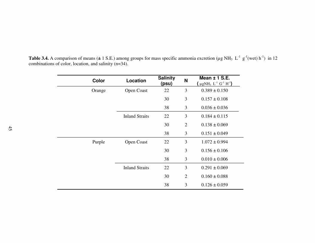
Table 3.4. A comparison of means (± 1 S.E.) among groups for mass specific ammonia excretion (µg NH3 L

-1 g-1(wet) h-1) in 12 combinations of color, location, and salinity (n=34).


(psu) N

Mean ± 1 S.E. ( µgNH3 L

-1 G-1 H-1)

Orange Open Coast 22 3 0.389 ± 0.150

30 3 0.157 ± 0.108

38 3 0.036 ± 0.036

Inland Straits 22 3 0.184 ± 0.115

30 2 0.138 ± 0.069

38 3 0.151 ± 0.049

Purple Open Coast 22 3 1.072 ± 0.994

30 3 0.156 ± 0.106

38 3 0.010 ± 0.006

Inland Straits 22 3 0.291 ± 0.069

30 2 0.160 ± 0.088

38 3 0.126 ± 0.059

45

Table 3.5. Results of a three-way Analysis of Variance (ANOVA) of rank-transformed ammonia excretion rates for color, location, and salinity (n=34).


Color 1 0.134 0.461 0.504 0.021

Location 1 0.137 0.471 0.500 0.021

Salinity 2 0.545 1.881 0.176 0.146

Color • Location 1 0.070 0.241 0.628 0.011

Color • Salinity 2 0.158 0.547 0.587 0.047



Error 22 0.290

46

47

Self-Righting

To evaluate the effects of salinity, color, and location on self-righting times in P.

ochraceus, a three-way ANOVA was conducted. These data did not meet the

assumptions of normality and homoscedasticity, so a rank-transformation was performed

before the statistical analysis was conducted. Size was used initially as a covariate in an

ANCOVA model, but was found non-significant (F1,23 = 0.005, p > 0.05). Subsequently

an ANOVA model was used to analyze these data.

A comparison of mean self-righting times of the groups for the three factors

analyzed (color, location and salinity) can be seen in Table 3.6 and Figure 3.4. There was

a significant difference in self-righting times for color (F1, 24 = 9.93, p<0.05), with orange

having faster turnover times than purple. There was also a significant difference for

location (F2, 24 = 4.837, p<0.05), with Inland Straits populations having faster righting

times than open coast ones. Salinity also was significant (F1, 24 = 5.818, p<0.05), with

individuals exhibiting faster self-righting times at 30 psu than at 40 or 20 psu. The results

of the three-way ANOVA test for these data can be seen in Table 3.7.

A post-hoc Tukey test of multiple comparisons was performed for salinity, and a

significant difference was found in self-righting times between 20 and 30 psu (20 psu:

1920 ± 493 sec; 30 psu: 474 ± 128 sec., p < 0.05) as well as between 30 and 40 psu (30

psu: 474 ± 128 sec; 40 psu: 1323 ± 515 sec., p < 0.05).

Table 3.6. A comparison of means (± 1 S.E.) between groups for self-righting times (seconds) in 12 combinations of color, location, and salinity (n = 36).


(psu) N Mean ± 1 S.E. (seconds)

Orange Open Coast 20 3 653 ± 481

30 3 201 ± 50

40 3 338 ± 112

Inland Straits 20 3 876 ± 442

30 3 503 ± 209

40 3 2057 ± 817

Purple Open Coast 20 3 3600 ± 0

30 3 304 ± 123

40 3 802 ± 376

Inland Straits 20 3 2551 ± 1049

30 3 887 ± 130

40 3 2095 ± 755

48

Table 3.7. Results of a three-way Analysis of Covariance (ANOVA) of rank-transformed self-righting times as a function of color, location, and salinity (n = 36).


Color 1 622.491 9.934 0.004* 0.250

Location 2 303.125 4.837 0.017* 0.245

Salinity 1 364.573 5.818 0.024* 0.166

Color • Location 2 156.752 2.501 0.103 0.147

Color • Salinity 1 10.614 0.169 0.684 0.006



Error 24 62.663

49

0

500

1000

1500

2000

2500

3000

3500

4000

20 30 40

Salinity (psu)

Se

co

nd

s

Figure 3.4. A comparison of the mean self-righting times (sec.) of different colors, locations and salinities. Means of orange-open coast individuals ( ), orange-inland straits individuals ( ), purple open coast individuals ( ), and purple inland straits individuals ( ), are reported ± 1 S.E. (n = 36).

50

51

CHAPTER FOUR

DISCUSSION

Aerobic Respiration

No significant differences were found among the mean metabolic rates in the 12

combinations of color, location, and salinity for wet mass. In addition, no significant

differences were identified in these combinations for dry mass metabolic rates. However,

there was a three-way interaction among color, location and salinity, but an analysis of

the simple main effects of this interaction showed no significance (p > 0.05).

Although these data point to the fact that color, location and salinity are not

correlated with metabolic rates, I suspect that under more extreme conditions, such as

greater salinity stress ( > ± 8 psu from environmental) or a greater sample size to reduce

the variance, the effects of color, salinity or location may have been detected.

Other studies, dealing with the physiology of intertidal organisms, have also

failed to show that location or physical environment significantly effect metabolic rates

of Pisaster ochraceus. Dalhoff et al.(2002) examined ecologically important, rocky

intertidal invertebrates from communities with distinct physical and oceanographic

characteristics on the wave exposed coast of Oregon. Although other invertebrate species

in the same study, such as the mussel, Mytilus californianus, the barnacle, Balanus

glandula, and the snail, Nucella ostrina, were found to have significant differences in

metabolic rates between the two environments in several of the experiments, P.

ochraceus did not.

As mentioned in the introduction chapter of this study, Binyon (1972b) suggests

that, in general, echinoderms are not as stenohaline as they were once considered to be.

52

Members of the phylum Echinodermata are found in salinities ranging from 8 - 46 psu.

My results are consistent with the idea that these organisms have incorporated

physiological mechanisms that allow them to maintain normal aerobic respiration within

certain ranges of salinity. This is in spite of the fact that these organisms are reported to

have poor abilities to osmo- and iono-regulate, and lack evidence of excretory systems

(Stickle and Diehl, 1987). These mechanisms are probably associated with the ecology of

Pisaster ochraceus and the environmental pressures associated with life in the intertidal

zone.

The physiological mechanisms for this ability to cope with salinity stress is one

that is currently undescribed in the literature. Brusca and Brusca (2003) comment on this

situation by recognizing that the evidence to date suggests that echinoderms are

osmoconformers. They recognize that both water and ions pass relatively freely across

the thin body surfaces of echinoderms, and they point out that the tonicity of the body

fluids vary with environmental fluctuation. They simply state however, that there

appears to be some sort of ionic regulation through active transport, but it is minimal.

If extracellular transport of ions is indeed minimal, then there may also be an

influence of intracellular regulation that allows these organisms to maintain aerobic

respiration, and essentially a steady state metabolism, in spite of acute changes in salinity

within a relatively narrow range

The findings of my aerobic respiration study suggest that salinity, at least in the

range of ± 8 psu with respect to the acclimation salinity has no effect on the aerobic

respiration of different color morphs of P. ochraceus from the open coast and inland

straits.

53

Ammonia Excretion

Results of the analysis of ammonia excretion rates also showed no significant

differences between the factors analyzed. This was surprising as salinity has been shown

to have a greater effect on ammonia excretion rates than on aerobic respiration rates in

other echinoderms (Talbot and Lawrence, 2002).

In most echinoderms dissolved nitrogenous wastes diffuse across the body

surfaces, such as the podia and papulae in asteroids (Brusca and Brusca, 2003). The

mechanisms by which amino acids are lost from the cells during low salinity exposure

include deamination and subsequent excretion of ammonia. However the mechanisms by

which amino acids accumulate in the cells during high salinity exposure have not been

identified in echinoderms (Diehl, 1986). For echinoderms transferred to altered salinity,

the adjustment of intracellular osmolality occurs as ions move into or out of the cells, but

the change in osmolality is sustained by the change in free amino acids (Sabourin and

Stickle, 1981; Diehl, 1986).

The ammonia excretion in response to salinity of the asteroid, Luidia clathrata, is

similar to that of P. ochraceus (Ellington and Lawrence, 1974). Increased rates of

ammonia excretion were observed when these sea stars were transferred from the

environmental (27 psu) to an hyposlaline condition (16 psu). My findings show trends

that agree with the work of Emerson (1968) who found rates of ammonia excretion to

increase when the sea cucumber, Eupentacta quinquesemita and the urchin,

Strongylocentrotus droebachiensis, were introduced into reduced salinities. Similarly

Shirley and Stickle (1982) found that the percentage of ammonia in the excreta was

significantly lower at 30 psu than at 20 or 15 psu in the sea star, Leptasterias hexactis.

54

Incidentally these six-rayed stars share the same ecological habitats as P. ochraceus, and

are their principle competitors (Lambert, 2000). Although excretion rates in my study

were not significantly different among treatments, increases in ammonia excretion rates

were seen in both colors and in both locations as salinities were reduced. In comparison

with other studies reviewed, I suggest that at greater salinity stress, these organisms may

have indeed exhibited these trends to show significant differences.

No significant differences were found when comparing the group means of

ammonia excretion as a function of color or location in this experiment. The effect of

reduced salinity on nitrogen excretion rates of echinoderms is thought to be related to the

method of exposure. Experiments have shown that abrupt exposure to hyposaline

conditions results in initial increases in excretion rates that may later return to control

levels (Shirley and Stickle, 1982). This may explain the lack of significance detected

among groups of different colors or locations as organisms were all acutely exposed to

experimental salinities. Actual times that sea stars were exposed to experimental salinities

ranged from 1.95 to 7.00 hrs. The fluctuation of excretion rates may have been affected

by the method of exposure due to these variances in chamber times, similar to the

fluctuations that were reported by Shirley and Stickle (1982). Non-significant differences

between ammonia excretion rates of different groups have also be observed in a 1988

study by Stickle that examined patterns of nitrogen excretion in echinoderms. Stickle

found that P. ochraceus is one of the most active carnivores with one of the highest total

nitrogen excretion rates of the organisms he examined. However, there was no significant

difference between the ammonia or urea excretion rates of the sea stars before and after

aerial exposure (Stickle, 1988). This in turn had an effect on the internal osmolality of the

55

organism. Data presented in other experiments as well as my own findings seem to

support the idea that P. ochraceus may have a wider range of tolerance to salinity stress

than had once been thought.

I recognize that errors may have occurred in the methods and analysis of the data

collected for this portion of the study. As discussed in the methods chapter, data were

analyzed separately and similar results were observed between the pooled data and the

individual analysis, with both tests identifying the same factors as significant. This

formed the basis for the decision to pool the results from the two separate subsets into

one analysis.

As with the aerobic respiration study, I suspect that under more extreme

conditions, such as salinity stress greater than ± 8 psu from the environmental salinity, or

a greater sample size to reduce the variance, a significant difference for the main effects

of color or location may have been detected.

Despite the extremely low concentrations of ammonia in samples, excretion rates

of P. ochraceus were still found to be significantly affected by acute changes in salinity,

but only showed non-significant trends. The data from this study however, do not support

the alternative hypothesis that ammonia excretion rates differ significantly between color

morphs of P. ochraceus. Further experimentation may lead to results that support

different conclusions from those made here.

56

Self-Righting

The results from the analyses of self-righting times for the two color morphs of P.

ochraceus from different locations revealed significant effects in all three main factors

(color, salinity and location). There were no interactions among factors.

The first interesting finding of this study was that organisms tested closer to their

environmental salinities (30 psu) had significantly faster self-righting times than

organisms exposed to hypo-and hyper-saline experimental salinities (20 and 40 psu,

respectively). The results of the post-hoc Tukey test identified a significant difference in

self-righting times between organisms tested at 20 psu and 30 psu, and between 30 psu

and 40 psu. These results are explained by the fact that 30 psu is the salinity that these

organisms were acclimated in and closest to the environmental salinities they were found

in. Thus, this suggests that organisms that were stressed the least were capable of faster

righting responses. Specimens that were tested at 20 psu and 40 psu all had significantly

slower self-righting response times. This could be due to the fact that individuals that are

more stressed by their environment may have a lower ability to carry out physiological

functions because they may be expending excessive energy carrying out intracellular

regulation (Ellington and Lawrence, 1974). Additionally, a decreased ability to conduct

behavioral functions such as righting responses may be explained by the turgor pressure

caused by an inflow of water across body tissues when organisms are placed acutely in a

hyposaline condition. Organisms that were placed in the hyposaline condition (20 psu)

took significantly longer to undergo self-righting than the organisms in the other two

salinities, and organisms at the hypersaline condition (40 psu) took longer than the ones

at the environmental condition (30 psu).

57

A second interesting finding is that in almost all cases, specimens from the open

coast would right themselves faster than ones from the Inland Straits. This could

potentially be due to the fact that they are smaller individuals which may contribute to

faster self-righting times.

The third finding was that in all cases, and for each condition, orange specimens

always had faster mean self-righting times than purple specimens. This was the first of

the three experiments to identify color as being associated with a different response. This

study was limited as it did not approach questions that address what factors of the color

polymorphism that occurs in P. ochraceus are related to responses such as rates of self-

righting. There are currently no clear answers presented by this study that would identify

causes for differences in response rates between the two color morphs examined in this

study. These findings lead to several questions that will need to be addressed in future

studies.

The self-righting study could have been strengthened by a larger sample size in

addition to more consistent methods. A sample size of 36 was not ideal for an

experiment such as this with so many uncontrollable variables. Further studies of this sort

with larger sample sizes and more precise controls may lead to more conclusive findings.

Despite the limitations of this experiment, these data do support the hypothesis that self-

righting times differ significantly in specimens from two locations, among different

salinities and between different color morphs.

58

Ecological Application of Results

The reason for P. ochraceus not showing significant differences in aerobic

respiration in this study could be tied to the ecology of these organisms. When compared

with most other rocky intertidal fauna in my study areas, Pisaster ochraceus is a large,

robust organism that is capable of withstanding several hours of desiccation during low

tide cycles. Because of their size, these organisms may not be covered by shade found in

tidepools as readily as smaller organisms such as the mussels, barnacles and whelks.

Thus, it is possible that P. ochraceus has different ranges of salinity stress that it is faced

with. Reduced metabolic responses to changing salinities may result in a greater tolerance

to acute changes in salinity within a certain range.

The idea that these sea stars have a greater tolerance to salinity stress within a

certain range is further supported by the work of Shirley and Stickle (1982) on the sea

star, Leptasterias hexactis. They found that when L. hexactis was placed in various

experimental salinities, the highest rate of oxygen consumption was at the environmental

salinity of 30 psu and at hyposaline conditions of 20 and 15 psu, oxygen consumption

rates were significantly lower. A decrease in oxygen consumption with decreasing

salinity has additionally been reported for several other echinoderm species (Giese and

Farmanfarmaian, 1963; Shumway, 1977; Sabourin and Stickle, 1981; Stickle and Diehl,

1987) however no physiological mechanisms for this change in physiology has been

identified.

The reason why this supports the idea that P. ochraceus has a greater tolerance to

salinity stress is because it has been shown that under more extreme conditions than my

experiments, echinoderms in general do actually exhibit significantly lower rates of

59

oxygen consumption (Millott, 1967; Shumway, 1977; Sabourin and Stickle, 1981; Stickle

and Diehl, 1987; Talbot and Lawrence, 2002). However when stressed at less of an

extreme, P. ochraceus did not exhibit a significant difference in rates of ammonia

excretion. The salinities that I used in my experiment may fall within a range that these

organisms may be faced with in their ecosystems, and thus suggests a range of tolerance

that has not previously reported.

Conclusions

Although measurements from the three experiments carried out in this study do

not all point to differences in responses of the two color morphs, they nonetheless

provide some evidence that color and location both have a significant effect on self-

righting times at the three salinities tested. Additionally, I found that salinity does not

affect respiration rates or ammonia excretion rates differently with regards to color or

location within the narrow range of salinities tested.

The results of my study suggest that, within a certain range (± 8 psu), P.

ochraceus appears to be able to maintain normal aerobic respiration and ammonia

excretion. When stressed to greater extremes outside of the range they are able to cope

with, such as salinities of ± 10 psu or greater, their basic functions of mobility, such as

self-righting, may be reduced.

60

Suggestions for Further Study

Although salinity was the only environmental variable examined in this study,

many other differences are seen between the two locations that show different color

frequencies of P. ochraceus. Variables that could potentially be tested include

temperature, sun and ultra violet (UV) exposure, tidal fluctuations, prey availability, diet,

pH of seawater, and wave exposure.

Differences between locations caused by anthropogenic factors can also be

identified. Differences between the two locations include greater eutrophication in the

Inland Straits due to the large amount of agricultural activity, more pollutants from

surface runoff from larger urban populations around the Inland Straits, and habitat

degradation due to human trampling of sea star habitats. Studies that examined these

effects could potentially identify links to the color differences seen between the two

locations.

61

LITERATURE CITED

Aarset, A. V. and T. Aunaas, 1990. "Influence of Environmental Salinity on Oxygen-Consumption and Ammonia Excretion of the Arctic under-Ice Amphipod Onisimus-Glacialis." Marine Biology 107(1): 9-15.

Bilton, D. T., J. Paula and J. D. D. Bishop, 2002. "Dispersal, genetic differentiation and speciation in estuarine organisms." Estuarine Coastal and Shelf Science 55(6): 937-952.

Binyon, J., Ed. 1966. Salinity tolerance and ionic regulation. Physiology of Echinodermata, Interscience.

Binyon, J., 1972a. "The effects of diluted sea water upon podial tissues of the starfish Asterias rubens L. ." Comparitive and Biochemical Physiology 41A: 1-6.

Binyon, J., 1972b. Physiology of echinoderms. Oxford, New York,, Pergamon Press.

Brusca, R. C. and G. J. Brusca, 2003. Invertebrates 2nd ed. Sunderland, MA, Sinauer Associates, Inc., Publishers.

Cannon, G. A., 2003. Circulation Variations in the Strait of Juan de Fuca. 2003 Georgia Basin/Puget Sound Research Conference.

Cohen, J., 1988. Statistical Power Analysis for the Behavioral Sciences. Mahwah, New Jersey, Lawrence Erlbaum.

Dalhoff, E. P., J. H. Stillman and B. A. Menge, 2002. "Physiological Community Ecology: Variation in Metabolic Activity of Ecologically Important Rocky Intertidal Invertebrates Along Environmental Gradients." Integrative and Comparative Biology 42: 862-871.

Diehl, W. J., 1986. "Osmoregulation in Echinoderms." Comparitive and Biochemical Physiology 84A(2): 199-205.

Dunbar, S. G. and M. Coates, 2004. "Differential tolerance of body fluid dilution in two species of tropical hermit crabs: not due to osmotic/ionic regulation." Comparative Biochemistry and Physiology 137A(2): 321-337.

62

Ellington, W. R. and J. M. Lawrence, 1974. "Coelomic fluid volume regulation and isoosmotic intracellular regulation by Luidia clathrata (Echinodermata: Asteroidea) in response to hyposmotic stress." Biological Bullitin 146: 20-31.

Emerson, D. N., 1968. "Influence of salinity on ammonia excretion rates and tissue constituents of euryhaline invertebrates." Comparitive and Biochemical Physiology 29A: 1115-1133.

Feder, H. M., 1957. Natural History Studies on the Starfish Pisaster Ochraceus (Brandt, 1835) in the Monterey Bay Area. Biological Sciences. Stanford, CA, Stanford University.

Feder, H. M., 1959. "The food of the starfish, Pisaster ochraceus along the California coast." Ecology 40: 721-724.

Feder, H. M. and A. M. Christensen, 1966. Chapter 5 Aspects of Asteroid Biology. Physiology of Echinodermata. R. A. Boolootian. New York, Interscience: 87-127.

Finlayson, D. P., 2004. The Large Scale Geomorphology of Puget Sound Shorelines. School of Oceanography. Seattle, University of Washington.

Forcucci, D. and J. M. Lawrence, 1986. "Effects of low salinity on the activity, feeding, growth and absorption of Luidia clathrata (Echinoderm: Asteroidea)." Marine Biology 91: 315-321.

Fox, D. and T. Hopkins, 1966. Chapter 12 -The Comparitive Biochemistry of Pigments. Physiology of Echinodermata. R. A. Boolootian. New York, Interscience: 277-300.

Fox, D. L. and T. S. Hopkins, 1941. "Comparitive studies of the pigments of some Pacific coast echinoderms." Biological Bullitin 80: 441-455.

Garza, C., 2005. "Prey productivity effects on the impact of predators of the mussel, Mytilus californianus (Conrad)." Journal of Experimental Marine Biology and Ecology 324(1): 76-88.

Giese, A. C. and A. Farmanfarmaian, 1963. "Resistance of the purple sea urchin to osmotic stress." Biological Bullitin 124: 182-192.

63

Green, J., 1968. The Biology of Estuarine Animals. Seattle, University of Washington.

Hendler, G., J. Miller, D. Pawson and K. Porter, 1995. Sea Stars, Sea Urchins, and Allies - Echinoderms of Florida and the Carribean. Washington, Smithsonian Institute Press.

Holbrook, J. R. and D. Halpern, 1982. "Winter-time near-surface currents in the Strait of Juan de Fuca." Atmosphere-Ocean 20: 327-339.

Humphreys, V. 2003. "The Biogeography of the Purple Ochre Sea Star (Pisaster

ochraceus)." Retrieved March 2,2006, 2006, from http://bss.sfsu.edu/holzman/courses/Fall%2003%20project/oseastar.htm.

Johnson, B. P., 1976. Daily Activity and Migration of the Starfish Pisaster Ochraceus. Biology. San Francisco, San Francisco State University.

Jury, S. H., M. T. Kinnison, W. H. Howell and W. H. Watson, 1994. "The Effects of Reduced Salinity on Lobster (Homarus-Americanus Milne-Edwards) Metabolism - Implications for Estuarine Populations." Journal of Experimental Marine Biology and Ecology 176(2): 167-185.

Karrer, P. and E. Jucker, 1950. Carotenoids. New York, Elsevier.

Kinne, O., 1963. "The effects of temperature and salinity on marine and brackish water animals I. Temperature." Oceanographic Marine Biology Annual Review 1: 301-340.

Lambert, P., 2000. Sea Stars of British Columbia, Southeast Alaska and Puget Sound. Vancouver, UBC Press.

Menge, B. A. and J. P. Sutherland, 1987. "Community Regulation - Variation in Disturbance, Competition, and Predation in Relation to Environmental-Stress and Recruitment." American Naturalist 130(5): 730-757.

Millott, N., 1967. Echinoderm Biology. Sympsia of the zoological society of London Number 20, Academic Press.

64

Morris, R., D. Abbot and E. Haderlie, 1980. Intertidal Invertebrates of California. Stanford, CA, Stanford University Press.

NEER, 2006. NOAA/National Estuarine Research Reserve system - Padilla Bay, http://cdmo.baruch.sc.edu/output, NOAA.

Newell, R. C., 1979. Biology of Intertidal Animals. Faversham [Eng.], Marine Ecological Surveys.

Paine, R. T., 1966. "Food web complexity and species diversity." American Naturalist 100: 65-75.

Paine, R. T., 1969. "A note on trophic complexity and community stability." American Naturalist 103: 91-93.

Raimondi, P., R. Sagarin, R. Ambrose, M. George, S. Lee, D. Lohse, C. M. Miner and S. Murray, 2004. "Color change and consistency in the sea star Pisaster ochraceus." Integrative and Comparative Biology 44(6): 626-626.

Raimondi, P., R. Sagarin, Richard Ambrose, Christy Bell, Maya George, Steven Lee, David Lohse, C. Melissa Miner and S. Murray, in press. Conspicuous color patterns in the sea star Pisaster ochraceus.: 13.

Rankin, J. C. and J. Davenport, 1981. Animal Osmoregulation. New York, Wiley.

Ricketts, E. F., J. Calvin and H. W. Joel, 1985. Between Pacific Tides. Stanford, CA, Stanford University Press.

Roller, R. A. and W. B. Stickle, 1985. "Effects of salinity on larval tolerance and early developmental rates of four species of echinoderms." Canadian Journal of Zoology 63(7): 1531-1538.

Sabourin, T. D. and W. B. Stickle, 1981. "Effects of salinity on respiration and nitrogen excretion in two species of echinoderms." Marine Biology 65: 91-99.

Sanford, E., 1999. "Regulation of keystone predation by small changes in ocean temperature." Science 283(5410): 2095-2097.

65

Sanford, E., 2001. "The effect of variation in water temperature on the keystone predator Pisaster ochraceus." American Zoologist 41(6): 1576-1576.

Shick, J. M., 1983. Respiratory Gas Exchange in Echinoderms. Echinoderm Studies. M. Jangoux and J. Lawrence. Rotterdam-Salem, NH, A.A. Balkema. 1: 67-110.

Shirley, T. C. and W. B. Stickle, 1982. "Responses of Leptasterias hexactis (Echinodermata: Asteroidea) to low salinity: II. Nitrogen metabolism, respiration, and energy budget." Marine Biology 69: 155-163.

Shumway, S. E., 1977. "The Effects of Fluctuating Salinities on Four Species of Asteroid Echinoderms." Comparitive and Biochemical Physiology 58A: 177-179.

Stickle, W. B., 1988. "Patterns of Nitrogen Excretion in The Phylum Echinodermata." Comparitive and Biochemical Physiology 91A(2): 317-321.

Stickle, W. B. and W. J. Diehl, 1987. Effects of Salinity on Echinoderms. Echinoderm Studies Vol. 2. M. Jangoux, Lawrence, J. Brookfield, A.A. Balkema. 2: 235-285.

Sweere, C., unpublished. Direct and Indirect Effects of Pisaster ochraceus on tide pool communities, University of California Berkley.

Talbot, T. D. and J. M. Lawrence, 2002. "The effect of salinity on respiration, excretion, regeneration and production in Ophiophragmus filograneus (Echinodermata : Ophiuroidea)." Journal of Experimental Marine Biology and Ecology 275(1): 1-14.

Vevers, H. G., 1966. Chapter 11 Pigmentation. Physiology of Echinodermata. R. A. Boolootian. New York, Interscience Publishers: 267-275.

YSI-Incorporated. 2006. "Appendix C - Oxygen Solubility Tables in YSI Model 52 Disolved Oxygen Meter Operations Manual." from http://www.ysi.com/extranet/EPGKL.nsf/5992085488f9da9d85256a550047c2a2/90a0378150c2d2dd85256a1f0073f295/$FILE/052010_D.pdf#search=%22ysi%20air%20saturation%20tables%22.

Documents

LOMA LINDA UNIVERSITY The School of Science and Technology Faculty